ECE 287A Presentation

Capacity, Diversity and Multiplexing Gain

for MIMO channels

Yuzhe Jin

June 12, 2007

Page 1

Outline

• Background

• Capacity of MIMO channels

– Deterministic– Fading– Outage

• Diversity and Multiplexing Gains

– Motivation– Fundamental tradeoff– Two practical schemes

• Extension to Multiple-Access Channels

• Conclusion

Page 2

Background: SISO Channel

Before we start, let’s recall the discrete-time AWGN channel:

Figure 1: AWGN Channel

Some important observations:

• A power constraint P on input X

• Capacity

C = maxp(x),P

I(X;Y ) = log(

1 +P

N

)Page 3

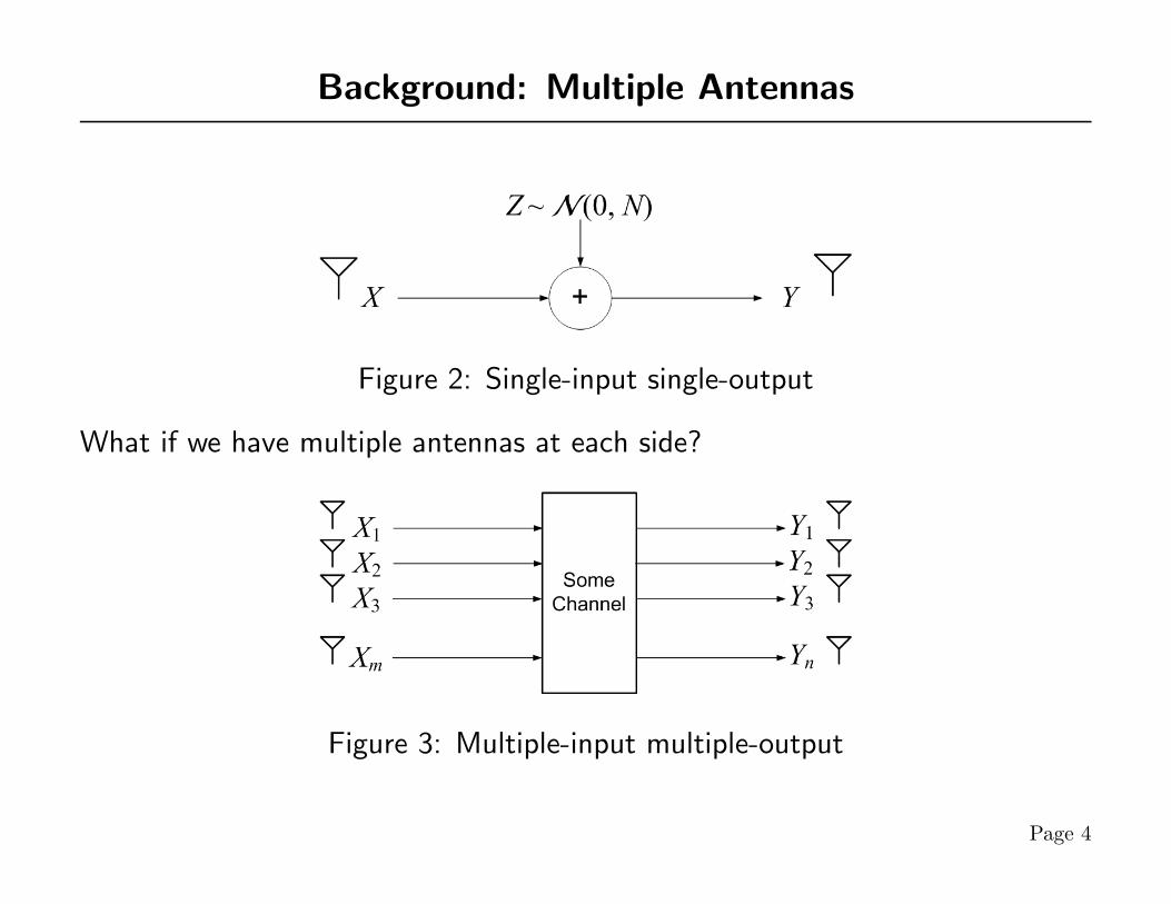
Background: Multiple Antennas

Figure 2: Single-input single-output

What if we have multiple antennas at each side?

Figure 3: Multiple-input multiple-output

Page 4

Background: Multiple-Antenna Gaussian Channels

Figure 4: Pair-wise relation

Adding in Gaussian noise, we have the channel model:

Y = HX + N

where Xm×1 is the channel input, Yn×1 is channel output. Hn×m is thecoefficient associated with each path between a transmit antenna and a receiverantenna, Nn×1 is zero-mean complex Gaussian noise, and E(NNH) = I.

Page 5

Capacity: When H is fixed and known

The channel is Y = HX + N . Suppose E(XXH) = Q.

I(X;Y ) = H(Y )−H(Y |X)

= H(Y )−H(N)

= log det(I + HQHH)

= log det(I + QHHH) (Property of det)

= log det(I + Λ1/2UQUH Λ1/2) (eigen-decomposition)

= log det(I + Λ1/2Q̃ Λ1/2)

≤∏

i

(1 + Q̃iiλi)

where Q̃ = UQUH, and Λ = diag(λ1, ..., λm).

Page 6

Capacity: When H is fixed and known, Cont’d

I(X;Y ) ≤∏

i

(1 + Q̃iiλi)

With equality, when Q̃ is diagonal, and optimal diagonal entries can be foundvia water-filling:

Q̃ii = (µ− λ−1i )+, i = 1, 2, 3..., m

where µ is chosen to satisfy∑

i Q̃ii = P .

Page 7

Capacity: When H is random

• Suppose each entry of H is independently drawn from a zero-mean complexGaussian distribution, with independent real and imaginary parts, each withvariance 1/2.

• Gaussian Channel with Rayleigh Fading

• What is the capacity?

Page 8

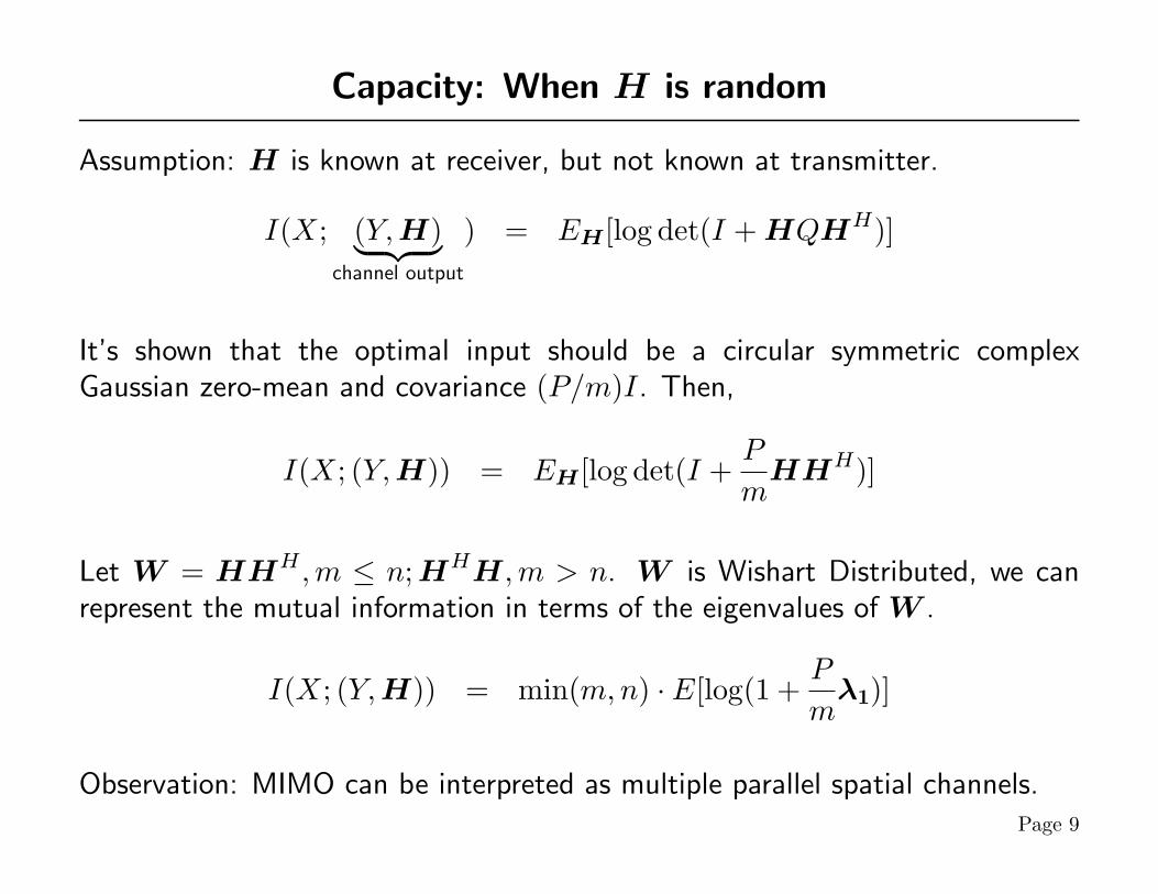
Capacity: When H is random

Assumption: H is known at receiver, but not known at transmitter.

I(X; (Y, H)︸ ︷︷ ︸channel output

) = EH[log det(I + HQHH)]

It’s shown that the optimal input should be a circular symmetric complexGaussian zero-mean and covariance (P/m)I. Then,

I(X; (Y, H)) = EH[log det(I +P

mHHH)]

Let W = HHH,m ≤ n;HHH,m > n. W is Wishart Distributed, we canrepresent the mutual information in terms of the eigenvalues of W .

I(X; (Y, H)) = min(m,n) · E[log(1 +P

mλ1)]

Observation: MIMO can be interpreted as multiple parallel spatial channels.Page 9

Capacity: When H is random, but realized only once

• Ergodic capacity doesn’t apply to this case. There will always be a positiveprobability that the realization of H is too bad to support a target rate R.

• Definition of OutageOutage is defined as the event that the mutual information of the channeldoes not support a target rate, due to a “bad” realization of channelcoefficients H.

• Outage Probability: The probability that an outage event occurs.

P ( R︸︷︷︸desired rate

> I(X, (Y, H))︸ ︷︷ ︸instantaneous mutual information

) = ε

• Question:

– Given a target rate, what’s the outage probability?– Given an outage probability, what’s the max rate we can achieve?

Page 10

Capacity: For more complicated cases

• When receiver doesn’t know the channel, what is the capacity andcorresponding input? and other complicated channel models?

• For more complicated channels, we may not be able to figure out channelcapacity in closed form. Meanwhile, the capacity-achieving input distributionis as well hard to characterize.

• Is there other metric that captures the characteristic of a channel, other thancapacity?

• In practice, given a coding scheme, is there other metric that can give usmore insight about the performance?

• We may need more than capacity result.

Page 11

Diversity

In a MIMO Channel with m transmit antennas and n receive antennas,

• Each pair of transmit-receive antennas provides a signal path from thetransmitter to receiver.

• If we send signals carrying the same information through different paths,multiple independently faded replicas of the data symbol can be obtained atthe receiver.

• More reliable reception can be achieved. (“reliable”?)

Page 12

Diversity: Reliable Reception

Suppose we have a slow Rayleigh fading channel with a single transmitter andn receivers,

• n different fading paths

• The average error probability can be made to decay like 1SNRn, at high SNR.

Note for a single-antenna fading channel, it’s 1SNR

• Use multiple paths to combat fading.

• A question: Can fading be beneficial?

Page 13

Multiplexing

• If the path gains between individual transmit-receive antenna pairs fadeindependently, the channel matrix will be well-conditioned with highprobability.

• Higher rate. (MIMO as multiple parallel spatial channels)

• It’s shown that at high SNR regime, the channel capacity is about

C(SNR) = min(m,n) log SNR + O(1)

• The channel capacity is increased by using multiple antennas due to spacialmultiplexing. We can transmit independent information streams in parallelthrough the spacial channels.

Page 14

Can we get both?

Figure 5: A conflict?

Obviously, the conflict between the two suggests a fundamental tradeoff betweenbenefits obtained from diversity and multiplexing.

Page 15

Definitions of Diversity and Multiplexing Gain [2]

Consider a family of codes C(SNR) of block length l, one at each SNR level.Let R(SNR) be the rate of the code C(SNR).

• C(SNR) is said to achieve diversity gain d if the average error probability

limSNR→∞

Pe(SNR)log SNR

= −d

• C(SNR) is said to achieve the multiplexing gain r if the data rate

limSNR→∞

R(SNR)log SNR

= r

• For each r, define d∗(r) to be the supremum of the diversity advantageachieved over all schemes.

Page 16

Optimal Tradeoff between d and r [2]

Theorem: Assume l ≥ m + n − 1. The optimal tradeoff curve d∗(r) isgiven by the piecewise-linear function connecting the points (k, d∗(k)), k =0, 1, ...,min(m,n), where d∗(k) = (m − k)(n − k). In particular, d∗max = mn,r∗max = min(m,n).

Figure 6: Diversity-multiplexing tradeoff, for general m, n, l ≥ m + n− 1Page 17

How do we interpret the Optimal Tradeoff?

• The optimal tradeoff curve intersects the r axis at min(m,n), i.e. themaximum achievable spatial multiplexing gain r∗max is the total number ofdegrees of freedom provided by the channel as suggested by the ergodiccapacity result.

• Intuitively, as r → r∗max, the data rate approaches the ergodic capacity.

• At this point, however, no positive diversity gain can be achieved, i.e. noprotection against the randomness in the fading channel.

Page 18

How do we interpret the Optimal Tradeoff?

• The curve intersects the d axis at the maximal diversity gain d∗max = mn,corresponding to the total number of random fading coefficients that ascheme can average over.

• In order to achieve the maximal diversity gain, no positive spatial multiplexinggain can be obtained at the same time.

Page 19

How do we interpret the Optimal Tradeoff?

• Bridges the gap between the two design criteria

• Positive diversity gain and multiplexing gain can be achieved simultaneously.

• Increasing one comes at a price of decreasing the other.

• This tradeoff curve provides a more complete picture of the achievableperformance over multiple-antenna channels than two extreme pointscorresponding to maximum diversity/multiplexing gain.

Page 20

How do we interpret the Optimal Tradeoff?

Figure 7: Adding one transmit and one receive antenna increases multiplexinggain by 1 at each diversity level. Curve shifted to the right by 1.

Page 21

Example: Two Practical Schemes

Repetition scheme vs. Alamouti scheme

X =[

x1 00 x1

]X =

[x1 −x∗2x2 x∗1

]

Figure 8: Diversity-Multiplexing tradeoff and comparison between two schemes.

Page 22

Beyond the examples

• If the performance of schemes only evaluated by maximal diversity gain d(0),we cannot distinguish the performance of repetition scheme and Alamoutischeme.

• Different coding schemes may be designed for different goals.

– Orthogonal Designs (e.g. Alamouti): Maximize the diversity gain.– V-BLAST: Maximize the spatial multiplexing gain.

• The diversity-multiplexing tradeoff provides a unified framework to make faircomparisons and helps us understand the characteristic of a particular schememore completely.

Page 23

Beyond the examples

Figure 9: Orthogonal Designs vs. V-BLAST

Page 24

Extension to Multiple-Access Channels

• The discussion on diversity-multiplexing tradeoff can be extended to channelswith multiple-access.

• Suppose we allow each user to have a diversity gain of d, then we cancharacterize the set of multiplexing gain tuples (r1, r2, ...rK).

• Theorem: If the block length l ≥ Km + n− 1,

R(d) =

{(r1, r2, ...rK) :

∑s∈S

rs ≤ r∗|S|m,n(d),∀S ⊆ 1, ...,K

}

where r∗|S|m,n(·) is the multiplexing-diversity tradeoff curve for a point-to-

point channel with |S|m transmit and n receive antennas.

Page 25

Conclusion

• We introduce the basic idea of multiple-antenna channels.

• Derive the capacity of the channels with different setup. The difficulty inevaluating channel capacity. Look for more practical measures to comparecoding scheme.

• Diversity and multiplexing gain. The fundamental tradeoff.

• Extension to multiple-access channel.

Page 26

References

[1] I. E. Telatar, “Capacity of Multi-antenna Gaussian Channels,” Rm.2C-174, Lucent Technologies, Bell Lab,1997.

[2] L. Zheng, D. Tse, “Diversity and Multiplexing: A Fundamental Tradeoff in Multiple-Antenna Channels,”IEEE Trans. on Information Theory, Vol. 49, No. 5, May 2003.

[3] D. Tse, P. Viswanath, L. Zheng, “Diversity-Multiplexing Tradeoff in Multiple-Access Channels,” IEEE Trans.on Information Theory, Vol. 50, No. 9, Sep 2004.

[4] T. M. Cover and J. A. Thomas, Elements of Information Theory, 2nd ed. New York: Wiley, 2006.

[5] D. Tse, P. Viswanath, Fundamentals of Wireless Communication, Cambridge University Press, May 2005.

Page 27