Embed Size (px)
Citation preview

Capacity Design Optimization of Steel
Building Frameworks Using Nonlinear
Time-History Analysis
by
Yusong Xue
A thesis
presented to the University of Waterloo
in fulfillment of the
thesis requirement for the degree of
Doctor of Philosophy
in
Civil Engineering
Waterloo, Ontario, Canada, 2012
©Yusong Xue 2012

ii
AUTHOR'S DECLARATION
I hereby declare that I am the sole author of this thesis. This is a true copy of the thesis, including
any required final revisions, as accepted by my examiners.
I understand that my thesis may be made electronically available to the public.

iii
Abstract
This study proposes a seismic design optimization method for steel building frameworks
following the capacity design principle. Currently, when a structural design employs an elastic
analysis to evaluate structural demands, the analysis results can be used only for the design of
fuse members, and the inelastic demands on non-fuse members have to be obtained by hand
calculations. Also, the elastic-analysis-based design method is unable to warrant a fully valid
seismic design since the evaluation tool cannot always capture the true inelastic behaviour of a
structure. The proposed method is to overcome these shortcomings by adopting the most
sophisticated nonlinear dynamic procedure, i.e., Nonlinear Time- (or Response-) History
Analysis as the evaluation tool for seismic demands.
The proposed optimal design formulation includes three objectives: the minimum weight or cost
of the seismic force resisting system, the minimum seismic input energy or potential earthquake
damage and the maximum hysteretic energy ratio of fuse members. The explicit design
constraints include the plastic rotation limits on individual frame members and the inter-story
drift limits on the overall performance of the structure. Strength designs of each member are
treated as implicit constraints through considering both geometric and material nonlinearities of
the structure in the nonlinear dynamic analysis procedure. A multi-objective Genetic Algorithm
is employed to search for the Pareto-optimal solutions.
The study provides design examples for moment resisting frames and eccentrically braced
frames. In the examples some numerical strategies, such as integrating load and resistance
factors in analysis, grouping design variables of a link and the beams outside the link, rounding-
off the objective function values, are introduced. The design examples confirm that the proposed
optimization formulation is able to conduct automated capacity design of steel frames. In
particular, the third objective, to maximize the hysteretic energy ratio of fuse members, drives
the optimization algorithm to search for design solutions with favorable plastic mechanisms,
which is the essence of the capacity design principle.
For the proposed inelastic-analysis-based design method, the seismic performance factors (i.e.,
ductility- and overstrength-related force reduction factors) are no longer needed. Furthermore,

iv
problem-dependent capacity design requirements, such as strong-column-weak-beam for
moment resisting frames, are not included in the design formulation. Thus, the proposed design
method is general and applicable to various types of building frames.

v
Acknowledgements
I would like to express my most sincere appreciation to my research supervisors, Professor
Yanglin Gong and Professor Lei Xu, for their valuable guidance, support and engagement in
completing this research.
Special thanks are also due to late Professor Donald E. Grierson who taught me structural
optimization theory and contributed his constructive criticism and praise during my graduate
program.
I greatly appreciate the other members of the examining committee Professor Elizabeth
Weckman, Professor Mahesh Pandey and Professor Wei-Chau Xie. Special thanks to Professor
Christopher M. Foley for serving as the external examiner.
The assistance of Professor Finley A. Charney, Professor Pierre Leger, and Professor Andre
Filiatrault is gratefully appreciated.
I would like to acknowledge the financial support through postgraduate scholarships provided by
the Natural Sciences and Engineering Research Council of Canada, the University of Waterloo
Graduate Scholarships, QEII-Graduate Scholarship in Science and Technology, and the Teaching
Assistantships granted by the Department of Civil and Environmental Engineering.
Finally, I dedicate this thesis to my wife Jiaoying and daughter Diana for their tremendous
patience, encouragement and love. I am also very grateful to our parents for their love and
support.

vi
Dedication
To my family

vii
Table of Contents
AUTHOR'S DECLARATION ....................................................................................................... ii
Abstract .......................................................................................................................................... iii
Acknowledgements ......................................................................................................................... v
Dedication ...................................................................................................................................... vi
Table of Contents .......................................................................................................................... vii
List of Figures ................................................................................................................................ ix
List of Tables ................................................................................................................................ xii
List of Notations .......................................................................................................................... xiii
Chapter 1 Introduction .................................................................................................................... 1
1.1 Current Practice of Seismic Design ...................................................................................... 3
1.1.1 Elastic-Analysis-Based Design Method ......................................................................... 5
1.1.2 Capacity Design .............................................................................................................. 8
1.2 Structural Optimization ....................................................................................................... 10
1.3 Seismic Design Optimization .............................................................................................. 14
1.4 Energy Method for Seismic Design .................................................................................... 18
1.5 Thesis Outline ..................................................................................................................... 20
1.6 Assumptions and Idealizations ............................................................................................ 21
Chapter 2 Nonlinear Dynamic Analysis Approach for Seismic Design ....................................... 22
2.1 Energy-Based Dynamic Analysis........................................................................................ 22
2.1.1 Seismic Energy Equation ............................................................................................. 23
2.1.2 Seismic Energy Computation ....................................................................................... 25
2.2 Structural Analysis Method ................................................................................................. 31
2.2.1 Nonlinear Time History Analysis ................................................................................. 31
2.2.2 Geometric and Material Nonlinear Analysis ................................................................ 37
2.2.3 Input Ground Motion Time Histories ........................................................................... 50
2.3 Comparison of Seismic Energy Input ................................................................................. 51
Chapter 3 Design Optimization Problem Formulation ................................................................. 54
3.1 Design Objective Functions ................................................................................................ 55
3.1.1 Minimum Cost of SFRS ............................................................................................... 55

viii
3.1.2 Minimum Seismic Input Energy .................................................................................. 56
3.1.3 Maximum Hysteretic Energy Dissipation of Fuse Members ....................................... 56
3.2 Design Constraints .............................................................................................................. 57
3.2.1 Performance Constraints............................................................................................... 57
3.2.2 Side Constraints ............................................................................................................ 61
3.3 Optimization Formulation and Algorithm........................................................................... 62
Chapter 4 Design of Moment Resisting Frames ........................................................................... 66
4.1 Geometry and Seismic Loading of the 3-Story-4-Bay MRF .............................................. 66
4.2 Design Example One ........................................................................................................... 70
4.3 Design Example Two .......................................................................................................... 78
Chapter 5 Design of Eccentrically Braced Frames ....................................................................... 88
5.1 Geometry and Seismic Loading of the 3-Story-1-Bay EBF ............................................... 88
5.2 Analytical Model of EBF .................................................................................................... 97
5.3 Design Results ................................................................................................................... 102
Chapter 6 Conclusions and Recommendations ........................................................................... 119
6.1 Summary and Conclusions ................................................................................................ 119
6.2 Recommendations for Future Research ............................................................................ 122
References ................................................................................................................................... 123
Appendices .................................................................................................................................. 129
Appendix 2.A Iterative Algorithm for Element State Determination ..................................... 129
Appendix 3.A Acceptance Criteria of Steel Frame Members ................................................. 131
Appendix 3.B Minimum Weight Seismic Design of a Steel Portal Frame ............................. 133
Appendix 4.A Selected Ground Motion Time-Histories ........................................................ 139

ix
List of Figures
Figure 1-1 Force-deformation curve ............................................................................................... 4
Figure 2-1 Typical energy time history (Charney 2004) .............................................................. 25
Figure 2-2 Typical hysteretic curves ............................................................................................. 27
Figure 2-3 Elastic strain energy and irrecoverable hysteretic energy of structural members ....... 29
Figure 2-4 Illustration of tangent stiffness and secant stiffness .................................................... 34
Figure 2-5 Element forces in different systems ............................................................................ 38
Figure 2-6 Deformed configuration of frame element .................................................................. 40
Figure 2-7 Basic (rotating) and global coordinate system (Neuenhofer and Filippou 1997) ....... 45
Figure 2-8 Evaluation of force-based element compatibility relation (Scott et al 2006) .............. 48
Figure 2-9 Plastic rotation in beam-column.................................................................................. 49
Figure 2-10 Steel portal frame for computation of seismic energy input ..................................... 51
Figure 2-11 Push-over curve (base shear – story displacement) for model calibration................ 52
Figure 2-12 Comparison of lateral displacement response histories ............................................ 52
Figure 2-13 Seismic energy input response history ...................................................................... 53
Figure 3-1Typical bending moment versus deformation curve .................................................... 60
Figure 3-2 Flowchart of the proposed design procedure .............................................................. 63
Figure 4-1 Plan view of the hypothetical office building ............................................................. 66
Figure 4-2 Side view of the E-W direction MRFs ........................................................................ 67
Figure 4-3 Response spectra ......................................................................................................... 68
Figure 4-4 Design variable groups of MRF .................................................................................. 69
Figure 4-5 Relationship between OBJ3 and moment ratio rm ....................................................... 77
Figure 4-6 Lateral displacement response histories ...................................................................... 82

x
Figure 4-7 Inter-story drift response histories .............................................................................. 83
Figure 4-8 Distribution of the maximum inter-story drift ............................................................ 83
Figure 4-9 Base shear response history ........................................................................................ 84
Figure 4-10 First story shear versus inter-story drift .................................................................... 85
Figure 4-11 Beam bending moment response histories (at the first column line) ........................ 85
Figure 4-12 Beam end plastic rotation response histories (at the first column line) .................... 86
Figure 4-13 Beam bending moment versus plastic rotation (Floor 2) .......................................... 86
Figure 4-14 Beam bending moment versus plastic rotation (Floor 3) .......................................... 87
Figure 4-15 Beam bending moment versus plastic rotation (Roof) .............................................. 87
Figure 5-1 Plan view of the hypothetical office building (EBF) .................................................. 88
Figure 5-2 Side view of the EBFs ................................................................................................. 89
Figure 5-3 Response spectra (for EBF design) ............................................................................. 91
Figure 5-4 Hybrid link element ..................................................................................................... 98
Figure 5-5 Multi-linear force-deformation relationship of link model ......................................... 98
Figure 5-6 Plastic configuration of EBF ....................................................................................... 99
Figure 5-7 Searched design solutions in objective space............................................................ 103
Figure 5-8 Feasible design solutions in objective space ............................................................. 103
Figure 5-9 Weight (OBJ1) versus seismic input energy (OBJ2) ................................................. 104
Figure 5-10 Hysteretic energy dissipation ratio (OBJ3) versus seismic input energy (OBJ2) .... 104
Figure 5-11 Hysteretic energy dissipation ratio (OBJ3) versus weight (OBJ1) .......................... 105
Figure 5-12 Relative objectives of the Pareto-optimal solutions ................................................ 111
Figure 5-13 Lateral displacement response history .................................................................... 113
Figure 5-14 Inter-story drift ratio response histories .................................................................. 113
Figure 5-15 Distribution of the maximum link rotation ............................................................. 114

xi
Figure 5-16 Link bending moment versus rotation (Floor 3, left end) ....................................... 114
Figure 5-17 Link bending moment versus rotation (Floor 3, right end) ..................................... 115
Figure 5-18 Link shear versus rotation hysteresis (Floor 2) ....................................................... 115
Figure 5-19 Link shear versus rotation hysteresis (Floor 3) ....................................................... 116
Figure 5-20 Link shear versus rotation hysteresis (Roof) ........................................................... 116
Figure 5-21 Compression versus bending moment (Story 1, left column) ................................. 117
Figure 5-22 Compression versus bending moment (Floor 2, left beam) .................................... 117
Figure 5-23 Compression versus bending moment (Story 1, left brace) .................................... 118
Figure 3.B-1 Side view of the steel portal frame ........................................................................ 133
Figure 3.B-2 Earthquake ground motion record ......................................................................... 134
Figure 3.B-3 Distribution of designs in objective - constraint space .......................................... 136
Figure 4.A-1 Ground motion record (1979 Imperial Valley: El Centro Array #12) .................. 139
Figure 4.A-2 Ground motion record (1989 Loma Prieta: Belmont Envirotech) ........................ 139
Figure 4.A-3 Ground motion record (1994 Northridge: Old Ridge RT 090) ............................. 140
Figure 4.A-4 Ground motion record (1989 Loma Prieta: Presidio)............................................ 140

xii
List of Tables
Table 3-1 Plastic rotation limits of structural members ................................................................ 60
Table 4-1 Selected ground motion time-histories ......................................................................... 68
Table 4-2 Section sets for design variables of design example one ............................................. 70
Table 4-3 Design results ............................................................................................................... 71
Table 4-4 Pareto-optimal solutions ............................................................................................... 74
Table 4-5 Ten runs' results of the MGA (population = 15) .......................................................... 75
Table 4-6 Section sets for design variables of design example two ............................................. 79
Table 4-7 Search results of design example two .......................................................................... 80
Table 4-8 Structural Response of design example two ................................................................. 81
Table 5-1 Selected ground motion time-histories for EBF design ............................................... 91
Table 5-2 Section sets for design variables of EBF design .......................................................... 95
Table 5-3 Plastic rotation limits for non-fuse members of EBF ................................................... 96
Table 5-4 Search results of MGA ............................................................................................... 107
Table 5-5 Structural response of search results of MGA ............................................................ 108
Table 5-6 Constraint values of the obtained optimal solutions................................................... 109
Table 5-7 Reduced Pareto-optimal solutions .............................................................................. 110
Table 3.B-1 Candidate sections for sizing variables x1, x2 ......................................................... 135
Table 3.B-2 Results of GA runs .................................................................................................. 138

xiii
List of Notations
αi load factors
hysteretic energy dissipation ratio of fuse members and mean value, respectively
β and γ parameters of the Newmark method
γ plastic rotation of link
δ generalized deformation
δ0 allowable value for inter-story drift
mean value of the sth
inter-story drift
ζ damping ratio
mean value of plastic deformation demand for the lth
fuse member
l,0 allowable plastic deformation limit for the lth
fuse member
p plastic inter-story drift ratio
y yield rotation of steel frame member
μ ductility factor
ρ mass density of material
Ф resistance factor
mean value of plastic deformation of the mth
non-fuse member
φm,0 allowable plastic deformation limit of the mth
non-fuse member
Δφt,k increment of end rotation of the kth
structural element from time (t-Δt) to time t

xiv
ωp and ωq the pth
and qth
natural frequencies, respectively
ξm and ωm location and associated weight of integration points of Gauss numerical method
Ak cross-sectional area of member k
am mass-proportional damping constant
a(x) force interpolation matrix
a and ag displacement-deformation compatibility matrix
ar and br rotation transformation matrix
bt, bi and bc stiffness-proportional damping constants
b and be equilibrium transformation matrix
bu, bs, bpΔ equilibrium transformation matrix using deformed frame element formation
[C] global viscous damping matrix
[C]t tangent damping matrix
Cj a set of discrete steel cross-sections
D section deformation vector
db beam depth
dc column depth
dex distance between extreme Pareto-optimal solutions
di crowding distance of Pareto-optimal solution i
E Young’s modulus of material

xv
Ea absorbed energy
Ed damping energy
Eh irrecoverable hysteretic energy
Eh,k hysteretic energy dissipation of the kth
structural member
Eh_fuse hysteretic energy of fuse members
Ei relative seismic input energy
Ei,m (t) seismic input energy of the mth
degree-of-freedom at time t
mean value of seismic input energies for ng ground motions
Ek kinetic energy
Es elastic strain energy
e link length
inertial force vector of the m
th degree-of-freedom at time t
{Fr(t)} global nonlinear restoring force vector at time t
F element flexibility matrix
Fe elastic element flexibility matrix
fs section flexibility matrix
f1, f2, f3 normalized objective functions
fy yield force of seismic force resisting system
Fyc yield strength of column steel

xvi
Fye expected steel yield stress
function of the lth
constraint
upper bound for the l
th constraint
I moment of inertia of frame member
IpD moment of inertia of fictitious column
IG moment of inertia of one typical gravity column
[K]c the last converged stiffness matrix of the current iteration
[K]i initial elastic stiffness matrix
[K]T tangent stiffness matrix
[K]t tangent stiffness matrix of the current iteration
geometric transformation stiffness matrix
material transformation stiffness matrix
geometric stiffness matrix using p-Δ transformation matrix
ks(x) section stiffness matrix
tangent stiffness matrix of frame element under deformed equilibrium equations
tangent stiffness of frame element in the basic system
tangent stiffness matrix in local system
L length of un-deformed frame element
Lk length of the kth
member

xvii
Ln length of deformed frame element
[M] global mass matrix
Mfc moment demand of columns
Mm mass value of the mth
degree-of-freedom
Mpb nominal plastic moment resistance of beams
Mpc nominal plastic moment resistance of columns
Mrc moment capacity of columns
Mt,k internal bending moment of the kth
frame element at time t
Np number of integration points of Gauss numerical method
n0 number of objectives
nc number of design constraints
ne number of structural members
nf number of fuse members
ng number of ground motions
nm number of degrees-of-freedom
nnf number of non-fuse members
nint number of interior Pareto-optimal solutions
ns number of stories
nx number of design variables

xviii
OBJ objective function vector
OBJ 1 weight objective function
OBJ 2 seismic input energy objective function
OBJ 3 hysteretic energy dissipation objective function
P, Pn axial compressive force and the corresponding nominal strength, respectively
P1, P2, P3 gravity loads of interior frames
Pt,k internal axial force of the kth
structural element at time t
Pye expected axial yield force
force vector in local coordinate system
p force vector in global coordinate system
Q generalized force
Q1, Q2, Q3 gravity loads directly applied to the frame members of EBFs
Ro overstrength-related modification factor
Rd ductility-related modification factor
Rn nominal resistance
Ry factor to estimate the probable yield stress of steel material
{r} support influence vector
rm moment ratio at a typical interior beam-to-column intersection
S section force vector

xix
Si load effects
sp spread of Pareto-optimal solutions
response vector of acceleration
response vector of velocity
response vector of displacement
um peak deformation of seismic force resisting system
uy yield deformation of seismic force resisting system
u displacement vector in global coordinate system
displacement vector in local coordinate system
Δut,m displacement increments of the mth
degree-of-freedom at time t
Δut-Δt,m displacement increments of the mth
degree-of-freedom at time (t-Δt)
, increment displacements in local system
virtual displacement vector in global coordinate system
Vh shear force acting at the beam plastic hinge location
Vt,k internal shear force of the kth
structural element at time t
V element deformation vector
v basic deformation vector of frame element
virtual deformation vector of frame element
W element force vector

xx
WMoment,k work done by the bending moment of the kth
member
WAxial,k work done by the axial force of the kth
member
WShear,k work done by the shear force of the kth
member
w basic force vector of frame element
X vector of design variables
Xj vector of a specified set of discrete values for design variable xj
xjl , xj
u lower and upper bounds for design variable xj, respectively
xj the jth
design variable
, ground acceleration at time t
Δxt,k increment of axial deformation of the kth
element from time (t-Δt) to time t
Δyt,k increment of shear deformation of the kth
element from time (t-Δt) to time t
Z plastic modulus
Zb plastic modulus of beam section
Zc plastic modulus of column section

1
Chapter 1
Introduction
In North America, ground motions with a probability of exceedance of 2% in 50 years have been
chosen as the seismic hazard level for structural design. It is generally uneconomical (and often
impractical) to design and construct building structures that will remain elastic during such a
strong earthquake ground motion (NRCC 2006). In seismic design, a certain amount of damage
is acceptable as long as the primary objectives, life safety and collapse prevention, are assured.
Thus, a Seismic Force Resisting System (SFRS) is supposed to be able to tolerate deformations
beyond its elastic limit without collapse during a strong earthquake.
Modern seismic provisions (AISC 2005a; CSA 2009) generally employ a force reduction factor
to account for the ductility of steel frames. The advantage of using a reduced force is that it is
suitable for use with an elastic structural analysis procedure for evaluating seismic demands.
However, this elastic-analysis-based design procedure is unable to capture the true strength of
the structure at its ultimate limit state. Since inelastic displacements cannot be obtained from an
elastic analysis, as an approximation, seismic provisions usually allow prediction of inelastic
displacements through multiplying elastic displacements by an amplification factor. However,
the values of the force reduction and displacement amplification factors used by seismic
provisions are often far from realistic.
Although the inelastic characteristic of structural performance can be often estimated by using a
nonlinear static procedure, the changes in dynamic response and the higher mode effects cannot
be accurately considered through a static analysis. To overcome the limitations of static analysis,
the nonlinear dynamic procedure, called Nonlinear Time- (or Response-) History Analysis,
should be employed. This procedure directly traces the seismic inelastic responses of a structure
through a step-by-step numerical integration algorithm estimating the sequence of yielding and
the corresponding distribution of inelastic deformation among members from the time history of
a ground motion. The analysis procedure can explicitly account for the effects of structural
member yielding, destabilizing effects of gravitational loads, and dynamic characteristics of the
earthquake loading. The merits of a Nonlinear Time-History Analysis to investigate the realistic

2
structural performance, either within the elastic region or beyond the elastic limit, make such
analysis appropriate for all building structures.
Based on lessons learned from past earthquakes, SFRSs are preferably designed to confine
inelastic deformations to suitable and appropriately detailed regions in order to achieve desirable
seismic response performance. Such design philosophy, the so-called Capacity Design Principle,
has been widely adopted in modern seismic provisions (e.g., Clause 27 in CSA-S16-09 (CSA
2009)). Capacity Design coupled with an elastic analysis is the prevailing design method for
current engineering practice.
However, the elastic-analysis-based capacity design approach has a major shortcoming: it is
mainly implemented by hand calculations instead of by computers because the corresponding
elastic analysis, which is conducted under a code specified lateral earthquake base shear, can
only obtain design forces for fuse members. The design forces for non-fuse members need to be
computed by considering the ultimate expected strength of the fuse members. This shortcoming
can only be possibly overcome by employing an inelastic-analysis-based design method. Thus,
an inelastic-analysis-based design tool specially developed for the capacity design of building
frameworks is desirable. Such a design tool will help engineers eliminate arduous hand
calculations and will be able to integrate an optimization technique into the design process to
obtain efficient and economical design solutions.
The optimal solution for a specific seismic design task cannot generally be achieved through
intuition and experience only. The traditional trial-and-error design method, if used with a
nonlinear time-history analysis as the evaluation tool, would be extremely difficult to implement
due to the daunting computational demands. An optimization method is needed to help structural
engineers to evaluate alternatives and to achieve an optimum design.
Seismic design approaches based on inelastic dynamic analyses are greatly needed for the further
development of modern seismic provisions. This is reflected by the adoption of nonlinear time-
history analysis by ASCE/SEI 41-06 (ASCE 2007), NEHRP (FEMA 2004a) and NBCC (NRCC
2010) as an efficient tool to evaluate seismic demands for the rehabilitation of existing structures
and for the design of new building structures. In this research, a unified capacity design

3
optimization methodology using a nonlinear time-history analysis is proposed to improve the
estimation of structural seismic response under strong earthquakes, to facilitate the arduous
computation work of Capacity Design, and to integrate an optimization technique into the design
process to obtain an optimum design solution.
1.1 Current Practice of Seismic Design
As it is recommended in the National Building Code of Canada (NBCC) 2010, the primary
objective of seismic design provisions is to provide an acceptable probability of attaining life
safety performance under the design level earthquake ground motions. In accordance with the
limit state design philosophy, a well-designed building structure is expected to have a very small
probability of exceeding the corresponding limit states. In structural design practice, the
satisfactory failure probability requirements are implicitly expressed everywhere from the
defining of loads and material properties to the criteria of design calculation.
Seismic loading is deemed as a rare load in comparison with sustained or frequently occurring
loads (such as dead and live loads), since earthquake actions last for a short time only. In the past
editions of National Building Code of Canada, seismic hazard was defined at a 10% probability
of exceedance in 50 years (return period of approximately 500 years). However, it has been
discovered that designing structures under that level of ground motion did not provide a uniform
probability against collapse (NRCC 2006; FEMA 2004b). In order to provide a uniform margin
of failure for structures under earthquake loading, a level of earthquake ground motion with a 2%
in 50 years probability of exceedance (return period of approximately 2500 years) has been
chosen for seismic hazard values in NBCC 2005 and 2010.
For the 2% in 50 years Design Ground Motions (DGMs), the earthquake level is too high to
design building structures to respond within elastic range of response. On the other hand, it has
been accepted that lack of strength (in comparison with an equivalent elastic system) does not
necessarily result in failure (Paulay and Priestly 1992; FEMA 2004b; NRCC 2006). A structure
could actually survive an earthquake, if its inelastic structural deformations resulted from the
lack of strength did not significantly further degrade the original structural strength.

4
Therefore, the paramount issue of conceptual seismic design is to separate the undesirable
inelastic deformation modes with subsequent severe strength reduction from the desirable ductile
limit states with little strength reduction, and to ensure the ductile structural response is achieved.
Indeed, such seismic design philosophy has been explicitly included in governing codes, such as
NBCC. However, it is customary in the structural design profession to use elastic-analysis-based
methods to proportion structural members and to estimate structural deformation response. The
current design methods usually employ a reduced lateral seismic base shear force to proportion a
SFRS while the expected ductile response is enforced by the corresponding detailing
requirements.
The rationale to employ an elastic analysis method with a reduced base shear force to estimate
inelastic seismic response can be derived from the investigation of the ductility property of a
building structure. The ductility, which represents the essential attribute of sustaining inelastic
deformations without significant loss of strength, has been quantitatively defined to explore the
structural seismic performance. For systems deforming into the inelastic range, as shown by the
force-deformation curve in Figure 1-1, the ratio of the peak deformation of the system, um, to the
yield deformation of the system, uy, is called ductility factor, μ.
(1 - 1)
Idealized
f
fy
O
u
uy um
Actual
Figure 1-1 Force-deformation curve

5
Theoretically, the earthquake loadings are earthquake-induced displacements acting on the
building structures rather than the traditional loads. For an elastic linear system, the strength
demands on the SFRS are proportional to the induced displacements. However, as shown in
Figure 1-1, the strength demand on a ductile SFRS can be significantly reduced to a lower value
neighbouring the yield strength of the system. In some sense, the ductility factor for a SFRS
represents the capacity to reduce the strength demand on the corresponding elastic system as
long as the total lateral displacement induced by earthquake ground motions is less than um. In
other words, it is possible to proportion structural members for a ductility-related reduced force
as long as ductility detailing requirements are satisfied. In comparison with the design method
which only relies on strength and stiffness to resist the imaginary lateral seismic forces, the
ductility-based design method provides an economical alternative to survive the large inelastic
displacements induced by a severe earthquake ground motion.
1.1.1 Elastic-Analysis-Based Design Method
The essence of earthquake effects on building structures is the dynamic nature of earthquake
loading. Structural responses (such as deformations and stresses) to an earthquake are dynamic
phenomena that depend on the dynamic characteristics of the structures and the intensity,
duration, and frequency contents of the ground motions. For this reason, elastic dynamic analysis
has been strictly required by NBCC 2010 (except for the structures in low seismicity zones or
regular structures with a medium-height).
In seismic design, the Modal Response Spectrum Analysis procedure has been widely adopted as
the primary dynamic analysis tool to estimate the seismic demands of building structures.
Practically, earthquake hazards or design seismic forces are represented as a function of the
periods of various structural vibration modes with respect to a design response spectrum. Thus,
seismic design can be conducted in the same manner as the analysis of the structure for static
loads.
The response spectrum method provides a practical approach to apply the knowledge of
structural dynamics to the development of lateral force requirements in building codes (Chopra
2007; Paz 1991). The elastic response obtained from a linear dynamic analysis is adjusted by

6
performance factors, such as ductility-related modification factor, Rd and overstrength-related
factor Ro, to determine the design values.
Design Response Spectrum
In general, response spectra are prepared by calculating the responses of single-degree-of-
freedom (SDOF) systems to a specified excitation with various amount of damping. The largest
values of a response for all frequencies of interest are recorded and plotted. For a direct response
spectrum analysis, the maximum displacement and/or acceleration responses are readily obtained
from the plot with respect to the natural period and damping ratio of the system. Then, the strain
and stress states are determined using the obtained spectral coordinates. Since no two
earthquakes are alike, the consequent response spectra and the computed strain and stress states
are different.
Different from the response spectrum for a specific earthquake ground motion, a Design
Response Spectrum incorporates the spectra of several earthquakes and represents the probability
characteristics of the ground motions. In practice, the base shear of a SFRS with a specific
vibration mode and damping ratio is determined in proportion to its spectral acceleration with
respect to the corresponding natural vibration period.
Modal Response Spectrum Method
In a Modal Response Spectrum Method, the maximum base shear of each participating vibration
mode of a multi-degree-of-freedom (MDOF) system is determined from the Design Response
Spectrum with respect to the corresponding natural period of the mode. Next, a force distribution
consistent with each modal shape is employed to estimate the modal structural response. Then, to
incorporate all the considered vibration modes of the SFRS, a specific combination rule is used
to approximate the maximum values of seismic responses. For building framework design, the
Square Root of the Sum of Squares of the modal contributions (SRSS method) is the most widely
adopted combination rule (Note that the modal maximum values generally do not occur
simultaneously).

7
Although the maximum structural response values can be obtained through a Modal Response
Spectrum Analysis, the phases of response quantities with respect to the considered vibration
modes are lost. Furthermore, tracing the sequence of yielding and the corresponding distribution
of inelastic deformation among structural members cannot be provided in the response spectrum
analysis. There is still a gap between the response spectrum analysis and the representation of the
actual seismic demands. In order to fully capture the process of yielding formulation and to
better understand the mechanism of nonlinear distribution within the building structure subjected
to a severe earthquake ground motion, a rigorous seismic design methodology must employ
Nonlinear Time-History Analysis to overcome the shortcomings of the response spectrum
analysis.
Ductility-Related Force Modification Factor (Rd)
In seismic provisions, ductile seismic response is deemed as the desirable and functional
performance of a SFRS. As shown in Figure 1-1, such a ductile response exhibits a high level of
inelastic deformation capacity. From the viewpoint of energy, it can be seen that an energy
dissipation mechanism for the seismic input energy can be functionally achieved by reducing the
force term (i.e. the strength demand) and increasing the displacement term (i.e. the capacity of
the inelastic deformation) simultaneously.
In NBCC 2010, the ductility-related force modification factor, Rd, is employed to determine the
required full-yield strength of a SFRS, fy in Figure 1-1 (i.e., the strength corresponding to the
successive plastifications leading to a plastic mechanism).
The force modification factor, Rd, in the denominator of the formula employed for calculating the
lateral earthquake force, represents the capability of the structure to dissipate seismic input
energy through hysteretic inelastic response. Therefore, a structure which has the ability to
undergo inelastic deformations is assigned a value of Rd greater than 1.0. The greater the
ductility of a structure is, the higher the assigned value of Rd. The interrelationship between
continuity, ductile detailing, and redundancy in a SFRS should be considered carefully to assure
the undergoing of nonlinear behaviour without a significant loss in strength and stiffness.

8
Overstrength-Related Force Modification Factors (Ro)
It was noted that the full-yield strength of a SFRS are generally greater than the prescribed
design seismic loading obtained from a design response spectrum. There are several sources
which increase the actual yield strength of a SFRS. Among them, the material overstrength may
be the first and the most evident one. Second, the limit state design method requires structures be
designed such that their factored resistance is equal to or greater than the factored load effect.
Specifically, designers may introduce additional overstrength by using larger sections than
needed. As a result, many steel structures, particularly those possessing ductile behaviour, can
provide a considerable reserve of strength, which is not explicitly accounted for in design. It has
been reported (FEMA 2004b) that the strength corresponding to the first actual significant
yielding of building structures may not occur until the applied load was 30 to 100 percent higher
than the prescribed design seismic force. Therefore, it is reasonable to include the reserve
strength in design provided it can be shown to exist (NRCC 2006).
In NBCC 2010, the overstrength-related force modification factor, Ro, in conjunction with the
type of SFRS, has been employed to approximate the dependable overstrength that arises from
the application of the design and detailing provisions. Same as the ductility-related force factors,
the determination of overstrength-related force factor, Ro, is based on the comparative results of
various SFRSs and engineering judgements (FEMA 2009). However, in order to account for the
realistic structural overstrength, a direct inelastic-analysis-based method rather than the
predefined SFRS-related factors is needed.
1.1.2 Capacity Design
In general, the earthquake impacts on building structures can be deemed as a large amount of
seismic energy acting on building structures in the form of displacements resulted from base
vibrations. The seismic energy is dissipated through the movements and deformations of the
building structures. It has been found that the dynamic inelastic deformation responses could be
effectively used to dissipate energy as long as the integrity of the system is assured (Housner
1956). Thus, structural seismic design has been encouraged to employ those inelastic
deformations (corresponding to a stable energy dissipation mechanism) to functionally survive

9
strong earthquakes. In concept, a systematic design tool is required to ensure a reliable energy
dissipation mechanism can be achieved under the Design Ground Motion. Such seismic design
philosophy leads to the Capacity Design principle being widely adopted in seismic provisions.
Capacity Design principle is an approach to design a structure such that it will respond to a
strong earthquake in the way required. Following Capacity Design, inelastic deformations are
confined to specific regions or members (called fuse members) where such pre-located inelastic
response can be developed without significant loss of strength during the cyclic seismic loading.
In consequence, a large amount of seismic energy can be dissipated through the stable inelastic
deformation response. Importantly, those inelastic action regions must be detailed to prevent
premature undesirable failure modes, such as local buckling and member instability. For non-
fuse members, it is required that they undergo only elastic response (or some non-detrimental
plastic deformation) for the duration of the Design Ground Motions. Hence, non-fuse members
have to be designed with respect to the possible maximum forces transmitted from fuse members
rather than the forces corresponding to the prescribed seismic design forces. As a result, the
likelihood of inelastic action or failure among non-fuse members can be effectively eliminated.
Clearly, the capacity design philosophy is deeply rooted in plastic analysis and design (Bruneau
et al 1998). In theory, once a fully plastic state has been reached, no additional force can be
imparted to either the fuse members or the whole structure, and as a result, non-fuse members are
protected against the effects of additional loading. To achieve such performance in a SFRS, the
ductile energy dissipating members or fuses must be clearly identified and detailed, and a proper
strength hierarchy must be provided to constrain inelastic behaviour to these fuse members.
In practice, capacity design approach requires re-assessment of structural demands subject to the
capacity of fuse members because the estimation of actual inelastic behaviours of fuse members
and the corresponding force responses cannot be provided by using an elastic analysis. The
accuracy of the assessment is dependent on a number of issues, including the acknowledgement
of the statistical variability of material properties (i.e., the expected yielding and ultimate
strengths), possible development of strain hardening in fuse members, and the characteristics and
impacts of the dynamic-loading. Thus, the facilitation and reliability of Capacity Design in
practice may be still questionable unless an inelastic analysis-based design method is employed.
10
1.2 Structural Optimization
Structural design is a process to design structural members to function as a whole structural
system. Driven by the motivation to maximize output or profit with respect to the limited
resources, the pursuit of the best design solutions becomes destined to prevail in the structural
design profession. Through taking advantage of the significant progress which has been made in
computer methods for analysis and design, structural designers are encouraged to employ
optimization techniques to design the best system.
Literally, design optimization is concerned with achieving the best outcome of a given
performance while satisfying certain restrictions. Mathematically, an optimization problem can
be stated in the form of a set of objective functions subject to the constraints which are
formulated in terms of design variables (Arora 2007). The constraints imposed on a design will
affect the final design and force the objective functions to assume higher or lower values than
they would take without the constraints. By employing an appropriate optimization algorithm
with regard to the characteristics of a mathematical model, the optimization problem is solved to
find the set of design variables corresponding to the best outcome of objective functions. In
general, optimization algorithms are numerical search techniques which start from an initial trial
and proceed in small steps to improve the values of the objective functions, or the degree of
compliance with the constraints, or both. The optimum is achieved when no progress can be
made in improving the objective functions without violating the constraints. For structural
optimization problems, weight, displacements, stresses, vibration frequencies, buckling loads and
cost or any combination of these can be used to construct the optimization objective functions or
constraints (Burns 2002). In this way, structural optimization can be viewed as a conceptual
framework for facilitation of the real-life structural design.
The development of the field of structural optimization may be traced back to the eighteenth
century. Although the maxima and minima in an optimization problem can be obtained through
ordinary Differential Calculus, Calculus of Variation, and method of Lagrange Multipliers, it has
been shown that such classical optimization techniques have limited value for the solution of
practical structural design problems except for very simple designs where the optimization
problems can be formulated in functional forms and solved analytically (Grierson 2009; Haftka

11
1992). On the other side, most structural design problems are simulated and analyzed by using a
discretized finite element model of the structure. The structural behaviours and/or response are
solved numerically with respect to the discretized model. Therefore, a numerical optimization
method has to be employed to solve majority of structural optimization problems. Among
mathematical programming methods, Linear Programming (LP) and Sequential Linear
Programming (SLP) have been known for many years as useful in structural optimization
profession. Specifically, the exact global optimum can be reached in a finite number of steps
when a structural optimization problem can be formulated in the form of a Linear Programming
problem. However, very few real-life structural optimization problems can be posed directly as
Linear Programming without involving a degree of appropriate simplification. Occasionally, if
an optimization problem in structural analysis and design can be linearly approximated with
reasonable simplification, then, the problem can be solved through the procedure of Sequential
Linear Programming. However, Sequential Linear Programming strategy can encounter
difficulties either with an infeasible initial ‘trial’ or without a proper choice of ‘move limits’.
Sometimes it is computationally convenient to employ unconstrained optimization techniques to
solve a constrained structural design problem if the problem can be transformed into an
equivalent unconstrained optimization problem. The common techniques for solving
unconstrained optimization problems can be classified into three distinct categories based on the
strategy used to establish numerical search direction. Accordingly, Direct Search Methods,
Gradient Methods and Newton Methods employ the values of objective function, the values of
objective function and its first derivatives, and the values of objective function and its first and
second derivatives, respectively, to reach the optimal design. For constrained optimization
problems, the design space is divided into a feasible domain and an infeasible domain based on
the violation states of the constraints. By using Lagrange multiplier method, the impact of
constraints on the objective function is included to obtain Kuhn-Tucker conditions for
extremizing the objective function. In practice, either the Gradient Projection Method (in which
the improvement of objective function is following the constraint boundaries) or the Feasible
Direction Method (in which the objective function is improved within the feasible domain) can
be employed to solve constrained optimization problems.

12
Over the years, devotion to providing optimization techniques in the design of steel frameworks
to achieve economical structures has gained wide acceptance in the academic community.
Widely used optimization objectives include minimum cost, minimum compliance, a fully
stressed state, desired component/system reliable levels, etc. Constraints can be placed on static
and dynamic displacements and stresses, natural frequencies, energy dissipating capacity and
member sizes. Approximation concepts based upon first-order Taylor series expansions,
sensitivity analysis, virtual load techniques, constraint-deletion and design variable linking may
be employed to convert structural design problems into a sequence of optimization problems,
which are solved using generalized optimization methods.
Grierson (1984) developed a design method for the minimum weight design of planar
frameworks under both service and ultimate loading conditions. Acceptable elastic stresses and
displacements were ensured at the service-load level while, simultaneously, adequate safety
against plastic collapse was ensured at the ultimate-load level. A computer-automated method
for the optimum design of steel frameworks accounting for the behaviour of semi-rigid
connections was developed by Xu and Grierson (1993). The method considered connection
stiffness and member sizes as continuous-valued and discrete-valued design variables,
respectively. A continuous-discrete optimization algorithm was applied to minimize the ‘cost’ of
connections and members of the structure subject to the constraints on stresses and
displacements under specified design loads. Chan, Grierson and Sherbourne (1995) presented an
automatic resizing technique for the optimal design of tall steel building frameworks. The
computer-based method was developed for the minimum weight design of lateral-load-resisting
steel frameworks subject to inter-story drift constraints and member strength and sizing
constraints in accordance with building code and fabrication requirements. The design
optimization problem was solved by an optimality criteria algorithm.
A dual approach for the optimal elastic-plastic design of large-scaled skeletal structures using
sensitivity analysis was presented by Mihara et al (1988). The main feature of the method was
that the sensitivity coefficients of the elasto-plastic deformation found analytically were
employed to efficiently perform the design calculation for large-scaled structures. Saka and
Hayalioglu (1990) formulated a structural optimization algorithm for geometrical nonlinear

13
elasto-plastic frames. The algorithm coupled optimality criteria approach with a large
deformation analysis method for elasto-plastic frames. The optimality criteria method was used
to develop a recursive relationship for design variables. It was shown that the consideration of
geometric and material nonlinearities in the optimum design not only led to a more realistic
approach but also lighter frames.
Although excellent approximation concepts have been developed for a wide variety of structural
optimization problems, the quality of such approximation depends very much on the nature of
the design variables. A common disadvantage of most gradient-based numerical methods is their
inability to distinguish local and global minima. Evolution strategies (or genetic-based search
algorithm) are very robust and are capable of being applied to an extremely wide range of
problem domains where traditional optimization algorithms are not. More recently, Simulated
Annealing and Genetic Algorithms (GA) have emerged as tools suited for solution of
optimization problems where a global minimum is sought or the design variables are required to
take discrete values.
A preliminary conceptual design model which coupled a genetic algorithm with a neural network
to generate best-concept design solutions was suggested by Grierson (1996). Park and Grierson
(1999) further presented a computational procedure for multi-criteria optimal conceptual design
of structural layout of buildings. Two objective criteria, minimization of building cost and the
flexibility of floor space usage, were considered for evaluating alternative designs. A multi-
criteria genetic algorithm was applied to solve the bi-objective conceptual building layout design
problem using Pareto optimization theory.
The minimization problem solved by evolutionary structural optimization (ESO) was examined
by Tanskanen (2002). It was noted that the sequential-linear-programming-based approximate
optimization method followed by the Simplex Algorithm was equivalent to ESO if a strain
energy rejection criterion is utilized. It was concluded that ESO is not just an intuitive method
(as it has a very distinct theoretical basis) but also it is very simple to employ in engineering
design problems. For this reason, ESO has great potential in developing design tools. Foley
(2003) proposed an object-oriented Evolutionary Algorithm (EA) for the automated design of
partially restrained and fully restrained steel frames. The design problem was developed using an

14
objective function which included frame member weight and connection cost/complexity.
Constraints related to both service and strength load levels were included. It was suggested that
the EA could be a useful methodology upon which to pursue the development of automated
performance-based design algorithms.
1.3 Seismic Design Optimization
The seismic design philosophy for building frameworks is usually associated with multi-tiered
performance criteria. As published by the Structural Engineers Association of California in its
blue book (SEAOC 1975), a properly designed structure should provide the following multi-
tiered performance capabilities:
1. Resist minor earthquake shaking without damage
2. Resist moderate earthquake shaking without structural damage but possibly with some
damage to non-structural features
3. Resist major levels of earthquake shaking with both structural and non-structural damage,
but without endangerment of the lives of occupants
In the past three decades, increased computational power makes accurate analysis techniques
(e.g., time-history analysis, nonlinear static analysis, and nonlinear dynamic analysis) available
throughout the profession. The significant progress in the development of structural optimization
techniques provides robust solution methods to achieve the optimal seismic structural designs for
a variety of loading and structure types (Foley 2002).
Balling et al (1983) presented a design method to directly quantify the accepted seismic-resistant
philosophy. It might be the first attempt to include dynamic nonlinear analysis within a design
process. In their paper, the design procedure was cast into a mathematical programming problem
with separated objective functions, including the minimization of structural volume as well as the
minimization of response quantities (such as story drifts and inelastically dissipated energy).
Quantified structural damage along with serviceability constraints under gravity loads only are
imposed on structural behaviour. The feasible direction optimization algorithm was employed to
ensure the successive design iterations remain feasible for the separated single-objective
optimization problems. It was recognized that further improvement in structural modelling was

15
needed to achieve a reliable design. Only one single ground motion record was involved during
development of the proposed design methodology.
Another early effort (Austin et al 1986, 1987) on seismic optimization was given to the multi-
tiered performance criteria and the related acceptable risk. Austin et al suggested a methodology
for the optimal probabilistic limit state design of seismic-resistant steel frames. A variety of
statistical structural responses under earthquake ground motions as well as designer preference
among objectives were used to drive a feasible direction optimization algorithm. The feature of
probabilistic satisfaction on constraints was demonstrated through a one-story shear structure
subject to moderate lateral loads. However, there were several difficulties in setting the
reliability index for each limit state. It was recognized that identifying an acceptable risk level
requires experience and engineering judgement.
To improve the estimation on the reliability of a structure under multi-objective seismic
performance, Takewaki et al (1991) presented a probabilistic multi-objective optimal design
method for concentrically braced steel frames aimed at finding a satisfactory design with the
least dissatisfaction level under multiple design conditions. The dissatisfaction level for
constraints was computed based on the 84% probability distribution of maximum response
obtained from response simulation for 100 artificial ground motions. The min-max problem
algorithm was implemented to improve the dissatisfaction level. It was shown that the proposed
optimization algorithm could be stopped at any stage within the feasible region depending upon
the available computational resources. In addition to the practicality of the approach, the
evaluated seismic response, in which only the maximum values of deformation and force were
considered, may be argued.
Kramer and Grierson (1987) developed a methodology for the minimum weight design of planar
frameworks subjected to dynamic loading. Constraints were placed on dynamic displacements,
dynamic stresses, natural frequencies and member sizes. The method could account for
combined axial and bending stresses, and could be used in designing minimum weight structures
under simultaneous static and dynamic loading. Cheng et al (Cheng 1989; Truman 1989)
formulated an optimization algorithm for both two and three dimensional, statically and
dynamically loaded steel frames based on an optimality criteria approach. Constraints were

16
imposed on static and dynamic displacement and stress, and natural frequency. The theoretical
work of scaling, sensitivity analyses, optimality criteria, and Lagrange multiplier determination
had been presented. The dynamic analyses were based on the procedures of equivalent lateral
forces and modal analysis methods. The objective functions of minimum construction and
damage costs were considered. Memari (1999) presented a structural optimization problem based
on the allowable stress design of two-dimensional braced and unbraced steel frames. Code-
defined equivalent static force and response spectrum analysis methods were considered. A
nonlinear constrained minimization algorithm was employed to improve the objective function
(the minimum weight of structure) subjected to the behaviour constraints which included
combined bending and axial stress, shear stress, buckling, slenderness, and drift. Cross-sectional
areas were used as design variables. Although the proposed method could provide an efficient
tool to conduct design under multiple performance constraints, the research work only
considered structures within the range of elastic response.
The performance-based seismic design in which the requirements of structural performance are
explicitly stated in probability terms has been developed in the last decade. The optimal
performance-based design provides a tractable alternative to design a steel structure performing
in a controllable way under various loading conditions. Foley (2002) provided background
information needed to begin to develop design algorithms and procedures for the implementation
of optimized performance-based engineering. In addition, a vision to the future of optimized
Performance Based Design using state-of-the-art optimization and computational techniques was
provided.
Liu et al (2003, 2006) presented a multi-objective optimization procedure for designing steel
moment resisting frame buildings within a performance-based seismic design framework. The
initial material costs, lifetime seismic damage costs and practical design complexity were taken
as separate objectives. AISC-LRFD (American Institute of Steel Construction – Load and
Resistance Factor Design) seismic provisions and NEHRP (National Earthquake Hazard
Reduction Program) provisions were used to check the validity of any design alternative. To
simplify the dynamic nonlinear analysis, an equivalent SDOF system obtained through a static
pushover analysis of the original MDOF frame building was used to evaluate the seismic

17
performance. The maximum inter-story drift ratio at each hazard level corresponding to a
specific exceedance probability formed a damage cost objective function. A modified standard
Genetic Algorithm was implemented with the elastic analysis to search for Pareto optimal
designs.
Gong, Xu and Grierson (2005) developed a computer-automated method for the optimum
performance-based design of steel frameworks under (equivalent static) seismic loading. Seismic
demands of the structures were evaluated using a nonlinear pushover analysis procedure. Explicit
forms of the objective function and constraints in terms of member sizing variables were
formulated to enable computer solution for the optimization model. Minimizing structural cost
(interpreted as structural weight) was taken as one objective. The other objective concerned
minimizing earthquake damage which was interpreted as providing a uniform inter-story drift
distribution over the height of a building. A generalized optimality criteria algorithm was
employed to find the least-weight structure that experiences minimal damage while
simultaneously satisfying all performance constraints at all hazard levels. Zou and Chan (2005)
proposed an effective computer-based technique that incorporated pushover analysis together
with numerical optimization procedures to automate the pushover drift performance design of
Reinforced Concrete (RC) buildings. Steel reinforcement ratios were taken as design variables
during the design optimization process. The optimality criteria technique was implemented for
solving the explicit performance-based seismic design optimization problem for RC buildings. It
was noted that the proposed method was confined to pseudo-dynamic analysis.
Foley et al (2007) and Alimoradi et al (2007) cast performance-based design methodology into
multiple-objective optimization problems in which reliability-based design was employed to
quantify risk associated with designs. To reliably preserve life safety after rare ground motions
as well as to minimize damage after more frequent ground motions were taken as the overall
objectives. An evolutionary (genetic) algorithm with radial fitness and balanced fitness functions
was developed to search for Pareto optimum designs. The application of the automated algorithm
to design steel frames with fully restrained and a variety of partially restrained connections was
illustrated through numerical examples.

18
1.4 Energy Method for Seismic Design
Since the energy-based design method (Housner 1956) was first presented, the approach has
gained extensive attention (Uang 1990; Fajfar 1994; Zahrah 1984; Leger 1992; Filiatrault 1994;
Akbas 2001; Chou 2003).
After Housner (1956) stated that seismic energy imparted to a SDOF system could be related to
the velocity response spectrum of the system, a lot of research on the energy concept has been
carried out. Zahrah and Hall (1984) used SDOF model to investigate the nonlinear response and
damage potential as measured in terms of the amount of energy imparted to a structure and the
amount of energy dissipated by inelastic deformation and by damping. The study showed that the
degree of structural damage due to strong ground motions is not only dependent upon the
maximum response of force or lateral displacement. Furthermore, structural damage does not
correlate very well with peak ground acceleration. A good descriptor of the damage potential of
an earthquake ground motion might be characterized by the amount of energy imparted to the
structure. Tembulkar and Nau (1987) employed single-degree-of-freedom oscillator model to
investigate the energy dissipation in inelastic structures. The results suggested that the use of
bilinear model should be appropriately qualified in order to reliably predict the seismic energies
imparted and dissipated. However, the studies had been limited to SDOF systems.
Cumulative yielding as a result of reversed inelastic deformations may still cause significant
damage to a structure. Such cumulative damage resulting from dissipated hysteretic energy
should be taken into account. It has been recognized that seismic input energy correlates better
with structural damage (Housner 1956; Akbas 2001; Wong 2001; Saatcioglu 2003) as the energy,
which serves as an alternative index to response quantities such as force or displacement,
includes the duration-related seismic damage effect.
The important research work on the evaluation of seismic energy in structures has been carried
out by Uang and Bertero (1990). In their paper, the inelastic input energy spectra for a SDOF
system were constructed to predict the input energy to multi-storey buildings under earthquake
ground motions. Good correlation was shown from the comparison between analytical prediction
and experimental results.

19
Energy computations on MDOF systems have also been proposed by several researchers
(Filiatrault 1994; Leger 1992). Filiatrault et al (1994) discussed using energy balance concept to
appreciate plastic behaviour and to access accurate inelastic seismic response. The effects of
algorithm damping in a numerical method have been investigated. Leger and Dussault (1992)
studied the effects of various mathematical models representing viscous damping in nonlinear
seismic analysis of MDOF structures. Damping was generally specified by numerical values of
modal damping ratios to represent the inelastic energy dissipation in linear systems. These
damping ratios would not be useful in inelastic dynamic analysis because the energy dissipation
by yielding was accounted for separately through nonlinear force-deformation relationships. The
study showed that the time-dependent Rayleigh damping model using the instantaneous stiffness
with the proportionality coefficients computed from elastic properties provides very good
agreement with the tangent damping model. Although knowledge on seismic energy of MDOF
systems had been significantly advanced, there were still gaps between the sophisticated analyses
and practical seismic designs.
Very recently, the design-related issues have been presented by several researchers (Akbas 2001;
Chou 2003; Tso 1993). Most of the research concentrated on the methodology of employing
inelastic energy spectra to evaluate nonlinear behaviour of building structures under severe
earthquake ground motions.
Tso, Zhu, and Heidebrecht (1993) examined the correlation between the seismic energy demands
of reinforced concrete ductile moment-resisting frames (DMRFs) and the equivalent single-
degree-of freedom systems. It was shown that the concept of equivalent SDOF systems might be
used to estimate the input and hysteretic energy demands for low-rise DMRFs. However, since
the higher modal effect could not be accounted for, it underestimated the inelastic deformation at
the upper floors of frames.
Akbas, Shen, and Hao (2001) suggested that cumulative plastic rotation capacity played an
important role in degrading the stiffness of structure. Based on previous experimental studies, an
assumed value of cumulative plastic rotation capacity for a welded-flange-bolted-web moment
connection was assigned to be between 5 and 10 percent. An energy-based design procedure, in
which hysteretic energy was only dissipated at beam ends, was proposed in respect to a pre-

20
defined energy interaction diagram. The degree of accuracy of the proposed method was highly
dependent on the average of cumulative plastic rotation capacity and seismic energy input.
Chou and Uang (2003) developed a procedure to evaluate the absorbed seismic energy in a
multistory frame from energy spectra. Since higher vibration modes also contribute to seismic
energy dissipation, the actual hysteretic energy demand cannot be predicted either through a
static pushover analysis or from an equivalent single-degree-of-freedom system. The proposed
method combined static modal pushover analysis with a SDOF system energy spectrum to
evaluate the seismic energy demand of frame structures. It showed that the damage distribution
of low- to medium-rise frames could be predicted through the combination of first two modes.
As part of the work for this thesis, Gong, Xue, Xu, and Grierson (2012) proposed an energy-
based design optimization method for steel building frameworks subjected to seismic loading
using a nonlinear response history analysis procedure.
1.5 Thesis Outline
The objective of this research is to develop a general capacity design optimization methodology
for various steel building frameworks. Nonlinear time-history analysis is employed to obtain
seismic demands of a structure subjected to earthquake ground motions. Hysteretic energy
dissipations of structural members as well as the seismic input energy of seismic force resisting
systems are used as the quantitative descriptions of seismic response.
The thesis is organized in the following manner:
Chapter 1 provides the background of this research. A literature survey on structural optimization,
seismic design optimization, and energy method for seismic design are presented.
Chapter 2 describes the nonlinear dynamic analysis approach for seismic design of steel building
frameworks. A method for calculating seismic input energy and hysteretic energy using the
structural responses obtained from a nonlinear time-history analysis is proposed.
Chapter 3 presents the formulation of the multi-objective optimization problem. Genetic
Algorithm for solving the optimization problem is discussed.

21
Chapter 4 outlines the design examples of Moment Resisting Frames. The feasibility and
practicability of the proposed design optimization methodology is demonstrated through
numerical examples.
Chapter 5 discusses the design of Eccentrically Braced Frames.
Chapter 6 summarizes the contributions and conclusions resulting from the study, and gives
recommendations for future study.
1.6 Assumptions and Idealizations
The following assumptions and idealizations are adopted in this research:
1) The layout of the building structures is predefined and fixed throughout a design process.
2) All framing members are prismatic and are selected from among commercially available
steel section shapes, unless otherwise noted. The cross-section sizes are chosen as design
variables.
3) All members are adequately braced such that lateral-torsional buckling can be neglected.
4) Only compact sections are chosen to ensure the members can develop inelastic behaviour.
5) Only fully rigid or ideally pinned connection models are considered in a design process.
6) Except for the shear link model where shear deformation is directly considered, shear
deformation is assumed to be negligible.
7) The model for panel zone at column-beam joints is not included.
8) Only two-dimensional plane models for steel frameworks are considered. The
contribution of a floor slab to beam stiffness and strength is not considered.

22
Chapter 2
Nonlinear Dynamic Analysis Approach for Seismic Design
Earthquake response of building structures is a dynamic phenomenon. The deformations and
stresses within a structure are created by its dynamic response to the random movement of its
base. Steel frameworks are generally expected to experience deformations that impart significant
inelastic demand during a strong earthquake motion.
2.1 Energy-Based Dynamic Analysis
The quantitative description of structural demand subjected to strong earthquake ground motions
has always been a challenging problem for the seismic design profession. The maximum
deformation values or ductility factors induced by a single plastic excursion do not describe
cumulative effects of earthquake ground motions. Capturing the time-dependent damage
sustained during strong earthquake ground motions is particularly interesting to seismic
researchers. Energy, which relates to not only force and deformation but also to the duration of
earthquake ground motions, has been proposed to evaluate structural damage or demand levels.
During a strong earthquake ground motion, the seismic energy imparted to a building is
dissipated through the movements and deformations of structural members in the forms of
kinetic energy, damping energy, elastic strain energy and inelastic hysteretic energy (Uang et al
1990). It is well accepted (Zahrah 1984; Tembulker 1987; Uang 1990; Filiatrault 1994; Leger
1992) that a structure can survive a strong earthquake if its structural energy absorption capacity
is greater than the input seismic energy. From a system viewpoint, the potential damage or
seismic demand of an earthquake ground motion can be characterized by the amount of energy
imparted to a system. Generally, less structural damage can be expected if seismic input energy
is effectively reduced.
It has been shown (Housner 1956) that the ability of a structure to absorb seismic energy is
critical for the structure to survive a strong earthquake. The input energy for an inelastic system
is dissipated by both damping and yielding when the structure comes to rest after an earthquake.
In the case that no damper is provided for a structural system (which is the case for this study)

23
the structural system needs to be designed to have sufficient capacity to dissipate energy by
material yielding (i.e., hysteretic energy capacity). Hysteretic energy calculation involves
considering the entire history of structural response, thus it reflects the cumulative effects of
material yielding (Pires 1994). For a structural member, the estimation serves as a good indicator
of the extent of its sustained plastification. The better estimation of distribution of nonlinear
response within a SFRS can be obtained through hysteretic energy evaluation.
In this research, hysteretic energy and seismic input energy are employed as primary
performance indicators of a SFRS.
2.1.1 Seismic Energy Equation
The equation of motion of a MDOF system is written as
(2 - 1)
where [M] is the global mass matrix; [C] is the global viscous damping matrix; {Fr(t)} is the
global nonlinear restoring force vector at time t; are the response vectors
of acceleration, velocity, and displacement respectively; {r} is the support influence vector;
is the ground acceleration at time t.
Energy E is the work done by a force through a distance. It is computed with respect to the time
varying force F(t) and the associated displacement , where superscript T refers to the
transpose of a vector.
(2 - 2)
Using the differential relationships between displacement, velocity and acceleration,
(2 - 3)
(2 - 4)
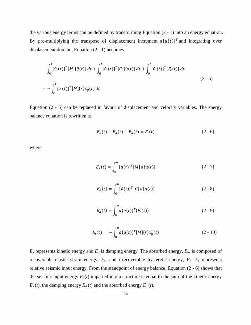
24
the various energy terms can be defined by transforming Equation (2 - 1) into an energy equation.
By pre-multiplying the transpose of displacement increment and integrating over
displacement domain, Equation (2 - 1) becomes
(2 - 5)
Equation (2 - 5) can be replaced in favour of displacement and velocity variables. The energy
balance equation is rewritten as
(2 - 6)
where
(2 - 7)
(2 - 8)
(2 - 9)
(2 - 10)
Ek represents kinetic energy and Ed is damping energy. The absorbed energy, Ea, is composed of
recoverable elastic strain energy, Es, and irrecoverable hysteretic energy, Eh. Ei represents
relative seismic input energy. From the standpoint of energy balance, Equation (2 - 6) shows that
the seismic input energy Ei (t) imparted into a structure is equal to the sum of the kinetic energy
Ek (t), the damping energy Ed (t) and the absorbed energy Ea (t).

25
Figure 2-1 Typical energy time history (Charney 2004)
Traditional energy-based design methods usually estimate seismic energy from an equivalent
SDOF system (Uang and Bertero 1990; Chou and Uang 2003). Figure 2-1 shows the energy
time-histories of an inelastic SDOF system (Charney 2004). It can be seen that the seismic input
energy continually increases during the ground motion. The SDOF method is based on the
assumption that the vibration shape developed during its motion can be determined by a single-
degree-of-freedom system. However, a steel building framework is an assemblage of beams and
columns connected at their ends and thus possesses a number of degrees of freedom. The
approximations obtained from a SDOF analysis cannot represent well the true dynamic behavior
of steel building frameworks. To accurately predict the seismic energy demand as well as the
hysteretic energy dissipation of building structures, a MDOF system model has to be included in
an analysis procedure. In the following, an approach to obtain seismic energies of a MDOF steel
building framework is proposed by making use of the results of an existing nonlinear time-
history analysis procedure.
2.1.2 Seismic Energy Computation
Seismic Input Energy
As shown in Equation (2 - 1), earthquake action on a SFRS can be interpreted as the inertial
forces resulting from the acceleration of ground motions. The seismic input energy Ei (t) in
0
5000
10000
15000
20000
0.0 5.0 10.0 15.0 20.0 25.0 30.0 35.0 40.0 45.0 50.0 55.0
En
erg
y (k
ip-i
n)
(1 k
ip-i
n =
0.1
13
kN
-m)
Time (second)
Hysteretic
Damping
Kinetic + Strain
Total

26
Equation (2 - 10), is a system level indicator of potential damage or demand description of a
SFRS.
It should be noted that the seismic input energy, Ei (t), represents the energy supplied
by instead by base movement, and for this reason, Ei (t) is called a ‘relative’
seismic input energy. As it was pointed out by Chopra (2007) that it is more meaningful to
employ an energy equation expressed in terms of relative motion than the one formulated in
terms of absolute velocity and displacement since it is the relative displacements that cause
forces in a structure.
For a MDOF system, its seismic input energy can be obtained by the following numerical
formulations:
where nm is the number of degrees-of-freedom; Ei,m (t) is the seismic input energy of the mth
degree-of-freedom at time t; and
(2 - 12)
where
(2 - 13)
is the inertial force vector of the m
th degree-of-freedom at time t; Mm is the mass value of
the mth
degree-of-freedom; is the ground acceleration at time t; Δut,m, Δut-Δt,m are the
displacement increments of mth
degree-of-freedom at time t and t-Δt, respectively.
Hysteretic Energy Dissipation
Compared to an elastic system, it is possible for an inelastic structural system to achieve less
kinetic and strain energy demand since its hysteretic energy dissipates part of the input energy.
(2 - 11)

27
The performance of a SFRS under a strong earthquake ground motion relies more on its
hysteretic energy dissipation capability since the properties of damping do not change
significantly.
At the structural system level, the energy dissipated through hysteretic behaviour can be
computed from the area enclosed by the lateral force-deformation curve of the SFRS as the
structure undergoes cyclic inelastic deformation. The representative lateral force-deformation
curves for two SFRSs are shown in Figure 2-2. Both systems possess the same strength and
deformation capacity. Figure 2-2-a shows a hysteretic behaviour in which nearly all of the
strength and stiffness of the SFRS can be maintained over a large number of cycles of inelastic
deformation. The wide and open force-deformation “loops” indicate that a large amount of
energy can be dissipated through hysteretic behaviour. On the other hand, Figure 2-2-b illustrates
a pinched hysteretic behaviour in which the SFRS suffers a rapid loss of stiffness under repeated
inelastic deformation. It is evident that the hysteretic energy dissipated through the inelastic
behaviours of the system shown in Figure 2-2-b is much lower than that of the system shown in
Figure 2-2-a. Conceptually, it can be concluded that the system shown in Figure 2-2-a will have
a higher level of possibility to survive under a severe earthquake ground motion. As a result,
maximizing the hysteretic energy dissipation capacity of a SFRS is usually one of the pursuits of
seismic design. Following such a design philosophy, seismic provisions always recommend that
a proper seismic design of a SFRS should employ an appropriate hysteretic energy dissipation
a) Ductile hysteretic loops
Deflection
Forc
e
b) Pinched hysteretic loops
Forc
e
Deflection
Figure 2-2 Typical hysteretic curves

28
mechanism to meet seismic energy demands rather than maintaining elastic structural response
under severe earthquake events.
In general, the actual capacity of hysteretic energy dissipation of a building structure depends not
only on the ductility of individual structural members but also upon the strength hierarchy and
the assemblage formulation among the system, and the dynamic characteristics of the earthquake
ground motion. In seismic design practice, it has been shown that various inelastic deformation
distributions among a SFRS do not lead to the same hysteretic energy dissipation capacity
(Paulay and Priestly 1992). Sometimes the differences are significant. Accordingly, capacity
design philosophy is employed to ensure structures dissipate seismic energy in a predictable and
stable manner under strong earthquakes. For steel Moment Resisting Frames (MRFs), it is
preferred to dissipate (FEMA 2004a; NRCC 2010) a large amount hysteretic energy through
formation of plastic hinges at the ends of beams rather than at the ends of columns. Namely,
beams are usually chosen as fuse members while columns are designed to deform elastically
(except at column bases where plastic hinges are often needed to allow for lateral inelastic drift)
to meet strength requirements. For steel Eccentrically Braced Frames (EBFs), shear links, which
are detailed to sustain the large inelastic deformations and thus have stable inelastic shear force-
deformation loops, are used as fuses to dissipate seismic energy and to protect the remainders of
the EBF from yielding.
When a structure is designed following the capacity design principle, the structure is
conceptually expected to form a favourable seismic energy dissipation mechanism under
earthquake. However, the extent of realizing the desired hysteretic energy dissipation mechanism
cannot be actually examined through an elastic analysis procedure. In order to quantify, rather
than just qualify, the hysteretic energy dissipation of a SFRS under an earthquake ground motion,
the dynamic response history of each individual member needs to be accounted for. The
hysteretic energy dissipation of a group of structural members can then be obtained by summing
the energies of individual members of the group. In this way, the hysteretic energy dissipations
of fuse and non-fuse members can be compared directly and the hysteretic energy dissipation
mechanism can be examined quantitatively.

29
In this section, a numerical approximation method to calculate the hysteretic energy of one
structural member is proposed by utilizing its seismic response history. The hysteretic energy
dissipations of fuse and non-fuse members will be employed as energy performance parameters
to direct the optimal design procedure.
Strains or deformations are produced when internal forces are induced within structural members.
Strain energy describes the energy absorbed during the deformation process. According to the
law of conservation of energy, the absorbed strain energy is equal to the work done by the
internal forces if no energy enters or leaves in the form of heat (Philpot 2008). To evaluate this
work, the manner in which the internal forces vary in respect to the deformations must be known.
In the typical force-deformation diagram of a structural member, as shown in Figure 2-3, the
vertical axis represents the generalized force (which may be the axial force, bending moment, or
shear force) and the horizontal axis represents the corresponding deformation of the structural
member. For a value of force Q1 on the load-deformation curve, its corresponding deformation is
denoted as δ1. As an increment dQ1 of the force produces an increment deformation dδ1, the work
done by the force during this incremental deformation is expressed as Q1dδ1. Geometrically, the
incremental work is represented by the area of the elemental strip below the force-deformation
B
C
Q
Q1
O
δ δ1
D
dδ1
dQ1
Irrecoverable
hysteretic energy
Elastic
strain energy
A
Figure 2-3 Elastic strain energy and irrecoverable hysteretic energy of structural members

30
curve in Figure 2-3. Consequently, the total work done by the force up to point B on the curve
can be denoted as the area below the load-deformation curve, i.e.,
(2 - 14)
For a structural member undergoing an inelastic strain beyond the elastic limit, a residual or
permanent strain remains in the member. As shown in Figure 2-3, the unloading line will be
parallel to the initial elastic portion of the curve when the force is removed. Of the total
deformation OC developed during the loading process, only portion CD is recovered and portion
OD remains as a permanent deformation. As a result, only part of the strain energy (i.e., the area
of triangle BCD) is recovered. The area OABD represents the energy permanently lost during the
loading history, i.e., irrecoverable hysteretic energy.
Various schemes are available to carry out the computation of hysteretic energy. The method
proposed hereafter is to utilize the force and displacement histories of structural members
obtained through the nonlinear time-history analysis procedure. For a frame member in a SFRS,
bending moment, axial force, and shear force are the primary internal force resultants. The frame
member will undergo flexing, changing in length, and warping in respect to these internal forces,
respectively. The hysteretic energy dissipation of a structural member Eh,k at the end of an
earthquake is expressed as the sum of the work of internal forces and corresponding
displacements, i.e.,
(2 - 15)
where
(2 - 16)
(2 - 17)

31
(2 - 18)
WMoment,k , WAxial,k, and WShear,k are the work done by the bending moment, axial force and shear
force of the kth
member, respectively; and ne is the number of the structural members. Mt,k, Pt,k,
and Vt,k are the internal bending moment, axial force and shear force of the kth
structural element
at time t, respectively. Δφt,k, Δxt,k, and Δyt,k are the increments of end rotation, axial deformation
and shear deformation of the kth
structural element from time (t-Δt) to time t, respectively. The
summation starts from time zero to the time point at which the time-history analysis ends. Then,
the hysteretic energy Eh can be expressed as
(2 - 19)
2.2 Structural Analysis Method
2.2.1 Nonlinear Time History Analysis
As a building structure deforms into its inelastic region, where the equation of motion governing
the dynamic response is denoted as Equation (2 - 1), the restoring force and the damping force
vectors may not remain proportional to the displacement or the velocity, respectively.
Furthermore, the ground motion acceleration varies arbitrarily with time, the analytical solution
of Equation (2 - 1) is usually impossible. As a consequence, the nonlinear responses of a MDOF
system will generally require a numerical procedure for the integration of differential equations.
A ground motion record is given by a set of discrete values (i.e., ), the
displacement, velocity, and acceleration vectors of a MDOF system are assumed to be known as
at time-step i, as well as the restoring force
vector .
These values satisfy Equation (2 - 1) at time-step i
(2 - 20)

32
The response quantities at a small time later, time i+1
(where ti+1 = ti + Δt), also satisfy Equation (2 - 1)
(2 - 21)
The incremental equilibrium equation of motion of the MDOF system can be obtained by
subtracting Equation (2 - 20) from Equation (2 - 21), i.e.,
(2 - 22)
where:
(2 - 23)
(2 - 24)
(2 - 25)
(2 - 26)
Although the restoring force vector {Fr} will not be proportional to the displacement vector {u}
when the structure deforms into its inelastic region, the incremental restoring force vector
Δ{Fr}t+Δt may be linearly approximated by assuming the tangent stiffness matrix [K]T constant
during the time increment Δt,
(2 - 27)
where Δ{u}t+Δt = {u}i+1 - {u}i.. Subsequently, the equation of motion of the MDOF system can be
approximated by a series of linear incremental equilibrium equations,
(2 - 28)

33
Employing Newmark method of direct integration, in which the variation of acceleration over the
time increment Δt is defined through the following equations by using parameters β and γ,
(2 - 29)
(2 - 30)
The structural response can be determined by an effective linear equation to calculate the
incremental displacement Δ{u}t+Δt
(2 - 31)
where:
(2 - 32)
(2 - 33)
Given the known initial conditions, , the quantities of structural response
at time step i+1 can be successively determined by using Equations
(2 - 22) to (2 - 33).
In the implementation of the Newmark method, the values of β and γ in Equations (2 - 29) and (2
- 30) need to be selected in advance. In this research, β = 0.25 and γ = 0.5 are adopted, since it
has been proven that the Newmark method is unconditionally stable when these parameter values
are used (Chopra 2007; Paz 1991).
For an inelastic system, a non-iterative procedure (i.e., from Equation (2 - 28) to Equation (2 -
33)) can lead to inaccurate results. As shown in Figure 2-4, discrepancies due to the use of the

34
tangent stiffness matrix can accumulate significant errors over a series of time steps. However,
the errors can be minimized by using Newton-Raphson iteration procedure.
To improve the numerical estimation during each time interval Δt, the iterative procedure starts
with the effective linear stiffness matrix and the initial unbalanced force
corresponding to displacement state of time ti,
(2 - 34)
where is the first approximation to the final increment ; is equal to the
incremental force vector calculated from Equation (2 - 33). In consequence, the first
approximation to deformation state of the whole system can be determined from
.
Figure 2-4 Illustration of tangent stiffness and secant stiffness
The force state, associated with
is evaluated to determine the corresponding
unbalanced force vector
(2 - 35)
Fr
O
U Ui
ΔU
Δ Fr
(Fr) i+1
(Fr) i
Ui+1
1
(Ki)sec
1
(Ki)T

35
The effective linear stiffness matrix is re-evaluated corresponding to the displacement
state of by using Equation (2 - 32).
Then, the second approximation is calculated by using the new effective stiffness
matrix and the new unbalanced force
(2 - 36)
The iterative process will continue until convergence is achieved. Once the norm of the
incremental displacement or the norm of the unbalanced force is less than a
specified tolerance, the final estimate of incremental displacement vector can be obtained,
(2 - 37)
With Δ{u}t+Δt known, the final estimate of incremental velocity and acceleration vector can be
solved using Equations (2 - 29) and (2 - 30),
(2 - 38)
(2 - 39)
Consequently, the quantities of are ready for the next time step. The
Newmark numerical integration method together with the Newton-Raphson iteration procedure
traces the displacement state of the whole MDOF system step-by-step till the end of the
excitation time history.
As shown in the incremental equilibrium equation (2 - 28), the direct numerical procedure of
integration for differential equations requires an explicit damping matrix [C]. However, the
damping properties of materials are not well established, and it is impractical to form the
damping matrix [C] directly from the properties of a structure. To account for the non-yielding

36
energy dissipation effect (such as the energy dissipated in friction at steel connections, stressing
of non-structural elements, and other similar mechanisms) in MDOF systems, the equivalent
viscous damping with recommended modal damping ratios varying between 3% and 7% is
adopted in structural engineering profession (Chopra 2007). Consequently, the damping matrix
[C] of a MDOF system can be determined from its modal damping ratios to simplify the
implementation. It should be noted that an increased damping ratio is often employed to estimate
energy losses due to anticipated inelastic effect in an elastic linear analysis. Such increased
damping values should be avoided in a nonlinear time-history analysis since the energy
dissipation effect of yielding is directly included in the analysis procedure.
It has been proven that classical Rayleigh-type damping is an appropriate idealization for the
dynamic analysis of a MDOF system (Leger and Dussault 1992; Paz 1991). For nonlinear time-
history analysis, a tangent damping matrix [C]t is employed to account for the continuous
changes in structural characteristics along the step-by-step numerical integration. Generally, the
tangent damping matrix [C]t can be expressed as a linear combination of mass matrix [M] with
various stiffness matrixes [K],
(2 - 40)
where [K]t is the tangent stiffness matrix of the current iteration; [K]i is the initial elastic
stiffness matrix; [K]c is the last converged stiffness matrix of the current iteration; am, bt, bi and
bc are the proportionality constants computed using the natural frequencies of the MDOF system.
The tangent damping matrix [C]t computed based on the initial stiffness matrix [K]i represents
constant damping during the analysis. On the other hand, the tangent damping matrix [C]t
computed using either the tangent stiffness matrix [K]t or the last converged stiffness matrix [K]c
of the current iteration accounts for the changes of stiffness matrix [K] in the process of time-
history analysis.
To be consistent with the aforedescribed step-by-step numerical integration procedure and
Newton-Raphson method, the tangent stiffness matrix [K]t of the current iteration is used (i.e., bi
= 0 and bc = 0) in Equation (2 - 40). Given two distinct frequencies, ωp and ωq (in practice, ωp is

37
taken as the first natural frequency and ωq is taken as the highest frequency to be considered in
the analysis), with damping ratios ξ = 5%, coefficients am and bt are expressed as
(2 - 41)
(2 - 42)
where, ωp and ωq are computed based on the initial elastic stiffness of the structure. The
experimental results agreed reasonably well with such determined damping matrix (Leger and
Dussault 1992).
During the Newton-Raphson iteration process defined by Equation (2 - 34) to Equation (2 - 37),
the determination of a force state corresponding to the displacement or deformation state of the
current time-step involves evaluation of both material and geometric nonlinearities. This
simulation of the nonlinearity of individual members is essential for structural nonlinear analysis.
2.2.2 Geometric and Material Nonlinear Analysis
Geometric and Material nonlinearities are two major concerns in the analysis of steel structures.
The nonlinearity properties of structural members are generally represented by advanced
analytical finite element models. Meanwhile, the structural responses, such as displacements and
internal forces, are approximated element by element through the aforementioned nonlinear
time-history analysis procedure.
Geometric Nonlinear Analysis
For a two-dimensional frame element, there are 6 unknown forces (with 3 at each end of the
element). As the corotational formulation of the frame element (Crisfield 1991) shown in Figure
2-5, it is assumed that (1) the basic system changes orientation as the element deforms; and (2)
the basic forces act on the deformed element with w1 always along the deformed element chord.

38
Practically, 3 element forces (i.e., axial force w1, end bending moment w2 and w3) are selected as
the basic forces to express the remainders by using 3 independent equilibrium equations.
Figure 2-5 Element forces in different systems
Considering equilibrium equations with respect to the un-deformed configuration, the element
end forces in the local coordinate system can be expressed in terms of the equilibrium
transformation matrix ,
(2 - 43)
By employing a rotation transformation matrix br, the element end forces p in the global
coordinate system can be stated as . Then, the equilibrium equations with respect to
the un-deformed configuration are expressed as
(2 - 44)
where be = br b. Similar to the transformation of the equilibrium equations from the basic system
to the global coordinate system, the geometric displacement-deformation compatibility relation
(w 2+ w 3)/L
w1
w 3
w 1
(w 2+ w 3)/L
I
J
P1
P5
P4
P3
I
J
P3
P1
I
J
w 2
P2
P6
P2
P5
P4
P6
α
X
Y
Basic system
Local system
Global system
Y
X

39
which transforms displacement u in the global coordinate system to the basic deformation v
(corresponding to the basic force w) is expressed symbolically as
(2 - 45)
where ag = ar a. By employing the virtual displacement principle which states that the work done
by element end force p on the virtual displacements is equal to the work done by internal
force w on the compatible virtual deformation , i.e.,
(2 - 46)
Equation (2 - 45) gives , then
(2 - 47)
If Equation (2 - 47) holds true for any possible virtual displacement then is
true. Comparing with Equation (2 - 44), the equilibrium Equation (2 - 47) demonstrates that the
equilibrium transformation matrix be is equal to the transpose of the displacement-deformation
compatibility matrix ag, i.e.,
(2 - 48)
Therefore, to transform the element force and displacement between different systems, only one
of these matrices is required to be established, the other can be obtained through a transpose
operation. In practice, if the forces transforms from the basic system (i.e., element end force w)
to the global coordinate system (i.e., element end force p) by using equilibrium transformation
matrix , then the displacements corresponding to forces transforms by using the
relationship .
A key step in the numerical algorithm for a nonlinear system is to determine the resisting forces
and the element stiffness matrix for a given displacement during the iteration process. The

40
tangent stiffness matrix of the element, is obtained as the partial derivative of the resisting
forces p with respect to the displacements u in the global coordinate system
(2 - 49)
where is the equilibrium transformation matrix under un-deformed configuration and
it does not depend on the displacement u; is the tangent stiffness of the basic
element associated with the yielding of material (i.e., the material nonlinearity property). Details
about will be discussed in the next section. The element force-deformation relation is
established in the basic system without rigid-body mode.
Figure 2-6 Deformed configuration of frame element
Equation (2 - 49) is derived on the assumption that the equilibrium equations are satisfied with
respect to the un-deformed configuration. To account for instability effect, element equilibrium
equations should be established based on the deformed configuration. As it is shown in Figure
2-6, since the rigid-body displacement of the element does not generate element deformation, the
displacement-deformation compatibility relation can be expressed as
Y
O
X
Local coordinate system
X
I
J
Y
L
I
Ln
v1
v2
u3=u3
β
v3
u6=u6
Δuy=u5-u2
Δux=u4-u1
Position of rigid mode
Deformed position
J
Basic system

41
(2 - 50)
where
(2 - 51)
(2 - 52)
The equilibrium equations of the free-body element are
(2 - 53)
Note that the equilibrium transformation matrix bu depends on the end displacements. In practice,
the terms of bu are approximated by a Taylor series with consistent order of magnitude. The
Equation (2 - 53) can be simplified to
(2 - 54)
In building frameworks, the shear force (w2 + w3) / L is usually small relative to the axial force
w1, and the transverse deformation is always less than 0.1 (Filippou and Fenves 2004).
Therefore, the so-called p-Δ transformation can be obtained with further simplification

42
(2 - 55)
Then, the rotation transformation matrix br is used to transform to the global coordinate system.
(2 - 56)
The tangent stiffness matrix of the element under deformed equilibrium equations can be
obtained,
(2 - 57)
From Equation (2 - 53), the tangent stiffness matrix in the local system is found as
(2 - 58)
When neglecting the difference between Ln and L in , it can be shown that the
condition holds.
Then, the tangent element stiffness matrix in the local system can be rewritten as
(2 - 59)
where
. According to Equation (2 - 59), it is noted that the geometric
transformation can be possibly separated from equilibrium transformation as long as the element
force-deformation relation is established in the basic system.

43
Combining Equations (2 - 57) and (2 - 59) gives
(2 - 60)
To obtain the exact geometric transformation, the geometric stiffness needs to be determined.
Using p-Δ transformation matrix to approximate the geometric stiffness is acceptable in
earthquake engineering.
(2 - 61)
In practice, the linear compatibility matrix be is used for the approximation of bu in the second
term of Equation (2 - 60). With such simplifications, the simplified form of Equation (2 - 60) can
be stated as
(2 - 62)
Using Equation (2 - 62), the material nonlinearity can be handled inside the basic system without
regard for the kinematic and equilibrium transformations outside the basic system.
Material Nonlinear Analysis
In general, the yielding effects of structural members are simulated in accordance with the stress-
strain relations of materials. The bilinear elastic-plastic stress-strain model is widely used in
earthquake engineering analysis. It has been found that the elasto-perfectly-plastic stress-strain
model (which neglects strain hardening) of structural steel material is generally conservative as
long as strength is the primary concern (Bruneau et al 1998). However, the influence of strain
hardening on plastic deformation calculations can be more significant. For uniaxial material
analysis, lower strain hardening values will generally produce larger maximum plastic strains

44
and curvatures while higher values will translate into higher stresses and moments. In this
research, the bilinear stress-strain relation of the Menegotto-Pinto model (Menegotto and Pinto
1973) with strain hardening (which is implemented in OpenSees analysis environment
(OpenSees 2008)) is employed for the nonlinear time-history analysis.
To simulate material nonlinear property of a structural member, either “concentrated plasticity
with elastic interior” or “distributed plasticity” models can be used through various approaches.
A concentrated plasticity analysis is often an approximate method as concentrated plasticity
models separate axial force-moment interaction from the member behaviour. However, the
actual end force-deformation relation of a frame member results from the integration of the
sectional response contribution along the element length. Thus, a calibration process against the
“concentrated plasticity element” is usually required to reflect the actual response under
idealized loading conditions. On the other hand, the gradual spread of yielding can be accurately
captured in a distributed plasticity analysis since the stress state is being updated with respect to
the integrated member sectional response. In this research, a distributed plasticity nonlinear
beam-column element is used to represent steel frame members.
Based on simplified assumptions such as plane sections remain plane, elements are subjected to
uniaxial bending, and shearing deformations are negligible, an efficient force-based nonlinear
beam-column element can be formulated in a manner that the equilibrium between bending
moment and axial force along the element can be strictly satisfied with regard to element
deformations. Specifically, the force-based element modeling starts with the analysis of the pre-
defined cross sections located along the element length. At each location, the element internal
forces are determined with respect to the equilibrium equation of the element, while the
corresponding sectional deformations at such locations are computed with respect to the defined
cross-sectional stress-strain relationship. It is obvious that the computed sectional deformations
should be compatible with the real deformations of the element with relation to the external
forces. Often, the reasonably accurate prediction of the nonlinear response can be achieved
through limited iterations. At the final step of the iterations, not only the internal forces but also
the nonlinear deformation distributions along the element length are obtained with respect to the
nonlinear stress-strain relationship of the structural material. Thus, the material nonlinear

45
property of the structural frame member can be directly defined in terms of the explicit relations
between the section force resultants and deformations.
Force-Based Distributed Plasticity Nonlinear Beam-Column in OpenSees
Figure 2-7 Basic (rotating) and global coordinate system (Neuenhofer and Filippou 1997)
Distributed plasticity of a beam-column member can be simulated either by displacement- or
force-based formulations. Following the standard displacement-based approach, the transverse
and axial displacements of a beam-column member are expressed as appropriate interpolation
functions of the nodal displacements. To approximate the nonlinear displacement field in the
displacement-based formulation, several elements are required along the length of a frame
member to represent the distributed plastic behaviour if the axial force is large. On the other
hand, the force-based beam-column element employs section forces interpolation functions to
formulate element flexibility matrix with respect to the element nodal forces. The ability to
maintain equilibrium within the element (even in the range of nonlinear response) makes it
possible to use one force-based element to simulate the nonlinear behaviour of a frame member
(Neuenhofer and Filippou 1997).
According to the corotational formulation (Crisfield, 1991), the element is formulated in the
basic system without rigid body modes and the specific transformation is employed to transform
the basic variables to the global system. The basic (rotating) and global coordinate systems of a
Y
O
X
X’
L
I
VE
I
J
Deformed position
J
Basic system
Y’
Section
D
X’
X’
S
MI
MJ
PE
Y’
Z’
Fiber
Hierarchy of element,
section, and fiber
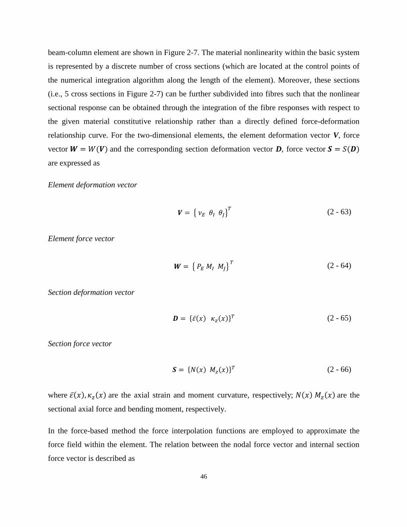
46
beam-column element are shown in Figure 2-7. The material nonlinearity within the basic system
is represented by a discrete number of cross sections (which are located at the control points of
the numerical integration algorithm along the length of the element). Moreover, these sections
(i.e., 5 cross sections in Figure 2-7) can be further subdivided into fibres such that the nonlinear
sectional response can be obtained through the integration of the fibre responses with respect to
the given material constitutive relationship rather than a directly defined force-deformation
relationship curve. For the two-dimensional elements, the element deformation vector V, force
vector and the corresponding section deformation vector D, force vector
are expressed as
Element deformation vector
(2 - 63)
Element force vector
(2 - 64)
Section deformation vector
(2 - 65)
Section force vector
(2 - 66)
where are the axial strain and moment curvature, respectively; are the
sectional axial force and bending moment, respectively.
In the force-based method the force interpolation functions are employed to approximate the
force field within the element. The relation between the nodal force vector and internal section
force vector is described as

47
(2 - 67)
where a(x) contains the force interpolation functions. Those interpolation functions can be
readily obtained from the equilibrium of axial forces and bending moments within the element.
For the two-dimensional elements shown in Figure 2-7, the interpolation function matrix is
expressed as
(2 - 68)
The compatibility relationship between the section and element deformations can be determined
by employing the principle of virtual force,
(2 - 69)
In the force-based Finite Element Analysis, the element flexibility matrix needs to be formulated
in advance. The linearization of deformation or displacement with respect to the corresponding
force yields the flexibility matrix. The section flexibility matrix fs and element flexibility matrix
F can be expressed, respectively, as
(2 - 70)
(2 - 71)
Substituting equations (2 - 67) and (2 - 70) into equation (2 - 71) yields the element flexibility
matrix
(2 - 72)

48
While the control sections are subdivided into fibres, the strain distribution in a section x can be
determined based on the assumption that the plane section remains plane and normal to the
longitudinal axis. Then the corresponding stresses and tangent modulus with respect to the strain
values at each fibre are computed according to the material constitutive relation. Subsequently,
the section stiffness ks(x) and resisting force S(x) are evaluated through a numerical integration
scheme, respectively. The section stiffness is then inverted to obtain the flexibility matrix fs(x).
Then, the element flexibility matrix F is computed from Equation (2 - 72).
As shown in the element formulation procedure, the advantage of the force-based element is that
it always comes up with force interpolation functions which satisfy equilibrium exactly.
However, the implementation of the force-based element model in a direct-stiffness-method-
based nonlinear analysis program is not straightforward (Neuenhofer and Filippou 1997; Scott et
al 2008). When iterative numerical methods (i.e., the procedure from Equation (2 - 34) to
Equation (2 - 39)) are employed to solve the nonlinear system differential equations, the element
stiffness matrix as well as the force state at each iteration step need to be determined. Although
the element stiffness matrix can be obtained by inverting the element flexibility matrix F, there
are no direct functions to compute the element generalized resisting forces (e.g., the element
forces corresponding to in Equation (2 - 35)) with respect to the section force vector S.
Figure 2-8 Evaluation of force-based element compatibility relation (Scott et al 2006)
ξ
ω3=0.36L
aTD
j
ξ1=0
ξ2=0.17L ξ3=0.5L ξ4=0.83L ξ5=1.0L
ω2=0.27L ω4=0.27L
ω1=0.05L ω5=0.05L

49
In practice, an iterative algorithm at the element level (Spacone et al 1996) is employed to
approach the element force state with respect to the updated deformation state. The detail of the
procedure is described in Appendix 2.A. It has been shown (Neuenhofer and Filippou 1998) that
by using the force-based nonlinear element, only one element is required to represent the
material nonlinearity of a frame member. Comparing to the displacement-based nonlinear
elements where several elements are needed to approximate the nonlinear displacement field, the
degrees of freedom of the structural model can be substantially reduced. Therefore, the potential
computational saving is obvious.
Figure 2-9 Plastic rotation in beam-column
To restore the element deformation from the section deformations, the Gauss-Lobatto quadrature
numerical method is employed to evaluate the integral of Equation (2 - 69). The numerical
procedure can be visually illustrated in Figure 2-8, where ξ and ω represent locations and
associated weights, respectively, of the Np integration points over the element length. The
method is equivalent to treating as constant over the length for the element deformation
evaluation. The relation between the element deformation and the convergenced section
deformation can be numerically expressed as
(2 - 73)
Elastic
unloading
q=0
Force
q
O
Deformation
ke
ke= (Fe)-1
vp
ve= (Fe)q
v

50
To assess the plastic rotation of a beam-column, the element deformation is decomposed into
elastic and plastic components. As shown in Figure 2-9, the plastic deformation can be computed
(Scott et al 2006) as
(2 - 74)
2.2.3 Input Ground Motion Time Histories
The inelastic behaviour of steel building frameworks depends not only on the dynamic
characteristics of the SFRSs, but also upon the properties of the input ground motion time
histories. For a nonlinear time-history analysis, the ground motion histories can be obtained by
scaling and/or modifying real records from past earthquakes or by employing suitable artificial
records. Tremblay (2001) showed that simulated time histories and real ground motion time
histories are functionally equivalent for both linear and nonlinear analyses.
The adopted ground motion time histories for conducting a nonlinear time-history analysis
should be consistent with the magnitude, fault distance, and source mechanism where the
building structure is to be built. Furthermore, due to the sensitivity of structural response to the
properties of a ground motion, a nonlinear time-history analysis using only one ground motion
time history input may not truly represent the actual seismic responses. To account for this
uncertainty in earthquake loading, an assembly of (e.g., at least three by NBCC 2010) different
ground motion time histories are required for one nonlinear time history analysis. When a
sufficient number of ground motions are included in a nonlinear time history analysis (e.g., 7 by
FEMA-450 (2004a)), the mean values of structural responses are used as the performance
parameters for design purposes. In this research, mean values of the structural responses such as
seismic input energy, hysteretic energy, and deformations are used in the design examples.
To serve the purpose of this research, an assembly of recorded “real time histories” selected from
the PEER Strong Ground Motion Database (PEER 2008) will be used. The adopted ground
motion time histories will be scaled to simulate the design earthquake hazard level. In particular,

51
as a design earthquake level is typically represented by a design spectrum, the adopted ground
motions will be scaled such that their response spectrum coordinates should equal to or exceed
the corresponding design spectrum value throughout the period range of interest. The details of
how to scale the selected ground motion time histories to be compatible with a design spectrum
are presented in the design examples in Chapter 4.
2.3 Comparison of Seismic Energy Input
In this section, an educational program called NONLIN (Charney 2004) has been employed to
validate the proposed numerical method for seismic energy computation (which is described in
Section 2.1.2).
As it is shown in Figure 2-10, a feasible design of the steel portal frame is subjected to a given
earthquake ground motion (the details of the design problem are shown in Appendix 3.B). Herein,
the educational software NONLIN (Charney 2004) serves as the baseline for comparison. Since
NONLIN is only applicable for the dynamic analysis of SDOF systems (i.e., only one mass is
considered by NONLIN), the analytical model for comparison needs to be calibrated. For this
reason, the design with the smallest column structural steel section size, W12x30 (W310x45),
and the largest structural steel beam section size, W18x106 (W460x158), in which the difference
between the lateral displacements of the two mass points (i.e., the two beam-to-column joints) is
the minimum among the total 256 trial designs so that the structural response can be estimated by
using a SDOF model, is employed for comparison.
W18x106
(W460x158)
W12x30
(W310x45)
Figure 2-10 Steel portal frame for computation of seismic energy input
W12x30
(W310x45)

52
Figure 2-11 Push-over curve (base shear – story displacement) for model calibration
First, an equivalent SDOF model of the portal frame needs to be established for NONLIN. The
lateral stiffness and strength parameters of the SDOF model are obtained from the push-over
curve of the steel portal frame. The solid-line shown in Figure 2-11 illustrates that the portal
frame is pushed to the lateral displacement of 3% story height (0.03x12x13=4.68 in (0.118 m)).
The bilinear dashed-line is used to approximate the lateral force vs. deflection of the SDOF
model. Thus, the parameters for the SDOF model are as follows: yield strength Fy=53.4 kip (237
kN), initial stiffness k1= 38 kip/in (6654 kN/m), and post yield stiffness k2=2 kip/in (350 kN/m).
Figure 2-12 Comparison of lateral displacement response histories
The lateral displacement response histories of the SDOF and MDOF models are compared in
Figure 2-12, where the curves are obtained by adopting the ground motion record of “Imperial
Valley 10/15/79 2316, El Centro array #12” (PEER 2008) with a scale factor of 3.0. It can be
0
10
20
30
40
50
60
70
0 1 2 3 4 5
Ba
se s
hea
r (k
ip,
1 k
ip =
4.4
48
kN
)
Story displacement (in, 1 in = 0.0254 m)
OpenSees_MDOF_Model
NONLIN_SDOF_Model
-3
-2
-1
0
1
2
0 2 4 6 8 10 12 14 16
No
de_
dis
pla
cem
ent
(in
, 1
in
= 0
.02
54
m)
Time (second)
NONLIN_Model
OpenSees_Model

53
seen that the nonlinear response of the SDOF model of NONLIN agrees well with the response
of the MDOF model of OpenSees.
Figure 2-13 Seismic energy input response history
Figure 2-13 shows the comparison of seismic input energy histories obtained by various methods.
The history curves “NONLIN_Numerical” and “OpenSees_Model” are obtained using the
proposed procedure in Section 2.1.2 (SDOF model in NONLIN and MDOF model in OpenSees).
The NONLIN program uses a step-by-step method to solve the nonlinear equations of motion.
The history curve “NONLIN_Result” is obtained by the embedded method in NONLIN program.
Indeed, all the curves show the same trend of the seismic input energy during the earthquake
ground motion. The curve of “NONLIN_Numerical” matches the curve of “NONLIN_Results”
perfectly. Some small differences can be observed between the energy history curves of
“NONLIN_Numerical” and “OpenSees_Model”, which is derived from the estimation errors of
the lateral displacement response histories (see Figure 2-12) of the two models. It can be
concluded from this numerical test that the proposed method for seismic energy computation
(Section 2.1.2) is valid.
0
50
100
150
200
0 2 4 6 8 10 12 14 16
Inp
ut
ener
gy
(k
ip-i
n)
(1 k
ip-i
n =
0.1
13
kN
-m)
Time (second)
NONLIN_Result
NONLIN_Numerical
OpenSees_Model

54
Chapter 3
Design Optimization Problem Formulation
The task of the seismic design of steel building frameworks is to proportion the member sizes of
a SFRS of a steel building as per the governing seismic provisions and economical requirements.
Conventionally, the design process involves repetitive application of structural analysis with
respect to the iterative changes in member sizes. Often, the trial-and-error design cycle could be
repeated quite a number of times. Specifically, the reanalysis-redesign cycle may lead to an
uncontrollable decision-making state when a nonlinear time-history analysis is employed as the
evaluating tool since it is much more difficult to predict the nonlinear structural response
beforehand with regard to the changes in member sizes. To overcome the computational
difficulties, efficient and reliable strategies are needed to facilitate the tedious analysis-design
procedure.
On the other hand, the conventional trial-and-error evolving design procedure can be
conceptually viewed as an optimization process. It is intuitive that an efficient and reliable
design methodology can be developed with the assistance of optimization techniques. Indeed,
devotion to providing optimization techniques in design of steel frameworks to achieve
economical structures has gained wide acceptance in academic community over years. This
research will extend optimization applications to develop an automatic capacity design procedure
for steel building frameworks by using nonlinear time-history analysis.
In this research, the optimal design solutions are sets of cross-section sizes of commercially
available steel shapes. In its general mathematical form, a multi-objective design optimization
problem can be expressed as
(3 - 1)
(3 - 2)

55
(3 - 3)
(3 - 4)
where: OBJ is a set of objective functions; X is the vector of nx design variables that are required
to be found in order to minimize the objective functions; gl(X) is the lth
constraint function
bounded by its upper limit, glu ; xj
l and xj
u are the lower bound and upper bound for design
variable xj respectively. For discrete variables, the variable xj should be selected from among a
predetermined set of Xj of discrete sizes.
Specifically, the details of the proposed energy-based optimal design methodology, i.e., the
formulations of design objective functions and the design constraints, are described in the
following sections.
3.1 Design Objective Functions
An objective function, also known as a cost or performance criterion which is used as a measure
of effectiveness of a design, is expressed in terms of design variables and serves as a decision
motivator. Generally, one design with a preferable objective value compared to another can be
deemed as a “better design” if all the design constraints are satisfied. For seismic design of steel
building frameworks, the proposed objective functions (along with the design constraints) must
represent the structural behaviour regarding to the design ground motions and reflect the seismic
design philosophy. The measures which are most interesting to structural engineers should be
included in the optimization framework. In this research, three design objectives are considered:
1) the minimum structural cost of SFRS; 2) the minimum seismic input energy imparted to the
SFRS; and 3) the maximum hysteretic energy dissipation of the fuse members of SFRS.
3.1.1 Minimum Cost of SFRS
Cost-saving is usually the pursuit of every structural design. Herein, minimum structural cost is
adopted, as in many other optimization problems. Under the assumption that member cost is in
proportion to its weight, the least-cost design can be interpreted as the least-weight design of the

56
structure; and the structural cost objective OBJ1 is thus expressed by the following minimization
function:
(3 - 5)
where: X is the vector of design cross-section size variables; ρ is the material mass density; Lk
and Ak are the length and cross-sectional area of the kth
member, respectively; and ne is the
number of the structural members in the SFRS.
3.1.2 Minimum Seismic Input Energy
The structural demands on a SFRS in terms of stiffness, strength, and energy dissipation are
interrelated with the supplies while the structure responds to earthquake ground motions. The
potential seismic damage depends on the severity of earthquake ground motions (or peak ground
acceleration), duration of earthquakes and the frequency contents of the ground excitations.
Seismic energy input quantities, rather than a single peak force or displacement response,
account for the duration and dynamic effects of seismic loading. The smaller the amount of
energy imparted into a SFRS is, the smaller the amount of consequential damage will be and the
greater the chance the structure will survive. It is desirable to design building structures with the
minimum damage potential with respect to earthquake ground motions; i.e., the objective OBJ2 is
expressed by the following minimization function:
(3 - 6)
where is the mean value of the seismic input energies for ng ground motions considered in the
nonlinear time-history analysis.
3.1.3 Maximum Hysteretic Energy Dissipation of Fuse Members
It has been widely accepted that (FEMA 2004b; NRCC 2006) a well performing SFRS should be
able to dissipate a large amount of seismic energy through its stable, non-degrading, predictable
cyclic inelastic behaviour. Indeed, the analysis of hysteretic energy dissipation mechanisms
forms the basis for seismic design. To dissipate seismic energy efficiently and safely, the

57
capacity design principle is explicitly required in seismic provisions. Since fuse members are
detailed to stably sustain large cyclic inelastic deformations, a large amount of seismic input
energy can be dissipated through fuse members without significant impact on the integrity of a
SFRS. From the viewpoint of energy, it is reasonable to say that the larger the amount of energy
dissipated through fuse members, the greater the chance the structure will survive. Thus, the
hysteretic energy dissipation objective which reflects the capacity design philosophy is expressed
by the following maximization function:
(3 - 7)
where is the mean value of the hysteretic energy
dissipation ratio of fuse members under ground motions; in which Eh_fuse is the hysteretic
energy of fuse members and Eh is the total hysteretic energy of the SFRS (it is shown in the
numerical examples that this objective function effectively serves to confine plastic deformation
to the fuse members of a SFRS).
3.2 Design Constraints
In general, the space of design solutions is divided into a feasible domain and an infeasible
domain based on the satisfaction of the imposed constraints. Following an optimization
procedure, while the objective functions are improved, a feasible design has to satisfy a host of
stress, displacement, buckling, fabrication and functional requirements.
The constraints that represent limitations to the performance of a system are termed performance
constraints. On the other hand, the constraints imposed on the availability, fabrication or other
physical limitations are called side constraints. For this research, the specific constraint functions
are described as follows.
3.2.1 Performance Constraints
All feasible designs are required to resist force and deformation actions within the acceptance
criteria stated in a governing code or specification. To be consistent with current seismic design
practice, the research considers the seismic performances of both individual structural members
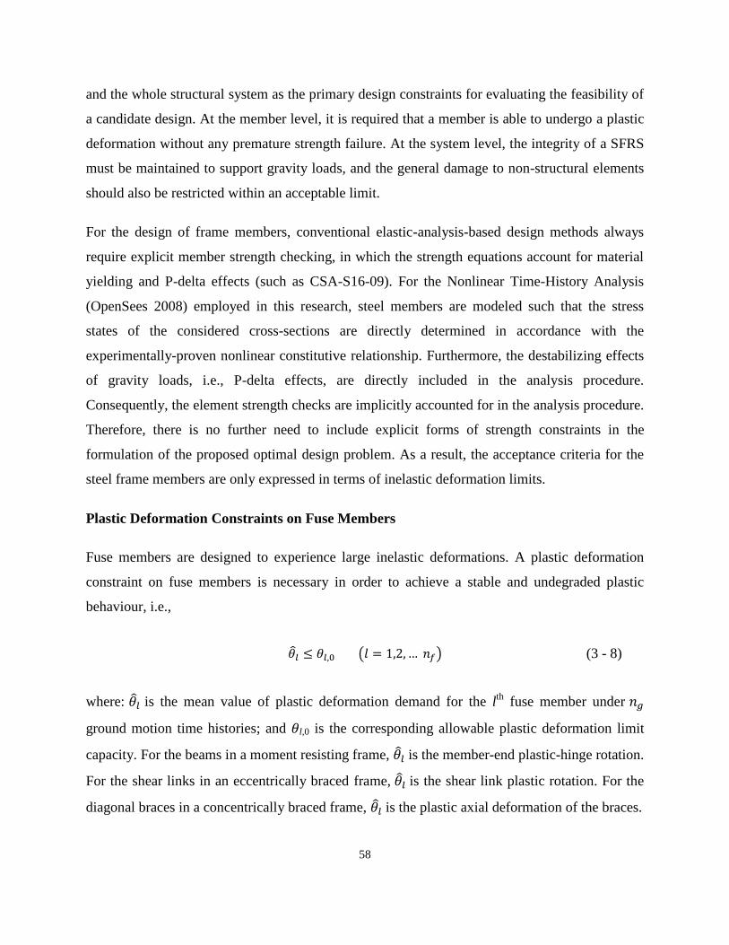
58
and the whole structural system as the primary design constraints for evaluating the feasibility of
a candidate design. At the member level, it is required that a member is able to undergo a plastic
deformation without any premature strength failure. At the system level, the integrity of a SFRS
must be maintained to support gravity loads, and the general damage to non-structural elements
should also be restricted within an acceptable limit.
For the design of frame members, conventional elastic-analysis-based design methods always
require explicit member strength checking, in which the strength equations account for material
yielding and P-delta effects (such as CSA-S16-09). For the Nonlinear Time-History Analysis
(OpenSees 2008) employed in this research, steel members are modeled such that the stress
states of the considered cross-sections are directly determined in accordance with the
experimentally-proven nonlinear constitutive relationship. Furthermore, the destabilizing effects
of gravity loads, i.e., P-delta effects, are directly included in the analysis procedure.
Consequently, the element strength checks are implicitly accounted for in the analysis procedure.
Therefore, there is no further need to include explicit forms of strength constraints in the
formulation of the proposed optimal design problem. As a result, the acceptance criteria for the
steel frame members are only expressed in terms of inelastic deformation limits.
Plastic Deformation Constraints on Fuse Members
Fuse members are designed to experience large inelastic deformations. A plastic deformation
constraint on fuse members is necessary in order to achieve a stable and undegraded plastic
behaviour, i.e.,
(3 - 8)
where: is the mean value of plastic deformation demand for the lth
fuse member under
ground motion time histories; and l,0 is the corresponding allowable plastic deformation limit
capacity. For the beams in a moment resisting frame, is the member-end plastic-hinge rotation.
For the shear links in an eccentrically braced frame, is the shear link plastic rotation. For the
diagonal braces in a concentrically braced frame, is the plastic axial deformation of the braces.

59
Plastic Deformation Constraints on Non-Fuse Members
For the non-fuse members in a SFRS, their plastic deformations usually need to be strictly
restricted. In its generic form, the deformation constraints on non-fuse members of SFRSs can be
expressed as
(3 - 9)
where: is the mean value of the plastic deformation demand of the mth
non-fuse member; and
φm,0 is the corresponding allowable plastic deformation. If no plastic deformation is permitted,
the value of φm,0 should be set to a very small number but non-zero to facilitate the numerical
instabilities in the design algorithm.
Plastic Deformation Capacities of Frame Members
The typical moment versus deformation curve of a steel member is illustrated in Figure 3-1. The
curve is composed of an elastic range, points O to A on the curve, and an inelastic range, points
A to C. The inelastic portion of the curve includes a strain hardening range, points A to B, and a
strength degraded range, points B to C. In general, the deformation acceptance criterion for a
ductile behaviour of a member should be within the ranges between O to B. Steel beams, having
a compact cross section, always exhibit a large plastic range without significant moment capacity
degradation. The failure of such a beam is characterised by the exhaust of its plastic deformation
capacity. For a beam-column, its plastic deformation capacity is greatly influenced by the
existence of an axial force. In general, the greater the axial force is, the less its plastic bending
deformation capacity will be. For example, if the axial force of a beam-column is equal to its
pure axial force resistance (i.e., the capacity of the member under axial force only), then its
plastic bending deformation capacity (the range AB) is zero.
The plastic rotation capacities of shear links in EBFs are taken as 0.08 radians in the Canadian
Standard CSA-S16-09. The plastic deformation capacity of a beam-column, l,0 or φm,0, is
dependent upon both its axial force and sectional slenderness ratio. According to the ASCE/SEI
standard 41-06 (ASCE 2007), (see Appendix 3.A for details) the plastic rotation capacity of a
ductile frame member, whose axial force ratio is less than 0.2, is at least 3.0 y, where y is the

60
yield rotation and is computed as . The plastic rotation capacity is at least
equal to 0.8 y if the member has a greater axial force. The actual chosen values for the plastic
limits in Equations (3 - 8) and (3 - 9) must reflect capacity design philosophy in addition to
satisfying the deformation capacity requirement.
It should be noted that the recommended acceptance criteria in Appendix 3.A correspond to
Collapse Prevention level. If the Immediate Occupancy performance level is required, the
acceptance criteria will be much more stringent (ASCE 2007). For example, in general, the
allowable plastic rotations under the Immediate Occupancy level are less than 1.0 y. Practically,
such a small plastic deformation level may be interpreted as non-detrimental plastification
allowed in non-fuse members for enforcing the capacity design requirements.
Table 3-1 Plastic rotation limits of structural members
Type of SFRS Fuse Members Non-Fuse Members
MRF Beams 8 y / 3 y Columns 2.0 y / 0.5 y
EBF Shear Link 0.08 radians
Beams 0.6 y
Columns 0.5 y
Braces 0.5 y
Table 3-1 gives the plastic deformation acceptance criteria adopted by the design examples for
MRFs in Chapter 4 and EBFs in Chapter 5. For MRFs, the allowable plastic rotation for columns
is taken as 2.0 y to 0.5 y depending on the relative magnitude of the column axial force. For
A
B
C
M
My
O
y
Figure 3-1Typical bending moment versus deformation curve

61
EBFs, 0.5 y and 0.6 y are adopted as the allowed non-detrimental plastic deformations for non-
fuse beam-column and beam members, respectively.
Deformation Constraints on SFRS
Stability of seismic force resisting systems is another essential issue for building structures to
survive a strong earthquake ground motion. To this end, controlling drift is still commonly
employed as a practical method to indirectly address the overall stability problem in spite of P-
delta effects being already considered in structural analysis procedures. It has been proven that
the earthquake damage to non-structural elements can also be restricted through drift controls
(FEMA 2004b).
Specifically, a SFRS is deemed to be lateral deformation acceptable if it satisfies the following
constraints on the inter-storey drifts,
(3 - 10)
where: is the mean value of the sth
inter-storey drift for ng ground motions; ns is the number of
stories; δ0 are the specified allowable values for drift.
3.2.2 Side Constraints
General speaking, it is desirable to use commercially available standard sections to proportion
steel frameworks. Furthermore, the local buckling failure of structural members should be
avoided to ensure the development of stable, non-degrading hysteretic behaviour. For this
research, the frame members are selected from among the compact sections if the development
of plastic hinges is anticipated. At present, the side constraints imposed on the optimization
problem can be expressed as
(3 - 11)
where: Cj is a set of discrete steel cross-sections (e.g., from AISC 2005b or CISC 2010) for
member j.

62
3.3 Optimization Formulation and Algorithm
From the forgoing, the multi-objective design optimization problem is formulated as follows:
(3 - 12)
(3 - 8)
(3 - 9)
(3 - 10)
(3 - 11)
where the objective vector OBJ consists of three objective criteria. The objective functions in
Equation (3 - 12) are normalized in order to facilitate numerical realization. The cost objective is
normalized as , where is the largest cross section in set
Ck or among the current group of evaluated designs. The input energy objective defined in
Equation (3 - 6) is normalized as , where is the maximum input energy
among the current group or population of evaluated designs. The third objective on hysteretic
energy in Equation (3 - 7) is transformed into a minimization criterion by rewriting it as
. Thus, all the three normalized objectives, f1 to f3, have a value ranging from 0 to 1.
For multi-objective optimization problems, it is common that there is no unique design that could
achieve all of the optimal criteria simultaneously. As the objectives generally conflict with each
other, it is expected that a set of optimal solutions with a varying degree of the objective values
are available. Such optimal solutions are known as ‘Pareto-optimal’ since none is dominated by
other feasible solutions for all of the objectives. Therefore, the important task for solving a multi-
objective optimization problem is to find as many Pareto-optimal solutions as possible (ideally,
all the Pareto-optimal solutions would be found). Although only one solution is required in a
real-world optimization problem, the knowledge of the optimal solutions can facilitate the trade
off study between various objectives.

63
Various optimization algorithms are available to solve a multi-objective design problems. A
classical method is to transform a multi-objective optimization problem into a single-objective
problem by introducing a weight vector for the multiple objectives. However, only a single
optimal solution can be found each time when using this converted single-objective formulation.
One has to use the algorithm many times in order to find a set of Pareto-optimal solutions
through adjusting the user-defined weight vector.
For this research, no preference is given to any particular criterion. Thus, a weight vector is not
employed. Instead, the Multi-objective Genetic Algorithm (MGA) based on the concept of
domination (Deb 2001) is adopted hereafter. Genetic Algorithm (GA), a procedure simulating
Start Initialize design variable list;
create sets Ck Generate initial population ‘bitString”
No
Conduct NRH analysis. Obtain values of objectives and
constraints. Store structural responses of ith
design.
Load up structural
responses of ith
design
Evaluate normalized objectives f1, f2 and f3. Apply penalty if necessary.
Generate next
generation
Stop
Has every design
of the generation
been evaluated?
Convergence?
Decode this Generation
Are the structural responses
of i th
design available?
Yes Output pareto
optimal solutions
GA black box
Yes
No
No
Yes
Figure 3-2 Flowchart of the proposed design procedure

64
the natural evolution process, has been successfully used in a wide array of applications due to
ease of implementation and robust performance. GA is especially suitable for the design problem
of this research since it does not require gradient information and it is the perfect fit for discrete
optimization problems. A typical GA uses reproduction, crossover and mutation operations to
create a subsequent generation based on the relative fitness values of the current generation.
Thus, the average quality of the solutions is improved from one generation to the next. The
striking advantage of using GA for multi-objective optimization problems is that a population of
solutions is processed in each iteration (or generation), and the outcome of one implementation is
also a population of solutions. In each generation of the adopted MGA, the pair-wise
comparisons (with respect to all of the objectives) are conducted to classify the population into a
non-dominated set and a dominated set (the solutions of the non-dominated set are better than
those of the dominated set). Thus, multiple trade-off solutions among each generation can be
determined in one single run. As the population set improved with respect to the non-dominated
set of solutions, the MGA will end up with the Pareto-optimal solutions in its final population.
For the multi-objective design optimization problem Equations (3 - 8) to (3 - 12), the design
procedure is described as follows:
1) Each of the design variables is encoded with a fixed-length binary
string regarding to the side constraints.
2) Each design is represented by a unique Binary String Chromosome formulated from the
encoded design variables.
3) The first generation of designs is randomly generated.
4) The objectives and constraints of each design of the current generation (or population)
are evaluated by using Nonlinear Time-History analysis.
5) The design objectives are normalized with respect to their maximum values among the
current population.
6) A penalty number 1.0 is added to all the three normalized objectives f1 to f3 if any of the
design constraints is violated.
7) The current population is handled by the Multi-objective Genetic Algorithm to generate a
new population set.

65
8) Repeat step 4 to step 7 until the convergence criterion is satisfied.
The overall design procedure is also illustrated by the flowchart in Figure 3-2. The MGA
algorithm embedded in MATLAB software package (The MathWorks Inc. 2009) is adopted and
treated as a black box during computer programming. The convergence criterion, called the
spread of Pareto-optimal solutions (Deb 2001) is defined as
(3 - 13)
where is the mean distance of interior Pareto-optimal solutions, and nint is the
number of interior Pareto-optimal solutions;
is the crowding distance
of Pareto-optimal solution i, defined as the objective difference of its two neighbouring solutions
(i+1) and (i-1); n0 is the number of objectives, which is equal to 3 for this study; dex is the
distance between extreme Pareto-optimal solutions; and for
interior Pareto-optimal solutions. The more detailed description of sp can be found in MATLAB.
A design iterative process is considered to converge if the average change of sp over a number of
generations is less than a specified tolerance. Alternatively, a design process may be terminated
if a specified maximum generation number is reached.
In summary, the nonlinear dynamic analysis-based capacity design of steel building frameworks
is cast into a multi-objective optimal design problem and it is solved using a genetic algorithm.

66
Chapter 4
Design of Moment Resisting Frames
This chapter presents optimal design solutions for a 3-story and 4-bay Moment Resisting Frame
(MRF). The design problems serve as the numerical examples to illustrate the effectiveness and
practicability of the proposed optimal design formulation in the previous chapter. The specific
techniques and numerical strategies required for conducting design of MRFs are demonstrated
through the examples.
4.1 Geometry and Seismic Loading of the 3-Story-4-Bay MRF
The MRF is the seismic force resisting system of a hypothetical three-story office building
located in Vancouver, British Columbia, Canada.
The plan view of the office building is shown in Figure 4-1. The structural layout is symmetric
and the seismic lateral loads in each principal direction are resisted by a pair of 4-bay MRFs
located at the perimeter of the building. The schematic side view of a MRF is illustrated in
MRF
MRF
MRF
MRF
Figure 4-1 Plan view of the hypothetical office building
9.14m x 4 = 36.56 m
9.1
4 m
x
6 =
54
.84 m

67
Figure 4-2. A fictitious lean-on column, connected with the MRF through a rigid link at each
floor level, is used in the analytical model to simulate the effect of interior simple gravity frames.
For the purpose of illustration, only east-west direction MRF design is considered in this
example.
All four bays are each 9.14 m wide (centerline dimensions) and all three stories are each 3.96 m
high. The design dead and live load are 4.79 kPa and 2.39 kPa for both of the first and second
story, respectively. The roof has dead load of 4.07 kPa and live load of 0.96 kPa. For each frame,
the seismic weights of floors 2, 3, and the roof are 4567 kN, 4567 kN, and 4850 kN, respectively.
The distribution of the seismic weights among the frame and the leaning column is illustrated in
Figure 4-2(b).
1
2
3
4
5
6
9
11
8
14
12
10
13
7
15
16
17
18
19
20
21
9.14 m x 4 = 36.56 m
23
24
25
26
27
Fictitious
Column
29.1 kN/m
29.1 kN/m
26.5 kN/m
3503kN
3503kN
3881kN
(a) member numbering
(b) seismic weight distribution
Figure 4-2 Side view of the E-W direction MRFs
3.9
6 m
x 3
= 1
1.8
8 m

68
Table 4-1 Selected ground motion time-histories
Record Name Earthquake
Magnitude
PGA
(g) PGV (cm/sec)
Scale
Factor
1979 Imperial Valley: El Centro Array #12 (EL_2.1) 6.5 0.143 17.6 2.1
1989 Loma Prieta: Belmont Envirotech (BES000_4.5) 6.9 0.108 11.8 4.5
1994 Northridge: Old Ridge RT 090 (ORR090_0.8) 6.7 0.568 52.1 0.8
1989 Loma Prieta: Presidio (PRS090_1.5) 6.9 0.2 32.4 1.5
Figure 4-3 Response spectra
The design response spectrum for Vancouver specified by the National Building Code of Canada
(NRCC 2010) is employed as the datum for scaling ground motions. The spectral acceleration
values are 0.97g, 0.65g, 0.32g, 0.17g, and 0.085g at period T = 0.2, 0.5, 1.0, 2.0, and 4.0 sec,
respectively (g is the gravity acceleration). Though FEMA-450 (FEMA 2004a) requires seven
ground motions to establish average values of the structural response, with the view to mitigate
calculation burden, only four ground motions (i.e., ng=4) are herein adopted from PEER (PEER
2008) for this example. The selected ground motion time-histories need to be scaled such that
their response spectra equal to or exceed the design response spectrum throughout the period
range of interest. The names of the adopted ground motion records and the corresponding scale
0.0
0.2
0.4
0.6
0.8
1.0
1.2
1.4
1.6
1.8
0.00 0.25 0.50 0.75 1.00 1.25 1.50 1.75 2.00 2.25
Sp
ectr
al
A
ccel
era
tio
n (g
)
Period (second)
Design Spectrum
EL_2.1
BES000_4.5
ORR090_0.8
PRS090_1.5

69
factors are shown in Table 4-1 (the ground motion acceleration histograms are given in
Appendix 4.A). Illustrated in Figure 4-3 are the response spectra of the scaled ground motions.
Note that these response spectra are equal to or greater than the design spectral values throughout
the period ranging from 1.0 sec to 2.25 sec.
The frame is assumed to have rigid beam-to-column connections, with all column bases fixed at
the ground level. All the columns use wide-flange sections of 345 MPa grade steel, while all the
beams use wide-flange sections of 248 MPa grade steel based on the consideration of ductility.
As shown in Figure 4-2(a), the MRF consists of 27 structural members. Two different numerical
examples will be executed for this MRF according to different member linking schemes. The
first example, with only two design variables, as shown in Figure 4-4(a), is used to illustrate the
basic behaviour of the design formulation. The second example, optimizing the same moment
resisting frame with more design variables, as shown in Figure 4-4(b), is carried out to illustrate
the method applied to a larger scale design problem.
(a) design variable groups of design example one
(b) design variable groups of design example two
x2
x2
x2
x1
x1
x1
x1
x1
x1
x3
x4
x5
x1
x1
x1
x1
x1
x1
x2
x2
x2
x2
x2
x2
x2
x2
x2
x3
x4
x5
x3
x4
x5
x3
x4
x5
x1
x1
x1
x1
x1
x1
x1
x1
x1
x2
x2
x2
x2
x2
x2
x2
x2
x2
Figure 4-4 Design variable groups of MRF

70
4.2 Design Example One
For example one (Figure 4-4(a)), all the beams have the same cross-section and are designed as a
fuse-member group, while all the columns are assumed to have the same cross-section and are
linked as a non-fuse-member group. The design problem has two variables. The first variable x1,
the column section, is to be selected from among W360 sections (which are the most commonly
used column shapes). The second variable x2, the beam section, is to be selected from among
W460 sections. Table 4-2 lists the W360 and W460 section sets C1 and C2, each consisting of
eight compact sections, whose other sectional properties can be found in Handbook of Steel
Construction (CISC 2010).
Table 4-2 Section sets for design variables of design example one
Index
Column
Section
C1
Section
area A
(mm2)
Plastic
modulus Z
(103 mm
3)
Moment of
inertia I
(106 mm
4)
Beam
Section
C2
Section
area A
(mm2)
Plastic
modulus Z
(103 mm
3)
Moment of
inertia I
(106 mm
4)
1 W360x262 33500 5260 894 W460x128 16400 3050 637
2 W360x237 30100 4690 788 W460x106 13500 2390 488
3 W360x216 27600 4260 712 W460x97 12300 2180 445
4 W360x196 25000 3840 636 W460x89 11400 2010 410
5 W360x179 22800 3480 575 W460x82 10400 1830 370
6 W360x122 15500 2270 365 W460x74 9450 1650 333
7 W360x101 12900 1880 301 W460x68 8730 1490 297
8 W360x79 10100 1430 226 W460x60 7590 1280 255
The reason to use compact sections is because the beams as fuse members are expected to form
plastic hinges and the columns might form plastic hinges at their base even though they are non-
fuse members. The sectional properties of the fictitious column include moment of inertia
845x106 mm
4 and cross-sectional area 89,000 mm
2, which are equal to the sum of the
corresponding values of all the gravity columns (which is taken as HSS254x254x13) divided by
the number of moment frames in the considered direction. In accordance with ASCE/SEI 41-06
(ASCE 2007), the plastic rotation limits for individual frame members are estimated to be
somewhere between 2.0θy and 3.0θy. For simplicity, this example adopts 0.015 radians as the

71
plastic rotation limit φ0 for all frame members. The inter-story drift limit δ0 is taken as 2.5% of
the story height (i.e., δ0 = 3960 × 0.025 = 99mm).
The seismic demands for the candidate design solutions under the four selected ground motion
time-histories are evaluated by using the programmed codes of OpenSees software (OpenSees
2008). The bilinear elastoplastic stress-strain relationship with 5% strain hardening is employed
to represent the material behaviour of structural steel. Based on the assumptions that the cross
sections of the structural member in bending remain plane and the stress-strain relationships are
uniaxial, the moment-curvature relationship of a W-section is obtained through the integration of
256 subdivided segments over a cross-section (where each portion of web and flanges has been
divided into 128 segments). The force-based beam-column elements with five Gauss-Labatto
numerical integration points along the length of one element are employed to account for the
distributed plasticity characteristic of columns and beams. The mass of a frame member is
represented by the point masses at its two nodes. The lumped mass at a joint of the frame is the
sum of the mass contributions of all the members connected to the joint. The Rayleigh damping
model is employed to construct the damping matrix. The proportionality constants are computed
from the frequencies of modes 1 and 3 with damping ratios of 0.05.
For two sizing variables that each has eight section choices, there are 64 possible design
solutions for this moment frame. Due to the small number of candidate design solutions we are
able to evaluate the structural responses for all the possible designs, which allow us to determine
the optimal solutions directly. The beam and column sections for each candidate solution are
listed in Table 4-3 along with the corresponding values of the three objectives, the maximum
inter-story drift and the maximum member-end plastic rotation.
Table 4-3 Design results
Design Column
Section
Beam
Section
Period
(sec)
Weight
OBJ1
(kN)
Input
Energy
OBJ2
(kN-m)
Hyst.
Energy
of
Beams
OBJ3
(%)
Member
End
Plastic-
Rotation
(rad)
Average
Maximum
Inter-Story
Drift
(mm)
Col.
Strength
Ratio
rm
Fea-
sible?
1 W360x262 W460x128 1.351 290.4 884.8 80.9 0.0085 78.0 1.6 Y
2 W360x237 W460x128 1.384 275.6 857.9 75.9 0.0080 75.4 1.4 Y

72
Design Column
Section
Beam
Section
Period
(sec)
Weight
OBJ1
(kN)
Input
Energy
OBJ2
(kN-m)
Hyst.
Energy
of
Beams
OBJ3
(%)
Member
End
Plastic-
Rotation
(rad)
Average
Maximum
Inter-Story
Drift
(mm)
Col.
Strength
Ratio
rm
Fea-
sible?
3 W360x216 W460x128 1.417 263.5 825.1 71.3 0.0076 75.0 1.3 Y
4 W360x196 W460x128 1.454 252.2 821.6 65.9 0.0076 75.9 1.2 Y
5 W360x179 W460x128 1.489 241.8 827.4 59.7 0.0081 79.0 1.1 Y
6 W360x122 W460x128 1.672 208.8 691.2 29.0 0.0109 95.3 0.7 Y
7 W360x101 W460x128 1.772 196.7 732.2 12.4 0.0142 97.2 0.6 Y
8 W360x79 W460x128 1.933 183.7 727.5 4.9 0.0160 101.4 0.4 N
9 W360x262 W460x106 1.459 266.4 790.1 88.0 0.0083 75.7 2.1 Y
10 W360x237 W460x106 1.493 251.6 796.9 86.1 0.0090 80.2 1.8 Y
11 W360x216 W460x106 1.526 239.5 790.5 83.0 0.0099 85.6 1.7 Y
12 W360x196 W460x106 1.564 228.2 762.7 77.8 0.0102 88.4 1.5 Y
13 W360x179 W460x106 1.599 217.8 736.1 72.2 0.0103 90.1 1.4 Y
14 W360x122 W460x106 1.780 184.8 730.2 47.0 0.0111 101.9 0.9 N
15 W360x101 W460x106 1.877 172.7 774.0 28.4 0.0143 102.5 0.7 N
16 W360x79 W460x106 2.034 159.7 714.3 10.9 0.0156 100.4 0.6 N
17 W360x262 W460x97 1.498 256.8 783.2 91.0 0.0096 82.2 2.3 Y
18 W360x237 W460x97 1.533 242.0 776.1 89.0 0.0105 85.8 2.0 Y
19 W360x216 W460x97 1.566 229.9 758.5 85.3 0.0109 88.8 1.8 Y
20 W360x196 W460x97 1.604 218.6 727.2 80.8 0.0111 90.6 1.7 Y
21 W360x179 W460x97 1.639 208.2 691.7 75.7 0.0108 91.1 1.5 Y
22 W360x122 W460x97 1.820 175.2 750.0 51.2 0.0117 103.2 1.0 N
23 W360x101 W460x97 1.917 163.1 773.2 35.4 0.0137 102.6 0.8 N
24 W360x79 W460x97 2.072 150.1 707.8 14.6 0.0157 101.0 0.6 N
25 W360x262 W460x89 1.543 248.7 758.9 93.5 0.0111 89.7 2.5 Y
26 W360x237 W460x89 1.577 234.0 744.2 90.7 0.0115 91.2 2.2 Y
27 W360x216 W460x89 1.612 221.9 718.4 87.5 0.0117 92.7 2.0 Y
28 W360x196 W460x89 1.650 210.6 683.8 84.0 0.0114 91.4 1.8 Y
29 W360x179 W460x89 1.685 200.2 657.9 79.5 0.0114 94.7 1.6 Y
30 W360x122 W460x89 1.866 167.2 777.9 54.4 0.0120 103.8 1.1 N
31 W360x101 W460x89 1.962 155.1 761.2 41.6 0.0134 101.8 0.9 N
32 W360x79 W460x89 2.116 142.1 702.6 19.6 0.0157 101.7 0.7 N
33 W360x262 W460x82 1.589 240.7 727.3 95.1 0.0121 94.4 2.7 Y
34 W360x237 W460x82 1.624 226.0 703.2 92.4 0.0122 94.8 2.4 Y

73
Design Column
Section
Beam
Section
Period
(sec)
Weight
OBJ1
(kN)
Input
Energy
OBJ2
(kN-m)
Hyst.
Energy
of
Beams
OBJ3
(%)
Member
End
Plastic-
Rotation
(rad)
Average
Maximum
Inter-Story
Drift
(mm)
Col.
Strength
Ratio
rm
Fea-
sible?
35 W360x216 W460x82 1.659 213.8 678.3 90.6 0.0121 94.9 2.2 Y
36 W360x196 W460x82 1.698 202.6 658.7 86.6 0.0124 94.6 2.0 Y
37 W360x179 W460x82 1.733 192.2 666.2 83.2 0.0128 98.3 1.8 Y
38 W360x122 W460x82 1.914 159.2 791.5 58.4 0.0120 103.3 1.2 N
39 W360x101 W460x82 2.010 147.1 745.0 47.8 0.0127 99.6 1.0 N
40 W360x79 W460x82 2.163 134.0 696.9 26.3 0.0155 101.2 0.7 N
41 W360x262 W460x74 1.641 232.7 686.2 96.2 0.0126 96.1 3.0 Y
42 W360x237 W460x74 1.677 218.0 670.5 94.8 0.0131 96.7 2.7 Y
43 W360x216 W460x74 1.712 205.8 666.4 92.7 0.0136 99.1 2.4 N
44 W360x196 W460x74 1.752 194.6 676.0 89.2 0.0140 100.6 2.2 N
45 W360x179 W460x74 1.788 184.2 696.3 86.0 0.0141 101.7 2.0 N
46 W360x122 W460x74 1.970 151.2 780.5 62.9 0.0119 101.3 1.3 N
47 W360x101 W460x74 2.066 139.1 726.6 55.4 0.0118 102.9 1.1 N
48 W360x79 W460x74 2.217 126.0 699.3 33.4 0.0152 100.3 0.8 N
49 W360x262 W460x68 1.699 226.3 670.9 97.3 0.0138 99.8 3.3 N
50 W360x237 W460x68 1.736 211.6 682.0 96.1 0.0146 103.9 3.0 N
51 W360x216 W460x68 1.772 199.4 687.6 93.5 0.0149 105.7 2.7 N
52 W360x196 W460x68 1.813 188.2 702.2 90.4 0.0150 106.4 2.4 N
53 W360x179 W460x68 1.849 177.8 741.6 87.3 0.0149 107.5 2.2 N
54 W360x122 W460x68 2.033 144.8 763.4 68.2 0.0117 99.2 1.4 N
55 W360x101 W460x68 2.129 132.6 717.5 59.5 0.0128 101.7 1.2 N
56 W360x79 W460x68 2.280 119.6 709.0 40.1 0.0150 99.9 0.9 N
57 W360x262 W460x60 1.782 216.7 705.3 97.6 0.0160 108.1 3.9 N
58 W360x237 W460x60 1.821 202.0 707.9 95.7 0.0157 110.0 3.4 N
59 W360x216 W460x60 1.859 189.8 724.9 93.7 0.0155 109.9 3.1 N
60 W360x196 W460x60 1.901 178.6 761.3 91.7 0.0155 110.2 2.8 N
61 W360x179 W460x60 1.939 168.1 782.0 89.5 0.0149 108.8 2.6 N
62 W360x122 W460x60 2.126 135.2 741.4 74.5 0.0129 103.1 1.7 N
63 W360x101 W460x60 2.222 123.0 708.7 67.1 0.0133 103.7 1.4 N
64 W360x79 W460x60 2.372 110.0 702.5 47.1 0.0139 100.4 1.1 N

74
Among the 64 designs, only 29 solutions are feasible. Design #37 best satisfies the minimum
weight objective (OBJ1 = 192.2 kN), design #29 best satisfies the seismic energy input objective
(OBJ2 = 657.9 kN-m), and design #41 best satisfies the hysteretic energy dissipation objective
(OBJ3 =96.2%). Most feasible solutions have the maximum inter-story drift close to its limit 99
mm, indicating the governing constraint in this example is inter-story drift.
The further scrutiny of the 29 feasible solutions reveals 6 Pareto-optimal solutions (Table 4-4).
Apparently, designs #37, #29 and #41 are optimal solutions. The other three design solutions, i.e.
designs #35, #36 and #42, are equally worthy candidate designs for further consideration. Tables
4-3 and 4-4 provide a means for validating the effectiveness of the proposed optimization
algorithm, as shown in the following.
Table 4-4 Pareto-optimal solutions
Design Column
Section
Beam
Section
Period
(sec)
Weight
OBJ1
(kN)
Input
Energy
OBJ2
(kN-m)
Hyst.
Energy of
Beams
OBJ3 (%)
Member
End
Plastic-
Rotation
(rad)
Average
Maximum
Inter-Story
Drift
(mm)
Col.
Strength
Ratio
29 W360x179 W460x89 1.685 200.2 657.9 79.5 0.0114 94.7 1.6
35 W360x216 W460x82 1.659 213.8 678.3 90.6 0.0121 94.9 2.2
36 W360x196 W460x82 1.698 202.6 658.7 86.6 0.0124 94.6 2.0
37 W360x179 W460x82 1.733 192.2 666.2 83.2 0.0128 98.3 1.8
41 W360x262 W460x74 1.641 232.7 686.2 96.2 0.0126 96.1 3.0
42 W360x237 W460x74 1.677 218.0 670.5 94.8 0.0131 96.7 2.7
For the optimization algorithm employed in this example, the population size is taken as 15, and
the mutation rate is taken as 0.05. During the design process, the seismic demands of each
generated design in MGA are to be evaluated by OpenSees Nonlinear Response History analysis
procedure. Since a design might be re-generated in the current and later generations, the seismic
demands for each design are stored for a later recovery, if necessary. As a design process
approaches the convergence of Pareto-optimal solutions, the demand recovery strategy becomes
very effective on saving the computation time. Generally, a MGA procedure can be terminated

75
when the obtained set of Pareto-optimal solutions does not change over a number of evolutional
generations. Specifically, for this example the convergence criterion of a design process is
1) the average changes of the spread sp of Pareto-optimal solutions (The MathWorks Inc.
2009) is less than 10-6
over 100 generations; or,
2) the number of the evolutional generations reaches 500.
Table 4-5 Ten runs' results of the MGA (population = 15)
Index Obtained solutions
Run 1 All the 6 Pareto-optimal solutions
Run 2 All the 6 Pareto-optimal solutions
Run 3 All the 6 Pareto-optimal solutions
Run 4 All the 6 Pareto-optimal solutions
Run 5 Solutions 35, 36, 37, 41, 42
Run 6 All the 6 Pareto-optimal solutions
Run 7 Solutions 29, 37, 41, 42
Run 8 Solutions 35, 36, 37, 41, 42
Run 9 Solutions 37, 41, 42
Run 10 Solutions 37, 41
As a typical characteristic of numerical evolutionary process (Grierson 2009), GA is not
guaranteed to converge to the correct result in a single run. Therefore, a total of 10 MGA runs
were conducted to arrive at the results listed in Table 4-5. Indeed, it is shown that although each
run does not necessarily lead to the same design group, the obtained solutions are either a subset
or the full set of the Pareto-optimal designs. As is a typical exercise for evolutionary algorithm
applications, the results of 10 runs are combined together to obtain a set of solutions, which is
exactly the same as those solutions in Table 4-4. It was noted that for the two design variables
with eight discrete values each, the average running time for one MGA search is about 240 min
on a desktop with Intel Core i5 750 CPU and 4 GB random access memory.
The specific requirement for the capacity design principle applied to Moment Resisting Frames
is the so-called strong-column-weak-beam. Thus, it is instructive to investigate how the design

76
criterion OBJ3 values impact the realization of this capacity design requirement in a design
process. To this end, in accordance with CSA-S16, rm, a parameter named moment-capacity-to-
demand ratio for the columns at a typical beam-to-column intersection is defined as
(4- 1)
where the moment capacity, ∑Mrc, and the moment demand, ∑Mfc, of the columns are
determined as
(4- 2)
(4- 3)
In the equations, Mpc and Mpb are the nominal plastic moment resistance of the columns and
beams at the intersection; Φ, Fyc and Zc are resistance factor, yield strength of column steel, and
plastic modulus of column section, respectively; Mpb = FybZb, and Fyb and Zb are yield strength of
beam steel and plastic modulus of beam section, respectively; dc is column depth; Ry is the factor
to estimate the probable yield stress of steel material during earthquake events (a code
recommended value of 1.1 is adopted for this example); Vh is the shear force acting at the beam
plastic hinge location when moment (1.1RyMpb) is reached at beam hinge locations. In general,
the plastic hinges of a beam are assumed to be ( ) away from the column face (hence,
in Equation (4- 3), where db is the beam depth).
For this example, since the columns and beams are selected among W360 and W460 sections,
the nominal depths of columns and beams are 0.36 m and 0.46 m, respectively. Taking Φ=0.9, as
it is suggested by CSA-S16, the value of Vh (x + dc / 2) can be approximated as 0.12Mpb.
Therefore, the moment ratio is rewritten as
(4- 4)

77
The value of the moment ratio rm at a typical interior beam-to-column intersection, the
intersection of members 4, 5, 16 and 19 in Figure 4-2, is given in the second last column in Table
4-3 for each design. The relationship between the OBJ3 and the moment ratio rm is shown in
Figure 4-5 for the feasible solutions. It is evident that the greater the relative strength of the
columns is, the greater the hysteretic energy dissipated through the fuse members is. It is also
noted that the rate of increase of beam hysteretic energy ratio becomes insignificant when the
moment ratio is greater than 2.0 (this value of ratio is dependent upon the configuration and
support conditions of the concerned moment resisting frame, and it is different for various
frames).
Figure 4-5 Relationship between OBJ3 and moment ratio rm
In Table 4-3, each of the feasible design with a moment ratio rm being greater than 1.0 is a design
satisfying the strong-column-weak-beam requirement. Solutions #6 and #7 are weak-column-
strong-beam designs among the feasible solutions. Inspection of the obtained Pareto-optimal
solutions reveals that the maximization of OBJ3 indeed enables us to obtain design solutions
following capacity design principle. Though the strong-column-weak-beam design requirement
can be easily included as an explicit constraint in the design formulation, Equations 3-8 to 3-12,
it is not necessary as demonstrated by this design example.
Among the 6 Pareto-optimal solutions, design #41 may not be selected as the final optimum
although its objective OBJ3 = 96.2% has the maximum value, i.e., the design dissipates almost
0
25
50
75
100
0.0 0.5 1.0 1.5 2.0 2.5 3.0 3.5
OB
J3 (
%)
Column moment ratio, rm

78
all of the hysteretic energy through its fuse-members’ inelastic behaviour. One reason is that
design #41 has the maximum weight among the Pareto-optimal solutions (whose OBJ1 = 232.7
kN, which is 21% heavier than that of design #37). Another reason is that, it has the largest
column moment-capacity-to-demand ratio (which is rm=3.0) among the Pareto-optimal solutions.
As discussed previously, the value of rm being greater than 2.0 is not necessary for this frame in
terms of structural efficiency.
Design #29 has the minimum seismic input energy, OBJ2 = 657.9 kN-m. However, comparing
with design #41 whose seismic input energy is 686.2 kN-m (the greatest value among the Pareto-
optimal solutions), there is only 4.2% improvement. On the other hand, design #29 has the least,
and much lesser than the others’, fuse-member hysteretic energy dissipation (whose OBJ3 =
79.5%, meaning almost 20% hysteretic energy dissipation occurs among the columns). By
inspection, design #36 appears a better solution than design #29 as both have similar OBJ1 and
OBJ2 values but design #36 has a much better value of OBJ3.
Design #37 is the minimum weight design. It has a column moment-capacity-to-demand ratio
rm=1.8, which satisfies strong-column-weak-beam requirement. It also has the average fuse-
member hysteretic dissipation among the Pareto-optimal solutions, and its seismic input energy
is only 1.2% greater than that of design #29. Therefore, design #37 appears more attractive in
comparison with other solutions.
The other 3 Pareto-optimal solutions further reflect the compromise among the three objectives.
Specifically, design #36 may be selected as the optimum because it has better fuse-member
hysteretic energy dissipation value than design #37 and it has the least weight among the 3
solutions.
In summary, although none of the 6 Pareto-optimal solutions can be shown to dominate, with the
help of above discussion, one can easily choose a final solution based on his/her preference.
4.3 Design Example Two
As shown in Figure 4-4(b), example two has five design variables. Design variables x1 and x2 are
the exterior W310 and interior W360 column sections, respectively. Design variables x3, x4, and

79
x5 are W610, W530 and W460 beam sections of floor 2, floor 3 and roof, respectively. Section
sets C1, C2, C3, C4 and C5 (Table 4-6), each consisting of four compact sections, are chosen with
respect to the six Pareto-optimal solutions of example one. To be consistent with example one,
the plastic rotation limits for columns and beams are still taken as 0.015 radians.
For five sizing variables with four section choices each, there are 1024 possible design solutions.
Following the same MGA algorithm, except that the population size is increased to 50, the
design results of 5 runs are summarized as follows.
Table 4-6 Section sets for design variables of design example two
Variable Section set Ci A (mm2) Zx (10
3 mm
3) I (10
6 mm
4)
Columns x1
W310x226 28900 3980 596
W310x202 25800 3510 520
W310x179 22800 3050 445
W310x158 20100 2670 386
Columns x2
W360x237 30100 4690 788
W360x216 27600 4260 712
W360x196 25000 3840 636
W360x179 22800 3480 575
Beams x3
W610x113 14400 3290 875
W610x101 13000 2900 764
W610x92 11800 2530 651
W610x82 10500 2210 565
Beams x4
W530x92 11800 2360 552
W530x85 10800 2100 485
W530x74 9520 1810 411
W530x66 8370 1560 351
Beams x5
W460x89 11400 2010 410
W460x82 10400 1830 370
W460x74 9450 1650 333
W460x68 8730 1490 297

80
As shown in Tables 4-7 and 4-8, a Pareto-optimal set with 17 solutions is obtained. The weight
of the optimal solutions ranges from 181 kN to 212 kN, while the seismic input energies fall in
the domain from 659 kN-m to 721 kN-m. All optimal designs have OBJ3 values greater than 85%
(i.e., at least 85 per cent seismic energy is dissipated by fuse members or beams).
From the viewpoint of optimization, an economical outcome can be expected when most of the
design constraints are active. In comparison with design example one, the constraint values of
the obtained Pareto-optimal solutions are more likely to be active simultaneously, i.e., both the
maximum member end plastic rotation and the maximum inter-story drift are near the allowable
values of 0.015 radians and 99mm, respectively.
Table 4-7 Search results of design example two
Index Exterior column x1(W)
Interior column x2(W)
Floor 2 beam x3(W)
Floor 3 beam x4(W)
Roof beam x5(W)
1 310x226 360x196 610x82 530x66
460x82
2 310x202 360x237 610x82 530x66
460x82
3 310x202 360x216 610x82 530x66
460x82
4 310x202 360x196 610x82 530x66
460x82
5 310x202 360x179 610x82 530x66
460x82
6 310x179 360x237 610x82 530x66
460x82
7 310x179 360x216 610x82 530x66
460x82
8 310x179 360x179 610x82 530x74
460x74
9 310x179 360x179 610x82 530x66
460x89
10 310x179 360x179 610x82 530x66
460x82
11 310x158 360x237 610x82 530x66
460x82
12 310x158 360x216 610x82 530x74
460x74
13 310x158 360x216 610x82 530x66
460x82
14 310x158 360x196 610x82 530x66
460x82
15 310x158 360x179 610x82 530x74
460x74
16 310x158 360x179 610x82 530x66
460x89
17 310x158 360x179 610x82 530x66
460x82

81
Table 4-8 Structural Response of design example two
Index Period
(sec)
Weight
OBJ1
(kN)
Input Energy
OBJ2
(kN-m)
Hyst. Energy of
Beams OBJ3
(%)
Member End
Plastic-Rotation
(radians)
Average
Maximum Inter-
Story Drift
(mm)
1 1.626 204 683 91 0.0138 98.1
2 1.587 212 721 94 0.0140 98.8
3 1.612 205 696 92 0.0139 98.4
4 1.639 198 672 90 0.0137 97.0
5 1.664 192 662 89 0.0140 96.9
6 1.599 207 708 93 0.0140 98.6
7 1.624 199 684 91 0.0138 97.4
8 1.656 187 673 88 0.0131 98.0
9 1.670 189 659 86 0.0139 93.8
10 1.677 186 662 88 0.0142 97.1
11 1.610 202 698 92 0.0140 98.1
12 1.615 195 693 90 0.0132 98.3
13 1.635 194 674 90 0.0138 96.6
14 1.664 188 663 89 0.0141 96.1
15 1.669 182 672 87 0.0133 97.7
16 1.683 184 661 85 0.0141 95.2
17 1.690 181 666 87 0.0145 98.0
Among the 17 optimal solutions, the difference between the beams of floor levels 2 and 3 is
minimal. It is shown that heavier column section sizes are generally corresponding to a higher
level of hysteretic energy dissipation of beams. If only changing the beam sections at roof level
occurs (e.g., designs #9 and #10, designs #16 and #17), a lighter beam section results in a greater
hysteretic energy dissipation ratio of beams. It is re-assured that objective function OBJ3 works
well to enforce the strong-column-weak-beam requirement.
Comparing with design example one, most of the optimal solutions of design example two have
a better OBJ1 value. Due to more design variables in design example two, the material

82
distribution among the MRF is more consistent with structural demands, which leads to more
economical design solutions.
The selection of a final solution among the Pareto-optimal set involves a trade-off among the
three design criteria. For this example, the author would recommend design #17, since its weight
is the least and its seismic input energy is only 1% greater than the best value (i.e., 659 kN-m of
design #9) and its fuse members dissipate 87% of the hysteretic energy.
In addition to the objective and design constraint values provided in Table 4-8, the detailed
responses of design #17 under ground motion “1979 Imperial Valley: El Centro Array #12” are
provided hereafter to illustrate the structural behaviour of the optimal design.
As shown in Figures 4-6 and 4-7, the peaks and valleys of the response histories of the lateral
deflection (read at the first column line) at various elevations follow the same trend. The
maximum inter-story drift was observed at story 2 while the maximum deflection occurs.
The height-wise distribution of maximum inter-story drift does not exhibit significant difference
(Figure 4-8), which suggests that a relatively uniform stiffness distribution exists height-wise.
The unexpected plastic localization would hardly happen.
Figure 4-6 Lateral displacement response histories
-200
-150
-100
-50
0
50
100
150
200
250
300
0 5 10 15 20 25 30
La
tera
l d
isp
lace
men
t
(m
m)
Time (second)
Roof
Floor 3
Floor 2

83
Figure 4-7 Inter-story drift response histories
Figure 4-8 Distribution of the maximum inter-story drift
-80
-60
-40
-20
0
20
40
60
80
100
120
0 5 10 15 20 25 30
Inte
r-s
tory
dri
ft
(mm
)
Time (second)
Story 1
Story 2
Story 3
Story 1
Story 2
Story 3
-60 -40 -20 0 20 40 60 80 100 120
-60 -40 -20 0 20 40 60 80 100 120
Maximum story drift (mm)

84
Figure 4-9 provides the history of the base shear, which is obtained by summing the shear force
of all the columns at the first story. The shape of the base shear history is somewhat different
than that of the lateral displacement in Figure 4-6. In particular, it is noticed that the peak base
shear occurs at 9.5 second while the peak roof drift occurs at 10.9 second. The reason for this
lack of synchronization is due to a softening effect that occurs at the first story, a phenomenon
shown in Figure 4-10 (note that the story shear decreases when the story drift is greater than
43mm).
Figures 4-11 and 4-12 give the bending moment and plastic rotation histories of the beam end at
the first column line. It is observed that the maximum plastic rotations occur at 10.9 second, the
same instant the maximum roof drift occurs. Figures 4-13 to 4-15 plot the bending moment -
plastic rotation hysteretic curves. As expected, the hysteresis loops are consistent with the
assumed ductile beam behaviour.
In summary, the analytical results show that design #17 satisfies design constraints and exhibits
excellent performance under the strong earthquake ground motion.
Figure 4-9 Base shear response history
-2,500
-2,000
-1,500
-1,000
-500
0
500
1,000
1,500
2,000
2,500
0 5 10 15 20 25 30
Ba
se s
hea
r (k
N)
Time (second)
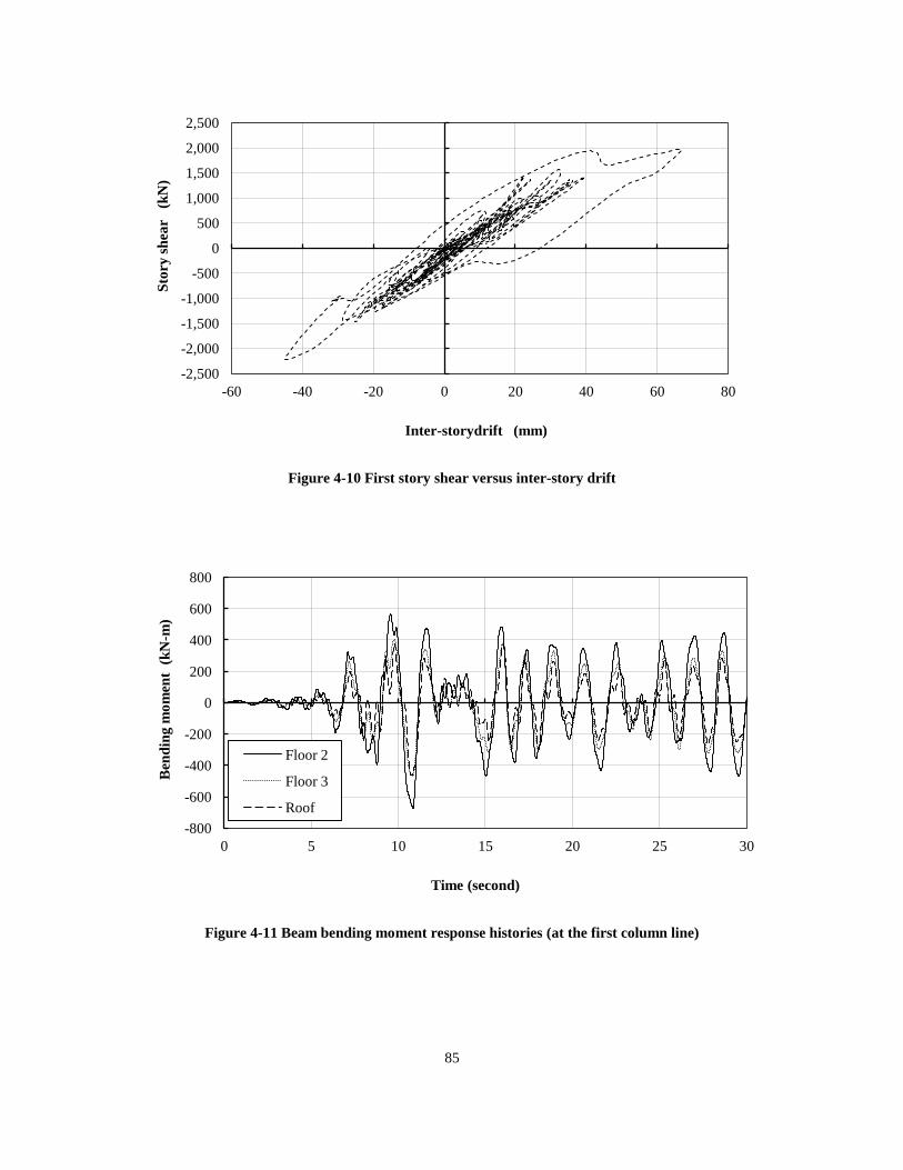
85
Figure 4-10 First story shear versus inter-story drift
Figure 4-11 Beam bending moment response histories (at the first column line)
-2,500
-2,000
-1,500
-1,000
-500
0
500
1,000
1,500
2,000
2,500
-60 -40 -20 0 20 40 60 80
Sto
ry s
hea
r
(kN
)
Inter-storydrift (mm)
-800
-600
-400
-200
0
200
400
600
800
0 5 10 15 20 25 30
Ben
din
g m
om
ent
(k
N-m
)
Time (second)
Floor 2
Floor 3
Roof

86
Figure 4-12 Beam end plastic rotation response histories (at the first column line)
Figure 4-13 Beam bending moment versus plastic rotation (Floor 2)
-0.014
-0.012
-0.010
-0.008
-0.006
-0.004
-0.002
0.000
0.002
0.004
0.006
0 5 10 15 20 25 30
Pla
stic
ro
tati
on
(r
ad
)
Time (second)
Floor 2
Floor 3
Roof
-800
-600
-400
-200
0
200
400
600
800
-0.015 -0.010 -0.005 0.000 0.005
Ben
din
g m
om
ent
(k
N-m
)
Plastic rotation (rad)
Floor 2

87
Figure 4-14 Beam bending moment versus plastic rotation (Floor 3)
Figure 4-15 Beam bending moment versus plastic rotation (Roof)
-600
-400
-200
0
200
400
600
-0.015 -0.010 -0.005 0.000 0.005
Ben
din
g m
om
ent
(k
N-m
)
Plastic rotation (rad)
Floor 3
-600
-400
-200
0
200
400
600
-0.015 -0.010 -0.005 0.000 0.005
Ben
din
g m
om
ent
(k
N-m
)
Plastic rotation (rad)
Roof

88
Chapter 5
Design of Eccentrically Braced Frames
This chapter illustrates the practical application of the capacity design formulation in Section 3.3
through the design process of an Eccentrically Braced Frame. In this example, the numerical
strategies such as including load and resistance factors in the analysis, grouping of design
variables considering link and beam outside the link, rounding-off of objective function values,
and ranking Pareto-optimal solutions for trade-off are introduced. An analytical model for
computing shear link rotation is developed as well.
5.1 Geometry and Seismic Loading of the 3-Story-1-Bay EBF
The hypothetical three-story office building, which was employed to demonstrate the
optimization design procedure of Moment Resisting Frames in Chapter 4, is redesigned herein by
using pairs of Eccentrically Braced Frame (EBF) as the Seismic Force Resisting System. As it is
shown in Figure 5-1, in both principal directions each of the original 3-story and 4-bay MRF is
EBF
Figure 5-1 Plan view of the hypothetical office building (EBF)
EBF
EBF
EBF
EBF
EBF EBF
EBF 9
.14
m
9.14 m

89
replaced by a pair of 3-story and 1-bay EBFs. For the purpose of illustration, only one EBF
design is considered in this example.
The schematic side view of the EBF is illustrated in Figure 5-2. The bay size is 9.14 m center-to-
center and all three stories are each 3.96 m high. The columns are continuous over the height and
the column bases are pinned. The symmetrically opposed brace pairs are used to maintain the
Q3
Fictitious Column
(b) Loading on EBF
Fictitious Column
Q2
Q1
P3
P2
P1
P3
P2
P1
BE2
P3 = 1100 kN
P2 = 1321 kN
P1 = 1321 kN
Q3 = 26.5 kN/m
Q2 = 29.1 kN/m
kN/m
Q1 = 29.1 kN/m
BE3
BE1
LK1
LK2
LK3
BR1
BR2
BR3
CL1 CL1
CL2
CL3
CL2
CL3
(a) member grouping
Figure 5-2 Side view of the EBFs
4.189 m 4.189 m
0.762 m
3.9
6 m
x 3
= 1
1.8
8 m

90
overall symmetry of seismic response within the plane of the lateral force resisting frames. As it
is shown in Figure 5-2(a), in order to avoid the link-to-column moment resisting connections
(which are generally expensive and vulnerable to brittle fracture), the braces are concentrically
connected to the columns. The beam- and brace-to-column connections are assumed to be pinned.
But the brace-to-beam and brace-to-link connections are designed to be rigid, which allows the
braces to contribute to the resisting of the moment developed at the end of the links.
Since the bending of the interior gravity columns due to building drift has an impact on the
overall lateral stiffness of the structural system, two fictitious lean-on columns are symmetrically
arranged to facilitate the simulation of the seismic weight and the destabilizing effect of the
gravity loads of the interior simple frames. The sectional properties (i.e., the moment of inertia
and the cross-sectional area) of the fictitious columns are taken to the sum of the corresponding
values of all the gravity columns (which are HSS254x254x13 sections) divided by the number of
EBFs (which is four, as it is shown in Figure 5-1) in the considered direction. Specifically, the
moment of inertia of each fictitious column is computed as IpD = (19 / 4 / 2) IG = 2.375 IG, where
IG is the moment of inertia of one gravity column.
For the EBF configuration shown in Figure 5-2(a), the horizontal component of the brace forces
are mainly resisted by the beam segment outside the links. Thus, large axial forces through links
are avoided. Popov and Engelhardt (1988) recommended that the brace-to-beam angles should
not be less than 40 degrees to avoid introducing greater-than-necessary axial force in frame
beams. In this example, it is assumed that the lengths of all the links are 762 mm, which
corresponds to a brace-to-beam angle of 43 degree.
The design of the EBF is based on the same gravity loads previously used for the examples of the
MRFs. The accompanying gravity loads are given in Figure 5-2(b), where Q1 to Q3 are the
gravity loads directly applied to the frame members, and P1 to P3 are the gravity loads of interior
frames which generate destabilizing effect. For this example, we should assume that the load
factors for the limit state design philosophy (e.g., NBCC 2010) are already included in the
computation of the gravity loads.

91
Table 5-1 Selected ground motion time-histories for EBF design
Record Name Earthquake
Magnitude
PGA
(g) PGV (cm/sec)
Scale
Factor
1979 Imperial Valley: El Centro Array #12 (EL_3.2) 6.5 0.143 17.6 3.2
1989 Loma Prieta: Belmont Envirotech (BES000_4.2) 6.9 0.108 11.8 4.2
1994 Northridge: Old Ridge RT 090 (ORR090_0.8) 6.7 0.568 52.1 0.8
Although more ground motion time history records are desirable (e.g., FEMA-450 requires seven)
to establish the average values of seismic demands, with the view to mitigate calculation burden
only three ground motion records from PEER (PEER 2008) are adopted for this example. As it is
required by governing codes, such as NBCC 2010, the employed ground motion time-histories
need to be scaled to the design level.
Figure 5-3 Response spectra (for EBF design)
For this example, the fundamental period of the 3-story steel EBF is estimated, according to
NBCC 2010, to be Ta = 0.025(hn) = 0.297 sec (where hn is the height of the building in meters).
However, in the subsequent nonlinear time-history analysis it is shown that the fundamental
period of the final designs ranges from 0.6 second to 0.8 second. To take into account the
deterioration of the Seismic Force Resisting System due to the material yielding, for the
nonlinear response history analysis it is conservative to define the period range of interest to
range from 0.3 second to 1.25 second. As it is shown in Table 5-1 and Figure 5-3, the selected
0
0.2
0.4
0.6
0.8
1
1.2
1.4
1.6
1.8
0.00 0.25 0.50 0.75 1.00 1.25 1.50
Sp
ectr
al
A
ccel
erati
on
(g
)
Period (second)
Design Spectrum
EL_3.2
BES000_4.2
ORR090_0.8

92
ground motion time histories are scaled such that their response spectra are compatible with the
design spectrum of NBCC 2010 throughout the periods of interest.
The proposed inelastic-analysis-based design is in essence a limit state design methodology. In a
limit state design, member strength equation is generally written as ∑αi Si ≤ ΦRn, where Φ and αi
are resistance factor and load factors, respectively; Si are load effects; and Rn is nominal
resistance. To be consistent with the limit state design philosophy, the uncertainty in the
prediction of member resistance (i.e., the resistance factor Φ) needs to be included in the design
formulation. For an inelastic-analysis-based design, it is more convenient to move the resistance
factor to the left side of the strength equation, i.e., to amplify the load effects by 1/Φ. Such
obtained load effects are called required nominal strength for members. Accordingly, for this
design example, the ground motion time-histories are amplified by 1/Φ to account the variation
of nominal member strength. Since Φ is typically equal to 0.9 in steel structural design (e.g.,
CSA-S16-09), the ground motion time-histories in Table 5-1 are further multiplied by 1.11 for
evaluating the seismic demands.
Determination of Design Variables
As it is shown in Figure 5-2(a), the member design variables include the column section, the
beam section, the brace section and the link section. The link length, which has a major impact
on the hysteresis behaviour of a link, is a geometric design variable. For this example, short
shear links are adopted since shear links are most commonly used due to their stable energy
dissipation capacity (a shear link is also called a shear hinge since the material yielding is
concentrated on the web of the link under shear force). In general, link length e should be less
than 1.6 Mp / Vp (where Mp and Vp are the plastic moment and shear resistance of the link,
respectively), as recommended in CSA-S16-09, in order for the link to act as a shear hinge.
Though it can be easily done to include e as a design variable for GA, this example chooses to
have a fixed link length of 762 mm throughout the design process in order to exclude link length
from its design variable set. The selected link length will satisfy e < 1.6 Mp / Vp for all the
candidate link sections.

93
If a link and the beam outside the link on the same floor level use one steel component, they are
then treated as one design variable. However, one may find it advantageous to design a link and
the beam outside the link with different sections due to the following reasons: 1) it is often
necessary to have a stronger beam outside the link to carry the combined effect of large axial
force and bending moment; and 2) it allows the practice of using replaceable links (Mansour et al
2009).
When a link and the beam outside the link are made using a single steel component, a common
practice for obtaining a stronger beam outside of the link is to use flange cover plates. In this
case, the strategy to relate the sectional properties of the link and the beam outside the link is as
follows. Assume the cross sectional area, plastic modulus and moment of inertia of a link are An,
Zn and In, respectively. The beam outside the link has a cross sectional area of (1 + kn) An, where
kn ≥ 0. The total sectional area of the two flange cover plates is knAn. The area of one cover plate
is (knAn)/2. The plastic modulus and moment of inertia of the beam outside the link are
Zn+(knAn/2)(dn+tc) and In+(knAn /4)(dn+tc)2, respectively, where dn is link section depth and tc is
cover plate thickness.
There are three ways to implement the above strategy. First, a link and the beam outside the link
use the same design variable with a predetermined kn value. The cover plate size for each link is
thus dependent on the section size of the link itself. Second, a link and the beam outside the link
use the same design variable with a predetermined cover plate size. The value of kn is thus
dependent on the size of the link. Third, a link and the beam outside the link use separate design
variables. For the third case, it is necessary to establish a cover plate size set. The link section is
a design variable while the beam outside the link is replaced by the cover plate size variable
which is chosen from among the cover plate size set.
For the illustration of this EBF design example, six design variables are chosen as follows
1) All the columns are designed to have the same section and grouped as the first design
variable, x1.
2) For each floor, the link and the beams outside the link are designed as one structural
component (if necessary, the beams outside of the link will be reinforced with 12mm

94
x100mm flange cover plates) and thus are treated as one variable. The links at floor levels
2, 3 and roof correspond to variables, x2, x3, and x4.
3) The two braces at story 1 are grouped as the fifth design variable, x5, and the braces at
stories 2 and 3 are the sixth design variable, x6.
Each design variable is to be selected from among 4 candidate section sizes (though more
candidate sections can be selected, this example uses four sections only to mitigate
computational burden). The properties of the sections are provided in Table 5-2, where the shape
for columns and beams is wide-flange I-section and for braces is hollow structural sections.
These candidate sections are chosen because they are commonly used in construction and they
satisfy the shear link criterion.
The requirements on section class and/or slenderness are accounted for in the selection of the
candidate sections. For example, as it is required by Canadian standard S16-09 (CSA 2009), only
compact sections are allowed for the columns and braces. However, developing an automated
selection of section sets is beyond the scope of this research, and it is the topic of future work.
Determination of Design Constraint Limits
The allowed inter-story drift limit (as per National Building Code of Canada 2010) is taken as
0.025h, where h is story height. In accordance with the requirements of CSA-S16-09 (CSA
2009), the link rotation capacity is taken as 0.08 radians. It has been suggested (CSA 2009;
Ricles and Popov 1994; Koboevic and Redwood 1997) that some yielding of the beams outside
the link is acceptable. For this example, the plastic rotation limits at the Immediate Occupancy
level as per ASCE/SEI 41-06 (ASCE 2007) are adopted as the non-detrimental plastification for
non-fuse members. These limits are estimated to be 0.5θy, 0.6θy, and 0.5θy [θy is yield rotation
and θy = (Z Fye L) / (6EI), where: Z, L, E are plastic modulus, length, and Young’s modulus of
the member, respectively] for columns, beams outside the links, and braces, respectively, and
they are provided in Table 5-3. In actual implementation, the plastic rotation limits on columns,
beams and braces are taken as 0.005, 0.005 and 0.010 radians, respectively.

95
Table 5-2 Section sets for design variables of EBF design
Variable Section Ci A (mm2) Zx (10
3 mm
3) I (10
6 mm
4)
I with cover
plates (10
6 mm
4)
1.6Mp/Vp
(mm)
Columns (CL)
x1
W310x107
13600 1770 248
W310x79 10100 1280 177
W310x52 6670 841 119
W310x33 4180 480 65
Link and
beams (BE1 & LK1)
x2
W410x100 12700 2130 398 507 1514
W410x74 9550 1510 275 383 1097
W410x60 7580 1190 216 321 1105
W410x46 5890 885 156 259 913
Link and
beams (BE2 & LK2)
x3
W410x74 9550 1510 275 383 1097
W410x60 7580 1190 216 321 1105
W410x46 5890 885 156 259 913
W360x39 4980 662 102 182 839
Link and
beams (BE3 & LK3)
x4
W410x60 7580 1190 216 321 1105
W410x46 5890 885 156 259 913
W360x39 4980 662 102 182 839
W360x33 4170 542 82.7 161 779
Braces of
story 1 (BR1)
x5
HSS 203x203x13 9260 651 54.7
HSS 203x203x9.5 7150 513 43.9
HSS178x178x8.0 5240 330 24.8
HSS178x178x6.4 4250 271 20.6
Braces of
upper stories (BR2 & BR3)
x6
HSS 203x203x9.5 7150 513 43.9
HSS178x178x8.0 5240 330 24.8
HSS178x178x6.4 4250 271 20.6
HSS152x152x6.4 3610 196 12.6

96
Table 5-3 Plastic rotation limits for non-fuse members of EBF
Members Size I (106 mm
4) Z (10
3 mm
3) L (mm) y (radians)
0.5 y (radians) or
0.6 y (radians)
CL
W310x107 248 1770 3936 8.90E-03 4.45E-03
W310x79 177 1280 3936 9.01E-03 4.51E-03
W310x52 119 841 3936 8.81 E-03 4.40E-03
W310x33 65 480 3936 9.20E-03 4.60E-03
BE1 (CP) CP: 12x100
W410x100 513 2672 4191 6.91E-03 4.14E-03
W410x74 383 2020 4191 6.99E-03 4.20E-03
W410x60 321 1693 4191 6.99E-03 4.19E-03
W410x46 259 1383 4191 7.08E-03 4.25E-03
BE2 (CP) CP: 12x100
W410x74 383 2020 4191 6.99E-03 4.20E-03
W410x60 321 1693 4191 6.99E-03 4.19E-03
W410x46 259 1383 4191 7.08E-03 4.25E-03
W360x39 182 1100 4191 8.02E-03 4.81E-03
BE3 (CP) CP: 12x100
W410x60 321 1693 4191 6.99E-03 4.19E-03
W410x46 259 1383 4191 7.08E-03 4.25E-03
W360x39 182 1100 4191 8.02E-03 4.81E-03
W360x33 161 975 4191 8.04E-03 4.83E-03
BR1
HSS 203x203x13 54.7 651 5768 2.17E-02 1.09E-02
HSS 203x203x9.5 43.9 513 5768 2.13E-02 1.07E-02
HSS 178x178x8.0 24.8 330 5768 2.43E-02 1.22E-02
HSS178x178x6.4 20.6 271 5768 2.40E-02 1.20E-02
BR2 &
BR3
HSS 203x203x9.5 43.9 513 5768 2.13E-02 1.07E-02
HSS 178x178x8.0 24.8 330 5768 2.43E-02 1.22E-02
HSS178x178x6.4 20.6 271 5768 2.40E-02 1.20E-02
HSS152x152x6.4 12.6 196 5768 2.84E-02 1.42E-02

97
5.2 Analytical Model of EBF
The capacity design approach for EBF assumes that the inelastic energy dissipation is primarily
restricted to links, while all other structural members respond elastically under severe earthquake
ground motion time-histories. Accordingly, the traditional design procedure starts with the link
proportioning in regard to a code-specified seismic base shear. Then, all other structural
members are proportioned with respect to the capacity of the links. Finally, the obtained design
is verified by maintaining the elastic-analysis-based prediction of plastic link deformation within
a code-imposed limitation.
In the past studies on EBFs (such as Popov and Engelhardt 1988; Ricles and Popov 1994;
Ramadan and Ghobarah 1995; Koboevic and Redwood 1997), non-fuse members are generally
modelled as elastic-response member only, while only links are simulated as inelastic-response
members.
However, for this study, the model for non-fuse members must be able to consider material
yielding as well since it is impossible to warrant an elastic behaviour for non-fuse members of a
randomly generated candidate design solution during a design process. Furthermore, as
mentioned previously, some limited yielding of non-fuse members is acceptable as long as the
minor plastification does not impact the integrity of SFRS.
Shear Link Modelling
In a well designed EBF, the axial force effect in the link can be neglected (Popov and Engelhardt
1988). Under lateral seismic loads (e.g., Engelhardt and Popov 1989; Popov et al 1990) high
shear force combined with high end moments develop simultaneously in the links of EBFs.
Influenced by strain hardening effect, both shear and flexural yielding may occur along the
length of link. Links are generally modelled based on the lumped plasticity approach with strain
hardening effect.

98
Several researchers have developed shear-link models (Ricles and Popov 1994; Ramadan and
Ghobarah 1995). A typical link element contains a linear beam element with a series of nonlinear
hinges/springs at each end. Multi-linear functions are employed to describe the yielding and
strain hardening behaviour of shear and flexure through the appropriately defined hinges/springs
Deformation δ
Vy3
O
δy1
Vy1
Vy2
δy2 δy3
Shea
r V
Rotation
My3
O
y1
My1
My2
y2 y3
Mom
ent
M
K1v
K2v
K3v
K4v
K1M
K2M
K3M
K4M
Figure 5-5 Multi-linear force-deformation relationship of link model
Hinge
2
1
3
7
1
8
Hinge
9
4
10
0
5
4
6
Zero Length Zero Length Link Length
e
Elastic Beam
Element
Master
Node i
Master
Node j
Slave
Node i’
Slave
Node j’
Figure 5-4 Hybrid link element
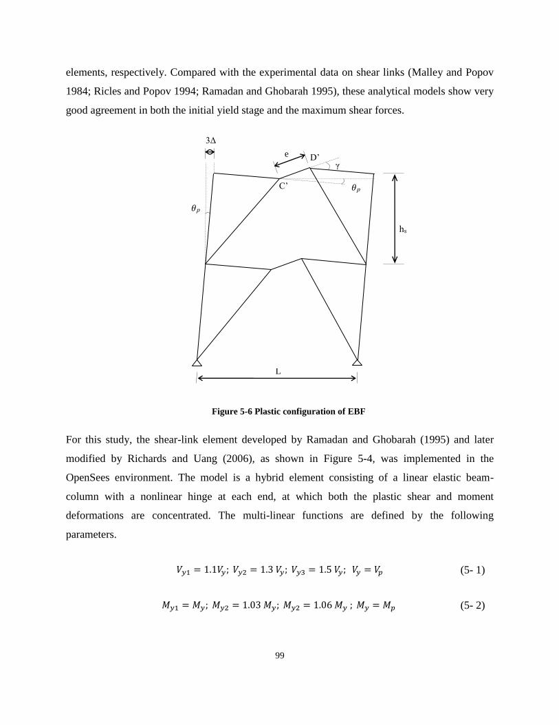
99
elements, respectively. Compared with the experimental data on shear links (Malley and Popov
1984; Ricles and Popov 1994; Ramadan and Ghobarah 1995), these analytical models show very
good agreement in both the initial yield stage and the maximum shear forces.
For this study, the shear-link element developed by Ramadan and Ghobarah (1995) and later
modified by Richards and Uang (2006), as shown in Figure 5-4, was implemented in the
OpenSees environment. The model is a hybrid element consisting of a linear elastic beam-
column with a nonlinear hinge at each end, at which both the plastic shear and moment
deformations are concentrated. The multi-linear functions are defined by the following
parameters.
(5- 1)
(5- 2)
D’
C’
γ
p
p
hs
3Δ
e
L
Figure 5-6 Plastic configuration of EBF

100
(5- 3)
(5- 4)
where Vp and Mp are the expected plastic shear capacity and plastic moment capacity of the link
section, respectively; Mp = Fye Zb, and Fye and Zb are the expected yield strength and plastic
modulus of link section, respectively; d, tf and tw are the link-
section depth, flange thickness and web thickness, respectively; E and G are the Young’s
modulus and shear modulus of the sectional material, respectively; I and Aweb are the moment of
inertia and the web area of the link section, respectively; e is the link length.
It is necessary to calculate shear link rotation demand since the design constraints include the
limit imposed on the plastic rotation of links. For an elastic-analysis-based design approach, the
rigid-plastic analysis methods are usually employed to approximate the plastic rotation demands
of shear link in terms of the plastic inter-story drift ratio p (where p is, recommended by
CSA-S16-09, to be taken as 3 times that of the elastic inter-story drift under the code specified
seismic load). As the EBF undergoes the target plastic mechanism shown in Figure 5-6, by
ignoring elastic deformation, the plastic rotation of a link is estimated to be γ = (L/e) p , where
L and e are bay width and the length of the link, respectively. For this study, a new method to
compute link rotation is necessary. As it is shown in Figure 5-6, the link rotation demand can be
directly computed in terms of the difference of the vertical displacements between the two ends
of the link,
(5- 5)
where yD’ and yC’ are the vertical displacements of the end nodes of the link element. Substituting
γ = (L/e) p into Equation (5-5) gives
(5- 6)

101
Nonlinear Element Models of Columns, Beams and Braces
Columns, beams and braces are modeled by the force-based beam-column element described in
Section 2.2.2. In general, the modeling of geometrically nonlinear behaviour can be improved by
subdividing the structural member into smaller elements when its axial force is very large. As it
is reflected in the literatures (Uriz, Filippou and Mahin 2008), the model of two elements for one
brace member agrees well with the results of the extensive set of experimental data with various
slenderness ratios.
For this example, each column, beam outside the link and brace are represented by two force-
based beam-column elements with five numerical integration points along the element length.
Furthermore, 1/500 of structural member length imperfection to columns, braces and beams (i.e.,
initial member crookedness) are considered through adjusting the end-nodes of internal elements.
The fictitious columns are modelled as elastic beam-column. Specifically, the simplified p-Δ
transformation matrix (i.e., Equation (2-55)) is used for the geometrical nonlinearity simulation
of the fictitious columns.
For the fibre discretization of the cross-section, each flange and web are discretized into eight
layers. The material behaviour of steel is bilinear elastoplastic with 5% strain hardening.
Strength and Damping
Since capacity design principle requires that non-fuse members are proportioned in respect to the
actual resistance of the links, the material strength for links in the nonlinear response history
analysis should use the probable or expected yield strength in addition to accounting for material
strain hardening. The probable yield stress shall be taken as Fye=RyFy, where Ry is an
amplification factor (which is equal to 1.1 in CSA-S16-09). It is assumed that all the structural
members in this example use 345 MPa grade steel. The link members use the expected yield
strength RyFy in the nonlinear response history analysis. Because the outer beam segments are
part of the same member as the link, the beams outside the link also use RyFy as yielding strength
in the analysis. However, the material strength of columns and braces are taken as the specified
value, 345 MPa, which is consistent with the normal design practice.

102
In analysis, seismic masses are concentrated on column lines as well as the master end nodes of
the hybrid link elements.
The damping matrix is constructed according to Rayleigh method. First, the proportionality
constants of Rayleigh damping for the mass matrix and tangent stiffness matrix are computed
from the frequencies of modes 1 and 3 with damping ratios of 0.05. Then, as it is recommended
by the literatures (Popov et al 1986; Ricles and Popov 1994; Koboevic and Redwood 1997), only
mass-related damping is assigned to the links (to minimize the impact of excessive viscous
damping forces in the links).
5.3 Design Results
The Multi-objective Genetic Algorithm (MGA) tool in the MATLAB software is employed to
search for the set of Pareto-optimal solutions. For six design variables that each has four
candidate sections, there are 4096 possible design solutions.
Each design is represented by a 12-bit binary string, in which each variable corresponds to a 2-
bit string with 22=4 values being available to the design. The population size of the GA is taken
as 30 while the mutation rate is taken as 0.05.
The MGA search is considered to converge if the average changes of the spread sp of Pareto
solutions is less than 10-6
over 50 generations. Or, the algorithm will be terminated if the
maximum number of generations reaches 150.
A test run was carried out first with the assumption that at each floor level the link and the beams
outside the link are of same cross section. This test run ended without a single feasible solution
being obtained. An examination of the analysis results revealed that the plastic rotation limits on
the beams outside the link were always violated despite the observation that the plastic rotations
of the links were usually within the limit. Thus, beams outside the link need to be reinforced with
flange cover plates.
Three runs of MGA were conducted. 1142 designs were evaluated. The searched design
solutions are plotted in a three-dimensional objective space (Figure 5-7). It was noted that the
average running time for one generated design is about 8 min on a desktop with Intel Core i5 750
CPU and 4 GB random access memory.

103
Figure 5-7 Searched design solutions in objective space
Figure 5-8 Feasible design solutions in objective space

104
Figure 5-9 Weight (OBJ1) versus seismic input energy (OBJ2)
Figure 5-10 Hysteretic energy dissipation ratio (OBJ3) versus seismic input energy (OBJ2)
30
40
50
60
70
80
720 740 760 780 800 820 840 860 880
Wei
gh
t (k
N)
Seismic input energy (kN-m)
96.0%
96.5%
97.0%
97.5%
98.0%
98.5%
99.0%
99.5%
100.0%
720 740 760 780 800 820 840 860 880
Hy
s. e
ner
gy
dis
sip
ati
on
ra
tio
Seismic input energy (kN-m)

105
Figure 5-11 Hysteretic energy dissipation ratio (OBJ3) versus weight (OBJ1)
As it is shown in Figure 5-7, OBJ1, structural weight objective, lies between 30 kN and 80 kN;
OBJ2, seismic input energy, ranges from 500 kN-m to 1000 kN-m; OBJ3, the fuse members’
hysteretic energy dissipation ratio, ranges between 0 to 1. Note that those design solutions, which
could not survive the ground motion time histories (i.e., the analysis could not converge to a
stable deformation state) are not included in the figure. Among them, the feasible solutions are
plotted in Figure 5-8.
It is observed (Figure 5-8) that all the feasible design solutions have OBJ3 values greater than
95%. For easier illustration, the feasible designs in three-dimensional objective space are re-
plotted in Figures 5-9 to 5-11 with each figure representing a two-dimensional objective space.
Combining the results of 3 runs gives a set of 18 Pareto-optimal solutions as summarized in
Tables 5-4 to 5-6. The following observations can be made from these tables:
1) The fundamental period of the optimal solutions fall in a narrow range from 0.55 sec to
0.70 sec.
2) OBJ2 value of the Pareto-optimal set ranges from 743 kN-m to 855 kN-m.
96.0%
96.5%
97.0%
97.5%
98.0%
98.5%
99.0%
99.5%
100.0%
30 40 50 60 70 80
Hy
s. e
ner
gy
dis
sip
ati
on
ra
tio
Weight (kN)

106
3) The optimal solutions show excellent hysteretic energy dissipation performance. Almost
100 per cent hysteretic energy is dissipated by fuse members. Capacity design philosophy
is successfully implemented in this example.
4) The value of OBJ1 displays large dispersion (the difference can be as high as 50%) even
among the optimal solutions, let alone among the feasible solutions. This further
demonstrates that it is very difficult to obtain even a single-objective (e.g., least-weight)
optimal design if traditional trial-and-error method is used.
5) The inter-story drift constraints are far from being active for all optimal solutions. It
appears the design of EBFs is more likely governed by the link plastic rotation constraints.
6) For this example, the plastic deformations of non-fuse members are negligible. Though, it
may suggest that it is possible to reduce the sectional sizes of columns, braces and beams,
the actual implementation will be difficult since the discrete design variables do not allow
“fine-tuning” sectional sizes. The fact that the adopted plastic rotation limits for non-fuse
members are small also contributes to this phenomenon.
Design results in Table 5-5 shows that it is necessary to introduce some numerical strategies in
the GA. For example, design #5 is worse than design #6 in terms of both structural weight and
seismic input energy, while it is better in terms of OBJ3. However, from the practical point of
view, the relative hysteretic energy capacities of the two designs are virtually the same. Thus, it
is reasonable to say that design #6 is better than design #5. Hence, a rounding-off strategy is
conceived in the following
1) Only integer numbers are kept for OBJ1 and OBJ2.
2) Only 2 significant digits after decimal point are kept for OBJ3 by rounding-off.
Following this strategy, a reduced Pareto-optimal set with 8 design solutions are obtained in
Table 5-7. Design #18 is the solution with the least weight (OBJ1 = 40 kN) while design #6 is the
design having the minimum seismic input energy (OBJ2 =743 kN-m). All the Pareto-optimal
solutions have a near 100 per cent OBJ3 values, indicating that the plastic deformations
exclusively occur within the links.

107
Table 5-4 Search results of MGA
Index Design Number
CL (W)
BE1 (W)
BE2 (W)
BE3 (W)
BR1 (HSS)
BR2 & BR3 (HSS)
1 177 310x107 410x100 410x46 360x33 203x203x13 203x203x9.5
2 369 310x107 410x74 410x60 360x33 203x203x13 203x203x9.5
3 1201 310x79 410x100 410x46 360x33 203x203x13 203x203x9.5
4 1457 310x79 410x74 410x46 360x33 203x203x13 203x203x9.5
5 2225 310x52 410x100 410x46 360x33 203x203x13 203x203x9.5
6 2226 310x52 410x100 410x46 360x33 203x203x13 178x178x8.0
7 2481 310x52 410x74 410x46 360x33 203x203x13 203x203x9.5
8 2482 310x52 410x74 410x46 360x33 203x203x13 178x178x8.0
9 2485 310x52 410x74 410x46 360x33 203x203x9.5 203x203x9.5
10 2486 310x52 410x74 410x46 360x33 203x203x9.5 178x178x8.0
11 2722 310x52 410x60 410x46 360x39 203x203x13 178x178x8.0
12 2738 310x52 410x60 410x46 360x33 203x203x13 178x178x8.0
13 3042 310x52 410x46 360x39 360x39 203x203x13 178x178x8.0
14 3057 310x52 410x46 360x39 360x33 203x203x13 203x203x9.5
15 3058 310x52 410x46 360x39 360x33 203x203x13 178x178x8.0
16 3065 310x52 410x46 360x39 360x33 178x178x8.0 203x203x9.5
17 3066 310x52 410x46 360x39 360x33 178x178x8.0 178x178x8.0
18 3067 310x52 410x46 360x39 360x33 178x178x8.0 178x178x6.4

108
Table 5-5 Structural response of search results of MGA
Index OBJ1
(kN) OBJ2
(kN-m) OBJ3 (%)
Max. Link
Rotation (radians)
Link D/C
Max.
Story
Drift (radians)
Drift D/C
Fundamental Period (sec)
1 67 795 99.86 6.70% 0.84 0.91% 0.37 0.549
2 66 824 99.87 5.33% 0.67 0.80% 0.32 0.550
3 60 788 99.85 6.70% 0.84 0.93% 0.37 0.556
4 58 796 99.82 6.55% 0.82 0.92% 0.37 0.566
5 54 774 99.80 6.59% 0.82 0.96% 0.38 0.570
6 51 743 99.01 5.82% 0.73 0.96% 0.38 0.597
7 52 778 99.80 6.49% 0.81 0.95% 0.38 0.580
8 48 757 99.13 5.77% 0.72 0.95% 0.38 0.606
9 50 788 99.68 6.59% 0.82 0.95% 0.38 0.597
10 47 790 98.91 5.71% 0.71 0.95% 0.38 0.623
11 48 801 99.70 6.89% 0.86 0.85% 0.34 0.613
12 47 805 99.72 6.54% 0.82 0.82% 0.33 0.616
13 46 820 99.72 6.89% 0.86 0.93% 0.37 0.638
14 49 819 99.82 7.06% 0.88 0.92% 0.37 0.615
15 45 822 99.73 6.56% 0.82 0.90% 0.36 0.641
16 45 855 99.02 6.90% 0.86 0.94% 0.38 0.660
17 42 834 98.95 7.01% 0.88 0.98% 0.39 0.684
18 40 810 97.95 6.95% 0.87 1.04% 0.42 0.703
D/C: Demand/Capacity

109
Table 5-6 Constraint values of the obtained optimal solutions
Index
Maximum Plastic Rotation
Columns (radians)
D/C Beams
(radians) D/C
Braces (radians)
D/C
1 2.85E-07 0.000 2.19E-04 0.044 1.67E-04 0.017
2 7.69E-09 0.000 1.18E-04 0.024 2.06E-04 0.021
3 4.63E-06 0.001 2.34E-04 0.047 1.74E-04 0.017
4 2.87E-06 0.001 2.46E-04 0.049 1.18E-04 0.012
5 2.78E-04 0.056 2.45E-04 0.049 1.38E-04 0.014
6 2.89E-04 0.058 2.86E-04 0.057 1.86E-03 0.186
7 2.06E-04 0.041 2.36E-04 0.047 1.28E-04 0.013
8 2.22E-04 0.044 2.93E-04 0.059 1.63E-03 0.163
9 1.55E-04 0.031 2.48E-04 0.050 4.28E-04 0.043
10 1.66E-04 0.033 3.11E-04 0.062 1.75E-03 0.175
11 3.44E-05 0.007 1.91E-04 0.038 1.04E-03 0.104
12 1.74E-05 0.003 1.80E-04 0.036 1.16E-03 0.116
13 1.74E-05 0.003 4.01E-04 0.080 4.90E-04 0.049
14 9.04E-06 0.002 3.14E-04 0.063 2.33E-05 0.002
15 1.63E-05 0.003 3.82E-04 0.076 4.87E-04 0.049
16 3.12E-06 0.001 5.65E-04 0.113 2.41E-03 0.241
17 6.53E-06 0.001 4.61E-04 0.092 1.92E-03 0.192
18 1.34E-05 0.003 5.55E-04 0.111 3.65E-03 0.365
D/C: Demand/Capacity

110
Table 5-7 Reduced Pareto-optimal solutions
Index OBJ1
(kN) OBJ2
(kN-m) OBJ3 (%)
Relative
OBJ1 (f1)
Relative
OBJ2 (f2)
Relative
OBJ3 (f3)
Relative
distance
(f) Rank
6 51 743 99 1.00 0.89 0.01 1.339 8
8 48 757 99 0.94 0.91 0.01 1.308 3
10 47 790 98 0.92 0.95 0.02 1.322 4
12 47 805 99 0.92 0.97 0.01 1.335 7
13 46 820 99 0.90 0.98 0.01 1.334 6
15 45 822 99 0.88 0.99 0.01 1.323 5
17 42 834 99 0.82 1.00 0.02 1.296 2
18 40 810 97 0.78 0.97 0.03 1.249 1
In general, it can be said that each Pareto-optimal solution is an equally worthy candidate design
for further consideration. For example, design #6 is 27 per cent heavier than design #18, and it
absorbs 9 per cent less of seismic input energy. Design #8 is 6 per cent lighter than design #6,
but its seismic input energy is only 2 per cent greater than that of design #6. If one considers the
difference of OBJ3 values among the Pareto-optimal set as being negligible, then design #13, #15
and #17 may be regarded as inferior to design #18. In summary, one may choose the final
solution based on his/her preference.
A unified decision process may be described in the following. With the values of the three
relative objective functions f1, f2 and f3 presented in Table 5-7 (where f1 and f2 are obtained by
normalizing OBJ1 and OBJ2 values by their respective maximum values among the Pareto-
optimal set), the reduced Pareto-optimal set is projected into the three-dimensional space shown
in Figure 5-12, where each objective is represented by one of the three coordinates of the
normalized objective space. It is obvious that, the origin of the coordinate system represents the
hypothetical optimum whose objective values are all at their minima, i.e., zeros, simultaneously
(though, such a case would never be reached). The overall performance of a Pareto-optimal
solution may be evaluated by checking how far the solution is away from the origin. Namely, a
measurement f represented by the distance between a design point and the origin is defined as
(Alimoradi et al 2007)

111
(5- 7)
Figure 5-12 Relative objectives of the Pareto-optimal solutions
The obtained Pareto-optimal solutions can then be ranked in regards to the values of f. For the
minimization problem, the smaller f value is, the better the overall performance of the design is.
Both the f values and the ranks of the Pareto-optimal solutions are included in Table 5-7.
It is observed that other ways in addition to Equation (5-7) are possible in defining f value by
normalizing OBJi (i=1, 2 and 3) values differently. For example, one may include his/her
preference through introducing weighting factors in fi values.
Though it might appear that design objective OBJ3 plays little role in selecting the final solution
among the Pareto-optimal set, OBJ3 actually played the vital role of driving the MGA to obtain
the optimal set (Note that it is possible to have a feasible solution with no yielding of the links).

112
In the following, detailed results of the nonlinear response history analysis of design #8 are
provided to demonstrate the structural behaviours of an obtained optimal design. The ground
motion history adopted is “1979 Imperial Valley: El Centro Array #12”.
Figures 5-13 and 5-14 show that the maximum roof drift and inter-story drift occur at 10.54
second. Those values are far from limits. Figure 5-15 gives the height-wise distribution of the
maximum rotations of the links, where relatively uniform distribution of link rotation is observed.
It is the link at floor 3 that experience the maximum rotation of 0.056 radians. Figures 5-16 and
5-17 show that both ends of floor 3 link remain elastic under bending moment during the entire
loading history. Figures 5-18 to 5-20 plot the shear versus link rotation angle hysteresis curves.
Strain hardening is evident in the hysteresis loops. As expected, the links undergo shear yielding.
For the links at floors 2, 3 and roof, the maximum shears 1140 kN, 907 kN and 594 kN
correspond to a load level of 1.39Vp, 1.53Vp and 1.39Vp, respectively [where
]. The load level of the links exceeds the value of 1.3Vp specified by
CSA-S16 by 7 to 18 per cent, suggesting that the code-specified overstrength factor may be
inadequate for this design.
The internal forces of the frame members in the first story are compared with the strength
formula of CSA-S16 in Figures 5-21 to 5-23 (Note that the beam-column strength equation shall
exclude resistance factor as the load and resistance factors have been already included in the
analysis). From the force points of the members, one can observe that the columns and braces are
dominated by their compressive forces while the beams are dominated by both axial force and
bending moment. All the force points fall within the nominal strength curve, which means the
member strengths are satisfactory.
In summary, design #8 has excellent seismic performance under the adopted ground motion.

113
Figure 5-13 Lateral displacement response history
Figure 5-14 Inter-story drift ratio response histories
-100
-80
-60
-40
-20
0
20
40
60
80
100
0 5 10 15 20 25 30
La
tera
l d
isp
lace
men
t (
mm
)
Time (second)
Roof
-1.5%
-1.0%
-0.5%
0.0%
0.5%
1.0%
1.5%
0 5 10 15 20 25 30
Inte
r-s
tory
dri
ft r
ati
o
Time (second)
Story 1
Story 2
Story 3

114
Figure 5-15 Distribution of the maximum link rotation
Figure 5-16 Link bending moment versus rotation (Floor 3, left end)
Floor 2
Floor 3
Roof
-6.0% -4.0% -2.0% 0.0% 2.0% 4.0% 6.0%
-6.0% -4.0% -2.0% 0.0% 2.0% 4.0% 6.0%
Maximum link rotation (rad)
-500
-400
-300
-200
-100
0
100
200
300
400
-0.0020 -0.0015 -0.0010 -0.0005 0.0000 0.0005 0.0010 0.0015
Ben
din
g m
om
ent
(k
N-m
)
Rotation (rad)
Floor 3 (left end)

115
Figure 5-17 Link bending moment versus rotation (Floor 3, right end)
Figure 5-18 Link shear versus rotation hysteresis (Floor 2)
-500
-400
-300
-200
-100
0
100
200
300
400
-0.0020 -0.0015 -0.0010 -0.0005 0.0000 0.0005 0.0010 0.0015
Ben
din
g m
om
ent
(k
N-m
)
Rotation (rad)
Floor 3 (right end)
-1200
-900
-600
-300
0
300
600
900
1200
-0.06 -0.04 -0.02 0.00 0.02 0.04 0.06
Sh
ear
(k
N)
Link deformation angle (rad)
Floor 2

116
Figure 5-19 Link shear versus rotation hysteresis (Floor 3)
Figure 5-20 Link shear versus rotation hysteresis (Roof)
-1200
-900
-600
-300
0
300
600
900
1200
-0.06 -0.04 -0.02 0.00 0.02 0.04 0.06
Sh
ear
(k
N)
Link deformation angle (rad)
Floor 3
-1200
-900
-600
-300
0
300
600
900
1200
-0.06 -0.04 -0.02 0.00 0.02 0.04 0.06
Sh
ear
(k
N)
Link deformation angle (rad)
Roof
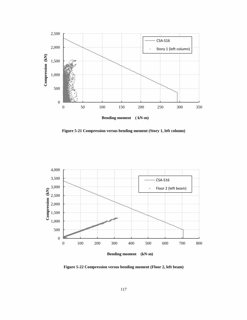
117
Figure 5-21 Compression versus bending moment (Story 1, left column)
Figure 5-22 Compression versus bending moment (Floor 2, left beam)
0
500
1,000
1,500
2,000
2,500
0 50 100 150 200 250 300 350
Co
mp
ress
ion
(k
N)
Bending moment ( kN-m)
CSA-S16
Story 1 (left column)
0
500
1,000
1,500
2,000
2,500
3,000
3,500
4,000
0 100 200 300 400 500 600 700 800
Co
mp
ress
ion
(k
N)
Bending moment (kN-m)
CSA-S16
Floor 2 (left beam)

118
Figure 5-23 Compression versus bending moment (Story 1, left brace)
0
500
1,000
1,500
2,000
2,500
3,000
3,500
0 50 100 150 200 250
Co
mp
ress
ion
(k
N)
Bending moment (kN-m)
Series1
Story 1 (left brace)

119
Chapter 6
Conclusions and Recommendations
6.1 Summary and Conclusions
The major contribution of this research is the development of a design synthesis which is able to
automate capacity design of steel building frameworks through the coupling of a nonlinear time
history analysis procedure and optimization techniques. Design optimization using dynamic
analysis procedures is not a new idea (e.g., Section 1.3). However, to the best knowledge of this
author, this research is the first attempt in developing a unified capacity design approach for
various steel frameworks.
Specifically, the original contributions of this research are:
1) The development of a numerical technique to compute seismic energies based on the
analysis results from an existing nonlinear dynamic analysis procedure (Section 2.1.2).
The technique was verified using the educational program NONLIN (Section 2.3).
2) The development of the optimal design formulation, Equations 3-8 to 3-12. In this
formulation, the minimum structural cost, the minimum seismic input energy, and the
maximum hysteresis energy ratio of fuse members were identified as the design
objectives. The cost objective is universal and serves to search for an economical design;
the input energy objective aims to reduce the potential earthquake damage to the structure;
and the hysteresis objective drives the optimization algorithm to search for design
solutions with favorable plastic mechanisms. The choice of using seismic energies as
design objectives allows us to capitalize on the adopted analytical tool since only a
nonlinear dynamic analysis tool is able to provide both seismic input energy and
hysteretic energy. Comparing with displacement or force responses, an energy response
has the advantage of not only reflecting the duration of ground motions but also
accounting for the cumulative effect of inelastic deformations. The structural design is
subjected to strength and deformation constraints. The strength checking is implicitly
included in the advanced analysis procedure in which both material and geometrical
nonlinearities are considered in the element models. The deformation checking is

120
explicitly expressed as the imposed plastic deformation limits, in which structural
performance levels and member deformation capacities are taken into account. For the
design method to be suitable for practical application, the obtained optimal designs are
expressed as discrete combinations of steel section shapes.
3) The coupling of a nonlinear dynamic analysis procedure (i.e., OpenSees) with a GA to
conduct capacity design automation. A numerical test was conducted to determine the
proper population size (Appendix 3.B). Design examples on Moment Resisting Frames
and Eccentrically Braced Frames were conducted. The correlation between the hysteretic
energy dissipation of fuse members and the strong-column-weak-beam requirement for
moment-resisting frames was investigated (Section 4.2). The numerical strategies, such
as introducing load and resistance factors in the analysis procedure, grouping of design
variables considering a link and the beam outside the link, rounding-off the objective
function values, etc., were introduced in the design examples. Also, Equation (5-6) was
proposed for the first time by this research as an approximation for computing shear link
rotation.
The technical merits of the proposed design synthesis include:
1) The evaluation tool is most sophisticated and accurate, which ensures a better
performance of the obtained structure under an earthquake hazard.
2) The design formulation is general. The methodology will greatly simplify the current
elastic-analysis-based design practice, in which one-set-of-rules-for-each-type-of-system
(CSA 2009) is necessary.
3) The limit state design philosophy is achieved at the structural system level.
4) The design automation tool will help engineers to carry out the capacity design principle
without arduous hand calculations. Thus, the design synthesis will greatly assist the
application of nonlinear analysis procedures in engineering offices in terms of ease,
efficiency and accuracy.
The following specific conclusions can be drawn from this study:
1) The developed optimization model can be used to conduct seismic design of steel
frameworks following the capacity design principle. The favorable plastic mechanism is

121
achieved through forcing the concentration of hysteretic energy dissipation among fuse
members.
2) Problem-dependent capacity design requirements, such as strong-column-weak-beam for
Moment Resisting Frames, are not included in the design formulation. Therefore, the
design method is general and applicable to various types of building frames.
3) The seismic performance factors, such as ductility-related force reduction factor and
overstrength-related force reduction factors, which are crucial in elastic-analysis-based
design methods, are no longer needed in inelastic-analysis-based design methods. Thus,
the approximations in obtaining these factors are completely eliminated in an inelastic-
analysis-based design method, which allows us to obtain design solutions with better
earthquake resistance behavior.
4) The Multi-objective Genetic Algorithm tool provided in MATLAB works well for the
proposed design formulation, though more work needs to be done in future study to
improve its computational efficiency
5) For a design problem, the number of feasible design solutions is generally large, and the
structural weights of the feasible designs spread over a wide range (this is mainly because
a larger structural weight or stiffness also attracts greater earthquake loads). The fact
indicates that without a design optimization tool it is not easy to obtain an economical
design when a nonlinear dynamic analysis procedure is adopted as the evaluating tool.
6) The distance between a Pareto-optimal solution point and the origin of the design
objective space is an overall performance index for trade-off analysing design decisions
to come to a final design.
7) It appears it is generally necessary for the beams outside links to be reinforced with
flange cover plates in order to satisfy the plastic rotation limits of the beams.
Overall, it can be concluded that the proposed nonlinear-analysis-based design optimization
methodology holds much promise as the base for practical and powerful tool for the capacity
design of steel building frameworks under strong earthquake ground motions. It extends and
improves the current design approaches for seismic design of steel buildings.

122
6.2 Recommendations for Future Research
It is recommended that the following future research be pursued to extend or enhance the
capability of the proposed optimal design.
Panel-Zone and Joint Modeling
The analytical models of the SFRSs in this thesis assumed that steel member connections were
either perfectly pinned or fixed. However, plastic deformations of connection panel-zones, if
they exist, can significantly impact the overall performance of a steel building framework. It is
recommended that advanced panel-zone and joint models be included to account for connection
behaviour in the future.
Three-Dimensional Structures
This research employed planar frame models only. To account for potential torsional effects
arising from the irregularity of building structures, it is desirable to extend the current work to
three-dimensional structural models.
Parallel Computing
The adopted Multi-objective Genetic Algorithm was very computational demanding. Although
this research is carried out on a regular personal computer system, the extension to an advanced
parallel computing system can be highly expected in the future.
Concrete Buildings
The proposed optimal design method is generally applicable to various types of Seismic Force
Resisting Systems. Concrete building structures can be easily included in the framework of the
proposed design method.
Parametric Study
A systematic parametric study on how the values of the plastic deformation limits impact design
results needs to be conducted. The parametric study might provide insights on how to
differentiate the so-called “ductile moment-resisting frames” from “limited-ductility moment
resisting frames” for inelastic-analysis-based design methods.

123
References
AISC (2005a). Seismic provisions for structural steel buildings (ANSI/AISC 341-05) (including
supplement no. 1) (ANSI/AISC 341s1-05). Chicago, IL: American Institute of Steel
Construction.
AISC (2005b). Specification for structural steel buildings (ANSI/AISC 360-05). Chicago, IL:
American Institute of Steel Construction.
ASCE (2007). Seismic Rehabilitation of existing Buildings (ASCE/SEI 41-06). Reston, Virginia:
American Society of Civil Engineers
Akbas, B., Shen, J., and Hao, H. (2001). Energy approach in performance-based seismic design
of steel moment resisting frames for basic safety objective. Structural Design of Tall
Buildings, 10(3), 193-217.
Alimoradi, A., Pezeshk, S., and Foley, C. M. (2007). Probabilistic performance-based optimal
design of steel moment-resisting frames II: Applications. Journal of Structural Engineering,
133(6), 767-776.
Arora, J. S. (2007). Optimization of structural and mechanical systems. Hackensack, NJ: World
Scientific.
Austin, M. A., Pister, K. S., and Mahin, S. A. (1986). PROBABILISTIC LIMIT STATES
DESIGN OF MOMENT-RESISTANT FRAMES UNDER SEISMIC LOADING. Recent
Developments in Structural Optimization. Proceedings of a Session at Structures Congress
'86. 1-16.
Austin, M. A., Pister, K. S., and Mahin, S. A. (1987). Probabilistic design of moment-resistant
frames under seismic loading. Journal of Structural Engineering, 113(8), 1660-1677.
Balling, R. J., Pister, K. S., and Ciampi, V. (1983). Optimal seismic-resistant design of a planar
steel frame. Earthquake Engineering & Structural Dynamics, 11(4), 541-556.
Bruneau, M., Uang, C., and Whittaker, A. S. (1998). Ductile design of steel structures. New
York: McGraw-Hill.
Chan, C., Grierson, D. E., and Sherbourne, A. N. (1995). Automatic optimal design of tall steel
building frameworks. Journal of Structural Engineering, 121(5), 838-847.
Charney, Finley A., and Barngrover, Brian (2004). NONLIN: Software for Earthquake
Engineering Education. Structures 2004. ASCE.

124
Cheng, F. Y., and Juang, D. S. (1989). Recursive optimization for seismic steel frames. Journal
of Structural Engineering, 115(2), 445-466.
Chopra, A. K. (2007). Dynamics of structures: Theory and applications to earthquake
engineering (3rd edition). Prentice Hall.
Chou, C., and Uang, C. (2003). A procedure for evaluating seismic energy demand of framed
structures. Earthquake Engineering and Structural Dynamics, 32(2), 229-244.
CISC (2010). Handbook of steel construction (10th edition). Willowdale, Ontario. Canadian
Institute of Steel Construction.
Crisfield, M. A. (1991). Non-linear finite element analysis of solids and structures. John Wiley &
Sons, Chichester, U.K.
CSA (2009). Limit States Design of Steel Structures (CAN/CSA-S16-09). Mississauga, ON,
Canada. Canadian Standards Association.
Engelhardt, M. D., and Popov, E. P. (1989). On design of eccentrically braced frames.
Earthquake Spectra, 5(3), 495-511.
FEMA (2004a). NEHRP recommended provisions for seismic regulations for new buildings and
other structures (FEMA 450) part 1 - provisions. Washington, DC, USA: Federal
Emergency Management Agency, BSSC.
FEMA (2004b). NEHRP recommended provisions for seismic regulations for new buildings and
other structures (FEMA 450) part 2 - commentary. Washington, DC, USA: Federal
Emergency Management Agency, BSSC.
FEMA (2009). Quantification of building seismic performance factors (FEMA P695).
Washington, DC, USA: Federal Emergency Management Agency, ATC.
Filiatrault, A., Leger, P., and Tinawi, R. (1994). Computation of seismic energy in inelastic
structures. Engineering Structures, 16(6), 425-436.
Filippou, Filip C. and Fenves, Gregory L. (2004) Methods of Analysis for Earthquake-Resistant
Structures. In book: Earthquake Engineering: From Engineering Seismology to
Performance-Based Engineering, Edited by Yousef Bozorgnia and Vitelmo V. Bertero.
CRC Press 2004.
Foley, C. M. (2002). Optimized performance-based design for buildings. Recent Advances in
Optimal Structural Design, 169-240.

125
Foley, C. M., and Schinler, D. (2003). Automated design of steel frames using advanced analysis
and object-oriented evolutionary computation. J. Structural Engineering, 129(5), 648-660.
Foley, C. M., Pezeshk, S., and Alimoradi, A. (2007). Probabilistic performance-based optimal
design of steel moment-resisting frames I: Formulation. Journal of Structural Engineering,
133(6), 757-766.
Gong, Y., Xu, L., and Grierson, D. E. (2005). Performance-based design sensitivity analysis of
steel moment frames under earthquake loading. International Journal for Numerical
Methods in Engineering, 63(9), 1229-1249.
Gong, Y., Xue, Y., Xu L., and Grierson, D.E. (2012). Energy-based design optimization of steel
building frameworks using nonlinear response history analysis. Journal of Constructional
Steel Research, 2012, 68(1):43-50.
Grierson, D. E. (1996). Conceptual design optimization of structural systems. Proceedings of the
1996 12th Conference on Analysis and Computation, April 15,1996 - April 18, 99-110.
Grierson, D. E. (2009). Structural Optimization, CIVE 700 Course Notes, Department of Civil
Engineering, University of Waterloo, Ontario, Canada, 2009.
Grierson, D. E., and Chiu, T.C.W. (1984). Optimal synthesis of frameworks under multilevel
performance constraints. Computers and Structures, 18(5), 889-98.
Haftka, R. T., and Gürdal, Z. (1992). Elements of structural optimization (3rd revised and
expanded edition). Dordrecht: Kluwer Academic Publishers.
Housner, George W. (1956). Limit Design of Structures to Resist Earthquakes. Proceedings of
World Conference on Earthquake Engineering, 1st, Berkeley, California, 1956.
Kramer, G. J. E., and Grierson, D. E. (1987). OPTIMAL DESIGN OF STRUCTURES UNDER
DYNAMIC LOADS. Computer Applications in Structural Engineering, 326-341.
Leger, M., and Dussault, S. (1992). Seismic-energy dissipation in MDOF structures. Journal of
Structural Engineering, 118(5), 1251-1269.
Koboevic, S., and Redwood, R. (1997). Design and seismic Response of Shear Critical
Eccentrically Braced Frames. Canadian Journal of Civil Engineering, 24: 761-771.
Liu, M., Burns, S. A., and Wen, Y. K. (2003). Optimal seismic design of steel frame buildings
based on life cycle cost considerations, Earthquake Engineering and Structural Dynamics,
32(9) 1313-1332.

126
Liu, M., Burns, S. A., and Wen, Y. K. (2006). Genetic algorithm based construction-conscious
minimum weight design of seismic steel moment-resisting frames. Journal of Structural
Engineering, 132(1), 50-58.
Malley, J. O., and Popov E. P. (1984). Shear links in Eccentrically Braced Frames. Journal of
Structural Engineering. ASCE, 110(9): 2275-2295
Mansour, Nabil, Christopoulos, Constantin, and Tremblay, Robert (2009) Experimental
performance of full-scale eccentrically braced frames with replaceable shear links. In book:
Behaviour of Steel Structures in Seismic Areas, proceedings STESSA 2009, Edited by
Richard Sause, Federico M. Mazzolani and James M. Ricles. CRC Press 2009.
Memari, A. M., and Madhkhan, M. (1999). Optimal design of steel frames subject to gravity and
seismic codes' prescribed lateral forces. Structural Optimization, 18(1), 56-66.
Menegotto, M., and Pinto P.E. (1973). Method of analysis for cyclically loaded reinforced
concrete plane frames including changes in geometry and non-elastic behaviour of
elements under combined normal force and bending. In: Proceedings of IABSE
symposium on resistance and ultimate deformability of structures acted on by well defined
repeated loads, Lisbon; 1973. p. 15–22.
Neuenhofer, Ansgar, and Filippou, Filip C. (1997). Evaluation of Nonlinear Frame Finite-
Element Models. Journal of Structural Engineering. ASCE, 123(7), 958-966.
Neuenhofer, Ansgar, and Filippou, Filip C. (1998). Geometrically Nonlinear Flexibility-Based
Frame Element. Journal of Structural Engineering. ASCE, 124(6), 704-711.
NRCC (2010). National building code of Canada 2010. Ottawa: National Research Council of
Canada.
NRCC (2006). User's guide - NBC 2005 structural commentaries (part 4 of division B). Ottawa:
National Research Council of Canada.
OpenSees (2008). Open System for Earthquake Engineering Simulation, Pacific Earthquake
Engineering Research Center, Berkeley, Calif., < http://opensees.berkeley.edu>.
Park, Kwang-Wook, and Grierson Donald E. (1999). Pareto-optimal conceptual design of the
structural layout of buildings using a multicriteria genetic algorithm. Computer-Aided
Civil and infrastructure Engineering, May 1999, v14, n3, p163-170.

127
Paulay, T. and Priestley, M. J. N. (1992). Seismic Design of Reinforced Concrete and Masonry
Buildings, Wiley Interscience, New York.
Paz, M. (1991). Structural dynamics: Theory and computation (3rd edition). New York: Van
Nostrand Reinhold.
Philpot, Timothy A. (2008). Mechanics of Materials: An Integrated Learning System. John
Wiley & Sons, Inc.
PEER (2008). Pacific Earthquake Engineering Research Center, < www.peer.berkeley.edu>.
Pires, J. A. (1994). Statistics of cumulative damage parameters based on hysteretic energy
dissipated. Nuclear Engineering and Design 147 (1994), 141-155.
Popov, E. P., Amin, Navin R., Louie, Jason J. C., and Stephen, Roy M. (1986). Cyclic Behavior
of Large Beam-Column Assembles, Engineering Journal, 23, 9-23.
Popov, E. P., and Engelhardt, Michael D. (1988). Seismic eccentrically braced frame. Journal of
Constructional Steel Research, 10, 321-354.
Popov, E. P., Engelhardt, Michael D., and Ricles, James M. (1990). Eccentrically braced frames:
US practice. Engineering Journal. 26, 66-80.
Richards, P. W. and Uang, C-M. (2006). Testing protocol for short links in eccentrically-braced
frames. Journal of Structural Engineering, ASCE, 132(8): 1183-1191
Ricles, J. M., and Popov, E. P. (1994). Inelastic Link Element for EBF Seismic Analysis. Journal
of Structural Engineering, ASCE, 120(2): 441-463
Ramadan, T. and Ghobarah, A. (1995). Analytical model for shear-link behavior. Journal of
Structural Engineering, 121(11), 1574-1580.
Saatcioglu, M., and Humar, J. (2003). Dynamic analysis of buildings for earthquake-resistant
design. Canadian Journal of Civil Engineering, 30(2), 338-359
SEAOC Seismology Committee (1975). Recommended lateral force requirements and
commentary. San Francisco, California: Structural Engineers Association of California.
Spacone, E., Filippou, F. C., and Taucer, F. F. (1996). Fiber beam-column model for non-linear
analysis of RC frames: Part I formulation, Earthquake Engineering and Structural
Dynamics.25, 711-725
Scott, Michael H., and Fenves, Gregory L. (2006). Plastic Hinge Integration Methods for Force-
based Beam-Column Elements. Journal of Structural Engineering, 132(2), 244-252.

128
Scott, Michael H., Fenves, Gregory L., McKenna, Frank, and Filippou, Filip C. (2008). Software
Patterns for Nonlinear Beam-Column Models. Journal of Structural Engineering, 134(4),
562-571.
Takewaki, I., Conte, J. P., Mahin, S. A., and Pister, K. S. (1991). Probabilistic multi-objective
optimal design of seismic-resistant braced steel frames using ARMA models. Computers
and Structures, 41(4), 687-707.
Tembulkar, J. M., and Nau, J. M. (1987). Inelastic Modeling and Seismic Energy Dissipation.
Journal of Structural Engineering, 113(6), 1373-1377.
The MathWorks Inc. (2009). MATLAB the language of technical computing (version 7.8),
<www.mathworks.com>.
Tso, W. K., Zhu, T. J., and Heidebrecht, A. C. (1993). Seismic energy demands on reinforced
concrete moment-resisting frames. Earthquake Engineering and Structural Dynamics,
22(6), 533-545.
Truman, K. Z., and Cheng, F. Y. (1989). Optimum assessment of irregular three-dimensional
seismic buildings. Journal of Structural Engineering, 116(12), 3324-3337.
Uang, C-M, and Bertero, V. V. (1990). Evaluation of seismic energy in structures. Earthquake
Engineering and Structural Dynamics (19) 77-90.
Uriz, Patix, Filippou, Filip C., and Mahin, Stephen A. (2008). Model for cyclic inelastic buckling
of steel braces, Journal of Structural Engineering. ASCE, 134(4), 619-628.
Wong, K. K. F., and Wang, Y. (2001). Energy-based damage assessment on structures during
earthquakes. Structural Design of Tall Buildings, 10(2), 135-154.
Xu, L., and Grierson, D. E. (1993). Computer-automated design of semi-rigid steel frameworks.
Journal of Structural Engineering, 119(6), 1740-1760.
Zahrah, T. F., and Hall, W. J. (1984). EARTHQUAKE ENERGY ABSORPTION IN SDOF
STRUCTURES. Journal of Structural Engineering, 110(8), 1757-1772.
Zou, X. K., and Chan, C. (2005). Optimal seismic performance-based design of reinforced
concrete buildings using nonlinear pushover analysis. Engineering Structures, 27(8), 1289-
1302.

129
Appendices
Appendix 2.A
Iterative Algorithm for Element State Determination
An iterative algorithm at the element level (Spacone et al 1996) is employed to approach the
element force state with respect to the updated deformation state (i.e., the displacement
corresponding to during the Newton-Raphson iterations) by checking the convergency
criteria for the residual element deformations. The first iteration step j=1 (which is within the ith
Newton-Raphson iteration) begins with the element deformation increment (which is related
to the displacement state of the MDOF system), the initial element stiffness matrix
, and the initial section stiffness matrix
(which is
evaluated based on the element state of the (i-1)th
Newton-Raphson iteration), the corresponding
element force increment vector the section force increment vector and the first
approximation of the section deformation increment are computed from Equation (2 - 71),
Equation (2 - 67), and Equation (2 - 70), respectively,
(2.A - 1)
(2.A - 2)
(2.A - 3)
The first approximation of section deformation and force are updated by
and , respectively. On the other hand, the section resisting force
vector
and flexibility matrix
are evaluated with respect to according to the
general numerical integration methods. Then the unbalanced section force
and the residual
section deformation are computed as follows,
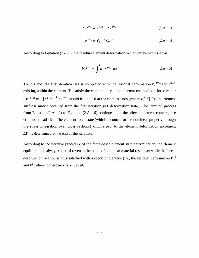
130
(2.A - 4)
(2.A - 5)
According to Equation (2 - 69), the residual element deformation vector can be expressed as
(2.A - 6)
To this end, the first iteration j=1 is completed with the residual deformation and
existing within the element. To satisfy the compatibility at the element end nodes, a force vector
should be applied at the element ends (where
is the element
stiffness matrix obtained from the first iteration j=1 deformation state). The iteration process
from Equation (2.A – 2) to Equation (2.A – 6) continues until the selected element convergence
criterion is satisfied. The element force state (which accounts for the nonlinear property through
the stress integration over cross sections) with respect to the element deformation increment
is determined at the end of the iteration.
According to the iterative procedure of the force-based element state determination, the element
equilibrium is always satisfied (even in the range of nonlinear material response) while the force-
deformation relation is only satisfied with a specific tolerance (i.e., the residual deformation
and ) when convergency is achieved.

131
Appendix 3.A
Acceptance Criteria of Steel Frame Members
The axial force of a frame member has a large impact on its plastic rotation capacity. In
accordance with ASCE/SEI 41-06 (ASCE 2007), the specified allowable plastic rotations for
a steel frame member under bending moment is
For zero axial force, i.e.,
(3.A - 1)
(3.A - 2)
For
(3.A - 3)
(3.A - 4)
For
(3.A - 5)
(3.A - 6)

132
For , the expected ductile behaviour of the column under a bending
moment cannot be guaranteed. Thus, its plastic rotation capacity is taken as zero (or a small
value determined using interpolation).
In the above equations, are the flange width and thickness, respectively; and are the
web height and thickness, respectively; Fye is the expected steel yield stress (in customary unit
ksi); P, Pn are the calculated axial compressive force and the corresponding nominal axial
compressive strength, respectively; (as shown in Figure 3-1) is the yield rotation of the
corresponding structural members and is computed as
(3.A - 7)
where L and I are the length and cross-sectional moment of inertia of the frame member,
respectively; Pye is the expected axial yield force of the member, and Pye = Ag Fye.
The expected material strength is obtained by multiplying its specified strength by an appropriate
factor. For example, CSA-S16-09 adopts Fye = 1.10 Fy.
With the assumption that out-of-plane buckling failure is prevented, the in-plane nominal
compressive strength can be determined using the equation from either AISC 360-05 (AISC
2005b) or CSA-S16-09 (CSA 2009). Herein, CSA-S16-09 equation is adopted due to its
simplicity,
(3.A - 8)
(3.A - 9)
(3.A - 10)
where n = 1.34 for hot-rolled, fabricated structural sections manufactured in accordance with
CSA G40.20, Class C (cold-formed non-stress-relieved).

133
Appendix 3.B
Minimum Weight Seismic Design of a Steel Portal Frame
A minimum weight seismic design problem of a steel portal frame is employed to test the
proposed optimization design methodology. The capability of using nonlinear time-history
analysis in practical design procedure is illustrated. The single objective optimal design problem
is solved by using a Genetic Algorithm.
The portal frame shown in Figure 3.B -1 is 30 ft (9.14 m) wide (centerline dimensions) and 13 ft
(3.96 m) high. The frame has rigid beam-to-column connections, with all column bases fixed at
the ground level. Only two design variables, x1 (column size) and x2 (beam size) are considered
in this design problem. The columns use a 50 ksi (345 MPa) steel wide-flange section, while the
beams use a 36 ksi (248 MPa) steel wide-flange section. The linear dead and live loads for the
roof beam are taken as 2.6 kip/ft (37.2 kN/m) and 0.6 kip/ft (8.8kN/m), respectively. The mass
used to compute the seismic load is
(3.B - 1)
where DL and LL are the dead and live loads, respectively; and g = 386 in/sec2 (9.8 m/sec
2).
1.0 DL + 0.5 LL
Beam
Column
Column
Figure 3.B -1 Side view of the steel portal frame

134
The earthquake ground motion, Northridge 01/17/94 1231, Santa Monica 090, available from the
Pacific Earthquake Engineering Research strong motion database (PEER 2008), is adopted as the
earthquake hazard for nonlinear time-history analysis. The portal frame is assumed to be
constructed at a location in Vancouver, British Columbia, Canada. To be compatible with the
design spectrum specified by NBCC 2010 for Vancouver, a scale factor of 3.2 is used to adjust
the ground motion.
Figure 3.B -2 Earthquake ground motion record
For deformation constraints, it is assumed that the allowable plastic rotation of steel members is
0.015 radians, and the allowable inter-storey drift is 2.5% of story height (i.e., lateral deflection
of the portal frame should not be greater than 3.9 in (99mm). Each of the two sectional variables
is selected from among a given group of compact sections (Table 3.B-1). The design
optimization problem is written as
(3.B - 2)
(3.B - 3)
(3.B - 4)
where: Ai is the cross sectional area for member i; Li is the length of member i; and ρ is the
material mass density of structural steel.
-1000
-500
0
500
1000
0 5 10 15 20
Acc
eler
ati
on
(m
m/s
ec/s
ec)
Time (second)
Northrige Earthquake - Santa Monica City Hall Ground

135
Table 3.B-1 Candidate sections for sizing variables x1, x2
Index Bitstring x1(column) x2(beam)
1 0000 W14x68 W18x106
2 0001 W14x61 W18x97
3 0010 W14x53 W18x86
4 0011 W14x48 W18x76
5 0100 W14x43 W18x71
6 0101 W14x38 W18x65
7 0110 W14x34 W18x60
8 0111 W14x30 W18x55
9 1000 W12x72 W16x100
10 1001 W12x58 W16x89
11 1010 W12x53 W16x77
12 1011 W12x50 W16x67
13 1100 W12x45 W16x57
14 1101 W12x40 W16x50
15 1110 W12x35 W16x45
16 1111 W12x30 W16x40
Bitstring: decode value of the size variables
Nonlinear time history analysis programmed in the OpenSees software (OpenSees 2008) is
employed to evaluate every candidate design. The steel material is modelled by a bilinear
elastoplastic stress-strain relationship with a 5% strain hardening. Frame members are modelled
using the force-based beam-column element with five Gauss-Labatto numerical integration
points. The lumped mass points are located at the beam-column joints of the frame. The mass
value at each joint is equal to half of the total mass. Newmark method of direct integration with
the assumption of constant average acceleration within a time interval is employed to construct
the system equations during iterations. The nonlinear equations during each time interval are
solved through Newton-Raphson numerical method. The Rayleigh damping matrix is determined
using the proportionality constants computed using the frequencies of modes 1 and 2 with
damping ratios of 0.05.
A Genetic Algorithm (implemented with the software of MATLAB) is applied to find the
optimal design. Since each design has 16 candidate sections, it is encoded with 4 bits (i.e., 24=16
sections). Each candidate design solution (i.e., a random combination of a column section and a
beam section) is represented by an 8-bit digit of chromosome. The first generation with a specific

136
population size is randomly generated. The violation of a constraint will cause the design
objective (i.e., ‘weight’ in this design problem) to be penalized. The population is improved
through the operations of crossover and mutation until the convergence criterion is reached. The
major parameters to control the GA are selected as follows,
Population Size: The parameter controls how many individual designs there are in each
generation. To investigate the effect of ‘Population Size’, a parameter study on various
values of ‘Population Size’ has been carried out from 10 to 35.
Crossover Rate: Crossover is an operation in which the genetic algorithm combines two
individuals, or parents, to produce an offspring. The crossover rate is taken to be 1 in this
problem.
Mutation Rate: To provide genetic diversity, a mutation rate is set to make small
random changes in individuals to create mutation children. The mutation rate is set to be
0.05 in this problem.
Design Results
Figure 3.B -3 Distribution of designs in objective - constraint space
It is found that all the candidate solutions satisfy the plastic rotation constraints on the columns
and the beam. The 256 design solutions are represented in the structural weight versus inter-
storey drift space, as shown in Figure 3.B-3. The drift constraint divides the design space into
2.5
3
3.5
4
4.5
5
5.5
6
6.5
1.5 2 2.5 3 3.5 4 4.5 5 5.5
Dri
ft (
in,
1 i
n =
0.0
25
4 m
)
Weight (kip, 1 kip = 4.448 kN)
infeasible
feasible optimal

137
feasible and infeasible subspaces. The optimal solution (i.e., the design with W14x43 beam and
W16x45 columns) is identified to be located at the far left of the feasible region (the weight is
2.468 kips (10.978 kN)) .
The results of 5 runs for each ‘population size’, total 30 runs, are shown in Table 3.B-2. It is
observed that the Genetic Algorithm is not guaranteed to obtain the minimum weight design
when only one run is implemented. Although each population size option leads to the optimal
design within 5 runs, it appears that the population size 30 (wherein 4 out of 5 runs obtain the
optimal design) is more effective for this design problem.
As illustrated in Figure 3.B-3, a specific inter-story drift can correspond to a large number of
design solutions. Generally, it is not easy to find the optimal solution through a trial-and-error
procedure.

138
Table 3.B-2 Results of GA runs
pop=10 bitstring x1 x2 Weight (kip) δ (in) φ (rad.)
Run1 01001110 W14x43 W16x45 2.468 3.80 0.0128
Run2 01101001 W14x34 W16x89 3.554 3.80 0.0141
Run3 00000101 W14x68 W18x65 3.718 3.70 0.0126
Run4 11000110 W12x45 W18x60 2.970 3.84 0.0129
Run5 11000110 W12x45 W18x60 2.970 3.84 0.0129
pop=15 bitstring x1 x2 Weight (kip) δ (in) φ (rad.)
Run1 00010111 W14x61 W18x55 3.236 3.86 0.0131
Run2 01010111 W14x38 W18x55 2.638 3.76 0.0137
Run3 11001011 W12x45 W16x67 3.180 3.88 0.0130
Run4 01001110 W14x43 W16x45 2.468 3.80 0.0128
Run5 01011100 W14x38 W16x57 2.698 3.87 0.0141
pop=20 bitstring x1 x2 Weight (kip) δ (in) φ (rad.)
Run1 01001110 W14x43 W16x45 2.468 3.80 0.0128
Run2 01100011 W14x34 W18x76 3.164 3.77 0.0140
Run3 01100011 W14x34 W18x76 3.164 3.77 0.0140
Run4 11001011 W12x45 W16x67 3.180 3.88 0.0130
Run5 01010111 W14x38 W18x55 2.638 3.76 0.0137
pop=25 bitstring x1 x2 Weight (kip) δ (in) φ (rad.)
Run1 01001110 W14x43 W16x45 2.468 3.80 0.0128
Run2 01010111 W14x38 W18x55 2.638 3.76 0.0137
Run3 01001110 W14x43 W16x45 2.468 3.80 0.0128
Run4 01010111 W14x38 W18x55 2.638 3.76 0.0137
Run5 00010111 W14x61 W18x55 3.236 3.86 0.0131
pop=30 bitstring x1 x2 Weight (kip) δ (in) φ (rad.)
Run1 01010111 W14x38 W18x55 2.638 3.76 0.0137
Run2 01001110 W14x43 W16x45 2.468 3.80 0.0128
Run3 01001110 W14x43 W16x45 2.468 3.80 0.0128
Run4 01001110 W14x43 W16x45 2.468 3.80 0.0128
Run5 01001110 W14x43 W16x45 2.468 3.80 0.0128
pop=35 bitstring x1 x2 Weight (kip) δ (in) φ (rad.)
Run1 01001110 W14x43 W16x45 2.468 3.80 0.0128
Run2 11000101 W12x45 W18x65 3.120 3.84 0.0129
Run3 01010111 W14x38 W18x55 2.638 3.76 0.0137
Run4 01010111 W14x38 W18x55 2.638 3.76 0.0137
Run5 01001110 W14x43 W16x45 2.468 3.80 0.0128 1 kip = 4.448 kN, 1 in = 0.0254 m

139
Appendix 4.A
Selected Ground Motion Time-Histories
Figure 4.A-1 Ground motion record (1979 Imperial Valley: El Centro Array #12)
Figure 4.A-2 Ground motion record (1989 Loma Prieta: Belmont Envirotech)
-0.15
-0.1
-0.05
0
0.05
0.1
0.15
0.2
0 5 10 15 20 25 30
Acc
ela
rati
on
(g
)
Time (second)
EL Centro
-0.15
-0.1
-0.05
0
0.05
0.1
0.15
0 5 10 15 20 25 30
Acc
ela
rati
on
(g
)
Time (second)
BES000

140
Figure 4.A-3 Ground motion record (1994 Northridge: Old Ridge RT 090)
Figure 4.A-4 Ground motion record (1989 Loma Prieta: Presidio)
-0.6
-0.4
-0.2
0
0.2
0.4
0.6
0.8
0 5 10 15 20 25 30
Acc
ela
rati
on
(g
)
Time (second)
ORR090
-0.25
-0.2
-0.15
-0.1
-0.05
0
0.05
0.1
0.15
0 5 10 15 20 25 30
Acc
ela
rati
on
(g
)
Time (second)
PRS090