Embed Size (px)
Citation preview
i
CAPACITIVE PROBE FOR ICE DETECTION AND
ACCRETION RATE MEASUREMENT: PROOF OF CONCEPT
By
Kwadwo Poku Owusu
A thesis submitted in partial fulfillment of the requirements for the degree of
Master of Science, Department of Mechanical Engineering
University of Manitoba
© Kwadwo Poku Owusu, 2010
ii
ABSTRACT
Ice accretion on wind turbines is a major problem in cold climates that reduces power generation
and fatigues turbine components. Effective anti-icing and de-icing strategies to manage ice
accretion require reliable local assessment of icing conditions and a measure of ice accretion rate
on structures. Such sensors could be located on meteorological towers near wind farms or the
nacelle of wind turbines. A new concept for the estimation of atmospheric ice accretion based
on the measurement of capacitance and resistance change between two charged cylinders as ice
accretes on the cylinders is introduced in this study. Numerical simulation of the electric field
between the charged cylinders is used to investigate the dependence of the sensitivity of
capacitance to the distance between the cylindrical probes and location of ice deposits. The
numerical results are validated experimentally using aluminum probes and a set of acrylic
cylindrical sleeves that fit over the probes to simulate icing with accurate geometries. A charged
cylindrical probes system constructed based on the numerical results is described and evaluated
under controlled rime and glaze icing conditions in the University of Manitoba Icing Wind
Tunnel. Test results indicate ice builds up on the cylindrical probes and the measured
capacitance increases while the resistance decreases. The change in measured capacitance
change correlates well with the increase in the ice mass. Rime and glaze ice are distinguishable
based on the rate of change of resistance with ice accretion. The numerical and experimental
results provide a proof of concept of the charged cylindrical probes ice accretion measurement
concept.

iii
ACKNOWLEDGMENTS
My sincere gratitude goes to my advisors Dr. David C.S. Kuhn and Dr. Eric L. Bibeau for their
supervision, support and encouragement throughout this research. Many thanks to Bruce Ellis,
for thoroughly training me in the use of the wind-icing tunnel as well helping me acquire data for
this research. Many thanks to all my friends for lending a hand when needed. Last but the most,
I am grateful to my parents and siblings for their unconditional love and support.

iv
TABLE OF CONTENTS
ABSTRACT .................................................................................................................................... ii
TABLE OF CONTENTS ............................................................................................................... iv
LIST OF TABLES ....................................................................................................................... viii
LIST OF FIGURES ....................................................................................................................... ix
Chapter 1 ......................................................................................................................................... 1
1.1 Background ...................................................................................................................... 1
1.2 Thesis objective .................................................................................................................. 3
Chapter 2 ......................................................................................................................................... 5
Literature survey ......................................................................................................................... 5
2.1 Introduction ...................................................................................................................... 5
2.2 General impact of icing .................................................................................................... 5
2.3 Atmospheric icing ............................................................................................................ 6
2.3.1 Glaze icing ................................................................................................................ 7
2.3.2 Rime icing ................................................................................................................. 8
2.4 Ice accretion process ........................................................................................................ 9
2.4.1 Collision efficiency ................................................................................................. 10
2.4.2 Sticking efficiency .................................................................................................. 12
2.4.3 Accretion efficiency ................................................................................................ 12
v
2.5 Methods of ice detection ................................................................................................ 13
2.5.1 Indirect methods of ice detection ........................................................................... 13
2.5.2 Direct methods of ice detection .............................................................................. 14
2.6 Icing sensors ................................................................................................................... 14
2.6.1 Goodrich ice detector models 0871LH1 ................................................................. 14
2.6.2 LID-3210C and LID-3210D ice detectors .............................................................. 15
2.6.3 METEO device ....................................................................................................... 16
2.6.4 Ice monitor .............................................................................................................. 16
2.6.5 HoloOptics T20-series ice detectors ....................................................................... 17
2.6.6 Instrumar limited ice sensor IM101 ........................................................................ 17
2.6.7 Heated and unheated anemometers ......................................................................... 17
2.6.8 Actual power generated versus predicted power from wind speed ........................ 18
2.7.1 Advantages of capacitive sensors ........................................................................... 19
2.8 Ice sensors detection ....................................................................................................... 20
Chapter 3 ....................................................................................................................................... 21
3.1 Introduction .................................................................................................................... 21
3.2 Working principles of the two-cylinder capacitance sensor .......................................... 21
3.3 Electric field lines ........................................................................................................... 24
3.3.1 Capacitance between two parallel cylindrical probes ............................................. 25
3.3.2 Resistance between two parallel-arranged cylinders .............................................. 29
vi
Chapter 4 ....................................................................................................................................... 31
4.1 Introduction ................................................................................................................... 31
4.2 Description of the two-cylinder capacitance sensor ....................................................... 31
4.3 Numerical simulations.................................................................................................... 32
4.3.1 Numerical procedure ................................................................................................ 33
4.4 Acrylic sleeve experiment .............................................................................................. 35
4.4.1 Acrylic experiment procedure .................................................................................. 37
4.5 The University of Manitoba icing wind tunnel .............................................................. 39
4.5.1 The icing wind tunnel ............................................................................................... 39
4.5.2 Icing wind tunnel calibration .................................................................................... 40
4.5.3 Experimental conditions ........................................................................................... 41
4.5.4 Experimental procedure ........................................................................................... 42
4.6 Error in measurements ................................................................................................... 44
Chapter 5 ....................................................................................................................................... 48
5.1 Introduction .................................................................................................................... 48
5.2 Numerical and acrylic studies ........................................................................................ 48
5.3 Wind icing tunnel experiments ..................................................................................... 56
5.3.1 Experiments at -10oC .............................................................................................. 56
5.3.2 Experiments at -2oC ................................................................................................. 60
5.3.3 Ice accretion rate ........................................................................................................... 64
vii
5.3.4 Capacitance variation with exposure time ............................................................... 67
5.3.5 Capacitance versus mass and thickness of ice accreted ........................................... 71
5.3.6 Sensitivity ................................................................................................................ 74
5.3.7 Resistance change against exposure time ................................................................ 77
5.4 Optimal sensor configuration ......................................................................................... 78
Chapter 6 ....................................................................................................................................... 80
6.1 Conclusions ..................................................................................................................... 80
Chapter 7 ....................................................................................................................................... 82
7.1 Recommendations .......................................................................................................... 82
Reference ...................................................................................................................................... 83
Appendix A ................................................................................................................................... 89
Appendix B ................................................................................................................................... 92

viii
LIST OF TABLES
Table 4.1: Dimensions of acrylic sleeves................................................................................37
Table 4.3: Dimensions of porous acrylic sleeves....................................................................38
Table 4.2: Experimental conditions for wind icing tunnel tests.............................................43
Table 5.1: Summary of porous acrylic sleeves experiments...................................................54
Table 5.2: Summary of rate of icing on the probe..................................................................66
Table 5.3: Optimal sensor configuration................................................................................78

ix
LIST OF FIGURES
Figure 2.1: A picture of glaze ice formed on the cylindrical probes .............................................. 8
Figure 2.2: A typical rime ice formation on the cylindrical probes ................................................ 9
Figure 3.1: Trajectory of supercooled water drops and air moving towards two cylindrical probes
....................................................................................................................................................... 23
Figure 3.2: Iced formation at the windward side of the cylindrical probes .................................. 23
Figure 3.3: Schematic of electric field lines between two opposite charged cylinders ................ 25
Figure 3.4: Plan view of the two cylindrical probes ..................................................................... 26
Figure 4.1: Schematic two-cylinder capacitance sensor and ancillary equipments ...................... 32
Figure 4.2: Cases considered for numerical simulation ................................................................ 34
Figure 4.3: 500,000 node computational domain ......................................................................... 36
Figure 4.4: Components of model icing experimental set up ....................................................... 37
Figure 4.5: Wind Icing Tunnel ...................................................................................................... 41
Figure 4.6: Schematic of (a) Inline and (b) Parallel orientations of the cylindrical probes in
relation to the wind and water drop direction ............................................................................... 42
Figure 4.7: Standard error estimates in the measured (a) mass and (b) thickness for both rime and
glaze ice at wind velocity of 5 m/s ................................................................................................ 46
Figure 4.8: Standard error estimates in the measured capacitance for both rime and glaze ice at
wind velocity of 5 m/s................................................................................................................... 47
Figure 4.9: Standard error estimates in the measured capacitance for acrylic experiments ......... 47
x
Figure 5.1: Capacitance variation with probe centre-to-centre distance, s ................................... 49
Figure 5.2: Electric field distribution calculated using QuickField™, s = 1.87 cm, d = 1.27 cm,
Q = 1 C .......................................................................................................................................... 50
Figure 5.3: Effect of decreasing the diameter of one of the cylindrical probes on the capacitance;
larger probe diameter, d=1.27 cm and s=1.87 cm ........................................................................ 52
Figure 5.5: Capacitance variation with size of acrylic sleeves. Inline case has a single sleeve on
one of the cylindrical probes while parallel case has sleeves on the two cylindrical probes ....... 54
Figure 5.6: Photographs of rime ice formed on the cylindrical probes for parallel orientation
(a and b) and inline orientation (c and d) at -10oC, time 4 and 15 minutes respectively, wind
speed of 5 m/s and LWC 0.8 g/m3 ................................................................................................ 57
Figure 5.7: Top view time evolution of rime ice accretion on cylindrical probes for inline
orientation at temperature of -10C, wind speed 5 m/s and LWC 0.8 g/m3 ................................. 58
Figure 5.8: Top view time evolution of rime ice accretion on the cylindrical probes for parallel
orientation at temperature of -10oC, wind speed 5 m/s and LWC 0.8 g/m3 ................................. 59
Figure 5.10: Glaze ice formation on cylindrical probes for the parallel orientation case with
horn-like impressions predominant on the right probe ................................................................. 62
Figure 5.12: Top view time evolution of glaze ice accretion on the cylindrical probes for inline
orientation at temperature of -2C, wind speed 5 m/s and LWC 2 g/m3 ...................................... 63
Figure 5.13: (a) Mass and (b) thickness variation with exposure time for rime ice at temperature
of -10oC and LWC 0.8 g/m3, standard error bars on the 5 m/s parallel case ................................ 65
xi
Figure 5.14: (a) Mass and (b) thickness variation with exposure time for glaze ice at temperature
of -2oC and LWC 2 g/m3, standard error bars on the 5 m/s parallel case ..................................... 66
Figure 5.15: Capacitance variation with exposure time for rime ice at -10oC, 0.8 g/m3 ............. 69
Figure 5.16: Capacitance variation with exposure time for glaze ice at -2oC, 2 g/m3 ................. 70
Figure 5.17: Capacitance variation with (a) mass and (b) thickness respectively for rime ice
conditions at various wind velocities at temperature -10oC and LWC 0.8 g/m3 .......................... 72
Figure 5.18: Capacitance variation with (a) mass and (b) thickness respectively for glaze ice at
various wind velocities at temperature -2oC and LWC 2 g/m3 ..................................................... 73
Figure 5.19: Capacitance normalized with (a) mass and (b) thickness respectively versus
exposure time for rime ice at various wind velocities at temperature -10oC and LWC 0.8 g/m3 . 75
Figure 5.20: Capacitance normalized with (a) mass and (b) thickness respectively versus
exposure time for glaze ice, at various wind velocities at temperature -2oC and LWC 2 g/m3 ... 76
Figure 5.21: Resistance variation with exposure time ................................................................. 78

1
Chapter 1
Introduction
1.1 Background
Globally, fossil fuels are the primary source of electricity with nuclear power plants and
hydropower being employed to meet the demands in certain regions of the world. In recent
times, concerns about the harmful effects of emissions of carbon and global warming have
created new demands for an alternative and suitable energy source such as wind energy. The
benefits of wind energy include an abundant source, pollution free, local power generation at site
that reduces long distances transmission losses [Patel, 2006] and economic gains such as
investments in rural development as well as creation of new jobs.
In 2007, worldwide wind energy generation was estimated at 94 GW. It is projected that the
global investment in the wind industry will reach $1 trillion by the year 2020, equivalent to
500 GW of electricity [CanWEA, 2008]. In Canada, wind power capacity is expected to rise
from 0.4 GW in 2004 to 8.5 GW in 2020. This according to Natural Resources Canada
represents 6% of the national generating capacity and 3.6% of total electricity production
[CanWEA, 2007]. In 2006, the Province of Manitoba reiterated its commitment of harvesting
1 GW of wind power over the next decade [Rondeau, 2006]. However, there are problems
associated with wind power generation in cold climates such as Canada, most notably icing.
Icing can cause problems ranging from decrease of power due to modifications in the
aerodynamics of the blades [Jasinski et al., 1998], aerodynamic changes of blade profile which
results in increased blade vibration and fatigue of wind turbine components [Ganander and
2
Ronsten, 2003], to additional safety concerns to people and wildlife due to detachment of
accumulated ice [Seifert, 2003].
These problems require prevention of ice adhering to the surface or removal of ice from the
blades once accretion has occurred. Anti-icing and de-icing techniques are commonly mentioned
in the literature as the means of ice mitigation. To effectively use anti-icing and de-icing
techniques, the detection of the onset of the icing event is foremost. In the wind engineering
industry, a number of methods have been devised to detect icing. These methods are categorised
into two groups: direct and indirect methods. The direct methods are based on the principle of
detecting a property change caused by the ice accretion. Examples of such properties include
mass and dielectric constants. The inductance change probe of Lee and Seegmiller [1996],
impedance change probe of Wallace et al., [2002] and the microwave ice detector of Magenheim
[1977] are examples of ice detectors based on direct methods. The indirect methods involve
detecting weather conditions such as humidity and temperature that lead to atmospheric icing
conditions or detecting effects of icing, e.g. reduction in power generation or reduction in the
speed of anemometers, with an empirical or deterministic model used to determine when icing is
occurring [Homola et.al, 2006]. The reduction in the speeds of the heated and unheated
anemometers of Craig and Craig [1995] and the noise generation frequency of Seifert [2003] are
examples of the indirect methods.
In the work of Homola et al., [2006], most of the 29 methods presented were found not to be
reliable for ice detection base on the study’s set of requirements. These requirements include
high sensitivity and wide area detection capabilities. However, they indicated that ice sensors
based on the changes in electric properties such as capacitance and inductance probes appear
promising for use in the detection of icing in the wind engineering industry. However, these
3
latter methods have not been scientifically investigated and assessed. Some of the reasons for
this assertion include knowledge of electrical property changes and the ability of such a probe to
detect icing over a wider area than at a single point. The latter is important because depending on
the mechanism of the icing event, ice accretion would generally tend not to occur at a single
point or location but rather at varying locations. For instance, glaze ice can accrete over a large
area due to water run-off freezing in different locations.
1.2 Thesis objectives
There is a lack of knowledge as to whether a capacitance probe can be an effective method for
ice detection. Although capacitance probes have been developed for other applications
(two-phase gas-liquid flows), there is a clear lack in the literature how effective capacitance
probes could be for ice detection. The objectives of this thesis are to:
1. Test the concept of estimation of atmospheric ice accretion on structures based on the
measurement of capacitance and resistance change between two electrically charged
cylindrical probes as ice accretes on the cylinders. The probes would be located on
metrological towers near wind farms or the nacelle of wind turbines.
2. Use a theoretical model to study the changes in capacitance with ice accretion, and
validate these studies in a laboratory setting using “modelled” ice growths.

4
3. Validate the charged cylindrical probes ice accretion measurement concept under
simulated rime and glaze ice conditions in the University of Manitoba Icing Wind Tunnel.
5
Chapter 2
Literature survey
2.1 Introduction
This chapter reviews the following topics: general impact of icing, atmospheric icing, ice
accretion process, methods of ice detection, icing sensors, general uses of capacitive sensors and
the two-cylinder capacitance device.
2.2 General impact of icing
In the past, wind turbines were mainly installed along coastal areas where extreme cold
temperatures that facilitate icing events do not occur or they had marginal importance on design
parameters [Wolff, 2000]. Recently, there is growing interest to install wind turbines at sites
prone to heavy icing events since there is large wind energy potential. Additionally, the rate of
icing increases with elevation and with taller wind turbines, the tips of the blades are more likely
to experience icing notwithstanding a location in a coastal area [Kimura et al., 2000]. With the
potential for more humidity in the air, climate change may make the situation more prominent.
Icing of wind turbine blades or other related components can lead to decreased power
production, overproduction of power by the wind turbine at low temperatures (higher air
density), increased fatigue loads or prolonged breaks in power production due to safety concerns
such as detachment of ice from the turbine blades.
To maximise the performance of these wind turbines, meteorological instruments are generally
mounted on meteorological towers to measure environmental parameters: humidity, ambient air
temperature, wind speed and direction. Various research groups have studied the effects of icing
6
on these meteorological instruments. An example of such studies was done by Seifert [2003]. He
studied the effect of winter conditions on two-cup anemometers — one heated and the other
unheated, at Tauren Wind Park, Austria. His findings indicate differences in the wind speed
recorded by the anemometers. This is consistent with most wind measurements in cold climates.
The wind speed measured by the unheated anemometer was consistent with expected results,
since there was no significant accumulation of ice on it. On the other hand, the heated
anemometer collected ice, melted, with the resulting liquid water moving outwards due to
centrifugal forces and refreezing at the tips. This increased the weight of the cups culminating in
a reduction of the wind speed measured by this anemometer.
Ice storms can also be very destructive. This has increased the interest in icing research,
particularly in developing reliable ice sensors/probes for mounting on meteorological towers.
There are currently few ice sensors/probes commercially available, which are capable of
detecting ice in addition to sensing ice accumulation rates (e.g. Goodrich ice sensor). However,
there is presently no ice sensor available that can detect ice, distinguish between the two types of
in-cloud icing and indicate the rate of icing. Therefore, the focus of this research is to
demonstrate a novel concept for an ice sensor capable of detecting ice, indicating icing rate as
well as distinguishing between the two types of in-cloud icing.
2.3 Atmospheric icing
Icing is the process by which snow or ice accretes on the surface of an object or a structure
exposed to the atmosphere. In-cloud icing and precipitation icing are the two main types of
atmospheric icing. In-cloud icing occurs when supercooled water drops impact on the surface of
a structure resulting in the formation of ice. There are two types of in-cloud icing: rime and glaze
7
icing [Homola et al., 2006 & Drage and Lange, 2005]. In-cloud ice accretion on a structure is
dependent on factors such as the wind speed, the dimensions of the exposed structure, the drop
size distribution, the liquid water content in the air, surface conditions of the exposure structure
and the air temperature [Frohboese et al., 2007 & Drage and Lange, 2005]. Precipitation icing
occurs when snow or rain freezes on impact with the surface of a structure. Freezing rain, which
differs from rime and glaze ice by virtue of its large drop size and wet snow, are the two types of
precipitation icing [Homola et al., 2006 & Drage and Lange, 2005].
In keeping with the set of objectives of this research, icing wind tunnel experiments were
focused on in-cloud icing. Moreover, in-cloud icing is the predominate form of icing which
affects wind turbines [Kraj, 2007].
2.3.1 Glaze icing
Glaze icing occurs when supercooled water drops impact the surface of a structure at or below
freezing temperatures under high liquid water content conditions. Glaze ice is typically
characterised by water run-offs on the icing surface, since the impinging drops do not have
enough time to freeze before the next drops impact the same area. Glaze ice growth is generally
termed wet [COST 727, 2006]. It occurs at temperatures between -4°C and 0°C [Bose, 1992].
Glaze ice is transparent in appearance with horns-like impressions on its surface. The density of
glaze ice typically ranges between 0.8 and 0.9 g/cm3 [Wang, 2008], which is comparatively larger
than rime ice as will be evident in the next section. Due to its higher density, glaze ice adheres
firmly to the surface when formed. The following are factors that favour glaze ice formation:
relatively large drop size distribution compared to rime ice, slow dissipation of the latent heat of
8
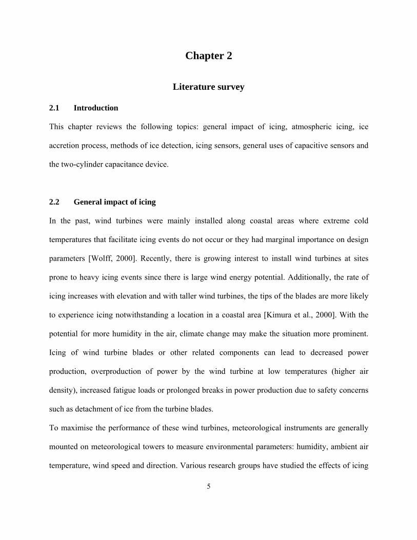
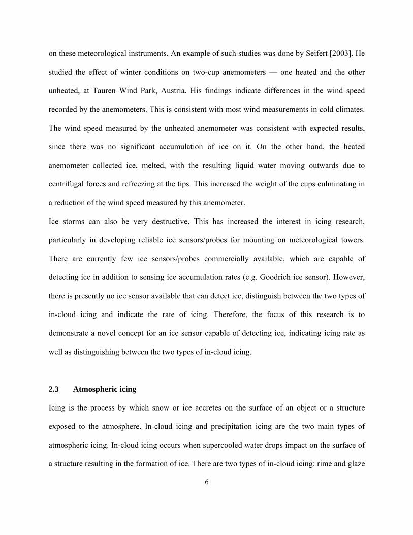
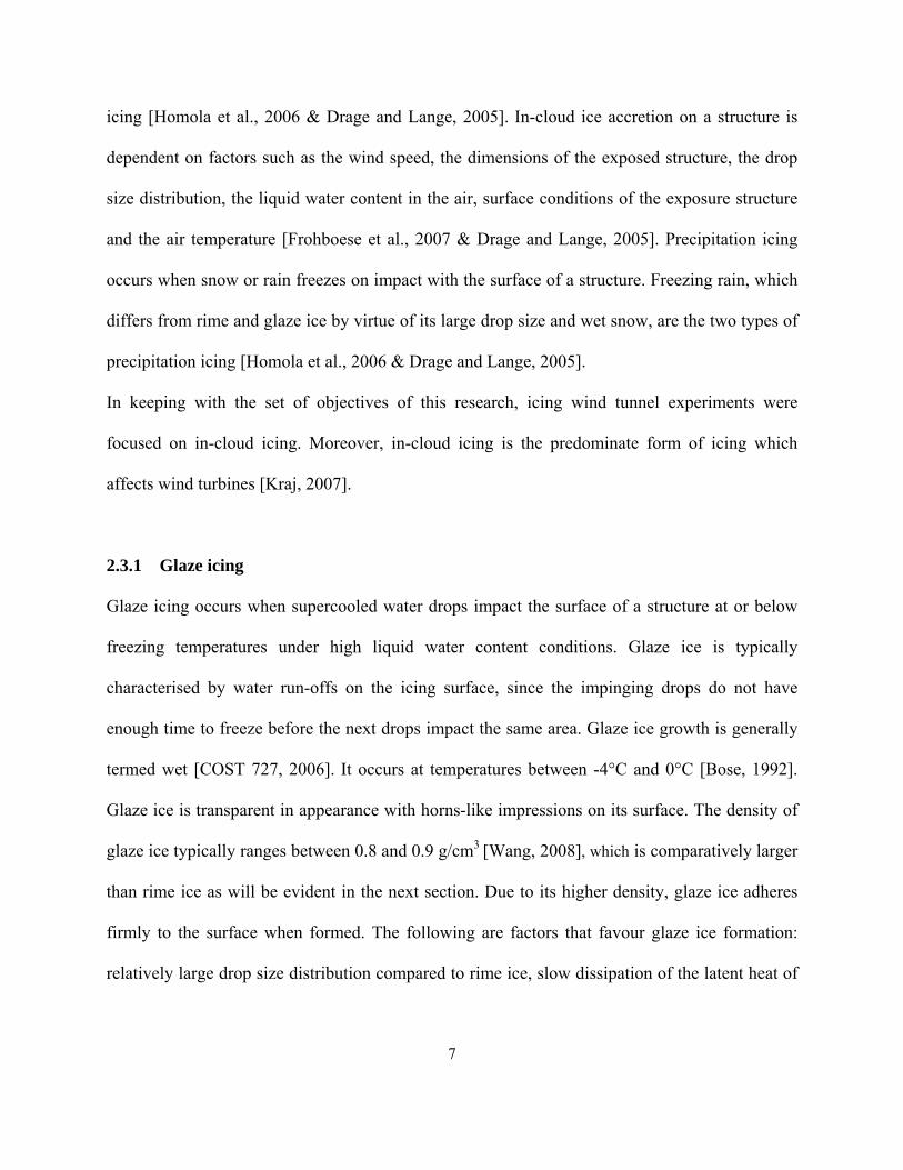
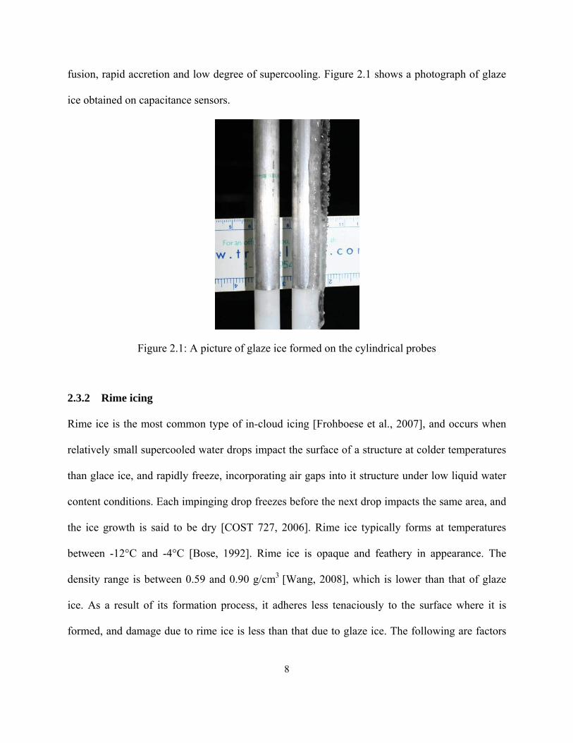
fusion, rapid accretion and low degree of supercooling. Figure 2.1 shows a photograph of glaze
ice obtained on capacitance sensors.
Figure 2.1: A picture of glaze ice formed on the cylindrical probes
2.3.2 Rime icing
Rime ice is the most common type of in-cloud icing [Frohboese et al., 2007], and occurs when
relatively small supercooled water drops impact the surface of a structure at colder temperatures
than glace ice, and rapidly freeze, incorporating air gaps into it structure under low liquid water
content conditions. Each impinging drop freezes before the next drop impacts the same area, and
the ice growth is said to be dry [COST 727, 2006]. Rime ice typically forms at temperatures
between -12°C and -4°C [Bose, 1992]. Rime ice is opaque and feathery in appearance. The
density range is between 0.59 and 0.90 g/cm3 [Wang, 2008], which is lower than that of glaze
ice. As a result of its formation process, it adheres less tenaciously to the surface where it is
formed, and damage due to rime ice is less than that due to glaze ice. The following are factors
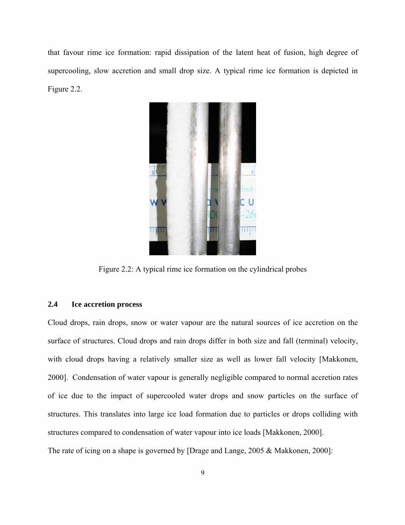
9
that favour rime ice formation: rapid dissipation of the latent heat of fusion, high degree of
supercooling, slow accretion and small drop size. A typical rime ice formation is depicted in
Figure 2.2.
Figure 2.2: A typical rime ice formation on the cylindrical probes
2.4 Ice accretion process
Cloud drops, rain drops, snow or water vapour are the natural sources of ice accretion on the
surface of structures. Cloud drops and rain drops differ in both size and fall (terminal) velocity,
with cloud drops having a relatively smaller size as well as lower fall velocity [Makkonen,
2000]. Condensation of water vapour is generally negligible compared to normal accretion rates
of ice due to the impact of supercooled water drops and snow particles on the surface of
structures. This translates into large ice load formation due to particles or drops colliding with
structures compared to condensation of water vapour into ice loads [Makkonen, 2000].
The rate of icing on a shape is governed by [Drage and Lange, 2005 & Makkonen, 2000]:
10
2.1
where is the flux density, that is, the product of the mass accumulation per unit volume and
the velocity of the particles relative to the structure, is the cross sectional area of the shape,
and , , are the collision, sticking and accretion efficiency, respectively.
2.4.1 Collision efficiency
Collision efficiency , is the ratio of the flux density of the drops that impinges on the surface to
the maximum flux density in the free stream. Collision efficiency is a function of the transport
mechanism of the drops in the air stream. Molecular diffusion, Brownian motion,
thermophoresis, turbulent diffusion and inertia impaction are possible transport mechanisms.
Molecular diffusion is the dominant transport mechanism for particles with sizes less than
0.1 μm. These particles follow the gas laws. Such particles tend to move with velocities close to
those of the gas molecules as well as follow the streamlines of the gas flow [Reid, 1971].
Brownian motion is applicable to particles falling within the size interval of 0.1 to 1 μm.
Brownian motion is characterised by the random motion of particles in the gas stream due to
collision with the gas molecules [Reid, 1971].
Particles within the size interval of 0.1 to 5 μm when subject to a temperature gradient move
toward the colder regions (i.e. down the temperature gradient) in a gas. Transportation of
particles due to this force is known as thermophoresis. This phenomenon occurs because the gas
molecules become more energetic on the hotter region pushing the particles towards the colder
region. In addition to particle size, thermophoresis is dependent on factors such as the steepness
11
of the temperature gradient and the heat absorption ability of the particles [Piazza and Parola,
2008].
Within the turbulent flow regime, particles of size 1 to 10 μm are able to move across the laminar
sub-layer to the surface of the structure. These particles achieve this fate by picking up higher
kinetic energy from the gas eddies. This type of transport mechanism is known as turbulent
diffusion [Reid, 1971].
With comparatively large particle sizes, inertia impaction transport mechanism dominates. Due
to their large size and higher density than the surrounding carrier gas, they acquire enough
momentum to move independently of local variations in the carrier gas, resulting in collision
with the surface of obstacles [Reid, 1971]. The dominate transport mechanism of falling
supercooled atmospheric water drops is inertia impaction.
As a supercooled water drop moves through the air stream, the probability of it impacting the
surface of a structure due to inertia is a function of the drop size, the geometry of the structure
and the flow field around the structure. The non-dimensional Stokes number characterises this
probability and is define as the ratio of the stopping distance of a particle to a characteristic
dimension of the obstacle. Particles with Stokes number greater than 1 will typically continue to
move in a straight path impacting the structure in its way while the air stream moves around the
structure. Particles with Stokes number less than 1 tend to follow the air stream [Crowe et al.,
1998].
The collision efficiency is reduced from a maximum value of 1 when the Stokes number is less
than 1. Additionally, collision efficiency is a function of the wind speed and the size of the
impinging structure [Drage and Lange, 2005 & Makkonen, 2000]. Determination of the collision
efficiency for non-simple structures is computationally expensive and complicated, since it
12
involves the numerical solution of both the airflow field and drop trajectories. However, for
practical engineering applications, simplified approaches based on the assumption that the icing
structure is cylindrical in shape are available [Makkonen, 2000].
2.4.2 Sticking efficiency
Sticking efficiency , is the ratio of the flux density of drops that hit and stick to the surface of
the structure to the flux density of the drops that hit the surface of the structure. Drops are
considered trapped or stuck to the surface of a structure when they are permanently collected or
their residence time is long enough to affect the rate of icing, for example, exchange heat with
the surface [Makkonen, 2000]. It is reduced from a maximum value of 1 when drops are
reflected or bounce off the surface of the structure. The sticking efficiency is assumed unity for
in-cloud icing [Ahti, and Makkonen, 1982]. For wet snow, the sticking efficiency is
approximately 1 [Makkonen, 2000] while for dry snow the sticking efficiency is approximately 0
[Wakahama et al., 1977]. Air temperature and humidity are known to affect the sticking
efficiency [Makkonen, 2000].
2.4.3 Accretion efficiency
Accretion efficiency , is the ratio of the rate of ice accretion in relation to the flux density of
the drops that stick to the surface. Accretion efficiency has a maximum value of 1, when the heat
flux from the accretion process is enough to cause sufficient freezing, thereby sticking drops all
lead to ice accretion. Rime ice has an accretion efficiency of 1, since all the impinging water
drops freeze upon impact with the exposed surface. Glaze ice however, has an accretion
efficiency of less than 1 because the freezing rate is controlled by the rate at which the latent heat
13
released in the freezing process can be transferred away from the icing surface. To determine the
accretion efficiency for a surface undergoing glaze icing, the budget of the heat transfer process
occurring on the surface is paramount [Makkonen, 2000].
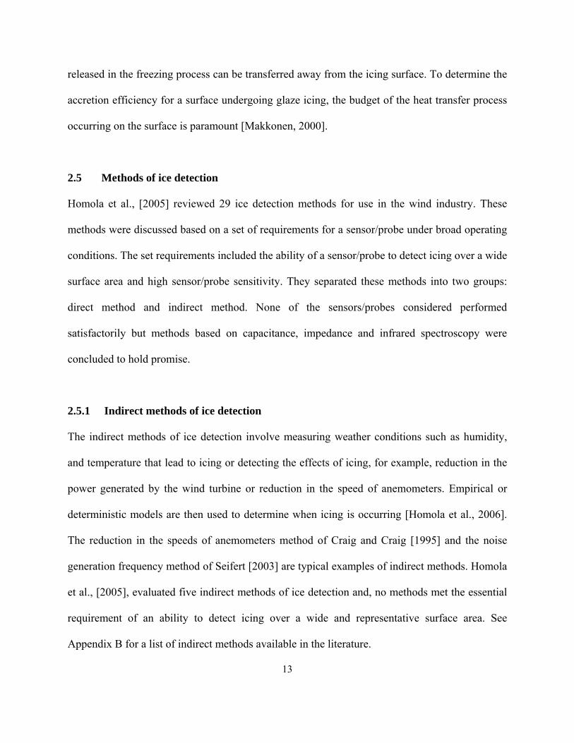
2.5 Methods of ice detection
Homola et al., [2005] reviewed 29 ice detection methods for use in the wind industry. These
methods were discussed based on a set of requirements for a sensor/probe under broad operating
conditions. The set requirements included the ability of a sensor/probe to detect icing over a wide
surface area and high sensor/probe sensitivity. They separated these methods into two groups:
direct method and indirect method. None of the sensors/probes considered performed
satisfactorily but methods based on capacitance, impedance and infrared spectroscopy were
concluded to hold promise.
2.5.1 Indirect methods of ice detection
The indirect methods of ice detection involve measuring weather conditions such as humidity,
and temperature that lead to icing or detecting the effects of icing, for example, reduction in the
power generated by the wind turbine or reduction in the speed of anemometers. Empirical or
deterministic models are then used to determine when icing is occurring [Homola et al., 2006].
The reduction in the speeds of anemometers method of Craig and Craig [1995] and the noise
generation frequency method of Seifert [2003] are typical examples of indirect methods. Homola
et al., [2005], evaluated five indirect methods of ice detection and, no methods met the essential
requirement of an ability to detect icing over a wide and representative surface area. See
Appendix B for a list of indirect methods available in the literature.
14
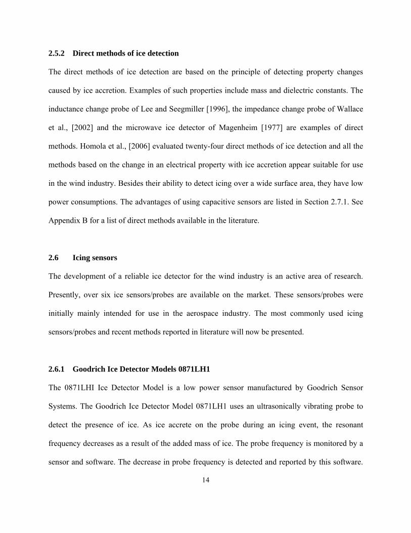
2.5.2 Direct methods of ice detection
The direct methods of ice detection are based on the principle of detecting property changes
caused by ice accretion. Examples of such properties include mass and dielectric constants. The
inductance change probe of Lee and Seegmiller [1996], the impedance change probe of Wallace
et al., [2002] and the microwave ice detector of Magenheim [1977] are examples of direct
methods. Homola et al., [2006] evaluated twenty-four direct methods of ice detection and all the
methods based on the change in an electrical property with ice accretion appear suitable for use
in the wind industry. Besides their ability to detect icing over a wide surface area, they have low
power consumptions. The advantages of using capacitive sensors are listed in Section 2.7.1. See
Appendix B for a list of direct methods available in the literature.
2.6 Icing sensors
The development of a reliable ice detector for the wind industry is an active area of research.
Presently, over six ice sensors/probes are available on the market. These sensors/probes were
initially mainly intended for use in the aerospace industry. The most commonly used icing
sensors/probes and recent methods reported in literature will now be presented.
2.6.1 Goodrich Ice Detector Models 0871LH1
The 0871LHI Ice Detector Model is a low power sensor manufactured by Goodrich Sensor
Systems. The Goodrich Ice Detector Model 0871LH1 uses an ultrasonically vibrating probe to
detect the presence of ice. As ice accrete on the probe during an icing event, the resonant
frequency decreases as a result of the added mass of ice. The probe frequency is monitored by a
sensor and software. The decrease in probe frequency is detected and reported by this software.
15
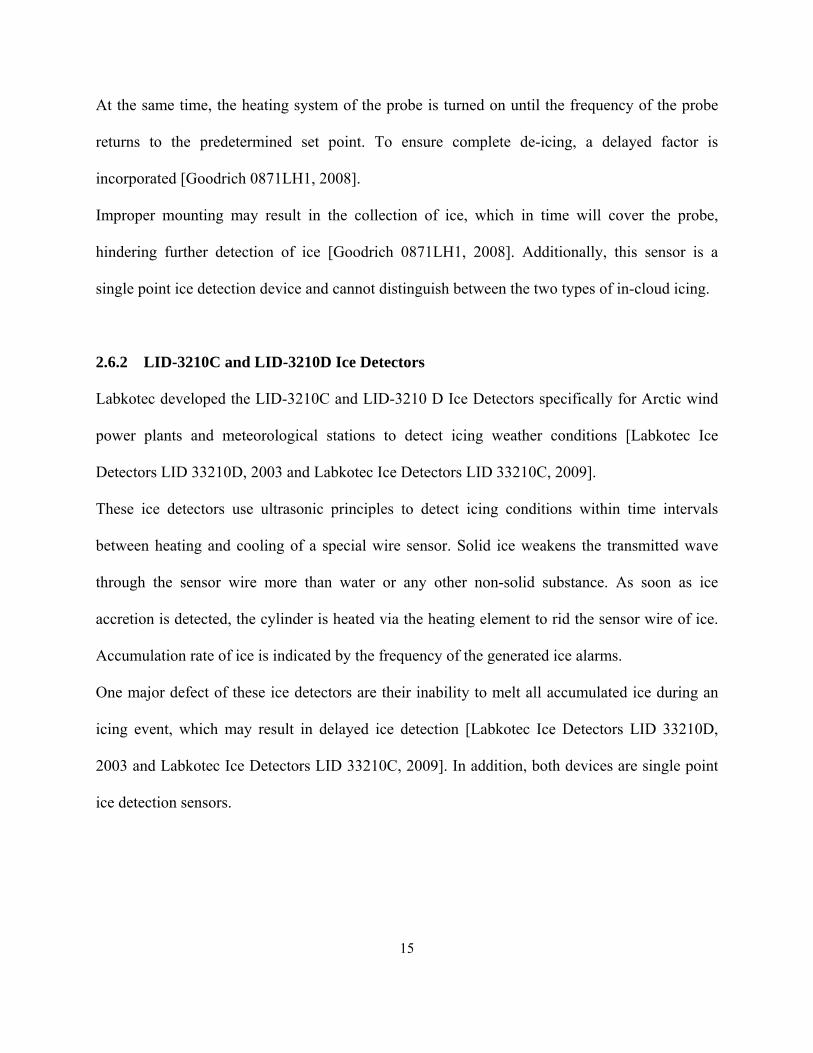
At the same time, the heating system of the probe is turned on until the frequency of the probe
returns to the predetermined set point. To ensure complete de-icing, a delayed factor is
incorporated [Goodrich 0871LH1, 2008].
Improper mounting may result in the collection of ice, which in time will cover the probe,
hindering further detection of ice [Goodrich 0871LH1, 2008]. Additionally, this sensor is a
single point ice detection device and cannot distinguish between the two types of in-cloud icing.
2.6.2 LID-3210C and LID-3210D Ice Detectors
Labkotec developed the LID-3210C and LID-3210 D Ice Detectors specifically for Arctic wind
power plants and meteorological stations to detect icing weather conditions [Labkotec Ice
Detectors LID 33210D, 2003 and Labkotec Ice Detectors LID 33210C, 2009].
These ice detectors use ultrasonic principles to detect icing conditions within time intervals
between heating and cooling of a special wire sensor. Solid ice weakens the transmitted wave
through the sensor wire more than water or any other non-solid substance. As soon as ice
accretion is detected, the cylinder is heated via the heating element to rid the sensor wire of ice.
Accumulation rate of ice is indicated by the frequency of the generated ice alarms.
One major defect of these ice detectors are their inability to melt all accumulated ice during an
icing event, which may result in delayed ice detection [Labkotec Ice Detectors LID 33210D,
2003 and Labkotec Ice Detectors LID 33210C, 2009]. In addition, both devices are single point
ice detection sensors.
16
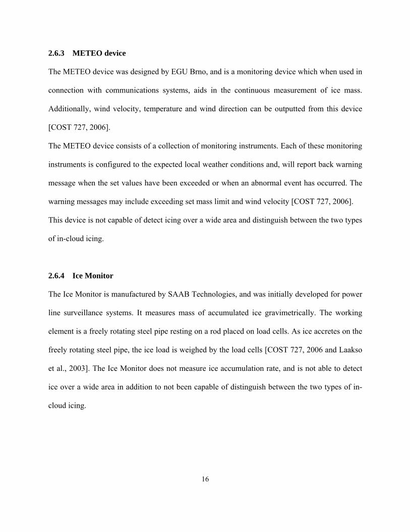
2.6.3 METEO device
The METEO device was designed by EGU Brno, and is a monitoring device which when used in
connection with communications systems, aids in the continuous measurement of ice mass.
Additionally, wind velocity, temperature and wind direction can be outputted from this device
[COST 727, 2006].
The METEO device consists of a collection of monitoring instruments. Each of these monitoring
instruments is configured to the expected local weather conditions and, will report back warning
message when the set values have been exceeded or when an abnormal event has occurred. The
warning messages may include exceeding set mass limit and wind velocity [COST 727, 2006].
This device is not capable of detect icing over a wide area and distinguish between the two types
of in-cloud icing.
2.6.4 Ice Monitor
The Ice Monitor is manufactured by SAAB Technologies, and was initially developed for power
line surveillance systems. It measures mass of accumulated ice gravimetrically. The working
element is a freely rotating steel pipe resting on a rod placed on load cells. As ice accretes on the
freely rotating steel pipe, the ice load is weighed by the load cells [COST 727, 2006 and Laakso
et al., 2003]. The Ice Monitor does not measure ice accumulation rate, and is not able to detect
ice over a wide area in addition to not been capable of distinguish between the two types of in-
cloud icing.
17
2.6.5 HoloOptics T20-series Ice Detectors
HoloOptics manufacture the T20-series. The T20-series Ice Detectors sense the presence of ice
as well as measuring ice accretion rate. The working element comprise of either a single head or
four heads with infrared emitter, a photo detector and a probe.
An icing event is recorded if more than 95% of the probe is covered with a 50 µm thick layer of
glaze ice or a 90 µm thick layer of other types of ice. Once icing is detected, the probe’s internal
heating system is activated to melt the accreted ice. The time it takes to deice is dependent solely
on the icing rate if sufficient amount of heating power is provided. The time lapse between icing
events is used to determine the icing rate [Laakso et al., 2003]. These ice detectors do not
distinguish between the two types of in-cloud icing.
2.6.6 Instrumar Limited Ice Sensor IM101
Instrumar Limited Ice Sensor IM101 measures both the surface temperature and electrical
impedance of a ceramic probe. This data is then used to determine the surface conditions of the
probe. An ‘icing’ signal is triggered when the parameters fall within the ‘icing window’ that is
already programmed into the device. The probe has a solid-state switch, which closes when an
icing event is indicated, and remains closed for a set time. The closure can be used to control
devices such as heaters, alarms or even turn on/off power devices. There is limited information
on this probe [Laakso et al., 2003].
2.6.7 Heated and unheated anemometers
As discussed earlier in Section 2.2, the measured wind speeds from a heated and unheated
anemometer are different during an icing event. This difference can be used to identify an icing
18
event [Craig and Craig, 1995]. Concerns about this approach includes: the uncertainty of the
speed difference between the unheated and heated anemometer for it to be interpreted as an icing
event, the possibility of false alarms emanating from wakes on the top of the wind turbine
nacelle and the longer time for a frozen standard unheated anemometer to deice, which can
impede determining the actual time when an icing event begun [Homola et al., 2006, Craig and
Craig, 1995 and Laakso et al., 2003].
2.6.8 Actual power generated versus predicted power from wind speed
The wind speed provided by the wind turbine nacelle anemometer can be used to compute the
anticipated power produced by the wind turbine. This anticipated power compared with the
actual power production from the wind turbine may provide a means of identifying an icing
event. This is because as ice accretes on the blades of the wind turbine, there is a reduction in the
power produced compared to the power curve. Concerns about this method include how small
should the power degradations be and how soon after an icing event can this method be used. In
addition, reduced power production can easily be attributed to “anemometer error” when in fact
icing is the cause [Laakso et al., 2003].
2.7 General uses of capacitive sensors
Capacitive based sensors find applications in numerous fields. Examples of such applications
include: measurement of instantaneous bulk void fraction in a vertical tube section [Rocha,
2009], void fraction measurement and flow pattern identification [Ahmed and Ismail, 2008],
estimation of the soil water content through the measurement of relative permittivity
19
[Robinson et al., 1998], and measurement of oil film thickness between the piston ring and liner
in internal combustion engines [Ducu et al., 2001].
In the wind and icing industries, capacitive based sensor applications includes measurement of
density and velocity of falling snow [Louge et al., 1997], recording profiles of dielectric
permittivity through dry snow [Louge et al., 1998] and detection of the presence of an icing
event [e.g. Geraldi et. al., 1996 ].
2.7.1 Advantages of capacitive sensors
Some of the advantages of capacitance sensing probes are [Wimmer et al., 2007]:
• No line-of-sight is required. Capacitive sensors generate an electric field to detect the
presence of dielectric materials. This electric field radiates outward around the probe
and a dielectric material in close proximity of the field affects the measured capacitance.
This attribute enables non-invasive measurements.
• Reliable data collection and greater speed. Analysis and post processing of data can be
done using a microcontroller. The update rate of a capacitive sensor or probe is
generally around 100 Hz. Faster data collection is possible; however, the signal-to-noise
ratio decreases.
• Inexpensive and easy to find components. Capacitive sensors or probes are generally
constructed from relatively few inexpensive and off-the-shelf components. The power
consumption of such a sensor is generally low.
• Smaller size and easily fit into integrated circuit or onto printed circuit boards (PC
boards). A capacitance sensor or probe of diameter 2 cm provides a sensor range of 10
cm or more with sensor resolutions in the millimetres range. Much thinner sensor
20
electrodes used in circuit boards can be used for ranges of up to a few centimetres.
Increasing the electrode size results in a corresponding sensor range. Sensors based on
capacitance theory can be fitted into integrated circuits or onto printed circuit boards.
2.8 Ice sensors detection
Currently, all the ice detectors available are capable of either one or both of the following:
• Detecting icing event
• Indicating rate of icing
There is no ice detector available that is capable of performing the above-mentioned functions in
addition to distinguishing between the two types of in-cloud icing (i.e. glaze ice and rime ice).
Distinguishing between rime and glaze ice is important for de-icing power requirement.
Depending on the type of ice accreted—glaze versus rime ice—de-icing power requirement will
be different. In this research, investigations are performed to investigate and evaluate a new
concept for such a sensor or ice detector. As ice sensors can be integrated with ice mitigation
systems, it is important for these sensors to relay as much information to the wind turbine
controller as to be able to operate anti-icing and de-icing mitigation strategies effectively.
21
Chapter 3
Theory
3.1 Introduction
This section introduces the working principles of a two-cylinder capacitance ice sensor suitable
for placement on a meteorological tower near wind farms or nacelle of a wind turbine. The
underlying concept of capacitance and resistance are expanded upon as applicable to the
development of the two-cylinder capacitance ice sensor. There is limited literature that details
how these concepts can be used for ice detection.
3.2 Working principles of the two-cylinder capacitance ice sensor
The two-cylinder capacitance concept is based on the principle that as ice accretes on two
electrically charged parallel-arranged cylindrical probes, the measured capacitance increases
while the resistance decreases.
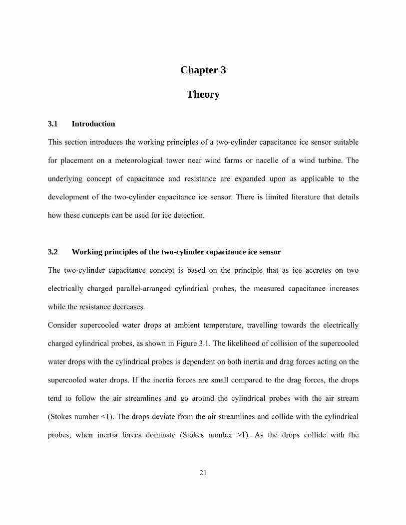
Consider supercooled water drops at ambient temperature, travelling towards the electrically
charged cylindrical probes, as shown in Figure 3.1. The likelihood of collision of the supercooled
water drops with the cylindrical probes is dependent on both inertia and drag forces acting on the
supercooled water drops. If the inertia forces are small compared to the drag forces, the drops
tend to follow the air streamlines and go around the cylindrical probes with the air stream
(Stokes number <1). The drops deviate from the air streamlines and collide with the cylindrical
probes, when inertia forces dominate (Stokes number >1). As the drops collide with the
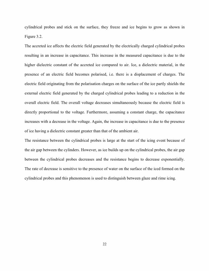
22
cylindrical probes and stick on the surface, they freeze and ice begins to grow as shown in
Figure 3.2.
The accreted ice affects the electric field generated by the electrically charged cylindrical probes
resulting in an increase in capacitance. This increase in the measured capacitance is due to the
higher dielectric constant of the accreted ice compared to air. Ice, a dielectric material, in the
presence of an electric field becomes polarised, i.e. there is a displacement of charges. The
electric field originating from the polarisation charges on the surface of the ice partly shields the
external electric field generated by the charged cylindrical probes leading to a reduction in the
overall electric field. The overall voltage decreases simultaneously because the electric field is
directly proportional to the voltage. Furthermore, assuming a constant charge, the capacitance
increases with a decrease in the voltage. Again, the increase in capacitance is due to the presence
of ice having a dielectric constant greater than that of the ambient air.
The resistance between the cylindrical probes is large at the start of the icing event because of
the air gap between the cylinders. However, as ice builds up on the cylindrical probes, the air gap
between the cylindrical probes decreases and the resistance begins to decrease exponentially.
The rate of decrease is sensitive to the presence of water on the surface of the iced formed on the
cylindrical probes and this phenomenon is used to distinguish between glaze and rime icing.
23
Figure 3.1: Trajectory of supercooled water drops and air moving towards two cylindrical probes
Figure 3.2: Iced formation at the windward side of the cylindrical probes
Sensing electric field
Trajectory of air
Supercooled water drops
24
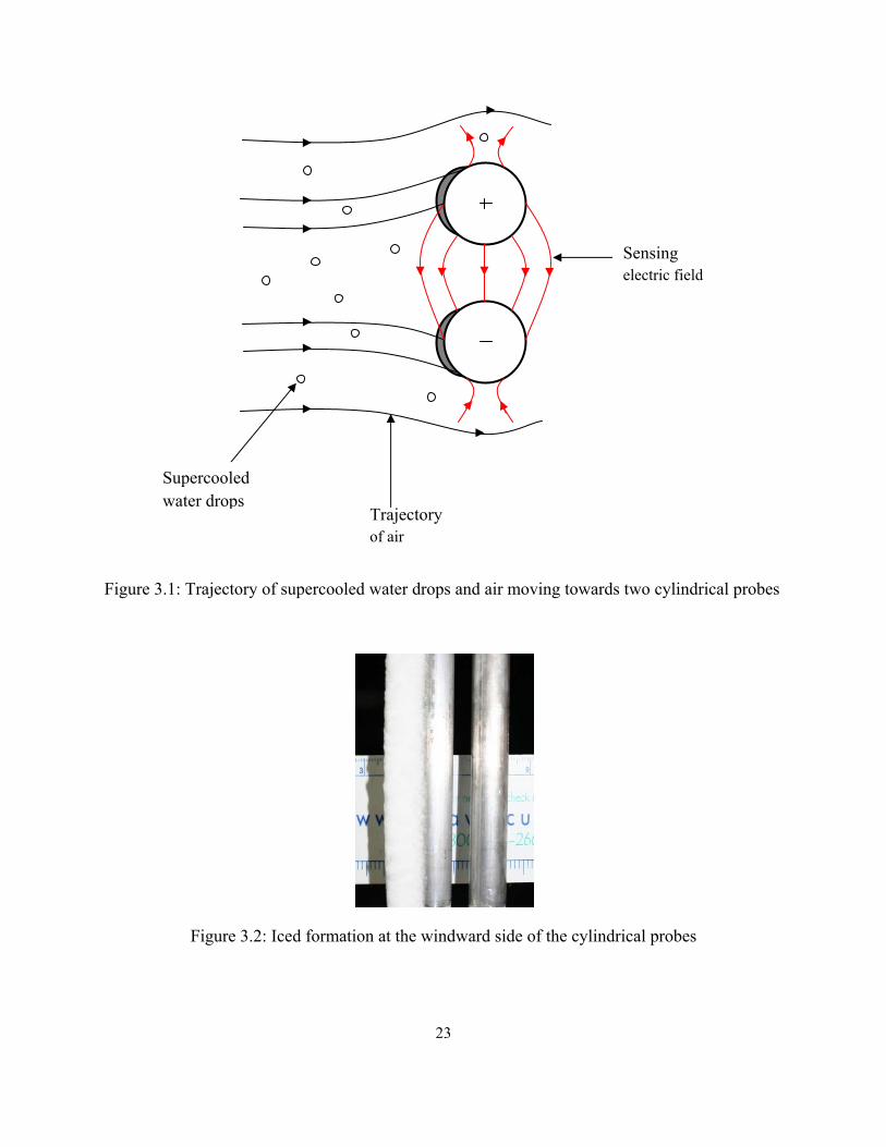
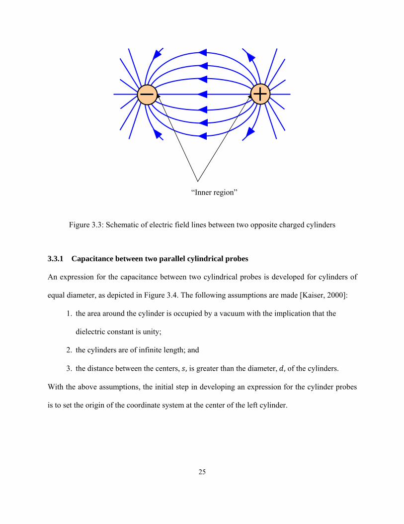
3.3 Electric field lines
An electric field is generated when two oppositely electrically charged cylinders are brought
close to each other as depicted in Figure 3.3. The resulting electric field lines are uniformly
distributed, parallel to each other and normal to a small surface on the “inner region” of the
cylinders (Figure 3.3).
At locations further from the “inner region”, i.e. along the circumference of the cylinders, the
electric field lines are non-uniformly distributed, bulging out (instead of been parallel to each
other), as one move away from the “inner region”, as depicted in Figure 3.3. This non-uniformity
of the electric field lines in these regions leads to a reduction in the electric field strength. This is
known as fringing. A decrease in capacitance is expected with fringing.
The electric field strength is stronger at the “inner region”, weakening along the circumference
of the cylinders from the “inner region”. Naturally, for measurement purposes, one would prefer
the supercooled liquid water drops to impact, and freeze in the most sensitive regions i.e. in the
“inner region”. However, this is not feasible as the aerodynamics of the flow dictates that the ice
forms at the windward side (front) of the cylinders.
25
Figure 3.3: Schematic of electric field lines between two opposite charged cylinders
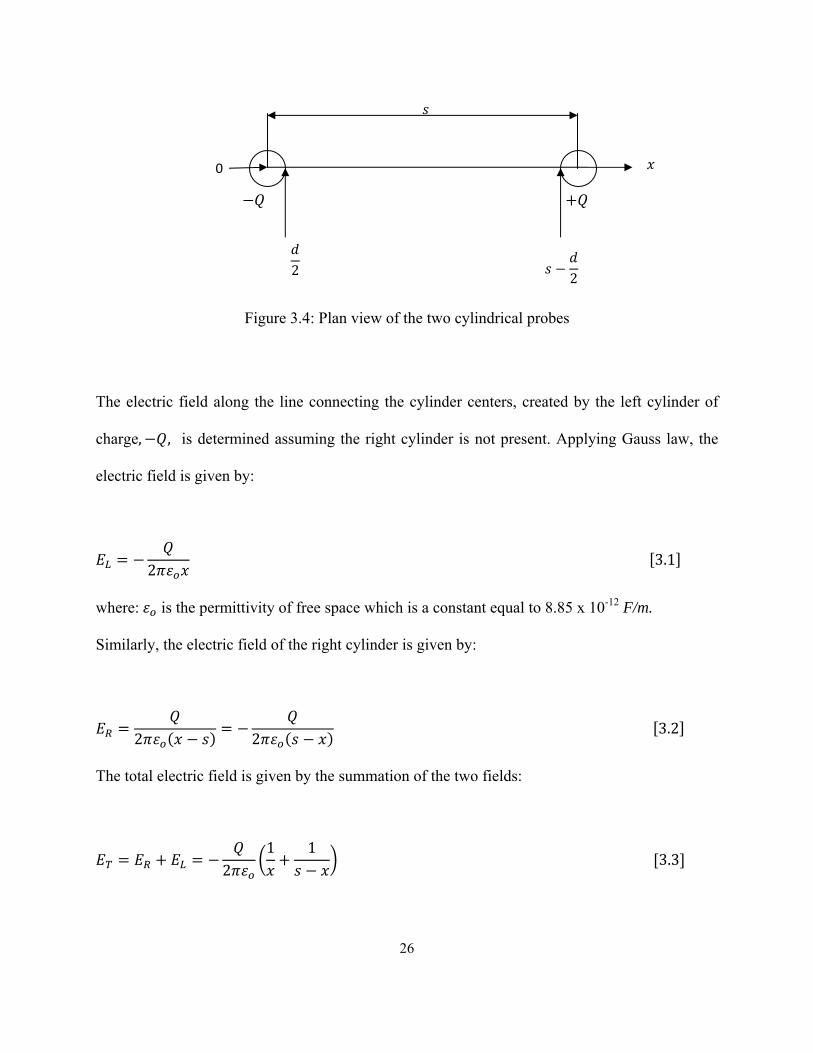
3.3.1 Capacitance between two parallel cylindrical probes
An expression for the capacitance between two cylindrical probes is developed for cylinders of
equal diameter, as depicted in Figure 3.4. The following assumptions are made [Kaiser, 2000]:
1. the area around the cylinder is occupied by a vacuum with the implication that the
dielectric constant is unity;
2. the cylinders are of infinite length; and
3. the distance between the centers, , is greater than the diameter, , of the cylinders.
With the above assumptions, the initial step in developing an expression for the cylinder probes
is to set the origin of the coordinate system at the center of the left cylinder.
“Inner region”
26
Figure 3.4: Plan view of the two cylindrical probes
The electric field along the line connecting the cylinder centers, created by the left cylinder of
charge, , is determined assuming the right cylinder is not present. Applying Gauss law, the
electric field is given by:
2 3.1
where: is the permittivity of free space which is a constant equal to 8.85 x 10⁻¹² F/m.
Similarly, the electric field of the right cylinder is given by:
2 2 3.2
The total electric field is given by the summation of the two fields:
21 1
3.3
2
0
2
27
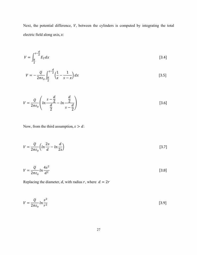
Next, the potential difference, , between the cylinders is computed by integrating the total
electric field along axis, :
3.4
21 1
3.5
22
2
2
2 3.6
Now, from the third assumption, :
22
2 3.7
24
3.8
Replacing the diameter, , with radius , where 2
2 3.9
28
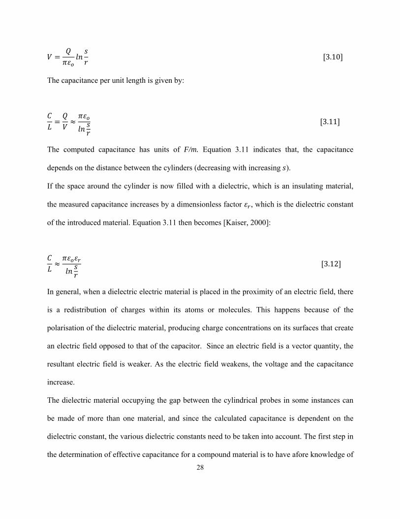
3.10
The capacitance per unit length is given by:
3.11
The computed capacitance has units of F/m. Equation 3.11 indicates that, the capacitance
depends on the distance between the cylinders (decreasing with increasing ).
If the space around the cylinder is now filled with a dielectric, which is an insulating material,
the measured capacitance increases by a dimensionless factor , which is the dielectric constant
of the introduced material. Equation 3.11 then becomes [Kaiser, 2000]:
3.12
In general, when a dielectric electric material is placed in the proximity of an electric field, there
is a redistribution of charges within its atoms or molecules. This happens because of the
polarisation of the dielectric material, producing charge concentrations on its surfaces that create
an electric field opposed to that of the capacitor. Since an electric field is a vector quantity, the
resultant electric field is weaker. As the electric field weakens, the voltage and the capacitance
increase.
The dielectric material occupying the gap between the cylindrical probes in some instances can
be made of more than one material, and since the calculated capacitance is dependent on the
dielectric constant, the various dielectric constants need to be taken into account. The first step in
the determination of effective capacitance for a compound material is to have afore knowledge of
29
how the dielectric materials are spatially arranged, i.e. either series or parallel or both. With this
information, series or parallel capacitance theory can be used to compute the effective
capacitance [Ahmed and Ismail, 2008]. This technique assumes that the electric field is shielded,
i.e. confined entirely between the cylinders without any fringing field. This technique is
applicable to porous dielectric materials as well. For simple arrangements, the accuracy of this
technique is excellent. However, for complex arrangement such as ice with ice pockets, it is not
easy to compute the effective capacitance, which could make developing a theoretical expression
for rime ice more difficult.
In summary, the presence of a dielectric material increases the measured capacitance and
because the dielectric constants are generally a unique material property, it is possible to detect
the presence of a material using changes in measured capacitance as described above.
3.3.2 Resistance between two parallel-arranged cylinders
The electrical resistance of a material gives a measure of how it opposes the flow of an electric
current. The resistance of a resistive material is related to the potential difference (V) and current
(I) by Ohm’s law [Paul, 2000].The resistance of a uniform material is a function of the length
( ), cross sectional area ( ) and the resistivity of the material ( ) [Paul, 2000].
Generally, insulators offer high degrees of opposition to the flow of electric currents. Air is an
excellent insulator. Consider the two cylinders configuration in Figure 3.1, with an air gap
between them. If a potential difference is applied across the cylinders, the measured electrical
resistance can be assumed to be infinite since the circuit is open circuit or severed due to the
presence of the air gap. Now, as the two cylinders are brought closer to each other, there is a

30
reduction in the air gap, with the measured electrical resistance approaching a small value as they
begin to touch. Therefore, reduction in the air gap forward of the probe resulting from ice
accretion will lead to a similar reduction in the measured resistance. Additionally, since the
electric field will interact with the surface of the iced region, conditions pertaining will aid in
distinguishing between the ice types based on resistance.
31
Chapter 4
Experimental and numerical procedures
4.1 Introduction
An experimental and theoretical program was designed to evaluate a new concept for the
detection of ice, estimation of ice accretion and to distinguish between rime and glace ice based
on the measurement of capacitance and resistance change between two electrically charged
cylinders as ice accretes on the cylinders. For ease of discussion, the cylindrical probes with
ancillary equipment were defined as the ice sensor. The ice sensor is described in detail in
Section 4.2. Section 4.3 describes two-dimensional numerical simulations used to solve the
electric field equations to determine the optimal center-to-center distance between the cylindrical
probes and understand the variation of capacitance with ice deposition and growth of ice. These
numerical simulations were validated with a series of laboratory experiments described in
Section 4.4. Finally, Section 4.5 deals with the experiments performed in the icing wind tunnel to
test the sensitivity and reproducibility of the ice sensor under various icing conditions. These
experiments were performed in the University of Manitoba Icing Wind Tunnel Facility.
4.2 Description of the two-cylinder capacitance ice sensor
The ice sensor consisting of two cylindrical probes made of aluminum connected to a
capacitance meter and computer to collect data are shown in Figure 4.1. Aluminum was selected
for its machinability, high corrosion resistance and relatively low cost. The two cylindrical
probes were made to have equal lengths to eliminate non-uniformity in the sensing electric field
[Elkow and Rezkallah, 1996]. The length and the diameter of the two cylindrical probes were
32
selected to minimise three-dimensional effects. An insulator of height 3 cm was fitted at the base
of the probes. This was done to prevent spikes in capacitance due to accumulation of water and
ice that deposit due to gravity at the base. The insulator was required to be non-conductive,
machinable and of low cost. Based on these criteria, Ultra High Molecular Weight (UHMW)
polyethylene was selected. The polyethylene was pressed fit to the aluminum electrodes. The
cylindrical probes were connected to a Hioki 3522-50 capacitance meter by lead wires. These
lead wires were selected to minimize parasitic capacitance. The Hioki 3522-50 capacitance meter
is an impedance meter with improved power for high-speed measurements of 5 ms and with an
accuracy of ± 0.08%. Data was collected at 100 KHz. The meter was connected to a computer
via an RS232 cable for data storage [Hioki, 3522-50 LCR HiTESTER, 2007].
Figure 4.1: Schematic two-cylinder capacitance sensor and ancillary equipments
4.3 Numerical simulations
This section introduces the set of numerical experiments performed using Quickfield™ electric
field professional software. The aim of these experiments was in part to the determine the
RS232 cableAluminum
Insulator
Lead wires Hioki 3522-50 Capacitance meter
Computer
33
optimal design dimensions for the cylindrical probes. Quickfield™ solves the two-dimensional
Poisson’s governing equations using the Domain Decomposition Method finite element
technique [QuickField™, 2005].
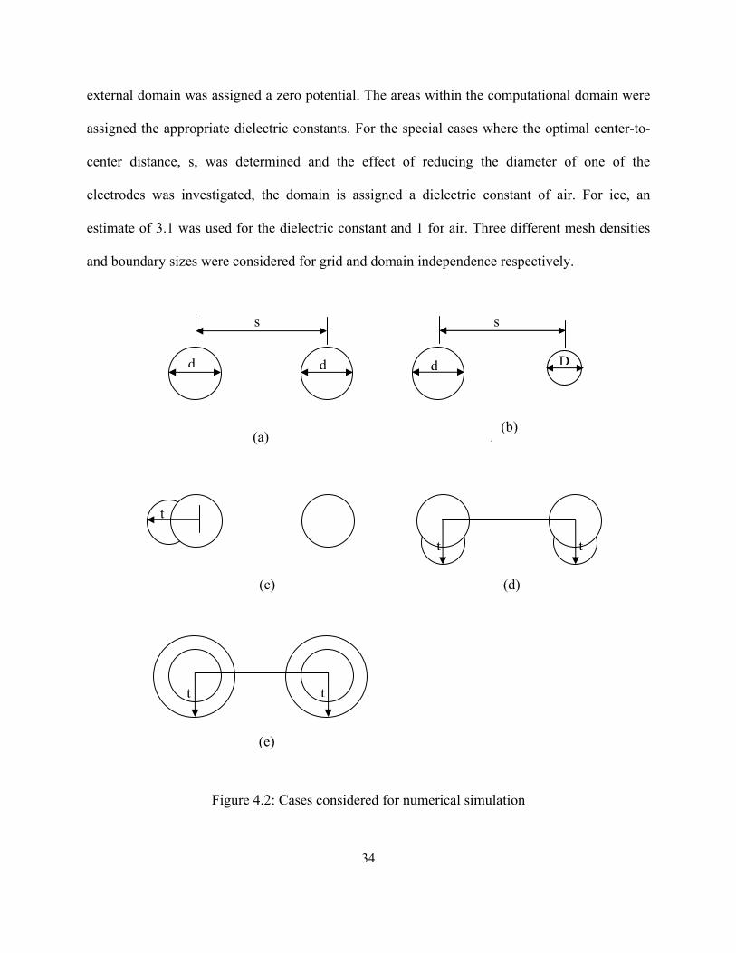
The various cases considered in the numerical experiments are shown in Figure 4.2. In the first
case study, different center-to-center distances, s, were considered using air as the dielectric
material surrounding the cylindrical probes (Figure 4.2a) to determine the optimal
center-to-center distance (s) between the cylindrical probes. Additionally, the electric field
distribution predicted by QuickField™ was used to characterise regions of high electric field
strength (high sensitivity) to ice deposition. In the second case, the effect of decreasing the
diameter of one of the cylindrical probes on the ice sensor’s sensitivity was studied (Figure
4.2b). In this case study, D is the varying diameter while d is the fixed diameter, 1.27 cm. For the
third case, ice depositions of varying thickness, t, were modelled around the cylindrical probes at
both the front (i.e. parallel orientation of probes) and side (i.e. inline orientation of probes) iced
regions to investigate the dependence of the ice sensor’s sensitivity on the location of accreted
ice (Figure 4.2c and 4.2d). In these experiments, the dielectric material comprise of both air and
ice. In the fourth case, ice depositions of varying thickness were modelled around the cylindrical
probes to investigate the variation of ice growth with capacitance (Figure 4.2e).
4.3.1 Numerical procedure
As discussed earlier, Quickfield™ solves the two-dimensional Poisson’s governing field
equations using the finite element method. The charged cylindrical probes were modelled as two-
dimensional equipotential circular surfaces. A non-uniform mesh was use: a dense mesh defined
around the cylindrical probes and a more course mesh far from the cylindrical probes. The
34
external domain was assigned a zero potential. The areas within the computational domain were
assigned the appropriate dielectric constants. For the special cases where the optimal center-to-
center distance, s, was determined and the effect of reducing the diameter of one of the
electrodes was investigated, the domain is assigned a dielectric constant of air. For ice, an
estimate of 3.1 was used for the dielectric constant and 1 for air. Three different mesh densities
and boundary sizes were considered for grid and domain independence respectively.
Figure 4.2: Cases considered for numerical simulation
(a)
dd
s
(b) )
s
Dd
(c)
t
(d)
tt
(e)
t t
35
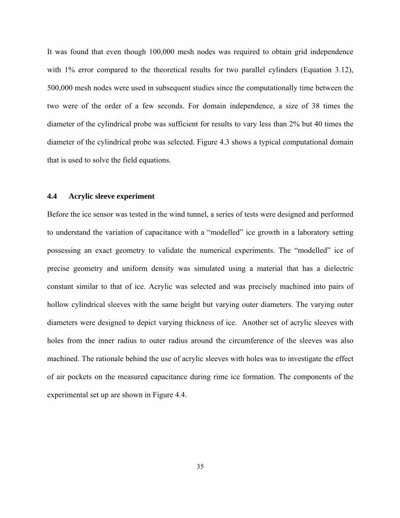
It was found that even though 100,000 mesh nodes was required to obtain grid independence
with 1% error compared to the theoretical results for two parallel cylinders (Equation 3.12),
500,000 mesh nodes were used in subsequent studies since the computationally time between the
two were of the order of a few seconds. For domain independence, a size of 38 times the
diameter of the cylindrical probe was sufficient for results to vary less than 2% but 40 times the
diameter of the cylindrical probe was selected. Figure 4.3 shows a typical computational domain
that is used to solve the field equations.
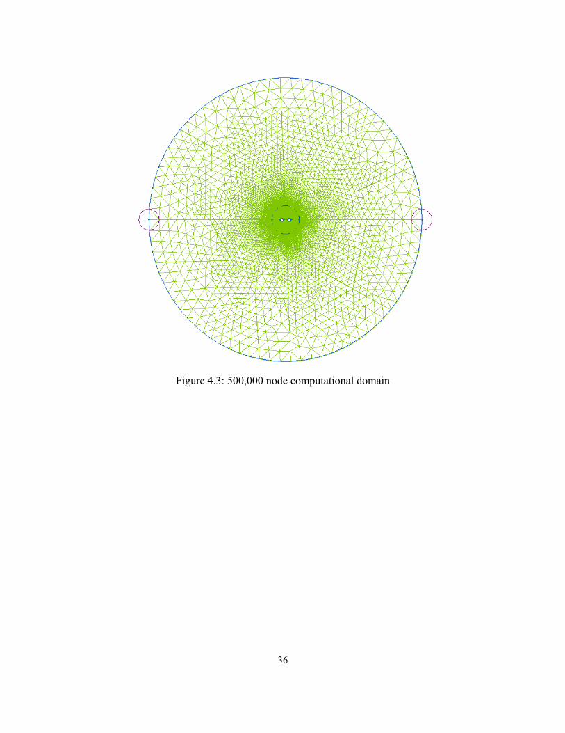
4.4 Acrylic sleeve experiment
Before the ice sensor was tested in the wind tunnel, a series of tests were designed and performed
to understand the variation of capacitance with a “modelled” ice growth in a laboratory setting
possessing an exact geometry to validate the numerical experiments. The “modelled” ice of
precise geometry and uniform density was simulated using a material that has a dielectric
constant similar to that of ice. Acrylic was selected and was precisely machined into pairs of
hollow cylindrical sleeves with the same height but varying outer diameters. The varying outer
diameters were designed to depict varying thickness of ice. Another set of acrylic sleeves with
holes from the inner radius to outer radius around the circumference of the sleeves was also
machined. The rationale behind the use of acrylic sleeves with holes was to investigate the effect
of air pockets on the measured capacitance during rime ice formation. The components of the
experimental set up are shown in Figure 4.4.
36
Figure 4.3: 500,000 node computational domain
37
Figure 4.4: Components of model icing experimental set up
4.4.1 Acrylic experiment procedure
With the cylindrical probes secured in the supporting base, the capacitance meter was allowed to
stand for an hour to warm up. Afterwards, a single or pair of acrylic sleeves of the same size was
then slipped around one or two of the cylindrical probes. The capacitance meter was then
connected to the cylindrical probes via the lead wires. The setup was allowed to stand for five
minutes for the readings to stabilize, before the measured capacitance was recorded. The lead
wires were disconnected from the cylindrical probes, the pair of acrylic sleeves slipped off and
the next pair of acrylic sleeves slipped back onto the cylindrical probes. The procedure was then
repeated. These set of experiments were generally performed three times to test reproducibility.
Acrylic sleeves
Capacitance meter Probe with acrylic sleeves
38
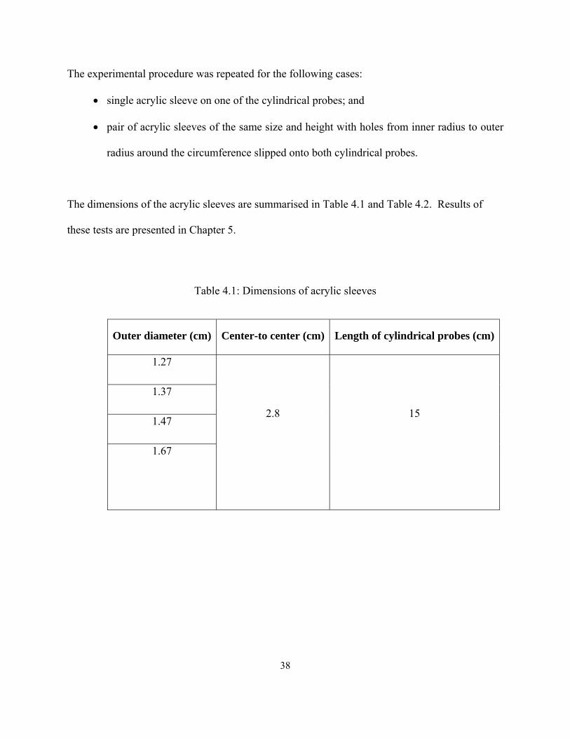
The experimental procedure was repeated for the following cases:
• single acrylic sleeve on one of the cylindrical probes; and
• pair of acrylic sleeves of the same size and height with holes from inner radius to outer
radius around the circumference slipped onto both cylindrical probes.
The dimensions of the acrylic sleeves are summarised in Table 4.1 and Table 4.2. Results of
these tests are presented in Chapter 5.
Table 4.1: Dimensions of acrylic sleeves
Outer diameter (cm) Center-to center (cm) Length of cylindrical probes (cm)
1.27
2.8
15
1.37
1.47
1.67
39
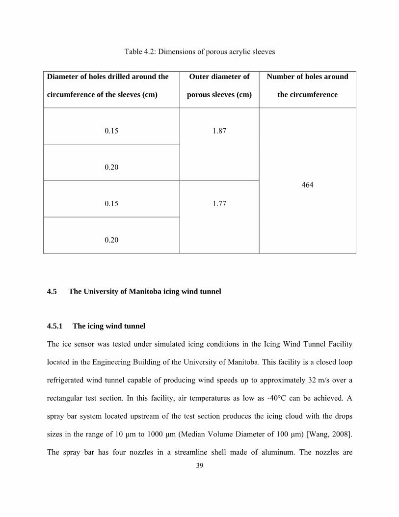
Table 4.2: Dimensions of porous acrylic sleeves
Diameter of holes drilled around the
circumference of the sleeves (cm)
Outer diameter of
porous sleeves (cm)
Number of holes around
the circumference
0.15
1.87
464
0.20
0.15
1.77
0.20
4.5 The University of Manitoba icing wind tunnel
4.5.1 The icing wind tunnel
The ice sensor was tested under simulated icing conditions in the Icing Wind Tunnel Facility
located in the Engineering Building of the University of Manitoba. This facility is a closed loop
refrigerated wind tunnel capable of producing wind speeds up to approximately 32 m/s over a
rectangular test section. In this facility, air temperatures as low as -40°C can be achieved. A
spray bar system located upstream of the test section produces the icing cloud with the drops
sizes in the range of 10 μm to 1000 μm (Median Volume Diameter of 100 μm) [Wang, 2008].
The spray bar has four nozzles in a streamline shell made of aluminum. The nozzles are
40
uniformly spaced to facilitate uniform distribution of the spray drop. Heating strips are installed
between nozzles and the aluminum shell to prevent the nozzles from clogging during low
temperature experiments. The distance from the spray bar to the test specimen is sufficient for
the drop to equilibrate with the ambient temperature before impact with the test specimen and
transforming into ice. Although the spray drops fills the entire test section, a central region of
constant liquid water content exist where the test specimen are located for each test. The liquid
water content can be varied from 0 to 2 g/m3 [Wang, 2008]. The ambient air velocity is adjusted
by varying the frequency of the fan blower motor. The window of the cold chamber is heated in
order to keep the surface free of frost and allow for visibility. For easy access to the spray bar,
test specimen adjustment, cleaning after a test and for maintenance purposes, doors are provided
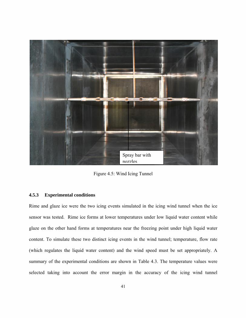
at vantage points along the perimeter of the tunnel. Figure 4.5 is a photograph of the inner duct
of the icing wind tunnel.
4.5.2 Icing wind tunnel calibration
Kraj [2007] previously did the calibration of the icing wind tunnel. The aim of the calibration
was to test the conditions for which glaze and rime ice can be simulated successfully. To
calibrate the tunnel, a series of tests were performed at varying temperatures to obtain data on
wind speeds in the inner duct of the icing wind tunnel. To do this, a pitot-tube manometer was
mounted behind the spray nozzles i.e. upstream of the inner duct of the wind tunnel while a
three-cup anemometer was placed downstream of the spray nozzles. The purpose of these
devices were to check the accuracy in the frequency of the wind tunnel motor fan and to calibrate
it for producing the correct wind speeds at these given temperatures. For detailed results on this
calibration, see Kraj [2007].
41
Figure 4.5: Wind Icing Tunnel
4.5.3 Experimental conditions
Rime and glaze ice were the two icing events simulated in the icing wind tunnel when the ice
sensor was tested. Rime ice forms at lower temperatures under low liquid water content while
glaze on the other hand forms at temperatures near the freezing point under high liquid water
content. To simulate these two distinct icing events in the wind tunnel; temperature, flow rate
(which regulates the liquid water content) and the wind speed must be set appropriately. A
summary of the experimental conditions are shown in Table 4.3. The temperature values were
selected taking into account the error margin in the accuracy of the icing wind tunnel
Spray bar with nozzles
42
thermocouples. The liquid water content (LWC) was estimated from rime ice growth. See
Appendix A for details.
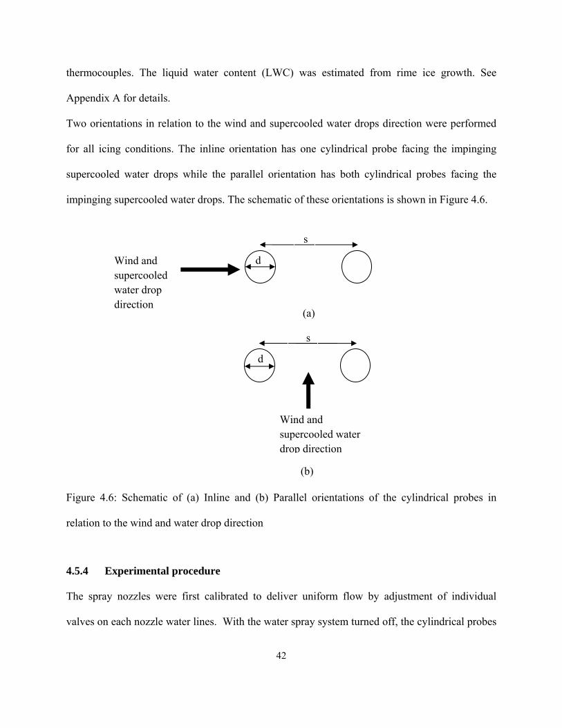
Two orientations in relation to the wind and supercooled water drops direction were performed
for all icing conditions. The inline orientation has one cylindrical probe facing the impinging
supercooled water drops while the parallel orientation has both cylindrical probes facing the
impinging supercooled water drops. The schematic of these orientations is shown in Figure 4.6.
Figure 4.6: Schematic of (a) Inline and (b) Parallel orientations of the cylindrical probes in
relation to the wind and water drop direction
4.5.4 Experimental procedure
The spray nozzles were first calibrated to deliver uniform flow by adjustment of individual
valves on each nozzle water lines. With the water spray system turned off, the cylindrical probes
Wind and supercooled water drop direction
s
(a)
d
Wind and supercooled water drop direction
s
d
(b)
43
were mounted on a support bar that spanned the length of the inner duct of the icing wind tunnel.
The location of the cylindrical probes on the bar was selected to be away from the walls of the
inner duct to have a homogenous ice growth and to eliminate the boundary layer effects. The
lead wires were connected to the cylindrical probes and back to the capacitance meter located
outside the tunnel. The capacitance meter was allowed to stand for an hour to warm up before the
start of the experiment. The tunnel air temperature was set to the required value for the formation
of a particular type of ice required. When this temperature was reached and stabilised, the spray
system was activated. The spray bar water mass flow rate and the injection pressures set the
required liquid water content and median volume diameter. Experiments were performed at 3, 4,
5, 10 and 20 minutes at each icing condition, wind velocity and orientation of cylindrical probes.
Capacitance and resistance was recorded every 5 seconds. Photographs were taken after the
experiments, and mass and thickness of the ice were measured. Mass and thickness were
measured as follows. The wind icing tunnel was turned off while ensuring the inside conditions
stays constant. The thickness of the ice was measured with a vernier calliper at various locations
and averaged. The accreted ice is then scrapped of the cylindrical probe(s) into a beaker and
weighed. Three icing experiments for both rime and glaze ice were performed to test the
reproducibility of the results. Results of these tests are presented in Chapter 5.
44
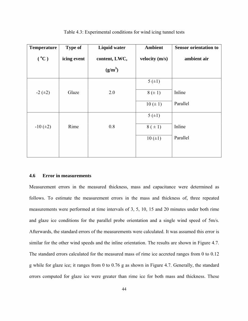
Table 4.3: Experimental conditions for wind icing tunnel tests
Temperature
( oC )
Type of
icing event
Liquid water
content, LWC,
(g/m3)
Ambient
velocity (m/s)
Sensor orientation to
ambient air
-2 (±2)
Glaze
2.0
5 (±1)
Inline
Parallel
8 (± 1)
10 (± 1)
-10 (±2)
Rime
0.8
5 (±1)
Inline
Parallel
8 ( ± 1)
10 (±1)
4.6 Error in measurements
Measurement errors in the measured thickness, mass and capacitance were determined as
follows. To estimate the measurement errors in the mass and thickness of, three repeated
measurements were performed at time intervals of 3, 5, 10, 15 and 20 minutes under both rime
and glaze ice conditions for the parallel probe orientation and a single wind speed of 5m/s.
Afterwards, the standard errors of the measurements were calculated. It was assumed this error is
similar for the other wind speeds and the inline orientation. The results are shown in Figure 4.7.
The standard errors calculated for the measured mass of rime ice accreted ranges from 0 to 0.12
g while for glaze ice; it ranges from 0 to 0.76 g as shown in Figure 4.7. Generally, the standard
errors computed for glaze ice were greater than rime ice for both mass and thickness. These
45
relatively higher computed standard errors in mass for glaze ice can be attributed to
predominantly the difficulty in removing all the accreted ice from the cylindrical probes for
measurement after the experiments, and to a lesser extent, the time delays in activating and
deactivating the spray bar systems during experimentations. The computed standard error for
the measurement for both rime and glaze ice ranged from 0 to 0.11 mm and 0 to 0.87 mm,
respectively as shown in Figure 4.8. The relatively higher standard error for glaze ice was due to
the horns on the surface which made the thickness measurement difficult.
The current sensor is sensitive to any change in the position of the lead wires connecting the two
cylindrical probes since it contributes significantly to parasitic capacitance. Additionally, it is
also sensitive to the ambient conditions. To estimate the measurement errors, three repeated
experiments were performed. The capacitance variation with time and sizes of acrylic recorded
for wind icing tests and for acrylic tests were measured. The results are shown in Figure 4.8 and
Figure 4.9 for icing wind experiments and acrylic experiments, respectively. The standard error
estimates for glaze ice experiments ranges from 0 to 0.27 pF while for rime ice it ranges from 0
to 0.21 pF. The variations in the ambient conditions within the icing tunnel can be attributed to
the standard errors computed. For the acrylic experiments, the ability to maintain near constant
ambient conditions during experimentations resulted in relatively lower computed standard
errors.
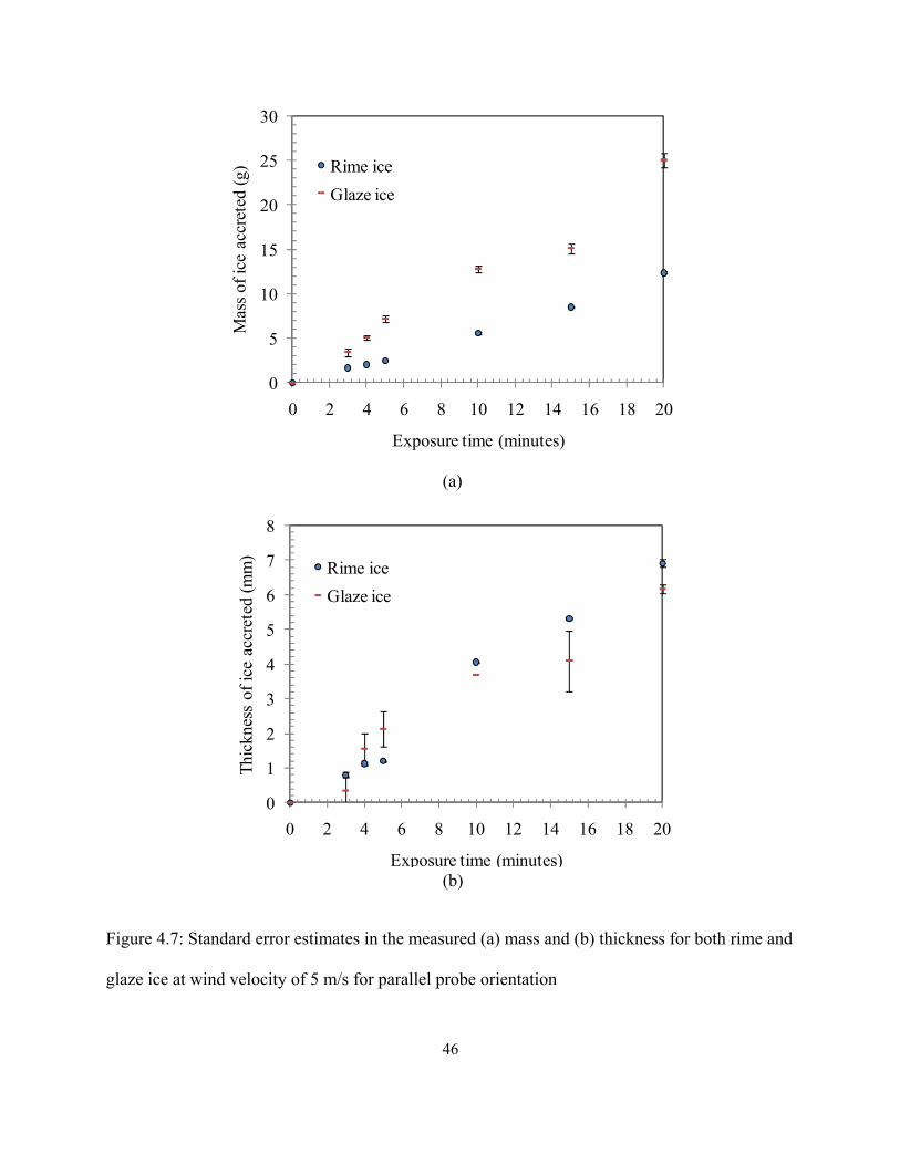
46
Figure 4.7: Standard error estimates in the measured (a) mass and (b) thickness for both rime and
glaze ice at wind velocity of 5 m/s for parallel probe orientation
0
5
10
15
20
25
30
0 2 4 6 8 10 12 14 16 18 20
Mas
s of i
ce a
ccre
ted
(g)
Exposure time (minutes)
Rime iceGlaze ice
0
1
2
3
4
5
6
7
8
0 2 4 6 8 10 12 14 16 18 20
Thic
knes
s of
ice
accr
eted
(mm
)
Exposure time (minutes)
Rime iceGlaze ice
(a)
(b)
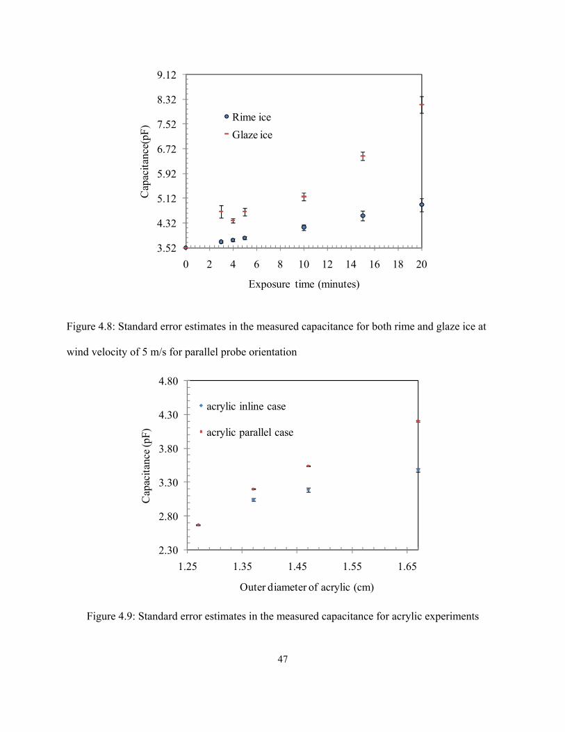
47
Figure 4.8: Standard error estimates in the measured capacitance for both rime and glaze ice at
wind velocity of 5 m/s for parallel probe orientation
Figure 4.9: Standard error estimates in the measured capacitance for acrylic experiments
3.52
4.32
5.12
5.92
6.72
7.52
8.32
9.12
0 2 4 6 8 10 12 14 16 18 20
Cap
acita
nce(
pF)
Exposure time (minutes)
Rime iceGlaze ice
2.30
2.80
3.30
3.80
4.30
4.80
1.25 1.35 1.45 1.55 1.65
Cap
acita
nce (
pF)
Outer diameter of acrylic (cm)
acrylic inline case
acrylic parallel case
48
Chapter 5
Results and Discussions
5.1 Introduction
This chapter presents and discusses the numerical and experimental results. The numerical and
acrylic results are discussed in Section 5.1. In Section 5.2, the wind icing tunnel experiments
results are presented and discussed. Finally, the optimal sensor configuration is presented in
Section 5.3.
5.2 Numerical and acrylic studies
The capacitance based numerical study indicates that the sensitivity of this sensor increases
approximately at an exponential rate as the center-to-center distance, s, of the cylindrical probes
decreases (Figure 5.1). This result is consistent with well-established analytic solutions, and is
due to the increase in the strength of the electric field as the distance between the centers of the
cylindrical probes decrease. However, in the present application there is a limit to how short the
center-to-center distance can be selected, since bringing the probes too close to each other will
lead to early bridging of ice between the probes. Early bridging is a local effect that does not
span cylinders and can result in over prediction of the icing rate. Additionally, results from early
bridging can be misleading, especially since the time to deice needs to be inferred from sensor
measurements. Based on both the results in Figure 5.1 and the concerns for early bridging, a
center-to-center distance of 1.87 cm was selected.
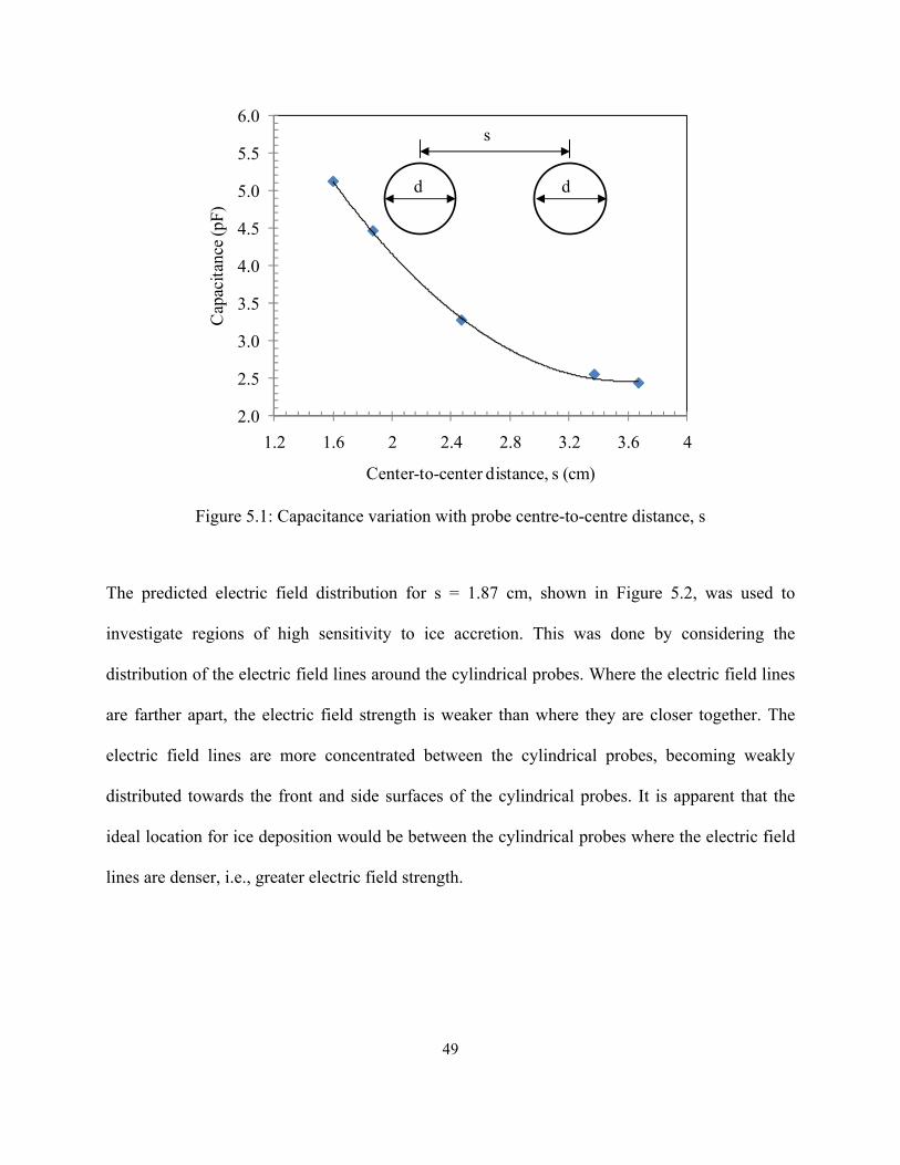
49
Figure 5.1: Capacitance variation with probe centre-to-centre distance, s
The predicted electric field distribution for s = 1.87 cm, shown in Figure 5.2, was used to
investigate regions of high sensitivity to ice accretion. This was done by considering the
distribution of the electric field lines around the cylindrical probes. Where the electric field lines
are farther apart, the electric field strength is weaker than where they are closer together. The
electric field lines are more concentrated between the cylindrical probes, becoming weakly
distributed towards the front and side surfaces of the cylindrical probes. It is apparent that the
ideal location for ice deposition would be between the cylindrical probes where the electric field
lines are denser, i.e., greater electric field strength.
2.0
2.5
3.0
3.5
4.0
4.5
5.0
5.5
6.0
1.2 1.6 2 2.4 2.8 3.2 3.6 4
Cap
acita
nce (
pF)
Center-to-center distance, s (cm)
s
d d
50
Figure 5.2: Electric field distribution calculated using QuickField™, s = 1.87 cm, d = 1.27 cm,
Q = 1 C
Based on the above observation, the case of two cylindrical probes with one smaller than the
other was investigated as a potentially more sensitive geometry to ice accretion. The concept was
to increase ice accretion between the probes, i.e. region most sensitive to ice accretion, by
orienting the probes inline with the flow direction with the smaller probe in the upstream
position. In this orientation, the stream of supercooled water drops flow past the smaller probe
and impinges on the front surface of the larger probe. There were however two major drawbacks
51
to this concept. Firstly, results from QuickField™ simulations indicate a reduction in the
sensitivity of the sensor with a reduction in size of one of the cylindrical probes, as shown in
Figure 5.3. Secondly, numerical studies of flow around two unequal cylindrical probes using
Fluent™ indicates that, to achieve a high deposition rate of supercooled drops on the larger
downstream probe, a long center-to-center distance between the probes is required for drops that
flow past the smaller upstream probe to move towards the front of the downstream probe. As
discussed above, this would inevitably lead to a reduction in the sensitivity of the probe. A
decrease of 18% was observed when the diameter of one of the electrodes was reduced from
1.27 cm to 0.89 cm for s=1.87 cm. Therefore, only probes of equal diameter were considered for
further study.
The sensitivity of the sensor as a function of the orientation of the two-cylindrical probes to the
supercooled water drops was investigated numerically using QuickField™. This was done by
modelling ice of varying thickness around the front surface of the two-cylindrical probes for the
case of parallel orientation while for the inline case; ice was modelled on the side surface of one
of the probes (see Figure 4.2c and Figure 4.2d). It should be noted that since QuickField™ is a
two-dimensional software package, more complex geometries of ice observed during icing
experiments cannot be modelled accurately. Hence, simple geometries of ice with varying
thickness were modelled and the variation of capacitance with probe orientation studied. The
results from the simulations, shown in Figure 5.4, indicate an increase in capacitance as the
thickness of the modelled ice increases. Additionally, the capacitance values for the parallel
orientation case were found to be higher than the inline orientation case. This indicates a higher
sensitivity for the parallel orientation compared to the inline orientation. This is due to the denser
52
distribution of electric field lines in front of the probes compared to the sides as shown in
Figure 5.2 and the larger amount of modelled ice in front of the parallel oriented probes.
Figure 5.3: Effect of decreasing the diameter of one of the cylindrical probes on the capacitance;
larger probe diameter, d=1.27 cm and s=1.87 cm
The acrylic experiments, which were designed to validate the numerical experiments, also
indicated an increase in capacitance with an increase in the size of the acrylic sleeve. The results
as shown in Figure 5.5 indicates that the measured capacitance with a single sleeve on one of the
cylindrical probes was smaller compared to an acrylic sleeve on both cylinders. In these
experiments, a single sleeve slipped around one of the cylindrical probes depicts the case where
the probe is oriented inline, while the case where both cylindrical probes have acrylic sleeves
around them depicts the parallel orientation. The results affirm the results from the numerical
3.6
3.8
4.0
4.2
4.4
4.6
0.89 0.99 1.09 1.19 1.29
Cap
acita
nce (
pF)
Diameter of electrode, D (cm)
s
Dd
53
simulations (see Figure 5.4) that the parallel orientation is the more sensitive of the two
orientations. The capacitance values from field calculations were smaller compared to the acrylic
results. Initially, the dielectric constant was believed to be the cause of this discrepancy.
However, the results were still smaller compared to the acrylic results after various dielectric
constants (within the range for acrylic) were assumed. Other possible causes of this discrepancy
include the capacitances in the lead wires and two-dimensional effects. The trend of an increase
in the measured capacitance with increasing size of the acrylic sleeves are in agreement with
results from QuickField™, as shown in Figure 5.5.
Figure 5.4: Sensitivity of ice accretion to probe orientation
4.4
4.5
4.6
4.7
4.8
4.9
0 0.2 0.4 0.6 0.8 1 1.2
Cap
acita
nce (
pF)
Thickness of modelled ice (cm)
inline orientation
parallel orientation
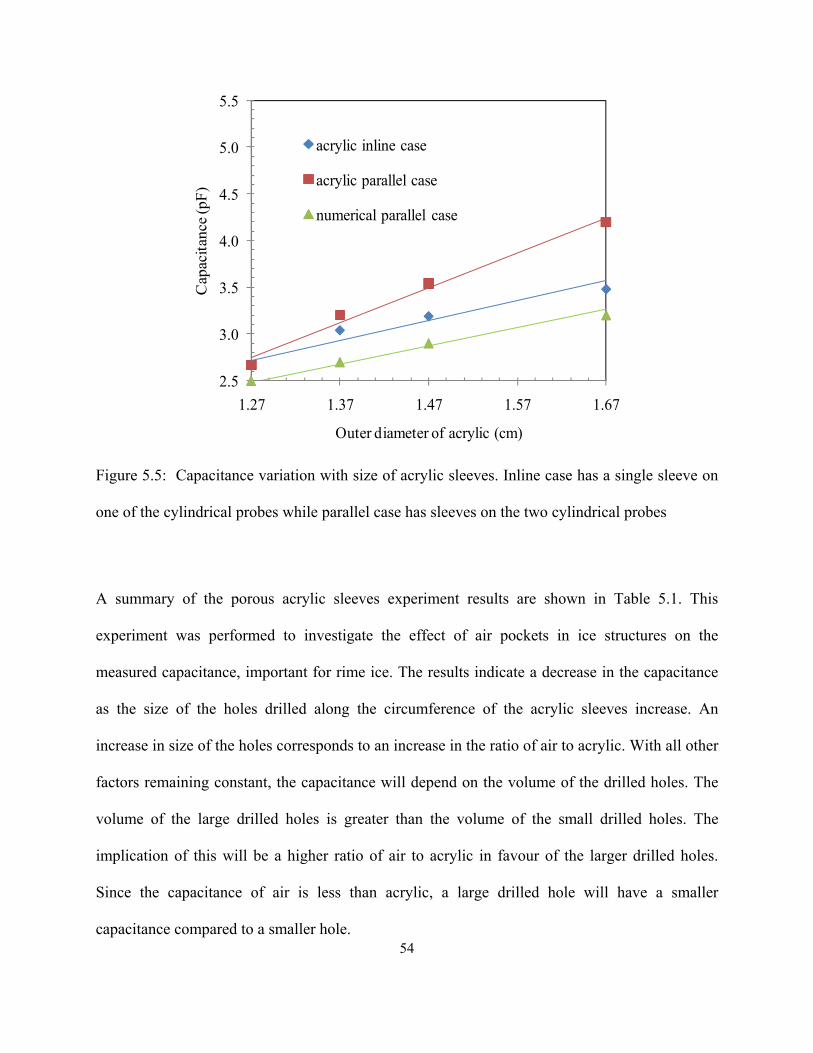
54
Figure 5.5: Capacitance variation with size of acrylic sleeves. Inline case has a single sleeve on
one of the cylindrical probes while parallel case has sleeves on the two cylindrical probes
A summary of the porous acrylic sleeves experiment results are shown in Table 5.1. This
experiment was performed to investigate the effect of air pockets in ice structures on the
measured capacitance, important for rime ice. The results indicate a decrease in the capacitance
as the size of the holes drilled along the circumference of the acrylic sleeves increase. An
increase in size of the holes corresponds to an increase in the ratio of air to acrylic. With all other
factors remaining constant, the capacitance will depend on the volume of the drilled holes. The
volume of the large drilled holes is greater than the volume of the small drilled holes. The
implication of this will be a higher ratio of air to acrylic in favour of the larger drilled holes.
Since the capacitance of air is less than acrylic, a large drilled hole will have a smaller
capacitance compared to a smaller hole.
2.5
3.0
3.5
4.0
4.5
5.0
5.5
1.27 1.37 1.47 1.57 1.67
Cap
acita
nce (
pF)
Outer diameter of acrylic (cm)
acrylic inline case
acrylic parallel case
numerical parallel case
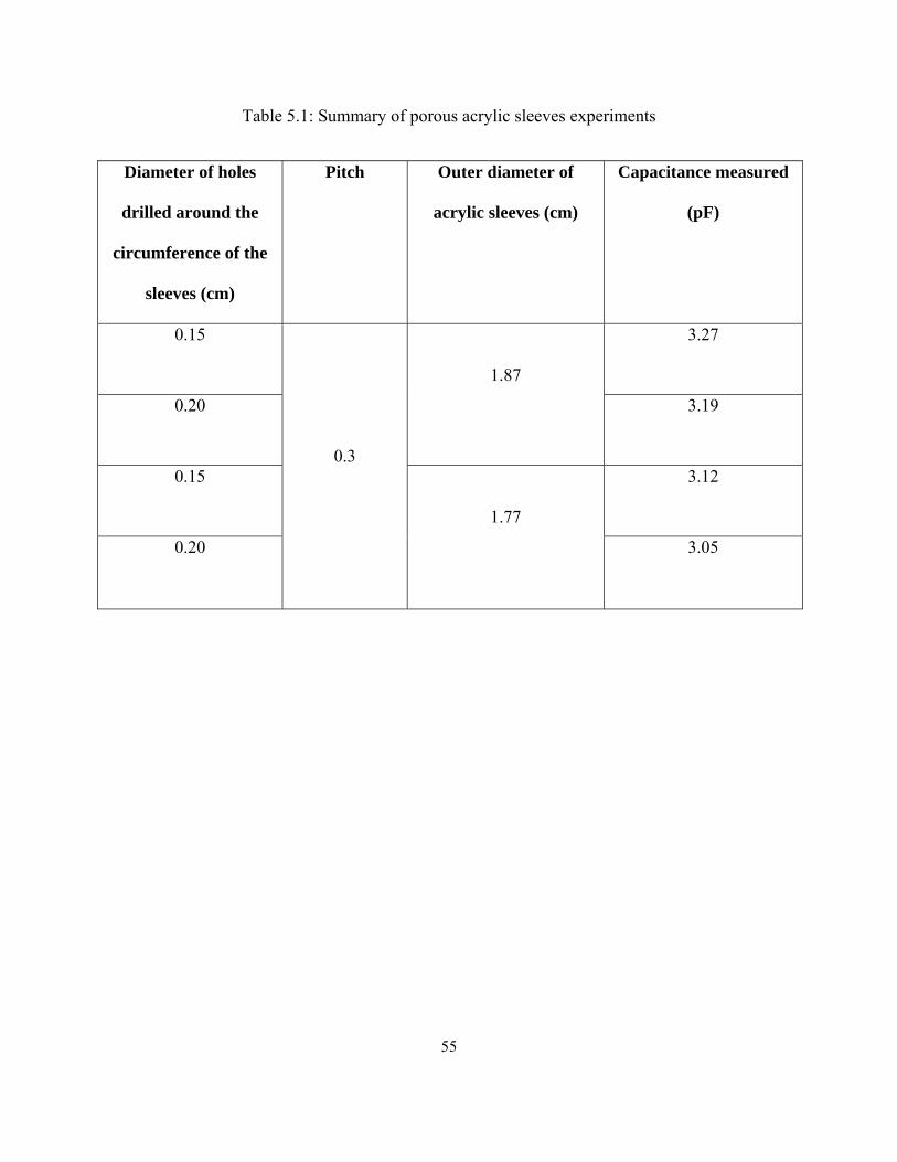
55
Table 5.1: Summary of porous acrylic sleeves experiments
Diameter of holes
drilled around the
circumference of the
sleeves (cm)
Pitch
Outer diameter of
acrylic sleeves (cm)
Capacitance measured
(pF)
0.15
0.3
1.87
3.27
0.20 3.19
0.15
1.77
3.12
0.20 3.05
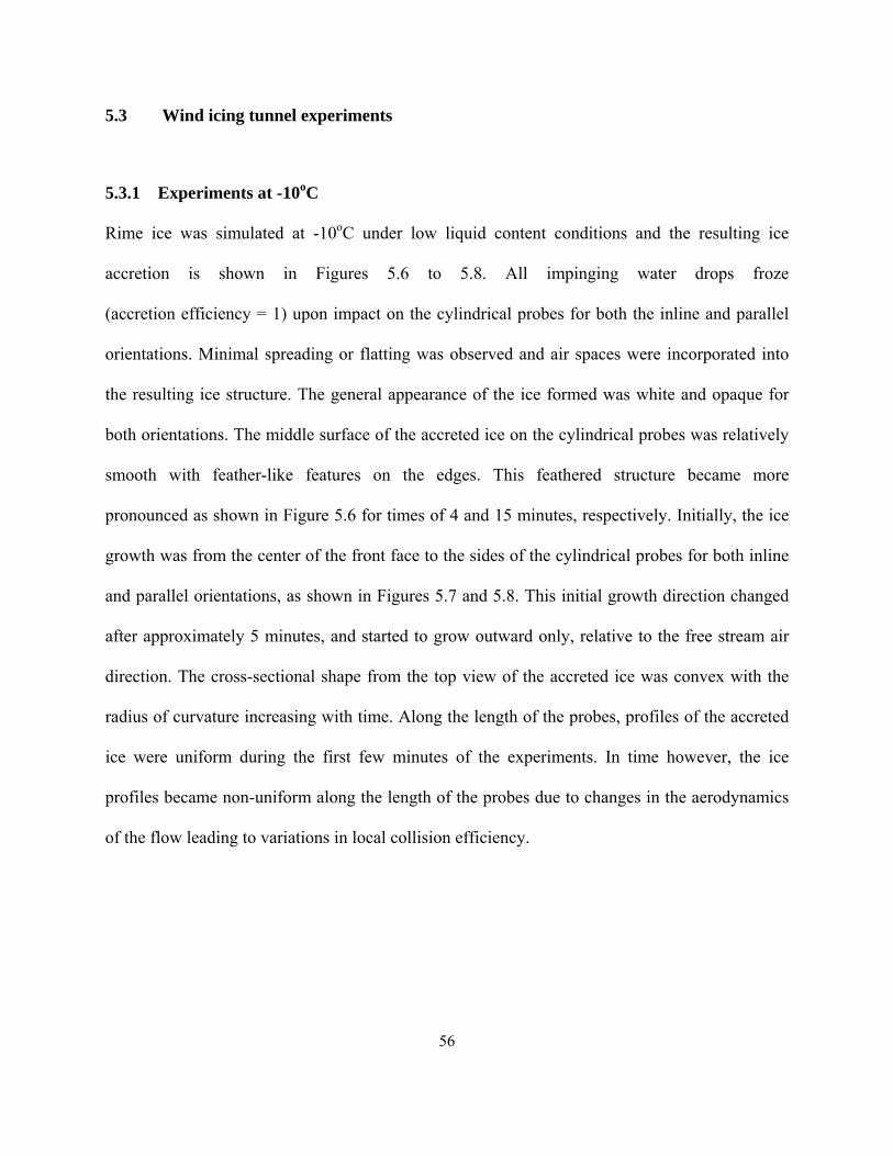
56
5.3 Wind icing tunnel experiments
5.3.1 Experiments at -10oC
Rime ice was simulated at -10oC under low liquid content conditions and the resulting ice
accretion is shown in Figures 5.6 to 5.8. All impinging water drops froze
(accretion efficiency = 1) upon impact on the cylindrical probes for both the inline and parallel
orientations. Minimal spreading or flatting was observed and air spaces were incorporated into
the resulting ice structure. The general appearance of the ice formed was white and opaque for
both orientations. The middle surface of the accreted ice on the cylindrical probes was relatively
smooth with feather-like features on the edges. This feathered structure became more
pronounced as shown in Figure 5.6 for times of 4 and 15 minutes, respectively. Initially, the ice
growth was from the center of the front face to the sides of the cylindrical probes for both inline
and parallel orientations, as shown in Figures 5.7 and 5.8. This initial growth direction changed
after approximately 5 minutes, and started to grow outward only, relative to the free stream air
direction. The cross-sectional shape from the top view of the accreted ice was convex with the
radius of curvature increasing with time. Along the length of the probes, profiles of the accreted
ice were uniform during the first few minutes of the experiments. In time however, the ice
profiles became non-uniform along the length of the probes due to changes in the aerodynamics
of the flow leading to variations in local collision efficiency.
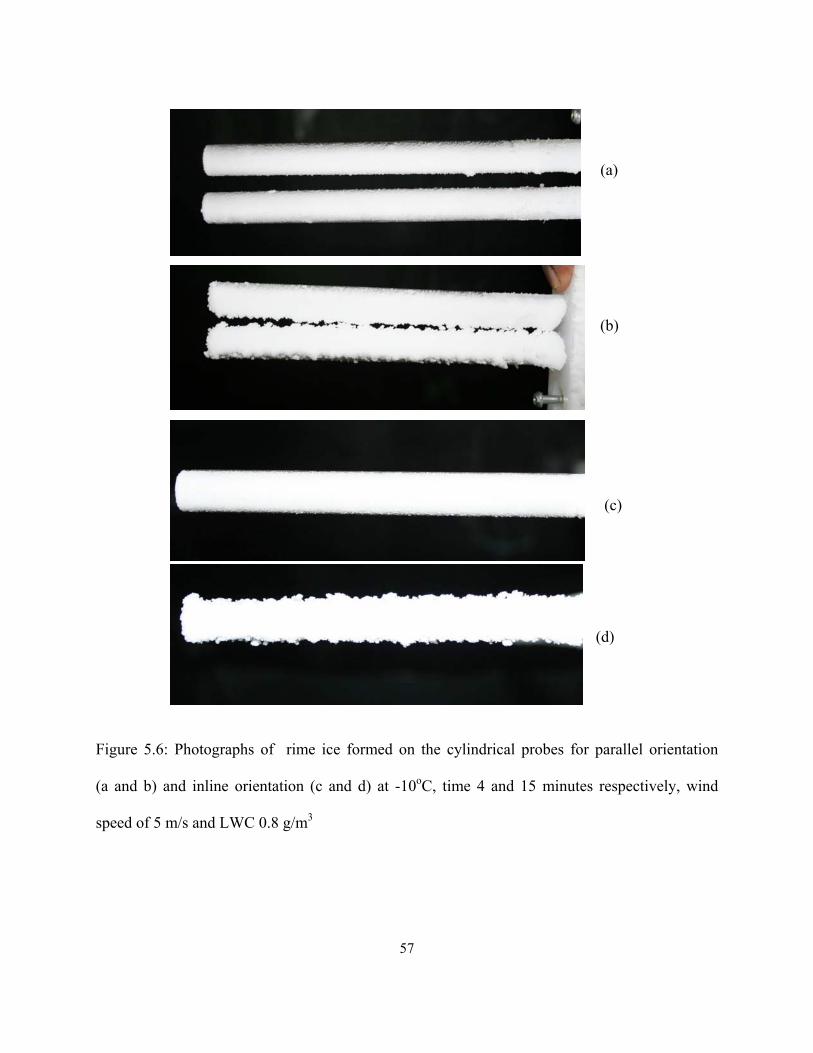
57
Figure 5.6: Photographs of rime ice formed on the cylindrical probes for parallel orientation
(a and b) and inline orientation (c and d) at -10oC, time 4 and 15 minutes respectively, wind
speed of 5 m/s and LWC 0.8 g/m3
(a)
(b)
(c)
(d)
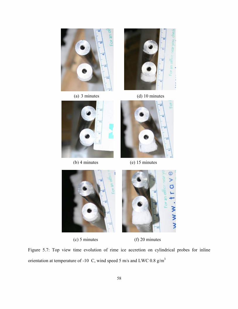
58
Figure 5.7: Top view time evolution of rime ice accretion on cylindrical probes for inline
orientation at temperature of -10C, wind speed 5 m/s and LWC 0.8 g/m3
(a) 3 minutes
(b) 4 minutes
(c) 5 minutes
(d) 10 minutes
(e) 15 minutes
(f) 20 minutes
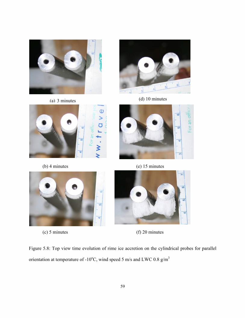
59
Figure 5.8: Top view time evolution of rime ice accretion on the cylindrical probes for parallel
orientation at temperature of -10oC, wind speed 5 m/s and LWC 0.8 g/m3
(a) 3 minutes
(b) 4 minutes
(c) 5 minutes
(d) 10 minutes
(e) 15 minutes
(f) 20 minutes
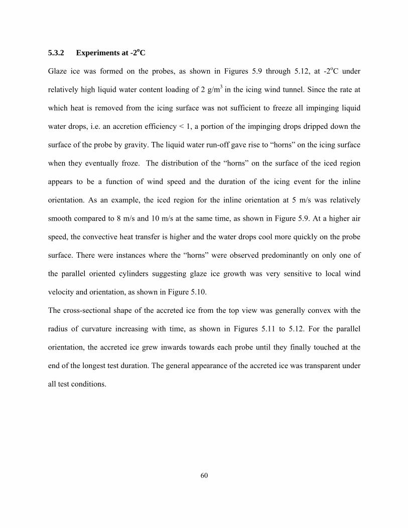
60
5.3.2 Experiments at -2oC
Glaze ice was formed on the probes, as shown in Figures 5.9 through 5.12, at -2oC under
relatively high liquid water content loading of 2 g/m3 in the icing wind tunnel. Since the rate at
which heat is removed from the icing surface was not sufficient to freeze all impinging liquid
water drops, i.e. an accretion efficiency < 1, a portion of the impinging drops dripped down the
surface of the probe by gravity. The liquid water run-off gave rise to “horns” on the icing surface
when they eventually froze. The distribution of the “horns” on the surface of the iced region
appears to be a function of wind speed and the duration of the icing event for the inline
orientation. As an example, the iced region for the inline orientation at 5 m/s was relatively
smooth compared to 8 m/s and 10 m/s at the same time, as shown in Figure 5.9. At a higher air
speed, the convective heat transfer is higher and the water drops cool more quickly on the probe
surface. There were instances where the “horns” were observed predominantly on only one of
the parallel oriented cylinders suggesting glaze ice growth was very sensitive to local wind
velocity and orientation, as shown in Figure 5.10.
The cross-sectional shape of the accreted ice from the top view was generally convex with the
radius of curvature increasing with time, as shown in Figures 5.11 to 5.12. For the parallel
orientation, the accreted ice grew inwards towards each probe until they finally touched at the
end of the longest test duration. The general appearance of the accreted ice was transparent under
all test conditions.
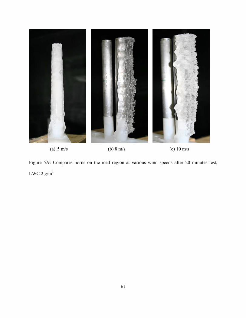
61
Figure 5.9: Compares horns on the iced region at various wind speeds after 20 minutes test,
LWC 2 g/m3
(a) 5 m/s (b) 8 m/s (c) 10 m/s
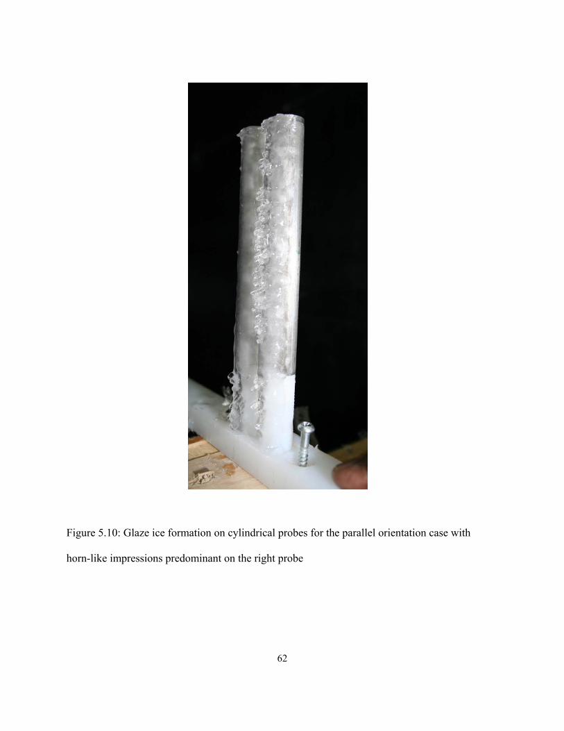
62
Figure 5.10: Glaze ice formation on cylindrical probes for the parallel orientation case with
horn-like impressions predominant on the right probe
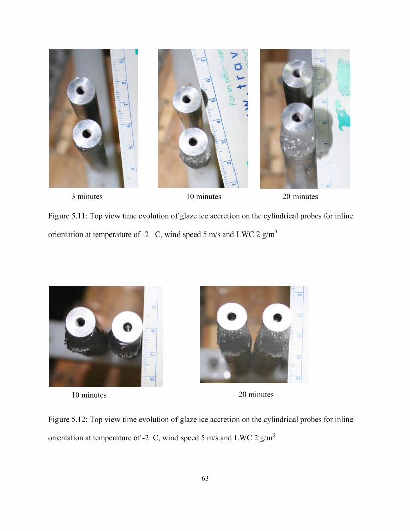
63
Figure 5.11: Top view time evolution of glaze ice accretion on the cylindrical probes for inline
orientation at temperature of -2C, wind speed 5 m/s and LWC 2 g/m3
Figure 5.12: Top view time evolution of glaze ice accretion on the cylindrical probes for inline
orientation at temperature of -2C, wind speed 5 m/s and LWC 2 g/m3
10 minutes 20 minutes
3 minutes 10 minutes 20 minutes
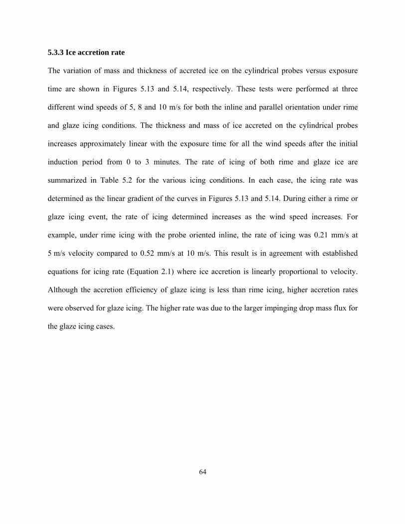
64
5.3.3 Ice accretion rate
The variation of mass and thickness of accreted ice on the cylindrical probes versus exposure
time are shown in Figures 5.13 and 5.14, respectively. These tests were performed at three
different wind speeds of 5, 8 and 10 m/s for both the inline and parallel orientation under rime
and glaze icing conditions. The thickness and mass of ice accreted on the cylindrical probes
increases approximately linear with the exposure time for all the wind speeds after the initial
induction period from 0 to 3 minutes. The rate of icing of both rime and glaze ice are
summarized in Table 5.2 for the various icing conditions. In each case, the icing rate was
determined as the linear gradient of the curves in Figures 5.13 and 5.14. During either a rime or
glaze icing event, the rate of icing determined increases as the wind speed increases. For
example, under rime icing with the probe oriented inline, the rate of icing was 0.21 mm/s at
5 m/s velocity compared to 0.52 mm/s at 10 m/s. This result is in agreement with established
equations for icing rate (Equation 2.1) where ice accretion is linearly proportional to velocity.
Although the accretion efficiency of glaze icing is less than rime icing, higher accretion rates
were observed for glaze icing. The higher rate was due to the larger impinging drop mass flux for
the glaze icing cases.
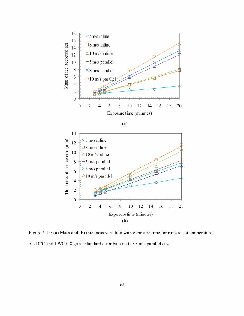
65
Figure 5.13: (a) Mass and (b) thickness variation with exposure time for rime ice at temperature
of -10oC and LWC 0.8 g/m3, standard error bars on the 5 m/s parallel case
02468
1012141618
0 2 4 6 8 10 12 14 16 18 20
Mas
s of
ice
accr
eted
(g)
Exposure time (minutes)
5m/s inline
8 m/s inline
10 m/s inline
5 m/s parallel
8 m/s parallel
10 m/s parallel
0
2
4
6
8
10
12
14
0 2 4 6 8 10 12 14 16 18 20
Thic
knes
s of i
ce a
ccre
ted
(mm
)
Exposure time (minutes)
5 m/s inline8 m/s inline10 m/s inline5 m/s parallel8 m/s parallel10 m/s parallel
(b)
(a)
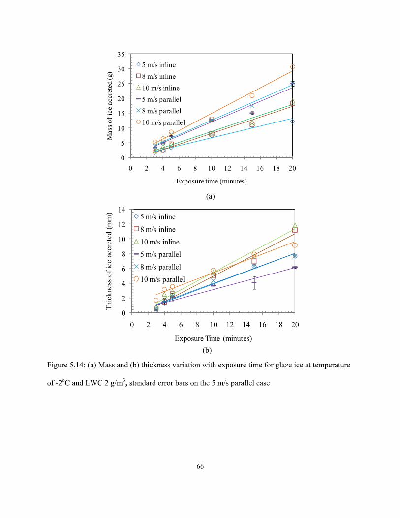
66
Figure 5.14: (a) Mass and (b) thickness variation with exposure time for glaze ice at temperature
of -2oC and LWC 2 g/m3, standard error bars on the 5 m/s parallel case
0
5
10
15
20
25
30
35
0 2 4 6 8 10 12 14 16 18 20
Mas
s of i
ce a
ccre
ted
(g)
Exposure time (minutes)
5 m/s inline8 m/s inline10 m/s inline5 m/s parallel8 m/s parallel10 m/s parallel
0
2
4
6
8
10
12
14
0 2 4 6 8 10 12 14 16 18 20
Thic
knes
s of
ice
accr
eted
(mm
)
Exposure Time (minutes)
5 m/s inline8 m/s inline10 m/s inline5 m/s parallel8 m/s parallel10 m/s parallel
(b)
(a)
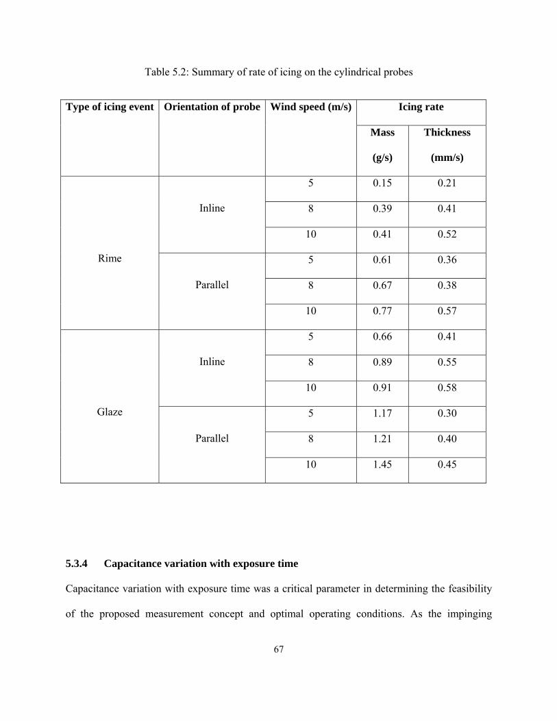
67
Table 5.2: Summary of rate of icing on the cylindrical probes
Type of icing event Orientation of probe Wind speed (m/s) Icing rate
Mass
(g/s)
Thickness
(mm/s)
Rime
Inline
5 0.15 0.21
8 0.39 0.41
10 0.41 0.52
Parallel
5 0.61 0.36
8 0.67 0.38
10 0.77 0.57
Glaze
Inline
5 0.66 0.41
8 0.89 0.55
10 0.91 0.58
Parallel
5 1.17 0.30
8 1.21 0.40
10 1.45 0.45
5.3.4 Capacitance variation with exposure time
Capacitance variation with exposure time was a critical parameter in determining the feasibility
of the proposed measurement concept and optimal operating conditions. As the impinging
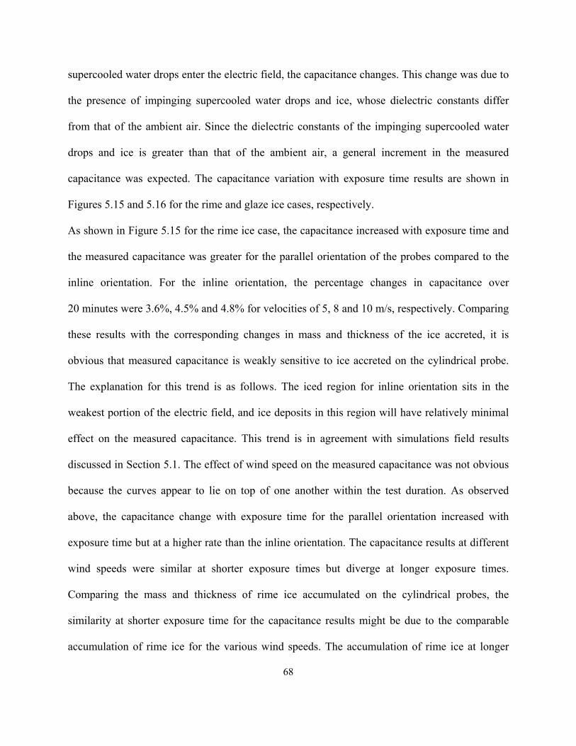
68
supercooled water drops enter the electric field, the capacitance changes. This change was due to
the presence of impinging supercooled water drops and ice, whose dielectric constants differ
from that of the ambient air. Since the dielectric constants of the impinging supercooled water
drops and ice is greater than that of the ambient air, a general increment in the measured
capacitance was expected. The capacitance variation with exposure time results are shown in
Figures 5.15 and 5.16 for the rime and glaze ice cases, respectively.
As shown in Figure 5.15 for the rime ice case, the capacitance increased with exposure time and
the measured capacitance was greater for the parallel orientation of the probes compared to the
inline orientation. For the inline orientation, the percentage changes in capacitance over
20 minutes were 3.6%, 4.5% and 4.8% for velocities of 5, 8 and 10 m/s, respectively. Comparing
these results with the corresponding changes in mass and thickness of the ice accreted, it is
obvious that measured capacitance is weakly sensitive to ice accreted on the cylindrical probe.
The explanation for this trend is as follows. The iced region for inline orientation sits in the
weakest portion of the electric field, and ice deposits in this region will have relatively minimal
effect on the measured capacitance. This trend is in agreement with simulations field results
discussed in Section 5.1. The effect of wind speed on the measured capacitance was not obvious
because the curves appear to lie on top of one another within the test duration. As observed
above, the capacitance change with exposure time for the parallel orientation increased with
exposure time but at a higher rate than the inline orientation. The capacitance results at different
wind speeds were similar at shorter exposure times but diverge at longer exposure times.
Comparing the mass and thickness of rime ice accumulated on the cylindrical probes, the
similarity at shorter exposure time for the capacitance results might be due to the comparable
accumulation of rime ice for the various wind speeds. The accumulation of rime ice at longer
69
exposure time however differs for the various wind speeds explored, and might be the cause of
the divergence in the measured capacitance. For the parallel orientation, the percentage change in
capacitance for 5, 8 and 10 m/s was 39.5%, 40.3% and 43.8%, respectively. These results
compared to changes in mass and thickness indicates higher sensitivity of the measured
capacitance to ice accretion than the inline orientation results. The results indicate, in agreement
with the simulation filed results and acrylic experiments in Section 5.1, that the parallel
orientation is more suitable for measuring capacitance change with ice accretion.
Figure 5.15: Capacitance variation with exposure time for rime ice at -10oC, 0.8 g/m3
3.52
3.72
3.92
4.12
4.32
4.52
4.72
4.92
5.12
5.32
0 2 4 6 8 10 12 14 16 18 20
Cap
acita
nce (
pF)
Exposure time (minutes)
5m/s inline
8 m/s inline
10 m/s inline
5 m/s parallel
8 m/s parallel
10 m/s parallel
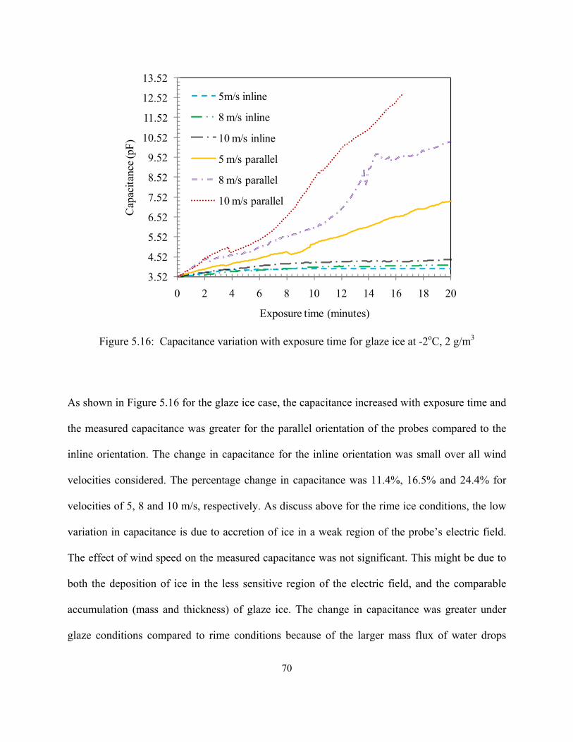
70
Figure 5.16: Capacitance variation with exposure time for glaze ice at -2oC, 2 g/m3
As shown in Figure 5.16 for the glaze ice case, the capacitance increased with exposure time and
the measured capacitance was greater for the parallel orientation of the probes compared to the
inline orientation. The change in capacitance for the inline orientation was small over all wind
velocities considered. The percentage change in capacitance was 11.4%, 16.5% and 24.4% for
velocities of 5, 8 and 10 m/s, respectively. As discuss above for the rime ice conditions, the low
variation in capacitance is due to accretion of ice in a weak region of the probe’s electric field.
The effect of wind speed on the measured capacitance was not significant. This might be due to
both the deposition of ice in the less sensitive region of the electric field, and the comparable
accumulation (mass and thickness) of glaze ice. The change in capacitance was greater under
glaze conditions compared to rime conditions because of the larger mass flux of water drops
3.52
4.52
5.52
6.52
7.52
8.52
9.52
10.52
11.52
12.52
13.52
0 2 4 6 8 10 12 14 16 18 20
Cap
acita
nce (
pF)
Exposure time (minutes)
5m/s inline
8 m/s inline
10 m/s inline
5 m/s parallel
8 m/s parallel
10 m/s parallel
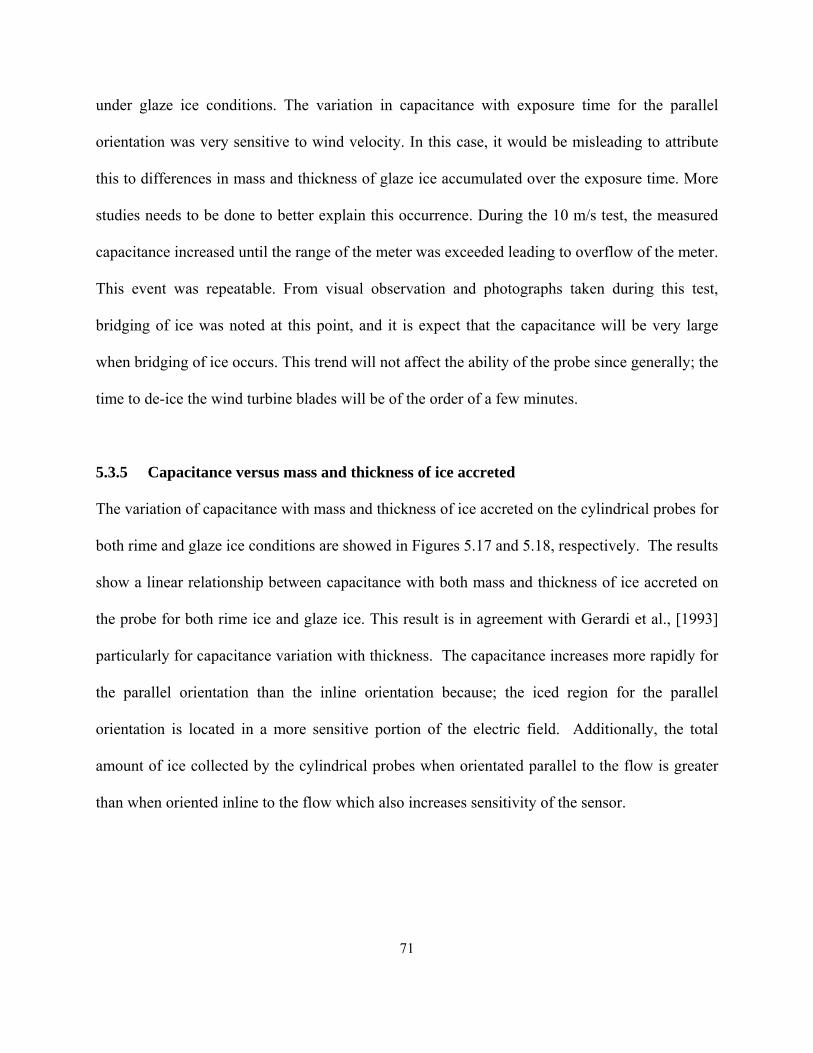
71
under glaze ice conditions. The variation in capacitance with exposure time for the parallel
orientation was very sensitive to wind velocity. In this case, it would be misleading to attribute
this to differences in mass and thickness of glaze ice accumulated over the exposure time. More
studies needs to be done to better explain this occurrence. During the 10 m/s test, the measured
capacitance increased until the range of the meter was exceeded leading to overflow of the meter.
This event was repeatable. From visual observation and photographs taken during this test,
bridging of ice was noted at this point, and it is expect that the capacitance will be very large
when bridging of ice occurs. This trend will not affect the ability of the probe since generally; the
time to de-ice the wind turbine blades will be of the order of a few minutes.
5.3.5 Capacitance versus mass and thickness of ice accreted
The variation of capacitance with mass and thickness of ice accreted on the cylindrical probes for
both rime and glaze ice conditions are showed in Figures 5.17 and 5.18, respectively. The results
show a linear relationship between capacitance with both mass and thickness of ice accreted on
the probe for both rime ice and glaze ice. This result is in agreement with Gerardi et al., [1993]
particularly for capacitance variation with thickness. The capacitance increases more rapidly for
the parallel orientation than the inline orientation because; the iced region for the parallel
orientation is located in a more sensitive portion of the electric field. Additionally, the total
amount of ice collected by the cylindrical probes when orientated parallel to the flow is greater
than when oriented inline to the flow which also increases sensitivity of the sensor.
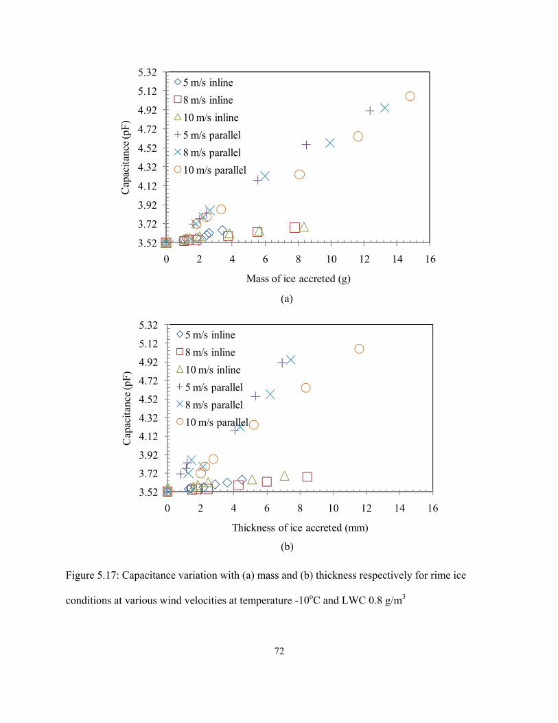
72
Figure 5.17: Capacitance variation with (a) mass and (b) thickness respectively for rime ice
conditions at various wind velocities at temperature -10oC and LWC 0.8 g/m3
3.52
3.72
3.92
4.12
4.32
4.52
4.72
4.92
5.12
5.32
0 2 4 6 8 10 12 14 16
Cap
acita
nce (
pF)
Mass of ice accreted (g)
5 m/s inline8 m/s inline10 m/s inline5 m/s parallel8 m/s parallel10 m/s parallel
3.52
3.72
3.92
4.12
4.32
4.52
4.72
4.92
5.12
5.32
0 2 4 6 8 10 12 14 16
Cap
acita
nce (
pF)
Thickness of ice accreted (mm)
5 m/s inline8 m/s inline10 m/s inline5 m/s parallel8 m/s parallel10 m/s parallel
(a)
(b)
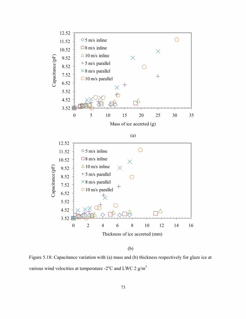
73
Figure 5.18: Capacitance variation with (a) mass and (b) thickness respectively for glaze ice at
various wind velocities at temperature -2oC and LWC 2 g/m3
3.52
4.52
5.52
6.52
7.52
8.52
9.52
10.52
11.52
12.52
0 5 10 15 20 25 30 35
Cap
acita
nce (
pF)
Mass of ice accreted (g)
5 m/s inline8 m/s inline10 m/s inline5 m/s parallel8 m/s parallel10 m/s parallel
3.52
4.52
5.52
6.52
7.52
8.52
9.52
10.52
11.52
12.52
0 2 4 6 8 10 12 14 16
Cap
acita
nce (
pF)
Thickness of ice accreted (mm)
5 m/s inline8 m/s inline10 m/s inline5 m/s parallel8 m/s parallel10 m/s parallel
(a)
(b)
74
5.3.6 Sensitivity
Capacitance normalized with mass and thickness versus exposure time is shown in Figure 5.19
and Figure 5.20 for both rime and glaze ice, respectively. Rime ice curves indicate a sharp
increase in the normalized capacitance with exposure time during the first few minutes
(3 to 5 minutes) after which the curves plateaus especially for the inline orientation. For the
parallel orientation case, there were a few variations in both capacitance per mass and
capacitance per thickness, as seen in Figure 5.19. This initial trend implies the sensor is more
sensitive within the first few minutes of icing events for rime ice. This high sensitivity in the
initial stages of an icing event would allow early implementation of wind turbine blade de-icing
strategies under sever icing conditions. However, the flat trend after the initial stage is equally of
importance especially in predicting ice type. This is because observations of time dependent ice
growth photographs from the wind icing experiments indicate slight variation in ice structure
within these periods. These trends are similar to when the glaze ice event was simulated in the
icing wind tunnel as shown in Figure 5.20. For both rime and glaze ice events, there was poor
correlation between thickness and capacitance.
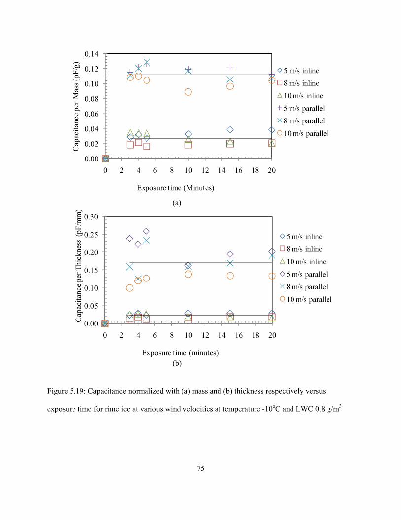
75
Figure 5.19: Capacitance normalized with (a) mass and (b) thickness respectively versus
exposure time for rime ice at various wind velocities at temperature -10oC and LWC 0.8 g/m3
0.00
0.02
0.04
0.06
0.08
0.10
0.12
0.14
0 2 4 6 8 10 12 14 16 18 20
Cap
acita
nce p
er M
ass (
pF/g
)
Exposure time (Minutes)
5 m/s inline8 m/s inline10 m/s inline5 m/s parallel8 m/s parallel10 m/s parallel
0.00
0.05
0.10
0.15
0.20
0.25
0.30
0 2 4 6 8 10 12 14 16 18 20
Cap
acita
nce p
er T
hick
ness
(pF
/mm
)
Exposure time (minutes)
5 m/s inline8 m/s inline10 m/s inline5 m/s parallel8 m/s parallel10 m/s parallel
(a)
(b)
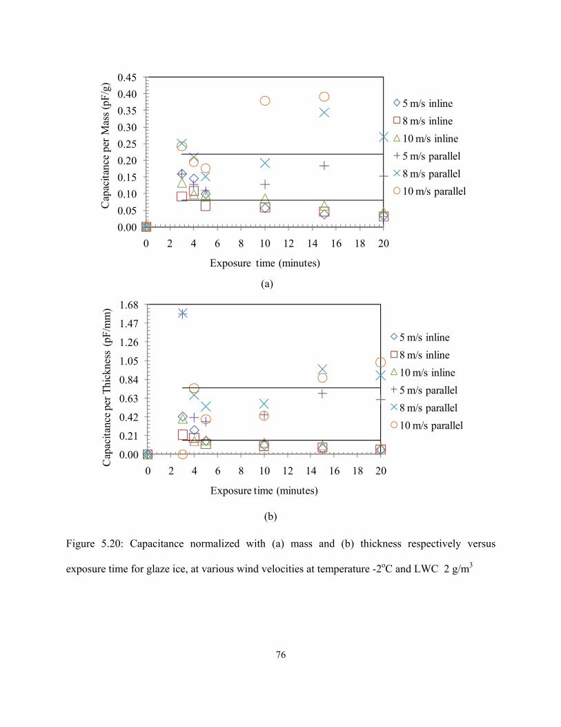
76
Figure 5.20: Capacitance normalized with (a) mass and (b) thickness respectively versus
exposure time for glaze ice, at various wind velocities at temperature -2oC and LWC 2 g/m3
0.000.050.100.150.200.250.300.350.400.45
0 2 4 6 8 10 12 14 16 18 20
Cap
acita
nce
per M
ass (
pF/g
)
Exposure time (minutes)
5 m/s inline8 m/s inline10 m/s inline5 m/s parallel8 m/s parallel10 m/s parallel
0.00
0.21
0.42
0.63
0.84
1.05
1.26
1.47
1.68
0 2 4 6 8 10 12 14 16 18 20
Cap
acita
nce p
er T
hick
ness
(pF
/mm
)
Exposure time (minutes)
5 m/s inline8 m/s inline10 m/s inline5 m/s parallel8 m/s parallel10 m/s parallel
(a)
(b)
77
5.3.7 Resistance change against exposure time
Changes in the measured capacitance with exposure time during the icing experiments as
previously discussed was due to differences in dielectric constants that could be attributed to
variation in the matrix of ice, air and supercooled water drops deposited on the iced region of the
probe. For this reason, the output capacitance recorded for both icing events gave an indication
of ice accretion type on the surface of the cylindrical probes. Therefore based on the capacitance
results, it would not be possible to decipher between the two icing events simulated in the icing
wind tunnel. Hence, to distinguish between rime and glaze ice in the icing wind tunnel, another
technique based on resistance measurements is proposed. The inline orientation was not
considered for the changes in resistance since the deposit is not between the cylindrical probes.
As ice deposits on the front face of the cylindrical probes, there is interaction with the electric
field as discussed earlier. Additionally, the air gap between the cylindrical probes decreases as
the accreted ice grows. Consequently, the resistance decreases with time for both the rime and
glaze ice conditions. Figure 5.21 shows an exponential decay rate for both icing events. It was
noted that the decay rate was slower for rime ice compared to glaze ice. This phenomenon was
explained as follows. Electric fields interact with the surface of the substance without penetrating
thereby eliminating any contributions from the internal structure of the accreted ice. Thus, the
conditions prevailing on the surface of the probe undergoing rime and glaze icing is paramount
to this trend. Glaze ice as discussed earlier, is characterised by water run-offs on the surface,
while the surface of rime ice is “dry” i.e. no water run-offs. Air has a higher resistance to electric
flow than water leading to the relatively slow decay of the measured resistance for rime ice
compared to glaze ice. Therefore, the decay rate was used to assert the type of in-cloud icing
event in our proposed method. It should be noted that the higher liquid content involved in glaze
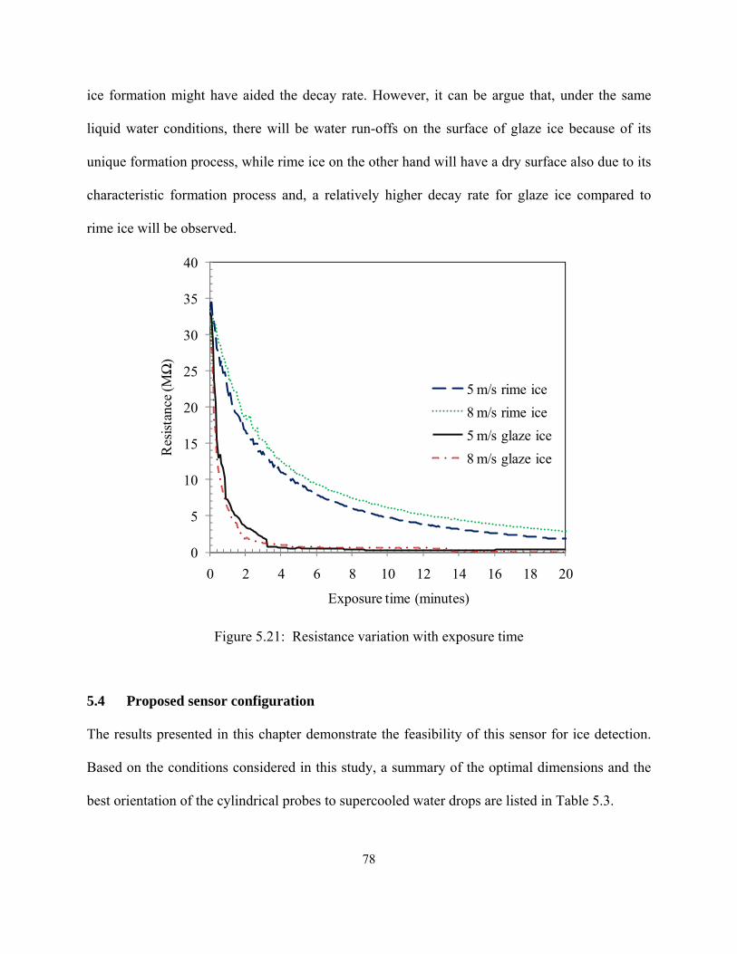
78
ice formation might have aided the decay rate. However, it can be argue that, under the same
liquid water conditions, there will be water run-offs on the surface of glaze ice because of its
unique formation process, while rime ice on the other hand will have a dry surface also due to its
characteristic formation process and, a relatively higher decay rate for glaze ice compared to
rime ice will be observed.
Figure 5.21: Resistance variation with exposure time
5.4 Proposed sensor configuration
The results presented in this chapter demonstrate the feasibility of this sensor for ice detection.
Based on the conditions considered in this study, a summary of the optimal dimensions and the
best orientation of the cylindrical probes to supercooled water drops are listed in Table 5.3.
0
5
10
15
20
25
30
35
40
0 2 4 6 8 10 12 14 16 18 20
Res
istan
ce (M
Ω)
Exposure time (minutes)
5 m/s rime ice8 m/s rime ice5 m/s glaze ice8 m/s glaze ice
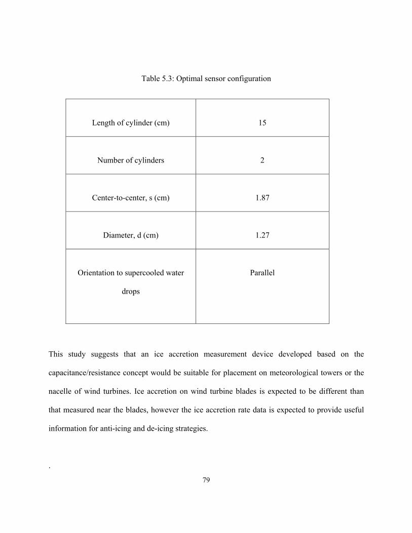
79
Table 5.3: Optimal sensor configuration
Length of cylinder (cm)
15
Number of cylinders
2
Center-to-center, s (cm)
1.87
Diameter, d (cm)
1.27
Orientation to supercooled water
drops
Parallel
This study suggests that an ice accretion measurement device developed based on the
capacitance/resistance concept would be suitable for placement on meteorological towers or the
nacelle of wind turbines. Ice accretion on wind turbine blades is expected to be different than
that measured near the blades, however the ice accretion rate data is expected to provide useful
information for anti-icing and de-icing strategies.
.
80
Chapter 6
Conclusions
6.1 Conclusions
Wind power production in ice prone regions is hindered by icing of wind turbines. Problems
associated with icing of wind turbines vary, and they all require removal of ice from the surface
of the wind turbine blades. In this research, an ice sensor base on a novel concept suitable for
measuring ice accretion on meteorological metrological towers near wind farms and nacelles of
wind turbines are numerically and experimentally demonstrated in a laboratory setting. This
concept is based on the changes in measured capacitance and resistance with ice accretion. Two
orientations of the ice sensor to supercooled drops laden wind, inline and parallel, under
simulated rime and glaze icing events in the wind icing tunnel, are analyzed.
Results from the numerical studies indicate that, the sensitivity of the ice sensor was a function
of the center-to-center distance between the cylindrical probes, the sizes of the cylindrical
probes, and the location of the ice deposition. The sensitivity of the ice sensor decreases with
increasing center-to-center distance. Additionally, two different sized cylindrical probes were
found to be less sensitive to icing compared to cylindrical probes of the same size. Finally, with
both the center-to-center distance and the diameter of the cylindrical probes fixed, modelled ice
deposition on the front surfaces of both cylindrical probes (parallel orientation) was more
sensitive than the case where the modelled deposition was on the side of only one of the
cylindrical probes (inline orientation). The high sensitivity for the parallel orientation case was
observed in the wind icing tunnel experiments. The high sensitivity for the parallel orientation
case implies preferentially orienting the cylindrical probes to the flow direction.
81
From the wind icing tunnel experiments, the icing rate was found to be relatively constant
indicating little or no change in the aerodynamics of the flow for both icing events after the
initial induction period. The calculated icing rates were found to increase with wind speed. The
measured capacitance, which gave an indication of an icing event, was observed to increases
with exposure time and ice deposition. The sensitivity of the ice sensor to ice deposition was
found to be high within the first few minutes (typically between 3 and 5 minutes) of exposure,
after which the curves level off. This high sensitivity of the sensor within the few minutes of
exposure is advantageous, since it would allow quick remedial action to the ice deposition on the
wind turbine blade. The flat trend after the initial stage is equally of importance especially in
predicting icing structure, since observations during the experiments indicate slight variation in
ice structure. It was not possible to categorically discriminate between rime and glaze icing
events exclusively based on the results from the measured capacitance and to do this, resistance
results were used. The resistance decreases exponentially with ice accretion, with resistance for
the glaze ice case decaying faster than for the rime ice case. For both icing events, the decay was
towards an asymptotic value.
82
Chapter 7
Recommendations
7.1 Recommendations
This study suggests that an ice accretion measurement device developed based on the
capacitance/resistance concept would be suitable for placement on meteorological towers or the
nacelle of wind turbines. The device could detect an icing event, mass accretion of ice and
differentiate between rime and glace icing events. However, there are more steps required in
order to commercialise this sensor. In this light, the following are recommended for future
investigations.
• Testing the sensor under a wider variation of liquid water contents (LWC).
• Testing the sensor under a wider variation of wind speeds.
• Testing the sensor under a wider variation of temperatures.
• Testing the sensor in real icing conditions and results compared with existing sensor.
• Testing the sensor under the other types of icing events not explored in this work e.g.
freezing rain, mixed rime and glaze etc.
• Develop a de-icing system for the sensor.
• Investigate if melting time during de-icing of sensor can correlate to ice thickness.
• Investigate the significant effect of changing the field frequency to detect the onset of
water deposition on the probe.
83
Reference
Admirat, P., Sakamoto, Y.,1988, “Wet Snow on Overhead Lines: State-of-Art,” Proc. 4th Int.
Workshop on Atmospheric Icing of Structures, pp. 8-13.
Ahmed W.H., Ismail, B.I., 2008, “Innovative Techniques for Two-Phase Flow Measurements,”
Recent Patents on Electrical Engineering, vol.1 no.1, pp. 1-13.
Ahti, K., Makkonen, L., 1982, “Observations on Rime Formation in Relation to Routinely
Measured Meteorological Parameters,” Geophysica vol. 19, pp. 75–85.
Bose, N., 1992, “Icing on a Small Horizontal Axis Wind Turbine-Part 1: Glaze Ice Profiles,”
Journal of wind engineering and industrial aerodynamics, vol. 45, pp. 75-85.
CanWEA, “Wind Generation to Experience Strong Growth,” Windlink, January 9, 2007, Issue
no. 6.
CanWEA, “Wind Vision 2025 Powering Canada’s Future,” 2008.
<http://www.windtrm.gc.ca/pdfs/windvision_summary_e.pdf>. accessed 19th December 2009.
Chamuel, J.R., 1984, “Ultrasonic Aircraft Ice Detector using Flexural Waves” United States
Patent number 4,461,178.
Paul, C., 2000, Fundamentals of Electric Circuit Analysis, John Wiley & Sons. Inc., 605 Third
Avenue, New York, NY 10158-0012.
COST 727, 2006, “Atmospheric Icing on Structures-Measurement and Data Collection on Icing:
State of The Art,” A compilation of the contributions of the Working Group 2 participants.
84
Craig, D.F., Craig, D.B., 1995, “An Investigation of Icing Events on Haeckel Hill,” Proceedings
of BOREAS III Conference, Finland.
Crowe, T.C., Sommerfeld, M., Tsuji, Y., 1998, Multiphase Flows with Droplets and Particles
CRC Press, Boca Raton, Florida.
DeAnna, R., 1999, “Ice Detection Sensor,” United States Patent number 5,886,256.
Drage, A., Lange, T.D., 2005, “Instruments for Measuring Atmospheric Icing,’’ Reports in
Meteorology and Oceanography.
Ducu, D.O., Donahue, R.J., Ghandhi, J.B., 2001, “Design of Capacitance Probes for Oil Film
Thickness Measurements Between the Piston Ring and Liner in Internal Combustion Engines,”
Journal of Engineering for Gas Turbines and Power, vol. 123, no. 3, pp. 633-643.
Elkow, K.J., Rezkallah, K.S., 1996, “Void Fraction Measurements in Gas-Liquid Flows using
Capacitance Sensors,” Measurement Science and Technology, vol. 7, pp. 1153-1163.
Federow, H.L., Silverman, J.H., 1994, “Laser Ice Detector,” United States Patent number
5,296,853.
Frohboese, P., Anders, A., 2007, “Effects of Icing on Wind Turbine Fatigue Loads,” IOP
Publishing Journal of Physics: Conference Series, Copenhagen.
Ganander, H., Ronsten, G., 2003, “Design Load Aspects due to Ice Loading on Wind Turbine
Blades,” Proceedings of the BOREAS VI Conference, Finland.
Geraldi,J.J., Hickman,G.A., Khatkhate,A.A., Pruzan, D.A., 1996, “Measuring Ice Distribution
Profiles with Attached Capacitance Electrodes,” United States Patent number 5,551,288.
85
Goldberg, J.L., Lardiere Jr., B.G., 1993, “Expulsive Ice Detector,” United States Patent number
5,523,959.
Goodrich 0871LH1 Freezing Rain Sensor Instrumentation Manual, Goodrich, 2008.
Hansman Jr., R.J., Kirby,M., “Measurement of Ice Growth during Simulated and Natural Icing
Conditions using Ultrasonic Pulse-Echo Techniques,” Journal of Aircrafts vol. 23 pp. 492-498.
HIOKI 3522-50 LCR HiTESTER Instruction Manual, HIOKI.E.E. Corporation, Japan, 2007.
Homola, C.M., Nicklasson, P.J., Sundsbø, P.J., 2006, “Ice Sensors for Wind Turbines,” Cold
Regions Science and Technology vol. 46, pp. 125-131.
Infralytic “Ice Sensor for Rotor Blades,” < www.infralytic.de>. accessed 25th May 2010.
Jasinski, W.J., Noe, S.C., Selig, M.S., Bragg, M.B., 1998, “Wind Turbine Performance under
Icing Conditions,” Transactions of the ASME, Journal of Solar Energy Engineering, vol. 120,
pp. 60-65.
Kaiser, K.L., 2000, Electromagnetic Compatibility Handbook, CRC Press, Boca Raton, Florida.
Khurgin, B., “Ice Detector with Movable Feeler,” United States Patent number 4,873,510, 1989.
Kimura, S., Tammelin, B., Santti, K., 2000, “Estimation of reduction of power production due
to icing from existing meteorological data,” BOREAS V, Finland.
Klainer, S.M., Milanovich, F.P., 1990, “Optical Sensor for the Detection of Ice Formation and
other Chemical Species,” United States Patent number 4, 913,519.
86
Kraj, A. G., 2007, “Icing Characteristics and Mitigation Strategies for Wind Turbines in Cold
Climates,” M.Sc thesis, University of Manitoba.
Laakso, T., Holttinen, H., Ronsten, G., Tallhaug L., Horbaty, R., Baring-Gould, I., Lacroix, A.,
Peltola, E., Tammelin, B., 2003, “State-of-the-Art of Wind Energy in Cold Climates.”
International Energy Agency, Annex XIX, Finland.
Labkotec Ice Detectors LID 33210C User Manual, Labkotec Oy, Finland, 2009.
Labkotec Ice Detectors LID 33210D User Manual, Labkotec Oy, Finland, 2003.
Lardiere Jr., B.G., Wells, B.F., 1998, “Integrated Planar Ice Detector” United States Patent
number 5,790,026.
Lee, H., Seegmiller, B., 1996, “Ice Detector and De-icing Fluid Effectiveness Monitoring
System,” United States Patent number 5,523,959.
Louge, M.Y., Steiner, R., Keast, S.C., Decker, R., Dent, J., Schneebeli, M., 1997, “Application
of Capacitance Instrumentation to the Measurement of Density and Velocity of Flowing Snow,”
Cold Regions Science and Technology, vol. 23, pp. 47-63.
Louge, M.Y., Foster, R.L., Jensen, N., Patterson, R., 1998, “A Portable Capacitance Snow
sounding Instrument”, Cold Regions Science and Technology, vol. 28, pp. 73-81.
Maatuk, J., 2004 “Microprocessor-based Liquid Sensor and Ice Detector,” United States Patent
number 6,776,037.
Magenheim, B., 1977, “Microwave Ice Detector,” United States Patent number 4,054,255.
87
Makkonen, L., 2000, “Models for the Growth of Rime, Glaze, Icicles and Wet Snow on
Structures,” Philosophical Transactions: Mathematical, Physical and Engineering Sciences, vol.
358, no. 1776, pp. 2913-2939.
Makkonen, L., 1984, “Modelling of Ice Accretion on Wires,” Journal of Climate and Applied
Meteorology, vol. 23, issue 6, pp. 929-939.
Patel, M.R., 2006, Wind and Solar Power System; Design, Analysis and Operation, Second
Edition, CRC Press, Florida.
Piazza, R., Parola, A., 2008, “Thermophoresis in Colloidal Suspensions,” Journal of Physics:
Condensed Matter, vol. 20.
OuickField™ User Guide Version 5.3, Tera Analysis Limited, Denmark, 2005.
Reid, W.T., 1971, External Corrosion and Deposits-boilers and Gas Turbines, American Elsevier
Publishing Company, New York.
Seifert,H., 2003, “Technical Requirements for Rotor Blades Operating in Cold Climates,”
proceedings of the BOREAS II conference Pyhätunturi, Finland.
Vibro-meter “ Vibro-meter.com/aerospace/ice.html” accessed 25th May 2010.
Wakahama, G., Kuroiwa, D., Goto, D., 1977, “Snow Accretion on Electric Wires and its
Prevention,” Journal of Glaciology vol. 19, no. 81, pp. 479–487.
Wallace, R.D., Gillespie, A.B., Sweet, D.B., Rauckhorst, R.L., Terry, M.J., Holyfield, M.E.,
2002, “Ice Thickness Detector,” United States Patent number 6,384,611.
88
Wang, X., 2008, “Convective Heat Transfer and Experimental Icing Aerodynamics of Wind
Turbine Blades,” Ph.D thesis, University of Manitoba.
Wimmer, R., Kranz, M., Boring, S., Schmidt Albrecht, 2007, “A Capacitive Sensing Toolkit for
Pervasive Activity Detection and Recognition,” Proceedings of the fifth IEEE International
Conference on Pervasive Computing and Communications, pp. 171-180.
Rondeau, J., “Rondeau Opens National Wind Energy Conference,” Winnipeg Canada. 23rd
October, 2006. < http://news.gov.mb.ca/news/index,print.html?archive=&item=178>. accessed
20th November 2009.
Robinson, D.A., Gardner, C.M.K., Evans, J., Cooper, J.D., Hodnett, M.G., Bell, J.P., 1998, “The
Dielectric Calibration of Capacitance Probes for Soil Hydrology using an Oscillation Frequency
Response Model,” Hydrology and Earth System Sciences, vol. 2, pp. 83-92.
Rocha, M.S., Cabral, E.L.L., Simões-Moreira, J.R., 2009, “Capacitance Sensor for Void Fraction
Measurement in a Natural Circulation Refrigeration Circuit,” International Nuclear Atlantic
Conference, Brazil.
RMS., 2008, “The 1998 Ice Storm: 10-year Retrospective,” Report by Risk Management
Solutions (RMS), Inc.
Ryerson, C.C., 2008, “Assessment of Superstructure Ice Protection as Applied to Offshore Oil
Operations Safety: Problems, Hazards, Needs, and Potential Transfer Technology,” US Army
Corps of Engineers, Cold Regions Research and Engineering Laboratory.
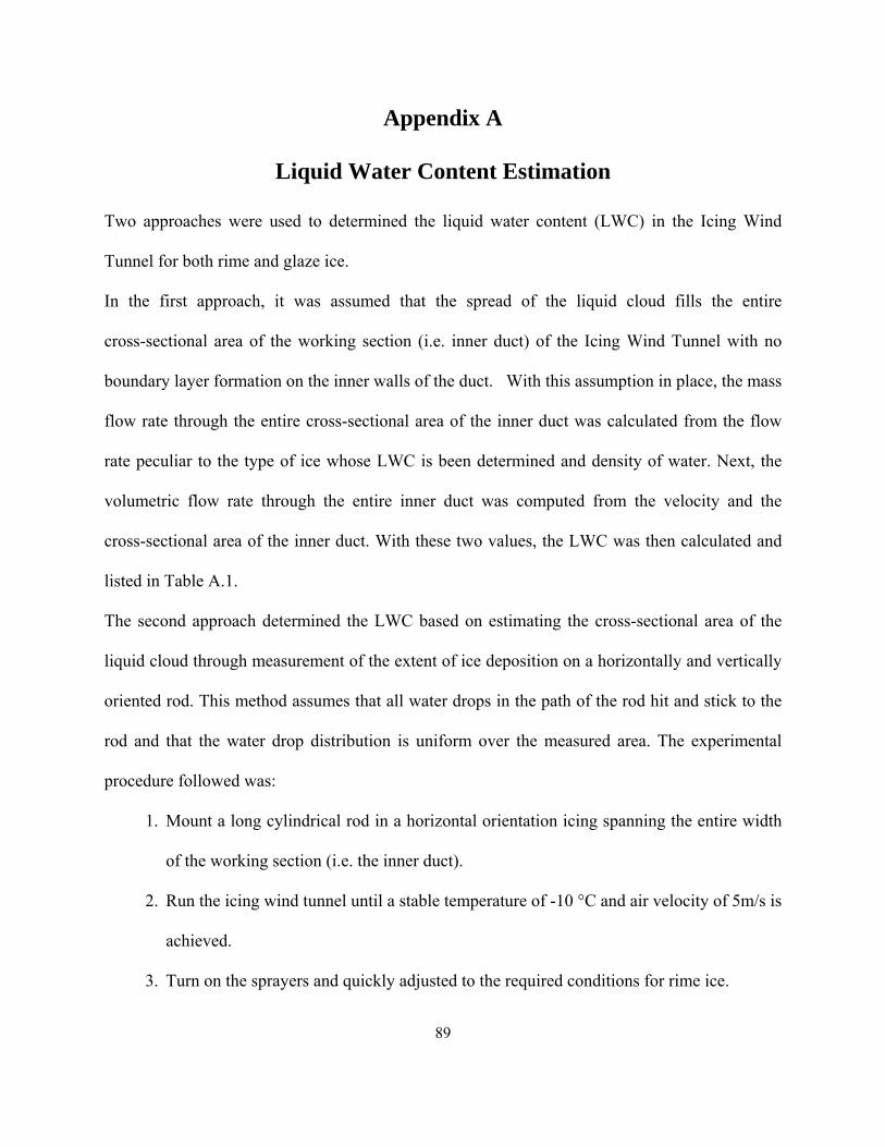
89
Appendix A
Liquid Water Content Estimation
Two approaches were used to determined the liquid water content (LWC) in the Icing Wind
Tunnel for both rime and glaze ice.
In the first approach, it was assumed that the spread of the liquid cloud fills the entire
cross-sectional area of the working section (i.e. inner duct) of the Icing Wind Tunnel with no
boundary layer formation on the inner walls of the duct. With this assumption in place, the mass
flow rate through the entire cross-sectional area of the inner duct was calculated from the flow
rate peculiar to the type of ice whose LWC is been determined and density of water. Next, the
volumetric flow rate through the entire inner duct was computed from the velocity and the
cross-sectional area of the inner duct. With these two values, the LWC was then calculated and
listed in Table A.1.
The second approach determined the LWC based on estimating the cross-sectional area of the
liquid cloud through measurement of the extent of ice deposition on a horizontally and vertically
oriented rod. This method assumes that all water drops in the path of the rod hit and stick to the
rod and that the water drop distribution is uniform over the measured area. The experimental
procedure followed was:
1. Mount a long cylindrical rod in a horizontal orientation icing spanning the entire width
of the working section (i.e. the inner duct).
2. Run the icing wind tunnel until a stable temperature of -10 °C and air velocity of 5m/s is
achieved.
3. Turn on the sprayers and quickly adjusted to the required conditions for rime ice.
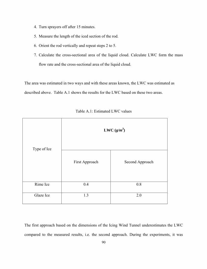
90
4. Turn sprayers off after 15 minutes.
5. Measure the length of the iced section of the rod.
6. Orient the rod vertically and repeat steps 2 to 5.
7. Calculate the cross-sectional area of the liquid cloud. Calculate LWC form the mass
flow rate and the cross-sectional area of the liquid cloud.
The area was estimated in two ways and with these areas known, the LWC was estimated as
described above. Table A.1 shows the results for the LWC based on these two areas.
Table A.1: Estimated LWC values
Type of Ice
LWC (g/m3)
First Approach
Second Approach
Rime Ice 0.4 0.8
Glaze Ice 1.3 2.0
The first approach based on the dimensions of the Icing Wind Tunnel underestimates the LWC
compared to the measured results, i.e. the second approach. During the experiments, it was

91
observed that the amount of ice deposited on the rod varied across the length of the rod, which
would tend to underestimate the LWC as would the assumption of 100% capture efficiency. The
values from the second approach were quoted in this research.
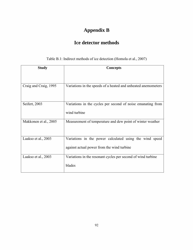
92
Appendix B
Ice detector methods
Table B.1: Indirect methods of ice detection (Homola et al., 2007)
Study Concepts
Craig and Craig, 1995 Variations in the speeds of a heated and unheated anemometers
Seifert, 2003 Variations in the cycles per second of noise emanating from
wind turbine
Makkonen et al., 2005 Measurement of temperature and dew point of winter weather
Laakso et al., 2003 Variations in the power calculated using the wind speed
against actual power from the wind turbine
Laakso et al., 2003 Variations in the resonant cycles per second of wind turbine
blades
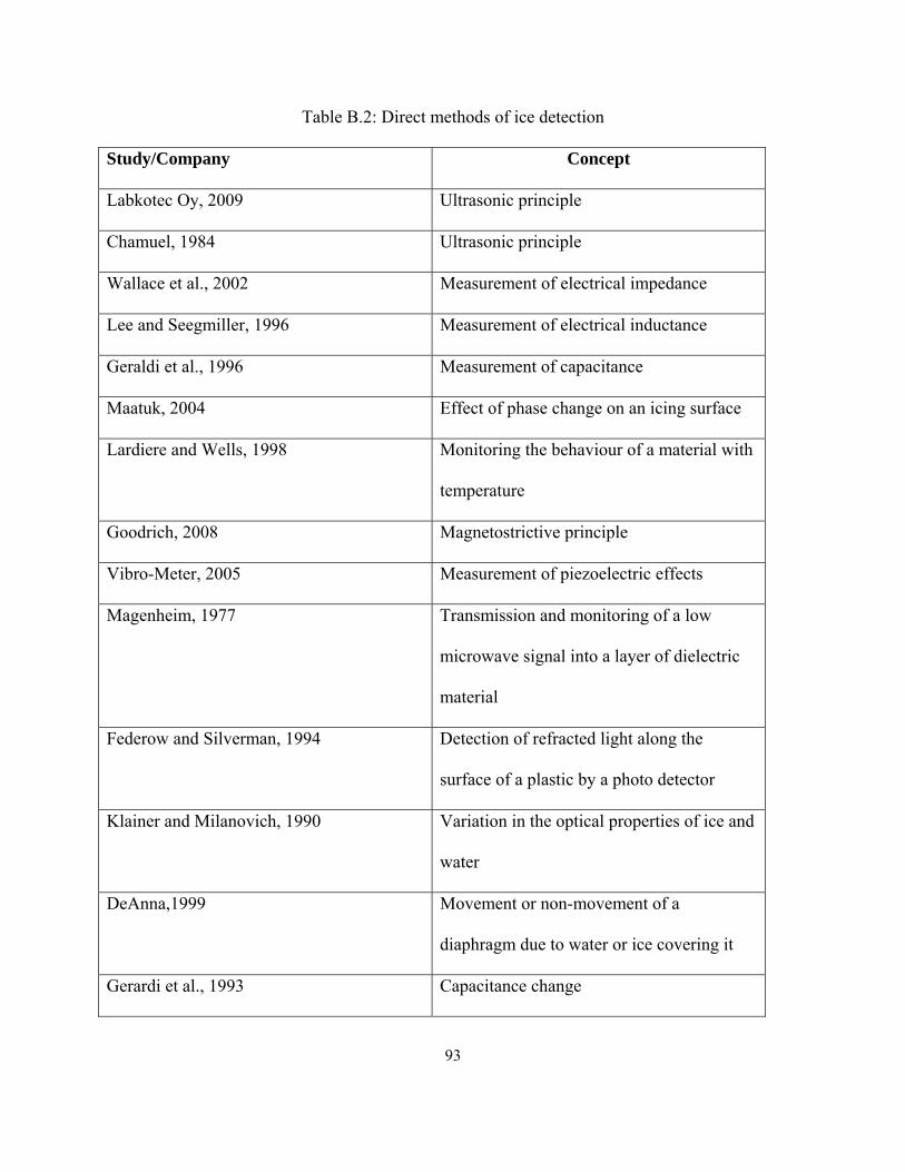
93
Table B.2: Direct methods of ice detection
Study/Company Concept
Labkotec Oy, 2009 Ultrasonic principle
Chamuel, 1984 Ultrasonic principle
Wallace et al., 2002 Measurement of electrical impedance
Lee and Seegmiller, 1996 Measurement of electrical inductance
Geraldi et al., 1996 Measurement of capacitance
Maatuk, 2004 Effect of phase change on an icing surface
Lardiere and Wells, 1998 Monitoring the behaviour of a material with
temperature
Goodrich, 2008 Magnetostrictive principle
Vibro-Meter, 2005 Measurement of piezoelectric effects
Magenheim, 1977 Transmission and monitoring of a low
microwave signal into a layer of dielectric
material
Federow and Silverman, 1994 Detection of refracted light along the
surface of a plastic by a photo detector
Klainer and Milanovich, 1990 Variation in the optical properties of ice and
water
DeAnna,1999 Movement or non-movement of a
diaphragm due to water or ice covering it
Gerardi et al., 1993 Capacitance change
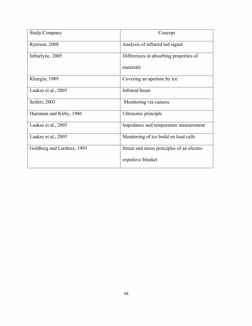
94
Study/Company Concept
Ryerson, 2008 Analysis of infrared red signal
Infrarlytic, 2005 Differences in absorbing properties of
materials
Khurgin, 1989 Covering an aperture by ice
Laakso et al., 2003 Infrared beam
Seifert, 2003 Monitoring via camera
Hansman and Kirby, 1986 Ultrasonic principle
Laakso et al., 2003 Impedance and temperature measurement
Laakso et al., 2003 Monitoring of ice build on load cells
Goldberg and Lardiere, 1993 Strain and stress principles of an electro-
expulsive blanket

95