Canonical sectors and evolution of rms in the US stock markets

January 19, 2018 Quantitative Finance MergedText

To appear in Quantitative Finance, Vol. 00, No. 00, Month 20XX, 1–22

Canonical sectors and evolution of firms in

the US stock markets

Lorien X. Hayden, Ricky Chachra, Alexander A. Alemi,Paul H. Ginsparg and James P. Sethna∗

Department of PhysicsCornell University, Ithaca, NY 14853 USA

(November 17th, 2016)

Contact Information

• Lorien X. Hayden◦ (573) 819-2155◦ [email protected]

• Ricky Chachra◦ (212) 729-7529◦ [email protected]

• Alexander A. Alemi◦ (814) 422-5364◦ [email protected]

• Paul H. Ginsparg◦ (607) 255-7371◦ [email protected]

• James P. Sethna◦ (607) 275-7748◦ [email protected]

Acknowledgements

We thank Jean–Philippe Bouchaud, Ming Huang and Janet Gao for helpful discussions.

Funding

This work was partially supported by NSF grants DMR-1312160, DMR-1719490, IIS-1247696 andDGE-1144153.

∗Corresponding author. Email: [email protected]

1

arX

iv:1

503.

0620

5v5

[q-

fin.

ST]

18

Jan

2018


Abstract

A classification of companies into sectors of the economy is important for macroeconomic analysis andfor investments in sector-specific financial indices and exchange traded funds (ETFs). Major industrialclassification systems and financial indices have historically been based on expert opinion and developedmanually. Here we show how unsupervised machine learning can provide a more objective and compre-hensive broad-level sector decomposition of stocks. An emergent low-dimensional structure in the space ofhistorical stock price returns automatically identifies ’canonical sectors’ in the market, and assigns everystock a participation weight into these sectors. Furthermore, by analyzing data from different periods,we show how these weights for listed firms have evolved over time.

Keywords: Machine Learning, Archetypal Analysis, Canonical Sectors, Computational Finance

JEL Classification: C38, G10

Main Text

Stock market performance is measured with aggregated quantities called indices that represent aweighted average price of a basket of stocks. Market-wide indices such as Russell 3000 R© (Russell3000 R© Index 2015) and the S&P 500 R© (S&P 500 R© Index 2014) consist of stocks from diversecompanies reflecting a broad cross-section of the market. Sector-specific indices such as the DowJones R© Financials Index (Dow Jones R© US Indices: Industry Indices 2015), CBOE R© Oil Index(CBOE R© Oil Index 2013) and the Morgan Stanley R© High-Tech 35 Index (Morgan Stanley R© High-Tech 35 Index 2005), etc., are more granular and their composition requires a classification ofcompanies into sectors. Major industrial classification schemes classify firms into sectors, albeit withmany ambiguities (Nadig and Crigger 2011). It is not clear, for example, how to assign a sector toconglomerates or diversified companies such as General Electric R©. Conversely, non-conglomerateswith exposure to firms outside their own sector (for example, an investment bank exclusively servingpharmaceutical firms) also blur the boundaries of sector-identification. Moreover, as companies andtheir economic environments evolve, neither the industrial sectors nor the firms’ sector associationremains static, necessitating updates to sector assignments and addition of new sectors.

A significant number of studies have previously aimed at identifying categories of stocks infinancial markets with a variety of approaches. Recent numerical techniques have included extensiveuse of random matrix theory, principal component analysis or associated eigenvalue decompositionof the correlation matrix (Plerou et al. 2002, Kim and Jeong 2005, Fenn et al. 2011, Conlon et al.2009, Eom et al. 2007, Coronnello et al. 2005), specialized clustering methods (Mantegna 1999,Bonanno et al. 2000, 2003, Heimo et al. 2009, Basalto et al. 2005, Kullmann et al. 2000, Musmeciet al. 2014) or time series analysis (Podobnik and Stanley 2008, Martins 2007), pairwise couplinganalysis (Bury 2013), and even topic-modeling of returns (Doyle and Elkan 2009). Indeed, relevantprior work analyzing historical stock price returns (Laloux et al. 1999, Plerou et al. 2002, Famaand French 1993) elucidated that the high-dimensional space of stock price returns has a low-dimensional representation.

In parallel with this, there is a long tradition of style analysis in finance in which time series canbe selected which serve as useful benchmarks for the performance of other stocks or indices. Thethree-factor model of Fama and French (Fama and French 1993) is one such example. Recently, D.Vistocco and C. Conversano (Vistocco and Conversano 2009) proposed that Archetypal Analysis(AA) (Cutler and Breiman 1994) could provide these benchmark time series while also providing away to plot this data in a meaningful way. In particular, they provide a triangular plot for Italianmutual funds and suggest parallel coordinate plots or asymmetric maps for higher dimensional rep-resentations. The positive decomposition of mutual funds into sectors using standard benchmarks(not derived using AA) was later studied by the same authors (Conversano and Vistocco 2010).

Here, we demonstrate a new, holistic way of classifying stocks into industrial sectors by utiliz-ing the emergent structure of price returns in data space. Beyond the proposal of Vistocco and

2


Figure 1.: Low-dimensional projection of the stock price return data. Stock price returnsare projected onto a plane spanned by two stiff vectors from the SVD of the emergent simplexcorners as described in Appendix E. Each colored circle corresponds to one of the 705 stocks inthe dataset used in the analysis. Colors denote the sectors assigned to companies by Scottrade R©

(Scottrade R© 2015) with the color scheme of Fig. B1. The grey corners of the simplex correspondto sector-defining prototype stocks, whereas all other circles are given by a suitably weighted sumof these grey corners. Projections along other singular vectors are shown in Fig. E1.

Table 1.: Canonical sectors and major business lines of primary constituentfirms. The eight canonical sectors identified by the analysis described here are listedin the column on the left; these were named in accord with the business lines (middlecolumn) of firms that show strong association with these sectors. Some examples areprovided in the right column; a full list is available on companion website (Chachra et al.2013).

Canonical sector Business lines Prototypical examplesc-cyclical general and specialty retail, discretionary goods Gap, Macy’s, Targetc-energy oil and gas services, equipment, operations Halliburton, Schlumberger

c-financial banks, insurance (except health) US Bancorp., Bank of Americac-industrial capital goods, basic materials, transport Kennametal, Regal–Beloit

c-non-cyclical consumer staples, healthcare Pepsi, Procter & Gamblec-real estate realty investments and operations Post Properties, Duke Realtyc-technology semiconductors, computers, comm. devices Cisco, Texas Instruments

c-utility electric and gas suppliers Duke Energy, Wisconsin Energy

Conversano, we provide an interpretation of the archetypes of AA as sectors of the economy. Thisstructure is purely contained in the geometry of the time series. Other methods, such as SVD, candiscern that there is some such structure but are not well suited to a clean description. ArchetypalAnalysis, on the other hand, determines the convex hull of the dataset making it uniquely suitedto creating a quantitative analysis of the data. In particular, if we take the log price returns of in-dividual stocks, remove the overall market return, normalize to zero mean and unit s.d., then stockreturns are well-approximated by a hyper-tetrahedral structure. Each lobe of the hyper-tetrahedronis populated by stocks of similar or related businesses (Fig. 1); the lobe-corners (canonical sectors)approximate the returns of companies that are prototypical of individual sectors (Table 1). Re-turns of each stock can be decomposed into a weighted sum (Fig. 2) of the canonical sector returns(Fig. 3). Lastly, the canonical sector weights for a given company are dynamic and lead to insightsinto its evolution (Fig. 5).

3


Apple

IBM

GE

Aetna

Ford

Kinder Morgan

AT&T

Lockheed

c-industrial

c-energy

c-real estate

c-cyclical

c-non-cyclical

c-technology

c-utility

c-financial

3M

Exxon

Mattel

JP Morgan Nike

Con Ed

Host Hotels

Figure 2.: Canonical sector decomposition of stocks of selected companies. A complete setof all 705 stocks is provided on the companion website (Chachra et al. 2013); the color schemeis shown on the right. Conglomerates like GE R© decompose roughly into their core business lines.Tech firms such as Apple R© that sell mass-market consumer goods have an important fraction inc-cyclical, whereas IBM R© has a significant portion of c-non-cyclical returns presumably due to itsgovernment contracts. Telecom companies like AT&T R© are generally classified under a separatetelecom category by major classification systems, yet analysis shows their returns are describedby a combination of c-non-cyclical and c-utility sectors. Health insurance providers like Aetna R©

are commonly classified as financial services firms, but their returns consist of a major part c-non-cyclical and only a minor part of c-financial—the healthcare sector is generally less prone toeconomic downturns. Defense contractors like Lockheed R© are listed as capital goods companies,but their returns are seen to be majority c-non-cyclical and only a smaller share of c-industrialsector.

The matrix of daily log returns of a stock s are defined as rts = logPts − logP(t−1)s wherePts are adjusted closing prices (i.e. corrected for stock splits and dividend issues) and t is intrading days. In the present analysis, we used normalized returns, R′ts = (rts − 〈rts〉t)/σs, whereσ2s = 〈r2

ts〉t − 〈rts〉2t is the variance (squared volatility) and 〈〉t represents the average over time(trading days). Overall market returns from each stock were also removed, yielding what we shallcall the log price returns Rts = R′ts − 〈R′ts〉s. (The two degrees of freedom we remove from eachstock – the variance and the overall return – are of practical interest elsewhere, but obscure theclassification into sectors.) The hyper-tetrahedron, or simplex, which emerges (Fig. 1) is a self-organized structure: it has prototypical firms in corners (Table 1), closely related firms clumpedtogether in each lobe, diversified companies (GE R©, Walt Disney R©, 3M R©, etc.) close to the center,and the number of lobes denoting how many distinct sectors are exhibited by the data. This suggestsa natural way to decompose stocks into canonical sectors: for convex sets, each interior point isrepresentable as a unique weighted sum of corner points, implying here that every stock’s returnis approximated by a weighted sum of returns from the canonical sectors. Conversely, the weightsfor a given stock quantify its exposure to the canonical sectors.

We applied an in house python implementation of the AA algorithm described by Mørup andHansen (Morup and Hansen 2012). The dataset consisted of 705 US firms’ stocks with a minimum$1 billion June 2013 market capitalization and with continuous 20 years (1993–2013) of listingon major exchanges (Appendix A). Analysis of this dataset (Appendices B and C) revealed eightemergent sectors which were named in accordance with the companies they comprised (prefix c-denotes “canonical”): c-cyclical (including retail), c-energy (including oil and gas), c-industrial(including capital goods and basic materials), c-financial, c-non-cyclical (including healthcare andconsumer non-cyclical goods), c-real estate, c-technology, and c-utility. Calculated participationweights for a sample of 12 firms in Fig. 2 show a decomposition of their stocks into the canonicalsectors with resulting insights discussed in the caption. Associated with each canonical sector f

4


-2

0

2Sect

or

log p

rice

retu

rns

c-cyclical c-energy c-financial c-industrial

95 01 07 13-2

0

2

Sect

or

log p

rice

retu

rns

c-non-cyclical

95 01 07 13

c-real estate

95 01 07 13

c-tech

95 01 07 13

c-utility

Figure 3.: Emergent sector time series. Annualized cumulative log price returns of the eightemergent sectors are shown. The time series capture all important features affecting different sec-tors: building-up of the dot-com bubble (c. 2000) followed by a burst, the soaring energy valuations(2003–08) followed by a crash, and the financial crisis of 2008. We note that the dot-com bubble wasconfined to the c-tech sector whereas the financial crisis effects were spread throughout the sectors.Precise definition of the cumulative returns plotted here is given in Eqn. C1; other measures ofsector dynamics are in Fig. C1.

Figure 4.: Changes in the decomposition with dimensionality. A Sankey diagram (generatedusing D3 (Bostock et al. 2011)) displaying the relationships between sector decompositions withn = N + 1 and n = N . Relative node sizes correspond roughly to the amount of the marketparticipating in the sector. Connection width depicts how strongly the sectors for decompositionswith different n relate. For details, see Appendix section G.1.

is a time series of returns. As expected, these series show hallmark historical events of individualsectors (Fig. 3): the dot-com bubble, the energy crisis, and the financial crisis being the majorevents in the last two decades.

Determining the correct number of canonical sectors that appropriately describe the space ofstock market returns is akin to the more general issue of selecting a signal-to-noise ratio cutoff, or

5


Figure 5.: Evolving sector participation weights. Results from the sector decomposition madewith rolling two-year Gaussian windows are shown for selected stocks. A complete set of 705 chartsis provided on the companion website (Chachra et al. 2013). For stable and focused companies suchas Pacific Gas & Electric R© or IBM R©, one sees no significant shifts in sector weights; changes intime agree with errors expected from unresolved fluctuations (Chachra et al. 2013). Wal-Mart R©’sreturns, on the other hand, have moved significantly from c-cyclical to c-non-cyclicals (consumerstaples) in the post-financial crisis years as shown; this is also true of other low-price consumercommodities retailers such as Costco R©, but not true of higher price retailers such as Whole Foods R©,Macy’s R©, etc. Corning R©, previously an industrial firm with a huge presence in optical fiber, sufferedin the aftermath of the dot-com crisis and now is classified as a tech firm presumably due to itsGorilla R© glass used in cellphones, laptop displays, and tablets. Berry Petroleum grew within itshome state of California in the early 1990s through development on properties that were purchasedin the earlier part of 20th century. In 2003, the company embarked on a transformation (BerryPetroleum Company History 2013) by direct acquisition of light oil and natural gas productionfacilities outside California. The figure shows a clear shift in the distribution of sector weights asthe company has moved toward c-energy and away from c-real estate. Similarly, as Plum Creek R©

Timber converted to a real estate investment trust (REIT) in the late 1990s (Plum Creek R© History2014), its sector weights have significantly shifted toward c-real estate sector.

a truncation threshold in the dimensional-reduction of data. The choice of this threshold is generallysensitive to sampling, yet the results presented here are reasonably robust with different choicesleading to meaningful and similar decompositions. Fig. 4 depicts the changes in the decompositionwith dimension. Details of how the figure was generated as well as more information on the twoand three dimensional decompositions are available in Appendix G.

In addition to the full data set of 20 years × 705 firms, we also applied the algorithm to overlap-ping, two-year Gaussian windows to study how the sector weights for firms have evolved in time(Fig. 5, see also Appendix C). As expected, the sector decomposition of firms is dynamic. Merg-ers, acquisitions, spin-offs, new products, effect of competitive environments or shifting consumerpreferences can change the business foci of firms and hence alter the sector association of firms.External events affecting companies in an idiosyncratic manner also show clear signature in thisanalysis.

The eight-factor decomposition presented here explains 11.1% of the total variation (r2) in thenormalized returns with the market mode removed, and 56% of the random matrix theory explain-able variation defined in Appendix F. For comparison, the classic three-factor decomposition ofportfolio returns by Fama and French (Fama and French 1993) into market mode, market capital-ization, and growth versus value yields an r2 value of only 4.75%. Indeed, if only three factors areused instead of the eight for the decomposition presented here, the regression yields a comparabler2 value (5.61%) but there appears to be no correspondence between three factors found by ourunsupervised model, and those of Fama and French (Fig. F1). Carrying out a similar comparison

6


with Fama and French’s analysis applied to model portfolio returns, the regression on the S&P500 R© yields an r2 value of 99.4% for Fama and French compared to 93.5% for our eight-factordecomposition (market mode reintroduced). Our decomposition was optimized without concernfor market capitalization, which appears to be the key difference: For an equal weighted index ofthe 338 stocks in the S&P 500 R© with current tickers and a complete data series in our time ofinterest, we obtain an r2 value of 99.0% (97.0% for 3 factors) compared to 95.8% for Fama andFrench. We conclude that a sector decomposition like the one presented here, perhaps weightedby market capitalization, should be an improved guide to investors, compared to the widespreadvalue/growth and large-cap/small-cap stock characterizations currently used.

Future work remains to address survivorship bias, effects of sampling at different frequencies,and incorporating market capitalization. Investors, analysts, and governments alike would benefitfrom the development of new investable sector indices (Appendix H) that measure the health of ourindustrial sectors just like the macroeconomic indicators (GDP, housing starts, unemployment rate,etc.) measure the health of our broader economy. Tracing the sectors back in time could elucidatethe incorporation of science and technology into our economic system. Finally, our unsuperviseddecomposition could provide data suitable for quantitative modeling of the internal and externaldynamics of our economic system.

Appendix A: Dataset Particulars

Company names, tickers, listed-sectors and market caps of US-based firms used in this analysiswere obtained from Scottrade R© (Scottrade R© 2015). Daily closing prices adjusted for stock splitsand dividend issues were obtained from Yahoo R© Finance (Yahoo! R© Finance 2015). The rare casesof missing prices in the time series were replaced with linearly interpolated values. A brief summaryof listed sectors and number of companies in each is provided in Table A1 and a full list of companynames, tickers, market caps and listed-sector info is available on the companion website (Chachraet al. 2013).

Listed sector Companies

Basic materials 58

Capital goods 61

Consumer cyclical 41Consumer non-cyclical 40

Energy 42

Financial (+Real estate) 138Healthcare 53

Services (+Retail) 101

Technology 93Telecom 6Utility 57

Transport 15

TOTAL 705

Table A1.: Listed sectors and number of companies dataset analyzed. Tickers for eachcompany were obtained from (Scottrade R© 2015).

Appendix B: Returns Factorization and Sector Decomposition

A variety of factorization algorithms have been developed in recent years for dimensional reduc-tion, classification or clustering. Examples include archetypal analysis (AA) (Cutler and Breiman

7


0

0.05c-cyclical c-energy

0

0.05c-financial c-industrial

0

0.05c-non-cyclical c-real estate

0 100 200 300 400 500 600 7000

0.05c-tech

0 100 200 300 400 500 600 700

c-utility

Basic

Capital

Cyclical

Energy

Financial

Health

Non-cyclical

Tech

Telecom

Utility

Services

Real estate

Retail

Transport

Figure B1.: Canonical Sector Constituents (shown as columns of the Csf ). Csf represents aweighted combination of stocks that defines the canonical sector each of which has a time seriesrepresented by Etf that is given by Etf = RtsCsf . The eight subplots show the constituent partic-ipation component of stocks in each canonical sector f . Canonical sectors are labeled on the plot;their names were chosen according to the listed sectors of firms that comprise them. Noteworthyfeatures seen above include the co-association of listed sectors: basic, capital, transport and partof cyclicals into industrial goods. Similarly, healthcare and non-cyclicals are coupled together inwhat we call non-cyclicals. Canonical retail goes primarily with listed retail and cyclicals. Stocksare colored by listed sectors as shown at the bottom. Listed sector information was obtained from(Scottrade R© 2015).

1994), heteroscedastic matrix factorization (Tsalmantza and Hogg 2012), binary matrix factoriza-tion (Zhang et al. 2007), K-means clustering (Ding and He 2004), simplex volume maximization(Thurau et al. 2010), independent component analysis (Hyvarinen and Oja 2000), non-negativematrix factorization (NMF) (Lee and Seung 1999, Wang and Zhang 2013) and its variants such asthe semi- and convex-NMF (Ding et al. 2010), convex hull NMF (Thurau et al. 2011) and hierar-chical convex NMF (Kersting et al. 2010), among others. Each method has a unique interpretation(Li and Ding 2006) and therefore, a successful application of any of these methods is contingentupon the underlying structure of the data.

The hyper-tetrahedral structure of log price returns seen in our analysis motivates a decompo-sition so that each stock’s return is a weighted mixture of canonical sectors, constrained to lie inthe convex hull of the data. Hence we employ AA factorization which is defined as:

8


Rts ∼ Rts′Cs′fWfs

Cs′f ≥ 0,∑

s′ Cs′f = 1,Wfs ≥ 0,

∑f Wfs = 1.

(B1)

Columns of RtsCsf = Etf are the emergent sector time series (basis vectors) representing then corners of the hyper-tetrahedron, and Wfs are the participation weights (Wfs ≥ 0) in sector fso that

∑f Wfs = 1 for each stock s. The sector matrix Etf is within the convex hull (C > 0,∑

sCsf = 1) of the data Rts. It can be found by either minimizing the squared error with convexconstraints in factorization as originally proposed (Cutler and Breiman 1994), or by making aconvex hull of the dataset and choosing one or more of its vertices to be basis vectors, or by makinga convex hull in low-dimensions and choosing one or more of its vertices to be basis vectors (Thurauet al. 2009), or by minimizing after initializing with candidate archetypes that are guaranteed tolie in the minimal convex set of the data (Morup and Hansen 2012). The columns of the C matrixare shown in Fig. B1.

Appendix C: Calculations and Convergence

-5

0

5

c-cyclical c-energy c-financial c-industrial c-non-cyclical c-real estate c-tech c-utility

-2

0

2

4

95 01 07 130

5

10

95 01 07 13 95 01 07 13 95 01 07 13 95 01 07 13 95 01 07 13 95 01 07 13 95 01 07 13

Figure C1.: Canonical sector time series. Top row: normalized log returns (columns of Etf ),middle row: cumulative log returns (same as Fig. 3 and defined in Eqn. C1), and bottom row:unweighted price index of canonical sectors (Eqn. H1).

Numerical computations were performed using an in-house Python language implementation ofthe principal convex hull analysis (PCHA) algorithm as described in (Morup and Hansen 2012).For the full dataset, the factorization R = EW , with E = RC as defined in Eqn. B1 converged in35 iterations to a predefined tolerance value of ∆SSE < 10−7, where ∆SSE is the average difference

9


0

1c-cyclical c-energy

0

1c-financial c-industrial

0

1c-non-cyclical c-real estate

0 100 200 300 400 500 600 7000

1c-tech

0 100 200 300 400 500 600 700

c-utility

Basic

Capital

Cyclical

Energy

Financial

Health

Non-cyclical

Tech

Telecom

Utility

Services

Real estate

Retail

Transport

Figure C2.: Weight distribution in canonical sectors. Each of the eight subplots shows theconstituent participation weights of all 705 companies in a canonical sector (rows of Wfs). Stocksare colored by listed sectors as shown at the bottom. Listed sector information was obtained from(Scottrade R© 2015).

in the sum of squared error per matrix element in R − EW from one iteration to the next. Theresulting columns of Etf are shown in Fig. C1 (top row). Annualized cumulative log returns areobtained by summing rows of Etf :

Qf (τ) =1√250

t=τ∑t=0

Etf (C1)

The time series Qf (τ) are shown in Fig. 3 and the middle row of Fig. C1. Weights Wfs for selectedstocks are shown in Fig. 2, the remainder are available on the companion website (Chachra et al.2013). In each canonical sector f , the component of weights for companies are shown in Fig. C2.

The analysis of evolving sector weights was performed similarly, but with a sliding Gaussiantime window. We decomposed the local normalized log returns for each stock into the canonicalsectors determined from the entire time series. Each column (time series) of the returns matrixRts was multiplied with a Gaussian, Gµ(τ) = exp(−(τ −µ)2/(2× 2502)) of standard deviation 250centered at µ to obtain Rµts. We use Cs′f found using the full dataset (Eqn. B1) (correspondingto keeping the sector-defining simplex corners fixed). Rµts is factorized to obtain new weights Wµ

fs

that describe sector decomposition of stocks in that period focused at t = µ: Rµ = Rµts′Cs′fWµfs. µ

is increased in steps of 50 starting at µ = 0 and ending at µ = 5000, and Wµ is calculated at each

10


µ with the corresponding Rµ. These results are plotted in Fig. 5 for a select group of companies;the remainder are available on the companion website (Chachra et al. 2013).

Figure C3.: Comparison between flow diagrams presented in Fig. 5 with simulated data. Thesimulated data is created from the dot product of the weight vector of the company with thecorner time series as described in this section. This yields a version of the company with constantweights in time. To this we add gaussian noise with standard deviation one and repeat the analysisto generate the flows in time. In the left column are the actual flows for companies, on the rightis their constant in time counterpart with added noise. We see that key features are in fact signalwhile small fluctuations correspond to noise. Color scheme as in Fig. 2 and Fig. 5.

To address the challenge of distinguishing signal from noise in the evolving sector weights, weemulated the effect of noise for each of the companies from Fig. 5. For each of these companies,we took its sector weights, ~ωf , and multiplied by Etf to obtain a time series for the company withweights that are constant in time. We then added gaussian random noise with standard deviationone and replaced these companies by this simulated data. Fig. C3 shows the comparison betweenthe real flows and the simulated constant data with noise added. General features are shown to besignal while small fluctuations are consistent with noise.

Appendix D: Dimensionality of the Space of Price Returns

It is often the case with large datasets that the effective dimensionality of the data space is muchlower when one filters out the noise. Of the many dimensional reduction methods, the most com-monly used is singular value decomposition (SVD) (Press et al. 2007), a deterministic matrix fac-torization. We discuss SVD in more detail in order to draw a contrast with previous SVD results,and to apply it for quantifying the explainable variation in the returns data.

An SVD of Rts is a matrix factorization (Press et al. 2007) Rts = UtfΣff ′V Tf ′s such that matrices

U and V are orthogonal; Σ is a diagonal matrix of “singular values”. If the goal were purelyrank-reduction, n entries of Σ chosen to lie above “noise threshold” are retained and the resttruncated so that 0 ≤ f, f ′ ≤ n. This effectively reduces the dimension of R to n. The choiceof n can be informed by the distribution of singular values as discussed later. The rows of V T

11


-0.1

0

0.1

market mode

-0.1

0

0.1

-0.1

0

0.1

0 100 200 300 400 500 600 700

-0.1

0

0.1

0 100 200 300 400 500 600 700

Basic

Capital

Cyclical

Energy

Financial

Health

Non-cyclical

Tech

Telecom

Utility

Services

Real estate

Retail

Transport

Figure D1.: Singular vectors V Tfs of the SVD of returns Rts. The orthonormal right singular

vectors (rows of V Tfs) of SVD of Rts are equivalent to the eigenvectors of the stock-stock correlation

matrix ξss′ ∼ RTR. Eight of these stiffest eigenvectors including the market mode are shown in rowsof two at a time. Each has 705 components corresponding to stocks in the dataset. The marketmode with all components in the same direction describes overall fluctuations in the market; itwas excluded from the analysis described in the paper. Previous work (Plerou et al. 2002) hassuggested that each eigenvector of the stock-stock correlation matrix describes a listed sector,however as seen above, a more correct interpretation is that each eigenvector is a mixture of listedsectors with opposite signs in components. For example, the stiffest direction (after market mode)has positive components in real estate and utility, but negative in tech. Less stiff eigenvectors(including the last one shown here), do not contain sector-relevant information. Stocks are coloredby listed sectors as shown at the bottom. Listed sector information was obtained from (Scottrade R©

2015).

are precisely the eigenvectors of the stock-stock returns correlation matrix, ξss′ ∼ RTstRts. It waspreviously reported that some components of the stiff eigenvectors of this stock-stock correlationmatrix loosely corresponded to firms belonging to the same conventionally identified business sector(Plerou et al. 2002) (but see Fig. D1).

After normalizing the log returns, the returns matrix R has entries of unit variance. If the entrieswere uncorrelated random variables drawn from a standard normal distribution, their singularvalues (which are also the positive square roots of the eigenvalues of RTR) would be describedby Wishart statistics (Mehta 2004). The Wishart ensemble for a matrix of size α × β predicts adistribution of singular values with a characteristic shape (Mehta 2004), bounded for large matricesby√α±√β. Comparing the stock correlations with Wishart statistics has been previously used to

12


filter noise from financial datasets (Laloux et al. 1999). As shown in Fig. D2, most singular valuesof the returns matrix R lie in the bulk below the bound set by the Wishart ensemble, whereas only∼20 fall outside that cutoff (The singular value bounds of a random Gaussian rectangular matrixof size α × β can be shown to be

√α ±√β for large matrices.) Historically, this has served as

indication that singular values within the bulk correspond to noise (Laloux et al. 1999). Recently,however, much progress has been made in the development of techniques to extract signal fromthe bulk (Burda et al. 2004, 2006, Livan et al. 2011). Our method does not claim to capture thisinformation. Rather, we measure its ability to capture variation in the data above the cutoff bymeans of random matrix theory explainable variation as defined in section F. The largest singularvalue of Rts corresponds to what we will refer to as the “market mode” as this represents overallsimultaneous rise and fall of stocks. In the analysis presented in this paper, this mode has beenfiltered from the returns matrix by projecting the R matrix into the subspace spanned by allnon-market mode eigenvectors. This is nearly equivalent to filtering the market mode using simplelinear regression (as done commonly (Plerou et al. 2002)), although more convenient.

0 50 100 150 200 250 3000.000

0.005

0.010

0.015

0.020

0.025

Figure D2.: Normalized distribution of singular values. Filled blue histogram correspondsto distribution of singular values of returns from the dataset Rts—one notices a clear separationof the hump-shaped bulk of singular values, and about 20 stiff singular values (the largest singularvalue ∼952, corresponding to the market mode is not shown). Pink line histogram outline showsthe distribution of singular values of a matrix of the same shape as R but containing purely randomGaussian entries.

Appendix E: Low-Dimensional Projections of Price Returns

The emergent low-dimensional, hyper-tetrahedral (simplex) structure of stock price returns can beseen by projecting the dataset into stiff “eigenplanes”. Eigenplanes are formed by pairs of rightsingular vectors from a SVD. Here, we construct an SVD of the simplex corners, Etf = XtkY Z

Tkf ;

simplex corners are mapped to columns of Y ZT because Y ZTkf = XTktEtf (in other words, XT

kt

is a projection operator). The plots in Fig. E1 are the projections of the dataset, XTktRts = vks.

The rows of v taken in pairs form the axes of the projections in Fig. 1 and Fig. E1. With thoseplots, it becomes clear that the eigenplanes represent projections of a simplex-like data into two-dimensions. Secondly, we note that the simplex structure becomes less clear as one looks at planescorresponding to smaller singular value directions; the signal eventually becomes buried in thenoise.

Similarly, the results of the factorization can be seen in eigenplanes from the SVD of EtfWsf =LtkMNT

ks. These results (rows of MNTks) are shown in Fig. E2, where we notice that the data is

now perfectly resides in simplex region as expected due to constraints.

13


20

0

20

20

0

20

15

0

15

0

15

15

0

0

15

40 20 0 2010

010

20 0 20 20 0 20 15 0 15 0 15 15 0 0 15

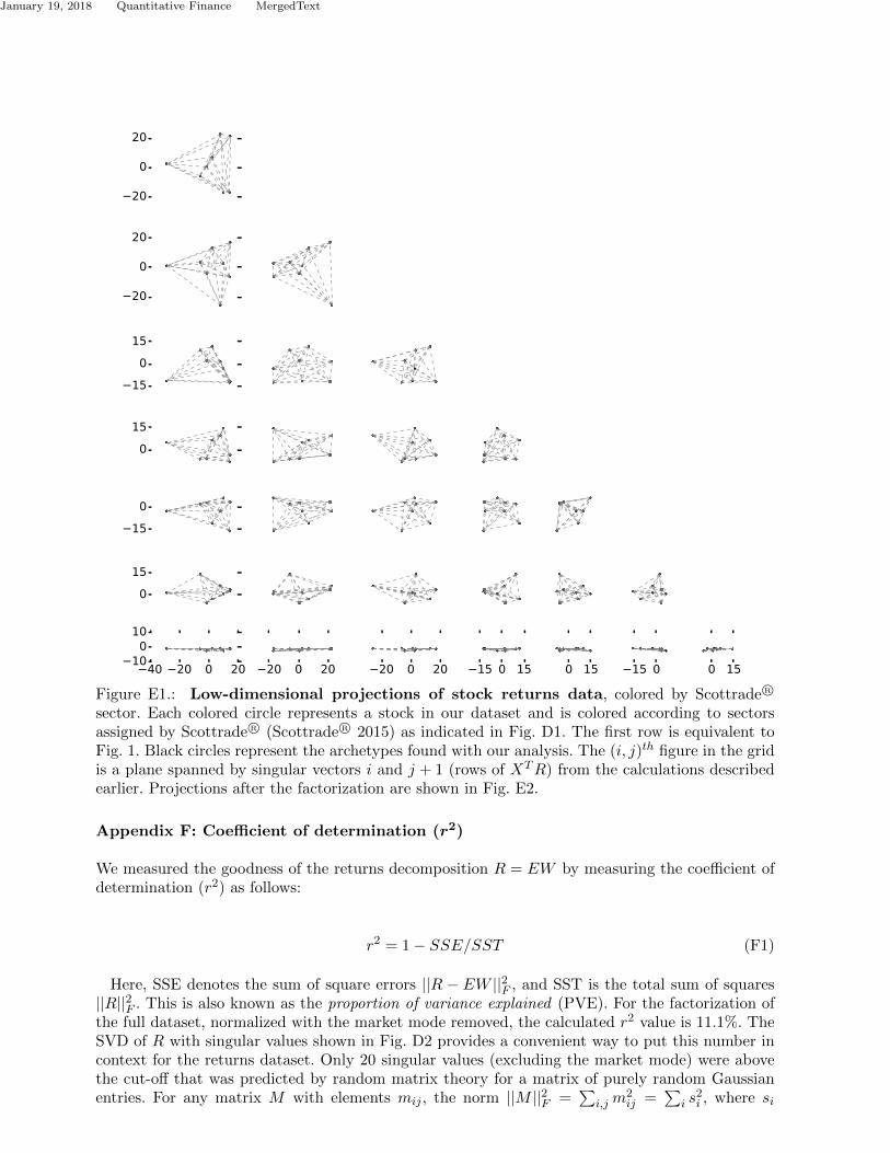
Figure E1.: Low-dimensional projections of stock returns data, colored by Scottrade R©

sector. Each colored circle represents a stock in our dataset and is colored according to sectorsassigned by Scottrade R© (Scottrade R© 2015) as indicated in Fig. D1. The first row is equivalent toFig. 1. Black circles represent the archetypes found with our analysis. The (i, j)th figure in the gridis a plane spanned by singular vectors i and j + 1 (rows of XTR) from the calculations describedearlier. Projections after the factorization are shown in Fig. E2.

Appendix F: Coefficient of determination (r2)

We measured the goodness of the returns decomposition R = EW by measuring the coefficient ofdetermination (r2) as follows:

r2 = 1− SSE/SST (F1)

Here, SSE denotes the sum of square errors ||R − EW ||2F , and SST is the total sum of squares||R||2F . This is also known as the proportion of variance explained (PVE). For the factorization ofthe full dataset, normalized with the market mode removed, the calculated r2 value is 11.1%. TheSVD of R with singular values shown in Fig. D2 provides a convenient way to put this number incontext for the returns dataset. Only 20 singular values (excluding the market mode) were abovethe cut-off that was predicted by random matrix theory for a matrix of purely random Gaussianentries. For any matrix M with elements mij , the norm ||M ||2F =

∑i,jm

2ij =

∑i s

2i , where si

14


10

0

10

20

20

10

0

10

10

0

10

0

10

10

0

0

10

20 10 0 100

10 0 10 20 20 10 0 10 10 0 10 0 10 10 0 0 10

Figure E2.: Cross-sections along eigenplanes of the factorized returns. Each colored circlerepresents a stock in our dataset and is colored according to the primary canonical sector associationwith the color scheme in Fig. 2. Black circles represent the archetypes found with our analysis. The(i, j)th figure in the grid is a plane spanned by singular vectors i and j + 1 (rows of MNT ) fromthe calculations described earlier. Projections of raw data (before the factorization) are shown inFig. E1. Note that the colors are very similar to those of the traditional Scottrade R© classificationshown in Fig. E1; the color schemes were designed to roughly match. Note that here all points havebeen projected into the hyper-tetrahedron by our factorization.

are the singular values (Press et al. 2007). Thus, the fraction of intrinsic variation in R abovethe cutoff is the sum of squares of the 20 singular values (not including market mode) divided

by SST,∑i=20

i=1 s2i /||R||2F = 19.8%. Therefore, as a first approximation, the factorization explains

11.1/19.8 = 56% of the random matrix theory (RMT) explainable variation.

For reference we provide the RMT explainable variation for the factor decomposition of Famaand French, the classification by Scottrade R©, and the top 8 singular vectors given by SVD. Thepercentage of the RMT explainable variation for different numbers of factors compared to the3 factor decomposition of Fama and French is shown in Table F1. Fama and French have thebenefit of allowing factors to have positive or negative weights. In order to compare with anothernon-negative decomposition, we fix the weight matrix according to the Scottrade R© labels and runarchetypal analysis for this n = 14 factor version. The r2 value for this decomposition is 10.7%with a corresponding RMT explainable variance of 54.2% compared to 56% for our 8 factors. For

15


Bulk Variation 80.2%Explainable Variation 19.8%

Factors Percent of Explainable VariationMarket Mode (MM) 8.0%2 factors + MM 26.0%3 factors + MM 36.1%4 factors + MM 42.8%5 factors + MM 48.9%6 factors + MM 55.3%7 factors + MM 59.4%8 factors + MM 63.7%9 factors + MM 68.1%Fama and French 24.0%

Table F1.: Percentage of the Explainable Variance captured by our model compared with theFama and French factor model. Regression is done on the normalized dataset of 705 stocks withoutthe market mode removed. To capture this, we add the market mode to factors obtained by ourdecomposition.

completeness, we also note that if R is rank-reduced to the eight stiffest components found by SVD(not including market mode), then the factorization explains 85% of the the RMT explainablevariation in R with overall results in good accord with the analysis presented here. This impliesthat sector decomposition information was already contained in the stiff modes from the SVD ofR, however SVD is not the appropriate tool for the decomposition. Fig. F1 further shows that ourunsupervised 3-factor decomposition appears quite distinct from Fama and French’s hand-createdone.

Appendix G: The Number n of Canonical Sectors

It is an open problem to determine the effective dimensionality (optimal rank) of a general dataset(matrix). One could select among models of different dimensions using statistical tests such asthe r2 discussed above, or information theory based criteria such as Akaike Information Criterion(AIC) or the Bayesian Information Criterion (BIC), but the choice of the selection criterion isitself generally made on an ad hoc basis. Therefore, a direct observation of the comprehensibilityof results is often the most reliable criterion. In the dataset used for analysis described here, afactorization with n > 8 yielded results where both the emergent time series Etf and weights inWfs showed qualitative signs of overfitting. For example, with n = 9 the results were in goodagreement with n = 8 except for an additional resulting sector involving participation from only11 seemingly unrelated stocks (Table G1 and Fig. 4). The high-level results of factorization withdifferent values of n may be explored in a number of ways, several of which are described below.

G.1. Sector Changes with Dimensionality

One approach to investigating how the sector decomposition changes with dimension is to produce aflow diagram. To do this, we performed the fit ||Et,f−Et,f ′Sf ′,f ||2F with the constraint

∑f ′ Sf ′,f = 1.

Hence the sectors for n = 9 can be expressed as a linear combination of sectors for n = 8, n = 8 as alinear combination of n = 7, and so forth. The results of these fits are presented in Fig. 5. The figurerepresents these relationships though connections between the decompositions for n = N + 1 and

16


Figure F1.: Three Factor Model vs. Fama and French. 2D projections of the weights foreach company in the SP500 with current tickers and data in the date range we consider. Reddenotes companies with large market caps (market cap >10 billion), blue denotes medium (marketcap 2-10 billion) and green denotes small (market cap < 2 billion). For our decomposition (a),there is no separation distinguishable by size of company. In comparison, for the Fama and Frenchdecomposition (b), there appears a gradation from large to small companies consistent with afactor of the model being related to size. (This is natural, since one of Fama and French’s factorsexplicitly is the difference between large and small-cap returns). Thus our unsupervised 3-factordecomposition appears quite distinct from Fama and French’s hand-created one.

Ticker Company Name LabelEQT EQT Corporation EnergyRDN Radian Group Inc. FinancialsSTT State Street Corporation FinancialsLH Laboratory Corp. of America Holdings HealthcareUHS Universal Health Services Inc. HealthcareSTZ Constellation Brands Inc. Non-CyclicalsCNL Cleco Corporation UtilitiesOKE ONEOK Inc. UtilitiesCAKE The Cheesecake Factory Incorporated CyclicalsEFX Equifax Inc. IndustrialsESRX Express Scripts Holding Company Non-Cyclicals

Table G1.: Companies which form a new sector when the dimensionality of the decomposition isincreased from n = 8 to n = 9. The labels given are those indicated by Scottrade R©.

n = N weighted according to the matrix S(N,N+1). More precisely, we create a node correspondingto each of the 9 sectors whose size is proportional to

∑sWf,s where Wf,s is the weight matrix

for the 9 sector decomposition. Hence, the relative node sizes represent the amount of the marketparticpating in the sector. Multiplying this vector by S(8,9) gives the approximate size for eachnode in n = 8. Multiplying this vector by S(7,8) gives the approximate size for each node in n = 7,and so on. In this way, we generate a Sankey diagram whose node sizes correspond roughly tothe amount of the market in the sector and whose connections depict how strongly the sectors fordecompositions with different n overlap. In the image, we see that the n = 9 decomposition givesthe 8 sector version with an additional small sector whose companies were listed in Table G1. We

17


c-assets label percent full name c-goods label percent full name

DDR real estate 1.77% DDR Corp. HON tech 0.53% Honeywell International Inc.

ONB financial 1.7% Old National Bankcorp. TMO health 0.51% Thermo Fisher Scientific Inc.BRE real estate 1.66% Brookfield Real Estate Serv. NAV cyclical 0.49% Navistar International Corp.

PEI real estate 1.54% Pennsylvania RIT CSL basic 0.47% Carlisle Companies Inc.FMBI financial 1.5% First Midwest Bancorp. Inc. IRF tech 0.47% International Rectifier Corp.PRK financial 1.5% Park National Corp. APD basic 0.46% Air Products & Chemicals Inc.

BAC financial 1.42% Bank of America Corp. PCP basic 0.43% Precision Castparts Corp.STI financial 1.41% SunTrust Banks Inc. OMC misc services 0.43% Omnicom Group Inc.DRE real estate 1.29% Duke Realty Corp. MXIM tech 0.43% Maxim Integrated Products, Inc.

UBSI financial 1.28% United Bankshares Inc. TFX health 0.41% Teleflex Inc.CPT real estate 1.28% Camden Property Trust NSC transport 0.41% Norfolk Southern Corp.PPS real estate 1.28% Post Properties Inc. NBL energy 0.4% Noble Energy Inc.

WABC financial 1.26% Westamerica Bancorp. SM energy 0.4% SM Energy CompanyFMER financial 1.26% FirstMerit Corp. WMT retail 0.39% Wal-Mart Stores Inc.CNA financial 1.26% CNA Financial Corp. CR basic 0.38% Crane Co.VLY financial 1.25% Valley National Bancorp. ADI tech 0.38% Analog Devices Inc.

MTB financial 1.24% M&T Bankcorp. ITW cyclical 0.38% Illinois Tool Works Inc.WRI real estate 1.23% Weingarten Realty Investors PPG basic 0.38% PPG Industries Inc.BDN real estate 1.21% Brandywine Realty Trust BA capital 0.38% The Boeing CompanyZION financial 1.2% Zions Bancorp. AME tech 0.38% Ametek Inc.

Total 27.54% Total 8.53%

Table G2.: Top 20 contributing companies to each sector in the two sector decomposition. Rankingis determined by the martix Cs,f which describes each sector as a linear combination of stocks.Labels are those given by Scottrade R© and percentage describes the percentage of the sector at-tributable to the company.

also see that for n = 7 c-finance and c-real estate merge. At n = 6, c-industrial and c-cyclicalmerge. For n = 5, the new sector containing c-industrial and c-cyclical merges with c-non-cyclical.For n = 4, c-utility and c-energy merge. Finally, for n = 3 and n = 2, no clear pattern emergesgiven this image alone.

G.2. Two and Three Sector Decompositions

We further explore the two and three sector decompositions by examining their constituent com-panies and looking at pie charts describing the relationship between our 8 sector decompositionand those with n = 2 and n = 3 respectively. Recall that each archetype is constrained to be alinear combination of companies, or in other words to lie in the convex hull of the data. Using thisinformation, we list the 20 companies which contribute the most to each sector in the two andthree factor decompositions (Tables G2, G3 and G4). For the two sector decomposition, we findthe sectors divide roughly into c-assets (e.g. financial and real estate companies) and c-goods (e.g.companies which provide goods and services). For n = 3, the division is less clear. Another way tolook at the constituents of these sectors is by examining pie chart representations of these decom-positions. Again consider the fit ||Et,f − Et,f ′Sf ′,f ||2F with the constraint

∑f ′ Sf ′,f = 1. Applying

this, we can express the two sector archetypes as linear combinations of the 8 sector archetypesand vice versa. Additionally, we can do the same for the three factor decomposition. The pie chartsthese fits produce are shown in Fig. G1. The results are consistent with the sector breakdownsdescribed from examining the constituent companies.

G.3. Robustness

In general, a factorization analysis of the returns dataset would be sensitive to number of stocksin the dataset, criteria applied for picking stocks, period over which historical prices are obtained,and frequency at which returns are computed. A robust macroeconomic analysis would thereforerequire a large number of stocks chosen without sampling bias, with returns calculated over the

18


sector 1 label percent sector 2 label percent sector 3 label percent

XOM energy 1.29% BRE real estate 2.16% IRF tech 1.29%

HP energy 1.22% PEI real estate 2.08% EMC tech 1.22%CVX energy 1.21% BWS retail 1.99% ADI tech 1.21%

ETR utility 1.2% CNA financial 1.79% CSCO tech 1.2%APD basic 1.2% ONB financial 1.73% TXN tech 1.2%OXY energy 1.19% DDR real estate 1.63% BMC tech 1.19%

NFG utility 1.18% PRK financial 1.59% SNPS tech 1.18%PX basic 1.17% CBSH financial 1.59% PLXS tech 1.17%CL non-cyclical 1.16% BC cyclical 1.56% CPWR tech 1.16%

NBL energy 1.15% FMER financial 1.55% AVT tech 1.15%OII energy 1.11% RDN financial 1.54% SWKS tech 1.11%LNT utility 1.11% MAS capital 1.54% HPQ tech 1.11%

D utility 1.08% DDS retail 1.47% PMCS tech 1.08%DTE utility 1.07% FMBI financial 1.47% MXIM tech 1.07%SCG utility 1.06% ALK transport 1.46% ARW tech 1.06%WEC utility 1.04% WABC financial 1.43% TER tech 1.04%

APA energy 0.99% PCH real estate 1.42% ATML tech 0.99%BAX health 0.98% VLY financial 1.41% MCHP tech 0.98%MUR energy 0.98% BAC financial 1.41% LRCX tech 0.98%CPB non-cyclical 0.98% STI financial 1.37% CGNX tech 0.98%

Total 22.38% Total 19.14% Total 32.18%

Table G3.: Top 20 contributing companies to each sector in the three sector decomposition.Ranking is determined by the martix Cs,f which describes each sector as a linear combinationof stocks. Labels are those given by Scottrade R© and percentage describes the percentage of thesector attributable to the company.

sector 1 full name sector 2 full name sector 3 full name

XOM Exxon Mobil Corp. BRE Brookfield Real Estate Serv. IRF International Rectifier Corp.

HP Helmerich & Payne Inc. PEI Pennsylvania RIT EMC EMC Corp.CVX Chevron Corp. BWS Brown Shoe Co. Inc. ADI Analog Devices Inc.ETR Entergy Corp. CNA CNA Financial Corp. CSCO Cisco Systems Inc.

APD Air Products & Chemicals Inc. ONB Old National Bancorp. TXN Texas Instruments Inc.OXY Occidental Petroleum DDR DDR Corp. BMC BMC Software Inc.NFG National Fuel Gas Company PRK Park National Corp. SNPS Synopsys Inc.PX Praxair Inc. CBSH Commerce Bancshares Inc. PLXS Plexus Corp.

CL Colgate-Palmolive Co. BC Brunswick Corp. CPWR Compuware Corp.NBL Noble Energy Inc. FMER FirstMerit Corp. AVT Avnet Inc.OII Oceaneering International Inc. RDN Radian Group Inc. SWKS Skyworks Solutions Inc.LNT Alliant ENergy Corp. MAS Masco Corp. HPQ Hewlett-Packard Company

D Dominion Resources Inc. DDS Dillard’s Inc. PMCS PMC-Sierra Inc.DTE DTE Energy Corp. FMBI First Midwest Bancorp. Inc. MXIM Maxim Integrated Products Inc.

SCG SCANA Corp. ALK Alaska Air Group Inc. ARW Arrow Electronics Inc.

WEC Wisconsin Energy Corp. WABC Westamerica Bancorp. TER Teradyne Inc.APA Apache Corp. PCH Potlatch Corp. ATML Atmel Corp.BAX Baxter International Inc. VLY Valley National Bancorp. MCHP Microchip Technology Inc.

MUR Murphy Oil Corp. BAC Bank of America Corp. LRCX Lam Research Corp.CPB Campbell Soup Company STI SunTrust Banks Inc. CGNX Cognex Corp.

Table G4.: Top 20 contributing companies to each sector in the three sector decomposition. Rankingis determined by the martix Cs,f which describes each sector as a linear combination of stocks.

period of interest and sensitivity checked for frequency of returns calculation. On the other hand,an equity fund manager faces a less daunting task for an analysis that is limited to the universeof her portfolio of stocks: either to find its canonical sectors, or to analyse the exposure of herholdings to the core sectors of the economy.

19


c-assets c-goods

c-industrial c-energy c-real estate c-cyclical c-non-cyclical c-tech c-utility c-financial

c-industrial c-energy c-real estate c-cyclical c-non-cyclical c-tech c-utility c-financial

(d)

(a) (b)

(c)

Figure G1.: Pie charts depicting sectors as linear combinations of other sector decom-positions having a different value of the dimensionality n. (a) Two sector decompositionwith respect to the eight sector version (b) Three with respect to eight (c) eight with respect to two(d) eight with respect to three. For (a) and (b) the color scheme is the same as used throughoutfor the eight sector decomposition. For (c) and (d) colors correspond to those in Fig. 4 for thetwo and three sector nodes. Through these charts it is evident that the two sector decompositionscorresponds to an c-assets sector containing c-finance and c-real estate. and a c-goods sector con-taining companies which provide goods and services. In (c) and (d) we see c-industrial, c-cyclicaland c-non-cyclical which merge by n = 5 split between the two and three factor decompositionsrespectively, consistent with Fig. 4.

Appendix H: Canonical Sector Indices

The matrix Csf in decomposition R = RCW represents how returns R of stocks smust be combinedto make canonical sector returns Etf = RtsCsf . Since a canonical sector is defined as a combinationof stocks, an investment in the sector f can made via buying a basket of constituent stocks s inproportions given by Csf or through an index Itf :

Itf = pts′Cs′f (H1)

where, p are stocks prices suitably weighted by market cap or other divisor as common practicefor common indices (Tagiliani 2009). An unweighted index of this kind is shown in the bottomrow of Fig. C1 for results corresponding to the analysis described in this paper. Conversely, apre-defined basket of stocks such as the S&P 500 R© can be unbundled to find its exposure to thecanonical sectors. With an investment strategy employing longs and shorts at the same time incorrect proportions, it is conceivable to invest in, for example, the c-tech component of S&P 500 R©.

The desirable features of an index include completeness, objectivity and investability (Pastoret al. 2013). The c-indices constructed using the ideas outlined here would not only be of valueto investors through investment vehicles such as ETFs, Futures, etc., but also serve as importanteconomic indicators.

References

Basalto, N., Bellotti, R., Carlo, F.D., Facchi, P. and Pascazio, S., Clustering stock market companies viachaotic map synchronization. Physica A: Statistical Mechanics and its Applications, 2005, 345, 196 – 206.

Berry Petroleum Company History, , 2013. Available online at: http://www.bry.com/pages/history.html(accessed 2015-01-01).

Bonanno, G., Caldarelli, G., Lillo, F. and Mantegna, R.N., Topology of correlation-based minimal spanningtrees in real and model markets. Phys. Rev. E, 2003, 68, 046130.

20


Bonanno, G., Vandewalle, N. and Mantegna, R.N., Taxonomy of stock market indices. Phys. Rev. E, 2000,62, R7615–R7618.

Bostock, M., Ogievetsky, V. and Heer, J., D3: Data-Driven Documents. IEEE Trans. Visualization & Comp.Graphics (Proc. InfoVis), 2011.

Burda, Z., Grlich, A., Jarosz, A. and Jurkiewicz, J., Physica A, 2004, 343.Burda, Z., Grlich, A., Jurkiewicz, J. and Wacaw, B., Eur. Phys. J. B, 2006, 49.Bury, T., Market structure explained by pairwise interactions. Physica A: Statistical Mechanics and its

Applications, 2013, 392, 1375 – 1385.CBOE R© Oil Index, , 2013. Available online at: http://www.cboe.com/products/IndexComponentsAuto.aspx?PRODUCT=OIX

(accessed 2015-01-01).Chachra, R., Alemi, A.A., Hayden, L., Ginsparg, P.H. and Sethna, J.P., Project Website with additional

figures and analyses [online]. , 2013. Available online at: www.lassp.cornell.edu/sethna/Finance (accessed2015-01-01).

Conlon, T., Ruskin, H. and Crane, M., Cross-correlation dynamics in financial time series. Physica A:Statistical Mechanics and its Applications, 2009, 388, 705 – 714.

Conversano, C. and Vistocco, D., Analysis of mutual funds management styles: a modeling, ranking andvisualizing approach. Journal of Applied Statistics, 2010, 37, 1825–1845.

Coronnello, C., Tumminello, M., Lillo, F., Micciche, S. and Mantegna, R., Sector identification in a setof stock return time series traded at the London Stock Exchange. Acta Physica Polonica B, 2005, 36,2653–2679.

Cutler, A. and Breiman, L., Archetypal Analysis. Technometrics, 1994, 36, 338–347.Ding, C. and He, X., K-means Clustering via Principal Component Analysis. In Proceedings of the Pro-

ceedings of the Twenty-first International Conference on Machine Learning, ICML ’04, Banff, Alberta,Canada, pp. 29–, 2004 (ACM: New York, NY, USA).

Ding, C.H.Q., Li, T. and Jordan, M.I., Convex and Semi-Nonnegative Matrix Factorizations. IEEE Trans.Pattern Anal. Mach. Intell., 2010, 32, 45–55.

Dow Jones R© US Indices: Industry Indices, , 2015. Available online at:www.djindexes.com/mdsidx/downloads/fact info/Dow Jones US Indices Industry Indices Fact Sheet.pdf(accessed 2015-01-01).

Doyle, G. and Elkan, C., Financial Topic Models. In Proceedings of the NIPS Workshop on Applications forTopic Models: Text and Beyond, 2009 (Whistler, Canada).

Eom, C., Oh, G., Jeong, H. and Kim, S., Topological Properties of Stock Networks Based on Random MatrixTheory in Financial Time Series. Papers, arXiv.org, 2007.

Fama, E.F. and French, K.R., Common risk factors in the returns on stocks and bonds. Journal of financialeconomics, 1993, 33, 3–56.

Fenn, D.J., Porter, M.A., Williams, S., McDonald, M., Johnson, N.F. and Jones, N.S., Temporal evolutionof financial-market correlations. Phys. Rev. E, 2011, 84, 026109.

Heimo, T., Kaski, K. and Saramki, J., Maximal spanning trees, asset graphs and random matrix denoisingin the analysis of dynamics of financial networks. Physica A: Statistical Mechanics and its Applications,2009, 388, 145 – 156.

Hyvarinen, A. and Oja, E., Independent Component Analysis: Algorithms and Applications. Neural Netw.,2000, 13, 411–430.

Kersting, K., Wahabzada, M., Thurau, C. and Bauckhage, C., Hierarchical Convex NMF for ClusteringMassive Data.. Journal of Machine Learning Research - Proceedings Track, 2010, 13, 253–268.

Kim, D.H. and Jeong, H., Systematic analysis of group identification in stock markets. Phys. Rev. E, 2005,72, 046133.

Kullmann, L., Kertesz, J. and Mantegna, R.N., Identification of clusters of companies in stock indices viaPotts super-paramagnetic transitions. Physica A: Statistical Mechanics and its Applications, 2000, 287,412–419.

Laloux, L., Cizeau, P., Bouchaud, J.P. and Potters, M., Noise Dressing of Financial Correlation Matrices.Phys. Rev. Lett., 1999, 83, 1467–1470.

Lee, D.D. and Seung, H.S., Learning the parts of objects by non-negative matrix factorization. Nature, 1999,401, 788–791.

Li, T. and Ding, C., The Relationships Among Various Nonnegative Matrix Factorization Methods forClustering. Data Mining, 2006. ICDM ’06. Sixth International Conference on, 2006, pp. 362–371.

Livan, G., Alfarano, S. and Scalas, E., Phys. Rev. E, 2011, 84.

21


Mantegna, R.N., Hierarchical structure in financial markets. The European Physical Journal B - CondensedMatter and Complex Systems, 1999, 11, 193–197.

Martins, A.C., Random, but not so much a parameterization for the returns and correlation matrix offinancial time series. Physica A: Statistical Mechanics and its Applications, 2007, 383, 527 – 532.

Mehta, M.L., Random Matrices, 3 , 2004 (Academic Press: Boston, MA, USA).Morgan Stanley R© High-Tech 35 Index, , 2005. Available online at:

www.nasdaq.com/options/indexes/msh.aspx (accessed 2015-01-01).Morup, M. and Hansen, L.K., Archetypal analysis for machine learning and data mining. Neurocomputing,

2012, 80, 54 – 63.Musmeci, N., Aste, T. and Di Matteo, T., Relation between Financial Market Structure and the Real

Economy: Comparison between Clustering Methods. SSRN, 2014.Nadig, D. and Crigger, L., Signal From Noise. Journal of Indexes, 2011, 14, 40–43, 50.Pastor, L., Heaton, J. and Foss, A., The index is dead. Long Live the Index. Journal of Indexes, 2013, 16,

16–21, 55.Plerou, V., Gopikrishnan, P., Rosenow, B., Amaral, L.A.N., Guhr, T. and Stanley, H.E., Random matrix

approach to cross correlations in financial data. Phys. Rev. E, 2002, 65, 066126.Plum Creek R© History, , 2014. Available online at: http://www.plumcreek.com/AboutPlumCreek/History/tabid/55/Default.aspx

(accessed 2015-01-01).Podobnik, B. and Stanley, H.E., Detrended Cross-Correlation Analysis: A New Method for Analyzing Two

Nonstationary Time Series. Phys. Rev. Lett., 2008, 100, 084102.Press, W.H., Teukolsky, S.A., Vetterling, W.T. and Flannery, B.P., Numerical Recipes 3rd Edition: The Art

of Scientific Computing, 3 , 2007 (Cambridge University Press: New York, NY, USA).Russell 3000 R© Index, , 2015. Available online at: www.russell.com/indexes/data/fact sheets/us/russell 3000 index.asp

(accessed 2015-01-01).Scottrade R©, , 2015. Available online at: www.scottrade.com (accessed 2015-01-01).S&P 500 R© Index, , 2014. Available online at: us.spindices.com/indices/equity/sp-500 (accessed 2015-01-01).Tagiliani, M., The Practical Guide to Wall Street, 1 , 2009 (John Wiley & Songs, Inc.: Hoboken, NJ, USA).Thurau, C., Kersting, K. and Bauckhage, C., Convex Non-negative Matrix Factorization in the Wild. In

Proceedings of the Data Mining, 2009. ICDM ’09. Ninth IEEE International Conference on, pp. 523–532,2009.

Thurau, C., Kersting, K. and Bauckhage, C., Yes We Can—simplex volume maximization for descriptiveweb scale matrix factorization.. In Proceedings of the CIKM, edited by J. Huang, N. Koudas, G.J.F. Jones,X. Wu, K. Collins-Thompson and A. An, pp. 1785–1788, 2010, ACM.

Thurau, C., Kersting, K., Wahabzada, M. and Bauckhage, C., Convex non-negative matrix factorization formassive datasets. Knowledge and Information Systems, 2011, 29, 457–478.

Tsalmantza, P. and Hogg, D.W., A Data-driven Model for Spectra: Finding Double Redshifts in the SloanDigital Sky Survey. The Astrophysical Journal, 2012, 753, 122.

Vistocco, D. and Conversano, C., Visualizing and clustering financial portfolios using internal compositions.SIS, 2009 Presented at Statistical Methods for the Analysis of Large Data-Sets Pescara, Italy, Septem-ber 23-25, http://new.sis-statistica.org/wp-content/uploads/2013/10/CO09-Visualizing-and-clustering-financial-portfolios-using.pdf.

Wang, Y.X. and Zhang, Y.J., Nonnegative Matrix Factorization: A Comprehensive Review. Knowledge andData Engineering, IEEE Transactions on, 2013, 25, 1336–1353.

Yahoo! R© Finance, , 2015. Available online at: finance.yahoo.com (accessed 2015-01-01).Zhang, Z., Li, T., Ding, C. and Zhang, X., Binary Matrix Factorization with Applications. In Proceedings

of the Proceedings of the 2007 Seventh IEEE International Conference on Data Mining, ICDM ’07, pp.391–400, 2007 (IEEE Computer Society: Washington, DC, USA).

22