CangeMlonUiest

Carnegie-Mel ios Univeri=y

GRADUATE SCHOOL OF INDUSTRIAL ADMINISTRATIONWILLIAM LA~MMU MIU&h POLINMu

AUG ~ 1968 1

Reproduced by theiCLEAR ING HOUSIF

for Federal Scgoienilic & Techntc.1t , ý .~n f o r m na f io n S P r i n g fi e l d V d 2 -d 15 1 1

hanagement Sciences Research Report No. 138

D!FCTqTOTT NWTV'jnVK PIANNING MODELS

by

*Wallace B. S. Crowston

May, 1968

* Carnegie-Mellon University

This report was prepared as part of the activities of the Management SciencesResearch Group, Carnegie-Mellon University, under Contract NONR 760(24)NR 047-048 with the U. S. Office of Navl Research. Reproduction in whole orin part is permitted for any pirpose of the U. S. Government.

Manageme't Scienc'ý.; Research GroupGraduate School of In~iustrial Administration

Carnegie-Mellon UniversityPittsburgh, Pennsylvania

S

Carnegie Mellon University

Committee on Graduate Degrees in the Social. Sciencesand

Industrial Administratijn

Dissertation

Submitted in partial fulfillment of the requirements for the degree ofDoctor of Philosophy in Industrial Administration.

Title: DECISION NETWORK PLANNING MODFLS

Presented by W. B. S. Crowston,

B.A.Sc. University of Toronto(1956)

S.M. Massachusetts Institute of Technology

(195,8)

M.Sc. Carnegie. Institute of Technology(1965)

Appr by the D!sprt~ t on Committee

* Chaix~man 411Date~

Approved by the Committee on Graduate Degrees in the Social Sciences andIndustrial Administration

Chairuag Date

! I

DECISION NETWORK PLANNING MODELS

by

Wallace Bruce Stewart Crowston

Submitted to the Graduate School of Industrial Administration on May 1,1968, in partial ful'illment of the requirements for the degree of

Doctor of rhilosophy.

ABSTRACT

This thesis develops project planning models that allow thepossibility of specifying alternate ways of performing any of the jobsin the project. The "job alternatives" for any task may have differenttimes, costs, resource requirements and possibly different precedence

relations with other jobs in the project network. The problem is toselect the particular way in which each job will be performed and schedulethe resulLing jobs so as to minimize the cost of the jobs plus the costassociated with the completion date of the project.

The problem of selecting the optimal job alternatives in networkswiti no resource constraints is formulated as an integer programmingproblem. One constraint in required for each set of job alternativesand one for each possible path in the original project network. Argumentsare developed to show that a substantial number of the precedence con-straints are redundant and may be eliminaced. To accomplish this re-duction in problem size an algorithm related to the critical pathalgorithm is developed to reduce each network to an equivalent networkcontaining only job alternatives and maximal distances between them.Jobs with no alteinative are eliminated.

TNo branch and bound routines are then developed to solve theproblcin. One of thtse is tested on a series of problems and is soI',n

to he efficient. An integer progranniing algorithm is developed toserve as a sub-routine in the branch and bouad algorithms. It is fastin that It uses the critical path algorithm to solve problems.

When resource requireme'nts are added to the tasks of the project,

and the total availability of resource per period is constrained, the

problem of scheduling the joba so as to minimize cTmpletion date becomes

extremely difficult. Nine 'icuristic routin., for the loading problem

I

are developed and tested. Of these a serial loading rule, operatingon a job list ordered by late start, with no job bumping, provessuperior. Three methrds of generating combinations of job alternativesto be loaded were cxami, 4. These were complete enumeration, pairwiseinterchange and multiple puirh interchange. None of the methods pro-vided good solutions in reasonable amounts of time.

To show the generality of the planning model developed the integerprogramming formulation of the project problem was adapted to the m x njob-shop scheduling problem, the single product assembly-line balancingproblem and the problem of planning projects under incentive contracts.

S

• Thesis Supervisor: C. L. Thompson

S

ACKN(MLEDGMMENT

In my first semester at Carnegie Institute I began my work for

Professor C. L. Thompson on a series of job-shop and project scheduling

problems. This association developed my interest in the research re-

ported in this dissertation. 1 would like to take this opportunity to

thank Professor Thompson for his guidance and for the support he has

given me as my thesis advisor.

I would also like to thank the other members of my committee,

Professors Kriebel and MacCrimnon for the valuable suggestions they of--

fered. I would also like to acknowledge the contribution of my prc~nt

colleagues, Professors Carroll and Pierce. Their advice, their encourage-

ment and support directly assist.ed the completion of this work.

Financially the research was made possible by a doctoral dissera..

tion grant from the Ford Foundation. However, the conclusions, opi-tions

and other statements in this work are those of the author Lnd are nnt

necessarily those of the Foundation. Additional support wns Drovided by

the Managemenr Science Research Group: Carnegie Institute of Technology,

undez Contract Nonr 760(24), NR 047-040 with the U.S. Office of Naval

Research.

Computation was supported in part by Project MAC, an M.I.T.

research program sponsored by the Advanced Research Projects Agency,

Department of Defense, under Offce of Naval Research Contract Number

Nonr-4102(01). Additional suppurz was given by the Graduate School of

Industrial Administration, Carnegie Institute of Technology and the

Alfred P. Sloan School of Managemet:t, M.I.T.

Finally, I would like to express my appreciation for the unlimited

patience and cooperation of my wife, Taka. Without her support the

dissertation could not have been completed tt Lhis time.

II _

di

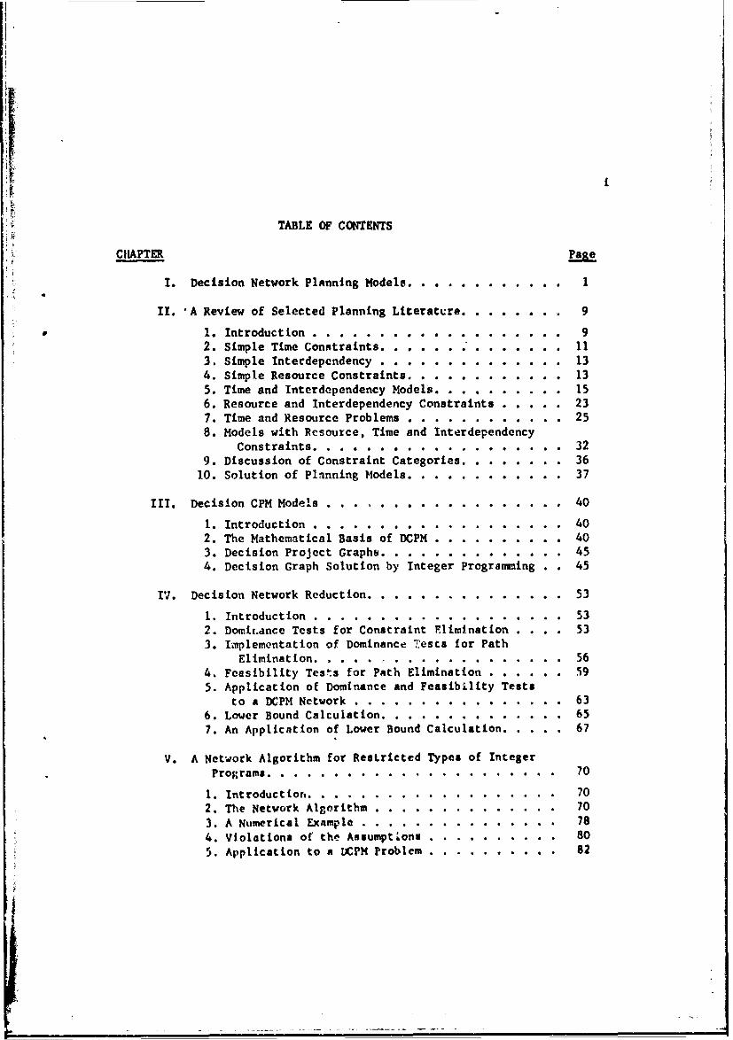
TABLE OF CONTENTS

CHAPTER Page

I. Decision Network Planning Models ................. . 1

II. 'A Review of Selected Planning Literature. . . . . . .. 9

1. Introduction . .................. 92. Simple Time Constraints. . .......... . 113. Simple Interdependency .. e. .... ........ 134. Simple Resource Constraints. . . . ....... 135. Time and Interdependency Models. .............. 156. Resource and Interdependency Constraints . . . 237. Time and Resource Problems .................. ... 258. Models with Resource, Time and Interdependency

Constraints. . . . . . .. . .. . ...... 329. Discussion of Constraint Categories. . ....... 36

10. Solution of Planning Models .......... . . . 37

III. Decision CPM Models ........ .................... 40

1. Introduction .......... .................. ... 402. The Mathematical Basis of DCPM .......... . . 403. Decision Project Graphs& ..... .............. .. 454. Decision Graph Solution by Integer Programming . 45

IV. Decision Network Reduction ......... .............. 53

1. Introduction ............ .......... 532. Domir.ance Tests for Constraint E1limination . ... 533. Implementation of Dominance Tests for Path

Elimination .......... .................. ... 564. Feasibility Tests for Path Elimination ........ .. 595. Application of Dominance and Feasibility Tests

to a DCPM Network ................... 636. Lower Bound Calculation ................. 657. An Application of Lower Bound Calculation. ..... 67

V. A Network Algorithm for ResLricted Types of IntegerPrograms .............. .......... . 70

1. Introduction ........... ................ ... 702. The Network Algorithm ..... .............. ... 70

3. A Numerical Example ..... ........... . . . 78

4. Violations of the Assumptions ...... ......... 80

5. ApplLcation to a tCPM Problem ........ ........ 82

ii

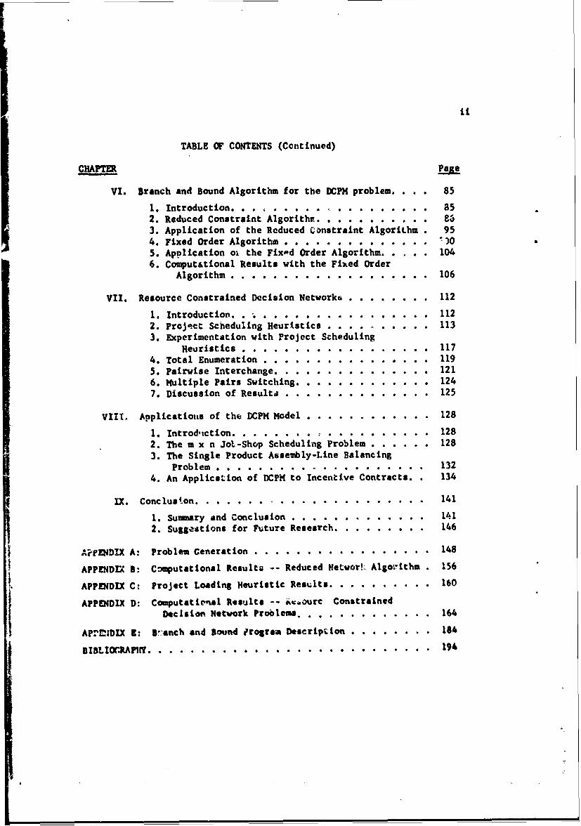
TABLE OF CONTENTS (Continued)

CHAP'TERf

VI. Branch and Bound Algorithm for the DCPM problem .... 85

1. Introduction ... *5

2. Reduced Constraint Algorithu. . . . . . . . . 86

3. Application of the Reduced Constraint AlgoriLhm . 954. Fixed Order Algorithm . . . .......... )5. Application oi the Fixpd Order Algorithm .. . 104

6. Computational Results with the Fixed OrderAlgorithm . . . . . . . . . . . . . . .*. . . . 106

VII. Resource Constrained Decision Networks . * . . . .... 112

1. Introduction. . . . . ....... . . 0 . 1122. Project Scheduling Heuristics . . . .. . 1133. Experimentation with Project Scheduling

Heuristics . . . . . . ......... . 1174. Total Enumeration ................ 119

5. Pairwise Interchange .................. 1216. Multiple Pairs Switching. . . . . . . . ..... 1247. Discussion of Resulta . . . . 0 . . . . . 125

VIII. Applications of the DCPM Model . . . . . . . . . . . . 128

1. Introdiction. . . . . . . . .......... 1282. The m x n Jot-Shop Scheduling Problem . . . ... 128

3. The Single Product Assembly-Line BalancingProblem . . .................. 132

4. An Application of DCPM to Incentive Contracts.. 134

IX. Concluson .... ........................ .. 141

1. Sumary and Conclusion . . . . ......... 141

2. Suggestion& for Future Research ..... ......... 146

AiPENDIX A: Problem Ceneration........ . . . . . . . . . . . 148

APPENDIX B: Cnmputational Resulto -- Reduced Netwer!:. Aljoi!1thm . 156

APPENDIX C: Project Loading Heuristic Results. . . . ...... 160

APPENDIX D: Computatic-nal Results -- i..ourc ConstrainedDecision Network Problem ..... ............. 164

APrC!IDIX 3: S5'ench and Sound Program Description . . ...... 184

U IBLIO(RAP1f... ............. . . . . . . . . .......... 194

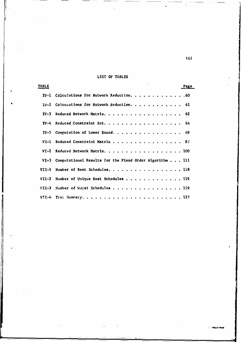
LIST OF TABLES

TABLE Pa•e

IV-1 Calcu!ations for Network Reduction . . . . .60

IV-2 COIcuiations for Network Reduction . . .. . . . . 61

IV-3 Reduced Network Matrix ...... ................... 62

IV-4 Reduced Constraint Set ...................... 64

IV-5 Computation of Lower Bound ...... ............... ... 69

VI-J Reduced Constraint Matrix ............ ............... 87

VI-2 Reduced Network Matrix ....... ................. .. 100

VI-3 Computational Results for the Fixed Order Algorithm . . Ill

VII-1 Number of Best Schedules ...... ................... 118

VII-2 Number of Unique Best Schedules ..... ............... 119

VII-3 Number of Worst Schedules ...... ................. 119

VTI-4 TtsL Suniary ........... ........................ 127

iv

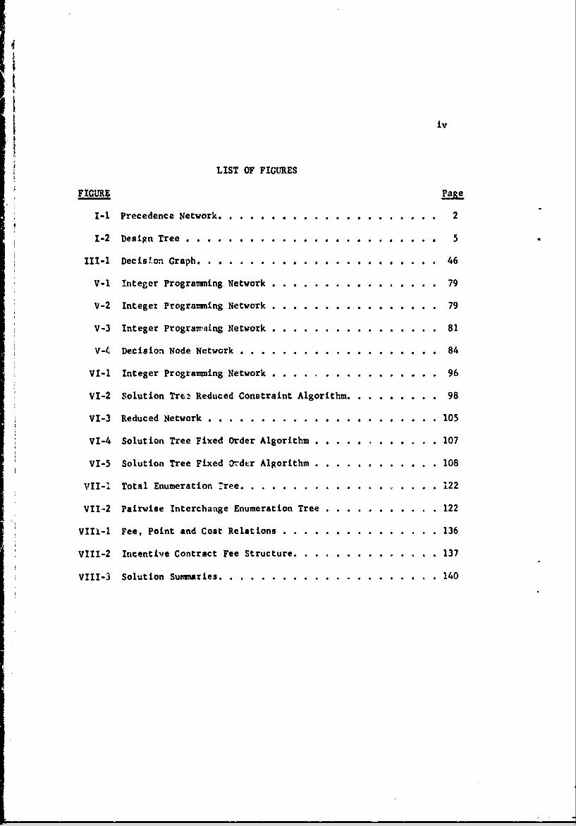
LIST OF FIGURES

FIGURE Page

I-i Precedence Network. . . . ......... . . ... . . .. . 2

1-2 Design Tree . . . . . . . . . . . . . . . . . . 5

III-1 Decision Graph....... . . . . . . . . . . . . . . . 46

V-1 Integer Programning Network ..... ................ 79

V-2 Integer Programming Network ....... * . . . . . . 79

V-3 Integer Prograin'ing Network ...... ................ ... 81

V-4 Decision Node Network ...... ................ . . . . 84

VI-1 Integer Programming Network ...... ................ ... 96

VI-2 Solution Trs2 Reduced Constraint Algorithm. . . . . . . .. 98

VI-3 Reduced Network ....... ... .......... 105

VI-4 Solution Tree Fixed Order Algorithm . . . . . . . ... 107

VI-5 Solution Tree Fixed Order Algorithm ............. . . 108

VII-. Total Enumeration Tree ........... .................... 122

VII-2 Pairwise Interchange Enumeration Tree ............. 122

VIII-l Fee, Point and Cost Relations ...... ............. .. 136

VIII-2 Incentive Contract Fee Structure ................ 137

VIII-3 Solution Summaries ......... ..................... .. 140

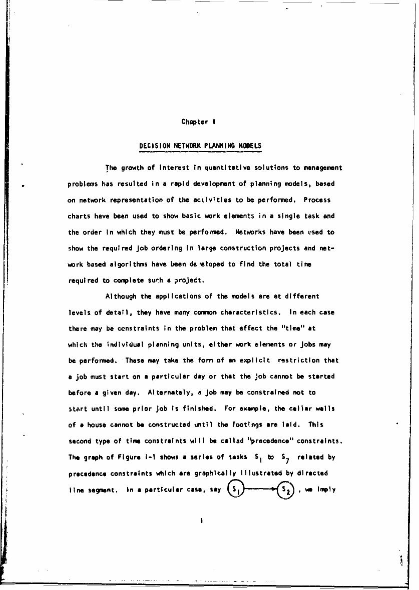
Chapter I

DECISION NETWORK PLANNING MODELS

The growth of Interest in quantitative solutions to management

problems has resulted in a rapid development of planning models, based

on network representation of the activities to be performed. Process

charts have been used to show basic work elements in a single task and

the order In which they must be performed. Networks have been Lsed to

show the required job ordering in large construction projects and net-

work based algorithms have been deteloped to find the total time

required to complete surh a project.

Although the applications of the models are at different

levels of detail, they have many common characteristics. In each case

there may be constraints in the problem that effect the "time" at

which the Individual planning units, either work elements or jobs may

be performed. These may take the form of an explicit restriction that

a job must start on a particular day or that the Job cannot be started

before a given day. Alternately, a Job may be constrained not to

ste,rt until some prior job is finished. For example, the cellar walls

of a house cannot be constructed until the footings are laid. This

second type of time constraints will be colled "precedence" constraints.

The graph of Figure i-I shows a series of tasks SI to S7 related by

precedence constraints which are graphically Illustrated by directed

line segment. In a particular case, say w e Imply

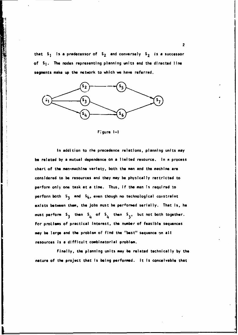
"4

2

that S1 Is a predecessor of S2 and conversely S2 Is a successor

of SI. The nodes representing planning units and the directed line

segments make up the netwrk to which we have referred.

F:gure 1-1

In addition to the precedence relations, planning units may

be related by a mutual dependence on a limited resource. In a process

chart of the man-machine variety, both the man and the machine are

considered to be resources and they may be physically restricted to

perforwm only one task at a time. Thus, if the man ts required to

perforn both S3 and S4, even though no technological cou~straint

exists between them, the Jobs must be perormed serially. That is, he

must perform S3 then S 4 of S4 then S30 but not both together.

For proLlems of practical Interest, the number of feasible sequences

may be large and the problem of find the "best" sequence o)n all

resources Is a difficult combinatorial problem.

Finally, the planning units may be related technically by the

nature of the project that Is being performed. It is conceivable that

3

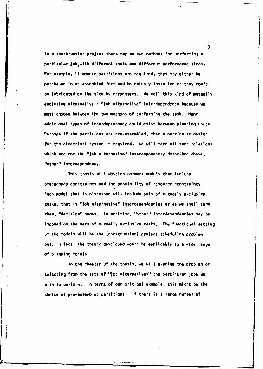
In a construction project there may be two methods for performing a

particular Job)with different costs and differerit performance times.

For example, if wooden partitions are required, they may either be

purchaied in an assembled form and be quickly Installed or they could

be fabricated on the site by carpenters. We call this kind of mutually

exclusive alternative a "Job alternative" Interdeperdency because we

must choose between the two methodi of performing the task. Many

additional types of Interdependency could exist between planning units.

Perhaps if the partitions are pre-assembled, then a particular design

for the electrical system Is required. We will term all such relations

which are not the "Job alternative" Interdependency described above,

"other" Interdepcndency.

This thesis will develop network mode!s that Irnclude

precedence constraints and the possibility of resource constraints.

Each model that is discussed will include sets of mutuaily exclusive

tasks, that is "Job alternative" Interdependencies or as we shall term

them, "decisionsl nodes. In addition, "other" Interdependencies may be

Imposed on the sets of mutually exclusive tasks. The functional setting

t the models will be the (construction) project scheduling problem

but, in fact, the theory developed would be applicable to a wide range

of planning models.

In one chapter if tie thesis, we will exanine the problem of

selecting from the sets of "Job alternatives" the partirular Jobs we

wish to perform. In terms of our original example, this might be the

choice of pro-assembled partitions. If there Is a large number of

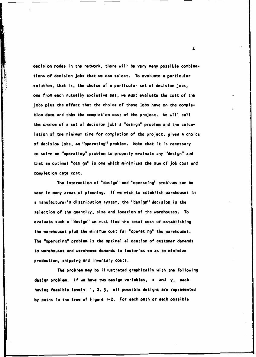
4

decision nodes in the network, there will be very many possible combina-

tions of decision jobs that we can select. To evaluate a particular

solution, that is, the choice of a particular set of decision Jobs,

one from each mutual y exclusive set, we must evaluate the cost of the

jobs plus the effect that the choice of these jobs have on the comple-

tion date and thus the completion cost of the project. We will call

the choice of a set of decision Jobs a "design" problem and the calcu-

lation of the minimum time for completion of the project, given a choice

of decision jobs, an "operating" problem. Note that it is necessary

to solve an "operating" problem to properly evaluate any "design" and

that an optimal "design" Is one which minimizes the sum of job cost and

completion date cost.

The interaction of "design" and "operating" problemms can be

seen In many areas of planning. If we wish to establish warehouses in

a manufacturer's distribution system, the "design" decision is the

selection of the quantity, size and location of the warehouses. To

evaluate such a "design" we must find the total cost of establishing

the warehouses plus the minimum cost for "operating" the warehouses.

The 11operating" problem is the optimal allocation of customer demands

to warehouses and warehouse demands to factories so as to minimize

production, shipping and Inventory costs.

The problem may be Illustrated graphically with the following

design problem. If we have two design variables, x and y, each

having feasible levels 1, 2. 3, all possIble designs are represented

by paths In the tree of Figure 1-2. For each path or each possible

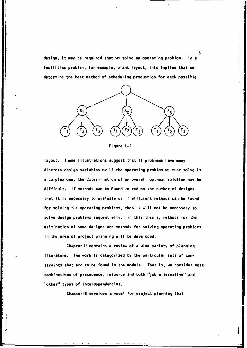
5

design, it may be required that we solve an operating problem. In a

facilities problem, for example, plant layout, this implies that we

determine the best method of scheduling production for each possiLe

Figure 1-2

layout. These illustrations suggest that if problems have many

discrete design variables or if the oparating problem we must solve is

a complex one, the •aterm!nation of an overall optimmn solution may be

difficult. If methods can be found to reduce the number of designs

that it is necessary to evaluate or if efficient methods can be found

for solving the operating problems, then it will not be necessery to

solve design problems sequentially. In this thesis, methods for the

ellmination of some designs and methods for solving operating problems

In tht area of project planning will be developed.

Chapter II contains a review of a wide variety of planning

literature. The work Is categorized by the particular sets of con-

straints that are to be found In the models. That Is, we consider most

combInations of precedence, resource and both "job alternative" and

"4other" types of Interck pondencles.

Chapterill develo1s a model for project planning that

6

contains precedence constraints and both "job alternative" and "other"

Interdependency constraints. It is assumad that in the project there

are a number of competing methods for performing some of the Jobs, each

method having a different cost, a different time, possibly different

precedence relations with other jobs and different interdependencies

with other jobs. All possible Jobs are considered in the project graph

and then in the scheduling phase the job alternatives that minimize

total cost are selected. A numerical problem is introduced here that.

w!ll be used to illustrate the material of Chapters III, IV and Vi. In

Chapter IV methods are developed to reduce the original decision network

so that the problem may reasonably be solved with standard integer

programming techniques.

In the solution of a decision network, it may be necessary

to solve sub-problems that minimize the .ost of the "design" selected

with no regard to the cost of the "operating" problem, that is, the

cost of the minimum completion date. Essentially, the sub-problem is

to find the set of decision jobs that meets the -'Job alternative" and

"other" interdependencies with minimum Job cost. Chapter V develops

an Integer programming algorithm specifically for this problem. Chapter

Videvelops two branch and bound algorithms which solve for the best

"design" given the cost of the decision jobs, the cost of the completion

date and the interdependency constraints. They solve the "design" and

the operating "problem" simultaneously. Computational results are

given for one of these methods.

In Chopter V11e consider the full model, that Is, project

7

planninq problems with precedence resource and interdependency

constraints. To solve the "operating" problem in models having no

limit on resource usage is relatively straight forward. It is simply

a matter of calculating the li&ngth of the critical path and evaluating

the-cost oa that finish date. When we add resource constraints, the

problem of calculating minimum project length for any given design may

be a very complex combinational problem. In fact, for large projects,

given current techniques and reasonable limits computer time, it is not

possible to find optimum or minimum length projects. For this reason,

we develop and experimentally test several heuristic loading technique3.

The best of these heuristics is then used as our "operating" rule to

evaluate various designs. The designs to be tested are generated first

by complete enumeration, then by pairwise Interchange and finally by

multiple pairs Interchange.

As we have stat.d aihonvi in~nv ninninn nrnh|mtm can be

represented by the combination of constraints we have discussed. To

illustrate this point, In Chapter VIMll the basic Integer programming

formulation of our decision network planning problem is used to formu-

late the job-shop scheduling problem and the assembly-line balancing

problem. These formulations prove to be substantially more compact than

competitive formulations of the problem..;. Finally, the model is adapted

to projects with more complex criterion fojnctions, specifically the cost

structure of incentive contracts. Chapter IMcontains a summary of the

work, conclusions and recomnendations for f,.vther research.

Several terms that are common in the literature of project

8

scheduling, such as early Start, will be used frequently In the

following chapters. These terms are defined rigorously elsewhere

[45, 49 so that we will review them only briefly here.

A "path" through a project network is connected sequence of

nodes (Jobs) and directed line segments extending from one node to some

other. fi Figure 1-1 we have a path from SI through S2 ard S to

S7 . The nodes S1, S4 and S5 do not lie on a common path. The

length of any path is simply the sum of the Job times for all Jobs on

the path. We now define the "early finish" of a job to be the longest

path from the first Job in the network to the Job under consideration.

"Early start" time is simply early finish time of a job less its Job

time. The "critical path" of a project i,.ý the longest path from the

first Job In the network to the final Job in the network and Is

equivalent to theminimumn numbe- of days required tc complete the

project.

The "latest start" date for a job Is defined as the day on

which the job must start if the project is to finish exactly on its

due date. We may calculate the value of late start for a job by sub-

tracting the length of the longjest pzth from the job to tihe ind of the

project from the due date of the project. Thus a job can begin no

earlier than the early start time because its predecessors must first

be completed and no later than late start or it will delay the finish

of the project beyond the due date. The difference between late start

and early start time Is defined as Job "slack" time, the masure of

permissible delay for a job. Other terms more uniquely related to the

models to be discussed will be defined as required.

Chapter II

A REVIEO OF SELECTED PLANNING LITERATURE

The management planning literature, like many other areas of

management actlvty, is susceptible to many possible categorizations.

Perhaps the most obvious breakdown follows the functional area of an

industrial concern and within this is a sub-grouping by problem area.

Thus under the production heading we have extensive and largely indepen-

dent literature growing up around the "Job-shop pwoblem" or the

"assembly-line balancing problem". In finance we have the "capital

budgeting of interrelated projects".

A second categorization might be by solution technique. Here

is a list of functional irea problems best solved by linear programming;

this list requires integer linear programming and so on. This approach

is closely related to a third categorization, the one to be used as the

frameework for our discussion. The third structure divides planning

problems by the type of constraint found in the problem. To be explicit,

we have defined in Chapter I time constraints, resource constraints and

Interdependency constraints as possible dimensions of planning problems.

For simplicity we will not discuss the dimension "uncertainty", nor will

we consider motivational and social problems of planning.

The possible combinations of the three dimensions and therefore

our subheadings will be simple timi constraints, simple resource limits,

simple interdependency, problems with time and Interdependency, with

-- - - - --- --..... Ane.e =d Interdependency and-.- e.'_ .r_ m a ra... r ... .. . ., ...... e

finally mouIls with all three characterlst'cs. To be Included In any

9

10

two or three dimension category the model must emphasize some Interesting

Interaction of the relevant dimensions.

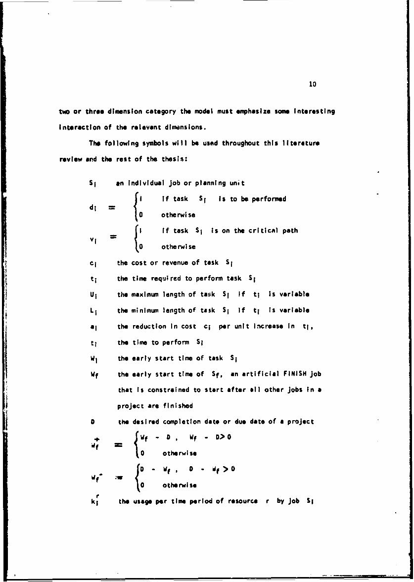
The following symbols will be used throughout this literature

review and the rest of the thesis:

SI an individual Job or planning unit

I If task Si Is to be performeddi -

0 otherwise

i JI if task Si is on the critical path

1 0 otherwise

c; the cost or revenue of task Si

ti the time required to perform task SI

Ui the maximum length of task SI if ti is variable

Li the minimum length of task SI if ti Is variable

ai the reduction in cost ci per unit Increase In ti,

ti the time to perform Si

W/I the early start time of task Si

Wf the early start time of Sf, an artificial FINISH Job

that is constrained to start after all other Jobs in a

project are finished

O the desired completion date or due date of a project

{Wf -0, WF - >O0Wf :

0 otherwi se

0 •O- f , 0 - f > 0

otherwise

rki the usage per time perlo-d of resource r by Job Si

11

Kr the availability per time period of resource r

Pi the probability of job SI occuring

Ss an artificial START Job that must be completed before

any other task can be started

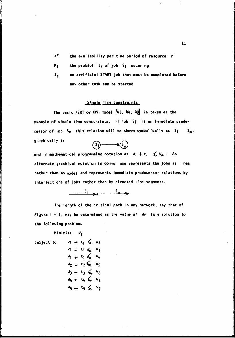
Simple Time Constraints

The basic PERT or CPH model k3, 44, 4j is taken as the

example of simple time constraints. if lob Si is an Immediate prede-

cessor of job Sm this relation will "e shown symbolically as Si Sm.

grbphlcally as

and in mathematical programnming notation as Wi + t1 W m . An

alternate graphical notation in conmon use represents the Jobs as lines

rather than as nodes and represents immediate predecessor relations by

intersections of Jobs rather than by directed line segments.

The length of the critical path in any network, say that of

Figure I - I, may be determined as the value of Wf in a solution to

the following problem.

Minimize Wf

SuhJuct to WI + t I w2

S.4. t1 W w3W1 -t- tli W4

V2 + t 2 ( w5

J3 + t 3 4 W6

W5-+ t5 < w7

12I + t6 W7W7 t tT7 '

Here w minimize the length of the project, subject to a set

of time constraints, one for each Immediate predecessor relation in the

graph.

*; The dual problem formulated by Charnes and Cooper 15] defines

a variable v, for each job In the network. Then all Jobs thet have no

predecessors are included in an equation of the form

VI = 1

to Initiate an artificial flow of one unit !nto tne network. For all

other Jobs, not including Sf , they constrain the flow in from the

predecessors or the jo1, (- .-AimUM of I unit) to equal the flow out to

immediate successois.

- V3 - vg + V6 = 0

ror the final node they establish a sink fnr the one unit flow.

- V5 - V6 = - I

These constraints guarantee that e set of Jobs will be chosen that will

form a path through the network. Finally the criterion function is

NMaximize ti VI , N= t~tal .umber of Jobs in the project

Thus w selo:t the longest path in the network.

A third possible formulation would establish a coistraint for

each path in the network and constrain dr to be longer than all

paths . Since this approach Implies complete knowledge of all paths.

It would be a simple matter to select the longest path directly.

13

Simple Interdependency.

"Job alternative" interdependency has been defined as a set of

mutually exclusive alternative planning units. Originally we considered

the units to be alternative methods of performing some job, but we may

also consider them different results of some stochastic process. A

natural source of such outcomes would be a research or development

project.

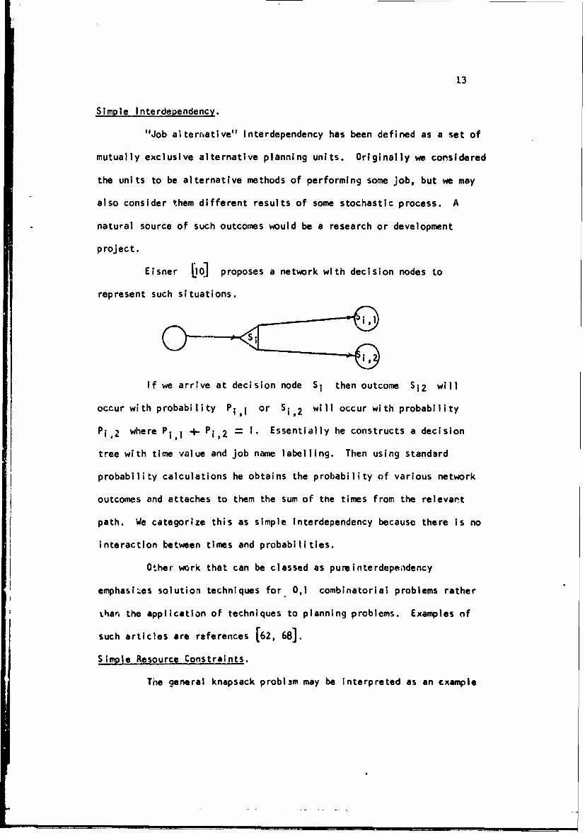
Eisner jL01 proposes a network with decision nodes to

represent such situations.

If we arrive at decision node Si then outcome S12 will

occur with probability PiI or Si,2 will occur with probability

Pi,2 where Pi, +-" Pi, 2 = 1. Essentially he constructs a decision

tree with time value and job name labelling. Then using standard

probability calculations he obtains the probability of various network

outcomes and attaches to them the sum of the times from the relevant

path. We categorize this as simple interdependency because there Is no

interaction between times and probabilities.

Other work that can be classed as puralnterdependency

emphasi;es solution techniques for 0,1 combinatorial problems rather

thar, the application of techniques to planning problems. Examples of

such articles are references [62, 68].

Simple Resource Constraints.

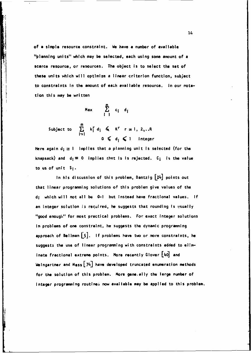
The general knapsack problim may be interpreted as an cxample

14

of a simple resource constraint. We have a number of available

"11planning units" which may be selected, each using some amount of a

scarce resource, or resources. The object is to select the set of

these units which will optimize a linear criterion function, subject

to constraints in the amount of each available resource. In our nota-

tion this may be written

Max , ci di

Subject to kr di 4 Kr r 1I, 2,. .R

0 C d1 < I integer

Here again di = I implies that a planning unit is selected (for the

knapsack) and di= 0 Implies thiet Is is rejected. Ci is the value

to us of unit SI.

In his discussion of this problem, Dantzig L24] points out

that linear programming solutions of this problem give values of the

di which will not all be 0-1 but instead have fractional values. If

an integer solution Is requ!red, he suggests that rounding is usually

"good enough" for most practical problems. For exact Integer solutions

In problems of one constraint, he suggests the dynamic programming

approach of Bellman L5]. If problems have two or ,ore constraints, he

suggests the use of linear programming with constraints added to ellm-

Inate fractional extreme points. More recently Glover [40] and

Weingartner and Ness [74] have developed truncated enumeration methods

for the solution of this problem. More gene.ally the large number of

Integer programming routinei now available may be applied to this problem.

15

Weingartner [75, 76) shows that the Lorle-Savage [521 capital

budgeting problem is essentially the knapsack problem as described

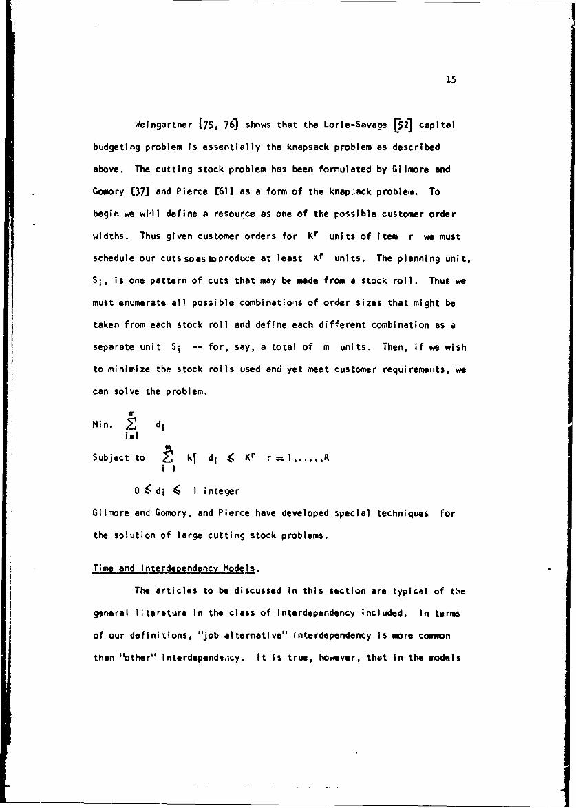
above. The cutting stock problem has been formulated by Gilmore and

Gomory (371 and Pierce C611 as a form of the knap.ack problem. To

begin we wi-ll define a resource as one of the possible customer order

widths. Thus given customer orders for Kr units of item r we must

schedule our cuts soasloproduce at least Kr units. The planning unit,

Si, is one pattern of cuts that may be made from a stock roll. Thus we

must enumerate all possible combinatioiis of order sizes that might be

taken from each stock roll and define each different combination as a

separate unit S; -- for, say, a total of m units. Then, if we wish

to minimize the stock rolls used and yet meet customer requirements, we

can solve the problem.

mMin. di

mSubject to • kf di .< Kr r = I .... it

iIl

0 < d 1 IK I integer

Gilmore and Gomory, and Pierce have developed special techniques for

the solution of large cutting stock problems.

Time and Interdependency Models.

The articles to be discussed In this section are typical of the

general literature in the class of Interdependency Included. In terms

of our definitions, "Job alternative" Interdependency Is more common

than "other" interdepend-jcy. It is true, however, that in the models

16

with Job alternatives generated by probabilistic research or production

outcomes, a Job whose sole preLjecessor may not be performed may be con-

sidered to be contingent on that predecessor. This, for example, is

true of the article by Eisner E281 discussed above.

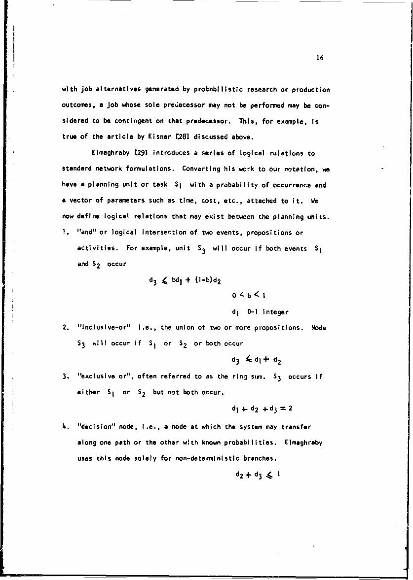
Elmaghraby [291 introduces a series of logical relations to

standard network formulations. Converting his work to our notation, we

have a planning unit or task Si with a probability of occurrence and

a vector of parameters such as time, cost, etc., attached to it. We

now define logical relations that may exist between the planning units.

L. "and" or logical intersection of two events, propositions or

activities. For example, unit S3 will occur if both events SI

and S2 occur

d3 . bdi - (l-b)d2

O0.b/l

d i 0-1 integer

2. "Inclusive-or" i.e., the union of two or more propositions. Node

S3 will occur if Sl or S2 or both occur

d 3 4di + d2

3. "exclusive or", often referred to as the ring stmn. S3 occurs if

either S, or S2 but not both occur.

di 4- d 2 +do1 = 2

4. "decision" node, i.e., a node at which the system may transfer

along one path or the other w~th known probabilities. Elmaghraby

uses this node solely for non-deterministic branches.

d2 + d 3 4. 1

[17

Note th)t relat!ons 1, 2, and 3 would be Included in our

definition of "other" interdk.pendency and 4 would be considered as "Job

alternative" Intetrdependency. A graphical symbol Is defined for each

interdependency relation so that n set of tasks and the rict!-ons

betweei them may be expressed graphically. However, if the nodes are

given performance times and the 0 relation is Interpreted

as an Immediate predecessor relationship, then it is only possible to

have interdependency relations between units that also have immediate

predecessor-successor relations unless new symbols are defined. This

is an unnecessary restriction introduced by his attempt to show all

relations graphically. As we shall see, a programming formulation has

no such restriction.

Given the model as described above, Elmaghraby suggests a

complete enumeration of paths and shows algebraically that for each

such path a time and probability of occurrence may be determined. He

concludes by combining path time and probability information for an

overall expected value for project completion.

The problem of determining a project cost function, that is,

total cost at various completion dates, for the deterministic case is

discussed by Kelley and Walker (431. The length of the project nay

vary because for each job there is a series of "job alternatives"

(actually a continuous linear function) with increasing cost. cl, and

decreasing time, ti. The operation time for job Si is co:istrained

to be within the uWer time limit UI and the lower limit LI, that is

0K L A t1I <U

18

and cost CI = bi - ajti

where bi is the cost of job Si performed in time LI

and al is the cost of decreasing ti by one time unit.

Then given an absolute due date, D , the objective function is

mMin b, - ajti

i=1

Subject to precedence constraints, one for each link In the graph

WI "+ ti 4 Wi

and finally Wf 4 D

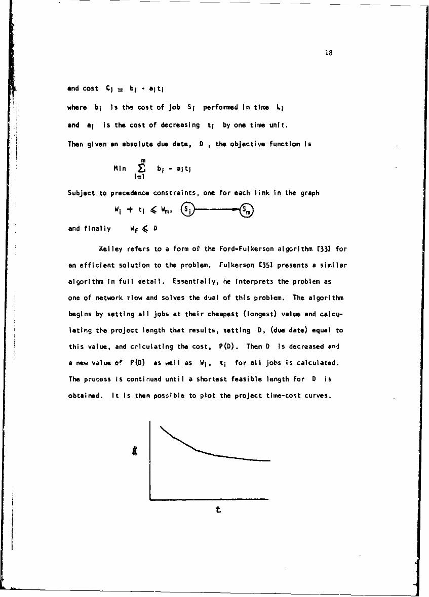
Kelley refers to a form of the Ford-Fulkerson algorithm 133) for

an efficient solution to the problem. Fulkerson 135J presents a similar

algorithm in full detail. Essentially, he interprets the problem as

one of network flow and solves the dual of this problem. The algorithm

begins by setting all jobs at their cheapest (longest) value and calcu-

lating the project length that results, setting D, (due date) equal to

this value, and crlculating the cost, P(D). Then D is decreased ond

a new value of P(D) as well as Wi, ti for all jobs is calculated.

The process is continued until a shortest feasible length for D is

obtained. It is then possible to plot the project time-cost curves.

t

19

Fulkerson points out that the breakpoints of this piecewise linear

function occur at integer values of time if the bounds on Job lengths

are integers. The algorithm has been shown to be efficient in practical

applications to large problems (601. In this formulation it may be

assumed that the variation in job time and cost is a result of the appli-

cation of more or less resources to the job. Since there Is no attempt

to restrict the amount of resource used at a particular point in time,

by all jobs, the model is not considered to have resource constraints.

In some instances it may be unrealistic to assume a continuous

linear relation between time and cost for a task in a project. For

example, if a job may be only performed by an eight man crew on regular

time, or by an eight man crew on regular time plus two hours overtime,

there are two discrete ways to perform the job (two "job alternatives")

and linear combinations of these methods may be technologically or

contractually infeasible. The problem of discrete "job alternatives"

in the time/cost problem is discussed in references[19, 26, 57, 51.

Moder and Phi lips (581 summarize some work by Meyer and Shaffer £57] on

this problem. Their formulation is as follows:

Min. cij dijij

S.t. precedenceW i+ t I •WJ , -

or if a job a!ternative situation is involved

WI + til dil 4. t12 di2.... ttik(i) dik(i) 4 Wj

and WF K D

20

whe reif job Sij is performed

dij 0 ootherwise

This assumes that each Job alternative

Sli , J-1 .... k(i)

has Identical precedence and successor relations.

Finally, we require an interdependence constraint

k(!)

del = Ij I

0 41dij 41 integer

A more general and more efficient integer programming formula-

tion is presented by Crowston and Thompson E191, 1967. This model will

be presented in detail later, but a short summary is included here.

The Job alternatives are again represented by 0-1 variables, dij,

which for any particular Job, are constrained

k(i)Y dij = Ijwl

In addition, however, any set of alternative interdependence constraints

may be written on these variables.

dlj + dmn - I

dij 4 dmn

dij <dmn

etc.

Note that although resource constraints are not considered specifically

here, alternative Interdependency constraints could be written to

21

constrain the total usage of a consumable resource over the life of the

project.

The length of the critica4 path as defined in Chapter I nn-

strained by a set of equations which represent paths in the network.

Paths which cannot become critical may be dropped from the problem.

Rather than generate a time/cost curve, they establish a due date, D,

with overtime penalty and undertime premium and solve directly for the

optimum set of Jobs to be performed. It would be possible, however, to

solve a series of problems, setting progressively tighter upper limits

on the critical path (WF<D) and thus generate a time/cost curve.

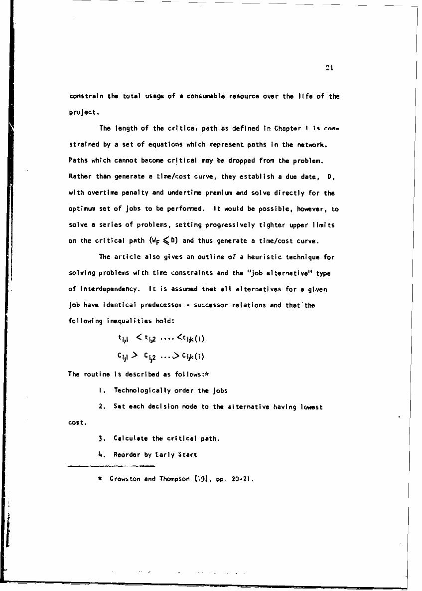
The article also gives an outline of a heuristic technique for

solving problems with time constraints and the "Job alternative" type

of Interdependency. It is assumed that all alternatives for a given

job have Identical predecessor - successor relations and that'the

following inequalities hold:

ttill < tlj,2 ... <t iik(i)

Cil. > C12 > Cilk(i)

The routine is described as follows:*

I. Technologically order the jobs

2. Set each decision node to the alternative having lowest

cost.

3. Calculate the critical path.

4. Reorder by Early Start

* Crowston and Thompson [191, pp. 20-21.

22

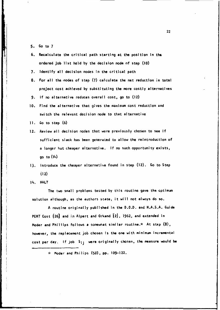
5. Go to 7

6. Recalculate the critical path starting at the position In the

ordered Job list held by the decision node nf step (10)

j 7. Identify all decision nodes in the critical path

8. For all the .nodes of step (7) calculate the net reduction ;n total

project cost achieved by substituting the more costly alternatives

9. If no alternative reduces overall cost, go to (12)

10. Find the alternative that gives the maximum cost reduction and

switch the relevant decision node to that alternative

1). Go to step (6)

12. Review all decision nodes that were previously chosen to see if

sufficient slack has been generated to allow the reintroduction of

a longer hut cheaper alternative. If no such opportunity exists,

go to (14)

13. Introduce the cheaper alternative found in step (12). Go to Step

(12)

14. HALT

The two small problems tested by this routine gave the optimum

solution although, as the authors state, it will not always do so.

A routine originally published in the D.O.D. and N.A.S.A. Guide

PERT Cost (26] and in Alpert and Orkand [21, 1962, and extended in

Koder and Phillips follows a somewhat similar routine.* At step (8).

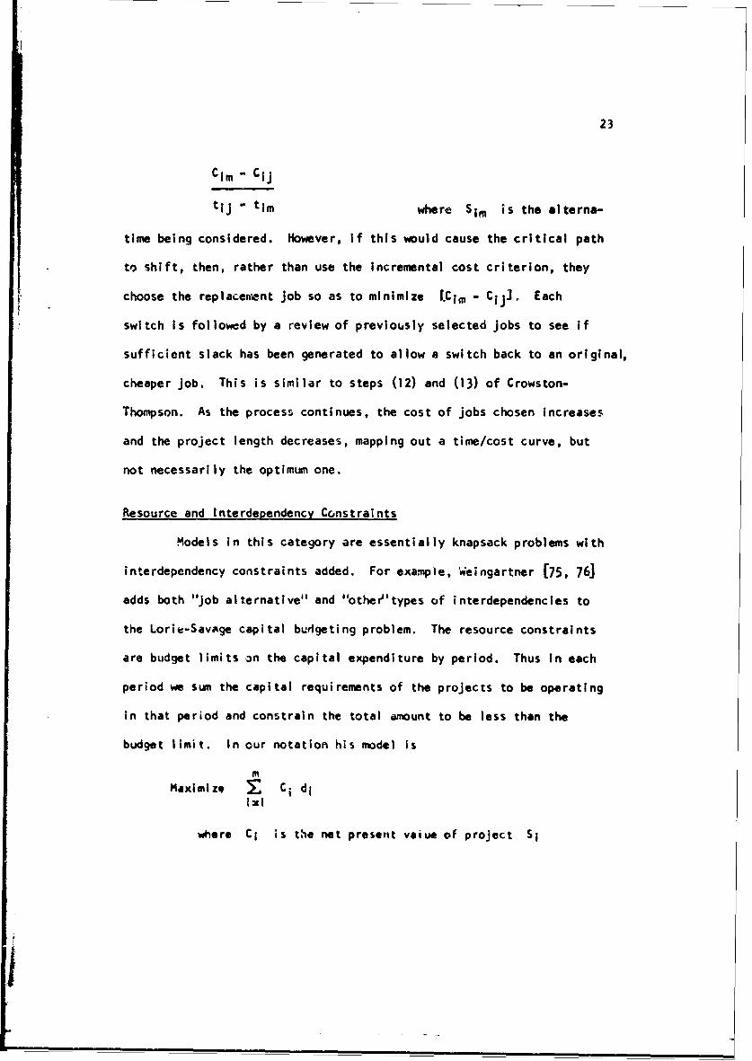
however, the replacement job chosen Is the one with minimum Incremental

cost per day. If Job Sij were originally chosen, the measure would be

* Moder and Philips (581, PP. 109-122.

23

Cim - Cij

tij - tim where Sim is the alterna-

time being considered. However, if this would cause the critical path

to shift, then, rather than use the Incremental cost criterion, they

choose the replacement job so as to minimize LCim - Cij]. Each

switch is followed by a review of previously selected jobs to see if

sufficient slack has been generated to allow a switch back to an original,

cheaper job. This is similar to steps (12) and (13) of Crowston-

Thompson. As the process continues, the cost of jobs chosen increases

and the project length decreases, mapping out a time/cost curve, but

not necessarily the optimum one.

Resource and Interdependency Constraints

Models in this category are essentially knapsack problems with

interdependency constraints added. For example, Weingartner (75, 761

adds both "job alternative" and "other'types of interdependencies to

the Lorie-Savage capital budgeting problem. The resource constraints

are budget limits an the capital expenditure by period. Thus in each

period we sum the capital requirements of the projects to be operating

in that period and constrain the total amount to be less than the

budget limit. In our notation his model Is

MMaximizq Y Ci di

where CI is the net present value of project S1

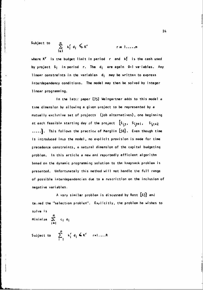
24

Subject to m k di < r= l.....Mi kz " ri K-Kr r- ..

where Kr is the budget limit in period r and ki is the cash used

by project SI in period r. The di are again 0-1 va-lables. Any

linear constraints in the variables di may be written to express

interdependency conditions. The model may then be solved by integer

linear programming.

In the latc' paper [75] Weingartner adds to this model a

time dimension by allowing a given project to be represented by a

mutually exclusive set of projects (job alternatives), one beginning

at each feasible starting day af the project [Sit, Siýt+I, Sit 4 2

.... .This follows the practice of Marglin [56]. Even though time

is introduced into the model, no explicit provision is made for time

Frecedence constraints, a natural dimension of the capital budgeting

problem. In this article a new and reportedly efficient algorithm

based on the dynamic programming solution to the knapsack problem is

presented. Unfortunately this method will not handle the full range

of possible interdependencies due to a rescriction on the inclusion of

negative variables.

A vary similar problem is discussed by Root [63) and

te:.ned the "selection problem". Explicitly, the problem he wishes to

solve ism

Minimize 'V ci di

i~l IrSub•ject to k ki di Kr r-l .... R

25

where the Kr are assumed to be integer and a set of linear Interde-

pendency constraints are written in the variables d1 i-l,...,m. For

example, the fact that a job may be performed by several resources or

resources in combination may be written ask(i)

J=l

where the k j would differ for the various alterrnatives. Root solves

the problem by applying a theorem from symbolic logic to reduce the

total set of possible solutions. Then by costing each remaining

solution, he can select the one with minimum cost.

Time and Resource Problems

Many in ortant scheduling problems may be described as

time and resource constraint problems. Among these are forms of the

project scheduling problem, the job-shop scheduling problem, and the

assembly-line balancing problem. The project scheduling problem, of

course, appears in contea.ts such as marketing and economic planning

[31] as well as production. All of these problems have been formulated

as integer linear programming problems but because of the high number

of constraints involved, these are not suggested as possible solution

methods for real problems. For example, Wiest L80] estimates that a

project with 55 jobs in 4 shops with a time span of 30 days would have

some 5,275 equations and 1,650 variables, not including slack variables

or constraints added to assure an integer solution. As a result,

heuristic solution methods have been developed for these problems.

The essential problem is that the level of resources is constrained by

26

period and the jobs, given the usual time constraints, may shift

through time. Thus,in programming formulations, it is necessary to

include the possibility that the job may shift through time, and this

requires many variables and many constraints. Heuristic solution

techniques can handle this problem with concise bookkeeping techniques.

The solutions, however, are not necessarily optimal.

We will examine several heuristic approaches to the

resource-levelling problem in project scheduling. It is assumed that

in this problem the resources are not fixed but that the criterion

function is so related to period by period resource levels that we are

motivated to smooth the daily resource usage. Burgess and Killibrew

0123 describe an iterative procedure that attempts to minimize the sum

of squares of daily resource usages. This criterion, while minimizing

the standard deviation from the project mean, still might allow - high

peak in any given time period.

The routine first technologically orders the jobs by

Early Start, and if jobs are tied, ranks the shortest first. In the

second stage the jobs are loaded, beginning at the bottom of the

technological list. Each job is scheduled as late as possible, subject

to the condition that the daily usage should not be too far above or

below the predetermined average daily resource usage. The late start

of each job is strictly set by the assigned start time of its successors.

The cycle is repeated, each time attempting to reduce deviations from

the mean, until no further improvements are made. The best schedule

is then chosen.

27

The method of Levy, Thompson and Wlest [50) concentrates

on reducing the peak usage of the project resource. Heuristics which

drive the solution to this goal would also work to meet the Burgess

criterion. The jobs from all projects to be simultaneously scheduled

are scheduled at Early Start and then the daily demand for ea-h resource

is plotted. For the fsrst resource an in'tial trigger level is set,

one unit below the maximum usage. It is assumed that the resources

are ordered based on some priority system, perhaps daily cost per unit.

Then all the jobs contributing to the particular peak and in addition

having enough slack so that they may be scheduled beyond the peak are

listed. Then one of the jobs is chosen probabilistically, the proba-

bilistic weight being proportional to the job's slack time, and the Job

is shifted a random amount within the slack, forward. The resource

peak again Is calculated and a lower trigger level set. This process

rontinues for the first resource until no further improvement is

realized. Then freezing the lowest feasible limit for the first

resource, the procedure is repeated for the second resource and so on

through ell recources. Now the jobs from each project are segregated

and again an attempt is made to shift them and reduce the aggregate

trigger level for all projects. Finally, when no further inprovement

is possible, the final schedule and trigger levels ate stored and the

process is completely repeated. Due to the probabilistic element in

the decision rule, a new schedule will result. After several repeti-

tions, the best schedule of those generated can be chosen.

The next problem class to be discussed will be scheduling

28

to meet stated resource constraints. The early solutions to problems

of this type were obtained with Gantt charts and their use in Job-shop

scheduling continues. The resource constraint in the Job-shop problem

will be the limit on machine availability and the time constraints are

provided by technological ordering of operations on a particular work

order. The criterion function may be to minimize completion time of the

whole job file as in the integer programming formulations of Bowman [8],

Manne [541, and iWagner (731. Alternately, it might be the minimization

of idle machine time (identical to ninimiun final completion time for

the fixed job file case) as in Conway and Maxwell 0181 or a complex

function of order delay cost as in Carroll r.141.

Many heuristic approaches have been developed for this

problem 118, 20, 381 and in many of these approaches similar decision

rules are used singly or in probabilistic combination to dispatch Jobs

from a queue to the machine. dIe will quote from a description of

several such rules: *

1. SlO (shortest imminent operation)

W/hen a facility is available, select that item in the queue

which has the shortest machining time on the facility.

2. LRT (longest remaining time)

Selec-t the item which has the most total machining time

remaini ng.

3. J.S. (job slack per operation remaining)

* Crowston, Glover, Thompson and Trawlck [201, p. 2.

29

Subtract the total remaining machine tir.,e for a given job

from an arbitrary finish date, DD. Divide this slack by

the number of operations remaining. Select the item with

minimum job slack per operation.

4. LIG (longest imminent operation)

5. FIFO (first in, first out)

Select the item that arrived first in the queue.

6. MS (machine slack)

For each machine calculate the total machining time remaining.

Select the job in the queue that goes to the most heavily

laden machine next. Break ties with S.I.O.

Many other rules have been attempted to specifically meet

more complicated criterion than the minimization of overall completion

time. It will be interesting to note below that attempts have been

made to apply several of the simple rules to the project scheduling

problem, but that more complex rules have not as yet been translated

to the project problem.

Two main approaches have been su :ed for solving the

fixed resource problem in the project scheduling context. Neither

approach guarantees an optimum solution, nor consistently outperforms

the other. Representative of the first approach is an article by

Kelley 1441. The routino may be summarized as follows:

I. Technologically order the jobs, calculate early start,

late start, and slack. Within the techno!ogical ordering, reorder by

slack, lowest slack first.

30

2. Start with the first activity and continue down the

list.

(a) Find the early start of the activity.

(b) Schedule the activity at early start if sufficient

resources are available. If resources are not avail-

able, two alternative routines are suggested cl, c2.

(cl) Serial Method: Begin thebJb at the earliest time

that resources are available to work it for one day.

The job may be split if necessary.

(c2) Parallel Method: Find the set of all jobs causing

the resource violation and rank them by total slack.

Delay a sufficient number of jobs with the highest

slack so that those remaining on the list can be

scheduled.

3. Repeat step 2 for all jobs.

4. Repeat the whole routine with various orderings on the

technological list.

In addition to the possibility of allowing job-splits,

Kelley suggests that we also allow resource limits to be violated by

small amounts. The basic heuristic In the original job ordering and in

the parallel loading technique is the use of Job-slack (JS) as a

criterion for shifting jobs forward. This is a reasonable approach

similar to that used by Levy (503.

The second approach, detailed in Mocder and Philips (58.1

uses Maximum Remaining Path Length, or equivalently Late Start, as a

i1

31

basis for delaying Jobs (LRTJ. Note that If two Jobs have a common

early start-time, both measures are equivalent. That Is, the Job

delayed because of a higher slack would In the same way be delayed

because of a lower Late Start time. Some other features of the routine

are differe'nt than that suggested by Kelley. A main feature is a list

of unscheduled Jobs whose predecessors have all been schaduled, ordered

by Late Start, and an ordered list of finish times of scheduled Jobs.

Thus the routine steps through time to only those days when a change

of resource usage is poss'ble. On such a day it examines the list of

available jobs and ends either when the resources are exhausted or the

job file is completed. At this point it again jumps ahead. As we

implied at the beginning of this section, examples can be constructed

co favor or penalize either of these approaches.

Finally, we will show that Salveson's [66i formulation of

the assembly-line balancing problem has the structure. of a time-resources

constraint problem. The resources, in this instance, are the work

stations and the work times at the station will be the resource level.

Then, If a precedence ordering exists between jobs, as would usually

be the case, a job may not be assigned to a work station unless all its

predecessors have previously been assioned to that work station or

earlier work stations. In addition to the above statement, the problem

may be complicated by any of the interdependenciks we have discussed.

For example, It may not be feasible to do a particular pair of Jobs at

one station, and therfore, we must constrain tht problem to prohibit

this. Also, it should be pointed out that "alternativ,. interdependency"

32

relations would probably be the most efficient method of actually

formulating the problem. Finally, as in the other problems of this

section, it must be noted that practical problems must be solved by

heuristic methods (72).

Models with Resource. Time and Interdependency Constraints.

Problems in this category abounid in the industrial world.

Wherever there is an element of physical design connected with a

scheduling problem, then interdependency is an implicit part of the

problem. For example, we may consider the problem of an industrial

engineer attempting to design a job with the graphical technique of

man-machine analysis [4]. There are several alternate ways for an

operator to perform each necessary function and operations when combined

may require less time than the sum of the same operations performed

singly. Finally, many possible orderings may be possible, although

scme technological ordering constraints are involved in many problems.

Each production alternative may have an important effect on the scheO-

uling problem. Similarly, design of construction projects will have

important scheduling implications.

With the exception of the Weingartner article 175J which

ooes not fully include the possibility of time ordering, no model was

found to include resource, time and 9Jh types of interdependerc) con-

straints. It is true, however, that the job-shop models of Bowman 181

and Wagner 73J) could be easily generalized to Include this possibility.

The use of job alternative Interdependency in heuristic programs Is not

uncommon.

33

Two master's theses written in the Sloan School of Manage-

ment, M.IT., expand the usual statement of the Job-shop scheduling

problem to include the possibility of Job alternatives, with two differ-

ent practical interpretations of what these alternatives might be.

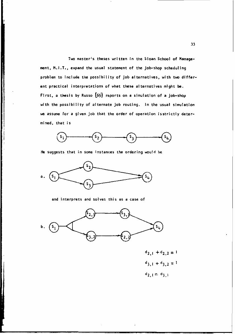
First, a thesis by Russo [65] reports on a simulation of a Job-shop

with the possibility of alternate Job routing. In the usual simulation

we assume for a given job that the order of operation isstrictly deter-

mined, that is

He suggests that in some instances the ordering wou!d be

and interprets and solves this as a case of

d 2 , 1 +"d 2 , 2 I

d 3 , 1 + d33 2 =

d2,1 = d3 ,1

34

It Is clear that this situaition can be categorizee as a time and resource

model, however, since his heuristics specifically detailed each alterna-

tive route, then calculated Information for local dispatching rules

based on the two alternatives and then decided between them, it is

included here. One of the most effective approaches he discusses, allows

all jobs in an alternate chain to enter queues for the!r respective

machines wher the predecessor of the alternate chain is completed. Then

in each queue the jobs from the alternate chain are ranked by a standard

dispatching rule. !4e then allows that job to 2o first, which is selected

by the machine queue discipline.

Clermont ['l7] allowed for the possibility of sevc-il

machines performing a given *2ob. This more clearly resembles our job

alternative interdependency case. His results show that the heuristic

Russo found so successful only improved performance of the simple dis-

patching ru~es when the total machine ;oadings were highly imbalanced.

In the case of balanced loads, switching actually decreased the perform-

ance of simple decision. For the balanced case only the simple switch-

ing heuristic "switch if the alternate queue is empty" consistently

improved performance of the simple dispatching rules. His results

also indicate that a dispatching rule "Covert' derived by Carroll (143

completely dominates all conventional rules tested.

Job alternativt- Interdependency is also found in scheduling

techniques designed for the lirge project problem. The series of SPAR

programs by Wiest (801 will now be discussed. With each job he associ-

ates three operating levels, maximum crew size, normal cre"? size and

35

minimum crew size. Of coursi-, thet length Is inversely a function

of resource level. The jobs originally at normal crew size are origin-

ally ordered by early start time, one possible technological order. Then,

as in the Moder and Philip routine discussed above, a sub-list is gen-

erated and continually updated of jobs available for scheduling. From

this list jobs are selected for schedulTng with a probability inversely

related to the available slack f the job. If a job is selected to be

scheduled and the resources are unavailable, it is left to be schedule

in a subsequent period.

Several subsidiary heuristic routines operate within the

basic framework outlined above. If the slack of a job is low, an

attempt is made to schedule it at maximum resource usage. If the

resources are not available for this, a subroutine attempts to borrow

resources from jobs operating on that day with normal or maximum

resource. A second approach is to find jobs using the tight resource

and delay their start for one or more periods. This frees their

rescurces for the critical jobs. Finally, if all elsc fails, the

critical job wouid be delayed one period. After the application of

these and other routines, a final schedule is produced. Since there

is a random element in the choice of jobs to schedule, it is suggested

that the process be repeated several times and the best schedule

selected.

An important addition to. the program is a search routine

that progressively shifts the leve! of initial resources from solution

to solution in attempt to find those limits that will minimize the sum

36

of re-ource cost and project completion time cost.

Discussion of Constraint Categories

As we have seen the categories chosen do not allow a

categorization of all plannirng models. In several cajes a goad

arnksment could ',e m'nde against the allocation we have decided on.

Nevertheless, for several reasons, this particular categorization is

useful. It does suggest that more complex models may have relevance

in functional areas where they have not yet appeared. For example,

time precedence constraints would seem relevatt to the capital budget-

ing problem, further use of alternative interdependencies '- the job-

shop problem and the assembly-line problem.

"An even more truitfui use of such a framework will be to

suggest that researchers examine a broad range of literature in their

search for suitable sclution techniques. Examples of this certainly

have already occrred. For examrile, Wiest [80i uses the 6o,,anan L8"

job-shop L.P. formulation as the base of his project scheduling formu-

lation. A thesis oy K*-iht [461 attemptl, to relate heuristics in the

job-shop problem to hturistics in the project sch..uulinq problem.

Finally, Wilson L821 shows how severa! line bal3ncang algorithms may

be applied LO resource leveling. Thi.- compa-ison also allows us to

n,Ake some 9en,.ral statements about the efficiency of various sdlution

techniques.

37

Solution of Planning Models

For several categories of problems, algorithms have been

developed that are much more efficient than any of the ex!sting program-

ming, routines. For example, the longest path algorithm very quickly

determines the critical path of a simple time constraint problem.

Similarly, the Ford-Fulkerson technique efficiently finds th's optimum

job lengths and job start times for a project given a fixed due date

and a bounded inverse linear relation between job cost and job time.

This, of course, is a special case of the time-interdependency constraint

case.

There is a second set of problems for which special

efficient solution techniques have been developed, but because of the

nature of the problem, the techniques may be considered as restricted

integer programming routines. In this category I would include the

truncated enumeratior, methods of Weingartner and Ness and that of

Glover appl~ed to the simple resource (or knapsack) problem. Also

Root's algorithm for the selection problem, which is a combined

resource-interdependency problem, is in this group. We may summarize

the above cases, then, by saying that we may obtain optimum solutions

more efficiently wfth existing techniques than with programming

methods.

We now shift in the spectrum to those problems for which

optinum solutions are only available through programming methods. It

38

should be emphasized that no clear line can be drawn between problems

in this group and those in the previous one. An example of this would

be problems with pure interdependency constraints. /e have stated

above that certain simple resource or resource-interdependency con-

straint problems ma' be solved with special computational methods. On

the other hand, if many resources were involved, It would be necessary to

turn to conventional integer programming techniques. Similarly, for

many large problems with pure interdependency constraints, the 0-1 tree

search algorithms wouid give th~e most efficient solutions. Finally,

the time-interdependency problem,when the job alternatives are discrete,

is best solved by conventional integer programming routines [70].

Techniques are available, however, for this problem, as we will show

later, that will significantly reduce the number of required constraints

and the number of variables. In this regard, it is interesting to

observe that for integer programming problems in 0-1 variables, added

interdependency constraints, by eliminating branches in the feasible

solution tree, actually make problems easier to solve.

Heuristic routines are available for the above problems,

and we have covered several approaches to the time-interdependency

problem, given discrete jobs, no alternative interdependency and commor,

precedence-successor relations for job alternatives. It can be shown

that existing heuristic methods are not at all appropriate for problems

with any reasonable alternative interdependency c:nplications.

The final category finds combinations of time and resource

constraints and, as we have discussed, this grouping requires large

39

numbers of constraints and variables for programming solutions. As a

result, these problems are solved almost exclusively In practice by

heuristic methods. As noted above some of the simpler job-shop problem

heuristics have been adapted to the project scheduling problem with

some success. This suggests that more complex heuristics, based on

variations of successful job-shop rules, should now be tested. When

job alternative interdependencies are added to the problem, as Wiest

[801 does, it is possible to build subsidiary switching routines based

on local (in the time dimension) resource usage information. If alter-

native interdependencies were added to the problem, such local informa-

tion might no longer be a sufficient base for a switching decision. In

fact, as we have seen, any purely heuristic method might have difficulty

approaching an optimum solution to this kind of problem.

Chapter III

DECISION CPM MODELS

The paper 'at will serve as the basis* for this chapter Is

that of reference .191 by Crowston and Thompson. This decision network

formulation contains "time" constraints and both "Job alternajive" and

"other" types of interdependency. The mathematical basis of Decision

CPM will be discussed as well as several alternate integer prugramming

formulations of the problem. A numerical problem is introduced in this

chapter '(FIGURE 111-1) that will also serve as an example in Chapters

IV and VI.

2. The Mathematical Basis of Decision CPM

This section will follow in part the article [2.1 by Levy,

Thompson, and Wiest. Let J='Sit, S2, S3 ...-J be a set of Job sets

that must be done to complete a project. Some job sets are unit sets

Si - {Silt and other job sets have several members, Si a {Sii. S12

.3..J. In order to complete the project, one of the jobs from each

job set must be completed. Associate with each job set

(1) si-{ý : ,S l -- sik(i)}

k(i) variables

*Sections 2, 3, 4 and 5 dre taken essentially verbatim from

f19] although a new numerical problem is introduced. Furthermore, thischapter will assume that exactly one Job alternative is selected fromeach job set, that is

I) dij I

j~l

40

41

(2) dil, ... , d k )

having the property that

fI if job Sij is to be performed

(3) dj

0 otherwise

Since exactly one of the jobs must be performed, then the mutually

excliusive or job alternative interdependence condition is expressed by

(4) ' dijji

If all job sets are unit sets (impiying condition (4) holds),

then all of the jobs in the project are independent and the project

reduces to the ordinary project of the usual ClPM variety. If one or

more of the job sets have more than one member, then for each such set

a decision must be nade as to which job of the set is to be done. Once

such a decision is made for each job set, the result is an ordinary CI'm

project.

It should be noted that the decisions may be complicated by

many other kinds co conditions than (4), which may be of the mutually

exclusive or contingent kind. For instance, the following equations

give examples ot such interdependencies among decisions.

(a) dij t dmn I

(b) dij ,ý dmn

(c) dij = dmn

42

Note that (a) says that we cannot do both Sij and Smn ; (b)

says that we can only do SIj if we also do Smn ; and (c) says

that we either do Sij and Stun or vie do neither. The above

discussion illustrates some of the possible complexity of problem

formulation that is possible within the Decision CPM framework.

In addition to the relations described above, there will be

precedence relations between the jobs of a decision project. Let I<'

denote a relation between pairs of jobs in J such that Sij <K<Smn

is defined for some pair of jobs Sij, Smn and is read Sij is an

immediate predecessor of Smn. The interpretation of this statement is

that all immediate predecessors of a job must be completed before that

job can be started. A decision project is the set J together with the

specified interdependencies and the relation << defined on J.

The decision project graph of a project, G, is a planar graph

with nodes representing jobs and a directed line segment, connecting

two nodes Sij, Smn it and only if Sij <<Smn holds. A•oath in G

is a set of nodes connected by immediate predecessor relations. A cycle

in G is a closed path of the form Sij = al <4 a2 << . . . «an= al -

Sij. A project graph is acyclic if and only if it has no cycles.

Definition: Sij < Smn implies Sij precedes Smn (or alternaitively

Smn succeeds Sij) if and only if there is a sLt of jobs a1, a2 ... an

n > 2 such that

Sij= al << a2 <-•a3 . . . <<Zan= Smn

in other words, Sij precedes Smn if and onli if theis is a path trom

it

43

Sij to Smn in the decision project graph G.

Assumption l:* The precedes relation is asymmetric, that is if Sij <Smn

thern it is false that Smn <Sij for all Sij and Smn in J. Defini-

tion: A relation that is transitive and asymmetric Is said to be a

preference relation.

Theorenm'nk i11-1: If assumption I holds, then the predecessor relation

is a preference relation, and the graph G is acyclic.

Definit;on; A technologically ordered job list J = (a, a2 . . . an)

is obtained from a set of jobs J-{ b, c . . by listing them so

that no job appears on the list until all of its predecessors have

al ready appeared.

Theorem** 111-2: Assumption I holds if and only if it is possible to

list the job- in J in a technologically ordered job list J.

In addition to these definitions and theorems from reference [4 9),

several additional conventions are necessary because of the fact that

some jobs may be eliminated from the decision project graph as the

result of decisions that are made. If we decide to do one of the jobs

in a job set, then all immediate predecessor relations that the job

satisfies must hold in the f;,,! qraph. If we decide not to do that job,

*Note that this assumption differs from the correspo,•dingassumption in (.49J in that the requirement of K-intransitivity isomitted. For this reason theorem I of that reference does not holdin the preset context.

**The proofs of these theorems are exactly as In reference 19).

44

then none of Its Immediate predecessor relations hold. In the decision

project graph, if we decide not to do a given job, then we must remove

that job togecher with all edges that Impinge on it from the decision

project graph to obtain the final project graph. It follows from this

that if any Job,. Sij has a sole immediate predecessor Smn, and if

that predecessor is a member of a job set, it will be necessary to

create a dummy immediate predecessor relation between Sij and a job

which is a predecessor of Smn. If this is not done, then it would be

possible for the path containing Sij to be broken and Sij would

lose Its project time ordering. Similarily a dummy immediate successor

relation must be established for jobs having only one immediate succes-

sor, !f that successor is a member of a job set. In addition it may be

n~cessary to create a dummy relation between two jobs even if both have

several immediate predecessors and successors. If on any path, two

jobs are separated by a job which could be elimiiated, and if it is

desired to maintain a technological ordering of the two jobs, a dummy

immediate prelecessor relation must be established between them.

For a given project, when the jobs are technologically ordered

and a!l planning dec;sions are made designating th6 jobs to be performed

in each set, the nonnal critical path analysis may then be carried out.

The usual concepts of early start, late start, critical path, etc.,

will apply to this redlcoid graph. These terms will be used throughout

the balance of the thesis without further definition.

45

3. Decision Proiect Graohs

A graphical representation of the combined planning and

scheduling problem is shown In the decision project graph of Figure

111-1. In this graph the circular nodes represent jobs and the triangu-

lar node-,s introduce the mutually exclusive decision job nodes of a job

set. In addition to the precedence constraints implied by the directed

line segments, we impose several "alternative interdependenries".

These are

(a) dg,I d6,2

(b) d6,2 = d12,1

where (a) says that S9,I rmay only be performed if S6 .2 is performed;

and (b) says that S6,2 and S 2,1 must both be performed or both

not be performed. The problem, then, is to select the project graph

which minimizes total project cost.

4. Deciheori Graph Solution by Integer Progr.__ning

Consider job set (1) and its associated decision vari-

ables with constraints given by (2) (3), and (4). Besides these,

there may be any J,' the othe- constraints descussed in the second

section of this chapter or other constraints showing various types of

complicated interdependencies betweer jobs in the project.

Wito each job Si, we asivciate a timpe, ti, and a cost,

cij. Also, we assume a reward of 'r' dollars per day for each day under

0, the required due date of the project, and a penalty payment lpl for

each day boyond 0. As defined earlier, 4f will be the number of

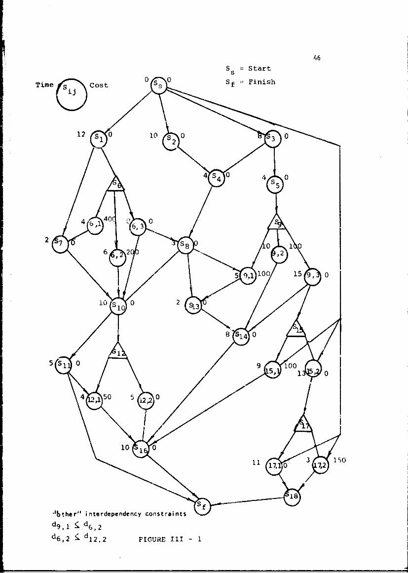
46

S =Start

s

Time si ost 0S fFns

d62 7 . FIUR 0l 1

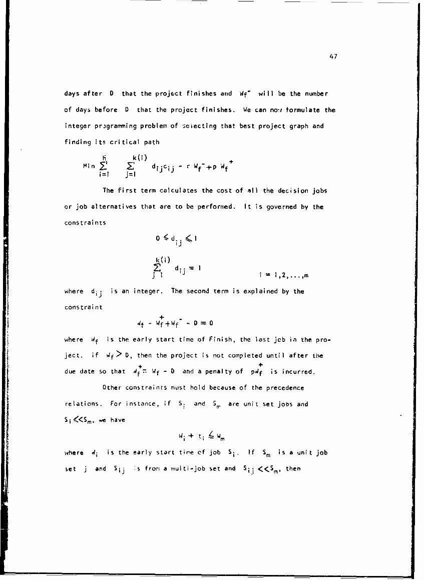
47

days after 0 that the project finishes and Wf" will be the number

of days before D that the project finishes. We can no.i formulate the

integer pr.)gramming problem of Geiecting that best project graph and

finding its critical path

ii k(i) +Min 2: dijcij - r Wf-p Wfi=1 j=l

The first term calculates the cost of all the decision jobs

or job alternatives that are to be performed. It is governed by the

constrai nts

k(i)Z dij= Ij I i -- 1= , . ,

where dij is an integer. The second term is explained by the

constraint

df - Wf +Wf - = 0

where 'f is the early start time of Finish, the last jcb in the pro-

ject. if 4ff> D, then the project is not completed until after the

+ +due date so that df- Wf - D and a penalty of pdf is incurred.

Other constraints must hold because of the precedence

relations. For instance, if S. and S, are unit set jobs and

j <<SmV we have

W•+ t; Wm

where 4i is the early start time of job Si. If Sm Is a unit job

set j and Sij ;s from a multi-job set and Sij <<Sm . then

48

-M(1 - dij) -t W ij+ tij

where M is a large enough number so that the :nequality does not

conutiain the variable dij unless dij = 1. Thus all paths through

Jobs that are not performed will be broken.

It Is inow possible to set up the problem of Figure 111-1 as

an Integer programming problem. Note that it is not necessary to include

the cost of unit set jobs in the functional or the finish node (Sf)

in the precedence constraints.

Min. 400 d6 , +!00 d6 , 2 +-Od6 ,3 + 200 d9 , 1+100 d9 , 2

0Odc 3+50d 1 2 , +Odj 2 ,2tl0Od 5 ,j+0d1 5 ,2÷0d; 7 ,

4+I50dl, 21PWf - rP~f

St.

Precedence Constraints (link formulation)

t 2 ko. W;

t3 4- W 1

t3 5

ti K, w6,1t i 4, W6,2

ti < W6,3

-M(l-d6,1)'lt6.1"f46,! W7

t7 - 7 10Wi

"6(-,2)+t6, &6,2 WIO

-M(I-d ,3 )+t6,3+W 6,3 WIO

-M (I-d6,3)+ t6,'4.1+ 3 •W8

49

t 4 +W4 <

t8-jW 8 <(W1 0

t 5 +W5 <-W9 ~

t5 +W5 W9,

t5 +4 5 (W 9 ,3

t 8-tW 8 W9 W9 I

t84 W8 W 13

-M(I-d 9 32)+t 99 ,+W 9 ,2 4 WI14

-M(I-d 9,34t9 ,3 tW9 3 <1 W15 ,2

t104 W11 1

10 10 12,1

t 13 4.W] 3 W1

t1 4 + W1 4. W16

-M( -d 5 .)4 5 , w 5 .2 w 7 .

-M( -d17 1) tl ,1WI .1 W1

-M(-d 7,21+t 1,eW7 ' W18

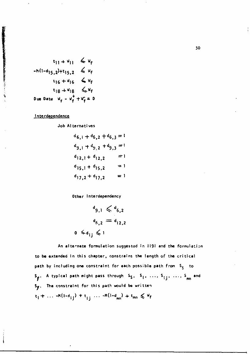
50

t)l I- + ! 'II W f

-h(1-dl5, 2)+tl15 2 tWf

tl l6 +"16 4Wf

t 18 -4-W18 -Wf

Due Date W - -tW- n

Interdependence

Job Alternatives

d 6 , 1 -+- d6 , 2 +±d6 , 3 1

dg, I t1 49 ý,2 + dq,3 -- '1

d 12 , 1 I+ d12 ,2 I

d 15, 1 "+ d1 5 , 2 1

d17,2 + d 17,2 1

Other Interdependency

d9 < d6 ,2

d6 ,2 - d2,2

An alternate formulation suggested in 1191 and the formulation

to be extended In this chapter, constrains the length of the critical

path by Including one constraint for each possible path from S, to

S V A typical path might pass through SS, SI, ... , Sij, ... , Smn and

S The constraint for this path would be wr;tten

tI÷ +.. -M(I-dij) + tIj ... -M(i-d mn ) + tmn <, Wf

51

The precedence constraints on the length of the critical path

for Figure 111-1 will now be shown In "path" fo~rm.

Precedence (paths).

tlt1-(1d,1 1t 6 1 1-tMtI 0-d K(1-d 1 ,12, 1 ,1 .t-t1 < Wf

t1-M(l-d6,1)+t6,1+t7+t10 -M(l-d1 2,2)+t1 2,2'tt1 6 4Wf

t1-M(l-d6 ,2)4t-t6,2tt10 tl-M(l-d1 2 ,1 )tt1 2,1+t1 6 <1Wf

t1 -M(I-d 6,2)i-t 6 3 +'t1 0 -M(l-d 1 2 ,1 )+t 1 2 ,1 +tl 6 < Wf

tl2+t4+t8 3+t60 41 1,' )441 2,14+t2 16 t6II

t M(-d )t - Wf

1- 63 63ýttO-Ml 1,2'+]2,+t) Uf

52

-M(l-dls,2)+ti 5,2-M(l-dl7,P.)ttl 7,2+t18 •"Wf

-140-dl 7,1I •ltl 7,14-tl8 < W f-M(I-d 17,2)+t17,24t18 < Wf

t3+t44-t8+tlo~tI l-M(i-d12,1d+t12,l4.t16 < Wf

t3"•t4+t8+t oMIO' ldl 2, )+tl 2, It16 < Wf

t 3+-t4+t84 t iO-P (I-d •2,2)-t 12,2-f.t 6 .<WF

t3+.t/•.lt8-H (1-d 9,1 ) + t9, I +t t It t 14tti6 < Wf

t3t t 4 +t8 •-t I 3"-t 14 < Wf

t 3+t5-M ( -d9 , I )+ t 9 , !t I 3t I 4 ttl 6 < Wf

t3 .t5 -M(I-dg•)-t t92+ 14+t16 < Wf

t 3÷t 5-M(I-d 9 , 3)-t 9 ,3.I-t! 4 +t 1 6 < Wf

. 3 +.-H(I-d 9 3)+t 9 ,-H(-d 1 5 2 )t 1 5 2 + Wf

-r(l-d 15,2) +tl 5 , 2 < Wf

I.g. t 7 4-tlO + tll <Wf

t- M(l-d 6 ,i) -+'-6,I + t 7 -t-O -I- tJI <If

t1 M ((l-d6 ,2) - t 6 ,2-+ tlOt tiI 4 Wf

t - M(I-d 6 , 3 ) -t6,3 -- t l0 tl I < Wf

ti- M(I-d 6 ,3)4 - t 6 , 3 +-t8 + tiO + tll K Wf

2 + 4t t8 + tI0 t til f

t, '- t+ 14 +t 8 + tlO 4- tl I Wf

We suggest that typically in the second formulation of the

precedence constraints (and It is also true of thl first) many of .te

constraints • il, be redundant. This may be observed in the constraints

representing the problem of this chapter. Tht next chapter will

develop an algorithm which -will select and eliminate the redu.,dant

constraints.

Chapter IV

Decision Network Reduction

The previous chapter formulated the DCPM problem as an integer

programming problem that included e~ther a r')nstraint for every link in

a precedence graph or a constraint for every path in the network. For

the relatively small network of Figure II1-1, either approach gives

approximately forty precedence constraints. In this chapter vi will

show that in the a"path" formulation of precedence zonstraints, many ot

the constraints are dominated and, therefore, -IK.t many of them may be

eliminated. It is also shown that the "other" interdependency relations

may make some precedence constraints infeasible and then-, too, may be

eliminated. Finally, an algorithm, is de,,eloped to reduce de,:ision

networks to equivalent networks containrng only decision jobs and

maximal distance between them. This reduced network could be used to

generate a set of undominated paths to be included in the ',iteger pro-

gramming formulation as precedence constraints.

2. Dominance Tests for Constraint Elimination

Given any decision network, it is possible to order the jobs,

including the decision jobs, from S. to Sf so that no job appears

on the list until all of its predecessors havc appeared. We may now

proceed down this technologically ordared list N-belling the decision

jobs u(0), u(2), ... , u(k), ... , u(h) wiere h is the total

number of decision jobs in the network. Thus we may uniquely specify

5-.

l4

54

any decision Job Stnn as SUi , ... , h

If we now clsilne P as the set of all paths from Ss to

Sf In the network, P may be partitioned into the folowing subsets,

P P r' P2, P p I. ,j Pb}

such that

PO f0 order paths, those containing j.rne of the decision jobsj

P1 - pst order paths, those containing one of the decision jobs•

(i th order paths, those contalning exactly j of the decision)(jobs

pb= (bth order paths, those containing exactly b of the decision).

(jobswhere b Is the maximum number of decision jobs on any path from S5

to Sf

It is now possible to sub-partition P1 into h subsets in

the following way.pI.= fpI() p, p Ip I

-- uP I)' u(Z)' .... ' u(k)' ""I' u(h)

where PuI is that subset of pzths coniaining only one decision job

which is $u(k)

Similariy, the 2nd order paths may be partitioned Into

h!

(h.z)!2! .subsets as follows.

P = j Pu(,).u(J)'• I=, , 1 .. 2 , h-,

j--i +1, ... , h

and PJ may be partitioned into

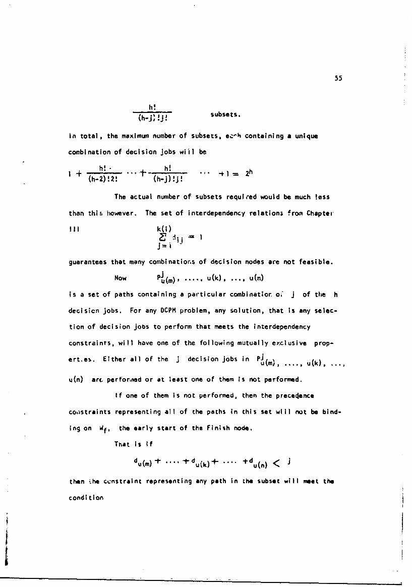
55

h!

(h-j,'!j7! subsets.

in total, the maximum number of subsets, e,-h containing a unique

combination of decision Jobs wiil be

I+ M . .. ,. h! I' - = 2h

(h-2)!2! (h-j)!J-

The actual number of subsets required would be much less

than this however. The set of interdependency relations from Chapter

ill k(l)

j = ij=i

guarantees that many combinations of decision nodes are not feasible.

Now Ptu(m)' .... , u(k), ... , u(n)

is a set of paths containing a particular combinatior ok" j of the h

declsicn jobs. For any DCPM problem, any solution, that is any selec-

tion of decision jobs to perform that meets the interdependency

constraints, will have one of the following mutually exclusive prop-

ert.es. Either all of the j decision Jobs in PJu(m), .. .,u(k), , .

u(n) arc performned or at least one of them is not performed.

If one of them is not performed, then the precedence

coostraints representing all of the paths in this set will not be bind-

ing on Wf, the early start of the Finish node.

That is if

du(m) - -du(k)- .. +du(n) < j

then ;.he ctcnstraint representing any path in the subset will meet the

condition

1 I

5C

M(-,• du(m)) l u(m) -...- (I-du(k))-I" tu(k) -..

-M(I-du(n)) + tu(n) + T <0 ': Wf

where T represents the sum of the times of non-decision Job, on the

path.

If all the jobs in the subset are performed, then the finish

day of the. project, Wf, will be constrained by equations representing

all paths in the subset. Since the constraints are identical except

that the. value for 7, the sum of the times of the non-decision jobs

on a particular path, vary, it is only necessary to retain the con-

straint that has the maximum value far T. All corstraints representing

other paths in the subset will be dominated by the one chosen. Thus we

require only ona path for-each possible combination of .':ision nodes.

We will term this path an "undominated" path.

3. Implementation of Dominance Tests for Path Elimination

This section will develop an algorithm based on the repeti Live

application of the largest path calculation to generate an undominated

set of paths in a daclsion network. As stated above, the undominated

path will simply be the longest path in a subset of paths which all

contain a particu!ar comtination of decision icts. For example, in

the -ubiet PJ I = I ...... j, if it is not empty, we must

calculate the longest path through jobs

Sso Su(i)' Su(2)' ..... u(k)' ..... 'u(j)' Sf

which goes through no other decision job. This is equi-a;ent to

J:I

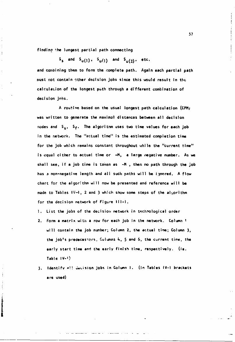
57

findina i-:he longest partial path connecting

Ss and Su(l), Su(l) and Su(2), etc.

and combining them to form the complete path. Again each partial path

niust not contain other dacision jobs since this would result In the

calculation of the longest p;th through a different combination of

decision jobs.

A routine based on the usual longest path calculation (CPMi

was written to generate the maximal distances between all decision

nodes and Ss, Sf. The algoritnm uses two time values for each Job

in the rnetwork. The "actual time" is the estimated completion time

for the job which remains constant throughout while the "current time"

is equal cither to actual time or -M, a large ,iegative number. As we

shall see, if a job time is taken as -M , then no path through the Job

has a non-negative iength and all such paths will be irnnred. A flow

chart for the algorithm will now be presented and reference will be

made to Tables IV-l, 2 and 3 which show some steps of the alqorithm

for the decision network of Figure I11-1.

1. List the jobs of the decisiori network in ttnchnological order

2. Form a matrix with a row for each Job in the network. Column I

will contain the job number; Column 2, the actual time; Column 3,

the job's predecestors, Columns 4, 5 and 6, the current ti",, the

early start time end the early finish time, respectively. (ie.

Table IV-.I'

3. Identify al! 4wicislon jobs in Column I. (in Tables IV-1 brackets

are used)

I

58

4. Set the current time, Column 4, for all decision jobs at -M, for

all other jobs set the current time equal to actual time. Set

counter ,1= Ss. Go to Step 8.

5. Beginning at I1, search down Column I for the first decision job

below II, say this is Su(n)- Set 11=Su(n).

6. Set the early start, Column 5, for all jobs above Il at -M.

7. Set the current time of I1 and the early start oý 11 at 0.

8. Calculate the ear!y start time of all jobs beneath I on the

technologically ordered Job list. If the early start value cal-

culated is negative, enter -M in the early start column. To

calculate :he early start of the job directiy beneath I1, list all

the predecessors of the job and for each predecessor add the

predecessors early start t•ime to its current time. The largest

of these values, for all predecessors, is the early start time for

the Job being considered. Then proceed to the text job on the

technologically ordered list for the next early start calculation.

9. For all decision jobs, add early start time to actual time to

compute early finish time, Column 6.

i0. For all 6ecislon jobs beneath II on the technological list and for

Sf, record the early finish time if It is non-negative. These

times will be the longest sub-path from the finish of decislon Job

I1 to the finish of the decision Job being examined (the longest

path containing no other decr.sloa Job).

II. If I1 Is the last decision Job in the technological list, go to

Step 12. If not, ejo to Step 5.

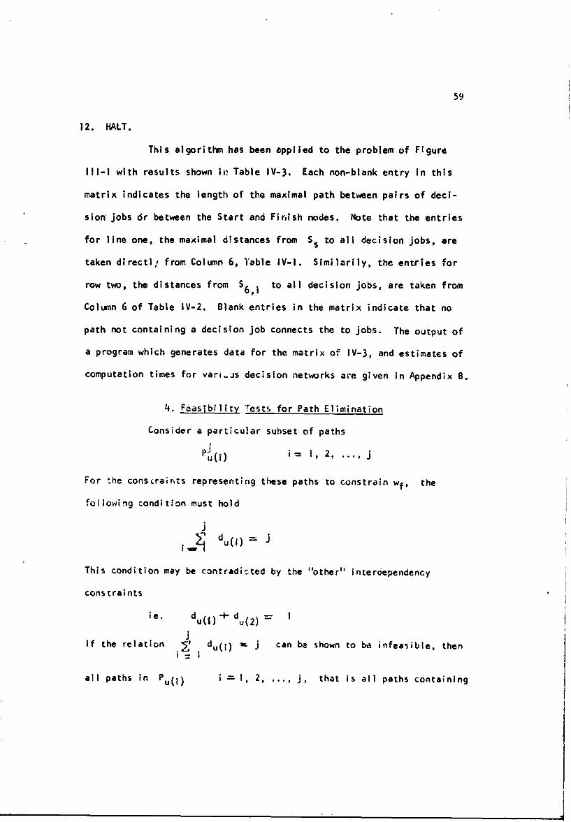
59

12. HALT.

This algorithm has been cpplled to the problem of Figure

I11-1 with results shown in, Table IV-3. Each non-blank entry in this

matrix indicates the length of the maximal path between pairs of deci-

sion jobs dr between the Start and Firish nodes. Note that the entries

for line one, the maximal distances from Ss to all decision Jobs, are

taken directi; from Column 6, Table IV-I. Similarily, the entries for

row two, the distances from $6,1 to all decision jobs, are taken from

Column 6 of Table IV-2. Blank entries in the matrix indicate that no

path not containing a decision job connects the to jobs. The output of

a program which generates data for the matrix of IV-3, and estimates of

computation times for vari-is decision networks are given in Appendix B.

4. Feastbility Tests for Path Elimination

Consider a particular subset of paths

,,i ) i -= , 2,. ..

For the consLrairits representing these paths to constrain wf, the

following condition must hold

jI_ du(1 )=J

This condition may be contradicted by the "other" interdependency

constraints

ie. du(i) + du( 2 ) 1

JIf the relation •, du(i) x. j can be shown to be infeasible, then

a= I

all paths in Pu(i) i - I, 2, ..... j, that Is all paths containing

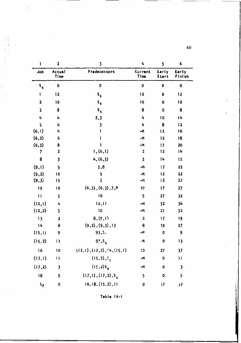
60

I 2 3 4 5 6

Job Actual Predecessors Current Early EarlyT; fTime Start Finish

S 0 0 0 0 0S

I 12 Ss 12 0 12

2 10 Ss 10 0 10

3 8 s5 8 0 8

4 4 2,3 4 10 14

5 4 3 4 8 12

(6,1) 4 1 -H 12 16

(6,2) 6 1 -M 12 18

(6,3) 8 1 -M 12 20

7 2 i,(6,1) 2 12 14

8 3 4,(6,3) 3 14 12(9, ) 5 5,8 -H 17 22

(9,2) 10 5 -M 12 22

(9.3) 15 5 -M i2 27

10 10 (6,3), (6,3),7,R 0 17 27

11 5 10 5 27 32

(12,1) 4 10,11 -M 32 36

(12,2) 5 10 -, 27 32

13 2 8,(9,11 2 17 19

14 8 (9,2),(9,3),13 8 19 27

(15,J) 9 93,S -M 0 9

(15,2) 13 97,s 5 *K 0 13

16 10 (12,1), (12,2) ,!4, (15,1) 10 27 37

(17,1) 11 (15,2),.5 -H 0 11

(17,2) 3 (5,,2)ss -m 0 3

18 5 07,1) ,(17,2),S 3 5 0 5

S 0 16,18,(15,211.1 0 t7

Table IV-l

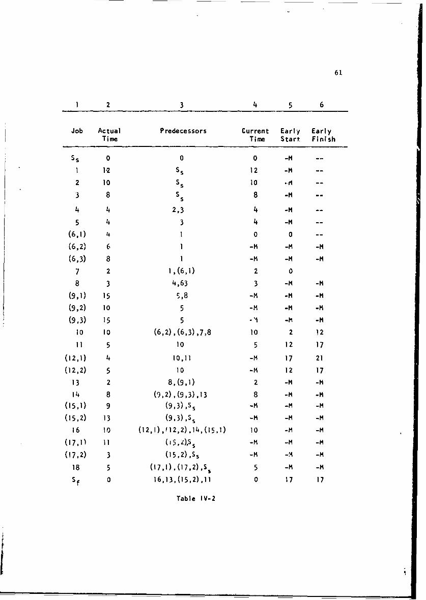
61

23 4 5 6

Job Actual Predecessors Current Early EarlyTime Time Start Finish

Ss 0 0 0 -M --

1 1.2 Ss 12 -M --

2 10 Ss 10 .--

3 8 S 8 -M

4 4 2,3 4 -M --

5 4 3 4 -M --

(6,1) 4 1 0 0 --

(6,2) 6 1 -M -M -M

(6,3) 8 1 -M -M -M

7 2 1,(6,1) 2 0

8 3 4,63 3 -M -M

(9,1) 15 5,8 -M -M -M

(9,2) 10 5 -M -M -M

(9,3) 15 5 I'1 -M -M

10 10 (6,2),(6,3),7,8 10 2 Q2

11 5 10 5 12 17

(12,1) 4 10,11 -M 17 21

(12,2) 5 10 -M 12 17

13 2 8,(9,1) 2 -M -M

14 8 (9,2), (9,3),13 8 -M -M

(15,1) 9 (9,3)#,s -M -M -M

(15,2) 13 (9,3),Ss -M -M -M

16 10 (12,1) ,,12,2) ,14, (15,I) 10 -M -M

(17,1) 11 (5, z),ss -M -M -M

(17,2) 3 (15,2),Ss -M -11 -M

18 5 (17,1),(17,2),Ss 5 -M -M

Sf 0 16,13,(15,2).1l 0 17 17

Table IV-2

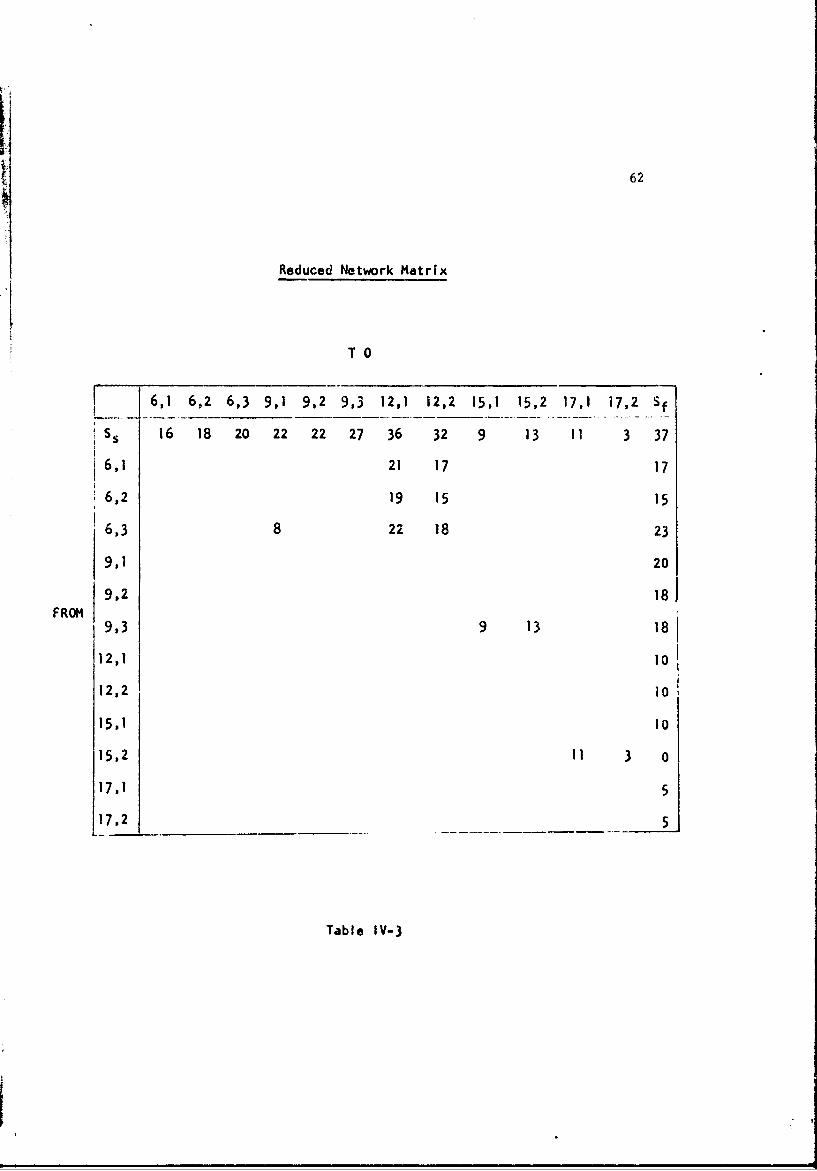
62

Reduced Network Matrix

TO

' 6,1 6,2 6,3 9,1 9,2 9,3 12,1 12,2 15,1 15,2 17,1 17,2 Sf

s 16 18 20 22 22 27 36 32 9 13 11 3 37

6,1 21 17 17

6,2 19 15 15

6,3 8 22 18 23

9,1 20

9,2 18FROM

9,3 9 13 18

12,1 10

12,2 10

15,1 10

15,2 I3 0

17,1 5

17.2 5

Table IV-3

63

the combination of decision jobs.

s i= , 2, .. ,

may be eliminated from the integer programming formulation of the DCPM

problem. Paths not eliminated by the interdependency constraints will

be termed `feasible" paths.

5. Application of Dominance and Feasibility Tests to a DCPM Network

When the tests of the previous three sections are applied

to precedency equations of the example Figure 111-1, the reduced set of

Sof Table IV-4 result. For example, the set P , containsequation' ( 2 ) cnan

the j paths

ti + t 7 + ti0 -M(l-d) 2, 1) + ti 2,- + t16 /f

t1 +'7 +tl4- tiI -H(idl2,1 )- t 12 , 1 + 16 416

t 2 + t 4 +t 8 +tl 0 'tti -"H(i-d 12, 1)-+ t 12, 1 + t 16 OWf

t2 + t4 + t 8 -+- tIO -M(I-dl2,j) - t ,12 ,1 t- t 16 -, f

t --4 + t8 4- tlo +" tl I"H(l'dl2,) -I-t1, -- tl]6 <Wf

t3 * 4 t--t 8 + t10 -H(l-dl2, 1 ) t-12,1 -$-t1 6 '4f

These may be rewritten

-M(I-d 12,1 ) 4- 38 • Wf

-M(I- l2, 1 ) + 43 ýi,

-M(l-dl2, 1 ) +46 1 4f

-M(I-d 12 ,) 4- 41 -'

i2,1 f

-MII 2 1) + 4

64

37 < wf

-M (I -d6.3) 4 43 4 wf

-MO (1 -. 42 <Wf

-M(0-dq, 2 ) + 40 (Wf

-M(I--d 9 ) + 45 •Wf

-M(I-dl2, 1 ) 4 46 Wf

-M(I-d1 ) -.1 42 ,Wf12,2

-MO(-d6,1) -M(1-d12 , 2 ) 4 43 <Wf

"-M(-d 6 ,2) -M(I-dl2, 1 ) +- 37 < Wf

-M(I-d 6 3 ) -M(1-d 12 2 ) +48 <Wf

-H(1-d9 3 ) -M(I-d-f) "46 < Wf

-M(l-d 9,2 ; -M(l-d -M(I-d,) + 56 (Wf15,3) 117,,2)

-M(I-di5, 2) -M(I-d 17, 1) +-29 (Wf

-M(I-dl,, 2) -M(i-d 17 , 2) -- 21 < Wf

4(1,-( d17,1) -4. 16 (< Wf

-M(I-d 1 7 , 2) + 8 <,Wf

-M(I-d9.3) -M'l-d15,2) -M(l-d17,1) 5T 4, 2 WVf

Table IV-4

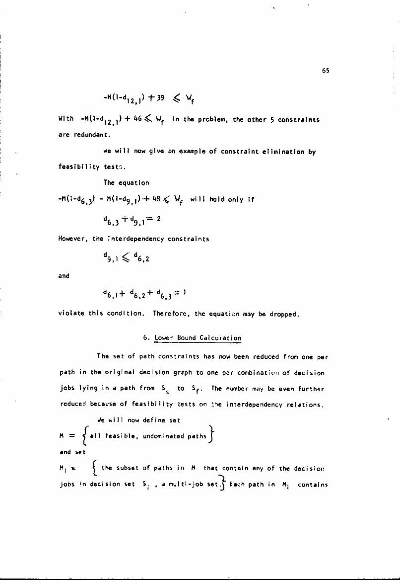
65

-M(I-dll "t-39 Wf

With -M(I-d 1 2 1)-l- 46•, '/f in the prcblem, the other 5 constraints

are redundant.

We will now give an example of constraint elimination by

feasibility testr,.

The equation

-M(i-d 6 , 3) - M(I-d 9 , 1)-4-48,•" Wf will hold only if

d6 , 3 t d9 l= 2

However, the interdependency constraints

d•! • d6,2

and

d6 ,1 + d6,2 + d6,3= I

violate this condition. Therefore, the equation may be dropped.

6. Lower Bound Calcuiation

The set of path constraints has now been reduced from one per

path in the original decision graph to one par combination of decision

Jobs lying in a path from Ss to Sf, The number may be even furth,,r

reduced because of feasibility iests on ".he interdependency relations.

We will now define set

M fall teasible, undominated paths

and set

Mi M -[ the subset of paths in M that contain any of the decision

jobs in decision set S.i , a multi-Job set.. Each path in Mi contains

66

exactly one of Sj, J= 1, 2, ... k(i) since we are assuming that

only one Job from each multi-Job set may be aelected, but they may also

contain other Jecision jobs.

We will now define a "feasible solution" to a DCPM problem as

a selection of a set of decision jobs that will satisfy all "alternative"

and "other" interdependency constraints on the problem. This set of

decision jobs will, with the non-decision jobs, form a usual project

graph of the critical path method. Given the project graph resultinq

from a "feasible solution", we state that one of the paths from Mi

will be included in that graph. If no such path exists, then no path

through Si exists in the network. This would violate our assumption

that Ss is a predecessor and Sf is a successor to all Jobs in the

project graph.

Each constraint representing a path from Mi will be of the

general form

.M(I-djj) .............. .M(I-dmn) + Ti, 4 4 W f

where Ti,, is the length of path e in Mi.

If one of the paths from Mi must be performed, then a

lower bound on Wf is the lowest value of Ti,e for all paths in Hi.

Furthermore if we calculate a ower bound for every decision node, we

may select the highest ot the iower bounds as a lower bound on 6f.

Any undominated, feasible pat., wh!ch is shorter than this Sound may be

ellmin~ted sincc it is redundant, given the bound on Wf.

Sii

67

An Application of bDwer Bound Calculation

The reduced set of equations from Table IV-4 will be used to

illustrate the dominance tests described above. The only feesible paths

through S6 , that is the set H6 , are the following paths,

-M(l-d 3)+ 43 Wf- 6l-,3 4wf

-M(I-d 6,) - M(I-d 12,t)-+ 47 Wf

-m(-4 6,2) - M(I-d2,2 2 ) -+ 43 . Wf

-M(l-d 6 , 3) - M(1-d 1 2 , 1 )4--52 4. Wf

The minimum of the T. e--,...,4, is 43 and therefore 43 is

a lower bound on the length of the critical path. Similarly, the lower

bound provided by M9 is 40, M12 is 42, M i5 is 21 and M17 is 8.

These calculations are shown in Table iV-5. The highest of the bounds

is then 43 and all paths shorter than or equal to th.s may be removed.

For this particular problem this reduction technique does not give any

further improvement. The final set of predecessor constraints may now

be written

(1)-!-43 Wf

(2) -M(I-d, 3 ) 9 45 4 Wf

-M(l-d,) + 46 ' WfC, ~ 1201f

-M(;-d, 3) -M(l--d1 5 1 ) -+ 46 , Wf

(5) -M(-(,6. -'4l-d 2 ,) -t 47 4 Wf

68

(6) -M(i-d ,3)-M(I-d 5,2) -(I-d 1,) 2 + 48 W f

(7) -M(I-d6,3) -M(I-dl 2 ,1 ) + 52 4. Wf

(8) -M1l-d 9 ,3)-M(I-d 15 ,) -MO(-dT17 ,) + 56 . Wf

By relecting appropriate values for M and combining, these

may be rewrl tten

(1) (3) 3d121, + 43 w f

(2) (4) 15d 9,34d 15 ,1 + 39 w Wf

(5) (7) 4d6, 1 4 9d 6 ,3-4 4dl2,1 + 39 w f

(6) (8) 15d 9 3 4 13d 1 5 ,2 +i~d 17 ,1 43d417v2+17 w f

The final problem, now in reduced path form, may be solved by

any standard integer programming technique.

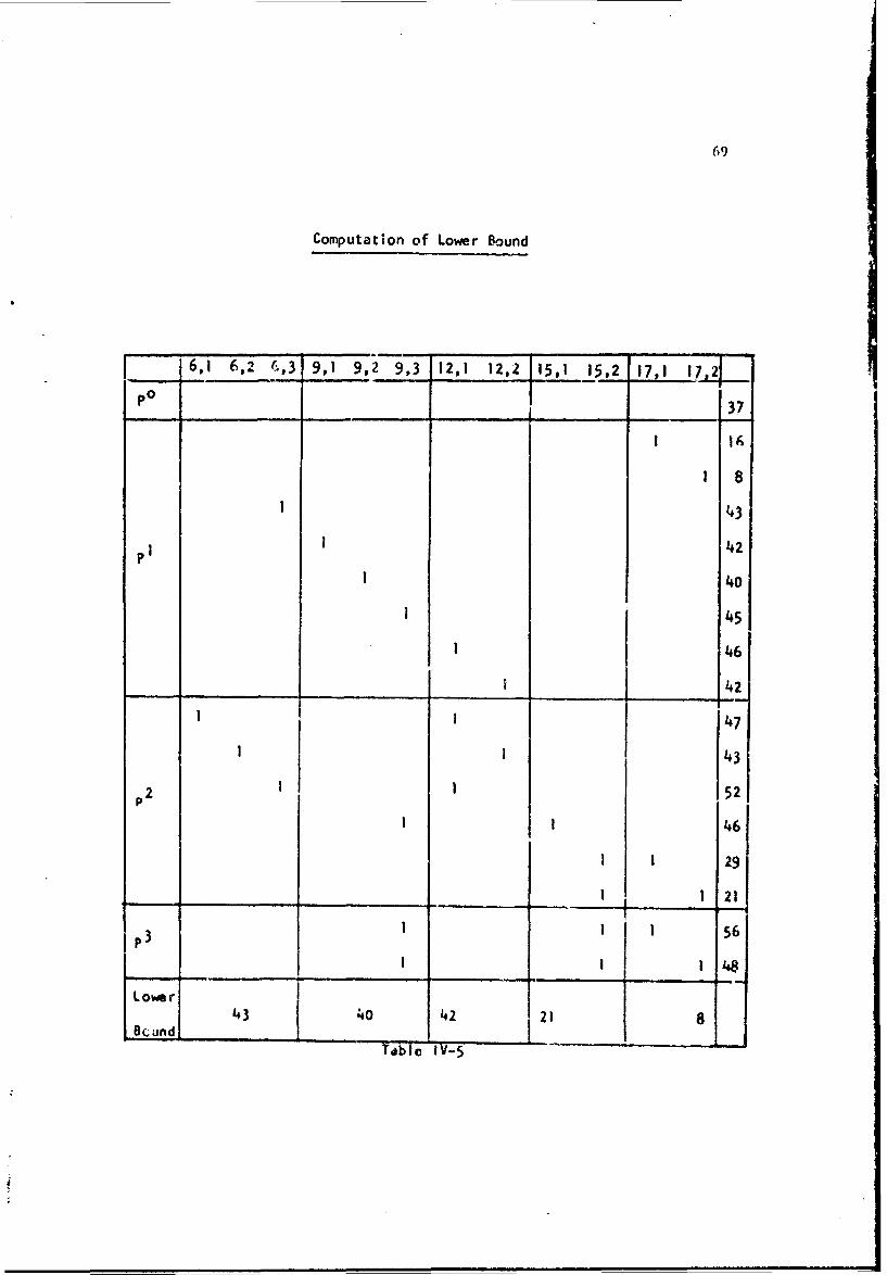
69

Computation of Lower Bound

6,1 6,2 6,3 9,1 9,2 9,3 12,1 12,2 15,1 15,2 17,1 17,2?

p 1 37

161 8

43

1 42

1 40

I 45

I 46

___42

1I 47

I 43p2 I 52

SI I46

I I 29

I i_ _ -•

1 2

Lower

43 40 42 21 8Tabnd _ _ _S.. . b•' tv-s

Chapter V

A Network Algorithm for Restricted Types of Integer P~ograms

In the literature review of Chapter I, we referred briefly

to several integer programming routines for probiems containing 0,1

variab•4s. In our terms, these techniques could optimize planning

problems with'Job alternative" and "other," types of interdependency.

We will now develop an algorithm based on the calcul.ations of the

critical path method which will solve certain restricted types of

Integer programs. A numerical example of the algorithm will be given

and then the algorithm will be applied to a problem taken from the

decision jobs and Interdependency constraints of a decision network.

2. The Network Alqorithm

Consider the integer progranwing problem

(I) Maximize wb-+ b0

Subject to wAo c

w o , w integer

where b is an m x I column ve,.tr, b is a scalar, c is a I x n0

row vector and o and w are I x m row vectors with values assigned

to w so as to maximize che objective function stjbjec*. to thre constraints

of (I). AO is an n, x n matrix which megts the following assumption.

Assumption I: All rrws of A0 contain a mcximtLn of two non-zero

entries and these are found in adjacent columns. The programming

70

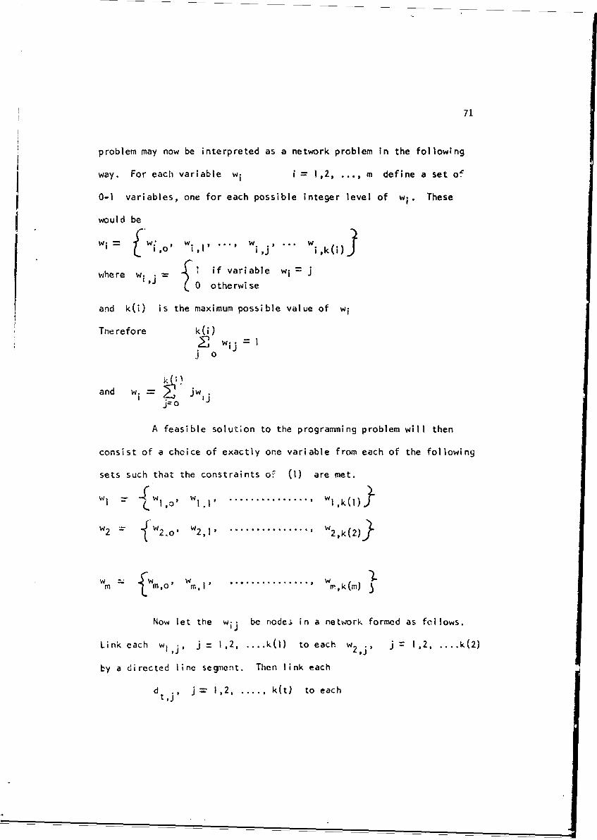
71

problem may now be interpreted as a network problem in the following

way. For each variable wi i = 1,2, ... , m define a set o,

0-I variables, one for each possible integer level of wi. These

would be

WiW , f Wi , ... , W. , ...wi I w ,o, ik(i)

whr wi if variable wi

where w,'J,- 0 otherwise

and k(i) is the maximum possible value of wi

Tnerefore k(i)~3 wo.j 0

and w. = WI

?~o

A feasible solution to the programming problem will then

consist of a choice of exactly one variable from each of the following

sets such that the constraints oC (I) are met.

WI w W . .. . . . .. . . . . . . . . . . . . . . w

w2 W2,o ' . ..w2,............... ,

Wm 2 w win, '.................. r, ,k(m) "

Now let the wij be node; in a netvwrk formed as follows.

Link each w1j, j = 1,2, .... k(l) to each w2 j, j - 1,2 .... k(2)

by a directed line segment. Then link each

d tj, j = 1,2. ..... k(t) to each

t ,i

72

dt + I,j' = 12, ...... k(t+ 1)

where t= 2, 3, .... , m-I

Since every variable in each set is linked to all veriables

in adjacent sets, the resulting network contains a path for all combina-

tions of integer values of wI, w2 , .... wm. Since there are no

links within a variable set, the restriction k(i).1I wij= Ij=o

Is maintained. Thus every feasible and non-feasible solution is repre-

sented by a path in the network and every path is a feasible or non-

feasible solution. Here a feasible solution is defined as the selection

of a level for each of the wi variables that meets tOe constraints

of (I). The network may now be modified to eliminate paths represent-

ing non-feasible solutions.

First vi will show how to calculate k(l), the maximum integer

value of variable w1 . Assume all variables wi, I-= 2, 3, .... m, r

have the value o, that is wo- I.

Then from the constraints in wA° 4 c of (I) that have

only positive entries, it is possible to calculate a maximixn value for

wi, that is k(l). Simnilarly, we may calculate maximum values for

all other variables.

We now have the graph

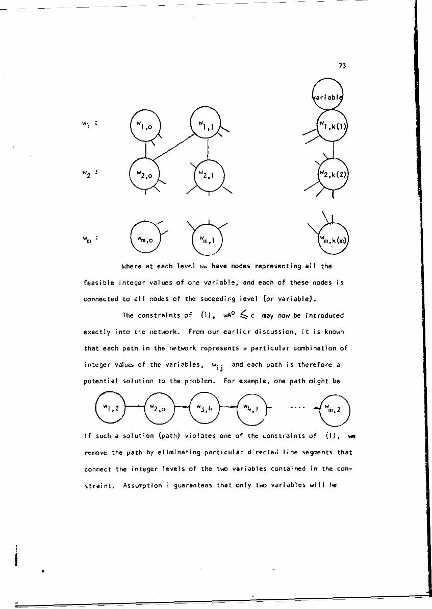
73

ariabi

WI ' o w I w I k(l)

W2W 2, W2 , 1 w2, k(2)

wm'o wm,lWkm

Where at each level w, have nodes representing all the

feasible integer values of one variab!e, and each of these nodes is

connected to all nodes of the suceedirg level (or variable).

The constraints of (1), wA° (c may now be introduced

exactly into the network. From our earlicr discussion, it is known

that each path in the network represents a particular combination of

integer vaoues of the variables, wj and each path is therefore a

potential solution to the problem. For example, one path might be

If such a solut'on (path) violates one of the constraints of (i), we

remove the path by eliminating particular d'rected line segments that

connect the integer levels of the two variables contained in the con-

straint. Assumption • guarantees that only two variables will be

I

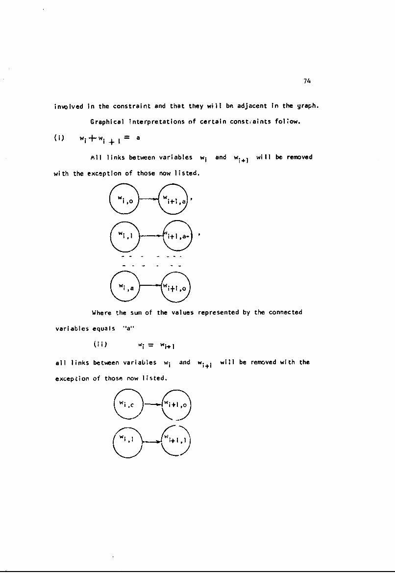
74

involved in the constraint and that they will be adjacent in the graph.

Graphical interpretations of certain constcaints fol'ow.

(i) wi- -+ w ---- a

All links between variables w, and w i+ will be removed

with the exception of those now listed.

& w i'o w i+l,aG-G.

& wi~a wi+l,o

Where the sum of the values represented by the connected

variables equals "a"

(ii) Wi = wi I

all links between variables wi and wi+i will be removed with the

exception of those now listed.

ilc

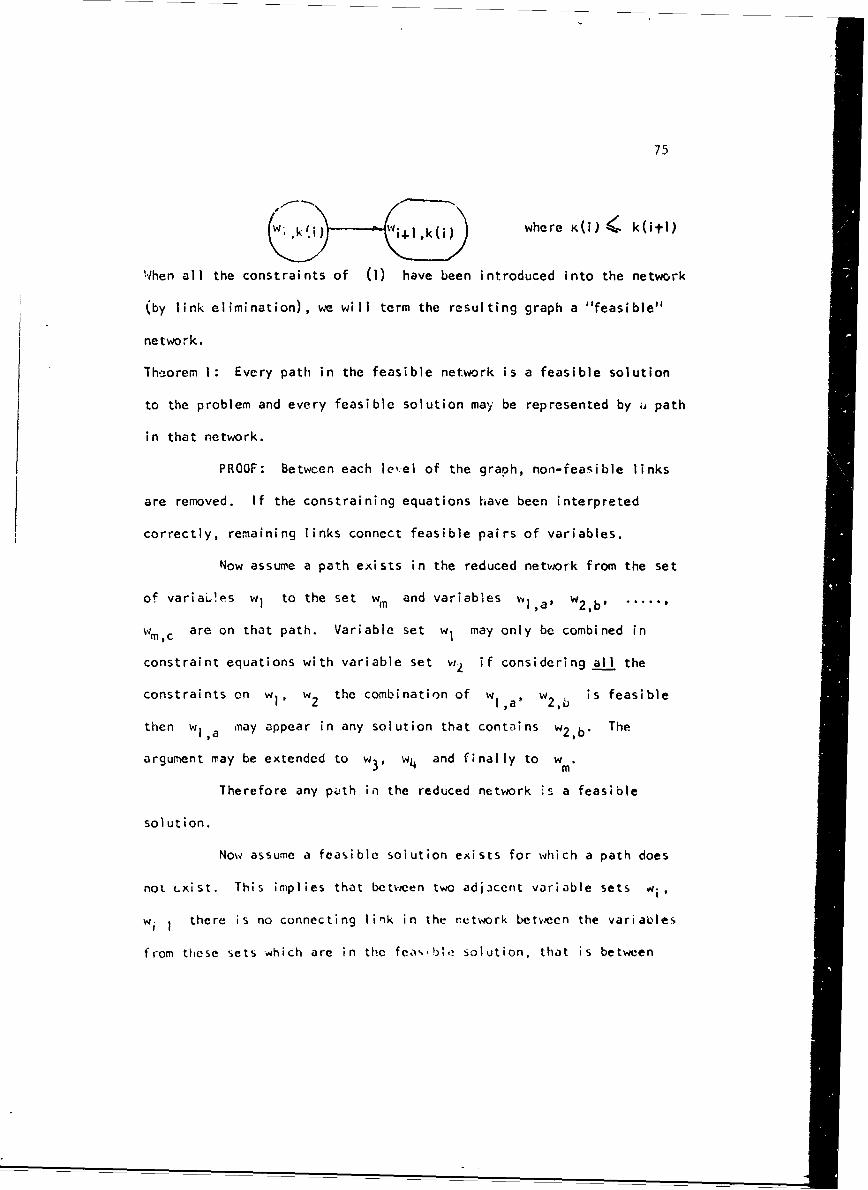
75

W' ,- Ow;ik(i) where K(i) -.' k(itl)

When all the constraints of (1) have been introduced into the network

(by link elimination), we will term the resulting graph a "feasible"

network.

Theorem 1: Every path in the feasible network is a feasible solution

to the problem and every feasible solution may be represented by i. path

in that network.

PROOF: Between each le,.el of the graph, non-feasible links

are removed. If the constraining equations have been interpreted

correctly, remaining links connect feasible pairs of variables.

Now assume a path exists in the reduced network from the set

of variaLlps w) to the set wm and variables wl,a' W2,b......

wm,c are on that path. Variable set w, may only be combined in

constraint equations with variable set w2 if considering all the

constraints on w,, w2 the combination of Wl,a'W 2 , is feasible

then wIa may appear in any solution that contains w2 ,b. The

argument may be extended to w3 , w4 and finally to w .m

Therefore any p~ith io the reduced network '- a feasible

solution.

Now assume a feasiblc solution exists for which a path does

not -xist. This implies that between two adjacent variable sets wi,

wi I there is no connecting link in the retwork between the variaeles

from these sets which are in the feo%,b•,, solution, that is between

76

W Wi+l,b" Since links are only removed if in combination they arc

infeasible under the constraints, then a solution containing wi a and

wi l,b is not feasible. Therefore every feasible solution must be

represented by a path.

Theorem 2: If each node, wij, of the netwo.K graph is evaluated at

jbi, the solution to maximization problem is the longest path in the

network.

PROOF: By Theorem I every path is a feasible solution to the

problem. Since wij represent the original variable wi at i teger

level j, the value of wij Tn the functional will be Jbi where bi

is the contribution of a unit of wi to the functional. The Fath

length for any solution is simply the value of the functional. The

variables on the longest path a;t those that give an optimum solution

to the maximization problem. Similarly the solution to a minimization

problem r iy be found by determining the shortest path.

The familiar rules of Critical Path Scheduling will calculate

the longest path in network. In this context the early start (E.S.)

for a variable wij is interpreted to be the maximum value of the

criterion function for variables w, to wi.I that may be feasibly

coib'ned with w.. (maximization). late start (L.S.) is the

maximum feasible value of the criterion function less the maximum value

of the criterion function for variablos wij to wm that may be

feasibly combineJI with wij.

In addition the "slak"' values calculate( by that technique

have meaning in this context. The slack values of a job indicates the

77

differmnce in length between the longest path on which the job Is found

and the longest path of the network. Since in the integer programming

problem, the path length is equivalent to the value of the functional,

and a solution is any path in the reduced network, the slack value

indicates the minimum change in the functional which will be realized

if wij is brought into the solution, Thus the "1slack" values are

exact evaluations for every wij, that is, for every variable wi at

every feasible level. These evaluations may be calculated for either

maximization or minimization problems. As we would expect, evaluators

for variables in the solution will be 0.

Theorem 3: If the variables in a problem which meets Assumption I may

be listed so that no constraint exists between wi, wi4 1l i -- 1.....

m-I then the optimum solution to a problem made up of the variables

w, . . . wi and the co:istraints relating to them and the optimum of

problem containing the variables wit . . w wi:1 together give an

optimum solution to the combined problem and the problems are independent.

PROOF: Let the optimum solution to the fiLt problem be a

path Wl,a, w2,b . . wi,,; and t0e solution to the second be

Wi l,a Wmb, Since rio constiaint exists betveen w., will, a1l

nodes are connected. Th,_-reore the longest path in the complete net-

work will consist of the lc.igest path aebve the level w. il plus the

longest path beiow wi, This will bc the sum of the individual solu-

tions to the two problems.

For purposes of the algorithm it is possible to have any set

of mrutually exclusive variables, rather than a series of mutw:lly;

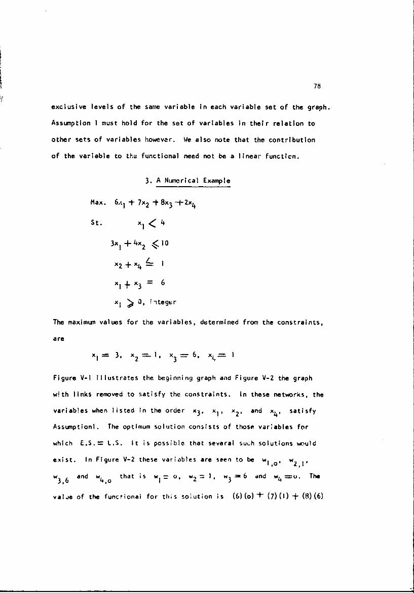
78

exclusive levels of the same variable in each variable set of the graph.

Assumption I must hold for the set of variables in their relation to

other sets of variables however. We also note that the contribution

of the variable to tha functional need not be a linear functicn.

3. A Numerical Example

Max. 6,t, + 7x 2 -t 8 x3 -- 2 x4

St. x, < 4

3x + 4x2 1,0

L 2x2-+FN4- 1

Xl+ x3 6

xi i 0, T'1teger

The maximum values for the variables, determined from the constraints,

are

x I = 3, x2 - l, x3 =-.- 6, - I

Figure V-I Illustrates the beginning graph and Figure V-2 the graph

wth links removed to satisfy the constraints. in these networks, the

variables when listed In the order x3 , x!, x2 , and x4 , satisfy

Assumptionl. The optimum solution consists of those variables for

which E.S.= L.S. It is possible that several such solutions would

exist. In Figure V-2 these variables are seen to be w],of w2

w and w that is wI- o, w2- = w3 == 6 and wi, =o. The

valie of the functional for this SOiution is (6)(o)"+ (7)() +- (8)(6)

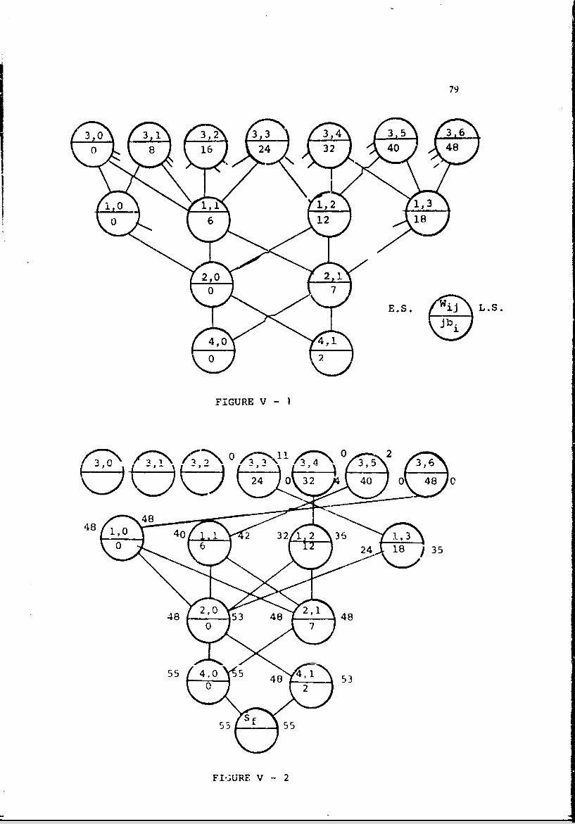
79

3•o 0 3 2 ,4• 3 5,3

0 6 12 183

FIGURE V-2

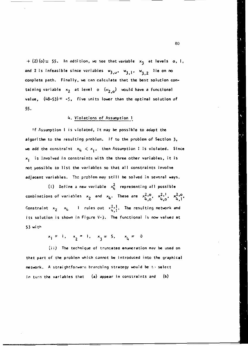
80

+ (2)(o)= 55. In addition, we see that variable x3 at levels 0, 1,

and 2 is infeasible since variabies w3 ,,, w3 ,1, w3, 2 lie on no

complete path. Finally, we can calculate that the best solution con-

taining variable x2 at level o (W2,o) would have a functional

value, (48-53)= -5, five units lower than the optimal solution of

55.

4. Violations of Assumption I

Of Assumption I is violated, it may be possible to adapt the

algorithm to the resulting problem. If to the problem of Section 3,

we add the constraint x4 < x!, then Assumption 1 is violated. Since

x I is invo!ved in constraints with the three other variables, it is

not possible to list the variables so that all constraints involve

adjacent variables. Tho- problem may still be solved in several ways.

(i) Define a new variable x2 representing all possible

combinations of variables x and x4 . These are x2o, x2', x2,o2 2,1 The reutn 4tr and4,1'

Constraint x2 x4 I rules out Y2,1. The resulting network and

its solution is shown in Figure V-3. The functional is now valued at

53 with

x= I, I, x3 = 5, x4 0

(ii) The technique of truncatea enur,-eration may be used on

that part of the problem which cannot be introduced into the graphical

network. A straightforward branching strategy would be t.l select

in turn the variables that (a) appear in constraints and (b)

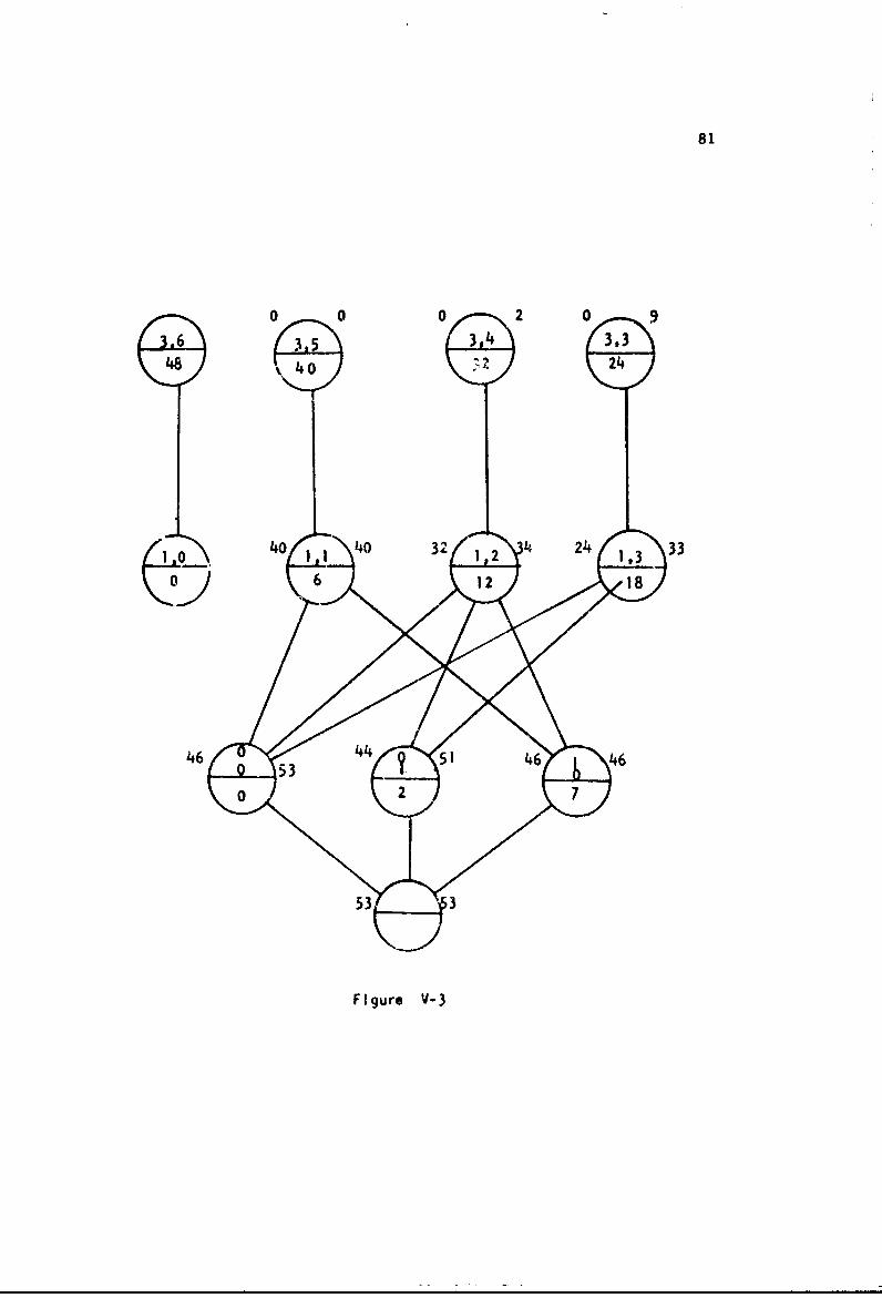
81

0 0 0 2 0 9

6 3 34 ý3,48 224

46 0 5 45 64

53 V 3

F Igure V-3

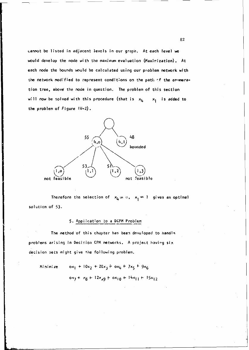
82

canrot be listed in adjacent levels in our graph. At each level we

would develop the node with the maximum evaluation (Maximization). At

each node the bounds would be calculated using our pioblem network with

the network modified to represent conditions on the path -f the enrtmera-

tion tree, above the node in question. The problem of this section

will now be solved with this procedure (that is x4 x1 is added to

the problem of Figure IV-2).

55 <,48

-bounded

not feasible not .easible

Therefore the selection of x4 = x, x1 I gives an optimal

soluticn of 53.

5. Appiicatton zo a DCPM Problem

The method of this chapter has been devutoped to handli

probl&ms arising in Decision CPM networks. A project hiavir.g six

decision sets might give the following problem.

Minimize ox, + I -N + 20,x4- ox4 + 7x 54 9x6

O°7 + x8 1 2 xA9 f °xlO 4- 14x, I 15x) 2

83

ox 1 j3-1 6x1 4 + ox1 5 + 13x 1 6 - k

Subject to "job alternative" interdependency

Job I xI 4 x2 4,.x 3 -- =

Job 2 x 4 + x 5 x6 =I

Job 3 x7 4-x 8 4-x 9 - I

Job 4 X 10 -r "I x12 -

Job 5 x 13 + x 14 = I

Job 6 x15 + x16 1

and "other" interdependency.

x 3 =x6

x7 = Xl

x5 ---x8

x2 + x5 4 1

x12 +.x l 1

x 8 '1 ]

xI -. x

If the job sets are ordered 6, 1, 2, 3, 4, 5, then all constraints may

be Inciuded in the first network. Figure V-4 illustrates the red-iced

graph and the evaluations of the variables. The minimum cost solution

to this problem is xIs-= 1 x2 1, xN =1, x7 -l, -10 1 and

x13 =1 for a total cost of 10.

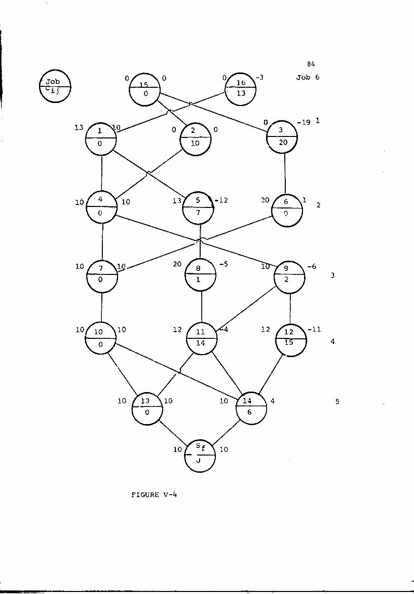
84

0 0 0 16 3job 6

0 13o

0• 10 20

I4

10 4_ 1 0 13 5 -12 20 6 1 2

I0 1 4 1 5 4 i

FIGURE V-4

Chapter Vi

Branch and Bound Algorithms for the DCPM Problem

In Chapter I1! the DCPH problem was formulated as an integer

programming problem but for large problems this approach would require

substantial computation time. Forthis reason, it was decided to

examine the applicability of rý,stricted enumeration solution techniques.

These methods, under the geneial name "branch and bound" have been

used for solving a series of .ather difficult cominatoria! problems.

The applications include the travelling salesman problem [27, 51-1

a version of the plant location problem L781, truck routing [62'1

and production sequencing problems •42, 47, 611. This work has

demonstrated that for a wide range of problems these techniques are

efficient.

The work "branch" in this context refers to a specific

decision rule for enumerating a tree of all possible solutions to the

problem. The "bound" term implies that at each node of the tree a

maximum value (for maximization problems) oi the criterion tunction is

calculated. This bound on the value of the criterion function for a

partial solution may indicate that no optimal solution will be found

that contains the particular partial solution and therefore search on

the path may he terminated. Alternately, the calculation may show that

the partial solution could be contained in an optimal solution to the

85

--I

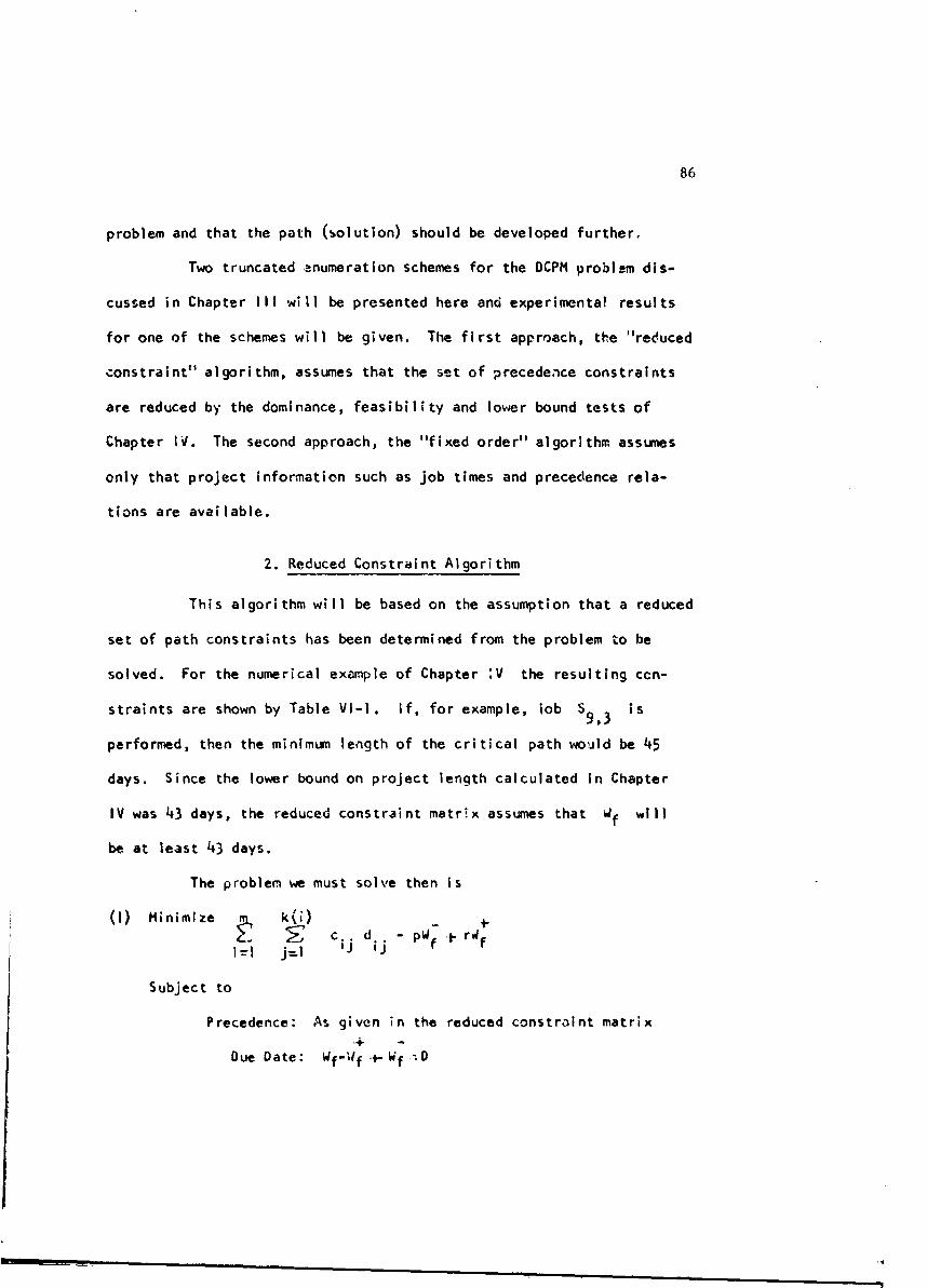
86

problem and that the path (solution) should be developed further.

Two truncated enumeration schemes for the OCPM problem dis-

cussed in Chapter III will be presented here and experimental results

for one of the schemes will be given. The first approach, the "reduced

constraint" algorithm, assumes that the set of precedence constraints

are reduced by the dominance, feasibility and lower bound tests of

Chapter IV. The second approach, the "fixed order" algorithm assumes

only that project information such as job times and precedence rela-

tions are available.

2. Reduced Constraint Algorithm

This algorithm will be based on the assumption that a reduced

set of path constraints has been determined from the problem to be

solved. For the numerical example of Chapter 'V the resulting ccn-

straints are shown by Table VI-i. If, for example, iob S9,3 is

performed, then the minimum length of the critical path would be 45

days. Since the lower bound on project length calculated In Chapter

IV was 43 days, the reduced constraint matrix assumes that Wf will

be at least 43 days.

The problem we must solve then is

(I) Minimize k(i) - 14 ' c d - pWf rf

I=1 j i ij

Subject to

Precedence: As given in the reduced constraint matrix

Due Date: Wrf-f .+-Wf --O

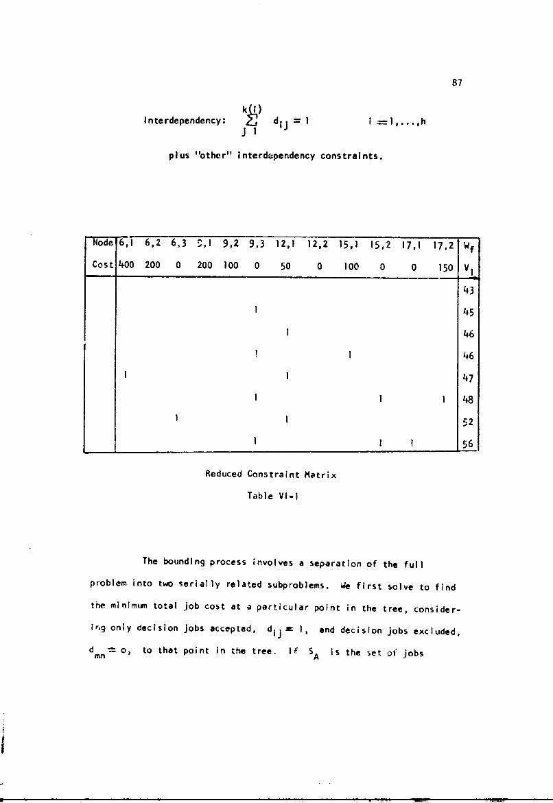
87

Interdependency: dij = I I-lJI

plus "other" interdependency constraints.

Node 6,1 6,2 6,3 n,l 9,2 9,3 12,1 12,2 15,1 15,2 17,1 17,2 Wf

Cost 400 200 0 200 100 0 50 0 100 0 0 150 VI

43

45

1 46

1 1 46

1 I47

I 1 1 48

11 52

1 1 156

Reduced Constraint Matrix

Table Vi-I

The bounding process involves a separation of the full

problem into two serially related subproblems. We first solve to find

the minimum total job cost at a particular point in the tree, consider-

ingg only decision Jobs accepted, dij = I, and decision jobs excluded,

d mn =o, to that point In the tree. If SA is the set of jobs

88

accepted and SE the set included

h k(i)(2) C= cij dij

i-= j=I

Subject to

ACCEPTANCE dij = I1 5ij {SA3

EXCLUSION dmn = Smn

Interdependency k(i)f dij--

jul

plus "other" interdependency constraints.

,'.'n optimal solution to this problem is the selection of a set

of the decision jobs which includes all of the jobs in SA, none of

the jobs in SE meets all interdependency constraints and minimizes

,job cost Cj. If no such solution exists, then that point of the tree

may be labelled as infeasible and no further search is required. If a

solution is found, then we can state that no set of decision jobs can

be selected, given existing constraints, that will have a lower total

job cost than Cj.

We have now calculated minimum job cost at a particular point

it, the tree and we now show that it is possible to add to it Cp, wh'ch

is a lower bound on penalty cost for the date of project comoletion.

Given the constraints implied by the jobs in SA and SF and given

the information from Table VI-',, it is possible to calculate a minimum

length for the critical path of the project. For example, if SA

contains job S9 , 3 and SE contains job Sl5,2' then we must do jobs

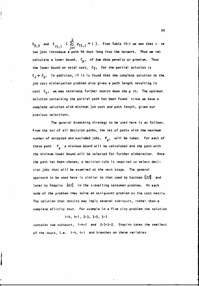
89

an9,3 15,1 d15 ,J d I ). From Table IV-I we see that t- seS9,315,1 j=l

two jobs introduce a path 46 days long Into the network. Thus we cars

calculate a lower bound, Cp, of due date penalty or premium. Thus

the lower bound on total cost, CT, for the partial solution is

Cj-+-Cp. In addition, if it is found that the complete solution to the

job cost minimization problem also gives a path length resulting in

cost Cp, we may terminate further search down the p th. The optimum

solution containing the partial path has been found since we have a

complete solution with minimum job cost and path length, given our

prev:ous selections.

The general branching strategy to be used here is as follows.

From the set of all decision paths, the set of paths with the maximum

number of accepted and excluded jobs, P,. will be taken. For each of

ppthese path P Pa minimum bound will be calculated and the path with

the minimum lower bound will be selected for further elaboration. Once

the path has been chosen, a decision rule is required EO select deci-

sion jobs that will be examined at the next stage. The general

approach to be used here is similar to that used by Eastman [27] and

later by Shapiro [67] in the t.ravelling salesman problem. At each

node of the problem they solve an assig9un.-nt problem on the cost matrix.

The solution that results may imply several sub-tours, rather than a

complete all-city tour. For example in a five city problem the solution

1-4, 4-1, 2-3, 3-5, 5-2

contains two subtours, 1-4-1 and 2-3-5-2. Shapiro takes the smallest

of the tours, i.e. 1-4, 4-1 and bra,,ches on these variables

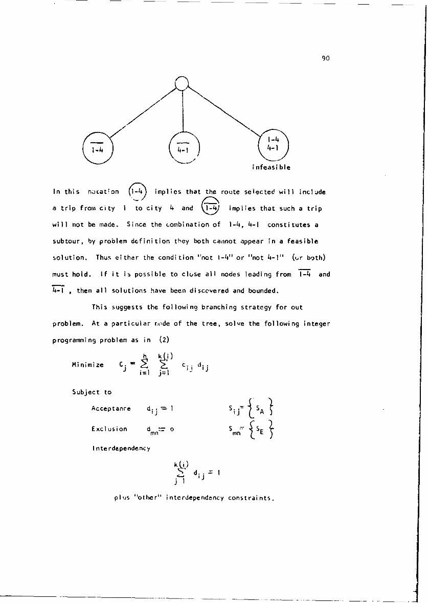
90

(& )11-4-infeasible

In this niataon (t', implies that the route selected will include

a trip from city 1 to city 4 and implies that such a trip

will not be made. Since the combination of 1-4, 4-1 constitutes a

subtour, by problem definition they both cannot appear in a feasible

solution. Thus either the condition '"not 1-4" or "not 4-1" (Or both)

must hold. If it is possible to close all nodes leading from 1-4 and

4-1 , then all solutions have been discovered and bounded.

This suggests the following branching strategy for out

problem. At a particular rode of the tree, solve the following integer

programming problem as in (2)

ý k i)Minimize C c.. d

J i=I j=l Ii

Subject to

Acceptance dij I S ij- SA A

Exclusion d n 0 o S -mn SE

Interdependency

k(Q)p o d..- c

plus "other"' interdependency constraints.

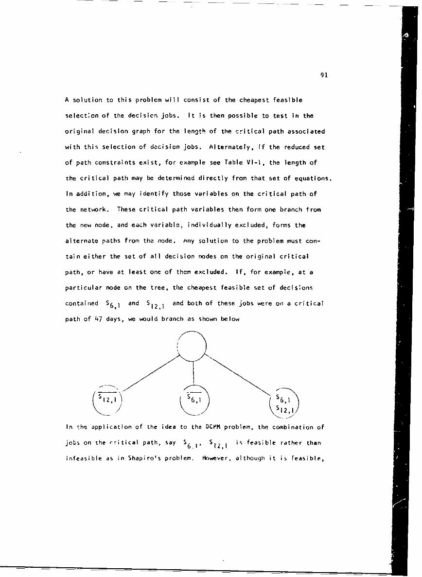
91

A solution to this problem will consist of the cheapest feasible

select:on of the decision jobs. It is then possible to test in the

original decision graph for the length of the critical path associated

with this selection of decision jobs. Alternately, If the reduced set

of path constraints exist, for example see Table VI-l, the length of

the critical path may be determined directly from that set of equations.

In addition, we may identify those variables on the critical path of

the network. These critical path variables then form one branch from

the new node, and each variable, individually excluded, forms the

alternate paths from the node. Any solution to the problem must con-

tain either the set of all decision nodes on the original critical

path, or have at least one of them excluded. If, for example, at a

particular node on the tree, the cheapest feasible set of decisions

contained S6,1 and SI2,1 and both of these jobs were on a critical

path of 47 days, we would branch as shown below

S6,

In th. application of the idea to the DCVM problem, the combination of

jobs on the rritical path, say S61. Si2, is feasible rather than

infeasible as in Shapiro's problem. However, although it is feasible,

92

it is never necessary to develop that particular node further. Given

the exclusions and acceptances to that point on the path, we solved a

programming problem to minimize the total job cost, Cj. The minimum

cost feasible set of jobs is then tested in the matrix of rable VI-I to

determine project length, project length cost Cp, and the set of jobs

on the critical path. Given that we do the set of jobs on the critical

path and that prior acceptances and exclusions be enforced, 'e total

cost can not be less than Cp-P- Cj and the solution that gives Cp

C. is a feasible solution to the problem. Thus the node is completely

developed.

If at any stage of the development of the tree, all new paths

generated are bounded by a previous complete solution or are infeasible

or if a complete solution has been ootained, it is necessary to ,,aove

backwards up the tree and pick new paths to develop. Again we find

the unbounded paths that have the maximum number of job acceptances

and exclusions and of these select the one with the minimum bound. This

implies that we move up th! tree to the first open node. The algorithm

will now be presented in flow chart form, then applied to the sample

problem of Figure Il-I.

Step I. Reduce the network by the dominance feasibility and lower

bound tests of Chapter IV to obtain the reduced constraint matrix.

Step 2a. Solve an integer programmlng problem to find the minimum cost

set of decision jobs that will meet all interdependency constraints.

Set the value of Cp to tjual the cost of this solution. Go to Step 3.

Step 2b. Select the complete ,olution and the job cost Cj calculated

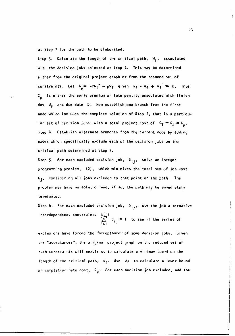
93

at Step 7 for the path to be elaborated.

S tlp 3. Calculate the length of the critical path, Wf, associated

witih the decision jobs selected at Step 2. This may be determined

either from the original project graph or from the reduced set of

constraintS. Let C -rWf -- pWf given Wf - Wf t Wf" = D. Thus

Cp is either the early premium or late pen ,Ity associated with finish

day Wf and due date D. Now establish one branch from the first

node which incluJes the complete solution of Step 2, that is a particu-

lar set of decision jtis; with a total project cost of C.T -l-C = ---

Step 4. Establish alternate branches from the current node by adding

nodes which specifically exclude each of the decision jobs on the

critical path determined at Step 3.

Step 5. For each excluded decision job, Sij, solve an integer

programming problem, (2), which minimizes the total sum uf job cost

Cj, considering all jobs excluded to that point on the path. The

problem may have no solution arid, if so, the path may be immediately

terminated.

Step 6. For each excluded decision job, Si,, use the job alternative

interdependency constraints k__)di -- I to see if the series of

'.I1

exclusions have forced the "acceptance" of some decision jobs. Given

the "acceptances", the original project graph on the reduced set of

path constraints will enable us to calculate a minimum bou--d on the

length of the criticai patr., Wf. Use 4f to calculate a lower bound

on comp',etion date cost, C . For each decision job excluded, add the

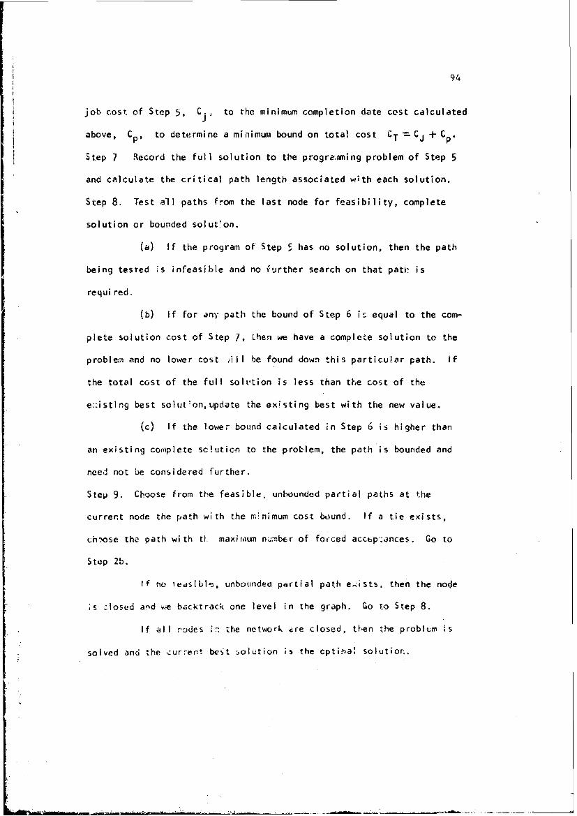
94

job cost of Step 5, Cj, to the minimum completion date cost calculated

above, Cp, to determine a minimum bound on total cost CT-= CJ + Cp.

Step 7 Record the full solution to the progranming problem of Step 5

and calculate the critical path length associated with each solution.

Step 8. Test all paths from the last node for feasibility, complete

solution or bounded solut'on.

(a) If the program of Step 5 has no solution, then the path

being tested is infeasible and no further search on that patr is

requi red.

(b) If for any path the bound of Step 6 if: equal to the com-

Splete solution cost of Step 7, then we have a complete solution to the

problem and no lower cost jill be found down this particular path. If

the total cost of the full solution is less than the cost of the

e.-isting best solution, update the existing best with the new value.

(c) If the lower bound calculated in Step 6 is higher than

an existing com'~plete sc!uticon to the problem, the path is bounded and

need not be considered further.

Step 9. Choose from th;e feasible, unbounded partial paths at the

currert node the path with the rrinimum cost bound. If a tie exists,

ch-ose tha path with t0. maximum number of forced accep--ances. Go to

Step 2b.

If no ieasible, unboundea partial path eCIsts, then the node

is Josed and we backtrack one level in the graph. Go to Step 8.

If all r.odes it zhe network are closed, toen the probl-.m is

solved and the current best solution is the cptional solutior,.

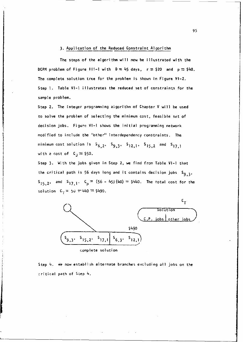
95

3. Application of the Reduced Constraint Algorithm

The steps of the algorithm will now be illustrated with the

DCPM problem of Figure 111-1 with D-- 45 days, r = $20 and p-- $40.

The complete solution tree for the problem is shown in Figure VI-2.

Step I. Table VI-I illustrates the reduced set of constraints for the

sample problem.

Step 2. The integer programming algorithm of Chapter V will be used

to solve the problem of selecting the minimum cost, feasible set of

decision jobs. Figure VI-I shows the initial programming network

modified to include the "other" interdependency constraints. The

minimum cost solution is J6,2, S9,3, 512,1, S15,2 and S17,1

with a cost of Cj $50.

Step 3. With the jobs given in Step 2, we find from Table VI-I that

the critical path is 56 days long and it contains decision jobs S9, 3 ,

$15,2, and S17,1- Cp (56 - 45)(40) $440. The total cost for the

solution C., 5U J-440 $490.

CT

Solution

C.P. jobsi other iobs

$490

S9, S II5lS S6, 3' Sl2,3l

complete solution

Step 4. We now establish alternate branches excluding all jobs on the

critical path of Step 4.

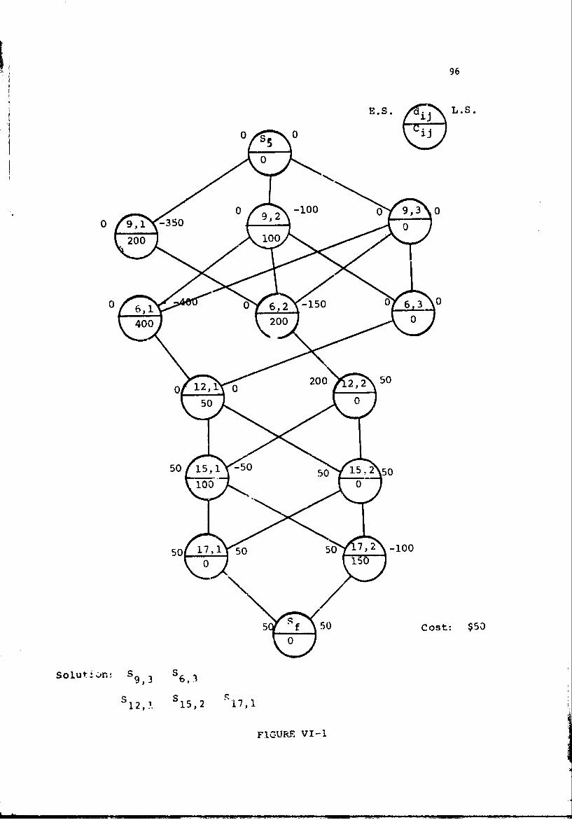
96

E.S. /t** L. S.

S C

o 9 1 -30 0, 2 100 0 9,3-

02,3 S15,2 "17,1

FIGURE VI-5

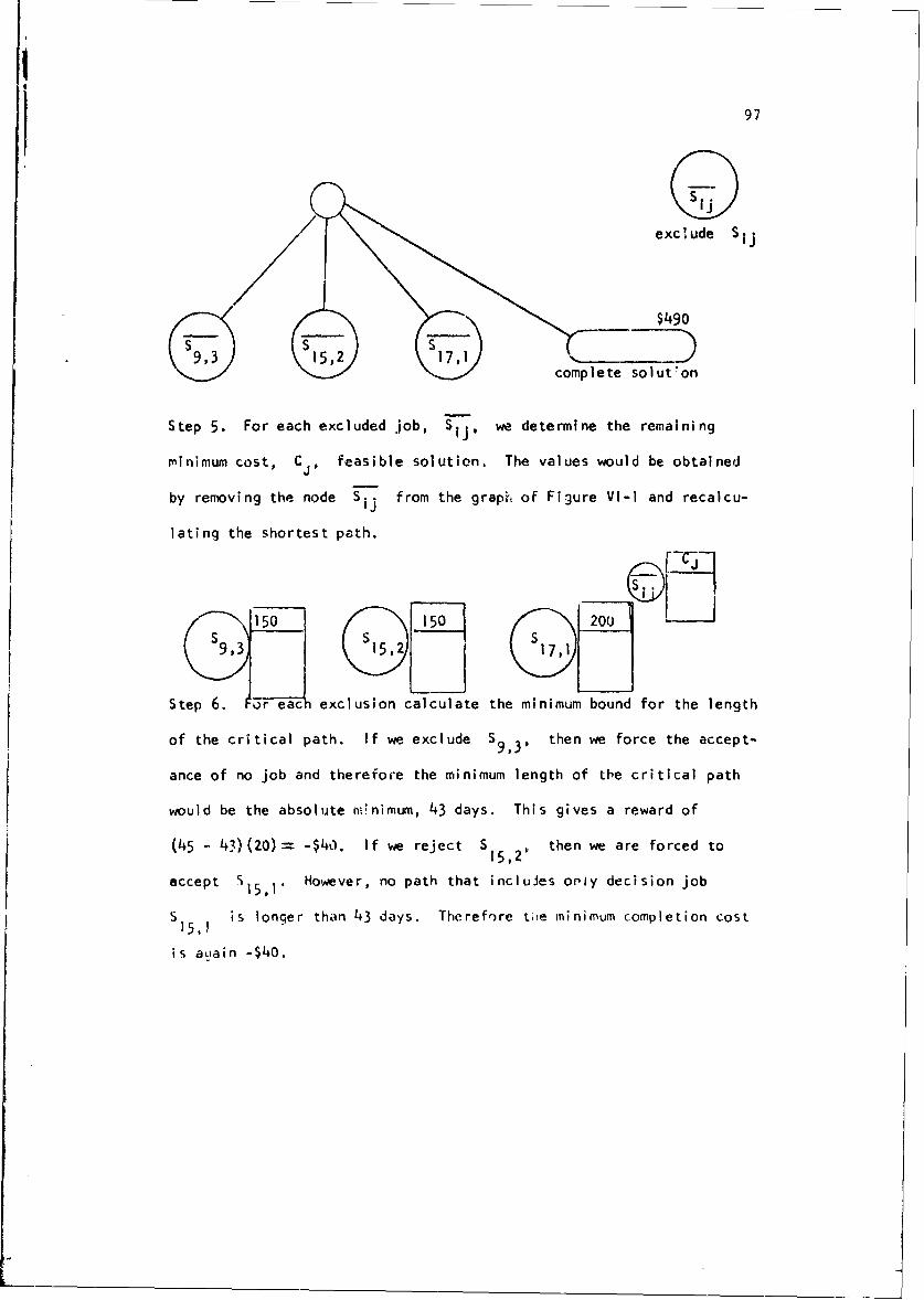
I

97

exclude Sjj

$490

complete solut~on

Step 5. For each excluded job, S-j, we determine the remaining

minimum cost, Cj, feasible solution. The values would be obtained

by removing the node Sij from the graph- of Figure VI-I and recalcu-

lating the shortest path.

S93 15 ,2 I

Step 6. JTr eac- exclusion calculate the minimum bound for the length

of the critical path. If we exclude S9, 3 , then we force the accept-

ance of no job and therefore the minimum length of the critical path

would be the absolute w-mnimum, 43 days. This gives a reward of

(45 - 43)(20)= -$40. If we reject Si5,2, then we are forced to

accept S1 5, 1 . However, no path that includes orly decision job

S is longer than 43 days. Therefore tie minimum completion cost

is auain -$40.

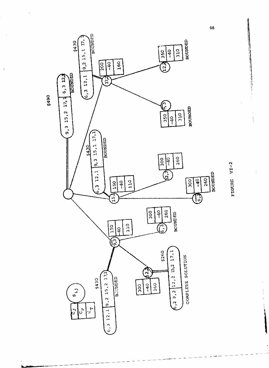
9B

0

0)

0 0r-4 N4

r4-

cn0

00

0 r- 0

r-44

ca 0

M C:I

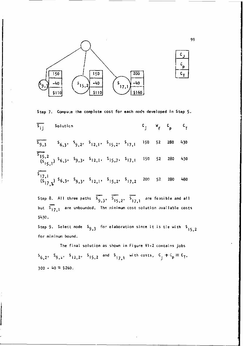
99

150I 1020

-40 .1 -L S C1.

9, -0S15,2 $110S 17,1

Step 7. Compute the complete cost for each node developed In Step 5.

C Solwuticn C Wf C CT

S9,3 S6,3$ 59,2, S12,1' S15 ,2, el7,1 150 52 280 430

=515,2) S63 S93 S12| S157 Sl 150 52 280 430

17 ) s6,3' s9 S 2's 200 52. 280 480(S9 6 ,3' 12,1' 15,7' 17,2

Step 8. All three paths S3' S5,2' Sl1,I1are fe3sible and all

but S 7,1 are unbounded. The minimum cost solution 3vaflable costs

$430.

Step 9. Select node S9 .3 for elaboration since it is tie with S152

for minimum bound.

The final solution as shown in Figure VI-2 contains jobs

S6,2, S9,zo S12,2, S15,2 and Sl17 l with costs, Cj -C P CT

300 - 40 $260.

100

4. Fixed Order Algorithm

The second scheme proposed works directly from the matrix of

Table IV-3, the reduced network matrix, which shows maximal distances

between decision Jobs in a decision 9raph. For convenience this table

will be reproduced as Vi-2.

Reduced Network Matrix

6) 6,2 63 9,1 9,2 93 12) 12,. 15,1 1542 17,1 17J2 Sf

Ss 16 18 20 22 22 27 36 32 9 13 11 3 37

41 21 17 17

6ý 1915 15

63 8 22 18 23

%l 20

9,2 18

V 9 13 18

12,2 10

11 ii 3 0

17,1 5

142 5

Table VI-2

It contains inplicitly a reduced set of project paths that exist in the

L.

101

original network Figure Ill-i . In this elgorithm the order of

selection of decision sets is strictly determined, that is for our

problem an ordering of decision set S6 , S9, S121 Si5 and S17

might be chosen. In elaborating a particular decision set, the paths

to be considered are simply all possible decision jobs in the set under

consideration. At Si we consider branching on all Sij ) j =-I,2,

... ,k(i). This involves a feasibility test to see if the new job Sij

is consistent with jobs previously chosen on the path givwn the "other"

interdependency constraints. A feasible path is then selected for

elaboration based on a calculation of a total cost bound for each

feasible path. As in the first algorithm, the path scaected will

always be from the most fully developed paths so that .e always push

directly down to a complete solution or halt bccause a path is bounded,

then backtrack up the tree closing open nodes as we find them.

At any node in the tree. it is possible to calculate

directly the total cost of decision jobs assigned on the path to that

point. If we add to this the total cout of minimum cost jobs in

decision sets from which no assignment has been made, we have a lower

uound on total job cost C In our problems the costs for jobs in

each decision set have been normalized, that is the smallest cost is

subtracted from all costs, ,o that the total minimum cost for unassigned

sets will always be zero.

At the node under consideration, it is also possible to

calculate a minimum length for the decision path under consideration.

A project graph can be constructed from the informration of Table VI-2

102

as we have done in Figure VI-3. The reduced graph is broken at all

unassigned decision nodes, and the longest path algorithm is applied

to find the shortest possible length of the network given previous

assignments. This value is a lower bound on project length and may be

used to calculate Cp -- minimum completion cost. CT- CJ 4- Cp gives

a lower bound for the particular path under consideration.

The stepS of the IgOrl ar.'-n . . .asfllo.

Step I. Normalize the cost of all jobs in decision sets by subtracting

the lowest cost for any mob in a set from all jobs in that set.

Step 2. Apply the routine of Chapter IV, Section 3, to find a reduced

network containing only decision jobs and maximal length paths between

decision jobs.

Step 3. Sequence the decision sets in a fixed order.

Step 4. Elaborate the first decision set in the fixed order list, for

which no assignment has been made and calculate total Job cost, Cj,

tor each resulting path. The integer programming algorithm of

Chapter V will find the minimum cost solution, given interdependency

constrairts and decision job acceptances. If no feasible solution

exists, then search on this path may be terminated.

Step 5. For each newly developed oath, find a minimum bound for the

length of the critical path, Wf, and evaluate the cost of this path

length as Cp. The reduced network from Step 2 may be used to compute

minimum project length. As in the algorithm of Chapter IV, Section 3,

we break Lhe recduced network at all decision jol-'s, then introduce only

those decision Jobs accepted on the partial path which is under

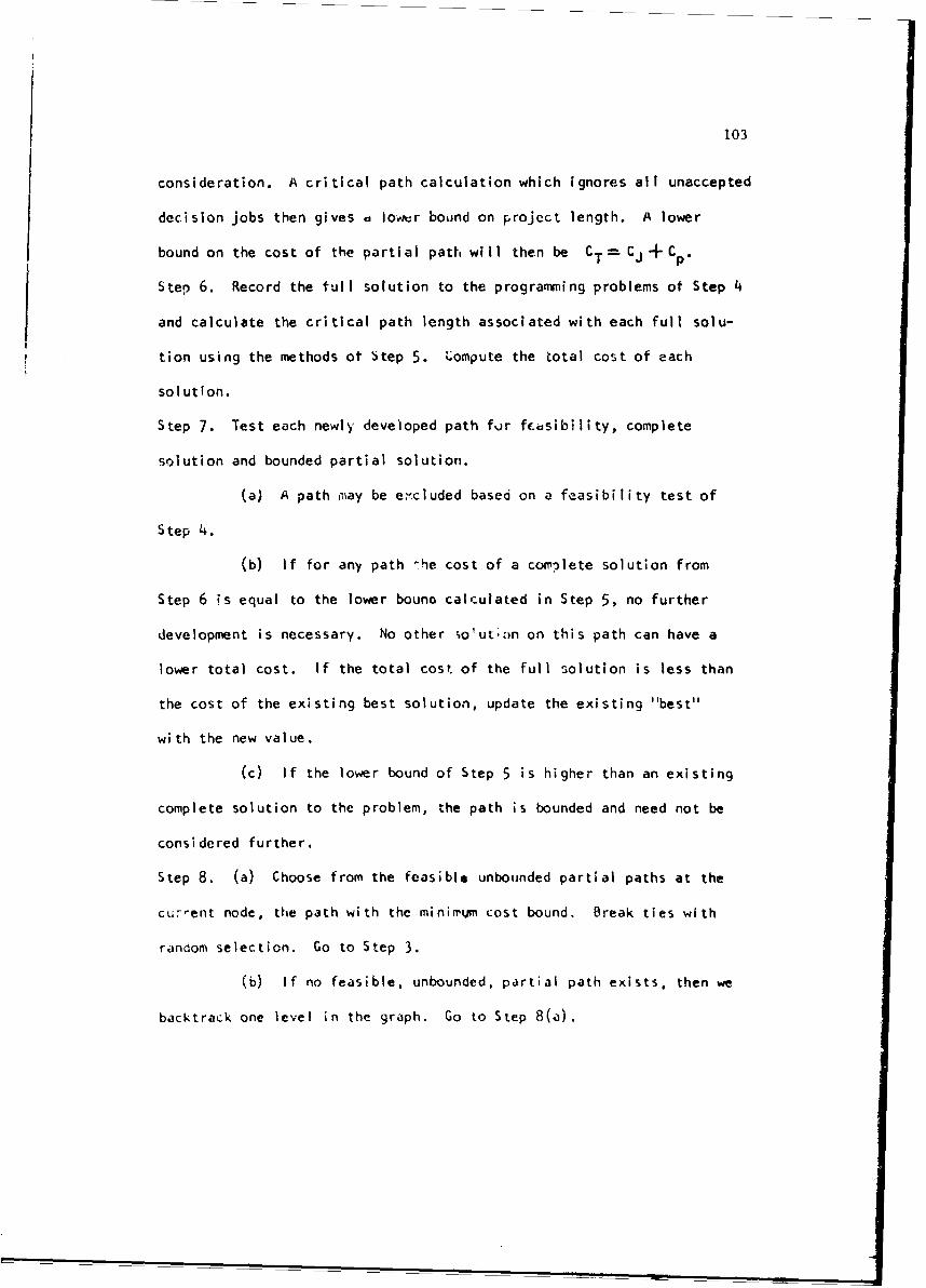
103

consideration. A critical path calculation which ignores all unaccepted

decision jobs then gives d laovr bound on project length. A lower

bound on the cost of the partial path will then be CT=CJ-+-Cp.

Step 6. Record the full solution to the programming problems of Step 4

and calculate the critical path length associated with each full solu-

tion using the methods of Step 5. c;ompute the total cost of each

solution.

Step 7. Test each newly developed path fur frdsibility, complete

solution and bounded partial solution.

(a) A path may be excluded based on a feasibility test of

Step 4.

(b) If for any path The cost of a complete solution from

Step 6 is equal to the lower bouno calculated in Step 5, no further

development is necessary. No other so!ut;;an on this path can have a

lower total cost. If the total cost of the full solution is less than

the cost of the existing best solution, update the existing "best"

with the new value.

(c) If the lower bound of Step 5 is higher than an existing

complete solution to the problem, the path is bounded and need not be

considered further.

Step 8. (a) Choose from the feasible unbounded partial paths at the

current node, the path with the minimum cost bound. Break ties with

random selection. Go to Step 3.

(b) If no feasible, unbounded, partial path exists, then we

backtrack one level in the graph. Go to Step 8(a).

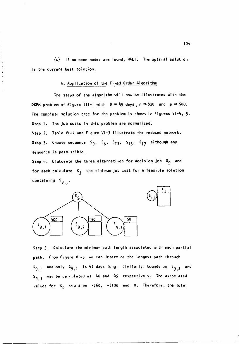
104

(c) If no open nodes are found, HALT. The optimal solution

is the current best solution.

5. Application of the Fixed Order Algorithm

The steps of the algorithm will now be il~ustrated with the

DCPH problem of Figure i1-1 with D - 45 days, r---$20 and p = $40.

The complete solution tree for the problem is shown in Figures VI-4, 5.

Step 1. The Jub costs in this problem are normalized.

Step 2. Table VI-I and Figure VI-3 i!lustrate the reduced network.

Step 3. Choose sequence S9 , S6, S12 , S1 5, S1 7 although any

sequence is permissible.

Step 4. Elaborate the three alternatives for decision job Sq and

for each calculate C. the minimum job cost for a feasible solution

containinln $9,1.

L90"(S9., 929.3

Step 5. Calculate the minimum path length associated with each partial

path. From Figure VI-3, we can Jetermine the longest path thrioigh

S9q, and only S9,, is 42 days long. Similarly, bounds on S,2 and

S9,3 may be cal•ulated as 40 and 45 respectively. The associated

values for Cp would be -$60, -$100 and 0. Therefore, the total

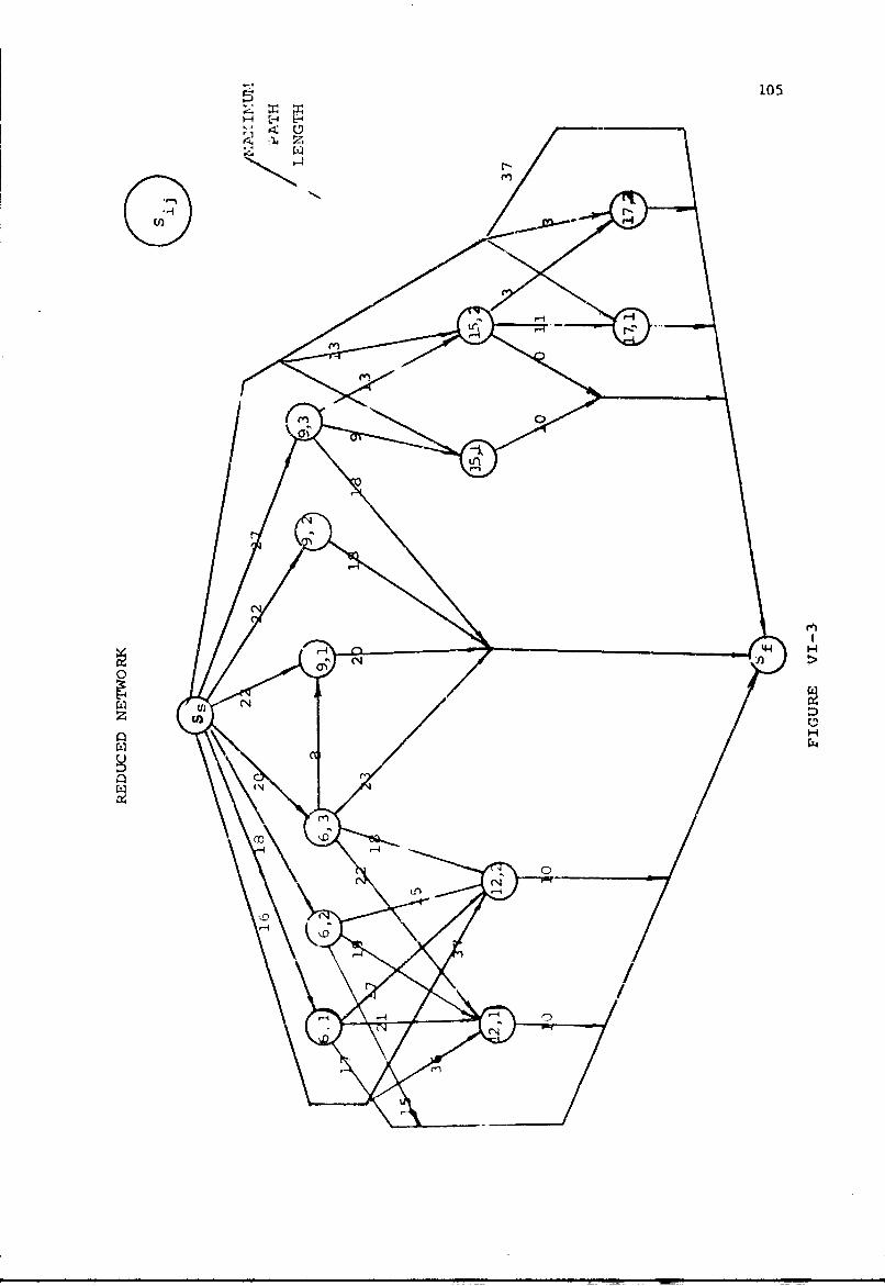
105E.4

HE44°14

0I

000 z b H

cr•

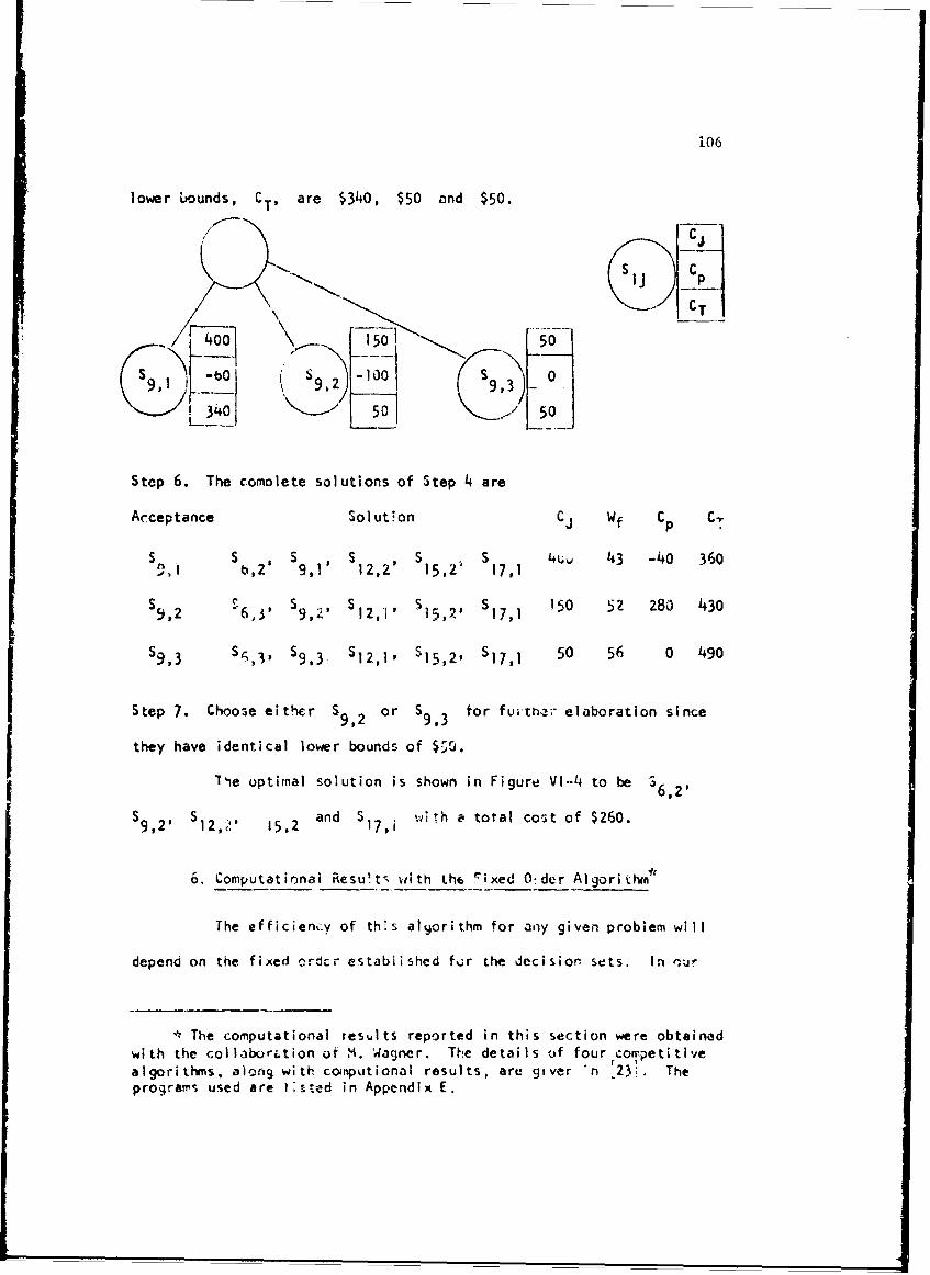
106

lower bounds, CT, are $340, $50 and $50.

I,- C

Aeceptance Sol uton CS Wf C Cp

2 S S9 , S ,S .5 4•v 43 -40 3604 , 0 0, 12,2 15,2k 17,1

S S S0 S 0

S9,2 r•6,3, 59,.1, 12,1', 15,2, S17,1 150 52 280 430

Sg,3 S•,3, S9 ,3 . $1, S15 ,2 , S 7, 50 56 0 490

Step 7. Choose eit~her S9, or S9, for fur-tive;- elaboration since

9,299,3

they have identical lower bounds of $•0.

S .he optimal solution is shown in Figure VI-4 to b

S9 S2 and a wh total cost of $260.- *

6. ComputationalResu'ts with the rixed O:der Algoritlh-* &=

The efficiency of this aliorit~hm for 3iny given problem willl

depend on the fixed rdcr estab9 l shed for the decisior sets. Ion sr

* The computational resouts reported In this section were obtainSdwith the colabor.ation of M. Wagner. The details Of four compethtive

algorithms, along with conpuitional results, are giver. *n _23;. Theprograms used are lIted in Appendix E.

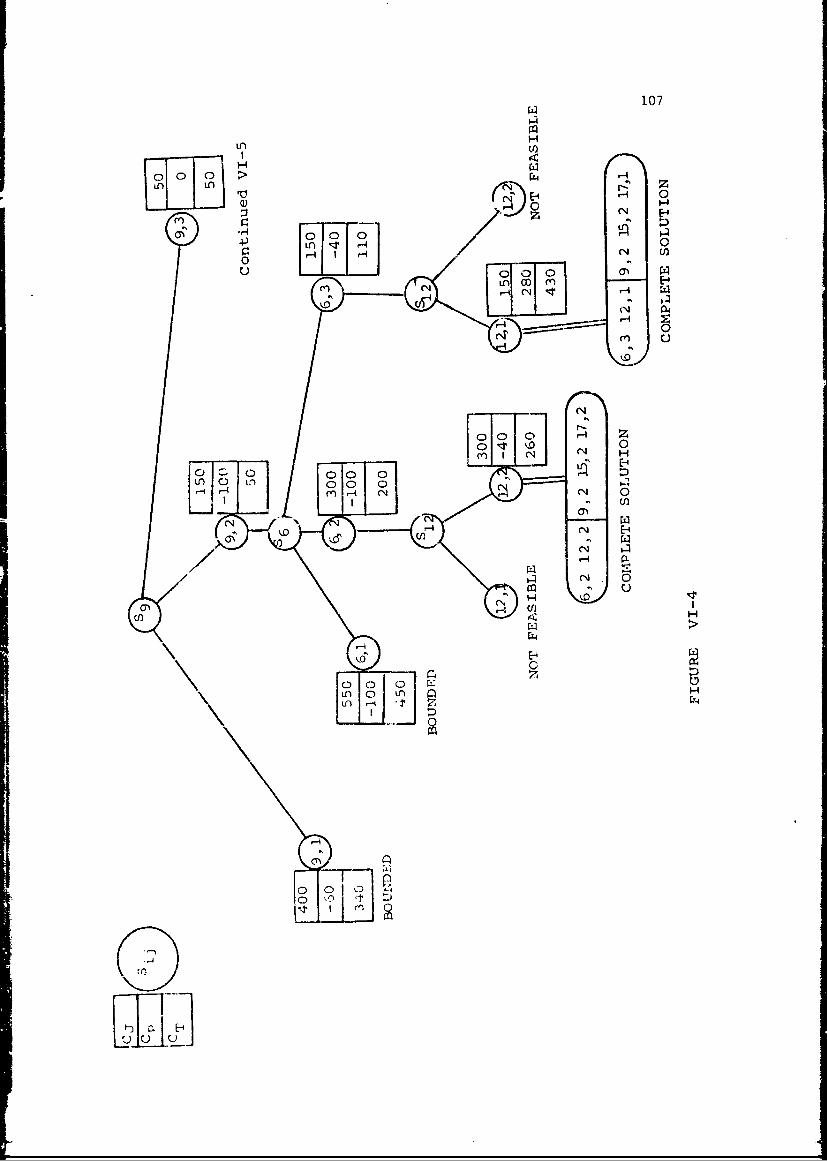
107

0n 0

cA -4 0-

p 11

00 0

u I o oo 00-4 4- CIH N Nt 001M -

0 0

0)0U) H

Ci)

CC

LI04 0 I

-E-p0

* 0 0 0-~~

-4

01-

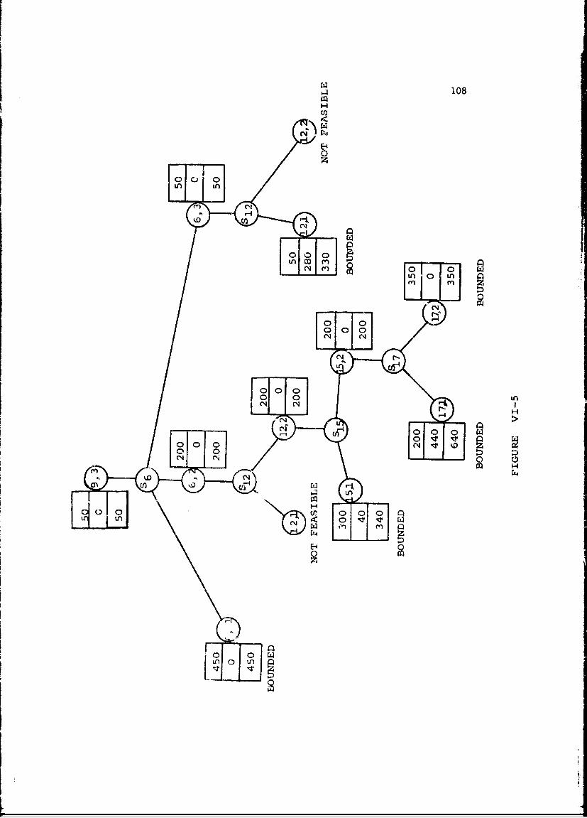
108

E-4

0

luoll- Ln

N

0 0in CO en

tn LnN

010 ol

0 0N N'D o C)

0 0 00 0 LnN N

H,>

0 Nr lc:ý0 0 0 N It %D0 0

010

0 jOn 0 Izr w

(P 0

0 11114

E-4

0 0 14Ln Ln

109

example, the fact that S9 I S6, and S,,2 appeared at the head of

the list coupled with the in.erdependency constraints on these job

sets, allowed substantial truncation based on feasibility tests. We

may also observe from this example that a combination of S.

S12,1 always gave a good project completion cost bound since they

allowed a long path to form in the network (52 days). This, of course,

could be observed directly in Table VI-l. This suggests that we might

cut search time if decision sets that appeared on long paths were

placed at the front of the fixed order list. This would certainly be

in the spirit of the first algorithm presented. In order to measure

criticality of the decision sets, the following procedure was used.

Step 1. At each decision set, the cheapest decision job was chosen.

Step 2. The resulting CP$ problem is solved and the slack for each

job calculated.

Step 3. Sequence the decision sets in increasing order of slack

measured for the member of that set in the CPM problem.

The algorithm wa-. tested on 10 problems of approximately 210

jobs and 15 three-job decision sets each. The total number of combina-

tions of decision jobs would therefore be 315.. 1.5 x 106. Character-

istics of the 10 job- are given in Appendix A.

Edch problem was srlvcd twice, the first time with a simple

technological ordering of decision sets, and the second time with the

slack ordering described above. Computational rclults are given in

Table VI-1. The algorithm was programmed in Fortran IV for an IBM 7094.

The program was run undcr a time-sharing system -- the time reported

110

derived from the system Interval timer and do not include swap times

imposed by tI. time-sharing system. Times required to obtain the

reduced network matrix are not Included here, but reported separately

in Appendix B. In addition to the times reported, these problems

required 2-6 seconds for reading data and performing certain in!tiali-

zing functions in preparation for the application of th. branch and bound

procedure. The computation times reported are exactly repeatable.

Computation results show an impressive superiority for

choosing decisions based on initial slack. Ratios of computation time

as high as 50:1 were found. In addition, the absolute amount of time

required by the algorithm using a slack ordered list suggests that the

algorithm is erficient for these problems.

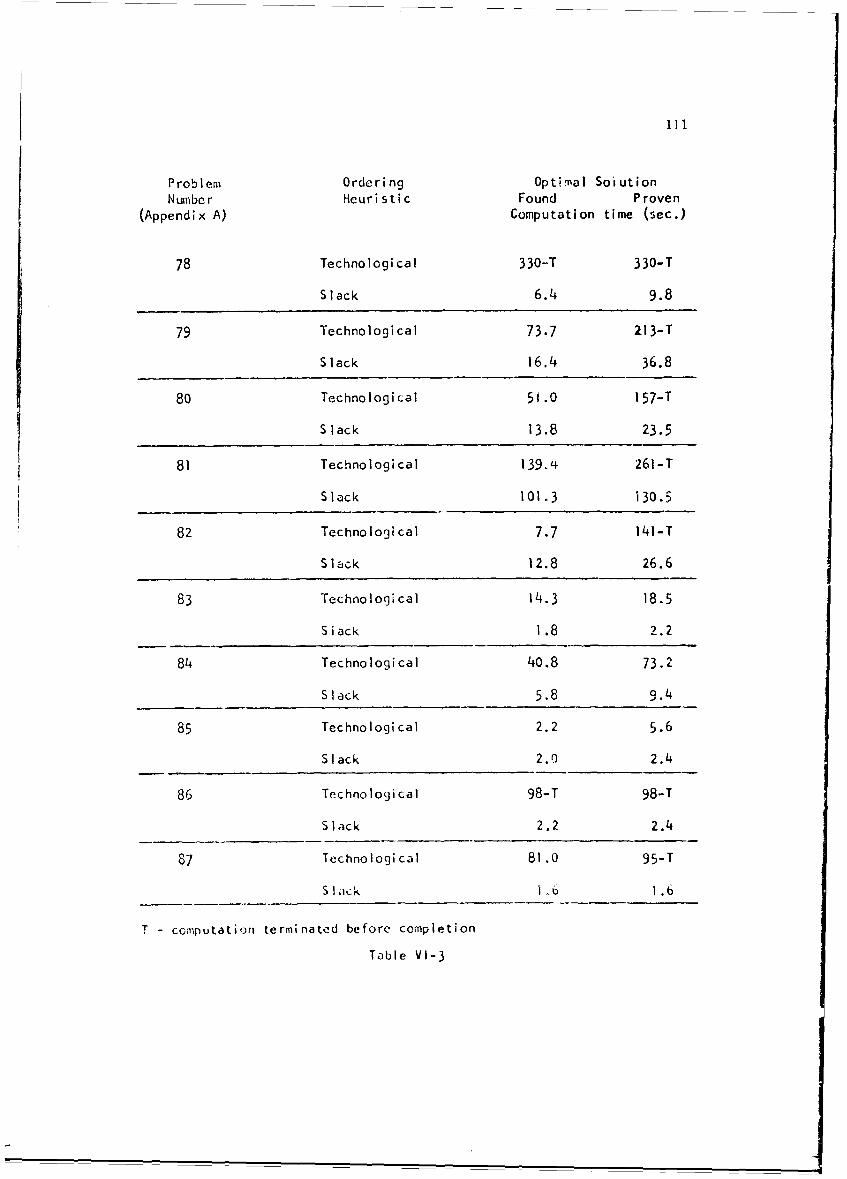
111

Problem Ordering Optimal SoiutionNumber Heur i s t i c Found Proven

(Appendix A) Computation time (sec.)

78 Technological 330-T 330-T

Slack 6.4 9.8

79 Technological 73.7 213-T

Slack 16.4 36.8

80 Technological 51.0 157-T

Slack 13.8 23.5

81 Technological 139.4 261-T

Slack 101.3 130.5

82 Technological 7.7 141-T

Slack 12.8 26.6

83 Technological 14.3 18.5

Slack 1.8 2.2

84 Technological 40.8 73.2

Slack 5.8 9.4

85 Technological 2.2 5.6

Slack 2.0 2.4

86 Technological 98-T 98-T

Slack 2.2 2.4

87 Technological 81.0 95-T

S lack I U6 1.6

T - computation terminated before completion

Table VI-3

Chapter VII

RESOURCE CONSTRAINED DECISION NETWORKS

The decision net.vorks we have considered in previous chapters

have included precedence and interdependency constraints. To evaluate

a particular design, that is a particular solution to the problem, it

was simply necessary to calcu)ate the length of the critical path for

the resulting network. Then the project cost could be determined

exactly. If resource constraints are added to this problem, it is no

longer a simple matter to find the mir:imum length of tha project.

Branch and bound techniques have been proposed to solve the problem

exactly, but for oroblems of reasonable size, the computation time is

excessive. Johnson [42] reports that a 100 task, single resource

problem ran 79 minuteq without proving an optimal solution. In a five

decision set problem, we woulH have 35 = 243 possible solutions to

evaluate in this manner.

For this reason it was decided to evaluate proposed soiutions

to the decision problem by loading them under the limited resource with

a "qood" heuristic rule. The heuristic to be used should L! efficient

so as to keep computation time within reasonable limi't, but it should

provide tight schedules. In tV's Tlhapter we will examine nine possible

heuristic Icading -ules and chocse the best of them for use in solving

resource constrain-.d decision mndels. 4e then examine three techniques

for choosing an optimal set of decisions. These include complete

112

113

enumeration, pairwise switching and multiple pairs switching.

2. Project Scheduling Heuristics

A graphical technique for project scheduling was first

proposed by Gantt L36.]. In this technique each resource is shown as a

bar ooi a bar chart where the horizontal dimension is time. Each task

can then be identified as a rectangic of resource use continuing for a

specific length of tiTne. Precedence relations between tasks and a

loading heuristics determine the relative position of the tasks in time

and the completion date of the project. Given this visual display, it

is possible for small projects to experiment with various sequences that

satisfy the precedence constraints, so as to determine the optimal,

that is minimal length, schedule.

For large projects this graphical technique is inefficient.

Not onl), is it difficult to attempt many sequences, buz it would require

much time to keep job infor,1 ation up to date. Therefore, in most

current applicatioiis, a computer model of the Gantt chart is maintained.

With a computer system, it is relatively easy to up-date project infor-

miation as jobs are completed, calculate job slacks and test various

loadinu heuristics. As we have discussed in Chapter II, various

heimristic- have been proposed for the lojj-ing problem F', 25, 43, 441,

but there has been little comparison .- !d of tin effectiveness of these

rules. The rules to be tested here are those that can be implefro.-rted

quickly and that have been w.11 regarded in previ.us work. They are

all basically serial loading techniques. The jobs in the project are

114

ordered first in technological order, then within technoloyical order

by a secondary measure. The loading routines take the first job on the

list, schedule it at its early start date, then proceed down the ordered

list scheduling each job in turn, The particular sequence of jobs in

the list will, therefore, strongly influence the completion date of

tne project. Two routines which wi!] be discussed below modify the

serial loading slightly to allow a previously scheduled job to be

shifted forward.

Nine rules are to be tested here. These consist of three

basic job sequences within the technological order, each sequence

loaded by three heuristic prog:-ams. The three orders to be tested are

1. random

2. increasinq early start

3. increasing late start

The three serial routines, LOADC, LOADh and LOAID will now be presented.

LOADC takes each job as it appears on the technologically

ordered list and places it in the schedule at the earliest possible

time. The start time of any job will be constrained by the finish

time of its predecessors and availability of resources. The flow chart

for the routine is as follows.

I. Technologically order the jobs.

2. Solve for the critical path of the network. Find

Early Start, Late Start and slack for each job.

3. Select the job sequence to be tested (random, E.S., L.S.

with;n the technological order) and reorder the jobs.

115

4. Set i=- I where i denotes a position on the ordered

job list.

5. Calculate ES., the Early Start day of the job in the

ith position on the list. Since the list is technologically ordered,

all predecessors of the job will be scheduled and Early Start can be

calculated in the usual way.

6. Attempt to schedule the job in the ;th position on day

ESi. If the job cannot be scheduled because of insufficient resources,

go to Step 8. If it can be scheduled, do so.and set i= i4- 1.

7. If alW jobs have been scheduled, go to Step 9. If not,

go to Step 5.

8. ES - ES + 1. Go to Step 6.

9. Halt.

RoutintR LOADN and LOAI) ae cimil•r to LOAMC pxrpnt that inhe

previously scheduled may be shifted forward to reduce the den md for

resources L,. a given day. A flow chart for LO',DN will now be presented.

1. Technologically order the jobs.

2. Solve for the critical path of the network. Find Early

Start, L:tz Start and Slack, (SL), for each job.

3. Select the job sequence to be tested and reorder the jobs.

4. Set i - I where i denotes a pos.ition on the ordered

job list.

5. Test to see if the job in the ith position is scheduled.

If it is scheduled, set i =- i -f-I and 9o to Step 5. If 't is not

scheduled, go to Step 6.

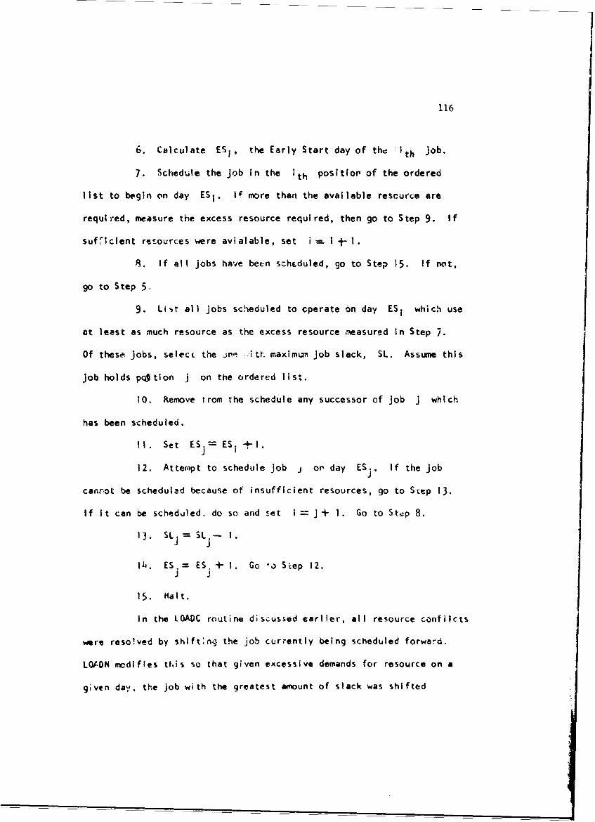
116

6. Calculate ES1 , the Early Start day of the i ith Job.

7. Schedule the job in the ith positior of the ordered

list to begin on day ESi. If more than the available rescurce are

required, measure the excess resource required, then go to Step 9. If

sufficient restources were avialable, set i-- I j- 1.

8. If all jobs have been scheduled, go to Step 15. If not,

go to Step 5.

9. List all jobs scheduled to operate on day ES1 which use

at least as much resource as the excess resource measured in Step 7.

Of these Jobs, select the jr! .. itý. maximun Job slack, SL. Assume this

job holds pcitlon 1 on the ordered list.

10. Remove trom the schedule any successor of Job j which

has been scheduled.II. Set ESj= ESi +1-.

12. Attempt to schedule job j or day ESj. If the Job

canrnot be schedul-d because of insufficient resources, go to Step 13.

If it can be scheduled, do so and set i =-j-+ 1. Go to Step 8.

13. SLJ = SLJ - 1.

I4. ES.= ES, -- I. Go "o Step 12.

15. Halt,

In the LOADC routine discussed earlier, all resource conflIcts

were resolved by shlft:n.- the job currently being scheduled forward.

LO-ON medifies tfis %o that given excessive demands for resource on a

given da,,. the job with the greatest anount of slack was shifted

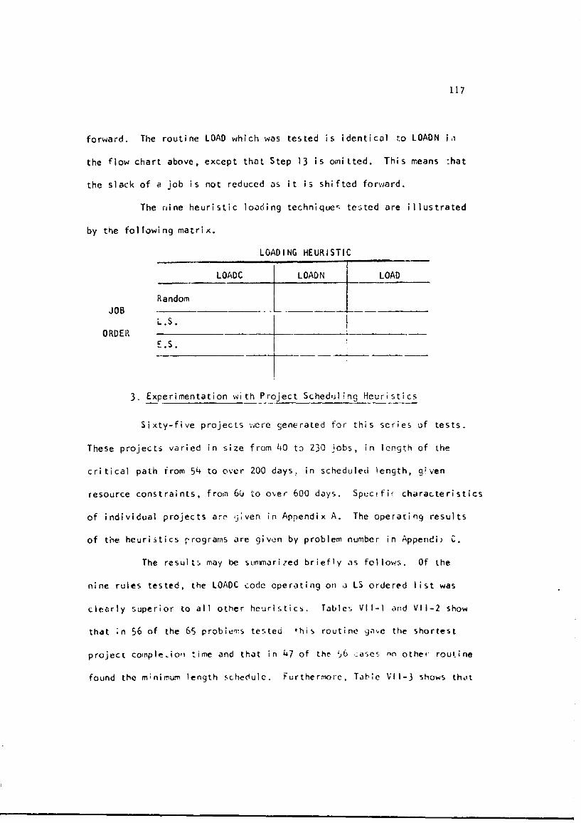
117

forward. The routine LOAD which was tested is identical to LOADN i.i

the flow chart above, except that Step 13 is omitted. This means :hat

the slack of a job is not reduced as it is shifted forward.

The fiine heuristic loading techniquer, tested are illustrated

by the following matrix.

LOADING HEURISTIC

LOADC LOADN LOAD

RandomJOB

ORDER L.S.

F.S.

3. Experimentation with Project Scheduling Heuristics

Sixty-five projects were generated for this series of tests.

These projects varied in size from 40 to 230 jobs, in length of the

critical path from 54 to over 200 days, in scheduled length, given

resource constraints, frot-i 6(1 to o',er 600 days. Spectfi• characteristics

of individual projects are jiven in Appendix A. The operating results

of the heuristics ý.rograris are given by problem number in Apperndib C.

The results may be sunu'arized briefly as follows. Of the

nine rules tested, the LOADC code operating on i LS ordered list was

clearly superior to all other heuristics. Tables VIlI- and VII-2 show

that ;n 56 of the 65 probieTs tested this routine ga,e the shortest

project compleiori time and that in 47 of the 56 :iases no other routine

found the m;nimum length schedule. Furthermore. Tabe VII-3 shows that

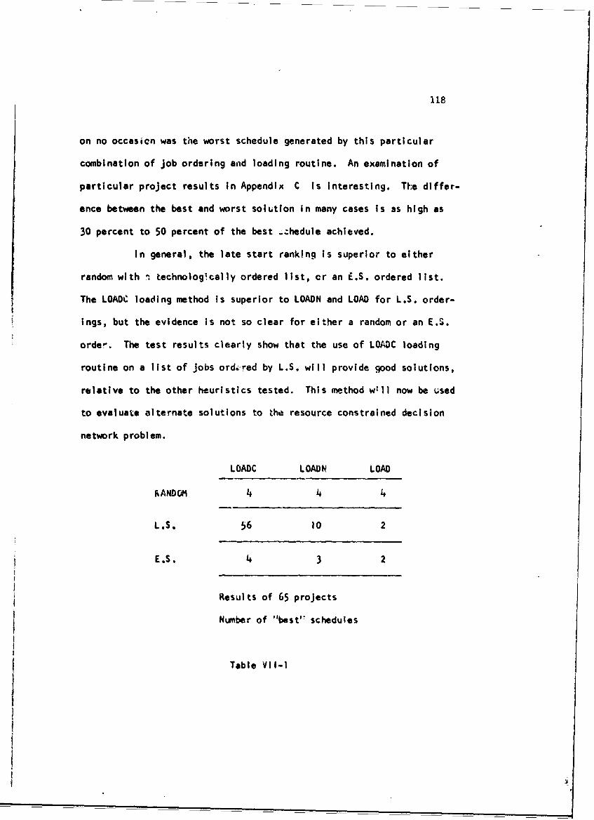
118

on no occasion was the worst schedule generated by this particular

combination of job ordering and loading routine. An examination of

particular project results in Appendix C is interesting. The differ-

ence between the best and worst solution in many cases is as high as

30 percent to 50 percent of the best .- hedule achieved.

In general, the late start ranking Is superior to either

random with n technolog!cally ordered list, or an E.S. ordered list.

The LOADC loading method is superior to LOADN and LOAD for L.S. order-

ings, but the evidence is not so clear for either a random or an E.S.

orde-. The test results clearly show that the use of LOADC loading

routine on a list of jobs ord red by L.S. will provide qood solutions,

relative to the other heuristics tested. This method w-ll now be used

to evaluate alternate solutions to the resource constrained decision

network problem.

LOADC LOADIN LOAD

RANDOM 4 4 4

LS. 56 10 2

E.S. 4 3 2

Results of 65 projects

Number of "best' schedules

Table VII-I

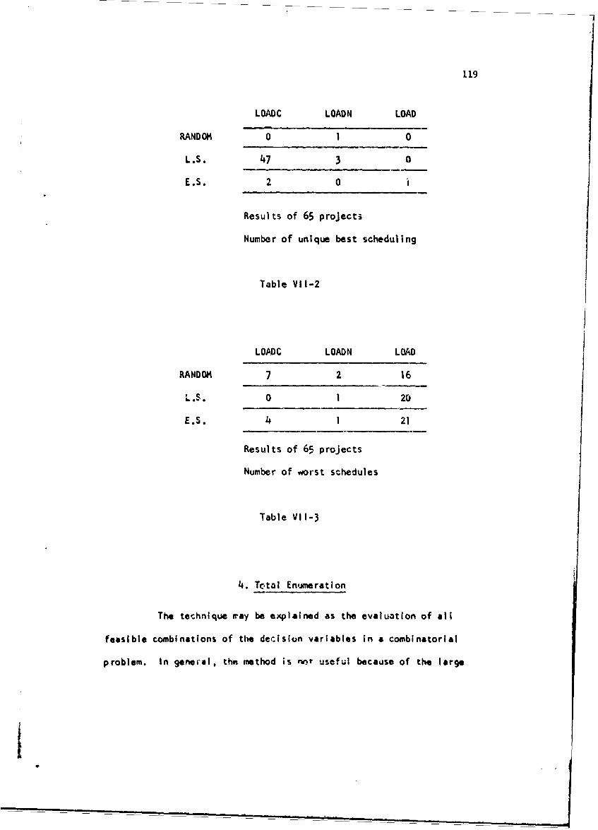
119

LOADC LOADN LOAD

RANDOM 0 1 0

L.S. 47 3 0

E.S. 2 0 i

Results of 65 projects

Number of unique best scheduling

Table VII-2

LOADC LOADN LOAD

RANDOM 7 2 16

L.S.. 0 1 20

E.S. 4 1 21

Results of 65 projects

Number of worst schedules

Table VII-3

4. Total Enumeration

The technique way be explained as the evaluation of all

feasible combinations of the decisikn variables in a combinatorial

problem. In general, the method is nnlt useful because of the large

II

120

amount of computer time required to solve problems. We use the method

here on a series of 10 small problems in order to h•,e some means of

evaluating the heuristics we. propose to use on the resource constrained

ducision network problem.

The problems to be tested have three active resource categories,

40-60 Jobs, 5 decision sets of 3 Jobs each. Thus, there are 35= 243

possible combinations af decision, jobs to be tested in each problem.

The routine iteratively activates a combination of five decision Jobs,

one f-om each job set, then calculates the critical path in the result-

ing project network, orders the jobs by late start and loads thein. under

specified resource limits. The cost of the decisicn jobs in a particular

combination and the resulting length of the project are recorded.

Table VII-4 reports the computation times for the complete

enumeration routines progranmmed in Fortran IV and run under a time-

sharing system on an IQ0 7094. The times reported are derived from

the system interval times and do not include swap times imposed by the

time-sharing system. The best solution found is also reported.

As explained above, the schedule lengths are heuristically

determined so that for any combination 6f decision jobs, we almost

certainly are not reporting the optimal schedule. It is our point,

however, that large problems of the type we are attempting to solve

cannot practically be solved by existing algorithms. To illustrate

this point, we note that since the running time for our 35 problem

is approximately 129 seconds, a problem with 15 decision sets would

require at least

121

3 . 129 x • 212 hours

35 60x 60

if we were to enwuerate all possible solutions and solve them heuristi-

cally. This number can be multiplied by 30 to 0)0 If the project has

60-100 tasks and we wish an optimal loading for each design. Appendix

0 reports all undominated solutions and a distribution of critical

path lengths and resource constrained schedult lerjths for the projects.

We now report a technique that will substantially reduce the

search required -- but, as will be explained, will rot guarantee that

the best set of decision jobs are selected.

5. Pairwise interchange

The palrwise interchange technique is a rechod of partialiy

enumerating combinations of variables in a problem. We will illustrate

the method in terms of a simple DCPM problem. If the decision network

contains three decision nodes Sl, S2 , S3 with respectively three,

two and two Job alternatives, then Figure VII-l shows an enumerated

tree --f all possible combinations of the variables.

A pairwise enumeration scheme would begin with one decision

job from decision set S1i one from S2 and one from S3* In our

routine the job with the lowest cust in each set is selected as a

starting solution. Assume the initial solution is SI,, S2,1 and

S 391, The oairwise interchange routine begins with one of the decision

jobs, say Si, and iterates It through all possible alternatives,

I$!

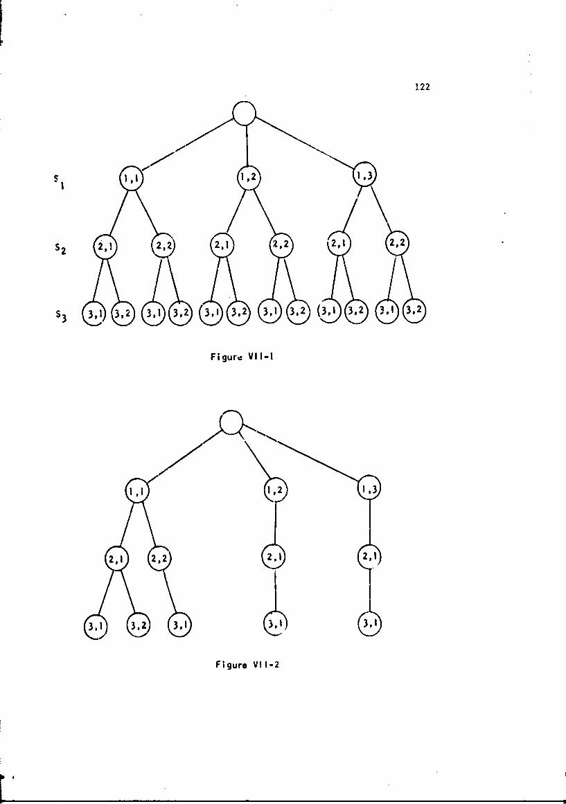
1.22

1,2, 1,3

S 3 3,1 3,2 3132 3132 3132(,4 . , ,

Figur4 VII-I

1,1 1,2 1,3

2.1 2,2 2,1 2 11

3.1 3,2 3.1 C3,1) 3,1

Figure VII-2

123

S ll1 S 1,2S and 51,3 while holding al: other jobs as they were ins

the ini~ial so2ution ( 2 ,1 , 3,1). Then the f~rst decision job is

returned to its original setting S 1 ,1 and then job S2 , then S3

are iterated through their possible alternatives. The combinations of

jobs examined are shown in Figure VII-2. Note that each solution con-

tains only one job that is different than the set of jobs in the initial

solution and in total we examine only four solutions in addition to the

initial solution.

For each combination of decision jobs, the initial solution

plus the set of four combinations generated by the pairwise interchange

routine, the project is scheduled using the heuristic discussed in

Section 2 of this chapter. For each of the fcur schedules, the sum of

job cost and completion date cost is calculated. The combination of

jobs with lowest total cost is compared to the cost of the ;nitial

solution if it is lower, this combination b.. nmes the new "initial"

solution and jobs in that solution are exchanged. The process continues

until no improvement is found.

The ten problems tested by complete enumeration were tested

again with the pairwise interchanqe routine. The cost of the best

solutions generated, along with computation times, are given in Table

Vli-4. Complete details of the solutions are given in Appendix D. A

review of results shows that for each of the ten projects, the optimal

solutions were found and that, In every case, the solutions stepped

from one undominated solution to another.

For comparison with a later heuristic two, fifteen decision

iCB

.124

set projects were attempted. The solutions obtained to these problems

are shown in Table VIlI-. It will be noted that these problems ran 268

and 465 seconds. These tmes suggest that a mcore efficient technique

Is required for large problems.

6. Multiple Pairs Switching

The pairwise interchange routine when applied to a five

decision set problem, three Jobs per set, exam!nes ten alternative

soolutions, then accepts the best of these for further exploration. In

some Instances, several good exchanges are discovered on the first pass,

but only the best exchange is accepted. Then, in the second set of

pairwise exchanges, a previously discovered change is found to be good

and at the end of the second pAss, it is accepted. This soiggests that

a mora efficient routine should, at each stage, accept all exchanges

that appear to be beneficial.

The routine developed proceeds as follows. It begins by

applying a simple pairwise switching routine to all decision variables.

The base solution used is simply that which contains the cheapest Job

from each decision set. For each new Job brought into the solution, vA

caiculate a project length based on the loading heuristic described

eari!er in this chapter. TSe total cost of this solution is compared

to the previous lowest cost solution and the difference is defined as

a price for the decision Job.

When all decision jobs not in the starting solution have been

evaluated In this way, we have 'prices" for all decsion Jobs. The

125

Implicit price of Jobs In the original solution is, of course, zero.

Now, using the algorithm of Chapter IV, with Job prices as definrid here,

we can solve fcr the best set of jobs to perform. A solution might

Imply that one or more variables are tb be ;-.,itched. This design can

then be evaluated by our loaoing heuristic and a total cost can be

calculated. If this cost is lower than our previous optimum, we

recalculate job "prices" with a pairwise int'rchange ,-outint., otherwise,

we stop. Results of this algorithm for our twew,! problems are shown

in TUble VII-4 and in more detail In Appendix 0.

7. Discussion of Results

Table VII-4 compares the computation times and quality of

solutions for the three routines applied to the full problem. For small

problems (five decision sets), the complete enumeration routine takes

approximately 6-9 times as long as pairwise interchange methods. Pair-

wise interchange techniques take approximately the same time as the

mdltipie pairs approach. In eight of the ten problems examined, both

the pairwise interchange and the multiple pairs exchange method found

the optimal solution as proved by complete enumeration. In one of the

remaining two problems, the pairwise interchange routine found a better

solution than multiple pairs.

For large problems (fifteen decision sets), the pairwise

interchange rcitine took longer but found superior solutions to the

multiple pairs method. For these problems, it was not practicol to

enumerate all possible designs and so the optimal solution is not

I126

known as ccxnputation tifis ror these proble.rms of 6 to 11 minutes suggests

that even the simple, routioes ,ojld not be practical for large problems.

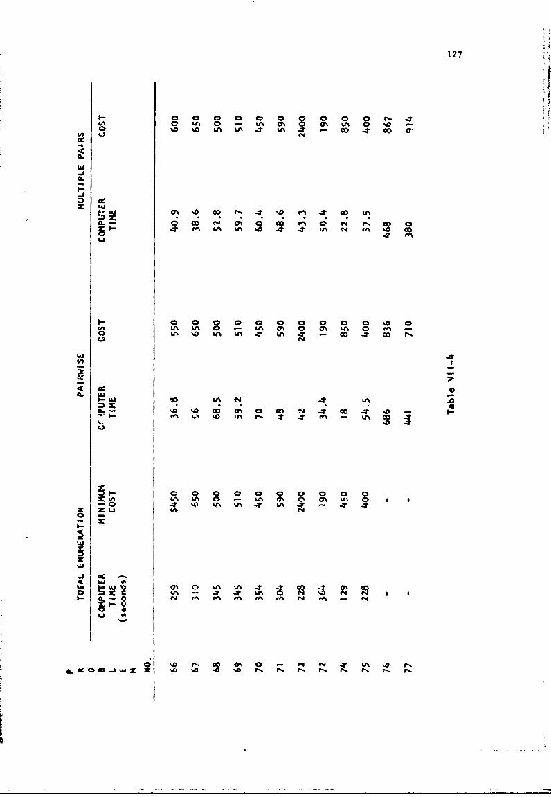
127

0 0 % 0 0A 0h 0 0 %0%0 %a 0o m A0%

-AiL

u-

W ~ 0 '0N w co 4l. - 0 m~ 4 00 m

CL . C; C6 'A 0; C; C4 4; IA Pd I

I- 0 0 00 0 0 00 '0 0'A 0n - A M% 0 0 0 Me -&o NO '0 % LA A L A co _- Go 4 -

I.- w -j LC6 'o N6 C f 4 -1 OD -T %

ONg WN I.% 0 LA fl. 4 4 Pr

0N 0 0%A WN 0T - L0%'A

0I --

%A 0; k^ A

&490=-Jw- %4 %0 %afIA-

Chapter Vill

APPLICATIONS OF THE DCPM MODEL

The ddclsion nodes of the DCPM model have been primarily used

throughout this thesis to represent job alternatives in the discrete

time-cost tradeoff problem. This chapter will show that the decision

nodes may also represent any given Job performed at different points in

time, or at different physical locations and with these inter'pretations,

the model may ba used to formulate the resource constrained project

scheduling problem and the single product assembly line balancing

problems as integer programming problems. In addition, the application

to project time cost trade-off problems will be extended to projects

under incentive contracts ,with non-linear crizerion functions.

2. The rwzxn Jch-Shop Scheduling Problem

This formulation assumes that the job-shop problem has been

so!veJ heurlsticb|ly [20, 28j and that a fe3sible finish date Wf, the

early start of artificial finish job Sf has been determined. For each

job, '6.', it is then possible to calculate an sarly start FESi and an

early and a late finish time, EF1i LFI, using the usual rules of the

criticol path method.

If the critericn function is to miiimize the make span for

the fixed job file under consideration, then job Si must begin on day

ES, or later and mu.-! finiVl on or before LSi. A start before ESI

128

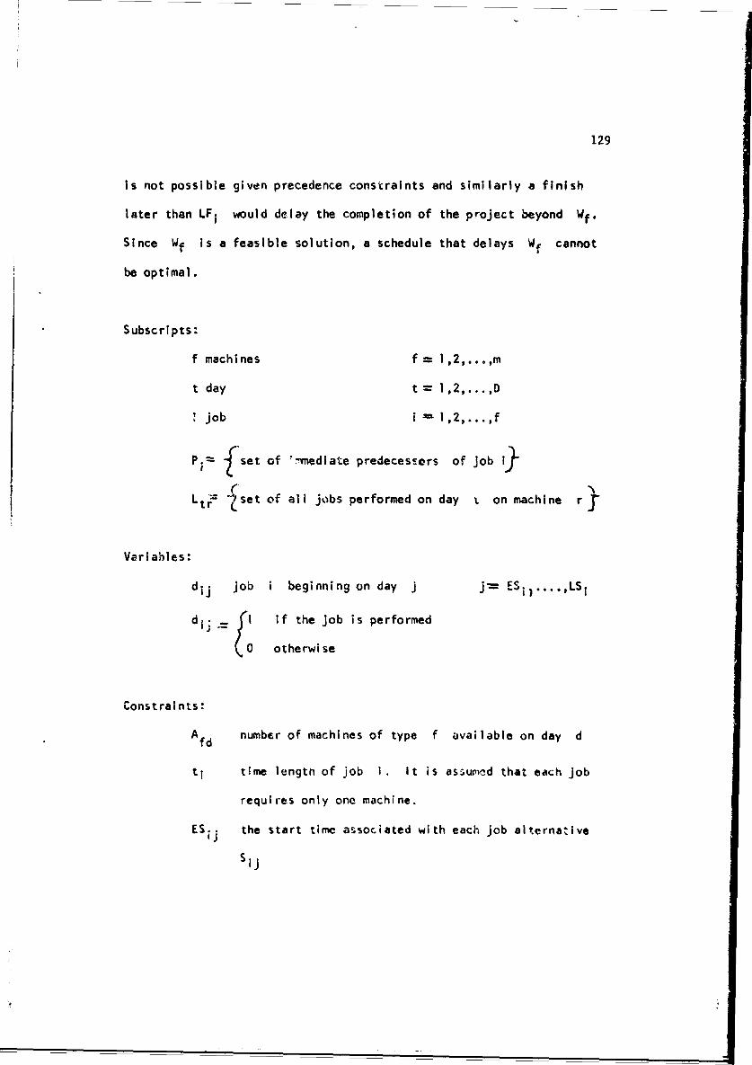
129

is not possible given precedence constraints and similarly a finish

later than LFi would delay the completion of the project beyond Wf.

Since Wf is a feasible solution, a schedule that delays Wf cannot

be optimal.

Subscripts:

f machines f= 1,2,...,m

t day t = 1,2,...,D

job i - 1,2,...,f

P.= f"set of '.mmediate predecessors of job

Ltr-- " set of all jobs performed on day i on machine r

Variables:

dij job i beginning on day j j= ES 1i)....,'LSi

d -= I1 if the job is performed

( otherwise

Constraints:

Afd number of machines of type f available on day d

ti time length of job I. It is assuragd that each job

requires only one machine.

ESij the start time associated with each job alternative

Sij

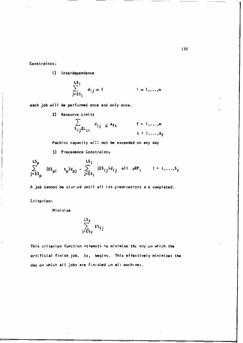
130

Constraints.

1) Interdependence

LSiYdij " -" , . ,m

j=ES1

each job will be performed once and only once.

2) Resource Limits

d dj < aft f l,...,mSijELtr t=I..W

Machirne capacity wil: not be exceeded on any day

3) Precedence Constraints

LSp LSI

(ESpl tp)dp - I (ES1 )dij all pEP 1 I = i,...,SfJ= ESp j=ES

A job cannot be stir-ed until all its predecescors a'e completed.

Criterion:

MI ninmi ze

LSf

j:E ESf

I zESf

This criterion function -ttemepts to minimize thc day on which the

artificial finish Job, Sf, begins. This effectively minimizes the

day on which all Jobs are finisked vn all machtnes.

13!

This formulation is related to that of Bowman [8J and may be

extended to the resource constrained project in the same way that Vdiest

L80] has extended Bowman's model. The project formulation may also be

extended to the resource constrained discrete time-co.t trade-off

problem by'expanding the decision set 'or e=.h job to include several

(k()) job alternatives.

Wiest L80] has estimated that a project with 55 jobs in 4

shops with a time span cf 3' days would require 5225 equations Ind 1650

variables. If job splits were not allowed, the number of equations

would rise to 6870. The formulation suggested here requires an inter-

dependency constraint for each job (55), a resource constraint for each

resource for each day (4 x 30 120) and a constraint for each precedence

relation (100 - 500). We car. then estimate that this formulation would

require 300 - 700 constraints -- approximately onc-tenth of those with

Bovwan-Wiest formulation, ! this formulation there would be at least

one variable for each d.,' of slack in the original heuristic schedule.

This number would I'_ substantially below the figure 1650, estimated by

Wiest. An ,.-stimate in the range 50-200 would not seem unreasonable here.

The exact number of constraint5 and variables will, of course, depend

on the s;'ecific problem.

It is difficult to make an exact comparikon with Manne's

formulot.on [54] since his approach is not suitable for the resource

constrained projec. problem. He implicitly assuries a resource level

of one by his use of non-interference constraints. Ile does estimate

th0 job file of ten tasks to be ne-ifo, .d on five machines would

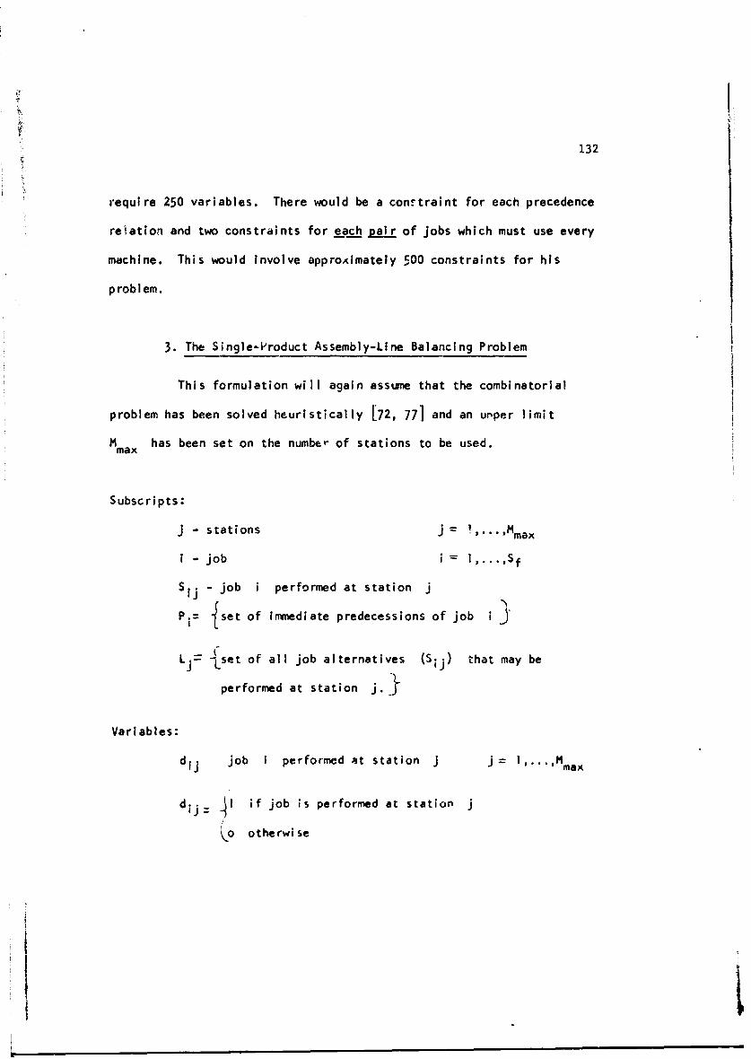
132

require 250 variables. There would be a con.traint for each precedence

reiation and two constraints for each pair of jobs which must use every

machine. This would involve approAlmately 500 constraints for his

problem.

3. The Single-Product Assembly-Line Balancing Problem

This formulation will again assume that the combinatorlal

problem has been solved heuristically [72, 77] and an unper limit

4 has been set on the number of stations to be used.max

Subscripts:

J - stations j = ,.' M max

i - job i = 1 ,...,Sf

sij - job i performed at station j

P .: 1set of immediate predecessions of job i 3

Lj= Lset of all job alternatives (Sij) that may be

performed at station j.j

Variables:

dij job i performed at station j j= I .... ,Mmax

dij= I if job is performed at station j

ýo otherwise

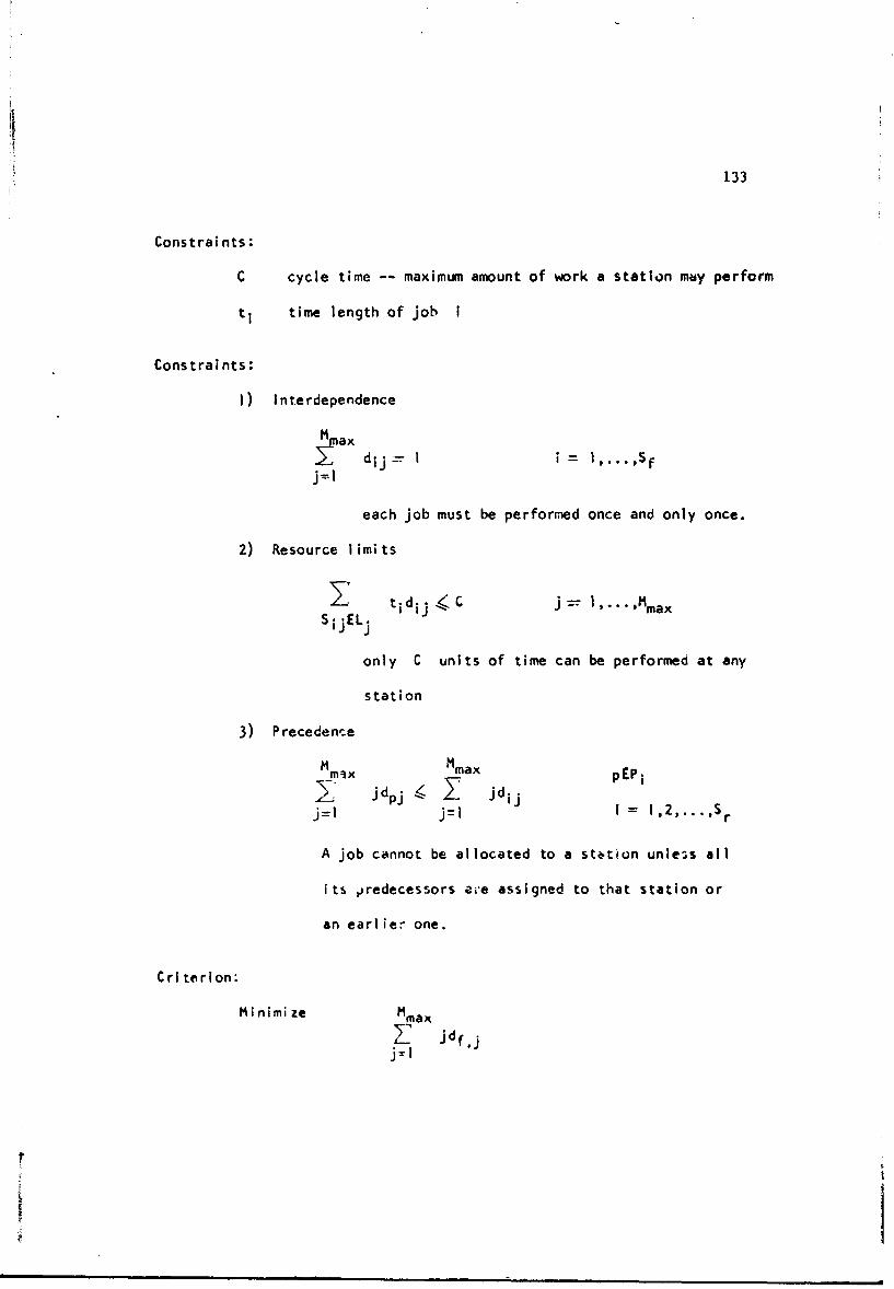
133

Constraints:

C cycle time -- maximum amount of work a station may perform

ti time length of job I

Constraints:

I) Interdependence

jfm dij -- I i = i,...,Sf

j--I

each job must be performed once and only once.

2) Resource limits

Y tidij <ýC j = I,...Mmax

SijEL.

only C units of time can be performed at any

station

3) Precedenc-e

Mmix Mmax pEPi

j=l jlI i = 1,2,r.. Sr

A job cannot be allocated to a stotion unless all

its )redecessors cie assigned to that station or

an earlier one.

Cri terion:

Minimize Mmax

Z7 Jdfj

rjI- ~

I

134

Here we attc.pt to minimize the number of the station in

which the final Job, Sf, appears. This effectively minimizes the

total number of stations used.

For the II j,., , -'olIem of Jackson [421 with C= 10 and an

initial heuristic solution of six stations, this formulation would

require eleven Interdependency constraints, six resource constraints

and fourteen precedence constraints for a total of 31. The maximum

number of variables would be 66, but this could be reduced by an ES-LS

argument to approximately 39. This is a substantially smaller prob'em

then competitive formulations.

4. An Application of Decision CPM to Incentive Contracts

Recently several government agencies have changed their

contracting procedures from predominantly cost-plus-fixed fee to

incentive fee contracts. The incentive contracts are written so that

the maximum fee obtainable decreases as cost of the project increases

[59.1 and the per cent of the maximum fee actually paid decreases with

decreasing performance. Performance poitcts may be awarded for success-

full performance or quality tests, and for meeting a series of

specifie6 due dates (or mile stones) within the project network. A

sample contract fee ":•ructure is shown in Figure ViII-1.

A manufacturer faced with a time-cost trade-off problem

within an incentive contract has an especially difficult problem. If

a job is "crashed", ic is possible that extra points will be earned as

a resu!t of meeting a particular due date. At the same time, the

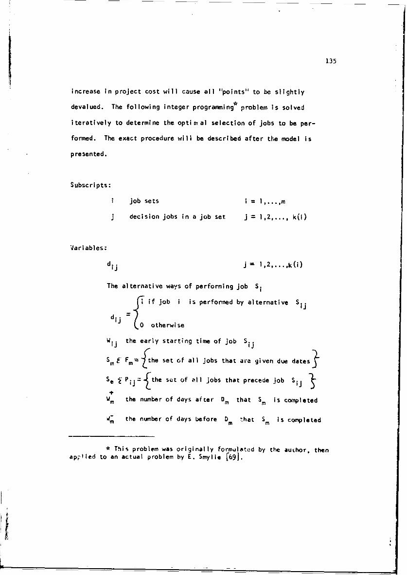
135

increase in project cost will cause all "points" to be slightly

devalued. The following integer programming problem is solved

iteratively to determine the optimal selection of jobs to be per-

formed. The exact procedure will be described after the model is

presented.

Subscripts:

I job sets I = ],...,m

j decision jobs in a job set j = 1,2,..., k(i)

Variables:

dij j = l,2,...,k(i)

The alternative ways of performing job Si

aI if job I is performed by alternative S ijdij = 0 otherwise

w ij the early starting time of job Sij

S m Fm = ft he set of all jobs that are given due dates

Se • P ij"fthe sea of -11 jobs that precede Job Sjj

Wm the number of days after Dm that Sm is completed

W_ the number of days before Dm that Sm Is completed

*This problem was originally formulatcd by the author, thenapplied to an actual problem by E. Smylie [691.

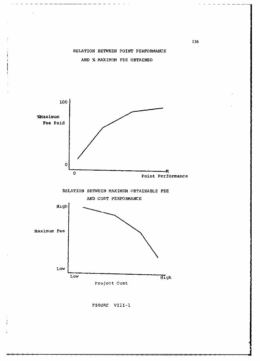
136

RELATION BETWEEN POINT PERFORMANCE

AND % MAXIMUM FEE OBTAINED

100

%MaximumFee Paid

0

0Point Performance

RELATION BETWEEN MAXIMUM OBTAINABLE FEE

AND COST PERFORMANCE

Higb

Maximum Fee

Low

Low High

Project Cost

FIGURE VIII-1

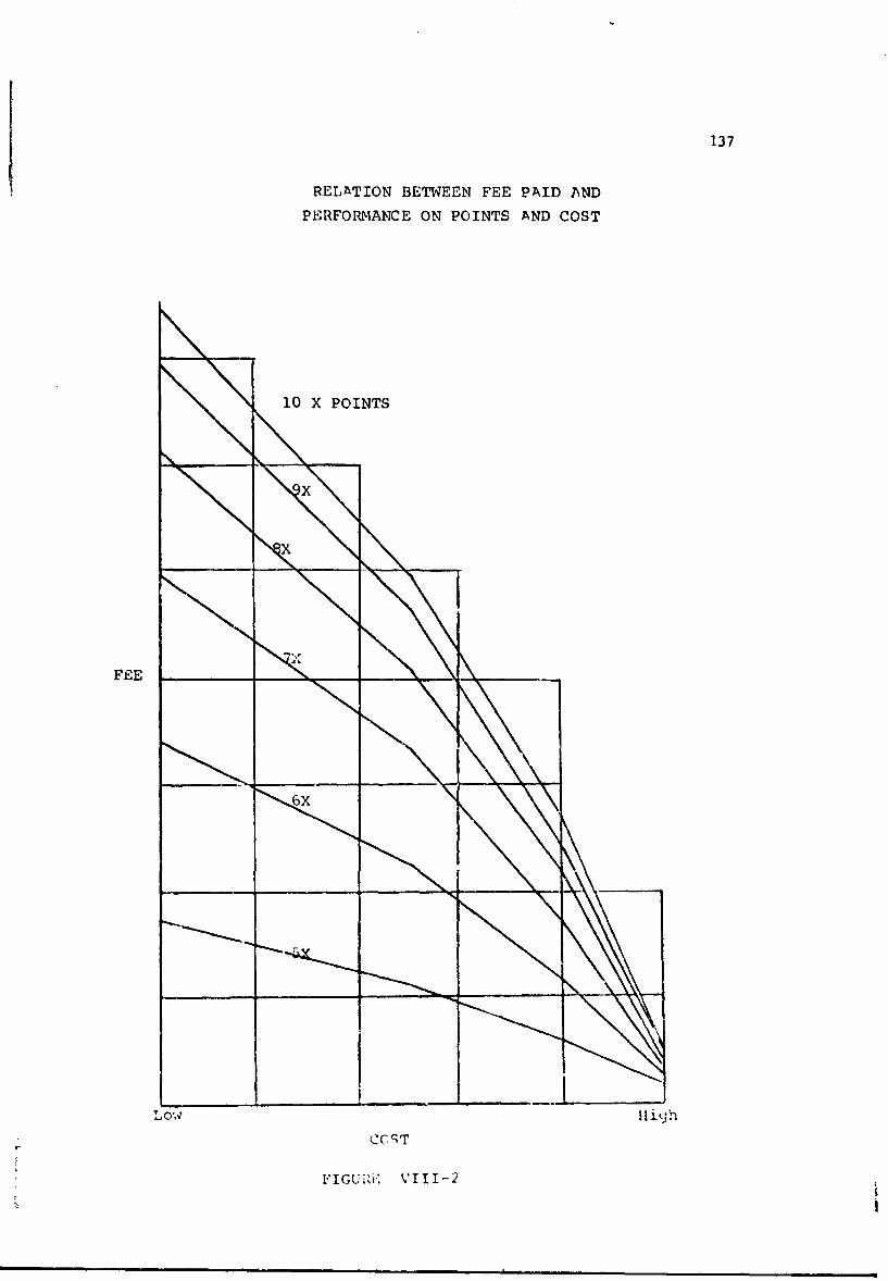
137

RELATION BETWEEN FEE PAID AND

PERFORMANCE ON POINTS AND COST

10 X POINTS

x

Llli(jh

VIII-2

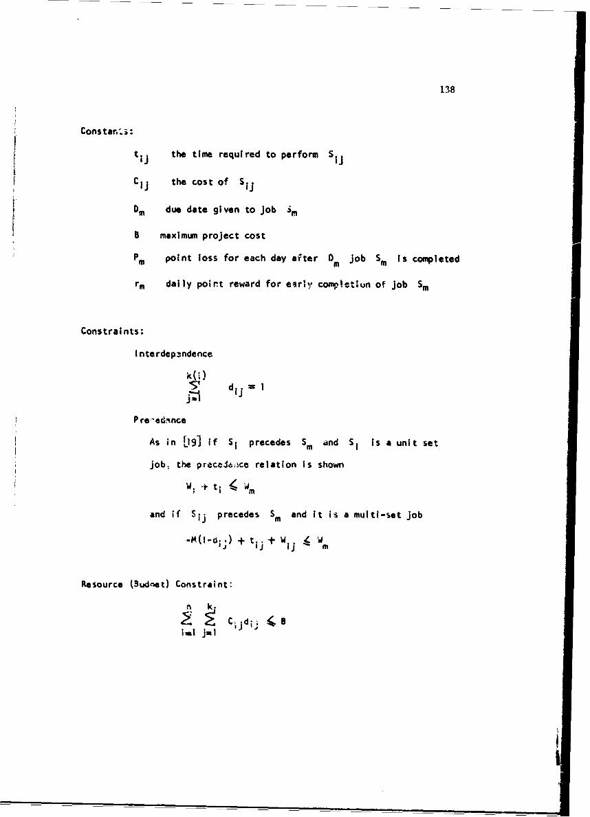
138

Constar..;:

t the time required to perform Sij i

Cij the cost of SIj

Dm due date given to job SM

B maximum project cost

Pm point loss for each day after Dm Job Sm Is completed

rm daily poir~t reward for ear',! comp!¢t1in of Job Sm

Constraints:

I nterdep3ndence

k(i) Sdi = 1I

P re'edince

As in F191 If Si precedes Sm and Si is a unit set

job, the preccJli•ce relation is shown

W; 't. ti 4Wm

and if Sij precedes Sm and it is a multi-set Job

- - + j ij m

Resource (Bud'net) Constraint:

n k

il Jul

139

Due Date Constraints:t

Wm - Wm Wm Dm m F,

Cri terion:

Maximize mrmWm- pmm

This fomulation maximizeh the number of performance points

obtained subject to cost limits on the complete project. Initially,

the problem is solved without a budget constraint to determine the

maximum available points and the cost associated with this solution.

B is then set one unit below the cost found above and the problem Is

resolved.

The routine is applied iteratively until the minimum cost

point is reached. At each solution the combination of performance

points obtained and budget cost will allow total fee to be calculated.

Figure VII-3 shows a series of such points with an optimal solution

marked. This approach has been applied to an actual oroject by Smylie

[69] and is reported by Crowston and Smylie [22].

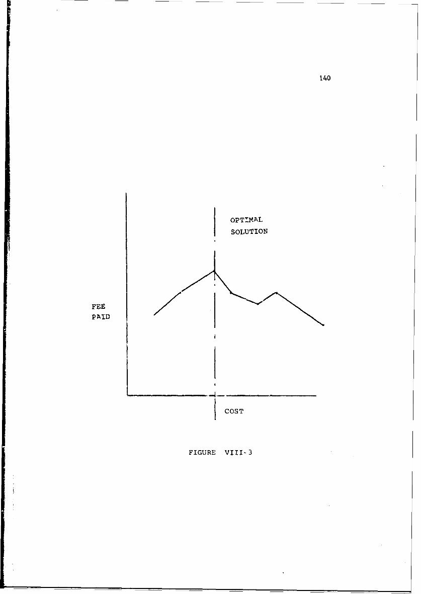
140

OPTIMAL

SOLUTION

FEEPAID

COST

FIGURE VIII- 3

Chapter IX

Sutmnary and Conclusions

Our original goal was to determine efficient procedures for

the solution of design problems in situations where the design could

only be evaluated in termý of optimal operating decisions for the

system. The study was confined to the area of project scheduling

although the models we used were related to many other planning problems.

The relationship between these problems was shown in the literature

review of Chapter II.

The articles reviewed there were categorized by the type of

constraint found in the model. These included time or precedence

constraints, showing the sequence in which the jobs were to be per-

foried, or putting time constraints on the start or finish time of a

particular job. The use of resource constraints implied that the Jobs

required resource inputs to be performed and that the availability of

the resource was limited in each time period. Finally, interdependency

constraints between individual tasks were introduced. One particular

type of interdependency, that is, the mutually exclusive relation

between sets of Jobs, was developed In some detail throughout the

thesis since the Job alternatives c.uld be used to represent design

alternatives in a planning problem.

Models w!th simple time constraints, the usual Critical Path

problem, could be solved optimally with longest path algorithm. Problems

141

iro1

142

that involve simple interdependency relations form a special class of

0 - I integer programming problem. Tree search schemes have been

developed for this class of problem. With time and interdependency

constraints in a model, ac we have in DCPMI, the literature suggest a

standard integer programming routine is required.

When resource demands and constraints are added to a model, it

becomes a diff~cult problem to solve it optimally. For example, given

time and resource constraints on a set of tasks, it is a difficult

combinational problem to find the sequence of jobs that m;nimize

project length. Branch and bound techniques have been developed for

small problems, but large problems must be solved heuristically. Only

a few models in,:Jude all three types of constraints that we have dis-

cussed, and these are solved heuristically.

The design problem tha•t is the central concern of the thesis

is the problem of selecting which jobs to perform, from a decision set

of mutually exclusive alternatives. The optimal set minimizes the

total of job cost and project completion date cost. This problem is

formulated in Chapter III as an integer programming problem. It is

shown in this chapter that the number of precedence constraints required

for any network would be o-le for each precedence link, or one for each

path in the network. This number could be so large that the problem

could not be solved by current integer prog.ramming routines.

In Chapter IV dominancc, feasibility and lower bound tests

are developed to eliminate many non-binding precedence constraints from

the integer programming model. This is equivalent to the elimination

143

of many paths, which can under no condition become critical, from the

decision network. The remaining set of paths which may become the

critical path are termed the "reduced constraint" set. An algorithm

Is developed to implement the dominance tests referred to above. In a

decision graph, the algorithm determines the longest path between all

pairs of decision jobs, if any path exists, and eliminates all paths

but the longest one. The result is a "reduced network" containing only

decision jobs and maximal length paths between decision jobs.

If we consider the set of tasks in any DCI'M problem and the

set of interdependence constra~nts defined on that set, we observe

large numbers of mutually exclusive relations, "job alternative" inter-

dependencies, and some number of constraints between individual members

of job sets, "other" interdependencies. In Chapter V an Integer progran-

ming network algorithm is developed to efficiently solve the problem of

seiecting the minimum cost set of decision jobs given chese types of

Interdependency constraints. The optimization technique used Is the

"longest path" calculation of the critical path method applied to a

network in which each patn through the network is a feasible solution

to the integer programming problem. The length of each path is exactly

equivalent to the value of the criterion function for the solution the

path represents. In this algorithm, the usual "slack" measure of the

critical path method may be interpreted as the dual evaluation of

variables which are not in the solution. When the structure of inter-

dependence in a problem does not allow the algorithm to be directly

applied, it is shown that it may be coupled with a branch and biand

144

algorithm to solve the problem.

In Chapter VI two branch and brand routines are developed to

solve tle DCIVM problem. Both of these use the algorithm of the previ-

ous chapter to handle the interdependency constraints. In the first

routine at each node, we calculate the minimum cost job selections,

given job selections and rejections to that point on the tree and

determine the critical path given these job selections. The branching

decisions are made so as to progressively break all critical paths, by

prohibiting the use of decision jobs on the path. The second algorithm

sets a fixed order in which the decision sets will be considered, and

at each node, evaluates all alternatives within that set. Given any

selection of alternatives, a lower bound on total project cost is given

by the sum of job cost, for those jobs previously committed, and a

project completion cost, based on a finish date determined from the

reduced network, with only the jobs that were previously committed

active in the network.

The second routine was coded and tested with two different

orderings of the job sets. The first fixed order was simply a tech-

nological order taken from the position of the decision sets in the

orig:nal network. The second fixed order was arranged so that the

decision sets were listed in order of increasing slack. This ilack

was determined by choosing from each decision set, the cheapest decision

job and solving the resultint critical path problem. The slack on these

jobs was then determined and its value used to rank the decision sets.

In every case, the slack order was superior to a technological order

145

and the superiority ranged from 5:1 to over 50:1. Using the slack order

problems of fifteen decision nodes or 1.5 x 106, possible designs were

solved in 1.6 to 130 seconds. This suggests that large decision networks

may be solved efficiently with this routine.

In Chapter VII, decision networks with resource limits were

introduced. Before the combined "design", "operatIng" problem was

attempted, it was necessary to determine a good "operating" rule, or, in

this case, a heuristic loadiný rule for sequencing project Jobs under

limited resources. Several rules from the litecature were tested and

of these a serial loading rule, operating on a job list ordered by late

start, with nr job bumping, proved superior.

This rule was then used in combination with three tree search

technique.. These were complete enumeration, to provide proof of the

optimal solution, pairwise interchange and multiple pairs exchange.

The pairwise interchange was superior to mL, tiple pairs routine in

that the computation times were approximately the same but the solutions

were superior. In ten problems the pairwise routine solved eight

optimally. It was concluded that none of the techniques were efficient

for large problems.

In the last chapter, the decision network integer programming

formulation was aoplied 1o the m x n Job shop scheduling problem, the

single product assembly-line balancing problem and the DCPM Incentive

contrast problem. For the tirst applications, the formulation was

markedly more efficient than the one existing integer programming formu-

lations used 6s a basis of comparison. The lost formulation was

I

I

146

interesting in that the model was applied to a problem with a non-linear

criterion function.

Suggestions for Future Research

The rsearch questions that have arisen in this study fall

into three broad categories. First we will suggest specific areas for

development of algorithmic and heuristic reoutines for the solution of

related problems. Then we will discuss the need for additional tests

of the models developed here on actual problerms aoid, finall], we will

discuss the extension of these models to other planning problems.

It is clear that much more work remains to be done on the

development of truncated enumeration schemes for the DCPM problem;

We have suggested two here and tested one of these. It would be

desirable to develop other appro-"hes to this problem, specifically

one that could operate on the original network and save the time

r1quired by our network reduction scheme. All models could then be

tested against a range of DCPM problems. In Chapter V we developed

an integer programming routine for restricted types of problems, and

suggested that it could be ýnupled with a tree siarch scheme for more

complex problems. It would be useful to develop a program for such z

combined model and test it on a series of problems.

The area that requires :he most work would be the solution

of resource constrained decision networks. de have attempted several

methods that give reasonable solutions, but use excessive amounts of

147

time. A routine patterned after the first branch and bound scheme of

Chapter VI would have some hope of success. In this application, the

critical sequence as defined by Wiest would appear to be useful in the

branching rule, rather than the critical path used here.

One application of the DCPM model [69] has been attempted

and, in that instance, the network reduction rules suggested here were

extremely powerful in reducing the size of the network that had to ýe

considered. This experience suggests that many real networks have

large areas with substantial slack, so that large reductions is possible.

If this is true in general, then the network reduction notions of this

thesis may be extremely useful to managers even though the;, do not use

full range of optimization techniques suggested here. If a large

problem is reduced to a small one, then the manager's heuristics may

perform better.

Finally, we believe that these models will be usefui at the

detail level of job-plannin$, that is, to the optimization of man-

machine and related process charts and to the most aggregate level of

policy-making within a fr-m. Wherever there is a variety of things to

be done, connected with the types of constraints we have discussed

throughout this thesis, our models, or some version of them, should be

relevant. vie hope, then, that this research will influence the

development of a wide range of planning models.

148

APPENDIX A

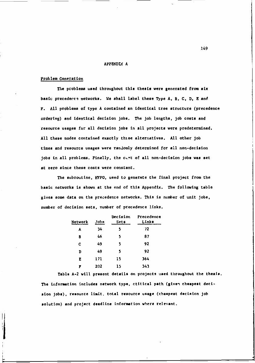
149

APPENDIX A

Problem Generation

The problems used throughout this thesis were generated from six

basic precedercs networks. We shall label these Type A, B, C, D, E and

F. All problems of type A contained an identical tree structure (precedence

ordering) and identical decision jobs. The job lengths, job costs and

resource usages for all decision jobs in all projects were predetermined.

All these nodes contained exactly thxee alternatives. All other job

times and resource usages were randomly determined for all non-decision

jobs in all problems. Finally, the c,!t of all non-decision jobs was set

at zero since these costs were constant.

The subroutine, HYPO, used to generate the final project from the

basic networks is shown at the end of this Appendix. The following table

gives some data on the precedence networks. This is number of unit jobs,

number of decision sets, number of precedence links.

Decision PrecedenceNetwork Jobs Sets Links

A 34 5 72

B 46 5 87

C 49 5 92

D 49 5 92

E 171 15 364

F 202 15 343

Table A-2 will present details on projects used throughout the thesis.

The itformation Includes network type, ctitical path (given cheapest deci-

sion jobs), resource limit, total resource usage (cheapest deciuien job

solution) and project deadline information where relevant.

ii

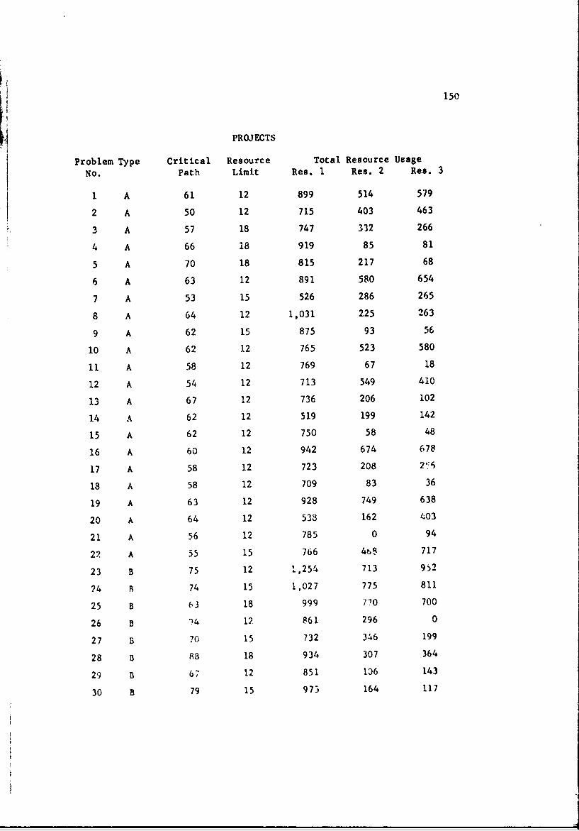
150

PROJECTS

Problem Type Critical Resource Total Resource Usage

No. Path Limit Res. 1 Res. 2 Res. 3

1 A 61 12 899 514 579

2 A 50 12 715 403 463

3 A 57 18 747 332 266

4 A 66 18 919 85 81

5 A 70 18 815 217 68

6 A 63 12 891 580 654

7 A 53 15 526 286 265

8 A 64 12 1,031 225 263

9 A 62 15 875 93 56

10 A 62 12 765 523 580

11 A 58 12 769 67 18

12 A 54 12 713 549 410

13 A 67 12 736 206 102

14 A 62 12 519 199 142

15 A 62 12 750 58 48

16 A 60 12 942 674 678

17 A 58 12 723 208 2"6

18 A 58 12 709 83 36

19 A 63 12 928 749 638

20 A 64 12 538 162 403

21 A 56 12 785 0 94

22 A 55 15 766 465 717

23 B 75 12 1,254 713 952

?4 R 74 15 1,027 775 811

25 B 63 18 999 770 700

26 B 14 12 $61 296 0

27 B 70 15 732 346 199

28 B 88 18 934 307 364

29 B 67 12 851 136 143

30 B 79 15 973 164 117

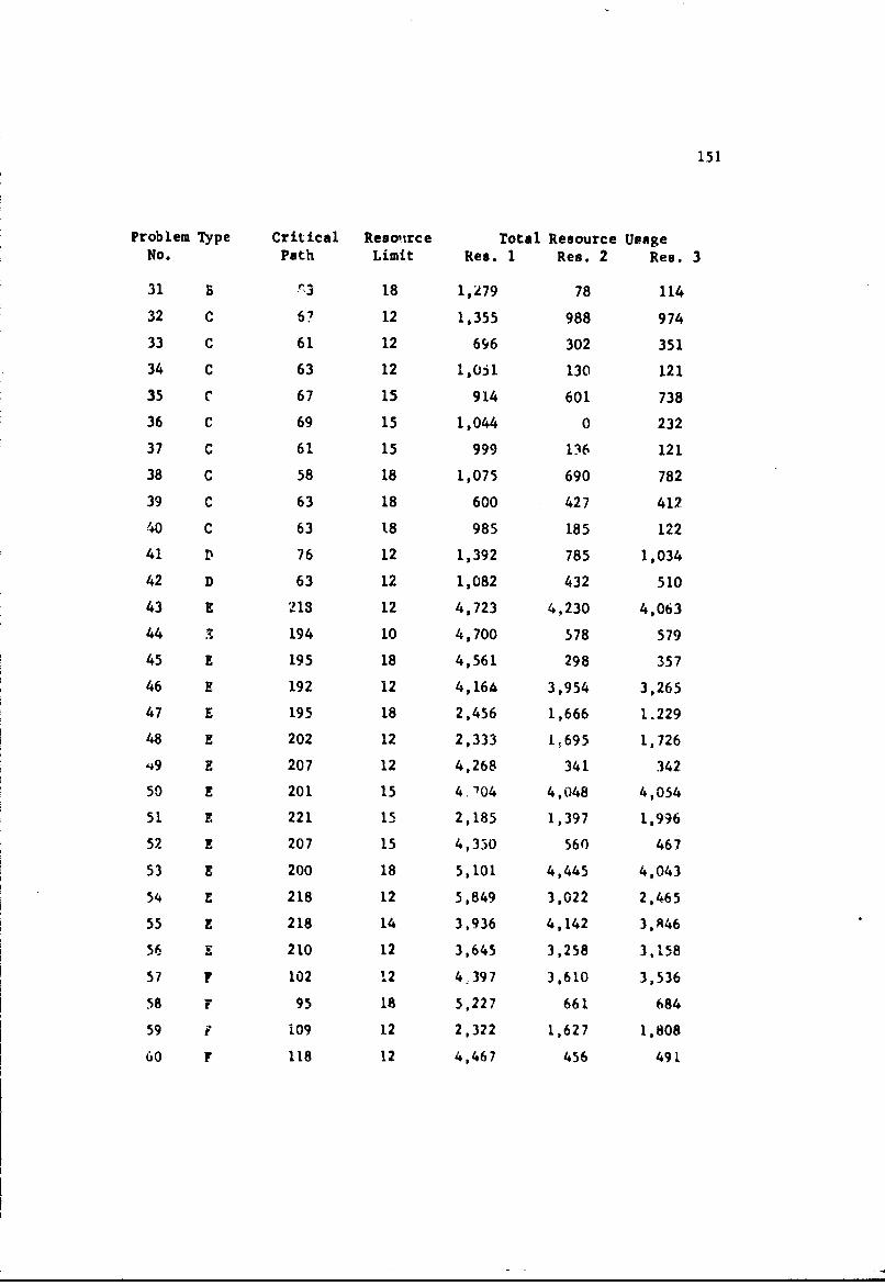
151

Problem Type Critical Reso'irce Total Resource UsageNo. Path Limit Res. 1 Res. 2 Res. 3

31 B f3 18 1,279 78 114

32 C 67 12 1,355 988 974

33 C 61 12 696 302 351

34 C 63 12 1,0,1 130 121

35 C 67 15 914 601 738

36 C 69 15 1,044 0 232

37 C 61 15 999 136 121

38 C 58 18 1,075 690 782

39 C 63 18 600 427 412

40 C 63 18 985 185 122

41 D 76 12 1,392 785 1,034

42 D 63 12 1,082 432 510

43 E 213 12 4,723 4,230 4,063

44 3 194 10 4,700 578 579

45 E 195 18 4,561 298 357

46 E 192 12 4,164 3,954 3,265

47 E 195 18 2,456 1,666 1.229

48 E 202 12 2,333 1,695 1,726

49 E 207 12 4,268 341 342

50 E 201 15 4704 4,048 4,054

51 E 221 15 2,185 1,397 1,996

52 E 207 15 4,350 560 467

53 E 200 18 5,101 4,445 4,043

54 E 218 12 5,849 3,022 2,465

55 E 218 14 3,936 4,142 3,846

56 E 210 12 3,645 3,258 3,158

57 F 102 12 4.397 3.610 3,536

58 F 95 18 5,227 661 684

59 f 109 12 2,322 1,627 1,808

60 F 118 12 4,467 456 491

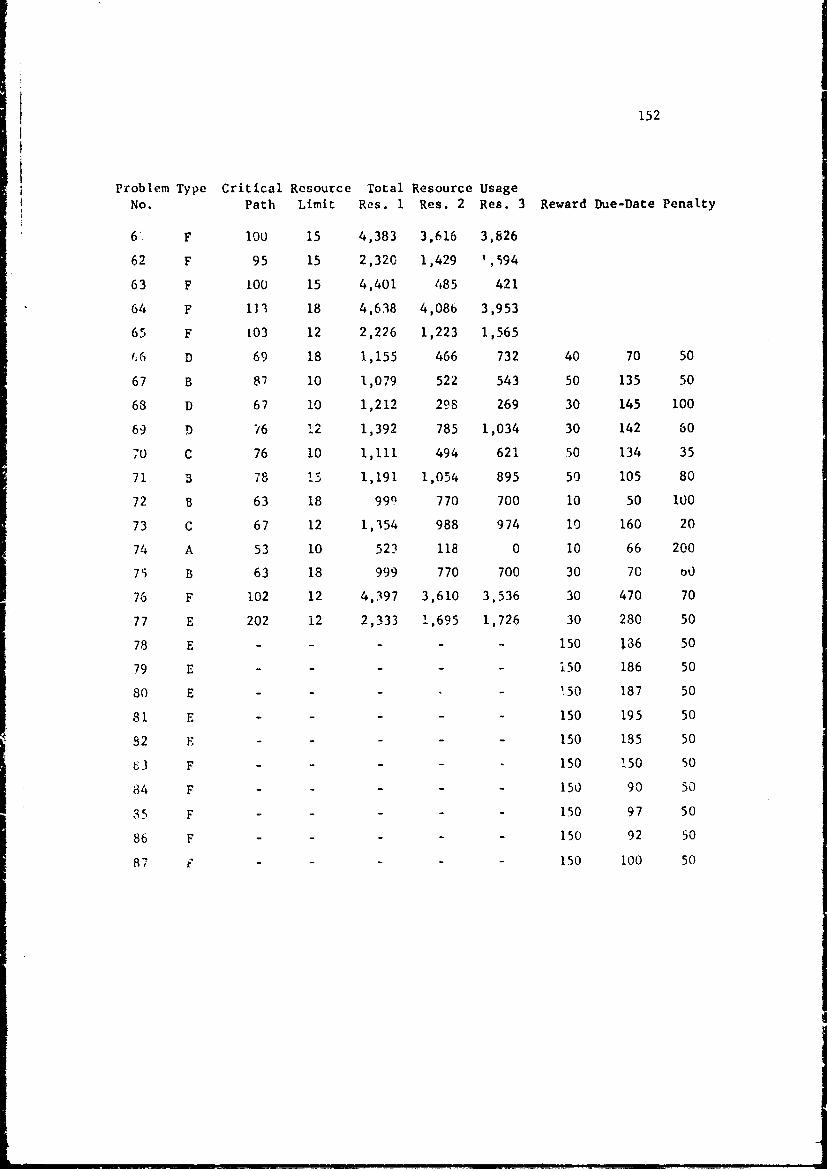
152

Problem Type Critical Resource Total Resource UsageNo. Path Limit Res. 1 Res. 2 Res. 3 Reward Due-Date Penalty

67 F 0OU 15 4,383 3,616 3,826

62 F 95 15 2,320 1,429 1,594

63 F iO0 15 4,401 485 421

64 F 1)' 18 4,638 4,086 3,953

65 F 103 12 2,226 1,223 1,565

'.6 D 69 18 1,155 466 732 40 70 50

67 B 87 10 1,079 522 543 50 135 50

68 D 67 10 1,212 298 269 30 145 100

69 D 76 12 1,392 785 1,034 30 142 60

70 C 76 10 1,111 494 621 50 134 35

71 B 78 1C 1,191 1,054 895 50 105 80

72 B 63 18 990 770 700 10 50 100

73 C 67 12 1,354 988 974 10 160 20

74 A 53 10 523 118 0 10 66 200

75 B 63 18 999 770 700 30 70 00

76 F 102 12 4,397 3,610 3,536 30 470 70

77 E 202 12 2,333 1,695 1,726 30 280 50

78 E - - - - - 150 136 50

79 E - - - - i50 186 50

80 E - - - - 150 187 50

81 E - - - - 150 195 50

52 F- - - 150 185 50

3 F - - - - 150 !50 50

84 F - - - - - 150 90 50

35 F - - - - - 150 97 50

86 F - - - - - 150 92 50

87 - - - 150 100 50

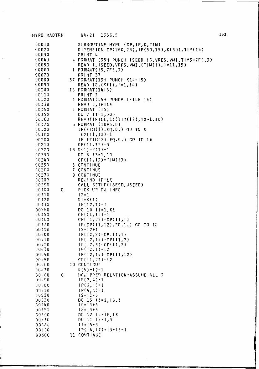
HYPO MADTRN 04/21 1356.5 153

00010 SUBROUTINE HYPO (CP,IP,K,TIM)00020 DIMENSION CP(260,25),IP(5O,15),K(30),TItA(15)00030 PRINT 400040 4 FORfIAT (35H PUNCH ISEED 15,VRES,VM1,TIM5-7F5.3)00050 READ 1,ISEED,VRFS,VM1,(TIM(1),1=11,15)00060 1 FOR.MAT(15,7F5.3)00070 PRINT 3700080 37 FORMAT(13H PUNCH K14-15)00090 READ 18,(K(I),1=1,14)00100 18 FORrIAT(1415)00110 PRINT 300120 3 FORMIAT(151H PUNCH IFILE 15)00130 READ 5,IFILE00140 5 FCR!4AT (15)00150 DO 7 11=1,30000160 READ( (IFILE,f,)(TIM(12), 12=1,10)00170 6 FORMAT (10F5.0)00180 IF(TI i(1).EQ.0.) GO TO 900190 CP(I1,12)=100200 IF (TIr4(2).EQ.0.) GO TO 1600210 CP(I11,12)=300220 16 K(1)=K(1)+100230 DO 8 13=1,1000240 CP(I1,13)='TIM(13)00250 8 CONTINUE00260 7 CONTINUE00270 9 CONTINUE00280 REWIND IFILF002C0 CALL SETUF(ISEED,USEED)00300 C PICK UP DJ INFO00310 12=100320 KI=K(1)00330 I P' 12, 1)=1003fi'0 DO 10 I1=1,KI00350 CP(I1,18)=100360 CP( l1,22)=CP(II,I)00370 IF(CP(I1,12).FO.1.) 0O TO 100038•0 12=12+1004l0 !P( 2,2)=CP,11,1)00410 IP(12,15)=CP(11,2)00420 I P( 12,3 )=CP• 11,2)00430 IP( 12,1)=1200440 IP( 2,14)=CP(11,12)00,150 CP(11,23)=120(;J4C0 10 CONTINUE00470 K(5)=12-10 080 C f)OW1 PRED RFLATION-ASSUME ALL 300490 IP(2,0)=10050c I1P(3,4)=1010)510 1 P(I,4) -100520 IS=12-500530 DO 13 13=2,IS,300540 16=13+3005 •J 1 = 13+500560 DO 12 II=16,180057(0 DO 11 15-1,3005U0 17=15*300590 IP(14,17)=13C15-100600 11 rONT INUE

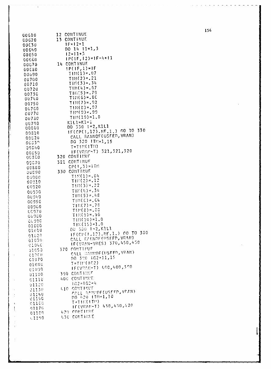
00610 12 CONTINUE15COG20 13 CONTINUEOUC30 IFrI2+100C'tO DO ,IZt 11-1,300G50 12=11+3

00670 1h CONTINUEo00Cs IP(IF,1)=IF00690O TIM(1).0700700 TltA(2)=.2100710 TINM(3.31;0 07 20 T I M('t G7

0 07 1i0 T 111(G) =. 900750 TIMM=(7.0206760 TiM(=.9700770 TIV(9)=.9900U7380 T111( 10 ) =.O-00790 K1L1=Kl-iGOHM DO 330 I=2,KlLl

00310 IF(CP(I,12).NF.l.) frO TO 330

0 0 20 CALL FRAfNOF(USFEfl,VRAN)06"3,) D0 320 IT[1=1,15

00"50 1IF ( VPl'-T) 321,321,320;)6 01 0 0 320 CONT I ru

OQOU70 3 21 CONT I NUF00, 800 CP(I , 3) =ITr

UUM 330 CONT INUF

OC'1210TIP(2)=.12

G09120 TW,(3>=.220 u9 310 T I tý( 1:) .3 1

0U9 1ý0 T I f i( 5) = .It06950 TWt(C)=.C~4

'o0 9 0 T 11. 7) .7 P

u G971 T IM(P)¾ubg920 T I N,(9 9

T1I,0'T' 151 . 0

0 1 2 1 F ( C'' I,?I NF . I.) r.0 TO 3 30

u 3 03 CALL fPlftl`NF (!lSFEP, VRAN)

61000IF(AM'l~ý-'IRES) 370,4i50,450"J50 370 roNTIVUr

CU\L ;\flr!OF~lSFFP),VPAV)

G610 70 PO 3'!C, 102=11,150 1 ()S T=Tlt'IIC2)U I li IF(VQýJ!-T) flC,400,3'fl

olQoo 300 COtiT I2UF011110C, CO'iT I "Ur

u 1121 C.-~G211,0t10 CONT I IFr,

Po , 1 IT t11 ,10

(I1170 Gir(VPVt-T) I430,4Ii)0,A20oli~q i?r 1 rn'T I f'JF

~190 U3 CONT I :[f

02200 CP( I, I r,2) =II T1501210 CALL RANr'OF(USEED, VRAN) 15501220 IF(VRAN-Vt1) 370,380,38001230 450 CONTINUE01240 380 CONTINUE01250 PRINT 17,Kl01260 17 FORMAT (15)91270 C DO 15 1=1,K101280 C PRINT 600,(,P(I,J),C=l,]5)01290 G00 FORMAT(15F5.0)01,00 15 CONT I NU E01310 'RETURN01320 END

R 5.283+1.566

156

APPENDIX B

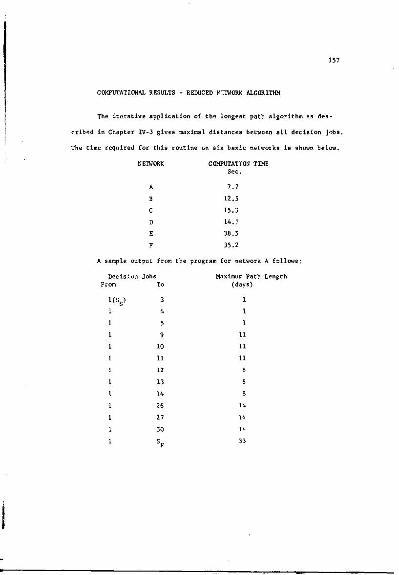
157

COMPUTATIONAL RESULTS - REDUCED F7]TWORK ALGORITHM

The iterative application of the longest path algorithm as des-

cribed in Chapter IV-3 gives maximal distances between all decision jobs.

The time required for this routine un six baxic networks is shown below.

NETWORK COMPUTATION TIMESec.

A 7.7

B 12.5

C 15.3

D 14.'

E 38.5

F 35.2

A sample output from the program for network A follows:

Decision Jobs Maximum Path LengthFrom To (days)

l(Ss) 3 1

1 4 1

1 5 1

1 9 II

1 10 11

1 11 11

1 12 8

1 13 8

1 14 8

1 26 14

1 27 14

1 30 11,

1 S F 33

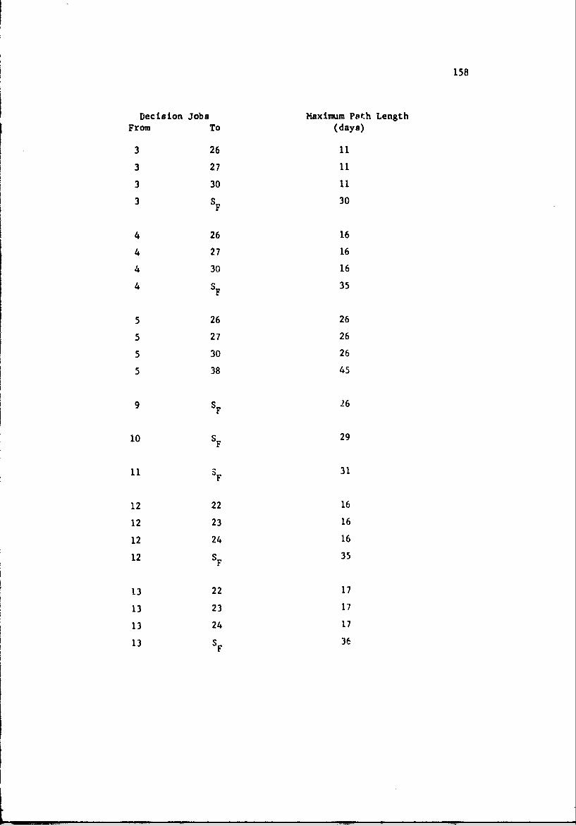
158

Decision Jobs Maximum Path LengthFrom To (days)

3 26 11

3 27 11

3 30 11

3 SF 30

4 26 16

4 27 16

4 30 16

4 SF 35

5 26 26

5 27 26

5 30 26

5 38 45

9 SF 26

10 SF 29

11 SF 31

12 22 16

12 23 16

12 24 16

12 SF 35

13 22 17

13 23 17

13 24 17

13 SF 36

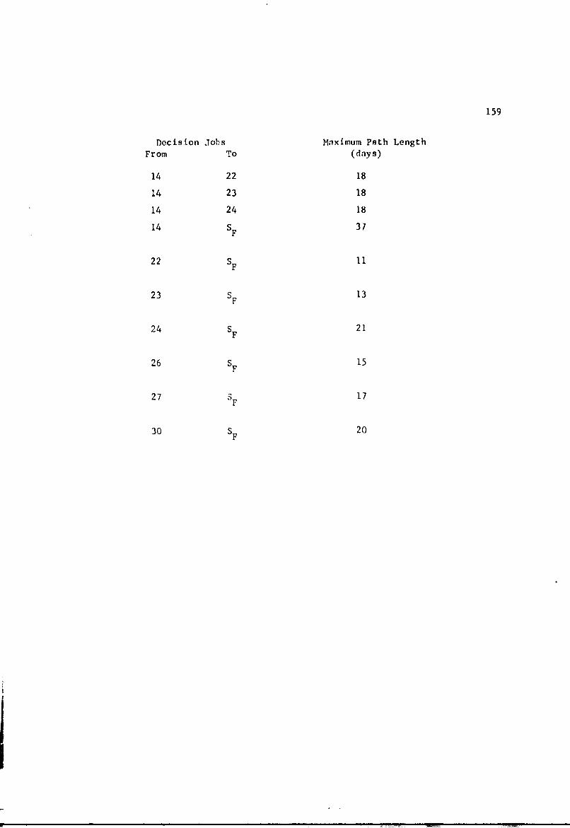
159

Decision Jobs Maximum PAth LengthFrom To (days)

14 22 18

14 23 18

14 24 18

14 SF 37

22 SF i1

23 SF 13

24 SF 21

26 SF 15

27 F 17

30 SF 20

160

APPENDIX C

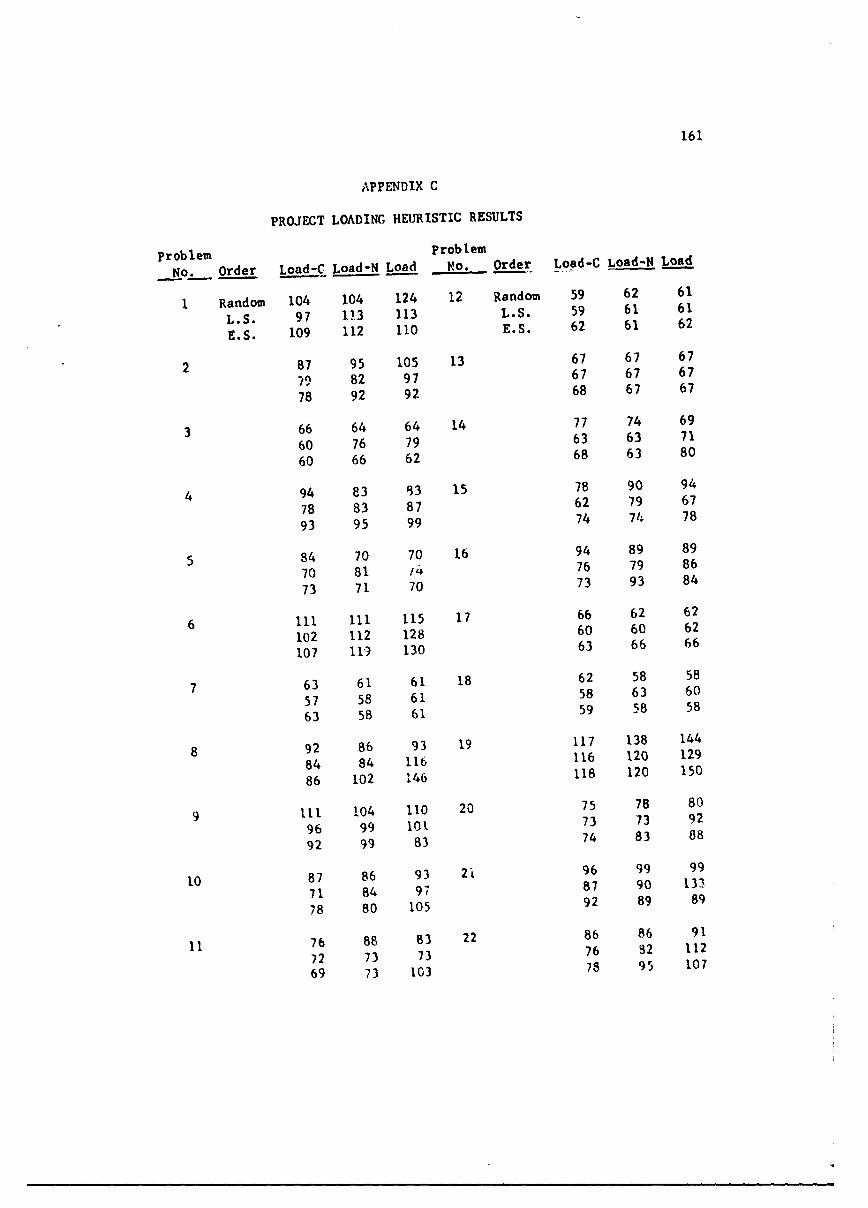
161

APPENDIX C

PROJECT LOADING HEURISTIC RESULTS

Problem Problem

o. Order oad- Load-N Load Yo. Order Load-C Load-N Load

1 Random 104 104 124 12 Random 59 62 61

L.S. 97 1.3 113 L.S. 59 61 61

E.S. 109 112 110 E.S. 62 61 62

2 87 95 105 13 67 67 67

79 82 97 67 67 67

78 92 92 68 67 67

3 66 64 64 14 77 74 69

60 76 79 63 63 71

60 66 62 68 63 80

4 94 83 93 15 78 90 94

78 83 87 62 79 67

93 95 99 74 714 78

5 84 70 70 16 94 89 89

70 81 14 76 79 86

73 71 70 73 93 84

6 ill ill 115 17 66 62 62

102 112 128 60 60 62

107 119 130 63 66 66

7 63 61 61 18 62 58 58

57 58 61 58 63 60

63 58 61 59 58 58

8 92 86 93 19 117 138 144

84 84 116 116 120 129

86 102 146 118 120 150

9 ill 104 110 20 75 78 80

96 99 10 73 73 92

92 99 83 74 83 88

10 87 86 93 2i 96 99 99

71 84 97 87 90 133

78 80 105 92 89 89

11 76 88 83 22 86 86 91

72 73 73 76 82 112

69 73 103 78 95 107

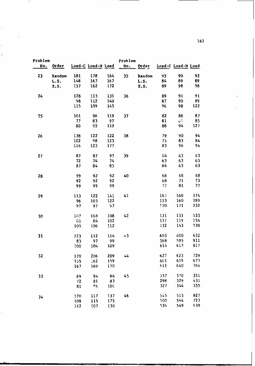
162

Problem Problem

No.- Order Load-C Load-N Load No. Order Load-C Load-N Load

23 Random 181 178 184 35 Random 95 90 92L.S. 148 167 167 L.S. 84 89 89

E.S. 157 162 172 E.S. 89 98 98

24 128 113 131 36 89 91 9198 112 140 87 90 89

115 109 145 96 98 122

25 101 98 119 37 82 88 8777 83 97 81 8588 95 110 88 94 127

26 138 122 122 38 79 90 94102 98 123 75 83 34116 123 177 83 96 94

27 87 87 97 39 64 63 6372 74 74 63 63 6387 84 85 64 63 63

28 99 92 92 40 68 68 6892 92 92 68 71 7399 99 99 77 81 77

29 113 122 141 41 16W 160 17496 103 122 153 160 18997 97 97 170 171 232

30 10? 108 108 42 131 131 133zo 84 102 1!) 119 156100 106 112 132 143 1.38

31 123 112 114 1-3 603 600 63283 97 99 568 595 911

100 104 109 614 613 817

32 170 206 209 44 627 623 729155 ý62 159 bOl 619 673167 169 170 611 640 764

33 89 94 94 45 337 370 35172 81 83 298 329 43181 06 106 327 344 355

34 120 117 137 46 545 513 827I09 115 175 500 564 723112 107 130 534 549 639

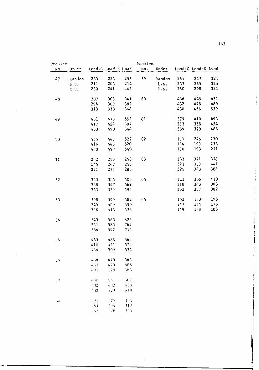
163

Prob lem P rob I emNo. Order Load-C Loa-'-N Load No. Order Load-C Load-N Load

47 R.ndnorm 233 223 255 59 Random 26i 267 321L.S. 211 203 214 L.S. 237 265 324E..S. 230 241 242 L.S. 250 298 321

48 307 308 341 60 466 445 651294 309 382 432 428 489313 330 368 430 456 559

49 451 476 552 61 379 410 493417 454 607 363 358 454433 490 644 369 379 486

50 435 447 522 62 197 245 230416 448 520 184 199 235440 497 540 190 193 271

51 262 256 258 63 333 371 378245 247 253 321 359 441271 276 288 325 348 388

52 353 385 403 64 323 306 410338 347 562 318 343 333

353 379 493 333 357 382

53 398 399 482 65 153 183 195349 40') 490 147 164 176368 415 47S 149 188 188

54 543 563 625531 583 762556 592 713

1453 488 663

410 fl 573464 509 574

56 488 470 565

51) 1

.88

,31 7l.,I .'i )" 31lo

3•) ) :',' •, 14

1,64

APPENDIX D

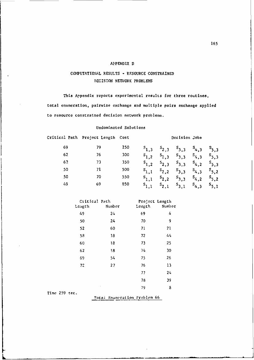
165

APPENDIX D

COMPUTATIONAL RESULTS - RESOURCE CONSTRAINED

DECISION NE1NORK PROBLEMS

This Appendix reports experimental results for three routines,

total enumeration, pairwise exchange and multiple pairs exchange applied

to resource constrained decision network problems.

Undominated Solutions

Critical Path Project Length Cost Decision Jobs

69 79 250 S1,3 52,3 S3,3 S4,3 S5,362 76 300 S1,2 $2,3 $3,3 $4,3 $5,3

62 73 350 S1,2 '2,3 $3, 3 S4,2 S5,3

50 71 500 S1,1 $2,2 S3 , 3 S4, 3 S5,2

50 70 550 Sl,1 S2,2 S3,3 S4,2 S5,2

49 69 850 S. S S2,1 $3,1 S4,3 S5,I

Critical Path Project LengthLciigth Number Length Number

49 24 69 4

50 24 70 9

52 60 71 21

58 18 72 44

60 18 73 25

62 i8 74 30

69 54 75 26

72 27 76 13

77 24

78 39

79 8Time 259 sec.

Total Enumeration Problem 66

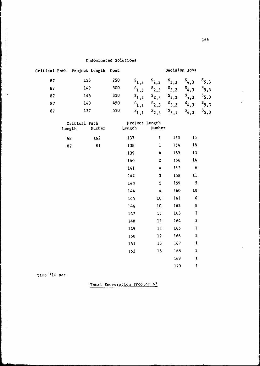
I

166

Undominaced Solutions

Critical Path Project Length Cost Decision Jobs

87 153 250 Si13 S2,3 S3,3 S4,3 S5,3

87 149 300 S1, 3 S2, 3 S3, 2 S4,3 qS,3

87 145 350 S1,2 $2,3 S3 , 2 S4, 3 S5,3

87 143 450 S ,1 $2,3 $3,2 S4,3 5,387 137 550 S,1 S2,3 S3,1 S4,3 S5,3

Critical Path Project Length

Length Number Length Number

68 162 137 1 153 15

87 81 138 1 154 18

139 4 155 13

140 2 156 14

141 4 1;7 6

142 2 158 11

143 5 159 5

144 4 160 10

145 10 161 6

146 10 162 8

147 15 163 3

148 12 164 3

149 13 165 1

150 12 166 2

151 13 167 1

152 15 168 2

169 1

170 1

Time '10 sec.

Total Enumeration Problem 67

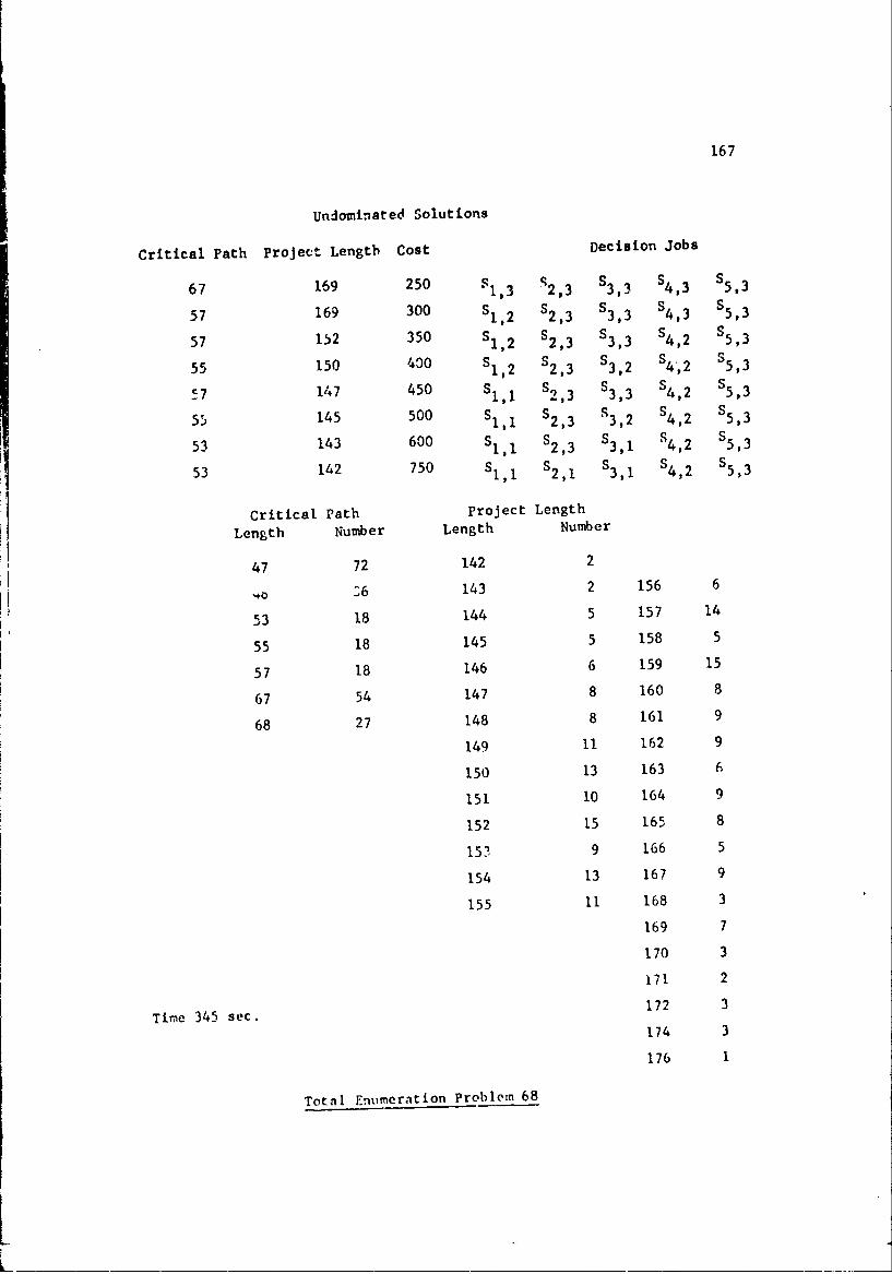
167

Undominated Solutions

Critical Path Project Length Cost Decision Jobs

67 169 250 S1,3 S2,3 S S3,3 4,3 S5,3

57 169 300 Sl12 $2,3 S3 , 3 $4,3 S5 , 3

57 152 350 S1 2 S S3,3 $4,2 S5,355 150 400 S 1,2 $2,3 $3,2 S4 ',2 $5,3

57 147 450 S1,1 $2,3 $3,3 4,2 $ 5,3

55 145 500 SII $2,3 S3,2 $4,2 $5,3

53 143 600 SIl $2,3 $3,1 '4,2 $5,3

51475 " S S S53 142 750 SI,1 $,! 3,1 4,2 5,3

Critical Path Project Length

Length Number Length Number

47 72 142 2

20 36 143 2 156 6

53 18 144 5 157 14

55 18 145 5 158 5

57 18 146 6 159 15

67 54 147 8 160 8

68 27 148 8 161 9

149 11 162 9

150 13 163 6

151 10 164 9

152 15 165 8

153 9 166 5

154 13 167 9

155 11 168 3

169 7

170 3

171 2

Time 345 sec. 172 3174 3

176 1

Total Enimeration Problem 68

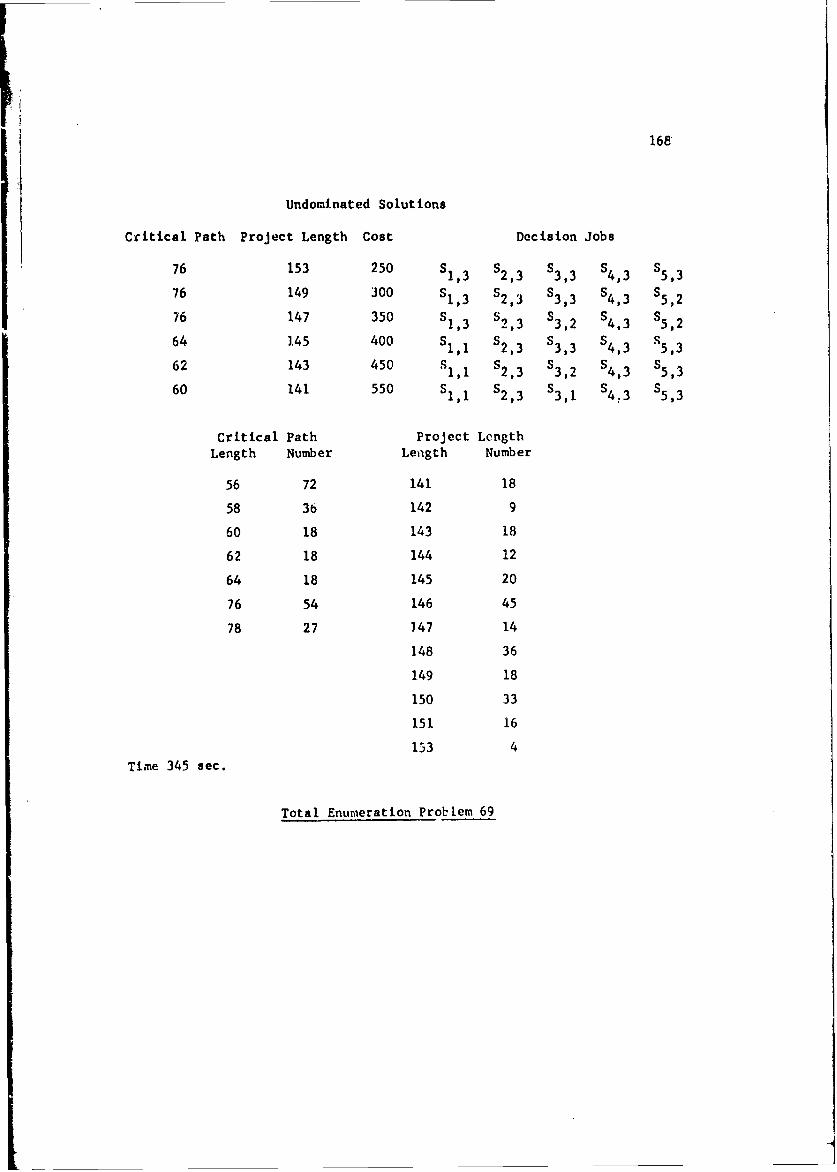
168

Undominated Solutions

Critical Path Project Length Cost Decision Jobs

76 153 250 S, 3 $23 S3 3 S4 3 S5 3

76 149 300 S1,3 $2,3 S3, 3 S4 , 3 S5,2

76 147 350 S1,3 S2 , 3 $3,2 S4, 3 S5,2

64 1145 400 S11 S2,3 S3,3 S4,3 S5,362 143 450 Sl,1 S2,3 S3,2 S 5,3

60 141 550 sl,1 S2,3 S3,1 S4.3 S5,3

Critical Path Project LengthLength Number Length Number

56 72 141 18

58 3b 142 9

60 18 143 18

62 18 144 12

64 18 145 20

76 54 146 45

78 27 147 14

148 36

149 18

150 33

151 16

133 4Time 345 sec.

Total Enumeration Problem 69

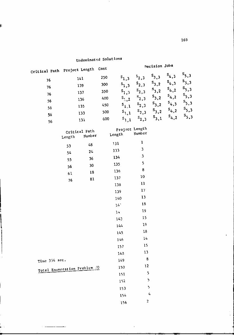
169

Undomilnated Solutions

Critical Path Project Length Cost necision Jobs

76 141 250 S1,3 $2,3 S3, 3 S4 , 3 S5 , 3

76 139 300 S1 , 3 $2,3 $3.2 54,3 S55 3

76 137 350 S] ,3 S23 S3,2 $4,2 S5,3

136 400 S, q2,3 3 ,2 S 2 5,3

56 1 , ,

56 135 450 S $2,3 $3,2 S4, 3 $5,3

56 133 500 S ,I $2,3 $3,2 S4, 2 $5,3

56 131 600 1.,1 2,3 S3 , 1 S4 ,2 $5,3

Critical Path Project Length

Length Number Length Number

53 48 131 1

54 24 133 3

55 36 134 3

56 30 135 5

61 18 136 8

76 81 137 10

138 11

139 17

140 13

14' 18

14 19

143 15

144 19

145 18

146 14

157 15

143 13

Time 354 sec. 149 8

Totjl Enumeration problem '0 150 12

151 5

152 5

153 5

154 4

156 2

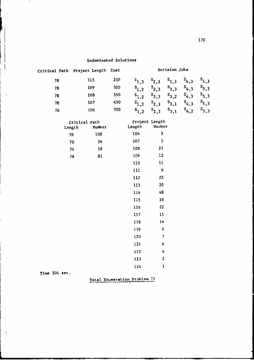
170

Undominated Solutions

Critical Path Project Length Cost Decision Jobs

78 115 250 S S S S S1.3 2,3 3,3 4,3 5,3

78 109 100 S S S S S1,2 2,3 3,3 4,3 5,3

78 108 350 S1,2 S2,3 S3,2 S4,3 $5,3

78 107 450 S1,2 S2,3 S3,1 $4,3 S5,3

78 106 500 S1,2 $2,3 S3,1 $4,2 S5,3

Critical Path Project Length

Length Number Length Number

59 108 106 3

70 36 107 3

74 18 108 21

78 81 109 12

110 11

1il 9

112 25

113 20

1U4 48

115 18

116 22

117 11

118 14

119 6

120 7

121 6

122 4

123 2

124 1

Time 304 sec.

Total Enumeration Problem 71

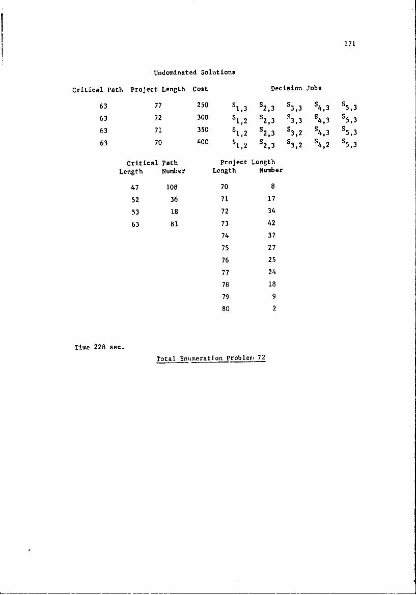
171

Undominated Solutions

Critical Path Project Length Cost Decision Jobs

63 77 250 SI,3 S2 , 3 S3, 3 S4,3 $ 5,3

63 72 300 S1,2 $2,3 S S3,3 4,3 S5,3

63 71 350 S1,2 S2,3 S3,2 S4, 3 S5 , 3

63 70 IAOO SI,2 S2,3 S3,2 S4,2 $5,3

Critical Path Project Length

Length Number Length Number

47 108 70 8

52 36 71 17

53 18 72 34

63 81 73 42

74 37

75 27

76 25

77 24

78 18

79 9

80 2

Time 228 sec.

Total Enumeration Problem 72

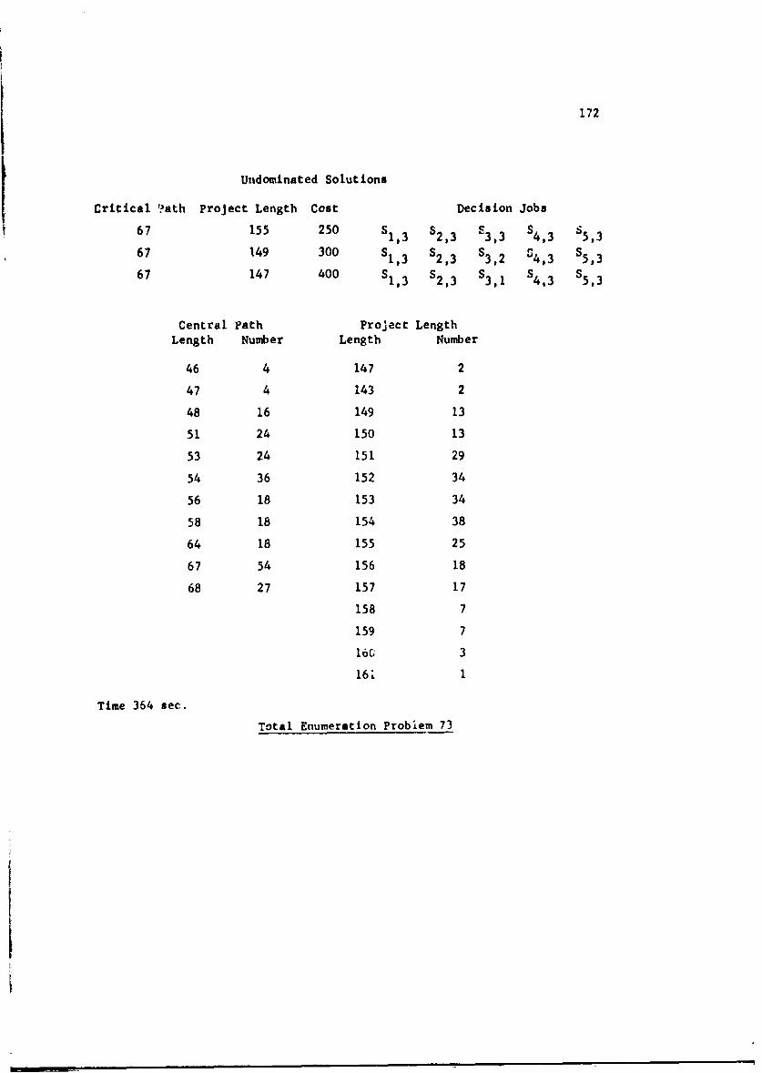
172

Undominated Solutions

Critical ?ath Project Length Cost Decision Jobs

67 155 250 S S I1,3 2,3 3,3 4,3 5,3

67 149 300 S1,3 3 S3,2 S4,3 $5,367 147 400 S1,3 $2,3 S3 , 1 S4,3 S5,3

Central Path Project LengthLength Number Length Number

46 4 147 2

47 4 143 2

48 16 149 13

51 24 150 13

53 24 151 29

54 36 152 34

56 18 153 34

58 18 154 38

64 18 155 25

67 54 156 18

68 27 157 17

158 7

159 7

16C 3

161 1

Time 364 sec.

Total Enumeration Problem 73

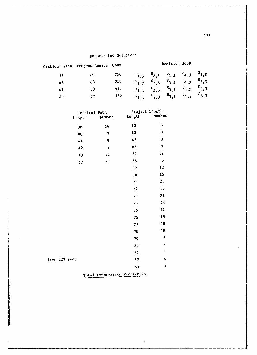
173

Undominated Solutions

Critical Path Prcject Length Cost Decision Jobs

53 69 250 $1,3 $2,3 $3,3 $4,3 S5,3

43 68 350 S1,2 S2,3 $3,2 S4,3 S5,3

41 63 450 $I1l $2,3 S3, 2 S4 ,3 $5,3

40 62 350 S 1 , 1 $2,3 $3,1 54, 3 $5,3

Critical Path Project Length

Length Number Length Number

38 54 62 3

40 9 63 3

41 9 65 3

42 9 66 9

43 81 67 12

53 81 68 6

69 12

70 15

71 21

72 15

73 21

74 18

75 21

76 15

77 18

78 18

79 15

80 6

81 3

Time 129 sec. 82 b83 3

Total Enumt ration Problem 74

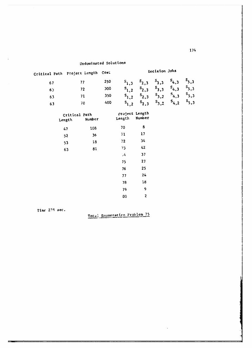
174

Undominated Solutions

Critical Path Project Length CosL Decision Jobs

67 77 250 S1.3 S 4,3 S5,3

63 72 300 S1,2 S2,3 S3,3 S4 , 3 S5,3

63 71 350 S12 $2.3 53,2 r4,3 $ 5,3

63 70 400 S1,2 S2,3 S3,2 S4 , 2 55,3

Critical Path eroject Length

Length Number Length Number

47 108 70 8

52 36 71 17

53 is 72 34

63 81 73 42

,t, I37

75 27

76 25

77 24

78 18

79 9

80 2

Time 2?9 sec.

Total Enumeraticn Problem 75

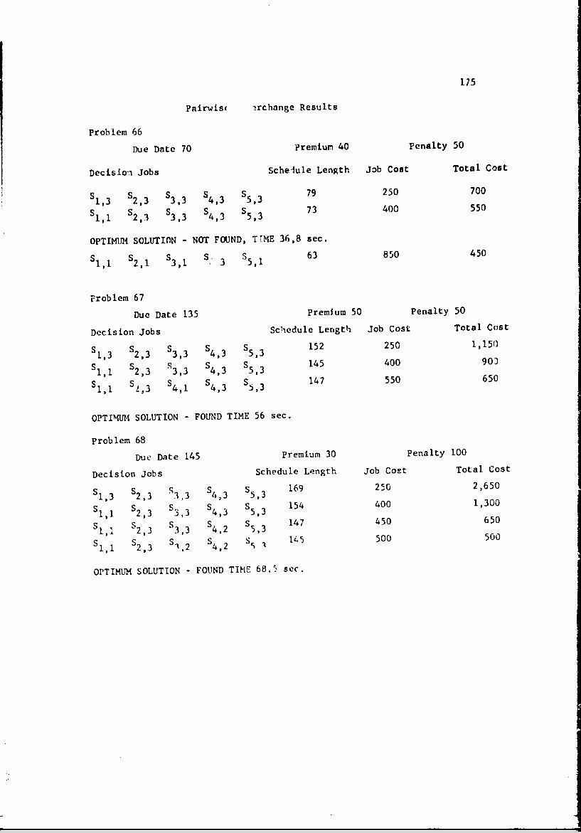
175

Pairwis • rchange Results

Problem 66

Due Date 70 ?remiun 40 Penalty 50

Decision. Jobs Scheiule Length Job Cost Total Cost

S S S S S 79 250 7001,3 2,3 3,3 4,3 5,3

SI, S2,3 S,3 $4,3 5,3 73 400 550

OPTIMUM SOLUTION - NOT FOUND, TTME 36,8 sec.

S 2 1 $S Si3 S 63 850 45011 21 3,1 3 5,1

Problem 67

Due Date 135 Premium 50 Penalty 50

Decision Jobs Schedule Length Job Cost Total Cost

1,3 2,3 3,3 4,3 5,3 152 250 1,150Sll $2,3 S3,3 $4,3 $5,3 145 400 90)

SII S2,3 $4,1 S4,3 $5, 3 147 550 650

OPTIMUM SOLUTION - FOUND TIME 56 sec.

Problem 68

Due Date 145 Premium 30 Penalty 100

Decision Jobs Schedule Length job Cost Total Cost

SI,3 $2,3 S3,3 S4,3 $5,3 169 250 2,650

SI S2 , 3 S3, 3 S4 , 3 S5 , 3 154 400 1,300

S1 S S3 S 5 147 450 650, $2, 3 ,3 $4,2 $5,3

SI,I $2,3 S 1,2 $4, 2 S5, 145 500 500

OPTIMUIM SOLUTION - FOUND TIME 68.5 sec.

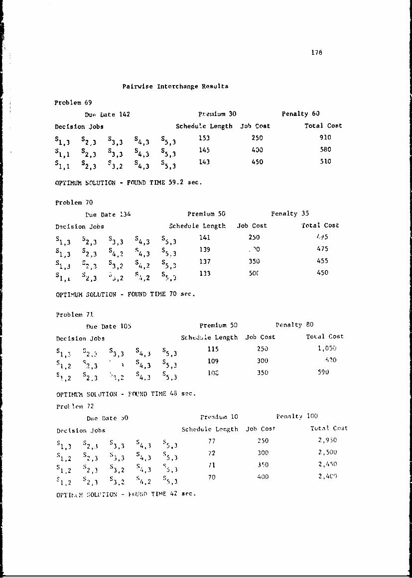
176

Pairwise Interchange Results

Problem 69

Due- Date 142 Premium 30 Penalty 60

Decision Jobs Schedule Length Job Cost Total Cost

S1,3 52,3 53,3 S4 , 3 S5, 3 153 250 910

Sl1 S2, 3 S3, 3 S4 , 3 S5, 3 145 430 58043 143 450 1

51, 5' 2,3 S"3,2 $ 4,3 S ,3 144550

OPTIMUM SOLUTION - FOUND TIME 59.2 sec.

Problem 70

Vue Date 13A Premium 50 Penalty 35

Decision Jobs Schedule Length Job Cost Total Cost

51,3 $2,3 $3,3 $4,3 55,3 141 250 4145

S S S 1 S13 ý471,3 2,3 $4,? 43 $5 139 0 475

S S" 3 3,? S 4,2 5 137 350 455

S S S S 133 50C 4501,1 2,3 j,2 4,2 55,3

OPTIMUM SOLUTION - FOUND TIME 70 sec.

Problem 71

Due Date 105 Premium 50 Penalty 80

Decision Jobs Schedule Length Job Cost Total CostS33 S5 3 115 250 1, 05

S1, 2,3 S 4,3 $5,3 109 300 0

SS S S 03559

,2 2,3 1.," $4, 553 lOC 350 590

OPTIMUM SOI.UTION - FOUND TIME 48 sec.

Prol lem 72

Due Date A0 rre:iuan 10 Penalty 100

Decision Jobs Schedule Length Job Cost TItdA Cost

S S 4 3 5S 77 250 2,9--1,3 '23 3,3 43 5,3

S11 S 3, S4,3 S 53 72 300 2,500

S1 ,2 S 2,3 S3 , 2 S4, 3 5,3 /1 350 2,450

S S3 S3 SS 70 400 2,4Cr)"1 ,2 2,3 3,2 "4,2 ,

OPTIM.iM ;0LU,'ION - IOU..JD TIN E 42 sec

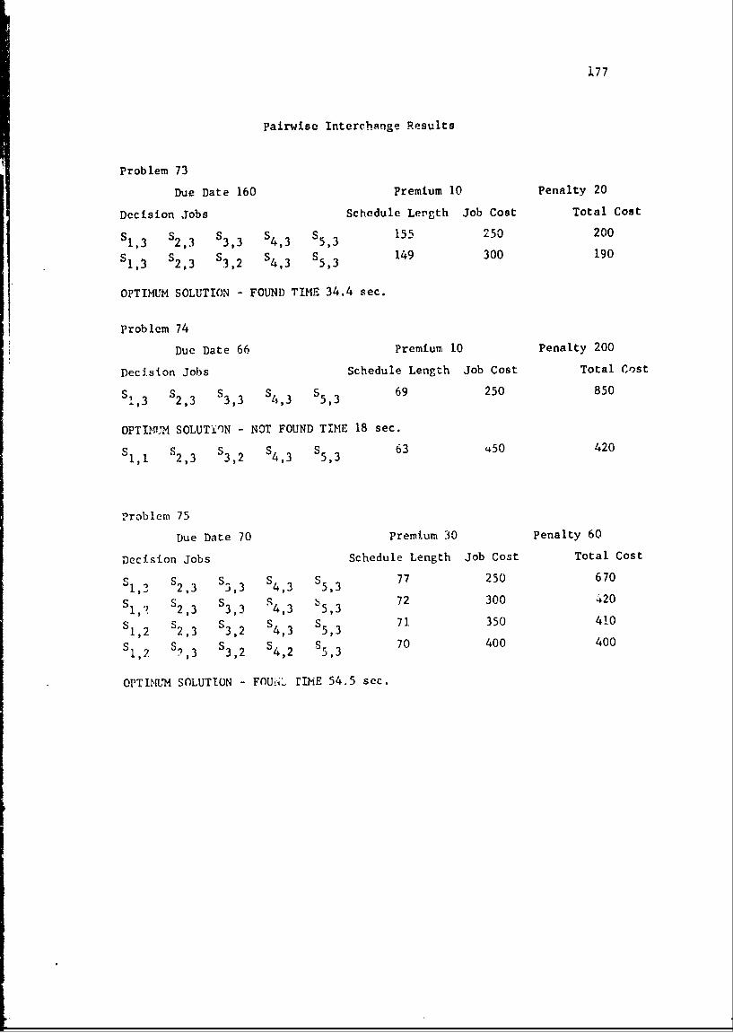
177

pairwise Interchange Results

Problem 73

Due Date 160 Premium 10 Penalty 20

Decision Jobs Schedule Length Job Cost Total Cost

S1,3 S2,3 S3,3 S S5,3 1.55 250 200

SI,3 S2, 3 S3, 2 S4, 3 S5 , 3 149 300 190

OPTIMUM SOLUTION - FOUND TIME 34.4 sec.

Problem 74

Due Date 66 Premium 10 Penalty 200

Decision Jobs Schedule Length Job Cost Total Cost

S',3 $2,3 S3, 3 $4,3 $5,3 69 250 850

OPTIMUM SOLUTION - NOT FOUND TIME 18 sec.

S1,1 $2,3 $3,2 $4,3 $5,3 63 450 420

problem 75

Due Date 70 Premium 30 Penalty 60

Decision Jobs Schedule Length Job Cost Total Cost

S1,3 $2,3 $3,3 $4,3 S5,3 77 250 670

S1,2 2,3 $3,3 *4,3 b5,3 72 300 420

S1,2 S2,3 $3,2 $4,3 $5,3 71 350 410

S1,2 $),3 $3,2 $4,2 S5, 3 70 400 400

OPTIMUM SOLUTION - FOUdiL rIME 54.5 sec.

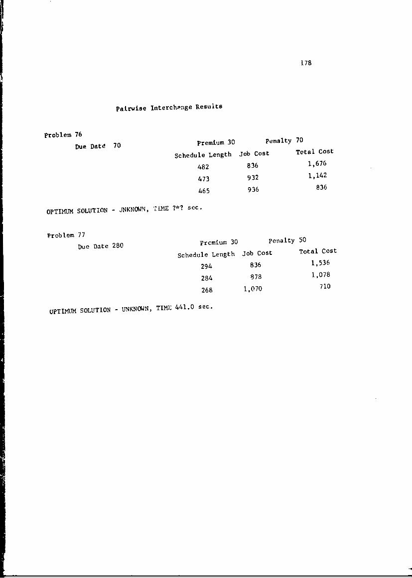
178

Pairwise Interchange Results

Problem 76

Due Datd 70 Premium 30 Penalty 70

Schedule Length Job Cost Total Cost

482 836 1,676

473 932 1,142

465 936 836

OPTIMUM SOLUTION - JNKNOWN, TiME ?*? sec.

Problem 77

Due Date 280 premium 30 penalty 50

Schedule Length Job Cost Total Cost

294 836 1,536

284 878 1,078

268 1,070 710

OPTIMUM SOLUTION - UNKNOWN, TIME 441.0 sec.

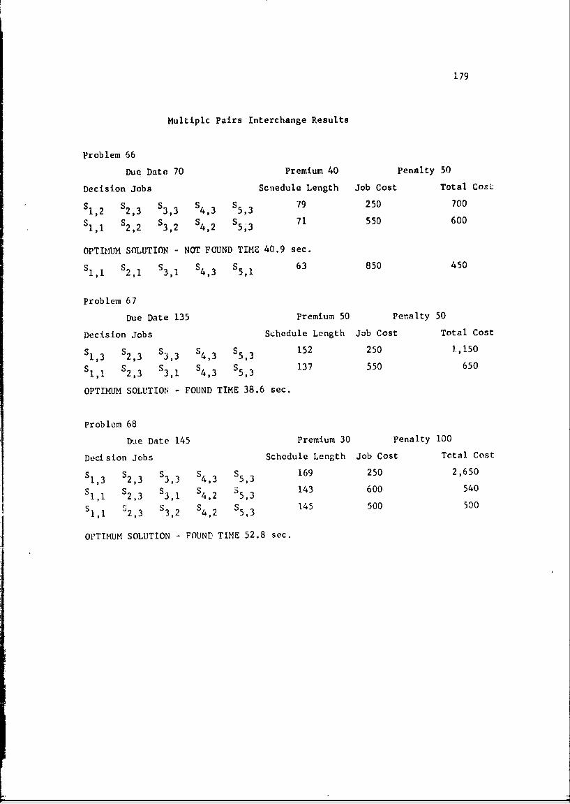
179

Multiplc Pairs Interchange Results

Problem 66

Due Date 70 Premium 40 Penalty 50

Decision Jobs Scnedule Length Job Cost Total CosL

S1,2 $2,3 $3,3 $4,3 $5,3 79 250 700

SI,1 $2,2 S 3,2 $4,2 S5,3 71 550 600

OPTI•NUM SOLUTION - NOT FOUND TIME 40.9 sec.

S1,1 $2,1 $3,1 $4,3 S5 , 1 63 850 450

Problem 67

Due Date 135 Premium 50 Penalty 50

Decision Jobs Schedule Length Job Cost Total Cost

S1,3 S2,3 $3,3 4,3 $ 5,3 152 250 1,150

Si,i. S2,3 S3 , 1 S4,3 S5 , 3 137 550 650

OPTIMUM SOLUTION - FOUND TIME 38.6 sec.

Problem 68

Due Date 145 Premium 30 Penalty 100

Decision Jobs Schedule Length Job Cost Total Cost

SI,3 $2,3 S3,3 $4,3 $5,3 169 250 2,650S,3 $2,3 $3,1 $4,2 $5,3 143 600 540

S S S S 143 600 54001,1 2,3 ~3,2 4,2 5,3OPI M 2,3 $3,2 $4,2 TIME 145 500 500

OPTIMUM SOLUTION - FOUND TIME 52.8 sec.

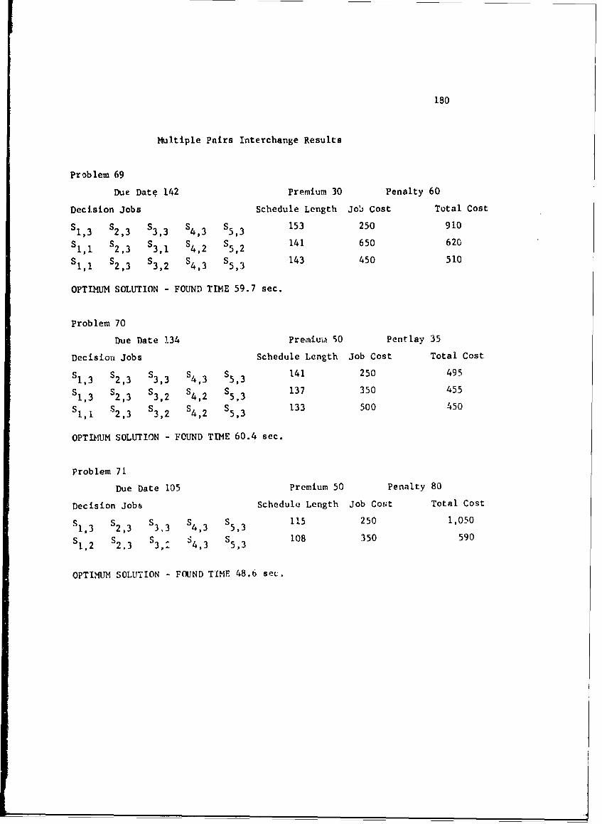
180

Multiple Pairs Interchange Results

Problem 69

Due Datq 142 Premium 30 Penalty 60

Decision Jobs Schedule Length Job Cost Total Cost

S1,3 $2,3 $3,3 S 4,3 $5,3 153 250 910

SI S2, 3 $3,1 $4,2 $5,2 141 650 620

S1,1 $2,3 $3,2 S4, 3 S5,3 143 450 510

OPTIMUM SOLUTION - FOUND TIME 59.7 sec.

Problem 70

Due Date 134 Premium 50 Pentlay 35

Decision Jobs Schedule Length Job Cost Total Cost

S1 , 3 $2,3 S3 , 3 $4,3 S5 , 3 141 250 495

S1,3 S2,3 S3,2 S4,2 S5 , 3 137 350 455

S,1 S2,3 $3,2 $4,2 S5 , 3 133 500 450

OPTIMUM SOLUTION - FOUND TIME 60.4 sec.

Problem 71

Due Date 105 Premium 50 Penalty 80

Decision Jobs Schedule Length Job Colit Total Cost

S1,3 S2,3 $3,3 4,3 $ 5,3 115 250 1,050

S1,2 S2,3 S3,: S4,3 $5,3 108 350 590

OPTIMUM! SOLUTION - FOUND TIME 48.6 sec.

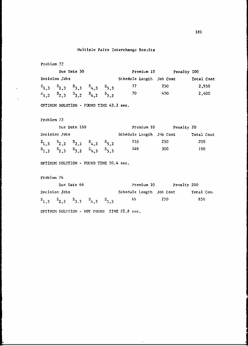
181

Multiple Pairs Interchange Results

Problem 72

Due Date 50 Premium 10 Penalty 100

Decision Jobs Schedule Length Job Cost Total Cost

S1,3 $2,3 S3 , 3 S4, 3 S5 , 3 77 250 2,950

S1,2 $2,3 '3,2 S4 , 2 S5 , 3 70 400 2,400

OPTIMUM SOLUTION - FOUND TIME 43.3 sec.

Problem 73

Due Date 160 Premium 10 Penalty 20

Decision Jobs Schedule Length Jnb Cost Total Cost

S1,3 S2,3 S3, 3 S4,3 S5,3 155 250 200

S1,3 $2,3 $3,2 S4,3 $5,3 149 300 190

OPTIMUM SOLUTION - FOUND TIME 50.4 sec.

Problem 74

Due Date 66 Premium 10 Penalty 200

Decision Jobs Schedule Length Job Cost Total CosL

S1,3 $2,3 $3,3 $4,,3 5 6 250 850

OPTTMUM SOLUTION - NOT FOUND TIME 22.8 sec.

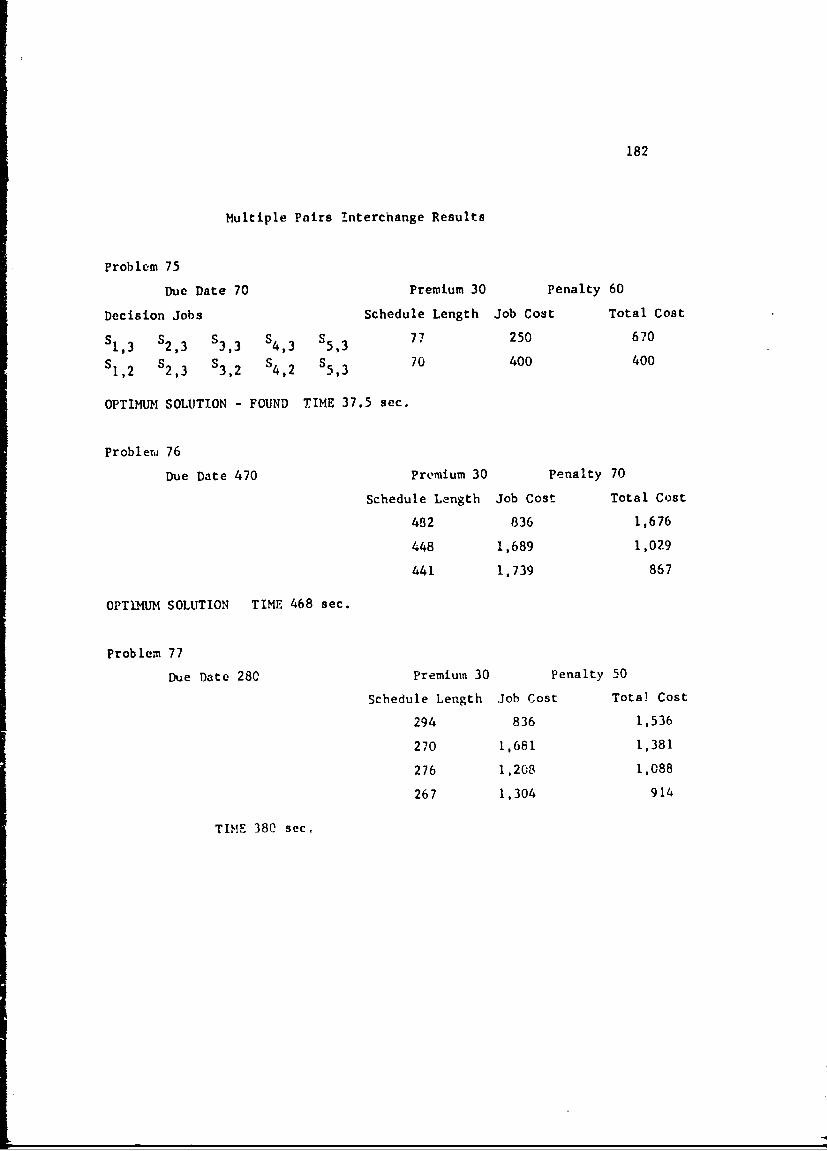
182

Multiple Pairs interchange Results

Problem 75

Due Date 70 Premium 30 Penalty 60

Decision Jobs Schedule Length Job Cost Total Cost

S1,3 $2,3 S3,3 $4,3 S5,3 77 250 670

S S,2 $2 , 3 $3,2 $4,2 S5 , 3 70 400 400

OPTIMUM SOLUTION - FOUND TIME 37.5 sec.

Problem 76

Due Date 470 Premium 30 Penalty 70

Schedule Length Job Cost Total Cost

482 836 1,676

448 1,689 1,029

441 1,739 867

OPTLMUM SOLUTION TIME 468 sec.

Problem 77

Due Date 280 Premium 30 Penalty 50

Schedule Length Job Cost Total Cost

294 836 1,536

270 1,681 1,381

276 1,208 1,088

267 1,304 914

TIME 380 sec.

h183

APPEN,ý)IX E

184

APPENDIX E

Branch and Bound Program Description

A. Main Program, Subroutines and Tapes:

One, Bonnie, Clyde, Five

The program will call tape .99. to find the number of the

problem tape. Format (14)

B. Problem Tape:

1. First Line LIM, TIME, BON, TLFX, LAST, IJND, JY

Format (IS, 3F5.O, 315) where

LIM = Number of Decision Nodes

TIME = Due Date

BON Penalty

TLFD = Premium

LAST = Node Number of Artificial •inish Job.

IJND Number of "other" Interdependency Constraints

JY - Number of Decision Nodes with More than Three Alternatives.

z. :;.-, "LIM + JY" Lines

jo0) Number, Job Number, Job Number, Cost, Cost, Ct:st

Format (315, 3F5.O, 1).

If there are not exactly three alternatives then In the

last position of the line- put the difft-rence htctwecn the ntmuber

anrd three.

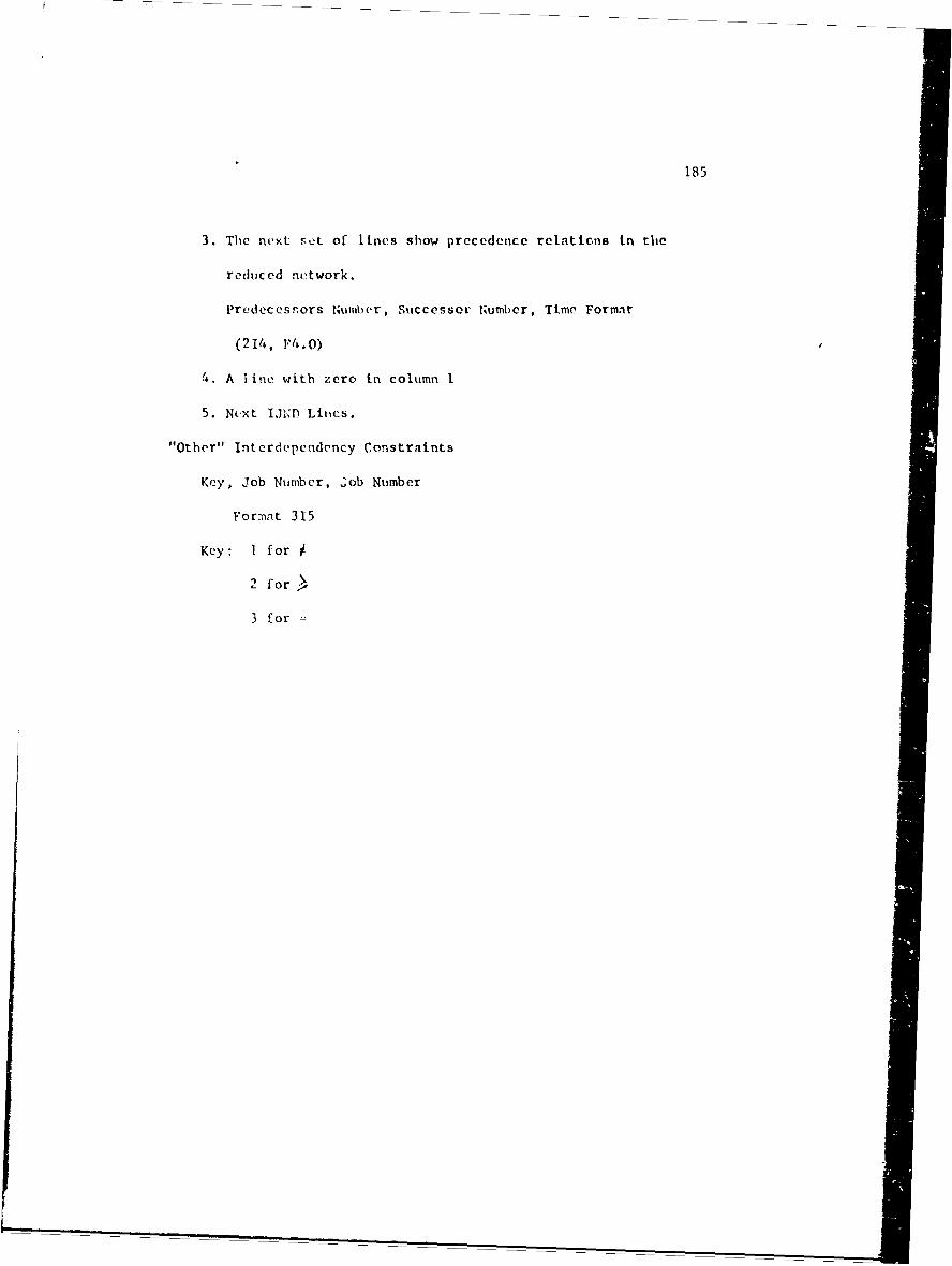
185

3. The next FeL of Lines show precedence relaticns in the

reduced network.

Predecessors Number, Successor Number, Time Format

(214, 114.0)

4. A line with zero in column 1

5. N(xt J,1W1D Lties.

"Other" Interdependency Constraints

Key, Job Number, ýob Number

For-nat 315

Key: I for #

2 for

3 for

186ONE MADThN

ONr APP 0S/ 2 2 ]1429. 2

oni Iý,r !)tFtSntfl !A-PATIU(5000) KLIST(20 It 2.) ,C0ST( 2O0),K!~p( COO,2),TB1(1O)ol0 02 0 1)1PIFiPI~StfI Om ~) (F.00fI), 3, f50),TR2 (10,TR3 ( 10 )LPATUf(101f),. ld50, 2

00030 r)ItMF1!!st() I0(k2)000110 C0"'01PTPT, 13rP,1B1, TB2, T3,TCOST, K, LIM, rIST, TI Mr.BON, TLEX~ LM,m, JY

00050 CALL- rcSCI.KýCoc0o RFAt)(D 10 VrrILF

oo07n 100 FOC'P"AT (I1h)lO0S0 1.30 FOr!,AT (315,3F5.0,15)00090, 140 FORMiAT ( 21It,4F4. 0)

00110) TrOST=O003 20 TA ( K FI LFr, 2Ij 0) L I fT It1f-R nN T L EX t-A T kiI ,j ý YP,0013 0 JYI Y + L I

0 ,j14 0LF" 3*JY00150 KOr nF= .F 1'+ 20,:,,*1C, PO 101 I-1,KrlCr00170ý 10] KI.IST(1,2)=O"0010 KU 7T(LF&+1, 1)=10 1io KL ~ S T ( L F '+2,1 LA c"T)0 ,020G LF-=I Ff--200210 290 FOMI1ýT (15,3F5.0,315)

n %) 23f 00O ltr =1,LPI",3

0 C ?710 R-IAF (YI LF ,130)(KL IST( J I J I L),(CfST( J),J=IL I, tl'

"1 0 27 0 1 F 1I r( 11-1 ) -(I c ) 23',,, 2.1~0 23~

00' G2 n 23S Ml~ 152 i?

1I KT F '1 0T()

c 03 KT F"r'=K LI rT'', Ir r S T(' =r"o2T (I)

IK. I ')T(" I) ~VL 1 OT I,1)

19)370 CO ST ( I )KT F" rlYLIST(l ! =T

1 ~2 ' r0tT 1I1 '1-'

1.0 9~ TrojzTlj'r F+CrrT( I 'r IPC SOr =r2'T' '

4 1YKV(' 2)

r~~~h ~ r r5-'o

KX K I I *- T I

P T

Dr -

CO Tn 179 18700! ~ ~ LFX 11 LE~-1Ofl5~0IF (I.J~'r) 198,175,1ýlf

0050n 188 Mao

opcio RF~fl (YFII.E,2?0) KFY,11,1200620 r-O TO (310,320,320),KFY00C.33 310 M=M+1

IjO40IJ(W,1)mMPATH( Il)

CA TA 329V1670 320 flO 328 *K=1,3

010 rli 0lIiIKF=(t.'PATH( I1)/3)*3+Kno0-qn IF(rO¶ST(WIMI)) 328,321,3z1fln7110 321 1r(ItI¶KF-MPATVI(,1))322,328,32201.71C 322 HM=M.100720 IJ(?i,l)=IMIKF0073V IJ(M/1-'=MPATM(12)r.-0740 328 rcONTINUFf'0750 GO TA (329,329,325),*KEYV'0 7 F ( 325 13=1200770 12-1100730 11=1300790 F=oc0u0o GO' TO 32n0081 . 329 CONT I HUF

908n30 270 FORMAT (315)natil;O 175 DO 190 I1-1,LEX00?.50 Kfmjp=Ksf(I,2)OOSRFO IF (KLI.5ýTVtOMP,2)) 182,181,182ý()017O 1381 KIIST(KOMP,2)-to0'l-*U0 182 Dn 185 J=i.LEX00899 It- (KRn(J+1,2)-KBD)(I,2)) 185,184,118500,00 18'It KRr(t..2)=J+1-00910 GO TO 190

llnl~o 185 CONTWVUF

0091.0 190 CONTINIUE00950 CALL JORTH(KIMF)009cO PRINT 1000,KTIMFJ

O~q7O 1000 FORMAT (10lH TI'AF USFP),15)110980 CALL f!P1M (KPn,FRn,KLIST,IJ,IJNn,1O)00990 CALL JORTM(KTIME)01000 PRINT 1000,KTIMF01010 CALL EXIT01920 ElnC

3.C33+1.6o0

I BONINIE MADTRN 188

~ONfltE MADTRN 05/22 14s17.0

00010 SL'TR0UTIM'F i'.P?* (Kgfl,FBD,KLIST,IJ,IJND,ln)00020 D I M-W'S IOf! V()(C2),START(5003),SLNGTH(60,10),SL(10)00030 1) 1 M'S I nt! 'PAT'4(50C,) P,0~(3,05),COST(200),TR1(10),LIST~t.(100)0004'0 DIMF1'SIOM TFS2(10),L!VF(350),FBD(600), IJ(5O, 2)00050 DIflEMSION IFEAS(10),D)(200),LISTEtl(I0),LPATH(10),TB3(10),Kr)C(60)O.00c P DWVENSION1-01 *OUT(6C),KBO(660,2),LSTD!J(62,2),KLIST(200,2),KZERO(650).00070 COMMONQ~ 'PATH,Rr'.Tgl,TB2,TB3,TrOST,K, LIM,COST,TIME,RON,TLEX,LMA,M,JI

003 LvAT.F WR'Ifl, KfUM) -( 2+L IM) *(t.DUM-1) +KfluI.00100 RFAr) (80,10) (rflc(I),I=1,LIM)QOliC 10 FOPI'AT(3012)00120 KLMPT'4=5C0n/(LIMi+2)C0150 no0 20 I=l, KLMG~TH00160 20 KZFRPOWI=I00170 Bnt(1,1)=0OO1SO BD(2,1)=l00190 RD(3,1):-000230 LE~rP~l0024i0 Kt'Tr-1=00250 r il00260 L-PLpAC=100270 M1l002PS0 LlI"E(1)=1001290 L00300 Ipt=000310 R 7,fl n= 9 9 n9,0 03 20 VMPATtl (1) =C0034i0 KEOP=3*(JY)+20C350 P(KFOP-1)=l

* 0fl60 KSTOP=KFOP-200370 D(KFOPI=l00380 70 FOPWAT (15M)00390f KZTOP=0

* 0040fl KZPLA(C=l00,110 1000 GO TO 7000004~20 1900 LI¶=LflCATFT(M,0)

004f50 00 TO 300000500 2010 IF(LL-1) 3700,2100,201500510 2-015 DO 2020 41L00520 LT=LI-flb10530 DO 2019 L=1,LT1)0540 L-P1=LISTEM(L)00550 LP2=LISTFM(L.1)005 60 IF (T2"3(LPl)-TB3CLP2)) 2019,2019,201800570 2018 LTEflP=LISTFM(L)00580 LISTF!'(L)=LISTF.'i(L+l)00590 LISTnrV(I+1)=LTFmP00600 2019 CONT I UF00610 202')0 CONTI MIiF

0020 2100 MPAW(LMU+2' =100630 M=LISTRI~(1)0064!0 L =L PPT1.1( N') +LM+ 200650 MPATH(IJ=IM.N00660 START(L)=SLCN)00680 IF(LPAT4Q(t)-LSF) 21.00,2110,21100 069 0 2109 L=LPIATH(tN)+1

0700 DO 2115 14I,LSF 18900710 =f12007203PT~ L~i (1-,10)07140 2115 START*(J)=S~ltOTH(I-1,f)G0750 2110 BD)(1,M)=TB1GI)00760 BD (2,M1)-TB 2 (M)00770 BI)(3,r91)T83(N)00860 IFtLL-1) 3700,3700,300000870 3000 KOUlJT=LPLAC+100880 D0 3080 M-ILL00890 KNTrP=KNTR+l00930 KZPLMr-KZPL.ACpl

00910 IF (KZPLAC-KLNr.T!J) 3050,3050,30CO00920~ 3060 PRINT •3314,LEN9,KZT0P,KZPLAC003 34FPA 1- L~ ZC ZLr3500940 KP~~no95O 35 Mi~Jln=KZFPC(KZPt.Ar)0 0960 Mm=rAFIPT,)00970 MPATH(LfFtlFN,+l)=MPATrfULtA+1),100930 MPATH(I.MEND.2)=l00900 Ktf=L ISTP101)31000 LI i T F!'( NI) =m.r i n01010 IF (f'l'ATH(LM+1)) 3051,3051,305501020 3051 tMPATH(UL1EM.3~',=INKN01030 SIART(LMENn+3;=SL(Kf,)01050 GV TO 308601060 3055 LSP=LSF+2

01070J=O01080 DO 30'.5 1=3,LSP

201090 KPB=LAMENP+011100 36 !F(rAT'1T(KRNKt,!) 77,053001110 30 6 F(-LATH(K)=I N(KV!)37,053701130 START(KR)lS'L(KM)011140 GO TO 308501150 3070 J=J+101160 k!PATH(KB)=LSTDIJCd,l)o1186 START(K'P) =SLNOTI-(, Kf)01190 3 03o5 rONT I NUF01200 30l,.6 RD (1, MEND) =TR1C(KN)0, L i0 P ,t'fr)= R (:N0122n Bfl(3,MFNP)=TS3(KN)C-1230 3080 CP MTtIrMU01z40 IF (KOtItPT-LFNn) 3120,3120,315501250 3120 KTEF'P=01,1261) r00 315f) LPUStf=Kot.WT, LEND);1270 MIKF=LFNI'+LL-1-KTEVP01280 llý L=[.F.ND-KTEItIP01290 LI "F(V I XF) =L'IVF (rFL)91300 3150 KTEftP=KT'F?,P+1.1310 "3155 DO 3200 ý.'=2,Ll-S' 3 20 HIiKF=KOU!tlT+M'-21,A30 3200 LIVE(!I KF)=LISTEM(N)71340 LElHI)=LEtifl+LL-10,1350 3700 14PATHILPf.1)'MPATli(LH+1)+10A~60 IF'Ll.) 5000,5000,400001370. 4000 IF(MPATH(LM.1)-~Lltl)1000,212ý5,2125011460 2125 FR(,)F;R)2521,5001470 2130 1IRfl-I nt"1+0148U L ISTRN(I nf) -M

1ý1490 0 TO 1433F111500 2150 BFspttn=Rr(3..m)

01510 Pl 19001520 L I '-TP1!(I RM =ti01530 4~03r CALL JORPTM&ATlI0154i0 PRINlT 3333,LFNfl,IFNr,RD(l1,M),11O(2,Ml),BD)(3,Mf~),MTI015511 3333 FOPMAT (2214 LI&SHP IFTfl floijinS TIM.F,,2I53F10.l,15)01560o 4050 IF (t.PLAC-LFNP)) 4i100,4#060,1406001A570 4060O LPLAr=l01580 G~O TO 415001590 4&100 LPLAC=t.PL~r+101600 4i15nl IF(LIFlr-Ir6N,) 6000,600,4O~15101610 4i151 IA=LIVF(LPLAC)016~20 L!I=LOfATE(IA,0)9i1630 IF (Rr)(;,I)-pESBNr.) 4.000t4OOO,5000OILC40 5000 IF (LENIP-LPLAC) 5001,5001,50050-1650 5001 LFUPC~l01650 (rO TO 501101570 5W0 D0 5010 M=LPLAC.LENn01680 5010 LIVE~fl)=LIVE(N'+1)01690 5011 LErND=LFND-101700 iF(KZTOP-1KLNrCTH) 5020,5030,533001710 5020 KZTOP=KZTOP+101720 GO TO 503501730 5030 KZ'TGP=10174i0 5035 KZEP.O(KZTCP)=M01750 0O TO 4~15001760 7000 MI =?PAT4(UL +1)01770 IM=(rKrC(VIr:+1)-1)*301730 V=HA4(UAC1790 MKCrI!101300o (O TO 190001810-o 8000 Li-=P01820 KSTrnP=KFOP-201830 DO 8011 1=1,KSTOP0134~0 8011 DC t)=001850 LSF=001P6~0 IF (K.1-2) 9260,9-2C0,921001370 9210 DO) 9250 L=3,KN01330 MIKE=LNI+L01390 I=MPAT'W(ItXF)01900 LSF=LSF+l01910 LSTDIJ CLSF,) =101020 LSTD'IJ C SF,2)=KLIST(I,1)01930 9250 D(I)=10ý19I0 0260 LSF=LSF.101950 LSTDlld(LSFI)=KEOP010,60 LSTPwdCLsr,2)=KLIST(KF.0P,l)01970 D0 9900 K=1,InUIT10180 IO=IN+K

01990 D(I0)=102000 DO 8220 1=1,LSF02010 ýF (KL-IS*( IO,1)-LSTDIJ( 1,2)) 8230,8220,822002020 8220 CO NT I NU0203n 8230 LPAT'4(K)=I0204~0 IF(tlJW)) ,n30,8300,803002050 '030 IF (K"I-2) 8800ý,8800,805002060 .1050 DO (2300 ILm1,IJMD02070 Wl~Kr~id(ii.,)02080 1 'FL= IJ ( It., 2)0201'0 TOSTDn(Iwirfl+Tn(PFL)-2.02100 IF (TOST) 8300,0900.83n0

pC

191

~)10 3300 rOfNTI fUF

"92120 s800 Iso=?-l)21.3u IF(IBO0) 8805,B810,3805)214.0 8805 D0 830(3 IZ=1,Is02150 141IrE=IYf+2+I Z:2110 Go 306 SLtlTII( IZ, K)=START(011KF)".2170 8810 CALL. TOf'F(KRD,KLIST,D,FBD,LSF,LSTDIJ,I,IO,SLNflTH,SL)

)2180 KOST=NOST(IO)J2190CALL PIOMFY (rKOST)~'2200IF(Tr83(K)-BFSRNT') 94s00,9400,9500

7,2210 9400f LL=LL+l0322 20 L ISTE1( CL) =K02230 r.0 TO 0900"22240 9500l CONTIN'UFJ2250 990V D(IO)=0P"1226 r.0 TO 2010".2270 6000 DO 602(0 IK=1,IRN

220I= L ISTrN( I K):)2290 MIKF=LorATE(1,0)+2)2300 JPO.=LIM+2')2310 PRINT C070 r)(1,t1),81)(2, 1),Prf(3, I)

*)2320 DO 06025s J=3,JPQ)2330 MIKE=T.IIKF4.1

*12340 NIKF-ý!PAT14(V~IKF)t)2350 (3025 LGUT(J)=KLIST(N-IIE1l)Pl23'00 6l020 PRINT 6050,I,(LOIJT(J),J-3,JPQ)

* )2370 DO 6030 N=l,IBtl)12380 6030 PRINT 60Cfl,8FSPrJ1),LISTBN(N)

PRINT 6071,KNTR:)2400 C071 FORtMATC5H'KNTP,15)ý2410 U-050 FORMAT C1X,14,511 PATH,1116/(11X,10I6))~2420 GOGC FORMAT (1X,F10.1,5X,14)!21430 (3070 FOrMAT (1X,79 BOLUNOS,3F10.1)

.!2440PRINT 6999,(KDC(I), I=1,LIM))2450 6900 FORMAT (11'1 NonF ORDFR,1514)

J21460 RETURN24+70 END.083+2.783

r~yp~ M!YrP.NCLYDE MADTRN19

'1 LO1l0 StiRPfPTI111 T(I'r(~r),Il.IST,r),F0P ,LST,I-STnl.J,Ut'SFPT,irO,si'r.TH4,SL)

no3o IIIFMFS ION n( 20nf) ,L.ýTn I J(62, I) ,L IST( 20n, 2) M)t( F00',2), LPPTI1(lC)

U00 05C DI IEF.'S I OM TS3(10) ,TB2(1 ) ,rOST( 20r)00060 COVTP0,, !!.T!R),B, ,B3TO KLIf!~,COST,TII.1E,POil,TLFX,U4A,M,JY

00070 HZF=3*JY+20 0.)0 PC 10 I=1,I'1IKrQOOOO 150 TLN(rT,1(I)=n

(,0110 IF(IRO) 120,137:120-00*11201 120 DO 125 I =1 ,I noo0l~0 KrO=LST!)Id (I , I)0014(f) 12'45 T1111T1(K)=~r4 , K00150 137 I=I!300017C LST=LST+1.00130 D0 200 ~J=INSFPT,LST00190 IF (d-INSERT) 130,135,130002200 130 1=1+100 2 10 [N0!W=LSTn I j 1)100220 G~O TO 1550 02 30 135 NOV,=I100 1)2 It0 155 KINOW11L ISICTOW2)0,-2 2 100 U ITEeT=KRrn(vIt.'W, 1)00370 IF (n(ITFST)) 300,700 ,25000380 25S0 F=T-TL?-Tll( I~rST)+Fl~t)(KV!~l-)00400 !F (TLK!cTl4(Ne'9-F) 2CO,30fl,30,0

0ut19 G 200 T L Nr-T! !) '~= F0 0 It20 300 K'!Kr n ( :ITMe,'2)0 0, 1 30 IF (K Irr)1,?0,,p~

0 4 C,200 C~TPI ( KT.LMC'IIF

00470 LST=Il)T-1)0fl190 DO 900 I=I?'SFPT,LST0 0 t 9 Kn= LSTP I d( I, 1)00500 900 SLNGTfl(t,K)=TLMrGTl!(K0l)00510 S L (K) =T I-MrT14(10

n05 20 RETURM00,530 EMI)

19

IVFi MADTRN 05/22 11413.519

S1 00010 SURPOIT~NE PMcN~y(rK0ST) FV ADaK100020 flIMENSION MPATti(50fl0),Bfl(3,C50),TB1(10),TB2(10),TB3t10),COST(200)

00030 COMMON MPATH,RD.,TS1,TB2,TB3,TC0STK, LIM,C.OSTTIMFBON,TLEX, L~M,MJY000140 TB2(K)uBD(2tM)+CKOST00050 A!-TB1(K)-TIME00060 IF(A1) ¶ý650,9670t96700fl070 9650 AlwTLFX*Ai00080 GO TO 968000090 9G70 AluBON*A100100 9680 T3i3(K)=TR2(K)+Al+TCOSTU0130 RETURN001140 n.900+.316

t 194

B IBIL IOGRAPIKY

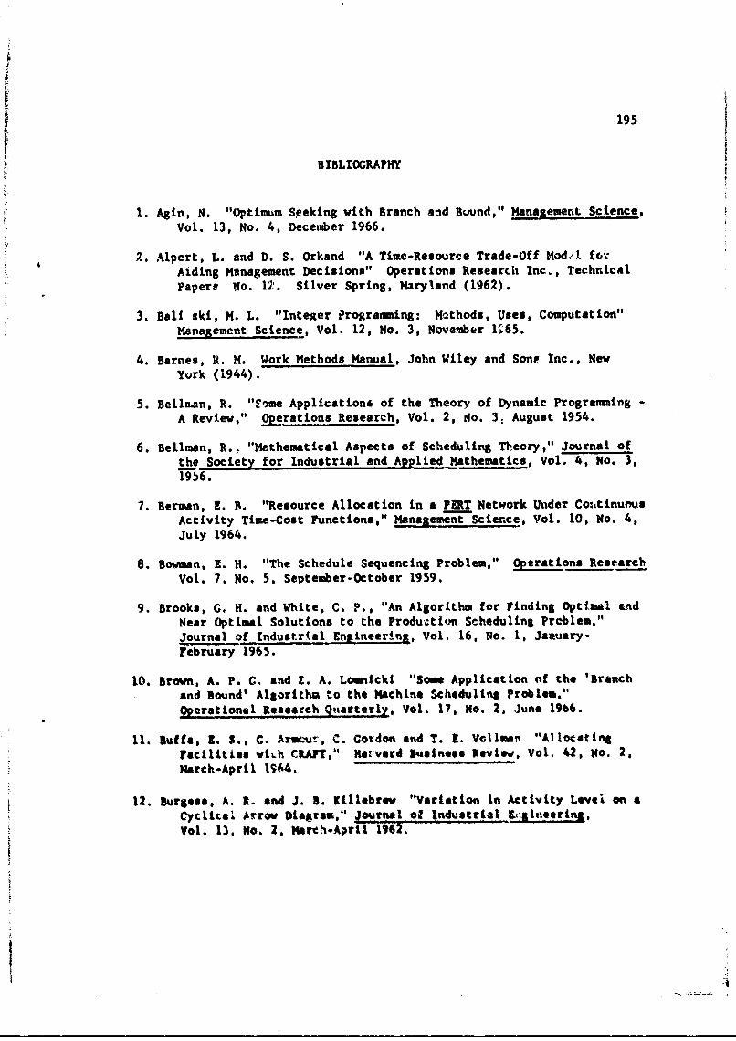
195

B IBLIOGRAPHY

1. Agin, N. "Optimum Seeking with Branch and Bound," Management Science,Vol. 13, No. 4, December 1966.

2. Alpert, L. and D. S. Orkand "A Time-Resource Trade-Off Mod.,l foo-Aiding Management Decisions" Operations Research Inc., TechnicalPapers No. 1;.. Silver Spring, Maryland (1962).

3. Ball ski, M. L. "Integer Programing: Mcthods, Uses, Computation"Management Science, Vol. 12, No. 3, November K•65.

4. Barnes, R. H. Work Methods Manual, John Wiley and Sons Inc., NewYurk (1944).

5. Bellu-an, R. "1,ome Applications of the Theory of Dynamic Programming -

A Review," Operations Research, Vol. 2, No. 3, August 1954.

6. Bellman, R., "Mathematical Aspects of Scheduling Theory," Journal ofthe Society for Industrial and Applied Mathematics, Vol. 4, No. 3,n9;6.

7. Berman, 3. A. "Resource Allocation in a PERT Network Under Co:,tinuousActivity Time-Cost Functions," Management Science, Vol. 10, No. 4,July 1964.

8. Bowman, E. H. "The Schedule Sequencing Problem," Operations ResearchVol. 7, No. 5, September-October 1959.

9. Brooks, G. H. and White, C. P., "An Algorithm for Finding Optimal andNear Optimal Solutions to the Produztitm Scheduling Problem,"Journal of Industr.al Engtneering, Vol. 16, No. 1, January-February 1965.

10. Brown, A. P. C. and Z. A. Lomnicki "Same Application of the 'Branchand Bound' Algorithm to the Machine Scheduling Problem."Operattonal Rese.rch Quartiely, Vol. 17, No. 2. June 1966.

11. Buffa, 1. S., G. Armour, C. Gotdon end T. 9. Vollman "AllocatingFacilitiSs vWLh CRAFT," Hatrvard fusiness Review, Vol. 42, No. 2,March-April 1964.

12. Burgess, A. I. and J. 5. Killebrev "Variation in Activity Levei on acyclical Arrow Diagras," journal of Industrial g,Vol. 13, No. 2, Mart-.April 1962.

It

i96

Bibliography. Cont' d.

13. Battersby, A. "Network Analysis," St. Hartin'e Press, 1964.

14. Carroll, D. C7. "Heuristic Sequencing of Single and Multi-ComponentOrders," Ph.D. Thesis, M.I.T., 1965.

15. Charnes, A. and W. W. Cooper '*A Network Interpretation and a DirectedSubdual Algorithm for Critical Path Scheduling," Journal ofIndustrial Engiaeering, Vol. 13, No. 4, August 1962.

16. Charnes, A., W. W. Cooper, J. E. Devoe, and D. B. Learner "DemonDecision Happing Via Optimum Go-No Net orks - A Model for MarketinRNew Products," Management Science, Vol. 12, No. 11, July 1966.

17. Clermont, P. "Substitution in a Job Shop," M.Sc. Thesis, M.I.T., 1966.

18. Conway, R. W. and W. L. Maxwell "Network Scheduling by the ShortestOperation Discipline," Industrial Scheduling, Muth and ThompsonEds., Prentice-Hall Inc., 1963.

19. Crowaton, W. B. and G. L. Thompson "Decision CPM: A Method forSimultaneoua Planning, Scheduling and Control of Projects,"Operations Research, Vol. 15, No. 3, May-June 1967.

20. Crowston, W. B., F. Glover, G. L. Thompson and J. Trawick "Probabilis-tic Ccmbinations of Local Job Shop Scheduling Rules," O.N.R. ResearchMemorandum, No. 117, Carnegie Institute of Technology, 1964.

21. Crowston, W. B. and C. L. Thompson "Reduction and Solution of DecisionNetworks," Working Paper, Sloan School of Management, Forthcoming.

22. Crowston, W. 3. and R. E. Smylle "The Application of Decision CPM toIncentive Contracts," Working Paper, Sloan School of Management,Forthcoming.

23. Crowston, W. B. aad M. Wagner "A Comparison of Tree Search Schemesfor Decision Networks," Working Paper, Sloan School of M.anagement,

Forthcoming.

24. Dantzig, C. B. "Discrete Variable Extremum Problems," OperationsResearch, Vol. 5, No. 2, April 1957.

25. Davis, Edward W. "Resource Allocation in Project Network Models - ASurvey,' `va Journal of Industrial Engineering, Vol. XVII, No. 4,April .•J6.

197

Bibliography, Cont'd.

26. "DOD and NASA Guide, PER/Cost," Office of the Secretary of Defenceand National Aeronautics and Space Administration, WashingtonD.C., 1962.

27. Eastman, W. L., "Linear Programming with Pattern Constraints," Ph.D.Thesis, Harvard University, 1958.

28. Efroym.7on, N. A. and T. L. Ray "A Branch-Bound Algorithm for PlantLocation," Operations Research, Vol. 14, No. 2, May-June 1966.

29. Eisner, H. "A Generalized Network Approach to the Planning andScheduling of a Research Project," Operations Research, Vol. 10,No. 1, January-February 1962.

30. Elmaghraby, S. F. "An Algebra for Analysis of Generalized ActivityNetworks," Manaement Science, Vol. 10, No. 3, April 1964.

31. Fernando, E. P C. 'The Implementation of Industrial DevelopmentPrograrz.4es Using Critical Path Network Theory," Working Paper149, Sloan School of Management, M.I.T., 1965.

32. Ford, L. P. Jr. and P. R. Fulkerson "A Simple Algorithia for FindingMaximum Network Flc is and an Application to the Hitchcock Problem,"Canadian Journal of Mathematics, Vol. 9, 1957.

33. Fcord, L. P. Jr. and D. R. Fulkerson "Flows in Networks," PrincetonUniversity Press, 1963.

34. Freeman, Raoul J. "A Generalized PERT." Operations Research, Vol. 8No. 2, May-June 1960.

35. Fulkerson, E. R. "A Network Flow Computation for Project Cost Curves,"

Management Science, Vol. 7, No. 2, January 1961.

36. Gannt, H. L. O:ganizing for Work, Harcourt, New York, 1919.

37. Gavett, J. W. and N. V. Plyter "The Optimal Assignment of Facilitiesto locations by Branch and Bound," Operations Research, Vol. 14,No. 2, March-April 1966.

38. Gere, W. S. Jr. "A Heuristic Approach to Job Shop Scheduling," Ph.D.! Thesis, Carnegie Institute of Technology, 1962.

V

198

ISibliography, Cont'd.

39. Cilmore, P. C. and R. E. Comory "A Linear Programming Approach to theCutting Stock Problem," Operations Research, Vol. 9, No. 6November-December 1961.

40. Clover. F. "The Knapsack Problem: Some Relations for an ImprovedAlgorithm," Management Sciences Research Report, No. 28, CarnegieInstitute of Technology, 1965.

41. Gomory, R. A. "An All-Integer, Integer Programming Algorithm"Industrial Scheduling, Thompson and Muth, Eds., Prentice-Hall, Inc.

42. Jackson, J. R. "A Computing Procedure for a Line Balancing Problem,"Management Science, Vol. 2, No. 3, 1956.

43. Johnson, T. J. R. "An Algorithm for the Resource Constrained ProjectScheduling Problem," Ph.D. Thesis, Sloan School of Yanagement,M.I.T., 1967.

44. Kelley, J. E. Jr. and M. R. Walker "Critical Path Planning andScheduling," 1959 Proceedings of the Eastern Joint ComputerConference.

45. Kelley, J. E. Jr. "The Ctitical Path Method: R,,sources Planning andScheduling," Industrial Scheduling, Mut'i and Thomp-on, Eds.,Prentice-Hall Inc., 1963.

46. Knight, R. M. "Resou.ce Allocation and Multi-Project Scheduling in aResearch and Development Environment," S. M. Thebis, M.I.T., 1966.

47. Lawler, E. L. and D. E. Wood "Branch-and-Bound Methods: A Survey,"Operations Research, Vol. 14, Nc. 4, ..july-August 1966.

48. Lawler, E. L. "The Quadratic Assignment Problem," Management ScienceIVol. 9, No. 4, July 1963.

49. Levy, F. K., G. L. Thompson and J. D. Wiest "Mathematical Basis of

the Critical-Path M.Athoc," industrial S&hedulinA, Thompson andMuth, Eds., Prentice-Hall En":., 19963.

50. Levy, F. K., G. L. Thompson and J. D. Wiest "Multi-Ship, Multi-ShopWorkload Smoothing Program," Naval Research Logiqtics Quarterly,Vol. 9, No. 1, March 1962.

fi

199

Bibliography, Cont'd.

51. Little, J. D. C., K. G. Murty, D. W. Sweeney, and C. Karel "AnAlgorithm for the Traveling-Salesman Problem," Operations ResearchVol. 11, No. 6, November-December 1963.

52. Lorie, J. H. and L. J. Savage "Three Problems in CapiLal Budgeting,"Journal of Business, XXIVIII, No, 4, October 1955.

53. MacCrimmon, Kenneth R. and Charles A. Ryavec "An Analytical Studyof the PERT Assumptions," Operations Research, Vol. 12, No. 1,January-February 1964.

54. Manne, A. S. "On the J-L, Shop Scheduling Problem," Operations Research,Vol. 8, No. 2, March-April 1960.

55. Mansoor, E. M. "Improvement on Gujahr and Nemhauser's Algorithmfor the Line Balancing Problem," Management Science, Vol. 14, No. 3,November 1967.

56. Marglin, S. A. Approaches to Dynamic Investment .lanning, North HollandPublishing Company, 1963.

57. Meyer, W. L. and L. R. Shaffer Extensions of the Critical Path MethodThrough the Application of Integer Programming, Report IssuedBy the Department of Civil Engineering, University of Illinois,Urbana, Illinois, July 1963.

58. Moder, J. J. and C. R. Philips Project Management with CPM and PERT,Rheinhold Publishing rorporation, 1964.

59. NASA, "Irn.entive CcLtracting Guide," NTC 403, National Aezonauticsand Srace AdmiIkstration, January 1965.

60. Philips, C. R. 'Fifteen Key Features of Computer Programs for CPMand PERT," The Journal of Industrial Engineering, Vol. 15, No. 1,January.-February 1964.

61. Pierce, j. F. Some Large Scale Production Scheduling Problems in thePaper Industry, Prentice-Hall Iac., 1964.

62. Pierce, J. F. "Application of Combinatorial Programmiag to a classof All-Zero One Integer Programming Problems," IBM CambridgeScientific Center Report 36,403, July 1966.

200

Bibliography, Cont'd.

63. Root, J. C. "An Application of Symbolic Logic to the SelectionProblem," Operations Research, Vol. 12, No. 4, July-August 1964.

64. Rowe, A. "Towards a Theory of icheduling," Jou:nal of IndustrialEngineering, Vol. 11, No. 2, March-April 1960.

65. Russo, F. J. "A Heuristic Approach to Alternate Routing in a Job-Shop,"M.Sc. Thesis, M.I.T., 1965.

66. Salveson, M. E. "The Assembly Line Balancing Problem," The Journalof industrial Enginecring, Vol. 6, No. 3, May-June 1955.

67. Shapiro, Donald M. "Algorithms for the Solution of the Optimal Costand Bottleneck Traveling-Salesman Problem," Washington UniversitySc.D. Thesis, 1966, Mathematics.

68. Shapiro, J. E. "A Group Theoretic Branch and Bound Algorithm forthe Zero-One Integer Programming Problem," M.I.T. Sloan SchoolWorking Paper, December 1967.

69. Smylie, R. E. "The Application of Decision CPM to Incentive Contracts,"S.M. Thesis, Sloan School of Management, M.I.T., 1967.

70. Thompson, G. L. "The StoppedSimplex Method: I. Basic Theory forMixed Integer: Integer Programming," Revue Francaise deRecherche Operationnelle, 1964.

71. Thompson, C. L. "Recent Developments in tha Job Shop SchedulingProblem," Naval Research Logistics Quarterly, Vol. 7, No. 4,December 1960.

72. Tonge, F. M. A Heuristic Program for Assembly Line Balancing,Prentice-Hall Inc., 1961.

73. Wagner, H. M. "An Integer Linear-Programming Model for MachineScheduling," Naval Research Logistics Quarterly, Vol. 7, No. 4,December 1960.

74. Weingartner, H. M. and D. N. Ness "Methods for the Solution of theMulti-Dimensional 0/I Knapsack Problem," Working Paper 177-66Sloan School of Management, M.I.T., April 1966.

75. Weingartner, H. M. "Capital Budgeting of Interrelated Projects:Survey and Synthesis," Management Science, Vol. 12, No. 2, March1966.

201

Bibliography, Cont 'd.

76. Weingartncr, H. M. Mathematical Programming and the Analysis ofCapital Budgeting Problems, Prentice-alla1, Inc., 1963.

77. Wester; L. and M. P. Killbridge "A Heuristic Method of Line Balarpcing'The Journal of Industrial Engineering, Vol. 12, No. 4, July-August1961.

78. Wester, L. and M. P. Killbridge "Heuristic Line Balancing: A Case,"The Journal of Industrial Engineering, Vol. 13, No. 3, May-June1962.

79. Weist, J D. "Some Properties of Schedules for Large Projects withLimited Resources," Opetations Rerearch, Vol. 12, No. 3, May-June1964.

80. Wiest, J. D. "The Scheduling of Large Project.ý with Limited Resources,"Ph.D. Thesis, Carnegie Institute of Technology, 1962.

81. Wiest, Jerome D. "A Heuristic Model for Scheduling Large Projectiwith Limited Resources," Management Science, Vol. 13, No. 6,February 1967.

82. Wilson, R. C. "Ass-.ibly Line Balancing and Resource L.;elling,"University of Michigan Summer Conference, Production and InventoryControl, 1964.

it

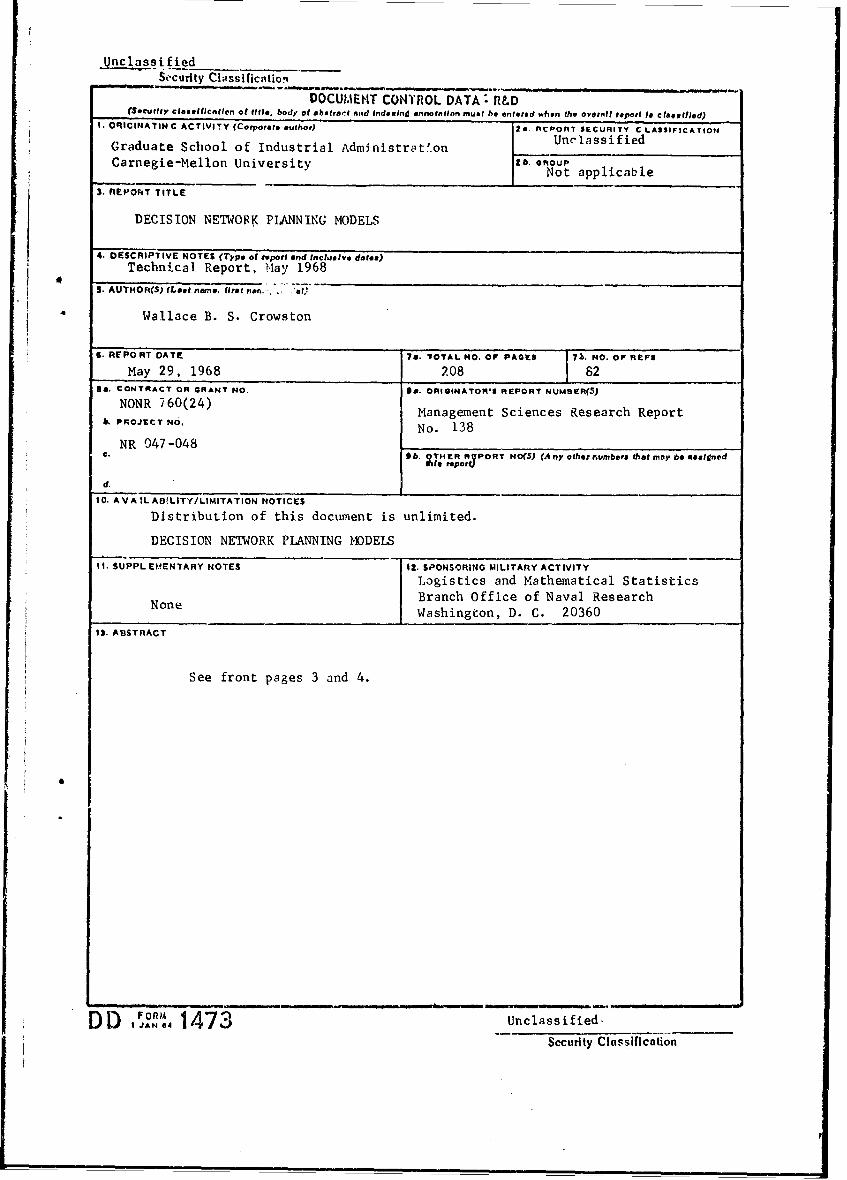
Unclassified•--• _Security Chasnificstio!%

DOCUtMIENT CONTROL DATA R&D.Security claautflcatlen of title, body of obatract and indexing onnotAtion muot be entered whien the overill report to ClaselIJed)

I. ORICINATIN C ACTIVITY (Corporate author) 20. AcPOflT SIECURITY C LASSIFICATION

Graduate School of Industrial Administrat'on Un-lassifiedCarnegie-Mellon University lb @OOUP

Not applicable3. nEOkT TITLE

DECISION NETWORK PLANNING MODELS

4. DESCRIPTIVE NOTES (Type of taport and Inclu.lye date*)

Technical Report, M.ay 1968

S. AUTHOR(S) (Lent name. Ifrat nn ... 'at)

Wallace B. S. Crowston

6. REPORT DATE 7@. TOTAL NO. OF PAGt9 7b. NO. OF REFS

May 29, 1968 208 62Sa. CONTRACT OR GRANT NO. 98. ORIGINATOR'$ REPORT NUMBER(S)

NONR 760(24) Management Sciences Research Reportb PROJECT NO. No. 138

NR 047-048e. ab. "PO RT NO(S) (Any other urnbere that may be aaatIned

d.

10. A VA IL ABfLITY/LIMITATION NOTICES

Distribution of this document is unlimited.

DECISION NETWORK PLIANING MODELS

Il. SUPPLEMAENTARY NOTES 12. SPONSORING MILITARY ACTIVITY

Logistics and Mathematical StatisticsNone Branch Office of Naval Research

Washington, D. C. 2036013. ABSTRACT

See front pages 3 and 4.

'°"'' 47 .. . . " -- -- ....-.

I JAN 14 Unclassified,

Security Classification

Security Classification,

KEYW~DSLtrJI A L114K 0 LINK C140L r WT V40LE Wf r OLC F T

Decision Critical Path Method

Critical Path Method

Integer Programming Application

Branch and bound application

Project planning models

INSTRUCTIONS1. ORIGINATING '.CTIVITY: Enter the name and address imposed by security classification, .;stng Atandard statementsof the contractor, suhcontractor, grantee, Department of Dc- such as:fense activity or other organization (corporate author) issuing (1) "'Qualified requesters may obtain copies of thisthe report. report from DOC."2s. REPORT SECURITY CLASSIFICATION: Enter the over- (2) "Foreign announcement ard 'lisseridnation of thisall security c lassificrition of the report. Indicate whether rpr yDCIsntatoie."Restricted Drita" is included. Marking in to be in accord-eotb DCi o atoieLance with app :opriate security regulations. (3) "U. S. Government agen.,cies may oauncopies of

this report directly frwn DDC. O-.neý- qualified DDC2b. GROUP: Automatic downgrading is specified in DoLo Di- users shall request throughrective 5200. 10 and Armed Forces Ine.ustrial Manue'l, Enterthe group numbe,. Also, when applicable, show that optional -

markings have bten used for Group 3 and Group 4 us auithor- (4) "U. S. millitary agencies may obtakn copies of thisizcd. report directly from DDC. Other qualified uscrs3. REPORT TITLC: Enter thie con,.letc iteport title In all shell request through

a ~cppitiil letters. Titi,!s in all cases should ~'o unclassified.If a neaningfuL title cannot be selected without classifica-tio:n, show title classification in all capitals in par nithesia (5) "All distribution of this report Is controlled. Qual.irimrediately following :he title. Iified DDC uscrs shall request through

4. DESCRIPTIVE NOTE~S: If stprupriate, enter the type of bet~por. eg.,intrim.prores, smmay, anua, o fial.If the report has been furnished to the Office of Technical

Cive the inclusive dates %,,hen a specific reporting period is Ser-,ices, Dt~partment of Commerce. for isale to the public, indi-covered, cute th~s fact and enter the price, if known.

~.AUT1HOR(S): Enter the name(s) of author(s) ris shown on It. SUPPLEMENTARY NOTES: Use for additional explana-or in the report. Entet lant n.ime, first name. -iiddle initi al. tory notes.11f military, rhow tank iind brantch of service. The name ofthe principal author is on afheolute minimum requirem-pnt. 12. SPONSORING MILITA.RY ACTIVITY: Enter the name of

th~e departmental project office or laboratory sponsoring (pay.6. REPORT DATE._ Enter the date of the report on day, In for the research and development. In,1ude address.month. year; or month, year. If more than one date appearbon the report, use dale of publication. 13. ABSTRACT:- Enter an abstract givine a brief and factual

summary of the document Indicative of the report, even thou:h7&. TOTAL NUMBIER OF PAGES: The total page count it may also appear elsewhere in the body of the technical re-sho!.id follow normal pa.-Ination procedures, i~e., enter *ha -urt. If additional space ia required, a continuation sheet shallnumber of page.i containing info-mation. i6 attached.7b. NUNI1ER OF RFFErENCE&i Enter the total number of It is highly desirable that the abstract of classified reportsreferences cited in the report. be unclassified. Each Paracs61r; of the abstract shall end withBa. CONTRACT OR GRANT NUMB3ER: If appropriate, entee an Indication of the military security classification of the ln-the applicable numbher of the contrac~t or grunt under whi.:h formation in the paragraph, represented as (rs). (s). (c). af (U)the report was written There io no limitation on the length of the abstract. H4ow-3b, 8c, & Bet. PROJECT NUMBER: Enter the ai-propriaite ever, the suggested length is fro," 1S0 to 22S words.military department identification, such usi project number, 1.KYWRS e od r t~nclymaigu eisubproject number, systemn numbers, tas.k number, etc.14KEWOD.eywrsa lnicl mnngutr%

or short ,hr~i~ex that rharacteripe a report and mala be used as9a. ORIGINATOR'S REPORT NUMBEFR(S): Enter the off- index entries for cataloging the repeet. Key wordsa must becial report number by whc6i the document will be identified selected slo that no aecu~ity classification is required. Ide di.and controlled uy the originating activity. This numbr, must tiers, such as equipmenit model designation, !-.ace name, militarybe unique to this re~port. project code r~ame, gror.,reptic location, may be used as key

9b. OThIER WrEPORT NUMIBE.R(S): If the report has been wotdb but will be followed by crn indication of technical con.assignied any ith,,t rep~ort numbi-t (eftIhrr by the Oigainator test. T~he assignment of links, rolev, and weilthts is iip'1 inet.

or by the sponstor), also enter this ivnubert(s)

10. AVAIIAIIII.ITY/LIlMI .ATION NOTICES.- Enter any limf-itations oin further disseroinnt iont of the report, other thAn thosel

SeuiyClant'ification