Cancer prevention - IARC effects of treatments given, as well as the ... Alternative formulae can, however, ... Cancer prevention 359

355

The preceding chapters of this book have focused on principles andmethods needed to study the determinants of disease and their effects.The ultimate goal of epidemiology, however, is to provide knowledge thatwill help in the formulation of public health policies aimed at preventingthe development of disease in healthy persons.

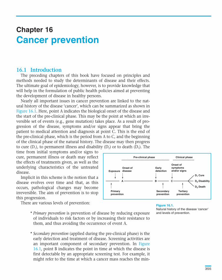
Nearly all important issues in cancer prevention are linked to the nat-ural history of the disease ‘cancer’, which can be summarized as shown in

. Here, point A indicates the biological onset of the disease andthe start of the pre-clinical phase. This may be the point at which an irre-versible set of events (e.g., gene mutation) takes place. As a result of pro-gression of the disease, symptoms and/or signs appear that bring thepatient to medical attention and diagnosis at point C. This is the end ofthe pre-clinical phase, which is the period from A to C, and the beginningof the clinical phase of the natural history. The disease may then progressto cure (D1), to permanent illness and disability (D2) or to death (D3). Thetime from initial symptoms and/or signs tocure, permanent illness or death may reflectthe effects of treatments given, as well as theunderlying characteristics of the untreateddisease.

Implicit in this scheme is the notion that adisease evolves over time and that, as thisoccurs, pathological changes may becomeirreversible. The aim of prevention is to stopthis progression.

There are various levels of prevention:

* Primary prevention is prevention of disease by reducing exposureof individuals to risk factors or by increasing their resistance tothem, and thus avoiding the occurrence of event A.

* Secondary prevention (applied during the pre-clinical phase) is theearly detection and treatment of disease. Screening activities arean important component of secondary prevention. In

, point B indicates the point in time at which the disease isfirst detectable by an appropriate screening test. For example, itmight refer to the time at which a cancer mass reaches the min-

Chapter 16

Pre-clinical phase Clinical phase

Onset ofsymptomsand/or signs

D1 Cure

D2 Disability

D3 Death

Earlydetection

Onset ofdiseaseExposure

Primaryprevention

Secondaryprevention

Tertiaryprevention

CBA

Natural history of the disease ‘cancer’

and levels of prevention.

Text book eng. Chap.16 final 27/05/02 14:12 Page 355 (Black/Process Black film)

16.1 Introduction

Figure 16.1

Figure16.1

Cancer prevention

Pre-clinical phase Clinical phase

Onset ofsymptomsand/or signs

D1 Cure

D2 Disability

D3 Death

Earlydetection

Onset ofdiseaseExposure

Primaryprevention

Secondaryprevention

Tertiaryprevention

CBA

Figure 16.1.

Text book eng. Chap.16 final 27/05/02 14:12 Page 355 (Black/Process Black film)TextText book book book eng. eng. eng. Chap.16 Chap.16 Chap.16 final final final 27/05/02 27/05/02 27/05/02 14:12 14:12 14:12 Page Page Page 355 355 355 (PANTONE (PANTONE (Black/Process 313 313 (Black/Process CV CV (Black/Process film) film) Black

imum size that can be seen by X-ray examination. Thus, the dis-tance from point B to C represents the ‘detectable pre-clinicalphase’. The location of point B varies markedly from one indi-vidual to another, and also depends on the screening techniqueused.

* Tertiary prevention (appropriate in the clinical phase) is the use oftreatment and rehabilitation programmes to improve the out-come of illness among affected individuals.

In the rest of this chapter, we consider each of these levels of preventionin detail.

The purpose of primary prevention is to limit the incidence of cancerby controlling exposure to risk factors or increasing individuals’ resistanceto them (e.g., by vaccination or chemoprevention). Clearly, the first stepis to identify the relevant exposures and to assess their impact on the riskof the disease in the population.

Much of epidemiology is concerned with identifying the risk factorsfor a disease, health problem or state of health. In assessing the strengthof the association between a particular exposure and a particular out-come, we calculate measures known as relative measures of effect. Asshown in Section 5.2.1, there are three types of relative measure (riskratio, rate ratio and odds ratio) which are often collectively called rela-tive risk.

Relative measures of effect provide answers to the question: How manytimes more likely are people exposed to a putative risk factor to develop the out-come of interest relative to those unexposed, assuming that the only differencebetween the two groups is the exposure under study? The magnitude of therelative risk is an important consideration (but not the only one—see

) in establishing whether a particular exposure is a cause ofthe outcome of interest.

Once we have established that an exposure is causally associated withthe outcome of interest, it is important to express the absolute magni-tude of its impact on the occurrence of the disease in the exposed group(see Section 5.2.2). If we have information on the usual risk (or rate) ofa particular disease in the absence of the exposure, as well as in its pres-ence, we can determine the excess risk (also known as attributable risk)associated with the exposure.

Excess risk = risk (or rate) in the exposed – risk (or rate) in the unexposed

Chapter 16

356


16.2 Primary prevention

16.2.1 How important is a particular exposure?

Relative and absolute measures of exposure effect

Chapter 13


It is useful to express the excess risk in relation to the total risk (or rate)of the disease among those exposed to the factor under study. This mea-sure is called excess fraction (also known as excess risk percentage or attribut-able risk percentage). It describes the proportion of disease in the exposedgroup which is attributable to the exposure.

Excess fraction (%) = 100 × (excess risk / risk (or rate) in the exposed)

Alternatively, it can be calculated by using the following formula:

Excess fraction (%) = 100 × (relative risk – 1) / relative risk

Excess fraction provides an answer to the question: What is the proportionof new cases of disease in the exposed that can be attributed to exposure?Another way of using this concept is to think of it as the decrease in the

Cancer prevention

357

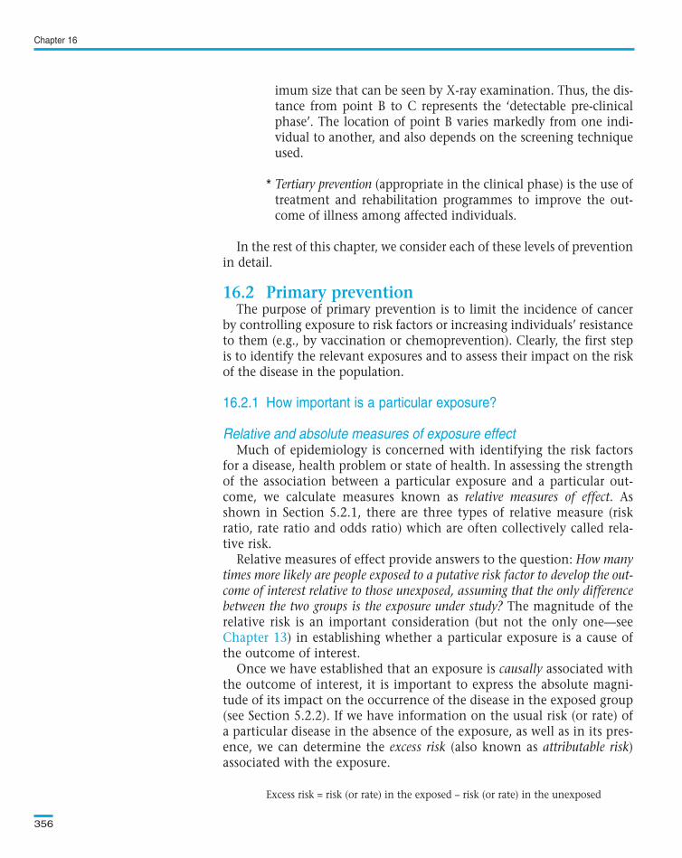
Example 16.1. Suppose that a cohort study was conducted in the townof Minas Gerais (Brazil) to assess the relationship between cigarettesmoking and lung cancer in men. We assume, for simplicity, that smok-ers and non-smokers were similar with respect to other risk factors forlung cancer such as age and occupational exposures. The results areshown in Table 16.1.

In this study, the rate ratio is

220 per 100 000 pyrs / 20 per 100 000 pyrs = 11

and the excess risk associated with smoking (assuming causality) is

Excess risk = 220 per 100 000 pyrs – 20 per 100 000 pyrs = 200 per 100 000 pyrs

To assess what proportion 200 per 100 000 pyrs is of the rate amongsmokers (220 per 100 000 pyrs), we can calculate the excess fraction:

Excess fraction (%) = 100 × (200 per 100 000 pyrs / 220 per 100 000 pyrs) = 91%

This is the proportion of lung cancer cases in smokers attributable tosmoking.

Smokers Non-smokers All

Number of cases 120 10 130

Person-years 54 545 50 000 104 545

Rate per 100 000 pyrs 220 20 124

Lung cancer incidence in smokers and

non-smokers: hypothetical data.


Example 16.1. Suppose that a cohort study was conducted in the townof Minas Gerais (Brazil) to assess the relationship between cigarettesmoking and lung cancer in men. We assume, for simplicity, that smok-ers and non-smokers were similar with respect to other risk factors forlung cancer such as age and occupational exposures. The results areshown in Table 16.1.

In this study, the rate ratio is

220 per 100 000 pyrs / 20 per 100 000 pyrs = 11

and the excess risk associated with smoking (assuming causality) is

Excess risk = 220 per 100 000 pyrs – 20 per 100 000 pyrs = 200 per 100 000 pyrs

To assess what proportion 200 per 100 000 pyrs is of the rate amongsmokers (220 per 100 000 pyrs), we can calculate the excess fraction:

Excess fraction (%) = 100 × (200 per 100 000 pyrs / 220 per 100 000 pyrs) = 91%

This is the proportion of lung cancer cases in smokers attributable tosmoking.



Person-years 54 545 50 000 104 545

Rate per 100 000 pyrs 220 20 124



Person-years 54 545 50 000 104 545

Rate per 100 000 pyrs 220 20 124

Table 16.1.


incidence of a disease that would have been seen if the exposed had neverbeen exposed. Thus, in , a maximum of 91% of lung cancercases in smokers could theoretically have been prevented if they had neversmoked.

If the exposure is protective, analogous measures can be calculated. Theyare usually called risk reduction (also known as prevented risk) and preventedfraction (also known as prevented risk percentage).

Risk reduction = risk (or rate) in the unexposed – risk (or rate) in the exposed

Prevented fraction (%) = 100 × (risk reduction / risk (or rate) in the unexposed)

Prevented fraction tends to be appreciably smaller than excess fraction( ). This is because it is generally impossible to eliminate theexposure completely and, even if possible, the incidence of the disease inthose who stop being exposed may never fall to the level in those who havenever been exposed.

Calculation of excess risk (or risk reduction) requires information on theincidence of disease in the exposed and unexposed groups. This informationis directly available in cohort and intervention studies. For case–control stud-ies, however, it is not possible to calculate the excess risk using the formulagiven above, because incidence of disease among the exposed and unexposedgroups is not known. We can still calculate excess fraction using the formulabased on relative risk, which in these studies is estimated by the odds ratio.Alternative formulae can, however, be used in population-based case–controlstudies to calculate excess risk. These are presented in Appendix 16.1.

Chapter 16

358

Example 16.2. A large randomized trial was carried out to assess the valueof a smoking cessation programme (the intervention) in reducing the occur-rence of lung cancer among smokers. By the end of the trial, the incidence oflung cancer was 155 per 100 000 pyrs among those who received the inter-vention and 240 per 100 000 pyrs among the controls. Thus, the maximumbenefit achieved by the intervention was

Risk reduction = 240 per 100 000 pyrs – 155 per 100 000 pyrs = 85 per 100 000 pyrs

Thus, 85 new cases of lung cancer per 100 000 pyrs were prevented by thesmoking cessation programme.

Prevented fraction (%) = 100 × (85 per 100 000 pyrs/ 240 per 100 000 pyrs) = 35%

Thus 35% of the expected lung cancer cases among smokers were pre-vented by the smoking cessation programme.


Example 16.1

Example 16.2

Example 16.2. A large randomized trial was carried out to assess the valueof a smoking cessation programme (the intervention) in reducing the occur-rence of lung cancer among smokers. By the end of the trial, the incidence oflung cancer was 155 per 100 000 pyrs among those who received the inter-vention and 240 per 100 000 pyrs among the controls. Thus, the maximumbenefit achieved by the intervention was

Risk reduction = 240 per 100 000 pyrs – 155 per 100 000 pyrs = 85 per 100 000 pyrs

Thus, 85 new cases of lung cancer per 100 000 pyrs were prevented by thesmoking cessation programme.

Prevented fraction (%) = 100 × (85 per 100 000 pyrs/ 240 per 100 000 pyrs) = 35%

Thus 35% of the expected lung cancer cases among smokers were pre-vented by the smoking cessation programme.


The measures of effect discussed so far compared the incidence of thedisease in the exposed group with the incidence in the unexposed group.To assess the extra disease incidence in the study population as a whole thatcan be attributed to the exposure, we can calculate a measure called thepopulation excess risk (also known as population attributable risk). This isdefined as

Population excess risk = risk (or rate) in the population – risk (or rate) in the unexposed

or, similarly, as

Population excess risk = excess risk × proportion of the population exposed to therisk factor

Analogously to the excess risk among exposed individuals, the populationexcess risk is a measure of the risk of disease in the study population which isattributable to an exposure ( ). We can express the populationexcess risk in relation to the total risk of the disease in the whole population.This measure is the population excess fraction (also known as population attrib-utable fraction).

population excess riskPopulation excess fraction (%) = 100 ×

rate (or risk) in the total population

Cancer prevention

359

Example 16.3. Returning to the hypothetical study described in Example16.1, the proportion of smokers in the whole cohort was 52%. If this 52% ofthe study population that smoked had never smoked, their incidence of lungcancer would have been reduced from 220 to 20 cases per 100 000 pyrs.

Population excess risk = (220 per 100 000 pyrs – 20 per 100 000 pyrs) × 0.52 =104 per 100 000 pyrs

Similarly, the population excess risk can be calculated by subtracting therate in the unexposed group from the rate in the total study population. Therate in the total study population was 124 per 100 000 pyrs (Table 16.1).Thus,

Population excess risk = 124 per 100 000 pyrs – 20 per 100 000 pyrs = 104 per100 000 pyrs

Thus, 104 cases of lung cancer per 100 000 pyrs could have been prevent-ed in the whole study population if none of the smokers had ever smoked.


Measures of population impact

Example 16.3

Example 16.3. Returning to the hypothetical study described in Example16.1, the proportion of smokers in the whole cohort was 52%. If this 52% ofthe study population that smoked had never smoked, their incidence of lungcancer would have been reduced from 220 to 20 cases per 100 000 pyrs.

Population excess risk = (220 per 100 000 pyrs – 20 per 100 000 pyrs) × 0.52 =104 per 100 000 pyrs

Similarly, the population excess risk can be calculated by subtracting therate in the unexposed group from the rate in the total study population. Therate in the total study population was 124 per 100 000 pyrs (Table 16.1).Thus,

Population excess risk = 124 per 100 000 pyrs – 20 per 100 000 pyrs = 104 per100 000 pyrs

Thus, 104 cases of lung cancer per 100 000 pyrs could have been prevent-ed in the whole study population if none of the smokers had ever smoked.


Alternatively, it can be calculated by using the following formula:

pe (relative risk – 1)Population excess fraction (%) = 100 ×

pe (relative risk – 1) + 1

where pe represents the prevalence of exposure in the population understudy.

Population excess fraction is an important measure. It provides ananswer to the question: What proportion (fraction) of the new cases of diseaseobserved in the study population is attributable to exposure to a risk factor? Ittherefore indicates what proportion of the disease experience in the pop-ulation could be prevented if exposure to the risk factor had neveroccurred ( ).

Note that the excess fraction among the exposed is always greater thanthe population excess fraction, since the study population includesalready some unexposed people who, obviously, cannot benefit from elim-ination of the exposure.

Sometimes it is useful to calculate the population excess fraction for amuch larger population than the study population. For instance, publichealth planners are particularly interested in using data from epidemio-logical studies conducted in subgroups of the population to estimate theproportion of cases in a region or in a country that are attributable to aparticular exposure ( ) . In this case, it is necessary to obtaindata on the prevalence of exposure in these populations from othersources.

shows how the population excess fraction varies in relationto the level of prevalence of the exposure in the population under study(pe) and the magnitude of the relative risk. It is clear that the proportionof cases in a particular population that can be attributed to a particularexposure depends both on the magnitude of the relative risk and on theprevalence of the exposure in the population. For instance, tobacco smok-ing, with a relative risk of about 5, and occupational exposure to aromat-ic amines, with a relative risk of about 500, are implicated as causes ofbladder cancer. Despite the fact that the relative risk is much smaller forsmoking than for aromatic amines, the population excess fraction is sub-

Chapter 16

360

Example 16.4. In Example 16.3, the population excess fraction would be

Population excess fraction (%) = 104 per 100 000 pyrs/124 per 100 000 pyrs = 84%.

This means that (assuming causality) approximately 84% of the lungcancer incidence in the study population is attributable to smoking. Thus,84% of the lung cancer cases in this population would have been preventedif the smokers had never smoked.


Example 16.4

Example 16.5

Table 16.2

Example 16.4. In Example 16.3, the population excess fraction would be

Population excess fraction (%) = 104 per 100 000 pyrs/124 per 100 000 pyrs = 84%.

This means that (assuming causality) approximately 84% of the lungcancer incidence in the study population is attributable to smoking. Thus,84% of the lung cancer cases in this population would have been preventedif the smokers had never smoked.


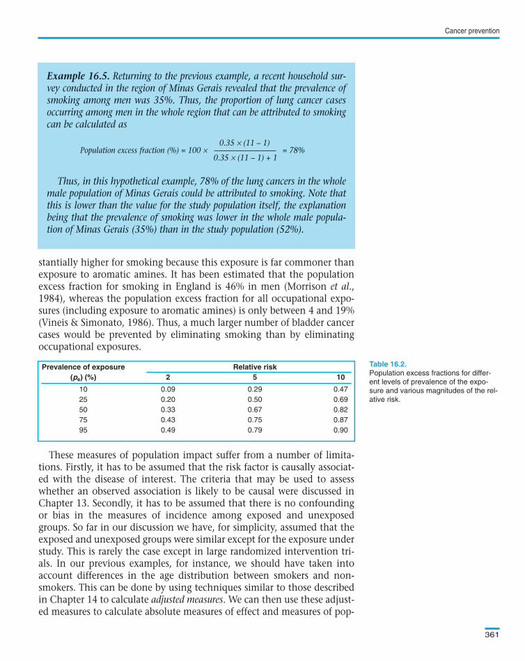
stantially higher for smoking because this exposure is far commoner thanexposure to aromatic amines. It has been estimated that the populationexcess fraction for smoking in England is 46% in men (Morrison et al.,1984), whereas the population excess fraction for all occupational expo-sures (including exposure to aromatic amines) is only between 4 and 19%(Vineis & Simonato, 1986). Thus, a much larger number of bladder cancercases would be prevented by eliminating smoking than by eliminatingoccupational exposures.

These measures of population impact suffer from a number of limita-tions. Firstly, it has to be assumed that the risk factor is causally associat-ed with the disease of interest. The criteria that may be used to assesswhether an observed association is likely to be causal were discussed inChapter 13. Secondly, it has to be assumed that there is no confoundingor bias in the measures of incidence among exposed and unexposedgroups. So far in our discussion we have, for simplicity, assumed that theexposed and unexposed groups were similar except for the exposure understudy. This is rarely the case except in large randomized intervention tri-als. In our previous examples, for instance, we should have taken intoaccount differences in the age distribution between smokers and non-smokers. This can be done by using techniques similar to those describedin Chapter 14 to calculate adjusted measures. We can then use these adjust-ed measures to calculate absolute measures of effect and measures of pop-

Cancer prevention

361

Prevalence of exposure Relative risk(pe) (%) 2 5 10

10 0.09 0.29 0.47

25 0.20 0.50 0.69

50 0.33 0.67 0.82

75 0.43 0.75 0.87

95 0.49 0.79 0.90

Population excess fractions for differ-

ent levels of prevalence of the expo-

sure and various magnitudes of the rel-

ative risk.

Example 16.5. Returning to the previous example, a recent household sur-vey conducted in the region of Minas Gerais revealed that the prevalence ofsmoking among men was 35%. Thus, the proportion of lung cancer casesoccurring among men in the whole region that can be attributed to smokingcan be calculated as

0.35 × (11 – 1)Population excess fraction (%) = 100 × = 78%

0.35 × (11 – 1) + 1

Thus, in this hypothetical example, 78% of the lung cancers in the wholemale population of Minas Gerais could be attributed to smoking. Note thatthis is lower than the value for the study population itself, the explanationbeing that the prevalence of smoking was lower in the whole male popula-tion of Minas Gerais (35%) than in the study population (52%).


Prevalence of exposure Relative risk(pe) (%) 2 5 10

10 0.09 0.29 0.47

25 0.20 0.50 0.69

50 0.33 0.67 0.82

75 0.43 0.75 0.87

95 0.49 0.79 0.90

Table 16.2.

Example 16.5. Returning to the previous example, a recent household sur-vey conducted in the region of Minas Gerais revealed that the prevalence ofsmoking among men was 35%. Thus, the proportion of lung cancer casesoccurring among men in the whole region that can be attributed to smokingcan be calculated as

0.35 × (11 – 1)Population excess fraction (%) = 100 × = 78%

0.35 × (11 – 1) + 1

Thus, in this hypothetical example, 78% of the lung cancers in the wholemale population of Minas Gerais could be attributed to smoking. Note thatthis is lower than the value for the study population itself, the explanationbeing that the prevalence of smoking was lower in the whole male popula-tion of Minas Gerais (35%) than in the study population (52%).


ulation impact using the same formulae as before. Thirdly, we mustremember that estimates of relative risk are generally derived fromcase–control, cohort or intervention studies. These studies are often con-ducted in special subgroups of the population such as migrants, manualworkers, etc. However, levels of exposure and intrinsic susceptibility inthese subgroups may be quite different from those in the general popula-tion. It is therefore important that the extrapolation of data from thesestudies to other populations is undertaken with caution. For instance,many cohort studies are based purposely on groups with exposure tomuch higher levels than the general population (e.g., occupationalcohorts) and the relative risks obtained from them should not be used assuch to provide estimates of population excess fractions for other popula-tions with much lower levels of exposure. This may be overcome if levelsof exposure are properly measured (rather than just ‘exposed’ versus‘unexposed’) and estimates of population excess fractions take them intoaccount.

We can calculate the proportion of a particular cancer in a certain pop-ulation that is caused by diet, by alcohol, by smoking, etc. These percent-ages may add up to more than 100%. This is because each individual cal-culation of population excess fraction does not take into account the factthat these risk factors interact with each other. For instance, in calculatingthe proportion of laryngeal cancer due to smoking, we ignore the fact thatsome of the cancers that occurred among smokers only occurred becausethey were also exposed to alcohol.

Once the risk factors have been identified and their impact in the pop-ulation estimated, it is important to consider methods to either eliminateor reduce the exposure to them. Primary prevention involves two strate-gies that are often complementary. It can focus on the whole populationwith the aim of reducing average risk (the population strategy) or on peopleat high risk (the high-risk individual strategy). Although the high-risk indi-vidual strategy, which aims to protect susceptible individuals, is most effi-cient for the people at greatest risk of a specific cancer, these people maycontribute little to the overall burden of the disease in the population. Forexample, organ transplant patients are particularly susceptible to non-melanoma skin cancer (Bouwes Bavinck et al., 1991). The tumour tends todevelop in highly sun-exposed areas of the body. Primary prevention cam-paigns for organ-transplanted patients involving reduction of sun expo-sure and sunscreen use are likely to be of great benefit to these patients,but will have little impact on the overall burden of disease in the popula-tion, because organ transplant patients represent a very small proportionof the population. In this situation, the population strategy or a combi-nation of both strategies should be applied.

The major advantage of the population strategy is that it is likely to pro-duce greater benefits at the population level and does not require identifi-

Chapter 16

362


16.2.2 Role and evaluation of primary preventive measures


cation of high-risk individuals. Its main disadvantage is that it requires theparticipation of large groups of people to the benefit of relatively few. Forexample, adoption by a population of measures to reduce sun exposure mayreduce the risk of skin cancer at a population level, but will be of littleapparent benefit to most individuals, since the disease is rare even amongthose exposed. This phenomenon is called the prevention paradox (Rose,1985).

Various approaches have been used to reduce or eliminate exposure to aparticular risk factor, some examples of which are given in .

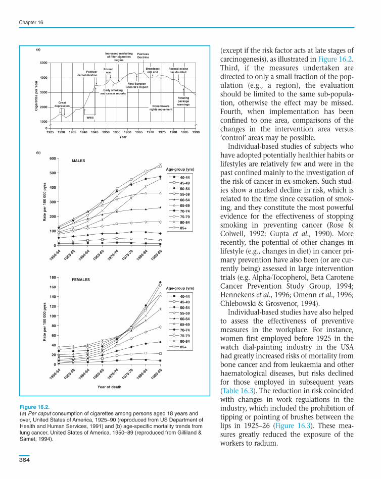
If specific preventive measures to reduce the incidence of a particularcancer have been adopted, it is essential to establish whether the effort hashad any positive effect. Evaluation of primary preventive efforts at the pop-ulation level is performed mainly in terms of monitoring changes in cancerincidence in relation to changes in exposure to risk factors. Thus, timetrends in cancer incidence may be compared with temporal changes inexposure to a particular risk factor to show whether the desired effect isbeing achieved. This is illustrated in , which shows trends in percaput consumption of cigarettes in the USA in relation to the timing ofimplementation of tobacco-control initiatives and important historicalevents, and trends in lung cancer mortality.

The following issues should be taken into account when interpretingincidence trends in relation to changes in exposure to risk factors. First, ifthe downward trend started long before the introduction of the preventivemeasure, it is difficult to attribute a recent decrease in incidence to the pre-ventive measure under investigation. Second, given the long inductionperiod of cancer, it may take many years or even decades before any effectof a preventive measure becomes apparent in incidence or mortality trends

Cancer prevention

363

Box 16.1. Examples of approaches used to reduce oreliminate exposure to a hazard risk factor

• Health education on an individual or community basis (e.g., media campaigns

promoting use of sunscreens).

• Regulation of carcinogens in occupational settings and in the environment (e.g.,

improvement of radiation protection).

• Price regulation (e.g., imposing taxes on cigarette and alcohol purchases).

• Advertising restrictions (e.g., banning of tobacco advertising or forcing the print-

ing of health warnings on cigarette packages).

• Time and place restrictions on consumption (e.g., banning smoking in public

places).


Box 16.1

Figure 16.2

Box 16.1. Examples of approaches used to reduce oreliminate exposure to a hazard risk factor

• Health education on an individual or community basis (e.g., media campaigns

promoting use of sunscreens).

• Regulation of carcinogens in occupational settings and in the environment (e.g.,

improvement of radiation protection).

• Price regulation (e.g., imposing taxes on cigarette and alcohol purchases).

• Advertising restrictions (e.g., banning of tobacco advertising or forcing the print-

ing of health warnings on cigarette packages).

• Time and place restrictions on consumption (e.g., banning smoking in public

places).

Box 16.1. Examples of approaches used to reduce orBox 16.1. Examples of approaches used to reduce orBoxBox 16.1. 16.1. Examples Examples of of approaches approaches used used to to reduce reduce or oreliminate exposure to a hazard risk factoreliminate exposure to a hazard risk factoreliminateeliminate exposure exposure to to a a hazard hazard risk risk factor factor


(except if the risk factor acts at late stages ofcarcinogenesis), as illustrated in .Third, if the measures undertaken aredirected to only a small fraction of the pop-ulation (e.g., a region), the evaluationshould be limited to the same sub-popula-tion, otherwise the effect may be missed.Fourth, when implementation has beenconfined to one area, comparisons of thechanges in the intervention area versus‘control’ areas may be possible.

Individual-based studies of subjects whohave adopted potentially healthier habits orlifestyles are relatively few and were in thepast confined mainly to the investigation ofthe risk of cancer in ex-smokers. Such stud-ies show a marked decline in risk, which isrelated to the time since cessation of smok-ing, and they constitute the most powerfulevidence for the effectiveness of stoppingsmoking in preventing cancer (Rose &Colwell, 1992; Gupta et al., 1990). Morerecently, the potential of other changes inlifestyle (e.g., changes in diet) in cancer pri-mary prevention have also been (or are cur-rently being) assessed in large interventiontrials (e.g. Alpha-Tocopherol, Beta CaroteneCancer Prevention Study Group, 1994;Hennekens et al., 1996; Omenn et al., 1996;Chlebowski & Grosvenor, 1994).

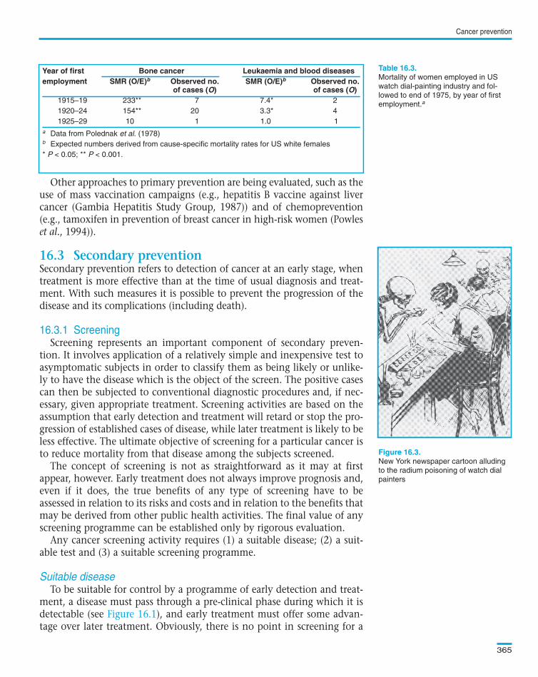
Individual-based studies have also helpedto assess the effectiveness of preventivemeasures in the workplace. For instance,women first employed before 1925 in thewatch dial-painting industry in the USAhad greatly increased risks of mortality frombone cancer and from leukaemia and otherhaematological diseases, but risks declinedfor those employed in subsequent years( ). The reduction in risk coincidedwith changes in work regulations in theindustry, which included the prohibition oftipping or pointing of brushes between thelips in 1925–26 ( ). These mea-sures greatly reduced the exposure of theworkers to radium.

Chapter 16

364

5000

(a)

(b)

4000

3000

2000

0

1000

1925 1930 1935 1940 1955 1960 1965Year

Cig

aret

tes

per

Yea

r

1945 1950 1970 1975 1980 1985 1990

Increased marketingof filter cigarettes

begins

FairnessDoctrine

Koreanwar

WWII

Early smokingand cancer reports

First SurgeonGeneral's Report

Broadcastads end

Federal excisetax doubled

RotatingpackagewarningsNonsmokers

rights movement

Postwardemobilization

Greatdepression

MALES600

40-44

Age-group (yrs)

45-49

50-54

55-59

60-64

65-69

70-74

75-79

80-84

85+

500

400

300

Rat

e p

er 1

00 0

00 p

yrs

200

100

1950

-54

1955

-59

1960

-64

1965

-69

1970

-74

1975

-79

1980

-84

1985

-89

0

FEMALES180

40-44

Age-group (yrs)

45-49

50-54

55-59

60-64

65-69

70-74

75-79

80-84

85+

160

140

100

80

120

40

Rat

e p

er 1

00 0

00 p

yrs

Year of death

60

20

1950

-54

1955

-59

1960

-64

1965

-69

1970

-74

1975

-79

1980

-84

1985

-89

0

(a) Per caput consumption of cigarettes among persons aged 18 years and

over, United States of America, 1925–90 (reproduced from US Department of

Health and Human Services, 1991) and (b) age-specific mortality trends from

lung cancer, United States of America, 1950–89 (reproduced from Gilliland &

Samet, 1994).


Figure 16.2

Table 16.3

Figure 16.3

5000

(a)

(b)

4000

3000

2000

0

1000

1925 1930 1935 1940 1955 1960 1965Year

Cig

aret

tes

per

Yea

r

1945 1950 1970 1975 1980 1985 1990

Increased marketingof filter cigarettes

begins

FairnessDoctrine

Koreanwar

WWII

Early smokingand cancer reports

First SurgeonGeneral's Report

Broadcastads end

Federal excisetax doubled

RotatingpackagewarningsNonsmokers

rights movement

Postwardemobilization

Greatdepression

MALES600

40-44

Age-group (yrs)

45-49

50-54

55-59

60-64

65-69

70-74

75-79

80-84

85+

500

400

300

Rat

e p

er 1

00 0

00 p

yrs

200

100

1950

-54

1955

-59

1960

-64

1965

-69

1970

-74

1975

-79

1980

-84

1985

-89

0

FEMALES180

40-44

Age-group (yrs)

45-49

50-54

55-59

60-64

65-69

70-74

75-79

80-84

85+

160

140

100

80

120

40

Rat

e p

er 1

00 0

00 p

yrs

Year of death

60

20

1950

-54

1955

-59

1960

-64

1965

-69

1970

-74

1975

-79

1980

-84

1985

-89

0

Figure 16.2.


Other approaches to primary prevention are being evaluated, such as theuse of mass vaccination campaigns (e.g., hepatitis B vaccine against livercancer (Gambia Hepatitis Study Group, 1987)) and of chemoprevention(e.g., tamoxifen in prevention of breast cancer in high-risk women (Powleset al., 1994)).

Secondary prevention refers to detection of cancer at an early stage, whentreatment is more effective than at the time of usual diagnosis and treat-ment. With such measures it is possible to prevent the progression of thedisease and its complications (including death).

Screening represents an important component of secondary preven-tion. It involves application of a relatively simple and inexpensive test toasymptomatic subjects in order to classify them as being likely or unlike-ly to have the disease which is the object of the screen. The positive casescan then be subjected to conventional diagnostic procedures and, if nec-essary, given appropriate treatment. Screening activities are based on theassumption that early detection and treatment will retard or stop the pro-gression of established cases of disease, while later treatment is likely to beless effective. The ultimate objective of screening for a particular cancer isto reduce mortality from that disease among the subjects screened.

The concept of screening is not as straightforward as it may at firstappear, however. Early treatment does not always improve prognosis and,even if it does, the true benefits of any type of screening have to beassessed in relation to its risks and costs and in relation to the benefits thatmay be derived from other public health activities. The final value of anyscreening programme can be established only by rigorous evaluation.

Any cancer screening activity requires (1) a suitable disease; (2) a suit-able test and (3) a suitable screening programme.

To be suitable for control by a programme of early detection and treat-ment, a disease must pass through a pre-clinical phase during which it isdetectable (see ), and early treatment must offer some advan-tage over later treatment. Obviously, there is no point in screening for a

Cancer prevention

365

Mortality of women employed in US

watch dial-painting industry and fol-

lowed to end of 1975, by year of first

employment.a

New York newspaper cartoon alluding

to the radium poisoning of watch dial

painters

Year of first Bone cancer Leukaemia and blood diseasesemployment SMR (O/E)b Observed no. SMR (O/E)b Observed no.

of cases (O) of cases (O)1915–19 233** 7 7.4* 2

1920–24 154** 20 3.3* 4

1925–29 10 1 1.0 1

a Data from Polednak et al. (1978)b Expected numbers derived from cause-specific mortality rates for US white females

* P < 0.05; ** P < 0.001.


16.3 Secondary prevention

16.3.1 Screening

Suitable disease

Figure 16.1

Table 16.3.

Figure 16.3.

Year of first Bone cancer Leukaemia and blood diseasesemployment SMR (O/E)b Observed no. SMR (O/E)b Observed no.

of cases (O) of cases (O)1915–19 233** 7 7.4* 2

1920–24 154** 20 3.3* 4

1925–29 10 1 1.0 1

a Data from Polednak et al. (1978)b Expected numbers derived from cause-specific mortality rates for US white females

* P < 0.05; ** P < 0.001.


disease that cannot be detected before symptoms bring it to medical atten-tion and, if early treatment is not especially helpful, there is no point inearly detection.

Detectable pre-clinical phaseThe pre-clinical phase of a cancer starts with the biological onset of the

disease (point A in ). The disease then progresses and reaches apoint at which it can be detected by the screening test (point B in

). From this point onwards, the pre-clinical phase of the disease is saidto be ‘detectable’. The starting point of this detectable pre-clinical phasedepends partly on the characteristics of the individual and partly on thecharacteristics of the test being used. A test which can detect a very ‘early’stage of the cancer is associated with a longer detectable pre-clinical phasethan a test which can detect only more advanced lesions.

The proportion of a population that has detectable pre-clinical disease(its prevalence) is an important determinant of the utility of screening incontrolling the disease. If the prevalence is very low, too few cases will bedetected to justify the costs of the screening programme. At the time ofinitial screening, the prevalence of the pre-clinical phase is determined byits incidence and its average duration (recall the discussion on prevalencein Section 4.2). In subsequent screening examinations, however, theprevalence of the pre-clinical phase is determined mainly by its incidence,the duration being relatively unimportant if the interval between exami-nations is short. Therefore, the number of cases detected by the pro-gramme is greatest at the first screening examination, while the shorterthe interval between examinations, the lower the number of cases detect-ed per examination (and the higher the cost per case detected).

Early treatmentFor screening to be of benefit, treatment given during the detectable

pre-clinical phase must result in a lower mortality than therapy given aftersymptoms develop. For example, cancer of the uterine cervix developsslowly, taking perhaps more than a decade for the cancer cells, which areinitially confined to the outer layer of the cervix, to progress to a phase ofinvasiveness. During this pre-invasive stage, the cancer is usually asymp-tomatic but can be detected by screening using the Papanicolaou (or Pap)smear test. The prognosis of the disease is much better if treatment beginsduring this stage than if the cancer has become invasive.

On the other hand, if early treatment makes no difference because theprognosis is equally good (or equally bad) whether treatment is begunbefore or after symptoms develop, the application of a screening test willbe neither necessary nor effective and it may even be harmful (see below).

Relative burden of diseasePrevalence, incidence or mortality rates can be used to assess whether a

cancer has sufficient public health importance to warrant instituting a

Chapter 16

366


Figure 16.1Figure

16.1


screening programme. Even if a disease is very rare but it is very seriousand easily preventable, it may be worth screening for it. The final judge-ment will depend on the benefits, costs and cost/benefit ratio in relationto other competing health care needs.

For a screening programme to be successful, it must be directed at a suit-able disease with a suitable test. In order to assess the suitability of ascreening test, it is necessary to consider its validity and acceptability.

ValidityThe preliminary assessment of a screening test should involve studies of

its reliability, which is evaluated as intra- and inter-observer variation (seeSection 2.6). Although even perfect reliability does not ensure validity, an

Cancer prevention

367

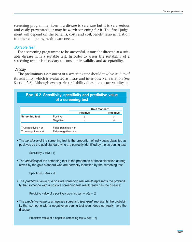
Box 16.2. Sensitivity, specificity and predictive value of a screening test

• The sensitivity of the screening test is the proportion of individuals classified as

positives by the gold standard who are correctly identified by the screening test:

Sensitivity = a/(a + c)

• The specificity of the screening test is the proportion of those classified as neg-

atives by the gold standard who are correctly identified by the screening test:

Specificity = d/(b + d)

• The predictive value of a positive screening test result represents the probabili-

ty that someone with a positive screening test result really has the disease:

Predictive value of a positive screening test = a/(a + b)

• The predictive value of a negative screening test result represents the probabil-

ity that someone with a negative screening test result does not really have the

disease:

Predictive value of a negative screening test = d/(c + d)

Gold standardPositive Negative

Screening test Positive a b

Negative c d

True positives = a False positives = b

True negatives = d False negatives = c


Suitable test

Box 16.2. Sensitivity, specificity and predictive valueof a screening test

• The sensitivity of the screening test is the proportion of individuals classified as

positives by the gold standard who are correctly identified by the screening test:

Sensitivity = a/(a + c)

• The specificity of the screening test is the proportion of those classified as neg-

atives by the gold standard who are correctly identified by the screening test:

Specificity = d/(b + d)

• The predictive value of a positive screening test result represents the probabili-

ty that someone with a positive screening test result really has the disease:

Predictive value of a positive screening test = a/(a + b)

• The predictive value of a negative screening test result represents the probabil-

ity that someone with a negative screening test result does not really have the

disease:

Predictive value of a negative screening test = d/(c + d)



Negative c d



Box 16.2. Sensitivity, specificity and predictive valueBox 16.2. Sensitivity, specificity and predictive valueof screening test

BoxBox 16.2. 16.2. Sensitivity, Sensitivity, specificity specificity and and predictive predictive value value Sensitivity, specificity predictiveof a screening testof a screening testofof a a screening screening test test



Negative c d




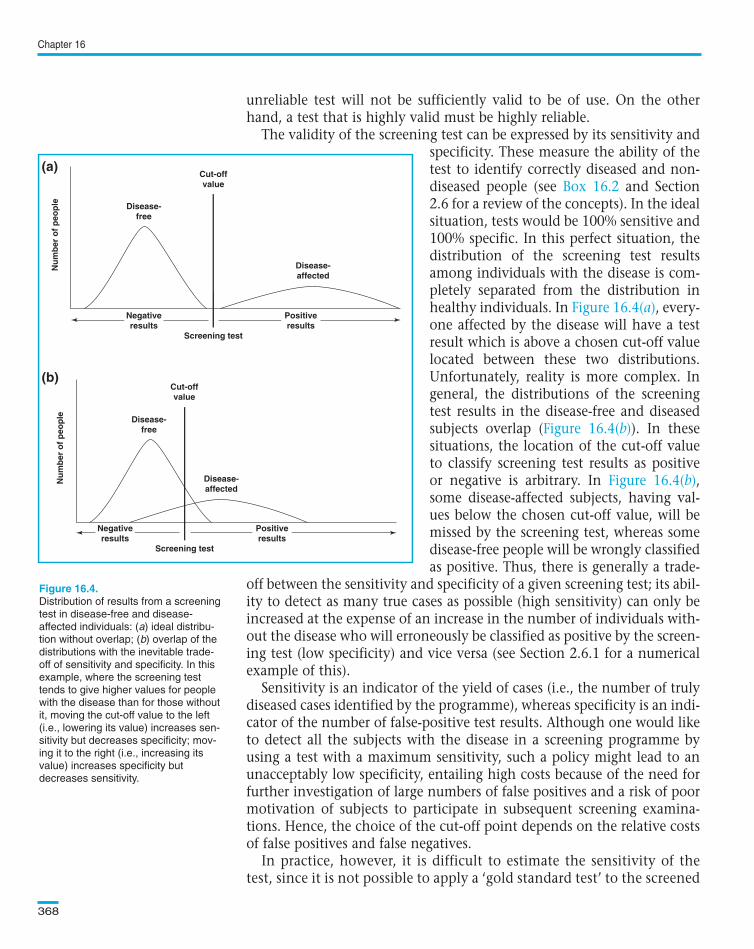
unreliable test will not be sufficiently valid to be of use. On the otherhand, a test that is highly valid must be highly reliable.

The validity of the screening test can be expressed by its sensitivity andspecificity. These measure the ability of thetest to identify correctly diseased and non-diseased people (see and Section2.6 for a review of the concepts). In the idealsituation, tests would be 100% sensitive and100% specific. In this perfect situation, thedistribution of the screening test resultsamong individuals with the disease is com-pletely separated from the distribution inhealthy individuals. In , every-one affected by the disease will have a testresult which is above a chosen cut-off valuelocated between these two distributions.Unfortunately, reality is more complex. Ingeneral, the distributions of the screeningtest results in the disease-free and diseasedsubjects overlap ( ). In thesesituations, the location of the cut-off valueto classify screening test results as positiveor negative is arbitrary. In ,some disease-affected subjects, having val-ues below the chosen cut-off value, will bemissed by the screening test, whereas somedisease-free people will be wrongly classifiedas positive. Thus, there is generally a trade-

off between the sensitivity and specificity of a given screening test; its abil-ity to detect as many true cases as possible (high sensitivity) can only beincreased at the expense of an increase in the number of individuals with-out the disease who will erroneously be classified as positive by the screen-ing test (low specificity) and vice versa (see Section 2.6.1 for a numericalexample of this).

Sensitivity is an indicator of the yield of cases (i.e., the number of trulydiseased cases identified by the programme), whereas specificity is an indi-cator of the number of false-positive test results. Although one would liketo detect all the subjects with the disease in a screening programme byusing a test with a maximum sensitivity, such a policy might lead to anunacceptably low specificity, entailing high costs because of the need forfurther investigation of large numbers of false positives and a risk of poormotivation of subjects to participate in subsequent screening examina-tions. Hence, the choice of the cut-off point depends on the relative costsof false positives and false negatives.

In practice, however, it is difficult to estimate the sensitivity of thetest, since it is not possible to apply a ‘gold standard test’ to the screened

Chapter 16

368

Cut-offvalue

Cut-offvalue

Screening test

Disease-free

Disease-affected

Nu

mb

er o

f p

eop

le

a)

Disease-free

Disease-affected

Nu

mb

er o

f p

eop

le

b)

Positiveresults

Negativeresults

Screening test

Positiveresults

Negativeresults

Distribution of results from a screening

test in disease-free and disease-

affected individuals: (a) ideal distribu-

tion without overlap; (b) overlap of the

distributions with the inevitable trade-

off of sensitivity and specificity. In this

example, where the screening test

tends to give higher values for people

with the disease than for those without

it, moving the cut-off value to the left

(i.e., lowering its value) increases sen-

sitivity but decreases specificity; mov-

ing it to the right (i.e., increasing its

value) increases specificity but

decreases sensitivity.

(a)

(b)


Box 16.2

Figure 16.4(a)

Figure 16.4(b)

Figure 16.4(b)

Cut-offvalue

Cut-offvalue

Screening test

Disease-free

Disease-affected

Nu

mb

er o

f p

eop

le

Disease-free

Disease-affected

Nu

mb

er o

f p

eop

le

Positiveresults

Negativeresults

Screening test

Positiveresults

Negativeresults

(a)

(b)

Figure 16.4.

(a)

(b)


population to find out the total number of diseased subjects (a + c in). The screening test gives us only the value of a, that is, the

number of persons who had a positive screening test and were con-firmed to have the condition after further diagnostic evaluation. Theusual approach to estimating sensitivity is to follow up subjects (usual-ly for one year) having negative screening results, in order to observehow many cancers eventually develop among them. These ‘interval’cases are regarded as false negatives (c). The sensitivity of the screeningtest can then be calculated as usual. However, the value of this approachis limited since it is difficult to achieve complete follow-up and becausesome of the ‘interval’cancers may have been true negatives at the timeof the screening examination (i.e., very fast-growing tumours).

It is easier to estimate specificity if the screening is aimed at a rarecondition such as cancer. Practically all those screened (N) are disease-free and thus N can be used to estimate the total number of people notaffected by the condition (b + d in ). Since all screen-positivesubjects are further investigated, the number of false positives (b in

) is also known and, therefore, the number of true negatives (d in) can be calculated as N – b. Specificity can then be estimated

as (N – b)/N.

Acceptability and costsIn addition to having adequate validity, a screening test should be low

in cost, convenient, simple and as painless as possible, and should notcause any complications. Many screening tests meet these criteria—thePap smear test for cervical precancerous lesions is a good example. Incontrast, although sigmoidoscopic screening might lead to a reductionin mortality from colon cancer, it is questionable whether such a testwould be acceptable because of the expense, the discomfort and the riskof bowel perforation.

The organized application of early diagnosis and treatment activitiesin large groups is often designated as mass screening or population screen-ing, and the set of procedures involved described as a screening pro-gramme.

A screening programme must encompass a diagnostic and a thera-peutic component, because early detection that is not followed by treat-ment is useless for disease control. The diagnostic component includesthe screening policy and the procedures for diagnostic evaluation ofpeople with positive screening test results. The screening policy shouldspecify precisely who is to be screened, at what age, at what frequency,with what test, etc., and it should be dynamic rather than fixed. Thetherapeutic component is the process by which confirmed cases aretreated. It should also be dynamic and be regulated by strict universalprocedures which offer the best current treatment to all identified cases.

Cancer prevention

369


Box 16.2

Box 16.2Box

16.2Box 16.2

Suitable screening programme


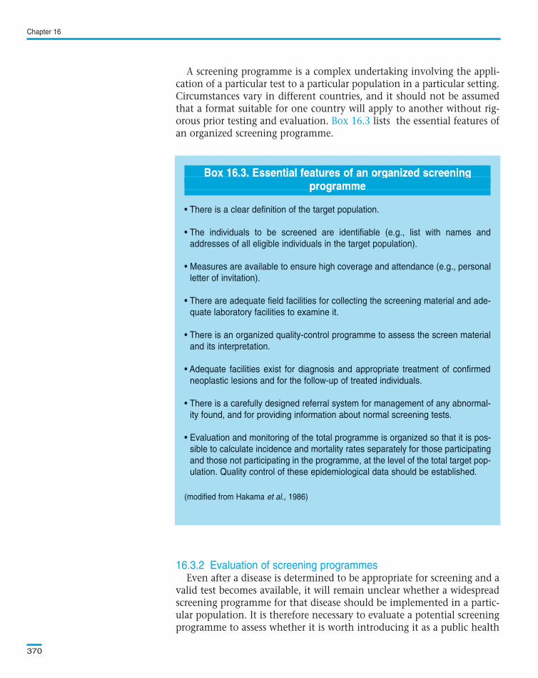
A screening programme is a complex undertaking involving the appli-cation of a particular test to a particular population in a particular setting.Circumstances vary in different countries, and it should not be assumedthat a format suitable for one country will apply to another without rig-orous prior testing and evaluation. lists the essential features ofan organized screening programme.

Even after a disease is determined to be appropriate for screening and avalid test becomes available, it will remain unclear whether a widespreadscreening programme for that disease should be implemented in a partic-ular population. It is therefore necessary to evaluate a potential screeningprogramme to assess whether it is worth introducing it as a public health

Chapter 16

370

Box 16.3. Essential features of an organized screening programme

• There is a clear definition of the target population.

• The individuals to be screened are identifiable (e.g., list with names and

addresses of all eligible individuals in the target population).

• Measures are available to ensure high coverage and attendance (e.g., personal

letter of invitation).

• There are adequate field facilities for collecting the screening material and ade-

quate laboratory facilities to examine it.

• There is an organized quality-control programme to assess the screen material

and its interpretation.

• Adequate facilities exist for diagnosis and appropriate treatment of confirmed

neoplastic lesions and for the follow-up of treated individuals.

• There is a carefully designed referral system for management of any abnormal-

ity found, and for providing information about normal screening tests.

• Evaluation and monitoring of the total programme is organized so that it is pos-

sible to calculate incidence and mortality rates separately for those participating

and those not participating in the programme, at the level of the total target pop-

ulation. Quality control of these epidemiological data should be established.

(modified from Hakama et al., 1986)


Box 16.3

16.3.2 Evaluation of screening programmes

Box 16.3. Essential features of an organized screeningprogramme

• There is a clear definition of the target population.

• The individuals to be screened are identifiable (e.g., list with names and

addresses of all eligible individuals in the target population).

• Measures are available to ensure high coverage and attendance (e.g., personal

letter of invitation).

• There are adequate field facilities for collecting the screening material and ade-

quate laboratory facilities to examine it.

• There is an organized quality-control programme to assess the screen material

and its interpretation.

• Adequate facilities exist for diagnosis and appropriate treatment of confirmed

neoplastic lesions and for the follow-up of treated individuals.

• There is a carefully designed referral system for management of any abnormal-

ity found, and for providing information about normal screening tests.

• Evaluation and monitoring of the total programme is organized so that it is pos-

sible to calculate incidence and mortality rates separately for those participating

and those not participating in the programme, at the level of the total target pop-

ulation. Quality control of these epidemiological data should be established.

(modified from Hakama et al., 1986)

Box 16.3. Essential features of an organized screeningBox 16.3. Essential features of an organized screeningBoxBox 16.3. 16.3. Essential Essential features features of of an an organized organized screening screening organized screeningprogrammeprogrammeprogrammeprogramme


measure to control a particular cancer. This involves consideration of twoissues: first, whether the organization of the proposed programme is feasi-ble and cost-effective (low cost per case detected), and second, whether itwill be effective in reducing the burden of the disease. Both must be consid-ered carefully. The implementation of a screening programme, no matterhow cost-effective, will not be warranted if it does not accomplish its goalof reducing morbidity and mortality in the target population.

The feasibility, acceptability and costs of a programme may be evaluatedby process measures, which are related to the administrative and organiza-tional aspects of the programme such as identification of the target popu-lation, number of persons examined, proportion of the target populationexamined, facilities for diagnosis and treatment in the health services,functioning of the referral system and its compliance, total costs, cost percase detected, etc. The major advantage of these process measures is thatthey are readily obtained and are helpful in monitoring the activity of theprogramme. Their main limitation is that they do not provide any indica-tion of whether those screened have lower mortality from the cancer beingtargetted by the programme than those who were not screened.

A particularly useful process measure is the predictive value of a positivetest. The predictive positive value (PPV) represents the proportion of per-sons found to have the disease in question after further diagnostic evalu-ation out of all those who were positive for the screening test (a/(a+b) in

). A high PPV suggests that a reasonably high proportion of thecosts of a programme are in fact being spent for the detection of diseaseduring its pre-clinical phase. A low PPV suggests that a high proportion ofthe costs are being wasted on the detection and diagnostic evaluation offalse positives (people whose screening result is positive but did not appearto have the disease on subsequent diagnostic investigation). It is impor-tant to emphasize, however, that the PPV is a proportional measure; a highPPV might be obtained even if the frequency of case detection is unac-ceptably low. For instance, the PPV may be 80% indicating that 80% ofthose who screened positive were truly diseased. However, if only 10 sub-jects screen positive, the number of cases detected by the programme willbe only 8! The main advantage of this measure is that it is available soonafter the screening programme is initiated and, in contrast to sensitivity,no follow-up is necessary for it to be estimated.

The PPV of a screening test depends upon both the number of true pos-itives a and the number of false positives b (see ). Thus, it can beincreased by either increasing the number of true positives or decreasingthe number of false positives. The number of true positives may beincreased by increasing the prevalence of detectable pre-clinical disease,for instance, by screening less frequently so as to maintain the prevalenceof pre-clinical disease in the target population at a higher level. The num-ber of false positives may be reduced by increasing the specificity of the

Cancer prevention

371


Process measures

Box 16.2

Box 16.2


test, that is, by changing the criterion of positivity or by repeating thescreening test after a positive test. A low PPV is more likely to be the resultof poor specificity than of poor sensitivity. It is the specificity of a test thatdetermines the number of false positives in people without the disease,who are the vast majority of people tested in virtually any programme.The sensitivity is less important for a rare disease because it operates onfewer people. By contrast, a small loss of specificity can lead to a largeincrease in the number of false positives, and a large loss of PPV.

The second, and definitive, aspect of evaluating a screening programmeis whether it is effective in reducing morbidity and mortality from the dis-ease being screened. Even if a screening programme will accurately andinexpensively identify large numbers of individuals with pre-clinical dis-ease, it will have little public health value if early diagnosis and treatmentdo not have an impact on the ultimate outcome of those cases.

Obtaining an accurate estimate of a reduction in mortality requires along-term follow-up of large populations. Consequently, intermediate out-come measures such as stage at diagnosis and survival (case-fatality) havebeen used which may be available in the early years of a screening pro-

gramme. For example, in a successful screeningprogramme, the stage distribution of the cancersdetected should be shifted towards the lessadvanced stages and the risk of dying from can-cer (case-fatality) should be lower for cases detect-ed through screening than for symptom-diag-nosed cases.

There are, however, critical shortcomings asso-ciated with the use of these intermediate end-points. Absence of a change in the parametersmay mean that the screening is not successful,but they do not provide an adequate measure ofevaluation because they suffer from a number ofbiases, namely, length bias, lead-time bias andoverdiagnosis bias.

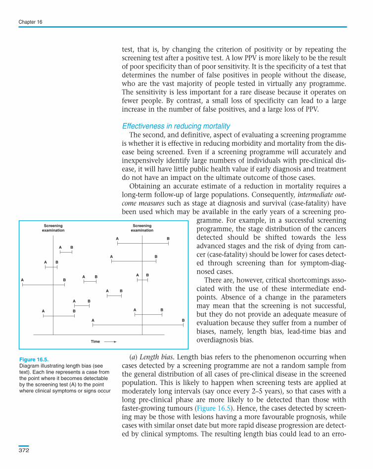
(a) Length bias. Length bias refers to the phenomenon occurring whencases detected by a screening programme are not a random sample fromthe general distribution of all cases of pre-clinical disease in the screenedpopulation. This is likely to happen when screening tests are applied atmoderately long intervals (say once every 2–5 years), so that cases with along pre-clinical phase are more likely to be detected than those withfaster-growing tumours ( ). Hence, the cases detected by screen-ing may be those with lesions having a more favourable prognosis, whilecases with similar onset date but more rapid disease progression are detect-ed by clinical symptoms. The resulting length bias could lead to an erro-

Chapter 16

372

A B

A B

A B

A B

A B

A B

A B

A B

A B

A B

A B

A B

Screeningexamination


Time

Diagram illustrating length bias (see

text). Each line represents a case from

the point where it becomes detectable

by the screening test (A) to the point

where clinical symptoms or signs occur


Effectiveness in reducing mortality

Figure 16.5

A B

A B

A B

A B

A B

A B

A B

A B

A B

A B

A B

A B



Time

Figure 16.5.


neous conclusion that screening was beneficial when, in fact, observed dif-ferences in survival (case-fatality) were a result merely of the detection ofless rapidly fatal cases through screening.

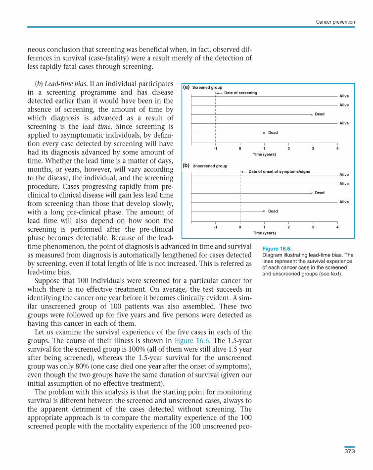
(b) Lead-time bias. If an individual participatesin a screening programme and has diseasedetected earlier than it would have been in theabsence of screening, the amount of time bywhich diagnosis is advanced as a result ofscreening is the lead time. Since screening isapplied to asymptomatic individuals, by defini-tion every case detected by screening will havehad its diagnosis advanced by some amount oftime. Whether the lead time is a matter of days,months, or years, however, will vary accordingto the disease, the individual, and the screeningprocedure. Cases progressing rapidly from pre-clinical to clinical disease will gain less lead timefrom screening than those that develop slowly,with a long pre-clinical phase. The amount oflead time will also depend on how soon thescreening is performed after the pre-clinicalphase becomes detectable. Because of the lead-time phenomenon, the point of diagnosis is advanced in time and survivalas measured from diagnosis is automatically lengthened for cases detectedby screening, even if total length of life is not increased. This is referred aslead-time bias.

Suppose that 100 individuals were screened for a particular cancer forwhich there is no effective treatment. On average, the test succeeds inidentifying the cancer one year before it becomes clinically evident. A sim-ilar unscreened group of 100 patients was also assembled. These twogroups were followed up for five years and five persons were detected ashaving this cancer in each of them.

Let us examine the survival experience of the five cases in each of thegroups. The course of their illness is shown in . The 1.5-yearsurvival for the screened group is 100% (all of them were still alive 1.5 yearafter being screened), whereas the 1.5-year survival for the unscreenedgroup was only 80% (one case died one year after the onset of symptoms),even though the two groups have the same duration of survival (given ourinitial assumption of no effective treatment).

The problem with this analysis is that the starting point for monitoringsurvival is different between the screened and unscreened cases, always tothe apparent detriment of the cases detected without screening. Theappropriate approach is to compare the mortality experience of the 100screened people with the mortality experience of the 100 unscreened peo-

Cancer prevention

373

-1 0 1

Time (years)

Dead

Dead

Date of screeninga) Screened group

Alive

Alive

Alive

2 3 4

-1 0 1

Time (years)

Dead

Dead

Date of onset of symptoms/signsb) Unscreened group

Alive

Alive

Alive

2 3 4

Diagram illustrating lead-time bias. The

lines represent the survival experience

of each cancer case in the screened

and unscreened groups (see text).

(a)

(b)


Figure 16.6

-1 0 1

Time (years)

Dead

Dead

Date of screening Screened group

Alive

Alive

Alive

2 3 4

-1 0 1

Time (years)

Dead

Dead

Date of onset of symptoms/signs Unscreened group

Alive

Alive

Alive

2 3 4

(a)

(b)

Figure 16.6.

(a)

(b)


ple from the time of screening. In the above example, the mortality rate inthe screened group is two deaths in 496 person-years (98 persons × 5 years,plus 1 person × 4 years, plus 1 person × 2 years). The rate is the same inthe unscreened group, since the number of person-years, counted fromthe time the screening would have taken place had it been done, is iden-tical to that for the screened group.

There are two ways in which the effect of lead time on the evaluationof the efficacy of a screening programme can be taken into account. Thefirst is to compare not the length of survival from diagnosis to death, butrather the mortality rates in the screened and unscreened groups (as donein the above example). Alternatively, if the lead time for a given diseasecan be estimated, it can be taken into account, allowing comparison of thesurvival experience of screen- and symptom-detected cases. For example,the average lead time for breast cancer has been estimated as approxi-mately one year (Shapiro et al., 1974). Thus, to evaluate the efficacy of abreast cancer screening programme, the two-, three-, four-, five- and six-year survival risks of the screened cases should be compared, respectively,with the one-, two-, three-, four- and five-year survival risks of theunscreened cases. However, determinations of lead time are difficult tocarry out and cannot be generalized, since they depend on the ability ofthe screening procedure to detect pre-clinical conditions.

(c) Overdiagnosis. It is possible that many of the lesions detected by thescreening programme would never have led to invasive cancer and death.These lesions are known as ‘pseudo-cancer’. Thus, the true benefit of iden-tifying pre-clinical lesions through screening may be much smaller than isperceived.

In short, although intermediate outcome measures, such as stage distri-bution and case fatality (survival), may appear to be suitable as surrogateendpoints in a screening programme, they are subject to lead time bias,length bias and overdiagnosis bias. Thus, the ultimate outcome measurewhich should be evaluated in screening programmes aimed at detectingearly cancer (e.g., breast and colon cancer screening) is reduction in mor-tality. When screening is aimed at detecting both pre-cancerous condi-tions and early cancers (e.g., cervical cancer screening), reduction in theincidence of invasive cancer and reduction in mortality are suitable out-come measures. This implies that any screening programme should beplanned in such a way that its evaluation in terms of change in mortality(and incidence) in the total target population is possible.

An illustration of how intermediate outcomes may be misleading isgiven in In this example, intermediate outcomes seemedto indicate that the use of chest X-ray and cytology was effective in lungcancer screening. However, no reduction in mortality was observed.Similar results have consistently been found in all randomized trials thathave addressed this issue.

Chapter 16

374


Example 16.6.


Intervention studiesThe randomized trial is the best study design for evaluating the effec-

tiveness of a screening programme, because it provides the opportunity fora rigorous experimental evaluation. When the sample size is sufficientlylarge, control of confounding is virtually assured by the process of ran-domization. Patient self-selection or volunteer bias, which is problematicfor the comparison of screened and unscreened groups in observationalstudies, cannot influence the validity of the results of randomized trials,since the screening programme is allocated at random by the investigatorsafter individuals have agreed to participate in the trial.

There are various problems with randomized trials, however. First, therecan be contamination of the control group (awareness of the screeningprogramme may lead subjects in the control group to seek screening).Second, a large number of subjects may be required in screening trials fordiseases with low incidence rate, such as most cancers, and/or if the trialis designed to show small benefits (as in ). Third, it may beunacceptable to randomize some subjects to be non-screened if a screen-ing programme has already been introduced despite the lack of experi-mental evidence (e.g., screening for cervical cancer).

Observational studiesWhile randomized trials can provide the best and most valid evidence

concerning the efficacy of a screening programme, as with the evaluationof etiological hypotheses, most evidence on the effects of screening pro-

Cancer prevention

375

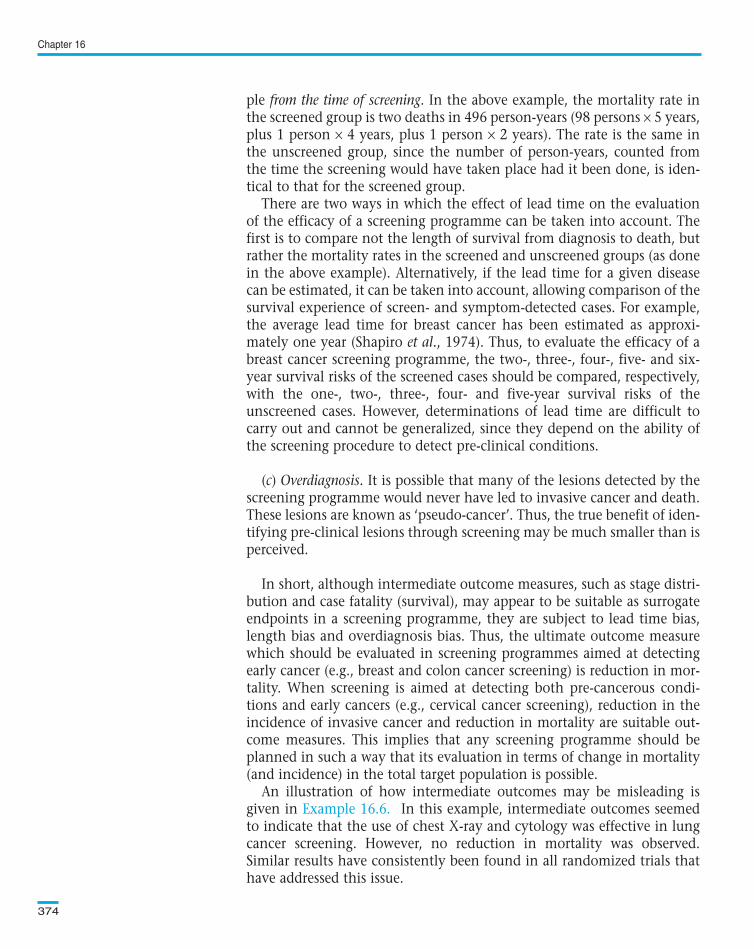
Example 16.6. A total of 6364 cigarette-smoking males aged 40–64 yearswere randomized into an intervention group which received six-monthlyscreening by chest X-ray and sputum cytology during three years, and a con-trol group which received a single examination at the end of the third year.Lung cancer cases detected by screening were identified at an earlier stage,were more often resectable, and had a significantly better survival thansymptom-detected cases. There was, however, no significant difference inmortality between the intervention and control groups (Kubik et al., 1990).

Example 16.7. A randomized controlled trial was set up in Sweden in 1977to assess the efficacy of mass screening with single-view mammography inreducing mortality from breast cancer. A total of 162 981 women aged 40years or more and living in the counties of Kopparberg and Östergötlandwere randomized to either be or not be offered screening every 2 or 3 years,depending on age. The results to the end of 1984 showed that among womenaged 40–74 years at the time of entry, there was a 31% reduction in mor-tality from breast cancer in the group invited for screening (Tabár et al.,1985).


Studies to evaluate the effectiveness of a screening programme

Example 16.7

Example 16.6. A total of 6364 cigarette-smoking males aged 40–64 yearswere randomized into an intervention group which received six-monthlyscreening by chest X-ray and sputum cytology during three years, and a con-trol group which received a single examination at the end of the third year.Lung cancer cases detected by screening were identified at an earlier stage,were more often resectable, and had a significantly better survival thansymptom-detected cases. There was, however, no significant difference inmortality between the intervention and control groups (Kubik et al., 1990).

Example 16.7. A randomized controlled trial was set up in Sweden in 1977to assess the efficacy of mass screening with single-view mammography inreducing mortality from breast cancer. A total of 162 981 women aged 40years or more and living in the counties of Kopparberg and Östergötlandwere randomized to either be or not be offered screening every 2 or 3 years,depending on age. The results to the end of 1984 showed that among womenaged 40–74 years at the time of entry, there was a 31% reduction in mor-tality from breast cancer in the group invited for screening (Tabár et al.,1985).


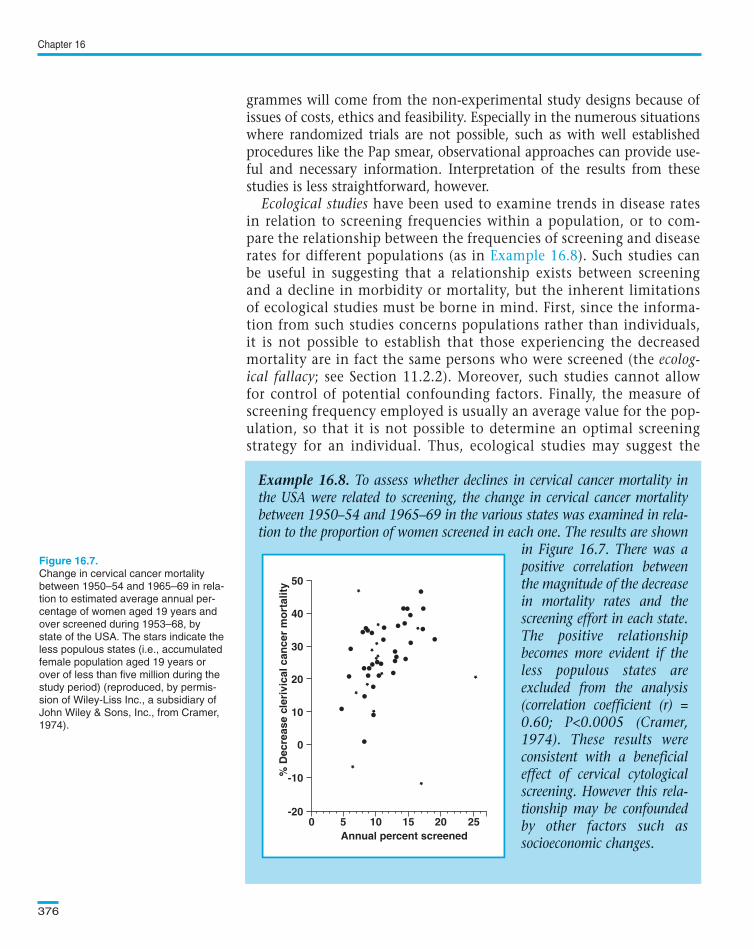
grammes will come from the non-experimental study designs because ofissues of costs, ethics and feasibility. Especially in the numerous situationswhere randomized trials are not possible, such as with well establishedprocedures like the Pap smear, observational approaches can provide use-ful and necessary information. Interpretation of the results from thesestudies is less straightforward, however.

Ecological studies have been used to examine trends in disease ratesin relation to screening frequencies within a population, or to com-pare the relationship between the frequencies of screening and diseaserates for different populations (as in ). Such studies canbe useful in suggesting that a relationship exists between screeningand a decline in morbidity or mortality, but the inherent limitationsof ecological studies must be borne in mind. First, since the informa-tion from such studies concerns populations rather than individuals,it is not possible to establish that those experiencing the decreasedmortality are in fact the same persons who were screened (the ecolog-ical fallacy; see Section 11.2.2). Moreover, such studies cannot allowfor control of potential confounding factors. Finally, the measure ofscreening frequency employed is usually an average value for the pop-ulation, so that it is not possible to determine an optimal screeningstrategy for an individual. Thus, ecological studies may suggest the

Chapter 16

376

Example 16.8. To assess whether declines in cervical cancer mortality inthe USA were related to screening, the change in cervical cancer mortalitybetween 1950–54 and 1965–69 in the various states was examined in rela-tion to the proportion of women screened in each one. The results are shown

in Figure 16.7. There was apositive correlation betweenthe magnitude of the decreasein mortality rates and thescreening effort in each state.The positive relationshipbecomes more evident if theless populous states areexcluded from the analysis(correlation coefficient (r) =0.60; P<0.0005 (Cramer,1974). These results wereconsistent with a beneficialeffect of cervical cytologicalscreening. However this rela-tionship may be confoundedby other factors such associoeconomic changes.

Change in cervical cancer mortality

between 1950–54 and 1965–69 in rela-

tion to estimated average annual per-

centage of women aged 19 years and

over screened during 1953–68, by

state of the USA. The stars indicate the

less populous states (i.e., accumulated

female population aged 19 years or

over of less than five million during the

study period) (reproduced, by permis-

sion of Wiley-Liss Inc., a subsidiary of

John Wiley & Sons, Inc., from Cramer,

1974).

40

50

10

0

-200 5 10 15 20 25

Annual percent screened

% D

ecre

ase

cler

ivic

al c

ance

r m

ort

alit

y

30

20

-10


Example 16.8

Example 16.8. To assess whether declines in cervical cancer mortality inthe USA were related to screening, the change in cervical cancer mortalitybetween 1950–54 and 1965–69 in the various states was examined in rela-tion to the proportion of women screened in each one. The results are shown

in Figure 16.7. There was apositive correlation betweenthe magnitude of the decreasein mortality rates and thescreening effort in each state.The positive relationshipbecomes more evident if theless populous states areexcluded from the analysis(correlation coefficient (r) =0.60; P<0.0005 (Cramer,1974). These results wereconsistent with a beneficialeffect of cervical cytologicalscreening. However this rela-tionship may be confoundedby other factors such associoeconomic changes.

40

50

10

0

-200 5 10 15 20 25


% D

ecre

ase

cler

ivic

al c

ance

r m

ort

alit

y

30

20

-10

Figure 16.7.

40

50

10

0

-200 5 10 15 20 25


% D

ecre

ase

cler

ivic

al c

ance

r m

ort

alit

y

30

20

-10


possibility of a benefit of a screening programme, but they cannot testthat hypothesis.

Cohort studies require long-term follow-up of screened and unscreenedsubjects. However, in interpreting the results of such studies, the potentialeffects of self-selection of participants must be taken into account( ).

In cohort studies such as that described in , the peopleundergoing screening are not chosen randomly and individuals whochoose to be screened may differ both from those who refuse screeningand from the population at large (selection bias). These volunteers mayhave very different prognoses compared with their unscreened counter-parts. In general, volunteers tend to have better health and lower mortal-ity rates than the general population and are more likely to adhere to pre-scribed medical regimens. On the other hand, those who volunteer for ascreening programme may represent the ‘worried well’, that is, asympto-matic individuals who are at higher risk of developing the disease becauseof medical or family history, or any number of lifestyle characteristics.Such individuals may have an increased risk of mortality regardless of theefficacy of the screening programme. The direction of the potential selec-tion bias may be difficult to predict and the magnitude of such effectseven more difficult to quantify.

Case–control studies of screening involve comparison of the screeninghistories of subjects who do, or do not, exhibit the outcome which screen-ing aims to prevent (death from cancer or incidence of invasive disease).Although case–control studies are increasingly used to evaluate screeningprogrammes, they cannot replace experimental studies because they areliable to confounding and bias (for instance, cases may differ from con-trols in their ability to recall past screening). However, once a form ofscreening is widespread, case–control studies may make use of existingrecords so that recall bias should not arise. The first study of this kind

Cancer prevention

377

Example 16.9. To examine the protective effect of Pap-smear screening forcervical cancer, a cohort study was conducted in two counties in Sweden(Uppsala and Gävleborg) where organized cytological screening was intro-duced in 1967 and 1972, respectively. A total of 386 990 women residentat any time during 1968 to 1992 in these two counties were identifiedthrough the Population Register and enrolled into the study. Each woman’sscreening history was ascertained from computerized registers of Pap smearstaken in the area and record-linkages allowed complete follow-up withregard to cancer incidence, out-migration and survival through to 1992. Atotal of 938 newly diagnosed cases of squamous cell cervical cancer occurredduring the follow-up of this cohort. Women who were ever screened werefound to have about half the risk of those never screened (rate ratio = 0.55;95% confidence interval 0.51–0.61) (Sparén, 1996).


Example 16.9

Example 16.9

Example 16.9. To examine the protective effect of Pap-smear screening forcervical cancer, a cohort study was conducted in two counties in Sweden(Uppsala and Gävleborg) where organized cytological screening was intro-duced in 1967 and 1972, respectively. A total of 386 990 women residentat any time during 1968 to 1992 in these two counties were identifiedthrough the Population Register and enrolled into the study. Each woman’sscreening history was ascertained from computerized registers of Pap smearstaken in the area and record-linkages allowed complete follow-up withregard to cancer incidence, out-migration and survival through to 1992. Atotal of 938 newly diagnosed cases of squamous cell cervical cancer occurredduring the follow-up of this cohort. Women who were ever screened werefound to have about half the risk of those never screened (rate ratio = 0.55;95% confidence interval 0.51–0.61) (Sparén, 1996).


compared the history of Pap smear screening in 212 hospital cases of inva-sive cervical cancer with age-matched neighbourhood controls (Clarke &Anderson, 1979). Fewer cases than controls had received a Pap smear dur-ing the five years before the year of diagnosis. The risk of invasive cervicalcancer among women who had not had a Pap smear was about three timesthat of women who were screened, after controlling for socioeconomicstatus. The authors attempted to examine the impact of potential recallbias by comparing the data obtained through a sample of personal inter-views with data from physicians’ records. There was no evidence that theinformation obtained during the interviews was affected by recall bias.

The use of case–control studies to evaluate screening programmes raisessome special methodological issues. Tests done for diagnostic rather thanscreening purposes should not be considered and, for the controls, thescreening history should be restricted up to the time of diagnosis of the case(as in ) to ensure that cases and controls are fully comparablewith respect to period of exposure to screening.

Case–control studies can be set up as an integral part of establishedscreening programmes, in order to assess the screening policy (e.g., the ageat which screening should be initiated or stopped, or the optimal frequencyof screening).

One way of reducing the costs of a screening programme is to target thescreening towards groups of individuals at higher than average risk of devel-oping the disease of interest. Most cancer screening programmes are limitedto certain age-groups. For instance, it is not worth screening women underage 40 for breast cancer, because very few cases occur at these ages.

Chapter 16

378

Example 16.10. In Cali (Colombia), screening for cervical cancer has beenoffered to all sexually active women and routinely performed in pre-natalclinics since the late 1960s. To evaluate the role of Pap smear in preventinginvasive carcinoma of the cervix in this population, a case–control study wascarried out. A total of 204 cases with newly diagnosed invasive cervical can-cer during the years 1977–81 were identified through the Cali population-based cancer registry and successfully interviewed. For each case, a neigh-bourhood control matched to year of birth of the case ± 2 years was select-ed. Cases and controls were interviewed about history of Pap smears per-formed for screening purposes during the period 12–72 months before thedate on which the case was diagnosed. Examinations performed within 12months of diagnosis were ignored because they were likely to be symptom- ordisease-related. For each control, the inquiry covered the same calendar timeinterval as that of the matching case, as determined by her date of diagno-sis. The risk of developing invasive carcinoma was 10 times greater inunscreened than in screened women (Aristizabal et al., 1984).


Example 16.10

16.3.3 Targeting high-risk groups

Example 16.10. In Cali (Colombia), screening for cervical cancer has beenoffered to all sexually active women and routinely performed in pre-natalclinics since the late 1960s. To evaluate the role of Pap smear in preventinginvasive carcinoma of the cervix in this population, a case–control study wascarried out. A total of 204 cases with newly diagnosed invasive cervical can-cer during the years 1977–81 were identified through the Cali population-based cancer registry and successfully interviewed. For each case, a neigh-bourhood control matched to year of birth of the case ± 2 years was select-ed. Cases and controls were interviewed about history of Pap smears per-formed for screening purposes during the period 12–72 months before thedate on which the case was diagnosed. Examinations performed within 12months of diagnosis were ignored because they were likely to be symptom- ordisease-related. For each control, the inquiry covered the same calendar timeinterval as that of the matching case, as determined by her date of diagno-sis. The risk of developing invasive carcinoma was 10 times greater inunscreened than in screened women (Aristizabal et al., 1984).


Screening programmes can also be targeted exclusively to high-riskgroups defined on the basis of factors such as family history, medical histo-ry or occupation. For instance, targeting breast cancer screening pro-grammes exclusively to women with a positive family history wouldincrease the proportion of cases detected among screened women, but thelarge majority of cases in the population would be missed since they occuramong people without a family history of this disease. Thus, restricting ascreening programme to selected high-risk groups is useful only if a sub-stantial fraction of all the cases in a population occur in these high-riskgroups.

Tertiary prevention consists of alleviation of disability resulting from diseasein order to improve the outcome of illness among affected individuals. Itincludes not only the treatment itself, but also all rehabilitation attempts torestore an affected individual to a useful, satisfying, and, where possible, self-sufficient role in society.

Randomized clinical trials are the only acceptable method to evaluate can-cer treatments (see ). However, data from population-based cancerregistries may provide a more representative picture for evaluating compre-hensive cancer care in a particular population, since they will include all can-cer cases in the population regardless of the treatment they might or mightnot have received. These issues are further discussed in Section 17.6.2.

Cancer prevention

379

Box 16.4. Key issues

• Epidemiology is a key discipline of public health which provides the scientific

background for formulation of policies aimed at preventing the development of

disease in healthy persons.

• There are three levels of cancer prevention:

(a) Primary prevention aimed at preventing the onset of the disease either

by reducing exposure to risk factors or by increasing the individuals’ resis-

tance to them. Measures of population impact are very useful in helping

to identify exposures that are potentially responsible for large numbers of

cases of a particular cancer in the population.

(b) Secondary prevention aimed at reducing mortality from a particular

cancer through early detection and treatment. Screening programmes are

an important part of secondary prevention.

(c) Tertiary prevention aimed at improving the prognosis and quality of

life of affected individuals by offering them the best available treatment

and rehabilitation programme.


16.4 Tertiary prevention

Chapter 7

Box 16.4. Key issues

• Epidemiology is a key discipline of public health which provides the scientific

background for formulation of policies aimed at preventing the development of

disease in healthy persons.

• There are three levels of cancer prevention:

(a) Primary prevention aimed at preventing the onset of the disease either

by reducing exposure to risk factors or by increasing the individuals’ resis-

tance to them. Measures of population impact are very useful in helping

to identify exposures that are potentially responsible for large numbers of

cases of a particular cancer in the population.

(b) Secondary prevention aimed at reducing mortality from a particular

cancer through early detection and treatment. Screening programmes are

an important part of secondary prevention.

(c) Tertiary prevention aimed at improving the prognosis and quality of

life of affected individuals by offering them the best available treatment

and rehabilitation programme.

Box 16.4. Key issuesBox 16.4. Key issuesBoxBox 16.4. 16.4. Key Key issues issues


Chapter 16

380

* A comprehensive discussion of

cancer screening programmes is

given in Cole & Morrison (1978).

Box 16.4. (Cont.)

• Screening involves the use of a simple and inexpensive test to detect early

stages of cancer at which treatment is more effective than at the time of usual diag-

nosis. Mass screening programmes should only be directed towards the control of

cancers for which there is an effective treatment that will reduce mortality, if applied

at early stages. There should also be valid, inexpensive and acceptable tests for the

detection of the cancer at early stages.

• The performance of a screening test in terms of its acceptability, feasibility and costs

can be monitored by process measures related to the administrative and organiza-

tional aspects of the programme (e.g., proportion of the target population examined,

functioning of the referral system, cost per case detected, etc.). Predictive value of a

positive test is a particularly useful measure because it provides an indication of

whether most of the effort of the programme is being used to identify cases at an early

stage or whether they are mainly wasted on the evaluation of false positives. Although

process measures are useful for monitoring the activity of the programme they do not

indicate whether those screened will have lower mortality than those not screened.

• The ultimate outcome measure to be used in evaluating the effectiveness of a screen-

ing programme aimed at detecting early cancer (e.g. mammography) is reduction in

mortality. When the programme is aimed at detecting both pre-cancerous conditions

and early cancer (e.g., Pap-smear screening), reduction in the incidence of invasive

cancer and reduction in mortality are suitable outcome measures. Intermediate out-

come measures such as stage distribution and case-fatality (survival) have also been

used, but although they give an indication of whether the programme is likely to be

effective, they are subject to length bias, lead time bias and overdiagnosis bias.

• The effectiveness of a screening programme should ideally be assessed by con-

ducting a randomized intervention trial. In practice, most of the evidence on the

effects of screening programmes comes from observational studies.


Further readingBox 16.4. (Cont.)

• Screening involves the use of a simple and inexpensive test to detect early

stages of cancer at which treatment is more effective than at the time of usual diag-

nosis. Mass screening programmes should only be directed towards the control of

cancers for which there is an effective treatment that will reduce mortality, if applied

at early stages. There should also be valid, inexpensive and acceptable tests for the

detection of the cancer at early stages.

• The performance of a screening test in terms of its acceptability, feasibility and costs

can be monitored by process measures related to the administrative and organiza-

tional aspects of the programme (e.g., proportion of the target population examined,

functioning of the referral system, cost per case detected, etc.). Predictive value of a

positive test is a particularly useful measure because it provides an indication of

whether most of the effort of the programme is being used to identify cases at an early

stage or whether they are mainly wasted on the evaluation of false positives. Although

process measures are useful for monitoring the activity of the programme they do not

indicate whether those screened will have lower mortality than those not screened.

• The ultimate outcome measure to be used in evaluating the effectiveness of a screen-

ing programme aimed at detecting early cancer (e.g. mammography) is reduction in

mortality. When the programme is aimed at detecting both pre-cancerous conditions

and early cancer (e.g., Pap-smear screening), reduction in the incidence of invasive

cancer and reduction in mortality are suitable outcome measures. Intermediate out-

come measures such as stage distribution and case-fatality (survival) have also been

used, but although they give an indication of whether the programme is likely to be

effective, they are subject to length bias, lead time bias and overdiagnosis bias.

• The effectiveness of a screening programme should ideally be assessed by con-

ducting a randomized intervention trial. In practice, most of the evidence on the

effects of screening programmes comes from observational studies.

Box 16.4. (Cont.)Box 16.4. (Cont.)BoxBox 16.4. 16.4. (Cont.) (Cont.)


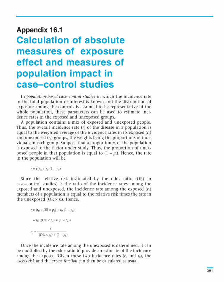
381

In population-based case–control studies in which the incidence ratein the total population of interest is known and the distribution ofexposure among the controls is assumed to be representative of thewhole population, these parameters can be used to estimate inci-dence rates in the exposed and unexposed groups.

A population contains a mix of exposed and unexposed people.Thus, the overall incidence rate (r) of the disease in a population isequal to the weighted average of the incidence rates in its exposed (r1)and unexposed (r0) groups, the weights being the proportions of indi-viduals in each group. Suppose that a proportion pe of the populationis exposed to the factor under study. Thus, the proportion of unex-posed people in that population is equal to (1 – pe). Hence, the ratein the population will be

r = r1pe + r0 (1 – pe)

Since the relative risk (estimated by the odds ratio (OR) incase–control studies) is the ratio of the incidence rates among theexposed and unexposed, the incidence rate among the exposed (r1)members of a population is equal to the relative risk times the rate inthe unexposed (OR × r0). Hence,

r = (r0 × OR × pe) + r0 (1 – pe)

= r0 ((OR × pe) + (1 – pe))

rr0 = —————————

(OR × pe) + (1 – pe)

Once the incidence rate among the unexposed is determined, it canbe multiplied by the odds ratio to provide an estimate of the incidenceamong the exposed. Given these two incidence rates (r1 and r0), theexcess risk and the excess fraction can then be calculated as usual.

Appendix 16.1


Calculation of absolute measures of exposureeffect and measures of population impact incase–control studies


Appendix 16.1

382

The population excess risk and the population excess fraction can then bedetermined as

Population excess risk = excess risk × proportion of the population exposed to the factor (pe)

population excess riskPopulation excess fraction (%) = 100 ×

rate in the total population (r)

The population excess fraction can also be calculated by using the formu-la given in Section 16.2.1:

pe (OR – 1)Population excess fraction (%) = 100 ×

pe (OR – 1) + 1

Example A16.1. In a hypothetical population-based case–control studyconducted in London, cases with lung cancer were nine times more likely tohave smoked cigarettes regularly in the past five years than men withoutlung cancer. The population lung cancer incidence rate in London was 40per 100 000 pyrs and the proportion of smokers among the controls 60%.Thus,

40 per 100 000 pyrsr0 = —————————— = 6.9 per 100 000 pyrs

(9 × 0.6) + (1 – 0.6)

r1 = 9 × 6.9 per 100 000 pyrs = 62.1 per 100 000 pyrs

Excess risk = 62.1 per 100 000 pyrs – 6.9 per 100 000 pyrs = 55.2 per 100 000 pyrs

Excess fraction (%) = 100 × (55.2 per 100 000 pyrs / 62.1 per 100 000 pyrs) = 89%

Note that the excess fraction could also have been calculated by using theformula given in Section 16.2.1:

(OR – 1)Excess fraction (%) = 100 ×

OR

(9 – 1)Excess fraction (%) = 100 × = 89%

9


Example A16.1. In a hypothetical population-based case–control studyconducted in London, cases with lung cancer were nine times more likely tohave smoked cigarettes regularly in the past five years than men withoutlung cancer. The population lung cancer incidence rate in London was 40per 100 000 pyrs and the proportion of smokers among the controls 60%.Thus,

40 per 100 000 pyrsr0 = —————————— = 6.9 per 100 000 pyrs

(9 × 0.6) + (1 – 0.6)

r1 = 9 × 6.9 per 100 000 pyrs = 62.1 per 100 000 pyrs

Excess risk = 62.1 per 100 000 pyrs – 6.9 per 100 000 pyrs = 55.2 per 100 000 pyrs

Excess fraction (%) = 100 × (55.2 per 100 000 pyrs / 62.1 per 100 000 pyrs) = 89%

Note that the excess fraction could also have been calculated by using theformula given in Section 16.2.1:

(OR – 1)Excess fraction (%) = 100 ×

OR

(9 – 1)Excess fraction (%) = 100 × = 89%

9


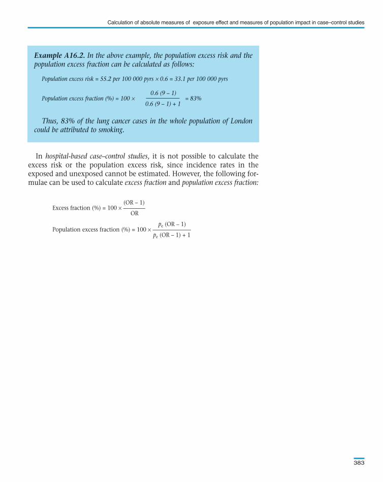
In hospital-based case–control studies, it is not possible to calculate theexcess risk or the population excess risk, since incidence rates in theexposed and unexposed cannot be estimated. However, the following for-mulae can be used to calculate excess fraction and population excess fraction:

(OR – 1)Excess fraction (%) = 100 × ————

OR

pe (OR – 1)Population excess fraction (%) = 100 × ———————

pe (OR – 1) + 1

Example A16.2. In the above example, the population excess risk and thepopulation excess fraction can be calculated as follows:

Population excess risk = 55.2 per 100 000 pyrs × 0.6 = 33.1 per 100 000 pyrs

0.6 (9 – 1)Population excess fraction (%) = 100 × = 83%

0.6 (9 – 1) + 1

Thus, 83% of the lung cancer cases in the whole population of Londoncould be attributed to smoking.

Calculation of absolute measures of exposure effect and measures of population impact in case–control studies

383


Example A16.2. In the above example, the population excess risk and thepopulation excess fraction can be calculated as follows:

Population excess risk = 55.2 per 100 000 pyrs × 0.6 = 33.1 per 100 000 pyrs

0.6 (9 – 1)Population excess fraction (%) = 100 × = 83%

0.6 (9 – 1) + 1

Thus, 83% of the lung cancer cases in the whole population of Londoncould be attributed to smoking.


Documents

Cancer prevention - IARC effects of treatments given, as well as the ... Alternative formulae can, however, ... Cancer prevention 359