Embed Size (px)
DESCRIPTION
The Canberra Group Handbook on Household Income Statistics, Second Edition (2011), provides a consolidated reference for those involved in producing, disseminating or analysing income distribution statistics. It reflects the current international standards, recommendations and best practice in household income measurement. It also contains updated and expanded information about country practices in this field of statistics and provides guidance on bestpractices for quality assurance and dissemination of these statistics.
Citation preview
UNITED NATIONS ECONOMIC COMMISSION FOR EUROPE
Canberra Group
Handbook on
Household Income
Statistics
Second Edition 2011
UNITED NATIONS
Geneva, 2011

NOTE
The designations employed and the presentation of the material in this publication do not imply the expression of any opinion whatsoever on the part of the Secretariat of the United Nations concerning the legal status of any country, territory, city or area, or of its authorities, or concerning the delimitation of its frontier or boundaries.
ECE/CES/11

iii
Preface In 2008, the Conference of European Statisticians (CES) completed an in-depth review of statistics on income, living conditions and poverty. The importance of this work was reinforced by the release of the Stiglitz-Sen-Fitoussi Commission Report on the Measurement of Economic Performance and Social Progress (2009), which includes recommendations about the need to focus on the household perspective and distributional aspects of economic well-being.
An outcome of the CES review was the formation of a small international Task Force to undertake a limited update of the Final Report and Recommendations of the Expert Group on Household Income Statistics (2001), commonly referred to as the Canberra Group Handbook. The purpose of the update was to incorporate new developments in the area of household income measurement and to expand the guidelines to take into account these new developments. The objective was to help achieve greater harmonisation of income concepts and measurement at the household level across countries.
The 2001 Canberra Group Handbook was the result of the work of an International Expert Group on Household Income Statistics, known as the 'Canberra Group', that was established in 1996 at the initiative of the Australian Bureau of Statistics. The initiative was in response to a growing awareness of the need to address the common conceptual, definitional and practical problems that national statistical offices faced in the area of household income distribution statistics.
The first edition of the handbook significantly advanced the available guidance on the production, dissemination and analysis of household income statistics and provided a significant reference point for national and international statistical agencies. It was also highly influential in the development of new international standards for micro level household income statistics, as set out in the resolution on standards for household income statistics adopted by the International Conference of Labour Statisticians (ICLS) in December 2003 (ILO, 2004).
In principle, there is no difference between the ICLS definition of household income and the concept of household income in the 2001 Canberra Group Handbook. The ICLS standard also follows, to a large extent, the definitional recommendations put forward by the first edition of the handbook. The only exceptions are in regard to the Value of unpaid domestic services and the Value of services from household consumer durables. These components were not included in the conceptual income definition of the first edition of the handbook, but listed as 'issues for the future'. In this second edition of the handbook the two components have been included in the conceptual definition to align with the 2004 ICLS standard.
The Canberra Group Handbook on Household Income Statistics, Second Edition (2011), provides a consolidated reference for those involved in producing, disseminating or analysing income distribution statistics. It reflects the current international standards, recommendations and best practice in household income measurement. It also contains updated and expanded information about country practices in this field of statistics and provides guidance on best practices for quality assurance and dissemination of these statistics.

iv
Acknowledgements This second edition of what is commonly referred to as the ‘Canberra Group Handbook’ has built on the important contribution made by the original Canberra City Group members reflected in the Handbook titled Final Report and Recommendations of the Expert Group on Household Income Statistics (2001). The Canberra City Group comprised experts in household income statistics from national statistical offices, government departments and research agencies from Europe, North and South America, Asia, Australia and New Zealand, as well as from a number of international organisations. The members are listed in the Acknowledgements section of the first edition.
This second edition has been prepared by a small international Task Force, operating under the auspices of the Conference of European Statisticians (CES) and sponsored by the United Nations Economic Commission for Europe (UNECE). The update also reflects the many comments received during the consultation process and the direct contributions made by the agencies who responded to the 2010 Survey of Country Practices. The countries from which responses were received are listed in Chapter 4. The Task Force members were: National statistical offices International agencies Australian Bureau of Statistics (Chair and Editor) Bob McColl John Billing Bindi Kindermann Heather Burgess Statistics Austria Matthias Till Statistics Canada Sylvie Michaud Karen Mirohean Alison Hale Statistics Norway Jon Epland US Bureau of the Census Kathleen Short David Johnson
United Nations Economic Commission for Europe (UNECE) (Secretariat) Carsten Boldsen Zeynep Orhun Anu Peltola Marietta Leni Jeppe International Labour Organization (ILO) Adriana Mata Greenwood Luxembourg Income Study (LIS) at CEPS/INSTEAD Markus Jantti Organisation for Economic Cooperation and Development (OECD) Marco Mira d’Ercole Nicolas Ruiz Statistical Office of the European Union (Eurostat) Jean-Louis Mercy Fabienne Montaigne
v
Abbreviations
ABS Australian Bureau of Statistics AIM-AP Accurate Income Measurement for the Assessment of Public Policies ASEC-CPS Annual Social and Economic Supplement of the Current Population Survey ASNA Australian System of National Accounts CES Conference of European Statisticians CFC Consumption of Fixed Capital CGH Canberra Group Handbook CNEF Cross National Equivalence File COICOP Classification of Individual Consumption According to Purpose CPI Consumer Price Index CSB Central Statistical Bureau (Latvia) DICAH Distribution of Income, Consumption and Accumulation of Households ECHP European Community Household Panel ERF Tax Revenues Survey (France) ESA European System of Accounts EU European Union Eurostat Statistical Office of the European Union EU-SILC European Union – Statistics on Income and Living Conditions FISIM Financial Intermediation Services Indirectly Measured GDP Gross Domestic Product GGH Canberra Group Handbook GMI Gross Mixed Income GOS Gross Operating Surplus HBS Household Budget Survey HILDA Household Income and Labour Dynamics in Australia IARIW International Association for Research in Income and Wealth ICLS International Conference of Labour Statisticians ICP International Comparison Programme ILO International Labour Organization LIS Luxembourg Income Study NA Not available NOS Net Operating Surplus NSO National Statistical Office OECD Organisation for Economic Cooperation and Development PPP Purchasing Power Parity PSID Panel Study of Income Dynamics (USA) PUMF Public Use Micro Data Files RIGA Rural Income Generating Activities RSE Relative Standard Error SAM Social Accounting Matrix SE Standard Error SCP Survey of Country Practices SIH Survey of Income and Housing (Australia) SIPP Survey of Income and Program Participation (USA) SLID Survey of Labour and Income Dynamics (Canada) SNA System of National Accounts SRS State Revenue Service (Latvia) SSIA State Social Insurance Agency (Latvia) STIK Social Transfers In Kind UN United Nations UNECE United Nations Economic Commission for Europe VAT Value Added Tax

vii
Table of contents Preface .............................................................................................................................................................. iii Acknowledgements .......................................................................................................................................... iv Abbreviations ..................................................................................................................................................... v Summary of chapters ........................................................................................................................................ xi
Chapter 1 Introduction ............................................................................................................................. 1 1.1 Aim of this Handbook ........................................................................................................................... 1 1.2 Why is income distribution important? ................................................................................................. 1 1.3 Economic well-being ............................................................................................................................. 2 1.4 Household income as a microeconomic and a macroeconomic concept ............................................... 4 1.5 Historical background ........................................................................................................................... 6
Chapter 2 Standard concepts and definitions ........................................................................... 9 2.1 Introduction ........................................................................................................................................... 9 2.2 The income concept ............................................................................................................................... 9 2.3 Income components ............................................................................................................................. 10
2.3.1 Income from employment ........................................................................................................... 11 2.3.2 Property income .......................................................................................................................... 13 2.3.3 Income from household production of services for own consumption ....................................... 14 2.3.4 Current transfers received ........................................................................................................... 15 2.3.5 Social transfers in kind ............................................................................................................... 16 2.3.6 Exclusions from income ............................................................................................................. 16
2.4 Income aggregation ............................................................................................................................. 17 2.5 Income and its relationship to the broader framework ........................................................................ 18
2.5.1 Introduction................................................................................................................................. 18 2.5.2 Extension to consumption and capital accumulation .................................................................. 18
Chapter 3 Income measurement ...................................................................................................... 21 3.1 Introduction ......................................................................................................................................... 21 3.2 Sources of household income statistics ............................................................................................... 21
3.2.1 Income surveys ........................................................................................................................... 21 3.2.2 Income data from registers ......................................................................................................... 22
3.3 General measurement issues ................................................................................................................ 24 3.3.1 Measurement units ...................................................................................................................... 24 3.3.2 Reference periods ....................................................................................................................... 26 3.3.3 Population weighting .................................................................................................................. 27 3.3.4 Benchmarking ............................................................................................................................. 28 3.3.5 Measurement errors .................................................................................................................... 29
3.4 Practical guidance for the measurement of selected income receipts .................................................. 32 3.4.1 Employee income in kind ........................................................................................................... 33 3.4.2 Income from self-employment .................................................................................................... 34 3.4.3 Property income .......................................................................................................................... 36 3.4.4 Income from household production of services for own consumption ....................................... 36 3.4.5 Current transfers ......................................................................................................................... 41
Chapter 4 Data availability ................................................................................................................... 49 4.1 Introduction ......................................................................................................................................... 49 4.2 Survey of Country Practices ................................................................................................................ 49
4.2.1 Robustness assessment ............................................................................................................... 49 4.2.2 Data item inventory .................................................................................................................... 52
4.3 Comparison of country practices between 2001 and 2010 .................................................................. 54 4.4 European Union Statistics on Income and Living Conditions (EU-SILC) .......................................... 54 4.5 Practical definition of income for use in international comparisons ................................................... 56
viii
Chapter 5 Quality assurance guidelines..................................................................................... 57 5.1 Introduction ........................................................................................................................................ 57 5.2 Quality assurance frameworks ............................................................................................................ 57 5.3 Quality assurance best practice ........................................................................................................... 58
Chapter 6 Data analysis and dissemination ............................................................................. 63 6.1 Introduction ........................................................................................................................................ 63 6.2 Uses of income data ............................................................................................................................ 63 6.3 Units and populations ......................................................................................................................... 64
6.3.1 Units of analysis ......................................................................................................................... 64 6.3.2 Population subgroups ................................................................................................................. 65
6.4 Equivalence scales .............................................................................................................................. 68 6.4.1 Choice of equivalence scale ....................................................................................................... 68 6.4.2 Derivation of equivalised household income ............................................................................. 70
6.5 Summary measures of income level ................................................................................................... 72 6.5.1 Counts ........................................................................................................................................ 72 6.5.2 Means ......................................................................................................................................... 72 6.5.3 Medians ...................................................................................................................................... 73
6.6 Measures of income dispersion ........................................................................................................... 73 6.6.1 Frequency distribution ............................................................................................................... 73 6.6.2 Quantile measures ...................................................................................................................... 74 6.6.3 Lorenz curves ............................................................................................................................. 75 6.6.4 Summary indicators of income dispersion ................................................................................. 78
6.7 Income composition ............................................................................................................................ 81 6.8 Adjusting for price differences ........................................................................................................... 84
6.8.1 Adjusting for price changes over time ....................................................................................... 84 6.8.2 Adjusting for price differences across geographical areas or types of household ...................... 86
6.9 Analysis of low income households and income poverty ................................................................... 88 6.9.1 Introduction ................................................................................................................................ 88 6.9.2 Income poverty approaches........................................................................................................ 88 6.9.3 Static versus dynamic views ...................................................................................................... 91 6.9.4 Non-monetary measures of material deprivation ....................................................................... 91
6.10 Analysis at the top of the income distribution .................................................................................... 93 6.10.1 Non-survey methods for measuring top incomes ....................................................................... 94
6.11 Best practice guidelines for dissemination of income data ................................................................. 96
Chapter 7 Comparing income distributions over time ..................................................... 101 7.1 Introduction ...................................................................................................................................... 101 7.2 Undertaking cross-time comparisons ................................................................................................ 101 7.3 Impact of measurement error ............................................................................................................ 102 7.4 Issues for the data originator ............................................................................................................. 102 7.5 Issues for secondary dataset producers ............................................................................................. 104 7.6 Issues for the end user ....................................................................................................................... 106
7.6.1 Detecting trends ....................................................................................................................... 106 7.6.2 Significance of changes ........................................................................................................... 108 7.6.3 Trends versus episodes ............................................................................................................. 108
Chapter 8 Income dynamics ............................................................................................................ 111 8.1 Introduction ...................................................................................................................................... 111 8.2 Advantages and disadvantages of longitudinal data ......................................................................... 111 8.3 Examples of longitudinal income surveys ........................................................................................ 113
8.3.1 Survey of Labour and Income Dynamics (Canada) ................................................................. 113 8.3.2 Panel Study of Income Dynamics (USA) ................................................................................ 114 8.3.3 Survey of Income and Program Participation (USA) ............................................................... 114 8.3.4 European Union's Statistics on Income and Living Conditions (EU-SILC) ............................ 115
8.4 Some applications of longitudinal surveys ....................................................................................... 115 8.4.1 Households income dynamics and intergenerational mobility ................................................. 115 8.4.2 Low income dynamics ............................................................................................................. 117 8.4.3 Labour market dynamics .......................................................................................................... 117
ix
Chapter 9 Future directions for international work ............................................................ 119 9.1 Introduction ....................................................................................................................................... 119 9.2 Better informing analyses of economic well-being ........................................................................... 119 9.3 Household income, consumption and wealth framework .................................................................. 120
Appendix 1 Comparison of income definitions between 2001 and 2011 editions of the Canberra Group Handbook ................................................................................................. 123
Appendix 2 Reconciliation of micro and macro approaches ....................................... 129
Appendix 3 Survey of Country Practices for measuring household income: Robustness assessment .................................................................................................................... 139
Appendix 4 Survey of Country Practices for measuring household income: Data item inventory ................................................................................................................................ 163
Appendix 5 Purchasing power parities ...................................................................................... 173
Bibliography ............................................................................................................................................... 177
Index ................................................................................................................................................................ 187 List of tables, figures and boxes Table 1.1 Brief history of household income measurement .................................................................................... 6 Table 2.1 Income components in the conceptual and operational definitions ....................................................... 11 Table 2.2 Extension to consumption and capital accumulation ............................................................................ 19 Table 3.1 High income censorship due to processing limits ................................................................................. 29 Table 3.2 Types of non-response .......................................................................................................................... 30 Table 4.1 Countries responding to the Survey of Country Practices..................................................................... 51 Table 4.2 Income components collected in EU-SILC ........................................................................................... 55 Table 4.3 Practical definitions of income for international comparisons .............................................................. 56 Table 5.1 Dimensions of quality assurance frameworks ....................................................................................... 57 Table 6.1 Comparison of three commonly used equivalence scales ..................................................................... 70 Table 6.2 From gross income to person weighted equivalised disposable income ............................................... 71 Table 6.3 Summary statistics of income dispersion .............................................................................................. 80 Table 6.4 Comparison of alternative treatments of persons with zero equivalised disposable household income ........ 81 Table 6.5 Distribution of household income, government benefits and taxes....................................................... 83 Table 6.6 Distribution of various household income measures ............................................................................ 83 Table 6.7 CPI differences for different households and locations ........................................................................ 86 Table 6.8 Income growth and top incomes (a) ...................................................................................................... 94 Table 7.1 Weekly income, new and former bases (a) ......................................................................................... 103
Appendix 1 Table 1 Classification of income components: 2001 CGH – 2011 CGH ............................................................ 126 Table 2 Classification of income components: 2011 CGH – 2001 CGH ............................................................ 127
Appendix 2 Table 1 Micro and macro household income concepts and measurement .......................................................... 130 Table 2 SIH and selected ASNA household income, (b) .................................................................................... 137 Table 3 Concordance between SIH and selected ASNA income items (a) ......................................................... 138
Appendix 3 Table 1 Main source of information .................................................................................................................... 140 Table 2 Scope and coverage ................................................................................................................................ 143 Table 3 Units ....................................................................................................................................................... 146 Table 4 Income recording ................................................................................................................................... 148
x
Table 5 Non-response rates for the main income components (%) .................................................................... 150 Table 6 Editing and imputation .......................................................................................................................... 152 Table 7 Dissemination ........................................................................................................................................ 154 Table 8 Websites for additional information ...................................................................................................... 156
Appendix 4 Table 1 Data item inventory: Summary of country practices ............................................................................. 164 Table 2 Data item inventory: Individual country practices ................................................................................ 166 Table 3 Countries that participated in the 2010 Survey of Country Practices .................................................... 172
Figure 3.1 The 2011 CGH conceptual definition of production of services for own consumption and the SNA production boundary ................................................................................................................................... 37
Figure 3.2 Private and final income, by private income quintile .......................................................................... 47 Figure 4.1 Survey of Country Practices: Proportion of countries collecting detailed income components (a) .... 53 Figure 6.1 Average equivalised disposable household income by life cycle stage .............................................. 67 Figure 6.2 Distribution of equivalised disposable household income .................................................................. 74 Figure 6.3 Lorenz curves: example 1 ................................................................................................................... 76 Figure 6.4 Frequency distributions ....................................................................................................................... 76 Figure 6.5 Lorenz curves: example 2 ................................................................................................................... 77 Figure 6.6 Cash benefits and household taxes as a proportion of disposable household income ......................... 82 Figure 7.1 Trends in income inequality: Examples of data interpretation issues ............................................... 107 Figure 7.2 Trends in income inequality: Index of Gini coefficients in country Z (a) ......................................... 107 Figure 7.3 Trends in income inequality (Gini coefficients): Average annual percentage change over time ...... 108 Figure 7.4 Trends in income inequality: Index of Gini coefficients (a) ............................................................. 109
Box 3.1 Examples of using administrative data ................................................................................................... 23 Box 3.2 Definition of household .......................................................................................................................... 25 Box 3.3 Example of censorship of income values during processing .................................................................. 29 Box 3.4 Examples of imputation methods for partial non-response ..................................................................... 31 Box 3.5 Examples of collection issues for inter-household transfers ................................................................... 43 Box 3.6 Excerpt from Growing Unequal? ........................................................................................................... 44 Box 3.7 Government benefits, taxes and household income in Australia ............................................................ 47 Box 5.1 EU-SILC quality reports ......................................................................................................................... 62 Box 6.1 Definitions of analytical units ................................................................................................................. 64 Box 6.2 Definitions of household types used in Australia ................................................................................... 67 Box 6.3 Spatial price indexes in Canada .............................................................................................................. 87 Box 6.4 Millennium Development Goals on global poverty ................................................................................ 91 Box 6.5 Some approaches to measuring economic hardship ............................................................................... 92 Box 6.6 Standard methodology for calculation of top income shares from tax return data ................................. 95 Box 7.1 Examples of income data changes ........................................................................................................ 103
xi
Summary of chapters Chapter 1 - Introduction
Chapter 1 sets out the intended purpose of this Handbook, as well as providing a brief history of developments in the field of household income statistics. It includes information on why income distribution is an important measure of economic well-being and considers the broader conceptual issues underlying economic well-being measures. The chapter also discusses the macroeconomic perspective and compares the different objectives and purposes of the micro and macro approaches to household income measurement.
Chapter 2 - The income concept
Chapter 2 establishes the conceptual and operational definitions of household income, as reflected in the 2004 International Conference of Labour Statisticians (ICLS) standard and adopted in this second edition of the Canberra Group Handbook. It shows how the income components can be aggregated to produce different measures of income. It also outlines the relationship between income and other types of household economic resources, and how all of these could be integrated into a broader framework.
Chapter 3 - Income measurement
This chapter examines the key measurement issues from the perspective of producing reliable and relevant household income distribution statistics. It presents the sources of household income statistics, the standard units of income measurement and the reference periods for collecting data for components of income. While not all income items are covered, practical guidance is provided on the collection or estimation of those income components which have known measurement or quality concerns. Issues of measurement at both the bottom and top of the income distribution are discussed.
Chapter 4 - Data availability
Chapter 4 provides information on the methodologies used and the income components included in household income datasets compiled for a wide variety of countries. This information has been obtained from the 2010 Survey of Country Practices. The chapter also recommends a practical definition of income to be used for the purposes of international comparisons of income distribution statistics.
Chapter 5 - Quality assurance guidelines
This chapter provides general guidelines on best practice methods for assessing the quality of household income statistics, such as reconciliation of concepts and estimates between various income sources.
xii
Chapter 6 - Data analysis and dissemination
Chapter 6 provides practical guidance on the analysis and dissemination of income distribution statistics. It outlines the range of analytical methods that may be applied. As the presentation used can significantly influence how the data are interpreted, best practice dissemination guidelines are highlighted.
Chapter 7 - Comparing income distributions over time
Chapter 7 discusses the compilation and analysis of time series on income distribution. The additional difficulty of comparing time trends across countries is also discussed. In this context, guidance is provided for: primary data producers; the compilers of secondary datasets which bring together time series estimates for multiple nations; and the researchers and analysts who use both primary and secondary sources.
Chapter 8 - Income dynamics
Chapter 8 presents the relative advantages and disadvantages, uses and policy implications associated with longitudinal data. Some examples of longitudinal surveys are provided, as well as potential research areas for which longitudinal data are well suited.
Chapter 9 - Future directions for international work
Chapter 9 proposes a research agenda that would support further advances in the field of household microeconomic statistics and the measurement of economic well-being. The development of an internationally agreed framework for the compilation of statistics on all of the dimensions of household economic resources, measured at the micro level, is essential to the production and analysis of harmonised and coherent information on the economic situation of the household.
The development of international standards for the collection and compilation of statistics on household wealth at the micro level would also be an important contribution to the research agenda.
1
Chapter 1 Introduction 1.1 Aim of this Handbook
This Handbook is a guide for producers and users of household income distribution statistics. It is firstly aimed at those responsible for compiling income distribution statistics, whether primary producers who collect and analyse data from original sources, or secondary producers who take processed data (micro, meso, or summary level) and derive their own estimates and datasets. However, it is of equal importance to researchers and analysts who make use of the outputs from primary and secondary producers, in leading them to a better understanding of the underlying principles of income distribution statistics and the pitfalls in their practical use.
The intention is to lay down useful guidelines for understanding the complex nature of income data, set in the context of international standards and best practices. The chapters cover many topics such as the income concept and definitions, best practices for the measurement of selected income receipts, availability of income data, quality assurance guidelines, and data analysis and dissemination.
The aim of the Handbook is to contribute to the availability of more accurate, complete, and internationally comparable income statistics, greater transparency in their presentation, and more informed use of what are inevitably some of the most complex statistics produced by national and international organisations.
1.2 Why is income distribution important?
Economic analysts and policy makers identify three main purposes for compiling information on income distribution.
The first is driven by a desire to understand the pattern of income distribution and how this can be related to the way in which societies are organised.
The second reflects the concern of policy makers to assess the impact of both universal and targeted actions on different socio-economic groups. Examples of policy issues where data on income distribution are important include welfare, taxation and other fiscal policies, housing, education, labour market and health.
The third is an interest in how different patterns of income distribution influence household well-being and people’s ability to acquire the goods and services they need to satisfy their needs, for example, studies of poverty and social exclusion, and research on consumer behaviour.
Producers of income distribution statistics therefore have to address such questions as:
How unequal is the distribution of income in a given country? How does this compare with earlier years, or with other countries?
Chapter 1 Introduction
2
What are the characteristics and circumstances of low income households and those considered to be at risk of poverty? Which groups are in greatest need of financial support? How does this compare with earlier years, or with other countries?
Are real incomes growing or declining over time? What might this mean for fiscal and monetary policies relating to the management of the economy?
How do tax transfer systems affect the economic well-being of particular groups within the population?
Do people have sufficient incomes in their working lives and in retirement to maintain an adequate standard of living?
Typically, the main focus of interest is on changes over time, with differences between countries coming a close second. Statisticians' statements about incomes may be interpreted as statements about the material living standards experienced by different sections of the population. Those with the lowest incomes are often assumed to have the lowest material living standards.
Interest in income distribution may be justified either per se as a way to see how national product is distributed across the population, or indirectly as the best proxy for the distribution of economic well-being. The national accounts provide essential information for macro economists about the overall performance of the whole economy, and aggregate outcomes for households. On the other hand, household income distribution statistics inform our understanding of the distribution of these resources over time, across regions or between subgroups of the population. In addition, household income distribution statistics take account of the way in which household needs vary on the basis of household composition and age. Understanding the distributional dimensions of economic well-being requires measurement at the household unit level.
However, income is not the only way in which the concept of economic well-being can be characterised, and it is therefore useful first to consider the broader conceptual issues underlying its nature.
1.3 Economic well-being
A household's economic well-being can be expressed in terms of its access to goods and services. The more that a household can consume, the higher its level of economic well-being. While other theoretical approaches have underlined the importance of other aspects of people’s lives as determinants of human well-being (reaching beyond the commodities that are available to them), this report focuses on the narrower concept of economic well-being.
Consumption is therefore an indicator of economic well-being. However, a household may be able to choose not to consume the maximum amount it could in any given period but to save at least some of the resources it has available. By saving, households can accumulate wealth through the purchase of assets which will generate income at a later date and serve as a 'nest-egg' for spending at a later time when income levels may be lower, or needs higher. As well as possibly earning a return for the household, ownership of wealth also affects their broader economic power and is another aspect of economic well-being. For example, households that own their own home outright generally have lower housing costs and may therefore have lower income requirements to satisfy their desired standard of living.
Canberra Group Handbook
3
Thus to capture fully the extent of a household’s economic well-being it is desirable to look at a number of different aspects of their economic situation, including not only their income, but also their levels of wealth, changes in the value of that wealth and levels of consumption.
The remainder of this section provides an overview of the relationship between economic well-being and income, consumption expenditure, change in the value of net worth, and the value of the stock of net worth.
Income and consumption expenditure
In broad terms, income refers to receipts, whether monetary or in kind, that are received at annual or more frequent intervals and are available for current consumption. For most people, household income is the most important determinant of economic well-being. Household income provides a measure of the resources available to the household for consumption and saving. However income is not the only economic resource available to households.
On the disbursements side of household accounts, consumption expenditure represents the day-to-day purchases that may be financed not only by household income but also by savings from previous periods or by incurring debt. For some households, such as retired households, the running down of capital for consumption may represent a deliberate attempt on their part to even out consumption over a lifetime. Other groups in the population, such as farmers, may also average out their consumption over a number of years, while their incomes may show quite wide fluctuations over the same period. In such cases, consumption expenditure may represent a better estimate of the household’s sustainable standard of living.
There are difficulties in collecting data on both income and consumption expenditure in household surveys. Income is a sensitive issue for many respondents and non-response or misreporting of some income components may be significant. On the other hand, high quality data on consumption expenditure are often onerous and costly to collect. In fact, the choice between the income or the consumption expenditure approach to measuring economic well-being is often made for the analyst by the fact that, at least in developed countries, income data may be more frequently available than data on consumption expenditure.
Change in value of net worth
Whether data on income or on consumption expenditure are used for measuring economic well-being, the data should ideally be accompanied by some assessment of the change in the value of the household’s net worth during the accounting period. Change in the level of net worth may result from saving, from capital transfers, or from other changes in the value of assets, including capital or holding gains. Such a household is likely to be better off in the long-term than a household with a similar level of consumption that has financed its consumption by dissaving, that is, running down assets or incurring a liability. Whether the dissaving has been involuntary, or has been planned by saving in earlier periods, is important in this context.
Value of stock of net worth
The value of the stock of net worth owned by a household is the value of accumulated assets less liabilities. As well as possibly earning a return for the household in the form of income, those households with substantial levels of net worth may use their assets as collateral to obtain credit for consumption or investment, or to more flexibly choose the timing for
Chapter 1 Introduction
4
different types of consumption and investment. For these reasons it is important to ascertain, if possible, the value of the household’s net worth to give a complete picture of the household’s command over economic resources and its economic well-being.
At a practical level, the collection of micro data on the assets and liabilities of households is not without its own difficulties. Such information may be as sensitive to the respondent as that on income and, because transactions are relatively infrequent, recall and valuation issues may pose difficulties. There are also difficulties in using data on the stock of wealth and on transactions or flows in a combined measure of economic well-being.
One option is to annuitise the net worth held by the household and add this (notional) annuity to the flow of income. However, annuitisation of net worth requires that a number of value judgements and assumptions be made in relation to, for example, the period over which the net worth should be annuitised (life of the householder or spouse) and the rates of return to be used. However, there are also simpler, but less sophisticated, methods available to use distributional information for income and wealth together.
Ideally, analysis of economic well-being would benefit greatly from the availability of fully articulated survey data covering all aspects: income, expenditure, saving, and the value of wealth held. This would enable observation of the size and nature of economic resources available to households, and how they were disposed of. Where it is not possible to collect survey data in all dimensions, it might be possible to match records or information from different sources to allow inferences on the joint distribution of various types of economic resources of households.
Section 2.5 sets out a conceptual framework in which income, consumption and accumulation of wealth can be related to each other. Future directions for further work in this area are discussed in Chapter 9.
1.4 Household income as a microeconomic and a macroeconomic concept
Household income measurement has two main traditions:
the macro approach, having its roots in national accounts and in particular the accounting based standards laid out in the System of National Accounts (SNA).
the micro approach, having its roots in microeconomics and particularly the study of poverty and its effect on different socio-economic groups within society.
SNA data are sectoral aggregates compiled from many sources and presented within the broader national accounting framework. The data show how the household sector relates to the corporate and government sectors and to the rest of the world. Generally they provide only aggregated information for the household sector as a whole or for major household subsectors. As only aggregate information is needed for this purpose, greater use can be made of partial data sources and imputation or estimation.
Micro datasets have long been used to analyse not only levels (aggregates), but also the distributions of income, consumption and wealth across the population, for various population subgroups, and over time. Micro data can also serve as input for compilation of macroeconomic statistics.
Canberra Group Handbook
5
Conceptually, macro and micro statistics on household income have much in common. However, there are significant differences in the objectives and purposes of the two datasets, in their coverage and the data sources used to compile them, and because of practical data reporting or estimation issues for individual households.
Many of the conceptual difficulties encountered in drawing together the guidelines on household income distribution statistics are the same or similar to those faced in developing related guidelines such as the SNA and it is sensible to adopt a consistent treatment across frameworks whenever possible. It should be noted, however, that there are some important conceptual differences between the two datasets, with some imputations in the SNA required for ensuring complete accounts for households, the corporate and government sectors, and the rest of the world.
One approach outlined in the SNA is a social accounting matrix (SAM), which typically focuses on the role of people within the economy. A SAM will disaggregate the household sector in order to analyse the interrelationships between structural features of an economy and the distribution of income and consumption expenditure among different socio-economic groups. In most SAMs it is therefore necessary to reconcile the macro aggregate of household income with the micro income statistics on which the disaggregation is based. However, although the intention of the SNA was to include a disaggregation of household income by socio-economic group as a standard part of national accounts output, in practice there are few countries who do so on a regular basis e.g. the Netherlands.
Most users of household income distribution statistics would expect the producers to have undertaken reconciliation between the macro aggregate of household income and the micro income statistics suitably grossed up to population totals. Even if this is not possible, the data producer should provide clear explanations when differences are known to exist. It is undoubtedly a considerable disservice to users when two sets of statistics both labelled 'household income' appear to produce different results, and possibly have different implications for social and economic policy. Such reconciliation, with any discrepancies clearly explained, is best practice for National Statistical Offices (NSOs). Appendix 2 of this Handbook aims to provide practical guidance on how such reconciliations might be approached in a practical sense.
There are other reasons to maximise comparability between household income distribution statistics and household income in the national accounts. First, there is a greater likelihood that any datasets collected can be used for multiple purposes, for example, the use of the micro data in compilation or benchmarking of national accounts estimates. Second, statistics compiled under the different frameworks can be compared as part of a mutual checking process, and users can be confident that the different sets of statistics can be brought together for analytical purposes.
Although these guidelines have been primarily produced for the needs of micro analysts, they also draw attention to areas of difference with the recommendations of the 2008 SNA and how the two may be reconciled. The intention is to aid understanding amongst micro analysts of the concerns and conventions of macro analysts, thus improving understanding between the two.
Chapter 1 Introduction
6
1.5 Historical background
Table 1.1 provides a chronology of the most important initiatives undertaken to improve the micro level measurement of household income. It provides useful context for the international development of household income statistics.
Table 1.1 Brief history of household income measurement 1966 United Nations Statistical Commission – 14th session
Following this session, a system of distribution statistics that covered income, consumption and accumulation of household wealth was to be gradually developed by the United Nations Statistical Office. The work was tied in with both the System of National Accounts (SNA) and the now obsolete System of Balances of the National Economy.
1972 United Nations Statistical Commission – 17th session
A final version of the full system of distribution statistics that covered income, consumption and accumulation of household wealth was adopted at this session. However, the Commission requested that amendments and simplifications be made in the light of its discussions.
1974 United Nations Statistical Commission – 18th session
A draft of the simplified system of distribution statistics that covered income, consumption and accumulation of household wealth was adopted with a number of reservations. In particular, the Commission felt that further simplification was desirable.
1977 The United Nations Statistical Office published Provisional Guidelines on Statistics of the Distribution of Income, Consumption and Accumulation of Households (United Nations, 1977).
The aim of the Provisional Guidelines was to assist countries to collect and disseminate income distribution statistics and to provide for international reporting and publication of comparable data. The need to link micro level income distribution statistics with macro level national accounting standards was emphasised.
The Provisional Guidelines were to be revised concurrently with the 1968 SNA (e.g. Norrlof, 1985). The Conference of European Statisticians (CES) in particular began work on revising the Provisional Guidelines and organised a number of Work Sessions and Seminars on statistics of household income with this in mind. Special attention was paid to the relevance of the revision of the SNA (e.g. United Nations, 1989), given that the revision process of the 1968 SNA had led to advances in conceptual thinking about the household sector and about the concept of income in particular. However, due to limited resources, progress in the revision of the Provisional Guidelines was limited.
1981 Surveys of national practices of income distribution statistics were published by the United Nations Statistical Office (United Nations, 1981 and 1985).
1983 At the inter-country level, the Luxembourg Income Study (LIS) was set up in 1983 to address the lack of comparability of household income data from different countries. Located in the Centre for Population, Poverty and Socio-Economic Policy Studies in Luxembourg, LIS draws together unit record data from a wide range of countries and reorganises them according to a common set of concepts and definitions.
Organisations such as the World Bank, the United Nations and the Organisation for Economic Co-operation and Development (OECD) all published inter-country comparisons during the 1990s in which the same country might have very different relative rankings depending on the concepts and data sources used.
1994 The Statistical Office of the European Union (Eurostat), with the agreement of the United Nations Economic Commission for Europe (UNECE), and the OECD, undertook to play a major role in the revision of the 1977 Provisional Guidelines.
The key objective was to update the Guidelines in light of the revised SNA and European System of Accounts (ESA) and new developments since 1977 relating to household income statistics (e.g. hidden and informal activities) and to extend and adapt them where appropriate to serve the analytical needs of economic and social policies. The geographical scope of the revised guidelines would initially be the countries of the European Economic Area.
Eurostat launched the European Community Household Panel (ECHP). The aim of this survey was to produce comparable statistics on income and other variables relating to social exclusion, within a longitudinal framework. ECHP was one of the most closely harmonized social surveys in the European Union (EU). A central feature of the project was the use of a common 'blue-print' questionnaire which served as the starting point for all national surveys. The use of this common instrument ensured not only common concepts and content for the surveys, but also their common operationalisation.
In addition, as a result of the 15th International Conference of Labour Statisticians (ICLS) in October 1993 the Bureau of Statistics of the International Labour Organization (ILO) took the initiative to improve the measurement of income from employment (e.g. Dupré, 1997).
Canberra Group Handbook
7
1996 The 24th General Conference of the International Association for Research in Income and Wealth (IARIW) in August 1996 included a session on International Standards on Income and Wealth Distribution (Smeeding, 1996). This session mainly focussed on efforts to revise the 1977 Provisional Guidelines on Statistics of the Distribution of Income, Consumption and Accumulation of Households (United Nations, 1977).
Once again, one of the main conclusions from the discussions was that the top down macro-to-micro approach was not sufficient from the perspective of micro data users. Both macro-to-micro and micro-to-macro viewpoints are valuable and new international guidelines were needed to address these issues.
A clear challenge emerged from the 1996 IARIW Session. Integration of theory and application would be difficult but not impossible, and revisions to the UN Provisional Guidelines should serve both purposes. However, a wider constituency of interest needed to be engaged in the discussions, particularly from NSOs, but also from a range of other national and international organisations.
Hence the birth of the Canberra Group in 1996. The Group was established to address the common conceptual, definitional, and practical problems that national and international statistical agencies faced in the area of household income distribution statistics. Its work was in support of a revision of international standards and guidelines for these statistics.
The Canberra Group provided a forum for expert opinions on conceptual and methodological issues. It comprised experts in household income statistics from NSOs, government departments and research agencies from Europe, North and South America, Asia, Australia and New Zealand, as well as from a number of international organisations.
1998 The 16th ICLS adopted a Resolution concerning the measurement of employment-related income (ILO, 1998).
2001 The Canberra Group’s Final Report and Recommendations was published providing valuable guidance on conceptual and practical issues related to the collection and analysis of household income distribution statistics. The Group’s recommendations were highly influential in the development of new international standards for micro level household income statistics.
2003 The revised international standards for household income statistics adopted by the 17th International Conference of Labour Statisticians (ICLS) followed to a large extent the recommendations put forward by the Canberra Group (see Appendix 1 for a comparison of the 2001 Canberra Group recommendations and the international standards).
The EU Statistics on Income and Living Conditions (EU-SILC) was introduced to replace the ECHP.

8
9
Chapter 2 Standard concepts and definitions 2.1 Introduction
This chapter provides the conceptual and operational definitions of household income, as reflected in the 2004 ICLS standard and adopted in this second edition of the Canberra Group Handbook. It shows how the various components of household income can be aggregated to produce particular income measures. It also outlines the relationship between the micro and macro level concepts of household income.
Household income, rather than personal income, is generally the preferred measure for analysis of people’s economic well-being. This is because the major determinant of economic well-being for most people is the level of income they and other family members living in the same dwelling receive. While income is usually received by individuals, it is normally shared with other household members present e.g. spouse and children.
2.2 The income concept
The conceptual definition determines what, in principle, should be included in a comprehensive measure of household income. In practice, income definitions adopted by individual countries may be more limited in scope, as some elements of household income may not be collected or modelled.
Household income statistics should be internationally comparable and consistent with related economic and social statistics. It was with these objectives in mind, that revised international standards for micro level statistics on household income were adopted by the Seventeenth ICLS in Resolution 1: Resolution concerning household income and expenditure statistics, in December 2003 (ILO, 2004).
In principle, there is no difference between the ICLS definition of household income and the concept of household income described in Chapter 2 of the final report of the Canberra Group on household income statistics (Canberra Group, 2001). The ICLS standard also follows, to a large extent, the definitional recommendations put forward by the 2001 Canberra Group report. The only exceptions are in regard to the Value of unpaid domestic services and the Value of services from household consumer durables. While these components of income are included in the income concept in Chapter 2 of the 2001 Canberra Group report, the definition and measurement issues were identified as 'issues for the future' in that 2001 report. The ICLS standard moved these components into its conceptual definition of income, but excluded them from its operational definition due to practical measurement issues. In this second edition of the Handbook the two components have been included in the conceptual definition to align with the ICLS standard.
The conceptual definition of household income established by the ICLS, and adopted in this Handbook, is as follows (ILO, 2004):
Household income consists of all receipts whether monetary or in kind (goods and services) that are received by the household or by individual members of the household at annual or more frequent intervals, but excludes windfall gains and other such irregular and typically one-time receipts.
Chapter 2 Standard concepts and definitions
10
Household income receipts are available for current consumption and do not reduce the net worth of the household through a reduction of its cash, the disposal of its other financial or non-financial assets or an increase in its liabilities.
Household income may be defined to cover: (i) income from employment (both paid and self-employment); (ii) property income; (iii) income from the production of household services for own consumption; and (iv) current transfers received.
The ICLS conceptual definition of income is consistent, where possible, with the definition of income used in the SNA which defines disposable household income, in concept, as:
... the maximum amount that a household or other unit can afford to spend on consumption goods or services during the accounting period without having to finance its expenditures by reducing its cash, by disposing of other financial or non-financial assets or by increasing its liabilities (SNA 2008, 8.25).
Despite the conceptual similarities between the micro and macro definitions, the different purposes of the statistics to be compiled result in some different treatments between the two. Income distribution statistics are primarily concerned with a particular set of microeconomic issues and require the construction of statistics which reflect the circumstances of individual households. The SNA is concerned with macroeconomic issues and the household sector is but one sector of interest. Some recommendations in the SNA that are targeted at non-household sectors, but which impact on the household sector in aggregate, may have to be treated differently in compiling household income distribution statistics.
The next section describes the components that constitute the conceptual and operational definitions of income, as defined in this Handbook. The conceptual definition reflects what should ideally be included to provide the most comprehensive measure of income. The operational definition is consistent with the conceptual definition, apart from the exclusion of the value of unpaid domestic services, the value of consumer durables and social transfers in kind, due to the difficulty in valuing these components.
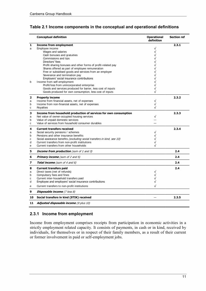
2.3 Income components
Table 2.1 provides an overview of the components that constitute the conceptual and operational definitions of income. It also shows the components that are included in the various measures of income (described further in section 2.4).
The classification provided in the international standards, and adopted in this edition of the Handbook, differs somewhat from the classification system applied in the 2001 Canberra Group Handbook in both its structure and level of detail. Appendix 1 compares Table 2.1 with the corresponding table published in the 2001 Canberra Group Handbook. Appendix 2 compares this table with the macro household income concepts in the SNA.
Canberra Group Handbook
11
Table 2.1 Income components in the conceptual and operational definitions
2.3.1 Income from employment
Income from employment comprises receipts from participation in economic activities in a strictly employment related capacity. It consists of payments, in cash or in kind, received by individuals, for themselves or in respect of their family members, as a result of their current or former involvement in paid or self-employment jobs.
Conceptual definition Operational definition
Section ref
1 Income from employment 2.3.1 a Employee income √ Wages and salaries √ Cash bonuses and gratuities √ Commissions and tips √ Directors’ fees √ Profit-sharing bonuses and other forms of profit-related pay √ Shares offered as part of employee remuneration √ Free or subsidised goods and services from an employer √ Severance and termination pay √ Employers’ social insurance contributions √ b Income from self-employment √ Profit/loss from unincorporated enterprise √ Goods and services produced for barter, less cost of inputs √ Goods produced for own consumption, less cost of inputs √
2 Property income 2.3.2 a Income from financial assets, net of expenses √ b Income from non-financial assets, net of expenses √ c Royalties √
3 Income from household production of services for own consumption 2.3.3 a Net value of owner-occupied housing services √ b Value of unpaid domestic services — c Value of services from household consumer durables —
4 Current transfers received 2.3.4 a Social security pensions / schemes √ b Pensions and other insurance benefits √ c Social assistance benefits (excluding social transfers in kind, see 10) √ d Current transfers from non-profit institutions √ e Current transfers from other households √
5 Income from production (sum of 1 and 3) 2.4
6 Primary income (sum of 2 and 5) 2.4
7 Total income (sum of 4 and 6) 2.4
8 Current transfers paid 2.4 a Direct taxes (net of refunds) √ b Compulsory fees and fines √ c Current inter-household transfers paid √ d Employee and employers’ social insurance contributions √
e Current transfers to non-profit institutions √
9 Disposable income (7 less 8)
10 Social transfers in kind (STIK) received — 2.3.5
11 Adjusted disposable income (9 plus 10)
Chapter 2 Standard concepts and definitions
12
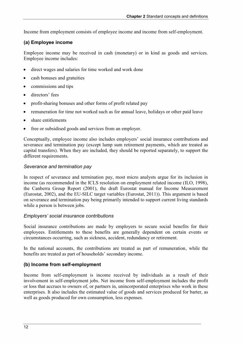
Income from employment consists of employee income and income from self-employment.
(a) Employee income
Employee income may be received in cash (monetary) or in kind as goods and services. Employee income includes:
direct wages and salaries for time worked and work done
cash bonuses and gratuities
commissions and tips
directors’ fees
profit-sharing bonuses and other forms of profit related pay
remuneration for time not worked such as for annual leave, holidays or other paid leave
share entitlements
free or subsidised goods and services from an employer.
Conceptually, employee income also includes employers’ social insurance contributions and severance and termination pay (except lump sum retirement payments, which are treated as capital transfers). When they are included, they should be reported separately, to support the different requirements.
Severance and termination pay
In respect of severance and termination pay, most micro analysts argue for its inclusion in income (as recommended in the ICLS resolution on employment related income (ILO, 1998), the Canberra Group Report (2001), the draft Eurostat manual for Income Measurement (Eurostat, 2002), and the EU-SILC target variables (Eurostat, 2011)). This argument is based on severance and termination pay being primarily intended to support current living standards while a person is between jobs.
Employers’ social insurance contributions
Social insurance contributions are made by employers to secure social benefits for their employees. Entitlements to these benefits are generally dependent on certain events or circumstances occurring, such as sickness, accident, redundancy or retirement.
In the national accounts, the contributions are treated as part of remuneration, while the benefits are treated as part of households’ secondary income.
(b) Income from self-employment
Income from self-employment is income received by individuals as a result of their involvement in self-employment jobs. Net income from self-employment includes the profit or loss that accrues to owners of, or partners in, unincorporated enterprises who work in these enterprises. It also includes the estimated value of goods and services produced for barter, as well as goods produced for own consumption, less expenses.
Canberra Group Handbook
13
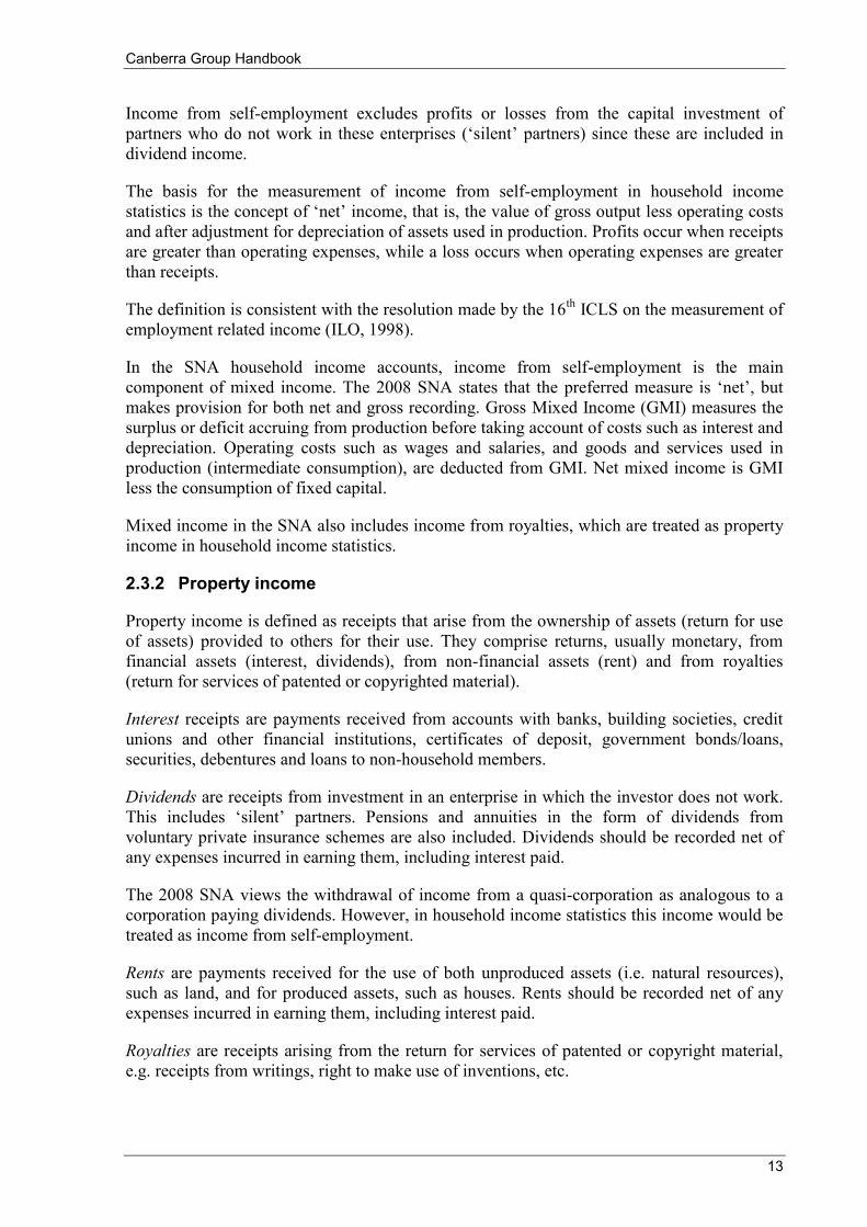
Income from self-employment excludes profits or losses from the capital investment of partners who do not work in these enterprises (‘silent’ partners) since these are included in dividend income.
The basis for the measurement of income from self-employment in household income statistics is the concept of ‘net’ income, that is, the value of gross output less operating costs and after adjustment for depreciation of assets used in production. Profits occur when receipts are greater than operating expenses, while a loss occurs when operating expenses are greater than receipts.
The definition is consistent with the resolution made by the 16th ICLS on the measurement of employment related income (ILO, 1998).
In the SNA household income accounts, income from self-employment is the main component of mixed income. The 2008 SNA states that the preferred measure is ‘net’, but makes provision for both net and gross recording. Gross Mixed Income (GMI) measures the surplus or deficit accruing from production before taking account of costs such as interest and depreciation. Operating costs such as wages and salaries, and goods and services used in production (intermediate consumption), are deducted from GMI. Net mixed income is GMI less the consumption of fixed capital.
Mixed income in the SNA also includes income from royalties, which are treated as property income in household income statistics.
2.3.2 Property income
Property income is defined as receipts that arise from the ownership of assets (return for use of assets) provided to others for their use. They comprise returns, usually monetary, from financial assets (interest, dividends), from non-financial assets (rent) and from royalties (return for services of patented or copyrighted material).
Interest receipts are payments received from accounts with banks, building societies, credit unions and other financial institutions, certificates of deposit, government bonds/loans, securities, debentures and loans to non-household members.
Dividends are receipts from investment in an enterprise in which the investor does not work. This includes ‘silent’ partners. Pensions and annuities in the form of dividends from voluntary private insurance schemes are also included. Dividends should be recorded net of any expenses incurred in earning them, including interest paid.
The 2008 SNA views the withdrawal of income from a quasi-corporation as analogous to a corporation paying dividends. However, in household income statistics this income would be treated as income from self-employment.
Rents are payments received for the use of both unproduced assets (i.e. natural resources), such as land, and for produced assets, such as houses. Rents should be recorded net of any expenses incurred in earning them, including interest paid.
Royalties are receipts arising from the return for services of patented or copyright material, e.g. receipts from writings, right to make use of inventions, etc.
Chapter 2 Standard concepts and definitions
14
The 2008 SNA concept of property income includes most of the concepts described above. However income from the rental of dwellings (both owner-occupied and rentals) are treated as an operating surplus for the household sector. Royalties and rental income from non-residential property (factories, shops, etc.) are included in mixed income rather than property income. As well, some additional imputations are included in the SNA as a result of flows from non-household sectors that impact on the household sector in aggregate. For example, a value is imputed for investment income on technical reserves held by insurance corporations which is attributed to insurance policyholders in the household sector.
2.3.3 Income from household production of services for own consumption
Income from household production of services for own consumption include services produced within the household for the household’s own consumption and not for the market. They include services from owner-occupied dwellings and from consumer durables owned, as well as own-produced domestic services. They are valued net of expenses that go into their production.
However, in the operational definition of income, the value of unpaid domestic services and of services from consumer durables are excluded for the reasons discussed in section 2.2.
The production of services by household members for their own final consumption, other than the services provided by owner-occupied dwellings, has also traditionally been excluded from measured production in the SNA.
(a) Net value of owner-occupied housing services (imputed rent)
Imputed rent is the net estimated value of housing services provided by owner-occupied dwellings. Imputed rent is included in income on a net basis, i.e. the imputed value of the services received less the value of the housing costs incurred by the household in their role as a landlord, including interest paid.
Imputed rent estimates should be presented separately from estimates for other services, so that data is available to support different types of analysis. Rent imputations should be made in a consistent manner in producing household income and expenditure statistics where these are to be analysed jointly.
In the 2008 SNA, income from imputed rent (imputed value of housing services less operating costs) is a component of gross operating surplus in the household income account.
(b) Unpaid domestic services
Unpaid domestic services include the estimated value of own-produced domestic services such as cooking, housekeeping, minor repairs, child care, etc. The contribution of unpaid work is important to analyses of economic and social well-being. Its importance was emphasised in the Report on the Measurement of Economic Performance and Social Progress (2009), which included in their list of recommendations the broadening of income measures to include non-market activities (Stiglitz et al., 2009).
(c) Services from household consumer durables
Income from services from household consumer durables, such as cars, washing machines, refrigerators, etc. refers to the imputed value of services provided by these items.
Canberra Group Handbook
15
2.3.4 Current transfers received
Transfers are receipts for which the recipient does not provide anything to the donor in direct return for the receipts. Transfers can consist of cash (in the monetary sense), of goods, or of services. Transfers may be made between households, between households and government, or between households and charities, both within or outside the country. The main motivation is to redistribute income either by government (e.g. pensions) or privately (e.g. child support).
Current transfers received directly affect the level of disposable income available and should influence the consumption of goods and services. They consist of all transfers that are not transfers of capital (see section 2.5.2(e) for a description of capital transfers). In concept, all current transfers received in cash and as goods or services are regarded as income.
(a) Social security pensions / schemes
Social security pensions, insurance benefits and allowances generated from government sponsored social insurance schemes (compulsory/legal schemes) such as pensions (including military and overseas pensions), unemployment and sickness benefits.
(b) Pensions and other insurance benefits
Pensions and other insurance benefits from employer sponsored social insurance schemes and private funded schemes not covered by social security legislation (both funded and unfunded).
Pensions received from contributory or private funded schemes may represent a running down of the household’s assets where the underlying capital is consumed. They are, however, included as income as they are considered as income by households, especially retired households, and are used for consumption. Otherwise the analysis of income distribution will be affected since many of these households have little or no other income.
When employer contributed pensions are included along with employers’ social contributions, some double counting will occur when total (or gross) income is aggregated across groups. Disposable income will be unaffected.
(c) Social assistance benefits
Social assistance benefits from governments (universal or means-tested) which provide the same benefits as social security schemes, but which are not provided for under such schemes.
(d) Current transfers from non-profit institutions
Current transfers from non-profit institutions (e.g. charities, trade unions and religious bodies) in the form of regular gifts and financial support, such as scholarships, union strike pay, union sickness benefits and relief payments.
Chapter 2 Standard concepts and definitions
16
(e) Current transfers from other households
Current transfers from other households in the form of family support payments (such as alimony, child and parental support), regular receipts from inheritances and trust funds, regular gifts, financial support or transfers in kind of goods or services (e.g. housing or child care services). They include transfers from non-resident households (remittances) which can be of significant importance to the economic well-being of some households and are of particular policy interest for a number of developing countries.
2.3.5 Social transfers in kind
Social transfers in kind (STIK) are defined as goods and services provided by government and non-profit institutions that benefit individuals but are provided free or at subsidised prices. For example, social transfers in kind may include medical services provided for free or at subsidised prices, including where medical expenses are initially met by individuals but are subsequently either fully or partly reimbursed by government. Other examples of STIK include government provided education, rental allowances and the subsidy element of publicly provided housing. In other words, the treatment is symmetrical, regardless of whether the subsidy is delivered as a lower initial cash price or as a rebate or refund on outlay – conceptually the consumption levels are the same and the income component is the social transfer in kind. Social transfers in kind are excluded from the operational definition of income for the reasons discussed in section 3.4.5(b).
2.3.6 Exclusions from income
Household income excludes the following receipts.
Holding gains or losses refer to changes in the value of financial and non-financial assets and liabilities over a reference period. A holding gain, the result of an increase in the value of assets or a reduction in the value of liabilities, increases the net worth of the owner’s assets while a holding loss has the opposite effect. All holding gains and losses are excluded from income, whether they are realised (if the owner sells the asset) or remain unrealised. Instead they are treated as changes in net worth.
Windfall gains and other such irregular and one-time lump sum receipts are excluded from the definition of income. They include lottery prizes, gambling winnings, non-life insurance claims, inheritances, lump sum retirement benefits, life insurance claims (except annuities), windfall gains, legal/injury compensation (except those in lieu of foregone earnings) and loan repayments.
Other receipts that result from a reduction in net worth are excluded from income. These include the sale of assets, loans obtained and withdrawals from savings.
For analytical and other purposes, data may be collected on receipts that are excluded from the concept of income to provide a broader understanding of the economic circumstances of households.
Canberra Group Handbook
17
2.4 Income aggregation
The components of income can be aggregated in a hierarchy to produce selected measures of income for particular analytical purposes. Total and disposable income are the main income aggregates produced.
The sum of income from employment and income from household production of services for own consumption is referred to as income from production. Income from employment is useful for analysis of the relationship between employment status and income, while income from production reflects all income from productive activities.
The sum of income from production and property income is called primary income. This is consistent with the 2008 SNA definition.
The balance of primary incomes of the household sector, as defined by the SNA, is the total value of production and property income receivable less property income payable (i.e. spending on interest charges, rents and other property income). It also includes income from housing services of owner-occupiers. It is used for analysis of the income available for secondary distribution.
Total income is the sum of primary income and transfer income. As stated previously, the inclusion of both employer and private contributions to social security schemes and benefits from these schemes will lead to double counting when this measure is aggregated across groups. The inclusion of inter-household transfers such as family support payments will also have this effect.
Disposable income is total income less current transfers paid. Transfers are treated as quasi-compulsory if the donor household considers that it reduces their ability to consume/save and that the household is under some non-formal obligation or moral commitment to make it, e.g. family support payments.
This is consistent with the SNA definition of disposable income except that, as with gross income, disposable income also includes certain kinds of imputed property income such as investment income earned by insurance and superannuation funds on insurance, annuity and pension entitlements.
Disposable income is usually the preferred measure for income distribution analyses as it is the income available to the household to support its consumption expenditure and saving during the reference period, noting that a reduction in net worth can also be used to support consumption. Given that most income tax regimes are progressive, income after tax is generally more equally distributed than income before tax.
Whenever it is possible to compute social transfers in kind, the sum of these receipts and disposable income constitutes adjusted disposable income.
Adjusted disposable income is likely to be more equally distributed than disposable income since a major objective of government in making essential services available via social transfers in kind is normally to effect a more equal access to those services. Adjusted disposable income is therefore the preferred measure for analysing the total redistributive effect of government intervention in the form of benefits and taxes on household income. In
Chapter 2 Standard concepts and definitions
18
such studies it may also be desirable to impute the value of indirect taxes to complete the picture.
2.5 Income and its relationship to the broader framework
2.5.1 Introduction
Although the extension to concepts of consumption, saving and net worth is outside the scope of this Handbook, this section briefly covers capital flows and their effect on household net worth. Consideration of the broader framework provides a more complete picture of household economic well-being than is provided by a discussion of household income alone.
2.5.2 Extension to consumption and capital accumulation
International standards currently exist only for household income and expenditure statistics. There are no corresponding agreed international standards for household wealth statistics. Practitioners in this area would benefit from a comprehensive framework that brings together internationally agreed standards for household income, expenditure and wealth statistics in an internally consistent and comprehensive manner.
In the absence of an agreed broader framework, the following table is included to show how the income concepts can be brought together with other transactional flows to enable changes in net worth in a given period to be derived.
In Table 2.2, net accumulation of capital is shown as the level of household saving (or dissaving) plus the net value of capital transfers received and/or paid in the reference period. In turn, household saving is shown as the difference between household income and expenditure. Definitions of each of the table components are provided below.
(a) Household consumption expenditure
Consumer goods and services are those used by a household to directly satisfy the personal needs and wants of its members. Household consumption expenditure is the value of consumer goods and services acquired, used or paid for by a household through direct monetary purchases, own account production, barter or as income in kind.
(b) Actual final consumption
The actual final consumption of a household is the sum of its household consumption expenditure and the value of consumer goods and services acquired or used by the household through transfers from government, non-profit institutions or other households. This is the most appropriate concept for welfare analysis, as it takes into account all consumer goods and services available to a household for the satisfaction of the needs and wants of its members.
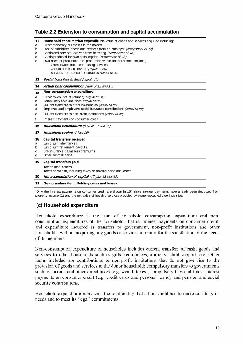
Canberra Group Handbook
19
Table 2.2 Extension to consumption and capital accumulation
12 Household consumption expenditure, value of goods and services acquired including: a Direct monetary purchases in the market b Free or subsidised goods and services from an employer (component of 1a) c Goods and services received from bartering (component of 1b) d Goods produced for own consumption (component of 1b) e Own account production, i.e. production within the household including: Gross owner-occupied housing services Unpaid domestic services (equal to 3b) Services from consumer durables (equal to 3c)
13 Social transfers in kind (equals 10)
14 Actual final consumption (sum of 12 and 13)
15 Non-consumption expenditure
a Direct taxes (net of refunds) (equal to 8a) b Compulsory fees and fines (equal to 8b) c Current transfers to other households (equal to 8c) d Employee and employers’ social insurance contributions (equal to 8d)
e Current transfers to non-profit institutions (equal to 8e)
f Interest payments on consumer credit1
16 Household expenditure (sum of 12 and 15)
17 Household saving (7 less 16)
18 Capital transfers received a Lump sum inheritances b Lump sum retirement payouts c Life insurance claims less premiums d Other windfall gains
19 Capital transfers paid
Tax on inheritances Taxes on wealth, including taxes on holding gains and losses
20 Net accumulation of capital (17 plus 18 less 19)
21 Memorandum item: Holding gains and losses
1Only the interest payments on consumer credit are shown in 15f, since interest payments have already been deducted from property income (2) and the net value of housing services provided by owner-occupied dwellings (3a).
(c) Household expenditure
Household expenditure is the sum of household consumption expenditure and non-consumption expenditures of the household, that is, interest payments on consumer credit, and expenditure incurred as transfers to government, non-profit institutions and other households, without acquiring any goods or services in return for the satisfaction of the needs of its members.
Non-consumption expenditure of households includes current transfers of cash, goods and services to other households such as gifts, remittances, alimony, child support, etc. Other items included are contributions to non-profit institutions that do not give rise to the provision of goods and services to the donor household; compulsory transfers to governments such as income and other direct taxes (e.g. wealth taxes), compulsory fees and fines; interest payments on consumer credit (e.g. credit cards and personal loans); and pension and social security contributions.
Household expenditure represents the total outlay that a household has to make to satisfy its needs and to meet its ‘legal’ commitments.
Chapter 2 Standard concepts and definitions
20
(d) Household saving
Saving is equal to total income, less household expenditure. In any given period, saving will be positive where income is greater than expenditure. Saving will be negative where expenditure is greater than income (i.e. dissaving). Saving is used to accumulate capital and may be supplemented by the receipt of capital transfers (less capital transfers paid).
(e) Capital transfers
Capital transfers refer to the acquisition or disposal of assets when the receiving party makes no payment to the provider of the asset. Capital transfers tend to be large, infrequent and irregular (e.g. inheritances). Capital transfers result in an addition to the stock of net worth of the recipient unit and a reduction in the stock of net worth of the donor unit.
Unlike retirement pensions, which are treated as part of income, lump sum retirement payments are recorded as a capital transfer received. A lump sum retirement payment, particularly when it is opted for at the discretion of the recipient, is not likely to be treated as just another source of income, but be earmarked for some specific purpose. Often this will relate to the acquisition of financial or other assets which may provide a future income flow, but even when it is used for current consumption, such as a significant holiday, it is likely to be regarded as dissaving rather than spending out of income.
(f) Net accumulation of capital
Net accumulation of capital is equal to savings plus capital transfers received, less capital transfers paid. In a given reference period, a household’s level of saving (or dissaving) and the net value of capital transfers will add to the household’s net worth at the end of the period.
(g) Holding gains and losses
Holding gains and losses are shown as a memorandum item in the table. Holding gains and losses may occur without any direct transaction of the owner, for example, changes in the value of stocks and shares. However a change in their net value will affect the value of net worth and will be taken into account in the compilation of balance sheets.
21
Chapter 3 Income measurement 3.1 Introduction
This chapter examines the key measurement issues from the perspective of producing reliable and relevant household income distribution statistics.
It presents the sources of household income statistics, the standard units of income measurement and the reference periods for collecting data for components of income. While not all income items are covered, practical guidance is provided on the collection or estimation of those income receipts which have known measurement or quality concerns. Issues of measurement at both the bottom and the top of the income distribution are also discussed.
3.2 Sources of household income statistics
Most income distribution statistics rely on data collected in household surveys, although there are administrative sources in some countries which can be used. Examples of administrative sources used are personal income registers, tax and/or social benefit records.
For some components of income it may be necessary to impute estimates due to the unavailability of suitable data. Examples include the imputation of tax estimates to calculate disposable income, or gross income from income reported on a net basis. Any imputation of data should be documented and made available to users of the data.
3.2.1 Income surveys
Income data are usually collected through sample surveys, either from specially designed household income surveys or from multi-topic surveys where income data are collected along with data on, for example, household consumption or labour force participation.
Household surveys generally collect information from usual residents of private dwellings (as distinct from non-private dwellings such as hostels, hotels and institutions). It is important that the design of the sample and the selection of sample households are made in accordance with appropriate sampling techniques in order to obtain results that are as precise as possible within the resources that are available. As far as possible, the sampling method used should permit the calculation of sampling errors.
The mode of data collection in household surveys may vary. The most common way of collecting income data is by personal interview, either a face-to-face interview or a telephone interview. Face-to-face interviews may produce data of higher quality due to generally higher response rates and the ability of respondents to easily refer to relevant statements or documents concerning the income questions, e.g. their pay slip or tax return.
Computer-assisted interviewing is frequently used to collect data, i.e. the responses are simultaneously entered into a computer that guides the interviewer through the questionnaire. Internal system edits can also be applied to the questionnaire to ensure the completeness and consistency of responses being provided. These edits can prevent the interviewer proceeding
Chapter 3 Income measurement
22
from one section of the interview to the next until responses have been appropriately completed. A number of range and consistency edits can also be programmed into a computer assisted instrument with automatic messages appearing on the screen if the information entered is outside the expected or permitted range for a particular question, or contradicts information already recorded. These edit queries can then be resolved on the spot with the respondent.
Income data should be collected directly from each relevant household member and separately for each income component. Although proxy interviewing sometimes may be necessary to obtain income data for absent household members, the quality of such data are considered inferior to data collected from the individual household members themselves.
Household surveys are constrained by the information that respondents are able to provide with reasonable accuracy during the course of an interview. This means that:
people must have knowledge of the income they are being asked to report, e.g. they may have little idea of the social contribution made on their behalf by their employer.
they must be able to recall the information with a reasonable degree of accuracy, which may influence the accounting period used as well as the questions asked.
the questions must appear relevant to the respondent - it may be difficult to get information which seems to have little connection with the circumstances of the respondent, such as the value of goods produced for home consumption where these are considered insignificant.
3.2.2 Income data from registers
For countries where suitable administrative data exists, and there is a legal basis to use it for statistical purposes, income data from registers may be used as a substitute for survey data. Nearly a third of all countries participating in the European Union’s Statistics on Income and Living Conditions (EU-SILC) collect at least some of their income data from registers. Outside Europe, Canada is one of the few countries that also collect some income data from registers.
Register-based statistics may provide total or near total population coverage and can therefore be used to produce more detailed statistics for small areas or population groups. They can also produce statistics for longitudinal analyses. Register data result in lower respondent burden and are generally a less costly means of producing statistics, with fewer resources needed to collect, impute or edit the collected data.
Compared to income data collected in surveys, register data are not subject to sampling and non-response errors. They may however, suffer from under coverage or missing data, e.g. due to tax evasion or low compliance. They may also be limited by the definitions and administrative practices of the authorities responsible for the register, which may also change over time.
A few countries have virtually all the register information required to produce household income distribution statistics for the entire population, e.g. Denmark, Finland, Iceland, Norway, Slovenia and Sweden. However the most common way of using income data from registers is by combining them with survey data. Some income components are obtained from the registers, while other income components are collected through interview. For example,
Canberra Group Handbook
23
countries that do not have a household-based register require survey data on household composition in order to produce household income statistics, e.g. the Swedish Income Distribution Survey.
The use of register data alongside survey data may improve the quality of income estimates that are often underreported in household surveys and also reduce interview times and respondent burden. However, compilers of income data should also be aware of some of the shortcomings of such data. In some countries register data on income may be incomplete and only be available for people who are tax filers, which may exclude a significant proportion of the population. In addition, tax data will not include income earned from informal (‘black’) work or private income support from other households, which in some countries may be substantial amounts.
Box 3.1 Examples of using administrative data
Austria In Austria, administrative sources on income are primarily tax and social insurance data. A special law passed in 2006 allows data linkage for statistical purposes using a special anonymised individual identification key (BpK).
The tax unit is individuals which can be matched to a population register. This process is used to allocate individuals to dwellings to obtain household information. However, the quality of the population register depends on the buildings and dwellings register which is not consistent for all regions. In addition, survey data on actual living arrangements indicates differences from the population register. Dwellings with a single person registered may be occupied by a couple or a family. Further the status of the register used for the sample may be half a year old at the day of interview.
It is estimated that about one-fifth of households are wrongly identified, with the number of single person households overestimated. As well, important income sources, such as inter-household transfers or welfare benefits from local authorities, cannot be obtained from administrative data.
In order to make administrative income data available at the household level, a special national regulation for the EU-SILC sample was established in 2010. This regulation commits to providing BpKs for household members contacted in the field who had not been in the original sampling frame. The first EU-SILC data collection using survey and administrative sources will be completed in 2011.
Canada Since 1997, Statistics Canada has used a mixed mode approach for collecting income data in its household survey. The introduction of tax credits has increased significantly the percentage of individuals who fill in a tax form. The mixed mode collection methodology offers the respondents the choice to give Statistics Canada access to their administrative data instead of responding to a number of questions in the survey. If a person is a non-filer for tax purposes, or if the person refuses to give permission to access their administrative records, the survey is administered.
This mixed mode methodology has decreased interview times from an average of 20 minutes to about 8 minutes per household. The methodology has also increased the quality of certain
Chapter 3 Income measurement
24
responses to questions (through a decrease in rounding of responses and better reporting of income taxes paid). A few questions are still asked on the survey to cover income sources that are not reported through the tax system.
France The main source for measuring income distribution in France is the Tax Revenues Survey (ERF), which uses both survey and administrative records. It is compiled by matching households and individuals surveyed during the last quarter of the Quarterly Labor Force Survey with fiscal registers from the tax administration (completed with information from official social institutions). Approximately 97% of the population is in scope of the survey. The matching is undertaken using anonymous identifying numbers in both sources that are paired up using a key held only by the fiscal administration.
Italy For the Italian EU-SILC, both administrative and survey micro data are available on cash profits or losses from self-employment. The tax and survey records are linked by exact matching. Income from self-employment is set to the higher of the two values. On the survey questionnaire, the self-employment income question is preceded by a 'reminder question' that provides a YES/NO list of the possible personal uses of earnings (consumption and saving). The use of both administrative and survey data for self-employment was adopted to minimise the impact of tax avoidance on the administrative data, or underreporting in the survey data, depending on which was greater.
Latvia Latvia commenced using administrative records for the EU-SILC in 2006. Data from the State Social Insurance Agency (SSIA) on old-age benefits, initially collected from personal interviews, were provided to the Central Statistical Bureau (CSB) after completion of fieldwork. Data from both sources were checked and validated. After analysis it was decided to use SSIA data in the 2006 EU-SILC.
After the 2007 EU-SILC fieldwork, the CSB received data from the SSIA and also from the State Revenue Service (SRS). All three data sources were checked and validated. It was then decided to use data from the SSIA and, to some extent, from the SRS. Pensions and state social benefits collected in the 2007 EU-SILC were replaced by data from the SSIA.
Some minor benefits administered by local authorities, pensions paid by other countries and service pensions are missing from the administrative data. The difference between the collected data and the administrative data is taken into account through use of the EU-SILC imputation flag.
3.3 General measurement issues
3.3.1 Measurement units
It is important to differentiate between the data collection unit and the data analysis unit. For data collection, the choice of unit will depend on the design of the survey (or the nature of the system through which administrative data are available). The starting unit is the individual, but as individuals typically share income with the other persons with whom they live, most surveys collect information on the income streams of all members of a larger statistical unit,
Canberra Group Handbook
25
most commonly the household. That is, while it is advisable to collect data about individuals, the household is the basic data collection unit. This approach maximises flexibility for analysis purposes, allowing analysis to be undertaken for both individuals and households.
Another issue is the element of income for which data are sought. For example, wages and salaries are best collected at the individual level whereas data to enable the estimation of imputed rent will have to be collected at the household level.
A full appraisal of income sharing within a household would require collecting data on the income transfers made within the household which would obviously be very difficult to implement. For these reasons, the choice of the household as the basic data collection unit for collecting income data remains the best compromise. Despite the fact that the choice of the household as the data collection unit is the most common, attention has to be paid to the comparability of its definition in order to ensure robustness of international comparisons. The definition of household used also needs to be sufficiently flexible to account for types of living arrangements that have become more common in recent years, and which are not always captured adequately by existing definitions.
Box 3.2 provides the international definition proposed by the UNECE (2009a) as the one that should be routinely used in population censuses. Implicitly, this definition provides the benchmark for household income surveys.
Box 3.2 Definition of household
A private household is either (a) a person living alone in a separate housing unit or who occupies, as a lodger, a separate room (or rooms) of a housing unit but does not join with any of the other occupants of the housing unit to form part of a multi-person household or (b) a group of two or more persons who combine to occupy the whole or part of a housing unit and to provide themselves with food and possibly other essentials for living. The group may be composed of related persons only or of unrelated persons or of a combination of both. The group may also pool their income.
Most definitions of households embody a notion of ‘usual’ residence. The general rule is that a person’s place of usual residence is where they most frequently sleep overnight. UNECE (2009a) also sets out conventions for the treatment of a number of special cases. For example, a child may alternate equally between two households (for instance after his or her parents are divorced). In this case the suggested convention is that the place of usual residence should be the place where the child was enumerated. While there is no proposed best practice, compilers of income statistics should document the definition of usual residence used.
Despite being closely related, the definition of a household is not the same as that of a family, which adds to the household concept the linkage of each of its members with a kinship tie. Households may include persons who are not related by blood, marriage or adoption while, conversely, families may include persons who are permanently absent from the household.
Chapter 3 Income measurement
26
Relationship matrices
A separate issue, but one that is becoming increasingly important due to changes in living arrangements and patterns of household formation, is that of collecting information about the relationships between each member of the household.
Most surveys ask respondents about their relationship to a selected household respondent in order that key relationships between persons usually resident in a given household can be identified and classified. This information may be used in its own right, but is also used in deriving other variables such as ‘household composition’.
More complex information about relationships between members of the household can be captured through the use of a relationship matrix, setting out, for each member, how she/he is related to all others. The use of a relationship matrix could be very important, in particular, for three types of living arrangements that are of growing importance (UNECE, 2009a):
Reconstituted families: These consist of cohabiting or registered couples with one or more children, where at least one is a non-common child. This category cannot be identified through the type of household definition used in most household income surveys. Nonetheless, there is much interest in the economic well-being of reconstituted families.
Commuters between households: These are usually defined as people who regularly live in a place that is different from their place of ‘usual residence’ for a limited amount of time. In general, their identification improves the quality of population enumeration by avoiding double counting; their impact on the measurement of income distribution could also be significant, in particular for the analysis of economic hardship. This problem is quite common in surveys based on area samples when people commute between households located in different areas. The UNECE (2009a) recommend that persons working away from home during the week and who return to the family home at the weekends should consider their family home as their usual place of residence.
Living apart together: These comprise people involved in an intimate relationship that is more than temporary but who live in separate housing units. Their identification would provide a better assessment of their economic well-being as their relationship implies, most of the time, a partial pooling of their resources.
3.3.2 Reference periods
It is necessary to decide the length of the accounting period to which the statistics refer. The international standards state that household income statistics should relate to a full year to take into account seasonal variations in incomes. Annual income includes the income obtained from all sources over a period of a year.
A twelve-month reference period is the common period for which owners of small enterprises derive a measure of profit or loss for their business if they are operating within the formal sector. If income statistics are compiled from administrative records such as income tax data, the data for wage and salary earners are also likely to be only available with a twelve-month reference period.
While a one-year reference period is the recommended accounting period, there are some practical difficulties in using annual income:
Canberra Group Handbook
27
given that it is generally necessary to collect annual income for the previous financial year (after records have been finalised for taxation purposes), the data may be quite old by the time it is released.
respondents to surveys may have difficulty recalling the income received over a period as long as a year, in particular those with periods of employment and unemployment, casual work and part-time work.
income received in the previous financial year may not relate directly to the socio-economic and other characteristics of the household at the time the survey is run.
For longitudinal studies, including household panel surveys, cohort surveys and administrative data panels, long reference periods prior to data collection can lead to an increased likelihood of household composition changes. This can have significant implications for household equivalised reweighting factors and limit comparability of household composition as a variable influencing the amount of household income earned (Jenkins, 2011).
It should also be noted that different accounting periods may suit different types of analysis. For example, some countries collect current income in addition to annual income. Current income is the income received by respondents at the time data are collected. Current income provides the most up to date information available and also relates to the same period in which most other survey topics relate.
Current income may be collected using a number of different reporting periods. For income from investments or own unincorporated business, respondents are generally asked to estimate the amount they expect to receive in the current financial year. For income from other sources, respondents are generally able to select the period to which the income amount relates, e.g. week, fortnight, month, year or other period.
In some studies a person’s lifetime is used as the reference period. Students, for example, may be poor this year, but be building up skills to provide for an above average income across their working life. On the other hand, lifetime average income is not a very useful measure for governments and other organisations concerned with assisting those in poverty today.
3.3.3 Population weighting
When income data are collected using a sample survey, weighting is the process of adjusting results from the sample to infer information for the total in-scope population whether that be persons or households. To do this, a 'weight' is allocated to each sample unit i.e. a person or a household. The weight is a value which indicates how many population units are represented by the sample unit. The first step in calculating weights for each unit is to assign an initial weight, which is the inverse of the probability of being selected in the survey. For example, if the probability of a household being selected in the survey was 1 in 600, then the household would have an initial weight of 600 (that is, it represents 600 households).
If the survey has an extended enumeration period, say one year, it may be beneficial to make an adjustment to the initial weights to account for changes in the sample across the four quarters of survey enumeration, so that the sum of the initial weights after this adjustment of households is equal in each quarter.
Chapter 3 Income measurement
28
Household income weights can be multiplied by the number of people in each unit to derive 'person weights'. By the application of these 'person weights' to equivalised household income, estimates of the distribution of income amongst all persons can be made. Thus a six person unit 'counts' six times as much as a one person unit. Person weighting produces an estimate of the overall distribution of equivalised income among individuals in the population, assuming that all household incomes are pooled.
This distribution reflects the assumption that household income is shared equally between all members of the household, and does not reflect the direct receipt of income by individuals. Because many household members receive no money income, e.g. younger children, such an assumption is hard to avoid in practice. One implication from the use of person weights is that the sum of equivalised income across all persons will differ from the total unadjusted income measured in the survey.
In some countries, complete income data are available for each individual within a household, except for children. In these cases, individual person weights are determined by the sample design used to produce income distribution estimates of the income earning population. Such design-based weights are distinct from the 'person weights' used in income distribution analysis described above. In this method different household members have different income values, and incomes are assumed not to be pooled. However, in order to estimate the distribution of incomes amongst all persons within a household unit, including children, the person weighting method first described above is recommended.
3.3.4 Benchmarking
As part of the process of assigning final weights to each household, initial weights may be calibrated to align with independent estimates of the population of interest, referred to as 'benchmarks'. Weights calibrated against population benchmarks ensure that the survey estimates conform to the independently estimated distribution of the population rather than to the distribution within the sample itself. When calculating the benchmarks, account should be taken of any scope exclusions. A population census is an example of a source of information that might be used for benchmarking household survey data.
Examples of suitable benchmarks that could be used are number of persons by:
total population
region by age by sex (with five year age groups up to an appropriate cut-off, say, 75+ or 80+ years)
region by labour force status (where labour force status could be ‘employed’, ‘unemployed’ or ‘not in the labour force)’.
The number of households can also be calibrated by household composition, for example, based on the number of adults (1, 2, 3 or more) and whether or not the household contains children.
Similarly, it may also be desirable to benchmark survey income estimates against reliable sources of administrative data that provide aggregate income data. An example could be the total value of government pensions paid during the reference period, which may be available from the government department administering these payments.
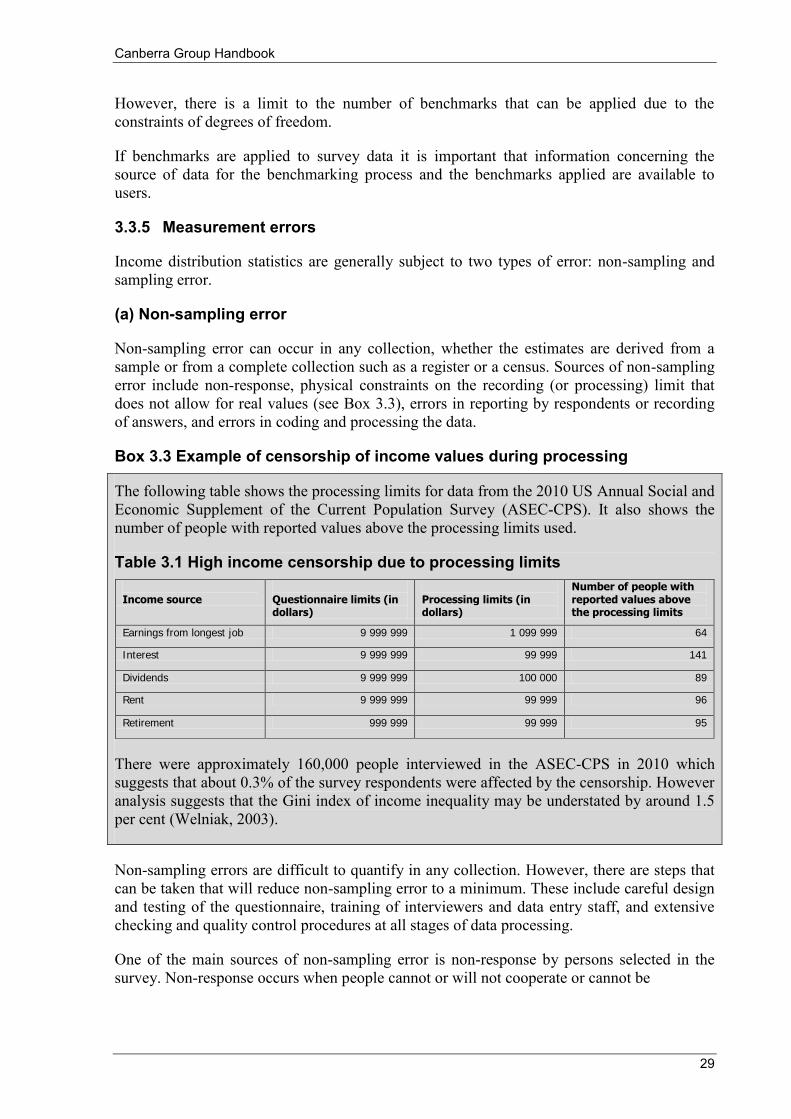
Canberra Group Handbook
29
However, there is a limit to the number of benchmarks that can be applied due to the constraints of degrees of freedom.
If benchmarks are applied to survey data it is important that information concerning the source of data for the benchmarking process and the benchmarks applied are available to users.
3.3.5 Measurement errors
Income distribution statistics are generally subject to two types of error: non-sampling and sampling error.
(a) Non-sampling error
Non-sampling error can occur in any collection, whether the estimates are derived from a sample or from a complete collection such as a register or a census. Sources of non-sampling error include non-response, physical constraints on the recording (or processing) limit that does not allow for real values (see Box 3.3), errors in reporting by respondents or recording of answers, and errors in coding and processing the data.
Box 3.3 Example of censorship of income values during processing
The following table shows the processing limits for data from the 2010 US Annual Social and Economic Supplement of the Current Population Survey (ASEC-CPS). It also shows the number of people with reported values above the processing limits used.
Table 3.1 High income censorship due to processing limits Income source
Questionnaire limits (in dollars)
Processing limits (in dollars)
Number of people with reported values above the processing limits
Earnings from longest job 9 999 999 1 099 999 64
Interest 9 999 999 99 999 141
Dividends 9 999 999 100 000 89
Rent 9 999 999 99 999 96
Retirement 999 999 99 999 95
There were approximately 160,000 people interviewed in the ASEC-CPS in 2010 which suggests that about 0.3% of the survey respondents were affected by the censorship. However analysis suggests that the Gini index of income inequality may be understated by around 1.5 per cent (Welniak, 2003).
Non-sampling errors are difficult to quantify in any collection. However, there are steps that can be taken that will reduce non-sampling error to a minimum. These include careful design and testing of the questionnaire, training of interviewers and data entry staff, and extensive checking and quality control procedures at all stages of data processing.
One of the main sources of non-sampling error is non-response by persons selected in the survey. Non-response occurs when people cannot or will not cooperate or cannot be
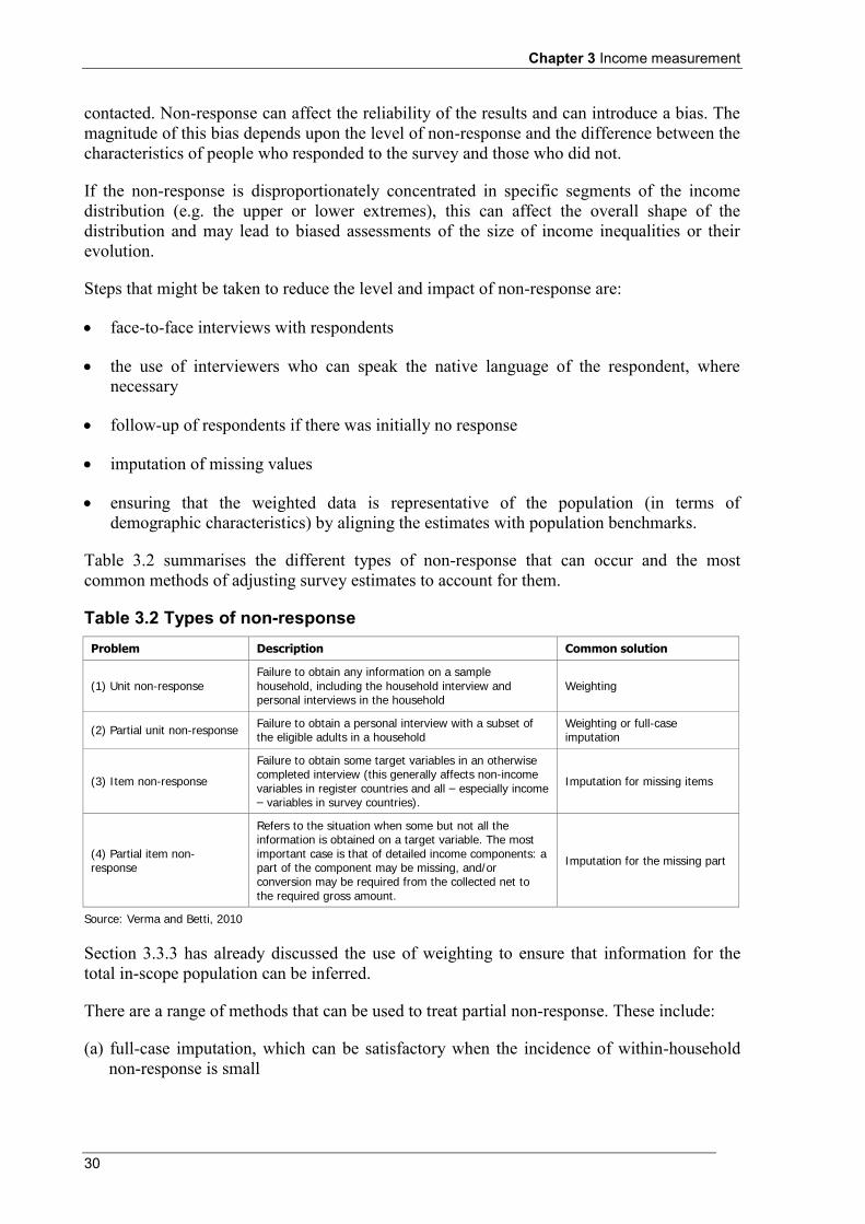
Chapter 3 Income measurement
30
contacted. Non-response can affect the reliability of the results and can introduce a bias. The magnitude of this bias depends upon the level of non-response and the difference between the characteristics of people who responded to the survey and those who did not.
If the non-response is disproportionately concentrated in specific segments of the income distribution (e.g. the upper or lower extremes), this can affect the overall shape of the distribution and may lead to biased assessments of the size of income inequalities or their evolution.
Steps that might be taken to reduce the level and impact of non-response are:
face-to-face interviews with respondents
the use of interviewers who can speak the native language of the respondent, where necessary
follow-up of respondents if there was initially no response
imputation of missing values
ensuring that the weighted data is representative of the population (in terms of demographic characteristics) by aligning the estimates with population benchmarks.
Table 3.2 summarises the different types of non-response that can occur and the most common methods of adjusting survey estimates to account for them.
Table 3.2 Types of non-response Problem Description Common solution
(1) Unit non-response Failure to obtain any information on a sample household, including the household interview and personal interviews in the household
Weighting
(2) Partial unit non-response Failure to obtain a personal interview with a subset of the eligible adults in a household
Weighting or full-case imputation
(3) Item non-response
Failure to obtain some target variables in an otherwise completed interview (this generally affects non-income variables in register countries and all – especially income – variables in survey countries).
Imputation for missing items
(4) Partial item non-response
Refers to the situation when some but not all the information is obtained on a target variable. The most important case is that of detailed income components: a part of the component may be missing, and/or conversion may be required from the collected net to the required gross amount.
Imputation for the missing part
Source: Verma and Betti, 2010
Section 3.3.3 has already discussed the use of weighting to ensure that information for the total in-scope population can be inferred.
There are a range of methods that can be used to treat partial non-response. These include:
(a) full-case imputation, which can be satisfactory when the incidence of within-household non-response is small
Canberra Group Handbook
31
(b) adjusting total income of the affected household by a factor determined on the basis of characteristics of the household and of the non-interviewed persons
(c) taking no action, which effectively treats the non-responding household members as having zero income
(d) removing households with one or more missing person.
(Verma and Betti, 2010)
Frick et al., (2010a) recommend imputation in preference to the other approaches as the best method to reduce bias and increase comparability of datasets over time. Imputation is also the most common solution to partial item non-response.
Box 3.4 Examples of imputation methods for partial non-response
European Union Imputation methods for partial non-response in the EU-SILC vary between countries. For example, in the 2009 EU-SILC, Belgium, the Czech Republic, Estonia, France, Cyprus, Italy, Lithuania, Austria, Poland, Spain and the United Kingdom applied full-case imputation; Bulgaria, Germany, Greece, Latvia, Portugal, Romania and Slovakia applied an adjustment factor to the total income based on characteristics of the household and of the non-interviewed persons; and Ireland, Malta, Luxembourg, the Netherlands and Hungary deleted all households with one or more missing persons.
Australia The Australian Bureau of Statistics imputes information for partial non-response when:
income or other data in a questionnaire are missing from one or more non-significant person's records
all key questions are answered by the significant person(s) but other data are missing.
Significant persons are defined as:
all members of lone person or couple only households all parents in a couple with children household or a single parent household the person aged 15 years or over in a group household where one person is aged 15
years or over and the other members of the household are less than 15 years old 50% of the persons aged 15 years and over in all other households.
Donor records are selected by finding fully responding persons with matching information on various characteristics (such as region, sex, age, labour force status and income) to the person with missing information. As far as possible, the imputed information is an appropriate proxy for the information that is missing. Depending on which values are to be imputed, donors are randomly chosen from the pool of individual records with complete information for the block of questions where the missing information occurs. (ABS, 2009b).
(b) Sampling error
Household survey estimates are based on a sample of possible observations and are subject to sampling variability. The sampling error is a measure of the variability that occurs by chance
Chapter 3 Income measurement
32
because a sample, rather than the entire population, is surveyed. One measure of the likely difference is given by the standard error (SE). Another measure of the likely difference is the relative standard error (RSE), which is obtained by expressing the SE as a percentage of the estimate. The RSE is a useful measure in that it provides an immediate indication of the percentage errors likely to have occurred due to sampling, and thus avoids the need to refer also to the size of the estimate.
Estimates of SEs or RSEs should be provided with all published output. One way of highlighting information on SEs is to only include estimates in tables with RSEs less than say 25% as being sufficiently reliable for most purposes. Estimates with larger RSEs, say between 25% and less than 50% could be included in output but be preceded by an asterisk (e.g. *3.4) to indicate they are subject to high SEs and should be used with caution. Estimates with RSEs of 50% or more could be preceded with a double asterisk (e.g. **0.6), indicating that these estimates are considered unreliable for most purposes.
(c) Significance testing
For comparing estimates between surveys or between populations within a survey it is useful to determine whether apparent differences are 'real' differences between the corresponding population characteristics or simply the product of differences between the survey samples. One way to examine this is to determine whether the difference between the estimates is statistically significant. This is done by calculating the standard error of the difference between two estimates (x and y) and using that to calculate the test statistic using the formula below:
yxSEyx
If the value of the statistic is greater than 1.96 then there is good evidence of a statistically significant difference at 95% confidence levels between the two populations with respect to that characteristic. Otherwise, it cannot be stated with confidence that there is a real difference between the populations.
3.4 Practical guidance for the measurement of selected income receipts
This section discusses the measurement of selected income receipts. Practical guidance is provided for those income receipts which are typically infrequently available in household income statistics or have known measurement or quality concerns. Income receipts discussed in this section are:
employee income in kind
income from self-employment (including net estimated value of goods and services produced for barter, as well as goods produced for own consumption)
property income
Canberra Group Handbook
33
income from household production of services for own consumption (including net value of housing services, unpaid domestic services and services from household consumer durables)
inter-household transfers
social transfers in kind.
3.4.1 Employee income in kind
Most employee remuneration is in a monetary form. However, increasingly, employees may receive other benefits in the form of goods and services. The provision of goods and services as part of remuneration may reflect taxation advantages for the employer or employee by avoiding payments in cash, or arrangements where the employer provides free or subsidised accommodation, travel, food, motor vehicles and other goods and services for the private use of employees.
Historically, non-cash benefits provided by employers have frequently been excluded in household income distribution measures largely due to practical considerations. These included concerns about the non-availability of this information for many countries and the different methods for valuing such receipts.
However, omission of employee income in kind in the definition and measurement of income may provide a misleading picture of the relative income position of the employees receiving these benefits, as well as comparisons across time and across countries. The growing recognition of the importance of employee income in kind is reflected in the results from the 2010 Survey of Country Practices which showed that data are now available for the majority of countries surveyed (see Chapter 4 and Appendix 4).
The minimum requirements for valuing employee income in kind are the quantities and qualities of goods and services provided, and appropriate market prices or self-valuation by the respondent.
The 2008 SNA and 2004 ICLS standards recommend valuing employee income at relevant market prices for equivalent goods and services or as the difference between the market value and the amount paid by the employee when provided at reduced prices.
In theory, the cost of elements such as transportation and marketing costs, taxes and subsidies, should be excluded from the market price. That is, instead of market prices, producer prices (market prices less transportation and value added tax) or basic prices should be used. The basic price is defined in the SNA as:
… the amount receivable by the producer from the purchaser for a unit of a good or service produced as output minus any tax payable, and plus any subsidy receivable, by the producer as a consequence of its production or sale. It excludes any transport charges invoiced separately by the producer (SNA 2008, 6.51).
For example, for agricultural produce it would be the ‘farm-gate’ price which excludes any transportation costs.
However, given the relative difficulty in obtaining detailed costings for these additional elements, valuation at the market price is recommended.
Chapter 3 Income measurement
34
Where the employee income in kind consists of the outputs of the employers’ production processes and are ‘imposed payments in kind’ with little or no market value, a zero value is applied in computing employee income.
3.4.2 Income from self-employment
Income from self-employment is income received by individuals over a given reference period, as a result of their involvement in self-employment jobs (ILO, 2004). It primarily concerns the profit or loss that accrues to owners of, or partners in, unincorporated enterprises, who work in these enterprises. A loss is treated as negative income. It excludes profits or losses from capital investment of partners who do not work in these enterprises, i.e. ‘silent’ partners (treated as property income) and directors’ fees paid to owners of incorporated enterprises (employee income).
Income from self-employment also includes the estimated value of goods and services produced for barter as well as goods produced for own consumption, less expenses. These sources can be particularly significant where subsistence agriculture and non-cash economies are dominant.
(a) Profit or loss from own unincorporated enterprise
Collecting data on self-employment income can be more difficult than collecting data on employee income. Self-employment income is more likely to be irregular because it may in large part be determined by fluctuating demands for the owner’s product or service. There may also be some confusion over what respondents are being asked to provide, as the self-employed may be dealing with a wide variety of figures and calculations, and what they think of as income may not be considered income under the classification system being used.
Particular difficulties in the measurement of self-employment income from own unincorporated enterprises in household surveys are discussed for the United Kingdom by Martin et al. (1996). The authors note that the self-employed are more likely to refuse to answer income questions and are more likely to refuse the whole interview than paid employees. Further, even those prepared to participate in a survey find it more difficult to provide the requested information. They recommended aids to help the self-employed identify themselves in this group and the presentation of clear definitions of the data that are being requested. Asking about data items typically required for tax purposes are more often well understood by these respondents.
While administrative records might also provide an alternative data source, in many countries a significant number of self-employed persons are not required to file tax returns due to their low incomes.
Juster et al. (2007) recommend that response rates to self-employment questions might be improved by using brackets or ranges when receiving a ‘don’t know’ or ‘refuse’ response, e.g. more than ‘a’ but less than ‘b’. By asking respondents to place themselves in a bracket, specific numerical values can be imputed more efficiently, thus improving the accuracy of the imputations.
An alternative approach to measuring self-employment income, which is sometimes discussed, is to collect information on ‘drawings’ from a business. This represents money that owners of unincorporated businesses have paid to themselves on a regular or irregular basis.
Canberra Group Handbook
35
However this approach is not generally recommended as it has both conceptual and practical difficulties. Irregular drawings are very difficult to measure and may be either less than income (the remainder being reinvested in the business) or more than income (representing a drawing down of assets of the business).
(b) Net estimated value of goods and services produced for barter, as well as goods produced for own consumption
Measurement approaches to the estimation of the net value of goods and services produced for barter, as well as goods produced for own consumption, are less well developed relative to other income items. Efforts have been made to standardize data collection of self-employment income activities for less developed economies. Areas of current work include the Rural Income Generating Activities (RIGA) project, which has constructed a database of 34 Household Living Standards Surveys with the goal of improving international comparability of income measures (Covarrubias et al., 2009, also see Glewwe, 2005; Grosh and Glewwe, 2000).
Examples of surveys that collect these data are the EU-SILC and the European Union's Household Budget Survey (HBS). Own consumption in the EU-SILC refers to food and beverages produced and consumed in the same household, whereas the HBS includes a question on withdrawals from own garden, farm or enterprise for the private consumption of the household.
In the EU-SILC the value of goods produced for own consumption should be collected when it constitutes a significant component of income. Countries where this component is not significant are allowed to not report the information. Where countries collect the information, the questions used are not always the same. Some countries use a detailed questionnaire, whereas others collect general information using just one or two questions. For more information on data availability by country, see Paats and Tiit (2010).
The main problem when measuring this type of self-employment income is the difficulty of assigning a monetary value to goods and services produced for barter or goods produced for home use, since these are not exchanged in the open market. There are two main ways of estimating the net value of these items which are described below.
The first option is to ask respondents to estimate the value of these items. While this method is relatively simple, respondents may not know the monetary value for the goods and services in question. This is especially likely to be a problem in less-developed countries where barter and subsistence production are common.
The second option is to ask respondents for the quantity of goods and services bartered and goods consumed in order that a value could be estimated based on what is known about the economy as a whole. There are two possible approaches to estimating this value:
the output based approach, which is to identify the same or similar goods on the market and use their prices.
the input based approach, which values the goods based on the costs of producing them, i.e. the value of goods and services used as inputs in the production process (compensation of employees, consumption of fixed capital and other taxes less subsidies).
Chapter 3 Income measurement
36
There are caveats to both methods. For the output based approach, the quality of the goods or services produced may not be the same as those available on the market. For the input based approach, there may be difficulty estimating the value of inputs. However, the main difference is that the latter does not include profits.
It is recommended, in line with the SNA, that the output-based approach be used. The items should be valued at the basic price at which they could be sold on the market (defined in section 3.4.1).
3.4.3 Property income
Property income is defined as receipts that arise from the ownership of assets that are provided to others for their use. It includes interest, dividends, rent and royalties. Income from these sources should be obtained at the component level using terminology that is readily understood.
Non-response rates for property income are high in some countries. This may be for a number of reasons. Some sources of property income, such as royalties and rents, can accrue irregularly, making it relatively more difficult for respondents to provide accurate information (Vaughan, 1993). Investment accounts can also provide a challenge for respondents, as these accounts accrue income at differing rates, even with short time periods, and are often managed by someone other than the respondent who, as a result, may not have exact knowledge of how much income these sources have generated at any given time. Additionally, for many people, property income is not a substantial source of income in the same way that wages or self-employment income are.
These measurement issues result from problems that can be addressed, at least to some degree, in the data collection process. Some of these issues could be solved or mitigated by encouraging the respondent to refer to administrative records, such as tax returns. While there is the potential problem of differences in reporting periods because relevant administrative records are not yet available for the required reference period, reference to the most recent documents available will generally provide a useful guide for the respondent to estimate their expected income.
Permission may also be sought from the respondent to access register data to supplement the information collected in the survey, e.g. from the tax department (if legal instruments exist to support this approach). In Australia, if a respondent states they “don’t know” their income from employment or their income from their investments, they are asked whether the interviewer could contact them at a later date when the information becomes available or alternatively whether the interviewer could contact their tax agent or accountant to obtain the information required.
3.4.4 Income from household production of services for own consumption
The SNA provides a general definition of production, but applies a more restricted definition. The general production boundary is defined as…“activity carried out under the control and responsibility of an institutional unit that uses inputs of labour, capital and goods and services to produce outputs of goods and services” (SNA 2008, 6.24). The more restricted SNA production boundary excludes all household production of services for own final use, except services from owner-occupied dwellings and services produced by employing paid domestic staff (SNA 2008, 6.26).
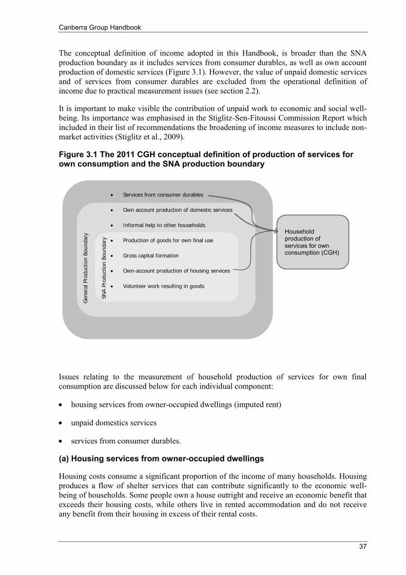
Canberra Group Handbook
37
The conceptual definition of income adopted in this Handbook, is broader than the SNA production boundary as it includes services from consumer durables, as well as own account production of domestic services (Figure 3.1). However, the value of unpaid domestic services and of services from consumer durables are excluded from the operational definition of income due to practical measurement issues (see section 2.2).
It is important to make visible the contribution of unpaid work to economic and social well-being. Its importance was emphasised in the Stiglitz-Sen-Fitoussi Commission Report which included in their list of recommendations the broadening of income measures to include non-market activities (Stiglitz et al., 2009).
Figure 3.1 The 2011 CGH conceptual definition of production of services for own consumption and the SNA production boundary
Issues relating to the measurement of household production of services for own final consumption are discussed below for each individual component:
housing services from owner-occupied dwellings (imputed rent)
unpaid domestics services
services from consumer durables.
(a) Housing services from owner-occupied dwellings
Housing costs consume a significant proportion of the income of many households. Housing produces a flow of shelter services that can contribute significantly to the economic well-being of households. Some people own a house outright and receive an economic benefit that exceeds their housing costs, while others live in rented accommodation and do not receive any benefit from their housing in excess of their rental costs.
SN
A P
roduct
ion B
oundary
Genera
l Pro
duct
ion B
oundary
Household production of services for own consumption (CGH)
Services from consumer durables
Own account production of domestic services
Informal help to other households
Production of goods for own final use
Gross capital formation
Own-account production of housing services
Volunteer work resulting in goods

Chapter 3 Income measurement
38
In order to value housing services consistently, the 2008 SNA treats every house owner as an unincorporated enterprise which leases the house back to the household. The value of the lease is set at the market rent for a similar house and the imputed income is equal to this value less the costs incurred by the household in their role as landlord.
When income distribution statistics are used to understand economic well-being, this treatment of owner-occupied housing allows differences in housing policies and structures of housing tenure to be accounted for. This is important for international comparisons as the rate of home ownership varies widely across countries. Estimates of net imputed rent for owner-occupied dwellings can be very important in countries where home ownership rates are high.
For owner-occupiers, housing services is the imputed value of the services received less the value of the housing costs incurred, i.e. the imputed market rent less the current expenses of the household in their role as a landlord, such as interest payments, intermediate inputs (property rates, repair and maintenance expenses, insurance costs, etc.), depreciation and taxes. Proper estimation of imputed rent therefore requires information about the dwelling (e.g. quality, size and location) to accurately estimate the market rent as well as the owner’s actual costs.
There are two main valuation methods that can be used, namely the rental equivalence (market rent) and the user cost (return to capital) approach. Where there is an established rental market, the rental equivalence approach is the recommended valuation approach since it is easier to use compared to the user cost approach (ILO, 2004). This is consistent with the 2008 SNA and with the EC Regulation on the principles for estimating dwelling services (European Commission, 2005).
The rental equivalence approach assumes that the imputed income is equal to the market rental value less housing costs. While self-reported valuations are sometimes used, regression is the most commonly used method. Survey data on reported rents paid by private market renters are regressed on the characteristics of their dwellings, e.g. location and dwelling structure. The estimated coefficients are then applied to the corresponding characteristics of owner-occupied dwellings to produce imputed values of the rental equivalence for these dwellings.
To estimate net rental income from owner-occupied dwellings, data should be collected on at least some of the following items:
(a) housing characteristics (age, size, type of construction and facilities, repair and maintenance costs, status of neighbourhood)
(b) rents for rented dwellings (from the survey or from other sources) and market value of dwellings
(c) housing costs normally paid by landlords for all dwellings
(d) duration of use for vacation and weekend homes
(e) the owner’s assessment of the rental value for owner-occupied dwellings, where relevant.
One shortcoming of the rental equivalence approach is the need for an established rental market in order to estimate a rental equivalent value. It is difficult to determine a rental equivalent value if rental markets are limited or do not exist, as may be the case in remote
Canberra Group Handbook
39
rural areas or in developing countries. Another issue is that differences in data sources and methods can result in different estimates of net rental income even for the same country (Mullan et al., 2007 and Garner and Short, 2009).
The user cost (return to capital) approach may be used in countries where rental markets are limited. The approach is based on the notion of an alternative use of capital (Smeeding et al., 1993). That is, owning a home represents a choice by the homeowner to forego the opportunity to invest in other financial assets. The value of the imputed return to home equity represents the income that might have been earned if the homeowner had not purchased the home. An interest rate is chosen to represent a safe private market rate of return. To compile these estimates data should be collected on the value of home and balance owed on mortgage.
A comparison of the rental equivalence and user cost approaches has been conducted for the US (Short et al., 2007). That study found that the capital market approach tended to overestimate net rental income for the non-elderly relative to other methods. The study also showed that the hedonic approach to estimating rental equivalence did not perform well for the U.S., where rental housing is generally of lower quality than owner-occupied homes.
The most coordinated work at the micro level on imputed rents has been conducted in Europe under the auspices of AIM-AP (Accurate Income Measurement for the Assessment of Public Policies), based on data from the Household Budget Survey (HBS) and EU-SILC. The primary focus of the studies has been to examine the distributional impact of imputed rent for dwelling services for which households do not pay full rent. Methodological issues have also been considered as part of this work (Frick et al., 2010b).
Some recent work undertaken by Sauli and Tormalehto (2010) examines the 2007 EU-SILC dataset which, for the first time, and for nearly all EU countries, contains estimates of imputed rents. The authors conclude that while the inclusion of imputed rent in income statistics has significant merit, the degree of comparability in the 2007 dataset was not yet satisfactory, with the results sensitive to underlying data and estimation methods.
It is therefore recommended, consistent with the ICLS resolution concerning household income and expenditure statistics, that where estimates of imputed rent are compiled, these should be made separately available to support different types of analyses (ILO, 2004). Similarly, the detailed housing costs should also be made available to facilitate different analytical and descriptive needs, e.g. international comparisons.
(b) Unpaid domestic services
Unpaid domestic services include own-produced services such as laundry, cooking meals, caring for adults and children, housekeeping and management, as well as unpaid volunteer work. Determining what should be included in unpaid domestic services is based on a ‘third party criterion’, i.e. the service is considered productive only if it can be delegated to someone else (SNA 2008, 6.25).
Whereas paid domestic services are included in the 2008 SNA, unpaid domestic services are excluded from the SNA production boundary for the following main reasons:
their production has limited impact on the rest of the economy, e.g. they are produced for immediate consumption and cannot be sold or bartered.
Chapter 3 Income measurement
40
it is not possible to identify market prices to value such services.
changes in such household services are not affected by, nor do they affect economic policy, as the imputed values are not equivalent to monetary flows, e.g. there is no impact on tax yields to the economy or the level of the exchange rate. (SNA 2008, 6.31).
However, there are many types of household services, such as caring for children or the elderly, which challenge these reasons. Mothers not working or working part-time in order to take care of their children have a direct impact on participation in the labour force and therefore the economy. Child care is sold on the market, so it is possible to derive a market price.
As unpaid domestic services may have an important impact on the economic well-being of households, these services are included in the conceptual definition of income, regardless of the practical difficulties in their measurement.
Similar to the methods proposed for valuing household production of goods for own final use (see section 3.4.2), two basic approaches have been suggested for valuing household production of services for own use. These are:
an output based approach, which values the outputs produced, or
an input based approach, which either values the labour inputs only, or that also accounts for the services from consumer durables entering their production.
In the first measure, the outputs of the service provided – the meal, the clean house, etc. – are valued at equivalent market prices and the value of intermediate inputs (food, cleaning materials, electricity, etc.), capital consumption and, in theory, any indirect taxes, are subtracted to obtain the mixed income from the service. This method requires the identification and quantification of the outputs and their valuation at the prices at which the household could sell or purchase an equivalent service in the market. The difficulties of applying the output based approach include:
most household services are produced simultaneously making it difficult to distinguish between separate household activities.
the identification of an equivalent service and price on the market may not be feasible for all household services, which is an obstacle to international comparison (Eurostat, 2003).
In the input based approach, the amount of labour time spent on household production of services for own final use is multiplied by an appropriate wage rate to impute an income from this production. The output is generally valued through labour input alone and the other inputs are not considered, e.g. contribution of household durables and expendable items such as fuels and cleaning or maintenance supplies.
For this approach, data will probably come from multiple data sources, such as time use surveys (to provide hours of unpaid work) and population and labour market or labour force surveys (to provide the cost of labour used in producing household goods and services).
There are three ways of calculating the appropriate wage rates. These are:
Canberra Group Handbook
41
the opportunity cost of the time of the person performing the service (based on their earnings in the labour market)
the market wage rate of a specialist, e.g. a domestic cleaner
the wage rate of a general purposes domestic employee.
Estimates based on these different approaches can vary substantially, e.g. Japan produced comparative statistics for the year 1996 using the three input based methods. Unpaid work was valued at 23% of GDP using the opportunity cost method, 20% for specialists, and 15% for generalists (Economic Planning Agency, 1998).
While there are some difficulties with each approach, the method that has been most widely used, and is therefore recommended if suitable data are available, is the input based approach using the wage rate of a general purpose domestic employee. However, the methodological limitations should be taken into account when using these estimates and it is suggested that these data be available separately until there is more widespread agreement on methods.
(c) Consumer durables
Services from consumer durables, e.g. cars, refrigerators, are difficult to measure. In the SNA, they are considered to be outside the general production boundary.
The ICLS includes services from consumer durables in the conceptual definition of income. For household production for own final use, the services of consumer durables are considered as the capital input to a household production function. The output of such production covers the benefit from using the durables at hand, e.g. number of meals cooked on a stove. However, the value of services from consumer durables are excluded from the operational definition of income due to practical measurement difficulties such as imputing a rate of return to capital, measuring depreciation and capital gains.
3.4.5 Current transfers
The measurement of inter-household transfers and social transfers in kind are discussed in this section. The measurement of indirect taxes when undertaking distributional analysis of the impact of government transfers and taxes on household income is also discussed.
(a) Inter-household transfers
Inter-household transfers can be significant to the economic well-being of households which receive them. For example, family members working abroad may make substantial transfers to family members in their home country, and parents of young adult students living away from home may provide significant financial support. Income sharing between households also occurs when families break up and one spouse (usually the one without custody of the children) makes supporting payments.
As outlined in Chapter 2, inter-household transfers are income or payments (in cash, goods or services) between households where there is no expectation of repayment, i.e. there is no ‘quid pro quo’. These transfers may be from within or outside a country. Since the monetary impact on the individual remains the same, there is no need to differentiate between these
Chapter 3 Income measurement
42
payments for the purpose of micro analysis of income. However at a macro level this distinction is important as resident to resident flows are netted out in the aggregation.
The most important issue when collecting information about inter-household transfers is to be able to differentiate current from capital transfers. The former, which are in scope of household income statistics, have the intent of supporting current consumption of recipients within the reference period. The latter are considered a transfer of wealth and should not be included in measures of current household income.
Users may wish to separately identify compulsory and quasi-compulsory transfers from other transfers. Quasi-compulsory transfers are difficult to identify as it would be necessary to determine whether the transfer was paid under a non-formal obligation or moral commitment which can only be determined subjectively. A further issue is that both the recipients’ use of the transfer and the donor’s intention/perception of the transfer are relevant, yet it will not be practically possible to interview both people involved in a single transaction.
For practical reasons, it is suggested that the collection of information be limited to payments between family members living in different households as this is the most likely situation where a moral obligation is felt, e.g. transfers from parents to student children, from children to aged parents, from former spouses for child maintenance and support.
When collecting data on current transfers, respondents cannot be expected to necessarily understand the concepts of current transfers, capital transfers, windfall gains, or to be able to provide information on the intention of the donor. Therefore, questionnaire design and instructions/training provided to interviewers are critical to obtaining the most accurate reporting of this data.
It is unlikely that accurate reporting will be achieved if just one question is asked. For this reason, it is better to break the types of transfers into different questions. Terms such as ‘alimony’ and ‘child support’ should be readily understood by respondents and are likely to be paid on a regular basis. Therefore specific questions are suggested for these items.
Collecting information on other inter-household transfers, particularly those paid either irregularly or infrequently, is more difficult. Transfer arrangements will differ between households (frequency, amount, type of payment) and some arrangements may span beyond the reference period. Others types of transfers may be intended to support consumption beyond the reference period, e.g. rental accommodation paid in advance.
A question that expresses the key dimensions of current consumption and the intention of financial assistance is recommended. For example: “Did any person not living with you, help with your annual living expenses by sending you money, goods or services in the reference period?”
To ensure that respondents think beyond pure monetary payments, a reference to ‘goods and services’ is advised, examples being purchase of food or transport tickets, payment of rent, etc. In particular financial support from family members not living in the same household should be targeted.
Efforts should also be made to ensure windfall gains, inheritances or loans are not erroneously reported by respondents. One method of limiting misreporting of these payments is to instruct interviewers to query and record the purpose of any amount over a certain limit
Canberra Group Handbook
43
in a write-in field in the questionnaire. If the payment reported is to purchase a car or house, it is clearly a capital transfer, whereas payments for general living costs or rent would support current consumption and are therefore considered part of household income.
The minimum data requirement for inter-household transfers is to measure money, goods and services received within the reference period, for both domestic inter-household transfers and cross-border remittances. In developing economies where in kind gifts and own production are of considerable importance, improving valuation methods for these transfers should be a high priority. Household surveys provide an important source of information for analysts interested in remittances.
Recording both receipts and payments by households are required, as payments by the household are a deduction when calculating disposable income.
Box 3.5 Examples of collection issues for inter-household transfers
Canada In the last ten years, Statistics Canada has employed four different questions to measure inter-household transfers in three surveys. Results varied, with between 11% and 40% of households reporting the receipt of inter-household transfers. For those that received inter-household transfers, these accounted for over half the total annual income of 12% of households. Questionnaire testing indicated that some respondents included in current transfers repayable loans from family members or friends and wealth transfers (as money gifts).
Australia The Australian Bureau of Statistics introduced a new question in its 2007-08 income survey, asking respondents whether they had received ‘financial support (in cash, goods or services), from family members not living in the household’. This replaced a previous question asking for ‘regular cash payments from persons not living in this household’. The change resulted in a six-fold increase in the number of households reporting these incomes and almost four-times the total income.
In summary, inter-household transfers remain as one of the most difficult issues in income measurement. The decision on how to implement these treatments in a practical sense may differ between countries and cultures. However, collection of this information is very important to properly understand the economic circumstances of some households.
(b) Social transfers in kind
Government social transfers in kind (STIK) are defined as goods and services provided by government that benefit individuals but which are provided free or at subsidised prices. STIK generally include education, health, social welfare, transport and cultural services.
It is important to account for the effect of STIK on the distribution of income when undertaking comparisons within and across countries. The absence of any estimates of STIK in a measure of income used to compare countries presents difficulties when the provision of such services differs greatly between them. In a country where STIK are relatively sparse, a higher income will be required to support a particular standard of living than in a country
Chapter 3 Income measurement
44
where a wide range of benefits are provided, all other things being equal. Within country comparisons are also affected when the benefits from STIK are spread unevenly across the income distribution, as they typically are. Thus the development of comparable estimates of STIK should have high priority if the accuracy as well as the international comparability of income distribution statistics is to be improved.
STIK also include collective services such as security (law and order), defence and public administration. Since the well-being of households is affected by the collective services provided by government, and since the range and level of these services provided differs between countries, it could be argued that in cross-country comparisons some allowance should be made for the extent of collective services provided. However, it is difficult to find a metric to say by how much expenditure on defence or on road-building increased the well-being of the inhabitants. Because of this difficulty, it is not usual to include government collective services in income comparisons.
There are difficulties in measuring the incidence and value of STIK. These issues are outlined in the OECD publication Growing Unequal? pp. 225-226 (OECD, 2008).
Box 3.6 Excerpt from Growing Unequal?
What services should be included? The boundaries of what can be included under the heading of “public services” to households are ill defined. Major items of public expenditure such as education and health are certainly included, but a priori any public expenditure – either directly or indirectly – benefits households, from spending on military equipment to operating costs of institutions. One can, however, categorise these different types of expenditure. Some services provided by government benefit households individually, as in the case of health, education and social housing. Others, conversely, benefit the whole population more or less indivisibly, for example infrastructure or security. A few studies have sought to allocate all public expenditure to households, from agricultural subsidies to construction of motorways (e.g. Ruggles and O’Higgins, 1981). Others have relied on a more precise classification of public services according to their impact on households (e.g. Wolff et al., 2004). In practice, most studies have focussed on more limited sectors of activity – notably education, health and certain other items of social expenditure – where services provided confer a personal benefit upon users.
● How to value government services to households? Public services are typically provided outside market settings. Because of the lack of market prices, these services are generally valued, in the national accounts system, at their production cost – which, in most cases, is further limited to labour costs, i.e. excluding costs for the use of capital equipment. This is a controversial choice when the objective is to value the well-being of individuals and households. An alternative to production costs would be to value these services by what an individual would have spent if similar services had been bought on the market or on the willingness of individuals to pay for them, but the information requirements of these approaches are demanding – and government services may have characteristics that differ from those purchased on the market. Despite these problems, the valuation of government output has a critical importance for all analyses of its distributive impact – underlining the importance of the ongoing discussion within the national accounts community of how best to measure government output (Atkinson, 2005). Most studies on the distributive impacts of government services value these at their production costs (e.g. Aaberge et al., 2010; Ruggles and O’Higgins, 1981; Smeeding et al., 1993), thus neglecting differences across countries in
Canberra Group Handbook
45
the efficiency of service provision.
● How to distribute the aggregate value of government services among individuals? The household surveys that are typically used to assess income distribution often provide only limited information on the actual use of different government services by each individual and household. This implies that most attempts to ‘individualise’ these benefits rely on imputation techniques, and are therefore exposed to errors. While for some services this individualisation is relatively straightforward (e.g. use of public education is limited to those households with a child of the relevant school age), for other types it requires more detailed information (e.g. on the number of medical and hospital visits in the case of public health). Most studies of the distributive impact of public health care services base the distribution of their aggregate value across individuals not on their actual use, but rather on characteristics of individuals (e.g. age, gender, education or income) and households (e.g. presence of children, work status of other adults in the family) – i.e. on the assumption that the probability that a person will access these services is the same as that prevailing for other individuals with the same characteristics.
● Should the value of government services be attributed to individuals or to the household in which they live? This methodological question is important for interpreting the results of different studies. Most studies of income distribution use the household as the unit within which resources are pooled and (equally) shared by individuals (i.e. individuals are attributed the income of the household where they live, after an adjustment for different needs across households of different size). This approach raises, however, specific problems in the case of government services, i.e. whether their benefits accrue to the individual user (for example, those who are attending university education) or extend to other household members (i.e. parents who may bear the costs of their children’s university studies). While this second approach is the one used by most studies, its application raises specific problems in the case of students in tertiary education, many of whom may be counted as being part of an independent household with low reported income. While some studies try to overcome this problem by attaching students to their family of origin, this is not always feasible.
● Redistribution over what period? The benefits of government services to individual users may not be limited to the moment in which they are consumed but extend to the long term (e.g. education services enhance the future earnings of students). Accounting for these long-term benefits, however, requires life-cycle models whose assumptions (in terms of preferences and risk aversion) are often ad hoc. Because of these difficulties, most studies in this field take a more limited, but also less arbitrary, static view of these benefits.
Two approaches have been used to distribute the aggregate value of government services among individuals, the actual consumption approach and the insurance value approach.
In principle the value of STIK should be allocated to the actual users of the service. However, in some cases, e.g. health care, this option may be less appropriate, as it ignores the greater needs that are associated with being ill. Using the actual consumption approach for health care would imply that sick people are, all other things being equal, better off than healthy people because they receive more health care services.
An alternative approach is the insurance value approach which has been used for allocating the monetary value of health care services to individuals. The insurance value of coverage to each person is imputed based on specific characteristics (such as age, sex and socio-economic status, although in practice mostly age group has been used). The insurance value is the
Chapter 3 Income measurement
46
amount that an insured person would have to pay so that the third party provider (in this case the government) would have just enough revenue to cover all claims for such persons (Smeeding, 1982). However, the insurance value approach does not entirely solve the issue of taking account of differences in needs (Smeeding et al., 2008 discusses the option of combining the insurance value approach with the introduction of an equivalence scale that incorporates health care needs).
In summary, a full consensus on definitions and methods is still lacking. More research is needed in this field. In order to allow a better imputation of STIK the following information would be useful in order to identify the beneficiaries and the level of the benefit received:
Health care: who is privately and who is publicly insured?
What is the level of out-of-pocket payments for health care?
Who is using privately or publicly funded education?
What is the level of tuition fees for education?
Who is using privately or publicly funded child care, aged care, disability care, etc.?
STIK is excluded from the operational definition of income due to practical measurement issues. Countries should however value STIK from time to time because of its importance for advanced welfare analysis.
(c) Indirect taxes
As outlined in the previous section, household income is increased directly by governments through social assistance benefits provided in cash (such as age pensions), and indirectly through social assistance benefits in kind (such as the provision of free or subsidised health and education services). On the other hand, household income is reduced by direct taxes on personal income and by indirect taxes passed on in the prices households pay for goods and services.
Indirect taxes, referred to as taxes on production in the SNA, comprise:
taxes on inputs into the production process of goods and services, e.g. taxes on capital and labour inputs which are assumed to be passed on to final consumers
taxes on final expenditure by households, e.g. value added tax or sales tax.
While indirect taxes are not included in the conceptual definition of household income, their effect on the distribution of household income has long been established. The rapid expansion of goods and services, or value added, taxes in recent times has resulted in a much larger proportion of taxes being levied on households at the point of consumption.
Extending analyses of income distribution to include indirect taxes, alongside STIK, provides a more comprehensive picture of the effects of government benefits and taxes on economic well-being. Their inclusion is important for comparisons within and across countries.
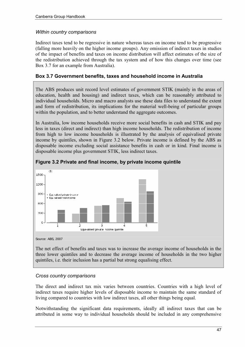
Canberra Group Handbook
47
Within country comparisons
Indirect taxes tend to be regressive in nature whereas taxes on income tend to be progressive (falling more heavily on the higher income groups). Any omission of indirect taxes in studies of the impact of benefits and taxes on income distribution will affect estimates of the size of the redistribution achieved through the tax system and of how this changes over time (see Box 3.7 for an example from Australia).
Box 3.7 Government benefits, taxes and household income in Australia
The ABS produces unit record level estimates of government STIK (mainly in the areas of education, health and housing) and indirect taxes, which can be reasonably attributed to individual households. Micro and macro analysts use these data files to understand the extent and form of redistribution, its implications for the material well-being of particular groups within the population, and to better understand the aggregate outcomes.
In Australia, low income households receive more social benefits in cash and STIK and pay less in taxes (direct and indirect) than high income households. The redistribution of income from high to low income households is illustrated by the analysis of equivalised private income by quintiles, shown in Figure 3.2 below. Private income is defined by the ABS as disposable income excluding social assistance benefits in cash or in kind. Final income is disposable income plus government STIK, less indirect taxes.
Figure 3.2 Private and final income, by private income quintile
Source: ABS, 2007
The net effect of benefits and taxes was to increase the average income of households in the three lower quintiles and to decrease the average income of households in the two higher quintiles, i.e. their inclusion has a partial but strong equalising effect.
Cross country comparisons
The direct and indirect tax mix varies between countries. Countries with a high level of indirect taxes require higher levels of disposable income to maintain the same standard of living compared to countries with low indirect taxes, all other things being equal.
Notwithstanding the significant data requirements, ideally all indirect taxes that can be attributed in some way to individual households should be included in any comprehensive
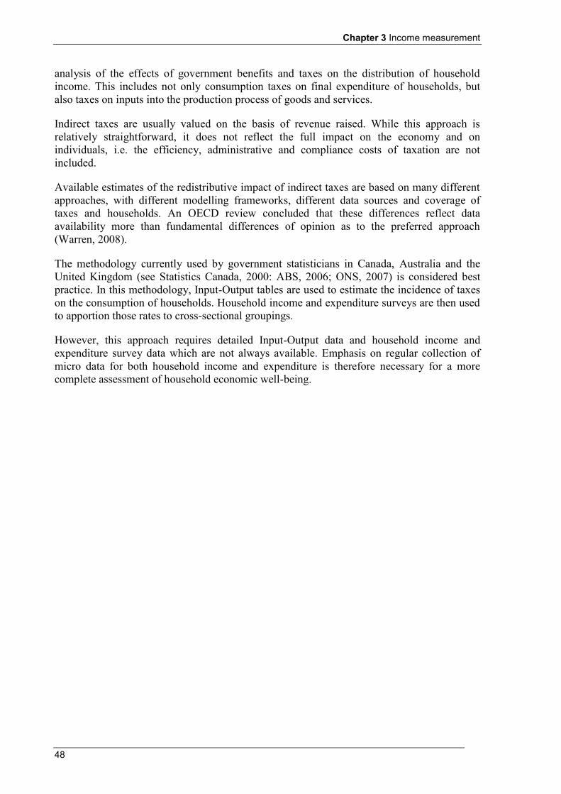
Chapter 3 Income measurement
48
analysis of the effects of government benefits and taxes on the distribution of household income. This includes not only consumption taxes on final expenditure of households, but also taxes on inputs into the production process of goods and services.
Indirect taxes are usually valued on the basis of revenue raised. While this approach is relatively straightforward, it does not reflect the full impact on the economy and on individuals, i.e. the efficiency, administrative and compliance costs of taxation are not included.
Available estimates of the redistributive impact of indirect taxes are based on many different approaches, with different modelling frameworks, different data sources and coverage of taxes and households. An OECD review concluded that these differences reflect data availability more than fundamental differences of opinion as to the preferred approach (Warren, 2008).
The methodology currently used by government statisticians in Canada, Australia and the United Kingdom (see Statistics Canada, 2000: ABS, 2006; ONS, 2007) is considered best practice. In this methodology, Input-Output tables are used to estimate the incidence of taxes on the consumption of households. Household income and expenditure surveys are then used to apportion those rates to cross-sectional groupings.
However, this approach requires detailed Input-Output data and household income and expenditure survey data which are not always available. Emphasis on regular collection of micro data for both household income and expenditure is therefore necessary for a more complete assessment of household economic well-being.
49
Chapter 4 Data availability 4.1 Introduction
This chapter provides information on the methodologies applied and the income components included in micro level datasets for household income compiled by a wide variety of countries. The information has been mostly compiled from the 2010 Survey of Country Practices conducted by the Task Force. The survey results have been supplemented with country information separately available for the European Union Statistics on Income and Living Conditions (EU-SILC).
The information provided is useful for improving understanding of recent developments in the collection of household income statistics. It also provides information on the availability of national data and the extent of comparability of country definitions when undertaking international comparisons. Based on this information, Chapter 4.5 recommends a practical definition of income for the purpose of international comparisons of income distribution.
Results of a similar survey were included in the 2001 edition of this Handbook. Since that time there have been efforts by many countries to improve their measures of household income according to the recommendations of the 2001 Handbook, as well as the 2004 ICLS standards and the 2008 SNA.
4.2 Survey of Country Practices
The Survey of Country Practices was designed to collect information on national practices in compiling micro level datasets for household income. The survey comprised two questionnaires: a robustness assessment and a data item inventory. Both questionnaires were sent to the NSOs of all UNECE member countries (encompassing all OECD member countries) and selected other countries in late 2009.
33 countries responded to the robustness assessment (Questionnaire 1) and 52 countries to the data item inventory (Questionnaire 2). For Questionnaire 1, EU-SILC information provided by Eurostat was used for another 15 countries, taking the number included to 48. The countries included are listed in Table 4.1. The responses relate to the main income survey data available, with the choice of the most appropriate source left to each NSO.
4.2.1 Robustness assessment
Questionnaire 1 was designed to collect information to help inform assessments of the robustness of national datasets on household income. It covered broad topics such as population coverage, collection methodology, editing and imputation, estimation and dissemination. Appendix 3 presents the detailed results obtained from the survey, supplemented with information provided by Eurostat as discussed above. A copy of the questionnaire used is included.
Table 1 in Appendix 3 shows that income distribution data are mainly sourced from household surveys, although they are, at least partially, based on population registers and
Chapter 4 Data availability
50
administrative data for a few countries. Income surveys are generally conducted yearly and collect cross-sectional data, although some also include a panel component.
As well as collecting income data, a number of countries collect information about other topics, including expenditure, wealth, material deprivation and housing. The time lag between data collection and the availability of results is usually between 1 and 2 years.
Table 2 indicates that, in all countries, information collected refers to the non-institutional population i.e. non-private dwellings such as boarding schools and institutions for long-term care are excluded. People with a non-permanent address are also excluded.
There are geographic exclusions specific to individual countries e.g. rural areas in China, northern territories and aboriginal reserves for Canada, sparsely populated areas in Australia and farm households in Korea. The proportion of the population falling outside the scope of the surveys is generally below 2%.
Most surveys had sample sizes sufficient to ensure weighted estimates were representative of the national population. In a few countries use of register data enabled complete coverage. Nearly half of countries had response rates in the range from 50% to 80%, suggesting that some may be exposed to sample selection bias. To help correct for this, almost all of the countries used benchmarking to ensure that their survey output was nationally representative.
Table 3 shows that almost all countries use the household as their main unit for output and analysis. In all countries, people needed to share a common dwelling to be considered part of the household, but some countries use additional criteria such as sharing a common budget.
In most countries all persons in the household above a certain age are interviewed, but some countries only interview a single household member who provides all information. Basic information on the relationships between household members is available in almost all countries. Individuals temporarily absent are generally included in the survey.
Table 4 indicates that, in about two thirds of countries, field work is undertaken for a specific period, but there are also a considerable number of countries in which field work is undertaken continuously throughout the year. Data are mainly collected through face-to-face interviews, but some countries also rely, at least partially, on phone interviews.
Respondents are generally asked about their income in the calendar year preceding the interview, but some countries ask for their income in the 12 months preceding the interview. Generally the reference period used for the different income components is the same. Upper limits are applied for reported income values in several countries.
Table 5 shows that, for units participating in the survey, non-response rates for individual income components are generally below 10%. The individual item non-response rates for self-employment income, interest and dividends are often higher than for other components.
Table 6 indicates that most statistical offices compare their survey results with external benchmarks such as national accounts aggregates and outlays for social benefits. These comparisons do not usually lead to adjustments to survey values. For over two thirds of countries, imputation is undertaken for missing values. Negative income items are mostly retained.
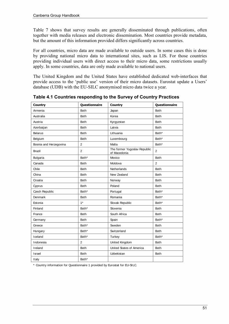
Canberra Group Handbook
51
Table 7 shows that survey results are generally disseminated through publications, often together with media releases and electronic dissemination. Most countries provide metadata, but the amount of this information provided differs significantly across countries.
For all countries, micro data are made available to outside users. In some cases this is done by providing national micro data to international sites, such as LIS. For those countries providing individual users with direct access to their micro data, some restrictions usually apply. In some countries, data are only made available to national users.
The United Kingdom and the United States have established dedicated web-interfaces that provide access to the ‘public use’ version of their micro datasets. Eurostat update a Users’ database (UDB) with the EU-SILC anonymised micro data twice a year.
Table 4.1 Countries responding to the Survey of Country Practices Country Questionnaire Country Questionnaire
Armenia Both Japan Both
Australia Both Korea Both
Austria Both Kyrgyzstan Both
Azerbaijan Both Latvia Both
Belarus Both Lithuania Both*
Belgium Both Luxembourg Both*
Bosnia and Herzegovina 2 Malta Both*
Brazil 2 The former Yugoslav Republic of Macedonia
2
Bulgaria Both* Mexico Both
Canada Both Moldova 2
Chile Both Netherlands Both
China Both New Zealand Both
Croatia Both Norway Both
Cyprus Both Poland Both
Czech Republic Both* Portugal Both*
Denmark Both Romania Both*
Estonia 1* Slovak Republic Both*
Finland Both* Slovenia Both
France Both South Africa Both
Germany Both Spain Both*
Greece Both* Sweden Both
Hungary Both* Switzerland Both
Iceland Both* Turkey Both*
Indonesia 2 United Kingdom Both
Ireland Both United States of America Both
Israel Both Uzbekistan Both
Italy Both*
* Country information for Questionnaire 1 provided by Eurostat for EU-SILC.
Chapter 4 Data availability
52
4.2.2 Data item inventory
The purpose of Questionnaire 2 was to obtain information about the income components collected by each country, to help determine the extent to which countries followed the international definition and recommended treatments (ILO, 2004).
For each income component, respondents were asked whether it was: collected completely, partially or not at all observed separately, jointly with another component, or imputed collected at the individual or household level recorded as gross or net of direct taxes and workers social security contributions.
The detailed country responses for Questionnaire 2 are presented in Appendix 4. The results are summarised in Figure 4.1.
The results indicate that wages and salaries, interest and dividends, government transfers in cash, and compulsory inter-household transfers (alimony and child support) are all collected by more than 90% of the countries that participated in the survey. The income components with least coverage were goods and services produced for barter, production of goods and services for own use, and transfers in kind from governments, non-profit institutions serving households (NPISHs) and other households.
The deductions required to calculate disposable income that are collected or imputed are direct taxes, employee social security contributions and current inter-household transfers such as alimony and child support (all by more than 70% of the participating countries).
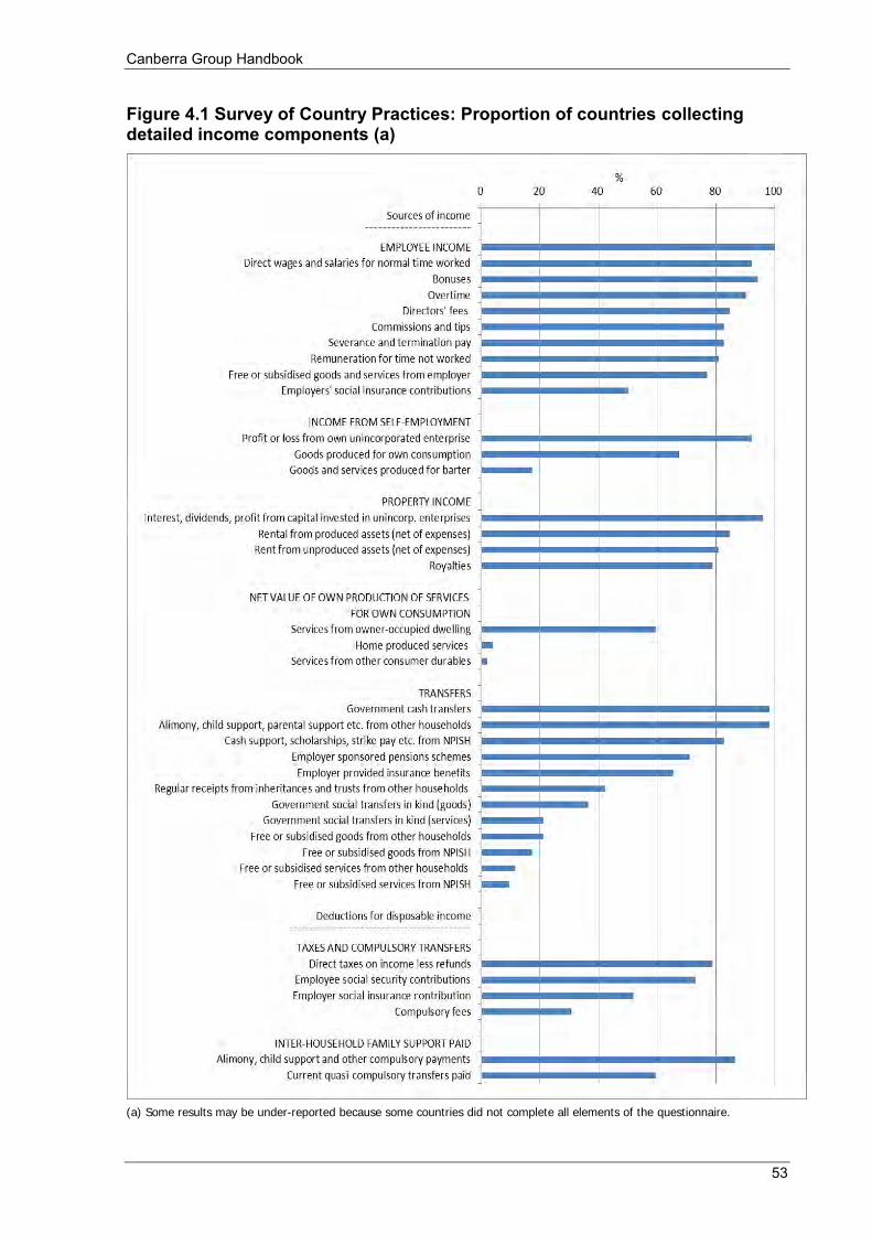
Canberra Group Handbook
53
Figure 4.1 Survey of Country Practices: Proportion of countries collecting detailed income components (a)
(a) Some results may be under-reported because some countries did not complete all elements of the questionnaire.
Chapter 4 Data availability
54
4.3 Comparison of country practices between 2001 and 2010
Seventeen of the countries that participated in the Survey of Country Practices included in the 2001 edition of this Handbook also provided responses in the 2010 survey. These countries were Australia, Brazil, Canada, Chile, China, Finland, Germany, Italy, Republic of Korea, Mexico, the Netherlands, New Zealand, Norway, Sweden, Switzerland, the United Kingdom, and the United States of America.
A comparison of the survey results for these countries indicates that the following income components are now compiled by significantly more countries:
estimated value of free or subsidised goods and services from a person’s employer (from 9 to 13)
current transfers from NPISHs (from 9 to 15) employee social security contributions (from 9 to 13) compulsory fees (from 0 to 7).
4.4 European Union Statistics on Income and Living Conditions (EU-SILC)
In recent years, the EU has made a concerted effort to harmonise the collection of household income data. An EC Regulation was adopted which set out the framework for the systematic production of income statistics. This was implemented by EU member states starting from 2004. The survey vehicle is the EU-SILC.
In 2010 the EU-SILC was produced for 31 countries (the 27 EU member states as well as Iceland, Norway, Switzerland and Turkey) and tested in three further countries (Croatia, the Former Yugoslav Republic of Macedonia and Serbia). These countries comprised a clear majority of participants in the Survey of Country Practices. Table 4.2 shows the income items collected by this instrument and those that are used to derive disposable income.
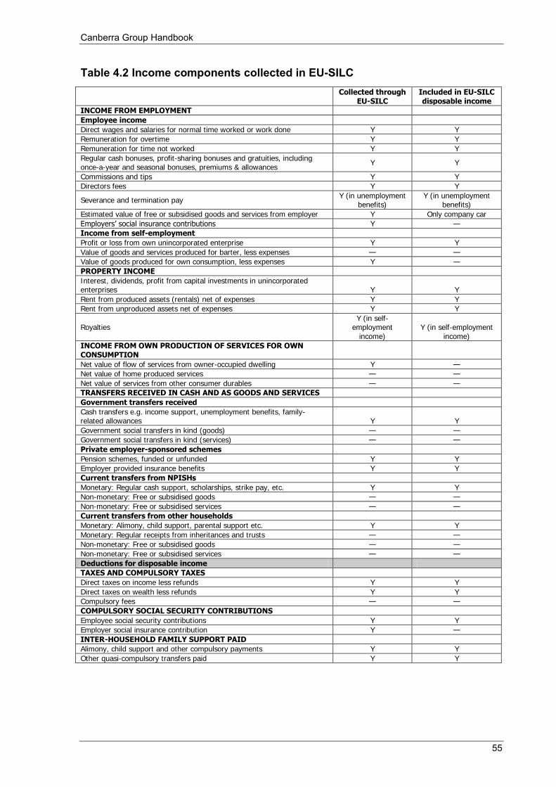
Canberra Group Handbook
55
Table 4.2 Income components collected in EU-SILC
Collected through
EU-SILC Included in EU-SILC disposable income
INCOME FROM EMPLOYMENT
Employee income
Direct wages and salaries for normal time worked or work done Y Y
Remuneration for overtime Y Y
Remuneration for time not worked Y Y
Regular cash bonuses, profit-sharing bonuses and gratuities, including once-a-year and seasonal bonuses, premiums & allowances
Y Y
Commissions and tips Y Y
Directors fees Y Y
Severance and termination pay Y (in unemployment
benefits) Y (in unemployment
benefits)
Estimated value of free or subsidised goods and services from employer Y Only company car
Employers’ social insurance contributions Y —
Income from self-employment
Profit or loss from own unincorporated enterprise Y Y
Value of goods and services produced for barter, less expenses — —
Value of goods produced for own consumption, less expenses Y —
PROPERTY INCOME
Interest, dividends, profit from capital investments in unincorporated enterprises Y Y
Rent from produced assets (rentals) net of expenses Y Y
Rent from unproduced assets net of expenses Y Y
Royalties Y (in self-
employment income)
Y (in self-employment income)
INCOME FROM OWN PRODUCTION OF SERVICES FOR OWN CONSUMPTION
Net value of flow of services from owner-occupied dwelling Y —
Net value of home produced services — —
Net value of services from other consumer durables — —
TRANSFERS RECEIVED IN CASH AND AS GOODS AND SERVICES
Government transfers received
Cash transfers e.g. income support, unemployment benefits, family-related allowances Y Y
Government social transfers in kind (goods) — —
Government social transfers in kind (services) — —
Private employer-sponsored schemes
Pension schemes, funded or unfunded Y Y
Employer provided insurance benefits Y Y
Current transfers from NPISHs
Monetary: Regular cash support, scholarships, strike pay, etc. Y Y
Non-monetary: Free or subsidised goods — —
Non-monetary: Free or subsidised services — —
Current transfers from other households
Monetary: Alimony, child support, parental support etc. Y Y
Monetary: Regular receipts from inheritances and trusts — —
Non-monetary: Free or subsidised goods — —
Non-monetary: Free or subsidised services — —
Deductions for disposable income
TAXES AND COMPULSORY TAXES
Direct taxes on income less refunds Y Y
Direct taxes on wealth less refunds Y Y
Compulsory fees — —
COMPULSORY SOCIAL SECURITY CONTRIBUTIONS
Employee social security contributions Y Y
Employer social insurance contribution Y —
INTER-HOUSEHOLD FAMILY SUPPORT PAID
Alimony, child support and other compulsory payments Y Y
Other quasi-compulsory transfers paid Y Y
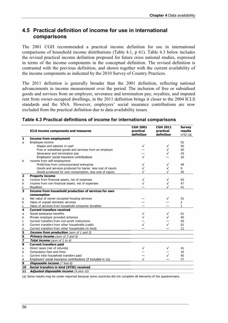
Chapter 4 Data availability
56
4.5 Practical definition of income for use in international comparisons
The 2001 CGH recommended a practical income definition for use in international comparisons of household income distributions (Table 4.1, p 61). Table 4.3 below includes the revised practical income definition proposed for future cross national studies, expressed in terms of the income components in the conceptual definition. The revised definition is contrasted with the previous definition, and shown together with the current availability of the income components as indicated by the 2010 Survey of Country Practices.
The 2011 definition is generally broader than the 2001 definition, reflecting national advancements in income measurement over the period. The inclusion of free or subsidised goods and services from an employer, severance and termination pay, royalties, and imputed rent from owner-occupied dwellings, in the 2011 definition brings it closer to the 2004 ICLS standards and the SNA. However, employers’ social insurance contributions are now excluded from the practical definition due to data availability issues.
Table 4.3 Practical definitions of income for international comparisons
(a) Some results may be under-reported because some countries did not complete all elements of the questionnaire.
ICLS income components and measures
CGH 2001 practical definition
CGH 2011 practical definition
Survey results n/52 (a)
1 Income from employment a Employee income 52 Wages and salaries in cash √ √ 50 Free or subsidised goods and services from an employer — √ 40 Severance and termination pay — √ 43 Employers’ social insurance contributions √ — 26 b Income from self-employment Profit/loss from unincorporated enterprise √ √ 48 Goods and services produced for barter, less cost of inputs √ √ 9 Goods produced for own consumption, less cost of inputs √ √ 35
2 Property income a Income from financial assets, net of expenses √ √ 50 b Income from non-financial assets, net of expenses √ √ 47 c Royalties — √ 41
3 Income from household production of services for own consumption
a Net value of owner-occupied housing services — √ 31 b Value of unpaid domestic services — — 2 c Value of services from household consumer durables — — 1
4 Current transfers received a Social assistance benefits √ √ 51 b Private employer provided schemes √ √ 40 c Current transfers from non-profit institutions — — 43 d Current transfers from other households (cash) √ √ 51 e Current transfers from other households (in kind) — — 11
5 Income from production (sum of 1 and 3)
6 Primary income (sum of 2 and 5)
7 Total income (sum of 1 to 4)
8 Current transfers paid a Direct taxes (net of refunds) √ √ 41 b Compulsory fees and fines — — 16 c Current inter-household transfers paid — √ 45 d Employers’ social insurance contributions (if included in 1a) √ — 27
9 Disposable income (7 less 8)
10 Social transfers in kind (STIK) received
11 Adjusted disposable income (9 plus 10)
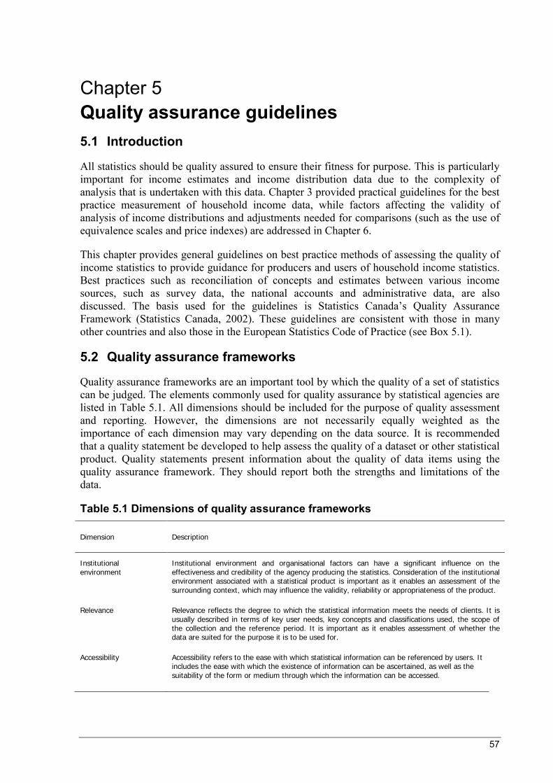
57
Chapter 5 Quality assurance guidelines 5.1 Introduction
All statistics should be quality assured to ensure their fitness for purpose. This is particularly important for income estimates and income distribution data due to the complexity of analysis that is undertaken with this data. Chapter 3 provided practical guidelines for the best practice measurement of household income data, while factors affecting the validity of analysis of income distributions and adjustments needed for comparisons (such as the use of equivalence scales and price indexes) are addressed in Chapter 6.
This chapter provides general guidelines on best practice methods of assessing the quality of income statistics to provide guidance for producers and users of household income statistics. Best practices such as reconciliation of concepts and estimates between various income sources, such as survey data, the national accounts and administrative data, are also discussed. The basis used for the guidelines is Statistics Canada’s Quality Assurance Framework (Statistics Canada, 2002). These guidelines are consistent with those in many other countries and also those in the European Statistics Code of Practice (see Box 5.1).
5.2 Quality assurance frameworks
Quality assurance frameworks are an important tool by which the quality of a set of statistics can be judged. The elements commonly used for quality assurance by statistical agencies are listed in Table 5.1. All dimensions should be included for the purpose of quality assessment and reporting. However, the dimensions are not necessarily equally weighted as the importance of each dimension may vary depending on the data source. It is recommended that a quality statement be developed to help assess the quality of a dataset or other statistical product. Quality statements present information about the quality of data items using the quality assurance framework. They should report both the strengths and limitations of the data.
Table 5.1 Dimensions of quality assurance frameworks
Dimension Description
Institutional environment
Institutional environment and organisational factors can have a significant influence on the effectiveness and credibility of the agency producing the statistics. Consideration of the institutional environment associated with a statistical product is important as it enables an assessment of the surrounding context, which may influence the validity, reliability or appropriateness of the product.
Relevance Relevance reflects the degree to which the statistical information meets the needs of clients. It is usually described in terms of key user needs, key concepts and classifications used, the scope of the collection and the reference period. It is important as it enables assessment of whether the data are suited for the purpose it is to be used for.
Accessibility Accessibility refers to the ease with which statistical information can be referenced by users. It includes the ease with which the existence of information can be ascertained, as well as the suitability of the form or medium through which the information can be accessed.
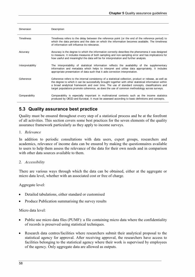
Chapter 5 Quality assurance guidelines
58
Dimension Description
Timeliness Timeliness refers to the delay between the reference point (or the end of the reference period) to which the data pertains and the date on which the information becomes available. The timeliness of information will influence its relevance.
Accuracy Accuracy is the degree to which the information correctly describes the phenomena it was designed to measure. It includes measures of both sampling and non-sampling error and has implications for how useful and meaningful the data will be for interpretation and further analysis.
Interpretability The interpretability of statistical information reflects the availability of the supplementary information and metadata which helps to interpret and utilise data appropriately. It includes appropriate presentation of data such that it aids correction interpretation.
Coherence Coherence refers to the internal consistency of a statistical collection, product or release, as well as the degree to which it can be successfully brought together with other statistical information within a broad analytical framework and over time. The use of standard concepts, classifications and target populations promote coherence, as does the use of common methodology across surveys.
Comparability Comparability is especially important in multinational contexts such as the income statistics produced by OECD and Eurostat. It must be assessed according to basic definitions and concepts.
5.3 Quality assurance best practice Quality must be ensured throughout every step of a statistical process and be at the forefront of all activities. This section covers some best practices for the seven elements of the quality assurance framework particularly as they apply to income surveys.
1. Relevance
In addition to periodic consultations with data users, expert groups, researchers and academics, relevance of income data can be ensured by making the questionnaires available to users to help them assess the relevance of the data for their own needs and in comparison with other data sources available to them.
2. Accessibility
There are various ways through which the data can be obtained, either at the aggregate or micro data level, whether with an associated cost or free of charge.
Aggregate level:
Detailed tabulations, either standard or customised
Produce Publication summarising the survey results
Micro data level:
Public use micro data files (PUMF): a file containing micro data where the confidentiality of records is preserved using statistical techniques.
Research data centres/facilities where researchers submit their analytical proposal to the statistical agency for approval. After receiving approval, the researchers have access to facilities belonging to the statistical agency where their work is supervised by employees of the agency. Only aggregate data are allowed as outputs.
Canberra Group Handbook
59
Initiatives to make available the PUMFs through universities to increase data access.
Remote access is a secure online data query service that approved clients can access to submit their queries against unit record files held by the statistical agency. The results of the queries are automatically checked then made available to the users via their desktops.
Remote execution is where researchers provide their programs to the statistical agency, usually for a fee. These programs are submitted by the statistical agency to run using the unit record database. Only aggregate outputs are provided to preserve confidentiality of the data.
Synthetic files: a file where data are statistically modelled to preserve the distributions of survey estimates and confidentiality of the data.
Perturbed data: where output in cells with few contributors is randomly adjusted to prevent disclosure of confidential data without impacting on aggregate estimates, i.e. perturbed figures are close enough to the 'true' figures for these cells to not impact on output.
International organisations: income data from some countries are available through the CNEF (Cross National Equivalence File) and the LIS (Luxembourg Income Study). This allows the data to be used in international comparisons and analyses.
3. Timeliness
The time span between fieldwork and the end of the income reference period should be kept as short as possible to avoid delays and ensure consistency of information on household composition and the income reference period.
There may be a trade-off between accuracy and timeliness if time allowed for certification of data is reduced. Caution must be exercised prior to implementing proposals for increasing timeliness of the data.
Products associated with the release of data can be disseminated in waves so as not to delay the initial dissemination of survey results.
The use of preliminary files should be considered when other sources of income data are used during the collection or processing of income data. However, this should depend on their impact on the income estimates.
Timeliness can be improved throughout the collection, processing and dissemination steps if operations, which are independent of each other, are undertaken in parallel instead of sequentially.
4. Accuracy
Undertaking thorough research and analysis concurrently with the production process can identify problems prior to finalising results.
Throughout the collection period, thorough testing of the computer applications, preparation of survey documentation, monitoring of response rates and close communications between subject matter and collection staff should occur.
Chapter 5 Quality assurance guidelines
60
Where possible, use generalised corporate systems and methodology services to reduce risks during the editing, transformation, imputation and estimation steps. System interdependencies should be identified and reduced when possible.
A contingency plan should be developed to deal with unplanned, last minute changes to data outputs (prior to dissemination of income estimates).
To control measurement errors in sample surveys, careful editing is required.
To enable the calculation of sampling errors, procedures must adhere strictly to probability sampling. Hence units are usually selected from area or list frames in which each element has a known, non-zero probability of selection. By definition, quota and random walk sampling do not allow the calculation of sampling errors.
To enable accuracy assessments by both internal and external users of income data, quality statements should include information on:
o Sampling
Type of sampling design (e.g. stratified, multi-stage, clustered)
Sampling units (one stage, multi-stage)
Stratification and sub-stratification criteria
Sample size and allocation criteria
Sample selection schemes
Renewal of sample: rotational groups (if applicable)
Substitutions of original units selected in the sample when information cannot be obtained
o Weightings
Design factor
Non-response adjustments
Adjustments using external data (level, variables used and sources)
Final cross-sectional weights
o Sampling errors
Standard error and effective sample size given the design effect. As a minimum, the effect implied by clustering and unequal probabilities of selection for key indicators (such as mean and median equivalised disposable income or the at-risk-of-poverty rate) should be considered.
Canberra Group Handbook
61
o Non-sampling errors
Sampling frame issues (including information on the procedure used to update the frame, frequency and duplicates), and a description of the main coverage problems (misclassification, under-coverage and over-coverage).
Potential sources of measurement errors, including information on the way the questionnaire was developed and tested. This includes information on its design, content and wording, the intensity and efficiency of interview training, and information on methodological studies, if available.
o Processing errors
A description of data entry and coding controls, and the editing system applied to the data.
o Non-response errors
Achieved sample size
Unit non-response and contact rates (before and after substitutions if applicable)
Item non-response including percentages of recipients, missing and partially recorded income components, and impact on key indicators such as mean and median equivalised disposable income and the at-risk-of-poverty rate.
o Imputations
o Methods used to estimate imputed rent (if applicable)
o Mode of data collection and rate of proxy information
o Interview duration
5. Interpretability
Outreach programs and support to major users and the media following each release will help increase the interpretability of income estimates.
Releases of income estimates should be accompanied by appropriate documentation related to the associated definitions, terminology, methodology and quality indicators, to help with the interpretation of the data.
6. Coherence
Other sources of income data, such as income tax data, can be used for comparability and coherence analysis.
Documentation throughout the year of changes to tax and social policies, or financial events, can be helpful to ensure coherence of income estimates.
Chapter 5 Quality assurance guidelines
62
Time series analysis tools can be used to ensure time series consistency and support in-depth coherence analysis.
Analysts not involved in the production process can assist by undertaking more complex analysis, and looking at the data from a different perspective, to identify inconsistencies that might not be observed earlier in the production cycle.
Review of income data at an early stage by staff of related programs (such as national accounts compilers) can also help ensure coherence.
If core variables are used in the same format across different data sources this facilitates comparison and calibration to external distributions. It also provides opportunities for the synthetic matching of information across sources, which cannot be obtained from one single source. This is particularly relevant for the joint assessment of income, expenditure, wealth and labour market data.
7. Comparability
While some degree of flexibility is inevitable for any international data collection, the European Commission regulation (1980/2003) on quality reports for EU-SILC (European Commission, 2003) specifies some minimum criteria for the assessment of quality:
Comparability of basic definitions, including reference population, private household definition, household membership, income reference period(s) used, the period for taxes on income and social insurance contributions, reference period for taxes on wealth, lag between the income reference period and current variables (e.g. household composition). The total duration of the data collection for the sample, basic information on employment status during the income reference period, differences between definitions, and an assessment of the consequences for each income component should also be provided.
The source or procedure used for the collection of income variables.
The form in which income variables at component level have been obtained (e.g. gross, net of taxes on income at source and social contributions).
The method used to obtain income target variables in the required form (i.e. as gross values)
Box 5.1 EU-SILC quality reports
The European Statistics Code of Practice, adopted in 2005, sets common standards for the independence, integrity and accountability of the national and EU statistical authorities. In the framework of this Code of Practice, a common EU definition of quality in statistics has been built where the dimensions of the quality assurance framework described in this chapter are covered. In the EU-SILC, this is monitored with annual intermediate and final quality reports prepared by both the member countries and Eurostat. Their objective is to evaluate the quality of EU-SILC data from a European perspective, i.e. by establishing cross-country comparisons of some of its key quality characteristics. The EU quality reports, as well as most of the national country reports, are available on the Eurostat website (e.g. see Eurostat, 2010).
63
Chapter 6 Data analysis and dissemination 6.1 Introduction
Household income statistics are one of the most complicated datasets produced by national statistical offices. They pose a major challenge for their producers in determining how to present them in the most useful and understandable way. The presentation used can significantly influence how the data are interpreted.
For particular kinds of analyses, different units of analysis may be used and different methods may be applied. These choices significantly influence how the results should be interpreted. The units, methods and assumptions used in the analyses should be clearly stated.
This chapter provides practical guidance in the presentation and analysis of income distribution statistics.
6.2 Uses of income data
Household income data provide valuable insights into a range of social and economic issues. It is particularly used to:
analyse the distribution of income within society
identify people who may be at risk of experiencing economic hardship
analyse the impact of proposed or new policies, such as changes to government benefits and tax rates, on particular people or subpopulations.
Monitoring income growth, sources of income and income distribution for particular subpopulations is important for assessing the economic well-being of individuals and of society as a whole. The extent of income inequality, and especially whether it is increasing or decreasing over time, is therefore of considerable interest. Large income disparities within a society raise issues of social justice.
The effectiveness of income redistribution policies and whether they are successful in reducing inequality in the distribution of resources can be assessed using household income data. The tax and transfer system is usually the primary mechanism by which economic resources are redistributed. It is important to understand the factors that might cause an increase in low income earners, such as rising unemployment or population ageing, because of their different policy consequences.
Economic hardship can lead to a range of social problems including poor health and education outcomes, increased crime rates and lower rates of community participation. If economic hardship persists for an extended period, it can lead to dependence on assistance from government and charitable organisations. Of particular policy interest and concern is the impact on children in affected families and the geographic distribution of the hardship.
Chapter 6 Data analysis and dissemination
64
Microsimulation techniques are a valuable tool to assess the effects of changes to government policies and programs. Personal and family characteristics are used, together with income data, to analyse the distributional and individual impacts of income tax and income support policies, and to estimate the fiscal and distributional impacts of reform. Modelling the proposed changes aims to ensure that there are no unintended consequences, and that the costs and benefits of the changes are fully understood prior to their implementation.
6.3 Units and populations
6.3.1 Units of analysis
Chapter 3 identified the household as the preferred data collection unit for income statistics, noting that data should be collected at the person level to provide better quality data, as well as flexibility for analysis purposes. Income data collected at the person level may be analysed by person or aggregated for analyses of households, families or income units (see Box 6.1).
Box 6.1 Definitions of analytical units
Household: is either (a) a person living alone in a separate housing unit or who occupies, as a lodger, a separate room (or rooms) of a housing unit but does not join with any of the other occupants of the housing unit to form part of a multi-person household or (b) a group of two or more persons who combine to occupy the whole or part of a housing unit and to provide themselves with food and possibly other essentials for living. The group may be composed of related persons only or of unrelated persons or of a combination of both. The group may also pool their income.
Income unit: one person or a group of related persons within a household, whose command over income is assumed to be shared. Income sharing is assumed to take place within married (registered or de facto) couples, and between parents and dependent children.
Family: two or more people, one of whom is at least 15 years of age, who are related by blood, marriage (registered or de facto), adoption, step or fostering, and who usually live in the same household. A separate family is formed for each married couple, or for each set of parent child relationships where only one parent is present.
When considering economic well-being, the household is the basic unit for income analysis because this is the level of aggregation of individual incomes at which an assumption of income sharing is most valid.
Implicit in producing any analysis that combines the income of persons is the assumption that all members of the unit share equally in the income of the unit. This may not be an entirely valid assumption, for example, one person within a household may spend most of the income of the household on themselves to the detriment of other household members. However, this is unlikely to be accurately quantifiable.
The two most common ways of presenting analysis of household income data are:
number of households with particular characteristics, or
number of persons in households with particular characteristics.
Canberra Group Handbook
65
When the household is used as the basic data analysis unit, each household, no matter its size, contributes the same. For example, each person in a four person household would have one-quarter the representation of a person in a single person household. To provide a better measure of the total population, the individual is therefore usually of most interest to analysts. There is also a preference for the equal representation of each person in such analysis.
An example of the impact of the unit of analysis is the statement that 'the bottom 20 per cent of the income distribution received 8 per cent of total income'. If referring to households, it would mean that the bottom 20 per cent of households, who might be more or less than 20 per cent of the population, received 8 per cent of total income, if referring to persons, the statement implies that the bottom 20 per cent of individuals received 8 per cent of total income.
When analysing persons in a household, each person in the household should be attributed with the characteristics of the household to which they belong. Based on this assumption, household income can be presented about the household or can be reweighted so that it represents the number of individuals instead of the number of households. These latter are sometimes known as person weighted estimates because the unit of analysis is the person. When person weighted estimates are compiled, the representation in the income distribution of each person in a household comprising four persons is the same as that for each person in a household comprising two persons.
6.3.2 Population subgroups
Analysts are often interested in analysing income data for particular population subgroups. When presenting income distribution statistics, it is often useful to categorise households according to characteristics such as:
household size and composition based on characteristics such as age and sex, marital status, number of dependent children, dependency ratio (i.e. the ratio of those outside the working age to those within), number of income earners, main source of income
housing status, e.g. ownership of home, access to subsidised housing, market renters
physical location, e.g. urban, non-urban, region.
Characteristics that can be assigned to individuals but not households may also be used. In this case the household can either be analysed by the characteristics of the household reference person or according to characteristics of particular individuals of interest, e.g. using gender or employment status.
If using the reference person, they should be chosen by applying to all household members an ordered set of criteria to select the person likely to best represent the household as a whole. An example of the selection criteria that could be used to identify the reference person is listed below. These criteria should be applied in the order listed until a single appropriate reference person is identified:
one of the partners in a registered or de facto marriage, with dependent children
one of the partners in a registered or de facto marriage, without dependent children
Chapter 6 Data analysis and dissemination
66
a lone parent with dependent children
the person with the highest income
the eldest person.
Applying these rules to a household containing a lone parent with a non-dependent child, the one with the higher income will become the reference person. However, if both individuals have the same income, the elder will become the reference person.
There are likely to be substantial differences in economic well-being between households where the number of economically active adults differ but all other characteristics are the same. The data producer must explain the basis on which households are assigned to categories: is a 'lone parent' a lone person with children, or a lone person with children and with no other adult in the household? Similarly, the definition of terms such as 'child' and 'economically active' must be made available. For example, a 'child' may be defined by their age, or by their educational status (whether or not still in full-time education), their relationship to other household members, or any combination of these factors.
Another example relates to life cycle stage. The income of individuals and households may vary significantly at different stages in their lives. Households with young children will in general have lower household incomes compared to older couples who have reached the peak of their earning capacity and where there are no children residing at home. Similarly, old-age pensioners will usually have lower income compared to working age households. To enable such analysis, a common method is to classify households according to the personal characteristics of the household reference person and the number of adults and children in the household.
Figure 6.1 and Box 6.2 show an example of how households can be classified into different types and the text that should accompany such a chart to explain the classification used. Household types are defined here based on both household size (lone persons, one parent families and couple families with and without dependent children) and according to the age of the reference person. The definitions in this example are those used in Australia. Other countries may use slightly different definitions, e.g. ‘dependent children’ may be based on a different age cut-off.
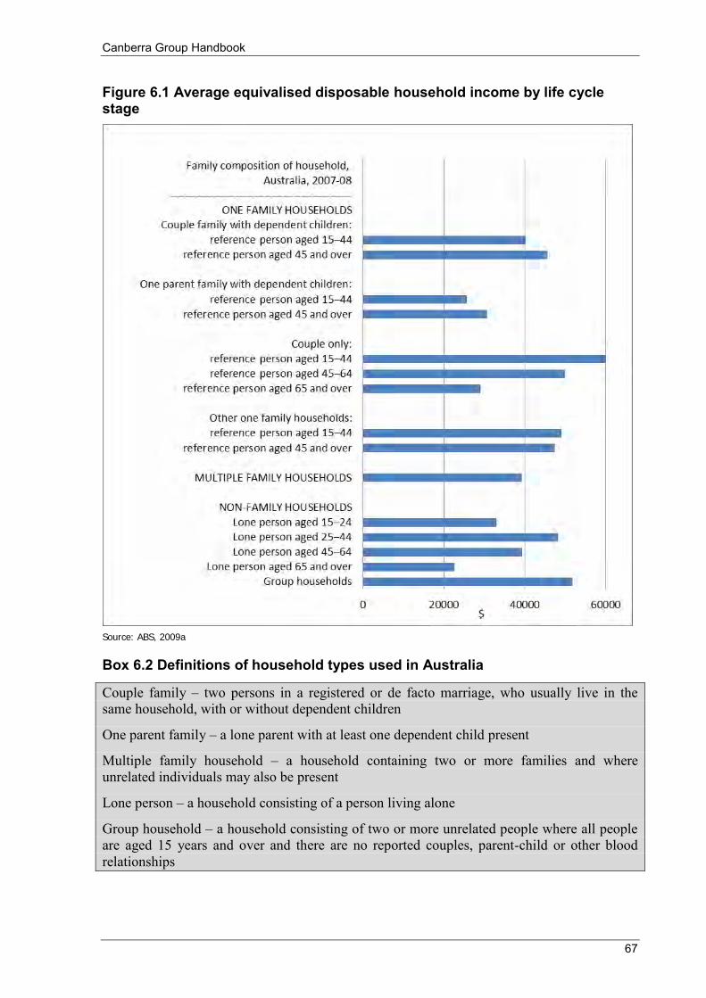
Canberra Group Handbook
67
Figure 6.1 Average equivalised disposable household income by life cycle stage
Source: ABS, 2009a
Box 6.2 Definitions of household types used in Australia
Couple family – two persons in a registered or de facto marriage, who usually live in the same household, with or without dependent children
One parent family – a lone parent with at least one dependent child present
Multiple family household – a household containing two or more families and where unrelated individuals may also be present
Lone person – a household consisting of a person living alone
Group household – a household consisting of two or more unrelated people where all people are aged 15 years and over and there are no reported couples, parent-child or other blood relationships
Chapter 6 Data analysis and dissemination
68
Reference person – person aged 15 years or over selected to represent the household based on a set of selection criteria related to home ownership, couple or parental status, income and/or age
Dependent children – persons aged less than 15 years; and persons aged 15-24 years who are full-time students, have a parent in the household, and do not have a partner or child of their own in the household
6.4 Equivalence scales
The needs of a household grow with each additional member but, due to economies of scale in consumption, not in a proportional way. For example, a household comprising three people would normally need more income than a lone person household if the two households are to enjoy the same standard of living. However, a household with three members is unlikely to need three times the housing space, electricity, etc. that a lone person household requires.
One way of adjusting for this difference in household size might be simply to divide the income of the household by the number of its members so that all income is presented on a per capita basis. However, such a simple adjustment assumes that all individuals have the same resource needs and that there are no economies of scale derived from living together.
Various calibrations, or equivalence scales, have been devised to make adjustments to the actual incomes of households in a way that recognises differences in the needs of individuals and the economies that flow from sharing resources. The scales differ in their detail and complexity, but commonly recognise that the extra level of resources required by larger groups of people living together is not directly proportional to the number of people in the group. They also typically recognise that children have fewer needs than adults.
When household income is adjusted according to an equivalence scale, the equivalised income can be viewed as an indicator of the economic resources available to a standardised household. When using a lone person household as the reference point, its equivalised income is equal to the actual income recorded. For a household comprising more than one person, equivalised income is an indicator of the household income that would be needed by a lone person household to enjoy the same level of economic well-being as the household in question.
Alternatively, equivalised household income can be viewed as an indicator of the economic resources available to each individual in a household. The latter view underpins the calculation of income distribution measures based on the number of people, rather than the number of households.
6.4.1 Choice of equivalence scale
While there has been considerable research by statistical and other agencies trying to estimate appropriate values for equivalence scales, no single standard has emerged. In theory, there are many factors that might be taken into account when devising equivalence scales. For example, people in the labour force are likely to face transport and other costs that can affect their standard of living. It might also be desirable to reflect the different needs of children at different ages, and the different costs faced by people living in different geographic areas. On the other hand, the tastes and preferences of people vary widely, resulting in markedly
Canberra Group Handbook
69
different expenditure patterns between households with similar income levels and composition.
Furthermore, it is likely that equivalence scales that appropriately adjust incomes of low income households are not as appropriate for high income households, and vice versa. This is because the proportion of total income spent on housing tends to fall as incomes rise, and cheaper per capita housing is a major source of the economies of scale that flow from people living together.
The choice of equivalence scale will also depend on the country considered, the structure of household consumption and other factors. In most countries, for example, the elderly live in households that are relatively small, while children live in relatively larger households. As a result, using an equivalence scale that assumes large economies of scale in consumption will understate child poverty and overstate poverty among the elderly.
It is therefore difficult to define, estimate and use equivalence scales which take all relevant factors into account. As a result, analysts tend to use simple equivalence scales which are chosen subjectively, but which are nevertheless consistent with the quantitative research that has been undertaken. A major advantage of simpler scales is that they are more transparent to the user, making it easier to evaluate the assumptions being made in the equivalising process.
With the help of equivalence scales each household type in the population is assigned a value in proportion to its needs. The factors commonly taken into account to assign these values are the size of the household and the age of its members (whether they are adults or children). A wide range of equivalence scales exist, many of which are reviewed in Atkinson et al. (1995). Some of the most commonly used scales include:
OECD equivalence scale – this assigns a value of 1 to the first household member, of 0.7 to each additional adult and of 0.5 to each child. This scale (also called ‘Oxford scale’) was mentioned by the OECD (1982) for possible use in ‘countries which have not established their own equivalence scale’. This scale is sometimes labelled ‘old OECD scale’.
OECD-modified scale – after having used the ‘old OECD scale’ in the 1980s and the earlier 1990s, Eurostat adopted in the late 1990s the so-called ‘OECD-modified equivalence scale’. This scale, first proposed by Haagenars et al. (1994), assigns a value of 1 to the household head, of 0.5 to each additional adult member and of 0.3 to each child.
Square root scale – recent OECD publications (e.g. OECD, 2008) comparing income inequality and poverty across countries use a scale which divides household income by the square root of household size. This implies that, for instance, a household of four persons has needs twice as large as one composed of a single person. However, some OECD country reviews, especially for non-member economies, apply the equivalence scales which are in use in each country.
Table 6.1 illustrates how needs are assumed to change as household size increases, for the three equivalence scales described above, and for the two ‘extreme’ cases of no sharing of resources within a household (per-capita income) and full sharing (household income). In general, there is no accepted method for determining equivalence scales, and no equivalence scale is recommended by the OECD for general use.
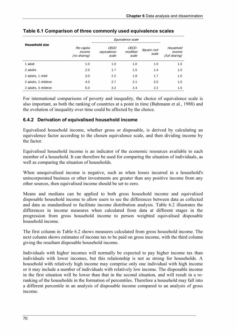
Chapter 6 Data analysis and dissemination
70
Table 6.1 Comparison of three commonly used equivalence scales
Equivalence scale
Household size Per-capita
income (no sharing)
OECD equivalence
scale
OECD-modified
scale
Square root scale
Household income
(full sharing)
1 adult 1.0 1.0 1.0 1.0 1.0
2 adults 2.0 1.7 1.5 1.4 1.0
2 adults, 1 child 3.0 2.2 1.8 1.7 1.0
2 adults, 2 children 4.0 2.7 2.1 2.0 1.0
2 adults, 3 children 5.0 3.2 2.4 2.2 1.0
For international comparisons of poverty and inequality, the choice of equivalence scale is also important, as both the ranking of countries at a point in time (Buhmann et al., 1988) and the evolution of inequality over time could be affected by the choice.
6.4.2 Derivation of equivalised household income
Equivalised household income, whether gross or disposable, is derived by calculating an equivalence factor according to the chosen equivalence scale, and then dividing income by the factor.
Equivalised household income is an indicator of the economic resources available to each member of a household. It can therefore be used for comparing the situation of individuals, as well as comparing the situation of households.
When unequivalised income is negative, such as when losses incurred in a household's unincorporated business or other investments are greater than any positive income from any other sources, then equivalised income should be set to zero.
Means and medians can be applied to both gross household income and equivalised disposable household income to allow users to see the differences between data as collected and data as standardised to facilitate income distribution analysis. Table 6.2 illustrates the differences in income measures when calculated from data at different stages in the progression from gross household income to person weighted equivalised disposable household income.
The first column in Table 6.2 shows measures calculated from gross household income. The next column shows estimates of income tax to be paid on gross income, with the third column giving the resultant disposable household income.
Individuals with higher incomes will normally be expected to pay higher income tax than individuals with lower incomes, but this relationship is not as strong for households. A household with relatively high income may comprise only one individual with high income or it may include a number of individuals with relatively low income. The disposable income in the first situation will be lower than that in the second situation, and will result in a re-ranking of the households in the formation of percentiles. Therefore a household may fall into a different percentile in an analysis of disposable income compared to an analysis of gross income.
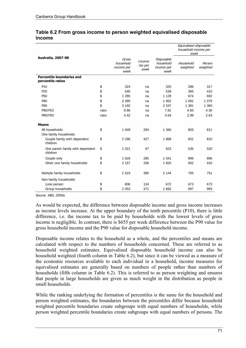
Canberra Group Handbook
71
Table 6.2 From gross income to person weighted equivalised disposable income
Equivalised disposable household income per
week Australia, 2007-08
Gross household
income per week
Income tax per
week
Disposable household
income per week
Household weighted
Person weighted
Percentile boundaries and percentile ratios
P10 $ 324 na 325 286 317
P20 $ 540 na 539 365 410
P50 $ 1 285 na 1 128 674 692
P80 $ 2 390 na 1 962 1 091 1 079
P90 $ 3 192 na 2 537 1 381 1 360
P90/P10 ratio 9.86 na 7.81 4.83 4.30
P80/P20 ratio 4.42 na 3.64 2.99 2.63
Means
All households $ 1 649 284 1 366 803 811
One family households
Couple family with dependent children
$ 2 296 427 1 868 831 810
One parent family with dependent children
$ 1 021 97 923 535 520
Couple only $ 1 626 285 1 341 896 896
Other one family households $ 2 157 336 1 820 902 916
Multiple family households $ 2 523 380 2 144 755 751
Non-family households
Lone person $ 806 134 672 673 673
Group households $ 2 053 371 1 682 997 993
Source: ABS, 2009a
As would be expected, the difference between disposable income and gross income increases as income levels increase. At the upper boundary of the tenth percentile (P10), there is little difference, i.e. the income tax to be paid by households with the lowest levels of gross income is negligible. In contrast, there is $655 per week difference between the P90 value for gross household income and the P90 value for disposable household income.
Disposable income relates to the household as a whole, and the percentiles and means are calculated with respect to the numbers of households concerned. These are referred to as household weighted estimates. Equivalised disposable household income can also be household weighted (fourth column in Table 6.2), but since it can be viewed as a measure of the economic resources available to each individual in a household, income measures for equivalised estimates are generally based on numbers of people rather than numbers of households (fifth column in Table 6.2). This is referred to as person weighting and ensures that people in large households are given as much weight in the distribution as people in small households.
While the ranking underlying the formation of percentiles is the same for the household and person weighted estimates, the boundaries between the percentiles differ because household weighted percentile boundaries create subgroups with equal numbers of households, while person weighted percentile boundaries create subgroups with equal numbers of persons. The
Chapter 6 Data analysis and dissemination
72
extent to which the boundaries differ reflects the extent to which the average household size differs between percentiles.
For example, the person weighted estimate of P10 ($317) is higher than the household weighted estimate of P10 ($286). This implies that households with the lowest rankings of equivalised disposable household income tend to comprise a lower than average number of persons. In other words, the 10% of people with the lowest income comprise more than 10% of households.
For lone person households, the two measures of equivalised disposable income are the same as each other ($673) and are just a little higher than disposable income ($672). Equivalised disposable income for lone person households is approximately the same as disposable income, because the equivalising factor for such households is 1.0. The reason for the slight difference between them is that some households have negative disposable income and these values are set to zero for the calculation of equivalised income.
For all other household compositions, equivalised disposable income is lower than disposable income, since income is adjusted to reflect household size and composition. Mean equivalised disposable income for couple households is the same for both the household weighted and the person weighted measures since there are only two persons in such households. For most other multi-person households, person weighted mean income is lower than the household weighted mean. This implies that, within each type, larger households tend to have lower equivalised disposable household income.
6.5 Summary measures of income level
There are a range of summary measures that can be used for analysing income data.
6.5.1 Counts
Counts of income units or households are derived by summing the weights assigned to each record of interest. Counts of persons can also be obtained this way, but only if all persons are recorded on the survey file. If there are no separate records for children, counts of persons including children would need to be derived by first multiplying each household weight by the number of persons in the household, and then summing the products.
6.5.2 Means
A frequently used measure to describe income levels is the arithmetic mean, or average, i.e. the sum of all income divided by the number of observations. One advantage of the mean is that it is easy to calculate and interpret. However, its main drawbacks are its vulnerability in respect to extreme values and to asymmetry of the distribution.
Despite its weakness as a measure of central tendency, the mean remains the most frequently used measure of income level by most producers of income statistics. It is also the obvious choice when presenting data on the composition of household income. For the lay user it is more satisfactory if the different income components sum to total income, which will be the case when the mean is used. It is not however true of the median except in exceptional cases.
The mean value of a data item is usually calculated by selecting all the survey records for the population of interest, multiplying the value of the data item in each record by the weight of
Canberra Group Handbook
73
the record, summing the resultant products, and then dividing the total by the sum of the weights of the records. For example, the mean gross income of a particular subpopulation of households is the weighted sum of the gross income of each such household divided by the sum of the weights relating to them.
For some purposes means for a household variable may be required with respect to all people in a population group, including children. Such measures (referred to as person weighted measures) are often used when analysing equivalised household income. Estimates of mean equivalised disposable household income are obtained by multiplying the equivalised disposable income of each household by the number of people in the household (including children) and by the weight of the household, summing across all households and then dividing by the estimated number of people in the population group.
6.5.3 Medians
An alternative measure of central tendency is the median. Observations are ranked from the lowest (smallest) to the highest (largest) and the middle observation of the distribution is the median. Compared to the mean, the median is a more stable and robust measure and is less affected by extreme values and sample fluctuations.
The median is often the preferred measure when a threshold for 'low' or 'high' income is required. The reason for this is that many define poverty in terms of the relative distance to a ‘typical’ level of income. The median is often considered superior to the mean as an indicator of a typical level of income for the whole population, because it is less affected by changes taking place at the lower and upper extremes of the distribution.
To identify the median record, the population is first ranked in ascending order according to the data item of interest. Except for person weighted measures of household variables, the weights of the records are then accumulated until half the population is accounted for. The record at which this occurs is the median record, and its value for the data item of interest is the median value. For person weighted measures of household variables, the household weights are multiplied by the number of persons in the household before accumulation.
6.6 Measures of income dispersion
The difference between the mean and the median can be regarded as one measure of income dispersion. In most countries mean (average) household income will be higher than the median household income. The reason for this is that the distribution of income is usually positively skewed, i.e. has a longer tail on the right of the distribution. The higher the ratio between the mean and the median, the greater is the inequality. However, this is a relatively crude measure of income inequality and a number of other measures have been developed.
6.6.1 Frequency distribution
The most basic presentation of income distribution is the frequency diagram, which illustrates the location and spread of income within a population for each sample unit for the chosen measure of income (gross income, disposable income, adjusted disposable income). In the distribution below, the population has been grouped into classes by size of household income and gives the number or proportion of people in each income range. A graph of the frequency distribution is a good way to portray the essence of the income distribution. Figure 6.2 shows an Australian example.
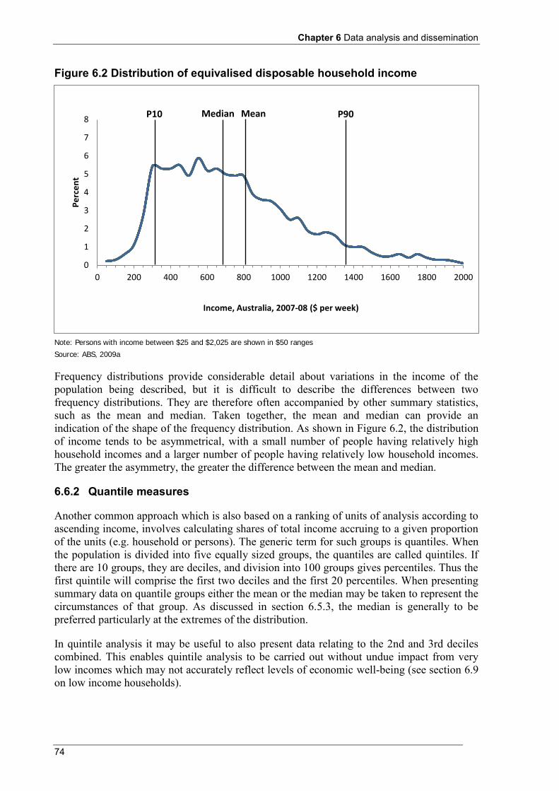
Chapter 6 Data analysis and dissemination
74
Figure 6.2 Distribution of equivalised disposable household income
Note: Persons with income between $25 and $2,025 are shown in $50 ranges
Source: ABS, 2009a
Frequency distributions provide considerable detail about variations in the income of the population being described, but it is difficult to describe the differences between two frequency distributions. They are therefore often accompanied by other summary statistics, such as the mean and median. Taken together, the mean and median can provide an indication of the shape of the frequency distribution. As shown in Figure 6.2, the distribution of income tends to be asymmetrical, with a small number of people having relatively high household incomes and a larger number of people having relatively low household incomes. The greater the asymmetry, the greater the difference between the mean and median.
6.6.2 Quantile measures
Another common approach which is also based on a ranking of units of analysis according to ascending income, involves calculating shares of total income accruing to a given proportion of the units (e.g. household or persons). The generic term for such groups is quantiles. When the population is divided into five equally sized groups, the quantiles are called quintiles. If there are 10 groups, they are deciles, and division into 100 groups gives percentiles. Thus the first quintile will comprise the first two deciles and the first 20 percentiles. When presenting summary data on quantile groups either the mean or the median may be taken to represent the circumstances of that group. As discussed in section 6.5.3, the median is generally to be preferred particularly at the extremes of the distribution.
In quintile analysis it may be useful to also present data relating to the 2nd and 3rd deciles combined. This enables quintile analysis to be carried out without undue impact from very low incomes which may not accurately reflect levels of economic well-being (see section 6.9 on low income households).
0
1
2
3
4
5
6
7
8
0 200 400 600 800 1000 1200 1400 1600 1800 2000
Pe
rce
nt
Income, Australia, 2007-08 ($ per week)
P10. P90 Median Mean
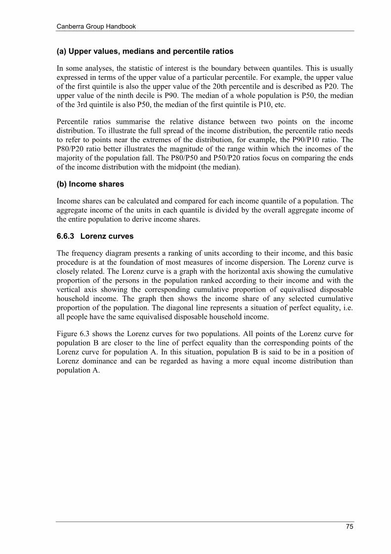
Canberra Group Handbook
75
(a) Upper values, medians and percentile ratios
In some analyses, the statistic of interest is the boundary between quantiles. This is usually expressed in terms of the upper value of a particular percentile. For example, the upper value of the first quintile is also the upper value of the 20th percentile and is described as P20. The upper value of the ninth decile is P90. The median of a whole population is P50, the median of the 3rd quintile is also P50, the median of the first quintile is P10, etc.
Percentile ratios summarise the relative distance between two points on the income distribution. To illustrate the full spread of the income distribution, the percentile ratio needs to refer to points near the extremes of the distribution, for example, the P90/P10 ratio. The P80/P20 ratio better illustrates the magnitude of the range within which the incomes of the majority of the population fall. The P80/P50 and P50/P20 ratios focus on comparing the ends of the income distribution with the midpoint (the median).
(b) Income shares
Income shares can be calculated and compared for each income quantile of a population. The aggregate income of the units in each quantile is divided by the overall aggregate income of the entire population to derive income shares.
6.6.3 Lorenz curves
The frequency diagram presents a ranking of units according to their income, and this basic procedure is at the foundation of most measures of income dispersion. The Lorenz curve is closely related. The Lorenz curve is a graph with the horizontal axis showing the cumulative proportion of the persons in the population ranked according to their income and with the vertical axis showing the corresponding cumulative proportion of equivalised disposable household income. The graph then shows the income share of any selected cumulative proportion of the population. The diagonal line represents a situation of perfect equality, i.e. all people have the same equivalised disposable household income.
Figure 6.3 shows the Lorenz curves for two populations. All points of the Lorenz curve for population B are closer to the line of perfect equality than the corresponding points of the Lorenz curve for population A. In this situation, population B is said to be in a position of Lorenz dominance and can be regarded as having a more equal income distribution than population A.
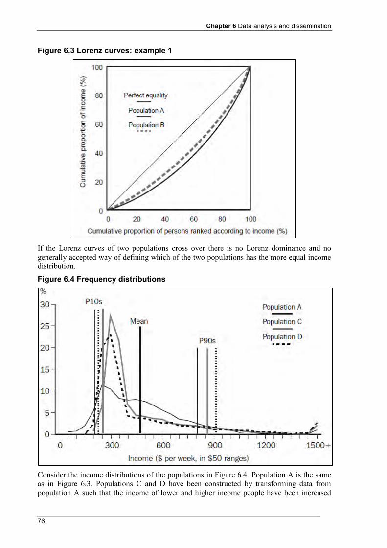
Chapter 6 Data analysis and dissemination
76
Figure 6.3 Lorenz curves: example 1
If the Lorenz curves of two populations cross over there is no Lorenz dominance and no generally accepted way of defining which of the two populations has the more equal income distribution.
Figure 6.4 Frequency distributions
Consider the income distributions of the populations in Figure 6.4. Population A is the same as in Figure 6.3. Populations C and D have been constructed by transforming data from population A such that the income of lower and higher income people have been increased
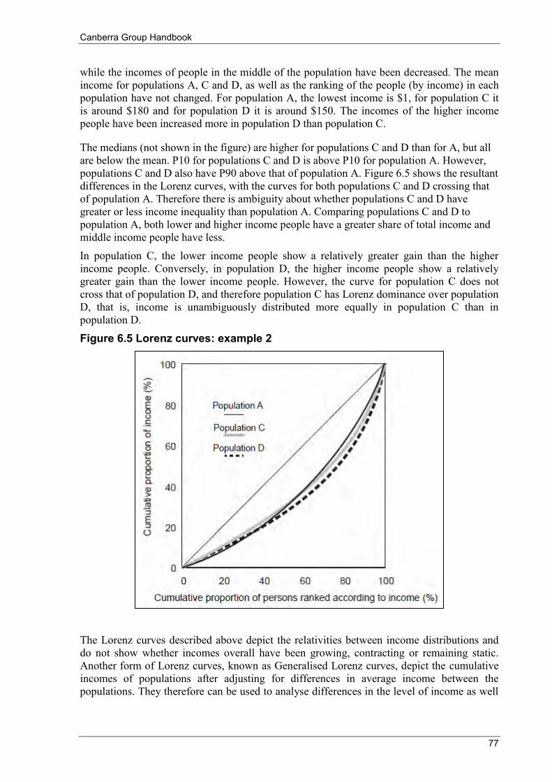
Canberra Group Handbook
77
while the incomes of people in the middle of the population have been decreased. The mean income for populations A, C and D, as well as the ranking of the people (by income) in each population have not changed. For population A, the lowest income is $1, for population C it is around $180 and for population D it is around $150. The incomes of the higher income people have been increased more in population D than population C.
The medians (not shown in the figure) are higher for populations C and D than for A, but all are below the mean. P10 for populations C and D is above P10 for population A. However, populations C and D also have P90 above that of population A. Figure 6.5 shows the resultant differences in the Lorenz curves, with the curves for both populations C and D crossing that of population A. Therefore there is ambiguity about whether populations C and D have greater or less income inequality than population A. Comparing populations C and D to population A, both lower and higher income people have a greater share of total income and middle income people have less.
In population C, the lower income people show a relatively greater gain than the higher income people. Conversely, in population D, the higher income people show a relatively greater gain than the lower income people. However, the curve for population C does not cross that of population D, and therefore population C has Lorenz dominance over population D, that is, income is unambiguously distributed more equally in population C than in population D.
Figure 6.5 Lorenz curves: example 2
The Lorenz curves described above depict the relativities between income distributions and do not show whether incomes overall have been growing, contracting or remaining static. Another form of Lorenz curves, known as Generalised Lorenz curves, depict the cumulative incomes of populations after adjusting for differences in average income between the populations. They therefore can be used to analyse differences in the level of income as well
Chapter 6 Data analysis and dissemination
78
as differences in distribution, but do not as clearly show differences in inequality (see for example, Deaton, 1997).
6.6.4 Summary indicators of income dispersion
There are three commonly used summary inequality measures, the Gini coefficient, the Theil index, and the Atkinson index. This section provides an overview of the main summary indicators used. Further details can be found in Atkinson (1983) and Deaton (1997).
(a) Gini coefficient
The Gini coefficient can be defined by referring to the Lorenz curve. It is the ratio of the area between the actual Lorenz curve and the diagonal (or line of equality) compared to the total area under the diagonal. The Gini coefficient equals zero when all people have the same level of income and equals one when one person receives all the income. In other words, the smaller the Gini coefficient the more equal the distribution of income, given the assumptions underlying the Gini coefficient.
Mathematically, the Gini coefficient can be expressed as
where
n is the number of people in the population
µ is the mean equivalised disposable household income of all people in the population
and yi and yj are the equivalised disposable household income of the ith and jth persons in the population.
The Gini coefficient is a summary of the differences between each person in the population and every other person in the population. The differences are the absolute arithmetic differences, and therefore a difference of $x between two relatively high income people contributes as much to the index as a difference of $x between two relatively low income people.
An increase in the income of a person with income greater than the median will always lead to an increase in the Gini coefficient, and a decrease in the income of a person with income lower than the median will also always lead to an increase in the coefficient. The extent of the increase will depend on the proportion of people that have income in the range between median income and the income of the person with the changed income, both before and after the change in income.
The Gini coefficient is sometimes criticised as being too sensitive to relative changes around the middle of the income distribution. This sensitivity arises because the derivation of the Gini coefficient reflects the ranking of the population, and ranking is most likely to change at the densest part of the income distribution, which is likely to be around the middle.
j
n
jii yy
nG
,22
1
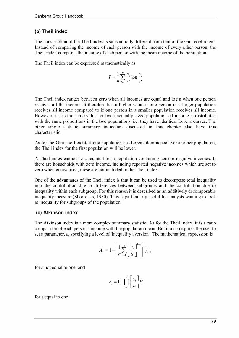
Canberra Group Handbook
79
(b) Theil index
The construction of the Theil index is substantially different from that of the Gini coefficient. Instead of comparing the income of each person with the income of every other person, the Theil index compares the income of each person with the mean income of the population.
The Theil index can be expressed mathematically as
The Theil index ranges between zero when all incomes are equal and log n when one person receives all the income. It therefore has a higher value if one person in a larger population receives all income compared to if one person in a smaller population receives all income. However, it has the same value for two unequally sized populations if income is distributed with the same proportions in the two populations, i.e. they have identical Lorenz curves. The other single statistic summary indicators discussed in this chapter also have this characteristic.
As for the Gini coefficient, if one population has Lorenz dominance over another population, the Theil index for the first population will be lower.
A Theil index cannot be calculated for a population containing zero or negative incomes. If there are households with zero income, including reported negative incomes which are set to zero when equivalised, these are not included in the Theil index.
One of the advantages of the Theil index is that it can be used to decompose total inequality into the contribution due to differences between subgroups and the contribution due to inequality within each subgroup. For this reason it is described as an additively decomposable inequality measure (Shorrocks, 1980). This is particularly useful for analysts wanting to look at inequality for subgroups of the population.
(c) Atkinson index
The Atkinson index is a more complex summary statistic. As for the Theil index, it is a ratio comparison of each person's income with the population mean. But it also requires the user to set a parameter, ε, specifying a level of 'inequality aversion'. The mathematical expression is
for ε not equal to one, and
for ε equal to one.
i
n
i
i yyn
T log11
1
1
1
1
11n
i
iyn
A
n
in
iyA1
11 1
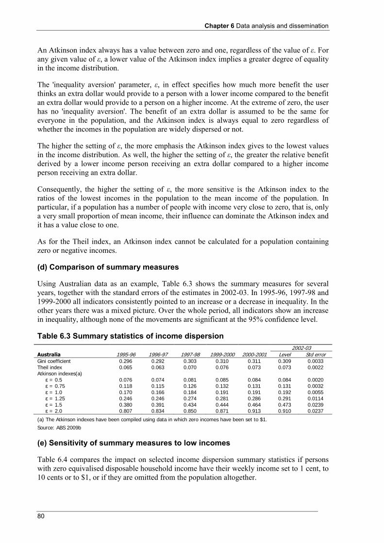
Chapter 6 Data analysis and dissemination
80
An Atkinson index always has a value between zero and one, regardless of the value of ε. For any given value of ε, a lower value of the Atkinson index implies a greater degree of equality in the income distribution.
The 'inequality aversion' parameter, ε, in effect specifies how much more benefit the user thinks an extra dollar would provide to a person with a lower income compared to the benefit an extra dollar would provide to a person on a higher income. At the extreme of zero, the user has no 'inequality aversion'. The benefit of an extra dollar is assumed to be the same for everyone in the population, and the Atkinson index is always equal to zero regardless of whether the incomes in the population are widely dispersed or not.
The higher the setting of ε, the more emphasis the Atkinson index gives to the lowest values in the income distribution. As well, the higher the setting of ε, the greater the relative benefit derived by a lower income person receiving an extra dollar compared to a higher income person receiving an extra dollar.
Consequently, the higher the setting of ε, the more sensitive is the Atkinson index to the ratios of the lowest incomes in the population to the mean income of the population. In particular, if a population has a number of people with income very close to zero, that is, only a very small proportion of mean income, their influence can dominate the Atkinson index and it has a value close to one.
As for the Theil index, an Atkinson index cannot be calculated for a population containing zero or negative incomes.
(d) Comparison of summary measures
Using Australian data as an example, Table 6.3 shows the summary measures for several years, together with the standard errors of the estimates in 2002-03. In 1995-96, 1997-98 and 1999-2000 all indicators consistently pointed to an increase or a decrease in inequality. In the other years there was a mixed picture. Over the whole period, all indicators show an increase in inequality, although none of the movements are significant at the 95% confidence level.
Table 6.3 Summary statistics of income dispersion 2002-03 Australia 1995-96 1996-97 1997-98 1999-2000 2000-2001 Level Std error Gini coefficient 0.296 0.292 0.303 0.310 0.311 0.309 0.0033 Theil index 0.065 0.063 0.070 0.076 0.073 0.073 0.0022 Atkinson indexes(a)
ε = 0.5 0.076 0.074 0.081 0.085 0.084 0.084 0.0020 ε = 0.75 0.118 0.115 0.126 0.132 0.131 0.131 0.0032 ε = 1.0 0.170 0.166 0.184 0.191 0.191 0.192 0.0055 ε = 1.25 0.246 0.246 0.274 0.281 0.286 0.291 0.0114 ε = 1.5 0.380 0.391 0.434 0.444 0.464 0.473 0.0239 ε = 2.0 0.807 0.834 0.850 0.871 0.913 0.910 0.0237
(a) The Atkinson indexes have been compiled using data in which zero incomes have been set to $1.
Source: ABS 2009b
(e) Sensitivity of summary measures to low incomes
Table 6.4 compares the impact on selected income dispersion summary statistics if persons with zero equivalised disposable household income have their weekly income set to 1 cent, to 10 cents or to $1, or if they are omitted from the population altogether.
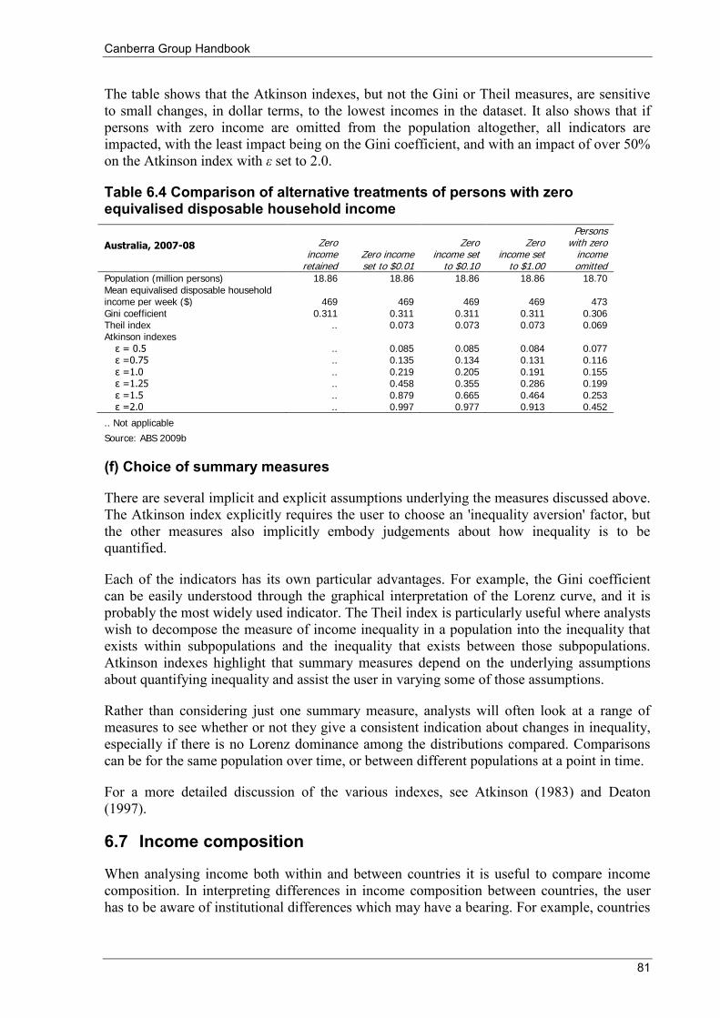
Canberra Group Handbook
81
The table shows that the Atkinson indexes, but not the Gini or Theil measures, are sensitive to small changes, in dollar terms, to the lowest incomes in the dataset. It also shows that if persons with zero income are omitted from the population altogether, all indicators are impacted, with the least impact being on the Gini coefficient, and with an impact of over 50% on the Atkinson index with ε set to 2.0.
Table 6.4 Comparison of alternative treatments of persons with zero equivalised disposable household income
Australia, 2007-08 Zero income
retained Zero income set to $0.01
Zero income set
to $0.10
Zero income set
to $1.00
Persons with zero
income omitted
Population (million persons) 18.86 18.86 18.86 18.86 18.70 Mean equivalised disposable household income per week ($) 469 469 469 469 473 Gini coefficient 0.311 0.311 0.311 0.311 0.306 Theil index .. 0.073 0.073 0.073 0.069 Atkinson indexes
ε = 0.5 .. 0.085 0.085 0.084 0.077 ε =0.75 .. 0.135 0.134 0.131 0.116 ε =1.0 .. 0.219 0.205 0.191 0.155 ε =1.25 .. 0.458 0.355 0.286 0.199 ε =1.5 .. 0.879 0.665 0.464 0.253 ε =2.0 .. 0.997 0.977 0.913 0.452
.. Not applicable
Source: ABS 2009b
(f) Choice of summary measures
There are several implicit and explicit assumptions underlying the measures discussed above. The Atkinson index explicitly requires the user to choose an 'inequality aversion' factor, but the other measures also implicitly embody judgements about how inequality is to be quantified.
Each of the indicators has its own particular advantages. For example, the Gini coefficient can be easily understood through the graphical interpretation of the Lorenz curve, and it is probably the most widely used indicator. The Theil index is particularly useful where analysts wish to decompose the measure of income inequality in a population into the inequality that exists within subpopulations and the inequality that exists between those subpopulations. Atkinson indexes highlight that summary measures depend on the underlying assumptions about quantifying inequality and assist the user in varying some of those assumptions.
Rather than considering just one summary measure, analysts will often look at a range of measures to see whether or not they give a consistent indication about changes in inequality, especially if there is no Lorenz dominance among the distributions compared. Comparisons can be for the same population over time, or between different populations at a point in time.
For a more detailed discussion of the various indexes, see Atkinson (1983) and Deaton (1997).
6.7 Income composition
When analysing income both within and between countries it is useful to compare income composition. In interpreting differences in income composition between countries, the user has to be aware of institutional differences which may have a bearing. For example, countries
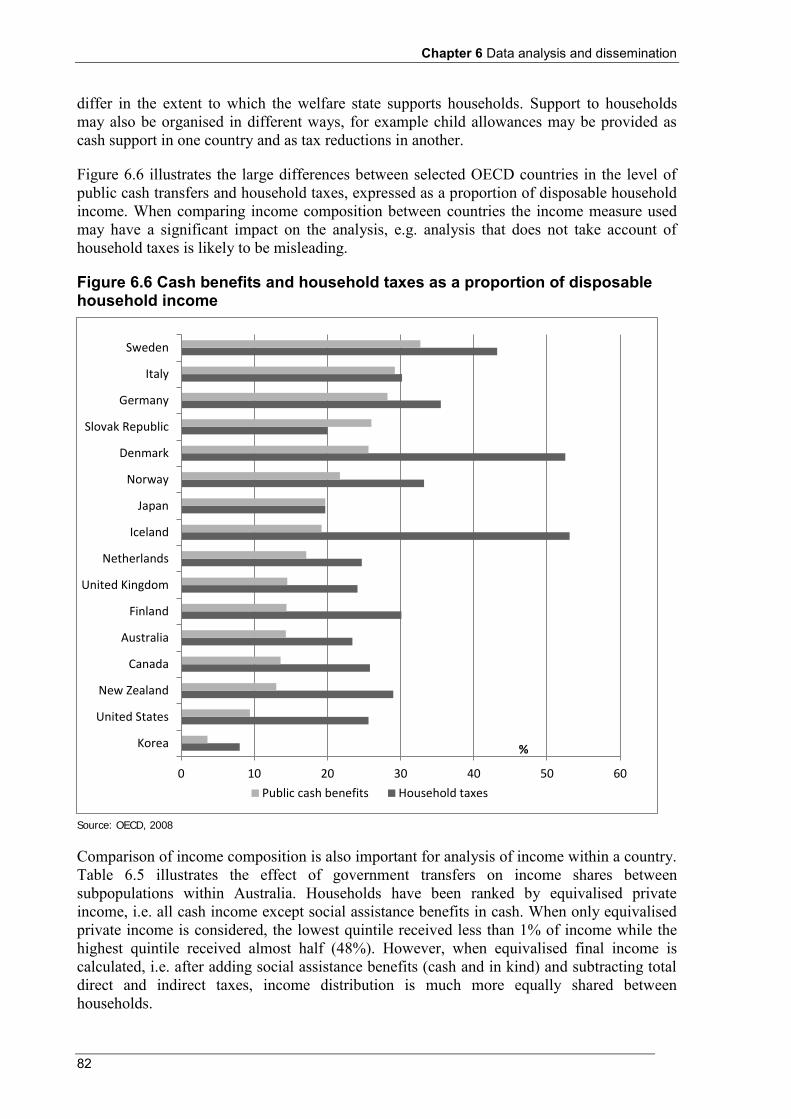
Chapter 6 Data analysis and dissemination
82
differ in the extent to which the welfare state supports households. Support to households may also be organised in different ways, for example child allowances may be provided as cash support in one country and as tax reductions in another.
Figure 6.6 illustrates the large differences between selected OECD countries in the level of public cash transfers and household taxes, expressed as a proportion of disposable household income. When comparing income composition between countries the income measure used may have a significant impact on the analysis, e.g. analysis that does not take account of household taxes is likely to be misleading.
Figure 6.6 Cash benefits and household taxes as a proportion of disposable household income
Source: OECD, 2008
Comparison of income composition is also important for analysis of income within a country. Table 6.5 illustrates the effect of government transfers on income shares between subpopulations within Australia. Households have been ranked by equivalised private income, i.e. all cash income except social assistance benefits in cash. When only equivalised private income is considered, the lowest quintile received less than 1% of income while the highest quintile received almost half (48%). However, when equivalised final income is calculated, i.e. after adding social assistance benefits (cash and in kind) and subtracting total direct and indirect taxes, income distribution is much more equally shared between households.
0 10 20 30 40 50 60
Korea
United States
New Zealand
Canada
Australia
Finland
United Kingdom
Netherlands
Iceland
Japan
Norway
Denmark
Slovak Republic
Germany
Italy
Sweden
%
Public cash benefits Household taxes
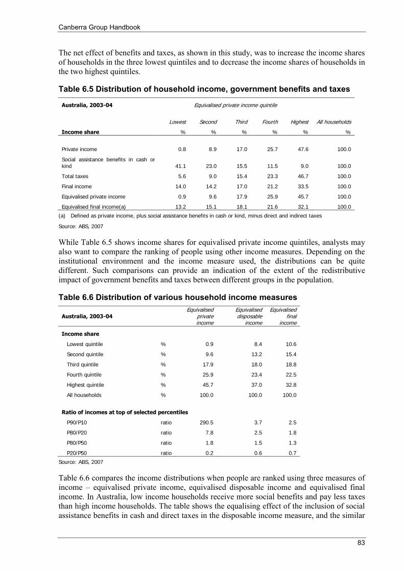
Canberra Group Handbook
83
The net effect of benefits and taxes, as shown in this study, was to increase the income shares of households in the three lowest quintiles and to decrease the income shares of households in the two highest quintiles.
Table 6.5 Distribution of household income, government benefits and taxes
Australia, 2003-04 Equivalised private income quintile
Lowest Second Third Fourth Highest All households
Income share % % % % % %
Private income 0.8 8.9 17.0 25.7 47.6 100.0
Social assistance benefits in cash or kind 41.1 23.0 15.5 11.5 9.0 100.0
Total taxes 5.6 9.0 15.4 23.3 46.7 100.0
Final income 14.0 14.2 17.0 21.2 33.5 100.0
Equivalised private income 0.9 9.6 17.9 25.9 45.7 100.0
Equivalised final income(a) 13.2 15.1 18.1 21.6 32.1 100.0
(a) Defined as private income, plus social assistance benefits in cash or kind, minus direct and indirect taxes
Source: ABS, 2007
While Table 6.5 shows income shares for equivalised private income quintiles, analysts may also want to compare the ranking of people using other income measures. Depending on the institutional environment and the income measure used, the distributions can be quite different. Such comparisons can provide an indication of the extent of the redistributive impact of government benefits and taxes between different groups in the population.
Table 6.6 Distribution of various household income measures
Australia, 2003-04
Equivalised private income
Equivalised disposable
income
Equivalised final
income
Income share
Lowest quintile % 0.9 8.4 10.6
Second quintile % 9.6 13.2 15.4
Third quintile % 17.9 18.0 18.8
Fourth quintile % 25.9 23.4 22.5
Highest quintile % 45.7 37.0 32.8
All households % 100.0 100.0 100.0
Ratio of incomes at top of selected percentiles
P90/P10 ratio 290.5 3.7 2.5
P80/P20 ratio 7.8 2.5 1.8
P80/P50 ratio 1.8 1.5 1.3
P20/P50 ratio 0.2 0.6 0.7
Source: ABS, 2007
Table 6.6 compares the income distributions when people are ranked using three measures of income – equivalised private income, equivalised disposable income and equivalised final income. In Australia, low income households receive more social benefits and pay less taxes than high income households. The table shows the equalising effect of the inclusion of social assistance benefits in cash and direct taxes in the disposable income measure, and the similar
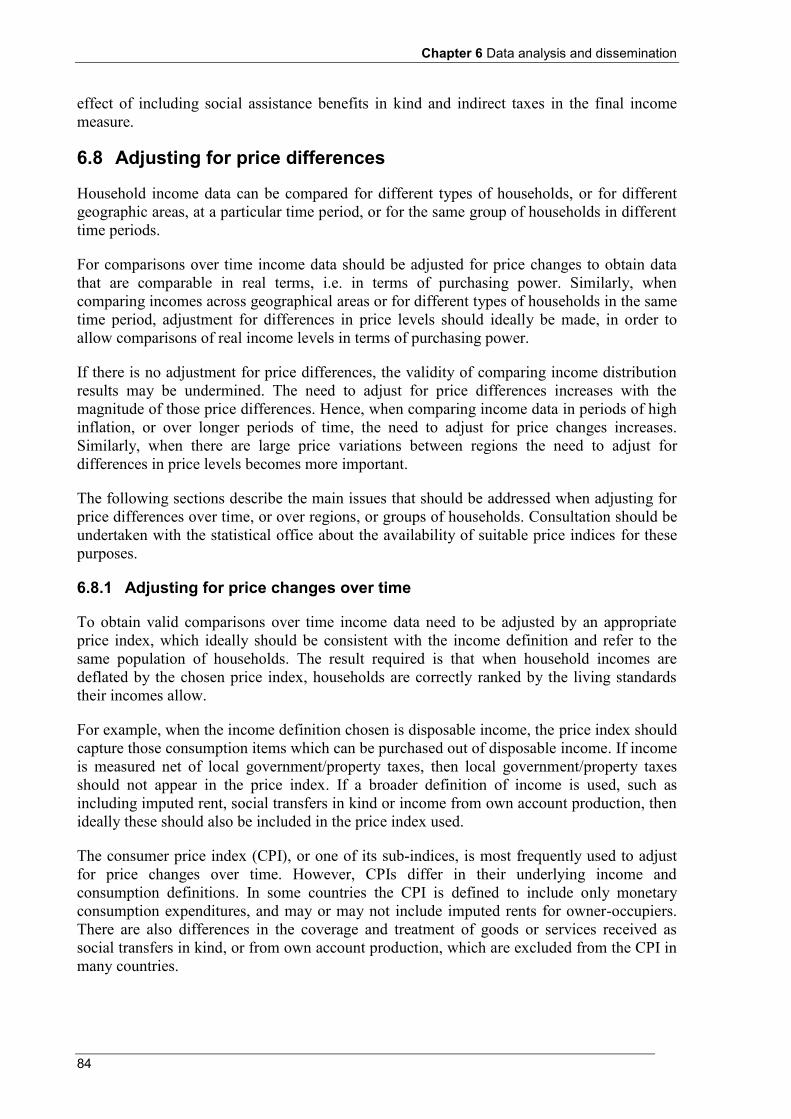
Chapter 6 Data analysis and dissemination
84
effect of including social assistance benefits in kind and indirect taxes in the final income measure.
6.8 Adjusting for price differences
Household income data can be compared for different types of households, or for different geographic areas, at a particular time period, or for the same group of households in different time periods.
For comparisons over time income data should be adjusted for price changes to obtain data that are comparable in real terms, i.e. in terms of purchasing power. Similarly, when comparing incomes across geographical areas or for different types of households in the same time period, adjustment for differences in price levels should ideally be made, in order to allow comparisons of real income levels in terms of purchasing power.
If there is no adjustment for price differences, the validity of comparing income distribution results may be undermined. The need to adjust for price differences increases with the magnitude of those price differences. Hence, when comparing income data in periods of high inflation, or over longer periods of time, the need to adjust for price changes increases. Similarly, when there are large price variations between regions the need to adjust for differences in price levels becomes more important.
The following sections describe the main issues that should be addressed when adjusting for price differences over time, or over regions, or groups of households. Consultation should be undertaken with the statistical office about the availability of suitable price indices for these purposes.
6.8.1 Adjusting for price changes over time
To obtain valid comparisons over time income data need to be adjusted by an appropriate price index, which ideally should be consistent with the income definition and refer to the same population of households. The result required is that when household incomes are deflated by the chosen price index, households are correctly ranked by the living standards their incomes allow.
For example, when the income definition chosen is disposable income, the price index should capture those consumption items which can be purchased out of disposable income. If income is measured net of local government/property taxes, then local government/property taxes should not appear in the price index. If a broader definition of income is used, such as including imputed rent, social transfers in kind or income from own account production, then ideally these should also be included in the price index used.
The consumer price index (CPI), or one of its sub-indices, is most frequently used to adjust for price changes over time. However, CPIs differ in their underlying income and consumption definitions. In some countries the CPI is defined to include only monetary consumption expenditures, and may or may not include imputed rents for owner-occupiers. There are also differences in the coverage and treatment of goods or services received as social transfers in kind, or from own account production, which are excluded from the CPI in many countries.
Canberra Group Handbook
85
The population and geographical coverage of the CPI should also be considered. Income data will often refer to resident households and consequently the ideal index for deflation should refer to the same population. However, the coverage of households in the CPI varies. In some countries the weights of the CPI are based on the so-called domestic concept, which includes consumption expenditure in the country, whether made by resident or foreign households. In countries with large cross-border shopping or substantial tourism this may mean that the overall CPI does not properly reflect the price changes that are experienced by resident households. Other countries apply the national concept for the CPI, which is based on the consumption expenditure of resident households, whether made in the country or abroad.
It is also important that the index be based on an appropriate price concept. To arrive at comparable income estimates in real terms, the price index used for deflation should be based on the prices actually paid by households, i.e. the purchaser prices, including indirect taxes and net of subsidies. This is usually the case for the CPI.
Even if a suitable CPI is available, the index may still introduce some bias if it does not reflect the actual cost of maintaining the same standard of living. CPIs keep the basket of goods and services constant for at least a year and up to five or six years. However, households tend to substitute away from goods or services with relative price increases to goods or services with relative price decreases. This means the CPI may overstate the effect of price increases on the cost of living of households. Another possible source of bias is if prices are not adjusted for quality changes.
The expenditure shares, or ‘weights’, of the goods and services in the CPI are usually calculated as the relative expenditures of the household sector. Therefore the consumption pattern of high income households, which often consume more, will be attributed a larger weight than the consumption pattern of low income households. While this is appropriate for measuring overall price changes it may not suit income studies that wish to attribute equal weights to all households.
To consider the appropriateness of the CPI in terms of coverage of goods and services, population and geographical coverage, and whether the index is likely to introduce any bias into the income statistics, analysts should consult with the compilers of the CPI or any other price index that is used. The index compilers will also be able to provide more information on the availability of price indices for types of households or by region.
Table 6.7 illustrates how consumer price inflation can differ between various population groups, e.g. lone parents and those living in Paris experienced higher annual inflation than the average rate for France as a whole, while households living in small towns and couples with children experienced a lower rate. For this exercise the CPI weights available at the national level were replaced by specific sets of weights for each of the household categories derived from the French Household Expenditure Survey. By applying these weights and the sub-indices of the national CPI, price indices for the specific groups of households were estimated. While the estimates only take into account differences in consumption patterns (and not in prices) between the household groups they provide a better measure of the conditions for specific groups.
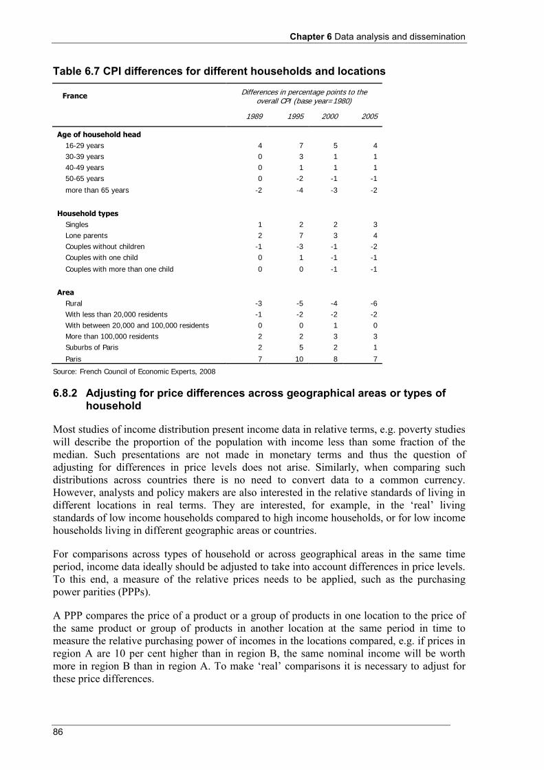
Chapter 6 Data analysis and dissemination
86
Table 6.7 CPI differences for different households and locations
France Differences in percentage points to the
overall CPI (base year=1980)
1989 1995 2000 2005
Age of household head
16-29 years 4 7 5 4
30-39 years 0 3 1 1
40-49 years 0 1 1 1
50-65 years 0 -2 -1 -1
more than 65 years -2 -4 -3 -2
Household types
Singles 1 2 2 3
Lone parents 2 7 3 4
Couples without children -1 -3 -1 -2
Couples with one child 0 1 -1 -1
Couples with more than one child 0 0 -1 -1
Area
Rural -3 -5 -4 -6
With less than 20,000 residents -1 -2 -2 -2
With between 20,000 and 100,000 residents 0 0 1 0
More than 100,000 residents 2 2 3 3
Suburbs of Paris 2 5 2 1
Paris 7 10 8 7
Source: French Council of Economic Experts, 2008
6.8.2 Adjusting for price differences across geographical areas or types of household
Most studies of income distribution present income data in relative terms, e.g. poverty studies will describe the proportion of the population with income less than some fraction of the median. Such presentations are not made in monetary terms and thus the question of adjusting for differences in price levels does not arise. Similarly, when comparing such distributions across countries there is no need to convert data to a common currency. However, analysts and policy makers are also interested in the relative standards of living in different locations in real terms. They are interested, for example, in the ‘real’ living standards of low income households compared to high income households, or for low income households living in different geographic areas or countries.
For comparisons across types of household or across geographical areas in the same time period, income data ideally should be adjusted to take into account differences in price levels. To this end, a measure of the relative prices needs to be applied, such as the purchasing power parities (PPPs).
A PPP compares the price of a product or a group of products in one location to the price of the same product or group of products in another location at the same period in time to measure the relative purchasing power of incomes in the locations compared, e.g. if prices in region A are 10 per cent higher than in region B, the same nominal income will be worth more in region B than in region A. To make ‘real’ comparisons it is necessary to adjust for these price differences.
Canberra Group Handbook
87
PPPs have primarily been developed to facilitate international comparisons of economic data, in particular the national accounts and its aggregates. They are therefore usually only compiled at country level, and cannot be broken down by regions or types of households. However, in some (usually larger) countries, PPPs may also be compiled at a regional level, and in other countries, PPP surveys that allow construction of regional aggregates may be conducted on an ad-hoc basis.
In most countries, PPPs are compiled to cover a wide range of goods and services beyond household consumption. When PPPs for individual consumption by households are available they should be used for income distribution. PPP sub-indices that exclude goods and services such as health care, education and housing, which may be purchased by households rather than provided by government in different countries, may also be available.
PPPs are regularly compiled by OECD and Eurostat for their member countries and some additional countries. PPPs are compiled less frequently by the World Bank for a wider range of countries as part of the International Comparison Programme. When PPPs are not available annually, those which are as close as possible to the years for which the household income data are to be compared should be used.
For international comparisons it is highly recommended that PPPs be used, rather than exchange rates for conversion into a common currency. When an economic aggregate such as household income is converted using PPPs for household consumption expenditure, the conversion is made on the basis of the goods and services likely to be purchased by households for consumption purposes, as well as taking account of differences in national price levels. This allows comparisons in real terms, or purchasing power, of the converted amounts.
The PPPs are compiled by comparing the average price of groups of goods and services in different countries. However, it may not always be possible to obtain identical products in different countries, or the products when found may be of different economic importance in the countries compared. Thus, PPPs for countries with similar structure and income level may provide fairly good indices for adjusting income data, while the suitability of the PPPs is likely to decrease the more the countries differ in structure and income level.
Differences in climate and natural resources also play a role, e.g. heating is important in colder climates, while air-conditioning is not. Food is another area where comparisons are difficult since a staple in one country may be a somewhat exotic article elsewhere.
Appendix 5 provides further information on the concepts and methodology of PPPs.
Box 6.3 outlines some analytical work undertaken by Statistics Canada on regional comparisons of low incomes.
Box 6.3 Spatial price indexes in Canada
Statistics Canada has examined what would happen to low income statistics if income was adjusted by a spatial price index, while keeping national low income thresholds constant (in Canada, the low income threshold is defined as 50% of the adjusted family income).
While at the aggregate level, low income (poverty) measures, both in terms of level and changes, did not change in any significant way after taking regional price differences into
Chapter 6 Data analysis and dissemination
88
consideration (Pendakar, 2002), low income statistics at the provincial and city level changed significantly. As might be expected, there were increases in the low income measure for cities and regions with higher costs of living, and decreases for cities and regions with lower costs of living.
The creation of a spatial price index can be costly and there might be alternative ways to reflect differential costs of living. Canada is examining the development of local low income measures as a possible way to take into account different costs of living, without having to calculate purchasing power parities.
6.9 Analysis of low income households and income poverty
6.9.1 Introduction
Income received may be used to purchase goods and services, or saved and invested to increase wealth. People living in low income households are more likely to have insufficient economic resources to support an acceptable standard of living. However, those people with low household income, but with reserves of wealth, can utilise those reserves to support their consumption.
A full understanding of economic well-being, or economic hardship, requires consideration of all types of economic resources, as well as people’s particular consumption patterns and living arrangements. In addition, a full understanding of poverty requires information in many non-economic dimensions because it does not consist merely of an insufficiency of resources, but also encompasses cumulative deprivation in relation to income, housing, education and health care (Atkinson et. al., 2002). However these types of analyses have significant data requirements.
Traditionally, measures of income poverty have classified households as being at risk of poverty if their income is less than the value of a given monetary threshold (‘poverty line’).
There is a vast literature on the measurement and analysis of income poverty. Over the past decade there have been three sets of international guidelines produced on the measurement of poverty:
Compendium of best practices in poverty measurement, produced by the Expert Group on Poverty Statistics (Rio Group, 2006)
Handbook on poverty statistics: Concepts, methods and policy use, under development by the United Nations Statistical Division
Handbook on poverty and inequality, published by the World Bank (Haughton and Khandker, 2009)
The chapter on Financial Poverty in Social Indicators, The EU and Social Inclusion also provides a useful reference (Atkinson et. al., 2002).
6.9.2 Income poverty approaches This section provides a brief overview of three basic, but widely used, approaches to define income poverty lines:
absolute or basket of goods poverty line
Canberra Group Handbook
89
poverty line based on social consensus
relative or distribution based poverty line.
As is generally the case for income distribution analyses, the household is the unit of analysis for poverty measurement. The methods described below identify people living in households at risk of income poverty.
Absolute or basket of goods poverty line
Many poverty lines ‘… represent the cost of buying a basket of goods that allows one to meet the absolute thresholds of satisfying certain basic needs' (Rio Group, 2006, p 53). Persons living in households with income below that needed to purchase the items required are deemed to be at risk of poverty. In some variants the threshold is set as a multiple of the price of a basic food basket to allow for non-food expenditure (Orshansky, 1965).
The basket of goods can be determined on a per-capita basis for each individual or can be distinguished for different types of households, thus providing an implicit scale of equivalence. To be effective, poverty lines which are based on a basket of goods need to reflect local prices and consumption patterns. A particular difficulty is determining the appropriate level of basic needs. While fixed poverty lines are often referred to as absolute, in practice they are always based on those basic needs defined by the cultural norms of society (Rio Group, 2006).
Absolute poverty lines aim to have the same real value across different times and places. However, this is difficult to achieve given the variation in circumstances between countries and often between regions within one country. Also the base of the absolute measure, that is the basket of goods, is likely to need updating over time as community standards or expectations change.
Poverty line based on social consensus
Other poverty lines use minimum thresholds decided by societal standards. For example, persons may be asked what minimum level of income they consider as adequate for a given type of household. The average of these responses would then provide a simple income cut-off for determining who is at risk of income poverty for any type of household. This idea inspired more refined, so-called subjective poverty lines reviewed for example by Karel Van den Bosch (2001).
An assumed advantage of poverty lines which are based on such subjective evaluations is that it is less arbitrary, as the definition of the poverty line is derived from the population itself and not by expert opinion. However, this approach also requires certain assumptions, including that households will have a similar notion of what should be considered income.
Relative or distribution based poverty lines
While basket of goods based poverty lines have traditionally dominated the practice of poverty measurement in developing countries, relative poverty lines are more commonly used in developed countries. A relative approach to poverty measurement uses data on the distribution of resources and defines the poverty line as a proportion of some notion of standards of living (Rio Group, 2006).
Chapter 6 Data analysis and dissemination
90
The most common measure is the ‘headcount ratio’ based on the proportion of people within a country with an income below a certain fraction of median equivalised disposable household income in that country, e.g. Eurostat commonly uses 60% while OECD reports often rely on 50%. While these measures adjust in some ways to shifting social norms in a country, the number of people identified as being in poverty is determined by a somewhat arbitrary limit to inequality of the income distribution.
By setting the low income threshold as a fraction of the median value, by definition, it is not possible to have a poverty rate higher than 50%. Values near 50% would imply a rather unusual shape of the income distribution and will seldom be observed. In practice, between 1998 and 2009 the 60% of median based at-risk-of-poverty rates never exceeded 26% in European countries.
Furthermore, if the shape of the distribution does not change, the same proportion of people will remain in relative poverty regardless of any changes in their circumstances. For example, if everyone in society increased their incomes by 10% in real terms, the proportion of people identified below the relative poverty line will not change.
On the other hand, if the shape of the distribution does change, the proportion of people identified by the measure can change dramatically. For example, in the Australian context, the thresholds identified at 40% and 50% of median incomes are particularly sensitive to change depending on the location of single and couple pension payment points in the income distribution.
For these reasons, many analysts measure poverty based on a poverty line fixed in real terms at a specified date. The number of years for which the fixed line in the base year can reasonably be carried forward depends on the growth of real income and on the changes that have taken place in the distribution (Atkinson et al., 2002).
With all poverty approaches methodological assumptions are important. Firstly, the definition and measurement of income have a significant impact. For example, social transfers in kind are often excluded from income definitions due to the absence of appropriate data. However an individual with access to social provisions such as education and health care is likely to be better off than an individual with the same monetary resources but without access to such social provisions.
The relative position of certain subpopulations may also be significantly affected by the income definition used. In Denmark, for example, the inclusion of imputed rent in the income definition lowers the (relative) at-risk-of-poverty headcount of the elderly from around 10% to around 4% (OECD, 2008).
A second consideration relates to the sensitivity concerning the equivalence scale used to determine the low income threshold. This choice predetermines the relative position of single person households against larger households. If the living cost for additional household members (in particular children) implicitly assumed in an equivalence scale is high, then single person households, typically the elderly, will be attributed a relatively better position in the income distribution compared to the low income line.
Lastly, a further limitation with the distribution based approach is the arbitrary decision concerning the specific fraction of median or mean income to be used.
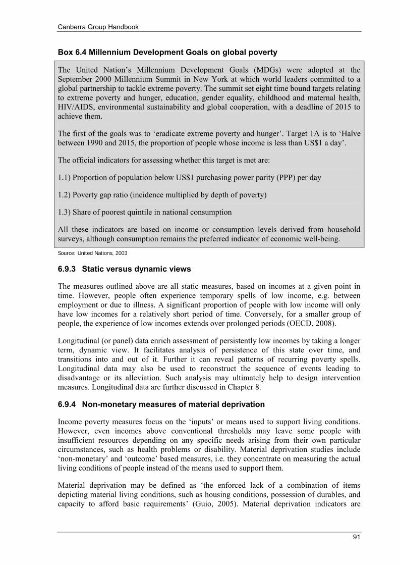
Canberra Group Handbook
91
Box 6.4 Millennium Development Goals on global poverty
The United Nation’s Millennium Development Goals (MDGs) were adopted at the September 2000 Millennium Summit in New York at which world leaders committed to a global partnership to tackle extreme poverty. The summit set eight time bound targets relating to extreme poverty and hunger, education, gender equality, childhood and maternal health, HIV/AIDS, environmental sustainability and global cooperation, with a deadline of 2015 to achieve them.
The first of the goals was to ‘eradicate extreme poverty and hunger’. Target 1A is to ‘Halve between 1990 and 2015, the proportion of people whose income is less than US$1 a day’.
The official indicators for assessing whether this target is met are:
1.1) Proportion of population below US$1 purchasing power parity (PPP) per day
1.2) Poverty gap ratio (incidence multiplied by depth of poverty)
1.3) Share of poorest quintile in national consumption
All these indicators are based on income or consumption levels derived from household surveys, although consumption remains the preferred indicator of economic well-being.
Source: United Nations, 2003
6.9.3 Static versus dynamic views
The measures outlined above are all static measures, based on incomes at a given point in time. However, people often experience temporary spells of low income, e.g. between employment or due to illness. A significant proportion of people with low income will only have low incomes for a relatively short period of time. Conversely, for a smaller group of people, the experience of low incomes extends over prolonged periods (OECD, 2008).
Longitudinal (or panel) data enrich assessment of persistently low incomes by taking a longer term, dynamic view. It facilitates analysis of persistence of this state over time, and transitions into and out of it. Further it can reveal patterns of recurring poverty spells. Longitudinal data may also be used to reconstruct the sequence of events leading to disadvantage or its alleviation. Such analysis may ultimately help to design intervention measures. Longitudinal data are further discussed in Chapter 8.
6.9.4 Non-monetary measures of material deprivation
Income poverty measures focus on the ‘inputs’ or means used to support living conditions. However, even incomes above conventional thresholds may leave some people with insufficient resources depending on any specific needs arising from their own particular circumstances, such as health problems or disability. Material deprivation studies include ‘non-monetary’ and ‘outcome’ based measures, i.e. they concentrate on measuring the actual living conditions of people instead of the means used to support them.
Material deprivation may be defined as ‘the enforced lack of a combination of items depicting material living conditions, such as housing conditions, possession of durables, and capacity to afford basic requirements’ (Guio, 2005). Material deprivation indicators are
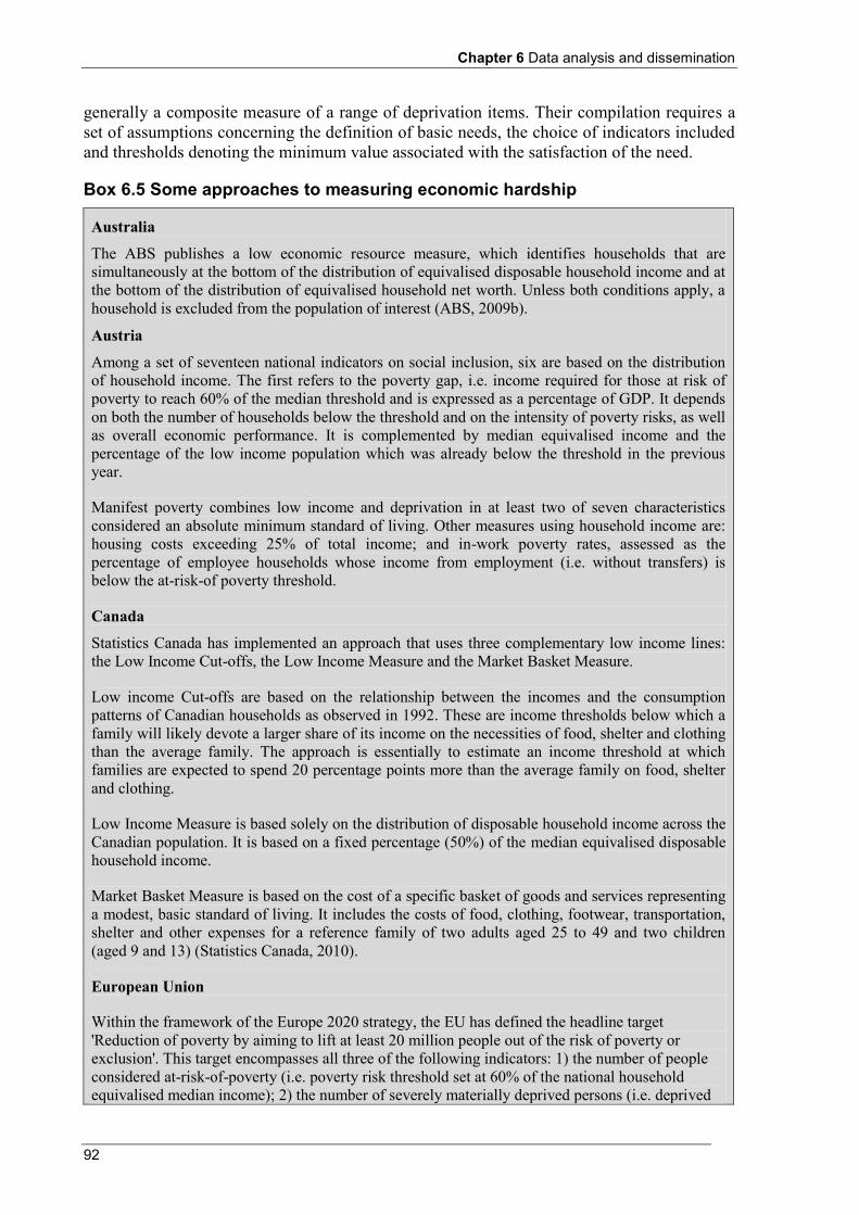
Chapter 6 Data analysis and dissemination
92
generally a composite measure of a range of deprivation items. Their compilation requires a set of assumptions concerning the definition of basic needs, the choice of indicators included and thresholds denoting the minimum value associated with the satisfaction of the need.
Box 6.5 Some approaches to measuring economic hardship
Australia The ABS publishes a low economic resource measure, which identifies households that are simultaneously at the bottom of the distribution of equivalised disposable household income and at the bottom of the distribution of equivalised household net worth. Unless both conditions apply, a household is excluded from the population of interest (ABS, 2009b). Austria Among a set of seventeen national indicators on social inclusion, six are based on the distribution of household income. The first refers to the poverty gap, i.e. income required for those at risk of poverty to reach 60% of the median threshold and is expressed as a percentage of GDP. It depends on both the number of households below the threshold and on the intensity of poverty risks, as well as overall economic performance. It is complemented by median equivalised income and the percentage of the low income population which was already below the threshold in the previous year.
Manifest poverty combines low income and deprivation in at least two of seven characteristics considered an absolute minimum standard of living. Other measures using household income are: housing costs exceeding 25% of total income; and in-work poverty rates, assessed as the percentage of employee households whose income from employment (i.e. without transfers) is below the at-risk-of poverty threshold.
Canada Statistics Canada has implemented an approach that uses three complementary low income lines: the Low Income Cut-offs, the Low Income Measure and the Market Basket Measure.
Low income Cut-offs are based on the relationship between the incomes and the consumption patterns of Canadian households as observed in 1992. These are income thresholds below which a family will likely devote a larger share of its income on the necessities of food, shelter and clothing than the average family. The approach is essentially to estimate an income threshold at which families are expected to spend 20 percentage points more than the average family on food, shelter and clothing.
Low Income Measure is based solely on the distribution of disposable household income across the Canadian population. It is based on a fixed percentage (50%) of the median equivalised disposable household income.
Market Basket Measure is based on the cost of a specific basket of goods and services representing a modest, basic standard of living. It includes the costs of food, clothing, footwear, transportation, shelter and other expenses for a reference family of two adults aged 25 to 49 and two children (aged 9 and 13) (Statistics Canada, 2010).
European Union
Within the framework of the Europe 2020 strategy, the EU has defined the headline target 'Reduction of poverty by aiming to lift at least 20 million people out of the risk of poverty or exclusion'. This target encompasses all three of the following indicators: 1) the number of people considered at-risk-of-poverty (i.e. poverty risk threshold set at 60% of the national household equivalised median income); 2) the number of severely materially deprived persons (i.e. deprived
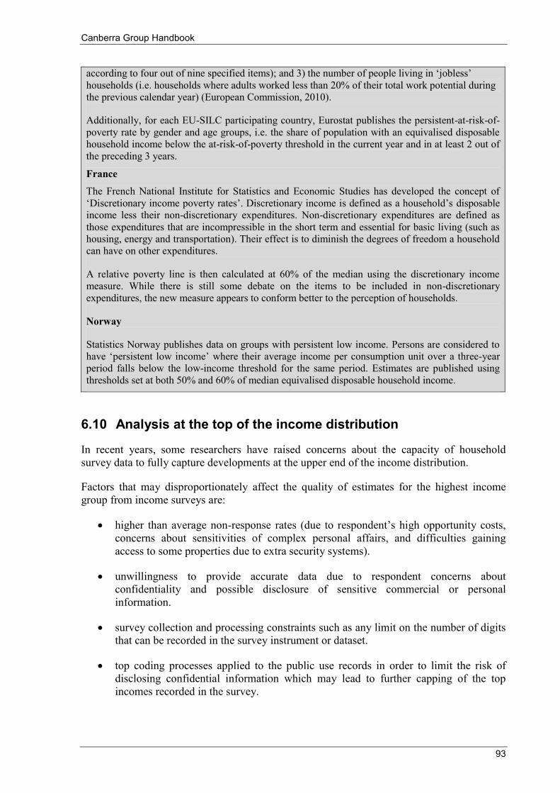
Canberra Group Handbook
93
according to four out of nine specified items); and 3) the number of people living in ‘jobless’ households (i.e. households where adults worked less than 20% of their total work potential during the previous calendar year) (European Commission, 2010).
Additionally, for each EU-SILC participating country, Eurostat publishes the persistent-at-risk-of-poverty rate by gender and age groups, i.e. the share of population with an equivalised disposable household income below the at-risk-of-poverty threshold in the current year and in at least 2 out of the preceding 3 years. France The French National Institute for Statistics and Economic Studies has developed the concept of ‘Discretionary income poverty rates’. Discretionary income is defined as a household’s disposable income less their non-discretionary expenditures. Non-discretionary expenditures are defined as those expenditures that are incompressible in the short term and essential for basic living (such as housing, energy and transportation). Their effect is to diminish the degrees of freedom a household can have on other expenditures.
A relative poverty line is then calculated at 60% of the median using the discretionary income measure. While there is still some debate on the items to be included in non-discretionary expenditures, the new measure appears to conform better to the perception of households.
Norway
Statistics Norway publishes data on groups with persistent low income. Persons are considered to have ‘persistent low income’ where their average income per consumption unit over a three-year period falls below the low-income threshold for the same period. Estimates are published using thresholds set at both 50% and 60% of median equivalised disposable household income.
6.10 Analysis at the top of the income distribution
In recent years, some researchers have raised concerns about the capacity of household survey data to fully capture developments at the upper end of the income distribution.
Factors that may disproportionately affect the quality of estimates for the highest income group from income surveys are:
higher than average non-response rates (due to respondent’s high opportunity costs, concerns about sensitivities of complex personal affairs, and difficulties gaining access to some properties due to extra security systems).
unwillingness to provide accurate data due to respondent concerns about confidentiality and possible disclosure of sensitive commercial or personal information.
survey collection and processing constraints such as any limit on the number of digits that can be recorded in the survey instrument or dataset.
top coding processes applied to the public use records in order to limit the risk of disclosing confidential information which may lead to further capping of the top incomes recorded in the survey.
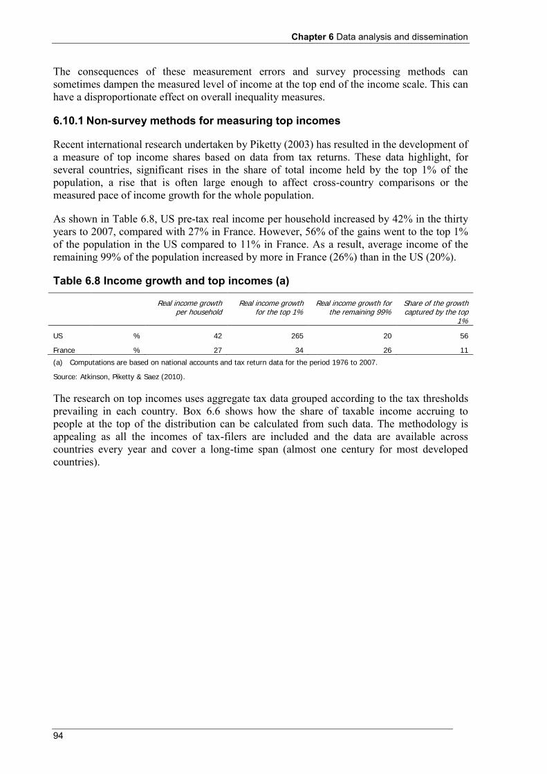
Chapter 6 Data analysis and dissemination
94
The consequences of these measurement errors and survey processing methods can sometimes dampen the measured level of income at the top end of the income scale. This can have a disproportionate effect on overall inequality measures.
6.10.1 Non-survey methods for measuring top incomes
Recent international research undertaken by Piketty (2003) has resulted in the development of a measure of top income shares based on data from tax returns. These data highlight, for several countries, significant rises in the share of total income held by the top 1% of the population, a rise that is often large enough to affect cross-country comparisons or the measured pace of income growth for the whole population.
As shown in Table 6.8, US pre-tax real income per household increased by 42% in the thirty years to 2007, compared with 27% in France. However, 56% of the gains went to the top 1% of the population in the US compared to 11% in France. As a result, average income of the remaining 99% of the population increased by more in France (26%) than in the US (20%).
Table 6.8 Income growth and top incomes (a)
Real income growth per household
Real income growth for the top 1%
Real income growth for the remaining 99%
Share of the growth captured by the top
1%
US % 42 265 20 56
France % 27 34 26 11
(a) Computations are based on national accounts and tax return data for the period 1976 to 2007.
Source: Atkinson, Piketty & Saez (2010).
The research on top incomes uses aggregate tax data grouped according to the tax thresholds prevailing in each country. Box 6.6 shows how the share of taxable income accruing to people at the top of the distribution can be calculated from such data. The methodology is appealing as all the incomes of tax-filers are included and the data are available across countries every year and cover a long-time span (almost one century for most developed countries).
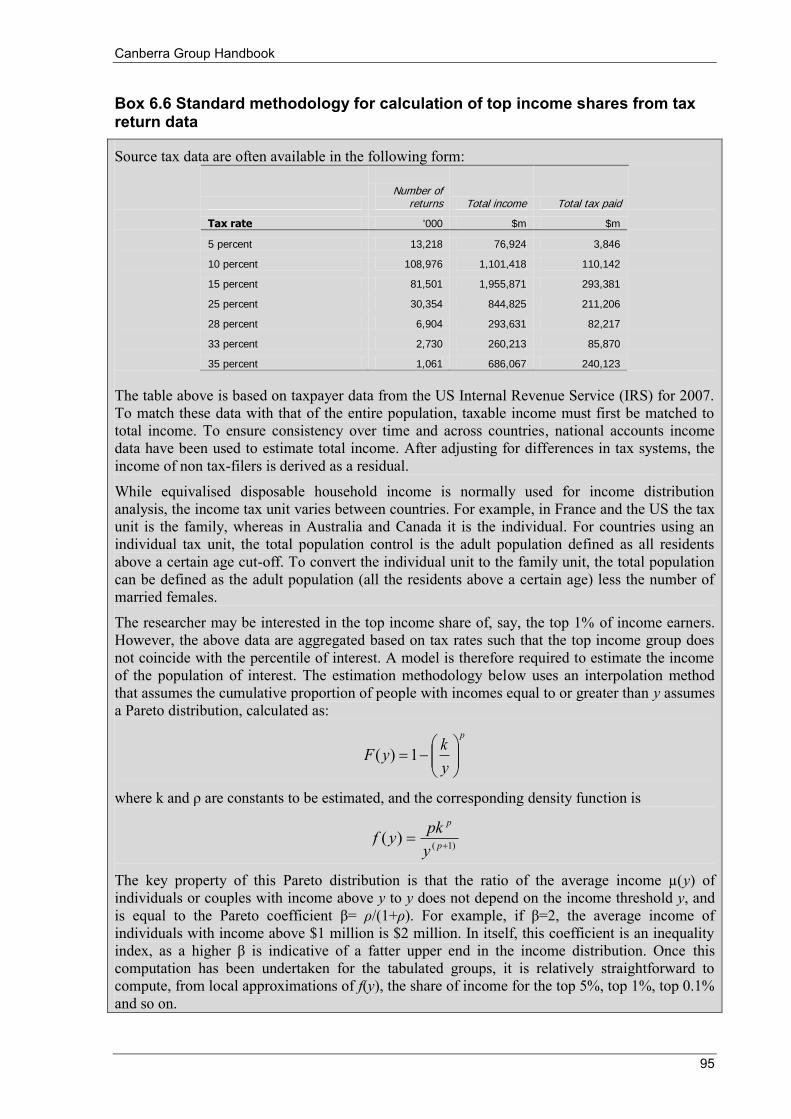
Canberra Group Handbook
95
Box 6.6 Standard methodology for calculation of top income shares from tax return data
Source tax data are often available in the following form:
Number of
returns Total income Total tax paid
Tax rate '000 $m $m
5 percent 13,218 76,924 3,846
10 percent 108,976 1,101,418 110,142
15 percent 81,501 1,955,871 293,381
25 percent 30,354 844,825 211,206
28 percent 6,904 293,631 82,217
33 percent 2,730 260,213 85,870
35 percent 1,061 686,067 240,123
The table above is based on taxpayer data from the US Internal Revenue Service (IRS) for 2007. To match these data with that of the entire population, taxable income must first be matched to total income. To ensure consistency over time and across countries, national accounts income data have been used to estimate total income. After adjusting for differences in tax systems, the income of non tax-filers is derived as a residual.
While equivalised disposable household income is normally used for income distribution analysis, the income tax unit varies between countries. For example, in France and the US the tax unit is the family, whereas in Australia and Canada it is the individual. For countries using an individual tax unit, the total population control is the adult population defined as all residents above a certain age cut-off. To convert the individual unit to the family unit, the total population can be defined as the adult population (all the residents above a certain age) less the number of married females.
The researcher may be interested in the top income share of, say, the top 1% of income earners. However, the above data are aggregated based on tax rates such that the top income group does not coincide with the percentile of interest. A model is therefore required to estimate the income of the population of interest. The estimation methodology below uses an interpolation method that assumes the cumulative proportion of people with incomes equal to or greater than y assumes a Pareto distribution, calculated as:
p
ykyF
1)(
where k and ρ are constants to be estimated, and the corresponding density function is
)1()(
p
p
ypkyf
The key property of this Pareto distribution is that the ratio of the average income µ(y) of individuals or couples with income above y to y does not depend on the income threshold y, and is equal to the Pareto coefficient β= ρ/(1+ρ). For example, if β=2, the average income of individuals with income above $1 million is $2 million. In itself, this coefficient is an inequality index, as a higher β is indicative of a fatter upper end in the income distribution. Once this computation has been undertaken for the tabulated groups, it is relatively straightforward to compute, from local approximations of f(y), the share of income for the top 5%, top 1%, top 0.1% and so on.
Chapter 6 Data analysis and dissemination
96
However, several factors can reduce the validity of analyses based on tax records. In particular:
changes in tax legislation, e.g. lowering of personal tax rates might lead individuals to shift their business income from corporate tax returns to individual tax returns, which may inflate the share of (personal) taxable income accruing to the very rich. That is, people with very high incomes may not earn more income but simply declare more of their income as part of their personal tax declaration.
tax evasion and tax avoidance schemes.
changes in marginal tax rates could lead to changes in the income that is reported on tax records. Most studies on the subject suggest that the elasticity of taxable income with respect to changes in tax rates is positive, and is typically between 0.5 and 1% (Gruber and Saez, 2002). This implies that, when the upper marginal income tax rate drops from 40 to 30% the amount of income reported would increase by between 8% and 16%. Again, the share of income going to the top income bracket may not mean that the rich are getting richer, only that more of their income is disclosed.
cash transfer payments are often targeted at low income families who may not be required to complete tax declarations. As well, the exclusion of these transfers from the income definition used in these studies reduces their usefulness to assess the size of the redistribution achieved in a country.
Despite these limitations, studies based on tax records point to patterns that are large enough to change analysts appreciation of what is happening to income distribution. They highlight that care must be taken to assess trends in the upper end of the distribution based on survey results alone, particularly if there is evidence that these may not be totally representative of the population.
6.11 Best practice guidelines for dissemination of income data
The key principle for dissemination of income statistics is to prioritise robustness statements and to highlight issues that users need to be aware of. The presentation should not tempt the reader to place more interpretation on the figures than they can reasonably bear. Due to their complexity, income statistics can never be self-explanatory. It is therefore inevitable that there will be a need to provide direct guidance for their correct interpretation and clear reference to more detailed metadata in all dissemination activities. Comprehensive and easily accessible metadata should always be disseminated.
As a source of institutional memory for future exercises, and for consultation by others who would need such information, a detailed methodological report should be prepared including full details of the procedures used, as well as lessons learned and conclusions.
As much as possible, without breaching the confidentiality of information collected, public use files (anonymised micro datasets) should be made available. They should always be accompanied by clear and comprehensive documentation on all aspects of the data collection and derivations. In particular, if top coding (restricting the maximum value disseminated for a variable) is used to protect the confidentiality of information, the details should be documented and the values should be identified, e.g. by flag variables indicating the percentage of imputed information.
Canberra Group Handbook
97
As data collected by government are a public good, public-use files should be made available free or at marginal cost to non-commercial institutions, agencies and researchers. Users of micro data should in turn provide information on their findings and be included in a bibliographic database. This will ensure effective utilisation of the data, stimulate more in depth study, and encourage dialogue and feedback between the data producers and users.
Best practice related to the quality assurance of statistical data has been discussed in Chapter 5. Useful guidelines for the general presentation and dissemination of statistical output have also been developed by UNECE (2009b and 2009c). Further guidance for the proper interpretation of income statistics is provided below.
(a) Concise and clear definitions of the income concepts and measures used
Glossary – a minimum would be an information box explaining what income components are included and excluded in the calculation of the income measures produced.
Illustrative calculations for model families – particularly for press releases or for releases aimed at a broader public. It is important to demonstrate how equivalised disposable household income relates to, for example, an individual’s gross salary.
Separation of measured and non-measured income – to what extent do the results cover non-measured income components, notably imputed incomes for owner-occupied housing, health and education consumption provided by government.
Indicators – for example, include a clear definition of the criteria for determining if someone is at risk of poverty for income based poverty statistics. Ideally, the algorithms used will be made available as metadata.
(b) Basic information about data sources
Source of data – whether data are taken from a census, administrative data, a sample survey, or a combination of sources. If the data are from a combination of sources, a description of how the data from the multiple sources are used to produce the estimates being disseminated should be provided. If comparative data are presented, it is important to acknowledge whether it was obtained by means of input harmonised surveys (such as the ECHP), output harmonised statistics (such as EU-SILC), ex-post harmonised data (such as in the LIS), or on the basis of standard tabulations (such as the detailed data questionnaires used by the OECD).
Purpose – a clear description of the purpose of the data source being disseminated is required. In the case of a survey, this would be a general description of the reasons the survey was conducted. For administrative data, this would be a description of the reason why the administrative data are collected and how it represents a source of data that is useful for statistical purposes.
Subject matter or content of the data source – a general description of the content areas or modules, including, possibly, a link to a questionnaire, file layout or data dictionary to provide information on the data available.
Statistical units – individuals, families or households.
Chapter 6 Data analysis and dissemination
98
Reference period(s) – the time period(s) covered in the data being disseminated.
Survey population – who is included, and equally important, excluded in the survey population. For example, does the data source include the entire population or only a subgroup of the population, such as a specific age group.
Sample size and design – including whether a probability sample has been used (or alternatively whether random walk or quota methods were applied); coverage of the survey population in the sampling frame; and whether the design was single stage or involved some clustering.
(c) Data quality
As noted in Chapter 5, it is important that there is a quality assurance framework applied for any statistical program. When disseminating income data, users should be informed of the quality of the data being presented, including the following information:
Sampling errors – where information is from probability samples, an indication of sampling error should be provided. Design effects due to clustering or unequal selection probabilities should be taken into account (see Chapter 5). As a minimum, the relative standard error, i.e. the standard error expressed as a percentage of the estimate for which it is calculated, should be provided for the key variables being disseminated.
Suppression of unreliable data – while it is recommended that figures for which the relative standard error exceeds a certain limit should not be published, the thresholds for suppression should be based on the professional’s judgment of the ‘fitness for use’ of the estimates. Estimates can be divided into three groups: those with a low RSE, which can be used without restriction; those with a higher RSE, where the data should be used with caution; and the third group, where data with a very high RSE are suppressed. In the case of complex designs or indicators, the standard errors may not be readily available for all estimates. In this case it can be appropriate to use the number of underlying observations instead. For example, if it was found that estimates with an acceptable standard error normally were based on at least 30 observations, then they would suppress any estimates based on fewer than 30 observations.
Response errors – these may be due to many factors, including faulty design of the questionnaire, interviewers’ or respondents’ misinterpretation of questions, or respondents’ lack of knowledge/records or faulty reporting. If there is information available on the type of response errors which may have occurred in a survey, this should be provided in the documentation which accompanies the dissemination of results.
Non-response errors – in surveys, non-response errors occur because some sample units do not respond to the survey. Response rates should be provided to users including any information available on the units who did not respond (e.g. if specific geographic areas or age groups had higher non-response rates) and, in the case of time series data, if the non-response pattern is different now than in the past. For correct interpretation of response rates it is useful to provide information on whether substitutions were allowed.
Canberra Group Handbook
99
Effect of large values – income data can be particularly affected by the presence or absence of extreme values. An explanation of any procedures applied to the data to account for extreme values should be included in the documentation. At a minimum, users should be informed of the fact that the results may include extreme values and that some estimates may be influenced by the presence or absence of these extremes.
Percentage of imputed information – for each income aggregate the number of incomplete units and the percentage of the income amount which was imputed should be specified.
Comparability of the data over time – when time series data are being disseminated it is important to inform users of any changes to the data that may have affected the data for the time period covered. For example, if the data source is tax records, it is important to provide to users information of any changes in the tax systems which might affect the data. In the case of a survey, if there were changes to the way in which the data were collected over the time period, or changes in survey concepts, then it is important to mention these changes in the documentation which accompanies the release of data. Ideally, data in a time series will be adjusted to ensure the data are comparable over time, but often it is not possible to quantify the precise effect of these changes.

100
101
Chapter 7 Comparing income distributions over time 7.1 Introduction
Economists and social policy analysts are increasingly focusing on long run trends in income distribution. The availability of 20 to 40 years or more of estimates in many nations is making it possible for analysts to study the determinants and consequences of long periods of distributional change, for example the relationship between income inequality and GDP growth.
The future will bring more uses of such data, and the policy discussions of national governments and international bodies may be heavily influenced by such trends and analyses. For this debate to be well informed, high standards must be set for the compilation of time series data on income distributions. This chapter discusses the compilation and analysis of income distributions over time, using data from repeated cross-sectional household surveys or administrative data sources.
7.2 Undertaking cross-time comparisons
Conceptually, cross-time comparisons within a country are not really different from cross-country comparisons at a point in time. The general consistency requirements are exactly the same. However the analysis of time series needs separate discussion for two reasons.
Firstly, cross-time comparisons within a country may appear to be based on more consistent definitions and source data than are cross-country comparisons, because they usually come from the same producer. However, this assumption may be unwarranted if the producer changes definitions, survey practices, or experiences a host of other non-random sampling or non-sampling errors which change over time. There are many cases where published time series are not internally consistent.
The longer the time frame, the more likely are non-random differences to occur. Data producers need to review and make improvements to their collection concepts and survey methods over time, and it is not always straightforward or even possible, to fully quantify the impact of some changes made. However, it is important that data producers and users are aware of these problems, and for the producer to be as consistent as possible, to provide overlapping observations when changes are implemented, and to provide historical data on changes in time series.
Secondly, the story gets much more complicated when comparing time series data across countries, because, in principle, there is a double (spatial and temporal) consistency constraint. Double international harmonisation across countries and over time is the ideal outcome. However, even when complete harmonisation across nations is a clear objective from the outset, experience has shown this is difficult to achieve in practice. The Luxembourg Income Study (LIS) has made considerable progress towards point-in-time cross-national consistency. However, both LIS harmonisation techniques and differences in national surveys made available to LIS at different points in time, hamper it from achieving double consistency over time.
Chapter 7 Comparing income distributions over time
102
7.3 Impact of measurement error
The problem of measurement error has been discussed in Chapter 3. This section considers whether the bias introduced by measurement error is aggravated in inter-temporal studies. A distinction needs to be made between measurement error that does and does not affect inter-temporal comparisons. This is not meant to minimise the importance of measurement error but rather to focus attention on the relevant source of error.
The key measurement of concern to inter-temporal studies is measurement error that differs both across the income distribution and across years. So for example, estimates of differences in inequality between two years may be biased inasmuch as income underreporting is greater at the bottom than at the top of the distribution and this degree of differential underreporting also differs across years. If the differential underreporting does not vary over time, no bias is introduced to time series comparisons of relative income distribution measures. Thus some but not all sources of measurement error affect inter-temporal inequality comparisons, within a country or across countries. The following generalisations emerge.
Firstly, measurement error that is independent of ranking in the distribution affects neither level nor trend in inequality in a single country, nor does it affect cross-national comparisons. For example, if the institutional population omitted from survey data is equally spread across the distribution, their omission will have no effect on measured trends in income distribution.
Secondly, measurement error that does not vary between years does not affect inter-temporal comparisons, but does affect income distribution measures each year. For example, underreporting of property income at the top of the distribution which does not vary over time will produce biased measures each year but comparisons between years will not be biased.
Finally, cross-national comparisons of trends in income dispersion measures are not affected by measurement error that is either time invariant or time varying but common across countries.
The difficulty that is faced when making these comparisons is understanding the comparative error structure of data within countries, across countries, and over time. It is vital that both primary and secondary data producers are aware of these errors and their impact, and make available information about them to the end users of the data.
7.4 Issues for the data originator
Many NSOs and other public sector organisations have produced time series estimates of income distribution – or annual estimates from which time series could be constructed – for many years. Wide dissemination of results and associated documentation is obviously important to inform public debate about income distribution and economic well-being. It also ensures that the results are available for peer review, which can be very beneficial in terms of improving future estimates.
Data originators have particular responsibilities when they make changes which have substantial effects on the validity of time series comparisons. Survey practices may change (e.g. with the introduction of computer assisted interviewing); the questionnaire may be expanded to capture a wider set of income components; or it may be reduced to simplify the
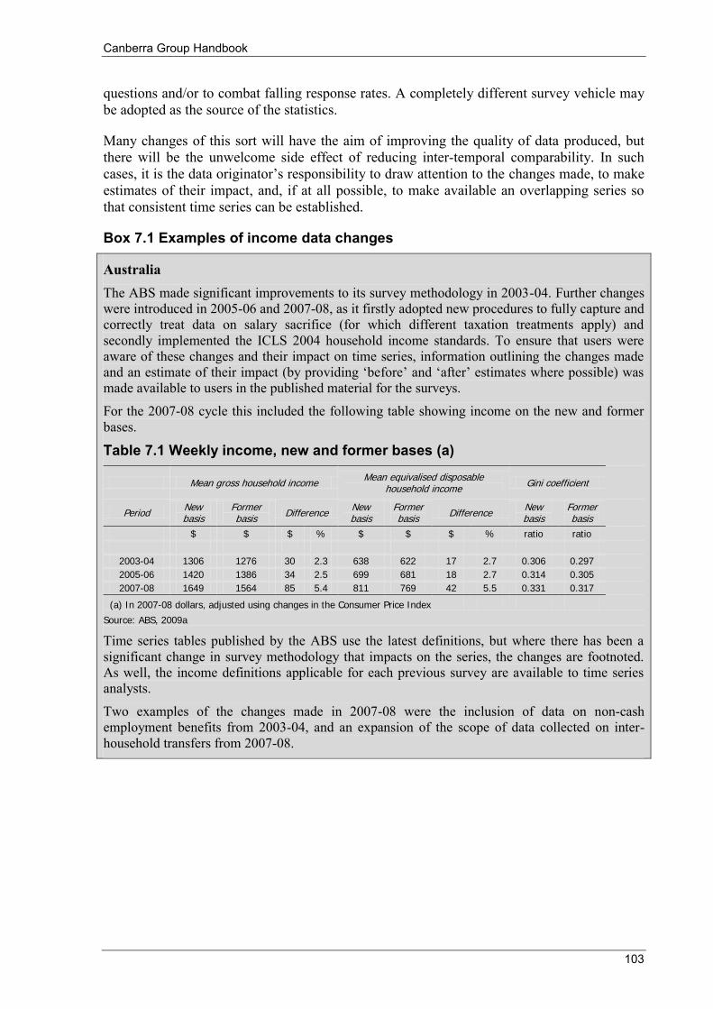
Canberra Group Handbook
103
questions and/or to combat falling response rates. A completely different survey vehicle may be adopted as the source of the statistics.
Many changes of this sort will have the aim of improving the quality of data produced, but there will be the unwelcome side effect of reducing inter-temporal comparability. In such cases, it is the data originator’s responsibility to draw attention to the changes made, to make estimates of their impact, and, if at all possible, to make available an overlapping series so that consistent time series can be established.
Box 7.1 Examples of income data changes
Australia The ABS made significant improvements to its survey methodology in 2003-04. Further changes were introduced in 2005-06 and 2007-08, as it firstly adopted new procedures to fully capture and correctly treat data on salary sacrifice (for which different taxation treatments apply) and secondly implemented the ICLS 2004 household income standards. To ensure that users were aware of these changes and their impact on time series, information outlining the changes made and an estimate of their impact (by providing ‘before’ and ‘after’ estimates where possible) was made available to users in the published material for the surveys.
For the 2007-08 cycle this included the following table showing income on the new and former bases.
Table 7.1 Weekly income, new and former bases (a)
Mean gross household income Mean equivalised disposable
household income Gini coefficient
Period New basis
Former basis
Difference New basis
Former basis
Difference New basis
Former basis
$ $ $ % $ $ $ % ratio ratio
2003-04 1306 1276 30 2.3 638 622 17 2.7 0.306 0.297
2005-06 1420 1386 34 2.5 699 681 18 2.7 0.314 0.305
2007-08 1649 1564 85 5.4 811 769 42 5.5 0.331 0.317
(a) In 2007-08 dollars, adjusted using changes in the Consumer Price Index
Source: ABS, 2009a
Time series tables published by the ABS use the latest definitions, but where there has been a significant change in survey methodology that impacts on the series, the changes are footnoted. As well, the income definitions applicable for each previous survey are available to time series analysts.
Two examples of the changes made in 2007-08 were the inclusion of data on non-cash employment benefits from 2003-04, and an expansion of the scope of data collected on inter-household transfers from 2007-08.
Chapter 7 Comparing income distributions over time
104
Canada Like many other countries, income measurement in Canada has been adapted through the years for two main reasons: firstly to reflect changes in programs or policies; and secondly to improve the relevance of the income concept by adding dimensions that have been either previously excluded or that posed measurement challenges.
Government transfers are an area where the income concept has stayed the same through the years but where measurement has changed to reflect modification to government programs. For example, universal child benefit programs in the early 1980s have been replaced by new programs targeted towards lower income families. While the concept hasn’t changed, it is important to document the differences in the programs through the years to allow a proper understanding of trends in income inequality.
Dimensions to the income concept have also been added to reflect aspects that are important. For example, while total income before taxes excludes capital gains, interest in studying the top of the income distribution has led to the need to examine realised capital gains. A ‘total income’ variable that includes realised capital gains is now available for researchers as a supplementary variable.
7.5 Issues for secondary dataset producers
The first problem for the producer of a ‘secondary’ dataset is to set internal standards for accepting or rejecting estimates. Selection criteria must be based on consistency of definition and quality, and the temptation must be resisted to include estimates just because they will extend the range of countries or years covered. For instance, Deininger and Squire (1996) chose the statistics to be included in their dataset by requiring that they be from national household surveys for expenditure or for income, that they be representative of the national population, and that all sources of income or expenditure be accounted for, including goods produced for own consumption.
As with primary data producers, the main duty of a researcher or organisation assembling a secondary dataset is to document the origin and characteristics of all estimates included, according to their selection criteria and the information made available by the primary data producer. The role of secondary datasets is to make accessible and enlarge the range of ‘ready made’ income distribution statistics. This process can take several forms, and it may be helpful to bear in mind the different origin of the ‘ready made’ income distribution statistics contained in secondary sources which may be:
calculated from individual national micro datasets, where there may be differences between ‘original’ and ‘public use’ datasets.
calculated from collections of harmonised micro datasets, such as LIS, which again may differ from those available in the original source.
calculated from tabulations published by (or supplied by) national sources. Here it should be noted that national sources may give differing degrees of detail (e.g. the data published in Statistical Yearbooks may have fewer ranges than in a specialised publication on income distribution), and that the published sources may be revised or published in alternative forms (e.g. based on different definitions).
calculated from tabulations in another secondary database.
Canberra Group Handbook
105
based on summary statistics published by (or supplied by) national sources.
based on summary statistics obtained directly from another secondary dataset producer or the publication of another analyst.
In all cases, the calculations involve decisions about how to treat the ‘raw’ data available. One issue affecting the consistency of time series data relates to changes in the application of procedures for top coding. This may happen in the course of the collection of the data, or as a decision of the researcher to reduce the noise that is typically concentrated in the tails of the distribution. Changes in these procedures may significantly affect the comparability of results. At the bottom of the distribution, there is the issue of how to treat zero or negative incomes. These may be bottom coded, be set to zero or a small positive number, or may be omitted. All of this needs to be documented.
A second example is the procedure for estimating quantile shares and inequality indices when the original data are only available in grouped form from primary sources. For example, if the disposable income of each household within a micro dataset is not available to the secondary data producer, but only, say, median income for each decile group, any attempt to fit a Lorenz curve (see Chapter 6) will be subject to error and the result is bound to differ from what would have been obtained had the full dataset been available. It would be advisable, and relatively inexpensive, to include in secondary datasets not only the recalculated series but also the original statistics. Equally, the upper and lower bounds for grouped data (obtained with different assumptions about the within-class distribution) are readily calculated and should be included.
In general, the procedures applied by secondary producers in processing the data should be fully documented, and the user should be allowed as wide a range of choice as possible. It should be noted that choices such as those regarding interpolation method or treatment of zero incomes may be implicit within the statistical package adopted, or in the formulae applied in the calculations, and that this may affect the conclusions drawn.
There is a long tradition, in the field of income distribution, of creating secondary datasets. A comparison of such compilations suggests some desirable features for a secondary dataset:
(a) Consolidation – in principle, multiple observations for the same country and the same date are justified where there are differences in definition (for example, household weights vs. person weights), or where different methods of calculation have been used. When there is no apparent reason for a difference, multiple observations need to be traced back to their original sources in order to identify the cause. It is important that data originators provide sufficient information for this to be possible. In view of their use in the past, keeping duplicate figures contained in earlier secondary datasets is valuable because it facilitates comparisons, but it should be clear that their status is that of memorandum items.
(b) Comprehensiveness – when other secondary sources are used, the documentation of such sources should be exhaustive. Omitting observations that fail to meet some pre-specified criteria may be convenient, but it may be preferable to include these unsatisfactory observations with a proper cautionary note.
(c) Full documentation – precise references and table numbers of the source data and a full account of all adjustments made should be given, so that observations in the dataset can be reproduced and their genealogy reconstructed.
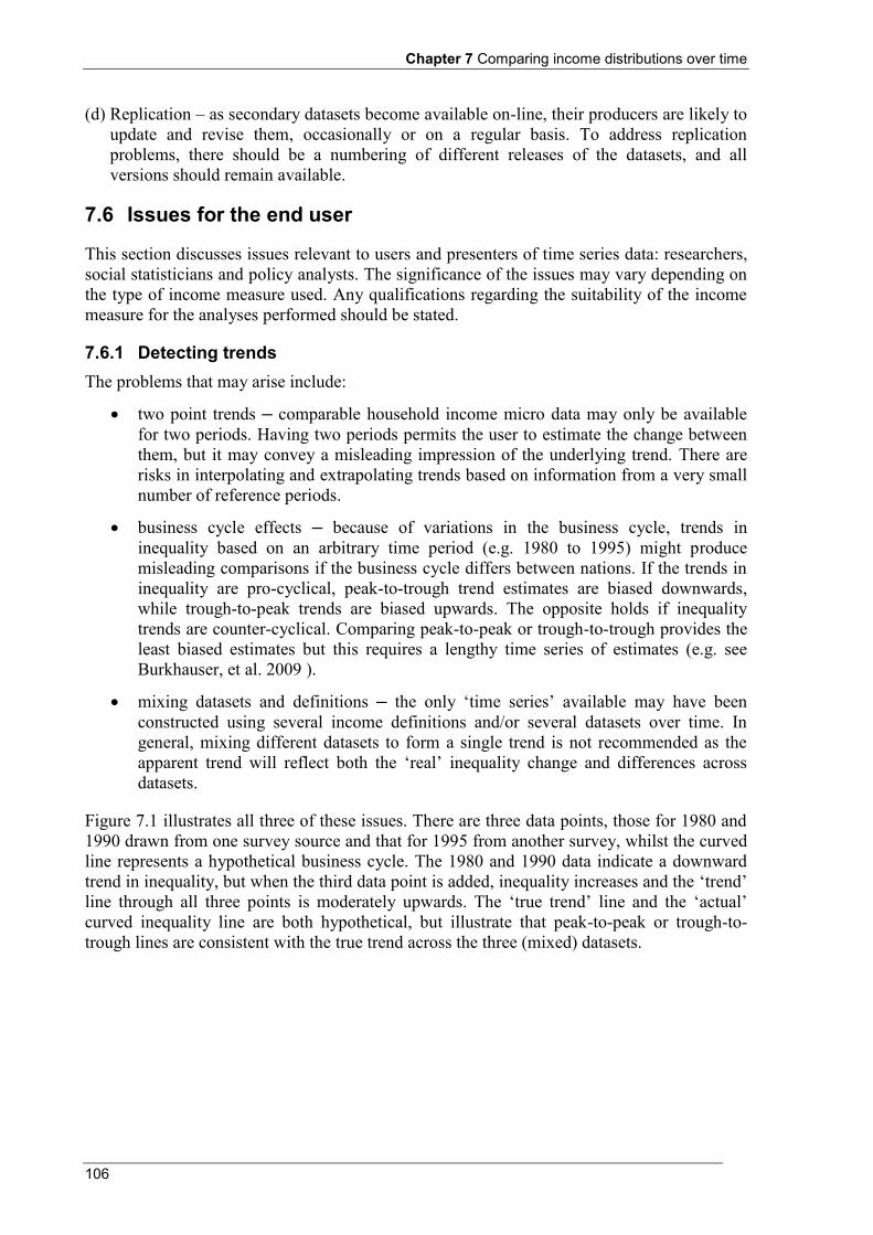
Chapter 7 Comparing income distributions over time
106
(d) Replication – as secondary datasets become available on-line, their producers are likely to update and revise them, occasionally or on a regular basis. To address replication problems, there should be a numbering of different releases of the datasets, and all versions should remain available.
7.6 Issues for the end user
This section discusses issues relevant to users and presenters of time series data: researchers, social statisticians and policy analysts. The significance of the issues may vary depending on the type of income measure used. Any qualifications regarding the suitability of the income measure for the analyses performed should be stated.
7.6.1 Detecting trends The problems that may arise include:
two point trends – comparable household income micro data may only be available for two periods. Having two periods permits the user to estimate the change between them, but it may convey a misleading impression of the underlying trend. There are risks in interpolating and extrapolating trends based on information from a very small number of reference periods.
business cycle effects – because of variations in the business cycle, trends in inequality based on an arbitrary time period (e.g. 1980 to 1995) might produce misleading comparisons if the business cycle differs between nations. If the trends in inequality are pro-cyclical, peak-to-trough trend estimates are biased downwards, while trough-to-peak trends are biased upwards. The opposite holds if inequality trends are counter-cyclical. Comparing peak-to-peak or trough-to-trough provides the least biased estimates but this requires a lengthy time series of estimates (e.g. see Burkhauser, et al. 2009 ).
mixing datasets and definitions – the only ‘time series’ available may have been constructed using several income definitions and/or several datasets over time. In general, mixing different datasets to form a single trend is not recommended as the apparent trend will reflect both the ‘real’ inequality change and differences across datasets.
Figure 7.1 illustrates all three of these issues. There are three data points, those for 1980 and 1990 drawn from one survey source and that for 1995 from another survey, whilst the curved line represents a hypothetical business cycle. The 1980 and 1990 data indicate a downward trend in inequality, but when the third data point is added, inequality increases and the ‘trend’ line through all three points is moderately upwards. The ‘true trend’ line and the ‘actual’ curved inequality line are both hypothetical, but illustrate that peak-to-peak or trough-to-trough lines are consistent with the true trend across the three (mixed) datasets.
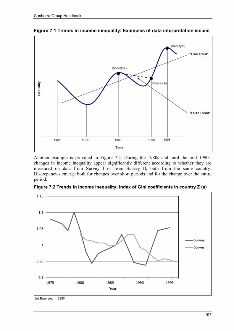
Canberra Group Handbook
107
Figure 7.1 Trends in income inequality: Examples of data interpretation issues
Another example is provided in Figure 7.2. During the 1980s and until the mid 1990s, changes in income inequality appear significantly different according to whether they are measured on data from Survey I or from Survey II, both from the same country. Discrepancies emerge both for changes over short periods and for the change over the entire period. Figure 7.2 Trends in income inequality: Index of Gini coefficients in country Z (a)
(a) Base year = 1986
0.9
0.95
1
1.05
1.1
1.15
1975 1980 1985 1990 1995
Year
Survey I
Survey II
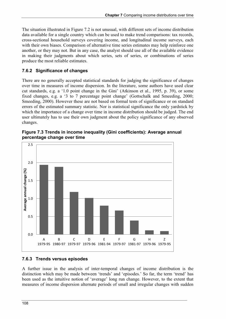
Chapter 7 Comparing income distributions over time
108
The situation illustrated in Figure 7.2 is not unusual, with different sets of income distribution data available for a single country which can be used to make trend comparisons: tax records, cross-sectional household surveys covering income, and longitudinal income surveys, each with their own biases. Comparison of alternative time series estimates may help reinforce one another, or they may not. But in any case, the analyst should use all of the available evidence in making their judgments about which series, sets of series, or combinations of series produce the most reliable estimates.
7.6.2 Significance of changes
There are no generally accepted statistical standards for judging the significance of changes over time in measures of income dispersion. In the literature, some authors have used clear cut standards, e.g. a ‘1.0 point change in the Gini’ (Atkinson et al., 1995, p. 39), or some fixed changes, e.g. a ‘3 to 7 percentage point change’ (Gottschalk and Smeeding, 2000; Smeeding, 2000). However these are not based on formal tests of significance or on standard errors of the estimated summary statistic. Nor is statistical significance the only yardstick by which the importance of a change over time in income distribution should be judged. The end user ultimately has to use their own judgment about the policy significance of any observed changes.
Figure 7.3 Trends in income inequality (Gini coefficients): Average annual percentage change over time
7.6.3 Trends versus episodes
A further issue in the analysis of inter-temporal changes of income distribution is the distinction which may be made between ‘trends’ and ‘episodes.’ So far, the term ‘trend’ has been used as the intuitive notion of ‘average’ long run change. However, to the extent that measures of income dispersion alternate periods of small and irregular changes with sudden
0.0
0.5
1.0
1.5
2.0
2.5
A1979-95
B1980-97
C1979-97
D1979-96
E1981-94
F1979-97
G1981-97
H1979-96
Z1979-95
Ave
rage
an
nu
al c
han
ge (
%)
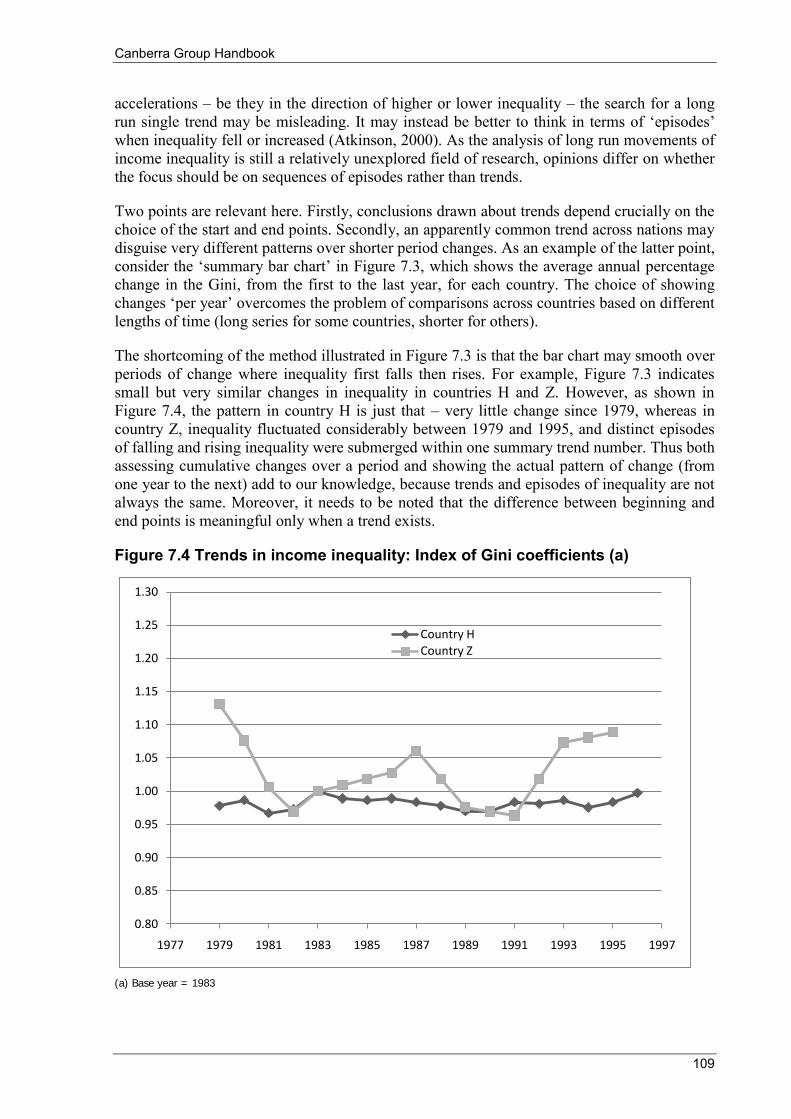
Canberra Group Handbook
109
accelerations – be they in the direction of higher or lower inequality – the search for a long run single trend may be misleading. It may instead be better to think in terms of ‘episodes’ when inequality fell or increased (Atkinson, 2000). As the analysis of long run movements of income inequality is still a relatively unexplored field of research, opinions differ on whether the focus should be on sequences of episodes rather than trends.
Two points are relevant here. Firstly, conclusions drawn about trends depend crucially on the choice of the start and end points. Secondly, an apparently common trend across nations may disguise very different patterns over shorter period changes. As an example of the latter point, consider the ‘summary bar chart’ in Figure 7.3, which shows the average annual percentage change in the Gini, from the first to the last year, for each country. The choice of showing changes ‘per year’ overcomes the problem of comparisons across countries based on different lengths of time (long series for some countries, shorter for others).
The shortcoming of the method illustrated in Figure 7.3 is that the bar chart may smooth over periods of change where inequality first falls then rises. For example, Figure 7.3 indicates small but very similar changes in inequality in countries H and Z. However, as shown in Figure 7.4, the pattern in country H is just that – very little change since 1979, whereas in country Z, inequality fluctuated considerably between 1979 and 1995, and distinct episodes of falling and rising inequality were submerged within one summary trend number. Thus both assessing cumulative changes over a period and showing the actual pattern of change (from one year to the next) add to our knowledge, because trends and episodes of inequality are not always the same. Moreover, it needs to be noted that the difference between beginning and end points is meaningful only when a trend exists.
Figure 7.4 Trends in income inequality: Index of Gini coefficients (a)
0.80
0.85
0.90
0.95
1.00
1.05
1.10
1.15
1.20
1.25
1.30
1977 1979 1981 1983 1985 1987 1989 1991 1993 1995 1997
Country H
Country Z
(a) Base year = 1983

110
111
Chapter 8 Income dynamics 8.1 Introduction
Chapter 7 discussed the comparison of income distributions over time using repeated cycles of cross-sectional data, i.e. income and other data collected for particular reference periods using independent samples.
Analysis of how the income of the same person (or household) changes over time is also very important. This chapter focuses on the relative advantages and disadvantages of longitudinal data, which permits this type of analysis. Some examples of longitudinal surveys are provided, as well as research areas for which they are potentially well suited.
The complex methodological issues associated with a good longitudinal panel are not explored in this chapter. Issues such as estimation (design of longitudinal weights) and adjustments for attrition have been documented in detail in other literature. Instead this chapter looks at the analytical opportunities available from longitudinal approaches to measuring household income.
8.2 Advantages and disadvantages of longitudinal data
Cross-sectional data give information about the ‘net effects’ and ‘net change’ of income on average, across households in a particular group, at given points in time. Cohort analysis of cross-sectional data can be used to build a stronger picture of relationships over time. On the other hand, longitudinal data enables analyses of records relating to the same individuals over time, where this can be satisfactorily achieved, and can be used to build a stronger understanding of income dynamics.
If unit record income data are available from population censuses or administrative datasets, detailed and potentially very reliable longitudinal analyses may be feasible. It is also possible to undertake longitudinal analysis using linked data from two or more collection datasets, including from different collection vehicles. Satisfactory matching or linking of individual records is central for these analyses.
Longitudinal data can also be collected in household surveys specifically designed for the purpose. The collection of longitudinal data from household surveys is not as common as cross-sectional data, due to the extra cost, complexity and data quality issues which apply to longitudinal surveys. However, the analytical power of longitudinal data has numerous advantages, and can be highly useful for informing the development of public policy, including: the exploration of changes experienced by individuals through time, and potential relationships between various socio-economic variables of interest at the person level.
A central feature of longitudinal data is the measurement of change at the individual level. To understand the processes involved in life histories, data needs to be collected at key transition points from the same individuals across time for an extended period. Cross-sectional data collected on repeated occasions enable the monitoring of the effects of societal change on the prevalence of population characteristics, i.e. 'net effects'. Conversely, longitudinal data are essential to investigate changes in individuals within the population, i.e. 'gross effects'.
Chapter 8 Income dynamics
112
Longitudinal income studies can help explain how particular life events develop, and can assist in drawing inferences and conclusions about their long term impact. Although cross-sectional data provide a representative sample of the population, they cannot capture, for the same group of individuals, changes in income and family characteristics, or what events tend to coincide in the individual’s life cycle.
For example, poor educational attainment in children may be attributed in part to low parental aspirations if changes in the former precede changes in the latter. A cross-sectional survey could establish only a correlation between parents' aspirations and children's educational attainment, with no basis on which to establish either cause or effect. Longitudinal data can give insight as to the nature of some of the 'cause and effect' relationships with children's educational attainment.
However, the value of longitudinal studies has to be judged against both the cost and the complexities of collecting the data, particularly when household surveys are used for this purpose. The most serious of these are data quality issues associated with non-response, particularly the loss (or attrition) of sample members over time. Subjects may disappear from the study because they have moved, or are no longer interested in taking part. Others move in and out of the study depending on their availability at the time each wave of the survey is conducted.
Non-response is a significant potential source of bias in these data. If those who do not agree to participate in the study are not representative of the population as a whole, or if those who leave the study after its inception are not typical of those who started it, the longitudinal data will become biased. Over a period of time these biases can become significant.
For example, people who are young and highly mobile, affected by family break-up, or who are recent immigrants, may become significantly underrepresented in the sample. These people are often of particular interest for analysis. Unless a longitudinal panel is regularly replenished it will gradually become less representative of the population as a whole.
Sample loss reduces the number of units (people or households) available for data analysis – a particular problem in longitudinal analysis, which demands complete records across the time span of the research.
On the other hand, unlike cross-sectional data, longitudinal data contain full information about the characteristics of units in the sample when the study began. Accordingly, if loss to the sample through attrition occurs differentially across groups, then the sample can be re-weighted at any point in time to reconstruct the key distributions of such variables and to compensate, to some degree, for the loss.
Other data quality issues relate to external sources of variation. Data collected at a particular point in time in a longitudinal study may be a product of the age of the individual concerned (age effect), the time when the individual was born (cohort effect) and the period at which data were collected (period or secular effect). Ideally all three sources of individual variation need to be accommodated for in the research design. To assess the size of the cohort effect (and to control for it), data needs to be collected from individuals of the same age but born at different points in time (cohorts). To assess and control the age effect, data needs to be collected from individuals of different ages in the same period. To assess and control the period effect, data needs to be collected from individuals of the same age at different periods.
Canberra Group Handbook
113
Where the income data collected relate to a previous reference period, and the household circumstances assessed at interview have changed since that time, problems are introduced. These problems are probably more significant for panel surveys than for cross-sectional surveys. Many household surveys, e.g. EU-SILC, collect annual income using the previous tax year as the income reference period. The motivation for this is that the respondents may consult income tax records. However, if there is a long gap between the income reference period and the time of data collection, the household situation or the employment status of the people in it may have changed. In such cases annual household income may not reflect the current financial situation of the individual.
As longitudinal surveys are far more complex than cross-sectional surveys, the costs of conducting a longitudinal survey are also higher. Large scale longitudinal studies tend to be expensive to carry out, and if they last a long time, require considerable commitment from a dedicated team to keep the study going. Effective longitudinal studies need a well funded infrastructure to ensure their continuation.
Longitudinal data also present additional difficulties to analyse the data and to present findings in a user-friendly way. Each wave of data can be regarded as adding another dimension to each sample unit, and the longitudinal linking of data presents formidable problems, both for processing and interpretation. However, modern information technology is making such problems less important.
8.3 Examples of longitudinal income surveys
Four longitudinal surveys are described below. Each of these surveys collects a wide array of socio-economic variables that may be used to explore complex socio-economic relationships. The surveys discussed are the Canadian Survey of Labour and Income Dynamics, the US Panel Study of Income Dynamics and the Survey of Income and Program Participation, and the European Union’s Statistics on Income and Living Conditions (EU-SILC) which covers more than 30 European countries. Other relatively long-standing longitudinal surveys include the German Socio-Economic Panel Survey, the British Household Panel Survey, the United States National Longitudinal Surveys of Labor Market Experience and the Survey of Household Income and Labour Dynamics in Australia (HILDA). Countries that collect income data from registers also produce longitudinal datasets, e.g. the Dutch Income Panel Survey and the register-based household income statistics of the Nordic countries.
8.3.1 Survey of Labour and Income Dynamics (Canada)
The Survey of Labour and Income Dynamics (SLID) was launched in 1993 by Statistics Canada. SLID is a multi-purpose survey designed to track the experiences of individuals in the labour market, their level and sources of income and changes in family life. The sample consists of two overlapping panels, with a new panel being introduced every three years and lasting six years. Each panel starts with about 15,000 households. All members are followed through time and new people with whom they live during the six year period are also covered. In addition to extensive historical information, covering marital history, fertility, work experience and educational attainment, persons 16 years and over are interviewed every January about their income and labour market activities throughout the previous year. Detailed income information is obtained from their tax records, unless they do not file a tax return or would prefer to provide this information by interview.
Chapter 8 Income dynamics
114
Major SLID research areas range from employment and unemployment dynamics and labour market transitions linked to the life cycle, to job quality, workplace inequality issues, family economic mobility (in particular shifts in income level), low income dynamics (or flows into or out of poverty), demographic events and the relationship between work and education. SLID is the first household survey ever to provide Canadian data on the fluctuations in income that a typical family or individual experiences through time, which provides greater insight on the nature and extent of low income in Canada. In addition to its longitudinal scope, SLID is Canada’s main data source for annual family income estimates. SLID is the only longitudinal survey to have this dual role.
8.3.2 Panel Study of Income Dynamics (USA)
The Panel Study of Income Dynamics (PSID), begun in 1968, is a longitudinal study of a representative sample of US individuals (including children) and the family units in which they reside. It emphasises the dynamic aspects of economic and demographic behaviour, but also includes sociological and psychological measures.
From 1968 to 1996, the PSID interviewed and reinterviewed individuals from families in the core sample every year, whether or not they were living in the same dwelling or with the same people. In 1997 the instrument was redesigned for biennial data collection and to keep the study representative of the US population. Two major changes were made to the sample: Firstly, a reduction of the core sample, and secondly, the introduction of a refresher sample of post 1968 immigrant families and their adult children.
As a consequence of low attrition rates, success in following young adults as they form their own families, and re-contact efforts for those not participating in one interview in prior years, the sample grew from 4,800 families in 1968 to more than 7,000 in 2001. As the end of 2003, the PSID had collected information about more than 65,000 individuals spanning as much as 36 years of their lives.
8.3.3 Survey of Income and Program Participation (USA)
The Survey of Income and Program Participation (SIPP), which began in 1983, is another major longitudinal survey which provides important information for analysing the economic situation of households and persons in the US. The information supplied by this survey provides a better understanding of the level and changes in the well-being of the population and how economic situations are related to the demographic and social characteristics of individuals.
The data collected in SIPP are especially useful in studying Federal transfer programs, estimating program cost and effectiveness, and assessing the effect of proposed changes in program regulations and benefit levels. Analysis of other important issues such as tax reform, welfare reform, social security costs and changes, and national health insurance can be expanded and refined, based on the information from this survey. It collects information from between 14,000 and 37,000 households once every four months for up to four years.

Canberra Group Handbook
115
8.3.4 European Union's Statistics on Income and Living Conditions (EU-SILC)
The EU-SILC is the main data source for the compilation of comparable indicators on social cohesion which are used for policy monitoring in the EU. It was launched in 2003 to replace the European Community Household panel (ECHP). Currently all EU-27 countries participate in EU-SILC, as well as Iceland, Norway, Switzerland and Turkey.
With effect from 2004, EU-SILC data collection is governed by a framework regulation of the Council and the Parliament and the implementation regulations of the EU Commission. Changes in methodology are developed in collaboration with relevant NSOs.
EU-SILC is a multi-purpose instrument. The survey collects data on income, poverty, social exclusion, housing conditions and living conditions. Every year, both cross-sectional data and longitudinal data are collected. The longitudinal component pertains to individual-level changes over time, observed periodically over, typically, a four year period. Detailed income components are collected mainly at the personal level although a few components are included at household level. In addition, information on social exclusion, housing conditions, labour, education and health is obtained.
The recommended panel duration in EU-SILC is four years, reduced from eight years in the ECHP. All countries follow the recommended rotation scheme, except France (8 years rotational design), Norway (9 years rotational design) and Luxembourg (pure panel). Minimum effective sample sizes are specified in the EU-SILC framework regulation. Separate minimum sample sizes are specified for the cross-sectional and longitudinal components.
8.4 Some applications of longitudinal surveys
Longitudinal data sources may take several years to pay dividends in terms of analytical results, but these results can be extremely useful to the development of social and labour market policy. Several longitudinal research themes contribute to the formation of public policy, in particular: economic mobility, low income dynamics and labour market dynamics.
8.4.1 Households income dynamics and intergenerational mobility
Household income data provide only a snapshot, at a point in time, of how income is distributed. From the perspective of people’s opportunities what matters the most is the probability of moving up or down the distribution over their life course, and the extent to which the position that one person ends up occupying depends on his/her starting point.
Most studies of the income dynamics of the same individual (intra-generational mobility) are based on the study of labour market earnings of economically active women and men. These studies are typically based on longitudinal data.
Changes in earnings inequality across individuals can come about, broadly speaking, in two different ways. Firstly, the distribution of long-run (‘permanent’) income may become more widely dispersed, and secondly, short-term fluctuations may become more or less common.
The availability of longitudinal data on individual workers offers the opportunity of understanding the nature of the changes in cross-sectional earnings inequality, in particular, if they are associated either with short term fluctuations or with long run inequality.
Chapter 8 Income dynamics
116
Longitudinal data can also be used to assess if more or fewer workers are subject to low pay, if the condition of being either a low or high earning worker persists for several periods, and if such persistence is becoming more or less common.
Household income surveys, even when they have a longitudinal component, rarely follow the same person for more than a few years. Moreover, the study of individual earnings from a longitudinal perspective, although important, is not sufficient for a thorough understanding of longitudinal aspects of individual economic well-being. This is partly because other sources of income contribute to well-being. An exclusive focus on labour earnings might lead to understating intergenerational mobility. Moreover, a substantial fraction of the population does not belong to the workforce in any given year, because they are children, in further education, retired or not in work for other reasons.
Because it is typically assumed that persons living in the same family or household share resources, a more comprehensive account of the dynamics of economic well-being needs to consider family or household economic mobility. Such a study does not necessarily need to focus on the same households over time. Indeed, following households across time is associated with many problems because households tend to dissolve and members form new households.
However, in order to have a clearer and more complete picture of the dynamics of economic well-being, it is important to consider the income of all the members of the household to which a given individual – who is followed longitudinally – belongs. Moreover, in order to be able to make, in any given period, the appropriate adjustments for economic needs, it is necessary to gather information on the household structure of that individual at different points in time.
The study of household income dynamics deals with both the measurement of household or family income mobility and instability, as well as the nature of income differences (permanent versus short term). Many studies in this area explicitly focus on the incidence of low income or poverty over time. An important feature of such studies is the examination of the determinants of income mobility. Some of the most important potential determinants are related to education, family demographics and labour market position, as well as changes in household or family structure, in particular family dissolution and formation.
Studies of family or household income dynamics are also often focussed on exploring whether the experience of low income in childhood is associated with adverse outcomes in adulthood. This is sometimes studied in terms of intermediate outcomes thought to be economically important, such as educational attainment, but also in terms of poverty outcomes in adulthood. Many studies have sought to examine the consequences of adverse economic conditions and different kinds of family events, such as parental divorce, at different points in childhood on later economic outcomes.
The availability of several long running longitudinal datasets, such as the Panel Study of Income Dynamics in the US and the German Socio-Economic Panel, that follow all individuals in the sampled families or households, as well as of register-based data that allow (in some countries) following up of members of the same household over generations, have allowed the study of intergenerational mobility, i.e. the extent to which the income of individuals differ from that of their parents.
Canberra Group Handbook
117
In principle it is possible to study intergenerational mobility using retrospective information. However, it is highly unlikely that retrospective information, asked of sample respondents about their parental incomes as they were growing up, would yield reliable information. Studies of intergenerational mobility based on retrospective information about parental occupation and education are much more likely to produce reliable information.
Intergenerational income mobility ideally requires longitudinal surveys, longitudinally linked census income measures, or register-based information about the socio-economic and demographic characteristics of the individual as an adult, and the same information for his/her parents as (s)he grew up. Ideally, information on both parents and their children in adulthood should be collected at roughly the same age. In this sense, the data should allow following up the same individuals first as children in their parental house (i.e. by collecting information about their parents) and later when the children have grown to be economically active adults. In practice, this means following individuals across decades rather than a few years.
The study of intergenerational income mobility must confront many of the data demands that apply to intragenerational income mobility, such as allowing analysts to distinguish between an individual's permanent income and transitory fluctuations around it.
8.4.2 Low income dynamics
Low income dynamics are related to the previous theme, but the emphasis is on people at the low end of the income scale. Studies of low income and poverty (such as those looking at flows of people into and out of poverty between years) can exaggerate the amount of turnover that occurs in the low income population, and understate the persistence of low income spells. Longitudinal data can be used to estimate ‘turnover’ in the low income population from year to year and over a longer period of time. It can show how many people on low income return into poverty, which may provide a more accurate picture of the nature of poverty.
Associated questions concern the determinants of flows into and out of low income. What are the demographic and labour market events that trigger a movement into or out of poverty? What is the role of government transfer payments? Longitudinal data allow study of the degree of economic dependency on these social programs over time, and the part played by each of these factors in bolstering family income.
Families that are economically disadvantaged in spite of their labour market involvement – ‘the working poor’ – are a particular concern, in that their precarious position may trigger labour market withdrawal. Longitudinal data may be of interest in income security policy research, especially given the move towards building work incentives into income support programs.
8.4.3 Labour market dynamics
Labour market dynamics refers to movements in the labour market experienced by each individual, such as shifts between employment, unemployment and inactivity. Studies based on retrospective questions in cross-sectional surveys indicate very large movements in the labour market over the period of a year or even a month. Such studies can improve understanding of how the labour market functions, and are useful supplements to ‘snapshot’ labour market data that measure ‘net’ change over some fixed time period. However, the evidence from retrospective questions remains limited. Longitudinal data provide insight into
Chapter 8 Income dynamics
118
issues such as: to what extent is unemployment experienced repeatedly by the same individuals, and how does the duration of unemployment spells vary over the business cycle? The longitudinal design allows studies of this type using completed spells, which can yield superior results compared to using truncated spells.
Other topics studied by labour market dynamics include flows into employment and unemployment and the events that trigger such movements. For example, what are the major determinants of labour market withdrawal? What family events act as triggers for labour market transitions? What precedes a transition into self-employment? Do family income (both its level and stability) and wealth impact on a worker's decision to become self-employed?
Similarly, studies of 'life-cycle related labour market transitions' put more emphasis on the individual's family circumstances or living arrangements, and deal with three major labour market transitions that dominate particular stages of the life cycle: school to work transitions, transitions from work to retirement, and work absences/temporary labour market withdrawal associated with childbirth or child-rearing.
School to work transitions can include long periods of inactivity and unemployment following school leaving, and are a labour market policy concern, not only because of lost productivity in the short term, but also because of the concomitant use of social assistance, the onset of discouragement and so on. These dynamic movements have a direct impact on income flows over time. Issues of interest in this area include labour market integration of people who drop out of high school, time required for school leavers to find their first full-time job, stability of the first full time job, wage and occupation in relation to education and major field of study, and back to school or further education transitions following early ventures into the labour market.
Issues around transitions from work to retirement include the distribution of wealth among seniors and the pre-retirement group, how wealth affects retirement decisions, self-employment following retirement from an employee job, or shifts to part time or lower wage pre-retirement jobs.
Work absences/temporary labour market withdrawal associated with childbirth or child-rearing are the third major area of life cycle transitions. It is possible to study wages before and after the absence and work arrangements and hours worked on returning to work. There may be some interest in the patterns associated with various family types, in particular, lone parent families. Another research area is the labour market impacts of family dissolution for working mothers.
The uses of longitudinal data are extensive and varied, and can provide many insights into the nature of socio-economic relationships that may be of interest to researchers and policy makers. Unlike cross-sectional data, which give a very accurate representation of net change (at any given point in time) for the population as a whole, longitudinal data provide insight into the impact that particular events have on an individual's outcomes and transitions. The knowledge garnered from this research is paramount to understanding the complex socio-economic relationships of today's societies and to help guide governmental programs and policies to achieve their goals.
119
Chapter 9 Future directions for international work 9.1 Introduction
The central concepts of household economic well-being are those dealing with income, wealth and consumption. These concepts are concerned with describing the total economic value of the resources received, owned or used up by people.
While a lot of coordinated international work has been undertaken in respect of micro household income statistics, far less work has been undertaken in respect of wealth and consumption statistics. This chapter proposes a research agenda that would support further advances in the field of household microeconomic statistics.
While not covered again in this chapter, the need to continue to develop practical methodologies to measure unpaid work and the value of services from consumer durables, and to develop data sources that support studies of the effects of social transfers in kind and indirect taxes on household income distribution, are noted.
9.2 Better informing analyses of economic well-being
Traditionally, analyses of economic well-being have focussed on a single dimension of household economic resources. In many developed countries, such studies have generally used income data, reflecting the relative frequency with which data on income is available, and also that, for many households, income is their most important economic resource for meeting everyday living expenses.
However, income only provides a partial view of economic well-being. Income, a flow measure, can be quite volatile for people making transitions between jobs, changing their hours of work, moving into or out of study, increasing or reducing time spent caring for children, or taking extended breaks from work. Some households with low income, for example, may report adequate levels of consumption expenditure or wealth.
Wealth, a stock measure, is more stable over time, reflecting accumulated savings and investments over time, which can be drawn on in times of need. People with reserves of wealth can also utilise these to generate income and to support a higher standard of living. While some wealth is held in assets that are not easily converted into money, its existence may allow people to borrow money to finance expenditures e.g. house extensions, motor vehicle purchases.
The importance of considering income and wealth together when assessing economic well-being has been given new impetus by several recommendations in the 'Report by the Commission on the Measurement of Economic Performance and Social Progress' (the 'Stiglitz-Sen-Fitoussi Commission' Report, 2009), particularly recommendation 4: Give more prominence to the distribution of income, consumption and wealth. The report explains the recommendation in the following terms:
Average income, consumption and wealth are meaningful statistics, but they do not tell the whole story about living standards. For example, a rise in average income could be unequally shared across groups, leaving some households relatively worse-off than others. Thus,
Chapter 9 Future directions for international work
120
average measures of income, consumption and wealth should be accompanied by indicators that reflect their distribution. Median consumption (income, wealth) provides a better measure of what is happening to the “typical” individual or household than average consumption (income or wealth). But for many purposes, it is also important to know what is happening at the bottom of the income/wealth distribution (captured in poverty statistics), or at the top. Ideally, such information should not come in isolation but be linked, i.e. one would like information about how well-off households are with regard to different dimensions of material living standards: income, consumption and wealth. After all, a low-income household with above-average wealth is not necessarily worse-off than a medium-income household with no wealth.
The recommendation arises from the well known limitations both of using only macroeconomic aggregates in the analysis of household economic behaviours, and of microeconomic analysis using single dimensions of household economic resources (such as income). The primary source of this type of information is household surveys.
The Stiglitz-Sen-Fitoussi Commission Report also recommends that comparisons of material living standards over time or across countries should account for how people spend their time on various activities such as paid and unpaid work, commuting and leisure. Time use data can be used to complement the picture provided by data on the distribution of income, consumption and wealth.
Together, this information could inform policies and programmes that better target households in need. These policies hold the promise of delivering improved economic well-being to individuals, stronger economy wide progress, and better individual and societal outcomes across a range of areas of social concern.
However, data to enable harmonised analyses that consider the joint distributions of income, consumption and wealth require internationally agreed standards and frameworks to support practitioners and data users in the field.
The next section proposes a research agenda that would support further advances in the field of household microeconomic statistics, including:
development of statistical standards for household wealth
development of a statistical framework that describes the relationships between household income, consumption and wealth
assessment of practical issues with the collection and analysis of income, expenditure and wealth data in an integrated manner.
9.3 Household income, consumption and wealth framework
The System of National Accounts (SNA) provides the main statistical framework for the analysis of household income, consumption and wealth data at the macro level. The SNA represents an agreed way of expressing, in statistical terms, most elements of a country’s economy and provides an international standard which is widely accepted and that can be practically applied at the macro level.
There is no such international framework for micro level household economic resource statistics, although there has been a lot of work undertaken in single dimensions (e.g. ILO, 2004). There have also been some significant broader contributions, such as the 1977 UN
Canberra Group Handbook
121
Provisional Guidelines on Statistics of the Distribution of Income, Consumption and Accumulation of Households, and the 1998 report, Statistics on the Distribution of Income, Consumption and Accumulation of Households (Franz et al., 1998).
There is strong international support for the development of an international framework for micro level household income, consumption and wealth statistics. This support was most recently reflected in the Stiglitz-Sen-Fitoussi Commission Report (2009) and also by the OECD decision to include the development of such a framework on its Forward Work Program for 2011 and 2012.
The development of an internationally agreed framework for the compilation of statistics on all of the dimensions of household economic resources, measured at the micro level, and with the needs of the micro statistician at the forefront, is essential to the production and analysis of harmonised and coherent information on the economic situation of the household.
This work would complement and expand the extensive work already undertaken with respect to the measurement of household income, including the international standards for household income statistics, as adopted by the 17th ICLS, and this Handbook, which provides a practical guide for their collection, analysis and dissemination. The presence of a broader framework will help inform analysis of economic well-being even where information is only available in a single dimension such as income.
An important contribution to the research agenda would be the development of international standards for the collection and compilation of statistics on household wealth at the micro level. In recent years there has been increased collection of wealth data by national statistical offices and central banks. The Luxembourg Wealth Study provides a common classification for national data on household assets and liabilities. Through an initiative undertaken by the European Central Bank with the Euro-System Survey on Household Finance and Consumption, new data based on definitions shared by all participating countries will be collected.
This expanded statistical activity reflects the importance of wealth in the analysis of household economic well-being and in understanding how households with different characteristics may respond to macroeconomic policy and to swings in the business cycle.
The research agenda should also identify elements that are currently missing and that are critical to assessing economic well-being. For instance, consumption expenditure is a critical dimension for household economic well-being. However, international standards for micro statistics on household expenditure are not designed specifically for analyses of household economic well-being.1
Finally, within the broader framework, the individual dimensions of household economic resources need to be collected in a consistent and coherent manner to support the analyses required e.g. measures that account for the joint distributions of income and wealth together, whether the data is collected concurrently or not.
1 International standards for micro statistics on household expenditure are contained within the ICLS resolution adopted in 2003. However, these standards are mainly driven by the goal of deriving weights for the compilation of consumer price indexes, and are not designed specifically for analyses of household economic well-being. International guidance is hence also required to allow the collection and compilation of comparable consumption expenditure data that can be used in welfare analysis.
Chapter 9 Future directions for international work
122
Some countries have been collecting information on household income, expenditure and wealth in an integrated manner through a single household survey for several years. Other countries and international organisations have experience in the matching of micro records from different surveys, which allow inferences to be drawn on the joint distribution of different dimensions of economic resources.
There is significant interest in both approaches. A review of these experiences, including a practical assessment of the feasibility of the approaches available, and identification of best practices in this field, would advance this research agenda considerably.
123
Appendix 1 Comparison of income definitions between 2001 and 2011 editions of the Canberra Group Handbook 1 Introduction
The 2001 Final Report and Recommendations of the Expert Group on Household Income Statistics, commonly referred to as the ‘Canberra Group Handbook’ (CGH), was highly influential in the development of new international standards for micro level household income statistics. In December 2003, the International Conference of Labour Statistics (ICLS) adopted a resolution containing updated standards for household income and expenditure statistics (ILO, 2004).
This edition of the CGH uses the new international standards as the starting point for discussion. It therefore differs in some respects from the original CGH.
This appendix compares the recommendations put forward by the Canberra Group in 2001 with those adopted in the 2003 international standards and in this second edition of the CGH. It covers differences in the income definitions and differences in how the conceptual components are classified.
Two tables are included at the end of this appendix to show concordances between the components of income in the 2001 and 2011 CGHs:
Table 1 shows the 2001 CGH classification of income components and their relationship to the 2011 CGH classification.
Table 2 shows the 2011 CGH classification of income components and their relationship to the 2001 CGH classification.
2 Income definitions
The ICLS standards, which are reflected in this 2011 edition of the CGH, largely follow the recommendations made by the Canberra Group, which were reflected in the 2001 edition of the CGH. In terms of broad principles and outcomes there were no major differences between the two standards.
The only practical exceptions concern the Value of unpaid domestic services and the Value of services from household consumer durables. These income components are included in the ICLS standards and therefore in the conceptual definition now included in this edition of the CGH. However, the 2001 edition of the CGH left these components out of the conceptual definition provided in Chapter 2 as it considered the definitional and measurement issues for these components as 'issues for the future'. So the differences are concerned with issues of practicality and timing, rather than principle.
The ICLS standards included these additional components within the income definition in a new broad classification category, Income from household production of services for home
Appendix 1 Comparison of income definitions between 2001 and 2011 editions of the CGH
124
consumption. The Net value of housing services (imputed rent) is the other component of this new category. In the 2001 CGH this was included as a component of self-employment income.
3 Classification of income components
The classification provided in the international standards, and adopted in this second edition of the Canberra Group Handbook, differs somewhat from the classification system applied in the 2001 CGH in both its structure and level of detail, although most components are classified in a similar way. The classification system presented in the international standards was organised according to the following broad groupings:
(a) Income from employment comprises receipts from involvement in economic activities, strictly in an employment related capacity as defined in the ICLS Resolution concerning statistics of the economically active population, employment, unemployment and underemployment (ILO, 2001). It consists of employee income, i.e. wages and self-employment income (return to labour).
(b) Property income from ownership of financial and other assets, including interest, dividends, rents for use of both unproduced assets (such as land), and produced assets (such as houses), and royalties.
(c) Income from household production of services for own consumption, including services of owner-occupied housing, household production of domestic services for own consumption and value of services from household consumer durables.
(d) Current transfers received in cash and in kind from government (e.g. pensions), other households (e.g. parental support) and non-profit institutions serving households (e.g. scholarships).
The classification system presented in the 2001 CGH was organised using slightly different principles and is summarised as follows:
(a) Employee income refers to remuneration from an employer.
(b) Income from self-employment has a broader scope than the ICLS category. In addition to profits from an own unincorporated enterprise and income from goods and services produced for barter or goods for home consumption, the Canberra Group also included royalties and the value of housing services from owner-occupied dwellings in this category.
(c) Income from rentals shows income less expenses from rentals (except rent of land) separately to property income.
(d) Property income comprises rent from land, interest received less interest paid, and dividends.
Canberra Group Handbook
125
(e) Current transfers received, consistent with the ICLS, comprises transfers from government (e.g. pensions), from other households (e.g. parental support) and from non-profit institutions serving households (e.g. scholarships).
A more detailed discussion of the rationale for where the Canberra Group classifications were not followed in the ICLS is provided in Report II on Household income and expenditure statistics (ILO, 2004).
4 Concordances between 2001 and 2011 CGH income definitions
Tables 1 and 2 provide concordances between the income definitions in the two editions of the CGH. Income components have been numbered in the first column of each table. These numbers have been used in the concordance for the complementary Table, i.e. the numbers referred to in the column ‘Concordance to the 2011 CGH’ in Table 1 are listed in the first column of Table 2 and the numbers referred to in the column ‘Concordance to the 2001 CGH’ in Table 2 are listed in the first column of Table 1.
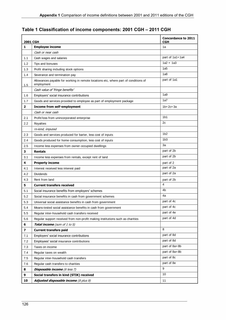
Appendix 1 Comparison of income definitions between 2001 and 2011 editions of the CGH
126
Table 1 Classification of income components: 2001 CGH – 2011 CGH
2001 CGH Concordance to 2011 CGH
1 Employee income 1a
Cash or near cash
1.1 Cash wages and salaries part of 1a1+1a4
1.2 Tips and bonuses 1a2 + 1a3
1.3 Profit sharing including stock options 1a5
1.4 Severance and termination pay 1a8
1.5
Allowances payable for working in remote locations etc, where part of conditions of employment
part of 1a1
Cash value of ‘fringe benefits’
1.6 Employers’ social insurance contributions 1a9
1.7 Goods and services provided to employee as part of employment package 1a7
2 Income from self-employment 1b+2c+3a
Cash or near cash
2.1 Profit/loss from unincorporated enterprise 1b1
2.2 Royalties 2c
In-kind, imputed
2.3 Goods and services produced for barter, less cost of inputs 1b2
2.4 Goods produced for home consumption, less cost of inputs 1b3
2.5 Income less expenses from owner-occupied dwellings 3a
3 Rentals part of 2b
3.1 Income less expenses from rentals, except rent of land part of 2b
4 Property income part of 2
4.1 Interest received less interest paid part of 2a
4.2 Dividends part of 2a
4.3 Rent from land part of 2b
5 Current transfers received 4
5.1 Social insurance benefits from employers’ schemes 4b
5.2 Social insurance benefits in cash from government schemes 4a
5.3 Universal social assistance benefits in cash from government part of 4c
5.4 Means-tested social assistance benefits in cash from government part of 4c
5.5 Regular inter-household cash transfers received part of 4e
5.6 Regular support received from non-profit making institutions such as charities part of 4d
6 Total income (sum of 1 to 5)
7 Current transfers paid 8
7.1 Employers’ social insurance contributions part of 8d
7.2 Employees’ social insurance contributions part of 8d
7.3 Taxes on income part of 8a+8b
7.4 Regular taxes on wealth part of 8a+8b
7.5 Regular inter-household cash transfers part of 8c
7.6 Regular cash transfers to charities part of 8e
8 Disposable income (6 less 7) 9
9 Social transfers in kind (STIK) received 10
10 Adjusted disposable income (8 plus 9) 11
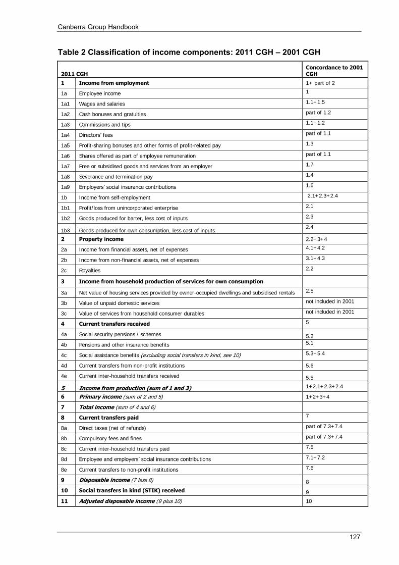
Canberra Group Handbook
127
Table 2 Classification of income components: 2011 CGH – 2001 CGH
2011 CGH Concordance to 2001 CGH
1 Income from employment 1+ part of 2
1a Employee income 1
1a1 Wages and salaries 1.1+1.5
1a2 Cash bonuses and gratuities part of 1.2
1a3 Commissions and tips 1.1+1.2
1a4 Directors’ fees part of 1.1
1a5 Profit-sharing bonuses and other forms of profit-related pay 1.3
1a6 Shares offered as part of employee remuneration part of 1.1
1a7 Free or subsidised goods and services from an employer 1.7
1a8 Severance and termination pay 1.4
1a9 Employers’ social insurance contributions 1.6
1b Income from self-employment 2.1+2.3+2.4
1b1 Profit/loss from unincorporated enterprise 2.1
1b2 Goods produced for barter, less cost of inputs 2.3
1b3 Goods produced for own consumption, less cost of inputs 2.4
2 Property income 2.2+3+4
2a Income from financial assets, net of expenses 4.1+4.2
2b Income from non-financial assets, net of expenses 3.1+4.3
2c Royalties 2.2
3 Income from household production of services for own consumption
3a Net value of housing services provided by owner-occupied dwellings and subsidised rentals 2.5
3b Value of unpaid domestic services not included in 2001
3c Value of services from household consumer durables not included in 2001
4 Current transfers received 5
4a Social security pensions / schemes 5.2
4b Pensions and other insurance benefits 5.1
4c Social assistance benefits (excluding social transfers in kind, see 10) 5.3+5.4
4d Current transfers from non-profit institutions 5.6
4e Current inter-household transfers received 5.5
5 Income from production (sum of 1 and 3) 1+2.1+2.3+2.4
6 Primary income (sum of 2 and 5) 1+2+3+4
7 Total income (sum of 4 and 6)
8 Current transfers paid 7
8a Direct taxes (net of refunds) part of 7.3+7.4
8b Compulsory fees and fines part of 7.3+7.4
8c Current inter-household transfers paid 7.5
8d Employee and employers’ social insurance contributions 7.1+7.2
8e Current transfers to non-profit institutions 7.6
9 Disposable income (7 less 8) 8
10 Social transfers in kind (STIK) received 9
11 Adjusted disposable income (9 plus 10) 10

128
129
Appendix 2 Reconciliation of micro and macro approaches 1 Introduction
The main framework developed for analysis of income at the macro level is the System of National Accounts (SNA). The SNA is a comprehensive system for expressing in statistical terms most elements of a country's economy in a way which articulates the relationships between the various sectors of the economy. The household sector is one such sector.
National accounts are compiled by bringing together data from a range of statistical surveys and from administrative sources. Household survey data are an important source for the compilation of household sector accounts in the SNA.
There is a continuing international focus on the importance of maximising the alignment of micro and macro datasets for household economic statistics, and in further integrating and analysing the data across their various dimensions. Regular confrontation of micro and macro estimates is important for understanding the strengths and weaknesses of the respective datasets and is likely to lead to a number of opportunities to maximise alignment between them over time.
There are three main parts to this Appendix. Section 2 explains the relationship between the micro and macro approaches to recording household income. Section 3 provides some practical guidance on how to confront data from the micro and macro sources. Section 4 provides an example of a data confrontation undertaken using Australian micro and macro household income data.
2 Reconciliation of micro and macro concepts and terminology
Table 1 summarises the relationship between the micro and macro income concepts from the perspective of the micro practitioner using the conceptual definition adopted by the ICLS and reflected in this second edition of the Canberra Group Handbook (CGH).
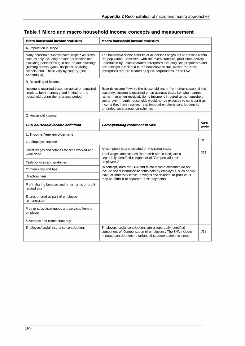
Appendix 2 Reconciliation of micro and macro approaches
130
Table 1 Micro and macro household income concepts and measurement Micro household income statistics Macro household income statistics
A. Population in scope
Many household surveys have scope exclusions such as only including private households and excluding persons living in non-private dwellings (nursing homes, gaols, hospitals, boarding schools, etc). These vary by country (see Appendix 3).
The household sector consists of all persons or groups of persons within the population. Consistent with the micro statistics, production activity undertaken by unincorporated enterprises including sole proprietors and partnerships is included in the household sector, except for those enterprises that are treated as quasi-corporations in the SNA.
B. Recording of income
Income is recorded based on actual or expected receipts, both monetary and in kind, of the household during the reference period.
Records income flows to the household sector from other sectors of the economy. Income is recorded on an accruals basis, i.e. when earned rather than when received. Some income is imputed to the household sector even though households would not be expected to consider it as income they have received, e.g. imputed employer contributions to unfunded superannuation schemes.
C. Household income
CGH household income definition Corresponding treatment in SNA SNA code
1. Income from employment
1a. Employee income D1
Direct wages and salaries for time worked and work done
All components are included on the same basis.
Total wages and salaries (both cash and in kind) are a separately identified component of ‘Compensation of employees.’
In concept, both the SNA and micro income measures do not include social insurance benefits paid by employers, such as sick leave or maternity leave, in wages and salaries. In practice, it may be difficult to separate these payments.
D11
Cash bonuses and gratuities
Commissions and tips
Directors’ fees
Profit-sharing bonuses and other forms of profit-related pay
Shares offered as part of employee remuneration
Free or subsidised goods and services from an employer
Severance and termination pay
Employers’ social insurance contributions Employers’ social contributions are a separately identified component of ‘Compensation of employees’. The SNA includes imputed contributions to unfunded superannuation schemes.
D12
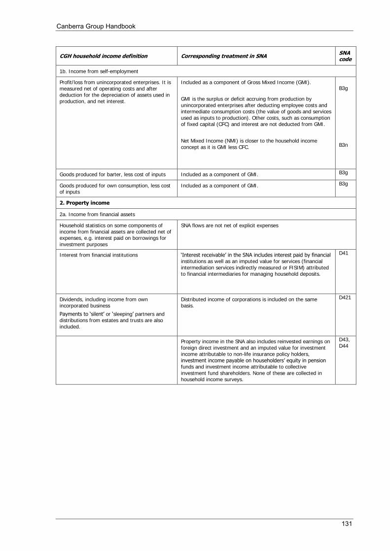
Canberra Group Handbook
131
CGH household income definition Corresponding treatment in SNA SNA code
1b. Income from self-employment
Profit/loss from unincorporated enterprises. It is measured net of operating costs and after deduction for the depreciation of assets used in production, and net interest.
Included as a component of Gross Mixed Income (GMI).
GMI is the surplus or deficit accruing from production by unincorporated enterprises after deducting employee costs and intermediate consumption costs (the value of goods and services used as inputs to production). Other costs, such as consumption of fixed capital (CFC) and interest are not deducted from GMI.
Net Mixed Income (NMI) is closer to the household income concept as it is GMI less CFC.
B3g
B3n
Goods produced for barter, less cost of inputs Included as a component of GMI. B3g
Goods produced for own consumption, less cost of inputs
Included as a component of GMI. B3g
2. Property income
2a. Income from financial assets
Household statistics on some components of income from financial assets are collected net of expenses, e.g. interest paid on borrowings for investment purposes
SNA flows are not net of explicit expenses
Interest from financial institutions ‘Interest receivable’ in the SNA includes interest paid by financial institutions as well as an imputed value for services (financial intermediation services indirectly measured or FISIM) attributed to financial intermediaries for managing household deposits.
D41
Dividends, including income from own incorporated business
Payments to ‘silent’ or ‘sleeping’ partners and distributions from estates and trusts are also included.
Distributed income of corporations is included on the same basis.
D421
Property income in the SNA also includes reinvested earnings on foreign direct investment and an imputed value for investment income attributable to non-life insurance policy holders, investment income payable on householders’ equity in pension funds and investment income attributable to collective investment fund shareholders. None of these are collected in household income surveys.
D43, D44
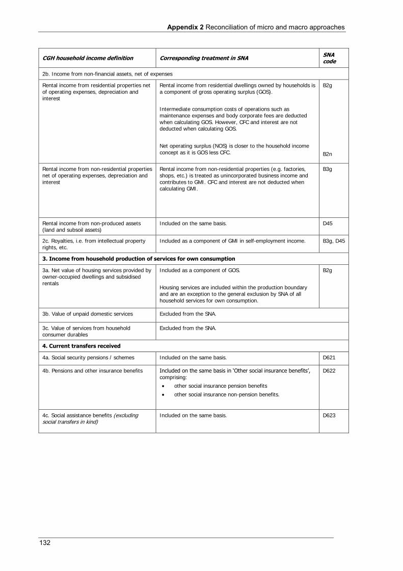
Appendix 2 Reconciliation of micro and macro approaches
132
CGH household income definition Corresponding treatment in SNA SNA code
2b. Income from non-financial assets, net of expenses
Rental income from residential properties net of operating expenses, depreciation and interest
Rental income from residential dwellings owned by households is a component of gross operating surplus (GOS).
Intermediate consumption costs of operations such as maintenance expenses and body corporate fees are deducted when calculating GOS. However, CFC and interest are not deducted when calculating GOS.
Net operating surplus (NOS) is closer to the household income concept as it is GOS less CFC.
B2g
B2n
Rental income from non-residential properties net of operating expenses, depreciation and interest
Rental income from non-residential properties (e.g. factories, shops, etc.) is treated as unincorporated business income and contributes to GMI. CFC and interest are not deducted when calculating GMI.
B3g
Rental income from non-produced assets (land and subsoil assets)
Included on the same basis. D45
2c. Royalties, i.e. from intellectual property rights, etc.
Included as a component of GMI in self-employment income. B3g, D45
3. Income from household production of services for own consumption
3a. Net value of housing services provided by owner-occupied dwellings and subsidised rentals
Included as a component of GOS.
Housing services are included within the production boundary and are an exception to the general exclusion by SNA of all household services for own consumption.
B2g
3b. Value of unpaid domestic services Excluded from the SNA.
3c. Value of services from household consumer durables
Excluded from the SNA.
4. Current transfers received
4a. Social security pensions / schemes Included on the same basis. D621
4b. Pensions and other insurance benefits Included on the same basis in ‘Other social insurance benefits’, comprising:
other social insurance pension benefits
other social insurance non-pension benefits.
D622
4c. Social assistance benefits (excluding social transfers in kind)
Included on the same basis. D623
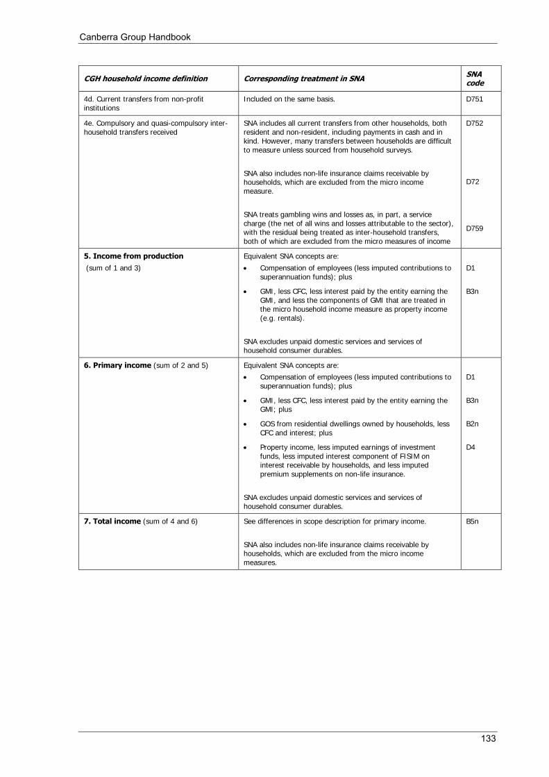
Canberra Group Handbook
133
CGH household income definition Corresponding treatment in SNA SNA code
4d. Current transfers from non-profit institutions
Included on the same basis. D751
4e. Compulsory and quasi-compulsory inter-household transfers received
SNA includes all current transfers from other households, both resident and non-resident, including payments in cash and in kind. However, many transfers between households are difficult to measure unless sourced from household surveys.
SNA also includes non-life insurance claims receivable by households, which are excluded from the micro income measure.
SNA treats gambling wins and losses as, in part, a service charge (the net of all wins and losses attributable to the sector), with the residual being treated as inter-household transfers, both of which are excluded from the micro measures of income
D752
D72
D759
5. Income from production
(sum of 1 and 3)
Equivalent SNA concepts are:
Compensation of employees (less imputed contributions to superannuation funds); plus
GMI, less CFC, less interest paid by the entity earning the GMI, and less the components of GMI that are treated in the micro household income measure as property income (e.g. rentals).
SNA excludes unpaid domestic services and services of household consumer durables.
D1
B3n
6. Primary income (sum of 2 and 5) Equivalent SNA concepts are:
Compensation of employees (less imputed contributions to superannuation funds); plus
GMI, less CFC, less interest paid by the entity earning the GMI; plus
GOS from residential dwellings owned by households, less CFC and interest; plus
Property income, less imputed earnings of investment funds, less imputed interest component of FISIM on interest receivable by households, and less imputed premium supplements on non-life insurance.
SNA excludes unpaid domestic services and services of household consumer durables.
D1
B3n
B2n
D4
7. Total income (sum of 4 and 6) See differences in scope description for primary income.
SNA also includes non-life insurance claims receivable by households, which are excluded from the micro income measures.
B5n

Appendix 2 Reconciliation of micro and macro approaches
134
CGH household income definition Corresponding treatment in SNA SNA code
8. Current transfers paid
8a. Direct taxes (net of refunds) Included on the same basis. D51
8b. Compulsory fees and fines Included on the same basis. D59
8c. Compulsory and quasi-compulsory inter-household transfers paid
SNA includes all current transfers from other households, both resident and non-resident, including payments in cash and in kind. However, many transfers between households are difficult to measure unless sourced from household surveys. SNA treats gambling wins and losses as, in part, a service charge (the net of all wins and losses attributable to the sector), with the residual being treated as inter-household transfers, both of which are excluded from the micro measures of income.
D752
8d. Employee and employers’ social insurance contributions (if included in 1a)
Employers’ social contributions are a separately identified component of ‘Compensation of employees’, and treated as transfers from households to the schemes. The SNA similarly includes imputed employer contributions to unfunded superannuation schemes, employees’ own contributions to pension funds, and premium supplements net of service charges.
D61
8.e. Current transfers to non-profit institutions Included on the same basis. D751
9. Disposable income (7 less 8) This differencing removes several of the offsetting SNA imputed flows into and out of households. The SNA concept of disposable income (net): removes CFC components that are a difference at the
various component levels noted above; removes interest and other payments by households that
form part of their cost of earning income, which moves the measures closer;
but also deducts other property income payments by households which are not deducted in compiling the micro level measure of disposable income.
B6n
10. Social transfers in kind (STIK) received Included on the same basis. D63
Adjusted disposable income (9 plus 10) A principal difference with the SNA remains the deduction of property income payable in deriving the macro measure of disposable income.
B7n
3 Data confrontation between micro and macro estimates
The treatment of income in micro and macro level statistics varies due to the different objectives of the two datasets. In the micro statistics, emphasis is on those receipts that are of direct benefit to individual households as well as the distribution of income across households. In the macro statistics, the total income accruing to households is described in relation to other aggregate components and sectors of the entire system of national accounts.
When undertaking data confrontation investigations between micro and macro datasets, it is necessary to understand the conceptual and methodological differences between the two sets of estimates. The components of the estimates must first be separated to identify data that can be compared and data that cannot be compared, because of these conceptual and methodological differences.
Canberra Group Handbook
135
It is also necessary to liaise with the national accounts compilation area to identify areas where they may diverge from the international standards. These differences will normally be due to data availability issues, particularly if administrative data such as tax records are used.
Manipulation of the data may also be required to allow better comparisons to be made. Access will be required to unpublished data from the national accounts compilation area for some data items. For example, interest estimates in the national accounts include financial intermediation services indirectly measured (FISIM), which are not included in household survey estimates. As FISIM will have been compiled separately by the national accounts area, it can be deducted before confronting the two sets of ‘interest’ estimates.
On the other hand, in some countries, data collected in household surveys on loans for investment purposes such as for rental properties or for the purchase of owner-occupied dwellings include the interest payable on the loan plus the repayment of capital. In other countries the interest component is collected separately from the capital repayments. When calculating income net of expenses, only the interest component should be included as any repayment of capital is an accumulation of wealth.
There are several income components that are particularly likely to affect any data confrontation of micro and macro household income estimates.
Imputed property income
The following items are not included in the micro concept of household income as a householder could not be expected to estimate a value for this income and it would not be possible to model them for individual households:
investment income attributable to non-life insurance policyholders investment income payable on householders’ equity in pension funds (including
imputed property income on unfunded pension schemes) investment income attributable to collective investment funds shareholders reinvested earnings on foreign direct investment.
The SNA uses data provided by financial institutions and other corporations to impute an income to the household sector as the policyholders and owners of pension funds, insurance policies, etc.
Depreciation versus consumption of fixed capital
There is a difference between the micro and macro estimates for depreciation (consumption of fixed capital in the SNA). When unincorporated enterprises or households with rental property deduct depreciation as an allowable expense, the value expensed is based on tax rules and the cost of the asset at the time of purchase (historical cost). In the SNA, consumption of fixed capital is measured based on the current value of the fixed assets.
In general, depreciation based on historical cost will be lower than an estimate based on current costs. Therefore, when confronting household survey estimates of unincorporated enterprise or rental income (net of expenses) with SNA net mixed income or net operating surplus estimates, the different valuation methods may be one factor contributing to any differences observed.
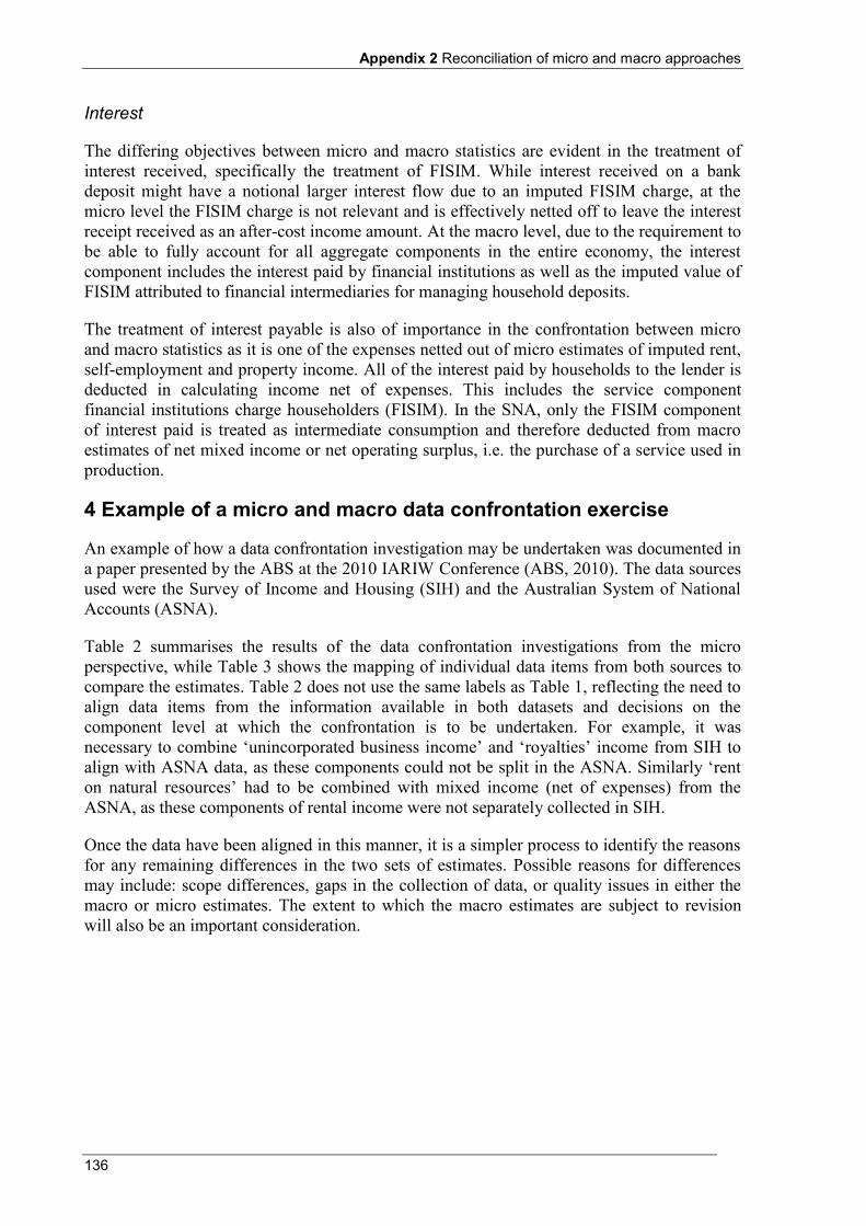
Appendix 2 Reconciliation of micro and macro approaches
136
Interest
The differing objectives between micro and macro statistics are evident in the treatment of interest received, specifically the treatment of FISIM. While interest received on a bank deposit might have a notional larger interest flow due to an imputed FISIM charge, at the micro level the FISIM charge is not relevant and is effectively netted off to leave the interest receipt received as an after-cost income amount. At the macro level, due to the requirement to be able to fully account for all aggregate components in the entire economy, the interest component includes the interest paid by financial institutions as well as the imputed value of FISIM attributed to financial intermediaries for managing household deposits.
The treatment of interest payable is also of importance in the confrontation between micro and macro statistics as it is one of the expenses netted out of micro estimates of imputed rent, self-employment and property income. All of the interest paid by households to the lender is deducted in calculating income net of expenses. This includes the service component financial institutions charge householders (FISIM). In the SNA, only the FISIM component of interest paid is treated as intermediate consumption and therefore deducted from macro estimates of net mixed income or net operating surplus, i.e. the purchase of a service used in production.
4 Example of a micro and macro data confrontation exercise
An example of how a data confrontation investigation may be undertaken was documented in a paper presented by the ABS at the 2010 IARIW Conference (ABS, 2010). The data sources used were the Survey of Income and Housing (SIH) and the Australian System of National Accounts (ASNA).
Table 2 summarises the results of the data confrontation investigations from the micro perspective, while Table 3 shows the mapping of individual data items from both sources to compare the estimates. Table 2 does not use the same labels as Table 1, reflecting the need to align data items from the information available in both datasets and decisions on the component level at which the confrontation is to be undertaken. For example, it was necessary to combine ‘unincorporated business income’ and ‘royalties’ income from SIH to align with ASNA data, as these components could not be split in the ASNA. Similarly ‘rent on natural resources’ had to be combined with mixed income (net of expenses) from the ASNA, as these components of rental income were not separately collected in SIH.
Once the data have been aligned in this manner, it is a simpler process to identify the reasons for any remaining differences in the two sets of estimates. Possible reasons for differences may include: scope differences, gaps in the collection of data, or quality issues in either the macro or micro estimates. The extent to which the macro estimates are subject to revision will also be an important consideration.
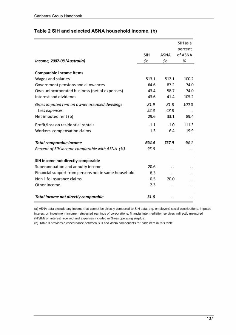
Canberra Group Handbook
137
Table 2 SIH and selected ASNA household income, (b)
(a) ASNA data exclude any income that cannot be directly compared to SIH data, e.g. employers' social contributions, imputed
interest on investment income, reinvested earnings of corporations, financial intermediation services indirectly measured
(FISIM) on interest received and expenses included in Gross operating surplus.
(b) Table 3 provides a concordance between SIH and ASNA components for each item in this table.
SIH ASNA
SIH as a
percent
of ASNA
Income, 2007-08 (Australia) $b $b %
Comparable income items
Wages and salaries 513.1 512.1 100.2
Government pensions and allowances 64.6 87.2 74.0
Own unincorporated business (net of expenses) 43.4 58.7 74.0
Interest and dividends 43.6 41.4 105.2
Gross imputed rent on owner occupied dwellings 81.9 81.8 100.0
Less expenses 52.3 48.8 . .
Net imputed rent (b) 29.6 33.1 89.4
Profit/loss on residential rentals -1.1 -1.0 111.3
Workers' compensation claims 1.3 6.4 19.9
Total comparable income 694.4 737.9 94.1
Percent of SIH income comparable with ASNA (%) 95.6 . . . .
SIH income not directly comparable
Superannuation and annuity income 20.6 . . . .
Financial support from persons not in same household 8.3 . . . .
Non-life insurance claims 0.5 20.0 . .
Other income 2.3 . . . .
Total income not directly comparable 31.6 . . . .
Appendix 2 Reconciliation of micro and macro approaches
138
Table 3 Concordance between SIH and selected ASNA income items (a)
SIH data items ASNA data items
Comparable income items (Label used in Table 2)
Wages and salaries
Wages and salaries
Compensation of employees less Employers’ social contributions
Government pensions and allowances
Australian government pensions and allowances
Social assistance benefits
Own unincorporated business (net of expenses)
Own unincorporated business (net of
expenses) Non-residential property (net of
expenses) Royalties
Mixed income (net of expenses) Rent on natural assets
Interest and dividends
Interest from financial institution
accounts Interest on debentures and bonds Dividends from own incorporated
businesses and trusts Dividends from shares Public unit trust income Silent partner income Other trust income (excl. public unit
trusts and own business income)
Interest (net of FISIM) Dividends
Net imputed rent on owner-occupied dwellings
Gross imputed rent on owner-occupied
dwellings less housing costs
Gross imputed rent on owner-occupied
dwellings less housing costs (on SIH basis - expenses derived using ASNA, tax and SIH data)
Profit/loss on residential rentals
Profit/loss on residential rentals
Net actual rent (on SIH basis) (part of
Gross operating surplus-dwellings owned by persons)
Workers' compensation claims
Workers' compensation
Workers' compensation (Social benefits
receivable)
SIH income not directly comparable with ASNA (Label used in Table 2)
Superannuation and annuity income
Superannuation/annuity/private pension
--
Inter household transfers
Financial support from persons not in
same household Child support/maintenance
--
Non-life insurance claims
Accident compensation and sickness
insurance
Non-life insurance claims
Other income
Overseas government pensions Interest on loans to persons not in
same household Scholarships Other financial investments nec Other regular income nec
Other current transfers
(a) ASNA data exclude any income that cannot be directly compared to SIH data, i.e. employers' social contributions, imputed interest on investment income, reinvested earnings of corporations, financial intermediation services indirectly measured (FISIM) on interest received; and selected expenses in GOS on dwellings and GMI (which were deducted to convert to SIH basis).
139
Appendix 3 Survey of Country Practices for measuring household income: Robustness assessment This appendix summarises the results of the robustness assessment undertaken as part of the Survey of Country Practices in early 2010.
The purpose of this component of the survey was to collect information about the main data source used to estimate the distribution of household income at the national level. The questionnaire covered a range of topics, the results of which are provided in the following tables:
Table 1 – Main source of information Table 2 – Scope and coverage Table 3 – Units Table 4 – Income reporting Table 5 – Non-response rates for main income components Table 6 – Editing and imputation Table 7 – Dissemination Table 8 – Websites for additional information
A copy of the questionnaire used is provided at the end of this Appendix.
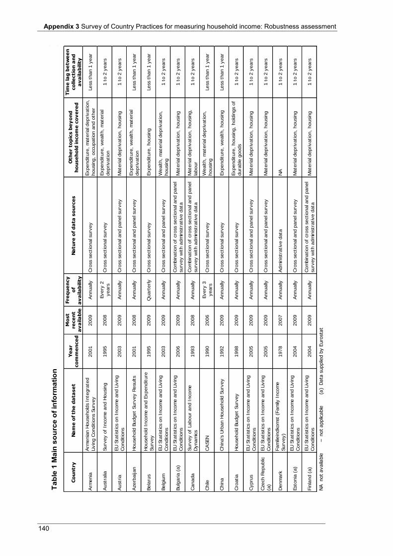
Appendix 3 Survey of Country Practices for measuring household income: Robustness assessment
140
Co
un
try
Na
me
of
th
e d
ata
se
tY
ea
r
co
mm
en
ce
d
Mo
st
re
ce
nt
av
aila
ble
Fre
qu
en
cy
of
av
aila
bilit
y
Na
tu
re
of
da
ta
so
urce
sO
th
er t
op
ics b
ey
on
d
ho
use
ho
ld in
co
me
co
ve
re
d
Tim
e la
g b
etw
ee
n
co
lle
ctio
n a
nd
av
aila
bilit
y
Arm
enia
Arm
enia
n H
ousehold
s I
nte
gra
ted
Liv
ing C
onditio
ns S
urv
ey
2001
2009
Annually
Cro
ss s
ectional surv
ey
Expenditure
, m
ate
rial deprivation,
housin
g,
occupation a
nd o
ther
Less t
han 1
year
Austr
alia
Surv
ey o
f In
com
e a
nd H
ousin
g1995
2008
Every
2
years
Cro
ss s
ectional surv
ey
Expenditure
, w
ealth,
mate
rial
deprivation
1 t
o 2
years
Austr
iaEU
Sta
tistics o
n I
ncom
e a
nd L
ivin
g
Conditio
ns
2003
2009
Annually
Cro
ss s
ectional and p
anel surv
ey
Mate
rial deprivation,
housin
g1 t
o 2
years
Azerb
aijan
Household
Budget
Surv
ey R
esults
2001
2008
Annually
Cro
ss s
ectional and p
anel surv
ey
Expenditure
, w
ealth,
mate
rial
deprivation
Less t
han 1
year
Bela
rus
Household
Incom
e a
nd E
xpenditure
Surv
ey
1995
2009
Quart
erly
Cro
ss s
ectional surv
ey
Expenditure
, housin
gLess t
han 1
year
Belg
ium
EU
Sta
tistics o
n I
ncom
e a
nd L
ivin
g
Conditio
ns
2003
2009
Annually
Cro
ss s
ectional and p
anel surv
ey
Wealth,
mate
rial deprivation,
housin
g1 t
o 2
years
Bulg
aria (
a)
EU
Sta
tistics o
n I
ncom
e a
nd L
ivin
g
Conditio
ns
2006
2009
Annually
Com
bin
ation o
f cro
ss s
ectional and p
anel
surv
ey w
ith a
dm
inis
trative d
ata
Mate
rial deprivation,
housin
g1 t
o 2
years
Canada
Surv
ey o
f Labour
and I
ncom
e
Dynam
ics
1993
2008
Annually
Com
bin
ation o
f cro
ss s
ectional and p
anel
surv
ey w
ith a
dm
inis
trative d
ata
Mate
rial deprivation,
housin
g,
labour
1 t
o 2
years
Chile
CA
SEN
1990
2006
Every
3
years
Cro
ss s
ectional surv
ey
Wealth,
mate
rial deprivation,
housin
gLess t
han 1
year
Chin
aC
hin
a's
Urb
an H
ousehold
Surv
ey
1992
2009
Annually
Cro
ss s
ectional surv
ey
Expenditure
, w
ealth,
housin
gLess t
han 1
year
Cro
atia
Household
Budget
Surv
ey
1998
2009
Annually
Cro
ss s
ectional surv
ey
Expenditure
, housin
g,
hold
ings o
f
dura
ble
goods
1 t
o 2
years
Cypru
sEU
Sta
tistics o
n I
ncom
e a
nd L
ivin
g
Conditio
ns
2005
2009
Annually
Cro
ss s
ectional and p
anel surv
ey
Mate
rial deprivation,
housin
g1 t
o 2
years
Czech R
epublic
(a)
EU
Sta
tistics o
n I
ncom
e a
nd L
ivin
g
Conditio
ns
2005
2009
Annually
Cro
ss s
ectional and p
anel surv
ey
Mate
rial deprivation,
housin
g1 t
o 2
years
Denm
ark
Fam
iliein
dkom
st
(Fam
ily I
ncom
e
Surv
ey)
1978
2007
Annually
Adm
inis
trative d
ata
NA
1 t
o 2
years
Esto
nia
(a)
EU
Sta
tistics o
n I
ncom
e a
nd L
ivin
g
Conditio
ns
2004
2009
Annually
Cro
ss s
ectional and p
anel surv
ey
Mate
rial deprivation,
housin
g
1 t
o 2
years
Fin
land (
a)
EU
Sta
tistics o
n I
ncom
e a
nd L
ivin
g
Conditio
ns
2004
2009
Annually
Com
bin
ation o
f cro
ss s
ectional and p
anel
surv
ey w
ith a
dm
inis
trative d
ata
M
ate
rial deprivation,
housin
g
1 t
o 2
years
NA
not
availa
ble
– not
applic
able
(a
) D
ata
supplie
d b
y E
uro
sta
t
Tabl
e 1
Mai
n so
urce
of i
nfor
mat
ion
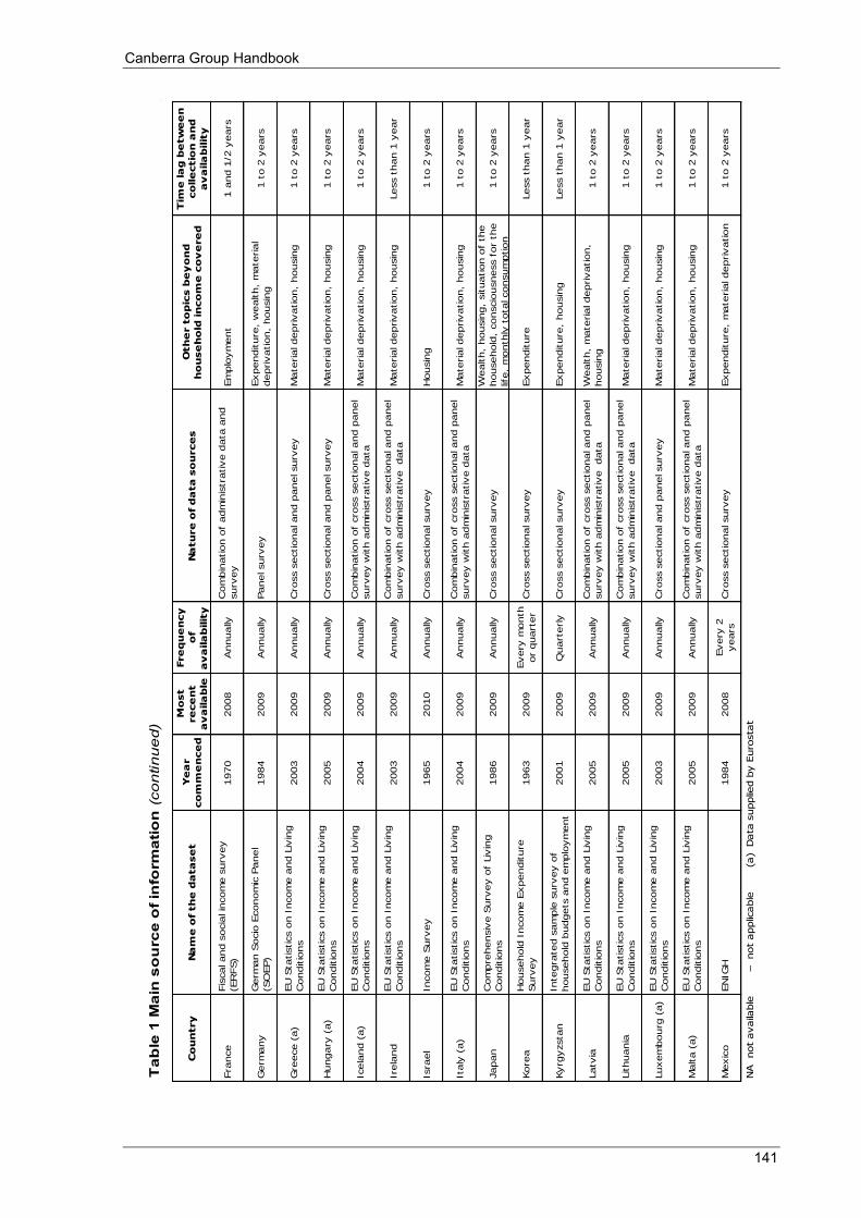
Canberra Group Handbook
141
Co
un
try
Na
me
of
th
e d
ata
se
tY
ea
r
co
mm
en
ce
d
Mo
st
re
ce
nt
av
aila
ble
Fre
qu
en
cy
of
av
aila
bilit
y
Na
tu
re
of
da
ta
so
urce
sO
th
er t
op
ics b
ey
on
d
ho
use
ho
ld in
co
me
co
ve
re
d
Tim
e la
g b
etw
ee
n
co
lle
ctio
n a
nd
av
aila
bilit
y
Fra
nce
Fis
cal and s
ocia
l in
com
e s
urv
ey
(ER
FS)
1970
2008
Annually
Com
bin
ation o
f adm
inis
trative d
ata
and
surv
ey
Em
plo
ym
ent
1 a
nd 1
/2 y
ears
Germ
any
Germ
an S
ocio
Econom
ic P
anel
(SO
EP)
1984
2009
Annually
Panel surv
ey
Expenditure
, w
ealth,
mate
rial
deprivation,
housin
g1 t
o 2
years
Gre
ece (
a)
EU
Sta
tistics o
n I
ncom
e a
nd L
ivin
g
Conditio
ns
2003
2009
Annually
Cro
ss s
ectional and p
anel surv
ey
Mate
rial deprivation,
housin
g1 t
o 2
years
Hungary
(a)
EU
Sta
tistics o
n I
ncom
e a
nd L
ivin
g
Conditio
ns
2005
2009
Annually
Cro
ss s
ectional and p
anel surv
ey
Mate
rial deprivation,
housin
g1 t
o 2
years
Icela
nd (
a)
EU
Sta
tistics o
n I
ncom
e a
nd L
ivin
g
Conditio
ns
2004
2009
Annually
Com
bin
ation o
f cro
ss s
ectional and p
anel
surv
ey w
ith a
dm
inis
trative d
ata
Mate
rial deprivation,
housin
g1 t
o 2
years
Irela
nd
EU
Sta
tistics o
n I
ncom
e a
nd L
ivin
g
Conditio
ns
2003
2009
Annually
Com
bin
ation o
f cro
ss s
ectional and p
anel
surv
ey w
ith a
dm
inis
trative data
Mate
rial deprivation,
housin
gLess t
han 1
year
Isra
el
Incom
e S
urv
ey
1965
2010
Annually
Cro
ss s
ectional surv
ey
Housin
g1 t
o 2
years
Italy
(a)
EU
Sta
tistics o
n I
ncom
e a
nd L
ivin
g
Conditio
ns
2004
2009
Annually
Com
bin
ation o
f cro
ss s
ectional and p
anel
surv
ey w
ith a
dm
inis
trative d
ata
Mate
rial deprivation,
housin
g1 t
o 2
years
Japan
Com
pre
hensiv
e S
urv
ey o
f Liv
ing
Conditio
ns
1986
2009
Annually
Cro
ss s
ectional surv
ey
Wealth,
housin
g,
situation o
f th
e
household
, conscio
usness f
or
the
life,
month
ly t
ota
l consum
ption
1 t
o 2
years
Kore
aH
ousehold
Incom
e E
xpenditure
Surv
ey
1963
2009
Every
month
or
quart
er
Cro
ss s
ectional surv
ey
Expenditure
Less t
han 1
year
Kyrg
yzsta
nIn
tegra
ted s
am
ple
surv
ey o
f
household
budgets
and e
mplo
ym
ent
2001
2009
Quart
erly
Cro
ss s
ectional surv
ey
Expenditure
, housin
gLess t
han 1
year
Latv
iaEU
Sta
tistics o
n I
ncom
e a
nd L
ivin
g
Conditio
ns
2005
2009
Annually
Com
bin
ation o
f cro
ss s
ectional and p
anel
surv
ey w
ith a
dm
inis
trative data
Wealth,
mate
rial deprivation,
housin
g1 t
o 2
years
Lithuania
EU
Sta
tistics o
n I
ncom
e a
nd L
ivin
g
Conditio
ns
2005
2009
Annually
Com
bin
ation o
f cro
ss s
ectional and p
anel
surv
ey w
ith a
dm
inis
trative data
Mate
rial deprivation,
housin
g1 t
o 2
years
Luxem
bourg
(a)
EU
Sta
tistics o
n I
ncom
e a
nd L
ivin
g
Conditio
ns
2003
2009
Annually
Cro
ss s
ectional and p
anel surv
ey
Mate
rial deprivation,
housin
g1 t
o 2
years
Malta (
a)
EU
Sta
tistics o
n I
ncom
e a
nd L
ivin
g
Conditio
ns
2005
2009
Annually
Com
bin
ation o
f cro
ss s
ectional and p
anel
surv
ey w
ith a
dm
inis
trative d
ata
Mate
rial deprivation,
housin
g1 t
o 2
years
Mexic
oEN
IGH
1984
2008
Every
2
years
Cro
ss s
ectional surv
ey
Expenditure
, m
ate
rial deprivation
1 t
o 2
years
NA
not
availa
ble
– not
applic
able
(a
) D
ata
supplie
d b
y E
uro
sta
t
Tab
le 1
Mai
n s
ou
rce
of i
nfo
rmat
ion
(co
ntin
ue
d)
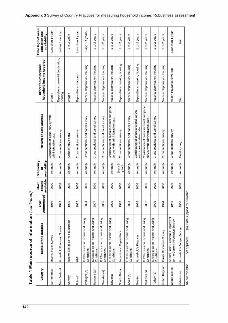
Appendix 3 Survey of Country Practices for measuring household income: Robustness assessment
142
Co
un
try
Na
me
of
the
da
tase
tY
ea
r
co
mm
en
ce
d
Mo
st
rece
nt
av
aila
ble
Fre
qu
en
cy
of
av
aila
bilit
y
Na
ture
of
da
ta s
ou
rce
sO
the
r to
pic
s b
ey
on
d
ho
use
ho
ld in
co
me
co
ve
red
Tim
e la
g b
etw
ee
n
co
lle
cti
on
an
d
av
aila
bilit
y
Neth
erlands
Inco
me P
anel S
urv
ey
1989
2009
Annually
Com
bin
ation o
f panel s
urv
ey w
ith
adm
inis
trative d
ata
Wealth
Less
than 1
year
New
Zeala
nd
House
hold
Eco
nom
ic S
urv
ey
1973
2009
Annually
Cro
ss s
ect
ional s
urv
ey
Expenditure
, m
ate
rial d
eprivation,
housi
ng
Within
5 m
onth
s
Norw
ay
Inco
me S
tatist
ics
for
House
hold
s1986
2008
Annually
Adm
inis
trative d
ata
Wealth
1 t
o 2
years
Pola
nd
HBS
1997
2009
Annually
Cro
ss s
ect
ional s
urv
ey
Expenditure
, housi
ng
Less
than 1
year
Port
ugal (
a)
EU
Sta
tist
ics
on I
nco
me a
nd L
ivin
g
Conditio
ns
2004
2009
Annually
Cro
ss s
ect
ional a
nd p
anel s
urv
ey
Mate
rial d
eprivation,
housi
ng
1 a
nd 1
/4 y
ears
Rom
ania
(a)
EU
Sta
tist
ics
on I
nco
me a
nd L
ivin
g
Conditio
ns
2007
2009
Annually
Cro
ss s
ect
ional a
nd p
anel s
urv
ey
Mate
rial d
eprivation,
housi
ng
1 t
o 2
years
Slo
vaki
a (
a)
EU
Sta
tist
ics
on I
nco
me a
nd L
ivin
g
Conditio
ns
2005
2009
Annually
Cro
ss s
ect
ional a
nd p
anel s
urv
ey
Mate
rial d
eprivation,
housi
ng
1 t
o 2
years
Slo
venia
EU
Sta
tist
ics
on I
nco
me a
nd L
ivin
g
Conditio
ns
2005
2009
Annually
Com
bin
ation o
f cr
oss
sect
ional a
nd p
anel
surv
ey w
ith a
dm
inis
trative d
ata
Mate
rial d
eprivation,
housi
ng
1 t
o 2
years
South
Afr
ica
Inco
me a
nd E
xpenditure
1995
2005
Every
5
years
Cro
ss s
ect
ional s
urv
ey
Expenditure
, w
ealth,
housi
ng
1 t
o 2
years
Spain
(a)
EU
Sta
tist
ics
on I
nco
me a
nd L
ivin
g
Conditio
ns
2004
2009
Annually
Cro
ss s
ect
ional a
nd p
anel s
urv
ey
Mate
rial d
eprivation,
housi
ng
1 t
o 2
years
Sw
eden
House
hold
's F
inance
s1975
2009
Annually
Com
bin
ation o
f cr
oss
sect
ional s
urv
ey
with a
dm
inis
trative d
ata
Expenditure
, w
ealth,
housi
ng
1 t
o 2
years
Sw
itze
rland
EU
Sta
tist
ics
on I
nco
me a
nd L
ivin
g
Conditio
ns
2007
2009
Annually
Com
bin
ation o
f cr
oss
sect
ional a
nd p
anel
surv
ey w
ith a
dm
inis
trative d
ata
Mate
rial d
eprivation,
housi
ng
1 t
o 2
years
Turk
ey (
a)
EU
Sta
tist
ics
on I
nco
me a
nd L
ivin
g
Conditio
ns
2006
2009
Annually
Cro
ss s
ect
ional a
nd p
anel s
urv
ey
Mate
rial d
eprivation,
housi
ng
1 t
o 2
years
United K
ingdom
Fam
ily R
eso
urc
es
Surv
ey
1994
2008
Annually
Cro
ss s
ect
ional s
urv
ey
Mate
rial d
eprivation,
housi
ng
1 t
o 2
years
United S
tate
sA
nnual S
oci
o-E
conom
ic S
upple
ment
to t
he C
urr
ent
Popula
tion S
urv
ey
1948
2008
Annually
Cro
ss s
ect
ional s
urv
ey
Health in
sura
nce
covera
ge
Less
than 1
year
Uzb
eki
stan
House
hold
s Budget
Surv
ey
2000
2009
Annually
Panel s
urv
ey
NA
NA
Tabl
e 1
Mai
n so
urce
of i
nfor
mat
ion
(con
tinue
d)
NA
not
availa
ble
– not
applic
able
(a
) D
ata
supplie
d b
y E
uro
stat
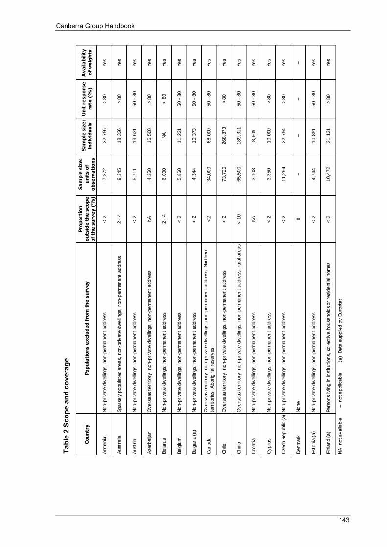
Canberra Group Handbook
143
Co
un
try
Po
pu
lati
on
s e
xclu
de
d f
rom
th
e s
urv
ey
Pro
po
rtio
n
ou
tsid
e t
he
sco
pe
of
the
su
rve
y (
%)
Sa
mp
le s
ize
:
un
its o
f
ob
se
rva
tio
ns
Sa
mp
le s
ize
:
ind
ivid
ua
ls
Un
it r
esp
on
se
rate
(%
)
Av
aila
bilit
y
of
we
igh
ts
Arm
enia
Non-p
rivate
dw
ellings,
non-p
erm
anent
addre
ss<
27,8
72
32,7
56
>80
Yes
Aust
ralia
Spars
ely
popula
ted a
reas,
non-p
rivate
dw
ellings,
non-p
erm
anent
addre
ss2 -
4
9,3
45
18,3
26
>80
Yes
Aust
ria
Non-p
rivate
dw
ellings,
non-p
erm
anent
addre
ss<
25,7
11
13,6
31
50 -
80
Yes
Aze
rbaija
nO
vers
eas
terr
itory
, non-p
rivate
dw
ellings,
non-p
erm
anent
addre
ssN
A4,2
50
16,5
00
>80
Yes
Bela
rus
Non-p
rivate
dw
ellings,
non-p
erm
anent
addre
ss2 -
46,0
00
NA
> 8
0Yes
Belg
ium
Non-p
rivate
dw
ellings,
non-p
erm
anent
addre
ss<
25,8
60
11,2
21
50 -
80
Yes
Bulg
aria (
a)
Non-p
rivate
dw
ellings,
non-p
erm
anent
addre
ss<
24,3
44
10,3
73
50 -
80
Yes
Canada
Overs
eas
terr
itory
, non-p
rivate
dw
ellings,
non-p
erm
anent
addre
ss,
Nort
hern
terr
itories,
Aborigin
al r
ese
rves
<2
34,0
00
68,0
00
50 -
80
Yes
Chile
Overs
eas
terr
itory
, non-p
rivate
dw
ellings,
non-p
erm
anent
addre
ss<
273,7
20
268,8
73
>80
Yes
Chin
aO
vers
eas
terr
itory
, non-p
rivate
dw
ellings,
non-p
erm
anent
addre
ss,
rura
l are
as
< 1
065,5
00
189,3
11
50 -
80
Yes
Cro
atia
Non-p
rivate
dw
ellings,
non-p
erm
anent
addre
ssN
A3,1
08
8,6
09
50 -
80
Yes
Cypru
sN
on-p
rivate
dw
ellings,
non-p
erm
anent
addre
ss<
23,3
50
10,0
00
>80
Yes
Cze
ch R
epublic
(a)
Non-p
rivate
dw
ellings,
non-p
erm
anent
addre
ss<
211,2
94
22,7
54
>80
Yes
Denm
ark
None
0–
––
–
Est
onia
(a)
Non-p
rivate
dw
ellings,
non-p
erm
anent
addre
ss<
24,7
44
10,8
51
50 -
80
Yes
Fin
land (
a)
Pers
ons
livin
g in
inst
itutions,
colle
ctiv
e h
ouse
hold
s or
resi
dential h
om
es
< 2
10,4
72
21,1
31
>80
Yes
Tabl
e 2
Scop
e an
d co
vera
ge
NA
not
availa
ble
– not
applic
able
(a
) D
ata
supplie
d b
y E
uro
stat
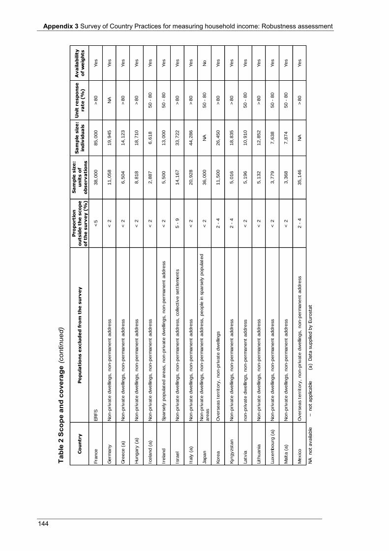
Appendix 3 Survey of Country Practices for measuring household income: Robustness assessment
144
Co
un
try
Po
pu
latio
ns e
xclu
de
d f
ro
m t
he
su
rv
ey
Pro
po
rtio
n
ou
tsid
e t
he
sco
pe
of
th
e s
urv
ey
(%
)
Sa
mp
le s
ize
:
un
its o
f
ob
se
rv
atio
ns
Sa
mp
le s
ize
:
ind
ivid
ua
ls
Un
it r
esp
on
se
ra
te
(%
)
Av
aila
bilit
y
of
we
igh
ts
Fra
nce
ER
FS
<5
38,0
00
85,0
00
>80
Yes
Germ
any
Non-p
rivate
dw
ellings,
non-p
erm
anent
addre
ss
< 2
11,0
58
19,9
45
NA
Yes
Gre
ece (
a)
Non-p
rivate
dw
ellings,
non-p
erm
anent
addre
ss
< 2
6,5
04
14,1
23
>80
Yes
Hungary
(a)
Non-p
rivate
dw
ellings,
non-p
erm
anent
addre
ss
< 2
8,8
18
18,7
10
>80
Yes
Icela
nd (
a)
Non-p
rivate
dw
ellings,
non-p
erm
anent
addre
ss
< 2
2,8
87
6,6
18
50 -
80
Yes
Irela
nd
Spars
ely
popula
ted a
reas,
non-p
rivate
dw
ellings,
non-p
erm
anent
addre
ss
< 2
5,5
00
13,0
00
50 -
80
Yes
Isra
el
Non-p
rivate
dw
ellings,
non-p
erm
anent
addre
ss,
colle
ctive s
ett
lem
ents
5 -
914,1
67
33,7
22
>80
Yes
Italy
(a)
Non-p
rivate
dw
ellings,
non-p
erm
anent
addre
ss
< 2
20,9
28
44,2
86
>80
Yes
Japan
Non-p
rivate
dw
ellings,
non-p
erm
anent
addre
ss,
people
in s
pars
ely
popula
ted
are
as
< 2
36,0
00
NA
50 -
80
No
Kore
aO
vers
eas t
err
itory
, non-p
rivate
dw
ellings
2 -
411,5
00
26,4
50
>80
Yes
Kyrg
yzsta
nN
on-p
rivate
dw
ellings,
non-p
erm
anent
addre
ss
2 -
45,0
16
18,8
35
>80
Yes
Latv
ianon-p
rivate
dw
ellings,
non-p
erm
anent
addre
ss
< 2
5,1
96
10,9
10
50 -
80
Yes
Lithuania
N
on-p
rivate
dw
ellings,
non-p
erm
anent
addre
ss
< 2
5,1
32
12,8
52
>80
Yes
Luxem
bourg
(a)
Non-p
rivate
dw
ellings,
non-p
erm
anent
addre
ss
< 2
3,7
79
7,6
38
50 -
80
Yes
Malta (
a)
Non-p
rivate
dw
ellings,
non-p
erm
anent
addre
ss
< 2
3,3
68
7,8
74
50 -
80
Yes
Mexic
oO
vers
eas t
err
itory
, non-p
rivate
dw
ellings,
non-p
erm
anent
addre
ss
2 -
435,1
46
NA
>80
Yes
Tabl
e 2
Sco
pe a
nd c
over
age
(con
tinue
d)
NA
not
availa
ble
– not
applic
able
(a
) D
ata
supplie
d b
y E
uro
sta
t
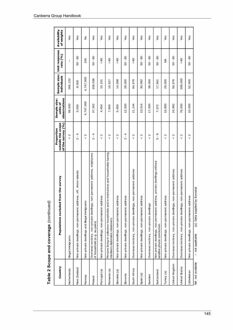
Canberra Group Handbook
145
Co
un
try
Po
pu
latio
ns e
xclu
de
d f
ro
m t
he
su
rv
ey
Pro
po
rtio
n
ou
tsid
e t
he
sco
pe
of
th
e s
urv
ey
(%
)
Sa
mp
le s
ize
:
un
its o
f
ob
se
rv
atio
ns
Sa
mp
le s
ize
:
ind
ivid
ua
ls
Un
it r
esp
on
se
ra
te
(%
)
Av
aila
bilit
y
of
we
igh
ts
Neth
erlands
Ille
gal im
mig
rants
< 2
99,5
00
266,1
20
–Yes
New
Zeala
nd
Non-p
rivate
dw
ellings,
non-p
erm
anent
addre
ss,
off
, shore
isla
nds
2 -
4
3,0
00
8,0
00
50 -
80
Yes
Norw
ay
Non-p
rivate
dw
ellings a
nd ille
gal im
mig
rants
< 2
4,7
47,0
00
4,7
47,0
00
100
No
Pola
nd
Overs
eas t
err
itory
, non-p
rivate
dw
ellings,
non-p
erm
anent
addre
ss,
em
plo
yees
of
household
(e.g
. au p
airs)
2 -
437,3
02
108,0
38
50 -
80
Yes
Port
ugal (a
)N
on-p
rivate
dw
ellings,
non-p
erm
anent
addre
ss
< 2
4,4
54
10,1
01
>80
Yes
Rom
ania
(a)
Pers
ons liv
ing in c
olle
ctive h
ousehold
s a
nd in institu
tions a
nd h
ousehold
s h
avin
g
mem
bers
dip
lom
atic m
issio
ners
< 2
7,8
05
16,5
27
>80
Yes
Slo
vakia
(a)
Non-p
rivate
dw
ellings,
non-p
erm
anent
addre
ss
< 2
5,4
50
14,0
98
>80
Yes
Slo
venia
Non-p
rivate
dw
ellings,
non-p
erm
anent
addre
ss
2 -
412,5
00
28,0
00
50 -
80
Yes
South
Afr
ica
Overs
eas t
err
itory
, non-p
rivate
dw
ellings,
non-p
erm
anent
addre
ss
< 2
21,1
44
84,9
78
>80
Yes
Spain
(a)
Non-p
rivate
dw
ellings,
non-p
erm
anent
addre
ss
< 2
13,0
14
30,0
82
50 -
80
Yes
Sw
eden
Overs
eas t
err
itory
, non-p
rivate
dw
ellings
< 2
17,0
00
38,0
00
50 -
80
Yes
Sw
itzerland
Non-p
rivate
dw
ellings,
non-p
erm
anent
addre
ss,
private
dw
ellings w
ithout
landlin
e p
hone c
onnection
5 -
97,3
72
17,5
61
50 -
80
Yes
Turk
ey (
a)
Non-p
rivate
dw
ellings,
non-p
erm
anent
addre
ss
< 2
10,8
00
29,0
00
NA
Yes
United K
ingdom
Overs
eas t
err
itory
, non-p
rivate
dw
ellings,
non-p
erm
anent
addre
ss
< 2
24,9
82
56,9
76
50 -
80
Yes
United S
tate
sO
vers
eas t
err
itory
, non-p
rivate
dw
ellings,
non-p
erm
anent
addre
ss
< 2
76,0
00
208,0
00
>80
Yes
Uzbekis
tan
Non-p
rivate
dw
ellings,
non-p
erm
anent
addre
ss
< 2
10,0
00
52,0
00
50 -
80
Yes
Tab
le 2
Sco
pe
and
co
vera
ge
(con
tinue
d)
NA
not
availa
ble
– not
applic
able
(a
) D
ata
supplie
d b
y E
uro
sta
t
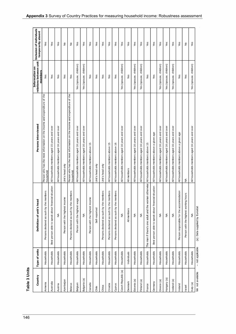
Appendix 3 Survey of Country Practices for measuring household income: Robustness assessment
146
Co
un
try
Ty
pe
of
un
its
De
fin
itio
n o
f u
nit
's h
ea
dP
erso
ns in
te
rv
iew
ed
In
form
atio
n o
n
re
latio
ns b
etw
ee
n u
nit
me
mb
ers
In
clu
sio
n o
f in
div
idu
als
te
mp
ora
rily
ab
se
nt
Arm
enia
Household
sPers
ons d
ecla
red a
s s
uch b
y t
he m
em
bers
Pers
on w
ho h
as t
he m
ost
info
rmation o
n t
he incom
e a
nd e
xpenditure
of
the
household
Yes
Yes
Austr
alia
Household
sBest
pers
on a
ble
to s
peak a
bout
financia
l situation
All
household
s m
em
bers
aged 1
5 y
ears
and o
ver
Yes
Yes
Austr
iaH
ousehold
sN
AA
ll household
s m
em
bers
aged 1
6 y
ears
and o
ver
Yes
Yes
Azerb
aijan
Household
sPers
on w
ith t
he h
ighest
incom
eU
nit's
head o
nly
Yes
No
Bela
rus
Household
sPers
ons d
ecla
red a
s s
uch b
y t
he m
em
bers
Pers
on w
ho h
as t
he m
ost
info
rmation o
n t
he incom
e a
nd e
xpenditure
of
the
household
Yes
No
Belg
ium
Household
sPers
on w
ith t
he h
ighest
wage
All
household
s m
em
bers
aged 1
6 y
ears
and o
ver
Yes (
spouse,
child
ren)
Yes
Bulg
aria (
a)
Household
sN
AA
ll household
s m
em
bers
aged 1
6 y
ears
and o
ver
Yes (
spouse,
child
ren)
Yes
Canada
Household
sPers
on w
ith t
he h
ighest
incom
eA
ll household
s m
em
bers
above 1
5Yes
Yes
Chile
Household
sSelf-r
eport
ed
Unit's
head o
nly
Yes
Yes
Chin
aH
ousehold
sPers
ons d
ecla
red a
s s
uch b
y t
he m
em
bers
Unit's
head o
nly
Yes
Yes
Cro
atia
Household
sPers
ons d
ecla
red a
s s
uch b
y t
he m
em
bers
All
household
s m
em
bers
above 1
5Yes
Yes
Cypru
sH
ousehold
sPers
ons d
ecla
red a
s s
uch b
y t
he m
em
bers
All
household
s m
em
bers
above 1
6Yes
Yes
Czech R
epublic
(a)
Household
sN
AA
ll household
s m
em
bers
aged 1
6 y
ears
and o
ver
Yes (
spouse,
child
ren)
Yes
Denm
ark
Indiv
iduals
All
mem
bers
All
mem
bers
Yes
Yes
Esto
nia
(a)
Household
sN
AA
ll household
s m
em
bers
aged 1
6 y
ears
and o
ver
Yes (
spouse,
child
ren)
Yes
Fin
land (
a)
Household
sN
AA
ll household
s m
em
bers
aged 1
6 y
ears
and o
ver
Yes (
spouse,
child
ren)
Yes
Fra
nce
Household
sThe m
an if
there
’s o
ne a
dult a
nd t
he w
om
an o
therw
ise A
ll household
s m
em
bers
above 1
5Yes
Yes
Germ
any
Household
sBest
pers
on a
ble
to s
peak a
bout
financia
l situation
All
household
s m
em
bers
above a
giv
en a
ge
Yes
Yes
Gre
ece (
a)
Household
sN
AA
ll household
s m
em
bers
aged 1
6 y
ears
and o
ver
Yes (
spouse,
child
ren)
Yes
Hungary
(a)
Household
sN
AA
ll household
s m
em
bers
aged 1
6 y
ears
and o
ver
Yes (
spouse,
child
ren)
Yes
Icela
nd (
a)
Household
sN
AA
ll household
s m
em
bers
aged 1
6 y
ears
and o
ver
Yes (
spouse,
child
ren)
Yes
Irela
nd
Household
sPers
on r
esponsib
le f
or
the a
ccom
modation
All
household
s m
em
bers
above a
giv
en a
ge
Yes
Yes
Isra
el
Household
sPers
on w
ith t
he h
ighest
work
ing h
ours
NA
Yes
No
Italy
(a)
Household
sN
AA
ll household
s m
em
bers
aged 1
6 y
ears
and o
ver
Yes (
spouse,
child
ren)
Yes
Tabl
e 3
Uni
ts
NA
not
availa
ble
– not
applic
able
(a
) D
ata
supplie
d b
y E
uro
sta
t
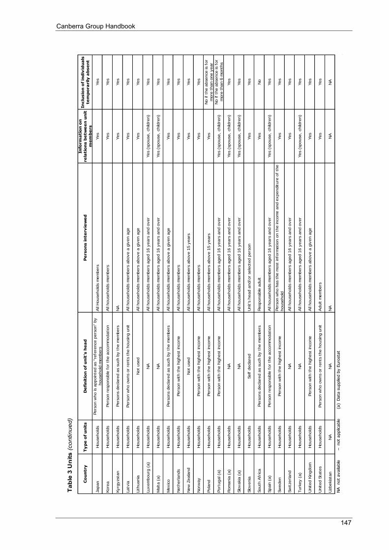
Canberra Group Handbook
147
Co
un
try
Ty
pe
of
un
its
De
fin
itio
n o
f u
nit
's h
ea
dP
erso
ns in
te
rv
iew
ed
In
form
atio
n o
n
re
latio
ns b
etw
ee
n u
nit
me
mb
ers
In
clu
sio
n o
f in
div
idu
als
te
mp
ora
rily
ab
se
nt
Japan
Household
sPers
on w
ho is a
ppoin
ted a
s "
refe
rence p
ers
on"
by
household
mem
bers
All
Household
s m
em
bers
Yes
Yes
Kore
aH
ousehold
sPers
on r
esponsib
le f
or
the a
ccom
modation
All
household
s m
em
bers
Yes
Yes
Kyrg
yzsta
nH
ousehold
sPers
ons d
ecla
red a
s s
uch b
y t
he m
em
bers
NA
Yes
Yes
Latv
iaH
ousehold
sPers
on w
ho o
wns o
r re
nts
the h
ousin
g u
nit
All
household
s m
em
bers
above a
giv
en a
ge
Yes
Yes
Lithuania
H
ousehold
sN
ot
used
All
household
s m
em
bers
above a
giv
en a
ge
Yes
Yes
Luxem
bourg
(a)
Household
sN
AA
ll household
s m
em
bers
aged 1
6 y
ears
and o
ver
Yes (
spouse,
child
ren)
Yes
Malta (
a)
Household
sN
AA
ll household
s m
em
bers
aged 1
6 y
ears
and o
ver
Yes (
spouse,
child
ren)
Yes
Mexic
oH
ousehold
sPers
ons d
ecla
red a
s s
uch b
y t
he m
em
bers
All
household
s m
em
bers
above a
giv
en a
ge
Yes
Yes
Neth
erlands
Household
sPers
on w
ith t
he h
ighest
incom
eA
ll household
s m
em
bers
Yes
Yes
New
Zeala
nd
Household
sN
ot
used
All
household
s m
em
bers
above 1
5 y
ears
Yes
Yes
Norw
ay
Household
sPers
on w
ith t
he h
ighest
incom
eA
ll household
s m
em
bers
Yes
Yes
Pola
nd
Household
sPers
on w
ith t
he h
ighest
incom
eA
ll household
s m
em
bers
above 1
5 y
ears
Yes
No if
the a
bsence is f
or
more
than o
ne y
ear
Port
ugal (a
)H
ousehold
sPers
on w
ith t
he h
ighest
incom
eA
ll household
s m
em
bers
aged 1
6 y
ears
and o
ver
Yes (
spouse,
child
ren)
No if
the a
bsence is f
or
more
than 6
month
s
Rom
ania
(a)
Household
sN
AA
ll household
s m
em
bers
aged 1
6 y
ears
and o
ver
Yes (
spouse,
child
ren)
Yes
Slo
vakia
(a)
Household
sN
AA
ll household
s m
em
bers
aged 1
6 y
ears
and o
ver
Yes (
spouse,
child
ren)
Yes
Slo
venia
Household
sSelf d
ecla
red
Unit's
head a
nd/o
r sele
cte
d p
ers
on
Yes
Yes
South
Afr
ica
Household
sPers
ons d
ecla
red a
s s
uch b
y t
he m
em
bers
Responsib
le a
dult
Yes
No
Spain
(a)
Household
sPers
on r
esponsib
le f
or
the a
ccom
modation
All
household
s m
em
bers
aged 1
6 y
ears
and o
ver
Yes (
spouse,
child
ren)
Yes
Sw
eden
Household
sPers
on w
ith t
he h
ighest
incom
ePers
on w
ho h
as t
he m
ost
info
rmation o
n t
he incom
e a
nd e
xpenditure
of
the
household
Yes
Yes
Sw
itzerland
Household
sN
AA
ll household
s m
em
bers
aged 1
6 y
ears
and o
ver
Yes
Yes
Turk
ey (
a)
Household
sN
AA
ll household
s m
em
bers
aged 1
6 y
ears
and o
ver
Yes (
spouse,
child
ren)
Yes
United K
ingdom
Household
sPers
on w
ith t
he h
ighest
incom
eA
ll household
s m
em
bers
above a
giv
en a
ge
Yes
Yes
United S
tate
sH
ousehold
sPers
on w
ho o
wns o
r re
nts
the h
ousin
g u
nit
Adult m
em
bers
Yes
Yes
Uzbekis
tan
NA
NA
NA
NA
NA
Tab
le 3
Un
its (c
ontin
ued)
NA
not
availa
ble
– not
applic
able
(a
) D
ata
supplie
d b
y E
uro
sta
t
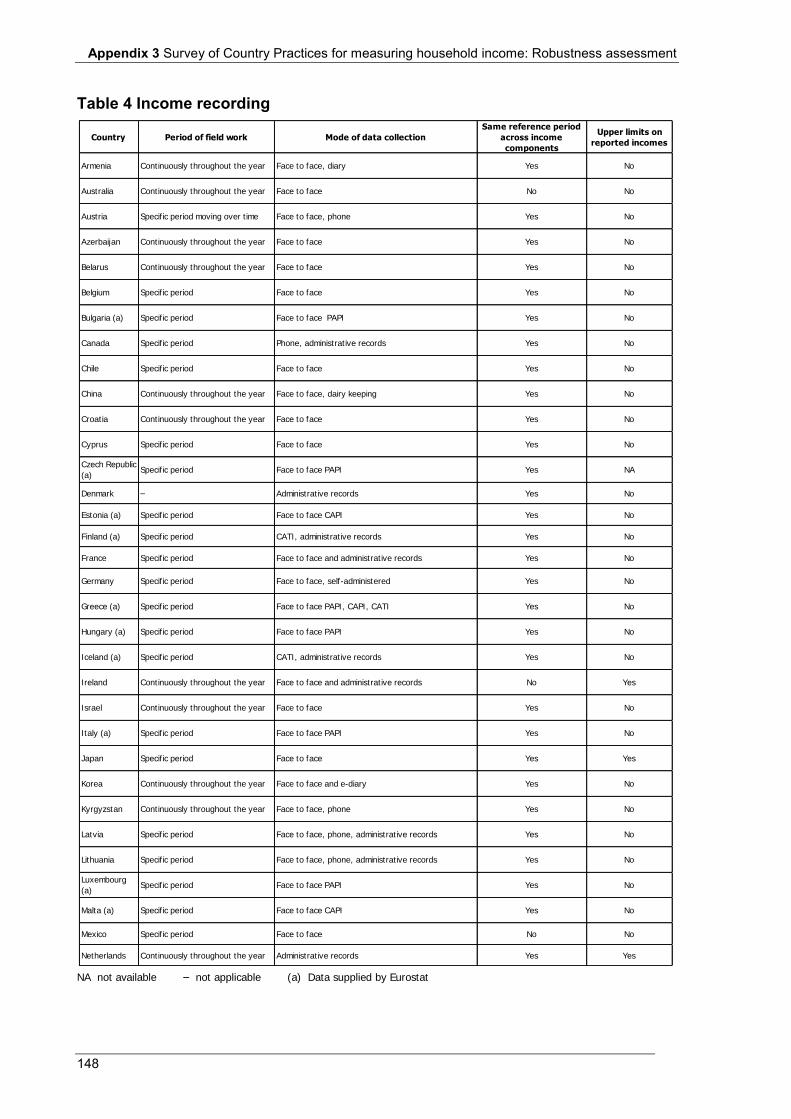
Appendix 3 Survey of Country Practices for measuring household income: Robustness assessment
148
Table 4 Income recording
NA not available – not applicable (a) Data supplied by Eurostat
Country Period of field work Mode of data collection
Same reference period
across income
components
Upper limits on
reported incomes
Armenia Continuously throughout the year Face to face, diary Yes No
Australia Continuously throughout the year Face to face No No
Austria Specific period moving over time Face to face, phone Yes No
Azerbaijan Continuously throughout the year Face to face Yes No
Belarus Continuously throughout the year Face to face Yes No
Belgium Specific period Face to face Yes No
Bulgaria (a) Specific period Face to face PAPI Yes No
Canada Specific period Phone, administrative records Yes No
Chile Specific period Face to face Yes No
China Continuously throughout the year Face to face, dairy keeping Yes No
Croatia Continuously throughout the year Face to face Yes No
Cyprus Specific period Face to face Yes No
Czech Republic
(a)Specific period Face to face PAPI Yes NA
Denmark – Administrative records Yes No
Estonia (a) Specific period Face to face CAPI Yes No
Finland (a) Specific period CATI, administrative records Yes No
France Specific period Face to face and administrative records Yes No
Germany Specific period Face to face, self-administered Yes No
Greece (a) Specific period Face to face PAPI, CAPI, CATI Yes No
Hungary (a) Specific period Face to face PAPI Yes No
Iceland (a) Specific period CATI, administrative records Yes No
Ireland Continuously throughout the year Face to face and administrative records No Yes
Israel Continuously throughout the year Face to face Yes No
Italy (a) Specific period Face to face PAPI Yes No
Japan Specific period Face to face Yes Yes
Korea Continuously throughout the year Face to face and e-diary Yes No
Kyrgyzstan Continuously throughout the year Face to face, phone Yes No
Latvia Specific period Face to face, phone, administrative records Yes No
Lithuania Specific period Face to face, phone, administrative records Yes No
Luxembourg
(a)Specific period Face to face PAPI Yes No
Malta (a) Specific period Face to face CAPI Yes No
Mexico Specific period Face to face No No
Netherlands Continuously throughout the year Administrative records Yes Yes
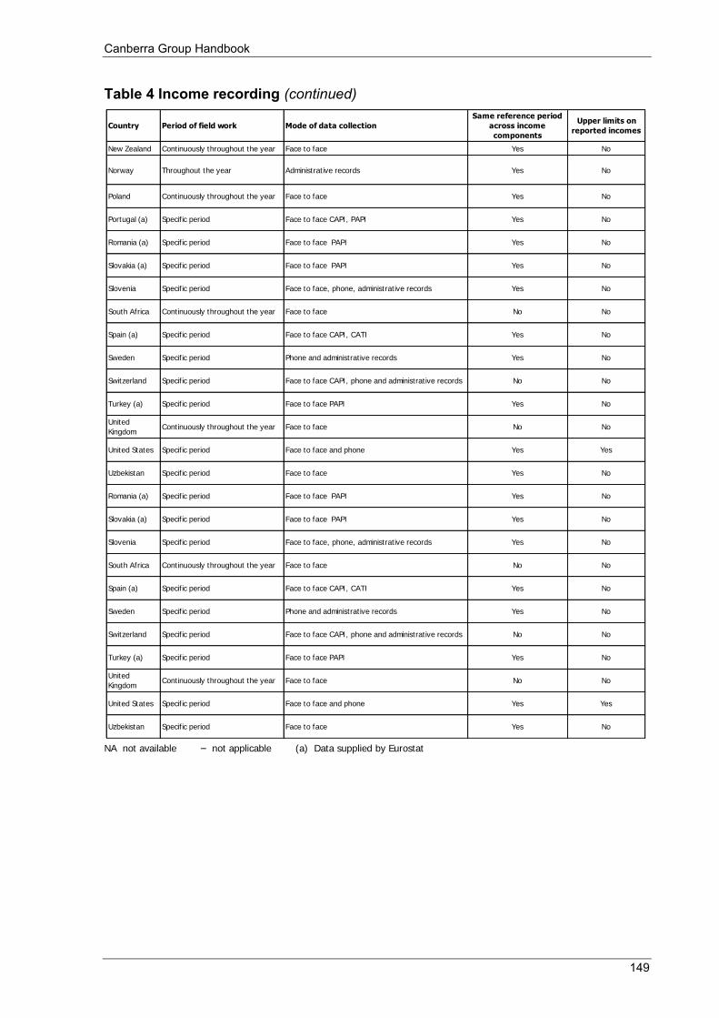
Canberra Group Handbook
149
Table 4 Income recording (continued)
NA not available – not applicable (a) Data supplied by Eurostat
Country Period of field work Mode of data collection
Same reference period
across income
components
Upper limits on
reported incomes
New Zealand Continuously throughout the year Face to face Yes No
Norway Throughout the year Administrative records Yes No
Poland Continuously throughout the year Face to face Yes No
Portugal (a) Specific period Face to face CAPI, PAPI Yes No
Romania (a) Specific period Face to face PAPI Yes No
Slovakia (a) Specific period Face to face PAPI Yes No
Slovenia Specific period Face to face, phone, administrative records Yes No
South Africa Continuously throughout the year Face to face No No
Spain (a) Specific period Face to face CAPI, CATI Yes No
Sweden Specific period Phone and administrative records Yes No
Switzerland Specific period Face to face CAPI, phone and administrative records No No
Turkey (a) Specific period Face to face PAPI Yes No
United
KingdomContinuously throughout the year Face to face No No
United States Specific period Face to face and phone Yes Yes
Uzbekistan Specific period Face to face Yes No
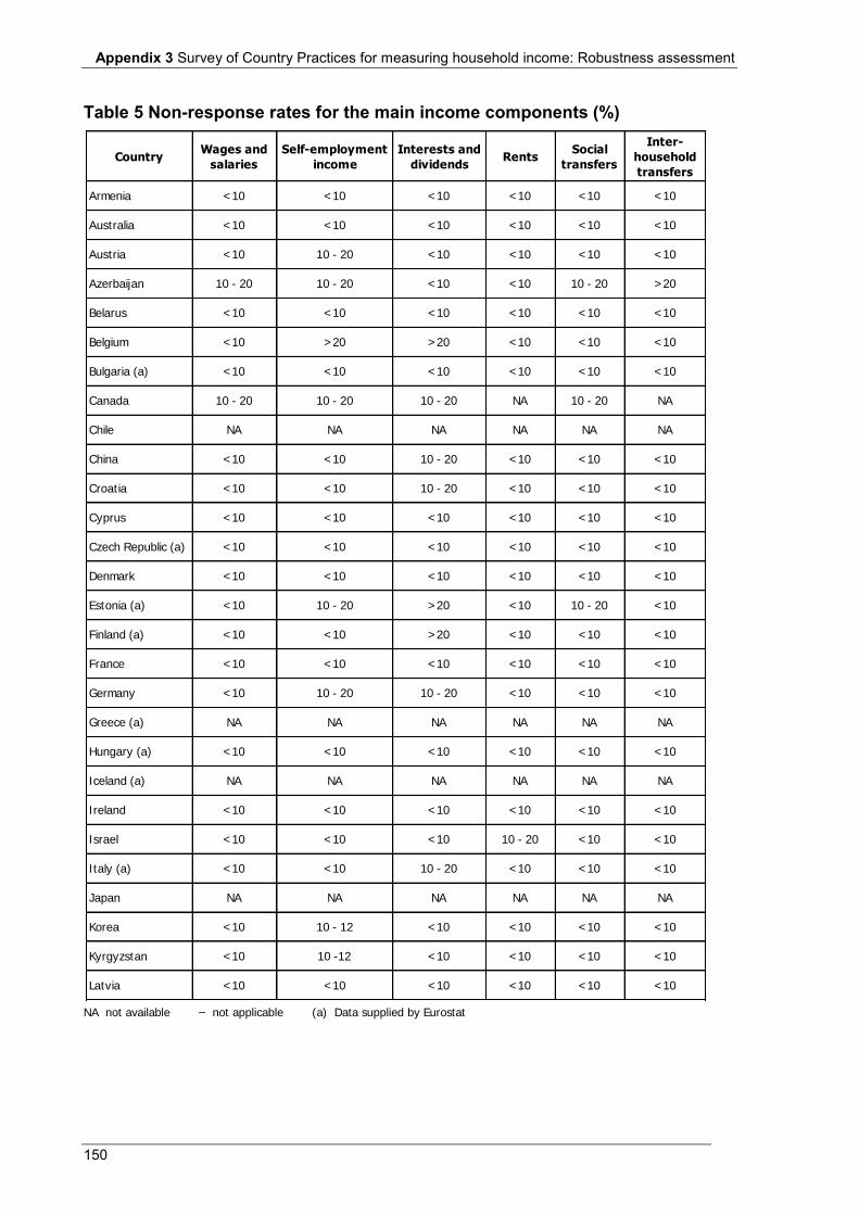
Appendix 3 Survey of Country Practices for measuring household income: Robustness assessment
150
Table 5 Non-response rates for the main income components (%)
NA not available – not applicable (a) Data supplied by Eurostat
CountryWages and
salaries
Self-employment
income
Interests and
dividendsRents
Social
transfers
Inter-
household
transfers
Armenia <10 <10 <10 <10 <10 <10
Australia <10 <10 <10 <10 <10 <10
Austria <10 10 - 20 <10 <10 <10 <10
Azerbaijan 10 - 20 10 - 20 <10 <10 10 - 20 >20
Belarus <10 <10 <10 <10 <10 <10
Belgium <10 >20 >20 <10 <10 <10
Bulgaria (a) <10 <10 <10 <10 <10 <10
Canada 10 - 20 10 - 20 10 - 20 NA 10 - 20 NA
Chile NA NA NA NA NA NA
China <10 <10 10 - 20 <10 <10 <10
Croatia <10 <10 10 - 20 <10 <10 <10
Cyprus <10 <10 <10 <10 <10 <10
Czech Republic (a) <10 <10 <10 <10 <10 <10
Denmark <10 <10 <10 <10 <10 <10
Estonia (a) <10 10 - 20 >20 <10 10 - 20 <10
Finland (a) <10 <10 >20 <10 <10 <10
France <10 <10 <10 <10 <10 <10
Germany <10 10 - 20 10 - 20 <10 <10 <10
Greece (a) NA NA NA NA NA NA
Hungary (a) <10 <10 <10 <10 <10 <10
Iceland (a) NA NA NA NA NA NA
Ireland <10 <10 <10 <10 <10 <10
Israel <10 <10 <10 10 - 20 <10 <10
Italy (a) <10 <10 10 - 20 <10 <10 <10
Japan NA NA NA NA NA NA
Korea <10 10 - 12 <10 <10 <10 <10
Kyrgyzstan <10 10 -12 <10 <10 <10 <10
Latvia <10 <10 <10 <10 <10 <10
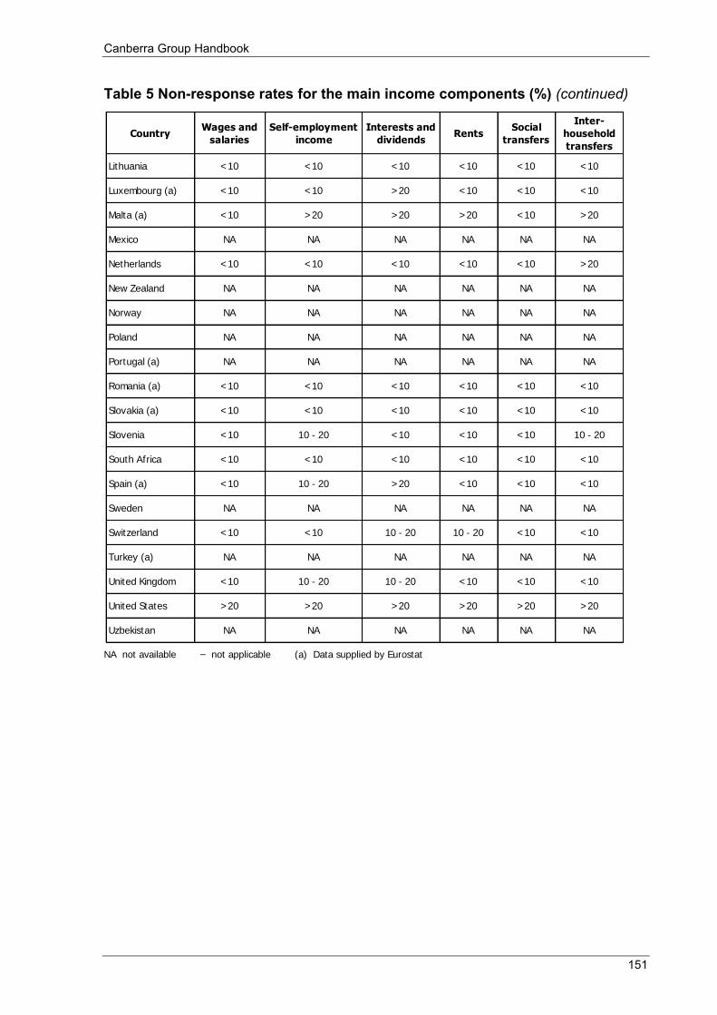
Canberra Group Handbook
151
Table 5 Non-response rates for the main income components (%) (continued)
NA not available – not applicable (a) Data supplied by Eurostat
CountryWages and
salaries
Self-employment
income
Interests and
dividendsRents
Social
transfers
Inter-
household
transfers
Lithuania <10 <10 <10 <10 <10 <10
Luxembourg (a) <10 <10 >20 <10 <10 <10
Malta (a) <10 >20 >20 >20 <10 >20
Mexico NA NA NA NA NA NA
Netherlands <10 <10 <10 <10 <10 >20
New Zealand NA NA NA NA NA NA
Norway NA NA NA NA NA NA
Poland NA NA NA NA NA NA
Portugal (a) NA NA NA NA NA NA
Romania (a) <10 <10 <10 <10 <10 <10
Slovakia (a) <10 <10 <10 <10 <10 <10
Slovenia <10 10 - 20 <10 <10 <10 10 - 20
South Africa <10 <10 <10 <10 <10 <10
Spain (a) <10 10 - 20 >20 <10 <10 <10
Sweden NA NA NA NA NA NA
Switzerland <10 <10 10 - 20 10 - 20 <10 <10
Turkey (a) NA NA NA NA NA NA
United Kingdom <10 10 - 20 10 - 20 <10 <10 <10
United States >20 >20 >20 >20 >20 >20
Uzbekistan NA NA NA NA NA NA
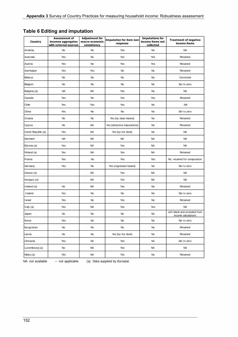
Appendix 3 Survey of Country Practices for measuring household income: Robustness assessment
152
Table 6 Editing and imputation
NA not available – not applicable (a) Data supplied by Eurostat
Country
Assessment of
incomes aggregates
with external sources
Adjustment for
macro-economic
consistency
Imputation for item non-
response
Imputations for
income items not
collected
Treatment of negative
income items
Armenia No No Yes No NA
Australia Yes No Yes Yes Retained
Austria Yes No Yes Yes Retained
Azerbaijan Yes Yes No No Retained
Belarus No No No No Corrected
Belgium No No No No Set to zero
Bulgaria (a) NA NA Yes No NA
Canada Yes No Yes Yes Retained
Chile Yes Yes Yes No .NA
China Yes No No No Set to zero
Croatia No No Yes (by class means) No Retained
Cyprus No NA Yes (deductive imputations) No Retained
Czech Republic (a) Yes NA Yes (by hot deck) No NA
Denmark NA NA NA NA NA
Estonia (a) Yes NA Yes NA NA
Finland (a) Yes NA Yes NA Retained
France Yes No Yes Yes No, retained for computation
Germany Yes No Yes (regression based) No Set to zero
Greece (a) NA Yes NA NA
Hungary (a) NA Yes NA NA
Iceland (a) No NA Yes No Retained
Ireland Yes No No No Set to zero
Israel Yes No Yes No Retained
Italy (a) Yes NA Yes Yes NA
Japan No No No NoLeft blank and excluded from
income calculations
Korea Yes No No No Set to zero
Kyrgyzstan No No No No Retained
Latvia No No Yes (by hot deck) No Retained
Lithuania Yes No Yes No Set to zero
Luxembourg (a) No NA Yes NA NA
Malta (a) Yes NA Yes No Retained
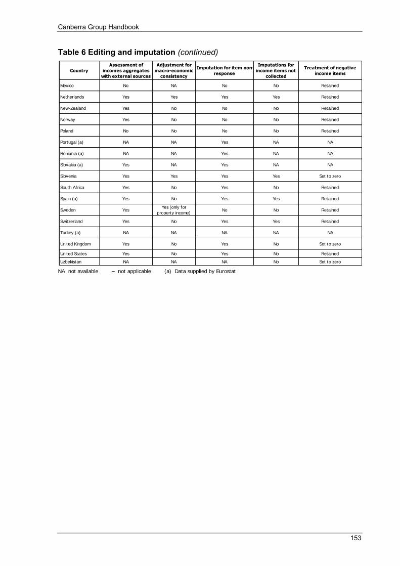
Canberra Group Handbook
153
Table 6 Editing and imputation (continued)
NA not available – not applicable (a) Data supplied by Eurostat
Country
Assessment of
incomes aggregates
with external sources
Adjustment for
macro-economic
consistency
Imputation for item non-
response
Imputations for
income items not
collected
Treatment of negative
income items
Mexico No NA No No Retained
Netherlands Yes Yes Yes Yes Retained
New-Zealand Yes No No No Retained
Norway Yes No No No Retained
Poland No No No No Retained
Portugal (a) NA NA Yes NA NA
Romania (a) NA NA Yes NA NA
Slovakia (a) Yes NA Yes NA NA
Slovenia Yes Yes Yes Yes Set to zero
South Africa Yes No Yes No Retained
Spain (a) Yes No Yes Yes Retained
Sweden YesYes (only for
property income)No No Retained
Switzerland Yes No Yes Yes Retained
Turkey (a) NA NA NA NA NA
United Kingdom Yes No Yes No Set to zero
United States Yes No Yes No Retained
Uzbekistan NA NA NA No Set to zero
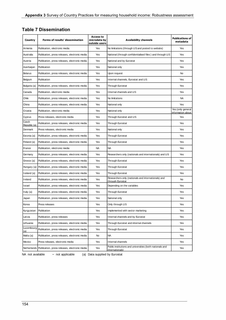
Appendix 3 Survey of Country Practices for measuring household income: Robustness assessment
154
Table 7 Dissemination
NA not available – not applicable (a) Data supplied by Eurostat
Country Forms of results' dissemination
Access to
microdata by
outside users
Availability channelsPublications of
metadata
Armenia Publication, electronic media Yes No limitations (through LIS and posted to website) Yes
Australia Publication, press releases, electronic media Yes National (through confidentialised files ) and through LIS Yes
Austria Publication, press releases, electronic media Yes National and by Eurostat Yes
Azerbaijan Publication Yes National only Yes
Belarus Publication, press releases, electronic media Yes Upon request No
Belgium Publication Yes Internal channels, Eurostat and LIS Yes
Bulgaria (a) Publication, press releases, electronic media Yes Through Eurostat Yes
Canada Publication, electronic media Yes Internal channels and LIS Yes
Chile Publication, press releases, electronic media Yes No limitations NA
China Publication, press releases, electronic media Yes National only Yes
Croatia Publication, electronic media Yes National onlyYes (only general
information about
Cyprus Press releases, electronic media Yes Through Eurostat and LIS Yes
Czech
Republic (a)Publication, press releases, electronic media Yes Through Eurostat Yes
Denmark Press releases, electronic media Yes National only Yes
Estonia (a) Publication, press releases, electronic media Yes Through Eurostat Yes
Finland (a) Publication, press releases, electronic media Yes Through Eurostat Yes
France Publication, electronic media NA NA Yes
Germany Publication, press releases, electronic media Yes Researchers only (nationals and internationals) and LIS Yes
Greece (a) Publication, press releases, electronic media Yes Through Eurostat Yes
Hungary (a) Publication, press releases, electronic media Yes Through Eurostat Yes
Iceland (a) Publication, press releases, electronic media Yes Through Eurostat Yes
Ireland Publication, press releases, electronic media YesResearchers only (nationals and internationals) and
through EurostatNo
Israel Publication, press releases, electronic media Yes Depending on the variables Yes
Italy (a) Publication, press releases, electronic media Yes Through Eurostat Yes
Japan Publication, press releases, electronic media Yes National only Yes
Korea Press releases Yes Only through LIS Yes
Kyrgyzstan Publication Yes Implemented with sector marketing Yes
Latvia Publication, press releases Yes Internal channels and by Eurostat Yes
Lithuania Publication, press releases, electronic media Yes Through Eurostat and internal channels Yes
Luxembourg
(a)Publication, press releases, electronic media Yes Through Eurostat Yes
Malta (a) Publication, press releases, electronic media No NA Yes
Mexico Press releases, electronic media Yes Internal channels Yes
Netherlands Publication, press releases, electronic media YesPublic institutions and universities (both nationals and
internationals)Yes
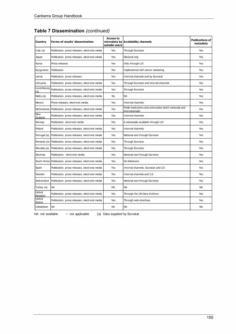
Canberra Group Handbook
155
Table 7 Dissemination (continued)
NA not available – not applicable (a) Data supplied by Eurostat
Country Forms of results' dissemination
Access to
microdata by
outside users
Availability channelsPublications of
metadata
Italy (a) Publication, press releases, electronic media Yes Through Eurostat Yes
Japan Publication, press releases, electronic media Yes National only Yes
Korea Press releases Yes Only through LIS Yes
Kyrgyzstan Publication Yes Implemented with sector marketing Yes
Latvia Publication, press releases Yes Internal channels and by Eurostat Yes
Lithuania Publication, press releases, electronic media Yes Through Eurostat and internal channels Yes
Luxembourg
(a)Publication, press releases, electronic media Yes Through Eurostat Yes
Malta (a) Publication, press releases, electronic media No NA Yes
Mexico Press releases, electronic media Yes Internal channels Yes
Netherlands Publication, press releases, electronic media YesPublic institutions and universities (both nationals and
internationals)Yes
New
ZealandPublication, press releases, electronic media Yes Internal channels Yes
Norway Publication, electronic media Yes A subsample available through LIS Yes
Poland Publication, press releases, electronic media Yes Internal channels Yes
Portugal (a) Publication, press releases, electronic media Yes National and through Eurostat Yes
Romania (a) Publication, press releases, electronic media Yes Through Eurostat Yes
Slovakia (a) Publication, press releases, electronic media Yes Through Eurostat Yes
Slovenia Publication, electronic media Yes National and through Eurostat Yes
South Africa Publication, press releases, electronic media Yes No limitations Yes
Spain Publication, press releases, electronic media Yes Internal channels, Eurostat and LIS Yes
Sweden Publication, press releases, electronic media Yes Internal channels and LIS Yes
Switzerland Publication, press releases, electronic media Yes National and through Eurostat Yes
Turkey (a) NA NA NA NA
United
KingdomPublication, press releases, electronic media Yes Through the UK Data Archives Yes
United
StatesPublication, press releases, electronic media Yes Through web-interface Yes
Uzbekistan NA NA NA NA
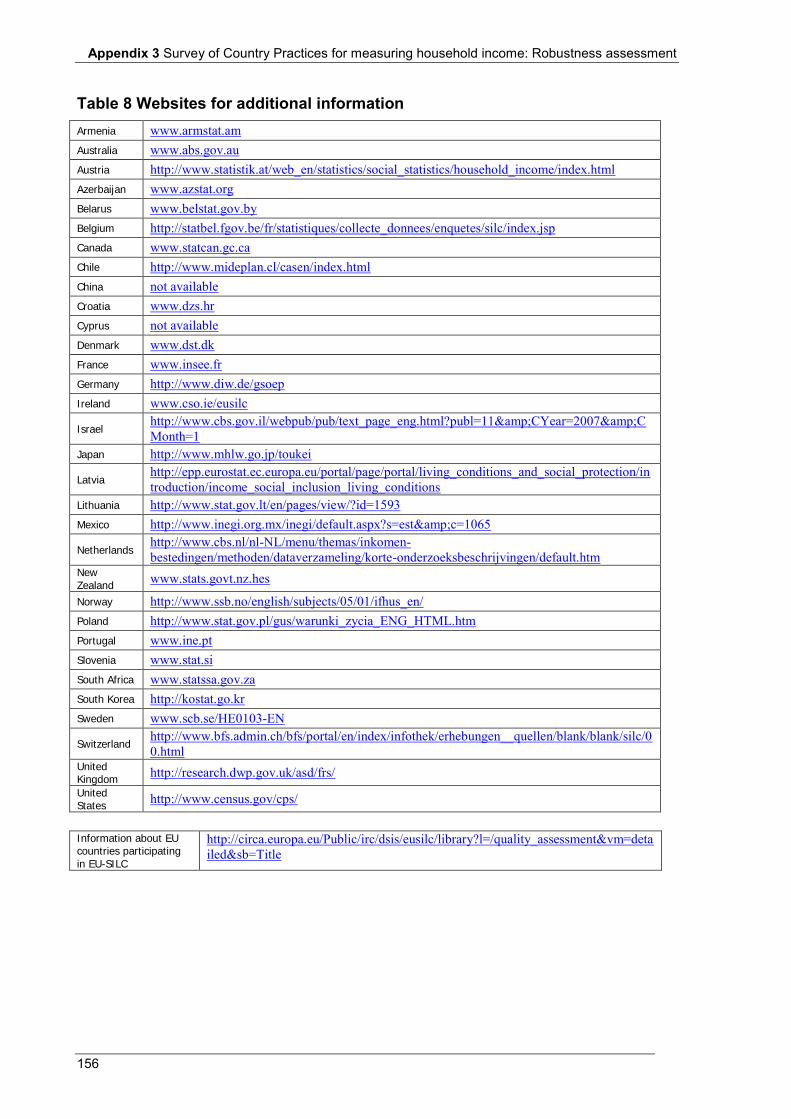
Appendix 3 Survey of Country Practices for measuring household income: Robustness assessment
156
Table 8 Websites for additional information Armenia www.armstat.am Australia www.abs.gov.au Austria http://www.statistik.at/web_en/statistics/social_statistics/household_income/index.html Azerbaijan www.azstat.org Belarus www.belstat.gov.by Belgium http://statbel.fgov.be/fr/statistiques/collecte_donnees/enquetes/silc/index.jsp Canada www.statcan.gc.ca Chile http://www.mideplan.cl/casen/index.html China not available Croatia www.dzs.hr Cyprus not available Denmark www.dst.dk France www.insee.fr Germany http://www.diw.de/gsoep Ireland www.cso.ie/eusilc
Israel http://www.cbs.gov.il/webpub/pub/text_page_eng.html?publ=11&CYear=2007&CMonth=1
Japan http://www.mhlw.go.jp/toukei
Latvia http://epp.eurostat.ec.europa.eu/portal/page/portal/living_conditions_and_social_protection/introduction/income_social_inclusion_living_conditions
Lithuania http://www.stat.gov.lt/en/pages/view/?id=1593 Mexico http://www.inegi.org.mx/inegi/default.aspx?s=est&c=1065
Netherlands http://www.cbs.nl/nl-NL/menu/themas/inkomen-bestedingen/methoden/dataverzameling/korte-onderzoeksbeschrijvingen/default.htm
New Zealand
www.stats.govt.nz.hes
Norway http://www.ssb.no/english/subjects/05/01/ifhus_en/ Poland http://www.stat.gov.pl/gus/warunki_zycia_ENG_HTML.htm Portugal www.ine.pt Slovenia www.stat.si South Africa www.statssa.gov.za South Korea http://kostat.go.kr Sweden www.scb.se/HE0103-EN
Switzerland http://www.bfs.admin.ch/bfs/portal/en/index/infothek/erhebungen__quellen/blank/blank/silc/00.html
United Kingdom
http://research.dwp.gov.uk/asd/frs/ United States
http://www.census.gov/cps/
Information about EU countries participating in EU-SILC
http://circa.europa.eu/Public/irc/dsis/eusilc/library?l=/quality_assessment&vm=detailed&sb=Title
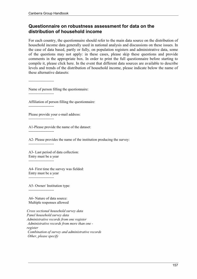
Canberra Group Handbook
157
Questionnaire on robustness assessment for data on the distribution of household income
For each country, the questionnaire should refer to the main data source on the distribution of household income data generally used in national analysis and discussions on these issues. In the case of data based, partly or fully, on population registers and administrative data, some of the questions may not apply: in these cases, please skip these questions and provide comments in the appropriate box. In order to print the full questionnaire before starting to compile it, please click here. In the event that different data sources are available to describe levels and trends of the distribution of household income, please indicate below the name of these alternative datasets:
--------------------- Name of person filling the questionnaire: --------------------- Affiliation of person filling the questionnaire: --------------------- Please provide your e-mail address: --------------------- A1-Please provide the name of the dataset: --------------------- A2- Please provides the name of the institution producing the survey: --------------------- A3- Last period of data collection: Entry must be a year --------------------- A4- First time the survey was fielded: Entry must be a year --------------------- A5- Owner/ Institution type: --------------------- A6- Nature of data source: Multiple responses allowed
Cross sectional household survey data Panel household survey data Administrative records from one register Administrative records from more than one -register Combination of survey and administrative records Other, please specify
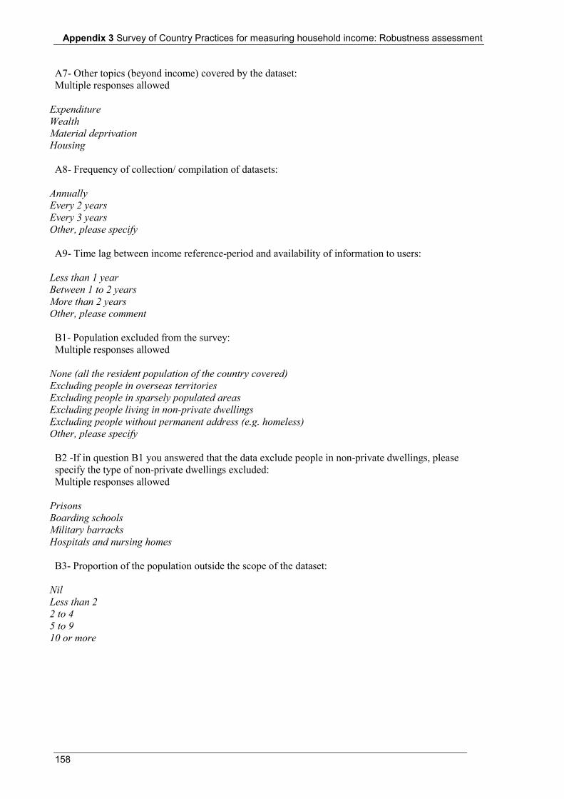
Appendix 3 Survey of Country Practices for measuring household income: Robustness assessment
158
A7- Other topics (beyond income) covered by the dataset: Multiple responses allowed
Expenditure Wealth Material deprivation Housing A8- Frequency of collection/ compilation of datasets:
Annually Every 2 years Every 3 years Other, please specify A9- Time lag between income reference-period and availability of information to users:
Less than 1 year Between 1 to 2 years More than 2 years Other, please comment B1- Population excluded from the survey: Multiple responses allowed
None (all the resident population of the country covered) Excluding people in overseas territories Excluding people in sparsely populated areas Excluding people living in non-private dwellings Excluding people without permanent address (e.g. homeless) Other, please specify B2 -If in question B1 you answered that the data exclude people in non-private dwellings, please specify the type of non-private dwellings excluded: Multiple responses allowed
Prisons Boarding schools Military barracks Hospitals and nursing homes B3- Proportion of the population outside the scope of the dataset:
Nil Less than 2 2 to 4 5 to 9 10 or more
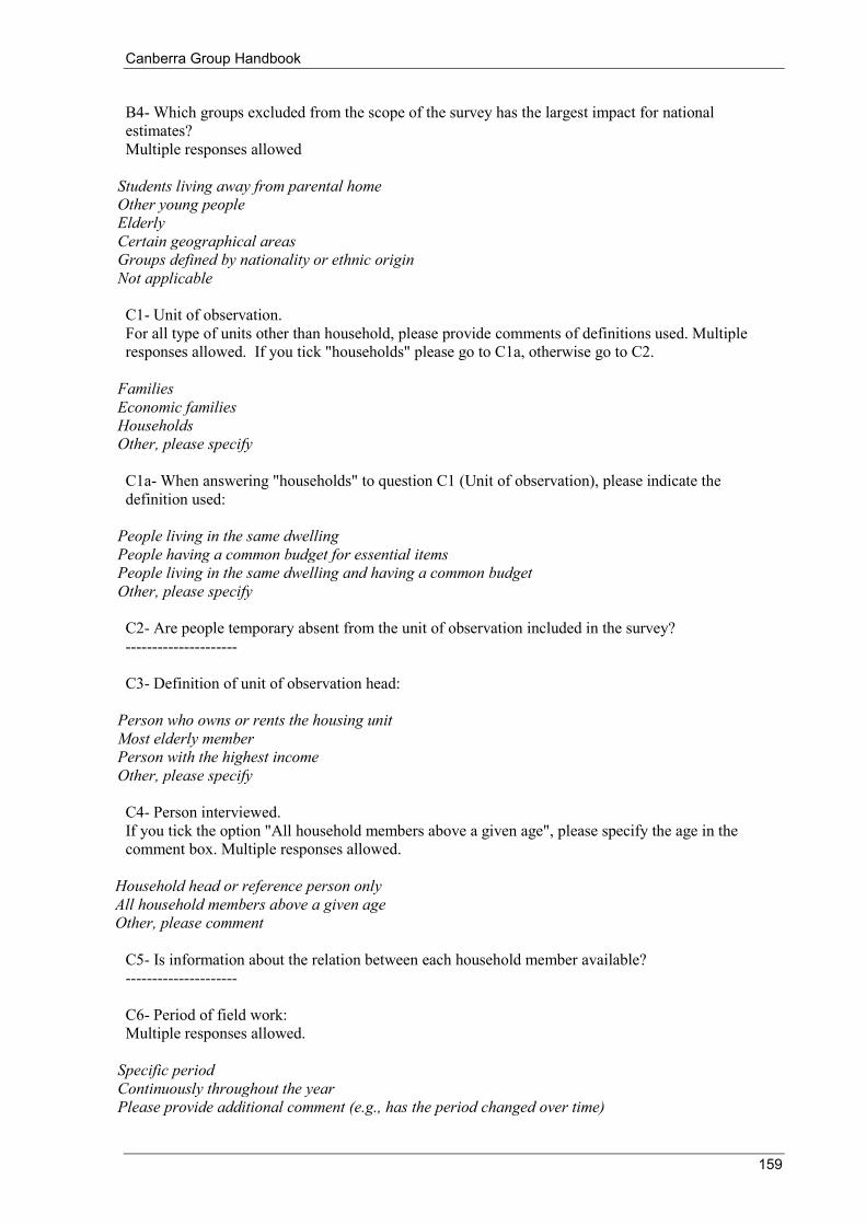
Canberra Group Handbook
159
B4- Which groups excluded from the scope of the survey has the largest impact for national estimates? Multiple responses allowed
Students living away from parental home Other young people Elderly Certain geographical areas Groups defined by nationality or ethnic origin Not applicable C1- Unit of observation. For all type of units other than household, please provide comments of definitions used. Multiple responses allowed. If you tick "households" please go to C1a, otherwise go to C2.
Families Economic families Households Other, please specify C1a- When answering "households" to question C1 (Unit of observation), please indicate the definition used:
People living in the same dwelling People having a common budget for essential items People living in the same dwelling and having a common budget Other, please specify C2- Are people temporary absent from the unit of observation included in the survey? --------------------- C3- Definition of unit of observation head:
Person who owns or rents the housing unit Most elderly member Person with the highest income Other, please specify C4- Person interviewed. If you tick the option "All household members above a given age", please specify the age in the comment box. Multiple responses allowed.
Household head or reference person only All household members above a given age Other, please comment
C5- Is information about the relation between each household member available? --------------------- C6- Period of field work: Multiple responses allowed.
Specific period Continuously throughout the year Please provide additional comment (e.g., has the period changed over time)
Appendix 3 Survey of Country Practices for measuring household income: Robustness assessment
160
C7- Mode of data collection: Multiple responses allowed
Face to face Telephone Mobiles Administrative records Other, please specify C8- Income reference period: is the reference period for all income components the same? If you tick "yes" please specify in the comment box if reference period is previous week/ calendar year or previous 12 months.
Yes No Other If yes please comment C9- Information on income streams: are respondents asked to provide written records of various income streams? Multiple responses allowed.
Yes No Not Applicable If yes, what type and for which income source? Are respondents generally able to provide this evidence? C10- Information on "employment status" or "main activity" of each member. Is this information available? If yes, please go to C10a, otherwise go to C11. --------------------- C10a- How are values for these classifying variables assigned? Multiple responses allowed
Self-reported (referring for the income reference period) ILO definitions (referring to the time of interview) Other, please specify C11- Does income information reported in the questionnaire has a lower or upper limit (i.e. above 10 millions)? If you tick "yes", please specify if the same levels are used for all income components. --------------------- D1- Sample size. Please specify the number of units (e.g. households) in the most recent year: --------------------- D2- Sample size. Please specify the number of individuals in the most recent year: ---------------------
Canberra Group Handbook
161
D3- Sample design used: Multiple responses allowed
Stratified or clustered Multi-stage Not Applicable Other, please specify D4- Unit response rate:
Less than 50 50 to 80 More than 80 Not Applicable D5- Availability of a set of weights: --------------------- D6- Benchmarks used in calibrating weights:
Yes No Not Applicable If yes, please specify sources E1- Incidence of non-response for various income items? Please tick appropriate values range of item non-response rate as share of the total number of survey responses: Employee income -- Income from self-employment -- Interests and dividends -- Property rents -- Social assistance pensions and benefits -- Current transfers from other households -- E2- Has the coherence of income aggregates with external data been assessed? If you tick "yes" please go to E2a, otherwise go to E3. --------------------- E2a- Have income data been adjusted to establish coherence with external aggregates? If you answer "yes", please specify in the comment box. ---------------------
Appendix 3 Survey of Country Practices for measuring household income: Robustness assessment
162
E3- Imputation for item non-response: --------------------- E4- In the case of income components not included in the surveys/registers, are imputations done? --------------------- E5- Treatment of negative income items:
Retained Set to zero Other, please comment E6- Are income cut-off levels used in data processing? --------------------- F1- Form of data dissemination of results: Multiple responses allowed.
Publication Press releases Electronic media Other, please comment F2- Availability of micro-data made to outside users: If you tick "yes", please go to F2a, otherwise go to F3. --------------------- F2a- If you answered "yes" to question F2 (availability of micro-data made to outside users) please specify if micro-data are:
Limited to national users Provided through internal channels Available through international sites (e.g. LIS) Data in PUF differ from those available internally Other, please comment F3- Publication of metadata: If you tick "yes" please go to F3a, otherwise go to F4. --------------------- F3a- Please tick the following relevant items:
Scope Sample design Archived sample size Response rates Editing strategy Imputation Information about modelled data items Benchmarks and weighting F4- Website where additional information on features of the data source are available: If available, please provide web address .
163
Appendix 4 Survey of Country Practices for measuring household income: Data item inventory This appendix summarises the data item inventory undertaken as part of the Survey of Country Practices conducted in early 2010. The purpose of this component of the survey was to collect information on the availability of data for each component of income.
Table 1 summarises the responses provided by the 52 countries that participated in the survey.
Table 2 presents the detailed responses from each country. The key below explains individual responses.
1= completely or partially collected N= not collected or only collected in a general question, e.g. ‘All other income’ NA = not available
Table 3 lists the countries that participated in the 2010 survey and the country abbreviations used in Table 2.
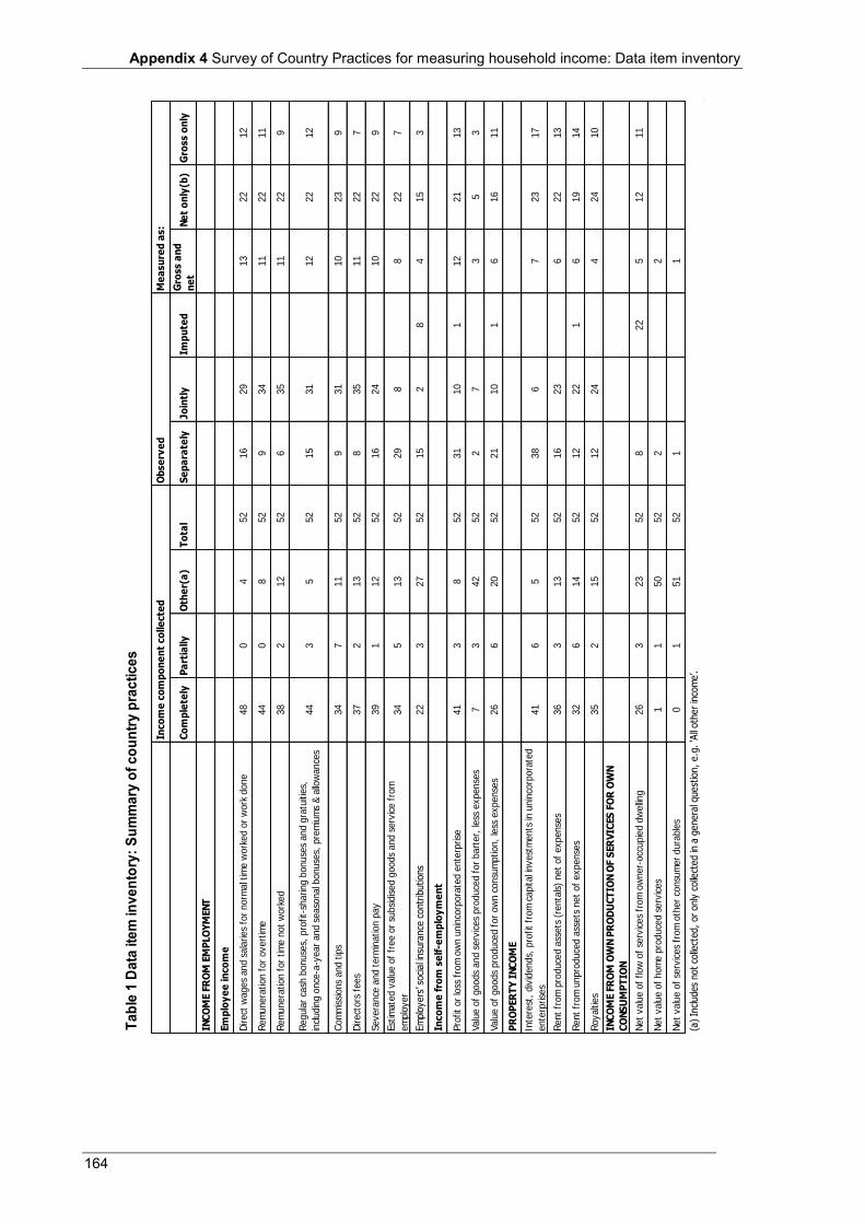
Appendix 4 Survey of Country Practices for measuring household income: Data item inventory
164
Co
mp
lete
lyP
art
ially
Oth
er(
a)
To
tal
Se
pa
rate
lyJo
intl
yIm
pu
ted
Gro
ss a
nd
ne
tN
et
on
ly(b
)G
ross o
nly
INC
OM
E F
RO
M E
MP
LO
YM
EN
T
Em
plo
ye
e in
co
me
Direct
wages
and s
ala
ries
for
norm
al t
ime w
ork
ed o
r w
ork
done
48
04
52
16
29
13
22
12
Rem
unera
tion f
or
overt
ime
44
08
52
934
11
22
11
Rem
unera
tion f
or
tim
e n
ot
work
ed
38
212
52
635
11
22
9
Regula
r ca
sh b
onuse
s, p
rofit-
sharing b
onuse
s and g
ratu
itie
s,
incl
udin
g o
nce
-a-y
ear
and s
easo
nal b
onuse
s, p
rem
ium
s &
allo
wance
s44
35
52
15
31
12
22
12
Com
mis
sions
and t
ips
34
711
52
931
10
23
9
Direct
ors
fees
37
213
52
835
11
22
7
Severa
nce
and t
erm
ination p
ay
39
112
52
16
24
10
22
9
Est
imate
d v
alu
e o
f fr
ee o
r su
bsi
dis
ed g
oods
and s
erv
ice f
rom
em
plo
yer
34
513
52
29
88
22
7
Em
plo
yers
’ soci
al i
nsu
rance
contr
ibutions
22
327
52
15
28
415
3
Inco
me
fro
m s
elf
-em
plo
ym
en
t
Pro
fit
or
loss
fro
m o
wn u
nin
corp
ora
ted e
nte
rprise
41
38
52
31
10
112
21
13
Valu
e o
f goods
and s
erv
ices
pro
duce
d f
or
bart
er,
less
expense
s7
342
52
27
35
3
Valu
e o
f goods
pro
duce
d f
or
ow
n c
onsu
mption,
less
expense
s26
620
52
21
10
16
16
11
PR
OP
ER
TY
IN
CO
ME
Inte
rest
, div
idends,
pro
fit
from
capital i
nvest
ments
in u
nin
corp
ora
ted
ente
rprise
s41
65
52
38
67
23
17
Rent
from
pro
duce
d a
ssets
(re
nta
ls)
net
of
expense
s36
313
52
16
23
622
13
Rent
from
unpro
duce
d a
ssets
net
of
expense
s32
614
52
12
22
16
19
14
Royaltie
s35
215
52
12
24
424
10
INC
OM
E F
RO
M O
WN
PR
OD
UC
TIO
N O
F S
ER
VIC
ES
FO
R O
WN
CO
NS
UM
PT
ION
Net
valu
e o
f flow
of
serv
ices
from
ow
ner-
occ
upie
d d
welling
26
323
52
822
512
11
Net
valu
e o
f hom
e p
roduce
d s
erv
ices
11
50
52
22
Net
valu
e o
f se
rvic
es
from
oth
er
consu
mer
dura
ble
s0
151
52
11
Tabl
e 1
Data
item
inve
ntor
y: S
umm
ary
of c
ount
ry p
ract
ices
(a)
Incl
udes
not
colle
cted,
or
only
colle
cted in
a g
enera
l quest
ion,
e.g
. ‘A
ll oth
er
inco
me’.
Inco
me
co
mp
on
en
t co
lle
cte
d
Ob
se
rve
d
Me
asu
red
as:
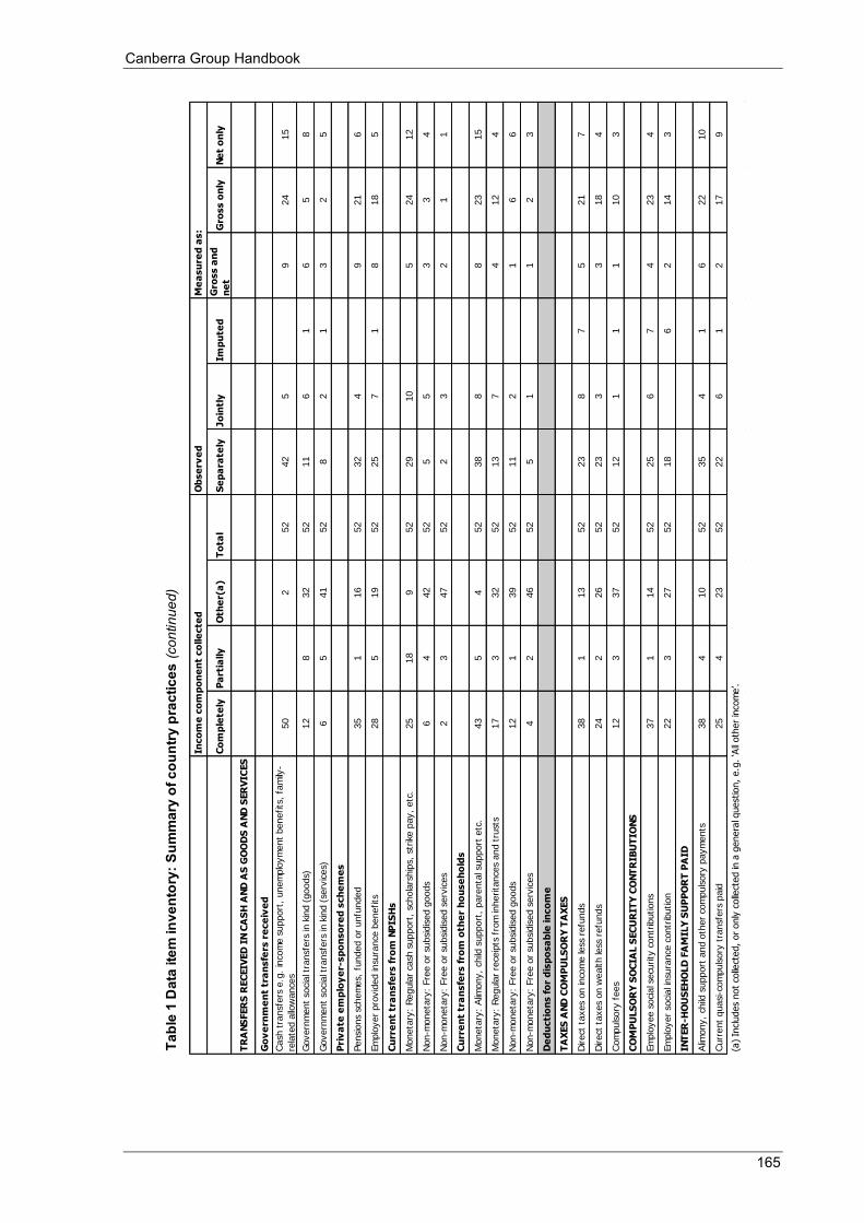
Canberra Group Handbook
165
Co
mp
lete
lyP
art
ially
Oth
er(
a)
To
tal
Se
pa
rate
lyJo
intl
yIm
pu
ted
Gro
ss a
nd
ne
tG
ross o
nly
Ne
t o
nly
TR
AN
SFER
S R
EC
EIV
ED
IN
CA
SH
AN
D A
S G
OO
DS
AN
D S
ER
VIC
ES
Go
ve
rnm
en
t tr
an
sfe
rs r
ece
ive
d
Cash
tra
nsf
ers
e.g
. in
com
e s
upport
, unem
plo
ym
ent
benefits
, fa
mily
-
rela
ted a
llow
ance
s50
252
42
59
24
15
Govern
ment
soci
al t
ransf
ers
in k
ind (
goods)
12
832
52
11
61
65
8
Govern
ment
soci
al t
ransf
ers
in k
ind (
serv
ices)
65
41
52
82
13
25
Pri
va
te e
mp
loy
er-
sp
on
so
red
sch
em
es
Pensi
ons
schem
es,
funded o
r unfu
nded
35
116
52
32
49
21
6
Em
plo
yer
pro
vid
ed in
sura
nce
benefits
28
519
52
25
71
818
5
Cu
rre
nt
tra
nsfe
rs f
rom
NP
ISH
s
Moneta
ry:
Regula
r ca
sh s
upport
, sc
hola
rship
s, s
trik
e p
ay,
etc
.25
18
952
29
10
524
12
Non-m
oneta
ry:
Fre
e o
r su
bsi
dis
ed g
oods
64
42
52
55
33
4
Non-m
oneta
ry:
Fre
e o
r su
bsi
dis
ed s
erv
ices
23
47
52
23
21
1
Cu
rre
nt
tra
nsfe
rs f
rom
oth
er
ho
use
ho
lds
Moneta
ry:
Alim
ony,
child
support
, pare
nta
l support
etc
.43
54
52
38
88
23
15
Moneta
ry:
Regula
r re
ceip
ts f
rom
inherita
nce
s and t
rust
s17
332
52
13
74
12
4
Non-m
oneta
ry:
Fre
e o
r su
bsi
dis
ed g
oods
12
139
52
11
21
66
Non-m
oneta
ry:
Fre
e o
r su
bsi
dis
ed s
erv
ices
42
46
52
51
12
3
De
du
cti
on
s f
or
dis
po
sa
ble
in
co
me
TA
XES
AN
D C
OM
PU
LS
OR
Y T
AX
ES
Direct
taxes
on in
com
e le
ss r
efu
nds
38
113
52
23
87
521
7
Direct
taxes
on w
ealth le
ss r
efu
nds
24
226
52
23
33
18
4
Com
puls
ory
fees
12
337
52
12
11
110
3
CO
MP
ULS
OR
Y S
OC
IAL S
EC
UR
ITY
CO
NT
RIB
UT
ION
S
Em
plo
yee s
oci
al s
ecu
rity
contr
ibutions
37
114
52
25
67
423
4
Em
plo
yer
soci
al i
nsu
rance
contr
ibution
22
327
52
18
62
14
3
INT
ER
-HO
US
EH
OLD
FA
MIL
Y S
UP
PO
RT
PA
ID
Alim
ony,
child
support
and o
ther
com
puls
ory
paym
ents
38
410
52
35
41
622
10
Curr
ent
quasi
-com
puls
ory
tra
nsf
ers
paid
25
423
52
22
61
217
9
Tabl
e 1
Dat
a ite
m in
vent
ory:
Sum
mar
y of
cou
ntry
pra
ctic
es (c
ontin
ued)
(a)
Incl
udes
not
colle
cted,
or
only
colle
cted in
a g
enera
l quest
ion,
e.g
. ‘A
ll oth
er
inco
me’.
Inco
me
co
mp
on
en
t co
lle
cte
d
Ob
se
rve
d
Me
asu
red
as:
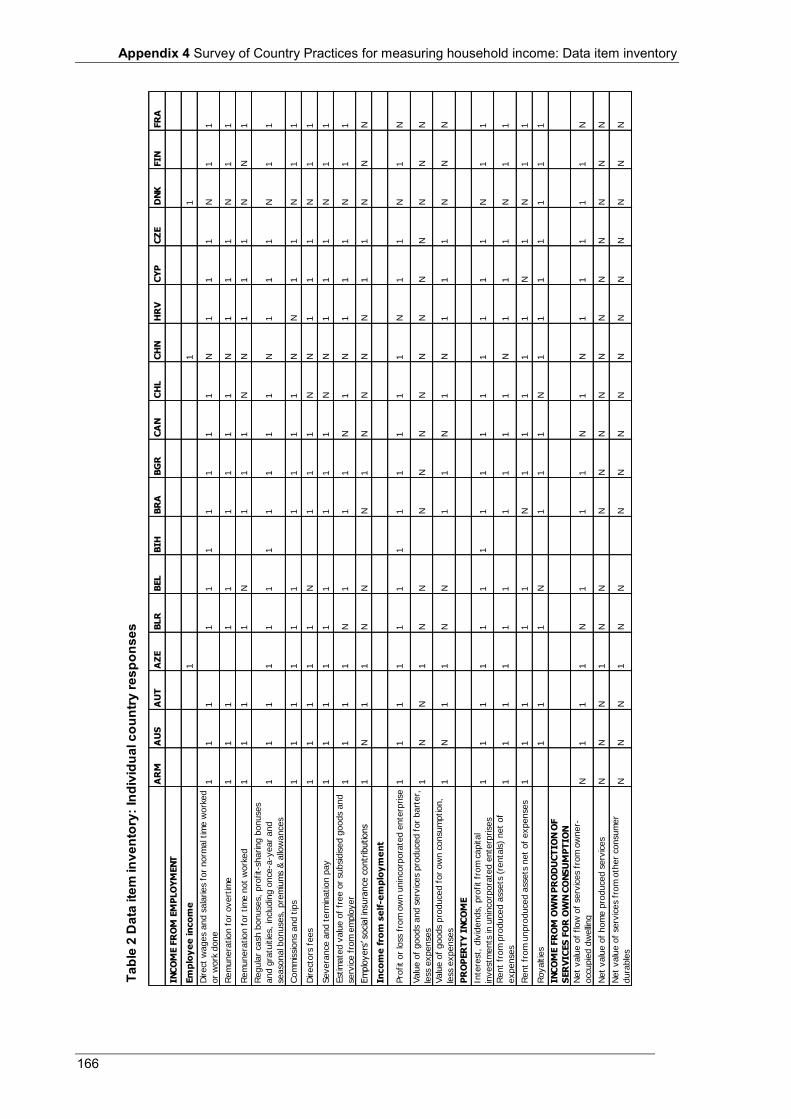
Appendix 4 Survey of Country Practices for measuring household income: Data item inventory
166
AR
MA
US
AU
TA
ZE
BLR
BEL
BIH
BR
AB
GR
CA
NC
HL
CH
NH
RV
CY
PC
ZE
DN
KFIN
FR
A
INC
OM
E F
RO
M E
MP
LO
YM
EN
T
Em
plo
ye
e in
co
me
11
1
Direct
wages
and s
ala
ries
for
norm
al t
ime w
ork
ed
or
work
done
11
11
11
11
11
N1
11
N1
1
Rem
unera
tion f
or
overt
ime
11
11
11
11
1N
11
1N
11
Rem
unera
tion f
or
tim
e n
ot
work
ed
11
11
N1
11
NN
11
1N
N1
Regula
r ca
sh b
onuse
s, p
rofit-
sharing b
onuse
s
and g
ratu
itie
s, in
cludin
g o
nce
-a-y
ear
and
seaso
nal b
onuse
s, p
rem
ium
s &
allo
wance
s
11
11
11
11
11
1N
11
1N
11
Com
mis
sions
and t
ips
11
11
11
11
11
NN
11
N1
1
Direct
ors
fees
11
11
1N
11
1N
N1
11
N1
1
Severa
nce
and t
erm
ination p
ay
11
11
11
11
1N
N1
11
N1
1
Est
imate
d v
alu
e o
f fr
ee o
r su
bsi
dis
ed g
oods
and
serv
ice f
rom
em
plo
yer
11
11
N1
11
N1
N1
11
N1
1
Em
plo
yers
’ soci
al i
nsu
rance
contr
ibutions
1N
11
NN
N1
NN
NN
11
NN
N
Inco
me
fro
m s
elf
-em
plo
ym
en
t
Pro
fit
or
loss
fro
m o
wn u
nin
corp
ora
ted e
nte
rprise
11
11
11
11
11
11
N1
1N
1N
Valu
e o
f goods
and s
erv
ices
pro
duce
d f
or
bart
er,
less
expense
s1
NN
1N
NN
NN
NN
NN
NN
NN
Valu
e o
f goods
pro
duce
d f
or
ow
n c
onsu
mption,
less
expense
s1
N1
1N
N1
1N
1N
11
1N
NN
PR
OP
ER
TY
IN
CO
ME
Inte
rest
, div
idends,
pro
fit
from
capital
invest
ments
in u
nin
corp
ora
ted e
nte
rprise
s1
11
11
11
11
11
11
11
N1
1
Rent
from
pro
duce
d a
ssets
(re
nta
ls)
net
of
expense
s1
11
11
11
11
1N
11
1N
11
Rent
from
unpro
duce
d a
ssets
net
of
expense
s1
11
11
N1
11
11
N1
N1
1
Royaltie
s1
11
N1
11
N1
11
11
11
INC
OM
E F
RO
M O
WN
PR
OD
UC
TIO
N O
F
SER
VIC
ES
FO
R O
WN
CO
NS
UM
PT
ION
Net
valu
e o
f flow
of
serv
ices
from
ow
ner-
occ
upie
d d
welling
N1
11
N1
11
N1
N1
11
11
N
Net
valu
e o
f hom
e p
roduce
d s
erv
ices
NN
N1
NN
NN
NN
NN
NN
NN
N
Net
valu
e o
f se
rvic
es
from
oth
er
consu
mer
dura
ble
sN
NN
1N
NN
NN
NN
NN
NN
NN
Tabl
e 2
Dat
a ite
m in
vent
ory:
Indi
vidu
al c
ount
ry re
spon
ses
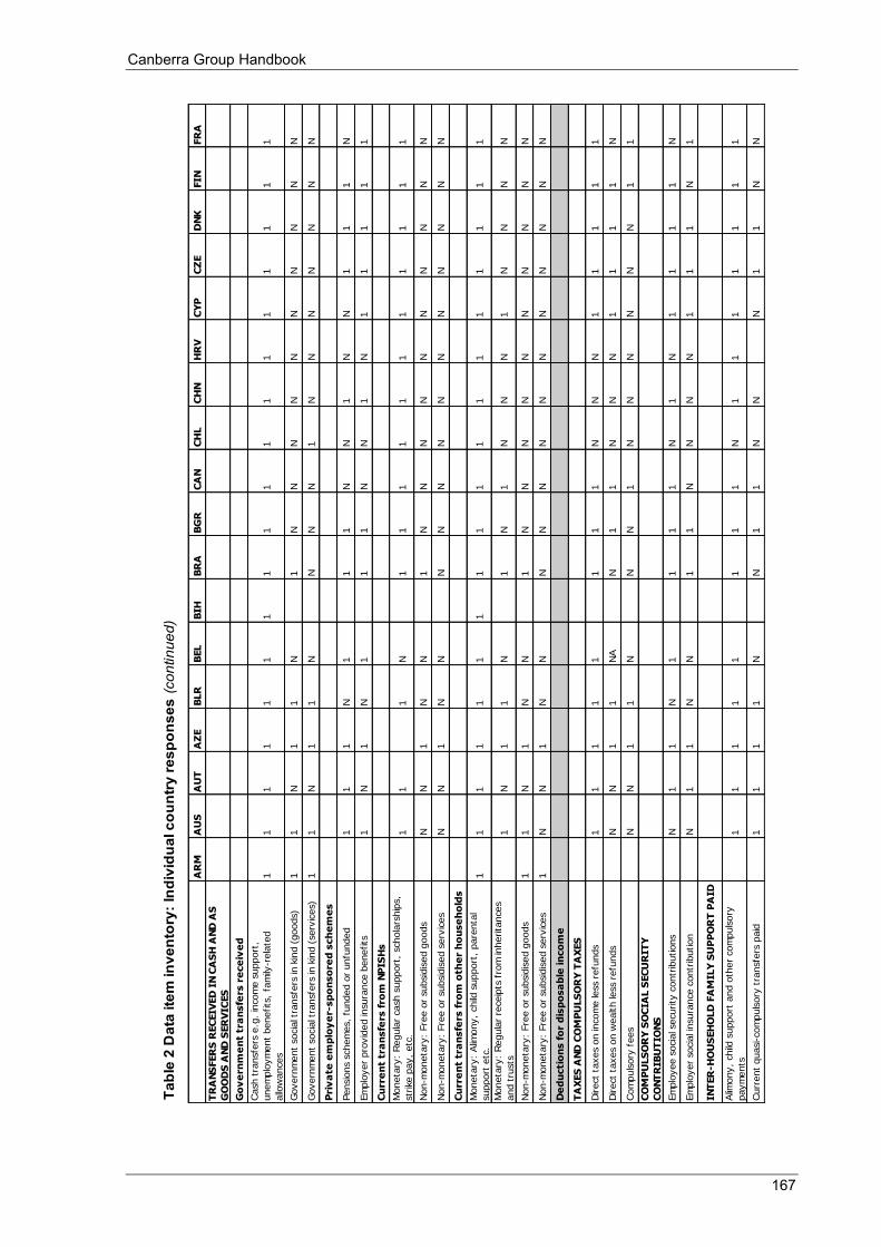
Canberra Group Handbook
167
AR
MA
US
AU
TA
ZE
BLR
BEL
BIH
BR
AB
GR
CA
NC
HL
CH
NH
RV
CY
PC
ZE
DN
KFIN
FR
A
TR
AN
SFER
S R
EC
EIV
ED
IN
CA
SH
AN
D A
S
GO
OD
S A
ND
SER
VIC
ES
Go
ve
rnm
en
t tr
an
sfe
rs r
ece
ive
d
Cash
tra
nsf
ers
e.g
. in
com
e s
upport
,
unem
plo
ym
ent
benefits
, fa
mily
-rela
ted
allo
wance
s
11
11
11
11
11
11
11
11
11
Govern
ment
soci
al t
ransf
ers
in k
ind (
goods)
11
N1
1N
1N
NN
NN
NN
NN
N
Govern
ment
soci
al t
ransf
ers
in k
ind (
serv
ices)
11
N1
1N
NN
N1
NN
NN
NN
N
Pri
va
te e
mp
loy
er-
sp
on
so
red
sch
em
es
Pensi
ons
schem
es,
funded o
r unfu
nded
11
1N
11
1N
N1
NN
11
1N
Em
plo
yer
pro
vid
ed in
sura
nce
benefits
1N
1N
11
1N
N1
N1
11
11
Cu
rre
nt
tra
nsfe
rs f
rom
NP
ISH
s
Moneta
ry:
Regula
r ca
sh s
upport
, sc
hola
rship
s,
strike
pay,
etc
.1
11
N1
11
11
11
11
11
Non-m
oneta
ry:
Fre
e o
r su
bsi
dis
ed g
oods
NN
1N
N1
NN
NN
NN
NN
NN
Non-m
oneta
ry:
Fre
e o
r su
bsi
dis
ed s
erv
ices
NN
1N
NN
NN
NN
NN
NN
NN
Cu
rre
nt
tra
nsfe
rs f
rom
oth
er
ho
use
ho
lds
Moneta
ry:
Alim
ony,
child
support
, pare
nta
l
support
etc
.1
11
11
11
11
11
11
11
11
1
Moneta
ry:
Regula
r re
ceip
ts f
rom
inherita
nce
s
and t
rust
s1
N1
1N
1N
1N
NN
1N
NN
N
Non-m
oneta
ry:
Fre
e o
r su
bsi
dis
ed g
oods
11
N1
NN
1N
NN
NN
NN
NN
N
Non-m
oneta
ry:
Fre
e o
r su
bsi
dis
ed s
erv
ices
1N
N1
NN
NN
NN
NN
NN
NN
N
De
du
cti
on
s f
or
dis
po
sa
ble
in
co
me
TA
XES
AN
D C
OM
PU
LS
OR
Y T
AX
ES
Direct
taxes
on in
com
e le
ss r
efu
nds
11
11
11
11
NN
N1
11
11
Direct
taxes
on w
ealth le
ss r
efu
nds
NN
11
NA
N1
1N
NN
11
11
N
Com
puls
ory
fees
NN
11
NN
N1
NN
NN
NN
11
CO
MP
ULS
OR
Y S
OC
IAL S
EC
UR
ITY
CO
NT
RIB
UT
ION
S
Em
plo
yee s
oci
al s
ecu
rity
contr
ibutions
N1
1N
11
11
N1
N1
11
1N
Em
plo
yer
soci
al i
nsu
rance
contr
ibution
N1
1N
N1
1N
NN
N1
11
N1
INT
ER
-HO
US
EH
OLD
FA
MIL
Y S
UP
PO
RT
PA
ID
Alim
ony,
child
support
and o
ther
com
puls
ory
paym
ents
11
11
11
11
N1
11
11
11
Curr
ent
quasi
-com
puls
ory
tra
nsf
ers
paid
11
11
NN
11
NN
N1
1N
N
Tabl
e 2
Dat
a ite
m in
vent
ory:
Indi
vidu
al c
ount
ry re
spon
ses
(con
tinue
d)
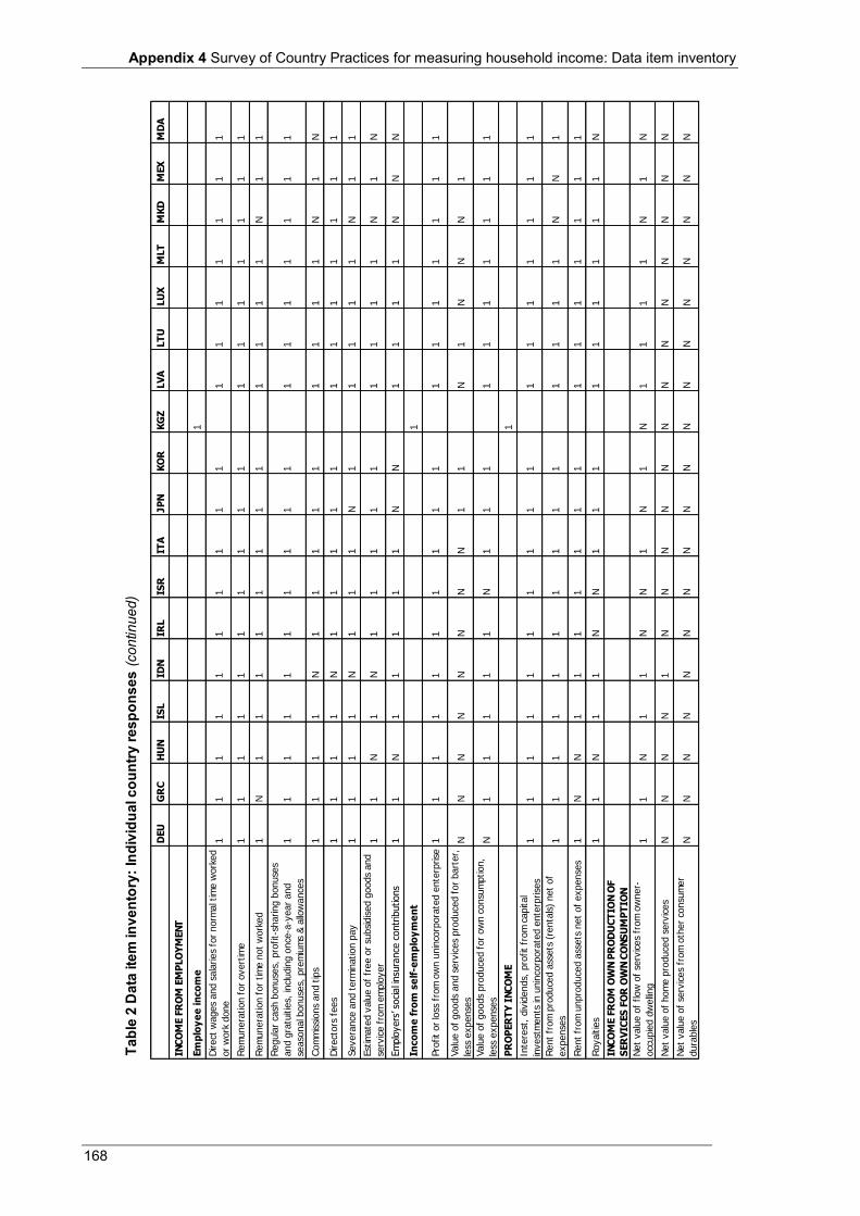
Appendix 4 Survey of Country Practices for measuring household income: Data item inventory
168
DEU
GR
CH
UN
ISL
IDN
IRL
ISR
ITA
JP
NK
OR
KG
ZLV
ALT
ULU
XM
LT
MK
DM
EX
MD
A
INC
OM
E F
RO
M E
MP
LO
YM
EN
T
Em
plo
ye
e in
co
me
1
Direct
wages
and s
ala
ries
for
norm
al t
ime w
ork
ed
or
work
done
11
11
11
11
11
11
11
11
1
Rem
unera
tion f
or
overt
ime
11
11
11
11
11
11
11
11
1
Rem
unera
tion f
or
tim
e n
ot
work
ed
1N
11
11
11
11
11
11
N1
1
Regula
r ca
sh b
onuse
s, p
rofit-
sharing b
onuse
s
and g
ratu
itie
s, in
cludin
g o
nce
-a-y
ear
and
seaso
nal b
onuse
s, p
rem
ium
s &
allo
wance
s
11
11
11
11
11
11
11
11
1
Com
mis
sions
and t
ips
11
11
N1
11
11
11
11
N1
N
Direct
ors
fees
11
11
N1
11
11
11
11
11
1
Severa
nce
and t
erm
ination p
ay
11
11
N1
11
N1
11
11
N1
1
Est
imate
d v
alu
e o
f fr
ee o
r su
bsi
dis
ed g
oods
and
serv
ice f
rom
em
plo
yer
11
N1
N1
11
11
11
11
N1
N
Em
plo
yers
’ soci
al i
nsu
rance
contr
ibutions
11
N1
11
11
NN
11
11
NN
N
Inco
me
fro
m s
elf
-em
plo
ym
en
t1
Pro
fit
or
loss
fro
m o
wn u
nin
corp
ora
ted e
nte
rprise
11
11
11
11
11
11
11
11
1
Valu
e o
f goods
and s
erv
ices
pro
duce
d f
or
bart
er,
less
expense
sN
NN
NN
NN
N1
1N
1N
NN
1
Valu
e o
f goods
pro
duce
d f
or
ow
n c
onsu
mption,
less
expense
sN
11
11
1N
11
11
11
11
11
PR
OP
ER
TY
IN
CO
ME
1
Inte
rest
, div
idends,
pro
fit
from
capital
invest
ments
in u
nin
corp
ora
ted e
nte
rprise
s1
11
11
11
11
11
11
11
11
Rent
from
pro
duce
d a
ssets
(re
nta
ls)
net
of
expense
s1
11
11
11
11
11
11
1N
N1
Rent
from
unpro
duce
d a
ssets
net
of
expense
s1
NN
11
11
11
11
11
11
11
Royaltie
s1
1N
11
NN
11
11
11
11
1N
INC
OM
E F
RO
M O
WN
PR
OD
UC
TIO
N O
F
SER
VIC
ES
FO
R O
WN
CO
NS
UM
PT
ION
Net
valu
e o
f flow
of
serv
ices
from
ow
ner-
occ
upie
d d
welling
11
N1
1N
N1
N1
N1
11
1N
1N
Net
valu
e o
f hom
e p
roduce
d s
erv
ices
NN
NN
1N
NN
NN
NN
NN
NN
NN
Net
valu
e o
f se
rvic
es
from
oth
er
consu
mer
dura
ble
sN
NN
NN
NN
NN
NN
NN
NN
NN
N
Tabl
e 2
Dat
a ite
m in
vent
ory:
Indi
vidu
al c
ount
ry re
spon
ses
(con
tinue
d)
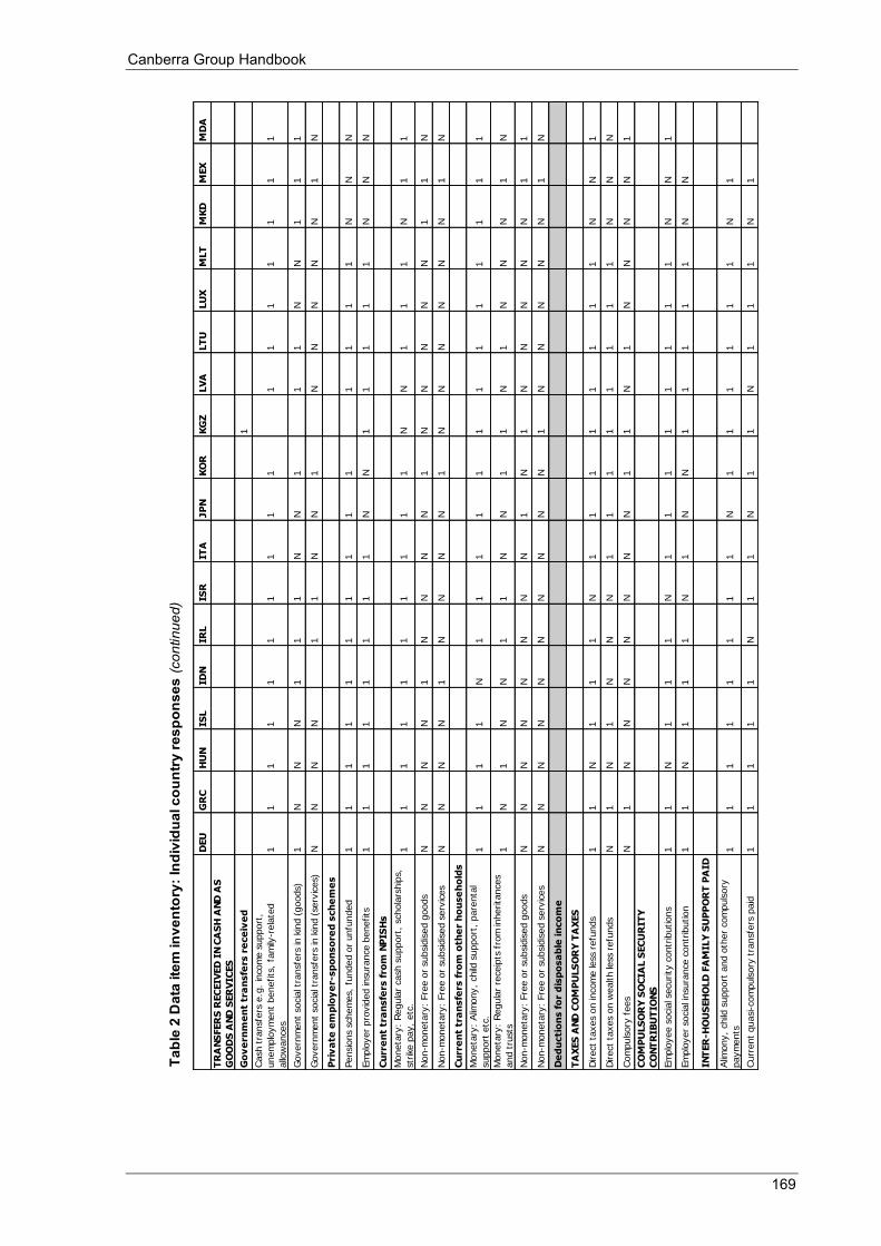
Canberra Group Handbook
169
DEU
GR
CH
UN
ISL
IDN
IRL
ISR
ITA
JP
NK
OR
KG
ZLV
ALT
ULU
XM
LT
MK
DM
EX
MD
A
TR
AN
SFER
S R
EC
EIV
ED
IN
CA
SH
AN
D A
S
GO
OD
S A
ND
SER
VIC
ES
Go
ve
rnm
en
t tr
an
sfe
rs r
ece
ive
d1
Cash
tra
nsf
ers
e.g
. in
com
e s
upport
,
unem
plo
ym
ent
benefits
, fa
mily
-rela
ted
allo
wance
s
11
11
11
11
11
11
11
11
1
Govern
ment
soci
al t
ransf
ers
in k
ind (
goods)
1N
NN
11
1N
N1
11
NN
11
1
Govern
ment
soci
al t
ransf
ers
in k
ind (
serv
ices)
NN
NN
11
NN
1N
NN
NN
1N
Pri
va
te e
mp
loy
er-
sp
on
so
red
sch
em
es
Pensi
ons
schem
es,
funded o
r unfu
nded
11
11
11
11
11
11
11
NN
N
Em
plo
yer
pro
vid
ed in
sura
nce
benefits
11
11
11
11
NN
11
11
1N
NN
Cu
rre
nt
tra
nsfe
rs f
rom
NP
ISH
s
Moneta
ry:
Regula
r ca
sh s
upport
, sc
hola
rship
s,
strike
pay,
etc
.1
11
11
11
11
1N
N1
11
N1
1
Non-m
oneta
ry:
Fre
e o
r su
bsi
dis
ed g
oods
NN
NN
1N
NN
N1
NN
NN
N1
1N
Non-m
oneta
ry:
Fre
e o
r su
bsi
dis
ed s
erv
ices
NN
NN
1N
NN
N1
NN
NN
NN
1N
Cu
rre
nt
tra
nsfe
rs f
rom
oth
er
ho
use
ho
lds
Moneta
ry:
Alim
ony,
child
support
, pare
nta
l
support
etc
.1
11
1N
11
11
11
11
11
11
1
Moneta
ry:
Regula
r re
ceip
ts f
rom
inherita
nce
s
and t
rust
s1
N1
NN
11
NN
11
N1
NN
N1
N
Non-m
oneta
ry:
Fre
e o
r su
bsi
dis
ed g
oods
NN
NN
NN
NN
1N
1N
NN
NN
11
Non-m
oneta
ry:
Fre
e o
r su
bsi
dis
ed s
erv
ices
NN
NN
NN
NN
NN
1N
NN
NN
1N
De
du
cti
on
s f
or
dis
po
sa
ble
in
co
me
TA
XES
AN
D C
OM
PU
LS
OR
Y T
AX
ES
Direct
taxes
on in
com
e le
ss r
efu
nds
11
N1
11
N1
11
11
11
1N
N1
Direct
taxes
on w
ealth le
ss r
efu
nds
N1
N1
NN
N1
11
11
11
1N
NN
Com
puls
ory
fees
N1
NN
NN
NN
N1
1N
1N
NN
N1
CO
MP
ULS
OR
Y S
OC
IAL S
EC
UR
ITY
CO
NT
RIB
UT
ION
S
Em
plo
yee s
oci
al s
ecu
rity
contr
ibutions
11
N1
11
N1
11
11
11
1N
N1
Em
plo
yer
soci
al i
nsu
rance
contr
ibution
11
N1
11
N1
NN
11
11
1N
N
INT
ER
-HO
US
EH
OLD
FA
MIL
Y S
UP
PO
RT
PA
ID
Alim
ony,
child
support
and o
ther
com
puls
ory
paym
ents
11
11
11
11
N1
11
11
1N
1
Curr
ent
quasi
-com
puls
ory
tra
nsf
ers
paid
11
11
1N
11
N1
1N
11
1N
1
Tabl
e 2
Dat
a ite
m in
vent
ory:
Indi
vidu
al c
ount
ry re
spon
ses
(con
tinue
d)
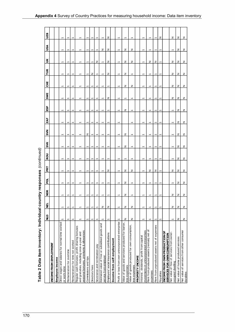
Appendix 4 Survey of Country Practices for measuring household income: Data item inventory
170
NLD
NZ
LN
OR
PO
LP
RT
RO
US
VK
SV
NZ
AF
ES
PS
WE
CH
ET
UR
UK
US
AU
ZB
IN
CO
ME F
RO
M E
MP
LO
YM
EN
T
Em
plo
ye
e in
co
me
Direct
wages a
nd s
ala
ries f
or
norm
al tim
e w
ork
ed
or
work
done
11
11
11
11
11
11
11
11
Rem
unera
tion f
or
overt
ime
11
11
11
11
11
11
11
11
Rem
unera
tion f
or
tim
e n
ot
work
ed
11
11
11
11
11
11
11
11
Regula
r cash b
onuses,
pro
fit-
sharing b
onuses
and g
ratu
itie
s,
inclu
din
g o
nce-a
-year
and
seasonal bonuses,
pre
miu
ms &
allo
wances
11
11
11
11
11
11
11
11
Com
mis
sio
ns a
nd t
ips
11
11
11
1N
11
11
11
11
Directo
rs f
ees
11
11
11
11
11
11
N1
11
Severa
nce a
nd t
erm
ination p
ay
11
11
11
11
11
11
1N
11
Estim
ate
d v
alu
e o
f fr
ee o
r subsid
ised g
oods a
nd
serv
ice f
rom
em
plo
yer
1N
11
11
11
11
11
11
N1
Em
plo
yers
’ socia
l in
sura
nce c
ontr
ibutions
1N
11
N1
11
11
N1
NN
NN
In
co
me
fro
m s
elf
-e
mp
loy
me
nt
Pro
fit
or
loss f
rom
ow
n u
nin
corp
ora
ted e
nte
rprise
11
11
11
11
11
11
11
11
Valu
e o
f goods a
nd s
erv
ices p
roduced f
or
bart
er,
less e
xpenses
NN
NN
N1
NN
N1
NN
NN
1
Valu
e o
f goods p
roduced f
or
ow
n c
onsum
ption,
less e
xpenses
NN
11
N1
11
11
1N
1N
N1
PR
OP
ER
TY
IN
CO
ME
Inte
rest,
div
idends,
pro
fit
from
capital
investm
ents
in u
nin
corp
ora
ted e
nte
rprises
11
11
11
11
11
11
11
11
Rent
from
pro
duced a
ssets
(re
nta
ls)
net
of
expenses
11
11
N1
11
11
11
1N
11
Rent
from
unpro
duced a
ssets
net
of
expenses
11
11
N1
11
11
11
1N
11
Royaltie
s1
11
11
11
11
11
11
11
N
IN
CO
ME F
RO
M O
WN
PR
OD
UC
TIO
N O
F
SER
VIC
ES
FO
R O
WN
CO
NS
UM
PT
IO
N
Net
valu
e o
f flow
of
serv
ices f
rom
ow
ner-
occupie
d d
welling
1N
N1
N1
11
11
NN
NN
1N
Net
valu
e o
f hom
e p
roduced s
erv
ices
NN
NN
NN
NN
NN
NN
NN
NN
Net
valu
e o
f serv
ices f
rom
oth
er
consum
er
dura
ble
sN
NN
NN
NN
NN
NN
NN
NN
N
Tabl
e 2
Dat
a ite
m in
vent
ory:
Indi
vidu
al c
ount
ry re
spon
ses
(con
tinue
d)
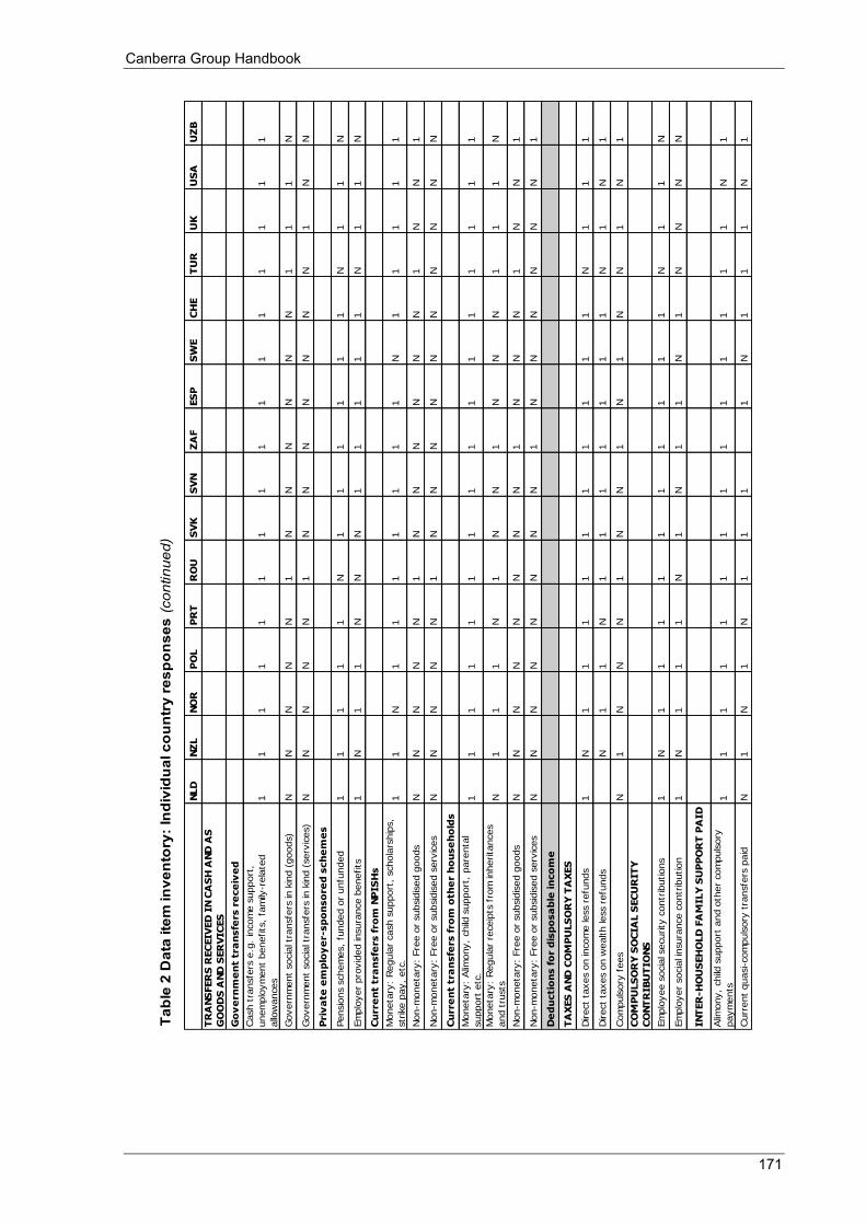
Canberra Group Handbook
171
NLD
NZ
LN
OR
PO
LP
RT
RO
US
VK
SV
NZ
AF
ES
PS
WE
CH
ET
UR
UK
US
AU
ZB
TR
AN
SFER
S R
EC
EIV
ED
IN
CA
SH
AN
D A
S
GO
OD
S A
ND
SER
VIC
ES
Go
ve
rn
me
nt t
ra
nsfe
rs r
ece
ive
d
Cash t
ransfe
rs e
.g.
incom
e s
upport
,
unem
plo
ym
ent
benefits
, fa
mily
-rela
ted
allo
wances
11
11
11
11
11
11
11
11
Govern
ment
socia
l tr
ansfe
rs in k
ind (
goods)
NN
NN
N1
NN
NN
NN
11
1N
Govern
ment
socia
l tr
ansfe
rs in k
ind (
serv
ices)
NN
NN
N1
NN
NN
NN
N1
NN
Priv
ate
em
plo
ye
r-sp
on
so
re
d s
ch
em
es
Pensio
ns s
chem
es,
funded o
r unfu
nded
11
11
1N
11
11
11
N1
1N
Em
plo
yer
pro
vid
ed insura
nce b
enefits
1N
11
NN
N1
11
11
N1
1N
Cu
rre
nt t
ra
nsfe
rs f
ro
m N
PIS
Hs
Moneta
ry:
Regula
r cash s
upport
, schola
rship
s,
str
ike p
ay,
etc
.1
1N
11
11
11
1N
11
11
1
Non-m
oneta
ry:
Fre
e o
r subsid
ised g
oods
NN
NN
N1
NN
NN
NN
1N
N1
Non-m
oneta
ry:
Fre
e o
r subsid
ised s
erv
ices
NN
NN
N1
NN
NN
NN
NN
NN
Cu
rre
nt t
ra
nsfe
rs f
ro
m o
th
er h
ou
se
ho
lds
Moneta
ry:
Alim
ony,
child
support
, pare
nta
l
support
etc
.1
11
11
11
11
11
11
11
1
Moneta
ry:
Regula
r re
ceip
ts f
rom
inherita
nces
and t
rusts
N1
11
N1
NN
1N
NN
11
1N
Non-m
oneta
ry:
Fre
e o
r subsid
ised g
oods
NN
NN
NN
NN
1N
NN
1N
N1
Non-m
oneta
ry:
Fre
e o
r subsid
ised s
erv
ices
NN
NN
NN
NN
1N
NN
NN
N1
De
du
ctio
ns f
or d
isp
osa
ble
in
co
me
TA
XES
AN
D C
OM
PU
LS
OR
Y T
AX
ES
Direct
taxes o
n incom
e less r
efu
nds
1N
11
11
11
11
11
N1
11
Direct
taxes o
n w
ealth less r
efu
nds
N1
1N
11
11
11
1N
1N
1
Com
puls
ory
fees
N1
NN
N1
NN
1N
1N
N1
N1
CO
MP
ULS
OR
Y S
OC
IA
L S
EC
UR
IT
Y
CO
NT
RIB
UT
IO
NS
Em
plo
yee s
ocia
l security
contr
ibutions
1N
11
11
11
11
11
N1
1N
Em
plo
yer
socia
l in
sura
nce c
ontr
ibution
1N
11
1N
1N
11
N1
NN
NN
IN
TER
-H
OU
SEH
OLD
FA
MILY
SU
PP
OR
T P
AID
Alim
ony,
child
support
and o
ther
com
puls
ory
paym
ents
11
11
11
11
11
11
11
N1
Curr
ent
quasi-com
puls
ory
tra
nsfe
rs p
aid
N1
N1
N1
11
1N
11
1N
1
Tabl
e 2
Dat
a ite
m in
vent
ory:
Indi
vidu
al c
ount
ry re
spon
ses
(con
tinue
d)
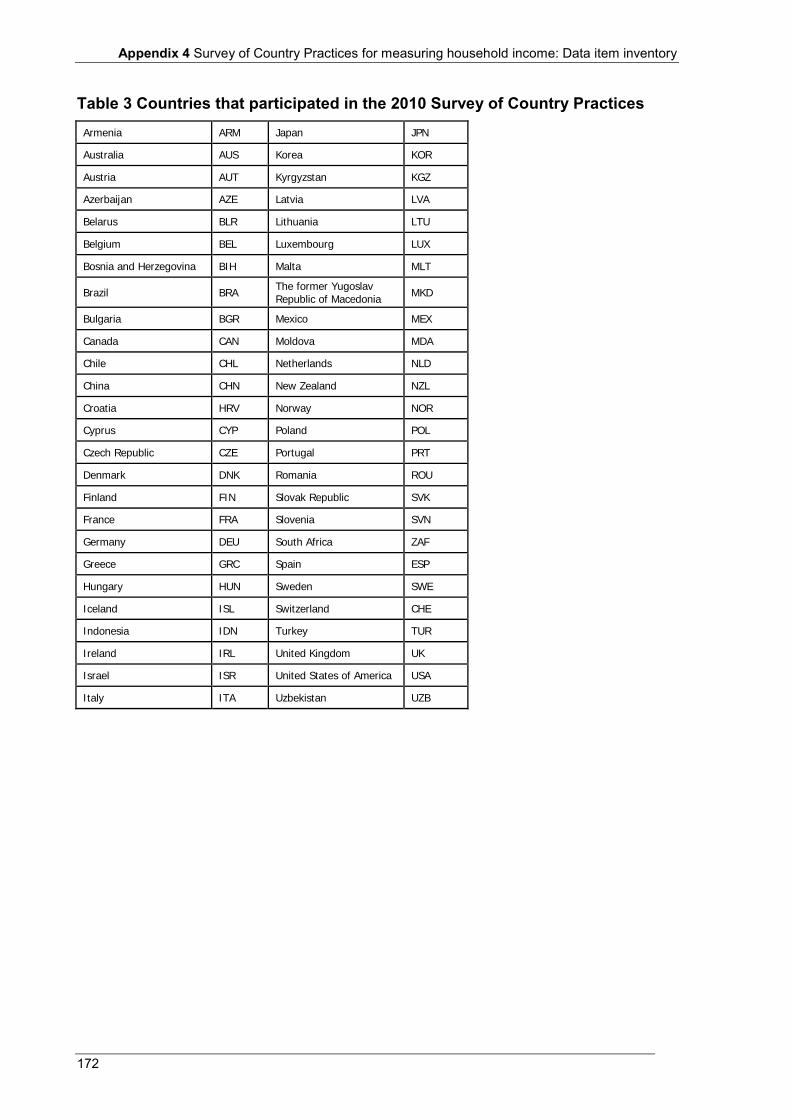
Appendix 4 Survey of Country Practices for measuring household income: Data item inventory
172
Table 3 Countries that participated in the 2010 Survey of Country Practices Armenia ARM Japan JPN
Australia AUS Korea KOR
Austria AUT Kyrgyzstan KGZ
Azerbaijan AZE Latvia LVA
Belarus BLR Lithuania LTU
Belgium BEL Luxembourg LUX
Bosnia and Herzegovina BIH Malta MLT
Brazil BRA The former Yugoslav Republic of Macedonia
MKD
Bulgaria BGR Mexico MEX
Canada CAN Moldova MDA
Chile CHL Netherlands NLD
China CHN New Zealand NZL
Croatia HRV Norway NOR
Cyprus CYP Poland POL
Czech Republic CZE Portugal PRT
Denmark DNK Romania ROU
Finland FIN Slovak Republic SVK
France FRA Slovenia SVN
Germany DEU South Africa ZAF
Greece GRC Spain ESP
Hungary HUN Sweden SWE
Iceland ISL Switzerland CHE
Indonesia IDN Turkey TUR
Ireland IRL United Kingdom UK
Israel ISR United States of America USA
Italy ITA Uzbekistan UZB
173
Appendix 5 Purchasing power parities 1 What is a Purchasing Power Parity?
A purchasing power parity (PPP) is the ratio of prices of two identical or comparable products or groups of products in different geographical locations, usually expressed as an index. The PPP between two countries attempts to show how many units of country A’s currency are needed to buy the same basket of goods and services as one unit of country B’s currency.
PPPs are not the same as exchange rates. Exchange rates for most countries are mainly determined by goods and services that are traded internationally, whereas PPPs are determined by all goods and services available within the country. The more the pattern of exports and imports of a country resemble the pattern of all goods and services circulating in the economy, the closer the exchange rate and PPP are likely to be, but they will only be exactly the same by coincidence. In all countries there are services provided by government which are not imported or exported, and there are many other goods that are not generally traded internationally.
In addition, capital movements may influence the exchange rate, a factor which also invalidates the use of exchange rates to measure the purchasing power of a currency in terms of the goods and services in circulation. Furthermore, the exchange rate is sometimes subject to significant fluctuations that are not mirrored in the relative prices of consumer goods and services. In such cases, conversion with the exchange rate will make the country appear richer or poorer in comparisons with other countries, even though there has been no change in real values.
For international comparisons it is therefore recommended that PPPs be used rather than exchange rates. This is important for all countries but especially so for developing countries whose basket of exports may be dominated by very few primary products.
2 How is a PPP calculated?
In making price comparisons over time, the starting point is usually a Paasche or Laspeyres index both of which are weighted averages of price ratios of goods and services. The Laspeyres index weights the price ratios together using the volumes of the base period and the Paasche index uses the volumes of the current period.
A simple two country PPP is analogous to this. Price ratios are formed for goods and services available in each country at the same point in time, each price being expressed in the local currency. The price ratios are then weighted together using the weights of country A or country B. By multiplying the Paasche and Laspeyres index and taking the square root of the product a spatial Fisher price index is obtained.
For a group of countries there is no a priori ordering available, so comparisons are made between all pairs of countries and then geometric averages are calculated of all direct and
Appendix 5 Purchasing power parities
174
indirect comparisons (an indirect comparison is to compare country I with country K and then country K with country J, thus giving an indirect comparison between countries I and J).
3 Compilation of PPPs
The compilation of PPPs is a major undertaking that involves the establishment of a list of products – goods and services – the prices of which have to be collected in the countries for which the PPPs are to be calculated. The products are specified in detail to ensure that only prices of comparable products are compared. The prices of products on the list are collected and recorded in the same period in time in the participating countries. The PPPs are calculated by aggregating the relative prices using the expenditure shares of the groups of products as weights. This involves several steps.
In the first step, unweighted PPPs for the detailed groups of products are calculated, the so called basic headings. Usually there is no reliable information available on expenditure shares on this level of aggregation. Instead, the products are marked according to whether they are representative in each country. The detailed binary PPP between two countries is calculated as the (geometric) average of the price ratios of products that are representative of the first country, and the price ratios of products that are representative of the second country.
In the second step the PPPs for aggregate groups of goods and services such as, say, household final consumption expenditure and GDP, are calculated. This is undertaken for each pair of countries by weighting together the basic heading PPPs using the weights of the first country, and then the weights of the second country, and finally by taking the geometric average of these two to arrive at the ‘Fisher type’ PPP between the two countries.
It is not always possible to compile PPPs directly. This happens when a product that is representative in country A is not available in country B, or it may not have been possible to collect prices for the product for some reason. In such cases an indirect comparison is made by using a third country as a bridge country or the missing price ratios are imputed using the price ratios of similar or comparable products. By applying additional methods it is ensured that the PPPs are base country invariant – that is, the PPP results are independent of which country is selected as a base country. For more information see Eurostat OECD, 2006.
A PPP can be calculated for a single product or a group of products at various levels of aggregation. The higher the level of aggregation, the less the results are influenced by outliers. The overall PPPs cover GDP and other national accounts aggregates including household final consumption expenditure. Often the PPPs for the main groupings of the Classification of Individual Consumption according to Purpose (COICOP) will be available. The results for GDP are the ones most often quoted.
4 Periodicity and availability
PPPs usually refer to the period of a year. From year to year the PPP will tend to follow the development in relative inflation rates in the countries compared. Hence, in periods of stable prices the PPP will be fairly stable from year to year. If there is a radical shift in inflation rates (say from the introduction of a VAT type tax) then the changes will be more significant.
Calculating PPPs is a major undertaking and thus it is not done routinely for all countries for every year. The OECD and Eurostat make comparisons for their member countries plus the countries of the Commonwealth of Independent States. For the EU countries, a three year
Canberra Group Handbook
175
rolling sample is applied where each year price surveys are conducted for one third of the goods and services. For the remaining two thirds of goods and services the corresponding consumer price index is used for extrapolating the prices for the intervening years. The rent surveys, earnings and weights are prepared on an annual basis.
A number of countries conduct PPP surveys every three years. For other countries, less frequent surveys are undertaken and brought together by the World Bank in the International Comparison Programme (ICP). Under the ICP, PPPs were compiled for 2005 and 2011. These then constitute the benchmark or reference years of the ICP PPPs on the basis of which PPPs for the years in between or after 2011 will be estimated using price indices.
In countries where data are collected less frequently than annually, PPPs are estimated by using the corresponding price indices in years where prices are not collected for the PPP. For example, if the PPP of country A relative to country B is available for year t, it can be extrapolated for year t+1 by multiplying the PPP of year t by an appropriate price index of country A from year t to t+1, and dividing by the appropriate price index for country B from t to t+1. Because of the long production process PPPs are usually only published with several years lag. Hence, the method described may be used to make forward projections of PPPs while waiting for the publication of the actual PPPs for a given period.
PPPs for different countries are available from the web pages or online databases of the World Bank, OECD, Eurostat and UNECE, where more detailed methodological documentation is also provided.
5 Which PPP?
PPPs are built up from expenditure data but since they show the purchasing power of money, they can also be applied to income measures. For comparison of household income data, PPPs based on households’ consumption expenditure should be applied when possible.
Which PPP to use will depend on the exact measure of income of interest. For example, a measure of income excluding subsistence agriculture and housing costs should in principle use a PPP which is calculated excluding these items. To compare income measures excluding social transfers in kind, PPPs for consumption expenditure should be used. For income measures including social transfers in kind, the PPPs for actual consumption should be used.
In principle it would also be possible to calculate a PPP for household consumption excluding all rent. Unfortunately though, PPPs are not additive because they are derived from Fisher indices and thus it is not possible for the reader of the published reports to make these sort of calculations exactly. However for most countries information on the PPPs relating to housing are available so some judgement can be made about when these could have a significant effect on the results.
6 Representativeness and comparability
To derive price relativities over time or geographical location, in principle the two prices should refer exactly to the same product or group of products. This is a problem for inter-temporal indices where the specification of goods and services changes over time but is even more acute in the cross country case. Not only are the goods or services likely to have different specifications, but how representative a given product is will be different from country to country. Taking representative products may distort the price ratios because some
Appendix 5 Purchasing power parities
176
quality differences will be included in prices. Taking exactly comparable products may equally distort the results because they are not representative of the basket of products actually bought.
It follows that PPPs for countries with similar economic structures and consumption patterns will usually be good estimations of the relative price levels, while the statistical uncertainty tends to increase when comparing countries that are more different in terms of structure and consumption patterns. In order to address this problem, PPPs are calculated on a regional basis whereby countries which are more or less similar in terms of the types and quantity of products purchased are compared together. Regional groupings are then linked by means of link countries which participate in more than one group. For each group several hundred prices are collected with some overlapping items, such as staple food products, in order to minimise the risk of error from non-representativeness and non-comparability.
7 PPPs for different income groups?
The question of representativeness applies also to different income groups within a single country. Pensioners are likely to have significantly different consumption patterns to young families. For example, even if a large size of frozen vegetables are cheaper than a smaller size, some groups may not be able to afford the greater absolute cost or many do not have a freezer in which to store it. Alternative price indices are sometimes calculated for different household groups depending on family circumstance. However, they are seldom calculated for decile groups although this is how income distribution is most often presented.
These problems become even more difficult when applied in the international context. If we compare the baskets of goods and services bought by income groups in two countries, one richer and one poorer, it may be that the basket bought by the middle quintile in the richer country is more like the basket bought by the richest quintile in the poorer country than that of the middle quintile. Thus matching similarly labelled groups may not necessarily improve the comparison in the manner expected. In part this is because of the different institutional arrangements concerning the provision of government services.
In practice, PPPs are not available for income groups. As for inter-temporal comparisons it would be necessary to collect not only price information but also quantity detail (large versus small packaging) for specific income groups. This is such a data demanding exercise, that it is difficult to see a full implementation on anything other than on an experimental basis for the immediate future.
Using a PPP instead of an exchange rate is still to be unequivocally recommended but it should be noted that this gives a measure of the average (not median) command over a basket of goods and services standard for the countries concerned.
177
Bibliography Aaberge, R., Bhuller, M., Langorgen, A., and Mogstad, M. (2010). The Distributional Impact of
Public Services when Needs Differ. IZA Working Paper Series, No. 4826. IZA Publishing. Available from http://ftp.iza.org/dp4826.pdf
Aboleda, H. (2000). Valuation of Unpaid Work in Household Production and Volunteer Services.
Paper presented at the Training Workshop on Statistical Aspects of Integrating Unpaid Work into National Policies. United Nations ESCAP. Bangkok, 11-15 September. Available from http://www.unescap.org/stat/meet/rrg3/twsa-03.pdf
ABS (2006). Research Paper: A Review of Methodology for Estimating Taxes on Production in the
Calculation of Household Final Income, 2003-04. Catalogue No. 1351.0.55.012. ABS. Canberra. Available from http://www.ausstats.abs.gov.au/ausstats/subscriber.nsf/0/4689B06FDBD46ABECA25714E007CD298/$File/1351055012_apr%202006.pdf
ABS (2007). Government Benefits, Taxes and Household Income, 2003-04. Catalogue No. 6537.0.
ABS. Canberra. Available from http://www.ausstats.abs.gov.au/ausstats/subscriber.nsf/0/30A1BDA7F5A93A9CCA2572F800133897/$File/65370_2003-04.pdf
ABS (2008). Experimental Estimates of Imputed Rent, 2003-04 and 2005-06. Catalogue No. 6525.0.
ABS. Canberra. Available from http://www.ausstats.abs.gov.au/ausstats/subscriber.nsf/0/9F1097CCC393BE69CA25743B00172002/$File/65250_2003-04%20and%202005-06.pdf
ABS (2009a). Household Income and Income Distribution, 2007-08. Catalogue No. 6523.0. ABS.
Canberra. Available from http://www.ausstats.abs.gov.au/Ausstats/subscriber.nsf/mf/6523.0 ABS (2009b). Information Paper: Survey of Income and Housing, User Guide, 2007-08. Catalogue
No. 6553.0. ABS. Canberra. Available from http://www.abs.gov.au/AUSSTATS/[email protected]/Lookup/6553.0 Main+Features 12007-08
ABS (2010). Micro and Macro Economic Estimates for Australian Households: Recent Developments
and Future Directions. Paper presented at the General Conference of the International Association for Research in Income and Wealth. IARIW. Switzerland, 22-28 August. Available from http://www.iariw.org/papers/2 010/7aKindermann.pdf
Atkinson, A.B. (1983). The Economics of Inequality. Second Edition, Oxford: Clarendon Press. Atkinson, A.B, Rainwater, L., and Smeeding, T.M. (1995). Income Distribution in OECD Countries.
OECD Social Policy Studies, No. 18. Paris. Atkinson, A.B. (2000). Is Rising Income Inequality Inevitable? A Critique of the Transatlantic
Consensus. WIDER Annual Lectures, No.3. Finland. United Nations World Institute for Development Economics Research.
Atkinson, A.B., Cantillon, B., Marlier, E. and Nolan, B. (2002). Social Indicators: The EU and Social
Inclusion. Oxford: Oxford University Press.
Bibliography
178
Atkinson, A.B. (2005). Atkinson Review: Final Report Measurement of Government Output and Productivity for the National Accounts. HMSO. United Kingdom. Available at http://www.statistics.gov.uk/about/data/methodology/specific/PublicSector/atkinson/default.asp
Atkinson, A.B., and Piketty, T. (2007). Top Incomes over the Twentieth Century: A Contrast between
Continental European and English-Speaking Countries. Oxford: Oxford University Press. Atkinson, A.B., Piketty. T., and Saez, E. (2010). Top Incomes in the Long Run of History. NBER
Working Paper Series, No.15408. NBER Publishing. Available from http://elsa.berkeley.edu/~saez/atkinson-piketty-saezJEL10
Atkinson, A.B., and Piketty, T. (2010). Top Incomes: A Global Perspective. Oxford: Oxford
University Press. Bivens, G., and Volker, C. (1986). ‘A Value-Added Approach to Household Production: The Special
Case of Meal Preparation’. The Journal of Consumer Research, 13(2):272-279. Buhmann, B., Rainwater, L., Schmaus, G., and Smeeding, T. (1988). ‘Equivalence scales, Well-being,
Inequality and Poverty: Sensitivity Across Ten Countries using the Luxembourg Income Study (LIS) Database’. Review of Income and Wealth, 13(2):115-142.
Burkhauser, R., Feng, S., Jenkins, S.P., and Larrimore, J. (2009). Recent Trends in Top Income Shares
in the USA: Reconciling Estimates from March CPS and IRS Tax return data. NBER Working Paper Series, No.15320. NBER Publishing.
The Canberra Group (2001). Expert Group on Household Income Statistics: Final Report and
Recommendations. Ottawa. Clémenceau, A., Museux, J.M., and Bauer, M. (2006). Comparative EU Statistics on Income and
Living Conditions: Issues and Challenges, proceedings from the EU-SILK conference. European Commission. Helsinki. Available from http://epp.eurostat.ec.europa.eu/cache/ITY_OFFPUB/KS-RA-07-007/EN/KS-RA-07-007-EN.PDF
Commission of the European Communities, International Monetary Fund, Organisation for Economic
Co-operation and Development, United Nations, and The World Bank (International Bank for Reconstruction and Development) (2008). System of National Accounts 2008. Brussels/Luxembourg: Eurostat; Washington, DC: IMF and The World Bank; Paris: OECD; New York, NY: United Nations. Available from http://unstats.un.org/unsd/nationalaccount/SNA 2008.pdf
Covarrubias, K., Campos, A., and Zezza, A. (2009). Accounting for the Diversity of Rural Income
Sources in Developing Countries: The Experience of the Rural Income Generating Activities Project. Paper presented at the Wye City Group Meeting on Rural Development and Agricultural Household Income. FAO. Rome, 5 November. Available from http://www.fao.org/fileadmin/user_upload/riga/pdf/Paper3_2Covarrubias AccountingfortheDiversity.pdf
Deaton, A. (1997). The Analysis of Household Surveys: A Microeconometric Approach to
Development Policy. Baltimore: The Johns Hopkins University Press. Deaton, A., and Paxson, C. (1998). ‘Economies of Scales, Household Size and the Demand for Food’.
Journal of Political Economy, 106(5):897-930.
Canberra Group Handbook
179
Deaton, A. (2005). Measuring Poverty in a Growing World (or measuring growth in a poor world). NBER Working Paper Series, No. 9822. NBER Publishing. Available from http://unstats.un.org/unsd/methods/poverty/Deaton %20June%202003%20Measuring%20 poverty%20in%20a%20growing%20world.pdf
Deininger, K. and Squire, L. (1996). ‘A New Data Set Measuring Income Inequality’. World Bank
Economic Review, 10(3):565-91. Dupre, M.T. (1997). The Current Status of the Concept of Income from Employment and its
Relationship with Existing Income Concepts. Paper prepared for the Advisory Income Steering Group. Eurostat Directorate of Social and Regional Statistics and Structural Plans. Luxembourg.
Economic Planning Agency (1998). Monetary valuation of unpaid work in 1996. Japan. European Commission (2003). Commission Regulation (EC), No. 1980/2005 of 21st October, 2003,
concerning Community Statistics on Income and Living Conditions (EU-SILC) as Regards to Definitions and Updated Definitions. Available from http://eur-lex.europa.eu/Le UriServ/LexUriServ.do?Uri =OJ:L:2003:298:0001:0022:EN:PDF
European Commission (2005). Commission Regulation (EC), No. 1722/2005 of 20th October, 2005,
concerning the Principles for Estimating Dwelling Services for the Purpose of Council Regulation on the harmonisation of gross national income at market prices. Available from http://eur-lex.europa.eu/smartapi/cgi/sga_doc?smartapi !celexapi!prod!CELEX numdoc&lg =en&numdoc = 32005R1722&model=guichett
European Commission (2010). Europe 2020 Indicators. Luxembourg. Available from
http://epp.eurostat.ec.europa.eu/portal/page/portal/europe_2020_indicators/headline_indicators Eurostat (2002). Income Measurement Manual: Draft manual (Report, Lot 2), Working Group on
Statistics on Income, Poverty and Social Exclusion. European Commission. Luxembourg. Eurostat (2003). Household Production and Consumption: Proposal for a Methodology of Household
Satellite Accounts. Working Paper Series, No. 3. European Commission. Luxembourg. Available from http://ec.europa.eu/eurostat/ramon/statmanuals/files/KS-CC-03-003-EN.pdf
Eurostat - OECD (2006). Methodological Manual on Purchasing Power Parities. European
Commission. Paris. Available from http://www.oecd.org/dataoecd / 5 9 / 1 0/37984252.pdf Eurostat (2010). Comparative EU Intermediate Quality Report, Version 2 - June 2010. European
Commission. Luxembourg. Available from http://epp.eurostat.ec.europa.eu/portal/page/portal/income_social_inclusion_living_conditions/documents/tab9/2007%20Comparative%20EU%20Final%20QR.pdf
Eurostat (2011). EU-SILC Description Target Variables. European Commission. Luxembourg.
Available from http://epp.eurostat.Ec.europa. Eu/portal/page/portal/ income_social_inclusion_living_conditions/documents/tab/Tab/Household%20data%20-%20basic%20data.pdf
Franz, A., Ramprakash, D., Walton, J. (1998). Statistics on the Distribution of Income,Consumption
and Accumulation of Households (DICAH), Report to Eurostat. Vienna, London, and Luxembourg. Mimeographed. French Council of Economic Experts (2008). The Measurement of Purchasing Power. Report of the French Council of Economic Experts, No.73.
Bibliography
180
Frick, J., Grabka, M., Groh-Samberg, O. (2010a). Dealing with Incomplete Household Panel Data in Inequality Research. Research Paper Series, No.290. DIW Publishing. Available from http://www.diw.de/documents/publikationen/73/diw_01.c.354683.de/diw_sp0290.pdf
Frick, J., Grabka, M., Smeeding, T., and Tsakloglou, P. (2010b). ‘Distributional Effects of Imputed
Rents in Five European Countries’. Journal of Housing Economics, 19:167-179. Garner, T., and Short, K. (2009). ‘Accounting for Owner-Occupied Dwelling Services: Aggregates
and Distributions’. Journal of Housing Economics, 18(3):233-248. Glewwe, P. (2005). An Overview of Questionnaire Design for Household Surveys in Developing
Countries: Household Sample Surveys in Developing and Transition Countries. UNDESA Working Paper Series, Studies in Methods, Series F, No. 96. New York. Available from http://unstats.un.org/unsd/HHsurveys/pdf /Household _ surveys.pdf
Gottschalk, P., and Smeeding, T. (2000). Empirical evidence on income inequality in industrialized
countries, in Anthony B. Atkinson and François Bourguignon (eds.), Handbook of Income Distribution, Handbooks in Economics, Amsterdam.
Grosh, M., and Glewwe, P. (2000). Designing Household Survey Questionnaires for Developing
Countries: Lessons from Fifteen Years of the Living Standard Measurement Study. Oxford: Oxford University Press. Available from http://econ.Worldbank.org/WEBSITE/EXTERNAL/EXTDEC/EXTRESEARCH/EXTLSMS/0,,contentMDK:21556161~pagePK:64168445~piPK:64168309~theSitePK:3358997,00.html
Groves, R., and Couper, M.P. (1998). Non Response in Household Interview Surveys. New York:
Wiley Press. Gruber, J., and Saez, E. (2002). ‘The Elasticity of Taxable Income: Evidence and Implications’.
Journal of Public Economics, 84:1-32. Guio, A. (2005). Material Deprivation in the EU. Eurostat Statistics in Focus Working Paper Series,
Population and Social Conditions, No. 21/2005. Luxembourg. Available from http://epp.eurostat.ec.europa.eu/cache/ITY_OFFPUB/KS-NK-05-021/EN/KS-NK-05-021-EN.PDF
Haddad, L., and Kanbur, R. (1990). ‘How Serious is the Neglect of Intra-household Inequality?’ The
Economic Journal, 100(402):866-881. Hagenaars, A.,Vos, K., and Zaidi, M.A. (1994). Poverty Statistics in the Late 1980s: Research Based
on Micro-Data. European Commission. Luxembourg. Haughton, J. and Khandker, S.R. (2009). Handbook on Poverty and Inequality. Washington DC:
World Bank. Hirway, I. (2000). Valuation of Unpaid Work: Issues Emerging from the Indian Pilot Time Use
Survey. Paper prepared for the Training Workshop on Statistical Aspects of Integrating Unpaid Work into National Policies. United Nations ESCAP. Bangkok, 11-15 September. Available from http://www.unescap.org/stat/meet/rrg3/twsa-08.pdf
Hunt, J., and Kiker, B.F. (1997). ‘Valuation of Household Services: Methodology and Estimation’.
The Journal of Risk and Insurance, 46 (4):697-706. ILO (1982). Resolution Concerning Statistics of the Economically Active Population, Employment,
Unemployment and Underemployment, adopted at the 13th International Conference of Labour
Canberra Group Handbook
181
Statisticians, October. Geneva. Available from http://www.ilo.org/public/english/bureau/stat/download/res/ecacpop.pdf
ILO (1998). Resolution Concerning the Measurement of Employment -related Income, 16th
International Conference of Labour Statisticians, October. Geneva. Available from http://www.ilo.org/global/statistics-and-databases/standards-and-guidelines/resolutions-adopted-by-international-conferences-of-labour-statisticians/WCMS_087490/lang--en/index.htm
ILO (2001). Household Income and Expenditure Statistics: Report 1: Household Income, and
Expenditure Statistics, and Consumer Price Indexes. Meeting of Experts of Labour Statistics. Geneva, 22 -31 of October. Available from http://www.ilo.org/public/english/bureau/stat/ techmeet/index.htm
ILO (2003). Report II: Household Income and Expenditure Statistics, prepared for the 17th
International Conference of Labour Statisticians, November. Geneva, 24 November – 3 December. Available from http://www.ilo.org/ public/english /bureau/stat/download/ 17 thicls/r2hies.pdf
ILO (2004). Resolution 1: Resolution Concerning Household Income and Expenditure Statistics,
adopted at the 17th International Conference of Labour Statisticians, December. Geneva. Available from http://www.ilo.org/global/statistics-and-databases/standards-and-guidelines/resolutions-adopted-by-international-conferences-of-labour-statisticians/ WCMS _087503/lang--en/index.htm
IMF (2007). The General Data Dissemination System: Guide for Participants and Users. Washington
DC. Available from http://www.imf.org/external/pubs/ft/gdds/guide/2007/gddsg uide.pdf Jenkins, S. (2011). Changing Fortunes: Income Mobility and Poverty Dynamics in Britain. Oxford:
Oxford University Press. Juster, F.T., Cao, H., Couper, M., Hill, D., Hurd, M., Lutpon, J., Perry, M., and Smith, J. (2007).
‘Enhancing the Quality of Data on the Measurement of Income and Wealth’. University of Michigan Retirement Research Center. Working Paper Series, No. 2007-151. Available from http://www.mrrc.isr.umich.edu/publications/Papers/pdf/wp151.pdf
Katz, A. (1983). ‘Valuing the Services of Consumer Durables.’ Review of Income and Wealth,
29(4):405-427. Kulshreshtha, A., and Singh, G. (1991). Valuation of Non-Market Household Production. Central
Statistical Organization. New Delhi. India. Available from http://www.unescap.org/stat/meet/timeuse/valuation_ses4.pdf
Lanjouw P., and Ravallion, M. (1995). ‘Poverty and Household Size.’ Economic Journal,
105(433):1415-1434. Marical, F., D’Ercole, M.M., Vaalavuo, M., and Verbist, G. (2008). Publicly-provided Services and
the Distribution of Households’ Economics Resources. OECD Economic Studies, No. 44, 2008/1. Available from http://www.oecd.org/dataoecd/39/4 4/42503533.pdf
Martin, J., Cheesbrough, S., Dodd, T., Farrant, G., and McKernan, A. (1996). Asking the Self-
Employed about their Income. ONS Working Paper, SW 397196. UK Government. Available from http://www.surveynet.ac.uk/sqb/qb/topics/income/semplyin.pdf
Bibliography
182
Moore, J., Stinson, L., and Welniak, E. (2000). ‘Income Measurement Errors in Surveys: A Review.’ Journal of Official Statistics, 16(4):331-362.
Mullan, K., Sutherland, H., and Zantomio, F. (2007). The Distributional Impact of Imputed Rents in
the United Kingdom. Paper prepared for the AIM-AP Project, Institute for Social and Economic Research. University of Essex. United Kingdom. Available from http://www.iser.essex.ac.uk/files/msu/emod/aim-ap/deliverables/AIM-AP1.1f.pdf
Norrlof, C. (1985). Issues in the Revision of the International Income Distribution Guidelines. Paper
presented at the 19th General Conference of the International Association for Research in Income and Wealth. IARIW. Noordwijkerhout, Netherlands, 25-31 August.
ONS (2007). Taxes and Benefits – The Effect on Household Income, 2005-06. UK Government.
London. Available from http://www.statistics.gov.uk/pdfdir/tx&b0507.pdf OECD (1982). The OECD List of Social Indicators. Paris. OECD (2008). Growing Unequal? Income Distribution and Poverty In OECD Countries. Paris.
Available from http://www.oecd.org/document/4/0,3343,en_2649_33933_41460917_1_1_1_1,00.html
Orshansky, M. (1965). ‘Counting the Poor: Another Look at the Poverty Profile.’ Social Security
Bulletin, 28:3-29. Paats, M., and Tiit, E. (2010). Income From Own Consumption (Ch 5) in Atkinson, A.B., and
Marlier, E. (eds.), Income and living conditions in Europe. Eurostat. Luxembourg. Available from http://epp.eurostat.ec.europa.eu/cache/ITY_OFFPUB/KS-31-10-555/EN/KS-31-10-555-EN.PDF
Paulus, A., Sutherland, H., and Tsakloglou, P. (2010). ‘The Distributional Impact of In-kind Public
Benefits in European Countries’. Journal of Policy Analysis and Management, 29 (2): 243-266. Pendakur, K. (2002). ‘Taking prices seriously in the measurement of inequality’. Journal of Public
Economics, Vol. 86: 47 – 69. Piketty, T. (2003). ‘Income Inequality in France, 1901-1998’. Journal of Political Economy,
111(5):1004-1042. Radner, D. (1997). ‘Non-cash Income, Equivalence Scales and the Measurement of Economic Well-
being’. Review of Income and Wealth, 43(1):71-88. Rendtel, U., Nordberg, L., Jäntti, M., Hanisch, Jens., and Basic, E. (2004). Report on Quality of
Income Data: Results of Work Package 5 of the CHINTEX Project. Working Paper Series, No 21. European Commission. Available from http://www.destatis.de/jetspeed/portal/cms/Sites/destatis/Internet/DE/Content/Wissenschaftsforum/Chintex/ResearchResults/Downloads/WorkingPaper21,property=file.pdf
Reynolds, A. (2007). Has U.S. Income Inequality Really Increased? Policy Analysis Working Paper
Series, No.586. Cato Institute Publishing. Available from http://www.cato.org/pubs/pas/pa586.pdf
Rio Group (2006). Compendium of Best Practices in Poverty Measurement. Expert Group on Poverty
Statistics. Rio de Janeiro. Available from http://www.ibge.gov.br/poverty/pdf/rIo _ group_compendium.pdf
Canberra Group Handbook
183
Ritakallio, V.M. (2003). ‘The Importance of Housing Costs in Cross-National Comparisons of Welfare Outcomes’. International Social Security Review, 56(2):81-101.
Roemer, M. (2000). Assessing the Quality of the March Current Population Survey and the Survey of
Income and Program Participation Income Estimates, 1990-1996. Housing and Household Economics Statistics Division. U.S. Census Bureau. Available from http://www.census.gov/hhes/www/income/publications/assess1.pdf
Ruggles, P., and O’Higgins, M. (1981). ‘The Distribution of Public Expenditures among Households
in the United States.’ Review of Income and Wealth, vol 27: 137-163. Sauli, H., and Törmälehto,V-M. (2010). The Distributional Impact of Imputed Rent (Ch 7) in
Atkinson, A.B., and Marlier, E. (eds.), Income and living conditions in Europe. Eurostat. Luxembourg. Available from http://epp.eurostat.ec.europa.eu/ cache/ITY_OFFPUB/KS-31-10-555/EN/KS-31-10-555-EN.PDF
Short, K., O’Hara, A., and Scott, S. (2007). Taking Account of Housing in Measures of Household
Income. Paper presented at the Annual Meeting of the Allied Social Sciences Associations, Society of Government Economists Session. Chicago, Illinois, 2 January.
Shorrocks, A.F. (1980). ‘The Class of Additively Decomposable Inequality Measures.’ Econometrica,
48(3): 613-625. Smeeding, T. (1982). Alternative Methods for Valuing Selected In-Kind Transfer Benefits and
Measuring Their Effect on Poverty. U.S Bureau of Census Technical Paper No. 50. Washington DC.
Smeeding, T., Saunders, P., Coder, J., Jenkins, S., Fritzel, J., Hagenaars, A., Hauser, R., and Wolfson,
R. (1993). ‘Poverty, Inequality, and Family Living Standards Impacts across Seven Nations: The Effect of Non Cash Subsidies for Health, Education and Housing’. Review of Income and Wealth, 30(3):229-256.
Smeeding, T. (1996). The IARIW Session on International Standards on Income and Wealth
Distributions: A Summary. Paper presented at the First meeting of the International Expert Group on Household Income Statistics. Canberra, 2-4 December.
Smeeding, T. (2000). Changing Income Inequality in OECD Countries: Updated Results from the
Luxembourg Income Study (LIS), in R. Hauser and I. Becker, (eds.), The Personal Distribution of Income in an International Perspective. Berlin: Springer-Verlag.
Smeeding T., Tsakloglou, P., and G. Verbist (2008). Distributional Effects of Public Health Care
Transfers in Seven European Countries. AIM-AP report. University of Essex. Available from http://www.euro.centre.org/data/1231495166_724.pdf
Statistics Canada (2000). Social Policy Simulation Database and Model (SPSD/M). Available from
http://www.statcan.gc.ca/microsimulation/spsdm-bdmsps/spsdm-bdmsps-eng.htm Statistics Canada (2002). Statistics Canada’s Quality Assurance Framework. Available from
http://www.statcan.gc.ca/pub/12-586-x/12-586-x2002001-eng.pdf Statistics Canada (2010). Low-income Lines, 2008-2009. Income Research Paper Series, No. 005.
Statistics Canada. Available from http://www.statcan.gc.ca/pub/75f0002m/75f0002m2010005-eng.pdf
Bibliography
184
Stiglitz, S.E., Sen, A., and Fitoussi, J. (2009). Report by the Commission on the Measurement of Economic Performance and Social Progress. Available from http://www.stiglitz-sen-fitoussi.fr/documents/rapport_anglais.pdf
United Nations (1968). A System of National Accounts. Working Paper Series, Studies in Methods,
Series F, No. 2, Rev. 3. UNDESA. New York. United Nations (1977). Provisional Guide-lines on Statistics of the Distribution of Income,
Consumption and Accumulation of Households. Working Paper Series, Studies in Methods, Series M, No.61.UNDESA. New York.
United Nations (1981). A Survey of National Sources of Income Distribution Statistics. Working
Paper Series, Studies in Methods, Series M, No. 72. UNDESA. New York. United Nations (1985). National Accounts Statistics: Compendium of Income Distribution Statistics.
Working Paper Series M, No. 79. UNDESA. New York. United Nations (1989). Items in the Revision of the SNA which are Relevant from the Point of View of
Statistics of Income in Households: Note by the Secretariat. Paper presented at the Conference of European Statisticians, Work Session on Statistics of the Distribution of Income of Households. UNECE. Geneva, 25-27 September.
United Nations (2003). Indicators for Monitoring Millennium Development Goals. New York.
Available from http://devdata.worldbank.org/ gmis/ mdg /UNDG % 20 document_final.pdf United Nations (2005a). Guide to Producing Statistics on Time Use, Measuring Paid and Unpaid
Work. UNDESA. New York. Available from http://unstats.un.org.unsd/publication/SeriesF/SeriesF_93E.pdf
United Nations (2005b). Handbook on Poverty Statistics: Concepts, Methods and Policy Use. UN Steering Committee on Poverty Statistics. UNDESA. New York. Available from https://unstats.un.org/unsd/methods/poverty/activityandmeeting.htm
United Nations (2009). Handbook on Measuring the Economically Active Population and Related
Characteristics in Population Censuses. UNDESA. New York. Available from http://unstats.un.org/unsd/censuskb20/Attachment458.aspx
UNECE (2009a). Measurement of Different Emerging Forms of Households and Families. Note
Prepared by the UNECE Task Force on Families and Households. Geneva. Available from http://www.unece.org/stats/publications/Measurement_ ermerging_forms_ households _ and_families.pdf
UNECE (2009b). Making Data Meaningful Part 1: A Guide to Writing Stories about Numbers.
Available from http://www.unece.org/stats/ documents/ writing/ MDM_ Part1English.pdf
UNECE (2009c). Making Data Meaningful Part 2: A Guide to Presenting Statistics. Available from
http://www.unece.org/stats/documents /writing/MDM_Part2_ English.pdf
UNECE and EUROSTAT (2006). Conference of European Statisticians: Recommendations for the 2010 Censuses of Population and Housing. United Nations. New York and Geneva. Available from http://www.unece.org/stats/publications /CES_2010_ Census _ Recommendations_English.pdf
Canberra Group Handbook
185
UNECE, Eurostat and OECD (2009). Generic Statistical Business Process Model. Joint UNECE/Eurostat/OECD Work Session on Statistical Metadata (METIS). Version 4.0, April. Available from http://www.unece.org/stats/documents/ece/ces/ge.61/2009/mtg1/zip.32.e.pdf
US Census Bureau (2004). The Effects of Government Taxes and Transfers on Income and Poverty.
Washington DC. Available from http://www.census.gov/hhes/www/income/publications /effects2004/effectofgovtandt2004.pdf
Van den Bosch, K. (2001). Identifying the Poor, Using Subjective and Consensual Measures.
Aldershot: Ashgate. Vaughan, D. (1993). Reflections on the Income Estimates from the Initial Panel of the Survey of
Income and Program Participation (SIPP). Working Paper Series, Studies in Income Distribution, No. 17. Social Security Administration. Washington DC.
Verma, J., and Betti, G.(2010). (Ch 3) in Atkinson, A.B., and Marlier, E. (eds.), Income and living
conditions in Europe. Eurostat. Luxembourg. Available from http://epp.eurostat.ec.europa.eu/ cache/ITY_OFFPUB/KS-31-10-555/EN/KS-31-10-555-EN.PDF
Warren, N. (2008). A Review of Studies on the Distributional Impact of Consumption Taxes in
OECD Countries. OECD Social, Employment and Migration Working Paper Series, No. 64, OECD Publishing. Available from http://www.oecd.org/dataoecd/34/57/40986444.pdf
Welniak, E. J. (2003). Measuring Household Income Inequality Using the CPS, Special Studies in
Federal Tax Statistics, in Dalton, J., and Kilss, B. (eds.), Statistics of Income Directorate, Inland Revenue Service. Washington DC.
Wolff, E.N., Zacharias, A., and Caner, A. (2004). Concept, Measurement and Findings: United
States, 1989 and 2000. The Levy Economics Institute. New York. Available from http://www.levyinstitute.org/pubs/limew/limew1203.pdf
Yates, J. (1994). ‘Imputed Rent and Income Distribution.’ Review of Income and Wealth, 40(1):43-66.

186
187
Index
A absolute poverty line, 89 accessibility of information (best practice), 57, 58–9 accounting periods, 26–7, 50 accuracy of information (best practice), 58, 59–61 actual consumption approach, in distribution of aggregate
value of government services, 45 actual final consumption, 18, 19, 20 adjusted disposable income, 17–18, 20 administrative data
benchmark for survey estimates, 28, 116 in reporting property income, 36 source of income data, 22–4, 34, 49–50, 113
alimony see family support payments analysis of income distribution statistics see data analysis annual income, 26–7 annuities, 13 see also social insurance assets
acquisition and disposal, 20 sales, 16
Atkinson index, 79–81 Australia
collection issues for inter-household transfers, 43 concordance ASNA with SIH, 136–8 data confrontation ASNA with SIH, 137 distribution of government benefits, taxes and
household income, 47, 82–3 economic hardship measurement, 92 estimates of government STIK, 47 household types definitions, 67–8 imputation methods for partial non-response, 31 income data changes, 103 poverty line, 90 survey methodology changes, 103 Survey of Income and Housing, 136–8
Austria economic hardship measurement, 92 income data, 23
B barter, 12, 18, 34
country data collection practices, 52 estimating net value, 35–6
basic price in estimating net value of goods, 36 SNA definition, 33
basket of goods poverty line, 89 benchmarking household survey data, 28–9 business cycle effects, detecting trends, 106–8 businesses, unincorporated, 34–5
C Canada
collection issues for inter-household transfers, 43 economic hardship measurement, 92 income data, 22, 23–4 income data changes, 104 regional comparisons of low incomes, 87–8 spatial price indexes, 87–8 Statistics Canada Quality Assurance Framework, 57 Survey of Labour and Income Dynamics, 113–14
capital fixed capital, consumption of, 135 net accumulation of, 18, 19, 20
capital transfers, 18, 19, 20, 42, 43 charities see non-profit institutions child care see unpaid domestic services child support see family support payments CNEF see Cross National Equivalence File coherence of data (best practice), 58, 61–2 commuters between households, 26 comparability of data (best practice), 58, 62, 99 computer-assisted interviewing, 21–2 consumer durables, 9, 11, 14, 37, 41 consumer goods and services acquired/used see
household consumption expenditure consumption expenditure see household consumption
expenditure consumption of fixed capital, 135 country practices see Survey of Country Practices counts (summary measure), 72 couple family, defined, 67 Cross National Equivalence File, 59 current income, 27 current transfers
inter-household, 16, 19, 41–3 measurement, 41–6 received, 15–16 social transfers in kind, 43–6
D data analysis
adjusting for price differences, 84–8 equivalence scales, 68–70 equivalised household income, 70–2 income composition, 81 longitudinal data, 112–13 low income households and income poverty, 88–93 measures of income dispersion, 73–81 opportunities from longitudinal approaches, 111–18 summary measures of income level, 72–3
Index
188
data analysis (cont). top incomes, 93–6 units and populations, 64–8 uses of income data, 63–4
data coding and processing error (non-sampling error), 29, 61, 93–4, 99
data collection computer-assisted interviewing, 21–2 country practices, 49–55 see also Survey of Country
Practices household as basic unit, 25, 50, 64 income measurement issues see household income income surveys, 21–2 see also household surveys as
source of income data non-sampling error, 29–31, 60–1 quality assurance, 57–62 questionnaire design and instructions, 29, 42–3 sampling error, 31–2, 60, 98 significance testing, 32 see also data analysis
data confrontation between micro and macro estimates, 134–8
data dissemination best practice guidelines, 96–9 comparability of data over time, 99 country practices, 51, 154–5 quality assurance, 58–9 suppression of unreliable data, 98
data linkage for statistical purposes, 23, 24, 111 data producer responsibilities, 102–6 see also data
dissemination deductions required to calculate disposable income, 52 Denmark, poverty line, 90 dependent children, defined, 68 depreciation, 135 direct taxes, 46, 47, 52 see also tax returns directors’ fees, 34 disposable income
adjusted disposable income, 17, 20 defined, 10, 17
dissaving, 3, 20 distribution based poverty line, 89–90 dividends
country data collection practices, 52 defined, 13
domestic services, paid see paid domestic domestic services, unpaid see unpaid domestic services drawings by owners of unincorporated businesses, 34–5 E economic hardship, 63–4, 88
income poverty analysis, 88–93 measurement approaches, 92–3 see also poverty and inequality
economic mobility, 115–17
economic well-being, 2–4, 66 analysis at top of income distribution, 93–6 future directions for international work, 119–20 household income as preferred measure of, 3, 9, 64 income poverty analysis, 88–93 Millennium Development Goals, 91
education, government provided see social transfers in kind
employee income concepts and definition, 12 country data collection practices, 52 in kind (measurement of), 33–4
employers’ social insurance contributions, 12, 56 employment, income from
concepts and definition, 11–13 self-employment, 12–13, 34–6, 50
equivalence scales, 68–72, 90 equivalised household income, 70–2, 74 errors (measurement errors)
impact in inter-temporal studies, 103 non-sampling error, 29–31 sampling error, 31–2, 98 significance testing, 32
European Central Bank, Euro-System Survey on Household Finance and Consumption, 121
European Statistics Code of Practice, 57, 62 European Union
economic hardship measurement, 92–3 socio-economic surveys (examples), 113, 115 see
also European Union Statistics on Income and Living Conditions
European Union Household Budget Survey, value of goods produced for own consumption, 35
European Union Statistics on Income and Living Conditions, 54–5, 115
country information, 49 imputation methods for partial non-response, 31 imputed rent data, 39 income items collected, 55 micro data availability, 51 quality assurance, 62 use of administrative data from registers, 22, 23, 24 value of goods produced for own consumption, 35
Eurostat micro data availability, 51 purchasing power parities, 87 quality reports, 62
exchange rates, 173 F families
family, defined, 25, 64 relationship matrices, 26
family support payments, 16, 17, 41–2 country data collection practices, 52 see also inter-household transfers
Canberra Group Handbook
189
financial intermediation services indirectly measured (FISIM), 135, 136
Fisher price index, 173, 174, 176 FISIM see financial intermediation services indirectly
measured France
economic hardship measurement, 93 income data, 24
frequency distribution, 73–4 future directions, 119–22 G gambling winnings, 16 Generalised Lorenz curves, 77–8 geographical areas, living standards comparisons, 86–8 Gini coefficient, 78, 80, 81, 108, 109 GMI see Gross Mixed Income goods and services produced for own consumption, 9, 11,
14 country data collection practices, 52 estimating net value, 35–6 household consumption expenditure, 18 income from production of services for own
consumption, 36–41 measurement issues, 37–41 'production', SNA definitions, 36 and self-employment income, 12 self-employment income, 34
goods and services provided by government (free/subsidised) see social transfers in kind
goods and services taxes, 46 government assistance, pensions and benefits see social
security government collective services measurement, 44–6 see
also social transfers in kind governments, compulsory transfers to, 19 Gross Mixed Income, 13 group household, defined, 67 Growing Unequal? (OECD), 44–5 H health care
included in STIK, 43 income measurement issues, 44–6
highest income group see top incomes analysis history of household income measurement, 6–7 holding gains or losses, 19, 20
defined, 16 household
analytical unit, defined, 64 basic data collection unit, 25, 50 basic income analysis unit, 64 classification see household types in population censuses, defined, 25 poverty risk, 89 see also poverty and inequality relationship matrices, 26
household consumer durables, value of services from, 9, 11, 14, 37, 41
household consumption expenditure, 3, 18, 19 consumption as an indicator of well-being, 2 income, consumption and wealth framework
research agenda, 120–2 household expenditure, defined, 19 household income, 10–16, 56
comparison of differences, 2001 and 2011 CGH, 123–7
concepts and approaches, 4–7 conceptual definition, 9–10, 11, 37 concordances, 125–7, 136–8 country practices see Survey of Country Practices data analysis see data analysis determinant of economic well-being, 3, 9, 63 equivalised, 70–2, 74 exclusions, 16 importance of statistics, 1–2 income aggregation, 17–18 income, consumption and wealth framework
research agenda, 120–2 income dispersion, 73–81 income level, 72–3 indicators of economic well-being, 2–4, 63–4 low income households, 88–93 see also economic
hardship; poverty and inequality measurement issues, 24–32, 36 measurement of selected income receipts, 32–48 operational definition, 9, 11, 14, 16, 37, 46 practical definition, for use in international
comparisons, 56 purposes and uses of data, 10, 63–4 quality assurance, 57–62 reconciliation of micro and macro approaches, 129–34 redistributive effect of government intervention
(benefits and taxes), 17, 43–8 sources of data, 21–4, 49–51, 140–7 see also income distribution; income distributions
over time; Survey of Country Practices household income dynamics, 115–17 household non-consumption expenditure, 19 household saving, 18, 19, 20 household surveys as source of income data, 21–2, 49–50,
116 Australia, 36, 43, 67, 92, 103 benchmarking, 28–9 Canada, 23–4, 113–14 EU, 113 see also European Union Statistics on
Income and Living Conditions measurement errors, 29–32 population weighting, 27–8 USA, 114 see also household income
household types, 65–8 Australian definitions, 67–8 living standards comparisons, 86–8
Index
190
household wealth income, consumption and wealth framework
research agenda, 120–2 statistics, and absence of agreed standards, 18 see also economic well-being
housekeeping see paid domestic services; unpaid domestic services
housing costs, 37–9 housing, publicly provided see social transfers in kind housing services from owner-occupied dwellings, 14, 17
valuation methods, 37–9 I ICLS see International Conference of Labour
Statisticians imputed values
country practices, 50 in data disseminated, 99 imputation methods for partial non-response in
surveys, 30–1 property income, 135 quality assurance, 61 rent, 14, 25, 37–9, 84
in kind income (employee income), measurement of, 33–4 income
annual income, 26–7 current income, 27 from employment, 11–13 Gross Mixed Income, 13 lifetime average income, 27 low income dynamics, 117 ‘net’ income concept, 13 primary income, 17 from production, 17 from self-employment, 12–13, 34–6, 50 surveys see income surveys top incomes, 93–6 total income, 17 see also disposable income; employee income;
household income; property income; self-employment income
income aggregation see under household income income composition, 81–3 income dispersion indicators, 78–81 income distribution, 1–2, 10, 63–4, 73–81
data analysis see data analysis see also household income
income distributions over time, 101–9 cross-time comparisons within a country, 101 data originator responsibilities, 102–4 issues for secondary dataset producers, 104–6 issues for the end user, 106–9 measurement error impacts, 102
income dynamics, 111–18 income mobility, intergenerational, 115–17
income poverty analysis, 88–93 measurement guidelines, 88 trend data interpretation issues, 106–9 see also poverty and inequality
income summary measures, 72–3 income surveys, 21–2, 49–50
longitudinal income surveys, 113–15 top of income distribution, 93–6 see also Survey of Country Practices
income tax see direct taxes income unit, defined, 64 indirect taxes effect on distribution of household income,
46–8 individuals, as data collection unit, 25–6 inequality measures, 69–70, 78–81 inheritances, 16, 42 input-based approaches
estimating net value of goods for own use, 35–6 valuing household production of services for own
use, 40–1 institutional environment and credibility, 57 insurance benefits, 12, 13, 15 insurance claims
life, 16, 19 non-life, 16
insurance value approach to allocation of monetary value of health care services to individuals, 45–6
inter-household transfers, 16, 17, 41–3 country data collection practices, 52
interest payable, 136 interest received, 13, 52, 136 intergenerational income mobility, 115–17 international comparisons
data sources, 51, 59 of poverty and inequality, 69–70 practical income definition, 56 quality assurance, 62 using purchasing power parities, 86–8, 173–6
International Conference of Labour Statisticians conceptual definition of household income, 9–10 operational definition of household income, 9 standards for household income, 56
international research agenda, 119–22 interpretability of information, 58, 61 interviewing (data collection), 21–2 investment income, 14, 36 see also property income Italy, income data, 24 L labour market dynamics, 117–18 Laspeyres index, 173 Latvia, income data, 24 legal/injury compensation, 16 life-cycle related labour market transitions, 118 life cycle stage, 66 life insurance claims, 16, 19 lifetime average income, 27
Canberra Group Handbook
191
LIS see Luxembourg Income Study living apart together, 26 living arrangements, 26 living standards, 2
comparisons across geographical areas or household types, 86–8
income poverty, 88–93 see also economic well-being; poverty and
inequality loan repayments, 16 loans obtained, 16, 42 lone person, defined, 67 longitudinal data, 91, 111–18
advantages and disadvantages, 111–13 applications, 115–18 data quality issues, 112–13 income surveys (examples), 113–15
Lorenz curves, 74–5 loss, 13, 34 lottery prizes, 16 low income dynamics, 117 low income households, 88–93 see also economic
hardship; poverty and inequality lump sum receipts (one-time), 16 lump sum retirement payments, 12, 16, 19, 20 Luxembourg Income Study, 59, 101 Luxembourg Wealth Study, 121 M macroeconomic approach to income measurement, 4–5
micro and macro data confrontation, 134–8 reconciliation of micro and macro approaches, 129–34 see also System of National Accounts
market price, 33 market rent see rental equivalence (market rent) method
of valuing housing services material deprivation, 91–3 see also income poverty mean, 72, 74 measurement errors (in income distribution statistics),
29–32 impact in inter-temporal studies, 103 non-sampling error, 29–31 sampling error, 31–2, 98 significance testing, 32
measurement units data collection/data analysis units, 24–6, 64–8 household as basic data collection unit, 25, 50, 64 income unit, defined, 64 poverty measurement, 89
median, 73, 74, 75 metadata, 51 methodologies see Survey of Country Practices micro data availability, 51, 58–9, 96 microeconomic approach to income measurement, 4–7
history of, 6–7 micro and macro data confrontation, 134–8 reconciliation of micro and macro approaches, 129–34
Millennium Development Goals, 91 mixed income, 13 multiple family household, defined, 67 N national accounts, 4–5, 10, 129 national data see Survey of Country Practices net accumulation of capital, 18, 19, 20 ‘net’ income concept, 13 net worth
annuitisation of, 4 change in value of, 3, 18, 19, 20 receipts resulting from a reduction in, 16 value of stock of, 3–4, 20
non-cash benefits provided by employers see employee income in kind
non-consumption expenditure of households, 19 non-life insurance claims, 16 non-market activities, contribution of, 14 non-monetary measures of material deprivation, 91–3 non-profit institutions
current transfers from, 15 current transfers to, 19 goods and services provided free/subsidised see
social transfers in kind non-resident households, transfers from, 16 see also
inter-household transfers non-residential property rental income, 14 non-response by selected persons (in surveys), 29–31,
50, 98 bias in longitudinal data, 112 partial non-response, 30–1 for property income, 36 quality statements, 61 types and solutions, 30
non-sampling error, 29–31, 61, 98–9 Norway, economic hardship measurement, 93 O one parent family, defined, 67 one-time lump sum receipts, 16 Organisation for Economic Cooperation and
Development equivalence scales, 69 purchasing power parities, 87
output-based approaches estimating net value of goods for own use, 35–6 valuing household production of services for own
use, 40–1 own consumption see goods and services produced for
own consumption owner-occupied dwellings, housing services valuation,
14, 17, 37–9 P Paasche index, 173 paid domestic services, 36, 39
Index
192
Panel Study of Income Dynamics (USA), 114, 116 parental support see family support payments pensions and benefits
private insurance schemes see social insurance social security see social security
percentile ratios, 75 person weighting, 28, 65, 71–2 policy analysis see public policy development population sub-groups, 65–7, 90 population weighting, 27–8 poverty and inequality
economic hardship measurement, 92–3 episodes of, 91, 108–9, 117, 118 inequality measures, 78–81 international comparisons of, 69–70 longitudinal data, 91 low income dynamics, 117 low income households and income poverty, 88–93 measurement standards, 88 Millennium Development Goals, 91 non-monetary measures of material deprivation, 91–
3 spatial price indexes in Canada, 87–8 trend data interpretation issues, 106–9 see also living standards
price differences, adjustments for, 84–8 across geographical areas or types of household,
86–8 changes over time, 84–6
primary income, 17 private insurance schemes see social insurance processing limits (non-sampling error), 29, 61, 93–4, 99 producer price, 33 production
income from, 17 SNA definitions, 36–7
profit, 13, 34 property income, 13, 17
defined, 13, 36 measurement of, 36 non-residential property rental income, 14 SNA concept of, 14, 17
public administration see government collective services public policy development
issues in time series comparisons, 106–9 role of longitudinal data, 111, 115 uses of income data, 63–4
public services expenditure see government collective services
public use micro data files, 58–9, 96–7 publications, 51 see also data dissemination publicly provided housing see social transfers in kind purchasing power parities, 86–8, 173–6
Q quality assurance
in data dissemination, 98–9 in longitudinal data, 112–13 statistical data, 57–62, 98–9
quantile measures, 74–5 questionnaire design and instructions, 29, 42–3 see also
data collection; Survey of Country Practices quintile analysis, 74–5 R receipts resulting from a reduction in net worth, 16 reconstituted families, 26 reference periods, 26–7, 50 reference person, defined, 68 registers as source of income data, 22–4 relationship matrices, 26 relative poverty line, 89–90 relative standard error, 32, 98 relevance to clients (best practice), 57, 58 religious bodies see non-profit institutions rental allowances see social transfers in kind rental equivalence (market rent) method of valuing
housing services, 38–9 rents
defined, 13 imputed rent, 14, 25, 38–9, 84 SNA treatment of, 14
Report on the Measurement of Economic Performance and Social Progress (Stiglitz-Sen-Fitoussi Commission' Report), 14, 119–20
research agenda, 119–22 issues in time series comparisons, 106–9
respondent error (non-sampling error), 29, 98 retirement payments
lump sums see lump sum retirement payments pensions see social insurance
return to capital approach see user cost (return to capital) method of valuing housing services
RIGA project, 35 road-building see government collective services robustness assessment for data on distribution of
household income see Survey of Country Practices royalties
defined, 13 as property income, 13 SNA treatment of, 13, 14
RSE see relative standard error Rural Income Generating Activities project, 35 S SAM see social accounting matrix sample surveys, 21–2
country practices, 50 non-sampling error, 29–31, 61, 98 quality statements, 60–1
Canberra Group Handbook
193
sample surveys (cont.) sample loss in longitudinal data, 112 sampling error, 31–2, 60, 98 significance testing, 32 weighting, 27–8, 60
sampling error, 29–31, 60, 98 saving (household) see household saving savings withdrawals, 16 SE see standard error secondary datasets, 104–6 security (law and order) see government collective
services self-employment income, 12–13
measurement of, 34–6 non-response rates, 34, 50
services produced for own consumption see goods and services produced for own consumption
severance and termination pay, 12 significance testing, 32 SIH see Survey of Income and Housing ‘silent’ partners, 13, 34 SNA see System of National Accounts social accounting matrix, 5 social assistance see social security social consensus poverty line, 89 social insurance
benefits from employer-sponsored or private schemes, 12, 13, 15
employer contributions, 12, 56 social security
pensions/benefits from government schemes, 15, 46 see also social transfers in kind
social statistics, and issues in time series comparisons, 106–9
social transfers in kind in adjusted disposable income, 17 in Australia, 47 country data collection practices, 52 defined, 16 economic well-being, 90 excluded from operational definition of income, 16,
46 inclusions, 43–4 measurement, 43–6 see also government collective services
social welfare see social security; social transfers in kind socio-economic surveys (examples), 113–15 see also
household surveys as source of income data; longitudinal data
standard error, 32 standard of living see living standards statistical output see data dissemination Stiglitz-Sen-Fitoussi Commission Report, 14, 119–20 STIK see social transfers in kind subpopulations see population sub-groups Survey of Country Practices, 49–54
availability of data on employee income in kind, 33 comparison of practices between 2001 and 2010, 54
Survey of Country Practices (cont.) countries participating, 51, 172 data item inventory, 49, 52–3, 163–71 practical income definition, 56 purpose, 49 robustness assessment, 49–51; questionnaire, 49,
157–62; results, 49–51, 139–56 Survey of Income and Housing (Australia) data items
concordance with ASNA, 136–8 data confrontation with ASNA, 137
Survey of Income and Program Participation (USA), 114 Survey of Labour and Income Dynamics (Canada), 113–14 System of National Accounts, 4–5, 10, 120, 129
balance of primary incomes, 17 disposable income, 17 domestic services, 39–40 household income accounts, 13 household income definition, 10
T tax returns
alternative source of income data, 34, 36, 113 data used in top incomes measurement, 94–6
taxes on production, 46 see also indirect taxes termination pay, 12 Theil index, 79, 80, 81 time series comparisons, 101–9 timeliness of data (best practice), 58, 59 top incomes analysis, 93–6 total income, 17 trade unions see non-profit institutions transfers
defined, 15 in income aggregation, 17 inter-household, 16, 17, 41–3, 52 see also capital transfers; current transfers; social
transfers in kind trends (time series data), 106–9 U unincorporated enterprises, drawings from
see self-employment income United Kingdom
indirect taxes redistributive impact estimation methodology, 48
micro data availability, 51 United Nations, Millennium Development Goals, 91 United States of America
housing services valuation approaches comparison, 39
micro data availability, 51 Panel Study of Income Dynamics, 114, 116 Survey of Income and Program Participation, 114
unpaid domestic services, value of, 11, 14 in conceptual definition of income, 9, 37, 40 measurement, 39–41
unpaid work, 14, 37, 40, 41, 119, 120
Index
194
user cost (return to capital) method of valuing housing services, 38, 39
usual residence, 25, 26 V value added taxes, 46 value of goods and services produced for barter/own
consumption see barter; goods and services produced for own consumption
value of services from household consumer durables, 9, 11, 14, 37, 41
value of unpaid domestic services, 9, 11, 14, 37, 39–41 very rich see top incomes analysis W wage rates for unpaid work, 40–1 wealth data
absence of standards and definitions, 121 income, consumption and wealth framework
research agenda, 120–2 see also economic well-being
weighting methodologies, 27–9, 60, 65, 71 welfare analysis, 18, 46, 114, 121 see also social
transfers in kind windfall gains, 16, 19, 42 work, transitions to and from see labour market dynamics ‘working poor’, 117 World Bank International Comparison Programme, 87