CANADIAN JOURNAL of EXPLORATION GEOPHYSlCS VOL. …

Building 3D stochastic exploration models fromborehole geophysical and petrophysical data: A Case StudyE. Bongajum1,3, B. Milkereit1, and J. Huang21University of Toronto, Toronto, Ontario, Canada2Applied Seismology Consultants Ltd, Shrewsbury, United Kingdom 3Present Address: University of Alberta, Edmonton, Alberta, Canada

Introduction

Physical rock properties are key parameters for characterizingthe earth’s heterogeneity. There is a wide range of rock propertiessuch as density, conductivity, permeability, porosity, and velocitythat are all subject to the in situ conditions of the rocks (pressure,temperature) and their mineral compositions. Considering thatmost petrophysical as well as geophysical data are usually undersampled, we are constantly faced with the problem of how toadequately estimate rock properties of interest at the unsampledlocations. In order to infer any physical property of interest at

these unsampled locations, kriging or sequential Gaussian simu-lation methods can be used (Matheron, 1963; Journel, 1974;Deutsch and Journel, 1998). Though the estimation of a givenrock property via kriging is often based solely on the availabilityof corresponding information, other sources of information suchas geology can be helpful in optimizing the kriging results.Incorporating secondary information in the estimation process(e.g. collocated cokriging) is largely dependent on the degree ofspatial correlation between the primary and secondary informa-tion. A vast literature has been published on the cokriging andthe stochastic simulation methods with applications in hydro-carbon exploration and environmental studies (Xu et al., 1992;Almeida and Journel, 1994; Doyen, 2007; Goovaerts, 1997).Another technique that also uses secondary (exhaustive) data toimprove the estimation of the primary parameter is kriging withexternal drift (Galli and Munier, 1987; Hudson and Wackernagel,1994). The stochastic models of physical rock properties derivedfrom these geostatistical methods are important for geophysical,geotechnical, environmental and hydrology applications.

This paper is organized as follows. We provide a brief descrip-tion of a methodology that uses geostatistical modeling tools tobuild multivariate 3D heterogeneous models. This approachincorporates simple kriging, cokriging and sequential Gaussiansimulation methods. The described methodology is then imple-mented to build 3D heterogeneous exploration models in aregion of dimensions 300x200x100m as part of an integratedexploration study to characterize the zinc-lead-silver (Zn-Pb-Ag) sulfide mineralization in Nash Creek, New Brunswick,Canada. This volume of study shall hence be referred as ModelVolume A (MVA). First, Sequential Gaussian simulation (SGS) isused to build a 3D density model from borehole-deriveddensity data. The density data constitutes part of a petrophys-ical database that also includes P-wave velocity, porosity, andresistivity measurements from core samples (Bongajum et al.,2009). The simulated density model is then used as secondaryinformation to conditionally simulate ore grade. The distribu-tion of the sulfides at Nash Creek renders such studies veryimportant since this can be incorporated as part of the decision-making process for various exploration projects.

Method

Probabilistic earth models are often tailored to solve specificproblems which could include aspects of exploration or deci-sion-making. The results of such analysis primarily depend onthe data quality which is subject to the sampling processadopted. Given that some geophysical data measurements (e.g.

CJEG 40 June 2013

CANADIAN JOURNAL of EXPLORATION GEOPHYSlCSVOL. 38, NO. 1 (June 2013), P. 40-50

Abstract

We demonstrate how geostatistical tools can be appliedto a petrophysical database for constructing a 3D explo-ration model that honours the statistics of the physicalproperties observed from borehole logs and cores. Theframework for using geostatistics in this study is prima-rily supported by the presence of a relatively densespatial sampling within the study area of various bore-hole information which is otherwise absent or sparselyavailable in most exploration projects. SequentialGaussian simulation (SGS) based on cokriging can beuseful to constrain the 3D exploration model by incorpo-rating the correlation between existing information ofvarious categories based on a preestablished hierarchy.We show an application of SGS where the derivedstochastic density models are used for base metal explo-ration in the Nash Creek area, New Brunswick, Canada.The proposed strategy for building 3D heterogeneousexploration models honours the information at all avail-able borehole locations. Such heterogeneous models areuseful in assessing the impact of heterogeneity on avariety of geophysical imaging methods, such as thoseapplicable to near surface exploration problems ingroundwater, environmental and geotechnical investiga-tions. In this work, the statistical analysis of the rockdensities and geochemical data suggests that the dissem-inated nature of the sulfide rich zones may underminethe effectiveness of geophysical imaging techniques suchas seismic and gravity.

Keywords: geostatistics, cokriging, rock physics, massivesulphides, heterogeneity

CJEG 41 June 2013

resistivity, gravity, seismic) are subject to combined effects ofmore than one petrophysical property, it is compelling toconsider multivariate geostatistical methods such as cokrigingto build probabilistic earth models for integrated studies.Moreover, the use of multivariate geostatistical methods is alsomotivated by the fact that various petrophysical properties aresampled at different depths.

In the event that there is a dense network of drillholes in a studyarea for either geophysical, geotechnical, or hydrology applica-tions, the following two steps are important for building realisticstochastic rock physics models:

a) Rock properties relevant to the problem at hand must besampled in all available boreholes. Most applications sampledata at defined depth intervals within the borehole.

However, a robust data framework warrants sampling atleast one of the key rock attributes throughout each boreholefrom top to bottom.

a) For joint estimation or simulation of more than one attributein the model space, collocated cokriging based on an estab-lished hierarchy between the rock property variables can beimplemented (Almeida and Journel, 1994). This classificationcan be based on the relative strength of the correlation coeffi-cient between various combinations of variable pairs,starting with the most important or better correlated vari-ables. Examples of such hierarchies for groundwater ormining application could be:

Case 1:Geology ➔ Resistivity ➔ Porosity; Case 2:Geology➔ Density ➔ Zn% ➔ Ag%

The outline above underscores the ideathat for any given combination of twovariables, for example the zinc metalcontent (Zn%) and the silver metalcontent (Ag%), Zn% is used assecondary information to estimate orsimulate Ag%. Ideally, the secondaryinformation needs to be exhaustive i.e.fully or densely sampled at grid loca-tions within the volume of interest.

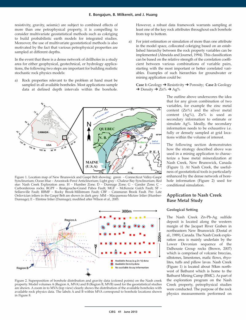
The following section demonstrateshow the strategy described above wasused in a mining application to charac-terize a base metal mineralization atNash Creek, New Brunswick, Canada(Figure 1). At Nash Creek, the useful-ness of geostatistical tools is particularlyenhanced by the dense network of bore-hole information (Figure 2) used forconditional simulation.

Application to Nash CreekBase Metal Study

Geological Setting

The Nash Creek Zn-Pb-Ag sulfidedeposit is located along the westernmargin of the Jacquet River Graben innortheastern New Brunswick (Dostal etal., 1989), Canada. The Nash Creek explo-ration area is mainly underlain by theLower Devonian sequence of theDalhousie Group rocks (Brown, 2007)which is comprised of volcanic breccias,siltstones, limestones, mafic flows, rhyo-lites, tuffs and pillow lavas. Nash Creek(Figure 1) is located about 50km north-west of Bathurst which is home to theBathurst Mining Camp (BMC). As part ofthe exploration program on the NashCreek property, petrophysical studieswere conducted. The purpose of the rockphysics measurements performed on

E. Bongajum, B. Milkereit, and J. Huang

Figure 1. Location map of New Brunswick and Gaspé Belt showing: green – Connecticut Valley-GaspéSynclinorium; Ocean blue – Aroostook-Percé Anticlinorium; Light gray – Chaleur Bay Synclinorium; Redstar: Nash Creek Exploration area. H – Humber Zone; D – Dunnage Zone; G – Gander Zone; C –Carboniferous rocks; RGPF – Restigouche-Grand Pabos Fault; MGF – McKenzie Gulch Fault; SF –Sellarsville Fault; RBMF – Rocky Brook-Millstream Fault; CBF – Catamaran Brook Fault. Pre- LateOrdovician inliers in the Gaspé Belt are shown in dark grey: MM – Macquereau-Mictaw Inlier (Humber-Dunnage); E – Elmtree Inlier (Dunnage); modified after Wilson et al., 2005.

Figure 2. Superposition of borehole distribution and gravity data (colored points) on the Nash creekproperty. Model volumes A (Region A, MVA) and B (Region B, MVB) used for the geostatistical studiesare shown. A zoom in to MVA (top view) clearly shows the distribution of the available boreholes withavailable rock physics data. The labels A and B within MVA correspond to borehole locations shownin Figure 8.

u α( )∈α+

u α( )∈α+

CJEG 42 June 2013

core samples from multiple boreholes in this area was to helpcharacterize the 3D nature of the Nash Creek Zn-Pb-Ag deposit.Understanding the spatial variation and correlation betweenthese physical properties is vital for every exploration project inthe study area.

Rock physics measurements, geochemical data and variogram analysis

Given that the diameters of drillholes in Nash Creek are smalland the boreholes were not suitable for gamma-gamma loggingtools, formation densities were measured on cores via the buoy-ancy method (Franklin et al., 1979). Density data were recordedfrom cores taken from 32 boreholes. In order to minimize theerrors from the data in our study, the instruments used werecalibrated by using an aluminum sample with known density.Given that most of the rocks in the Nash Creek property are ofmafic or felsic type, 2.3 gcm-3 was used as the cutoff valuebelow which the density measurements were considered to beerroneous for the geostatistical study. Sampling intervalsranged from 0.5 m-1 m, resulting in approximately 6000 densitydata points. Details of the geochemical data (e.g. Zn%) aredocumented by Brown (2007). From the 32 drillholes, we

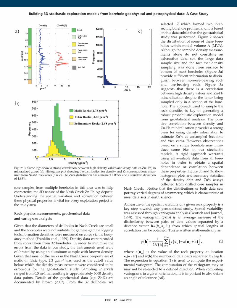
selected 17 which formed two inter-secting borehole profiles, and it is basedon this data subset that the geostatisticalstudy was performed. Figure 2 showsthe distribution of some of these bore-holes within model volume A (MVA).Although the sampled density measure-ments alone do not constitute anexhaustive data set, the large datasample size and the fact that densitysampling was done from surface tobottom of most boreholes (Figure 3a)provide sufficient information to distin-guish between non-ore-bearing rockand ore-bearing rock. Figure 3asuggests that there is a correlationbetween high density values and Zn-Pbmineralization despite the latter beingsampled only in a section of the bore-hole. The approach used to sample therock densities is key in generating arobust probabilistic exploration modelfrom geostatistical analysis. The posi-tive correlation between density andZn-Pb mineralization provides a strongbasis for using density information toestimate Zn% at unsampled locationsand vice versa. However, observationsbased on a single borehole may intro-duce some bias in our stochasticmodels. A rigid approach warrantsusing all available data from all bore-holes in order to obtain a spatialdependence or correlation betweenthese properties. Figure 3b and 3c showhistogram plots and summary statisticsof the density data and Zn% assayscollected from drilled core samples in

Nash Creek. Notice that the distributions of both data setsportray varied degrees of asymmetry, which is characteristic ofmost data sets in earth science.

A measure of the spatial variability of a given rock property is akey step towards any geostatistical study. Spatial variabilitywas assessed through variogram analysis (Deutsch and Journel,1998). The variogram (g (h)) is an average measure of thedissimilarity between pairs of data values separated by adistance vector h=(hx,hy,hz) from which spatial lengths ofcorrelation can be obtained. This is written mathematically as:

(1)

where z(ua) is the value of the rock property at location and N(h) the number of data pairs separated by lag h.

The expression in equation (1) is used to compute the experi-mental variogram. The computation of the variogram may ormay not be restricted to a defined direction. When computingvariograms in a given orientation, it is important to also definean angle of tolerance (D).

Building 3D stochastic exploration models from borehole geophysical and petrophysical data: A Case Study

Nz zh

hu u h

1

2,

N h

1

2

∑γ ( ) ( ) ( ) ( )= − + α αα

( )

=

Nz zh

hu u h

1

2,

N h

1

2

∑γ ( ) ( ) ( ) ( )= − + α αα

( )

=

Figure 3. Some logs show a strong correlation between high density values and assay data (%Zn+Pb) inmineralized zones (a). Histogram plot showing the distribution for density and Zn concentrations meas-ured from Nash Creek cores (b & c). The Zn% distribution has a mean of 1.085% and a standard deviationof 1.93%.

CJEG 43 June 2013

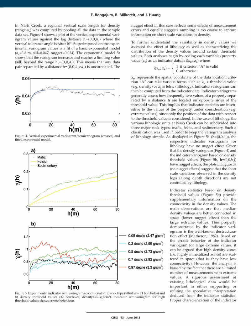
In Nash Creek, a regional vertical scale length for density(range-az) was computed by pooling all the data in the sampledata set. Figure 4 shows a plot of the vertical experimental vari-ogram values against the lag distance h=(0,0,hz) where thevertical tolerance angle is D=±10°. Superimposed on the exper-imental variogram values is a fit of a basic exponential model(az=3.8 m, sill=0.047, nugget=0.034). The exponential model fitshows that the variogram increases and reaches a limiting value(sill) beyond the range hr=(0,0,az). This means that any datapair separated by a distance h=(0,0,hz>az) is uncorrelated. The

nugget effect in this case reflects some effects of measurementerrors and equally suggests sampling is too coarse to captureinformation on short scale variations in density.

To further understand the variability in density values weassessed the effect of lithology as well as characterizing thedistribution of the density values around certain thresholdvalues. Both analyses begin by coding each variable/propertyvalue (zk) as an indicator datum i(xm; zk) where

i(xm; zk) =1 if criterion “A” is valid0 otherwise

xm represents the spatial coordinate of the data location; crite-rion “A” can take various forms such as zk < threshold value(e.g. density) or zk is felsic (lithology). Indicator variograms canthen be computed from the indicator data. Indicator variogramsgenerally assess how frequently two values of a property sepa-rated by a distance h are located on opposite sides of thethreshold value. This implies that indicator statistics are insen-sitive to the values of the property under consideration (e.g.extreme values), since only the position of the data with respectto the threshold value is considered. In the case of lithology, thevarious lithologic units at Nash Creek can be subdivided intothree major rock types: mafic, felsic, and sedimentary. Such aclassification was used in order to keep the variogram analysisof lithology simple. As displayed in Figure 5a (h=(0,0,hz)), the

respective indicator variograms forlithology have no nugget effect. Giventhat the density variogram (Figure 4) andthe indicator variogram based on densitythreshold values (Figure 5b, h=(0,0,hz))have nugget effects, the plots in Figure 5a(no nugget effects) suggest that the shortscale variations observed in the densitylogs (along depth direction) are notcontrolled by lithology.

Indicator statistics based on densitythreshold values (Figure 5b) providesupplementary information on theconnectivity in the density values. Themain observations are that mediandensity values are better connected inspace (lower nugget effect) than thelarge extreme values. This propertydemonstrated by the indicator vari-ograms is the well-known destructura-tion effect (Matheron, 1982). Based onthe erratic behavior of the indicatorvariogram for large extreme values, itcan be argued that high density zones(i.e. highly mineralized zones) are scat-tered in space (that is, they have lowconnectivity). However, the analysis isbiased by the fact that there are a limitednumber of measurements with extremevalues. A rigorous assessment ofexisting lithological data would beimportant in either supporting orrefuting the speculative interpretationdeduced from the indicator statistics.Proper characterization of the indicator


{

Figure 4. Vertical experimental variogram/semivariogram (crosses) andfitted exponential model.

Figure 5. Experimental indicator semivariograms conditional to: a) rock type (lithology- 21 boreholes) andb) density threshold values (32 boreholes, density>=2.3g/cm3). Indicator semivariogram for highthreshold values shows erratic behaviour.

CJEG 44 June 2013

statistics for extreme values is critical to the choice of method-ology adopted to characterize the distribution of mineralizedzones and hence resource estimates. Also, notice that the rangeof the intermediate densities compares with those derived fromthe mafic and felsic indicator variograms. To some extent, theseresults corroborate the observation that the major lithologicunits may influence the large scale spatial variability of theintermediate densities.

In addition to the vertical scale length, there is also need todefine the horizontal scale lengths for 3D modeling. In thegeostatistics literature, horizontal scale lengths (ax and ay) canbe obtained by analysing unidirectional or omnidirectionalvariograms. When the computation of horizontal variograms isdirection dependent, the unidirectional variograms arecomputed for several directions in the horizontal plane usingsmall tolerance angles that allow for sufficient data pairs toensure the computation of stable experimental variograms.Alternatively, horizontal spatial variability can also be meas-ured by considering a secondary property that is closely relatedto the property of interest. Deriving the variogram parametersfrom a secondary dataset has been applied successfully in someoil and gas applications (Cole et al., 2003). In the case of densitydata, for example, a suitable candidate for secondary data isgravity data. Due to the paucity of data on the horizontal plane(few vertical boreholes/ no horizontal boreholes) in this study,analysis for horizontal spatial variability was more challenging.Although the horizontal scale lengths are typically expected tobe larger than the vertical scale length, the subsequentmodeling results used isotropic scale lengths (ax = ay = az) thatwere based on the reliable estimate of the vertical scale length(az). This choice of the horizontal scale lengths is also motivatedby field observations where it was difficult to observe signifi-cant lateral correlation of the high grade zones between theboreholes intervals (25-50m).

Density model

Having characterized the sample population of density andassay data, the next step is to quantitatively model the spatialstatistics of the various populations from the available sampledata over the study area. The approach used to obtain values ofdensity at unsampled locations within MVA is based on kriging(Matheron, 1963). Kriging entails building models that honourthe statistics and other characteristics of the observed data suchas the spatial continuity, for example, of large values (highdensities) throughout MVA. In cases where the estimation (orinterpolation) process within a target volume is applied toseveral variables simultaneously, this is called cokriging(Deutsch and Journel, 1998). Both the kriging and cokrigingtechniques are based on the minimization of the estimationerror (i.e. the error between the true and the estimated value ofthe target variable(s) and therefore produces smoothed interpo-lated maps. The degree of smoothness will depend on both thenugget and range values computed in the variogram(s).

As in most geostatistical methods, the spatial distribution of therock property (variable) is considered to be characterized by asecond order stationary random function. Before implementingthe kriging algorithm, the well data was up-scaled to the gridcells by assigning the property value to the grid cell that isclosest to it. In order to preserve the variogram properties of the

original input data, the grid dimensions used were 2m x 2m x1m. The three variants of geostatistical techniques considered inthis study include: simple kriging (SK), cokriging, and condi-tional sequential Gaussian simulation (SGS, Deutsch andJournel, 1998). While the kriging and cokriging methods reduceto the expected (mean) value at estimation locations that are farfrom any borehole location (beyond the range of the variogrammodel), the SGS method allows for the fluctuations in themodeled property at similar estimation locations. This meansthat simple kriging results underestimate the fluctuations in theproperty (continuous random variable) within the volume ofstudy. Typically, interpolation algorithms result in underestima-tion of large values and overestimation of small values(Goovaerts, 1997, p370). This is a disadvantage especially whenthe detection of patterns in extreme values (e.g. zones of highore grade) is of interest.

On the other hand, conditional simulations are useful in thisrespect because they help reproduce the geological texture(spatial variability) conditional to the existing information of thetarget variable. Simulations produce several realizations of thetarget variable and each realization is an equally probableoutcome. The simulation technique may incorporate either thekriging or cokriging (for multiple variables) techniques in orderto constrain the simulation to the available data. In this study, forexample, the conditional simulations of density incorporate thesimple kriging technique (SKSGS, Deutsch and Journel, 1998).Often, the simulated property has implications for decision-making processes such as risk assessment for contaminationareas (Goovaerts, 1997, p259), forward modeling to optimizegeophysical imaging parameters (Huang et al., 2009), or in theassessment of available and recoverable ore at a mine site(Emery et al., 2006). In such applications, it is thus useful tomodel the spatial uncertainty of the property at unknown loca-tions. This makes a simulation algorithm a very powerful tool asit attempts to reproduce the spatial variability through alterna-tive, equally probable, high-resolution models. Consequently,the simple kriging results are not shown in this study.

Conceptually, the SKSGS algorithm implemented for a givenattribute such as density on a 2D/3D grid involves sequentiallyvisiting each grid node following a random path and deriving asimulated value for density. At each step, the density value issimulated by sampling from a Gaussian conditional probabilitydensity function (PDF) with parameters (i.e. mean and vari-ance) given respectively by a kriging estimate and kriging vari-ance (Doyen 2007, p80). The workflow used in our study is asfollows:

a) Pick a non-simulated grid node j at random.

b) Compute the kriging estimate and variance (based on simplekriging)

(2)

where Y(xj): gaussian transformed version of the targetvariable Z(xj),

m : constant mean,

Wisk(xj): kriging weight, and the error variance given in

terms of the covariances as:


Y w Y m mx x x[ ]j i

sk

ji

n x

i

*

1

sk ∑( ) ( ) ( )= − +( )

=

Y w Y m mx x x[ ]j i

sk

ji

n x

i

*

1

sk ∑( ) ( ) ( )= − +( )

=

CJEG 45 June 2013

.

Note that the covariances C(h) are related to the bounded vari-ogram (g (h)) of the variable Y(xj). In the strict stationary case,g (h)=C(0)–C(h).

c) Draw a simulated value of density Y(xj) at random from theprobability distribution:

. (3)

d) Treat the simulated Y(xj) value as an additional controlpoint.

e) Go back to step a) and repeat until all nodes in the 3D grid aresimulated.

Notice that the looping process (step (e)) in the SKSGS is critical toensuring that the realizations are spatially correlated (Doyen,2007, p81). Moreover, the influence of limitations in search neigh-bourhood of conditioning data wasaddressed by implementing the multi-grid concept: first simulate on a coarsegrid using larger search neighbourhoods,then simulate the remaining nodes usinga smaller search neighbourhood.

When computer hardware require-ments (processor speeds and memory)are met, SGS is computationallyconvenient and reasonably efficientdespite inherent shortcomings, whichare as follows: (i) SGS results in a highlydisordered model (Journel and Deutsch,1993) whereby extreme values arehighly disconnected; (ii) SGS relies on amulti-variate gaussianity assumption;(iii) the reproduction of the originalvariogram (derived from the originaldata) model as well as indicator vari-ograms are not guaranteed. Given thatthe connectivity between extremevalues is not evidenced by availabledata (e.g. density) from the Nash creekproperty, the first shortcoming (i) of theSGS method was overlooked in thisstudy. For simulation of the densityattribute conditional to well logs usingthe SKSGS approach, the followingsteps were followed:

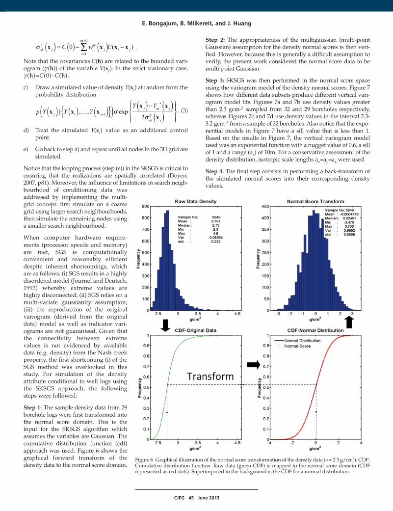
Step 1: The sample density data from 29borehole logs were first transformed intothe normal score domain. This is theinput for the SKSGS algorithm whichassumes the variables are Gaussian. Thecumulative distribution function (cdf)approach was used. Figure 6 shows thegraphical forward transform of thedensity data to the normal score domain.

Step 2: The appropriateness of the multigaussian (multi-pointGaussian) assumption for the density normal scores is then veri-fied. However, because this is generally a difficult assumption toverify, the present work considered the normal score data to bemulti-point Gaussian.

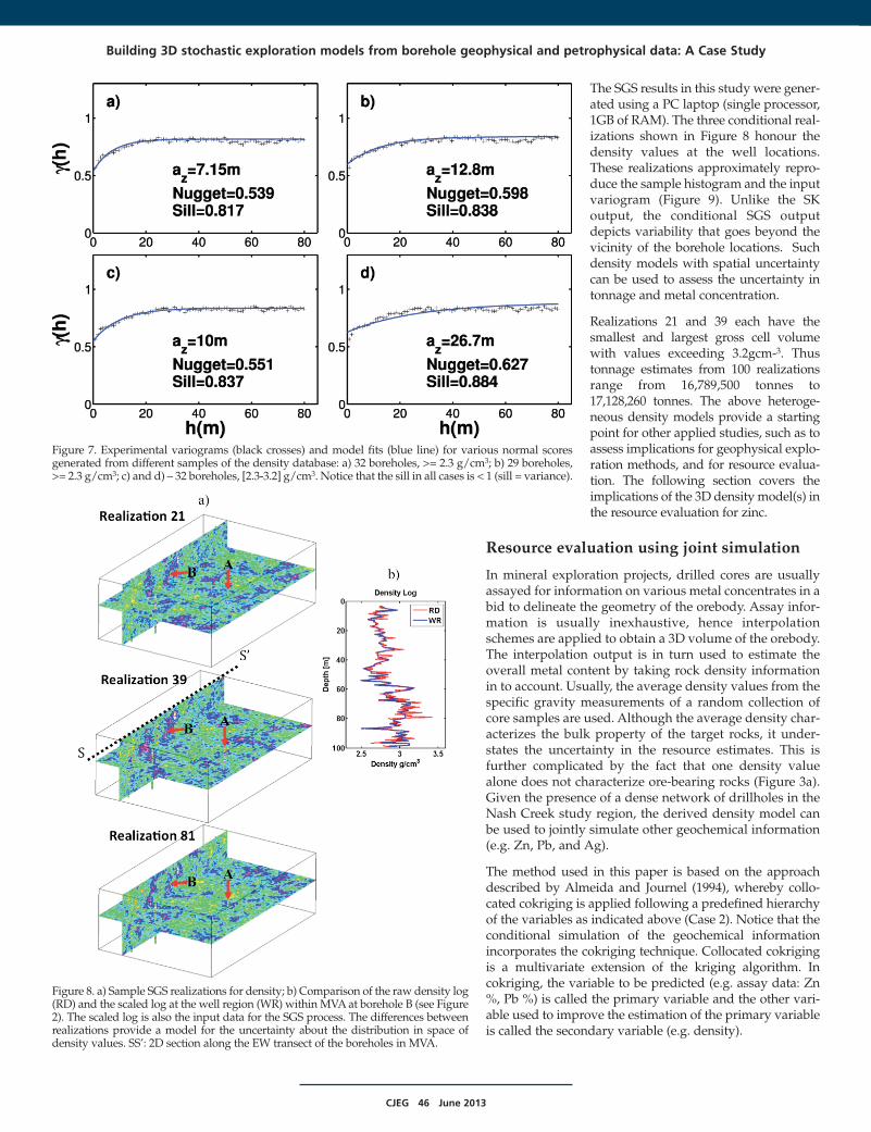
Step 3: SKSGS was then performed in the normal score spaceusing the variogram model of the density normal scores. Figure 7shows how different data subsets produce different vertical vari-ogram model fits. Figures 7a and 7b use density values greaterthan 2.3 gcm-3 sampled from 32 and 29 boreholes respectively,whereas Figures 7c and 7d use density values in the interval 2.3-3.2 gcm-3 from a sample of 32 boreholes. Also notice that the expo-nential models in Figure 7 have a sill value that is less than 1.Based on the results in Figure 7, the vertical variogram modelused was an exponential function with a nugget value of 0.6, a sillof 1 and a range (az) of 10m. For a conservative assessment of thedensity distribution, isotropic scale lengths ax=ay=az were used.

Step 4: The final step consists in performing a back-transform ofthe simulated normal scores into their corresponding densityvalues.


Figure 6. Graphical illustration of the normal score transformation of the density data (>= 2.3 g/cm3). CDF:Cumulative distribution function. Raw data (green CDF) is mapped to the normal score domain (CDFrepresented as red dots). Superimposed in the background is the CDF for a normal distribution.

C w Cx x x x0 ( )sk j i

sk

ji

n x

i j

2

1

( )

∑σ ( ) ( )( )= − −=

C w Cx x x x0 ( )sk j i

sk

ji

n x

i j

2

1

( )

∑σ ( ) ( )( )= − −=

p Y Y YY Y

x x xx x

x| ,...., exp

2j j

j sk j

sk j

1 1

*

2ασ

( ){ }( ) ( ) ( ) ( )( )( )

−

−

p Y Y YY Y

x x xx x

x| ,...., exp

2j j

j sk j

sk j

1 1

*

2α

σ( ){ }( ) ( ) ( ) ( )( )( )

−

−

CJEG 46 June 2013

The SGS results in this study were gener-ated using a PC laptop (single processor,1GB of RAM). The three conditional real-izations shown in Figure 8 honour thedensity values at the well locations.These realizations approximately repro-duce the sample histogram and the inputvariogram (Figure 9). Unlike the SKoutput, the conditional SGS outputdepicts variability that goes beyond thevicinity of the borehole locations. Suchdensity models with spatial uncertaintycan be used to assess the uncertainty intonnage and metal concentration.

Realizations 21 and 39 each have thesmallest and largest gross cell volumewith values exceeding 3.2gcm-3. Thustonnage estimates from 100 realizationsrange from 16,789,500 tonnes to17,128,260 tonnes. The above heteroge-neous density models provide a startingpoint for other applied studies, such as toassess implications for geophysical explo-ration methods, and for resource evalua-tion. The following section covers theimplications of the 3D density model(s) inthe resource evaluation for zinc.

Resource evaluation using joint simulation

In mineral exploration projects, drilled cores are usuallyassayed for information on various metal concentrates in abid to delineate the geometry of the orebody. Assay infor-mation is usually inexhaustive, hence interpolationschemes are applied to obtain a 3D volume of the orebody.The interpolation output is in turn used to estimate theoverall metal content by taking rock density informationin to account. Usually, the average density values from thespecific gravity measurements of a random collection ofcore samples are used. Although the average density char-acterizes the bulk property of the target rocks, it under-states the uncertainty in the resource estimates. This isfurther complicated by the fact that one density valuealone does not characterize ore-bearing rocks (Figure 3a).Given the presence of a dense network of drillholes in theNash Creek study region, the derived density model canbe used to jointly simulate other geochemical information(e.g. Zn, Pb, and Ag).

The method used in this paper is based on the approachdescribed by Almeida and Journel (1994), whereby collo-cated cokriging is applied following a predefined hierarchyof the variables as indicated above (Case 2). Notice that theconditional simulation of the geochemical informationincorporates the cokriging technique. Collocated cokrigingis a multivariate extension of the kriging algorithm. Incokriging, the variable to be predicted (e.g. assay data: Zn%, Pb %) is called the primary variable and the other vari-able used to improve the estimation of the primary variableis called the secondary variable (e.g. density).


Figure 8. a) Sample SGS realizations for density; b) Comparison of the raw density log(RD) and the scaled log at the well region (WR) within MVA at borehole B (see Figure2). The scaled log is also the input data for the SGS process. The differences betweenrealizations provide a model for the uncertainty about the distribution in space ofdensity values. SS’: 2D section along the EW transect of the boreholes in MVA.

Figure 7. Experimental variograms (black crosses) and model fits (blue line) for various normal scoresgenerated from different samples of the density database: a) 32 boreholes, >= 2.3 g/cm3; b) 29 boreholes,>= 2.3 g/cm3; c) and d) – 32 boreholes, [2.3-3.2] g/cm3. Notice that the sill in all cases is < 1 (sill = variance).

CJEG 47 June 2013

The approach by Almeida and Journel (1994) allows for the useof the markov-type approximation used in collocated cokriging(Xu et al., 1992; Doyen, 2007; Goovaerts, 1997). This approxima-tion assumes that the dependence of the secondary variable onthe primary is limited to the collocated primary datum. Hence,the cross-covariances between the primary (Z1) and secondary(Z2) variables are linearly related to the autocovariances of theprimary variable by the following equation:

(4)

The following markov-type independence relation between theprimary (Z1) and secondary (Z2) variables is a sufficient condi-tion for the approximation in equation (4) to be valid:

(5)

The predefined classification between variables can be based onthe relative strength of the correlation coefficient betweenvarious combinations of variable pairs, starting with the most

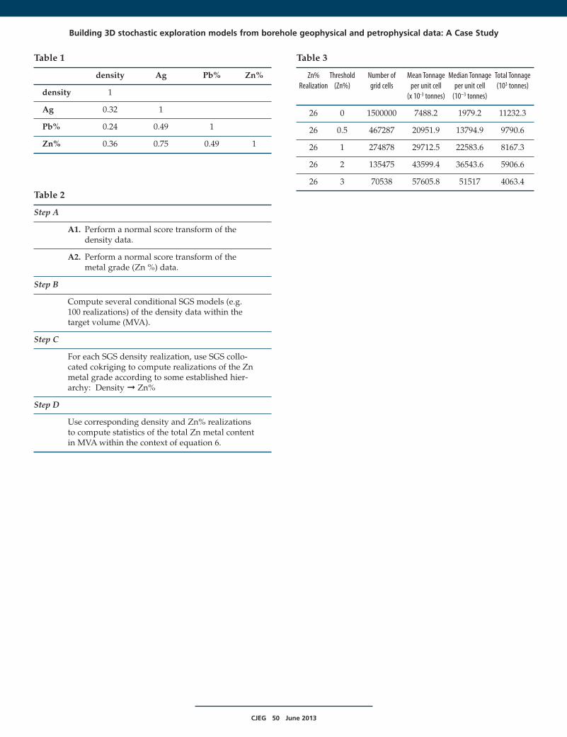
important or better auto-correlated variable (Table 1). Thisapproach is used in the case discussed here where possiblehierarchies include:

Density➔ Zn(Zinc) ➔ Ag(Silver) ➔ Pb(Lead)

The hierarchy above underscores the idea that density is usedas secondary information to estimate or simulate Zn%; silverconcentration (Ag%) is simulated in turn with Zn% and densityas secondary information and simulations for Pb% are donewith Ag%, Zn% and density as secondary information.

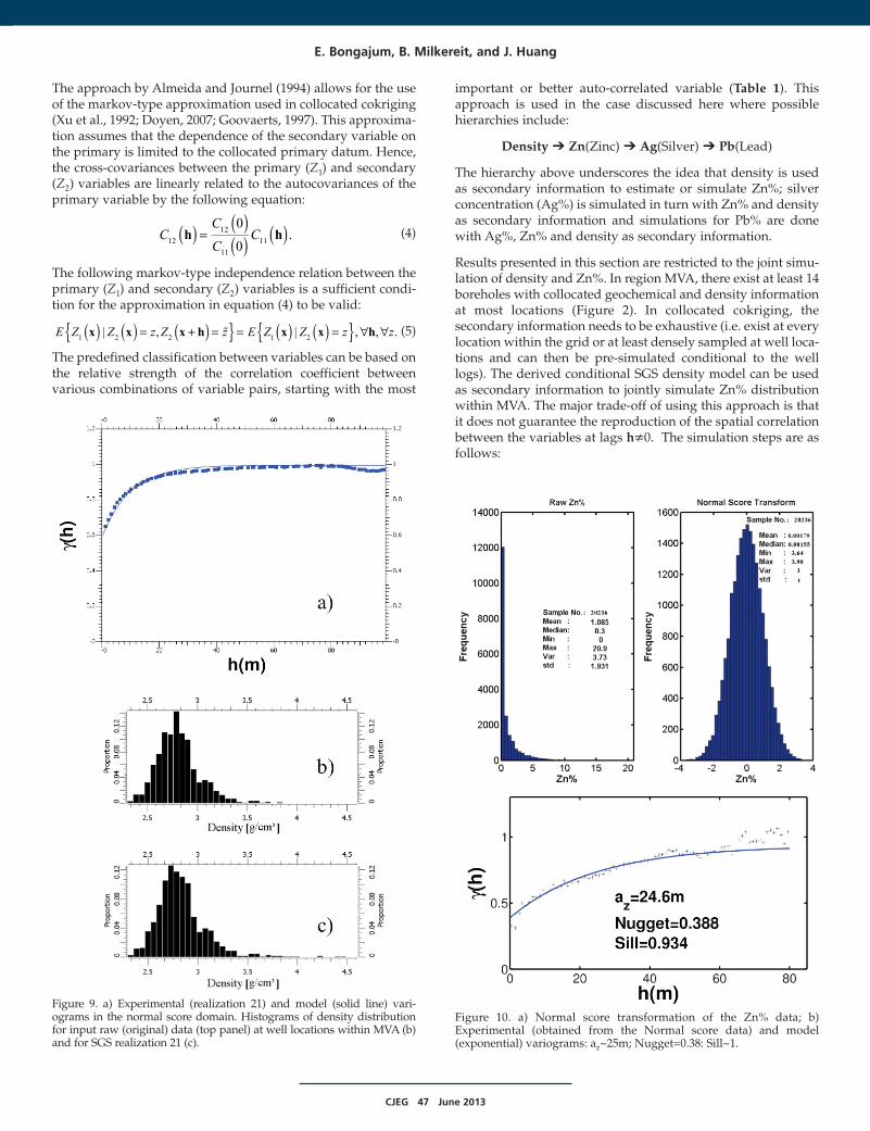
Results presented in this section are restricted to the joint simu-lation of density and Zn%. In region MVA, there exist at least 14boreholes with collocated geochemical and density informationat most locations (Figure 2). In collocated cokriging, thesecondary information needs to be exhaustive (i.e. exist at everylocation within the grid or at least densely sampled at well loca-tions and can then be pre-simulated conditional to the welllogs). The derived conditional SGS density model can be usedas secondary information to jointly simulate Zn% distributionwithin MVA. The major trade-off of using this approach is thatit does not guarantee the reproduction of the spatial correlationbetween the variables at lags h≠0. The simulation steps are asfollows:


Figure 9. a) Experimental (realization 21) and model (solid line) vari-ograms in the normal score domain. Histograms of density distributionfor input raw (original) data (top panel) at well locations within MVA (b)and for SGS realization 21 (c).

CC

CCh h

0

0.12

12

11

11( ) ( )( ) ( )=

CC

CCh h

0

0.

12

12

11

11( ) ( )( ) ( )=

E Z Z z Z z E Z Z z zx x x h x x h| , | , , .1 2 2 1 2{ } { }( ) ( ) ( ) ( ) ( )= + = = = ∀ ∀

E Z Z z Z z E Z Z z zx x x h x x h| , | , , .1 2 2 1 2{ } { }( ) ( ) ( ) ( ) ( )= + = = = ∀ ∀

Figure 10. a) Normal score transformation of the Zn% data; b)Experimental (obtained from the Normal score data) and model (exponential) variograms: az~25m; Nugget=0.38: Sill~1.

CJEG 48 June 2013

a) Define a hierarchy of variables starting with themost important or better correlated variables.

b) Transform all variables into the normal scoredomain:

where Zi and Yi identify the variables in the rawdata and normal score domain; i is the indexidentifying the various variables. Also check thatthe conditions for bigaussianity are met. In thispresent study, this condition is assumed to bevalid.

c) Pre-simulate independently the secondary vari-able(s) conditional to information at well locations.The drawback in doing this is that dependencybetween secondary variables is not accounted bythe pre-simulations. However, this approximationis acceptable because of the characteristic densesampling of secondary variables (Almeida andJournel, 1994). For the Nash Creek case, this is notof major concern since only one primary variable(zinc) and one secondary variable (density) areconsidered.

d) Define a random path visiting each node of thegrid only once.

3) At each node x, determine the Gaussian condi-tional cumulative distribution function (ccdf) ofthe primary variable at x given the n neigh-bouring primary data of the same type and theonly collocated secondary data. This requiressolving the simple cokriging system of dimen-sion (n+1). Then draw a simulated value y1

(1)(x)from the ccdf and add it to the file of hard Y1-conditioning data set.

f) Repeat step e) until all N nodes are simulated.

g) Back transform the simulated values to the original values.

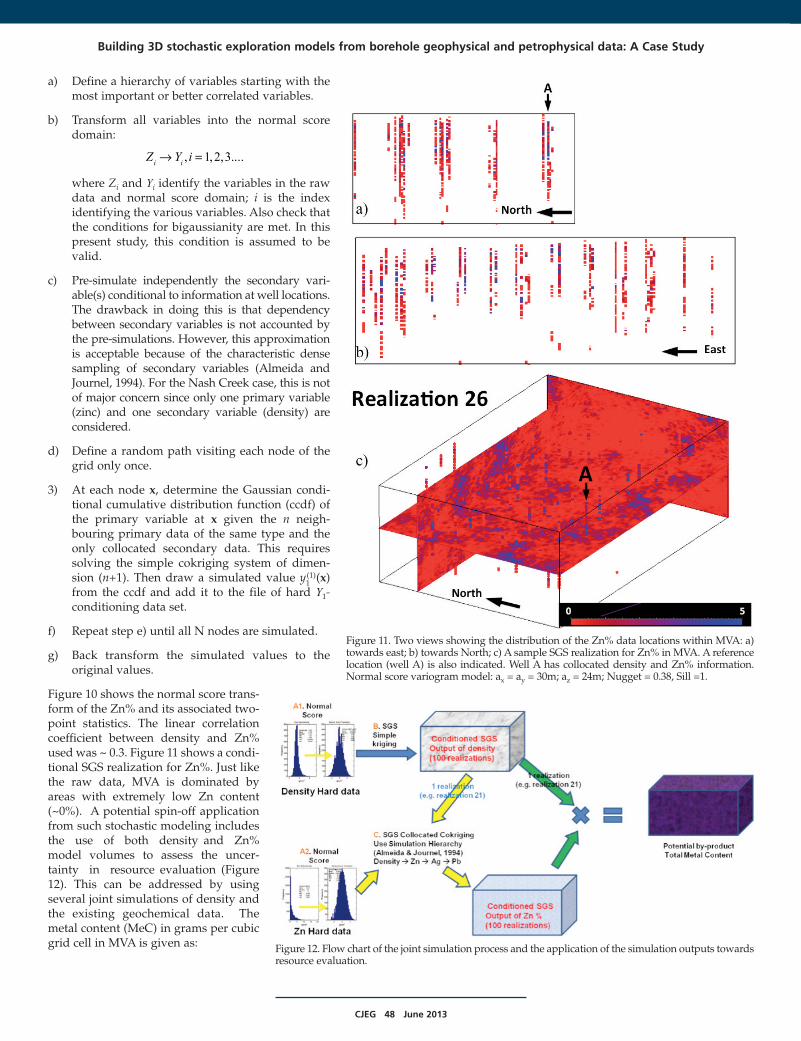
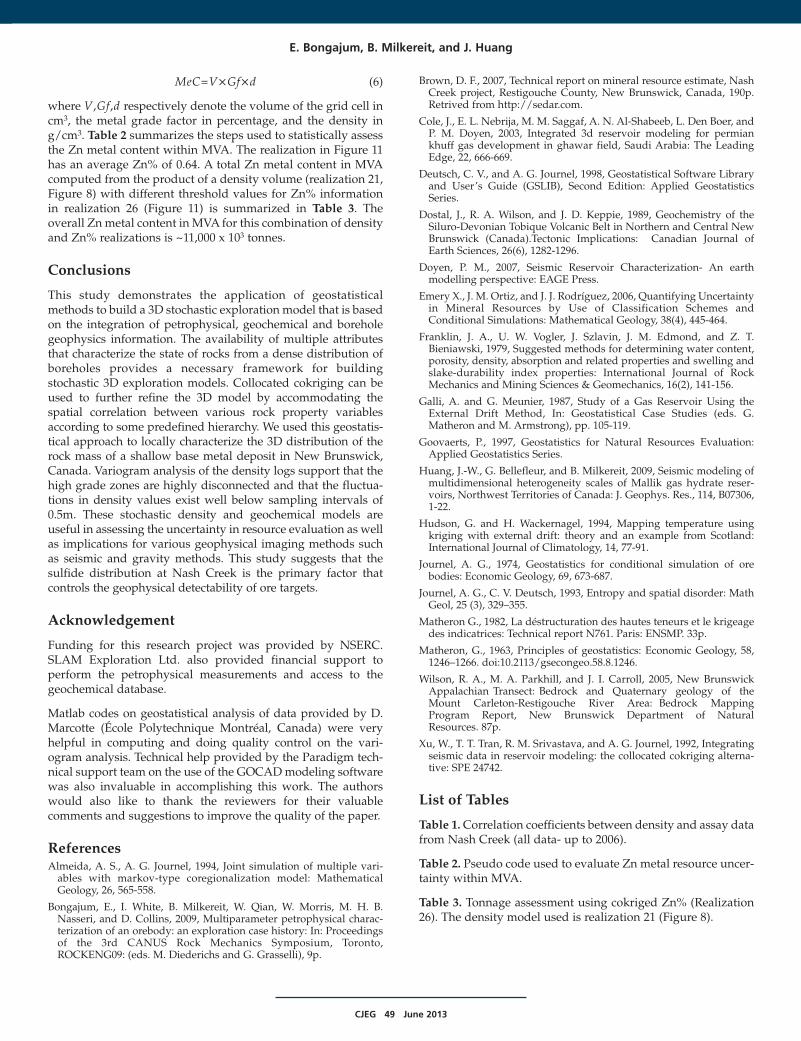
Figure 10 shows the normal score trans-form of the Zn% and its associated two-point statistics. The linear correlationcoefficient between density and Zn%used was ~ 0.3. Figure 11 shows a condi-tional SGS realization for Zn%. Just likethe raw data, MVA is dominated byareas with extremely low Zn content(~0%). A potential spin-off applicationfrom such stochastic modeling includesthe use of both density and Zn%model volumes to assess the uncer-tainty in resource evaluation (Figure12). This can be addressed by usingseveral joint simulations of density andthe existing geochemical data. Themetal content (MeC) in grams per cubicgrid cell in MVA is given as:


Figure 11. Two views showing the distribution of the Zn% data locations within MVA: a)towards east; b) towards North; c) A sample SGS realization for Zn% in MVA. A referencelocation (well A) is also indicated. Well A has collocated density and Zn% information.Normal score variogram model: ax = ay = 30m; az = 24m; Nugget = 0.38, Sill =1.

Figure 12. Flow chart of the joint simulation process and the application of the simulation outputs towardsresource evaluation.

Z Y i, 1,2,3....i i→ =

Z Y i, 1,2,3....i i→ =

CJEG 49 June 2013

MeC=V×Gf×d (6)

where V,Gf,d respectively denote the volume of the grid cell incm3, the metal grade factor in percentage, and the density ing/cm3. Table 2 summarizes the steps used to statistically assessthe Zn metal content within MVA. The realization in Figure 11has an average Zn% of 0.64. A total Zn metal content in MVAcomputed from the product of a density volume (realization 21,Figure 8) with different threshold values for Zn% informationin realization 26 (Figure 11) is summarized in Table 3. Theoverall Zn metal content in MVA for this combination of densityand Zn% realizations is ~11,000 x 103 tonnes.

Conclusions

This study demonstrates the application of geostatisticalmethods to build a 3D stochastic exploration model that is basedon the integration of petrophysical, geochemical and boreholegeophysics information. The availability of multiple attributesthat characterize the state of rocks from a dense distribution ofboreholes provides a necessary framework for buildingstochastic 3D exploration models. Collocated cokriging can beused to further refine the 3D model by accommodating thespatial correlation between various rock property variablesaccording to some predefined hierarchy. We used this geostatis-tical approach to locally characterize the 3D distribution of therock mass of a shallow base metal deposit in New Brunswick,Canada. Variogram analysis of the density logs support that thehigh grade zones are highly disconnected and that the fluctua-tions in density values exist well below sampling intervals of0.5m. These stochastic density and geochemical models areuseful in assessing the uncertainty in resource evaluation as wellas implications for various geophysical imaging methods suchas seismic and gravity methods. This study suggests that thesulfide distribution at Nash Creek is the primary factor thatcontrols the geophysical detectability of ore targets.

Acknowledgement

Funding for this research project was provided by NSERC.SLAM Exploration Ltd. also provided financial support toperform the petrophysical measurements and access to thegeochemical database.

Matlab codes on geostatistical analysis of data provided by D.Marcotte (École Polytechnique Montréal, Canada) were veryhelpful in computing and doing quality control on the vari-ogram analysis. Technical help provided by the Paradigm tech-nical support team on the use of the GOCAD modeling softwarewas also invaluable in accomplishing this work. The authorswould also like to thank the reviewers for their valuablecomments and suggestions to improve the quality of the paper.

ReferencesAlmeida, A. S., A. G. Journel, 1994, Joint simulation of multiple vari-ables with markov-type coregionalization model: MathematicalGeology, 26, 565-558.

Bongajum, E., I. White, B. Milkereit, W. Qian, W. Morris, M. H. B.Nasseri, and D. Collins, 2009, Multiparameter petrophysical charac-terization of an orebody: an exploration case history: In: Proceedingsof the 3rd CANUS Rock Mechanics Symposium, Toronto,ROCKENG09: (eds. M. Diederichs and G. Grasselli), 9p.

Brown, D. F., 2007, Technical report on mineral resource estimate, NashCreek project, Restigouche County, New Brunswick, Canada, 190p.Retrived from http://sedar.com.

Cole, J., E. L. Nebrija, M. M. Saggaf, A. N. Al-Shabeeb, L. Den Boer, andP. M. Doyen, 2003, Integrated 3d reservoir modeling for permiankhuff gas development in ghawar field, Saudi Arabia: The LeadingEdge, 22, 666-669.

Deutsch, C. V., and A. G. Journel, 1998, Geostatistical Software Libraryand User’s Guide (GSLIB), Second Edition: Applied GeostatisticsSeries.

Dostal, J., R. A. Wilson, and J. D. Keppie, 1989, Geochemistry of theSiluro-Devonian Tobique Volcanic Belt in Northern and Central NewBrunswick (Canada).Tectonic Implications: Canadian Journal ofEarth Sciences, 26(6), 1282-1296.

Doyen, P. M., 2007, Seismic Reservoir Characterization- An earthmodelling perspective: EAGE Press.

Emery X., J. M. Ortiz, and J. J. Rodríguez, 2006, Quantifying Uncertaintyin Mineral Resources by Use of Classification Schemes andConditional Simulations: Mathematical Geology, 38(4), 445-464.

Franklin, J. A., U. W. Vogler, J. Szlavin, J. M. Edmond, and Z. T.Bieniawski, 1979, Suggested methods for determining water content,porosity, density, absorption and related properties and swelling andslake-durability index properties: International Journal of RockMechanics and Mining Sciences & Geomechanics, 16(2), 141-156.

Galli, A. and G. Meunier, 1987, Study of a Gas Reservoir Using theExternal Drift Method, In: Geostatistical Case Studies (eds. G.Matheron and M. Armstrong), pp. 105-119.

Goovaerts, P., 1997, Geostatistics for Natural Resources Evaluation:Applied Geostatistics Series.

Huang, J.-W., G. Bellefleur, and B. Milkereit, 2009, Seismic modeling ofmultidimensional heterogeneity scales of Mallik gas hydrate reser-voirs, Northwest Territories of Canada: J. Geophys. Res., 114, B07306,1-22.

Hudson, G. and H. Wackernagel, 1994, Mapping temperature usingkriging with external drift: theory and an example from Scotland:International Journal of Climatology, 14, 77-91.

Journel, A. G., 1974, Geostatistics for conditional simulation of orebodies: Economic Geology, 69, 673-687.

Journel, A. G., C. V. Deutsch, 1993, Entropy and spatial disorder: MathGeol, 25 (3), 329–355.

Matheron G., 1982, La déstructuration des hautes teneurs et le krigeagedes indicatrices: Technical report N761. Paris: ENSMP. 33p.

Matheron, G., 1963, Principles of geostatistics: Economic Geology, 58,1246–1266. doi:10.2113/gsecongeo.58.8.1246.

Wilson, R. A., M. A. Parkhill, and J. I. Carroll, 2005, New BrunswickAppalachian Transect: Bedrock and Quaternary geology of theMount Carleton-Restigouche River Area: Bedrock MappingProgram Report, New Brunswick Department of NaturalResources. 87p.

Xu, W., T. T. Tran, R. M. Srivastava, and A. G. Journel, 1992, Integratingseismic data in reservoir modeling: the collocated cokriging alterna-tive: SPE 24742.

List of Tables

Table 1. Correlation coefficients between density and assay datafrom Nash Creek (all data- up to 2006).

Table 2. Pseudo code used to evaluate Zn metal resource uncer-tainty within MVA.

Table 3. Tonnage assessment using cokriged Zn% (Realization26). The density model used is realization 21 (Figure 8).


CJEG 50 June 2013

Table 1

density Ag Pb% Zn%

density 1

Ag 0.32 1

Pb% 0.24 0.49 1

Zn% 0.36 0.75 0.49 1

Table 2

Step A

A1. Perform a normal score transform of thedensity data.

A2. Perform a normal score transform of themetal grade (Zn %) data.

Step B

Compute several conditional SGS models (e.g.100 realizations) of the density data within thetarget volume (MVA).

Step C

For each SGS density realization, use SGS collo-cated cokriging to compute realizations of the Znmetal grade according to some established hier-archy: Density ➞ Zn%

Step D

Use corresponding density and Zn% realizationsto compute statistics of the total Zn metal contentin MVA within the context of equation 6.

Table 3

Zn% Threshold Number of Mean Tonnage Median Tonnage Total TonnageRealization (Zn%) grid cells per unit cell per unit cell (103 tonnes)

(x 10-3 tonnes) (10–3 tonnes)

26 0 1500000 7488.2 1979.2 11232.3

26 0.5 467287 20951.9 13794.9 9790.6

26 1 274878 29712.5 22583.6 8167.3

26 2 135475 43599.4 36543.6 5906.6

26 3 70538 57605.8 51517 4063.4


Documents

CANADIAN JOURNAL of EXPLORATION GEOPHYSlCS VOL. …