Can We Group Storage? Statistical Techniques to Identify Predictive Groupings … · 2016-02-04 · 7 Can We Group Storage? Statistical Techniques to Identify Predictive Groupings

7

Can We Group Storage? Statistical Techniques to Identify PredictiveGroupings in Storage System Accesses

AVANI WILDANI, The Salk Institute for Biological StudiesETHAN L. MILLER, University of California, Santa Cruz

Storing large amounts of data for different users has become the new normal in a modern distributedcloud storage environment. Storing data successfully requires a balance of availability, reliability, cost, andperformance. Typically, systems design for this balance with minimal information about the data that willpass through them. We propose a series of methods to derive groupings from data that have predictive value,informing layout decisions for data on disk.

Unlike previous grouping work, we focus on dynamically identifying groupings in data that can be gatheredfrom active systems in real time with minimal impact using spatiotemporal locality. We outline severaltechniques we have developed and discuss how we select particular techniques for particular workloads andapplication domains. Our statistical and machine-learning-based grouping algorithms answer questionssuch as “What can a grouping be based on?” and “Is a given grouping meaningful for a given application?”We design our models to be flexible and require minimal domain information so that our results are asbroadly applicable as possible. We intend for this work to provide a launchpad for future specialized systemdesign using groupings in combination with caching policies and architectural distinctions such as tieredstorage to create the next generation of scalable storage systems.

Categories and Subject Descriptors: I.5.1 [Pattern Recognition]: Models; D.4.2 [Operating Systems]:Storage Management

General Terms: Design, Algorithms, Measurement, Performance

Additional Key Words and Phrases: Data layout, storage optimization, tiered storage, predictive modeling

ACM Reference Format:Avani Wildani and Ethan L. Miller. 2016. Can we group storage? Statistical techniques to identify predictivegroupings in storage system accesses. ACM Trans. Storage 12, 2, Article 7 (February 2016), 33 pages.DOI: http://dx.doi.org/10.1145/2738042

1. INTRODUCTION

A pressing issue in systems is management of “big data,” data that is too massive toimmediately process, which leads to results that themselves are nontrivial to processand store. Moreover, big data is likely to be stored on a petascale or exascale storagesystem that is designed around the paradigm of “cloud computing,” meaning that themultiuser, multiapplication system must appear as a dedicated server to each user.

This research was also supported in part by the National Science Foundation under awards CNS-0917396(part of the American Recovery and Reinvestment Act of 2009 [Public Law 111-5]) and IIP-0934401, and bythe Department of Energy’s Petascale Data Storage Institute under award DE-FC02-06ER25768. We alsothank Sandia National Laboratories and the industrial sponsors of the Storage Systems Research Centerand the Center for Research in Intelligent Storage for their generous support.Authors’ addresses: A. Wildani, Dept. of Math & CS, Emory University, 400 Dowman Dr., W401, Atlanta,GA 30322; email: [email protected]; E. L. Miller, Computer Science Department, Baskin School ofEngineering, University of California, 1156 High Street, MS SOE3; email: [email protected] to make digital or hard copies of part or all of this work for personal or classroom use is grantedwithout fee provided that copies are not made or distributed for profit or commercial advantage and thatcopies show this notice on the first page or initial screen of a display along with the full citation. Copyrights forcomponents of this work owned by others than ACM must be honored. Abstracting with credit is permitted.To copy otherwise, to republish, to post on servers, to redistribute to lists, or to use any component of thiswork in other works requires prior specific permission and/or a fee. Permissions may be requested fromPublications Dept., ACM, Inc., 2 Penn Plaza, Suite 701, New York, NY 10121-0701 USA, fax +1 (212)869-0481, or [email protected]© 2016 ACM 1553-3077/2016/02-ART7 $15.00DOI: http://dx.doi.org/10.1145/2738042

ACM Transactions on Storage, Vol. 12, No. 2, Article 7, Publication date: February 2016.

http://dx.doi.org/10.1145/2738042

http://dx.doi.org/10.1145/2738042

7:2 A. Wildani and E. L. Miller

This article approaches the problem of availability and power requirements of bigdata on large, heterogeneous systems by identifying groups within the data that sharea high probability of coaccess to approximate a dedicated server for different users orapplications through informed cache population and data layout. Similar grouping inspecialized systems has been shown to help avoid crossing track boundaries [Schindleret al. 2002], isolate faults [Sivathanu et al. 2005], and avoid power consumption fromexcessive disk activity [Pinheiro and Bianchini 2004]. The main contributions of ourgrouping methods are adaptability and domain independence. By examining the basicstatistics of the training workloads, we can quickly adjust our model to changes inworkload characteristics.

We define a group as any set of storage units, such as blocks, files, or objects, thatare likely to be accessed together within a defined amount of time, which is typically afunction of the rate of storage requests. Consequently, any element of a group acts as apredictor for other elements in that group. Groups typically arise from working sets ofuser or application data, though they can also represent higher-level correlations suchas interapplication dependencies and operating system interactions.

In an ideal world, we would be able to group objects based on either data con-tents of the application, user, or use case typical for that object. We term this sortof information-driven labeling categorical grouping. Categorical grouping is a well-studied problem [Arpaci-Dusseau et al. 2006], and thus for datasets with rich meta-data, we can treat the grouping problem as mostly solved and focus on datasets thatlack this metadata.

We show that with the level of input or output requests per second (IOPS) in modernstorage systems, it is possible to collect enough data in real time to identify statisticallybased groupings that can predict future access patterns, even in the absence of anymetadata. We discuss a variety of techniques for finding groups in this data includinggraph theoretic clique formation and agglomerative clustering, but we primarily focuson a naıve statistical method we developed called N-Neighborhood Partitioning (NNP).NNP runs in O(n) and is less memory intensive than our other methods, making itthe best choice for a high IOPS environment with quickly shifting workloads. Slowertechniques are reserved for more steady workloads where calculations can be done overa long period of time and data can be rearranged lazily.

The end goal of this work is to predict future access probabilities based on priorinformation to the extent that these access patterns can inform scalable system design.Once groups exist, we can place them on the same types of physical media, prefetchelements a group at a time, or even structure reliability schemes to minimize intergroupavailability disruptions. We have tested some of our techniques to address system powerconsumption through group-based layout and idle disk spin-down [Wildani and Miller2010], and we have also had positive results using groups to populate a memory-basedindex cache for online deduplication [Wildani et al. 2013].

After reviewing other work in the field, we present our statistical similarity metricsand partitioning algorithms, along with a discussion of how parameters are selectedand which methodology is best suited to which type of workload. We then present theworking set groupings that each of these partitioning algorithms returns. We finallydiscuss the validity of our groupings and conclude with a discussion of the implicationsof our groupings and the work we are currently doing to both improve groupings andcharacterize workloads based on ability to be grouped into working sets.

2. BACKGROUND AND RELATED WORK

Grouping data for performance gains and other optimizations has a long history. Theoriginal BSD FFS aimed to localize associated data and metadata blocks within thesame cylinder groups to avoid excessive seeks [McKusick and Fabry 1984].


Statistical Techniques to Identify Predictive Groupings in Storage System Accesses 7:3

Subsequent projects have focused on specific workloads or applications where group-ing could provide a benefit. The DGRAID project demonstrated that placing seman-tically related blocks of a file adjacent to each other on a disk reduced the systemimpact on failure, since adjacent blocks tend to fail together [Sivathanu et al. 2005].Localizing the failure to a specific file reduces the number of files that have to be re-trieved from backups. Our grouping methodology will allow for failures to be localizedto working sets, which represent use cases, allowing more of the system to be usablein case of failure. Schindler et al. show the potential gain from groupings by defin-ing track-aligned extents and showing how careful groupings prevent accesses fromcrossing these borders [Schindler et al. 2002]. They also demonstrate the prevalence ofsequential full-file access and make a strong case for predicting access patterns acrossdata objects in environments with small files.

Since most files in a typical mixed workload are still under 3,000 bytes [Tanenbaumet al. 2006], we believe our technique can be used to help define track-aligned extents.Our end goal is to tease apart the accesses instigated by separate applications inorder to obtain sets of blocks that are likely to be read or written to together. In oneof our datasets, we find that the read:write ratio is almost 10:90, implying that ourworkload is directly comparable to the workload for personal computers with singledisks in Riska’s workload characterization study [Riska and Riedel 2006]. Riska alsosuggests the idea of using a protocol analyzer to collect I/O data without impactingthe underlying system, opening block I/O analysis to active HPC systems that cannottolerate any performance degradation for tracing.

Arpaci-Dusseau et al. have made a variety of advances in semantically aware disksystems [Sivathanu et al. 2003; Arpaci-Dusseau et al. 2006]. Their online inferencemechanism had trouble with the asynchronous nature of modern operating systems.We use a longer history of block associations to uncouple the relationships betweenapplications, and we are working on implementing their inference techniques as a sec-ondary classification layer. Their techniques for inode inference and block associationgain a great amount of information by querying the blocks; however, there is an implicitassumption here that we can identify and parse the metadata. We collect only the bareminimum of data, which allows our algorithms to work almost domain blind.

Dorimani and Iamnitchi [2008] discuss a need for characterization of HPC workloadsfor the purpose of file grouping. They also demonstrate a grouping using static, prela-beled groups, where the mean group size is about an order of magnitude larger thanthe mean file size. Prelabeled groupings such as these are hard to obtain for generalworkloads, and they are susceptible to evolving usage patterns and other variation inworkload. By focusing on the core issue of interaccess similarity, we hope to be ableto form dynamic groups from real-time access data. Oly and Reed [2002] present aMarkov model to predict I/O requests in scientific applications. By focusing on scien-tific applications, their work bypasses the issue of interleaved groups. Yadwadkar et al.[2010] also use Markov modeling, and they apply their model to NFS traces, doing bestwhen groups are not interleaved. Their method is more difficult to adapt to online datathan the algorithm we present.

Essary and Amer [2008] provide a strong theoretical framework for power savings bydynamically grouping blocks nearby on a disk. Other predictive methods have showngood results by offering the choice of “no prediction,” allowing a predictor to signal un-certainty in the prediction [Amer et al. 2002]. C-Miner uses frequent sequence matchingon block I/O data, using a global frequent sequence database [Li et al. 2004]. Frequentsequence matching is susceptible to interlaced working sets within data and thus bestfor more specialized workloads, whereas our technique is suitable for multiapplicationsystems.



2.1. Grouping Versus Caching and Prefetching

Cache prefetching and clustering active disk data exploit the fact that recently accesseddata is more likely to be accessed again in the near future on a typical server [Staelinand Garcia-Molina 1990]. Unlike several techniques that group data based on popu-larity or “hotness,” we group data by likelihood of contemporaneous and related accessregardless of the likelihood for the group, or any of its members, to be accessed atall. We also present partitioning algorithms including graph theoretic techniques thathave not yet been considered for predictive grouping.

Caching can be defined as looking for groupings of data that are likely to be accessedsoon, based on any one of a number of criteria. Caching algorithms can even be adaptiveand cache criteria picked based on what provides that best hit rate [Ari et al. 2002].The cache criteria can involve file or block grouping [Pinheiro and Bianchini 2004],but typically only in the context of grouping together popular or hot blocks of the sys-tem [Wang and Hu 2001]. This is necessary because cache space is precious, so placingrelated, but less accessed data into the cache would only serve to pollute it [Zhuangand Lee 2007]. DULO biases the cache toward elements that have low spatial locality,increasing program throughput, but is affected by cache pollution issues for data thatis rarely accessed [Jiang et al. 2005].

Our work is strongly based on previous work in cache prefetching techniques thatpredict file system actions based on previous events. Kroeger and Long [1996, 2001]examined using a variant of frequent sequence matching to prefetch files into cache.Their work provides strong evidence that some workloads (Sprite traces, in this case)have consistent and exploitable relationships between file accesses. We are targeting adifferent problem, though with the same motivations. Instead of deciding what wouldbe most advantageous to cache, we would like to discover what is most important toplace together on disk so that when the cache comes looking for it, the data has highphysical locality and can be transferred to cache with minimal disk activity. We assumethat our methods will be used alongside a traditional cache because they complementeach other, and it has been shown that both read and write caches amplify the benefitsof grouping [Narayanan et al. 2008].

Minimizing disk activity for disk accesses is especially important on some types ofsystems such as MAID where data is distributed around mostly idle disks [Colarelliand Grunwald 2002]. Diskseen performs prefetching at the level of the disk layoutusing a combination of history and sequence matching [Ding et al. 2007]. Pinheiro andBianchini [2004] group active data together on disk to minimize the total number ofdisk spin-ups, but they are vulnerable to workloads where several blocks are typicallyaccessed together but accessed infrequently. In a large system for long-term storage, theeffect of these infrequent accesses can accumulate to be a large drain on power [Wildaniand Miller 2010]. Recent studies have investigated using temporal locality [Lo et al.2014] or spatial locality [Wu and He 2012] to more intelligently manage the flashtranslation in solid-state devices. The grouping methodologies we discuss have beentested for a variety of use cases including selectively prefetching fingerprints into acache [Wildani et al. 2013], which may be a useful starting point for a generalized flashgrouping technique.

2.2. Statistical Grouping Versus Categorical Grouping

Departing from previous work, we pay more attention to statistical grouping over cat-egorical. Recent studies indicate that categorical grouping does not have the flexibilitynecessary for modern, shifting workloads [Wildani et al. 2014]. One silver lining of themassive amounts of data that modern systems create is that it is easier to train statis-tical learning systems on systems with high IOPS, since we have more data to support



or contradict any prior calculations. Thus, we revisit the problem of statistical groupingand have found that on several workloads, statistical grouping tracks real-world usagepatterns without adding excessive computational overhead.

Categorical grouping by definition requires some functional knowledge of the datathat relies on human curation, either in manual labeling or metadata upkeep [Adamset al. 2012]. Example categorical attributes include size, name, type, owner, path,or even whole file content. Both metadata and domain knowledge require upkeepby a local expert in the system workload. Over time, the logging methodology canchange, leading to inconsistent interpretations for metadata fields [Adams et al. 2012].Also, if administrators leave, their terminology and understanding of the system mustbe accurately transferred to their successor. Finally, the most important flaw withcategorical, rich metadata systems is that usage patterns, especially in multiuser,multipurpose storage systems, are constantly shifting. This makes it almost impossibleto develop a generalizable technique to derive groups that have long-term predictivecapability based on categorical data.

2.3. Grouping Versus Clustering

Clustering refers to a class of unsupervised learning techniques that group n-dimensional heterogeneous data. Many techniques rely on a known or predictableunderlying distribution in the dataset or a derivable number of clusters. Additionally,many clustering methods need to perform expensive computation to add points. Wehave found that popular methods such as k-means give undue weight to very largegroups and ignore smaller or partially overlapping clusters. This is especially unfortu-nate as we believe the actual grouping underlying all of the datasets we have observedthus far is strongly biased toward small clusters, and small clusters are better forapplications such as pulling data into cache. These properties make many clusteringalgorithms unsuitable for real-time grouping selection.

One class of clustering algorithms that shows promise are agglomerative. In ag-glomerative clusterings, every element starts as its own cluster and the clusters arethen merged until the algorithm converges. iClust is a particularly strong candidate:it does not require an a priori similarity metric or underlying distribution, it is invari-ant to changes in the representation of the data, and it naturally captures nonlinearrelations [Slonim et al. 2005]. iClust has been used mainly in biology applications tocluster genes by expression data such that members of a cluster have high codepen-dency [Zaman et al. 2009]. Though we did not use iClust to calculate the groupings forour applications because it is still much slower than NNP (Section 3.2.2), we believethat for a large, static system it would outperform bag-of-edges on more volatile data.

3. DESIGN

Grouping data is the necessary first step before we can explore colocation for powersavings, fault isolation, avoiding track boundaries [Schindler et al. 2002], implementingSLAs, or doing intelligent data distribution in heterogeneous storage systems. The endgoal of any grouping is to be able to predict future data usage, whether accesses ordependencies.

Modern storage systems are shifting from individual, low IOPS deployments to largeshared storage servers such as Amazon’s S3 that are under constant load. The preva-lence of these systems is growing with the popularity of the cloud, as storage man-agement is consolidated and heterogeneous data such as stables of virtual machineimages, for instance, are stored together on a storage system accessed by disparatenodes [Constantinescu et al. 2011]. In some systems, such as systems designed for high-performance computing, collecting rich metadata from storage accesses introduces anunacceptable amount of overhead in the form of additional disk operations. In others,



groups need to be calculated in real time to provide benefits such as cache prefetching,so any grouping must be fast to obtain and process—ideally low dimensional. Both ofthese purposes are served by grouping using raw I/O traces at the block, file, or objectlevel. On a real system, it is frequently impractical for security or performance reasonsto put in hooks to collect even file-level access data. The classification into groups isthen just based on spatiotemporal distance, as defined by the particular environment.

Our statistical techniques are designed to create groups quickly to adapt to changingconditions, using dynamically updated likelihood values and periodic regrouping basedon performance, all while requiring a minimal amount of overhead. The tradeoff isthat we will not be able to reach the same level of predictive accuracy that a domain-specified grouping can get in its best case, where, for example, it is known exactly whatthe working sets will be. However, we have found that in most cases, the adaptabilityof statistical grouping provides better long-term predictive capability to the groupingscompared to static domain-based groupings, which mirrors earlier results that showthat dynamic grouping has a lower overhead and higher value [Coffman and Ryan1972].

Another reason we found that this was a better way to do trace-based prediction isprivacy concerns, where organizations do not want to release data that could identifythe users or applications that created a trace. We have found that obtaining data to dopredictive analysis is easier if one can make a clear argument that sharing data willnot create any privacy concerns for the source organization. After well-documentedcases of failed or insufficient data anonymization, such as the infamous AOL dataleak [Barbaro and Jr. 2006], companies are very aggressively defending internal privacyto the detriment of well-meaning researchers. This concern is part of the reason muchmodern research in predictive grouping uses data that is 5 to 10 years out of date, ifthey use real data at all [Adams et al. 2012].

The statistical grouping techniques we have researched all use data that can be col-lected nonintrusively from a running system with minimal modification. For example,much of our work uses block I/O traces, which can be obtained by attaching a pro-tocol analyzer to the disk bus to watch the low-level communication to the disks andreconstruct a block I/O trace from these patterns. In addition to alleviating privacy con-cerns, this type of data is straightforward to collect without impacting the performanceof high-performance systems. This technique has been successfully used to collect blockI/O traces at Seagate [Riska and Riedel 2006].

3.1. Calculation

Our statistical classification scheme has two components: the distance metric used fordetermining distance between data points and the partitioning algorithm that identi-fies working sets based on these distances. We offer three different partitioning algo-rithms and explain how each could fit a particular type of workload and environment.

Statistical grouping requires data with at least two dimensions: time and somethingthat can serve as an identifier as well as provide additional locality. The additionallocality has the benefit of keeping our groupings resistant to noisy changes: for example,if a block offset is used as a UID, we can incorporate the bias in initial placementthat offset indicates. Finally, this method of characterization could expose previouslyundetected high-level activities such as undeclared application dependencies or suddenbehavior changes implying a security event.

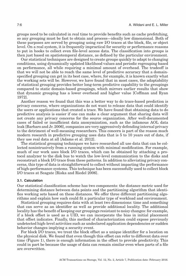
For block I/O traces, we treat the block offset as a unique identifier for a location onthe physical disk. We found that even though this offset can refer to different data overtime (Figure 1), there is enough information in the offset to provide predictivity. Thiscould in part be because the usage of data can remain similar even when parts of a fileare overwritten.



Fig. 1. An example of offset-data mismatches over time for a university (fiu) and an enterprise (ent-storage)dataset. Logical block addresses are used in place of physical offsets, and each LBA corresponds to a datafingerprint. In the enterprise dataset, ent-storage, labels remain consistent for many accesses before thepercentage changed creeps up, while in the research university dataset represented by fiu, the mapping wasmore volatile. We recalculated groupings after about 250,000 accesses because predictivity was dropping,partly due to the mismatch. Surprisingly, the fiu workload ended up with more predictive groups than theent-storage workload.

The uniqueness assumption for block offsets generally holds for application files andother static filesystem components, though it will break down for volatile areas suchas caches or log structured file systems. As we see in Figure 1, the spatial dimensionmay map well to the data for some time. Making this assumption allows us to usevery sparse data for our analysis, since spatiotemporal data is ubiquitous in dynamictraces and, when the spatial component can be treated as a unique ID, it can be usedto classify data.

To compare accesses in these dimensions, we need to define an effective distance met-ric over time and space that has few parameters and is fast to compute. Though thereare many possible choices, we have focused on variants of Euclidean distance so far forsimplicity and generalizability. With more dimensions, we have a wide array of statisti-cal similarity metrics available such as the Sørensen similarity index [Sørenson 1948],which biases against outliers, and Tanimoto Distance [Jaccard 1901], which providesa set comparison that is optimized for grouping seemingly dissimilar sets [Magurran2004].

DistanceOur partitioning algorithms depend on a precalculated list of distances between ev-ery pair of points, where points each represent single accesses and are of the form〈time, offset〉. We experimented with using points of the form 〈time, (offset, size)〉, butwe found this decreased the signal-to-noise ratio of our data considerably. We believethis is a result of controller- and OS-level prefetching techniques that decorrelate thesize parameter from the working set. In a dataset with more fixed size accesses, using(offset, size) should result in a tighter classification.

In production, our system is designed to look at trace data in real time. This intro-duces an inherent bias toward accesses that are close in time versus accesses closein space, since accesses close in time are continuously coming in while accesses closein space are distributed across the scope of the trace. Intuitively, this is acceptable



because the question we are trying to answer is “Are these blocks related in how theyare accessed?,” which implies that we care more about 10 datapoints scattered through-out the system that are accessed, repeatedly, within a second of each other than we doabout 10 datapoints that are adjacent on disk but accessed at random times over thecourse of our trace. For most of our grouping methods, we use a precalculated list ofdistances between every pair of points.

We create two different types of distance lists. The first is a simple n × n matrixthat represents the distance between every pair of accesses (pi, pj), with d(pi, pi) = 0.We calculate the distances in this matrix using simple weighted Euclidean distance,defined as d(pi, pj) = d(pj, pi) = √

(ti − tj)2 + oscale ∗ (oi − o j)2, where a point pi =(ti, oi) and the variables are t =time and o = the unique ID dimension, and oscale isan IOPS-dependent weighting factor on the UID. As IOPS increases, the informationin the current location of blocks decreases (Figure 1 shows the loss of information overtime for ent-storage, a high IOPS workload, vs. fiu, a low IOPS workload), so a lowervalue of oscale should be used.

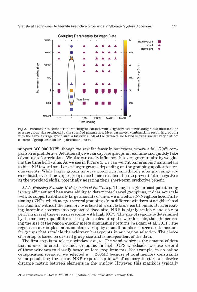
Figure 3 shows average group sizes across the entire parameter space for a partic-ular n-neighborhood partitioning grouping (Section 3.2.2). It shows that for a givenworkload, only a small range of oscale values produce a nontrivial grouping. For thedatasets we tested, only large variations of oscale produced appreciable changes in theresultant groupings, implying that oscale is relatively stable.

In this global comparison of accesses, we were most interested in recurring blockoffset pairs that were accessed in short succession. As a result, we also calculated anm × m matrix, where m is the number of unique block offsets in our dataset. Thismatrix was calculated by identifying all the differences in timestamps T = [T1 =ti1 − tj1, T2 = ti1 − tj2, T3 = ti2 − tj1, . . .] between the two offsets oi and o j . Note thatthis is more complex than a straightforward Hamming distance because offsets occurmultiple times within a trace window. After some experimentation, we decided to treatthe unweighted average of these timestamp distances as the time element in ourdistance calculation. Thus, the distance between two offsets is

d(oi, o j) =

√√√√(∑|T |i=1 Ti

|T |

)2

+ oscale ∗ (oi − o j)2.

Ranged and Leveled Distance ListsCalculating the full matrix of distances is computationally prohibitive with very largetraces and impossible in an online system. We need to handle real-time data whererelationships within the data are likely to have to have a set lifetime, so we also lookedinto creating lists of distances between the most relevant pairs of offsets. To do this, weagain bias toward offsets that are close in time. For very dense workloads, we suggestchoosing a range r in time around each point and calculating the distances from thatpoint to all of the accesses that fall in range, averaging the timestamps for accessesthat occur with the same offset, as in the previous section. For real-time traces, therange has to be large enough to capture repeated accesses to each central point toreduce noise. Section 3.2.2 discusses one scalability approach we successfully used tohandle traces with over 300,000 IOPS.

For static trace analysis, where groups do not need to be calculated quickly, we havethe ability to paint a more complete picture of how a given offset is related to otheroffsets. Instead of calculating ranges around each point, we calculate ranges aroundeach instance of a given offset oi. We do this by calculating the distance list aroundeach of N instances of the offset, rDist(oi1) = [(o j, d(oi1, o j)), (o j+1, d(oi1, o j+1), . . .]. Wethen take the list that each instance returns and combine them. This gives us a better



understanding of trends in our trace and strength of association. If an offset oi appearsnext to o j multiple times, we have more reason to believe they are related. To combinethe list, we first create a new list of the offsets that only appear in one of our lists—these being elements that do not need to be combined. For the remaining elements, wetake the sum inversely weighted by the time between their occurrences. For example,say we have an offset o that is accessed twice in our trace, at times t1 and t2, withdistance lists: [(o, oi, d(o, oi)1), (o, o j, d(o, o j)1] and [(o, oi, d(o, oi)2), (o, om, d(o, om)2]. Thecombined distance list would then be

[(o, oi, d(o, oi)1 + d(o, oi)2

|t1 − t2| , (o, o j, d(o, o j)1, (o, om, d(o, om)2)].

This heavily weights offset pairs that occur near to each other, which results in dynamicgroupings as these relationships change. Switching the inversely weighted sum to aninversely weighted average smoothes this effect but results in groups that are lessconsistent across groupings.

If accesses are sparse, we set the range in terms of levels instead of temporal distance.A level is defined as the closest two points preceding and succeeding a given access intime. A k-level distance list around a point pi is then the distance list comparing pi tothe k accesses that occurred beforehand and the k accesses that occurred afterward. Insparse, static traces, we use these levels to manage the tradeoff between computationalpower and accuracy. Therefore, our work sets a minimum k as the median group sizeand increases this value based on computational availability. The distance lists arecalculated the same way as they are for a set range.

3.2. Statistical Partitioning Algorithms

The goal of all of the group partitioning algorithms we work with is to identify groupsthat have a high probability of coaccess within a small amount of time. These groupscould correspond to individual working sets in the data but are equally likely to arisefrom system-wide trends.

We are particularly interested in untangling groups that are interleaved in the diskaccess stream. Large, long-term storage systems that grow organically also developheavily interleaved access patterns as more use cases are added to the system. Ourdistance calculations return a definitive answer for the question “How far is offset afrom offset b?” With this similarity information precomputed, we now look at the actualgrouping of accesses into working sets.

3.2.1. Neighborhood Partitioning/N-Neighborhood Partitioning. Neighborhood partitioning(NP) is an online, agglomerative technique for picking groups in multidimensionaldata with a defined distance metric. It is the best technique for data with more thantwo dimensions: distances are calculated over all dimensions and then the groupingitself runs linearly in the number of points. N-Neighborhood Partitioning (NNP) is avariation that improves scalability for dynamic grouping by dividing the stream intooverlapping windows and combining resultant groupings. We do not use ranged orleveled distance lists with this method to limit computational overhead.

The partitioning steps for NP are as follows:

(1) Collect data.(2) Calculate the pairwise distance matrix.(3) Calculate the neighborhood threshold and sequentially detect groups in the I/O

stream.(4) Update likelihood values based on group reappearance.(5) Drop groups below a likelihood threshold.



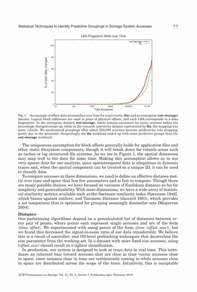
Fig. 2. Each incoming access is compared to the preceding access to determine whether it falls within theneighborhood (N) to be in the same group. If it does not, a new group is formed with the incoming access.

In this technique, we start with a set of accesses ordered by timestamp. We firstcalculate a value for the neighborhood threshold, N. In the online case, N must beselected a priori from a small set of training data and then recalculated once enoughdata has entered the system to smooth out any cyclic spikes. The amount of data youneed depends on what is considered a normal span of activity for the workload. In thestatic case, N is global and calculated as a weighting parameter times the standarddeviation of the accesses, assuming the accesses are uniformly distributed over time.Once the threshold is calculated, the algorithm looks at every access in turn. The firstaccess starts as a member of group g1. If the next access occurs within N, the nextaccess is placed into group g1; otherwise, it is placed into a new group g2, and so on.Figure 2 illustrates a simple case.

Neighborhood partitioning is especially well suited to rapidly changing usage pat-terns because it operates on accesses instead of offsets. When an offset occurs again inthe trace, it is evaluated again, with no memory of the previous occurrence. This is alsothe largest disadvantage of this technique: most of the valuable information in blockI/O traces lies in repeated correlations between accesses. The groups that result fromneighborhood partitioning are by design myopic and will miss any trend data.

For our write-heavy, research dataset, we found that neighborhood partitioning wasvery susceptible to small fluctuations of its initial parameters and to the spike of writesin our workload. The modifications made to neighborhood partitioning to handle thehigh IOPs dataset (Section 3.2.2) fixes many of these issues to produce a consistentgrouping across more parameter values.

Neighborhood partitioning runs in O(n), where n is the size of the neighborhood, sinceit only needs to pass through each neighborhood twice: once to calculate the neighbor-hood threshold and again to collect the working sets. Once these passes are made, thecumulative symmetric difference can be calculated in O(G), where G is the number ofgroups [Li 2008]. In our tests, we observed G � n, and so drop the term. Intuitively, thisruntime makes sense because there is no n×n comparison step in NP; it is simply a lin-ear agglomerator in a constrained window. This makes it an attractive grouping mech-anism for workloads with high IOPS (e.g., the enterprise system we worked with can



Fig. 3. Parameter selection for the Washington dataset with Neighborhood Partitioning. Color indicates theaverage group size produced by the specified parameters. Most parameter combinations result in groupingwith the same average group size: a bit over 3. All of the datasets we tested showed similar very distinctclusters of group sizes under a parameter search.

support 300,000 IOPS, though we saw far fewer in our trace), where a full O(n2) com-parison is prohibitive. Additionally, we can capture groups in real time and quickly takeadvantage of correlations. We also can easily influence the average group size by weight-ing the threshold value. As we see in Figure 3, we can weight our grouping parametersto bias NP toward smaller or larger groups depending on the grouping application re-quirements. While larger groups improve prediction immediately after groupings arecalculated, over time larger groups need more recalculation to prevent false negativesas the workload shifts, potentially negating their short-term predictive benefit.

3.2.2. Grouping Scalably: N-Neighborhood Partitioning. Though neighborhood partitioningis very efficient and has some ability to detect interleaved groupings, it does not scalewell. To support arbitrarily large amounts of data, we introduce N-Neighborhood Parti-tioning (NNP), which merges several groupings from different windows of neighborhoodpartitioning without the memory overhead of a single large partitioning. By aggregat-ing incoming accesses into regions of fixed size, NNP is highly scalable and able toperform in real time even in systems with high IOPS. The size of regions is determinedby the memory capabilities of the system calculating the working sets, though increas-ing the size of the region quickly meets diminishing returns [Wildani et al. 2011]. Theregions in our implementation also overlap by a small number of accesses to accountfor groups that straddle the arbitrary breakpoints in our region selection. The choiceof overlap is based on desired group size and is independent of the data.

The first step is to select a window size, w. The window size is the amount of datathat is used to create a single grouping. In high IOPS workloads, we use severalof these windows to classify based on local requirements. For example, in an onlinededuplication scenario, we selected w = 250MB because of local memory constraintswhen populating the cache. NNP requires up to w2 of memory to store a pairwisedistance matrix between elements in the window. However, this matrix is typically



sparse since, below a threshold, we set similarity to 0, and moreover it is only updatedwhen the predictivity of the overall grouping falls below a threshold. Sparsity is relatedto the access density of the workload; in the workloads we used, rows rarely hadmore than a few thousand elements even though we had tens of thousands of uniquedata blocks. The windows overlap by twice the current average group size to limitovercounting.

For NNP, for each window, the partitioning steps are as follows:

(1) Collect data.(2) Perform neighborhood partitioning.(3) Combine the new grouping with any prior groupings.(4) Adjust likelihood of current groups.

As accesses enter the system, they are divided into regions and a grouping is calcu-lated for each region using neighborhood partitioning. A grouping Gi is a set of groupsg1, . . . , gl that were calculated from the ith region of accesses. Each group gi has mem-bers xi1, xi2, . . . , xin. Unlike NP, NNP is not memoryless; older groupings are combinedwith newer to form an aggregate grouping that is representative of trends over a longerperiod of time.

We combine groupings through fuzzy set intersection between groupings and sym-metric difference between groups within the groupings. So, for groupings

G1, G2, . . . Gz, the total grouping G is

G = (Gi ∩ Gj) ∪ (Gi�gGj) ∀i, j 1 ≤ i, j ≤ z,

where �g, the groupwise symmetric difference, is defined as every group that is notin Gi ∩ Gj and also shares no members with a group in Gi ∩ Gj . For example, fortwo group lists G1 = [(x1, x4, x7), (x1, x5), (x8, x7)] and G2 = [(x1, x3, x7), (x1, x5), (x2, x9)],the resulting grouping would be G1 ∩ G2 = (x1, x5) ∪ G1 �g G2 = (x2, x9), yielding agrouping of [(x1, x5), (x2, x9)]. (x1, x4, x7), (x1, x3, x7), and (x8, x7) were excluded becausethey share some members but not all.

NNP is especially well suited to rapidly changing usage patterns because individualregions do not share information until the group combination stage. Combining theregions into a single grouping helps mitigate the disadvantage of losing the informationof repeated correlations between accesses without additional bias. The groups thatresult from NNP are by design myopic and will ignore long-term trend data, reducingthe impact of spatial locality shifts over time.

3.2.3. Nearest Neighbor Search. k-nearest-neighbor (k-NN) is based on a standardmachine-learning technique that relies on the identification of neighborhoods wherethe probability of group similarity is highest [Duda et al. 2001]. In the canonical case, anew element is compared to a large set of previously labeled examples using a distancemetric defined over all elements. The new element is then classified into the largestgroup that falls within the prescribed neighborhood. This is in contrast to neighborhoodpartitioning, where everything within a neighborhood is in the same group.

For this work, we modified the basic k-NN algorithm to be unsupervised since thereis no ground-truth labeling possible for groups. We also incorporated weights. Thegoal of weighting is to lessen the impact of access to offsets that occur frequently andindependently of other accesses. In particular, in the absence of weights, it is likely thata workload with an on-disk cache would return a single group, where every elementhas been classified into the cache group, which is a group of size 44,000 that wasconsistently identified by both the k-NN and bag-of-edges algorithms. Similar effectsoccur with a background process doing periodic disk accesses.



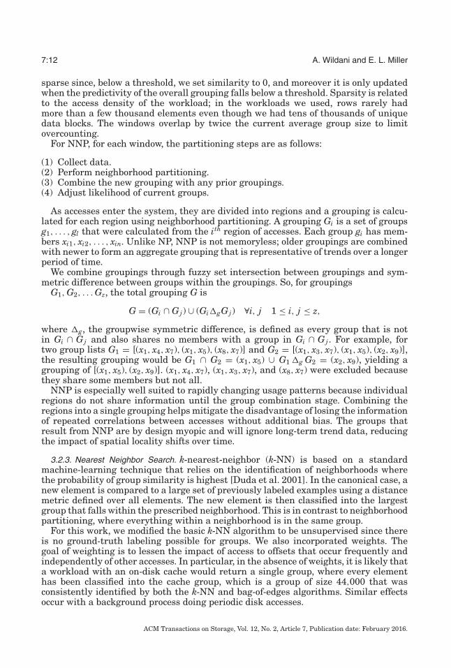
Fig. 4. A clique cover of a graph of accesses. Nodes represent accesses, while edges represent at least athreshold level of similarity between edges.

In our algorithm, we start with an m× m distance matrix as defined in Section 3.1,where m is the number of unique block offset values. We chose k by taking the averagedistance between offsets in our dataset and multiplying it by a weighting factor. For thefirst offset, we label all of the offsets within k of that offset into a group. For subsequentoffsets, we scan the elements within k of our offset and place our offset in the best-represented group. The value of k is the most important parameter in our weightedk-NN algorithm. If the workload consists of cleanly separable groups, it should be easierto see groupings with smaller values of k. On the other hand, a small value of k canplace too much weight on accesses that turn out to be noise. Noisy workloads reducethe accuracy of k-NN because with a large k, the groups frequently end up too large tobe useful. We found that as long as we start above the average distance, the weightingfactor on k did not have a large influence until it got to be large enough to cover mostof the dataset.

3.2.4. Graph Covering. The final method we used begins with representing accesses asnodes in a graph and edges as the distance between nodes. Presenting this informationas a graph exposes the interrelationships between data but can result in a thick tangleof edges. A large, fully connected graph is of little use, so we determined a thresholdof similarity beyond which the nodes no longer qualify as connected. This simplifiesour graph and lowers our runtime, but more importantly, removing obviously weakconnections allows us to identify groups based on the edges that remain connected.This does not impact classification since these edges connect nodes that by definitionbear little similarity to each other. Once we have this graph, we define a group as allsets of nodes such that every node in the set has an edge to every other node in the set;this is defined as a clique in graph theory. Figure 4 shows an example clique coveringof an access graph. Note that every element is a member of a single working set thatcorresponds to the largest of the potential cliques it is a member of. The problem thenof finding all such sets reduces to the problem of clique cover, which is known to beNP-complete and difficult to approximate in the general case [Cormen et al. 1990]. Thisis in direct contrast to nearest neighbor search, which is O(n2 log(n)).

Though clique cover is difficult to approximate, it is much faster to compute inworkloads with many small groups and relatively few larger groups. We begin bytaking all the pairs in a k-level distance list and comparing them against the largerdataset to find all groups of size 3. This is by far the most time-intensive step, runningin O(n2). We then proceed to compare groups of size 3 for overlap, and then groupsof size 4, and so forth, taking advantage of the fact that a fully connected graph Knis composed of two graphs Kn − 1 plus a connecting edge to reduce our search spacesignificantly. As a result, even though the worst case for our algorithm is O(n|Gx |) (in



addition to the distance list calculation), where n is the number of nodes and |Gx| thesize of the maximal group, our expected runtime is

∑x2 |Gi|i, where |Gi| is the number

of groups of size i. We observe in Figure 6 that the average group size tends to be small,and our runtime results in Section 5.3 show that this holds in real traces.

We discovered that in typical workloads, this method is too strict to discover mostgroups. This is likely because the accesses within a working set are the result of anordered process. This implies that while the accesses will likely occur within a givenrange, the first and last access in the set may look unrelated without the context of theremainder of the set and thus lack an edge connecting them. We fix this by returningto an implicit assumption from the neighborhood partitioning algorithm that groupingis largely transitive. This makes intuitive sense because of the sequential nature ofmany patterns of accesses, such as those from an application that processes a directoryof files in order.

In our transitive model, we use a more restrictive threshold to offset the tendencyfor intermittent noise points to group together otherwise disparate groups of points.We then calculate the minimum spanning tree of this graph and look for the longestpath. We have to calculate the minimum spanning tree because longest path is NP-complete in the general case but reduces to the much simpler negated shortest pathwhen working with a tree. This process runs in O(n2 log(n)), since the graph containsat most e = n(n−1)

2 edges and Dijkstra’s shortest path algorithm runs in O(n + e) beforeoptimization [Cormen et al. 1990]. We refer to this technique as the bag-of-edges algo-rithm because it is similar to picking up an edge and shaking it to see what strands arelongest. Bag-of-edges is much less computationally expensive than a complete graphcovering and is additionally more representative of the sequential nature of many ap-plication disk accesses than our previous graph algorithm. We found that in our small,mixed-application workload, this technique offered the best combination of accuracyand performance, but this grouping algorithm was much too slow for dynamic groupingof high IOPS workloads.

3.3. Group Likelihood and Predictivity

Group recalculation for all of the algorithms in the previous section happens in thebackground during periods of low activity. As accesses come in, however, we need to alsoproactively update groups to reflect a changing reality. We do this by storing a likelihoodvalue for every group. This numerical value starts as the median intergroup distancevalue and is incremented when the grouping is pulled into cache and successfullypredicts a future access. Groups below a certain likelihood threshold can be discarded,though we only do this when there is an external limit on the number of groups (such aswhen the group table is being stored in memory) since these groups tend to be droppedduring the periodic background regrouping. The algorithm is structured to reinforceprior good behavior.

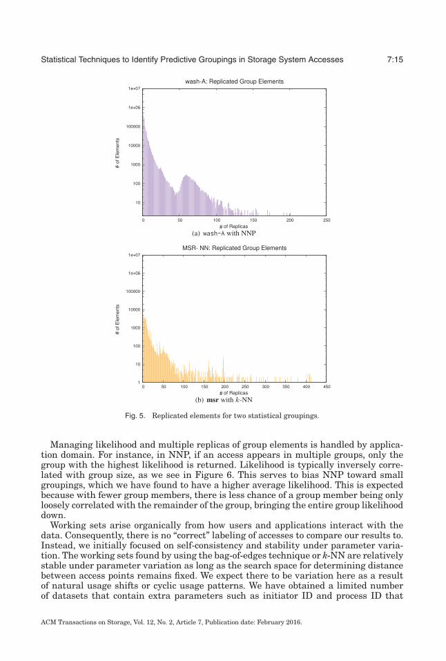
Another point where a likelihood value is necessary is when an element is a memberof multiple groups. Grouping is neither 1 − 1 nor onto, and it is unsurprising thatone element can be in several groups. Figure 5 shows replicated elements in twostatistical groupings. In both, we see that most elements are members of relativelyfew (<10) groups. Depending on the application, elements can be indexed as membersof several groups, just stored once with their most likely group, or even replicatedper group instance. The elements in the long tail that belong to many groups areanother indicator of the quality of the grouping method for the particular workload:more ultra-popular elements—elements that fall outside two standard deviations ofthe mean replica count—indicate that the grouping is overclassifying elements insteadof labeling them as “noise.”



Fig. 5. Replicated elements for two statistical groupings.

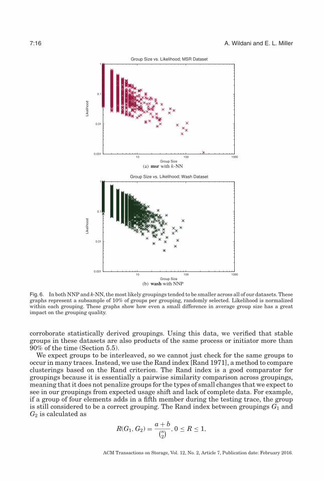
Managing likelihood and multiple replicas of group elements is handled by applica-tion domain. For instance, in NNP, if an access appears in multiple groups, only thegroup with the highest likelihood is returned. Likelihood is typically inversely corre-lated with group size, as we see in Figure 6. This serves to bias NNP toward smallgroupings, which we have found to have a higher average likelihood. This is expectedbecause with fewer group members, there is less chance of a group member being onlyloosely correlated with the remainder of the group, bringing the entire group likelihooddown.

Working sets arise organically from how users and applications interact with thedata. Consequently, there is no “correct” labeling of accesses to compare our results to.Instead, we initially focused on self-consistency and stability under parameter varia-tion. The working sets found by using the bag-of-edges technique or k-NN are relativelystable under parameter variation as long as the search space for determining distancebetween access points remains fixed. We expect there to be variation here as a resultof natural usage shifts or cyclic usage patterns. We have obtained a limited numberof datasets that contain extra parameters such as initiator ID and process ID that



Fig. 6. In both NNP and k-NN, the most likely groupings tended to be smaller across all of our datasets. Thesegraphs represent a subsample of 10% of groups per grouping, randomly selected. Likelihood is normalizedwithin each grouping. These graphs show how even a small difference in average group size has a greatimpact on the grouping quality.

corroborate statistically derived groupings. Using this data, we verified that stablegroups in these datasets are also products of the same process or initiator more than90% of the time (Section 5.5).

We expect groups to be interleaved, so we cannot just check for the same groups tooccur in many traces. Instead, we use the Rand index [Rand 1971], a method to compareclusterings based on the Rand criterion. The Rand index is a good comparator forgroupings because it is essentially a pairwise similarity comparison across groupings,meaning that it does not penalize groups for the types of small changes that we expect tosee in our groupings from expected usage shift and lack of complete data. For example,if a group of four elements adds in a fifth member during the testing trace, the groupis still considered to be a correct grouping. The Rand index between groupings G1 andG2 is calculated as

R(G1, G2) = a + b(n2

) , 0 ≤ R ≤ 1,



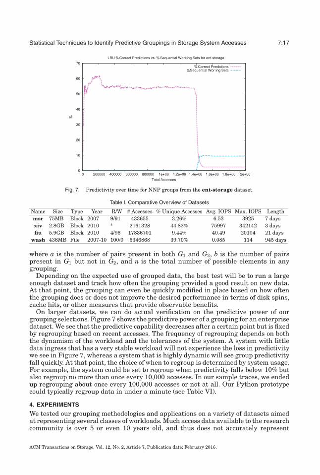
Fig. 7. Predictivity over time for NNP groups from the ent-storage dataset.

Table I. Comparative Overview of Datasets

Name Size Type Year R/W # Accesses % Unique Accesses Avg. IOPS Max. IOPS Lengthmsr 75MB Block 2007 9/91 433655 3.26% 6.53 3925 7 daysxiv 2.8GB Block 2010 * 2161328 44.82% 75997 342142 3 daysfiu 5.9GB Block 2010 4/96 17836701 9.44% 40.49 20104 21 days

wash 436MB File 2007-10 100/0 5346868 39.70% 0.085 114 945 days

where a is the number of pairs present in both G1 and G2, b is the number of pairspresent in G1 but not in G2, and n is the total number of possible elements in anygrouping.

Depending on the expected use of grouped data, the best test will be to run a largeenough dataset and track how often the grouping provided a good result on new data.At that point, the grouping can even be quickly modified in place based on how oftenthe grouping does or does not improve the desired performance in terms of disk spins,cache hits, or other measures that provide observable benefits.

On larger datasets, we can do actual verification on the predictive power of ourgrouping selections. Figure 7 shows the predictive power of a grouping for an enterprisedataset. We see that the predictive capability decreases after a certain point but is fixedby regrouping based on recent accesses. The frequency of regrouping depends on boththe dynamism of the workload and the tolerances of the system. A system with littledata ingress that has a very stable workload will not experience the loss in predictivitywe see in Figure 7, whereas a system that is highly dynamic will see group predictivityfall quickly. At that point, the choice of when to regroup is determined by system usage.For example, the system could be set to regroup when predictivity falls below 10% butalso regroup no more than once every 10,000 accesses. In our sample traces, we endedup regrouping about once every 100,000 accesses or not at all. Our Python prototypecould typically regroup data in under a minute (see Table VI).

4. EXPERIMENTS

We tested our grouping methodologies and applications on a variety of datasets aimedat representing several classes of workloads. Much access data available to the researchcommunity is over 5 or even 10 years old, and thus does not accurately represent



how systems are being used in our cloud and always-connected world. To ensure thatour results are applicable to real workloads, we focused on getting access traces thatwere collected recently—within the last decade—and that cover a variety of differentworkload types.

To analyze grouping, ideally one has the ability to gather complete block-level logs fora system with many users and many applications over a period of time commensurateto the dynamicity of a trace. Additionally, this trace would be collected before any file-system- and hardware-specific biases (e.g., write off-loading, sequential access removal)are introduced. Finally, having metadata or content ID to verify that elements that areselected to be in the same group have some semantic correlation is useful for groupvalidation.

Finding traces with all of these attributes is difficult for researchers because of theprivacy implications of rich metadata and the tracing overhead that collecting largeamounts of data on an active systems incurs. The datasets we use in this thesis areselected to provide as much breadth of workload type given what we had available.

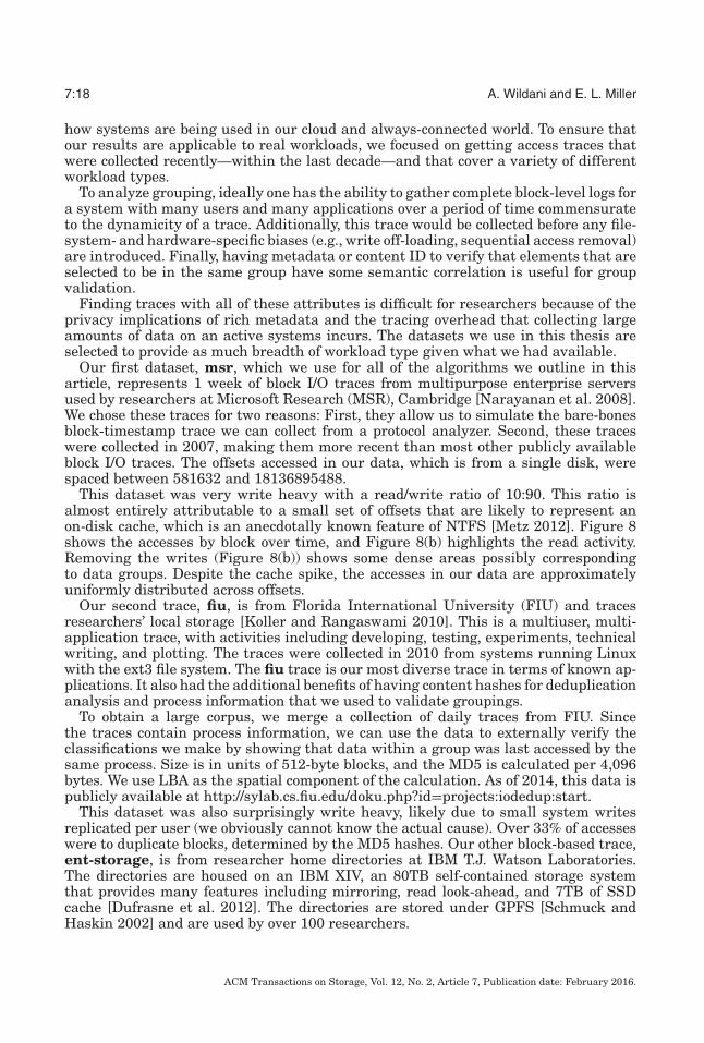
Our first dataset, msr, which we use for all of the algorithms we outline in thisarticle, represents 1 week of block I/O traces from multipurpose enterprise serversused by researchers at Microsoft Research (MSR), Cambridge [Narayanan et al. 2008].We chose these traces for two reasons: First, they allow us to simulate the bare-bonesblock-timestamp trace we can collect from a protocol analyzer. Second, these traceswere collected in 2007, making them more recent than most other publicly availableblock I/O traces. The offsets accessed in our data, which is from a single disk, werespaced between 581632 and 18136895488.

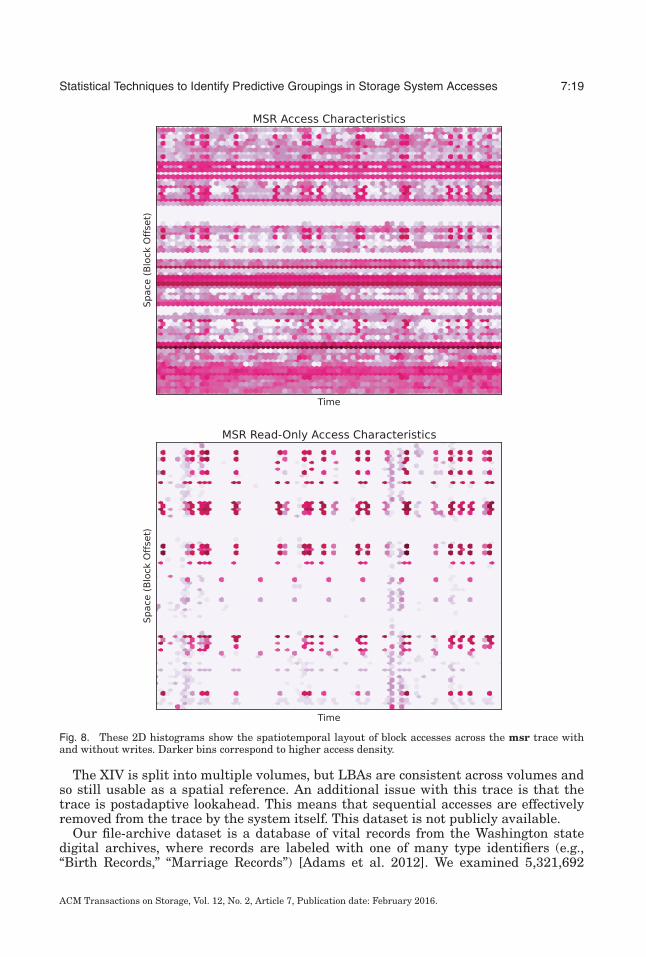
This dataset was very write heavy with a read/write ratio of 10:90. This ratio isalmost entirely attributable to a small set of offsets that are likely to represent anon-disk cache, which is an anecdotally known feature of NTFS [Metz 2012]. Figure 8shows the accesses by block over time, and Figure 8(b) highlights the read activity.Removing the writes (Figure 8(b)) shows some dense areas possibly correspondingto data groups. Despite the cache spike, the accesses in our data are approximatelyuniformly distributed across offsets.

Our second trace, fiu, is from Florida International University (FIU) and tracesresearchers’ local storage [Koller and Rangaswami 2010]. This is a multiuser, multi-application trace, with activities including developing, testing, experiments, technicalwriting, and plotting. The traces were collected in 2010 from systems running Linuxwith the ext3 file system. The fiu trace is our most diverse trace in terms of known ap-plications. It also had the additional benefits of having content hashes for deduplicationanalysis and process information that we used to validate groupings.

To obtain a large corpus, we merge a collection of daily traces from FIU. Sincethe traces contain process information, we can use the data to externally verify theclassifications we make by showing that data within a group was last accessed by thesame process. Size is in units of 512-byte blocks, and the MD5 is calculated per 4,096bytes. We use LBA as the spatial component of the calculation. As of 2014, this data ispublicly available at http://sylab.cs.fiu.edu/doku.php?id=projects:iodedup:start.

This dataset was also surprisingly write heavy, likely due to small system writesreplicated per user (we obviously cannot know the actual cause). Over 33% of accesseswere to duplicate blocks, determined by the MD5 hashes. Our other block-based trace,ent-storage, is from researcher home directories at IBM T.J. Watson Laboratories.The directories are housed on an IBM XIV, an 80TB self-contained storage systemthat provides many features including mirroring, read look-ahead, and 7TB of SSDcache [Dufrasne et al. 2012]. The directories are stored under GPFS [Schmuck andHaskin 2002] and are used by over 100 researchers.


http://sylab.cs.fiu.edu/doku.php?id$=$projects:iodedup:start


Fig. 8. These 2D histograms show the spatiotemporal layout of block accesses across the msr trace withand without writes. Darker bins correspond to higher access density.

The XIV is split into multiple volumes, but LBAs are consistent across volumes andso still usable as a spatial reference. An additional issue with this trace is that thetrace is postadaptive lookahead. This means that sequential accesses are effectivelyremoved from the trace by the system itself. This dataset is not publicly available.

Our file-archive dataset is a database of vital records from the Washington statedigital archives, where records are labeled with one of many type identifiers (e.g.,“Birth Records,” “Marriage Records”) [Adams et al. 2012]. We examined 5,321,692



Table II. Sample Data from MSR Cambridge Research Machines

Timestamp Type Block Offset Size Response Time128166372003061629 Read 7014609920 24576 41286128166372016382155 Write 1317441536 8192 1963128166372026382245 Write 2436440064 4096 1835

Table III. Sample Data from Florida International University Research Machines

Timestamp PID Process LBA Size R/W Maj. Device # Min. Device # MD50 4892 syslogd 904265560 8 W 6 0 531e779...39064 2559 kjournald 926858672 8 W 6 0 4fd0c43...467651 2522 kjournald 644661632 8 W 6 0 98b9cb7...

Table IV. Sample Data From IBM Watson, Stored on an XIV

Kind # Blocks is_read LBA Time Volume initiator_id Fingerprint0 47 1 825850448 1313956791731167 101921 1000012 6c5fb8d...0 61 1 825848704 1313956791765460 101921 1000002 d10b05c...0 8 1 1485868928 1313956791817914 102669 1000009 76ca22b...

accesses from 2007 through 2010 that were made to a 16.5TB database. In additionto the supplied type identifiers, each record accessed had a static1 RecordID that isassigned as records are added to the system. We use these IDs as a second dimensionwhen calculating statistical groupings.

In addition to the access trace in Table V, we also had a file that mapped most ofthe RecordID values to assorted RecordType values such as “BirthRecord,” “Marraige-Record,” and so forth. We treat RecordType as a prelabeled group for categorical group-ing, but also use RecordID as a spatial dimension to statistically group the washdataset. Though RecordID does not directly map to an on-disk location, we assume itcorrelates to ingress and assume that records are originally laid out sequentially byRecordID.

5. RESULTS

We ran every algorithm with msr and show that NNP provides consistently predictivegroupings while bag-of-edges is the most stable. We also show the remainder of ourdatasets under NNP to demonstrate the versatility of the algorithm.

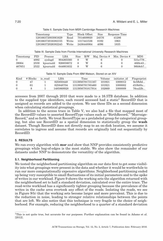
5.1. Neighborhood Partitioning

We tested the neighborhood partitioning algorithm on our data first to get some visibil-ity into what groupings were present in the data and whether it would be worthwhile torun our more computationally expensive algorithms. Neighborhood partitioning endedup being very susceptible to small fluctuations of its initial parameters and to the spikeof writes in our workload. Figure 9 shows the working sets the algorithm returned withthe neighborhood set to half a standard deviation, calculated over the entire trace. Theread-write workload has a significantly tighter grouping because the prevalence of thewrites in the cache area overtook any effect of the reads. Isolating the reads, we seein Figure 9(b) that the working sets become larger and more prevalent. This is due tothe reduction in noise, leading to stronger relative relationships between the pointsthat are left. We also notice that this technique is very fragile to the choice of neigh-borhood. For example, reducing the neighborhood to a quarter of a standard deviation

1This is not quite true, but accurate for our purposes. Further explanation can be found in Adams et al.[2012].



Table V. Sample Data from Washington Department of Records

RetrieveTrackingID UserSessionID RecordID RetrieveDate1 {C8E99715-4725-427A-BCDF-708109D4935F} 34358 2007-09-27 13:31:10.4072 {D2B7A983-7CC6-46C8-A10F-7B2557CF204F} 94267 2007-09-27 15:36:13.2873 {1CE276B9-06F4-4AF7-9A08-E4038D83BBFB} 46679 2007-09-27 15:59:42.737

Fig. 9. Working sets with Neighborhood Partitioning in msr for different values of stdweight (the weightingof the standard deviation). Groupings vary drastically based on neighborhood size and workload density.

(Figure 9(c)) causes the number of large groups to fall sharply and correspondinglyincreases the prevalence of small groups.

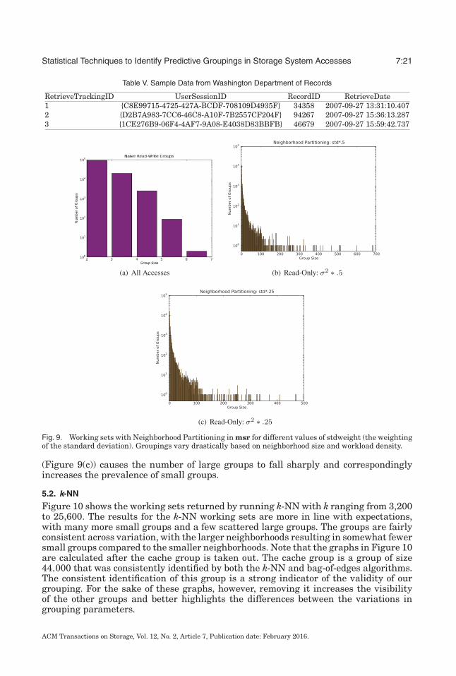
5.2. k-NN

Figure 10 shows the working sets returned by running k-NN with k ranging from 3,200to 25,600. The results for the k-NN working sets are more in line with expectations,with many more small groups and a few scattered large groups. The groups are fairlyconsistent across variation, with the larger neighborhoods resulting in somewhat fewersmall groups compared to the smaller neighborhoods. Note that the graphs in Figure 10are calculated after the cache group is taken out. The cache group is a group of size44,000 that was consistently identified by both the k-NN and bag-of-edges algorithms.The consistent identification of this group is a strong indicator of the validity of ourgrouping. For the sake of these graphs, however, removing it increases the visibilityof the other groups and better highlights the differences between the variations ingrouping parameters.



Fig. 10. Working sets with k-Nearest Neighbor. If k is very high or low, fewer large groups are found.

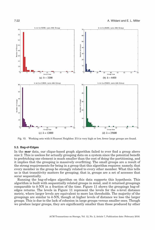
5.3. Bag-of-Edges

In the msr data, our clique-based graph algorithm failed to ever find a group abovesize 2. This is useless for actually grouping data on a system since the potential benefitto prefetching one element is much smaller than the cost of doing the partitioning, andit implies that the grouping is massively overfitting. The small groups are a result ofthe strong requirements for being in a group that this algorithm requires: namely, thatevery member in the group be strongly related to every other member. What this tellsus is that transitivity matters for grouping; that is, groups are a set of accesses thatoccur sequentially.

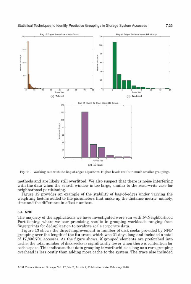
Running the bag-of-edges algorithm on this data supports this hypothesis. Thisalgorithm is built with sequentially related groups in mind, and it returned groupingscomparable to k-NN in a fraction of the time. Figure 11 shows the groupings bag-of-edges returns. The levels in Figure 11 represent the levels for the n-level distancemetric, where larger levels are equivalent to more lax thresholds. The majority of thegroupings are similar to k-NN, though at higher levels of distance we lose the largergroups. This is due to the lack of cohesion in large groups versus smaller ones. Thoughwe produce larger groups, they are significantly smaller than those produced by other



Fig. 11. Working sets with the bag-of-edges algorithm. Higher levels result in much smaller groupings.

methods and are likely still overfitted. We also suspect that there is noise interferingwith the data when the search window is too large, similar to the read-write case forneighborhood partitioning.

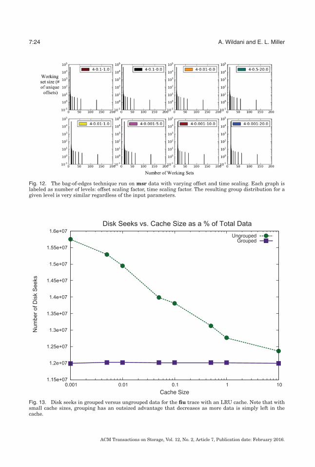
Figure 12 provides an example of the stability of bag-of-edges under varying theweighting factors added to the parameters that make up the distance metric: namely,time and the difference in offset numbers.

5.4. NNP

The majority of the applications we have investigated were run with N-NeighborhoodPartitioning, where we saw promising results in grouping workloads ranging fromfingerprints for deduplication to terabyte scale corporate data.

Figure 13 shows the direct improvement in number of disk seeks provided by NNPgrouping over the length of the fiu trace, which was 21 days long and included a totalof 17,836,701 accesses. As the figure shows, if grouped elements are prefetched intocache, the total number of disk seeks is significantly lower when there is contention forcache space. This indicates that data grouping is worthwhile as long as a rare groupingoverhead is less costly than adding more cache to the system. The trace also included



Fig. 12. The bag-of-edges technique run on msr data with varying offset and time scaling. Each graph islabeled as number of levels: offset scaling factor, time scaling factor. The resulting group distribution for agiven level is very similar regardless of the input parameters.

Fig. 13. Disk seeks in grouped versus ungrouped data for the fiu trace with an LRU cache. Note that withsmall cache sizes, grouping has an outsized advantage that decreases as more data is simply left in thecache.



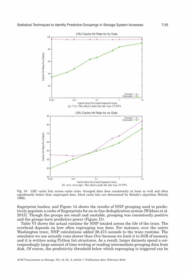
Fig. 14. LRU cache hits across cache sizes. Grouped data does consistently at least as well and oftensignificantly better than ungrouped data. Ideal cache hits are determined by Belady’s algorithm [Belady1966].

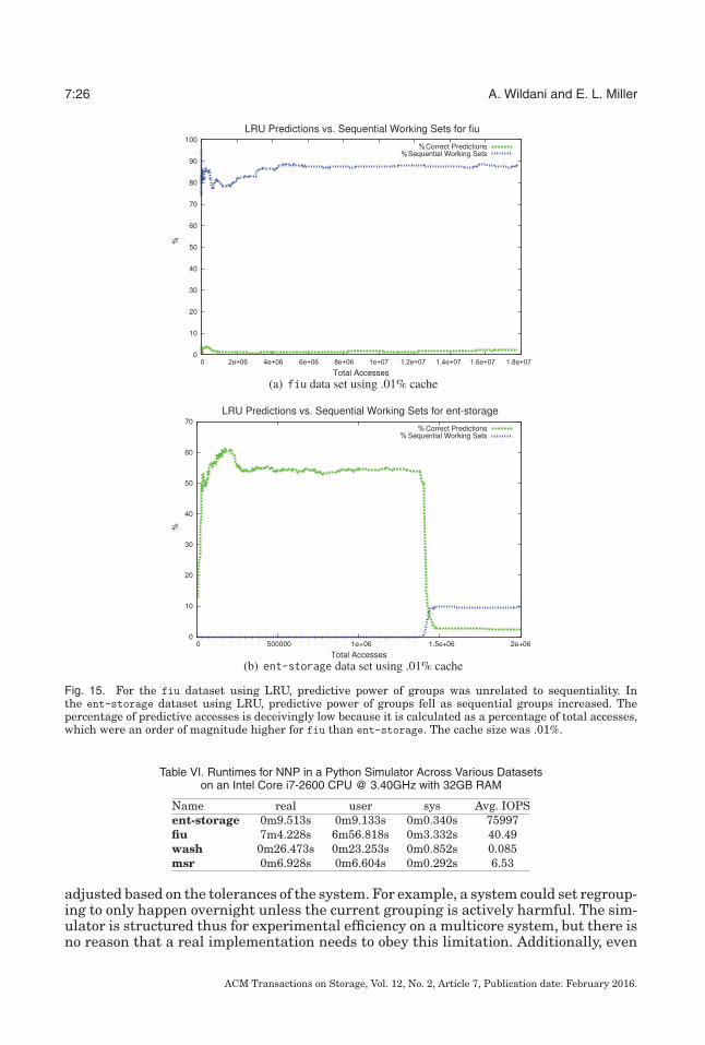
fingerprint hashes, and Figure 14 shows the results of NNP grouping used to predic-tively populate a cache of fingerprints for an in-line deduplication system [Wildani et al.2013]. Though the groups are small and unstable, grouping was consistently positiveand the groups have predictive power (Figure 15).

Table VI shows the actual runtime for NNP totaled across the life of the trace. Theoverhead depends on how often regrouping was done. For instance, over the entireWashington trace, NNP calculations added 26.473 seconds to the trace runtime. Thesimulator we use actually runs slower than O(n) because we limit it to 5GB of memory,and it is written using Python list structures. As a result, larger datasets spend a cor-respondingly large amount of time writing or reading intermediate grouping data fromdisk. Of course, the predictivity threshold below which regrouping is triggered can be



Fig. 15. For the fiu dataset using LRU, predictive power of groups was unrelated to sequentiality. Inthe ent-storage dataset using LRU, predictive power of groups fell as sequential groups increased. Thepercentage of predictive accesses is deceivingly low because it is calculated as a percentage of total accesses,which were an order of magnitude higher for fiu than ent-storage. The cache size was .01%.

Table VI. Runtimes for NNP in a Python Simulator Across Various Datasetson an Intel Core i7-2600 CPU @ 3.40GHz with 32GB RAM

Name real user sys Avg. IOPSent-storage 0m9.513s 0m9.133s 0m0.340s 75997fiu 7m4.228s 6m56.818s 0m3.332s 40.49wash 0m26.473s 0m23.253s 0m0.852s 0.085msr 0m6.928s 0m6.604s 0m0.292s 6.53

adjusted based on the tolerances of the system. For example, a system could set regroup-ing to only happen overnight unless the current grouping is actively harmful. The sim-ulator is structured thus for experimental efficiency on a multicore system, but there isno reason that a real implementation needs to obey this limitation. Additionally, even



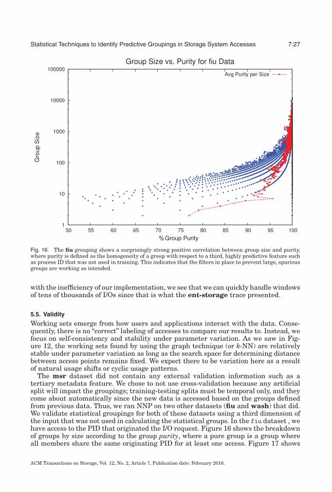
Fig. 16. The fiu grouping shows a surprisingly strong positive correlation between group size and purity,where purity is defined as the homogeneity of a group with respect to a third, highly predictive feature suchas process ID that was not used in training. This indicates that the filters in place to prevent large, spuriousgroups are working as intended.

with the inefficiency of our implementation, we see that we can quickly handle windowsof tens of thousands of I/Os since that is what the ent-storage trace presented.

5.5. Validity

Working sets emerge from how users and applications interact with the data. Conse-quently, there is no “correct” labeling of accesses to compare our results to. Instead, wefocus on self-consistency and stability under parameter variation. As we saw in Fig-ure 12, the working sets found by using the graph technique (or k-NN) are relativelystable under parameter variation as long as the search space for determining distancebetween access points remains fixed. We expect there to be variation here as a resultof natural usage shifts or cyclic usage patterns.

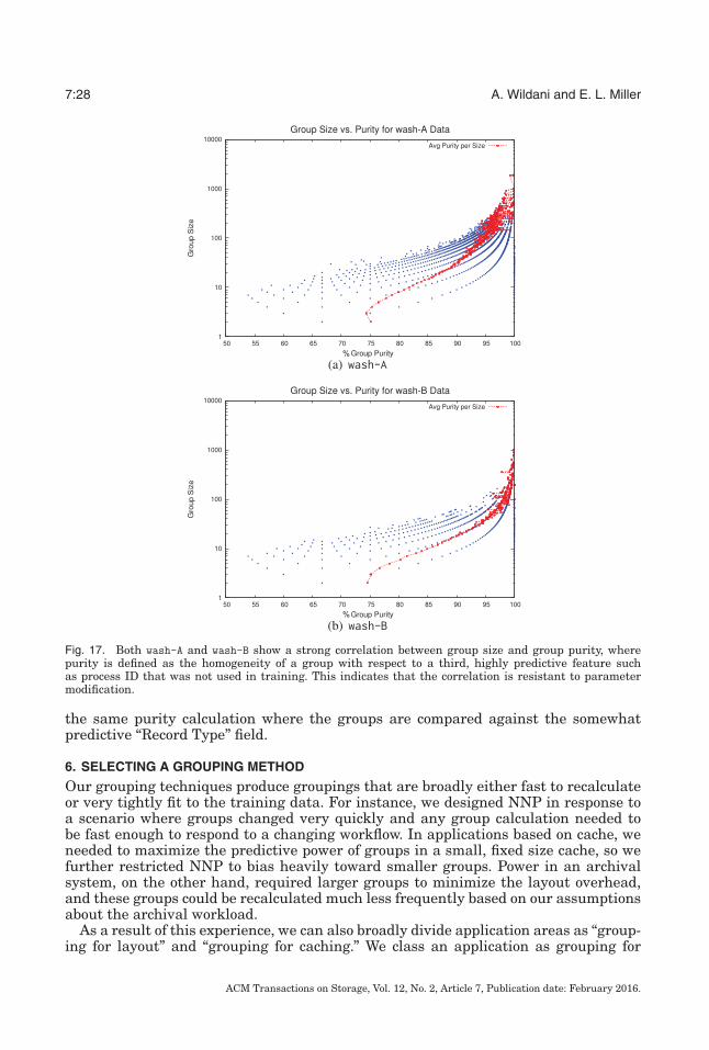
The msr dataset did not contain any external validation information such as atertiary metadata feature. We chose to not use cross-validation because any artificialsplit will impact the groupings; training-testing splits must be temporal only, and theycome about automatically since the new data is accessed based on the groups definedfrom previous data. Thus, we ran NNP on two other datasets (fiu and wash) that did.We validate statistical groupings for both of these datasets using a third dimension ofthe input that was not used in calculating the statistical groups. In the fiu dataset , wehave access to the PID that originated the I/O request. Figure 16 shows the breakdownof groups by size according to the group purity, where a pure group is a group whereall members share the same originating PID for at least one access. Figure 17 shows



Fig. 17. Both wash-A and wash-B show a strong correlation between group size and group purity, wherepurity is defined as the homogeneity of a group with respect to a third, highly predictive feature suchas process ID that was not used in training. This indicates that the correlation is resistant to parametermodification.

the same purity calculation where the groups are compared against the somewhatpredictive “Record Type” field.

6. SELECTING A GROUPING METHOD

Our grouping techniques produce groupings that are broadly either fast to recalculateor very tightly fit to the training data. For instance, we designed NNP in response toa scenario where groups changed very quickly and any group calculation needed tobe fast enough to respond to a changing workflow. In applications based on cache, weneeded to maximize the predictive power of groups in a small, fixed size cache, so wefurther restricted NNP to bias heavily toward smaller groups. Power in an archivalsystem, on the other hand, required larger groups to minimize the layout overhead,and these groups could be recalculated much less frequently based on our assumptionsabout the archival workload.

As a result of this experience, we can also broadly divide application areas as “group-ing for layout” and “grouping for caching.” We class an application as grouping for



layout when the goal of the grouping is to lay out data on physical media such thatcolocated data has a high probability of coaccess. We showed instances of this ap-plication type when using groups to reduce power consumption [Wildani and Miller2010] and improve availability [Wildani et al. 2014]. In these scenarios, space isrelatively plentiful but groups can not change quickly, since the change requires alayout overhead. Here, we want larger, more stable groups, such as those produced byour bag-of-edges technique, along with ideally a more stable workload.

Grouping for cache management, on the other hand, requires a grouping techniquethat biases toward smaller groups in order to avoid cache churn: when the additionaldata pulled in by the grouping is evicted before it has a chance to be useful. Along withsmaller groups, groupings that populate caches should have parameter weights set tobias more strongly toward temporal correlations since the lifetime of the group in cacheis so limited. If an application has a rapidly changing workload, a grouping techniquesuch as neighborhood partitioning that has a strong bias toward newer correlationssignificantly outperforms grouping techniques that need more history. This is also whywe set window size for NNP as a function of the incoming IOPS: NNP is designed tocapture recent workload shifts.

7. DISCUSSION

A concern early on was that the access groups we discovered would overlap, leadingto a need to disambiguate and manually tune our models to the dataset. It turnedout, however, that in every classification scheme we saw no chains of more than threeoverlapping groups. This allowed us to keep our methodology general and more likelyto be easily portable to other data. More importantly, this is a strong indication that ourgroupings represent separate access patterns. If they did not, it is likely some of themwould have had overlapping components since the accesses are uniformly distributed.

Another encouraging result of our study was the consistency of groupings in thedata despite the sparsity of the traces. This indicates that it is worthwhile to look forgroupings in similar multiuser and multiapplication workloads even if the only dataavailable is block offsets and timestamps. Being able to collect useful workloads withoutimpacting privacy or performance is invaluable for continuing research in predictivedata grouping. This also reduces the cost of our analysis substantially, since we candetermine whether a workload will be separable before trying advanced techniques toidentify groupings and disrupting the system to group working sets together on disk.

For this research work, we were not concerned with the speed of computations as longas the algorithms were efficient. While testing algorithms, we wrote all code in Pythonand did not optimize for speed. Under this constraint, the localized distance techniquessuch as NP ran nearly instantaneously, while the global techniques, particularly thegraph techniques, took between 20 and 35 minutes per run on a server with an 8-core2.4GHz Intel R©Xeon processor and 24GB of RAM. We believe that much of this speedcan be regained by tighter code. Also, online implementations will handle less data pertimestamp than static test cases.

We realize the assumption that implicitly defined UIDs such as block offset do notuniquely identify a piece of data is not strictly true in some systems. A majority of datathat is frequently overwritten is in the cache block, however, and this is consistentlyidentified as a single group by our algorithms. The less frequent overwrites that occuras a result of normal system use should be handled by the adaptability of our algorithmsover time. If the content of a block offset changes, it will start being placed into differentgroups as the algorithms update the distance matrix.

One surprising feature of the msr dataset was that it had a long list of consecutivewrites to the same block. We believe that these writes are the result of overwrite activityin a log or a disk-based cache. These types of points are frequently present but filtered



in other block I/O traces [Amer and Long 2002]. We intentionally include these pointsin our classifications to verify that they trivially classify into their own working set.Our k-NN and bag-of-edges methods can work around the noise of the spike to producerealistic working set groups given reasonable parameters.

8. CONCLUSIONS

We have presented two distance metrics and three partitioning algorithms for sepa-rating a stream of I/O data into working sets. We have found that the working setsdiscovered by our method are stable under perturbation, implying that they have ahigh-level basis for existing.

Overall, NNP outperformed every other method in terms of scalability even thoughit, like NP, lacks stability. At the other extreme, bag-of-edges is a stable method forsituations where runtime is less of a concern. We also present an evaluation of how tochoose which grouping technique is best for which workload. Our methods are broadlyapplicable across workloads, and we have presented an analysis of how different work-loads should respond to different partitioning methods. Unlike previous work in thefield, we perform analysis using only data that can be collected without impacting theperformance of the system. Our methods are also designed to separate working setsthat are interleaved within the I/O stream. Finally, our methods are designed for useon disks instead of cache, changing the design goals from “likely to be accessed next”to “likely to be accessed together.”

A consistent, easily calculable grouping that is not tied to a specific workload opensup two main avenues of work that is essential for the next stage of exascale systemdevelopment. First, we will be able to characterize workloads based on how they areseparated and how separable they are. Knowing a workload is likely separable allowsus to move onto the next step, which is dynamically rearranging data across a largestorage system according to the working set classification of the data. Being able torearrange data to minimize spin-ups will be essential to keeping down power cost andincreasing the long-term reliability of these increasingly vital storage systems.

8.1. Future Work

Our current project is to use a protocol analyzer to collect block I/O data from a mixed-use, multidisk educational storage system to provide a direct comparison and validitynumbers to extend this work. With this data stream, we hope to implement workingset detection in real time, as well as track potential power savings and reliabilitygains from grouping the data together according to the assigned working set. We areanalyzing our groupings using a variety of techniques that will be meaningful once wehave additional datasets to compare statistics with. This includes calculating the directoverlap of elements between different groupings of working sets, calculating mutualentropy between different groupings, and calculating a discrete Rand index value acrossgroupings [Rand 1971]. In the absence of other data, the numbers tell us little morethan our graphs do. Calculating these indices for two workloads would be a good firststep toward characterizing workloads based on their separability into working sets.The final determinant of group validity will be the improvement in power consumptionand system usability that results in rearranging data in separable workloads to placeworking sets together on disk.

Once we have more data, our next step is to discover what about a workload makesit amenable to this sort of grouping. We believe that workloads with distinct use cases,whether they be from an application or a user, are the best bet for future groupingefforts, but many HPC and long-term storage workloads share some of the surface-level properties that make the application servers good candidates. The goal of this



line of questioning is to derive a set of characteristics of a workload that would indicatehow easy it is to group along with what parameters to try first.

Another angle we are interested in is backtracking from our working sets to discoverwhich sources tend to access the same offsets of data. Once we know this, we canimplement more informed cache prefetching and, in large systems, physically movethe correlated offsets near to each other on disk to avoid unnecessary disk activity.Previous work has led us to believe that even if files are duplicated across disks,the potential gain from catching subsequent accesses in large, mostly idle systems ishigh enough to make it worthwhile [Wildani and Miller 2010]. We are also interested inrefining the graph covering algorithm to accept groups that are only partially connectedinstead of requiring complete cliques by implementing techniques from communitydetection [Lancichinetti and Fortunato 2009].

REFERENCES

I. F. Adams, M. W. Storer, and E. L. Miller. 2012. Analysis of workload behavior in scientific and historicallong-term data repositories. ACM Transactions on Storage (TOS) 8, 2 (2012), 6.

A. Amer and D. D. E. Long. 2002. Aggregating caches: A mechanism for implicit file prefetching. InIEEE International Symposium on Modeling, Analysis, and Simulation of Computer and Telecommuni-cation Systems (MASCOTS). IEEE, 293–301.

A. Amer, D. D. E. Long, J. F. Paris, and R. C. Burns. 2002. File access prediction with adjustable accuracy.In IEEE International Conference on Performance, Computing and Communications (IPCCC). IEEEComputer Society, 131–140.

I. Ari, A. Amer, R. Gramacy, E. L. Miller, S. A. Brandt, and D. D. E. Long. 2002. ACME: Adaptive cachingusing multiple experts. In Proceedings in Informatics, Vol. 14. Citeseer, 143–158.

A. C. Arpaci-Dusseau, R. H. Arpaci-Dusseau, L. N. Bairavasundaram, T. E. Denehy, F. I. Popovici, V.Prabhakaran, and M. Sivathanu. 2006. Semantically-smart disk systems: Past, present, and future.ACM SIGMETRICS Performance Evaluation Review 33, 4 (2006), 29–35.

M. Barbaro and T. Zeller Jr. 2006. A face is exposed for aol searcher no. 4417749. (August 2006).L. A. Belady. 1966. A study of replacement algorithms for a virtual-storage computer. IBM Systems Journal

5, 2 (1966), 78–101.E. G. Coffman, Jr. and Thomas A. Ryan, Jr. 1972. A study of storage partitioning using a mathematical

model of locality. Communications of the ACM 15, 3 (March 1972), 185–190.D. Colarelli and D. Grunwald. 2002. Massive arrays of idle disks for storage archives. In Proceedings of the

2002 ACM/IEEE Conference on Supercomputing. IEEE Computer Society Press, 11.C. Constantinescu, J. Glider, and D. Chambliss. 2011. Mixing deduplication and compression on active data

sets. In 2011 Data Compression Conference. IEEE, 393–402.T. H. Cormen, C. E. Leiserson, and R. L. Rivest. 1990. Algorithms. MIT Press, Cambridge, MA.X. Ding, S. Jiang, F. Chen, K. Davis, and X. Zhang. 2007. DiskSeen: Exploiting disk layout and access history

to enhance I/O prefetch. In 2007 USENIX ATC. USENIX Association, 1–14.S. Doraimani and A. Iamnitchi. 2008. File grouping for scientific data management: Lessons from exper-

imenting with real traces. In Proceedings of the 17th International Symposium on High PerformanceDistributed Computing. ACM, 153–164.

R. O. Duda, P. E. Hart, and D. G. Stork. 2001. Pattern Classification. Vol. 2. Citeseer.D. Essary and A. Amer. 2008. Predictive data grouping: Defining the bounds of energy and latency reduction

through predictive data grouping and replication. Transactions on Storage 4, 1 (2008), 1–23.Bert Dufrasne, Roger Eriksson, Lisa Martinez, and Wenzel Kalabza. 2012. IBM XIV Storage System Gen3 Ar-

chitecture, Implementation, and Usage. IBM, International Technical Support Organization. 426 pages.P. Jaccard. 1901. Distribution de la flore alpine dans le bassin des Dranses et dans quelques regions voisines.

Bulletin del la Societe Vaudoise des Sciences Naturelles 37 (1901), 241–272.S. Jiang, X. Ding, F. Chen, E. Tan, and X. Zhang. 2005. DULO: An effective buffer cache management scheme

to exploit both temporal and spatial locality. In USENIX Conference on File and Storage Technologies(FAST). USENIX Association, 8.

R. Koller and R. Rangaswami. 2010. I/O deduplication: Utilizing content similarity to improve I/O perfor-mance. ACM Transactions on Storage (TOS) 6, 3 (2010), 1–26.

T. M. Kroeger and D. D. E. Long. 1996. Predicting file system actions from prior events. In Proceedings of the1996 Annual Conference on USENIX Annual Technical Conference. Usenix Association, 26.



T. M. Kroeger and D. D. E. Long. 2001. Design and implementation of a predictive file prefetching algorithm.In USENIX Annual Technical Conference, General Track. 105–118.

A. Lancichinetti and S. Fortunato. 2009. Community detection algorithms: A comparative analysis. PhysicalReview E 80, 5 (2009), 056117.

W. Li. 2008. An Efficient Query System for High-Dimensional Spatio-Temporal Data. Ph.D. Dissertation.University of Massachusetts Lowell.

Z. Li, Z. Chen, S. M. Srinivasan, and Y. Zhou. 2004. C-miner: Mining block correlations in storage systems.In Proceedings of the 3rd USENIX Conference on File and Storage Technologies. USENIX Association,173–186.

S.-w. Lo, B.-H. Chen, Y.-W. Chen, T.-C. Shen, and Y.-C. Lin. 2014. ICAP, a new flash wear-leveling algorithminspired by locality. In Proceedings of the 29th Annual ACM Symposium on Applied Computing. ACM,1478–1483.

S. J. Leffler M. K. McKusick, W. N. Joy, and R. S. Fabry. 1984. A fast file system for UNIX. ACM Transactionson Computer Systems 2, 3 (Aug. 1984), 181–197.

A. E. Magurran. 2004. Measuring biological diversity. In African Journal of Aquatic Science 29, 2, 285–286.J. Metz. 2012. Working document of the new technologies file system (NTFS). 0.0.3 (2012).D. Narayanan, A. Donnelly, and A. Rowstron. 2008. Write off-loading: Practical power management for

enterprise storage. ACM Transactions on Storage (TOS) 4, 3 (2008), 1–23.J. Oly and D. A. Reed. 2002. Markov model prediction of I/O requests for scientific applications. In Proceedings

of the 16th International Conference on Supercomputing. ACM, 147–155.E. Pinheiro and R. Bianchini. 2004. Energy conservation techniques for disk array-based servers. In ICS’04.

ACM, 68–78.W. M. Rand. 1971. Objective criteria for the evaluation of clustering methods. Journal of the American

Statistical Association 66 (1971), 846–850.A. Riska and E. Riedel. 2006. Disk drive level workload characterization. In Proceedings of the USENIX

Annual Technical Conference. 97–103.J. Schindler, J. L. Griffin, C. R. Lumb, and G. R. Ganger. 2002. Track-aligned extents: Matching access

patterns to disk drive characteristics. In Conference on File and Storage Technologies.F. Schmuck and R. Haskin. 2002. GPFS: A shared-disk file system for large computing clusters. In

Proceedings of the 2002 Conference on File and Storage Technologies (FAST’02). USENIX, 231–244.http://www.ssrc.ucsc.edu/PaperArchive/schmuck-fast02.pdf.

M. Sivathanu, V. Prabhakaran, A. C. Arpaci-Dusseau, and R. H. Arpaci-Dusseau. 2005. Improving storagesystem availability with D-GRAID. ACM Transactions on Storage (TOS) 1, 2 (2005), 133–170.

M. Sivathanu, V. Prabhakaran, F. I. Popovici, T. E. Denehy, A. C. Arpaci-Dusseau, and R. H. Arpaci-Dusseau.2003. Semantically-smart disk systems. In Proceedings of the 2nd USENIX Conference on File andStorage Technologies. 73–88.

N. Slonim, G. Singh Atwal, G. Tkacik, and W. Bialek. 2005. Information-based clustering. Proceedings of theNational Academy of Science 1021 (Dec. 2005), 18297–18302.

T. Sørenson. 1948. A method of establishing groups of equal amplitude in plant sociology based oil similarityof species content. Biologiske Skrifter/Kongelige Danske Videnskabernes Selskab (1948), 1–34.

C. Staelin and H. Garcia-Molina. 1990. Clustering active disk data to improve disk performance. Princeton,NJ, Tech. Rep. CS–TR–298–90 (1990).

A. S. Tanenbaum, J. N. Herder, and H. Bos. 2006. File size distribution on UNIX systems: Then and now.ACM SIGOPS Operating Systems Review 40, 1 (2006), 104.

J. Wang and Y. Hu. 2001. PROFS-performance-oriented data reorganization for log-structured file system onmulti-zone disks. In IEEE International Symposium on Modeling, Analysis, and Simulation of Computerand Telecommunication Systems (MASCOTS). Published by the IEEE Computer Society, 0285.

A. Wildani and E. L. Miller. 2010. Semantic data placement for power management in archival storage. In2010 5th Petascale Data Storage Workshop (PDSW’10). IEEE, 1–5.

A. Wildani, E. L. Miller, and O. Rodeh. 2013. HANDS: A heuristically arranged non-backup in-line dedu-plication system. In 2013 IEEE 29th International Conference on Data Engineering (ICDE’13). IEEE,446–457.

A. Wildani, E. L. Miller, and L. Ward. 2011. Efficiently identifying working sets in block I/O streams. InProceedings of the 4th Annual International Conference on Systems and Storage. 5.

A. Wildani, E. L. Miller, I. Adams, and D. D. E. Long. 2014. PERSES: Data layout for low impact fail-ures. In 22th IEEE International Symposium on Modeling, Analysis, and Simulation of Computer andTelecommunication Systems (MASCOTS’14).


http://www.ssrc.ucsc.edu/PaperArchive/schmuck-fast02.pdf


G. Wu and X. He. 2012. Delta-FTL: Improving SSD lifetime via exploiting content locality. In Proceedings ofthe 7th ACM European Conference on Computer Systems. ACM, 253–266.

N. J. Yadwadkar, C. Bhattacharyya, K. Gopinath, T. Niranjan, and S. Susarla. 2010. Discovery of applicationworkloads from network file traces. In Proceedings of the 8th USENIX Conference on File and StorageTechnologies. USENIX Association, 14.

S. Zaman, S. I. Lippman, L. Schneper, N. Slonim, and J. R. Broach. 2009. Glucose regulates transcription inyeast through a network of signaling pathways. Molecular Systems Biology 5, 1 (2009).

X. Zhuang and H. H. S. Lee. 2007. Reducing cache pollution via dynamic data prefetch filtering. IEEETransactions on Computers (2007), 18–31.

Received April 2014; revised December 2014; accepted February 2015


Documents

Can We Group Storage? Statistical Techniques to Identify Predictive Groupings … · 2016-02-04 · 7 Can We Group Storage? Statistical Techniques to Identify Predictive Groupings