Embed Size (px)
Citation preview

i
Can Taxes on Cars and on Gasoline Mimic an Unavailable Tax on Emissions?
by
Don Fullerton
and
Sarah West
Department of EconomicsThe University of Texas at Austin
Austin, Texas 78712
March, 1999
We are grateful for helpful comments from Winston Harrington, Robert Innes, RaymondRobertson, Dan Slesnick, Kenneth Small, Margaret Walls, Pete Wilcoxen, Paul Wilson, and AnnWolverton. In addition, we would like to thank the Public Policy Institute of California (PPIC)for funding this research. This paper is part of NBER’s research program in Public Economics.Any opinions expressed are those of the authors and not those of the PPIC or the NationalBureau of Economic Research.
ii
Can Taxes on Cars and on Gasoline Mimic an Unavailable Tax on Emissions?
ABSTRACT
A tax on vehicle emissions can efficiently induce all of the cheapest forms of abatement.
Consumers could drive less, buy a smaller car with better gas mileage, use cleaner gasoline, and
repair pollution control equipment (PCE). However, the technology is not yet available to
measure and tax each car’s total emissions. We thus investigate alternative instruments. In a
simple model with identical consumers, we show conditions under which the same efficiency can
be attained by the combination of a tax on gas, a tax on engine size, and a subsidy to PCE. In a
model with heterogeneous consumers, the same efficiency can again be obtained, but only if
each person’s gasoline tax rate can be made to depend on the characteristics of the car. We solve
for these first-best tax rates. Assuming that tax rates must be uniform across consumers, we then
characterize second-best tax rates on gasoline and on car characteristics.
Don Fullerton Sarah WestDepartment of Economics Department of EconomicsUniversity of Texas at Austin University of Texas at AustinAustin, TX 78712 Austin, TX 78712and NBER [email protected]@eco.utexas.edu

1
Continued growth of cities, increases in vehicle-miles traveled, and Americans’ renewed
love for large vehicles contribute to increasing externalities from vehicle emissions, including
worsened health, diminished visibility, and possible global warming. Technological advances in
the measurement of car emissions renew hope that a tax can be levied directly on these emissions
(Harrington, et al., 1994). If so, individuals would reduce pollution efficiently (Pigou, 1932). At
least for the time being, however, the emissions taxes or permits that work well for stationary
sources such as electric generating plants are not considered feasible for mobile sources of
pollution. The technology is not available to measure the emissions of each vehicle in a way that
is cost-effective and reliable, that is resistant to tampering by the vehicle’s owner, and that
satisfies legal restrictions against the search of a private vehicle. In this paper, we investigate
alternative market incentives for the reduction of car pollution.
We focus on economic incentives because these kinds of policies “tend to be less costly
than approaches which regulate the technology of the car or the fuel” (Harrington, et al., 1994: p.
16).1 If a true Pigovian tax on vehicle emissions were available, it would reduce pollution by
inducing households to drive fewer miles, to buy fuel-efficient cars, to install pollution control
equipment (PCE), to purchase cleaner fuel, to avoid cold start-ups, and perhaps to drive less
aggressively.2 Thus, any efficient alternative policy would need to induce the same behavior. In
this paper, we investigate combinations of other policies that would influence people to buy
1 For an estimate of the cost savings from the use of incentive instruments rather than mandates, see Kling (1994).For a review of such studies, see Bohm and Russell (1985). Many researchers evaluate costs of current air pollutionor the costs and benefits of abatement due to new vehicle and fuel technologies (Faiz, et al., 1996; Hall, et al., 1992;Kahn, 1996a; Kazimi, 1997; Krupnick and Portney, 1991; Krupnick and Walls, 1992; Small and Kazimi, 1995).Others focus on the effects of command and control (CAC) policies such as emissions requirements and CorporateAverage Fuel Economy (CAFE) standards (Goldberg, 1998; Harrington, 1997; Kahn, 1996b).
2 Because of cold-start up emissions, Burmich (1989) finds that a 5-mile trip has almost three times the emissionsper mile as a 20-mile trip at the same speed. Sierra Research (1994) finds that a car driven aggressively has a carbonmonoxide emissions rate that is almost 20 times higher than when driven normally.
2
smaller cars, better pollution control equipment, and cleaner fuel with lower volatility or higher
levels of oxygenation. Moreover, a true Pigovian tax would automatically account for consumer
heterogeneity. For example, the driver of a dirty car would pay more tax than the driver of a
clean car, for the same miles.
Our specific question is whether a combination of taxes on gasoline and on cars can
achieve this efficient outcome. It is an example of the general problem in public economics
regarding the optimal correction of externalities in the face of heterogeneity.
To determine the form of these efficient policy combinations, we model the household
choice of miles, vehicle attributes, pollution control equipment (PCE), fuel cleanliness, and other
goods. Initially, we clarify our basic framework using a model of homogeneous consumers. We
then allow consumers to differ by income and by two taste parameters, one for miles and the
other for vehicle size. We use our model of heterogeneous consumers to find closed-form
solutions for a first-best gas tax that depends on the vehicle, and a tax on the vehicle that depends
on miles driven. Since these measurements may be too costly, we derive conditions that
characterize second-best optimal uniform tax rates. We then discuss how these optimal uniform
tax and subsidy rates may depend on the joint distribution of tastes for miles and engine size.3
This paper builds upon a large literature pertaining to vehicle emissions, but it also builds
upon a different body of literature pertaining to other types of emissions when a Pigovian tax is
not available. Eskeland and Devarajan (1996) show how different combinations of policies can
be used to approach the effect of a Pigovian tax. Fullerton (1997) introduces a “two-part
instrument” and shows how it can exactly match the effects of a Pigovian tax on industrial
3 Optimal tax results are derived here analytically, using general functional forms. In a later paper, Fullerton andWest (1999) assign specific functional forms, use a large sample of households, simulate second-best policies, andcompare welfare gains as a percentage of the gain from the ideal-but-unavailable Pigovian tax.

3
emissions, at least in a simple model with homogeneous firms and consumers. As shown in
Fullerton and Wolverton (1999), a tax on output is equivalent to a tax on all inputs, including
both clean inputs and dirty inputs (emissions). Then this tax is returned as a subsidy to all inputs
except emissions. In this way, emissions remain the sole taxed input.
The vehicle emission literature also struggles with the special information problems
associated with pollution.4 For example, Eskeland (1994) builds a simple general equilibrium
model with homogeneous consumers and fixed abatement mandates, and he then finds the
additional welfare-improving tax on gasoline. Harrington, et al. (1998) consider the cost-
effectiveness of a mandated vehicle inspection and maintenance (I/M) program compared to an
incentive program under conditions of uncertainty. The incentive is a fee that is based on the
vehicle’s emission rate, assuming miles are not observable. Thus, motorists can reduce their fee
by repairing their vehicle, but not by driving less. Sevigny (1998) incorporates the choice of
miles with a second-best emissions tax, but this tax requires knowledge of each vehicle’s average
emissions per mile and the accurate measurement of miles traveled.5
Since our paper provides a general equilibrium model with heterogeneous consumers
who can choose miles and car characteristics, it is most similar to the existing paper by Innes
(1996). He also analyzes first-best and second-best combinations of feasible policy instruments.
We state below where some of our results confirm those of Innes, but we also show how some
4 For example, Kohn (1996) shows that any combination of a tax on vehicle emissions and a subsidy to emissionsabatement are equivalent. For any such combination to be administered, however, emissions must be measurable.Train, et al. (1997) analyze “feebates,” in which rebates are provided to vehicles with higher-than-average fuelefficiency and fees are levied on less efficient vehicles. These feebates are feasible incentives because fuelefficiency can be measured, but they are not perfectly efficient because they do not depend on miles driven.
5 All of these schemes are imperfect. Emissions per mile (EPM) cannot be measured perfectly, because it dependson how the car is driven. Miles cannot be measured perfectly, because drivers can roll back the odometer.Harrington et al ( 1994) discuss remote sensing at a selection of locations as a good approximation, but some driversmay disproportionately miss or intentionally avoid those locations. Our schemes are not perfect either, as they misssome behaviors mentioned above (cold start-ups, aggressive driving).

4
other results differ in ways that can be attributed to assumptions employed in each model.
Because of the recent increase in consumers’ affinity for large vehicles, we focus on engine size
as one important determinant of emissions.6 Thus our model differs from Innes in three respects.
First, we allow consumer heterogeneity in terms of two different taste parameters (for miles and
for engine size). Second, we write explicit expressions for miles per gallon (MPG) and
emissions per mile (EPM) that are functions of engine size and other car characteristics. Third,
we derive closed-form solutions for first-best tax rates on gasoline, engine size, and PCE.
In a simple model with homogeneous consumers, we find that the effects of a first-best
Pigovian tax on emissions can be replicated perfectly by a three-part instrument with tax rates on
gasoline, engine size, and PCE. In a model with heterogeneity, however, the first best requires
that the gasoline tax depend on engine size and that the tax on size depend on miles driven. Such
rates may not be feasible, so we solve for conditions that characterize the second-best uniform
rate of tax on gasoline (for all vehicles) and on engine size (for any mileage). This model
presents policymakers with complicated conditions for setting these second best tax rates, so we
then investigate easier approaches. In particular, we investigate the bias from the simple but
erroneous assumption that consumers are homogeneous and that all drive the mean number of
miles in the mean sized car (using the closed-form expressions for first-best tax rates, evaluated
at mean miles and engine size). As it turns out, this bias depends on convexity of MPG and
EPM as functions of engine size, and on the correlation in consumer preferences for desired
miles and engine size. Preliminary evidence suggests that both MPG and EPM are convex, and
6 Current Clean Air Act regulations impose the same restrictions on all cars, so new-vehicle emissions vary byengine size only because of weaker regulations for trucks and sport utility vehicles (SUV). Light trucks and SUVsare “one out of every two family vehicles sold,” and will be the “fastest growing source of global warming gases inthe United States over the next decade” (Bradsher, 1997,p. A24). In addition, actual subsequent emissions rates mayvary by engine size, even within a vehicle class.
5
that therefore the erroneous assumption of homogeneity would understate the desired second-
best uniform tax on gasoline. On the other hand, preliminary evidence suggests that miles and
engine size are negatively correlated and that therefore the erroneous assumption of homogeneity
would overstate the desired second-best uniform tax on engine size.
I. Homogeneous Consumers
In this section, we use a simple model of homogeneous consumers to exposit the basic
characteristics of a first-best policy package. This model provides three main insights into the
problem of controlling vehicle pollution. First, this model shows a case in which a three-part
instrument is equivalent to a Pigovian tax on car emissions. This policy package includes taxes
on gasoline and “size” and a subsidy to a “clean-car characteristic.” Second, if emissions per
mile depend on clean-fuel characteristics, a subsidy to such attributes is not necessary as long as
the gas tax can depend on the amount of this attribute. Third, consumers may or may not derive
utility from the clean-car or clean-fuel characteristic. If not, the government would have to
subsidize consumers by 100 percent of the cost of the clean characteristic (such as PCE or fuel
additives) in order to influence them to buy any of it. Moreover, because consumers are then
indifferent between buying and not buying the clean good, the quantity purchased is
indeterminate. These are the reasons that Innes (1996) includes mandates for cleaner fuel in his
optimal second-best policy package.7
7 We ignore existing mandates in the theoretical model below, but we recognize that these mandates affect theestimated ways in which actual emissions per mile depend on engine size and other car characteristics. Thus,incentive policies may work because they encourage purchase of regulated cars.

6
The homogeneous-consumer model is constructed in the spirit of Baumol and Oates
(1988), as extended by Fullerton and Wolverton (1999). For this exposition, we simplify the
analysis by assuming that information is perfect, lump-sum taxes are available, and the only
market failure is a negative externality from emissions. This is a general equilibrium model, but
a simple one where production prices are fixed (and consumer prices vary with tax rates). The
economy consists of n identical households, each of which owns one vehicle. Each vehicle is
made up of characteristics that affect emissions such as engine size, fuel efficiency, and PCE,
and characteristics that do not affect emissions (such as leather seats or a sunroof). Households
buy gasoline in order to drive miles, and they choose among grades of fuel-cleanliness.
Households gain utility from driving miles m , the “size” of the vehicle s , and a
composite-commodity, x. Broadly interpreted, s represents any vehicle characteristic that gives
households utility and that increases emissions per mile. More specifically, we can define s to
be a measure of engine size such as cubic inches of displacement (CID). Also, consumers may
gain or lose utility from pollution-control equipment, c, and per-gallon fuel cleanliness, f .
Pollution-control equipment includes catalytic converters and other emissions-reducing
equipment directly installed on a vehicle. In general, this c should reflect the condition as well
as the amount of PCE. Fuel cleanliness is an attribute of gasoline such as volatility or
oxygenation.8 We assume that cleaner fuel is more expensive. The composite commodity
consists of all vehicle characteristics not related to emissions and all other goods purchased by
8 More volatile gasoline leads to more evaporative emissions. The addition of oxygenates to gasoline alters thestoichiometric air/fuel ratio. Provided the carburetor setting is unchanged, this alteration may reduce emissions ofcarbon monoxide (CO) and hydrocarbons (HC), but can also increase emissions of oxides of nitrogen (NOX). And,if the mixture becomes too lean (high air/fuel), HC emissions can increase due to misfiring (OECD, 1995).

7
the consumer. In addition, household utility is affected by aggregate auto emissions, E. Thus
the household’s utility function is: 9
),,,,,( Exfcsmuu = (1)
The emissions per mile (EPM) that a car discharges depends positively on size and
negatively on PCE and the clean-fuel characteristic. Thus ),,( fcsEPMEPM = . Since each of
the n households drives m miles, aggregate emissions E can be calculated by nmEPM(s,c,f).
Next, fuel efficiency is measured in miles per gallon (MPG) and depends on engine size and the
quantity of the clean-car good on the vehicle,10 so ),( csMPGMPG = . Cars with larger engines
get lower gas mileage, so MPGs ��03*��V is negative. The addition of a clean-car
characteristic such as a catalytic converter adds weight to a vehicle, diminishing fuel efficiency,
and therefore MPGc is also likely to be negative.11
Consumers do not purchase m directly, but through the combination they choose of
gasoline (g), size (s), and the clean-car characteristic (c). In other words, the demand for
gasoline is a derived demand, where
),( csMPG
mg = (2)
9 Driver utility may also be affected by the age of the vehicle, and vintage is an important determinant of emissions.For simplicity, in this paper, we ignore vintage and thus the possibility of a subsidy to newness. Adding vintage isstraightforward, and it yields a newness subsidy analogous to the size tax below (see Fullerton and West, 1999).
10 Fuel efficiency may also be a function of the clean-fuel characteristic, f . Oxygenated fuel contains methyltertiary butyl ether (MTBE) or ethanol, each of which have lower energy content per gallon than conventionalgasoline. For simplicity, we do not incorporate f into MPG . Instead, we provide intuitive explanation of thiseffect when warranted.
11 According to Dunleep (1992), the addition of one cylinder decreases fuel efficiency by 3 percent. Also, theequipment mandated in U.S. tier 1 emissions regulations lowers fuel efficiency by 1 percent.

8
Consumers incorporate these relationships when they decide what size car and how much
gasoline will maximize their utility in equation (1) above.
Our research strategy is to solve the social planner’s problem, then solve the household’s
problem, and compare. We then find tax rates in the household’s optimization problem that
induce households to behave in a way that achieves the outcome of the social planner’s problem.
A. The Social Planner’s Problem
The social planner maximizes the utility of the representative household, subject to the
household’s income, y , by choosing m, s, c, f, and x. The social planner recognizes that
individuals’ choices affect aggregate emissions. In other words, the social planner maximizes
utility in equation (1) subject to equation (2) and a resource constraint:
[ ]
−−−
+−+ xcpspm
csMPG
fppyfcsnmEPMxfcsmu cs
fg
),(),,(,,,,, δ (3)
with respect to m, s, c, f, and x. The price per gallon of gasoline without any clean
characteristic is pg , and the price per unit of the clean-fuel characteristic per gallon is pf . The
total price of a gallon of gasoline is (pg + pf f), and the private cost of driving a mile is
(pg+pff)/MPG(s,c). The price of s is ps , which represents the price of adding an additional
cubic inch of displacement to an engine. The price per unit of the clean-car characteristic is pc ,
and the price of x is normalized to one.12
12 In practice, in order to get constant production prices for s, c, and f , one could define these variables asdeviations from their mean values.
9
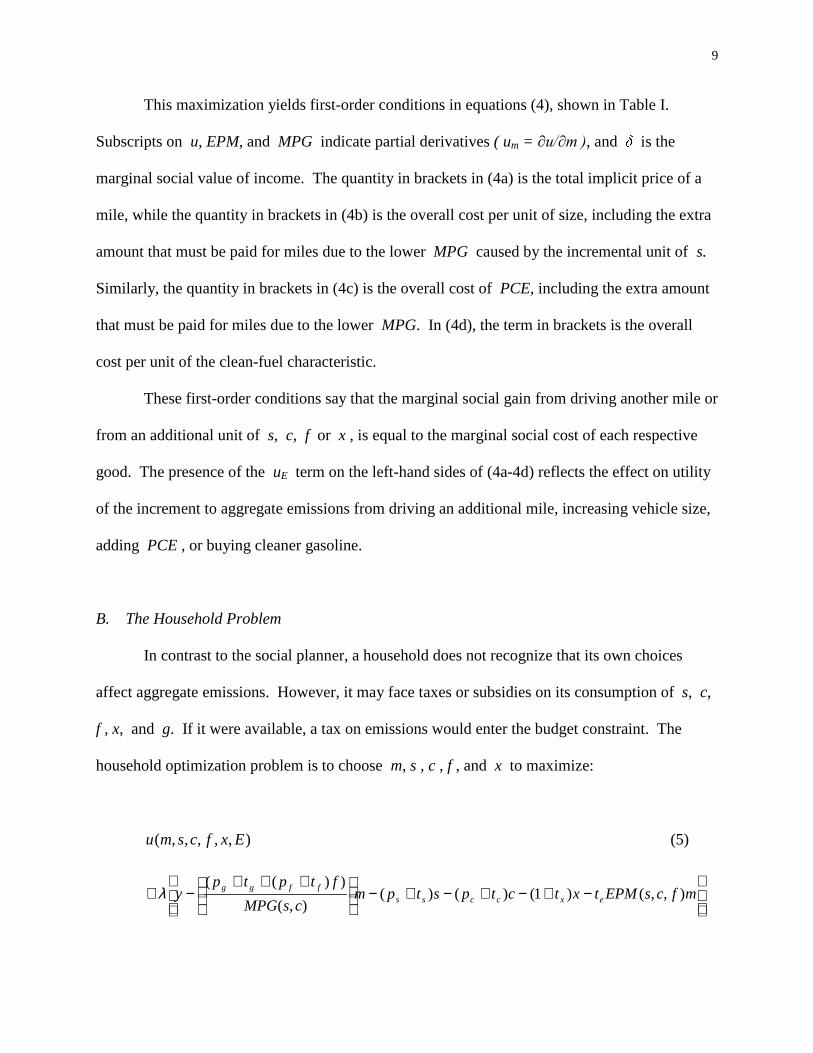
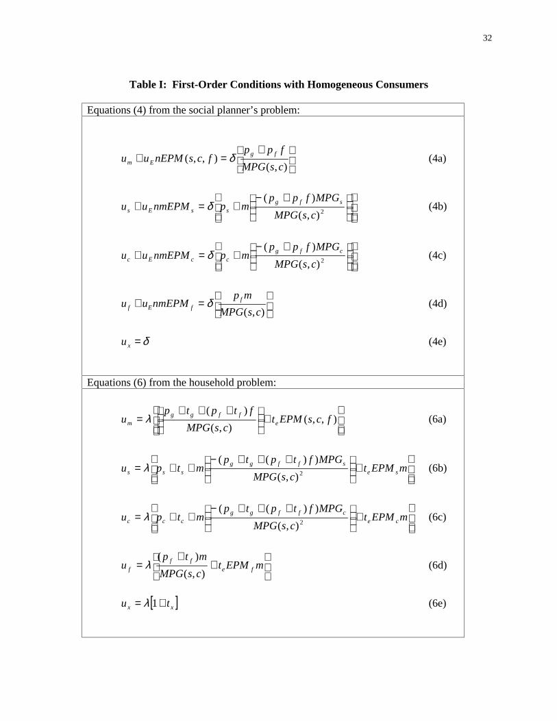
This maximization yields first-order conditions in equations (4), shown in Table I.
Subscripts on u, EPM, and MPG indicate partial derivatives ( um = �X��P��, and is the
marginal social value of income. The quantity in brackets in (4a) is the total implicit price of a
mile, while the quantity in brackets in (4b) is the overall cost per unit of size, including the extra
amount that must be paid for miles due to the lower MPG caused by the incremental unit of s.
Similarly, the quantity in brackets in (4c) is the overall cost of PCE, including the extra amount
that must be paid for miles due to the lower MPG. In (4d), the term in brackets is the overall
cost per unit of the clean-fuel characteristic.
These first-order conditions say that the marginal social gain from driving another mile or
from an additional unit of s, c, f or x , is equal to the marginal social cost of each respective
good. The presence of the uE term on the left-hand sides of (4a-4d) reflects the effect on utility
of the increment to aggregate emissions from driving an additional mile, increasing vehicle size,
adding PCE , or buying cleaner gasoline.
B. The Household Problem
In contrast to the social planner, a household does not recognize that its own choices
affect aggregate emissions. However, it may face taxes or subsidies on its consumption of s, c,
f , x, and g. If it were available, a tax on emissions would enter the budget constraint. The
household optimization problem is to choose m, s , c , f , and x to maximize:
),,,,,( Exfcsmu (5)
−+−+−+−
+++−+ mfcsEPMtxtctpstpm
csMPG
ftptpy exccss
ffgg ),,()1()()(),(
))((λ
10
In the budget constraint, tg is the tax per gallon of gas, tf is the tax per unit of clean-fuel
characteristic, ts is the tax per unit of size, tc is the tax per unit of PCE, tx is the tax per unit
of x, and te is the tax per unit of emissions.
The first-order conditions for this problem are equations (6), also shown in Table I.
Emissions can be made to enter the consumer problem implicitly through the pollution tax te .
The price per mile would then include the emissions tax per mile. Similarly, the implicit prices
of s, c, and f include the emissions tax associated with the change in emissions.
C. Solutions
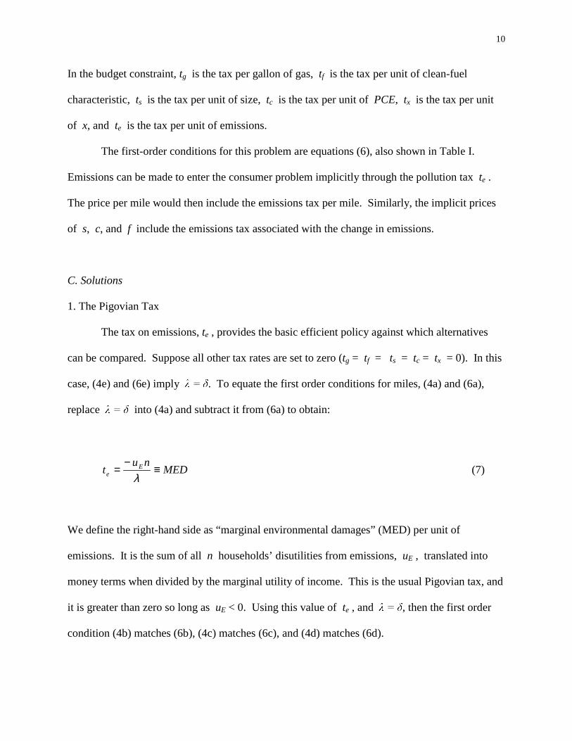
1. The Pigovian Tax
The tax on emissions, te , provides the basic efficient policy against which alternatives
can be compared. Suppose all other tax rates are set to zero (tg = tf = ts = tc = tx = 0). In this
case, (4e) and (6e) imply � � . To equate the first order conditions for miles, (4a) and (6a),
replace � � into (4a) and subtract it from (6a) to obtain:
MEDnu
t Ee ≡
−=
λ(7)
We define the right-hand side as “marginal environmental damages” (MED) per unit of
emissions. It is the sum of all n households’ disutilities from emissions, uE , translated into
money terms when divided by the marginal utility of income. This is the usual Pigovian tax, and
it is greater than zero so long as uE < 0. Using this value of te , and�� � � , then the first order
condition (4b) matches (6b), (4c) matches (6c), and (4d) matches (6d).

11
Thus the Pigovian tax on emissions by itself induces households to make all the optimal
choices. Because of the tax on emissions, consumers will drive fewer miles, buy smaller cars,
buy cleaner fuel, and install more pollution control equipment (or opt for a vehicle model that is
already equipped with better pollution control equipment).
2. Taxes on Gasoline and Size with a Subsidy to PCE
If the measurement of emissions were difficult or impossible, so that te = 0, we can find a
different policy combination that attains the exact same efficient outcome. This policy is a three-
part instrument that begins with a tax schedule for gasoline and is complemented by a tax on size
and a subsidy to PCE. For ease of exposition, we solve for a subsidy on f and show how it can
be incorporated into the gasoline tax. To solve for the policy parameters, assume for the moment
that c and f do enter household utility ( uc ����DQG��uf ��� ). Then, set tx = te = 0. Thus
still equals , and we have equality between (4e) and (6e). Using � � , we can solve for the
subsidy on the clean-fuel characteristic by equating (4d) and (6d) to get:
),( csMPGEPMnu
t fE
f λ−
= (8)
This tax is negative (a subsidy) as long as emissions per mile decrease with an incremental unit
of clean-fuel characteristic. It equals the value of the emissions reduction due to an additional
unit of cleanliness per gallon, calculated as the damage per unit of emissions (MED) times the
change in emissions per mile (EPMf ) times miles per gallon (MPG).13
13 If the clean-fuel characteristic negatively affects MPG, the clean-fuel subsidy in (8) would include a positivesecond term, and the gas tax (below) would include an offsetting term (to leave only the direct effect on emissions).
12
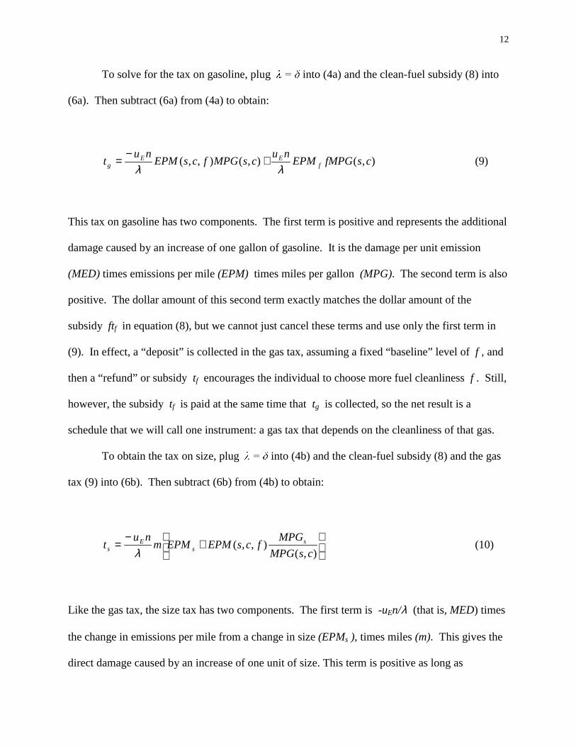
To solve for the tax on gasoline, plug � � into (4a) and the clean-fuel subsidy (8) into
(6a). Then subtract (6a) from (4a) to obtain:
),(),(),,( csfMPGEPMnu
csMPGfcsEPMnu
t fEE
g λλ+
−= (9)
This tax on gasoline has two components. The first term is positive and represents the additional
damage caused by an increase of one gallon of gasoline. It is the damage per unit emission
(MED) times emissions per mile (EPM) times miles per gallon (MPG). The second term is also
positive. The dollar amount of this second term exactly matches the dollar amount of the
subsidy ftf in equation (8), but we cannot just cancel these terms and use only the first term in
(9). In effect, a “deposit” is collected in the gas tax, assuming a fixed “baseline” level of f , and
then a “refund” or subsidy tf encourages the individual to choose more fuel cleanliness f . Still,
however, the subsidy tf is paid at the same time that tg is collected, so the net result is a
schedule that we will call one instrument: a gas tax that depends on the cleanliness of that gas.
To obtain the tax on size, plug � � into (4b) and the clean-fuel subsidy (8) and the gas
tax (9) into (6b). Then subtract (6b) from (4b) to obtain:
+
−=
),(),,(
csMPG
MPGfcsEPMEPMm
nut s
sE
s λ(10)
Like the gas tax, the size tax has two components. The first term is -uEn/λ (that is, MED) times
the change in emissions per mile from a change in size (EPMs ), times miles (m). This gives the
direct damage caused by an increase of one unit of size. This term is positive as long as
13
emissions affect utility negatively (uE < 0) and size affects emissions positively (EPMs > 0). The
second term is an indirect effect from an additional unit of size through its effect on fuel
efficiency.14 As long as MPGs < 0, this term is negative and is thus a rebate. Specifically, it is a
rebate of part of the gas tax in (9). Because an additional unit of size decreases fuel efficiency,
the household knows that an increase in the size of its vehicle’s engine will cost additional gas
tax. Thus part of the external cost of size is already internalized by the gas tax. After this rebate,
only the cost of size that is separate from its effect on MPG remains taxed. Conceptually, this
rebate is the same as that which appears in Innes’ second-best vehicle tax, where that tax
approximately equals the “predicted social costs of emissions, less the portion of these costs that
are internalized by the gasoline tax” (Innes, 1996: p. 212).
Because the two components of the size tax are opposite in sign, this theory does not
predict the sign of ts . Since the right-hand term before the brackets is positive, the sign of ts is
determined by the sign within the brackets. Thus the size tax is positive whenever
),(),,( csMPG
MPG
fcsEPM
EPM ss −> (11)
These two terms are proportional effects of size on emissions per mile (EPM) and on miles per
gallon (MPG). When an additional unit of size brings about a larger percentage change in
emissions per mile than in fuel efficiency, the size tax is positive. If emissions rise at the same
rate that fuel efficiency deteriorates, then the size tax is zero. If fuel efficiency deteriorates
proportionally more than emissions increase, then size is subsidized! In this last case, the
14 Both of these terms contain m , the “baseline” number of miles. This m is not the individual’s own choice ofmiles, or else the individual’s first order condition (8a) would include the derivative of ts with respect to m .
14
gasoline tax more than completely internalizes the impact of size on emissions. Empirical
exploration of the relative effects in (11) will uncover the sign of the size tax.15
To solve for the tax on PCE, we follow similar procedures to obtain:
),(),,(
csMPG
MPGmfcsEPM
numEPM
nut cE
cE
c λλ−
+−
= (12)
The tax on PCE is perfectly analogous to the size tax. The first term is negative to reflect the
effect on damages of an added unit of PCE. The second term is a rebate due to the effect that
PCE has on fuel efficiency (already internalized by the gas tax). Since the second term is also
negative, the sign of the clean-car tax is always negative. That is, tc is necessarily a subsidy.16
All of these tax rates together induce households to make socially optimal trade-offs at
the margin, so they are valid only for internal solutions. A more complete analysis is required to
deal with corner solutions.17 If households dislike pollution control equipment enough ( uc <<
0), then the subsidy in (12) may not induce them to buy any of it. In this extreme case, the
corner solution with c = 0 is indeed part of the social optimum, even though the marginal
conditions (6) are not satisfied. If households care nothing about this equipment, however, then
a different problem arises. To see this, note that when uc = 0, the right-hand side of first order
condition (6c) must equal zero at the optimum. By assumption, for this analysis, the emissions
15 Also, note that the size tax in (10) depends on the number of miles driven. Of course, in this model withhomogeneous consumers, all households drive the same type of vehicle the same number of miles per year, and thesize tax is the same for everyone. When we introduce heterogeneity in Section II, the first-best solution requires thateach household pay a size tax that reflects its own choice of miles.
16 If c measures the amount of PCE installed, this subsidy could be paid upon purchase of the vehicle. Moregenerally, if c reflects the condition of the equipment as well as the amount, then this subsidy could reward testing,maintenance, and repair of PCE.
17 We derived Kuhn-Tucker conditions from a model with non-negativity constraints on the purchase of clean-carand clean-fuel characteristics. The results of that model include equations (9), (10) and (12) for internal solutionsand an inequality to characterize each corner solution. The additional intuition is minimal, however, so we justoutline these results in the text.
15
tax is set equal to zero. Therefore, to induce consumers to buy any pollution equipment, the
subsidy to PCE (tc ) must be equal to the entire private cost of PCE, including both the direct
cost of equipment, pc , and the extra gasoline costs incurred due to the negative effect that PCE
has on fuel efficiency. With a 100 percent subsidy, however, the choice of c is indeterminate.
Thus, if uc = 0, then incentives do not work. The optimal PCE can only be achieved by a
mandate (as in Innes, 1996).
The same analysis applies to the clean-fuel characteristic. When uf = 0, the right-hand
side of (6d) must equal zero at the optimum. For households to choose cleaner gas, the subsidy
must equal the entire cost of the attribute, pf .
Individuals may or may not gain utility from driving cleaner cars and using cleaner fuel.
People may like using the latest technologies, or feel peer pressure do so. On the other hand,
pollution control equipment may negatively affect performance by increasing vehicle weight and
decreasing acceleration. In addition, if cleaner fuel can be found only in a limited number of
locations, the inconvenience costs of refueling could be high.
For these reasons, we think that uc and uf are unlikely to be exactly zero. In fact, these
marginal utilities are likely to fall with the amount of c or f . Even if uc is negative, a big
enough subsidy can induce the household to buy more of this good, until uc on the left-hand side
of (6c) falls to the level of the (negative) private marginal cost on the right-hand side of (6c).
The optimality of these results also depends on our assumptions about the available
abatement technologies. Since emissions depend on EPM(s, c, f), the three-part instrument
(tg , ts , tc ) attains the same first-best equilibrium as that reached by the Pigovian tax. Despite
the fact that emissions are never measured, the three-part policy can attain 100 percent of the
improvement in social welfare achieved by the Pigovian tax.
16
II. Heterogeneous Consumers
The tax rates derived in the previous section are uniform across all consumers. In this
section, we introduce heterogeneity to see if and when the optimal tax rates need to differ among
consumers. If the emissions tax te were available, we confirm that a single te = MED would
achieve the first-best social optimum (FBSO). If not, then individual-specific tax rates on other
goods can still achieve the FBSO. If policy is unable to apply individual-specific tax rates, then
it cannot achieve the FBSO. We then characterize the second-best uniform tax rates that best
approximate the unavailable tax on emissions.
In his model of heterogeneous consumers, Innes (1996) allows households to differ in
terms of income and one taste parameter. In our model, we wish to allow households to differ in
terms of income and two taste parameters. We use the parameter to represent the household’s
preference for miles, and we use the parameter to represent the preference for size of the car.
Together with income, these parameters are jointly distributed according to the distribution
function��K�� ��� ��\� with positive support on [ ] [ ] [ ]yy,,, ×× ββαα . The integral of this
distribution over �, �, and y is the population, n . In a CES or Cobb-Douglas specification of
utility, for example, could be the weight on miles, would be the weight on size, and ���� ��
� would be the weight on x. Our analysis is not limited to these special cases, however, and it
is not limited by any particular relationship between and . Those who live far from their
place of work have a high demand for miles � �, but they may prefer either a small car (for better
gas mileage) or a large car (for comfort and safety). We show the importance of the correlation
between and .
17
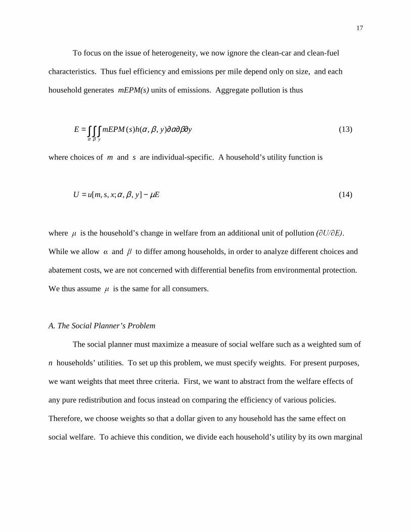
To focus on the issue of heterogeneity, we now ignore the clean-car and clean-fuel
characteristics. Thus fuel efficiency and emissions per mile depend only on size, and each
household generates mEPM(s) units of emissions. Aggregate pollution is thus
∫ ∫ ∫ ∂∂∂=α β
βαβαy
yyhsmEPME ),,()( (13)
where choices of m and s are individual-specific. A household’s utility function is
EyxsmuU µβα −= ],,;,,[ (14)
where � is the household’s change in welfare from an additional unit of pollution (�8��(�.
While we allow ��and to differ among households, in order to analyze different choices and
abatement costs, we are not concerned with differential benefits from environmental protection.
We thus assume is the same for all consumers.
A. The Social Planner’s Problem
The social planner must maximize a measure of social welfare such as a weighted sum of
n households’ utilities. To set up this problem, we must specify weights. For present purposes,
we want weights that meet three criteria. First, we want to abstract from the welfare effects of
any pure redistribution and focus instead on comparing the efficiency of various policies.
Therefore, we choose weights so that a dollar given to any household has the same effect on
social welfare. To achieve this condition, we divide each household’s utility by its own marginal

18
utility of income � �.18 Second, when te is available, we want the maximization of our social
welfare function to yield the solution of Pigou (1932). Since this solution is based on marginal
conditions (such as marginal environmental damages) at the optimum, we use the values for
that occur at the first-best social optimum � �. Third, we want to be able to compare policies
using the same welfare weights. When first-best instruments are not available, we want to be
able to find second-best uniform tax rates that maximize the same social welfare function.
Therefore we use prices at the Pigovian equilibrium to evaluate ���and we use those to get
the weights ��� � for all subsequent evaluations of other policies. The result is a money-metric
measure of social welfare.
The social planner’s problem is to maximize this welfare function subject to a resource
constraint (the integral over all individual budget constraints):
[ ] yyhyyhsmEPMxsmu
y y
∂∂∂
∂∂∂−∫ ∫ ∫ ∫ ∫ ∫ βαβαβαβαµ
λα β α β
),,(),,()(],,[
* (15)
∂∂∂
−−−+ ∫ ∫ ∫
α β
βαβαδ yyhxspmsMPG
py
y
sg ),,(
)(
with respect to each consumer’s m, s , and x (given their individual , and y ). The
multiplier on the resource constraint is �, the marginal social value of income. To maximize
(15), we can ignore the outer integral to obtain the individual marginal conditions and then
18 To avoid redistributions in the tax rate problem below, we assume that all tax revenues are returned in lump-sumfashion to the same consumer.
19
incorporate the impact an individual’s choice of miles and size has on emissions by
differentiating the aggregate emissions term with respect to the individual’s m and s.
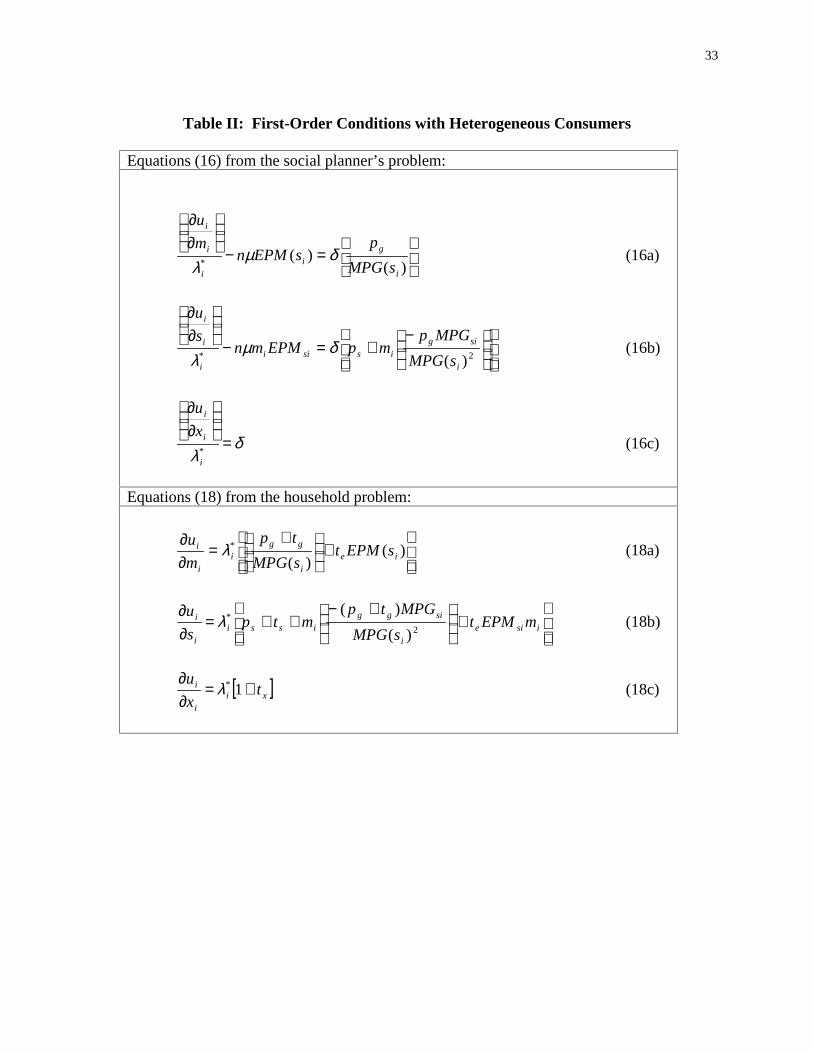
The resulting first-order conditions for household i are equations (16), shown in the top
of Table II. The first term in each equation represents the individual’s money value of marginal
utility from each good. The second term in (16a) represents the external cost of an additional
mile driven by individual i . Similarly, the second term in (16b) represents the external cost of
an additional unit of size purchased by individual i. The first-order conditions (16) say that the
money-metric social marginal utility of each good equals the social marginal cost of that good.
Also, looking at (16c), note that the left-hand side equals individual i’s change in utility from an
additional unit of x, divided by the marginal utility of income. In other words, it is the dollar
value of another unit of x (the price of x). Since the price of x equals one, (16c) says that the
social marginal utility of income, , also equals one.
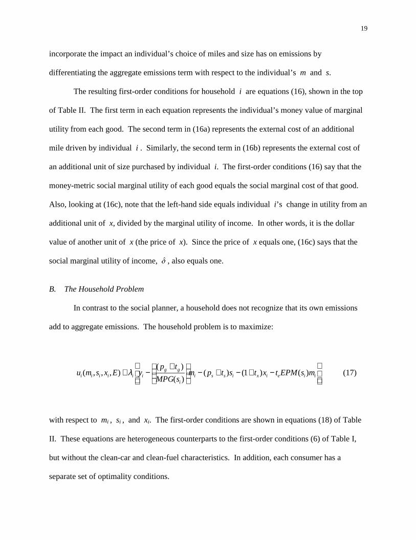
B. The Household Problem
In contrast to the social planner, a household does not recognize that its own emissions
add to aggregate emissions. The household problem is to maximize:
−+−+−
+−+ iieixissi
i
ggiiiiii msEPMtxtstpm
sMPG
tpyExsmu )()1()(
)(
)(),,,( λ (17)
with respect to mi , si , and xi. The first-order conditions are shown in equations (18) of Table
II. These equations are heterogeneous counterparts to the first-order conditions (6) of Table I,
but without the clean-car and clean-fuel characteristics. In addition, each consumer has a
separate set of optimality conditions.

20
C. Solutions
1. The Pigovian Tax
To solve for a Pigovian tax, set all taxes except te equal to zero ( ts = tg = tx = 0 ).
Then, using � = 1, (16c) and (18c) match each other. Also using = 1, set (16a) and (18a)
equal to each other. The household-specific variables drop out, leaving:
MEDn
te ≡=δµ
(19)
Using = 1 and this value of te , then first-order conditions for size (16b) and (18b), also match
each other.
Thus, given the weights we have chosen, a uniform Pigovian tax on emissions by itself
induces all households, no matter their tastes for miles and size, to drive the optimal number of
miles in the right sized cars. Of course, policy makers do not necessarily weight households so
that income to one is the same as income given to another. They may want instead to
incorporate explicit distributional concerns into environmental taxes. In this paper, however, we
are not concerned with issues of distribution. We weight households simply in a way that
implies that the maximization of social welfare yields the standard Pigovian formula in (19).
This first-best uniform Pigovian tax can be used as a benchmark to identify other first-best policy
instruments, and more importantly, against which to evaluate other second-best instruments.
2. First-best Taxes on Gasoline and Size

21
As in the representative-agent model, when a Pigovian tax is not possible (te = 0), we can
derive another first-best set of instruments. Using the solution technique explained in Section
I.C, we obtain the heterogeneous counterpart of the gasoline tax:
)()( iigi sMPGsEPMnt µ= (20)
The subscript i on size indicates that the first-best tax on gasoline would have to differ across
consumers according to their chosen size (si). In order for the FBSO to be attained, the tax on
gasoline must differ according to characteristics of the vehicle at the pump. Such a gas tax
would be costly to administer.19
With heterogeneous consumers, the size tax is also household-specific:20
)(
)(
i
isiiisisi sMPG
mMPGsEPMnmEPMnt
µµ += (21)
To implement this tax on a car of size si , its miles would have to be known. If the size tax were
assessed when the vehicle is purchased, then some measure of the discounted total expected
miles for the life of the vehicle would be necessary. Since conditions change, however, the one
time size tax would not provide the right subsequent incentives (e.g. retirement). If the size tax
19 “For example, a tamper-resistant computer code would likely be required on each automobile; similarly, gasolinepumps would have to be equipped to automatically tack the appropriate tax onto any gasoline that is dispensed to aparticular automobile. Moreover, since a simple siphoning of gas will permit consumers to bypass taxes on high-emission vehicles, the scope for abuse, particularly among those high-emitting consumers who are arguably the mostimportant targets of the tax, would be tremendous” (Innes, 1996: p. 226).
20 Again, the FBSO requires that government know mi , in order to set the baseline mi in (21), but that theindividual face a fixed tsi that does not depend on individual choice of m (the individual optimization of (17) doesnot take a derivative of ts with respect to m).
22
were assessed yearly, then annual odometer readings would be necessary. This would provide
incentive for individuals to roll back their odometers.21
These results can be reconciled with those of Innes (1996). He does not solve for first-
best tax rates on gasoline or car characteristics that would replicate the effects of an emissions
tax, but he finds that the outcome would include a fuel-content standard, an auto-specific fuel
tax, and no regulation of the automobile (p. 226). We derive the auto-specific fuel tax (in 20),
but we also find a mileage-specific auto tax (in 21). This difference in results can be attributed
directly to differences between the models. The consumer’s optimization problem in (17) writes
MPG and EPM explicitly as functions of si , but it treats tax rates as parameters that are fixed
to the consumer. Yet (20) says that the optimal tgi is )()( ii sMPGsEPMnµ , a function of si. If
we plug that tgi function into (17) before we differentiate with respect to si, then additional
terms in the first order condition (18b) would involve derivatives EPMsi and MPGsi, just like
in (21). The tax on size in (21) would then be unnecessary (Innes, 1996). In other words, results
depend on what consumers are assumed to know. If individuals know that their individualized
gas tax rate will depend on their own choice of engine size, then that gas tax alone can induce the
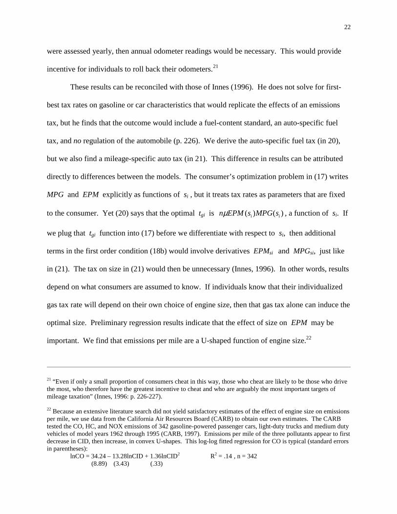
optimal size. Preliminary regression results indicate that the effect of size on EPM may be
important. We find that emissions per mile are a U-shaped function of engine size.22
21 “Even if only a small proportion of consumers cheat in this way, those who cheat are likely to be those who drivethe most, who therefore have the greatest incentive to cheat and who are arguably the most important targets ofmileage taxation” (Innes, 1996: p. 226-227).
22 Because an extensive literature search did not yield satisfactory estimates of the effect of engine size on emissionsper mile, we use data from the California Air Resources Board (CARB) to obtain our own estimates. The CARBtested the CO, HC, and NOX emissions of 342 gasoline-powered passenger cars, light-duty trucks and medium dutyvehicles of model years 1962 through 1995 (CARB, 1997). Emissions per mile of the three pollutants appear to firstdecrease in CID, then increase, in convex U-shapes. This log-log fitted regression for CO is typical (standard errorsin parentheses):
lnCO = 34.24 – 13.28lnCID + 1.36lnCID2 R2 = .14 , n = 342 (8.89) (3.43) (.33)
23
Successful implementation of these first-best policies seems unlikely. Therefore, we next
assume that policy is limited. If the gas tax cannot be made to depend on vehicle type, then a
separate tax on size becomes important. If both the size tax and the gas tax are constrained to be
uniform across consumers, and therefore fixed to each consumer, then how should these rates be
set? Since the tax rates in (20) and (21) depend on s and m, one possibility is that the size and
gas tax could be calculated from (20) and (21) using the mean size and miles. How well these
uniform tax rates would perform depends on the technological relationships EPM(s) and
MPG(s) and the relationship in preferences between size and miles. In the next section, we find
conditions that characterize second-best (uniform) tax rates. Then, we discuss how these rates
might compare with those from (20) and (21) using mean size and miles.
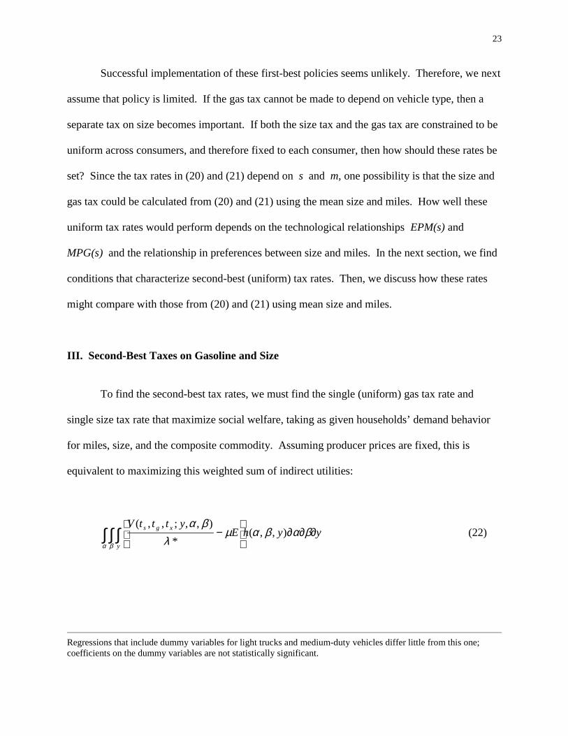
III. Second-Best Taxes on Gasoline and Size
To find the second-best tax rates, we must find the single (uniform) gas tax rate and
single size tax rate that maximize social welfare, taking as given households’ demand behavior
for miles, size, and the composite commodity. Assuming producer prices are fixed, this is
equivalent to maximizing this weighted sum of indirect utilities:
∫ ∫ ∫ ∂∂∂
−
α β
βαβαµλ
βαyyhE
ytttV
y
xgs ),,(*
),,;,,((22)
Regressions that include dummy variables for light trucks and medium-duty vehicles differ little from this one;coefficients on the dummy variables are not statistically significant.

24
with respect to ts and tg . As a normalization, the tax on x can be set to zero, as in the first-best
scenario.23 Using Roy’s Identity, this maximization results in the first order conditions:
[ ] 0),,(),,()(*
=∂∂∂
∂∂∂−−
∫ ∫ ∫ ∫ ∫ ∫ yyhyyhtAs
y y
s βαβαβαβαµλλ
α β α β(23a)
[ ] 0),,(),,()(*
=∂∂∂
∂∂∂−−
∫ ∫ ∫ ∫ ∫ ∫ yyhyyhtAg
y y
g βαβαβαβαµλλ
α β α β
(23b)
where, (for j = s, g):
jjs
jsj t
gsMPGsEPM
t
sMPGsgEPM
t
sEPMsgMPGtA
∂∂+
∂∂+
∂∂≡ )()()()()( (24)
The chosen quantities (s, g, and x) as well as the marginal utility of income � ��are functions of
� and . In (23a), the first term in the integral (- V� ) represents the change in welfare from a
change in the size tax, holding aggregate emissions constant. The second term, involving A(ts ),
is the change in utility due to the effect that a size tax has on aggregate emissions.24 Similarly,
the first term in (23b) is the change in welfare from a change in the gas tax, holding aggregate
emissions constant. The second term incorporates the change in welfare from the effect that the
gas tax has on aggregate emissions.
Thus the tax rates on size and gasoline should each be set so that the aggregate marginal
gain in private welfare equals the aggregate loss from the effect on emissions. As shown in the
A(tj) term of each first order condition, the extent to which emissions are reduced depends on the
23 Income, y , is exogenous, so a (lump-sum) tax on income ty is equivalent to a tax on all commodities at the samerate; any set of (ts , tg, tx) can be scaled up or down, with commensurate changes in ty . Thus any one rate can beset to zero (see Fullerton, 1997).
24 When an emissions tax achieves the FBSO, where = , then (23a) says that the cost to the taxpayer of anincrease in ts is the amount of s purchased, and that this marginal cost should be equal to the marginal benefits interms of reduced emissions.
25
degree of responsiveness of miles and size to taxes on size and gasoline. Thus second-best
optimal (SBO) tax rates on size and gasoline depend on the elasticities of demand for these
goods. But the way in which changes in size affect emissions is through the technological
relationships that size has with emissions per mile and fuel efficiency. The functions EPM(s)
and MPG(s) are therefore major determinants of the second-best tax rates.
These first order conditions cannot be used to solve for the second-best uniform tax rates
on size and gasoline. To find closed-form solutions we would have to specify the functional
forms of K� , ��\�, EPM(s), MPG(s) and the demands for size, miles, and the composite
commodity. Still, these first order conditions can be used to shed some light on the nature of
such taxes. First, note how this problem differs from the usual second-best optimal tax problem.
Much of the public economics literature assumes that consumers demand leisure and other
goods, that leisure cannot be taxed, and that the government must set other tax rates to minimize
excess burden subject to a revenue requirement. The resulting second-best tax rates depend
primarily on price elasticities: higher tax rates are placed on goods that are inelastically
demanded or that are complements to leisure.25 In contrast, our problem does not involve any
labor/leisure choice, or even a revenue requirement. Individual-specific lump-sum taxes are
available. For this reason, the resulting second-best tax rates will not depend in the same way on
behavioral responses to prices. The goal here, instead, is to tax something that approximates the
consumer’s emissions. In particular, if consumers with a high preference for miles (high ) also
happen to have a high preference for size (high ), then that correlation is likely to affect the
second-best optimal tg and ts . In addition, preferences for size determine emissions through the
relationship size has with MPG and EPM.
25 For comprehensive treatments of optimal taxation, see Auerbach (1985) or Stern (1987).

26
We therefore want to investigate the potential importance of these technological
relationships and of the correlation between miles and size. In addition, first order conditions
(23) do not provide clear guidance about how to set uniform tax rates in the face of
heterogeneity. Closed-form solutions for the SBO tax rates are not available, but two
alternatives come to mind. First, we can calculate the “expected value” or weighted average of
the first-best individual-specific tax rates in equations (20) and (21). These average rates might
then be applied uniformly to all individuals. These rates are not the same as the SBO rates from
(23), but at least they incorporate information about the distribution K� �� ��\� of heterogeneous
individuals. Second, policymakers might simply ignore heterogeneity, and just use the
economy-wide means for miles and size as if all individuals were the same. A comparison of
these two alternatives will reveal the direction of the bias from ignoring heterogeneity.
The average of all different gas tax rates in (20) is:
yyhsMPGsEPMyyh
yyhsMPGsEPMn
t ii
y
y
i
y
i
g ∂∂∂=∂∂∂
∂∂∂
= ∫ ∫ ∫∫ ∫ ∫
∫ ∫ ∫βαβαµ
βαβα
βαβαµ
α βα β
α β),,()()(
),,(
),,()()(
(25)
We ask how this concept differs from the simple calculation of the gas tax rate for the person
with average choices:
)()()( sMPGsEPMnst g µ= (26)
Specifically, we want to identify the circumstances under which the average of the gas tax in
(25) is greater than the gas tax rate for the person with average choices in (26). We can thus
27
discover the conditions under which uniform taxes based on average choices would likely fall
short of attaining the second-best emissions reduction.
Note that households with bigger cars driving proportionally more miles than small-car
owners would pay a proportionally higher gas tax even with a uniform gas tax rate, because they
would use more gas to drive the extra miles. Whether (25) exceeds (26) depends on the
characteristics of EPM(s) and MPG(s) and particularly on the convexity of each function.
Convexity of EPM(s), for example, would mean that increases in size increase emissions per
mile at an increasing rate. This would raise the weighted average using EPM(si) in (25) relative
to the tax rate using average size in (26). Convexity in MPG(s) also raises (25) relative to (26).
So, if either function is sufficiently convex (or if both are convex), then the use of average size to
calculate the gas tax rate would understate the second-best uniform tax rate. Conversely, if
either EPM(s) or MPG(s) is sufficiently concave, then using the average value of size to
calculate the gas tax rate would overstate the second-best uniform tax rate.
To determine the likely magnitude of (25) relative to (26), we need estimates of the
possible nonlinear effect of engine size on fuel efficiency and emissions. While it is widely
known that fuel efficiency decreases with engine size, a literature search locates no statistical
estimates of the nonlinear nature of this relationship. Nor could we find any estimates of the
effect of size on emissions per mile.26 For these reasons, we use the CARB data to estimate
EPM and MPG as polynomial functions of engine size. These regressions omit other
explanatory variables in order to capture the full effect of size, the only taxed characteristic.
These very preliminary results suggest that EPM is increasing over most of the range of size
26 Dunleep (1992) provides only rough estimates of the effect of size on MPG. Kahn (1996b) examines the effectof size on emissions in parts per million rather than on emissions per mile.

28
and convex, while MPG is decreasing and also convex in size.27 Thus the use of average car
size would likely understate the second-best optimal gas tax.
Now consider the individual-specific size tax rate in (21). We want to reveal the
circumstances under which the average of the size tax rate,
yyhsMPG
mMPGsEPMyyhmEPMt
y i
isiii
y
sis ∂∂∂+∂∂∂= ∫ ∫ ∫∫ ∫ ∫ βαβαµβαβαµα βα β
),,()(
)(),,( (27)
is larger than the size tax for the person with the average choices,
)(
)(),(
sMPG
mMPGsEPMnmEPMnmst s
ss
µµ += (28)
If the size tax is positive, then emissions per mile increase proportionately more with size
than fuel efficiency deteriorates, and the first terms in (27) and (28) dominate the second terms.
In this case, whether the average size tax rate (27) exceeds the size tax rate using average miles
and size (in 28) depends only on whether the first term in (27) exceeds the first term in (28).
Note that in the first term of each equation, EPMs is multiplied by m. If size and miles are
positively correlated, because and are positively correlated, then this term is superadditive
in miles and size. In this case, even if EPM(s) is linear, (27) exceeds (28). The use of the
average person’s size tax is likely to understate the second-best size tax, if those who own larger
27 Typical results for regressions of EPM on size are shown in footnote (22). The following regression indicatesthat MPG is decreasing and also convex in engine size measured by CID (standard errors in parentheses):
MPG = 35.41 – .106CID + .00012CID2 R2 = .72, n = 342 (.88) (.0085) (.000017)EPA data on MPG yield similar results.

29
cars drive proportionately more miles than those with smaller cars. Moreover, if EPM is a
convex function of size, then the optimal size tax increases even more quickly with miles and
size. Conversely, if miles and size are negatively correlated and EPM is linear or concave in
size, then (27) would be less than (28).
We use the 1994 Residential Transportation Energy Consumption Survey (RTECS) to
find preliminary evidence on the correlation of size and miles, and find a very small but
statistically significant negative correlation.28 However, since preliminary estimates show
EPM(s) to be convex, we cannot determine whether the size tax based on average size would
likely overstate or understate the second-best uniform size tax.
Do uniform tax rates calculated using mean miles and size and (20) and (21) approximate
the second-best tax rates? We have shown that the answer depends on the technological
relationships EPM(s) and MPG(s), and the relationship between preferences for size and miles
K� �� ��\�. The average gas tax is likely to exceed the tax calculated using average size, since
EPM and MPG are found to be convex in size. The average size tax may exceed the size tax
calculated using average size and miles, but only if size and miles are positively correlated
and/or EPM is sufficiently convex in size. In contrast, if tastes for size and miles are
independently distributed and emissions per mile and miles per gallon are linear functions of
size, then average tax rates equal the tax rates calculated using mean miles and size.
It appears unlikely that the second-best uniform tax rates would be closely approximated
by the rates based on the means. In order to maximize social welfare, we need a comprehensive
28 We use the RTECS because other sources lack data on annual miles or engine size. CARB data does not listannual mileage, while the Nationwide Personal Transportation Survey (NPTS) has annual miles but not engine size.The 1994 Consumer Expenditure Survey has multiple odometer readings that enable mileage to be calculated, and ithas the number of cylinders, but not CID. Using vehicles in the RTECS, the correlation between CID and annualmiles is -.0439, significant at the 2.6% level. Also, regression analysis indicates that miles and size may benonlinearly related.

30
empirical investigation of the technological relationships EPM(s) and MPG(s), the distribution
h( , ,y), and behavioral parameters.
IV. Conclusions
In a simple model, we duplicate the outcome from a tax on emissions by instead taxing
gasoline and engine size, and by subsidizing PCE . The gas tax induces households to drive
fewer miles and to buy more fuel-efficient cars. In addition, since the rate of tax depends on the
cleanliness of the gasoline, the optimal gas tax also encourages households to buy cleaner fuel.
The tax on size induces households to buy cars with smaller engines, while a subsidy to PCE
encourages purchase and repair of emissions-reducing equipment. Of course, vehicle age is also
an important determinant of emissions, because emissions standards have become increasingly
stringent over time, because emissions-control equipment deteriorates over time, and because
new technologies and lighter materials have become available. Thus policies that accelerate
vehicle retirement might also reduce emissions in a cost-effective way. The theory in this paper
could be extended to incorporate such policies.29
Current policies for the control of car pollution already involve many government
mandates, in addition to some economic incentives. We do not include any explicit vehicle-
emissions standards in our model, but we recognize that existing standards affect the current
relationships between vehicle size, vehicle age, and emissions per mile. Thus incentives that
affect the choice of vehicle rely for their effectiveness on the existence of those standards.
While the model of homogeneous consumers is useful to clarify the role of each
alternative policy in attaining the social optimum, it cannot tell us how variation in tastes for

31
miles and size might affect optimal tax or subsidy rates. To explore this issue, we build a model
of consumers that differ by tastes for miles and engine size. The first-best alternative policies are
household-specific taxes on gasoline and size. For the first-best gas tax to be feasible, the
attributes of each vehicle would have to be identifiable at the pump.
Because such implementation would likely be expensive, we characterize second-best
uniform tax rates. A simple alternative is based on the erroneous assumption that consumers are
identical and so all drive the mean number of miles in the mean sized car. We reach two main
conclusions. First, if the addition of a unit of size increases emissions per mile at an increasing
rate, or if it decreases fuel efficiency at a decreasing rate, then a second-best uniform gas tax rate
would exceed that simple calculation (using mean size and miles). Second, because we identify
consumer preferences using two parameters, one for miles and one for size, we find that a higher
positive correlation of these taste parameters increases the second-best uniform tax on size.
If tastes for miles and size are positively correlated, and EPM and MPG are convex in
size, then second-best uniform tax rates are likely to be larger than tax rates calculated by
ignoring heterogeneity (using the means of size and miles). Only if tastes are independently
distributed and both EPM and MPG are linear would the tax rates evaluated at the means be
optimal. Thus an investigation of the economic incentives for the control of car pollution
requires empirical exploration of the technological relationships between vehicle attributes and
emissions per mile, and of the distribution of preferences for miles and size.
29 Alberini, et al., (1995, 1996) derive a theoretical model of owners’ car tenure and scrappage decisions, and theyanalyze the results from an experimental vehicle retirement program in Delaware. Innes (1996) and Fullerton andWest (1999) also incorporate vintage choice into their models.
32
Table I: First-Order Conditions with Homogeneous Consumers
Equations (4) from the social planner’s problem:
+=+
),(),,(
csMPG
fppfcsnEPMuu fg
Em δ (4a)
+−+=+
2),(
)(
csMPG
MPGfppmpnmEPMuu sfg
ssEs δ (4b)
+−+=+
2),(
)(
csMPG
MPGfppmpnmEPMuu cfg
ccEc δ (4c)
=+
),( csMPG
mpnmEPMuu f
fEf δ (4d)
δ=xu (4e)
Equations (6) from the household problem:
+
+++= ),,(
),(
)(fcsEPMt
csMPG
ftptpu e
ffggm λ (6a)
+
+++−++= mEPMt
csMPG
MPGftptpmtpu se
sffggsss 2),(
))((λ (6b)
+
+++−++= mEPMt
csMPG
MPGftptpmtpu ce
cffggccc 2),(
))((λ (6c)
+
+= mEPMt
csMPG
mtpu fe
fff ),(
)(λ (6d)
[ ]xx tu += 1λ (6e)
33
Table II: First-Order Conditions with Heterogeneous Consumers
Equations (16) from the social planner’s problem:
=−
∂∂
)()(
*i
gi
i
i
i
sMPG
psEPMn
m
u
δµλ
(16a)
−+=−
∂∂
2* )( i
sigissii
i
i
i
sMPG
MPGpmpEPMmn
s
u
δµλ
(16b)
δλ
=
∂∂
*i
i
i
x
u
(16c)
Equations (18) from the household problem:
+
+=
∂∂
)()(
*ie
i
ggi
i
i sEPMtsMPG
tp
m
u λ (18a)
+
+−++=
∂∂
isie
i
siggissi
i
i mEPMtsMPG
MPGtpmtp
s
u2
*
)(
)(λ (18b)
[ ]xii
i tx
u+=
∂∂
1*λ (18c)
34
References
Alberini, Anna, Winston Harrington and Virginia McConnell. “Determinants of Participation inAccelerated Vehicle-retirement Programs.” The Rand Journal of Economics 26 (Spring1995): 93-112.
Alberini, Anna, Winston Harrington and Virginia McConnell. “Estimating an Emissions SupplyFunction from Accelerated Vehicle Retirement Programs.” The Review of Economicsand Statistics 78 (May 1996): 251-263.
Auerbach, Alan J. “The Theory of Excess Burden and Optimal Taxation,” in Martin Feldsteinand Alan Auerbach, eds., Handbook of Public Economics, Volume 1. (Amsterdam: NorthHolland, 1985): 61-125.
Baumol, William J. and Wallace E. Oates. Theory of Environmental Policy. Second edition.(New York: Cambridge University Press, 1988).
Bohm, Peter and Clifford S. Russell. “Comparative Analysis of Alternative Policy Instruments,”in Allen V. Kneese and James L. Sweeney, eds., Handbook of Natural Resource andEnergy Economics, Volume 1. (Amsterdam: North Holland, 1985): 395-460.
Bradsher, Keith. “Favors Benefit Light Trucks, But May Be Harmful.” The Austin American-Statesman. (December 7, 1997): A25, A42, A43.
Burmich, Pam. The Air Pollution-Transportation Linkage. (Sacramento, CA: State of CaliforniaAir Resources Board, Office of Strategic Planning, 1989).
California Air Resources Board (CARB). Test Report of the Light-Duty Vehicle SurveillanceProgram, Series 13 (LDVSP13) Project. (September 3, 1997).
Dunleep, K.G. NEMS Transportation Sector Model. (Arlington, VA: Energy and EnvironmentalAnalysis, 1992).
Eskeland, Gunnar. “A Presumptive Pigovian Tax: Complementing Regulation to Mimic anEmissions Fee.” The World Bank Economic Review 8.3 (September 1994): 373-394.
Eskeland, Gunnar and Shantayanan Devarajan. Taxing Bads by Taxing Goods: PollutionControl with Presumptive Charges. (Washington, DC: The World Bank, 1996).
Faiz, Asif, Christopher S. Weaver and Michael P. Walsh. Air Pollution From Motor Vehicles.(Washington, DC: The World Bank, 1996).
Fullerton, Don. “Environmental Levies and Distortionary Taxation: Comment.” The AmericanEconomic Review 87 (March 1997): 245-251.
35
Fullerton, Don and Ann Wolverton. “The Case for a Two-Part Instrument: Presumptive Tax andEnvironmental Subsidy,” forthcoming in Paul R. Portney and Robert M. Schwab, eds.,Environmental Economics and Public Policy: Essays in Honor of Wallace E. Oates.(Cheltenham, UK: Edward Elgar Publishing Ltd., 1999).
Fullerton, Don and Sarah West. “Tax and Subsidy Combinations for the Control of CarPollution.” Working paper prepared for the Public Policy Institute of California (March,1999).
Goldberg, Pinelopi K. “The Effects of Corporate Average Fuel Efficiency Standards in the US.”The Journal of Industrial Economics 46 (March 1998): 1-33.
Hall, Jane V., Arthur M. Winer, Michael T. Kleinman, Frederick W. Lurmann, Victor Brajer andSteven D. Colome. “Valuing the Health Benefits of Clean Air.” Science 255 (February14, 1992): 812-817.
Harrington, Winston. “Fuel Economy and Motor Vehicle Emissions.” Journal of EnvironmentalEconomics and Management 33 (July 1997): 240-252.
Harrington, Winston, Margaret Walls and Virginia McConnell. “Shifting Gears: New Directionsfor Cars and Clean Air.” Discussion Paper 94-26-REV. (Washington, DC: Resources forthe Future, 1994).
Harrington, Winston, Virginia McConnell and Anna Alberini. “Economic Incentive Policiesunder Uncertainty: The Case of Vehicle Emission Fees,” in Roberto Roson and KennethA. Small, eds., Environment and Transport in Economic Modelling. (Dordrect, TheNetherlands: Kluwer Academic Publishers, 1998).
Innes, Robert. “Regulating Automobile Pollution Under Certainty, Competition, and ImperfectInformation.” Journal of Environmental Economics and Management 31 (September1996): 219-239.
Kahn, Matthew E. “New Estimates of the Benefits of Vehicle Emissions Regulation.”Economics Letters 51 (June 1996a): 363-369.
Kahn, Matthew E. “New Evidence on Trends in Vehicle Emissions.” Rand Journal ofEconomics 27 (Spring 1996b): 183-196.
Kazimi, Camilla. “Evaluating the Environmental Impact of Alternative-Fuel Vehicles.” Journalof Environmental Economics and Management 33 (June 1997): 163-185.
Kling, Catherine L. “Emissions Trading versus Rigid Regulations in the Control of VehicleEmissions.” Land Economics 70 (May 1994): 174-188.
Kohn, Robert E. “An Additive Tax and Subsidy for Controlling Automobile Pollution.” AppliedEconomics Letters 3 (July 1996): 459-462.
36
Krupnick, Alan J. and Paul R. Portney. “Controlling Urban Air Pollution: A Benefit CostAssessment.” Science 252 (April 26, 1991): 522-528.
Krupnick, Alan J. and Margaret A. Walls. “The Cost-effectiveness of Methanol for ReducingMotor Vehicle Emissions and Urban Ozone.” Journal of Policy Analysis andManagement 11 (Summer 1992): 373-396.
Organization for Economic Co-operation and Development (OECD). Motor Vehicle Pollution:Reduction Strategies Beyond 2010. (Paris: OECD, 1995).
Pigou, Arthur C. The Economics of Welfare. Fourth edition. (London: MacMillan and Co.,1932).
Sevigny, Maureen. Taxing Automobile Emissions for Pollution Control. (Cheltenham, UK:Edward Elgar Publishing Ltd., 1998).
Sierra Research. “Analysis of the Effectiveness and Cost-Effectiveness of Remote SensingDevices.” Report SR94-05-05, prepared for the U.S. Environmental Protection Agency.(Sacramento, CA: Sierra Research, 1994).
Small, Kenneth A. and Camilla Kazimi. “On the Costs of Air Pollution from Motor Vehicles.”Journal of Transport Economics and Policy 29 (January 1995): 7-32.
Stern, Nicholas H. “The Theory of Optimal Commodity and Income Taxation: An Introduction,”in David M. Newbery and Nicholas H. Stern, eds., The Theory of Taxation in DevelopingCountries. (Oxford: Oxford University Press, 1987): 22-59.
Train, Kenneth E., William B. Davis and Mark D. Levine. “Fees and Rebates on New Vehicles:Impacts on Fuel Efficiency, Carbon Dioxide Emissions, and Consumer Surplus.”Transportation Research (Logistics and Transportation Review) 33 (1997): 1-13.