Embed Size (px)
Citation preview
Can Referral Improve Targeting? Evidence from a Vocational
Training Experiment∗
Marcel Fafchamps
Stanford University†
Asad Islam
Monash University
Abdul Malek
BRAC
Debayan Pakrashi
IIT, Kanpur
November 2017
Abstract
We seek to improve the targeting of agricultural extension training by inviting past
trainees to select future trainees from a candidate pool. Some referees are rewarded or
incentivized. Training increases the adoption of recommended practices and improves per-
formance on average, but not all trainees adopt. Referred trainees are 3.7% more likely
to adopt and randomly selected trainees, but rewarding or incentivizing referees does not
improve referral quality. When referees receive financial compensation, average adoption
increases and referee and referred are more likely to coordinate their adoption behavior. Ad-
dtional adopters induced by incentivizing referral adopt imperfectly and incur losses from
∗We benefitted from comments and suggestions from: Pamela Jakiela, Jeremy Magruder, Craig McIntosh,Eleonora Pattachini, Rebecca Thornton, Chris Udry, and Yves Zenou; from seminar participants at UC Berkeley,the University of Maryland, Cornell Univeristy, University of Illinois at Urbana-Champaign and the North SouthUniversity; and from conference participants at the BRAC centre, the Department of Agricultural Extension(DAE) of the Ministry of Agriculture of Bangladesh, the IGC conference in Dhaka, and the Australasian Devel-opment Economics Workshop (ADEW) 2017. We thank Chris Barrett and Sisira Jayasuriya for many helpfuldiscussion and suggestions in initiating this project. Sakiba Tasneem, Latiful Haque and Tanvir Shatil providedexcellent support for the field work, survey design and data collection. This work would not be possible withoutencouragement and support from the late Mahabub Hossain, ex-executive director of BRAC. We thank the BRACresearch and evaluation division for support and the BRAC agriculture and food security program for conductingthe field work, training and surveys. We also received funding from the International Growth Centre (IGC). Theusual disclaimer applies.†Freeman Spogli Institute for International Studies, Stanford University, 616 Serra Street, Stanford CA 94305.
Tel: 650-497-4602. Email: [email protected]

adoption; they also tend to abandon the new practices in the following year.
1. Introduction
The returns to many policy interventions vary a lot across individuals. To be imparted in a cost-
effective manner, these interventions need to target individuals who most benefit from them.
This is particularly true for vocational training, especially when the trainee needs to have a
specific combination of ability, interest, and need in order to put the imparted skills to use.
Mistargeting results in wasted training resources, and wasted time for the trainees.
In this paper we present results from a field experiment designed to test whether the targeting
of vocational training can be improved by relying on referral by past trainees. The experimental
design is inspired from the work of Beaman and Magruder (2012) — hereafter BM2012. In
that experiment, lab subjects who performed an incentivized productivity task on day one were
invited to refer a friend for the same task on day two. Some referees were paid a fixed fee;
others were paid more if the person they referred turned out to be more productive. BM2012
find that referred day-two subjects are, on average, less productive than the day-one subjects
who referred them. This difference is partially eliminated when referees are incentivized to refer
someone productive.
Our experiment deviates from this design in two important dimensions. First, BM2012 fo-
cus on work referral while we focus on vocational training. Secondly, they rely on a laboratory
experiment while we rely on a randomized controlled trial with a standard vocational training
intervention. The reason for these changes is to make our findings more policy-relevant. Employ-
ers have incentives to use whatever recruitment method yields the best candidates —including
referral if deemed useful (e.g., Granovetter 1974). Hence the need for policy intervention is
unclear. In contrast, vocational training is often offered for free or at a subsidized price by a
2

governmental or non-profit organization. This makes effi cient targeting more diffi cult and less
likely to arise serendipitously. Hence the need to explore better ways of selecting trainees in
order to avoid the waste of public funds.
Our design differs from BM2012 in other, more subtle ways. We expand the range of in-
centives offered to referees to include no payment for referral. The objective of this inclusion
is to investigate whether a payment is necessary or even useful —e.g., perhaps paying referees
blunts intrinsic incentives to refer someone suitable (e.g., Gneezy and Rustichini 2000a, 2000b;
Gneezy, Meier and Rey-Biel 2011). Secondly, in BM2012, referral is largely unconstrained. In
contrast, we allow trainees to only refer someone within a small pre-selected set of individuals.
This introduces random variation in the extent to which referees face constraints in who they
can refer. This helps us cast light on the motives pursued by referees when they recommend
someone.
In practical terms, the intervention that we study is a short training course on a System of
Rice Intensification (SRI) offered to rice farmers in rural Bangladesh. SRI is a low-input-intensity
approach to rice cultivation that increases yields but requires more time and attention from the
farmer (Uphoff 2003). While it offers promising prospects in Bangladesh, given the prevalence
of rice cultivation and the abundance of labor, it is known not to be well suited for all farmers
because it requires superior farming management skills (Moser and Barrett 2006). This makes it
suitable to investigate whether referral can help target SRI training towards farmers capable of
adopting it. The short training course was developed by BRAC, a large non-profit organization
with operations in Bangladesh and other parts of the developing world. The SRI training that
we offered follows the standard BRAC curriculum for SRI, ensuring the external validity of our
results to this particular form of agricultural extension. Our measure of targeting quality is the
extent to which trainees subsequently adopts some aspects of SRI: since SRI does not suit all
3

farmers, cost-effectiveness considerations dictate that the training ought to be targeted towards
farmers who are most likely to adopt it.
Our paper makes contributions to several literatures. First, we contribute to the literature
on referral. Since Montgomery’s (1991) seminal paper, referral has been studied principally in
the context of labor markets. Referred workers have often been shown to earn higher wages, have
higher productivity, and enjoy lower turnover and higher tenure than other workers (Datcher
1983; Korenman and Turner 1994; Holzer 1997; Kugler 2003; Antoninis 2006).1 Such findings
have often been interpreted by these authors as evidence of better match quality for referred
workers (see also Castilla 2005). But there have been some dissenting voices, e.g., Fafchamps and
Moradi (2016) find that Ghanaian army recruits hired through referral have lower unobserved
quality. Others have argued that referral enhances effi ciency by increasing effort and productivity
through employee monitoring (e.g., Kugler 2003; Bandiera, Barankay and Rasul 2005; Heath
2017).
The experimental work of Beaman and Magruder (2012) have cast suspicion on the wisdom
of relying blindly on worker referral to identify high productivity workers: even when referral
is incentivized, the productivity of referred workers is no better than that of workers recruited
directly. Our findings go in the same general direction, except that they apply to trainees of a
vocational training course. In our case, trainee quality is assessed by their likelihood of putting
in practice what they learned during their training. We find that referred trainees are on average
little or no better than trainees selected at random from the same pool of potential candidates.
Contrary to BM2012, we do not find that incentivizing referral produces a sizeable improvement
in the average match quality of recruits for the training course. But when referees are more
constrained in their choice of referral, they tend to pick a less bad match than they otherwise
1See however Bentolila, Michelacci and Suarez (2010) who find that US and European workers referred throughfamily and friends have a lower start-up wage.
4

would. We also uncover evidence that, when constrained, referees are more likely to recommend
someone with whom they have social ties.
Our findings also contribute to the literature on the diffusion of information in local com-
munities, e.g., agricultural extension (Foster and Rosenzweig 1995, Bandiera and Rasul 2006,
Conley and Udry 2010, Duflo et al. 2011, Genius et al. 2013), microfinance (Banerjee et al.
2013), or health information (Centola 2011, Oster and Thornton 2012). A common approach to
extension is to rely on a small number of local agents or ‘model farmers’who receive training
and are then expected, without incentives, to spread the information to others in their commu-
nity. Beaman et al. (2015) use a randomized controlled trial to test the effectiveness of this
diffusion policy in Malawi. They find little evidence that agricultural knowledge spreads beyond
the individuals directly targeted for training: most farmers need to learn about the technology
from multiple people before they adopt themselves. In the same vein, Berg et al. (2017) show
that health information diffused in local communities by unincentivized trained agents is often
confined to members of the same caste. Only by incentivizing agents does information reach
beyond caste boundaries. These examples illustrate the role of incentivization in circulating in-
formation locally. Our results unfortunately suggest that incentivization is insuffi cient to induce
the elicitation of local information in order to better target information diffusion.
Our results also suggest that, when incentivized, the referral process generates peer effects.
Different types of peer effects have been discussed in the context of diffusion processes. Some
simply relate to the diffusion of information and its subsequent effect on behavior (e.g., Ryan
and Gross 1947, Topa 2001, Oster and Thornton 2012, Fafchamps and Quinn 2016, BenYishay
and Mobarak 2015). Others have emphasized herding behavior and imitation (e.g., Banerjee
1992, Bobonis and Finan 2009, Centola 2010, Cai et al. 2013). Some of the spillover effects
that we uncover could be driven by either of these processes. One possible channel that has
5

received less attention is coordinated behavior between peers. An example of such pattern is
documented in Bandiera et al. (2010) who show that, when matched into the same team, peers
tend to adopt a similar behavior. The monitoring of referred co-workers can be put into the
same broad category (e.g., Kugler 2003; Bandiera, Barankay and Rasul 2005; Heath 2017). We
find that, when incentivized, a referee is more likely to coordinate his adoption behavior with
that of the person he referred. A possible behavioral interpretation is that the referred trainee
only adopts if the referee adopts as well —as if the referee is expected to ‘put his money where
his mouth is’, that is, to practice himself what he recommended to a friend whose adoption will
benefit him. Put differently, it is as if incentivizing the referee casts doubt on the value of the
recommendation in the eyes of the referred trainee, and the referee has to demonstrate his own
interest in the technology by adoption as well. If the referee fails to do so, the referred trainee
refrains from doing as well.
The paper is organized as follows. In Section 2 we describe the experiment and sampling.
Our conceptual framework and testing strategy are presented in Section 3. Empirical results
appear in Section 4. The last section concludes.
2. Experimental design
The experiment is organized around a training program introducing farmers to a set of rice
management practice commonly referred to as SRI (System of Rice Intensification). This set
of practices has a demonstrated potential for increasing rice yields without requiring additional
purchased inputs. For this reason SRI is often billed as pro-poor innovation. But it requires
careful management of the plants, soil, water, and nutrients. Consequently it is intensive in
labor and requires detailed knowledge and strong management skills.2 For these reasons, it
2More details about SRI are given in Appendix A.
6

is not suited to all farmers. Targeting SRI training towards suitable farmers should therefore
improve its cost-effectiveness. Unfortunately external agencies — such as BRAC, the provider
of SRI training in our case —seldom have enough information to target farmers effectively, and
adoption rates after training are low (Stoop et al. 2002; Karmakar et al. 2004).
The objective of our experimental design is to improve targeting by accessing the knowledge
that rice farmers have about each other’s labor capacity, management skills, ability to learn —
and hence potential interest in SRI. To this effect, we divide the training into two batches, named
B1 and B2. Farmers in the first batch are selected randomly. We ask them at the end of their
training —when they have a better understanding of SRI requirements —to each nominate one
other farmer for the second batch of training. The main premise behind the experiment is that
the benefits from SRI training vary across farmers. Since only farmers who benefit from SRI
should adopt it, we assume throughout that unobserved variation in the usefulness of training
is correlated with subsequent adoption of the technique.
We expect trainees to nominate farmers for whom SRI is better suited if three conditions are
satisfied: first, trainees are better able to predict who would most benefit from the training than
random assignment by the training agency; secondly, they are willing to share this information
with the training agency; and thirdly, they care enough about other farmers to want to nominate
those who would benefit most from receiving the training.
The first condition is a priori reasonable: in small rural communities, farmers often know
much about each other’s strengths and weaknesses. It nonetheless requires that trainees not
just know the characteristics of other farmers, but also be able to identify those characteristics
required to benefit from SRI training. If the other conditions are satisfied, the first condition
can be tested by comparing adoption rates between farmers who are referred for training and
farmers who are randomly assigned to training. If referees are able to predict who benefits from
7

training, adoption rates should be higher among trainees who were referred (i.e., B2 farmers)
than among trainees who were chosen randomly (i.e., B1 farmers).
For this test to work, however, the other two conditions must hold. The second condition
may fail if referring a well suited farmer takes care and effort. Without receiving a compensation
for this effort from the training agency, the referee may refrain from putting suffi cient effort in
working out who would most benefit from training. To investigate this possibility, we vary the
unconditional compensation offered to referees: in the first referral treatment (T1), referees
receive no compensation, while in the second (T2) they receive a fixed fee for serving as referee.
If referees are capable of identifying suitable candidates but need to be compensated to put in
the effort, adoption rates among referred trainees should be higher under T2 than under T1.
It is also conceivable that conditions 1 and 2 are satisfied, but the third condition fails:
trainees do not care enough about other farmers to want the training to be allocated to those
who would benefit most. If farmers are indifferent to other farmers, there is no reason for
them to make the effort to refer those who benefit from training: they need to be compensated
to make the effort. To investigate this possibility, we introduce a third treatment (T3) in
which referees receive a payment that is conditional on subsequent adoption by the person they
referred. If trainees only recommend suitable farmers when incentivized, then adoption rates
among randomly selected trainees should be equal to that of referred trainees in treatments T1
and T2, but lower than that of trainees referred in T3.
If referees resent farmers more successful than themselves, we expect them not to refer farm-
ers that are more successful than themselves. To the extent that SRI requires good management
skills and enough cognitive ability to understand and put in practice the complex SRI recom-
mendations, it is reasonable to expect that those who would benefit from SRI already are better
farmers before training. If this is true and referees behave in a rival or invidious manner, we ex-
8
pect referred trainees to be, on average, less likely to adopt SRI than randomly selected trainees.
Incentivizing referees, either unconditionally (T2) or conditionally (T3), may nonetheless reverse
this tendency. In this case, we expect adoption rates among referred trainees to be higher in T2
and/or T3 than in T1. If incentives fully compensate for rivalry, then adoption rates should be
higher in T2 and/or T3 than among randomly assigned trainees.
As described so far, our experimental design resembles the work referral experiment of Bea-
man and Magruder (2012), except that it applies to farmers invited to an actual training pro-
gram, and that an unincentivized referral treatment (T1) has been added. There is, however,
one important innovation in our design to which we now turn. In the original experiment of Bea-
man and Magruder, referees can refer anyone they like —with a few exceptions (e.g., household
members). In our experiment, referees must choose someone within a specific pool of farmers
identified by the training agency as potential targets for SRI. This seriously limits the range of
individuals they can refer. In practice this is achieved by first identifying in each study village
a pool of 30-35 or so potential trainees3. We then set the size of each training batch bv in a
village v to be a random value between 5 and 15. A number bv of farmers is then randomly
selected from the village pool to be trained first. We refer to these as B1 farmers. We then train
a second batch of farmers, referred to as B2 farmers.. These are selected as follows. At the end
of their training, each B1 trainee in treatments T1, T2 or T3 is asked to refer one farmer out of
those remaining in the pool. Since each B1 trainee refers one and only one B2 training, the size
of the B2 training pool is also bv. The selection is done sequentially, as follows. Trainees are
first put in a random order. The trainee at the top of the line is asked to refer one trainee out of
the remaining 30− bv. That trainee is then taken out of the remaining pool. The next trainee
is then invited to refer someone out of the remaining 30 − bv − 1, and so on until all trainees
3The selection of farmers and villages are explained in section 4.
9

have referred one farmer from the pool. As a result, trainees who select first have more room
for choice than those who select last. Variation in bv further ensures variation across villages in
how constrained the choice of B2 farmers is for referees.
This design has two benefits. First, it enables us to investigate whether farmers referred
first are different from those referred last. This is particularly useful to clarify the respective
roles of altruism and rivalry in explaining referral patterns. If farmers seek to refer those most
likely to benefit from SRI training, then we should observe that those referred last are less likely
to adopt SRI than those referred first. This is because it is easier to find high adopters when
the pool is large than when it is small. The opposite is also true: if farmers deliberately seek
out low adopters, e.g., out of spite for high adopters, or in the (misguided) intention of helping
less able farmers, then those referred first should be less likely to adopt than those referred last.
Second, it also generates exogenous variation in social and economic proximity between trainees,
depending on the order in which they select a referral. This may provide better identification
in the identification of peer effects, a point discussed more in detail at the end of the empirical
section.
3. Testing strategy
Our testing strategy is directly based on our experimental design, and can be summarized as
follows. The first three tests verify that the conditions are satisfied for targeting to be a relevant
policy question. Tests 4 and 5 estimate the average treatment effects of selection due to the
referral treatments. Test 6 investigates whether referral quality is higher when the choice of
referees is less constrained. These are the main tests coming from our experimental design. All
regressions have standard errors clustered at the village level. To check the robustness of our
results to possible lack of balance on some household characteristics, we also estimate each test
10

with additional controls.
1. Does training induce SRI adoption? To answer this question we test whether SRI adoption
is higher among treated villages. If training has no effect on adoption, there is no point in
testing the effect of referral. The regression estimated over the entire sample is:
yi = α0 +
3∑k=1
αkVki + ui (3.1)
where yi is an SRI adoption index for farmer i, with yi = 1 if i adopts, and Vki = 1 if farmer
i resides in a village that received treatment k and 0 otherwise. If farmers in untreated
villages do not practice SRI, then α0 = 0. If training induces SRI adoption, then αk > 0
for all k. To demonstrate that the treatment has real effects on material welfare, we also
test whether the treatments affect crop production, revenue, costs, and profits using the
same regression model.
2. Does training induce SRI adoption only by some farmers? The purpose of this test is
to verify our assumption that returns to the SRI training vary across individuals. The
estimated model is:
yi = α0 +3∑k=1
αkTki + ui for i ∈ C ∪B1 (3.2)
where C denotes the set of control farmers, and Tki = 1 if trainee i received treatment k
and 0 otherwise. If SRI is not suitable for all farmers (or SRI training is not fully effective),
then trainees will not all adopt SRI, and αk < 1 for all k. We only use B1 trainees because
they are randomly selected.
3. Does the knowledge imparted by the SRI training diffuse immediately to all potential rice
farmers in a village? If this is the case, we expect adoption rates to be similar between
11

trained and untrained farmers within a village. If SRI knowledge diffuses easily, the policy
relevance of better targeting of the training vanishes. The estimated model is:
yi = α0 +
3∑k=1
αkTki + Si
3∑k=1
βkTki + ui for i ∈ C ∪ U ∪B1 (3.3)
where U denotes the set of untrained farmers in treated villages and Si = 1 if farmer i
was trained and 0 otherwise. If untrained and trained farmers have the same propensity
to adopt SRI, then βk = 0 for all k. The bigger βk, the bigger the role of training; the
bigger γk, the stronger diffusion is.
4. Do B1 trainees refer individuals who are better targets for training? To answer this
question, we test whether SRI adoption is higher among B2 trainees than among B1
trainees under any of the treatments. The estimated regression is:
yi =3∑k=1
αkTki +Ri
3∑k=1
βkTki + ui for i ∈ B1 ∪B2 (3.4)
where Ri = 1 if farmer i was referred (i.e., belongs to B2) and 0 otherwise. If referral
yields better targeting for treatment k, then βk > 0.
5. Do B1 trainees refer better training targets when they are compensated or when they are
incentivized? To answer the first question, we test whether SRI adoption if higher among
B2 trainees under T2 and T3 than under T1. To answer the second, we test whether SRI
adoption if higher among B2 trainees under T3 than under T1 and T2. The estimated
regression is:
yi =
3∑k=1
αkTki + ui for i ∈ B2 (3.5)
The first test implies α1 < α2, α3. The second test implies α3 > α2, α1.
12

6. Do B1 trainees refer better training targets when their choice is less constrained? To
answer this question, we estimate a model of the form:
yi =
3∑k=1
αkTki + Ci
3∑k=1
βkTki + ui for i ∈ B2 (3.6)
where Ci measures the size of the pool faced by the farmer who recommended i for train-
ing.4 If βk = 0 it means that targeting does not depend on the size of the pool from
which B1 farmers can select someone to recommend. If referees make an effort to identify
farmers who would most benefit from the training, we expect βk > 0: the less constrained
their referee is, the more likely they are to have been positively selected.
We also investigate the presence of other patterns of interest in the data, in order to provide
additional support to our findings. In particular, we test the following:
1. Does the referral behavior of B1 trainees suggest a preference towards socially proximate
individuals? If referees tend to favor friends and relatives, it may be preferable to exclude
such individuals from the list of people they can recommend. The estimated model is:
xij = β0 + β1Lij + β2LijCi + εij (3.7)
where xij = 1 if trainee i refers farmer j and 0 otherwise, Lij = 1 if i and j are socially
close, and Ci measures the size of the selection pool when i made a referral. If referral is
influenced by social proximity, we expect β1 > 0 —farmers are more likely to refer someone
4More precisely, let Nv be the number of sampled farmers in village v and let rj be the referral rank of the B1farmer who referred i —i.e., rj = 3 if i was referred by B1 farmer j who was in third position when called to refera B2 trainee. Then:
Ci =Nv − bv − rj
30It follows that Ci = 0 when i was the only farmer that his referee could have recommended, i.e., the only remainingfarmer in the pool. Division by 30 facilitates interpretation of coeffi cient βk: when Ci = 1 it means that i’s refereecould have pick i among any of the 30 farmers in the (average) village sample.
13

socially proximate —and β2 > 0 —preferential referral is more likely when the pool is less
constrained (and i is more likely to find a socially proximate person in it). If we do find
evidence of such behavior in T1, we can investigate whether unconditional and conditional
compensation offered in treatments T2 and T3 mitigate these effects by adding interaction
terms.
2. Can referees predict SRI adoption better than what an external observer such as BRAC
could do based on observables? The purpose of this test is to provide confirmation that
referees have access to relevant information that the training agency could not extract
directly from farmers’observables. Only if this is the case does it make sense to incentivize
referral.5 To investigate this possibility we first estimate a predictive regression based on
a vector of farmer observables Zi:
yi = θ0 + θ1Zi + ui for i ∈ B1 (3.8)
We only use B1 farmers to avoid selection effects. Given Zi, the training agency could
predict SRI adoption based on observables. We then use the estimated model to obtain a
prediction of SRI adoption for B1 and B2 farmers. Let that prediction be denoted yi. We
then test whether the predicted adoption is better for referred farmers:
yi = λ0 + λ1yi + λ2Ri + ui for i ∈ B1 ∪B2 (3.9)
whereRi as before is 1 if i was referred and 0 otherwise. If λ2 > 0 this indicates that referees
have access to additional predictive information. If referral quality varies by treatment,
we can expand the above regressions to include treatment dummies. In this case, the
5Or even to use referral at all, if it is more cumbersome to implement in the field.
14
estimated models become:
yi = θ1Zi +3∑k=1
αkTki + ui for i ∈ B1 (3.10)
yi = λ0 + λ1yi +Ri
3∑k=2
λkTki + ui for i ∈ B1 ∪B2 (3.11)
4. Implementation and data collection
The experiment was conducted in collaboration with BRAC, a large international NGO based
in Bangladesh. The day-long SRI training follows the curriculum defined by BRAC and was
administered by specially trained BRAC staff.6 It included a multimedia presentation and a
video demonstrating the principles of SRI in Bangladesh. At the end of the training, each
farmer completed a test of their SRI knowledge.
Five districts were chosen for the experiment: Kishoreganj, Pabna, Lalmonirat, Gopalgonj
and Shirajgonj. Within these districts, a total number of 182 villages were identified as suitable
for SRI training by BRAC.7 The 182 villages were then randomized into: 62 villages assigned
to a control treatment without training; and 40 villages were assigned to each of the three
treatments (T1, T2 and T3). In control villages, no one receives SRI training.
Within each of the 182 selected villages, BRAC conducted a listing exercise of all potential
SRI adopters, defined as all farmers who cultivate rice and have a cultivate acreage of at least half
an acre (50 decimals) and at most 10 acres.8 From these lists we randomly drew approximately
6The trainers were recruited among BRAC agricultural field offi cers. They received a five-day training admin-istered by experienced SRI researchers who have previously worked at the Bangladesh Rice Research institute(BRRI).
7These districts are spread all over the country. Suitability in a village is determined according to the followingcriteria: SRI cultivation is feasible in the Boro season; and SRI is not already practiced in the village. In addition,attention is restricted to villages in which BRAC already operates, partly for logistical reasons, and partly toensure that farmers are familiar with BRAC in order to minimize trust issues.
8 In Bangladesh, more than 10 acres of land is regarded as too large a farm for our intervention. Farmers withless than 0.5 acre of land are excluded because they tend to be occasional or seasonal farmers.
15

30-35 farmers in each village.9 Table 1 summarizes the breakdown of the sample into the different
treatments. Farmers are then invited for SRI training according to the protocol detailed below.
All the training takes place at approximately the same time, before the rice season has begun.
This means that B1 farmers have not had an opportunity to experiment with SRI in their field
before nominating another farmer. Referral is based purely on what B1 farmers have learned
about SRI during training. This approach may lower referral quality because referees do not
have full knowledge of what SRI adoption would entail. It nonetheless offers several advantages.
First, it matches the field conditions under which farmer training takes place: BRAC delivers
extension services as part of a training campaign targeting a few villages at a time. It is
logistically cheaper for them to deliver all the training in a village at approximately the same
time. Secondly, since most B1 trainees do not adopt, asking them to refer after a year would
mean that some referees have adopted and learned more about SRI, while others have not and
presumably forgotten their training. This would create a strong selection bias in referral quality.
Our design obviates these problems.
The first batch of B1 farmers is randomly selected from the list and invited for SRI training.10
As explained earlier, the number of invited B1 farmers is randomly varied across villages to be
between 5 and 15. At the end of training, each of the B1 farmers in treated villages (T1,
T2 and T3) is asked to refer one farmer from those remaining in the pool, in the sequential
way explained in the previous section. Each B1 farmer refers one and only one B2 farmer.11
9The actual number of famers per village varies between 29 and 36, with an average of 31. Most villages have30 farmers. We conducted a census of all farmers in each village and identified those who cultivate boro riceon owned or leased land. Experimental subjects were selected randomly from the list of those whoe meet thiscriterion. In large villages with many eligible farmers, we identified geographically distinct neighborhoods andregarded these as a village for the purpose of the experiment.10Selection was implemented using balanced stratified sampling with four cells: farmers aged below and above
45; and farm size below and above the median of 120 decimals (i.e., 1.2 acres).11All B1 farmers who attended the training did refer someone from the list of allowed candidates. Invited B1
farmers who did not come to training could not, by design, refer anyone. More than 90% of invited B1 and B2farmers attended the training. The participation rate does not vary across treatment arms. The main reasonsgiven for not attending training are illness and absence from home on the day of the training.
16

Unselected farmers are left untreated. The total number of trainees by village varies between 10
and 30. We present in Figure 1 a smoothed distribution of the proportion of farmers available
to be referred by each B1 farmer, expressed as a percentage of the village sample. Given that
the sample contains 30-35 farmers in each village, we see that there is widespread variation in
the size of the pool from which each B1 trainee can select a referral: clearly some B1 trainees
are more constrained in their choices than others.
For both B1 and B2 farmers, an invitation to the training was delivered in writing by a
BRAC staff at the farmer’s residence. The training took place one week after the invitation
was distributed. B2 farmers in treated villages were told they were nominated for training by a
fellow farmer, and who referred them. B2 farmers received training one week after B1 farmers.
All trainees received BDT 300 for their participation in the training, which is slightly more than
the agricultural daily wage. In addition, they were given lunch, refreshments and snacks for the
day. They were also given a certificate from BRAC.
Referees in treatment T1 received no compensation in addition to their participation fee. In
contrast, referees in treatment T2 received an additional fixed payment of BDT 300 while referees
in treatment T3 received a payment of BDT 600, but only if the referred farmer subsequently
adopted SRI practices.12 The rules of compensation were explained to referees before they
selected someone from the pool. For both T2 and T3 farmers, compensation was paid a few
weeks after training, at a time when the adoption of SRI practices could be verified in the field
by BRAC staff. It is important to note that the compensation offered to referees in T2 and
T3 is negligible relative to the potential material and labor cost of wrongly adopting SRI. It is
therefore extremely unlikely that a T3 referee would be able to induce a B2 farmer into adopting
only to share the incentive payment with him.
12The level of compensation for T2 and T3 is intended to be the same in expected value, assuming a 50% SRIadoption rate.
17
Each participating farmer completed a baseline household survey covering demographics,
income, and assets. Detailed agricultural production information was gathered on input use, crop
output, production techniques, knowledge about cultivation methods, and attitudes towards the
adoption of new agricultural techniques —such as SRI. We also performed three tests of cognitive
ability —Raven’s matrices, numeracy, and memory span —and we measured numerical reasoning
using simple deduction and counting tests.
In addition, respondents were asked detailed information about their social ties to other
farmers in the village sample: family ties (close relative, neighbor, friend, or other); and social
ties (how often they discuss agriculture and finance-related matters, frequency of social visits,
whether they regard the listed person to the best Boro farmer in their village). We also collected
information on the physical distance between the home or land of each pair of farmers in the
village sample. In addition, each respondent was asked to recommend up to five farmers who
could potentially engage in SRI farming. This rich level of information was collected to measure
social proximity Rij for the estimation of regression model (3.7).
We also conducted an endline survey after the harvesting season to capture SRI adoption,
as well as a short survey at transplanting to find out whether the respondent had applied any of
the SRI recommendations on his field. Our measure of SRI adoption is constructed from these
two data sources. Using visual assessments of BRAC trainers through field visits, a farmer is
considered to have adopted SRI for the purpose of this paper if he followed at least three of the
six key principles of SRI on any of his plots.13
Balance on key demographic and socio-economic characteristics is illustrated in Table 2. In
the first panel of the Table, we compare control and treatment villages. We find that none of
13The six key principles consist of the following interdependent components: early transplanting of seedlings(20-days-old seedlings); shallow planting (1—2 cm) of one or two seedlings; transplanting in wider i spacing (25 x20 cm); reduced use of synthetic chemical fertilizers; intermittent irrigation; and complementary weed and pestcontrol. Regarding the spacing, age, and number of seedlings, practitioners recommend adoptin values adaptedto the local context. This is the set of practices recommended by BRRI and BRAC for SRI in Bangladesh.
18
the p-values is statistically significant, indicating that the randomized partition of villages into
treatment and control was successful. Pairwise comparisons between the three treatment arms
T1, T2 and T3 similarly confirms adequate balance: differences in household characteristics
between treatments are small in magnitude and generally not significant, except for a slightly
higher average education level in T2. We repeat this comparison for B1 trainees in the three
treatment arms (Panel B of Table 2), and find no significant differences, as it should be since
B1 trainees are selected at random. If we repeat the same exercise for B2 trainees, we find that
referred farmers in treatment T1 are slightly older, and they have a slightly larger household
size in treatment T3. This is the first indication that the treatments may have induced different
types of selection. The differences are not large in magnitude, however.
As can be seen from Table 1, attrition between baseline and endline is around 10% in
the sample at large, with some variation across treatments and controls. Attrition analysis is
presented in Appendix Table 1. We estimate a probit model of overall attrition and attrition
by treatment status controlling farmers’characteristics. We find little evidence that treatment
differentially predicts attrition in our data.
5. Empirical analysis
5.1. Average treatment effect
We start by testing whether treatments T1, T2 and T3 have an effect on the adoption of SRI
practices. Coeffi cient estimates for model (3.1) are reported in Table 3, without and with
additional household controls. All participants are included in the regression, and treatment
dummies refer to the status of each village. Results should thus be interpreted as intent-to-treat
estimates since only a subset of farmers received the training. Results show that treatment
triggered some adoption in all cases, relative to baseline adoption which was 0%. They are
19

virtually identical when we include additional controls, providing reassurance that findings are
not affected by imbalance that may have arisen on these variables. The ITT effect is large in
magnitude: 28% for T1, and 34-35% for T2-T3. Similar results obtain if we use alternative
measures of adoption — see Online Appendix Table A1.14 These findings are interesting in
themselves, given the adoption diffi culties encountered elsewhere with SRI cultivation (Moser
and Barrett, 2006).
In Table 4 we present similar estimation results for crop production, revenue, costs, family
labor inputs15, and profits. Each dependent variable is measured at endline and is expressed
per unit of land area. Following current practice, the baseline value of the dependent variable
is included as additional regressor to capture possible persistence over time. The baseline level
of the dependent variable is shown at the bottom of each regression. We find a large significant
ITT effect of treatments on production, revenue, and profits per unit of land area. These results
indicate that exposing Bangladesh rice farmers to SRI training has on average a beneficial effect
on their agricultural performance in rice production. Except for treatment T2, the results also
indicate a significant positive effect on input and labor costs —and hence total costs —as well
as on unpaid family labor. This as expected: SRI is known to be more labor and management
intensive than more traditional methods of production. In all cases, the magnitude of ITT
coeffi cients is large relative to baseline: production and revenue per area both increase by 17 to
19% while profit increases by 19 to 27%. Total production costs per area (net of family labor)
increase by 3 to 18% while family labor inputs increase by 2 to 12%. Results are virtually
identical if we include household controls.
14The alternative measures of adoption of SRI are: (1) direct response from farmers if they have adopted SRI(self-assessed SRI adoption); (2) enumerator assessed SRI adoption (whether enumerator thinks that a farmerfollowed SRI principles on any plot of land); (3) the extent of SRI adoption (number of adopted practices); and(4) the proportion of land on which SRI principles were applied.15Given that trainees are told SRI requires higher labor inputs, this variable is subject to response bias due
to experimenter demand. This is why we report regression results for total costs and profit with and withoutimputed family labor.
20

To provide a better sense of the magnitude of the SRI benefits for adopters, we estimate in
Appendix Tables A2a-d a local average treatment effects (LATE) version of Table 4 in which
we instrument adoption with treatment. Estimates indicate that, on average, rice yield and the
revenue from rice cultivation increase by 52% and 45% relative to control farmers, respectively.
Cost increases are all positive, particularly for family labor (+34%) and hired labor (+28%),
as expected. Total cost goes up by a quarter and profits by 65-70% relative to controls. These
effects are large in magnitude. From this we conclude that SRI is beneficial for adopters, even if
more costly. We also note that increases in yield and crop revenue are slightly lower for T2 and
T3 relative to T1: although the latter treatments increase adoption, they also reduce slightly the
average yield and revenue gain from adoption. This is our first indication that these treatments
attract additional adopters who, on average, benefit less from SRI than T1 adopters. In other
words, T2 and T3 seem to reduce targeting quality, an issue that we revisit in detail below.
From this evidence we conclude that training has a positive effect on the adoption of SRI
practices and on material crop outcomes. However, adoption falls far short of 100% even among
those who receive training. To document this in a way that does not suffer from possible
selection bias, we compare B1 trainees to control farmers using regression model (3.2). Results
are presented in Table 5. We see that average adoption rates among B1 trainees varies between
37 and 49%, depending on treatment. This suggests that farmers differ in their interest in SRI
—and hence their propensity to adopt it.
Before we test whether referral helps targeting, we need to verify that the knowledge imparted
by the SRI training does not diffuse immediately to all farmers in the village. Testing this
formally is the object of regression model (3.3), which compares untreated and B1 farmers to
control farmers. To recall, the purpose of the regression is to test whether adoption rates among
untreated and B1 farmers is identical, which would happen if information dispensed during
21

training diffuses to all and all farmers are similarly attracted by SRI. Results are presented in
Table 6. We note some spillover of training onto untrained farmers in treated villages: being in
a treated village significantly increases SRI adoption for all three treatments. The magnitude
of this diffusion effect nonetheless remains well below the effect of training on B1 farmers, as
evidenced by the large magnitude and significance of the coeffi cient on being a B1 farmer in a
treated village.
Taken together, Tables 5 and 6 indicate that effi ciency could be improved by targeting train-
ing towards those most susceptible to benefit from it. This provides the necessary justification
for seeking to improve targeting by incentivizing trainees to refer individuals who are more likely
to adopt. To this we now turn.
5.2. Referral, selection, and targeting
We start by using regression model (3.4) to investigate whether referral brings to training farmers
who are more likely to subsequently adopt SRI. Results shown in Table 7 indicate that the
interaction coeffi cient between referral and each of the three treatments is positive but relatively
small in magnitude and never statistically significant. However, if we use an F -test to investigate
the joint significance of the three interaction terms, we obtain a p-value of 0.079. From this we
conclude that B2 farmers are slightly more likely to adopt SRI than randomly selected B1
farmers. This finding is consistent with referral providing somewhat better targeting.
Next we examine whether rewarding or incentivizing referees makes a difference in referral
quality. We start by noting that point estimates reported in Table 7 do not support this idea: if
anything, the coeffi cients of the interaction terms between B2 trainees and treatments T2 and
T3 are smaller than that for T1. To investigate this further, we then test whether SRI adoption
by B2 farmers is statistically different across incentivization treatments. Results, summarized
22

at the bottom of Table 7, are all non-significant. From this we conclude that rewarding or
incentivizing referees does not improve targeting on average.
The average may nonetheless hide differential targeting depending on how constrained refer-
ees are when selecting a trainee among those not already selected. We investigate this possibility
by applying regression model (3.6) to B2 farmers. Results are presented in Table 8. To recall, Ci
is the proportion of sample farmers from which the referee of B2 trainee i could have selected.
It captures how unconstrained the referee is: the higher Ci, the less constrained was the referee
of trainee i. Since less constrained referees are in a better position to identify a farmer who is
more likely to benefit from treatment, we expect the coeffi cient of Ci to be positive in general,
but particular in treatments T2 and T3 when referees are rewarded or incentivized. Results
show that less constrained referees select better targeted trainees in T1, but not in the other
two treatments: for treatment T2 the coeffi cient on Ci is even negative. In both cases, however,
the coeffi cient is not significant. At first glance, this result does not agree with our initial expec-
tations. However, if we plot the predicted adoption of B2 farmers relative to Ci for each of the
three treatments (see Figure 2), we see that all three treatments yield the same level of predicted
adoption when the referee is unconstrained, suggesting that incentivizing unconstrained referees
does not, at least, reduce the quality of referral. Furthermore, while the quality of B2 trainees
falls in T1 as Ci falls, this decrease in quality essentially disappears in T2 and T3. One possible
explanation is that, when rewarded (T2) or incentivized (T3), constrained referees make more of
an effort to identify a better target for training. In contrast, T1 referees identify good trainees
when unconstrained, but the quality of the farmers they refer drops significantly as the choice
set of possible referees shrinks. This is a priori consistent with T2 and T3 farmers making more
of an effort to identify good targets for training.
Another way to look at the evidence is to examine whether, in the absence of reward or
23

incentive, B1 farmers are more likely to recommend socially proximate individuals, especially
when the set of farmers they can choose from is unrestricted. We investigate this issue by
estimating dyadic regression model (3.7). The dependent variable xij is defined for each pair
of farmers in the village sample. It takes value 1 if i refers j and 0 otherwise. Standard
errors are clustered at the village level, which also takes care of network interdependence across
observations (e.g., Fafchamps and Gubert 2007). The unconditional average of xij is low since
each B1 farmers only recommend one farmers out of the set of possible referees.
Different estimates are presented in Table 9, based on different possible definition of social
proximity. The evidence clearly shows that, on average, B1 farmers tend to refer farmers to
whom they are socially close, irrespective of how closeness is defined: the coeffi cient of the
‘socially close’dummy is positive and significant in all cases except one —when social proximity
only includes friends and neighbors. The effect is large in magnitude: in column 1, for instance,
the probability that xij = 1 rises from 5.2% (the intercept term) to 6.3% for a socially proximate
farmer —an increase of 21%. For other columns, the relative increase is even larger: 41 − 42%
for columns 2, 5, and 6, and 64% in column 4.
This pattern, however, is significantly weaker when B1 farmers are less constrained: the
coeffi cient of the interaction coeffi cient between social proximity and Ci is negative and significant
in all cases except one —when socially close individuals only include relatives. Given that Ci
varies between 0.8 (least constrained) to 0 (most constrained), estimated coeffi cients imply that
homophily is reversed when referees are least unconstrained. To illustrate, let us compare a
highly constrained farmer to a less constrained farmer while keeping Ci within the range of
plausible values shown in Figure 1: when Ci = 0.1, a B1 farmer is 0.011 − 0.022 × 0.1 = 0.9%
more likely to refer an socially close individual —an increase of 17% over socially distant farmers.
In contrast, when Ci = 0.7, the net effect becomes a negative −0.4%. Put differently, B1 farmers
24

are less likely to refer a socially close farmer when they have more freedom to choose.
This results could suggest that respondents strive to refer non-socially proximate farmers
when choices are less restricted. Does it follow that they make more of an effort when their are
rewarded or incentivized? Table 9 dispels this notion: interacting selection with treatment yields
coeffi cients that are small in magnitude and never significant. What may happen instead is that
referees first aim to recommend someone who is widely known to be a good farmer. When
this choice has already been taken, however, they pick someone whose name they recognize,
and this tends to be a friend, neighbor or relative. This suggests that participants use friends
and relatives as fallback when more appropriate trainees are no longer in the pool of selectable
individuals.
Our last attempt at uncovering evidence of targeting relies on estimating predictive model
(3.8) on B1 farmers, and testing with models (3.9) and (3.10) whether referral has an added
predictive power over and above what can be predicted from characteristics observable to BRAC
agents. Results for equation (3.8) are shown in Table 10. The low R2 means that observable
characteristics have little predictive power on SRI adoption —and hence that accessing infor-
mation in the hands of other farmers may improve targeting. Results for (3.9) and (3.10) are
presented in Table 11. The evidence presented in column 1 suggests that referred farmers are
on average 3.7% more likely to adopt SRI, conditional on their predicted adoption rate if they
were randomly selected. There is, however, no evidence that rewarding or incentivizing referees
improves referral quality: when we interact being a B2 farmer with each of the three treatments,
we find no evidence that T2 or T3 have a larger coeffi cient than T1 —if anything, point estimates
are small. None of the coeffi cients is individually significant although, from column 1, we know
that they are jointly significant.
Taken together, the evidence therefore suggests that referred B2 farmers are slightly more
25

likely to adopt SRI after training than randomly selected B1 farmers. But rewarding or in-
centivizing farmers does not improve targeting. We do find some evidence that rewards and
incentives induce referees to recommend more promising trainees when their choice set is most
constrained. But there is nothing in the results to suggest that rewarded or incentivized referees
are less likely to refer socially proximate individuals when constrained: they may select a trainee
more carefully under constraint, but they are nevertheless equally likely to select someone from
their social circle.
5.3. Peer effects
So far we have implicitly assumed that the treatments have no effect on the adoption behavior
of B1 farmers. This assumption arises from the observation that since B1 referees are selected
randomly from their village pool, they are not affected by selection effects. Treatments are
randomly allocated across villages in a balanced way, so there is no reason to expect SRI to be
more suitable to T2 and T3 farmers. Furthermore, B1 farmers receive no incentive to adopt
other than the training, and the training is identical across treatment villages. Based on this, it
is a priori reasonable not to expect any systematic variation in adoption by B1 trainees across
treatments. Still, there may be.
To investigate this possibility, we estimate test whether adoption by B1 farmers varies with
treatment:
yi =
3∑k=1
αkTki + ui for i ∈ B1 (5.1)
Results, presented in Table 12, show that adoption by B1 farmers in T2 and T3 is approximately
12% higher than in T1 villages. Why this is the case is unclear. One possibility is that providing
financial compensation to referees heightens interest in the training —e.g., because of a salience
effect, or because of reciprocity or experimenter demand considerations.
26

Another possibility is that the referral process creates a symbolic link between referee and
referred, and this link causes them to coordinate their adoption decisions. If so, we would
expect the link to be stronger when referees receive financial compensation. Indeed referred
farmers may point out to their referee that they should ‘put their money where their mouth
is’. To understand why, put yourself in the shoes of the referred farmer. Another farmer was
paid to recommend someone for training and chose to recommend me. If that farmer thought
that the training was a waste of time, it would have been unkind of him to recommend me. I
therefore expect the referee to demonstrate interest in the technology by adopting it himself.
Not doing so would demonstrate a lack of care about the value of my time, and a mercenary
attitude to friendship. This is particularly true in T3 when the financial compensation received
by the referee depends on my adoption. If this were the reasoning following by referred farmers,
we would expect correlation in adoption decisions between referred and referee: the fact that
my referee adopts convinces me that he thinks the training was beneficial, and hence that I
too should adopt. In contrast, there is no reason to expect such coordination to arise from an
experimenter demand effect or salience effect.
To investigate this hypothesis, we test whether the adoption behavior of referee and referred
is more similar than for other farmer pairs in the same village. We do this in two ways. The
simplest model is of the following form:
|yi − yj | = α0 + α1mij +mij
3∑k=2
αkTki + ui for all ij pairs in B1 ∪B2 (5.2)
where mij = 1 if i referred j or vice-versa. A negative α2 or α3 means that adoption decisions
are more similar —i.e., less different —for referee-referred pairs. As a by-product, model (5.2)
also yields a test of Montgomery’s (1991) key assumption, namely, that because of homophily
referee and referred tend to be more similar than randomly matched pairs. If this were true,
27

we would observe α1 < 0: referee and referred would be less different on average than random
farmer pairs.
Estimation results are presented in Table 13. We find that α1 is positive and not significantly
different from 0. This provides no support from the assortative matching hypothesis central to
Montgomery’s model. We however find that α3 is significantly lower than 0, with our without
village fixed effects. This implies that T3 induces adoption decisions of referred and referee to
be more similar than those of other farmer pairs. Since a similar effect is absent from T1 and
T2, this suggests coordination in adoption only for T3 subjects.
To refine the above test, we would like net out correlation due to positive assorting on
observables: B1 farmers may recommend someone sharing similar characteristics and thus a
similar propensity to adopt, and this may drive the correlation in their decisions. To purge our
estimates from this possibility, we look at the correlation in behavior that cannot be predicted
from similarity in characteristics. Formally, let yi as before be the predicted adoption from
regression (3.10) estimated from B1 farmers, and define ui = yi − yi for i ∈ B1 ∪ B2. In other
words, ui captures the variation in yi that cannot be predicted from i’s characteristics. If referee
and referral coordinate their adoption over and above the coordination that naturally arises
from shared characteristics, then ui should be more correlated with uj when i referred j than
for any other farmer pair. This yields the following test:
ui = uj
3∑k=1
τkTki + ujmij
3∑k=1
ϕkTki + εij for all ij pairs in B1 ∪B2 (5.3)
We expect τk = 0 since the predicting equation (3.10) includes treatment dummies. If there is
coordination in adoption for treatment k, then ϕk > 0. Results, presented in Table 14, confirm
the findings from Table 13: ϕ1 is again positive and non-significant. More importantly, ϕ3 > 0,
indicating that, in treatment T3, there is significantly more correlation in adoption choices of
28

referee and referred than would arise from random pairing. We cannot reject that ϕ3 = ϕ2
— a coordination effect may also be present in treatment T2, but the point estimate is not
statistically significant for T2.
5.4. Over-adoption
If T2 and T3 increase adoption not because of better selection but because of peer effects, this
raises the concern that increased adoption attracts farmers less able to benefit from the SRI
technology. We thus would like to know whether rewarding or incentivizing referral leads to
over-adoption. How can we figure it out?
By definition, the average treatment effect for a village is the village total effect divided by
the number of villagers. Thus if a treatment increases adoption but reduces the village total
relative to another treatment, it must mean that the additional adopters reduce the village
total — i.e., they experience a reduction in performance as a result of adoption. To formalize
this intuition, let zt be the proportion of adopters under treatment t and let wt be the average
outcome for adopters. The ITT effect is ztwt divided by the number of farmers n —which we
assume identical across villages and subsequently ignore. We wish to compare two treatments
i and j, the second of which contains an additional intervention on top of treatment i. We
observe higher adoption in treatment j —i.e., zj > zi. Since treatment j combines treatment
i with another intervention, we can think of the zj adopters are composed to two groups: zi
adopters who enjoy treatment effect wi, and additional adopters zj = zj−zi who enjoy treatment
effect wj . We have:
zjwj = ziwi + zjwj
wj =zjwj − ziwizj − zi
(5.4)
29
where ziwi and zjwj are the ITT coeffi cients for treatments i and j, respectively, and zj − zi is
the increase in adoption achieved by going from treatment i to treatment j. The sign of wj tells
us whether, on average, adoption increase the outcome variable for infra-marginal individuals
induced to adopt by switching from treatment i to j.
Adoption probabilities zt are given in Table 3, while ITT estimates ziwi are given in Table 4
for different outcome variables. In Table 15 we use formula (5.4) to estimate the value of wj from
these estimated coeffi cients. Results indicate that additional adopters in the T3 treatment on
average lose from adoption: if we exclude family labor, which is always notoriously diffi cult to
measure (and, in this case, subject to response bias), they have lower yields, lower revenues, and
lower profits. They also incur lower costs per area than T1 farmers, suggesting improper SRI
adoption —to recall, SRI requires more inputs, especially in management and labor. Additional
adopters under T2 appear to have higher yields and earn higher profits than T1 adopters, but
they also use much fewer inputs, which also indicates a superficial adoption of SRI practices.
Why T2 additional adopters have higher yields —and hence profits —is unclear. But these findings
nonetheless suggest caution when interpreting increased adoption as a beneficial outcome of
treatment: the peer effects triggered by incentivizing referees seem to have induced adoption by
infra-marginal farmers whose performance decreases as a result of adoption, and whose adoption
is often incomplete. Put differently, rewarding or incentivizing referral reduced targeting quality.
5.5. Persistence over time
As a final check on the evidence, we revisited 60 of the treated villages a year after the original
endline survey,16 and asked identical questions about SRI adoption in the preceding agricultural
season. No additional SRI training was provided in the intervening year. Average adoption
16These 60 villages are selected randomly from the original sample of 120 treated villages, with 20 villages fromeach of the three treatment arms. Village and farmer characteritics are similar to those of the 60 unselectedvillages.
30

levels in the second endline are reported in Table 16 for all villagers, B1 trainees only, and
B1+B2 trainees only. Since adoption in control villages remains 0, these coeffi cients represent
average treatment effects one year after treatment.
Estimates reported in the first two columns are directly comparable to those in Table 4.
We see that, one year after treatment, average adoption levels remain broadly similar to those
observed at the first endline. There is a slight drop in adoption levels in T2 and T3 relative
to Table 4, however. This finding is consistent with the idea that rewarding or incentivizing
referral induced adoption by infra-marginal farmers, who subsequently reverted to their original
practices. This reversion effect is particularly noticeable for B1 farmers, as we would expect if
peer effects induced ineffi cient adoption. This is best seen by comparing the results reported
in Table 5 to those in columns 3 and 4 of Table 16: average adoption among B1 trainees falls
slightly relative to endline in treatments T2 and T3, but rises slightly among T1 farmers. A
similar conclusion can be drawn for B2 trainees: in treatments T2 and T3 their average adoption
rate was around 52-53% at first endline; they were much lower at second endline, suggesting
a similar rate of retrenchment as for B1 trainees. We do not observe a similar retrenchment
for T1 farmers. Taken together, these findings support our interpretation that rewarding or
incentivizing referral triggered unwanted peer effects that induced a temporary over-adoption of
the SRI technology by infra-marginal farmers; these farmers subsequently reverted to their old
practices.
6. Conclusion
Many policy interventions provide vocational training that is expected to benefit only a subset
of the target population. Implementation agencies are often unable to identify all potential
beneficiaries, and self-selection into treatment is ineffective if members of the target population
31

are unable to assess beforehand whether they would benefit from the training —i.e., they do not
know what they do not know. As a result, vocational training is poorly targeted and financial
incentives are often required to encourage potential beneficiaries to attend.
In such a context, asking past trainees to recommend potential candidates for training could
potentially improve matters: after receiving the training, past trainees are better able to assess
its usefulness, not only for themselves but also for others like them. Hence they may be able to
identify individuals who would benefit more from the training —possibly with a suitable reward
or incentive.
We investigated this possibility using a randomized controlled trial in Bangladesh. Vocational
training on SRI is offered to rice farmers. The first batch of trainees is presented with a list
of farmers from the same village, and asked to recommend someone for subsequent training.
Treated referees received either an unconditional reward for recommending someone from a list
of potential candidates; others received a reward conditional on adoption by the referred person.
Controls did not receive any financial incentives.
Results indicate that training significantly raises the likelihood of SRI adoption, with some
spillover to untrained farmers in treated villages. Results also indicate that treated villages
have higher yields, revenues, and profits per area, as well as higher input costs. These results
are interesting in their own right because efforts to introduce SRI have not been particularly
successful elsewhere (Moser and Barrett 2006). Yet only 40-50% of trainees adopt SRI and many
adopters do not follow all recommended practices, suggesting that training may not be perfectly
targeted towards farmers most likely to benefit from it. SRI is not for everyone.
Does referral improve targeting? We find that referred farmers are on average 3.7% more
likely to adopt SRI, conditional on their predicted adoption rate if they were randomly selected.
But there is no evidence that rewarding or incentivizing referees improves referral quality. We
32

nonetheless find evidence that rewarded and incentivized trainees make more of an effort to
identify potential adopters for training when their choice of potential beneficiary is more con-
strained. The results also suggest that participants use friends and relatives as fallback when
more appropriate trainees are no longer in the pool of selectable individuals.
When we compare the behavior of referees and referred, we find that, when referral is re-
warded or incentivized, average adoption increases by 12 percentage points for both referees and
referred farmers. This may consistent with a demonstration effect: by offering financial incen-
tives, the training agency may have convinced more farmers of the relevance of the training.
Another possibility is that a referee who has received money to recommend someone else for
treatment needs to ‘put his money where his mouth is’, that is, must demonstrate interest in
the technology by adopting it himself. If this is true, adoption is more likely by the referred
when the referee adopts too, and vice versa. We test this prediction and indeed find that, when
referees receive a payment conditional on adoption by the farmer they referred, they are more
likely to coordinate their adoption behavior with that farmer.
The data also indicate that, while an increase in adoption rate is achieved when referees are
rewarded or incentivized, this increase does not translate into increased performance for all. Sim-
ple calculations indeed suggest that the additional adopters generated by referee incentivization
only adopt superficially and that they experience a fall in performance. Furthermore, we find
that the additional adoption induced by rewarding or incentivizing referees is reversed a year
later. Incentivizing referees appears to have triggered a feedback mechanism that encouraged
infra-marginal farmers to adopt a technology for which they were ill-suited — i.e., it reduced
targeting effi ciency. While it is unclear to what extent our findings would generalize to other
settings, they are nonetheless suffi ciently troubling to suggest caution when introducing trainee
referral for targeting purposes, especially with financial compensation.
33

References
Antoninis, M. (2006). "The Wage Effects from the Use of Personal Contacts as Hiring
Channels." Journal of Economic Behavior & Organization, 59(1): 133-46.
Bandiera, O., Barankay, I., & Rasul, I. (2005). "Social Preferences and the Response to
Incentives: Evidence from Personnel Data." Quarterly Journal of Economics, 120(3): 917-62.
Bandiera, O., & Rasul, I. (2006). "Social networks and technology adoption in Northern
Mozambique", Economic Journal, 116(514): 869—902.
Bandiera, O., Barankay, I., & Rasul, I. (2010). "Social incentives in the workplace", Review
of Economic Studies, 77(2): 417—58.
Banerjee, A., Chandrasekhar, A.G., Duflo, E., & Jackson, M.O. (2013). "The diffusion of
microfinance", Science, 341(6144).
Banerjee, A. (1992). "A simple model of herd behavior", Quarterly Journal of Economics,
107: 797-817
Berg, E., Ghatak, M., Manjula, R., Rajasekhar, D., & Roy, S. (2017). "Motivating knowledge
agents: Can incentive pay overcome social distance?", Economic Journal (forthcoming)
Beaman, L., & Magruder, J. (2012). "Who gets the job referral? Evidence from a social
networks experiment", American Economic Review, 102: 3574—3593.
Beaman, L., BenYishay, A.J ., & Mobarak, A.M. (2015). "Can Network Theory-based
Targeting Increase Technology Adoption?", Yale University, June (mimeo)
Bentolila, S., Michelacci, C., & Suarez, J. (2010). "Social Contacts and Occupational
Choice." Economica, 77: 20-45.
BenYishay, A., & Mobarak, A.M. (2015). "Social learning and incentives for experimentation
and communication", Review of Economic Studies, forthcoming.
Bobonis, G.J., & Finan, F. (2009). "Neighbourhood peer effects in secondary school enrol-
34

ment decisions", Review of Economics and Statistics, 91(4): 695—716.
Cai, J., Janvry, A.D., & Sadoulet, E. (2013). "Social networks and the decision to insure",
American Economic Journal: Applied Economics, 7(2): 81—108.
Castilla, E. (2005). "Social networks and employee performance in a call center", American
Journal of Sociology, 110: 1243—83.
Centola, D. (2010). "The spread of behavior in an online social network experiment", Science,
329: 1194—97.
Conley, T.G., & Udry, C.R. (2010). "Learning about a new technology: Pineapple in Ghana",
American Economic Review, 100(1): 35—69.
Datcher, L. (1983). "The Impact of Informal Networks on Quit Behavior." Review of Eco-
nomics and Statistics, 55: 491-95.
Duflo, E., Kremer, M., & Robinson, J. (2011). "Nudging farmers to use fertilizer: Theory
and experimental evidence from Kenya", American Economic Review, 101: 2350—90.
Fafchamps, M., & Gubert, T. (2007). "The formation of risk sharing networks", Journal of
Development Economics, 83(2): 326—50.
Fafchamps, M., & Moradi, A. (2015). "Referral and Job Performance: Evidence from the
Ghana Colonial Army", Economic Development and Cultural Change, 63(4): 715-52.
Fafchamps, M., & Quinn, S. (2016). "Networks and Manufacturing Firms in Africa: Results
from a Randomized Field Experiment", World Bank Economic Review (forthcoming)
Foster, A.D., & Rosenzweig, M.R. (1995). "Learning by doing and learning from others:
Human capital and technical change in agriculture", Journal of Political Economy, 103: 1176—
209.
Genius, M., Koundouri, P., Nauges, C., & Tzouvelekas, V. (2013). "Information transmission
in irrigation technology adoption and diffusion: Social learning, extension services, and spatial
35

effects", American Journal of Agricultural Economics, 96(1): 328—44.
Gneezy, U., & Rustichini, A. (2000a). "A Fine is a Price", Journal of Legal Studies, 29(1):
1-17, January.
Gneezy, U., & Rustichini, A. (2000b). "Pay Enough or Don’t Pay at All", Quarterly Journal
of Economics, 115(3): 791-810
Gneezy, U., Meier, S., & Rey-Biel, P. (2011). "When and Why Incentives (Don’t) Work to
Modify Behavior", Journal of Economic Perspectives, 25(4): 1—21
Granovetter, M. (1974). Getting a Job: A Study of Contracts and Careers, University of
Chicago Press, Chicago, revised in 1985 and 1995
Heath, R. (2017). "Why Do Firms Hire Using Referrals? Evidence from Bangladeshi Gar-
ment Factories" , Journal of Political Economy (forthcoming)
Holzer, H.J. (1997). "Hiring Procedures in the Firm: Their Economic Determinants and
Outcomes." In Human Resources and the Performance of the Firm, ed. Morris M. Kleiner,
Richard N.Block, Myron Roomkin and Sidney W. Salsburg. Madison: Industrial Relations
Research Association.
Karmakar, B., Latif, M.A., Duxbury, J., & Meisner, C. (2004). "Validation of System of Rice
Intensification (SRI) practice through spacing, seedling age and water management", Bangladesh
Agronomy Journal, 10(1 & 2): 13-21
Korenman, S., & Turner, S. (1994). "On Employment Contacts and Minority White Wage
Differences." Industrial Relations, 35: 106-22.
Kugler, A.D. (2003). "Employee Referrals and Effi ciency Wages." Labour Economics, 10(5):
531-56.
Montgomery, J.D. (1991). "Social Networks and Labor-Market Outcomes: Toward an Eco-
nomic Analysis", American Economic Review, 81(5): 1408-18, December
36

Moser, C.M., & Barrett, C.B. (2006). "The complex dynamics of smallholder technology
adoption: The case of SRI in Madagascar", Agricultural Economics, 35: 373—88.
Oster, M., & Thornton, R. (2012). "Determinants of technology adoption: Peer effects in
menstrual cup take-up", Journal of the European Economic Association, 10(6): 1263—93.
Ryan, B., & Gross, N. (1943). "The diffusion of hybrid seed corn in two Iowa communities",
Rural Sociology, 8(1).
Stoop, W., Uphoff, N., & Kassam, A. (2002). "A review of agricultural research issues raised
by the System of Rice Intensification (SRI) from Madagascar: Opportunities for improving
farming systems for resource-poor farmers", Agricultural Systems, 71: 249-74.
Topa, G. (2001). "Social Interactions, Local Spillovers and Unemployment", Review of
Economic Studies, 68(2): 261-95.
Uphoff, N. (2003). "Higher yields with fewer external inputs? The System of Rice Inten-
sification and potential contributions to agricultural sustainability", International Journal of
Agricultural Sustainability, 1: 38-50.
37
7. Appendix A: SRI
The System of Rice Intensification (SRI) was developed in Madagascar in the 1980s for small-
holder farmers like those in Bangladesh (Moser and Barrett, 2006). SRI involves changing a
range of rice management practices in which the management of soil, water, plant and nutrients
is altered in order to achieve greater root growth and to nurture microbial diversity resulting
in healthier soil and plant conditions (Karmakar et al. 2004). The SRI practices enhance the
rice plants’growing conditions by reducing the recovery time seedlings need after transplanting;
reducing crowding and competition; promoting greater root development; and optimizing soil
and water conditions. Specifically, it involves transplanting single young seedlings with wider
spacing, carefully and quickly into fields that are not kept continuously flooded, and whose soil
has more organic matter and is actively aerated. It requires neither new seed varieties nor addi-
tional external inputs. SRI is, however, a knowledge-intensive technique and requires significant
labor for field preparation, water management, weeding, and harvesting, and is to be adapted in
local context. It has demonstrated dramatic potential for increasing rice yields without requiring
additional purchased inputs (seed, fertilizer, etc.), nor increased irrigation.
A number of non-experimental studies indicate that SRI is associated with significantly
higher yields (30—80%) and increased profits. Takahashi and Barrett (2014) show that the SRI
generates average yield gains of around 64% relative to conventional methods in a study of
Indonesian farmers. Sinha and Talati (2007) find average yield increases of 32% among farmers
who partially adopt SRI in West Bengal. Styger et al. (2011) show 66% increases in yields
among plots farmed using the SRI relative to experimentally controlled plots using farming
methods similar to those of local rice farmers in Mali. Barrett et al. (2004) find SRI yields to be
84% higher than those produced by alternative strategies practiced by farmers in Madagascar.
A pilot project conducted in Bihar, India– the state with the lowest agricultural productivity
38

and highest share of marginal farmers in India, which is very similar to Bangladesh in many
respects– has recorded 86% increases in rice productivity resulting from SRI adoption. Another
pilot project conducted by the BRAC in Bangladesh (see Islam et al., 2012) shows higher yields
of around 50% among those who adopt SRI.
In spite of this, SRI diffusion has been sluggish, and uptake rates have been low in many
of the areas where it has been introduced (Moser and Barrett, 2006). Given its purported
productivity and earnings potential, the low uptake of SRI technology, even in countries with
surplus and unemployed family labor, is puzzling. The primary impediments to adoption appear
to involve the effort needed to learn the principles and practices required for this knowledge-
intensive method and the possible social constraints to adopting visibly different rice production
and water management methods within ostensibly homogenous production communities (Moser
and Barrett 2006), or what we now term ‘homophily’(Banerjee et al., 2013).
There is evidence that farmers are constrained by the information and skills necessary for
local adaptation. Yield risk appears to be greater under SRI than under traditional cultivation
methods (Barrett et al., 2004); thus, farmers must be willing and able to absorb increased output
risk. Finally, in the absence of inter-household uptake coordination, adopting visibly different
rice production and water management methods within ostensibly homogenous production com-
munities may produce social stigma effects (Moser and Barrett, 2006). Because SRI fields differ
visibly from traditional rice fields, social norms and conformity pressures may discourage adapta-
tion and the ultimate decision to adopt. In the rural Bangladeshi context of resource constraints
on extension and adaptive research facilities and limited access to formal finance sources, social
(i.e., village, kinship, or friendship) networks may offer a viable alternative.
Addtional References
Barrett, C.B., Moser, C.M., McHugh, O. C., & Barison, J. (2004). "Better technology,
39

better plots, or better farmers? Identifying changes in productivity and risk among Malagasy
rice farmers", American Journal of Agricultural Economics, 86(4): 869—88.
Islam, S., Islam, J., Faruk, O., & Kabir, A. (2012). "System of Rice Intensification (SRI)– A
supplementary way for sustainable rice production", Mimeo.
Sinha, S. & Talati, J. (2007). "Productivity impacts of the system of rice intensification
(SRI): A case study in West Bengal, India", Agricultural Water Management, 87(1): 55—60.
Styger, E., Malick A., Hamidou G., Harouna I., Mahamane D., Ibrahima A, & Mohamed T.
(2011). "Application of system of rice intensification practices in the arid environment of the
Timbuktu region in Mali", Paddy and Water Environment, 9(1): 137—44.
Takahashi, K., & Barrett, C.B. (2014). "The System of Rice Intensification and its impacts
on household income and child schooling: Evidence from rural Indonesia", American Journal of
Agricultural Economics, 96(1): 269—89.
40

Table 1: Sample Breakdown Villages Farmers at
baseline B1 B2 Untreated Farmers at
endline Control 62 1856 0 0 0 1663 Treatment T1 40 1192 407 342 443 1036 Treatment T2 40 1216 394 351 471 1124 Treatment T3 40 1222 384 348 490 1111 Total 182 5486 1185 1041 1404 4934

Table 2: Balancedness Panel A: All farmers Control All Treatment farmers p-value
Overall T1 T2 T3 (1) (2) (3) (4) Average age of the household (above 15 years) 36.4 36.8 37.0 36.8 36.6 0.14 0.47 0.19 0.53 Average education of the household 4.3 4.3 4.2 4.5 4.2 0.67 0.01 0.90 0.01 Cultivable farm area in last Boro season (decimals) 165.9 163.5 160.7 163.6 166.6 0.57 0.68 0.39 0.60 Household size 5.2 5.1 5.1 5.1 5.1 0.25 0.69 0.68 1.00 Maximum education of any household member 8.7 8.5 8.5 8.7 8.4 0.14 0.10 0.90 0.07 Working age members in the household 3.2 3.1 3.2 3.1 3.1 0.58 0.61 0.28 0.55 No. of observations 1856 3630 1192 1216 1222
Panel B: B1 farmers B1 trainees p-value
T1 T2 T3 (2) (3) (4) Average Age of the household (above 15 years) 36.9 36.9 36.5 0.97 0.43 0.43 Average Education of the household 4.3 4.4 4.3 0.54 0.98 0.56 Cultivable farm area in last Boro season (decimals) 149.5 154.5 163.2 0.57 0.14 0.32 Household size 5.1 5.2 5.1 0.54 0.88 0.64 Maximum education by any household member 8.6 8.7 8.6 0.68 0.79 0.89 Working age members in the household 3.2 3.2 3.1 0.81 0.32 0.2 No. of observations 407 394 384 Notes: Reported p-values are for a two-tailed test of the null hypothesis that group means are equal. Column 1 compares controls to all treatment farmers; column 2 compares T1 and T2 farmers; column 3 compares T1 and T3 farmers; column 4 compares T2 and T3 farmers.

Table 3: ITT effect on SRI-adoption in the village
Dependent variable SRI-adoption (1=yes, 0=No)
(1) (2) Treatment T1 0.280*** 0.285***
(0.034) (0.034) Treatment T2 0.350*** 0.353***
(0.035) (0.034) Treatment T3 0.336*** 0.336***
(0.038) (0.038)
Controls No Yes Observations 4,934 4,934 R-squared 0.142 0.147 Notes: Estimator is linear probability model. Standard errors in parentheses are clustered at the village level. *** p<0.01, ** p <0.05, * p <0.1. All sampled farmers are included. Baseline adoption in control villages is 0. Controls include: age dummy if household head is above 45 years of age; education dummy if household head has primary schooling; farm size dummy if cultivable area is above median land size of 120 decimals.

Table 4: ITT effect on agricultural performance per area
Dependent variable Yield in Kg Revenue per area
Hired labour per
area
Total labour cost per
area
Total cost per area
Total cost per area
(including family labor)
Estimated profit per
area
Estimated profit per
area (including
family labor)
Treatment T1 3.824*** 136.684*** 31.517*** 51.059*** 50.777*** 69.878*** 83.769*** 65.275**
(0.694) (23.042) -11.922 -11.044 -16.161 -14.867 -23.64 -27.971 Treatment T2 4.248*** 135.369*** 7.846 19.626* 9.294 23.482 119.598*** 106.070***
(0.647) (19.591) -10.875 -10.775 -15.594 -14.824 -21.17 -22.592 Treatment T3 3.718*** 123.157*** 23.430* 38.332*** 36.639** 53.841*** 82.835*** 67.059***
(0.681) (23.91) -12.052 -11.081 -16.902 -15.08 -23.416 -25.214 Baseline value 0.230*** 0.189*** 0.212*** 0.039** 0.037** 0.025** 0.015 0.034**
(0.025) (0.022) -0.025 -0.016 -0.016 -0.01 -0.016 -0.015
R-squared 0.12 0.117 0.093 0.032 0.035 0.042 0.043 0.03
Baseline level in control villages 22.51 733.14 199.1 296.28 413.23 510.41 452.87 355.69
Notes: Standard errors in parentheses are clustered at the village level. *** p<0.01, ** p<0.05, * p<0.1. All dependent variables are measured at endline and expressed in quantity or value per decimal. Input costs include seed, urea, pesticide, etc. Labor costs include both hired and contractual labour. Family labor cost is calculated at the same wage rate as hired labor. Total cost combines input and labor costs. All values are in BDT. All outcome variables are expressed in per decimal terms. All sampled farmers are included. Number of observation is 4763. Similar results are obtained if we add the same controls as in Table 3
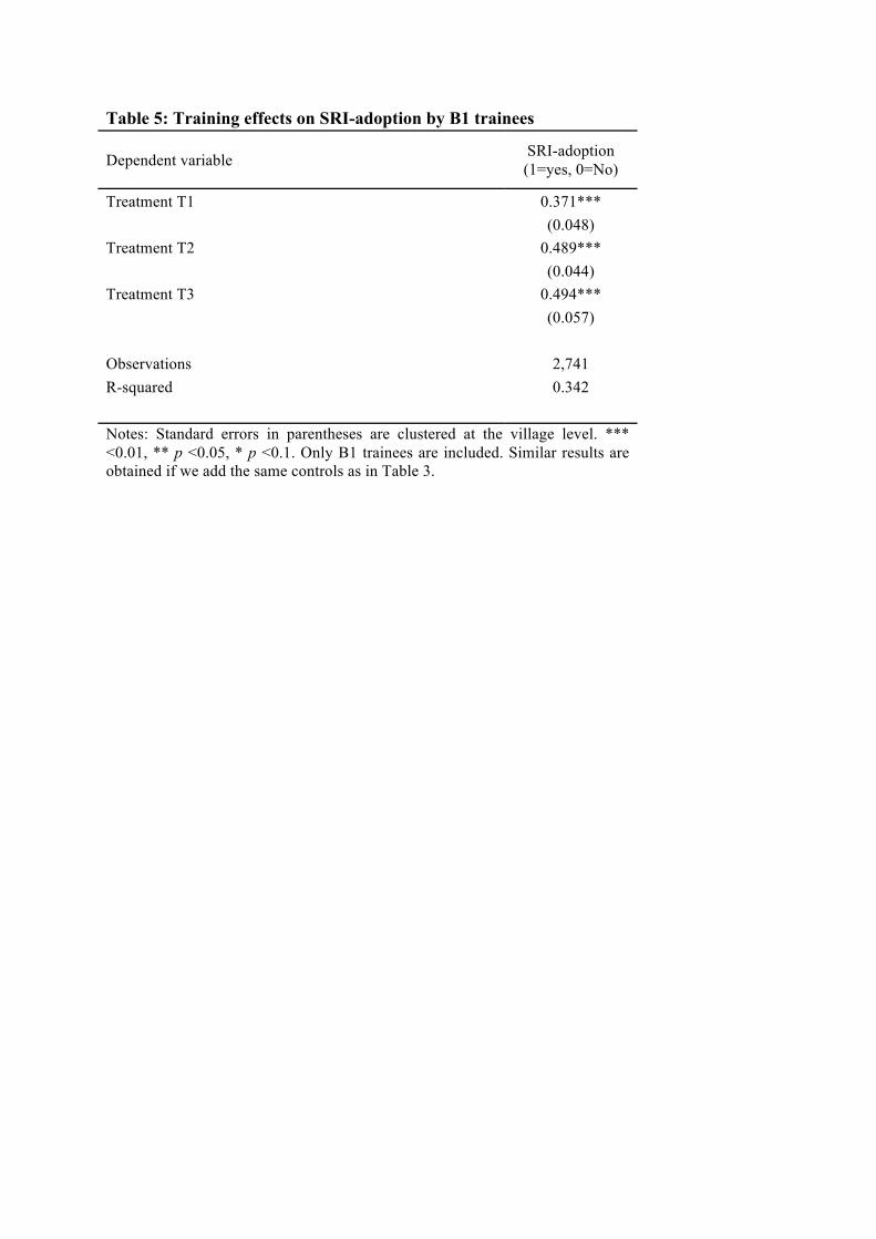
Table 5: Training effects on SRI-adoption by B1 trainees
Dependent variable SRI-adoption (1=yes, 0=No)
Treatment T1 0.371***
(0.048) Treatment T2 0.489***
(0.044) Treatment T3 0.494***
(0.057)
Observations 2,741 R-squared 0.342 Notes: Standard errors in parentheses are clustered at the village level. *** <0.01, ** p <0.05, * p <0.1. Only B1 trainees are included. Similar results are obtained if we add the same controls as in Table 3.

Table 6: Training effects on SRI-adoption by B1 trainees and non-trainees
Dependent variable SRI'(adoption (1=yes, 0=No)
Village Treatment T1 0.077***
(0.014) Village Treatment T2 0.080***
(0.018) Village Treatment T3 0.067***
(0.013) Village Treatment T1 x trainee 0.293***
(0.042) Village Treatment T2 x trainee 0.409***
(0.036) Village Treatment T3 x trainee 0.427***
(0.054)
Observations 3,975 R-squared 0.295 Notes: Standard errors in parentheses are clustered at the village level. *** p<0.01, ** p <0.05, * p <0.1. Includes observations on B1 trainees and non-trainees. B2 trainees are excluded. Similar results are obtained if we add the same controls as in Table 3.

Table 7: Training effects on SRI-adoption by B1 and B2 trainees
Dependent variable SRI-adoption (1=yes, 0=No)
Village Treatment T1 0.371*** (0.048)
Village Treatment T2 0.489*** (0.044)
Village Treatment T3 0.494*** (0.057)
Village Treatment T1 x B2 trainee 0.058 (0.039)
Village Treatment T2 x B2 trainee 0.041 (0.035)
Village Treatment T3 x B2 trainee 0.029 (0.032)
Observations 2,047 R-squared 0.479 Notes: Standard errors in parentheses are clustered at the village level. *** p<0.01, ** p <0.05, * p <0.1. Only B1 and B2 trainees are included. Similar results are obtained if we add the same controls as in Table 3.

Table 8: Training effects on SRI-adoption by B2 trainees Dependent variable SRI-adoption
(1=yes, 0=No)
Treatment T1 0.261**
(0.107) Treatment T2 0.648***
(0.113) Treatment T3 0.451***
(0.168)
Treatment T1 x Ci 0.381*
(0.225) Treatment T2 x Ci -0.237
(0.215) Treatment T3 x Ci 0.122
(0.294)
Observations 885 R-squared 0.501 Notes: Standard errors in parentheses are clustered at the village level. *** p<0.01, ** p <0.05, * p <0.1. Only B2 trainees are included. Similar results are obtained if we add the same controls as in Table 3.

Table 9: Dyadic regression on referral and social proximity Dependent variable Whether B2 trainee as referred by B1 trainee
(1) (2) (3) (4) (5) (6) Socially close 0.011** 0.018** -0.008 0.030* 0.019*** 0.018**
(0.005) (0.008) (0.006) (0.016) (0.005) (0.008) Socially close x Ci -0.022*** -0.022*** -0.025*** 0.022 -0.008 -0.023***
(0.004) (0.004) (0.005) (0.035) (0.01) (0.003)
Socially close x Ci x T2 -0.001 -0.002 -0.001 -0.042 -0.006 -0.001
(0.003) (0.003) (0.004) (0.028) (0.008) (0.002) Socially close x Ci x T3 -0.002 0.00 0.00 -0.032 -0.012* -0.001
(0.003) (0.002) (0.004) (0.026) (0.007) (0.002)
Constant 0.052*** 0.044*** 0.068*** 0.047*** 0.045*** 0.044***
(0.005) (0.008) (0.004) (0.001) (0.002) (0.008)
Observations 21,063 21,063 21,063 21,063 21,063 21,063 R-squared 0.0003 0.0003 0.001 0.002 0.001 0.0003 Notes: Observations include all possible pairs of B1 and B2 trainees in a village. The dependent variable is 1 if the B2 trainee was referred by the B1 trainee. Standard errors in parentheses are clustered at the village level. *** p<0.01, ** p <0.05, * p <0.1. Similar results are obtained if we add the same controls as in Table 3. The meaning of socially close varies across columns: (1) neighbor, friend or has neighboring land; (2) neighbor, friend or close relative; (3) neighbor or friend; (4) close relative; (5) makes social visits each month; (6) discusses agricultural or financial matters with referee.
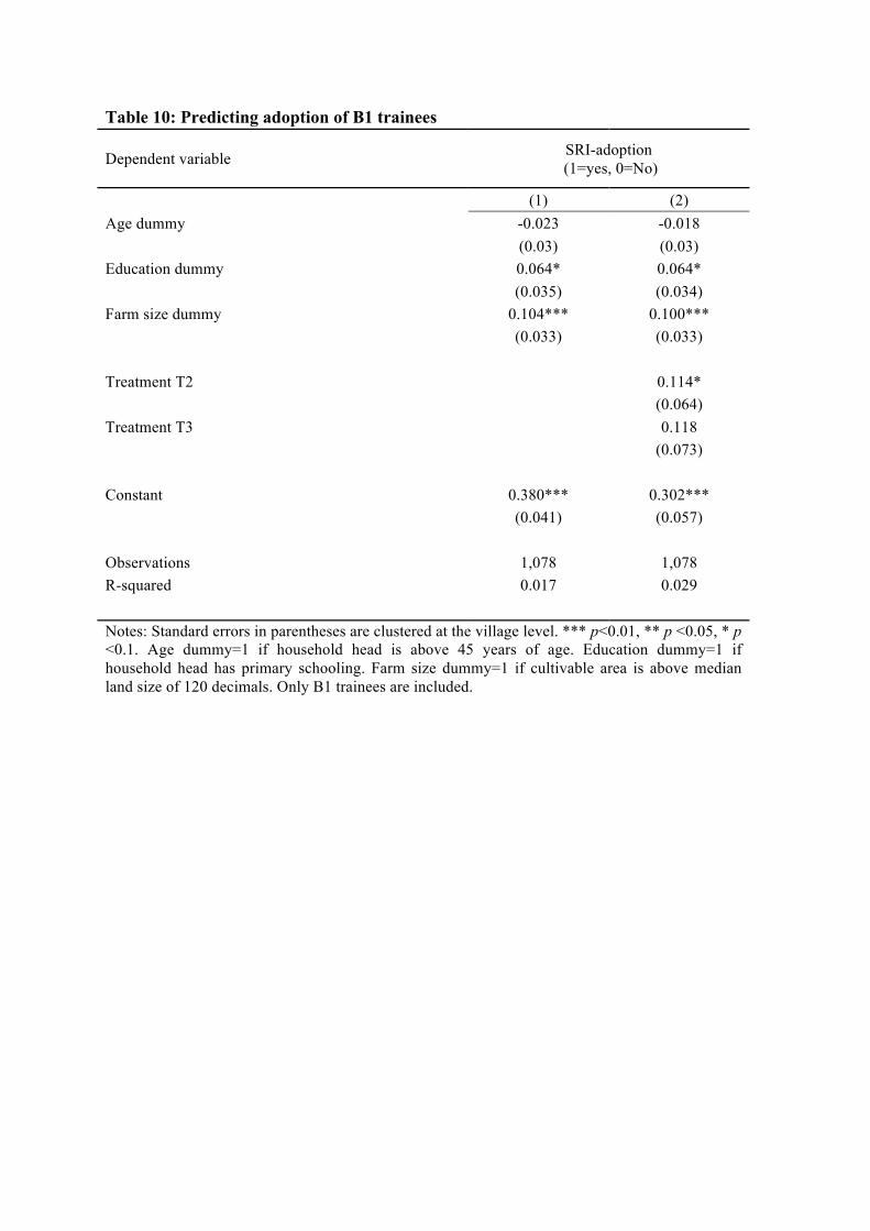
Table 10: Predicting adoption of B1 trainees
Dependent variable SRI-adoption (1=yes, 0=No)
(1) (2) Age dummy -0.023 -0.018
(0.03) (0.03) Education dummy 0.064* 0.064*
(0.035) (0.034) Farm size dummy 0.104*** 0.100***
(0.033) (0.033)
Treatment T2 0.114*
(0.064) Treatment T3 0.118
(0.073)
Constant 0.380*** 0.302***
(0.041) (0.057)
Observations 1,078 1,078 R-squared 0.017 0.029 Notes: Standard errors in parentheses are clustered at the village level. *** p<0.01, ** p <0.05, * p <0.1. Age dummy=1 if household head is above 45 years of age. Education dummy=1 if household head has primary schooling. Farm size dummy=1 if cultivable area is above median land size of 120 decimals. Only B1 trainees are included.

Table 11: Training effects on SRI-adoption by B1 and B2 trainees
Dependent variable SRI-adoption (1=yes, 0=No)
(1) (2) Predicted SRI adoption from Table 10 0.897*** 0.920***
(0.216) (0.207) B2 trainee 0.037*
(0.02) B2 trainee x Treatment T1 0.045
(0.044) B2 trainee x Treatment T2 0.042
(0.043) B2 trainee x Treatment T3 0.022
(0.046) Constant 0.047 0.036
(0.097) (0.094)
Observations 2,047 2,047 R-squared 0.016 0.025 Notes: Standard errors in parentheses are clustered at the village level. *** p<0.01, ** p <0.05, * p <0.1. Observations include B1 and B2 trainees.

Table 12: ITT effect on SRI-adoption of B1 trainees. Dependent variable SRI-adoption
(1=yes, 0=No) Treatment T2 0.118*
(0.065) Treatment T3 0.123
(0.075) Constant 0.371***
(0.048)
Observations 1,078 R-squared 0.013 Notes: Standard errors in parentheses are clustered at the village level. *** p<0.01, ** p <0.05, * p <0.1. Observations include only B1 trainees.
Table 13: Dyadic regression on coordination between referee and referral
Dependent variable Dummy=1 if adoption by referee and referral differ
Referred dummy 0.028 0.023
(0.031) (0.022) Referred dummy x T2 0.005 -0.039
(0.053) (0.038) Referred dummy x T3 -0.112** -0.059**
(0.044) (0.029)
Constant 0.355*** 0.497***
(0.018) (0.002)
Village fixed effects No Yes Observations 8,546 8,546 R-squared 0.001 0.13 Notes: Observations include all possible ij pairs of B1 and B2 trainees in a village. The dependent variable is 1 if the adoption decision of the B2 trainee j differs from the adoption decision of the B1 trainee i (i.e., one adopts and the other does not). The referred dummy =1 if the B2 trainee j was referred by the B1 trainee i. Standard errors in parentheses are clustered at the village level. *** p<0.01, ** p <0.05, * p <0.1.

Table 14: Dyadic regression of correlation in residuals between referee and referral Dependent variable Ui Treatment T1 x Uj 0.008
(0.01) Treatment T2 x Uj -0.006
(0.006) Treatment T3 x Uj -0.010**
(0.005)
Treatment T1 x Uj x Referred dummy 0.009
(0.04) Treatment T2 x Uj x Referred dummy 0.053
(0.06) Treatment T3 x Uj x Referred dummy 0.081*
(0.043)
Village Fixed Effects Yes Observations 8,546 R-squared 0.347 Notes: Observations include all possible ij pairs of B1 and B2 trainees in a village. Ui and Uj are estimated residual from a predictive regression similar to that presented in Table 10 that includes B1 and B2 trainees. Regressors include: Age dummy=1 if household head is above 45 years of age; Education dummy=1 if household head has primary schooling; Farm size dummy=1 if cultivable area is above median land size of 120 decimals; and Treatment dummies T1, T2 and T3. As in Table 13, the referred dummy =1 if the B2 trainee j was referred by the B1 trainee i. Standard errors in parentheses are clustered at the village level. *** p<0.01, ** p <0.05, * p <0.1.

Table 15. Imputed change for additional adopters induced by treatments T2 and T3
Dependent variable Yield in Kg Revenue per area
Hired labour per
area
Total labour cost per
area
Total cost per area
Total cost per area
(including family labour)
Estimated profit per
area
Estimated profit per
area (including
family labour)
Treatment T2 6 -19 -338 -449 -593 -663 512 583
Treatment T3 -2 -242 -144 -227 -252 -286 -17 32
Note: Calculated from Tables 3 and 4 using formula (5.4) -- see paper for details. Revenue, cost and profit values are in BDT in per decimal terms.

Table 16. Persistence of adoption at second endline Dependent variable SRI adoption (1=yes, 0=No) at second endline
Treatment T1 0.298*** 0.301*** 0.408*** 0.409*** 0.415*** 0.417***
-0.052 -0.051 -0.066 -0.065 -0.063 -0.063
Treatment T2 0.209*** 0.210*** 0.302*** 0.301*** 0.310*** 0.311***
-0.041 -0.041 -0.073 -0.072 -0.062 -0.062
Treatment T3 0.299*** 0.299*** 0.466*** 0.466*** 0.428*** 0.428***
-0.045 -0.043 -0.063 -0.063 -0.055 -0.054
Sample All All B1 B1 B1&B2 B1&B2
Controls No Yes No Yes No Yes
Observations 2,753 2,753 1,856 1,856 2,242 2,242
R-squared 0.17 0.173 0.349 0.351 0.296 0.299
Notes: Includes all control villages plus 60 treated villages revisited a year after the first endline. Estimator is linear probability model. Standard errors in parenthesis are clustered at the village level. *** p<0.01, ** p<0.05, * p<0.1. Baseline adoption in control villages is 0. Controls include: age dummy if household head is above 45 years of age; education dummy household head has primary schooling; farm size dummy if cultivable area is above median land size of 120 decimals.

Appendix Table 1: Attrition by Treatment Status: Balancedness Panel A: All farmers Control All Treatment farmers p-value
Overall T1 T2 T3 (1) (2) (3) (4) Average age of the household (above 15 years) 37.01 37.1 37.59 36.21 37.14
0.9 0.18 0.65 0.42
Average education of the household 4.36 4.55 4.7 4.31 4.56
0.41 0.28 0.66 0.48 Cultivable farm area in last Boro season (decimals) 141.52 141.03 150.4 126.42 139.95
0.97 0.22 0.59 0.45
Household size 4.68 4.93 4.72 4.98 5.2
0.16 0.31 0.08 0.48 Maximum education of any household member 8.56 8.78 8.99 8.24 8.92
0.53 0.15 0.87 0.2
Working age members in the household 2.91 3.04 2.91 3.17 3.13
0.27 0.12 0.23 0.83 No. of observations 193 359 156 92 111 Notes: Reported p-values are for a two-tailed test of the null hypothesis that group means are equal. Column 1 compares controls to all treatment farmers; column 2 compares T1 and T2 farmers; column 3 compares T1 and T3 farmers; column 4 compares T2 and T3 farmers.

Figure 1: Proportion of farmers available to be referred by each B1 farmer (% of the village sample)
0.5
11.
52
2.5
Den
sity
0 .2 .4 .6 .8 1Freedom of choice of referee
kernel = epanechnikov, bandwidth = 0.05

Figure 2: Targeting and incentives
0%
10%
20%
30%
40%
50%
60%
70%
0 0.1 0.2 0.3 0.4 0.5 0.6 0.7 0.8
Pred
icte
d pr
obab
ility
of a
dopt
ion
Ci = Freedom of choice of referee
T1 T2 T3
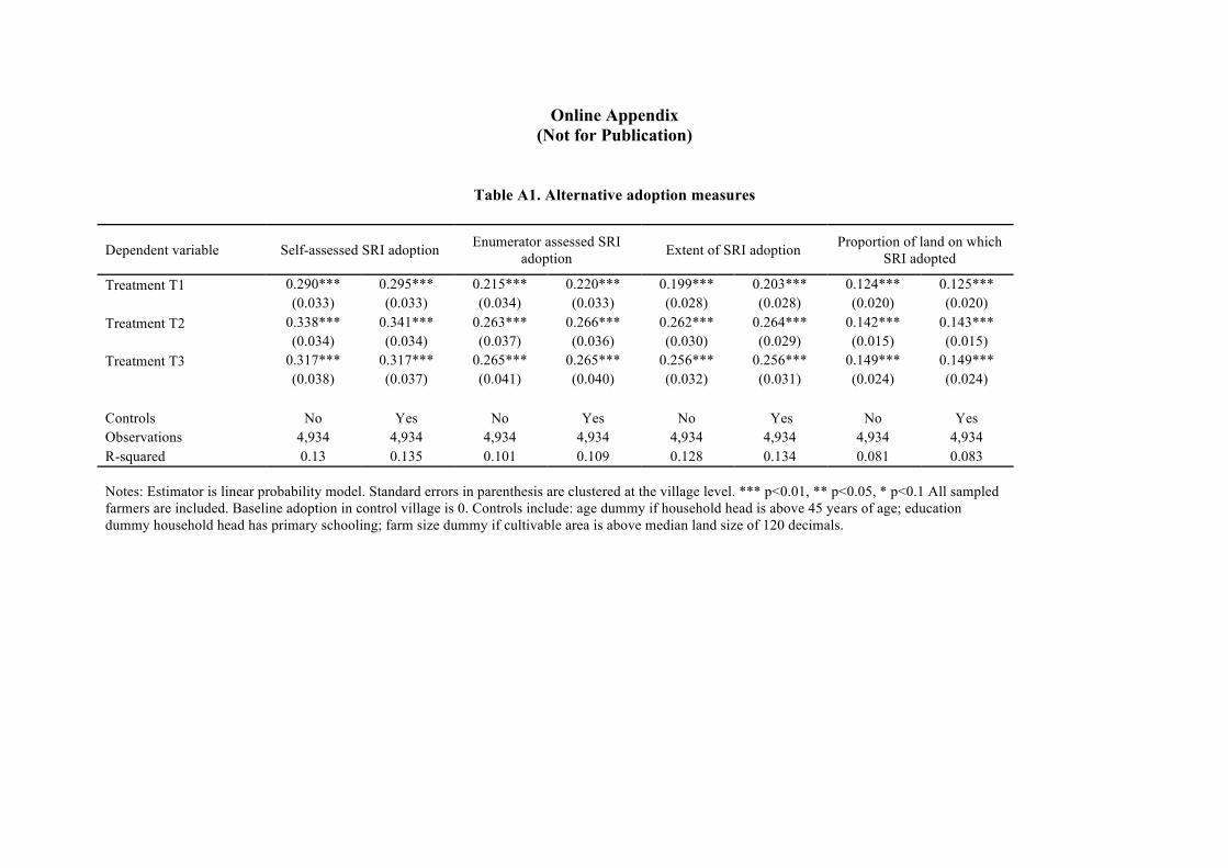
Online Appendix (Not for Publication)
Table A1. Alternative adoption measures
Dependent variable Self-assessed SRI adoption Enumerator assessed SRI adoption Extent of SRI adoption Proportion of land on which
SRI adopted
Treatment T1 0.290*** 0.295*** 0.215*** 0.220*** 0.199*** 0.203*** 0.124*** 0.125***
(0.033) (0.033) (0.034) (0.033) (0.028) (0.028) (0.020) (0.020)
Treatment T2 0.338*** 0.341*** 0.263*** 0.266*** 0.262*** 0.264*** 0.142*** 0.143***
(0.034) (0.034) (0.037) (0.036) (0.030) (0.029) (0.015) (0.015)
Treatment T3 0.317*** 0.317*** 0.265*** 0.265*** 0.256*** 0.256*** 0.149*** 0.149***
(0.038) (0.037) (0.041) (0.040) (0.032) (0.031) (0.024) (0.024)
Controls No Yes No Yes No Yes No Yes Observations 4,934 4,934 4,934 4,934 4,934 4,934 4,934 4,934 R-squared 0.13 0.135 0.101 0.109 0.128 0.134 0.081 0.083
Notes: Estimator is linear probability model. Standard errors in parenthesis are clustered at the village level. *** p<0.01, ** p<0.05, * p<0.1 All sampled farmers are included. Baseline adoption in control village is 0. Controls include: age dummy if household head is above 45 years of age; education dummy household head has primary schooling; farm size dummy if cultivable area is above median land size of 120 decimals.

Table A2a. LATE treatment effect on agricultural performance per area -- All farmers
Yield in
kg Revenue from grain per area
Input cost per area
Hired labour per area
Total labour cost per area
Total cost per area
Total cost per area (including family
labour)
Estimated profit per area
Estimated profit per area (including family labour)
Panel A SRI adoption 11.867*** 392.930*** 33.138*** 56.344* 99.452*** 84.007** 133.980*** 296.105*** 252.633*** (1.601) (54.247) (12.542) (28.809) (27.522) (40.074) (37.608) (51.995) (57.201) Baseline value 0.217*** 0.199*** 0.010 0.226*** 0.033** 0.032* 0.012 0.034** 0.057*** (0.031) (0.026) (0.009) (0.027) (0.017) (0.018) (0.012) (0.016) (0.017) Pane B SRI adoption_T1 13.103*** 468.592*** 62.992*** 107.777** 176.032*** 174.053*** 241.223*** 287.895*** 226.598** (2.776) (100.279) (18.276) (46.986) (44.340) (64.955) (59.300) (85.001) (101.675) SRI adoption_T2 12.078*** 385.691*** 10.244 22.645 56.308* 26.068 67.630 341.039*** 304.645*** (2.023) (66.991) (14.765) (31.919) (30.341) (45.304) (42.435) (59.869) (72.387) SRI adoption_T3 11.013*** 364.659*** 46.338*** 69.529* 114.259*** 108.944* 162.388*** 247.040*** 203.107** (2.670) (96.124) (17.489) (39.956) (36.892) (56.672) (51.282) (78.151) (85.167) Baseline value 0.219*** 0.200*** 0.007 0.222*** 0.028* 0.028 0.007 0.032** 0.055*** (0.031) (0.027) (0.008) (0.029) (0.016) (0.019) (0.011) (0.016) (0.017) Baseline value in control villages
22.61 866.10 214.13 199.10 296.28 413.23 510.41 452.87 355.69
Notes: sample includes all farmers in Treatment (batch 1+batch2+untreated) and control group (N=4763). Treatment status of a village is used as an instrument for adoption. Each column in each panel reports separate regressions. Panel A reports the overall effects of adoption, while panel B reports the effects of adoption by treatment status of the villages. Standard errors in parentheses are clustered at the village level. *** p<0.01, ** p<0.05, * p<0.1. All dependent variables are measured at endline and expressed in quantity or value per decimal. Input costs include seed, urea, pesticide, etc. Labor costs include both hired and contractual labour. Family labor cost is calculated at the same wage rate as hired labor. Total cost combines input and labor costs. All values are in BDT.

Table A2b. LATE treatment effect on agricultural performance per area -- B1 farmers only Variables of Interest Yield in
kg Revenue from grain per area
Input cost per area
Hired labour per area
Total labour cost per area
Total cost per area
Total cost per area (including family
labour)
Estimated profit per area
Estimated profit per area (including family labour)
Panel A SRI adoption 10.033*** 330.450*** 28.083*** 47.332** 98.426*** 71.066** 127.323*** 249.888*** 195.217*** (1.199) (40.867) (9.428) (21.751) (22.631) (30.123) (29.897) (39.901) (43.251) Baseline value 0.165*** 0.175*** 0.017* 0.218*** 0.014 0.037* 0.005 0.012 0.019 (0.030) (0.025) (0.009) (0.036) (0.023) (0.020) (0.014) (0.019) (0.018) Panel B SRI adoption_T1 12.238*** 429.214*** 55.885*** 89.004** 165.897*** 148.233*** 221.910*** 278.176*** 204.743** (2.271) (80.314) (15.069) (40.193) (42.533) (55.325) (54.365) (68.899) (81.677) SRI adoption_T2 10.200*** 323.788*** 2.766 11.874 58.094** 8.106 61.348 302.256*** 249.832*** (1.389) (46.279) (11.575) (25.072) (28.345) (35.130) (37.445) (43.807) (54.601) SRI adoption_T3 8.771*** 288.897*** 40.763*** 63.346** 107.606*** 98.878** 149.645*** 181.309*** 133.650** (2.010) (71.772) (12.718) (29.408) (30.308) (41.011) (39.786) (60.374) (64.576) Baseline value 0.166*** 0.176*** 0.016* 0.215*** 0.011 0.035* 0.003 0.012 0.019 (0.031) (0.025) (0.009) (0.037) (0.022) (0.019) (0.013) (0.019) (0.018) Baseline value in control villages
22.61 866.10 214.13 199.10 296.28 413.23 510.41 452.87 355.69
Notes: as in table A2a. Sample includes only batch 1 farmers from treatment villages and all farmers from control villages (N=2654)

Table A2c. LATE treatment effect on agricultural performance per area -- B2 farmers only Variables of Interest
Yield in kg
Revenue from grain per area
Input cost per area
Hired labour per area
Total labour cost per area
Total cost per area
Total cost per area (including family
labour)
Estimated profit per area
Estimated profit per area (including family labour)
Panel A SRI adoption 8.974*** 287.737*** 24.601*** 26.292 102.033*** 46.710* 127.170*** 233.211*** 153.648*** (1.166) (38.187) (8.419) (19.347) (19.764) (26.933) (26.281) (37.017) (38.498) Baseline value 0.154*** 0.164*** 0.017** 0.212*** 0.009 0.035** 0.005 -0.000 0.007 (0.031) (0.025) (0.008) (0.034) (0.021) (0.018) (0.012) (0.020) (0.018) Panel B SRI adoption_T1 9.653*** 343.086*** 44.295*** 64.040** 155.231*** 108.888** 200.073*** 224.084*** 134.637* (1.945) (67.188) (13.884) (32.430) (35.788) (44.632) (46.572) (62.729) (75.247) SRI adoption_T2 8.950*** 273.044*** 11.277 6.007 81.559*** 8.946 92.834*** 255.973*** 170.915*** (1.609) (50.819) (9.499) (22.641) (21.785) (31.220) (29.027) (45.287) (50.097) SRI adoption_T3 8.610*** 272.218*** 28.087** 26.271 94.510*** 52.418 123.814*** 213.744*** 145.457** (1.957) (66.404) (12.165) (25.499) (27.477) (37.358) (37.050) (57.827) (58.489) Baseline value 0.155*** 0.164*** 0.015* 0.210*** 0.005 0.031* 0.002 -0.001 0.006 (0.031) (0.025) (0.008) (0.035) (0.021) (0.019) (0.012) (0.020) (0.018) Baseline value in control villages
22.61 866.10 214.13 199.10 296.28 413.23 510.41 452.87 355.69
Notes: as in table A2a. Sample includes only batch 2 farmers from treatment villages and all farmers from control villages (N=2556)

Table A2d. LATE treatment effect on agricultural performance per area -- B1 and B2 farmers only Variables of Interest
Yield in kg
Revenue from grain per area
Input cost per area
Hired labour per area
Total labour cost per area
Total cost per area
Total cost per area (including family
labour)
Estimated profit per area
Estimated profit per area (including family labour)
SRI adoption 9.444*** 307.713*** 25.558*** 35.876* 97.023*** 56.333** 123.716*** 242.667*** 178.003*** (1.153) (38.631) (8.737) (20.148) (20.320) (28.132) (27.213) (37.542) (40.009) Baseline value 0.194*** 0.183*** 0.012 0.231*** 0.031 0.041** 0.011 0.020 0.034** (0.032) (0.026) (0.009) (0.031) (0.020) (0.019) (0.013) (0.018) (0.017) SRI adoption_T1 10.962*** 386.978*** 50.061*** 76.438** 159.375*** 128.584*** 210.768*** 252.079*** 172.151** (1.981) (70.061) (13.741) (34.484) (36.814) (48.041) (47.876) (62.259) (75.211) SRI adoption_T2 9.551*** 299.703*** 6.981 9.590 69.159*** 8.652 76.797** 279.658*** 212.725*** (1.436) (46.795) (10.171) (23.327) (22.893) (32.489) (31.017) (42.693) (49.878) SRI adoption_T3 8.644*** 281.014*** 34.824*** 44.980* 99.785*** 75.477* 136.197*** 198.766*** 143.009** (1.923) (67.518) (12.071) (26.947) (27.974) (38.761) (37.700) (57.296) (60.275) Baseline value 0.196*** 0.185*** 0.009 0.227*** 0.026 0.036* 0.006 0.019 0.033* (0.032) (0.027) (0.009) (0.032) (0.019) (0.020) (0.012) (0.018) (0.017) Baseline value in control villages
22.61 866.10 214.13 199.10 296.28 413.23 510.41 452.87 355.69
Notes: as in table A2a. Sample excludes untreated farmers from treatment villages. It includes only batch 1 and batch 2 farmers from treatment villages and all farmers from control villages (N=3594)