Can Rationing Affect Long Run Behavior?Evidence from Brazil

Francisco JM Costa∗

June 13, 2013

Abstract

I examine whether a temporary policy can affect long-run household behavior.I look at evidence from a nine-month compulsory rationing imposed on Brazilianhouseholds’ electricity use in 2001, exploiting differences in the policy’s implemen-tation across regions as a quasi-experiment to test its short-and long-run impactson households’ electricity consumption patterns. I find that the rationing programled to a persistent reduction in electricity use of 14% even ten years later. Uniquehousehold level microdata on appliance ownership and consumption habits suggestthat the main source of persistence is changes in the utilization of electricity ser-vices, rather than technology adoption.JEL Codes: D12, O13, Q41, Q48.Keywords: electricity, rationing, persistence, energy efficiency.

∗Department of Economics and STICERD, London School of Economics, Houghton Street, LondonWC2A 2AE, United Kingdom, F.J.Costa@lse.ac.uk. Acknowledgements: I am grateful to Gharad Bryan,Robin Burgess, Greg Fischer, Maitreesh Ghatak, Gilat Levy, and Gerard Padró i Miquel for their adviceand encouragement. I appreciate the discussions with Maximilian Auffhammer, Michael Best, Ben Faber,Cláudio Ferraz, Frederico Finan, Jason Garred, Jerry Hausman, Matthew Kahn, Ralf Martin, EmilioMatsumura, Mushfiq Mobarak, Emerson Salvador, Daniela Scur, my colleagues at LSE, and seminarparticipants at LSE, PacDev 2012, EEA 2012, EconCon 2012, Behavioral Environmental Economics(Toulouse), PSE, University of Cambridge (EPRG), IFS (EDePo), Thema, LBS, Granthan Institute forClimate Change, UC Berkeley (ERG), ASU (WP Carey), University of Chicago (Harris School), WorldBank (Dime and DRG), IADB, EPGE/FGV, Puc-Rio, FEA/USP, and University of Bristol. I also thankANEEL, PROCEL, and IBRE/FGV for providing data. A very preliminary version of this paper begancirculating in December 2011 with the title "Just Do It: Temporary Restrictions and New ConsumptionHabits".

A whole class of economic models has multiple steady states. A common featureof these models is that temporary interventions can have long run effects by makingindividuals switch steady states. In policy terms, the possibility of addressing long runissues with temporary policies, rather than with permanent interventions, is appealingsince it might only require transitory investments and would not necessarily be relianton long term commitment of policy makers. Although the associated debate goes backas far as Rosenstein-Rodan (1943), the feasibility of using temporary interventions togenerate such sustainable effects on individual behavior is still contentious as it lackssupporting empirical evidence. This paper presents a temporary intervention which hadlasting impacts on households’ behavior towards energy consumption.

The empirical literature shows that small interventions, such as nudges, affect indi-vidual behavior in the short run, but with limited long run effects, which is consistentwith standard multiple-steady-state models.1 On the other hand, persistent effects ofmajor historical episodes have been observed,2 suggesting that specific events can placeotherwise identical economic agents in different steady states. It is therefore still anopen question whether it is possible to use policy to induce long-run behavioral changes.Recent field experiments designed specifically to investigate this question have reacheddivergent conclusions. While Giné et al. (2010) and Dupas (2012) find that temporaryprograms can still affect individuals’ health consumption patterns one year later, Kremerand Miguel (2007) finds that replacing subsidies with sustainable health control measureswere ineffective.

The main contribution of this paper is to provide empirical evidence that a temporarypolicy - electricity rationing - can affect long run household behavior. I look at evidencefrom a rationing program in Brazil in 2001-2002, when households had to reduce elec-tricity use by at least 20% for nine months. This episode is of particular interest forthe above debate because it was a large demand response program which was limited tocertain regions due to a combination of weather conditions and infrastructure constraints,generating a credible counterfactual. Evidence from administrative data suggest that theaverage household reduced electricity use by 14% in the long run - ten years later - byswitching to a less energy-intensive steady state.

I first present a simple theoretical framework in which individual consumption opti-mization leads to multiple steady states. In theory, this multiplicity could emerge frommany mechanisms, such as habits, beliefs, social norms, reference-dependency, or learn-ing.3 For example, biased beliefs about the returns to investing in energy-efficiency could

1See Charness and Gneezy (2009), Thogersen (2009), Allcott and Mullainathan (2010), Acland andLevy (2011), Agarwal et al. (2011), Ferraro and Price (2011), John et al. (2011), Haselhuhn et al. (2012),or Gneezy et al. (2011) for a survey.

2See Bloom et al. (2003), Redding et al. (2010), Dell (2010), Acemoglu et al. (2012), and Bleakleyand Lin (2012).

3For example, Naik and Moore (1996), Piketty (1995), Obstfeld (1984), Koszegi and Rabin (2006),

1

sustain different levels of energy efficiency, or social norms could affect household electric-ity use (Allcott 2011a, 2011b). The model presented illustrates this class of phenomenausing a simple mechanism: intertemporal complementarity of consumption (Becker andMurphy 1988). In this model, the past level of electricity use affects the individual’s cur-rent utility from consuming electricity services. For example, the more one uses electricalappliances in the past, the bigger the disutility from not having access to their servicesin the present.

I then examine the Brazilian electricity rationing episode of 2001 in order to testwhether this induced switching between steady states in consumption. In the beginningof 2001 the electricity generation capacity of some Brazilian states was severely reduceddue to extremely low stream-flow level in the rivers that serve the hydroelectric power-plants in these states. Since the Brazilian electricity system is partitioned, it was notpossible to reallocate electricity between regions. In order to prevent general blackouts,the government planned and implemented an emergency rationing program for the af-fected regions within a couple of months.4 In June 2001, households in the Southeast andMidwest were asked to reduce electricity consumption by 20% relative to their historicalaverage consumption for a period of nine months. Households were subject to fines andthe threat of supply interruption if they did not meet their targets, and received bonusesfor additional energy saved. At the same time, the government issued a national infor-mation campaign, and introduced subsidies to energy-efficient appliances countrywide.After the end of the program in February 2002, electricity supply and prices went backto normal.

To estimate the rationing’s impact on final household electricity consumption, I use apanel of average household electricity use and price by utility company, monthly from 1991to 2011. This is administrative data from the Brazilian Electricity Regulatory Agency(ANEEL). The main empirical strategy of this paper is a difference-in-differences spec-ification using households in the non-rationed states in the South of Brazil as a controlgroup for the rationed households in the Southeast/Midwest. Under the assumption thathouseholds’ electricity use in these regions would otherwise have followed a common trendduring the period studied, the estimated regression coefficients can be interpreted as theaverage effect of the treatment on the treated.5

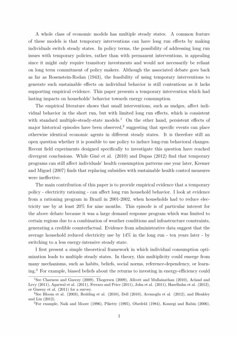
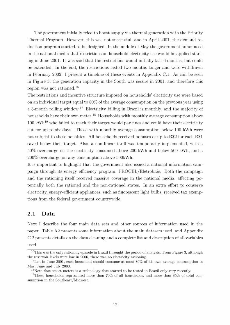
Figure 1 presents the monthly average household electricity consumption, relative to

and Lindbeck (1997).4The rationing was a sudden change in government strategy, and as such was fairly unexpected by

households. The electricity shortage was detected in March 2001. Until May, the government tried tosolve the problem with other measures, such as pure price schemes and increasing the generation capacityof thermal power plants.

5The Northeast region was rationed as well. However, as discussed in Section 2, the Northern stateswere at a very different initial development stage, and experienced a substantially different growth patternduring the 2000s. The common trend assumption required for identification thus does not hold for theseregions. The main results still hold when all states are included in the analysis.

2

Rationing.6.7

.8.9

11.

11.

2

1991m1 1993m7 1996m1 1998m7 2001m1 2003m7 2006m1 2008m7 2011m1

South (Control) Southeast/Midwest (Rationed)

Avg.

Hou

seho

ld E

lect

. Use

(bas

e Ja

n/20

01)

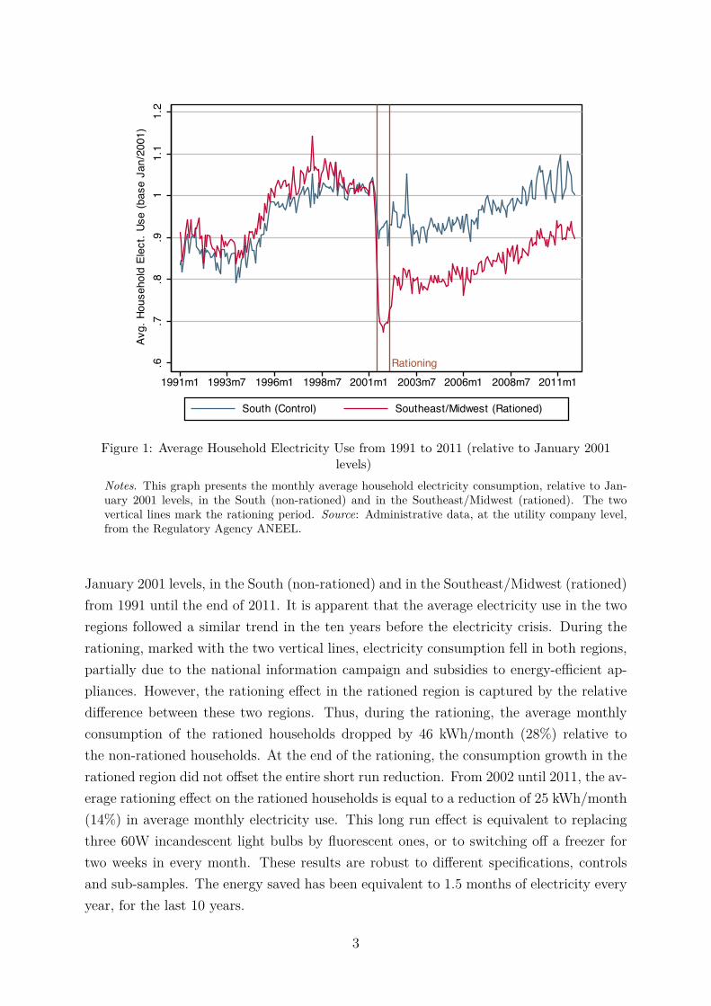
Figure 1: Average Household Electricity Use from 1991 to 2011 (relative to January 2001levels)

Notes. This graph presents the monthly average household electricity consumption, relative to Jan-uary 2001 levels, in the South (non-rationed) and in the Southeast/Midwest (rationed). The twovertical lines mark the rationing period. Source: Administrative data, at the utility company level,from the Regulatory Agency ANEEL.

January 2001 levels, in the South (non-rationed) and in the Southeast/Midwest (rationed)from 1991 until the end of 2011. It is apparent that the average electricity use in the tworegions followed a similar trend in the ten years before the electricity crisis. During therationing, marked with the two vertical lines, electricity consumption fell in both regions,partially due to the national information campaign and subsidies to energy-efficient ap-pliances. However, the rationing effect in the rationed region is captured by the relativedifference between these two regions. Thus, during the rationing, the average monthlyconsumption of the rationed households dropped by 46 kWh/month (28%) relative tothe non-rationed households. At the end of the rationing, the consumption growth in therationed region did not offset the entire short run reduction. From 2002 until 2011, the av-erage rationing effect on the rationed households is equal to a reduction of 25 kWh/month(14%) in average monthly electricity use. This long run effect is equivalent to replacingthree 60W incandescent light bulbs by fluorescent ones, or to switching off a freezer fortwo weeks in every month. These results are robust to different specifications, controlsand sub-samples. The energy saved has been equivalent to 1.5 months of electricity everyyear, for the last 10 years.

3

This persistent change gives some evidence that households settled into a new steadystate with lower consumption levels after the rationing. Two non-competing mechanismscould be underlying this long run energy conservation: households could have changedhow they use electrical appliances, and/or acquired more energy efficient appliances. Itis important to distinguish these two channels because they relate to different economicmodels, and would have different policy interpretations. I use household level microdatato shed light on the channels supporting the long run reduction in electricity use.

To investigate the consumption habits channel, I exploit household level microdatafrom a survey of the appliance holdings and consumption habits of over eleven thousandfamilies conducted by the Brazilian energy efficiency program PROCEL in 1998/1999and 2004/2005. The picture emerging from this dataset supports the hypothesis thathouseholds actually changed the way they use electric appliances. Even three years afterthe rationing, I still find that rationed households maintain the thermostats of showerheads with electric heating at a lower level, and weakly use fewer freezers, relative tonon-rationed households. These two results by themselves could account for all of theobserved long run energy conservation in the Southeast/Midwest.

To assess if the energy-efficiency level of the inventory of appliances in these tworegions is underlying the long run energy conservation, I use a second household leveldataset of more than fifty thousand families from the Brazilian Geography & StatisticsInstitute (IBGE) from the three points in time 1996/1997, 2002/2003, and 2008/2009.This microdata suggests that the difference in composition of appliances between thetwo regions did not change substantially in the long run. During the rationing, affectedhouseholds seem to have substituted old refrigerators and postponed investment in newfreezers and air conditioners. By 2008-2009, however, I find no effect on the averagestock of appliances - both quantity and vintage.6 To rationalize these findings, I presentin Appendix A an extended version of the baseline model, adding endogenous choice ofappliances’ characteristic as in Dubin and McFadden (1984).

Taken together, this is evidence that households adopted new consumption behaviorsduring the rationing, shifting to a new stable steady state with lower electricity use.7

The identification of long run impacts obviously faces important challenges, namely: (i)omitted variables that lead to endogeneity between the outcome variables and the imple-mentation of the rationing, (ii) initial cross-sectional differences, and (iii) divergence inthe time series and potential general equilibrium effects that may emerge over the years.

6I also find no effect on the average size of appliances. Further, I use microdata on appliances’ pricescollected in stores in both regions to assess the models of the appliances available in the shelves in theseregions. As discussed in Appendix C.1, products available in the stores of the Southeast/Midwest becamemore likely to be available in the stores of the South after 2001.

7Time series analysis indicates that there is a structural break in electricity demand in 2001 (Maciel etal. 2009). In a paper not being circulated, Mation and Ferraz (2011) analyze the effects of the electricitycrisis on firms’ productivity.

4

I address each issue in turn in Section 3.This paper relates to different strands of the literature. First, it highlights the crucial

importance of considering human behavior when designing energy and environmentalpolicies. This is particularly related to the “energy efficiency gap” debate, which focuseson the difference between the available cost-effective, energy-efficient technologies andthose actually adopted by consumers. Engineering analyses of the performance of differenttechnologies estimates this gap to be worth over US$1.2 trillion in the US (McKinsey &Co. 2009). However, how people use new technologies needs to be taken into account inthis calculation (Allcott and Greenstone 2012). A field experiment in Mexico shows thathouseholds increase final electricity use when old appliances are replaced by new energy-efficient ones (Davis et al. 2012). In the Brazilian case, most of the energy conservationafter rationing seems to come from the utilization margin, which again suggests that wecannot discuss an “energy efficiency gap” without considering its behavioral counterpart.

This paper also forms part of a wider literature on the economics of energy conser-vation. It has been shown that demand response programs are a promising avenue forpromoting energy conservation. For example, Reiss and White (2008) show that publicappeals during the 2000 California energy crisis led to a short run reduction of 7% inhousehold electricity use. Allcott and Rogers (2012) find that households who receiveenergy conservation information by mail for two years maintain a 2% lower electricity useup to two years after the last letter.8

In a closely related paper, Gerard (2012) also analyzes the impact of the 2001 Brazilianelectricity crisis on short and long run households’ electricity use. Gerard concentrates onunderstanding whether the impact of the rationing is consistent with a calibrated modelof consumer behavior. In contrast, my work concentrates on disentangling the mecha-nisms underlying the long run energy conservation and I make use of richer householdlevel microdata on consumer behavior, paired with a difference-in-differences strategy, toundertake this analysis. The two papers should be considered complementary.

The paper is organized as follows: I present the basic theoretical framework in Section1. In Section 2 I describe the background and the data. In Section 3 I present theempirical methods and the results on electricity use. Section 4 examines the channels ofpersistence, consumption habits and stocks of appliances. Section 5 concludes.9

8Others include Allcott and Mullainathan 2010), Allcott (2011b), Costa and Kahn (2011), Leightyand Meier (2011), and Jessoe and Rapson (2012).

9Appendix A presents an extended version of the theoretical framework in Section 1, and AppendixB contains further empirical results. Online Appendix C presents the timeline of events, describes thedata cleaning, and contains other specifications and robustness.

5

1 Theoretical Framework

This section outlines a simple model that illustrates how temporary restrictions can gener-ate long run effects when multiple steady states exist. In this model, multiplicity emergesas a consequence of intertemporal complementarity of consumption, as in Becker andMurphy (1988). In order to derive further relevant predictions, Appendix A presents anextended version of the model which explicitly accounts for strategic investment in ap-pliances’ efficiency. In particular, I extend the classic tow-stage discrete choice model ofDubin and McFadden (1984) into a dynamic model where intertemporal complementar-ity of consumption generates multiple steady states. It is worthy to reiterate that thismultiplicity could emerge from many mechanisms, which would lead to the same observ-able outcome in the context of the Brazilian electricity rationing. The model presentedillustrates this class of phenomena using one simple mechanism.

Suppose an infinitely lived individual, with exponential time discount factor β < 1.Every period the individual chooses ordinary consumption, ct, and services from electric-ity, et. Assume preferences are such that electricity services consumed at different pointsin time are complements, as in Becker and Murphy (1988). That is, the individual’s cur-rent utility is represented by u(ct, et, st), where st captures the past electricity use relevantfor current utility. This stock of past electricity use evolves according to st+1 = δst + et,where δ < 1 is depreciation in the stock of past consumption. Assume that u is strictlyconcave in c and e, and that uc > 0, ue > 0 for all c, e, s ≥ 0.

Assumption 1. Current and past consumption of electricity services are complements,that is, ues > 0 for all c, e, s ≥ 0.

This assumption introduces some path dependency to the utility derived from theutilization of electricity services. It means that the higher the past electricity utilization,the higher the marginal utility of current utilization. For example, the more one useselectrical appliances, the greater the disutility from not having access to their services.Assume that the individual is fully aware of her preferences, and maximizes utility takinginto account that her current choices affect the marginal utility of her future consumptionchoices.

Assume that the individual has fixed income y in every period, the price of ordinaryconsumption is normalized to 1, and the electricity price is p. Suppose also that thereis no credit market.10 Then, the individual solves the following dynamic optimization

10The results are not affected if we assume a perfect credit market with interest rate R−1 = β.

6

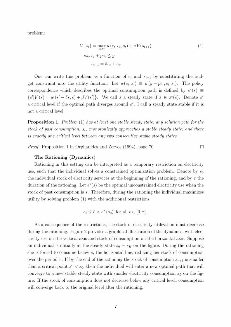
problem:

V (st) = maxct,et

u (ct, et, st) + βV (st+1) (1)

s.t. ct + pet ≤ y

st+1 = δst + et.

One can write this problem as a function of et and st+1 by substituting the bud-get constraint into the utility function. Let w(et, st) ≡ u (y − pet, et, st). The policycorrespondence which describes the optimal consumption path is defined by s∗(s) ≡{s′|V (s) = w (s′ − δs, s) + βV (s′)}. We call s a steady state if s ∈ s∗(s). Denote sc

a critical level if the optimal path diverges around sc. I call a steady state stable if it isnot a critical level.

Proposition 1. Problem (1) has at least one stable steady state; any solution path for thestock of past consumption, st, monotonically approaches a stable steady state; and thereis exactly one critical level between any two consecutive stable steady states.

Proof. Proposition 1 in Orphanides and Zervos (1994), page 70.

The Rationing (Dynamics)Rationing in this setting can be interpreted as a temporary restriction on electricity

use, such that the individual solves a constrained optimization problem. Denote by s0

the individual stock of electricity services at the beginning of the rationing, and by τ theduration of the rationing. Let e∗(s) be the optimal unconstrained electricity use when thestock of past consumption is s. Therefore, during the rationing the individual maximizesutility by solving problem (1) with the additional restrictions

et ≤ e < e∗ (s0) for all t ∈ [0, τ ] .

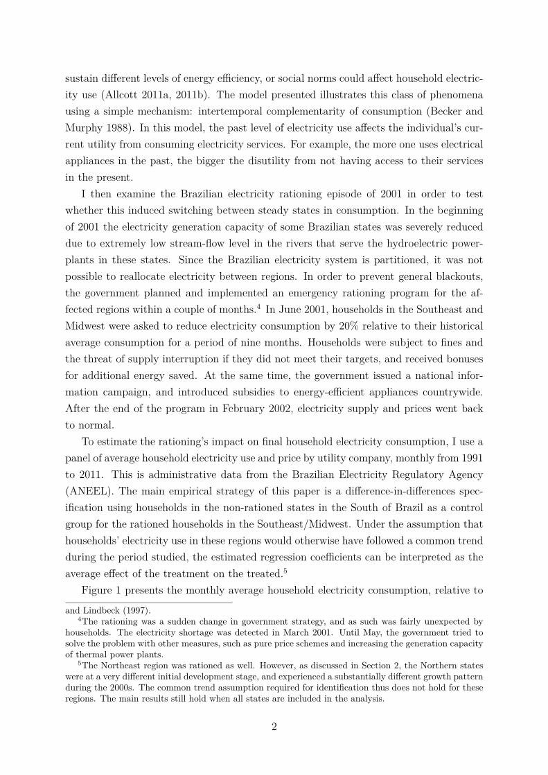
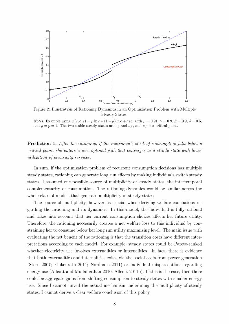
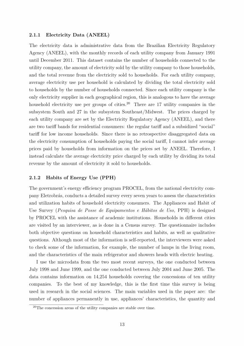
As a consequence of the restrictions, the stock of electricity utilization must decreaseduring the rationing. Figure 2 provides a graphical illustration of the dynamics, with elec-tricity use on the vertical axis and stock of consumption on the horizontal axis. Supposean individual is initially at the steady state s0 = sH on the figure. During the rationingshe is forced to consume below e, the horizontal line, reducing her stock of consumptionover the period τ . If by the end of the rationing the stock of consumption sτ+1 is smallerthan a critical point sc < s0, then the individual will enter a new optimal path that willconverge to a new stable steady state with smaller electricity consumption sL on the fig-ure. If the stock of consumption does not decrease below any critical level, consumptionwill converge back to the original level after the rationing.

7

0 0.2 0.4 0.6 0.8 1 1.2 1.4 1.60

0.1

0.2

0.3

0.4

0.5

0.6

0.7

0.8

Current Consumption Stock (st)

Ele

ctric

ity S

ervi

ces

(et)

Steady state line

e*(st)

s*H

s*L

sC

Consumption Cap

Figure 2: Illustration of Rationing Dynamics in an Optimization Problem with MultipleSteady States

Notes. Example using u (c, e, s) = µ ln c+ (1− µ) ln e+ γse, with µ = 0.91, γ = 0.9, β = 0.9, δ = 0.5,and y = p = 1. The two stable steady states are sL and sH , and sC is a critical point.

Prediction 1. After the rationing, if the individual’s stock of consumption falls below acritical point, she enters a new optimal path that converges to a steady state with lowerutilization of electricity services.

In sum, if the optimization problem of recurrent consumption decisions has multiplesteady states, rationing can generate long run effects by making individuals switch steadystates. I assumed one possible source of multiplicity of steady states, the intertemporalcomplementarity of consumption. The rationing dynamics would be similar across thewhole class of models that generate multiplicity of steady states.

The source of multiplicity, however, is crucial when deriving welfare conclusions re-garding the rationing and its dynamics. In this model, the individual is fully rationaland takes into account that her current consumption choices affects her future utility.Therefore, the rationing necessarily creates a net welfare loss to this individual by con-straining her to consume below her long run utility maximizing level. The main issue withevaluating the net benefit of the rationing is that the transition costs have different inter-pretations according to each model. For example, steady states could be Pareto-rankedwhether electricity use involves externalities or internalities. In fact, there is evidencethat both externalities and internalities exist, via the social costs from power generation(Stern 2007; Finkenrath 2011; Nordhaus 2011) or individual misperceptions regardingenergy use (Allcott and Mullainathan 2010; Allcott 2011b). If this is the case, then therecould be aggregate gains from shifting consumption to steady states with smaller energyuse. Since I cannot unveil the actual mechanism underlining the multiplicity of steadystates, I cannot derive a clear welfare conclusion of this policy.

8

In contrast, consider the introduction of a temporary marginal incentive, such as amarginal price increase. For the duration of the incentives, all steady states will shift tolower levels. Once the incentive is removed, the stock of consumption will be close toits original steady state level and it will converge back to its original consumption levels.However, if the price change is large enough then the individual may switch to new stablesteady states as in the constrained problem above.

The extended version of the model presented in Appendix A, which accounts forinvestment in durables, has analogous findings. Any persistent change in appliances’acquisition is due to switching to steady states with different utilization of electricityservices. The extended model is closer to those found in the energy and durables literature,and contains predictions on how specific appliances should be affected by the rationing.These predictions will be discussed in the context of the empirical analysis in Secion 5.2.

2 Background and Data

In this section I explain the Brazilian electricity rationing, describe the data used, andprovide summary statistics.

The Brazilian electricity system relies almost exclusively on hydrological resources. In2000, 94% of the electricity used in the country was generated by hydroelectric powerplants (ONS 2011). The national electricity grid is divided into four subsystems: South(S), Southeast/Midwest (SE), Northeast (NE), and North (N). The subsystems are con-nected with transmission lines which support limited exchange of electricity between re-gions.11 I restrict attention to the period after the privatization of the Brazilian electricitysector and the creation of the Regulatory Agency (ANEEL) in 1996. Under the new reg-ulatory framework, utility companies receive concessions to supply energy in delimitedareas, and face no competition. The Regulatory Agency defines the electricity price.12

Since the states in the North and the Northeast were in an early development stage atthe time of the rationing, I focus only on the most developed regions of Brazil: the South,Southeast and Midwest. While the electricity grid in the Southern states was alreadydeveloped in 2000, with more that 97% of electricity penetration among households, inthe Northern states electricity covered only around 80% of households.13 Including theNorthern states in the empirical analysis substantially changes the household samplecomposition, and undermines the common trend assumption which I will return in the

11The only exception is the subsystem North that is not connected to the other three. The nationalgrid is controlled by the National System Operator (ONS), which coordinates electricity generation andtransmission.

12There are two tariff bands, the regular tariff (B1) and a subsidized rate for households who receivetransfers from the government.

13Lipscomb et al. (2013) investigates the effects of electrification across Brazil until 2000.

9

next section.14 Table 1 presents some relevant summary statistics for these regions from2000 (i.e., before the rationing).

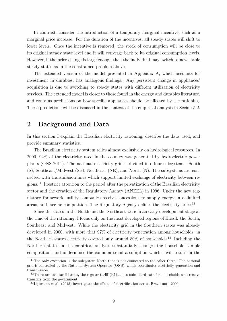
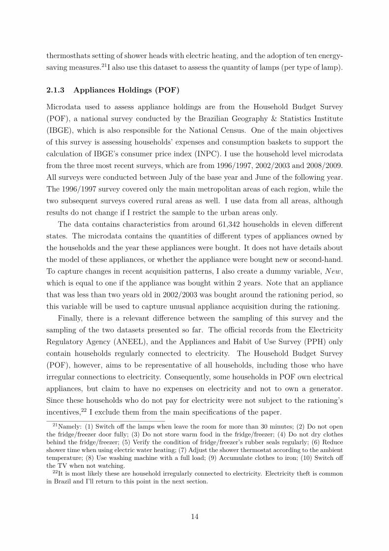
Only supply factors were responsible for the eminent collapse of the electricity systemin 2001. Figure 3 shows the reservoirs’ levels as a percentage of their maximum capacityfor the subsystems Southeast/Midwest and South, from 1996 to 2010. The first halfof the year is the wet season of subsystem Southeast/Midwest, when its power plants’reservoirs are filled to guarantee electricity supply later in the year. It happened that thestream-flow level of rivers which serve the powerplants in this subsystem was extremelylow in the first months of 2001, recording some of the lowest levels of the historical seriesas shown in Figure A1 in the Online Appendix. As a consequence, the reservoirs in theSoutheast/Midwest reached critically low levels, and in March 2001 ONS asked the federalgovernment for an intervention that would reduce demand by 20% in this region.15

Average

2040

6080

100

Sou

thea

st/M

idw

est

1996 1998 2000 2002 2004 2006 2008 2010

Average

Average

2040

6080

100

Sou

th

1996 1998 2000 2002 2004 2006 2008 2010

% o

f Max

imum

Cap

acity

Figure 3: Annual Average Water Level in the Power Plants’ Reservoir as Percentage of theirMaximum Capacity (1996-2011)

Notes. The solid line is the annual average water level in the reservoirs as a percentage of theirmaximum capacity for each subsystem and year. The dashed lines demarcate an area within onestandard deviation from the mean. Source: National System Operator (ONS).

14In particular, at the beginning of this century, the federal government launched the program LuzPara Todos (Light For Everyone) which aims to bring electricity to every household in the country. TheNorthern states were the most affected by this policy, and electricity coverage in these states increasedto nearly 95% in less than a decade.

15Notice that in the beginning of 2000, the reservoirs’ levels in the Southeast/Midwest were at acritically low level similar to 2001, and the reservoirs in the South were below average as well. However,these regions experienced above average stream-flow in 2000, which saved the system from a collapse inthat year. If both regions had experienced in 2000 the stream-flow of the Southeast/Midwest in 2001,both the Southeast/Midwest and the South would have been rationed in 2000 (Kelman 2001).

10

Table 1: Summary Statistics (Year 2000)

South Southeast/Midwest North Northeast(1) (2) (3) (4)

Panel A. ElectricityShare of households with electricity (%) 97.9 98.5 79.5 86.6Number of households with electricity (millions) 6.1 22.4 1.9 9.2Number of utility companies 17 27 8 11Average household electricity use (kWh/month) 178.1 (6.1) 201.7 (6.5) 162.6 (5.3) 113.2 (5.6)

Average household electricity price (R$/kWh) .157 (.009) .162 (.006) .152 (.007) .148 (.005)

Share of households paying for electricity .92 (.01) .90 (.01) .87 (.01) .79 (.01)

Panel B. Macro CovariatesConsumer Price Index (base 2001) .89 .90 .92 .94Average wage (R$) 654.1 809.9 650.9 523.4Average temperature (oc) 19.2 23.2 26.5 25.0

Panel C. Households’ CharacteristicsAverage household size 3.5 (1.6) 3.6 (1.8) 4.5 (2.4) 4.3 (2.3)

Share of households with refrigerators/freezers .91 (.29) .89 (.31) .62 (.48) .59 (.49)

Share of households with air conditioners .07 (.26) .07 (.26) .09 (.29) .04 (.44)

Notes. This table displays the descriptive statistics from the regions in columns. The share of households paying forelectricity is from 1996/1997, all other statistics refer to 2000. Standard deviations in parentheses. The statistics in PanelA are from the Electricity Regulatory Agency (ANEEL) balance sheet, which is disaggregated at month-utility companylevel (528 observations in the year 2000); except the share of households connected to electricity from 2000 National Census;and the share of households paying for electricity from the Household Budget Survey 1996/1997 (POF/IBGE) microdatacalculated using sampling weights. Panel B’s statistics come from three different sources: Consumer Price Index fromINPC/IBGE, at month-metropolitan area level, relative to the index in January 2001; wages from the Ministry of Labor’sregister (RAIS) at year-state level; and temperature from the National Meteorology Institute (INMET). The statistics inPanel C are from the 2000 National Census (IBGE) microdata.

11

The government initially tried to boost supply via thermal generation with the PriorityThermal Program. However, this was not successful, and in April 2001, the demand re-duction program started to be designed. In the middle of May the government announcedin the national media that restrictions on household electricity use would be applied start-ing in June 2001. It was said that the restrictions would initially last 6 months, but couldbe extended. In the end, the restrictions lasted two months longer and were withdrawnin February 2002. I present a timeline of these events in Appendix C.1. As can be seenin Figure 3, the generation capacity in the South was secure in 2001, and therefore thisregion was not rationed.16

The restrictions and incentive structure imposed on households’ electricity use were basedon an individual target equal to 80% of the average consumption on the previous year usinga 3-month rolling window.17 Electricity billing in Brazil is monthly, and the majority ofhouseholds have their own meter.18 Households with monthly average consumption above100 kWh19 who failed to reach their target would pay fines and could have their electricitycut for up to six days. Those with monthly average consumption below 100 kWh werenot subject to these penalties. All households received bonuses of up to R$2 for each R$1saved below their target. Also, a non-linear tariff was temporarily implemented, with a50% overcharge on the electricity consumed above 200 kWh and below 500 kWh, and a200% overcharge on any consumption above 500kWh.It is important to highlight that the government also issued a national information cam-paign through its energy efficiency program, PROCEL/Eletrobrás. Both the campaignand the rationing itself received massive coverage in the national media, affecting po-tentially both the rationed and the non-rationed states. In an extra effort to conserveelectricity, energy-efficient appliances, such as fluorescent light bulbs, received tax exemp-tions from the federal government countrywide.

2.1 Data

Next I describe the four main data sets and other sources of information used in thepaper. Table A2 presents some information about the main datasets used, and AppendixC.2 presents details on the data cleaning and a complete list and description of all variablesused.

16This was the only rationing episode in Brazil throught the period of analysis. From Figure 3, althoughthe reservoir levels were low in 2006, there was no electricity rationing.

17I.e., in June 2001, each household should consume at most 80% of his own average consumption inMay, June and July 2000.

18Note that smart meters is a technology that started to be tested in Brazil only very recently.19These households represented more than 70% of all households, and more than 85% of total con-

sumption in the Southeast/Midwest.

12

2.1.1 Electricity Data (ANEEL)

The electricity data is administrative data from the Brazilian Electricity RegulatoryAgency (ANEEL), with the monthly records of each utility company from January 1991until December 2011. This dataset contains the number of households connected to theutility company, the amount of electricity sold by the utility company to those households,and the total revenue from the electricity sold to households. For each utility company,average electricity use per household is calculated by dividing the total electricity soldto households by the number of households connected. Since each utility company is theonly electricity supplier in each geographical region, this is analogous to have the averagehousehold electricity use per groups of cities.20 There are 17 utility companies in thesubsystem South and 27 in the subsystem Southeast/Midwest. The prices charged byeach utility company are set by the Electricity Regulatory Agency (ANEEL), and thereare two tariff bands for residential consumers: the regular tariff and a subsidized “social”tariff for low income households. Since there is no retrospective disaggregated data onthe electricity consumption of households paying the social tariff, I cannot infer averageprices paid by households from information on the prices set by ANEEL. Therefore, Iinstead calculate the average electricity price charged by each utility by dividing its totalrevenue by the amount of electricity it sold to households.

2.1.2 Habits of Energy Use (PPH)

The government’s energy efficiency program PROCEL, from the national electricity com-pany Eletrobrás, conducts a detailed survey every seven years to assess the characteristicsand utilization habits of household electricity consumers. The Appliances and Habit ofUse Survey (Pesquisa de Posse de Equipamentos e Hábitos de Uso, PPH) is designedby PROCEL with the assistance of academic institutions. Households in different citiesare visited by an interviewer, as is done in a Census survey. The questionnaire includesboth objective questions on household characteristics and habits, as well as qualitativequestions. Although most of the information is self-reported, the interviewers were askedto check some of the information, for example, the number of lamps in the living room,and the characteristics of the main refrigerator and showers heads with electric heating.

I use the microdata from the two most recent surveys, the one conducted betweenJuly 1998 and June 1999, and the one conducted between July 2004 and June 2005. Thedata contains information on 14,254 households covering the concessions of ten utilitycompanies. To the best of my knowledge, this is the first time this survey is beingused in research in the social sciences. The main variables used in the paper are: thenumber of appliances permanently in use, appliances’ characteristics, the quantity and

20The concession areas of the utility companies are stable over time.

13

thermosthats setting of shower heads with electric heating, and the adoption of ten energy-saving measures.21I also use this dataset to assess the quantity of lamps (per type of lamp).

2.1.3 Appliances Holdings (POF)

Microdata used to assess appliance holdings are from the Household Budget Survey(POF), a national survey conducted by the Brazilian Geography & Statistics Institute(IBGE), which is also responsible for the National Census. One of the main objectivesof this survey is assessing households’ expenses and consumption baskets to support thecalculation of IBGE’s consumer price index (INPC). I use the household level microdatafrom the three most recent surveys, which are from 1996/1997, 2002/2003 and 2008/2009.All surveys were conducted between July of the base year and June of the following year.The 1996/1997 survey covered only the main metropolitan areas of each region, while thetwo subsequent surveys covered rural areas as well. I use data from all areas, althoughresults do not change if I restrict the sample to the urban areas only.

The data contains characteristics from around 61,342 households in eleven differentstates. The microdata contains the quantities of different types of appliances owned bythe households and the year these appliances were bought. It does not have details aboutthe model of these appliances, or whether the appliance were bought new or second-hand.To capture changes in recent acquisition patterns, I also create a dummy variable, New,which is equal to one if the appliance was bought within 2 years. Note that an appliancethat was less than two years old in 2002/2003 was bought around the rationing period, sothis variable will be used to capture unusual appliance acquisition during the rationing.

Finally, there is a relevant difference between the sampling of this survey and thesampling of the two datasets presented so far. The official records from the ElectricityRegulatory Agency (ANEEL), and the Appliances and Habit of Use Survey (PPH) onlycontain households regularly connected to electricity. The Household Budget Survey(POF), however, aims to be representative of all households, including those who haveirregular connections to electricity. Consequently, some households in POF own electricalappliances, but claim to have no expenses on electricity and not to own a generator.Since these households who do not pay for electricity were not subject to the rationing’sincentives,22 I exclude them from the main specifications of the paper.

21Namely: (1) Switch off the lamps when leave the room for more than 30 minutes; (2) Do not openthe fridge/freezer door fully; (3) Do not store warm food in the fridge/freezer; (4) Do not dry clothesbehind the fridge/freezer; (5) Verify the condition of fridge/freezer’s rubber seals regularly; (6) Reduceshower time when using electric water heating; (7) Adjust the shower thermostat according to the ambienttemperature; (8) Use washing machine with a full load; (9) Accumulate clothes to iron; (10) Switch offthe TV when not watching.

22It is most likely these are household irregularly connected to electricity. Electricity theft is commonin Brazil and I’ll return to this point in the next section.

14

2.1.4 Appliances’ Prices

Microdata on appliances’ prices is collected as a component of consumer price index (IPC)produced by IBRE/FGV. From 2001 to 2005, prices were surveyed daily in eight majorcities within the South and Southeast/Midwest: Porto Alegre, Curitiba, Florianopolis,São Paulo, Rio de Janeiro, Belo Horizonte, Goiania and Brasília. 23 From 2006 on, priceswere surveyed only in Porto Alegre (in the South), and São Paulo and Rio de Janeiro(both in the Southeast). The smaller observational unit in the cross-section is a tripleproduct*informer*store.

I use this data with two objectives. First, I use only the three capitals with a long timeseries to build an unweighted appliance price index for each region to investigate generalequilibrium effects on appliances’ prices, methodology described in Appendix C.2. Second,I use the description of the products to assess the rationing effect on the products availablein the stores in both regions. Prices are surveyed in stores according to the productsavailable on the shelves in that day. Since product descriptions are very detailed,24 Icompare the availability of products in both regions and how this changed over time. Inthis second exercise, I use all capitals and restrict attention to 2001-2005.

2.1.5 Other Data

Nominal wages and the number of workers in formal employment come from the RAISdataset (Brazilian Ministry of Labor), aggregated by year-state, from 1997 to 2010. Theconsumer price index is INPC produced by IBGE, which contains monthly indices for themain metropolitan areas in each region. Unfortunately, Brazil does not have a periodicconsumer price index for rural areas. I compute prices and wages in real terms by dividingnominal variables by the INPC index. Data on electricity generation, rivers’ conditionsand levels of reservoirs are from the National System Operator (ONS), the body respon-sible for running the electricity generation and transmission systems in Brazil. Weatherdata is from the National Meteorology Institute (INMET), and includes daily measuresfrom 45 meteorological stations in the region. Data on total month-state consumptionof of natural gas (GLP) and gasoline is from the National Agency of Petroleum, NaturalGas and Biofuels (ANP). Note that I could not find data on the quantity of these fuelsconsumed by households, so this data helps assessing if there was any significant changein the overall demand for these fuels. I use information on gas expentiture from theHousehold Budget Survey to complement this analysis. Remaining information is fromthe National Census 2000 (IGBE).

23IPC methodology: http://portalibre.fgv.br/main.jsp?lumChannelId=402880811D8E34B9011D92B7350710C724For example, “REFRIGERADOR DOMESTICO 440 LITROS MOD:DOUBLE 44 ELECTROLUX

(UNID)”.

15

3 Empirical Method and Main Results

The main identification strategy to estimate the short and long run effects of the rationingis a difference-in-differences specification using the non-rationed South of Brazil as acontrol group for the rationed Southeast/Midwest. As mentioned in the introduction,any causal inference of this estimation hinges on a few assumptions. Before listing theseand assessing their plausibility, I present the basic regression equation:

Yit = α + βDDuringt ∗Rationi + βPPostt ∗Rationi + γt + γi + γXit + εit (2)

where Yit is the dependent variable measured at the level of utility i in year-month t.Duringt and Postt are dummies equal to one for months during and after the rationingrespectively, Rationi is a dummy equal to one if the utility was rationed, γi and γt areutility and year-month fixed effects, and Xit is a vector of covariates - for example, realwage, and real electricity price. I do not impose any structure on the errors’ correlationover time and cluster errors at the utility company level, i, as in Bertrand et al. (2004).

The parameters of interest are βD and βP . The estimates of βD can be interpreted asthe program’s average short run effect on the treated25 if there are no omitted variablesassociated with both the rationing allocation (timing and across locations) and withhouseholds’ potential electricity use [Assumption 1 ], and if the evolution of householdelectricity use were following a common trend in the South and the Southeast/Midwest[Assumption 2 ].26 The estimates of βP capture the program’s average long run effect onthe treated if, in addition to these two assumptions, there would have been no divergencein the time series of electricity use and covariates over the years following the rationing[Assumption 3 ].

Section 2 provides clear evidence supporting Assumption 1. The official diagnosis ofthe energy crisis concludes that local supply factors aggravated by severe stream-flowlevels triggered the rationing, and states: “the realized electricity consumption growth[from 1997 and 2000] corresponded to the growth forecast and had no influence on thegeneration crisis” (Kelman 2001, pg. 5).27 Table 1 presents some summary statistics ofall regions immediately before the rationing.

25It is worth highlighting that the treatment captured here is the rationing program faced by householdsnet of the effects of pure information provision and subsidies, which were implemented in the South aswell.

26See Manski and Pepper (2012) for a full discussion on identification.27Table A3 presents the realized electricity demand as a fraction of the forecasted demand from the

Decennial Energy Plan 1997-2007 (PDE, 1997) for each year and region. From 1998 and 2000, the realizeddemand was below the expected one, even when considering households market only. That is, there wasno unexpected growth of electricity demand in the years prior 2001. Further, the installed generationcapacity would support the forecasted demand under regular natural conditions. The official report aboutthe rationing’s causes concludes that “no demand factor contributed to the unbalancing of the systemand the collapse in 2001” (Kelman, 2001).

16

Figure 1 shows that average electricity use in the South and Southeast/Midwest hadbeen following roughly the same trend since 1991. In the period between the privatizationof the electricity sector and the rationing (from 1997 to 2001), I reject a common pre-trendhypothesis, and thus Assumption 2. However, the treatment effects turn out to be bigcompared to the estimated differences in trends. Also, I allow for different trends in thespecification, meaning that I only need Assumptions 1 and 3 for identification.

Assumption 3 is the key challenge of assessing long run impacts of any policy: main-taining a meaningful counterfactual for several years. In order to overcome this issue, Iuse different regression specifications controlling for a series of time-varying covariates.Figure A2 plots the evolution over time of electricity prices and wages in these regions. Wecannot observe a discontinuity in these graphs as we do in Figure 1.28 Table A1 presentsa set of simple difference-in-differences estimates of the rationing effects on time-varyingcovariates. I find no significant differences between the two regions specific to the post-rationing period, for any of the variables examined. The only exception is temperature,which seems to have increased by an additional 0.2oc in the South over the last decade,meaning that the estimates of the long run effects of rationing are downwards biased.2930

Furthermore, I do not find evidence of economically meaningful migration across the re-gions,31 or that households evaded rationing by spreading usage across more meters orirregular connections.32

Table A4 presents the same difference-in-differences estimation to illustrate the differ-ent evolution between the North and the Northeast regions specific to the post-rationingperiod. One cannot reject the hypothesis that, during the years studied, more householdswere connected to electricity in the Northeast than in the North, and that the share ofhouseholds paying for electricity increased, the number of employed workers increased,and the average wage decreased in the Northeast relative to the North. Since the North-ern states fail to satisfy Assumptions 2 and 3, and the inclusion of these states wouldsubstantially change the household sample composition, I discard them in the empirical

28I also do not find evidence of a change in the total consumption of other sources of energy. FigureA3 plots the evolution over time of monthly total sales of two alternative fuels - natural gas (GLP) andgasoline - divided by the number of employed households in each region. Again, we fail to observe adiscontinuity in these graphs as we do in Figure 1. Table A1 (Part 2) presents the statistical tests.

29Temperature in the Southeast/Midwest virtually did not change relative to the late nineties. I wouldfind similar results if I count the number of days above 32oc in these regions.

30Some of these variables investigated have a small number of clusters what can lead to an over rejectionof the null hypothesis. To address this issue I estimate standard errors using the wild-cluster bootstrapestimator (Cameron, Gelbach and Miller 2008) in all cases in which the dependent variable has less than40 clusters.

31Oliveira and Oliveira (2011) documents that the Southeast experienced a net out-migration in theperiods from 2000 to 2004 and from 2005 to 2009. The magnitude of these numbers are no larger than0.2% of the Southeast population, and 0.5% of the South population.

32Data from the Regulatory Agency shows no difference in the evolution of the number of meters inthe two regions. I find no difference in the number of households irregularly connected to electricity inthe POF data, and the PPH data shows no difference in the number of households with a home business.

17

analysis. The main results still hold when all states are included in the analysis.This evidence, together with the robustness checks, supports the plausibility of the

identification strategy. Further potential issues with the identification will be discussedin Section 4.

3.1 Main Results

Table 2 presents the estimates of equation (2), using various different sets of controlsand samples. The base specification suggests that during the rationing, households inthe Southeast/Midwest reduced consumption by 46.7 kWh per month relative to the onesin the South region in the same period, a reduction of 28%; other specifications yieldsimilar estimates. This is equivalent to each rationed household switching off a freezer ora medium sized refrigerator across the nine months of the rationing. The long run effectis about half of this value in all specifications - i.e., households in the Southeast/Midwestreduced consumption by 25.7 kWh per month (or 14%) relative to the ones in the Southregion in every month after February 2002. That is, it appears that households took sometemporary measures to reduce electricity consumption during the rationing, however partof these new consumption pattern remained in place after the crisis.

As previously discussed, the evolution of covariates such as wages and prices couldaffect electricity demand over the years, especially because general equilibrium effectscould emerge. To deal with this issue I control for real electricity prices, real wages andtemperature as shown in columns 2 to 4. I also control for a cubic polynomial of thesevariables, in column 6, and results are largely unaffected. To address the issue of non-parallel trends, I run one specification with a specific time trend for each of the rationedand non-rationed regions, in column 5. The estimated rationing impacts get even largerin this case, and I cannot reject that the coefficients of the two trends are equal.

A further concern is that since households in both regions are heterogeneous, theycould respond differently to covariates. That is, even if prices and wages evolved similarlyin the two regions after the rationing, households could have different elasticities.33 Thespecification in column 7 addresses this point by permitting utility-specific price and wageelasticities. I control for the interactions “price × utility dummy” and “wage × utilitydummy”. This is the specification under which the rationing had the smallest estimatedshort and long run effects, about 12% smaller than the base specification. Even so, I findthat long run electricity use decreased 22.6 kWh per month in the Southeast/Midwestrelative to the South using this specification, which can be interpreted as a lower-boundestimate. Column 8’s specification uses all controls together. I cannot reject the nullhypothesis of equality of the long run effects across all eight specifications.

33For example, if households in the Southeast were more price elastic than those in the South, a commonprice increase in both regions would lead to different consumption changes.

18

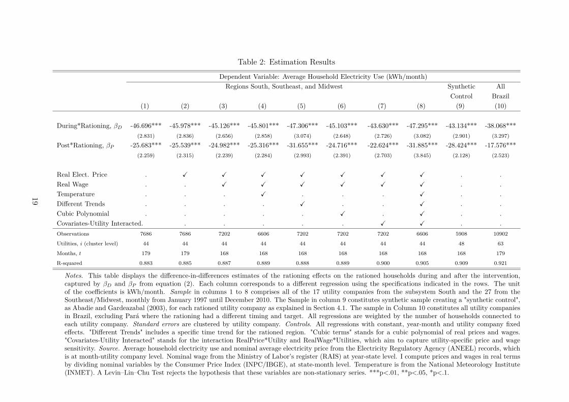
Table 2: Estimation Results

Dependent Variable: Average Household Electricity Use (kWh/month)Regions South, Southeast, and Midwest Synthetic All

Control Brazil(1) (2) (3) (4) (5) (6) (7) (8) (9) (10)

During*Rationing, βD -46.696*** -45.978*** -45.126*** -45.801*** -47.306*** -45.103*** -43.630*** -47.295*** -43.134*** -38.068***(2.831) (2.836) (2.656) (2.858) (3.074) (2.648) (2.726) (3.082) (2.901) (3.297)

Post*Rationing, βP -25.683*** -25.539*** -24.982*** -25.316*** -31.655*** -24.716*** -22.624*** -31.885*** -28.424*** -17.576***(2.259) (2.315) (2.239) (2.284) (2.993) (2.391) (2.703) (3.845) (2.128) (2.523)

Real Elect. Price . X X X X X X X . .Real Wage . . X X X X X X . .Temperature . . . X . . . X . .Different Trends . . . . X . . X . .Cubic Polynomial . . . . . X . X . .Covariates-Utility Interacted. . . . . . X X . .Observations 7686 7686 7202 6606 7202 7202 7202 6606 5908 10902

Utilities, i (cluster level) 44 44 44 44 44 44 44 44 48 63

Months, t 179 179 168 168 168 168 168 168 168 179

R-squared 0.883 0.885 0.887 0.889 0.888 0.889 0.900 0.905 0.909 0.921

Notes. This table displays the difference-in-differences estimates of the rationing effects on the rationed households during and after the intervention,captured by βD and βP from equation (2). Each column corresponds to a different regression using the specifications indicated in the rows. The unitof the coefficients is kWh/month. Sample in columns 1 to 8 comprises all of the 17 utility companies from the subsystem South and the 27 from theSoutheast/Midwest, monthly from January 1997 until December 2010. The Sample in column 9 constitutes synthetic sample creating a "synthetic control",as Abadie and Gardeazabal (2003), for each rationed utility company as explained in Section 4.1. The sample in Column 10 constitutes all utility companiesin Brazil, excluding Pará where the rationing had a different timing and target. All regressions are weighted by the number of households connected toeach utility company. Standard errors are clustered by utility company. Controls. All regressions with constant, year-month and utility company fixedeffects. "Different Trends" includes a specific time trend for the rationed region. "Cubic terms" stands for a cubic polynomial of real prices and wages."Covariates-Utility Interacted" stands for the interaction RealPrice*Utility and RealWage*Utilities, which aim to capture utility-specific price and wagesensitivity. Source. Average household electricity use and nominal average electricity price from the Electricity Regulatory Agency (ANEEL) records, whichis at month-utility company level. Nominal wage from the Ministry of Labor’s register (RAIS) at year-state level. I compute prices and wages in real termsby dividing nominal variables by the Consumer Price Index (INPC/IBGE), at state-month level. Temperature is from the National Meteorology Institute(INMET). A Levin–Lin–Chu Test rejects the hypothesis that these variables are non-stationary series. ***p<.01, **p<.05, *p<.1.

19

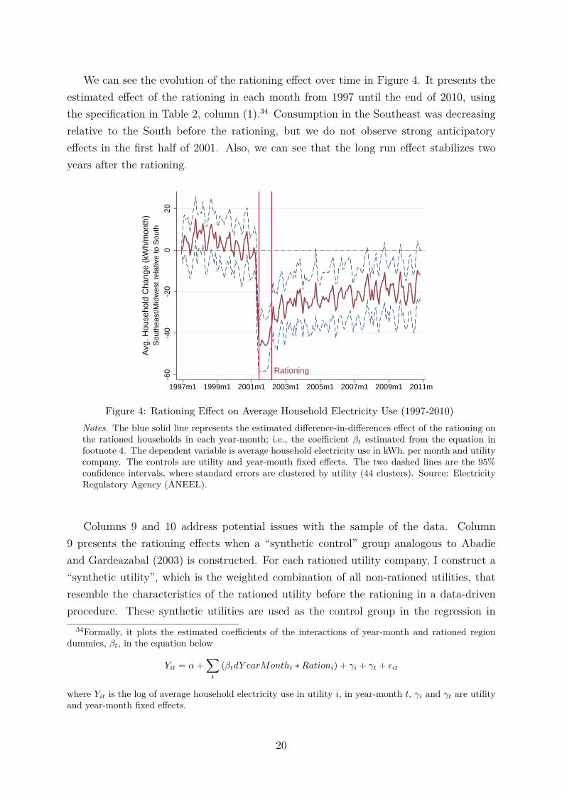
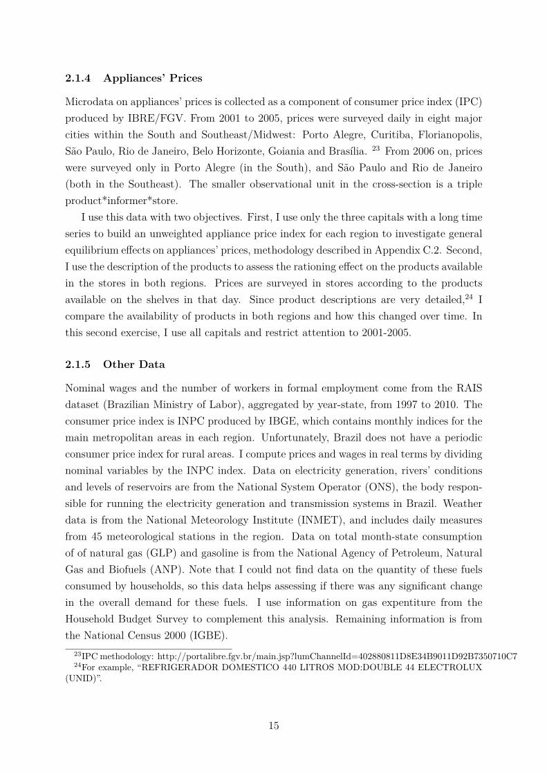
We can see the evolution of the rationing effect over time in Figure 4. It presents theestimated effect of the rationing in each month from 1997 until the end of 2010, usingthe specification in Table 2, column (1).34 Consumption in the Southeast was decreasingrelative to the South before the rationing, but we do not observe strong anticipatoryeffects in the first half of 2001. Also, we can see that the long run effect stabilizes twoyears after the rationing.

Rationing

-60

-40

-20

020

1997m1 1999m1 2001m1 2003m1 2005m1 2007m1 2009m1 2011m1

Sou

thea

st/M

idw

est r

elat

ive

to S

outh

Avg

. Hou

seho

ld C

hang

e (k

Wh/

mon

th)

Figure 4: Rationing Effect on Average Household Electricity Use (1997-2010)Notes. The blue solid line represents the estimated difference-in-differences effect of the rationing onthe rationed households in each year-month; i.e., the coefficient βt estimated from the equation infootnote 4. The dependent variable is average household electricity use in kWh, per month and utilitycompany. The controls are utility and year-month fixed effects. The two dashed lines are the 95%confidence intervals, where standard errors are clustered by utility (44 clusters). Source: ElectricityRegulatory Agency (ANEEL).

Columns 9 and 10 address potential issues with the sample of the data. Column9 presents the rationing effects when a “synthetic control” group analogous to Abadieand Gardeazabal (2003) is constructed. For each rationed utility company, I construct a“synthetic utility”, which is the weighted combination of all non-rationed utilities, thatresemble the characteristics of the rationed utility before the rationing in a data-drivenprocedure. These synthetic utilities are used as the control group in the regression in

34Formally, it plots the estimated coefficients of the interactions of year-month and rationed regiondummies, βt, in the equation below

Yit = α+∑

t

(βtdY earMontht ∗Rationi) + γi + γt + εit

where Yit is the log of average household electricity use in utility i, in year-month t, γi and γt are utilityand year-month fixed effects.

20

column 9.35 Column 10 presents results pooling all 63 utility companies in the country,including those in the North and Northeast. In both cases, the estimated effects are notseverely affected.

Also, one can interpret the difference-in-difference estimates of the rationing effectson time-varying covariates presented in Table A1 as a placebo. As discussed above, I findthat the rationing had statistically significant effects in the case of only one of the ninevariables, temperature, which would bias downwards the long run results on electricityuse.

Overall, there is evidence that the temporary demand response program did changefinal household electricity demand in the long run, i.e., for the ten-year period studied.This effect, a conservation of around 25 kWh/month per household, is economically mean-ingful. The total energy saved in the Southeast/Midwest during the nine years after therationing adds up to 59.4 TWh, the equivalent to 50% of the wind energy generated inthe USA in 2011 (EIA 2012). Also, this effect is robust to a range of specification andis flat since 2003, consistent with a scenario in which some affected households switchedbetween steady states in electricity consumption.

4 Channels of Persistence

In this section I use household level microdata to shed light on the channels supportingthe long run reduction in electricity use in the region affected by the rationing. There aretwo non-competing stories which could be underlying the long run energy conservation:households could have changed how they use electrical appliances, and/or invested in moreenergy efficient appliances.36 It is important to disentangle the intensive and extensivemargin of consumption because these relate to different economic mechanisms, and wouldlead to different policy conclusions.

The first channel would require that for given prices, income and technology, house-holds would be using appliances differently. This mechanism can emerge from economicmodels in which the individual optimization problem has multiple steady states; as inthe model presented in Section 1, through consumption complementarity, or because ofhabits, beliefs, or social norms. In the first part of this section I present direct evidencefrom household level microdata that individuals’ utilization of electrical appliances wasaffected by the rationing.

At the same time, the rationing could have affected households’ investments in energy35The weights used to create the synthetic control are estimated based on using Abadie and Gardeazabal

(2003) procedure. Observable characteristics used are average household electricity use, real electricityprice, real wage, number of households connected to electricity and consumer price index.

36Households could have substituted electricity by other sources of energy, such as natural gas (GLP)and gasoline. I address this issue in Section 4.2.

21

efficiency. In this case, households marginally indifferent between keeping an old applianceand replacing it with a new one would have been prompted to buy a new appliance bythe rationing. The acquisition of a new appliance which consumes less electricity wouldhave lasting impacts on final household energy demand, because appliances are kept fora long time. To illustrate this point, I present in Appendix A an extended version ofthe model, adding endogenous choice of appliances’ characteristic. In Subsection 4.2,I investigate the contribution of this mechanism to the long run energy conservation. Iexploit household level microdata which gives me snapshots of the quantity and vintage ofhouseholds’ appliances holdings in different periods. Evidence suggests that the differencein composition of appliances between the two regions did not change substantially in thelong run.37

I restrict attention to the five appliances which represent 85% of average householdelectricity use (PROCEL, 2007): shower heads with electric heating, refrigerators, freez-ers, air conditioners, and lamps. I use the same identification strategy described in theprevious section, performing the following difference-in-differences estimation:

Yhit = α +∑t>0

βtdY eart ∗Rationi + γt + γi + γXhit + εhit (3)

where Yhit is the dependent variable of household h, in region i and year t (region i can beutility company or state according to the dataset), dY eart are dummies for years, Rationiis a dummy equal to one if the region i was rationed, γi and γt are region and year fixedeffects, and Xhit is a vector of controls with household characteristics. I do not imposeany structure on the errors’ correlation over time and cluster errors by region i using wild-cluster bootstrap estimator to deal with the small number of clusters (Cameron, Gelbachand Miller 2008).

There is one caveat for identification in this section. By the nature of the data (re-peated cross-section), I cannot explicitly test the common trend hypothesis for the de-pendent variables. To attenuate this issue, I control for many household characteristicswhich may be correlated with different trends.

37Note that I do not investigate appliances’ optimal life cycle. To precisely assess if households attitudestowards technology adoption changed in the period, one would need data with the flow of new appliancesbought by households and the flow of the destination of the old appliances (i.e., if old appliances aredisplaced or sold in the second hand market). Unfortunately, this data does not exist. I use stock datawhich only provides indirect evidence on appliances’ life cycle. However, the data used does providedirect evidence on the average energy efficiency of households’ inventory of appliances in different pointsin time.

22

4.1 Electricity Consumption Habits

This subsection presents results on consumption behaviors using data from the Appli-ances and Habits of Use Survey (PPH) 1998/1999 and 2004/2005. Table 3 presentsdescriptive statistics of the appliance inventories and habits of electricity utilization ofthe average household in the two regions and years. As we can see, the three electricityservices which account for most of the average household’s electricity use are shower headswith electric heating, refrigerators and lighting. In 1998/1999 the average household inthe Southeast/Midwest had an overall higher utilization of appliances than the averagehousehold in the South; except freezer and lighting. We also see that households in theSoutheast/Midwest used to adopt less energy-saving measures than those in the South.

Table 4 presents the estimates of difference-in-differences regression (3) for each ofthese variables, controlling for utility company and year fixed effects, income, squaredincome, number of household members, residence build-up area,38 and dummies for richneighborhood and for proximity to slums ("favelas"). As indicated in the table, I presentresults in units of kWh/month whenever it is possible.39

The use of shower heads with electric heating corresponds to more than a fifth ofaverage electricity use. The regression results presented in column 1 suggest that therationing affected households’ choice of shower temperature, generating savings of around15 kWh per month.40 I do not find that the rationing had a statistically significant impacton any of the other variables, including utilization of refrigerators, freezer, lighting andair conditioners, as shown in columns 2 to 7. However, all point estimates are negative.I would like to draw attention to one of these appliances: freezers. As shown in column3, the point estimate suggest that households in the Southeast/Midwest reduced freezerutilization due to the rationing, saving around 10 kWh per month on average. This resultis not statistically significant because the standard errors estimated with the wild-clusterbootstrap estimator are large, but it turns to be significant when other estimators areused. These two results by themselves could account for most of the observed long runenergy conservation in the Southeast/Midwest. As shown in column 8, the rationing hadno statistically significant impact on the probability of households adopting at least oneof the ten energy-saving measures described in Section 2.1.2.41

38Build-up area is the area enclosed within the walls of the residence, plus the thickness of walls.39I convert each variable to kWh/month by calculating: [Number of appliances per type and intensity

of use] * [Average electricity consumption per type and intensity of use].40The thermostat of a shower head with electric heating can be switched off or set at “Low Power”

(Modo Verão) or “High Power” (Modo Inverno). A shower set at Low Power consumes on average 30%less electricity than one set at High Power.

41Table A6 in the Appendix presents the rationing effect on the adoption of each of these 10 measures,using a logit estimation. I find a statistically significant increase in the adoption of four of these tenmeasures, all relating to refrigerator, freezer or shower utilization (for example, “reduce shower time whenusing electric water heating” in column 6, and “adjust the shower thermostat according to the ambienttemperature” in column 7). I find no statistically significant effect on the remaining six measures.

23

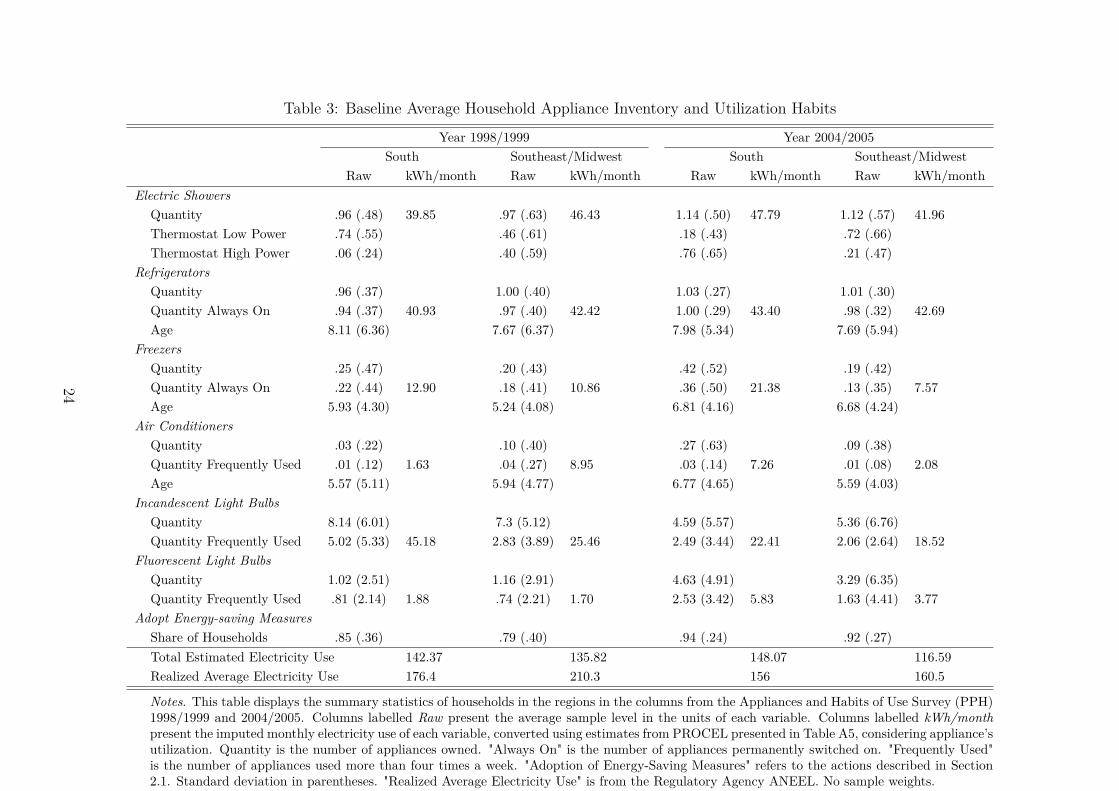
Table 3: Baseline Average Household Appliance Inventory and Utilization Habits

Year 1998/1999 Year 2004/2005South Southeast/Midwest South Southeast/Midwest

Raw kWh/month Raw kWh/month Raw kWh/month Raw kWh/monthElectric Showers

Quantity .96 (.48) 39.85 .97 (.63) 46.43 1.14 (.50) 47.79 1.12 (.57) 41.96Thermostat Low Power .74 (.55) .46 (.61) .18 (.43) .72 (.66)Thermostat High Power .06 (.24) .40 (.59) .76 (.65) .21 (.47)

RefrigeratorsQuantity .96 (.37) 1.00 (.40) 1.03 (.27) 1.01 (.30)Quantity Always On .94 (.37) 40.93 .97 (.40) 42.42 1.00 (.29) 43.40 .98 (.32) 42.69Age 8.11 (6.36) 7.67 (6.37) 7.98 (5.34) 7.69 (5.94)

FreezersQuantity .25 (.47) .20 (.43) .42 (.52) .19 (.42)Quantity Always On .22 (.44) 12.90 .18 (.41) 10.86 .36 (.50) 21.38 .13 (.35) 7.57Age 5.93 (4.30) 5.24 (4.08) 6.81 (4.16) 6.68 (4.24)

Air ConditionersQuantity .03 (.22) .10 (.40) .27 (.63) .09 (.38)Quantity Frequently Used .01 (.12) 1.63 .04 (.27) 8.95 .03 (.14) 7.26 .01 (.08) 2.08Age 5.57 (5.11) 5.94 (4.77) 6.77 (4.65) 5.59 (4.03)

Incandescent Light BulbsQuantity 8.14 (6.01) 7.3 (5.12) 4.59 (5.57) 5.36 (6.76)Quantity Frequently Used 5.02 (5.33) 45.18 2.83 (3.89) 25.46 2.49 (3.44) 22.41 2.06 (2.64) 18.52

Fluorescent Light BulbsQuantity 1.02 (2.51) 1.16 (2.91) 4.63 (4.91) 3.29 (6.35)Quantity Frequently Used .81 (2.14) 1.88 .74 (2.21) 1.70 2.53 (3.42) 5.83 1.63 (4.41) 3.77

Adopt Energy-saving MeasuresShare of Households .85 (.36) .79 (.40) .94 (.24) .92 (.27)Total Estimated Electricity Use 142.37 135.82 148.07 116.59Realized Average Electricity Use 176.4 210.3 156 160.5

Notes. This table displays the summary statistics of households in the regions in the columns from the Appliances and Habits of Use Survey (PPH)1998/1999 and 2004/2005. Columns labelled Raw present the average sample level in the units of each variable. Columns labelled kWh/monthpresent the imputed monthly electricity use of each variable, converted using estimates from PROCEL presented in Table A5, considering appliance’sutilization. Quantity is the number of appliances owned. "Always On" is the number of appliances permanently switched on. "Frequently Used"is the number of appliances used more than four times a week. "Adoption of Energy-Saving Measures" refers to the actions described in Section2.1. Standard deviation in parentheses. "Realized Average Electricity Use" is from the Regulatory Agency ANEEL. No sample weights.

24

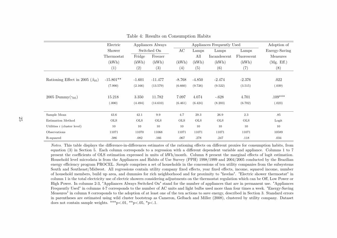
Table 4: Results on Consumption Habits

Electric Appliances Always Appliances Frequently Used Adoption ofShower Switched On AC Lamps Lamps Lamps Energy-Saving

Thermostat Fridge Freezer All Incandescent Fluorescent Measures(kWh) (kWh) (kWh) (kWh) (kWh) (kWh) (kWh) (Mg. Eff.)(1) (2) (3) (4) (5) (6) (7) (8)

Rationing Effect in 2005 (β05) -15.801** -1.601 -11.477 -8.768 -4.850 -2.474 -2.376 .022(7.990) (2.166) (13.579) (6.660) (9.726) (9.522) (3.515) (.039)

2005 Dummy(γ05) 15.218 3.350 11.782 7.097 4.074 -.628 4.701 .109***(.000) (4.494) (14.610) (6.461) (6.424) (8.203) (6.702) (.023)

Sample Mean 43.6 42.1 9.9 4.7 29.3 26.9 2.3 .85

Estimation Method OLS OLS OLS OLS OLS OLS OLS Logit

Utilities i (cluster level) 10 10 10 10 10 10 10 10

Observations 11071 11070 11068 11071 11071 11071 11071 10589

R-squared .386 .082 .166 .067 .278 .247 .118 .034

Notes. This table displays the difference-in-differences estimates of the rationing effects on different proxies for consumption habits, fromequation (3) in Section 5. Each column corresponds to a regression with a different dependent variable and appliance. Columns 1 to 7present the coefficients of OLS estimation expressed in units of kWh/month. Column 8 present the marginal effects of logit estimation.Household level microdata is from the Appliances and Habits of Use Survey (PPH) 1998/1999 and 2004/2005 conducted by the Brazilianenergy efficiency program PROCEL. Sample comprises a set of households in the concessions of ten utility companies from the subsystemsSouth and Southeast/Midwest. All regressions contain utility company fixed effects, year fixed effects, income, squared income, numberof household members, build up area, and dummies for rich neighborhood and for proximity to "favelas". "Electric shower thermostat" incolumn 1 is the total electricity use of electric showers considering adjustments on the thermostat regulation which can be Off, Low Power orHigh Power. In columns 2-3, "Appliances Always Switched On" stand for the number of appliances that are in permanent use. "AppliancesFrequently Used" in columns 4-7 corresponds to the number of AC units and light bulbs used more than four times a week. "Energy-SavingMeasures" in column 8 corresponds to the adoption of at least one of the ten actions to save energy, described in Section 3. Standard errorsin parentheses are estimated using wild cluster bootstrap as Cameron, Gelbach and Miller (2008), clustered by utility company. Datasetdoes not contain sample weights. ***p<.01, **p<.05, *p<.1.

25

These findings suggest that households changed their regular usage patterns for elec-tricity services, even controlling for a series of individual characteristics. These results arelargely unaffected when using different specifications. Furthermore, responses to quali-tative questions asked to rationed households in 2004/2005 are consistent with thesefindings, as shown in Table A9. This is further evidence that the rationing did makehouseholds switch steady states.

4.2 Electrical Appliances Holdings

This section shows that a newer and more energy-efficient stock of appliances cannot ac-count for the long run relative reduction in electricity demand in the rationed region. Inorder to assess whether the rationing affected the average stock of appliances, I use mi-crodata from the Household Budget Survey (POF) 1996/1997, 2002/2003 and 2008/2009,and Appliances and Habit of Use Survey (PPH) 1998/1999 and 2004/2005. As discussedabove, I characterize the inventory of appliances using three variables: the quantity ofappliances owned, the age of each appliance, and the dummy New which is equal to onefor appliances bought within the last two years.

The first part of Table 5 presents the estimates of the difference-in-differences regres-sion (3) using POF data controlling for state fixed effects, year fixed effects, income,squared income, number of bedrooms, number of household members, and a dummy forrural regions. These are sample weighted regressions using only those households whopay for electricity, that is, those regularly connected to electricity as described in Section2.1.3.

Consistent with the habits of use data, in column 4 we can see that the rationing hada negative, but not statistically significant, effect on the average number of freezers in theSoutheast/Midwest relative to the South. Although one cannot reject the equality of thecoefficients capturing the short and long run effects on the quantity of freezers, I find thatthe short run effect is statistically significant when standard errors are estimated usingother methods rather than the wild-cluster bootstrap estimator. The short run effectsof changes in the stock of freezers would be responsible for the conservation of around 4kWh per month. Columns 1 and 7 also show no effect on the quantity of refrigerators andair conditioners either in the short or long run.

Although the quantity of appliances does not seem to have been significantly affected,the rationing could have influenced the households’ decision to replace old applianceswith more efficient ones. Columns 2 and 3 provide evidence that households in theSoutheast strategically substituted refrigerators during the rationing. In 2002/2003, whilethe rationing did not affect the number of refrigerators owned (column 1), it did reduce theaverage age of refrigerators (column 2), and increased by 2.5% the share of households whobought a refrigerator in the previous two years (column 3). However, this effect dissipates

26

over time and I find no effect on the stock - quantity and vintage - of refrigerators in2008/2009.

Columns 6 and 9 suggest that the share of households who bought freezers or airconditioners in the previous two years became relatively smaller in the rationed regionboth in the short and long run. We also see in column 8 that the average air conditionerbecame relatively older in the Southeast/Midwest. This is indirect evidence that therationing reduced the replacement rate of these appliances in the Southeast/Midwest. Allthese results are robust to different specifications and to restricting to sub-samples, suchas to metropolitan areas.

The POF dataset does not contain information on lamps and showers, or on the char-acteristics of appliances. I use data from the PPH to examine the stock of these appliancesand their characteristics. As shown in Table 5 (Part 2), I find no significant change in thenumber of lamps or shower heads with electric water heating in the Southeast/Midwestrelative to the South. Note that when we compare these results with those in Table 4,we see that it is the intensive margin of utilization which is driving the reduction in theelectricity consumption of shower heads with electric water heating.

Although these results suggest that the quantity and vintage of the stock of appli-ances owned by households were not affected, it could be that households in the South-east/Midwest started to acquire smaller or more energy-efficient appliances. Table A7presents the estimates of the difference-in-differences regression (3) using PPH data onthe average size of refrigerators and freezers (measured in liters) and the power of airconditioners (measured in BTUs). I find that the rationing had no effect on the char-acteristic of these appliances. Another issue to be considered is that retail stores inthe Southeast/Midwest could have specialized in energy-efficient products potentially notavailable in the South. In Appendix C.3, I use microdata on appliances’ prices collectedin stores to investigate this issue. As presented in Table A8, products available in thestores of the Southeast/Midwest became more likely to be available in the stores of theSouth after 2001.

These results together are consistent with the standard model of appliance acquisitionand utilization (Dubin and McFadden 1984) when extended to allow for multiplicity ofsteady states, as described in Appendix A. In this model, appliances that provide price-elastic electricity services (e.g., freezers) are less likely to be utilized during the rationing,reducing the incentives to invest in new appliances in the short run. In the long run,price-elastic services will be the most affected when individuals converge to a new steadystate with less services from electricity. A smaller utilization of electricity services reducesthe incentives to invest in newer and more energy-efficient technologies, leading to longrun effects on the stock and utilization of appliances.

27

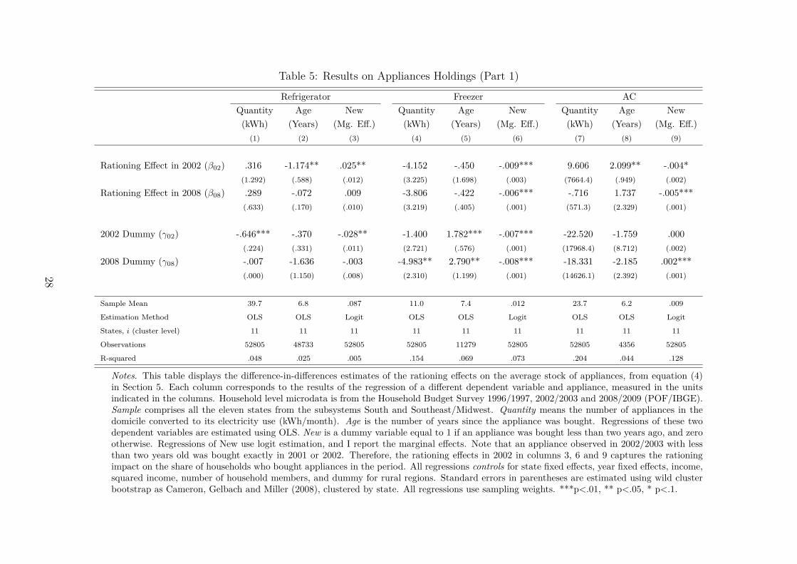
Table 5: Results on Appliances Holdings (Part 1)

Refrigerator Freezer ACQuantity Age New Quantity Age New Quantity Age New(kWh) (Years) (Mg. Eff.) (kWh) (Years) (Mg. Eff.) (kWh) (Years) (Mg. Eff.)

(1) (2) (3) (4) (5) (6) (7) (8) (9)

Rationing Effect in 2002 (β02) .316 -1.174** .025** -4.152 -.450 -.009*** 9.606 2.099** -.004*(1.292) (.588) (.012) (3.225) (1.698) (.003) (7664.4) (.949) (.002)

Rationing Effect in 2008 (β08) .289 -.072 .009 -3.806 -.422 -.006*** -.716 1.737 -.005***(.633) (.170) (.010) (3.219) (.405) (.001) (571.3) (2.329) (.001)

2002 Dummy (γ02) -.646*** -.370 -.028** -1.400 1.782*** -.007*** -22.520 -1.759 .000(.224) (.331) (.011) (2.721) (.576) (.001) (17968.4) (8.712) (.002)

2008 Dummy (γ08) -.007 -1.636 -.003 -4.983** 2.790** -.008*** -18.331 -2.185 .002***(.000) (1.150) (.008) (2.310) (1.199) (.001) (14626.1) (2.392) (.001)

Sample Mean 39.7 6.8 .087 11.0 7.4 .012 23.7 6.2 .009

Estimation Method OLS OLS Logit OLS OLS Logit OLS OLS Logit

States, i (cluster level) 11 11 11 11 11 11 11 11 11

Observations 52805 48733 52805 52805 11279 52805 52805 4356 52805

R-squared .048 .025 .005 .154 .069 .073 .204 .044 .128

Notes. This table displays the difference-in-differences estimates of the rationing effects on the average stock of appliances, from equation (4)in Section 5. Each column corresponds to the results of the regression of a different dependent variable and appliance, measured in the unitsindicated in the columns. Household level microdata is from the Household Budget Survey 1996/1997, 2002/2003 and 2008/2009 (POF/IBGE).Sample comprises all the eleven states from the subsystems South and Southeast/Midwest. Quantity means the number of appliances in thedomicile converted to its electricity use (kWh/month). Age is the number of years since the appliance was bought. Regressions of these twodependent variables are estimated using OLS. New is a dummy variable equal to 1 if an appliance was bought less than two years ago, and zerootherwise. Regressions of New use logit estimation, and I report the marginal effects. Note that an appliance observed in 2002/2003 with lessthan two years old was bought exactly in 2001 or 2002. Therefore, the rationing effects in 2002 in columns 3, 6 and 9 captures the rationingimpact on the share of households who bought appliances in the period. All regressions controls for state fixed effects, year fixed effects, income,squared income, number of household members, and dummy for rural regions. Standard errors in parentheses are estimated using wild clusterbootstrap as Cameron, Gelbach and Miller (2008), clustered by state. All regressions use sampling weights. ***p<.01, ** p<.05, * p<.1.

28

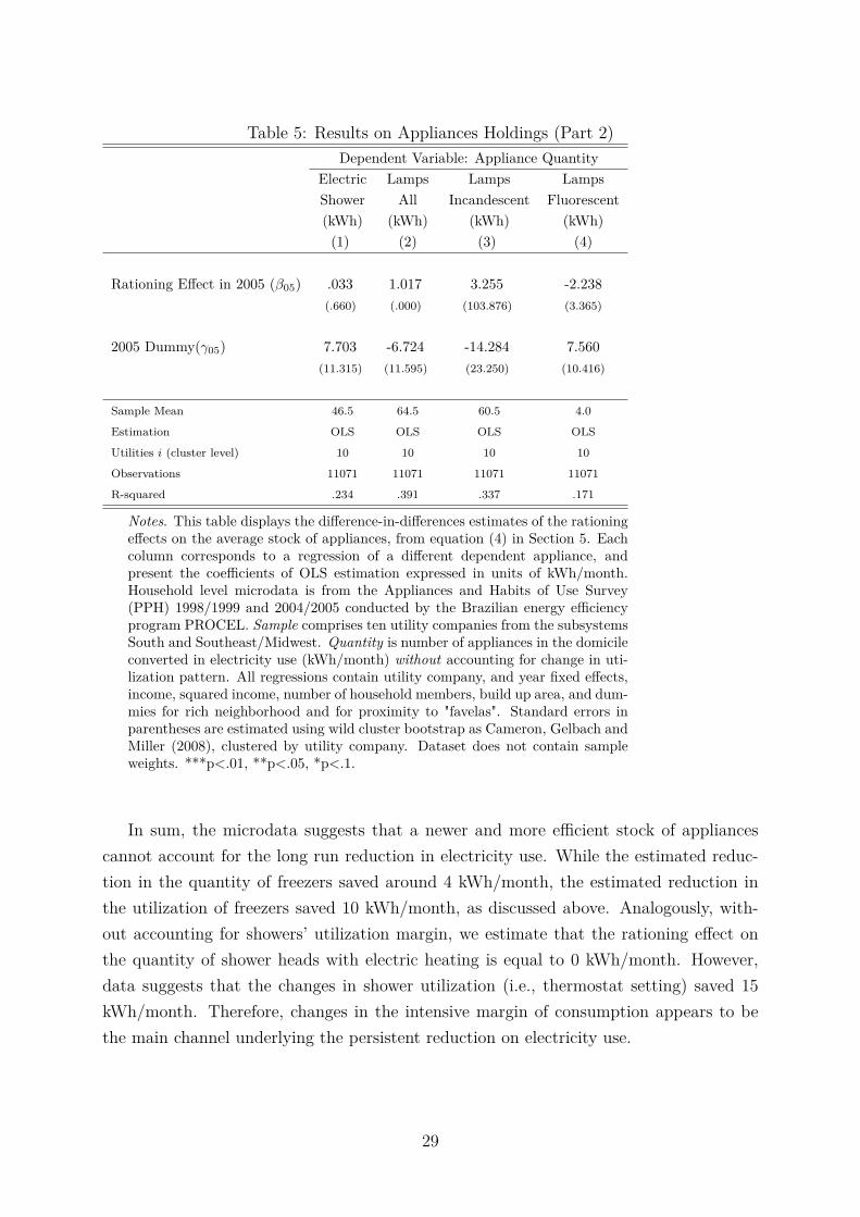
Table 5: Results on Appliances Holdings (Part 2)Dependent Variable: Appliance Quantity

Electric Lamps Lamps LampsShower All Incandescent Fluorescent(kWh) (kWh) (kWh) (kWh)(1) (2) (3) (4)

Rationing Effect in 2005 (β05) .033 1.017 3.255 -2.238(.660) (.000) (103.876) (3.365)

2005 Dummy(γ05) 7.703 -6.724 -14.284 7.560(11.315) (11.595) (23.250) (10.416)

Sample Mean 46.5 64.5 60.5 4.0

Estimation OLS OLS OLS OLS

Utilities i (cluster level) 10 10 10 10

Observations 11071 11071 11071 11071

R-squared .234 .391 .337 .171

Notes. This table displays the difference-in-differences estimates of the rationingeffects on the average stock of appliances, from equation (4) in Section 5. Eachcolumn corresponds to a regression of a different dependent appliance, andpresent the coefficients of OLS estimation expressed in units of kWh/month.Household level microdata is from the Appliances and Habits of Use Survey(PPH) 1998/1999 and 2004/2005 conducted by the Brazilian energy efficiencyprogram PROCEL. Sample comprises ten utility companies from the subsystemsSouth and Southeast/Midwest. Quantity is number of appliances in the domicileconverted in electricity use (kWh/month) without accounting for change in uti-lization pattern. All regressions contain utility company, and year fixed effects,income, squared income, number of household members, build up area, and dum-mies for rich neighborhood and for proximity to "favelas". Standard errors inparentheses are estimated using wild cluster bootstrap as Cameron, Gelbach andMiller (2008), clustered by utility company. Dataset does not contain sampleweights. ***p<.01, **p<.05, *p<.1.

In sum, the microdata suggests that a newer and more efficient stock of appliancescannot account for the long run reduction in electricity use. While the estimated reduc-tion in the quantity of freezers saved around 4 kWh/month, the estimated reduction inthe utilization of freezers saved 10 kWh/month, as discussed above. Analogously, with-out accounting for showers’ utilization margin, we estimate that the rationing effect onthe quantity of shower heads with electric heating is equal to 0 kWh/month. However,data suggests that the changes in shower utilization (i.e., thermostat setting) saved 15kWh/month. Therefore, changes in the intensive margin of consumption appears to bethe main channel underlying the persistent reduction on electricity use.

29

5 Conclusion

Both economic theory and empirical evidence recognize that economic problems may havemultiple steady states. However, the feasibility of using temporary interventions to in-duce individuals to switch steady states with sustainable effects is still being discussed bythe empirical literature and policy makers. This paper contributes to this discussion byanalyzing households’ response to an electricity rationing program in Brazil in 2001-2002.The main contribution of this paper is to provide empirical evidence that a temporaryintervention appears to have promoted sustained changes in consumption behavior. Theresults suggest that households can switch to steady states with smaller energy consump-tion in response to a temporary demand response program. The long run effect observedis stable over time, and the energy saved has been equivalent to 1.5 months of electricityevery year, for the last 10 years, and counting.

The picture emerging from the household level microdata shows that the temporaryrationing had a lasting impact on people’s behavior and appliances utilization, rather thanincreasing long run adoption of energy-efficient technology. From an energy perspective,this is important because it suggests that we cannot discuss an “energy efficiency gap”solely on the basis of technology, we should consider its behavioral counterpart as well.

A caveat of this paper is that I cannot empirically disentangle which economic mech-anisms are underlying the long run effects. The design of the quasi-experiment studiedhere restricts the identification of the precise mechanism within a class of economic mod-els which generate similar revealed preferences in this context. Understanding the precisemodel driving the results is crucial in order to estimate the welfare cost of the transitionbetween steady states. In particular, if these mechanisms involve externalities or inter-nalities of electricity use (Stern 2007; Nordhaus 2011; Allcott and Mullainathan 2010),then there could be aggregate welfare gains from shifting consumption to steady stateswith smaller energy use.

A key difference between this paper and the literature that assesses the persistenceof large historical events is that the policy studied here could be feasibly replicated.And a difference between this policy and most of the demand response programs in theliterature is that it was not a nudge, or a surgical incentive given to individuals, but anationwide intervention. In particular, its breadth allows for general equilibrium effects totake place, as well as potential complementarity between different economic mechanisms,such as price, information, social norms, and habits.

30

ReferencesAbadie, Alberto, & Gardeazabal, Javier. 2003. The economic costs of conflict:A case study of the Basque Country. American Economic Review, 113–132.

Acemoglu, Daron, García-Jimeno, Camilo, & Robinson, James A. 2012. Find-ing Eldorado: Slavery and long-run development in Colombia. Journal of ComparativeEconomics.

Acland, Dan, & Levy, Matthew. Habit Formation, Naivete, and Projection Bias inGym Attendance.

Agarwal, Sumit, Driscoll, John C, Gabaix, Xavier, & Laibson, David. 2008.Learning in the credit card market. Tech. rept. National Bureau of Economic Research.

Allcott, Hunt. 2011a. Consumers’ Perceptions and Misperceptions of Energy Costs.The American Economic Review, 101(3), 98–104.

Allcott, Hunt. 2011b. Social norms and energy conservation. Journal of Public Eco-nomics, 95(9), 1082–1095.

Allcott, Hunt, & Greenstone, Michael. 2012. Is There an Energy EfficiencyGap? The Journal of Economic Perspectives, 26(1), 3–28.

Allcott, Hunt, & Mullainathan, Sendhil. 2010. Behavioral science and energypolicy. Science, 327(5970), 1204–1205.

Allcott, Hunt, & Rogers, Todd. 2012. The short-run and long-run effects ofbehavioral interventions: Experimental evidence from energy conservation. Tech. rept.National Bureau of Economic Research.

Becker, Gary S, & Murphy, Kevin M. 1988. A theory of rational addiction. TheJournal of Political Economy, 675–700.

Bertrand, Marianne, Duflo, Esther, & Mullainathan, Sendhil. 2004. Howmuch should we trust differences-in-differences estimates? The Quarterly Journal ofEconomics, 119(1), 249–275.

Bleakley, Hoyt, & Lin, Jeffrey. 2012. Portage and path dependence. The QuarterlyJournal of Economics, 127(2), 587–644.

Bloom, David E, Canning, David, & Sevilla, Jaypee. 2003. Geography andpoverty traps. Journal of Economic Growth, 8(4), 355–378.

Cameron, A Colin, Gelbach, Jonah B, & Miller, Douglas L. 2008. Bootstrap-based improvements for inference with clustered errors. The Review of Economics andStatistics, 90(3), 414–427.

Charness, Gary, & Gneezy, Uri. 2009. Incentives to exercise. Econometrica, 77(3),909–931.

Co., McKinsey &. 2009. Unlocking Energy Efficiency in the U.S. Economy. Tech. rept.

31

Collier Jr, Irwin L. 1986. Effective purchasing power in a quantity constrained econ-omy: An estimate for the German Democratic Republic. The Review of Economics andStatistics, 24–32.

Costa, Dora L, & Kahn, Matthew E. 2010. Energy conservation" nudges" andenvironmentalist ideology: Evidence from a randomized residential electricity field ex-periment. Tech. rept. National Bureau of Economic Research.

Davis, Lucas W, Fuchs, Alan, & Gertler, Paul J. 2012. Cash for Coolers. Tech.rept. National Bureau of Economic Research.

de Oliveira, Luiz Antônio Pinto, & de Oliveira, Antônio Tadeu Ribeiro.2011. Reflexões sobre os deslocamentos populacionais no Brasil. IBGE.

Dell, Melissa. 2010. The persistent effects of Peru’s mining Mita. Econometrica, 78(6),1863–1903.

Diamond, Peter A. 1982. Aggregate demand management in search equilibrium. TheJournal of Political Economy, 881–894.

Dubin, Jeffrey A, & McFadden, Daniel L. 1984. An econometric analysis ofresidential electric appliance holdings and consumption. Econometrica: Journal of theEconometric Society, 345–362.

Dupas, Pascaline. 2010. Short-run subsidies and long-run adoption of new health prod-ucts: evidence from a field experiment. Tech. rept. National Bureau of Economic Re-search.

EIA, US. 2011. Annual energy review. Energy Information Administration, US Depart-ment of Energy: Washington, DC www. eia. doe. gov/emeu/aer.

Ferraro, Paul J, & Price, Michael K. 2011. Using non-pecuniary strategies toinfluence behavior: Evidence from a large scale field experiment. Tech. rept. NationalBureau of Economic Research.

Finkenrath, Matthias. 2011. Cost and performance of carbon dioxide capture frompower generation. Tech. rept. OECD Publishing.

Gerard, Francois. 2012. Energy Crisis Management, Temporary Incentives, Long-Term Effects: Evidence from the 2001 Brazilian Electricity Crisis. Available at SSRN:http:// ssrn. com/ abstract=2097195.

Giné, Xavier, Karlan, Dean, & Zinman, Jonathan. 2010. Put your money whereyour butt is: a commitment contract for smoking cessation. American Economic Jour-nal: Applied Economics, 213–235.

Gneezy, Uri, Meier, Stephan, & Rey-Biel, Pedro. 2011. When and why incen-tives (don’t) work to modify behavior. The Journal of Economic Perspectives, 25(4),191–209.

Haselhuhn, Michael P, Pope, Devin G, Schweitzer, Maurice E, & Fishman,Peter. 2012. The impact of personal experience on behavior: Evidence from video-rental fines. Management Science, 58(1), 52–61.

32

John, Leslie K, Norton, Laurie, Fassbender, Jennifer E, & Volpp, Kevin G.2011. Financial incentives for extended weight loss: a randomized, controlled trial.Journal of general internal medicine, 26(6), 621–626.

Kelman, Jelson. 2001. Relatório da Comissão de Análise do Sistema Hidrotérmico deEnergia Elétrica. Governo Federal do Brasil.

Kőszegi, Botond, & Rabin, Matthew. 2006. A model of reference-dependent pref-erences. The Quarterly Journal of Economics, 121(4), 1133–1165.

Kremer, Michael, & Miguel, Edward. 2007. The illusion of sustainability. TheQuarterly Journal of Economics, 122(3), 1007–1065.

Liebman, Jeffrey B, Katz, Lawrence F, & Kling, Jeffrey R. 2004. Beyondtreatment effects: Estimating the relationship between neighborhood poverty and indi-vidual outcomes in the MTO experiment. Harvard University, John F. Kennedy Schoolof Government.

Lindbeck, Assar. 1997. Incentives and social norms in household behavior. The Amer-ican Economic Review, 87(2), 370–377.

Lipscomb, Molly, Mobarak, Ahmed Mushfiq, & Barham, Tania. 2013. Devel-opment Effects of Electrification: Evidence from the Topographic Placement of Hy-dropower Plants in Brazil. American Economic Journal: Applied Economics, 5(2),200–231.

Manski, C, & Pepper, J. 2012. Partial identification of treatment response with dataon repeated cross sections. Department of Economics, Northwestern University.

Mation, Lucas, & Ferraz, Claudio. 2011. How Do Firms React to InfrastructureConstraints?

Naik, Narayan Y, & Moore, Michael J. 1996. Habit formation and intertemporalsubstitution in individual food consumption. The Review of Economics and Statistics,321–328.

Neary, J Peter, & Roberts, Kevin WS. 1980. The theory of household behaviourunder rationing. European economic review, 13(1), 25–42.

Nordhaus, William D. 2011. Estimates of the social cost of carbon: background andresults from the RICE-2011 model. Tech. rept. National Bureau of Economic Research.

Obstfeld, Maurice. 1984. Multiple stable equilibria in an optimizing perfect-foresightmodel. Econometrica: Journal of the Econometric Society, 223–228.

ONS, Operador Nacional do Sistema Eletrico. 2011. Plano Decenal de Energia.Tech. rept.

Orphanides, Athanasios, & Zervos, David. 1994. Optimal consumption dynamicswith non-concave habit-forming utility. Economics Letters, 44(1), 67–72.

PDE. 1997. Plano Decenal de Energia. Tech. rept. EPE/Ministério de Minas e Energia.

33

Piketty, Thomas. 1995. Social mobility and redistributive politics. The Quarterlyjournal of economics, 110(3), 551–584.

Pimenta, Amanda, Notini, Hilton, & Maciel, Luis Felipe. 2009. Brazilian Elec-tricity Demand Estimation: What Has Changed after the Rationing in 2001? AnApplication of Time Varying Parameter Error Correction Model.

Pollak, Robert A, & Wachter, Michael L. 1975. The relevance of the householdproduction function and its implications for the allocation of time. The Journal ofPolitical Economy, 255–278.

PROCEL, Programa Nacional de Conservação de Energia Elétrica. 2007.Pesquisa de Posse de Equipamentos e Hábitos de Uso – ano Base 2005 – Classe resi-dencial – relatório Brasil. Rio de Janeiro: ELETROBRAS/PROCEL.

Ravallion, Martin, Galasso, Emanuela, Lazo, Teodoro, & Philipp,Ernesto. 2005. What Can Ex-participants Reveal about a Program’s Impact? Journalof Human Resources, 40(1), 208–230.

Redding, Stephen J, Sturm, Daniel M, & Wolf, Nikolaus. 2011. History andindustry location: Evidence from german airports. Review of Economics and Statistics,93(3), 814–831.

Reiss, Peter C, & White, Matthew W. 2008. What changes energy consumption?Prices and public pressures. The RAND Journal of Economics, 39(3), 636–663.

Rosenstein-Rodan, Paul N. 1943. Problems of industrialisation of eastern and south-eastern Europe. The Economic Journal, 53(210/211), 202–211.

Stern, Nicholas. 2007. The economics of climate change: the Stern review. cambridgeUniversity press.

Thøgersen, John. 2009. Promoting public transport as a subscription service: Effectsof a free month travel card. Transport Policy, 16(6), 335–343.

Tobin, James. 1952. A Survey of the Theory of Rationing. Econometrica: Journal ofthe Econometric Society, 521–553.

Zweiniger-Bargielowska, Ina. 2000. Austerity in Britain: rationing, controls, andconsumption, 1939-1955. Oxford University Press on Demand.

34

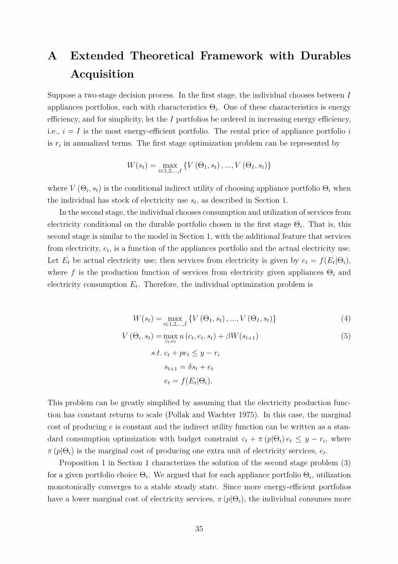
A Extended Theoretical Framework with DurablesAcquisition

Suppose a two-stage decision process. In the first stage, the individual chooses between Iappliances portfolios, each with characteristics Θi. One of these characteristics is energyefficiency, and for simplicity, let the I portfolios be ordered in increasing energy efficiency,i.e., i = I is the most energy-efficient portfolio. The rental price of appliance portfolio iis ri in annualized terms. The first stage optimization problem can be represented by

W (st) = maxi∈1,2,...,I

{V (Θ1, st) , ..., V (ΘI , st)}

where V (Θi, st) is the conditional indirect utility of choosing appliance portfolio Θi whenthe individual has stock of electricity use st, as described in Section 1.

In the second stage, the individual chooses consumption and utilization of services fromelectricity conditional on the durable portfolio chosen in the first stage Θi. That is, thissecond stage is similar to the model in Section 1, with the additional feature that servicesfrom electricity, et, is a function of the appliances portfolio and the actual electricity use.Let Et be actual electricity use; then services from electricity is given by et = f(Et|Θi),where f is the production function of services from electricity given appliances Θi andelectricity consumption Et. Therefore, the individual optimization problem is

W (st) = maxi∈1,2,...,I

{V (Θ1, st) , ..., V (ΘI , st)} (4)

V (Θi, st) = maxct,et

u (ct, et, st) + βW (st+1) (5)

s.t. ct + pet ≤ y − rist+1 = δst + et

et = f(Et|Θi).

This problem can be greatly simplified by assuming that the electricity production func-tion has constant returns to scale (Pollak and Wachter 1975). In this case, the marginalcost of producing e is constant and the indirect utility function can be written as a stan-dard consumption optimization with budget constraint ct + π (p|Θi) et ≤ y − ri, whereπ (p|Θi) is the marginal cost of producing one extra unit of electricity services, et.

Proposition 1 in Section 1 characterizes the solution of the second stage problem (3)for a given portfolio choice Θi. We argued that for each appliance portfolio Θi, utilizationmonotonically converges to a stable steady state. Since more energy-efficient portfolioshave a lower marginal cost of electricity services, π (p|Θi), the individual consumes more

35

services from electricity, assuming the income effect associated with electricity priceschanges to be sufficiently small. Therefore, more energy-efficient portfolios are associatedwith steady states with a higher utilization of services from electricity. For any initial stockof electricity use st, the optimal appliance choice and utilization of electricity services willthus monotonically converge to the steady state of one of the appliances portfolios Θi.

The Rationing (Dynamics)Rationing in this setting can be interpreted as a temporary restriction on electricity

use, Et. That is, the individual optimization problem has an extra constraint Et ≤ E <

E∗i∗ , where E∗i∗ is her initial optimal choice. This can be written as a restriction on theutilization of appliance portfolios. During the rationing, for any appliance portfolio i, theoptimal services from electricity is min

{e∗ (p, y − ri|Θi) ; f(E|Θi)

}.

As discussed in Davis, Fuchs, and Gertler (2012), the optimal appliance portfolio choiceduring the rationing - i.e. whether or not one invests in more energy-efficient appliances- depends on the price elasticity of the electricity services of each appliance. Durablesthat provide inelastic services which cannot be substituted with less energy-intensiveservices, such as basic food refrigeration, would be substituted with more energy-efficientappliances in order to maintain the service level. On the other hand, appliances thatprovide elastic services which can be substituted with less energy-intensive technologies,such as air conditioners, would be less utilized and, consequently, would receive smallerinvestments. This yields two additional predictions.

Prediction 2. During the rationing, the average stock of appliances that provide inelastic(elastic) services tend to become more (less) energy-efficient.

The results from Section 4 are consistent with this prediction. The evidence suggeststhat during the rationing households substituted old refrigerators with new and moreefficient ones. At the same time, households switched off freezers and utilized fewer airconditioners, postponing the acquisition of these appliances.

Once the rationing is over, incentives regarding durables are back to normal, and theindividual is back to the unconstrained problem (4) and (5). Therefore, any long runeffects will emerge through new steady states in the consumption of electricity services.In particular, appliances portfolios can be affected in two directions. An individual whoinvested in energy-efficiency during the rationing would be able to sustain a higher utiliza-tion level and her consumption stock would be less likely to fall below a critical level andconverge to a lower steady state. Alternatively, an individual who postponed investmentsin appliances and reduced utilization during the rationing, would have a smaller stock ofservices from electricity by the end of the rationing and would be more likely to switchsteady states.

Prediction 3. After the rationing, the individual enters an optimal path that monotoni-

36

cally converges to a steady state with weakly lower consumption of services from electricity,and a portfolio with weakly less energy-efficient appliances.

An individual who joins a new optimal path and converges to a steady state with lowerservices utilization will have less incentive to invest in appliances’ efficiency, because hermarginal utility of utilization is smaller than initially. Thus, her new optimal portfoliochoice will be weakly less energy-efficient than her original one. Evidence from freezerspresented in Section 4 is consistent with this prediction.

37

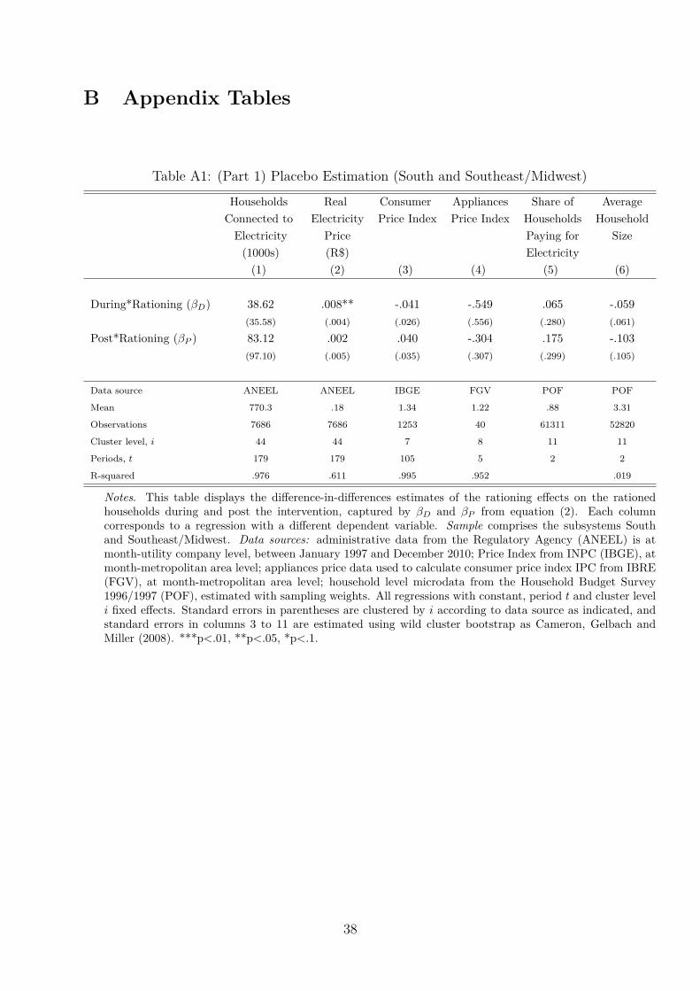
B Appendix Tables

Table A1: (Part 1) Placebo Estimation (South and Southeast/Midwest)

Households Real Consumer Appliances Share of AverageConnected to Electricity Price Index Price Index Households HouseholdElectricity Price Paying for Size(1000s) (R$) Electricity(1) (2) (3) (4) (5) (6)

During*Rationing (βD) 38.62 .008** -.041 -.549 .065 -.059(35.58) (.004) (.026) (.556) (.280) (.061)

Post*Rationing (βP ) 83.12 .002 .040 -.304 .175 -.103(97.10) (.005) (.035) (.307) (.299) (.105)

Data source ANEEL ANEEL IBGE FGV POF POF

Mean 770.3 .18 1.34 1.22 .88 3.31

Observations 7686 7686 1253 40 61311 52820

Cluster level, i 44 44 7 8 11 11

Periods, t 179 179 105 5 2 2

R-squared .976 .611 .995 .952 .019

Notes. This table displays the difference-in-differences estimates of the rationing effects on the rationedhouseholds during and post the intervention, captured by βD and βP from equation (2). Each columncorresponds to a regression with a different dependent variable. Sample comprises the subsystems Southand Southeast/Midwest. Data sources: administrative data from the Regulatory Agency (ANEEL) is atmonth-utility company level, between January 1997 and December 2010; Price Index from INPC (IBGE), atmonth-metropolitan area level; appliances price data used to calculate consumer price index IPC from IBRE(FGV), at month-metropolitan area level; household level microdata from the Household Budget Survey1996/1997 (POF), estimated with sampling weights. All regressions with constant, period t and cluster leveli fixed effects. Standard errors in parentheses are clustered by i according to data source as indicated, andstandard errors in columns 3 to 11 are estimated using wild cluster bootstrap as Cameron, Gelbach andMiller (2008). ***p<.01, **p<.05, *p<.1.

38

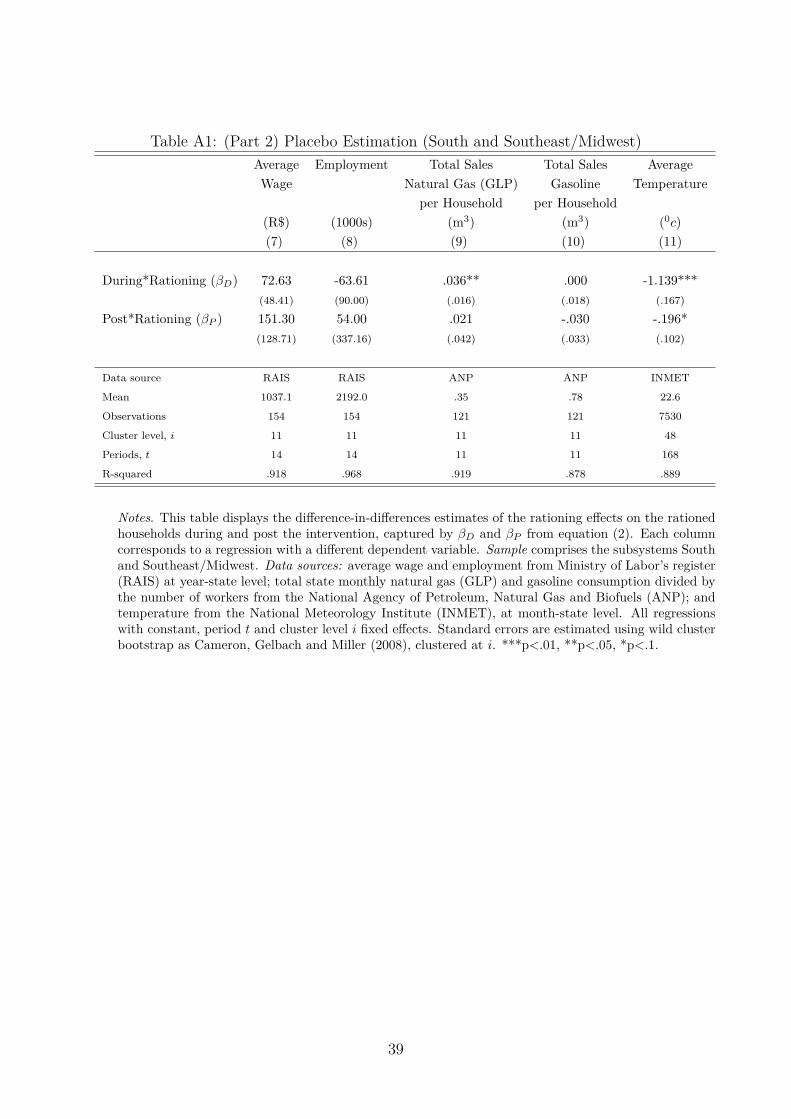
Table A1: (Part 2) Placebo Estimation (South and Southeast/Midwest)Average Employment Total Sales Total Sales AverageWage Natural Gas (GLP) Gasoline Temperature

per Household per Household(R$) (1000s) (m3) (m3) (0c)(7) (8) (9) (10) (11)

During*Rationing (βD) 72.63 -63.61 .036** .000 -1.139***(48.41) (90.00) (.016) (.018) (.167)

Post*Rationing (βP ) 151.30 54.00 .021 -.030 -.196*(128.71) (337.16) (.042) (.033) (.102)

Data source RAIS RAIS ANP ANP INMET

Mean 1037.1 2192.0 .35 .78 22.6

Observations 154 154 121 121 7530

Cluster level, i 11 11 11 11 48

Periods, t 14 14 11 11 168

R-squared .918 .968 .919 .878 .889

Notes. This table displays the difference-in-differences estimates of the rationing effects on the rationedhouseholds during and post the intervention, captured by βD and βP from equation (2). Each columncorresponds to a regression with a different dependent variable. Sample comprises the subsystems Southand Southeast/Midwest. Data sources: average wage and employment from Ministry of Labor’s register(RAIS) at year-state level; total state monthly natural gas (GLP) and gasoline consumption divided bythe number of workers from the National Agency of Petroleum, Natural Gas and Biofuels (ANP); andtemperature from the National Meteorology Institute (INMET), at month-state level. All regressionswith constant, period t and cluster level i fixed effects. Standard errors are estimated using wild clusterbootstrap as Cameron, Gelbach and Miller (2008), clustered at i. ***p<.01, **p<.05, *p<.1.

39

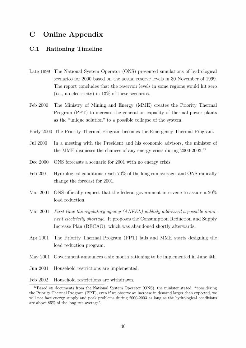
C Online Appendix

C.1 Rationing Timeline

Late 1999 The National System Operator (ONS) presented simulations of hydrologicalscenarios for 2000 based on the actual reserve levels in 30 November of 1999.The report concludes that the reservoir levels in some regions would hit zero(i.e., no electricity) in 13% of these scenarios.

Feb 2000 The Ministry of Mining and Energy (MME) creates the Priority ThermalProgram (PPT) to increase the generation capacity of thermal power plantsas the “unique solution” to a possible collapse of the system.

Early 2000 The Priority Thermal Program becomes the Emergency Thermal Program.

Jul 2000 In a meeting with the President and his economic advisors, the minister ofthe MME dismisses the chances of any energy crisis during 2000-2003.42

Dec 2000 ONS forecasts a scenario for 2001 with no energy crisis.

Feb 2001 Hydrological conditions reach 70% of the long run average, and ONS radicallychange the forecast for 2001.

Mar 2001 ONS officially request that the federal government intervene to assure a 20%load reduction.

Mar 2001 First time the regulatory agency (ANEEL) publicly addressed a possible immi-nent electricity shortage. It proposes the Consumption Reduction and SupplyIncrease Plan (RECAO), which was abandoned shortly afterwards.

Apr 2001 The Priority Thermal Program (PPT) fails and MME starts designing theload reduction program.

May 2001 Government announces a six month rationing to be implemented in June 4th.

Jun 2001 Household restrictions are implemented.

Feb 2002 Household restrictions are withdrawn.42Based on documents from the National System Operator (ONS), the minister stated: “considering

the Priority Thermal Program (PPT), even if we observe an increase in demand larger than expected, wewill not face energy supply and peak problems during 2000-2003 as long as the hydrological conditionsare above 85% of the long run average”.

40

C.2 Data Cleaning

I convert all variables I can in units of electricity utilization (kWh/month). The hypothet-ical average electricity use of appliances was calculated by the Brazilian energy efficiencyprogram PROCEL based on technical characteristics of appliances and hypothetical uti-lization. Table A5 presents these values.

Electricity Data (ANEEL). I discard December 2011 from the sample because val-ues had not been revised by the Regulatory Agency (ANEEL). I use synth state function togenerate the synthetic controls in the estimation (http://www.mit.edu/~jhainm/software.htm).

Habits of Energy Use (PPH). Quantity of appliances is the number of appliancesowned by the household multiplied by the appliance utilization in Table A5. Appliancesfrequently use stand for appliances utilized more than four times a week. Shower ther-mostats could be regulated at three different levels: Off, Low Power (Mode Verão), orHigh Power (Modo Inverno). A shower regulated in Low Power consumes 30% less energythan one regulated in High Power. I calculate the electricity inputed in each shower bymultiplying [number of people who uses the shower]*[shower electricity use for its ther-mostat setting]. I consider the average shower time reported in the 2004/2005 survey,which is 12 minutes.

Appliances Holdings (POF). In the Household Budget Survey (POF), a householdmay declare having more than one house, I discard second houses and restrict attention tothe main domicile. As discussed in the text, I restrict the sample of the regressions to thehouseholds who pay for electricity. I define a household who do not pay for electricity asa household who own at least one electrical appliance and claim no expenses on electricityor own an electricity generator. I truncate appliances’ age at 15 years, because the yearan old appliance was bought is subject to severe measurement errors.

Appliances’ Prices. The smaller unit in the cross-section is a triple product*informer*store. An informer*store i is located in the capital of state s, and a product k is a spe-cific model of appliance a - e.g., product, k, may be “Fluorescent light bulb universal20/40W General Eletrics”, which is a model of appliance, a, “Lamp”. That is, the unitof observation is the price observed by informer i, in state s, of product k on date t:pi,s,k,t. I construct price indeces following the (unweighted) methodology of the officialprice indexes from IBRE/FGV, who provided the microdata. This price index constitutesof calculating the month inflation rate per observational unit (informer & product) andaggregate it using geometric average. Hence, the inflation rate of product k, and appliancea, on state s month t are respectively:

∆ps,k,t =(

Πipi,s,k,tpi,s,k,t−1

) 1#i

, and ∆ps,a,t = (Πk∆ps,k,t)1

#k

41

where #i and and #k are the number of informers and product models in state s, appliancea, respectively. I use the monthly inflation rate to create the accumulated price indexrelative to January 2001, the first month in the sample for which I have observations inthe South, Is,a,t = Πt

τ=1∆Ps,a,τ .

C.3 Retailer Market Composition

Another issue to consider is if retailers are stocking and advertising different appliancesin different regions, what would affect the type of appliances available in the stores acrossthe regions. I use microdata on appliances’ prices collected in stores by IBRE/FGV toinvestigate this issue. Prices are surveyed in stores according to the products available onthe shelves. Since product descriptions are very detailed,43 I can compare the availabilityof products in the shelves in both regions and how this changed over time.

I aggregate products observed, k, by year, t, and rationed region, r, and verify foreach product if it is present in both rationed regions in that year. Let Cktr be a dummyequal to one if product k in region r year t is also present in region −r in the same year.Because I only observe prices in both regions from 2001 on, I test if the share of productsbeing sold in both regions changed after 2001 by performing a logit regression:

Cktr = α + βPPostt ∗Rationr + γr + γt + εktr (6)

where Rationr is a dummy equal to one for the rationed regions, Postt is a dummy equalto one for years 2002 to 2005, and γs are region and year fixed effects. I also run onespecification with appliance fixed effects, and weighting the regressions with the number ofstores selling each product. I display standard errors robust and clustered at the appliancelevel.

Table A7 presents the results. Since the baseline in this regression is 2001, I read theseresults with caution. First, we see that around eighty percent of products are availablein stores in both regions. Also, the logit estimates suggest that products available in thestores of the Southeast/Midwest became more likely to be present in the stores of theSouth as well. This is evidence against the hypothesis that the composition of productsin the stores of the Southeast/Midwest specialized in products not available in the Southregion.

43For example, “REFRIGERADOR DOMESTICO 440 LITROS MOD:DOUBLE 44 ELECTROLUX(UNID)”.

42

6080

100

120

140

160

Per

cent

age

of A

vera

ge M

W in

the

mon

th (

%)

1 2 3 4 5 6 7 8 9 10 11 12Month

2001

Southeast/Midwest

010

020

030

040

0

Per

cent

age

of A

vera

ge M

W in

the

mon

th (

%)

1 2 3 4 5 6 7 8 9 10 11 12Month

2001

South

Figure A1: stream-flow Energy of Rivers as Percentage of Subsystems’ Historical Average(1996-2010)

Notes. This figure presents the stream-flow energy level of the rivers in each month as a percentage ofthe subsystem’s historical average for each month. That is, a value 100 means that in that month-yearthe stream-flow level was equal to the average stream-flow level in that month of the year. Each linerepresents a different year from 1996-2010. As we can see, the stream-flow level in the subsystemSoutheast/Midwest in the first half of 2001 is practically the lower envelope of the historical series inthe first months of the year. This low stream-flow level triggered the rationing in early 2001. Source:National System Operator (ONS).

43

Rationing.4.6

.81

1.21

.41.

6 1.8

2

1995m1 1997m1 1999m1 2001m1 2003m1 2005m1 2007m1 2009m1 2011m1

South (Control) Southeast/Midwest (Rationed)

Avg

. Ele

ct. P

rice

(rel

ativ

e to

Jan

/200

1)

.51

1.5

22.

5

1995 1997 1999 2001 2003 2005 2007 2009

Ave

rage

Wag

e (r

elat

ive

to 2

000)

Figure A2: Evolution of Electricity Prices and Wages Normalized to Pre-Rationing LevelsNotes. The first graph presents the monthly average electricity prices in the South and South-east/Midwest, normalized to prices of January 2001. The two vertical lines mark the rationingperiod. Data from the Regulatory Agency ANEEL. The second graph presents the annual averagewage in the South and Southeast/Midwest, normalized to wages of 2000 (before the rationing). Thevertical line marks 2001, the rationing year. Data from the Ministry of Labor’s register (RAIS).

44

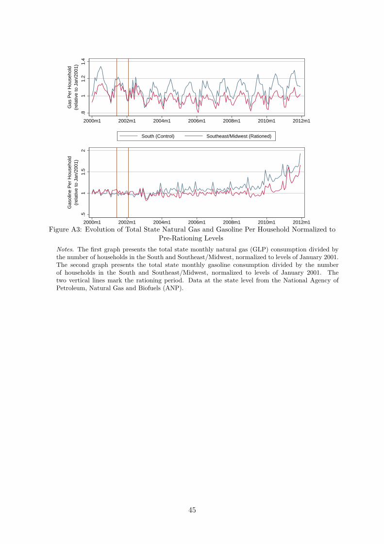
.81

1.2

1.4

2000m1 2002m1 2004m1 2006m1 2008m1 2010m1 2012m1

South (Control) Southeast/Midwest (Rationed)

(rel

ativ

e to

Jan

/200

1)G

as P

er H

ouse

hold

.51

1.5

2

2000m1 2002m1 2004m1 2006m1 2008m1 2010m1 2012m1

(rel

ativ

e to

Jan

/200

1)G

asol

ine

Per

Hou

seho

ld

Figure A3: Evolution of Total State Natural Gas and Gasoline Per Household Normalized toPre-Rationing Levels

Notes. The first graph presents the total state monthly natural gas (GLP) consumption divided bythe number of households in the South and Southeast/Midwest, normalized to levels of January 2001.The second graph presents the total state monthly gasoline consumption divided by the numberof households in the South and Southeast/Midwest, normalized to levels of January 2001. Thetwo vertical lines mark the rationing period. Data at the state level from the National Agency ofPetroleum, Natural Gas and Biofuels (ANP).

45

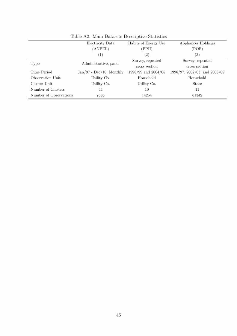
Table A2: Main Datasets Descriptive StatisticsElectricity Data Habits of Energy Use Appliances Holdings

(ANEEL) (PPH) (POF)(1) (2) (3)

Type Administrative, panelSurvey, repeated Survey, repeatedcross section cross section

Time Period Jan/97 - Dec/10, Monthly 1998/99 and 2004/05 1996/97, 2002/03, and 2008/09Observation Unit Utility Co. Household HouseholdCluster Unit Utility Co. Utility Co. StateNumber of Clusters 44 10 11Number of Observations 7686 14254 61342

46

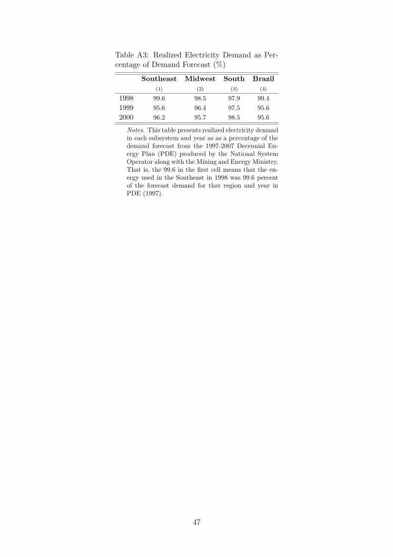
Table A3: Realized Electricity Demand as Per-centage of Demand Forecast (%)

Southeast Midwest South Brazil(1) (2) (3) (4)

1998 99.6 98.5 97.9 99.41999 95.6 96.4 97.5 95.62000 96.2 95.7 98.5 95.6

Notes. This table presents realized electricity demandin each subsystem and year as as a percentage of thedemand forecast from the 1997-2007 Decennial En-ergy Plan (PDE) produced by the National SystemOperator along with the Mining and Energy Ministry.That is, the 99.6 in the first cell means that the en-ergy used in the Southeast in 1998 was 99.6 percentof the forecast demand for that region and year inPDE (1997).

47

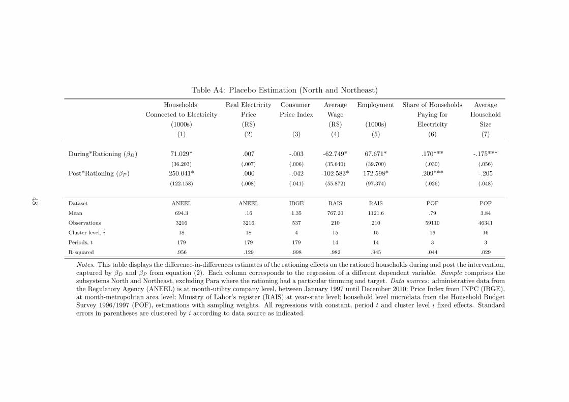
Table A4: Placebo Estimation (North and Northeast)

Households Real Electricity Consumer Average Employment Share of Households AverageConnected to Electricity Price Price Index Wage Paying for Household

(1000s) (R$) (R$) (1000s) Electricity Size(1) (2) (3) (4) (5) (6) (7)

During*Rationing (βD) 71.029* .007 -.003 -62.749* 67.671* .170*** -.175***(36.203) (.007) (.006) (35.640) (39.700) (.030) (.056)

Post*Rationing (βP ) 250.041* .000 -.042 -102.583* 172.598* .209*** -.205(122.158) (.008) (.041) (55.872) (97.374) (.026) (.048)

Dataset ANEEL ANEEL IBGE RAIS RAIS POF POF

Mean 694.3 .16 1.35 767.20 1121.6 .79 3.84

Observations 3216 3216 537 210 210 59110 46341

Cluster level, i 18 18 4 15 15 16 16

Periods, t 179 179 179 14 14 3 3

R-squared .956 .129 .998 .982 .945 .044 .029

Notes. This table displays the difference-in-differences estimates of the rationing effects on the rationed households during and post the intervention,captured by βD and βP from equation (2). Each column corresponds to the regression of a different dependent variable. Sample comprises thesubsystems North and Northeast, excluding Para where the rationing had a particular timming and target. Data sources: administrative data fromthe Regulatory Agency (ANEEL) is at month-utility company level, between January 1997 until December 2010; Price Index from INPC (IBGE),at month-metropolitan area level; Ministry of Labor’s register (RAIS) at year-state level; household level microdata from the Household BudgetSurvey 1996/1997 (POF), estimations with sampling weights. All regressions with constant, period t and cluster level i fixed effects. Standarderrors in parentheses are clustered by i according to data source as indicated.

48

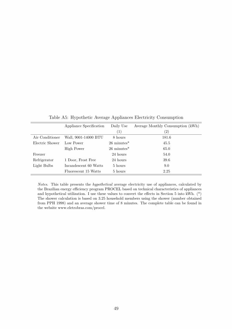
Table A5: Hypothetic Average Appliances Electricity Consumption

Appliance Specification Daily Use Average Monthly Consumption (kWh)(1) (2)

Air Conditioner Wall, 9001-14000 BTU 8 hours 181.6Electric Shower Low Power 26 minutes* 45.5

High Power 26 minutes* 65.0Freezer 24 hours 54.0Refrigerator 1 Door, Frost Free 24 hours 39.6Light Bulbs Incandescent 60 Watts 5 hours 9.0

Fluorescent 15 Watts 5 hours 2.25

Notes. This table presents the hypothetical average electricity use of appliances, calculated bythe Brazilian energy efficiency program PROCEL based on technical characteristics of appliancesand hypothetical utilization. I use these values to convert the effects in Section 5 into kWh. (*)The shower calculation is based on 3.25 household members using the shower (number obtainedfrom PPH 1998) and an average shower time of 8 minutes. The complete table can be found inthe website www.eletrobras.com/procel.

49

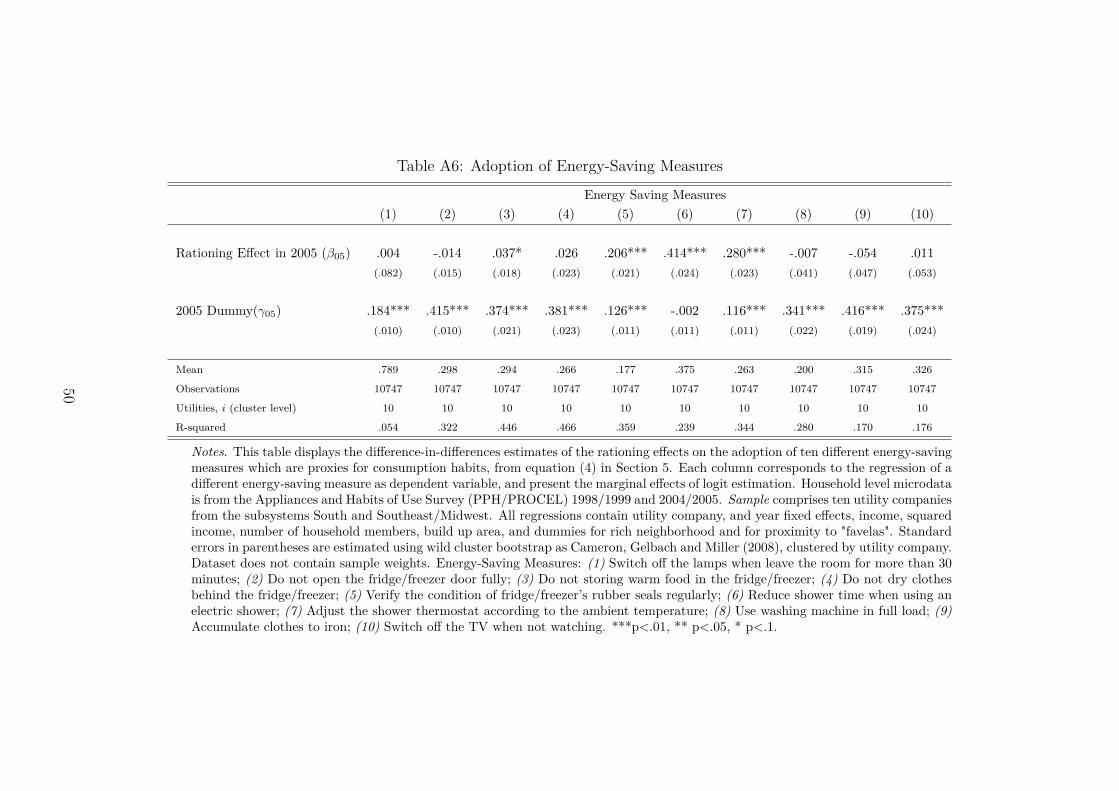
Table A6: Adoption of Energy-Saving Measures

Energy Saving Measures(1) (2) (3) (4) (5) (6) (7) (8) (9) (10)

Rationing Effect in 2005 (β05) .004 -.014 .037* .026 .206*** .414*** .280*** -.007 -.054 .011(.082) (.015) (.018) (.023) (.021) (.024) (.023) (.041) (.047) (.053)

2005 Dummy(γ05) .184*** .415*** .374*** .381*** .126*** -.002 .116*** .341*** .416*** .375***(.010) (.010) (.021) (.023) (.011) (.011) (.011) (.022) (.019) (.024)

Mean .789 .298 .294 .266 .177 .375 .263 .200 .315 .326

Observations 10747 10747 10747 10747 10747 10747 10747 10747 10747 10747

Utilities, i (cluster level) 10 10 10 10 10 10 10 10 10 10

R-squared .054 .322 .446 .466 .359 .239 .344 .280 .170 .176

Notes. This table displays the difference-in-differences estimates of the rationing effects on the adoption of ten different energy-savingmeasures which are proxies for consumption habits, from equation (4) in Section 5. Each column corresponds to the regression of adifferent energy-saving measure as dependent variable, and present the marginal effects of logit estimation. Household level microdatais from the Appliances and Habits of Use Survey (PPH/PROCEL) 1998/1999 and 2004/2005. Sample comprises ten utility companiesfrom the subsystems South and Southeast/Midwest. All regressions contain utility company, and year fixed effects, income, squaredincome, number of household members, build up area, and dummies for rich neighborhood and for proximity to "favelas". Standarderrors in parentheses are estimated using wild cluster bootstrap as Cameron, Gelbach and Miller (2008), clustered by utility company.Dataset does not contain sample weights. Energy-Saving Measures: (1) Switch off the lamps when leave the room for more than 30minutes; (2) Do not open the fridge/freezer door fully; (3) Do not storing warm food in the fridge/freezer; (4) Do not dry clothesbehind the fridge/freezer; (5) Verify the condition of fridge/freezer’s rubber seals regularly; (6) Reduce shower time when using anelectric shower; (7) Adjust the shower thermostat according to the ambient temperature; (8) Use washing machine in full load; (9)Accumulate clothes to iron; (10) Switch off the TV when not watching. ***p<.01, ** p<.05, * p<.1.

50

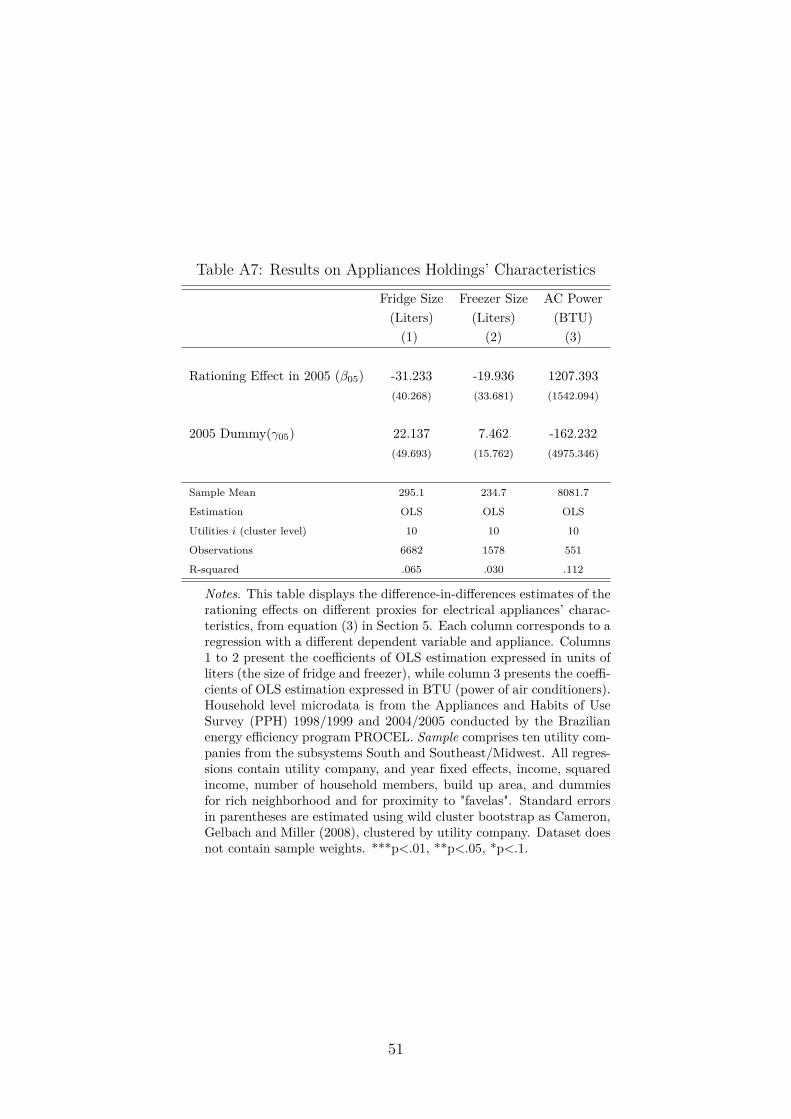
Table A7: Results on Appliances Holdings’ Characteristics

Fridge Size Freezer Size AC Power(Liters) (Liters) (BTU)(1) (2) (3)

Rationing Effect in 2005 (β05) -31.233 -19.936 1207.393(40.268) (33.681) (1542.094)

2005 Dummy(γ05) 22.137 7.462 -162.232(49.693) (15.762) (4975.346)

Sample Mean 295.1 234.7 8081.7

Estimation OLS OLS OLS

Utilities i (cluster level) 10 10 10

Observations 6682 1578 551

R-squared .065 .030 .112

Notes. This table displays the difference-in-differences estimates of therationing effects on different proxies for electrical appliances’ charac-teristics, from equation (3) in Section 5. Each column corresponds to aregression with a different dependent variable and appliance. Columns1 to 2 present the coefficients of OLS estimation expressed in units ofliters (the size of fridge and freezer), while column 3 presents the coeffi-cients of OLS estimation expressed in BTU (power of air conditioners).Household level microdata is from the Appliances and Habits of UseSurvey (PPH) 1998/1999 and 2004/2005 conducted by the Brazilianenergy efficiency program PROCEL. Sample comprises ten utility com-panies from the subsystems South and Southeast/Midwest. All regres-sions contain utility company, and year fixed effects, income, squaredincome, number of household members, build up area, and dummiesfor rich neighborhood and for proximity to "favelas". Standard errorsin parentheses are estimated using wild cluster bootstrap as Cameron,Gelbach and Miller (2008), clustered by utility company. Dataset doesnot contain sample weights. ***p<.01, **p<.05, *p<.1.

51

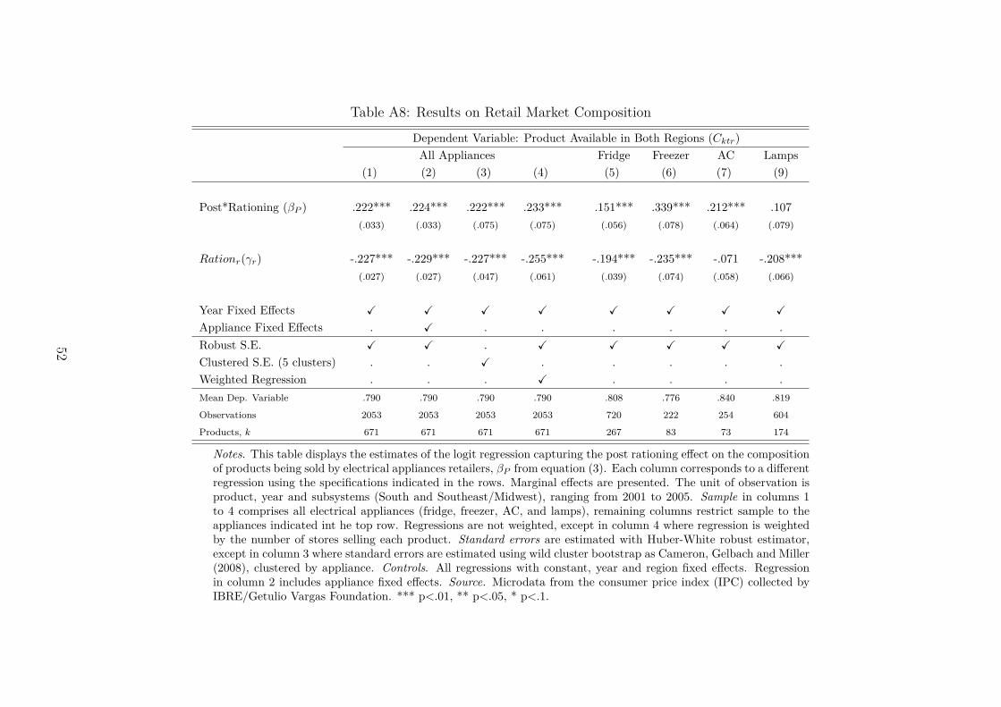
Table A8: Results on Retail Market Composition

Dependent Variable: Product Available in Both Regions (Cktr)All Appliances Fridge Freezer AC Lamps

(1) (2) (3) (4) (5) (6) (7) (9)

Post*Rationing (βP ) .222*** .224*** .222*** .233*** .151*** .339*** .212*** .107(.033) (.033) (.075) (.075) (.056) (.078) (.064) (.079)

Rationr(γr) -.227*** -.229*** -.227*** -.255*** -.194*** -.235*** -.071 -.208***(.027) (.027) (.047) (.061) (.039) (.074) (.058) (.066)

Year Fixed Effects X X X X X X X X

Appliance Fixed Effects . X . . . . . .Robust S.E. X X . X X X X X

Clustered S.E. (5 clusters) . . X . . . . .Weighted Regression . . . X . . . .Mean Dep. Variable .790 .790 .790 .790 .808 .776 .840 .819

Observations 2053 2053 2053 2053 720 222 254 604

Products, k 671 671 671 671 267 83 73 174

Notes. This table displays the estimates of the logit regression capturing the post rationing effect on the compositionof products being sold by electrical appliances retailers, βP from equation (3). Each column corresponds to a differentregression using the specifications indicated in the rows. Marginal effects are presented. The unit of observation isproduct, year and subsystems (South and Southeast/Midwest), ranging from 2001 to 2005. Sample in columns 1to 4 comprises all electrical appliances (fridge, freezer, AC, and lamps), remaining columns restrict sample to theappliances indicated int he top row. Regressions are not weighted, except in column 4 where regression is weightedby the number of stores selling each product. Standard errors are estimated with Huber-White robust estimator,except in column 3 where standard errors are estimated using wild cluster bootstrap as Cameron, Gelbach and Miller(2008), clustered by appliance. Controls. All regressions with constant, year and region fixed effects. Regressionin column 2 includes appliance fixed effects. Source. Microdata from the consumer price index (IPC) collected byIBRE/Getulio Vargas Foundation. *** p<.01, ** p<.05, * p<.1.

52

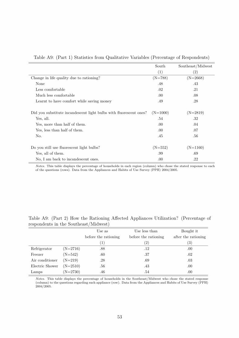
Table A9: (Part 1) Statistics from Qualitative Variables (Percentage of Respondents)

South Southeast/Midwest(1) (2)

Change in life quality due to rationing? (N=788) (N=2668)None .48 .43Less comfortable .02 .21Much less comfortable .00 .08Learnt to have comfort while saving money .49 .28

Did you substitute incandescent light bulbs with fluorescent ones? (N=1000) (N=2819)Yes, all. .54 .32Yes, more than half of them. .00 .04Yes, less than half of them. .00 .07No. .45 .56

Do you still use fluorescent light bulbs? (N=552) (N=1160)Yes, all of them. .99 .69No, I am back to incandescent ones. .00 .22Notes. This table displays the percentage of households in each region (column) who chose the stated response to eachof the questions (rows). Data from the Appliances and Habits of Use Survey (PPH) 2004/2005.

Table A9: (Part 2) How the Rationing Affected Appliances Utilization? (Percentage ofrespondents in the Southeast/Midwest)

Use as Use less than Bought itbefore the rationing before the rationing after the rationing

(1) (2) (3)Refrigerator (N=2716) .88 .12 .00Freezer (N=542) .60 .37 .02Air conditioner (N=219) .28 .69 .03Electric Shower (N=2510) .56 .43 .00Lamps (N=2730) .46 .54 .00

Notes. This table displays the percentage of households in the Southeast/Midwest who chose the stated response(column) to the questions regarding each appliance (row). Data from the Appliances and Habits of Use Survey (PPH)2004/2005.

53