Can Population Genetic Structure Be Predicted from Life-History Traits?

vol. 169, no. 5 the american naturalist may 2007 �

Can Population Genetic Structure Be Predicted

from Life-History Traits?

Jerome Duminil,1,* Silvia Fineschi,2,† Arndt Hampe,3,‡ Pedro Jordano,3,§ Daniela Salvini,4,k

Giovanni G. Vendramin,5,# and Remy J. Petit1,**

1. Unite Mixte de Recherche Biodiversite Genes et Ecosystemes,Institut National de Recherches Agronomiques Cestas, France;2. Istituto per la Protezione delle Piante, Consiglio Nazionale delleRicerche, Sesto Fiorentino, Italy;3. Integrative Ecology Group, Consejo Superior de InvestigacionesCientıficas, Estacion Biologica de Donana, Sevilla, Spain;4. Danish Center for Forest, Landscape, and Planning, RoyalVeterinary and Agricultural University, Hørsholm, Denmark;5. Istituto di Genetica Vegetale, Consiglio Nazionale delle Ricerche,Sesto Fiorentino, Italy

Submitted February 2, 2006; Accepted November 30, 2006;Electronically published March 12, 2007

Online enhancements: appendixes.

abstract: Population genetic structure is a key parameter in evo-lutionary biology. Earlier comparative studies have shown that ge-netic structure depends on species ecological attributes and life-history traits, but species phylogenetic relatedness had not beenaccounted for. Here we reevaluate the relationships between geneticstructure and species traits in seed plants. Each species is character-ized by a set of life-history and ecological features as well as by itsgeographic range size, its heterozygote deficit, and its genetic struc-ture at nuclear and organelle markers to distinguish between pollen-and seed-mediated gene flow. We use both a conventional regressionapproach and a method that controls for phylogenetic relationships.Once phylogenetic conservatism and covariation among traits aretaken into account, genetic structure is shown to be related withonly a few synthetic traits, such as mating system for nuclear markersand seed dispersal mode or geographic range size for organelle mark-

* E-mail: [email protected].

† E-mail: [email protected].

‡ E-mail: [email protected].

§ E-mail: [email protected].

k E-mail: [email protected].

# E-mail: [email protected].

** Corresponding author; e-mail: [email protected].

Am. Nat. 2007. Vol. 169, pp. 662–672. � 2007 by The University of Chicago.0003-0147/2007/16905-41603$15.00. All rights reserved.

ers. Along with other studies on invasiveness or rarity, our workillustrates the fact that predicting the fate of species across a broadtaxonomic assemblage on the basis of simple traits is rarely possible,a testimony of the highly contingent nature of evolution.

Keywords: comparative method, chloroplast markers, independentcontrasts, nuclear markers, pollen dispersal, seed dispersal.

Investigations of population genetic structure are a pre-requisite for the understanding of species evolution, be-cause they help in assessing to what extent distinct pop-ulations have embarked on separate evolutionarytrajectories or remain linked by gene flow; whereas weakgenetic structure points to species cohesion, the contrarycan imply incipient speciation. As a consequence, geneticstructure has been investigated and its causes discussed inthousands of studies involving virtually any type of or-ganism. Both population history and species-specific char-acteristics have been considered to shape genetic structure.For instance, it is now well documented that past climaticvariations have strongly affected the current geographicdistribution of genetic lineages (Hewitt 2000; Petit et al.2003, 2005a). Genetic structure should also be influencedby life-history traits (LHT), species distribution, and otherecological features of species that are more or less directlyrelated to gene dispersal (hereafter collectively referred toas LHT). However, evaluating the relative dispersal abilityof distantly related species on the basis of the assessmentof specific traits is not straightforward. For instance, anincrease in seed mass is unlikely to have the same con-sequence on seed dispersal in orchids (whose tiny seedsare dispersed by wind) and in oaks (whose acorns arecached by animals).

It is therefore surprising that previous cross-speciesanalyses of the plant population genetics literature havefound such strong associations between measures of theorganization of genetic diversity (such as GST, which mea-sures the proportion of total genetic variation that residesamong populations) and various characteristics of the spe-cies. In particular, mating system, life form, and, to a lesser

Predicting Population Genetic Structure 663

extent, mode of pollen and seed dispersal and geographicrange have been considered to be predictors of GST insurveys of the isozyme literature (Loveless and Hamrick1984; Hamrick and Godt 1989; Hamrick et al. 1992; Ham-rick and Godt 1996), and similar conclusions have beenreached in recent reviews based on nuclear DNA markers(Nybom and Bartish 2000; Nybom 2004). These reviewsand meta-analyses have generated much interest and con-tinue to motivate theoretical or empirical research in thefield. For instance, Austerlitz et al. (2000) justify theirtheoretical work on the effects of colonization process intrees versus annual plants by the empirical evidence of alower GST in trees than in herbs. Similarly, Pacheco andSimonetti (2000, p. 1767) introduce their study of a mi-mosoid tree deprived of its seed disperser by recalling that“species that are biotically dispersed generally show lesspopulation differentiation than those abiotically dis-persed.” More recently, Moyle (2006, p. 1068) recalled that“broad-scale comparisons among endemic versus wide-spread … species have shown contrasting and distinctivepatterns of genetic variation among populations in thesegroups.”

The implicit assumption behind these widely acceptedtenets is that an evolutionary correlation exists betweenecological traits and GST across species, resulting in similarGST values for species sharing similar LHT. However, thereare two potential pitfalls when attempting to interpret therelationships between GST and LHT using cross-speciesanalyses: nonindependence of the taxa and nonindepend-ence of the LHT themselves.

First, most published studies have treated species as in-dependent data points without attempting to account forphylogenetic nonindependence (but see Gitzendanner andSoltis 2000 and Aguinagalde et al. 2005 for plants or Bo-honak 1999 for animals). Such direct cross-species com-parisons have been dubbed TIPs because they comparethe extant species at the tips of the phylogeny (Martinsand Garland 1991). However, LHT often present a strongphylogenetic inertia, that is, a tendency to resist evolu-tionary change despite environmental changes (Morales2000). Biologically, this means that patterns of shared an-cestry, not adaptation to the changing environment, aredriving variation in LHT across species. Statistically, thisresults in nonindependence of data in cross-species anal-yses and hence in an increase in the Type I error rate (therisk of incorrectly rejecting the null hypothesis of no re-lationship among traits; Garland et al. 2005). An importantaspect of this problem, which is not yet widely appreciated,is that this lack of independence between species cannotbe compensated for by increasing sample size (Ackerly2000). This is because the critical values for significancetesting decline rapidly with increasing sample sizes,whereas the number of truly independent comparisons

increases only slowly, so more of the outcomes are judgedsignificant when standard statistical criteria based on theusual assumption of independence are used. Fortunately,different methods have been developed to deal with thisproblem, and they are increasingly used in comparativestudies (e.g., Felsenstein 1985; Martins and Garland 1991;Paradis and Claude 2002; Housworth et al. 2004).

Second, LHT are often correlated with each other,thereby confounding the relationships with GST. Examplesof associations between traits that have been detected incross-species comparisons include those between breedingsystem (i.e., gender variation), pollen dispersal, and growthform of the species (Renner and Ricklefs 1995); betweenanimal-mediated dispersal and fruit diameter (Jordano1995); between seed mass, dispersal mode, and growthform (Westoby et al. 1996); between breeding system, plantdistribution, growth form, and pollen dispersal (Vamosiet al. 2003); between seed mass and growth form (Moleset al. 2005); between longevity and mating system (Barrettet al. 1996); and between mating system and pollen dis-persal (Vogler and Kalisz 2001). Hence, we need to accountfor phylogenetic effects and to cope for trait interactionswhen assessing the evolutionary relationships between GST

and LHT.Previous comparative studies could not take advantage

of the complementary information provided by differenttypes of DNA markers, because the bulk of the literatureon organelle DNA variation in plants is very recent (Petitet al. 2005b; Petit and Vendramin 2006). Plants have threedistinct intracellular genomes characterized by a con-trasted mode of inheritance (Petit et al. 2005b). In seedplants, the rule is that organelle DNA is inherited mater-nally (except chloroplast DNA in conifers, which is pre-dominantly paternally inherited). In contrast, the nucleargenome is biparentally inherited. Hence, whereas nuclearmarkers are transmitted via pollen and seeds, maternallyinherited markers are transmitted via seeds only. Accord-ingly, LHT could differentially affect genetic structure atbiparentally inherited markers (hereafter GSTb) and at ma-ternally inherited markers (hereafter GSTm), and the inclu-sion of both fixation indexes (GSTb and GSTm) should helpdistinguish between the consequences of pollen- and seed-mediated gene flow on genetic structure.

Here we test the influence of a set of LHT on GSTb andGSTm in seed plants. Traits that have been reported to di-rectly or indirectly influence gene flow through pollen orseeds were investigated (growth form, plant size, peren-niality, seed dispersal mode, seed mass, reproduction type,and geographic range for both GSTb and GSTm; pollinationmode, mating system, and breeding system for GSTb only).We also consider the relationship between GSTb and thewithin-population inbreeding coefficient FIS (Wright1951). We use both TIPs and Felsenstein’s method based

664 The American Naturalist

on phylogenetically independent contrasts (PICs) to in-vestigate whether previous studies (based on TIPs) haveresulted in robust inferences. We also examine whetherthe identified relationships persist when other traits areused as covariates in the analyses.

Material and Methods

List of Studied Taxa

Of the 164 studies of the distribution of genetic diversitywithin and among plant populations based on maternallyinherited organelle DNA markers compiled previously(Petit et al. 2005b), we discarded those dealing with aquaticspecies (insufficiently represented) and those studies thathad first pooled individuals for screening variation, be-cause this seemed to result in some bias in the estimateof GSTm (Petit et al. 2005b). Altogether 141 species wereretained. When a species had been studied with both chlo-roplast and mitochondrial markers, the mean between thetwo GSTm estimates was used if both genomes were similarlymaternally inherited (there were eight species in that case),because GSTm estimated with markers from either genomeclosely co-vary (Petit et al. 2005b). The molecular tech-niques employed in the different genetic diversity studieswere as described by Petit et al. (2005b). The set of speciescovers all five continents and all climatic zones, althoughNorthern Hemisphere species are overrepresented. Thesame database was used to investigate the genetic structureat nuclear markers (GSTb). A total of 112 species were avail-able for this purpose, including 103 common with theprevious set of 141 species (150 distinct species in total).

List of Plant Species Characters

For each species, a set of LHT was compiled (see app. Ain the online edition of the American Naturalist). The in-formation was obtained from various sources, includingthe original articles used to compile genetic structure(listed in Petit et al. 2005b), standard works such as florasand peer-reviewed publications identified with Isi Web ofScience, and direct contact with the authors of the originalarticles.

We considered a widely used list of plant features inorder to maximize the comparability of our results withformer work. We merged some of the categories used byprevious authors in order to obtain a sufficient samplesize. Categories were as follows.

Taxonomic status of the species. Each species has beenclassified at five taxonomic levels (plant group, subclass,order, family, genus) according to the classification usedon the NCBI taxonomy browser Web site (http://www.ncbi.nlm.nih.gov/Taxonomy/). The first level (termed

plant group) defines whether the species is a gymnosperm,a eumagnoliid, or a eudicot. Then each species is charac-terized by its subclass, order, family, and genus. Six sub-classes were represented (Asteridae, Caryophyllidae, Coni-feropsida, Liliidae, Magnoliidae, and Rosidae), as well as 25orders, 45 families, and 86 genera (see app. A).

Growth form. Herbaceous: , vine,forb � graminoidshrub, tree. A shrub was defined as a woody plant, usuallysmaller than a tree, that produces several stems rather thana single trunk from the base. A tree was defined as aperennial plant that grows from the ground with a single,normally tall, woody, self-supporting trunk or stem andan elevated crown of branches and foliage. Because onlytwo species (Hedera helix and Vitis vinifera) were vines inour data set, this category was not included in the analysisof relationships between GST and growth form.

Perenniality. Annual, biennial, short-lived perennial,long-lived perennial.

Seed dispersal. Wind, animal ingested, animal attached,animal cached, gravity. The corresponding botanicalnames are anemochorous, endozoochorous, epizoocho-rous, diszoochorous, and barochorous, respectively, but forthe sake of clarity, we stick to the simpler terms in thetext. Assignment to these categories was based either onparticular anatomic features that hint at specific modes ofdispersal or on published field observations.

Pollen dispersal. Anemophilous, zoophilous.Mating system. Selfed, mixed, outcrossed.Heterozygote deficit (FIS). Data were taken directly from

studies on nuclear diversity based on codominant geneticmarkers. Sometimes other publications than the articlethat provided the GST estimate had to be consulted.

Breeding system. Hermaphrodite/monoecious, gyno-dioecious, dioecious. The distribution of sexes is consid-ered at the level of the plant, not at the level of the flower.Hence, hermaphrodite plants (male and female functionboth present in the same flowers) were pooled with mon-oecious plants (male and female function in separate flow-ers of the same individual).

Reproduction. Both sexual and vegetative, sexual only.Geographic range. Endemic, narrow, regional, and wide-

spread. Following previous surveys, we used a thresholdof 50,000 km2 to define endemic species. A species’ geo-graphic range size was considered narrow if it occupies!25% of its continent, regional if it is distributed over125% but !50%, and widespread if it is distributed over150%.

Seed mass and plant size. We used estimates of dry seedmass (mg seed�1) and plant height (m).

Data Analysis

Transformation of the Variables. To improve normality, GST

and FIS estimates were arcsine–square root transformed,


and seed mass and plant size were log transformed. Theremaining variables are either binary (pollination mode,reproductive type) or multiple-state categorical variables.Among the latter, all but one (mode of seed dispersal)could be ranked to yield semiquantitative variables. Thefollowing notations were used: for growth form,

, , ; for perenniality,herbaceous p 1 shrub p 2 tree p 3, , short-lived ,annual p 1 biennial p 2 perennial p 3

long-lived ; for pollination mode,perennial p 4, ; for reproductiveanemophilous p 0 zoophilous p 1

type, sexual and , sexual ; for mat-vegetative p 0 only p 1ing system, , , ; forselfed p 1 mixed p 2 outcrossed p 3breeding system, , ,monoecious p 1 gynodioecious p 2

; for geographic range, ,dioecious p 3 endemic p 1, , . Each of thenarrow p 2 regional p 3 widespread p 4

five seed dispersal categories was transformed into a 0, 1dummy variable because we could not think of an objectiveway to rank them to yield a semiquantitative variable.

Taxonomic Effects. For the nested ANOVA, we specifiedthe taxonomic levels (plant group, subclass, order, family,genus) as nested random effects within each higher level.We estimated the variance components for the sequentialType I sum of squares because the results were consistentwith those obtained with Type III sum of squares for ourunbalanced design (Bell 1989). A PROC GLM procedurewas used to fit the nested ANOVA model with SAS software(ver. 9.1 for Windows 2004; SAS Institute, Cary, NC).Computations of Abouheif’s (1999) test for serial depen-dence were carried out using R (ver. 2.0.1; Ihaka and Gen-tleman 1996) with the ade4 package (available at http://www.r-project.org/). Phylogenetic signal was measured foreach continuous or ranked variable: seed mass, plant size,perenniality, growth form, breeding system, range size,pollen dispersal, reproduction type, FIS, GSTm, and GSTb.

Conventional Comparisons (TIPs). Simple linear regres-sions and one-way ANOVAs with the GLM procedure wereperformed with SYSTAT, version 10.2.05 (SYSTAT 2002).To facilitate comparisons between TIPs and PICs ap-proaches, the conventional (TIPs) approach was based onregressions rather than on ANOVAs. However, we alsoperformed ANOVAs, and the conclusions were identical(results not shown).

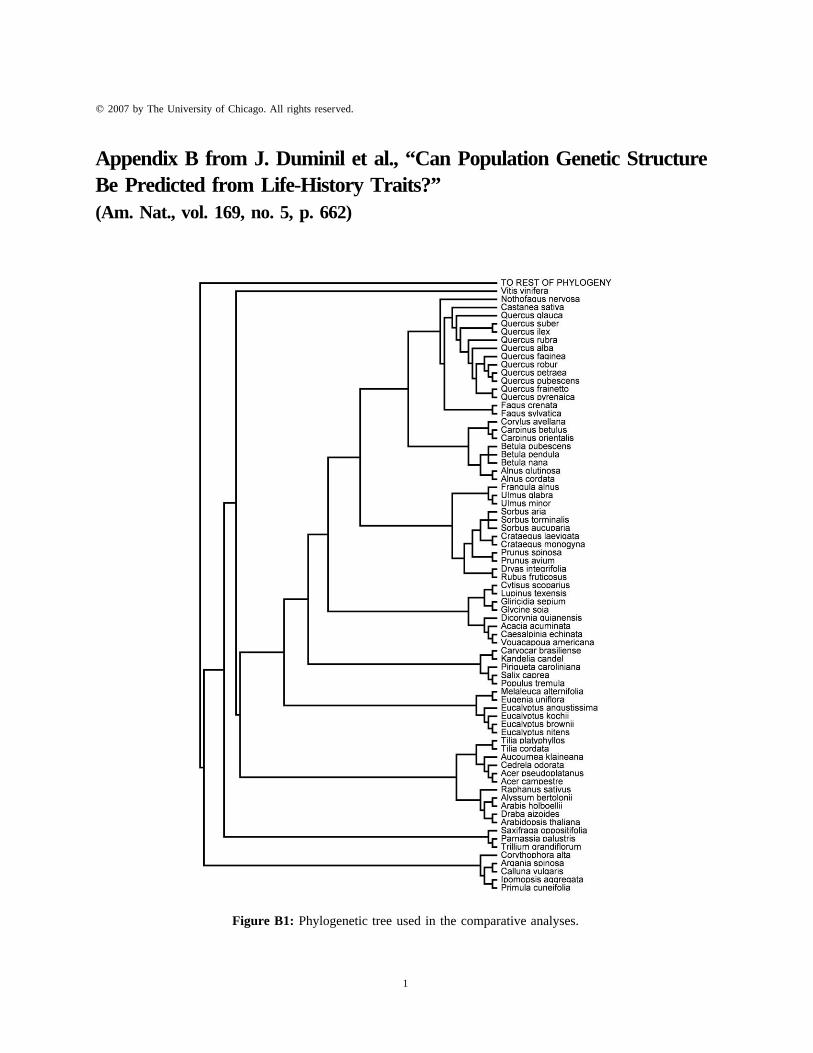
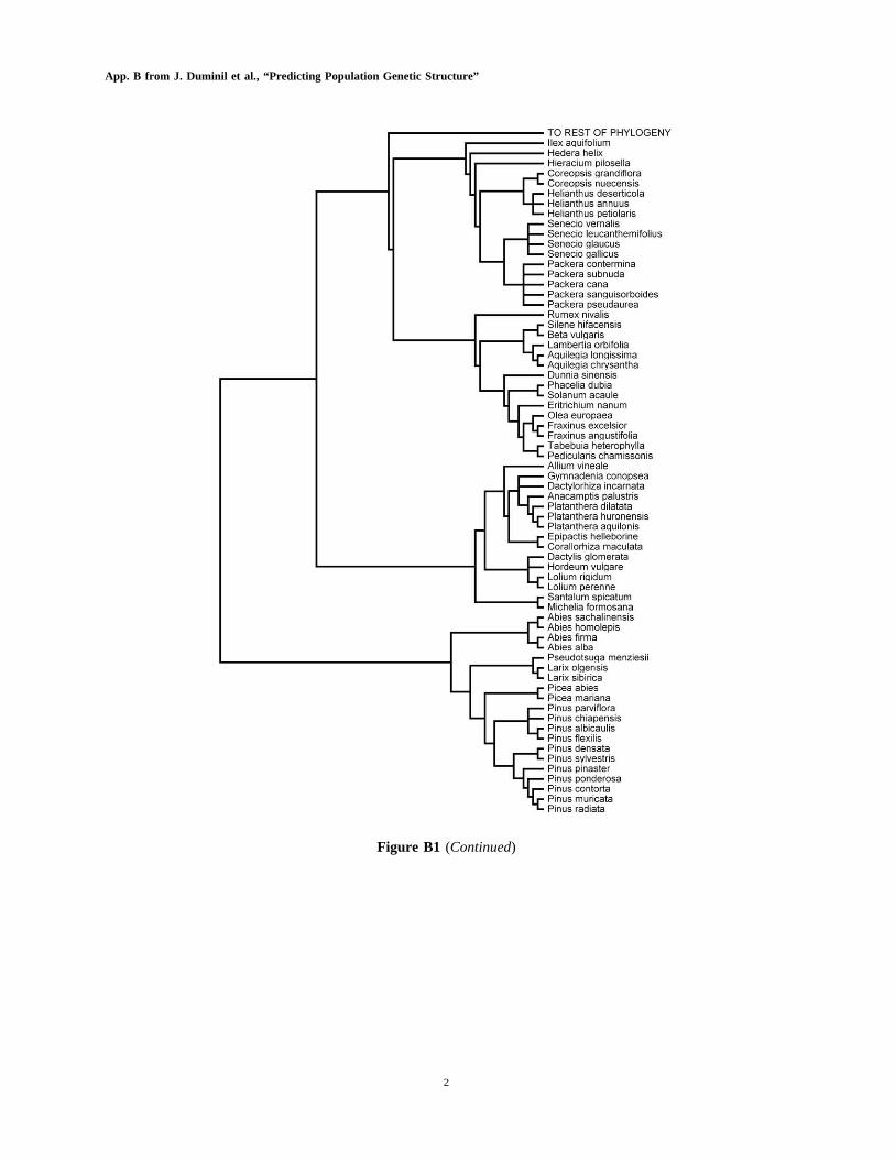
Phylogenetically Independent Contrasts (PICs). The refer-ence plant phylogeny used is that of Soltis et al. (2000).Because not all studied species were present in this phy-logeny, missing species were grafted according to infor-mation available in other phylogenetic studies (Rieseberg1991; Wang and Szmidt 1993; Schilling and Linder 1998;Hedren 2001; Hedren et al. 2001; Soltis et al. 2001; A.Wolfe, personal communication). Either intragenus phy-

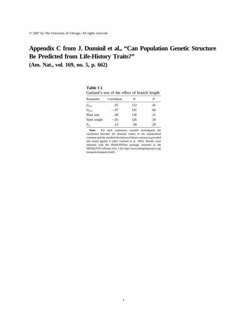
logenetic relationships were reconstructed following Ar-duino et al. (1996), Liston et al. (1999), Manos et al.(1999), and http://www.fmnh.helsinki.fi/users/haaramo/Plantae/Coniferophyta/Pinaceae/Abies.htm, or they wereleft as soft polytomies when the infragenus relationshipscould not be resolved with the available information (inthe case of Betula sp., Helianthus sp., Sorbus sp., Seneciosp., Packera sp.). The phylogenetic supertree used for theanalyses is presented in appendix B in the online editionof the American Naturalist. All branch lengths were as-signed a value of 1. With Felsenstein’s (1985) method ofindependent contrasts, one assumption is that charactersevolve following a Brownian motion model and thatbranch lengths are expressed in units of expected amountof character change. However, this method generally per-forms well when information on branch lengths is missing(Martins and Garland 1991). Considering all branchesequal signifies that the characters investigated are assumedto follow a model of a punctuational evolution, withchanges taking place only at speciation events (Martinsand Garland 1991). A standard procedure to ascertain thatthe punctuational model of evolution assumptions leadsto adequately standardized independent contrasts was pro-posed by Garland et al. (1992). The verification procedureconsists of plotting the absolute value of each standardizedindependent contrast as a function of its standard devi-ation. Any significant trend in the plot indicates that thecontrasts are not adequately standardized and that phe-notypic data or branch lengths have to be transformed.All regressions had a slope close to 0 (data not shown),indicating that the assumption of equal branch lengths isnot biasing the results (app. C in the online edition of theAmerican Naturalist).

Independent contrasts (Felsenstein 1985) were esti-mated with CAIC, version 2.6 (Purvis and Rambaud 1995).When dealing with categorical data, the Brunch optionwas used (Purvis and Rambaud 1995).

Partial Regressions. To check whether observed relation-ships between given LHT traits and GSTb could be the resultof correlations between predictor LHT variables, partialregressions were performed on the independent contrastsusing SYSTAT, version 10.2.05 (SYSTAT 2002). Regressionswere forced through the origin (Felsenstein 1985).

Results

Phylogenetic Signal

A first logical step in comparative approaches is to testwhether there is a phylogenetic signal in the data (Freck-leton et al. 2002). Nested ANOVAs (Bell 1989) and testsfor serial dependence (Abouheif 1999) were used for this


Table 1: Nested ANOVA and variance component estimations for population genetic structure indexesbased on biparentally (GSTb) and maternally inherited markers (GSTm)

Level

GSTb GSTm

df SS F P

Variancecomponent

(%) df SS F P

Variancecomponent

(%)

Plant group 2 .194 2.76 .079 2.48 2 .314 3.25 .046 2.30Subclass 3 .297 2.82 .054 3.80 3 .061 .42 .737 .45Order 14 1.881 3.83 !.001 24.06 19 4.267 4.65 !.001 31.30Family 11 1.403 3.63 .002 17.94 19 2.273 2.48 .005 16.68Genus 26 2.921 3.20 .001 37.35 40 4.061 2.1 .005 29.79Error term 32 1.124 … … 14.37 55 2.655 … … 19.48

Note: of squares. Significant P values in bold.SS p sum

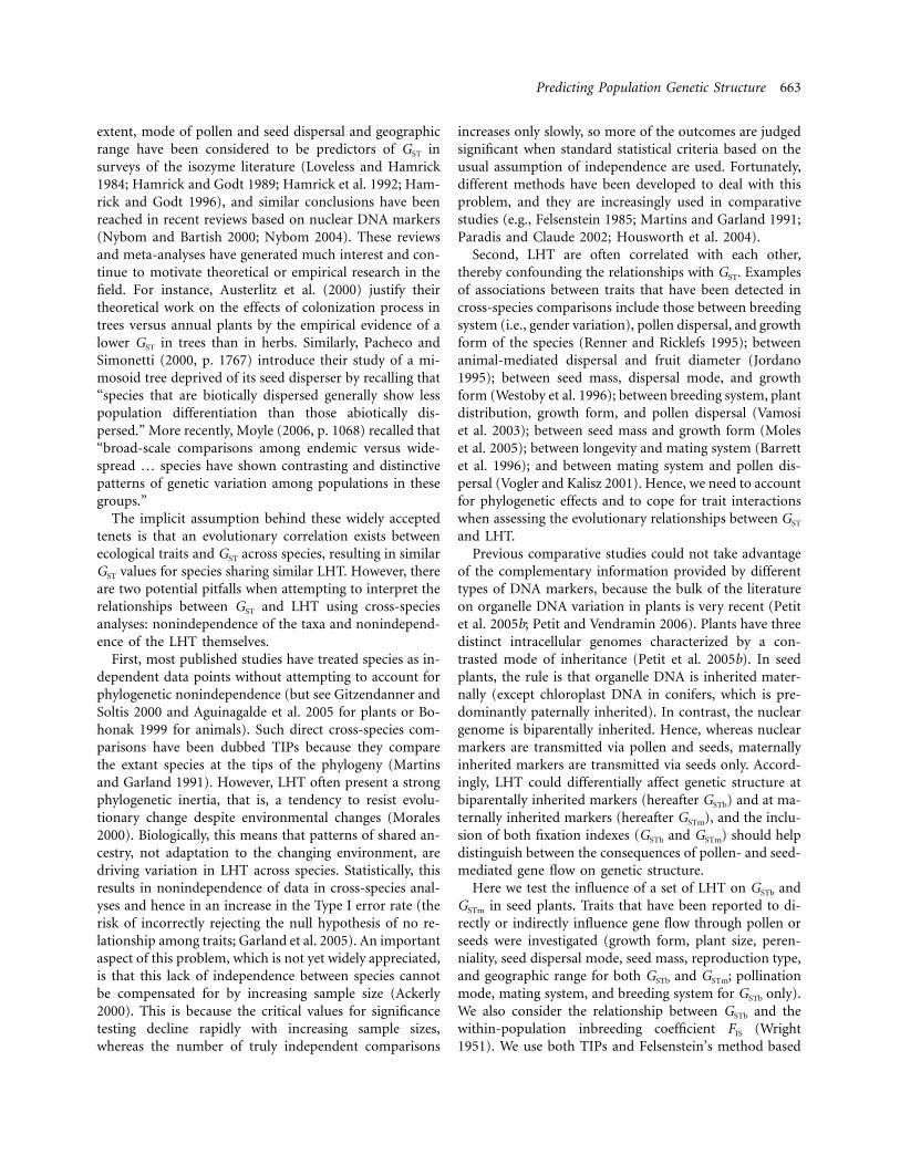
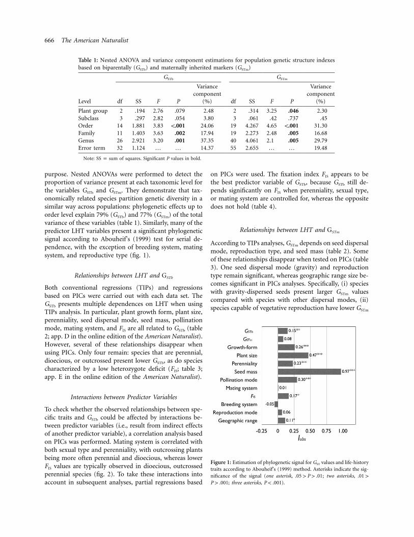
Figure 1: Estimation of phylogenetic signal for GST values and life-historytraits according to Abouheif’s (1999) method. Asterisks indicate the sig-nificance of the signal (one asterisk, ; two asterisks,.05 1 P 1 .01 .01 1

; three asterisks, ).P 1 .001 P ! .001

purpose. Nested ANOVAs were performed to detect theproportion of variance present at each taxonomic level forthe variables GSTb and GSTm. They demonstrate that tax-onomically related species partition genetic diversity in asimilar way across populations: phylogenetic effects up toorder level explain 79% (GSTb) and 77% (GSTm) of the totalvariance of these variables (table 1). Similarly, many of thepredictor LHT variables present a significant phylogeneticsignal according to Abouheif’s (1999) test for serial de-pendence, with the exception of breeding system, matingsystem, and reproductive type (fig. 1).

Relationships between LHT and GSTb

Both conventional regressions (TIPs) and regressionsbased on PICs were carried out with each data set. TheGSTb presents multiple dependences on LHT when usingTIPs analysis. In particular, plant growth form, plant size,perenniality, seed dispersal mode, seed mass, pollinationmode, mating system, and FIS are all related to GSTb (table2; app. D in the online edition of the American Naturalist).However, several of these relationships disappear whenusing PICs. Only four remain: species that are perennial,dioecious, or outcrossed present lower GSTb, as do speciescharacterized by a low heterozygote deficit (FIS; table 3;app. E in the online edition of the American Naturalist).

Interactions between Predictor Variables

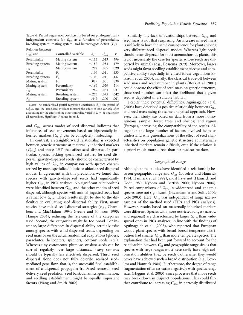
To check whether the observed relationships between spe-cific traits and GSTb could be affected by interactions be-tween predictor variables (i.e., result from indirect effectsof another predictor variable), a correlation analysis basedon PICs was performed. Mating system is correlated withboth sexual type and perenniality, with outcrossing plantsbeing more often perennial and dioecious, whereas lowerFIS values are typically observed in dioecious, outcrossedperennial species (fig. 2). To take these interactions intoaccount in subsequent analyses, partial regressions based

on PICs were used. The fixation index FIS appears to bethe best predictor variable of GSTb, because GSTb still de-pends significantly on FIS when perenniality, sexual type,or mating system are controlled for, whereas the oppositedoes not hold (table 4).

Relationships between LHT and GSTm

According to TIPs analyses, GSTm depends on seed dispersalmode, reproduction type, and seed mass (table 2). Someof these relationships disappear when tested on PICs (table3). One seed dispersal mode (gravity) and reproductiontype remain significant, whereas geographic range size be-comes significant in PICs analyses. Specifically, (i) specieswith gravity-dispersed seeds present larger GSTm valuescompared with species with other dispersal modes, (ii)species capable of vegetative reproduction have lower GSTm


Table 2: Conventional regressions (TIPs) between GSTb or GSTm and independentlife-history trait variables

Variable

GSTb GSTm

N Sign R2 P N Sign R2 P

Growth form 115 � .15 !.001 139 � .01 .258Plant size 110 � .14 !.001 132 � .01 .207Perenniality 116 � .10 !.001 141 � .01 .203Seed dispersal mode:

Wind 109 .00 .808 134 .00 .712Gravity 109 � .02 .114 134 � .01 .181Animal attached 109 � .02 .133 134 � .01 .264Animal ingested 109 .00 .658 134 � .04 .029Animal cached 109 � .08 .003 134 � .04 .015

Seed mass 112 � .04 .030 136 � .06 .005Pollination mode 108 � .13 !.001 … … …Mating system 112 � .16 !.001 … … …FIS 69 � .31 !.001 … … …Breeding system 116 .00 .948 141 .00 .567Reproduction type 103 .00 .684 102 � .15 !.001Geographic range 116 .00 .669 140 � .02 .074

Note: N indicates number of species (number of TIPs). The sign refers to the slope of the

regression. Ellipses indicate relations that were not tested. Significant P values in bold.

values than species with pure sexual reproduction (mar-ginally; cf. the small R2), and (iii) species with large rangesize tend to have low GSTm values.

Discussion

Related species tend to partition genetic diversity in similarways within and among populations: nested ANOVAs and,to a lesser extent, tests for serial dependence indicate thatmuch of the variation in GST at both nuclear and organellemarkers is accounted for by the phylogenetic (or taxo-nomic) affinity of the species. Earlier studies had alreadydemonstrated that GSTb tends to be similar in species be-longing to the same family (e.g., Hamrick and Godt 1996),but this effect had not been further tested and quantified.Taxonomic affinity and phylogenetic relationships are notcompletely equivalent, which might explain some differ-ences observed between nested ANOVAs and tests of serialdependence. Because closely related species tend to havesimilar ecological attributes and traits, it is a priori notsurprising that they partition genetic diversity similarlywithin and among populations.

Using the conventional TIP approach, we confirmedmany of the relationships identified previously betweenLHT and GSTb (Hamrick and Godt 1989, 1996), eventhough our data set is more limited. However, the existenceof a strong phylogenetic signal supports our contentionthat the dependency of GST on LHT cannot be inferredfrom simple conventional comparisons across species. Ac-cordingly, the results based on PICs reveal far fewer sig-

nificant relations than those based on TIPs. In addition,most of the remaining relationships vanish when we con-sider the interactions among different LHT: only the re-lation of mating system with nuclear genetic structure re-mains significant. Hence, our results suggest thatpreviously identified relationships between genetic struc-ture and LHT need to be reevaluated within an explicitevolutionary context.

Mating System

The mating system seems to represent the only factor thatdirectly affects genetic structure at nuclear genes (GSTb)across most seed plants. According to Charlesworth (2003,p. 1052), “[The mating system is] probably among thefactors with major effects on variability, clear enough tobe discernible even in the presence of other factors.” Ourresults fully support this view. Other factors such as pe-renniality or breeding system are also suitable predictorsof GSTb, but direct causal relationships seem unlikely be-cause the effects of these factors are no longer significantwhen controlling for variation in mating system. We at-tribute this to the fact that perenniality and breeding sys-tem are strongly correlated with the mating system. Forinstance, all dioecious species are necessarily allogamous,and no predominantly selfing tree species is known (Bar-rett 1998).


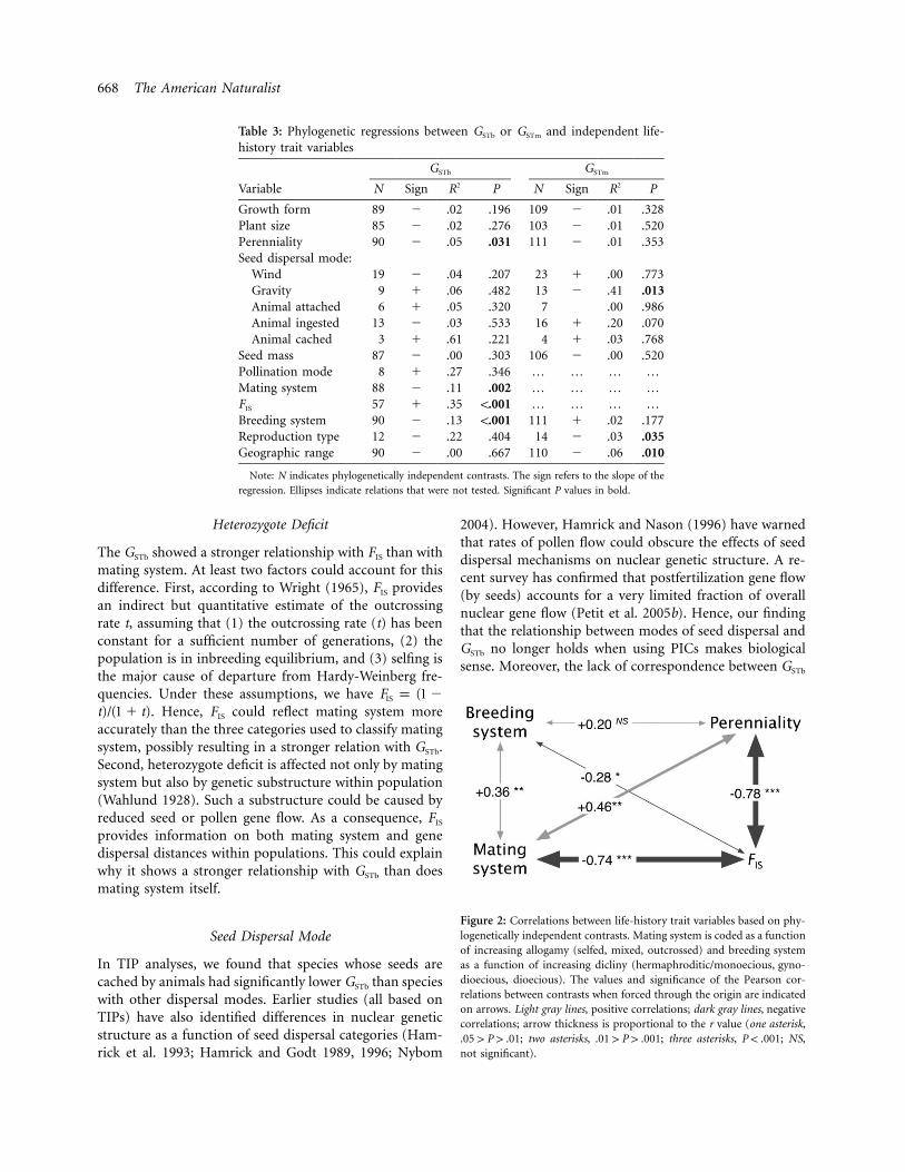
Table 3: Phylogenetic regressions between GSTb or GSTm and independent life-history trait variables

Variable

GSTb GSTm

N Sign R2 P N Sign R2 P

Growth form 89 � .02 .196 109 � .01 .328Plant size 85 � .02 .276 103 � .01 .520Perenniality 90 � .05 .031 111 � .01 .353Seed dispersal mode:

Wind 19 � .04 .207 23 � .00 .773Gravity 9 � .06 .482 13 � .41 .013Animal attached 6 � .05 .320 7 .00 .986Animal ingested 13 � .03 .533 16 � .20 .070Animal cached 3 � .61 .221 4 � .03 .768

Seed mass 87 � .00 .303 106 � .00 .520Pollination mode 8 � .27 .346 … … … …Mating system 88 � .11 .002 … … … …FIS 57 � .35 !.001 … … … …Breeding system 90 � .13 !.001 111 � .02 .177Reproduction type 12 � .22 .404 14 � .03 .035Geographic range 90 � .00 .667 110 � .06 .010

Note: N indicates phylogenetically independent contrasts. The sign refers to the slope of the

regression. Ellipses indicate relations that were not tested. Significant P values in bold.

Figure 2: Correlations between life-history trait variables based on phy-logenetically independent contrasts. Mating system is coded as a functionof increasing allogamy (selfed, mixed, outcrossed) and breeding systemas a function of increasing dicliny (hermaphroditic/monoecious, gyno-dioecious, dioecious). The values and significance of the Pearson cor-relations between contrasts when forced through the origin are indicatedon arrows. Light gray lines, positive correlations; dark gray lines, negativecorrelations; arrow thickness is proportional to the r value (one asterisk,

; two asterisks, ; three asterisks, ; NS,.05 1 P 1 .01 .01 1 P 1 .001 P ! .001not significant).

Heterozygote Deficit

The GSTb showed a stronger relationship with FIS than withmating system. At least two factors could account for thisdifference. First, according to Wright (1965), FIS providesan indirect but quantitative estimate of the outcrossingrate t, assuming that (1) the outcrossing rate (t) has beenconstant for a sufficient number of generations, (2) thepopulation is in inbreeding equilibrium, and (3) selfing isthe major cause of departure from Hardy-Weinberg fre-quencies. Under these assumptions, we have F p (1 �IS

. Hence, FIS could reflect mating system moret)/(1 � t)accurately than the three categories used to classify matingsystem, possibly resulting in a stronger relation with GSTb.Second, heterozygote deficit is affected not only by matingsystem but also by genetic substructure within population(Wahlund 1928). Such a substructure could be caused byreduced seed or pollen gene flow. As a consequence, FIS

provides information on both mating system and genedispersal distances within populations. This could explainwhy it shows a stronger relationship with GSTb than doesmating system itself.

Seed Dispersal Mode

In TIP analyses, we found that species whose seeds arecached by animals had significantly lower GSTb than specieswith other dispersal modes. Earlier studies (all based onTIPs) have also identified differences in nuclear geneticstructure as a function of seed dispersal categories (Ham-rick et al. 1993; Hamrick and Godt 1989, 1996; Nybom

2004). However, Hamrick and Nason (1996) have warnedthat rates of pollen flow could obscure the effects of seeddispersal mechanisms on nuclear genetic structure. A re-cent survey has confirmed that postfertilization gene flow(by seeds) accounts for a very limited fraction of overallnuclear gene flow (Petit et al. 2005b). Hence, our findingthat the relationship between modes of seed dispersal andGSTb no longer holds when using PICs makes biologicalsense. Moreover, the lack of correspondence between GSTb


Table 4: Partial regression coefficients based on phylogeneticallyindependent contrasts for GSTb as a function of perenniality,breeding system, mating system, and heterozygote deficit (FIS)

Relation betweenGSTb and Controlled variable bst

2Rpart P

Perenniality Mating system �.116 .013 .396Breeding system Mating system �.182 .033 .179FIS Mating system .292 .085 .029Perenniality FIS .106 .011 .435Breeding system FIS �.106 .011 .437Mating system FIS .029 .001 .830Mating system Perenniality �.169 .029 .214FIS Perenniality .289 .083 .031Mating system Breeding system �.273 .075 .042FIS Breeding system .447 .200 .001

Note: The standardized partial regression coefficients (bst), the partial R2

( ), and the associated P values measure the effect of one variable after2Rpart

accounting for the effects of the other controlled variable; species forN p 55

all regressions. Significant P values in bold.

and GSTm across modes of seed dispersal indicates thatinferences of seed movements based on biparentally in-herited markers (GSTb) can be completely misleading.

In contrast, a straightforward relationship is expectedbetween genetic structure at maternally inherited markers(GSTm) and those LHT that affect seed dispersal. In par-ticular, species lacking specialized features for seed dis-persal (gravity-dispersed seeds) should be characterized byhigh values of GSTm in comparison with species charac-terized by more specialized biotic or abiotic seed dispersalmodes. In agreement with this prediction, we found thatspecies with gravity-dispersed seeds had significantlyhigher GSTm in PICs analyses. No significant relationshipswere identified between GSTm and the other modes of seeddispersal, although species with animal-ingested seeds hada rather low GSTm. These results might be due to the dif-ficulties in evaluating seed dispersal ability. First, manyspecies have mixed seed dispersal strategies (e.g., Cham-bers and MacMahon 1994; Greene and Johnson 1995;Hampe 2004), reducing the relevance of the categoriesused. Second, the categories might be too broad. For in-stance, large differences in dispersal ability certainly existamong species with wind-dispersed seeds, depending onseed mass or on the actual anatomical adaptations (gliders,parachutes, helicopters, spinners, cottony seeds, etc.).Whereas tiny cottoneous, plumose, or dust seeds can becarried regularly over large distances, heavy samarasshould be typically less effectively dispersed. Third, seeddispersal alone does not fully describe realized seed-mediated gene flow, that is, the successful final establish-ment of a dispersed propagule; fruit/seed removal, seeddelivery, seed predation, seed bank dynamics, germination,and seedling establishment might be equally importantfactors (Wang and Smith 2002).

Similarly, the lack of relationships between GSTm andseed mass is not that surprising. An increase in seed massis unlikely to have the same consequence for plants havingvery different seed dispersal modes. Whereas light seedsshould favor dispersal for most anemochorous plants, thisis not necessarily the case for species whose seeds are dis-persed by animals (e.g., Bossema 1979). Moreover, largerseeds might favor seedling establishment success and com-petitive ability (especially in closed forest vegetation; Er-iksson et al. 2000). Finally, the classical trade-off betweenseed mass and seed number in plants (Rees et al. 2001)could obscure the effect of seed mass on genetic structure,since seed number can affect the likelihood that a givenseed is deposited in a suitable habitat.

Despite these potential difficulties, Aguinagalde et al.(2005) have described a positive relationship between GSTm

and seed mass using the same analytical approach. How-ever, their study was based on data from a more homo-geneous sample (forest trees and shrubs) and region(Europe), increasing the comparability of the results. Al-together, the large number of factors involved helps usunderstand why generalizations of the effect of seed char-acteristics on population genetic structure at maternallyinherited markers remain difficult, even if the relation isa priori much more direct than for nuclear markers.

Geographical Range

Although some studies have identified a relationship be-tween geographic range and GSTb (Loveless and Hamrick1984; Hamrick et al. 1992), most have not (Hamrick andGodt 1989; Nybom and Bartish 2000; Nybom 2004).Paired comparisons of GSTb in widespread and endemicspecies were not significant (Gitzendanner and Soltis 2000;Cole 2003). Here, GSTb was independent of range size re-gardless of the method used (TIPs and PICs analyses).However, results based on maternally inherited markerswere different. Species with more restricted ranges (narrowand regional) are characterized by larger GSTm than wide-spread ones in PICs analyses, in line with the findings ofAguinagalde et al. (2005), who reported that Europeanwoody plant species with broad boreal-temperate distri-bution had smaller GSTm than more temperate species. Theexplanation that had been put forward to account for therelationship between GST and geographic range size is thatspecies with large ranges must necessarily have high col-onization abilities (i.e., by seeds); otherwise, they wouldnever have achieved such a broad distribution (e.g., Love-less and Hamrick 1984). Furthermore, the degree of rangefragmentation often co-varies negatively with species rangesizes (Higgins et al. 2003), since processes that move seedsmay break down in disjunct populations. This could fur-ther contribute to increasing GSTm in narrowly distributed


species. In any case, the fact that a relation with geographicrange size was found for GSTm but not for GSTb makes sense,given the overwhelming importance of seed dispersal onrange expansion. However, this relation does not hold forspecies with particularly small ranges (i.e., belonging tothe endemic category), thus restricting the generality ofthis finding.

Conclusions

Few direct relations between genetic structure and LHTwere supported by our analyses when explicitly testing forcorrelated evolution within a phylogenetic framework. TheGSTm is weakly related with geographic range size and withreproduction type. The only other factors that we foundto be related with genetic structure are mating system(selfing vs. outcrossing) for nuclear markers and seed dis-persal mode (gravity vs. the other categories) for mater-nally inherited markers. These two cases correspond to themost trivial distinctions in terms of dispersal of pollen andseeds: selfing represents the case of total lack of pollengene flow, whereas the category gravity corresponds in factto the absence of adaptation for seed dispersal. Althoughsome LHT such as perenniality can still be used to predictthe partitioning of genetic diversity at nuclear genes, weshowed that their association with genetic structure is onlyindirect, mediated by evolutionary covariation with themating system.

On the contrary, related species generally have similarlevels of genetic structure at both maternally and bipa-rentally inherited markers, to the extent that 77%–79% ofall variation in GST is accounted for by species’ taxonomicclassification. However, it is difficult to imagine that ge-netic structure itself could be directly inherited across spe-cies following speciation. Rather, phenotypic traits affect-ing gene flow appear to be the most likely causes of thismarked similarity in the organization of genetic structureof closely related taxa. Nevertheless, genetic structure didnot show evolutionary correlations with most LHT in ourstudy of seed plants: only a few LHT such as mating system(for nuclear markers) and seed dispersal mode or geo-graphic range (for organelle markers) had explanatorypower for interspecific variation in genetic structure withinan explicit evolutionary scenario. This paradox can be ex-plained if we consider that LHT do affect genetic structurebut in ways that depend largely on the particular context(historical, ecological, and especially taxonomical). Thesecontingencies have been previously emphasized to explainwhy there are so few traits consistently affecting the di-versification of plant lineages (de Queiroz 2002).

Efforts by ecologists to identify traits that can help pre-dict the fate of a species (e.g., whether it will becomeinvasive or will remain rare and whether it will diversify

by speciation or become extinct) have also been met withrelatively little success. For instance, Stebbins (1965) wasunable to find attributes common to plants that have be-come weeds in California. Subsequently, several authorshave shown little optimism that single organisms’ featuresmay indicate their potential of invasiveness and have at-tributed this to the idiosyncrasy of each invasion (e.g.,Goodwin et al. 1999; Muth and Pigliucci 2006). Otherresearchers remain optimistic regarding the possibility topredict invasions but stress the need to better specify thecontext where this will apply (e.g., Hamilton et al. 2005).The difficulty to identify universal constraints on basicspecies properties such as invasiveness or genetic structureshould probably not come as a surprise. It simply illus-trates the numerous strategies that exist for the successfulexpansion and diversification of species on Earth.

Acknowledgments

We are grateful to F. Gugerli, S. Mariette, E. Rezende, andtwo anonymous reviewers for their critical comments ona previous version of the manuscript. We thank P. Garnier-Gere for her help on nested comparative analysis. We thankI. Aguinagalde, J. Arroyo, J. Bain, S. Barrett, M. Beilstein,M. Byrne, M. A. Cardoso, P. Carmen, E. Collin, S. Coz-zolino, N. Devos, R. Diaz-Delgado, C. Dutech, J. Felsen-stein, T. Garland Jr., J. A. Godoy, C. Gonnelli, B. L. Gross,B. Hahn, M. Hamilton, M. Hedren, J. Holman, S.-Y.Hwang, A. Jones, M. Koch, M. Konnert, T. Lacombe, M.Lascoux, E. Martins, A. Meade, A. Mengoni, A. Merchant,B. Musch, C. Navarro, N. Ollat, S. Ollier, D. Prat, J. Provan,A. Purvis, F. Salgueiro, L. G. Sanchez, J. G. SeguarraMoragues, D. Soltis, D. Steane, I. Stehlik, N. Tani, J. Tib-bits, R. Timme, S. Trewick, R. Vaillancourt, L. Wallace, A.Widmer, P. Wolf, and A. Wolfe for providing informationon LHT or on phylogenetic relationships of the species.The research was supported by grants from the EuropeanCommission research program FAIR5-CT97-3795, by theBureau des Ressources Genetiques to R.J.P., and by theSpanish Ministry of Education (grant REN2003-00273)and RNM-305 (Junta de Andalucıa) to P.J. We also ac-knowledge support to J.D. from the Marie Curie RT5 post-doctoral training facility at Estacion Biologica de Donana(Consejo Superior de Investigaciones Cientıficas) and sup-port from projects BOS2002-01162 and 025383ACOR-DISP to A.H.

Literature Cited

Abouheif, E. 1999. A method for testing the assumption of phylo-genetic independence in comparative data. Evolutionary EcologyResearch 1:895–909.

Ackerly, D. D. 2000. Taxon sampling, correlated evolution, and in-dependent contrast. Evolution 54:1480–1492.


Aguinagalde, I., A. Hampe, A. Mohanty, J. P. Martin, J. Duminil,and R. J. Petit. 2005. Effects of life history traits and species dis-tribution on genetic structure at maternally inherited markers inEuropean trees and shrubs. Journal of Biogeography 32:329–339.

Arduino, P., F. Verra, R. Cianchi, W. Rossi, B. Corrias, and L. Bullini.1996. Genetic variation and natural hybridization between Orchislaxiflora and Orchis palustris (Orchidaceae). Plant Systematics andEvolution 202:87–109.

Austerlitz, F., S. Mariette, N. Machon, P. H. Gouyon, and B. Godelle.2000. Effects of colonization processes on genetic diversity: dif-ferences between annual plants and tree species. Genetics 154:1309–1321.

Barrett, S. C. H. 1998. The evolution of mating strategies in floweringplants. Trends in Plant Science 3:335–341.

Barrett, S. C. H., L. D. Harder, and A. C. Worley. 1996. The com-parative biology of pollination and mating in flowering plants.Philosophical Transactions of the Royal Society B: Biological Sci-ences 351:1271–1280.

Bell, G. 1989. A comparative method. American Naturalist 133:553–571.

Bohonak, A. J. 1999. Dispersal, gene flow, and population structure.Quarterly Review of Biology 74:21–45.

Bossema, I. 1979. Jays and oaks: an eco-ethological study of a sym-biosis. Behaviour 70:1–117.

Chambers, J. C., and J. A. MacMahon. 1994. A day in the life of aseed: movements and fates of seeds and their implications fornatural and managed systems. Annual Review of Ecology and Sys-tematics 25:263–292.

Charlesworth, D. 2003. Effects of inbreeding on the genetic diversityof populations. Philosophical Transactions of the Royal Society B:Biological Sciences 358:1051–1070.

Cole, C. T. 2003. Genetic variation in rare and common plants.Annual Review of Ecology Evolution and Systematics 34:213–237.

de Queiroz, A. 2002. Contingent predictability in evolution: key traitsand diversification. Systematic Biology 51:917–929.

Eriksson, O., E. M. Friis, and P. Lofgren. 2000. Seed size, fruit size,and dispersal systems in angiosperms from the Early Cretaceousto the Late Tertiary. American Naturalist 156:47–58.

Felsenstein, J. 1985. Phylogenies and the comparative method. Amer-ican Naturalist 125:1–15.

Freckleton, R. P., P. H. Harvey, and M. Pagel. 2002. Phylogeneticanalysis and comparative data: a test and review of evidence. Amer-ican Naturalist 160:712–726.

Garland, T., Jr., P. H. Harvey, and A. Ives. 1992. Procedures for theanalysis of comparative data using phylogenetically independentcontrasts. Systematic Biology 41:18–32.

Garland, T., Jr., A. F. Bennett, and E. L. Rezende. 2005. Phylogeneticapproaches in comparative physiology. Journal of ExperimentalBiology 208:3015–3035.

Gitzendanner, M. A., and P. S. Soltis. 2000. Patterns of genetic var-iation in rare and widespread plant congeners. American Journalof Botany 87:783–792.

Goodwin, B. J., A. J. McAllister, and L. Fahrig. 1999. Predictinginvasiveness of plant species based on biological information. Con-servation Biology 13:422–426.

Greene, D. F., and E. A. Johnson. 1995. Long-distance wind dispersalof tree seeds. Canadian Journal of Botany 73:1036–1045.

Hamilton, M. A., B. R. Murray, M. W. Cadotte, G. C. Hose, A. C.Baker, C. J. Harris, and D. Licari. 2005. Life-history correlates of

plant invasiveness at regional and continental scales. Ecology Let-ters 8:1066–1074.

Hampe, A. 2004. Extensive hydrochory uncouples spatiotemporalpatterns of seedfall and seedling recruitment in a “bird-dispersed”riparian tree. Journal of Ecology 92:797–807.

Hamrick, J. L., and M. J. W. Godt. 1989. Allozyme diversity in plantspecies. Pages 43–63 in A. H. D. Brown, M. T. Clegg, A. L. Kahler,and B. S. Weir, eds. Plant population genetics, breeding and germ-plasm resources. Sinauer, Sunderland, MA.

———. 1996. Effects of life history traits on genetic diversity in plantspecies. Philosophical Transactions of the Royal Society B: Bio-logical Sciences 351:1291–1298.

Hamrick, J. L., and J. D. Nason. 1996. Consequences of dispersal inplants. Pages 203–236 in O. E. Rhodes, R. K. Chesser, and M. H.Smith, eds. Population dynamics in ecological space and time.University of Chicago Press, Chicago.

Hamrick, J. L., M. J. W. Godt, M. D. A. Murawski, and M. D. Loveless.1992. Factors influencing levels of genetic diversity in woody plantspecies. New Forests 6:95–124.

Hamrick, J. L., D. A. Murawski, and J. D. Nason. 1993. The influenceof seed dispersal mechanisms on the genetic structure of tropicaltree populations. Vegetatio 107/108:281–297.

Hedren, M. 2001. Systematics of the Dactylorhiza euxina/incarnata/maculata polyploid complex (Orchidaceae) in Turkey: evidencefrom allozyme data. Plant Systematics and Evolution 229:23–44.

Hedren, M., M. F. Fay, and M. W. Chase. 2001. Amplified fragmentlength polymorphisms (AFLP) reveal details of polyploid evolutionin Dactylorhiza (Orchidaceae). American Journal of Botany 88:1868–1880.

Hewitt, G. 2000. The genetic legacy of the Quaternary ice ages. Nature405:907–913.

Higgins, S. I., S. Lavorel, and E. Revilla. 2003. Estimating plant mi-gration rates under habitat loss and fragmentation. Oikos 101:354–366.

Housworth, E. A., E. P. Martins, and M. Lynch. 2004. The phylo-genetic mixed model. American Naturalist 163:84–96.

Ihaka, A., and R. Gentleman. 1996. R: a language for data analysisand graphics. Journal of Computational and Graphical Statistics5:299–314.

Jordano, P. 1995. Angiosperm fleshy fruits and seed dispersers: acomparative analysis of adaptation and constraints in plant-animalinteractions. American Naturalist 145:163–191.

Liston, A., W. A. Robinson, D. Pinero, and E. R. Alvarez-Buylla.1999. Phylogenetics of Pinus (Pinaceae) based on nuclear ribo-somal DNA internal transcribed spacer region sequences. Molec-ular Phylogenetics and Evolution 11:95–109.

Loveless, M. D., and J. L. Hamrick. 1984. Ecological determinantsof genetic structure in plant populations. Annual Review of Ecol-ogy and Systematics 15:65–95.

Manos, P. S., J. J. Doyle, and K. C. Nixon. 1999. Phylogeny, bioge-ography, and processes of molecular differentiation in Quercussubgenus Quercus (Fagaceae). Molecular Phylogenetics and Evo-lution 12:333–349.

Martins, E. P., and T. Garland Jr. 1991. Phylogenetic analyses of thecorrelated evolution of continuous characters: a simulation study.Evolution 45:534–557.

Moles, A. T., D. D. Ackerly, C. O. Webb, J. C. Tweddle, J. B. Dickie,and M. Westoby. 2005. A brief history of seed size. Science 307:576–580.


Morales, E. 2000. Estimating phylogenetic inertia in Thitonia (As-teraceae): a comparative approach. Evolution 54:475–484.

Moyle, L. C. 2006. Correlates of genetic differentiation and isolationby distance in 17 congeneric Silene species. Molecular Ecology 15:1067–1081.

Muth, N. Z., and M. Pigliucci. 2006. Traits of invasives reconsidered:phenotypic comparisons of introduced invasives and introducednoninvasive plant species within two closely related clades. Amer-ican Naturalist 93:188–196.

Nybom, H. 2004. Comparison of different nuclear DNA markers forestimating intraspecific genetic diversity in plants. Molecular Ecol-ogy 13:1143–1155.

Nybom, H., and I. V. Bartish. 2000. Effects of life history traits andsampling strategies on genetic diversity estimates obtained withRAPD markers in plants. Perspectives in Plant Ecology Evolutionand Systematics 3/2:93–114.

Pacheco, L. F., and J. A. Simonetti. 2000. Genetic structure of amimosoid tree deprived of its seed disperser, the spider monkey.Conservation Biology 14:1766–1775.

Paradis, E., and J. Claude. 2002. Analysis of comparative data usinggeneralized estimating equations. Journal of Theoretical Biology218:175–185.

Petit, R. J., and G. G. Vendramin. 2006. Phylogeography of organelleDNA in plants: an introduction. Pages 23–97 in S. Weiss and N.Ferrand, eds. Phylogeography of southern European refugia.Springer, Vienna.

Petit, R. J., I. Aguinagalde, J. L. de Beaulieu, C. Bittkau, S. Brewer,R. Cheddadi, R. Ennos, et al. 2003. Glacial refugia: hotspots butnot melting pots of genetic diversity. Science 300:1563–1565.

Petit, R. J., A. Hampe, and R. Cheddadi. 2005a. Climate changes andtree phylogeography in the Mediterranean. Taxon 54:877–885.

Petit, R. J., J. Duminil, S. Fineschi, A. Hampe, D. Salvini, and G. G.Vendramin. 2005b. Comparative organisation of chloroplast, mi-tochondrial and nuclear diversity in plant populations. MolecularEcology 14:689–711.

Purvis, A., and A. Rambaud. 1995. Comparative analysis by inde-pendent contrasts (CAIC): an Apple Macintosh application foranalysis of comparative data. Computer Applications in the Bio-sciences 11:247–251.

Rees, M., R. Condit, M. Crawley, S. Pacala, and D. Tilman. 2001.Long-term studies of vegetation dynamics. Science 293:650–655.

Renner, S. S., and R. E. Ricklefs. 1995. Dioecy and its correlates inthe flowering plants. American Journal of Botany 82:596–606.

Rieseberg, L. H. 1991. Homoploid reticulate evolution in Helianthus(Asteraceae): evidence from ribosomal genes. American Journal ofBotany 78:1218–1237.

Schilling, E. E., and C. R. Linder. 1998. Phylogenetic relationshipsin Helianthus (Asteraceae) based on nuclear ribosomal DNA in-ternal transcribed spacer region sequence data. Systematic Botany23:177–187.

Soltis, D. E., P. S. Soltis, M. W. Chase, M. E. Mort, D. C. Albach,M. Zanis, V. Savolainen, et al. 2000. Angiosperm phylogeny in-ferred from 18S rDNA, rbcL, and atpB sequences. Botanical Journalof the Linnean Society 133:381–461.

Soltis, D. E., R. K. Kuzoff, M. E. Mort, M. Zanis, M. Fishbein, L.Hufford, J. Koontz, and M. K. Arroyo. 2001. Elucidating deep-level phylogenetic relationships in Saxifragaceae using sequencesfor six chloroplastic and nuclear DNA regions. Annals of the Mis-souri Botanical Garden 88:669–693.

Stebbins, G. L. 1965. Colonizing species of the native California flora.Pages 173–191 in H. G. Baker and L. G. Stebbins, eds. The geneticsof colonizing species. Academic Press, New York.

SYSTAT. 2002. SYSTAT for Windows. Version 10.2. Statistics. SYSTAT,Evanston, IL.

Vamosi, J. C., S. P. Otto, and S. C. H. Barrett. 2003. Phylogeneticanalysis of the ecological correlates of dioecy in angiosperms. Jour-nal of Evolutionary Biology 16:1006–1018.

Vogler, D. W., and S. Kalisz. 2001. Sex among the flowers: the dis-tribution of plant mating systems. Evolution 55:202–204.

Wahlund, S. 1928. Zusammensetzung von Population und Korre-lationserscheinung vom Standpunkt der Vererbungslehre aus be-trachtet. Hereditas 11:65–106.

Wang, B. C., and T. B. Smith. 2002. Closing the seed dispersal loop.Trends in Ecology & Evolution 17:379–385.

Wang, X. R., and A. E. Szmidt. 1993. Chloroplast DNA-based phy-logeny of Asian Pinus species (Pinaceae). Plant Systematics andEvolution 188:197–211.

Westoby, M., M. Leishman, and J. Lord. 1996. Comparative ecologyof seed size and dispersal. Philosophical Transactions of the RoyalSociety B: Biological Sciences 351:1309–1317.

Wright, S. 1951. The genetical structure of populations. Annals ofEugenics 15:323–354.

———. 1965. The interpretation of population structure by F-statistics with special regards to systems of mating. Evolution 19:395–420.

Associate Editor and Editor: Michael C. Whitlock

� 2007 by The University of Chicago. All rights reserved.

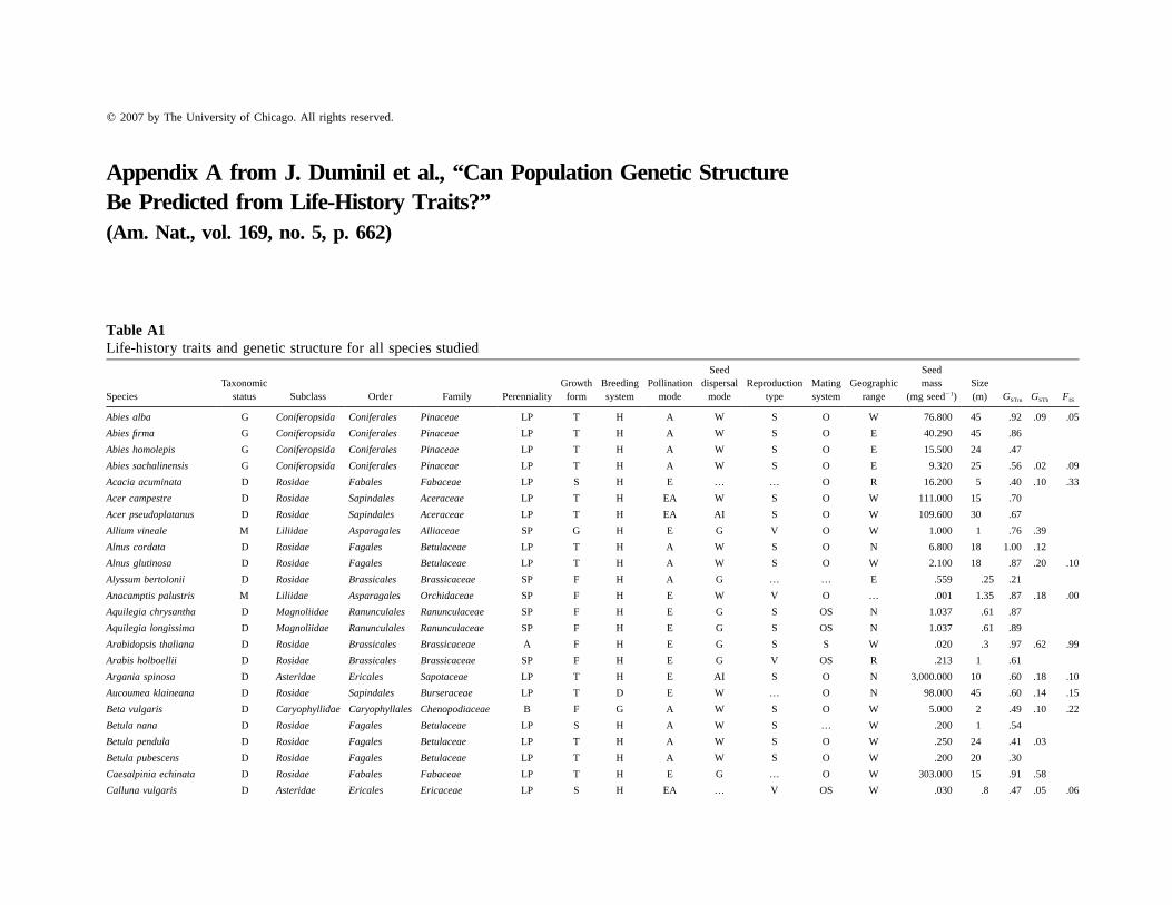
Appendix A from J. Duminil et al., “Can Population Genetic StructureBe Predicted from Life-History Traits?”(Am. Nat., vol. 169, no. 5, p. 662)

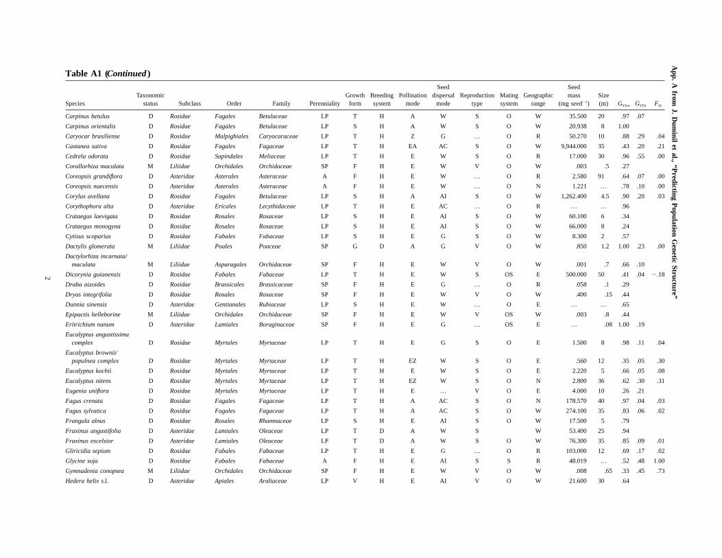
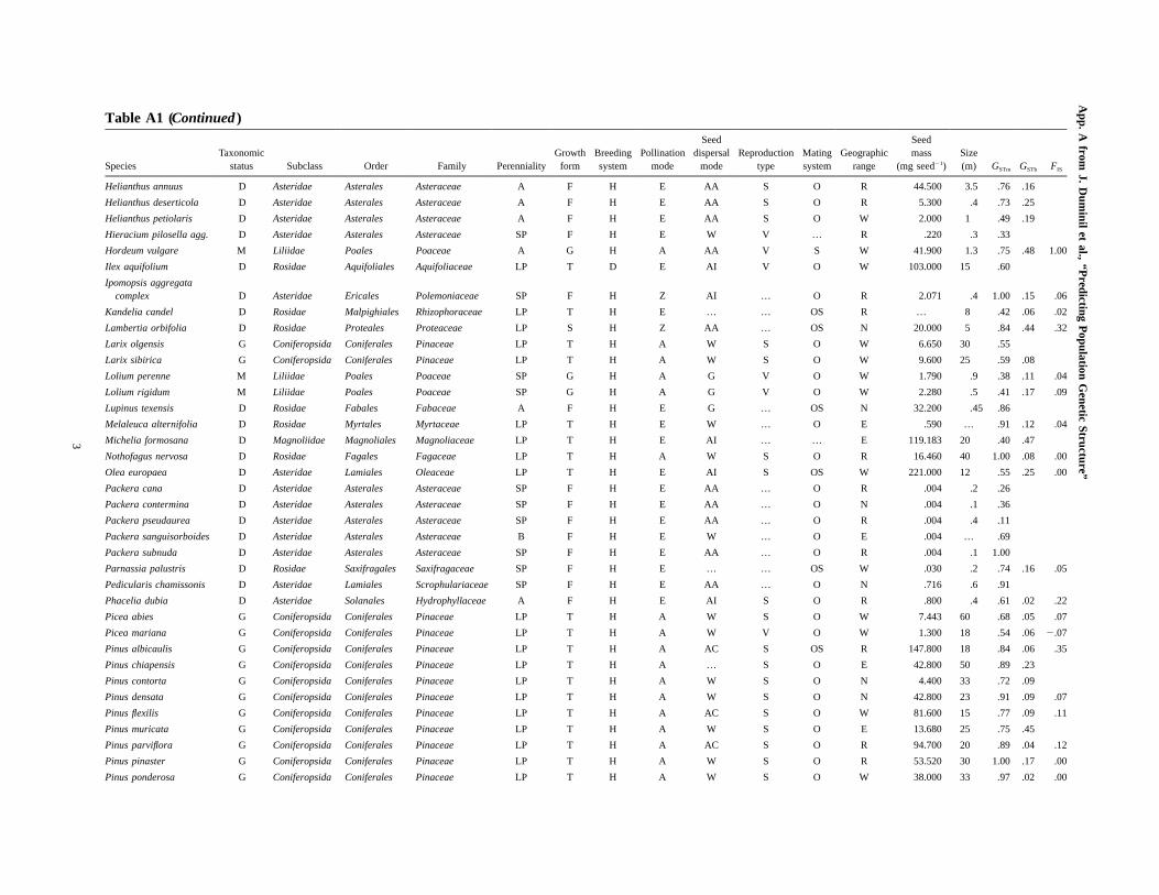
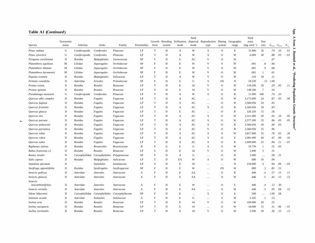
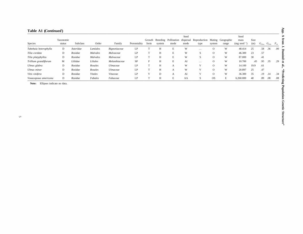
Table A1Life-history traits and genetic structure for all species studied

SpeciesTaxonomic

status Subclass Order Family PerennialityGrowth

formBreedingsystem

Pollinationmode

Seeddispersal

modeReproduction

typeMatingsystem

Geographicrange

Seedmass

(mg seed�1)Size(m) GSTm GSTb FIS

Abies alba G Coniferopsida Coniferales Pinaceae LP T H A W S O W 76.800 45 .92 .09 .05

Abies firma G Coniferopsida Coniferales Pinaceae LP T H A W S O E 40.290 45 .86

Abies homolepis G Coniferopsida Coniferales Pinaceae LP T H A W S O E 15.500 24 .47

Abies sachalinensis G Coniferopsida Coniferales Pinaceae LP T H A W S O E 9.320 25 .56 .02 .09

Acacia acuminata D Rosidae Fabales Fabaceae LP S H E … … O R 16.200 5 .40 .10 .33

Acer campestre D Rosidae Sapindales Aceraceae LP T H EA W S O W 111.000 15 .70

Acer pseudoplatanus D Rosidae Sapindales Aceraceae LP T H EA AI S O W 109.600 30 .67

Allium vineale M Liliidae Asparagales Alliaceae SP G H E G V O W 1.000 1 .76 .39

Alnus cordata D Rosidae Fagales Betulaceae LP T H A W S O N 6.800 18 1.00 .12

Alnus glutinosa D Rosidae Fagales Betulaceae LP T H A W S O W 2.100 18 .87 .20 .10

Alyssum bertolonii D Rosidae Brassicales Brassicaceae SP F H A G … … E .559 .25 .21

Anacamptis palustris M Liliidae Asparagales Orchidaceae SP F H E W V O … .001 1.35 .87 .18 .00

Aquilegia chrysantha D Magnoliidae Ranunculales Ranunculaceae SP F H E G S OS N 1.037 .61 .87

Aquilegia longissima D Magnoliidae Ranunculales Ranunculaceae SP F H E G S OS N 1.037 .61 .89

Arabidopsis thaliana D Rosidae Brassicales Brassicaceae A F H E G S S W .020 .3 .97 .62 .99

Arabis holboellii D Rosidae Brassicales Brassicaceae SP F H E G V OS R .213 1 .61

Argania spinosa D Asteridae Ericales Sapotaceae LP T H E AI S O N 3,000.000 10 .60 .18 .10

Aucoumea klaineana D Rosidae Sapindales Burseraceae LP T D E W … O N 98.000 45 .60 .14 .15

Beta vulgaris D Caryophyllidae Caryophyllales Chenopodiaceae B F G A W S O W 5.000 2 .49 .10 .22

Betula nana D Rosidae Fagales Betulaceae LP S H A W S … W .200 1 .54

Betula pendula D Rosidae Fagales Betulaceae LP T H A W S O W .250 24 .41 .03

Betula pubescens D Rosidae Fagales Betulaceae LP T H A W S O W .200 20 .30

Caesalpinia echinata D Rosidae Fabales Fabaceae LP T H E G … O W 303.000 15 .91 .58

Calluna vulgaris D Asteridae Ericales Ericaceae LP S H EA … V OS W .030 .8 .47 .05 .06

App.

Afrom

J.D

uminil

etal.,

“Predicting

Population

Genetic

Structure”

2

Table A1 (Continued )

SpeciesTaxonomic


formBreedingsystem

Pollinationmode

Seeddispersal

modeReproduction

typeMatingsystem

Geographicrange

Seedmass


Carpinus betulus D Rosidae Fagales Betulaceae LP T H A W S O W 35.500 20 .97 .07

Carpinus orientalis D Rosidae Fagales Betulaceae LP S H A W S O W 20.938 8 1.00

Caryocar brasiliense D Rosidae Malpighiales Caryocaraceae LP T H Z G … O R 50.270 10 .88 .29 .04

Castanea sativa D Rosidae Fagales Fagaceae LP T H EA AC S O W 9,944.000 35 .43 .20 .21

Cedrela odorata D Rosidae Sapindales Meliaceae LP T H E W S O R 17.000 30 .96 .55 .00

Corallorhiza maculata M Liliidae Orchidales Orchidaceae SP F H E W V O W .003 .5 .27

Coreopsis grandiflora D Asteridae Asterales Asteraceae A F H E W … O R 2.580 91 .64 .07 .00

Coreopsis nuecensis D Asteridae Asterales Asteraceae A F H E W … O N 1.221 … .78 .10 .00

Corylus avellana D Rosidae Fagales Betulaceae LP S H A AI S O W 1,262.400 4.5 .90 .20 .03

Corythophora alta D Asteridae Ericales Lecythidaceae LP T H E AC … O R … … .96

Crataegus laevigata D Rosidae Rosales Rosaceae LP S H E AI S O W 60.100 6 .34

Crataegus monogyna D Rosidae Rosales Rosaceae LP S H E AI S O W 66.000 8 .24

Cytisus scoparius D Rosidae Fabales Fabaceae LP S H E G S O W 8.300 2 .57

Dactylis glomerata M Liliidae Poales Poaceae SP G D A G V O W .850 1.2 1.00 .23 .00

Dactylorhiza incarnata/maculata M Liliidae Asparagales Orchidaceae SP F H E W V O W .001 .7 .66 .10

Dicorynia guianensis D Rosidae Fabales Fabaceae LP T H E W S OS E 500.000 50 .41 .04 �.18

Draba aizoides D Rosidae Brassicales Brassicaceae SP F H E G … O R .058 .1 .29

Dryas integrifolia D Rosidae Rosales Rosaceae SP F H E W V O W .400 .15 .44

Dunnia sinensis D Asteridae Gentianales Rubiaceae LP S H E W … O E … … .65

Epipactis helleborine M Liliidae Orchidales Orchidaceae SP F H E W V OS W .003 .8 .44

Eritrichium nanum D Asteridae Lamiales Boraginaceae SP F H E G … OS E … .08 1.00 .19

Eucalyptus angustissimacomplex D Rosidae Myrtales Myrtaceae LP T H E G S O E 1.500 8 .98 .11 .04

Eucalyptus brownii/populnea complex D Rosidae Myrtales Myrtaceae LP T H EZ W S O E .560 12 .35 .05 .30

Eucalyptus kochii D Rosidae Myrtales Myrtaceae LP T H E W S O E 2.220 5 .66 .05 .08

Eucalyptus nitens D Rosidae Myrtales Myrtaceae LP T H EZ W S O N 2.800 36 .62 .30 .31

Eugenia uniflora D Rosidae Myrtales Myrtaceae LP T H E … V O E 4.000 10 .26 .21

Fagus crenata D Rosidae Fagales Fagaceae LP T H A AC S O N 178.570 40 .97 .04 .03

Fagus sylvatica D Rosidae Fagales Fagaceae LP T H A AC S O W 274.100 35 .83 .06 .02

Frangula alnus D Rosidae Rosales Rhamnaceae LP S H E AI S O W 17.500 5 .79

Fraxinus angustifolia D Asteridae Lamiales Oleaceae LP T D A W S W 53.400 25 .94

Fraxinus excelsior D Asteridae Lamiales Oleaceae LP T D A W S O W 76.300 35 .85 .09 .01

Gliricidia sepium D Rosidae Fabales Fabaceae LP T H E G … O R 103.000 12 .69 .17 .02

Glycine soja D Rosidae Fabales Fabaceae A F H E AI S S R 48.019 … .52 .48 1.00

Gymnadenia conopsea M Liliidae Orchidales Orchidaceae SP F H E W V O W .008 .65 .33 .45 .73

Hedera helix s.l. D Asteridae Apiales Araliaceae LP V H E AI V O W 21.600 30 .64

App.

Afrom

J.D

uminil

etal.,

“Predicting

Population

Genetic

Structure”

3


SpeciesTaxonomic


formBreedingsystem

Pollinationmode

Seeddispersal

modeReproduction

typeMatingsystem

Geographicrange

Seedmass


Helianthus annuus D Asteridae Asterales Asteraceae A F H E AA S O R 44.500 3.5 .76 .16

Helianthus deserticola D Asteridae Asterales Asteraceae A F H E AA S O R 5.300 .4 .73 .25

Helianthus petiolaris D Asteridae Asterales Asteraceae A F H E AA S O W 2.000 1 .49 .19

Hieracium pilosella agg. D Asteridae Asterales Asteraceae SP F H E W V … R .220 .3 .33

Hordeum vulgare M Liliidae Poales Poaceae A G H A AA V S W 41.900 1.3 .75 .48 1.00

Ilex aquifolium D Rosidae Aquifoliales Aquifoliaceae LP T D E AI V O W 103.000 15 .60

Ipomopsis aggregatacomplex D Asteridae Ericales Polemoniaceae SP F H Z AI … O R 2.071 .4 1.00 .15 .06

Kandelia candel D Rosidae Malpighiales Rhizophoraceae LP T H E … … OS R … 8 .42 .06 .02

Lambertia orbifolia D Rosidae Proteales Proteaceae LP S H Z AA … OS N 20.000 5 .84 .44 .32

Larix olgensis G Coniferopsida Coniferales Pinaceae LP T H A W S O W 6.650 30 .55

Larix sibirica G Coniferopsida Coniferales Pinaceae LP T H A W S O W 9.600 25 .59 .08

Lolium perenne M Liliidae Poales Poaceae SP G H A G V O W 1.790 .9 .38 .11 .04

Lolium rigidum M Liliidae Poales Poaceae SP G H A G V O W 2.280 .5 .41 .17 .09

Lupinus texensis D Rosidae Fabales Fabaceae A F H E G … OS N 32.200 .45 .86

Melaleuca alternifolia D Rosidae Myrtales Myrtaceae LP T H E W … O E .590 … .91 .12 .04

Michelia formosana D Magnoliidae Magnoliales Magnoliaceae LP T H E AI … … E 119.183 20 .40 .47

Nothofagus nervosa D Rosidae Fagales Fagaceae LP T H A W S O R 16.460 40 1.00 .08 .00

Olea europaea D Asteridae Lamiales Oleaceae LP T H E AI S OS W 221.000 12 .55 .25 .00

Packera cana D Asteridae Asterales Asteraceae SP F H E AA … O R .004 .2 .26

Packera contermina D Asteridae Asterales Asteraceae SP F H E AA … O N .004 .1 .36

Packera pseudaurea D Asteridae Asterales Asteraceae SP F H E AA … O R .004 .4 .11

Packera sanguisorboides D Asteridae Asterales Asteraceae B F H E W … O E .004 … .69

Packera subnuda D Asteridae Asterales Asteraceae SP F H E AA … O R .004 .1 1.00

Parnassia palustris D Rosidae Saxifragales Saxifragaceae SP F H E … … OS W .030 .2 .74 .16 .05

Pedicularis chamissonis D Asteridae Lamiales Scrophulariaceae SP F H E AA … O N .716 .6 .91

Phacelia dubia D Asteridae Solanales Hydrophyllaceae A F H E AI S O R .800 .4 .61 .02 .22

Picea abies G Coniferopsida Coniferales Pinaceae LP T H A W S O W 7.443 60 .68 .05 .07

Picea mariana G Coniferopsida Coniferales Pinaceae LP T H A W V O W 1.300 18 .54 .06 �.07

Pinus albicaulis G Coniferopsida Coniferales Pinaceae LP T H A AC S OS R 147.800 18 .84 .06 .35

Pinus chiapensis G Coniferopsida Coniferales Pinaceae LP T H A … S O E 42.800 50 .89 .23

Pinus contorta G Coniferopsida Coniferales Pinaceae LP T H A W S O N 4.400 33 .72 .09

Pinus densata G Coniferopsida Coniferales Pinaceae LP T H A W S O N 42.800 23 .91 .09 .07

Pinus flexilis G Coniferopsida Coniferales Pinaceae LP T H A AC S O W 81.600 15 .77 .09 .11

Pinus muricata G Coniferopsida Coniferales Pinaceae LP T H A W S O E 13.680 25 .75 .45

Pinus parviflora G Coniferopsida Coniferales Pinaceae LP T H A AC S O R 94.700 20 .89 .04 .12

Pinus pinaster G Coniferopsida Coniferales Pinaceae LP T H A W S O R 53.520 30 1.00 .17 .00

Pinus ponderosa G Coniferopsida Coniferales Pinaceae LP T H A W S O W 38.000 33 .97 .02 .00

App.

Afrom

J.D

uminil

etal.,

“Predicting

Population

Genetic

Structure”

4


SpeciesTaxonomic


formBreedingsystem

Pollinationmode

Seeddispersal

modeReproduction

typeMatingsystem

Geographicrange

Seedmass


Pinus radiata G Coniferopsida Coniferales Pinaceae LP T H A W S O E 31.900 35 .74 .16 .01

Pinus sylvestris G Coniferopsida Coniferales Pinaceae LP T H A W S O W 6.000 30 .88 .03 �.01

Piriqueta caroliniana D Rosidae Malpighiales Turneraceae SP F H E AC V O W … … .67

Platanthera aquilonis M Liliidae Asparagales Orchidaceae SP F H E W V S W .001 .8 .84

Platanthera dilatata M Liliidae Asparagales Orchidaceae SP F H E W V O W .001 .9 .68

Platanthera huronensis M Liliidae Asparagales Orchidaceae SP F H E W V O W .001 1 .61

Populus tremula D Rosidae Malpighiales Salicaceae LP T D A W V O W .110 18 .11

Primula cuneifolia D Asteridae Ericales Primulaceae SP F H E G S OS N 24.320 .15 1.00

Prunus avium D Rosidae Rosales Rosaceae LP T H E AI V O W 118.200 20 .29 .05 .11

Prunus spinosa D Rosidae Rosales Rosaceae LP S H E AI V O W 148.500 7 .34

Pseudotsuga menziesii G Coniferopsida Coniferales Pinaceae LP T H A W S O R 11.000 100 .74 .23

Quercus alba complex D Rosidae Fagales Fagaceae LP T H A AC … O W 3,173.000 24 .87 .03 .00

Quercus faginea D Rosidae Fagales Fagaceae LP T H A AC … O R 2,560.056 20 .95

Quercus frainetto D Rosidae Fagales Fagaceae LP T H A AC S O R 2,560.056 30 .83

Quercus glauca D Rosidae Fagales Fagaceae LP T H E AC … O R 526.320 15 .56

Quercus ilex D Rosidae Fagales Fagaceae LP T H A AC S O W 2,311.000 20 .92 .10 .05

Quercus petraea D Rosidae Fagales Fagaceae LP T H A AC S O W 2,577.200 35 .86 .03 .05

Quercus pubescens D Rosidae Fagales Fagaceae LP T H A AC S O R 2,560.056 20 .90 .03

Quercus pyrenaica D Rosidae Fagales Fagaceae LP T H A AC V O R 2,560.056 25 .96

Quercus robur D Rosidae Fagales Fagaceae LP T H A AC S O W 3,817.000 35 .78 .02 .20

Quercus rubra D Rosidae Fagales Fagaceae LP T H A AC S O E 2,981.000 40 .47 .09 .10

Quercus suber D Rosidae Fagales Fagaceae LP T H A AC S O R 2,609.000 25 .84 .11 �.01

Raphanus sativus D Rosidae Brassicales Brassicaceae B F G E G S O W 10.750 1 .55 .03

Rubus fruticosus s.l. D Rosidae Rosales Rosaceae LP S H E AI V O W 2.490 3 .31

Rumex nivalis D Caryophyllidae Caryophyllales Polygonaceae SP F D A G … O R 1.000 … .58 .21

Salix caprea D Rosidae Malpighiales Salicaceae LP T D EA W S O W .090 10 .09

Santalum spicatum D Santalales Santalaceae LP S H E AI … … N 234.000 4 .94 .09 �.03

Saxifraga oppositifolia D Rosidae Saxifragales Saxifragaceae SP F H E W … OS W .089 .3 .82 .15

Senecio gallicus D Asteridae Asterales Asteraceae A F H E AA … O R .446 .4 .57 .15 .11

Senecio glaucus D Asteridae Asterales Asteraceae A F H E AA … O W .446 .5 .42 .12 .12

Senecioleucanthemifolius D Asteridae Asterales Asteraceae A F H E W … O E .446 .4 .12 .30

Senecio vernalis D Asteridae Asterales Asteraceae A F H E AA … O W .446 .5 .05 .04 .12

Silene hifacensis D Caryophyllidae Caryophyllales Caryophyllaceae SP F D E … S O E .500 … 1.00 .58

Solanum acaule D Asteridae Solanales Solanaceae A F H E G … S W 2.105 .1 .53

Sorbus aria D Rosidae Rosales Rosaceae LP T H E AI V O W 169.000 20 .25

Sorbus aucuparia D Rosidae Rosales Rosaceae LP T H E AI … O W 34.000 15 .31 .06 �.01

Sorbus torminalis D Rosidae Rosales Rosaceae LP T H E AI V O W 5.500 20 .36 .15 .13

App.

Afrom

J.D

uminil

etal.,

“Predicting

Population

Genetic

Structure”

5


SpeciesTaxonomic


formBreedingsystem

Pollinationmode

Seeddispersal

modeReproduction

typeMatingsystem

Geographicrange

Seedmass


Tabebuia heterophylla D Asteridae Lamiales Bignoniaceae LP T H E W … O W 48.414 25 .58 .36 .00

Tilia cordata D Rosidae Malvales Malvaceae LP T H E W S O W 46.300 23 .57

Tilia platyphyllos D Rosidae Malvales Malvaceae LP T H E W S O W 87.000 30 .41

Trillium grandiflorum M Liliidae Liliales Melanthiaceae SP F H E AI … O W 10.700 .45 .95 .35 .29

Ulmus glabra D Rosidae Rosales Ulmaceae LP T H A W V O W 14.100 19.9 .61

Ulmus minor D Rosidae Rosales Ulmaceae LP T H A W V O W 20.897 25 .47

Vitis vinifera D Rosidae Vitales Vitaceae LP V D A AI V O W 36.300 35 .19 .14 .34

Vouacapoua americana D Rosidae Fabales Fabaceae LP T H E AA S OS E 6,260.000 40 .89 .08 .08

Note: Ellipses indicate no data.

1


Appendix B from J. Duminil et al., “Can Population Genetic StructureBe Predicted from Life-History Traits?”(Am. Nat., vol. 169, no. 5, p. 662)

Figure B1: Phylogenetic tree used in the comparative analyses.

App. B from J. Duminil et al., “Predicting Population Genetic Structure”

2

Figure B1 (Continued)

1


Appendix C from J. Duminil et al., “Can Population Genetic StructureBe Predicted from Life-History Traits?”(Am. Nat., vol. 169, no. 5, p. 662)

Table C1Garland’s test of the effect of branch length

Parameter Correlation N P

GSTb .05 112 .41

GSTm �.07 141 .60

Plant size .09 126 .31

Seed weight �.05 126 .58

FIS .13 69 .29

Note: For each continuous variable investigated, thecorrelation between the absolute values of the standardizedcontrasts and the standard deviations of those contrasts is providedand tested against 0 (after Garland et al. 1992). Results wereobtained with the PDAP:PDTree package enclosed in theMESQUITE software (ver. 1.02; http://www.mesquiteproject.org/mesquite/mesquite.html).

1


Appendix D from J. Duminil et al., “Can Population Genetic StructureBe Predicted from Life-History Traits?”(Am. Nat., vol. 169, no. 5, p. 662)

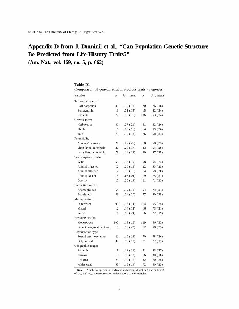
Table D1Comparison of genetic structure across traits categories

Variable N GSTb mean N GSTm mean

Taxonomic status:

Gymnosperms 31 .12 (.11) 20 .76 (.16)

Eumagnoliid 13 .31 (.14) 15 .62 (.24)

Eudicots 72 .16 (.15) 106 .63 (.24)

Growth form:

Herbaceous 40 .27 (.21) 51 .62 (.26)

Shrub 5 .20 (.16) 14 .59 (.26)

Tree 73 .13 (.13) 76 .68 (.24)

Perenniality:

Annuals/biennials 20 .27 (.25) 18 .58 (.23)

Short-lived perennials 20 .28 (.17) 33 .64 (.28)

Long-lived perennials 76 .14 (.13) 90 .67 (.25)

Seed dispersal mode:

Wind 53 .18 (.19) 58 .64 (.24)

Animal ingested 12 .26 (.18) 22 .53 (.25)

Animal attached 12 .25 (.16) 14 .58 (.30)

Animal cached 15 .06 (.04) 19 .75 (.21)

Gravity 17 .20 (.14) 21 .71 (.25)

Pollination mode:

Anemophilous 54 .12 (.11) 54 .73 (.24)

Zoophilous 53 .24 (.20) 77 .60 (.25)

Mating system:

Outcrossed 93 .16 (.14) 114 .65 (.25)

Mixed 12 .14 (.12) 16 .73 (.21)

Selfed 6 .56 (.24) 6 .72 (.19)

Breeding system:

Monoecious 105 .19 (.18) 129 .66 (.25)

Dioecious/gynodioecious 5 .19 (.23) 12 .58 (.33)

Reproduction type:

Sexual and vegetative 21 .19 (.14) 70 .58 (.26)

Only sexual 82 .18 (.18) 71 .72 (.22)

Geographic range:

Endemic 19 .18 (.16) 21 .63 (.27)

Narrow 15 .18 (.18) 16 .80 (.18)

Regional 29 .19 (.15) 32 .70 (.25)

Widespread 53 .18 (.19) 72 .60 (.25)

Note: Number of species (N) and mean and average deviation (in parentheses)of GSTb and GSTm are reported for each category of the variables.

1


Appendix E from J. Duminil et al., “Can Population Genetic StructureBe Predicted from Life-History Traits?”(Am. Nat., vol. 169, no. 5, p. 662)

App. E from J. Duminil et al., “Predicting Population Genetic Structure”

2

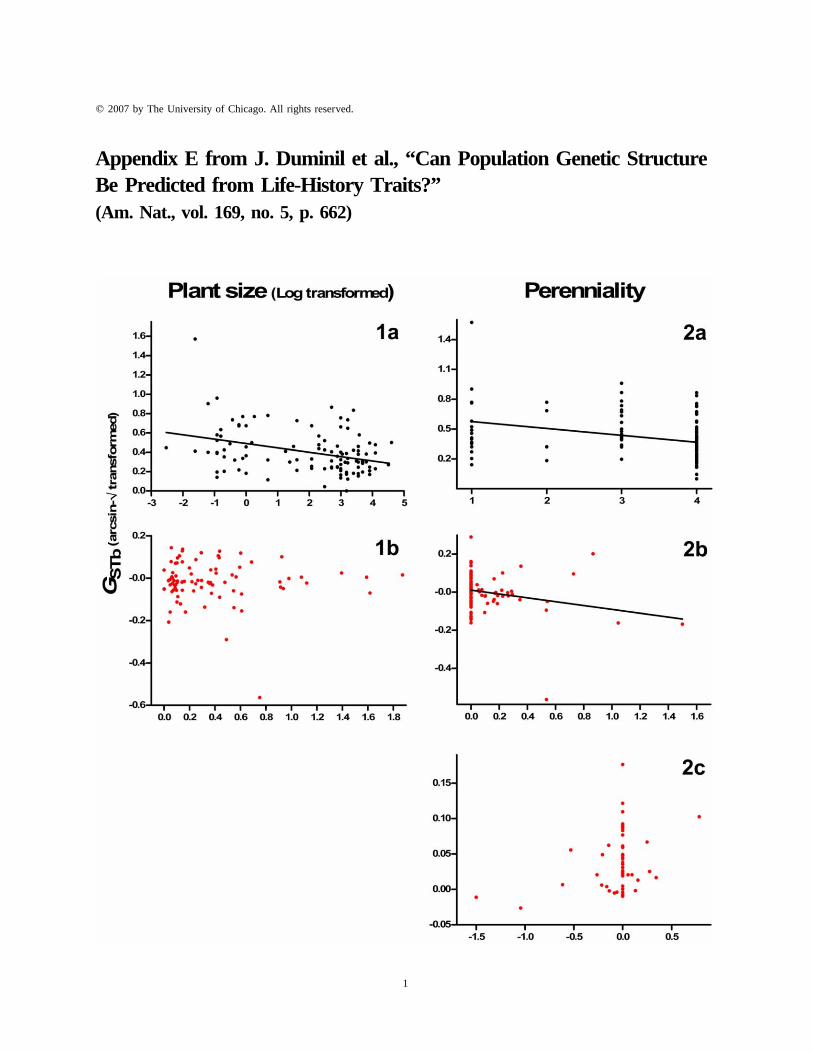
Figure E1: Illustration of the necessity to control for phylogenetic relationships and confounding covariates incross-species analyses of genetic structure. 1a, Plot of GSTb on plant size (TIPs analysis). 1b, Plot of the contrastsof GSTb on the contrasts of plant size (PICs analysis). The major axis regression line is shown when significant.The relation initially detected is no longer significant when controlling for phylogeny. 2a, Plot of GSTb onperenniality (TIPs analysis). 2b, Plot of the contrasts of GSTb on the contrasts of the perenniality (PICs analysis).2c, Plot of the contrasts of GSTb on the contrasts of the perenniality (PICs analysis) when FIS is used as acovariate. The major axis regression line is shown when significant. The relation is still significant whencontrolling for phylogeny but not when including FIS as a covariate.

Documents

Can Population Genetic Structure Be Predicted from Life-History Traits?