Can. J. Remote Sensing, Vol. 36, No. 2, pp. 129–141, 2010

Integration of GLAS and Landsat TM datafor aboveground biomass estimation

L.I. Duncanson, K.O. Niemann, and M.A. Wulder

Abstract. Current regional aboveground biomass estimation techniques, such as those that require extensive fieldwork or

airborne light detection and ranging (lidar) data for validation, are time and cost intensive. The use of freely available

satellite-based data for carbon stock estimation mitigates both the cost and the spatial limitations of field-based techniques.

Spaceborne lidar data have been demonstrated as useful for aboveground biomass (AGBM) estimation over a wide range

of biomass values and forest types. However, the application of these data is limited because of their spatially discrete

nature. Spaceborne multispectral sensors have been used extensively to estimate AGBM, but these methods have been

demonstrated as inappropriate for forest structure characterization in high-biomass mature forests. This study uses an

integration of ICESat Geospatial Laser Altimeter System (GLAS) lidar and Landsat data to develop methods to estimate

AGBM in an area of south-central British Columbia, Canada. We compare estimates with a reliable AGBM map of the

area derived from high-resolution airborne lidar data to assess the accuracy of satellite-based AGBM estimates. Further,

we use the airborne lidar dataset in combination with forest inventory data to explore the relationship between model error

and canopy height, AGBM, stand age, canopy rugosity, mean diameter at breast height (DBH), canopy cover, terrain

slope, and dominant species type. GLAS AGBM models were shown to reliably estimate AGBM (R2 5 0.77) over a range

of biomass conditions. A partial least squares AGBM model using Landsat input data to estimate AGBM (derived from

GLAS) had an R2 of 0.60 and was found to underestimate AGBM by an average of 26 Mg/ha per pixel when applied to

areas outside of the GLAS transect. This study demonstrates that Landsat and GLAS data integration are most useful for

forests with less than 120 Mg/ha of AGBM, less than 60 years of age, and less than 60% canopy cover. These techniques

have high associated error when applied to areas with greater than 200 Mg/ha of AGBM.

Resume. Les techniques actuelles d’estimation de la biomasse aerienne a l’echelle regionale, telles que celles qui requierent

beaucoup de travail de terrain ou des donnees lidar (« light detection and ranging ») aeroportees pour validation, sont

onereuses en termes de temps et de couts. L’utilisation de donnees satellite disponibles gratuitement pour l’estimation des

stocks de carbone permet de pallier les couts et les limitations spatiales lies aux techniques basees sur les campagnes de

terrain. L’utilite des donnees satellite lidar a ete demontree pour l’estimation de la biomasse aerienne (AGBM) et ce pour

une grande variete de valeurs de biomasse et de types de forets. Toutefois, l’application de ces donnees est limitee en raison

de la nature spatialement discrete de ces dernieres. Les capteurs satellitaires multispectraux ont ete utilises largement pour

estimer l’AGBM, mais ces methodes se sont averees inappropriees pour la caracterisation de la structure de la foret dans les

forets de forte biomasse et matures. La presente etude utilise une integration des donnees du systeme GLAS (« Geospatial

Laser Altimeter System ») de ICESAT ainsi que des donnees lidar et de Landsat pour developper des methodes pour

l’estimation de l’AGBM dans un secteur du centre sud de la Colombie-britannique, au Canada. On compare ces

estimations par rapport a une carte fiable de l’AGBM pour la zone derivee des donnees lidar aeroportees a haute

resolution afin d’evaluer la precision des estimations de l’AGBM basees sur les donnees satellite. De plus, on utilise

l’ensemble de donnees lidar aeroportees en combinaison avec des donnees d’inventaire forestier pour documenter la

relation entre l’erreur liee au modele et la hauteur du couvert, l’AGBM, l’age du peuplement, la rugosite du couvert, le

DHP moyen, la nature du couvert, la pente du terrain et le type d’especes dominantes. Les modeles d’AGBM de GLAS ont

demontre leur fiabilite dans l’estimation de l’AGBM (R2 5 0,77) dans une variete de conditions de biomasse. Un modele

des moindres carres partiels de l’AGBM utilisant comme donnees d’entree des donnees de Landsat pour estimer l’AGBM

(derivee de GLAS) affichait un R2 de 0,60 et on a pu observer qu’il sous-estime l’AGBM par en moyenne 26 Mg/ha par

pixel lorsqu’on l’applique dans des zones a l’exterieur du transect de GLAS. Cette etude a demontre que l’integration des

donnees de Landsat et de GLAS est tres utile pour les forets ayant moins de 120 Mg/ha d’AGBM, moins de soixante ans

d’age et moins de 60 % de couvert. Ces techniques presentent des erreurs associees elevees lorsque appliquees dans des zones

avec plus de 200 Mg/ha d’AGBM.

[Traduit par la Redaction]

Received 2 November 2009. Accepted 18 May 2010. Published on the Web at http://pubservices.nrc-cnrc.ca/cjrs on 24 September 2010.

L.I. Duncanson and K.O. Niemann.1 Hyperspectral – LiDAR Research Group, Department of Geography, University of Victoria, Victoria,BC V8W 3R4, Canada.

M.A. Wulder. Canadian Forest Service (Pacific Forestry Centre), Natural Resources Canada, Victoria, BC V8Z 1M5, Canada.

1Corresponding author (e-mail: [email protected]).

Can. J. Remote Sensing, Vol. 36, No. 2, pp. 129–141, 2010

E 2010 CASI 129

Introduction

The need exists to develop a systematic approach to

inventory and monitor global forests, both for carbon stock

evaluation and for land use change analysis (Rosenqvist

et al., 2003). Carbon stock estimation is also important given

the development of international carbon credit trading

schemes, which can be utilized to reduce deforestation and

degradation, particularly in developing nations (Gibbs et al.,

2007). Remote sensing provides the ability to collect data

from remote forested areas that would otherwise be costly

and logistically difficult to collect. Various remote sensing

technologies have been demonstrated as useful for different

aspects of forest research. Airborne hyperspectral remote

sensing instruments have been demonstrated to provide

highly accurate information pertaining to species type and

composition (Clark et al., 2005; Van Aardt and Wynne,

2007), and airborne light detection and ranging (lidar)

instruments provide the ability to accurately estimate tree

height (Means et al., 1999), volume, and aboveground bio-

mass (AGBM) or carbon content (Patenaude et al., 2004;

Nelson et al., 2003). As such, technologies are available that

can be used to study a forest’s interaction with light and its

physical structure. However, these airborne technologies

have high associated data volumes and costs (Wulder et al.,

2008). Consequently, they are best suited for studying forests

over relatively small, localized areas or for use in sampling

strategies (Wulder and Seemann, 2003).

Satellite-based remote sensing technologies provide the

ability to collect data over regional, national, and global

scales. Multispectral satellite data, such as those collected

by the Landsat Thematic Mapper (TM), have been widely

used for landscape classification and change detection in

forested areas (Wulder, 1998). Studying forest structural

properties with multispectral data is more problematic,

although many studies have attempted to model forest struc-

tural parameters using multispectral imagery with varying

levels of success (Hall et al., 1995; Cohen and Spies, 1992;

Cohen et al., 2003; Zheng et al., 2004). The normalized dif-

ference vegetation index (NDVI) and tassel cap transforma-

tions are two of the most common types of vegetation indices

used in multispectral studies of forest structure (Rogan et al.,

2002). Freitas et al. (2005) found that forest structural prop-

erties could be estimated using Landsat-derived vegetation

indices R2 5 0.49–0.72) for a tropical rainforest. Zheng et al.

(2004) modeled AGBM in a managed forest in Wisconsin

with Landsat 7 Enhanced Thematic Mapper Plus (ETM+)

data (R2 5 0.67). Hall et al. (2006) found that stand height

(R2 5 0.65) and crown closure (R2 5 0.57) could also be

estimated from Landsat ETM+ data in an area of Alberta

with forest cover similar to that of the study area used in this

research.

Collinearity is a common issue when using vegetation indi-

ces in combination with raw Landsat bands (Hensen and

Schjoerring, 2003). One method to extract the most mean-

ingful information from multispectral data is partial least

squares (PLS) regression. Collinearity and data dimension-

ality reduce the utility of ordinary least squares (OLS)

regression (Hensen and Schjoerring, 2003), and PLS regres-

sion is one statistical technique that can be used to mitigate

this problem (Næsset et al., 2004). PLS involves the extrac-

tion of linear combinations of the original input variables

and produces a new set of variables than can then be used to

model the desired output, in this case AGBM. PLS has been

demonstrated as useful for studies of biomass using optical

data (Cai et al., 2009; Hensen and Schjoerring, 2003).

Despite attempts to model biomass directly from Landsat

data, studies have demonstrated that models developed to

estimate forest structure from multispectral data are sens-

itive to tree height (Donoghue and Watt, 2006), shadows

(Hall et al., 1995), and high biomass densities (Foody et al.,

2001). Thus, although the spatially continuous nature of

optical satellite imagery renders it ideal for studying phe-

nomena over large areas, regional analyses of forest struc-

tural properties require information about the vertical

distribution of biomass in a forest. Studies using optical

imagery to model such vertical properties are limited because

optical data integrate the vertical profile of a forest into a

single reflectance value per pixel (Hall et al., 1995).

Satellite-based lidar provides an opportunity to accurately

estimate AGBM from space. Recent studies have focused on

using spaceborne lidar data to accurately model forest height

and AGBM. The National Aeronautics and Space Admin-

istration (NASA) Geospatial Laser Altimeter System

(GLAS) instrument onboard ICESat is a full-waveform

satellite-based lidar system with a 65 m diameter footprint

(Schutz et al., 2005). The returned waveforms from these

footprints can be used to estimate tree height, AGBM, and

basal area (Lefsky et al., 2007; Sun et al., 2008; Ranson et al.,

2007; Rosette et al., 2008). The accuracy of these models was

found to depend on both canopy density and terrain slope.

Increasing density and slope increase the complexity of

GLAS waveform footprints, and in high-relief or high-

biomass areas it can be difficult to resolve ground reflection

from canopy reflection within waveforms. This confusion

can be reduced through the introduction of ground filtering

techniques. Duncanson et al. (2010) developed a methodo-

logy to estimate and account for terrain relief in GLAS

AGBM estimates and determined that adjusting for terrain

relief increases the accuracy of GLAS AGBM models.

A number of issues render GLAS data less than ideal for

large-area forest inventories. The first is the limited nature of

the data coverage. The design of the satellite orbit yields

nearly contiguous coverage of the polar regions. The swaths

diverge away from the poles, however, so other areas are

covered by discrete orbits. Additionally, the GLAS laser

samples along the flight path so that a 65 m diameter foot-

print is spaced every 172 m. This sampling scheme yields an

incomplete coverage. A second issue involves atmospheric

noise. As lidar is a line-of-sight sensor, it is affected by

clouds, and only cloud-free waveforms are appropriate for

terrain analysis. Lastly, because of technological issues early

Vol. 36, No. 2, April/avril 2010

130 E 2010 CASI

in the GLAS mission, GLAS does not continually sense the

Earth’s surface but instead operates in three annual 33 day

campaigns (Schutz et al., 2005). Considering these limita-

tions, the GLAS data available from the National Ice and

Snow Data Distribution Centre (NISDC) are not spatially

continuous but represent a series of transects. The distri-

bution of footprints available from any region depends lar-

gely on the location of the region and the atmospheric

conditions at the time of GLAS passage. Although GLAS

data have the potential to be useful for the estimation of

AGBM and carbon content of forests, these logistics limit

the applicability of GLAS-derived models for regional bio-

mass mapping.

Integrating the two-dimensional, spatially continuous

data from Landsat TM with the three-dimensional, spatially

discrete GLAS data may provide a systematic method to

estimate AGBM over large areas, on regional, national,

and even global scales. Studies have integrated passive

optical and lidar technology in attempts to either extrapolate

lidar forest structure measurements to areas with spectral

properties similar to those sensed by lidar (Hudak et al.,

2002; Donoghue and Watt, 2006) or more meaningfully

interpret results from lidar studies (Wulder et al., 2007). This

study employs a regression-based AGBM modeling

approach similar to those used in other Landsat AGBM

studies. This approach was selected because it does not rely

on field data and can be applied using only freely available

satellite data. The availability of high-resolution airborne

lidar data and a current forest inventory for the entire study

area allows us to evaluate the accuracy of Landsat and

GLAS integration AGBM estimates on a pixel-by-pixel

basis. This allows the comparison of model error with terrain

characteristics to improve our understanding of the utility of

these methods. The objectives of this study are to (i) develop

a method to model AGBM from GLAS and Landsat inte-

gration; (ii) determine the relationships between model error

and forest cover properties, such as dominant species and

stand age; and (iii) establish reliable ranges of forest struc-

tural properties for which GLAS and Landsat data inte-

gration is appropriate for AGBM estimation.

Methods

Study area

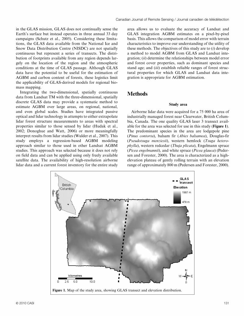
Airborne lidar data were acquired for a 75 000 ha area of

industrially managed forest near Clearwater, British Colum-

bia, Canada. The one quality GLAS laser 3 transect avail-

able for the area was selected for use in this study (Figure 1).

The predominant species in the area are lodgepole pine

(Pinus contorta), balsam fir (Abies balsamea), Douglas-fir

(Pseudotsuga menziesii), western hemlock (Tsuga hetero-

phylla), western redcedar (Thuja plicata), Engelmann spruce

(Picea engelmannii), and white spruce (Picea glauca) (Peder-

sen and Forester, 2000). The area is characterized as a high-

elevation plateau of gently rolling terrain with an elevation

range of approximately 800 m (Pedersen and Forester, 2000).

Figure 1. Map of the study area, showing GLAS transect and elevation distribution.

Canadian Journal of Remote Sensing / Journal canadien de teledetection

E 2010 CASI 131

Airborne lidar data

Airborne scanning laser lidar data were acquired in Aug-

ust 2006 using the University of Victoria TERRA Multisen-

sor Airborne Platform (MAP). This system has an integrated

lidar and full-range (400–2500 nm) hyperspectral imaging

system. The data used for this project consist of discrete,

first- and last-return 100 kHz lidar data with a maximum

scan angle of ¡20u and a scanning speed of 37 Hz. The pulse

repetition frequency (PRF) of the dataset used was 60 kHz.

The platform was flown 1600 m above ground, which in

combination with the PRF resulted in approximately 1.25

points per square metre at nadir and 2.25 lidar returns per

square metre when side overlap was included. Processing was

conducted to separate ground returns from those of vegeta-

tion. Bare-earth and canopy-height models (CHM) were

subsequently generated; the CHM heights were calculated

as the difference between the elevation of a return and the

coincident elevation of the bare-earth model. These data

were also used to calculate terrain slope and rugosity (stand-

ard deviation) of hits height which were used to explore

model results.

Field data

Field data were collected during a 4 day period in October

2008. Diameter at breast height (DBH), tree species, and tree

height were measured for every tree within a 10 m diameter

plot for 35 plots representative of the cover classes found in

the study area. Plots were positioned to within 2 m absolute

accuracy using a post-processed differential global position-

ing system (GPS).

AGBM map

An ordinary-least squares regression was fit between field-

estimated AGBM and a series of airborne lidar measure-

ments. The natural logarithm of the total AGBM (dry

weight) was found to be a function of the natural logarithms

of the 55th percentile of laser canopy height (Lh0.55) and

laser canopy cover (CC; the percentage of all laser returns

found at canopy heights §2 m):

ln TAGB~0:0914z1:0496ln Lh0:55z0:5719ln CC ð1Þ

where TAGB is the total AGBM (dry weight, in Mg/ha). The

fitted model produced an R2 value of 0.89, a root mean

square error (RMSE) of 46.07 Mg/ha, and a mean bias of

2.38 Mg/ha. Back-transformation of the fitted regression

model to arithmetic units was accomplished following the

procedures of Sprugel (1983). To estimate AGBM in the

field, species-specific allometric equations were used as pre-

sented by Jenkins et al. (2003). Because generalized allo-

metric equations were used to estimate AGBM on a per

tree (dry weight) basis (Jenkins et al., 2003) from field data,

we expect that this dataset will have a larger RMSE and bias

compared with those of locally acquired allometric equa-

tions (Hall and Case, 2008). Nevertheless, we expect these

data to be sufficiently precise (Jenkins et al., 2003) for the

purposes of calibration of our airborne lidar dataset.

This model was used to generate a spatially continuous,

20 m 6 20 m estimate of AGBM from the airborne lidar

available for the area. This AGBM map, henceforth referred

to as the AGBM control map, provides unique wide-area

calibration–validation for AGBM estimates made using the

GLAS and Landsat data.

Satellite-based lidar

GLAS is a full-waveform lidar sensor using a 1064 nm

laser operating at 40 Hz. The GLAS data used in this study

were acquired on 26 June 2006 and represent a transect with

105 GLAS waveforms. This was the only temporally coin-

cident transect available in the study site from GLAS laser 3

data. Laser 2 transects were available, but where laser 3

footprints approximate 65 m diameter circles, laser 2 foot-

prints are more elliptical, and the spatial pattern of light

reflection varies considerably between footprints. As such,

the airborne lidar data could not be reliably matched to laser

2 footprints, and these were not included in the analysis.

Details on the processing of these data can be found in

Duncanson et al. (2010). A series of waveform metrics were

calculated describing the shape of each waveform in terms of

both their vertical (temporal) distribution and the energy-

return distribution. Table 1 provides a description of the

waveform metrics used in this study.

Satellite multispectral

A single Landsat TM scene was selected for use in this

study based on its temporal proximity to the acquisition of

both the GLAS and airborne lidar data and based on the

atmospheric conditions of the scene (,1% cloud). The image

was acquired on 17 August 2006. It is unlikely that note-

worthy change in AGBM occurred between the acquisition

of the GLAS, airborne lidar, and Landsat datasets. We

therefore assume that any change in AGBM between June

and August of 2006 was negligible. Top-of-atmosphere cor-

rection was applied using the methodology presented in Han

et al. (2007).

Table 1. Waveform metrics and abbreviations as outlined in Dun-

canson et al. (2010).

Metric

abbreviation Description

wf_max_e Highest energy value in waveform

wf_variance Variance of waveform

wf_skew Skew of waveform

e_44 Proportion of energy in highest elevation quarter

e_34 Proportion of energy in second highest elevation

quarter

startpeak Difference in elevation between beginning of signal

and position of wf_max_e

wf_n_gs Number of Gaussian curves found in waveform


132 E 2010 CASI

Ancillary data map

The British Columbia Vegetation Resources Inventory

(VRI) (Ministry of Sustainable Resource Management,

2003) was used to explore the results found in this study.

The variables explored using this inventory were canopy

height, stand age, percent canopy cover, dominant species,

and mean DBH.

Analysis

This study involved the development of several models to

estimate AGBM from various sets of input data. First, a

relationship was developed between field data and airborne

lidar data, and a control AGBM map for the study area was

generated. Second, the AGBM control map values were

modeled from GLAS waveform metrics. Third, GLAS

AGBM estimates were modeled from Landsat data. This

third model is henceforth referred to as the Landsat-GLAS

model. The GLAS estimates were modeled from Landsat

rather than the more accurate AGBM control map values

in an attempt to assess the accuracy of methods using only

satellite data. The Landsat model was applied to the entire

study area, and the differences between the observed

(AGBM control map) values and the predicted (Landsat-

GLAS) values were evaluated for different species types

and forest structural characteristics using forest inventory

data and airborne lidar.

Successfully modeling AGBM from GLAS waveforms

relied on the assumption that the AGBM control map could

be manipulated to provide a single AGBM estimate for the

65 m diameter circle illuminated by each GLAS pulse. To

achieve this, 65 m diameter circles, with centroids located at

each GLAS centroid, were overlaid on the AGBM control

map. The control map was translated into polygons, which

were then clipped to the overlaid GLAS footprints. An aver-

age of 12 control map pixels fell within or partially within

each GLAS footprint. A weighted average was used to cal-

culate the average AGBM in megagrams per hectare for each

GLAS footprint by multiplying each polygon’s control map

AGBM value by the area within the GLAS footprint, sum-

ming the resulting values for each footprint, and dividing by

the area of the footprint. Thus, we generated a dataset repre-

senting a ‘‘control’’ value of AGBM for the area correspond-

ing to each GLAS pixel.

These AGBM values were then root-transformed to

reduce the positive skew of AGBM for the scene (Figure 2)

and improve normality and linearity among variables. Fol-

lowing the methods presented in Duncanson et al. (2010), an

ordinary least squares model was developed to predict these

AGBM values from GLAS data. Binary-coded dummy vari-

able GLAS waveform metrics were used to correct for ter-

rain relief. Only variables with a correlation of less than 0.5

with any other input variable were used in this model. The

dummy variables were coded based on maximum terrain

relief estimated from GLAS waveform metrics, without reli-

ance on ancillary topographic data, as outlined in Duncan-

son et al (2010). Dummy variables were used to adjust for

different relationships between waveform metrics and

Figure 2. AGBM distribution for the study area, as estimated from airborne lidar data. The

subset shows the AGBM distribution from the GLAS transect.


E 2010 CASI 133

AGBM in flat (0–7 m), moderate-relief (7–15 m), or high-

relief (.15 m) areas. The predictions from this model were

squared to produce predictions of AGBM in megagrams per

hectare for each GLAS footprint.

PLS regression was used to estimate the relationship of the

Landsat data to the GLAS AGBM estimates. Due to the

65 m spatial resolution of the GLAS data, the Landsat

image, AGBM map, and forest inventory map were

resampled to 60 m pixels using nearest neighbour resam-

pling. We rely on the assumption that the Landsat pixel

coincident to a GLAS centroid location represents the multi-

spectral response corresponding to a GLAS waveform.

Landsat TM bands 1–5 and 7 and NDVI and three tassel

cap transformation bands (brightness, greenness, wetness)

were used as potential inputs into the PLS regression model

to estimate the GLAS-predicted square root of AGBM. The

best PLS model was applied to the entire study area, gen-

erating a spatially continuous 60 m 6 60 m Landsat-GLAS

estimate map of AGBM (in Mg/ha).

The AGBM control map was subtracted from the

Landsat-GLAS AGBM map. To ensure that only areas

forested at the time of data acquisition were included in

the study, the airborne lidar data were used to mask out zero

AGBM pixels. The resulting error map, representing the

overprediction and underprediction of AGBM for each

pixel, was therefore masked for zero biomass.

The VRI maps of dominant species, canopy height, age,

percent canopy cover, and mean DBH were used to decom-

pose both the original AGBM map and the error map

to explore differences in AGBM and error in areas of differ-

ing land cover. The mean observed AGBM (in Mg/ha),

standard deviation of observed AGBM (in Mg/ha), and

standard deviation of error (in Mg/ha) were calculated for

the area associated with each dominant species (see Figure 5).

Box and whiskers plots were created to visualize trends

in error over increasing canopy height, AGBM, age, rugos-

ity, mean DBM, percent canopy cover, and terrain slope

(see Figure 6).

Results

GLAS and Landsat-GLAS model results

The results of the comparison of the predicted versus

control biomass estimates are summarized in Table 2, and

Figure 3 shows the results of the GLAS model (model 1 in

Table 2). Table 2 also summarizes the Landsat-GLAS PLS

model (model 2), which estimates the predictions from the

GLAS model (model 1). Figure 3 shows the results of both

models 1 and 2, and Figure 4 shows the spatial distribution of

the Landsat-GLAS estimates subtracting the AGBM controlmap. Three components, or latent variables, were used in the

generation of the PLS model.

Error image decomposition

The standard deviation of model error for the study area

was 89.3 Mg/ha, the mean AGBM was 146.5 Mg/ha, and the

standard deviation of AGBM was 85.9 Mg/ha. The errorassociated with the Landsat-GLAS model was decomposed

based on terrain and forest cover characteristics derived

from the airborne lidar data or the forest inventory. The

standard deviation of error, mean AGBM, and standard

deviation of AGBM related to the dominant species are

shown in Figure 5. Douglas-fir, immature lodgepole pine,

trembling aspen, birch, and paper birch are the species for

which the standard deviation of error was greater than100 Mg/ha, well above the average error of 81.4 Mg/ha.

Douglas-fir had a high average AGBM and standard devi-

ation of AGBM. The areas of immature lodgepole pine

tended to be overestimated. Balsam fir, subalpine fir, and

white spruce were the species for which the standard devi-

ation of error was lowest.

Figure 6 shows the change in error mean, error median,error range, and 10th–90th percentiles of error with increas-

ing canopy height, AGBM, age, rugosity, mean DBH, and

percent canopy cover. The open diamonds represent the

error median, and the line represents the error average.

For the purposes of this study we deem error median and

means of less than ¡25 Mg/ha with an associated 10th–90th

percentile error range of ,50 Mg/ha to be areas for which

the model is useful, error median and means of less than¡50 Mg/ha with an associated 10th–90th percentile error

range of ,100 Mg/ha to be areas for which the model is

somewhat useful, and areas where the median and means

of greater than ¡50 Mg/ha and associated 10th–90th per-

centile error ranges of .100 Mg/ha to be areas for which the

model does not perform well.

Due to the masking of zero AGBM data, the pixels that

would normally fall into classes of zero or low AGBM, per-

cent canopy cover, age, DBH, or canopy height often have a

Table 2. AGBM model information.

Model Equation R2 SE

(1) GLAS AGBM0:5terrain inclusion ~ 4:21 z 0:13 startpeak2ð Þz 3:86 wf skew0ð Þ

z 0:42 startpeak1ð Þ{ 22:41 wf variance1ð Þ{ 32:05 wf variance2ð Þz 0:51 wf n gs2ð Þ{ 1:40 wf max e0ð Þ

0.77 2.2

(2) Landsat-GLAS AGBM0:5terrain inclusion ~ 20:84 { 193:00 band7ð Þz 75:82 band5ð Þ

{ 51:58 band4ð Þz 220:03 band3ð Þ{ 312:80 band2ð Þz 131:28 band1ð Þ0.60 2.0

Note: All model coefficients are statistically significant to 95% confidence.


134 E 2010 CASI

Figure 3. Results from (a) the GLAS model and (b) the Landsat-GLAS model. The GLAS model estimates the square root (Sqrt.) of

observed airborne lidar AGBM using GLAS waveform metrics, and the Landsat-GLAS model estimates the square root of GLAS AGBM

estimates using Landsat bands 1–5 and 7.

Figure 4. Model 3 spatial distribution of error (model minus control AGBM per pixel).


E 2010 CASI 135

pixel value of ‘‘no data.’’ The class divisions and number of

pixels within each class are shown in Table 3. There is an

overestimate of approximately 30 Mg/ha of AGBM when

AGBM is less than approximately 120 Mg/ha (Figure 6b).

After 200 Mg/ha of AGBM, there is an average underestima-

tion of greater than 100 Mg/ha of AGBM, and the average

underestimation increases to 200 Mg/ha after 300 Mg/ha of

AGBM.

The relationship between age and model error is more

complicated than many of the other relationships

(Figure 6c). Forests between 1 and 40 years of age have rela-

tively small error distributions (less than ¡100 Mg/ha), and

AGBM has an average overestimate of approximately 15 Mg/

ha. Between 41 and 60 years of age, the model overestimates

AGBM by an average of only 2 Mg/ha, but the distribution

of error is ¡100 Mg/ha. Between 61 and 120 years of age, the

model underestimates AGBM, as do forests older than

250 years, and these have the widest range of errors. Inter-

estingly, stands between 141 and 250 years of age show over-

estimates of AGBM and narrower error distributions.

The model overestimated AGBM when canopy height was

less than 20 m (by approximately 20 Mg/ha) or greater than

30 m (by approximately 5 Mg/ha). The distribution of error

increases by 21 Mg/ha in canopies ranging from 11 to 20 m

and by 32 m for stands with canopies greater than 20 m high.

The model was somewhat useful for canopies less than 20 m

and greater than 20 m high.

As mean DBH increases so does the distribution of error

(Figure 6e); however, DBH does not appear to be a useful

characteristic by which to divide the study area because the

model performs poorly in all but the 0–10 cm DBH class, for

which it is only somewhat useful. Similarly, the overall

increase in error distribution associated with increases in ver-

tical complexity of the forest (rugosity) is 50 Mg/ha, and the

model performs poorly in all but the lowest rugosity classes.

Canopy cover yields a different relationship with model

error (Figure 6f). The model is somewhat successful between

0% and 20% canopy cover, performs well between 20% and

40% canopy cover, is somewhat successful between 40% and

60% canopy cover, and performs poorly after 60% canopy

cover. The exception, however, is for the class of 90%–100%

canopy cover, for which the model performs well.

Discussion

GLAS AGBM estimation

The GLAS estimates of AGBM compare favorably with

those from other studies (Lefsky et al., 2005, R2 5 0.59–0.68;

Sun et al., 2007, R2 5 0.73) which include high-AGBM areas

(.250 Mg/ha). The relationship between GLAS waveform

metrics and AGBM is linear, and error does not increase

with increasing AGBM. These results reaffirm that GLAS

is an appropriate tool for AGBM estimation.

Figure 5. Standard deviation (SD) of model 3 error, mean AGBM, and standard deviation of

AGBM for dominant species segmentation. The number of 60 m Landsat pixels falling in

each species class is provided.


136 E 2010 CASI

Landsat AGBM estimation

The utility of GLAS and Landsat integration depends on

the characteristics of the landscape, as seen in Figure 6. The

applicability of these methods depends on the assumption

that the relationship between AGBM and vegetation spectral

response is consistent between the transect sensed by GLASand the study area. The highest biomass areas fall outside of

the GLAS transect, which may explain the trend to under-

estimating the AGBM in the study area by the Landsat-

Figure 6. Box and whiskers plots (10th–90th percentiles of error) decomposing pixel-based error into various forest

parameter classes. Lines represent medians, and diamonds means.


E 2010 CASI 137

GLAS model developed in this study. However, from decon-

structing the scene into biomass classes, it was observed that

the underestimation of AGBM began at approximately

140 Mg/ha, within the AGBM range sampled by the GLAS

transect. Therefore we believe that, although transect sam-

pling may have empirically influenced the AGBM estimates,

this influence was not sufficiently notable to alter the results

or conclusions of this study. The underestimation exhibited

across the study area in areas of greater than 120 Mg/ha

AGBM is likely due to the spectral similarity of forests in

these higher AGBM classes.

Partial least squares regression was found to be a reliable

estimation technique for AGBM estimation from Landsat

and GLAS data integration. This is attributed to the ability

to include more input variables in PLS than in methods such

as OLS regression, regardless of collinearity among input

variables. All six Landsat bands were used as inputs to the

PLS models, although the inclusion of NDVI or any of the

tassel cap bands did not improve the model.

There were pixels with errors of ¡100 Mg/ha AGBM even

in structural classes for which the model was most successful.

This wide range of error is likely related to both the limita-

tions associated with the utility of TM data for AGBM

estimation (i.e., saturation effects) and the lowered observ-

able variance associated with satellite-based estimates that

are incapable of documenting the variance observed with

high-resolution airborne data. This second issue is largely

related to the spatial resolution of data. Spectral signals

related to areas with mixtures of high and low biomass are

aggregated to moderate levels of biomass, resulting in large

underpredictions and overpredictions dependent on the

resampling of imagery. Future satellite lidar missions (e.g.,

DesDynI) will have smaller footprint sizes, which may elim-

inate the need to aggregate Landsat data to 60 m. This may

increase the utility of spaceborne lidar integration with

Landsat, although it is unlikely that this will increase the

utility of Landsat for areas of AGBM greater than 140 Mg/

ha due to the spectral similarity of high-biomass forests.

Error decomposition

The standard deviation of error in the Landsat-GLAS

model was the statistic deemed most indicative of model

performance, as it enables a description of the breadth of

error distribution. The wide range of AGBM values (0–

612 Mg/ha) in this study area likely increased the distri-

bution of errors.

Figure 5 shows the standard deviation of the Landsat-

GLAS model error and the mean and standard deviation

of AGBM. The large error associated with Douglas-fir and

immature lodgepole pine may be site specific to our study

area. Douglas-fir were present in the most underpredicted

areas and are representative of old-growth stands

(.250 years) that are known to have variable AGBM in

the study area. Immature lodgepole pine stands likely had

spectral signatures similar to those of older, higher biomass

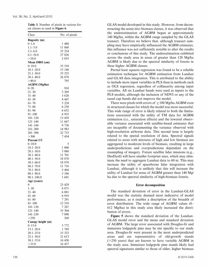
Table 3. Number of pixels in various for-

est classes as used in Figure 6.

Class No. of pixels

Rugosity (m)

0–1.0 1 480

1.1–3.0 11 868

3.1–6.0 35 254

6.1–10.0 27 026

.10.0 2 055

Mean DBH (cm)

0–10.0 35 510

10.1–20.0 15 140

21.1–30.0 35 255

30.1–40.0 26 078

.40.0 795

AGBM (Mg/ha)

0–20 910

21–30 3 269

31–40 3 620

41–50 4 447

61–70 5 224

71–80 6 258

81–90 6 652

91–100 6 955

101–120 13 439

121–140 11 667

141–160 9 738

161–200 14 983

201–300 22 733

.300 7 454

Percent CC

0–10.0 5

10.1–20.0 1 000

20.1–30.0 5 080

30.1–40.0 11 701

40.1–50.0 18 870

50.1–60.0 18 970

60.1–70.0 11 716

70.1–80.0 5 464

80.1–90.0 3 186

90.1–100.0 1 691

Age (years)

0 23 429

1–20 8 871

21–40 6 081

41–60 6 919

61–80 7 291

81–100 12 518

101–120 7 267

121–140 33 304

141–250 7 098

.250 369

Canopy height (m)

0–15.0 3 772

15.1–20.0 1 769

20.1–25.0 15 323

25.1–30.0 21 613

30.1–35.0 16 450

.35.0 16 437


138 E 2010 CASI

members of their species that were prevalent across the land-

scape. The areas of immature lodgepole pine tended to be

overestimated, although some were also underestimated,

which likely caused the high standard deviation of error

for this species.

The lower standard deviations of error associated with

balsam fir, subapline fir, and white spruce may be related

to the low mean and standard deviation of AGBM asso-

ciated with these areas, and therefore also may have been

site specific. Although GLAS estimates for these areas were

likely successfully extrapolated, the model may not have

performed as well if these species had been more prevalent

in higher AGBM areas. Additionally, the field validation of

the airborne lidar AGBM estimates was conducted almost

exclusively within conifer forests, which may have influenced

the accuracy of AGBM estimates in broadleaf environments.

Despite differences between the error distributions asso-

ciated with different dominant species, the model did not

perform well for any of the species divisions. It performed

slightly better for conifer forests, but individual species

results indicate that it is not the species of forest that deter-

mines the utility of the AGBM modeling approach

developed in this study. Instead, the forest structural char-

acteristics have a stronger relationship with model error, and

researchers should focus on assessing these characteristics

rather than species composition when considering applying

similar methodologies.

The relationships between forest properties and error

show that modeling AGBM using Landsat is more appro-

priate for forested environments with less than 120 Mg/ha of

AGBM and that the conditions of a forest should be known

prior to the application of these methods. Figure 6 shows a

visualization of six relationships between increasing forest

structural metrics and the distribution of error in each struc-

ture division.

Canopy height, DBH, and rugosity

The Landsat-GLAS model, as expected, was more suc-

cessful for shorter canopies because these are typically less

complex and will have a lower proportion of understory and

shaded trees, for which Landsat data are less useful. The

majority of AGBM in this study area is stored in the boles

of the larger trees, and the smaller understory trees will con-

tribute to the Landsat signal disproportionately to their

AGBM contribution. However, canopy height was less use-

ful for differentiating between model performance than

other structural characteristics, indicating that it has a weak

relationship with model performance. After 20 m of canopy

height, the model performs poorly, regardless of canopy

height increases. This indicates that either GLAS or, more

likely, Landsat data are not useful for differentiation of can-

opies greater than 20 m high.

Similarly, the model only performed somewhat well for

the smallest trees with DBH values between 0 and 10 cm.

We believe that DBH is not a controlling factor to the utility

of the Landsat-GLAS model. Larger trees have higher asso-

ciated error, but even small trees (DBH 5 10–30 cm) are

associated with high error and wide error distributions. This

may be attributed to the fact that small-DBH trees are typ-

ically found in young, immature forests with a high density

of trees. The spectral response from these actively growing

forests may be indistinguishable from that of older forests

with an active understory combined with large, productive

canopies.

Rugosity is a measure of the vertical complexity of the

canopy and is the square root of the variance of the standard

deviation of lidar hits height. We expected that vertical com-

plexity would play a significant role in the success of our

models. However, there was no consistent trend as rugosity

increased, and the model performed somewhat well or

poorly across the rugosity classes. There appears to be a

slight increase in the distribution as rugosity increases, but

the results are generally inconclusive.

AGBM

The trend between error and AGBM is the most note-

worthy trend portrayed in Figure 6. The results indicate that

these methods should not be used to estimate AGBM for

forests with values greater than 200 Mg/ha and should be

used with caution for forests with ranges between 120 and

200 Mg/ha. This depends on the information needs of an

AGBM evaluation.

As expected, a saturation threshold of AGBM was appar-

ent, after which Landsat spectral signals are indistinguish-

able with increasing AGBM. In this study this saturation

point appears to be between 120 and 200 Mg/ha.

Age

The relationship between age and model error is more

complicated than many of the other relationships. These

age divisions were taken from the divisions provided in the

forest inventory. Forests of age ‘‘0’’ are likely recently clear-

cut or planted stands or nonforest environments that fell

outside the zero-AGBM mask and may not be appropriately

comparable with the lidar data. The relationship between

forest age and Landsat-GLAS model error is likely a func-

tion of the relationship between age and AGBM itself.

Therefore age may only be a useful variable for approximat-

ing AGBM when AGBM information is unavailable.

A comparison of the observed AGBM map and the

inventory-age map showed that biomass increased with age

until approximately 61–80 years. After this age, biomass no

longer had a clear relationship with age; some of the highest

biomass pixels were between 61 and 80 years of age, and some

of the oldest stands had biomass values as low as 100 Mg/ha.

These old, lower biomass stands may have been affected by

disturbances such as wind damage. Consequently, if a forest

stand is older than approximately 60 years, Landsat data may

be useful for AGBM estimation, but this is dependent on other

forest structural properties, and not age in particular.


E 2010 CASI 139

Percent canopy cover

The decrease in model accuracy after approximately 60%

canopy cover is likely related to the relationships between

age, canopy cover, and AGBM in the study area. An analysis

of the associated maps shows that canopy covers greater

than 60% typically correspond to stand ages of 41–140 years.

Older canopies typically have a canopy cover of 50%–60%,

and younger stands have ,50% canopy cover. Similarly, the

AGBM over 60% canopy cover varies independently of

canopy cover, whereas lower values of canopy cover are

related to AGBM; 60% canopy cover has an associated

AGBM of approximately 140 Mg/ha. As a consequence,

canopy cover may be a useful measure for determining

whether Landsat is useful for AGBM estimation if an ancil-

lary estimate of AGBM itself is not available.

Conclusion

Landsat and GLAS integration may be useful for biomass

estimation when funding or logistical limitations prevent

extensive data collection. The advantage of these data types

is that they are freely available and have near-global coverage.

These methods offer an improvement over some carbon

estimation methods, such as biome-based AGBM extrapola-

tions, which are the only estimation technique available for

many remote areas of tropical forest (Gibbs et al., 2007).

The strength of this study was its ability to test empirically

derived models in a spatially contiguous area outside of the

dataset from which they were generated. Our first objective

was to develop a method to model AGBM from GLAS and

Landsat integration. This was achieved, and it was deter-

mined that the best method was to develop a PLS model

of GLAS-estimated AGBM using the optical Landsat bands

1–5 and 7.

Our second objective was to determine the relationships

between model error and forest cover properties, and we

conclude that model performance varies between broadleaf

and coniferous forests. The model estimates are more accur-

ate in areas with lower average AGBM and lower standard

deviation of AGBM because these simpler forests yield spec-

tral responses below the documented saturation level for

Landsat.

Our third objective was to establish ranges of forest struc-

tural properties for which these methods are most appropri-

ate. We determined that AGBM was the best indicator of

model applicability, with optimal model performance corres-

ponding to areas with less than 120 Mg/ha AGBM. These

models may also perform well in areas with between 120 and

200 Mg/ha AGBM. Forest age and percent canopy cover

may also be useful indicators of model applicability, with

60% canopy cover and 60 years of age acting as thresholds

under which the model performs well. However, if AGBM is

higher than 120 Mg/ha, this method should be used with

caution even in young forests or forests with .60% canopy

cover. These methods may be appropriate above these

thresholds depending on the required accuracy of AGBM

estimation.

Additionally, the models presented in this paper are more

accurate in conifer forests. This may be due to the favouring

of conifer plots in the validation of the airborne lidar and

because the majority of the study site is forested by conifers.

For forests outside the recommended range of conditions,

we believe the use of satellite-based multispectral data will

limit the accuracy of AGBM estimation.

References

Cai, T., Ju, C., and Yang, X. 2009. Comparison of ridge regression and

partial least squares regression for estimating above-ground biomass with

Landsat images and terrain data in Mu US Sandy Land, China. Arid

Land Research and Management, Vol. 23, pp. 248–261. doi:10.1080/

15324980903038701.

Clark, M.L., Roberts, D.A., and Clark, D.B. 2005. Hyperspectral discrimina-

tion of tropical rain forest tree species at leaf to crown scales. Remote

Sensing of Environment, Vol. 96, pp. 375–398. doi:10.1016/j.rse.2005.03.009.

Cohen, W.B., and Spies, T.A. 1992. Estimating structural attributes of Dou-

glas-fir/western hemlock forest stands from Landsat and SPOT imagery.

Remote Sensing of Environment, Vol. 41, pp. 1–17. doi:10.1016/0034-

4257(92)90056-P.

Cohen, W.B., Maiersperger, T.K., Gower, S.T., and Turner, D.P. 2003. An

improved strategy for regression of biophysical variables from Landsat

ETM+ data. Remote Sensing of Environment, Vol. 84, pp. 561–571.

doi:10.1016/S0034-4257(02)00173-6.

Donoghue, D.N.M., and Watt, P.J. 2006. Using lidar to compare forest

height estimates from IKONOS and Landsat ETM+ data in Sitka spruce

plantation forests. International Journal of Remote Sensing, Vol. 27,

pp. 2161–2175.

Duncanson, L.I., Niemann, K.O., and Wulder, M.A. 2010. Estimating for-

est canopy height and terrain relief from GLAS waveform metrics.

Remote Sensing of Environment, Vol. 114, No. 1, pp. 138–154. doi:10.

1016/j.rse.2009.08.018

Foody, G.M., Cutler, M.E., McMorrow, J., Pelz, D., Tangka, H., Boyd,

D.S., and Douglas, I. 2001. Mapping the biomass of Bornean tropical

rain forest from remotely sensed data. Global Ecology and Biogeography,

Vol. 10, pp. 379–387. doi:10.1046/j.1466-822X.2001.00248.x.

Freitas, S.R., Mello, M.C.S., and Cruz, C.B.M. 2005. Relationships between

forest structure and vegetation indices in Atlantic Rainforest. Forest Eco-

logy and Management, Vol. 218, pp. 353–362. doi:10.1016/j.foreco.2005.

08.036.

Gibbs, H.K., Brown, S., Niles, J.O., and Foley, J.A. 2007. Monitoring and

estimation tropical forest carbon stocks: making REDD a reality. Envir-

onmental Research Letters, Vol. 2, No. 045023. doi:10.1088/1748-9326/2/

4/045023.

Hall, R.J., and Case, B.S. 2008. Assessing prediction errors of generalized

tree biomass and volume equations for the boreal forest region of west-

central Canada. Canadian Journal of Forestry Management, Vol. 38,

pp. 878–889. doi:10.1139/X07-212.

Hall, F.G., Shimabukuro, Y.E., and Huemmrich, K.F. 1995. Remote sens-

ing of forest biophysical structure using mixture decomposition and geo-

metric reflectance models. Ecological Applications, Vol. 5, pp. 993–1013.

doi:10.2307/2269350.


140 E 2010 CASI

Hall, R.J., Skakun, R.S., Arsenault, E.J., and Case, B.S. 2006. Modeling forest

stand structure attributes using Landsat ETM+ data: Application to map-

ping of aboveground biomass and stand volume. Forest Ecology and Man-

agement, Vol. 225, pp. 378–390. doi:10.1016/j.foreco.2006.01.014.

Han, T., Wulder, M.A., White, J.C., Coops, N.C., Alvarez, M.F., and But-

son, C. 2007. An efficient protocol to process Landsat images for change

detection with tasseled cap transformation. Geoscience and Remote Sens-

ing Letters, Vol. 4, pp. 147–151. doi:10.1109/LGRS.2006.887066.

Hensen, P.M., and Schjoerring, J.K. 2003. Reflectance measurement of

canopy biomass and nitrogen status in wheat crops using normalized

vegetation indices and partial least squares regression. Remote Sensing

of Environment, Vol. 86, pp. 542–553. doi:10.1016/S0034-4257(03)00131-7.

Hudak, A.T., Lefsky, M.A., Cohen, W.B., and Berterretche, M. 2002. Inte-

gration of lidar and Landsat ETM+ data for estimating and mapping

forest canopy height. Remote Sensing of Environment, Vol. 82, pp. 397–

416. doi:10.1016/S0034-4257(02)00056-1.

Jenkins, J.C., Chojnacky, D.C., Heath, L.S., and Birdsey, R.A. 2003.

National-scale biomass estimators for United States tree species. Forest

Science, Vol. 49, pp. 12–35.

Lefsky, M.A., Harding, D.J., Keller, M., Cohen, W.B., Carabajal, C.C.,

Espirito-Santo, F.D.B., Hunter, M.O., and de Oliveira, R., Jr. 2005. Esti-

mates of forest canopy height and aboveground biomass using ICESat.

Geophysical Research Letters, Vol. 32, L22S02. doi:10.1029/2005GL023971.

Lefsky, M.A., Keller, M., Pang, Y., de Camargo, P.B., and Hunter, M.O.

2007. Revised method for forest canopy height estimation from

Geoscience Laser Altimeter System waveforms. Journal of Applied

Remote Sensing, Vol. 1, No. 013537. doi:10.1117/1.2795724.

Means, J.E., Acker, S.A., Harding, D.J., Blair, J.B., Lefsky, M.A., Cohen,

W.B., Harmon, M.E., and McKeww, W.A. 1999. Use of large-footprint

scanning airborne LiDAR to estimate forest stand characteristics in the

Western Cascades of Oregon. Remote Sensing of Environment, Vol. 67,

pp. 298–308. doi:10.1016/S0034-4257(98)00091-1.

Ministry of Sustainable Resource Management. 2003. Vegetation resources

inventory: quality assurance procedures for VRI ground sampling.

Resources Information Standards Committee, Ministry of Sustainable

Resource Management, Victoria, B.C.

Næsset, E., Bollandsas, O.M., and Gobakken, T. 2004. Comparing regres-

sion methods in estimation of biophysical properties of forest stands from

two different inventories using laser scanner data. Remote Sensing of

Environment, Vol. 28, pp. 541–553.

Nelson, R., Valenti, M.A., Short, A., and Keller, C. 2003. A multiple resource

inventory of Delaware using airborne laser data. BioScience, Vol. 53,

pp. 981–992. doi:10.1641/0006-3568(2003)053[0981:AMRIOD]2.0.CO;2.

Patenaude, G., Hill, R.A., Milne, R., Gaveau, D.L.A., Briggs, B.B.J., and

Dawson, T.P. 2004. Quantifying forest above ground carbon content

using LiDAR remote sensing. Remote Sensing of Environment, Vol. 93,

pp. 368–380. doi:10.1016/j.rse.2004.07.016.

Pedersen, L., and Forester, C. 2000. Tree farm license 18: rationale for

allowable annual cut (AAC) determination. British Columbia Ministry

of Forests, Victoria, B.C.

Ranson, K.J., Kimes, D., Sun, G., Nelson, R., Khaaruk, V., and Monte-

sano, P. 2007. Using MODIS and GLAS data to develop timber volume

estimates in central Siberia. In IGARSS’07: Proceedings of the Inter-

national Geoscience and Remote Sensing Symposium, 23–26 July 2007,

Barcelona, Spain. IEEE, Piscataway, N.J. pp. 2306–2309.

Rogan, J., Franklin, J., and Roberts, D.A. 2002. A comparison of methods

for monitoring multitemporal vegetation change using Thematic Mapper

imagery. Remote Sensing of Environment, Vol. 80, pp. 143–156. doi:10.

1016/S0034-4257(01)00296-6.

Rosenqvist, A., Milne, A., Lucas, R., Imhoff, M., and Dobson, C. 2003. A

review of remote sensing technology in support of the Kyoto Protocol.

Environmental Science and Policy, Vol. 6, pp. 441–455. doi:10.1016/

S1462-9011(03)00070-4.

Rosette, J.A.B., North, P.R.J., and Suarez, J.C. 2008. Vegetation height

estimates for a mixed temperate forest using satellite laser altimetry.

International Journal of Remote Sensing, Vol. 29, pp. 1475–1493.

doi:10.1080/01431160701736380.

Schutz., B.E., Zwally, H.J., Shuman, C.A., Hancock, D., and DiMarzio,

J.P. 2005. Overview of the ICESat Mission. Geophysical Research Letters,

Vol. 32, L21S01.

Sprugel, D.G. 1983. Correcting for bias in log-transformed allometric equa-

tions. Ecology, Vol. 64, pp. 209–210. doi:10.2307/1937343.

Sun, G., Ranson, K.J., Masek, J., Fu, A., and Wang, D. 2007. Predicting

tree height and biomass from GLAS data. In Proceedings of the 10th

International Symposium on Physical Measurements and Signatures in

Remote Sensing (ISPMSRS’07), 12–14 March 2002, Davos, Switzer-

land. Edited by M.E. Schaepman, S. Liang, N.E. Groot, and M. Kneu-

buhler. ITC, Enschede, The Netherlands.

Sun, G., Ranson, K.J., Kimes, D.S., Blair, J.B., and Kovacs, K. 2008. Forest

vertical structure from GLAS: An evaluation using LVIS and SRTM

data. Remote Sensing of Environment, Vol. 112, pp. 107–117. doi:10.

1016/j.rse.2006.09.036.

Van Aardt, J.A.N., and Wynne, R.H. 2007. Examining pine spectral sepa-

rability using hyperspectral data from an airborne sensor: an extension of

field-based results. International Journal of Remote Sensing, Vol. 28,

pp. 431–436. doi:10.1080/01431160500444772.

Wulder, M. 1998. Optical remote-sensing techniques for the assessment of

forest inventory and biophysical parameters. Progress in Physical Geo-

graphy, Vol. 22, pp. 449–476.

Wulder, M.A., and Seemann, D. 2003. Forest inventory height update

through the integration of lidar data with segmented Landsat imagery.

Canadian Journal of Remote Sensing, Vol. 29, No. 5, pp. 536–543.

Wulder, M.A., Han, T., White, J.C., Sweda, T., and Tsuzuki, H. 2007. Inte-

grating profiling LiDAR with Landsat data for regional boreal forest

canopy attribute estimation and change characterization. Remote Sensing

of Environment, Vol. 110, No. 1, pp. 123–137. doi:10.1016/j.rse.2007.02.002.

Wulder, M.A., Bater, C.W., Coops, N.C., Hilker, T., and White, J.C. 2008.

The role of lidar in sustainable forest management. The Forestry Chron-

icle, Vol. 84, No. 6, pp. 807–826.

Zheng, D., Rademacher, J., Chen, J., Crow, T., Bresse, M., Le Moine, J., and

Ryu, S.R. 2004. Estimating aboveground biomass using Landsat 7 ETM+data across a managed landscape in northern Wisconsin, USA. Remote

Sensing of Environment, Vol. 93, pp. 402–411. doi:10.1016/j.rse.2004.08.008.


E 2010 CASI 141

Documents

Can. J. Remote Sensing, Vol. 36, No. 2, pp. 129–141, 2010