Can climate models capture the structure of extratropical cyclones? Article 

Published Version 

Catto, J. L., Shaffrey, L. C. and Hodges, K. I. (2010) Can climate models capture the structure of extratropical cyclones? Journal of Climate, 23 (7). pp. 1621­1635. ISSN 1520­0442 doi: https://doi.org/10.1175/2009JCLI3318.1 Available at http://centaur.reading.ac.uk/5769/ 

It is advisable to refer to the publisher’s version if you intend to cite from the work. Published version at: http://journals.ametsoc.org/doi/abs/10.1175/2009JCLI3318.1 

To link to this article DOI: http://dx.doi.org/10.1175/2009JCLI3318.1 

Publisher: American Meteorological Society 

All outputs in CentAUR are protected by Intellectual Property Rights law, including copyright law. Copyright and IPR is retained by the creators or other copyright holders. Terms and conditions for use of this material are defined in the End User Agreement  . 

www.reading.ac.uk/centaur   

CentAUR 

Central Archive at the University of Reading 

Reading’s research outputs online

Can Climate Models Capture the Structure of Extratropical Cyclones?

JENNIFER L. CATTO

Department of Meteorology, University of Reading, Reading, United Kingdom

LEN C. SHAFFREY

National Centre for Atmospheric Science, Department of Meteorology, University of Reading, Reading,

United Kingdom

KEVIN I. HODGES

Environmental Systems Science Centre, University of Reading, Reading, United Kingdom

(Manuscript received 26 June 2009, in final form 2 November 2009)

ABSTRACT

Composites of wind speeds, equivalent potential temperature, mean sea level pressure, vertical velocity,

and relative humidity have been produced for the 100 most intense extratropical cyclones in the Northern

Hemisphere winter for the 40-yr ECMWF Re-Analysis (ERA-40) and the high resolution global environment

model (HiGEM). Features of conceptual models of cyclone structure—the warm conveyor belt, cold con-

veyor belt, and dry intrusion—have been identified in the composites from ERA-40 and compared to

HiGEM. Such features can be identified in the composite fields despite the smoothing that occurs in the

compositing process. The surface features and the three-dimensional structure of the cyclones in HiGEM

compare very well with those from ERA-40. The warm conveyor belt is identified in the temperature and wind

fields as a mass of warm air undergoing moist isentropic uplift and is very similar in ERA-40 and HiGEM. The

rate of ascent is lower in HiGEM, associated with a shallower slope of the moist isentropes in the warm sector.

There are also differences in the relative humidity fields in the warm conveyor belt. In ERA-40, the high

values of relative humidity are strongly associated with the moist isentropic uplift, whereas in HiGEM these

are not so strongly associated. The cold conveyor belt is identified as rearward flowing air that undercuts the

warm conveyor belt and produces a low-level jet, and is very similar in HiGEM and ERA-40. The dry in-

trusion is identified in the 500-hPa vertical velocity and relative humidity. The structure of the dry intrusion

compares well between HiGEM and ERA-40 but the descent is weaker in HiGEM because of weaker along-

isentrope flow behind the composite cyclone. HiGEM’s ability to represent the key features of extratropical

cyclone structure can give confidence in future predictions from this model.

1. Introduction

To have confidence in predictions of future climate, it

is necessary for current climate models to be able to

adequately represent extratropical cyclones, from the

spatial distribution of storm tracks down to the structure

of the storms. Extratropical cyclones are important for

providing the day-to-day variability of weather in the

midlatitudes. The most intense of these extratropical

cyclones can have huge socioeconomic impacts due to

their associated strong winds and heavy rain. It is pos-

sible that with a changing climate, these impacts may be

more severe or located in different regions. For exam-

ple, Bengtsson et al. (2009) found that in the Max Planck

Institute atmosphere model (ECHAM5; Roeckner et al.

2003), the wind speeds related to extratropical cyclones

remained fairly constant in a future climate scenario but

the associated rainfall increased and became more ex-

treme. Extratropical cyclones are mainly driven by the

strong temperature and moisture gradients across the

polar front and often develop in the baroclinic regions

over the Gulf Stream or Kuroshio Current in the Northern

Hemisphere. These transient systems play an important

Corresponding author address: Jennifer Catto, Dept. of Meteo-

rology, University of Reading, Earley Gate, P.O. Box 243, Reading

RG6 6BB, United Kingdom.

E-mail: j.l.catto@reading.ac.uk

VOLUME 23 J O U R N A L O F C L I M A T E 1 APRIL 2010

DOI: 10.1175/2009JCLI3318.1

� 2010 American Meteorological Society 1621

role in the large-scale atmospheric circulation as they

travel from west to east across the ocean basins, trans-

porting heat and moisture from the equator to the poles.

It is therefore very important for climate models to

represent the dynamical processes and airflows of extra-

tropical cyclones in order to be able to correctly predict

the large-scale atmospheric flow.

This study aims to investigate how well the structures

of the most intense extratropical cyclones are repre-

sented in the high resolution global environment model

(HiGEM; Shaffrey et al. 2009), which is a coupled cli-

mate model. This will be evaluated against the 40-yr

European Centre for Medium-Range Weather Forecasts

(ECMWF) Re-Analysis (ERA-40). Because identical

cyclones cannot be compared between models and re-

analysis, a compositing methodology has been used. This

allows a statistical comparison to be made between the

extratropical cyclones in the model and those from the

reanalysis dataset. Using this compositing it is possible to

identify the key features present in the cyclones. Con-

ceptual models of cyclone structure are then used to guide

the comparison between model and reanalysis storms.

Our understanding of the structure of extratropical

cyclones has developed through numerous case studies

of individual cyclones. The early ideas of Bjerknes and

Solberg (1922) of different air masses battling at the

polar front led to more detailed analysis. Harrold (1973)

first described the warm conveyor belt (WCB) flow

within a cyclone. Since then there have been a number of

studies that attempt to generalize the theory of extra-

tropical cyclone structure using individual case studies

(e.g., Browning and Roberts 1994; Neiman and Shapiro

1993). Others have used a number of cyclones from

observational campaigns (e.g., Deveson et al. 2002).

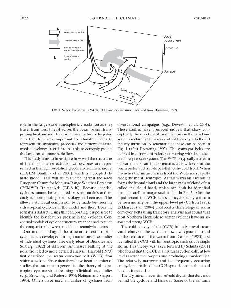
These studies have produced models that show con-

ceptually the structure of, and the flows within, cyclonic

systems including the warm and cold conveyor belts and

the dry intrusion. A schematic of these can be seen in

Fig. 1 (after Browning 1997). The conveyor belts are

defined in a frame of reference moving with its associ-

ated low pressure system. The WCB is typically a stream

of warm moist air that originates at low levels in the

warm sector and travels parallel to the cold front. When

it reaches the surface warm front the WCB rises rapidly

along the moist isentropes. As this warm air ascends, it

forms the frontal cloud and the large mass of cloud often

called the cloud head, which can both be identified

through satellite images such as that in Fig. 2. After the

rapid ascent the WCB turns anticyclonically and can

be seen moving with the upper-level jet (Carlson 1980).

Eckhardt et al. (2004) produced a climatology of warm

conveyor belts using trajectory analysis and found that

most Northern Hemisphere winter cyclones have an as-

sociated strong WCB.

The cold conveyor belt (CCB) initially travels rear-

ward relative to the cyclone at low levels parallel to and

on the cold side of the warm front. Carlson (1980) first

identified the CCB with his isentropic analysis of a single

storm. This theory was taken forward by Schultz (2001)

who found that the CCB mainly turns cyclonically at low

levels around the low pressure producing a low-level jet.

The relatively narrower and less frequently occurring

anticyclonic path of the CCB spreads out in the cloud

head as it ascends.

The dry intrusion consists of cold dry air that descends

behind the cyclone and fans out. Some of the air turns

FIG. 1. Schematic showing WCB, CCB, and dry intrusion (adapted from Browning 1997).

1622 J O U R N A L O F C L I M A T E VOLUME 23

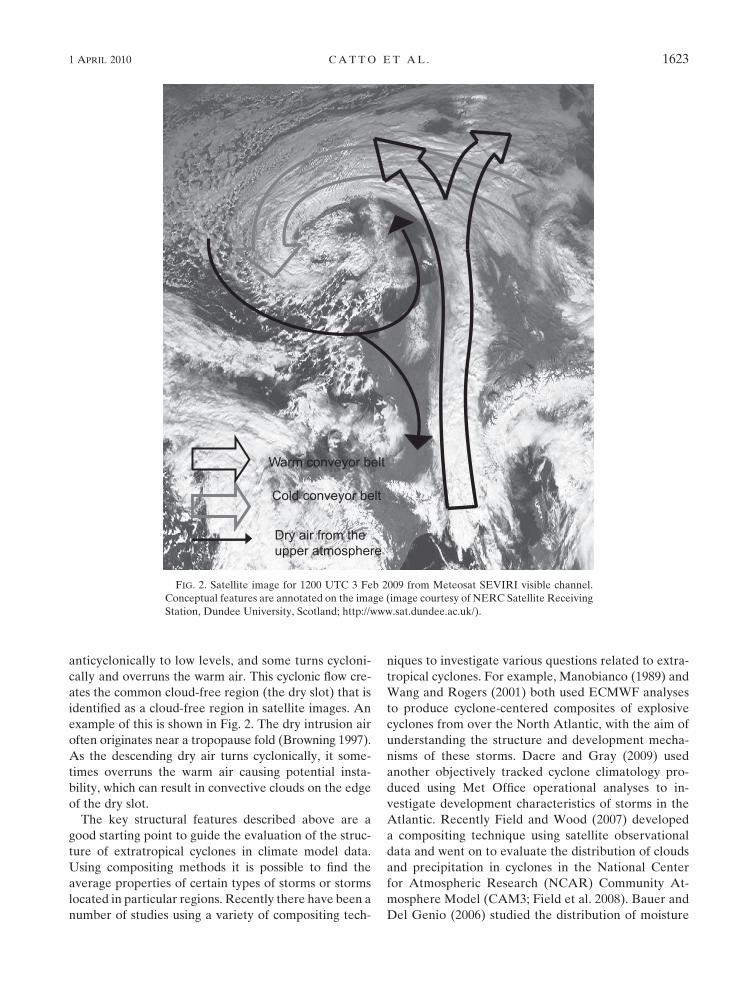
anticyclonically to low levels, and some turns cycloni-

cally and overruns the warm air. This cyclonic flow cre-

ates the common cloud-free region (the dry slot) that is

identified as a cloud-free region in satellite images. An

example of this is shown in Fig. 2. The dry intrusion air

often originates near a tropopause fold (Browning 1997).

As the descending dry air turns cyclonically, it some-

times overruns the warm air causing potential insta-

bility, which can result in convective clouds on the edge

of the dry slot.

The key structural features described above are a

good starting point to guide the evaluation of the struc-

ture of extratropical cyclones in climate model data.

Using compositing methods it is possible to find the

average properties of certain types of storms or storms

located in particular regions. Recently there have been a

number of studies using a variety of compositing tech-

niques to investigate various questions related to extra-

tropical cyclones. For example, Manobianco (1989) and

Wang and Rogers (2001) both used ECMWF analyses

to produce cyclone-centered composites of explosive

cyclones from over the North Atlantic, with the aim of

understanding the structure and development mecha-

nisms of these storms. Dacre and Gray (2009) used

another objectively tracked cyclone climatology pro-

duced using Met Office operational analyses to in-

vestigate development characteristics of storms in the

Atlantic. Recently Field and Wood (2007) developed

a compositing technique using satellite observational

data and went on to evaluate the distribution of clouds

and precipitation in cyclones in the National Center

for Atmospheric Research (NCAR) Community At-

mosphere Model (CAM3; Field et al. 2008). Bauer and

Del Genio (2006) studied the distribution of moisture

FIG. 2. Satellite image for 1200 UTC 3 Feb 2009 from Meteosat SEVIRI visible channel.

Conceptual features are annotated on the image (image courtesy of NERC Satellite Receiving

Station, Dundee University, Scotland; http://www.sat.dundee.ac.uk/).

1 APRIL 2010 C A T T O E T A L . 1623

in composites of extratropical cyclones in the Goddard

Institute for Space Studies (GISS) GCM with comparison

to reanalyses. Bengtsson et al. (2009) took composites

of the 100 most intense cyclones from ERA-40 and the

ECHAM5 to compare the surface winds, mean sea

level pressure (MSLP), and precipitation for present-

day climate and went on to investigate changes with

a warming climate. In the present study the composit-

ing method is used to look at the structure of the cy-

clones in ERA-40 and HiGEM in much more detail.

Using both horizontal and vertical composites of many

different variables, a much more detailed understand-

ing of the structure of the cyclones in HiGEM and

ERA-40 can be gained and interpreted within the frame-

work of conceptual models.

One of the key questions is whether the horizontal

resolution of climate models used in the Intergovern-

mental Panel on Climate Change (IPCC) Fourth As-

sessment Report (AR4), which is typically between 1.58

and 3.08 (Randall et al. 2007), is sufficient to adequately

represent the structure of extratropical cyclones, some

of the features of which may be much smaller than the

grid length. HiGEM (Shaffrey and et al. 2009) is a new

coupled climate model based on the Hadley Centre

Global Environment Model (HadGEM1; Johns et al.

2006) with a horizontal resolution of 0.838 latitude 3

1.258 longitude (N144). We might expect that at higher

resolution, extratropical cyclones may be better re-

solved (Jung et al. 2006).

In this study, a fully automated, cyclone-centered

compositing scheme is used that takes into account the

different stages of the cyclone life cycle, as well as the

direction in which the cyclone is traveling. The emphasis

of this paper is on extreme cyclones, so composites of the

100 most intense cyclones in the Northern Hemisphere

from HiGEM and ERA-40 have been produced. Using

the features of the observation-based conceptual model

shown schematically in Fig. 1 (e.g., Browning and Roberts

1994; Schultz 2001) to guide a comparison between the

cyclones in ERA-40 and HiGEM, the following ques-

tions will be addressed.

d Using the compositing methodology is it possible to

identify in the reanalysis data, the key features of ex-

tratropical cyclone structure as identified in concep-

tual models?d How well does HiGEM compare to ERA-40 in the

representation of these features?

The rest of the paper is structured as follows. Section 2

details the reanalysis and the model data used along with

details of the cyclone tracking and compositing meth-

odologies. Results are given in section 3 and discussion

and conclusions are in section 4.

2. Data and methodology

a. Model and reanalysis data

The model used in this study is HiGEM, a new cou-

pled climate model based on the Met Office Hadley

Centre model HadGEM1 (Johns et al. 2006; Ringer

et al. 2006). The resolution of the model has been in-

creased to 0.838 latitude 3 1.258 longitude (N144) in the

atmosphere and 1/38 3 1/38 in the ocean. Full details of the

changes made to HadGEM1 to produce HiGEM can be

found in Shaffrey et al. (2009). The model used here is

referred to as HiGEM1.2, and the data are taken from

a control run based on present-day radiative forcings.

The net top of atmosphere radiation and the upper

ocean are considered to be spun up after 20 years, so

for this reason the first 20 years of the integration have

been rejected. The cyclones considered in this study

come from 50 winters (December, January, and February)

from years 21–70 of the control integration.

The data used to assess HiGEM come from ERA-40

(for more details see Uppala et al. 2005), a global, gridded

dataset, which is constrained by observations. It has been

used because of the length of the dataset (45 years), the

spatial resolution of approximately 1.18 3 1.18 in the

tropics (T159 linear), and the temporal resolution of 6 h.

The long period of the data allows the statistics of many

storms to be included in the analysis. There are, however,

some problems with using a reanalysis product for veri-

fication of model data, as the reanalysis depends itself on

a model. It is also highly dependent on the number of

observations available and the data assimilation tech-

niques used, and therefore the data from regions with

sparse observations in the presatellite period (such as the

Southern Ocean; Hodges et al. 2003) will be less con-

strained than in regions with many observations. In this

study the focus is on storms in the Northern Hemisphere

where there are stronger observational constraints on

the reanalysis. Despite the issues, reanalysis products are

the best datasets constrained by observations available

for studies such as this.

b. Cyclone identification and feature tracking

Objective feature tracking is becoming a frequently

used way to produce information on the spatial distri-

bution and frequency of extratropical cyclones using

both reanalysis and model data. Such tracking algo-

rithms can identify cyclones by a pressure minimum

(e.g., Jung et al. 2006; Loptien et al. 2008; Hoskins and

Hodges 2002), geopotential height minima (Blender and

Schubert 2000), or a maximum in vorticity (e.g., Sinclair

1994; Hoskins and Hodges 2002). The tracking algo-

rithm used here is that of Hodges (1994, 1995, 1999) and

1624 J O U R N A L O F C L I M A T E VOLUME 23

Hoskins and Hodges (2002) using maxima of 850-hPa

relative vorticity to identify features in the Northern

Hemisphere. The main benefits to using relative vor-

ticity rather than MSLP for the tracking are that it can

pick up smaller-scale storms and can identify storms

earlier in their life cycle before a closed pressure contour

has been formed. Also, vorticity does not rely on ex-

trapolation to the extent that pressure does as it is cal-

culated directly from the winds at the chosen level.

Vorticity, however, is a noisy field, so before the tracking

is performed, the vorticity field is spectrally truncated at

42 wavenumbers (T42). This means that although the

datasets are of differing resolutions, the tracking can be

performed on the same resolution data, therefore iden-

tifying the same spatial scales. A background field of

wavenumber n # 5 is also removed, a step that is more

important for tracking MSLP to remove the planetary-

scale waves, but which has been performed here for

consistency with previous studies (e.g., Hoskins and

Hodges 2002). The feature points (i.e., vorticity max-

ima) are identified at 6-hourly intervals and are initial-

ized into tracks using a nearest neighbor approach and

the smoothest set of tracks are achieved by minimizing

a cost function. In order not to introduce noise into the

composites from very short tracks, the tracks that are

kept for the compositing must have lifetimes of over

4 days.

c. Cyclone compositing

The compositing methodology used here has previously

been used in Bengtsson et al. (2007) to study tropical

cyclone structure and in Bengtsson et al. (2009) to com-

pare extratropical cyclones in ECHAM5 for present day

and future climate forcings. A detailed description of the

methodology can be found in the appendix of Bengtsson

et al. (2007), but the process will also be outlined here.

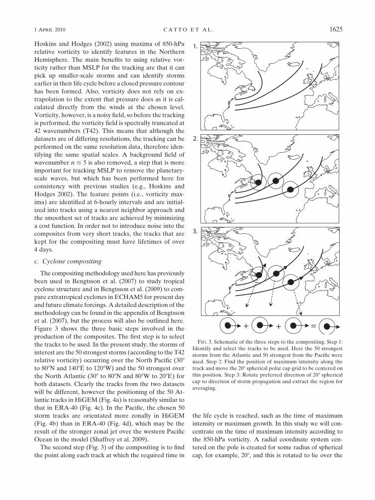
Figure 3 shows the three basic steps involved in the

production of the composites. The first step is to select

the tracks to be used. In the present study, the storms of

interest are the 50 strongest storms (according to the T42

relative vorticity) occurring over the North Pacific (308

to 808N and 1408E to 1208W) and the 50 strongest over

the North Atlantic (308 to 808N and 808W to 208E) for

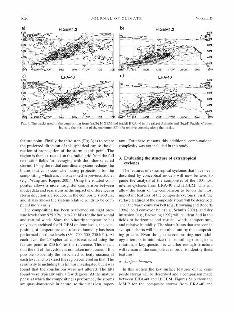
both datasets. Clearly the tracks from the two datasets

will be different, however the positioning of the 50 At-

lantic tracks in HiGEM (Fig. 4a) is reasonably similar to

that in ERA-40 (Fig. 4c). In the Pacific, the chosen 50

storm tracks are orientated more zonally in HiGEM

(Fig. 4b) than in ERA-40 (Fig. 4d), which may be the

result of the stronger zonal jet over the western Pacific

Ocean in the model (Shaffrey et al. 2009).

The second step (Fig. 3) of the compositing is to find

the point along each track at which the required time in

the life cycle is reached, such as the time of maximum

intensity or maximum growth. In this study we will con-

centrate on the time of maximum intensity according to

the 850-hPa vorticity. A radial coordinate system cen-

tered on the pole is created for some radius of spherical

cap, for example, 208, and this is rotated to lie over the

FIG. 3. Schematic of the three steps to the compositing. Step 1:

Identify and select the tracks to be used. Here the 50 strongest

storms from the Atlantic and 50 strongest from the Pacific were

used. Step 2: Find the position of maximum intensity along the

track and move the 208 spherical polar cap grid to be centered on

this position. Step 3: Rotate preferred direction of 208 spherical

cap to direction of storm propagation and extract the region for

averaging.

1 APRIL 2010 C A T T O E T A L . 1625

feature point. Finally the third step (Fig. 3) is to rotate

the preferred direction of this spherical cap to the di-

rection of propagation of the storm at this point. The

region is then extracted on the radial grid from the full

resolution fields for averaging with the other selected

storms. Using the radial coordinate system reduces the

biases that can occur when using projections for the

compositing, which was an issue noted in previous studies

(e.g., Wang and Rogers 2001). Using the rotated com-

posites allows a more insightful comparison between

model data and reanalysis as the impact of differences in

storm direction are reduced in the composite structure,

and it also allows the system-relative winds to be com-

puted more easily.

The compositing has been performed on eight pres-

sure levels from 925 hPa up to 200 hPa for the horizontal

and vertical winds. Since the 6-hourly temperature has

only been archived for HiGEM on four levels, the com-

positing of temperature and relative humidity has been

performed on these levels (850, 700, 500, 250 hPa). At

each level, the 208 spherical cap is extracted using the

feature point at 850 hPa as the reference. This means

that the tilt of the cyclone is not taken into account. It is

possible to identify the associated vorticity maxima at

each level and to extract the region centered on that. The

sensitivity to including this tilt was investigated but it was

found that the conclusions were not altered. The tilts

found were typically only a few degrees. At the mature

phase at which the compositing is performed, the storms

are quasi-barotropic in nature, so the tilt is less impor-

tant. For these reasons this additional computational

complexity was not included in this study.

3. Evaluating the structure of extratropicalcyclones

The features of extratropical cyclones that have been

described by conceptual models will now be used to

guide the analysis of the composites of the 100 most

intense cyclones from ERA-40 and HiGEM. This will

allow the focus of the comparison to be on the most

important features of the composite cyclones. First, the

surface features of the composite storm will be described.

Then the warm conveyor belt (e.g., Browning and Roberts

1994), cold conveyor belt (e.g., Schultz 2001), and dry

intrusion (e.g., Browning 1997) will be identified in the

fields of horizontal and vertical winds, temperature,

and relative humidity. The sharp fronts that are seen in

synoptic charts will be smoothed out by the composit-

ing process. Even though the compositing methodol-

ogy attempts to minimize this smoothing through the

rotation, a key question is whether enough structure

will remain in the composites in order to identify these

features.

a. Surface features

In this section the key surface features of the com-

posite storms will be described and a comparison made

between ERA-40 and HiGEM. Figures 5a,b show the

MSLP for the composite storms from ERA-40 and

FIG. 4. The tracks used in the compositing from (a),(b) HiGEM and (c),(d) ERA-40 in the (a),(c) Atlantic and (b),(d) Pacific. Crosses

indicate the position of the maximum 850-hPa relative vorticity along the tracks.

1626 J O U R N A L O F C L I M A T E VOLUME 23

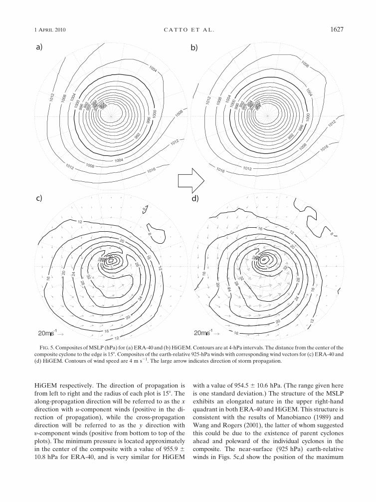
HiGEM respectively. The direction of propagation is

from left to right and the radius of each plot is 158. The

along-propagation direction will be referred to as the x

direction with u-component winds (positive in the di-

rection of propagation), while the cross-propagation

direction will be referred to as the y direction with

y-component winds (positive from bottom to top of the

plots). The minimum pressure is located approximately

in the center of the composite with a value of 955.9 6

10.8 hPa for ERA-40, and is very similar for HiGEM

with a value of 954.5 6 10.6 hPa. (The range given here

is one standard deviation.) The structure of the MSLP

exhibits an elongated nature in the upper right-hand

quadrant in both ERA-40 and HiGEM. This structure is

consistent with the results of Manobianco (1989) and

Wang and Rogers (2001), the latter of whom suggested

this could be due to the existence of parent cyclones

ahead and poleward of the individual cyclones in the

composite. The near-surface (925 hPa) earth-relative

winds in Figs. 5c,d show the position of the maximum

FIG. 5. Composites of MSLP (hPa) for (a) ERA-40 and (b) HiGEM. Contours are at 4-hPa intervals. The distance from the center of the

composite cyclone to the edge is 158. Composites of the earth-relative 925-hPa winds with corresponding wind vectors for (c) ERA-40 and

(d) HiGEM. Contours of wind speed are 4 m s21. The large arrow indicates direction of storm propagation.

1 APRIL 2010 C A T T O E T A L . 1627

winds that would be experienced behind and to the right

of the storm center. The spatial pattern of the winds are

very similar between ERA-40 and HiGEM but the values

in HiGEM are slightly higher, particularly in the bottom

half of the plot. As can be seen in Figs. 5c,d, the distri-

bution of winds around the cyclone is axially asymmetric.

Some of the strongest winds occur in the bottom right-

hand quadrant of the composite cyclone where the WCB

is found. To quantify the differences in the wind speeds

between HiGEM and ERA-40, the maximum speed that

occurs in the bottom right-hand quadrant of each cy-

clone was found, as well as the radial distance from the

center at which it occurs. The average maximum wind

speed for ERA-40 is 39.1 6 3.5 m s21 at 5.1 6 2.78 and

for HiGEM is 41.5 6 3.7 m s21 at 4.9 6 2.28 indicating

that the strength and position of the maximum wind

speeds from HiGEM compare well against ERA-40

within the spread.

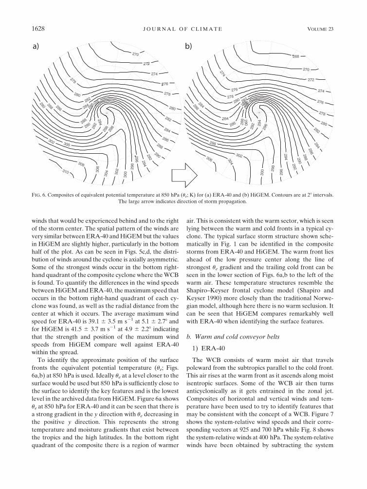
To identify the approximate position of the surface

fronts the equivalent potential temperature (ue; Figs.

6a,b) at 850 hPa is used. Ideally ue at a level closer to the

surface would be used but 850 hPa is sufficiently close to

the surface to identify the key features and is the lowest

level in the archived data from HiGEM. Figure 6a shows

ue at 850 hPa for ERA-40 and it can be seen that there is

a strong gradient in the y direction with ue decreasing in

the positive y direction. This represents the strong

temperature and moisture gradients that exist between

the tropics and the high latitudes. In the bottom right

quadrant of the composite there is a region of warmer

air. This is consistent with the warm sector, which is seen

lying between the warm and cold fronts in a typical cy-

clone. The typical surface storm structure shown sche-

matically in Fig. 1 can be identified in the composite

storms from ERA-40 and HiGEM. The warm front lies

ahead of the low pressure center along the line of

strongest ue gradient and the trailing cold front can be

seen in the lower section of Figs. 6a,b to the left of the

warm air. These temperature structures resemble the

Shapiro–Keyser frontal cyclone model (Shapiro and

Keyser 1990) more closely than the traditional Norwe-

gian model, although here there is no warm seclusion. It

can be seen that HiGEM compares remarkably well

with ERA-40 when identifying the surface features.

b. Warm and cold conveyor belts

1) ERA-40

The WCB consists of warm moist air that travels

poleward from the subtropics parallel to the cold front.

This air rises at the warm front as it ascends along moist

isentropic surfaces. Some of the WCB air then turns

anticyclonically as it gets entrained in the zonal jet.

Composites of horizontal and vertical winds and tem-

perature have been used to try to identify features that

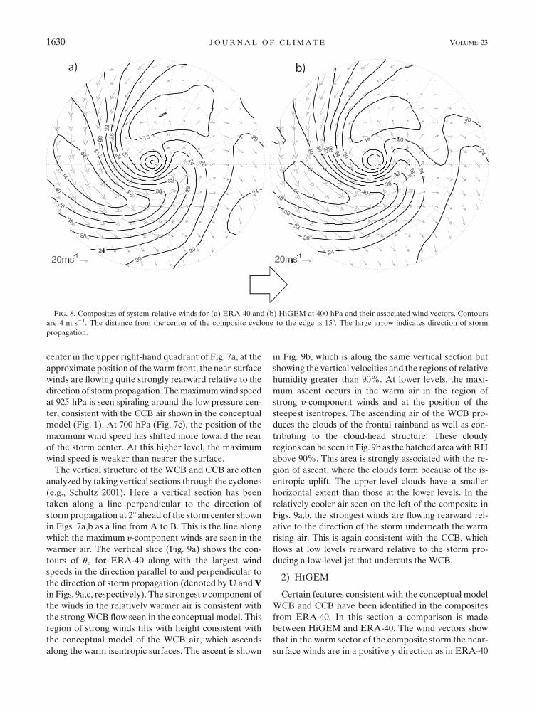
may be consistent with the concept of a WCB. Figure 7

shows the system-relative wind speeds and their corre-

sponding vectors at 925 and 700 hPa while Fig. 8 shows

the system-relative winds at 400 hPa. The system-relative

winds have been obtained by subtracting the system

FIG. 6. Composites of equivalent potential temperature at 850 hPa (ue; K) for (a) ERA-40 and (b) HiGEM. Contours are at 28 intervals.

The large arrow indicates direction of storm propagation.

1628 J O U R N A L O F C L I M A T E VOLUME 23

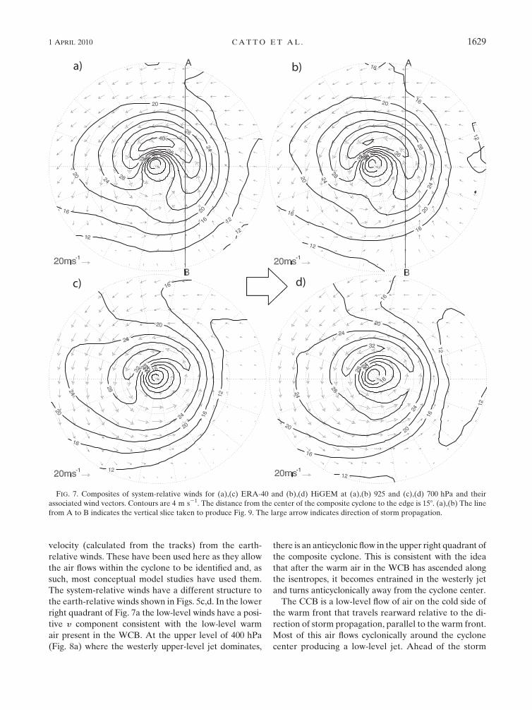
velocity (calculated from the tracks) from the earth-

relative winds. These have been used here as they allow

the air flows within the cyclone to be identified and, as

such, most conceptual model studies have used them.

The system-relative winds have a different structure to

the earth-relative winds shown in Figs. 5c,d. In the lower

right quadrant of Fig. 7a the low-level winds have a posi-

tive y component consistent with the low-level warm

air present in the WCB. At the upper level of 400 hPa

(Fig. 8a) where the westerly upper-level jet dominates,

there is an anticyclonic flow in the upper right quadrant of

the composite cyclone. This is consistent with the idea

that after the warm air in the WCB has ascended along

the isentropes, it becomes entrained in the westerly jet

and turns anticyclonically away from the cyclone center.

The CCB is a low-level flow of air on the cold side of

the warm front that travels rearward relative to the di-

rection of storm propagation, parallel to the warm front.

Most of this air flows cyclonically around the cyclone

center producing a low-level jet. Ahead of the storm

FIG. 7. Composites of system-relative winds for (a),(c) ERA-40 and (b),(d) HiGEM at (a),(b) 925 and (c),(d) 700 hPa and their

associated wind vectors. Contours are 4 m s21. The distance from the center of the composite cyclone to the edge is 158. (a),(b) The line

from A to B indicates the vertical slice taken to produce Fig. 9. The large arrow indicates direction of storm propagation.

1 APRIL 2010 C A T T O E T A L . 1629

center in the upper right-hand quadrant of Fig. 7a, at the

approximate position of the warm front, the near-surface

winds are flowing quite strongly rearward relative to the

direction of storm propagation. The maximum wind speed

at 925 hPa is seen spiraling around the low pressure cen-

ter, consistent with the CCB air shown in the conceptual

model (Fig. 1). At 700 hPa (Fig. 7c), the position of the

maximum wind speed has shifted more toward the rear

of the storm center. At this higher level, the maximum

wind speed is weaker than nearer the surface.

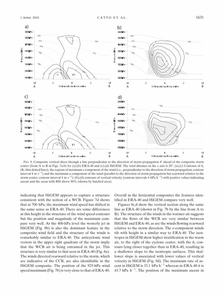
The vertical structure of the WCB and CCB are often

analyzed by taking vertical sections through the cyclones

(e.g., Schultz 2001). Here a vertical section has been

taken along a line perpendicular to the direction of

storm propagation at 28 ahead of the storm center shown

in Figs. 7a,b as a line from A to B. This is the line along

which the maximum y-component winds are seen in the

warmer air. The vertical slice (Fig. 9a) shows the con-

tours of ue for ERA-40 along with the largest wind

speeds in the direction parallel to and perpendicular to

the direction of storm propagation (denoted by U and V

in Figs. 9a,c, respectively). The strongest y component of

the winds in the relatively warmer air is consistent with

the strong WCB flow seen in the conceptual model. This

region of strong winds tilts with height consistent with

the conceptual model of the WCB air, which ascends

along the warm isentropic surfaces. The ascent is shown

in Fig. 9b, which is along the same vertical section but

showing the vertical velocities and the regions of relative

humidity greater than 90%. At lower levels, the maxi-

mum ascent occurs in the warm air in the region of

strong y-component winds and at the position of the

steepest isentropes. The ascending air of the WCB pro-

duces the clouds of the frontal rainband as well as con-

tributing to the cloud-head structure. These cloudy

regions can be seen in Fig. 9b as the hatched area with RH

above 90%. This area is strongly associated with the re-

gion of ascent, where the clouds form because of the is-

entropic uplift. The upper-level clouds have a smaller

horizontal extent than those at the lower levels. In the

relatively cooler air seen on the left of the composite in

Figs. 9a,b, the strongest winds are flowing rearward rel-

ative to the direction of the storm underneath the warm

rising air. This is again consistent with the CCB, which

flows at low levels rearward relative to the storm pro-

ducing a low-level jet that undercuts the WCB.

2) HIGEM

Certain features consistent with the conceptual model

WCB and CCB have been identified in the composites

from ERA-40. In this section a comparison is made

between HiGEM and ERA-40. The wind vectors show

that in the warm sector of the composite storm the near-

surface winds are in a positive y direction as in ERA-40

FIG. 8. Composites of system-relative winds for (a) ERA-40 and (b) HiGEM at 400 hPa and their associated wind vectors. Contours

are 4 m s21. The distance from the center of the composite cyclone to the edge is 158. The large arrow indicates direction of storm

propagation.

1630 J O U R N A L O F C L I M A T E VOLUME 23

indicating that HiGEM appears to capture a structure

consistent with the notion of a WCB. Figure 7d shows

that at 700 hPa, the maximum wind speed has shifted in

the same sense as ERA-40. There are some differences

at this height in the structure of the wind speed contours

but the position and magnitude of the maximum com-

pare very well. At the 400-hPa level the westerly jet in

HiGEM (Fig. 8b) is also the dominant feature in the

composite wind field and the structure of the winds is

remarkably similar to ERA-40. The anticyclonic wind

vectors in the upper right quadrant of the storm imply

that the WCB air is being entrained in the jet. This

structure is very similar to that seen in ERA-40 (Fig. 8a).

The winds directed rearward relative to the storm, which

are indicative of the CCB, are also identifiable in the

HiGEM composite. The position of the 925-hPa wind

speed maximum (Fig. 7b) is very close to that of ERA-40.

Overall in the horizontal composites the features iden-

tified in ERA-40 and HiGEM compare very well.

Figures 9c,d show the vertical section along the same

line as ERA-40 (shown in Fig. 7b by the line from A to

B). The structure of the winds in the warmer air suggests

that the flows of the WCB are very similar between

HiGEM and ERA-40, as are the winds flowing rearward

relative to the storm direction. The y-component winds

tilt with height in a similar way to ERA-40. The isen-

tropes in HiGEM show higher stratification in the warm

air, to the right of the cyclone center, with the ue con-

tours lying closer together than in ERA-40, resulting in

a shallower slope to the isentropic surfaces. This shal-

lower slope is associated with lower values of vertical

velocity in HiGEM (Fig. 9d). The maximum rate of as-

cent in HiGEM is 33.1 hPa h21 whereas in ERA-40 it is

43.7 hPa h21. The position of the maximum ascent in

FIG. 9. Composite vertical slices through a line perpendicular to the direction of storm propagation 48 ahead of the composite storm

center (from A to B in Figs. 7a,b) for (a),(b) ERA-40 and (c),(d) HiGEM. The total distance in the x axis is 208. (a),(c) Contours of ue

(K; thin dotted lines), the regions of maximum y component of the wind (i.e., perpendicular to the direction of storm propagation; contour

interval 4 m s21) and the maximum u component of the wind (parallel to the direction of storm propagation but rearward relative to the

storm center; contour interval 4 m s21); (b),(d) contours of vertical velocity (contour intervals 4 hPa h21) with positive values indicating

ascent and the areas with RH above 90% (shown by hatched area).

1 APRIL 2010 C A T T O E T A L . 1631

HiGEM does coincide with the maximum slope of the

isentropes consistent with the conceptual model of the

WCB. Large differences between HiGEM and ERA-40

can be seen in the extent and structure of the region of

relative humidity above 90% shown by the hatched areas

in Figs. 9b,d. The cloudy area has a larger horizontal

extent at upper levels compared to ERA-40. There are

a number of possible reasons that the vertical tempera-

ture, cloud, and humidity structures are different in the

WCB of the composite cyclones from ERA-40 and

HiGEM. The most likely explanation is that the diabatic

processes that modify the air flowing through the WCB

are represented differently in HiGEM and ERA-40.

This will be examined in the concluding discussion.

c. Dry intrusion

1) ERA-40

The dry intrusion is a feature usually identified in

satellite images (e.g., Fig. 2) as the cloud-free region just

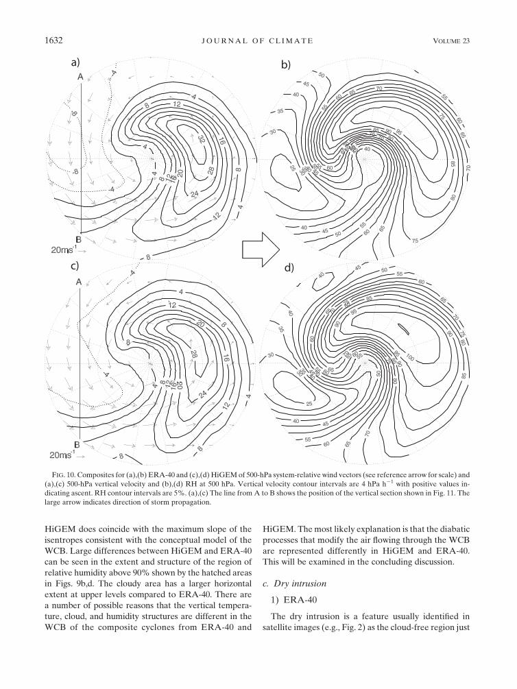
FIG. 10. Composites for (a),(b) ERA-40 and (c),(d) HiGEM of 500-hPa system-relative wind vectors (see reference arrow for scale) and

(a),(c) 500-hPa vertical velocity and (b),(d) RH at 500 hPa. Vertical velocity contour intervals are 4 hPa h21 with positive values in-

dicating ascent. RH contour intervals are 5%. (a),(c) The line from A to B shows the position of the vertical section shown in Fig. 11. The

large arrow indicates direction of storm propagation.

1632 J O U R N A L O F C L I M A T E VOLUME 23

behind the cold front. Very dry air descends from upper

levels and some of the air turns anticyclonically away

from the cyclone, while some turns cyclonically up and

over the cyclone (Browning 1997). Figure 10a shows the

system-relative wind vectors and the vertical velocity at

500 hPa for ERA-40, indicating the region of descent

behind the composite cyclone with a maximum rate of

descent of 9.7 hPa h21. The wind vectors show in the

region of descent that the air is turning cyclonically

around the composite cyclone. This region of descent

coincides with an area of very low relative humidity

(RH) at the same level (Fig. 10b), suggesting that the air

has come from the upper troposphere where there is

very little moisture. These features are consistent with

the conceptual model of the dry intrusion.

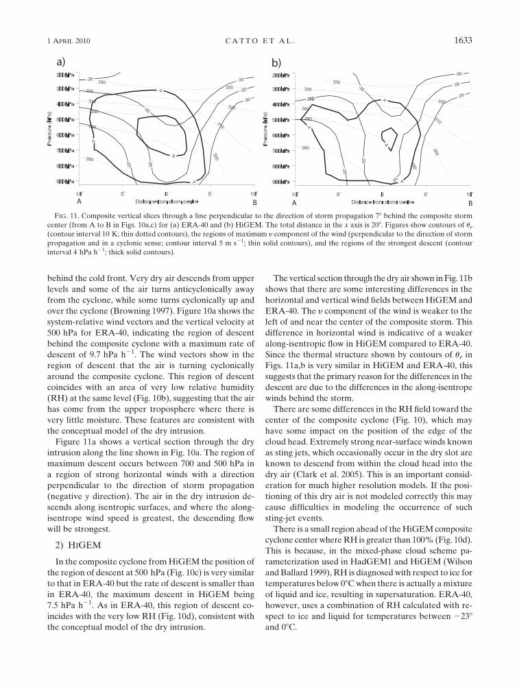
Figure 11a shows a vertical section through the dry

intrusion along the line shown in Fig. 10a. The region of

maximum descent occurs between 700 and 500 hPa in

a region of strong horizontal winds with a direction

perpendicular to the direction of storm propagation

(negative y direction). The air in the dry intrusion de-

scends along isentropic surfaces, and where the along-

isentrope wind speed is greatest, the descending flow

will be strongest.

2) HIGEM

In the composite cyclone from HiGEM the position of

the region of descent at 500 hPa (Fig. 10c) is very similar

to that in ERA-40 but the rate of descent is smaller than

in ERA-40, the maximum descent in HiGEM being

7.5 hPa h21. As in ERA-40, this region of descent co-

incides with the very low RH (Fig. 10d), consistent with

the conceptual model of the dry intrusion.

The vertical section through the dry air shown in Fig. 11b

shows that there are some interesting differences in the

horizontal and vertical wind fields between HiGEM and

ERA-40. The y component of the wind is weaker to the

left of and near the center of the composite storm. This

difference in horizontal wind is indicative of a weaker

along-isentropic flow in HiGEM compared to ERA-40.

Since the thermal structure shown by contours of ue in

Figs. 11a,b is very similar in HiGEM and ERA-40, this

suggests that the primary reason for the differences in the

descent are due to the differences in the along-isentrope

winds behind the storm.

There are some differences in the RH field toward the

center of the composite cyclone (Fig. 10), which may

have some impact on the position of the edge of the

cloud head. Extremely strong near-surface winds known

as sting jets, which occasionally occur in the dry slot are

known to descend from within the cloud head into the

dry air (Clark et al. 2005). This is an important consid-

eration for much higher resolution models. If the posi-

tioning of this dry air is not modeled correctly this may

cause difficulties in modeling the occurrence of such

sting-jet events.

There is a small region ahead of the HiGEM composite

cyclone center where RH is greater than 100% (Fig. 10d).

This is because, in the mixed-phase cloud scheme pa-

rameterization used in HadGEM1 and HiGEM (Wilson

and Ballard 1999), RH is diagnosed with respect to ice for

temperatures below 08C when there is actually a mixture

of liquid and ice, resulting in supersaturation. ERA-40,

however, uses a combination of RH calculated with re-

spect to ice and liquid for temperatures between 2238

and 08C.

FIG. 11. Composite vertical slices through a line perpendicular to the direction of storm propagation 78 behind the composite storm

center (from A to B in Figs. 10a,c) for (a) ERA-40 and (b) HiGEM. The total distance in the x axis is 208. Figures show contours of ue

(contour interval 10 K; thin dotted contours), the regions of maximum y component of the wind (perpendicular to the direction of storm

propagation and in a cyclonic sense; contour interval 5 m s21; thin solid contours), and the regions of the strongest descent (contour

interval 4 hPa h21; thick solid contours).

1 APRIL 2010 C A T T O E T A L . 1633

4. Discussion and conclusions

The aim of this paper is to investigate the represen-

tation of extratropical cyclones in a high resolution

coupled climate model, HiGEM, and in the ERA-40

reanalysis. A compositing methodology that takes into

account the direction of propagation of the storms was

used to produce composites of the 100 most intense

cyclones occurring over the North Atlantic and North

Pacific Ocean basins found in HiGEM and in ERA-40.

Certain features of conceptual models of extratropical

cyclones have been used to aid the comparison of the

composite cyclones from the two datasets. The key re-

sults of the study are as follows:

d The compositing methodology is capable of producing

composite cyclones from the reanalysis data, which

exhibit features of extratropical cyclones consistent

with those from conceptual models.d The conceptual features of the warm conveyor belt,

cold conveyor belt, and dry intrusion can be identi-

fied in both the reanalysis and the model composite

cyclones.d The surface features of mean sea level pressure and

equivalent potential temperature have very similar struc-

ture and magnitude between HiGEM and ERA-40.d The structure of the near-surface wind speeds com-

pares very well between HiGEM and ERA-40 espe-

cially in the WCB and CCB.d Differences in the ascent ahead of the storm can be

attributed to the slope of the moist isentropes in this

region with steeper moist isentropes and stronger as-

cent in ERA-40 compared to HiGEM.d The rate of descent behind the cyclone is lower in

HiGEM compared to ERA-40, which is mainly due to

the weaker winds along the isentropes in this region in

the model.

The fact that the features identified in the two datasets

compare so well is a good indication that HiGEM can

capture the structures seen in extratropical cyclones in

the ERA-40 reanalysis. This demonstrates that climate

models can capture the structural features of extra-

tropical cyclones. This gives us more confidence in fu-

ture predictions of extratropical cyclones. It is unclear

whether the results seen here would be robust over

a range of different climate models and reanalyses.

Some of the smaller-scale features, such as the narrow

band of cold air traveling rearward behind the warm

front are at a scale of a few grid boxes of the model grid,

so it raises the question of whether a lower-resolution

model could also capture the same features. It is also

possible that a much higher-resolution model or rean-

alysis dataset could capture these features even better

than seen here. These questions will be addressed through

future work using different resolution models and the new

reanalysis product from ECMWF (ECMWF-Interim),

which, with a resolution of 80 km might be more ap-

propriate for this type of study.

Another issue is that parameterizations of diabatic

processes, which have a strong influence on the develop-

ment of extratropical cyclones, differ between climate

models. It was seen in section 3b that differences occurred

along the WCB in the vertical profiles of temperature and

relative humidity fields between ERA-40 and HiGEM

(Fig. 9). A possible suggestion for this discrepancy is that

in ERA-40 the cloud appears to occur because of the

large-scale isentropic uplift of the air in the WCB (Fig. 9b).

In HiGEM, however, the region of cloud appears less

strongly related to the isentropic uplift, suggesting that

there could be convection triggered in the warm air be-

fore it ascends (Fig. 9d). It is not possible to confirm this

using the compositing methodology because of the lack of

6-hourly cloud or precipitation fields but if this indeed is

the case it would have impacts on the positioning of the

precipitation in frontal systems.

At the scale of individual cyclones, the reanalysis is

relatively unconstrained in terms of clouds and humid-

ity, so another method needs to be found to diagnose the

diabatic processes seen in the extratropical cyclone

composites. For example, Field et al. (2008) used satel-

lite observations to produce composites of clouds, rain

rates, and liquid water path to assess the extratropical

cyclones within the NCAR Community Atmosphere

Model (CAM3). To be able to more precisely define the

conveyor belt flows, isentropic or trajectory analyses

could be performed. Conceptual models, such as those

produced by Browning and Roberts (1994), use isen-

tropic and trajectory analysis to identify the airstreams.

Such an analysis is beyond the scope of this particular

study but may lead to deeper insights into the ability of

climate models to capture the structure of extratropical

cyclones. The present study could also be extended to

investigate the structure of extratropical cyclones at

different stages of their life cycles, giving additional in-

formation on the processes captured in the model.

The issues highlighted here are areas that need future

research in order to gain a more complete picture of how

well extratropical cyclones are represented in a range of

models and reanalyses so that we can have confidence in

future predictions. Even given these issues, this study

has demonstrated that compositing is a powerful tool for

investigating the structure of intense extratropical cy-

clones from reanalysis and model data.

Acknowledgments. The authors acknowledge finan-

cial support provided by NERC. The authors thank

1634 J O U R N A L O F C L I M A T E VOLUME 23

ECMWF for their provision of the ERA-40 reanalysis

data and Dundee Satellite Receiving Station for use of their

images. The helpful comments and suggestions of three

anonymous reviewers are also gratefully acknowledged.

REFERENCES

Bauer, M., and A. D. Del Genio, 2006: Composite analysis of

winter cyclones in a GCM: Influence on climatological hu-

midity. J. Climate, 19, 1652–1672.

Bengtsson, L., K. I. Hodges, M. Esch, N. Keenlyside, L. Kornblueh,

J.-J. Luo, and T. Yamagata, 2007: How may tropical cyclones

change in a warmer climate? Tellus, 59A, 539–561.

——, ——, and N. Keenlyside, 2009: Will extratropical storms in-

tensify in a warmer climate? J. Climate, 22, 2276–2301.

Bjerknes, J., and H. Solberg, 1922: Life cycle of cyclones and the

polar front theory of atmospheric circulation. Geofys. Publ., 3,

1–18.

Blender, R., and M. Schubert, 2000: Cyclone tracking in different

spatial and temporal resolutions. Mon. Wea. Rev., 128, 377–384.

Browning, K. A., 1997: The dry intrusion perspective of extra-

tropical cyclone development. Meteor. Appl., 4, 317–324.

——, and N. M. Roberts, 1994: Structure of a frontal cyclone.

Quart. J. Roy. Meteor. Soc., 120, 1535–1557.

Carlson, T. N., 1980: Airflow through midlatitude cyclones and the

comma cloud pattern. Mon. Wea. Rev., 108, 1498–1509.

Clark, P. A., K. A. Browning, and C. Wang, 2005: The sting at the end

of the tail: Model diagnostics of fine-scale three-dimensional

structure of the cloud head. Quart. J. Roy. Meteor. Soc., 131,

2263–2292.

Dacre, H. F., and S. L. Gray, 2009: The spatial distribution and

evolution characteristics of North Atlantic cyclones. Mon.

Wea. Rev., 137, 99–115.

Deveson, A. C. L., K. A. Browning, and T. D. Hewson, 2002:

A classification of FASTEX cyclones using a height-attributable

quasi-geostrophic vertical-motion diagnostic. Quart. J. Roy.

Meteor. Soc., 128, 93–117.

Eckhardt, S., A. Stohl, H. Wernli, P. James, C. Forster, and

N. Spichtinger, 2004: A 15-year climatology of warm conveyor

belts. J. Climate, 17, 218–237.

Field, P. R., and R. Wood, 2007: Precipitation and cloud structure

in midlatitude cyclones. J. Climate, 20, 233–254.

——, A. Gettelman, R. Neale, R. Wood, P. J. Rasch, and

H. Morrison, 2008: Midlatitude cyclone compositing to con-

strain climate model behavior using satellite observations.

J. Climate, 21, 5887–5903.

Harrold, T. W., 1973: Mechanisms influencing the distribution of

precipitation within baroclinic disturbances. Quart. J. Roy.

Meteor. Soc., 99, 232–251.

Hodges, K. I., 1994: A general method for tracking analysis and its

application to meteorological data. Mon. Wea. Rev., 122,

2573–2586.

——, 1995: Feature tracking on the unit sphere. Mon. Wea. Rev.,

123, 3458–3465.

——, 1999: Adaptive constraints for feature tracking. Mon. Wea.

Rev., 127, 1362–1373.

——, B. J. Hoskins, J. Boyle, and C. Thorncroft, 2003: A compar-

ison of recent reanalysis datasets using objective feature

tracking: Storm tracks and tropical easterly waves. Mon. Wea.

Rev., 131, 2012–2037.

Hoskins, B. J., and K. I. Hodges, 2002: New perspectives on the

Northern Hemisphere winter storm tracks. J. Atmos. Sci., 59,

1041–1061.

Johns, T. C., and Coauthors, 2006: The new Hadley Centre Cli-

mate Model (HadGEM1): Evaluation of coupled simulations.

J. Climate, 19, 1327–1353.

Jung, T., S. K. Gulev, I. Rudeva, and V. Soloviov, 2006: Sensitivity

of extratropical cyclone characteristics to horizontal resolu-

tion in the ECMWF model. Quart. J. Roy. Meteor. Soc., 132,

1839–1857.

Loptien, U., O. Zolina, S. Gulev, M. Latif, and V. Soloviov, 2008:

Cyclone life cycle characteristics over the Northern Hemi-

sphere in coupled GCMs. Climate Dyn., 31, 507–532.

Manobianco, J., 1989: Explosive east coast cyclogenesis over the

west-central North Atlantic Ocean: A composite study de-

rived from ECMWF operational analyses. Mon. Wea. Rev.,

117, 2365–2383.

Neiman, P. J., and M. A. Shapiro, 1993: The life cycle of an ex-

tratropical marine cyclone. Part I: Frontal-cyclone evolution

and thermodynamic air–sea interaction. Mon. Wea. Rev., 121,

2153–2176.

Randall, D. A., and Coauthors, 2007: Climate models and their

evaluation. Climate Change 2007: The Physical Basis, Contri-

bution of Working Group I to the Fourth Assessment Report of

the Intergovernmental Panel on Climate Change, S. Solomon

et al., Eds., Cambridge University Press, 589–662.

Ringer, M. A., and Coauthors, 2006: The physical properties of the

atmosphere in the new Hadley Centre global environmental

model (HadGEM1). Part II: Aspects of variability and re-

gional climate. J. Climate, 19, 1302–1326.

Roeckner, E., and Coauthors, 2003: The atmospheric general cir-

culation model ECHAM 5. Part I: Model description. Max

Planck Institute for Meteorology Rep. 349, 140 pp.

Schultz, D. M., 2001: Reexamining the cold conveyor belt. Mon.

Wea. Rev., 129, 2205–2225.

Shaffrey, L. C., and Coauthors, 2009: UK-HiGEM: The new UK

high resolution global environment model—Model de-

scription and basic evaluation. J. Climate, 22, 1861–1896.

Shapiro, M. A., and D. Keyser, 1990: Fronts, jet streams and the

tropopause. Extratropical Cyclones, The Erik Palmen Me-

morial Volume, C. W. Newton and E. O. Holopainen, Eds.,

Amer. Meteor. Soc., 167–191.

Sinclair, M. R., 1994: An objective cyclone climatology for the

Southern Hemisphere. Mon. Wea. Rev., 122, 2239–2256.

Uppala, S. M., and Coauthors, 2005: The ERA-40 re-analysis.

Quart. J. Roy. Meteor. Soc., 131, 2961–3012.

Wang, C.-C., and J. C. Rogers, 2001: A composite study of explo-

sive cyclogenesis in different sectors of the North Atlantic.

Part I: Cyclone structure and evolution. Mon. Wea. Rev., 129,

1481–1499.

Wilson, D. R., and S. P. Ballard, 1999: A microphysically based

precipitation scheme for the UK Meteorological Office Uni-

fied Model. Quart. J. Roy. Meteor. Soc., 125, 1607–1636.

1 APRIL 2010 C A T T O E T A L . 1635