Can a Parabolic Evolution of the Entropy

of the Universe Provide the Foundation for

the Second Law of Thermodynamics?

Paula ReichertMathematisches Institut

Ludwig-Maximilians-Universtat Munchen

A thesis submitted for the degree of

Master of Science

Supervisor:

Prof. Dr. Detlef Durr

December 2012

Can a Parabolic Evolution of the Entropy of the

Universe Provide the Foundation for the Second

Law of Thermodynamics?

Paula ReichertMathematisches Institut

Ludwig-Maximilians-Universtat Munchen

Abstract

In this thesis, we want to address the foundations of the second law of thermodynam-

ics. More explicit, we want to discuss a cosmological model featuring a parabolic-like

evolution of the entropy of the universe which was proposed by Sean Carroll and Jen-

nifer Chen and which was meant to serve as an explanation for why entropy increases,

has been increasing and will be increasing for all times. Analyzing their suggestion,

a toy model will help us to argue that it is not reasonable to assume a parabolic-like

evolution of the entropy of the universe. Instead, we should rather expect the entropy

to stay constant. In a second step we nevertheless show that, if against our expect-

ations a parabolic-like evolution of the entropy existed, this could indeed provide the

foundation for the asymmetry in time in thermodynamics (as stated by the second

law) - although this would mean that Boltzmann’s statistical reasoning has to be re-

jected. In a third step we discuss arguments for why we should expect the asymmetry

in time we experience to be such that entropy increases rather than decreases, even if

we considered an overall time-symmetric model like the one suggested by Carroll and

Chen.

2

Acknowledgements

I very much thank Professor Detlef Durr, Professor Peter Pickl and Dustin Lazarovici

for the many thorough discussions, for their never ending interest in this topic and for

the great e↵ort they put in trying to get things clear. For me it was a great chance to

have been able to work with them. Especially, I thank Professor Detlef Durr for his

excellent work as a supervisor.

Also I thank everybody who spent his or her time taking care of Jakob, thereby

allowing me to write this thesis. These are especially my boyfriend Tobias, his parents

Hanne and Erhard, my sister Anna, and, from time to time, my mother Monika and

Tobi’s sister Anna.

3

Contents

1 Introduction 6

2 Classical statistical mechanics 10

2.1 Hamiltonian mechanics . . . . . . . . . . . . . . . . . . . . . . . . . . . 10

2.2 The notion of a measure on phase space . . . . . . . . . . . . . . . . . 11

2.3 Liouville’s theorem . . . . . . . . . . . . . . . . . . . . . . . . . . . . . 13

2.4 The microcanonical measure . . . . . . . . . . . . . . . . . . . . . . . . 14

3 The second law of thermodynamics 16

3.1 Historical introduction . . . . . . . . . . . . . . . . . . . . . . . . . . . 16

3.2 Boltzmann entropy . . . . . . . . . . . . . . . . . . . . . . . . . . . . . 17

3.3 The second law in terms of Boltzmann entropy . . . . . . . . . . . . . . 19

3.4 Reversibility and recurrence objection . . . . . . . . . . . . . . . . . . . 22

3.4.1 The reversibility objection . . . . . . . . . . . . . . . . . . . . . 22

3.4.2 Comments on the reversibility objection . . . . . . . . . . . . . 24

3.4.3 The recurrence objection . . . . . . . . . . . . . . . . . . . . . . 25

3.5 The problem of the special initial conditions . . . . . . . . . . . . . . . 27

4 The evolution of the entropy of the universe 28

4.1 The universe and its subsystems . . . . . . . . . . . . . . . . . . . . . . 28

4.2 The fluctuation scenario by Boltzmann . . . . . . . . . . . . . . . . . . 31

4.3 Discussion of the fluctuation scenario . . . . . . . . . . . . . . . . . . . 33

4.4 The Past-Hypothesis by Albert . . . . . . . . . . . . . . . . . . . . . . 35

4.5 Discussion of the Past-Hypothesis . . . . . . . . . . . . . . . . . . . . . 38

5 The multiverse scenario due to Carroll and Chen 40

5.1 The evolution of the entropy of the multiverse . . . . . . . . . . . . . . 41

5.2 The cosmological model . . . . . . . . . . . . . . . . . . . . . . . . . . 44

5.3 Discussion of a toy model . . . . . . . . . . . . . . . . . . . . . . . . . 46

5.3.1 Introduction to the model . . . . . . . . . . . . . . . . . . . . . 46

5.3.2 The first macrovariable . . . . . . . . . . . . . . . . . . . . . . . 47

5.3.3 The second macrovariable . . . . . . . . . . . . . . . . . . . . . 49

5.3.4 The evolution of the entropy . . . . . . . . . . . . . . . . . . . . 56

5.4 Scope and relevance of the toy model . . . . . . . . . . . . . . . . . . . 57

5.5 On the notion of typicality in case an entropy curve like the one suggested

really exists . . . . . . . . . . . . . . . . . . . . . . . . . . . . . . . . . 59

5.5.1 The suggested entropy curve . . . . . . . . . . . . . . . . . . . . 59

5.5.2 Conditional measures . . . . . . . . . . . . . . . . . . . . . . . . 61

4

5.5.3 A non-normalizable measure . . . . . . . . . . . . . . . . . . . . 64

5.6 Justification of the statistical hypothesis . . . . . . . . . . . . . . . . . 67

5.7 Further discussion of the multiverse scenario . . . . . . . . . . . . . . . 69

6 Entropy increase versus entropy decrease 69

6.1 Psychological arrows of time . . . . . . . . . . . . . . . . . . . . . . . . 70

6.2 Interdependence of the psychological arrows of time . . . . . . . . . . . 71

6.3 Connection to the thermodynamic arrow of time . . . . . . . . . . . . . 73

6.3.1 Asymmetry in records . . . . . . . . . . . . . . . . . . . . . . . 74

6.3.2 Asymmetry in interventions . . . . . . . . . . . . . . . . . . . . 77

7 Comparison 79

8 Conclusion and outlook 81

5

1 Introduction

When a glass falls down a table, it bursts into many, many pieces - many pieces of glass

on the other hand do not assemble to form an unbroken glass again. Letting a drop of

ink drop into a bowl of water, the water will turn slightly purple - purple water on the

other hand doesn’t show an accumulation of ink, forming an ink drop at any time in

the future. Why do some processes in nature go on in one direction of time, but not in

the other? Imagine there were a motion picture of one of the two processes described.

If you played it forwards and backwards, you could easily tell which was the right way

to play it - at least, if you tried to show what has actually happened in nature.

Maybe you haven’t wondered about this asymmetry in time so far, but you start

wondering as soon as you know that the underlying physical laws are reversible, i.e.,

they don’t change under the transformation t to �t (when t is the time variable).

Analyzing the motion of the atoms and molecules, it turns out that both processes,

the one forward, the other one backward in time, are equally correct according to

physical law. Both are solutions of the Newtonian second law of motion and therefore

should be processes that actually occur in nature. So why do certain processes like the

breaking of a glass only go on in one direction of time, but not in the other? How can

time reversibility on a microscopic level, i.e., regarding the motion of the atoms and

molecules, and time irreversibility on a macroscopic level, i.e., regarding the dynamics

of visible objects, be reconciled? Moreover, how can a physical law like the second

law of thermodynamics, stating the irreversibility of macroscopic processes, be derived

from time-reversal invariant laws for the microscopic constituents of matter?

Studying Boltzmann gives you a first answer to these questions. The student of

Boltzmann’s ideas will learn how to connect microscopic reversibility and macroscopic

irreversibility. He or she will learn that it is the special initial state of a system which

is responsible for its irreversible evolution afterwards. Isn’t this a good and su�cient

answer? Is there anything unsatisfying about this result? To get an answer to these

questions, the following has to be taken into account. According to Boltzmann, any

irreversible evolution will finally come to an end. Any system will finally reach its

equilibrium state which is by far the most likely state of the system. Then, once the

system has reached equilibrium, it will stay there virtually forever which means that

it will stop showing any directedness in time. Taking this for granted, the question

arises why any system should ever be in a special state far away from equilibrium.

Looking at ever bigger systems finally considering the universe as a whole, we can

formulate a new question, namely: Why is the universe in such a special state as it

is in now? Explicitly, why is it not in equilibrium where no time-directed processes

occur if to be in such a state is by far the most likely? A question which, as we made

6

out, accounts for the question why, at this moment, we experience any time-directed

thermodynamic processes at all. Beyond that another question arises, namely: Why

has the universe in its past been in a much more special state, even further away of

equilibrium? For it seems to us that also in the past time-directed processes occurred

pushing the universe further from a very special state to a less special one finally driving

it towards equilibrium.

Historically, essentially two di↵erent conceptions have been invoked to explain the

fact that the present state of the universe is special, thereby providing two di↵erent

candidates for the foundation of the second law of thermodynamics. These conceptions

correspond to two di↵erent scenarios with respect to the evolution of the entropy of

the universe. They are known as the fluctuation scenario on the one hand and the past

hypothesis on the other hand. Both scenarios have first been suggested by Boltzmann,

who, in the end, argued in favor of the fluctuation scenario while today’s physicists

typically promote some kind of past hypothesis.1 As we will see, both scenarios di↵er

in a crucial way regarding what they can say about an even more special state of the

universe in its past. Later in this thesis we will discuss both scenarios thoroughly

thereby presenting the arguments which exist in favor of and against each.

Still, the discussion has not come to an end. Recently a new suggestion for the

foundation of the second law of thermodynamics has been advertised. It is connected

to a cosmological model proposed by Sean Carroll and Jennifer Chen and is suggested

by them in an article published in 2004 called ‘Spontaneous inflation and the origin of

the arrow of time’. There they propose, in connection to their cosmological model, an

evolution of the entropy of the universe (which, in their case, is actually a multiverse)

which is such that entropy increases from a given initial value of minimal entropy

unbounded both towards the future an the past. It will be the main task of this thesis

to explore the suggestion made by Carroll and Chen. It shall be clarified whether

their suggestion can provide an explanation for the fact that entropy increases (or

stays the same, but never decreases). In other words, it shall be analyzed whether

the evolution of the entropy of the universe they propose can provide a foundation for

the second law of thermodynamics. As far as the physics are concerned, this analysis

consists of two parts. First, it has to be clarified whether a more or less parabolic

evolution of the entropy of the universe is in any way conceivable, or possible, in a

physical meaningful way.2 For if we could reasonably argue against the possibility of

such an evolution, there would be no way to establish it as the foundation of the second

1As far as Boltzmann is concerned, cf. [2], pp. 256-259.2As I will comment on below, the shape of the entropy curve does not necessarily have to be a

parabola. It has to be unbounded towards the future and the past with a minimum somewhere inbetween, that’s all. Anyway, to have a more or less correct picture in mind, I want to refer to thiscurve from time to time as a parabola.

7

law of thermodynamics. Second, under the hypothetical assumption that an entropy

curve like the one suggested exists, it has to be analyzed whether this evolution of the

universe’s entropy actually provides us with what we are looking for, namely with an

explanation for the increase of entropy in all subsystems of the universe throughout all

times.

With respect to the first part of the analysis, a simple toy model will be presented

and analyzed. It will be shown that, although this model fulfills all the necessary

conditions in order for an evolution of the entropy like the one suggested to exist,

in this model entropy does neither increase nor decrease, but stays the same for all

relevant times. By determining scope and relevance of this model, the connection to

the universe shall be drawn. We will argue that, just like in the case of the toy model,

the evolution of the entropy of the universe should not be expected to grow unbounded

towards the future and the past. With respect to the second part of the analysis we

will show that, if there existed a parabolic-like evolution of the entropy of the universe,

it would indeed be possible to argue that the given evolution provides the foundation

of the second law of thermodynamics, although this would mean that Boltzmann’s

way of reasoning has to be rejected - something which is certainly not a trivial step.

This second part of the analysis will essentially involve the notion and properties of a

non-normalizable measure on infinite phase space.

There is a third part of the analysis which is rather philosophical and which shall

be treated in an additional chapter in the end. It deals with the question whether

we can distinguish a decrease of entropy from an increase of entropy, i.e., whether

or not we call the ‘past’ that direction in time in which the universe is in states

of lower entropy whereas we call the ‘future’ that direction in time in which it is

states of higher entropy. Physicists like Boltzmann or Carroll simply assume this to

be true, but actually it is far from obvious.3 It would mean that we could reduce any

‘psychological’ asymmetry in time which we use to determine, or define, the notions

of past and future to the asymmetry given by the thermodynamic arrow of time (the

direction of entropy increase in thermodynamics). Only if this were true, models like

Boltzmann’s fluctuation scenario or Carroll’s cosmological model, which both feature

a period of decreasing entropy of the same length as a period of increasing entropy,

would be able to provide an explanation for the fact that we experience entropy to

increase and not to decrease.

By examining whether the evolution of the entropy of the universe suggested by

Carroll and Chen can provide a foundation for the second law of thermodynamics, this

thesis shall be a contribution to the search for the final answer to the question why

there exist and have existed thermodynamic processes that go on in one direction in

3Cf. Boltzmann [2], p. 257, and Carroll [9], p. 362.

8

time, but not in the other. By including the philosophical part, this thesis not only

focuses on the question why there are processes that are directed in time in general,

but also on the question why the direction is the one it is rather than the opposite one.

These questions are related to, but not the same as the question whether time itself

is asymmetric. It might for example be that time ends in one direction, but extends

infinitely in the other. In this thesis, the question whether time itself is asymmetric

shall only be discussed as far as it is important for the thesis’ task. Also, we only want

to examine the asymmetry in time in thermodynamics. There are certain physical

phenomena related to electromagnetism and cosmology which show an asymmetry

in time as well, but shall not be discussed here.4 Since those asymmetries are not

psychological, they will not even appear in the philosophical part.

In short, this is the outline of the thesis: In chapter 2, the mathematical and physical

background shall be given, i.e., the setting of classical statistical mechanics shall be

introduced. Chapter 3 will then focus on the second law of thermodynamics. The

notion of entropy shall be clarified and the problem of the special initial conditions shall

be explained. In chapter 4, the connection to the universe shall be drawn. The two

main historical suggestions for how the problem of the special initial conditions can be

solved, which are the fluctuation scenario and the past hypothesis, shall be presented.

The problems and/or the explanatory value of each scenario shall be discussed. Chapter

5 will then focus on the cosmological model due to Carroll and Chen. Their suggestion

of an alternative foundation of the second law of thermodynamics shall be analyzed

and discussed in detail. Connected to the main problem, chapter 6 will be a necessary,

though somewhat philosophical detour on the connection between the asymmetry in

time in thermodynamics and our common sense distinction between future and past.

Eventually, chapter 7 shall be dedicated to a comparison between the di↵erent scenarios

we presented as possible candidates for explaining the fact that entropy increases. In

chapter 8, the conclusion shall be drawn and an outlook to possible future research

connected to this problem shall be given.

4To name only the two most apparent asymmetries: These are, as far as electrodynamics is con-cerned, the asymmetry in time of radiation (where only the retarded, but not the advanced solutionsof Maxwell’s equations are actually experienced in nature), and, as far as cosmology is concerned, thefact that the universe has been, is, and will probably be expanding for all times. Interestingly enough,regarding the asymmetry in time of radiation there actually exists a time-symmetric theory which isknown as Wheeler-Feynman electromagnetism. There, just like in the case of thermodynamics, theapparent asymmetry in time is due to the special initial conditions, but this is something which shallnot be discussed here.

9

2 Classical statistical mechanics

In this section, providing the basis for further discussion, all important mathematical

and physical concepts shall be presented. This includes, first, an introduction to the

Hamiltonian formalism, which we introduce in order to be able to deal with and under-

stand the dynamics of classical systems of big numbers of particles. In a second step,

in order to understand Boltzmann’s notion of entropy and his conception of the second

law, the notion and the properties of a measure on phase space shall be clarified.

2.1 Hamiltonian mechanics

We consider a system of N classical particles. Within the Hamiltonian formalism the

state of a system of N particles is described by a point (q,p) = (q1, ...,qN ,p1, ..,pN)

in the 6N -dimensional phase space ⌦ = R6N . Here qi is the position and pi the mo-

mentum of the i-th particle. The motion of the particles is governed by the Hamiltonian

laws of motion:

q =@H

@p, p = �@H

@q, (1)

which correspond to the Newtonian second law of motion (which can easily be checked).

Here q is the time derivative of q and H = H(q,p) is a function on phase space

representing the energy of the system.5

Now let us have a closer look at the formulation of these laws. The Hamiltonian

function H(q,p), representing the energy of the system, defines a vector field on phase

space:

vH(q,p) =

@H@p

�@H@q

!. (2)

This vector field is a velocity field. All possible trajectories of the system are given

by the integral curves along this vector field. Let us for t 2 R define a one-parameter

mapping, the Hamiltonian flow THt , representing the time-evolution of a point on phase

space, as

THt (q,p) =

q(t, (q,p))

p(t, (q,p))

!.

Then the laws of motion are given by

d

dtTHt (q,p) = vH(q,p). (3)

From this it follows that any trajectory is completely determined once the state of

the system (q(t0),p(t0)) at some arbitrary time t0 is given. This fact can likewise

5For an introduction to Hamiltonian mechanics, cf., e.g., Durr [11], pp. 13-24.

10

be expressed as the fact that no trajectory ever crosses another. There is a simple

reason for this: Since for any point in phase space there exists only one vector of the

given vector field, there is only one integral curve passing through the given point, too.

Thus we can conclude that any integral curve represents the unique time-evolution

of a system of N particles with fixed initial conditions. The evolution is completely

determined, forwards as well as backwards in time.

2.2 The notion of a measure on phase space

In order to be able to deal with systems of big numbers of particles, we need the notion

of a measure on phase space. What conditions does a measure have to fulfill to be

meaningful and suitable for the given physical context?6 Let us consider the measure

µ on phase space ⌦. Let B(⌦) be the set of all measurable subsets of ⌦. Explicitly,

let B(⌦) be the Borel-Algebra which is the smallest �-Algebra of ⌦ (containing all

open sets). We know from probability theory that the triple (⌦,B(⌦), µ) defines a

measure space.7 Now let (Tt)t2R be a one-parameter family of maps, i.e., a flow, on

phase space. Let us ask how the measure changes under the flow. Therefore consider

the time-evoluted measure µt. Any flow naturally defines the time-evolution of the

measure as

µt(A) = µ(T�tA) (4)

8t 2 R and 8A 2 B(⌦). This equation is called the continuity equation in integral

form. It’s di↵erential form, which is better known, shall be given below. The meaning

of this equation is the following: The change of the measure in time is due to the

change of sets under the Hamiltonian flow.

There is another condition the measure we are interested in has to fulfill. It has to

be invariant under time-evolution:

µt(A) = µ(A). (5)

Such a measure is called a stationary measure. In his works on statistical mechanics

Boltzmann introduces the stationary measure as the measure which is suitable for

the given physical context. Paul and Tatjana Ehrenfest who summarize Boltzmann’s

ideas in an article of the ‘Enzyklopadie der mathematischen Wissenschaften’ remark

without giving any further justification that such a measure is of special importance.8

Anyway, it is quite clear that a stationary measure plays a distinguished role. In fact,

6For a discussion of the correct notion of a measure, cf. Durr [11], pp. 19-20.7For the fundamental notions from measure theory, compare any textbook on measure or probab-

ility theory.8Cf. Ehrenfest [12], p. 28-29.

11

it directly corresponds to the notion of a measure-preserving transformation Tt (which

is a one-parameter mapping for which µ(T�tA) = µ(A)).

In the following, let us reconsider equation (4) which we introduced as the continuity

equation in integral form. To get its di↵erential form which is the common way of

denoting it we need to define a density on phase space. In the following, let ⇢ be the

density or ‘weight’ of the measure µ with respect to the Lebesgue measure �. The

Lebesgue measure is known to be the ideal measure of volume. It determines the

volume of any n-dimensional geometrical object as well as the measure of all open and

closed sets. The Lebesgue measure is connected to the Lebesgue integral which, at this

point, shall not be discussed in any detail. It shall only be emphasized that whenever

the notation d�(x) appears you can simply think of dnx.9 Thus, to get the continuity

equation let us for A 2 B(⌦) and x 2 ⌦ (here as well as in the following we will use

the short notation x for a point (q, p) in phase space) define a non-negative density

⇢(x) � 0 as

µ(A) =

ZIA(x)dµ(x) =:

ZIA(x)⇢(x)d�(x). (6)

Here IA is the indicator function of the set A. With respect to the time-evoluted

measure µt we will define a time-dependend density ⇢(t,x) in the same way,

µt(A) =:

ZIA(x)⇢(t,x)d�(x). (7)

If we now use definitions (6) and (7) to express equation (4) in terms of ⇢, we get after

a small computation10 the continuity equation in its di↵erential form:

@

@t⇢(t,x) +r(v(x)⇢(t,x)) = 0. (8)

This equation can still be simplified. Therefor recall that the velocity field v(x) is

given by the Hamiltonian vector field vH(x). This vector field has a certain property.

It is divergence-free:

rvH =

✓@

@q,

@

@p

◆ @H@p

�@H@q

!=

@2H

@q@p� @2H

@p@q= 0. (9)

The fact that the Hamiltonian vector field has zero divergence tells us that the Hamilto-

nian flow is incompressible. This means that no trajectories are created or destroyed.

From this Liouville’s theorem, stating the conservation of volume under the Hamilto-

9For the notion of the Lebesgue measure and Lebesgue integral, cf. Durr [11], pp. 96-97.10For the computation, insert equations (6) and (7) in (4) and replace the indicator function by a

smooth function of compact support. Take the time derivative of everything, use equation (3) andafter some simple calculation you will get the continuity equation in its di↵erential form.

12

nian flow, can be derived.

Inserting (9) in (8) we get

@

@t⇢(t,x) + v(x)r(⇢(t,x)) = 0. (10)

Moreover, since ddt⇢(t,x) = @

@t⇢(t,x) + v(x)r(⇢(t,x)), we can rewrite this in even

shorter terms, namely ddt⇢(t,x) = 0.

If we now assume the measure to be stationary, which means that ⇢(t,x) = ⇢(x) 8tor equivalently @

@t⇢ = 0, we get the following equation:

v(x)r(⇢(t,x)) = 0. (11)

This equation is solved by ⇢(x) = const and ⇢(x) = f(H) for some function f (for the

correctness of the second solution, see section 2.4).

2.3 Liouville’s theorem

The easiest choice you can make for a stationary measure density satisfying the con-

tinuity equation is ⇢(x) = 1. Of course, the main point of this choice is that the

measure density can be taken to be a constant number taking it to be 1 for reasons of

simplicity. With ⇢(x) = 1 the measure µ is just the Lebesgue measure �. Explicitly,

for ⇢(x) = 1, A 2 B(⌦), and x 2 ⌦ equation (6) yields

µ(A) =

ZIA(x)d�(x) = �(A).

But what does it mean that with respect to the Hamiltonian flow we get the Lebesgue

measure as an example for a stationary measure satisfying the continuity equation? It

tells us that the Lebesgue measure is preserved under the Hamiltonian flow, i.e.,

�(T�tA) = �(A), (12)

or, in other words, Liouville’s theorem holds.

Theorem (Liouville’s theorem): The Hamiltonian flow Tt preserves the Lebesgue

measure � on R6N .

The proof of this theorem has already been given in 2.2. At this point let us focus

on the meaning of this theorem. Since the Lebesgue measure is the natural measure of

volume of sets, the theorem tells us that the volume of any arbitrary set A 2 B(⌦), A ⇢

13

⌦ is conserved under the Hamiltonian flow. To say it in terms more related to physics:

The volume of any region in phase space is conserved during time-evolution.11

2.4 The microcanonical measure

You can make another choice for a stationary measure density satisfying the continuity

equation, namely ⇢(x) = f(H), for some arbitrary function f = f(H). This is a pos-

sible choice since the total time derivative of the Hamiltonian function H(x) vanishes,

d

dtH(x) = 0, (13)

from which it follows that

d

dtf(H) = vHrf(H) = q

@H

@q

@f

@H+ p

@H

@p

@f

@H=

dH

dt

@f

@H= 0. (14)

Here the first equation directly follows from the Hamiltonian equations of motion. (It

means that total energy is conserved.) As far as the second equation is concerned, we

notice that this is the continuity equation with respect to the Hamiltonian flow (for

which rv = 0). Thus, any function f = f(H) constitutes the density of a measure

which is preserved under the Hamiltonian flow.

In general, there are many choices for a measure with a density of the type ⇢(x) =

f(H), each applying to a di↵erent kind of physical situation. A listing and discussion

of several distinct measures of this type has first been given by Gibbs in [14]. Gibbs

also introduced what is now the common name for a special measure - the one we are

interested in - namely the measure of the microcanonical ensemble. Since it is mislead-

ing to think of an ensemble of systems though, we will just call it the microcanonical

measure. This measure has originally been introduced by Boltzmann in his statistical

formulation of the notion of entropy.12 In what follows it will become clear why the

microcanonical measure is just the right measure for this purpose.

The microcanonical measure is appropriate for systems which do not exchange

particles or energy with their environment. Such systems are called isolated systems.

If a system is isolated, it follows from the definition that energy is conserved. The

description of such a system can therefore be restricted to the set of all points in phase

space for which total energy E is fixed:

⌦E = {(q,p)|H(q,p) = E}.11For Liouville’s theorem, cf. Petersen [21], pp. 5-6, and Ehrenfest [12], pp. 27-28.12Cf. Ehrenfest [12], pp. 32-33.

14

In order for the microcanonical measure to be a measure on this set, it has to be a

measure of volume of arbitrary subsets of ⌦E. To fulfill this condition, it has to give

di↵erent weight to di↵erent points of ⌦ (the overall phase space) ‘counting’ all points

corresponding to states of total energy E and neglecting all other points. In addition,

it has to be such that all points corresponding to states of total energy E are of equal

weight. In other words, it has to be uniform over all points of ⌦E. Fulfilling these

conditions, you can immediately write down an expression for the relevant measure

density, namely

⇢E(q,p) =�(H(q,p)� E)

Z(E)(15)

with

Z(E) =

Z�(H(q,p)� E)d3Nqd3Np, (16)

which leads to the following expression for the microcanonical measure PE of a set

A 2 B(⌦E):

PE(A) =1

Z(E)

ZIA�(H(q,p)� E)d3Nqd3Np. (17)

Here � is the Dirac delta function (which, strictly speaking, is a distribution that only

makes sense under an integral, but this shall not concern us here) and Z(E) is the

normalization. It is the correct factor in order for the norm to be 1, PE(⌦E) = 1. As

the sum of all states, Z(E) is typically called the (microcanonical) partition function.

In fact, as far as the second law of thermodynamics is concerned, it is not necessary

that the measure is normalized (or even normalizable). This is something which is

important to keep in mind. Still, whenever we refer to the original definition of the

microcanonical measure, we refer to the normalized measure.

There is another formulation of the microcanonical measure. It is connected to the

fact that the extra-condition H(q,p) = E implies that the trajectory of the system

is restricted to a (6N � 1)-dimensional hypersurface, the so-called energy surface ⌦E.

The microcanonical measure is then given in terms of the surface element dSE of this

hypersurface divided by the gradient of H:

PE(A) =1

Z(E)

Z

A

dSE

||gradH|| (18)

with Z(E) =R⌦E

dSE||gradH|| . It can be shown that the measure dµE = dSE

||gradH|| is preserved

under the Hamiltonian flow and that, in fact, dSE||gradH|| corresponds to �(H(q,p) �

E)d3Nqd3Np.13

Since the microcanonical measure is appropriate for isolated systems, it is applicable

to a wide range of physical situations corresponding to a wide range of (dynamical)

13For the proof, cf. Durr [11], pp. 67-69.

15

physical systems. In particular, it is the correct measure in case we deal with the

universe as a whole. By definition, the universe as the entirety of all being is an

isolated system.

3 The second law of thermodynamics

Why do certain thermodynamic processes go on in one direction of time, but not in the

other? Part of the answer is given by the statistical formulation of the second law of

thermodynamics which is due to Ludwig Boltzmann. In what follows, this conception

shall be presented and discussed, thereby clarifying the notion of entropy and, fol-

lowing from that, the connection between macroscopic irreversibility and microscopic

reversibility. This eventually leads us to point out the remaining problem of the special

initial conditions.

3.1 Historical introduction

The second law of thermodynamics has first been stated in the middle of the 19th

century. It was at a time when processes like the Carnot process were studied for the

first time. Before, irreversible processes like the di↵usion of liquids or heat exchange

had been well known, but had never been treated scientifically. Due to these studies,

the desire to be able to treat irreversible processes in exact, mathematical terms arose.

A law had to be formulated which accounted for the phenomenon of irreversibility.

One of the first formulations of this law which has later become known as the second

law of thermodynamics was the following qualitative statement:

Heat flows from a hotter to a colder body.

To make this formulation mathematically precise, physicist Rudolf Clausius introduced

a new physical quantity which he called the entropy S of a system.14 In terms of those

physical quantities which had already been known by that time the entropy S can

be expressed as a di↵erential the following way: dS = 1T(dE + PdV ). Here T is the

temperature, E the internal energy, P the pressure and V the volume of a given physical

system. For an isolated physical system, the second law of thermodynamics can then

be stated as

dS � 0.15 (19)

This means the entropy of an isolated physical system never decreases. Either it stays

the same or it increases, providing thereby a process which is directed in time. Of

14For a historical introduction, cf. Reichenbach [23], pp. 49-50, and Penrose [20], p. 689.15For the physics, compare any textbook on thermodynamics, e.g., Schwabl [27] p. 44 and p. 106.

16

course, a process which is governed by the second law of thermodynamics marks a

direction in time. This is the case because the reversed process, i.e. the process of

decreasing entropy, never occurs. The direction of entropy increase, therefore, marks a

direction of physical processes in time, or, to use a more fashionable expression which

has recently become popular, it constitutes an arrow (a directed, linear axis) of time.

Since this law in addition to the law of energy conservation completely determines

the evolution of all (thermodynamic) physical quantities in time, it has been called the

second law of thermodynamics (where the law of energy conservation is the first law).16

3.2 Boltzmann entropy

It has been Boltzmann’s insight how to connect the second law of thermodynamics,

expressing the phenomenon of macroscopic irreversibilty, to the time-reversal invariant

Newtonian laws, governing the motion of the particles, atoms or molecules, involved.

By means of this connection, Boltzmann was able to explain the phenomenon of irre-

versibility to a great extent. The key towards his understanding is Boltzmann’s notion

of entropy. This notion is founded on his statistical approach towards thermodynamics

which, in turn, is founded on his belief in the atomistic structure of matter which at

that time was by no means common belief.17

Regarding matter as being constituted of atoms or molecules, an important step

towards Boltzmann’s notion of entropy, which I will simply call Boltzmann’s entropy

from now on, is the distinction between micro- and macrostate of a system.18 According

to Boltzmann, the state of a system is determined in two di↵erent ways. On the one

hand it is given by the positions and the momenta of all the particles involved. This

is called the microstate X of the system. In mathematical terms it is just a point

X = (q,p) in the 6N -dimensional phase space ⌦ = R6N where N is the number of

particles, atoms or molecules, involved. On the other hand the state of a system is

determined by its macro-variables, the so-called thermodynamic variables of state, like

pressure, temperature, or volume. These define the macrostate � of the system.19

Obviously, the macrostate depends on the microstate, so we have � = �(X).

Many di↵erent microstates realize the same macrostate. That this is the case, is easy

16Cf. Reichenbach [23], pp. 49-50.17Cf. Boltzmann’s introduction in [2], and Broda [3].18Cf. Bricmont [4], p. 12.19One comment regarding the definition of a macrostate: At this point it is enough to think of a

macrostate as a distinct observable state of a system. This means we can distinguish two di↵erentmacrostates by just looking at the corresponding system at the corresponding moments in time. Forexample, we see an unbroken glass at one moment and a broken glass at the other, or a drop of inkat one moment and purple water at the other. As we will see later, a macrostate is perfectly welldetermined by the thermodynamic variables of state and the region of phase space corresponding to acertain macrostate can be computed exactly by integrating over q and p under the given constraints.

17

to be seen. You can think, for example, of the isolated system of a gas distributed in a

box. Whereas the temperature and the pressure of the gas may be held constant for a

certain time, the gas molecules constantly move changing their positions and velocities

(due to collisions) all the time. As this simple example shows, the same macrostate

can be realized by a number of microstates. Thus, whereas X is a point on phase

space, �(X) corresponds to a set containing all those points which realize the same

macrostate. In fact, � is what is called a coarse-graining function on phase space.

This means it defines a partition of ⌦ into regions (subsets) of di↵erent volume. Each

region thereby represents a distinct macrostate and consists of all those points which

represent microstates realizing this distinct macrostate.

It was Boltzmann’s insight to connect the notion of entropy to the phase space volume

of a given macrostate. Let |�(X)| denote the phase space volume of the macrostate

�(X). As we have seen, for an isolated physical system the right measure of volume is

given by the microcanonical measure. Now it was Boltzmann who noticed that for the

entropy the following holds:

S = kb ln |�(X)|.

Here kb is a constant, called Boltzmann’s constant. As the definition shows, the entropy

of a system is a measure of the number of microstates realizing a certain macrostate.20

You can still wonder about the fact that the logarithm appears. Some simple con-

siderations, though, will show that it makes sense. On the one hand entropy as it

has been defined by Clausius is an additive quantity. On the other hand, if you take

several systems and have a look at the possible microstates, you realize that the num-

ber of microstates factorizes. Just consider two systems: Each microstate of the first

system can be ‘coupled’ to any microstate of the second. But when a product has to

be transformed into a sum, the logarithm is just the right tool to use.

Computation of the entropy of an ideal gas in a box:

In the following, let us for means of demonstration compute the entropy of an isolated

system of an ideal gas in a box. Thus, consider a system of N gas particles (point

particles) moving through a box of volume V . Assume this system to be isolated, i.e.,

energy as well as the number of particles is conserved. Then the entropy of this system

is given by the Sackur-Tetrode-Equation:

S(V,E,N) = kBN ln

V

N

✓E

N

◆ 32

!+

3

2kBN ln

✓4⇡m

3h2

◆+

5

2kBN. (20)

20For the introduction to Boltzmann’s entropy, cf. Goldstein [15], pp. 42-43.

18

Here V , E, and N refer to the conserved quantities of the system: volume, total energy,

and number of particles (gas molecules).

Derivation (Sackur-Tetrode-Equation): Starting from Boltzmann’s entropy formula,

S = kB ln |�(X)|, the entropy of the isolated system of a gas in a box can easily be com-

puted. Let us, therefore, rewrite Boltzmann’s equation in terms of the microcanonical

partition function (the sum of all states), Z(V,E,N) = |�(X)|. In order to avoid the

double-counting of indistinguishable states, which exist due to the indistinguishability

of the particles, we have to insert in the partition function an additional factor of 1N ! ,

also, since there is only one state per Planck volume h3N , we have to insert 1h3N . Thus,

with H(q,p) =PN

i=1p2i

2m :

Z(V,E,N) =1

N !

1

h3N

Zd3Nq

Zd3Np �(E �

NX

i=1

p2i

2m)

=1

N !

1

h3NV N

Zd3N⌦

Z 1

0

dp p3N�1�(E �NX

i=1

p2i

2m)

=1

N !

1

h3NV N 2⇡

3N2

�(3N2 )m(2mE)

3N�22 ,

which with �(3N2 ) = (3N2 � 1)! and N ! = NNe�N (Stirling � formula) gives for the

entropy S(V,E,N):

S(V,E,N) = kB lnZ(V,E,N)

= kBN ln

V

N

✓E

N

◆ 32

!+

3

2kBN ln

4⇡m

3h2+

5

2kBN + kB ln

3N

2E.

For big N the last term can be neglected (since it is only logarithmic with N) and we

have the Sackur-Tetrode-Equation.21

3.3 The second law in terms of Boltzmann entropy

Starting from Boltzmann’s notion of entropy, the second law of thermodynamics can

easily be derived. Consider for example a drop of ink in a bowl of water. Assume

the whole system to be isolated from the rest of the world. What you observe, is that

as time passes the drop of ink spreads further and further until in the end all there

is left is a liquid of slightly purple colour. From this moment towards the future the

system will stay in this state. It has reached what is called the state of thermodynamic

21For the Sackur-Tetrode-Equation and its derivation, cf. Schwabl [27], pp. 30-31 and p. 46.

19

equilibrium.

Let us have a look at the microstates corresponding to the relevant macrostates.

You can easily distinguish two di↵erent macrostates, one at the beginning, one at the

end of the process. The first macrostate (the one at the beginning) is characterized

as a drop of ink surrounded by water. The second macrostate (the one at the end) is

characterized as an amount of ink spread uniformly throughout the water or simply as

a liquid of slightly purple colour.22 If we have a look at the corresponding microstates,

we directly notice that there are many more microstates realizing the second than

realizing the first macrostate. To realize the first macrostate, all ink molecules have to

be located in a very small region (namely the region of the drop). To realize the second

macrostate, each ink molecule can be located somewhere within the overall volume.

Certainly, the number of possibilities to distribute all ink molecules such that they fill

the whole volume is much bigger than the number of possibilities to distribute them

within the region of the drop. Thus, counting23 the microstates, it is clear that the

system will evolve towards the future towards that state which is characterized as a

liquid of purple colour. There are just many more microstates realizing this state!24

Let us analyze this quantitatively. Therefore consider the simple example of a gas

of N molecules in a box of volume V . Assume that at the beginning all the particles

of the gas are in the left half of the box. At the moment we are not interested in

how such an initial state can be obtained. We just want to have a look at the future

evolution of this state. As anybody, if asked, would correctly predict, the gas will fill

more and more of the volume of the box until in the end the whole box is entirely

filled. A simple consideration will tell us the proportion of the number of microstates

realizing two di↵erent macrostates. Explicitly, let us compare the macrostate which

is given by all particles being located in one half of the box filling a region of volume

22One more comment regarding the macrostates: Very often a macrostate of low entropy is called anordered state whereas a macrostate of high entropy is called a disordered state. The given example is agood example for this denotation. Two di↵erent liquids while being separated or ‘ordered’ constitute asystem in a state of low entropy. On the contrary, a system consisting of two mixed liquids constitutesa state of high entropy and is and is called a disordered state.

23Maybe the word ‘counting’ is a bit misleading. Of course, there is no countable set of microstatessince space and time are naturally assumed to be continuous. Still, for a better readability andto convey a better intuition, I would like to use the word ‘counting’ or talk about the number ofmicrostates as if it were a finite number. What you should always have in mind, though, is the phasespace volume (in terms of the Lebesgue measure) of the relevant regions in phase space.

24For a better understanding of the Boltzmann entropy and the fact that it increases with time,see Klein [19]. Klein explicitly discusses the notion of the Boltzmann entropy and the fact that itincreases in the context of the Ehrenfest urn model. He distinguishes the Boltzmann entropy from theGibbs entropy, SG = ⇢ ln ⇢ where ⇢ is some probability distribution, which is very often mistakenlyreferred to in the context of the second law and shows that the Boltzmann entropy increases, whilethe Gibbs entropy does not. He also shows that both entropies are the same whenever a system is inequilibrium. It is interesting to compare the Boltzmann entropy and the Gibbs entropy, but in thisthesis we shall only make this remark and not discuss further details.

20

V2 and the macrostate which is given by the particles filling the whole box of volume

V . Obviously, since the particles may fill a bigger space there are more possibilities

to realize the second macrostate. While in the first case the particles’ positions are

constrained to one half of the box, in the second case there is no such constraint. This,

of course, increases the number of possibilities for each particle’s position by 2. This

means that for N particles the number of possible microstates is increased by a factor

of 2N (since the momenta are arbitrary in the first case as well as in the second, it is

only the positions which account for the proportion of microstates). But this is a big

number since for any relevant physical system N is of order 1023! Maybe one remark:

Of course, we would have got the same result by reading it o↵ the computation we did

in the last chapter. There we derived that the partition function Z is proportional to

V N from which it follows that the proportion of microstates is (V2 : V )N = (12)N .

It was Boltzmann’s insight to define entropy in terms of the number of microstates

corresponding to a certain macrostate. Having this definition in mind, it is clear why

any system typically evolves such that its entropy increases.25 The reason is: There are

just many more microstates corresponding to a state of higher entropy. Still, in order

to have an entirely clear picture in mind regarding the connection between microscopic

reversibility and macroscopic irreversibility, some further considerations have to be

made.

As we have shown in the beginning, the dynamics on phase space with the equations

of motion given by classical mechanics imply that Liouville’s theorem holds. This means

the number of microstates corresponding to a certain macrostate at a certain moment

in time stays the same during time-evolution. Thus, also the number of microstates

corresponding to a state of low entropy at a certain moment in time stays the same.

In other words, microstates corresponding to special initial states (when special refers

to the phase space volume) stay special, in a certain sense, all the time (just imagine

you reverse the velocities of all the particles involved - they would very fast go back

to the special initial state thereby showing an atypical evolution). But how, then, can

entropy increase? The answer is that the partitioning of phase space into regions of

di↵erent volume depending on the macro-variables is coarse-graining. This means that

for any microstate which at some moment in time belongs to a small region in phase

space corresponding to a special low-entropy macrostate the time-evoluted microstate

will eventually be embedded in a region of phase space corresponding to a di↵erent

25Note the word ‘typical’ in this sentence. We will examine its meaning in detail when the objectionsto Boltzmann’s conception of the second law are being discussed. At this point only a short commentshall be made: Of course, since the derivation of the second law is based on statistical considerations,there have to be exceptions to the second law. Still, if we recall that the number of particles wetypically deal with (which determines the proportion of volumes of di↵erent regions in phase space)is very, very large, it is equally clear that these exceptions have to be very rare. Whether they are ofany relevance, shall be discussed below.

21

macrostate. Typically this will be a macrostate of larger phase space volume. Thus,

although Liouville’s theorem holds, entropy increases.26

There is another consideration to be made. As the previous examples have shown, for

an isolated system there exists a state of maximum entropy called the state of thermo-

dynamic equilibrium. Let us have a look at the proportional size of the corresponding

region in phase space. In fact, for a realistic physical system for which the number

of particles N is of order 1023, the volume of the region in phase space corresponding

to thermal equilibrium is nearly as big as the volume of the entire phase space! This

follows from the above reasoning. Just recall the example of an isolated gas in a box

and consider the equilibrium state, when the gas molecules fill the whole volume V ,

compared to a non-equilibrium state, when the gas particles fill the volume Vnfor some

n 2 N. As we have learned, the proportion of the regions in phase space corresponding

to these two macrostates is 1 : nN ⇡ 1 : n1023 . Thus, the region in phase space corres-

ponding to thermodynamic equilibrium is nearly as big as the entire phase space. (Any

other region only contributes with a volume of order ( 1n)N , with ( 1

n)N

N!1���! 0.) From

this it follows, both, that an overwhelming majority of those systems which are not in

equilibrium at a certain moment in time evolve towards equilibrium very quickly and

that once they have reached equilibrium they stay there for an extremely long time.27

In the following, we will discuss the statistical character of the second law. This

means that we will have a look at the word ‘typical’ we used when talking about the

second law (or about statements which were inferred from that). Of course, taking

the above reasoning serious, there have to be exceptions to the second law. This fact

became source of some misunderstandings and certain objections against Boltzmann‘s

conception were formulated. Having a look at the objections, though, we will show

that they miss the point. Still, the discussion will be useful to clarify the conception

of the second law Boltzmann had in mind.

3.4 Reversibility and recurrence objection

3.4.1 The reversibility objection

When Boltzmann first published his conception of irreversibility and the second law,

he did this in a non-statistical manner. In other words, he stated that the second law of

thermodynamics would always hold. Of course, this is not true and it didn’t take long

until some critzism was formulated. It was Loschmidt, one of Boltzmann’s colleagues,

who pointed out that there existed the possibility that a system would evolve such that

its entropy decreases rather than increases. This objection has become known as the

26Cf. Bricmont [4], pp. 29-30 and Durr [11], p. 84.27Cf. Goldstein [15], p. 43.

22

‘Umkehreinwand’ (reversibility objection).28 An example can easily be constructed.

Take a system evolving from an initial state of low entropy towards a state of higher

entropy and at some point in time reverse the velocities of all the particles. Obviously,

the system will evolve back to the special state it started out from thereby decreasing

its entropy. Loschmidt correctly pointed out that for any process of increasing entropy

there existed a time-reversed process of decreasing entropy. Thus, in total there exist

as many evolutions corresponding to decreasing entropy as evolutions corresponding

to an increase of entropy in time.29

This objection made Boltzmann change his formulation of the second law. What he

then said and what one eventually can say, is the following: For a given macrostate

almost all systems which are in the beginning in that macrostate evolve such that their

entropy increases or stays the same (where it stays the same if the system has already

reached thermodynamic equilibrium). Thus, the new statement emphasizes: There

do exist exceptions to the second law, but they are extremely rare. In other words,

take a typical system and you will find the second law to hold. But what does typical

mean? If one recalls that for any reasonable physical system the phase space volume of

a non-equilibrium state compared to the phase space volume of the equilibrium state

is about 1 : 21023, the notion of typicality becomes clearer. The statement ‘A system

typically evolves towards equilibrium’ should then be read as ‘A system evolves towards

equilibrium’. This is what Boltzmann must have had in mind when he first published

his notion of the second law in a non-statistical manner. But stop. How can it be

that there are as many entropy-decreasing as entropy-increasing processes and still the

second law of thermodynamics holds for almost all cases?

Let us examine the statistical version of the second law a bit closer. Let us for

simplicity restrict our considerations to macrostates of less-than-maximal phase space

volume. In this case the statistical version of the second law states that for any given

macrostate (of less-than-maximal phase space volume) almost all systems starting out

from that macrostate evolve such that their entropy increases. That this is true, a

short look at the partitioning of phase space demonstrates. Comparing the volume

of di↵erent regions in phase space, it is evident that almost all trajectories that pass

through a region of less-than-maximal volume have to be such that the section which

corresponds to the future runs through regions of larger phase space volume finally

running through the region corresponding to equilibrium (where almost all trajectories

stay for an overwhelmingly long time). There is no doubt about that. You just have

to compare the volumes of the di↵erent regions in phase space. In fact, this is what

28For the objection and comments, cf. Ehrenfest [12], pp. 22-24. For a discussion of Boltzmann’sanswers, cf. Durr [11], pp. 87-88.

29For a person misinterpreting this result, compare the prisoner James invoked by Schrodinger in[24].

23

Boltzmann’s statistical reasoning is all about. But now it is equally evident that the

very same reasoning also applies to the past! For any given macrostate corresponding

to a region of less-than-maximal phase space volume almost all systems which are

in that macrostate now must have been in a state of higher entropy corresponding to

larger phase space volume before. This means, for any macrostate of less-than-maximal

phase space volume almost all systems which are in that state now are at this moment

at the minimum of the entropy curve. This is an important insight. It is just what

Boltzmann’s statistical reasoning tells us.

3.4.2 Comments on the reversibility objection

Maybe some comments regarding this result should be added. Somehow, the above

conclusion seems to be a subtle one. At least, it has not always been properly recog-

nized. Thus, for example, the philosopher of science Hans Reichenbach seems to have

mixed it all up when he says that, in contrast to the future, for the past Boltzmann’s

way of reasoning (what he calls an inference in terms of entropy) is not the right way

of reasoning.30 Of course, this statement cannot be made. At this point we can cite

another philosopher, Huw Price, who would reply that starting from a time-symmetric

theory, which is classical mechanics in our case, any reasoning which is applied towards

the future also has to be applied towards the past! Price repeatedly states that any

argument which is valid for the future also has to be valid for the past.31 Otherwise

we would no longer have any reason to believe in its validity for the future (which we

assume). That this is the case is easy to be seen. Since with respect to past and future

there are only two possible cases in which the argument might hold, this means that, if

it didn’t hold in one of these cases, we would need an additional reason to believe that

it will hold in the other case. Thus, if Reichenbach states that Boltzmann’s reasoning

does not apply to the past, he will no longer be able to assume that it applied to the

future. That any reasoning which is applied towards the future also has to be applied

towards the past, is the main point Price, when discussing the asymmetry in time in

physics, emphasizes over and over again. If we didn’t take it serious, he says, we would

make a mistake which he calls the double standard fallacy. This means, we would mis-

takenly apply a double standard when reasoning about the future and the past.32 For

a correct presentation of the above conclusion, namely that an overwhelming majority

of the systems which are not in equilibrium at a certain point in time are, at that

point in time, at the minimum of the entropy curve, compare the work of Albert [1],

30Cf. Reichenbach [23], pp. 129-130. For a discussion of Reichenbach’s statement compare also thefootnote of Albert in [1], p. 93.

31Cf. Price [22], p. 86.32Cf. Price [22], pp. 46-47.

24

pp. 77-78. In addition, it shall be noted that the same conclusion will be discussed in

another context (namely the fluctuation scenario) later on.

As the preceding considerations have shown, the apparant contradiction between the

two facts, the fact that starting from a given macrostate entropy increases on the one

hand, and the fact that there are as many entropy-decreasing as entropy-increasing

processes on the other hand, is removed: For any non-equilibrium state we should

expect entropy to increase towards the future, but also towards the past. The system

is most likely to be at the minimum of its entropy curve, thereby providing an overall

symmetric situation and process, respectively. But how then can we explain that we

never observe entropy-decreasing processes? This question can be answered easily. For

a system in a state of high entropy, say equilibrium, it is highly unlikely that it will ever

evolve to a state of lower entropy. In fact, for almost all realistic physical systems this

will never happen, at least not on the time scales we deal with. To believe this just recall

the proportion of the volumes of di↵erent regions in phase space. As we have seen, the

region corresponding to equilibrium is about 21023(just to give an approximate number

of the right scale) as big as a region corresponding to a low-entropy state. Taking this

for granted, is there still anything which has to be explained? Does anything remain

puzzling? Yes. After all, it remains puzzling that, in our universe, there are so many

systems which start out from states of low entropy so often! This is what remains to be

explained. In other words, we still have to find an answer to the question why systems

are experienced to start out from low-entropy initial conditions very, very often. But

let us go on for a moment.

3.4.3 The recurrence objection

There has been a second objection to Boltzmann’s conception of the second law which

is known as the ‘Wiederkehreinwand’ (recurrence objection).33 It was formulated by

Zermelo and is founded on the Poincare recurrence theorem. According to the Poincare

recurrence theorem, for any finite dynamical system (⌦,B(⌦), T, µ), i.e. for any system

described within the following setting: phase space ⌦, measurable sets on phase space

corresponding to B(⌦), a flow T and a measure µ on phase space with the measure

of the entire phase µ(⌦) space being finite, the following holds: The flow (T n!)n2N is

such that it contains any point in phase space up to an arbitrarily small distance for

an infinite number of times. Explicitly, the following theorem can be proven:

Theorem (Poincare recurrence theorem): Let (⌦,B(⌦), T, µ) be a dynamical system

and µ(⌦) < 1. Let M ⇢ ⌦. Then, for almost all ! 2 M (i.e. for all ! 2 M apart

33Regarding this objection, compare again Ehrenfest [12], pp. 22-23.

25

from a set of measure 0), (T n!)n2Z is contained in M infinitely often (where M may

be arbitrarily small).

As we will comment on below, what is interesting about this theorem, is not the fact

that a certain trajectory contains any point in phase space infinitely often (at least

up to an arbitrarily small distance), but rather that any trajectory which contains

a certain point once is going to contain the same point once again . Thus, in the

following, we will prove the theorem for one recurrence only.

Proof (for one recurrence): Let, for simplicity, T be invertible. Let, in addition,

µ(⌦) = 1 (normalized). Let N ⇢ M be the set of”bad“ points, i.e. the set of points

! 2 M for which (T n!)n2Z is not contained in M for any n 2 Z \ {0}. Then, for all

n � 1

T n(N) \M = ;

and for n > k

T n(N) \ T k(N) = T k(T n�k(N) \N) = ;.

Since for disjunct sets the measure of the conjunction is just the sum of the measures

of the individual sets, and, in addition, since the measure is stationary, the following

holds:

1 � µ

1[

n=0

T n(N)

!=

1X

n=0

µ(T n(N)) =1X

n=0

µ(N).

From this it follows that µ(N) = 0.34

To get an idea of the meaning of this theorem, let us recall the simple example of

a drop of ink within water. Regarding this example the theorem states that, starting

from a state which is characterized as a drop of ink surrounded by water, if we wait

long enough, eventually there will be the same state showing a drop of ink surrounded

by water. Of course, this is not in accordance with our experience and, therefore, it is

definitely not what we would like to have to expect.

Boltzmann, when being confronted with this objection (the objection that any state

of arbitrary ‘specialness’ recurrs again and again), supposedly answered: ‘You should

live that long’. In fact, it is evident that for any realistic physical system to go through

one of the Ponincare cycles would take longer than the universe existed. This is the

reason why we never observe Poincare recurrence to happen.35 36

34For the theorem as well as the proof, compare Albert [1], p. 75, and Durr [11], p. 88.35Cf. Bricmont [4], p. 19. In order to compute the recurrence time, you may use the ergodic

property of the system. What ergodic means and whether any realistic physical system can ever beassumed to be ergodic, is a question which shall not be discussed here. Anyway, it is clear from whatwe said before that for any realistic physical system the time interval of one cycle has to be immense.

36For a discussion of the reversibility and recurrence objection with respect to a simple model,

26

3.5 The problem of the special initial conditions

So far we have shown that it is possible that there exist irreversible processes although

the underlying physical laws are reversible. It is the statistics that is responsible for this

result. Still, there remains one question, namely the question why there actually exist

thermodynamic processes that are directed in time. For there is a di↵erence between

the possibility to exist and actual existence. This question is connected to the special

initial conditions. As the previous considerations have shown, according to Boltzmann,

irreversible processes occur because of the fact that systems start out from low-entropy

initial states corresponding to small phase space volume (small, of course, compared to

the overall phase space volume). Since there are regions of (much) larger phase space

volume, most systems will soon find themselves in such regions finally heading towards

the region of maximal phase space volume corresponding to thermal equilibrium. In

fact, almost all systems directly evolve towards equilibrium and, once they are there,

stay there for almost all the time. But as we have seen, these considerations lead to the

following question: Why do, in our universe, so many systems start out from states of

low entropy if it is highly unlikely for a system to ever be in such a state? Why don’t

we find all systems being in equilibrium? In order to be able to answer these questions,

some considerations regarding the connection between the universe and its subsystems

have to be made. It will be shown that it is one task to show that entropy increases

from one moment in time towards the future, but it is another task to explain that

entropy has always been increasing. To make the right predictions about the past, we

will have to find an explanation for the second case, too. In order to, finally, be able to

explain why there exist (and have existed) processes that are directed in time, certain

hypotheses and/or arguments regarding the evolution of the universe have to be made.

Since there doesn’t exist one explanation for the existence of the thermodynamic arrow

of time, di↵erent important suggestions shall be presented and their explanatory value

shall be discussed. In a first step, let us compare the two scenarios that have for a long

time predominated the discussions about the evolution of the entropy of the universe,

namely the fluctuation scenario and the so-called past hypothesis. In a second step, we

want to analyze the model recently proposed by Sean Carroll and Jennifer Chen. It will

be the task of this thesis to find out whether the evolution of the entropy of the universe

there proposed can provide the foundation of the second law of thermodynamics.

namely the Ehrenfest urn model, cf. Kac [18], pp. 72-80.

27

4 The evolution of the entropy of the universe

Die Einseitigkeit [eines] Vorgangs, welche [in der Zunahme der Entropie]

liegt, ist o↵enbar nicht in den fur die Molekule geltenden Bewegungsgleichun-

gen begrundet. Denn diese andern sich nicht, wenn die Zeit ihr Vorzeichen

wechselt. Diese Einseitigkeit liegt vielmehr einzig und allein in den An-

fangsbedingungen.37

4.1 The universe and its subsystems

As we have learned by now and as the above quotation emphasizes once again, it is the

special initial conditions which are responsable for the asymmetry of thermodynamic

processes in time. As the following considerations will show, if we ask for the origin

of the initial states systems starts out from, we have to discuss the relevant systems

as being part of the universe. Didn’t we do that before? No. So far we considered

subsystems of the universe like the gas in a box making a simplifying assumption.

Namely, we assumed these systems to be isolated. In reality, within our universe, there

do not exist isolated systems. In fact, any system is part of a larger system which is

part of a larger system - a chain which only comes to an end for the universe as a

whole.

In fact, the universe is the only existing truely isolated38 and, what is part of that,

energy conserving system. That this feature is true for the universe follows from its

definition as the entirety of all being. Certainly, then, the universe is isolated and, what

is part of that, energy is conserved. So let us have a closer look at the universe. What

is the right way to talk about the universe? Since it is an isolated system, the microca-

nonical measure, which has been introduced as the measure for an energy-conserving

system, is just the right measure for the universe. Apart from that, all the considera-

tions we made regarding the question of entropy increase (or decrease) actually apply

to the universe. This includes the considerations made regarding reversibility and re-

currence as well as the problem of the special initial conditions. But let’s make a step

backwards and reconsider the problem of the special initial conditions of subsystems,

37Boltzmann [2], p. 251. Transl.: The asymmetry in time a certain process shows, which is dueto the increase of entropy, has no foundation in the equalities of motion of the molecules since thesedo not change under time transformation. Instead, the asymmetry in time has its foundation and itsonly foundation in the special initial conditions.

38Why truely isolated and not merely isolated? As we have seen, certain physical systems like thegas in a box can be regarded as being isolated for a short period in time. This is important forotherwise we would not have been able to make the considerations we made above (regarding theevolution of such a system). Still, it is an idealization and it only works if the energy exchange withthe surroundings is very small compared to the energy of the system. And as anybody, if asked, wouldcertainly admit: In most cases, regarding a realistic physical system, this idealization can only bemade for very short periods in time (only until a so-called intervention occurs).

28

like the gas in a box, now that we know that these systems are part of the universe.

If we ask for the special low-entropy states of di↵erent subsystems around the world

at this moment in time and we take into account that all these systems are part of a

bigger system, namely the universe, the question for the origin of these states at this

very moment reduces to the question for the origin of the special low-entropy state of

the universe at this very moment in time. In other words, we can and have to ask:

Why is the universe in the special state it is in now? Why, above all, is it not in

equilibrium? If we were able to answer these questions, we would have an explanation

for the fact that from this moment towards the future entropy increases. That this is

the right conclusion to be drawn is something we have learned by now. But what about

the past? Don’t we believe that there existed entropy-increasing processes during the

past as well? This is something the statistical reasoning given the evidence of the

present macrostate alone cannot explain. (In fact, we would expect entropy to have

been higher and not lower in the past as well.) Thus, in order to be able to explain

this, we have to find an answer to another question, namely: Why has the universe,

in its past, been in a much more special state than it is now? This, of course, would

account for the fact that also in the past entropy-increasing processes occured pushing

the universe from states of lower entropy to states of higher entropy finally towards

equilibrium.

At this point, one comment has to be made. Maybe you would expect a di↵erent

reasoning for how to correctly take the universe into account. Thus, why is the argu-

ment not going like this: There is a subsystem which consists of a drop of ink within a

bowl of water. If we ask for the origin of this special ‘initial’ state, we will have to take

into account that this system is part of a larger system including a person, a vessel

of ink and so on. Then, the argument goes, the creation of the special ‘initial’ state

we were wondering about, in reality, is part of a process of the larger system during

which, since the second law holds, overall entropy is being increased. This may be due,

in this case, to the production of heat while the person is moving the arm such as to

drop a bit of ink into the water. Now looking, in turn, for the origin of the low-entropy

initial state of this process, we would again take into account an even larger system

finally considering the universe as a whole. In the end, we would have to ask for the

low-entropy initial state of the universe which made all that is happening now part of

an overall entropy-increasing process.

This way of reasoning is perfectly fine as long as you remember that in order to

explain why entropy increases towards the future it is enough to explain the special

state the universe is in now. And additionally, though reasoning this way, you should

not forget that given the present macrostate you have to be very careful in making

statements about the past which you don’t make for the future (like e.g. explain a

29

special state now by alluding to a special state in the past and not in the future). But

this will be discussed in detail throughout the following part of the thesis. What the

preceding considerations should have made clear, though, is that we need to have a

look at the universe when trying to explain the low-entropy initial states subsystems

of the universe start out from often.

The sun as the source of low entropy on our earth:

At this point let us make a comment on how it is possible that, on our earth, which is

one subsystem of the universe, life is possible. Certainly, the notion of life is connected

to the ability of those living to produce states of low entropy. For example, men are

able to press a certain amount of gas molecules in one half of a given box with the

help of a piston, thereby providing a state of low entropy of the gas in the box after

the piston has been taken out. Or men can pour milk in a co↵ee, again providing a

low entropy state of the more or less isolated system of milk and co↵ee. Of course, as

we emphasized before, any such process has to be such that overall entropy increases.

In the latter case, while pouring milk into the co↵ee the person acting produces heat,

which is ‘disordered energy’, thus contributing to the increase of entropy in that case.

(In fact, the second law tells us that the increase of entropy due to the production of

heat has to surmount the decrease of entropy due to the work that has been done.)

But how is it possible that man or any living creature is able to produce low entropy

states in its environment over and over again? In other words, how is life on our earth

possible? The ultimate answer to this question is that the sun is the source of low

entropy on our earth. In fact, the scenario, which has first been proposed by Roger

Penrose, is the following: The sun sends a certain number of high-energy photons (i.e.,

photons of small wavelengths) onto our earth; there the photons are absorbed by the

plants providing them with low entropy and, as the plants nourish men and animals,

low entropy is passed to men and animals, too; in the course of time and as life on

earth proceeds, entropy grows; in the end, the earth sends o↵ a much bigger number of

photons, compared to the initial number of photons, this time photons of low energy

(i.e., large wavelengths). Thus, in total, energy is conserved, but entropy increases.39

And although overall entropy steadily increases, the process of increasing entropy is

very slow on our earth. This is, as we learned, due to the fact that the sun acts as the

source of low entropy on our earth, thereby allowing for the possibility that there exist

living beings who are able to do work and continuously produce states of low entropy

in their environment.

39As far as this scenario is concerned, cf. Penrose [20], p. 706.

30

4.2 The fluctuation scenario by Boltzmann

Boltzmann correctly recognized that in order to finally explain the occurrence of irre-

versible processes he had to explain the special state of the universe. Before presenting

his way of explanation, the notion of the universe he had in mind shall be presented

and analyzed. According to Boltzmann, the universe can be conceived as a mechanical

system composed of a huge number of particles evolving within the frame of eternal

time. In essence, therefore, he believes it to behave like an isolated gas in a box evolving

for all times.40

There are two important assumptions concerning this conception of the universe.

First, Boltzmann assumes time to be eternal. This is an important point, since there

is another way of explaining the special state of the universe and the thermodynamic

arrow of time which essentially involves the fact that time is not eternal, but that

there is a beginning in time. Boltzmann, on the contrary, emphasizes that he tried to

find an explanation which were in accordance with what he believed to be the most

natural conception of time, namely the conception that time is eternal. In addition, he

emphazises that he is able to explain the phenomenon of irreversibility without draw-

ing a distinction between past and future, thus providing an overall time-symmetric

theory.41

The second important assumption concerns the ‘gas in a box’ - analogon. For an

isolated system of a gas in a box there exists a state of thermodynamic equilibrium.

Similarly, Boltzmann believes that there exists an equilibrium state of the universe.42

Clearly, if the overall volume of the phase space of the universe is finite, such an equi-

librium state has to exist.43 Still, as we will see, one could imagine the universe’s phase

space to be infinite such that entropy can grow without bounds. This possibility is con-

siderd by Carroll an Chen who suggest a special cosmological model with this feature,

thereby providing a third kind of explanation for the existence of a thermodynamic

arrow of time.

But let’s for the moment stay with Boltzmann and discuss the scenario he proposes.

For a universe like the one Boltzmann had in mind, just like for the gas in a box, one

would expect the system to be in thermal equilibrium. Still, if time extends infinitely

towards the past and the future, there have to occur fluctuations from equilibrium, i.e.

there have to be times at which entropy decreases, thereby leading to some kind of

40Cf. Boltzmann [2], pp. 256-257.41Cf. Boltzmann [2], pp. 256-257.42Cf. Boltzmann [2], p. 257.43That there exists a region in phase space of maximal volume, if the overall volume of phase space

is finite, is easy to be seen. Since the overall volume is finite, the volume of any region in phasespace is finite, too, and is bounded by the (invariant) size of the entire phase space. Thus, a regionof maximal phase space has to exist. (Of course, there might as well be be two or more regions ofmaximal phase space volume, but this shall not be discussed here.)

31

ordered state, and increases again, leading back to equilibrium. Since time is eternal,

arbitrarily large fluctuations can occur (and have to occur if one takes the Poincare

recurrence theorem serious). Quoting Boltzmann:

Man kann sich die Welt als ein mechanisches System von einer enorm großen

Anzahl von Bestandtheilen und von enorm langer Dauer denken [...]. Es

mussen dann im Universum, das sonst uberall im Warmegleichgewichte,

also todt ist, hier und da solche verhaltnismassig kleinen Bezirke von der

Ausdehung unseres Sternenraumes [...] vorkommen, die wahrend der verhalt-

nismassig kurzen Zeit von Aeonen erheblich vom Warmegleichgewichte ab-

weichen.44

Still, even if fluctuations from equilibrium may occur, the statistical reasoning tells us

that almost all regions of the universe will be in equilibrium almost all of the time.

Thus, one can ask the following question: Why should we be in a fluctuation if such

a fluctuation is highly unlikely? At this point Boltzmann implicitly invokes what has

later become known as an anthropic principle:45 Of course, we as human beings and

all that exists within our observable universe wouldn’t exist if we were in a region of

space which is in equilibrium. So we have to be part of a fluctuation. Otherwise we

wouldn’t exist and couldn’t think about being part of a fluctuation or not.

But why do we experience that entropy increases rather than decreases? If we were

part of a fluctuation, we could, at this moment in time, be at that part of the fluctuation

which is characterized by an decrease of entropy instead of being at that part which

is characterized by an increase of entropy. Both is equally likely. Boltzmann’s answer

to this question is the following: Even if we were at that part of the fluctuation which

is characterized by a decrease of entropy, we wouldn’t realize. In fact, we as human

beings would always call ‘past’ the direction in time corresponding to states of lower

entropy whereas we would call ‘future’ the direction corresponding to states of higher

entropy.46 This, definitely, is a point which needs further discussion. Is it possible that

the distinction of past and future we as human beings draw and experienced can be

reduced to the asymmetry in time in thermodynamics? Boltzmann just takes it for

granted. So let us, for this moment, assume he is right and postpone the discussion of

this question to chapter 5 where it shall be considered in detail.

44Boltzmann [2], p. 257. Transl.: You can think of the world as of a mechanical system composedof a very big number of constituents, a system evolving for a very long time. Due to this fact ouruniverse, which is in thermodynamic equilibrium (that is, dead) almost everywhere, has to containsome regions of the relatively small size of our galaxy which are not in thermodynamic equilibriumfor a relatively short period of some eons.

45Cf. Boltzmann [2], p. 257. For the notion of an anthropic principle compare, e.g., Carroll andChen [6], p. 7.

46Cf. Boltzmann [2], p. 257.

32

Let us sum up the results. First, the fluctuation scenario provides an explanation for

the existence of ordered states of the size of our universe. Second, consider a section of

the entropy curve which belongs to a fluctuation, then for any point of this section which

is not the minimum a thermodynamic arrow of time exists (which we as human beings

always experience to be such that entropy increases rather than decreases). Third,

although there exists an arrow of time in subsystems of the universe, the evolution

of the universe as a whole is time-symmetric. This means the fluctuation scenario is

overall time-symmetric.

4.3 Discussion of the fluctuation scenario

The main problem of the fluctuation scenario is connected to the statement which has

been discussed previously, namely the statement that any non-equilibrium state is most

likely to be at the minimum of its entropy curve. This is just what should be true for

a fluctuation, too. But let us discuss this in some detail. An explicit analysis of the

problem is due to Feynman and can be found in [13], pp. 115-116. There Feynman calls

the idea that the world is a fluctuation from equilibrium ‘ridiculous’. Why that? As

he notes the very notion of a fluctuation from equilibrium essentially implies that the

deviance from equilibrium is not larger than it has to be. In other words, a fluctuation

always is of the size it is, not larger. But this is exactly what we found out, too: Any

isolated system (like the universe) which is not in equilibrium at a given moment in

time should, at that moment in time, be at the minimum of the entropy curve.

We could stop here and simply agree with the scenario which follows from that.

Thus, we would agree that the present macrostate (with all which is included in it:

all our observations, knowledge, memories) is a mere fluctuation out of equilibrium.

What we believe to have happened in the past, then, has never actually happened. For

instance, assume there were a half-melted ice cube in my glass and I would remember

to have it put there, unmelted, five minutes ago. Now assume this to be a fluctuation.

Then five minutes ago, the ice-cube had been fully melted (and I had who knows

which memories at that time). Well, this is a possible scenario. In fact, it seems to

be the scenario if we take Boltzmann’s reasoning serious. Already in 1931, Sir Arthur

Eddington reckognized this point. He stated that for a universe which is a statistical

fluctuation out of equilibrium the following should be true:

A universe containing mathematical physicists will at any assigned date be

in the state of maximum disorganisation which is not inconsistent with the

existence of such creatures.47

47This quotation is taken from Carroll [8], p. 5.

33

In the literature, an extreme version of this scenario has become known as ‘Boltzmann’s

Brain’. In that case, all that is fluctuated is one brain (with a certain configuration

including all the impressions and memories we have at the assigned moment in time).48

If one agrees with this scenario, there is nothing which remains to be explained. How-

ever, there will probably not be many people who believe this scenario to be a good

explanation for our world.

In a second step we could argue that we didn’t have to be that strict. We could

allow the fluctuation to be that big that it included everything we know about the past

(for example that there was an unmelted ice-cube five minutes ago). This means we

just assumed the fluctuation to be bigger than it were necessary to explain the present

macrostate. We just assumed it to be as big as it were necessary to be in accordance

with what we know about the past. Of course, such a fluctuation is by far less likely

than a fluctuation which accounts for the present state alone. But, at least, it would

provide us with a past and it is not impossible, so let’s just assume it were the case.

What is ridiculous about that? Let us have a look at the predictions we would make

in that case. Here we can again quote Feynman who states alluding to the observation

of stars:

[A]lthough when we look at the stars and we look at the world we see

everything is ordered, if there were a fluctuation, the prediction would be

that if we looked at a place where we have not looked before, it would be

disordered and a mess.49

In other words, if the observable universe were a fluctuation, we would expect that

anywhere we looked where we have not looked before there were disorder and chaos

corresponding to thermal equilibrium. Feynman also invokes the example of a dinosaur

bone. If we digged in the desert and found a bone, we should not expect to find another

bone. Well, even if we expected it, we shouldn’t find any. According to Boltzmann’s

reasoning the bone should be a fluctuation and not a record of a dinosaur, the existence

of which would correspond to a more ordered state further in the past. Still, this is not

what we observe. Looking further and further into the past, we always find ordered

states instead of disorder and chaos. But this leads to a ridiculty. On the one hand we

should expect the fluctuation to be not larger than necessary, on the other hand every

time we learn more about the past we have to assume it to have been larger. In other

words, we have to adapt the size of the fluctuation every time we learn something new

about the past. This is what Feynman calls ridiculous. Instead of doing this, we should

rather postulate the existence of a more ordered state, corresponding to lower entropy,

48Cf. Bricmont [4], p. 25, and Carroll [6] p. 7.49Feynman [13], p. 115.

34

in the past. That’s the additional hypothesis which in his eyes has to be invoked to

make sense and convey an understanding of the phenomenon of irreversibility in our

world. To sum the whole argument up, I would like to let Feynman speak for himself:

And since we always make the prediction that in a place where we have not

looked we shall see stars in a similar condition, or find the same statement

about Napoleon, or that we shall see bones like the bones that we have

seen before, the success of all those sciences indicates that the world did

not come from a fluctuation, but came from a condition which was morde

separated, more organized, in the past than at the present time. Therefore

I think it necessary to add to the physical laws the hypothesis that the

universe was more ordered [...] than it is today.50

In the following, we will discuss the idea of a hypothesis of a low-entropy initial con-

dition of the universe. Therefore we will have a look at the Past-Hypothesis by David

Albert. Before we go on, though, the essence of the problem we have discussed so far

shall be recalled and emphasized: Boltzmann’s statistical reasoning is good to make

predictions about the future, but it is entirely wrong if we try to make predictions (or

retrodictions, in this case) about the past.

4.4 The Past-Hypothesis by Albert

David Albert comes across what he calls the Past-Hypothesis when looking for the right

‘Newtonian statistical-mechanical contraption for making inferences about the world’51.

In other words, what he is in search of is a kind of apparatus which allows one to make

the right predictions towards the future as well as towards the past. In the following,

this ‘apparatus’ shall be presented. Whether it also provides a good explanation for

the thermodynamic arrow of time, is a question which shall be discussed in the end.

As we have seen the problem about Boltzmann’s reasoning is that it makes the

wrong predictions towards the past. To clarify this point and to find out what is going

wrong, Albert invokes the following example: Imagine several glasses of warm water

containing half-melted ice cubes at a certain moment in time, say now. In addition to

these glasses we may remember that someone put them there, unmelted, five minutes

ago. If we now conditioned on the present macrocondition, i.e. if we took into account

the empirical fact of the present macrostate (including our memory) and assumed a

uniform distribution over those regions in phase space which are compatible with this

macrostate, then we would make the wrong prediction towards the past, namely we

50Feynman [13], pp. 115-116.51Albert [1], p. 96

35

would expect the ice cubes to have been fully melted five minutes ago.52 In order to

avoid this conclusion, Albert suggests the following:

[P]osit (in accord with our memory) that five minutes ago the glasses in

question had fully unmelted ice cubes in them, and that the microcondition-

probability was uniform - on the standard measure - over the macrocondi-

tion then.53

In other words, postulate the existence of a special state of even lower entropy five

minutes ago and consider the measure which was uniform over the macrostate at that

time. Of course, then, all predictions concerning the last five minutes are going to be

correct. Still, any prediction regarding the macrocondition at an earlier time (any time

before those five minutes) will be false again. To remedy that, we have to posit the

existence of another state of even lower entropy at an even earlier time. This way of

positing low-entropy states can be continued until we arrive at the beginning of the

universe. Therefore, in order to make correct predictions for any time in the past,

Albert proposes that one had to posit the existence of a low-entropy initial state of

the entire universe.54 This is what he calls the Past-Hypothesis. How this low-entropy

state shall look like in detail, Albert doesn’t say. Instead he suggests that cosmology

will eventually provide us with the correct low-entropy initial state of the universe. It

will be some sort of Big Bang.55

In addition to this hypothesis and in order to be able to make any predictions at

all, we still need a measure on phase space. Here Albert invokes the measure which

is uniform over those regions in phase space which are compatible with the present

macrostate and the special initial state corresponding to the Past-Hypothesis. This is

what he calls the Statistical Postulate.56 Of course, if we ‘count’ only those microstates

which, in addition to the present macrostate, realize the special low-entropy state of the

universe at the beginning of time, we will get that almost all evolutions of the universe

contain entropy-increasing processes during the past. To sum it up in one sentence:

Albert suggests that the world be typical within atypicality.57 In other words, start

from a very atypical low-entropy initial state and from then on all you get, the whole

evolution of the universe, is typical.

Regarding Albert’s conception, there is still something worth to be noted. Albert

refers to the two postulates, the Past-Hypothesis on the one hand and the Statistical

Postulate on the other, as laws. This is a strange denotation. Usually, in physics, laws

52Cf. Albert [1], pp. 82-8353Albert [1], p. 83. For the standard measure Albert refers to, just think of the Lesbegue measure.54Cf. Albert [1], p. 85.55Cf. Albert [1], p. 96.56Albert [1], pp. 95-96.57For this notion, compare Durr [11], pp. 81-82.

36

are given by di↵erential equations, not by mere statements (even if those statements

are fundamental). Albert instead seems to use the notion of a law a bit di↵erently.

He seems to call anything a law which is needed to provide the minimal setting for

making inferences about the world, or, as he also puts it, to provide the simplest and

most informative description of the world.58 In total, therefore, Albert knows three

laws which together with one empirical fact constitute what he calls the ‘classical

statistical-mechanical contraption’ for making inferences about the world. These are

the Newtonian law of motion (which is F = ma), the Past-Hypothesis and the Stat-

istical Postulate as laws, and, as the empirical fact, it is the present macrostate (with

all which is included in that, which is the direct surveyable condition of the world and

- as far as I am concerned - my memories and knowledge about the world).59

Penrose’s numerical estimate of the specialness of the early universe:

As the quotation from Feynman showed, Albert was not the first to postulate that

the universe started out from a low-entropy initial state. And he was not the last one

either. In fact, among physicists the idea of a low-entropy initial state of the universe

has become quite popular. There were indications for this coming from another side,

namely from cosmology. Research in cosmology predicted a beginning in time, the Big

Bang, and together with this a very special (in non-statistical terms) initial state of

the universe. It was even possible to make an estimate for the entropy at the time

soon after the Big Bang and compare it with the entropy of the present state as well

as with its maximal value. This estimate is due to Roger Penrose. He recognized that,

if one took gravitation into account, an increase of entropy would be connected to an

assembling of masses, forming stars and galaxies, finally leading to the creation of black

holes.60 This evolution, then, is just opposed to the evolution of free particles in a box

where the state of maximal entropy is a uniform distribution of all the particles over

the entire volume. In total, Penrose was able to make three estimates for the entropy

of the universe: One for the mixture of radiation and matter soon after the Big Bang,

one for the present state including a certain amount of black holes, and one for the

final state consisting of a single black hole containing all the matter of the observable

universe. To compute the black hole entropy, Penrose used the Bekenstein-Hawking

formula

SBH =A

4G. (21)

Here A is the horizon area of the black hole and G the gravitational constant. As a

58Cf. Albert [1], p. 96 and p. 126.59Cf. Albert [1], p. 96.60Cf. Penrose [20], pp. 706-707.

37

numerical basis he used the number of 1080 particles which is about the content of the

observable universe. The values of the entropy of the very early state (Si), the present

state (Sp), and the final state (Sf ) then amount to

Si = 1088, Sp = 10101, and Sf = 10123,

respectively.61 Let us recall Boltzmann’s entropy formula. According to this formula,

the corresponding phase space volume is given as the exponentials of these numbers.

In particular, the probability for the universe to be, let’s say, in the initial state instead

of the present state is

P(initial state : present state) = e1

kB(Si�Sp) ⇡ 1 : 1010

101,

and the probability to be in the initial or present state instead of the final state is

P(initial or present state : final state) ⇡ 1 : 1010123!

4.5 Discussion of the Past-Hypothesis

Let us comment the scenario proposed by David Albert. Certainly nobody will doubt

that this model ensures that you make the right inferences towards the past as well

as towards the future. Still, you may ask for the explanatory value of this model. We

arrived here in search for an explanation for the existence of the thermodynamic arrow

of time or, rather, for the occurrence of entropy-increasing processes. What we started

out with was the motion of particles according to time-reversal invariant classical laws.

What we tried to explain was the phenomenon of irreversibility. That was the task. If

we now followed David Albert and accounted for the phenomenon of irreversibility by

means of a past hypothesis, we would base the asymmetry in time on an asymmetric

assumption (namely the assumption of a low-entropy state in one direction of time,

but not in the other). But what is the explanatory value of such a conception? Huw

Price would probably deny that an assumption like the Past-Hypothesis presented

any kind of explanation at all. In his book ‘Time’s Arrow & Archimedes’ Point’ he

emphasizes again and again that anything is in need of explanation which is not overall

time-symmetric. If we accounted for an asymmetry in time by making an asymmetric

assumption, he would probably answer that this only pushes the problem further away

- instead of explaining anything. According to Price, the only solution for what he

61For the estimates, cf. Penrose [20], p. 728.

38

calls the basic dilemma, which consists in the problem to derive an asymmetry in time

from time-symmetric physical laws, would be an overall time-symmetric theory which

nevertheless provided a thermodynamic arrow of time.62

As an example for such a theory, Price discusses the scenario of the Gold universe.63

In this scenario, the universe expands until it reaches some maximal volume and then

recontracts. This evolution might (it doesn’t have to) be connected to an increase in

entropy during the phase of expansion and a decrease in entropy during the phase of

contraction. Thus, we would have an overall time-symmetric scenario which never-

theless features an arrow of time. This sounds perfect. What is the problem of this

scenario? The main problem is that recent observations have shown that we do not live

in a universe which eventually recontracts. Instead, the universe will expand forever.

However, let us keep the idea of Price in mind. Maybe we will need it another time.

For the moment, let us talk about the pros of the Past-Hypothesis. First of all, you

might like its predictive power. Once this additional assumption is taken into account,

you can make inferences towards the past and it will turn out that you are right in

doing so. Apart from that, although in a scenario which contains a past hypothesis the

beginning is special, everything which follows afterwards is just typical! Some people

might even like the proposal that the universe should have started out from a very, very

special state. This would allow the possibility that it was God who put it there. But

what is more important than all these considerations: It just seems as if the hypothesis

of a low-entropy initial state of the universe were the only possible solution, the only

possible explanation which accounted for the actual occurence of entropy-increasing

processes during the past. Only a past hypothesis like the one of Albert will allow us

to make the right predictions concerning events in the past.

Above all, the scenario seems to be in accordance with cosmology, too. The big

bang scenario of cosmologists provides us with a beginning in time and a very special

initial state of the universe. Thus, everything seems to fit nicely! However, recent

contributions from cosmology again invoke the idea of eternal time. Di↵erent scenarios

have been suggested in which the big bang merely marks an instant within the setting

of eternal time, just some moment in the eternal evolution of the universe. These sug-

gestions anew allow the possibility to explain the thermodynamic arrow of time within

an overall time-symmetric setting. This had been Price’s hope. Let’s see whether it

can be realized.

62Cf. Price [22], pp. 93-94.63Cf. Price [22], pp. 87-113.

39

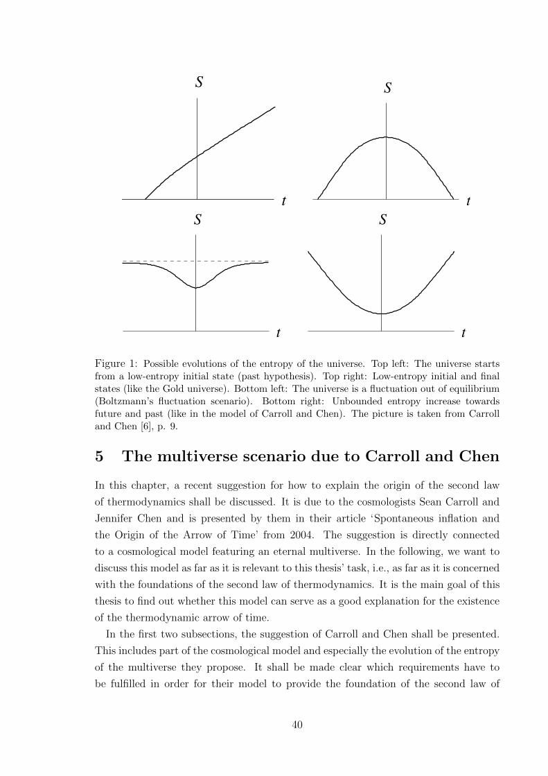
t

S

t

S

t

S

t

S

Figure 2: Possible evolutions of the entropy of the universe. At top left, a universe that comesinto existence with prescribed low-entropy conditions in the past; at top right, a universewith low-entropy conditions in both the past and future. At bottom left, a fluctuation froman equilibrium value of maximum entropy, portrayed by the dashed line. At bottom right,a universe with unbounded entropy to the past and future.

problems. As a bonus, it provides a natural mechanism for the origin of the approximatelyscale-free density perturbations that serve as the origin of structure in our universe. Perhapsequally importantly, it provides a natural explanation for why the observable universe shouldbe large and expanding at all, as inflation can create a fantastic number of particles from amicroscopically small initial patch of spacetime.

However, there are some lurking problems in our understanding of the onset of inflationand the role of initial conditions. In this section we review some of the existing controversiesover initial conditions for inflation and the role of entropy, arguing as e↵ectively as we canthat there really is a serious issue that has yet to be addressed concerning the onset ofinflation. This discussion will set the stage for our suggested resolution of this problem inlater sections.

9

Figure 1: Possible evolutions of the entropy of the universe. Top left: The universe startsfrom a low-entropy initial state (past hypothesis). Top right: Low-entropy initial and finalstates (like the Gold universe). Bottom left: The universe is a fluctuation out of equilibrium(Boltzmann’s fluctuation scenario). Bottom right: Unbounded entropy increase towardsfuture and past (like in the model of Carroll and Chen). The picture is taken from Carrolland Chen [6], p. 9.

5 The multiverse scenario due to Carroll and Chen

In this chapter, a recent suggestion for how to explain the origin of the second law

of thermodynamics shall be discussed. It is due to the cosmologists Sean Carroll and

Jennifer Chen and is presented by them in their article ‘Spontaneous inflation and

the Origin of the Arrow of Time’ from 2004. The suggestion is directly connected

to a cosmological model featuring an eternal multiverse. In the following, we want to

discuss this model as far as it is relevant to this thesis’ task, i.e., as far as it is concerned

with the foundations of the second law of thermodynamics. It is the main goal of this

thesis to find out whether this model can serve as a good explanation for the existence

of the thermodynamic arrow of time.

In the first two subsections, the suggestion of Carroll and Chen shall be presented.

This includes part of the cosmological model and especially the evolution of the entropy

of the multiverse they propose. It shall be made clear which requirements have to

be fulfilled in order for their model to provide the foundation of the second law of

40

thermodynamics. Thereby, their way of arguing for this connection shall be presented.

In all further subsections, their model shall be revised and critically discussed. The

introduction and discussion of a toy model will provide some evidence which leads us

to argue against their suggestion that, for our universe, an unbounded evolution of the

entropy like the one suggested can in principle exist. Apart from that, we will show

that, if there were such an evolution of the overall entropy, it would indeed be possible

to argue their way - although this would mean to reject Boltzmann’s way of arguing

which is by no means a trivial step.

5.1 The evolution of the entropy of the multiverse

Let us first focus on the evolution of the entropy of the universe Carroll and Chen

propose. This, of course, is most relevant to us. In fact, in the proposed scenario the

universe is really a multiverse, but this distinction shall not concern us here. What we

want to focus on is the evolution of the entropy of the entirety of all being, no matter

whether this is called the universe or a multiverse.

According to Carroll and Chen, the entropy of the universe/multiverse increases

without bounds both towards the future and towards the past. In detail, the entropy

curve they propose looks like this: There is a state of minimal entropy at some arbitrary

point in time - actually, at this point in time, entropy is arbitrarily high, but still

minimal - and, starting from this point in time, entropy increases without bounds in

both directions of time.64 To have an idea of the proposed entropy curve, you can

think of a parabola. Of course, the evolution of the entropy does not necessarily have

to be parabolic, it might also have the shape of the hyperbolic cosine (in which case the

curve would be called a catenary), but this is nothing which shall concern us here. Also

Carroll and Chen say nothing about that. Still, you can think of a parabola in order to

have more or less the correct picture in mind. This was also my intention when I used

the word ‘parabolic’ in the heading of this thesis. It should invoke without making

much words the more or less correct picture of the proposed entropy curve. It should

not mean that the curve is strictly speaking a function in which the argument is taken

to the square.

At this point it is necessary to mention that Carroll and Chen assume the evolution

of the multiverse to be unitary.65 That is, the dynamics governing the evolution of the

microstates is assumed to be reversible. In other words, the number of possible states

does not change in the course of time - no states are being created nor destroyed. The

assumption of unitarity is not only a somewhat natural assumption; it is crucial in

64Carroll and Chen [6], pp. 7-8.65Cf. Carroll and Chen [6], pp. 15-16.

41

order to be able to make any argument on statistical grounds, as Carroll and Chen do

and as we will do in the following.

What are the necessary requirements in order for an entropy curve like the one

described to exist? The most distinct feature of the proposed entropy curve is that

there is no equilibrium state. Entropy grows unbounded in both directions of time.

But the very fact that entropy is unbounded above is, according to Carroll and Chen,

already the necessary and su�cient condition in order for an evolution of the entropy

like the one suggested to exist:

All that is needed to have an arrow of time arise dynamically is for the

entropy to be unbounded above, so that it can always increase from any

given starting point.66

What do we need for the entropy to be unbounded? In order for the entropy to be

unbounded above, the measure of the region of phase space to which the evolution of

the multiverse is restricted has to be infinite. Only if the measure of the relevant part

of phase space is infinite, it is in principle possible for the trajectory of the multiverse

to pass through regions of bigger and bigger phase space volume without ever reaching

a region of maximal phase space volume. Only then entropy can grow without bounds.

In fact, the requirement that the entropy is unbounded above is equivalent to the

requirement that phase space is infinite. So far, so good. This is a formal requirement.

But how does this connect to the physics?

At this point we should ask whether the idea of an entropy increasing without bounds

is in any way compatible with a realistic dynamical evolution of the universe. In fact,

Carroll and Chen argue that as far as their model is concerned the dynamics are such

that overall entropy increases without bounds both towards the future and towards the

past. These dynamics involve inflation and the evaporation of black holes as well as

quantum fluctuations on a De Sitter space, to name only some of the most important

cosmological details. Explicitly, Carroll and Chen present a scenario featuring what

is known as spontaneous eternal inflation.67 Of course, the whole scenario is highly

speculative and you might have objections against di↵erent features of the cosmological

part of the model, but this is not what shall concern us here. What is important for us,

is to find out, first, whether it is reasonable to believe that the entropy of the universe

might in principle increase without bounds in both directions of time and, second,

assume such an evolution of the entropy existed, to examine whether it could provide

a foundation for the second law of thermodynamics. Only if there is a positive reply

to both of these points, the proposed scenario will be able to provide a foundation for

66Carroll and Chen [6], pp. 7-8.67Cf. Carroll and Chen [6], pp. 20-21.

42

the second law of thermodynamics. We will come back to the first part of this question

when introducing the toy model in subsection 5.3. As far as the second part of the

question is concerned, let us, at this point, make some introductory considerations,

thereby presenting the way Carroll and Chen argue with respect to this issue. Later,

in subsection 5.4, we will revise this point and discuss it again in more detail.

So what about the thermodynamic arrow of time? Is the asymmetry in time in

thermodynamics compatible with or even explicable by the proposed evolution of the

entropy of the universe? At a first glance, this seems to be true. And this is how Carroll

and Chen argue. They say for a universe which evolves according to the suggested

entropy curve the arrow of time is given.68 In fact, the suggested scenario features an

asymmetry in time at any point apart from that point at which the entropy of the

universe is minimal. But this is only one point compared to an infinite number of

points corresponding to increasing or decreasing entropy. Of course, one single point

has measure zero. But this means that the universe should never be found in that

state. Even if we had to exclude a certain interval around the point corresponding

to minimal entropy, which might be necessary to explain the world we experience, at

least if we try to account for the existence of a past, even this should not be a problem.

Since this interval is finite, it will always be small compared to the remaining period

which is infinite in extent. So it seems like there remains nothing to be explained. But

this is only part of the story. Actually, the considerations we made do not go through

so easily. But this we will discuss, as we already stated, in a separate chapter later.

In addition to the suggested evolution of the entropy of the multiverse there is another

necessary requirement that has to be satisfied in order for the multiverse scenario to

provide an explanation for the second law of thermodynamics. This requirement is

related to the following question, namely: How is the present state of our universe

attained within the scenario proposed by Carroll and Chen? Is it a typical state? For

otherwise the proposed scenario can not serve as an explanation for what we experience,

even if it provided a thermodynamic arrow of time for all times. Let us, at this point,

add one comment on what we mean by an explanation: We assume something to be

explained if it is typical, i.e., if it is true for almost all possible cases. In their 2004

paper, Carroll and Chen list the requirement that states similar to the present state

of our universe have to be typical states in the evolution of the multiverse as the

second requirement to their model. Together with the unboundedness of the entropy

it shall su�ce to let the suggested scenario provide an explanation for the second law

of thermodynamics we experience.69 In what follows, let us therefore have a look at

how the present state of our universe is attained within the cosmological model they

68Cf. Carroll and Chen [7], p. 4, and Carroll [9], pp. 359-362.69Cf. Carroll and Chen [6], p. 8.

43

suggest in order for the description of our world.

5.2 The cosmological model

As we already discussed, the scenario Carroll and Chen propose corresponds to a

multiverse. In other words, there exists an unbounded number of universes like our own

universe. Starting from that point in time at which the entropy attains its minimum,

the evolution of the multiverse in both directions of time is as follows: Universes like

our own come into existence, undergo the evolution we know from our universe and

finally ‘die’, thereby providing the right conditions for the ‘coming into existence’ of

new universes like our own.

The dynamics driving this evolution is given by the dynamics of spontaneous eternal

inflation. Explicitly, it is argued that any universe like our own universe finally empties

out, due to the evaporation of black holes, thereby approaching a vacuum state which

is flat De Sitter space. Then, under the assumption that there exists an inflaton field

together with a small positive vacuum energy, it is shown that De Sitter is unstable

to the onset of spontaneous inflation due to quantum fluctuations. From time to time,

then, Inflation gives rise to the early state of a universe similar to the early state of

our own universe. Thus, another universe like our own comes into existence, evolves

like our own universe and finally empties out giving rise to new baby universes.70

At this point, let us consider the present macrostate (and all that is included in

that like our memory, knowledge, etc) of our observable universe. Is this macrostate

with respect to the scenario of Carroll and Chen a typical state? The answer is yes,

because there is an unbounded number of such states in the scenario they propose. To

be sure of this, notice the following: Being within one of the single universes of their

multiverse, there is no possibility to achieve any information from outside this single

universe.71 Thus, whenever you live in one of these universes, you experience nothing

from outside that certain universe (In fact, you only have access to the observable part

of the relevant universe). Now, since in their model there is an unbounded number

of universes similar to our own universe, there is an unbounded number of universal

macrostates similar to the present macrostate of our universe. So you really should

expect to find yourself in what we experience as and refer to as the world’s present

macrostate.

But again, how can we, within the proposed scenario, explain why the entropy of

the present macrostate is as low as it is? Did not Carroll and Chen tell us that the

entropy of the multiverse is arbitrarily high, even at its lowest point. This apparent

70Cf. Carroll and Chen [6], p. 1 and pp. 21-26. For an introduction to the model, compare alsoCarroll [9], pp. 359-365.

71Cf. Carroll and Chen [6], pp. 26-28.

44

contradiction can be resolved as follows. According to the multiverse scenario, any of

the single universes is, say, at its beginning in an initial state of low entropy. Still,

overall entropy is not low, because it does not only contain the entropy of the single

universe, but also the entropy of all the surrounding De Sitter space from which the

single universe fluctuated into existence and of all the other universes which fluctuated

into existence at an earlier time. Because, from within our own universe, we have no

access to any information from outside, we cannot determine the entropy of the entirety

of all being. It may at any moment be arbitrarily high. We can only determine the

value of the entropy within our own single universe. But this entropy is small whenever

a new single universe comes into existence.

Let us make this point more explicit. According to the proposed scenario of Carroll

and Chen, the dynamical evolution of the multiverse is connected to the evolution of the

entropy as follows. Starting from a low-entropy initial state, entropy increases within

one single universe. This increase of entropy within one universe at the same time

contributes to the increase of overall entropy of the entire multiverse. Now, overall

entropy can increase without bound since there is no equilibrium state for a single

universe. Although at some point in time the evolution of a single universe nearly

comes to an end, which means that there are hardly any time-directed processes left,

there are still some rare events which lead to the creation of new universes. These new

universes, again, have small entropy at their beginning, but as they exist in addition to

what has existed before, overall entropy is then higher. And this process of emerging

and dying universes goes on, according to Carroll and Chen, both towards the future

and towards the past, starting from some Cauchy surface of generic initial data at

some arbitrary point in time.72 Thus, here we really have the kind of scenario Price

argues for arduously. The scenario is overall time-symmetric and the asymmetry in

time emerges only when we look at those ‘short’ times that are accessible to us.

Thus, if we follow Carroll’s and Chen’s reasoning, we conclude that the present

macrostate of our observable universe is a typical state. Furthermore, we acknowledge

that due to the parabolic evolution of the overall entropy, the thermodynamic arrow

of time is given at any time. Also, we take it as no surprise that the entropy of

our observable universe is as high as it is (and not smaller). This is simply due to

the fact that, within the evolution of the multiverse, there is an unbounded number of

macrostates of universes like our own corresponding to this certain value of the entropy.

Thus, everything appears to be typical. We don’t need any special initial conditions

in order to account for the present state of the universe. Moreover, the suggested

scenario satisfies the condition set up by Price. It is time-symmetric at a fundamental

level leaving the asymmetry in time as a feature of those processes and times that are

72Cf. Carroll and Chen [7], p. 4.

45

within our small focus of observation accessible to us.

In the following subsections, we will review the main statements of the proposed

scenario thereby arguing that the way Carroll and Chen reason can not so easily be

followed. Explicitly, and as a first step, we will show that there exist arguments against

the assumption that a parabolic evolution of the entropy might in principle exist.

5.3 Discussion of a toy model

In the following, we will consider a simple toy model which fulfills all the necessary

(though, as we will show, not su�cient!) conditions in order for an evolution of the

entropy like the one suggested by Carroll and Chen to exist.73 Having a look at the

model it seems, at first glance, as if the model actually realizes the evolution of the

entropy suggested by Carroll and Chen. Analyzing it further, though, it will turn out

that this is not true. In our analysis, we argue that in leading order and for all relevant

times, for the system described in this model, the entropy does neither increase nor

decrease, but stays the same. After the analysis of this model, we will use the result

to argue that we should not expect an evolution of the entropy like the one suggested

by Carroll and Chen for any system. Instead we should expect that the entropy stays

constant for any relevant system, thus, also in the case of the universe. But let us have

a look at the model first.

5.3.1 Introduction to the model

We consider a system of N non-interacting particles moving through infinite three-

dimensional Euclidian space. Comparing this scenario with the system of an ideal gas

of N particles in a box, there is a crucial di↵erence, namely that this time, for the

system we analyze, there is no box. This means, in essence, that phase space is allowed

to be infinite. Thus, entropy may in principle increase without bounds. This is, as we

have seen, the necessary condition in order for an entropy curve like the one suggested

by Carroll and Chen to exist. Back to the model, we have the following description of

the fundamental entities: The i-th particle has a position qi, a momentum pi, and a

mass mi = 1. Its position at time t is given by

qi(t) = qi(0) + t pi(t) (22)

73I owe the idea to this model to Sheldon Goldstein, Roderich Tumulka, and Nino Zanghi whothemselves refer to Carroll as the originator. The model is presented in the yet unpublished paper[16]. In fact, they came up with this model in order to argue in the opposite direction than I do inthe following. The way I argue, as opposed to what they intended, is my own.

46

with pi(t) = pi(0) 8t. In the following, we will work in the center of mass frame, i.e.PN

i=1 qi =PN

i=1 pi = 0.

5.3.2 The first macrovariable

Clearly, for t ! ±1 all particles are very far from each other and from the center of

mass. In order to be able to assign an entropy to the system, we need a macrovariable

that represents the volume of the system. For this purpose, we can define the following

macrovariable:

y =1

N

NX

i=1

q2i . (23)

In fact, y is the moment of inertia of the system. Since we don’t have a box of a certain

volume to which the motion of the particles is confined, we can’t use the volume V as

a macrovariable. Instead, it seems sensible to have a look at the moment of inertia of

the particles, which can be computed at any moment in time and which can be seen

as an indicator of the volume the particles fill. From the dynamics we have that y is a

function of t of the following form:

y =1

N

NX

i=1

(qi(t))2

=1

N

NX

i=1

(qi(0) + tpi(0))2

=2E

N

t+

1

2E

NX

i=1

qi(0)pi(0)

!2

� 1

E2

NX

i=1

qi(0)pi(0)

!2

+1

N

NX

i=1

(qi(0))2.

Here E = 12

PNi=1 p

2i is the total energy of the system. In short, the following holds:

y =2E

N(t� ⌧)2 + ↵ (24)

with ⌧ and ↵ as defined by he expressions above.

If you now recall that with respect to the microcanonical measure the entropy of

a system is given in terms of volume, total energy, and particle number, i.e. S =

S(V,E,N), you might at first sight be tempted to stop at this point and compute the

entropy in terms of moment of inertia (representing the volume), energy, and particle

number, i.e., S = S(y, E,N). In fact, we will do this computation in a moment.

However, as far as our model is concerned, the three given macrovariables do not su�ce

to tell us everything about the macroscopic state of the system. Why this? What is

missing? What we have not taken into account so far is that, because the particles

47

do not hit anything, neither the wall of a box nor each other, they don’t change their

velocities (not even by direction). In other words, there is no mixing of velocities. To

make it explicit: Not only the average distance of the particles to the center of mass

continuously grows with time (starting from some initial moment when all particles

are closest to each other), also, as time evolves, the particles become more and more

segregated according to their fix initial velocities. Starting from a certain moment

in time at which all particles are entirely mixed (where mixed refers to the values of

the velocities), in the past as well as in the future of that moment the particles will

distribute themselves more and more according to the values of their initial velocities.

The fast particles will overtake the slow particles until, in the end, all particles will be

aligned according to the values of their velocities. Eventually, for big times, the fastest

particle will be the furthest away from the center of mass, the second fastest the second

furthest and so on and so on. Clearly, this e↵ect of decomposition has to show up in

the entropy of the system. Counting the microstates like Boltzmann, it turns out that

there are far less microstates representing a macrostate which is given by a distribution

of particles according to their velocities than there are microstates corresponding to

a macrostate of a distribution of particles of mixed velocities. But the weight of this

contribution to the entropy shall be determined in a second step. Let us first compute

the entropy in terms of y, E, and N only.

Let y, E, and N be fixed. The Boltzmann entropy is given by the phase space

volume, S(y, E,N) = kB ln |�y,E,N |, which can be computed by integration over R6N

under the given constraints:

|�y,E,N | =

Zd3Nq �

y � 1

N

NX

i=1

q2i

!Zd3Np �

E � 1

2

NX

i=1

p2i

!

=

✓Zd3N⌦

◆2 Zdq q3N�1�

y � 1

N

NX

i=1

q2i

!Zdp p3N�1�

E � 1

2

NX

i=1

p2i

!

=

2⇡

3N2

�(3N2 )

!2N

2(Ny)

3N�22 (2E)

3N�22 .

Since, in our model, the total energy and the particle number are fixed while the

moment of inertia y varies with time, we can rewrite this equation focussing on y only.

We then have:

|�y,E,N | = const(E,N) y3N�2

2 (25)

In the following, let us neglect the constant depending on E and N . Let us just notice

that it will turn into an additional factor to the total entropy, depending on E and

N only, which we will denote by S(E,N). Now let us denote by |�y| the y-dependent

48

factor contributing to the phase space volume, i.e., |�y| = y3N�2

2 . Computing the

entropy, this factor turns into a summand which we shall denote by Sy. We thus have

for the y-dependent term of the entropy:

Sy =

✓3N � 2

2

◆kB ln y. (26)

In the following, let us have a look at the evolution of the entropy in time. Since, in

our model, the moment of inertia is not fixed, but varies with time, also the entropy has

to vary with time. In fact, since the logarithm is a monotonously increasing function,

the dependence of S on t will be qualitatively the same as the dependence of y on t.

From (24) we know that y is proportional to the square of t. Thus, also the entropy is

minimal for a certain moment in time and increases without bounds both towards the

future and the past.

If we now stopped at this point and assumed that we correctly computed the entropy,

we would mistakenly conclude that the evolution of the entropy is such as it has been

suggested by Carroll and Chen. Our toy model would then not only satisfy all the

conditions necessary in order for such an evolution of the entropy to exist, it would

actually represent a simple example of the scenario Carroll has in mind - a scenario

in which the dynamics of the entire system are such that entropy increases without

bounds both towards the future and the past. Unluckily (or luckily, as we will argue)

this is not the case! So far we didn’t take everything that is relevant to Boltzmann’s

notion of entropy into account. As we already discussed, it is inherent to our model

that the particles become more and more distributed according to their velocities. In

the following, let us determine the impact of this e↵ect on the phase space volume and,

thus, on the entropy of the system. After that, since the entropy changes in time due

to both e↵ects - one e↵ect makes it increase, the other decrease -, let us combine the

new result with the contribution we got from the y-variable. Making this last step,

we will finally be able to determine the actual evolution of the entropy (now correctly

defined) of the system in time.

5.3.3 The second macrovariable

As another macrovariable we can take the average of the local variance of the values

of the velocities. Since the fast particles will eventually be far from the slow particles,

the local variance will decrease, approaching zero for big times. Clearly, the new

macrovariable is connected to the notion of temperature. For big times, the average

kinetic energy of the particles far from the center of mass is much higher than the

average kinetic energy of the particles close to the center of mass, while the local

variance is small compared to the local variance at small times.

49

It is evident that, like there is a moment in time ⌧ at which the moment of inertia

is minimal, there is a moment in time ⌧ 0 at which the mixing of particles of di↵erent

velocities is maximal. At this moment, the local variance of the values of the velocities

is maximal. In general, of course, this ‘mixing of velocities’ (i.e. the mixing of particles

of di↵erent velocities) may have two maxima. Why this? Obviously, for t ! ±1all particles are maximally ordered according to their velocities, i.e., the fastest is the

furthest from the center of mass, the second fastest the second furthest and so on and so

on. But, in contrast to the moment of inertia which may approach zero, but which can

never be negative, the mixing of velocities may change sign: There exist trajectories

(i.e. possible evolutions of the system on phase space) for which, at some moment, the

fast particles are closer to the center of mass than the slow particles. Thus, for some

evolutions there are two moments in time which correspond to maximal mixing. (It is

not possible that there are more than two maxima. This, of course, follows from the

dynamics.)

At this point let us reason about the temporal correlation of the two (or three)

extrema corresponding to the two di↵erent macrovariables. For sure, we can imagine

special initial conditions for which the moment of inertia is minimal, but the mixing

of velocities is not maximal, i.e. ⌧ 6= ⌧ 0. In this case, the mixing of velocities has two

maxima and the evolution is as follows: For t ! �1 the fast particles are further

from the center of mass than the slow particles while all particles approach the center

of mass; at some moment ⌧ 01 of maximal mixing, the fast particles overtake the slow

particles (at least in average), all particles still approaching the center of mass (in

average again) thereby still diminishing the moment of inertia; then, after the moment

of inertia has been minimal at ⌧ there will again be a moment ⌧ 02 at which the fast

particles overtake the slow particles; from then on the distance between fast and slow

particles increases continuously. However, it seems plausible and it should be possible

to argue that these evolutions are very rare and that, typically, both extrema, i.e.,

the maximum of the mixing of velocities and the minimum of the moment of inertia,

are attained at the same moment. But, in fact, we don’t even need this much. For

our purposes it su�ces that the time interval between the di↵erent extrema is small

compared to the rest of the evolution. What does this mean?

If we have a look at the local variance of the velocities, this means that we compute

the variance of the particles’ velocities within a certain region of a certain size. In other

words, even if the fast particles were a bit closer to the center of mass than the slow

particles, given that the relevant volume is big enough, the macrovariable will not reflect

the fact that the mixing is at that moment less-than-maximal. Again, in other words,

the macrovariable is coarse-graining. If we choose the volume which we refer to when

determining the local variance to be that big that our macrovariable cannot distinguish

50

between a state in which the mixing is maximal and any state in which the mixing is

less-than-maximal while the faster particles are closer to the center of mass than the

slower particles, then the macrovariable has only one maximum. But, of course, we

cannot choose a volume of arbitrary size. As far as this is concerned we are restricted

by the fact that we want the system to attain several distinct macrostates within the

course of time. Otherwise we will not be able to determine the time-dependence of the

macrovariable. Thus we need that the time between ⌧ 01 and ⌧ 02 is small compared to

the rest of the (de)mixing process. But this is definitely the case for almost all possible

evolutions of the system! Let us therefore take it for granted that we can choose the

reference volume with respect to which we define the local variance of the velocities

such that the moment of minimal expansion (or minimal moment of inertia) of the

particles corresponds to the moment of maximal mixing.

There is another restriction on the relevant time interval. Of course, the decrease in

the local variance of the velocities is bounded from below. Whatever the exact definition

of the macrovariable looks like, the local variance of velocities vanishes at some finite

time T . (Let us, for simplicity, restrict to positive times. The same argument, of course,

applies to the past.) For t � T the fastest particles is the furthest from the center of

mass, the second fastest the second furthest and so on and so on - the particles are

maximally ordered. Thus, the e↵ect which makes the entropy decrease ends at some

moment, T , and for all bigger times t � T , only the moment of inertia continuously

grows, continuously letting the entropy grow - at least apparently, but this we will

discuss in a minute. Now it is quite evident that the evolution of the system that takes

place in the time interval t � T is not meaningful in any physical meaningful way. At

least, an evolution of the overall entropy in this interval can not serve as a foundation

of the second law of thermodynamics for subsystems, because for t � T the system

evolves without changing its structure. In other words, in any imaginable subsystem

nothing happens: For t � T any state looks the same, only the absolute distances grow

growing faster far from the center of mass and slower close to the center of mass.

At this point, there is something important to recognize. It may very well be that

the notion of entropy we have, whatever it looks like, cannot be trusted for t � T .

This is due to the following fact: For the time t � T we could equally well describe the

evolution of the whole system not by particles moving according to some dynamics,

but by stationary particles in the setting of a non-homogeneously expanding space.

Non-homogeneously, because the distances between those particles that are far from

the center of mass grow faster than the distances between particles that are close to

the center of mass. But what does this mean? In their 2004 and 2005 articles, Carroll

and Chen still assume that an expansion of space can increase the entropy of a given

state. They assert:

51

General relativity allows us to increase the entropy of nearly any state by

increasing the volume of space and scattering the constituents to the far

corners of the universe.74

In 2010, Carroll seems to have changed his mind. At least in an article published at

that time, Carroll argues that the entropy of a system does not change solely due to

the expansion of space. And the argument he gives at this point is very convincing.

This is the argument in short: Assume that the evolution of the universe is unitary.

As we know, an evolution is called unitarity if the dynamics governing the evolution of

the microstates are reversible. That is, any microstate has to evolve into one definite

other microstate. And this must hold independently of whether the universe expands

or contracts for both scenarios are solutions of the Friedmann equations. Therefore the

number of states has to stay the same during expansion or contraction - no states can

be created or annihilated. Thus the state of space cannot be increased by an increase

of the scale factor.75 This last statement immediately implies that the entropy cannot

grow solely due to an increase of the scale factor. Di↵erent configurations which are

the same apart form the scale factor have to be counted as one configuration. Given

our considerations are true, we are in lack of the correct notion of entropy in the case of

expanding space, but this is nothing which shall concern us here. Anyway, whether the

entropy increases, but this fact does not constitute anything physically meaningful,

or whether it does not increase at all, we conclude at this point that, as far as our

following considerations are concerned, the times t � T can be neglected.

So let us consider those times which we determined as relevant. Let therefore t 2[⌧, T ] and let, for means of simplicity, ⌧ and T be positive. That is we restrict ourselves

to the ‘positive’ time interval between the moment of maximal mixing and the moment

of perfect ordering. As we have argued, in this regime the typical particle moves away

from the center of mass. Its distance to the center of mass then evolves in time as

|qi(t)| = |qi(⌧)|+ t|pi(0)|, (27)

where qi(⌧) = qi(0) + ⌧pi(0) depends on the initial conditions and, as before, pi(t) =

pi(0) 8t.At this point let us make some considerations about the ensemble of particles. Let

us divide the particles in two groups a N2 particles, each. Let the division be such that

all particles of the first group (1) are slower than the particles of the second group (2).

As you can easily see, for big times the average distance d12 between the two groups

74Carroll and Chen [7], p. 3. Cf. also [6], pp. 19-20.75Cf. Carroll [10], pp. 8-9.

52

increases with time,

d12(t) = r2(t)� r1(t) =2

N

0

@X

(2)

|qi(t)|�X

(1)

|qj(t)|

1

A

⇡ 2

N

0

@X

(2)

|pi|�X

(1)

|pj|

1

A t+ �

=2

N�t+ �, (28)

whereP

(2) andP

(1) sum over the particles of group (2) and (1), respectively, � is a

constant depending on the initial conditions and the constant � = �(|p1|, |p2|, ..., |pN |)is clearly positive since it is defined as the sum of the N

2 higher values of the velocities

minus the sum of the N2 lower values of the velocities. (Of course, for special initial

conditions � may also be zero, but that’s not an interesting case. In that case y is

constant, too.)

As a next step, let us determine the evolution of the volume between the fast and

slow particles. Therefore, consider two balls around the center of mass with radius r1

and r2, respectively, where r1 and r2 are defined as above. Of course, the fast half of

the particles will be positioned close to the surface of the ball of radius r2, the slow

half of the particles close to the surface of the ball of radius r1. As time evolves, the

volume between the surfaces increases as the cube of t:

�V (t) = V2(t)� V1(t) =4

3⇡(r32(t)� r31(t))

⇡ 4

3⇡

8

N3

0

@

0

@X

(2)

|pi|

1

A3

�

0

@X

(1)

|pj|

1

A31

A t3 +O(t2)

=32⇡

3N3�t3 +O(t2), (29)

where the constant, � = �(|p1|, |p2|, ..., |pN |), which is defined by the line above, is

clearly positive again.

In the following, let us try to define a macrovariable that represents the local variance

of the velocities. As the volume increases, the fast and slow half of the particles get

more and more separated. In fact, at that moment at which the average distance

between the fast and slow half of the particles exceeds the sum of the respective mean

deviances, d12 � �1 + �2, we may assume that the particles are completely separated.

Let V0 be the corresponding volume, in other words, let it be the volume between the

surfaces of the balls of radius r1 and r2 at that time. As soon as �V (t) � V0, we will

denote by n = 2 the fact that we have two separated groups of particles (at least in

53

average). Before that moment we have, of course, n = 1 group. As the volume between

the particles grows, we divide, in discrete steps, the particles in more and more groups,

in every step assigning an equal number of particles to each group (i.e. after n steps

we have n groups each consisting of Nn

particles). The division is such that, in each

step, we divide the particles according to the values of their velocities. Explicitly, when

we have n groups, group 1 consist of the Nnslowest particles, group 2 of the N

nsecond

slowest particles and so on and so on. Of course, the number of groups is bounded from

above. There are maximally n = N groups, each containing one particle. Explicitly,

the dynamic of the division is the following: Whenever the volume between the fast

and the slow half of the particles has grown by an amount of V0 there is a new group.

Thus, the number of groups is

n(t) = 1 +

��V (t)

V0

⌫, (30)

where bxc refers to the next integer which is equal to or smaller than x. Using (29) we

get, in leading order of t, that

n(t) = 1 +

�t3

t30

⌫, (31)

where t0 is the value of t for which in leading order �V (t) = V0. Explicitly, t0 is given

by the following equation:32⇡

3N3�t30 = V0. (32)

Maybe one remark regarding the separation of the particles of di↵erent groups is

necessary. If we choose the volume V0 such that for n = 2 the average distance between

the fast and slow particles is bigger than or equal to the sum of the mean deviances,

d12 � �1+�2, then we cannot only be sure that, in average, the particles are separated

for n = 2, but we also get that they are separated in any other case, i.e., we have that

they are separated for n � 2. This is the case because the sum of the mean deviances

of neighboring groups decreases as the number of groups increases, which, again, is the

case because there are less particles per group for a bigger number of groups (thus, the

variance is smaller).

Since we cannot determine the exact number of particles in each of the regions of

volume V0, we assume that the particles are more or less equally distributed throughout

the overall volume. Of course, this is true for almost all initial conditions. (Only for spe-

cial initial conditions, certain numbers of particles clump together for long times with

the e↵ect that the overall density of particles is on a relevant scale non-homogeneous.)

The given assumption allows us to connect the number of groups, as defined above, to

54

the notion of the mean local variance of the values of the velocities of the particles. How

is the local variance of the values of the velocities defined? Let there be m particles

within a volume V0. Then the variance with respect to that volume V0 is given by

V ar(|p|) = 1

m

mX

i=1

|pi|�

1

m

mX

i=1

|pi|!2

.

But what is the connection between the number of groups and the mean local vari-

ance of the values of the velocities of the particles? Since an increase in the number

of groups is connected to a decrease in the number of particles of deviant velocities

per group and since this is a local e↵ect because for every additional group there is an

additional volume V0 (thus, there are in e↵ect less particles of deviant velocities per

volume), it follows that an increase in the number of groups is connected to a decrease

in the mean local variance of the velocities. Thus we have a correlation between the

number of groups and the mean local variance of the particles. The explicit argument

is the following: For n groups, there are Nnparticles per group and, since the groups

are formed with respect to the values of the velocities of the particles, there is a 1 : 1

correlation between the number of groups and the mean variance of the velocities per

group,

n ! 1

n

nX

i=1

V ar(i)(|p|).

Here V ar(i)(|p|) refers to the variance of velocities of the i-th group of particles. If

we now assume that the particles are more or less equally distributed over the whole

volume, then this 1:1 correlation will not only hold for the mean variance per group,

but also for the mean local variance of the values of the velocities of the particles. In

the following, the number of groups will be our macrovariable. As we have seen, it

represents the mean local variance of the values of the velocities of the particles.

What is the phase space volume corresponding to a certain n? The number of groups,

n, represents the degree of mixing of the particles, so we have to do some combinatorics.

In this model, the particles are distinguishable. They keep their velocities. This fact is

reflected in the fact that the mean local variance of the velocities decreases with time.

But back to the combinatorics. In general, there are N ! possibilities to distribute N

distinguishable particles, but, of course, if the particles are partially ordered, there are

far less possibilities. Assume that like in the case of n = 2 we have two separated

groups of N2 particles each. In this case, the number of possibilities to distribute the

55

particles is (N2 )!(N2 )!. If we normalize this by the total number of possibilities, we get

(N2 )!(N2 )!

N !=

1�NN2

� .

This is the ‘weight’ which determines the phase space volume corresponding to the

macrostate n = 2. In general, for n groups, the number of possibilities normalized by

the factor N ! is1

N !

✓✓N

n

◆!

◆n

. (33)

Let us denote this contribution to the phase space volume by |�n|. It is a multiplying

factor with respect to the total phase space volume and, thus, appears as an additional

factor Sn in the total entropy,

Sn = kB ln |�n|

= kB ln

✓1

N !

✓✓N

n

◆!

◆n◆(34)

In total, the entropy is therefore given in terms of the four macro variables moment

of inertia, number of groups/ mean local variance of the velocities, total energy and

particles number: S = S(y, n, E,N), where

S(y, n, E,N) = S(E,N) + Sy + Sn. (35)

Of course, we may still separate in (34) those terms which depend on n from those

which depend on N only. Those terms which depend on N , we can add to S(E,N).

Using Stirling’s formula we get that the remaining n-dependent term of the entropy is

Sn = �NkB lnn (36)

5.3.4 The evolution of the entropy

In what follows, let us compare the time-dependent contributions to the total entropy,

Sy and Sn, arising from the moment of inertia and from the local variance of velocities,

respectively. This will finally give us an answer to our original question, namely how

the total entropy changes in time. In what follows, we will consider the leading order in

t. So what is the time-dependence of Sy? From (26) and (24) we have that, in leading

order in t,

Sy(t) =

✓3N � 2

2

◆kB ln y =

✓3N � 2

2

◆kB ln(t2) ⇡ 3NkB ln t.

56

With respect to Sn we get from (36) and (31), approximating the discrete variable n

by a continuous variable n ⇠ t3, that

Sn(t) = �NkB lnn = �NkB ln(t3) = �3NkB ln t.

Thus, the result is that, in leading order in t, the two contributions cancel each other

out,

Sy(t)� Sn(t) = 0.

5.4 Scope and relevance of the toy model

Let us determine what the toy model tells us. There is a couple of new statements we

are, due to the analysis of this model, allowed to make. Among other things, this is

what we learned: First, the fact that phase space is infinite does not necessarily imply

that entropy grows without bound. We learned that like in the case of our model the

region in phase space to which the evolution of the system is restricted may be infinite,

but still entropy neither increases nor decreases, but stays the same, for all relevant

times. But this is directly at odds with Carroll’s and Chen’s statement that all that is

needed for an eternal thermodynamic arrow of time is that the entropy is unbounded,

a requirement which is equivalent to demanding that phase space is infinite. Let us

repeat what they say:

All that is needed to have an arrow of time arise dynamically is for the

entropy to be unbounded above, so that it can always increase from any

given starting point.76

We showed that this is not true. In fact, we presented a dynamical model, namely

the given toy model, which, although it satisfies condition of infinite phase space,

nevertheless does not feature the proposed evolution of the entropy. We thus showed

that the condition of infinite phase space is not a necessary and su�cient condition

as Carroll and Chen put it to be. There have to be additional requirements to ensure

that the evolution of the entropy is such as proposed. But what shall these be? Why

should the evolution of the entropy of the multiverse not be like the evolution that

has appeared to hold for our toy model (where entropy stays constant for all relevant

times)?

In our toy model, we consider particles as the fundamental beings and assume that

they move according to a very simple law. Explicitly, we take the dynamics to be

those of free motion in three-dimensional Euclidian space. What is the scope of this

model? As we already mentioned before, this model is like the scenario of an ideal gas

76Carroll and Chen [6], pp. 7-8.

57

in a box, only that this time there is no box. That there is no box, was the necessary

requirement in order to allow for the relevant region in phase space to be infinite. Of

course, in contrast to the model of an ideal gas in a box, in our model there is no

mixing of velocities which, with respect to the entropy, makes all the di↵erence, but

this is not an additional distinction between the two models, it is just something which

comes from the fact that there is no box. We could also say that this is what is meant

by ‘there is no box’. Now Boltzmann refers to the example of the ‘gas in a box’ in

order to show anything about the universe. In fact, he assumes the universe to be

a mechanical system of particles moving according to Newton’s laws.77 In any case,

Boltzmann’s way of reasoning for the universe, as for any other system, can be made

entirely clear with respect to and shows itself in its entirety for the case of an ideal gas

in a box. There you can find all the important concepts like - you can speak about

an increase and decrease of entropy, fluctuations, special initial conditions, and the

equilibrium state - and the evolution of the gas in the box may serve as an example

for any system, even as an example for the universe.

Why can we not take our toy model in order to argue for the entire universe? First,

let us again emphasize the di↵erence to Boltzmann. In contrast to Boltzmann we

assume, as Carroll and Chen do, that phase space is infinite and that, thus, entropy

may in principle increase without bounds. But, as we have shown, in the case of a

simple mechanical model this is not the case. Instead of increasing without bounds,

entropy rather stays the same for all relevant times. Of course, you might answer, the

dynamics driving the evolution of the universe are far more complicated than those our

toy model can cover. The dynamics are not just simple mechanics as it was believed

by Boltzmann. Instead we have to deal with quantum fluctuations, the evaporation

of black holes, inflation, and the expansion of space. Therefore, you argue, it is not

enough to consider a simple mechanical model - this model simply doesn’t tell us

anything about the universe.

It is true that the dynamics governing the evolution of the universe are still little

known to us and even less we know how they connect to the notion of entropy. There

is no general notion of entropy in the context of gravity, even less in the context of

quantum gravity or some other theory which might become important in the description

of the evolution of the universe. But this we can also use as an argument for us, to

make the point we want to make. Since there is no evidence for the fact that entropy

should increase without bounds both towards the future and the past, we should also

not expect such an evolution to be true. A simple mechanical model shows a very

di↵erent evolution of the entropy, namely that it stays constant for all relevant times

(and apart from fluctuations). Thus, we should expect this to be the correct evolution

77Cf. Boltzmann [2], p. 257.

58

of the entropy, rather than anything else.This point really has to be emphasized. It

simply tells us what we should expect and what not, given everything we know about

the world.

Still, we cannot strictly exclude the possibility that an entropy curve like the one

suggested might in principle exist. If this evolution of the entropy would be able to

explain the fact that entropy increases (or stays the same, but not decreases) in almost

all subsystems of the universe, you might even use this fact in order to argue in favor

of the existence of such an entropy curve. But does the suggested entropy curve really

provide an explanation for the second law of thermodynamics? This we will discuss in

the following subsection.

5.5 On the notion of typicality in case an entropy curve like

the one suggested really exists

5.5.1 The suggested entropy curve

In this subsection, let us assume that an evolution of the entropy of the universe/

multiverse like the one suggested actually exists. In order for this evolution to provide

the foundation for the asymmetry in time in thermodynamics, we still have to show

that the second law of thermodynamics as we experience it can be derived from that.

By ‘as we experience it’ we imply that we take it for granted that we have a past, i.e.,

that entropy has been increasing also during the past and our present macrostate is

not merely a fluctuation. This means that we have to show that we are somewhere

on the suggested entropy curve, but not close to the minimum. Again, it has to be

shown that, given that entropy increases without bounds in both directions of time,

we are not close to the minimum of this evolution, but far from it. Why can we not

simply argue the way we already did, that given the curve is infinite in extent, we are

typically somewhere on this curve, but not close to the minimum? Well, it is not so

simple. We can not so easily argue this way, because Boltzmann’s statistical reasoning

tells us that, no matter what, we should be at the minimum. Or, to make this more

explicit: There are by far more trajectories corresponding to an entropy curve of the

suggested shape which run through a point in phase space corresponding to our current

macrostate which are, at that moment in time, at the minimum of the entropy curve,

than there are trajectories running through the same point which are, at that moment,

not at the minimum. Just count the microstates!

How can this apparent contradiction be resolved? Before we answer this question,

let us put the above statements in mathematical terms. Therefore let us construct a

case in which the evolution of the entropy is such as suggested by Carroll and Chen.

Let therefore, for means of simplicity, the macrovariables determining the entropy be

59

such that only one of them, y, is time-dependent, y = y(t). Thus the evolution of the

entropy in time depends only on this macrovariable. Now let the time-dependence of

the macrovariable be simply quadratic,

y = ↵(t� ⌧)2 + �, (37)

where the constant � is non-negative and where we assume, again for means of sim-

plicity, that ↵ = 1. In the following, let us denote by x the time lapse between the

moment of minimal entropy, ⌧ , and the time t,

x ⌘ |t� ⌧ |. (38)

Thus we can rewrite equation (37), getting

y = x2 + �. (39)

Now let the phase space volume of the macrostate �y which is determined by the

macrovariable y be given as

|�y| = y� (40)

with � a positive constants. We choose this dependence between phase space volume

and macrovariable because it is quite intuitive. For many macrovariables, it is the case.

In fact, it holds for any macrovariable which is the sum of the positions or momenta,

up to some power, of all the particles involved (like the energy or the moment of

inertia). In that case, � depends on the number of particles, the dimension of space

and the power to which the positions or momenta enter in y. Once we have the phase

space volume, we get the time-dependent part of the entropy Sy by using Boltzmann’s

formula S = kB ln |�|. Thus,Sy = kB ln y�. (41)

Since the logarithm and the power of x where x is positive are monotone increasing

functions, the entropy evolves in time just like the macrovariable y evolves in time. Of

course, this statement is true for the total entropy, not just for the time-dependent part

of the entropy: This is the case because the time-independent part of the entropy is

just an additional factor shifting the entire entropy curve by a certain constant amount.

Thus, just like the macrovariable the entropy has a minimum at time ⌧ and, starting

from that minimum, increases without bounds in both directions of time. Thus, we

constructed what we wanted to construct, an entropy curve a la Carroll and Chen.

60

5.5.2 Conditional measures

We started out in order to compare the statistical reasoning of Boltzmann to the

reasoning of Carroll and Chen. The question with respect to which the comparison

was meant to be drawn is the following: Given the entropy evolves such as suggested

by Carroll and Chen and given the present macrostate of the universe, is it typical that

we are, at this moment in time, close to the minimum of the entropy curve or is it not?

Let us first determine the way Boltzmann is reasoning. According to Boltzmann, the

correct measure of typicality is the uniform, or microcanonical, measure on phase space

conditioned under the present macrostate.78 Thus let us recall what we determined to

be the phase space volume, computed via the microcanonical measure, of a macrostate

�y (where the macrostate is determined by the value of the macrovariable y only). This

was |�y| = y�. Now let us derive from that the reduced measure ⇢(x, y) which depends

only on the value of the macrovariable y and the distance of the respective macrostate,

�y to the minimum of the entropy curve, given in terms of the time lapse, x. In the

following, we will consider the reduced measure (which is, instead of being a measure

on phase space, a measure on the two-dimensional (x, y)-space) because we are only

interested in the question whether a typical system is, for a certain value of y, close to

the minimum of the entropy curve - then x is small -, or far from it - then x is big.

How does the reduced measure ⇢(x, y) look like? Therefore consider the (x, y)-space

which is the two-dimensional space that is spanned by the variables x and y. Also,

recall equation (39) which tells us that

y = x2 + �.

At this point, let us reemphasize that any point (x, y) refers to a macrostate �y and

a time interval x, where x tells us how much time has elapsed between the occurrence

of �y and the occurrence of the macrostate corresponding to minimal entropy. What

we have already, is the microcanonical measure of the macrostate on phase space,

|�y| = y�. What we are interested in, is the projection of this measure on the two-

dimensional (x, y)-space. But this can easily be achieved from equation (39). That

equation tells us that any system which is at time x = 0 (let us for simplicity refer to

x = t� ⌧ as the time) in the macrostate ��, i.e., y = �, this system is at time x = X

in the macrostate �Y , i.e., y = Y . Here by X and Y we shall denote the values of the

variables, whereas x and y refers to the variables. Thus the number of systems whose

macrovariable is of the value y = � at time x = 0 is the same as the number of systems

78Again, the idea to discuss di↵erent conditional measures as well as the idea to consider cut-o↵s,which we will do later, thereby revealing the problems connected to a non-normalizable measure, goesback to Sheldon Goldstein, Roderich Tumulka, and Nino Zanghi. Compare [16].

61

whose macrovariable is of the value y = Y at time x = X. This means, in terms of the

(microcanonical) phase space measure, that the phase space measure corresponding to

the point (0, �) is the same as the phase space measure corresponding to (X, Y ). Now

let � be a variable, too. Of course, the phase space measure of macrostates of di↵erent

� is di↵erent. Explicitly, the measure on phase space of those systems which are at

time x = 0 in the macrostate �� is

|��| = ��. (42)

But now we know that this measure is the same as the measure of those systems which

are at time x = X in the macrostate �Y , when y = Y . To put it in equivalent terms,

we know that y = x2 + �. So just insert this in equation (42) and we have what we

were looking for, namely the reduced measure depending on x and y:

⇢(x, y) = (y � x2)�. (43)

Since the entropy can never be negative, this measure is restricted to the region

{(x, y)|y � x2}. (This was the condition that � is non-negative.) In order to show

what we want to show we can replace the above measure by a simpler �-independent

measure, namely

⇢(x, y) = ey�x2(44)

restricted to the upper half-plane {(x, y)|y � 0}. In the following, let us refer to this

measure only.

Now let us assume the macrostate �y0 is given. That is, y = y0. Given this mac-

rostate, are we typically far from or close to the minimum of the entropy curve? To

answer this question we need the conditional measure ⇢y0(x), which is

⇢y0(x) = ⇢(x|y = y0) =⇢(x, y0)R +1

�1 ⇢(x, y0)dx=

1p⇡e�x2

. (45)

What does this measure tell us? We notice that it is peaked around x = 0. This

means it is very likely that the present macrostate is close to the minimum of the

entropy curve. Even more, since the measure ⇢y0(x) is independent of y0, it seems

as if this fact should hold not only for any arbitrary macrostate y0, but in general

for all macrostates. That’s it. This is the conclusion we would draw if we followed

Boltzmann’s way of reasoning. This is the answer. Take the microcanonical measure,

condition under the present macrostate, and you will find no matter what, no matter

how the overall entropy curve looks like, that you are close to the minimum of the

entropy curve.

62

Let us put this result in quantitative terms. Let therefore A be the vertical strip

of, let’s say, width 4 around the y-axis. (We take width 4 at this point because then

we get a nice numerical result in the end, but, of course, this is an arbitrary choice.)

Remember that we refer to the upper half of the (x, y)-plane and that all possible

entropy curves are given as parabolas of the shape y = x2 + � on this plane. This

means A is the vertical strip (of width 4) around the minima of the curves. Now let us

compute the conditional measure ⇢y0 of the set A for some fix macrostate y0. We get

⇢y0(A) =1p⇡

Z

A

e�x2dx =

1p⇡

Z +2

�2

e�x2dx > 0.9.

Since this result is independent of y0, we assume that it should hold in general. There-

fore let ⌦ be the set of all points (x, y) that may describe the relevant physical system.

Then we assume that independently of y0 the following should hold:

⇢(A)

⇢(⌦)> 0.9.

On the other hand it is possible to follow another way, conditioning di↵erently, which

leads to an entirely di↵erent result. In the course of discussion it will turn out that this

is the appropriate way in order to make the point Carroll and Chen wish to make. In

fact, Carroll and Chen refer to this way of reasoning without working it out explicitly.

They don’t discuss it in the context of measure theory nor do they give, and that is

maybe most important, an argument for why, if you reason like them, Boltzmannn’s

way of reasoning, which we have gone through before, can be avoided.79

Thus let us follow the second way of reasoning. Therefore let us condition not on

the macrostate, but on the entropy curve which our universe, or rather its present

macrostate, is part of. That is, let us condition on �. (Conditioning on � means

conditioning on the entropy curve, because di↵erent entropy curves are distinguished

by di↵erent values of �.) Apart from that let us assume that the measure on any such

curve is uniform. That is, any point on a curve is as likely as any other. This weighting,

in fact, is equivalent to the weighting we had before. When following Boltzmann we

took the microcanonical measure, which is the uniform measure on phase space, and

projected it on the (x, y)-space. What we got was a measure that is constant (and thus

uniform) along the curves.

Conditioning on � gives us the conditional measure ⇢�(x). Now, given this condi-

tioning, we have to attribute small measure to any small strip around the minimum

of the entropy curve. The way to see this is the following: If we are somewhere on

the entire entropy curve, and to be at one point is as likely as to be at another, then

79Cf. Carroll and Chen [6], p. 7.

63

we must not expect to be somewhere close to the minimum of the entropy curve -

whatever close means in this case. (It is fine as long as we refer by ‘close’ to some finite

distance.) Now let us again invoke the set A which we defined as the vertical strip of

width 4 around the y-axis. Also, let ⌦ be the set of all physical points as before. Then

we are definitely allowed to say that

⇢�(A)

⇢�(⌦)<< 1.

Also, this result holds for any �. So it seems like it should hold in general. Thus we

should conclude that independently of �

⇢(A)

⇢(⌦)<< 1.

In other words, we should conclude that, whatever macrostate y0 we find when looking

at our universe, this macrostate should typically be far from the minimum of the

entropy curve. And this might actually be how Carroll and Chen argue.

But this is definitely a contradiction to what we have shown before, when following

Boltzmann’s way of reasoning. It cannot be that it is, at the same time, typical to be

close to and far from the minimum of the entropy curve. Who is right? In the next

section we will show how the apparent contradiction can be resolved.

5.5.3 A non-normalizable measure

How can it be that we get di↵erent answers when conditioning di↵erently? Should not

the equation

⇢(B)⇢(A|B) = ⇢(C)⇢(A|C) (46)

hold for any set A and any two partitions B and C on phase space? We know from

probability theory that this equation holds for any normalized measure ⇢. But it

apparently does not hold if the measure is non-normalizable - like it is in our scenario

the case. The fact that in the scenario proposed by Carroll and Chen phase space has

to be infinite implies that there exists no normalizable measure on that space.

From the fact that the measure is non-normalizable it follows, as we have seen, that

we cannot sensibly derive the notion of a conditional measure. Any result we will get

will depend on what we have been conditioning. Now you could ask: What about the

possibility to make a cut-o↵ and provide by this means the foundation for a measure

that is normalizable? The answer is that we cannot simply do this. Again, any result

we will get in the end will depend on the special cut-o↵ we make. How can you see

this? Therefore let us compare the following two cut-o↵s.

64

Cut-o↵ 1: In the first case, you cut o↵ all y that are below a certain value y1 and

all y that are above a certain value y2. Thus you restrict the given (non-normalizable)

measure to that area. That is, you have

⇢(x, y) =

8<

:ey�x2

for {(x, y)|y1 y y2} ⌘ ⌦0

0 otherwise.

Given this cut-o↵, you have a normalizable measure. Now let us use this to compute

the normed measure of the vertical strip A which we referred to before. Thus, let us

determine the proportion of the measures of A and ⌦0. We then get:

⇢(A)

⇢(⌦0)=

R y2y1

dyR +2

�2 dxey�x2

R y2y1

dyR +1�1 dxey�x2

=1p⇡

Z +2

�2

dxe�x2> 0.9.

As you will immediately notice, this is the same as what we got by conditioning on the

macrostate y0. Now let us try another cut-o↵ and see the result we get then.

Cut-o↵ 2: The second cut-o↵ shall be such that we cut o↵ along two entropy curves

and along two axes of constant x. That is we restrict the measure to the area that

corresponds to values of y � x2 that lie between two constants C1 and C2 and values

of x that lie between �x0 and +x0 for some constant x0. That is we have

⇢(x, y) =

8<

:ey�x2

for {(x, y)|C1 y � x2 C2;�x0 x +x0} ⌘ ⌦00

0 otherwise.

Like before, this cut-o↵ implies that the measure is normalizable. Now let us again

compute the normed measure of the set A. We then get:

⇢(A)

⇢(⌦00)=

R +2

�2 dxR C2+x2

C1+x2 dyey�x2

R +x0

�x0dxR C2+x2

C1+x2 dyey�x2=

4(eC2 � eC1)

2x0(eC2 � eC1)=

2

x0

Now we can choose x0 arbitrarily. In particular, we can choose it to be arbitrarily big.

But for arbitrarily big x0 the given proportion becomes arbitarily small. To give a

numerical demonstration: For x0 � 2000,

⇢(A)

⇢(⌦00) 0.001 << 1.

The introduction of the two cut-o↵s has shown that by making di↵erent cut-o↵s and

normalizing the measure accordingly di↵erent or even contrary results can be obtained.

65

One cut-o↵ leads us to assign high measure to the set A, the other leads us to assign

little. The first cut-o↵ makes us conclude that it is typical to be close to the minimum

of the entropy curve, the second that it is typical to be far from it. Eventually, both

of the contrary results we got from the two di↵erent ways of conditioning can be re-

obtained by making di↵erent cut-o↵s. Thus we cannot apply this tool in order to

get a normalized measure. At least, we cannot trust in what this measure tell us.

As we have seen, di↵erent normalized measures derived from di↵erent cut-o↵s assign

di↵erent or even contrary measure to the same set A. Thus we are left with the non-

normalizable measure we had in the beginning and have to determine, in the following,

which conclusions we are still allowed to draw.

Let us, at this point, go back to the two ways of conditioning which represented

the two di↵erent ways of arguing, either in favor of or against the hypothesis that the

current macrostate of the universe is close to the minimum of the entropy curve. Do not

all the considerations we made so far imply that we should not do any conditioning? Did

we not find out that we simply cannot answer the question we posed in the beginning,

whether it is typical to be close to or far from the minimum of the entropy curve?

No. The only thing our considerations tell us is that we have to be very cautious. It

does not mean that we cannot make any statement. In fact, what we get as a result is

that we may argue either way, the way Boltzmann argues or the way Carroll and Chen

argue, as we like it, without ever being able to make a decision in favor of one of these

ways.

Let us go over this important point in more detail. According to what we found,

how is it possible for Carroll and Chen to assign little phase space volume to those

states that are close to the minimum of the entropy curve? Why is there no counter-

argument provided by the fact that Boltzmann’s way of reasoning leads to the contrary

conclusion, namely that it is very likely to be at (or very close to) the minimum? The

answer seems to be the following: When we follow Carroll and Chen, we do not invoke

Boltzmann’s way of reasoning at any point. We simply don’t need it, neither to explain

the increase of entropy in the past, nor to explain the increase of entropy to the future.

We can explain the asymmetry in time otherwise, namely by the fact that the evolution

of the entropy of the multiverse is such as their scenario tells us it is. Thus we should

not refer to Boltzmann’s argument, not even as a counter-argument, because it simply

has nothing whatsoever to do with it. This is the way Carroll and Chen can argue.

Of course, you may also argue like this along Boltzmann’s line, but you don’t have to.

There is no argument which tells us to prefer one way of arguing over the other.

Why are we not entirely happy about this conclusion, namely that the evolution of

the entropy to the multiverse Carroll and Chen propose, given it existed, can serve

as the foundation of the thermodynamic arrow of time? The reason is the following:

66

If we take this conclusion for granted, Boltzmann’s way of reasoning appears to be

merely superficial. For a Carroll and Chen type universe the thermodynamic arrow of

time is given. From this fact we infer that Boltzmann’s statistical reasoning is correct

when applied towards the future, but is incorrect when applied towards the past. But

that is all. There is no more to it. This means Boltzmann’s way of reasoning, the

statistical reasoning, is no longer fundamental. It is no more part of the explanation

(part because we still need the special initial conditions) for why entropy increases.

This is definitely nothing to take easy. In the next subsection, we want to analyze

whether there arise any problems with respect to subsystems of the universe when we

reject Boltzmann’s argument. Maybe Carroll and Chen can explain the existence of a

universal thermodynamic arrow of time, but maybe it is hard for them to argue that

there exists an arrow of time, and the correct one, in almost all subsystems. We already

argued that, following Boltzmann, the relevant connection between subsystems and the

universe can be drawn. Let us now consider this connection under the assumption the

scenario Carroll and Chen suggest were true. Let us examine the status of Boltzmann’s

way of reasoning for nearly isolated subsystems given that his way of reasoning does

no more provide an argument for the universe as a whole.

5.6 Justification of the statistical hypothesis

In this section, we want to address the problem how to get the second law of ther-

modynamics for subsystems. This is what I call the ‘justification of the statistical

hypothesis’. The statistical hypothesis is merely the hypothesis that, given an asym-

metry in time for the universe, there exists the very same asymmetry in almost all

subsystems of the universe. In other words, if entropy increases in the universe, it also

increases in almost all subsystems of the universe. In section 4.1, we argued that this

connection holds between subsystems of the universe and the universe itself in case we

invoke Boltzmann’s way of statistical reasoning and no more than that. Maybe there

is a di↵erence if we assume Carroll’s and Chen’s reasoning to be fundamental in the

case of the universe. How does this reasoning connect to subsystems? In the following,

let us discuss this.

Thus let us assume that the multiverse scenario proposed by Carroll and Chen is

true and explains the existence of a universal thermodynamic arrow of time. But this

implies that there exist arrows of time pointing in the same direction in almost all

subsystems. Only if the entropy increases in almost all subsystems, the total entropy

which is the sum of the local entropies of spatially disjunct subsystems will increase,

too. Thus we have an arrow of time also in subsystems. Apart from that, the proposed

scenario tells us something else, namely that Boltzmann’s way of statistical reasoning

67

can be applied towards the future, but must not be invoked towards the past.

Taken the scenario suggested by Carroll and Chen, what is the status of the ar-

gument that entropy increases towards the future because the number of microstates

corresponding to a future macrostate is higher? The answer is: It is simply a rule that

makes correct predictions, but it is not a fundamental argument. It does not explain

why entropy increases towards the future - otherwise we had to invoke it also towards

the past, which is in no way di↵erent to the future as long as there is no fundamental

asymmetry in time already given. Now assume there were such a fundamental asym-

metry given by the fact that the evolution of the multiverse is such as suggested. Then

there remains nothing to be explained. The given asymmetry already tells us that

entropy is lower in the past and higher in the future and, since the total entropy is the

sum of the local entropies, this doesn’t hold for the universe only, but for almost all

subsystems of the universe. Thus Boltzmann’s way of reasoning is not fundamental. It

is merely a rule that makes correct predictions if applied in one direction of time, but

goes entirely wrong if applied in the other direction of time.

Let us at this point emphasize that this scenario is possible. It is possible that

Boltzmann’s way of reasoning is displaced by the reasoning put forward by Carroll and

Chen. Still, let us make two comments. On the one hand, Boltzmann’s argument for

why entropy increases has been and is a very powerful one. It came up, at his time,

as a revolution in the fundaments of physics and has for more than one hundred years

kept its status as the means of understanding irreversibility. Thus it is not easy to

simply brush it aside. At least, if there are not strong reasons for doing that. On

the other hand, even if we discard Boltzmann’s reasoning from being fundamental,

it will still make sense to refer to it in many cases, simply adding the rule that it

applies to the future, but not to the past, as we have always done. Also notice that

for any isolated system whose evolution is restricted to a finite region in phase space,

Boltzmann’s argument is still true. And, of course, almost every time we discuss a

subsystem we make the idealization that the certain subsystem we refer to is isolated.

Given this idealization, Boltzmann’s argument holds. But again, we are then left with

the problem of the special initial conditions. In order to solve this problem you need

something else. Now if a parabolic-like evolution of the universe existed, the scenario

proposed by Carroll and Chen would be able to explain the special initial conditions and

thereby the irreversibility of thermodynamic processes in subsystems of the universe -

but this implies that you have to reject Boltzmann’s reasoning as a truly valid way of

reasoning.

68

5.7 Further discussion of the multiverse scenario

There is another point which remains to be analyzed. We would like to get a finite value

for the entropy, even if it is the overall entropy of some strange kind of a multiverse.

Why might this be a problem? Let us for this purpose recall the toy model we invoked.

Or, what is the same, let us consider a simple scenario Carroll refers to as an analogon

in order to clarify the shape of the entropy curve. There he suggests the following:

Think of two particles moving on straight lines in an otherwise empty three-

dimensional space. No matter how we choose the lines, there will always

be some point of closest approach, while the distance between the particles

will grow without bound su�ciently far in the future and in the past.80

But is this reasoning correct? Why is it not rather like this: No matter when we look

at the particles, they will always be infinitely far from each other. This question is far

from clear. It arises as a consequence of the fact that the notion of infinity plays such

an important role in your reasoning. But let us go on without giving a final answer to

this question.

6 Entropy increase versus entropy decrease

In the course of this thesis, we considered three di↵erent models making three di↵erent

statements about the entropy curve of the universe, each providing a thermodynamic

arrow of time. In this chapter, we don’t want to discuss these models any longer,

but we want to consider an issue we have neglected so far. As we have seen, two of

these models, the model of Boltzmann and the model of Carroll and Chen, are overall

time-symmetric which means that they feature a period of time during which entropy

decreases as well as a period of time of the same length during which entropy increases.

If these models shall explain not only that there exist time-directed processes, but

also that these processes are such that we experience entropy to increase rather than

decrease, some further considerations have to be made. It has to be shown that, even

if we lived in a universe in which entropy decreases, we would believe that entropy

increases. This means we will have to show that we always refer to the ‘past’ as the

direction of time which is connected to states of lower entropy whereas we refer to

the ‘future’ as the direction of time which is connected to states of higher entropy.

Physicists like Boltzmann or Carroll and Chen simply assume this to be true.81 Still,

it is far from obvious and definitely needs some further discussion.

80Carroll [8], p. 881Cf. Boltzmann [2], p. 257, and Carroll and Chen [6], p. 28.

69

I would like to remark already in the beginning that as far as this topic is concerned

there is much room for speculation. There exists by far no generally accepted con-

ception. Still, I would like to present the most important concepts and discuss them

adding some ideas of my own.

6.1 Psychological arrows of time

It is necessary to point out in the beginning that we do not assume the past or the

future to have any physical reality as such. That is, past and future are not given. They

do not exist per se in our world. Instead, ‘past’ and ‘future’ are only names. They

help us to distinguish between the two directions of time which, in our world, appear

to be distinguishable because they di↵er with respect to certain classes of phenomena.

Any such class of phenomena marks by itself a separate arrow of time. Thereby none

is connected to the past as such or the future as such, because we assume that there is

no such thing as the past as such or the future as such.

In what follows, any class of phenomena with respect to which the past appears

di↵erent to us than the future, thereby determining what we mean by past and future,

shall be distinguished and presented. This distinction helps us to find out what it is

that we call the past and what it is that we call the future. More explicit, it helps us

to define the terms ‘future’ and ‘past’. Together the di↵erent arrows of time which

all together or each by each - we still have to discuss their mutual dependency, thus

let us so far assume that all together - define the meaning of future and past shall be

referred to as psychological arrows of time. In contrast to the thermodynamic arrow of

time or any other arrow of time which is directly connected to physical theory, these

arrows can not be put in a ‘quantitative’ or ‘metrical’ mathematical form. Instead,

they describe a qualitative asymmetry in time. As the following considerations will

show, though, it may be possible to reduce them to the thermodynamic arrow of time

or, at least, to argue that they point in the same direction. Then we would be able to

confirm the statement of Boltzmann and Carroll, namely that the past is the direction

of time which is connected to a state of lower entropy whereas the future is the direction

of time which is connected to a state of higher entropy. But let us, first, list all the

psychological arrows we can distinguish.

In accordance with David Albert we can, as a first trial, distinguish four di↵erent

psychological arrows of time:82

1. We have knowledge of the past, but not of the future.

2. There exist records of the past, but not of the future.

82Cf. Albert [1], p. 113 and pp. 125-126.

70

3. We believe that we can change the future, but not the past.

4. There is a causal dependence between past and future, at least in form of a

counterfactual, i.e., we assume that if the present were di↵erent, the future would

be di↵erent, but not the past.

Maybe you wondered why the second of these asymmetries, the one concerning records

of the past, is called a ‘psychological’ asymmetry. This is due to the fact that the

present state of the universe is just the state it is and whether some object or anything

which is contained in it is called a record is something we make of it. In fact, the

asymmetry regarding records can also be stated as an asymmetry regarding inferences:

Given the present macrostate there are certain configurations of subsystems which

allow us to make inferences towards the past, but not towards the future.

6.2 Interdependence of the psychological arrows of time

Let us see whether all of the above asymmetries actually refer to separate arrows of

time. For the following part of the thesis, which consists of this section and the next

one, we will mainly consider the contributions from David Albert and Hans Reichen-

bach, which are the most important in this context.83 Both try to show that the

psychological arrows of time point in the same direction as the thermodynamic ar-

row of time, but whereas Reichenbach tries to reduce the above asymmetries to the

asymmetry in thermodynamics, Albert proposes that all asymmetries (including the

thermodynamic one) can be grounded on one and the same foundation (which he be-

lieves to be the Past-Hypothesis). Since the approaches di↵er, it will be interesting to

compare them. First, though, let us analyze how according to each Reichenbach and

Albert the psychological arrows are connected to each other.

At this point, let us start with Reichenbach. Like Albert he introduces four di↵er-

ent qualitative asymmetries in time, three of which are identical with the ones listed

above. These are the first three of the asymmetries we denoted. Regarding the fourth

asymmetry he di↵ers. As a fourth statement Reichenbach proposes:

The past is determined; the future is undetermined.84

But is this an asymmetry we believe to experience? Or rather, does this statement

involve any asymmetry we believe to experience which exceeds the asymmetries that

were given in statements 3) and 4) of our listing? I don’t believe so for the following

reason. There may very well be some people who will deny the statement that the

83For the significance of their contributions to this subject matter, see Callender [5], chapter 3.84Cf. Reichenbach [23], p. 23. For a listing of the other asymmetries, cf. pp. 21-23.

71

future is undetermined whereas they will agree with the formulation of the counter-

factual, namely that if the present were di↵erent, so would be the future, but not the

past (statement 4 from above). Thus experience does not seem to tell us that the

future is undetermined, but rather that the weaker statement, which is the counter-

factual, holds. Also Reichenbach, in order to explain his fourth asymmetry refers to

quantum mechanics. He concludes that taking into account the indeterminacy relation

of quantum mechanics it follows that the future is undetermined whereas the past is

determined.85 But this has definitely nothing to do with our discussion. This thesis is

about classical (statistical) mechanics only. In the following, let us therefore neglect

the asymmetry of determinism and stay with the listing we made above.

Among the first three asymmetries of the listing Reichenbach excludes the first asym-

metry, the asymmetry in knowledge, right at the beginning. In fact, he denies that

this asymmetry really exists. According to him, the statement that we have know-

ledge of (what we call) the past, but not of (what we call) the future, is simply false

for the following reason. He argues that there are some future events that we know,

like astronomical events, and there are many past events that we don’t know. There-

fore, he concludes, the ‘di↵erence between the past and the future is not a di↵erence

between knowing and not-knowing’86. Instead, he adds, there is only a di↵erence with

respect to the way we acquire knowledge which is based on records.87 Thus Reichen-

bach concludes that there is only an asymmetry of records, but not an asymmetry of

knowledge.

I don’t think that you can get rid of the epistemic arrow of time so easily. At least,

the argument that we know certain future events while there are many past events

we don’t know doesn’t necessarily lead to the conclusion that there is no asymmetry

between the past and the future with respect to our knowledge. It merely shows that

it is false to say that we have an entire knowledge of (what we call) the past or that

we have no knowledge at all of (what we call) the future. In contrast to Reichenbach

Albert recognizes this fact. Still he doesn’t discuss the asymmetry in knowledge in

much more detail, because he isn’t able to give a precise answer to the question what

the asymmetry of knowledge actually consists in. What he does instead is to analyze

the way we acquire knowledge (like Reichenbach, in fact). This, for sure, is di↵erent

with respect to the past and the future.

According to Albert, there are two di↵erent ways to acquire knowledge. First, we can

consider the present macrostate and assume a uniform distribution over the microstates

realizing this macrostate. This will enable us to make predictions and retrodictions,

85Cf. Reichenbach [23], p. 269.86Reichenbach [23], p. 2187Cf. Reichenbach [23], p. 21.

72

thereby acquiring certain knowledge of the future and of the past, respectively. On

the other hand we are able to acquire knowledge of the past, but not of the future, by

means of records. To conclude, Albert apparently tries to argue that the asymmetry

in records is fundamental to whatever kind of asymmetry in knowledge there is88 - an

approach which seems quite convincing.

But what about the second two asymmetries? According to Albert, these asymmet-

ries belong closely together. Therefore consider the asymmetry in influence, or control,

which we believe to have over the future, but not over the past. Albert points out that

there is no contradiction between our conviction that we can change the future and

the idea that we live in a deterministic world. According to him, what we mean when

we say that our actions are able to change the future, is not that we actually believe

that the future could be any di↵erent than it is going to be, but that, if we were doing

di↵erently than we are doing, the future would be di↵erent, but not the past.89 This

means we think in terms of a counterfactual. In other words, statements 3) and 4) of

our listing belong closely together. You can take it to be one asymmetry and call it

the asymmetry in interventions.

As we have seen, it is possible to argue that not all of the four asymmetries from

above, given by statements 1) - 4), are fundamental. Instead of the four asymmetries

from there remain only two asymmetries, namely the asymmetry in records and the

asymmetry in interventions. This, of course, still implies that whenever we call a

direction in time the ‘past’ any of the four statements from above, at least the assertion

which it makes for the past, has to hold. Still, from a logical point of view only two

asymmetries need to be given - if these are given, the others can be deduced. Thus

if we were able to show that the two arrows of time which come from the asymmetry

in records and the asymmetry in interventions point in the same direction as the

thermodynamic arrow of time, then we would be able to conclude what Boltzmann

and Carroll assumed to be true, namely that we would always call the ‘past’ that

direction in time corresponding to a state of lower entropy whereas we would call the

‘future’ that direction in time corresponding to a state of higher entropy.

6.3 Connection to the thermodynamic arrow of time

In the following, the main arguments for why the psychological arrows of time should

point in the same direction as the thermodynamic arrow of time shall be presented. We

will first discuss the asymmetry in records (thereby covering the asymmetry in know-

ledge) and, in a second step, have a look at the counterfactual asymmetry (including

88Cf. Albert [1], p. 113.89Cf. Albert [1], p. 125.

73

the asymmetry with respect to our belief of having influence on the future, but not on

the past).

6.3.1 Asymmetry in records

According to Reichenbach, the asymmetry in records can be reduced to the thermo-

dynamic arrow of time. In order to show this, Reichenbach refers to the example of

footprints in the sand: Suppose you find some kind of an ordered state. Let it be foot-

prints in the sand. If we dealt with an isolated system which is constituted by the sand

and the wind only, this would definitely be a special state far away from equilibrium.

So Reichenbach asks: How should we reason about this state? If the system had been

isolated for all times, we would have to conclude that it is a fluctuation. But if we

assumed that an interaction took place which left the system in a state of even lower

entropy the present state would be quite likely. At this point the general knowledge

we have tells us that such interactions frequently occur. Therefore we will infer that

the present state is the record of an interaction and - and this is the crucial step - tak-

ing into account the fact that entropy increases (and not decreases), we will conclude

that the interaction has to lie in the past of the present state. Thus we conclude that

we have records of the past, but not of the future.90 The asymmetry in records can

therefore directly be reduced to the thermodynamic asymmetry in time.

What are the problems of this conception? First, according to Reichenbach a record

has to be a low-entropy state, a state which is not in equilibrium. But this does not

necessarily apply to all records. We can perfectly well imagine a high-entropy state,

say a state of thermodynamic equilibrium which we call a record, maybe of the fact

that a certain interaction has not taken place. Apart from that, the main problem of

the above reasoning is that it involves a wide notion of entropy. In order to account

for all kinds of records we need a notion of entropy which can be applied to any kind

of physical system (not merely to gases or liquids) in any kind of physical situation.

But we don’t have such a broad notion of entropy. In the following, let us compare

how Albert treats the asymmetry in records.

We say that there exist records of (what we call) the past, but not of (what we call)

the future. But what exactly do we mean when we talk of records? To give an answer

to this question, Albert introduces the notion of a measuring device. According to him,

a measuring device is a sort of system which undergoes a certain transition if and only

if it interacts with another physical system which, at the time of the interaction, is in

a certain physical situation. The measuring process will then provide a record of the

following structure:

90Cf. Reichenbach [23], pp. 149-151, and Albert [1], pp. 123-124.

74

The ‘record’ which emerges from a measuring process is a relation between

the conditions of the measuring device at the two opposite temporal ends

of the interaction.91

Explicitly, Albert argues that in order for anything to be a record we need two states,

the ‘record-bearing state’, which is the state of the system ‘after’ an interaction has

taken place, and the so-called ‘ready-state’, which is the state of the system ‘before’

the interaction. I put the parenthesis because so far everything is time-symmetric. We

could equally well switch the perspective, i.e., reverse time, and call the former ready-

state the record-bearing state and vice versa. We have only an ordering of states:

ready-state, state in between, record-bearing state, but not a direction. Now, only

if we know the two states at the opposite ends of the interaction, we will be able to

make inferences about the time in between. And only then we will have a record of the

interaction which has taken place.92 Still everything is symmetric and we will have to

find out why we have records in one direction of time only.

Let us clarify this issue. Therefore consider the simple example, which is due to

Albert, of an isolated collection of billiard balls moving along a frictionless table.93

Let us have a look at one of the billiard balls, say billiard ball number 1. Assume

billiard ball number 1 to be currently at rest. Now suppose we would like to know

whether billiard ball number 1 has collided with any of the other balls during the last

ten seconds. We could at this point equally well ask whether it will collide with any

of the other balls during the next ten seconds. This ready-state/ record-bearing state-

analysis is entirely symmetric with respect to what we call the past and what we call

the future. Let us in the following for means of simplicity use the terminology of the

past, but be aware that the entire analysis also goes through for the future.

Thus, how can we get an answer to the question whether billiard ball number 1,

which is currently at rest, has collided with any of the other balls during the last

ten seconds? There are two possibilities. Either we figure out all the positions and

velocities of all the other particles at the present moment in time. This together with

the laws of motion will tell us whether billiard ball number 1 has collided with any of

the other balls during the last ten second. Or we just need to know that billiard ball

number 1 has been moving ten seconds ago. This information alone su�ces to give an

answer to the question whether billiard ball number 1, which is currently at rest, has

collided with any of the other balls during the last ten seconds. In this example, the

state ‘billiard ball number 1 at rest’ is the record-bearing state while the state ‘billiard

ball number 1 in motion’ is the ready state of the system. At this point, notice that

91Albert [1], p. 11792Cf. Albert [1], p. 117.93For the example, compare Albert [1], pp. 117-118.

75

the entire scenario is time-symmetric. We could equally well reverse time and call

the former ready-state the record-bearing state and vice versa. In any case we learn

something about the time in between. We learn that in the time in between there has

been, or will be - as we take it-, a collision. In other words, we have the record of a

collision.

The question which remains is why we experience an asymmetry in records. Now

this, according to Albert, has to do with how we get to know about the ready states.

More explicit, Albert asserts that the asymmetry in record comes from the fact that

there is an asymmetry in time with respect to our knowledge of the ready-states. We

only have knowledge of ready-states in one direction of time - this will be the direction

in time we call the past -, but not in the other. How does this look like in detail?

According to Albert, in order to be able to say that we have knowledge of a certain

ready-state, we need to have a record of this ready-state. But in order to have a record

of this ready-state, we need to know about another ready-state, even further distant in

time, for which we again need a record, for which we need a ready-state and so on and

so on. At this point Albert asserts that what we need is something like a ‘mother of

all ready states’, something we know without having a record of it, without inferring

from the present state, something which is earlier in time than anything we can have

a record of and this, according to Albert, is given by the Past-Hypothesis. In his eyes

the Past-Hypothesis serves as the most fundamental of all ready states. Due to the

Past-Hypothesis we have knowledge of those ready-states which have to be known to

us in order to make anything we now call a record a record. Since the Past-Hypothesis

is given for the past and only for the past, we have records of the past and only of

the past. Thus, it is the Past-Hypothesis which, according to Albert, accounts for the

asymmetry in records as well as for the thermodynamic asymmetry in time.94

There is definitely a deficiency in Albert’s conception. Let us reconsider the example

of the billiard balls. Let us assume that the system constituted of the billiard balls

moving on a frictionless table is all there is in the world. That is, this system is the

universe. In addition, assume the present state to be given as before, i.e., billiard ball

number 1 is not moving at present. Then what we need to know (in addition to our

knowledge of the present state) in order to have the record of a past collision of this

billiard ball is the following: We need to know that, in the past, a certain ready state

had been the case, namely billiard ball number 1 had been moving in the past. In our

example, this ready-state, or rather the knowledge of this ready-state, would account

for the Past-Hypothesis. If this were given, we would in accordance with Albert’s

scheme have a record of the past. But notice that what we need to know in order to

have records is not that there is a state of low entropy in one direction of time, say

94Cf. Albert [1], p. 118.

76

the past, but that the state is such as it is, namely, in our case, that there is a state

involving billiard ball number 1 in movement. This means, to explain that we have

records of the past we don’t need a past hypothesis which is such that there is only

a low-entropy state postulated in the past, we need much more information or details

about this state. Otherwise we don’t have enough knowledge about the ready-states

- only from knowing that there is a state of low-entropy is the past, we know hardly

anything about the record-states. Be also aware that if a macrostate corresponds

to smaller phase space volume than another, this does not mean that we have more

knowledge about the details of this state. Entropy might be very low, but still we know

little about the macrostate.

Although both Albert’s and Reichenbach’s account seem to be deficient in some way

or the other - at least you can formulate some critique -, they nevertheless indicate the

possibility to argue in favor of a connection between the asymmetry in records and the

thermodynamic asymmetry in time. It seems like there should be such a connection,

although a coherent way of arguing for that has still to be found. In the following, let

us examine how, according to Albert and Reichenbach, the asymmetry in interventions

can be connected to the thermodynamic asymmetry in time. Also with respect to this

asymmetry it has to be shown that the arrows of time point in the same direction.

6.3.2 Asymmetry in interventions

Thus let us turn to the asymmetry in interventions. Let us again start with Reichen-

bach. How does Reichenbach discuss the statement that we belief to be able to change

the future, but not the past? He notices that as far as this psychological phenomenon

is concerned, any physical process which is reversible in time is also symmetric in this

respect. In other words, any time-reversible physical process is symmetric with respect

to our interventions - where by intervention we mean an act that we believe to have

some e↵ect, i.e., an act which we believe to change something.

Imagine the example of a tennis player who hits a tennis ball with his racket at, say,

the present moment. The tennis player might believe that his intervention, his hitting

the ball with the racket, changed what we want to call the future evolution of the ball.

He might believe that, after the ball had come over the net onto his side, he made the

ball return onto the other side of the tennis field, instead of letting it go straight on.

Thus by hitting the ball with the racket he changed what we want, for the moment,

to call the future evolution of the ball. The ball went back onto the other side instead

of going straight on. But this is only one out of two possible perspectives. It only

works if you take the trajectory of the tennis ball which lies in what we called the

past for granted. If you reverse time and take what we called the future trajectory of

77

the tennis ball for granted, you would again call the player’s hitting the tennis ball an

intervention, this time interfering and changing what we called the past before. More

explicit, when you reverse time, you see the tennis ball coming from the other side of

the tennis field, hitting the racket, then going back onto the other side. If it had not

hit the racket, it would have fallen down on earth. In other words, you believe that

the intervention of the tennis player changed the course of events, also in the time-

reversed perspective.95 Thus, according to Reichenbach, there exists no asymmetry in

interventions as far as reversible processes are concerned. But there surely does exist

an asymmetry as far as irreversible processes are concerned? Although Reichenbach

does not discuss this explicitly, he refers to the notion of an intervention in the example

of the footsteps in the sand, when he tries to reduce the asymmetry in records to the

thermodynamic arrow of time.96 Thus it seems as if he wanted to assert that the

asymmetry in interventions is not so important, or maybe only superficial, definitely

non-existing in case of reversible processes and a mere by-product of the asymmetry in

thermodynamics, i.e., a mere by-product in case the processes are irreversible. In any

case, Reichenbach seems to take the asymmetry in interventions to be less important

than the asymmetry in records. At least, he only discusses explicitly how to reduce

the latter asymmetry to the thermodynamic arrow of time.

David Albert on the other hand accepts the asymmetry in interventions as a genuine

one. He argues that this asymmetry, just like the asymmetry in records, is based on

the Past-Hypothesis. To illustrate this claim he again refers to the example of billiard

balls on a frictionless table. Imagine the same setting as before. Also, let us again

right from the beginning refer to the past, and not to the future, as the direction

in time in which the intervention occurred (of course, as far as the Past-Hypothesis

is not involved, everything is still time-symmetric). Thus, imagine that billiard ball

number 1 is currently at rest and we know that ten seconds ago it has been moving.

Now consider the future evolution of this billiard ball. It is quite clear that any small

change in any of the other particles’ present states will change the future evolution of

billiard ball number 1. On the other hand there is absolutely no possible change of the

present state of any other particle which will change the fact that billiard ball number

1 has been involved in a collision during the last ten seconds, as long as we know

that this billiard ball is currently at rest and that it had been moving ten seconds

ago. Only if we changed the present state of billiard ball number 1 itself, the past

history of this billiard ball, given we still know that it had been moving ten seconds

ago, could be any di↵erent. Only a change in the present state of billiard ball number

1 itself would have any influence on its past. Remember that we know all the time that

95Cf. Reichenbach [23], pp. 43-47.96Cf. Reichenbach [23], pp. 149-151.

78

it had been moving ten seconds ago. Again this knowledge, in this simple example,

stands for the Past-Hypothesis. Thus, given the Past-Hypothesis there are by far less

possible changes of the present state of the world - let’s get back from the billiard table

to the world - which influence the past, than there are changes which influence the

future. This, according to Albert, gives rise to the counterfactual which says that, if

the present were di↵erent, so would be the future, but not the past. Moreover, with

respect to human interventions this means, so Albert, that whatever part of the world

we assume ourselves to have a direct control on, it will always be the future we change

and not the past.97

We notice immediately that the same critique we formulated as a reply to Albert’s

account of the asymmetry in records also applies here. This time as well as before we

need to know the exact ready-state and not only that there was some low-entropy state

in the past of the world. The latter condition is much too vague. Apart from that,

Albert’s conception can only explain the fact that all arrows of time point in the same

direction as the thermodynamic arrow of time, if you take the Past-Hypothesis to be

the correct explanation for the asymmetry in time in thermodynamics. If you didn’t

refer to the Past-Hypothesis in this case, you should not bring it about to explain the

other asymmetries. If the asymmetry in time in thermodynamics did not follow from

a past hypothesis, but, e.g., from the model of Carroll and Chen, then you would have

to derive the other asymmetries from the model of Carroll and Chen, too. Anyway, let

us conclude that there exist arguments, although deficient in some way or another, for

the fact that all arrows of time point in the same direction. Still, it is clear that what

has been discussed in this chapter definitely needs some further clarification.

7 Comparison

In this section, let us compare the di↵erent scenarios that have been proposed in order

to give an answer to the question why the entropy of the current macrostate of the

universe is as low as it is, and why it has been even lower in the past, thereby summing

up the arguments in favor of and against each.

We have seen that Boltzmann’s statistical reasoning alone cannot account for the

fact that entropy increases and has been increasing. We can rely on it when we try to

predict future events, but not when we try to make inferences towards the past. The

fluctuation scenario, though possible in principle, does not provide a satisfying answer

to the question why we experience the world we experience.

In contrast to this, the Past-Hypothesis is of a great predictive power. Once it is

postulated, everything turns out to be nice: We make the right predictions and apart

97Cf. Albert [1], pp. 125-130.

79

from the initial specialness everything is typical. Just like Boltzmann would have liked

it. Still, the following points can be criticized. First, it is not an overall time-symmetric

model. In fact, the asymmetry in time is fundamental. Also, time is not eternal, but

has a beginning. And the initial state of the universe is extraordinarily special. But

this may be an advantage, too. You might feel comfortable to live in a world with a

special beginning. Also, you can put the answer to many problems into the specialty

of the initial conditions - although this is not quite what you should want to do as a

physicist.

The cosmological model on the other hand is such that everything appears to be

typical. Still, as we made out, the main problem here is that it doesn’t seem reasonable

to believe in the existence of a parabolic-like evolution of the entropy of the universe,

as it is suggested by Carroll and Chen. Now if such an evolution did not exist, of

course, the whole scenario would fail to be the foundation of the asymmetry in time

in thermodynamics. On the other hand, in case such an evolution of the entropy

nevertheless existed, we showed that then you would in fact be able to take this as the

foundation of the asymmetry in time in thermodynamics. Although this would at the

same time force you to give up the conception that Boltzmann’s statistical reasoning

is somehow fundamental, which is, as we already discussed, for sure not a trivial step.

Also, given the notion of an infinite phase space the question why the entropy is not

simply infinite at any time is not entirely clear. Moreover, in order to explain why we

experience entropy to increase rather than decrease we have to give good arguments

for why the so-called psychological arrows of time should point in the same direction

as the thermodynamic one. Although there exist arguments, the connection is still

far from clear. These are definitely some severe problems. It has nevertheless to be

emphasized that the proposed scenario could, if a parabolic-like evolution of the entropy

existed, in principle be able to provide an explanation for the asymmetry in time in

thermodynamics at this moment and in the future as well as in the past.

Comparing the last two scenarios it turns out that there is still one more point to

be discussed. Whereas the cosmological model is only able to tell us that the present

state of the universe is some arbitrary state within the evolution of the multiverse, the

past hypothesis has a localizing function. It helps us to localize ourselves (or rather,

the present macrostate) within the entire evolution of the universe. We can say we

are at a certain point now. This is something a model which essentially involves the

notion of infinity, or unboundedness, cannot do. In the end you will probably never be

able to find a model which helps you to localize yourself and, at the same time, makes

the present macrostate appear to be typical - it seems like both notions can hardly be

combined.

80

8 Conclusion and outlook

As we have seen, the model proposed by Carroll and Chen might serve as an explanation

for why entropy increases, has been increasing and will be increasing for all times given

that a parabolic-like evolution of the entropy of the universe actually existed. Still,

this is the main problem of the model. We have shown that there exist good arguments

against the assumption that such an evolution of the entropy of the universe might in

principle exist. It nevertheless remains to be analyzed whether the special dynamics

proposed by Carroll and Chen, including inflation, quantum fluctuations on a De Sitter

space and the evaporation of black holes, might against all our expectations lead to a

parabolic-like evolution of the entropy of the universe. This is a di�cult task because

the notion of entropy in the context of the before mentioned dynamics is very far from

clear. There doesn’t even exist a notion of entropy in the context of gravity. Still,

a thorough analysis of the cosmological details, the processes and dynamics involved,

might reveal some things and might bring us a step further to a final answer to the

question whether it is reasonable to believe that a parabolic-like evolution of the entropy

of the universe exists.

Apart from that, in the course of this thesis the question has arisen to me whether

any asymmetry in time can be reduced to the asymmetry in time stated by the second

law of thermodynamics. In the last section, we already discussed the possibility to

reduce the so-called psychological arrows of time to the thermodynamic one. As we

have seen, there do in principle exist arguments for that (which, of course, have to

be further investigated). Still, we have not yet discussed all the asymmetries in time

that exist. So far we have left out those asymmetries which arise from other physical

theories. This is in particular the asymmetry in time in electromagnetism. In this

case, apart from the standard way of treating electromagnetism in an asymmetric

manner, there exists a time-symmetric theory due to Wheeler and Feynman which

explains the apparent asymmetry via special initial conditions. Just like in the case

of thermodynamics. Thus it seems worth a trial to look for a possibility to reduce all

existing asymmetries in time to a single one. But there remains much to be done for

that.

81

References

[1] Albert, D.: Time and Chance (2000). Harvard University Press, Cambridge,

London.

[2] Boltzmann, L.: Vorlesungen uber Gastheorie (1896). Verlag v. J. A. Barth,

Leipzig (Nabu Public Domain Reprints).

[3] Broda, E.: Ludwig Boltzmann. Mensch. Physiker. Philosoph (1955). Franz Deut-

icke Verlagsgesellschaft, Wien.

[4] Bricmont, J.: ‘Science of Chaos or Chaos in Science?’ (1995) In: Physicalia

Magazine 17.

[5] Callender, C.: ‘Thermodynamic Asymmetry in Time’ (22011). In: Stanford

Encyclopedia of Philosophy.

[6] Carroll, S. and Chen, J.: ‘Spontaneous Inflation and the Origin of the Arrow of

Time’ (2004). ArXiv: hep-th/0410270.

[7] Carroll, S. and Chen, J.: ‘Does Inflation Provide Natural Initial Conditions for

the Universe?’ (2005). ArXiv: gr-qc/0505037v1.

[8] Carroll, S.: ‘What if time really exists?’ (2008) ArXiv: 0811.3772v1[gr-qc].

[9] Carroll, S.: From Eternity to Here. The Quest for the Ultimate Theory of Time

(2010). Dutton, Penguin Group (USA) Inc.

[10] Carroll, S. and Tam, H.: ‘Unitary Evolution and Cosmological Fine-Tuning’

(2010). ArXiv: 1007.1407 [hep-th].

[11] Durr, D.: Bohmian Mechanics (2009). Springer-Verlag, Berlin, Heidelberg.

[12] Ehrenfest, P. und T.: ‘Begri✏iche Grundlagen der statistischen Au↵assung

in der Mechanik’, in: Enzyklopadie der mathematischen Wissenschaften mit

Einschluss ihrer Anwendungen (1911), Band 4.

[13] Feynman, R.: The Character of Physical Law (1967). The M.I.T. Press, Cam-

bridge.

[14] Gibbs, J. W.: Elementare Grundlagen der Statistischen Mechanik. Entwick-

elt besonders im Hinblick auf eine rationelle Begrundung der Thermodynamik

(1905). Deutsch bearbeitet von E. Zermelo. Verlag v. J. A. Barth, Leipzig (Nabu

Public Domain Reprints).

82

[15] Goldstein, S.: ‘Boltzmann’s Approach to Statistical Mechanics’, in: Bricmont,

J., Durr, D., et.al.: Chance in Physics. Foundations and Perspectives (2001).

Springer-Verlag, Berlin, Heidelberg.

[16] Goldstein, S., Tumulka, R. Zanghi, N.: ‘Is the hypothesis about a low entropy

initial state of the universe necessary for explaining the arrow of time?’ (Draft

from august 2011). Not yet published.

[17] Goldstein, S., Tumulka, R.: ‘Opposite Arrows of Time Can Reconcile Relativity

and Nonlocality’. (2003) ArXiv:quant-ph/0105040.

[18] Kac, M.: Probability and Related Topics in Physical Sciences (1959). Interscience

Publishers Inc., New York.

[19] Klein, M. J.: ‘Entropy and the Ehrenfest Urn Model’ (1956). In: Physica XXII.

[20] Penrose, R.: The Road to Reality (62006). Alfred A. Knopf, New York.

[21] Petersen, K.: Ergodic theory (1983). Cambridge University Press, Cambridge.

[22] Price, H.: Time’s Arrow & Archimedes’ Point. New Directions for the Physics

of Time (1996). Oxford University Press, New York, Oxford.

[23] Reichenbach, H.: The Direction of Time (1956). Edited by Maria Reichenbach.

University of California Press, Berkeley, Los Angeles.

[24] Schrodinger, E.: ‘Irreversibility’ (1950). In: Proceedings of the Royal Irish

Academy.

[25] Schulman, L.S.: ‘Opposite Thermodynamic Arrows of Time’ (1999).

ArXiv:cond-mat/9911101v1.

[26] Schulman, L.S.: ‘Resolution of causal paradoxes arising from opposing thermo-

dynamic arrows of time’ (2001). ArXiv:cond-mat/0102014v1.

[27] Schwabl, F.: Statistische Mechanik (32006). Springer-Verlag, Berlin, Heidelberg.

83

Declaration of Authorship

I hereby certify that the thesis I am submitting is entirely my own original work except

where otherwise indicated. Any use of the works of any other author, in any form, is

properly acknowledge at their point of use.

Munchen, 12 december 2012 Paula Reichert

84