Lund UniversityEricsson Mobile Platforms

Master Thesis

Camera focus controlled byface detection on GPU

Authors:Karl BerggrenMaster of Science in Computer Science and EngineeringLund UniversityPär GregerssonMaster of Science in Computer Science and EngineeringLund University

Advisors:Beatriz GrafullaNew Technology Research DepartmentEricsson Mobile PlatformsJon HasselgrenDepartment of Computer ScienceLund University

AbstractThis master thesis investigates the possibility to use the GPU of a mobileplatform to detect faces and adjust the focus of the camera accordingly.Requirements for such an application are given, and different methods forface detection are described and evaluated according to these requirements.A GPU implementation of the cascade classifier is described. A CPU ref-erence implementation with results is also presented. Methods for settingfocus correctly when faces are detected are discussed. Issues when workingwith OpenGL ES 2.0 are described, and finally future work in the area isproposed.

October 16, 2008

Contents

1 Introduction 31.1 Terminology . . . . . . . . . . . . . . . . . . . . . . . . . . . . . . 41.2 Working Environment . . . . . . . . . . . . . . . . . . . . . . . . 51.3 Thesis outline . . . . . . . . . . . . . . . . . . . . . . . . . . . . . 5

2 Face detection methods 62.1 Face detection algorithms . . . . . . . . . . . . . . . . . . . . . . 6

2.1.1 Eigenfaces . . . . . . . . . . . . . . . . . . . . . . . . . . . 62.1.2 Skin tone detection . . . . . . . . . . . . . . . . . . . . . . 72.1.3 Haar feature based detection . . . . . . . . . . . . . . . . 7

2.2 Selected method: Haar feature based detection in detail . . . . . 82.2.1 Haar-like features . . . . . . . . . . . . . . . . . . . . . . . 92.2.2 The integral image . . . . . . . . . . . . . . . . . . . . . . 92.2.3 The weak classifier . . . . . . . . . . . . . . . . . . . . . . 112.2.4 The strong classifier . . . . . . . . . . . . . . . . . . . . . 112.2.5 The cascade . . . . . . . . . . . . . . . . . . . . . . . . . . 12

3 Training the face detector 133.1 Face and non-face database . . . . . . . . . . . . . . . . . . . . . 133.2 The training steps . . . . . . . . . . . . . . . . . . . . . . . . . . 13

3.2.1 Weak classifier training . . . . . . . . . . . . . . . . . . . 143.2.2 Strong classifier training using adaboost . . . . . . . . . . 153.2.3 The cascade . . . . . . . . . . . . . . . . . . . . . . . . . . 16

3.3 Training results . . . . . . . . . . . . . . . . . . . . . . . . . . . . 18

4 Implementation of the face detector 224.1 GPU implementation . . . . . . . . . . . . . . . . . . . . . . . . . 22

4.1.1 Accessing the integral image on GPU . . . . . . . . . . . 234.1.2 GPU implementation of the detector . . . . . . . . . . . . 234.1.3 GPU results and issues . . . . . . . . . . . . . . . . . . . 27

4.2 CPU reference implementation . . . . . . . . . . . . . . . . . . . 284.3 Example detections . . . . . . . . . . . . . . . . . . . . . . . . . . 28

5 Detection on the target platform 315.1 Fetching and showing images . . . . . . . . . . . . . . . . . . . . 315.2 Controlling the focus . . . . . . . . . . . . . . . . . . . . . . . . . 32

5.2.1 Focus control using GPU . . . . . . . . . . . . . . . . . . 325.2.2 Implementation issues . . . . . . . . . . . . . . . . . . . . 32

1

5.3 Performance . . . . . . . . . . . . . . . . . . . . . . . . . . . . . . 345.4 Contrast issues . . . . . . . . . . . . . . . . . . . . . . . . . . . . 34

6 Conclusions and future work 356.1 Conclusion . . . . . . . . . . . . . . . . . . . . . . . . . . . . . . 356.2 Discussion and future work . . . . . . . . . . . . . . . . . . . . . 35

6.2.1 Open GL ES 2.0 . . . . . . . . . . . . . . . . . . . . . . . 356.2.2 Normalized detection windows . . . . . . . . . . . . . . . 366.2.3 Focusing algorithm optimization . . . . . . . . . . . . . . 366.2.4 Float conversion . . . . . . . . . . . . . . . . . . . . . . . 366.2.5 Choosing a suitable database . . . . . . . . . . . . . . . . 366.2.6 Skin tone methods . . . . . . . . . . . . . . . . . . . . . . 37

7 Acknowledgements 38

2

Chapter 1

Introduction

The introduction of graphics processing units in mobile devices have spawned anew field of research. Developers are not only interested in the use of 3D graph-ics, but also in the possibility to use this new hardware for other purposes.Concurrently many mobile devices today are equipped with cameras. Theseare rapidly evolving, merging the fields of compact digital cameras and mobilephones. When adjustable focus capabilities became available on mobile devices,the demand for intelligent focus control arose. Compact digital cameras are of-ten equipped with face detection as part of the focus control, a similar feature isdesirable in mobile devices such as mobile phones. Both hardware and softwareimplementations of such face detection exist today.

The purpose of this master thesis is to examine if graphics hardware can beused to perform face detection in order to control the focus of a camera module.This thesis will hopefully help to determine if face detection algoritms need tobe integrated in the camera ISP block, or if they can be implemented usinggraphics hardware. The conclusions of this thesis might also be of interest toGPGPU developers in other fields than face or object detection.

The work plan was to study existing face detection algorithms, in order tofind one suitable for GPU implementation. We were supposed to get familiarwith the supplied platform and set up an image flow from the camera to thescreen. The selected face detection algorithm should be used to detect faces andadjust the focus of the camera accordingly.

Note that this report is primarily directed to software developers and re-searchers with prior knowledge of the OpenGL API and graphics hardwareprogramming.

3

1.1 Terminology

GRAPHICS RELATEDGPU Graphics processing unit.GPGPU General-purpose computing on graphics processing

units.OpenGL Open Graphics Library, a cross-language and cross-

platform API for writing applications that uses 2D and3D graphics.

OpenGL ES OpenGL for embedded systems.GLSL OpenGL Shading Language, a language specification for

programming graphics hardware.GLSL ES OpenGL Shading Language for embedded systems.

FACE DETECTIONDetectionwindow

The region of an image where the face detector is cur-rently tested. It works as a sliding window in the imagethat is scanned.

Face An image or region of an image containing a humanface.

Non-face An image or region of an image not containing a humanface.

Correctdetection

An image or region of an image correctly classified as aface.

False Positive An image or region of an image incorrectly classified asa face.

Feature A property in an image, ex. a feature can be that acertain region is darker than the region surrounding it.

Weakclassifier

A weak classifier can use one or a few features togetherwith thresholds to classify an image as a face or non-face.

Strongclassifier

A combination of weak classifiers with correspondingweights used to determine whether an image or a regionof an image contains a face.

Cascadeclassifier

A sequence of strong classifiers that classifies an imageor a region as a face or non-face, by discarding non-facesas early as possible in the sequence.

HARDWARE AND IMPLEMENTATIONDirectFB Direct Frame Buffer is a thin library that provides hard-

ware graphics acceleration, input device handling andabstraction on top of the Linux Framebuffer Device.

ISP Image signal processing.V4L2 - VideoFor Linux 2

This is a video capture/overlay API of the linux kernel.

4

1.2 Working EnvironmentFor this master thesis project, we were given access to an ARM based platformwith OpenGL ES 2.0 acceleration and a QVGA touch screen emulating a mobiledevice. The platform had a single core Universal Scalable Shader Engine forboth vertex and fragment program execution. The hardware platform also hada 5 megapixel camera with autofocus and camera drivers implementing VideoFor Linux 2.

1.3 Thesis outlineThis thesis is structured as follows:

• In chapter 2, we discuss the requirements for the face detector, and eval-uate some detection methods according to these requirements. We alsoprovide details of the selected method.

• In chapter 3, we explain how the face detector was constructed accordingto the selected method.

• In chapter 4, we give a suggestion of how the face detector can be im-plemented on GPU, and how a reference implementation running on theCPU of the supplied platform was implemented.

• In chapter 5, we describe the complete setup of the detection on the plat-form. Fetching images, performing detection, presenting the result onscreen and handling the focus.

• Lastly, in chapter 6, we draw conclusions from our results, discuss issueswe encountered and suggest future work.

5

Chapter 2

Face detection methods

Face detection is an extensive research field, where numerous methods havebeen investigated. When constructing a face detector, its intended use hasto be considered, since a universal detector is not the best solution for everysituation. The correct detection and the false positive rates are the two mostimportant parameters. An ideal face detector would yield a correct detectionrate of 1, and a false positive rate of 0. In practice however, a high detection ratewill increase the number of false positives. Several different methods have beensuccessfully used to achieve high detection with an acceptable number of falsepositives. In order to select one of these methods for our project, the followingrequirements were considered:

• Hardware - The face detector should be executed on a provided embeddedsystem, which means limited memory bandwidth and processing power.

• GPU - The face detector should be implemented mainly on GPU, tounburden the CPU of the platform and to efficiently use the platformresources.

• Real-time - The face detector should be able to track faces and set thecamera focus accordingly in real-time, in order to be useful when pho-tographing people.

2.1 Face detection algorithmsThe following sections present the most relevant methods by giving a brief de-scription and evaluating advantages and disadvantages according to the require-ments above.

2.1.1 EigenfacesThe Eigenface method is one of the earliest successful methods for detecting,and recognizing faces. A successful implementation is described by Turk andPentland [8]. The creation of such a detector consists of the following steps:

1. Begin with a large image set of faces.

6

2. Subtract the mean of all faces from every face.

3. Calculate the covariance matrix for all of the faces.

4. Calculate the eigenvalues and corresponding eigenvectors of the covari-ance matrix. The largest eigenvectors will be chosen as a basis for facerepresentation. These eigenvectors are called ”eigenfaces”.

When trying to determine whether a detection window is a face, the image inthe detection window is transformed to the eigenface basis. Since the eigenbasisis incomplete, image information will be lost in the transformation process. Thedifference, or error, between the detection window and its eigenface representa-tion will then be thresholded to classify the detection window. If the differenceis small, then there is a large probability that the detection window representsa face.

While this method has been sucessfully used, a disadvantage is that it iscomputationally heavy to express every detection window using the eigenfacebasis. This means that the eigenface method is not suitable for real-time use onan embedded system. At least not without heavy optimizations which is beyondthe scope of this thesis.

2.1.2 Skin tone detectionUnder normal lighting conditions, all human skin tones have certain propertiesin color space that can be used for skin tone detection. Faces can be found bydetecting which pixels in an image represent human skin, and further examiningskin regions of the image with segmentation or other classifying methods.

Thorough research on the subject has been done by Störring [7], and aworking face detector using skin color detection is described by Singh, Chauhan,Vatsa and Singh [6]. They show that when all different skin tones are plottedin different color spaces, ex. RGB, YUV and HSL, they span certain volumes ofthe color spaces. These volumes can be enclosed by surrounding planes. Colorvalues can then be tested to see if they lie within this skin tone volume.

The main advantage of this method related to this thesis is that it is wellsuited for GPU implementation. The pixel shader could efficiently examine if apixel color lies within a skin tone volume, since this type of per pixel evaluationis what GPUs are designed for. There are however a few disadvantages with skindetection methods. For accuracy, normalized color images are required. Unlessthis functionality is provided by the ISP block, each image has to be normalizedbefore use. Also, after the initial skin tone detection, the skin regions foundrequires further processing to determine whether they contain faces. Clusteringand/or segmentation of skin regions to eliminate the effect of noise might alsobe required before the actual face detection. As powerful as skin tone detectionis, the method can often be more useful as a preceeding step to another typeof face detector, as it will reduce the number of regions that have to be tested.However, care has to be taken when processing pictures with unnatural lightingconditions so that faces are not incorrectly discarded by the skin detector.

2.1.3 Haar feature based detectionHaar feature based detection methods are based on comparing the sum of in-tensities in adjacent regions inside a detection window. Typically two or more

7

Feature

Feature applied in current detection window

Figure 2.1: The feature on the left has a specific position and scale insidethe detection window. The detection window is slided across the whole imageand at each window position, the features are evaluated to see if the currentdetection window is centered around a face or not.

adjacent regions are combined, forming what is commonly referred to as a Haar-like feature. Features make use of the fact that objects often have some generalproperties. An example for faces is the darker region around the eyes comparedto the forehead, as illustrated in figure 2.1. Several features are tested within adetection window to determine whether the window contains a face or not.

There are many types of basic shapes for features, as illustrated in figure2.2. By varying the position and size of these features within the detectionwindow, an overcomplete set of different features is constructed. The creationof the detector then consists of finding the best combination of features toseparate faces from non-faces. This is commonly referred to as the training ofthe detector.

The main advantage of this method is that the detection process consistsmainly of additions and threshold comparisons. This makes the detection fast,even on systems with limited resources, like mobile devices. On the other hand,the accuracy of the face detector is highly dependent on the database used fortraining. The main disadvantage is the need to calculate sums of intensitiesfor each feature evaluation. This will require lots of lookups in the detectionwindow, depending on the area covered by the feature. Fortunately, Viola andJones [9] provide the integral image as a solution to this problem (see section2.2.2). Using this technique, they successfully implemented a real-time facedetector on an embedded system. The use of the integral image allows a Haarbased detector to be implemented on GPU, since it is possible to calculate thesum of a region using only a few lookups. This means that this method holdsall of the requirements.

2.2 Selected method: Haar feature based detectionin detail

After careful evaluation of the methods above, we chose to implement Haarfeature based face detection. The performance of the method is mainly de-pendent on the number of texture lookups and additions that the system can

8

Figure 2.2: Basic types of Haar features.

handle. Graphics hardware is rapidly evolving to handle huge amounts of tex-ture lookups and arithmetics on a per pixel basis. This makes Haar featurebased detection GPGPU friendly by design.

Our main reference for the implementation of the Haar feature method wasthe work done by Viola and Jones [9]. They successfully implemented a facedetector that runs in real-time on an embedded system, two of the requirementsof this thesis project.

2.2.1 Haar-like featuresThe starting point for Haar feature based face detection is the set of featuresused. The complete set of features is constructed using basic shapes similarto those used for finding the coefficients in Haar wavelet transforms, thus thename ”Haar features”. This set is overcomplete and the number of features isfar greater than the number of pixels in the detection window. Therefore it isnot required to use all of the basic shapes to construct a feature set.

When searching for a face, a detection window is scanned with several Haarfeatures at different scales and positions. An example with just one featureevaluation was illustrated in figure 2.1. Since feature evaluation is based onsums of intensities, the evaluation requires visiting every pixel in order to sumtheir intensity values. This means lots of lookups which are both time andbandwidth consuming. The concept of the integral image can be used to speedup the evaluation of features.

2.2.2 The integral imageIt is possible to traverse an image once and store the intensity sums of all pixelsabove and to the left of the current pixel in a new image. This new imagerepresentation is the integral image. An example of how an integral image isconstructed is illustrated in 2.3

An efficient way to calculate an integral image I from an original image O isto create it sequentially row-wise or column-wise from the top left corner. Thefollowing equation shows how to create an integral image (given that lookups

9

13 2 6564 53 5

3 3 25 3442 34

24223

173 5 16104012 226 33

9 18 5633 47614311 7324

8672502914

=!Figure 2.3: Integrating the image to the left using equation 2.1 will result inthe integral image to the right.

A B

C D

P1 P2

P3 P4

Figure 2.4: To evaluate the sum in area D, only four lookups, p1−4, arerequired. The area can then be calculated as D = p1 − p2 − p3 + p4. (Sincep1 − p2 − p3 + p4 = A− (A + B)− (A + C) + (A + B + C + D) = D).

outside the integral image are zero).

Ix,y = Ix,y−1 + Ix−1,y − Ix−1,y−1 +Ox,y (2.1)

The exact same concept as the integral image has existed for a long time in thefield of computer graphics, known as the summed-area table. The summed-areatable is thoroughly described by Crow [3].

Since the fragment processor visits fragments at arbitrary time, the integralimage, or summed-area table, can not be calculated in one pass on GPU. Aworking GPU implementation for calculating the summed-area table is proposedby Scheuermann [5]. But there is little to gain from implementing this on anembedded system due to the number of calculations and multiple passes needed.

One disadvantage with the integral image is that it is only possible to calcu-late sums of axis aligned rectangle regions, due to the way the integral image isconstructed. This can easily be seen in figure 2.4. Each lookup in the integral

10

Figure 2.5: Basic types of Haar features. The highlighted ones are those usedby our detector.

image contains the sum of the axis aligned rectangle from the upper left cornerof the image to the lookup point. For instance the value at p1 in the integral im-age in figure 2.4 contains the intensity sum of region A. Analogously p2 containsthe sum of regions A + B. Because of these properties of the integral image,and the real-time requirement for the thesis project, we chose to use only theaxis aligned features previously proven to yield good results [4]. These featuresare highlighted in figure 2.5.

2.2.3 The weak classifierWeak classifiers are constructed using one or a few Haar features with trainedthreshold values. In this thesis we used one feature for every weak classifer.These classify a detection window as positive (face) or negative (non-face) de-pending on if the feature evaluation is above or below the corresponding tresh-old. The result from just one weak classifier does not give enough information,but several combined into a strong classifier can determine whether a detectionwindow contains a face or not.

2.2.4 The strong classifierThe strong classifier is a combination of several weak classifiers. Each of theweak classifiers are given weights depending on their detection accuracy. Whenclassifying a detection window with a strong classifier, all of the weak classifiersare evaluated. The pretrained weights of the weak classifiers that classify thewindow as a face are added together. In the end, the sum of weights is comparedwith a predefined threshold to determine if the strong classifier classifies thedetection window as a face or not. The threshold for the strong classifier hasto be chosen to maximize the amount of correct detections while maintaining alow number of false positives. If the false positive rate is too high, the strongclassifier needs more weak classifiers. The process of choosing weak classifiersand combining them is described in section 3.2.2.

11

Strong Classifier 1

Weak Classifier 1Weak Classifier 2Weak Classifier 3

...Weak Classifier n

Strong Classifier 2

Weak Classifier 1Weak Classifier 2Weak Classifier 3

...Weak Classifier n

Possible face

Strong Classifier 3

Weak Classifier 1Weak Classifier 2Weak Classifier 3

...Weak Classifier n

Possible Face Face detected

Not a face

Discarded

Discarded Discarded

Figure 2.6: A cascade of three strong classifiers.

2.2.5 The cascadeInstead of evaluating one large strong classifier on a detection window, Violaand Jones [9] suggest the concept of a cascade. It is simply a sequence of strongclassifiers which all have a high correct detection rate (ex. 0.99), and a prettylow false positive rate (ex. 0.30). If a strong classifier classifies a detectionwindow as a non-face, it is immediately rejected (as illustrated in figure 2.6).This way, the only time the whole cascade is evaluated is when an actual face,or something similar to a face is found. Since most detection windows do notactually contain a face, the full depth of the cascade will seldom have to beevaluated. Therefore, the average amount of evaluations for each detectionwindow will be lower than if only one strong classifier is used. The minimumpossible average of weak classifier evaluations will be equal to the number ofweak classifiers in the first strong classifier of the cascade, since the first stepin the cascade will always be executed. Viola and Jones [9] suggest that thetrained cascade should be preceded by a strong classifier with only two relevantweak classifiers with a correct detection rate of approximately 1.00. Any twoweak classifiers with a false positive rate < 1.00 will help lower the average ofevaluations considerably.

For each strong classifier i in a cascade, we denote the correct detection ratecdi, and the false positive rate fpi. Then the correct detection rate cdfinal andfalse positive rate fpfinal for the full cascade will be:

cdfinal =n∏

i=1

cdi fpfinal =n∏

i=1

fpi (2.2)

This means that if every step of the cascade has a cdi = 0.99 and fpi = 0.30,a 10 step cascade will have a final correct detection rate cdfinal ≈ 0.90 and afinal false positive rate fpfinal ≈ 5.9e−6

12

Chapter 3

Training the face detector

We trained our face detector using the adaboost algoritm as described by Violaand Jones [9] and Meynet [4]. We first implemented the training framework inMathworks Matlab, due to the mathematic and statistic nature of the method.When the results proved that our implementation was going in the right di-rection, we switched to C++, speeding up the training process by a factor ofapproximately 100.

3.1 Face and non-face databaseIn order to train our face detector we needed a database of faces and non-facesas a statistical input. We chose to use the Cambridge AT&T Laboratories facedatabase [2], since it was freely available and also contained a set of non-facesfor the training and a test set. There were 2429 face images and 4548 non-faceimages in the training database. All the images were 19x19 pixels in grayscale,stored in pgm format. Using only the original AT&T database we got toohigh false positive rates when evaluated on the test set included. To lower thenumber of false positives, we expanded the non-face examples in the trainingset. This was done by running a primitive face detector (trained from the firsttraining set) on images that did not contain any faces. Every detection in thatset was obviously a false positive that could be collected and included as a non-face example in the training set. Examples from the Cambridge database areshown in figure 3.1(a), and examples of false positives collected by our primitivedetector are shown in figure 3.1(b).

3.2 The training stepsWe started by constructing a large set of Haar-like features, using the basefeature types illustrated in figure 2.5. These base types can all be inverted, sowe decided to combine every base feature type with a polarity, creating twiceas many base feature types. Since our database consists of 19x19 pixel images,we did not create features with width or height larger than 19 pixels. To makethe resulting detector more robust, we decided not to use features with a widthor height less than 3 pixels. Each combination of base types, polarities, widthsand heights where positioned at every possible offset within a 19x19 pixel frame

13

3.1(a): Example faces from the CambridgeAT&T Laboratories database.

3.1(b): Examples of difficult false positivescollected using a primitive face de-tector by scanning images not con-taining faces.

Figure 3.1: Examples of images from the training set.

to create the complete set of features used. The total amount of features canbe describes as:

Ftotal = Fbase · 2 ·W∑

w=wmin

H∑h=hmin

((W + 1)− w)((H + 1)− h) (3.1)

Where Ftotal is the total amount of possible features, Fbase is the amount ofbase features types (illustrated in figure 2.5), 2 represents that every featurehas two polarities, W is the window width, H the window height, wmin theminimum feature width and hmin the minimum feature height. The number ofpossible offsets in equation 3.1 is dependent on the current width w and heighth. The offsets for every possible width and height are summed to express thetotal number of size and position combinations. In our case, the total amountof features was:

Ftotal = 5 · 2 ·19∑

w=3

19∑h=3

((19 + 1)− w)((19 + 1)− h) = 234090 (3.2)

3.2.1 Weak classifier trainingThe 234090 features we created were evaluated one by one on the whole trainingset to determine the feature individual thresholds that best separates faces fromnon-faces, thus creating weak classifiers. To find the optimal thresholds, we usedthe following approach for each weak classifier:

1. Start with the lowest possible threshold.

2. Evaluate the weak classifier with the current threshold on every face ex-ample, and store the sum of correctly classified faces in a histogram Hfaces

at the current threshold.

3. Evaluate the weak classifier with the current threshold on every non-faceexample, and store the sum of incorrectly classified non-faces in anotherhistogram Hnon−faces at the current threshold.

14

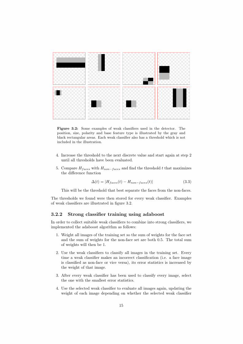
Figure 3.2: Some examples of weak classifiers used in the detector. Theposition, size, polarity and base feature type is illustrated by the gray andblack rectangular areas. Each weak classifier also has a threshold which is notincluded in the illustration.

4. Increase the threshold to the next discrete value and start again at step 2until all thresholds have been evaluated.

5. Compare Hfaces with Hnon−faces and find the threshold t that maximizesthe difference function

∆(t) = |Hfaces(t)−Hnon−faces(t)| (3.3)

This will be the threshold that best separate the faces from the non-faces.

The thresholds we found were then stored for every weak classifier. Examplesof weak classifiers are illustrated in figure 3.2.

3.2.2 Strong classifier training using adaboostIn order to collect suitable weak classifiers to combine into strong classifiers, weimplemented the adaboost algorithm as follows:

1. Weight all images of the training set so the sum of weights for the face setand the sum of weights for the non-face set are both 0.5. The total sumof weights will then be 1.

2. Use the weak classifiers to classify all images in the training set. Everytime a weak classifier makes an incorrect classification (i.e. a face imageis classified as non-face or vice versa), its error statistics is increased bythe weight of that image.

3. After every weak classifier has been used to classify every image, selectthe one with the smallest error statistics.

4. Use the selected weak classifier to evaluate all images again, updating theweight of each image depending on whether the selected weak classifier

15

classifies it correctly. If an image is correctly classified its weight is in-creased, otherwise it is left unchanged.

5. When all weights have been updated, normalize them so that their sum isonce again 1.

6. Finally, append the selected weak classifier to the strong classifier.

7. Returns to step 2 to find the next weak classifier.

When the process is repeated, the error values that are stored for every classifierwill be dependent of the previously chosen weak classifiers. This way, each strongclassifier contains a set of weak classifiers that are all good at detecting similartypes of faces, or discarding similar types of non-faces.

The strong classifier stores a weight for every weak classifier it contains,indicating how well the individual weak classifier classified the complete set.Every time a weak classifier is appended, the strong classifier is evaluated onthe complete set to determine if another weak classifier is needed. This is doneby comparing the correct detection rate and false positive rate of the strongclassifier to a wanted value. When the strong classifier is a part of a cascade,its correct detection rate and false positive rate are cdi and fpi of equation 2.2.

To evaluate a strong classifier on a detection window, its weak classifiersare evaluated one by one. The weights of the weak classifiers that classifythe detection window as a face are added together. That sum of weights isthen compared to a threshold to determine the result of the strong classifier.The result of the strong classifier simply indicates if enough weak classifiersclassified the detection window as a face. The threshold of the strong classifiermust be retrained when a weak classifier is added. We did this by adjusting thethreshold until a correct detection rate of 0.99 was achieved, and added moreweak classifiers until the false positive rate was acceptably low. Since we trainedstrong classifiers to combine into a cascade, the acceptable false positive rate ofeach strong classifier was as high as 0.3− 0.5 (as described in section 2.2.5).

3.2.3 The cascadeThe training of our cascade was performed by iteratively training strong clas-sifiers using adaboost. The first strong classifier was trained with the wholetraining set of faces and non-faces. The second strong classifier used a trainingset containing all faces but only the non-faces that the previous strong classifiercould not classify correctly. In this way, strong classifiers in the later steps ofthe cascade can focus on different non-faces than the previous steps. This meansthat the cascade consists of strong classifiers that each are good at separatingdifferent sets of non-faces from the faces. As an optimization of the algorithm,the thresholds of the weak classifiers can be retrained after updating the train-ing set. This will remove dependencies from discarded non-face examples. Theiterative method of training the cascade is illustrated in figure 3.3. The initialstrong classifiers were trained to achieve a correct detection rate of 0.99 anda false positive rate of 0.30. In later steps of the cascade, we increased therequired false positive rate to approximately 0.80. Selecting the wanted falsepositive rate was tricky, since it is not worth adding a large amount of weakclassifiers to achieve only a small decrease of the false positive rate. Even so,

16

Resulting Cascade

ADABOOSTTraining

Initial Data

CompleteTraining

set

Weak classifier

set

1 StrongClassifier

"A"

Evaluate "A" and discard

correctly detected non-

faces.

Training set

evaluated by "A"

ADABOOSTTraining

1 StrongClassifier

"B"

Evaluate "B" and discard

correctly detected non-

faces.

Training set evaluated by "A" and "B"

ADABOOSTTraining

1 StrongClassifier

"C"

Evaluate "C" and discard

correctly detected non-

faces.

Training set evaluated by "A", "B" and

"C"

Retrain weak

classifierset

Weak classifier

set

Retrain weak

classifierset

Weak classifier

set

StrongClassifier

"A"

StrongClassifier

"B"

StrongClassifier

"C"

Further training...

Figure 3.3: The process of training a cascade as described in section 3.2.3.

17

1

21

2

65

34

12

8

141516

1

32

...

Optimizingstrong classifier

Base cascade from original training set

Cascade from extended non-face training set

O B E

Figure 3.4: This is our final cascade, containing 12 strong classifiers. Thefirst part is an optimization using two weak classifiers. The middle part isthe cascade from the training on the original Cambridge AT&T Laboratoriesdatabase. The final part of the cascade is the result of training on the extendednon-face set.

with several steps in the cascade, the total false positive rate will still steadilydecrease, as described in section 2.2.5. The cascade we trained from the initialdatabase had a correct detection rate above 0.9 and a false positive rate of 0.This sounds like an optimal false positive rate, but since it is measured on thetraining set, it is actually not good at all. This is discussed further in section3.3.

3.3 Training resultsThe cascade we obtained from training on the Cambridge AT&T Laboratoriesdatabase using the algorithm described in section 3.2.3 consisted of 6 strongclassifiers illustrated by the the middle part of the cascade in figure 3.4.

After the sixth step, the adaboost algorithm had successfully discarded all ofthe non-face examples. Thus further training was impossible without extendingthe database with more and harder non-faces. We used the method describedin section 3.1 with pictures collected from the internet depicting landscapes,vegetation and interior decoration. Using these images we quickly generated anon-face set of approximately 80.000 non-faces. Since all of the collected non-faces were incorrectly classified as faces in the previous steps of the cascade,we continued the cascade training using only the new non-faces and the facesused to train the previous steps. This improved the false positive rate on the

18

3.5(a): Result of face detection using onlythe middle cascade from figure 3.4.

3.5(b): Result of face detection using themiddle and the last cascade fromfigure 3.4

Figure 3.5: Detection examples illustrating a decrease in the number of falsepositives using different cascades. The false positive count in this case waslowered by a factor 5.

3.6(a): Result of face detection using onlythe middle cascade from figure 3.4.

3.6(b): Result of face detection using themiddle and the last cascade fromfigure 3.4

Figure 3.6: Detection examples illustrating a decrease in the number of falsepositives using different cascades. The false positive count in this case waslowered by a factor 10.

detection examples shown in figures 3.5 and 3.6 by a factor between 5− 10.As discussed in section 2.2.5, a single strong classifier was added as a first

step in our cascade to lower the average number of features evaluated. Thisstrong classifier was constructed using the two individually best weak classifierfrom the base types selected for our detector.

Statistics for different combinations of the three steps in the cascade fromfigure 3.4 are presented in tables 3.1, 3.2 and 3.3. The presence of the first,middle and last steps are denoted O for optimization, B for base cascade, andE for extension cascade. Column Correct det. contains the correct detectionrate for the cascade combinations, column False pos. contains the false positiverate of the cascade combinations and column Average eval. contains the averageamount of weak classifier evaluations required to reject the non-faces in the testset. It is important to note that the number of faces in the sets used to generatethese metrics are much higher than the number of faces found in most pictures.

19

Therefore the number of average weak classifier evaluations is not calculatedusing the complete set, but rather using only the non-face examples.

Table 3.1: Different cascade combinations evaluated on the original trainingset in the Cambridge AT&T Laboratories database

Cascade Correct det. False pos. Average eval.O - - 0.9716 0.3467 2.0000- B - 0.9671 0 11.0330- - E 0.9737 0.0836 28.3967- B E 0.9481 0 11.0330O B E 0.9329 0 8.5871

The results in table 3.1 show that cascade B has a false positive rate of0 on the training set as discussed in the beginning of this section. Anothernoteworthy result is the optimization cascade, which alone was able to rejectalmost two thirds of the non-faces.

Table 3.2: Different cascade combinations evaluated on the collected false pos-itives and the original faces from the Cambridge AT&T Laboratories database

Cascade Correct det. False pos. Average eval.O - - 0.9716 0.7910 2.0000- B - 0.9671 1.0000 81.0000- - E 0.9737 0.1558 38.3886- B E 0.9481 0.1557 119.3886O B E 0.9329 0.1467 99.2246

In table 3.2, the B cascade has the same correct detection rate as in table3.1 since both sets contain the same faces. Its false positive rate however, is 1.This is due to the fact that all non-face examples in that set are false positivescollected using the B cascade. This is also the explanation of the fact that theaverage number of weak classifier evaluations is equal to the total amount weakclassifiers in cascade B. The high average amount of evaluations for all of thecascade combinations in table 3.2 shows that the non-face examples collectedwere much harder to classify than those supplied with the Cambridge AT&TLaboratories database training set.

Table 3.3: Different cascade combinations evaluated on the original test setin the Cambridge AT&T Laboratories database

Cascade Correct det. False pos. Average eval.O - - 0.7500 0.3397 2.0000- B - 0.1822 0.0083 10.9367- - E 0.3157 0.0313 21.6856- B E 0.1314 0.0034 11.4712O B E 0.1292 0.0034 8.7759

The results on the test set in the Cambridge AT&T Laboratories database(table 3.3) were poor compared to the same measures on the sets used for

20

training (table 3.1 and 3.2). This shows the importance of selecting a suitabletraining set when creating a face detector. A trained detector will be limited tofind faces similar to those in its training set.

As can be seen in the tables above, the use of the optimization cascadereduces not only the false positive rate, but also the correct detection rate asdescribed in equation 2.2. However, the average amount of evaluations is alwayslower when using the optimization cascade. Therefore, the optimization stageis useful when higher performance is wanted.

21

Chapter 4

Implementation of the facedetector

Implementing a face detector framework is challenging as many different subsys-tems can be used. Obviously, every face detector needs an image source. Thiscould simply be an image file, but the image provider could also be a camera,like in this thesis project. After the detection process, the results can be usedfor whatever purpose the face detector was implemented. It is often useful tovisualize the result of the detection on screen, or in an image. This represen-tation will require some type of post-processing, like marking the faces found.The different parts in our detection framework are illustrated in figure 4.1.

Since one of the requirements for our thesis project was to use the GPUfor the detection process, our framework includes a GPU part in addition tothe classic components. This chapter will focus on the implementation of thedetector part of the framework.

4.1 GPU implementationAs described in chapter 2, one of the requirements was that the face detectorshould be implemented mainly on GPU, to unburden the CPU of the platformand to efficiently use the platform resources. Early tests on the target platformshowed that it could calculate approximately 75 integral images of size 640*480pixels per second using the CPU. Due to these results, and the fact that a GPUimplementation of the integral image construction would require several passesof the fragment shader, we decided to create the integral image on CPU andleave only the actual evaluation of features to the GPU. This will conform tothe second part of the requirement: to efficiently use the platform resources.

Unfortunately for the handling of the integral image, OpenGL ES 2.0 doesnot specify a high precision texture format suitable for representing the integralimage. Instead of simply accessing the values of the integral image in the shaderprogram using a regular sampler, we had to do it in a more resource demandingway.

22

GPU Accelerated detector

Image Provider

Output/ Result-usage

CPU Application

GPU

Classic detector

Figure 4.1: A framework for face detection with and without GPU accelera-tion.

4.1.1 Accessing the integral image on GPUThe integral image needs to store the intensity sum of all pixels in the originalimage, therefore it needs a high precision storage type. The size of the storagetype has to be able to store values larger or equal to w ·h ·I where w is the imagewidth, h is the height of the image and I is the number of possible intensityvalues. If the original image has 256 levels of intensity and the integral imagestorage type is an array of 32 bit unsigned int values, the following simplecalculation shows how large the original image can be:

w · h · 28 ≤ 232 ⇒ w · h ≤ 224

Given the values above, the image is limited to a size of 224 pixels (approxi-mately 16 megapixels), which is more than enough to detect faces on a 19x19pixel scale. In GLSL ES 2.0 the highp precision qualifier supplies sufficientprecision for handling an integral image. The GLSL ES 2.0 standard defines thehighp precision qualifier in the fragment shader as optional, but fortunately ourhardware has a unified shader GPU and therefore supports the highp qualifierin both vertex and fragment shader programs.

It is possible to upload the 32 bit integral image to the GPU by configuringa texture to contain RGBA values with storage type unsigned byte. Afteruploading the data to the GPU, the 32 bit unsigned int values will be treatedas four unsigned byte values. When accessing the texture on the GPU, thevalues are read individually as float values that vary in 28 steps between 0 and1 (illustrated in figure 4.2). Therefore we first have to scale them to vary in28 steps between 0 and 255. Then we would like to shift them bitwise to theircorrect magnitude, unfortunately bitwise operations are not supported in GLSLES 2.0. So we have to use multiplication instead. The conversion is illustratedin figure 4.3.

4.1.2 GPU implementation of the detectorWhen the integral image can be accessed and converted back to its actual valuein the fragment program, it is possible to implement the cascade in shader code.

23

33FFCC00

8 bits

32 bits

33

FF

CC

00 =

=

=

=

A

B

G

R

⇒⇒⇒⇒

CPUDomain

GPUDomain 0.8

1.0

0.0

0.2

Integral image valueas 4 float values inShader program

0x00CCFF33

Integral image value as unsigned int in

CPU domain.

Figure 4.2: How the unsigned integer value is represented when used in theshader program.

GPUDomain

A = 0.0B = 0.8G = 1.0R = 0.2

Integral image valueas 4 float values

*256.0^3 ⇒*256.0^2 ⇒*256.0^1 ⇒*256.0^0 ⇒

*255.0 ⇒ 0.0*255.0 ⇒ 204.0*255.0 ⇒ 255.0*255.0 ⇒ 51.0

0.013369344.0

65280.051.0

+

13434675

(= 0x00CCFF33)

Values scaled to interval:0.0-255.0

Values scaled according to theirmagnitude in the integral image

The actual value wanted fromthe integral image.

Figure 4.3: How the texture lookup float values are converted into the integralimage value in the shader program.

24

The code for our GPU version of the detector is abstracted into weak classifierevaluation, strong classifier evaluation and cascade evaluation.

Weak classifier implementation

To evaluate the weak Haar classifiers in the strong classifiers, we created func-tions in GLSL ES code according to this prototype:

1 uniform highp float size;2 float evalHaarClassifierTypeA( xpos, ypos, width,3 height, polarity, threshold)4 {5 // Evaluate classifier in current detection window.6 // Return 1.0 if detection window classified as7 // a face, otherwise 0.0.8 }

The process of evaluating a weak classifier is as follows:

1. Modify the window-size relative input parameters to fit the current detectionwindow size, indicated by the uniform size.

2. Do lookups in the texture containing the integral image.

3. Convert the values from step 2 to the actual values of the integral image,as described in figure 4.3.

4. Subtract and add integral image values according to classifier type scheme.

5. Compare the result value with the given threshold, using the polarityparameter to indicate whether the result value should be larger or smallerthan the threshold.

6. Return result of comparison (1.0 for true, 0.0 for false).

These functions are created individually for the different types of haar classifiersillustrated in figure 2.5.

Strong classifier implementation

The only difference between different strong classifiers is the number of weakclassifiers that are evaluated and the properties of these weak classifiers (posi-tion, size, type, polarity and threshold). After the training process is complete,it is a simple matter to store the strong classifiers as shader code functions.The properties of the weak classifiers can be stored as static values in functioncalls, and all weights and thresholds can be stored in variable assignments asthe following code prototype shows:

25

1 bool strong1()2 {3 float r1 = 1.47299*evalHaarClassifierTypeA( 8.0, 5.0, 5.0,4 19.0, 1.0, -611.0);5 float r2 = 1.27765*evalHaarClassifierTypeB(20.0, 0.0, 4.0,6 23.0,-1.0, 137.0);7 float r3 = 1.30542*evalHaarClassifierTypeA( 8.0, 3.0, 10.0,8 11.0, 1.0,-1718.0);9 float thresh = 2.02803;

10 float res = r1 + r2 + r3;11 return res>thresh;12 }

The variables r1, r2 and r3 will contain the corresponding weak classifiersweights if the weak classifiers classified the detection window as a face, otherwisethe value will be 0. When determining the result of the strong classifier, thesum is simply compared to the strong classifier threshold.

Cascade implementation

In our implementation of the GPU cascade, we set the color of the pixel to bewhite if a face is detected and black otherwise. The actual cascade evaluationcode was straightforward:

1 void main2 {3 gl_FragColor = vec4(0.0,0.0,0.0,0.0);4 if (!strong1()){5 discard;6 }7 if (!strong2()){8 discard;9 }

10 .11 .12 .13 if (!strongN()){14 discard;15 }16 gl_FragColor = vec4(1.0,1.0,1.0,1.0);17 }

There were some issues when implementing the cascade on the GPU. Shaderprograms can only have a limited size, defined by the OpenGL ES 2.0 confor-mance tests (which are not finished at the time of writing this thesis). Becauseof the growing number of weak classifiers in each strong classifier, the cascadeimplementation resulted in long shader programs. The OpenGL ES 2.0 specifi-cation requires that compiling too long shader programs result in a compilationerror. The drivers supplied with the platform refused to compile shader codecontaining the full cascade, but did not explicitly indicate that the length ofthe code was the problem. When the cascade length was reduced to only onestrong classifier, the code compiled successfully. Since the same function callswere used in both cases, only fewer times in the latter case, we deduced thatthe actual problem was the length of the code. The solution was to split thecascade into several passes. This was implemented using frame buffer objects

26

Found Faces

Pass 1 Pass 3Pass 2

Framebuffer Texture 1 Integral Image

SamplerPrevious Result

Sampler

Output image

Shader program context

Framebuffer Texture 2

Integral Image

Integral Image Sampler

Output image

Shader program context

Previous Result Sampler

Integral Image Sampler

Output image

Shader program context

Previous Result Sampler

Integral ImageIntegral Image

Framebuffer Texture 1

Framebuffer Texture 1

Framebuffer Texture 2

Framebuffer Texture 2

Figure 4.4: The cascade implemented using several passes on the fragmentshader.

which all share the same integral image texture, and every pass uses the resultfrom the previous step. This method is illustrated in figure 4.4, but when tryingimplement the method on the platform, we encountered driver related issues.

4.1.3 GPU results and issuesBefore the delivery of the graphics drivers for the platform, a simulated OpenGLES 2.0 environment running on a desktop PC with Linux was used. In the sim-ulated environment, the OpenGL ES 2.0 calls mapped to the desktop OpenGL2.x hardware. Since OpenGL ES 2.0 is not a true subset of OpenGL 2.x, someof the functionality in OpenGL ES 2.0, like high precision float values, had nocounterpart in the simulated environment. The highp precision qualifier wasneeded to convert the integral image data (as described in section 4.1.1), butsince there is no precision qualifier support in OpenGL 2.x, the qualifiers weresimply ignored. This was solved by disabling the hardware support for OpenGL2.x vertex and fragment shaders. By forcing the shaders to run in softwaremode, the high precision was emulated correctly. This decreased the perfor-mance, but we could at least verify that the face detector behaved as expectedwhen implemented in GLSL ES 2.0.

Changing from the simulated environment to the actual hardware provedmore troublesome than anticipated. The highp precision qualifier did not seemto work unless a redundant calculation using highp int values was evaluatedbetween our texture lookup calls and the conversion to integral image values.Since the functionality did not depend on the result of the redundant calculation,it was abstracted into a function void precisionfix(void). This seeminglypointless function was then called inside every weak classifier evaluation. Thisexpanded the shader program length, further restricting the cascade implemen-tation. To the end of this thesis, we did not find the source of this noteworthybehaviour. Due to these circumstances and the late delivery of the GPU drivers,we could not successfully implement the detector with GPU acceleration. In-stead we moved on to a CPU reference implementation of the detector to beable to explore the focus control on the target platform.

27

Figure 4.5: Output after evaluating our final cascade in our CPU referenceimplementation. A rectangle overlap test algorithm have grouped multiple hitstogether.

4.2 CPU reference implementationDue to the restrictions in our supplied GPU drivers, a reference implementationin C running completely on the platform CPU was implemented. This imple-mentation is basically two for-loops that evaluate the cascade in every detectionwindow of the resulting image, which would represent the fragment shader ex-ecuting the cascade on every fragment on the GPU. With this implementation,we were able to execute the full cascade with promising results. The detec-tor fetches images from the camera module of the platform, detects faces andpresents the results on the screen of the platform. The complete framework isfurther described in chapter 5.

4.3 Example detectionsExample outputs from our CPU reference implementation are shown in figure4.5, 4.6 and 4.7. These were all created by running the detector on the suppliedplatform.

28

Figure 4.6: Output after evaluating our final cascade in the CPU referenceimplementation. A rectangle overlap test algorithm have grouped multiple hitstogether.

29

Figure 4.7: Output after evaluating our final cascade in our CPU referenceimplementation. A rectangle overlap test algorithm have grouped multiple hitstogether.

30

Chapter 5

Detection on the targetplatform

The target platform for this master thesis project had a camera module withfocus capabilities and a QVGA touch screen. The platform environment wasembedded Linux, with V4L2 drivers for the camera, and DirectFB support forhandling input events and showing images on the screen.

5.1 Fetching and showing imagesIn addition to the V4L2 API, the camera included proprietary drivers supportingISP functionality like exposure and white balance. The camera was completelycontrolled through these drivers. In the detection framework, the camera wasset up to supply images in pixel format YUV422. This format consists of a 4 bitY (luminance) channel, 2 bit U (blue chrominance) channel and a 2 bit V (redchrominance) channel for every pixel. Since the detection method used does notneed high resolution images, a resolution fitting the screen was selected.

DirectFB has support for the YUV422 pixel format, therefore the imageswere kept in YUV422 for the final on-screen representation. Since the detectoronly uses the intensity values in the image, the color information was discardedbefore creating the integral image.

To display images on screen, a pointer to the screen buffer was requestedfrom the DirectFB context. This pointer could then be used to write images toscreen. Images were fetched from the camera module by requesting a pointerto the memory area where the camera module had stored the image. Thissetup is illustrated in figure 5.1. From the camera image, we created an integralimage used to evaluate the cascade. The resulting detections were indicatedby drawing squares on top of the fetched camera image, and copying the resultimage to the screen buffer memory area. This application flow is illustrated infigure 5.2.

31

Detector Application

Screen surface

memory area

Camera buffer

memory area

V4L2 Ioctrl calls

DirectFB calls

SCREENDirectFB

CAMERA MODULEV4L2 Driver

Application reads camera image

Application writes result image

Figure 5.1: The setup of the target platforms camera and screen.

5.2 Controlling the focusFaces are often the subject of interest when taking photographs. Face detectioncan therefore be used to select a region in the viewfinder for camera focus setup.

5.2.1 Focus control using GPUAn implementation of region based autofocus control using GPU is suggestedby Berglund and Andreen [1]. When a region of an image is detected as aface, the contrast of adjacent pixels in that region can be measured while thefocus is changing. If the contrast increases, the region becomes more focused.When a peak occurs, the wanted focal length of the camera has been found. Ifdifferent parts of the measured region have different distances to the camera,false peaks can occur - in the sense that something else than the wanted area isin focus. Using face detection, regions containing only faces can be used to findthe optimal focal length.

5.2.2 Implementation issuesPlatform drivers were supplied that could set the focus to values between 0−100,mapping to the complete focal span of the camera. Unfortunately the drivers didnot actually set the focus, thus preventing the implementation of focus controlusing face detection techniques. At the time of writing this report, the supplierhas not yet provided a working focus control.

32

Setting up camera module

Setup Camera

Setting up screen

Setup Screen

Request surface buffer pointer

Pointer to surface buffer

Fetching image to

buffer

Fetch image

Pointer to image bufferDetect faces

and write result to screen surface

Updating screen

Update screen

Detector Application

V4L2 Camera Driver

DirectFB screen handler

Adjusting focus

Adjust camera focus

WANTED FOCUSING STEP

WHI

LE L

OO

P

Figure 5.2: The process of fetching images, detecting faces in them andpresenting them on screen. The step of setting the camera focus could not beimplemented with the given drivers of the platform.

33

5.3 PerformanceBecause of the issues described in section 4.1.3, we were unable to benchmarkthe performance of a GPU implementation. And since the running concept inthe simulated environment uses a software shader driver, the execution time inthis environment is irrelevant.

The CPU reference implementation was compiled with gcc, using an ARMtoolchain with optimization level 3 (the -O3 flag). When the cascade evaluationis switched off, the framework fetches 320 times 240 pixel images, integratesthem and writes a result image to the screen at a frame rate of approximately4 frames per second.

The detector was configured to evaluate the cascade in detection windows,slided across the image in steps of 1 − 10 pixels, depending on the size of thedetection window. For detection windows of size 19 times 19 pixels, the step sizeis 1 pixel, and for detection windows of size 190 times 190 pixels, the step sizeis 10 pixels. When the detector is running with detection windows of 4 differentsizes between 60 and 100 pixels (in both width and height), it can detect andfollow a face at a frame rate of 2 frames per second. When the detector isrunning with detection windows of 4 different sizes between 40 and 100 pixels,it can detect and follow a face at a frame rate of 1 frame per second.

5.4 Contrast issuesThe images fetched from the camera module had poor contrast, making facedetection difficult. Normalizing the images before detection was therefore nec-essary. The camera module had support for histogram equalization, but we wereunable to set up the histogram module using the supplied drivers. Therefore weimplemented a simple software histogram equalization to obtain higher contrastimages for the detector.

34

Chapter 6

Conclusions and future work

6.1 ConclusionIn the beginning of the thesis, we evaluated different face detection methodsaccording to the given requirements. We selected the method thought to bemost suitable and implemented a training framework for such a detector. Theadaboost training proved to be challenging in a number of ways, and was con-stantly refined throughout the duration of the thesis project. Using the resultsfrom the training, a detector prototype was implemented in a simulated OpenGLES 2.0 environment. A framework for the target platform - capabable of fetchingimages from the camera module, processing them and presenting them on theplatform screen - was successfully implemented. Using a CPU reference imple-mentation of the detector, this framework ran at a frame rate of approximately1− 2 frames per second without platform-specific optimization.

The initial objective of this thesis was to implement a face detection al-gorithm on GPU using OpenGL ES 2.0. When moving from the simulatedenvironment to the actual target hardware, the graphics framework of the tar-get was pushed to its limits. This was manifested in undefined behaviours, ashave been previously discussed in section 4.1.3. Conclusions drawn from thisis that the platform with the current drivers might be ready for regular 3Dgraphics development, but not yet for GPGPU.

Because of this, we were unable to gather sufficient results to determinewhether a GPGPU accelerated face detection was implementable. Indicationsfrom our incomplete GPU implementation suggest that a complete detector,using the selected method, would have been too slow for real-time use.

6.2 Discussion and future work

6.2.1 Open GL ES 2.0Writing a program in a simulated OpenGL ES 2.0 environment is not enough,it is always important to test with actual target drivers. Since OpenGL ES2.0 is not a true subset of OpenGL 2.0, an application working in a simulatedenvironment could be problematic to run on actual ES hardware. A lot of timeand effort can be saved if platform specific bugs are found in early stages of

35

development.

6.2.2 Normalized detection windowsFor the detector to be illumination invariant, it must first be trained on anormalized database. Every single detection window must then be individuallynormalized during detection. Viola and Jones [9] suggest that the detectionwindow normalization should be done by adjusting the threshold values of theweak classifiers, instead of normalizing the detection window on a per pixelbasis. The intensity variance σ2 in each detection window could be used for thethreshold adjustment. The variance could be calculated using another type ofintegral image containing the sum of squared intensity values from the originalimage. Such a representation would require even higher precision. Therefore,this method of normalization was not feasible as a GPU implementation on thetarget platform.

Our detector however, was trained with a database that was not normal-ized. Therefore it can detect faces without having to normalize every detectionwindow. This is not as robust as the method above but will only require a nor-malization of the complete image, which can be done quite efficiently on CPUor by a camera ISP block.

6.2.3 Focusing algorithm optimizationWhen a face has been detected in an image, the size of the face will be known.The size of the face, together with biometric statistics can be used as a roughestimation of the distance from the camera to the face. This distance can beused to limit the search range of the focusing algorithm. If a detected face coversa large area of the camera’s viewfinder, the focusing algorithm can predict thatit is highly probable that the face is close to the camera. Similarly, if a facecovers a small portion of the viewfinder, the face is probably further away.

It is important to note that this optimization would require the detection tobe an actual face and not a billboard or a small photograph depicting a face.

6.2.4 Float conversionThe conversion procedure concerning float values described in section 4.1.1requires a lot of operations. This is a computationally expensive way to transferhigh precision values between the CPU and GPU domains. Since graphicshardware manufacturers are aware of the demands from GPGPU programmers,better support for high precision textures is expected. Desktop GPUs alreadysupport this type of as extensions. It is highly likely that also OpenGL EShardware will evolve to include such support.

6.2.5 Choosing a suitable databaseHaar feature based detection is highly dependent on the database used for train-ing, as explained in section 3.3. Face databases are often constructed with pho-tos taken under similar lighting conditions, using the same background in everyphoto. A robust face detector should not be dependent on circumstances suchas background and light conditions. To create a robust detector several different

36

databases can be merged into one training set. Since adaboost training requiresimages to be consistent in size and position, the merge of different databasescan be problematic. It may require a considerable amount of manual labour,like scaling and aligning the images. Some of the most successful implementa-tions of Haar based detectors, like the one by Viola and Jones [9], have beentrained with images collected by crawling the internet for random faces. Thiswill obviously yield a higher statistic variance for the collected images comparedto a database of systematically photographed faces. Higher statistic variance inthe training database will have a positive impact on the detector.

Another important aspect of the database is how much of the face is croppedaway. The database used in this thesis only contained the center part of theface, cropping away the outlines like hair, ears, and chin. This can be seen infigure 3.1(a). The tradeoff from cropping is that face shaped objects are easierto discard, as nothing from the outline of the face is used for the detection.It will however, be more difficult to find enough information to eliminate falsepositives. Which is one of the major weaknesses of our detector. In retrospect,we would have liked to use a database with faces less cropped. Unfortunately,we were unable to accquire such a database during this thesis project.

Non-face examples are also required, but a lot easier to aquire. Cutting outrandom parts from images not containing faces will quickly give a large non-face set. However only a fraction of these non-faces will be of any real use forthe detector. Most non-faces will be easy to separate from the set of faces andthus will be discarded early. An effective way to extract more challenging non-faces is to run a primitive incomplete face detector on images not containingfaces, and collect the false positives. This will give a higher difficulty amongstthe non-faces that would be hard to achieve using a truly random collectionmethod.

6.2.6 Skin tone methodsTo decrease the average of weak classifier evaluations in the cascade, it is possibleto do a preceding skin tone test. This would mean that the original color imagehas to be uploaded to the GPU, in addition to the integral image.

Before the cascade evaluations begin, a few texture lookups in the originalimage can be used to determine if the current search window contains enoughskin color. If not, the cascade does not need to evaluate any classifiers. Thesmallest possible amount of texture lookups to evaluate a weak classifier is 6, andthe first strong classifier in the cascade should contain at least two weak clas-sifiers. Therefore, a skin test that rejects large areas of an image that does notcontain any faces should decrease the average number of evaluated weak classi-fiers per pixel considerably. One problem though, is that a skin tone detectionmight incorrectly reject face regions due to unnatural lighting conditions. Thismeans that a color normalization is required for robust skin tone detection.The performance benefit of this method on GPU is dependent on the branchingcapabilities of the hardware, as described in section 2.2.5.

Many of the difficulties encountered in this thesis were due to the need ofhigh precision. Skin tone based methods does not require high precision values,but rather regular color values. Since GPUs are designed for handling suchcolor values, it would be interesting to further explore the possibilities of GPUaccelerated skin tone based face detection.

37

Chapter 7

Acknowledgements

Thanks to Beatriz Grafulla for support throughout the thesis and while writingthe report.

Thanks to Harald Gustafsson for discussions about the target platform.

Thanks to Per Persson for linux support and setting up the development envi-ronment.

Thanks to Jon Hasselgren for OpenGL related discussions.

Thanks to Jim Rasmusson for some Very good pieces of advice.

Thanks to the entire Ericsson new technology and research department for sup-plying a friendly working environment for thesis workers.

38

Bibliography

[1] Fredrik Berglund and Mikael Andreen. Camera isp applied on a pro-grammable gpu, 2008.

[2] AT&T Laboratories Cambridge and Cambridge University ComputerLaboratory. http://www.cl.cam.ac.uk/research/dtg/attarchive/facedatabase.html.

[3] Franklin C. Crow. Summed-area tables for texture mapping. http://www.cse.ucsc.edu/classes/cmps160/Fall05/papers/p207-crow.pdf, 1984.

[4] Julien Meynet. Fast face detection using adaboost. http://people.epfl.ch/julien.meynet, 2003.

[5] Thorsten Scheuermann. Summed-area tables and their application to dy-namic glossy environment reflections. http://ati.amd.com/developer/gdc/GDC2005_SATEnvironmentReflections.pdf, 2005.

[6] Sanjay Kr. Singh, D. S. Chauhan, Mayank Vatsa, and Richa Singh. Arobust skin color based face detection algorithm. http://www2.tku.edu.tw/~tkjse/6-4/6-4-6.pdf, 2003.

[7] Moritz Störring. Computer vision and human skin colour. http://www.cvmt.dk/~mst/Publications/phd/index.html.

[8] M. Turk and A. Pentland. Face recognition using eigenfaces. http://people.epfl.ch/julien.meynet, 1991.

[9] Paul Viola and Michael J. Jones. Rapid object detection using a boostedcascade of simple features. www.hpl.hp.com/techreports/Compaq-DEC/CRL-2001-1.pdf, 2001.

39