Camera Calibrationclass 9

Multiple View GeometryComp 290-089Marc Pollefeys

Multiple View Geometry course schedule(subject to change)

Jan. 7, 9 Intro & motivation Projective 2D Geometry

Jan. 14, 16

(no class) Projective 2D Geometry

Jan. 21, 23

Projective 3D Geometry (no class)

Jan. 28, 30

Parameter Estimation Parameter Estimation

Feb. 4, 6 Algorithm Evaluation Camera Models

Feb. 11, 13

Camera Calibration Single View Geometry

Feb. 18, 20

Epipolar Geometry 3D reconstruction

Feb. 25, 27

Fund. Matrix Comp. Structure Comp.

Mar. 4, 6 Planes & Homographies Trifocal Tensor

Mar. 18, 20

Three View Reconstruction

Multiple View Geometry

Mar. 25, 27

MultipleView Reconstruction

Bundle adjustment

Apr. 1, 3 Auto-Calibration Papers

Apr. 8, 10

Dynamic SfM Papers

Apr. 15, 17

Cheirality Papers

Apr. 22, 24

Duality Project Demos

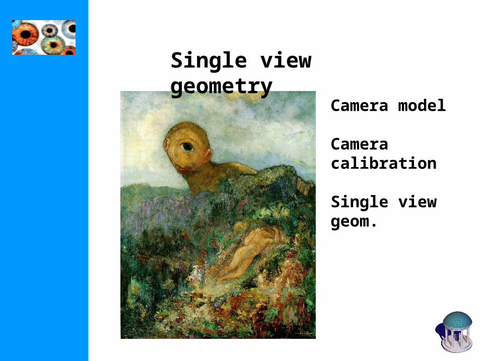
Single view geometry

Camera model

Camera calibration

Single view geom.

Pinhole camera

10

tR0|IKPPXx

Camera anatomy

Camera centerColumn pointsPrincipal planeAxis planePrincipal pointPrincipal ray

Affine cameras

Decomposition of P∞

0

2x302x2

0t~R

~

10x~K

Pd

10t~R

~

10x~K 2x302x2

-10d

absorb d0 in K2x2

10

0R~

10

x~t~KK

10

x~Kt~R~

10

0K

10

x~t~KR~

K

02x22x2

0-12x22x202x22x2

10

0R~

10

x~K

10

t~R~

10

0KP 02x22x2

alternatives, because 8dof (3+3+2), not more

Summary parallel projection

1000

0010

0001

P canonical representation

10

0KK 22 calibration matrix

principal point is not defined

A hierarchy of affine cameras

Orthographic projection

Scaled orthographic projection

1000

0010

0001

P

10

tRH

10rr

P 21T

11T

tt

ktt

/10rr

P 21T

11T

(5dof)

(6dof)

A hierarchy of affine cameras

Weak perspective projection

ktt

y

x

/10rr

1α

αP 2

1T1

1T

(7dof)

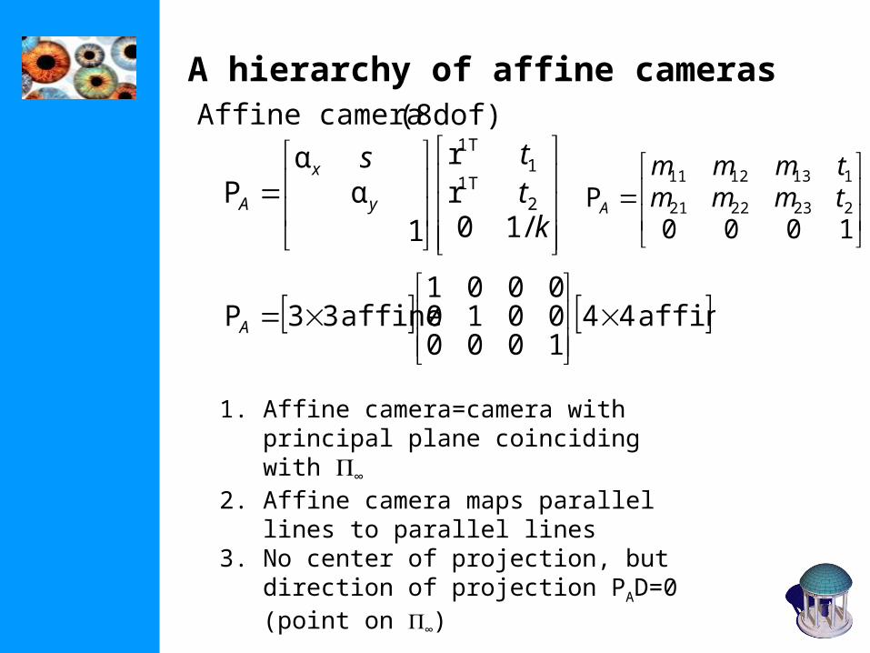
1. Affine camera=camera with principal plane coinciding with ∞

2. Affine camera maps parallel lines to parallel lines

3. No center of projection, but direction of projection PAD=0(point on ∞)

A hierarchy of affine camerasAffine camera

ktts

y

x

A

/10rr

1α

αP 2

1T1

1T

(8dof)

1000P 2232221

1131211

tmmmtmmm

A

affine 44100000100001

affine 33P

A

Pushbroom cameras

T)(X X,Y,X,T T),,(PX wyx T)/,( wyx

Straight lines are not mapped to straight lines!(otherwise it would be a projective camera)

(11dof)

Line cameras

ZYX

pppppp

yx

232221

131211(5dof)

Null-space PC=0 yields camera center

Also decomposition c~|IRKP 22222232

Camera calibration

ii xX ? P

Resectioning

Basic equations

ii PXx

ii PXx

0Ap

Basic equations

0Ap

minimal solution

Over-determined solution

5½ correspondences needed (say 6)

P has 11 dof, 2 independent eq./points

n 6 points

Apminimize subject to constraint

1p

1p̂3 3p̂

P

Degenerate configurations

More complicate than 2D case (see Ch.21)

(i) Camera and points on a twisted cubic

(ii) Points lie on plane or single line passing through projection center

Less obvious

(i) Simple, as before

(ii) Anisotropic scaling

Data normalization

32

Line correspondences

Extend DLT to lines

ilPT

ii 1TPXl

(back-project line)

ii 2TPXl (2 independent eq.)

Geometric error

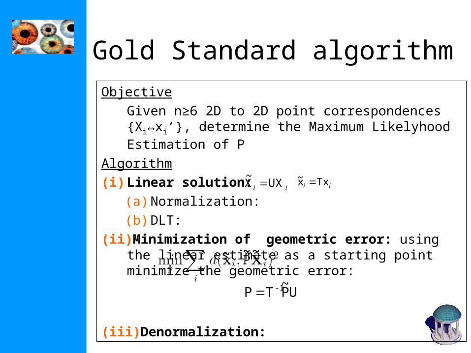
Gold Standard algorithmObjective

Given n≥6 2D to 2D point correspondences {Xi↔xi’}, determine the Maximum Likelyhood Estimation of P

Algorithm

(i) Linear solution:

(a) Normalization:

(b) DLT:

(ii) Minimization of geometric error: using the linear estimate as a starting point minimize the geometric error:

(iii) Denormalization:

ii UXX~ ii Txx~

UP~

TP -1

~ ~~

Calibration example

(i) Canny edge detection(ii) Straight line fitting to the detected edges(iii) Intersecting the lines to obtain the images corners

typically precision <1/10

(HZ rule of thumb: 5n constraints for n unknowns

Errors in the world

Errors in the image and in the world

ii XPx

iX

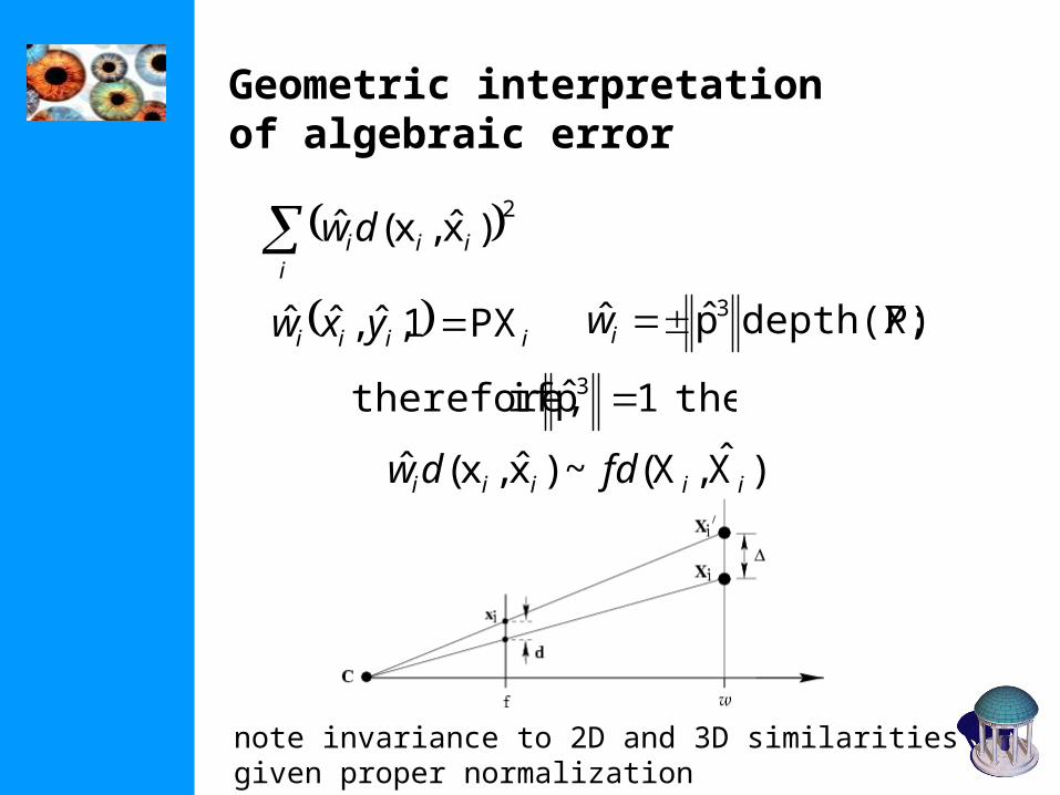
Geometric interpretation of algebraic error

2)x̂,x(ˆ

iiiidw

iiii yxw PX1,ˆ,ˆˆ P)depth(X;p̂ˆ 3iw

)X̂,X(~)x̂,x(ˆ iiiii fddw

then1p̂ if therefore, 3

note invariance to 2D and 3D similarities given proper normalization

Estimation of affine camera

note that in this case algebraic error = geometric error

Gold Standard algorithmObjective

Given n≥4 2D to 2D point correspondences {Xi↔xi’}, determine the Maximum Likelyhood Estimation of P

(remember P3T=(0,0,0,1))

Algorithm

(i) Normalization:

(ii) For each correspondence

(iii) solution is

(iv) Denormalization:

ii UXX~ ii Txx~

UP~

TP -1

bpA 88

bAp 88

Restricted camera estimation

Minimize geometric error impose constraint through parametrizationImage only 9 2n, otherwise 3n+9 5n

Find best fit that satisfies• skew s is zero• pixels are square • principal point is known• complete camera matrix K is known

Minimize algebraic error assume map from param q P=K[R|-RC], i.e. p=g(q)minimize ||Ag(q)||

Reduced measurement matrix

One only has to work with 12x12 matrix, not 2nx12

pA~

ApApAp TT

Restricted camera estimation

Initialization • Use general DLT• Clamp values to desired values, e.g. s=0, x= y

Note: can sometimes cause big jump in error

Alternative initialization• Use general DLT• Impose soft constraints

• gradually increase weights

Exterior orientation

Calibrated camera, position and orientation unkown

Pose estimation

6 dof 3 points minimal (4 solutions in general)

Covariance estimation

ML residual error

Example: n=197, =0.365, =0.37

Covariance for estimated camera

Compute Jacobian at ML solution, then

JJ 1x

TP

(variance per parameter can be found on diagonal)

2χ(chi-square distribution =distribution of sum of squares)

cumulative-1

short and long focal length

Radial distortion

Correction of distortion

Choice of the distortion function and center

Computing the parameters of the distortion function(i) Minimize with additional unknowns(ii) Straighten lines(iii) …

Next class: More Single-View Geometry

• Projective cameras and planes, lines, conics and quadrics.

• Camera calibration and vanishing points, calibrating conic and the IAC

** CPPQ T

coneQCPP T