Embed Size (px)
Citation preview
Cambridge Rocketry Toolbox for Octave
Instruction Manual
Introduction
The Octave High Power Rocket Simulation Toolbox is a collection of functions that
can be used to perform various types of simulation of the flight path and parachute
recovery of high power rockets. The simulations have six degrees of freedom and use
data on a rocket design and atmospheric conditions as inputs.
Examples of tasks that can be performed using the toolbox are:
• Simulate the flight path and parachute recovery of a high power rocket.
• Simulate a dual deploy parachute system
• Simulate a two stage rocket or a boosted dart
• Use Monte Carlo simulations to account for uncertainties in the input data and
generate splash down plots.
• Simulate failure modes, e.g. what happens if the parachute does not deploy
• Calculate the required launch angle to achieve a desired landing location for the
rocket.
• Read simulation input data from Rocksim files.
• Read simulation input data from Met Office .pp files
This manual is divided into two parts: Part1 describes how to encode rocket design
and atmospheric data so that it can be used in the toolbox’s simulation functions. And
then goes on to describe in detail how to use each of the simulation functions and
related auxiliary functions. Specific knowledge of how the code works is not required
to use any of the functions described in Part 1.
1
Part 2 is a reference section for users who wish to use functions in the toolbox to
create their own simulators to perform tasks that are not catered for directly in the
main simulation functions. An example could be a simulation of a three stage rocket.
Part 2 is structured into a list of help documents on each of the additional functions
in the toolbox arranged in alphabetical order. The most important functions listed in
this part are ascentcalc and descentcalc. These are the functions that form the
backbone of all the simulation functions described in Part 1. The simulation func-
tions in Part 1 are designed to be usable by someone with good knowledge of Octave
or Matlab without the necessity to understand the code behind the functions. This
necessarily restricts the scope of the simulations that can be performed. ascentcalc
and descentcalc are much more flexible and can be used to simulate a wide range of
scenarios if the user is willing to write a little code of their own incorporating these
functions.
Also listed in part 2 are many functions that can be used as a stand-alone calculator
to perform a specific task. For example Barrowman calc can be used to calculate the
centre of pressure and normal force coefficient of a rocket.
2
Contents
I Instructions on How to Use the Toolbox To Simulate Rocket
Flights 5
1 The Rocket Design 5
1.1 Encoding the rocket design data using Rocksim and readrsim . . . . . . 5
1.1.1 Rules for the Rocksim file . . . . . . . . . . . . . . . . . . . . . . 5
1.1.2 The readrsim function . . . . . . . . . . . . . . . . . . . . . . . 6
1.1.3 The Motor argument . . . . . . . . . . . . . . . . . . . . . . . . . 7
1.1.4 Output Arguments . . . . . . . . . . . . . . . . . . . . . . . . . . 8
1.2 Encoding the rocket design Manually . . . . . . . . . . . . . . . . . . . . 8
1.2.1 The rocket part variables . . . . . . . . . . . . . . . . . . . . . . 9
1.2.2 Using intab builder . . . . . . . . . . . . . . . . . . . . . . . . 11
2 The Atmospheric Data 12
2.1 Forecast data in .pp format . . . . . . . . . . . . . . . . . . . . . . . . . 12
2.1.1 The Netcdf Format . . . . . . . . . . . . . . . . . . . . . . . . . . 13
2.1.2 intab4build . . . . . . . . . . . . . . . . . . . . . . . . . . . . . 13
2.2 Forecast data from the F214 form . . . . . . . . . . . . . . . . . . . . . . 14
2.2.1 f214read . . . . . . . . . . . . . . . . . . . . . . . . . . . . . . . 14
3 The Simulations 15
3.1 rocketflight . . . . . . . . . . . . . . . . . . . . . . . . . . . . . . . . . 16
3.2 rocketflight 2 stage . . . . . . . . . . . . . . . . . . . . . . . . . . . 17
3.3 rocketflight monte . . . . . . . . . . . . . . . . . . . . . . . . . . . . . 18
3.4 rocketflight 2 stage monte . . . . . . . . . . . . . . . . . . . . . . . . 22
3.5 The ‘ballisticfailure’ argument . . . . . . . . . . . . . . . . . . . . 25
3.6 rocketflight delivery . . . . . . . . . . . . . . . . . . . . . . . . . . . 25
3.7 rocketflight 2 stage delivery . . . . . . . . . . . . . . . . . . . . . . 26
3.8 flight variables . . . . . . . . . . . . . . . . . . . . . . . . . . . . . . 27
II Additional Toolbox Functions 30
4 ascentcalc 30
5 axi com 33
3
6 Barrowman calc 33
7 bearing to vector 35
8 descentcalc 35
9 drag datcom 37
10 impulse and mass 38
11 lltoeq 38
12 quaternion to matrix 39
13 Roc mom inert 39
14 vector to bearing 41
15 vectormag 41
16 vectornorm 42
4
Part I
Instructions on How to Use the Toolbox
To Simulate Rocket Flights
1 The Rocket Design
Some of the most important inputs for the rocket simulation functions are the rocket
design data. These data are encoded in a single cell array structure called INTAB. This
structure can be built manually by the user using data from an “on paper” design.
Alternatively if the user has designed their rocket using the software “Rocksim” then
the toolbox contains a function to read the Rocksim file and build INTAB automatically.
This section describes how to build INTAB using these two methods.
1.1 Encoding the rocket design data using Rocksim and readrsim
Caveat The readrsim function has been extensively tested using many rocket designs
however not every possible permutation of rocket design available in Rocksim has been
tested. Therefore it is recommended that the user keep rocket design files simple. The
important aspects of the rocket design, which must be in the file, are the geometric
shape of the rocket, the mass distribution in the rocket and the area and drag coefficient
of any parachutes. As long as these are accurately represented then the simulation
functions will have all the necessary information. It is also recommended that user
checks the output data file as this can be edited if necessary (see section 1.2).
1.1.1 Rules for the Rocksim file
Create your rocket using Rocksim as normal and save it without a motor loaded.
Dual Deploy readrsim handles multiple parachutes in a Rocksim design by labelling
the parachute closest to the front of the rocket as the drogue and the parachute closest
to the rear as the main. If the parachute configuration in your rocket is reversed from
this make sure that the two parachutes have the correct mass and location in the rocket
but edit the values of parachute area and coefficient of drag so the foremost parachute
has the values of the drogue and the rearmost parachute has the values of the main.
readrsim can handle streamers so it is fine to use these. If you are using a drogueless
recovery i.e. no parachute but a separated rocket. Then add a parachute close to the
nose in your Rocksim file but specify the mass as 0. The drag coefficient and area of the
5
parachute should reflect the drag on the drougless rocket. As a good first approximation
use the side-view plan-form area of the rocket and a coefficient of drag of 0.6.
2–Stage Rockets Do not use Rocksim’s staging facility, all Rocksim files sent to
readrsim must be single stage. If your rocket is two stage then you must create 3
Rocksim files. The first contains the design of the complete rocket with the stages
joined, the upper stage must contain (in place of the upper stage motor) a cylinder
specified to have the same mass and dimensions of the primed motor. The booster
stage must be unloaded when the file is saved. The second Rocksim file contains a
design for the booster stage only. In place of the motor this design must contain a
cylinder of same dimensions and burned-out mass as the booster motor. The third
Rocksim file must contain the design for the upper stage of the rocket, saved without
and motor loaded. If the upper stage is a boosted dart simply create the design with
no motor and save as normal.
1.1.2 The readrsim function
Syntax:
[INTAB,Pout]=readrsim(‘filename.rkt’,Motor,Lmot)
The function has three arguments the first ‘filename.rkt’ is a string containing
the file name and path of the Rocksim file. The second, Motor, is The data file for the
rocket motor which will be discussed shortly. The third Lmot is the distance from the
rocket nose tip to the most forward point of the motor in metres.
For a two stage rocket you need to run the function three times, once for each file.
saving the INTAB data structure under a different name each time. The following syntax
is recommended:
INTAB TR – For the total rocket file
INTAB BS – For the booster stage file
INTAB US – For the upper stage file
The Motor argument for the total rocket file refers to the booster stage motor, for
the upper stage file it refers to the upper stage motor. For the booster stage file omit
the second and third arguments so the syntax is as follows.
[INTAB,Pout]=readrsim(‘filename.rkt’)
6
You should also use this syntax for the upper stage if it is a boosted dart.
1.1.3 The Motor argument
Table 1 shows a list of rocket motors for which the high power rocketry toolbox has
data files. Using the command load ‘filename’ creates a variable called Motor in the
workspace that contains data for the relevant motor, this can be input into readrsim.
Manufacturer Name Filename
Cesaroni H153 ‘engH153’
Cesaroni I540 ‘engI540’
Cesaroni K445 ‘engK445’
Cesaroni K570 ‘engK570’
Cesaroni K660 ‘engK660’
Cesaroni L730 ‘engL730’
Cesaroni L1115 ‘engL1115’
Cesaroni M795 ‘engM795’
Cesaroni N2500 ‘engN2500’
Table 1: Motors whose data is contained in the toolbox
create a new ‘eng’ file If the motor you are using is not one of the ones listed
in table 1 you can create your own file. The Motor variable is a cell array with the
following structure.
Motor={‘motor’,‘K660’,Ttable,length,diameter,0}
The first two cells contain strings, the first ‘motor’ identifies the part for readrsim,
the second is the motor name. The third cell contains a data table with thrust–time
data and mass–time data for the motor. The first column of the table is Time (s), the
second column is Thrust (N) and the third is Mass (kg).
Thrust–time data is available from motor manufacturers, and mass–time data can
be calculated using the impulse and mass function described in part 2.
The fourth and fifth cells contain the length and the diameter of the motor in
metres. The sixth cell is a zero this just holds a space for the position of the motor in
the rocket (‘Lmot’) which is filled in by the code when the user specifies it in the input
arguments for readrsim.
7
Once a Motor variable has been created save it for later using
save -mat-binary filename Motor
The file can be loaded using
load filename
1.1.4 Output Arguments
The output arguments of readrsim are [INTAB,Pout]. For every rocket part in the
Rocksim file readrsim creates a cell array variable holding the data on that part. These
variables are listed in Pout. This is output so it can be checked for errors. In the next
section we shall describe how the user can specify a rocket design using only these
variables.
The INTAB cell array, as has already been explained, contains the rocket design data
that is needed for the other functions in the toolbox which simulate rocket flights. The
structure of INTAB is as follows.
INTAB={INTAB1,INATB2,INTAB3,landa,paratab,}
Where INTAB1 is a table of time dependant data including thrust, mass and centre
of mass data calculated using axi com (sec 5) and moments of inertia calculated using
Roc mom inert (sec 13). INTAB2 is a drag data table calculated using drag datcom (sec
9). INTAB3 is a table containing normal force and centre of pressure data calculated
using Barrowman calc (sec 6). landa contains the rocket length and cross sectional
area. paratab contains data on the rockets parachute(s).
1.2 Encoding the rocket design Manually
It is possible to accurately represent the external shape, and internal mass distribution
of a rocket with relatively conventional shape by breaking it down into simple parts
that can be categorised into 8 groups: nose cones, cylinders, tubes, conical transitions,
point masses, fin sets parachutes and motors. Each part is represented as a cell array
variable, then the variables can all be input into the function intab build.
8
1.2.1 The rocket part variables
Here we show the structure of the cell array variables that represent each of the per-
missible part types.
Nose cone Below is an example of the cell array structure for a variable (n1) which
represents a nose cone part.
n1={‘nose’,‘ogive’,L,d,M,X}
The string ‘nose’ is a label identifying the part. The string ‘ogive’ describes the
shape of the nose cone, other permissible string here are ‘conical’ and ‘parabolic’.
L is the length of the nose cone (this and all other dimensions are always in metres). d
is the diameter at the nose cone base, M is mass of the nose cone in kg, X is the distance
of the foremost part of the nose cone to the foremost part of the rocket. This is usually
zero, unless the rocket has multiple nose cones on external boosters perhaps.
Cylinders Below is an example of the cell array structure for a variable (c1) which
represents a cylinder part.
c1={‘cylinder’,‘yes’,L,d,M,X}
The string ‘cylinder’ is a label, the string ‘yes’ identifies that the outer surface
of the cylinder forms part of the rocket’s body surface. If this is not the case then the
string should read ‘no’. L,d,M,X are the length, diameter, mass and position of the
cylinder in the rocket respectively. position is taken as the distance from the nose cone
tip to the foremost part of the cylinder body. This rule is followed for all other parts
as well.
Tubes Below is an example of the cell array structure for a variable (t1) which rep-
resents a tube part.
t1={‘tube’,‘yes’,L,Id,Od,M,X}
The string ‘tube’ is a label, the string ‘yes’ identifies that the outer surface of
the tube forms part of the rocket’s body surface. If this is not the case then the string
should read ‘no’. L,Id,Od,M,X are the length, inner diameter, outer diameter, mass
and position of the tube in the rocket respectively.
9
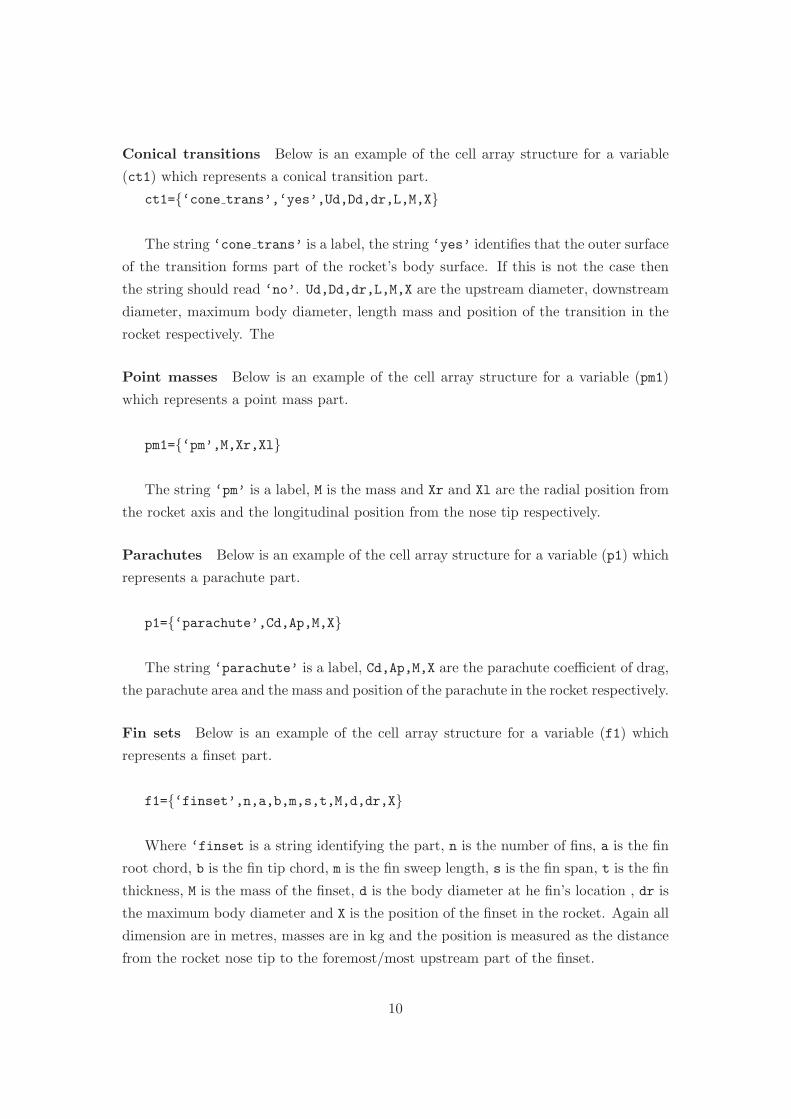
Conical transitions Below is an example of the cell array structure for a variable
(ct1) which represents a conical transition part.
ct1={‘cone trans’,‘yes’,Ud,Dd,dr,L,M,X}
The string ‘cone trans’ is a label, the string ‘yes’ identifies that the outer surface
of the transition forms part of the rocket’s body surface. If this is not the case then
the string should read ‘no’. Ud,Dd,dr,L,M,X are the upstream diameter, downstream
diameter, maximum body diameter, length mass and position of the transition in the
rocket respectively. The
Point masses Below is an example of the cell array structure for a variable (pm1)
which represents a point mass part.
pm1={‘pm’,M,Xr,Xl}
The string ‘pm’ is a label, M is the mass and Xr and Xl are the radial position from
the rocket axis and the longitudinal position from the nose tip respectively.
Parachutes Below is an example of the cell array structure for a variable (p1) which
represents a parachute part.
p1={‘parachute’,Cd,Ap,M,X}
The string ‘parachute’ is a label, Cd,Ap,M,X are the parachute coefficient of drag,
the parachute area and the mass and position of the parachute in the rocket respectively.
Fin sets Below is an example of the cell array structure for a variable (f1) which
represents a finset part.
f1={‘finset’,n,a,b,m,s,t,M,d,dr,X}
Where ‘finset is a string identifying the part, n is the number of fins, a is the fin
root chord, b is the fin tip chord, m is the fin sweep length, s is the fin span, t is the fin
thickness, M is the mass of the finset, d is the body diameter at he fin’s location , dr is
the maximum body diameter and X is the position of the finset in the rocket. Again all
dimension are in metres, masses are in kg and the position is measured as the distance
from the rocket nose tip to the foremost/most upstream part of the finset.
10
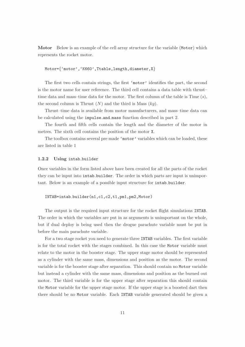
Motor Below is an example of the cell array structure for the variable (Motor) which
represents the rocket motor.
Motor={‘motor’,‘K660’,Ttable,length,diameter,X}
The first two cells contain strings, the first ‘motor’ identifies the part, the second
is the motor name for user reference. The third cell contains a data table with thrust–
time data and mass–time data for the motor. The first column of the table is Time (s),
the second column is Thrust (N) and the third is Mass (kg).
Thrust–time data is available from motor manufacturers, and mass–time data can
be calculated using the impulse and mass function described in part 2.
The fourth and fifth cells contain the length and the diameter of the motor in
metres. The sixth cell contains the position of the motor X.
The toolbox contains several pre made ‘motor’ variables which can be loaded, these
are listed in table 1
1.2.2 Using intab builder
Once variables in the form listed above have been created for all the parts of the rocket
they can be input into intab builder. The order in which parts are input is unimpor-
tant. Below is an example of a possible input structure for intab builder.
INTAB=intab builder(n1,c1,c2,t1,pm1,pm2,Motor)
The output is the required input structure for the rocket flight simulations INTAB.
The order in which the variables are put in as arguments is unimportant on the whole,
but if dual deploy is being used then the drogue parachute variable must be put in
before the main parachute variable.
For a two stage rocket you need to generate three INTAB variables. The first variable
is for the total rocket with the stages combined. In this case the Motor variable must
relate to the motor in the booster stage. The upper stage motor should be represented
as a cylinder with the same mass, dimensions and position as the motor. The second
variable is for the booster stage after separation. This should contain no Motor variable
but instead a cylinder with the same mass, dimensions and position as the burned out
motor. The third variable is for the upper stage after separation this should contain
the Motor variable for the upper stage motor. If the upper stage is a boosted dart then
there should be no Motor variable. Each INTAB variable generated should be given a
11
different name, the following syntax is recommended.
INTAB TR – For the total rocket file
INTAB BS – For the booster stage file
INTAB US – For the upper stage file
2 The Atmospheric Data
In section 1 we described how the rocket design data are encoded for input to the simu-
lation functions. Here we do the same for the atmospheric data. The data are contained
in an array called INTAB4. The first column of INTAB4 contains altitude data from 0m
up to some unspecified high altitude. Columns 2 to 6 contain corresponding data for
the following atmospheric variables: Easterly wind component (m/s), Northerly wind
component(m/s), vertical wind component(m/s), atmospheric density (kg/m3) and
atmospheric temperature (K) respectively.
It is of course a trivial matter for the user to create an INTAB4 array containing
theoretical data for use in the simulations. This section describes how to populate
INTAB4 using Met office forecast data either in the form of a .pp file or an F214 form.
2.1 Forecast data in .pp format
Output data from the Met Office’s Numerical Weather Prediction (NWP) service is
available for academic use through the British Atmospheric Data Centre (BADC).
Once an account has been set up NWP output data in .pp format can be downloaded
from the BADC website1.
The data that needs to be downloaded is the mesoscale forecast data, in The BADC
archives the files are organised by date and hour. A typical file name for a .pp is given
below.
lbfm2004060806 00002 01.pp
where lb indicates that the file contains “mesoscale” data (as opposed to ag for “global”
data), fm indicates that it is “forecast model” data. 20040608 is the date of the forecast
(not to be confused with the date the forecast was made) in Year-Month-Day format.
06 is the hour of the forecast. The number between the underscores -00002 is called
the “stash code” and identifies which variable the data in the file refers to, more details
1[http://badc.nerc.ac.uk/home/index.html]
12
of stash codes will be given shortly. The final number 01 is the number of hours prior
to the date and time time of the forecast (2004060806) that the forecast was made.
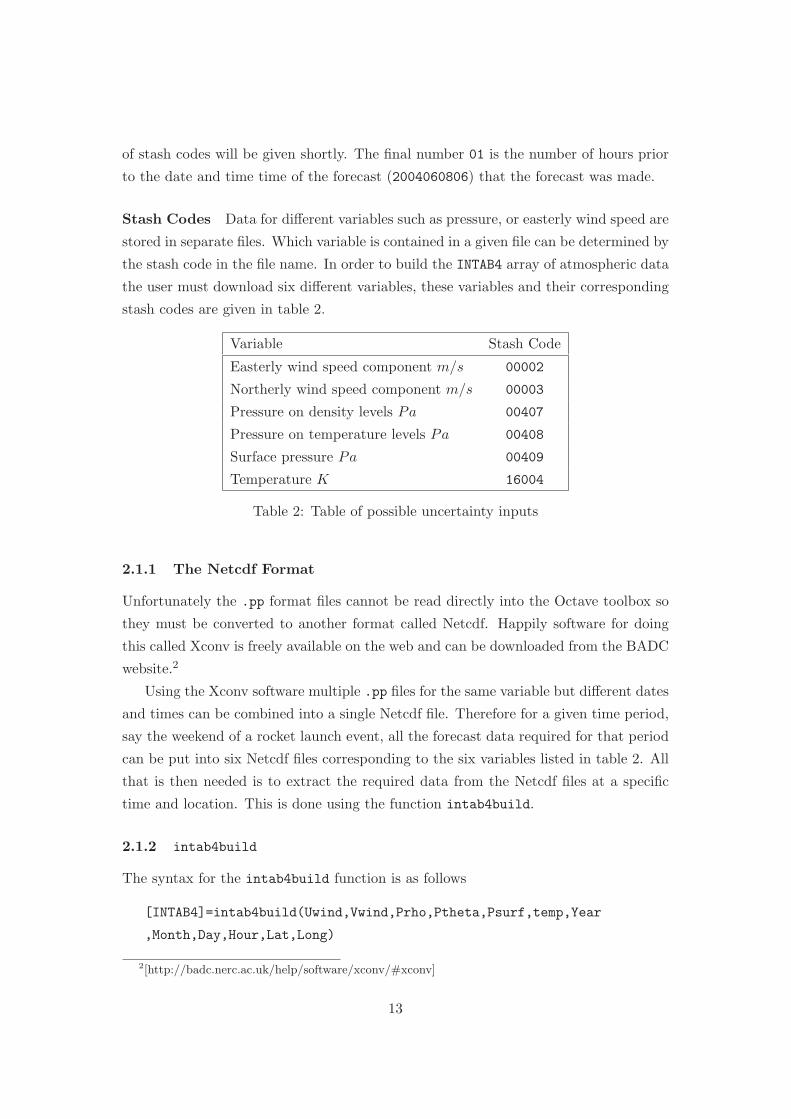
Stash Codes Data for different variables such as pressure, or easterly wind speed are
stored in separate files. Which variable is contained in a given file can be determined by
the stash code in the file name. In order to build the INTAB4 array of atmospheric data
the user must download six different variables, these variables and their corresponding
stash codes are given in table 2.
Variable Stash Code
Easterly wind speed component m/s 00002
Northerly wind speed component m/s 00003
Pressure on density levels Pa 00407
Pressure on temperature levels Pa 00408
Surface pressure Pa 00409
Temperature K 16004
Table 2: Table of possible uncertainty inputs
2.1.1 The Netcdf Format
Unfortunately the .pp format files cannot be read directly into the Octave toolbox so
they must be converted to another format called Netcdf. Happily software for doing
this called Xconv is freely available on the web and can be downloaded from the BADC
website.2
Using the Xconv software multiple .pp files for the same variable but different dates
and times can be combined into a single Netcdf file. Therefore for a given time period,
say the weekend of a rocket launch event, all the forecast data required for that period
can be put into six Netcdf files corresponding to the six variables listed in table 2. All
that is then needed is to extract the required data from the Netcdf files at a specific
time and location. This is done using the function intab4build.
2.1.2 intab4build
The syntax for the intab4build function is as follows
[INTAB4]=intab4build(Uwind,Vwind,Prho,Ptheta,Psurf,temp,Year
,Month,Day,Hour,Lat,Long)
2[http://badc.nerc.ac.uk/help/software/xconv/#xconv]
13
The output argument of intab4build is the array INTAB4 ready for input into the
simulation functions. The input arguments are as follows: Uwind is a string containing
the file path to the Netcdf file which contains the Easterly wind speed component data.
Vwind is a string containing the file path to the Netcdf file which contains the Northerly
wind speed component data. Prho is a string containing the file path to the Netcdf
file which contains the pressure on density levels data. Ptheta is a string containing
the file path to the Netcdf file which contains the pressure on temperature levels data.
Psurf is a string containing the file path to the Netcdf file which contains the surface
pressure data. temp is a string containing the file path to the Netcdf file which contains
the temperature data. Year is a number representing the year of the forecast e.g. 2004.
Month is the month e.g. 3,or 11. Day is the day e.g. 2, or 24. Hour is the hour which
the forecast is for. This cannot be any hour as usually Met office forecasts are for either
00:00, 06:00, 12:00 or 18:00, so in order to avoid getting an error message the specified
value of Hour must be 0,6,12 or 18. Lat and Long are the coordinates of the rocket
launch site for which the atmospheric data are required in latitude and longitude using
the decimal format e.g. 0.043 and 52.175.
2.2 Forecast data from the F214 form
If Met Office NWP data is not available directly then it is possible to get a very
simplified form of the data in the form of the F214 aviation briefing form. This is freely
available to download from the Met Office website and contains data for wind speed,
wind direction and temperature at six altitudes between 1000 and 24,000 ft on a coarse
grid (5◦ lat ×5◦ long) across the UK.
The data from an F214 form can be converted into an INTAB4 array using the
function f214read.
2.2.1 f214read
The syntax for f214read is
[INTAB4]=f214read(F214)
The input F214 is an array created by the user which should contain the data from
the F214 form as it appears on the form. It has four columns the first is altitude in
feet, the second is wind direction in degrees from true North, the third column is wind
speed in knots and the fourth column is temperature in degrees centigrade. It is also a
good idea to add a row at the bottom of the F214 with altitude 0, wind speed at this
altitude is 0 and temperature is the local temperature at the launch site. If the wind
14
speed on the ground at the launch site is being measured it is also a good idea to add
a row containing this data at the altitude the measurement is being taken.
The output is the data table INTAB4, ready for use in the simulations.
3 The Simulations
Once the INTAB and INTAB4 data structures for the rocket design and the atmospheric
conditions have been defined the the user can proceed to the rocket simulations. If the
user wants to dive straight in and play with the simulations then then toolbox contains
a number of pre-made INTAB and INTAB4 data structures for various types of one and
two stage rockets. These can be loaded into the workspace, the names of the pre-made
input files are listed in table 3.
Description Filename
Single stage rocket INTAB data intab CLV2s1 K660
Single stage rocket INTAB data intab cirrusdart H153
Boosted dart, dart stage INTAB data intab camdart
Boosted dart, booster stage INTAB data intab cambooster
Boosted dart, combined stages INTAB data intab camdart plus booster
INTAB4 atmospheric data intab4 2006100809
INTAB4 atmospheric data intab4 2006100812
INTAB4 atmospheric data intab4 2006100815
INTAB4 atmospheric data intab4 2006100818
Table 3: Pre-made input data variables that can be loaded from the toolbox
This section describes seven functions, the first six are the rocket simulation func-
tions, these are listed below.
rocketflight [Simulation of 1-stage rocket flight.]
rocketflight 2 stage [Simulation of 2-stage rocket flight.]
rocketflight monte [1-stage simulation with Monte Carlo.]
rocketflight 2 stage monte [2-stage sim with Monte Carlo.]
rocketflight delivery [Landing location optimiser.]
rocketflight 2 stage delivery [Landing location optimiser.]
The outputs of these functions are graphical plots of the rocket flight paths and splash
patterns etc. and also limited data tables giving the rockets translational and rotational
position and the rockets linear and angular momentum, varying with time. If the user
15
requires more detailed data about how all the rocket variables are changing with time
then the a post processing operation can be performed using the seventh function
described in this section - flight variables.
3.1 rocketflight
This function simulates the flight path and parachute recovery of a single stage rocket.
The syntax for the rocketflight function is
[Asc,Des,Landing,Apogee]=rocketflight(INTAB,INTAB4,altpd,Rl,Ra,Rb)
Input arguments INTAB is the data structure containing the rocket design data,
INTAB4 is the data structure containing the atmospheric data. altpd is the altitude
for the deployment of the main parachute when using a dual deploy system. If the
rocket has a single deploy system altpd must still be specified, the value specified will
not affect the situation although it is best practice to use ‘0’. Rl is the length of the
rocket launch rail or tower in meters. Ra is the angle (degrees) of the launch tower’s
declination from the vertical, Rb is the bearing (degrees from north) to which the launch
tower is pointing.
Output arguments Asc is a data table for the Ascent portion of the rocket flight
the table has fifteen columns. Columns 1-4 are, time (s), Easterly (X) position(m),
Northerly (Y) position(m) and Altitude (Z)(m). Columns 5-8 contain the four elements
of a quaternion describing the rockets rotational position. Columns 9-11 contain the
three elements of the rockets linear momentum vector. Columns 12-14 contain the
three elements of the rockets angular momentum vector.
Des is a data table for the Descent portion of the rocket flight the table has seven
columns. Columns 1-4 are time and X,Y,and Z position. Columns (5-7) are the three
elements of a vector describing the linear momentum of the rocket under parachute.
Landing contains the coordinates of the rocket’s landing position and Apogee con-
tains the coordinates of the rocket’s apogee.
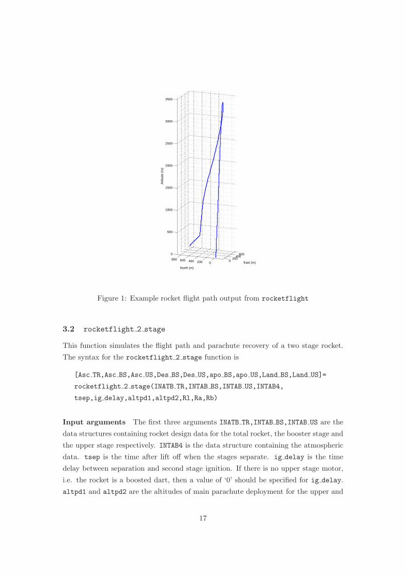
In addition to the output arguments, rocketflight also outputs a 3-d graphical
plot of the rocket’s flight path like the one shown in fig 1.
16
0200
400600
0200400600800
0
500
1000
1500
2000
2500
3000
3500
East (m)
North (m)
Alti
tude
(m
)
Figure 1: Example rocket flight path output from rocketflight
3.2 rocketflight 2 stage
This function simulates the flight path and parachute recovery of a two stage rocket.
The syntax for the rocketflight 2 stage function is
[Asc TR,Asc BS,Asc US,Des BS,Des US,apo BS,apo US,Land BS,Land US]=
rocketflight 2 stage(INATB TR,INTAB BS,INTAB US,INTAB4,
tsep,ig delay,altpd1,altpd2,Rl,Ra,Rb)
Input arguments The first three arguments INATB TR,INTAB BS,INTAB US are the
data structures containing rocket design data for the total rocket, the booster stage and
the upper stage respectively. INTAB4 is the data structure containing the atmospheric
data. tsep is the time after lift off when the stages separate. ig delay is the time
delay between separation and second stage ignition. If there is no upper stage motor,
i.e. the rocket is a boosted dart, then a value of ‘0’ should be specified for ig delay.
altpd1 and altpd2 are the altitudes of main parachute deployment for the upper and
17
booster stages respectively. If dual deploy is not being used then ‘0’ should be specified.
Rl,Ra,Rb are the launch tower length, declination angle and bearing respectively.
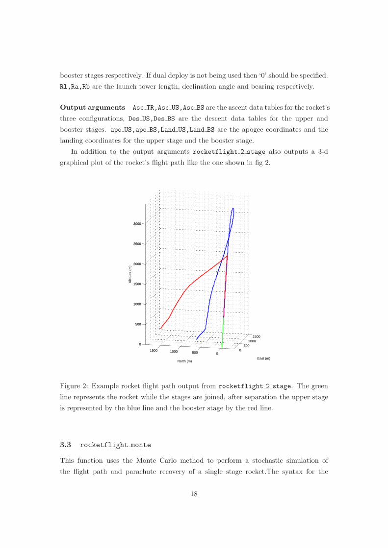
Output arguments Asc TR,Asc US,Asc BS are the ascent data tables for the rocket’s
three configurations, Des US,Des BS are the descent data tables for the upper and
booster stages. apo US,apo BS,Land US,Land BS are the apogee coordinates and the
landing coordinates for the upper stage and the booster stage.
In addition to the output arguments rocketflight 2 stage also outputs a 3-d
graphical plot of the rocket’s flight path like the one shown in fig 2.
0500
10001500
050010001500
0
500
1000
1500
2000
2500
3000
East (m)North (m)
Alti
tude
(m
)
Figure 2: Example rocket flight path output from rocketflight 2 stage. The green
line represents the rocket while the stages are joined, after separation the upper stage
is represented by the blue line and the booster stage by the red line.
3.3 rocketflight monte
This function uses the Monte Carlo method to perform a stochastic simulation of
the flight path and parachute recovery of a single stage rocket.The syntax for the
18
rocketflight monte function is
[Ascbig,Desbig,Landing,Apogee]=
rocketflight monte(INTAB,INTAB4,altpd,Rl,Ra,Rb,noi)
Input arguments The input arguments shown in the syntax above are the same as
for rocketflight (sec 3.1) with the addition of the final argument noi which specifies
the number of Monte Carlo iterations. Using the above syntax will cause the code to run
using the default values for uncertainty in the variables which are perturbed during the
simulation. It is possible to input user specified values for uncertainty, however here we
do not specify how these values are handled by the software, but simply how to modify
them. Therefore it is recommended that the default values are used unless the user has
a good understanding of how the uncertainty values are implemented.
To change an uncertainty variable you have to add two arguments to the end of
the inputs firstly a string label to identify the variable to be changed and then the new
value of the uncertainty variable. for example:
.....Ra,Rb,noi,‘Cdmult’,0.4)
A table detailing the various uncertainty values that can be specified and the appro-
priate syntax is given in table 4. Any number of the variables can be changed by simply
adding the relevant syntax to the end of the input arguments in any order. Specifying
new values for the uncertainty variables will not change them permanently, if a value
is not specified the next time the code is run then it will revert to the default value.
Variable Label Class
Rocket drag coefficient multiplier ‘CDmult’ scaler
Centre of pressure multiplier ‘CPmult’ scalar
Normal force coefficient multiplier ‘CNmult’ scalar
Drogue ’chute drag multiplier ‘CDDmult’ scalar
Main ’chute drag multiplier ‘CDPmult’ scalar
Wind Gaussian process mean ‘MU’ 15 × 1 vector
Wind Gaussian process covariance ‘SIGMA’ 15 × 15 matrix
Table 4: Table of possible uncertainty inputs
Output arguments The output arguments are similar to those of rocketflight.
Ascbig and Desbig are cell arrays where the cells contain the ascent and descent data
19
tables for each Monte Carlo iteration preformed by the function. Landing and Apogee
are tables of coordinates for the landing position and apogee of each iteration. In the
first iteration of any run all uncertain variables have their mean value.
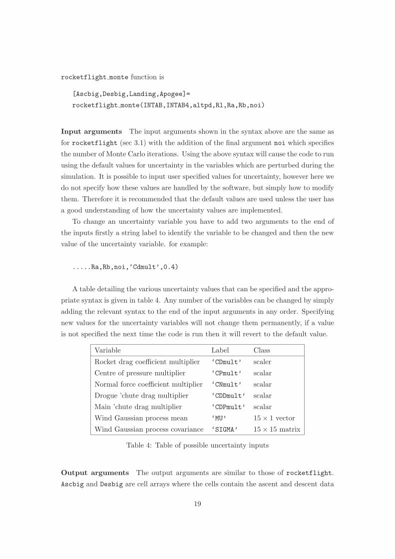
In addition to the output arguments rocketflight monte also outputs 3 plots.
Figure 3 is an example of the first plot which shows a 3-D flight path corresponding
to a the flight path for a rocket where of all the uncertain variables are at their mean
value. Also shown are Gaussian ellipses marking the probable landing zones, where the
red ellipse marks the area corresponding to one standard deviation and the green ellipse
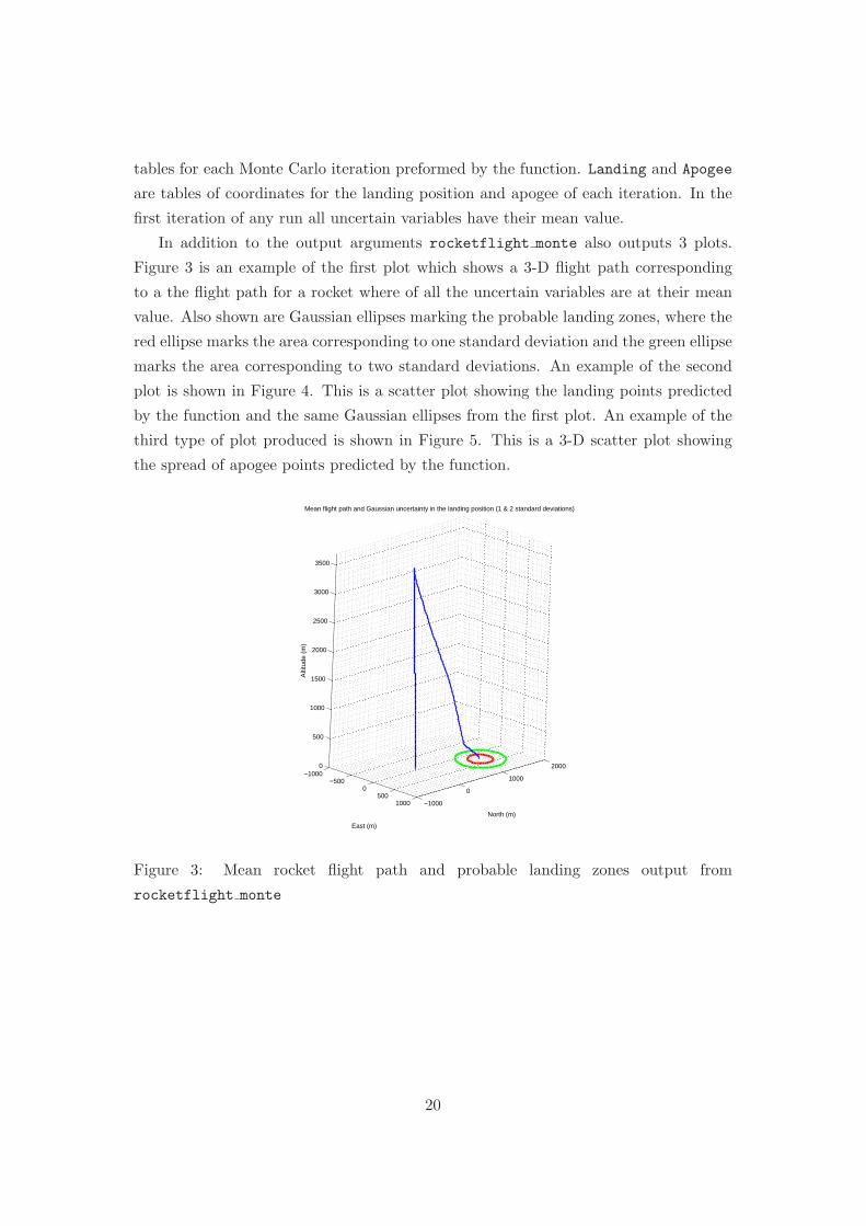
marks the area corresponding to two standard deviations. An example of the second
plot is shown in Figure 4. This is a scatter plot showing the landing points predicted
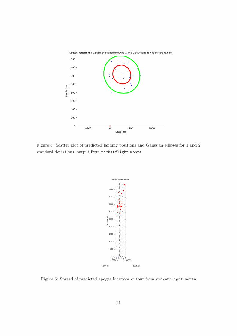
by the function and the same Gaussian ellipses from the first plot. An example of the
third type of plot produced is shown in Figure 5. This is a 3-D scatter plot showing
the spread of apogee points predicted by the function.
−1000−500
0500
1000 −1000
0
1000
20000
500
1000
1500
2000
2500
3000
3500
North (m)
Mean flight path and Gaussian uncertainty in the landing position (1 & 2 standard deviations)
East (m)
Alti
tude
(m
)
Figure 3: Mean rocket flight path and probable landing zones output from
rocketflight monte
20
−500 0 500 10000
200
400
600
800
1000
1200
1400
1600
East (m)
Nor
th (
m)
Splash pattern and Gaussian elipses showing 1 and 2 standard deviations probability
Figure 4: Scatter plot of predicted landing positions and Gaussian ellipses for 1 and 2
standard deviations, output from rocketflight monte
−1000100200−400−2000
0
500
1000
1500
2000
2500
3000
3500
4000
4500
East (m)
apogee scatter pattern
North (m)
Alti
tude
(m
)
Figure 5: Spread of predicted apogee locations output from rocketflight monte
21
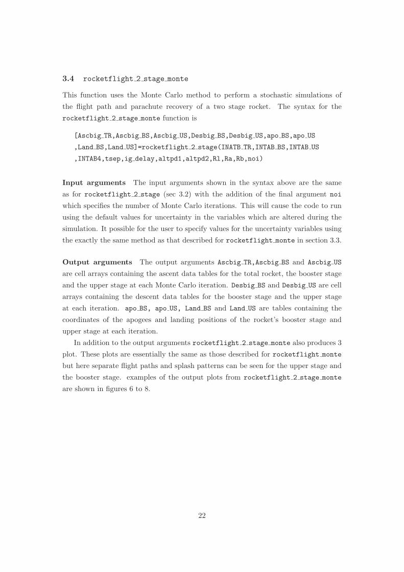
3.4 rocketflight 2 stage monte
This function uses the Monte Carlo method to perform a stochastic simulations of
the flight path and parachute recovery of a two stage rocket. The syntax for the
rocketflight 2 stage monte function is
[Ascbig TR,Ascbig BS,Ascbig US,Desbig BS,Desbig US,apo BS,apo US
,Land BS,Land US]=rocketflight 2 stage(INATB TR,INTAB BS,INTAB US
,INTAB4,tsep,ig delay,altpd1,altpd2,Rl,Ra,Rb,noi)
Input arguments The input arguments shown in the syntax above are the same
as for rocketflight 2 stage (sec 3.2) with the addition of the final argument noi
which specifies the number of Monte Carlo iterations. This will cause the code to run
using the default values for uncertainty in the variables which are altered during the
simulation. It possible for the user to specify values for the uncertainty variables using
the exactly the same method as that described for rocketflight monte in section 3.3.
Output arguments The output arguments Ascbig TR,Ascbig BS and Ascbig US
are cell arrays containing the ascent data tables for the total rocket, the booster stage
and the upper stage at each Monte Carlo iteration. Desbig BS and Desbig US are cell
arrays containing the descent data tables for the booster stage and the upper stage
at each iteration. apo BS, apo US, Land BS and Land US are tables containing the
coordinates of the apogees and landing positions of the rocket’s booster stage and
upper stage at each iteration.
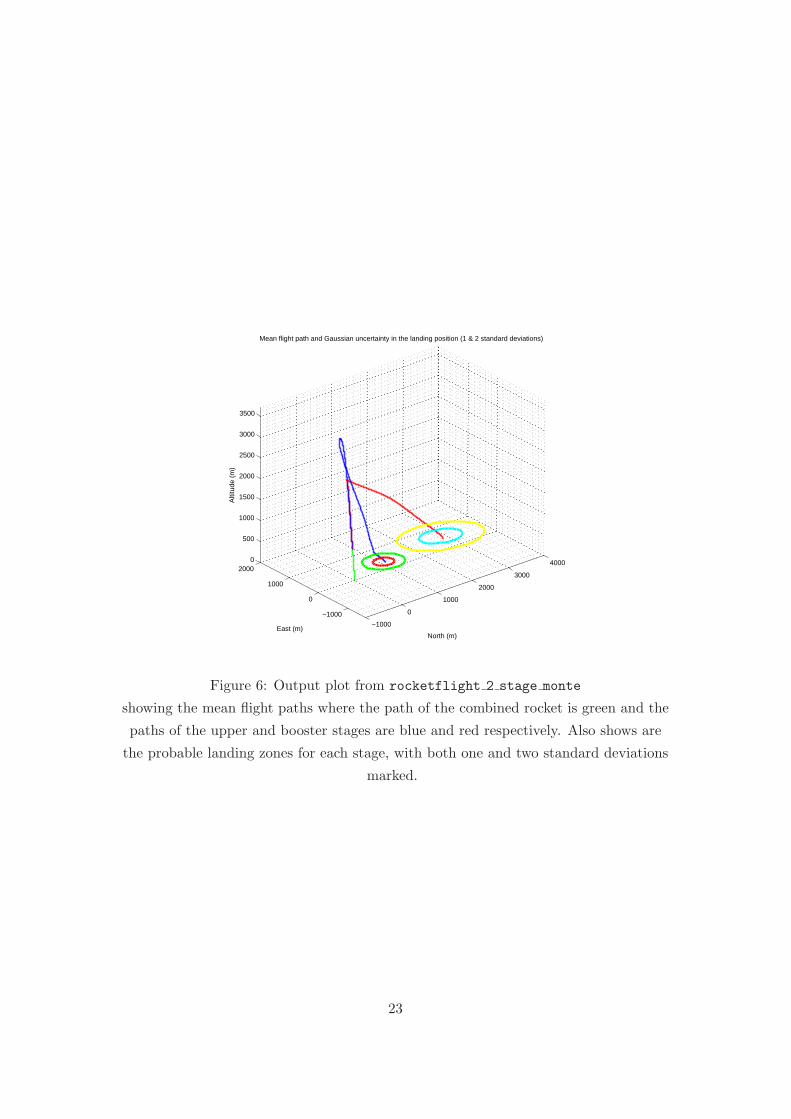
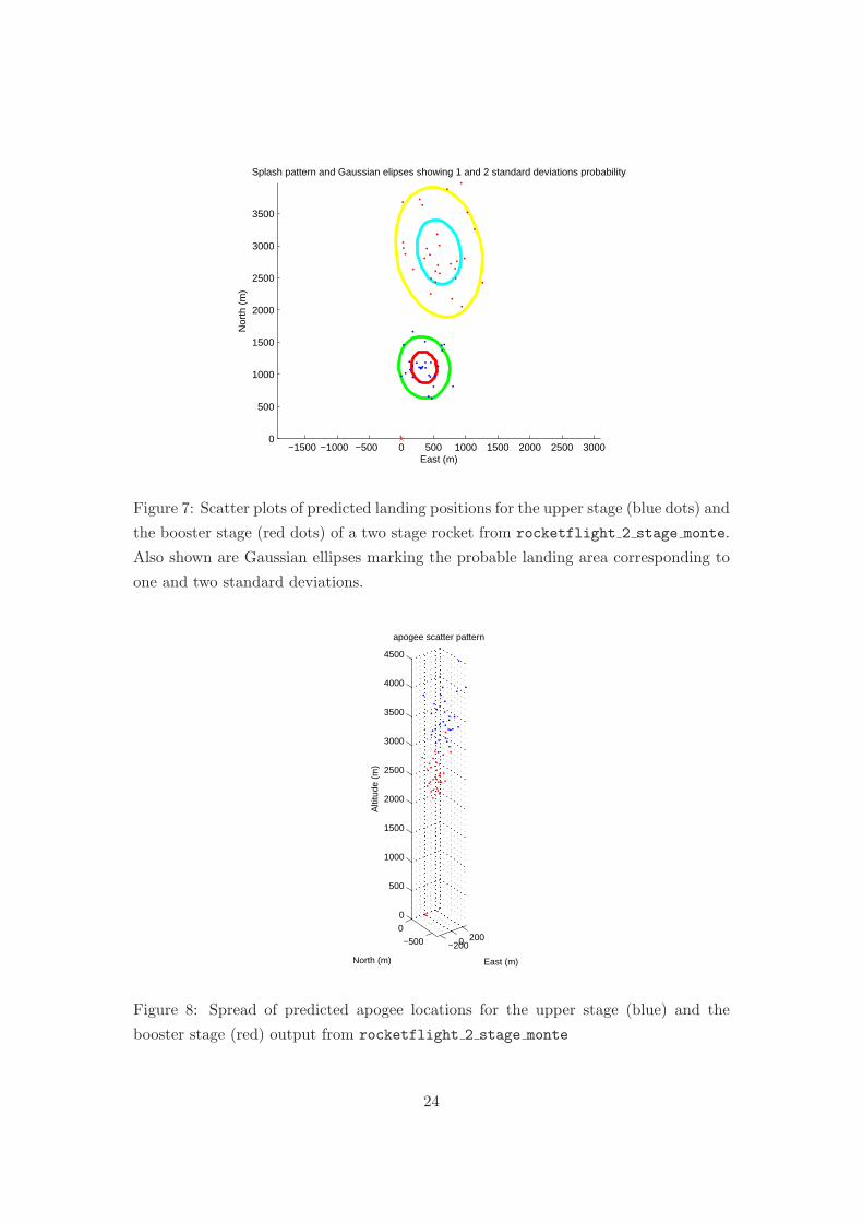
In addition to the output arguments rocketflight 2 stage monte also produces 3
plot. These plots are essentially the same as those described for rocketflight monte
but here separate flight paths and splash patterns can be seen for the upper stage and
the booster stage. examples of the output plots from rocketflight 2 stage monte
are shown in figures 6 to 8.
22
−1000
0
1000
2000
−1000
0
1000
2000
3000
40000
500
1000
1500
2000
2500
3000
3500
North (m)
Mean flight path and Gaussian uncertainty in the landing position (1 & 2 standard deviations)
East (m)
Alti
tude
(m
)
Figure 6: Output plot from rocketflight 2 stage monte
showing the mean flight paths where the path of the combined rocket is green and the
paths of the upper and booster stages are blue and red respectively. Also shows are
the probable landing zones for each stage, with both one and two standard deviations
marked.
23
−1500 −1000 −500 0 500 1000 1500 2000 2500 30000
500
1000
1500
2000
2500
3000
3500
East (m)
Nor
th (
m)
Splash pattern and Gaussian elipses showing 1 and 2 standard deviations probability
Figure 7: Scatter plots of predicted landing positions for the upper stage (blue dots) and
the booster stage (red dots) of a two stage rocket from rocketflight 2 stage monte.
Also shown are Gaussian ellipses marking the probable landing area corresponding to
one and two standard deviations.
−2000 200−500
0
0
500
1000
1500
2000
2500
3000
3500
4000
4500
East (m)
apogee scatter pattern
North (m)
Alti
tude
(m
)
Figure 8: Spread of predicted apogee locations for the upper stage (blue) and the
booster stage (red) output from rocketflight 2 stage monte
24
3.5 The ‘ballisticfailure’ argument
As well able being a to simulate what happens when the a rocket flight goes according
to plan it is also possible to simulate the flight path when things go wrong. In the event
that the rockets electronics fail and the parachutes do not deploy then the rocket will
follow a ballistic flight path. The four functions described in sections 3.1 to 3.4 can be
used to simulate the events of a ballistic failure. This is done by adding the argument
‘ballisticfailure’ to the function inputs. When using the functions rocketflight
or rocketflight 2 stage then ‘ballisticfailure’ must be the last input argument.
When using the functions rocketflight monte or rocketflight 2 stage monte using
the function’s default values for the uncertainty variables then ‘ballisticfailure’
must be the final input argument, however if any user specified uncertainty variables
are being used then ‘ballisticfailure’ must come before these arguments. An ex-
ample of the syntax for this situation is given below.
[Ascbig,Desbig,Landing,Apogee]=rocketflight monte(INTAB,INTAB4,altpd,
Rl,Ra,Rb,noi,‘ballisticfailure’,‘CDmult’,value1,‘CDPmult’,value2)
When the ‘ballisticfailure’ argument is added the function performs in the
same way as described in sections 3.1 to 3.4 except it is assumed that no parachutes
are deployed and that the rocket remains intact. In two stage simulations it is assumed
that the stages separate.
3.6 rocketflight delivery
This function allows the user to specify a desired landing location for a single stage
rocket. The code then runs simulations iteratively to find the angles of declination and
bearing in the launch tower that will achieve the desired landing location.
The syntax for the rocketflight delivery function is
[Dec,Bea,Asc,Des,Landing,Apogee]=
rocketflight delivery(INTAB,INTAB4,altpd,Rl,address,rsen,imax)
Input arguments The arguments INTAB,INTAB4,altpd and Rl have the same mean-
ings as described in section 3.1 on the rocketflight function. The argument address
is a two element vector containing the coordinates of the desired landing location assum-
ing a standard Cartesian coordinate system where East is the positive X-direction and
North is the positive Y -direction and the launchpad lies at the origin. The argument
rsen is the accuracy with which the landing position is to be determined. In practice
25
the function will stop integrating when the current landing position of the rocket lies
inside a circle of radius rsen surrounding the coordinates specified in address. The
argument imax specifies the maximum number of iterations to be carried out. It is
important to specify a sensible number here as the function cannot detect when the
address is out of range. For a value of rsen=10m it is usual for convergence to be
reached in 5 iterations or less. Therefore a sensible value for imax might be 20. failure
to converge in this number of iterations would indicate that the specified address is,
almost certainly, out of range.
Output arguments The argument Dec is the angle of declination in the launch rail
required to achieve the landing position, defined as the angle between the launch rain
and the vertical in degrees. The argument Bea is the bearing to which the launch rail
is pointing in degrees from due North. The output arguments from Asc up to Apogee
are the same as those for the standard rocketflight function described in section 3.1.
rocketflight delivery also outputs a 3-D plot of the flight path of the rocket
landing at the specified location.
3.7 rocketflight 2 stage delivery
This function does exactly the same as rocketflight delivery for a two stage rocket.
It is the landing position of the upper stage which the function tries to optimise.
The syntax for rocketflight 2 stage delivery is as follows:
[Dec,Bea,Asc TR,Asc BS,Asc US,Des BS,Des US,apo BS,apo US,Land BS,Land US]=
rocketflight 2 stage delivery(INATB TR,INTAB BS,INTAB US,INTAB4,
tsep,ig delay,altpd1,altpd2,Rl,address,rsen,imax)
Input arguments The input arguments from INTAB TR up to Rl are the same as
those for the standard rocketflight 2 stage function described in section 3.2. The
argument address is a two element vector containing the coordinates of the desired
landing location assuming a standard Cartesian coordinate system where East is the
positive X-direction and North is the positive Y -direction and the launchpad lies at
the origin. The argument rsen is the accuracy with which the landing position is to
be determined. In practice the function will stop integrating when the current landing
position of the rocket lies inside a circle of radius rsen surrounding the coordinates
specified in address. The argument imax specifies the maximum number of iterations
to be carried out.
26
Output arguments The argument Dec is the angle of declination in the launch rail
required to achieve the landing position for the rockets upper stage, defined as the angle
between the launch rain and the vertical in degrees. The argument Bea is the bearing to
which the launch rail is pointing in degrees from due North. The output arguments from
Asc TR up to Land US are the same as those for the standard rocketflight 2 stage
function described in section 3.2.
rocketflight 2 stage delivery also outputs a 3-D plot of the flight paths of the
rocket’s stages, with the upper stage landing at the specified location.
3.8 flight variables
All the “rocketflight” functions described above output “Asc” tables containing data on
the portion of the flight before the rocket deploys a parachute. An Asc table has fourteen
columns. Columns 1-4 are, time (s), X position(m), Y position(m), Z position(m).
Columns 5-8 contain the four elements of a quaternion describing the rockets rotational
position. Columns 9-11 contain the three elements of the rockets linear momentum
vector. Columns 12-14 contain the three elements of the rockets angular momentum
vector. However the user analysing the simulation may require data on variables other
than those listed above such as the forces on the rocket and the position of the rocket’s
centre of mass.
The function flight variables takes the Asc table as well as the input data tables
for the corresponding portion of flight and produces a much larger more comprehensive
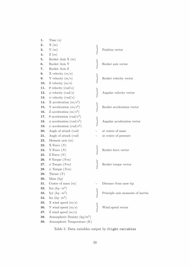
data table. The larger table has 39 columns The variables that are in these columns
are given in table 5. flight variables generates a table in octave containing these
data and also a comma separated data file (.csv) which can be opened and viewed
using spreadsheet software such as Open Office Spreadsheet or Microsoft Excel.
The syntax for flight variables is as follows.
[headers,RDT]=flight variables(‘filename’,Asc,INTAB,INTAB4,
Rl,Ra,Rbea,igdelay)
Input arguments The filename argument is a string that contains the path and
filename for the .csv file created by flight variables. The Asc argument is the a
flight data table output from one of the simulation functions. If a two stage rocket
is being simulated then there will be three of these tables, these must be analysed
separately and individually with flight variables. The following arguments must
be the same as those used by the simulation function to generate Asc. INTAB contains
the rocket design data, INTAB4 contains the atmospheric data. Rl, Ra and Rbea are
27
1. Time (s)
2. X (m) }
Position vector3. Y (m)
4. Z (m)
5. Rocket Axis X (m) }
Rocket axis vector6. Rocket Axis Y
7. Rocket Axis Z
8. X velocity (m/s) }
Rocket velocity vector9. Y velocity (m/s)
10. Z velocity (m/s)
11. θ velocity (rad/s) }
Angular velocity vector12. φ velocity (rad/s)
13. ψ velocity (rad/s)
14. X acceleration (m/s2) }
Rocket acceleration vector15. Y acceleration (m/s2)
16. Z acceleration (m/s2)
17. θ acceleration (rad/s2) }
Angular acceleration vector18. φ acceleration (rad/s2)
19. ψ acceleration (rad/s2)
20. Angle of attack (rad) - at centre of mass
21. Angle of attack (rad) - at centre of pressure
22. Moment arm (m)
23. X Force (N) }
Rocket force vector24. Y Force (N)
25. Z Force (N)
26. θ Torque (Nm) }
Rocket torque vector27. φ Torque (Nm)
28. ψ Torque (Nm)
29. Thrust (N)
30. Mass (kg)
31. Centre of mass (m) - Distance from nose tip
32. Ixx (kg ·m2) }
Principle axis moments of inertia33. Iyy (kg ·m2)
34. Izz (kg ·m2)
35. X wind speed (m/s) }
Wind speed vector36. Y wind speed (m/s)
37. Z wind speed (m/s)
38. Atmospheric Density (kg/m3)
39. Atmospheric Temperature (K)
Table 5: Data variables output by flight variables
28
the launch rail length, angle and bearing respectively. If it is the latter stages of a
two stage flight that are being analysed then these values are unimportant, but some
values must be specified to act as spacers. The final argument igdelay is an optional
variable that can be omitted if not necessary, If analysing the second stage of a two
stage flight igdelay is the time delay in seconds between stage separation and second
stage ignition.
Output arguments RDT is the rocket data table containing data on how 38 variables
are changing with time during the rocket flight. headers is a 1×39 cell array of strings
containing labels identifying which variable is in which column of RDT, these correspond
to the variables listed in table 5.
29
Part II
Additional Toolbox Functions
Part I describes the main functions of the High power rocketry toolbox and the various
ways to use these functions in order to simulate rocket flights. The toolbox contains
many other functions which are called by the main functions described in part I. While
it is not necessary to have knowledge of these functions to use the toolbox for simula-
tions, a user wishing to write their own functions to perform specific rocketry oriented
tasks may find them very useful. Part II contains basic help information on a number
of these additional functions organised alphabetically by function name.
4 ascentcalc
ascentcalc along with descentcalc(see sec 8) form the backbone of all the rocket
simulation functions. ascentcalc is used to simulate the rocket portion of the flight
while descentcalc is used to simulate the parachute descent.
A user might wish to simulate a particular type of rocket or flight behaviour that
it is not possible to do using any of the available simulation functions, for example a
three stage rocket. It is possible for a user to write their own code to deal with this
using ascentcalc and descentcalc.
ascentcalc simulates rocket flights by numerical integration of the rocket’s equa-
tions of motion using the Runge Kutta method, and the rocket’s rotational position is
tracked using quaternions. The syntax for ascentcalc is
[tt,z]=ascentcalc(ttspan,z0,YA0,PA0,RA0,INTAB1,INTAB2,INTAB3,INTAB4,
Ar,Rl,Ra,mu,RBL,G,label,igdelay)
Input arguments
ttspan is a two element array specifying the time span the simulation is to run for e.g.
[0 100] would cause the simulation to run from 0 to 100 seconds. The simulation will
also stop automatically if certain conditions are met, this will be discussed shortly.
z0 is a 1 × 13 array containing the initial conditions for the simulations. Elements
1−3 contain the Cartesian coordinates of the rocket’s initial position it is recommended
that these be [0,0,0]. Elements 4 − 7 contain a quaternion describing the initial
orientation of the rocket’s body axes relative to the global coordinate axes. Elements
30
8−10 contain the rocket’s initial linear momentum vector, and elements 11−13 contain
the rocket’s initial angular momentum vector.
YA0,PA0 and RA0 are unit vectors describing the global Cartesian axes, it is un-
likely that these should require any values other than [1;0;0], [0;1;0] and [0;0;1]
respectively.
INTAB1,INTAB2 and INTAB3 are data tables containing time-dependent data, drag
data and centre of pressure data and they are unpacked from INTAB(see section 1.1.4).
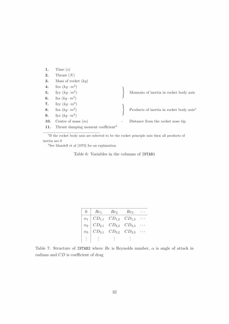
INTAB1 is an eleven column array containing data on time dependent rocket variables,
table 6 shows the variables contained in INTAB1. INTAB2 is a 2-D data table which
can be of any size and contains values of the rocket coefficient of drag varying with
Reynolds number and angle of attack. The structure of INTAB2 is shown in table 7.
INTAB3 is a two element array where the first element is the coefficient of normal force
for the rocket, and the second is the distance of the rocket’s centre of pressure from the
nose tip in metres.
The input argument INTAB4 is the table of atmospheric data which is described in
section 2. Ar is the frontal cross-sectional area of the rocket body. Rl and Ra are the
launch rail length and launch rail angle of declination (in degrees) respectively. RBL is
the length of the rocket body in metres. G is the universal gravitational constant. label
is a string, if this string reads anything other than ‘ballisticfailure’ then the rocket
simulation will terminate at apogee, however if it does read ‘ballisticfailure’ then
the rocket simulation will terminate when the rocket hits the ground. If the user wants
the simulation to end at any other time then they can specify a specific end time using
ttspan. This will only work if the simulation reaches the end time before the rocket
reaches apogee in the normal case, or before the rocket hits the ground in the ballistic
failure case. The final argument igdelay is optional and inserts a delay of “igdelay”
seconds between the start of the simulation and motor ignition, this is useful when using
ascentcalc to simulate the upper stages of a multi-stage rocket. igdelay should not
be used to insert a delay in ignition when the rocket is stationary on the launch pad as
this can cause problems with the time step size in the numerical integration.
31
1. Time (s)
2. Thrust (N)
3. Mass of rocket (kg)
4. Ixx (kg ·m2) }
Moments of inertia in rocket body axis5. Iyy (kg ·m2)
6. Izz (kg ·m2)
7. Ixy (kg ·m2) }
Products of inertia in rocket body axisa8. Ixz (kg ·m2)
9. Iyz (kg ·m2)
10. Centre of mass (m) - Distance from the rocket nose tip
11. Thrust damping moment coefficientb
aIf the rocket body axis are selected to be the rocket principle axis then all products of
inertia are 0bSee Mandell et al [1973] for an explanation
Table 6: Variables in the columns of INTAB1
0 Re1 Re2 Re3 · · ·
α1 CD1,1 CD1,2 CD1,3 · · ·
α2 CD2,1 CD2,2 CD2,3 · · ·
α3 CD3,1 CD3,2 CD3,3 · · ·...
......
...
Table 7: Structure of INTAB2 where Re is Reynolds number, α is angle of attack in
radians and CD is coefficient of drag
32
Output arguments
The output argument z is a thirteen column array containing the following variables:
Columns 1 − 3 contain Cartesian coordinates of the rocket’s position. Columns 4 − 7
contain the elements of a quaternion describing the orientation of the rocket’s body
axes relative to the global coordinate axes. Columns 8 − 10 contain the rocket’s linear
momentum vector, and columns 11−13 contain the rocket’s angular momentum vector.
The argument tt is a single column array with the same number or rows as z containing
the times in seconds that correspond to the rows of z. In the simulation functions
described in section 3 these two arrays are combined into a single array called Asc.
5 axi com
The function axi com performs a simple 1-D calculation of the centre of mass for an
axi-symmetric body (like a rocket) assuming that the body can be represented by a
number of point masses that all lie on a line, in this case the axis of the rocket. The
syntax for axi com is:
Xcm=axi com(PM1,PM2,PM3....)
Arguments
any single input argument to axi com must be a two element array representing a point
mass of the form [M,X], where M is the mass in and X is the distance from some reference
point, this is usually the nose tip of the rocket. axi com can accept any number of point
mass inputs, but all must be referenced to the same point.
The output argument Xcm is the distance of the centre of mass from the reference
point.
6 Barrowman calc
This function uses the “Barrowman method” [Barrowman & Barrowman, 1966] to
calculate the normal force coefficient and location of the centre of pressure for a rocket.
The function works by calculating these two parameters for each rocket component
individually. The three types of rocket component for which the centre of pressure can
be calculated are nose cones, conical transitions, and finsets. Given that the normal
33
force on the body tube is taken to be negligible by the Barrowman method these three
shapes are sufficient for the calculations on most rockets of relatively simple shape.
The syntax for Barrowman calc is as follows.
[Cna,Xcp]=Barrowman calc(N1,CT1,F1...)
Arguments
Barrowman calc can accept three types of argument that are cell arrays containing
data on one of three components, either a nose cone, a conical transition or a finset.
However Barrowman calc can accept any number of these arguments in any order.
Nose cone argument
This is a cell array with three cells, the first must contain the string ‘nose’ to identify
the part. The second cell contains another string describing the shape of the nose,
this can be either ‘conical’, ‘parabolic’ or ‘ogive’. The final cell contains a two
element array with two numbers in it, firstly the length on the nose cone in meters
and secondly the distance from the most upstream part of the nose cone to the most
upstream part of the rocket (this is usually 0).
{‘nose’,‘conical’,[L,X]}
Conical transition argument
This is a two cell, cell array. The first cell contains the string ‘cone trans’ to identify
the part. The second cell contains an array with the following data: the reference diam-
eter (dr) (diameter of the rocket at the base of the nose cone), the transition upstream
diameter (du), the transition downstream diameter (dd), the length of the transition
(L) and the position (X) (distance from the nose tip to the most upstream part of the
transition).
{‘cone trans’,[dr,du,dd,L,X]}
34
Finset argument
This is a two cell, cell array. The first cell contains the string ‘finset’ to identify the
part. The second cell cell contains an array with the following data: the number of
fins (n), the rocket body diameter at the finset (d), the reference diameter (dr), the fin
root length (a), the fin tip length (b), the fin sweep length (m), the fin span (s) and
the finset position (X) (the distance between the nose tip and the most upstream part
of the finset).
{‘finset’,[n,d,dr,a,b,m,s,X]}
Output arguments
The output arguments are Cna the coefficient of normal force for the rocket, and Xcp
the position of the centre of pressure on the rocket, i.e. the distance from the nose cone
tip to the centre of pressure.
7 bearing to vector
This functions converts a bearing, that is a direction in the plane of the earth’s surface
defined as degrees from true north in the clockwise direction, to a vector where the pos-
itive X-direction is East and the Positive Y -direction is North. The output vector also
contains a value for the Z-direction which is zero. The syntax for bearing to vector is
vector=bearing to vector(bearing)
bearing is a single value of degrees, and vector is a three element vector.
8 descentcalc
This function performs a 3-degree-of-freedom simulation of a rocket descending under a
parachute. descentcalc is used in conjunction with ascentcalc to simulate complete
rocket flights. The syntax for descentcalc is
[tt,z]=descentcalc(ttspan,z0,INTAB4,INTAB1,paratab,altpd,G)
35
Input arguments
ttspan is a two element array specifying the time span the simulation is to run for e.g.
[0 100] would cause the simulation to run from 0 to 100 seconds. The simulation will
also stop automatically if certain conditions are met, this will be discussed shortly.
z0 is a 1 × 6 array containing the initial conditions for the simulations. Elements
1 − 3 contain the Cartesian coordinates of the parachute’s initial position. Elements
4 − 6 contain the parachute’s initial linear momentum vector.
The input argument INTAB4 is the table of atmospheric data which is described in
section 2. The input argument INTAB1 is the data table containing the rocket time-
dependant data this is described in more detail in section 4.
If the rocket uses a single parachute deployment at apogee then paratab is a two
element array containing the coefficient of drag of the parachute, and the area of the
parachute respectively, e.g. [Cd,Ap]. If the rocket is using a dual deploy system then
paratab has four elements and the 3rd and fourth elements contain the coefficient of
drag, and the area of the second parachute, e.g. [Cd1,Ap1,Cd2,Ap2]. If the first stage
of the rocket recovery is drogueless then the first two elements of paratab should ap-
proximate the drag on the separated rocket. As a good first approximation a coefficient
of drag of 0.6 and an area equalling the side-view planfom area of the rocket can be
used.
The first parachute in paratab is assumed to be deployed at the start of the simu-
lation, the second is deployed at a specific altitude defined in the argument altpd. If
the rocket has only one parachute the value of altpd is unimportant but a value must
be specified as a spacer.
The final argument G is the universal gravitational constant.
Output arguments
The output argument z is a six column array containing the following variables: Columns
1−3 contain the Cartesian coordinates of the parachute’s position. Columns 4−6 con-
tain the parachute’s linear momentum vector. The argument tt is a single column
array with the same number or rows as z containing the times in seconds that corre-
spond to the rows of z. In the Simulation functions described in section 3 these two
arrays are combined into a single array called Des.
36
9 drag datcom
This function uses the US D.A.T.C.O.M. method for calculating the drag on a simple
shaped rocket. The method is described in detail in Mandell et al [1973]. The syntax
for drag datcom is as follows.
CD=drag datcom(Ltb,Re,Recrit,alpha,B1,F1...)
Arguments
The Ltb argument is the total length of the rocket. Re is the Reynolds number of
the rocket calculated using the rockets atmosphere-relative velocity and the length of
the rocket as the characteristic dimension. Recrit is the critical Reynolds number, a
sensible value for this is 105. alpha is the angle of attack at which the rocket is flying
in radians.
After these inputs the number of further input arguments is optional. These argu-
ments contain geometrical data about the shape of the rocket, there are two permissible
types of argument one containing measurements of the rocket body and one containing
measurements of the rocket’s finset. Any number of these inputs can be used in any
order, this is useful if your rocket has more than one finset.
body data input
This is a cell array where the first cell must contain the string ’body’ to identify it.
The second cell must be an array, the elements of which contain the rocket dimensions.
The input has the following form.
B1={‘body’,[ln,lb,lt,dm,db]}
where ln is the nose cone length in metres, lb is the body tube length, lt is the length
of a conical boat tail (if present), dm is the diameter of the rocket body at it’s widest
part and db is the diameter of the rocket body base.
finset data input
This has the similar form to the body data input. The syntax is shown below
37
F1={‘finset’,[n,a,b,m,s,t,d]}
where n is the number of fins in the set, a is the fin root length in metres, b is the fin
tip length, m is the fin sweep length, s is the fin span, t is the fin thickness and d is the
diameter of the body tube at the point where the fins are attached.
Output argument
The output argument is very simple, this is simply the CD the coefficient of drag given
the input data. It is important to note that this coefficient of drag is not valid for the
compressible flow regime i.e. when the rocket is travelling with Mach number greater
than 0.4 in this instance the Prandtl-Glauert compressibility correction factor must be
applied. This is done automatically by ascentcalc.
10 impulse and mass
Given thrust-time data for a rocket motor and it’s initial mass this function can be
used to calculate the mass-time data using the assumption that the mass ejected is
proportional to the trust produced. It also calculates the total impulse of the rocket
motor. The syntax for impulse and mass is as follows.
[M,I]=impulse and mass(t,T,m)
Input arguments
t is an n × 1 array containing the time data, T is an n × 1 array containing the
corresponding thrust data. m is the initial mass of the propellant in the motor.
Output arguments
M is an n× 1 array containing the mass data corresponding to the time data in t. I is
the total impulse of the motor.
11 lltoeq
The Met Office’s Numerical Weather Prediction service outputs mesoscale atmospheric
data on a grid across northern Europe. The grid lines do not follow standard latitude
and longitude but rather a rotated version is used so that it appears that Europe is
38
closer to the equator and hence the gridlines are more square. lltoeq3 can be used to
convert between the rotated grid and standard equatorial latitude and longitude. The
syntax is
[phi eq,lambda eq]=lltoeq(phi,lambda,polelat,polelong)
Arguments
All values of latitude and longitude are in decimal format. The input arguments phi
and lambda are the latitude and longitude coordinates respectively in the rotated grid.
polelat and polelong are the coordinates of the North pole of the rotated grid in
standard equatorial latitude and longitude.
The outputs phi eq and lambda eq are the coordinates of phi and lambda in stan-
dard equatorial latitude and longitude.
12 quaternion to matrix
This function converts a quaternion into a rotation matrix for use in calculating the
rotational position of the rocket. The syntax is
[R]=quaternion to matrix(q)
Arguments
The input to quaternion to matrix is the quaternion q which is a four element vector
and the output is R, which is a nine element matrix.
13 Roc mom inert
This function can be used to calculate the moments of inertia about the rocket’s prin-
ciple axes, assuming that the rocket shape is axisymmetric. This is done using the
simplifying assumption that all the components of the rocket can be defined in one of
three ways, either as a cylinder, a tube or a point mass. The point mass assumption is
fine for small components and those components that are a significant distance away
3This function was originally written by A. Dickinson (11/8/89) in FORTRAN 77 and has been
converted into Matlab by Simon Box (10/07/06).
39
from the centre of mass. Breaking down a rocket design in this way and inputting the
data into the Roc mom inert function results in a good approximation of the moments
of inertia.
The position of components in the rocket are defined using two numbers: the dis-
tance of the centre of mass of the component from the centre of mass of the rocket
along the rockets axis (X) and the radial distance between the centre of mass of the
component and the rockets axis (r).
The syntax for Roc mom inert is
[Ix,Iy,Iz]=Roc mom inert(Cyl1,tube1,PM1,PM2.....)
Input arguments
There are three permissible types of input argument described below, any number of
these arguments can be input in any order.
Cylinder input
The cylinder input is a two cell, cell array. The first cell is the string ‘cylinder’ to
identify the part. The second cell contains an array, the elements of which are the
dimensions and position of the cylinder. The argument takes the following form.
{‘cylinder’,[M,R,L,X]}
where M is the mass of the cylinder in kg, R is the radius of the cylinder in metres. L is
the length of the cylinder. X is the position of the cylinder on the rocket’s axis.
Tube input
The tube input is a two cell, cell array. The first cell is the string ‘tube’ to identify
the part. The second cell contains an array, the elements of which are the dimensions
and position of the tube. The argument takes the following form.
{‘tube’,[M,Ri,Ro,L,X]}
where M is the mass of the tube in kg, Ri is the internal radius of the tube in metres.
Ro is the outer radius of the tube. L is the length of the tube. X is the position of the
tube on the rocket’s axis.
40
Point mass input
The point mass input is a two cell, cell array. The first cell is the string ‘pm’ to identify
the part. The second cell contains an array, the elements of which are the mass and
position of the tube. The argument takes the following form.
{‘pm’,[M,r,X]}
where M is the mass in kg, r is the radial position of the point mass. X is the position
of the mass on the rocket’s axis.
Output arguments
The output arguments Ix,Iy and Iz are the moments of inertia about the rockets
principle axes, where ‘z’ represents the rockets main axis. As axisymmetry has been
assumed Ix and Iy are the same.
14 vector to bearing
This function converts a two or three dimensional vector into a bearing. Where the
X − Y plane of the vector is assumed to be equivalent to the East-North plane of the
Earth’s surface. The bearing is in degrees clockwise from North. If the vector is three
dimensional the bearing returned is the direction that the vector is pointing in the
X − Y plane. The syntax is as follows
[bea,range]=vector to bearing(vec)
Arguments
The input argument vec is a two or three element vector. The output argument bea is
the bearing of the vectors direction in degrees from true North. The output argument
range is the length of the vector in the X − Y plane in case the vector is being used
to denote a position as well as a direction.
15 vectormag
This function calculates the magnitude of a vector with any number of dimensions.
The syntax is
41
[mag]=vectormag(vec)
where vec is the vector and mag is the magnitude of a vector
16 vectornorm
This function normalises a vector with any number of dimensions, except in the case
that the magnitude of the vector is 0 when the function returns a vector of zeros with
the same dimensionality as the input vector. The syntax is.
[vnorm]=vectornorm(vec)
where vec is the vector and vnorm is vec normalised such that it’s magnitude is 1.
Except for the case described above where the magnitude of vec is 0.
References
Barrowman. J.S. and Barrowman J.A. (1966) The Theoretical prediction of the centre
of pressure. NARAM-8, Technical paper
Mandell, G.K., Caporaso, G.J., Bengen, W.P. (1973) Topics in Advanced model Rock-
etry. MIT press classics
42