Embed Size (px)
Citation preview

Cambridge-INET Working Paper Series No: 2020/17
Cambridge Working Papers in Economics: 2031
SOCIAL DISTANCING AND SUPPLY DISRUPTIONS IN A PANDEMIC
Martin Bodenstein Giancarlo Corsetti Luca Guerrieri (Federal Reserve Board) (University of Cambridge) (Federal Reserve Board)
Drastic public health measures such as social distancing or lockdowns can reduce the loss of human life by keeping the number of infected individuals from exceeding the capacity of the health care system but are often criticized because of the social and economic costs they entail. We question this view by combining an epidemiological model, calibrated to capture the spread of the COVID-19 virus, with a multisector model, designed to capture key characteristics of the U.S. Input Output Tables. Our two-sector model features a core sector that produces intermediate inputs not easily replaced by inputs from the other sector, subject to minimum-scale requirements. We show that, by affecting workers in this core sector, the high peak of an infection not mitigated by social distancing may cause very large upfront economic costs in terms of output, consumption and investment. Social distancing measures can reduce these costs, especially if skewed towards non-core industries and occupations with tasks that can be performed from home, helping to smooth the surge in infections among workers in the core sector. JEL classifications: E1, E3, I1. Keywords: infectious disease, epidemic, recession, COVID-19.
Cambridge-INET Institute
Faculty of Economics

Social Distancing and Supply Disruptions in a Pandemic∗
Martin Bodenstein Giancarlo Corsetti Luca GuerrieriFederal Reserve Board University of Cambridge Federal Reserve Board
May 2, 2020
Abstract
Drastic public health measures such as social distancing or lockdowns can reduce theloss of human life by keeping the number of infected individuals from exceeding the capacityof the health care system but are often criticized because of the social and economic coststhey entail. We question this view by combining an epidemiological model, calibrated tocapture the spread of the COVID-19 virus, with a multisector model, designed to capturekey characteristics of the U.S. Input Output Tables. Our two-sector model features acore sector that produces intermediate inputs not easily replaced by inputs from the othersector, subject to minimum-scale requirements. We show that, by affecting workers in thiscore sector, the high peak of an infection not mitigated by social distancing may causevery large upfront economic costs in terms of output, consumption and investment. Socialdistancing measures can reduce these costs, especially if skewed towards non-core industriesand occupations with tasks that can be performed from home, helping to smooth the surgein infections among workers in the core sector.
JEL classifications: E1, E3, I1.
Keywords: infectious disease, epidemic, recession, COVID-19.
∗ The views expressed in this paper are solely the responsibility of the authors and should not beinterpreted as reflecting the views of the Board of Governors of the Federal Reserve System or of anyother person associated with the Federal Reserve System. We thank Jason Brown and Zeina Hasnafor useful suggestions. Giancarlo Corsetti gratefully acknowledges support from Cambridge-INET.
1

1 Introduction
By the end of March 2020, nearly four months after the first detection of significant
coronavirus infections in China, most advanced economies have adopted measures
restricting people’s movements and activity on their territory, introduced tough con-
trols at their borders, and mandated norms implementing social distancing. If only
with some delay, governments have now converged on the idea that some restrictions
are required to reduce the human cost of the disease.
The main motivation for public health measures that range from laxer social dis-
tancing to lockdowns is that our health care systems are capacity-constrained, and
the stress of a surge in the number of infected people will cause mortality rates to
rise steeply.1 Among the many excellent papers articulating this point, Eichenbaum,
Rebelo, and Trabandt (2020) shows that, if mortality rates were independent of the
number of infected people, the “optimal” lockdown would be gradual and modu-
lated to the spread of the disease. The optimal lockdown is front-loaded otherwise.
Moreover, they show that, because of the spillovers of individual health safety de-
cision, mandated measures are desirable even if households take consumption and
labor supply decisions trading off economic benefits with the risk of contagion. In
the same vein, Jones, Philippon, and Venkateswaran (2020) clarifies that a social
planner would worry about two externalities, an infection externality and a health-
care congestion externality. Because of these externalities, the incentives for private
agents to undertake action that could mitigate contagion are too weak from a social
perspectives—motivating public interventions. In the presence of a constraint the
health care sector, Alvarez, Argente, and Lippi (2020) shows that strong measures,
which would be especially effective if implemented very early, remain optimal even
at an advanced stage of diffusion of the disease. Despite the uncertainty surround-
ing the parameters driving the dynamic of the disease, discussed by, e.g., Atkeson
(2020b), these results appear to be quite robust.2
1 A complementary argument from the medical profession is that understanding the effects of a new virus maytake some time. It may be advisable to slow down the spread the disease to let medical and pharmaceuticalresearch advance.
2 The economic literature on the economic effects of the COVID-19 pandemic is growing very fast. A partiallist of recent contributions includes Alfaro, Chari, Greenland, and Schott (2020),Baker, Bloom, Davis, Kost,Sammon, and Viratyosin (2020), Guerrieri, Lorenzoni, Straub, and Werning (2020), and Koren and Peto (2020).
2

We consider a different, complementary argument. Without some form of public
health restrictions, the random spread of the disease may end up hitting industries
and parts of the economy that, directly and indirectly, provide essential inputs to
production and/or are essential for the economy to run. By incapacitating industries
in this “core sector,” an unchecked spread of the disease would result in a steep fall
in economic activity. While it may be difficult to identify precisely which specific
industries and activities produce essential inputs and services and hence should be
included in the core sector, there are some natural choices: distribution services,
transportation, sanitation, energy supply, health care services, and food.3 With this
list, even if only as a working hypothesis, we can use a macroeconomic model to
quantify the implications of a pandemic for overall economic activity, when the dis-
ease impairs the core industries. We argue that, in this case, the economic recession
can be greatly amplified, because, first, the output of the core sector is not easily
substitutable, and, second, the production processes in many industries in this sec-
tor may be subject to a minimum-scale requirement for labor—i.e., they require a
sufficient numer of specialized and not easily substitutable employees to show up for
work.
There are at least two key policy-relevant questions related to our argument. The
first is whether and how differentiating public health restrictions by sector and oc-
cupational tasks could reduce the economic cost. As our baseline, we consider social
distancing measures that in each sector require individuals who can continue working
from home to do so, and be subject to a lockdown. This lockdown is extended to
the non-working-age population in the same proportion as for the overall population.
Combined, based on survey evidence for the United States, these measures would
affect about one-third of the population. To avoid a resurgence of the epidemic,
the policy would need to stay in place for 8 months. Using our model, we show
how these restrictions can smooth out the trough in economic activity, as reduced
contacts between the workers in the core sector and the rest of the population also
smooth out the share of infected workers in the core sector. Intuitively, social dis-
3 For an analysis of production structures and core sectors, see Carvalho (2014) and Carvalho and Tah-baz-Salehi (2018). Barrot, Grassi, and Sauvagnat (2020) offers a sectoral analysis of the effect of the COVID-19pandemic.
3

tancing has an “infection externality”: it helps shield the core sector from surges in
infection that could disproportionally reduce its output—thus undermining activity
in the economy as a whole. Over time, with social distancing in place, workers in
both the core and the non-core sectors are infected and develop immunity, but at
a lower speed than without health measures, so that, at a later stage, the risk of
a sharp reduction in activity due to shortage or disruption of core services remains
contained. As a caveat, we should note that the peak of the infection implied by
our baseline calibration would still well exceed the capacity of health care systems
to deal with the critically ill.
The second question concerns possibly consequential trade-offs between the length
and the coverage of public health measures within and across sectors. According to
our argument, smoothing the fall in economic activity requires pursuing a fine balance
between avoiding supply shortages and allowing workers to acquire immunity. Strict
and prolonged lockdowns do reduce the peak of the infection, but also tend to delay
immunity, while constraining production. Moreover, absent a medical breakthrough
on vaccination or treatment, lifting a strict lockdown may result in a reactivation of
the epidemic. The dynamic of the epidemic when strict measures are relaxed may
simply delay the economic damage from a sharp rise in in the number of infected
people—which could be expected to occur after a lengthy period in which policy
already keeps economic activity at a very low level.4 We attempt to offer some
ballpark estimates of the economic costs of waiting for a vaccine. If the wait lasted
18 months, at one end of the range, our calculations point to no reduction in labor
supply, and hence no change in economic activity in our model, and at the other
end of the range, costs as high as 40 percent of GDP for the duration of the wait.
The wide range reflects that uncertainty from our imperfect understanding of the
working of a complex economic system is compounded by uncertainty about basic
characteristics of the disease.
To carry out our analysis, we develop a stylized “integrated assessment model
for infectious diseases.”5 By combining a simple deterministic epidemiological model
4 In this respect, our pessimistic scenario is in line with the conclusions by Atkeson (2020a).5 We deliberately borrow the term “integrated assessment model” from the literature on climate change to
emphasize the importance of linking economics to phenomena that are relevant for the well-being of humankind
4

with a two-sector growth model our framework provides a map from the intensity
of social distancing into the disease spread and the number of people able to work
and, via this channel, into economic activity. The question we want to address is
how much output can potentially be lost (via the mechanism we model in our paper)
by letting the disease spread to its natural intensity, as opposed to trying to slow
it down via social distancing. The epidemiological model tracks the progression of
the infection across workers who provide labor inputs to the two production sectors.
For our economic model, labor supply is exogenously driven by the epidemiological
model. The labor supply, in turn, is reduced by the spread of the infection, as the
symptomatic infective individuals cannot work, and by the social distancing measures
put in place.
In our framework, the infectious disease affects economic activity directly and
indirectly: directly, through its negative impact on the labor force, as symptomatic
infected workers become unable to work; and indirectly, as a contraction in the output
of the core sector has nonlinear effects on aggregate activity. The epidemiological and
economic models are also linked through health policy measures.6 Absent effective
pharmacological instruments, isolating people through social distancing is the main
tool of slowing the spread of the disease. Yet, such measures may come at direct
economic costs if they result in a reduction of the number of workers, inefficient work
arrangements and/or outright shut-downs of production facilities. Labor supply and
productivity fall, causing total output to fall.
The key features of our model are as follows. For the epidemiological block of
our framework, we expand the standard susceptible-infective-removed (SIR) model
with a homogeneous population to a setting with multiple groups to account for the
heterogeneous roles that individuals play in the economic production process.7 This
but that are outside the traditional focus of the economics profession. As in the case of climate change policies,public health policies may have consequences for economic activity that can influence the choices of policymakers.
6 To be clear, we abstract from other links, such as the ones related to the endogenous behavioral response ofpeople to the spread of the disease, and the economic disruption from the “sudden stop”.
7 The origins of the SIR model and other closely related models of mathematical epidemiology trace backto the seminal contributions of Kermack and McKendrick (1927). Brauer, Driessche, and Wu (2008) offer anintroduction to state-of-the-art mathematical epidemiology with numerous models that are more detailed aboutthe dynamics of infectious diseases. However, most of these models feature the SIR model (or its close cousinthe SIS model) at their core.
5

setup gives us the flexibility to allow different lockdown coverage across groups, by
sector and occupational task.
In the economic block of our framework, we assume a low degree of substitutabil-
ity between core and non-core inputs in producing final output goods, as well as
a realistically low degree of worker mobility across sectors (i.e., we set intersectoral
mobility to zero). Most crucially, we posit that work in the core sector is subject to a
minimum-scale requirement. This scale requirement captures the idea that technol-
ogy in the industries in this sector is such that workers need to operate as members
of a team. Close to the minimum scale, output falls more than proportionally to
the labor input, reflecting that replacing team members with specialized skills could
become more difficult. In addition, we allow for endogenous capacity utilization and
put a lower bound on disinvestment, implying that accumulated capital cannot be
consumed.
The key transmission channel between our epidemiological and our economic
model is the change in the labor supply due to illness only—the disease incapac-
itates symptomatic workers. Via this channel, both the epidemic and the health
policy response can have large effects on economic activity by reducing labor supply
which, in turn, depresses aggregate consumption and investment. Relative to the
existing literature our analysis of the dynamics of investment and capital utilization
adds an important element to the picture of the macroeconomic risks associated
with the current crisis. By no means is this the only relevant economic channel.
We abstract from possible changes in consumption patterns, under an unfettered
epidemic or a lockdown, that could intensify the economic contraction.8 We also
abstract from the endogenous fall in demand due to financial frictions and nominal
rigidities. Arguably, adding these realistic elements would exacerbate the shock am-
plification mechanism in spite of strong fiscal and monetary responses by national
and international authorities.
The rest of the paper is organized as follows. Section 2 introduces the model,
8 For some early estimates of such changes for the COVID-19 epidemic, see Baker, Farrokhnia, Meyer, Pagel,and Yannelis (2020). Jorda, Singh, and Taylor (2020) provide estimates on how epidemics are different fromother destructive episodes, such as wars, based on a dataset stretching back to the 14th century. For pandemics,they point to changes in consumption that they attribute to heightened precautionary behavior.
6

specifying both the epidemiological and the economic elements as well as the struc-
ture of social distancing. Section 3 discusses our calibration and solution methods.
Section 4 discusses our results varying the type and intensity of social distancing mea-
sures. Section 5 considers how widespread testing would have to be to keep health
outcomes unchanged while relaxing the intensity of social distancing measures. Sec-
tion 6 concludes. Details on the model and sensitivity analysis are presented in the
appendix.
2 The Integrated Model
Our integrated assessment model for infectious diseases combines a deterministic
compartmental SIR model of epidemiology with a two-sector economic growth model.
Epidemiological models attempt to map the complex transmission interactions of
infectious diseases in a population into a formal mathematical structure that can
describe the large scale dynamics. To integrate epidemiological and economic mod-
els, we have to make assumptions about the interaction of the spread of the disease
with economic activity. In our framework, we allow for three channels. First, if at
least some of the individuals who have fallen ill from the disease cannot work, the
aggregate labor supply shrinks temporarily and reduces economic activity. Second,
public health measures put in place to control the spreading of the infectious dis-
ease either prevent individuals from conducting their work altogether or limit the
their productivity (e.g., by imposing inefficient home-office arrangements). Again,
the reduction in effective labor causes economic activity to fall and, if the health
policy measures are implemented over a long time period, a decline in investment
activity may cushion the near-term fall in consumption but add persistence to the
economic repercussions. Third, in our two-sector economic growth model, it matters
importantly for economic activity how the health measures affect the labor supply
within and across sectors.
The SIR model captures how an infectious disease, such as COVID-19, spreads by
direct person-to-person contact in a population. As an introduction to our variant
of this model and the relevant terminology, in the next section we lay out a standard
7

specification assuming that the population is homogeneous and has no distinguishing
characteristics except for the health status. In the following section, we extend this
one-group SIR model to a three-group SIR model in which the groups differ by the
role of their members in the production process. The exposition of the one-group
SIR model follows Hethcote (1989) and Allen (1994). Our three-group model borrows
form work on epidemiological models with discrete spatial heterogeneity, see Chapter
7 in Brauer, Driessche, and Wu (2008).
2.1 Assumptions, Notation, and the One-Group SIR Model
Time is discrete and measured in days. In the one-group model, individuals only
differ with regard to their health status. In particular, they have no distinguishing
socioeconomic characteristics. At every instant in time, total population N is divided
into three classes:
1. susceptible individuals of share St in population can incur the disease but are
not yet infected;
2. infective individuals of share It in population transmit the disease;
3. removed individuals of share Rt in population are removed from the susceptible-
infective interaction by recovery with immunity, isolation, or death.
We abstract from vital dynamics (births and natural deaths) and assume N to be
constant and sufficiently large to treat each class as a continuous variable.
The population in the SIR model is homogenously mixing and hence the “law of
mass action” applies: the rate at which infective and susceptible individuals meet
is proportional to their spatial density StIt. The effective contact rate per period
β is the average number of adequate contacts per infective period. An adequate
contact of an infective individual is an interaction that results in infection of the
other individual if that person is susceptible. Thus, β can be expressed as the
product of the average of all contacts and the probability of infection (transmission
risk) given contact between an infectious and a susceptible individual. The parameter
β is typically viewed to be constant over time, absent public health measures such as
social distancing. In the rest of the paper, we will refer to this as the basic contact
8

rate, as opposed to the running contact rate resulting from the imposition of social
distancing measures. Infected individuals recover at the constant daily recovery rate
γ, and receive permanent immunity as is often the case for viral diseases.9
Abstracting from the lethality of the viral disease, we write the discrete time SIR
model as:
St+1 = St − βItSt, (1)
It+1 = It + βItSt − γIt, (2)
Rt+1 = Rt + γIt, (3)
1 = St + It +Rt, (4)
with the initial conditions S0 > 0 and I0 > 0. In addition, St ≥ 0, It ≥ 0, and
St + It ≤ 1, and N = 1.
The basic reproduction number R0 = β
γS0 determines whether the infectious
disease becomes an epidemic, i.e., the disease goes through the population in a
relatively short period of time, or not. This is the case for β
γS0 > 1; otherwise, the
number of infective individuals decreases to zero as time passes, without an epidemic.
If R0 ≤ 1 the number of infectives converges monotonically to zero (disease-free
equilibrium).10
2.2 Three-Group SIR Model
Moving to the three-group SIR model, we assume that the total population N is
split into three groups. The size of group j =∈ {1, 2, 3} is denoted by Nj with
N1 +N2 +N3 = 1. The members of each group are homogeneous and share specific
socioeconomic characteristics. More specifically, we assume that the members of the
9 While it is widely presumed that recovery from COVID-19 yields at least temporary immunity, the juryis still out whether the immunity is permanent. If the recovery does not give permanent immunity, then theindividual can be infected again and moves eventually back into the group of susceptible individuals, as capturedin SIRS models or SIS models. SI(R)S models are the appropriate choice for a range of bacterial agent diseases.See also Hethcote (1989).
10 A closely related concept is the time-dependent running reproduction number, Rt =βγSt, which measures the
number of secondary infections in period t caused by a single infective individual. At the peak of the epidemic,when the number of currently infected individuals reaches its maximum, the running reproduction number dropsbelow 1.
9

first two groups are in the labor force. In the two-sector economic model presented
below, individuals of group j work in sector j with j ∈ {1, 2}. The members of Group
3 are not in the labor force; this group can be thought of as including individual
outside the labor force, the young and the elderly.11
As in the one-group model, Sj,t, Ij,t, Rj,t denote the susceptible, infective, and
removed subpopulations in each group with Sj,t + Ij,t + Rj,t = Nj.12 As both the
average number of contacts per person and the probability of transmission can differ
between the members of the three groups, the effective contact rate transmission
can be group-dependent.13 Let βj,k,t denote the group-dependent contact rate which
measures the probability that a susceptible person in group j meets an infective
person from group k and becomes infective. For convenience, we define the force of
infection λj,t for group j as
λj,t =3∑
k=1
βj,k,tIk,t. (5)
The group-dependent recovery rate is denoted by γj and j is the death rate.
With these definitions in place, the system of equations for the three-group SIR
model is given by:
Sj,t+1 − Sj,t = −λj,tSj,t, (6)
Ij,t+1 − Ij,t = λj,tSj,t − (γj +j)Ij,t, (7)
Rj,t+1 −Rj,t = γjIj,t, (8)
with j =∈ {1, 2, 3}. Note that if βj,k,t = βt, then λj,t = βtIt where It =∑3
j=1 Ij,t
denotes the number of total infectives and the dynamics of the three-group SIR
model are identical with the one-group model. We return to the discussion of these
parameters when describing social distancing measures in Section 2.4.2.
11 It would be straightforward to model the young and the elderly as separate groups. Such an extension wouldallow for even more differentiated health policy measures than our stylized model affords.
12 For a detailed mathematical analysis of a SIR model with two groups, see Magal, Seydi, and Webb (2016).13 A straightforward example of two groups with different transmission coefficients are hospital patients and
medical personnel.
10

2.3 A Two-Sector Macroeconomic Model
Individuals live in identical households that pool consumption risk across the differ-
ent household members, i.e., the composition of each household reflects the relative
group sizes in the population. Absent social distancing, all susceptible and recov-
ered individuals work. We allow for the possibility that infective individuals may
be symptomatic or asymptomatic and assume that symptomatic individuals do not
work. To be clear, ours is not a model that integrates strategic behavioral choices into
an epidemiological framework, along the lines of Kremer (1996) and of Greenwood,
Kircher, Santos, and Tertilt (2019). Nonetheless, the expected exogenous reduction
in labor supply linked to the inability of the symptomatic ill individuals to work or
to social distancing measures is integrated into the economic decisions we model.
Our model comprises two intermediate sectors, Sector 1 and Sector 2. Individuals
in Group 1 provide labor services inelastically to firms in Sector 1. Individuals in
Group 2 provide labor services inelastically to firms in Sector 2. Individuals in Group
3 are the young and the elderly who are not in the labor force. Final goods are
produced with inputs from the two intermediate sectors with a constant elasticity of
substitution function. These inputs are imperfect substitutes for each other.14 The
two sectors differ by their production structure. In Sector 1, labor inputs are subject
to a minimum scale requirement. This scale requirement is a simple way to capture
the specialized skills of different workers, all of which are necessary to produce a
certain product. Larger labor shortfalls make it more likely that production will
be impaired by the absence of essential members of a team. We abstract from
modeling the interaction of capital with the labor input in Sector 1. We have in
mind production structures in which capital cannot easily compensate for shortfalls
in the labor input. For example, if doctors and nurses do not show up for work, it
seems unlikely that adjustments could be made to compensate for their absence. By
contrast, with Sector 2, we are attempting to capture production processes in which
the utilization of capital services can be more easily adapted, and in which labor
14 Krueger, Uhlig, and Xie (2020) also bridge an epidemiological model and a two-sector economic model,building on the setup of Eichenbaum, Rebelo, and Trabandt (2020). In the model of Krueger, Uhlig, and Xie(2020), different contact rates distinguish each sector. Furthermore, labor is the only input into production andlabor mobility across sectors helps blunt the economic impact of the epidemic.
11

inputs are more readily substitutable for capital services.
Households maximize consumption and supply two types of labor, l1,t and l2,t
inelastically. Households also rent capital services utkt−1 to firms in Sector 2, where
ut captures variable capacity utilization that can also be adjusted for those services.
The utility function of households is:
Ut = Et
∞∑
i=0
θi log(ct+i − κct+i−1). (9)
Households choose streams of consumption, investment, capital and utilization to
maximize utility subject to the budget constraint
ct + it = w1,tl1,t + w2,tl2,t + rk,tutkt−1 − ν0u1+νt
1 + ν, (10)
where the term −ν0u1+νt
1+νcaptures costs from adjusting capital utilization. The pa-
rameter ν0 allows us to normalize utilization to 1 in the steady state. Households’
utility maximization is also subject to the law of motion for capital, given by
kt = (1− δ)kt−1 + it, (11)
and to a threshold level of investment,
it ≥ φi, (12)
where φi denotes a fraction of steady-state investment. Notice that when φ = 0,
Equation 12 implies the irreversibility of capital.
Moving to the description of the production sector, firms in Sector 1 use labor
l1,t to produce the intermediate good v1,t and charge the price p1,t. The production
function is given by
v1,t = η (l1,t − χ) . (13)
Firms in Sector 2 use capital kt−1 and labor l2,t to produce an intermediate good v2,t,
v2,t =(
utkαt−1
)
l1−α2,t . (14)
12

Sector 2 combines its intermediate good with the good produced in Sector 1 to
produce the final output good:
yt =(
(1− ω)ρ
1+ρ (v1,t)1
1+ρ + ωρ
1+ρ (v2,t)1
1+ρ
)1+ρ
. (15)
2.4 Integrating the Epidemiological and the Macroeconomic
Model
The dynamics of the epidemiological and the macroeconomic models are tightly
connected. As we assume that symptomatic infective individuals cannot work, the
labor supply for each sector depends on the spread of the disease within the relevant
population group. Moreover, social distancing measures can also affect economic
activity if they reduce the labor supply.
2.4.1 Disease Spread and the Labor Supply
Without the disease, the labor supply in each sector is
lj,t = Nj, (16)
for j ∈ [1, 2] for all t. As the disease starts spreading, assuming that symptomatic
infective individuals cannot work, the labor supply in sector j is given by
lj,t = Nj − (1− ι) Ij,t, (17)
for j ∈ [1, 2]. We denote with ι the share of infective individuals who are asymp-
tomatic, which is assumed to be constant in time and across the three groups.
2.4.2 Social Distancing and the Labor Supply
Social distancing and other non-pharmaceutical public health measures are modelled
as a reduction in the effective contact rates, for the time span over which the measures
are in place. Let Nj,t be the number of individuals in group j directly affected by
social distancing during period t; the share of group j individuals affected by the
13

policy measure is therefore Nj,t/Nj. The effectiveness of social distancing in reducing
contact rates is controlled by the parameter ϑ ∈ [0, 1].15 If ϑ = 0 social distancing
has no effects on the contact rates. We model the group-dependent running contact
rates in the presence of social distancing as
βj,k,t = β∗
(
1− ϑNj,t
Nj
)(
1− ϑNk,t
Nk
)
. (18)
The parameter β∗ is the basic contact rate that applies absent social distancing—
assumed to be constant. The other two terms account for the reduction in the
effective contact rates due to social distancing. As the intensity of social distancing
can vary across groups, the effective contact rates βj,k,t vary across groups even if
the basic contact rate does not.
Our approach to modeling social distancing embraces the key assumption of ho-
mogeneous mixing underlying the SIR model. Under the “law of mass action” the
rate at which infective and susceptible individuals meet is proportional to their spa-
tial density. For the case of ϑ = 1, Equation 18 implies that the terms of the kind
βj,k,tSj,tIk,t in Equation 6 can be written as
β∗
(
1−Nj,t
Nj
)
Sj,t
(
1−Nk,t
Nk
)
Ik,t = β∗Sj,tIk,t (19)
where Sj,t and Ij,t reflect the numbers of susceptible and infective individuals that are
not affected by social distancing in this example. Hence, social distancing reduces
the spatial density in our setting.
As we assume that social distancing applies to all group members regardless of
their individual health status, the labor supply in sector j is given by
lj,t = Nj −max
[
Nj,t
Nj
− υj, 0
]
Nj −min
[
Nj,t
Nj
, υj
]
(1− ι)Ij,t −
(
1−Nj,t
Nj
)
(1− ι)Ij,t.
(20)
In Equation 20, the term max[
Nj,t
Nj− υj, 0
]
Nj is the number of individuals in group
j under lockdown, where υj is the share of individuals in group j who can continue
15 This parameter accounts for the fact that even after closing down physical work places, individuals maycontinue to have close physical contacts in non-work settings.
14

working from home. The term min[
Nj,t
Nj, υj
]
(1 − ι)Ij,t is the number of sick and
symptomatic individuals in group j who are under lockdown and are working from
home. For the same group, the term(
1−Nj,t
Nj
)
(1−ι)Ij,t is the number of individuals
who get sick and are symptomatic but are not under lockdown.
2.5 The Special Case of a One-Sector Macroeconomic Model
Our three-group/two-sector model nests a one-sector model that more closely resem-
bles the setup that has been used in previous studies that considered the cost of
social distancing measures. Trivially, the three-group SIR model readily collapses to
a two-group model when we impose that all the shares pertaining to Group 1 are
zero, i.e., S1,t = I1,t = R1,t = N1 = 0. For comparability of results across models, we
continue to assume the presence of Group 3, the non-working-age population. Corre-
spondingly the two-sector model collapses to a prototypical one-sector real business
cycle model when we impose that the quasi-share parameter omega in Equation 15
is one.
3 Calibration and Solution
In this section, first we present our calibration, summarized in Table 1, distinguish-
ing parameters relevant for the SIR model and for the two-sector economic model.
Second, we discuss the solution method.
3.1 The Parameters of the SIR model
In calibrating the SIR model we need to set the values of the disease-specific parameters—
the group-dependent contact rates βj,k,t, recovery rates γj, and death rates j—and
the sizes of the three groups Nj. We assume that, absent social distancing measures,
the three groups are identical from an epidemiological perspective. More specifically,
the effective contact rates within and across groups are identical and constant over
time, i.e., βj,k,t = β, ∀j, k. Similarly, it is γj = γ and j = . In agreement with
recent papers by economists on the spread of the COVID-19 disease, we set β equal
15

to 0.2 and the recovery rate γ at 1/20 implying a duration of illness of 20 days.16
We abstract from the lethality of the disease and highlight the direct implications
of the pandemic for the economy. Hence, we set = 0 in our baseline calibration.
The basic reproduction number R0 implied by these parameter choices is equal to 4
meeting the condition for the disease to spread as an epidemic. Finally, we set to 1
the parameter ϑ, which governs the effectiveness of social distancing measures and
consider alternative values for robustness purposes.
It is worth reiterating that the calibration of our SIR model is daily. In order to
link the results from the epidemiological model to the macroeconomic models, we
average the results of the epidemiological model across thirty-day intervals.
3.2 The Parameters of the Economic Model
The relative sizes of the three groups are informed by the employment to population
ratio, the age distribution of the U.S. population, and the employment share in the
core sector. We set the combined size of Group 1 and Group 2, N1 +N2, at 0.65 or
65 percent of the total population, in line with data from the U.S. Bureau of Labor
Statistics (BLS) for the employment-to-population ratio. Group 3 (the young and
the elderly) accounts for 35 percent of the population, and thus N3 = 0.35.
The individual group sizes N1 and N2 reflect the employment share of the group
of industries in the economy that we deem essential and that are reported in Table
2. The data on value added come from the tables on GDP by Industry of the Bureau
of Economic Analysis (BEA). The employment shares are based by matching the in-
dustries in the BEA table with data on hours worked by industry in the Productivity
Release of the BLS. The shares reported in the table are for 2018, the latest year
for which data are available at the time of writing. The total share of employment
for the industries listed in the table is about 38 percent. Identifying the individuals
working in the essential industries as the Group 1 individuals in the SIR model we
16 The choices for β and γ are in line with those in Alvarez, Argente, and Lippi (2020) and are close to thosein Eichenbaum, Rebelo, and Trabandt (2020). Under our parameterization, the one-group SIR model producessimilar dynamics for the classes of susceptibles, infectives, and recovered as the slightly richer SEIR model (withthe addition of an exposed class) discussed in Atkeson (2020b). There is considerable uncertainty about theexact values of these parameters that will likely persist into the future as non-pharmaceutical interventions andthe possible emergence of herd immunity will complicate the econometric analysis.
16

set N1 = 0.65× 0.38 ≈ 0.25. Hence, Group 2 is of size N2 = 0.4.
The total share of GDP for the industries listed in the table is about 27 percent.
We fix the quasi-share parameter ω so that the value added of Sector 1 in the steady
state is the same percent of total output in the model, i.e., denoting steady-state
variables by omitting the time subscript, p1v1y1
= 0.27.
The unit of time for the economic model is set to 1 month. We set the discount
factor θ to 1− 4100
/12, implying an annualized interest rate of 4 percent in the steady
state. The depreciation rate δ is set to 110/12, implying an annual depreciation rate
of 10 percent. The parameters governing consumption habits κ is set to 0.6, in line
with estimates for medium-scale macro models such as Smets and Wouters (2007).
We set χ, the minimum scale parameter for the production function of Sector 1, to
0.5 times l1, implying that one-half of the steady state labor input for sector 1 is
essential for production. The scaling parameter η is set to 2, offsetting the reduction
in productivity implied by our choice of the minimum-scale parameter in the steady
state. This choice for η leaves the steady state production level unchanged relative to
a case without a minimum scale (i.e., when χ is 0). We set the parameter α governing
the share of capital in the production function of Sector 2 to 0.3. The elasticiy of
substitution between factor inputs is 13, implying a choice of ρ = 1
1− 1
3
as derived in
the appendix. We set the parameter ν governing the elasticity of capacity utilization
to 0.01, as in Christiano, Eichenbaum, and Evans (2005). Finally, the parameter φ
is equal to 0, implying that investment, once installed as capital, is irreversible.
3.3 Cross-model Parameters
In our model, the macroeconomic cost of inaction is driven by the reduction in the
labor supply caused by the inability of symptomatic infective individuals to work
until recovered. To calculate the reduction in labor supply, we need to rely on an
estimate of the asymptomatic infected individuals. A study of the passengers of
the Diamond Princess cruise ship provides useful guidance. As reported in Rus-
sell, Hellewell, Jarvis, Zandvoort, Abbott, Ratnayake, Flasche, Eggo, Edmunds, and
Kucharski (2020), about half of the passengers that tested positive for the virus were
asymptomatic. The asymptomatic share was also found to be different by age group.
17

We use a 40 percent estimate that applies to passengers of working age, i.e. ι = 0.4.
Given that labor supply is exogenous in our economic model, the fall in labor supply
becomes more acute as the infective share increases.
When we study social distancing measures, we need to allow for the possibility
that a fraction of the individuals subject to lockdown measures may still be able to
work from home. To estimate the fraction of individuals who can do so, we use the
American Time Use Survey of the BLS. According to survey data for 2018, the latest
available at the time of writing, about 30 percent of American workers can work from
home. The survey also provides differential rates by industry. Mapping the coarser
industry categories onto our industry choices for Sector 1 as listed in Table 2, we
extrapolate that 15 percent of individuals in Group 1 can work from home, compared
to 40 percent of individuals in Group 2. Thus, we set υ1 = 0.15 and υ2 = 0.4.
3.4 Solution Method
The solution method has three important characteristics: First, it allows for a so-
lution of the SIR model that is exact up to numerical precision; second, it conveys
the expected path of the labor supply in each group to the economic model as a
set of predetermined conditions, following the numerical approach detailed in the
appendix of Bodenstein, Guerrieri, and Gust (2013); and third, it resolves the com-
plication of the occasionally binding constraints, implied by capital irreversibility,
with a regime switching approach following Guerrieri and Iacoviello (2015). The
modular solution approach has the advantage of allowing us to consider extensions
of either module without complicating the solution of the other. The advantage of
the regime-switching method of Guerrieri and Iacoviello (2015) is that it is remark-
ably resilient to the curse of dimensionality, while still accurate for the class of models
we consider.17
17 Guerrieri and Iacoviello (2015) provide extensive comparisons of the performance of different solution methodsfor the same case of capital irreversibility considered here.
18

4 Simulation Results
We are now ready to discuss our model predictions concerning the macroeconomic
consequences of the spread of a contagious disease such as COVID-19. In a first exer-
cise, we compare the results from our two-sector model relative to those from a model
without sectoral differentiation—the special case of a one-sector model described in
Section 2.5. In this exercise, we abstract from the effects of social distancing, hence
we dub this case as policy inaction. In the following set of exercises, we compare
the model under social distancing with the model under inaction, focusing on the
macroeconomic effects of measures that successfully flatten the infective curve, at
least for a time.
4.1 The Macroeconomic Costs of Inaction
The results from our first exercise, comparing the one-sector to the two-sector model
in the absence of social distancing measures are shown in Figures 1 to 3. Figure
1 plots the evolution of susceptible, infective and removed individuals in the total
population at the daily frequency. As we assume that the basic contact rates within
and across groups are identical, the disease dynamics for each groups mirrors the
evolution in the total population in this scenario without social distancing measures.
With a slow start, the spread of the disease picks up momentum after 30 days. The
population share of infective individuals peaks at 41 percent after 65 days. In the
case plotted in the figure, almost all individuals will eventually have been infected
by the virus.
Moving to the economic implications, we turn to Figure 2. The top two panels of
this figure show the progression of the infection with the data now aggregated at the
monthly frequency. For the one-sector model, we back out the reduction in the labor
supply from the population share of infected individuals in groups 1 and 2 combined
— adjusted by the proportion of asymptomatic sick individuals that, in the absence
of widespread testing, could be expected to continue working. This combined share
of infected individuals is shown on the top left panel. For the two-sector model,
instead, we need to track the infected shares for groups 1 and 2 separately. These
19

shares evolve as shown in the top right panel.18
In our model, the direct macroeconomic cost of inaction is driven by the reduction
in the labor supply caused by the inability of symptomatic infective individuals to
work until they recover. Using the estimates suggested by the case study of the
Diamond Princess cruise ship discussed in the calibration section, we set the share
of asymptomatic infective workers who can continue to work equal to 40 percent.
As shown in Figure 2, the reduction in total output tracks closely the share of
infective individuals. However, the one- and two-sector models have very different
quantitative implications. The trough in output is about 20 percent below steady
state for the one-sector model, compared to about 30 percent for the two-sector
model.19
Before discussing the other macro variables, it is useful to consider the infective
shares and labor supplied by group, together with value added by sector, shown in
Figure 3. The top two panels of this figure make it clear that the infection proceeds
apace across the two groups, hence, the share of each group that is infective is the
same. Given our assumptions, the decline in labor supply is also the same. What is
not the same is the reduction in value added for the two sectors. The same reduction
in labor supply results in a bigger contraction in value added for Sector 1, given the
minimum scale assumption in Equation 13.
Returning to Figure 2, the asymmetric sectoral contraction has key aggregate
implications. Since the two sectoral inputs are imperfectly substitutable, there are
reduced benefits from using them in proportions that deviate from the steady state
share: it pays to reduce capacity utilization for Sector 2, amplifying the collapse in
the output of Sector 2.
In the two-sector model, the consumption collapse mirrors the larger drop in
output—both are V-shaped. The deeper and persistent contraction in consumption
in turn reflects capital irreversibility—when this constraint becomes binding, invest-
18 Since in our baseline calibration the contact rates are the same within and across groups, in the absence ofsocial distancing differentiated by group, we can aggregate the three-group SIR model into either a two-group SIRmodel or a one-group SIR model. There would be no loss of information from aggregation because group-specificpaths could always be backed out from the aggregate path.
19 Using more common quarterly averages, the decline in output in the first quarter of the simulation is 13percent for the one-sector model, versus 18 percent for the two-sector model.
20

ment cannot be reduced by an extent sufficient to smooth the consumption path as
desirable. Note that wealth effects are so large that consumption plummets already
in the first month, ahead of the drop in labor.20
By contrast, consumption holds up much better in the one-sector model—mostly
because, in this framework, households are able to finance their spending by reducing
investment without running in supply and capital irreversibility constraints. To be
clear: in comparison, investment (and capacity utilization) falls by more in the two-
sector model. However, this contraction mostly reflects that the the supply disruption
in Sector 1 has a disproportionate effect on aggregate output.
The main takeaway from this first exercise is that the one-sector model may
understate the collapse in output associated with an unchecked evolution of the
disease predicted by our epidemiological model, with drastically different implications
for aggregate consumption. In our two-sector model, the core sector operates subject
to a minimum-production scale, hence it can respond sharply to a deep decline in
labor supply as workers become ill in large numbers and stop working. On top of the
direct negative effect of a falling workforce on production, activity is hit indirectly,
but possibly strongly, by the supply disruption in essential production linkages among
industries.
One may argue that the model overestimates the economic disruption because it
does not account for the optimizing reaction by households, who may follow sponta-
neous, self-interested social distancing, reducing the contact rate and therefore the
running reproduction number. However, we know from ongoing work on the sub-
ject that, even accounting for the spontaneous reaction by households, the initial
rise in infections would remain rather steep (e.g., see Farboodi, Jarosch, and Shimer
(2020)). Moreover, the optimizing decision by rational agents may consist of not go-
ing to work, even when the individual is not infected—a reaction that may be quite
strong if one accounts for the considerable uncertainty about the nature and the
effects of the disease. Finally, in sensitivity analysis, we show that results are quite
insensitive to the basic reproduction number, unless this number falls very close to
1. If only loosely, this sensitivity exercise accounts for the potential aggregate effects
20 As output is predetermined in the first period, investment turns positive before falling.
21

of different spontaneous reactions to the spread of the disease.
4.2 Comparing the Macroeconomic Consequences of Inac-
tion and Social Distancing
Using our two-sector model, the following analysis considers the macroeconomic
consequences of social distancing measures designed to smooth out the infection
curve. We compare these consequences with those of the inaction case studied in the
previous section. We stress from the start that our exercises are only meant to provide
insight on how the dynamics of the disease and of the economy are interconnected.
An exercise in optimal policy design would require a much more articulated model.
Yet we may note here that a lockdown has a straightforward motivation as a policy
action that internalizes the infection externality from individual interactions—that
would not be internalized even if individuals optimally trade-off consumption and
labor supply decisions with the risk of being infected (see, e.g., Eichenbaum, Rebelo,
and Trabandt (2020)).
4.2.1 A Baseline
In our analysis, we consider the possibility that social distancing measures could be
targeting first and foremost workers who are able to continue supplying their labor
services from home. In line with the American Time Use Survey, conducted by the
Bureau of Labor Statistics, the share of the labor force that can work from home is 15
percent of workers in Group 1 (the group that supplies labor to the core sector), and
40 percent of workers in Group 2 (the group that supplies labor to the other sector).
Requiring this subset of workers to work from home and observe a strict lockdown
produces benefits for the rest of the population and other workers, for instance, by
reducing the chance of contagion during commuting to the workplace. With regard
to individuals not in the labor force, Group 3, we consider strict social distancing
measures applied to about 30 percent of group members, the same proportion as for
the overall population. Under this policy setup, keeping all the above measures in
place for 8 months can avoid a resurgence of the epidemic once these measures are
22

lifted.
The health consequences of this policy in the three-group SIR model are illus-
trated by Figure 4. The top panels in this figure show the effects at a daily fre-
quency for the aggregate population, first for the inaction scenario, then with social
distancing in place. It is apparent that the policy successfully flattens the infection
curve. The peak of the infection share drops from about 40 percent to about 15
percent—unfortunately still very high relative to the capacity constraint of health
care systems, even when taking account for the fact that not all infected individuals
experience symptoms. However, note that about 10 percent of the population never
becomes infected. The bottom three panels of the figure show group-specific health
outcomes. Strikingly, the health outcomes of workers in Group 1, who continue
working in higher proportion, are analogous to those of individuals in Group 2 and
Group 3. This is because the higher degree of social distancing in the latter groups
also helps shield individuals in Group 1.
The economic consequences of social distancing and inaction are shown at the
monthly frequency in Figure 5. Recall that, in our setup, the economic costs of the
disease arise directly from the inability of the symptomatic ill to continue working,
and indirectly from possible supply constraints on the economy due to a large con-
traction of the core sector. Having said so, the figure suggests that smoothing out
the peak of the infection curve does benefit economic activity. The peak contraction
in output is less than one half relative to the case of inaction (at monthly rates, 15
percent as opposed to about 30 percent). Disinvestment for consumption smoothing
purposes never runs into the irreversibility constraint. Consumption is not V-shaped,
but holds up rather well (at the cost of a lower capital stock over time). As apparent
from Figure 6, key to this result is that the social distancing policy in this exercise
compresses the trough for value added in both sectors, but particularly in Sector 1,
which contracts only 20 percent, as opposed to 40 percent in the scenario without
intervention.
In sum, apart from containing the loss of life, social distancing can significantly
smooth the output and consumption costs of the disease.21 This economically bene-
21 Correia, Luck, and Verner (2020) finds empirical evidence for beneficial effects of health policies for the case
23

ficial effect stems from lockdown policies skewed towards the non-active population
and workers in the non-core sector, and is targeted at the share of workers who could
reasonably keep performing their occupational tasks from home. This combination
of measures is successful to the extent that, through a positive health externality
from the share of individuals at home, it keeps the infection rate among the workers
in core industries low. A key implication highlighted by our two-sector model is that
the contraction in value added in the two sectors remains roughly comparable, which
helps contain the aggregate decline in activity.
4.2.2 Trading Off Coverage and Duration of Social Distancing
The measures we considered so far limit social distancing to individuals who can
work from home—assuming that, unless ill with symptoms, all other workers go to
the workplace.22 We now consider whether, based on the same mechanism, there are
economic gains from taking stricter health measures that cover a greater share of the
population.
Figure 7 shows the effect of a lockdown that is extended to a share of individuals
equal to 18 percent in Group 1 and 45 percent in Group 2. This alternative policy
implies an increase of 3 and 5 percentage points, respectively, relative to the previous
policy. Individuals in Group 3 continue to be locked down in the same proportion as
for groups 1 and 2 combined (about 35 percent in this case as opposed to about 30
percent in the previous case). Since these changes slow down the build-up of herd
immunity, the implementation of these new measures for eight months (as above)
would not be sufficient to avoid a resurgence of the share of infected individuals once
social distancing is ended. For consistency with our previous exercise, we set the
duration of the lockdown to 9 months.
The stricter and longer measures significantly flatten the infection curve, whose
peak is now at about 11 percent. All else equal, a lower infection peak shields
better the core sector, resulting in economic gains (while reducing the strain on
the national health care systems). However, these gains now imply some economic
of the 1918 influenza epidemic.22 This is likely an upper bound: as discussed by Eichenbaum, Rebelo, and Trabandt (2020) it is individually
rational to cut on labor supply.
24

losses from reducing the labor supply and some economic gains from smoothing
out the infection peak. Still, Figure 7, suggests that, on balance, the cumulative
decline in consumption over 24 months is smaller than the cumulative decline without
intervention.
4.2.3 Sensitivity
Underlying our analysis is the concern that a precipitous decline in employment
brought about by infectious diseases may expose links in the production chain that
are hard to predict. In our model, we capture this possibility by conjecturing that
a critical mass of workers is needed for the core sector (Sector 1) to produce value
added. The higher this critical mass is, the larger the effect of an infection spike
among individuals in Group 1. We study the sensitivity of our results to this param-
eter in the appendix.
Among the parameters governing the disease dynamics, the highest uncertainty
is probably about the value of the contact rate β. As shown in the appendix, the
economic costs of COVID-19 in the two-sector model are sizeable and exceed those
in the one-sector model as long as β does not drop below 0.075, a level that would
also greatly curtail the spread of the disease.
Finally, we also analyze the trade-off in differentiating social distancing measures
across groups. Namely, these measures can be made more stringent for Group 3,
and less stringent for the groups in the labor force, improving economic outcomes
without a significant deterioration in health outcomes, as shown in the appendix.23
4.3 Extensions and Discussion
The rest of this section presents an exploratory analysis of lockdowns that do not
prevent the resurgence of the epidemic when lifted, or are put in place in view of the
availability of a vaccine, and a discussion of open issues, raised by the considerable
uncertainty surrounding the parameters of the model.
23 The reduction in economic cost will be apparent by comparing Figure 9, discussed in Section 4.3.3, andFigure A.4, in the appendix. A higher share of individuals under lockdown in Group 3 for Figure A.4, allowsa reduction of the lockdown shares in Group 1 and Group 2. Accordingly, the lockdowns considered for thosefigures obtain comparable peak infection shares, while resulting in very different economic costs.
25
4.3.1 Lockdowns that “Go Wrong.”
Figure 8 reports results for implementing a social distancing policy that is stricter
relative to our baseline but is kept in place for a shorter time period. Namely, we
posit that the lockdown is extended to 40 percent of individuals in Group 1 and 90
percent of individuals in both Group 2 and Group 3, for a period of 3 months, after
which, all measures are removed.
In this scenario, at the time in which the lockdown is lifted, the disease has not
had a chance to reduce the size of the susceptible population, implying insufficient
herd immunity to smooth out the peak of the infection share relative to the case of
inaction. As a result, the economic costs grow. A strict lockdown produces staggering
economic costs upfront, through the reduction in labor supply. In addition, the
economy suffers a second-round drop in activity, when the infection peaks, that is,
by itself, comparable to the case of inaction.
4.3.2 Waiting for a Vaccine
All of the policies considered thus far smooth out the infection curve but do not
go insofar as preventing the infective share from surging for a prolonged period
of time—which in all likelihood remains well above the level consistent with the
response capacity of the health care system. The question we now address concerns
the output loss associated with strict measures undertaken to keep the share of
infected individuals low enough for the health care system to cope, and long enough
to benefit from a vaccine at some point in the (not so near) future. Namely, we
focus on measures able to keep the population share of infected individuals below
1.5 percent for 18 months, which, based on estimates cited in press reports at the
time of writing, is the timespan required for a safe vaccine to be developed.24
In our model economy, the cost of keeping down the population share of the
infected is reduced by policies that strive to equalize the reduction in value added
across Sectors 1 and 2. Given the sectoral differences in the ability to work remotely,
24 We use the 1.5 percent share for illustrative purposes and offer sensitivity analysis. One way to set the targetpeak incidence of the disease is to link it explicitly to the capacity of the health care sector as in Moghadas,Shoukat, Fitzpatrick, Wells, Sah, Pandey, Sachs, Wang, Meyers, Singer, and Galvani (2020).
26

and given the minimum scale requirement for the labor inputs of the core sector, we
set lockdown shares of 25, 60, and 47 percent for Groups 1, 2, and 3, respectively
(note that the lockdown share for Group 3 is the the same as the share for Group 1
and 2 combined). Results for this scenario are shown in Figure 9, where we assume
that the immunization program can be completed before lifting the lockdown. The
figure shows that the economy suffers a sustained reduction in output, about 20
percent, throughout the time-span in which the social distancing measures are in
place. Note that the reduction in consumption would persist beyond the arrival
of the vaccine, as investment would have to rise for some time, to rebuild the lost
(consumed) capital stock.
The figure is generated under the assumption that the vaccine is successfully
deployed after the development period and immunizes the entire susceptible popu-
lation. As can be extrapolated from Figure 8, should the vaccine development fail,
the epidemic spreads again at the end of the lockdown, causing additional economic
costs similar to a scenario of inaction.
4.3.3 Discussion
The economic consequences of waiting for a vaccine can vary drastically depend on
characteristics of the COVID-19 virus and the related effectiveness of lockdowns. To
date, the parameters of the epidemiological models for the spread of this corona virus
are still a topic of intense debate.
In all the cases presented, we have assumed that the social distancing measures
would be completely effective at mitigating the contagion rate—we set the parameter
ϑ in Equation 19 equal to 1. Alvarez, Argente, and Lippi (2020) consider a lower
effectiveness of social distancing, and set ϑ to 0.8. In this case, without a stricter
social distancing measure, the peak of the population share of infective individuals
would rise from about 1.5 percent to about 8 percent. Attempting to bring the
infective share back down to 1.5 percent requires tightening the lockdown. While
reiterating that optimal policies are beyond our goals, we note that in this case raising
the share of individuals in groups 1, 2 and 3 to 32, 75, and 59 percent, respectively
27

can achieve the goal of keeping the infective share below 1.5 percent.25 With this
policy in place, our model points to an output drop of about 40 percent for the
duration of the wait for a vaccine.26.
On a more “hopeful” note, other changes to the design of the lockdown policy
could reduce its economic cost without devaluing its beneficial effect on public health.
One such change would consist of adopting stricter measures towards individuals out-
side the labor force—for instance, by bringing the share of Group 3 under lockdown
to 80 percent (with an effectiveness parameter ϑ equal to 1). This change would
allow policymakers to achieve the 1.5 percent target peak share of infected individ-
uals while reducing the shares of individuals in groups 1 and 2 under lockdown to
17 and 44 percent, respectively. With these shares close to the shares of individuals
that could be expected to work from home for both groups, the output cost would
be compressed to an average of about 5 percent for the 18 month wait.27
There is still general uncertainty about the relevant value of R0 in the absence
of policy interventions. The challenges are considerable. At the time of the writing,
testing is skewed towards symptomatic infected individuals.28 Furthermore, health
measures also influence the spread of the disease, complicating the measurement
issues. In our baseline calibration, choices for β and γ imply a value of R0 equal to
4. The cost of waiting for a vaccine would be lower if the relevant R0 were lower.
Following the estimates by Moghadas, Shoukat, Fitzpatrick, Wells, Sah, Pandey,
Sachs, Wang, Meyers, Singer, and Galvani (2020), we consider the effect of lowering
β from 0.2 to 0.1, which brings R0 to 2. With this change, if all individuals who can
work from home did so, i.e 15 percent of Group 1 and 40 percent of Group 2, and
if an additional 30 percent share of the young and the elderly were under lockdown
(under the assumption that the lockdown is perfectly effective), the peak infection
share would drop to 0.3 percent of the population. Halving the values for β and R0
relative to our baseline, the lockdown would not entail a reduction in labor supply
25 We still constrain the share of individuals under lockdown in Group 3 to match the share for groups 1 and2 combined.
26 See Figure A.3 in the appendix27 See Figure A.4 in the appendix.28 Stock (2020) cites alternative estimates and quantifies the importance of an asymptomatic infective group,
more likely to be subjected to testing, to influence the available (non-randomized) data and affect the estimatesof the parameter β in the SIR model.
28

due to the infection. And the much lower peak infection share would relieve the
strain on the health care sector.29
5 Widespread Randomized Testing
The economic costs of a lockdown preventing a high peak of infections over the
timespan required to develop and administer a vaccine could be staggeringly high.
Widespread randomized testing has been proposed as an additional health measure
that could help reduce the population under a lockdown, thereby containing the
economic costs of prolonged social distancing measures, see Romer and Shah (2020).
In what follows, we offer a quantitative assessment of this measure integrating
it in the context of our model. We do so under three simplifying, “best scenario”
hypotheses: (a) tests are perfectly accurate, (b) the test results are available quickly,
and (c) it is possible to isolate any infected individual who tests positive quickly and
effectively. Under these assumptions, we can model the effects of random testing
by extending the baseline three-group SIR model to include within each group a
subpopulation of individuals with positive test results:
Sj,t+1 − Sj,t = −λj,tSj,t, (21)
Ij,t+1 − Ij,t = λj,tSj,t − (γj +j)Ij,t − ϕj,t
(
1−Nj
Nj
)
Ij,t, (22)
Ij,t+1 − Ij,t = ϕj,t
(
1−Nj
Nj
)
Ij,t − (γj +j)Ij,t (23)
Rj,t+1 −Rj,t = γj
(
Ij,t + Ij,t
)
, (24)
with j =∈ {1, 2, 3} and where λj,t =∑3
k=1 βj,k,tIk,t. As before βj,k,t is influenced
by social distancing measures, as in Equation 18. The term Ij,t denotes the new
subpopulation of infected individuals, within Group j. They are identified as infected
by testing individuals in Group j not under the lockdown at the daily rate ϕj,t.30
29 Moghadas, Shoukat, Fitzpatrick, Wells, Sah, Pandey, Sachs, Wang, Meyers, Singer, and Galvani (2020) showthat with R0 = 2, the peak incidence share associated with not exceeding ICU capacity in the United States isroughly 0.4 percent of the population. See Figure 2, Panel E and related discussion in their study.
30 We assume that all infected individuals in Group j recover or die at the same rate whether they are inisolation or not.
29

Randomized testing identifies infected individuals regardless of whether or not they
are symptomatic, so they can be isolated, thereby reducing the spread of the disease.
It should be intuitive that, technology and budget permitting, repeating the testing
daily at a sufficiently high rate could suppress the spread of the disease altogether.
We carry out our analysis of testing building on simulations in the previous sec-
tion, where we considered measures able to keep the population share of infected
individuals below 1.5 percent over the course of 18 months. There, we showed that
lockdown shares of 25, 60, and 47 percent for groups 1, 2, and 3, respectively, would
achieve this goal at the cost of a 20 percent drop in output. Relative to this sce-
nario, reducing the lockdown shares to 20, 50, and 39 percent for groups 1, 2, and
3, respectively, would halve the drop in output to about 10 percent but push up the
peak for the share of infected individual to about 7 percent of the population.31
Starting from the latter, milder scenario, we ask: how much randomized testing
would be necessary to bring the peak share of infected individuals down from 7 to
1.5 percent? In addressing this question, following the logic of our model, we skew
the testing towards individuals in Group 1. This would be the most efficient way
to achieve the goal of lowering the peak, given that individuals in Group 1, being
subject to the lowest lockdown share, have the highest contact rates. Our simulation
suggests that bringing the peak of total infections down would require setting the
parameter ϕ1 to 0.09; i.e., 9 percent of individuals in Group 1 not under lockdown
would have to be randomly selected for testing every day to compensate for the
relaxation in the lockdown described above.
To put this result in perspective recall that Group 1 accounts for about 25 percent
of the population and that 20 percent of this group would be under lockdown; it
follows that the share of the population that would need to be randomly tested daily
is 0.25× (1− 0.20) ∗ 0.09 ≈ 0.018. With the current U.S. population at around 330
million, about 6 million people would have to be randomly selected to be tested each
day. This may sound like a staggering goal. Yet, if the cost of a test were to be
pegged at $100 per person, with U.S. GDP at about $20.5 trillion, the annual cost
31 We have imposed again that the individuals in Group 3 are under lockdown in the same proportion as theentire population.
30

of testing would amount to a little over 1% of GDP.32 According to our model, this
alternative would be about ten times cheaper than the additional cost of a stricter
lockdown required to achieve the same health-related goal.
While widespread randomized testing could, in principle, be a cheaper alternative
to a strict lockdown vis-a-vis the goal of reducing contact rates, current capacity is
far from the scale of testing required to relax substantially social distancing measures
without compromising health outcomes. At the time of writing, newspaper reports
point to roughly 150 thousand tests per day in the United States. Additional health
measures, such as capillary contact tracing could enhance the effectiveness of testing
even if the wide scale implied by our calculations could not be achieved.
6 Conclusion
A precipitous decline in employment brought about by the spread of an infectious
disease can increase economic costs non-linearly if it ends up compromising linkages
in the production structure that are critical for the working of the economy as a
whole. To explore the economics of this scenario, we specify a two-sector model
featuring a set of industries that produce core inputs used by all the other industries.
Essential to our result is that these core inputs are both poorly substitutable with
other inputs, and produced subject to a minimum scale of production.
Once combined with an epidemiological model, our integrated assessment frame-
work suggests that the way an unchecked spread of an epidemic can create vast
damage to the economy is by bringing the core industries to operate at their mini-
mum scale—with the result of undermining efficient production in other sectors and
thus aggregate economic activity. This is an argument for social distancing, on top
of the argument stressing the need to reduce the loss of human life resulting from
congestion overwhelming hospitals and health care systems.
In our model, the direct economic cost of the disease stems from the inability
of symptomatic infected individuals to continue working. The indirect costs come
32 The cost estimate of $100 in our calculations is based on the Medicare reimbursement rate for Covid-19 testsin force at the time of writing.
31

from the constraint that malfunctioning core industries may place on other industries
via input-output linkages. Social distancing measures modulated to shield essential
economic linkages can buffet the fall in aggregate economic activity effectively and
without compromising the primary goal of flattening the infection curve. The ex-
periments we consider in this paper consist of applying social distancing measures
to the non-working-age population, and to parts of the labor force—proportionately
more to workers in non-core industries and to occupations that involve tasks that
can be performed from home. These measures work through a key epidemiological
externality that ends up protecting workers in the core industries.
Simulations of our integrated assessment model for infectious diseases suggest that
even moderate public health restrictions may actually improve economic outcomes
relative to inaction. Nonetheless, we reiterate that the goals of our analysis are
specific and modest. There are many missing elements that would be required for
a precise quantification and/or the assessment and design of optimal policy, and we
shy away from the difficult task of assigning an economic value to the loss of life.
In particular, our stylized model abstracts from the endogenous fall in demand due
to financial frictions and nominal rigidities. We also stress that we do not explicitly
take into account issues in the congestion of the health care system. Given the range
of current estimates for the parameters governing the epidemiological model, the least
costly public health measures we consider in our baseline—keeping at home workers
that can continue working from home, and extending a lockdown of the young and
elderly in the same proportion as for the working population—seems unlikely to
reduce the share of infected individuals to an extent sufficient to avoid overwhelming
the health care system.
We attempt to offer some rough estimates of the cost of imposing lockdowns that
can bring down the infection peak from the level implied by our baseline without
intervention. We focus on measures that could keep the peak population share of
infected individuals below 1.5 percent for 18 months. Our calculations point to a
wide range of possible costs stemming from the reduction in labor supply. Depending
on which parameters we use for the epidemiological segment of the model, the least
costly social distancing measures we consider could avoid a reduction in labor supply
32

altogether—but could also cause GDP losses as high as 40 percent of GDP for the
duration of the wait. Because of the lingering uncertainty on the way the disease
spreads, these estimates cannot be but useful blueprints for further analysis.
33

References
Alfaro, L., A. Chari, A. N. Greenland, and P. K. Schott (2020). Aggregate andfirm-level stock returns during pandemics, in real time. Technical report, NBERWorking Paper No. 26950. [2]
Allen, L. (1994). Some discrete-time SI, SIR, and SIS epidemic models. Mathe-
matical Bioscience 124 (1), 83–105. [8]
Alvarez, F., D. Argente, and F. Lippi (2020). A Simple Planning Problem forCOVID-19 Lockdown. Technical report, NBER working paper 26981. [2, 16,27]
Atkeson, A. (2020a). Lockdowns and gdp is there a tradeoff? Technical report. [4]
Atkeson, A. (2020b). What Will be the Economic Impact of COVID-19 in the US?Rough Estimates of Disease Scenarios. Staff Report 595, Federal Reserve Bankof Minneapolis. [2, 16]
Baker, S. R., N. Bloom, S. J. Davis, K. J. Kost, M. C. Sammon, and T. Viratyosin(2020). The unprecedente stock market impact of covid-19. Technical report,NBER Working Paper No. 26945. [2]
Baker, S. R., R. Farrokhnia, S. Meyer, M. Pagel, and C. Yannelis (2020). Howdoes household spending respond to an epidemic? consumption during the2020 covid-19 pandemic. Technical report, NBER Working Paper No. 26949.[6]
Barrot, J., B. Grassi, and J. Sauvagnat (2020). Sectoral Effects of Social Distanc-ing. Covid Economics 1 (3), 85–102. [3]
Bodenstein, M., L. Guerrieri, and C. J. Gust (2013). Oil shocks and the zero boundon nominal interest rates. Journal of International Money and Finance 32 (C),941–967. [18]
Brauer, F., P. Driessche, and J. Wu (2008). Mathematical Epidemiology. Number1945 in Lecture Notes in Mathematics,. Springer, Berlin, Heidelberg. [5, 8]
Carvalho, V. M. (2014). From Micro to Macro via Production Networks. Journalof Economic Perspectives 28 (4), 23–48. [3]
Carvalho, V. M. and A. Tahbaz-Salehi (2018). Production Networks: A Primer.Cambridge Working Papers in Economics 1856, Faculty of Economics, Univer-sity of Cambridge. [3]
Christiano, L. J., M. Eichenbaum, and C. L. Evans (2005). Nominal Rigiditiesand the Dynamic Effects of a Shock to Monetary Policy. Journal of PoliticalEconomy 113 (1), 1–45. [17]
Correia, S., S. Luck, and E. Verner (2020). Pandemics depress the economy, publichealth interventions do not: Evidence from the 1918 flu. Technical report,available at SSRN. [23]
Eichenbaum, M. S., S. Rebelo, and M. Trabandt (2020). The Macroeconomicsof Epidemics. NBER Working Papers 26882, National Bureau of EconomicResearch, Inc. [2, 11, 16, 22, 24]
Farboodi, M., G. Jarosch, and R. Shimer (2020). Internal and external effects ofsocial distancing in a pandemic. Technical report, NBER working paper 27059.[21]
34

Greenwood, J., P. Kircher, C. Santos, and M. Tertilt (2019). An equilibrium modelof the african hiv/aids epidemic. Econometrica 87 (4), 1081–1113. [11]
Guerrieri, L. and M. Iacoviello (2015). OccBin: A toolkit for solving dynamicmodels with occasionally binding constraints easily. Journal of Monetary Eco-
nomics 70 (C), 22–38. [18]
Guerrieri, V., G. Lorenzoni, L. Straub, and I. Werning (2020). Macroeconomicimplications of covid-19: Can negative supply shocks cause demand shortages?Technical report, NBER Working Paper No. 26918. [2]
Hethcote, H. (1989). Three Basic Epidemiological Models. In S. Levin, T. Hal-lam, and L. G. (eds) (Eds.), Applied Mathematical Ecology. Biomathematics.Springer, Berlin, Heidelberg. [8, 9]
Jones, C., T. Philippon, and V. Venkateswaran (2020). Optimal Mitigation Policiesin a Pandemic: Social Distancing and Working from Home . Technical report,NBER working paper 26984. [2]
Jorda, O., S. R. Singh, and A. M. Taylor (2020). Longer-run economic conse-quences of pandemics. Technical report, NBER Working Paper No. 26934. [6]
Kermack, W. O. and A. G. McKendrick (1927). A contribution to the mathemat-ical theory of epidemics. Proceedings of the Royal Society A(115), 700–721.[5]
Koren, M. and R. Peto (2020). Business disruptions from social distancing. Tech-nical report, arXiv:2003.13983. [2]
Kremer, M. (1996). Integrating Behavioral Choice into Epidemiological Models ofAIDS. The Quarterly Journal of Economics 111 (2), 549–573. [11]
Krueger, D., H. Uhlig, and T. Xie (2020). Macroeconomic dynamics and reallo-cation in an epidemic. Working Paper 27047, National Bureau of EconomicResearch. [11]
Magal, P., O. Seydi, and G. Webb (2016). Final size of an epidemic for a two-groupsir model. SIAM Journal on Applied Mathematics 76 (5), 2042–2059. [10]
Moghadas, S. M., A. Shoukat, M. C. Fitzpatrick, C. R. Wells, P. Sah, A. Pandey,J. D. Sachs, Z. Wang, L. A. Meyers, B. H. Singer, and A. P. Galvani (2020).Projecting hospital utilization during the covid-19 outbreaks in the unitedstates. Technical report, Proceedings of the National Academy of Sciences ofthe United States of America. [26, 28, 29]
Romer, P. and R. Shah (2020, April). Testing is our way out. The Wall StreetJournal. [29]
Russell, T. W., J. Hellewell, C. I. Jarvis, K. V. Zandvoort, S. Abbott, R. Rat-nayake, S. Flasche, R. M. Eggo, W. J. Edmunds, and A. J. Kucharski (2020).Estimating the infection and case fatality ratio for covid-19 using age-adjusteddata from the outbreak on the diamond princess cruise ship. Technical report,MedRxiv. [17]
Smets, F. and R. Wouters (2007). Shocks and Frictions in US Business Cycles: ABayesian DSGE Approach. American Economic Review 97 (3), 586–606. [17]
Stock, J. H. (2020). Data gaps and the policy response to the novel coronavirus.Technical report, NBER working paper 26902. [28]
35

Table 1: Parameters for the Integrated Assessment Model
Parameter Used to Determine Parameter Used to Determine
β = 0.2 contact rate (daily) γ = 1/20 removal rate (daily)
= 0 death rate (daily) ϑ = 1 effectiveness social distancing
ι = 0.40 share of symptomatic infectives N1 = 0.25 size Group 1
N2 = 0.40 size Group 2 N3 = 0.35 size Group 3
υ1 = 0.15 share working from home Sector/Group 1 υ2 = 0.40 share working from home Sector/Group 2
θ = 1− 4
100/12 discount factor (monthly) δ = 1
10/12 capital depreciation rate (monthly)
κ = 0.6 habit persistence ν = 0.001 elasticity capacity utilization
φ = 0 degree of capital reversibility 1− ω = 0.27 quasi-share value added Sector 1
η = 2 scaling parameter Sector 1 χ = 1
2N1 minimum scale Sector 1
ρ = 1
1−1/3 substitution elasticity Sectors 1 and 2 α = 0.3 share capital in production Sector 2
Note: This table summarizes the parameterization of the baseline integrated assessment model.
36

Table 2: The Core Sector: Share of GDP and of Employment
Line Sector Value Added,$ bn. Percent of GDP Percent of Employment
3 Agriculture, forestry, fishing, and hunting 166.5 0.81 2.65
10 Utilities 325.9 1.58 0.52
26 Food and beverage and tobacco products 268.9 1.31 1.86
31 Petroleum and coal products 172.2 0.84 0.12
37 Food and beverage stores 156.4 0.76 2.2
40 Transportation and warehousing 658.1 3.2 5.27
76 Health care and social assistance 1536.9 7.47 8.66
91 Federal government, general services 729.0 3.54 0.88
96 State government, general services 1600.5 7.78 15.38
Total 5614.4 27.29 37.56
Source: Authors’ calculations based on Bureau of Economic Analysis, GDP by Industry, and Bureau of Labor Statistics,
Productivity Release.
37

Figure 1: Dynamics in the SIR Model
0 20 40 60 80 100 120 140 160 180
Days
0
0.1
0.2
0.3
0.4
0.5
0.6
0.7
0.8
0.9
1
Po
pu
latio
n s
ha
re
Susceptible
Infective
Removed
Note: The paths shown are for the total population. The parameters β and γ are 0.2 and and 1/20, respectively,implying that R0 is 4. The contact rates are assumed to be identical across groups.
38

Figure 2: Aggregate Economic Consequences of COVID-19 Without Social Distancing: Com-paring One-Sector and Two-Sector Modeling Approaches
2 4 6 8 10 12
5
10
15
20
25
30
35
% o
f p
op
ula
tio
n
1. Infected, Group 1 and 2 Total
2 4 6 8 10 12
5
10
15
20
% o
f p
op
ula
tio
n
2. Infected
Group 1
Group 2
2 4 6 8 10 12
-30
-25
-20
-15
-10
-5
% d
ev.
fro
m s
tea
dy s
tate
3. Output, Total
Two-sector model
One-sector model
2 4 6 8 10 12
-35
-30
-25
-20
-15
-10
-5
% d
ev.
fro
m s
tea
dy s
tate
4. Capacity Utilization
2 4 6 8 10 12
Months
-8
-6
-4
-2
% d
ev.
fro
m s
tea
dy s
tate
5. Consumption
2 4 6 8 10 12
Months
-100
-80
-60
-40
-20
0
% d
ev.
fro
m s
tea
dy s
tate
6. Investment
Note: In this figure, we assume that no social distancing measures are taken to reduce the spread of the disease.The economic costs stem from the reduction in labor supply from symptomatic infected individuals. Based onthe case study for the Diamond Princess cruise ship, we assume that 40 percent of individuals of working agewould be asymptomatic when infected and, in the absence of widespread testing, would continue working.
39

Figure 3: Sectoral Economic Consequences of COVID-19 Without Social Distancing
2 4 6 8 10 12
5
10
15
20
25
30
35
% o
f g
rou
p s
ize
1. Infecte, Group 1
2 4 6 8 10 12
5
10
15
20
25
30
35
% o
f g
rou
p s
ize
2. Infected, Group 2
2 4 6 8 10 12
-20
-15
-10
-5
% d
ev.
fro
m s
tea
dy s
tate
3. Labor, Sector 1
2 4 6 8 10 12
-20
-15
-10
-5
% d
ev.
fro
m s
tea
dy s
tate
4. Labor, Sector 2
2 4 6 8 10 12
Months
-40
-30
-20
-10
% d
ev.
fro
m s
tea
dy s
tate
5. Value Added, Sector 1
2 4 6 8 10 12
Months
-25
-20
-15
-10
-5
% d
ev.
fro
m s
tea
dy s
tate
6. Value Added, Sector 2
Note: This figure provides additional sectoral details for the two-sector model, complementing the paths foraggregate variables shown in Figure 2.
40

Figure 4: Dynamics in the Three-Group SIR Model
50 100 150 200 250 300 350
Days
0
0.5
1
Po
pu
latio
n s
ha
re
No Social Distancing, Aggregate Population Outcomes
Susceptible
Infective
Removed
50 100 150 200 250 300 350
Days
0
0.5
1
Po
pu
latio
n s
ha
re
Social Distancing, Aggregate Population Outcomes
50 100 150 200 250 300 350
Days
0
0.5
1
Gro
up
1 s
ha
re
Social Distancing, Group-1 Outcomes
50 100 150 200 250 300 350
Days
0
0.5
1
Gro
up
2 s
ha
re
Social Distancing, Group-2 Outcomes
50 100 150 200 250 300 350
Days
0
0.5
1
Gro
up
3 s
ha
re
Social Distancing, Group-3 Outcomes
Note: The top panel presents the aggregate output of our three-group SIR model for the case of no intervention.The other panels pertain to a health policy that locks down individuals in Group 1 and Group 2 who can continueworking from home (15 and 40 percent, respectively), and individuals in Group 3, who are not in the labor force,in the same proportion as for the overall population (about 30 percent). To avoid a resurgence of the disease,the lockdowns last 8 months.
41

Figure 5: Comparing the Aggregate Economic Consequences of COVID-19 with and WithoutSocial Distancing: A Two-Sector Approach
2 4 6 8 10 12
5
10
15
20
25
30
35
% o
f g
rou
p s
ize
1. Group-1 Infected
Do Nothing
Social Distancing
2 4 6 8 10 12
5
10
15
20
25
30
35
% o
f g
rou
p s
ize
2. Group-2 Infected
2 4 6 8 10 12
-30
-25
-20
-15
-10
-5
% d
ev.
fro
m s
tea
dy s
tate
3. Output, Total
2 4 6 8 10 12
-35
-30
-25
-20
-15
-10
-5
% d
ev.
fro
m s
tea
dy s
tate
4. Capacity Utilization
2 4 6 8 10 12
Months
-8
-6
-4
-2
% d
ev.
fro
m s
tea
dy s
tate
5. Consumption
2 4 6 8 10 12
Months
-100
-80
-60
-40
-20
0
% d
ev.
fro
m s
tea
dy s
tate
6. Investment
Note: This figure compares the economic consequences of no health policy intervention and of the social distancingpolicy whose health outcomes are more fully illustrated in Figure 4. The health policy considered here locksdown individuals in groups 1 and 2 who can continue working from home (15 and 40 percent, respectively) andare assumed to be equally productive at home. Individuals in Group 3, those who are not in the labor force, arelocked down in the same proportion as for the overall population (about 30 percent). To avoid a resurgence ofthe disease, the lockdowns last 8 months.
42

Figure 6: Comparing the Sectoral Economic Consequences of COVID-19 with and WithoutSocial Distancing
2 4 6 8 10 12
5
10
15
20
25
30
35
% o
f g
rou
p s
ize
1. Group-1 Infected
Do Nothing
Social Distancing
2 4 6 8 10 12
5
10
15
20
25
30
35
% o
f g
rou
p s
ize
2. Group-2 Infected
2 4 6 8 10 12
-20
-15
-10
-5
% d
ev.
fro
m s
tea
dy s
tate
3. Labor, Sector 1
2 4 6 8 10 12
-20
-15
-10
-5
% d
ev.
fro
m s
tea
dy s
tate
4. Labor, Sector 2
2 4 6 8 10 12
Months
-40
-30
-20
-10
% d
ev.
fro
m s
tea
dy s
tate
5. Value Added, Sector 1
2 4 6 8 10 12
Months
-25
-20
-15
-10
-5
% d
ev.
fro
m s
tea
dy s
tate
6. Value Added, Sector 2
Note: This figure provides additional sectoral details for the two-sector model, complementing the paths foraggregate variables shown in Figure 5
43

Figure 7: More Aggressive Social Distancing Measures
5 10 15 20
5
10
15
20
25
30
35
% o
f g
rou
p s
ize
1. Group-1 Infected
Do Nothing
Social Distancing
5 10 15 20
5
10
15
20
25
30
35
% o
f g
rou
p s
ize
2. Group-2 Infected
5 10 15 20
-30
-25
-20
-15
-10
-5
% d
ev.
fro
m s
tea
dy s
tate
3. Output, Total
5 10 15 20
-35
-30
-25
-20
-15
-10
-5%
de
v.
fro
m s
tea
dy s
tate
4. Capacity Utilization
5 10 15 20
Months
-8
-6
-4
-2
% d
ev.
fro
m s
tea
dy s
tate
5. Consumption
5 10 15 20
Months
-100
-80
-60
-40
-20
0
% d
ev.
fro
m s
tea
dy s
tate
6. Investment
Note: The health policy considered locks down 18 percent of individuals in Group 1 and 45 percent in Group 2,increases of 3 and 5 percentage points, respectively, relative to the case of Figure 5. Individuals in Group 3, whoare not in the labor force, continue to be locked down in the same proportion as for Groups 1 and 2 combined(about 35 percent, compared with 30 percent for the previous case). To avoid a resurgence of the disease, thelockdowns last 9 months, one month longer than for the previous case.
44

Figure 8: Social Distancing Gone Wrong
2 4 6 8 10 12
5
10
15
20
25
30
35
% o
f g
rou
p s
ize
1. Group-1 Infected
Do Nothing
Social Distancing
2 4 6 8 10 12
5
10
15
20
25
30
35
% o
f g
rou
p s
ize
2. Group-2 Infected
2 4 6 8 10 12
-50
-40
-30
-20
-10
% d
ev.
fro
m s
tea
dy s
tate
3. Output, Total
2 4 6 8 10 12
-50
-40
-30
-20
-10
% d
ev.
fro
m s
tea
dy s
tate
4. Capacity Utilization
2 4 6 8 10 12
Months
-35
-30
-25
-20
-15
-10
-5
% d
ev.
fro
m s
tea
dy s
tate
5. Consumption
2 4 6 8 10 12
Months
-100
-50
0
50
% d
ev.
fro
m s
tea
dy s
tate
6. Investment
Note: Under the health policy considered, 40 percent of individuals in Group 1 and 90 percent of individuals inboth Group 2 and Group 3 are locked down for a period of 3 months, after which, all measures are lifted.
45

Figure 9: Waiting for a Vaccine
5 10 15 20 25 30
5
10
15
20
25
30
35
% o
f g
rou
p s
ize
1. Group-1 Infected
Do Nothing
Social Distancing
5 10 15 20 25 30
5
10
15
20
25
30
35
% o
f g
rou
p s
ize
2. Group-2 Infected
5 10 15 20 25 30
-30
-25
-20
-15
-10
-5
% d
ev.
fro
m s
tea
dy s
tate
3. Output, Total
5 10 15 20 25 30
-35
-30
-25
-20
-15
-10
-5%
de
v.
fro
m s
tea
dy s
tate
4. Capacity Utilization
5 10 15 20 25 30
Months
-8
-6
-4
-2
% d
ev.
fro
m s
tea
dy s
tate
5. Consumption
5 10 15 20 25 30
Months
-100
-80
-60
-40
-20
0
% d
ev.
fro
m s
tea
dy s
tate
6. Investment
Note: To keep the peak share of infected individuals below 1.5 percent of the population, we set lockdown sharesof 25, 60, and 47 percent for Groups 1, 2, and 3, respectively (note that the lockdown share for Group 3 is thesame as for the overall population). The lockdown shares in Groups 1 and 2 were chosen to align the reductionin value added across the two economic sectors, compressing the decline in aggregate output. A vaccine that isperfectly effective is assumed to become available after 18 months.
46

Appendix
A Additional Details for the Two-Sector Model
This appendix derives the equilibrium conditions for the two-sector model and thesteady-state condition. Finally, it also shows the derivation of the elasticity of sub-stitution between the two factor inputs in the production function for final outputgoods.
A.1 Equilibrium conditions
Households maximize
maxct,λc,t,it,kt,λk,t,ut,λi,tEt
∑
∞
i=0 βi [log(ct+i − κct+i−1)
+λc,t+i
(
−ct+i − it+i + w1,t+il1,t+i + w2,t+il2,t+i + rk,t+iutkt+i−1 − ν0u1+νt
1+ν
)
+λk,t+i (−kt+i + (1− δ)kt+i−1 + it+i) + λi,t+i (it − φi)] .
These are the first-order conditions from the households’ problem:
1
ct − κct−1
− θκEt
1
ct+1 − κct= λc,t, (25)
ct + it = w1,tl1,t + w2,tl2,t + rk,tkt−1, (26)
λc,t = λk,t + λi,t+i, (27)
Etλc,t+1rk,t+1ut+1 − λk,t + θ(1− δ)Etλk,t+1 = 0, (28)
kt = (1− δ)kt−1 + it, (29)
λc,trk,tkt−1 = λc,tν0uνt , (30)
and the complementary slackness condition
λi,t+i (it − φi) = 0. (31)
Firms in Sector 1 solve this cost-minimization problem
minl1t
wtl1t + p1t
[
v1 − η(
l1t − ν)]
And from the production function, we also have that
v1,t = max [η (l1,t − χ) , 0] (32)
and thatwt = ηp1,t. (33)
Firms in Sector 2 solve this cost-minimization problem
minutkt−1,l2,t,v1,t rk,tutkt−1 + w2,tl2,t + p1,tv1,t
+
[
yt −(
(1− ω)ρ
1+ρ (v1,t)1
1+ρ + ωρ
1+ρ
(
(utkt−1)α (l2,t)
1−α)
1
1+ρ
)1+ρ]
A.1

Appendix
Notice that firms choose utkt−1 as if it were a single input, representing capitalservices. The first-order conditions for this problem are:
rk,t − (1 + ρ)(
(1− ω)ρ
1+ρ (v1,t)1
1+ρ + ωρ
1+ρ
(
kαt−1l
1−α2,t
)1
1+ρ
)ρ
11+ρ
ωρ
1+ρ
(
(utkt−1)α l1−α
2,t
)1
1+ρ−1
α (utkt−1)α−1 l1−α
2,t = 0.
Notice that yx =(
(1− ω)ρ
1+ρ (v1,t)1
1+ρ + ωρ
1+ρ
(
(utkt−1)α (l2,t)
1−α)
1
1+ρ
)(1+ρ)x
. Find x,
such that x(1 + ρ) = ρ. That is x = ρ
1+ρ. Accordingly,
rk,t − yρ
1+ρωρ
1+ρ (v2,t)−
ρ
1+ρ αv2,t
utkt−1
= 0.
Which can be further simplified as
rk,t = α
(
ωytv2,t
)ρ
1+ρ v2,tutkt−1
. (34)
w2,t = (1− α)
(
ωytv2,t
)ρ
1+ρ v2,tl2,t
. (35)
p1,t−(1 + ρ)(
(1− ω)ρ
1+ρ (v1,t)1
1+ρ + ωρ
1+ρ
(
(utkt−1)α (l2,t)
1−α)
1
1+ρ
)ρ 1
1 + ρ(1−ω)
ρ
1+ρ (v1,t)1
1+ρ−1 = 0.
Simplifyingp1,t − y
ρ
1+ρ (1− ω)ρ
1+ρ (v1,t)−
ρ
1+ρ = 0.
p1,t =
(
(1− ω) y
v1,t
)ρ
1+ρ
. (36)
And from the production function,
yt =(
(1− ω)ρ
1+ρ (v1,t)1
1+ρ + ωρ
1+ρ (v2,t)1
1+ρ
)1+ρ
(37)
and wherev2,t = (utkt−1)
α (l2,t)1−α . (38)
And from the budget constraint we can derive that the goods market must clear
yt = ct + it + ν0u1+νt
1 + ν.
The 13 equations above allow us to determine 14 variables yt, v1,t, v2,t, ct, it, kt, ut,λc,t, λi,t, λk,t, p1,t, w1,t, w2,t, rk,t, with l1,t and l2,t determined by exogenous processes.
A.2 Steady-State Conditions
Set ut = 1 and later set ν0 to support this choice. Notice that the investmentconstraint must be slack in the steady state, so
A.2
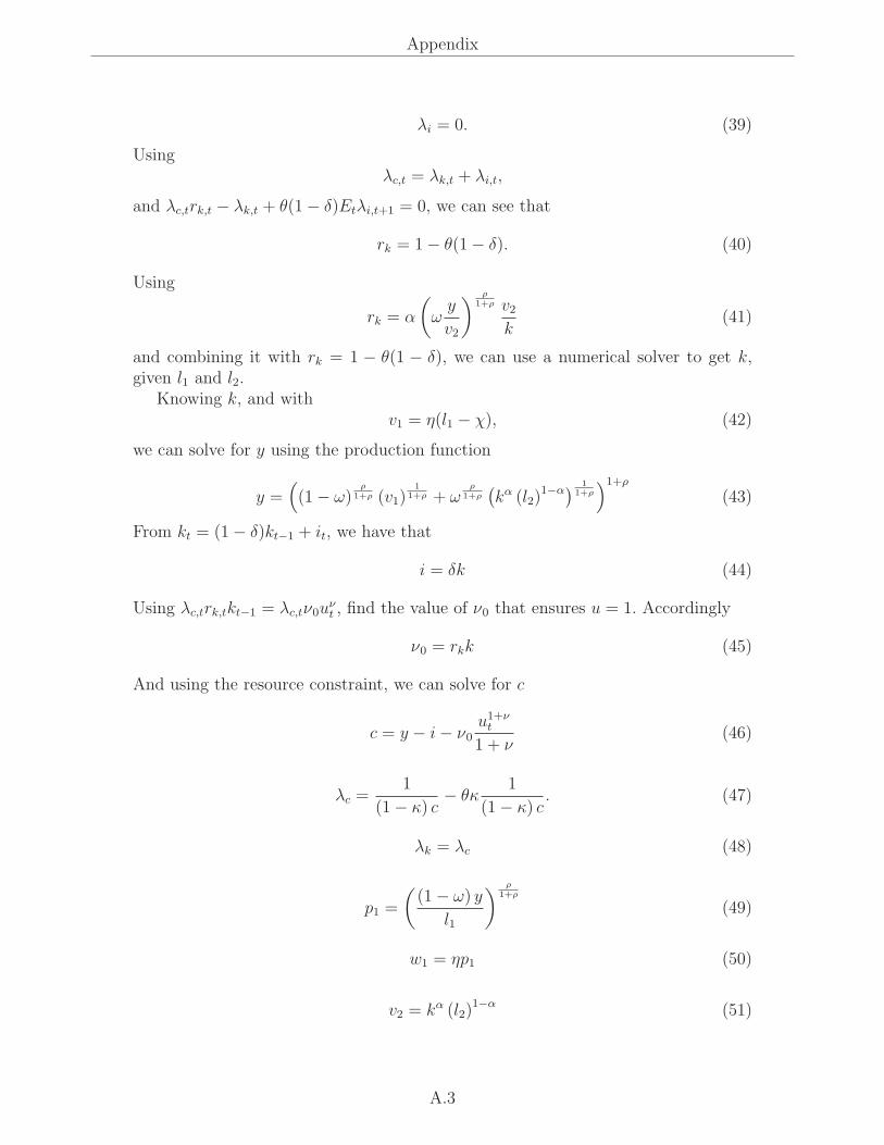
Appendix
λi = 0. (39)
Usingλc,t = λk,t + λi,t,
and λc,trk,t − λk,t + θ(1− δ)Etλi,t+1 = 0, we can see that
rk = 1− θ(1− δ). (40)
Using
rk = α
(
ωy
v2
)ρ
1+ρ v2k
(41)
and combining it with rk = 1 − θ(1 − δ), we can use a numerical solver to get k,given l1 and l2.
Knowing k, and withv1 = η(l1 − χ), (42)
we can solve for y using the production function
y =(
(1− ω)ρ
1+ρ (v1)1
1+ρ + ωρ
1+ρ
(
kα (l2)1−α)
1
1+ρ
)1+ρ
(43)
From kt = (1− δ)kt−1 + it, we have that
i = δk (44)
Using λc,trk,tkt−1 = λc,tν0uνt , find the value of ν0 that ensures u = 1. Accordingly
ν0 = rkk (45)
And using the resource constraint, we can solve for c
c = y − i− ν0u1+νt
1 + ν(46)
λc =1
(1− κ) c− θκ
1
(1− κ) c. (47)
λk = λc (48)
p1 =
(
(1− ω) y
l1
)ρ
1+ρ
(49)
w1 = ηp1 (50)
v2 = kα (l2)1−α (51)
A.3

Appendix
w2 = (1− α)
(
ωy
v2
)ρ
1+ρ v2l2
(52)
A.3 Deriving the Elasticity of Substitution for the Produc-
tion Function of Sector 2
yt =(
(1− ω)ρ
1+ρ (v1t)1
1+ρ + ωρ
1+ρ (v2,t)1
1+ρ
)1+ρ
∂yt∂v1,t
= (1 + ρ)(
(1− ω)ρ
1+ρ (η(l1,t − ν))1
1+ρ + ωρ
1+ρ (v2,t)1
1+ρ
)ρ 1
1 + ρ(1−ω)
ρ
1+ρ (v1,t)1
1+ρ−1
Notice again that yx =(
(1− ω)ρ
1+ρ (η(l1,t − ν))1
1+ρ + ωρ
1+ρ (v2,t)1
1+ρ
)(1+ρ)x
. Find
x, such that x(1 + ρ) = ρ. That is x = ρ
1+ρ. Accordingly,
∂yt∂v1,t
= yρ
1+ρ (1− ω)ρ
1+ρη (v1,t)−
ρ
1+ρ
∂yt∂v2,t
= yρ
1+ρ (ω)ρ
1+ρ (v2,t)−
ρ
1+ρ
∂yt∂v1,t
∂yt∂v2,t
=(1− ω)
ρ
1+ρ (v1,t)−
ρ
1+ρ
(ω)ρ
1+ρ (v2,t)−
ρ
1+ρ
log
∂yt∂v1,t
∂yt∂v2,t
= log
(
(1− ω)ρ
1+ρ (v1,t)−
ρ
1+ρ
(ω)ρ
1+ρ (v2,t)−
ρ
1+ρ
)
= log
(
(1− ω)ρ
1+ρ
(ω)ρ
1+ρ
)
+ρ
1 + ρlog
v2,tv1,t
The elasticity id given by
Elast =dlog(v2,t/v1,t)
dlog( ∂yt∂v1,t
/ ∂yt∂v2,t
)=
1 + ρ
ρ
Therefore to hit a destired elasticity set ρ as
ρElast− ρ = 1
ρ =1
Elast− 1.
A.4

Appendix
B Additional Sensitivity Analysis
Figures A.1 and A.2 offer sensitivity analysis pertaining to the comparison on theeconomic effects of the Spread of COVID-19 without any social distancing measures.The compare the economic effects using one- and two-sector models. Figure A.1shows dynamic responses analogous to those in Figure 2, but increases the minimumscale parameter χ from one-half of the steady state labor supply to six-tenths. FigureA.2 considers sensitivity to a range of values of the contact rate parameter, β. Itshows that the differences between the one- and two-sector models persist as long asthe contact rate does not drop below about 0.075, a level that would also curtail thespread of the disease.
Figures A.3 and A.4 complement the discussion of the cost of waiting for a vaccineoffered in Section 4.3.3. They pertain, respectively, to sensitivity analysis to theeffectiveness of the lockdown and to the share to of the population to which thelockdown applies.
A.5

Appendix
Figure A.1: Aggregate Economic Consequences of COVID-19 Without Social Distancing: AnIncrease in the Minimum Scale of Sector 1
2 4 6 8 10 12
5
10
15
20
25
30
35
% o
f p
op
ula
tio
n
1. Infected, Group 1 and 2 Total
2 4 6 8 10 12
5
10
15
20
% o
f p
op
ula
tio
n
2. Infected
Group 1
Group 2
2 4 6 8 10 12
-40
-30
-20
-10
0
% d
ev.
fro
m s
tea
dy s
tate
3. Output, Total
Two-sector model
One-sector model
2 4 6 8 10 12
-60
-50
-40
-30
-20
-10
% d
ev.
fro
m s
tea
dy s
tate
4. Capacity Utilization
2 4 6 8 10 12
Months
-30
-25
-20
-15
-10
-5
0
% d
ev.
fro
m s
tea
dy s
tate
5. Consumption
2 4 6 8 10 12
Months
-100
-50
0
50
% d
ev.
fro
m s
tea
dy s
tate
6. Investment
Note: We assume that no social distancing measures are taken to reduce the spread of the disease. The outputloss stems from the reduction in labor supply from symptomatic infected individuals. For the case shown here,we have increased the minimum scale parameter for Sector 1, χ, to five-sixths of the steady state labor input, asopposed to one-half in the baseline calibration.
A.6

Appendix
Figure A.2: Comparing the Aggregate Economic Consequences of COVID-19 Without SocialDistancing in One- and Two-Sector Models: Sensitivity to the Contact Rate
0.05 0.1 0.15 0.2 0.25 0.3 0.35 0.4 0.45 0.5
Contact rate
0
1
2
3
4
5
6
7
8
9
10
Ave
rag
e o
utp
ut
loss o
ve
r 6
mo
nth
s
Contact Rate and Cumulative Output Loss
Two-Sector Model
One-Sector Model
0.05 0.1 0.15 0.2 0.25 0.3 0.35 0.4 0.45 0.5
Contact rate
0
2
4
6
8
10
12
14
Ave
rag
e o
utp
ut
loss o
ve
r 6
mo
nth
s
A Higher Minimum Scale Parameter For Sector 2
Note: We assume that no social distancing measures are taken to reduce the spread of the disease. The outputloss stems from the reduction in labor supply from symptomatic infected individuals. The figure shows thecumulative output loss over six months alternatively based on one- and two-sector models for different values ofβ (set at 0.2 in our baseline). The top panel keeps all other parameters at their baseline values. For the bottompanel, we have increased the minimum scale parameter for Sector 1, χ, to five-sixths of the steady state laborinput, as opposed to one-half in the baseline calibration.
A.7

Appendix
Figure A.3: Waiting for a Vaccine: Assuming a Lower Effectiveness of the Lockdown at ReducingContact Rates
5 10 15 20 25 30
5
10
15
20
25
30
35
% o
f g
rou
p s
ize
1. Group-1 Infected
Do Nothing
Social Distancing
5 10 15 20 25 30
5
10
15
20
25
30
35
% o
f g
rou
p s
ize
2. Group-2 Infected
5 10 15 20 25 30
-40
-30
-20
-10
% d
ev.
fro
m s
tea
dy s
tate
3. Output, Total
5 10 15 20 25 30
-35
-30
-25
-20
-15
-10
-5
% d
ev.
fro
m s
tea
dy s
tate
4. Capacity Utilization
5 10 15 20 25 30
Months
-25
-20
-15
-10
-5
% d
ev.
fro
m s
tea
dy s
tate
5. Consumption
5 10 15 20 25 30
Months
-100
-50
0
50
% d
ev.
fro
m s
tea
dy s
tate
6. Investment
Note: We model the reduction in effectiveness by setting ϑ to 0.8. Raising the share of individuals in Groups1, 2 and 3 to 32, 75, and 59 percent, respectively, as considered here, can keep the share of infective individualsbelow 1.5 percent while waiting for a vaccine for 18 months.
A.8

Appendix
Figure A.4: Waiting for a Vaccine
5 10 15 20 25 30
5
10
15
20
25
30
35
% o
f g
rou
p s
ize
1. Group-1 Infected
Do Nothing
Social Distancing
5 10 15 20 25 30
5
10
15
20
25
30
35
% o
f g
rou
p s
ize
2. Group-2 Infected
5 10 15 20 25 30
-30
-25
-20
-15
-10
-5
% d
ev.
fro
m s
tea
dy s
tate
3. Output, Total
5 10 15 20 25 30
-35
-30
-25
-20
-15
-10
-5
% d
ev.
fro
m s
tea
dy s
tate
4. Capacity Utilization
5 10 15 20 25 30
Months
-8
-6
-4
-2
% d
ev.
fro
m s
tea
dy s
tate
5. Consumption
5 10 15 20 25 30
Months
-100
-80
-60
-40
-20
0
% d
ev.
fro
m s
tea
dy s
tate
6. Investment
Note: The alternative policy considered extends the lockdown to 80 percent of individuals outside the laborforce, those in Group 3 (with an effectiveness parameter ϑ equal to 1). This change would achieve the target ofa 1.5 percent share of infected individuals even with a reduction of the shares of individuals in Groups 1 and 2under lockdown to 17 and 44 percent, respectively.
A.9