Individual Inquiry

CALTEX’S LYTTON REFINERYSTEAM BALANCE

Richard Loro

Department of Chemical Engineering

Supervisor: Mr R.J. Wiles

27th October 2000

Acknowledgements

There are a number of people to whom I owe thanks:

To the engineers at Caltex, especially Mr Choo Kiong Looi, my industry supervisor,for approaching me with the project.

To Mr R.J “Gus” Wiles, my academic supervisor, for his instruction.

To Catherine Parker, who helped me get this thing started.

To Poo-finger, Baloney, Mong and Dr. James Crow of the Unit 5 Train – thanks forkeeping me sane.

And finally to my parents, for without their support I never would have got there.

ABSTRACT

This project was aimed at developing a program through which the steam system

headers within Caltex’s Lytton Refinery, Brisbane, could be quantified. A simple

node-and-arc network was used to represent the system with data generation

techniques including flowmeters, pump and compressor turbine calculations, valve

calculations and exchanger balances.

The developed spreadsheet balance was complemented by the introduction of a small

amount of nodal reconciliation, although lack of data meant that the full extent of the

process could not be realised.

Due to difficulties with plant operation, a data set representing general operation

could not be obtained. Instead data, albeit from a period where the alkylation and

polymerisation plants were shutdown, had to be used. Several areas within the steam

system were identified as lacking steam, causing in some cases header reversal. This

corresponded well with comments by engineers that the steam system appeared to be

malfunctioning at the time.

Further work needs to include an analysis of the model with data corresponding to

general operation. Depending on the degree of success experienced, moves could be

taken to implement this project into the operators control panel. At the same time,

points have been identified which would greatly benefit the monitoring system from

the installation of a flowmeter. Installation may occur as part of the scheduled 2001

shutdown.

Table of Contents

Abstract ................................................................................................i

Background..........................................................................................1

Introduction ..........................................................................................3

The Existing Steam System .................................................................4

Literature Review .................................................................................6

Previous Work......................................................................................8

Nodal Network Representation of Process Flow Diagrams..................9

Steam Balancing Program ...................................................................10

Reconciliation.......................................................................................12

Balance Results ...................................................................................14

Analysis................................................................................................15

Further ApplicationsCaltex..........................................................................17Other Areas ................................................................18

Bibliography .........................................................................................19

Appendix A: Nomenclature

Appendix B: Data Generation Techniques

Appendix C: Steam Process Flow Diagrams

Appendix D: Node Descriptions

Appendix E: Nodal Network

Appendix F: Arc File

Appendix G: Reliability Factor Calculations

Background

The one thing almost every processing plant shares is steam. Its predominate function

within the processing industry context is to transfer energy over relatively short

distances (∼2 kilometres). What sets steam apart from other possible carriers is its

extraordinarily high latent heat of vaporisation. In fact, in comparison with butane,

the energy released from one kilogram of steam is around 8 times of that of a similar

amount of butane. As well as this, steam is safe to handle (in comparison to butane

for example) and is generated from water which while not free, is usually relatively

inexpensive.

Steam has enjoyed many traditional applications. These include:

Ø Turbines

Ø Exchangers / Reboilers

Ø Stripping Medium (particularly in the Petrochemical Industry)

Ø Atomising and Soot-Blowing e.g. Boilers etc

Ø Eductors

Ø Lift gas

Ø Purge Medium

Ø Used to increase the velocity of heavier liquid streams e.g. Furnace Tubes

The majority of the above are still relevant to many processes throughout the world

and many of these applications are looked at in greater depth in the following

sections.

It has already been mentioned that steam is best used in applications where the

distance between the boiler-house and unit is less than 2 kilometres. For greater

distances it is best to use electricity, as wastage due to friction and / or loss through

insulation significantly lessens the extent of energy transferred. Most electricity is

produced from steam, however, due to inefficiencies in the generation stage it

generally requires around 3 kW of steam to produce 1 kW of electricity. Therefore

for nearby unit operations it is best to use steam directly as a heating medium, while

those at a distance should be serviced by electricity.

Caltex is an international crude oil refiner and marketer of petroleum and convenience

products for motorists. Texaco and Chevron have jointly owned Caltex since its

inception around 60 years ago by their predecessor companies – Texas Company and

Standard Oil Company of California.

Lytton refinery is one of Caltex’s two Australian refineries. It is located on the

southern shore at the mouth of the Brisbane River in Queensland. Lytton boasts a

history of 35 years, coming online around 1965. Since then, Lytton has grown to

become Queensland’s largest petroleum refinery, processing around 2/3 of

Queensland’s petrol as well as producing a wide range of petroleum products. The

refinery is designed to process mainly low sulfur crudes (feed stocks), with crudes

coming from many different parts of the world. Because of this, Lytton needs to be

flexible in its operation to meet the changing demands of each.

Introduction

The steam system has played an integral role in the refining process at Caltex Lytton

since the plant’s construction in 1965. This is proven by the wide variety of

applications which utilise steam. Unfortunately steam was not considered an

important (expensive) enough material at the time to justify fully metering the system.

The gradual but persistent increase in world oil prices has placed considerable

pressure on refineries to optimise their processes to wring every cent out of each

barrel. Attitudes towards the worth of steam have consequently changed since.

The complexity of the steam system has also grown over the years it has been

established. New plants have been added and several originals made obsolete. As far

as can be ascertained, no accurate records of these modifications, in particular their

impact upon header flowrates, have been kept. Planning new, and retrofits to existing

equipment becomes difficult, as engineers and operators are unsure of the amount of

steam available or the consumption’s effect on the entire steam header as a whole.

This project, then, is aimed at developing a program which enables both operators and

engineers alike to monitor steam flows throughout the refinery.

The Existing Steam System

Despite the many modifications made to the steam system over the years, it has

retained its original structure. The refinery is serviced by a steam system consisting

of three main headers each at a distinct pressure. These headers are internally labelled

as the high, medium and low pressure headers at 4100 (600), 1000 (150) and 350 (50)

kPag (psi) respectively. As well as this, a conjugate condensate system (again at high,

medium and low pressures) operates to capture and return condensate for reboiling

and/or flashing.

One would expect that the 4100 kPag header be significantly better instrumented than

the 1000 kPag header due to its higher specific energy content, and this indeed is seen

to be the case. Following the same logic, this argument can be extended to include

the 350 kPag header. This observation is indeed reflected in the nature of the

calculations performed within the steam balance. That is, the number of indirect

calculations needed to quantify the steam flows increases as the steam loses pressure.

As an aside to the above discussion, the steam balance is also extended to include the

boiler-houses and make-up stream flow. This area of the plant is well instrumented

for obvious reasons.

Apart from 11E-4 and 3E-7 (medium pressure steam generators) and the medium and

low pressure flashing units, all process steam generated within the refinery is at (or

near) 4100 kPag. The medium and low pressure steam systems are serviced through a

process of “let-downs”, from one header pressure to another. This, for example, may

take the form of a turbine operating with an inlet of high pressure steam with its

exhaust pressure set such that its “waste steam” can be fed directly to the medium

pressure header. This ‘trickling down’ through the network is very efficient in terms

of boiler usage (i.e. don’t need separate HP, MP and LP boilers) and energy

consumption. However, problems could arise if the low pressure steam consumption

was greater than the higher pressure requirements. Fortunately, this has been planned

for through the presence of special “let-down” stations (essentially control valves)

designed to convert high pressure to medium pressure and medium pressure to low

pressure steam. This is, however, inefficient solution, if it must be maintained for a

significant period, due to the magnitude of losses involved and is generally avoided if

at all possible.

Literature Review

The project can be separated into two separate sections – data generation and initial

balancing, data reconciliation and some rectification.

Data generation concerns firstly identifying those flows which need to be quantified

and then determining ways to evaluate them. Most of the methods used can be found

in any general engineering texts and consequently are not discussed in detail here.

Appendix B gives an overview of techniques and equations used.

There are numerous articles on the topic of data reconciliation and rectification.

Perry’s Chemical Engineers’ Handbook1 defines the difference between reconciliation

and rectification as:

“Reconciliation adjusts the measurements to close constraints subject to their

uncertainty. The numerical methods for reconciliation are based on the restriction

that the measurements are only subject to random errors. Since all measurements

have some unknown bias, this restriction is violated. The resultant adjusted

measurements propagate these biases…

Rectification is the detection of the presence of significant bias in a set of

measurements, the isolation of specific bias in a set of measurements, the isolation of

the specific measurements containing bias, and the removal of those measurements

from subsequent reconciliation and interpretation.”

Due to the difficulty in rectifying data computationally, most rectification was

accomplished using the author’s judgement.

Mah, Stanley and Downing2 provide a reasonable overview of general techniques

used in the reconciliation analysis of process data. Consider the situation in which all

process streams have been measured. Let vj denote the measured variable, Vj the

estimated value and µj the true value of stream j. Hence the adjustment (xj) and

measurement error (εj) may be written as:

xj = Vj - νj (for j = 1,2...m)

εj = νj - µj (for j = 1,2…m)

Assume now that the measurement errors are normally distributed random variables

with a zero mean and positive covariance matrix, Q. The least-squares estimation for

this problem is given by

min (V – ν)T Q-1 (V - ν) w.r.t V

subject to the material conservation constraints

AV = 0

where A is the nodal incidence matrix.

The above ideally holds for systems in which rectification has already been

performed, and in which the data range does not vary by more than ∼103. As well as

this, data should be obtained by a single technique e.g. flowmetering. Typically this

is rarely the case. Instead, the general situation involves several different and often

creative means from which arc flows can be generated. Because of this, arc values no

longer have a uniform reliability. Reconciliation therefore becomes more difficult

than simply applying the above process.

Previous Work

In December 1989 the BILVAP project was launched as part of the Fuel And

Utilities Monitoring System (FAUMS) initiative. Davy McKee prepared the

drawings of the refinery steam system upon which TOTAL derived the initial nodal

network. The outcome of this study proposed that 17 new flowmeters be installed and

2 relocated, to enable analysis of the main units, during the 1992 shutdown. This

never occurred as was planned and the project came, more-or-less, to a standstill.

The venture was resurrected during 2000 as part of the refinery’s work experience

program, although limited progress was made during this time due to, among other

problems, software issues.

Work completed to date includes; the update of steam process flow diagrams and the

nodal network. Where flowmeters are unavailable, methods to generate flow

estimates from indirect process measurements have been devised. An overall steam

reconciliation program has been developed which alters inputted data to satisfy

conservation and deviation minimization constraints. Initial analysis of these returned

flowrates has also been commenced.

Nodal Network Representation of Process FlowDiagrams

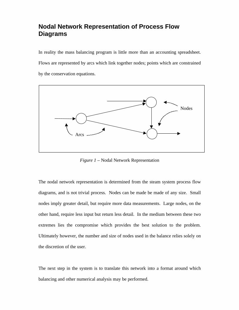
In reality the mass balancing program is little more than an accounting spreadsheet.

Flows are represented by arcs which link together nodes; points which are constrained

by the conservation equations.

Figure 1 – Nodal Network Representation

The nodal network representation is determined from the steam system process flow

diagrams, and is not trivial process. Nodes can be made be made of any size. Small

nodes imply greater detail, but require more data measurements. Large nodes, on the

other hand, require less input but return less detail. In the medium between these two

extremes lies the compromise which provides the best solution to the problem.

Ultimately however, the number and size of nodes used in the balance relies solely on

the discretion of the user.

The next step in the system is to translate this network into a format around which

balancing and other numerical analysis may be performed.

Arcs

Nodes

Steam Balancing Program

When this author sat down to write this program there were several goals that were

identified to be vital for success.

Firstly, the program had to work. It had to correctly handle data in such a way as to

provide an accurate representation of the operation of the steam system. The program

was required to do this within a reasonable time frame.

Secondly, it needed to be user-friendly. This goal covered a number of objectives.

The program to be used was settled by the site engineers (those most likely to make

use of the balance). Several were considered, however, Excel was finally chosen as it

was the one which the engineers felt most at ease with. Within this program, there

was still the choice of how to format this mass balance. While not as elegant as

matrices, a traditional balance sheet approach was selected for several reasons. With

the large amount of data to be handled, this method provided an easy way to both

monitor and pick up any mistakes made. At the same time, this layout enables the

program to be easily understood and hence it can be modified without difficulty.

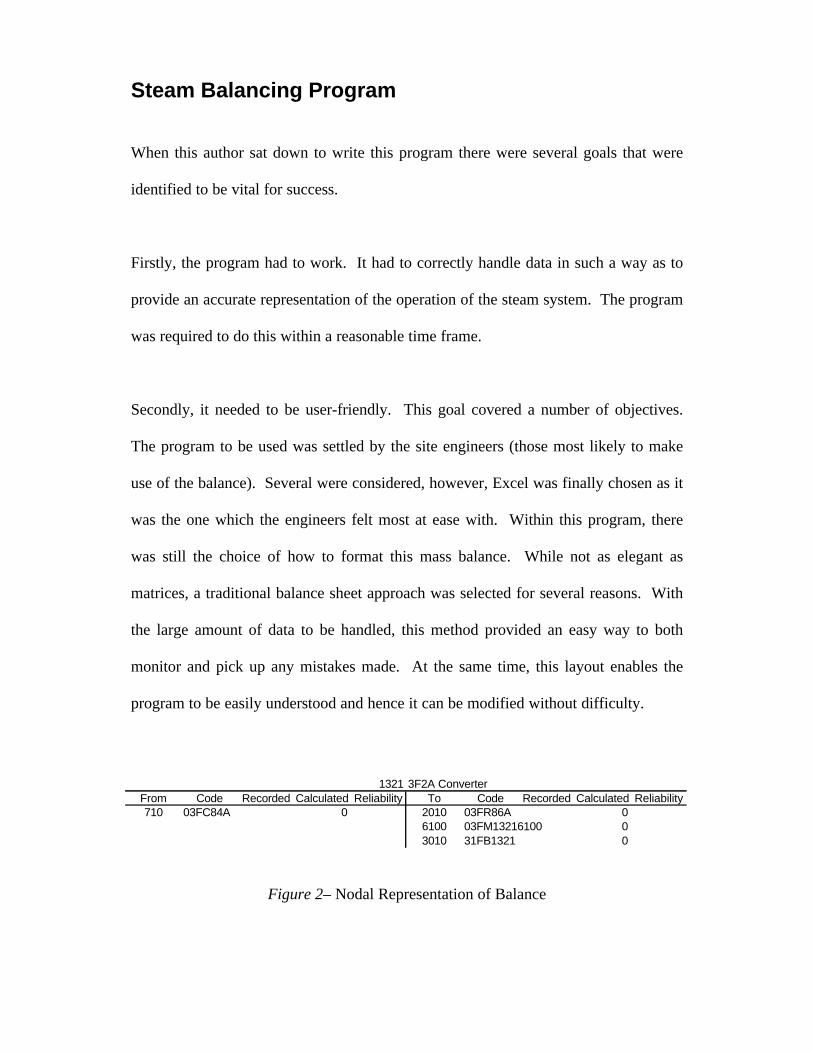
Figure 2– Nodal Representation of Balance

1321 3F2A ConverterFrom Code Recorded Calculated Reliability To Code Recorded Calculated Reliability710 03FC84A 0 2010 03FR86A 0

6100 03FM13216100 03010 31FB1321 0

Figure 2 gives a basic idea on how the balance is constructed. On the left, arc flows

entering the node are listed. We see that this node receives material from the boiler

feed water header (0710). As one would expect, the exiting arcs and their consequent

nodes are given on the right.

The conservation principle constrains that the difference between sum of inlet flows

and exiting flows must be zero. This fact is taken into account by the “FB” (flow

balance) arc which is determined by satisfying this conservation. That is, the flow

value is set by the difference between inlets and exits to a node. This technique for

characterisation is used quite regularly throughout the balance, especially around

nodes which contain arcs that cannot be accurately determined. The ease of this

method is counteracted by the fact that reconciliation can no longer be performed over

that node. Hence, where possible, all information from the plant is used.

Reconciliation

As has already been discussed, reconciliation is a technique whereby constraints are

satisfied by essentially ‘juggling’ arc values based upon their uncertainty. Before

reconciliation can be performed, several things are needed. Firstly, the node to be

reconciled must be overspecified i.e. no flow balances. This overspecification will

contradict the conservation principle and hence this provides the constraint to be met.

Secondly in order for any meaningful reconciliation, accurate arc reliability factors

must be specified. The reliability factor is essentially a measure the trustworthiness of

input. For example it is obvious that flowmeter is likely to consistently produce flow

measurements of a better quality than an indirect method (e.g. obscure heat balance

over crude tanks). Following this then, one would expect that during reconciliation,

where arc values are adjusted to close the mass balance, the degree by which a flow

alters should be inversely proportional to its reliability. Appendix G gives the method

used to calculate these factors.

The literature review outlines several reasons why, as it stands, the literature-stated

error variable is not suitable for this application. In an effort to deal with this

problem, a new variable has been developed in place of the adjustment variable. This

variable is described as the deviation variable and has the form:

δj = (Vj – νj) ϕj / νj

where δ represents the deviation variable and ϕ the reliability factor.

Reconciliation will then be based upon

min Σ δ2 w.r.t δ

and subject to the mass conservation equation.

The above form is a measure of the relative deviation of a flow, and is applicable to

any data set regardless of its range of sizes. This ability is primarily due to the

normalising effect achieved through the division by νj.

I make a note here that there apparently exists a conventional way of dealing with this

problem. However, during the course of my research I did not come across it.

Instead I realised the potential problems with what I saw as the existing approach and

altered it to suit. From what I can see, both methods perform in roughly the same

manner and use similar variables. i.e. conventional method uses W – weighting

factor, the above method uses ϕ - reliability factor.

Balance Results

Unfortunately, a complete data set was unable to be taken from Lytton Refinery

during the closing stages of this project. This was due to a number of reasons, the

most important of which was the fact that the refinery has been only semi-operational

of late. Because of this the full extent of the program developed could not be

evaluated.

However, data from a period earlier in the year was available. Again this was not

perfect as this period corresponded to a time where the alkylation and polymerisation

plants were off-line. Nevertheless it was decided that this set should be used to gain

some feel for possible trouble areas within the refinery, even though it was not a true

reflection of refinery steam system operation.

Results from the trial can be seen in the Excel spreadsheet “Trial”.

Analysis

From the data supplied, some limited analysis may be initiated on the steam system

and program.

At this early stage, reconciliation was only required over six nodes; the boiler,

converter and the loss nodes. The results appear promising. In all cases the

conservation constraint was satisfied and arc values deviated in accordance with their

reliability factors.

The majority of arcs remained unchanged. This was expected due to the large number

of flow balance arcs required within the system. As has been stated this undermines

the reconciliation process and renders it unnecessary. In several places at least, data

reliability would benefit greatly from the presence of a metering device. For example,

one such area would be around node 3040, the plant 3 subheader. From the node, one

immediately sees that flow has been reversed in the header and is in fact trying to

draw steam from general consumption. This is obviously not possible, and so it

should trigger warning lights.

Following this node backwards through all its connections, one sees that quite a few

headers have been reversed in direction in an effort to try to supply the steam where it

was needed. Talking with several engineers about this, it seems that during the period

in which these measurements were taken, the steam system was in fact experiencing

difficulties. The above may point to one of the many possible sources of problems.

The make-up water flowrate forms approximately 43% of the boiler feed water.

Lieberman and Lieberman3 suggest that a general steam system working adequately

should present a condensate recovery above 70% (i.e. make-up flowrate < 30%). Of

course the ideal ratio varies from process to process depending on the level and types

of consumption. However could this percentage be improved, considerable savings

may be made in the energy and chemicals needed to prepare the boiler feed water and,

to a lesser extent, wastewater effluent treatment.

Further Applications

Caltex

Using the data provided, it is difficult to determine whether the spreadsheet is

providing an acceptable solution to the steam balance. Obviously then, the next

logical step is to obtain a data set which does accurately represent the general

operation of the steam system. Consultation with Appendix F enables the necessary

measurements to be identified.

Should the spreadsheet prove adequate to characterise the system, the beginnings of a

continuous steam-monitoring system has been developed. There has been some

indication from operators that they would appreciate this system being at least

partially integrated into the TDC. During times of electrical blackout, this system

may prove invaluable in the monitoring of header flows to prevent equipment damage

etc.

In February 2001, Lytton is scheduled for a complete shutdown. This provides an

excellent window of opportunity in which to update the existing metering system.

The areas that would most benefit the balance with metering have been identified and

are listed on the steam process flow diagrams (Appendix C ). In general, these points

correspond to major headers with no flowmeters. In some cases the orifice plates and

tapping points already exist in the line – all that is required is a metering unit.

Other Areas

At it stands, the spreadsheet is customised specifically for the Lytton Refinery’s steam

system. However the methods used and principles identified apply for any network.

In particular other plants with similar equipment, for example mills, power plants and

mineral processing plants, may benefit directly from the data generation techniques

Bibliography

1. Perry, R.H., and D.W.Green, Perry’s Chemical Engineers’ Handbook 7th

Edition, McGraw-Hill, 1997, 30-29

2. Mah, R.S., G.M. Stanley, and D.M. Downing, “Reconciliation andRectification of Process Flow and Inventory Data”, Industrial andEngineering Chemistry, Process Design and Development, 15(1) 1976, 175-183

3. Lieberman, P.L., and E.T. Lieberman, A Working Guide to ProcessEquipment, McGraw-Hill, 1997 Ch 15: Deaerators and Steam Systems

4. Lyon, A.J., Dealing With Data, Pergamon Press, 1970

5. Reid, E.C., and J.C.Renshaw, Steam, Cole Publications, 1982

6. Urbaniec, K., Modern Energy Economy in Beet Sugar Factories, Elsevier,1989

7. Young, D.F., B.R. Munson and T.H. Okiishi, A Brief Introduction to FluidMechanics, Wiley

APPENDIX A:

Nomenclature

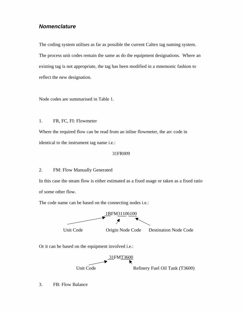
Nomenclature

The coding system utilises as far as possible the current Caltex tag naming system.

The process unit codes remain the same as do the equipment designations. Where an

existing tag is not appropriate, the tag has been modified in a mnemonic fashion to

reflect the new designation.

Node codes are summarised in Table 1.

1. FR, FC, FI: Flowmeter

Where the required flow can be read from an inline flowmeter, the arc code in

identical to the instrument tag name i.e.:

31FR009

2. FM: Flow Manually Generated

In this case the steam flow is either estimated as a fixed usage or taken as a fixed ratio

of some other flow.

The code name can be based on the connecting nodes i.e.:

1BFM31106100

Unit Code Origin Node Code Destination Node Code

Or it can be based on the equipment involved i.e.:

31FMT3600

Unit Code Refinery Fuel Oil Tank (T3600)

3. FB: Flow Balance

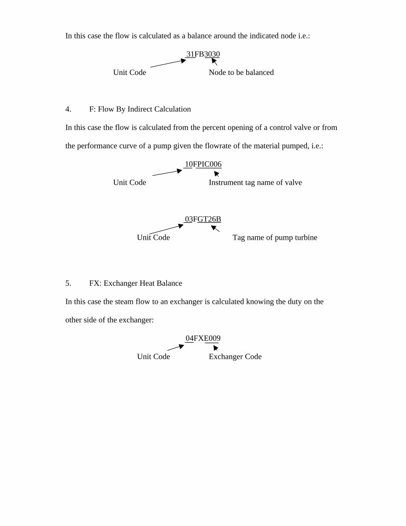
In this case the flow is calculated as a balance around the indicated node i.e.:

31FB3030

Unit Code Node to be balanced

4. F: Flow By Indirect Calculation

In this case the flow is calculated from the percent opening of a control valve or from

the performance curve of a pump given the flowrate of the material pumped, i.e.:

10FPIC006

Unit Code Instrument tag name of valve

03FGT26B

Unit Code Tag name of pump turbine

5. FX: Exchanger Heat Balance

In this case the steam flow to an exchanger is calculated knowing the duty on the

other side of the exchanger:

04FXE009

Unit Code Exchanger Code

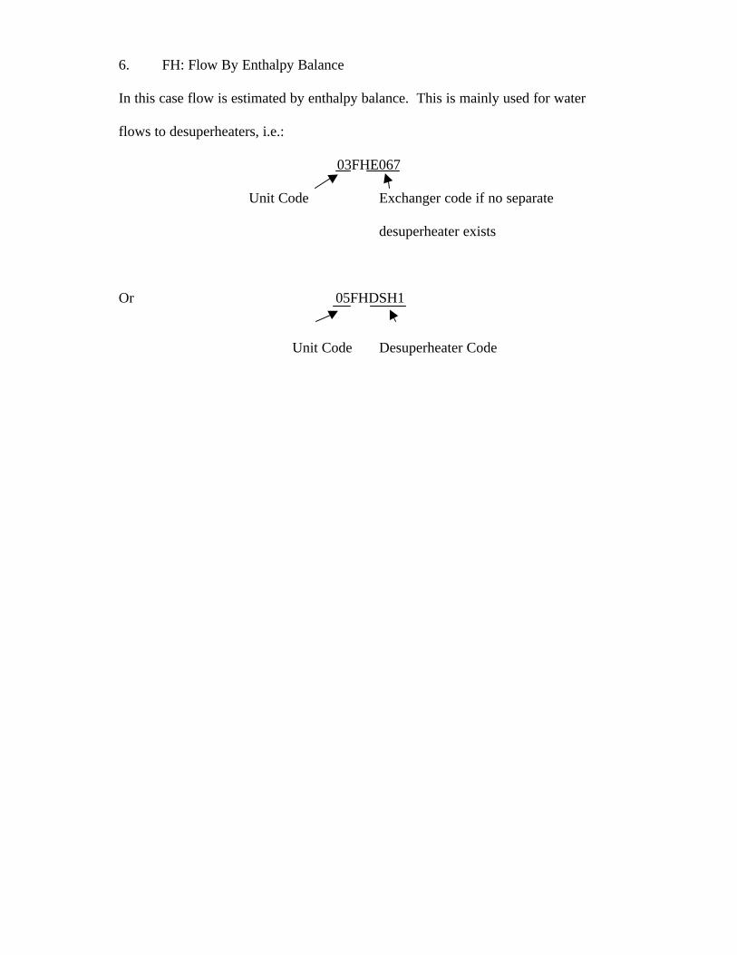
6. FH: Flow By Enthalpy Balance

In this case flow is estimated by enthalpy balance. This is mainly used for water

flows to desuperheaters, i.e.:

03FHE067

Unit Code Exchanger code if no separate

desuperheater exists

Or 05FHDSH1

Unit Code Desuperheater Code

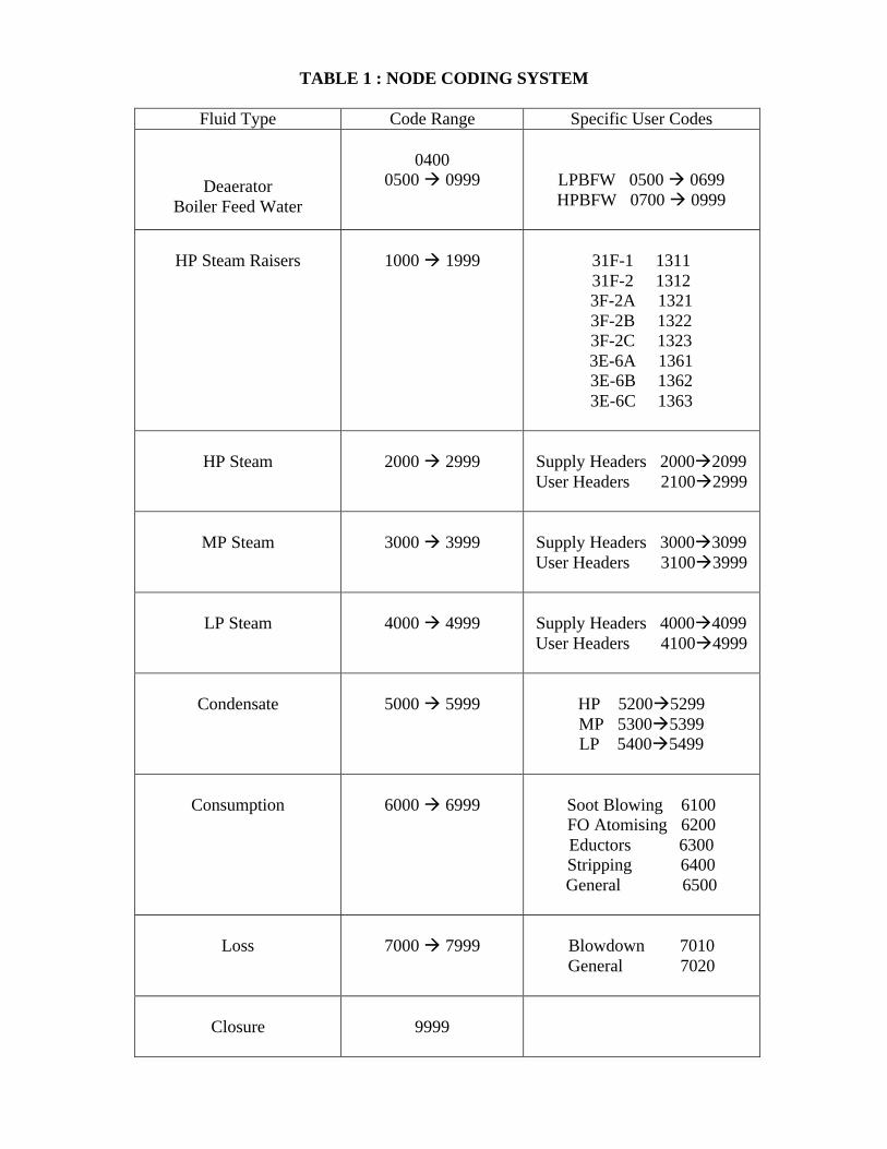
TABLE 1 : NODE CODING SYSTEM

Fluid Type Code Range Specific User Codes

DeaeratorBoiler Feed Water

04000500 à 0999 LPBFW 0500 à 0699

HPBFW 0700 à 0999

HP Steam Raisers 1000 à 1999 31F-1 131131F-2 13123F-2A 13213F-2B 13223F-2C 13233E-6A 13613E-6B 13623E-6C 1363

HP Steam 2000 à 2999 Supply Headers 2000à2099User Headers 2100à2999

MP Steam 3000 à 3999 Supply Headers 3000à3099User Headers 3100à3999

LP Steam 4000 à 4999 Supply Headers 4000à4099User Headers 4100à4999

Condensate 5000 à 5999 HP 5200à5299MP 5300à5399LP 5400à5499

Consumption 6000 à 6999 Soot Blowing 6100FO Atomising 6200Eductors 6300Stripping 6400General 6500

Loss 7000 à 7999 Blowdown 7010General 7020

Closure 9999

APPENDIX B:

Data Generation Techniques

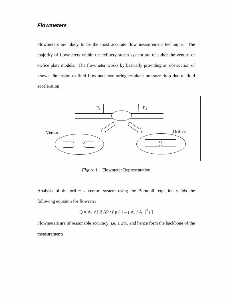
Flowmeters

Flowmeters are likely to be the most accurate flow measurement technique. The

majority of flowmeters within the refinery steam system are of either the venturi or

orifice plate models. The flowmeter works by basically providing an obstruction of

known dimension to fluid flow and monitoring resultant pressure drop due to fluid

acceleration.

Figure 1 – Flowmeter Representation

Analysis of the orifice / venturi system using the Bernoulli equation yields the

following equation for flowrate:

Q = A2 √ [ 2 ∆P / ( ρ ( 1 – ( A2 / A1 )2 ) ]

Flowmeters are of reasonable accuracy, i.e. ± 2%, and hence form the backbone of the

measurements.

OrificeVenturi

P2P1

Turbine Calculations

One of the most prevalent functions of steam within the refinery involves the

powering of steam turbines. Indeed, this application forms a large percentage of the

calculations performed for the indirect data generation. In situations which require a

variable speed drive (e.g. most large compressors and some pumps) the steam turbine

provides an effective way of supplying this. As well as this reason, many process

critical units e.g. many pumps, have a steam turbine on standby in case of electric

motor failure.

Turbine steam usage is generally quantified by the turbine specific steam rate

(T.S.S.R), which relates the rate of steam consumption to produce 1 hp. This number

is specific to each turbine (and its supply and exhaust states) and is generally

calculated and recorded on equipment data sheets during commissioning tests.

Several turbines do, however, lack this information. Perry’s Chemical Engineers’

Handbook, for known steam inlet and exit conditions, turbine rpm and wheel

diameter, gives a general approximation of T.S.S.R.

Once this value has been determined, simply working out the supplied horsepower is

all that is required. For pumps with complete data sheets this can be achieved by first

determining the pump flowrate (either metered or using pump curve with differential

pressure) and then applying it to the power curve (generally supplied on data sheets).

A note is also made that turbines on standby also have some associated consumption.

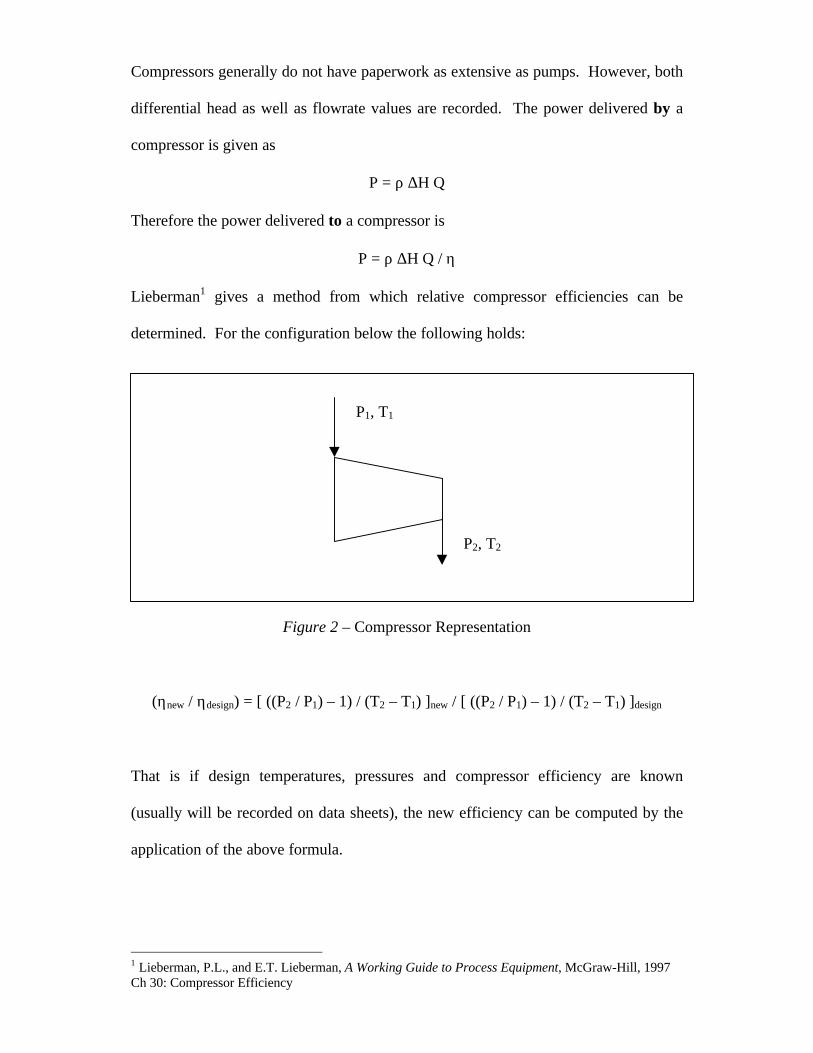
Compressors generally do not have paperwork as extensive as pumps. However, both

differential head as well as flowrate values are recorded. The power delivered by a

compressor is given as

P = ρ ∆H Q

Therefore the power delivered to a compressor is

P = ρ ∆H Q / η

Lieberman1 gives a method from which relative compressor efficiencies can be

determined. For the configuration below the following holds:

Figure 2 – Compressor Representation

(ηnew / ηdesign) = [ ((P2 / P1) – 1) / (T2 – T1) ]new / [ ((P2 / P1) – 1) / (T2 – T1) ]design

That is if design temperatures, pressures and compressor efficiency are known

(usually will be recorded on data sheets), the new efficiency can be computed by the

application of the above formula.

1 Lieberman, P.L., and E.T. Lieberman, A Working Guide to Process Equipment, McGraw-Hill, 1997Ch 30: Compressor Efficiency

P1, T1

P2, T2

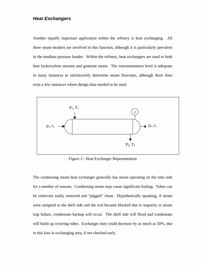
Heat Exchangers

Another equally important application within the refinery is heat exchanging. All

three steam headers are involved in this function, although it is particularly prevalent

in the medium pressure header. Within the refinery, heat exchangers are used to both

heat hydrocarbon streams and generate steam. The instrumentation level is adequate

in many instances to satisfactorily determine steam flowrates, although there does

exist a few instances where design data needed to be used.

Figure 3 - Heat Exchanger Representation

The condensing steam heat exchanger generally has steam operating on the tube side

for a number of reasons. Condensing steam may cause significant fouling. Tubes can

be relatively easily removed and “pigged” clean. Hypothetically speaking, if steam

were assigned to the shell side and the exit became blocked due to impurity or steam

trap failure, condensate backup will occur. The shell side will flood and condensate

will build up covering tubes. Exchanger duty could decrease by as much as 50%, due

to this loss in exchanging area, if not checked early.

P1, T1

P2, T2

p2, t2

P

p1, t1

Condensate flow, exiting the channel head, is usually controlled by the steam trap.

This piece of equipment ensures (when working properly) that only liquid leaves the

exchanger. It does this by intending to open only when its float is lifted by water. It

reseals when the remaining liquid level is not sufficient to raise the float.

The heat duty can be determined several ways, the most convenient of which is to

assume the hydrocarbon pressure drop is negligible (or that specific heat remains

constant) and then applying the well known formula:

Q = m cp ∆T = m cp (T2 – T1)

The vast majority of exchangers rely on the condensation of steam in the transfer of

energy. The high latent heat of condensation means that enormous amounts of

thermal energy can be transferred for a relatively small steam flowrate and is the main

reason why steam proves so successful as a heat transfer medium.

Ideally the exchanger internal pressure will be monitored, and from this it is possible

to determine exactly where within the water vapour-liquid envelope condensation is

occurring, and what the release of energy (kJ/kg) is. The required flow of steam is

then calculated at:

F = m cp (T2 – T1) / ∆Hv

Unfortunately this pressure is rarely instrumented. Therefore an approximation can

be made by individually determining the enthalpy conditions of the inlet and exit

steam streams, h1 and h2 respectively. The flow now becomes:

F = m cp (T2 – T1) / (h2 – h1)

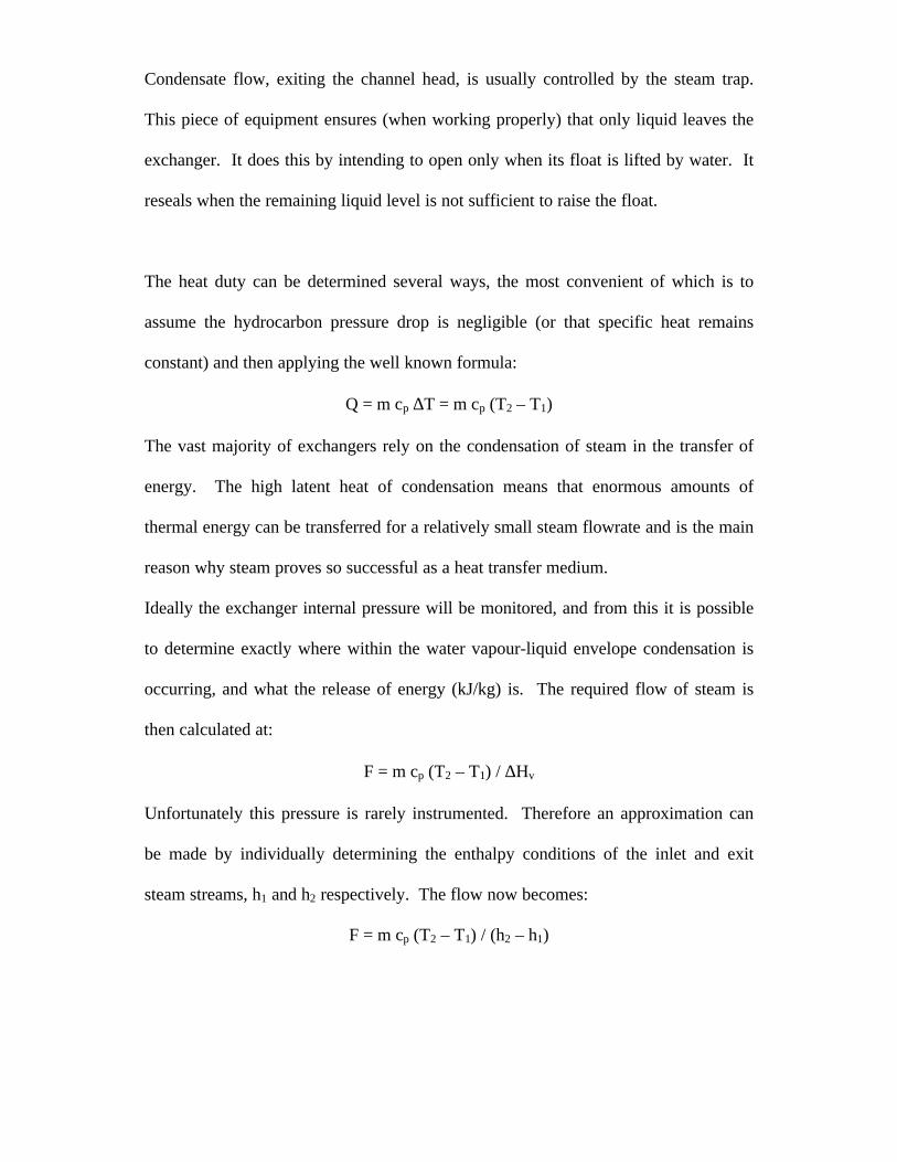
Valve Calculations

The control valve is essential in the manipulation of process flows. They are common

throughout all process plants and may be used for nearly any fluid. There are several

different types of control valve, however all work on the principle of changing flow

area to adjust pressure drop and hence flowrate. Arguably the most important control

valves for the steam system exist as letdown stations i.e. HP à MP à LP for when

steam is required.

Valve calculations are fairly standard and can be found in most engineering texts.

They require knowledge of the valve type, its percentage to fully open and pressure

drop over the unit. Knowing the valve specification and its position, one may

determine the valve constant, Cv, from manufacturer’s data. Some manufacturers also

specify Cs, a constant developed specifically for steam.

Figure 4 – Valve Representation

Figure 4 depicts the general situation for a control valve. In this manner when:

∆P < P1/2, flow is subsonic: Q = Cs √∆P

∆P > P1/2, flow is sonic: Q = Cs √P1 only.

P1 P2

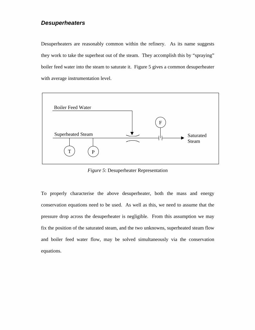
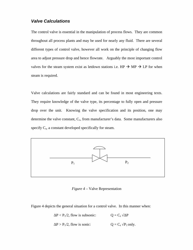
Desuperheaters

Desuperheaters are reasonably common within the refinery. As its name suggests

they work to take the superheat out of the steam. They accomplish this by “spraying”

boiler feed water into the steam to saturate it. Figure 5 gives a common desuperheater

with average instrumentation level.

Figure 5: Desuperheater Representation

To properly characterise the above desuperheater, both the mass and energy

conservation equations need to be used. As well as this, we need to assume that the

pressure drop across the desuperheater is negligible. From this assumption we may

fix the position of the saturated steam, and the two unknowns, superheated steam flow

and boiler feed water flow, may be solved simultaneously via the conservation

equations.

Boiler Feed Water

Superheated Steam

T P

F

SaturatedSteam

Stripping / Atomising Steam

This measurement is based on the assumption that the steam rate is proportional to

the hydrocarbon / fuel oil flowrate.

Fortunately, for most stripping applications, steam flowrate is well instrumented and

data-logged.

Atomising steam, as its name suggests, is used to break the fuel oil jet into a fine mist

for better, more efficient combustion. Perry gives a range of between 5 to 30 % of

fuel oil flow, depending on the type of fuel oil used. Caltex’s internal policy is a flow

ratio of 10%. The equation therefore becomes:

Qsteam = 0.1 QHC

Line Size Calculations

The basis for line sizing calculations result from heuristics used in the sizing of steam

lines. That is, it is recommended that steam velocities, within main steam pipes, be

between the values of 4000 and 8000 ft/min. Once pipe areas are established and

knowing roughly the density of the steam, a flowrate can be determined, which while

not completely reliable is at least based upon some sort of technique.

The flowrate is:

Q = π d2 v ρ / 4

Note that this technique is used as a last resort only. That is, those measurements

where there are no other techniques available for determination of an arc which must

be quantified. Consequently, these measurements incur the lowest reliability value in

order to try to account for this.

APPENDIX C:

Steam Process Flow Diagrams

APPENDIX D:

Node Descriptions

APPENDIX E:

Nodal Network

APPENDIX F:

Arc File

APPENDIX G:

Reliability Factor Calculations

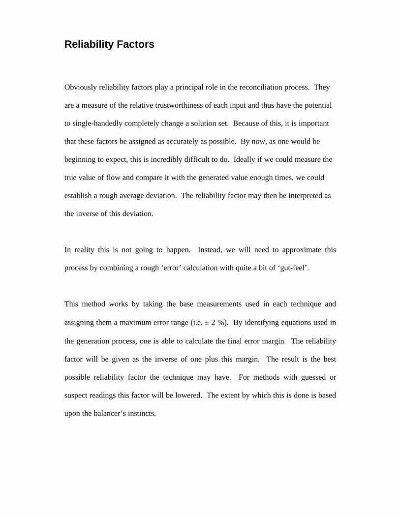
Reliability Factors

Obviously reliability factors play a principal role in the reconciliation process. They

are a measure of the relative trustworthiness of each input and thus have the potential

to single-handedly completely change a solution set. Because of this, it is important

that these factors be assigned as accurately as possible. By now, as one would be

beginning to expect, this is incredibly difficult to do. Ideally if we could measure the

true value of flow and compare it with the generated value enough times, we could

establish a rough average deviation. The reliability factor may then be interpreted as

the inverse of this deviation.

In reality this is not going to happen. Instead, we will need to approximate this

process by combining a rough ‘error’ calculation with quite a bit of ‘gut-feel’.

This method works by taking the base measurements used in each technique and

assigning them a maximum error range (i.e. ± 2 %). By identifying equations used in

the generation process, one is able to calculate the final error margin. The reliability

factor will be given as the inverse of one plus this margin. The result is the best

possible reliability factor the technique may have. For methods with guessed or

suspect readings this factor will be lowered. The extent by which this is done is based

upon the balancer’s instincts.

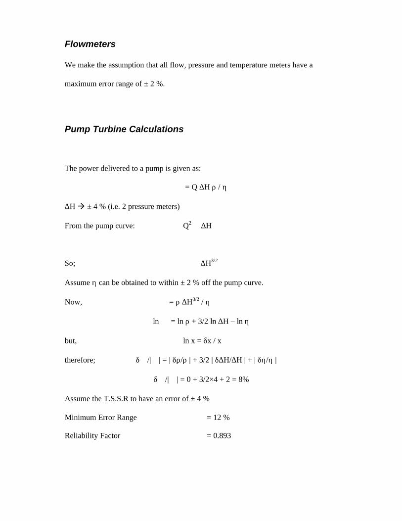
Flowmeters

We make the assumption that all flow, pressure and temperature meters have a

maximum error range of ± 2 %.

Pump Turbine Calculations

The power delivered to a pump is given as:

℘ = Q ∆H ρ / η

∆H à ± 4 % (i.e. 2 pressure meters)

From the pump curve: Q2 ∝ ∆H

So; ℘ ∝ ∆H3/2

Assume η can be obtained to within ± 2 % off the pump curve.

Now, ℘ = ρ ∆H3/2 / η

ln ℘ = ln ρ + 3/2 ln ∆H – ln η

but, ln x = δx / x

therefore; δ℘/|℘| = | δρ/ρ | + 3/2 | δ∆H/∆H | + | δη/η |

δ℘/|℘| = 0 + 3/2×4 + 2 = 8%

Assume the T.S.S.R to have an error of ± 4 %

Minimum Error Range = 12 %

Reliability Factor = 0.893

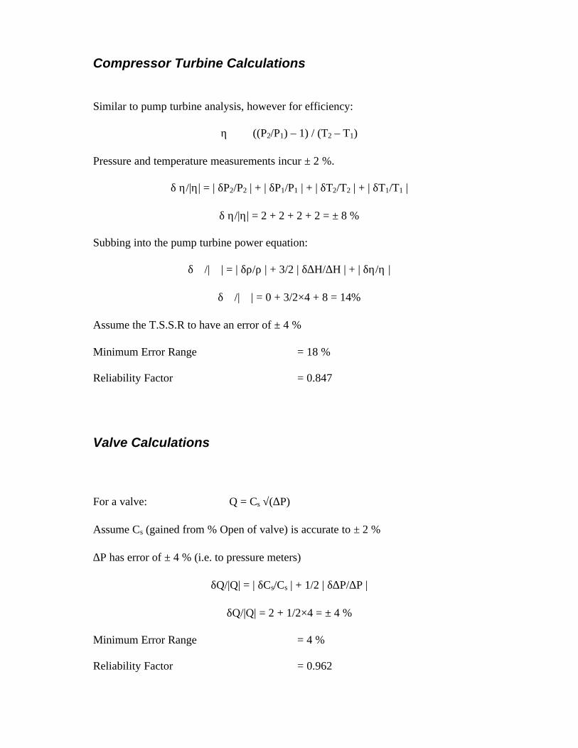
Compressor Turbine Calculations

Similar to pump turbine analysis, however for efficiency:

η ∝ ((P2/P1) – 1) / (T2 – T1)

Pressure and temperature measurements incur ± 2 %.

δ η/|η| = | δP2/P2 | + | δP1/P1 | + | δT2/T2 | + | δT1/T1 |

δ η/|η| = 2 + 2 + 2 + 2 = ± 8 %

Subbing into the pump turbine power equation:

δ℘/|℘| = | δρ/ρ | + 3/2 | δ∆H/∆H | + | δη/η |

δ℘/|℘| = 0 + 3/2×4 + 8 = 14%

Assume the T.S.S.R to have an error of ± 4 %

Minimum Error Range = 18 %

Reliability Factor = 0.847

Valve Calculations

For a valve: Q = Cs √(∆P)

Assume Cs (gained from % Open of valve) is accurate to ± 2 %

∆P has error of ± 4 % (i.e. to pressure meters)

δQ/|Q| = | δCs/Cs | + 1/2 | δ∆P/∆P |

δQ/|Q| = 2 + 1/2×4 = ± 4 %

Minimum Error Range = 4 %

Reliability Factor = 0.962

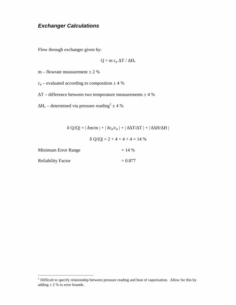
Exchanger Calculations

Flow through exchanger given by:

Q = m cp ∆T / ∆Hv

m – flowrate measurement ± 2 %

cp – evaluated according to composition ± 4 %

∆T – difference between two temperature measurements ± 4 %

∆Hv – determined via pressure reading2 ± 4 %

δ Q/|Q| = | δm/m | + | δcp/cp | + | δ∆T/∆T | + | δ∆H/∆H |

δ Q/|Q| = 2 + 4 + 4 + 4 = 14 %

Minimum Error Range = 14 %

Reliability Factor = 0.877

2 Difficult to specify relationship between pressure reading and heat of vaporisation. Allow for this byadding ± 2 % to error bounds.