California’s School Finance Reform: An Experiment in ...econ.ucsb.edu/~jon/Publications/ExperimentFiscalFederalism.pdf · 55 California’s School Finance Reform: An Experiment

55

California’s School Finance Reform:An Experiment in Fiscal Federalism�Eric J . Brunner

Jon Sonstelie

Although public education is the largest category of local public expenditure,Tiebout (1956) didn’t make public schools the primary example in his classictheory of those expenditures. Perhaps inspired by his locale, he chose to exem-plify his theory by a community with a 500-yard beach. Whatever the motiva-tion, his choice was a prudent one. It is one thing to argue for the efficiency ofpartitioning families among communities according to their demand for beachspace; it is quite another to advance the same argument for partitioning fami-lies according to their demand for something as important as the education oftheir children.

Oates (1969) was more forthright. In his seminal paper on capitalization, heexplicitly defined and estimated the price of public school quality. Families gotgood schools for their children if they were willing to pay for them. Moreover,in his theory of fiscal federalism, Oates (1972) had a ready answer for those whomight object that the willingness to pay for good public schools is determinedlargely by a family’s income. The equitable distribution of income is bestaddressed at a higher level of government, Oates argued; a public service shouldbe provided by the lowest level of government consistent with economies ofscale. Because economies of scale in education are achieved at very low popu-lations (Kenny 1982), public education ought to be provided by many, smallschool districts; higher levels of government can deal with the inequities stem-ming from that system.

Legal theorists didn’t see it that way. Looking at the local provision of publiceducation through the lens of Brown v. Board of Education, 347 U.S. 483 (1954),

3

06635_Ch03.qxd 03/02/2006 9:39 PM Page 55

they saw the wide disparities in spending per pupil across school districts as justanother violation of the equal protection clause of the Fourteenth Amendment.This view had its first legal victory in California with the ruling of the state’sSupreme Court in Serrano v. Priest, 96 Cal. Rptr. 601 (1971). The ruling initiateda chain of events that abruptly ended local financing of public schools inCalifornia. In seven short years, California transformed its school finance systemfrom a decentralized one in which local communities chose how much to spendon their schools to a centralized one in which the state legislature determines theexpenditures of every school district. The Serrano ruling led to similar rulings inother states, although no state reacted quite as radically as California.

It would be an exaggeration to claim that California’s transformation was anatural experiment in fiscal federalism. The Serrano ruling could have led thestate down many different paths, and the path California chose reflected its owncomplex politics. That qualification notwithstanding, California’s story hasmany lessons for students of fiscal federalism. This article describes California’sschool finance system before Serrano and traces the transformation from localto state finance and delineate some consequences of that transformation. Itconcludes with lessons from California’s experience.

School Finance in 1970 and the Serrano Ruling

California school districts differ considerably in size and grade span. In1969–1970, there were 236 unified districts (kindergarten to grade 12), 723 ele-mentary districts, and 120 high school districts. Sixty-four percent of studentswere enrolled in unified districts, with an average enrollment of 12,452. One ofthose districts, Los Angeles Unified, had over 650,000 students, 14 percent ofthe state’s total. No other district was even remotely as large (San Diego was sec-ond with 130,000 students), though there were 12 districts with more than35,000 students. All 12 were unified districts. In contrast, the average enroll-ment for the elementary districts was only 1,573. High school districts averaged4,488 students. Though these smaller districts were numerous, it is importantto remember that per-pupil statistics for California public schools are signifi-cantly influenced by a few large districts.

California school districts were larger on average than districts in otherstates. In California, the average was about 4,200 students; in the rest of thecountry, the average was less than 2,500. The larger average for California waspartly due to the state’s program to encourage the unification of elementaryand high school districts. In 1935, the state had over 3,000 districts, none ofthem unified. By 1965, there were fewer than 1,500 districts, 191 of which wereunified. In addition, during the same period in which the number of districtsfell by half, the state’s population tripled.

56 ERIC J. BRUNNER AND JON SONSTELIE

06635_Ch03.qxd 03/02/2006 9:39 PM Page 56

Before the Serrano decision, California’s school finance system was similar tosystems in other states. School districts levied their own property tax rates, andthe state supplemented that revenue with apportionments from the state schoolfund. The state apportionments were based on a foundation formula with aminimum, called basic aid. The state imposed a maximum on each district’sgeneral purpose tax rate, and that maximum could only be exceeded ifapproved by a majority of a district’s voters. In 1968–1969, all but 11 districtshad rates in excess of this maximum, making school levy elections a regularoccurrence. Districts could also impose of number of special tax rates withoutvoter approval. The revenues from these special rates were earmarked for spe-cific purposes. Property taxes were about 55 percent of the total revenue ofschool districts.

Assessed value per pupil differed widely across districts. In unified districts, 25percent of students were enrolled in districts with assessed value per pupil above$13,456, and 25 percent were in districts with assessed value per pupil less than$7,946—a gap of 69 percent. The gap between the top 5 percent and the bottom5 percent was 343 percent. Similar disparities existed for elementary and highschool districts.

The disparities in assessed value per pupil were greater than the disparitiesin revenue per pupil. The state apportionment formula distributed more stateaid to school districts with lower assessed value per pupil, and school districtswith low assessed value tended to levy higher tax rates. For students in unifieddistricts, the gap in revenue per pupil between the top 25 percent and the bot-tom 25 percent was only 14 percent. However, the gap between the top 5 per-cent and the bottom 5 percent was 70 percent.

Disparities in both revenue and assessed value caused the Serrano com-plaint. Specifically, the plaintiffs argued that those differences violated theequal protection clause of the Fourteenth Amendment. Under the legal frame-work that was developed from previous Supreme Court rulings, a state couldclassify people differently under the law if it had a reasonable rationale fordoing so. Under certain circumstances, however, the state faced a higher hur-dle in proving that its laws were reasonable. If a law affected a fundamentalright, such as voting, and involved a suspect classification of people, such asrace, the state’s law would be subject to “strict scrutiny.” The Warren Courtexpanded the definition of both fundamental rights and suspect classifica-tions. In Brown v. Board of Education, it declared that segregated educationviolated the fundamental rights of black children. In Harper v. Virginia Boardof Elections, 383 U.S. 663 (1966), it overturned Virginia’s poll tax becauseit declared individual wealth a suspect classification. In Baker v. Carr, 369U.S. 186 (1962), the Court declared that legislative districts had to have equalpopulations, making geography, in some respects, a suspect classification.

CALIFORNIA’S SCHOOL FINANCE REFORM 57

06635_Ch03.qxd 03/02/2006 9:39 PM Page 57

Reviewing those rulings, Wise (1967) argued that the local provision of edu-cation must also violate the Fourteenth Amendment. The Court had impliedthat education was a fundamental right and that wealth and geography weresuspect classifications, so a system in which the quality of local public schoolsdepends on geography and the wealth of families and their neighbors wouldnot pass judicial scrutiny.

Similar theories were being advanced by Harold Horowitz (1966), a law pro-fessor at UCLA. Horowitz found a receptive audience in Derrick A. Bell Jr. Bellhad worked with Thurgood Marshall in the NAACP Legal Defense andEducation Fund and was head of the Western Center of Law and Poverty, a pub-lic interest law firm funded by the federal Office of Economic Opportunity. Thetwo decided to test Horowitz’s theories in court, making the Serrano suit theproduct of the “egalitarian revolution” spawned by the Warren Court (Kurland1963) and the war on poverty initiated by President Lyndon Johnson. Theplaintiffs were a number of schoolchildren and their parents, including JohnSerrano Jr., a parent. The defendants were a number of state and local govern-ment officials, including Ivy Baker Priest, state treasurer.

In their complaint, the Serrano lawyers made two specific claims. The twoclaims seem quite different, but they were connected by the plaintiffs’ belief thatassessed value per pupil was highly correlated with family income.1 One claimwas that, because assessed value per pupil varied across school districts, tax-payers in districts with low assessed value per pupil had to pay higher tax ratesto achieve the same spending per pupil. The other claim was that students fromdisadvantaged families might require more educational resources than otherstudents to have the same educational opportunities. The assumed correlationbetween income and assessed valuation implied that the taxpayers in districtswith low assessed value per pupil were also low-income families who needed tospend more on their children’s education. To provide the same educationalopportunity for their children, low-income families would have to pay highertax rates than other families. With regard to a fundamental right, education, thestate treated individuals differently according to a suspect classification: wealth.

The Serrano complaint was filed in Los Angeles Superior Court, but theclaims of the plaintiffs were not immediately tested in court. The defendantsdemurred, the plaintiffs appealed, and the case eventually reached the Cal-ifornia Supreme Court. Because of two other events, the Serrano lawyers narrowed their argument to the fiscal inequities of the school finance system.The first event was the ruling of a federal court in McInnis v. Shapiro, 293 F.


1 In their petition to the California Supreme Court, the Serrano lawyers wrote, “The relative wealthof school district residents correlates to a high degree with the relative wealth of school districts as meas-ured by the assessed valuation per pupil.”

06635_Ch03.qxd 03/02/2006 9:39 PM Page 58

Supp. 327 (N.D. Ill. 1968). In that case, the plaintiffs claimed a violation ofequal protection because the school finance system in Illinois did not provideenough revenue to meet the educational needs of disadvantaged students.The federal court rejected that argument because educational need was toonebulous to adjudicate. McInnis was appealed to the U.S. Supreme Court,which affirmed the decision of the lower court (394 U.S. 322). As a conse-quence, in their appeal to the California Supreme Court, the Serrano lawyersdownplayed their claim about the additional resource needs of disadvantagedstudents and focused more on the fiscal inequities arising from variations inassessed value per pupil. The Serrano lawyers were aided in this new focusby the second event: the 1970 publication of Private Wealth and PublicEducation, by Coons, Clune, and Sugarman. Coons and his coauthors took amore conservative approach than Horowitz in their legal critique of publicschool finance. They did not include differing educational needs as an ele-ment in their critique, taking revenue per pupil as the measure of educationalquality. This measure put a spotlight on the fiscal inequities due to variationsin assessed value per pupil.

The California Supreme Court accepted the logic of Coons and coauthors. Itruled that education was a fundamental right and school district wealth was asuspect classification. Differences in revenue per pupil due to differences inassessed value per pupil thus violated equal protection. In declaring districtwealth a suspect classification, the court had entered new territory. The defen-dants argued that the concept of a suspect classification was meant to beapplied to individuals, not to government entities. This argument would haverequired the plaintiffs to show that there was a correlation between the assessedvalue of a district and the income of families living in that district. The courtrejected that argument, however, ruling that discrimination on the basis of dis-trict wealth is as invalid as discrimination based on individual wealth. TheSupreme Court returned the case to the Superior Court for hearing, but itsground rules determined the outcome. The lower court was not required toexamine evidence about the relationship between assessed value and familyincome or spending per pupil and family income. It could focus instead onvariation in assessed value per pupil and whether school districts with lowerassessed value per pupil had to levy higher tax rates to have the same spendingper pupil. The answer to both questions was clearly affirmative, and theSuperior Court ruled in favor of the plaintiffs.

If the Supreme Court had asked the Superior Court to examine the linkbetween individual wealth and district wealth, the outcome may have beendifferent. That examination would have been difficult at the time becauseCensus data was not aggregated to the school district level. The CensusBureau completed that task in the late 1970s, however, allowing us now to


06635_Ch03.qxd 03/02/2006 9:39 PM Page 59

examine the evidence.2 Our framework for doing so is a simplified versionof the median voter model due to Borcherding and Deacon (1972) andBergstrom and Goodman (1973). A family’s demand for school spending is afunction of its income and its tax-price for school spending. The tax-price isthe increase in the family’s property taxes if the school district increases prop-erty tax revenue by one dollar per pupil. That tax-price equals the assessedvalue of the family’s home divided by the district’s assessed value per pupil.In logarithmic terms, this price is p = h - v, where h is the log of the family’sassessed value and v is the log of the district’s assessed value per pupil.Assume that the assessed value of a family’s house is determined by itsincome, h = h0 + qy , where y is the log of the family’s income and q is the incomeelasticity of housing demand. Assume further that a family’s demand func-tion for spending per pupil has constant price and income elasticities,s = s0 + ep + hy, where s is the log of the demand for spending per pupil, e isthe price elasticity of demand, and h is the income elasticity of demand.Combining the previous three equations, the demand for spending per pupilis s = b0 + b1v + b2y, where b0 = s0 + eh0, b1 = -e, and b2 = (eq + h). With theassumptions that spending per pupil in a district equals the demand of themedian voter and that the median voter has median income, this demandfunction leads to the regression reported in table 3.1.

The model in table 3.1 excludes several important factors. For example, itignores the fact that renters may face a different tax-price than homeowners(Oates 2005) and that parents with children in private school may have differ-ent demands for public school spending than parents with children in public


Table 3.1

Coefficient Estimates for Median Voter Regressions, 1969–1970 DependentVariable: Log of Spending Per Pupil (Standard Errors in Parentheses)

Elementary High School Coefficient (variable) Districts Districts Unified Districts

b1(log of assessed 0.171 (0.013) 0.265 (0.025) 0.267 (0.015)value per pupil)

b2 (log of median 0.137 (0.029) 0.002 (0.043) 0.035 (0.033)family income)

Observations 401 110 228

Adjusted R-squared 0.346 0.508 0.569

2 The tabulation was done for only 739 of the 1,079 districts existing in 1969–1970, but those 739 dis-tricts enrolled 98 percent of students in 1969–1970.

06635_Ch03.qxd 03/02/2006 9:39 PM Page 60

schools (Sonstelie 1982). Yet, despite these omissions, the model explains morethan 30 percent of the variation in spending per pupil for elementary districtsand more than 50 percent for high school and unified districts. Moreover,the estimated coefficients are consistent with expectations. The coefficient b1

should be positive because it is the negative of the price elasticity of demand.The coefficient is positive and more than 10 times its standard error in all threeregressions. The coefficient b2 is a function of the price elasticity of the demandfor school spending, e the income elasticity of the demand for spending, h andthe income elasticity of housing demand, q Specific ally, b2 = (eq + h). Becauseboth income elasticities should be positive and the price elasticity negative, b2

could be positive or negative. In fact, as table 3.1 shows, the coefficient is posi-tive for all three types of districts but not significantly different from zero forhigh school and unified districts.

The insignificant coefficients on median family income seem to suggest thatincome had little effect on spending per pupil, at least for high school and uni-fied districts. That is, two districts with the same assessed value per pupil butdifferent levels of median family income had roughly the same spending perpupil. While this is strictly true, the qualification about assessed value is impor-tant. Because housing is a normal good, the assessed value per pupil of resi-dential property should rise with family income. If two districts had the sameassessed values but different incomes, the lower-income district must thereforehave had either more nonresidential property per pupil or fewer students perfamily. Either factor would lower the district’s tax-price and thus offset the neg-ative effect on demand of its lower income.

The critical relationship between income and assessed value is best illustratedwith a simple example. Suppose that all property is residential and all districts havethe same number of students per family. Then, assessed value per pupil would beroughly proportional to median family income, the tax-price of education wouldbe approximately the same for all districts, and spending per pupil would prima-rily be a function of family income. The two variables in our median voter regres-sions would be nearly collinear, making it difficult to estimate their coefficients.A simple regression of spending per pupil on median family income would workvery well, however. Most important, in this world, the complaint of the Serranolawyers would have been exactly right. The quality of public schools, as measuredby revenue per pupil, would have been determined almost solely by family income.

This example points to the critical role of the correlation between the log ofmedian family income and the log of assessed value per pupil. In the exampleof the previous paragraph, that correlation is close to unity. Among Californiaschool districts in 1969–1970, the correlation was far short of unity. For ele-mentary districts, it was .12. For unified districts, it was only .04, and for highschool districts it was actually negative, −.05.


06635_Ch03.qxd 03/02/2006 9:39 PM Page 61

These low correlations of median family income and assessed value perpupil could be due to two basic factors. The first is variations in studentsper family. As Fischel (2004) pointed out in his analysis of voting patterns onProposition 13, districts with many senior citizens had relatively high assessedvalue per pupil because they had fewer students per family. A second factor isthe distribution of nonresidential property. While we do not know the value ofnonresidential property in each school district, assessed values for California’slargest school districts seem consistent with an uneven distribution of nonres-idential property. Among the largest ten school districts, San Juan and GardenGrove, both middle-income suburban districts with little commercial or indus-trial property, had the lowest assessed value per pupil (less than $7,000 perpupil). Conversely, Oakland, Long Beach, and San Francisco, central cities withlarge amounts of industrial and commercial property, had assessed valuesgreater than $15,000 per pupil.

Both factors, variations in nonresidential property and students per family,surely explain some of the variation in assessed value per pupil across districts.The question is whether they can explain the unexpectedly low correlationbetween median family income and assessed value per pupil. In particular, didthe distributions of either variable across districts offset what we presume to bea strongly positive correlation between median family income and the averagevalue of residences? In the case of students per family, the correlation withmedian family income would have had to have been strongly positive. In fact, thecorrelation between the logs of those two variables was very small for unifieddistricts (.01) and negative for elementary and high school districts (−.21 and −.04). The distribution of students per family was not the explanation of the lowcorrelation between median family income and assessed value per pupil.

This finding leaves the distribution of nonresidential property as a possibleexplanation. Evidence in favor of this explanation is the low correlation betweenmedian family income and assessed value per family. That is, when total assessedvalue, residential and nonresidential, is normalized by families instead of stu-dents, the correlation with median family income is low. For unified districts,the correlation was .05, for elementary districts −.21, and for high school districts −.04. If total assessed value per family is not correlated with median family income,a negative relationship between nonresidential property per family and familyincome must have offset the almost certainly positive relationship betweenassessed values of houses and the income of their residents.

Whatever the explanation, because assessed value per pupil was not stronglycorrelated with median family income in a district, high-income districts faced,on average, higher tax-prices for public school spending. The higher tax-pricepartially offset the direct effect of income on demand for public school spend-ing, resulting in a weak relationship between spending per pupil and family


06635_Ch03.qxd 03/02/2006 9:39 PM Page 62

income. In 1969–1970, the correlation of the log of spending per pupil to thelog of median family income was .26 for elementary districts, .07 for unifieddistricts, and −.05 for high school districts. In the Appendix, the correlation ofmedian family income and spending per pupil is expressed as a function of thecorrelation of median family income and assessed value per pupil, providing amathematical representation of the intuition we have presented for this result.

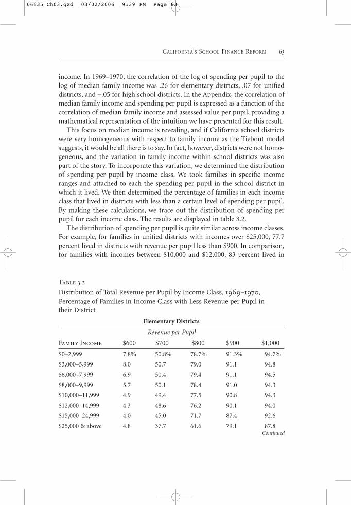
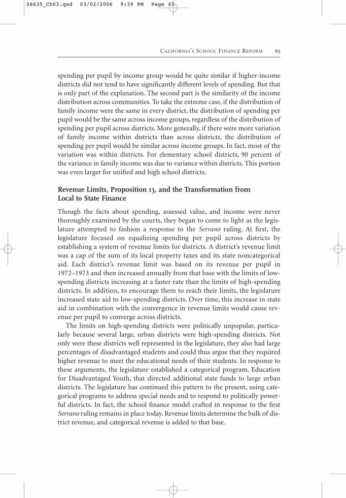
This focus on median income is revealing, and if California school districtswere very homogeneous with respect to family income as the Tiebout modelsuggests, it would be all there is to say. In fact, however, districts were not homo-geneous, and the variation in family income within school districts was alsopart of the story. To incorporate this variation, we determined the distributionof spending per pupil by income class. We took families in specific incomeranges and attached to each the spending per pupil in the school district inwhich it lived. We then determined the percentage of families in each incomeclass that lived in districts with less than a certain level of spending per pupil.By making these calculations, we trace out the distribution of spending perpupil for each income class. The results are displayed in table 3.2.

The distribution of spending per pupil is quite similar across income classes.For example, for families in unified districts with incomes over $25,000, 77.7percent lived in districts with revenue per pupil less than $900. In comparison,for families with incomes between $10,000 and $12,000, 83 percent lived in


Table 3.2

Distribution of Total Revenue per Pupil by Income Class, 1969–1970,Percentage of Families in Income Class with Less Revenue per Pupil intheir District

Elementary Districts

Revenue per Pupil

Family Income $600 $700 $800 $900 $1,000

$0–2,999 7.8% 50.8% 78.7% 91.3% 94.7%

$3,000–5,999 8.0 50.7 79.0 91.1 94.8

$6,000–7,999 6.9 50.4 79.4 91.1 94.5

$8,000–9,999 5.7 50.1 78.4 91.0 94.3

$10,000–11,999 4.9 49.4 77.5 90.8 94.3

$12,000–14,999 4.3 48.6 76.2 90.1 94.0

$15,000–24,999 4.0 45.0 71.7 87.4 92.6

$25,000 & above 4.8 37.7 61.6 79.1 87.8Continued

06635_Ch03.qxd 03/02/2006 9:39 PM Page 63

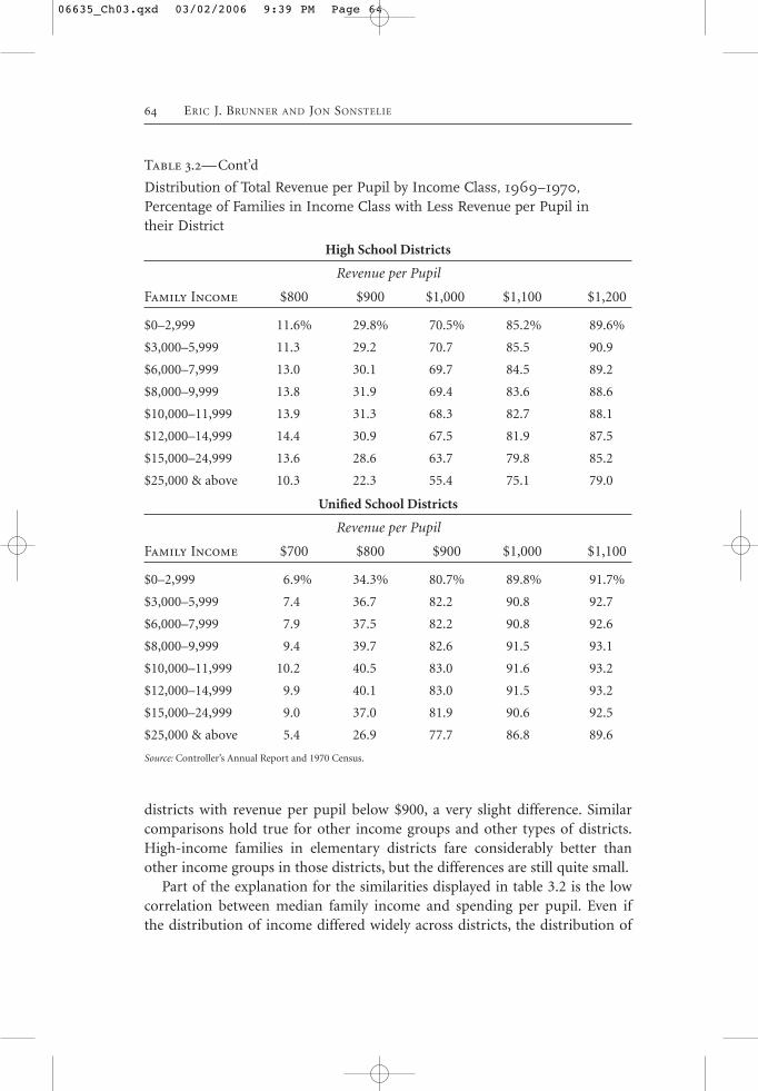
districts with revenue per pupil below $900, a very slight difference. Similarcomparisons hold true for other income groups and other types of districts.High-income families in elementary districts fare considerably better thanother income groups in those districts, but the differences are still quite small.

Part of the explanation for the similarities displayed in table 3.2 is the lowcorrelation between median family income and spending per pupil. Even ifthe distribution of income differed widely across districts, the distribution of


Table 3.2—Cont’d

Distribution of Total Revenue per Pupil by Income Class, 1969–1970,Percentage of Families in Income Class with Less Revenue per Pupil intheir District

High School Districts

Revenue per Pupil

Family Income $800 $900 $1,000 $1,100 $1,200

$0–2,999 11.6% 29.8% 70.5% 85.2% 89.6%

$3,000–5,999 11.3 29.2 70.7 85.5 90.9

$6,000–7,999 13.0 30.1 69.7 84.5 89.2

$8,000–9,999 13.8 31.9 69.4 83.6 88.6

$10,000–11,999 13.9 31.3 68.3 82.7 88.1

$12,000–14,999 14.4 30.9 67.5 81.9 87.5

$15,000–24,999 13.6 28.6 63.7 79.8 85.2

$25,000 & above 10.3 22.3 55.4 75.1 79.0

Unified School Districts

Revenue per Pupil

Family Income $700 $800 $900 $1,000 $1,100

$0–2,999 6.9% 34.3% 80.7% 89.8% 91.7%

$3,000–5,999 7.4 36.7 82.2 90.8 92.7

$6,000–7,999 7.9 37.5 82.2 90.8 92.6

$8,000–9,999 9.4 39.7 82.6 91.5 93.1

$10,000–11,999 10.2 40.5 83.0 91.6 93.2

$12,000–14,999 9.9 40.1 83.0 91.5 93.2

$15,000–24,999 9.0 37.0 81.9 90.6 92.5

$25,000 & above 5.4 26.9 77.7 86.8 89.6

Source: Controller’s Annual Report and 1970 Census.

06635_Ch03.qxd 03/02/2006 9:39 PM Page 64

spending per pupil by income group would be quite similar if higher-incomedistricts did not tend to have significantly different levels of spending. But thatis only part of the explanation. The second part is the similarity of the incomedistribution across communities. To take the extreme case, if the distribution offamily income were the same in every district, the distribution of spending perpupil would be the same across income groups, regardless of the distribution ofspending per pupil across districts. More generally, if there were more variationof family income within districts than across districts, the distribution ofspending per pupil would be similar across income groups. In fact, most of thevariation was within districts. For elementary school districts, 90 percent ofthe variance in family income was due to variance within districts. This portionwas even larger for unified and high school districts.

Revenue Limits, Proposition 13, and the Transformation from Local to State Finance

Though the facts about spending, assessed value, and income were neverthoroughly examined by the courts, they began to come to light as the legis-lature attempted to fashion a response to the Serrano ruling. At first, the legislature focused on equalizing spending per pupil across districts by establishing a system of revenue limits for districts. A district’s revenue limitwas a cap of the sum of its local property taxes and its state noncategoricalaid. Each district’s revenue limit was based on its revenue per pupil in1972–1973 and then increased annually from that base with the limits of low-spending districts increasing at a faster rate than the limits of high-spendingdistricts. In addition, to encourage them to reach their limits, the legislatureincreased state aid to low-spending districts. Over time, this increase in stateaid in combination with the convergence in revenue limits would cause rev-enue per pupil to converge across districts.

The limits on high-spending districts were politically unpopular, particu-larly because several large, urban districts were high-spending districts. Notonly were these districts well represented in the legislature, they also had largepercentages of disadvantaged students and could thus argue that they requiredhigher revenue to meet the educational needs of their students. In response tothese arguments, the legislature established a categorical program, Educationfor Disadvantaged Youth, that directed additional state funds to large urbandistricts. The legislature has continued this pattern to the present, using cate-gorical programs to address special needs and to respond to politically power-ful districts. In fact, the school finance model crafted in response to the firstSerrano ruling remains in place today. Revenue limits determine the bulk of dis-trict revenue, and categorical revenue is added to that base.


06635_Ch03.qxd 03/02/2006 9:39 PM Page 65

The legislature’s response to the Serrano ruling did not satisfy the Los AngelesSuperior Court. The equalization of revenue limits would take too long, andschool districts constrained by the limits had a ready escape. They could over-ride their limits with a simple majority vote of their residents. Because almost allCalifornia school districts had been regularly passing levy elections beforeSerrano, the override provision eviscerated the revenue limit system.

The Court’s rejection of this system caused the legislature to attempt a moreambitious reform. It kept revenue limits and the override provision but sub-jected overrides to power equalization. For districts with low assessed value perpupil, the state would supplement their tax revenue from an override so thatevery school district would receive the same revenue from the same increase inproperty tax rates. This additional aid would be costly to the state, but it had asurplus at the time, which many legislators were earmarking for a solution tothe Serrano ruling.

Power equalization was never implemented. Less than a month before it wasslated to begin, the voters of California passed Proposition 13, which set a 1 per-cent limit on the property tax rate and gave to the legislature the authority toallocate the revenue from that rate among local governments. The legislaturebased its allocations on historical patterns, but because the 1 percent rate wasless than half of the average rate before Proposition 13, those allocations fell farshort of what governments had previously received. To compensate, the stateincreased aid to local governments, using the surplus it had accumulated. Forschool districts, state aid was determined by revenue limits. Each district’s aidwas the difference between its revenue limit and the property tax revenue it wasallocated.3 In other words, each district’s revenue limit was the revenue perpupil it received from the property tax and state aid. In that sense, the state nowdetermines each district’s revenue.

Fischel (1989, 1996, 2001, 2004) has argued that the Serrano ruling causedProposition 13. Faced with the prospect of losing control of their property taxrevenue, homeowners voted to limit it. As evidence of his explanation, Fischelpointed out that voters had earlier rejected ballot initiatives to limit the prop-erty tax and to shift the financing of public schools toward the state. Only afterthe Serrano ruling placed the nexus between their taxes and their schools injeopardy, Fischel argued, did voters change their minds and decide to limitproperty taxes. In any event, Proposition 13 did provide the legislature with arelatively straightforward response to the Serrano ruling. It made the property


3 A few districts receive more property tax revenue than their revenue limit. Under the current law, theykeep that excess and also receive a small amount of basic aid from the state. The number of these districtschanges as their enrollments and property tax revenues change. However, the number has never been large.Today there are only about 50 of these districts, enrolling less than 3 percent of the state’s students.

06635_Ch03.qxd 03/02/2006 9:39 PM Page 66

tax a state tax and ended what remained after Serrano of the local finance ofpublic education.

Since Proposition 13, the legislature has gradually equalized revenue limitsand thus revenue per pupil. In 1986, the Los Angeles Superior Court found thatthis equalization had gone far enough to satisfy the Serrano ruling. The legisla-ture has continued to equalize revenue, however, by periodically bringing upthe revenue limits of districts below the average. By 1999–2000, these differ-ences were quite small. In unified districts, 25 percent of students were enrolledin districts with revenue limit funds greater than $3,901 per pupil, and 25 per-cent of students were enrolled in districts with revenue limit funds less than$3,806. The gap between the 75th and 25th percentiles was only 2 percent. Forthe 95th and 5th percentiles, the gap was 11 percent. In contrast, the equivalentgaps for 1969–1970 were 14 percent and 70 percent, respectively.

State categorical programs have continued to grow. In 1999–2000, these pro-grams constituted 25 percent of the revenue of unified districts, 22 percentof the revenue of elementary districts, and 18 percent of the revenue of highschool districts. The legislature has also allowed districts to levy a tax on parcelsof real property. We discuss this tax in more detail following.

State and federal categorical programs widen the disparities in revenue perpupil. In general, however, these disparities favor districts with high propor-tions of disadvantaged students. For example, for total revenue per pupil inunified districts in 1999–2000, the gap between the 75th and 25th percentiles is$962, much higher than the $95 gap in revenue limit funds. A simple regressionof revenue per pupil on the percentage of low-income students (measured byeligibility for the free or reduced-price lunch program) reveals that most of thatgap can be explained by categorical revenue favoring low-income students. Forunified districts in 1999–2000, a low-income student yielded about $1,018more revenue than other students. For an elementary school district, this incre-ment was $451, and for a high school district, the increment was actually neg-ative—specifically, −$301. There are large variations around these averages,however.

Though the finance of public schools has been centralized, the governance ofthose schools is still a local function. Local voters still elect school boards for theirdistricts, and the school boards hire and fire top management, approve schooldistrict budgets, and set district policies. Each school district bargains with itsemployee unions over salaries, benefits, and working conditions, though theparameters for that bargaining are established by the budget decisions made inSacramento. A key issue, of course, is the total revenue provided to schools. Forcollective bargaining, another important issue is the division of that total revenuebetween unrestricted revenue and categorical revenue. Unrestricted revenuefunds salaries; categorical revenue is often protected from collective bargaining.


06635_Ch03.qxd 03/02/2006 9:39 PM Page 67

For those reasons, the employee unions are active lobbyists in Sacramento, fight-ing to increase the flow of unrestricted revenue and thus the pool of money avail-able for salary increases for their members. On the other hand, some categoricalprograms such as the large K–3 Class Size Reduction program were motivated atleast partly by the desire to limit those salary increases. As a consequence, the leg-islature’s decisions about how much district revenue to make unrestricted andhow much to tie up in categorical programs are the first round of collective bar-gaining between districts and their employee unions.

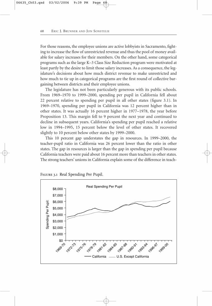
The legislature has not been particularly generous with its public schools.From 1969–1970 to 1999–2000, spending per pupil in California fell about22 percent relative to spending per pupil in all other states (figure 3.1). In1969–1970, spending per pupil in California was 12 percent higher than inother states. It was actually 16 percent higher in 1977–1978, the year beforeProposition 13. This margin fell to 9 percent the next year and continued todecline in subsequent years. California’s spending per pupil reached a relativelow in 1994–1995, 15 percent below the level of other states. It recoveredslightly to 10 percent below other states by 1999–2000.

This 10 percent gap understates the gap in resources. In 1999–2000, theteacher-pupil ratio in California was 26 percent lower than the ratio in otherstates. The gap in resources is larger than the gap in spending per pupil becauseCalifornia teachers were paid about 16 percent more than teachers in other states.The strong teachers’ unions in California explain some of the difference in teach-


Real Spending Per Pupil$8,000

$7,000

$6,000

$5,000

$4,000

$3,000

$2,000

$1,000

$0

1969

-70

1972

-73

1975

-76

1978

-79

1981

-82

1984

-85

1987

-88

1990

-91

1993

-94

1996

-97

1999

-00

Spe

ndin

g P

er P

upil:

California U.S. Except California

Figure 3.1 Real Spending Per Pupil.

06635_Ch03.qxd 03/02/2006 9:39 PM Page 68

ers’ salaries, but the 16 percent premium is not far out of line with other salarydifferences. In 1999–2000, employees with bachelor’s degrees earned about 14percent more in California than in the rest of the country (Rose et al. 2003).

Since Serrano, courts have overturned school finance systems in several otherstates. California’s relative decline in spending per pupil is not a general trendamong these states. Manwaring and Sheffrin (1997) compare public schoolspending in states with court-order reform to spending in other states. Using adynamic model that allows for lagged adjustment to reform and for the effectof reform to depend on a variety of state characteristics, they find that theexpenditures of some states are higher than they would have been withoutreform, while expenditures in others are lower. Downes and Shah (1995) use asimilar approach and reach a similar conclusion. Murray, Evans, and Schwab(1998) examine this issue at the school district level, revealing the effect ofreform not just on average spending per pupil in a state but also on the distri-bution of spending per pupil across districts. They find that court-order reformtended to level up spending per pupil within a state. It raised expendituresin low-spending districts and had no effect on high-spending districts. Awareof the inconsistency of their results with California’s experience, they reesti-mated their model without California districts and found that omitting thesedistricts increased the positive effect of reform on expenditures. They attrib-uted California’s exceptional response to court-ordered reform to the strict rev-enue equality demanded by California’s courts, though they did not explainwhy revenue equality necessarily leads to a leveling down.

One possible explanation of California’s exceptional response is simply thatit was first. Before the Serrano ruling, state legislatures could not have reason-ably anticipated that the courts would overturn their school finance systems.After the Serrano ruling, however, many state legislatures began to examinetheir own liabilities and to reform their school finance systems. As a conse-quence, it is not quite as clear that the world can be neatly divided into statesthat reformed their systems after a court order and states that did not. Amongboth classes are surely some states that reformed their systems in an attempt tothwart a court order to do so.

Another possible explanation of California’s exceptional response is that itsschool finance reform was accompanied by a property tax limitation. As we havejust noted, Fischel has argued that Serrano caused Proposition 13, an argumentthat would disqualify property tax limitations as an independent explanation. Butseveral states had tax limitations without court-ordered reform, providing anopportunity to separate the effects of tax limitations from the effects of court-ordered reform. Figlio (1997) demonstrated the promise of that explanationby showing that, after enacting limits, states increased student-teacher ratiosand decreased teacher salaries. As further evidence of this negative effect, Figlio


06635_Ch03.qxd 03/02/2006 9:39 PM Page 69

and Rueben (2001) showed that states with property tax limits experienced areduction in the average quality of new public school teachers.

Though these studies do not identify the mechanism through which a prop-erty tax limitation affects public school quality, the mechanism seems obvious.The limit reduces property tax revenue, which reduces funds for public schoolsand thus public school quality. But lower property tax revenue can be replacedby other taxes or by increased aid to local governments from the state. In fact,California followed exactly this path. Despite the limit on the property tax rate,in 1999–2000 state and local governments in California spent 9 percent more percapita than governments in other states. Thus, California’s relatively low publicschool spending cannot be explained by a generally low level of public expendi-tures. In an accounting sense, California’s low public school spending is due totwo factors. First, it had about 8 percent more pupils per capita than other states.Second, despite the first factor, the state allocated a lower share of public fundsto schools than other states. In California in 1999–2000, the expenditures ofpublic schools constituted 22 percent of state and local public expenditures. Inthe rest of the country, this share was 24.6 percent. California’s relative decline inspending per pupil does not reflect a general decline in the public sector butrather a choice about the allocation of a relatively abundant stream of state andlocal revenue.

Another explanation for California’s relative decline in spending per pupilfocuses on how school finance reform changed the tax-price of school spending.In response to court orders, other states implemented district power equaliza-tion and other financing schemes that alter the tax-price for school districtspending but left districts with some authority over their own property tax rates.California took away from school districts the authority to tax property, which,from the perspective of school districts, made the property tax-price infinite.Hoxby (2001) determined how school finance reforms altered tax-prices for dis-tricts and then estimated how spending per pupil in districts responded to thosechanges in tax-prices. The tax-price in her analysis is the increase in districtproperty tax revenue required to increase spending by one dollar. Before Serranoin California, this price was unity; after Serrano, it is infinite. Hoxby estimatesthan an increase in tax-price from unity to infinity decreases spending per pupilby 15 percent, thus explaining most of California’s relative decline.4


4 Because a least squares regression is impossible when a regressor has an infinite value, Hoxby esti-mated spending per student as a function of the inverse of the tax-price. California’s inverse tax-price isunity before Serrano and zero after Serrano. All school districts in New Mexico have inverse tax-pricesof unity before reform and 0.05 after reform. In Oklahoma, some districts have inverse tax-prices as lowas 0.15 after reform. In all other states, the lowest inverse tax-price after reform is 0.53, and inverse tax-prices are unity in 36 states after reform. Thus, the tax-price effect of school finance reform appears tobe primarily identified by the postreform, relative decline in spending per pupil in California, NewMexico, and Oklahoma.

06635_Ch03.qxd 03/02/2006 9:39 PM Page 70

This explanation is misleading, however, because it implicitly assumes thatschool spending decisions in California are made at the school district level. Aswe show in what follows, some limited school spending decisions are made atthe school district level through parcel tax elections. However, the most impor-tant spending decisions are made by the legislature when it decides whetherto increase revenue limit funding and categorical programs. At that level, thetax-price of school spending is certainly not infinite. School spending can beincreased by increasing income or sales tax rates or by decreasing expendituresin other areas. Of course, legislatures in other states make similar decisionswhen they decide to increase foundation or equalization aid. What distin-guishes California from those other states is the balance between state and localdecisions. Almost all the spending decisions that count in California are madeby the state legislature. Virtually none are made locally.

Picus (1991) focused directly on this issue, arguing that the indirect linkbetween taxpayers and their local public schools has caused California’s relativedecline in school spending. Homeowners pay property, sales, and income taxes,which are then blended in Sacramento and returned to their local publicschools. Compared to the days before Serrano in which they could simply voteto increase their property tax rates, taxpayers and families have no simple wayto affect the funds of their local public schools. It is less clear why this shouldlead to lower spending on schools, however, because school districts and teach-ers’ unions are very well represented in Sacramento.

Silva and Sonstelie (1995) propose another explanation that is also based onthe change in the level of government at which educational spending decisionsare made. If the demand for education is determined by family income andfamilies are partitioned among school districts according to their income asthe Tiebout model suggests, the statewide average of spending per pupilshould approximately equal the average demand, which is then the demand ofa family with average income. Under state finance, however, average spendingper pupil, which will be the same in every district, should reflect the demandsof the median voter, which is the demand of the family with median income.Because average income is greater than median income, the average of spend-ing per pupil under local finance will be greater than spending per pupilunder state finance. With this explanation, Silva and Sonstelie can explainabout half of California’s decline in spending per pupil. The difficulty with thisexplanation, however, is that school districts in California were not homoge-neous with respect to family income. In 1970, there was much more variationof family income within school districts than across districts. Furthermore,nonresidential property was inversely correlated with median family income,and thus many school districts with low median income had high spendingper pupil.


06635_Ch03.qxd 03/02/2006 9:39 PM Page 71

A related explanation was offered by Fernandez and Rogerson (1999), whoincorporate the foundation aid system that California had in 1970. Under thatsystem, low-income school districts find it cheaper to increase their spending byincreasing the foundation than by increasing their own taxes. They thus supporta relatively high foundation level, which higher-income districts supplementwith their own taxes. The result is a higher level of spending than if all districtsare required to have the same level of spending, as under state finance. Like Silvaand Sonstelie, this explanation depends on the unrealistic assumption thatschool districts are homogeneous with respect to family income and that allproperty was residential. In addition, it has the unrealistic implication that manyschool districts do not supplement state foundation aid. In fact, as just related,all but 11 California school districts in 1970 voted in favor of property tax ratesexceeding the statutory maximum, and every California school in 1968–1969supplemented its foundation aid by at least $130 per pupil.

A fourth explanation is directly related to the median voter model in table3.1. In 1969–1970, the property tax was the source of marginal funds for schooldistricts. For a homeowner, the tax-price of spending per pupil was its assessedvalue divided by the assessed value per pupil in its school district. For the stateas a whole, nonresidential property made up 45 percent of that total (Sonstelie,Brunner, and Ardon 2000). Thus, on average, homeowners received a 45 per-cent subsidy for school spending. Proposition 13 put a strict lid on property taxrevenue, and so the source of marginal funds for schools became the incomeand sales taxes. Both sources tax individuals directly, with very small percent-ages paid by business. Thus, Proposition 13 increased the tax-price of schoolspending by about 45 percent.

The effect of this price increase is determined by the price elasticity ofdemand, which is the negative of the coefficient on assessed value per pupil inthe simple median voter model in table 3.1. That number is probably an under-estimate, however. Spending per pupil was positively correlated with state aid,which was negatively correlated with assessed value per pupil. Thus, our esti-mate of the price elasticity is biased toward zero. Because of the flypaper effect(Hines and Thaler 1995), state aid may have had a relatively large effect onschool district spending, making this bias quite large. In any event, our estimateof the price elasticity is −.171 for elementary districts, −.265 for high school dis-tricts, and −.267 for unified districts. Based on that evidence and the likelihoodthat the price elasticity is lower than our estimates, let us suppose that the priceelasticity was −.25. A 45 percent increase in the tax-price of spending per pupilwould then entail an 11 percent reduction in spending per pupil, which wouldexplain about half the relative reduction California experienced.

If this explanation has validity, it only raises another question. Why doesn’tCalifornia find another tax source to fund its schools, a source with the same


06635_Ch03.qxd 03/02/2006 9:39 PM Page 72

subsidies from business? In fact, some school districts appear to be gropingtoward that solution as they refine their implementation of the parcel tax. Theserefinements are discussed below in the section on reform. If school resourcesaffect student achievement, California’s relative decline in resources per pupilshould be reflected in a relative decline in student achievement. This appears tohave occurred. During the 1990s, California students performed poorly on theNational Assessment of Educational Progress (NAEP), a standardized testin writing and mathematics administered to a sample of fourth- and eighth-graders throughout the country. This poor performance partly reflects the largepercentage of immigrant students in the state, but even when corrections aremade for family characteristics, California students are well below students inother states. As reported in Carroll et al. (2005), for the battery of NAEP testsadministered between 1990 and 2003, California students scored .18 standarddeviations below the national mean after adjusting for family characteristics.California’s average adjusted score was the lowest of any state participating inthe NAEP.

California students performed considerably better in the period before thetransformation from local to state finance. The first piece of evidence comesfrom the National Longitudinal Study of the High School Class of 1972 (NLS).The study administered a standardized test to a sample of high school seniorsin 1972 and also collected information about the characteristics of their fami-lies, including race, ethnicity, family income, and parental education. Using thatdata, Sonstelie et al. (2000) regressed test scores on family characteristics and adummy variable indicating whether the student was a California resident. Thecoefficient on that dummy variable was not significantly different from zero.A similar regression produced the same result with data from High School andBeyond (HSB). The HSB test was administrated to tenth- and twelfth-gradersin 1980, two years after the transformation from local to state finance. However,the students taking the test would have received most of their educationbefore the transformation.

This apparent decline in average performance would be less troubling if itwere accompanied by an equalization of achievement across districts andincome groups. There is little evidence of equalization across school districts,however. Downes (1992) examined district averages on a state-mandatedachievement test. The distribution of district scores is very similar in 1976–1977and 1985–1986. Moreover, in school districts with low spending per pupil in1976–1977, and thus relatively large increases in spending from 1976–1977 to1985–1986, student achievement did not rise faster than in other districts.

There is less evidence about the equalization of achievement across incomegroups. Because of the growing number of categorical programs, school districtswith high proportions of low-income students do tend to receive more revenue


06635_Ch03.qxd 03/02/2006 9:39 PM Page 73

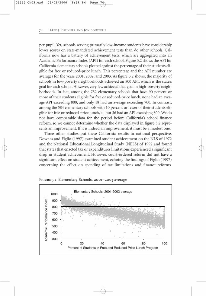
per pupil. Yet, schools serving primarily low-income students have considerablylower scores on state-mandated achievement tests than do other schools. Cal-ifornia now has a battery of achievement tests, which are aggregated into anAcademic Performance Index (API) for each school. Figure 3.2 shows the API forCalifornia elementary schools plotted against the percentage of their students eli-gible for free or reduced-price lunch. This percentage and the API number areaverages for the years 2001, 2002, and 2003. As figure 3.2 shows, the majority ofschools in low-poverty neighborhoods achieved an 800 API, which is the state’sgoal for each school. However, very few achieved that goal in high-poverty neigh-borhoods. In fact, among the 752 elementary schools that have 90 percent ormore of their students eligible for free or reduced-price lunch, none had an aver-age API exceeding 800, and only 18 had an average exceeding 700. In contrast,among the 584 elementary schools with 10 percent or fewer of their students eli-gible for free or reduced-price lunch, all but 36 had an API exceeding 800. We donot have comparable data for the period before California’s school financereform, so we cannot determine whether the data displayed in figure 3.2 repre-sents an improvement. If it is indeed an improvement, it must be a modest one.

Three other studies put these California results in national perspective.Downes and Figlio (1997) examined student achievement on the NLS of 1972and the National Educational Longitudinal Study (NELS) of 1992 and foundthat states that enacted tax or expenditures limitations experienced a significantdrop in student achievement. However, court-ordered reform did not have asignificant effect on student achievement, echoing the findings of Figlio (1997)concerning the effect on spending of tax limitations and finance reforms.


Elementary Schools, 2001-2003 average

300

400

500

600

700

800

900

1000

0 20 40 60 80 100Percent of Students in Free and Reduced-Price Lunch Program

Aca

dem

ic P

erfo

rman

ce In

dex

:

Figure 3.2 Elementary Schools, 2001–2003 average

06635_Ch03.qxd 03/02/2006 9:39 PM Page 74

Limitations have an effect, but reform by itself does not. These results suggestthat California’s decline in student achievement was due to its particularapproach to school finance reform. Husted and Kenny (2000) focus on how dif-ferent approaches to school finance reform affected student achievement. Theymeasured reform by the extent to which a state has equalized spending perpupil across districts, the one measure by which California’s reform ranks nearthe top. Using SAT scores from 1987 to 1992 as a measure of achievement, theyfound that average achievement was lower in states that had equalized spend-ing. Furthermore, they also found that equalization had no effect on the dis-parity in student achievement within a state.

Card and Payne (2002) also investigate SAT scores but use a different meas-ure of school finance reform. For each state, they estimate the relationshipacross school districts between median family income and spending per pupil.Court-ordered reform tends to flatten that gradient, and states that have flat-tened their gradients have also narrowed the gap between the SAT scores of stu-dents from highly and poorly educated families. The effects are relatively small,however. The estimated reductions are for SAT scores in 1990 through 1992compared to scores in 1978 through 1980. For the 12 states that implemented acourt-ordered reform during this period, the achievement gap was reduced byabout 5 percent. California was not one of those states, and we do not knowwhether the SAT achievement gap in California narrowed in the 1980s.

Responses to Reform

The transformation described in the previous section affected the educationalopportunities perceived by California families. After the transformation to statefinance, public school resources were much more equally distributed acrossschool districts but lower on average than districts in other states. As a conse-quence, for many California families, local public schools must have had fewerresources than they were willing to pay for. How have these families respondedto this gap between their demand and the opportunities presented by the pub-lic sector? One possible response is private schooling. Another response is tosupplement the public school resources provided by the state through eithervoluntary contributions or by enacting a local parcel tax. This section examinesthe magnitude of each of these responses.

Private School Enrollments

We examine trends in private school enrollment using data on familieswith school-age children from the 1970, 1980, 1990, and 2000 Public UseMicrodata Samples (PUMS). For each year, we assigned families to decilesbased on their annual income and then calculated the percentage of students


06635_Ch03.qxd 03/02/2006 9:39 PM Page 75

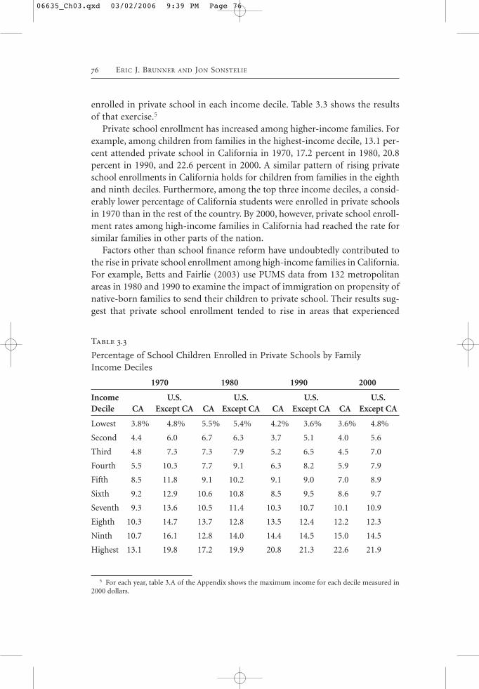
enrolled in private school in each income decile. Table 3.3 shows the resultsof that exercise.5

Private school enrollment has increased among higher-income families. Forexample, among children from families in the highest-income decile, 13.1 per-cent attended private school in California in 1970, 17.2 percent in 1980, 20.8percent in 1990, and 22.6 percent in 2000. A similar pattern of rising privateschool enrollments in California holds for children from families in the eighthand ninth deciles. Furthermore, among the top three income deciles, a consid-erably lower percentage of California students were enrolled in private schoolsin 1970 than in the rest of the country. By 2000, however, private school enroll-ment rates among high-income families in California had reached the rate forsimilar families in other parts of the nation.

Factors other than school finance reform have undoubtedly contributed tothe rise in private school enrollment among high-income families in California.For example, Betts and Fairlie (2003) use PUMS data from 132 metropolitanareas in 1980 and 1990 to examine the impact of immigration on propensity ofnative-born families to send their children to private school. Their results sug-gest that private school enrollment tended to rise in areas that experienced


Table 3.3

Percentage of School Children Enrolled in Private Schools by FamilyIncome Deciles

1970 1980 1990 2000

Income U.S. U.S. U.S. U.S.Decile CA Except CA CA Except CA CA Except CA CA Except CA

Lowest 3.8% 4.8% 5.5% 5.4% 4.2% 3.6% 3.6% 4.8%

Second 4.4 6.0 6.7 6.3 3.7 5.1 4.0 5.6

Third 4.8 7.3 7.3 7.9 5.2 6.5 4.5 7.0

Fourth 5.5 10.3 7.7 9.1 6.3 8.2 5.9 7.9

Fifth 8.5 11.8 9.1 10.2 9.1 9.0 7.0 8.9

Sixth 9.2 12.9 10.6 10.8 8.5 9.5 8.6 9.7

Seventh 9.3 13.6 10.5 11.4 10.3 10.7 10.1 10.9

Eighth 10.3 14.7 13.7 12.8 13.5 12.4 12.2 12.3

Ninth 10.7 16.1 12.8 14.0 14.4 14.5 15.0 14.5

Highest 13.1 19.8 17.2 19.9 20.8 21.3 22.6 21.9

5 For each year, table 3.A of the Appendix shows the maximum income for each decile measured in2000 dollars.

06635_Ch03.qxd 03/02/2006 9:39 PM Page 76

inflows of immigrant children. Over the last three decades, California has cer-tainly experienced large immigrant inflows, suggesting that some of the rise inprivate school enrollment is due to its effect. Nevertheless, it seems reasonableto conclude that at least part of the increase in private school enrollment wasdue to school finance reform.

Several recent studies provide evidence consistent with that notion. Usingdistrict-level data from California in 1970 and 1980, Downes and Schoeman(1998) found that private school enrollment rose in districts that experienceda decline in real spending per pupil over the same time period. They con-cluded that roughly half of the rise in private school enrollment in Californiabetween 1970 and 1980 could be directly attributed to school finance reform.Similarly, Husted and Kenny (2002) examined changes in private schoolenrollment in 159 metropolitan statistical areas (MSAs) in 1970, 1980, and1990. They found that private school enrollments tended to rise in MSAslocated in states that adopted policies designed to equalize spending perpupil. Furthermore, their results suggest that the leveling of school spendinghad a particularly large effect on private school enrollments in high-incomeMSAs.

These studies suggest that at least part of the rise in private school enroll-ment in California was a direct response to school finance reform.Nevertheless, it still seems surprising that more families did not opt out of thepublic sector. Nechyba (2003a, 2003b) provides an explanation for this mod-erate response. In his analysis, school finance centralization and spendingequalization have two distinct effects on private school enrollment. First,while equalization causes spending per pupil to fall in some districts, it alsocauses spending per pupil to rise in other districts. As a result, while privateschool enrollment rates may rise in previously high-spending districts, theymay fall in previously low-spending districts. Second, when public schools arefinanced at the local level with property tax revenues, families wishing to sendtheir child to private school have an incentive to reside in low-quality/low-spending districts to take advantage of lower housing prices and to reducetheir tax burdens. In contrast, when public schools are financed at the statelevel with statewide income tax revenues, families can no longer reduce theirtax burdens by living in a low-quality/low-spending district. Consequently,school finance centralization increases the opportunity cost of living in a low-quality district and sending a child to private school. As a result, some familiesthat previously chose to send their child to private school and live in a low-quality district may now choose to move to a high-quality district (those withhigh student peer quality) and send their child to public school. Simulationsconducted by Nechyba suggest that this secondary effect of school finance cen-tralization may be quite significant.


06635_Ch03.qxd 03/02/2006 9:39 PM Page 77

Voluntary Contributions

While school finance reform may not have engendered a dramatic increase inprivate school enrollments, it did provoke another response. In the aftermath ofschool finance reform, many districts established educational foundations tochannel private contributions into public schools. Prior to 1970 there werefewer than 10 of these organizations operating in California. There are nowmore than 500. In addition, over the last several decades Parent TeacherAssociations (PTAs) and booster clubs have become much more active in rais-ing private contributions to supplement local school budgets. To examine howsuccessful schools and school districts have been at raising voluntary contribu-tions, we used data from the Internal Revenue Service’s Master Business File toidentify the contributions raised by all nonprofit organizations that supportedeither an individual school or a school district in California in 2001.6 At theschool level, contributions are raised primarily by PTAs and booster clubs.At the district level, contributions are raised primarily by local educationalfoundations.

As table 3.4 demonstrates, a number of schools and school districts have beenquite successful in raising voluntary contributions. For example, 36 schools hadcontributions per pupil in excess of $500 in 2001, and among those schools theaverage contribution per pupil was $805. Similarly, 12 districts had contribu-tions per pupil in excess of $500, and among those districts the average contri-bution per pupil was $1,776. As the fourth column demonstrates, the schoolsand school districts that were most successful in raising voluntary contributionswere populated by the highest-income families.7 Family income averaged$223,759 in the 12 districts with contributions per pupil in excess of $500. Incontrast, it averaged only $68,690 in the 63 districts with contributions per pupilof less than $10.

Although several schools and school districts have been successful at raisingvoluntary contributions, overall the use of voluntary contributions is quite lim-ited. In 2001, over 8,000 schools were operating in California, and only 36 of


6 While the IRS Master File includes all nonprofit organizations supporting K–12 schools inCalifornia, it only contains revenue data for those organizations with revenues of $25,000 or more. Thus,we are unable to identify the amount of revenue raised by organizations with revenues of less than$25,000. As a result, our data provide a lower bound on the actual amount raised by organizations sup-porting K–12 schools in California. For a detailed description of the methodology used to identify nonprofit organizations supporting K–12 schools and the revenue raised by those organizations, seeBrunner and Sonstelie (1996) and Brunner and Imazeki (2005).

7 District-level data on average family income in 2000 was obtained from school district demographicfiles prepared by the U.S. Census Bureau. Data on average family income by school attendance zone is notavailable. As a result, we used data on the location of each school in California to match schools to cen-sus tracts in 2000. We then used the average family income of the census tract in which the school waslocated as a proxy for the average income of families within a school attendance zone.

06635_Ch03.qxd 03/02/2006 9:39 PM Page 78

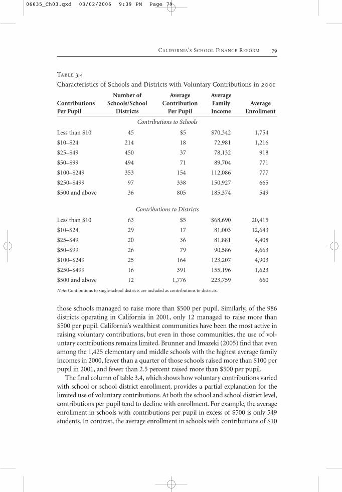
those schools managed to raise more than $500 per pupil. Similarly, of the 986districts operating in California in 2001, only 12 managed to raise more than$500 per pupil. California’s wealthiest communities have been the most active inraising voluntary contributions, but even in those communities, the use of vol-untary contributions remains limited. Brunner and Imazeki (2005) find that evenamong the 1,425 elementary and middle schools with the highest average familyincomes in 2000, fewer than a quarter of those schools raised more than $100 perpupil in 2001, and fewer than 2.5 percent raised more than $500 per pupil.

The final column of table 3.4, which shows how voluntary contributions variedwith school or school district enrollment, provides a partial explanation for thelimited use of voluntary contributions. At both the school and school district level,contributions per pupil tend to decline with enrollment. For example, the averageenrollment in schools with contributions per pupil in excess of $500 is only 549students. In contrast, the average enrollment in schools with contributions of $10


Table 3.4

Characteristics of Schools and Districts with Voluntary Contributions in 2001

Number of Average Average Contributions Schools/School Contribution Family Average Per Pupil Districts Per Pupil Income Enrollment

Contributions to Schools

Less than $10 45 $5 $70,342 1,754

$10–$24 214 18 72,981 1,216

$25–$49 450 37 78,132 918

$50–$99 494 71 89,704 771

$100–$249 353 154 112,086 777

$250–$499 97 338 150,927 665

$500 and above 36 805 185,374 549

Contributions to Districts

Less than $10 63 $5 $68,690 20,415

$10–$24 29 17 81,003 12,643

$25–$49 20 36 81,881 4,408

$50–$99 26 79 90,586 4,663

$100–$249 25 164 123,207 4,903

$250–$499 16 391 155,196 1,623

$500 and above 12 1,776 223,759 660

Note: Contibutions to single-school districts are included as contributions to districts.

06635_Ch03.qxd 03/02/2006 9:39 PM Page 79

or less is 1,754 students. The inverse relationship between school size and contri-butions per pupil alludes to an important limitation schools and school districtsface when attempting to replace lost property tax revenue with voluntary contri-butions. Property tax payments are mandatory, whereas contributions are volun-tary. That distinction is particularly important given the public good nature ofvoluntary contributions. Once a family contributes to their local public school,their contribution benefits not only their own child but also the children of allother families who attend the same school. As a result, it is in the self interest ofany one family not to contribute and free ride off the contributions of other fam-ilies. Furthermore, as noted by Sandler (1992), among others, the incentive to freeride tends to increase with the group size. Using data on voluntary contributionsto California’s public schools in 1994, Brunner and Sonstelie (2003a) find that a 1percent increase in student enrollment leads to a .56 percent reduction in contri-butions per pupil. Thus, a doubling of school size would lead to a 56 percentdecline in contributions per pupil. These results illustrate an important point:When the source of discretionary revenue is changed from the property tax to voluntary contributions, the price of school spending is likely to rise, since noenforcement mechanism exists to ensure each family contributes. Thus, even inCalifornia’s highest-income communities, the ability to replace lost property taxrevenue with voluntary contributions is likely to be quite limited.

Parcel Taxes

For taxpayers seeking to supplement the revenue of their local public schools,another option is the parcel tax. Unlike the property tax, the parcel tax is tax onreal estate parcels, not the value of those parcels. Prior to the passage ofProposition 13, the state constitution explicitly prohibited the use of parceltaxes because it required property to be taxed in proportion to its full value.However, Section 4 of Proposition 13 gave local governments, including schooldistricts, the authority to levy “special taxes” subject to the approval of two-thirds of the local electorate. Shortly after the passage of Proposition 13, thestate legislature successfully argued that parcel taxes were special taxes as longas they were earmarked for a particular purpose (Doerr 1997). School districtsin California first began placing parcel tax initiatives on their local ballots in1983. As of 2005, there have been 369 parcel tax elections held by school dis-tricts, and of those elections, 189 were successful.8

Table 3.5 summarizes the size and distribution of parcel tax revenue perpupil in 2003–2004. As table 3.5 illustrates, the parcel tax has been used suc-


8 Almost all school districts have imposed parcel taxes on a per-parcel basis (e.g., $100 per parcel)and for a relatively short time period (e.g., five years).

06635_Ch03.qxd 03/02/2006 9:39 PM Page 80

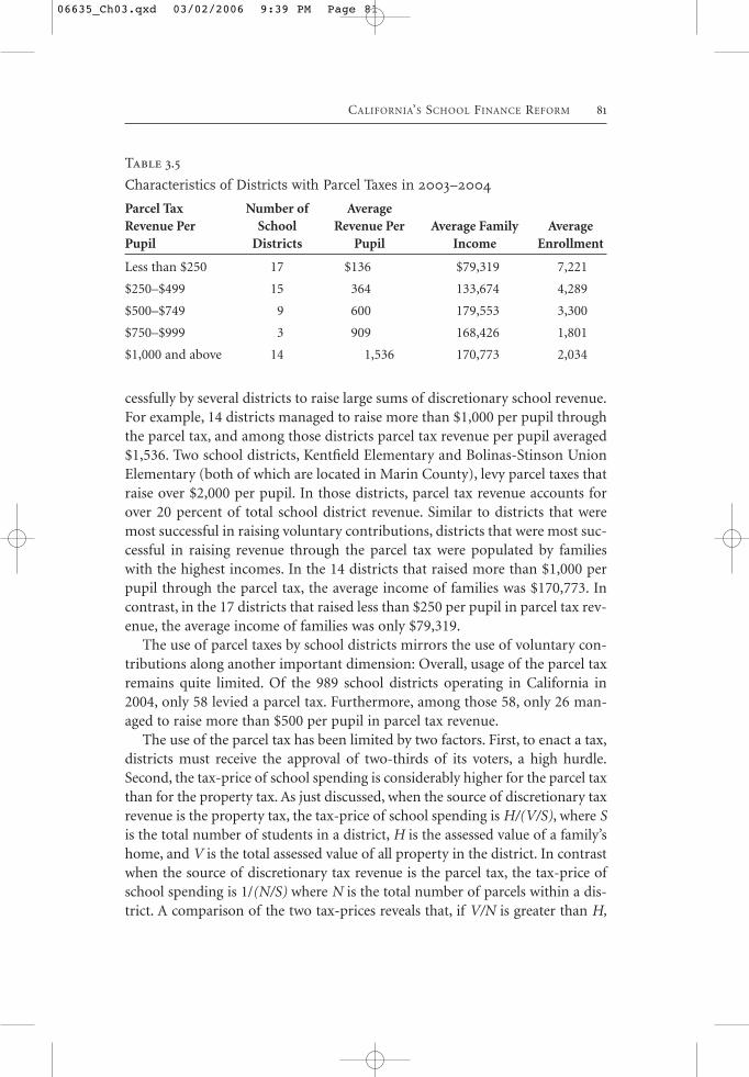
cessfully by several districts to raise large sums of discretionary school revenue.For example, 14 districts managed to raise more than $1,000 per pupil throughthe parcel tax, and among those districts parcel tax revenue per pupil averaged$1,536. Two school districts, Kentfield Elementary and Bolinas-Stinson UnionElementary (both of which are located in Marin County), levy parcel taxes thatraise over $2,000 per pupil. In those districts, parcel tax revenue accounts forover 20 percent of total school district revenue. Similar to districts that weremost successful in raising voluntary contributions, districts that were most suc-cessful in raising revenue through the parcel tax were populated by familieswith the highest incomes. In the 14 districts that raised more than $1,000 perpupil through the parcel tax, the average income of families was $170,773. Incontrast, in the 17 districts that raised less than $250 per pupil in parcel tax rev-enue, the average income of families was only $79,319.

The use of parcel taxes by school districts mirrors the use of voluntary con-tributions along another important dimension: Overall, usage of the parcel taxremains quite limited. Of the 989 school districts operating in California in2004, only 58 levied a parcel tax. Furthermore, among those 58, only 26 man-aged to raise more than $500 per pupil in parcel tax revenue.

The use of the parcel tax has been limited by two factors. First, to enact a tax,districts must receive the approval of two-thirds of its voters, a high hurdle.Second, the tax-price of school spending is considerably higher for the parcel taxthan for the property tax. As just discussed, when the source of discretionary taxrevenue is the property tax, the tax-price of school spending is H/(V/S), where Sis the total number of students in a district, H is the assessed value of a family’shome, and V is the total assessed value of all property in the district. In contrastwhen the source of discretionary tax revenue is the parcel tax, the tax-price ofschool spending is 1/(N/S) where N is the total number of parcels within a dis-trict. A comparison of the two tax-prices reveals that, if V/N is greater than H,


Table 3.5

Characteristics of Districts with Parcel Taxes in 2003–2004

Parcel Tax Number of Average Revenue Per School Revenue Per Average Family Average Pupil Districts Pupil Income Enrollment

Less than $250 17 $136 $79,319 7,221

$250–$499 15 364 133,674 4,289

$500–$749 9 600 179,553 3,300

$750–$999 3 909 168,426 1,801

$1,000 and above 14 1,536 170,773 2,034

06635_Ch03.qxd 03/02/2006 9:39 PM Page 81

switching the source of discretionary tax revenue from the property tax to theparcel tax increases a family’s tax-price. As it turns out, the tax-price of schoolspending does tend to be larger under the parcel tax. Brunner (2001) comparesthe tax-price of school spending under the property tax with the tax-price underthe parcel tax for school districts located in Los Angeles County in 2000. His cal-culations suggest that switching the source of discretionary school revenue fromthe property tax to the parcel tax increases the tax-price of school spending forthe average family by approximately 35 percent.

The primary reason for this sharp increase in the tax-price of school spend-ing is related to the subsidy homeowners receive from nonresidential property.With the property tax, the size of the subsidy depends on the value of nonresi-dential parcels as a percentage of total assessed value. With the parcel tax, thesize of the subsidy depends on the number of nonresidential parcels as a per-centage of the total number of parcels. Using data on the value and numberof residential and nonresidential parcels in four California counties in 2000,Brunner (2001) found that the subsidy from nonresidential property is muchhigher under the property tax than it is under the parcel tax.9 For example,homeowners in Los Angeles County would have received a 34 percent subsidyfrom nonresidential property if the source of discretionary school revenue werethe property tax and only an 11 percent subsidy if the source of discretionaryschool revenue were the parcel tax.

For most districts in California, switching the source of discretionary schoolrevenue from the property tax to the parcel tax led to a large increase in the tax-price of school spending, an increase that most likely made the parcel tax unap-pealing to all but the wealthiest districts. In support of that notion, nearly alldistricts that have managed to raise significant amounts of revenue through theparcel tax are located in suburbs and populated by high-income, highly edu-cated, and white families. The one big exception is Emory Unified, a relativelysmall, urban school district located in Alameda County, with an average familyincome of only $43,582 and a student population that is over 98 percent non-white. Despite those facts, the school district raised $1,727 per pupil throughthe parcel tax in 2003–2004. Why has Emory been so successful in raising sup-plemental revenue through the parcel tax? The two most compelling answers tothat question are related to the composition of Emory’s property base and thetype of parcel tax utilized by the district. In contrast to most other school dis-tricts with parcel taxes, Emory Unified contains a significant amount of com-mercial property. Furthermore, unlike most other school districts, which haveimposed parcel taxes on a per-parcel basis, Emory imposes a parcel tax of $0.10per square foot of improved property (i.e., structures such as homes, retail


9 The four counties analyzed were Los Angeles, San Diego, San Mateo, and Marin.

06635_Ch03.qxd 03/02/2006 9:39 PM Page 82

shops, and factories).10 Because commercial and industrial property tends to belarger than residential property, under a square footage parcel tax, the ownersof nonresidential property pay a larger share of any increase in school spend-ing. As a result, such a parcel tax restores the subsidy from nonresidential prop-erty that existed under the property tax. In the case of Emory Unified, thatsubsidy was quite large: Approximately 75 percent of Emory’s parcel tax rev-enue comes from nonresidential property (Smart Voter 2003).

In addition to restoring the subsidy from nonresidential property, a parcel taxbased on square footage has another advantage: Because parcel size tends toincrease with homeowner income, a tax on the square footage of parcels is lessregressive than a fixed-dollar tax per parcel of land. In light of these advantages,it seems natural to ask whether a square footage parcel tax might represent aviable source of discretionary tax revenue for other districts seeking to supple-ment their revenues. As noted by Brunner (2001), the answer to that questiondepends on whether such a tax would violate the guidelines set forth by theCalifornia Supreme Court in Serrano v. Priest. Recall that the court mandatedthe state to develop a school finance system that was fiscally neutral, implyingthat identical property tax rates should yield the same revenue per pupil.Unfortunately, a parcel tax based on square footage is unlikely to satisfy thecourt’s definition of fiscal neutrality. To illustrate that point, consider two schooldistricts, A and B, that are identical in every relevant respect (same number ofstudents and the same number of parcels) except that in district A, each parcelis 1,000 square feet, and in district B, each parcel is 2,000 square feet. If both dis-tricts levied the same tax rate per square foot of property, district A would raiseonly half as much revenue as district B. As a result, such a tax would most likelyviolate the court’s interpretation of fiscal neutrality—identical tax rates wouldnot yield the same revenue per pupil. While the legality of square footage parceltaxes has not been challenged in court to date, it seems likely that broader use ofthe square footage parcel tax could lead to another Serrano-style lawsuit.11

School Finance Reform and Support for Private School Vouchers

Private schooling, voluntary contributions, and parcel taxes are local actions,options for individual families in the case of private schools or for groups offamilies connected to a school or school district in the case of contributions andparcel taxes. Californians have also had the opportunity to respond on a larger


10 Two other districts, Albany Unified and Berkeley Unified, have imposed parcel taxes that are basedon the square footage of property.

11 As noted by Brunner (2001), if tax revenues from a square footage parcel tax were subject to dis-trict power equalization, a system of local school finance based on a square footage parcel tax would befiscally neutral. As a result, the square footage parcel tax could be turned into a viable and flexible sourceof discretionary school revenue for school districts.

06635_Ch03.qxd 03/02/2006 9:39 PM Page 83

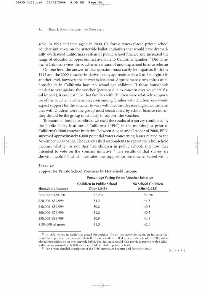
scale. In 1993 and then again in 2000, California voters placed private schoolvoucher initiatives on the statewide ballot, initiatives that would have dramati-cally overhauled California’s system of public school finance and increased therange of educational opportunities available to California families.12 Did fami-lies in California view the voucher as a means of undoing school finance reform?

On one level the answer to that question must surely be negative: Both the1993 and the 2000 voucher initiative lost by approximately a 2 to 1 margin. Onanother level, however, the answer is less clear. Approximately two-thirds of allhouseholds in California have no school-age children. If those householdstended to vote against the voucher (perhaps due to concern over vouchers’ fis-cal impact), it could still be that families with children were relatively support-ive of the voucher. Furthermore, even among families with children, one wouldexpect support for the voucher to vary with income. Because high-income fam-ilies with children were the group most constrained by school finance reform,they should be the group most likely to support the voucher.

To examine those possibilities, we used the results of a survey conducted bythe Public Policy Institute of California (PPIC) in the months just prior toCalifornia’s 2000 voucher initiative. Between August and October of 2000, PPICsurveyed approximately 6,000 potential voters concerning issues related to theNovember 2000 ballot. The survey asked respondents to report their householdincome, whether or not they had children in public school, and how theyintended to vote on the voucher initiative.13 The results of that survey areshown in table 3.6, which illustrates how support for the voucher varied with a


Table 3.6

Support for Private School Vouchers by Household Income

Percentage Voting Yes on Voucher Initative

Children in Public School No School Children Household Income (Obs=1,343) (Obs=2,923)

Less than $20,000 62.2% 53.8%

$20,000–$39,999 54.2 44.5

$40,000–$59,999 50.8 40.3

$60,000–$79,999 51.2 40.5

$80,000–$99,999 50.9 44.3

$100,000 of more 41.5 42.6

12 In 1993, voters in California placed Proposition 174 on the statewide ballot, an initiative thatwould have provided parents with $2,600 for every child enrolled in a private school. In 2000, votersplaced Proposition 38 on the statewide ballot. That initiative would have provided parents with a schol-arship of approximately $4,000 for every child enrolled in private school.

13 For a more detailed description of the PPIC survey, see Brunner and Sonstelie (2003).[AU: a or b? b]

06635_Ch03.qxd 03/02/2006 9:39 PM Page 84

respondent’s household income and whether the respondent had childrenenrolled in public school.14

The results of the PPIC survey reveal that voters with children in public schoolwere indeed more likely to support the voucher than voters with no school-agechildren. For example, among voters with children in public school, 54.2 percentof those with income between $20,000 and $39,999 stated they would support thevoucher initiative. In contrast, only 44.5 percent of voters with no school-age chil-dren in the same income range stated they would support the voucher. However,contrary to expectations, high-income voters with children were less likely to sup-port the voucher than low-income voters with children. Voters with children inthe highest-income groups were over 20 percentage points less likely to supportthe voucher than voters with children in the lowest-income group. In fact, voterswith children in the highest-income group were no more likely to support thevoucher than voters of similar income with no school children. Thus, despitethe fact that high-income families with children were the group most constrainedby school finance reform, they were also the group least likely to support thevoucher.

What explains these puzzling reactions? Our answer to that question beginswith a fundamental observation: School quality depends on more than justspending per pupil; it also depends on factors such as the quality of a student’speer group and school efficiency. To the extent that these other factors areimportant determinants of school quality, equalizing spending will not equal-ize school quality. This point was demonstrated by Nechyba (2003b, 2004),using a computable, general equilibrium model. In the model, school qualitydepends on both spending per pupil and a vector of inputs correlated withparental income. Those inputs include student peer quality, parental monitor-ing, and voluntary contributions. His simulations suggest that centralizationand the equalization of spending per pupil results in only a modest decline inresidential income segregation. With state finance, school districts are still strat-ified by income, peer quality, and, thus, school quality. Epple and Romano(2003) reach a similar conclusion using a general equilibrium model that char-acterizes how families sort across neighborhood schools within a single schooldistrict. In their model, student achievement depends both on a student’sown ability (which is assumed to be correlated with family income) and theability of the student’s peer group. Because all neighborhood schools areassumed to have the same level of spending per pupil, variation in school qual-ity arises solely from variation in average student peer quality across schools.


14 Of the 6,006 survey respondents, a total of 1,343 reported having children enrolled in publicschool and also answered the questions about their household income and how they intended to vote onthe voucher initiative. Similarly, a total of 2,923 respondents reported having no school-age children andanswered the questions about household income and how they intended to voter on the voucher.

06635_Ch03.qxd 03/02/2006 9:39 PM Page 85

Equilibrium in their model is characterized by income, peer quality and schoolquality stratification, with the highest-income families living in neighborhoodswith the highest quality schools (schools with the highest-quality peer group),and the lowest-income families living in the neighborhoods with the lowestquality schools.

These studies suggest that even in California, where spending per pupil hasbeen essentially equalized, there may still be significant income stratificationacross neighborhood schools and school districts, stratification that perpetu-ates large differences in school quality. To examine that possibility we useddata from the California Department of Education on the percentage free orreduced-price lunch students (low-income students) in each elementary schoolin 2003–2004. Figure 3.3 illustrates how low-income students are distributedacross the 2,127 elementary schools in the Los Angeles metropolitan area andthe 849 elementary schools in the San Francisco metropolitan area.15 In the fig-ure, schools are ranked in descending order according to their percentage offree or reduced-price lunch students. If low-income students were randomlydistributed across schools, each school should contain roughly the same per-centage of these students. In the Los Angeles metropolitan area, this wouldimply that roughly 62 percent of students in each school were eligible for a freeor reduced-price lunch (as illustrated by the horizontal dotted line). Similarly,in the San Francisco metropolitan area, random assignment would imply thatroughly 40 percent of students in each school were eligible for a free orreduced-price lunch. As figure 3.3 makes clear, however, that is not the case: Inboth the Los Angeles and San Francisco metropolitan areas there is a significantdegree of income stratification across schools.16

The stratification of schools by family income is also a stratification ofschools by student achievement. The relationship between student perform-ance and family income is clearly represented in figure 3.2, a relationship thatis consistent with the basic assumption underlying the model of Epple andRomano: School quality depends both on a student’s own ability and the abil-ity of his or her peers.

These differences in school quality may explain why high-income familieswere unwilling to support the voucher. Numerous studies have shown that


15 The Los Angeles metropolitan area includes the counties of Los Angeles, Orange, San Bernardino,and Riverside, while the San Francisco metropolitan area includes the counties of San Francisco,Alameda, Contra Costa, Marin, San Mateo, and Santa Clara.

16 Epple and Romano (2003) present similar evidence of income stratification across high schools inthe Los Angeles metropolitan area. Similarly, Bayer, Ferreira, and McMillan (2003, 2005) estimate anequilibrium model of residential sorting across neighborhood schools located in the San Francisco Bayarea. Their results reveal substantial stratification along racial and socioeconomic lines across neighbor-hoods, with white, highly educated, and high-income households clustering in neighborhoods that con-tain the highest-quality schools.

06635_Ch03.qxd 03/02/2006 9:39 PM Page 86

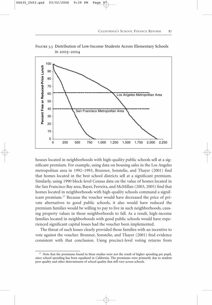
houses located in neighborhoods with high-quality public schools sell at a sig-nificant premium. For example, using data on housing sales in the Los Angelesmetropolitan area in 1992–1993, Brunner, Sonstelie, and Thayer (2001) findthat homes located in the best school districts sell at a significant premium.Similarly, using 1990 block-level Census data on the value of homes located inthe San Francisco Bay area, Bayer, Ferreira, and McMillan (2003, 2005) find thathomes located in neighborhoods with high-quality schools command a signif-icant premium.17 Because the voucher would have decreased the price of pri-vate alternatives to good public schools, it also would have reduced thepremium families would be willing to pay to live in such neighborhoods, caus-ing property values in those neighborhoods to fall. As a result, high-incomefamilies located in neighborhoods with good public schools would have expe-rienced significant capital losses had the voucher been implemented.

The threat of such losses clearly provided those families with an incentive tovote against the voucher. Brunner, Sonstelie, and Thayer (2001) find evidenceconsistent with that conclusion. Using precinct-level voting returns from


0

10

20

30

40

50

60

70

80

90

100

0 250 500 750 1,000 1,250 1,500 1,750 2,000 2,250

Los Angeles Metropolitan Area

San Francisco Metropolitan Area

Per

cen

t F

ree

or

Red

uce

d-P

rice

Lu

nch

Figure 3.3 Distribution of Low-Income Students Across Elementary Schoolsin 2003–2004

17 Note that the premiums found in these studies were not the result of higher spending per pupil,since school spending has been equalized in California. The premiums were primarily due to studentpeer quality and other determinants of school quality that still vary across schools.

06635_Ch03.qxd 03/02/2006 9:39 PM Page 87

California’s 1993 voucher initiative, they find that homeowners located inschool districts with high housing price premiums were significantly less likelyto support the voucher than homeowners located in neighborhoods with lowhousing price premiums. They conclude that the most plausible explanation fortheir results is that homeowners located in good school districts voted againstthe voucher to protect their housing values. Brunner and Sonstelie (2003b)reached the same conclusion based on their analysis of individual voting behav-ior on California’s 2000 voucher initiative.

While the results of the preceding studies may explain why homeownerslocated in good school districts were unwilling to support the voucher, theycannot explain why both California’s 1993 and 2000 voucher initiatives lost bya 2 to 1 margin. Does the overwhelming lack of support for school voucherssuggest that Californians were by and large satisfied with their public schools?Results from the PPIC’s August 2000 survey suggest the answer to that questionis clearly no. When asked to grade the quality of their local public schools on ascale of “A” to “F,” less than 10 percent of voters gave their local public schoolsand “A,” and more than 60 percent of voters gave their schools a grade of “C” orlower (Baldassare 2000). Evidently, even though the majority of California’svoters are unsatisfied with the quality of their local public schools, that dissat-isfaction has not engendered widespread support for school vouchers.

Conclusion

The lessons to be drawn from California’s experience depend on the perspec-tive one brings to it. For champions of decentralized government, the lessonsare easy to draw. Since the centralization of school finance in California, schoolresources and student achievement have declined relative to other states.Families have attempted to circumvent the centralized system by opting outinto the private sector and by using voluntary contributions and parcel taxes tosupplement the inadequate public school resources provided by the state.Centralization has been a dubious achievement.

For fiscal conservatives, the lessons are very different. Under local finance,commercial and industrial property subsidized school spending. The subsidywas ended by Proposition 13, and now families are facing the true cost of pub-lic school spending. Given that cost, they have chosen to spend less, thus tem-pering the rapid rise in real spending per pupil over the last three decades(Hanushek and Rivkin 1997). The dismal performance of California students onachievement tests is a disappointment, but that performance is due more to theinefficiency with which funds are deployed than to the paucity of those funds.

For supporters of centralization, the lessons are more complicated. The cen-tralization of school finance has permitted the state to direct more resources to


06635_Ch03.qxd 03/02/2006 9:39 PM Page 88

school districts serving low-income students. Those students still do not perform at the level of other students, so there is more work to be done.Furthermore, families have done very little to circumvent the new system.Private school enrollment is not significantly higher than other states, voluntarycontributions are not a major factor, parcel taxes have been enacted in only afew districts, and voters have overwhelming rejected the voucher. Centralizedfinance is politically stable, thus providing a platform for an even more pro-gressive redistribution of educational resources.

Supporters of centralization might also add that their preferred system hasnot been given a fair test. California has centralized the finance of its publicschools without centralizing the governance of those schools. This mismatchbetween finance and governance has undermined the effectiveness of the schoolsystem and made centralization less successful than it could be. For example,because school districts still engage in collective bargaining with their employ-ees, the legislature feels obligated to tie up funds in categorical programs thatmay undermine the effectiveness of those funds. Furthermore, possibilities foraddressing the needs of low-income students would likely increase if local gov-ernance were eliminated. In the current system, those needs are addressedthrough categorical programs that attempt to channel funds from the state toschools serving disadvantaged students. Those funds must pass through schooldistricts, however, where local politics may frustrate the state’s intention.

The transformation from local governance to state governance will notoccur as rapidly as the transformation from local finance to state finance.Though they handed the property tax to the state legislature, the voters ofCalifornia deeply distrust Sacramento, and it is impossible to imagine that theywould favor an initiative to eliminate school districts and local school boards.Yet, there are clear signs that the institutions of local governance are crumbling.Schrag (1998) notes that because property tax rates are not determined at thelocal level, business in California has lost interest in local school districts,diminishing a traditional source of fiscal conservatism on local school boards.California’s ambitious accountability system has also eroded local governance.The state has yet to take over a failing school, but it clearly has the power to doso, and it is only a matter of time before it does. Likewise, after an initial exper-iment with bonuses for teachers in high-performing schools, the state ran intofiscal difficulties and suspended the program. However, it seems only logicalthat an improved system of performance bonuses will be instituted as soon asthe state’s budget improves. Last, it is not impossible to imagine that the state’scurrent bilevel system of collective bargaining—once with the state legislatureand again with each school district—will yield to a more rational system ofstatewide collective bargaining. Any one of these changes would make the oth-ers more likely.


06635_Ch03.qxd 03/02/2006 9:39 PM Page 89

Champions of decentralized government will argue the folly of this trend.A school system that reports directly to Sacramento will become disconnectedfrom the concerns of local residents, lose political support, and deteriorate evenfurther. For these critics of the current direction, hope lies with the parcel tax.If the threshold for enacting the parcel tax were reduced to a simple majority,many more parcel taxes would be passed. Each such event would reconnect res-idents to their local school districts and reinvigorate local governance. A con-stitutional amendment is required to reduce the two-thirds requirement to asimple majority, but California’s constitution must be the most pliable of anystate’s.

References

Baldassare, Mark. 2000. PPIC statewide survey: Californians and their government, August2000. San Francisco: Public Policy Institute of California.

Bayer, Patrick, Fernando Ferreira, and Robert McMillan. 2003. A unified framework formeasuring preferences for schools and neighborhoods. Working paper. Department ofEconomics: Yale University.

———. 2005. Tiebout sorting, social multipliers and the demand for school quality.Working paper. Department of Economics: Yale University.

Bergstrom, Theodore C., and Robert P. Goodman. 1973. Private demands for public goods.American Economic Review 63:280–296.

Betts, Julian R., and Robert W. Fairlie. 2003. Does immigration induce “native flight” frompublic schools into private schools? Journal of Public Economic 87:987–1012.

Borcherding, Thomas E., and Robert T. Deacon. 1972. The demand for the services of non-federal governments. American Economic Review 62:891–906.

Brunner, Eric J. 2001. The parcel tax. In Essays for the joint committee to develop a master planfor education—Kindergarten through university, Jon Sonstelie and Peter Richardson, eds.San Francisco: Public Policy Institute of California.

Brunner, Eric J., and Jennifer Imazeki. 2005. Fiscal stress and voluntary contributions to pub-lic schools. In Developments in school finance: 2004. William J. Fowler, ed. Washington,DC: National Center for Educational Statistics.

Brunner, Eric J., and Jon C. Sonstelie. 1996. Coping with Serrano: Private contributions toCalifornia’s public schools. Proceedings of the Eighty-Ninth Annual Conference on Tax-ation, National Tax Association, 372–381.

———. 2003a. School finance reform and voluntary fiscal federalism. Journal of PublicEconomics 87:2157–2185.

———. 2003b. Homeowners, property values, and the political economy of the schoolvoucher. Journal of Urban Economics 54:239–257.

Brunner, Eric J., Jon C. Sonstelie and Mark Thayer. 2001. Capitalization and the voucher.Journal of Urban Economics 50:517–536.

Card, David, and Abigail Payne. 2002. School finance reform, the distribution of schoolspending, and the distribution of student test scores. Journal of Public Economics 83:49–82.

Carroll, Stephen J., Cathy Krop, Jeremy Arkes, Peter A. Morrison, and Ann Flanagan. 2005.California’s K–12 public schools: How are they doing? Santa Monica, CA: RANDCorporation.


06635_Ch03.qxd 03/02/2006 9:39 PM Page 90

Coons, John E., William D. Clune, and Stephen D. Sugarman. 1970. Private wealth and pub-lic education. Cambridge, MA: Harvard University Press.

Doerr, David R. 1997, February. The genesis of Proposition 218: A history of local taxingauthority. Cal-Tax Digest.

Downes, Thomas A. 1992. Evaluating the impact of school finance reform on the provisionof public education: The California case. National Tax Journal 45:405–419.

Downes, Thomas A., and David N. Figlio. 1997. School finance reform, tax limits, and stu-dent performance: Do reforms level-up or dumb down? Working paper. Department ofEconomics: Tufts University.

Downes, Thomas A., and David Schoeman. 1998. School finance reform and private schoolenrollment: Evidence from California. Journal of Urban Economics 43:443–481.

Downes, Thomas A., and Mona P. Shah. 1995. The effects of school finance reforms on thelevel and growth of per pupil expenditures. Working paper. Department of Economics:Tufts University.

Epple, Dennis, and Richard Romano. 2003. Neighborhood schools, choice, and the distribu-tion of educational benefits. In: The Economics of School Choice. Caroline M. Hoxby ed.Chicago: University of Chicago Press.

Fernandez, Raquel, and Richard Rogerson. 1999. Education finance reform and investmentin human capital: Lessons from California. Journal of Public Economics 74:327–350.

Figlio, David N. 1997. Did the tax revolt reduce school performance? Journal of PublicEconomics 65:245–269.

Figlio, David N., and Kim S. Rueben. 2001. Tax limits and the qualifications of new teachers.Journal of Public Economics 80:49–71.

Fischel, William A. 1989. Did Serrano cause Proposition 13? National Tax Journal 42:465–473.———. 1996. How Serrano caused Proposition 13. Journal of Law and Politics 12:607–636.———. 2001. The homevoter hypothesis: How home values influence local government taxa-

tion, school finance, and land-use policies. Cambridge, MA: Harvard University Press.———. 2004. Did John Serrano vote for Proposition 13? UCLA Law Review 51:887–932.Hanushek, Eric A., and Steven G. Rivkin. 1997. Understanding the 20th century growth in

U.S. school spending. Journal of Human Resources 32:35–69.Hines, James, and Richard Thaler. 1995. The flypaper effect. Journal of Economic Perspectives

9:217–226.Horowitz, Harold W. 1966. Unseparate but unequal — The emerging Fourteenth

Amendment issue in public school education. UCLA Law Review 13:1147–1172.Hoxby, Caroline M. 2001. All school finance equalizations are not created equal. Quarterly

Journal of Economics 116:1189–1231.Husted, Thomas A., and Lawrence W. Kenny. 2000. Evidence on the impact of state govern-

ment on primary and secondary education and the equity-efficiency trade-off. Journal ofLaw and Economics 43:285–308.

———. 2002. The legacy of Serrano: The impact of mandated equal spending on privateschool enrollment. Southern Economic Journal 68:566–583.

Kenny, Lawrence W. 1982. Economies of scale in schooling. Economics of Education Review2:1–24.

Kurland, Philip B. 1963. The Supreme Court, 1963 term. Foreword: Equal in origin and equalin title to the legislative and executive branches of the government. Harvard Law Review78:143–176.

Manwaring, Robert L., and Steven M. Sheffrin. 1997. Litigation, school finance reform andaggregate educational spending. International Tax and Public Finance 4:107–127.


06635_Ch03.qxd 03/02/2006 9:39 PM Page 91

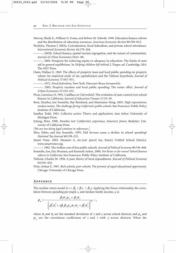
Murray, Sheila E., William N. Evans, and Robert M. Schwab. 1998. Education finance reformand the distribution of education resources. American Economic Review 88:789–812.

Nechyba, Thomas J. 2003a. Centralization, fiscal federalism, and private school attendance.International Economic Review 44:179–204.

———. 2003b. School finance, spatial income segregation, and the nature of communities.Journal of Urban Economics 54:61–88.

———. 2004. Prospects for achieving equity or adequacy in education: The limits of stateaid in general equilibrium. In Helping children left behind, J. Yinger, ed. Cambridge, MA:The MIT Press.

Oates, Wallace E. 1969. The effects of property taxes and local public spending on propertyvalues: An empirical study of tax capitalization and the Tiebout hypothesis. Journal ofPolitical Economy 77:957–971.

———. 1972. Fiscal federalism. New York: Harcourt Brace Jovanovich.———. 2005. Property taxation and local public spending: The renter effect. Journal of

Urban Economics 57:419–431.Picus, Lawrence O. 1991. Cadillacs or Chevrolets?: The evolution of state control over school

finance in California. Journal of Education Finance 17:33–59.Rose, Heather, Jon Sonstelie, Ray Reinhard, and Sharmaine Heng. 2003. High expectations,

modest means: The challenge facing California’s public schools. San Francisco: Public PolicyInstitute of California.

Sandler, Todd. 1992. Collective action: Theory and applications. Ann Arbor: University ofMichigan Press.

Schrag, Peter. 1998. Paradise lost: California’s experience, America’s future. Berkeley: Uni-versity of California Press.

[We are not doing legal citations in references.]Silva, Fabio, and Jon Sonstelie. 1995. Did Serrano cause a decline in school spending?

National Tax Journal 48:199–215.Smart Voter. 2003. Measure A, six-year parcel tax, Emery Unified School District.

www.smartvoter.org.———. 1982. The welfare cost of free public schools. Journal of Political Economy 90:749–808.Sonstelie, Jon, Eric Brunner, and Kenneth Ardon. 2000. For better or for worse? School finance

reform in California. San Francisco: Public Policy Institute of California.Tiebout, Charles M. 1956. A pure theory of local expenditures. Journal of Political Economy

64:416–424.Wise, Arthur E. 1967. Rich schools, poor schools: The promise of equal educational opportunity.

Chicago: University of Chicago Press.

Appendix

The median voters model is s = b0 + b1v + b2y. Applying this linear relationship, the corre-lation between spending per pupil, s, and median family income, y, is

2

/sy

v vy v y y

v vy y

1

2 2

1 2 2

2 21 2

1 2=

+ +

+t

b v b b t v v b v

b v t b v

J

L

KK

N

P

OO

,

where sv and sy are the standard deviations of v and y across school districts, and rsy andrvy are the correlation coefficients of s and v with y across districts. When the


06635_Ch03.qxd 03/02/2006 9:39 PM Page 92

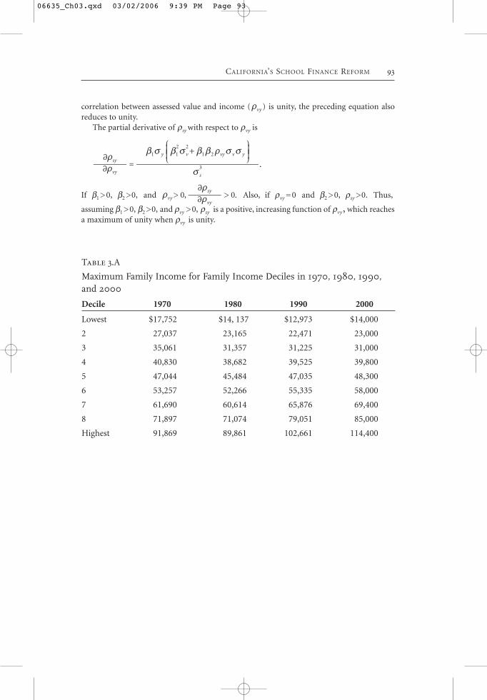
correlation between assessed value and income ( )vyt is unity, the preceding equation alsoreduces to unity.

The partial derivative of rsy with respect to rvy is

vy

sy

s

y v vy v y

3

1 1

2 2

1 2

2

2=

+

t

t

v

b v b v b b t v vJ

L

KK

N

P

OO

.

If b1 >0, b2 >0, and > , > .0 0vyvy

sy

2

2t t

tAlso, if rvy =0 and b2 >0, rsy >0. Thus,

assuming b1 >0, b2 >0, and rvy >0, rsy is a positive, increasing function of rvy , which reachesa maximum of unity when rvy is unity.


Table 3.A

Maximum Family Income for Family Income Deciles in 1970, 1980, 1990,and 2000

Decile 1970 1980 1990 2000

Lowest $17,752 $14, 137 $12,973 $14,000

2 27,037 23,165 22,471 23,000

3 35,061 31,357 31,225 31,000

4 40,830 38,682 39,525 39,800

5 47,044 45,484 47,035 48,300

6 53,257 52,266 55,335 58,000

7 61,690 60,614 65,876 69,400

8 71,897 71,074 79,051 85,000

Highest 91,869 89,861 102,661 114,400

06635_Ch03.qxd 03/02/2006 9:39 PM Page 93

Commentary�David Figlio

California has experienced remarkable changes in its finance of schools over thelast three decades, and countless scholars have discussed these major changes—the school finance reforms and their accompanying tax and expenditure limi-tations. This very thoughtful piece by Brunner and Sonstelie casts California’sexperiences in the light of fiscal federalism. Although the authors are carefulnot to overstate the degree to which California’s school finance reform is anexperiment in fiscal federalism (despite the title, which says just that), theauthors do show some ways in which California’s experiences could be seen asproviding lessons for fiscal federalism.

The authors present a fascinating picture of California’s school finance land-scape prior to the Serrano ruling, and then describe the ways in which Serranoand other forces led California from a system of primarily local finance of edu-cation into a system of nearly pure state finance of education, and they identifysome of the consequences of that massive change.

When looking back at California’s experience, it is useful to begin—as theauthors do—with California’s experiment in school finance reform. Whenevaluating the pre-Serrano landscape in California, one is immediately struckby the lack of a strong relationship between the resources available to familiesand the resources allocated to their students. There existed a small, positive cor-relation between median family income and spending per pupil for elemen-tary-only school districts and no apparent relationship whatsoever for highschool or unified school districts. If this lack of a relationship between familyincome and school revenues was due to the fact that per-pupil revenues did notvary much across school districts, this finding would not be particularly strik-ing. However, as the authors point out, there existed considerable variation inresources per pupil in pre-Serrano schools in California; this variation was justnot highly linked to family incomes.

06635_Ch03.qxd 03/02/2006 9:39 PM Page 94

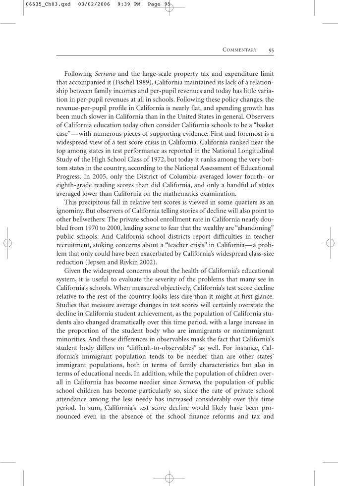
Following Serrano and the large-scale property tax and expenditure limitthat accompanied it (Fischel 1989), California maintained its lack of a relation-ship between family incomes and per-pupil revenues and today has little varia-tion in per-pupil revenues at all in schools. Following these policy changes, therevenue-per-pupil profile in California is nearly flat, and spending growth hasbeen much slower in California than in the United States in general. Observersof California education today often consider California schools to be a “basketcase”—with numerous pieces of supporting evidence: First and foremost is awidespread view of a test score crisis in California. California ranked near thetop among states in test performance as reported in the National LongitudinalStudy of the High School Class of 1972, but today it ranks among the very bot-tom states in the country, according to the National Assessment of EducationalProgress. In 2005, only the District of Columbia averaged lower fourth- oreighth-grade reading scores than did California, and only a handful of statesaveraged lower than California on the mathematics examination.

This precipitous fall in relative test scores is viewed in some quarters as anignominy. But observers of California telling stories of decline will also point toother bellwethers: The private school enrollment rate in California nearly dou-bled from 1970 to 2000, leading some to fear that the wealthy are “abandoning”public schools. And California school districts report difficulties in teacherrecruitment, stoking concerns about a “teacher crisis” in California—a prob-lem that only could have been exacerbated by California’s widespread class-sizereduction (Jepsen and Rivkin 2002).

Given the widespread concerns about the health of California’s educationalsystem, it is useful to evaluate the severity of the problems that many see inCalifornia’s schools. When measured objectively, California’s test score declinerelative to the rest of the country looks less dire than it might at first glance.Studies that measure average changes in test scores will certainly overstate thedecline in California student achievement, as the population of California stu-dents also changed dramatically over this time period, with a large increase inthe proportion of the student body who are immigrants or nonimmigrantminorities. And these differences in observables mask the fact that California’sstudent body differs on “difficult-to-observables” as well. For instance, Cal-ifornia’s immigrant population tends to be needier than are other states’immigrant populations, both in terms of family characteristics but also interms of educational needs. In addition, while the population of children over-all in California has become needier since Serrano, the population of publicschool children has become particularly so, since the rate of private schoolattendance among the less needy has increased considerably over this timeperiod. In sum, California’s test score decline would likely have been pro-nounced even in the absence of the school finance reforms and tax and

COMMENTARY 95

06635_Ch03.qxd 03/02/2006 9:39 PM Page 95

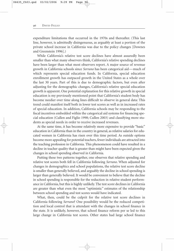
expenditure limitations that occurred in the 1970s and thereafter. (This lastline, however, is admittedly disingenuous, as arguably at least a portion of theprivate school increase in California was due to the policy changes [Downesand Greenstein 1996].)

While California’s relative test score declines have almost assuredly beensmaller than what many observers think, California’s relative spending declineshave been larger than what most observers report. A major source of revenuegrowth in California schools since Serrano has been categorical aid—much ofwhich represents special education funds. In California, special educationenrollment growth has outpaced growth in the United States as a whole overthe last 30 years. Part of this is due to demographic factors, but even afteradjusting for the demographic changes, California’s relative special educationgrowth is apparent. One potential explanation for this relative growth in specialeducation is my previously mentioned point that California’s student body hasbecome needier over time along lines difficult to observe in general data: Thistrend could manifest itself both in lower test scores as well as in increased ratesof special education. In addition, California schools may be responding to thefiscal incentives embedded within the categorical aid systems for financing spe-cial education (Cullen and Figlio 1998; Cullen 2003) and classifying more stu-dents as special needs in order to receive increased revenues.

At the same time, it has become relatively more expensive to provide “basic”education in California than in the country in general, as relative salaries for edu-cated women in California has risen over this time period. As outside optionsbecome more appealing for potential teachers, fewer individuals are attracted intothe teaching profession in California. This phenomenon could have resulted in adecline in teacher quality that is greater than might have been expected given thechanges in school spending observed in California.

Putting these two patterns together, one observes that relative spending andrelative test scores both fell in California following Serrano. When adjusted forchanges in demographics and school populations, the relative test score declineis smaller than generally believed, and arguably the decline in school spending islarger than generally believed. It would be convenient to believe that the declinein school spending is responsible for the reduction in relative student perform-ance in California, but this is highly unlikely. The test score declines in Californiaare greater than what even the most “optimistic” estimates of the relationshipbetween school spending and test scores would have indicated.

What, then, could be the culprit for the relative test score declines inCalifornia following Serrano? One possibility would be the reduced competi-tion and local control that is attendant with the changes in school finance inthe state. It is unlikely, however, that school finance reform per se led to thislarge change in California test scores. Other states had large school finance

96 DAVID FIGLIO

06635_Ch03.qxd 03/02/2006 9:39 PM Page 96

equalizations without large declines in test scores; Florida, for example, has aschool finance profile that is just as flat as California’s but without the largereduction in test scores. One difference between California and other states thatcould explain why California experienced particularly large reductions is thetax and expenditure limitation that occurred hand-in-hand with Serrano:Proposition 13 had a “lock-in effect” that could reduce schools’ responsivenessto progressively less-footloose residents. Put differently, in California a loss oflocal control in school finance was coupled with an increasing inability for res-idents to shop for better options among other (constrained) communities.

Proposition 13—California’s particularly restrictive tax and expenditure lim-itation—is likely to be responsible for a large fraction of the reduction in rela-tive test scores in California. While tax and expenditure limitations often do notdramatically reduce school spending in the states that impose them, they areassociated with substantially reduced student test scores (Figlio 1997; Downesand Figlio 1999) that far outstrip the levels that would be predicted by thespending declines. One possible explanation for this factor is a teacher–qualitylink: Figlio and Rueben (2001) find that states that enact tax and expenditurelimitations experience large declines in relative teacher quality, as measured bythe qualifications of entrants into the teaching profession. These declines arethemselves larger than what might be expected based on (generally modest)changes in teacher salaries in a state, suggesting that there is a “zeitgeist effect”associated with tax and expenditure limitations: Potential teachers may viewteaching as a less-desirable profession in states that impose these limitations,largely because of a change in the perceived environment of teaching.

The incidence of this teacher quality effect is borne by districts and schoolsthat serve lower-income families. This finding is consistent with the percep-tion that there has been less of a teacher quality “crisis” in middle-class Cal-ifornia than there has been in the areas serving low-income families. (Thiscould also be because middle-class school districts may “poach” quality teach-ers from schools serving low-income families.) In any account, this differentialeffect may also contribute to the test score decline in California if lower-income students’ test scores are more responsive to school inputs than arehigher-income students’ scores (Betts 1995).

The comparison between California and Florida now becomes potentiallymore interesting. As just mentioned, Florida also experienced a large equaliza-tion in the 1970s, as well as a tax and expenditure limitation that is even morebinding in some dimensions than was Proposition 13. However, Florida did notexperience the same types of test score declines seen in California since Serrano.

What could be some reasons for the California-Florida difference in out-comes? One possible explanation is that Florida’s tax and expenditure limita-tion was passed by the legislature and not directly by voters, so potential

COMMENTARY 97

06635_Ch03.qxd 03/02/2006 9:39 PM Page 97

teachers in Florida may have viewed the tax cap as less of a referendum than didCalifornia’s potential teachers. It may be the case that the “zeitgeist effect” foundby Figlio and Rueben (2001) is less pronounced (or nonexistent) in the case oftax and expenditure limitations not passed by voters. Florida also already hadextremely centralized school provision prior to the school finance reforms inthe 1970s. Several large metropolitan areas already had only one school districtprior to the changes in school funding; perhaps centralization matters less ifjurisdictions are already centralized.

One lesson to be learned both from California’s experience and its compar-ison with Florida is that not all school finance reforms are created equal. Butthis lesson goes beyond Hoxby’s (2001) paper with that same title; two schoolfinance reforms with very large changes in marginal tax prices can have verydifferent consequences. It is not necessarily the case that large changes in schoolfinance will lead to large reductions in student test scores; the devil is certainlyin the details.

While the absolute magnitude of the effects of California’s school financereforms and accompanying tax and expenditure limitations on the level anddistribution of spending, local control and school performance can be debated,there is no question that these policies had large-scale consequences for schoolsin California. It is also apparent that similar-looking policies can and do havedifferent effects in other settings, depending on the context of those settings.California schools and districts have sought alternative revenue sources—direct contributions and parcel taxes—in order to raise revenues that may havebeen locally raised in a different policy environment. The use of these alterna-tive revenue streams in a serious way has been quite limited to date, partiallybecause the parcel tax requires a high threshold of voter support for passing.

But while making it easier to enact parcel taxes would help to restore localgovernance over school revenues and spending, it will not come close to undo-ing the effects of Serrano and Proposition 13 in California. Much of this is dueto the likelihood, described earlier, that the largest effects of Serrano andProposition 13 have been due not to the direct financial impacts of the policies,but to the attendant changes in teacher labor markets and other factors associ-ated with the policy changes. If the withdrawal of money per se is not the forceprimarily responsible for any degradation of education in California, then thereinstatement of money on a small-scale, local basis is also not likely to com-pletely undo the estimated negative effects of Serrano and Proposition 13.Moreover, offering local voters the opportunity to override a tax and expendi-ture limitation could itself induce some new inefficiencies (Figlio andO’Sullivan 2001). In sum, while reducing the parcel tax threshold would allowmore communities the opportunity to enact a more desired level of schoolspending, it is unlikely to be a panacea for schools.

98 DAVID FIGLIO

06635_Ch03.qxd 03/02/2006 9:39 PM Page 98

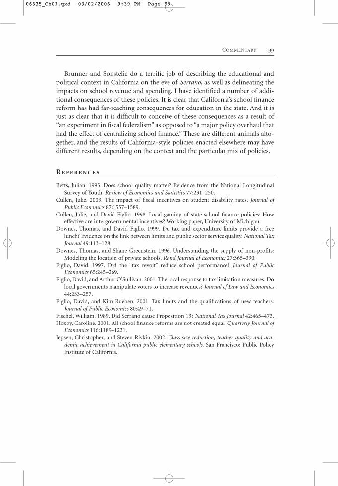
Brunner and Sonstelie do a terrific job of describing the educational andpolitical context in California on the eve of Serrano, as well as delineating theimpacts on school revenue and spending. I have identified a number of addi-tional consequences of these policies. It is clear that California’s school financereform has had far-reaching consequences for education in the state. And it isjust as clear that it is difficult to conceive of these consequences as a result of“an experiment in fiscal federalism” as opposed to “a major policy overhaul thathad the effect of centralizing school finance.” These are different animals alto-gether, and the results of California-style policies enacted elsewhere may havedifferent results, depending on the context and the particular mix of policies.

References

Betts, Julian. 1995. Does school quality matter? Evidence from the National LongitudinalSurvey of Youth. Review of Economics and Statistics 77:231–250.

Cullen, Julie. 2003. The impact of fiscal incentives on student disability rates. Journal ofPublic Economics 87:1557–1589.

Cullen, Julie, and David Figlio. 1998. Local gaming of state school finance policies: Howeffective are intergovernmental incentives? Working paper, University of Michigan.

Downes, Thomas, and David Figlio. 1999. Do tax and expenditure limits provide a freelunch? Evidence on the link between limits and public sector service quality. National TaxJournal 49:113–128.

Downes, Thomas, and Shane Greenstein. 1996. Understanding the supply of non-profits:Modeling the location of private schools. Rand Journal of Economics 27:365–390.

Figlio, David. 1997. Did the “tax revolt” reduce school performance? Journal of PublicEconomics 65:245–269.

Figlio, David, and Arthur O’Sullivan. 2001. The local response to tax limitation measures: Dolocal governments manipulate voters to increase revenues? Journal of Law and Economics44:233–257.

Figlio, David, and Kim Rueben. 2001. Tax limits and the qualifications of new teachers.Journal of Public Economics 80:49–71.

Fischel, William. 1989. Did Serrano cause Proposition 13? National Tax Journal 42:465–473.Hoxby, Caroline. 2001. All school finance reforms are not created equal. Quarterly Journal of

Economics 116:1189–1231.Jepsen, Christopher, and Steven Rivkin. 2002. Class size reduction, teacher quality and aca-

demic achievement in California public elementary schools. San Francisco: Public PolicyInstitute of California.

COMMENTARY 99

06635_Ch03.qxd 03/02/2006 9:39 PM Page 99

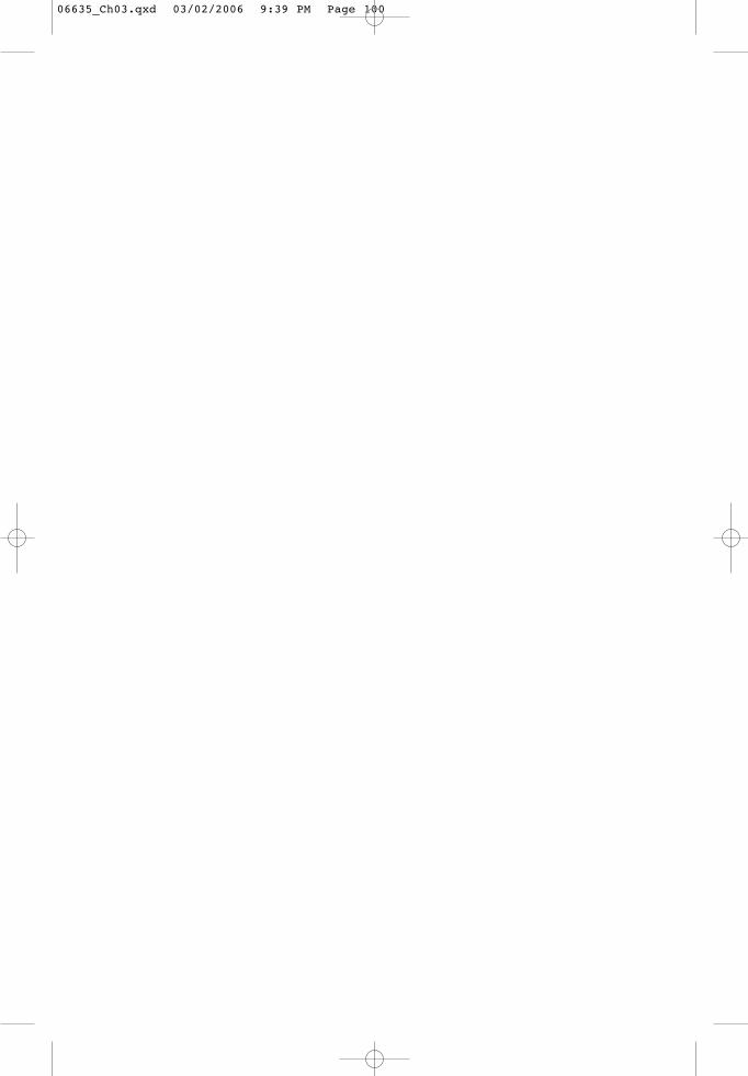
06635_Ch03.qxd 03/02/2006 9:39 PM Page 100

Documents

California’s School Finance Reform: An Experiment in ...econ.ucsb.edu/~jon/Publications/ExperimentFiscalFederalism.pdf · 55 California’s School Finance Reform: An Experiment