Embed Size (px)
Citation preview

T R A N S P O R T A T I O N R E S E A R C H
Number E-C079 September 2005
Calibration to
Determine Load and
Resistance Factors for
Geotechnical and
Structural Design

TRANSPORTATION RESEARCH BOARD 2005 EXECUTIVE COMMITTEE OFFICERS Chair: John R. Njord, Executive Director, Utah Department of Transportation, Salt Lake City Vice Chair: Michael D. Meyer, Professor, School of Civil and Environmental Engineering, Georgia
Institute of Technology, Atlanta Division Chair for NRC Oversight: C. Michael Walton, Ernest H. Cockrell Centennial Chair in
Engineering, University of Texas, Austin Executive Director: Robert E. Skinner, Jr., Transportation Research Board TRANSPORTATION RESEARCH BOARD 2005 TECHNICAL ACTIVITIES COUNCIL Chair: Neil J. Pedersen, State Highway Administrator, Maryland State Highway Administration,
Baltimore Technical Activities Director: Mark R. Norman, Transportation Research Board Christopher P. L. Barkan, Associate Professor and Director, Railroad Engineering, University of Illinois
at Urbana–Champaign, Rail Group Chair Christina S. Casgar, Office of the Secretary of Transportation, Office of Intermodalism, Washington,
D.C., Freight Systems Group Chair Larry L. Daggett, Vice President/Engineer, Waterway Simulation Technology, Inc., Vicksburg,
Mississippi, Marine Group Chair Brelend C. Gowan, Deputy Chief Counsel, California Department of Transportation, Sacramento,
Legal Resources Group Chair Robert C. Johns, Director, Center for Transportation Studies, University of Minnesota, Minneapolis,
Policy and Organization Group Chair Patricia V. McLaughlin, Principal, Moore Iacofano Golstman, Inc., Pasadena, California,
Public Transportation Group Chair Marcy S. Schwartz, Senior Vice President, CH2M HILL, Portland, Oregon, Planning and Environment
Group Chair Agam N. Sinha, Vice President, MITRE Corporation, McLean, Virginia, Aviation Group Chair Leland D. Smithson, AASHTO SICOP Coordinator, Iowa Department of Transportation, Ames,
Operations and Maintenance Group Chair L. David Suits, Albany, New York, Design and Construction Group Chair Barry M. Sweedler, Partner, Safety & Policy Analysis International, Lafayette, California, System Users
Group Chair
TRANSPORTATION RESEARCH CIRCULAR E-C079
Calibration to Determine Load and Resistance Factors for
Geotechnical and Structural Design
September 2005
Tony M. Allen Washington State Department of Transportation
Andrzej S. Nowak
University of Nebraska
Richard J. Bathurst GeoEngineering Centre at Queen’s–RMC, Royal Military College of Canada
Sponsored by Transportation Research Board
Foundations of Bridges and Other Structures Committee General Structures Committee
Transportation Research Board Washington, D.C.
www.TRB.org

TRANSPORTATION RESEARCH CIRCULAR E-C079 ISSN 0097-8515
The Transportation Research Board is a division of the National Research Council, which serves as an independent advisor to the federal government on scientific and technical questions of national importance. The National Research Council, jointly administered by the National Academy of Sciences, the National Academy of Engineering, and the Institute of Medicine, brings the resources of the entire scientific and technical communities to bear on national problems through its volunteer advisory committees. The Transportation Research Board is distributing this Circular to make the information contained herein available for use by individual practitioners in state and local transportation agencies, researchers in academic institutions, and other members of the transportation research community. The information in this Circular was taken directly from the submission of the authors. This document is not a report of the National Research Council or of the National Academy of Sciences.
Design and Construction Group
L. David Suits, Chair
Soil Mechanics Section Deborah J. Goodings, University of Maryland, Chair
Structures Section
Mary Lou Ralls, Ralls Newman, LLC, Chair
Foundations of Bridges and Other Structures Committee Mark J. Morvant, Louisiana Transportation Research Center, Chair
Tony M. Allen
Darrin P. Beckett James J. Brennan
Randy Ray Cannon Thomas L. Cooling
Christopher E. Dumas Richard L. Engel
J. David Frost
George G. Goble An-Bin Huang
Edward Kavazanjian, Jr. Kyung Jun Kim Laura Krusinski San-Shyan Lin
Samuel G. Paikowsky Paul D. Passe
Thomas W. Pelnik III Gary Person
Anand J. Puppala Thomas Shantz Sunil Sharma
James M. Sheahan Jan L. Six
Darin L. Sjoblom
G.P. Jayaprakash, TRB Staff Representative
General Structures Committee Harry A. Capers, Jr., New Jersey Department of Transportation, Chair
Martin P. Burke, Jr. H. Joseph Dagher
Sheila Rimal Duwadi Fouad Fanous
Gregg C. Fredrick Antonio M. Garcia
Frederick Gottemoeller Mark Hirota
David P. Hohmann Ramankutty Kannankutty
Dimitris Kosteas Paul V. Liles, Jr. Tom W. Melton
Andrzej S. Nowak Guy S. Puccio
Wojciech Radomski
Timothy V. Rountree Arunprakash M. Shirole
Bryan J. Spangler Bala Tharmabala Wagdy G. Wassef Kenneth R. White Stanley W. Woods
Nur Yazdani
Stephen F. Maher, TRB Staff Representative
Transportation Research Board 500 Fifth Street, NW
Washington, DC 20001 www.TRB.org
Norman Solomon, Production Editor; Mary McLaughlin, Proofreader; Jennifer J. Weeks, Layout

i
Foreword
he development of this Circular started as an outgrowth of NCHRP 12-55, Load and Resistance Factors for Earth Pressures on Bridge Substructures and Retaining Walls, and the
calibration effort being conducted as part of a regional pooled fund study SPR-03(072), Strength and Deformation Analysis of Mechanically Stabilized Earth (MSE) Walls at Working Loads and Failure. This Circular also addresses structural calibration issues raised at an LRFD Calibration Workshop sponsored by the AASHTO Bridge subcommittee�s LRFD Oversight Committee held in Washington, D.C., after the 2004 Transportation Research Board Annual meeting. Many bridge subcommittee members have recognized that there is a general lack of understanding of the calibration process. This lack of understanding may be hindering the development of the LRFD specifications, and supporting documentation, that will allow the profession to accept and advance the new design specifications. The writers of this Circular have drawn from input received at the workshop to more fully address the issues raised and to maximize its usefulness to the AASHTO Subcommittee on Bridges and Structures and state agencies sponsoring research on LRFD.
The purpose of this Circular is to assist both structural and geotechnical engineers to better understand the calibration process and what information is required to perform such calibrations. The Circular describes how such calibration efforts need to be documented so that the calibration results become a heritage for future users of the AASHTO LRFD specifications and thereby enhance future LRFD research and development. There are certain places in the LRFD specifications where other methods are allowed, but users are faced with determining their own resistance factors. This Circular is intended to help standardize the approach used to statistically characterize data for use in the calibration process. It describes how to conduct the actual calibration and, once completed, how to apply the results to the development of LRFD design specifications.
This document does not explain how to apply the AASHTO LRFD design specifications. It is not meant for practicing geotechnical or structural design engineers who simply want to know how to use LRFD for their specific design situation. This Circular is for the researcher or sophisticated design engineer who is faced with conducting calibrations using locally available data, validating a design method not covered by the current specifications, or developing specifications at a national level. This Circular is also for the engineer who is faced with setting up the scope of work for calibration research to be done by others so that the appropriate research tasks are requested and usable products delivered. It should be recognized that the average engineer, who is likely to be unfamiliar with advanced statistics theory, will need to expend significant effort to understand and attempt to apply these concepts. It should not be expected that the average practicing engineer will be able to casually read this Circular and know how to do calibration. However, it is intended to provide enough understanding of the subject so those faced with such calibration efforts can ask the right questions and provide the right guidance to researchers to get the products they need.
LRFD research calibration efforts can be expensive. Data need to be collected, statistical analyses performed, and results properly documented. Research investments must be preserved for future advancements. Inadequate documentation can lead to additional costs for reconditioning databases, redoing statistical analyses, or simply understanding original calibration information and processes. The documentation of any calibration effort must be
T

ii TR Circular E-C079: Calibration to Determine LRF for Geotechnical and Structural Design
consistent and usable for researchers to apply such data to extend previous calibration work. This Circular describes how to document calibration efforts so that they will be usable for future generations as the LRFD design specifications continue to be developed.
This document is being sponsored by the TRB Foundations of Bridges and Other Structures (AFS30) and General Structures (AFF10) Committees. The review of this document was performed by members and friends of these committees and the AASHTO Bridge subcommittee�s LRFD Oversight Committee. Comments or inquiries about this document should be sent to Mark J. Morvant or Harry A. Capers, c/o G. P. Jayaprakash, Transportation Research Board, 500 Fifth Street, NW, Keck 488, Washington, DC 20001 (telephone 202-334-2952, fax 202-334-2003, e-mail [email protected]).
Contents Abstract...........................................................................................................................................1 1 Introduction................................................................................................................................2 2 Overview of Calibration Approach..........................................................................................3 3 Limit State Equation Development and Calibration Concepts .............................................5 4 Selection of the Target Reliability Index .................................................................................9 5 Statistical Characterization and
Calibration Considerations .............................................................................................12 5.1 Obtaining Statistical Parameters .................................................................................12
5.2 Quality and Quantity of the Data ................................................................................15 5.3 Scaling Bias Data to Obtain Statistics for R and Q.....................................................17 5.4 Locating the Design Point and Its Influence on the Statistical Parameters Chosen ...18
5.4.1 Rackwitz-Fiessler Procedure Summary.......................................................20 5.4.2 Example: Design Point Determination for the
Steel Grid Wall Pullout Limit State ...........................................................21 5.5 Final Preparation of Statistics for Use in LRFD Calibration......................................26
6 Estimating the Load Factor ....................................................................................................29 7 Estimating the Resistance Factor ...........................................................................................32 8 Calibration Using Monte Carlo Method:
Geotechnical Application with Single Load Source......................................................34 9 Calibration Using the Monte Carlo Method:
Geotechnical Application with Multiple Load Sources................................................41 10 Calibration Using the Monte Carlo Method:
Geotechnical Application Treating Design Model Input Parameters as Random Variables .......................................................................................................43
11 Calibration Using the Monte Carlo Method:
Structural Application.....................................................................................................48 11.1 Interior Girder Design...............................................................................................48 11.2 Reliability Analysis for Interior Girder Design ........................................................52
12 Practical Considerations for Calibration When Data Are
Limited or Not Available.................................................................................................58
13 Final Selection of Load and Resistance Factors..................................................................62 14 Documentation of Load and Resistance Factor Calibration..............................................63 15 Concluding Remarks .............................................................................................................64 References.....................................................................................................................................65 Acknowledgments ........................................................................................................................67 Appendixes
Appendix A: Statistical Data Distribution and Characterization Concepts .............68 Appendix B: Excel Function Equations........................................................................75
Appendix C: Supporting Documentation Required for Calibration to Develop Load and Resistance Factors ..............................................................................76
Appendix D: Abbreviations and Notations ..................................................................80
1
Abstract
Calibration to Determine Load and Resistance Factors for Geotechnical and Structural Design
ith the advent of limit states design methodology in North American design specifications, there has been increasing demand to obtain statistical data to assess the reliability of
structural and geotechnical designs. Reliability depends on load and resistance factors that are determined through calibration procedures using available statistical data. This Circular describes methodologies that can be used to determine load and resistance factors for geotechnical and structural design. The Circular begins with basic reliability concepts, continues with detailed procedures that can be used to characterize data to develop the statistics and functions needed for reliability analysis, presents detailed step-by-step examples, and concludes with practical considerations when statistical data are limited. Closed-form solutions for estimating load and resistance factors that can be used for simple cases, as well as more rigorous probabilistic analysis methods such as the Monte Carlo method, are discussed in detail. Procedures are provided for situations where either single or multiple loads must be considered. An example is also provided that demonstrates the effect of considering only the variability of the input parameters for a given design methodology versus considering the overall variability of the design method. Such an approach can also be used to assess the effect of variability of a given design parameter on the reliability of the design.
This Circular is written to educate users of AASHTO, or similar Load and Resistance Factor Design (LRFD) specifications, on how load and resistance factors are developed. Furthermore, there are some cases when new load and/or resistance factors must be developed, or when current load or resistance factors are not directly applicable due to project- or region-specific issues. The information provided herein can be used to estimate load and resistance factors where adjustment of these factors is justified based on local experience and data. Criteria for documentation of calibration input and results are also provided. This Circular has been written with the assumption that the reader has some familiarity with basic statistical concepts and tools. However, for the convenience of those lacking that familiarity, a brief summary of basic statistical concepts is provided in an appendix.
W

2
1
Introduction
ith the advent of limit states design methodology in North American design specifications, for example, the Ontario Highway Bridge Design Code (Ministry of Transportation 1979,
1983, 1991), the Canadian Highway Bridge Design Code (CSA 2000), and the AASHTO Load and Resistance Factor Design (LRFD) Bridge Design Specifications (AASHTO 1992, 1998, 2004), there has been increasing demand to obtain data that can be used to assess the uncertainty and reliability of the methods used in those specifications for structural and geotechnical design. Goals in the development of these design codes and specifications have been to investigate the reliability associated with the design methods used, and to develop load and resistance factors that provide a consistent margin of safety for the design of all structural components. The process of using data, from which statistical parameters characteristic of the design method can be derived, and the determination of the magnitude of load and resistance factors needed to obtain acceptable margins of safety, is termed �calibration.�
A past impediment to conversion of structural and geotechnical design models to the LRFD format from the previous allowable stress design (ASD) practices was the lack of high-quality data to calibrate load and resistance factors. Now that data of adequate quality to perform calibration are becoming available, assessment of design reliability can be improved. For example, the writers have collected a detailed database of 20 well-instrumented steel reinforced soil wall sections (Allen, et al., 2001), as well as laboratory in-soil pullout and tensile (or yield) strength test results, that can be used to calculate load and resistance factors for LRFD-based reinforced soil wall design models. For structural design of bridges, statistical data that can be used for this level of calibration are reported by Nowak (1999).
This Circular provides detailed description of the process used to perform calibration of load and resistance factors as applied to limit states design, in particular for the development of LRFD structural and geotechnical design. Also provided are examples of the calibration process using the aforementioned reinforced soil wall data, specifically focusing on steel reinforced soil walls, and structural design of a bridge component using data provided by Nowak (1999). Goble (1999) and Becker (1996a, b) provide overviews of limit states design practice in foundation engineering. Nowak and Collins (2000) provide background on reliability theory, as applied to structural design and the development of the AASHTO LRFD structural design specifications, as well as an in-depth treatment of the various statistical tools and concepts needed to conduct reliability analyses. A brief summary of these statistical tools and concepts is also provided in Appendices A and B, for those who lack familiarity with the relevant statistical tools. Finally, information is provided on how to document calibration input parameters and results so that the calibration work can be useful for implementation in design and can be improved upon as more data become available or as design method improvements are made (see Appendix C).
W
3
2
Overview of Calibration Approach
here are three levels of probabilistic design: Levels I, II, and III (Withiam et al. 1998; Nowak and Collins 2000). The Level I method is the least accurate. It is sufficient here to
point out that only Level III is a fully probabilistic method. Level III requires complex statistical data beyond what is generally available in geotechnical and structural engineering practice. Level II and Level I probabilistic methods are more viable approaches for geotechnical and structural design. In Level I design methods, safety is measured in terms of a safety factor, or the ratio of nominal (design) resistance and nominal (design) load. In Level II, safety is expressed in terms of the reliability index, β. The Level II approach generally requires iterative techniques best performed using computer algorithms. For simpler cases, closed-form solutions to estimate β are available. Closed-form analytical procedures to estimate load and resistance factors should be considered approximate, with the exception of very simple cases where an exact closed-form solution exists (see Section 3). Alternatively, spreadsheet programs running on personal computers can be used to estimate load and resistance factors using the more rigorous and adaptable Monte Carlo simulation technique, which in turn can be used to accomplish a Level II probabilistic analysis.
The goal of Level I or II analyses is to develop factors that increase the nominal load or decrease the nominal resistance to give a design with an acceptable and consistent probability of failure. To accomplish this, an equation that incorporates and relates together all of the variables that affect the potential for failure of the structure or structural component must be developed for each limit state. The parameters of load and resistance are considered as random variables, with the variation modeled using the available statistical data. A random variable is a parameter that can take different values that are not predictable. An example is compressive strength of a concrete cylinder, fc�, that can be determined using a testing machine. If all the values of fc� are obtained on the same testing machine, all concrete specimens are from the same sample, and if all tests are carried out and interpreted in exactly the same manner, then non-random external influences on the test results are not present, and the test results are completely random in nature. This is not a formal mathematical definition, but it can be used in engineering applications (Nowak and Collins 2000).
For LRFD calibration purposes, statistical characterization should focus on the prediction of load or resistance relative to what is actually measured in a structure. Therefore, this statistical characterization is typically applied to the ratio of the measured to predicted value, termed the �bias.� The predicted (nominal) value is calculated using the design model being investigated. Note that the term bias factor (or bias) is typically defined as the ratio of the mean of the measured value divided by the nominal (predicted) value. However, for the purposes described herein, the term bias is used to refer to individual measured values of load or resistance divided by the predicted value corresponding to that measured value.
Regardless of the level of probabilistic design used to perform LRFD calibration, the steps needed to conduct a calibration are as follows:
1. Develop the limit state equation to be evaluated, so that the correct random variables
are considered. Each limit state equation must be developed based on a prescribed failure
T
4 TR Circular E-C079: Calibration to Determine LRF for Geotechnical and Structural Design
mechanism. The limit state equation should include all the parameters that describe the failure mechanism and that would normally be used to carry out a deterministic design of the structure or structural component.
2. Statistically characterize the data upon which the calibration will be based (i.e., the data that statistically represent each random variable in the limit state equation being calibrated). Key parameters include the mean, standard deviation, and coefficient of variation (COV) as well as the type of distribution that best fits the data (i.e., often normal or lognormal). See Appendix A for a conceptual description and mathematical definition of these statistical terms.
3. Select a target reliability value based on the margin of safety implied in current designs, considering the need for consistency with reliability values used in the development of other AASHTO LRFD specifications, and considering levels of reliability for design as reported in the literature for similar structures.
4. Determine load and resistance factors using reliability theory consistent with the selected target reliability.
It must be recognized that the accuracy of the results of a reliability theory analysis is directly dependent on the adequacy, in terms of quantity and quality, of the input data used. The final decision made regarding the magnitude of the load and resistance factor selected for a given limit state must consider the adequacy of the data. If the adequacy of the input data is questionable, the final load and resistance factor combination selected should be more heavily weighted toward a level of safety that is consistent with past successful design practice, using the reliability theory results to gain insight as to whether or not past practice is conservative or non-conservative. See Allen (2005) for examples of how this issue is applied in the selection of load and resistance factors.
5
3
Limit State Equation Development and Calibration Concepts
he following basic equation can be used to represent limit states design from the North American perspective (AASHTO 2004):
nini RQγ∑ ≤ ϕ (1) where γi = load factor applicable to a specific load component; Qni = a specific nominal load component; ΣγiQni = the total factored load for the load group applicable to the limit state being considered; ϕ = the resistance factor; and Rn = the nominal resistance available (either ultimate or the resistance available at a given deformation).
A limit state is a condition, related to a design objective, in which a combination of one or more loads is just equal to the available resistance, so that the structure is at incipient failure defined by a prescribed failure criterion (or deformed beyond an acceptable prescribed amount). Each failure criterion is represented by an equation having the general form of Equation 1.
The load and resistance factors in Equation 1 are used to account for material variability, uncertainty in magnitude of the applied loads, design model prediction uncertainty, and other sources of uncertainty. The objective in LRFD is to ensure that for each limit state the available resistance (factored resistance term) is at least as large as the total load (sum of factored load contributions).
Equation 1 is the design equation, but it can serve as the basis for the development of a limit state equation that can be used for calibration purposes. To fully define this design equation, a trial structure geometry may need to be established. This trial structure geometry is used to define the mathematical relationship between the random variables that contribute to uncertainty in the predicted loads and resistances included in the equation. If there is only one load component, Qn, then Equation 1 can be shown as: ϕRRn �γQQn ≥ 0 (2) where Rn = the nominal resistance value; Qn = the nominal load value; ϕR = a resistance factor; and γQ = a load factor.
T
6 TR Circular E-C079: Calibration to Determine LRF for Geotechnical and Structural Design
The limit state equation that corresponds to Equation 2 is: g = R � Q > 0 (3) where g = a random variable representing the safety margin; R = a random variable representing resistance; and Q = a random variable representing load.
The factored values for load and resistance are calculated from Equation 3 by setting the left side of the relationship equal to zero, the point at which the limit state is just reached. Generally, the resistance required is calculated knowing the load applied, and the resistance is increased to be greater than the load by a combination of load and resistance factors so that failure due to inadequate resistance is unlikely. At this point, what is important to understand is that the nominal values of load and resistance must be properly related to one another through the use of the design equation corresponding to the considered limit state function. From Equation 2, the minimum required Rn is calculated as follows:
R
nQn
QR
ϕγ
= (4)
For a given nominal value of the load Qn, Rn must be greater than Qn by some factor that is a function of the load and resistance factors used for design, as illustrated in Equation 4. Specific examples of design equation and corresponding limit state equation development for specific design situations are provided later in this Circular.
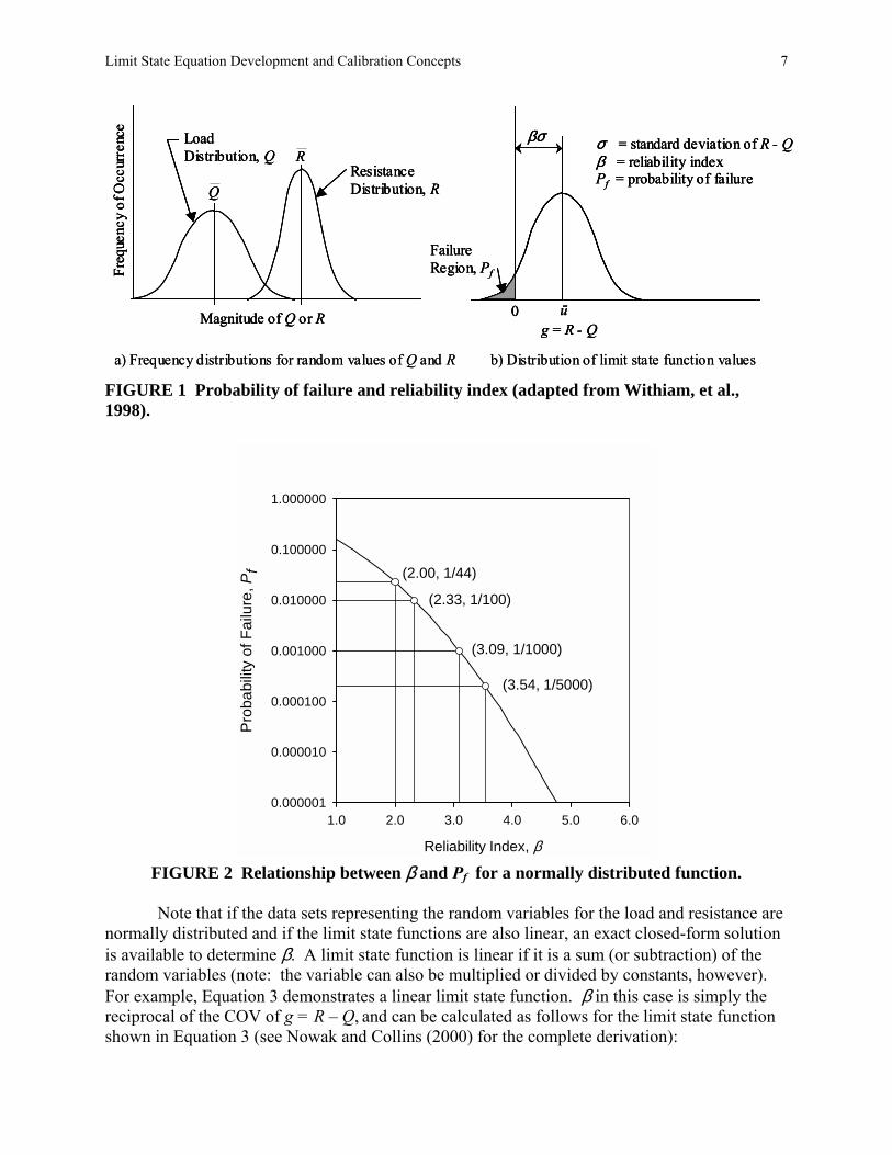
The magnitude of the load and resistance factors, and the difference between R and Q, are determined such that the probability of failure, Pf, that Q is greater than R is acceptably small. The idea is to separate the load and resistance distributions far enough apart that the probability of failure is acceptably low. Figure 1 illustrates the principle, in this case for two normal distributions. Pf is typically represented by the reliability index term β, shown in the right hand figure. Parameter β is equal to 1/COV for the limit state function, g = R � Q, and is related to the probability of failure (i.e., when R � Q < 0).
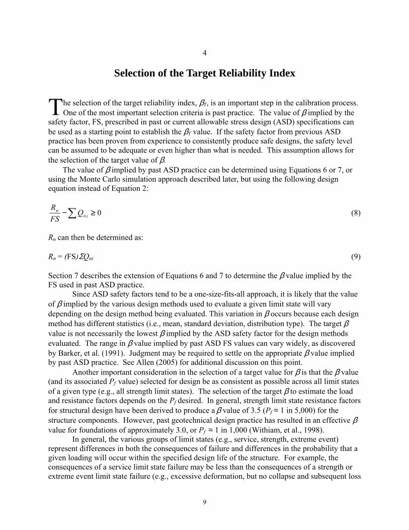
Figure 2 illustrates the relationship between β and the probability of failure Pf. This relationship is developed from Equation 5, using the Microsoft Excel Function NORMSDIST, which returns the standard normal cumulative distribution function (CDF) value for a given value of β, as shown below (see Appendix B for the full equation): Pf = 1 � NORMSDIST(β) (5)
Figure 2 applies to a normally distributed function, g. The more the limit state function value, g, departs from a normal distribution, the more approximate the relationship shown in Figure 2 becomes. However, the individual variables used to calculate g do not necessarily need to be normally distributed.
Limit State Equation Development and Calibration Concepts 7
g = R - Qū
βσ
Resistance Distribution, R
Load Distribution, Q
Freq
uenc
y of
Occ
urre
nce
0
FailureRegion, Pf
Magnitude of Q or R
σ = standard deviation of R - Qβ = reliability indexPf = probability of failure
Q
R
a) Frequency distributions for random values of Q and R b) Distribution of limit state function values
g = R - Qū
βσ
Resistance Distribution, R
Load Distribution, Q
Freq
uenc
y of
Occ
urre
nce
0
FailureRegion, Pf
Magnitude of Q or R
σ = standard deviation of R - Qβ = reliability indexPf = probability of failure
Q
R
g = R - Qū
βσ
Resistance Distribution, R
Load Distribution, Q
Freq
uenc
y of
Occ
urre
nce
0
FailureRegion, Pf
Magnitude of Q or R
σ = standard deviation of R - Qβ = reliability indexPf = probability of failure
Q
R
a) Frequency distributions for random values of Q and R b) Distribution of limit state function values FIGURE 1 Probability of failure and reliability index (adapted from Withiam, et al., 1998).
Reliability Index, β
1.0 2.0 3.0 4.0 5.0 6.0
Pro
babi
lity
of F
ailu
re, P
f
0.000001
0.000010
0.000100
0.001000
0.010000
0.100000
1.000000
(2.33, 1/100)
(3.09, 1/1000)
(2.00, 1/44)
(3.54, 1/5000)
FIGURE 2 Relationship between β and Pf for a normally distributed function.
Note that if the data sets representing the random variables for the load and resistance are
normally distributed and if the limit state functions are also linear, an exact closed-form solution is available to determine β. A limit state function is linear if it is a sum (or subtraction) of the random variables (note: the variable can also be multiplied or divided by constants, however). For example, Equation 3 demonstrates a linear limit state function. β in this case is simply the reciprocal of the COV of g = R � Q, and can be calculated as follows for the limit state function shown in Equation 3 (see Nowak and Collins (2000) for the complete derivation):

8 TR Circular E-C079: Calibration to Determine LRF for Geotechnical and Structural Design
22QR
QRσσ
β+
−= (6)
where R = the mean of the resistance R; Q = the mean of the load Q; σR = the standard deviation for the resistance R; and σQ = the standard deviation for the load Q. The closed-form solution (Equation 6) for this very simple case could be used in lieu of the more rigorous Monte Carlo simulation method described later. The equation provides accurate results if both R and Q are normal random variables; otherwise it is an approximation.
If both the load and resistance distributions are lognormal, and the limit state function is a product of random variables, then β can be calculated using a closed-form solution reported by Withiam, et al. (1998) and Nowak (1999). If g = R/Q � 1, then β can be determined using:
( ) ( )( )( )
2 2
2 2
LN / 1 1
LN 1 1
Q R
Q R
R Q COV COV
COV COVβ
+ + = + +
(7)
where R = the mean of the resistance R; Q = the mean of the load Q; COVR = the coefficient of variation for the resistance; COVQ = the coefficient of variation for the load; and β = the reliability index.
In general, the separation between R and Q (see Figure 1) is established to produce an acceptable magnitude of β, as calculated, for example, using Equation 6 or 7. An acceptable magnitude for β is simply the magnitude of β that results in the desired value of Pf. This desired β value is termed the target reliability index, βT.
9
4
Selection of the Target Reliability Index
he selection of the target reliability index, βT, is an important step in the calibration process. One of the most important selection criteria is past practice. The value of β implied by the
safety factor, FS, prescribed in past or current allowable stress design (ASD) specifications can be used as a starting point to establish the βT value. If the safety factor from previous ASD practice has been proven from experience to consistently produce safe designs, the safety level can be assumed to be adequate or even higher than what is needed. This assumption allows for the selection of the target value of β.
The value of β implied by past ASD practice can be determined using Equations 6 or 7, or using the Monte Carlo simulation approach described later, but using the following design equation instead of Equation 2:
∑ ≥− 0inn Q
FSR
(8)
Rn can then be determined as: Rn = (FS)ΣQni (9) Section 7 describes the extension of Equations 6 and 7 to determine the β value implied by the FS used in past ASD practice.
Since ASD safety factors tend to be a one-size-fits-all approach, it is likely that the value of β implied by the various design methods used to evaluate a given limit state will vary depending on the design method being evaluated. This variation in β occurs because each design method has different statistics (i.e., mean, standard deviation, distribution type). The target β value is not necessarily the lowest β implied by the ASD safety factor for the design methods evaluated. The range in β value implied by past ASD FS values can vary widely, as discovered by Barker, et al. (1991). Judgment may be required to settle on the appropriate β value implied by past ASD practice. See Allen (2005) for additional discussion on this point.
Another important consideration in the selection of a target value for β is that the β value (and its associated Pf value) selected for design be as consistent as possible across all limit states of a given type (e.g., all strength limit states). The selection of the target β to estimate the load and resistance factors depends on the Pf desired. In general, strength limit state resistance factors for structural design have been derived to produce a β value of 3.5 (Pf ≈ 1 in 5,000) for the structure components. However, past geotechnical design practice has resulted in an effective β value for foundations of approximately 3.0, or Pf ≈ 1 in 1,000 (Withiam, et al., 1998).
In general, the various groups of limit states (e.g., service, strength, extreme event) represent differences in both the consequences of failure and differences in the probability that a given loading will occur within the specified design life of the structure. For example, the consequences of a service limit state failure may be less than the consequences of a strength or extreme event limit state failure (e.g., excessive deformation, but no collapse and subsequent loss
T

10 TR Circular E-C079: Calibration to Determine LRF for Geotechnical and Structural Design
of life). The consequences (cost) of failure are a major consideration in the selection of βτ. However, the expected cost of failure is the product of the probability of failure and absolute value of the cost of failure. Therefore, for higher β value (i.e., lower probability of failure), a higher cost of failure may be acceptable.
For the case of extreme event loading (e.g., earthquake), the probability that the load combination associated with that limit state occurs may be considerably lower than the probability that a given strength limit state load combination will occur. Therefore, more severe consequences of failure, or a less stringent failure criterion, can be acceptable (e.g., allowing plastic hinging rather than requiring the stresses to stay below the elastic limit). In current ASD practice for geotechnical design, the safety factor is typically reduced when considering load combinations with a lower probability of occurrence such as those including impact or seismic loading, implying a lower βΤ. For structural allowable stress (service load) design, a certain amount of overstress is allowed for less probable strength and extreme event limit state load combinations (AASHTO, 2002). At present, no specific guidance is available for the selection of βΤ for lower probability load groups (e.g., extreme event limit state and some strength limit state load combinations).
Establishment of the target reliability index value, βΤ, for a given limit state and structure component being designed also depends on the redundancy inherent in the system. For example, if the component fails, would failure of the system result, or would load sharing to adjacent components occur, effectively reducing the probability that the entire structural system would fail? Zhang, et al. (2001) indicate that, because of redundancy, a higher probability of failure may be acceptable for evaluating limit states for a load-carrying element within a group of load-carrying elements to produce the desired probability of failure for the group. To extend the work done by Ghosn and Moses (1998) to quantify redundancy and its affect on system reliability to bridge substructure components, Liu, et al. (2001) analyzed single and multiple column bents with various foundation stiffness values, although the foundations themselves were not analyzed. They defined a substructure to be redundant if the system reliability index, β, was 0.5 higher than the component reliability index. For this definition of redundancy, they found that the load needed to be 20% higher to cause collapse of the substructure unit than to cause collapse of an individual member within the substructure unit. Many foundation systems, especially considering the ability of the soil as a load bearing component in combination with a larger number of members, likely have greater redundancy than the column bents analyzed in that study.
In the case of foundations and other geotechnical structures, some redundancy is usually present, depending on the size of the group or the number of reinforcement elements in the system. For example, in pile foundations, the lack of resistance available for a single overloaded pile does not necessarily mean that the entire foundation will fail, as adjacent piles that may be more lightly loaded could take some of the additional load (Zhang, et al., 2001). Reinforced soil walls depend on many reinforcement layers or strips for internal stability, and the failure or overstress of a single reinforcement layer or strip will not result in failure of the wall. Furthermore, the flexibility of the soil contributes to the ability of the foundation or reinforced soil system to share and redistribute load. Hence, geotechnical structures can be designed for a lower βT than the typical structure component due to this inherent redundancy. The exception to this might be a single drilled shaft or footing supporting an entire bridge pier, where, due to lack of redundancy, designing to a βT of 3.5 (i.e., Pf approaching 1 in 5,000) is appropriate.
Selection of the Target Reliability Index 11
Barker, et al. (1991) calculated the β value implied by the FS values used in ASD practice. Based on the statistical data available at the time, they found that a βT of 2.0 to 2.5 ( Pf ≈ 1 in 100) was consistent with the level of safety used in ASD practice for design of pile groups. However, for footings, they found past practice implied a βT value of 3.5 (Pf ≈ 1 in 5,000), and for shafts, the implied βT value was 2.5 to 3.0 (Pf ≈ 1 in 1,000). D�Appolonia (1999) and Paikowsky, et al. (2004) determined resistance factors for permanent reinforced soil walls and pile foundations, respectively, by using a βT of 2.3 because of this inherent redundancy. Zhang, et al. (2001) performed analyses of system reliability in comparison to component reliability and came to similar conclusions regarding the βT value needed for a foundation element to produce a foundation system βT value of 3.5 to be consistent with the βT used to calibrate superstructure design. Paikowsky, et al. (2004) assessed the minimum number of piles or shafts in a foundation group to be considered redundant enough to justify a βT value of 2.3. They indicated that a pile or shaft group can be considered redundant if the group contains a minimum of five piles or shafts. If the group contained less than five piles or shafts, they concluded that a βT value of 3.0 (Pf ≈ 1 in 1,000) is needed. While Paikowsky, et al. (2004) did not specifically address the situation where only a single foundation element supports the entire bridge pier, based on the conclusions made by Barker, et al. (1991), a βT value of 3.5 (Pf ≈ 1 in 5,000) should be used in that case. Note that this jump in the βT value (and a corresponding reduction in Pf) is reasonably consistent with the difference in βT value for systems classified as redundant/non-redundant as determined by Liu, et al. (2001).
For structural components, such as steel girders and prestressed concrete girders, the target reliability index is βT of 3.5 for strength limit states, corresponding to Pf ≈ 1 in 5,000. However, for a girder bridge treated as a structural system, β exceeds 5.5, corresponding to Pf ≈ 1 in 50 million. Conversely, for wood components such as stringers, a β of 2.0, corresponding to Pf of 1 in 50, is adequate. This is considerably lower than the βT of 3.5 for steel and concrete girders. However, steel and prestressed concrete girders are usually spaced at 1.8 to 2.4 m, and wood stringers are spaced at 0.3 to 0.5 m. Therefore, a single steel or prestressed concrete girder can be considered as equivalent to a subsystem of four to six wood stringers. Due to the ability of closely spaced stringers to share the load, the equivalent reliability index for a subsystem of four to six stringers is about 3.5 when individual wood stringers are designed to achieve a reliability index of 2.0.
The final selection of a βT value to use for a given limit state must take into account the range of β values implied by past successful design and construction practice, and consistency with the βT values used for design of structures in general, with consideration of the redundancy inherent in the structural or foundation component to be designed. As experience is gained in the application of LRFD to design, the role of past successful ASD practice will become less important, and consistency with the value of β used for structural design in general will become more important, lessening the need for the application of judgment to make the final selection of the βT.
12
5
Statistical Characterization and Calibration Considerations 5.1 OBTAINING STATISTICAL PARAMETERS To perform calibration using reliability analysis, the mean, standard deviation, and coefficient of variation (COV) as well as the type of distribution that best fits the data (i.e., typically normal or lognormal) must be determined for each random variable considered in the limit state function. Measured values of the random variable and the design model nominal prediction are used to generate the needed statistics. The bias, defined previously as the ratio of the measured to nominal (predicted) value, is used to generate the needed statistics. The statistical characterization procedures that follow apply to the situation where detailed statistical data are available. Practical considerations for the situation where such data are not available are provided in Section 12.
To characterize load and resistance data, a cumulative distribution function (CDF) of the data must be developed. The CDF is a function that represents the probability that a bias value less than or equal to a given value will occur. This probability can be transformed to the standard normal variable (or variate), z, and plotted against the bias (X) values for each data point. This plotting approach is essentially the equivalent of plotting the bias values and their associated probability values on normal probability paper. See Appendices A and B for a description of what a CDF is, how it is created, and how the standard normal variable, z, is determined.
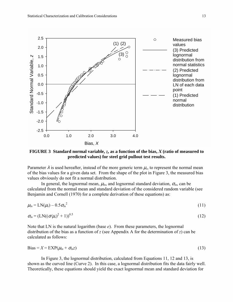
Figure 3 provides an example of a CDF plotted using the standard normal variable as the vertical axis. This figure provides the results of a number of steel grid reinforcement (i.e., welded wire and bar mat) pullout tests in granular soils where the bias was determined by dividing each test result, Rmeasured, by the predicted value, Rn (see Equation 21 provided later in this Circular for the method used to calculate Rn). As described in Appendix A, an important property of a CDF plotted in this manner (i.e., using the standard normal variable in place of the cumulative probability) is that normally distributed data plot as a straight line with a slope equal to 1/σ, where σ is the standard deviation, and the horizontal (bias) axis intercept is equal to the mean, µs. Lognormally distributed data on the other hand will plot as a curve.
The data shown in Figure 3 are presented as measured to predicted values (bias), with µs = λ = 1.48 (λ is defined below) and σ = 0.817 (calculated mathematically, rather than estimated graphically). The theoretical normal distribution is shown as the straight line in Figure 3 (Curve 1), calculated using the following equation: bias = X = λ + σz (10) where X = the bias, which is the measured/predicted value (i.e., the horizontal axis in the figure); and λ = the normal mean of the bias values contained in the data set.
Statistical Characterization and Calibration Considerations 13
Bias, X
0.0 1.0 2.0 3.0 4.0
Sta
ndar
d N
orm
al V
aria
ble,
z
-2.5
-2.0
-1.5
-1.0
-0.5
0.0
0.5
1.0
1.5
2.0
2.5 Measured biasvalues (3) Predictedlognormal distribution from normal statistics (2) Predictedlognormaldistribution from LN of each datapoint (1) Predictednormaldistribution
(1) (2)
(3)
FIGURE 3 Standard normal variable, z, as a function of the bias, X (ratio of measured to
predicted values) for steel grid pullout test results. Parameter λ is used hereafter, instead of the more generic term µs, to represent the normal mean of the bias values for a given data set. From the shape of the plot in Figure 3, the measured bias values obviously do not fit a normal distribution.
In general, the lognormal mean, µln, and lognormal standard deviation, σln, can be calculated from the normal mean and standard deviation of the considered random variable (see Benjamin and Cornell (1970) for a complete derivation of these equations) as: µln = LN(µs) � 0.5σln
2 (11) σln = (LN((σ/µs)2 + 1))0.5 (12) Note that LN is the natural logarithm (base e). From these parameters, the lognormal distribution of the bias as a function of z (see Appendix A for the determination of z) can be calculated as follows: Bias = X = EXP(µln + σlnz) (13)
In Figure 3, the lognormal distribution, calculated from Equations 11, 12 and 13, is shown as the curved line (Curve 2). In this case, a lognormal distribution fits the data fairly well. Theoretically, these equations should yield the exact lognormal mean and standard deviation for

14 TR Circular E-C079: Calibration to Determine LRF for Geotechnical and Structural Design
the data set. However, these equations were derived for an idealized lognormal distribution, not a sample distribution from actual data that does not necessarily fit an idealized lognormal distribution. Consequently, good agreement may not be obtained for the statistical parameters derived using the theoretical equations versus determining the mean and standard deviation directly from the natural logarithms of each data point in the distribution, especially if the COV of the data is greater than approximately 20 to 30%. This difference is evident in Figure 3, where the lognormal distributions using Equation 13 are plotted for lognormal parameters determined using both approaches (Curves 2 and 3). For the steel grid pullout normal statistics provided previously, µln and σln determined from Equations 11 and 12 are 0.262 and 0.515, respectively. However, if these parameters are calculated directly by taking the mean and standard deviation from the natural logarithm of all of the data points, µln and σln are equal to 0.273 and 0.480, respectively.
Some of the data at the upper or lower ends may require further consideration to determine whether they are �outliers.� If justified, these points can be removed from the data set so the statistical parameters are not skewed by a few data points which do not appear to be a part of the data set. However, identification and removal of the �outliers� involves subjective judgment, and it should be performed with caution. Typical reasons to consider a given data point to be an outlier include:
• The data obtained near a structure boundary are not specifically accounted for in the
design model being used (e.g., data obtained near the top or bottom of a wall), • A different criterion is used to establish the value of a given point or set of points
(i.e., a different failure criterion), • A different measurement technique is used, • Data from a source that may be suspect, • Data that are affected by regional factors (e.g., regional geology effects on soil or
rock properties), or • Any other issues that would cause the data within a given data set to not be
completely random in nature.
It is important that the statistical data used to characterize a given random variable truly represent random processes. If not, the statistics will be erroneous. This is especially important to check when attempting to group data from multiple sources together to form the data set used to characterize the random variable in question. For example, if different failure criteria have been used to develop the failure data from different sources, combining those data sets may not be representative of a random variable. If the data set was derived from data involving fundamentally different materials, the combined data set will likely not be truly random in nature if the material type significantly influences the results. In the case of the data provided in Figure 3, no outliers were removed, as none of the potential reasons for consideration of data as outliers (i.e., the bullets listed previously) appear to be applicable.
A final point that will become apparent in the following sections is the special attention that must be paid to the distribution of data in the tails of any cumulative distribution (e.g., see Figure 3). In most cases the data in the tails control the magnitude of the estimated load and resistance factors that are the objective of the LRFD calibration exercise. Simply removing data in the tails to obtain a better fit between the bulk of the data set and an assumed normal or lognormal cumulative distribution function may lead to significant errors in the estimation of the

Statistical Characterization and Calibration Considerations 15
magnitude of the load and resistance factors for a given limit state. For this reason use of statistical tests to remove outliers, such as the elimination of all data that are more than two standard deviations away from the mean, should not be used to improve the fit of a theoretical distribution to the data. 5.2 QUALITY AND QUANTITY OF THE DATA The statistical parameters of the input data are very important in reliability analyses. These parameters reflect not only the degree of uncertainty involved in load and resistance, but also the quality and quantity of the data. When assessing the quality and quantity of the data set used as part of a reliability analysis, the following should be considered:
• Do the data used to develop the statistics accurately represent the variable being modeled, including all sources of uncertainty that can affect the variable?
• Is enough known about how the data were developed and the conditions the data represent to be confident that the data can be used to represent the variable in question (i.e., is adequate documentation of the data available)?
• Are enough data available to ensure the mean, standard deviation, and cumulative distribution function adequately characterize the data?
• Have outliers been properly identified and removed from the data set (see Section 5.1)?
Quality and quantity of the data, including how well the data address the various sources of error, are very important, as they determine the accuracy of the results. It is desirable to have available hundreds of accurately measured data points representative of the random variable in question from which to establish statistics suitable for reliability analysis. Furthermore, these data points should all be measured using the same technique. However, it is rare that a large data set with this degree of quality and quantity is available.
Sources of uncertainty that can affect the statistics used to characterize a random variable include systematic error, inherent spatial variability, model error, and error associated with data quality and quantity problems. Systematic error is the result of inconsistency, or lack of repeatability, in the testing and analysis procedures used to measure or obtain the values in the data set. As a minimum, the statistical parameters derived from the data set used to represent the random variable (i.e., λrandom and COVrandom, the bias and coefficient of variation, respectively, determined through statistical analysis of the data representing the random variable) will address this type of error. Spatial variability is the variability of the measured input parameters over a distance, area, or volume of the material being evaluated (e.g., soil and rock properties in particular are known to vary from point to point, causing the measurement of a given property at a point to have a higher variability/uncertainty than the average of a number of measurements taken at various points in the soil or rock deposit surrounding the foundation element to be designed). Model error is the error resulting from the ability of the design model itself, including any transformations needed to obtain design input parameters (e.g., conversion of Standard Penetration Test values to soil shear strength), to accurately predict the nominal load or resistance (i.e., how well does theory match reality?). The data used to estimate the bias and COV of the random variable (i.e., λrandom and COVrandom) must be evaluated to determine whether
16 TR Circular E-C079: Calibration to Determine LRF for Geotechnical and Structural Design
or not they address these other sources of uncertainty. In general, measurements of load or resistance in full-scale structures do account for these other sources of uncertainty (with the exception of error associated with data quality and quantity problems), but measurements from model scale structures and measurements of specific design input parameters (e.g., laboratory measurements of material strength or unit weight) may not consider all sources of uncertainty.
When conducting reliability analyses, a decision must be made, and in some cases judgment applied, about how large the data set must be and what degree of quality it must have to produce statistics that are sufficiently reliable for calibration purposes. This can be especially true when attempting to develop geotechnical load and resistance factors, as typically there is a shortage of statistical data to represent geotechnical random variables, and the variability of the data is often quite high. As such, the degree of uncertainty in the random variable may not be fully reflected in the statistical parameters such as bias and COV measured or estimated from the available data. Uncertainty due to quality of input data must also be considered. The bias due to data quality issues can be assumed equal to 1.0 for most cases. Data quality issues primarily affect the COV of the random variable. The specific value of this additional uncertainty cannot be determined analytically at this time, and must be estimated based on judgment. Specific considerations for the determination of this additional uncertainty include:
• The degree of scatter in the standard normal variable versus bias plot of the data (e.g., see Figure 3).
• How well the measurements obtained reflect the actual situation being modeled (e.g., are the measurements based on small scale model studies or full-scale structures, does the laboratory test used to get the data accurately reflect how that parameter affects performance, etc.).
• Whether or not the data are from a single source or multiple sources. • The consistency in the criterion or criteria used to establish the measured values (e.g.,
failure criteria).
The quantity of the data can have a strong effect on the estimation of the statistical parameters (mean value and coefficient of variation), depending on the required confidence level. The higher the confidence level desired, the larger the number of samples required. For a given confidence level, the required number of samples can be determined using the formulas and tables provided in textbooks on statistics (e.g., Lloyd and Lipow, 1982). The quantity of data also affects the amount of extrapolation required when performing reliability analyses (see Section 8, in particular Figure 11, for an example).
This data quality/quantity uncertainty, and the other sources of uncertainty described herein, should be considered in the determination of the total bias (λtotal) and the total coefficient of variation (COVtotal) for the data set used to represent the random variable. If it is determined that these other sources of uncertainty (e.g., spatial variability and model error) are not already included in bias and COV of the random variable (i.e., λrandom and COVrandom), a first order approach to combining these sources of uncertainty to obtain the final statistics used as input in the reliability analyses is provided in the following equations:
.....total random spatial model dqλ λ λ λ λ= × × × × (14)
Statistical Characterization and Calibration Considerations 17
2222dqmodelspatialrandomtotal COVCOVCOVCOVCOV ++++= L (15)
where λrandom = the bias for the data set used to represent the random variable under consideration; λspatial = the bias resulting from spatial variability of the parameter; λmodel = the bias resulting from design model uncertainty; λdq = the bias caused by having inadequate data quality; COVrandom = the coefficient of variation for the data set used to represent the random variable under consideration; COVspatial = the coefficient of variation resulting from spatial variability of the parameter; COVmodel = coefficient of variation resulting from design model uncertainty; and COVdq = the additional uncertainty caused by having inadequate data quality. A more detailed discussion of these sources of uncertainty (with the exception of COVdq) and their effect on both the COV and bias is provided by Withiam, et al. (1998) and Vanmarke (1977). In addition, Section 10 of this Circular demonstrates the effect of these additional sources of uncertainty on calibration results. 5.3 SCALING BIAS DATA TO OBTAIN STATISTICS FOR R AND Q As mentioned previously, the statistics available to perform reliability analyses, i.e., λ, σ, and distribution type, are typically for load and resistance data points expressed as measured/predicted (bias) values. However, the analysis based on Equations 1 through 7 and on Figure 1 (and as illustrated later in this Circular in Figure 4) requires Q and R, and their associated statistical parameters λ and σ, directly, rather than the measured/predicted values. The statistical parameters in Equations 6 and 7 used to calculate β must be based on the measured values of load and resistance, Qmeasured and Rmeasured, respectively (i.e., the distributions FQ and FR shown later in this Circular in Figure 4). To obtain Qmeasured and Rmeasured, the bias statistics are scaled to represent the statistics for Q and R, using the design equation (Equation 2) to determine nominal (i.e., predicted) values Qn and Rn. Hence,
QnQQ λ×= (16)
RnRR λ×= (17)
QCOVQQ ×=σ (18)
RCOVRR ×=σ (19)
18 TR Circular E-C079: Calibration to Determine LRF for Geotechnical and Structural Design
where Q = the mean value of measured load Qmeasured; R = the mean value of measured resistance Rmeasured; Qn = the nominal (predicted) value of load for the limit state considered; Rn = the nominal (predicted) value of resistance for the limit state considered; λQ = the mean of the bias values (measured/predicted) for the load; λR = the mean of the bias values (measured/predicted) for the resistance; σQ = the standard deviation of the measured load; σR = the standard deviation of the measured resistance; COVQ = the coefficient of variation of the bias values for the load; and COVR = the coefficient of variation of the bias values for the resistance.
Scaling the bias statistics in this manner is the same as multiplying each bias data point in the data set by the single nominal (predicted) value Qn or Rn obtained from the limit state design calculation. The scaled data points are then used to produce the CDF of measured load or resistance values. This was in fact done to produce the pullout (resistance) data plotted in Figures 5 and 6 presented later in this Circular from the data in Figure 3. This scaling can be carried out for both normal and lognormal distributions of Q and R. Once the mean and standard deviation for Q and R have been scaled from the bias statistics, the value of β can be determined for the selected load and resistance factors using either Equation 6 or 7, or by performing a Monte Carlo simulation as described in Sections 8 through 11.
Note that the bias statistics were obtained from many case histories and are assumed to be characteristic of the statistics in general for the random variable under consideration. Therefore, the statistical distribution can be scaled uniformly by the single nominal value of Rn or Qn calculated at a specific location in a specific structure for which the limit state calculation is performed. 5.4 LOCATING THE DESIGN POINT AND ITS INFLUENCE ON THE STATISTICAL PARAMETERS CHOSEN Once outliers have been identified and removed and the randomness of the data for the variable in question checked, the next step is to make sure that the normal or lognormal parameters selected produce the best fit possible in the region of the CDF that is nearest the design point. The design point location concept is rather abstract due to the mathematical theory involved. However, if the limit state function is described in terms of reduced variables, it can be defined as the location on the limit state failure boundary (i.e., where g = R � Q = 0, or R = Q; see Equation 3) that is the shortest distance from the origin of the reduced variables (i.e., 0,0) to the limit state failure boundary. See Nowak and Collins (2000) for a more detailed definition of the design point location. In practice, the design point is typically located within the tails of the cumulative load and resistance distributions (i.e., in the upper tail for the load and the lower tail for the resistance as illustrated in Figure 4). This location corresponds to the general region where the load and resistance distributions overlap as shown in Figure 1(a). The specific location of the design point within the tail regions of the distributions depends on the mathematical functions used to approximate each distribution. Note that for some combinations
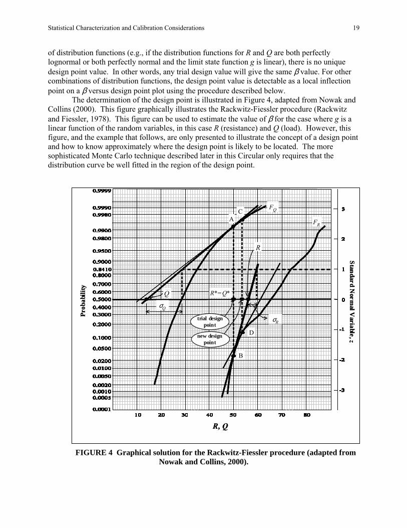
Statistical Characterization and Calibration Considerations 19
of distribution functions (e.g., if the distribution functions for R and Q are both perfectly lognormal or both perfectly normal and the limit state function g is linear), there is no unique design point value. In other words, any trial design value will give the same β value. For other combinations of distribution functions, the design point value is detectable as a local inflection point on a β versus design point plot using the procedure described below.
The determination of the design point is illustrated in Figure 4, adapted from Nowak and Collins (2000). This figure graphically illustrates the Rackwitz-Fiessler procedure (Rackwitz and Fiessler, 1978). This figure can be used to estimate the value of β for the case where g is a linear function of the random variables, in this case R (resistance) and Q (load). However, this figure, and the example that follows, are only presented to illustrate the concept of a design point and how to know approximately where the design point is likely to be located. The more sophisticated Monte Carlo technique described later in this Circular only requires that the distribution curve be well fitted in the region of the design point.
R, Q
Standard Norm
al Variable, z
Prob
abili
ty
new design point
trial design point
Q
R
R*=Q*
σQ
AC
σR
FQ
FR
D
B
R, Q
Standard Norm
al Variable, z
Prob
abili
ty
new design point
trial design point
Q
R
R*=Q*
σQ
AC
σR
FQ
FR
D
B
FIGURE 4 Graphical solution for the Rackwitz-Fiessler procedure (adapted from
Nowak and Collins, 2000).
20 TR Circular E-C079: Calibration to Determine LRF for Geotechnical and Structural Design
To perform the graphical version of the Rackwitz-Fiessler procedure, the cumulative probability distributions are plotted for both the load and resistance data on the same figure. Note that R and Q do have units, but their units will depend on specifically what parameter is being characterized. A trial design point is selected, at a point R = Q (i.e., g = R � Q = 0), identified as R* and Q* in Figure 4. Using tangents to the distribution curves at the value of R* and Q* selected (points A and B, respectively, for the first trial), the mean of the load and resistance data, Q and R , and standard deviation, σQ and σR, can be determined directly from the plots for the distributions of R and Q at the selected trial design point (i.e., the mean values represent the points where the tangent lines intersect the horizontal axis at z = 0 and the standard deviations are the inverse slope values of each tangent line). From these four parameters, β can be estimated using Equation 6. Once the β value for the first trial has been determined, select another trial design point (e.g., �new design point� in Figure 4), then select tangents to those curves at the new points, and recalculate β. This process is continued for several trial design points until convergence is obtained. 5.4.1 Rackwitz-Fiessler Procedure Summary Based on the information provided in Section 5.4, a step-by-step approach for carrying out the Rackwitz-Fiessler procedure graphically, with reference to Figure 4, is as follows:
1. Develop a plot of the load and resistance data (FQ and FR) illustrated in Figure 4, Note that if using bias values to create the statistical distributions, values for FQ and FR are determined by scaling the bias values as discussed in Section 5.3.
2. Estimate an initial value of the design point (i.e., R* = Q*). 3. Draw a vertical line at the design point. 4. Plot tangents to FR and FQ at their intersection with the vertical line (i.e., the assumed
design point). 5. Read equivalent parameters ,Q σQ, ,R and σR directly from the graph. 6. Calculate β using Equation 6. 7. Iterate to achieve convergence on value of β, calculating a new design point using the
following equation (Nowak and Collins, 2000):
( )( ) ( )22
2
*QR
RRRσσ
βσ
+−= (20)
8. Repeat the process until β converges. Generally, if the change in β is less than ±0.05,
further iteration is not necessary.
This iterative procedure simply facilitates locating the design point using this graphical procedure. Determining tangents graphically in this manner does require some judgment, hence the need for a trend line (or curve) to select trial tangent lines.
A more accurate approach is to determine the tangents at each trial design point analytically by establishing the equation of a best-fit trend line (or curve) for the distribution, and taking the derivative of that equation to obtain the tangent equation at the specified trial design
Statistical Characterization and Calibration Considerations 21
point location (R = Q). Note that the function used for this curve fitting exercise does not have to be normal or lognormal. Any function that best fits the distribution can be used. Once the tangent line equations are determined, parameters ,Q σQ, ,R and σR are determined analytically from the tangent lines rather than graphically as described in Step 5. Then β is determined using Equation 6 as described in Step 6. An analytical approach allows a wide range of design point values to be investigated and corresponding values of β computed. The final design point corresponds to a local inflection point in a plot of β versus design point values where the final design point is in the range of the tails of the two distribution curves. The procedure is illustrated in the next section. 5.4.2 Example: Design Point Determination for the Steel Grid Wall Pullout Limit State The determination of the design point and the best statistical parameters for calibration purposes is illustrated in the following example, using the Rackwitz-Fiessler procedure previously described. However, instead of determining the tangents at each trial design point graphically, they are determined analytically as described in Section 5.4.1.
In this example, the limit state to be investigated is the pullout of a steel grid reinforcement layer in a reinforced soil wall. In this case, the reinforcement layer must be designed to have adequate pullout resistance, Rn, to resist the applied load, Qn, where Rn is calculated as: Rn = Tpo = αγszdCLeF* (21) where Tpo = the pullout resistance; α = pullout scale effect correction factor (for steel, deterministically set equal to 1.0); γs = soil unit weight; zd = depth of soil above reinforcement in resisting zone; C = reinforcement surface area geometry factor (equals 2 for grid and strip reinforcement); Le = length of reinforcement in the resisting zone; and F* = the pullout resistance factor (in this case, F* is a function of the thickness and horizontal spacing of transverse bars, and the depth zd of the reinforcement). Note that the calculated load is load per unit length of wall face.
The load for this limit state calculation is assumed to be from gravity forces due to the wall mass (i.e., no live load or other types of loads). The load is calculated using the Simplified Method (AASHTO, 2004) as follows:
Qn = Tmax = SvσvKr (22) where Tmax = the maximum load in the reinforcement layer; Sv = tributary area (equivalent to the vertical spacing of the reinforcement in the vicinity of each layer when analyses are carried out per unit length of wall);
22 TR Circular E-C079: Calibration to Determine LRF for Geotechnical and Structural Design
σv = average vertical earth pressure acting at the reinforcement layer depth; Kr = lateral earth pressure coefficient acting at the reinforcement layer depth (for bar mat and welded wire walls, Kr varies from 2.5Ka to 1.2Ka at the top of the wall to a depth of 6 m below the wall top, respectively, and remains at 1.2Ka below 6 m), and Ka = the coefficient of lateral earth pressure.
The load data used in this example to generate statistical parameters are from Allen, et al. (2001), obtained from the database of full-scale instrumented reinforced soil walls mentioned in the Introduction (see Figure 7 provided later in this Circular for the load bias values used in this example). Only the bar mat and welded wire wall load data were considered (a total of 6 instrumented wall sections). The grid pullout data were obtained from D�Appolonia (1999), and the bias values for these pullout data are plotted in Figure 3.
For this example, the details of Equations 21 and 22 are not important regarding the development of the limit state equations, as the available statistics are for the load or resistance, Tmax (representing the load Qn) and Tpo (representing the resistance Rn), rather than the input parameters used to calculate Tmax and Tpo. Therefore, the design equation in this case is as follows: ϕRTpo - γQTmax ≥ 0 (23) Using Equation 23, Tpo is determined as follows:
maxR
Qpo TT
ϕγ
= (24)
This example is illustrated in Figures 5 and 6. Consistent with Section 5.3, the CDF plots
shown in Figures 5 and 6 were created by multiplying the reinforcement load CDF bias values in Figure 7 with a nominal value for Tmax = 1.0 kN/m, and the pullout resistance CDF in Figure 3 by the nominal value for the resistance (i.e., by ( )( )1.0Q Rγ ϕ ). The nominal value of Tmax (i.e., the unfactored load Qn) is assumed to be equal to 1.0 times the measured/predicted value of Q for convenience. What is important here is the relationship between Qn and Rn, not the absolute magnitude of the nominal value of Qn (i.e., Tpo must always be greater than Tmax by the ratio γQ/ϕR). As discussed later in Section 7, it can be shown that for relatively simple design equations such as Equation 23, Qn, or in this case Tmax, actually cancels out of the equation.
Figure 5 shows the case where γQ = 1.75 and ϕR = 0.6, and Figure 6 shows the case where γQ = 1.75 and ϕR = 1.0. These specific load and resistance factors were selected for this example to be consistent with the load and resistance factors used later in this Circular for the Monte Carlo simulations, to facilitate direct comparisons (see Section 6 for the determination of the load factor based on the load statistics). These two cases are also used to illustrate the effect changing the resistance factor has on the estimate of β and the location of the design point.
As mentioned previously, no outliers were removed from the pullout data set because none of the potential reasons for removal of a data point as an outlier identified in Section 5.1 appeared to be applicable. Therefore, curve fitting was conducted using the full data set, with no outliers removed. Similarly, no outliers were removed from the reinforcement load data set. Several types of curve fits are superimposed on each set of data in Figures 5a and 6a. For the
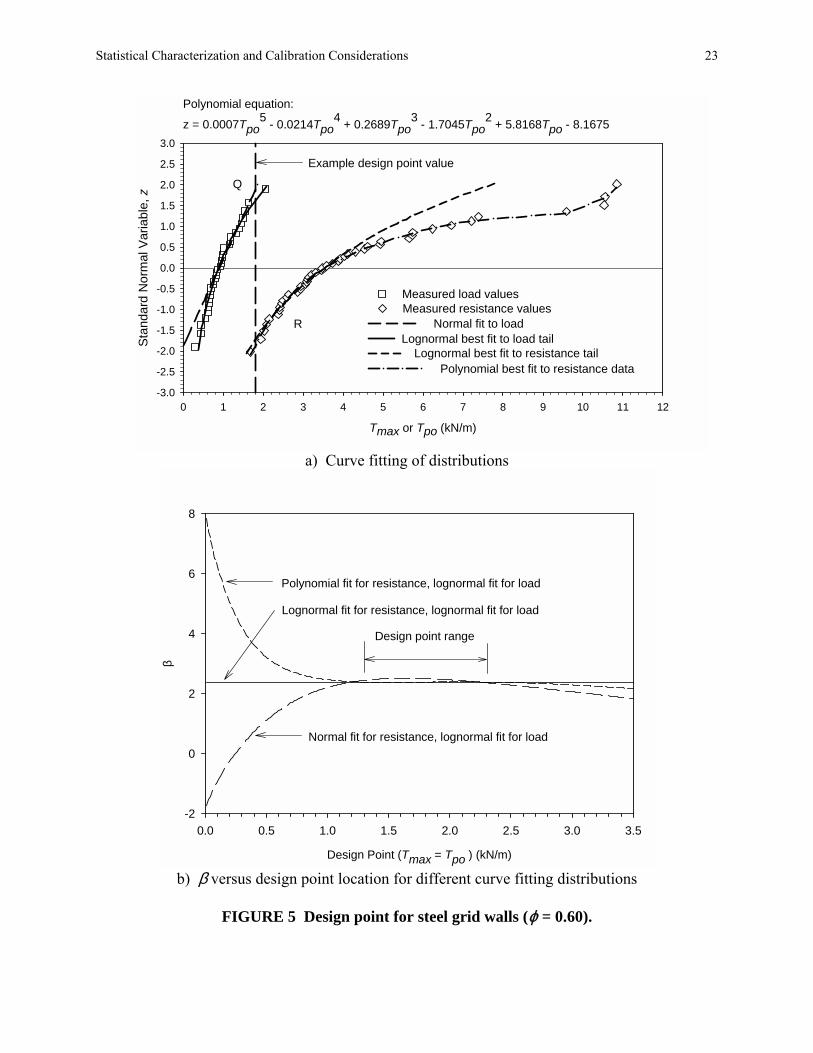
Statistical Characterization and Calibration Considerations 23
Tmax or Tpo (kN/m)
0 1 2 3 4 5 6 7 8 9 10 11 12
Stan
dard
Nor
mal
Var
iabl
e, z
-3.0
-2.5
-2.0
-1.5
-1.0
-0.5
0.0
0.5
1.0
1.5
2.0
2.5
3.0
Example design point value
Q
R
Polynomial equation:
z = 0.0007Tpo5 - 0.0214Tpo
4 + 0.2689Tpo3 - 1.7045Tpo
2 + 5.8168Tpo - 8.1675
Measured load valuesMeasured resistance values
Normal fit to load
Lognormal best fit to resistance tailLognormal best fit to load tail
Polynomial best fit to resistance data
a) Curve fitting of distributions
Design Point (Tmax = Tpo ) (kN/m)
0.0 0.5 1.0 1.5 2.0 2.5 3.0 3.5
β
-2
0
2
4
6
8
Polynomial fit for resistance, lognormal fit for load
Lognormal fit for resistance, lognormal fit for load
Normal fit for resistance, lognormal fit for load
Design point range
b) β versus design point location for different curve fitting distributions
FIGURE 5 Design point for steel grid walls (ϕ = 0.60).
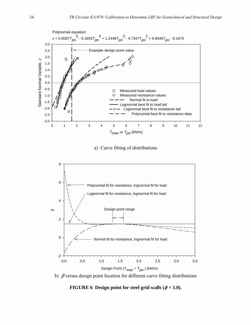
24 TR Circular E-C079: Calibration to Determine LRF for Geotechnical and Structural Design
Tmax or Tpo (kN/m)
0 1 2 3 4 5 6 7 8 9 10 11 12
Stan
dard
Nor
mal
Var
iabl
e, z
-3.0
-2.5
-2.0
-1.5
-1.0
-0.5
0.0
0.5
1.0
1.5
2.0
2.5
3.0
Example design point value
Q
R
Polynomial equation:
z = 0.0087Tpo5 - 0.1655Tpo
4 + 1.2448Tpo3 - 4.7347Tpo
2 + 9.6946Tpo - 8.1675
Measured load valuesMeasured resistance values
Normal fit to load
Lognormal best fit to resistance tailLognormal best fit to load tail
Polynomial best fit to resistance data
a) Curve fitting of distributions
Design Point (Tmax = Tpo ) (kN/m)
0.0 0.5 1.0 1.5 2.0 2.5 3.0 3.5
β
-2
0
2
4
6
8
Polynomial fit for resistance, lognormal fit for load
Lognormal fit for resistance, lognormal fit for load
Normal fit for resistance, lognormal fit for load
Design point range
b) β versus design point location for different curve fitting distributions
FIGURE 6 Design point for steel grid walls (ϕ = 1.0).

Statistical Characterization and Calibration Considerations 25
lognormal curve fit, the lognormal curve input parameters have been adjusted so that the curves visually fit the upper and lower tail regions of the load and resistance distributions, respectively, where the fit to the data is most critical. This curve fitting approach (i.e., fitting to the tails) is used and discussed in more detail later in the Circular. For the load distribution, a normal fit was also attempted and is shown in Figures 5a and 6a. A polynomial curve has also been used to approximate the entire resistance distribution, so that the effect of the design point location on the magnitude of β can be more clearly seen. Figures 5b and 6b were produced by taking the derivative of the equations used to fit the distributions and this derivative (local slope) used to compute the tangent line equations.
Key aspects of the results of the analyses shown in Figures 5 and 6 are summarized in Tables 1 and 2. As can be seen in Figures 5b and 6b, with the exception of the case where lognormal fits are used for both distributions, the design point is located at the first maximum peak in the plots. As illustrated in these figures and tables, if a larger resistance factor is used, the load and resistance data sets are closer, the design point tends to intersect the CDF curves at smaller values of z, and β decreases.
TABLE 1 Summary of the Rackwitz-Fiessler Reliability Analyses, Assuming γQ = 1.75 and ϕR = 0.6 (see Figure 5).
Function Used for Curve Fitting β (Equation 6) Location of Design Point R* and Q* (kN/m)
Lognormal for load, lognormal for resistance 2.36 Not applicable
Lognormal for load, polynomial for resistance 2.40 2.1 (β approx. constant for design pt. range of 1.8 to 2.3)
Normal for load, lognormal for resistance 2.51 1.6 (β approx. constant for design pt. range of 1.5 to 1.8)
TABLE 2 Summary of Rackwitz-Fiessler Reliability Analyses,
Assuming γQ = 1.75 and ϕR = 1.0 (see Figure 6).
Function Used for Curve Fitting β (Equation 6) Location of Design Point R* and Q* (kN/m)
Lognormal for load, lognormal for resistance 1.49 Not applicable
Lognormal for load, polynomial for resistance 1.47 1.5 (β approx. constant for design pt. range of 1.4 to 1.6)
Normal for load, lognormal for resistance 1.49 1.4 (β approx. constant for design pt. range of 1.35 to 1.45)
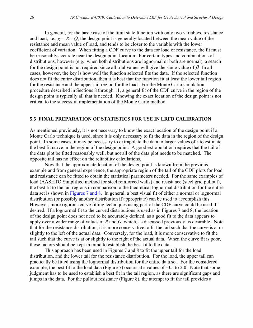
26 TR Circular E-C079: Calibration to Determine LRF for Geotechnical and Structural Design
In general, for the basic case of the limit state function with only two variables, resistance and load, i.e., g = R � Q, the design point is generally located between the mean value of the resistance and mean value of load, and tends to be closer to the variable with the lower coefficient of variation. When fitting a CDF curve to the data for load or resistance, the fit must be reasonably accurate near the design point location. For certain types and combinations of distributions, however (e.g., when both distributions are lognormal or both are normal), a search for the design point is not required since all trial values will give the same value of β. In all cases, however, the key is how well the function selected fits the data. If the selected function does not fit the entire distribution, then it is best that the function fit at least the lower tail region for the resistance and the upper tail region for the load. For the Monte Carlo simulation procedure described in Sections 8 through 11, a general fit of the CDF curve in the region of the design point is typically all that is needed. Knowing the exact location of the design point is not critical to the successful implementation of the Monte Carlo method. 5.5 FINAL PREPARATION OF STATISTICS FOR USE IN LRFD CALIBRATION As mentioned previously, it is not necessary to know the exact location of the design point if a Monte Carlo technique is used, since it is only necessary to fit the data in the region of the design point. In some cases, it may be necessary to extrapolate the data to larger values of z to estimate the best fit curve in the region of the design point. A good extrapolation requires that the tail of the data plot be fitted reasonably well, but not all of the data plot needs to be matched. The opposite tail has no effect on the reliability calculations.
Now that the approximate location of the design point is known from the previous example and from general experience, the appropriate region of the tail of the CDF plots for load and resistance can be fitted to obtain the statistical parameters needed. For the same examples of load (AASHTO Simplified method for steel reinforced walls) and resistance (steel grid pullout), the best fit to the tail regions in comparison to the theoretical lognormal distribution for the entire data set is shown in Figures 7 and 8. In general, a best visual fit of either a normal or lognormal distribution (or possibly another distribution if appropriate) can be used to accomplish this. However, more rigorous curve fitting techniques using part of the CDF curve could be used if desired. If a lognormal fit to the curved distributions is used as in Figures 7 and 8, the location of the design point does not need to be accurately defined, as a good fit to the data appears to apply over a wider range of values of R and Q, which, as discussed previously, is desirable. Note that for the resistance distribution, it is more conservative to fit the tail such that the curve is at or slightly to the left of the actual data. Conversely, for the load, it is more conservative to fit the tail such that the curve is at or slightly to the right of the actual data. When the curve fit is poor, these factors should be kept in mind to establish the best fit to the data.
This approach has been used in Figures 7 and 8 to fit the upper tail for the load distribution, and the lower tail for the resistance distribution. For the load, the upper tail can practically be fitted using the lognormal distribution for the entire data set. For the considered example, the best fit to the load data (Figure 7) occurs at z values of -0.5 to 2.0. Note that some judgment has to be used to establish a best fit in the tail region, as there are significant gaps and jumps in the data. For the pullout resistance (Figure 8), the attempt to fit the tail provides a
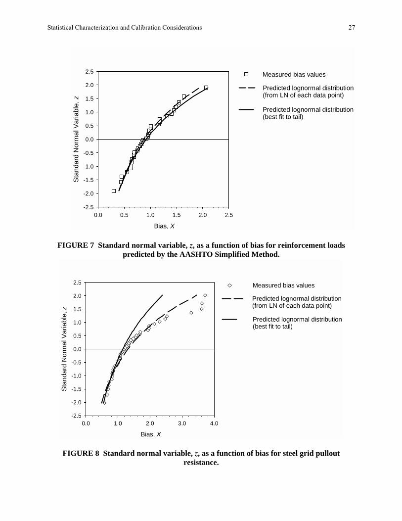
Statistical Characterization and Calibration Considerations 27
Predicted lognormal distribution(from LN of each data point)
Bias, X
0.0 0.5 1.0 1.5 2.0 2.5
Sta
ndar
d N
orm
al V
aria
ble,
z
-2.5
-2.0
-1.5
-1.0
-0.5
0.0
0.5
1.0
1.5
2.0
2.5 Measured bias values
Predicted lognormal distribution (best fit to tail)
FIGURE 7 Standard normal variable, z, as a function of bias for reinforcement loads predicted by the AASHTO Simplified Method.
Bias, X
0.0 1.0 2.0 3.0 4.0
Sta
ndar
d N
orm
al V
aria
ble,
z
-2.5
-2.0
-1.5
-1.0
-0.5
0.0
0.5
1.0
1.5
2.0
2.5 Measured bias values
Predicted lognormal distribution (best fit to tail)
Predicted lognormal distribution(from LN of each data point)
FIGURE 8 Standard normal variable, z, as a function of bias for steel grid pullout resistance.
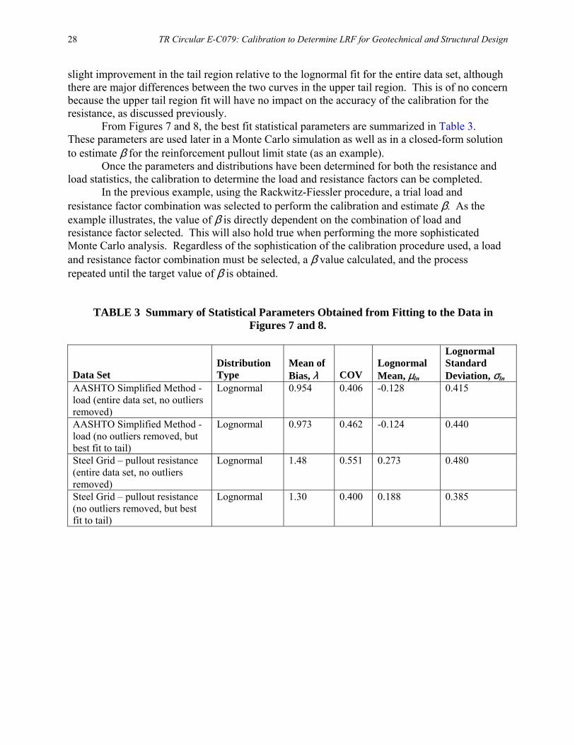
28 TR Circular E-C079: Calibration to Determine LRF for Geotechnical and Structural Design
slight improvement in the tail region relative to the lognormal fit for the entire data set, although there are major differences between the two curves in the upper tail region. This is of no concern because the upper tail region fit will have no impact on the accuracy of the calibration for the resistance, as discussed previously.
From Figures 7 and 8, the best fit statistical parameters are summarized in Table 3. These parameters are used later in a Monte Carlo simulation as well as in a closed-form solution to estimate β for the reinforcement pullout limit state (as an example).
Once the parameters and distributions have been determined for both the resistance and load statistics, the calibration to determine the load and resistance factors can be completed.
In the previous example, using the Rackwitz-Fiessler procedure, a trial load and resistance factor combination was selected to perform the calibration and estimate β. As the example illustrates, the value of β is directly dependent on the combination of load and resistance factor selected. This will also hold true when performing the more sophisticated Monte Carlo analysis. Regardless of the sophistication of the calibration procedure used, a load and resistance factor combination must be selected, a β value calculated, and the process repeated until the target value of β is obtained.
TABLE 3 Summary of Statistical Parameters Obtained from Fitting to the Data in Figures 7 and 8.
Data Set
Distribution Type
Mean of Bias, λ
COV
Lognormal Mean, µln
Lognormal Standard Deviation, σln
AASHTO Simplified Method - load (entire data set, no outliers removed)
Lognormal 0.954 0.406 -0.128 0.415
AASHTO Simplified Method - load (no outliers removed, but best fit to tail)
Lognormal 0.973 0.462 -0.124 0.440
Steel Grid � pullout resistance (entire data set, no outliers removed)
Lognormal 1.48 0.551 0.273 0.480
Steel Grid � pullout resistance (no outliers removed, but best fit to tail)
Lognormal 1.30 0.400 0.188 0.385
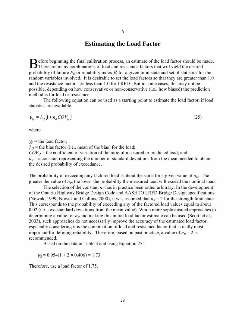
29
6
Estimating the Load Factor
efore beginning the final calibration process, an estimate of the load factor should be made. There are many combinations of load and resistance factors that will yield the desired
probability of failure Pf, or reliability index β, for a given limit state and set of statistics for the random variables involved. It is desirable to set the load factors so that they are greater than 1.0 and the resistance factors are less than 1.0 for LRFD. But in some cases, this may not be possible, depending on how conservative or non-conservative (i.e., how biased) the prediction method is for load or resistance.
The following equation can be used as a starting point to estimate the load factor, if load statistics are available:
( )QQQ COVnσλγ += 1 (25) where γQ = the load factor; λQ = the bias factor (i.e., mean of the bias) for the load; COVQ = the coefficient of variation of the ratio of measured to predicted load; and nσ = a constant representing the number of standard deviations from the mean needed to obtain the desired probability of exceedance. The probability of exceeding any factored load is about the same for a given value of nσ. The greater the value of nσ, the lower the probability the measured load will exceed the nominal load.
The selection of the constant nσ has in practice been rather arbitrary. In the development of the Ontario Highway Bridge Design Code and AASHTO LRFD Bridge Design specifications (Nowak, 1999; Nowak and Collins, 2000), it was assumed that nσ = 2 for the strength limit state. This corresponds to the probability of exceeding any of the factored load values equal to about 0.02 (i.e., two standard deviations from the mean value). While more sophisticated approaches to determining a value for nσ and making this initial load factor estimate can be used (Scott, et al., 2003), such approaches do not necessarily improve the accuracy of the estimated load factor, especially considering it is the combination of load and resistance factor that is really most important for defining reliability. Therefore, based on past practice, a value of nσ = 2 is recommended.
Based on the data in Table 3 and using Equation 25: γQ = 0.954(1 + 2 × 0.406) = 1.73
Therefore, use a load factor of 1.75.
B
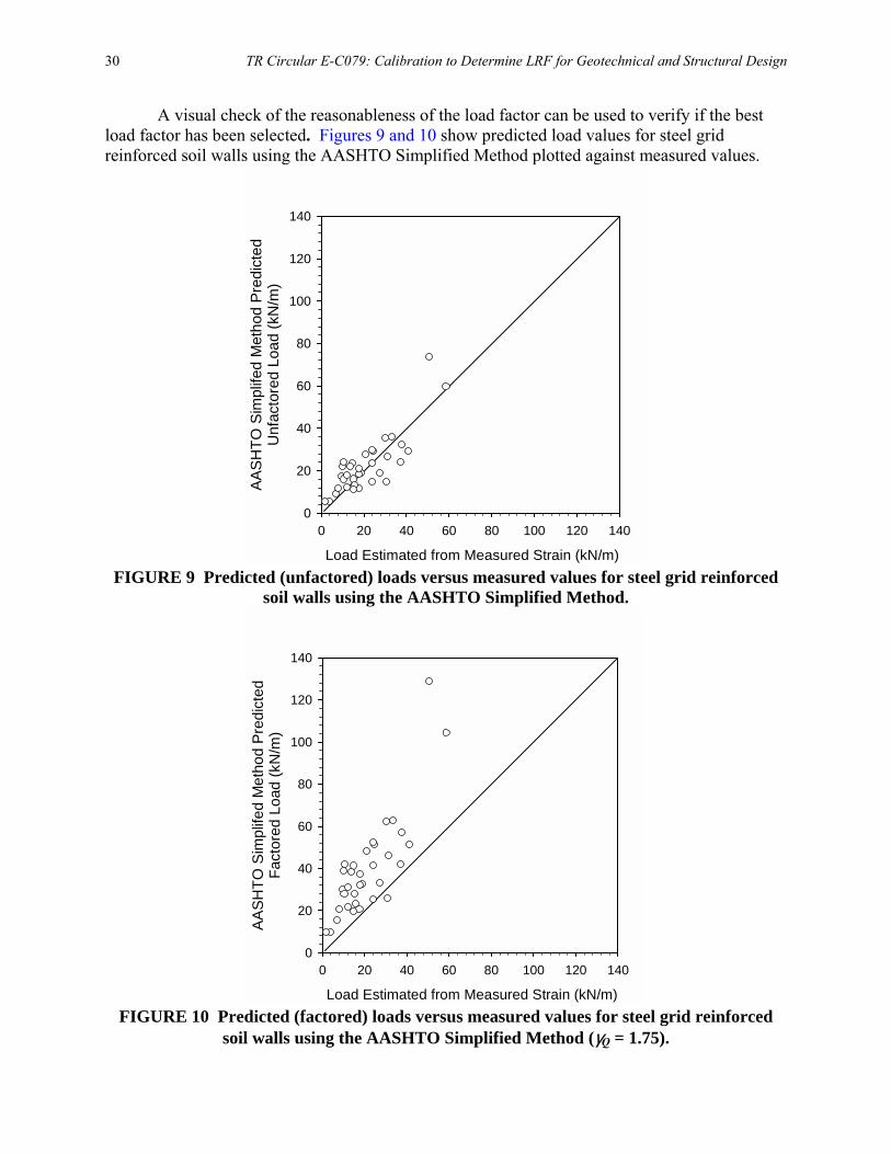
30 TR Circular E-C079: Calibration to Determine LRF for Geotechnical and Structural Design
A visual check of the reasonableness of the load factor can be used to verify if the best load factor has been selected. Figures 9 and 10 show predicted load values for steel grid reinforced soil walls using the AASHTO Simplified Method plotted against measured values.
Load Estimated from Measured Strain (kN/m)
0 20 40 60 80 100 120 140
AA
SH
TO S
impl
ifed
Met
hod
Pre
dict
edU
nfac
tore
d Lo
ad (k
N/m
)
0
20
40
60
80
100
120
140
FIGURE 9 Predicted (unfactored) loads versus measured values for steel grid reinforced
soil walls using the AASHTO Simplified Method.
Load Estimated from Measured Strain (kN/m)
0 20 40 60 80 100 120 140
AA
SHTO
Sim
plife
d M
etho
d P
redi
cted
Fact
ored
Loa
d (k
N/m
)
0
20
40
60
80
100
120
140
FIGURE 10 Predicted (factored) loads versus measured values for steel grid reinforced
soil walls using the AASHTO Simplified Method (γQ = 1.75).

Estimating the Load Factor 31
Figure 9 shows that many of the data points are below the 1:1 correspondence line. It is desirable that most of the data points, after the load factor is applied, are above the 1:1 correspondence line. Figure 10 illustrates that the load factor γQ = 1.75 obtained using Equation 25 is adequate to accomplish this, and no further adjustment is required in this case.
Note that load factors are often used for multiple limit states. As resistance factors are developed for each limit state (see Section 7), minor adjustments to the load factor may be needed to ensure that for a single value of the load factor, all the applicable limit states can achieve the desired target β value using a reasonable resistance factor for each limit state.
32
7
Estimating the Resistance Factor
nce the load factor is selected, the resistance factor can be estimated through iteration to produce the desired magnitude for β. This can be accomplished through using exact or
approximate closed-form solutions if applicable (e.g., Equations 6 or 7), the Rackwitz-Fiessler procedure illustrated previously, or the more adaptable and rigorous Monte Carlo method described in the next section.
The use of closed-form solutions is illustrated here. For normal distributions of load and resistance values, a linear limit state function, and only one load source, Equation 6 can be written as:
( ) ( )22QnQRnR
QnRn
QCOVRCOV
QR
λλ
λλβ
+
−= (26a)
where all quantities have been defined previously. This closed-form solution is exact when both distributions are normal and the limit state function is linear, as discussed previously. Note that if the limit state equation as developed in Equations 2, 3 and 4 is used, Rn in Equation 26a can be replaced with ( )Q R nQγ ϕ , resulting in Equation 26b:
( )22
QQRR
QR
QRR
Q
COVCOV λλϕγ
λλϕγ
β
+
−
= (26b)
Note that Qn cancels out and is eliminated from the equation.
For lognormal distributions for load and resistance values, a linear limit state function, and a single load source, Equation 7 can be written as:
( ) ( )
( )( )[ ]22
22
11
11
RQ
RQQn
Rn
COVCOVLN
COVCOVQR
LN
++
++
=λλ
β (27a)
where all quantities were defined previously. As was done to produce Equation 26a, if Rn in Equation 27a is replaced with ( )Q R nQγ ϕ , Equation 27b results:
O

Estimating the Resistance Factor 33
( ) ( )
( )( )[ ]22
22
11
11
RQ
RQQR
RQ
COVCOVLN
COVCOVLN
++
++
=λϕλγ
β (27b)
Note again that Qn cancels out and is eliminated from the equation. In both Equations 26 and 27, this puts γQ and ϕR into the equation so that a relationship between β, γQ, and ϕR can be developed.
If the limit state equation as developed in Equations 8 and 9 is used, Rn in Equations 26a and 27a is replaced with (FS)Qn. This allows the β value implied by a FS value from previous ASD practice to be determined.
Equations 26 and 27 can be used as a starting point to obtain a more exact solution using, for example, the Monte Carlo method when the distribution of the data is neither perfectly normal nor perfectly lognormal, or the limit state function is not linear.
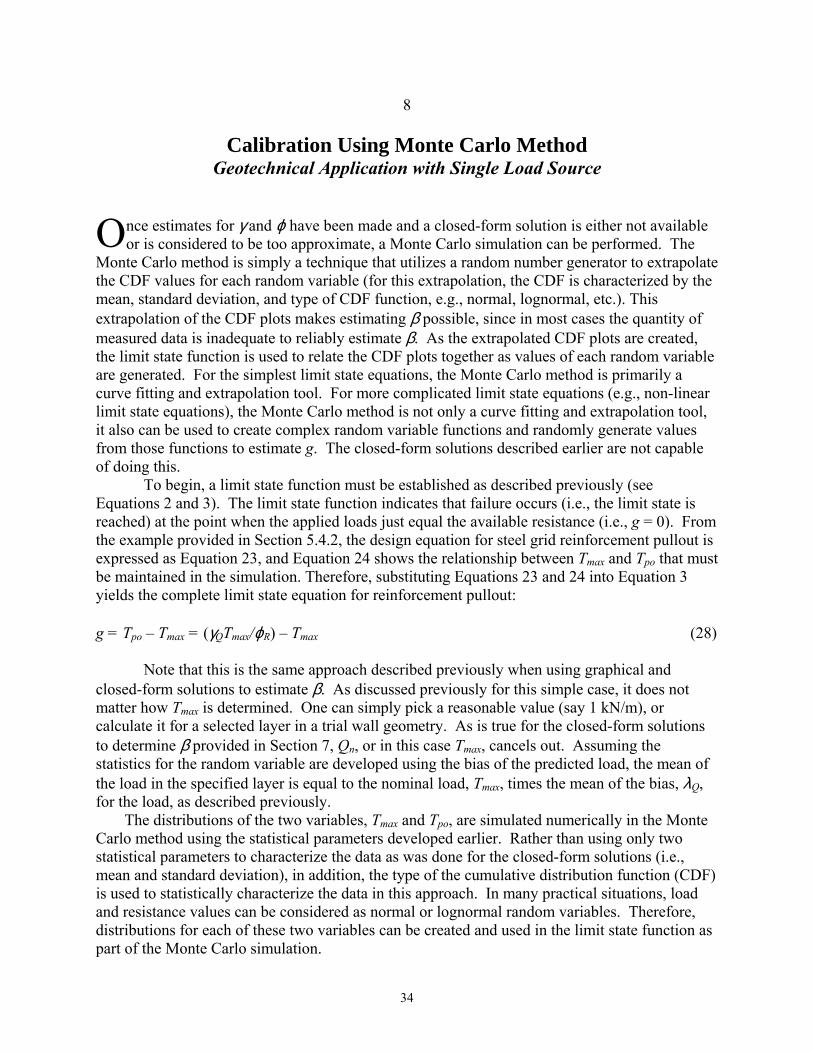
34
8
Calibration Using Monte Carlo Method Geotechnical Application with Single Load Source
nce estimates for γ and ϕ have been made and a closed-form solution is either not available or is considered to be too approximate, a Monte Carlo simulation can be performed. The
Monte Carlo method is simply a technique that utilizes a random number generator to extrapolate the CDF values for each random variable (for this extrapolation, the CDF is characterized by the mean, standard deviation, and type of CDF function, e.g., normal, lognormal, etc.). This extrapolation of the CDF plots makes estimating β possible, since in most cases the quantity of measured data is inadequate to reliably estimate β. As the extrapolated CDF plots are created, the limit state function is used to relate the CDF plots together as values of each random variable are generated. For the simplest limit state equations, the Monte Carlo method is primarily a curve fitting and extrapolation tool. For more complicated limit state equations (e.g., non-linear limit state equations), the Monte Carlo method is not only a curve fitting and extrapolation tool, it also can be used to create complex random variable functions and randomly generate values from those functions to estimate g. The closed-form solutions described earlier are not capable of doing this.
To begin, a limit state function must be established as described previously (see Equations 2 and 3). The limit state function indicates that failure occurs (i.e., the limit state is reached) at the point when the applied loads just equal the available resistance (i.e., g = 0). From the example provided in Section 5.4.2, the design equation for steel grid reinforcement pullout is expressed as Equation 23, and Equation 24 shows the relationship between Tmax and Tpo that must be maintained in the simulation. Therefore, substituting Equations 23 and 24 into Equation 3 yields the complete limit state equation for reinforcement pullout: g = Tpo � Tmax = (γQTmax/ϕR) � Tmax (28)
Note that this is the same approach described previously when using graphical and closed-form solutions to estimate β. As discussed previously for this simple case, it does not matter how Tmax is determined. One can simply pick a reasonable value (say 1 kN/m), or calculate it for a selected layer in a trial wall geometry. As is true for the closed-form solutions to determine β provided in Section 7, Qn, or in this case Tmax, cancels out. Assuming the statistics for the random variable are developed using the bias of the predicted load, the mean of the load in the specified layer is equal to the nominal load, Tmax, times the mean of the bias, λQ, for the load, as described previously.
The distributions of the two variables, Tmax and Tpo, are simulated numerically in the Monte Carlo method using the statistical parameters developed earlier. Rather than using only two statistical parameters to characterize the data as was done for the closed-form solutions (i.e., mean and standard deviation), in addition, the type of the cumulative distribution function (CDF) is used to statistically characterize the data in this approach. In many practical situations, load and resistance values can be considered as normal or lognormal random variables. Therefore, distributions for each of these two variables can be created and used in the limit state function as part of the Monte Carlo simulation.
O
Monte Carlo Method: Geotechnical Application with Single Load Source 35
If Tmax is normally distributed, randomly determined values of Tmax that fit within a specified distribution characterized by a mean, a standard deviation, and a coefficient of variation (COV) can be generated using a random number generator as follows (Nowak and Collins, 2000): Tmaxi = maxT (1 + COVQ zi) (29) where Tmaxi = a randomly generated value of Tmax using a specified set of statistical parameters; maxT = the normal mean value of Tmax and is equal to λQTmax; λQ = the normal mean of the bias for Tmax; COVQ = the coefficient of variation of the bias for Tmax (which will be the same as the COVQ
for Tmax); zi = Φ-1(uia) (inverse normal function); and uia = a random number between 0 and 1 representing a probability of occurrence. See Appendix B for how to calculate the inverse normal function Φ-1(uia). As described in Appendix B, the Microsoft Excel function NORMSINV can be used to calculate values for this function. In this case, this function is applied to the random number, and the random number represents a probability that can range anywhere from 0 to 1 (i.e., 0 to 100%). Therefore, using Microsoft Excel, zi is calculated as NORMSINV(RAND()).
If Tmax is lognormally distributed, randomly calculated values of Tmax that fit within a specified distribution characterized by a lognormal mean µln and lognormal standard deviation σln can be generated using a random number generator as follows (Nowak and Collins, 2000): Tmaxi = EXP(µln + σln zi) (30) where µln = LN( maxT ) � 0.5σln
2 (31) σln = {LN[(COVQ)2 + 1]}0.5 (32) and all other variables are defined previously.
Similarly, if pullout resistance values, Tpo, are lognormally distributed, randomly calculated values of Tpo that fit within a specified distribution characterized by a lognormal mean µln and lognormal standard deviation σln can be generated using a random number generator as follows: Tpoi = EXP(µln + σln zi) (33)
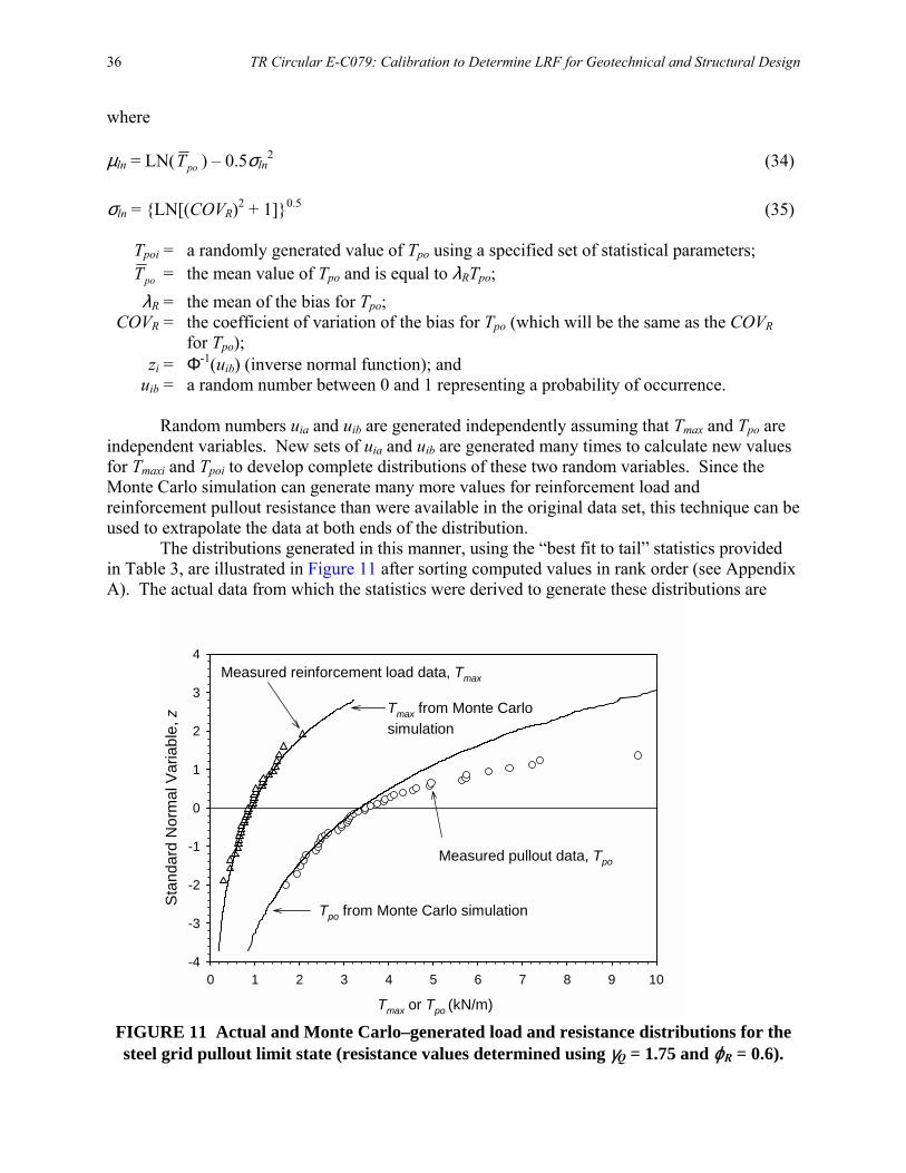
36 TR Circular E-C079: Calibration to Determine LRF for Geotechnical and Structural Design
where µln = LN( poT ) � 0.5σln
2 (34) σln = {LN[(COVR)2 + 1]}0.5 (35) Tpoi = a randomly generated value of Tpo using a specified set of statistical parameters; poT = the mean value of Tpo and is equal to λRTpo; λR = the mean of the bias for Tpo; COVR = the coefficient of variation of the bias for Tpo (which will be the same as the COVR for Tpo); zi = Φ-1(uib) (inverse normal function); and uib = a random number between 0 and 1 representing a probability of occurrence.
Random numbers uia and uib are generated independently assuming that Tmax and Tpo are independent variables. New sets of uia and uib are generated many times to calculate new values for Tmaxi and Tpoi to develop complete distributions of these two random variables. Since the Monte Carlo simulation can generate many more values for reinforcement load and reinforcement pullout resistance than were available in the original data set, this technique can be used to extrapolate the data at both ends of the distribution.
The distributions generated in this manner, using the �best fit to tail� statistics provided in Table 3, are illustrated in Figure 11 after sorting computed values in rank order (see Appendix A). The actual data from which the statistics were derived to generate these distributions are
Tmax or Tpo (kN/m)
0 1 2 3 4 5 6 7 8 9 10
Sta
ndar
d N
orm
al V
aria
ble,
z
-4
-3
-2
-1
0
1
2
3
4
Tmax from Monte Carlosimulation
Measured reinforcement load data, Tmax
Measured pullout data, Tpo
Tpo from Monte Carlo simulation
FIGURE 11 Actual and Monte Carlo–generated load and resistance distributions for the steel grid pullout limit state (resistance values determined using γQ = 1.75 and ϕR = 0.6).
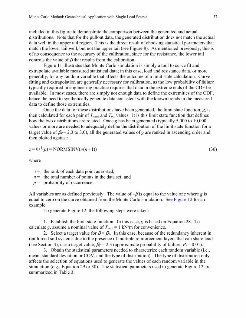
Monte Carlo Method: Geotechnical Application with Single Load Source 37
included in this figure to demonstrate the comparison between the generated and actual distributions. Note that for the pullout data, the generated distribution does not match the actual data well in the upper tail region. This is the direct result of choosing statistical parameters that match the lower tail well, but not the upper tail (see Figure 8). As mentioned previously, this is of no consequence to the accuracy of the calibration, since for the resistance, the lower tail controls the value of β that results from the calibration.
Figure 11 illustrates that Monte Carlo simulation is simply a tool to curve fit and extrapolate available measured statistical data; in this case, load and resistance data, or more generally, for any random variable that affects the outcome of a limit state calculation. Curve fitting and extrapolation are generally necessary for calibration, as the low probability of failure typically required in engineering practice requires that data in the extreme ends of the CDF be available. In most cases, there are simply not enough data to define the extremities of the CDF, hence the need to synthetically generate data consistent with the known trends in the measured data to define those extremities.
Once the data for these distributions have been generated, the limit state function, g, is then calculated for each pair of Tmaxi and Tpoi values. It is this limit state function that defines how the two distributions are related. Once g has been generated (typically 5,000 to 10,000 values or more are needed to adequately define the distribution of the limit state function for a target value of βT = 2.3 to 3.0), all the generated values of g are ranked in ascending order and then plotted against: z = Φ-1(p) = NORMSINV(i/(n +1)) (36) where i = the rank of each data point as sorted; n = the total number of points in the data set; and p = probability of occurrence. All variables are as defined previously. The value of �β is equal to the value of z where g is equal to zero on the curve obtained from the Monte Carlo simulation. See Figure 12 for an example.
To generate Figure 12, the following steps were taken:
1. Establish the limit state function. In this case, g is based on Equation 28. To calculate g, assume a nominal value of Tmax = 1 kN/m for convenience.
2. Select a target value for β = βT. In this case, because of the redundancy inherent in reinforced soil systems due to the presence of multiple reinforcement layers that can share load (see Section 4), use a target value, βT = 2.3 (approximate probability of failure, Pf = 0.01).
3. Obtain the statistical parameters needed to characterize each random variable (i.e., mean, standard deviation or COV, and the type of distribution). The type of distribution only affects the selection of equations used to generate the values of each random variable in the simulation (e.g., Equation 29 or 30). The statistical parameters used to generate Figure 12 are summarized in Table 3.
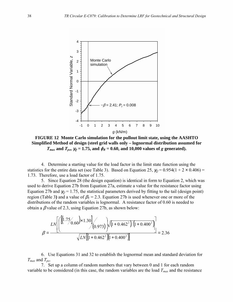
38 TR Circular E-C079: Calibration to Determine LRF for Geotechnical and Structural Design
g (kN/m)
-1 0 1 2 3 4 5 6 7 8 9 10
Sta
ndar
d N
orm
al V
aria
ble,
z
-4
-3
-2
-1
0
1
2
3
4
Monte Carlosimulation
−β = 2.41; Pf = 0.008
FIGURE 12 Monte Carlo simulation for the pullout limit state, using the AASHTO
Simplified Method of design (steel grid walls only – lognormal distribution assumed for Tmax and Tpo, γQ = 1.75, and ϕR = 0.60, and 10,000 values of g generated).
4. Determine a starting value for the load factor in the limit state function using the statistics for the entire data set (see Table 3). Based on Equation 25, γQ = 0.954(1 + 2 × 0.406) = 1.73. Therefore, use a load factor of 1.75.
5. Since Equation 28 (the design equation) is identical in form to Equation 2, which was used to derive Equation 27b from Equation 27a, estimate a value for the resistance factor using Equation 27b and γQ = 1.75, the statistical parameters derived by fitting to the tail (design point) region (Table 3) and a value of βT = 2.3. Equation 27b is used whenever one or more of the distributions of the random variables is lognormal. A resistance factor of 0.60 is needed to obtain a β value of 2.3, using Equation 27b, as shown below:
( )[ ]
( ) ( ) ( )
( )( )[ ] 36.2400.01462.01
400.01462.01973.030.160.0
75.1
22
22
=++
++
×
=LN
LN
β
6. Use Equations 31 and 32 to establish the lognormal mean and standard deviation for
Tmax and Tpo. 7. Set up a column of random numbers that vary between 0 and 1 for each random
variable to be considered (in this case, the random variables are the load Tmax and the resistance

Monte Carlo Method: Geotechnical Application with Single Load Source 39
Tpo). In Excel, the function RAND can be used to accomplish this. Since for this example there are two random variables, two columns of random numbers should be created.
8. Set up columns in the spreadsheet to calculate random values of each random variable, in this case Tmaxi and Tpoi, using Equations 30 and 33, since both random variables are lognormal.
9. Calculate random values of g using the limit state equation established in Step 1, and the load and resistance factors determined in Step 3. In general, a minimum of 5,000 to 10,000 values of g should be generated to adequately estimate a β value of 2.3 to 3.0.
10. Using all of the g values generated, calculate the probability of failure, Pf, directly by taking the number of values of g calculated that are less than 0 and dividing them by the total number of g values. Then calculate β (in Excel) using the Excel function NORMSINV as shown in Equation 37:
β = NORMSINV(Pf) (37)
To accomplish the same objective graphically, rank the values of g from lowest to highest and calculate the associated probability in the cumulative distribution as i/(n + 1), calculating z in Excel as shown in Equation 36. Identify the value of the standard normal variable z where g = 0. This value will be equal to �β.
11. The trial load and resistance factors used in the simulation are simply a starting point. If the simulation does not result in the desired β value, change the load and/or resistance factor (though it would be better to leave the load factor alone at this point), recalculate the limit state function, and rerun the Monte Carlo simulation. Repeat the simulation until the desired β value is obtained. The load and resistance factors used to obtain the target β value are the ones that can be used for design to obtain the desired probability of failure.
Figure 12 shows the simulation result assuming a load factor of 1.75 and a resistance factor of 0.60, with 10,000 values of g generated. In this case, Pf = 0.0080. From Equation 37, β = 2.41. Note that this value of β is close to the value determined in Figure 5 and summarized in Table 1 for this limit state and combination of load and resistance factors (β = 2.36 in Table 1 versus 2.41 for the Monte Carlo simulation. The closed-form approximation (Equation 27) also produces results that are very close to the Monte Carlo simulation, which shows that the closed-form solution does provide accurate results for those cases where it is applicable.
Another Monte Carlo simulation was conducted for the case of a resistance factor of 1.0 rather than 0.60, so that a comparison could be made between the Monte Carlo simulation result for this case, and the Rackwitz-Fiessler procedure demonstrated in Figure 6 and Table 2. The Monte Carlo simulation in this case gave β = 1.49, whereas the value of β from Table 2 using the Rackwitz-Fiessler procedure was also 1.49 for the case where a lognormal fit is used for both the load and resistance distributions. Again the two methods produce similar results.
Also note that each time a new set of random numbers is generated for the same input values, and load and resistance factors, the resulting value of β from a Monte Carlo simulation may change. However, for the same input parameters, β should not vary by more than ±0.10, assuming that an adequate number of g values are generated.
The accuracy of the probability of failure, Pf, calculation depends on the total number of g values generated, N. The coefficient of variation of the estimated Pf can be determined as a
40 TR Circular E-C079: Calibration to Determine LRF for Geotechnical and Structural Design
function of the true probability of failure, Ptrue (the target probability can be used to represent Ptrue), as follows (Nowak and Collins, 2000):
true
trueP PN
PCOV
×−
=1
(38)
where PCOV is the coefficient of variation of the estimated probability of failure, and the other variables are as defined above. For this example, using Equation 38, N = 10,000 values, and Ptrue is equal to the target Pf value of 0.01, PCOV = 0.10. Typically, a COV for Pf of 0.10 is sufficient. Therefore, a larger simulation is not needed. But this does demonstrate that one should not get too carried away with significant figures when attempting to estimate β. Estimating β to 0.05 to 0.1 is in general the best that can be done. Note that if the number of simulations is not adequate, then the value of β can be determined by extrapolation if necessary, though it will be less accurate.
41
9
Calibration Using the Monte Carlo Method Geotechnical Application with Multiple Load Sources
f multiple loads having different load factors and associated statistics contribute to Tmax (e.g., dead load and live load), the key is to estimate the contribution of the other load sources to
Tmax. For the considered example provided in Section 8, the relative contribution of the various load sources will likely be specific to the wall geometry and the specific elevation in the wall where the limit state calculation is carried out. This must be taken into account in the development of the design equation and the limit state function, g. The limit state function is developed as follows, based on the limit state used in the previous example: Tmax = TmaxDL + TmaxLL (39) Tpo = (TmaxDL γQD + TmaxLL γLL)/ϕR (40) Substituting Equations 39 and 40 into Equation 3, g = (TmaxDL γQD + TmaxLL γLL)/ϕR � (TmaxDL + TmaxLL) (41) where TmaxDL = the dead load contribution to Tmax at the specified location; TmaxLL = the live load contribution to Tmax at the specified location; γQD = the load factor for the reinforcement load resulting from dead load; and γLL = the load factor for the reinforcement load resulting from live load. Other variables are as defined previously.
Equations 29, 30, and/or 33 are used to generate values for each random variable, making sure that the random numbers for each random variable are generated independently (i.e., a random number uic would be generated in addition to uia and uib), which in this case would include TmaxDL, TmaxLL, and Tpo. A value of g is then calculated for each set of random variables that are generated, and the process continues as presented earlier for the single load source case.
To generate preliminary load and resistance factors as starting points for the Monte Carlo simulation with multiple load sources, Equation 6 can be modified to include the additional load source as shown in Equation 42 for normally distributed data:
( )222LLQDR
LLD QQR
σσσβ
++
+−= (42)
I
42 TR Circular E-C079: Calibration to Determine LRF for Geotechnical and Structural Design
where R = mean of the measured resistance, calculated as λRRn, and Rn is the predicted (nominal)
value of resistance determined from the limit state function for the design case being investigated (e.g., see Equation 41 for a multiple load case example);
DQ = mean of the measured dead load, calculated as λQDQD, and QD is the predicted (nominal) value of dead load;
LLQ = mean of the live load, calculated as λLLQLL, and QLL is the predicted (nominal) value of live load;
λR = mean of the bias values (measured/predicted) for the resistance; λQD = the mean of the bias values (measured/predicted) for the dead load; λLL = the mean of the bias values (measured/predicted) for the live load; σQD = the standard deviation of the measured dead load, calculated as COVQD DQ ; σLL = the standard deviation of the measured live load, calculated as COVLL LLQ ; σR = the standard deviation of the measured resistance, calculated as COVR R ; COVQD = the coefficient of variation of the bias values for the dead load; COVLL = the coefficient of variation of the bias values for the live load; and COVR = the coefficient of variation of the bias values for the resistance.
Note that Equation 42 provides an exact solution if the data sets representing the random variables for the loads and resistance are normally distributed and if all of the variables are also linear (as is true for Equation 6). See Withiam, et al. (1998) for approximate closed-form solutions that can be used for multiple load sources in which the loads and/or resistances are lognormally distributed.
Continuing with the previous example, but this time including live load (λLL = 1.33, COVLL = 0.18, assuming a normal distribution � see Nowak, 1999, and Sections 11.1 and 11.2 for additional discussion on live load statistics and the applicability of dynamic load allowance for walls), a load factor of 1.75 for the dead load portion of the reinforcement load Tmax, and a load factor of 1.75 as required in the AASHTO specifications (AASHTO, 2004) for the live load portion of the reinforcement load, the following results were obtained from the Monte Carlo simulations:
• For a dead load to live load ratio of 10 and β = 2.3, ϕR = 0.61 • For a dead load to live load ratio of 3 and β = 2.3, ϕR = 0.65
Considering that without live load, the resistance factor ϕR = 0.60, it appears that the
presence of live load has very little effect on the resistance factor needed for this example, which is consistent with the results obtained by others where the resistance variability is high, as is the case here (Withiam, et al., 1998).
43
10
Calibration Using the Monte Carlo Method Geotechnical Application Treating Design Model Input Parameters
as Random Variables
ather than using statistics for Tmax, one can use statistics for the variation of the input parameters used to calculate Tmax. For example, one can obtain mean and standard deviation
data for the soil friction angle or Ka, and the soil unit weight, both of which affect the magnitude Tmax based on the AASHTO Simplified Method. Treating each input parameter as a random variable, one can combine the random variables together to get Tmaxi using the equation for Tmax (Equation 22). The limit state function can then be calculated for each generated set of values for the soil friction angle and unit weight. However, doing the calculation this way will not account for uncertainty and bias in the design model, and may also not account for spatial variability in the parameters (see Section 5.2).
In this case, the complete limit state equation is as follows for reinforcement pullout: g = Tpo – Tmax = γQTmax/ϕR – Tmax (43) where Equation 22 can be expanded to define Tmax as follows: Tmax = SvγszdKr/atan2(45°-φ/2) (44) where γs = unit weight of soil; zd = depth of reinforcement layer below wall top; Kr/a = a factor applied to the active lateral earth pressure coefficient; and φ = the backfill soil friction angle (degrees). All other variables are defined previously. Equation 44 assumes that no surcharge is present above the wall and the wall face is vertical. The factor Kr/a is a multiplier to the active earth pressure coefficient and is a function of depth below the wall top according to AASHTO (2004). This factor varies for steel grid walls from 2.5 at the wall top to 1.2 at a depth of 6 m, and remains constant at 1.2 at depths greater than 6 m. Note that the soil friction angle φ must be no greater than 40o in accordance with AASHTO (2004). This constraint is part of the design model.
Statistical parameters for the two random variables that contribute to Tmax are summarized in Table 4. All other variables in Equation 44 are treated as deterministic in this analysis. For soil unit weight, COV values are provided for the following cases:
• A highly controlled wall installation case which represents the smallest likely COV
for engineered fill unit weight, and
R
44 TR Circular E-C079: Calibration to Determine LRF for Geotechnical and Structural Design
TABLE 4 Statistical Parameters for Soil Unit Weight and Friction Angle. Data Set
Source for Data
Distribution Type
Number of Data Points in Data Set
Mean of Bias, λ
COV
Soil unit weight (entire data set – no outliers removed, and best fit to tail)
See Figure 13 for typical data; Figure 14 for highly controlled test wall data
Normal 181 1.0 0.021 (typical) to 0.011 (highly controlled test wall)
Soil friction angle (summary statistics only)
Phoon, et al., 1995 Lognormal Not available
1.0 0.10
• A typical wall installation case corresponding to a more likely value of the COV for
engineered fill unit weight.
The COV value for the second case is used in the analysis. For convenience, the bias of the soil unit weight and soil friction angle is assumed to be 1.0 (i.e., the nominal design values are assumed to be equal to the mean of the measured data). However, the bias of the actual design values selected will depend on how conservative the designer is in selecting design parameters.
Since the soil unit weight statistics are normally distributed, randomly calculated values of soil unit weight (γs) that fit within a specified distribution characterized by a mean, a standard deviation, and a coefficient of variation (COV) can be generated using a random number generator as follows:
( )isssi zCOVγγγ += 1 (45) where γsi = a randomly generated value of γs using a specified set of statistical parameters; sγ = the normal mean value of γs; COVγs = the coefficient of variation for γs; zi = Φ-1(uia) (inverse normal function); and uia = a random number between 0 and 1.
Since the soil friction angle is lognormally distributed, random values of φ that fit within a specified distribution characterized by a lognormal mean µln and lognormal standard deviation σln can be generated using a random number generator as follows: φi = EXP(µln + σln zi) (46) where φi = randomly generated value of soil friction angle; µln is determined using Equation 31 by substituting φ for maxT ; σln is determined using Equation 32 by substituting COVφ for COVQ; φ = the normal mean value of φ; and COVφ = the coefficient of variation for φ.
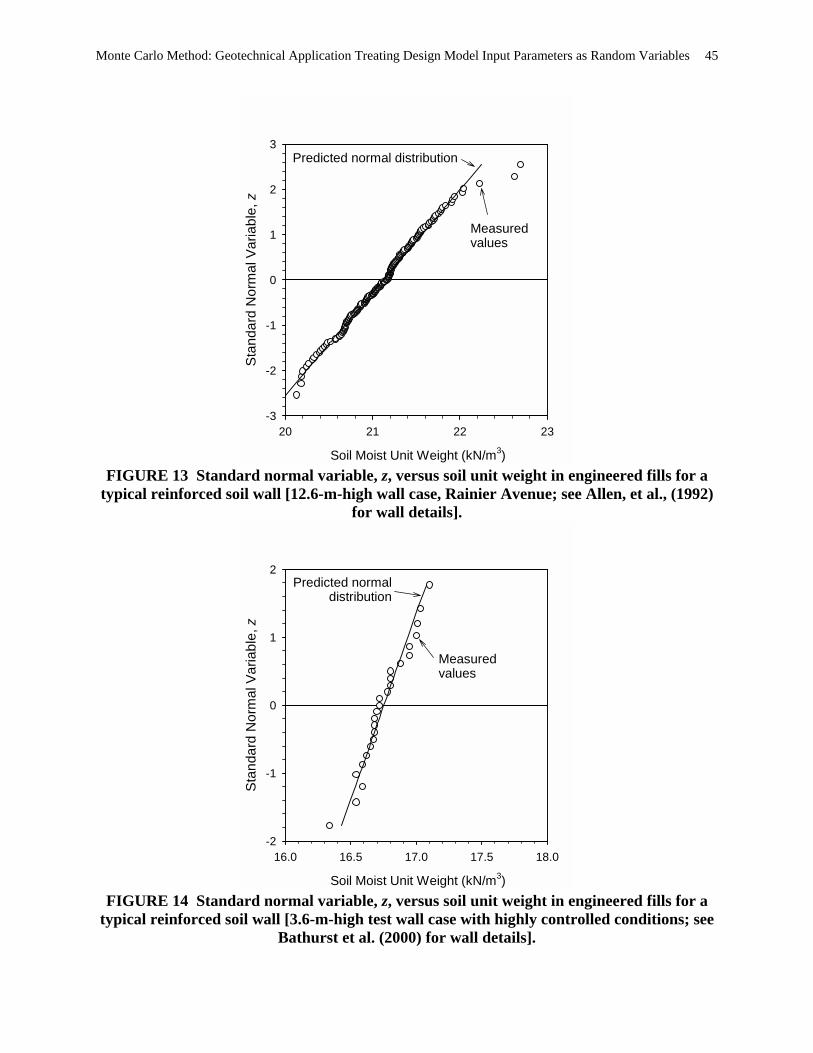
Monte Carlo Method: Geotechnical Application Treating Design Model Input Parameters as Random Variables 45
Soil Moist Unit Weight (kN/m3)
20 21 22 23
Sta
ndar
d N
orm
al V
aria
ble,
z
-3
-2
-1
0
1
2
3
Measuredvalues
Predicted normal distribution
FIGURE 13 Standard normal variable, z, versus soil unit weight in engineered fills for a
typical reinforced soil wall [12.6-m-high wall case, Rainier Avenue; see Allen, et al., (1992) for wall details].
Soil Moist Unit Weight (kN/m3)
16.0 16.5 17.0 17.5 18.0
Sta
ndar
d N
orm
al V
aria
ble,
z
-2
-1
0
1
2
Measuredvalues
Predicted normaldistribution
FIGURE 14 Standard normal variable, z, versus soil unit weight in engineered fills for a
typical reinforced soil wall [3.6-m-high test wall case with highly controlled conditions; see Bathurst et al. (2000) for wall details].

46 TR Circular E-C079: Calibration to Determine LRF for Geotechnical and Structural Design
All other variables are defined previously. Using Equations 45 and 46 to generate random values of γs and φ, using Equation 44 to
combine these two random variables to calculate random values of Tmax, calculating Tpo as described previously, and using Equation 43 to calculate g, then, the Monte Carlo simulation can be completed and the value of β estimated for the selected combination of load and resistance factors. For this simulation, the resistance factor ϕR was adjusted to obtain a β value approximately equal to βT of 2.3. The result of the simulation is shown in Figure 15.
To obtain the βT = 2.3, for the case where soil unit weight and soil shear strength are treated as random variables, a resistance factor of 0.82 is needed. This is higher than the resistance factor needed if Tmax itself is treated as the random variable (i.e., 0.60). The difference in resistance factors for these two approaches can be attributed primarily to the fact that design model uncertainty and bias are not taken into account when treating the Tmax design model input parameters as random variables. The comparison of these two approaches demonstrates the importance of considering the potential for design model uncertainty when conducting reliability analyses, especially for design models that are empirically based or that use approximations in their derivation. This is an important issue for geotechnical design, where empiricism and approximation are often necessary. However, this is not as important for many aspects of structural design, in which case theory usually matches performance more closely.
g (kN/m)
-20 0 20 40 60 80 100 120 140 160 180 200
Sta
ndar
d N
orm
al V
aria
ble,
z
-4
-3
-2
-1
0
1
2
3
4Monte Carlosimulation
−β = 2.31; Pf = 0.010
FIGURE 15 Monte Carlo simulation for the pullout limit state, using the AASHTO
Simplified Method (bar mat and welded wire walls only; treating γs, φ, and Tpo as random variables, using γQ = 1.75 and ϕR = 0.82).

Monte Carlo Method: Geotechnical Application Treating Design Model Input Parameters as Random Variables 47
Despite the problem of accounting for design model uncertainty, this approach can be useful for conducting parametric analyses of the key input parameters for a given limit state. For example, if the basis for the current resistance factors in the design specifications is known, and if site- or material-specific information or experience regarding the bias and uncertainty of specific input parameters can be obtained, this technique can be used to assess what adjustments need to be made to the resistance factor for site-specific designs. For example, if the source of material to be used for wall backfill has the potential to be highly variable, the COV for the soil friction angle could be increased and a Monte Carlo simulation performed, resulting in a new resistance factor to obtain the desired β value. This simulation could be compared to the one performed for the more typical soil friction angle COV, comparing the resistance factors obtained from both simulations. Next, the difference in those resistance factors is determined, and the resistance factor recommended in the current specifications could be adjusted accordingly. This assumes that knowledge regarding the basis of the current load and resistance factors for the limit state in question is available.
48
11
Calibration Using the Monte Carlo Method Structural Application
he relationship between the load and resistance factors, γ and ϕ, respectively, and the reliability index, β, is also demonstrated using a bridge girder design example. A non-
composite steel girder two lane bridge is designed in accordance with the AASHTO LRFD Bridge Design Specifications (AASHTO, 2004). The analysis is performed for an interior girder as shown in Figure 16. The girder is assumed to be simply supported, and has a span length of 12 m, a girder spacing of 1.8 m, and uses A50 structural steel (yield strength, Fy = 350 MPa). The slab is assumed to have a concrete compressive strength, fc’, of 30 MPa. The strength limit state is considered, with the loads being represented by the applied moments, and the resistance being the moment carrying capacity of the beam. Only beam flexure is analyzed for this example, the purpose of which is to demonstrate the application of reliability theory to the design of a structural component. Other modes of failure should be checked to perform a complete beam design for the strength limit state. The reliability analysis is performed using the Monte Carlo method to determine the reliability index for the designed girder, considering only flexure. Then, for comparison, the girder is redesigned using a higher resistance factor, and the corresponding reliability index is calculated.
Since the size of the beam affects the applied load, due to the beam self weight, the girder must first be designed (sized). The final nominal values of load and resistance obtained from the design become the nominal values representing the random variables in the Monte Carlo simulation, to which the statistical parameters (e.g., bias and COV) representative of the CDF are applied to create distributions of load and resistance. It should be noted that through the design process, the nominal resistance is determined using the assumed load and resistance factors, just as is done for the wall reinforcement example (see Equation 40 for the multiple load source case). Since beams come in standard sizes, the nominal resistance used in the simulation is the value representative of the minimum beam that meets the design requirement, not the calculated minimum value of resistance. Therefore, the nominal resistance used in this example is slightly larger than that of the theoretical minimum beam size required. This is simply a practical consideration that has been implemented for this example. 11.1 INTERIOR GIRDER DESIGN To set up the design, the loads and required resistance must be determined. The unfactored maximum moment resulting from the dead load is calculated for the configuration shown in Figure 16 using Equation 47 as follows:
8
2wLM = (47)
T
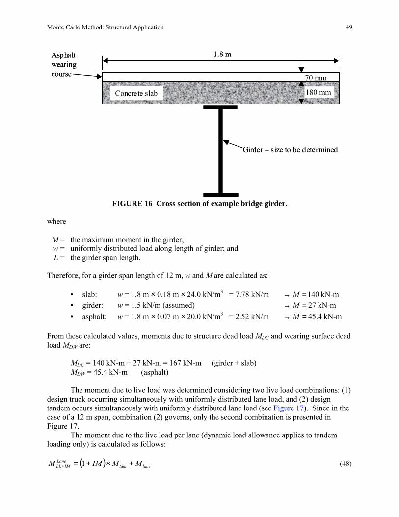
Monte Carlo Method: Structural Application 49
Girder � size to be determined
Concrete slab
Asphaltwearingcourse
1.8 m
180 mm
70 mm
Girder � size to be determined
Concrete slab
Asphaltwearingcourse
1.8 m
180 mm
70 mm
FIGURE 16 Cross section of example bridge girder.
where M = the maximum moment in the girder; w = uniformly distributed load along length of girder; and L = the girder span length. Therefore, for a girder span length of 12 m, w and M are calculated as:
• slab: w = 1.8 m × 0.18 m × 24.0 kN/m3 = 7.78 kN/m 140 kN-mM→ = • girder: w = 1.5 kN/m (assumed) 27 kN-mM→ = • asphalt: w = 1.8 m × 0.07 m × 20.0 kN/m3 = 2.52 kN/m 45.4 kN-mM→ =
From these calculated values, moments due to structure dead load MDC and wearing surface dead load MDW are:
MDC = 140 kN-m + 27 kN-m = 167 kN-m (girder + slab) MDW = 45.4 kN-m (asphalt) The moment due to live load was determined considering two live load combinations: (1)
design truck occurring simultaneously with uniformly distributed lane load, and (2) design tandem occurs simultaneously with uniformly distributed lane load (see Figure 17). Since in the case of a 12 m span, combination (2) governs, only the second combination is presented in Figure 17.
The moment due to the live load per lane (dynamic load allowance applies to tandem loading only) is calculated as follows:
( ) lanetdmLane
IMLL MMIMM +×+=+ 1 (48)
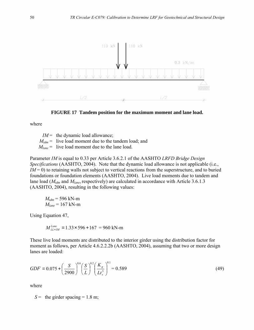
50 TR Circular E-C079: Calibration to Determine LRF for Geotechnical and Structural Design
FIGURE 17 Tandem position for the maximum moment and lane load.
where IM = the dynamic load allowance; Mtdm = live load moment due to the tandem load; and Mlane = live load moment due to the lane load. Parameter IM is equal to 0.33 per Article 3.6.2.1 of the AASHTO LRFD Bridge Design Specifications (AASHTO, 2004). Note that the dynamic load allowance is not applicable (i.e., IM = 0) to retaining walls not subject to vertical reactions from the superstructure, and to buried foundations or foundation elements (AASHTO, 2004). Live load moments due to tandem and lane load (Mtdm and Mlane, respectively) are calculated in accordance with Article 3.6.1.3 (AASHTO, 2004), resulting in the following values:
Mtdm = 596 kN-m Mlane = 167 kN-m
Using Equation 47,
16759633.1 +×=+Lane
IMLLM = 960 kN-m These live load moments are distributed to the interior girder using the distribution factor for moment as follows, per Article 4.6.2.2.2b (AASHTO, 2004), assuming that two or more design lanes are loaded:
GDF 1.0
3
2.06.0
2900075.0
+=
s
g
LtK
LSS = 0.589 (49)
where S = the girder spacing = 1.8 m;
Monte Carlo Method: Structural Application 51
L = the span length = 12 m; Kg = longitudinal stiffness parameter; and ts = depth of concrete slab.
According to Article 4.6.2.2.2b (AASHTO, 2004), as an approximation, the term 3s
g
LtK
may
be taken as 1. Therefore, the total moment due to live load (including dynamic load) per girder, MLL, is calculated as follows:
960589.0 ×=×= +Lane
IMLLLL MGDFM = 566 kN-m (50)
The load factors from the AASHTO LRFD specifications (AASHTO, 2004), per Article 3.4.1, are:
γDC = 1.25 γDW = 1.50 γLL = 1.75
Therefore, the total factored moment per girder, Mfac, is as follows:
( )∑ ×+×+××=×= LLLLDWDWDCDCiifac MMMMM γγγηγη (51)
where η = factor related to redundancy, ductility, and operational importance, and is equal to 1.0; γi = the load factor applicable to the i�th moment; and Mi = the i�th moment. Therefore,
( )56675.14.455.116725.10.1 ×+×+××=facM = 1,270 kN-m
The required nominal flexural resistance, as represented by the plastic section modulus, Zreq, is calculated as:
y
facreq F
MZ = (52)
where Fy = yield strength of the steel. All other variables are defined previously. For Fy equal to 350 MN/m2,
000,1350
1270×
=reqZ = 0.00363 m3
52 TR Circular E-C079: Calibration to Determine LRF for Geotechnical and Structural Design
The minimum size steel beam that meets this requirement is a W 690×125, with Zx = 0.00400 m3.
Recalculating the moment resulting from the beam self weight using the exact W 690×125 beam dead weight (w = 1.23 kN/m), and using Equation 47, M = 22.1 kN-m. The new total factored moment is therefore: Mfac = [ ]56675.14.455.1)1.22140(25.1 ×+×++× = 1,260 kN-m
Next, recalculate the resistance using the W 690x125 beam to make sure that the factored applied moment, Mfac, is less than the available factored flexural resistance, Mrf, using a resistance factor ϕf = 1.0 for flexure of steel beams in accordance with Article 6.5.4.2 (AASHTO, 2004):
xyfRfrf ZFMM ××=×= ϕϕ (53) where MR = the nominal flexural resistance. All other variables are defined previously. Therefore, 1000m 004.0MPa 3500.1 3 ×××=×× xyf ZFϕ = 1,400 kN-m
facrf MM > ? 1,400 kN-m > 1,200 kN-m OK!
This completes the beam flexural design for the purposes of this example, and the
nominal flexural resistance, MR (since the resistance factor is 1.0) is 1,400 kN-m. The nominal values determined from this design can now be used as the basis of a reliability analysis to estimate the β value this design represents. 11.2 RELIABILITY ANALYSIS FOR INTERIOR GIRDER DESIGN The load components include moment due to the dead load of the structural components, MDC, the moment due to the wearing surface, MDW, and moment due to live load, MLL (including dynamic load). The statistical parameters and types of distribution functions for the loads and the resistance used for this example presented in Table 5 are taken from Nowak (1999). Since only summary statistics are available, the assumption is made that the data upon which these statistics are based perfectly match the distribution and statistical parameters provided in the table. Because of this, there is no �fitting to the tail� step as described in Section 5.5, and the location of the design point is not critical to the design in this case. Nominal (design) values of moments, M, resulting from the applied loads, Q, and resistance, R, are given in Table 5. These nominal values were obtained from the example calculation provided in Section 11.1.
Live load in Table 5 includes the static component of the live load, and dynamic component (i.e., dynamic load allowance), IM. The nominal value of the combined static and dynamic live load components is as calculated in Equations 48 and 50. To correctly calculate the mean live load using the available live load statistics, the live load bias of λLL = 1.33 is only

Monte Carlo Method: Structural Application 53
applied to the static component of the live load. The mean value of the static component of the live load is determined as (Nowak, 1999):
LLSM = λLL × MLLS (54) where LLSM = the mean value of the moment due to the static component of the live load; MLLS = moment due to static component of the live load; and λLL = live load bias.
The mean value of the moment due to the dynamic component of live load, IMM , can be calculated as a percentage of the mean static live load, LLSM (Nowak, 1999). Dynamic load as fraction of live load was considered analytically (Hwang and Nowak, 1991) and experimentally (Kim and Nowak, 1997; Eom and Nowak, 2001). They observed that for two lanes fully loaded, the dynamic load factor (i.e., ratio of dynamic load and corresponding static live load) does not exceed 0.10. Therefore:
LLSIM MM ×= 10.0 (55)
Using Equation 48, but taking only the static portion of the live load (i.e., setting IM = 0), the static component of the live load (i.e., without the dynamic load allowance) is:
MLLS = [(1 + 0.0) × 596 + 167] × 0.589 = 449 kN-m
Using Equation 54, the mean static live load is:
LLSM = 449 × 1.33 = 598 kN-m Using the approach by Nowak (1999) shown in Equation 55, the total mean live load, LLM , is calculated as:
LLM = LLSM + IMM = (1 + 0.1) × LLSM (56)
where all variables are described previously. Therefore,
LLM = 598 × 1.1 = 658 kN-m
Note that this value of the mean total live load LLM results in a bias for the combination of the static and dynamic live load components of LLM /MLL = 658/566 = 1.16, where MLL is as calculated in Equation 50. The coefficient of variation for the live load of 0.18 (Nowak 1999), however, applies to both the static and dynamic components of the live load.
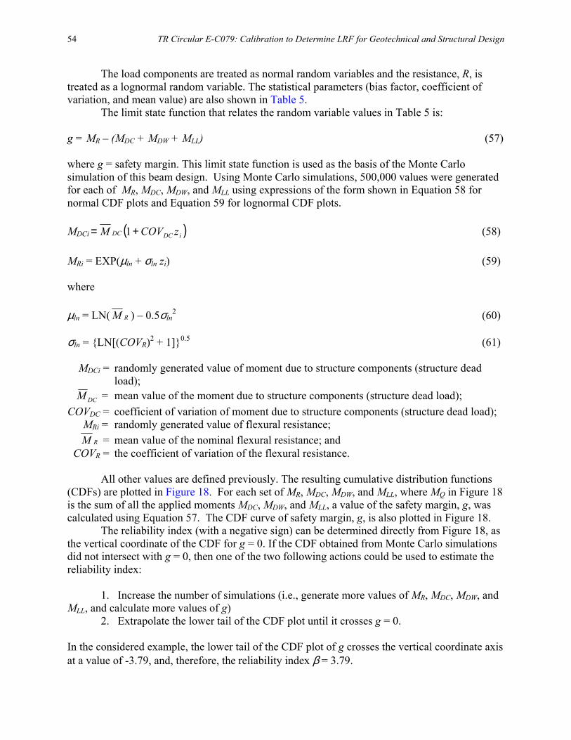
54 TR Circular E-C079: Calibration to Determine LRF for Geotechnical and Structural Design
The load components are treated as normal random variables and the resistance, R, is treated as a lognormal random variable. The statistical parameters (bias factor, coefficient of variation, and mean value) are also shown in Table 5.
The limit state function that relates the random variable values in Table 5 is: g = MR � (MDC + MDW + MLL) (57) where g = safety margin. This limit state function is used as the basis of the Monte Carlo simulation of this beam design. Using Monte Carlo simulations, 500,000 values were generated for each of MR, MDC, MDW, and MLL using expressions of the form shown in Equation 58 for normal CDF plots and Equation 59 for lognormal CDF plots. MDCi ( )iDCDC zCOVM += 1 (58) MRi = EXP(µln + σln zi) (59) where µln = LN( RM ) � 0.5σln
2 (60) σln = {LN[(COVR)2 + 1]}0.5 (61) MDCi = randomly generated value of moment due to structure components (structure dead
load); DCM = mean value of the moment due to structure components (structure dead load); COVDC = coefficient of variation of moment due to structure components (structure dead load); MRi = randomly generated value of flexural resistance; RM = mean value of the nominal flexural resistance; and COVR = the coefficient of variation of the flexural resistance.
All other values are defined previously. The resulting cumulative distribution functions (CDFs) are plotted in Figure 18. For each set of MR, MDC, MDW, and MLL, where MQ in Figure 18 is the sum of all the applied moments MDC, MDW, and MLL, a value of the safety margin, g, was calculated using Equation 57. The CDF curve of safety margin, g, is also plotted in Figure 18.
The reliability index (with a negative sign) can be determined directly from Figure 18, as the vertical coordinate of the CDF for g = 0. If the CDF obtained from Monte Carlo simulations did not intersect with g = 0, then one of the two following actions could be used to estimate the reliability index:
1. Increase the number of simulations (i.e., generate more values of MR, MDC, MDW, and MLL, and calculate more values of g)
2. Extrapolate the lower tail of the CDF plot until it crosses g = 0. In the considered example, the lower tail of the CDF plot of g crosses the vertical coordinate axis at a value of -3.79, and, therefore, the reliability index β = 3.79.
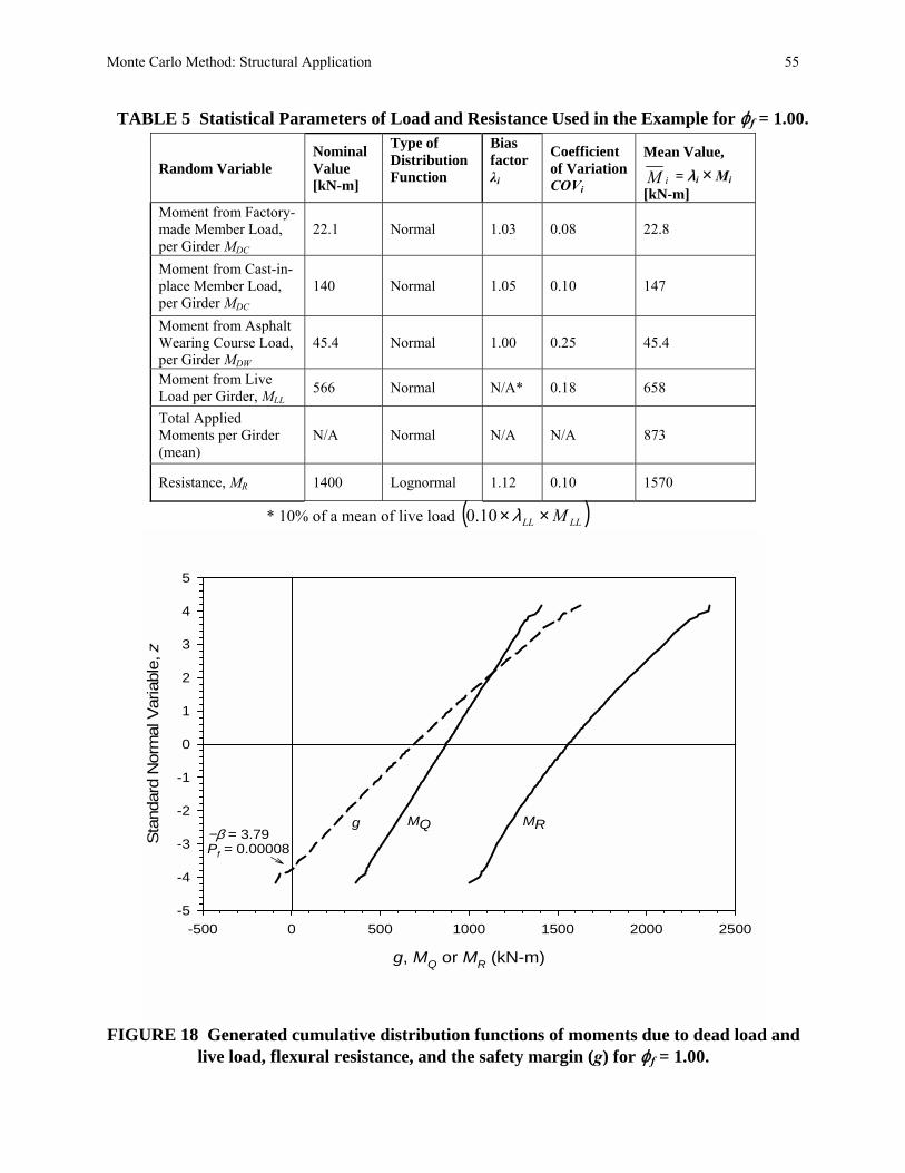
Monte Carlo Method: Structural Application 55
TABLE 5 Statistical Parameters of Load and Resistance Used in the Example for ϕf = 1.00.
Random Variable Nominal Value [kN-m]
Type of Distribution Function
Bias factor λi
Coefficient of Variation COVi
Mean Value,
iM = λ i × Mi
[kN-m] Moment from Factory-made Member Load, per Girder MDC
22.1 Normal 1.03 0.08 22.8
Moment from Cast-in-place Member Load, per Girder MDC
140 Normal 1.05 0.10 147
Moment from Asphalt Wearing Course Load, per Girder MDW
45.4 Normal 1.00 0.25 45.4
Moment from Live Load per Girder, MLL 566 Normal N/A* 0.18 658
Total Applied Moments per Girder (mean)
N/A Normal N/A N/A 873
Resistance, MR 1400 Lognormal 1.12 0.10 1570
* 10% of a mean of live load ( )LLLL M××λ10.0
g, MQ or MR (kN-m)
-500 0 500 1000 1500 2000 2500
Sta
ndar
d N
orm
al V
aria
ble,
z
-5
-4
-3
-2
-1
0
1
2
3
4
5
−β = 3.79Pf = 0.00008
MQ MRg
FIGURE 18 Generated cumulative distribution functions of moments due to dead load and
live load, flexural resistance, and the safety margin (g) for ϕf = 1.00.
56 TR Circular E-C079: Calibration to Determine LRF for Geotechnical and Structural Design
To demonstrate the effect of increasing the resistance factor ϕf on the value of β that results, the value of ϕf is increased to 1.10, the girder is redesigned, and the reliability index is calculated.
For 10.1=fϕ ,
30.00327 mfacreq
f y
MZ
Fϕ= =
×
For W 690x125: 1.10 350 0.00367 1000 1410 kN-mf n f y xM F Zφ φ× = × × = × × × =
facnf MM >×ϕ ? 1410 kN-m > 1260 kN-m OK! (where ϕf = 1.10)
The bias factor, coefficient of variation, and mean value are shown in Table 6. The mean and standard deviation of resistance are different compared to the previous case, since the resistance factor has changed and is equal to 1.10.
The format of the limit state function is the same as in the previous calculation for this example (Equation 57). Using Monte Carlo simulations, 500,000 values were generated for MR, MDC, MDW, and MLL using expressions of the form shown in Equation 58 for normal CDF plots and Equation 59 for lognormal CDF plots. The resulting cumulative distribution functions
TABLE 6 Statistical Parameters of Load and Resistance Used in Example for ϕf = 1.10.
Random Variable Nominal Value [kN-m]
Type of Distribution Function
Bias factor λi
Coefficient of Variation COVi
Mean Value,
iM = λ i × Mi [kN-m]
Moment from Factory-made Member Load, per Girder MDC
22.1 Normal 1.03 0.08 22.8
Moment from Cast-in-place Member Load, per Girder MDC
140 Normal 1.05 0.10 147
Moment from Asphalt Wearing Course Load, per Girder MDW
45.4 Normal 1.00 0.25 45.4
Moment from Live Load, MLL per Girder 566 Normal N/A* 0.18 658
Total Applied Moments per Girder N/A Normal N/A N/A 873
Resistance per Girder, MR 1290 Lognormal 1.12 0.10 1440
*10% of a mean of live load ( )LLLL M××λ10.0
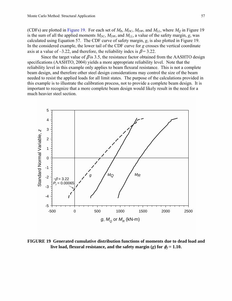
Monte Carlo Method: Structural Application 57
(CDFs) are plotted in Figure 19. For each set of MR, MDC, MDW, and MLL, where MQ in Figure 19 is the sum of all the applied moments MDC, MDW, and MLL, a value of the safety margin, g, was calculated using Equation 57. The CDF curve of safety margin, g, is also plotted in Figure 19. In the considered example, the lower tail of the CDF curve for g crosses the vertical coordinate axis at a value of �3.22, and therefore, the reliability index is β = 3.22.
Since the target value of β is 3.5, the resistance factor obtained from the AASHTO design specifications (AASHTO, 2004) yields a more appropriate reliability level. Note that the reliability level in this example only applies to beam flexural resistance. This is not a complete beam design, and therefore other steel design considerations may control the size of the beam needed to resist the applied loads for all limit states. The purpose of the calculations provided in this example is to illustrate the calibration process, not to provide a complete beam design. It is important to recognize that a more complete beam design would likely result in the need for a much heavier steel section.
β = 3.77
MQ MRg
g, MQ or MR (kN-m)
-500 0 500 1000 1500 2000 2500
Sta
ndar
d N
orm
al V
aria
ble,
z
-5
-4
-3
-2
-1
0
1
2
3
4
5
−β = 3.22Pf = 0.00065
MQ MRg
FIGURE 19 Generated cumulative distribution functions of moments due to dead load and
live load, flexural resistance, and the safety margin (g) for ϕf = 1.10.
58
12
Practical Considerations for Calibration When Data Are Limited or Not Available
nfortunately, detailed statistical data for the applicable loads and resistance for a specific limit state such as those illustrated herein may not always be available. If such data are
limited or not available, this does not mean that the principles and procedures provided in this Circular cannot be used. Keep in mind that the Monte Carlo simulation technique is simply curve fitting the available statistical data and extrapolating it so that the load and resistance factors needed to produce an acceptably low probability of failure can be estimated from limited statistical data. Figure 11 illustrates this point.
What if only statistical parameters such as the mean and COV for a given randomvariable are available from previously published information? The principles and proceduresprovided herein could still be used in this case, as demonstrated, for example, in Section 11.The unknown distribution type can be approximated by a normal or lognormal distribution,if the distribution type is not specifically stated, and the reliability index can be calculatedusing one of the closed-form expressions provided earlier (Equation 6 or 7), or by MonteCarlo simulations. However, the published statistics may not be representative of all of the sources of uncertainty affecting the considered random variable, or may not be of the level of quality desired (see Section 5.2). It is therefore important to have as much background information on the source and nature of the published statistics as possible, if they are to be used for a reliability analysis.
There may be cases where even published statistical parameters are not available. For these situations, calibration can still be conducted, but the results will be less accurate.Duncan (2000, 2001) provides some practical guidelines for estimating statistical input parameters based on experience and judgment regarding specific design input parameters or design methods. For example, in addition to the use of published statistical parameters, the Three-Sigma Rule can be used to estimate the standard deviation of a given parameter. This �rule-of-thumb� is as follows (Duncan 2000):
6LCVHCV −=σ (62)
where σ = the standard deviation; HCV = the highest conceivable value of the parameter; and LCV = the lowest conceivable value of the parameter.
HCV and LCV values are estimated based on experience and judgment. Duncan (2000) reports that there is a tendency to underestimate the true range of a given parameter, and that this tendency needs to be considered when estimating the standard deviation in this manner. Hence, Duncan (2001) recommends that the Three-Sigma Rule be modified to a Two-Sigma Rule by
U
Practical Considerations for Calibration When Data Are Limited or Not Available 59
replacing the �6� in Equation 62 with a �4.� The average value of the parameter and its distribution (e.g., normal or lognormal) must also be estimated, which could be based on limited measurements or experience.
For example, if it is desired to evaluate the tensile capacity rather than the pullout limit state for the internal stability of welded wire reinforced soil walls, knowledge of how steel yield strength is specified could be used to estimate the mean and standard deviation for steel yield strength, if detailed statistical data are not available. Typically, for soil reinforcement in reinforced soil walls, the minimum specification value is 450 MPa, which also happens to be the value that would be used for design. If it is known from testing experience, or knowledge of how steels of similar grades are produced, that the highest likely value is approximately 600 MPa. Hence, using the more conservative Two-Sigma Rule and assuming a normal distribution, the mean and standard deviation would be estimated as 530 MPa and 38 MPa, respectively, resulting in a COV of 7.2%. Since the design value is 450 MPa, the mean bias would be 530/450 = 1.2. These statistics, in combination with the load statistics reported in this Circular, could then be used to estimate the resistance factor needed for the reinforcement yield limit state, if detailed steel yield statistical data are not available.
When working with limited statistical data, it is probably not justified to perform a Monte Carlo simulation if the parameter distributions are either all lognormal or all normal and the limit state function of the random variables is linear. In this case, the closed-form solutions provided herein are sufficiently accurate considering the approximate nature of the statistical input parameters. If this is not the case, then a Monte Carlo simulation could still be used.
If there is a significant degree of uncertainty regarding the statistical input parameters, it would be wise to compare the results of the calibration with the load and resistance factors that would be required for the specific limit state to be consistent with previous successful design practice. Estimating load and resistance factors so that they are reasonably consistent with previous successful design practice is called �calibration by fitting.� The approach is demonstrated by Equation 63 as follows (Withiam, et al., 1998):
in
ini
QFSQΣ
Σ=
γϕ (63)
where FS is the safety factor applicable for the limit state using the allowable stress design approach, and all other variables are as defined previously. Using Equation 63, assuming only one load source, Qni cancels out, and the resistance factor is calculated using calibration by fitting to allowable stress design (ASD) as follows:
FSiγϕ = (64)
For two load sources (e.g., dead load DL and live load LL), the two load sources can be expressed as a ratio, and Equation 63 becomes:
( )FSLLDL
LLDL
LLDL
1+
+=
γγϕ (65)
60 TR Circular E-C079: Calibration to Determine LRF for Geotechnical and Structural Design
where all variables are described previously.
Note that this approach does not address the actual bias or variability of the load or resistance prediction methods nor is there any consideration given to the probability of failure, Pf. These equations simply provide a way to obtain an average value for the load factor considering the use of one or more different load factors applicable to their respective load sources, and considering the relative magnitudes of each load. In the most basic terms, the ASD factor of safety (FS) is simply the average load factor divided by the resistance factor. All that is being done here is to calculate the magnitude of a resistance factor, for a given set of load factors, that when combined with the load factors, provides the same magnitude of FS as is currently used for ASD. Therefore, whatever margin of safety was implied by the ASD safety factor, the load and resistance factor combination that results from this type of analysis will have the same unknown margin of safety.
The reliability of the load and resistance factor combination determined using this approach is based on the performance of structures designed using the method(s) and associated FS value(s) in question in consideration of long-term professional engineering practice. Note, however, that perception can play a significant role in defining what is considered successful past practice. The true safety factor could be much higher or much lower than the one specified from past practice, though generally not near or less than 1.0, or failure would occur. Nevertheless, if the quality of the statistical data is questionable, the use of theoretical reliability-based techniques such as the Monte Carlo method will not necessarily provide a more accurate assessment of the level of safety than �successful� past design practice. This should be considered when developing and selecting a load and resistance factor combination for design.
For the pullout limit state for the steel grid reinforced walls analyzed previously, thesafety factor used in past design practice was FS = 1.5 (AASHTO, 2002), and the currently prescribed load factor applicable for internal wall stability for earth pressure due to soil self-weight is 1.35. Using Equation 64, assuming only one load source, the resistance factor is calculated using calibration by fitting to allowable stress design (ASD) as:
9.05.1
35.1
===FS
iγϕ
From Section 6, the load factor was estimated to be 1.75 based on the actual statistical
load data available, and in Section 8 the resistance factor was determined to be 0.6, based on the Monte Carlo simulation, again using the available statistical data. It is obvious the available statistical data indicate that a more conservative pullout design is needed than has been used in past practice (i.e., a load factor of 1.75 versus 1.35, and a resistance factor of 0.6 versus 0.9).
Considering the significant amount of data available to justify the statistical parameters and that the pattern in the data is fairly consistent, it appears justified to increase the margin of safety for this limit state, even though there is little evidence of pullout failure in these types of walls. It is possible that the good performance observed in the past regarding this limit state could be the result of other conservative practices that have contributed to the safety of these walls. For example, a minimum reinforcement length of 70% of the wall height, or 2.4 m, whichever is greater, is currently specified (AASHTO, 2004). This could be more than enough reinforcement length to account for the width of the active zone plus the length of reinforcement needed beyond the active zone for pullout. Conservative selection of soil shear strength for

Practical Considerations for Calibration When Data Are Limited or Not Available 61
design could also contribute to additional safety margin, as could load sharing between the upper layers of soil reinforcement. However, in the end, deciding which numbers to believe is a judgment call that those who approve the design codes and specifications must make.

62
13
Final Selection of Load and Resistance Factors
ow heavily one relies on reliability theory calibration results depends on how much confidence one has in the statistics used to conduct the reliability analysis. The level of
confidence in the statistics used for the reliability analysis is directly dependent on the quality and quantity of data available, as discussed in Section 5.2, and should be considered when making the final selection of load and resistance factors to use for design.
Designers have an inherent confidence in past successful design practice and the safety margins embodied in those design practices. Therefore, if a decision is made to deviate from past successful design practice, there should be a good reason for doing so. A strong and reliable database coupled with reliability theory could be an adequate reason for deviating from past practice, especially if it is recognized that past practice has been excessively conservative and if evidence is available to prove that, or if past practice has resulted in a higher than acceptable failure rate. However, if the quality or quantity of the data used as input in reliability theory calibrations is questionable, it is justified to weight the final resistance or load factor selection toward the values representative of past successful practice, but with the recognition that the definition of �successful past practice� can be affected by perception.
H
63
14
Documentation of Load and Resistance Factor Calibration
hen performing load and resistance factor calibration for structural and geotechnical design specifications, the focus of the calibration is often on a specific design method
used to calculate the load or resistance. This is especially true for geotechnical design, where the design method itself contributes to the bias and variability of the nominal value, but may also be true for structural design. As structural and geotechnical design specifications evolve, and as more statistical data become available that allow the calibration of load and resistance factors to be improved, there will be a need to perform new calibrations. Considering the significant effort required to gather the data needed to perform calibration, it is important that the data gathered be adequately documented so that the data can be used, as appropriate, to update load and resistance factors as design specification improvements are made or as new statistical data become available.
Objectives of the documentation process are as follows:
• The documentation is detailed enough for users of the design specifications to understand the basis of the calibrations used to develop the load and resistance factors, to make it possible for designers to rationally apply engineering judgment and adapt those factors for project- or site-specific considerations when necessary.
• Rationale for omitting outlier data is explained. • The input data and assumptions used are documented in adequate detail so that future
researchers can reproduce the nominal prediction of each measured resistance or load contained in the database.
• The methods and criteria used to measure resistances, loads, or input parameters (i.e., those parameters defined as the random variables in the calibration) are adequately documented to allow rational combination of those data with future data gathered for the purpose of expanding the database.
• The documentation is developed in a way that it can be stored in an accessible repository to ensure that the investment made in gathering the extensive data necessary to conduct reliable calibrations is not lost.
Details regarding the type of documentation needed to meet these objectives are provided in Appendix C. Also provided in Appendix C is an example of this type of documentation, specifically the reinforced soil wall data used herein to illustrate the calibration process.
W

64
15
Concluding Remarks
alibration, and especially probabilistic analysis, can seem daunting to the average user of design codes or specifications that employ a limit states approach. To render this process
less complex, this Circular has been developed to provide information on the calibration process, starting from basic concepts, and continuing with step-by-step procedures and examples to describe the process clearly. If detailed statistical data are available, this circular should enable the researcher or sophisticated designer to assess the load and resistance factors needed to provide the desired margin of safety. If detailed statistical data are not available, some information and tools have been provided to help the designer estimate the parameters needed to assess these factors. The examples provided also illustrate the importance of understanding the basis of the load and resistance factors prescribed in design codes and specifications.
C

65
References AASHTO, 1992, LRFD Bridge Design Specifications, American Association of State Highway
and Transportation Officials, 1st ed., Washington, D.C., USA. AASHTO, 1998, LRFD Bridge Design Specifications, American Association of State Highway
and Transportation Officials, 2nd ed., Washington, D.C., USA. AASHTO, 2002, Standard Specifications for Highway Bridges, American Association of State
Highway and Transportation Officials, 17th ed., Washington, D.C. AASHTO, 2004, LRFD Bridge Design Specifications, American Association of State Highway
and Transportation Officials, 3rd ed., Washington, D.C., USA. Allen, T. M., 2005, Development of Geotechnical Resistance Factors and Downdrag Load
Factors for LRFD Foundation Strength Limit State Design, Publication No. FHWA-NHI-05-052, Federal Highway Administration, Washington, D.C., 41 pp.
Allen, T. M., Christopher, B. R., Elias, V., and DiMaggio, J., 2001, Development of the Simplified Method for Internal Stability of Mechanically Stabilized Earth (MSE) Walls, Washington State Department of Transportation, Report WA-RD 513.1, 108 pp.
Allen, T. M., Christopher, B. R., and Holtz, R. D., 1992, Performance of a 12.6 m High Geotextile Wall in Seattle, Washington, Geosynthetic Reinforced Soil Retaining Walls, J. T. H. Wu (editor), Rotterdam: Balkema, pp. 81-100.
Barker, R. M., Duncan, J. M., Rojiani, K. B., Ooi, P. S. K., Tan, C. K., and Kim, S. G., 1991, Manuals for the Design of Bridge Foundations: Shallow Foundations, Driven Piles, Retaining Walls and Abutments, Drilled Shafts, Estimating Tolerable Movements, and Load Factor Design Specifications and Commentary, NCHRP Report 343, TRB, National Research Council, Washington, D.C.
Bathurst, R. J., Walters, D., Vlachopoulos, N., Burgess, P., and Allen, T. M., 2000, Full Scale Testing of Geosynthetic Reinforced Walls, ASCE Special Publication No. 103, Advances in Transportation and Geoenvironmental Systems Using Geosynthetics, Proceedings of Geo-Denver 2000, August 5-8, 2000, Denver, Colorado, pp. 201-217.
Becker, D. E., 1996a, Eighteenth Canadian Geotechnical Colloquium: Limit States Design for Foundations. Part I. An Overview of the Foundation Design Process, Canadian Geotechnical Journal, 33: 956-983.
Becker, D. E., 1996b, Eighteenth Canadian Geotechnical Colloquium: Limit States Design for Foundations. Part II. Development for the National Building Code of Canada, Canadian Geotechnical Journal, 33: 984-1007.
Benjamin, J. R., and Cornell, C. A., 1970, Probability, Statistics, and Decision for Civil Engineers, New York: McGraw-Hill.
CSA, 2000, Canadian Highway Bridge Design Code, Canadian Standards Association, Toronto, Ontario, Canada.
D�Appolonia, 1999, Developing New AASHTO LRFD Specifications for Retaining Walls, Report for NCHRP Project 20-7, Task 88, 63 pp.
Duncan, J. M., 2000, Factors of Safety and Reliability in Geotechnical Engineering, Journal of Geotechnical and Geoenvironmental Engineering, ASCE, Vol. 126, No. 4, pp. 307-316.
Duncan, J. M., 2001, Factors of Safety and Reliability in Geotechnical Engineering � Closure, Journal of Geotechnical and Geoenvironmental Engineering, ASCE, Vol. 126, No. 4, pp. 717-721.

66 TR Circular E-C079: Calibration to Determine LRF for Geotechnical and Structural Design
Eom, J. and Nowak, A. S., 2001, Live Load Distribution for Steel Girder Bridges, ASCE Journal of Bridge Engineering, Vol. 6, No. 6, pp. 489-497.
Ghosn, M., and Moses, F., 1998, Redundancy in Highway Bridge Superstructures, NCHRP Report 406, Transportation Research Board, National Research Council, Washington, D.C.
Goble, G., 1999, Geotechnical Related Development and Implementation of Load and Resistance Factor Design (LRFD) Methods, NCHRP Synthesis of Highway Practice 276, Transportation Research Board, National Research Council, Washington, D.C., 69 pp.
Hwang, E.-S., and Nowak, A. S., 1991, Simulation of Dynamic Load for Bridges, ASCE Journal of Structural Engineering, Vol. 117, No. 5, pp. 1413-1434.
Kim, S.-J., and Nowak, A. S., 1997, Load Distribution and Impact Factors for I-Girder Bridges, ASCE Journal of Bridge Engineering, Vol. 2, No. 3, pp. 97-104.
Liu, W. D., Neuenhoffer, A., Ghosn, M., and Moses, F., 2001, Redundancy in Highway Bridge Substructures, NCHRP Report 458, Transportation Research Board, National Research Council, Washington, D.C., 98 pp.
Lloyd, D. K., and Lipow, M., 1982, Reliability: Management, Methods and Mathematics, Prentice-Hall.
Ministry of Transportation and Communication, 1979, Ontario Highway Bridge Design Code (OHBDC), 1st ed., Highway Engineering Division, Downsview, Ontario.
Ministry of Transportation and Communication, 1983, Ontario Highway Bridge Design Code (OHBDC), 2nd ed., Highway Engineering Division, Downsview, Ontario, Vol. 1 and 2.
Ministry of Transportation of Ontario, 1991, Ontario Highway Bridge Design Code (OHBDC), 3rd ed., Downsview, Ontario, Vol. 1 and 2.
Nowak, A. S., 1999, Calibration of LRFD Bridge Design Code, NCHRP Report 368, Transportation Research Board, National Research Council, Washington, D.C.
Nowak, A. S., and Collins, K. R., 2000, Reliability of Structures, New York: McGraw-Hill. Paikowsky, S. G., Birgisson, B., McVay, M., Nguyen, T., Kuo, C., Baecher, G., Ayyub, B.,
Stenersen, K., O�Malley, K., Chernauskas, L., and O�Neill, M., 2004, Load and Resistance Factor Design (LRFD) for Deep Foundations, NCHRP Report 507, Transportation Research Board of the National Academies, Washington, D.C., 126 pp.
Phoon, K.-K., Kulhawy, F. H., and Grigoriu, M. D., 1995, Reliability-Based Design of Foundations for Transmission Line Structures, Report TR-105000, Electric Power Research Institute, Palo Alto, Calif.
Rackwitz, R., and Fiessler, B., 1978, Structural Reliability Under Combined Random Load Sequences, Computers and Structures, Vol. 9, pp. 489-494.
Scott, B., Kim, B. J., and Salgado, R., 2003, Assessment of Current Load Factors for Use in Geotechnical Load and Resistance Factor Design, Journal of Geotechnical and Geoenvironmental Engineering, ASCE, Vol. 129, No. 4, pp. 287-295.
Vanmarke, E. H., 1977, Probabilistic Modelling of Soil Profiles, Journal of Geotechnical Engineering, ASCE, Vol. 103, No GT11, pp. 1227-1246.
Withiam, J. L., Voytko, E. P., Barker, R. M., Duncan, J. M., Kelly, B. C., Musser, S. C., and Elias, V., 1998, Load and Resistance Factor Design (LRFD) for Highway Bridge Substructures, FHWA HI-98-032, Federal Highway Administration, Washington, D.C.
Zhang, L., Tang, W. H., and Ng, C. W. W., 2001, Reliability of Axially Loaded Driven Pile Groups, Journal of Geotechnical and Environmental Engineering, ASCE, Vol. 127, No. 12, pp. 1051-1060.

67
Acknowledgments
he writers express their appreciation to David Beal (NCHRP), who facilitated the collaboration between the writers to produce this Circular, and who also provided valuable
technical input. The writers also acknowledge the efforts of Artur Czarnecki and Pascal Laumet for their assistance in developing the structural example. The writers gratefully acknowledge the funding provided by the National Cooperative Highway Research Program and the Mechanically Stabilized Earth Pooled Fund Study. The states contributing to the pooled fund include Alaska Department of Transportation, Arizona Department of Transportation, California Department of Transportation, Colorado Department of Transportation, Idaho Transportation Department, Minnesota Department of Transportation, New York Department of Transportation, North Dakota Department of Transportation, Oregon Department of Transportation, Utah Department of Transportation, Washington State Department of Transportation, and Wyoming Department of Transportation.
T
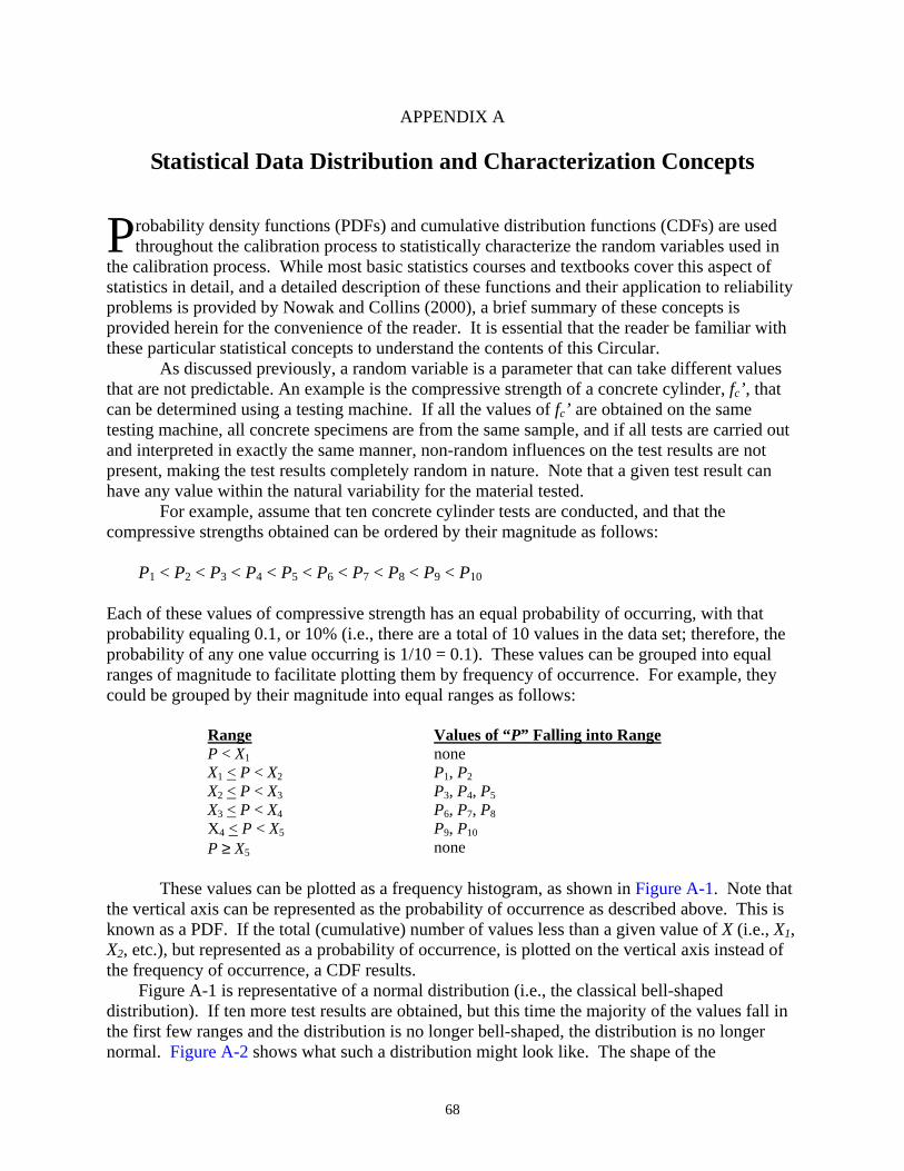
68
APPENDIX A
Statistical Data Distribution and Characterization Concepts
robability density functions (PDFs) and cumulative distribution functions (CDFs) are used throughout the calibration process to statistically characterize the random variables used in
the calibration process. While most basic statistics courses and textbooks cover this aspect of statistics in detail, and a detailed description of these functions and their application to reliability problems is provided by Nowak and Collins (2000), a brief summary of these concepts is provided herein for the convenience of the reader. It is essential that the reader be familiar with these particular statistical concepts to understand the contents of this Circular.
As discussed previously, a random variable is a parameter that can take different values that are not predictable. An example is the compressive strength of a concrete cylinder, fc’, that can be determined using a testing machine. If all the values of fc’ are obtained on the same testing machine, all concrete specimens are from the same sample, and if all tests are carried out and interpreted in exactly the same manner, non-random influences on the test results are not present, making the test results completely random in nature. Note that a given test result can have any value within the natural variability for the material tested.
For example, assume that ten concrete cylinder tests are conducted, and that the compressive strengths obtained can be ordered by their magnitude as follows:
P1 < P2 < P3 < P4 < P5 < P6 < P7 < P8 < P9 < P10
Each of these values of compressive strength has an equal probability of occurring, with that probability equaling 0.1, or 10% (i.e., there are a total of 10 values in the data set; therefore, the probability of any one value occurring is 1/10 = 0.1). These values can be grouped into equal ranges of magnitude to facilitate plotting them by frequency of occurrence. For example, they could be grouped by their magnitude into equal ranges as follows:
Range Values of “P” Falling into Range P < X1 none X1 < P < X2 P1, P2 X2 < P < X3 P3, P4, P5 X3 < P < X4 P6, P7, P8 X4 < P < X5 P9, P10 P ≥ X5 none
These values can be plotted as a frequency histogram, as shown in Figure A-1. Note that
the vertical axis can be represented as the probability of occurrence as described above. This is known as a PDF. If the total (cumulative) number of values less than a given value of X (i.e., X1, X2, etc.), but represented as a probability of occurrence, is plotted on the vertical axis instead of the frequency of occurrence, a CDF results.
Figure A-1 is representative of a normal distribution (i.e., the classical bell-shaped distribution). If ten more test results are obtained, but this time the majority of the values fall in the first few ranges and the distribution is no longer bell-shaped, the distribution is no longer normal. Figure A-2 shows what such a distribution might look like. The shape of the
P
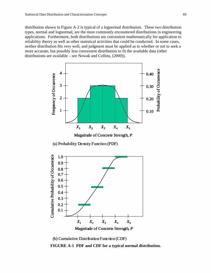
Statistical Data Distribution and Characterization Concepts 69
distribution shown in Figure A-2 is typical of a lognormal distribution. These two distribution types, normal and lognormal, are the most commonly encountered distributions in engineering applications. Furthermore, both distributions are convenient mathematically for application to reliability theory as well as other statistical activities that could be conducted. In some cases, neither distribution fits very well, and judgment must be applied as to whether or not to seek a more accurate, but possibly less convenient distribution to fit the available data (other distributions are available – see Nowak and Collins, (2000)).
X1 X2 X3 X4 X5
0.10.20.30.4
Cum
ulat
ive
Prob
abili
ty o
f Occ
urre
nce
Magnitude of Concrete Strength, P
0.50.60.70.80.91.0
X1 X2 X3 X4 X5
Freq
uenc
y of
Occ
urre
nce
1
2
3
4
Prob
abili
ty o
f Occ
urre
nce
0.10
0.20
0.30
0.40
Magnitude of Concrete Strength, P
(a) Probability Density Function (PDF)
(b) Cumulative Distribution Function (CDF)
X1 X2 X3 X4 X5
0.10.20.30.4
Cum
ulat
ive
Prob
abili
ty o
f Occ
urre
nce
Magnitude of Concrete Strength, P
0.50.60.70.80.91.0
X1 X2 X3 X4 X5
0.10.20.30.4
Cum
ulat
ive
Prob
abili
ty o
f Occ
urre
nce
Magnitude of Concrete Strength, P
0.50.60.70.80.91.0
X1 X2 X3 X4 X5
Freq
uenc
y of
Occ
urre
nce
1
2
3
4
Prob
abili
ty o
f Occ
urre
nce
0.10
0.20
0.30
0.40
Magnitude of Concrete Strength, P
X1 X2 X3 X4 X5
Freq
uenc
y of
Occ
urre
nce
1
2
3
4
Prob
abili
ty o
f Occ
urre
nce
0.10
0.20
0.30
0.40
Magnitude of Concrete Strength, P
(a) Probability Density Function (PDF)
(b) Cumulative Distribution Function (CDF)
FIGURE A-1 PDF and CDF for a typical normal distribution.
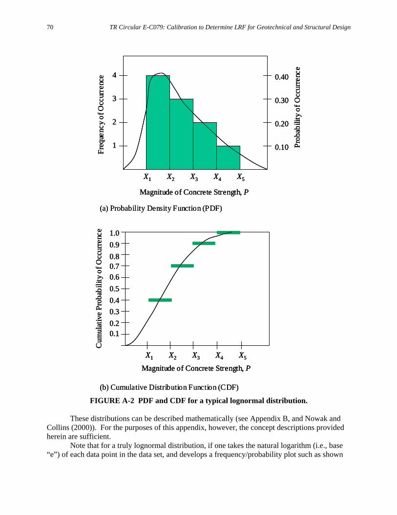
70 TR Circular E-C079: Calibration to Determine LRF for Geotechnical and Structural Design
X1 X2 X3 X4 X5
Freq
uenc
y of
Occ
urre
nce
1
2
3
4
Prob
abili
ty o
f Occ
urre
nce
0.10
0.20
0.30
0.40
Magnitude of Concrete Strength, P
X1 X2 X3 X4 X5
0.10.20.30.4
Cum
ulat
ive
Prob
abili
ty o
f Occ
urre
nce
Magnitude of Concrete Strength, P
0.50.60.70.80.91.0
(a) Probability Density Function (PDF)
(b) Cumulative Distribution Function (CDF)
X1 X2 X3 X4 X5
Freq
uenc
y of
Occ
urre
nce
1
2
3
4
Prob
abili
ty o
f Occ
urre
nce
0.10
0.20
0.30
0.40
Magnitude of Concrete Strength, P
X1 X2 X3 X4 X5
Freq
uenc
y of
Occ
urre
nce
1
2
3
4
Prob
abili
ty o
f Occ
urre
nce
0.10
0.20
0.30
0.40
Magnitude of Concrete Strength, P
X1 X2 X3 X4 X5
0.10.20.30.4
Cum
ulat
ive
Prob
abili
ty o
f Occ
urre
nce
Magnitude of Concrete Strength, P
0.50.60.70.80.91.0
X1 X2 X3 X4 X5
0.10.20.30.4
Cum
ulat
ive
Prob
abili
ty o
f Occ
urre
nce
Magnitude of Concrete Strength, P
0.50.60.70.80.91.0
(a) Probability Density Function (PDF)
(b) Cumulative Distribution Function (CDF)
FIGURE A-2 PDF and CDF for a typical lognormal distribution.
These distributions can be described mathematically (see Appendix B, and Nowak and Collins (2000)). For the purposes of this appendix, however, the concept descriptions provided herein are sufficient.
Note that for a truly lognormal distribution, if one takes the natural logarithm (i.e., base “e”) of each data point in the data set, and develops a frequency/probability plot such as shown

Statistical Data Distribution and Characterization Concepts 71
for Figure A-1, the distribution (PDF and CDF) of the logarithms of the data will be normal. This fact can be used to advantage when statistically characterizing data sets.
These distributions can also be characterized through the use of statistical parameters, including the mean, standard deviation, and COV. For a normal distribution, the mean, µs, of a sample (i.e., a data set of measured values that represent the random variable to be characterized) is simply the sum of the individual values (X1, X2, etc., with Xi representing the i’th value in the data set) divided by the total number of values (n), as shown below:
nXXX i
s+++
=L21µ (A-1)
The standard deviation, σ, which is a measure of the dispersion about the mean of the data representing the random variable, is calculated as follows for the sample, for a normal distribution:
( )
11
2
−
−=∑
=
n
Xn
isi µ
σ (A-2)
The coefficient of variation (COV) is not really a third statistical parameter, but is simply the standard deviation normalized by the mean:
s
COVµσ= (A-3)
Sometimes the term “variance” is used. This is not the same as the COV, but is simply the square of the standard deviation (i.e., σ2).
These equations can be used for lognormal distributions by taking the natural logarithm of each data point in the data set, and replacing X1, X2, and Xi, with LN(X1), LN(X2), and LN(Xi) in Equations A-1 and A-2. Alternatively, µs and σ can be determined using X1, X2, and Xi, and µs and σ can be converted to the lognormal distribution values µln and σln using Equations 11 and 12. See Nowak and Collins (2000) for how to handle other distribution types.
Conceptually, as the standard deviation gets smaller, the shape of the curve shown in Figure A-1(a) gets narrower and more peaked, and as the standard deviation gets bigger, the shape of the curve gets broader and flatter. A similar effect occurs for lognormal distributions. Note that the number of standard deviations can be related to the probability of occurrence. In general, one standard deviation (both sides of the mean) is representative of a probability of occurrence of approximately 67%, and two standard deviations are representative of a probability of occurrence of approximately 95%. Graphically, this probability of occurrence is the area under the PDF between the standard deviation values as shown in Figure A-3. Note that probability of failure, Pf, is typically focused on the area under the PDF that is to the left of a selected standard deviation range for a data set that is representative of a failure criterion (e.g., for the situation where the PDF is for R - Q - see Figure 1).
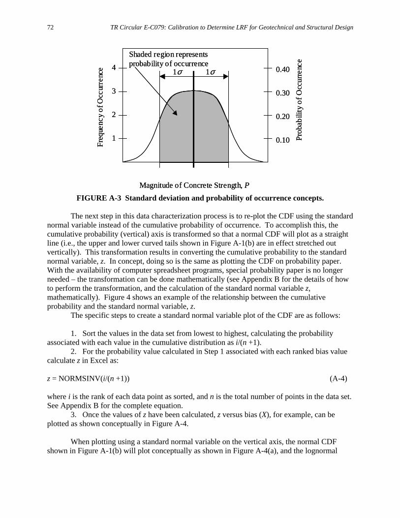
72 TR Circular E-C079: Calibration to Determine LRF for Geotechnical and Structural Design
Freq
uenc
y of
Occ
urre
nce
1
2
3
4
Prob
abili
ty o
f Occ
urre
nce
0.10
0.20
0.30
0.40
Magnitude of Concrete Strength, P
1σ 1σ
Shaded region representsprobability of occurrence
Freq
uenc
y of
Occ
urre
nce
1
2
3
4
Prob
abili
ty o
f Occ
urre
nce
0.10
0.20
0.30
0.40
Magnitude of Concrete Strength, P
1σ 1σ
Shaded region representsprobability of occurrence
FIGURE A-3 Standard deviation and probability of occurrence concepts.
The next step in this data characterization process is to re-plot the CDF using the standard
normal variable instead of the cumulative probability of occurrence. To accomplish this, the cumulative probability (vertical) axis is transformed so that a normal CDF will plot as a straight line (i.e., the upper and lower curved tails shown in Figure A-1(b) are in effect stretched out vertically). This transformation results in converting the cumulative probability to the standard normal variable, z. In concept, doing so is the same as plotting the CDF on probability paper. With the availability of computer spreadsheet programs, special probability paper is no longer needed – the transformation can be done mathematically (see Appendix B for the details of how to perform the transformation, and the calculation of the standard normal variable z, mathematically). Figure 4 shows an example of the relationship between the cumulative probability and the standard normal variable, z.
The specific steps to create a standard normal variable plot of the CDF are as follows:
1. Sort the values in the data set from lowest to highest, calculating the probability associated with each value in the cumulative distribution as i/(n +1).
2. For the probability value calculated in Step 1 associated with each ranked bias value calculate z in Excel as: z = NORMSINV(i/(n +1)) (A-4) where i is the rank of each data point as sorted, and n is the total number of points in the data set. See Appendix B for the complete equation.
3. Once the values of z have been calculated, z versus bias (X), for example, can be plotted as shown conceptually in Figure A-4.
When plotting using a standard normal variable on the vertical axis, the normal CDF
shown in Figure A-1(b) will plot conceptually as shown in Figure A-4(a), and the lognormal
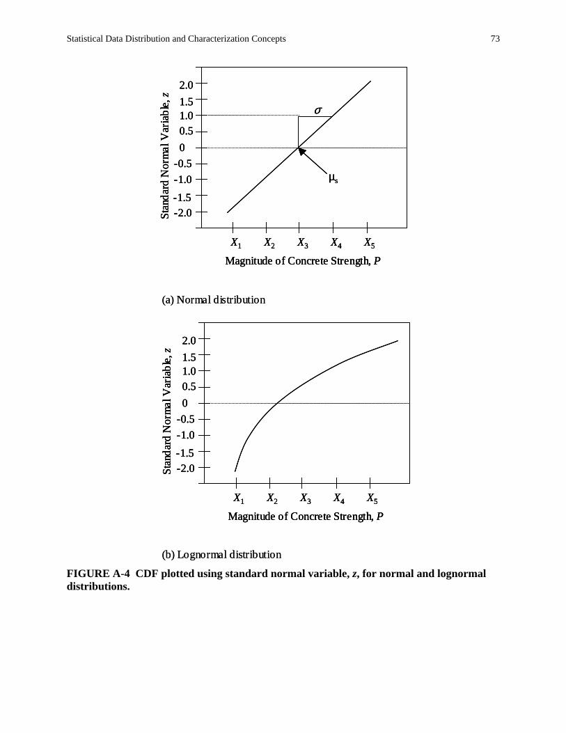
Statistical Data Distribution and Characterization Concepts 73
(a) Normal distribution
(b) Lognormal distribution
X1 X2 X3 X4 X5
-2.0-1.5-1.0-0.5
Stan
dard
Nor
mal
Var
iabl
e, z
Magnitude of Concrete Strength, P
00.51.01.52.0
X1 X2 X3 X4 X5
-2.0-1.5-1.0-0.5
Stan
dard
Nor
mal
Var
iabl
e, z
Magnitude of Concrete Strength, P
00.51.01.52.0
µs
σ
(a) Normal distribution
(b) Lognormal distribution
X1 X2 X3 X4 X5
-2.0-1.5-1.0-0.5
Stan
dard
Nor
mal
Var
iabl
e, z
Magnitude of Concrete Strength, P
00.51.01.52.0
X1 X2 X3 X4 X5
-2.0-1.5-1.0-0.5
Stan
dard
Nor
mal
Var
iabl
e, z
Magnitude of Concrete Strength, P
00.51.01.52.0
X1 X2 X3 X4 X5
-2.0-1.5-1.0-0.5
Stan
dard
Nor
mal
Var
iabl
e, z
Magnitude of Concrete Strength, P
00.51.01.52.0
µs
σ
X1 X2 X3 X4 X5
-2.0-1.5-1.0-0.5
Stan
dard
Nor
mal
Var
iabl
e, z
Magnitude of Concrete Strength, P
00.51.01.52.0
µs
σ
FIGURE A-4 CDF plotted using standard normal variable, z, for normal and lognormal distributions.

74 TR Circular E-C079: Calibration to Determine LRF for Geotechnical and Structural Design
CDF shown in Figure A-1(b) will plot conceptually as shown in Figure A-4(b). Note the standard normal variable is equal to 0 when cumulative probability of occurrence is 0.5 (i.e., one-half of the values in the data set are less than or equal to the value in the data set associated with a probability of 0.5 determined from Step 1). See Nowak and Collins (2000) for additional details regarding this transformation of the vertical axis to create the standard normal variable plot of the CDF.
An important property of a CDF plotted in this manner (i.e., as a standard normal variable) is that data which are normally distributed plot as a straight line with a slope equal to 1/σ, where σ is the standard deviation, and the horizontal axis intercept is equal to the mean, µs. However, lognormally distributed data plot as a curve. Note that a lognormally distributed data set can be made to plot as a straight line by plotting the natural logarithm of each data point.
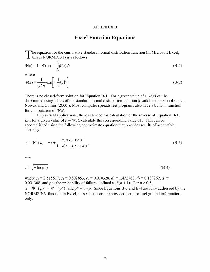
75
APPENDIX B
Excel Function Equations
he equation for the cumulative standard normal distribution function (in Microsoft Excel, this is NORMDIST) is as follows:
Φ(z) = 1 - Φ(-z) = ∫∞−
z
dzz)(ϕ (B-1)
where
( )
−= 2
21exp
21)( zzπ
ϕ (B-2)
There is no closed-form solution for Equation B-1. For a given value of z, Φ(z) can be determined using tables of the standard normal distribution function (available in textbooks, e.g., Nowak and Collins (2000)). Most computer spreadsheet programs also have a built-in function for computation of Φ(z).
In practical applications, there is a need for calculation of the inverse of Equation B-1, i.e., for a given value of p = Φ(z), calculate the corresponding value of z. This can be accomplished using the following approximate equation that provides results of acceptable accuracy:
33
221
22101
1 )(
tdtdtdtctcc
tpz+++
+++−=Φ= − (B-3)
and
)ln( 2pt −= (B-4) where c0 = 2.515517, c1 = 0.802853, c2 = 0.010328, d1 = 1.432788, d2 = 0.189269, d3 = 0.001308, and p is the probability of failure, defined as i/(n + 1). For p > 0.5,
*)( )( 11 ppz −− Φ−=Φ= , and p* = 1 - p. Since Equations B-3 and B-4 are fully addressed by the NORMSINV function in Excel, these equations are provided here for background information only.
T
76
APPENDIX C
Supporting Documentation Required for Calibration to Develop Load and Resistance Factors
nowing what to document requires an understanding of the calibration process, the specific design procedures being calibrated, and the typical design assumptions needed to
implement them. This is especially important in geotechnical design, where judgment and design assumptions are critical. For measured resistances, one must know the failure criteria used (strength or extreme event limit states). For nominal value predictions, one must know all of the input parameters and design assumptions used to calculate the nominal value.
When developing databases to support reliability theory calibration, the following summary data should be included as a minimum:
• Description of random variable for which data are available; • If a random variable is a design method result (e.g., shaft bearing resistance, beam
bending, etc.), identify the design method used, including source and date of publication of the method (an example calculation could be useful here);
• Source of data; • Number of data points, including outliers; • Number of data points when outliers are removed; • If outliers are removed, provide reason for removal; • Normal mean of measured/predicted values (bias); • Normal COV of measured/predicted values; • Type of distribution used to characterize the data (e.g., normal, lognormal, etc.); • Final normal mean of measured/predicted values used for calibration (bias)�best fit
to tail; • Final normal COV of measured/predicted values used for calibration�best fit to tail; • Type of distribution used to characterize the tail (e.g., normal, lognormal, etc.); and • For each random variable reported in the summary table, provide a standard normal
variable versus measured/predicted value plot, and show on the plot: − Each individual data point; − The distribution calculated from the mean and COV of the entire data set (after
outliers are removed); and − Distribution used for the best fit to tail, and its mean and standard deviation (used
for the final calibration). Example tables of this summary data are provided in Tables C-1 and C-2 for the
reinforced soil wall pullout limit state analysis provided in this Circular. Examples of the standard normal variable versus measured/predicted value plot are provided in Figures 7 and 8.
The following detailed data should be archived for future use, and should be adequate for future researchers to be able to reproduce the measured and predicted nominal values:
K

Supporting Documentation Required for Calibration to Develop Load and Resistance Factors 77
• For each measured/predicted value in the data set, for each random variable, tabulate: − Each measured value, including
○ The test methods and criteria used to determine those values, including test sample size, if applicable, or measurement method used, and any information on the accuracy of the method used; ○ The geometry of structural element on which measurements were taken;
and ○ The source of the data.
− Each predicted value, including all input data used to calculate the predicted value, including
○ Structure and surrounding structure geometry that affects the nominal value; ○ Input parameters that were assumed to be deterministic; ○ Any simplification or modification of the design method used to calculate
the nominal values; ○ Any design assumptions, test data, or correlations used to generate the
input design parameters for the nominal value design equation, including the test methods used to obtain measured parameters, specimen size, and any modifications to the test methods used that are not reflected in the test standard; and ○ The source of the data.
− Include this in a report appendix and an electronic spreadsheet.
For the reliability analyses conducted, the following information should be provided:
• Provide detailed design and limit state equations (g) used, including their derivation and source, and include the load and resistance factors in the design equation that are to be determined or considered in the calibration.
• Identify any assumptions used to develop the limit state equation. • Provide the target β value to be used and the reason for the selection of that target
value. • For resistance factor calibration, identify loads considered and load factors used, and
describe the calibration approach. • For load factor calibration, describe equations, process, and logic used to determine
load factors.

TABLE C-1 Summary of Load Statistics for Welded Wire and Bar Mat Reinforced Soil Walls.
[1]Normal Distribution Parameters for Reinforcement Load
Load Prediction Method
Wall and Reinforcement Type
Load Case
Data Source
n, with outliers
n, outliers removed
Reason for Outlier Removal Biasall/Biastail COVall/COVtail
Actual Distribution Type (all/tail)
[2]Calculated γQ
Selected Final γQ
AASHTO Simplified Method, φ limited to 40o max for steel walls; otherwise, average measured γs and triaxial/direct shear φ used
Bar mat and welded wire reinforced wall
1
Allen, et al. (2001)
34
34
N/A
0.954 / 0.973
0.406 / 0.462
Log/Log
1.73
1.75
Live load, per AASHTO LRFD
All
2
Nowak (1999)
N/A
N/A
N/A
1.33*
0.18*
Norm*
1.75
1.75
Notes: All = all data in distribution, after outliers removed - these statistics were not used in the final calibration. Tail = best fit distribution to tail (in vicinity of design point), without outliers - these statistics were used for the final calibration. [1] All statistics reported above represent normal distribution parameters. If the actual distribution type is reported as lognormal, these normal distribution statistics were converted to lognormal statistics (i.e., lognormal mean and standard deviation) as part of the calibration process using Equations 11 and 12. Details of wall geometry and input parameters for estimating the nominal load for steel reinforced walls are provided in Allen, et al. (2001). [2] γQ was calculated using Equation 25. *Only summary statistics were available from the data source, and were therefore used for the final calibration.
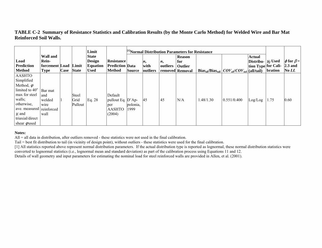
TABLE C-2 Summary of Resistance Statistics and Calibration Results (by the Monte Carlo Method) for Welded Wire and Bar Mat Reinforced Soil Walls.
[1]Normal Distribution Parameters for Resistance
Load Prediction Method
Wall and Rein-forcement Type
Load Case
Limit State
Limit State Design Equation Used
Resistance Prediction Method
Data Source
n, with outliers
n, outliers removed
Reason for Outlier Removal Biasall/Biastail COVall/COVtail
Actual Distribu-tion Type (all/tail)
γQ Used for Cali-bration
ϕ for β = 2.3 and No LL
AASHTO Simplified Method, φ limited to 40o max for steel walls; otherwise, ave. measured γs and triaxial/direct shear φ used
Bar mat and welded wire reinforced wall
1
Steel Grid Pullout
Eq. 28
Default pullout Eq. per AASHTO (2004)
D�Ap-polonia, 1999
45
45
N/A
1.48/1.30
0.551/0.400
Log/Log
1.75
0.60
Notes: All = all data in distribution, after outliers removed - these statistics were not used in the final calibration. Tail = best fit distribution to tail (in vicinity of design point), without outliers - these statistics were used for the final calibration. [1] All statistics reported above represent normal distribution parameters. If the actual distribution type is reported as lognormal, these normal distribution statistics were converted to lognormal statistics (i.e., lognormal mean and standard deviation) as part of the calibration process using Equations 11 and 12. Details of wall geometry and input parameters for estimating the nominal load for steel reinforced walls are provided in Allen, et al. (2001).

80
APPENDIX D
Abbreviations and Notations AASHTO American Association of State Highway and Transportation Officials ASD allowable stress design CDF cumulative distribution function COV coefficient of variation (equal to the standard deviation/mean) FS factor of safety LRFD load and resistance factor design NORMDIST a Microsoft Excel function that returns the cumulative normal distribution (see
Appendix B) NORMSINV a Microsoft Excel function that returns the inverse of the standard normal
distribution (see Appendix B) OHBDC Ontario Highway Bridge Design Code PDF probability density function RAND a Microsoft Excel function that returns a random number between 0 and 1 NOTATIONS C reinforcement surface area geometry factor (equal to 2 for grid and strip
reinforcement) COV coefficient of variation (equal to the standard deviation/mean) COVall coefficient of variation for the entire data set COVDC coefficient of variation of moment due to structure components (structure dead
load) COVdq coefficient of variation due to inadequate data quality COVi coefficient of variation for the i�th load component COVLL coefficient of variation of live load or coefficient of variation of the bias values
for the live load PCOV coefficient of variation of the estimated probability of failure
COVQ coefficient of variation of the load or coefficient of variation of the bias values for the load
COVQD coefficient of variation of dead load or coefficient of variation of the bias values for the dead load
COVmodel coefficient of variation due to model uncertainty COVR coefficient of variation of the resistance or coefficient of variation of the bias
values for the resistance COVrandom coefficient of variation determined from the data set used to represent the random
variable COVspatial coefficient of variation due to spatial variability COVtail coefficient of variation of the CDF that best fits the tail region of the data set COVtotal total coefficient of variation COVφ coefficient of variation for the soil friction angle φ COVγs coefficient of variation for soil unit weight γs

Abbreviations and Notations 81
DL dead load fc� compressive strength of concrete F* pullout resistance factor FQ cumulative distribution function (CDF) representing the load FR cumulative distribution function (CDF) representing the resistance FS safety factor applicable for the limit state using the allowable stress design (ASD)
approach Fy yield strength HCV highest conceivable value of the parameter g limit state function, safety margin, or random variable representing the safety
margin GDF girder distribution factor i rank of each data point in sorted data set IM dynamic load allowance Ka active lateral earth pressure coefficient Kg longitudinal stiffness parameter Kr lateral earth pressure coefficient acting at the reinforcement layer depth Kr/a factor applied to the active lateral earth pressure coefficient to obtain Kr L girder span length Le length of reinforcement in the resisting zone LCV lowest conceivable value of the parameter LL live load M moment or maximum moment MDC moment due to structure components (structure dead load)
DCM mean value of the moment due to structure components (structure dead load) MDCi randomly generated value of moment due to structure components (structure dead
load) MDW moment due to wearing course on bridge deck (wearing surface dead load) Mfac total factored moment per girder Mi the i�th moment
iM mean of the i�th moment MIM moment due to dynamic component of live load
IMM mean value of the moment due to the dynamic component of live load MLL moment due to the total live load (static and dynamic) per girder
LLM mean value of the moment due to the total live load (static and dynamic) per girder
MLLS moment due to static component of live load LLSM the mean value of the moment due to the static component of the live load
MQ the sum of all applied moments for a beam in flexure MR nominal flexural resistance MRi randomly generated value of flexural resistance
RM mean value of the nominal flexural resistance Mrf factored nominal flexural resistance Mlane live load moment due to lane load
LaneIMLLM + moment due to live load per lane
82 TR Circular E-C079: Calibration to Determine LRF for Geotechnical and Structural Design
Mtdm live load moment due to tandem load n total number of points in data set nσ a constant representing the number of standard deviations from the mean needed
to obtain the desired probability of exceedance N total number of generated g values P probability of occurrence Pf probability of failure Ptrue true probability of failure Q a random variable representing the load; load distribution Q mean of the load Q or of the measured load Qmeasured
Q* load at the design point Qmeasured measured load value Qn, Qni nominal load component
DQ mean of the dead load or measured dead load = λQDQD
QD predicted (nominal) value of dead load QLL predicted (nominal) value of live load
LLQ mean of the live load = λLLQLL
R a random variable representing the resistance; resistance distribution R mean of the resistance R or of the measured resistance Rmeasured R* resistance at the design point Rn nominal resistance Rmeasured measured resistance value S girder spacing Sv tributary area (equivalent to the vertical spacing of the reinforcement in the
vicinity of each layer when analyses are carried out per unit length of wall) Tmax maximum load in the reinforcement layer
maxT mean value of Tmax = λQTmax
Tmaxi Randomly generated value of Tmax Tpo pullout resistance Tpoi Randomly generated value of Tpo
poT mean value of Tpo = λRTpo TmaxDL dead load contribution to Tmax at the specified location TmaxLL live load contribution to Tmax at the specified location ts depth of concrete slab uia, uib, uic random number between 0 and 1 representing a probability of occurrence w uniformly distributed load along length of girder X bias (measured/predicted value) Xi I�th value in a data set z standard normal variable or variate Zreq required plastic section modulus Zx plastic section modulus of selected beam zi the value of the standard normal variable corresponding to the i�th value of the
random variable zd depth of soil above reinforcement in resisting zone

Abbreviations and Notations 83
α pullout scale effect correction factor β reliability index βT target reliability index φ backfill soil friction angle φ mean value of the soil friction angle
φi randomly generated value of soil friction angle γi load factor applicable to a specific load component γs soil unit weight γsi randomly generated value of soil unit weight
sγ mean value of soil unit weight γ,γQ load factor γDC load factor for structure components (dead load) γDW load factor for wearing course (dead load) γQD load factor for dead load, or reinforcement load resulting from the dead load γLL load factor for live load, or reinforcement load resulting from the live load η factor related to redundancy, ductility, and operational importance ϕ, ϕR resistance factor ϕf resistance factor for beam flexure λ normal mean of the bias values (measured/predicted) or bias factor λdq the bias caused by having inadequate data quality λLL normal mean of the bias values (measured/predicted) for the live load λmodel the bias resulting from design model uncertainty λQ normal mean of the bias values (measured/predicted) for the load λQD normal mean of the bias values (measured/predicted) for the dead load λR normal mean of the bias values (measured/predicted) for the resistance λrandom the bias for the data set used to represent the random variable under consideration λspatial the bias resulting from spatial variability of the parameter µln lognormal mean value µs normal mean value σ standard deviation σLL standard deviation for the live load or measured live load σln lognormal standard deviation σQ standard deviation for the load Q or the measured load Qmeasured σQD standard deviation for the dead load or measured dead load σR standard deviation for the resistance R or the measured resistance Rmeasured σv average vertical earth pressure acting at the reinforcement layer depth

scholars
The National Academy of Sciences is a private, nonprofit, self-perpetuating society of distinguished
engaged in scientific and engineering research, dedicated to the furtherance of science and technology and to their use for the general welfare. On the authority of the charter granted to it by the Congress in 1863, the Academy has a mandate that requires it to advise the federal government on scientific and technical matters. Dr. Ralph J. Cicerone is president of the National Academy of Sciences. The National Academy of Engineering was established in 1964, under the charter of the National Academy of Sciences, as a parallel organization of outstanding engineers. It is autonomous in its administration and in the selection of its members, sharing with the National Academy of Sciences the responsibility for advising the federal government. The National Academy of Engineering also sponsors engineering programs aimed at meeting national needs, encourages education and research, and recognizes the superior achievements of engineers. Dr. William A. Wulf is president of the National Academy of Engineering. The Institute of Medicine was established in 1970 by the National Academy of Sciences to secure the services of eminent members of appropriate professions in the examination of policy matters pertaining to the health of the public. The Institute acts under the responsibility given to the National Academy of Sciences by its congressional charter to be an adviser to the federal government and, on its own initiative, to identify issues of medical care, research, and education. Dr. Harvey V. Fineberg is president of the Institute of Medicine. The National Research Council was organized by the National Academy of Sciences in 1916 to associate the broad community of science and technology with the Academy’s purposes of furthering knowledge and advising the federal government. Functioning in accordance with general policies determined by the Academy, the Council has become the principal operating agency of both the National Academy of Sciences and the National Academy of Engineering in providing services to the government, the public, and the scientific and engineering communities. The Council is administered jointly by both the Academies and the Institute of Medicine. Dr. Ralph J. Cicerone and Dr. William A. Wulf are chair and vice chair, respectively, of the National Research Council. The Transportation Research Board is a division of the National Research Council, which serves the National Academy of Sciences and the National Academy of Engineering. The Board’s mission is to promote innovation and progress in transportation through research. In an objective and interdisciplinary setting, the Board facilitates the sharing of information on transportation practice and policy by researchers and practitioners; stimulates research and offers research management services that promote technical excellence; provides expert advice on transportation policy and programs; and disseminates research results broadly and encourages their implementation. The Board’s varied activities annually engage more than 5,000 engineers, scientists, and other transportation researchers and practitioners from the public and private sectors and academia, all of whom contribute their expertise in the public interest. The program is supported by state transportation departments, federal agencies including the component administrations of the U.S. Department of Transportation, and other organizations and individuals interested in the development of transportation. www.TRB.orgwww.national-academies.org

TRANSPORTATION RESEARCH BOARD 500 Fifth Street, NW Washington, DC 20001 ADDRESS SERVICE REQUESTED