Calibration of Automatic NetworkAnalysis and Computer Aided

Microwave Measurement

Jeffrey S. Kasten

Center for Communications and Signal ProcessingDepartment of Electrical and Computer Engineering

North Carolina State University

CCSP TR-90j2

Table of Contents

111

....................Original Contributions

1 Introduction

1.1 Motivation

1.2 Thesis Overview

1.3

........... . .

.............

1

1

3

5

2 Review of Calibration Theory

Literature Review2.1

2.1.1

...........................

Introduction to Calibration of Network Analysis

7

7

12

2.1.2 The One Port Error Model 13

2.1.3 One Port Calibration Standards 17

2.1.4 AN A Two Port Error Models 19

2.1.5 Fixture Two Port Error Models . 26

2.2 Conclusion

3.3 Evolution from an Asymmetric to Symmetric Fixture

3 Calibration Using a Symmetric Fixture

3.1 Introduction .

Motivation for Using Symmetrical Arguments3.2

2.1.6

3.3.1

3.3.2

Fixture Two Port De-embedding Standards

First Order Symmetric Fixture ·

Second Order Symmetric Fixture

30

37

38

:~8

38

39

41

43

lV

3.4 Review of Symmetrical Methods ..... . . . . . . . . . . . . .. 43

3.5 Development of Through-Symmetry-Line - TSL Using First Order

Symmetry .

3.6 Enhanced Through-Symmetry-Line - ETSL (ETRL)

3.6.1 Motivation: Failure of TRL Assumptions ....

3.6.2 Calculation of Complex Characteristic Impedance

3.5.1

3.5.2

3.6.3

3.6.4

TRL to TSL

Synthesize Reflection Standards.

Calculation of Propagation Constant

Modifying TSL Algorithm .

46

46

49

53

53

54

57

58

3.7 Development of Through-Symmetric Fixture - TSF Using Second

Order Symmetry

3.8 Conclusion

4 SPANA: Computer Program for Computer Aided Microwave Mea-

59

62

4.4 Conclusion

surement

4.1

,1.2

4.3

Introduction to SPANA

St r uc t u re .

Tools available in SPANA

63

63

f)·1

64

67

5 Results and Discussion

5.1 Introduction. . . . . . .........................

68

68

v

5.2 Verification of the Through-Symnletry-Line De-embedding Method 69

5.2.1

5.2.2

Introduction

Measurement and Fixture Design

69

69

5.2.3 Synthesis of Open and Short Circuit Reflection Coefficients 78

5.2.4

5.2.5

TSL De-embedding Results

Conclusion .

81

84

5.3 Verification of the Enhanced Through-Symmetry-Line De-embedding

Method .

5.3.3 Embedded Microst rip Transmission Line Parameters

5.3.1

5.3.2

5.3.4

5.3.5

Introduction

Coaxial Transmission Line Parameters

ETSL De-embedding Results

Conclusion .

87

87

87

94

104

104

5.4 Results of the Through-Symmetric Fixture De-embedding Method 107

Measurement and Fixture Design

TSF De-embedding Reslllts

5.4.1

5.4.2

5.4.3

5.4.4

Introduction

Conclusion

..........................

...........................

107

107

109

121

5.5 conclusion ····················· 121

6 Conclusion 122

6.1 Summary . . . . . . . . . . . ................ 122

6.2

6.3

Discussion . . . . . . . . . . .

Suggestion for Further Study

Vl

123

124

A De-cascading: Removal of fixture error

B SPANA Semantic Command Description

B.O.I get.

B.0.2 put.

B.O.3 disp

B.O.4 del.

131

cxxxiii

CXXXVI

CXXXIX

cxliii

cxlv

B.O.S

B.O.6

B.O.7

B.O.8

ptor

rtop

stoy

sym

cxlvi

cxlvii

cxlviii

cl

B.0.9 pul.

B.O.IO win

B.O.II strp

B.O.12 dmb2

B.0.13 bId.

B.O.14 stop

B.0.15 drnb3

B.0.16 gain .

B.0.17 sigma ..............................

eli

clii

cliv

elvi

clxiii

clxiv

eIxv

elxix

elxx

VB

B.O.18 pie . . . . . . . . . . . . . . . . . . . . . . . . . . . . . . . . clxxi

eSPANA "shell" Syntax 172

Chapter 1

Introduction

1.1 Motivation

Computer technology increases each year and we can associate this to the in­

creased computational power. These increases are spawned by increased clock

speeds and data rates that require knowledge of transmission line effects to suc­

cessfully design and fabricate systems. It has come to the attention of an ever

increasing number of people that we must include effects such as transmission line

discontinuities or at the very least delay associated with the lines. There exist

two methods of predicting these effects. One, the discontinuity can be studied

analytically by calculating its parameters based on electromagnetic field theory;

analytic modeling. Two, the discontinuity parameters are measured; empirical

model. Analytic models provide a compact representation of the discontinuity yet

they still require experimental verjfir-ation. So regflrrlless of the modeling rnethorl

chosen, measurement of transmission line effects is required.

The discontinuity parameters can be described with scattering parameters (s

parameters) and measurement of scattering parameters is a well define process. S

parameters are measured with a network analyzer where by a single frequency sinu-

2

soid is applied to the network and energy reflected from and t ransrnit ted through

the network define its s parameters. The introduction of the Automatic Net­

work Analyzer (ANA), has given engineers the measurement tool needed to study

transmission line effects with high degree of accuracy.

Inherent to AN A's is the ability to remove systematic error by measuring sev­

eral known networks (standards). This process is referred to by several names;

calibration, error correction or de-embedding. The calibration of automatic net­

work analysis is a general concept that has direct application to the AN A's and

in this study we consider its application to the measurement of Printed Circuit

Board (PCB) discontinuities.

The AN A calibration is done wit h coaxial standards but PCB transmission line

structures are microstrip or stripline. This requires adaption from coaxial to PCB

structures and this introduces systematic error. The premise of PCB error cor­

rection is to determine the error associated with this adaption and remove it. An

application of ANA calibration could produce this result, however, manufacturing

of printed circuit boards imparts limitation.

First it is necessary to measure many different st r ur tures on several rCB's

such that manufacturing variations can be included, this requires a large num­

ber of measurements. Additionally, P(~B manufacturing does not allow insertion

of calibration standards without physically altering the board, i.e. destructive

measurements such as cutting the board and inserting conventional standards.

3

Again, emphasizing the number of measurements needed is large therefore we

need a non-destructive calibration method. Fortunately PCB manufacturing of­

fers an important property. They are manufactured with repeatable uniformity

on an individual board. With this in mind we are motivated to investigate PCB

calibration.

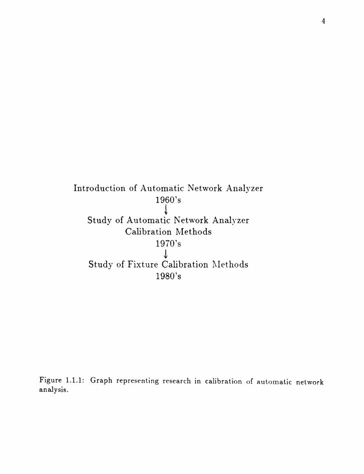
Calibration of automatic network analysis has been a popular research area

over the last two decades. Fig. 1.1.1 is an indication of past research effort and

potential research. The graph indicates three regions of popularity. First, the late

1960's when the automatic network analyzer was introduced, second early to mid

1970's study of ANA calibration methods and third, early 1980's to future, study

of fixture calibration methods. Our intention is to contribute to the rapid growth

of fixture calibration methods by developing methods that address printed circuit

board fixture calibration. In the following section we provide an overview of this

report.

1.2 Thesis Overview

The pur-pose of t his report i~ t"I'O fnld. Fired. t"I'O nrrrldps nf rpsp~rrh ha s i nt rorlu ce

a considerable amount of information concerning calibration of network analysis.

The purpose of Chapter 2 is to review calibration methods by organizing this

information into two catagories; one and t\\I'O port calibration. As an introduction

to this, we discuss the history of the Automatic Network Analyzer. One port

4

Introduction of Automatic Network Analyzer1960's

!Study of Automatic Network Analyzer

Calibration Methods1970's

!Study of Fixture Calibration Methods

1980's

Figure 1.1.1: Graph representing research in calibration of automatic networkanalysis.

5

calibration is discussed and concludes with a discussion of previous authors choice

of standards and their motivation. Two port calibration begins with a thorough

review of ANA error models and concludes with fixture two port models and a

discussion about fixture calibration standards. The second focus of this report is

application of symmetrical arguments to printed circuit board fixture calibration.

Printed circuit board is a non-insertable measurement medium and is easily cal­

ibrated using symmetrical arguments. Chapter 3 defines symmetrical arguments

and develops new calibration methods that exploit symmetry. Chapter 5 contains

the results from experimental verification the algorithms developed in Chapter 3.

Chapter 4 introduces SPAN A: Signal Processing of Automatic Network Analy­

sis; the computer program where algorithms are implemented and other various

data manipulations are carried out. Finally, we conclude with summary of work

accomplished and suggestions for future work in Chapter 6.

This report also contains three appendices. One contains a discussion of de-

cascading error networks and lists the necessary transformations. Another is a

user's manual for SPANA giving semantic information about commands that are

available. The last appendix discusses the SPANA "shell" com rna nrl where t.he

reader is lead through an example shell subroutine to show how it can be rnndifif'd.

1.3 Original Contributions

The original contributions reported here include:

6

i) the Through-Symmetry-Line de-emhedding algorithm whereby symmetric

arguments are used to synthesize either open or short circuit reflection coef­

ficients,

ii) the development of Enhanced Through-Symmetry-Line de-embedding al­

gorithm that calculates the cornplex characteristic impedance of the line

standard using the experimentally determined propagation constant and the

free-space capacitance of the line standard,

iii) the direct application of this enhancement to the Through-RefIect- Line de­

embedding algorithm and Line-Reflect-Line algorithm,

iv) the development of Through-Symmetric Fixture de-embedding algorithm for

use on second order symmetric fixtures, and

v) the development of the computer program SPAN A for algorithm implemen­

tation and other data manipulations.

7

Chapter 2

Review of Calibration Theory

2.1 Literature Review

The determination of network parameters or network analysis is fundamental to

the understanding and design of all microwave systems. It provides a tool for veri­

fication of theoretical research and gives design engineers data needed to complete

their tasks.

Before the introduction of the network analyzer in the late 1960's, one-port

impedance measurements dominated the measurement arena. Slotted lines and

graphical interpretation maintained engineers until the development of the network

analyzer. It was well understood that impedances could be measured through an

unknown junction. If the unknown junction is lossless and represented by an effec­

tive impedance, then reflection coefficient measurements with a matched load and

short circuit at the ou t put of the junction give sufficient information to determine

the unknown impedance. In 1953, Deschamps developed a graphical method to

determine impedance if the junction is Iossless. Through his result it was possi­

ble to determine the unknown impedance by synthesizing the matched load with

several offset shorts [1]. A similar process for lossy junctions was introduced by

8

Storer et al. [2] in 1953, where by the junction parameters (inpnt, output reflec­

tion coefficients, and transmission coefficient) could be determined by graphical

means. Finally, in 1956 Wentworth and Barthel combined this previous work and

introduced a simplified graphical calibration technique [3].

Graphica.l methods provide invaluable insight into processes that effect rru­

crowave measurement yet they are tedious and based on the users interpretation.

To advance the state of the art in microwave measurement it was necessary to

consider other methods for microwave measurement. In the mid 1960's, scatter­

ing parameters (s parameters) began finding use in the circuit design community

replacing reflection and transmission coefficients. The need to measure two-port

network parameters became increasingly necessary while existing one-port graphi­

cal methods provided no extension to two-port measurement. There is little doubt

why an automatic means of microwave measurement is essential and history shows

that two-port network analysis is inherently calibratable.

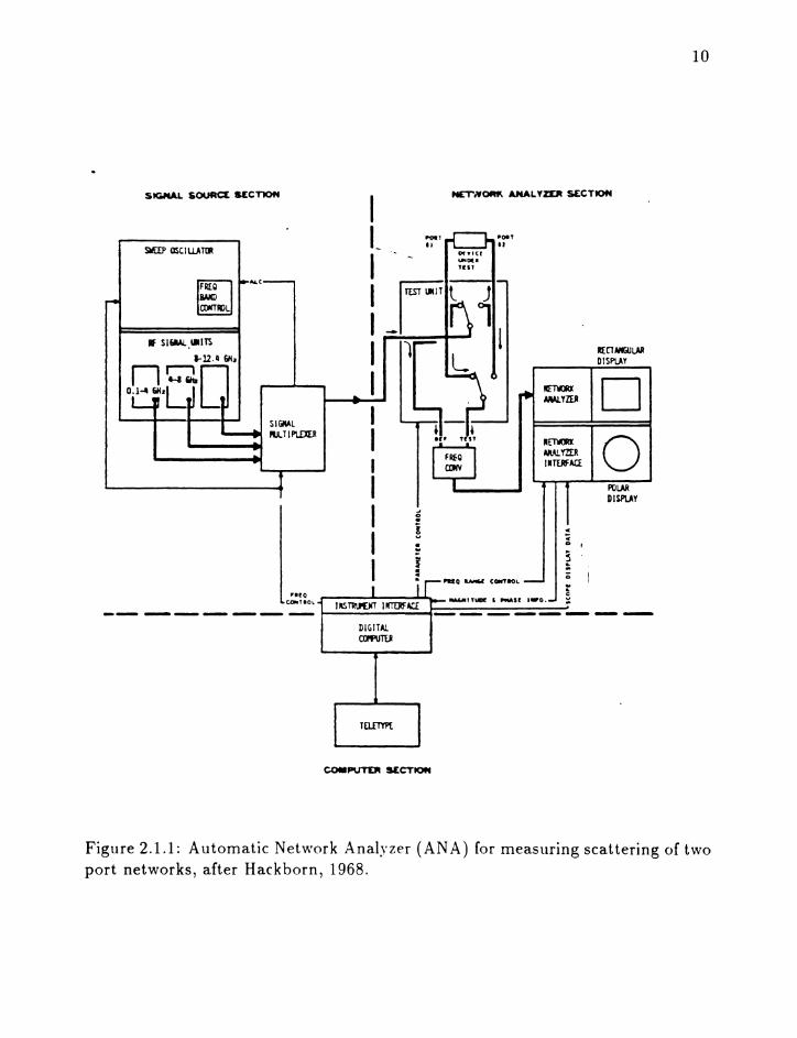
In the late 1960's Hackborn introduced the automatic network analyzer [5]

(ANA) capable of measuring scattering parameters of two port networks. The

way to assure accuracy. Calibration was analytic and performed by cornpu ter ron­

trol as compared to previous graphical methods and the automatic measurement

significantly increased measurement speed. By modeling the network analyzer

systematic error, Hackborn developed the foundation of calibra.tion in use today.

9

Imperfections in the network analyzer were modeled as deviations from an

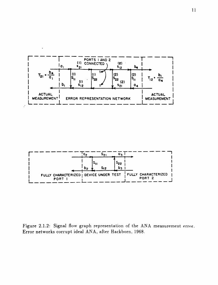
ideal analyzer and referred to as error representation networks, see Fig. 2.1.1.

Error for each AN A port was modeled with a corresponding scattering matrix

with four complex parameters and easily represented with a signal flow diagram,

see Fig. 2.1.2. Since graphical calibration used known standards e.g. matched

load short circuits or offset short circuits, it would seem appropriate to measure

similar standards with the new ANA in order to determine the error networks i.e.

calibrate. This is exactly what Hackborn did.

First for one port calibration, he measured reflection coefficients with the error

network terminated with an ideal short circuit, offset short and sliding matched

load. These three measurements were sufficient to determine the error network

and repeating this procedure for the second port gave six calibration terms (error

s parameters or products. This result was sufficient for one port measurements

on either ANA port but {or full two port measurements two additional calibration

terms needed to be calculated. A measurement of forward and reverse transmis­

sion coefficients with the error networks connected together (through connection)

completed the two port calihra t ion procedure. Finally, t he removal of the error

involved an iterative solution of nonlinear equations based on the signal Ilovv diu­

gram of the device placed between the port error networks. Soon after this work

was published, Kruppa and Sodomsky revealed that Hackborn's iterative solution

was in fact explicit [8].

5 GNAL S()UA(% HenoN

SWEU OStIw TtIt

1= ICDKTJI>L

If S161Al.WlITS

1-12.Q &HInQ0.1-- 6H.I

SIWLJIIJlTlPlDD

IL

REClMGULARDISPlAY

~ DMAL.YZD

"E"T'Ol 0Nll.!..mRIITUtFACL

POWDlSfUY

c•Q

10

~~~OL .----......--.....---- IWoC.'IITUDr , PMsr .-0.

-- - - - - - - ~==~~~=-l====-===-====-:DIGITALCIJlf\llU

T[L[lYP[

Figure 2.1.1: Automatic Network Analyzer (ANA) for measuring scattering of twoport networks, after Hack born, 1968.

11

r----I---PORTS~~----r---lI I (1) CONNECTED (2) . I II a, '21 512 ~ II T

Z1s b4 I (I) (I) 1 (21 (2) b, I

I a'I 5" m . ~ ~ (2) 51! T'2· a; II I b. 512 521 04 II ACTUAL I I ACTUAL :

~E~REMENi~RRO~EPRESEN~IO~TWORK__~EASUREM~~

r--------~~--~--~T-------i

I I ~ I II I SII Sz2 I II _ I b2 , _ 5'2 _b3 I I

I FULLY CHARACTER~ZED IDEVICE UNDER TEST IFULLY CHARACTERIZED IL ~RT_l__ L ~-_~OR~~__ ~

Figure 2.1.2: Signal flow graph representation of the ANA measurement error.

Error networks corrupt ideal ANA, after Hackborn, 1968.

12

Since the introduction of Ifackborn's AN A many authors have considered its

use and studied network analyzers of different component topologies. IIackborn's

error models have stood the test of time only receiving minor improvements. His

contributions include one and two port error models represented by signal flow

diagrams and calibration algorithm for removing these errors.

The history of network analysis calibration shows a significant change as meth­

ods of network analyzer calibration became widely accepted. At this point, authors

began considering fixture calibration rather than ANA calibration since many de­

vices to be measured were in transmission media that was of dissimilar geometry

than the analyzer i.e. planar devices and coaxial analyzers. One and two port

error models were still valid only the physical interpretation of the error terms

changed. This resulted in direct application of network analyzer calibration meth­

ods to fixture measurements. However this was only moderately successful and

new procedures were developed.

2.1.1 Introduction to Calibration of Network Analysis

gate subtopics that form the calibration process. First we must look at one port

measurements and discuss general methods of accomplishing one port calibration

followed by a review of previous investigators. Second we expand one port results

to two port and discuss the motivation of major contributors who evolved the

13

Hackborn error model.

2.1.2 The One Port Error Model

The measurement of reflection coefficients or impedance at microwave frequencies

requires the determination of systematic error and then removing it i.e. calibrating.

Here we state one port calibration in a general fashion and then review calibration

methods developed by previous authors. The Hackborn one port error model

shown in Fig. 2.1.3, has been examined by many authors. The measured reflection

coefficient Pl'tf is related to the desired reflection coefficient PL by the familiar

bilinear transform.

Rearranging,

PAl == (2.1.1)

(2.1.2)

(2.1.3)

we can see that the desired reflection coefficient is altered by the error network

which is comprised of scattering parameters eoo, Ell' and the product EOlelO' Two

methods exit for calculating the error network: classical three te rtu i na t i-m «llId

redundant terminations, or the impedance associated with PL can be determine

without calculating the error network by using properties of the bilinear transform.

Let us consider these in more detail.

]4

e10a 1~---...- -~

eoo) ella I fL

~'-----~---_-.:..''- -~·-r

(-lola

Figure 2.1.3: Signal flow graph for one port error network. Desired load r~nprfinn

coefficient PI is masked by error coefficients eij and Pm is the measured reflectioncoefficient.

]5

Classical Result of One Port Calibration

Classical one port calibration is the calculation of these terms based on measure-

ments made with three known terminations (standards) connected to the refer-

ence plane. The standards have associated reflection coefficients r 1, r 2 and I'3 and

corresponding measured reflection coefficients 1\[1, A[2 and 1\13. These reflection

coefficients along with equation 2.1.2 form three simultaneous equations for the

error terms with the solution:

~4 - 1ell =

~4r 3 - r 2

( ..~ [2 - 1\II )(1 - elI r 1 ) (1 - elI r 2 )

f 2 - I',

(2.1.4)

(2.1.5)

and

with

(2.1.6)

(2.1.7)

A final measurement and evaluation of 2.1.2 with the desired load in place yields

the error corrected reflection coefficient. When a sweep frequency measurement is

required, these error terms are calrnlaf.ed for each Irequen cv therehv providing an

error corrected reflection coefficient versus frequency.

Use of Redundant Standards

Three standards are necessary and sufficient but sensitive to experimental error.

In 1974 Bauer and Penfield developed the use of redundant standards to improve

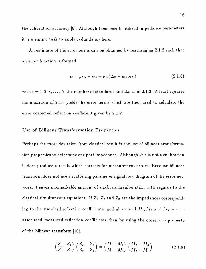
16

the calibration accuracy [9]. Although th eir results utilized irn pedance pa ra meters

it is a simple task to apply redundancy here.

An estimate of the error terms can be obtained by rearranging 2.1.2 such that

an error function is formed

(2.1.8)

with i = 1,2,3, ... , N the number of standards and ~e as in 2.1.3. A least squares

minimization of 2.1.8 yields the error terms which are then used to calculate the

error corrected reflection coefficient giyen by 2.1.2.

Use of Bilinear Transformation Properties

Perhaps the most deviation from classical result is the use of bilinear transforma-

tion properties to determine one port impedance. Although this is not a calibration

it does produce a result which corrects for measurement errors. Because bilinear

transform does not use a scattering parameter signal flow diagram of the error net-

work, it saves a remarkable amount of algebraic manipulation with regards to the

classical simultaneous equations. If Zl' Z2 and Z3 are the impedances correspond-

associated measured reflection coefficients then by using the cross rn t io property

of the bilinear transform [10],

(2.1.9)

]7

we can directly find the luad im ped ance Z Irorn the measure of its reflection

coefficient AI.

]'.[ -]'.[1 ]'.[2 - 1'.[3

1'.[ - 1113 1'.[2 - 1'.[1

Z2-Z3Z2- Z 1

(2.1.10)

(2.1.11)

The classical corrected reflection coefficient can be used to determine this impedance

however the converse is not true because the reflection coefficient is a function of

the output impedance of the error network which we do not know.

Classical one port, redundancy, and bilinear transform methods encompass the

published results of this area of microwave measurement. The classical one port

is frequently discussed by previous authors and it is directly extendable to two

port calibration. This extention will be discussed in subsequent sections, but first,

discussion of one port calibration standards will conclude the one port methods.

2.1.3 One Port Calibration Standards

Previous authors introduced three known terminations for use with the classical

one port calibration. The investigators were motivated to use their standards

choice for standards was influenced by need. A direct short circuit, offset short,

and a sliding load were used [5]. He chose the sliding matched load because it

compensates for an imperfect load. Since then authors have studied the sliding

load in great detail [6,7].

18

In 1971, Kruppa and Sodomsky used open and short circuits, and a matched

load [8]. Their apparent motivation was the simplicity these ideal standards offer

to the calibration equations. In 1973, Da Silva and Mc Phun replaced the sliding

load with a direct short circuit and two offset shorts [11]. A short circuit was

convenient and required less space. Similarly, Shurmer was motivated to avoid the

sliding load. His standards included an open circuit, direct short, and offset short

[12]. Gould et al. used matcheclload, short circuit, and mismatch load standards

and they were placed directly at the reference plane. Gould chose these standards

because their characteristics vary slightly with frequency therefore reducing the

need for accurate frequency measurements [13]. In 1974, Kzisa analyzed the sliding

termination and found that it was possible to use a known load with two different

sliding terminations [6].

In each case, the authors have indicated that the standard terminations where

known either by an ideal assumption or appropriate model. For example, short

circuits or offset shorts are assumed ideal with reflection coefficients of r = -1

or exp jfJ. An open circuit standard is assumed ideal or the parasitic capacitance

associated with fringing electric field is determined. Of course this capacit a nce is

geometric and frequency dependent and can be difficult to determine. Tu improve

calibration accuracy we need to increase the certainty of the standards used.

In 1978, Da Silva and McPhun examined redunda.nt measurements as a method

to reduce the uncertainty of their standards i.e. combinations of short and offset

19

short circuit terminations, or open and offset open circuit terminations [11]. Their

motivation was straight forward: offset standards require knowledge of the prop­

agation constant of the offset line. A fourth standard (one redundant standard)

gave sufficient information to determine the line propagation constant and if a

fifth standard was used, it was possible to determine the reflection coefficient of

an unknown termination such as an imperfect open circuit.

From this summary, it should be noted that ,"re can use any combination of at

least three standards and the choice is influenced by the accuracy of the standards.

Many of these authors provided an extension of their one port result to a two port

calibration procedure with Hackborn leading the way. Moreover , with a similar

format as one port calibration methods, we will discuss t\VO port calibration.

Two port calibration, containing additional error terrn s , has undergone changes

since the Hackborn model. First, let's examine the Hackborn two port model then

discuss the motivation of authors that followed him, a.nd finally, look at the most

recent model.

2.1.4 ANA Two Port Error Models

Common to all two port calibration methods is the attempt to rno dvl syste-m

imperfections with error networks. These networks, being system dependent, have

taken on different descriptions to suit the system designer. Hackborn extended

his one port model to two port by connecting the reference ports together and

20

measurIng Iorward and reverse t ran smission frum port une tu two. Fig. 2.1.4

shows the signal flow graph his through connection. These measurements were

sufficient to calibrate his AN A giving a total of eight error terms, six one port

error terms and two transmission terms. This eight term result is derived assuming

that no leakage path exits between ports, an assumption which seems intuitively

impossible.

In 1973 Shurmer introduced the concept of leakage and developed a six term

two port error model [12], or simply a "one path" model. Shurmer's motivation

was straight forward, his network analyzer was not automatic. That is, he used

two hardware configurations, one for reflection and another for transmission mea­

surements. This required a reversal of input-output connections of a device under

test (dut) to measure its s parameters. Fig. 2.1.5 shows the "one path" model

introduced by Shurmer. If leakage was important for this model why not Hack­

born's eight term model? Rehnmark, in 1974, introduced the ten term model by

including forward and reverse leakage in the Hackborn model [15], see Fig. 2.1.6.

Automatic network analyzers used today model system error with a twelve term

monel which is a Shurrner one pa t h for earh direction. This idea "TClS int rod nred

in 1978 by Fitzpatrick and is shown in Fig. 2.1.7 [16]. However, it is not t.he most

comprehensive model that exists. Digressing for a moment, we need to briefly

discuss components that are used in constructing an automatic network analyzer

to fully understand this comprehensive model.

21

EXF,-'7--- ----------- -.--",---.......,-, SI - - 2J",

: ETFII

: 51 J• ERRRFIN F u-T--t~-r~~-,--'-...,.-o--4-.....--.. n

Ia

EOF ESF : 522•I

SII. ESRII•

DEVICEUNDERTEST

IIIII,II

-~--"""'-- 4---- -- --- ------ __ -JEx..

Figure 2.1.4: Through connection of the eight term error model. Each port IS

described with four 5 parameters, Si~2, after Hackborn, 1968.

Reference 1 5 21

Reflectioneoo e,l Js~ E:MR e0 1 t 5 12 t

Unknown Return

TransmissioftM,

Figure 2.1.5: One path error model. Six error terms, eij embed the device sparameters, Sij and for full characterization the device must be reversed.

22

erence)

r-30

nee~10

Js~21~r32 M..... -- - -- - - - --(M

a fOO r11 r22 I r33- -- - -)~ . ~ - --f0 1 5 12 f

23 (RefI

-

R.fere

Figure 2.1.6: Ten term error model. Extension of Hackborn model bv includingthe leakage to and from each port, e30 and e03, after Rehnmark, 74.

ELF, ELR-Load Match

ETF, ETR-Trans. Tracking

EXF, EXR-Isolation

2J

RF IN1

PORT 2III

IELR I

II

EDF, EDR-Directivity

ESF, ESR-Source Match

ERF, ERR-Refl. Tracking

PORT 1II

REVERSE I

S12A II

PORT 2

DUT

ERF II

PORT 1

EXR III

FORWARD:

II

1 IRF IN

Figure 2.1.7: Twelve term error model. Introduce by Fit.zpatrick, this model is adual "one path". Full characterization of the device is done without interchanging

ports.

2,t

True automatic network analysis frees the user from interchanging the dut

connections. This useful feature is possible by redirecting the microwave source

between measurement ports and possibly using one complex ratio detector to

determine amplitude and phase information for both ports. Under this condition

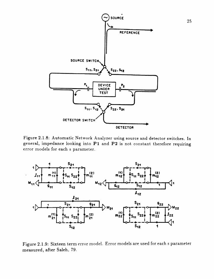
two switches are needed as shown in Fig. 2.1.8. In 1979, Saleh examined this

test set indicating that the measurement port impedances looking into PI and

P2 can be functions of the switch positions [17]. In other words, a general error

model would require terms that model each s parameter measured, Fig. 2.1.9, and

a solution of systems of nonlinear equations would be necessary for calibration.

Fortunately, test sets can be designed that do not require this general model.

For example, by using two detectors it is accurate to use the twelve term model

mentioned above.

Up to this point, we have discussed two port error models needed for calibrating

network analysis. Each author has developed a calibration method based upon

their model yet they have chosen from the "available" one port standards. We

find that new standards were introduced after these models had become widely

accepted and calibra tion of network analvsis hegan focusing on fixt ure r alilira t ion.

The next level of discussion applies these models to fixture calibration wit h the

assumption that the network analyzer has been calibrated using one of the above

models. This is important to note since it will be shown that fixture error models

are comparatively simple wit h regards to the number of error terms. In fact,

SOURCE2.5

REFERENCE

SOURCE SWITCH

SZ2' SZ1

DEVICEUNDERTEST

DETECTOR SWITCH

DETECTOR

Figure 2.1.8: Automatic Network Analyzer using source and detector switches. Ingeneral, impedance looking into PI and P2 is not constant therefore requiringerror models for each s parameter.

1 521 5211 -.--rJ --+-

(1 ) I I (2) (1) I I (2)111 m11 "511 522+ m11 m12 ~S11 S22t "'12

I I : IM11

L_+_..& M12 - ..-~ 1

911 512 ~2 512 1

l12J 21

1 521 021 521 Q221 r-"- M21

o-~-'M22

I I (1) I I (2)(1) ~ t m(Z) m22 "5-.1 522 t m22 J22m 21 1511 5221 21 I IL_.. _ -+-- 1512 512 1

Figure 2.1.9: Sixteen term error model. Error models are used for each s parameter

measured, after Saleh, 79.

26

Chapter 3 develops new calibration methods that exploit the simplicity of fixture

error models.

2.1.5 Fixture Two Port Error Models

The s parameter measurement of an arbitrary t\VO port network can be divided into

two tiers. First we have the calibration of the network analyzer, i.e. measurement

and calculation of AN ..~ error terms, and second we need to interface our arbitrary

network to the network analyzer. This interface or adaptor is commonly referred

to as the fixture. For example, if we were interested in measuring the s parameters

of a microstrip transmission line we need a fixture to adapt from a coaxial AN A to

microstrip and then back again, Fig. 2.1.10. Fixturing introduces error into our

measurement and modeling and additional calibration measurements we can re­

move this error. This fixture calibration is sometimes referred to as de-embedding

because the device to be measured is embedded within the fixture. From this point

on the terms calibration and de-embedding will be interchangeable.

Fig. 2.1.11 shows the fixture error model. It is composed of two error networks

classical one port calibration, there are six independent error terms for t his model

and we can use one port calibration standards to calculate them. This result is

accurate if forward and reverse transmission through the fixture are equal. Fig.

2.1.12 shows a signal flow graph for the fixture error, and application of Masorr's

.:Microstrip Line

Coaxial Reference Planes

, ,, ,

:~ L .:, .

"'/MicrostripReference Planes

Figure 2.1.10: Example of microstrip t\VO port fixture.

27

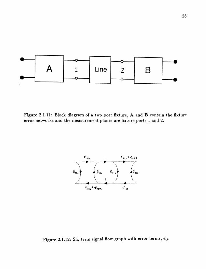
A 1 Line 2 8

28

Figure 2.1.11: Block diagram of a two port fixture, A and B contain the fixtureerror networks and the measurement planes are fixture ports 1 and 2.

~----I----"------'-"""""""----+- ----,e'Ob

Figure 2.1.12: Six term signal flow graph with error terms, eij·

29

rule verifies this fact. In general, a fixture is passive and non magnetic therefore

must have equivalent forward and reverse transmission coefficients. This is the

only difference between Hackborn's ANA two port error model and the six term

fixture model. The ANA, however , can only be minimally modeled by the eight

term two port model. Additionally, fixtures can be constructed such that port to

port coupling is much smaller than that internal to the ANA and we do not need

to modify the fixture error model. The disadvantage with fixture de-embedding

is that its geometry can be very different from one port calibration standards

discussed above.

Unfortunately many fixtures encountered in microwave measurement can not

use the classical one port calibration standards and there exits a need for unique

two port fixture standards or de-embedding standards. To strengthen this point,

consider a microstrip fixture. We have seen that it is advantageous to use a

matched load standard since it allows direct measurement of one error term. This

of course assumes we know its reflection coefficient. In microstrip we can not fab-

ricate an effective matched load and a sliding termination is physically impractical

so we must 1) se ot her st an rI a rd s. Sirnl1c:l rlv a n open r irr-n it. ~1 anna rrl is rli ffi r ul f t.o

model so we need to avoid it as well.

2.1.6 Fixture Two Port De-embedding Standards

How can we de-embed planar fixtures? Most classical one port standards can not

be used so we need to introduce standards unique to two port de-embedding. It

is well known that we can calculate the two port parameters of a transmission

line of different geometries. By measuring our fixture with a known two port

(transmission line) inserted between the fixture error networks we introduce a

distributed de-embedding standard.

In 1975 Franzen and Speciale introduced distributed standards for calibrating

their AN A. Although their result is not a two-tier approach it is significant be­

cause they were the first to introduce distributed standards. Their technique was

conveniently called Through-Short-Delay or TSD [18].

At this point we would like to briefly outline the next discussion of various

fixture calibration procedures. First \\Te will look at the standards used and con­

sider the authors motivation and second we will examine the disadvantages we can

encounter when using them.

TSD - Through-Short-Delay

TSD is based on both reflection and transmission measurements and it ()rrer~ f \YO

advantages. First, a matched load standard in not required and second it uses

mechanically simple standards. In addition, Franzen and Speciale found that an

addition delay line could be used to insure consistency within their measurements.

31

TSD is not without disadvantage. The delay standard was assumed lossless and

nonreflecting i.e. the propagation constant was pure delay and the impedance was

that of the measurement system or 50 ohms. Also, TSD although not mentioned

by these two, requires information from two delays; the through connection and

the actual delay. If the phase difference between these two is near zero or 180

degrees the algorithm will fail to return a valid result. This is a limitation of any

de-embedding technique that uses a delay type standard. Franzen and Speciale did

not apply their results to a planar fixture but their work is significant. In 1976,

Bianco et al. considered the planar problem first hand by applying distributed

standards to a microstrip fixture [19].

Line-Offset Open-Line

Bianco used a total of three distributed standards; two delay lines and one offset

open circuit for de-embedding standards. Just as with TSD, the delay lines were

nonreflecting but they were not assumed lossless, in fact, the propagation constant

and open circuit reflection coefficient could be determined for the microstrip line.

The mechanics of their de-embedding required a separate measurement for each

inserted delay line and a one port measurement with the error networks terminated

with the offset open circuit. Of course their algorithm was subjected to the 180

degree bandwidth limitation wit h an added problem. When two delays are used

it is assumed uniform and they have equivalent characteristic impedances. It is

interesting to note that this result was reintroduced in 1979 by Engen and Hoer

32

under t he familiar name Thru-ReAect-Line [20].

TRL - Thru-Reflect-Line

TRL as developed by Engen and Roer used only one delay standard wit h a through

connection and an arbitrary reflection to calibrate their network analyzer. The

delay standard could be arbitrary, that is, its propagation constant need not be

known, however, the line was assumed nonreflecting. The reflection standard

could be any repeatable reflecting load and they suggested either an open or short

circuit. Again, this result was stated by Bianco but Engen was the first to consider

algorithm singularities associated wit h distributed standards.

Neither the Bianco or Engen work had been applied directly to a fixture.

Benet, in 1982, introduced the universal 1\f11IC test fixture that required sev­

eral distributed standards for calibration yet they chose yet another calibration

algorithm.

Open-Short-Five Offset Lines

Benet developed the open-short-five offset line calibration using a one tier ap­

proach [21]. As discussed before, the one tier calihratioll is usually n'IItnl'" Oil

the twelve term AN A error model, t hat is, six for each direction of measurement.

To determine the six terms Benet measured the fixture's response with open and

short circuits at the fixture reference plane and then a minimum of three offset

thru lines were inserted and measured. By approximation the offset lines caused

the measured reflection of the fixture to scribe a circle and at the center was an

additional error term. Two additional offset lines were used to allow a least squares

fit of the circle to these measurements. Returning to the open and short circuit

error equations, he showed that two additional error terms could be determined.

Finally, by approximation he determined the propagation constant of the thru

lines and the remaining error terms. Benet's contribution showed that insertable

distributed standards could be used to calibrate a test fixture. Next we will see

that a two tier de-embedding method obtains a similar result and requires fewer

assumptions.

Open-Short-Modeled Through Line

Under some circumstances the fixture can not be calibrated using insertable stan­

dards such as a transistor test fixture. Here the fixture can not be separated

to insert the de-embedding standards. In 1982 Vaitkus and Scheitlin proposed a

method of de-embedding such a fixture by considering a two tier de-embedding

method. The AN A was first calibrated using OSL and its twelve term error model

and then fixture de-embedding measurements were done. Their standards were

an open and short circuit and a modeled through line [22]. The error model was

simply a one port error network for each fixture port and tV-TO leakage terms to

compensate for a leakage path around the transistor chip. This is a simplification

of Rehnmark '8 ten term AN A error model. Vaitkus and Scheitlin exploited the

passive nature of the fixture and the assumption that forward and reverse leakage

34

would be identical. This allowing them to reduce the total number of error terms

to seven. Comparing this de-embedding result with Benet's, simplification is pos­

sible if a two tier calibration/de-embedding method is applied because the fixture

offers a reduced number of error terms.

A through line standard had been previously used by others but Vaitkus dif­

fered by using a modeled through line and determined its equivalent circuit by

optimization. A bond wire through line connected the fixture ports together and

the equivalent circuit was optimized to fit the measured fixture s parameters.

A similar procedure was performed on the bond wire short circuits. Vaitkus and

Scheitlin produced results using a through line standard but a general examination

of Open-Short-Through line was introduced later by Vaitkus himself [23] in 1986.

Rather than model the through line, he assumed knowledge of line propagation

constant, short circuit inductance, and open circuit capacitance.

Double Through Line

In 1987, Pennock et al. introduced a de-embedding technique for characterizing

transitions between novel transmission media [24]. Their motivation was a lack of

conventional standards and a need to reduce the tot al ueedvd. In 1!ri(i, I ~i(t fH"O ct

ale eluded to the fact that transition parameters could be determined to within a

multiplicative constant if only two through line standards are used [19]. They also

showed that measurement of an additional through line was a linear combination

of the first two and the constant could not be determined. Pennock exploited

35

the multiplicative constant and proceeded to use two line standards for their de­

embedding.

Their fixture error model was the commonly used six term two port error model

and we know that to completely characterize it we need three standards. Pennock

showed that the Bianco constant was a ratio of two error terms. In fact, this

ratio is nearly equal to unity for reasonable transitions and Pennock proceeded to

de-embed the fixture under this assumption.

This result is not without problems. First, as stated before distributed stan­

dards must avoid >../2 singularities and second, the line must be reflectionless.

Additionally, the line attenuation constant is known or assumed equal (lossless

line) .

TTT - Triple Through

In 1988, Meys introduced a fixture de-embedding method that uses an auxiliary

two port and matched load for standards [25]. Beginning with the standard two

port error model, the A and B error networks are connected together and mea­

sured. Also, the auxiliary two port C is cascaded to either side of A a nrl n t.o

form the measured two ports Be and CA. These and the AB t\VO port provide

necessary but not sufficient information to determine the error networks. TIle

reflection coefficient for the auxiliary two port terminated with a matched load is

sufficient to determine the error networks.

The use of a matched load is undesirable but Meys points out that if the C

36

two port exhibits low SWR we can assume its reflection coefficient is zero and

eliminate the matched load requirement. Since distributed standards are not used

TTT is inherently broad- band.

Results of Eul and Schiek

In 1988, Eul and Schiek examined the conventional two port measurement system

from a linear algebraic point of view. Their worked showed results noted by previ­

ous authors such as a need for at least three de- embedding two ports for complete

characterization and previous de-embedding techniques. Their main contribution

was the study of redundancy [26]. When three standards are inserted between the

error networks and subsequently measured, the total number of unique measured

quantities is twelve, yet there are only eight error terms linearly independent.

This redundant information can be used to reduce the required knowledge of the

standards used and as a result they proposed several de-embedding methods Thru-

Match-Reflect is one example.

TMR - Thru-Match-Reftect

Thru-f'vlatch-Reflect uses a through connection, a matched luad (Of a ny other

known reflection coefficient) and an arbitrary reflection. It offers the broad-band

advantage of these standards however we need a prior knowledge of at least one

standard i.e. the matched load. The reader is referred to [26] for discussion of the

calibration algorithm used with these standard combinations.

37

2.2 Conclusion

The review of calibration theory encompassed one port measurements, automatic

network analyzer error models and calibration methods and finally fixture de­

embedding. It is clear that calibration of network analysis has been an ever chang­

ing study covering much of our recent history. It contains a variety of methods

because the results of one may not be applicable to another or someone has a

unique de-embedding requirement. It is important to note that when approach­

ing a calibration dilemma one should look at the problem from a know / unknown

point of view. In other words, consider the total number of unknowns in the mea­

surement system and then decide on the variety of standards that are available.

We feel that this review has provided the insight into calibration methods and

hopefully given the reader a "what if we use ... " attitude towards their calibration

of network analysis. The next chapter approaches new calibration methods and

embodies this philosophy.

38

Chapter 3

Calibration Using a Symmetric Fixture

3.1 Introduction

As we have seen from Chapter 2, it is clear that a calibration can take many forms.

Naturally, we feel that another calibration topic remains untouched; exploitation

of the symmetrical nature of measurement fixtures. As with past calibration meth­

ods, there was a need for something "new" and we are similarly motivated with

this study.

Chapter 3 concentrates on discussing advantages of symmetry arguments, re­

viewing symmetrical de-embedding methods, and the development of two new

symmetrical de-embedding algorithms. In addition, we will re- examine TRL cal­

ibration and develop a practical enhancement.

3.2 Motivation for Using Syrnmet r ical Argurnents

When considering the history of calibration of network analysis, two directions

have been pursued by the measurement community. On one hand, there was a

need to compensate for imperfections in calibration standards, and on the other

hand, calibration accuracy is directly related to the certainty of standards and if

39

at all possible choose the minimum necessary. A symmetrical argument allows a

reduction in required standards thereby improving the certainty. In fact, later in

this chapter we show that it is possibly to reduce the total number of standards

to one. With this in mind, when can we use a symmetric argument or when is a

fixture symmetric?

3.3 Evolution frorn an Asyrnmet r-ic to Symmetric Fixture

A symmetric fixture is a special case of the general asymmetric fixture. In Fig.

3.3.1, we see the conventional two port error network and its corresponding signal

flow graph. It is composed of two error networks A and B and in general, the

individual signal paths 5 i j a and 5 i j b are unique forcing fixture s parameters 5 i j /

to be unequal to each other. This represents an asymmetric fixture.

A fixture is symmetric if the port 1 and 2 reflection coefficients are equal and

the fixture is reciprocal, i.e. if 5 11/ == 5 22/ and 5 21 / == 5 12/ . Reciprocity is true

when the fixture is passive and non-magnetic and these symmetrical equalities are

possible with two orders of symmetry; first and second order.

are related to the individual error terms,

S - C' S21a Sl2a S l l b11J - ,,"7 11a + 1 S S

- 220 lIb(3.3.1)

(3.3.2)

•e-

B-..,

40

~Il t/

--- -----.--~

Sl2(b)

elOa 1 eOl b

~.--~. '<, • -

eoo) (ell. I ell) tOOh

~~ ~- < ~ ~

eOla elOb

(c)

Figure 3.3.1: Two port error model for an asymmetric fixture (a). Fixture errorcan be described with eight error term SijQ and Sijb. Port 1 and 2 are the calibratedANA measurement ports. Sijj are the measured fixture s parameters.

41

and

SS12aS12b

12/ =1 - S22a S l l b

(3.3.3)

(3.3.4)

Equating 3.3.1 and 3.3.2 and applying reciprocity we find one equation in six

complex unknowns.

(3.3.5)

This is the symmetry condition equation representing an under determined sys-

tern. This implies that symmetry can be produced with an infinite number of six

error parameters. Fortunately, symmetry corresponds to the physical nature of

the fixture which limits the symmetric solutions to two; first and second order

symmetry.

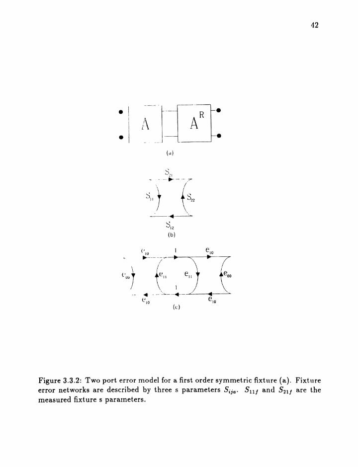
3.3.1 First Order Syrnmetr ic Fixture

A first-order symmetric fixture has identical fixture halves that are asymmetric,

see Fig. 3.3.2. The port two error network, B, is now a port reverse of A, or

c;'} ~ [. ,r ('( )v f' rI 2 II,' 1\ ,

these conditions satisfy the symmetry condition equation 3.3.5. A "coaxial to rTll-

crostrip" - "microstrip to coaxial" fixture is an example of first order fixturing.

Most important, the signal flow graph shows that the symmetry reduces the num-

ber of error terms to three, that of the A network only. In other words, symmetry

•

•(0)

•

42

elO

1 e lo~-----.- • "" • 7I

I

(. 7 \~Il ell \00uu

.- --~--+-<' ~------""-

t'10 e,o(c)

Figure 3.3.2: Two port error model for a first order symmetric fixture (a). Fixtureerror networks are described by three s parameters Sija. 8 11J and 821J are themeasured fixture s parameters.

43

allows a reduced number of error terms for a two port fixture, and this reduction

is strictly a function of the manufacturing repeatability with direct application to

printed circuit board measurements.

3.3.2 Second Order Symmetric Fixture

If the fixture halves are identical and symmetric, the fixture is second order sym­

metric. This implies that network B is equal to A or all reflection s parameters,

Su; or 5iib , are equal,( = 5 11 ) and all transmission s parameters are equal, Sija or

5i j b , (= 5 21 ) , see Fig. 3.3.3. A second order fixture satisfies the symmetry condi­

tion equation 3.3.5 and a lumped element transistor test fixture is an example of

second order fixturing.

3.4 Review of Syrnrnet r ical Methods

Previous authors have examined symmetric fixtures. In 1982, Souza et. al. used

a rnicrostrip first order fixture to develop a method to calculate the fixture half.

Their results are based on further assumptions. First, the microst rip line used

fixture half has a low return loss [27J. However, this result can not be applied to

a fixture that introduces significant error. If the fixture microstrip line impedance

is different from 50 ohms, both assumptions are invalid.

In 1983, Pollard and Lane indirectly used a first order symmetry assumption

44

e- ••A A

e-

(0)

s,H _ ~ _______

, I

SII} (~2~._--.-~

S12(b)

Q' Q

.--.----;;--

6 (6 IJ {61 ,

./ ~~ ~./

~

a Q'

(c)

Figure 3.3.3: Two port error network for a second order symmetric fixture. Fixtureerror is described with two s parameters 5 1 1 and 5 2 1 .

45

by modelling their fixture half wit h a pi equivalent circuit with different shunt

capacitances [35]. Their calibration standards are an open and short circuit and

a through connection. The fixture input impedance equations for the open and

short standards give sufficient information to extract the pi equivalent parameters

if second order frequency terms are neglected. As with the Souza result, they use

assumptions in addition to symmetry. Their result is invalid when the fixture is

considerably long or can not be modeled with a lumped element circuit. In 1986,

Ehlers was the first to apply symmetry without additional fixture assumptions.

Ehlers studied a finline first order symmetric fixture. The standards include

a through connection and either a matched load or a reflectionless transmission

line [37]. He pointed out that a symmetric fixture requires two standards for cali­

bration. This is true only if the matched load or a reflectionless transmission line

can be fabricated. If neither are accurately possible (as is the case for microstrip

fixtures) then an additional standard is needed. For the finline example his result

is adequate.

Most recently, In 1989, Enders developed an iterative de-embedding method

that uses three line standards to determine the pararnet ers of a first order fixture

[36]. His result affirms the belief that symmetry is useful for calibrating fixtures

and in the next section we will apply symmetrical arguments and distributed cal­

ibration standards. A second order fixturing was examined by Martin and Duke­

man in 1987. They found that a second order fixture requires only one standard;

46

a through connection [31]. Their result uses extensive matrix renormizations that

need not be done and in a following section a similar result based on signal now

theory is developed.

3.5 Development of Through-SYlllmetry-Line - TSL Using

First Order Symmetry

3.5.1 TRL to TSL

As we have seen before, the calibration of a planar measurement fixture, e.g.

microstrip and stripline, requires distributed standards. The preferred method

for planar fixture de-embedding is Thru-Reflect-Line (TRL) or Line-Reflect-Line

(LRL) because the distributed standards are easily modeled and constructed. A

typical microstrip fixture, shown in Fig. 3.5.1, is a first order symmetric fixture.

Identical coax to microstrip transitions and identical microstrip line lengths are the

requirements for symmetry. These can be achieved into low microwave frequencies

and at higher frequencies through careful design.

Because first orrler svrnrnetrv allows 1he fixt nre t o he rpprpsentpd 'Ylf h f hrpp

error terms, three standards are needed. Symmetry permits synthesis of 'I'Rl,

reflection standards thereby eliminating their need. TRL standards are shown

in Fig. 3.5.2; through connection, an reflection and a reference transmission line

of length I. The reflection is arbitrary and is typically a short circuit. For the

47

GroundPlanes

I' Embedded

- ....~ MicrostripUne

,

:~ L =348 mils

L =1348 mils(a)

Coaxial Reference Planes

8M .. QJ. ..~ MicrostriP~" Q.? ..A ~ Reference Planes

M1 M2

Vi

(b)

Figure 3.5.1: Typical microstrip fixture.

18

e h

AJ-("">-1~:n~1-~ r~ B--(") -c~-

-- --- -

-- .•

Figure 3.5.2: TRL calibration standards. (a) Through connection, (b) Arbitraryreflection, r, placed at each fixture port and (c) Line connection.

·19

symmetrical through connection, we can calculate the reflection coefficient with

the microstrip ports terminated in ideal open or short circuits. Either synthesized

reflection coefficient can be applied to the TRL algorithm. Conforming to the

naming of de- embedding methods we will refer this substitution as Through-

Symmetry- Line or TSL.

3.5.2 Synthesize Reflection Standards

The TSL standards are a through and line connections, Fig. 3.5.3. These are

similar to Souza et al. [27] however their result is based on symmetry and a

low fixture return loss assumption. Note, the symmetry reflection coefficients can

be used with the LRL algorithm with similar results. Next we will expound the

derivation of ideal open and short circuit reflection coefficients.

Referring to the signal flow graphs of Fig. 3.5.4, we consider the through

connection 5 parameters given by, 511 / ( == 522 / ) and 521 / ( == 512 / ) , and the actual

parameters of the A network being 0, Q and 1 for 5 110.,5210. == 5120. and 5220.

respectively. In addition, the input reflection coefficient with an ideal short circuit

placed at port. 1h of A is

(3.5.1)

Before we used Mason's rule to relate the fixture parameters to the individual

network parameters 3.3.1 - 3.3...1 here a similar result is given for the first order

50

.--A.-

--.BThrough

(a)

:G:J~D Delay t:r B t:

(b)

Figure 3.5.3: TSL calibration standards. (a) Through connection and (1») Lineconnection. TRL reflection standard is synthesized using symmetry.

51

• r--~\ A

R10.. ~, Jb ~

• J-- -.(a)

0(.

~--;-

I

r'(I

J t\

(b)

S.?I-:.. - - - -.- --/7

~ ~ (-.., II ) :)22

I ~ ">

SJ2(c)

Figure 3.5.4: TSL signal Row graphs. (a) Measured fixture s parameters, (1))Fixture error model described by parameter 6, a and, and (c) Signal How graphwith ideal short circuit placed at fixt ure port 1b.

52

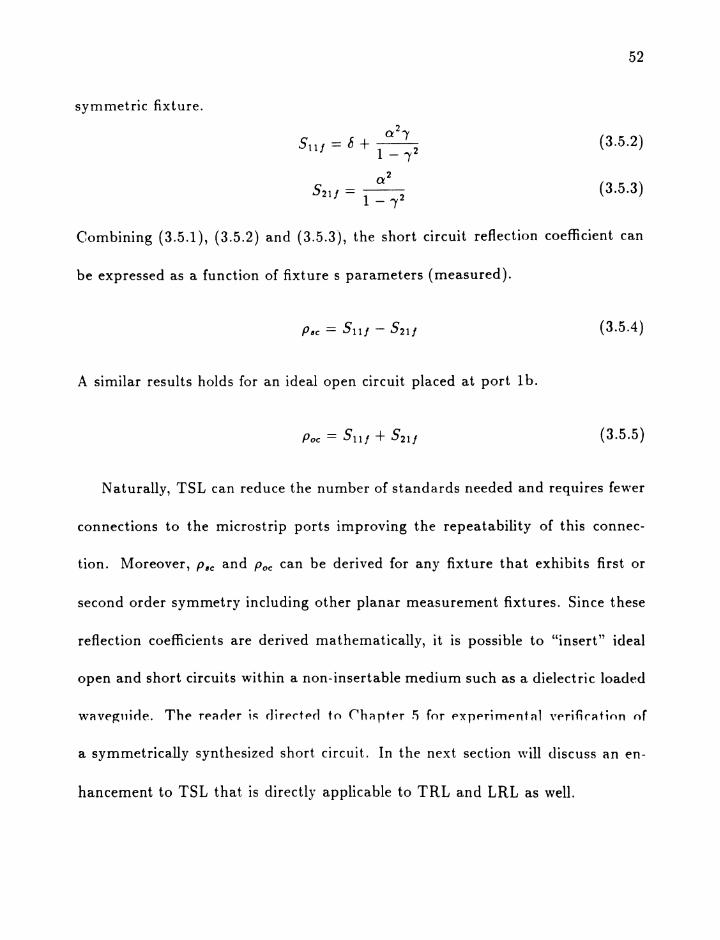
symmetric fixture.

(3.5.2)

(3.5.3)

Combining (3.5.1), (3.5.2) and (3.5.3), the short circuit reflection coefficient can

be expressed as a function of fixture s parameters (measured).

(3.5.4)

A similar results holds for an ideal open circuit placed at port 1b.

(3.5.5)

Naturally, TSL can reduce the number of standards needed and requires fewer

connections to the microstrip ports improving the repeatability of this connec-

tion. Moreover, Pae and Poe can be derived for any fixture that exhibits first or

second order symmetry including other planar measurement fixtures. Since these

reflection coefficients are derived mathematically, it is possible to "insert" ideal

open and short circuits within a non-insertable medium such as a dielectric loaded

a symmetrically synthesized short circuit. In the next section will discuss an en-

hancement to TSL that is directly applicable to TRL and LRL as well.

53

3.6 Enhanced Through-Symmetry-Line - ETSL (ETRL)

3.6.1 Motivation: Failure of TRL Assumpt ions

The development of ETSL, hence ETRL, is necessary because of assumptions

inherent to the TRL algorithm. As introduced in 1979 by Engen and Hoer [20],

the algorithm requires the characteristic impedance of the line standard to be

equal to the measurement system impedance. If not then we its value has to be

determined. Also, the algorithm assumes a pure real characteristic impedance with

no frequency dependence. If the fixture to be calibrated is composed of dispersive

transmission lines, e.g. microstrip, it becomes necessary to determine the complex

characteristic impedance Z; as a function of frequency. We present a method

that enhances the TSL algorithm by determining the characteristic impedance;

Enhanced Through-Symmetry-Line - ETSL. For the sake of discussion we will

consider an embedded rnicrostrip fixture. Application of ETSL to an embedded

microstrip fixture follows in Chapter 5.

An approximate value of Z; can be made USIng time domain reflectometry

(TDR), however, TDR can not determine frequency va ri a tions of the microstrip

characteristic impedance which can vary by as much as 5 percent from DC to 10

GHz for a typical rnicrostrip line [32]. Also, accurate modeling of Z; is complicated

by several factors; accepted models predict different frequency variations; material

parameters may not be known; and ideal microstrip geometry may be corrupted

54

by dielectric coverings such as a passivation or solder resist layer as in the case of

printed circuit boards, see Fig. 3.6.1. ETSL det.ermines t he complex characteristic

impedance using the free- space capacitance of the microstrip geometry and an

experimentally determined propagation constant, , == a + jj3.

The impedance calculated in this fashion, if used in the conventional TRL

algorithm, compensates for the algorithm assumptions. By using a free-space

capacitance explicit knowledge of the dielectric parameters i.e. relative dielectric

constant and loss tangent are not necessary. Also, we can determine characteristic

impedances of geometries that are atypical such as embedded rnicrostrip or any

uniform TEM transmission line. Additionally, by incorporating the propagation

constant we embody the effect loss has on the characteristic impedance (complex

Zc). In short, this method can be used to determine characteristic impedances of

any arbitrary uniform TErvI transmission line. In the next section we will develop

the characteristic impedance algorithm with microstrip being the transmission

line.

3.6.2 Calculation of Cornplex Characteristic Impedance

Microstrip lines are non-homogeneous transmission lines that support. a f)11~~1-

TEM mode [32]. However the TSL algorithm requires the equivalent TElvl mode

characteristic impedance. For uniform TE1'1 transmission lines the characteristic

impedance is related to the free- space capacitance and the effective dielectric

Metal Thickness = 3.6 milResist Layer Thickness = 4. mil

DielectricThicknessH = 5.6 mil

t t

Microstrip Width = 8. mil

[§] Solder Resist Layer

D Substrate Dielectric

• Metal (copper)

GP Thickness = 1. mil

Figure 3.6.1: Embedded microstrip encountered in printed circuit board technol­

ogy.

56

constant by [33]

with

1Zo ==­

Coc

(3.6.1 )

(3.6.2)

where Z; is the dielectric loaded characteristic impedance of the line, Zo is its free-

space characteristic impedance, Co is the free-space capacitance, c is the velocity

of light and f e is the effective dielectric constant. Co is a geometrical dependent

factor and is the capacitance of the structure in a dielectric-free medium. It is well

known that the effective dielectric constant is related to the propagation constant

, by [28]

(3.6.3)

where, == a + j(3 is available from measurement as a by product of the TRL

algorithm. Recently, Mondal and Chen reported that the TRL algorithm can be

used to determine the propagation constant of the TRL line standard. That is

[29]

where

A == TIlt· T22 1 + TIll· T22 t - T21 t • TI21 - TI2 t . T21 ,

(3.6.4)

(3.6.5)

Tijl and Tijt are the chain scat tering parameters for the line and through calibra-

tion standards respectively, and I is the length of the line standard. Conversion

.57

from s to t parameters is given by,

(3.6.6 )

where

(3.6.7)

This result can be derived for any fixture, symmetric or otherwise, and it is a nat-

ural progression to incorporate this information to determine the complex charac-

teristic impedance. Combining (3.6.1)- (3.6.3) and taking the negative root

JWz, == ~Cc 0, (3.6.8)

The negative root is chosen because the result must be positive when the line is

lossless and the impedance is positive pure real. This characteristic impedance is

used to overcome impedance assumptions of TRL and is applicable to the TSL

algorithm. The reader is directed to Chapter 5 where this derivation is experimen-

tally verified with a fifty ohm coaxial example. Also, Chapter 5 contains complex

rnicrostrip characteristic impedance calculated with the verified algorithm. Next

we examine singularities that arise when distributed standards are used and ex-

pand on the effect these singularities have on calculating t lie propagation rf)ll~f ;'l1f.

3.6.3 Calculation of Propagation Constant

Inherent to the TRL algorithm is the need to separate the error networks with a

transmission line. The line standard must be sufficiently long to produced a mea-

58

surable phase difference between through and line fixtures. Naturally, at lower

frequencies this becomes this difference is limited by the network analyzer mea­

surement resolution. Additionally, if the electrical length of the line is near 180

degrees it appears transparent. TRL returns invalid results in either case. In­

tuitively the "farthest" we can be from 180 degrees (or zero) would be a phase

difference of 90 degrees and reliable propagation constants can be extracted from

20 to 160 phase differences [30]. By choosing line standards with electrical lengths

within this range the characteristic impedance can be determined with no effect

from the singularities.

3.6.4 Modifying TSL Algorithm

Again, the TRL (TSL) algorithm requires a reflectionless line. This is achieved

by transforming each calibration measurement from the measurement reference

impedance to Zco Application of TRL then determines the S parameters of the er­

ror network referenced to Zc. To complete calibration the s parameters of the error

network are returned to the measurement reference impedance system, (usually

50 ohms).

.19

3.7 Development of Through-Symmetric Fixture - TSF

U sing Second Order Symmetry

What if the fixture is second order syrnmetric? Again, we define second order

symmetry as a first order fixture with symmetric halves. As we have just seen,

symmetry can be used to reduce the number of standards needed. When second

order symmetry is valid the two port error network is represented with two error

terms. Naturally, this allows us to use fewer de-embedding standards, in fact, a

second order fixture requires only one measurement configuration, a through con-

nection, thus in conformance with the practice of naming calibration procedures,

we designate the new technique Through Symmetric Fixture - TSF method.

Fig. 3.7.1 shows the signal flow graph for the fixture s parameters SiiJ and

the corresponding two port error model. Each error is identical and symmetric

therefore the scattering matrix of each is

b Q

[Sija] == (3.7.1)

Q 6

The goal of TSF is to determine the error terms (Q and 6) and based on Mason 's

non-touching loop rule, unlike the matrix renormalizations used by Mar tiu c\11(1

Dukeman [31]. S parameter measurements of the through connection yield t\VO

independent quantities, 5 u / and 5 21 / , as 5u / = 5 22 / and 5 12 / = 5 21/ because of

symmetry and reciprocity. This is sufficient to determine 5 i j a • For clarity, we will

let the subscript ijt (t - through) represent the measured fixture s parameters ijf·

•

•A

(a)

S~I<, -- - .. --

/

~ t i~·II,' \::ia-'---__~__-A.

Sl2(b)

-.-.

60

(c)

Figure 3.7.1: Signal flow graphs used IJy TSF. (a.) Measured fixture s parametersand (b) fixture error network described by s parameters 6 and Q.

61

The signal flow graph provides two algebraic relationships for the known qu a n-

tities as functions of the error terms ,

Rearranging

0:2

S ---21t - 1 _ 62

(3.i.2)

(3.i.3)

(3.7.4)

where

Q== (3.7.5)

b == 1 + S21t (3.7.6)

The square root gives t \VO possible solutions and the root choice depends upon the

electrical length (L e ) of the through connection. The positive root is valid when

where

(2n + l)AnA < L; < ---­

2

n == 0,1,2, · ..

(3.7.7)

(3.7.8)

otherwise the negative root is correct. This choice of roots is based on (l 1"'.' sical

constraint. The a term is the transmission coefficient of the error network and at

low frequency the phase of Q must be negative therefore the positive root choice

in this interval.

62

Equation 3.7.4 contains a singularity that limits the bandwidth of TSF. When

the fixture S21t is nearly equal to -1 equation 3.7.4 will return invalid results for

fJ this can occur when the fixture is n2).. . This singularity can be avoided if the

length of the fixture is constructed such that it is not an integer half wavelength

long at any frequency in a desired measurement range. TSF can be used on a

lumped-element transistor test fixture "There this restriction does not exist. Sim­

ilar singularity restrictions exist when other distributed de-embedding techniques

are employed. The reader is directed to Chapter' 5 where TSF is experimentally

verified.

3.8 Conclusion

In Chapter 3, we have presented new de-embedding algorithms. By using sym­

metric arguments, it is possible to reduce the required calibration standards. It

was shown that reflection standards can be synthesized from a through measure­

ment. Also, the complex characteristic impedance of uniform TEM transmission

lines can be determined if the transmission line free-space capacitance is known.

T~kln~ this irn perlan ce into arcou n t . "?P r a n pnhf'nrp thp T~T, or TnT} tllgnrlihms.

Computer implementation of these algorithms is necessary for verification pur­

poses. The next chapter develops SPANA or Signal Processing of Automatic

Network Analysis a command level program useful for algorithm implementation

and other computer aided data manipulation.

63

Chapter 4

SPANA: Computer Program for Computer

Aided Microwave Measurement

4.1 Introduction to SPANA

Computer processing of microwave measurements is necessary to free the engineer

from the costly measurement time. It is very reasonable to assume that computer

processing is needed since a single t\VO port measurement can produce sixty four

kilobytes (64K) of data. SPANA (Signal Processing for Automatic Network Anal-

ysis) has been developed to meet the needs of automatic microwave measuring

systems.

SPAN A is a tool to be used for processing measured S parameter data and its

prime use is to implement de-embedding algorithms. SPAN A also performs various

tasks such as input/output of data, data format conversions, and others. Written

SPAN A is by the simplest definitions an operating system and the operations

are carried out by using a command language. These commands allow the user

to interact with the data freely. One of the most important assets of SPANA is

that a series of commands can be sequentially read from a command file; a macro.

6·1

SPAN A is adaptable to outside programmers since it maintains all data 1/0 and

frees the programmer to concentrate on the processing of data.

4.2 Structure

SPANA has two program levels and each level has the capability to inform the

user if a syntax error occurs. At the top is the command interpreter and its

task is to determine which command is to be executed. The next layer is the

actual command function which may in turn nest several sub-layers to complete

the function. When a command is completed, control is returned back to the

command interpreter for subsequent command processing. It is important to note

that SPANA is not a menu driven program but rather a command interpreter.

Commands available in SPAN A are given in the next section.

4.3 Tools available in SPANA

To use SPANA, data is input to the program by "GETing" a measurement set.

After this it is available for processing by executing other commands. Finally, the

using TSF requires a measurement for the through standard and the embedded

device. Two "GETs" and a call to DIvIB2 (with appropriate Ty"PE) will calculate

the error networks and the de-embedded device. "P'U'I'ting" these results will save

them for later use. Below is a list of the functions and a brief discription of their

purpose. The reader is directed to Appendix B for a complete discussion of the

semantics of each command and Appendix C where the "SHELL" command is

example for the potential programmer.

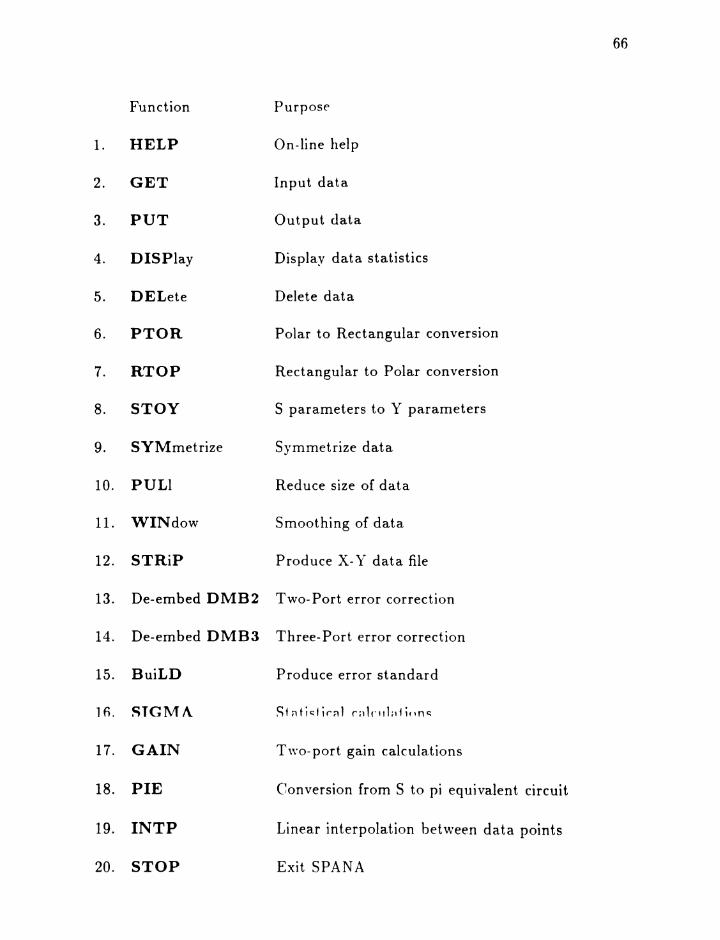
Function Purpose

1. HELP On-line help

2. GET Input data

3. PUT Output data

4. DISPlay Display data statistics

5. DELete Delete data

6. PTOR Polar to Rectangular conversion

7. RTOP Rectangular to Polar conversion

8. STOY S parameters to Y parameters

9. SYMmetrize Symmetrize data

10. PULl Reduce size of data

11. WINdow Smoothing of data

12. STRiP Produce X. Y data file

13. De-embed DMB2 Two-Port error correction

14. De-embed DMB3 Three-Port error correction

15. BuiLD Produce error standard

1s. STGM/\. St"tl~t;r~l r;d(",,1;dlnn~

17. GAIN Two-port gain calculations

18. PIE Conversion from S to pi equivalent circuit

19. INTP Linear interpolation between data points

20. STOP Exit SPANA

66

67

4.4 Conclusion

This chapter introduces SP.!\N A with its purpose to aid microwave measurements.

The ability to execute command macros is essential to extensive measurement

calculations and SPAN A can be modified by adding command to the interpreter

and writing the appropriate sub-layers.

68

Chapter 5

Results and Discussion

5.1 Introduction

In this chapter the calibration techniques developed in Chapter 3 are verified.

Through-Symmetry-Line and Enhanced Through-Symmetry-Line are applied to

an embedded microstrip fixture commonly encountered in Printed Circuit Board

technology. The error networks determined from these methods are removed from

a PCB via and a pi equivalent circuit is imposed on t he via measurements. Finally,

Through-Symmetric Fixture is applied to a second order symmetric fixture and

the results are compared directly with measured fixture halves and a de-embedded

low pass filter. The use of scattering parameters is common to all results. With

exception to TSF and a coaxial verification, a frequency range of 45 Mhz to 10

Ghz is used for the TSL and ETSL measurements.

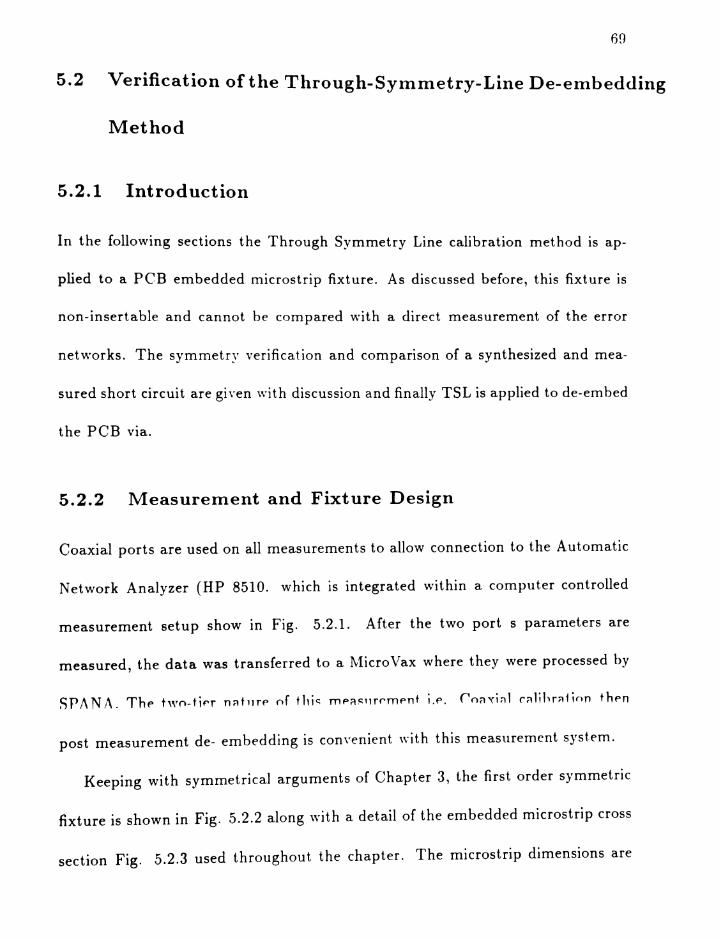
69

5.2 Verification of the Through-Symmetry-Line De-embedding

Method

5.2.1 Introduction

In the following sections the Through Symmetry Line calibration method is ap­

plied to a PCB embedded microstrip fixture. As discussed before, this fixture is

non-insertable and cannot be compared with a direct measurement of the error

networks, The symmetry verification and comparison of a synthesized and mea­

sured short circuit are given wit h discussion and finally TSL is applied to de-embed

the PCB via.

5.2.2 Measurement and Fixture Design

Coaxial ports are used on all measurements to allow connection to the Automatic

Network Analyzer (HP 8510. which is integrated within a computer controlled

measurement setup show in Fig. 5.2.1. After the two port s parameters are

measured, the data was transferred to a MicroVax where they were processed by

post measurement de- embedding is convenient w it h this measurement system.

Keeping with symmetrical arguments of Chapter 3, the first order symmetric

fixture is shown in Fig. 5.2.2 along with a detail of the embedded microstrip cross

section Fig. 5.2.3 used throughout the chapter. The microstrip dimensions are

70

NETWORK ANALYZER CONFIGURATION

~NCIDENT

OUT

SIGNAL

SEPARATION

TRANSMITTED

X v~ "

INCIDENT REFLECTED TRANSMITTED

PROCESSOR/DISPLAY

Figure 5.2.1: S parameter measurement setup. The HP 8510 measures the devices parameters under control of the controller, then the data is transmitted to theMicroVax for further processing.

71

GroundPlanes

, Embedded- ...~~ Microstrip

Line

:~ L =348 mils

L=1348mils

Coaxial Reference Pfanes

8M .. Q! ..~ MicrostriP~" Q.~ ..A '" Reference Planes

M1 M2

Figure 5.2.2: First order symmetric fixture used throughout Chapter 5. Cl andC2 are the calibrated coaxial measurement planes and Ml and M2 are the mi­crostrip reference planes. Embedded structures are inserted at Ml and M2.

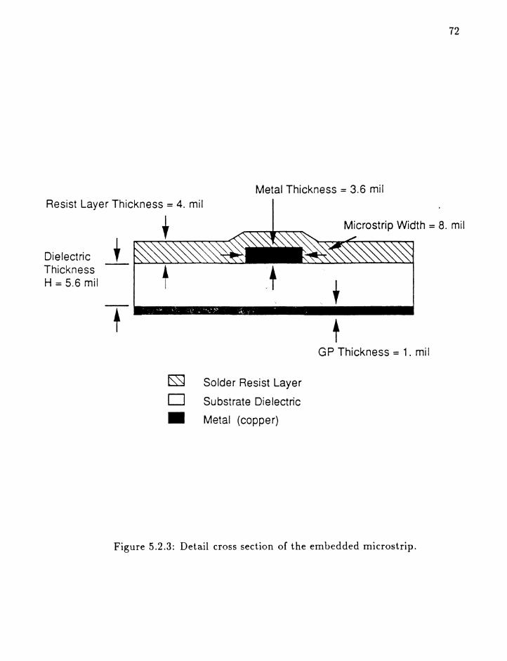
72

Metal Thickness = 3.6 milResist Layer Thickness = 4. mil

DielectricThicknessH = 5.6 mil

t .' i, .....' : " . : 1-;-;'. •, "'.: .~".. ..~., ~- , " '.

lSS] Solder Resist Layer

D Substrate Dielectric

• Metal (copper)

Microstrip Width = 8. mil

,t

GP Thickness = 1. mil

Figure 5.2.3: Detail cross section of the embedded microstrip.

71

width( w)=8 mils, height( h)=5.6 mils, met al thickness( t)=3.6 mils and the covering

dielectric layer (solder resist layer) is approximately ·1 mils thick. The length( I) of

the microstrip portion of the fixture is 1000 mils. These physical dimensions (ex­

cept length) were used because PCB manufacturing resources required them. Note,

these dimensions were intended to result in a 50 ohm characteristic impedance and

as we will see this is not the case. The microstrip length can be arbitrarily chosen

with only coaxial connector clearance restricting the minimum value.

The network analyzer is calibrated to the coaxial reference planes Cl and

C2 using the network analyzer Open Short Load calibration procedure. The

fixture is connected to the coaxial reference planes and a full two port s parameter

measurement is made. The magnitude and phase of the fixture s parameters 5 11/ ,

5 22 / and 5 21 / are shown in Fig. 5.2.4, 5.2.5 and 5.2.6 with the exception of 5 12/

which is identical to 5 21 / and has been omitted.

Symmetry requires that the 5 i i / parameters be equal and from Fig 5.2.4-5.2.6

this is true with minor deviations at frequencies were the fixture is resona.nt (f=.8,

4.5 and 8 GHz). These resonances are are associated with discontinuity capaci­

tances a n d for discussion, we rn av morlel t hp fixture wi t h rliscont inu itv r;-)rr.rit~n("p~

at either coaxial port and a uniform transmission line between them, fig. 5.2.7.

These capacitances reduce the electrical length of the line and when the effective

line length is an odd multiple of half wavelengths, the 5i i j values exhibit minima.

Sensitivity of the fixture symmetry at these frequencies is due to differences in

74

o.

- 10.

~co0 - 20.'-""

(1)-c~~.-c

- 30.0)co~

- 40.

- 50.o. 2.0 4.0 6.0

Frequency (GHz)

8.0 10.

Figure 5.2.4: Embedded microstrip fixture s parameters. l\lagnitude of ([1) 511/ ,

(+) 521/ and (6) 5221 0

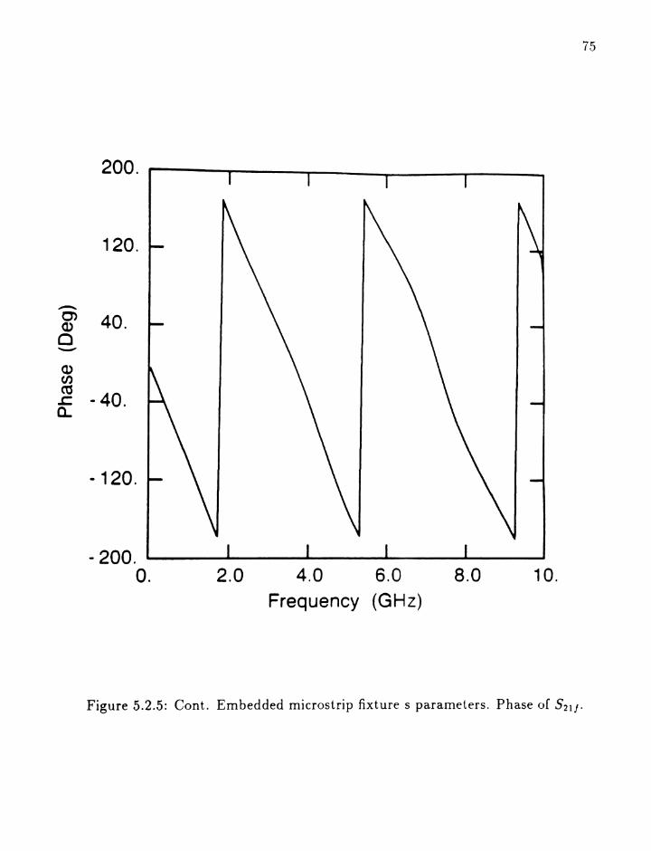
200.

120.

~

0) 40.<1>0"""--"'"

<1>(fJco

- 40 .s:o,

-120.

- 200.o. 2.0 4.0 6.0

Frequency (GHz)

8.0 10.

75

Figure 5.2.5: Cont. Embedded microstrip fixture s parameters. Phase of 52 1 j .

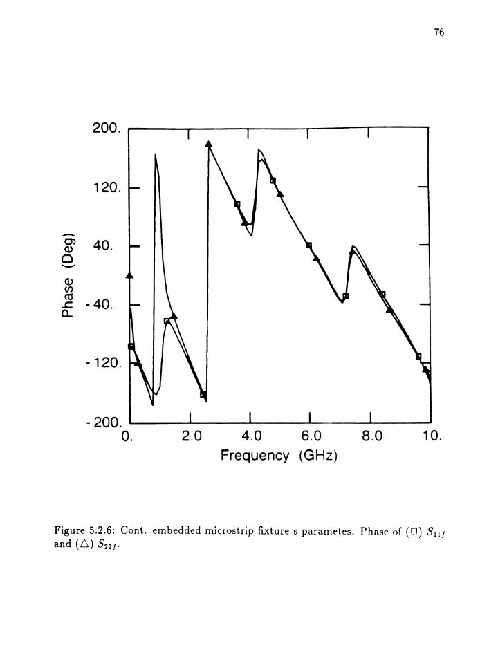
76

8.02.0 4.0 6.0Frequency (GHz)

120.

200.

- 200. L...-__....&..-__-...- ...-.....__--..

O. 10.

-120.

...----.0) 40.(1)

0~

(1)(jJCQ

- 40 ..J.:a..

Figure 5.2.6: Cont. embedded microstrip fixture s parametes. Phase of (Cl) Sll!

and (6) 522 / ,

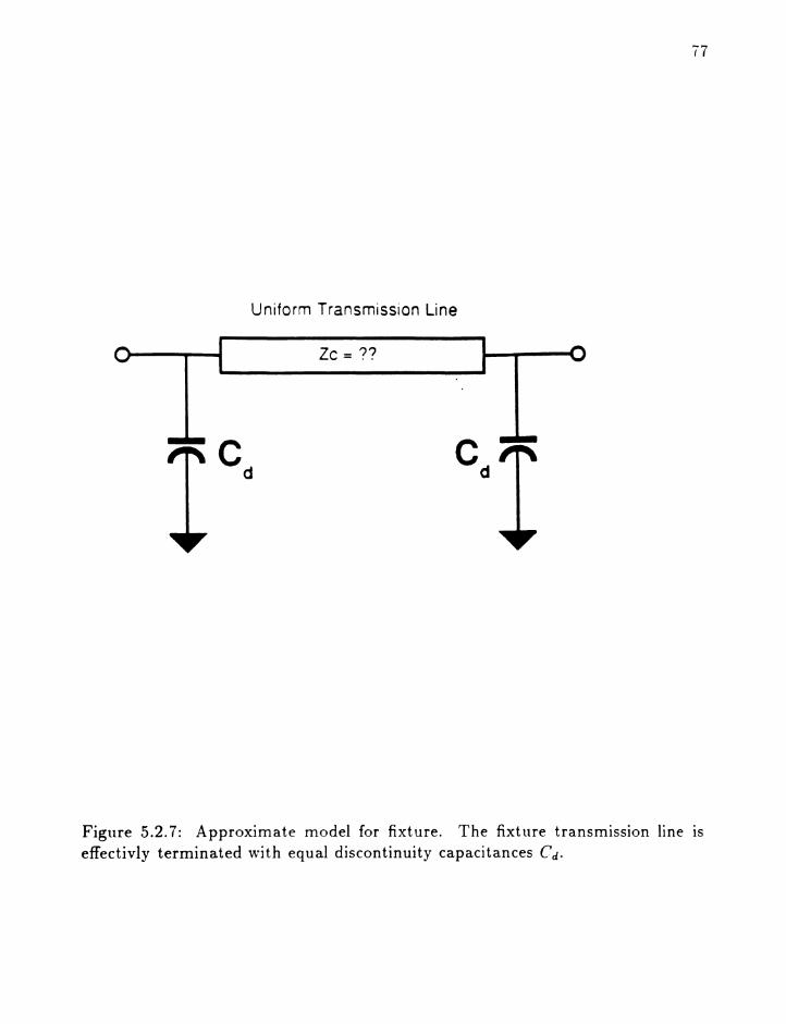
77

Uniform Transmission Line

Zc = ??

Figure 5.2.7: Approximate model for fixture. The fixture transmission line IS

effectivly terminated with equal discontinuity capacitances Cd-

78

the discontinuity capacitances. Additionally, at other frequencies reflection from

the microstrip line dominate the reflection terms. When designing a symmetrical

fixture, one can apply common sense arguments, such as reduce the discontinuity

capacitance and use short lengths of microstrip. The symmetry of the network is

exemplified by the synthesized short circuit verification.

5.2.3 Synthesis of Open and Short Circuit Reflection Co­

efficients

The Through Symmetry Line algorithm synthesizes the reflection standard needed

in the TRL calibration method by using symmetry. To verify this is possible a

low inductance short circuit was placed at the microstrip reference plane Ml,

shown on Fig. 5.2.2. The measured short circuit reflection coefficient is compared

in magnitude and phase with the synthesized value in Fig. 5.2.8 and 5.2.9. In

addition, the synthesized open circuit is also shown. The magnitude minimum is

slightly different between measured and calculated. This minimum corresponds to

the resonance of the discontinuity capacitance with the inductive input impedance

asitic inductance that will lower the resonant frequency from t.he ideal synthesized

short. In fact, it may be possible to extract an inductance value from this fre­

quency shift. In any event, the TRL reflection standard can be synthesized and

the next section presents results using TSL.

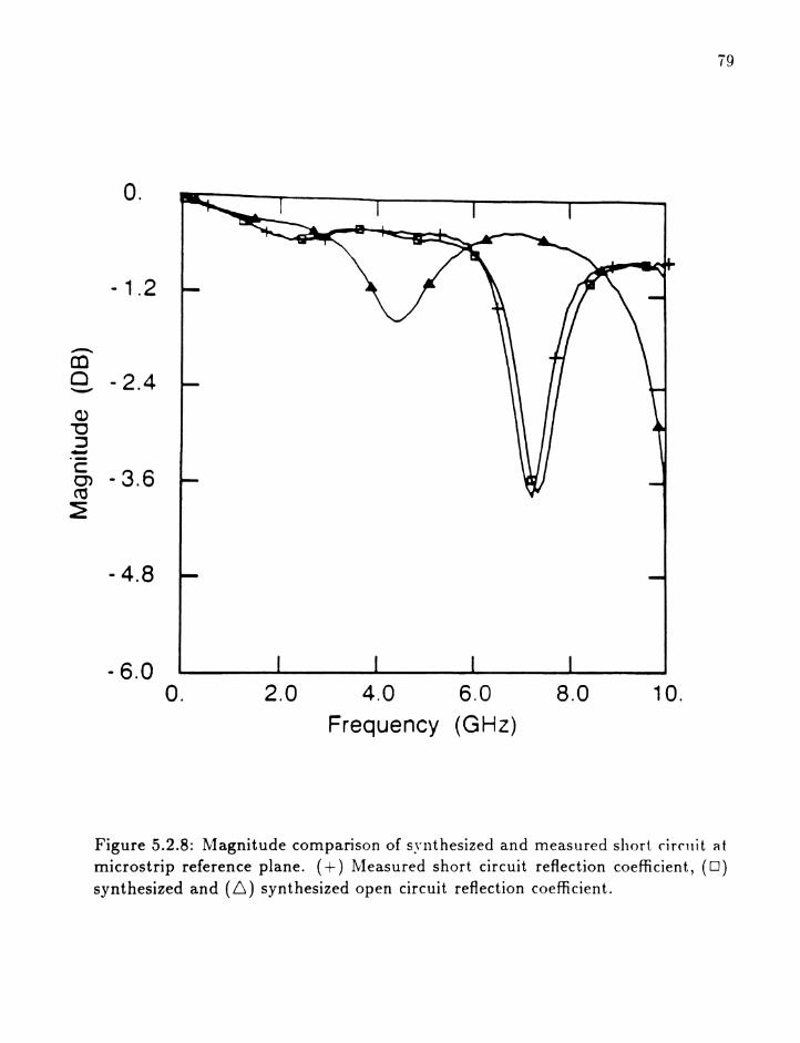
79

o.

- 1.2

.....-.....CO0 - 2.4'-"'"

Q)1:)~...,c

- 3.6CJ)co~

- 4.8

- 6.0o. 2.0 4.0 6.0

Frequency (GHz)8.0 10.

Figure 5.2.8: Magnitude comparison of synthesized and measured short circuit a t

rnicrostrip reference plane. (+) Measured short circuit reflection coefficient, (0)synthesized and (6) synthesized open circuit reflection coefficient.

80

200.

120.

~

0) 40.Q.)

Q""'--"

<l>so~

- 40 ..l:a..

- 120.

- 200.O. 2.0 4.0 6.0

Frequency (GHz)

8.0 10.

Figure 5.2.9: Phase comparison of synthesized and measured short circuit (\1. rni­crostrip reference plane. (0) Phase of synthesized short circuit reflection coeffi­cient, (+) measured short circuit and (6) synthsized open circuit.

5.2.4 TSL De-embedding Results

81

The TSL algorithm was used to determine the pi equivalent circuit of a PCB via

and to do so we need to remove it from the fixture. In effect, the via is inserted

at the microstrip reference planes. As discussed before, PCB measurements are

non-insertable so we must replicate the through fixture with the line standard and

finally the device under test (DDT) inserted.

Fig. 5.2.10 shows the standards and the device to be de-embedded. The line

length was 1348 mils giving a length difference, ~l, between the through and line

standards of 348 mils. The useful measurement range for ~l == 348 is within the 45

Mllz to 10 GHz measurement range, with the first TRL singularity near 10 GHz.

The exact calculation of this singularity is not possible because the frequency

variation of the effective dielectric constant and we can only approximate its mag­

nitude. However the singularity does correspond to the ~l being an electrical half

wavelength.

A printed circuit board VIa is a plated hole through the PCB connecting a

fixture halve on each side of the board and can be modeled with a pi equivalent

are shown in Fig. 5.2.11. After applying the TSL algorit hm to the embedded

via measurement we can extract the pi equivalent circuit from the de-embedded

via s parameters, see Appendix A for complete discussion of error removal by

de-cascading. This extraction is done by converting the via s parameters to ad-

82

GroundPlanes

I' Embedded

- ...~~ MicrostripUne

,

:~ L =348 mils

L=1348mils(a)

Coaxial Reference Planes

SM .. .Q1 ..~ Microstrip ~.. Q.~ .,A '" Reference Planes

M1 M2

(b)

Figure 5.2.10: Diagram of the fixture wit h line standard inserted (a) and via (b).

83

Lower___~GP

Upper-_.~GP

Resist Layer Thickness = 4. mil,Microstrip Metal Thickness3.6 mil

+Via Length = 62.5 mil

lS1 Solder Resist Layer D Substrate Dielectric

• Metal (copper)

ViaDiameter

45. mi I ---1r-----a~

GPThickness

1.mil'

''''~H = 5.6 mil-

~-

(a)

T--C

'Tr

(b)

Figure 5.2.11: Detail cross section of printed circuit board via (<I) <Inc! l he pi

equivalent circuit (b).

84

mittance parameters, which form a pi equivalent circuit, and then inverting these

admittances. The resulting shunt capacitance (in pico Farads) and series inductive

reactance (in ohms) are shown in Fig. 5.2.12 and Fig. 5.2.13 respectively.

When interpreting the TSL results, we should consider the fact that we have

imposing a pi equivalent model to the via and at higher frequencies this result will

decrease in accuracy. The series reactance behaves as an inductor through two

GHz and the capacitance is constant to five. The increasing capacitance (with

frequency) is associated with the increased energy stored in the fringe electric

fields and the non-ideal inductance arises from resonances with other parisitic

capacitances (Cp , 5.2.11).

A final note about the characteristic impedance of the line standard used in

TSL. As mentioned in Chapter 3, the TRL algorithm requires that the line stan­

dard be reflectionless or we need to determine the impedance. The TSL results

were determined using Time Domain Reflectometry (TDR) and found to be 57

ohms. This is different from the manufactures 50 ohm design goal but its effect

can be removed as described in ETSL section.

5.2.5 Conclusion

The Through-Symmetry-Line de-embedding method has been used to calculate the

pi equivalent circuit of a printed circuit board via. The close agreement between

measured and synthesized short circuits verifies that a symmetrical argument can

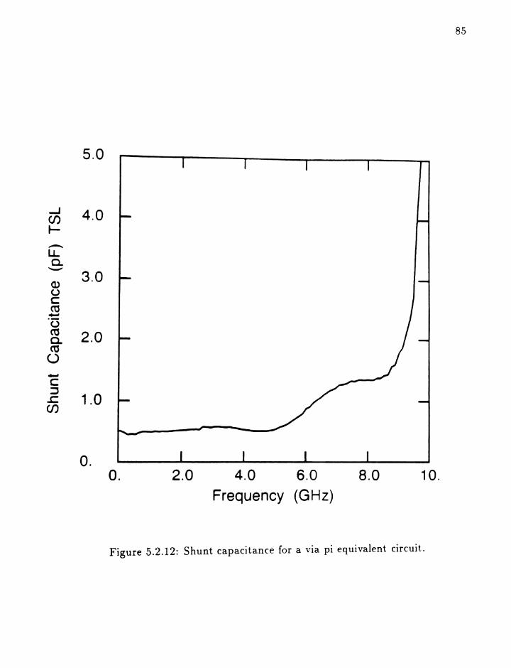
5.0

--J 4.0(f)t-~

U.a.

"-'"

(1)3.0

oc::co~

'(3co 2.0a.~

o~

c:~

1.0..c:(f)

o.o. 2.0 4.0 6.0

Frequency (GHz)

8.0 10.

85

Figure 5.2.12: Shunt capacitance for a via pi equivalent circuit.

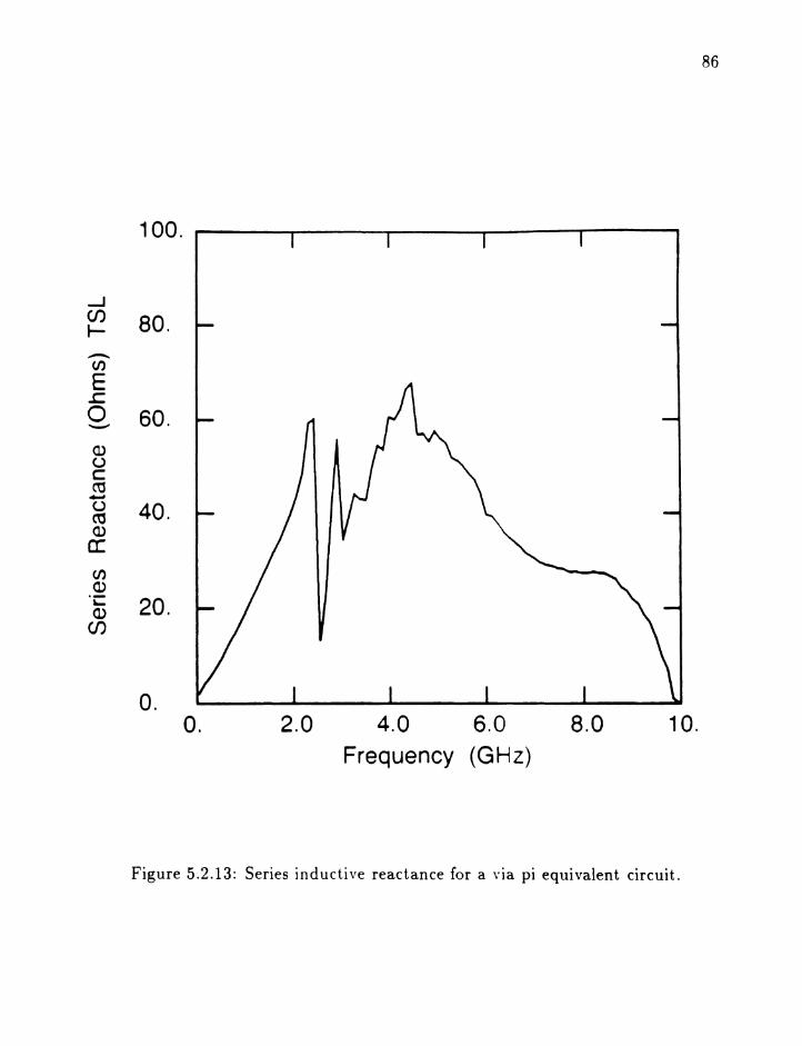
100.

-JC/) 80.I-~

(J)

E..c0 60.'-'"'"

Q.)uCt\3~

o 40.CQQ.)

a:(J)Q.).t:

20.(l)C/)

o.o. 2.0 4.0 6.0

Frequency (GHz)

8.0 10.

86

Figure 5.2.13: Series inductive reactance for a via pi equivalent circuit.

87

be used to modify the TRL algorithm to TSL.

5.3 Verification of the Enhanced Through-Symmetry-Line

De-ernbedding Method

5.3.1 Introduction

This section contains verification of the impedance enhancement to TSL and its use

in the new ETSL algorithm. Verification is done by calculating the impedance of

a precision 50 ohm air line as well as other transmission line parameters including

dielectric and propagation constants.

5.3.2 Coaxial Transmission Line Parameters

Fixturing for this verification is shown in Fig. 5.3.1. It includes two fixture halves

each composed of APC-7 to female SMA and a male SMA to APC-7 adaptors.

The through connection is the connection of the fixture halves and the air line

was inserted between the halves for a line connection. The air line length is

10.21 em and the air dieler t ri c allows a cr u ra te calrnlat ion of 1he half wavelength

singularities. These are f = 1.4691 i G Hz, where i = 1, 2, 3, .. '.

This fixturing was chosen for two reasons. First, the precision air line connec­

tions were APC-7 requiring a similar mating connector. Secondly, it was desirable

to have a fixture of a non-zero length thus allowing direct application to the mi-

88

Through Connection

APC·7 to Female SMAi~ ~,

APC-7 to Male SMA

(a)

Line Connection

10.21 em Air Lins.lI~

(b)

Figure 5.3.1: Coaxial fixturing used to verify TSL impedance enhancement. (a)Through connection and (b) 10.21 em precision 50 ohm air line inserted in fixture.

89

crostrip fixture used in the previous TSL results. Next we will present the coaxial

transmission line parameters.

Attenuation Constant (Q)

The through and line connections were measured over a 15 to 3000 Mllz frequency

range and the propagation constant was calculated. Fig. 5.3.2 shows the atten­

uation constant, Q, with per meter units. Several observations can be made. It

is clear over this frequency range that we encounter two of the predicted halve

wavelength singularities since the per meter attenuation values are unrealistically

high. These constitute invalid regions. The second observation is low attenuation

values within valid regions. This is typical of precision coaxial lines. Finally, we

see that at low frequencies (below 200 ~IHz) we cannot measure significant phase

difference between the through and line connection.

Propagation Factor (j3)

The calculated propagation factor, {3 = ~, has been normalized with respect to a

free-space propaga.tion factor, j30 == ~ where c is the speed of light, to reveal its

accuracy. Tile precision air line shouJd linve a free-space prnpClgatinn filct .... and

the normalized j3 should be unity. This result is shown in Fig. 5.3.3.

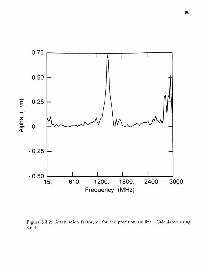
90

2400.610. 1200. 1800.Frequency (MHz)

0.50

O. 75 r-----p----...--.0111..------.---~--~

- 0.50 ~_--.....___.a___~__~ ____

15. 3000.

- 0.25

~

0.25E-..-...........",

~..c:a. O.<

Figure 5.3.2: Attenuation factor, a, for the precision air line. Calculated using3.6.4.

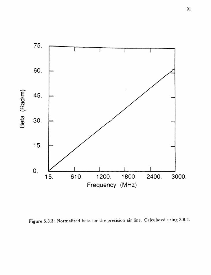
91

75.

60.

,-....".

E 45.~

-0~

a:~

ra30 .....

Q)CD

15.

o.15. 610. 1200. 1800.

Frequency (MHz)

2400. 3000.

Figure 5.3.3: Normalized beta for the precision air line. Calculated using 3.6.4.

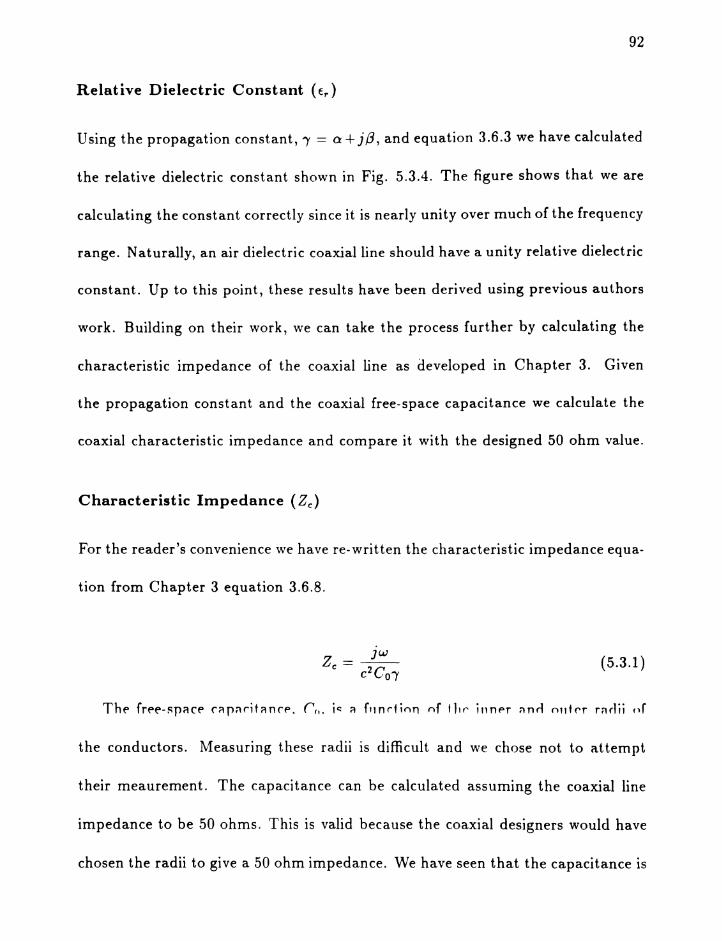
92

Relative Dielectric Constant (€r)

Using the propagation constant, , == Q + j/3, and equation 3.6.3 we have calculated

the relative dielectric constant shown in Fig. 5.3.4. The figure shows that we are

calculating the constant correctly since it is nearly unity over much of the frequency

range. Naturally, an air dielectric coaxial line should have a unity relative dielectric

constant. Up to this point, these results have been derived using previous authors

work. Building on their work, we can take the process further by calculating the

characteristic impedance of the coaxial line as developed in Chapter 3. Given

the propagation constant and the coaxial free-space capacitance we calculate the

coaxial characteristic impedance and compare it with the designed 50 ohm value.

Characteristic Impedance (Zc)

For the reader's convenience we have re-written the characteristic impedance equa-

tion from Chapter 3 equation 3.6.8.

(5.3.1)

the conductors. Measuring these radii is difficult and we chose not to attempt

their rneaurement. The capacitance can be calculated assuming the coaxial line

impedance to be 50 ohms. This is valid because the coaxial designers would have

chosen the radii to give a 50 ohm impedance. We have seen that the capacitance is

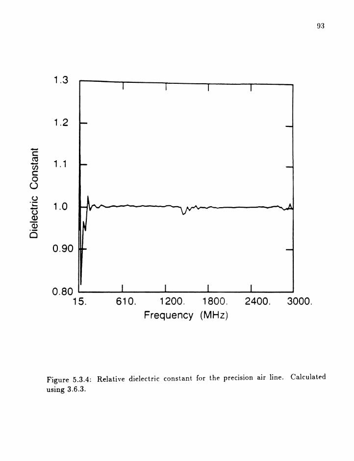
93

3000.2400.61 O. 1200. 1800.

Frequency (MHz)

1.3

1.2

0.80 '---__.....-.-__..&.-__...-.__......I-..__...J

15.

...,c~ 1 .1...,(/)c0oo.~ 1.0~oQ)

<l>0

0.90

Figure 5.3.4: Relative dielectric constant for the precision air line. Calculated

using 3.6.3.

94

a function of the impedance in Chapter 3 and using equation 3.6.2 we calculate t.he

coaxial free-space capacitance to be 66.71 pico Farads per meter. Applying this to

equation 5.3.1 yields the characteristic impedance. Fig. 5.3.5 and 5.3.6 show the

real and imaginary values of the coaxial characteristic impedance. The real value

is within one tenth of an ohm to 50 ohms and the imaginary is esentially zero

showing good agreement with expected values. Now we can apply this impedance

calculation to the embedded microstrip fixture used in the TSL results.

5.3.3 Ernbedcled Microstrip Transmission Line Parameters

This section presents transmission line results calculated in the same manner as

the coaxial example above. The fixturing used here is identical to the TSL fixture.

With TSL, we determined the characteristic impedance of the line standards using

TDR and here we will see that the impedance is complex and that the embedded

microstrip lines are dispersive. The ~l used in this section is five em. This value is

necessary to extract reliable results at the lowest measurent frequency, 45 Mflz yet

it does increase the number of invalid regions. The results show that these regions

exist but have little effect on calculat.ing the ernberlrled m ir.rostrip t.ra nsrnission

line parameters.

Attenuation, and Propagation Constants (Q and {3)

Embedded microstrip attenuation constant IS shown In Fig. 5.3.7, with units

58.

----...-.....(fJ

E 55 ..c:0"--'"

OJUc:

53.~\J<l>a.Eo 50.'';::(/)

'i::Q)...,uco'- 48.~s:o-..-.'

<l>a:

45.15. 610. 1200. 1800. 2400. 3000.

Frequency (MHz)

Figure 5.3.5: Real portion of the coaxial characteristic impedance. Calculated

using the free-space capacitance and equation 5.3.1.

96

----~(/'J

E 1.0.c:0"'-'"

Q.)oc: 0.50n1

1:)Q.)a.Eo O.~

(/J.~

(1)~o~

- 0.50'-~.c:o-...-E

1.5

- 1.015. 61 O. 1200. 1800.

Frequency (MHz)

2400. 3000.

Figure 5.3.6: Imaginary portion of the coaxial characteristic impedance. Calcu­lated using the free-space capacitance and equation 5.3.1.

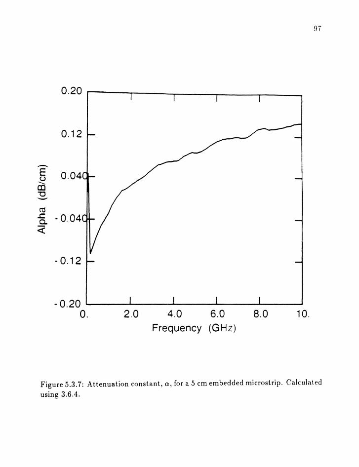
97

0.20 r---,-----.--~-----.-----

0.12

....-.....E 0.04u

""""'"CD-0~

C'Cs: - 0.04a.-c

- 0.12

10.8.02.0 4.0 6.0Frequency (GHz)

-a.20 ~__-......-.__...........__..._..._____L_____J

O.

Figure 5.3.7: Attenuation constant, a, for a 5 cm embedded microstrip. Calculated

using 3.6.4.

98

of dB / em. Also, Fig. 5.3.8 shows the normalized propagation factor for the

transmission line. The normalized (3 is a decreasing function of frequency therefore

the line is dispersive. Additionally, values are greater than unity therefore the

effective dielectric constant must also be greater than one.

Effective Dielectric Constant (f r )

As with the coaxial line, we calculate the real and imaginary parts of the em­

bedded microstrip effective dielectric constant, Re(f.~JJ) and Im(f.eJJ) Fig. 5.3.9

and 5.3.10 respectively. The singularity effects are more pronounced here but

they are still not significant. The decreasing Re( f.ef J) represents dispersion and

is intuitively clear since the amount of electric field contained in the air above

the microstrip increases wit h frequency therefore lowering the effective dielectric

constant. Moreover, I m( f.~J f) increases to a constant value for similar reasons.

Note, Im(f.eJJ) == 0.1 corresponds to a loss tangent of 0.03.

Characteristic Impedance (Zc)

The free-space capacitance has been calculated as described by Bah] and St nchlv

[33] and for this study has been Iou nr] 10 bp :Jl ..Pj!J pic n lurad s 1'(" tl1l'fl'r. (:i\",,, f'Iis

and the propagation constant we calculate the complex characteristic impedance

Zc with results given in Fig. 5.3.11, and Fig. 5.3.12 imaginary impedance. The

characteristic impedance is complex with increasing real and decreasing imaginary

parts. These relationships are caused by the dielectric covering which effectively

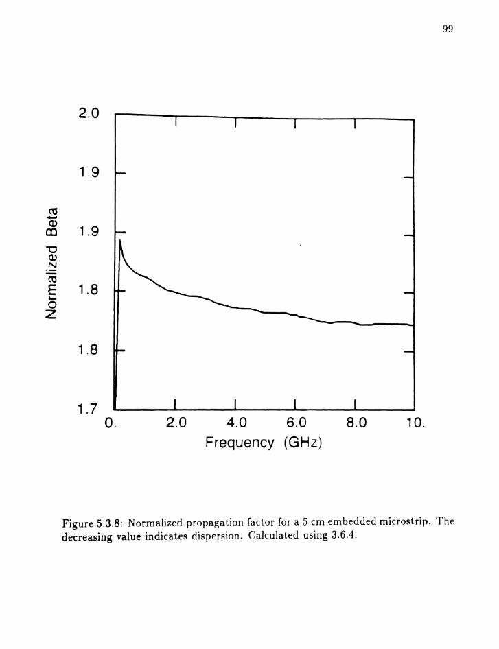
99

2.0

1.9

~~

(l)1.9CD

\:)Q.)N

(ijE 1.8'-0z

1.8

1.7o. 2.0 4.0 6.0

Frequency (GHz)

8.0 10.

Figure 5.3.8: Normalized propagation factor for a 5 cm embedded rnicrostrip. Thedecreasing value indicates dispersion. Calculated using 3.6.4.

100

4.0

.---.. 3.8...-c:co...-(/)c0o 3.6o.~

...-o<l)

Q) 3.40Q)

>...-o<l) 3.2~

~

UJ-,.-Q.)

a::3.0

o. 2.0 4.0 6.0 8.0 10.

Frequency (GHz)

Figure 5.3.9: Real portion of the effective dielectric constant for a .5 em pn,heddt"dmicrostrip. Again, a decreasing value indicates dispersion. Calculated using 3.6.3.

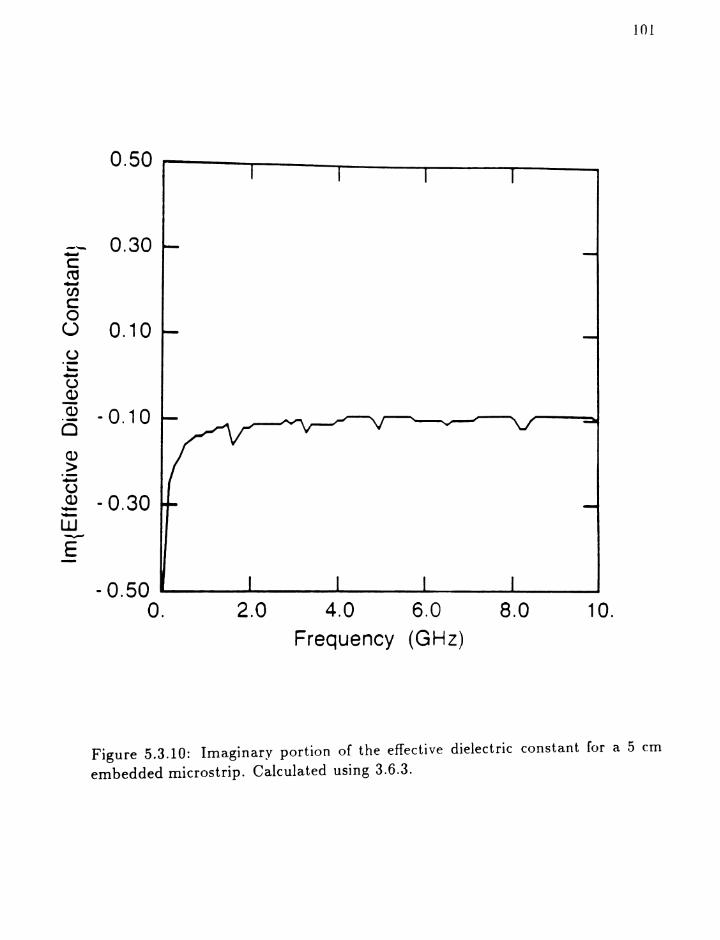
101

0.50 I--,-----r----r------,.---

-'-. 0.30~

c~...(/)

c0U 0.10o.~....u(1)

(1) - 0.10.-0(1)

>....o(1) - 0.30~

~

UJ-.,...-

E

- 0.50O. 2.0 4.0 6.0 8.0 10.

Frequency (GHz)

Figure 5.3,10: Imaginary portion of the effective dielectric constant for a 5 cm

embedded microstrip. Calculated using 3.6.3.

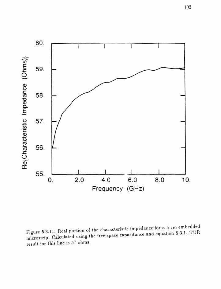
102

60.

-'-.....-....(/)

E 59 ..c:0~

(1)oc

58.ro-cQ)a.Eo 57.'';:;(/)'~

(1)~o~~ 56.C1:3s:o~

Q)

a:55.

O. 2.0 4.0 6.0 8.0 10.

Frequency (GHz)

Figure 5.3.11: Real portion of the characteristic impedance for a 5 ern emheddedmicrostrip. Calculated using the free-space capacitance and equation 5.3.1. TDR

result for this line is 57 ohms.

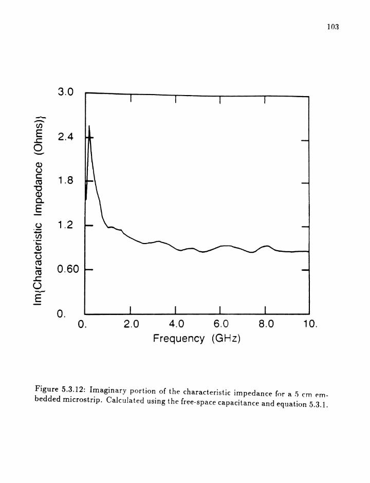
103

3.0

-----,.......(/)

E 2.4.c0'-'

Q)oc 1.8ro-0Q.)a.Eo 1.2.-en.~

Q.).-oca

0.60'-cas:o~

EO.

4.0 6.0 8.0 10.O. 2.0Frequency (GHz)

Figure 5.3.12: Imaginary portion of the characteristic impedance for a .1 em ern­bedded microstrip. Calculated using the free-space capacitance and equation 5.3.1.

104

contains much of the fringe electric field. At higher frequencies, the electric field

occupies more of the free-space above the cover layer and the embedded microst rip

exhibits microstrip behavior.

5.3.4 ETSL De-embedding Results

Finally, we apply this characteristic impedance profile to the line standard used

in TSL and de-embed the same PCB via. Shunt capacitance and series inductive

reactance are shown in Fig. 5.3.13 and Fig. 5.3.14 respectively.

5.3.5 Conclusion

The calculation of transmission line parameters for a preCISIon 50 ohm coaxial

line indicates that it is possible to determine the impedance using a free-space

capacitance. Application of this calculation to the embedded microstrip makes

it possible to calculate the complex characteristic impedance and then use it to

improve the TSL algorithm. Enhanced Through-Symmetry-Line has been used to

de-embed a PCB via from a symmetric fixture.

characteristic impedances. Also, loss reduces the effect of TRL singularities asso­

ciated with half wavelength line standards. IT p to now we have refered to these

invalid regions as singularities yet the results only show minor pertibations in these

regions. In fact, they are not mathematical singularities because the line standard

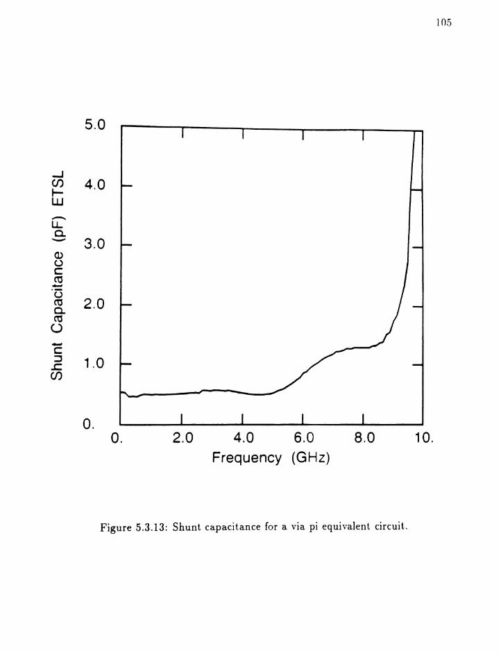
5.0

....Jen 4.0J--W~

u..c..~ 3.0(1)occt1....,

.(3ct1 2.0c..ct1o...,C::J 1.0J::,

en

o.o. 2.0 4.0 6.0

Frequency (GHz)

8.0 10.

lOS

Figure 5.3.13: Shunt capacitance for a via pi equivalent circuit.

100.

......Jen~ 80.w...-....enE..c0 60.~

Q)oc~~ 40.o~(1)

a:en(1)

20 ..~(1)

en

o.o. 2.0 4.0 6.0

Frequency (GHz)8.0 10.

106

Figure 5.3.14: Series inductive reactance for a via pi equivalent circuit.

107

has higher per unit length loss than the through standard. At half wavelength fre­

quencies, the line appears transparent only contributing an additional attenuation

above that of the through.

A direct comparison of the via inductive reactance between TSL and ETSL

IS shown in Fig. 5.3.15. There is difference over the middle to upper frequency

range. It is in this region that the complex impedance is farthest from the TDR

57 ohm value. More important than this comparison is that we can calculate the

complex impedance of a uniform transmission line and include dispersion.

5.4 Results of the Through-Sy:mrnetric Fixture De-embedding

Method

5.4.1 Introduction

This section contains verification of the TSF algorithm over a frequency range of

45 to 800 MHz. Also, TSF uses different fixturing so we will discuss its design

and measurement. Verification is done by direct measurement of both the fixture

halves and a de-embedded low pass filter.

5.4.2 Meaaureruent and Fixture Design

It was shown in Chapter 3, that TSF requires a second order symmetric fixture.

This forces the fixture halves to be symmetric and identical. The fixture was

108

--J 70.(/)t-UJ

-cc 56.co

-..J(/)r-...-... 42 .enE.c0'-""

OJ 28.occo...,ocoOJa: 14.enOJ'i::<J.)

(/)

o.O. 2.0 4.0 6.0 8.0 10.

Frequency (GHz)

Figure 5.3.15: Comparison of via inductive reactance calculated wit h (0) TSL and

(6) ETSL.

109

design to introduce significant error in the embedded measurement and still main­

tain the symmetry requirement. This was accomplished with an shunt inductive

discontinuity placed between an APC-7 to female SMA adaptor and a male SMA

to APC-7 adaptor, see Fig. 5.4.1. These connector combinations allow direct

measurement and subsequent comparison with the error networks calculated with

TSF.

The approximate inductance is ten nano Henries and connected as a shunt

element appears as a short circuit at low frequencies and open at higher frequen­

cies. This creates significant error yet it is possible to construct two of these

fixture halves and satisfy the symmetrical requirements. Fig. 5.4.2 and 5.4.3 show

the magnitude and phase of Sijl respectively for the fixture s parameters. Only

511 ! and 521 ! need be shown because 5 22! == 5 11! and 5 12! == 5 21! ; the fixture is

symmetric. The next section presents results of the TSF algorithm.

5.4.3 TSF De-ernbedd'ing Results

TSF was applied to the embedded low pass filter (DDT) and results are shown

in Fig. 5.4.4- 5.4.11. These gre:tphs show t.he significflnt effect. t.he fi xt nre error

networks impose and comparison, in magnit ude and phase, between direrf mra-

surement and the TSF de-embedded filter.

110

Through Connection

(a)

Embedded Filter

500 MHz Low Pass Filter

(b)

Figure 5.4.1: Fixturing for verification of TSF. (a) Fixture through con nect.ion

and (b) embedded 500 MHz low pass filter. The fixture halve is composed of twoadaptors (APC-7 to male SMA) and the shunt inductor (10 nano henries) mountedin a SMA through.

111

o.

- 8.0

,-...

CD0 - 16.~

Q)-0~~

c:- 24.0)

co~

- 32.

- 40.45. 200. 350. 500.

Frequency (MHz)

650. 800.

Figure 5.4.2: Magnitude of the TSF fixture s parameters, (0) 5 11! and (6) 52 1! .

112

800.650.200. 350. 500.

Frequency (MHz)

200. r--------.-----...------.-.----r---~

120.

- 120.

- 200.45.

...-.-....0) 40.Q)

0~

Q)(f){\j

- 40 ....cQ..

Figure 5.4.3: Phase of the TSF fixture s parameters, (0) 5 11! and (6) 521! ·

113

o.

- 12.

,-....

COC) - 24.'-""

Q)~:J~

C- 36.0>ru

~

- 48.

- 60.45. 200. 350. 500

Frequency (MHz)

650. 800.

Figure 5.4.4: Magnitude of the filter 5 2 1 , (0) direct measurement and (6) embed­ded. The fixture error significantly alters the filter measurement.

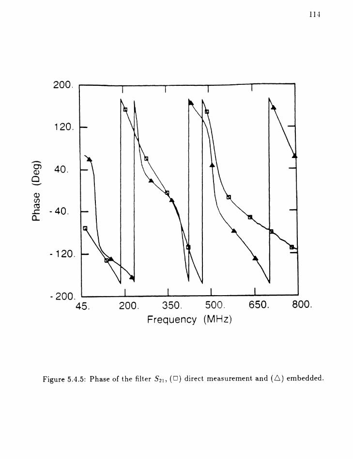
114

200.

120.

.....-...0) 40.(J)

0"""-"'""

Q.)(j)

~- 40.~

o,

- 120.

- 200.45. 200. 350. 500.

Frequency (MHz)

650. 800.

Figure 5.4.5: Phase of the filter 5 2 1 , (D) direct measurement and (6) embedded.

115

Magnitude of S11, dl3o.

- 6.4

- 13.

- 19.• [),rel- t

A [mtw,1jed

+ De - '='[1 l[ledded

- 26.

- 32.60. 210. 360. 500. 650. 800.

1- requency, Mhz

Figure 5.4.6: Magnitude of the filter 5 11 , (0) direct measurement and (6) embed­

ded.

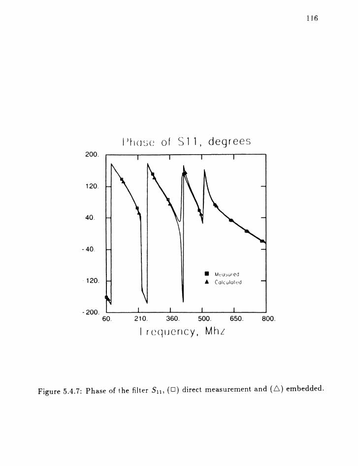
116

I 'ho:«: of S 11, degrees200.

120.

40.

- 40.

- 120.

- 200.60.

• Mt:'u~ur Ctj

A Coleulot td

210. 360. 500. 650.

I rcqucncy, MhL800.

Figure 5.4.7: Phase of the filter 5 11 , (0) direct measurement and (6) embedded.

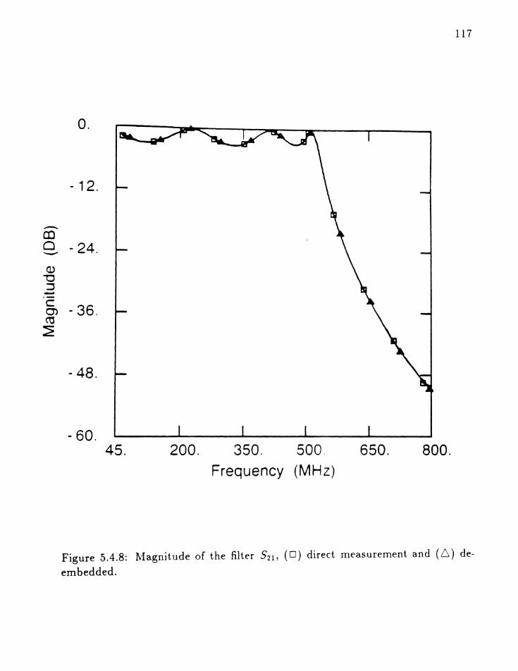
117

o.

- 12.

~

CO0 - 24."-"

Q.)""0:J...,c:

- 36.enro~

- 48.

- 60.45. 200. 350. 500.

Frequency (MHz)

650. 800.

Figure 5.4.8: Magnitude of the filter S21l (0) direct measurement and (.6) de­

embedded.

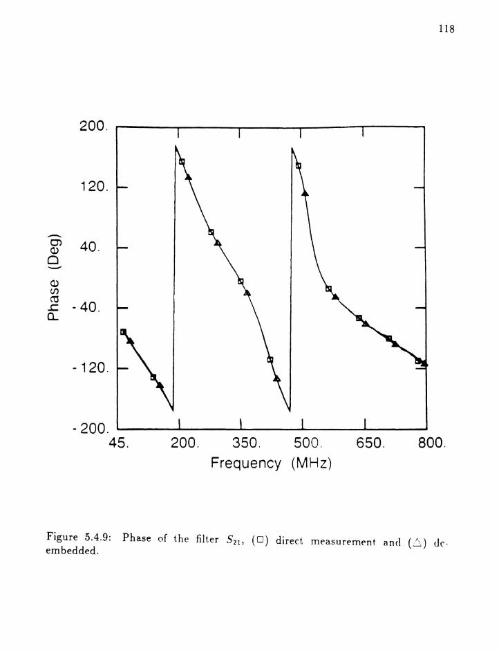
118

200.

120.

~

0) 40.0)

0........""

0)(/)C\]

- 40 ...co,

- 120.

- 200.45. 200. 350. 500.

Frequency (MHz)

650. 800.

Figure 5.4.9: Phase of the filter 5 21 , (0) direct measu re ment and C~) de-­embedded.

119

o.

- 8.0

~enCl - 16."""-'

a>-c:J...,c

- 24.CJ)~

~

- 32.

- 40.45. 200. 350. 500.

Frequency (MHz)

650. 800.

Figure 5.4.10: Magnitude of the filter 5 11 , (0) direct measurement and (6) de­embedded.

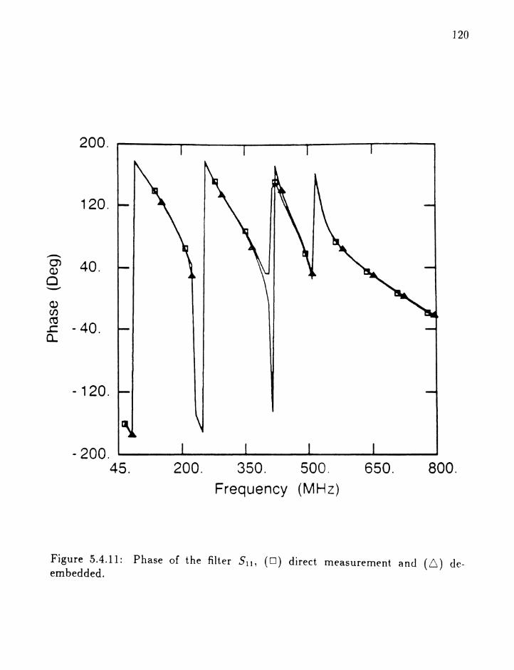
120

200.

120.

~

0) 40.Q)

0~

Q)(/)

~- 40 .s:

o,

- 120.

- 200.45. 200. 350. 500.

Frequency (MHz)

650. 800.

Figure 5.4.11: Phase of the filter 5 11 , (0) direct measurement and (6) de­embedded.

5.4.4 Conclusion

121

Tllis section has shown that w hen a fixture is second order sv mrnel.ric TSF can~ ,

be used to remove the fixture error from a DDT. TSF algorithm is not with out

singularities however they did not influence this measurement because they existed

beyond the measurement range.

5.5 conclusion

In this chapter we have presented experimental results for each of tile symmetrical

de-embedding methods developed in Chapter 3. TSL and ETSL were applied to a

embedded microstrip fixture and the impedance enhancement to TSL was verified

wit h a 50 ohm coaxial example. The complex characteristic impedance of an

embedded microstrip was calculated and this result is not a function of symmetry

and is directly applicable to TRL and LRL de-embedding methods.

It was also shown that TSF can be used to de-embed a second order symmetric

fixture. This was accomplished by designing a second order fixture with essentially

a lumped element. The next chapter concludes the work done here and hopes

design.

122

Chapter 6

Conclusion

6.1 Summary

The objective of this study was to study calibration of automatic network analysis.

This work consists of two parts: the organization of existing calibration methods,

and development of fixture calibration methods that address printed circuit board

concerns.

In the first part, the exiting methods were organized l)y categorizing calibration

methods into one or two port error models. Two port error models were further

divided to automatic network analyzer models and fixture models. To complete the

categorization calibration standards used for by previous authors were presented

and discussion of their motivation was given.

In the second part of this study, symmetrical calibration methods were devel-

oped to combat the non-inser t able nat nre of printed circuit hoard rneasu rement ,

i.e. use a minimum number of standards and do so without physically inserting

them. Through-Symmetry-Line was possible because the PCB fixture was sym­

metric allowing a third standard to be synthesized from two standards namely

the through and line. The synthesized short circuit was experimentally verified

123

indicating that symmetry can be used to reduce the number of standards.

TSL was enhanced by calculating the complex characteristic impedance of the

line standards. In order to verify this enhancement, a precision 50 ohm coaxial

air line was measured and its transmission line parameters were calculated. Ex­

cellent agreement between expected coaxial parameters an calculated validate the

enhancement. The transmission line parameters for an embedded microstrip were

subsequently determined. This enhancement is not a function of the symmetry

and can be applied to TRL and LRL de-embedding methods. Both TSL and ETSL

were used to de- embed the pi equivalent circuit of a PCB via. Finally, their result

was compared and the difference noted.

The final symmetrical method, Through-Symmetric Fixture was applied to

directly measurable fixtures and embedded device (lo'v pass filter). Again excellent

agreement between measured and calculated responses show that TSF is successful

at removing error from a second order fixture. In all cases, SPANA was used to

implement the algorithms and present the da.ta for this report.

6.2 Discussion

In general, calibration of network analysis models the systematic error of the

measurement system. Under most circumstances the random measurement er­

ror is negligible but random process that effect the uniformity of transmission

lines should be considered. This further strengthens the desirability to reduce the

124

standards needed.

Most new methods have been developed out of need. If a matched load cannot

be fabricated then consider another standard to replace it. Having a review of

existing techniques allows one to chose the most accurate method. When investi­

gating a new measurement system it is valuable to keep a "what if we use a ... "

attitude when selecting standards. In addition, by using a two tier calibration

method the choice of algorithms is bountiful.

6.3 Suggestion for Further Study

Additional areas of study include:

i) effect of random variation of transmission line parameters on de- embedding

results, and

ii) applying symmetrical de-embedding methods to wafer probe calibration.

12.5

References

[1] G. A. Deschamps, "Determination of reflection coefficients and insertion lossof a waveguide junction," J. Appl. PhY3. vol. 24 pp. 1046-1050 August1953. '"

[2] J. E. Storer, L. S. Sheingold, and S. Stein, "A simplified calibration of two­port transmission line devices." Proc. of the IRE, vol. 41, pp. 1004-1013,August 1953.

[3] F. L. Wentworth and D. R. Barthel, "A simplified calibration of two-porttransmission line devices," IRE Trans. Alicrowave Theory Tech., pp. 173­175, July 1956.

[4] S. J. Mason, "Feedback theory - further properties of signal flow graphs,"Proc. of the IRE, vol. 4~, pp. 920-926, 1956.

[5] R. A. Hackborn, "An automatic vetwork analyzer system," Microuiave J.,pp. 45-52, May 1968.

[6] I. Kasa, "Closed-form mathematical solutions to some network analyzer cal­ibration equations," IEEE Trans. Itisirurn. Meas., vol. I1tI-23, no. 4, pp.399-402, December 1974.

[7] H. C. Heyker, "The choice of sliding load positions to improve network anal­yser calibration," Proc. 17th European Alicrowave Conf., pp. 429-434,1987.

[8J W. Kruppa and K. F. Sodomsky, "An explicit solution for the scatteringparameters of a linear two-port measured with an imperfect test set," IEEETrans. Microuiave Theory and Tech., vol. ~ITT-19, no. 1, pp. 122-123, Jan­uary 1971.

[9] R. F. Bauer and P. Penfield Jr., "De-embedding and unterminating," IEEETrans. Microuiave Theory Tech., vol. MTT-22, no. 3, pp. 282-288, March1974.

[10] 1\1. S. Horlgart 'I "Microwave im perl nnce r1rtprmln~tlnn h~r rrflrrtlnn-coellicient measurement t hroug l: a u arbitrary lin f ' '' ' ~ 1"'" ';\~ff·'t1"· /'/,,"

tron. Lett., vol. 12, no. 8, pp. 184-186, April 1976.

[11] E. F. Da Silva and lvl. K. McPhun , "Calibratiun of microwave network anal­yser for computer-corrected s-parameter measurements," Electron. Lett., vol.9, no. 14, pp. 126-128, March 1973.

[12] H. V. Shurmer, "Calibration procedure for computer corrected s parametercharacterization of devices mounted in microstrip," Electron. Leii., vol. 9,no. 14, pp. 323-324, July 1973.

126

[13] J. W. Gould and G. M. Rhodes, "Computer correction of a microwave net­work analyser without accurate frequency measurment," Electron. Lett., vol.9, no. 21, pp. 494-495, October 1973.

[14] E. F. Da Silva and 1\1. K. Mc Phun , "Calibration of an automatic net­work analyser system using transmission lines of unknown characteristicimpedance, loss and dispersion," Radio Electron. Eng., vol. 48, no. 5, pp.227-234, May 1978.

[15] S. Rehnmark, "On the calibration process of automatic network analyzersystems," IEEE Trans. AJicrowave Theory Tech., vol. M'f'f-22, no. 4, pp.457-458, April 1974.

[16] J. Fitzpatrick, "Error models for systems measurement," Microuiane J., pp.63-66, May 1978.

[17] A. M. Saleh, "Explicit formulas for error correction in microwave measur­ing sets with switching-dependent port mismatches," IEEE Trans. Inslrum,Meas., vol. IM-28, no. 1, pp. 67-71, March 1979.

[18] N. R. Franzen and R. A. Spaciale, "A new proceedure for system calibra­tion and error removal in automated s-pararneter measurements," Proc. 5thEuropean Microwave Conj., pp. 69-73,1975.

[19] B. Bianco, M. Parodi, S. Ridella and F. Selvaggi, "Launcher and microstripcharacterization," IEEE Trans. Insirum: Meas., vol. 11'1-25, no. 4, pp. 320­323, December 1976.

[20] G. F. Engen and C. A. Hoer, "Thru-reflect-line: an improved techniquefor calibrating the dual six-port automatic network analyzer," IEEE Trans.Microuiave Theory Tech., vol. MTT-27, no. 12, pp. 987-993, December 1979.

[21] J. A. Benet, "The design a.nd calibration of a universal mmic test fixture,"IEEE lYfTT-S International Microwave Sympo3ium Dig., pp. 36-41, 1982.

[22] R. Vaitkus and D. Scheitlin, "A two-tier deembedding technique for packagedtransistors," IEEE AJTT-S International Microuiaue Sympo3ium Dig., pp.328-330, 1982.

[23] R. L. Vaitkus, "Wide-band de-embedding with a short, an open, and athrough line," Proc. of tlie IEEE, vol. 74, no. 1, pp. 71-74, January 1986.

[2·1] S. n. Pcn nock . r. 1\J. n. nyrrnfi. P. n. ~h('plH'rd a nr l T. n,tZ7,t. "'r":'f1~i

tion characterisation for de-embedding purposes," Proc . 17th European Ali­crowave Conf., pp. 355-360, 1987.

[25] R. P. Meys, "A triple-through method for characterizing test fixtures," IEEETrans. Microuiane Theory Tech., vol. MTT-36, no. 6, pp. 1043-1046, June1988.

[26] H. J. Eul and B. Schiek, "Thru-match-reflect: one result of a rigorous the­ory for de-embedding and network analyzer calibration," Proc. 18th. Europ.Microuiaue ConI., pp. 909-914, 1988.

(30]

[29]

[28]

]27

[27] J. R. Souza and E. C. Ta.lboys, "S-parameter characterisation of coaxial tomicrostrip transition," lEE Proc. vol. 129 Pt. H no. 1 pp.37-40 February1982. " " ,

B. Bianco, A. Corana, S. Ridclla and C. Simicich "Evaluation of errorsin calibration procedures for measurements of reflection coefficient" IEEETrans. Itistrum: Meas., vol. 111-27, no. 4, pp. 354-358, December !!}78.

J. P. Mondal and T. H. Chen, "Propagation constant determination in mi­crowave fixture de-embedding procedure," IEEE Trans, Microwave TheoryTech., vol. MTT-36, no. 4, pp. 706-714, April 1988.

Hewlett Packard, "Network analysis: applying the HP 8510B trl calibrationfor non-coaxial measurements," Product Note 8510-8, pp. 1-22, 1987.

[31] A. R. Martin and 11. Dukeman, "Measurement of device parameters usinga symmetric ixture," Microuiaue J., pp. 299-306, May 1987.

[32] W.J. Getsinger, "Measurement and modeling of the apparent characteristicimpedance of microstrip," IEEE Trans, Alicrowave Theory Tech., vol. MTT­31, pp. 624-632, August 1983.

[33] I. Bahl and S. Stuchly, "Analysis of a microstrip covered with a lossy di­electric," IEEE Trans. Microuiaoe Theory Tech., vol. MTT-28, pp. 104-109,February 1980.

[34] T. Wang, R.F. Harrington and J.R. Mautz , "Quasi-static analysis of a mi­crostrip via through a hole in a ground plane," IEEE Trans. MicrouiaveTheory Tech., vol. 11TT-36, pp. 1008-1013, June 1988.

[35] R. D. Pollard and R. Q. Lane, "The calibration of a universal test fixture,"IEEE AfTT-S International Microwave SympoJium Dig., pp. 498-500, 1983.

[36] A. Enders, "An Accurate Measurement Technique for Line Properties, J unc­tion Effects, and Dielectric and Magnetic Material Parameters," IEEETran3. ~Iicrowave Theory Tech., vol. MTT-37, no. 3, pp. 598-605, March1989.

[37] E. R. Ehlers, "Symmetric Test Fixture Calibration," IEEE MTT-S Interna­tional Microwave SympoJium Dig., pp. 275-278, 1986.

[38] S.J. Mason, "Power g"in in feerlhttrk a m plifiers ," T.n.R. Tran s. rirrll;I Thf'­ory , Vt) I. t 'T . I . .J 11" f' I q.l I. Pp. :~ fl :!:).

RELATED REFERENCES NOT REFERRED TO IN TEXT:

[39] H. V. Shurmer, "New method of calibrating a network analyser," Elect.Letters, vol. 6, no. 23, November 1970, pp. 733-734.

[40] G. F. Engen, "Calibration tec~niq~e for automated ~etwork analyzers withapplication to adapter evaluation, IEEE Trans. Microwave Theory Tecli.,vol. JvITT-22, no. 12, December 1974, pp. 1255-1260.

128

[41] D. Woods, "Rigorous derivation of computer-correct.ed network-analyser cal­ibration equations," Elect. Leiters, 1.'01. 11, no. 17, A uqus! 1975, pp. 403-405.

[42] R. A. Speciale, "A Generalization of the tsd network-analyzer calibrationprocedure, covering n-port scattering-parameter measurements, affected byleakage errors," IEEE Trans, AJicrowave Theory Tech.., vol AfTT-£5, no. 12,December 1977, pp. 1100-1115.

[43] G. F. Engen, "Calibrating the six-port reflectometer by means of slidingtermination," IEEE Tran3. Microuiaue Theory Tech., vol AJTT-26, no. 12,December 1978, pp. 951-957.

[44] A. Baranyi and J. Ladvanszky, "On the Exact S-Parameter Measurement ofActive Devices," Proc. 10th European Microuiaue Conf., 1980, pp. 278-282.

[45] L. Gruner, "The Determination of the Scattering Parameters of MicrowaveN-Port Networks," IEEE Trans. Insirurn, Meos., vol. Ilvl-:JO, no. 3, Septem­ber 1981, pp. 198-201.

[46] J. Dibeneditto and A. Uhlir Jr., "Frequency Dependence of 50-(ohm) CoaxialOpen-Circuit Reflection Standa.rd," IEEE Trans, lnstrurn; AJea3., vol. IAl­30, no. 3, September 1981, pp. 228-229.

[47] P. C. Sharma and K. C. Gupta, '~A Generalized Method for De-embeddingof Multiport Networks," IEEE Trans. Instrurn, AIea3., vol. lA/-30, no. 4,December 1981, pp. 305-307.

[48] K. Brantervik a.nd E. L. Kollberg, "A New Four-Port Automatic NetworkAnalyzer: Part I-Description and Performance," IEEE Trans. Insirurn,AIea3., vol. IAJ-:J3, no. 7, July 1985, pp. 563-568.

[49] H. E. Stinehelfer Sr., "Discussion of De-Embedding Techniques Using Time­Domain Analysis," Proc. of the IEEE, vol. 74, no. 1, January 1986, pp.90-94.

[50] P.R. Shepherd and R. D. Pollard, "Direct Calibration and Measurement ofMicrostrip Structures on Gallium Arsenide," IEEE Trans. AJicrowave The­ory Tech., vol AJTT-:J4, no. 12, December 1986, pp. 1421-1426.

[51] J. Curran, "Applying TRL Calibration for Noncoaxial Measurernents ," Ali­crowave SY3tem3 Neuis fj Communication Technology, vol., no., Marcli 1988,pp. 91-92, ~·1, 97-9R.8

[52] G. J. Scalzi, A. J. Slobodnik Jr. and G. A. Roberts, "Network AnalyzerCalibration Using Offset Shorts," IEEE Trans, Alicrowave Theory Tech.,vol kITT·36, no. 6, June 1988, pp. 1097-1100.

[53] D. F. Williams and T. H. l\liers, "De-embedding Coplanar Probes withPlanar Distributed Standards," IEEE Trans. Alicrowave Theory Tech., volMTT-36, no. 12, December 1988, pp. 1876-1880.

129

[54] K. Bra~,tervik, "A New Four-Port Automatic Network Analyzer: Part 11­Theory, IEEE Trans. Microwave Theory Tech., vol. MTT-!J3, no. 7, July1985, pp. 569-575.

[55] L.. Dunl~avy and P. ~; Katehi. "Eliminate Suprises When De-EmheddingMicrostrip Launchers, Aficrowave~ fj RF vol. no. Auqusi 1987 pp. 117-118,120-122. ' " ,

[56] Hewlet Packard, "Accuracy Enhancement Fundementals " HP8510 NetworkAnalyser Operating and Programm Afanual, 1987, pp. Hi5-180, 207-208.8

[57] D. Brubaker and J. Eisenberg, "Measuring S-Parameters with the TSD Tech­nique," Microuiaues fj RF, vol., no., November 1985, pp. 97-98,100-101,159.159

[58] G. Elmore, "De-Embedding Device Data with a Network Analzer," Ali­crouiaves £3 RF, vol., no., November 1985, pp. 145-146.

[59] J. G. Evans, "Measuring Frequency Characteristics of Linear Two-Port Net­works Automatically," Bell SY3tem Technical Journal, vol., no., May-June1969, pp. 1313-1338.

[60] D. Woods, "Reappraisal of Computer-Corrected Network Analyser Designand Calibration," Proc. lEE, vol. 124, no. 3, A/arch 1977, pp. 205-211.

[61] S. F. Adam, "A New Precision Automatic Microwave Measurement System,"IEEE Trans. Instrurn: AJea3., vol. IAI-17, no. 4, December 1968, pp. 308-313.

[62] O. J. Davies, R. B. Doshi and B. Nagenthiram, "Correction of Microwave­Network-Analyser Measurements of 2-Port Devices," Electron. Lett., vol.,no., November 1973, pp. 543-544.

[63] H. B. Sequeira, M. W. Trippe and R. Jakhete, "A Network Analyzer Cali­bration Using Redundancy," Proc. 18th. Europ. Microuiaue Con/., 1988, pp.321-325.

[64] J. G. Evans, F. W. Kerfoot and R. L. Nichols, "Automated Network Ana­lyzers for the 0.9- to 12.4-GHz Range," Bell Sy~tem Technical Journal, vol.55, no. 6, July-A uqus! 1976, pp. 691-721.

r6r>1 V. (1. Gelnn,,~tch~ ".1\ rnmplltpf Prngfrlm fnr thr Dlrf'ct r,.lil'frttinn nf T,vo­Port Rellectometers for ,\utuluatl'd !\Ji( I"n\\il\'" ~'(';'l:""'''l' nf ,:." l lF]: li n n >.

Microwave Theory Tech., vol. A/TT·24, no. 1, January 1976, pp. ~!)-,17.

[66] L. A. Glasser, "An Analysis of Microwave De-embedding Errors," IEEETran~. Microuiave Theory Tech., 1101 /l;fTT.26, no. 5, Alay 1978, pp. 379-380.

[67] T. E. MaeKenzie and A. E. Sanderson, "Some fundamental design principlesfor the development of precision coaxial standards and components," IEEETrans. Microwave Theory Tech., vol AITT.14, no. 1, January 1966, pp. 29-39.

130

[68] R. Q. Lane and G. L. NlcCollum, "A new sel-calihrating t ra.nsistor testfixture," IEEE AfTT-S International Alicrowave Sympo"ium Dig., 1979, pp.99-101.

[69] B. Donecker, "Accuracy prediction for a new generation network analyzer,"Microwave J., June 1984, pp. 127-128,130-132,134, 136,138,141.

[70] R. Lane, "De-embedding device scattering parameters," Microwave J., Au­qus! 198~, pp. 149-150,152,154-156.54-156

[71] G. R. Simpson and R. Q. Lane, "A microstrip chip carrier and insert for thetransistor test fixture," ARFTG ~p , June 1985, pp. 144-157.

[72] J. Archer, "Implementing the tsd calibration technique," Microuraue Sy"tem"New" (3 Communication Technology, AJay 1987, pp. 54, 56, 58, 60-61.61

[73] rvl. A. Maury, S. L. March and G. R. Simpson, "Lrl calibration of vectorautomatic network analyzers," Alicrowave J., AIay 1987, pp. 387-392.

[74] L. DuBois, "New microstrip fixture and method for de-embedding," Ali­crowave Sy3tem" NeW3 fj Communication Technology, September 1987, p.96, 98, 100.

[75] C. Beccari and U. Pisani, "Automatic discontinuity de-embedding In s­parameter measurement system," Alta Frequenza, }"ol. L }"'II, No.5, June1988, pp. 249-257.

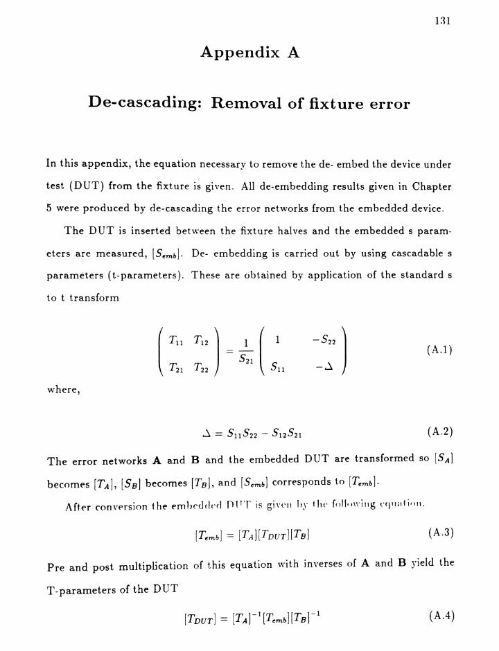
l:JI

Appendix A

De-cascading: Removal of fixture error

In this appendix, the equation necessary to remove the de- embed the device under

test (DDT) from the fixture is given. All de-embedding results given in Chapter

5 were produced by de-cascading the error networks from the embedded device.

The DDT is inserted bet\veen the fixture halves and the embedded s param­

eters are measured, [Semb]. De- embedding is carried out by using cascadable s

parameters (t-pararneters). These are obtained by application of the standard s

to t transform

TIl Tl 2 1 1 -522

-521

(A.l )

T21 T22 511 -~

where,

(A.2)

The error networks A and B and the embedded DUT are transformed so [SA]

becomes [TAl, [Sa] becomes [Ta], and [Semb] corresponds to [Tem b] .

Aft.er conversion the embedded fllT'r is giYCIl hy f h(' [o"f)\\'i"g cCj1lcdifl " .

(A.3)

Pre and post multiplication of this equation with inverses of A and B yield the

T-parameters of the DDT

(A.4)

and thus its S parameters

132

(A.5)

1

For first order symmetric fixtures B == A R and second order B == A.

133

Appendix B

SPANA Semantic Command Description

This appendix is a user's manual for SPAN A. Its purpose is to inform the user uf

the command syntax and the requirer] command line parameters. SPAN A is not

case sensitive and for clarity this appendix will use bold face characters to indicate

command syntax.

Some of the functions require command parameters in addition to the command

itself for example.

*dmb2 meas== 1 type== 1 dest==2 stan==3

The command parameters provide the function with information. Each com­

mand parameter is separated with a space and the argument to the right of the

parameter is the data to be passed to the function. The order of command param­

eters is not important but a complete command line is required. The arguments

can be delimited with any white space character. If a command syntax occurs the

line will be aborted and a message given.

Help. Example: help more

P'nrpose. TTET,P i~ thp nn-llnr hr1r f(lrl1;t~.. fnr l1~ting thp corn ma nrl s th,lt nre

available in SPAN A as well as a brief description of each command. The possible

help arguments are shown below.

Arguments.

more

page2

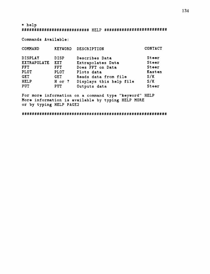
* help########################### HELP #########################

Commands Available:

COMMAND KEYWORD DESCRIPTION CONTACT

DISPLAY DISP Describes Data SteerEXTRAPOLATE EXT Extrapolates Data SteerFFT FFT Does FFT on Data SteerPLOT PLOT Plots data KastenGET GET Reads data from file S/KHELP H or ? Displays this help file S/KPUT PUT Outputs data Steer

For more information on a command type "keyllord" HELPMore information is available by typing HELP MOREor by typing HELP PAGE2

##########################################################

134

1;J5

* help page2###################### HELP PAGE2 ########################

Commands Available:

COMMAND KEYWORD DESCRIPTION CONTACT

DE-EMBED DMB2 or 3 De-embeds OUT data S/KBUILD BLD Makes standard from data KastenPOLAR>RECT PTOR Polar to rect conversion KastenRECT>POLAR RTOP Rect to polar conversion KastenSYMMETRIZE SYH Symmetrize data SteerWINDOW WIN Smooths Data Kasten

For more information on a conunand type "keyvord" HELPMore information is available by typing HELP MORE

##########################################################

* help more####################### HELP MORE ########################

The folloving input/output commands are availabl~:

vriteeofendtitlepromptecho onecho off

read filename : the file filename is opened for inputread : the previously opened file is nov used for

inputfilename the file filename is opened for output

the input data file is closedthe input data file is temporarily closedvrite line to output filevrite line to terminalthe flag prt is setthe flag prt is cleared

If prt is set all lines input are echoed.

##########################################################

136

B.0.1 get

Example: get rneas e l ftle==dut.s2p format==magang

Purpose. GET is used to input a measurement set into SPANA.

Arguments.

help

meas

file

format

nl

filename

magang

a-l-jb

!\IEAS designates the measurement set (nl) that the data will be loaded into.

The argument must be less than the maximum number of measurement sets. GET

will over write an existing measurement set.

FILE designates the filename from which the data will be read from. The

filename can be any acceptable name including a directory path provided the

total number of characters is less than thirty.

SPAN A allows for text information to be placed above the data. Each line

of this text must begin with a comment delimiter (! or #) in the first or second

column however the first line in the file is taken as the data identifier and it is used

in the PUT and DISPlay functions. Any subsequent comment lines will be ignored

line. The data is read in until the end of file is encountered. Below is an example

file.

137

S parameters for DlTT (This is an example data identifier)

This line will be ignored

1.500 0.015 35.5 0.995 95.4 0.995 95.4 0.02 20.5

If the data is in the frequency or time domain than the independent variable is

assumed to be in megahertz or nanoseconds respectively.

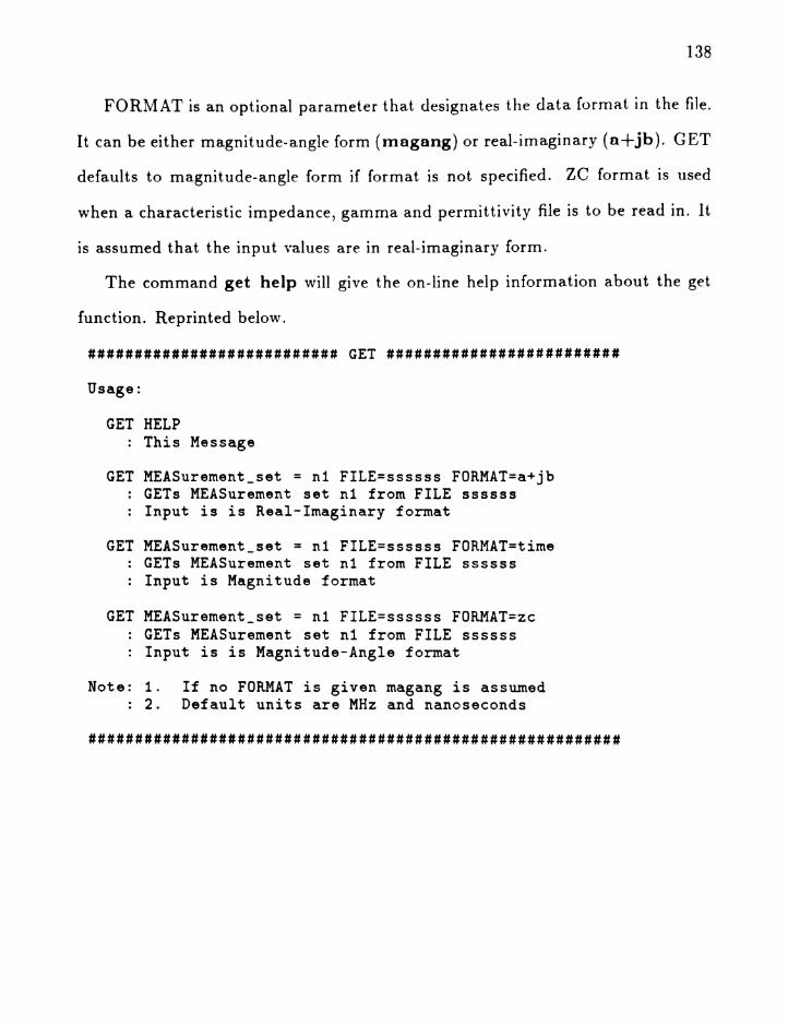
138

FORMAT is an optional parameter that designates the data format in the file.

It can be either magnitude-angle form (magang) or real-imaginary (a+jb). GET

defaults to magnitude-angle form if format is not specified. ZC format is used

when a characteristic impedance, gamma and permittivity file is to be read in. It

is assumed that the input values are in real-imaginary form.

The command get help will give the on-line help information about the get

function. Reprinted below.

########################### GET #########################

Usage:

GET HELPThis Message

GET MEASurement_set = n1 FILE=ssssss FORMAT=a+jbGETs MEASurement set n1 from FILE 9SS5S9

Input is is Real-Imaginary format

GET MEASurement_set = n1 FILE=ssssss FORMAT=timeGETs MEASurement set n1 from FILE ssssssInput is Magnitude format

GET MEASurement_set = nl FILE=sss5ss FORMAT=zcGETs MEASurement set nl from FILE S5S5S5Input is is Magnitude-Angle format

Note: 1.2.

If no FORMAT is given magang is assumedDefault units are MHz and nanoseconds

#########################################################

139

B.O.2 put

Example: put m eas e n ftle==dut.s2p

Purpose. PUT is used to output a measurement set to the terminal screen or to

a specified filename.

Arguments.

help

rrieas

file

inline

nl

filename

n2

option 1 for option

11EAS designates the measurement set (nl) that will be processed. The argu-

ment must be less than the maximum number of measurement sets. If MEAS is

the only argument then the measurement set will be put to the terminal screen

and attached to the beginning of the data will be the PUT banner.

FILE designates the filename to which the data will be written to. The filename

just as for GET can be any acceptable name including a directory path provided

the total number of characters is less than thirty. Below are two banners that

PUT would attach to the beginning of PUT file.

S parameters for OUT-~~----------------------------------------------

MEASUREMENT SET 1Two-port S parametersFrequency-Domain Data: Magnitude-Angle FormNumber of Frequency points: 1Frequency Interval: O. MHzLov Frequency: 1000.00 MHzHigh Frequency: 1000.00 MHzValid Measurement DataCharacteristic Impedance: 50.0000

Identifier:S parameters for OUT

FREQ(MHz)

511Mag Angle

521Mag Angle

512Mag Angle

1·10

522Mag Angle

1000.0 0.01944 -151.31 0.97351 -102.56 0.97470 -102.43 0.01784 136.54

141

Three port de-embeded result (DMB3). Part 1 of 3.-------------------------------------------------

Form

Part 1 of 3.513523533

Mag Angle

50.0000

de-embeded result (DMB3).511 512521 522531 532

Angle Mag AngleMag

MEASUREMENT SET 9Three-port 5 parametersFrequency-Domain Data: Magnitude-AngleNumber of Frequency points: 1Frequency Interval: o. MHzLov Frequency: 1000.00 MHzHigh Frequency: 1000.00 MHzValid De-embeded DataCharacteristic Impedance:

Identifier:Three port

FREQ

. (MHz)!1000.0000 0.59842 -169.85 0.22104 -33.48 0.21382 -33.49

0.22104 -33.48 0.75168 -167.80 0.30034 -30.960.21382 -33.49 0.30034 -30.96 0.72729 -168.10

The banner that preceds the data depends on measurement statistics (see display

command for information about possible statistics) with the above examples show-

ing two and three port data. The file format (magang, a+jb, zc or time) is specified

by the format type of the measurement set to be written out.

The IN LINE argument is used to place the data on one line with the line

containing all the data for one frequency or time point. This is default for two

port data but may be used for three and four port data output.

OPTION can be used to reduce a ZC format measurement set to only the

reduce if an option value of one is entered the option is executed.

The command put help will give the on-line help information about the put

function. Reprinted below.

########################### PUT #########################

Usage:

PUT HELPThis Message

PUT MEASurement_set = n1Types MEASurement on terminal

PUT MEASurement set = n1 INLINEPuts results on a single line used with three portsand higher

PUT MEASurement set = n1 OPTION = n2Outputs results using special option

PUT MEASurement_set = n1 FILE=ssssssPUTs MEASurement set n1 in FILE ssssss

#########################################################

142

B.0.3 disp

Example: disp==l

Purpose. Display is used to list measurement parameters for one set or all.

Arguments.

help

all

nl

If a measurement set number (n1) is given then the measurement statistics will

be displayed. Statistics available include the following.

1, 2, 3 or 4 port S or v parameters

System characteristic impedance

Start/Stop frequency or time

Number of data points

Data status (measured, converted or de-embedded)

Domain of data (frequency or time)

Data format (magang, a+jb)

If the all argument is given then statistics will be displayed for all availa hle mea-

(disp help).

MEASUREMENT SET 1Tvo-port S parametersFrequency-Domain Data: Magnitude-Angle FormNumber of Frequency points: 1Frequency Interval: 0.00 MHzLov Frequency: 1000.00 MHzHigh Frequency: 1000.00 MHzValid Measurement DataCharacteristic Impedance: 50.0000

Identifier:S parameters for DUT

######################### DISPlay #####################

Usage:

DISP HELP: This Message

DISP: DISPlay data about all Measurement sets

DISP n: DISPlay data about Measurement set n

#########################################################

144

14.1

B.O.4 del

Example: del meas== 1

Purpose. Delete is a house cleaning tool and is used to delete an exiting measure­

ment set making it available for reuse.

Arguments.

help

meas= nl

SPAN ...\ will delete the measurement set designated by nl. This deletion is

permanent and should be used with caution. Note: del does not delete files

stored on disk. If del help is entered. the on-line help for delete will be displayed

and is reprinted below.

########################### DEL #########################

Usage:

DEL HELPThis Message

DEL MEASurement_set = n1DELetes MEASurement set n1

#########################################################

B.O.5 ptor

146

Example: ptor meas== 1

Purpose. PTOR is for conversion from polar to rectangular format.

Arguments.

help

meas == n1

MEAS designates the measurement set that is to be converted. T'his is de-

structive since the measurement set is overwritten. PTOR will not convert a

measurement set if it is currently in magang format. Note: ZC format can be

converted however time format can not.

On-line help is available for PTOR by entering ptor help. The help message

is reprin ted below.

####################### PTOR ######################

Usage:

PTOR HELP: This Message

PTOR MEAS_set = n1

#####################################################

B.O.6 rtop

147

Example: rtop meas e 1

Purpose. RTOP is for conversion from rectangular to polar format.

Arguments.

help

meas == nl

MEAS designates the measurement set that is to be converted. This is de-

structive since the measurement set is overwritten. RTOP will not convert a mea-

surernent set if it is currently in a+jb format. Note: ZC format can be converted

however time format can not.

On-line help is available for RTOP by entering rtop help. The help message

is reprinted below.

####################### RTOP ######################

Usage:

RTOP HELP: This Message

RTOP MEAS_set = n1

#####################################################

148

B.O.7 stoy

Example: stoy meas== 1 dest==2 rect

Purpose. STOY is used to convert S parameter sets to Y parameters.

Arguments.

help

mess == n1

dest == n2

rect

magang

MEAS designates the measurement set that is to be converted and the result

is place in the DEST measurement set. The default format is that of the MEAS

set however by using either RECT or ~lAGANG arguments the result format

can be forced accordingly. Note: This conversion is only valid for S parameter

measurement sets.

On-line help is availiable for STOY by entering stoy help. The help message

is reprinted below.

####################### STOY ######################

Usage:

STOY HELP: This Message

STOY MEAS_set = n1 DEST_set = n2Convert S parameters data to Y parameters

using current format.

STOY MEAS_set = n1 DEST_set = n2 RECTangularConvert S parameters data to Y parameters

outputing data in complex rectangular form.

STOY MEAS_set = n1 DEST_set = n2 MAGANG: Convert S parameters data to Y parameters

outputing data in magnitude-angle form.

#####################################################

149

1.50

B.O.8 SYDl

Example: sym rne as e I dest==2

Purpose. Sy~M is used to symmetrize the specified measurement set.

Arguments.

help

mess == nl

dest == n2

Symmetrization of a 1IEAS set is done by replacing 11 and 22 and 21 and 12

with the respective average of the two. The format of the DEST set will be that

of the MEAS.

On-line help is availiable for S'Ylvl by entering sym help. The help message

is reprinted below.

#################### SYMmetrize ####################

Usage:

SYM HELPThis Message

SYM MEAS set = n1 DEST_set = n2Averages data in measurement set n1 and putsoutput in measurement set n2Output in columns 1 and 4 = average of data in inputcolumns 1 and 4Output in columns 2 and 3 = average of data in inputcolumns 2 and 3Averaging is done in real imaginary form and nata isreturned in the input format.

#####################################################

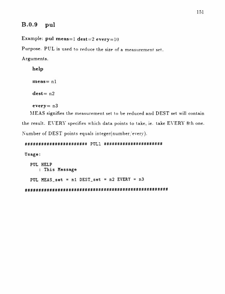
151

B.O.9 pul

Example: pul meas== 1 dest ==2 every== 1U

Purpose. PlTL is used to reduce the size of a measurement set.

Arguments.

help

mess== nl

dest== n2

every== n3

11EAS signifies the measurement set to be reduced and DEST set will contain

the result. E\·ER"l:T specifies which data points to take, ie. take E\,rER)" 8th one.

Number of DEST points equals int egerf number zeverv].

####################### PULl ######################

Usage:

PUL HELP: This Message

PUL MEAS_set = nl DEST_set = n2 EVERY = n3

#####################################################

B.O.I0.

win

152

Example: win meas=l dest=2 p arm e l l size==81

Purpose. Windowing is used to smooth a parameter in an existing measurement

set.

Arguments.

help

meas nl

dest n2

parm 11

21

12

22

size n3

IvfEAS designates the measurement set that will be smoothed with the result

to be place in the DEST measurement set. Windowing is done on the a+jb

form of the PARM that is specified so both real and imaginary or magnitude and

phase are smoothed together. The argument PARM is needed to designate which

columns of data within the measurement set are to be smoothed. 11,21,12, and

22 cor-respond respect ivelv to r ol nrn n s 1 -:? 1-1. t~-n. a n d 7-R. of thp measu rr-rnent

set. This is done so that any data format can be windowed.

SIZE is the width of the window and it is a number of samples and needs to

be odd.

On-line help is availiable for \\lIN by entering win help. The help message is

reprinted below.

####################### WINdov ######################Usage:

WIN HELPThis Message

WIN MEASurement_set = n1 DESTination set = n2PARAmeter = ?? ~indov SIZE = n3

Note: Windov size is an odd number of samples.#####################################################

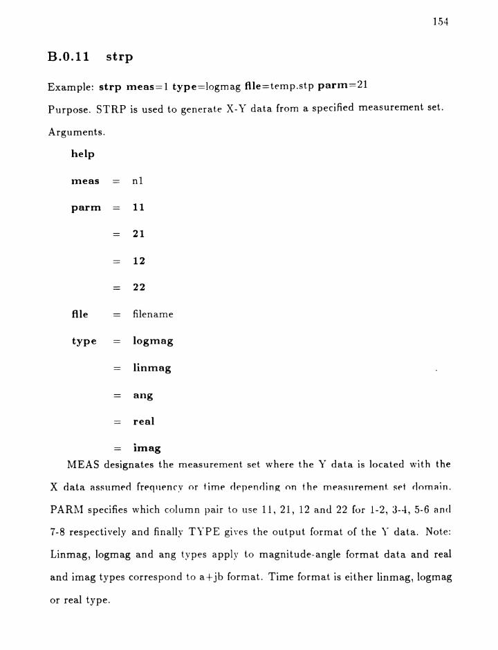
B.0.l1 strp

1.54

Example: strp meas==1 type==logmag ftle==temp.stp parm==21

Purpose. STRP is used to generate X- \9" data from a specified measurement set.

Arguments.

help

meas nl

parm 11

21

12

22

file

type

filename

logmag

linmag

aog

real

imag

MEAS designates the measurement set where the Y data is located wit h the

X data assumed frequenrv or time depending on t.he measurement set domrtln.

PAR~1 specifies which column pair to use 11,21,12 and 22 for 1-2,3-4,5-6 and

7-8 respectively and finally T\"PE gives the output format of the ) .. data. Note:

Linmag, logmag and ang types apply to magnitude-angle format data and real

and imag types correspond to a+jb format. Time format is either linmag, logmag

or real type.

15.5

On-line help is availiable for STRP by entering strp help. The help message

is reprinted below.

######################### STRiP #########################

Usage:

STRP HELP: This Message

STRP MEASurement set = nl FILE=ssssssPARM = n2 TYPE = n3

Strips parameter either magnitude or phaseand places along vith frequency (x,y) in thefile designated

#########################################################

156

B.O.12 drnb2

Example: dmb2 meas==l dest==2 type==4 h==5.6 1==2000 w==8 t==3.6

Purpose. DMB2 contains all the two port de-embedding routines and their purpose

is to do error correction.

Arguments.

1.57

help

meas nl

dest n2

error n3

stan n-l

thru n5

line n6

z m e as n7

reflect n r

type 1

2

3

4

t

w

h

eps

?

?

?

?

?

ZC ?

The de-embedding routines are executed by providing the required arguments

and possibly some optional arguments. The de-embedding types 1-4 require the

following; MEAS set, DEST set and Ty9"PE choice and some form of standard

158

information. The MEAS set contains the raw S parameters of the device under

test (dut) and the result or error corrected parameters are placed in the DEST

set. If the ERROR set is specified the de-embedding routines will place the error

two-port to this measurement set. Only argument semantics will be discussed

here with a detail discussion of de-embedding techniques left to the De-embedding

Theory section of this manual.

?

159

type 1 Microstrip Open-Short-LoBd

Required arguments.

stan n4

Type 1 (rvlicrostrip Open-Short-Load) requires a STAN measurement set that

contains the reflection coefficients for the three standards (open, short and load or

matched termination). This ST...\N set is generated using the BLD command (see

BLD for further information). Of course the result is placed in the MEAS set.

type 2 Through-Symmetric-Fixture

Required arguments.

stan n4

Type 2 (Through-Symmetric-Fixture) requires a STAN measurement set that

contains the through connection measurement of the embedding fixture.

type 3 Through-Symmetric-Line [enhanced]

Required arguments Optional arguments

thru n5

line n6zmeae n7

t ?

short n7

w ?

zc ?

h ?

epsType 3 (Through-Symmetric-Line [enhanced]) is a combination of type 3 de-

embedding routines. The combinations exist because of the optional arguments.

160

First the required arguments, type 3 needs two S parameter measurements, TIIRlT

set and LINE set, and some physical information; we microst rip width, t e metal

thickness, h==dielectric height and eps e.dielect ric constant. Note: All dimensions

are in mils. The default type 3 calculates the microstrip characteristic impedance

(zcmic) based on the physical parameters. This zcmic can be replaced by a fixed

impedance ZC==?? or a measurement set ZrvIEAS. The ZMEAS characteristic

impedance is contained in position 11 of the measurement set and is usually gen­

erated by type 4 de-embedding. If zcmic is not used w, t, h, eps need not be

specified.

The SHORT argument specifies a measurement set that contains the mea­

sured reflection coefficient (in the S11 position) with a physical short placed at

the microstrip port of the embedding fixture. If SHORT is not specified then

the symmetrical option is used. See the De-embedding Theory section for more

information.

type 4 Through-Symmetric-Line

Required arguments.

thru n4

line

t

w

h

n5

?

?

?

?

Type 4 (Through-Symmetric-Line) 15 used generally to determine the char-

acteristic impedance of the microstrip. This in turn is used with type 3 de-

161

embedding. Type 4 requires two S parameter measurement sets, THRU set and

LINE set as well as the physical parameters w==micrastrip widt.h , t==metal thick­

ness, h e dielectric height and l==difference between the physical lengths of the line

and thru standards. Reminder, all dimensions are in mils. For example if the thru

microstrip is 1000 mils long and the line strip is 3000 mils long one would use 2000

mils as the length (1).

The characteristic impedance, propagation factor (gamma) and effective dielec-

tric constant are outputs of type 4 and are placed in the last available measurement

set. Typing disp all will inform the user what measurement set this is. This mea-

surement set is assumed empty at all times and any data that may exist there

is overwritten by type 4. This measurement set can be PUT just as any normal

measurement set however if it is subsequently read in by GET the user will have to

specify the FOR11AT==ZC option to correctly input the data. See the command

descriptions for Pl~T and GET for further information about this I/O operation.

This finishes the argument semantics discussion and below is a reprint of the

on-line help that is available far D~lB2 (type dmb2 help).

############ Tvo Port De-embedding (DMB2) ############

Usage:

DMB HELP: This Message

DMB MEAS = n1 DEST = n2 TYPE = n3 ERROR = ?? (opt)

Type

Type

Type

Type

1: Microstrip Open-Short-LoadSTAN = n42: Through-Symmetric-FixtureSTAN = n43: Through-Symmetric-Line (enhanced)THRU = n4 LINE = n5 W(idth) = ? H(eight) = ?T(hicknes) = ? EPSilon = ? ZC = optionalZMEAS = n6 (optional) SHORT = n7 (optional)4: Through-Symmetric-LineTHRU = n4 LINE = n5 W(idth) = ? H(eight) = ?T(hicknes) = ? L(ength) = ?

Note: All dimensions are in mils

#####################################################

162

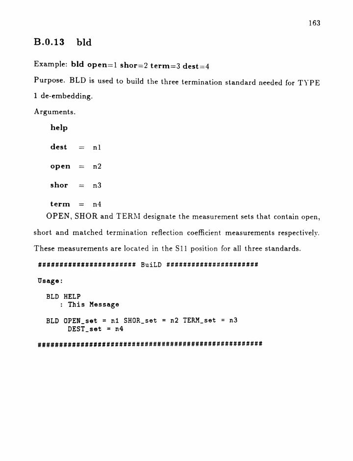
163

B.O.13 bId

Example: bid open==l shor==2 term==3 dest==4

Purpose. BLD is used to build the three termination standard needed for T't'"PE

1 de-embedding.

Arguments.

help

dest n1

open n2

shor n3

term n4

OPEN, SHOR and TER~I designate the measurement sets that contain open,

short and matched termination reflection coefficient measurements respectively.

These measurements are located in the S11 position for all three standards.

####################### BuiLD ######################

Usage:

BLD HELP: This Message

BLD OPEN_set = n1 SHOR set = n2 TERM_set = n3DEST_set = n4

#####################################################

B.O.14 stop

Example: stop

Purpose. Stop is used to exit SPAN A

164

B.O.15 drnb3

165

Example: Incomplete write up.

Purpose. Three port de-embedding.

####### DMB3 De-embedding of Three Ports ##############Usage:

DMB3 HELP: This Message

DMB3 MEASA1 = n1 MEASB1 = n2 MEASC1 n3 LOAD1 = n4MEASA2 = n5 MEASB2 = n6 MEASC2 = n7 LOAD2 = n8DEST = n9

Note: The output viII be a three port. Threemeasurement sets are required to store allof the parameters. n9, (n9+1) and (n9+2) areused to store the output

#####################################################

DMB3

PURPOSE:De-embeds a three port.

3o 0

1 1____ I __ 1 _

1 1

0-----1 1-----01 I I 2

0-----1 1-----01 1

Six tvo port measurements are required for maximum accuracy.

measa1:1

Tvo port betveen ports 2 and 3 vith a termination at port

of reflection coefficient fgama.Port 2 of the three port is connected to port 1 of thenetwork analyzer.

measa2:1

Two port between ports 2 and 3 with a termination at port

of reflection coefficient sgama.Port 2 of the three port is connected to port 1 of thenetwork analyzer.

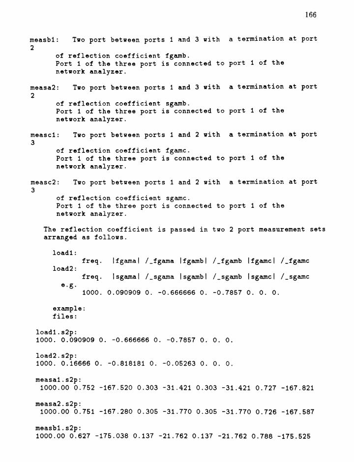
measb1:2

166

Tvo port bet~een ports 1 and 3 with a termination at port

of reflection coefficient fgamb.Port 1 of the three port is connected to port 1 of thenetwork analyzer.

measa2:2

Tvo port between ports 1 and 3 with a termination at port

of reflection coefficient sgamb.Port 1 of the three port is connected to port 1 of thenetwork analyzer.

measc1:3

Two port bet~een ports 1 and 2 with a termination at port

of reflection coefficient fgamc.Port 1 of the three port is connected to port 1 of thenetwork analyzer.

measc2:3

Tvo port between ports 1 and 2 with a termination at port

of reflection coefficient sgamc.Port 1 of the three port is connected to port 1 of thenetvork analyzer.

The reflection coefficient is passed in t~o 2 port measurement setsarranged as follovs.

loadl:

load2:

e.g.

freq. Ifgamal I_fgama Ifgambl I_fgamb Ifgamcl I_fgamc

freq. Isgamal I_sgama Isgambl I_sgamb I sgamc I I_sgamc

1000. 0.090909 O. -0.666666 o. -0.7857 o. o. o.

example:files:

loadl.s2p:1000. 0.090909 O. -0.666666 o. -0.7857 O. o. o.

load2.s2p:1000. 0.16666 O. -0.818181 o. -0.05263 o. o. o.

measa1.s2p:1000.00 0.752 -167.520 0.303 -31.421 0.303 -31.421 0.727 -167.821

measa2.s2p:1000.00 0.751 -167.280 0.305 -31.770 0.305 -31.770 0.726 -167.587

measb1.s2p:1000.00 0.627 -175.038 0.137 -21.762 0.137 -21.762 0.788 -175.525

167

measb2.s2p:

1000.00 0.663 -177.033 0.093 -15.439 0.093 -15.439 0.839 -178.065

measc1.s2p:1000.00 0.639 -176.141 0.118 -18.531 0.118 -18.531 0.842 -176.896

measc2.s2p:1000.00 0.599 -170.085 0.218 -33.007 0.218 -33.007 0.754 -168.193

spana

######################### SPANA #########################

get meas 1 file=load1.s2pget meas 2 file=load2.s2pget meas 3 file=measa1.s2pget meas 4 file=measa2.s2pget meas 5 file=measb1.s2pget meas 6 file=measb2.s2pget meas 7 file=measc1.s2pget meas 8 file=measc2.s2pdmb3 measa1=3 measa2=4 measb1=5 measb2=6 meascl=7 measc2=8 \load1=1 load2=2 dest=9

* put meas 9

Three port de-embeded result (DMB3). Part 1 of 3.

Form

Part 1 of 3.513523533

Mag Angle

50.nona

de-embeded result (DMB3).511 512521 522531 532

Angle Mag AngleMag(MHz)

MEASUREMENT SET 9Three-port 5 parametersFrequency-Domain Data: Magnitude-AngleNumber of Frequency points: 1Frequency Interval: o. MHzLov Frequency: 1000.00 MHzHigh Frequency: 1000.00 MHzValid De-embeded DataCharacteristic Impedance:

Identifier:Three port

FREQ

1000.0000 0.59842 -169.85 0.22104 -33.48 0.21382 -33.490.22104 -33.48 0.75168 -167.80 0.30034 -30.960.21382 -33.49 0.30034 -30.96 0.72729 -168.10

B.O.16 .gain

169

Example: Incomplete write up.

####################### GAIN ######################

Usage:

GAIN HELPThis Message

GAIN MEAS_set = n1 [GAIN = n2] [MERIT = n3] [NOISE = n4]Get gain, noise and figure of merit informationof a decie described by the two-port measurementS parameters in measurement set n1.The gain information is put in set n2 and thefigure of merit information in set n3 and thenoise information in set n4.The parameters in [] s are optional.

#####################################################

B.O.17 .sigma

170

Example: Incomplete write up.

###################### SIGMA #######################

Usage:

SIGMA HELP: This Message

SIGMA MEAS = n1 X = n2 XX = n3 mean = n4 stddev = n5Each entry of measurement set n1 is added to setn2 and its square is added to set n3. From theseaccumulated values the mean (put in set n4) andstandard deviation (put in set n5) are calculated.

SIGMA CLEAR X = n2 XX = n3: Clears measurement sets n2 and n3

#####################################################

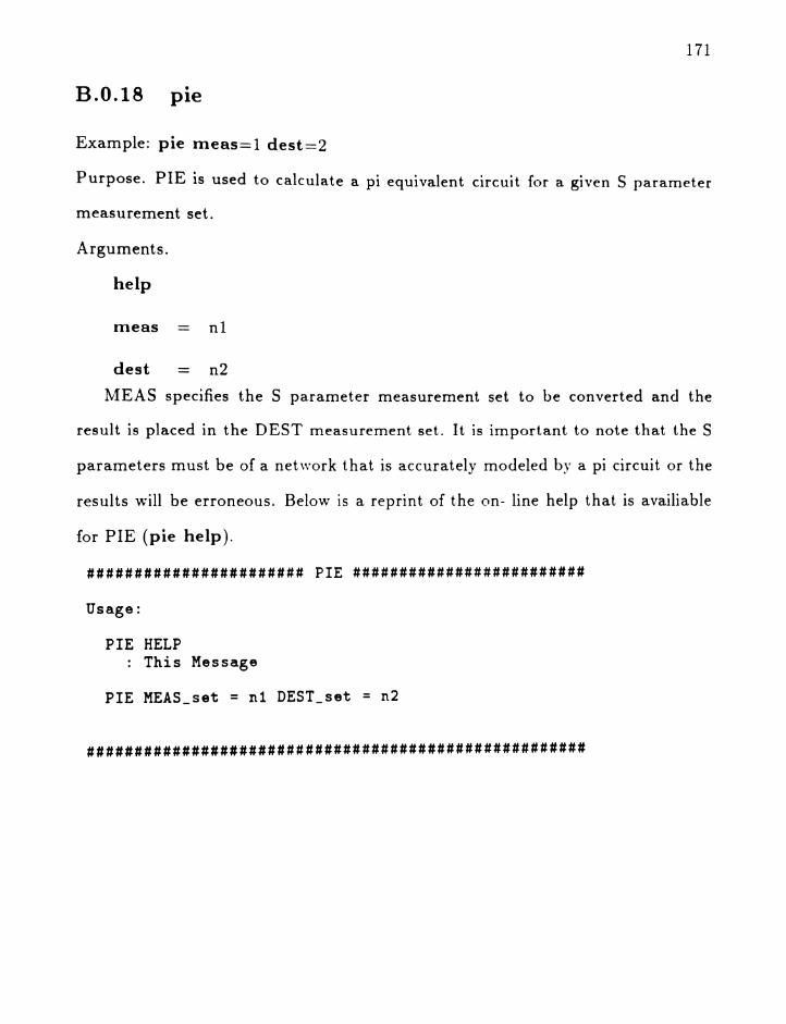
B.O.IS .pie

171

Example: pie rne as e, 1 dest==2

Purpose. PIE is used to calculate a pi equivalent circuit for a given S parameter

measurement set.

Arguments.

help

meas nl

dest n2

MEAS specifies the S parameter measurement set to be converted and the

result is placed in the DEST measurement set. It is important to note that the S

parameters must be of a network that is accurately modeled by a pi circuit or the

results will be erroneous. Below is a reprint of the on- line help that is availiable

for PIE (pie help).

####################### PIE #########################

Usage:

PIE HELPThis Message

PIE MEAS_set = n1 DEST set = n2

#####################################################

172

Appendix C

SPANA "shell" Syntax

The SPANA shell feature is available to prototype user subprograms. The code

follows.

c .

c

c SPSHELL

c

c PURPOSE: Used to impliment special calculations

c

c ...........•........................ · · . · · .. · • · .• · · · · .

c

subroutine spshell(parrnx,parmy,parmf,arg,noarg,ident)

c

real parmx(mxarg,rnxparm,mxmeas),parmy(mxarg,rnxparm,mxmeas)

real arg(mxarg,mxmeas),parmf(mxform,mxmeas)

integer noarg(mxmeas),tmparg

common/parmax/rnxarg,mxmeas,rnxparm,rnxform

c

character*40 str

character*80 ident(mxmeas)

logical kf,fin,prt,ofile,rfile,pecho

common/freerd/nvrite,ntype,aval,ival,ich,kf,fin,prt

+ ,ofile,rfile,pecho,str

173

c

logical lmeas,ldest

integer meas,dest

complex ptor,s11,s22,s21,s12,short,short1,short2

complex open,open1,open2

real ms11,ms22,as11,as22

call fread

c

if(str(1:4).eq. 'HELP'.or.str(1:4).eq. 'help')then

c call qsmode(2)

vrite(ntype,50)

if(prt)vrite(nvrite,50)

50 formate

+ ' ####################### SHELL ######################',11,

+ ' Usage:',II,

+ SHELL HELP',I,

+ : This Message',II,

+ SHELL MEAS_set = n1 DEST_set = n2',II,

+ Options: X = ? Y = ? etc. input parameters',11

+ '##################ff#ff#########ff######ffff###ffff#~#ffff##ffff')

return

endif

c

c Reset parameter flags (used to test that all parameters have been

input)

c

Imeas=.false.

ldest=.false.

c

c Parse rest of command line

c

100 if(fin)goto 150

if(str(1:4).eq.'MEAS'.or.str(1:4).eq. 'meas')then

call fread

meas=ival

if(meas.lt.1.or.meas.gt.mxmeas.or.parmf(3,meas).eq.0.)then

vrite(ntype,*)' Measurment Set not available'

goto 600

endif

lmeas=.true.

elseif(str(1:4).eq. 'DEST'.or.str(1:4).eq. 'dest')then

call fread

dest=ival

if(dest.lt.1.or.dest.gt.mxmeas)then

vrite(ntype,*)' Destination Set not available'

goto 600

endif

Idest=.true.

endif

call fread

goto 100

174

175

c

c Check that all parameters have been specified

c

150 if(lmeas .eqv.. false .. or.ldest .eqv .. false.)then

vrite(ntype,*)' Not enough parameters specified in command line'

goto 600

endif

c

do 10 n=1,noarg(meas)

c

c Begin shell calculations here

c

sll=ptor(parmx(n,l,meas),parmy(n,l,meas))

s21=ptor(parmx(n,2,meas),parmy(n,2,meas))

s12=ptor(parmx(n,3,rneas),parmy(n,3,meas))

s22=ptor(parmx(n,4,meas),parmy(n,4,meas))

msll=parmx(n,l,meas)

ms22=parmx(n,4,meas)

asl1=parmy(n,1,meas)

as22=parmy(n,4,meas)

short1=s11-s21

short2=s22-s21

open1=s11+s21

open2=s22+s21

short=(short1+short2)/2.0

open=(open2+open2)/2.0

rtd=180./3.1415927

c

parmx(n,1,dest)=cabs(short)

parmy(n,1,dest)=atan2(aimag(short),real(short))*rtd

parmx(n,2,dest)=cabs(open)

parmy(n,2,dest)=atan2(aimag(open),real(open))*rtd

parmx(n,3,dest)=abs(ms11-ms22)

parmy(n,3,dest)=abs(as11-as22)

parmx(n,4,dest)=cabs(short2)

parmy(n,4,dest)=atan2(aimag(short2),real(short2))*rtd

c

arg(n,dest)=arg(n,meas)

c

10 continue

noarg(dest)=noarg(meas)

c

c Set-up descripter

c

do 20 i=1,mxform

parmf(i,dest)=parmf(i,meas)

20 continue

c

c Identifier

c

ident(dest)='GSC (avg), GOC (avg), Symmetry, GSC (522)'

return

176

c

600 vrite(ntype,*), Command Error -- Command Ignored'

return

end

] 77