Embed Size (px)
Citation preview
International Journal of Advance Research in Engineering, Science &Technology (IJAREST), ISSN (O):2393-9877, ISSN (P): 2394-2444, Volume 2, Issue 5, May- 2015, Impact Factor: 2.125
CALIBRATION OF GRAVITY MODEL: A CASE STUDY OF
AVKUDA REGION
Roshani J. Makwana1, Dr. L.B.Zala2, Prof.A.A.Amin3
I. INTRODUCTION
Transportation engineering is the application of scientific
principles to the planning, design, operation and management of
transportation system. The transportation System in the reference
to society as a whole because it provides a service for the
movements of goods and people from place to place. Population
growth and Economic growth seems to have generated levels of
demand exceeding the capacity of most transport facilities. Due to
the continuing expansion of cities with the development of
societies and technology the existing transportation systems are not
sufficient to meet the increasing demands. To provide the free and
safe flow of traffic from one place to another without encountering
any congestion problem, it might be necessary to improve the
existing transportation facilities or to construct new facilities.
Transportation Planning Process plays an important role in
construction of new transport facilities. The basic purpose of
transportation planning and management is to match transportation
supply with travel demand.
II. TRIP DISTRIBUTION
Synthetic Models
Gravity Model
Opportunity Model
B) GRAVITY MODEL
The concept of gravity model came from Newton’s law of gravity,
which states that:
Where, F = Force of attraction between m1and m2
m1and m2 =Mass of object 1 and 2
d = Distance between objects
k = Constant
The application of this concept to trip distribution takes the form:
Classical form of gravity model:
Calibration of gravity model:
Where F(dij) = 1/dijc = Distance impedance
Tij = Total number of trips between zone i and zone j
Pi = Total number of productions at zone i
Aj = Total number of attractions at zone j
dij = Distance, Cost or Time between zone i and j
kij = socio economic factor
Trip distribution is important and complex stage in
transportation planning Process. Trip distribution is used to
estimate present as well as future trips. A trip distribution model
produces an origin-destination trip matrix to reflect trips made by
population. Trip distribution models used to forecast the origin-
destination pattern of travel into the future and produce a trip
matrix.
Trip distribution models connect the trip origins and
destination estimated by the trip generation models to create
estimated trips. It provides the planner with a systematic procedure
capable of estimating zonal trip interchanges for alternate plans of
both land use and transportation facilities.
A) METHODS OF TRIP DISTRIBUTION
Growth Factor Methods
Uniform Growth Factor Method
Average Growth Factor Method
Fratar Method
Furness Method
Detroit Method
All Rights Reserved, @IJAREST-2015 1
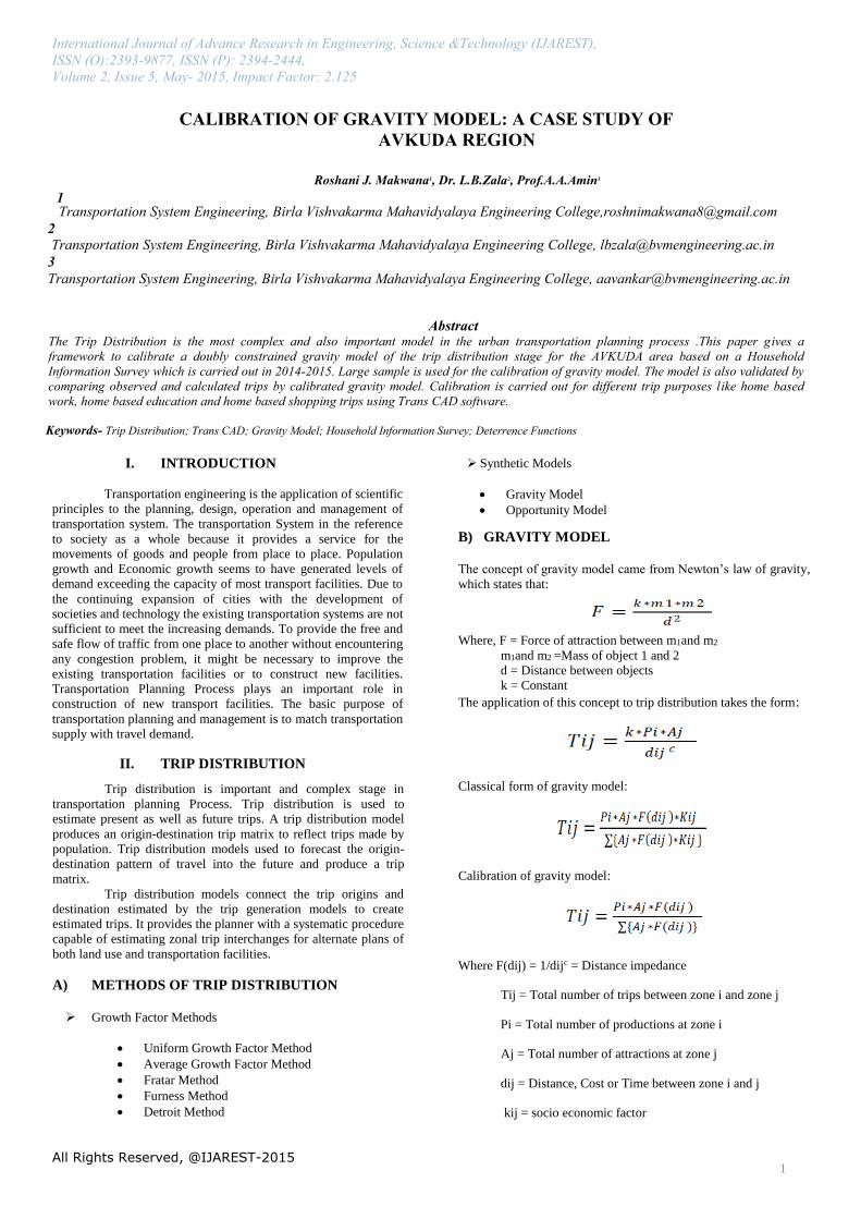
Abstract The Trip Distribution is the most complex and also important model in the urban transportation planning process .This paper gives a
framework to calibrate a doubly constrained gravity model of the trip distribution stage for the AVKUDA area based on a Household
Information Survey which is carried out in 2014-2015. Large sample is used for the calibration of gravity model. The model is also validated by
comparing observed and calculated trips by calibrated gravity model. Calibration is carried out for different trip purposes like home based
work, home based education and home based shopping trips using Trans CAD software.
Transportation System Engineering, Birla Vishvakarma Mahavidyalaya Engineering College,[email protected]
2 Transportation System Engineering, Birla Vishvakarma Mahavidyalaya Engineering College, [email protected]
3
Transportation System Engineering, Birla Vishvakarma Mahavidyalaya Engineering College, [email protected]
Keywords- Trip Distribution; Trans CAD; Gravity Model; Household Information Survey; Deterrence Functions
1
International Journal of Advance Research in Engineering, Science &Technology (IJAREST), ISSN (O):2393-9877, ISSN (P): 2394-2444, Volume No 2, Issue No 5, May- 2015, Impact Factor: 2.125
III. STUDY AREA PROFILE
The constituted AVKUDA (Anand Vidhyanagar
Karamsad Urban Development Authority) area is covering 29
villages of Anand taluka and in addition to the Anand, Karamsad,
Vallabh Vidhyanagar, Boriyavi nagarpalika and Vitthal
Udyognagar, a notified area. The developed area of AVKUDA is
well connected with road and railway network to other regions of
state. The linkages in the region currently provide help in growth
of settlements with better economic potential and future prospects.
The AVKUDA having area of 279.62 km2 and population of area
is 501526 as per census 2011.
Zoning of study area is done by Trans CAD software as
shown in figure 1. Study area is divided into 33 zones based on
administrative boundaries.
V. ANALYSIS
Figure 1 : Zoning of study area
IV. HOUSEHOLD INFORMATION SURVEY
The data collected from household information survey
is entered into Microsoft Excel. Then these entered data is
imported into Trans CAD software for analysis purpose.
The decision to travel for a given purpose is called trip
generation. The decision to choose destination from origin is
directional distribution of trips forms the second stage of travel
demand modeling. Trip distribution is determined by the number
of trips end originated in zone-i to number of trips end attracted to
zone-j, which can be understood by the matrix between zones. The
matrix is called origin–destination (O-D Matrix).
From the household information data, using Trans
CAD tool the observed O-D matrix is obtained as given in Figure
2. The desire line diagram for O-D matrix is given in Figure 3.
Figure 2 : Observed O-D Matrix
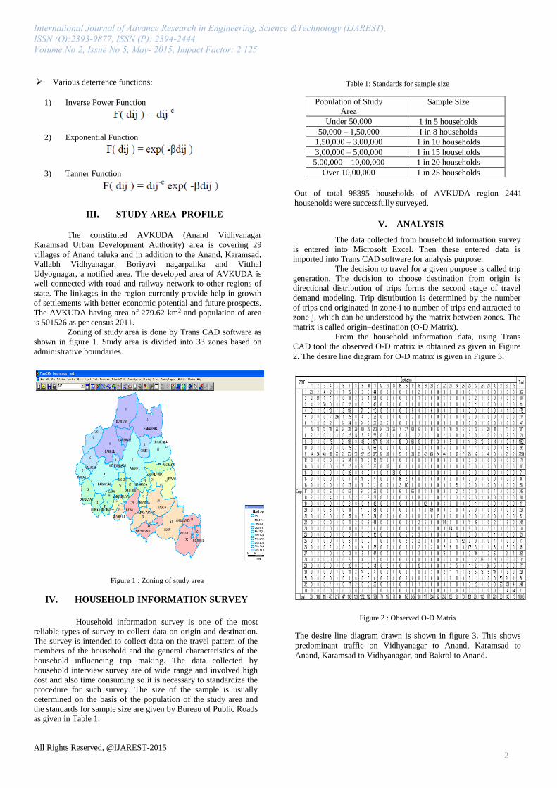
The desire line diagram drawn is shown in figure 3. This shows
predominant traffic on Vidhyanagar to Anand, Karamsad to
Anand, Karamsad to Vidhyanagar, and Bakrol to Anand.
Household information survey is one of the most
reliable types of survey to collect data on origin and destination.
The survey is intended to collect data on the travel pattern of the
members of the household and the general characteristics of the
household influencing trip making. The data collected by
household interview survey are of wide range and involved high
cost and also time consuming so it is necessary to standardize the
procedure for such survey. The size of the sample is usually
determined on the basis of the population of the study area and
the standards for sample size are given by Bureau of Public Roads
as given in Table 1.
2
All Rights Reserved, @IJAREST-2015
Population of Study
Area Sample Size
Under 50,000 1 in 5 households
50,000 – 1,50,000 I in 8 households
1,50,000 – 3,00,000 1 in 10 households
3,00,000 – 5,00,000 1 in 15 households
5,00,000 – 10,00,000 1 in 20 households
Over 10,00,000 1 in 25 households
Out of total 98395 households of AVKUDA region 2441
households were successfully surveyed.
Table 1: Standards for sample size
Various deterrence functions:
1) Inverse Power Function
2) Exponential Function
3) Tanner Function
International Journal of Advance Research in Engineering, Science &Technology (IJAREST), ISSN (O):2393-9877, ISSN (P): 2394-2444, Volume No 2, Issue No 5, May- 2015, Impact Factor: 2.125
Trans CAD software is used for calibration of gravity
model using Travel Time, Travel Cost and Travel Distance
attributes for number of iterations. The calibrated exponent values
for educational trips, work trips and shopping trips are as shown in
Table 2. Table 2 : Calibrated value of Exponents
Trip Type Travel
Impedance
Inverse Power
Function
Exponential
Function
c β
Work Distance 1.4804 0.1834
Time 1.5764 0.0581
Cost 1.6122 0.0622
Study Distance 2.0708 0.2827
Time 2.2255 0.0913
Cost 2.9744 0.1301
Shopping Distance 1.9726 0.5234
Time 1.4770 0.0628
Cost 0.0763 0.0762
VII. CONCLUSIONS
1. The population growth rate in the last decade (2001-2011) is
1.3%.
2. The trip rate observed is 4.5 trips/HH/day.
3. The proportion of purpose based trip types is 54.4% Work,
41.6% Educational trips, 0.62% Social trips, 2% Shopping
trips, 1.42% Recreational trips. 4. The derived final O-D Matrix can be used for transportation
corridor planning.
5. The exponent in inverse power function c for work, study and
shopping trips are 1.48, 2.07, 1.97 for distance; 1.57, 2.22,
1.5 for time and 1.61, 2.97 and 0.08 for cost.
6. The exponent in exponential function β for work, study and
shopping trips are 0.18, 0.28, 0.52 for distance; 0.06, 0.09,
0.06 for time and 0.06, 0.13 and 0.07 for cost.
VIII. REFERENCES
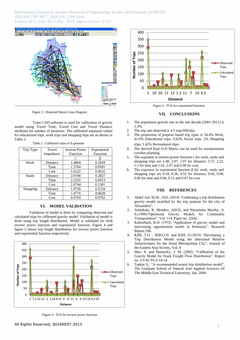
Figure 4 : TLD for Inverse power function
1. Abdel Aal, M.M., AEJ, (2014) “Calibrating a trip distribution
gravity model stratified by the trip purpose for the city of
Alexandria”.
2. Ashtakala, B. Member, ASCE, and Narasimha Murthy, A.
S.(1988)“Optimized Gravity Models for Commodity
Transportation”. Vol. 114, Paper no. 22641.
3. Kaltenbach, K.D. (1972) “Application of gravity model and
intervening opportunities model in Kentucky”. Research
Report 336.
4. KIM, T.G. , RHO,J.H. and KIM, G.(2010) “Developing a
Trip Distribution Model using the Interzonal Relative
Attractiveness for the Seoul Metropolitan City”, Journal of
the Eastern Asia Society, Vol. 8
5. Mao, S. and Demetsky, J. M. (2002) “Calibration of the
Gravity Model for Truck Freight Flow Distribution”. Report
no. UVACTS-5-14-14.
6. Tapkin S., “A recommended neural trip distribution model”,
The Graduate School of Natural And Applied Sciences Of
The Middle East Technical University, Jan. 2004.
VI. MODEL VALIDATION
Validation of model is done by comparing observed and
calculated trips by calibrated gravity model. Validation of model is
done using trip length distribution. Model is validated for both
inverse power function and exponential function. Figure 4 and
figure 5 shows trip length distribution for inverse power function
and exponential function respectively.
Figure 5 : TLD for exponential function
All Rights Reserved, @IJAREST-2015 3
Figure 3 : Observed Desire Lines Diagram
0
50
100
150
200
250
300
350
400
1 7.2 10 11 3 11 8.4 15 9 8 11 4 9 9.5 25 4.2 10
Nu
mb
er
of
Trip
s
Distance
ObservedTrips
CalculatedTrips
0
50
100
150
200
250
300
350
400
1 10 20 11 12 1.2 11 7 10 4.2
Nu
mb
er
of
Trip
s
Distance
ObservedTrips
CalculatedTrips