Embed Size (px)
Citation preview
CCeennttrree ffoorr PPrraaccttiiccaall QQuuaannttiittaattiivvee FFiinnaannccee
CPQF Working Paper Series
No. 25
On the Calibration of the Cheyette
Interest Rate Model
Ingo Beyna, Uwe Wystup
Authors: Ingo Beyna Uwe Uwe Wystup PhD Student CPQF Professor of Quantitative Finance Frankfurt School of Finance & Management Frankfurt School of Finance & Management
Frankfurt/Main Frankfurt/Main [email protected] u.wystup@frankfurt-school.
June 2010
Publisher: Frankfurt School of Finance & Management Phone: +49 (0) 69 154 008-0 Fax: +49 (0) 69 154 008-728 Sonnemannstr. 9-11 D-60314 Frankfurt/M. Germany
On the Calibration of the Cheyette
Interest Rate Model
Ingo Beyna ∗
Frankfurt School of Finance & Management
Centre for Practical Quantitative Finance
Sonnemannstraÿe 9-11, 60314 Frankfurt, Germany
Uwe Wystup
Frankfurt School of Finance & Management
Centre for Practical Quantitative Finance
Sonnemannstraÿe 9-11, 60314 Frankfurt, Germany
June 28, 2010
Abstract
We investigate the robustness of existing methods to calibrate the
Cheyette interest rate model to at-the-money swaption, caps and oors.
Existing algorithms may fail, because they suer from numerical in-
stability of derivatives. Therefore, we apply derivative-free techniques
and nd that they stabilize the calibration. Furthermore, we iden-
tify auspicious volatility parametrizations determining the Cheyette
model. In combination with the established calibration techniques the
results imply an accurate market reproduction and stay robust against
changes in the initial values. In contrast to existing approaches that
use approximations, we apply exact semi-close-form pricing formulas.
Keywords: Cheyette Model, Calibration, Optimization without derivatives,Genetic Optimization
∗We would like to thank Prof. Dr. P. Roÿbach (Frankfurt School of Finance & Man-agement), Prof. Dr. H. Mittelmann (Arizona State University) and Prof. Dr. W. Schmidt(Frankfurt School of Finance & Management) for their support and advice on this paper.
1
Beyna and Wystup - On the Calibration of the Cheyette Interest Rate Model 2
Contents
1 Introduction 3
2 Literature Review 4
3 The Cheyette Interest Rate Models 5
3.1 Derivation of the Model . . . . . . . . . . . . . . . . . . . . . 53.1.1 The Heath-Jarrow-Morton framework . . . . . . . . . . 53.1.2 The Cheyette Model . . . . . . . . . . . . . . . . . . . 7
3.2 Volatility Parametrization . . . . . . . . . . . . . . . . . . . . 103.3 Pricing Formulas . . . . . . . . . . . . . . . . . . . . . . . . . 13
4 The Calibration Problem 16
4.1 Formulation . . . . . . . . . . . . . . . . . . . . . . . . . . . . 164.2 Constraints . . . . . . . . . . . . . . . . . . . . . . . . . . . . 184.3 Characterization of the optimization space . . . . . . . . . . . 184.4 Quality Check . . . . . . . . . . . . . . . . . . . . . . . . . . . 22
5 Optimization Methods 23
5.1 Overview of methods . . . . . . . . . . . . . . . . . . . . . . . 235.2 Assessment of methods . . . . . . . . . . . . . . . . . . . . . . 24
5.2.1 Newton Algorithm . . . . . . . . . . . . . . . . . . . . 245.2.1.1 Description . . . . . . . . . . . . . . . . . . . 245.2.1.2 Results . . . . . . . . . . . . . . . . . . . . . 24
5.2.2 Powell Algorithm . . . . . . . . . . . . . . . . . . . . . 245.2.2.1 Description . . . . . . . . . . . . . . . . . . . 245.2.2.2 Results . . . . . . . . . . . . . . . . . . . . . 25
5.2.3 Downhill Simplex Algorithm . . . . . . . . . . . . . . . 265.2.3.1 Description . . . . . . . . . . . . . . . . . . . 265.2.3.2 Results . . . . . . . . . . . . . . . . . . . . . 27
5.2.4 Simulated Annealing . . . . . . . . . . . . . . . . . . . 305.2.4.1 Description . . . . . . . . . . . . . . . . . . . 305.2.4.2 Results . . . . . . . . . . . . . . . . . . . . . 31
5.2.5 Genetic Optimization . . . . . . . . . . . . . . . . . . . 345.2.5.1 Description . . . . . . . . . . . . . . . . . . . 345.2.5.2 Results . . . . . . . . . . . . . . . . . . . . . 36
5.3 Conclusions . . . . . . . . . . . . . . . . . . . . . . . . . . . . 37
A Appendix 41
References 42
Beyna and Wystup - On the Calibration of the Cheyette Interest Rate Model 3
1 Introduction
In 1992, D. Heath, R. Jarrow and A. Morton (HJM) [Mor92] have standard-ized a valuation approach on the basis of mainly two assumptions: the rstone postulates, that it is not possible to gain riskless prot (No-arbitragecondition), and the second one assumes the completeness of the nancialmarket. The HJM model, or strictly speaking the HJM framework, is a gen-eral model environment and incorporates many previously developed mod-els like the Vasicek model (1977) [Vas77] or the Hull-White model (1990)[Whi90]. The general setting mainly suers from two disadvantages: rst ofall the diculty to apply the model in market practice and second, the ex-tensive computational complexity caused by the high-dimensional stochasticprocess of the underlying. The rst disadvantage was improved by the devel-opment of the LIBOR Market Model (1997) introduced by [Mus97], [Jam97]and [San97], which combines the general risk-neutral yield curve model withmarket standards. The second disadvantage can be improved by restrictingthe general HJM model to a subset of models with a similar specicationof the volatility structure. The resulting system of Stochastic DierentialEquations (SDE) describing the yield curve dynamic breaks down from ahigh-dimensional process into a low-dimensional structure of Markovian pro-cesses. Furthermore, the dependence on the current state of the processallows the valuation by a certain Partial Dierential Equation (PDE). Thisapproach was developed by O. Cheyette in 1994 [Che94].
The framework proposed by Cheyette for modeling interest rates leavesthe user with a wide choice of alternatives. The model is completely de-termined by the selection of (separable) volatility functions and given aparametrization, one might end up in known models like Ho-Lee (constantvolatility) or Hull-White (exponential volatility structure). Each model bearsdierent advantages and the selection of a model depends on its application.In order to use one model in practice it needs to be calibrated to liquidlytraded interest rate derivatives. The aim of the calibration is minimizingthe dierences in prices between the market quotes and the model impliedprices. The minimization is performed with respect to the free parametersof the model in case of the Cheyette framework to the coecients of the vo-latility parametrization. Alternatively, the calibration can be implementedto minimize the dierences in implied (Black-Scholes) volatility. The com-parison of the volatilities is more standardized, because it is independent ofthe notional and the maturity. Furthermore, the quotation in the market ofprices and implied volatility coincides for plain products, thus the calibrationproblem stays unchanged.
Beyna and Wystup - On the Calibration of the Cheyette Interest Rate Model 4
The calibration of an interest rate model is one of the most importantsteps for pricing exotic products. Surprisingly, very little literature is knowndealing with the applicability of optimization algorithms. The special struc-ture of the Cheyette model inuences the performance of the minimizationmethods. The pricing formulas are given semi-explicitly [Hen03] and theirderivations are not given in closed-form. One should thus apply derivative-free minimization algorithms like the Downhill Simplex algorithm or GeneticOptimization techniques. In our work we have applied several methods tothe calibration problem and in this paper we discuss their behavior in detail.The results are quite dierent for the analyzed techniques and the choice ofan adequate optimization algorithm plays an important role. As the calibra-tion problem seeks a global minimum, we have incorporated some stochasticalgorithms which do not guarantee the detection of the global minimum, butreach it with high probability. Furthermore, its application to the calibrationof interest rate models is not well explored yet and we give a starting pointin this paper.
2 Literature Review
The calibration of interest rate models to plain derivatives can be formu-lated theoretically quite easy as a minimization of the dierences in pricesbetween the model and the market quotes. Taking the specic pricing for-mulas into account, the characteristics of the optimization problem appear.Brigo and Mercurio [Mer05] formulate the calibration problem for the generalHJM framework in an abstract way and concentrate on swaptions and caps.Unfortunately, they neither discuss the practicability nor analyze the nu-merical tractability. Andersen and Andreasen [And02] identify several prob-lems concerning the numerical tractability of the general calibration problemfor the Gaussian HJM model. Especially the computation time of pricingvanilla caps and swaptions complicates the accurate calibration. They there-fore suggest an approximation by asymptotic expansions and apply it tolow-dimensional HJM models. They receive accurate results for small ma-turities, but for long maturities these worsen sometimes. A discussion ofthe used optimization algorithms or the applicability of known techniquesis missing as well. A slightly dierent approach is presented by Andreasen[And05], who approximates the underlying stochastic dierential equationby a time-homogeneous model. Thus he receives (quasi) closed-form pricingformulas. This type of asymptotic solution just takes simple volatility struc-tures into account and does not deliver convincing results. Again Andreasen
Beyna and Wystup - On the Calibration of the Cheyette Interest Rate Model 5
[And00] suggests another approach to simplify the calibration especially toswaptions. He approximates the dynamic of the swap rate, which makes thebootstrapping of the volatility possible. The method is based on the pric-ing PDE and uses Finite Dierences techniques to compute the prices. Thealgorithm is really fast, but it can only be applied to really easy volatilityparametrizations in low-dimensional HJM models so far.
All the presented approaches incorporate an approximation of the pric-ing formula to simplify the minimization problem. In this paper we use theexact pricing formulas developed by [Hen03] and analyze several optimiza-tion techniques to receive accurate results in reasonable computation time.Thus, we do not simply adjust the problem, but apply dierent optimizationtechniques to solve it.
3 The Cheyette Interest Rate Models
3.1 Derivation of the Model
The Cheyette interest rate model is a specialization of the general HJMframework, so that we will present the general setup rst. In the second stepwe will limit the class of models to a specic process structure of the yieldcurve dynamic. This technique will guide us to the representation of the classof Cheyette models.
3.1.1 The Heath-Jarrow-Morton framework
The Heath-Jarrow-Morton approach yields a general framework for evalu-ating interest-rate derivatives. It can be classied as a forward-rate model,in contrast to short rate models or market models. The uncertainty in theeconomy is characterized by the probability space (Ω,F , Q), where Ω is thestate space, F is the σ-algebra representing measurable events, and Q is aprobability measure. The dynamic of the forward rate is given by an Itôprocess
df(t, T ) = µ(t, T )dt + σ(t, T )dW (t). (1)
It is assumed that W(t) is an m-dimensional (Q-)Brownian motion and thedrift µ = (µ(t, T ))t∈[t0,T ] and the volatility of the forward rateσ = (σ(t, T ))t∈[t0,T ] are m-dimensional progressively measurable stochasticprocesses satisfying certain conditions on the regularity:
Beyna and Wystup - On the Calibration of the Cheyette Interest Rate Model 6
T∫
t0
|µ(s, T )|ds < ∞ Q − a.s. ∀t0 ≤ T ≤ T ∗, (2)
T∫
t0
σ2j (s, T )ds < ∞ Q − a.s. ∀t0 ≤ T ≤ T ∗, j = 1, ...,m, (3)
T ∗
∫
t0
|f(t0, s)|ds < ∞ Q − a.s., (4)
T ∗
∫
t0
u∫
t0
|µ(s, u)|ds
du < ∞ Q − a.s.. (5)
The notations use the xed maturities T ≥ t as well as the maximum timehorizon T ∗ ≥ T . Then the forward rate is given by
f(t, T ) = f(0, T ) +
t∫
t0
µ(s, T )ds +
t∫
t0
σ(s, T )dW (s). (6)
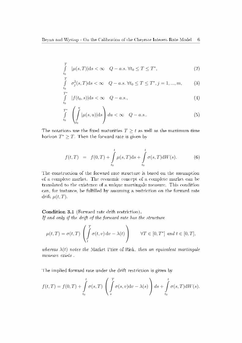
The construction of the forward rate structure is based on the assumptionof a complete market. The economic concept of a complete market can betranslated to the existence of a unique martingale measure. This conditioncan, for instance, be fullled by assuming a restriction on the forward ratedrift µ(t, T ).
Condition 3.1 (Forward rate drift restriction).If and only if the drift of the forward rate has the structure
µ(t, T ) = σ(t, T )
T∫
t
σ(t, v) dv − λ(t)
∀T ∈ [0, T ∗] and t ∈ [0, T ],
whereas λ(t) notes the Market Price of Risk, then an equivalent martingalemeasure exists .
The implied forward rate under the drift restriction is given by
f(t, T ) = f(0, T ) +
t∫
t0
σ(s, T )
T∫
s
σ(s, v)dv − λ(s)
ds +
t∫
t0
σ(s, T )dW (s).
Beyna and Wystup - On the Calibration of the Cheyette Interest Rate Model 7
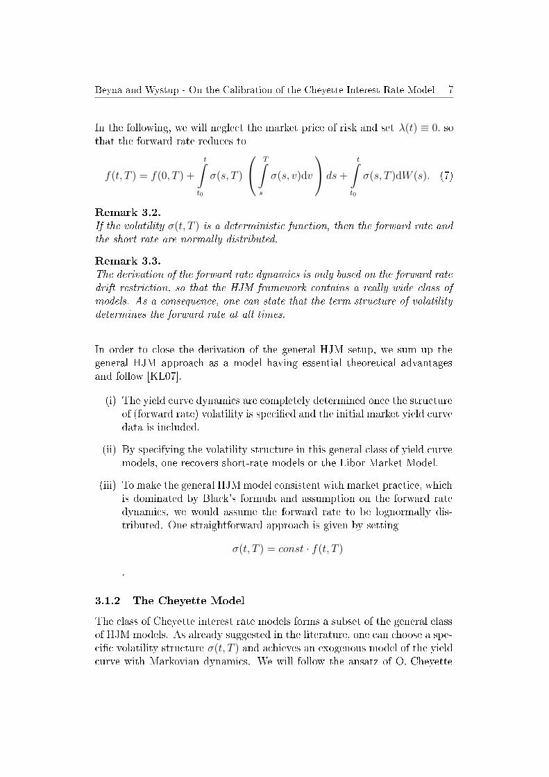
In the following, we will neglect the market price of risk and set λ(t) ≡ 0, sothat the forward rate reduces to
f(t, T ) = f(0, T ) +
t∫
t0
σ(s, T )
T∫
s
σ(s, v)dv
ds +
t∫
t0
σ(s, T )dW (s). (7)
Remark 3.2.
If the volatility σ(t, T ) is a deterministic function, then the forward rate andthe short rate are normally distributed.
Remark 3.3.
The derivation of the forward rate dynamics is only based on the forward ratedrift restriction, so that the HJM framework contains a really wide class ofmodels. As a consequence, one can state that the term structure of volatilitydetermines the forward rate at all times.
In order to close the derivation of the general HJM setup, we sum up thegeneral HJM approach as a model having essential theoretical advantagesand follow [KL07].
(i) The yield curve dynamics are completely determined once the structureof (forward rate) volatility is specied and the initial market yield curvedata is included.
(ii) By specifying the volatility structure in this general class of yield curvemodels, one recovers short-rate models or the Libor Market Model.
(iii) To make the general HJM model consistent with market practice, whichis dominated by Black's formula and assumption on the forward ratedynamics, we would assume the forward rate to be lognormally dis-tributed. One straightforward approach is given by setting
σ(t, T ) = const · f(t, T )
.
3.1.2 The Cheyette Model
The class of Cheyette interest rate models forms a subset of the general classof HJM models. As already suggested in the literature, one can choose a spe-cic volatility structure σ(t, T ) and achieves an exogenous model of the yieldcurve with Markovian dynamics. We will follow the ansatz of O. Cheyette
Beyna and Wystup - On the Calibration of the Cheyette Interest Rate Model 8
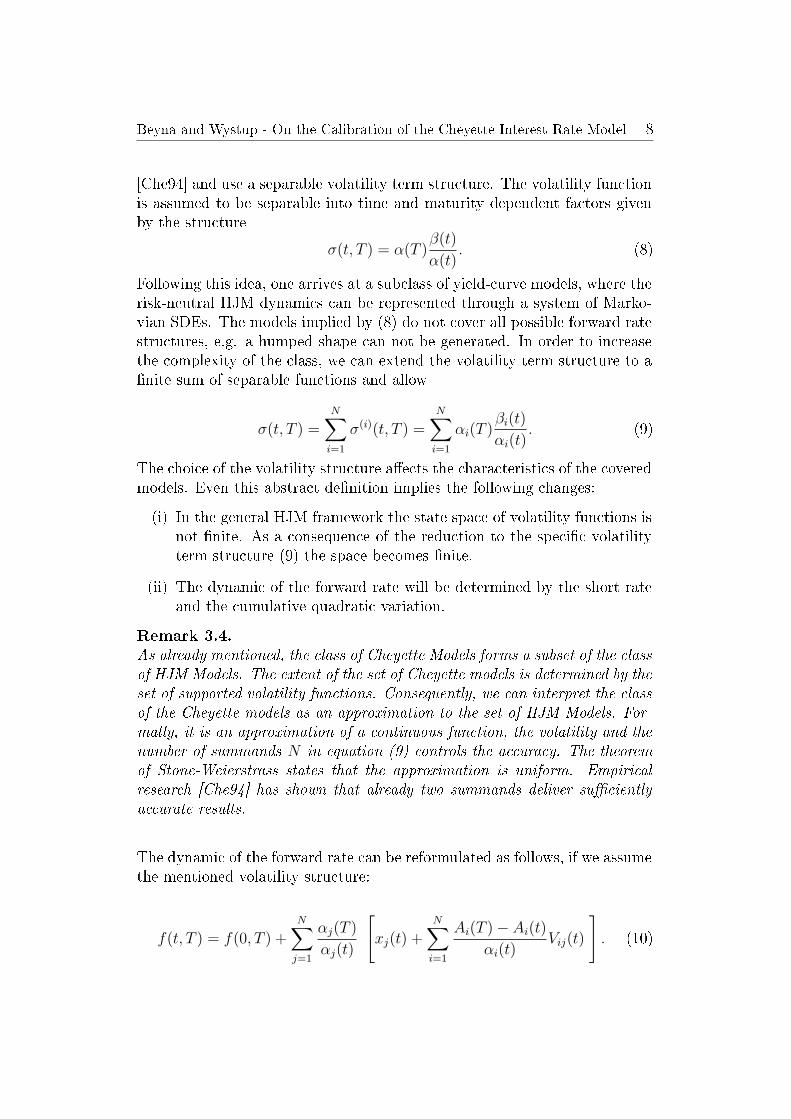
[Che94] and use a separable volatility term structure. The volatility functionis assumed to be separable into time and maturity dependent factors givenby the structure
σ(t, T ) = α(T )β(t)
α(t). (8)
Following this idea, one arrives at a subclass of yield-curve models, where therisk-neutral HJM dynamics can be represented through a system of Marko-vian SDEs. The models implied by (8) do not cover all possible forward ratestructures, e.g. a humped shape can not be generated. In order to increasethe complexity of the class, we can extend the volatility term structure to anite sum of separable functions and allow
σ(t, T ) =N∑
i=1
σ(i)(t, T ) =N∑
i=1
αi(T )βi(t)
αi(t). (9)
The choice of the volatility structure aects the characteristics of the coveredmodels. Even this abstract denition implies the following changes:
(i) In the general HJM framework the state space of volatility functions isnot nite. As a consequence of the reduction to the specic volatilityterm structure (9) the space becomes nite.
(ii) The dynamic of the forward rate will be determined by the short rateand the cumulative quadratic variation.
Remark 3.4.
As already mentioned, the class of Cheyette Models forms a subset of the classof HJM Models. The extent of the set of Cheyette models is determined by theset of supported volatility functions. Consequently, we can interpret the classof the Cheyette models as an approximation to the set of HJM Models. For-mally, it is an approximation of a continuous function, the volatility and thenumber of summands N in equation (9) controls the accuracy. The theoremof Stone-Weierstrass states that the approximation is uniform. Empiricalresearch [Che94] has shown that already two summands deliver sucientlyaccurate results.
The dynamic of the forward rate can be reformulated as follows, if we assumethe mentioned volatility structure:
f(t, T ) = f(0, T ) +N∑
j=1
αj(T )
αj(t)
[
xj(t) +N∑
i=1
Ai(T ) − Ai(t)
αi(t)Vij(t)
]
. (10)
Beyna and Wystup - On the Calibration of the Cheyette Interest Rate Model 9
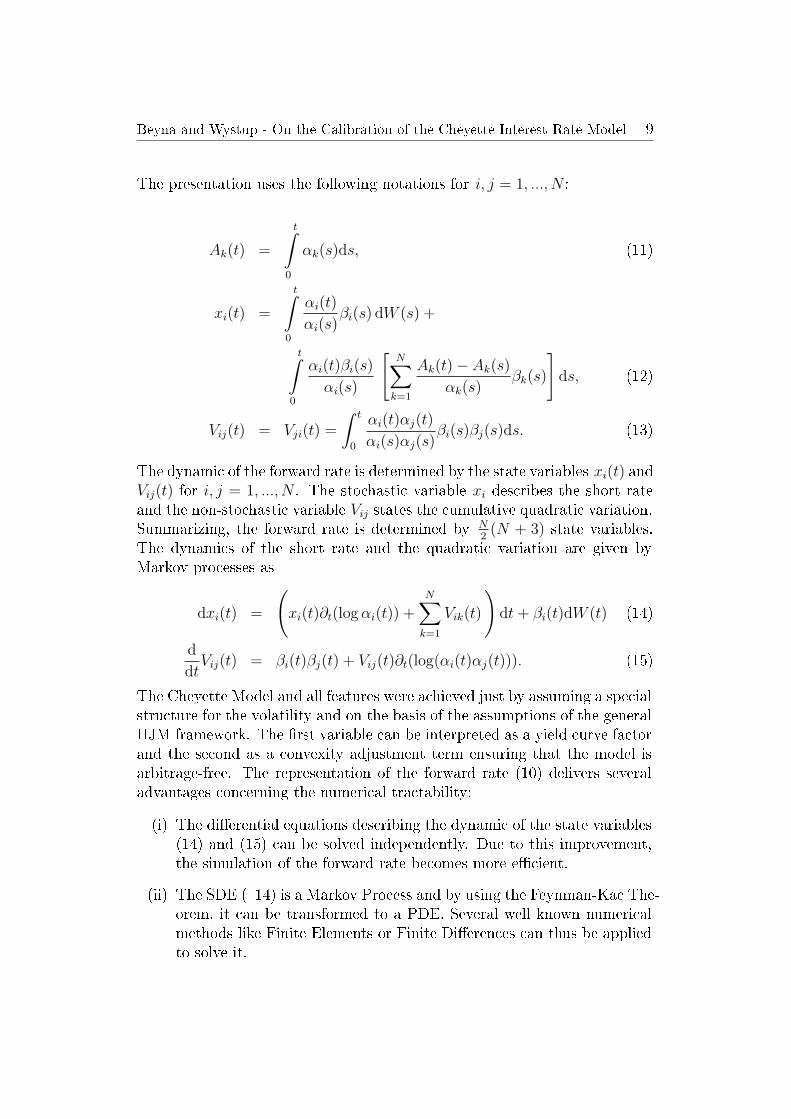
The presentation uses the following notations for i, j = 1, ..., N :
Ak(t) =
t∫
0
αk(s)ds, (11)
xi(t) =
t∫
0
αi(t)
αi(s)βi(s) dW (s) +
t∫
0
αi(t)βi(s)
αi(s)
[
N∑
k=1
Ak(t) − Ak(s)
αk(s)βk(s)
]
ds, (12)
Vij(t) = Vji(t) =
∫ t
0
αi(t)αj(t)
αi(s)αj(s)βi(s)βj(s)ds. (13)
The dynamic of the forward rate is determined by the state variables xi(t) andVij(t) for i, j = 1, ..., N . The stochastic variable xi describes the short rateand the non-stochastic variable Vij states the cumulative quadratic variation.Summarizing, the forward rate is determined by N
2(N + 3) state variables.
The dynamics of the short rate and the quadratic variation are given byMarkov processes as
dxi(t) =
(
xi(t)∂t(log αi(t)) +N∑
k=1
Vik(t)
)
dt + βi(t)dW (t) (14)
d
dtVij(t) = βi(t)βj(t) + Vij(t)∂t(log(αi(t)αj(t))). (15)
The Cheyette Model and all features were achieved just by assuming a specialstructure for the volatility and on the basis of the assumptions of the generalHJM framework. The rst variable can be interpreted as a yield curve factorand the second as a convexity adjustment term ensuring that the model isarbitrage-free. The representation of the forward rate (10) delivers severaladvantages concerning the numerical tractability:
(i) The dierential equations describing the dynamic of the state variables(14) and (15) can be solved independently. Due to this improvement,the simulation of the forward rate becomes more ecient.
(ii) The SDE ( 14) is a Markov Process and by using the Feynman-Kac The-orem, it can be transformed to a PDE. Several well known numericalmethods like Finite Elements or Finite Dierences can thus be appliedto solve it.
Beyna and Wystup - On the Calibration of the Cheyette Interest Rate Model 10
At this stage, the Cheyette Model is dened as a one factor model, but itcan easily be generalized to a multi-factor model. The additional factors aregiven by several independent Brownian motions and the forward rate is givenby
f(t, T ) = f(0, T ) +M∑
i=1
f i(t, T ), (16)
where f i(t, T ) denotes a one factor forward rate dened by (10).
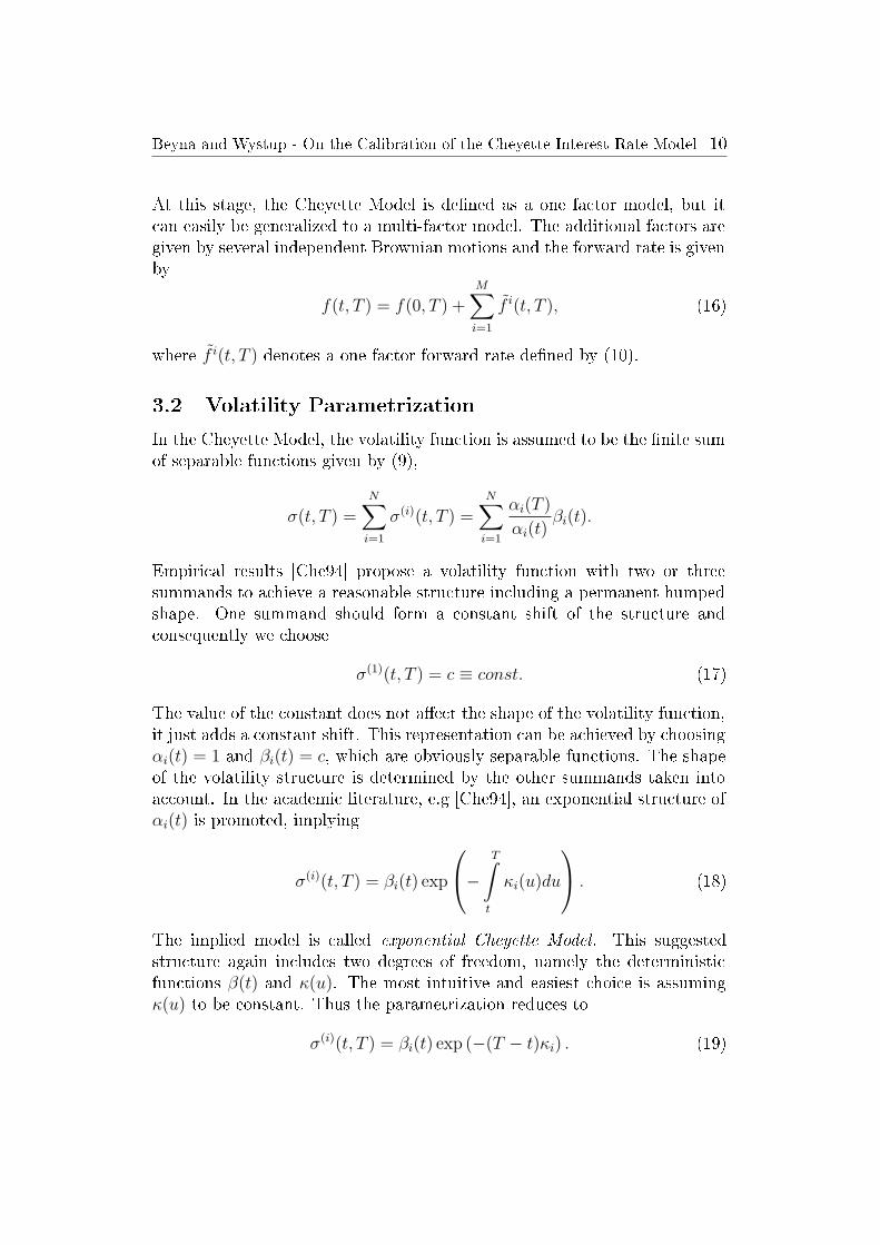
3.2 Volatility Parametrization
In the Cheyette Model, the volatility function is assumed to be the nite sumof separable functions given by (9),
σ(t, T ) =N∑
i=1
σ(i)(t, T ) =N∑
i=1
αi(T )
αi(t)βi(t).
Empirical results [Che94] propose a volatility function with two or threesummands to achieve a reasonable structure including a permanent humpedshape. One summand should form a constant shift of the structure andconsequently we choose
σ(1)(t, T ) = c ≡ const. (17)
The value of the constant does not aect the shape of the volatility function,it just adds a constant shift. This representation can be achieved by choosingαi(t) = 1 and βi(t) = c, which are obviously separable functions. The shapeof the volatility structure is determined by the other summands taken intoaccount. In the academic literature, e.g [Che94], an exponential structure ofαi(t) is promoted, implying
σ(i)(t, T ) = βi(t) exp
−
T∫
t
κi(u)du
. (18)
The implied model is called exponential Cheyette Model. This suggestedstructure again includes two degrees of freedom, namely the deterministicfunctions β(t) and κ(u). The most intuitive and easiest choice is assumingκ(u) to be constant. Thus the parametrization reduces to
σ(i)(t, T ) = βi(t) exp (−(T − t)κi) . (19)
Beyna and Wystup - On the Calibration of the Cheyette Interest Rate Model 11
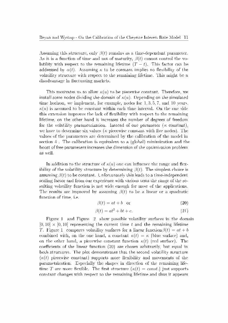
Assuming this structure, only β(t) remains as a time-dependant parameter.As it is a function of time and not of maturity, β(t) cannot control the vo-latility with respect to the remaining lifetime (T − t). This factor can beaddressed by α(t). Assuming κ to be constant implies no exibility of thevolatility structure with respect to the remaining lifetime. This might be adisadvantage in uctuating markets.
This motivates us to allow κ(u) to be piecewise constant. Therefore, weinstall some nodes dividing the domain of κ(u). Depending on the simulatedtime horizon, we implement, for example, nodes for 1, 3, 5, 7, and 10 years.κ(u) is assumed to be constant within each time interval. On the one sidethis extension improves the lack of exibility with respect to the remaininglifetime, on the other hand it increases the number of degrees of freedomfor the volatility parametrization. Instead of one parameter (κ constant),we have to determine six values (κ piecewise constant with ve nodes). Thevalues of the parameters are determined by the calibration of the model insection 4 . The calibration is equivalent to a (global) minimization and theboost of free parameters increases the dimension of the optimization problemas well.
In addition to the structure of κ(u) one can inuence the range and ex-ibility of the volatility structure by determining β(t). The simplest choice isassuming β(t) to be constant. Unfortunately this leads to a time-independentscaling factor and from our experience with various tests the range of the re-sulting volatility function is not wide enough for most of the applications.The results are improved by assuming β(t) to be a linear or a quadraticfunction of time, i.e.
β(t) = at + b or (20)
β(t) = at2 + bt + c. (21)
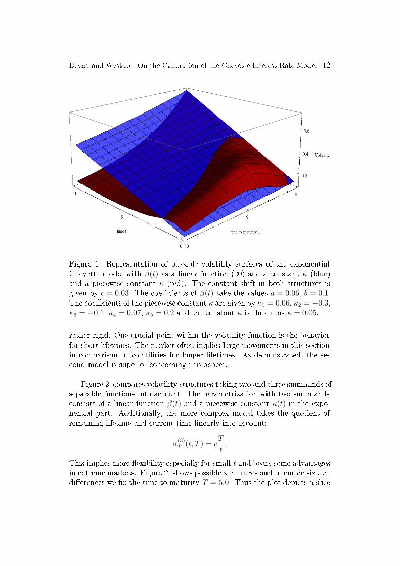
Figure 1 and Figure 2 show possible volatility surfaces in the domain[0, 10] × [0, 10] representing the current time t and the remaining lifetimeT . Figure 1 compares volatility surfaces for a linear functionβ(t) = at + bcombined with, on the one hand, a constant κ(t) = κ (blue surface) and,on the other hand, a piecewise constant function κ(t) (red surface). Thecoecients of the linear function (20) are chosen arbitrarily, but equal inboth structures. The plot demonstrates that the second volatility structure(κ(t) piecewise constant) supports more exibility and movements of theparametrization. Especially the shapes in direction of the remaining life-time T are more exible. The rst structure (κ(t) = const.) just supportsconstant changes with respect to the remaining lifetime and thus it appears
Beyna and Wystup - On the Calibration of the Cheyette Interest Rate Model 12
Figure 1: Representation of possible volatility surfaces of the exponentialCheyette model with β(t) as a linear function (20) and a constant κ (blue)and a piecewise constant κ (red). The constant shift in both structures isgiven by c = 0.03. The coecients of β(t) take the values a = 0.06, b = 0.1.The coecients of the piecewise constant κ are given by κ1 = 0.06, κ2 = −0.3,κ3 = −0.1, κ4 = 0.07, κ5 = 0.2 and the constant κ is chosen as κ = 0.05.
rather rigid. One crucial point within the volatility function is the behaviorfor short lifetimes. The market often implies large movements in this sectionin comparison to volatilities for longer lifetimes. As demonstrated, the se-cond model is superior concerning this aspect.
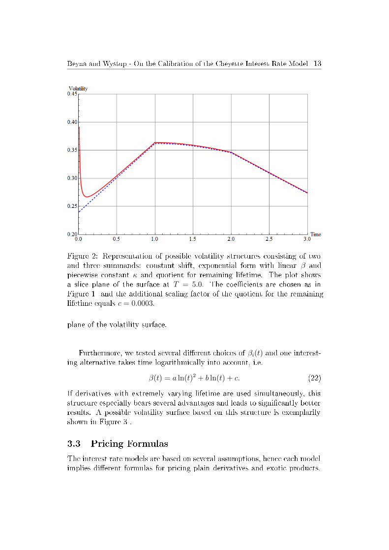
Figure 2 compares volatility structures taking two and three summands ofseparable functions into account. The parametrization with two summandsconsists of a linear function β(t) and a piecewise constant κ(t) in the expo-nential part. Additionally, the more complex model takes the quotient ofremaining lifetime and current time linearly into account:
σ(3)T (t, T ) = c
T
t.
This implies more exibility especially for small t and bears some advantagesin extreme markets. Figure 2 shows possible structures and to emphasize thedierences we x the time to maturity T = 5.0. Thus the plot depicts a slice
Beyna and Wystup - On the Calibration of the Cheyette Interest Rate Model 13
Figure 2: Representation of possible volatility structures consisting of twoand three summands: constant shift, exponential form with linear β andpiecewise constant κ and quotient for remaining lifetime. The plot showsa slice plane of the surface at T = 5.0. The coecients are chosen as inFigure 1 and the additional scaling factor of the quotient for the remaininglifetime equals c = 0.0003.
plane of the volatility surface.
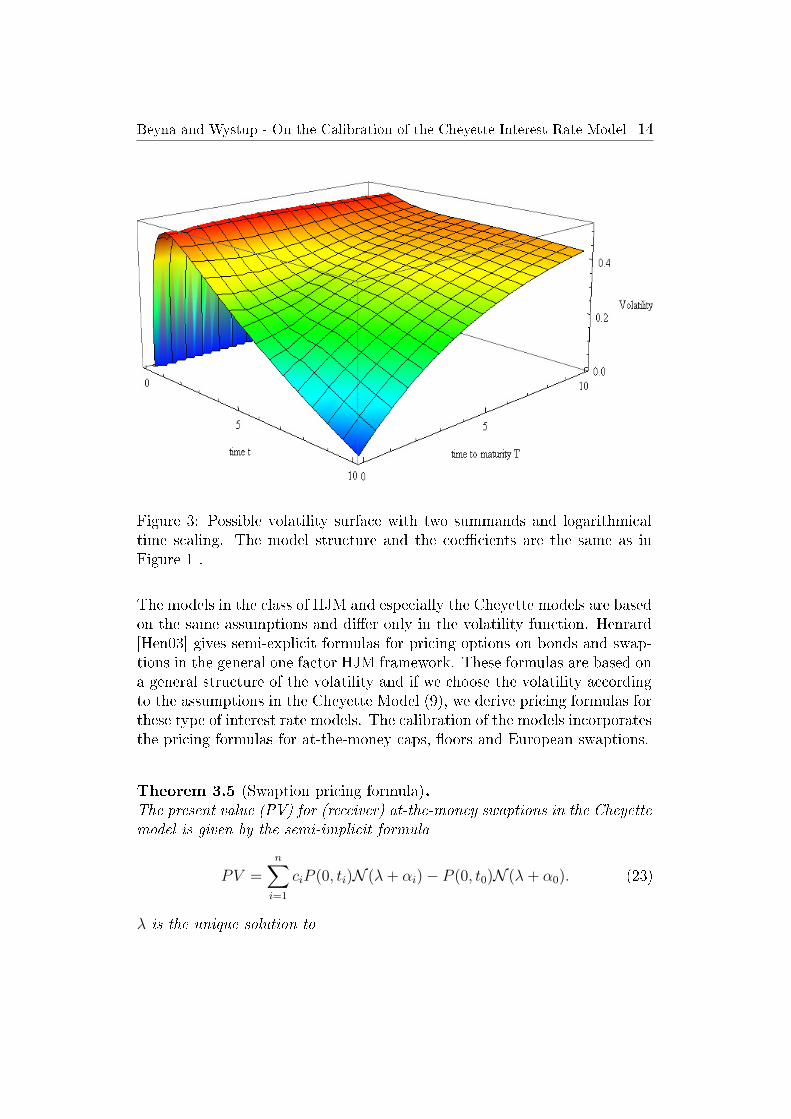
Furthermore, we tested several dierent choices of βi(t) and one interest-ing alternative takes time logarithmically into account, i.e.
β(t) = a ln(t)2 + b ln(t) + c. (22)
If derivatives with extremely varying lifetime are used simultaneously, thisstructure especially bears several advantages and leads to signicantly betterresults. A possible volatility surface based on this structure is exemplarilyshown in Figure 3 .
3.3 Pricing Formulas
The interest rate models are based on several assumptions, hence each modelimplies dierent formulas for pricing plain derivatives and exotic products.
Beyna and Wystup - On the Calibration of the Cheyette Interest Rate Model 14
Figure 3: Possible volatility surface with two summands and logarithmicaltime scaling. The model structure and the coecients are the same as inFigure 1 .
The models in the class of HJM and especially the Cheyette models are basedon the same assumptions and dier only in the volatility function. Henrard[Hen03] gives semi-explicit formulas for pricing options on bonds and swap-tions in the general one factor HJM framework. These formulas are based ona general structure of the volatility and if we choose the volatility accordingto the assumptions in the Cheyette Model (9), we derive pricing formulas forthese type of interest rate models. The calibration of the models incorporatesthe pricing formulas for at-the-money caps, oors and European swaptions.
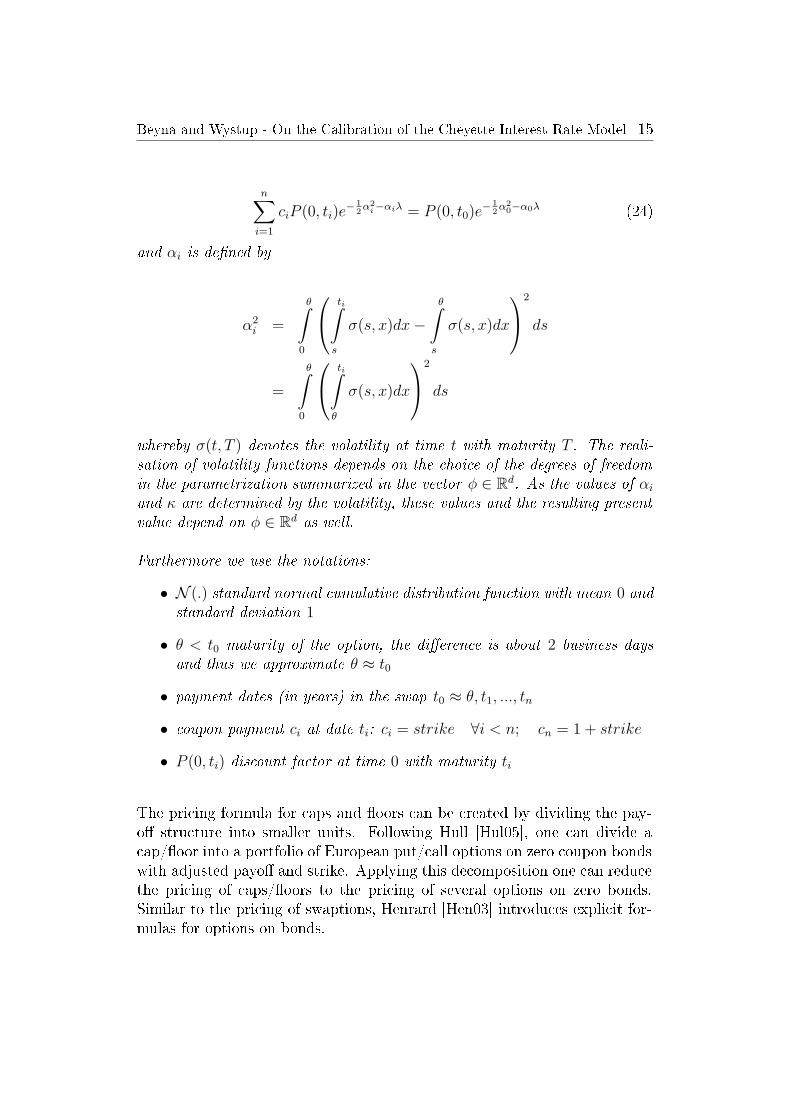
Theorem 3.5 (Swaption pricing formula).The present value (PV) for (receiver) at-the-money swaptions in the Cheyettemodel is given by the semi-implicit formula
PV =n∑
i=1
ciP (0, ti)N (λ + αi) − P (0, t0)N (λ + α0). (23)
λ is the unique solution to
Beyna and Wystup - On the Calibration of the Cheyette Interest Rate Model 15
n∑
i=1
ciP (0, ti)e−
1
2α2
i−αiλ = P (0, t0)e
−1
2α2
0−α0λ (24)
and αi is dened by
α2i =
θ∫
0
ti∫
s
σ(s, x)dx −
θ∫
s
σ(s, x)dx
2
ds
=
θ∫
0
ti∫
θ
σ(s, x)dx
2
ds
whereby σ(t, T ) denotes the volatility at time t with maturity T . The reali-sation of volatility functions depends on the choice of the degrees of freedomin the parametrization summarized in the vector φ ∈ R
d. As the values of αi
and κ are determined by the volatility, these values and the resulting presentvalue depend on φ ∈ R
d as well.
Furthermore we use the notations:
• N (.) standard normal cumulative distribution function with mean 0 andstandard deviation 1
• θ < t0 maturity of the option, the dierence is about 2 business daysand thus we approximate θ ≈ t0
• payment dates (in years) in the swap t0 ≈ θ, t1, ..., tn
• coupon payment ci at date ti: ci = strike ∀i < n; cn = 1 + strike
• P (0, ti) discount factor at time 0 with maturity ti
The pricing formula for caps and oors can be created by dividing the pay-o structure into smaller units. Following Hull [Hul05], one can divide acap/oor into a portfolio of European put/call options on zero coupon bondswith adjusted payo and strike. Applying this decomposition one can reducethe pricing of caps/oors to the pricing of several options on zero bonds.Similar to the pricing of swaptions, Henrard [Hen03] introduces explicit for-mulas for options on bonds.
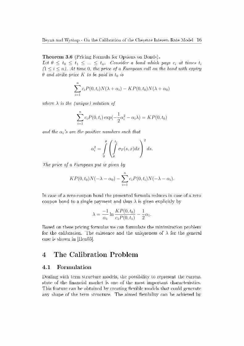
Beyna and Wystup - On the Calibration of the Cheyette Interest Rate Model 16
Theorem 3.6 (Pricing Formula for Options on Bonds).Let θ ≤ t0 ≤ t1 ≤ ... ≤ tn. Consider a bond which pays ci at times ti(1 ≤ i ≤ n). At time 0, the price of a European call on the bond with expiryθ and strike price K to be paid in t0 is
n∑
i=1
ciP (0, ti)N(λ + αi) − KP (0, t0)N(λ + α0)
where λ is the (unique) solution of
n∑
i=1
ciP (0, ti) exp(−1
2α2
i − αiλ) = KP (0, t0)
and the αi's are the positive numbers such that
α2i =
θ∫
0
ti∫
θ
σT (s, x)dx
2
ds.
The price of a European put is given by
KP (0, t0)N(−λ − α0) −n∑
i=1
ciP (0, ti)N(−λ − αi).
In case of a zero coupon bond the presented formula reduces in case of a zerocoupon bond to a single payment and thus λ is given explicitly by
λ =−1
α1
lnKP (0, t0)
c1P (0, t1)−
1
2α1.
Based on these pricing formulas we can formulate the minimization problemfor the calibration. The existence and the uniqueness of λ for the generalcase is shown in [Hen03].
4 The Calibration Problem
4.1 Formulation
Dealing with term structure models, the possibility to represent the currentstate of the nancial market is one of the most important characteristics.This feature can be obtained by creating exible models that could generateany shape of the term structure. The aimed exibility can be achieved by
Beyna and Wystup - On the Calibration of the Cheyette Interest Rate Model 17
term structure models taking several (stochastic) factors into account. Eachfactor represents a predened shape, e.g. parallel shift or twist. As a conse-quence the models become more complex and the mathematical tractabilitydecreases. In sum, the model should rebuild a reasonable fraction of the -nancial market at best and at the same time stay as simple as possible. Thequality of the approximation of the market can be measured by comparingcharacteristic numbers of standardized nancial instruments quoted in thismarket fraction, e.g. prices or volatility. A common method to measure theaccuracy of the approximation is based on the dierences in pricing betweenthe observed market prices and the model implied prices. Changing the pointof view slightly, we can look for a term structure model minimizing these dif-ferences for a specic market section, i.e. we calibrate a model to a specicmarket section. The formulation of the calibration problem is based on thedegrees of freedom within the specic structure. The number of free modelparameters depends on the number of included factors, so the complexity ofthe model appears proportional to this number.
Cheyette models have a special volatility term structure that is param-eterized by a sum of separable functions. As a consequence the major pro-cesses have the Markov property that forms an advantage for the subsequentnumerical simulation. The set of free parameters in the model is limited tothe coecients representing the parametrization of the volatility.
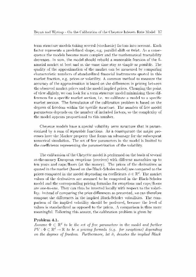
The calibration of the Cheyette model is performed on the basis of severalat-the-money European swaptions (receiver) with dierent maturities up toten years and caps/oors (at the money). The prices of the derivatives asquoted in the market (based on the Black-Scholes model) are compared to theprices computed in the model depending on coecients φ ∈ R
d. The marketvalues of the derivatives are assumed to be computed in the Black-Scholesmodel and the corresponding pricing formulas for swaptions and caps/oorsare one-to-one. They can thus be inverted locally with respect to the volati-lity. Instead of comparing the price dierences as presented, we can thereforecompare the dierences in the implied Black-Scholes volatilities. The com-parison of the implied volatility should be preferred, because the level ofvalues is standardized as opposed to the prices. A comparison is thus moremeaningful. Following this ansatz, the calibration problem is given by
Problem 4.1.
Assume Φ ⊂ Rd to be the set of free parameters in the model and further
PV : Φ ⊂ Rd → R to be a pricing formula (e.g. for swaptions) depending
on the degrees of freedom. Furthermore, let σi denotes the implied Black-
Beyna and Wystup - On the Calibration of the Cheyette Interest Rate Model 18
Scholes volatility as observed in the market and σi(PVi(φ)) the implied Black-Scholes volatility representing the price PVi(φ) in the Cheyette model with theparameter set φ ∈ Φ. In the calibration process we are looking for the globalminimum of the function E : R
d → R.
infφ∈Φ
E(φ), E(φ) =I∑
i=0
ωi|σ(PVi(φ)) − σi|2. (25)
The integer I denotes the number of all derivatives taken into account forthe calibration and ωi ∈ R denotes weights that control the inuence of anyinstrument; for example swaptions and caps might be weighted dierently.
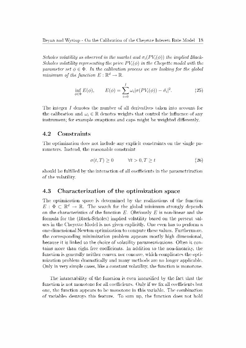
4.2 Constraints
The optimization does not include any explicit constraints on the single pa-rameters. Instead, the reasonable constraint
σ(t, T ) ≥ 0 ∀t > 0, T ≥ t (26)
should be fullled by the interaction of all coecients in the parametrizationof the volatility.
4.3 Characterization of the optimization space
The optimization space is determined by the realizations of the functionE : Φ ⊂ R
d → R. The search for the global minimum strongly dependson the characteristics of the function E. Obviously E is non-linear and theformula for the (Black-Scholes) implied volatility based on the present val-ues in the Cheyette Model is not given explicitly. One even has to perform aone-dimensional Newton optimization to compute these values. Furthermore,the corresponding minimization problem appears mostly high dimensional,because it is linked to the choice of volatility parametrizations. Often it con-tains more than eight free coecients. In addition to the non-linearity, thefunction is generally neither convex nor concave, which complicates the opti-mization problem dramatically and many methods are no longer applicable.Only in very simple cases, like a constant volatility, the function is monotone.
The intractability of the function is even intensied by the fact that thefunction is not monotone for all coecients. Only if we x all coecients butone, the function appears to be monotone in this variable. The combinationof variables destroys this feature. To sum up, the function does not hold
Beyna and Wystup - On the Calibration of the Cheyette Interest Rate Model 19
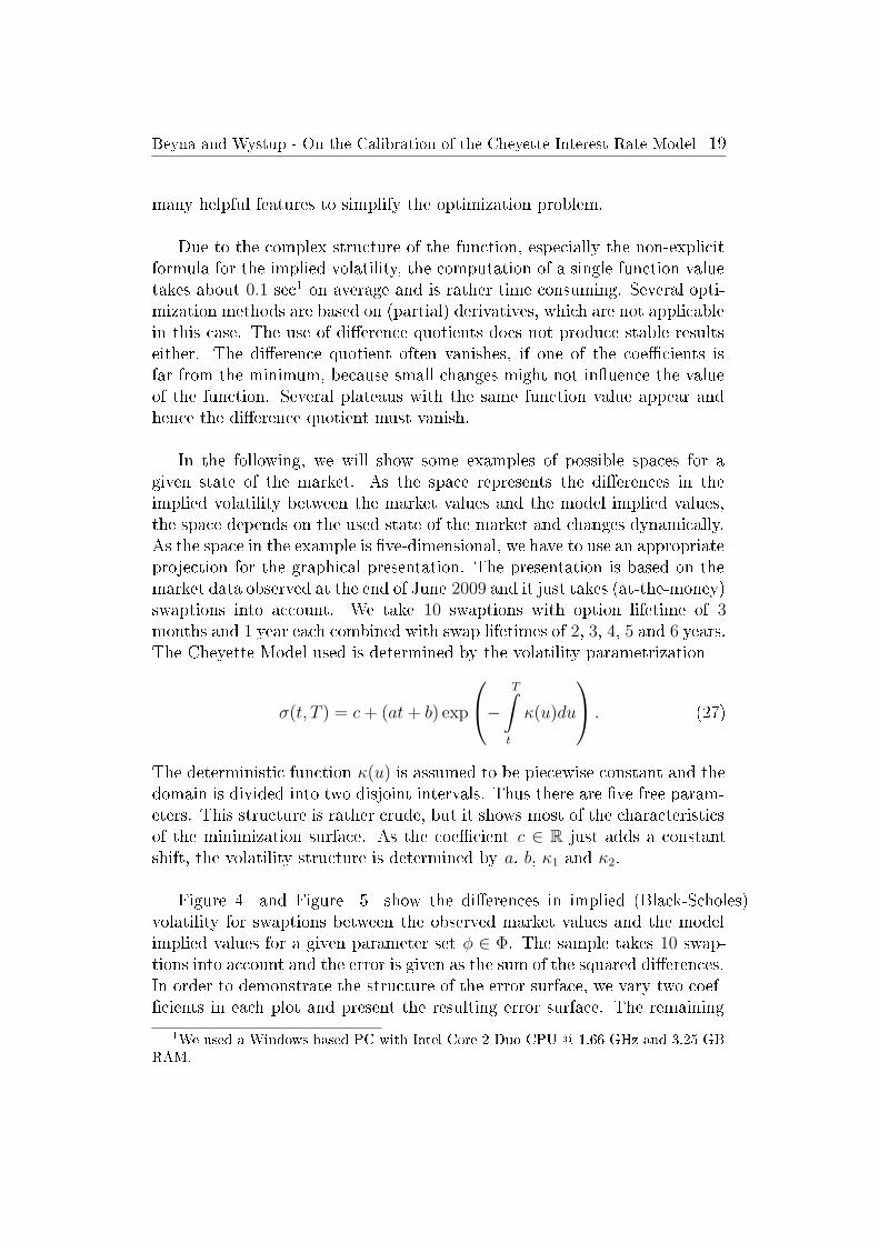
many helpful features to simplify the optimization problem.
Due to the complex structure of the function, especially the non-explicitformula for the implied volatility, the computation of a single function valuetakes about 0.1 sec1 on average and is rather time consuming. Several opti-mization methods are based on (partial) derivatives, which are not applicablein this case. The use of dierence quotients does not produce stable resultseither. The dierence quotient often vanishes, if one of the coecients isfar from the minimum, because small changes might not inuence the valueof the function. Several plateaus with the same function value appear andhence the dierence quotient must vanish.
In the following, we will show some examples of possible spaces for agiven state of the market. As the space represents the dierences in theimplied volatility between the market values and the model implied values,the space depends on the used state of the market and changes dynamically.As the space in the example is ve-dimensional, we have to use an appropriateprojection for the graphical presentation. The presentation is based on themarket data observed at the end of June 2009 and it just takes (at-the-money)swaptions into account. We take 10 swaptions with option lifetime of 3months and 1 year each combined with swap lifetimes of 2, 3, 4, 5 and 6 years.The Cheyette Model used is determined by the volatility parametrization
σ(t, T ) = c + (at + b) exp
−
T∫
t
κ(u)du
. (27)
The deterministic function κ(u) is assumed to be piecewise constant and thedomain is divided into two disjoint intervals. Thus there are ve free param-eters. This structure is rather crude, but it shows most of the characteristicsof the minimization surface. As the coecient c ∈ R just adds a constantshift, the volatility structure is determined by a, b, κ1 and κ2.
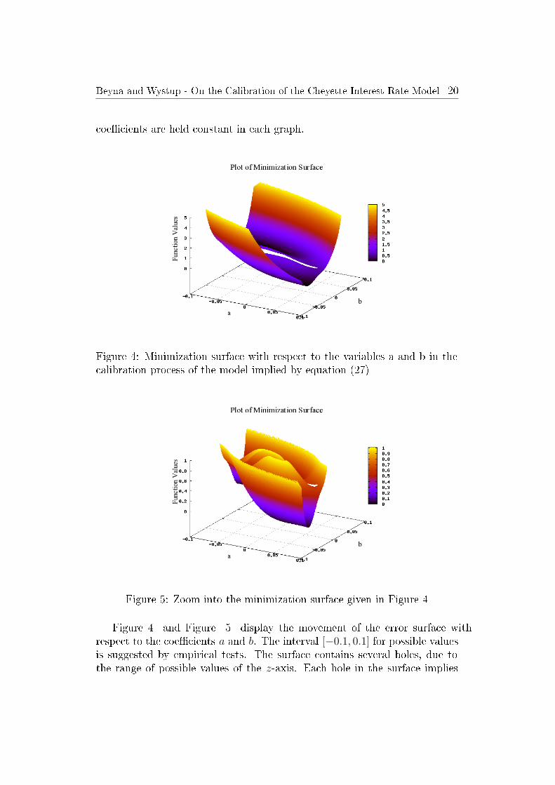
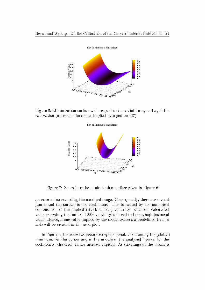
Figure 4 and Figure 5 show the dierences in implied (Black-Scholes)volatility for swaptions between the observed market values and the modelimplied values for a given parameter set φ ∈ Φ. The sample takes 10 swap-tions into account and the error is given as the sum of the squared dierences.In order to demonstrate the structure of the error surface, we vary two coef-cients in each plot and present the resulting error surface. The remaining
1We used a Windows based PC with Intel Core 2 Duo CPU @ 1.66 GHz and 3.25 GBRAM.
Beyna and Wystup - On the Calibration of the Cheyette Interest Rate Model 20
coecients are held constant in each graph.
Figure 4: Minimization surface with respect to the variables a and b in thecalibration process of the model implied by equation (27)
Figure 5: Zoom into the minimization surface given in Figure 4
Figure 4 and Figure 5 display the movement of the error surface withrespect to the coecients a and b. The interval [−0.1, 0.1] for possible valuesis suggested by empirical tests. The surface contains several holes, due tothe range of possible values of the z-axis. Each hole in the surface implies
Beyna and Wystup - On the Calibration of the Cheyette Interest Rate Model 21
Figure 6: Minimization surface with respect to the variables κ1 and κ2 in thecalibration process of the model implied by equation (27)
Figure 7: Zoom into the minimization surface given in Figure 6
an error value exceeding the maximal range. Consequently, there are severaljumps and the surface is not continuous. This is caused by the numericalcomputation of the implied (Black-Scholes) volatility, because a calculatedvalue exceeding the limit of 100% volatility is forced to take a high technicalvalue. Hence, if one value implied by the model exceeds a predened level, ahole will be created in the used plot.
In Figure 4 there are two separate regions possibly containing the (global)minimum. At the border and in the middle of the analyzed interval for thecoecients, the error values increase rapidly. As the range of the z-axis is
Beyna and Wystup - On the Calibration of the Cheyette Interest Rate Model 22
rather big, we zoomed in and displayed the same surface in Figure 5 for asmaller range of values. This gure demonstrates that there are valleys inthe surface and that the error reacts sensitively to small changes in thesecoecients. Figure 6 and Figure 7 display the movement of the error surfacewith respect to the coecients κ1 and κ2 of the piecewise constant functionκ(u). The remaining coecients are xed and chosen to minimize the errorfor the given data set. The surface appears rather regular and contains nohills. The structure of the surface suggests that the choice of κ(u) does notchange the values dramatically. But the pictured surfaces only include twodegrees of freedom for illustration. In general, κ(u) takes at least ve coe-cients into account and thus several valleys, including (local) minima, emerge.
Each of the presented surfaces only depends on two parameters. Thewhole surface is given as a combination of these structures. Thus the result-ing surface becomes more turbulent and irregular. Consequently, there areseveral local minima, jumps and hills, that have to be treated in the opti-mization process. Several methods that can handle these functions exist, butnone of them guarantees the convergence to a global optimum.
4.4 Quality Check
The evaluation of the calibration results leaves much freedom to the user. Inorder to apply a standardized technique, we come up with several conditionsto the prices and the implied Black-Scholes volatility to evaluate the calibra-tion. We focus on the price and volatility residuals between the Cheyetteand the Black-Scholes model. The implemented check of the calibration con-sists of twelve conditions subdivided into four core and eight secondary ones.The design and the denition of the quality check is comparable to the cri-teria used in the pricing software `FINCAD Analytics Suite 2009'. The coreconditions are given by:
• Price Bias ≤ 30%:At most 30% of the relative price dierences exceed the limit of 30%
• Volatility Bias ≤ 30%:At most 30% of the relative volatility dierences exceed the limit of30%
• Mean price residual < σ:The mean of all price residuals does not exceed the standard deviationσ with mean 0
Beyna and Wystup - On the Calibration of the Cheyette Interest Rate Model 23
• Mean volatility residual < σ:The mean of all volatility residuals does not exceed the standard devi-ation σ with mean 0
Furthermore we identied several secondary conditions given by:
• Convergence of the minimization algorithm
• Minimum does not lie on the boundary
• All volatility residuals are bounded by 3σ
• All price residuals are bounded by 3σ
• 90% of the volatility residuals are less than 2σ
• 90% of the price residuals are less than 2σ
• Maximal volatility residual does not exceed 5%
• Mean of squared volatility residuals is limited by 1
The quality check delivers three possible outcomes: good, passed and failed.If all conditions - core and secondary - are fullled, the calibration is assumedto be `good'. If at most one secondary condition does not hold, the calibrationis interpreted to be still valid and thus the algorithm will deliver `passed'.The calibration algorithm fails, if one or more of the core conditions or morethan one of the additional conditions are violated.
5 Optimization Methods
5.1 Overview of methods
Developing the calibration method, we have implemented several minimiza-tion algorithms. Mainly, we can classify the tested algorithms into threedierent classes:
1. non-linear optimization methods with derivatives, e.g. Newton algo-rithm with and without step size adjustment,
2. non-linear optimization methods without derivatives, e.g. DownhillSimplex and Powell algorithm and
3. stochastic optimization methods, e.g. Simulated Annealing and Ge-netic Optimization.
Beyna and Wystup - On the Calibration of the Cheyette Interest Rate Model 24
5.2 Assessment of methods
In the following we present the analysis of the optimization methods consist-ing of method descriptions followed by the results of the application to thecalibration problem.
5.2.1 Newton Algorithm
5.2.1.1 Description
The Newton algorithm is a local optimization method developed by IsaacNewton in 1669. This method makes use of the rst and second derivativeswith respect to all directions. The resulting Jacobi- and Hessian matrix areassumed to have full rank and furthermore the Hessian matrix has to beinvertible. Based on these matrices, the iterations steps are computed. Thealgorithm will terminate in a position where the rst derivatives vanish andthus the algorithm in general detects only local optima.
5.2.1.2 Results
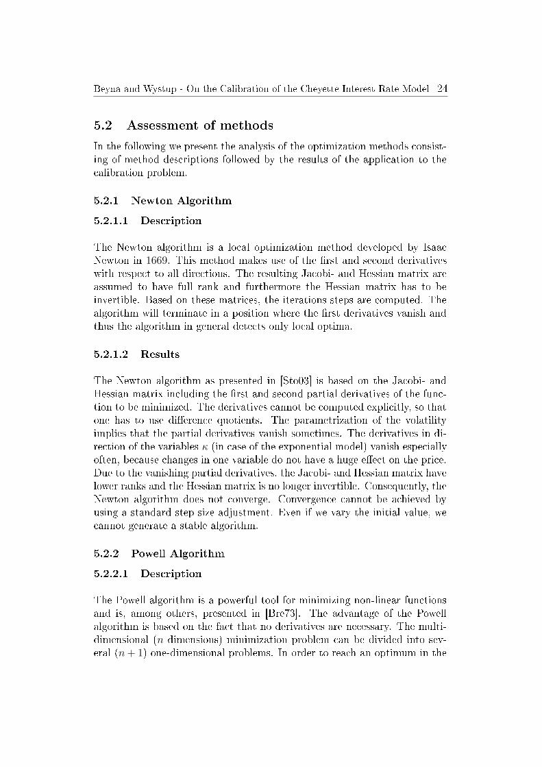
The Newton algorithm as presented in [Sto03] is based on the Jacobi- andHessian matrix including the rst and second partial derivatives of the func-tion to be minimized. The derivatives cannot be computed explicitly, so thatone has to use dierence quotients. The parametrization of the volatilityimplies that the partial derivatives vanish sometimes. The derivatives in di-rection of the variables κ (in case of the exponential model) vanish especiallyoften, because changes in one variable do not have a huge eect on the price.Due to the vanishing partial derivatives, the Jacobi- and Hessian matrix havelower ranks and the Hessian matrix is no longer invertible. Consequently, theNewton algorithm does not converge. Convergence cannot be achieved byusing a standard step size adjustment. Even if we vary the initial value, wecannot generate a stable algorithm.
5.2.2 Powell Algorithm
5.2.2.1 Description
The Powell algorithm is a powerful tool for minimizing non-linear functionsand is, among others, presented in [Bre73]. The advantage of the Powellalgorithm is based on the fact that no derivatives are necessary. The multi-dimensional (n dimensions) minimization problem can be divided into sev-eral (n + 1) one-dimensional problems. In order to reach an optimum in the
Beyna and Wystup - On the Calibration of the Cheyette Interest Rate Model 25
superior algorithm, we need to nd the global optimum in each of the one-dimensional optimization problems. First, the one-dimensional minimizationis performed separately along a line in direction of each volatility coecient.In this case, the one-dimensional problem is easy, because the function ap-pears monotone. Based on these results, new directions for the optimizationare created by combining dierent one-dimensional optima. The new direc-tions eect more than one coecient of the volatility function. As a result,the monotonicity is lost and the one-dimensional problems becomes morecomplicated. The corresponding minimization space does not stay monotoneany longer, but several waves will appear complicating the minimization.Due to this fact, we have to use a brute force algorithm testing more or lessall possible values in a predened interval. This method costs a lot of time,but we need to nd a global minimum of the one-dimensional problem inorder to reach the global minimum with the superior algorithm. We reini-tialize the basis of directions to search after processing n iterations with thepurpose to improve the Powell algorithm and decrease the linear dependency.
5.2.2.2 Results
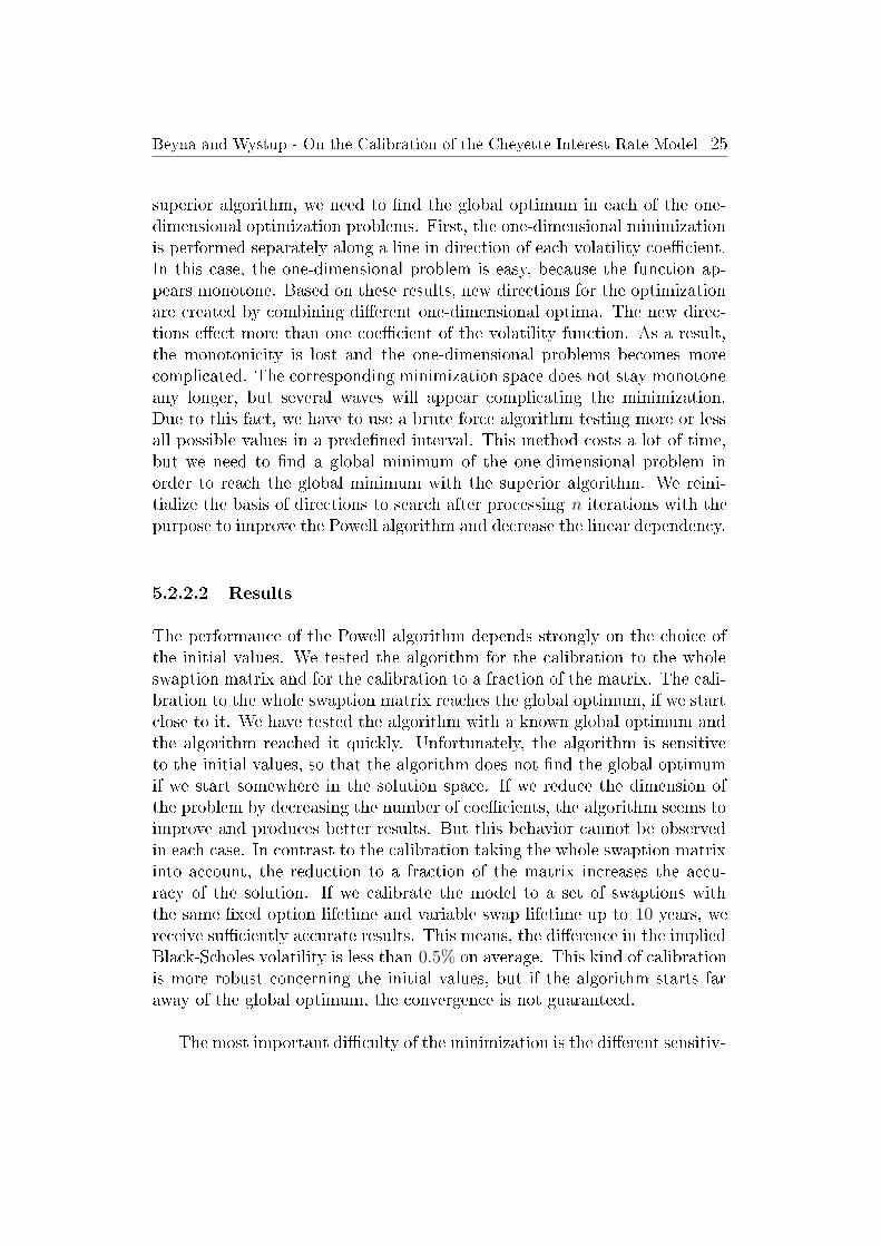
The performance of the Powell algorithm depends strongly on the choice ofthe initial values. We tested the algorithm for the calibration to the wholeswaption matrix and for the calibration to a fraction of the matrix. The cali-bration to the whole swaption matrix reaches the global optimum, if we startclose to it. We have tested the algorithm with a known global optimum andthe algorithm reached it quickly. Unfortunately, the algorithm is sensitiveto the initial values, so that the algorithm does not nd the global optimumif we start somewhere in the solution space. If we reduce the dimension ofthe problem by decreasing the number of coecients, the algorithm seems toimprove and produces better results. But this behavior cannot be observedin each case. In contrast to the calibration taking the whole swaption matrixinto account, the reduction to a fraction of the matrix increases the accu-racy of the solution. If we calibrate the model to a set of swaptions withthe same xed option lifetime and variable swap lifetime up to 10 years, wereceive suciently accurate results. This means, the dierence in the impliedBlack-Scholes volatility is less than 0.5% on average. This kind of calibrationis more robust concerning the initial values, but if the algorithm starts faraway of the global optimum, the convergence is not guaranteed.
The most important diculty of the minimization is the dierent sensitiv-
Beyna and Wystup - On the Calibration of the Cheyette Interest Rate Model 26
ity of the coecients to the minimization function. While, for example, theconstant and the coecients of the linear function (in the case of the examplepresented in (27)) have a strong eect on the minimization function, the eectof the coecients of the piecewise constant function κ(t) is relatively small.Thus one has to use dierent discretizations or step sizes for the coecientsto receive suciently accurate results and minimize iterations. The idea ofthe Powell algorithm includes the minimization along one-dimensional linesand the directions are composed by several coecients. The discretizationand the step size must thus be adapted to all coecients which implies alarge number of iterations and consequently large computation times. Thisis even intensied by the characteristics of the one-dimensional minimizationproblem possessing several waves. As the global optimum (along the line) isrequired only naive algorithms are available taking lots of time. In combi-nation one single step in the Powell algorithm is time consuming and thusthis algorithm is not ecient for the calibration of the Cheyette Model. Thesetup of the model carries undesired features destroying the advantages ofthe Powell algorithm for high dimensions.
5.2.3 Downhill Simplex Algorithm
5.2.3.1 Description
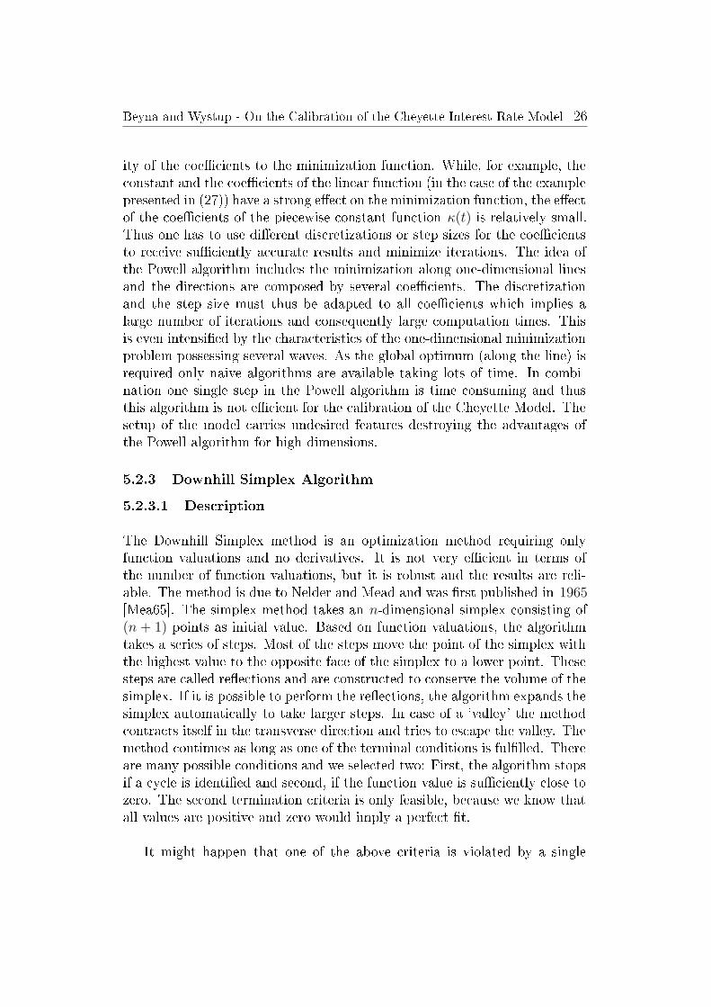
The Downhill Simplex method is an optimization method requiring onlyfunction valuations and no derivatives. It is not very ecient in terms ofthe number of function valuations, but it is robust and the results are reli-able. The method is due to Nelder and Mead and was rst published in 1965[Mea65]. The simplex method takes an n-dimensional simplex consisting of(n + 1) points as initial value. Based on function valuations, the algorithmtakes a series of steps. Most of the steps move the point of the simplex withthe highest value to the opposite face of the simplex to a lower point. Thesesteps are called reections and are constructed to conserve the volume of thesimplex. If it is possible to perform the reections, the algorithm expands thesimplex automatically to take larger steps. In case of a `valley' the methodcontracts itself in the transverse direction and tries to escape the valley. Themethod continues as long as one of the terminal conditions is fullled. Thereare many possible conditions and we selected two: First, the algorithm stopsif a cycle is identied and second, if the function value is suciently close tozero. The second termination criteria is only feasible, because we know thatall values are positive and zero would imply a perfect t.
It might happen that one of the above criteria is violated by a single
Beyna and Wystup - On the Calibration of the Cheyette Interest Rate Model 27
abnormality in the function. It is therefore a good idea to restart the mini-mization routine at a point where it claims to have found a minimum. Thedownhill simplex algorithm includes four parameters that control the move-ment of the simplex. The choice of these values inuences the speed of themethod and might change the computed optimum.
• α controls the reection.
• β controls the contraction.
• γ controls the expansion.
• σ controls the compression.
Numerous publications mention only three parameters for the Downhill-Simplex algorithm and in this case they do not distinguish between parameterβ and σ.
5.2.3.2 Results
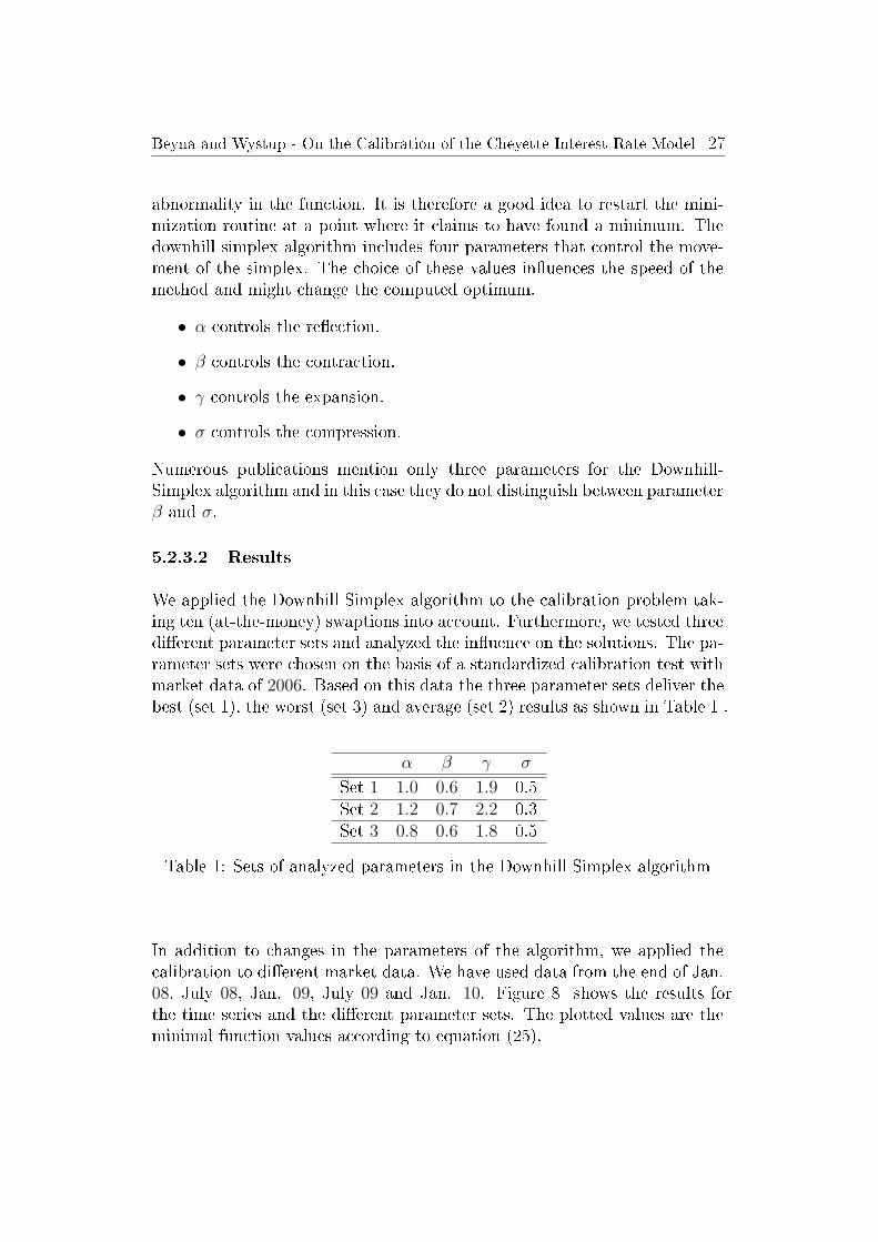
We applied the Downhill Simplex algorithm to the calibration problem tak-ing ten (at-the-money) swaptions into account. Furthermore, we tested threedierent parameter sets and analyzed the inuence on the solutions. The pa-rameter sets were chosen on the basis of a standardized calibration test withmarket data of 2006. Based on this data the three parameter sets deliver thebest (set 1), the worst (set 3) and average (set 2) results as shown in Table 1 .
α β γ σ
Set 1 1.0 0.6 1.9 0.5Set 2 1.2 0.7 2.2 0.3Set 3 0.8 0.6 1.8 0.5
Table 1: Sets of analyzed parameters in the Downhill Simplex algorithm
In addition to changes in the parameters of the algorithm, we applied thecalibration to dierent market data. We have used data from the end of Jan.08, July 08, Jan. 09, July 09 and Jan. 10. Figure 8 shows the results forthe time series and the dierent parameter sets. The plotted values are theminimal function values according to equation (25).
Beyna and Wystup - On the Calibration of the Cheyette Interest Rate Model 28
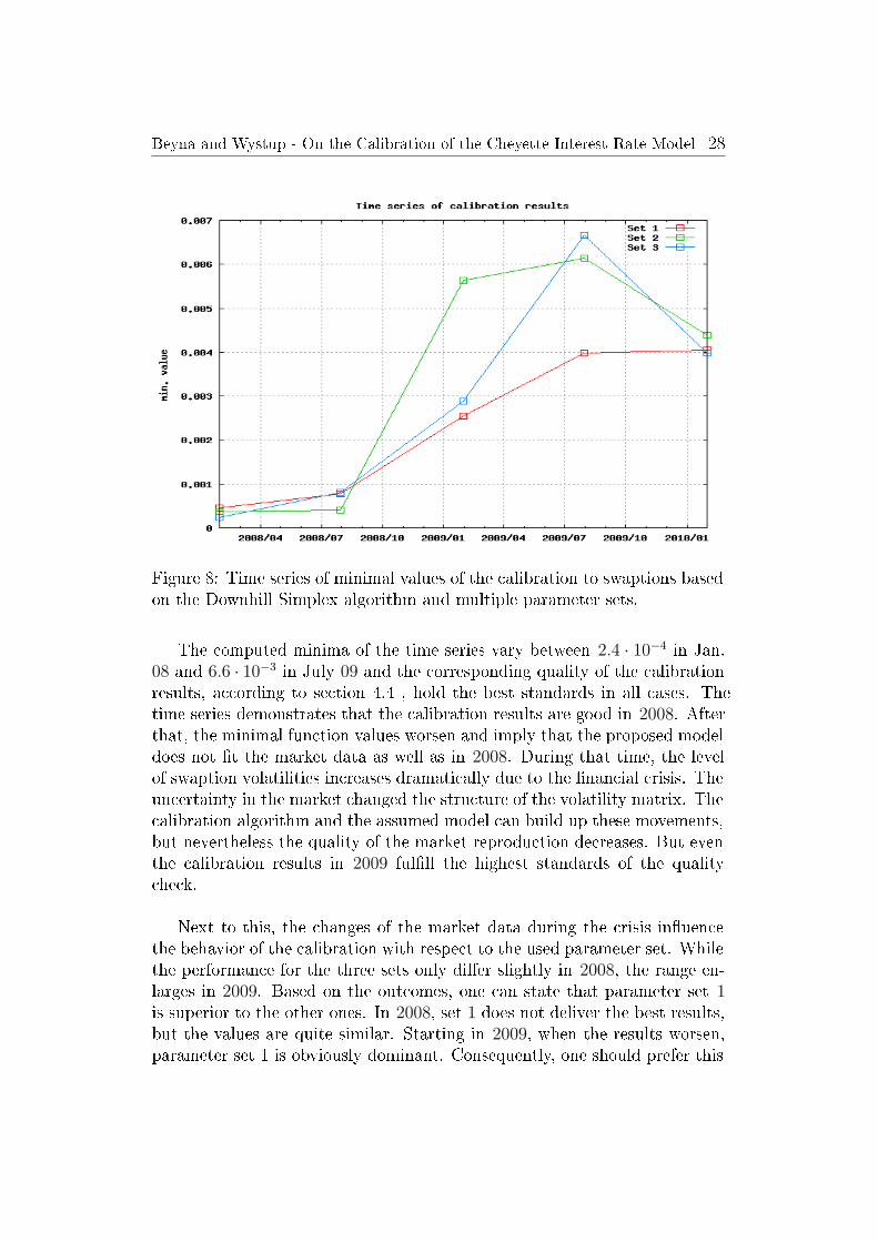
Figure 8: Time series of minimal values of the calibration to swaptions basedon the Downhill Simplex algorithm and multiple parameter sets.
The computed minima of the time series vary between 2.4 · 10−4 in Jan.08 and 6.6 · 10−3 in July 09 and the corresponding quality of the calibrationresults, according to section 4.4 , hold the best standards in all cases. Thetime series demonstrates that the calibration results are good in 2008. Afterthat, the minimal function values worsen and imply that the proposed modeldoes not t the market data as well as in 2008. During that time, the levelof swaption volatilities increases dramatically due to the nancial crisis. Theuncertainty in the market changed the structure of the volatility matrix. Thecalibration algorithm and the assumed model can build up these movements,but nevertheless the quality of the market reproduction decreases. But eventhe calibration results in 2009 fulll the highest standards of the qualitycheck.
Next to this, the changes of the market data during the crisis inuencethe behavior of the calibration with respect to the used parameter set. Whilethe performance for the three sets only dier slightly in 2008, the range en-larges in 2009. Based on the outcomes, one can state that parameter set 1is superior to the other ones. In 2008, set 1 does not deliver the best results,but the values are quite similar. Starting in 2009, when the results worsen,parameter set 1 is obviously dominant. Consequently, one should prefer this
Beyna and Wystup - On the Calibration of the Cheyette Interest Rate Model 29
setting, although it does not always produce the best results.
The presented eects are all based on the same initial values for theminimization algorithm. A signicant criterion for reasonable optimizationis the stability with respect to changes in the starting points. We tested136 dierent initial values for the calibration and monitored the changes inthe minimal values and in the coecients of the minimum. The dierencesbetween the coecients of two minima can be measured by the vector norm
|x(1) − x(2)| =d∑
i=1
|x(1)i − x(2)i|2 (28)
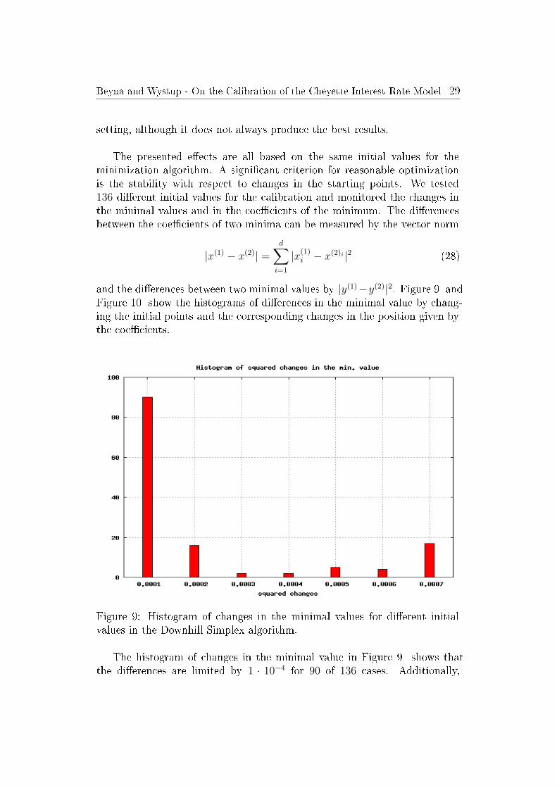
and the dierences between two minimal values by |y(1)−y(2)|2. Figure 9 andFigure 10 show the histograms of dierences in the minimal value by chang-ing the initial points and the corresponding changes in the position given bythe coecients.
Figure 9: Histogram of changes in the minimal values for dierent initialvalues in the Downhill Simplex algorithm.
The histogram of changes in the minimal value in Figure 9 shows thatthe dierences are limited by 1 · 10−4 for 90 of 136 cases. Additionally,
Beyna and Wystup - On the Calibration of the Cheyette Interest Rate Model 30
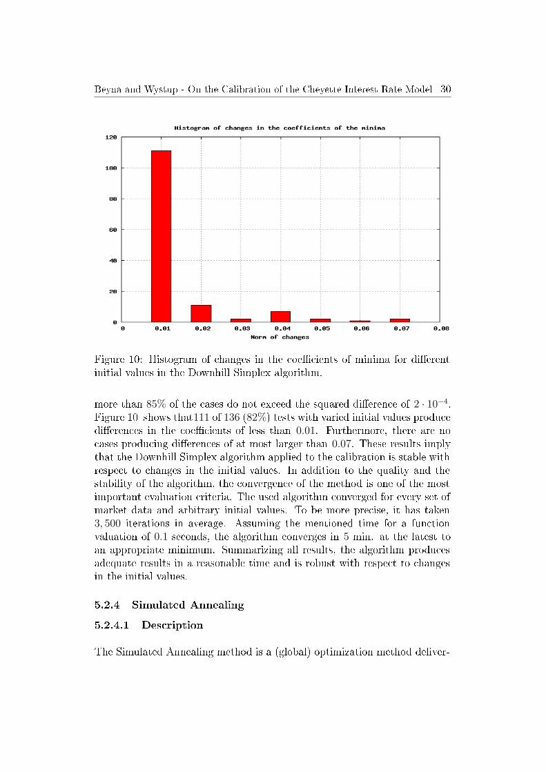
Figure 10: Histogram of changes in the coecients of minima for dierentinitial values in the Downhill Simplex algorithm.
more than 85% of the cases do not exceed the squared dierence of 2 · 10−4.Figure 10 shows that111 of 136 (82%) tests with varied initial values producedierences in the coecients of less than 0.01. Furthermore, there are nocases producing dierences of at most larger than 0.07. These results implythat the Downhill Simplex algorithm applied to the calibration is stable withrespect to changes in the initial values. In addition to the quality and thestability of the algorithm, the convergence of the method is one of the mostimportant evaluation criteria. The used algorithm converged for every set ofmarket data and arbitrary initial values. To be more precise, it has taken3, 500 iterations in average. Assuming the mentioned time for a functionvaluation of 0.1 seconds, the algorithm converges in 5 min. at the latest toan appropriate minimum. Summarizing all results, the algorithm producesadequate results in a reasonable time and is robust with respect to changesin the initial values.
5.2.4 Simulated Annealing
5.2.4.1 Description
The Simulated Annealing method is a (global) optimization method deliver-
Beyna and Wystup - On the Calibration of the Cheyette Interest Rate Model 31
ing remarkable results if a desired global extremum is hidden among manylocal optima. Unfortunately it does not guarantee the convergence to theglobal optimum, but especially combinatorial minimizations like the `Travel-ing Salesman Problem' were solved eciently by this technique. The methodof Simulated Annealing is inspired by thermodynamics, especially the way offreezing and crystallizing liquids. In nature, the thermal mobility of atomsdecreases for cooling liquids and ends in crystals forming the state of min-imum energy for this system. The method of Simulated Annealing pics upthis idea and allows more movements even uphill (worse solution) for `hightemperature'. Thus it is possible that the algorithm leaves local minima orvalleys and increases the probability of nding the global extremum. TheBoltzmann probability distribution controls the likelihood of exploring thespace and allowing temporally worse movements. The probability is linked tothe `temperature' and the algorithm converges in dependence to a predenedannealing schedule. Empirical tests have shown that the temperature shouldbe reduced suciently slowly to achieve the best results [Pre02].
In addition to the annealing schedule, there must be a procedure for it-erating the solution. Following the ideas of [Pre02] this generator should berobust and stay ecient even in narrow valleys. Consequently we based theimplementation of the Simulated Annealing method on a modied DownhillSimplex algorithm. The modication allows uphill movements whose maxi-mal length depends on a synthetic temperature T controlled in the annealingschedule. In the limit T → 0, this algorithm reduces exactly to the DownhillSimplex method.
5.2.4.2 Results
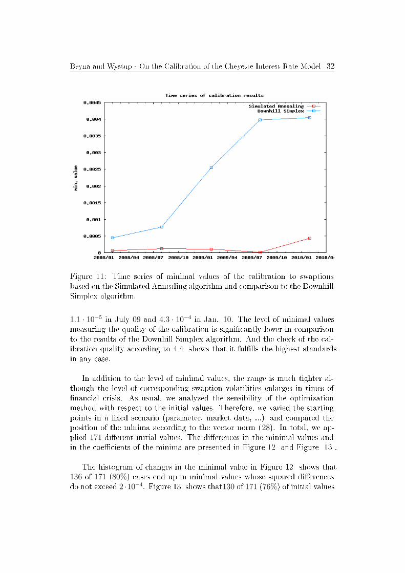
In analogy to the tests of the Downhill Simplex algorithm, we applied theSimulated Annealing method to the same market data. As previously de-scribed, the algorithm makes use of the Downhill Simplex method. Accord-ing to the results in section 5.2.3.2 we used parameter set1. We appliedthe calibration method to a series of market data starting in Jan. 2008 andending in Jan. 2010. Figure 11 presents the results of these calibrations toat-the-money swaptions in form of the minimal values according to equation(25) and compares them to the corresponding outcomes of the Downhill Sim-plex algorithm. We used the same set of swaptions as described in section5.2.3.
The minimal values of the calibration in the time series vary between
Beyna and Wystup - On the Calibration of the Cheyette Interest Rate Model 32
Figure 11: Time series of minimal values of the calibration to swaptionsbased on the Simulated Annealing algorithm and comparison to the DownhillSimplex algorithm.
1.1 · 10−5 in July 09 and 4.3 · 10−4 in Jan. 10. The level of minimal valuesmeasuring the quality of the calibration is signicantly lower in comparisonto the results of the Downhill Simplex algorithm. And the check of the cal-ibration quality according to 4.4 shows that it fullls the highest standardsin any case.
In addition to the level of minimal values, the range is much tighter al-though the level of corresponding swaption volatilities enlarges in times ofnancial crisis. As usual, we analyzed the sensibility of the optimizationmethod with respect to the initial values. Therefore, we varied the startingpoints in a xed scenario (parameter, market data, ...) and compared theposition of the minima according to the vector norm (28). In total, we ap-plied 171 dierent initial values. The dierences in the minimal values andin the coecients of the minima are presented in Figure 12 and Figure 13 .
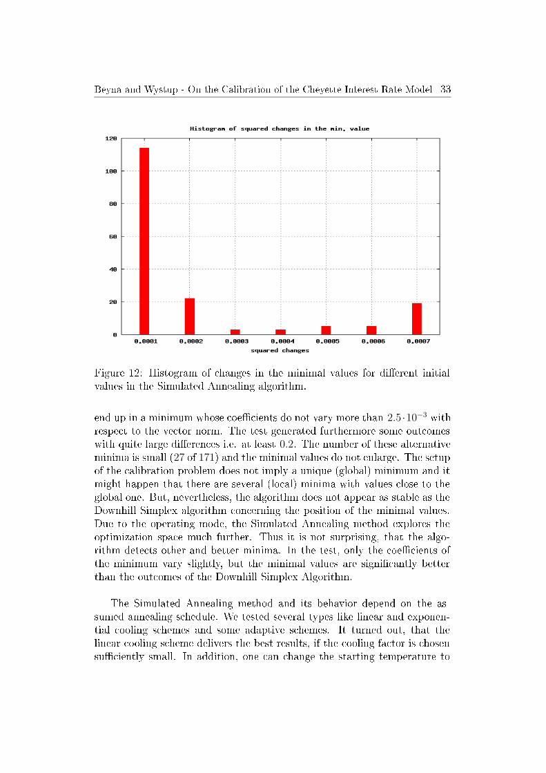
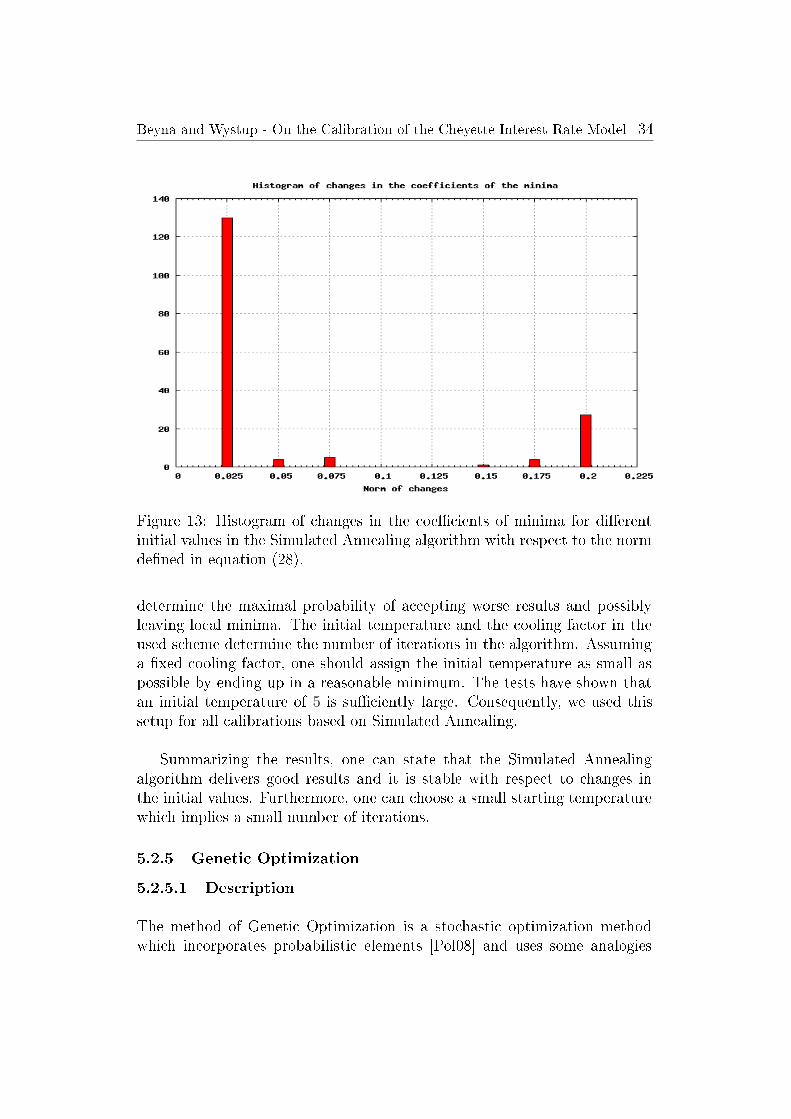
The histogram of changes in the minimal value in Figure 12 shows that136 of 171 (80%) cases end up in minimal values whose squared dierencesdo not exceed 2 ·10−4. Figure 13 shows that130 of 171 (76%) of initial values
Beyna and Wystup - On the Calibration of the Cheyette Interest Rate Model 33
Figure 12: Histogram of changes in the minimal values for dierent initialvalues in the Simulated Annealing algorithm.
end up in a minimum whose coecients do not vary more than 2.5 ·10−3 withrespect to the vector norm. The test generated furthermore some outcomeswith quite large dierences i.e. at least 0.2. The number of these alternativeminima is small (27 of 171) and the minimal values do not enlarge. The setupof the calibration problem does not imply a unique (global) minimum and itmight happen that there are several (local) minima with values close to theglobal one. But, nevertheless, the algorithm does not appear as stable as theDownhill Simplex algorithm concerning the position of the minimal values.Due to the operating mode, the Simulated Annealing method explores theoptimization space much further. Thus it is not surprising, that the algo-rithm detects other and better minima. In the test, only the coecients ofthe minimum vary slightly, but the minimal values are signicantly betterthan the outcomes of the Downhill Simplex Algorithm.
The Simulated Annealing method and its behavior depend on the as-sumed annealing schedule. We tested several types like linear and exponen-tial cooling schemes and some adaptive schemes. It turned out, that thelinear cooling scheme delivers the best results, if the cooling factor is chosensuciently small. In addition, one can change the starting temperature to
Beyna and Wystup - On the Calibration of the Cheyette Interest Rate Model 34
Figure 13: Histogram of changes in the coecients of minima for dierentinitial values in the Simulated Annealing algorithm with respect to the normdened in equation (28).
determine the maximal probability of accepting worse results and possiblyleaving local minima. The initial temperature and the cooling factor in theused scheme determine the number of iterations in the algorithm. Assuminga xed cooling factor, one should assign the initial temperature as small aspossible by ending up in a reasonable minimum. The tests have shown thatan initial temperature of 5 is suciently large. Consequently, we used thissetup for all calibrations based on Simulated Annealing.
Summarizing the results, one can state that the Simulated Annealingalgorithm delivers good results and it is stable with respect to changes inthe initial values. Furthermore, one can choose a small starting temperaturewhich implies a small number of iterations.
5.2.5 Genetic Optimization
5.2.5.1 Description
The method of Genetic Optimization is a stochastic optimization methodwhich incorporates probabilistic elements [Pol08] and uses some analogies
Beyna and Wystup - On the Calibration of the Cheyette Interest Rate Model 35
to the evolution theory in biology developed by Charles Darwin. Based ona randomly chosen set of potential solutions, the algorithm tries to nd aglobal optimum by creating new solutions. This is done by combining andadjusting the previous solutions stochastically. The iterations within the al-gorithm are determined by three operators: selection, cross and mutation.The application is based on the binary code of the possible solutions, i.e. astring of 0/1. Therefore each coecient is encoded to a binary representa-tion consisting of single bits and all these codes are combined to a stringrepresenting one possible solution. First the cross operator selects a pair ofsolutions x and y with a predened probability. The corresponding binarycodes are both cut in the middle (after half of the number of bits) and onereaches the representation x = x1 ∪ x2 and y = y1 ∪ y2. As a second step,the cross operator swaps the ends of both binary codes and creates two newsolutions x = x1 ∪ y2 and y = y1 ∪ x2. The mutation operator is appliedto a single solution respectively its binary code. Each bit is changed with agiven probability and consequently new solutions are created stochastically.As a last step, the selection operator identies the best/worst solutions sofar and duplicates the best by deleting the worst at the same time. Theselection operator implies a concentration of the set of solutions somewherein the optimization space. The algorithm stops, if a solution is found, thatis suciently close to the optimum or the set of solution does not vary anylonger.
As the genetic optimization method is based on some stochastic part in-cluded in the creation of the initial set of solutions and in the continuousadjustment, the detection of the global minimum is not guaranteed. Theconvergence is controlled by the set of initial values and typically we haveto use a large set of numbers to explore the space of solutions. Consider forexample a 9-dimensional optimization problem with coecients that havevalues in an interval of length 1. If we discretize each interval with a stepsize of 10−3, the resulting discrete solution space includes 1024 possible values.The discretization is incorporated by the choice of the binary code speciallythe number of used bits. So, we need a sucient large set of candidates toreach adequate results with high probability. As the valuation of the functionto minimize is expensive, the optimization may take long time to nd the op-timum. This eect is even intensied by the fact, that sometimes solutionsare reevaluated at subsequent steps, since they could be generated severaltimes.
The Genetic Optimization method searches the (global) optimum just ina discrete and nite space. The discrete space is created by discretization
Beyna and Wystup - On the Calibration of the Cheyette Interest Rate Model 36
of the continuous one and hence it is an approximation. The discretizationcontrols the quality of the approximation and in the limit `grid size → 0' thesespaces are equivalent. Thus, the optima of the discrete and the continuousspace correspond in the limit as well.
5.2.5.2 Results
The Genetic Optimization method does not guarantee the convergence tothe global minimum. The behavior of the algorithm is mainly determined bysome specications like the number of candidates, the probabilities of crossand mutation and the discretization of the domain of each coecient. Thechoice of the probabilities is mainly independent of the problem. These valuesaect the exploration of the optimization space by the algorithm. In contrastthe number of candidates and the discretization are strongly problem-specic.The range and the grid size of the discretization depends on the possible val-ues of the coecients and on the sensibility with respect to small changes.The minimization function for the calibration shows strong sensitivity withrespect to changes in some coecients like the constant shift. Thus the gridsize has to be chosen quite small to represent all possible values accurately. Ifthe grid size is chosen too large, the constructed discrete space is not a goodapproximation to the continuous one and consequently the results would notcontain any conclusions. As the coecients of the volatility parametrizationeect the minimization function dierently, the choice of the grid size shouldbe done separately for each component. One should implement equidistantdiscretizations in each dimension to simplify the valuation. The number ofcandidates depends on the dimension of the problem and on the used dis-cretization. The elements of the initial set are the origin of the explorationand even if the evolution is smart, the number of candidates should be cho-sen suciently high. Within the mentioned example, there are 1024 possiblesolutions and one should at least use 10, 000 candidates to cover a signi-cant part. If the number is chosen too small, then the exploration is limitedbecause of the selection operator. This operator forces a concentration some-where in the space by duplication of the best solutions. If there are not manysolutions outside this area left, then the space will not be well explored withhigh probability.
Unfortunately the valuation of the minimization function is time consum-ing. Within the mentioned example with 1024 possible values, one should atleast use 10, 000 candidates. Numerical tests have shown, that the algorithmneeds in average at least 500 iterations to identify the global optimum. The
Beyna and Wystup - On the Calibration of the Cheyette Interest Rate Model 37
function valuation takes in average 0.1 seconds and this implies a total com-putation time of about 140 hours. In order to decrease the computationtime, one has to decrease the dimension or to coarsen the grid, but this im-plies worse results and with high probability inadequate ones. Summarizing,this optimization method can only be applied reasonably to low dimensionalcalibration problems.
5.3 Conclusions
The presentation of the results produced by the dierent minimization al-gorithms has shown that the Downhill Simplex algorithm delivers reliableand reasonable results. Furthermore this methods is robust with respect tochanges in the initial values and thus it can reasonably be applied to thecalibration problem. Nevertheless the Simulated Annealing algorithm seemsto produce slightly better results, because it incorporates the possibility toleave local minima with a predened probability. Thus the probability of de-tecting the global minimum is higher in comparison to the Downhill Simplexalgorithm which is originally a local minimization algorithm. One possibleextension not discussed so far is the combination of both. First one appliesthe Simulated Annealing algorithm with a high initial temperature to explorethe space. Afterwards one starts the Downhill Simplex algorithm with theresults of the Simulated Annealing method as initial values. Numerical testshave shown that this combination improves the results slightly, but therewas no substantial gain measurable. This is not really surprising, becausethe Simulated Annealing algorithm is based on the Downhill Simplex methodand in the limit Temperature → 0 both methods are identical. The subse-quent application just enlarges the number of iterations.
The Newton algorithm does not produce stable results as it makes use ofderivations. But in combination with a previous Simulated Annealing min-imization, it just has to work locally in a normal area. Unfortunately thealgorithm sometimes runs far away from the initial values which destroysthis method again. In the successful case the results are not superior to thecorresponding ones produced by the Downhill Simplex algorithm.
The Genetic Optimization algorithm is really auspicious, because it ex-plores the space extensively. Unfortunately the space in this setup is oftenof high dimension. In combination of a function whose valuation takes quitelong, the optimization method is not practicable. The Powell algorithm oersa good opportunity of dimensional reduction. Unfortunately the minimiza-tion function does not oer any benecial features, thus each one dimensional
Beyna and Wystup - On the Calibration of the Cheyette Interest Rate Model 38
optimization is hard to solve globally. This fact destroys the produced ad-vantages of decomposing the dimensions. Consequently the Powell algorithmdoes not work convincingly in the setup of the calibration of the CheyetteModel.
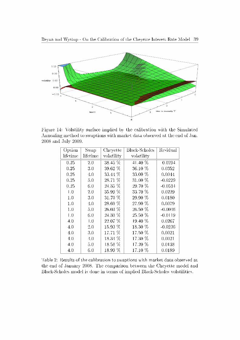
Summarizing, the minimization methods Downhill Simplex and Simu-lated Annealing deliver the best and reliable results for the calibration of theCheyette model. In addition to the analysis of the behavior and the accuracyof the algorithm we present the results of the calibration in form of the volati-lity surface. Using the volatility parametrization (27) and calibrate the modelto 16 swaptions observed at Jan. 2008 (red) and July 2009 (green) we receivetwo volatility surfaces presented in Figure 14 . The results of the calibrationas a comparison between the Cheyette model and the Black-Scholes modelin terms of implied volatility is given in Table 2 and Table 3 . The calibrationto market data observed at the end of Jan. 2008 fullls all conditions on thequality dened in section 4.4 and consequently it is evaluated as `good'. Theresults of the second calibration violates one secondary condition and thusit is evaluated as `passed'. The minimal values are given by 6.5 · 10−3 (Jan.08) and 8.5 · 10−3 (July 09). The implied surfaces have dierent shapes andincludes some negative values as well. This eect has happened, because thecalibration is performed on a market fraction. The extrapolation of theseresults might imply some negative values. The volatility surface of Jan. 08shows several waves, while the surface of July 09 appears quite calm. Thisexample demonstrates that the appearance of the volatility surface changesover time and the model should support maximal exibility by the choice ofthe volatility parametrization.
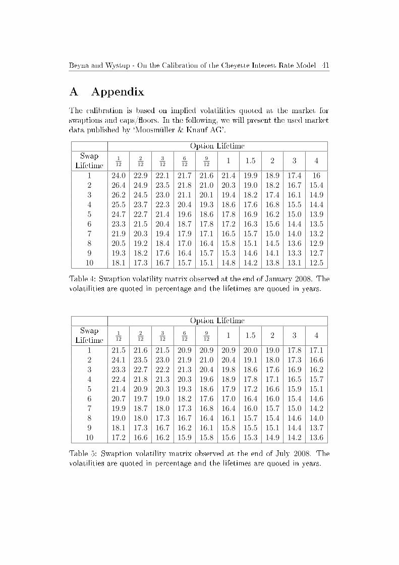
In addition to the calibration to swaptions, we have applied the calibra-tion to caps and oors as well. Again we have used the market data of Jan.08 (red) and July 09 (green) and the implied surfaces are displayed in Fig-ure 15 . The calibration to caps/oors is evaluated as `passed' in both casesand the minimal value is given by 3.8 · 10−5 (Jan. 08) and 1.1 · 10−4 (July09). The implied volatility surfaces have dierent shapes again, but in thiscase the volatility surface of Jan. 08 appears quite regular and calm. Thisappearance diers from the structure of the volatility implied by the calibra-tion to swaptions and underlines the need of exible models.
Beyna and Wystup - On the Calibration of the Cheyette Interest Rate Model 39
Figure 14: Volatility surface implied by the calibration with the SimulatedAnnealing method to swaptions with market data observed at the end of Jan.2008 and July 2009.
Option Swap Cheyette Black-Scholes Residuallifetime lifetime volatility volatility
0.25 2.0 38.45 % 41.40 % -0.02940.25 3.0 39.62 % 36.10 % 0.03520.25 4.0 33.44 % 33.00 % 0.00440.25 5.0 28.71 % 31.00 % -0.02290.25 6.0 24.35 % 29.70 % -0.05341.0 2.0 35.99 % 33.70 % 0.02291.0 3.0 31.70 % 29.90 % 0.01801.0 4.0 28.69 % 27.90 % 0.00791.0 5.0 26.03 % 26.50 % -0.00461.0 6.0 24.30 % 25.50 % -0.01194.0 1.0 22.07 % 19.40 % 0.02674.0 2.0 15.93 % 18.30 % -0.02364.0 3.0 17.71 % 17.50 % 0.00214.0 4.0 18.34 % 17.30 % 0.00214.0 5.0 18.58 % 17.20 % 0.01384.0 6.0 18.99 % 17.10 % 0.0189
Table 2: Results of the calibration to swaptions with market data observed atthe end of January 2008. The comparison between the Cheyette model andBlack-Scholes model is done in terms of implied Black-Scholes volatilities.
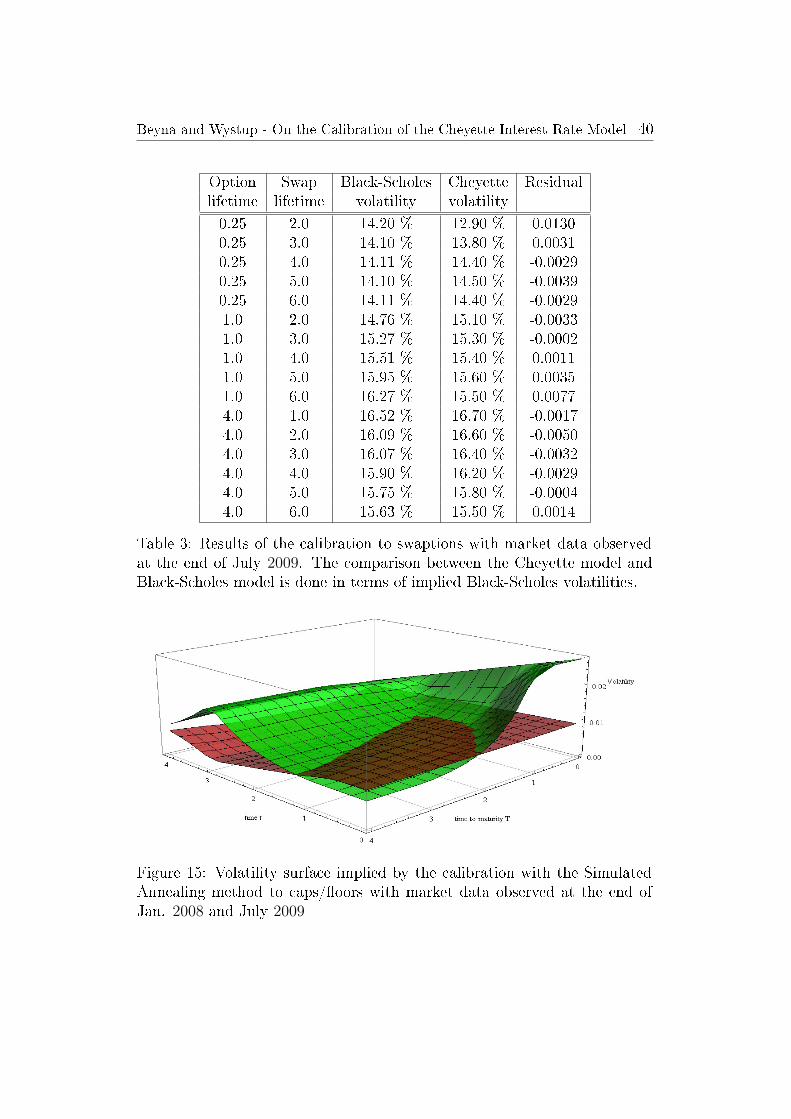
Beyna and Wystup - On the Calibration of the Cheyette Interest Rate Model 40
Option Swap Black-Scholes Cheyette Residuallifetime lifetime volatility volatility
0.25 2.0 14.20 % 12.90 % 0.01300.25 3.0 14.10 % 13.80 % 0.00310.25 4.0 14.11 % 14.40 % -0.00290.25 5.0 14.10 % 14.50 % -0.00390.25 6.0 14.11 % 14.40 % -0.00291.0 2.0 14.76 % 15.10 % -0.00331.0 3.0 15.27 % 15.30 % -0.00021.0 4.0 15.51 % 15.40 % 0.00111.0 5.0 15.95 % 15.60 % 0.00351.0 6.0 16.27 % 15.50 % 0.00774.0 1.0 16.52 % 16.70 % -0.00174.0 2.0 16.09 % 16.60 % -0.00504.0 3.0 16.07 % 16.40 % -0.00324.0 4.0 15.90 % 16.20 % -0.00294.0 5.0 15.75 % 15.80 % -0.00044.0 6.0 15.63 % 15.50 % 0.0014
Table 3: Results of the calibration to swaptions with market data observedat the end of July 2009. The comparison between the Cheyette model andBlack-Scholes model is done in terms of implied Black-Scholes volatilities.
Figure 15: Volatility surface implied by the calibration with the SimulatedAnnealing method to caps/oors with market data observed at the end ofJan. 2008 and July 2009
Beyna and Wystup - On the Calibration of the Cheyette Interest Rate Model 41
A Appendix
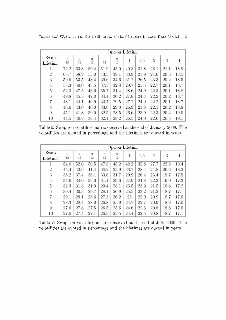
The calibration is based on implied volatilities quoted at the market forswaptions and caps/oors. In the following, we will present the used marketdata published by `Moosmüller & Knauf AG'.
Option LifetimeSwap 1
12212
312
612
912
1 1.5 2 3 4Lifetime
1 24.0 22.9 22.1 21.7 21.6 21.4 19.9 18.9 17.4 162 26.4 24.9 23.5 21.8 21.0 20.3 19.0 18.2 16.7 15.43 26.2 24.5 23.0 21.1 20.1 19.4 18.2 17.4 16.1 14.94 25.5 23.7 22.3 20.4 19.3 18.6 17.6 16.8 15.5 14.45 24.7 22.7 21.4 19.6 18.6 17.8 16.9 16.2 15.0 13.96 23.3 21.5 20.4 18.7 17.8 17.2 16.3 15.6 14.4 13.57 21.9 20.3 19.4 17.9 17.1 16.5 15.7 15.0 14.0 13.28 20.5 19.2 18.4 17.0 16.4 15.8 15.1 14.5 13.6 12.99 19.3 18.2 17.6 16.4 15.7 15.3 14.6 14.1 13.3 12.710 18.1 17.3 16.7 15.7 15.1 14.8 14.2 13.8 13.1 12.5
Table 4: Swaption volatility matrix observed at the end of January 2008. Thevolatilities are quoted in percentage and the lifetimes are quoted in years.
Option LifetimeSwap 1
12212
312
612
912
1 1.5 2 3 4Lifetime
1 21.5 21.6 21.5 20.9 20.9 20.9 20.0 19.0 17.8 17.12 24.1 23.5 23.0 21.9 21.0 20.4 19.1 18.0 17.3 16.63 23.3 22.7 22.2 21.3 20.4 19.8 18.6 17.6 16.9 16.24 22.4 21.8 21.3 20.3 19.6 18.9 17.8 17.1 16.5 15.75 21.4 20.9 20.3 19.3 18.6 17.9 17.2 16.6 15.9 15.16 20.7 19.7 19.0 18.2 17.6 17.0 16.4 16.0 15.4 14.67 19.9 18.7 18.0 17.3 16.8 16.4 16.0 15.7 15.0 14.28 19.0 18.0 17.3 16.7 16.4 16.1 15.7 15.4 14.6 14.09 18.1 17.3 16.7 16.2 16.1 15.8 15.5 15.1 14.4 13.710 17.2 16.6 16.2 15.9 15.8 15.6 15.3 14.9 14.2 13.6
Table 5: Swaption volatility matrix observed at the end of July 2008. Thevolatilities are quoted in percentage and the lifetimes are quoted in years.
Beyna and Wystup - On the Calibration of the Cheyette Interest Rate Model 42
Option LifetimeSwap 1
12212
312
612
912
1 1.5 2 3 4Lifetime
1 72.2 63.8 59.4 51.9 45.9 40.3 31.8 26.1 21.1 18.92 65.7 58.9 53.0 43.5 38.1 33.9 27.9 24.0 20.3 18.53 59.6 53.5 48.4 39.6 34.6 31.2 26.5 23.3 20.2 18.54 55.3 50.0 45.5 37.3 32.8 29.7 25.5 22.7 20.1 18.75 52.3 47.5 43.6 35.7 31.4 28.6 24.9 22.3 20.1 18.86 49.8 45.5 42.0 34.4 30.2 27.8 24.4 22.2 20.2 18.77 48.1 44.1 40.9 33.7 29.5 27.2 24.0 22.2 20.1 18.78 46.6 43.0 40.0 33.0 29.0 26.9 23.8 22.1 20.2 18.89 45.1 41.8 39.0 32.5 28.5 26.6 23.9 22.3 20.4 19.010 44.5 40.8 38.4 32.1 28.2 26.5 24.0 22.6 20.5 19.1
Table 6: Swaption volatility matrix observed at the end of January 2009. Thevolatilities are quoted in percentage and the lifetimes are quoted in years.
Option LifetimeSwap 1
12212
312
612
912
1 1.5 2 3 4Lifetime
1 54.6 52.0 50.5 47.8 45.2 42.2 32.8 27.7 22.2 19.42 44.4 42.9 41.4 38.2 35.9 33.7 28.4 24.8 20.6 18.33 38.2 37.4 36.1 33.6 31.7 29.9 26.4 23.4 19.7 17.54 34.6 34.0 33.0 31.1 29.6 27.9 24.8 22.3 19.0 17.35 32.3 31.8 31.0 29.4 28.1 26.5 23.9 21.5 18.8 17.26 30.4 30.3 29.7 28.1 26.9 25.5 23.2 21.2 18.7 17.17 29.1 29.1 28.6 27.3 26.2 25 22.9 20.9 18.7 17.08 28.3 28.4 28.0 26.8 25.9 24.7 22.7 20.9 18.6 17.09 27.6 27.8 27.5 26.5 25.6 24.6 22.6 20.8 18.6 17.010 27.0 27.4 27.1 26.3 25.5 24.4 22.5 20.8 18.7 17.1
Table 7: Swaption volatility matrix observed at the end of July 2009. Thevolatilities are quoted in percentage and the lifetimes are quoted in years.
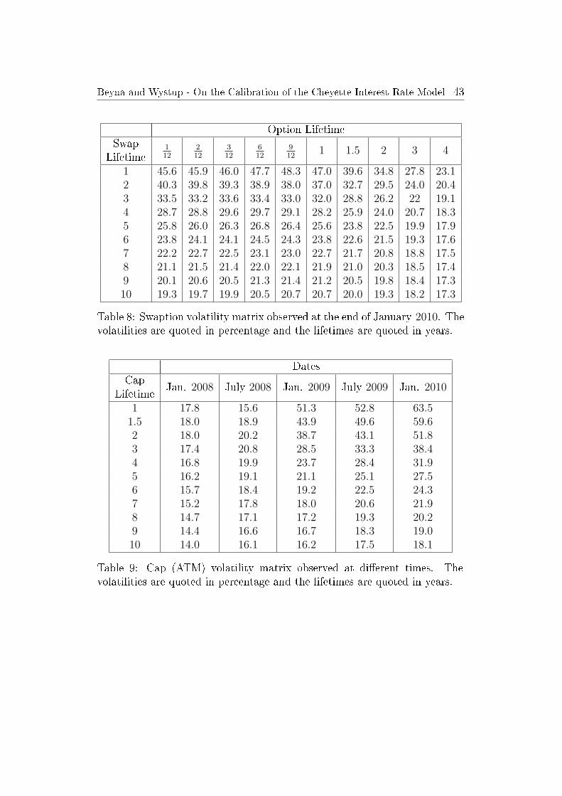
Beyna and Wystup - On the Calibration of the Cheyette Interest Rate Model 43
Option LifetimeSwap 1
12212
312
612
912
1 1.5 2 3 4Lifetime
1 45.6 45.9 46.0 47.7 48.3 47.0 39.6 34.8 27.8 23.12 40.3 39.8 39.3 38.9 38.0 37.0 32.7 29.5 24.0 20.43 33.5 33.2 33.6 33.4 33.0 32.0 28.8 26.2 22 19.14 28.7 28.8 29.6 29.7 29.1 28.2 25.9 24.0 20.7 18.35 25.8 26.0 26.3 26.8 26.4 25.6 23.8 22.5 19.9 17.96 23.8 24.1 24.1 24.5 24.3 23.8 22.6 21.5 19.3 17.67 22.2 22.7 22.5 23.1 23.0 22.7 21.7 20.8 18.8 17.58 21.1 21.5 21.4 22.0 22.1 21.9 21.0 20.3 18.5 17.49 20.1 20.6 20.5 21.3 21.4 21.2 20.5 19.8 18.4 17.310 19.3 19.7 19.9 20.5 20.7 20.7 20.0 19.3 18.2 17.3
Table 8: Swaption volatility matrix observed at the end of January 2010. Thevolatilities are quoted in percentage and the lifetimes are quoted in years.
DatesCap
Jan. 2008 July 2008 Jan. 2009 July 2009 Jan. 2010Lifetime
1 17.8 15.6 51.3 52.8 63.51.5 18.0 18.9 43.9 49.6 59.62 18.0 20.2 38.7 43.1 51.83 17.4 20.8 28.5 33.3 38.44 16.8 19.9 23.7 28.4 31.95 16.2 19.1 21.1 25.1 27.56 15.7 18.4 19.2 22.5 24.37 15.2 17.8 18.0 20.6 21.98 14.7 17.1 17.2 19.3 20.29 14.4 16.6 16.7 18.3 19.010 14.0 16.1 16.2 17.5 18.1
Table 9: Cap (ATM) volatility matrix observed at dierent times. Thevolatilities are quoted in percentage and the lifetimes are quoted in years.
Beyna and Wystup - On the Calibration of the Cheyette Interest Rate Model 44
References
[And00] Jesper Andreasen. Turbo Charging the Cheyette Model. WorkingPaper Gen Re Securities, 2000.
[And02] Leif Andersen; Jesper Andreasen. Volatile Volatilities. Risk Maga-zine, December 2002.
[And05] Jesper Andreasen. Back to the future. Risk Magazine, September2005.
[Bre73] Richard P. Brent. Algorithms for the Minimization without Deriva-tives. Prentice Hall, 1973.
[Che94] Oren Cheyette. Markov Representation of the Heath-Jarrow-Morton Model. BARRA Inc. working paper, May 1994.
[Hen03] Marc Henrard. Explicit bond option and swaption formula in Heath-Jarrow-Morton one factor model. Finance, EconWPA, October2003.
[Hul05] John C. Hull. Options, Futures, and Other Derivatives. FinancialTimes, 5 edition, 2005.
[Jam97] Farshid Jamshidian. LIBOR and Swap Market Models and Mea-sures. Finance and Stochstics, 1:293330, 1997.
[KL07] Peter Kohl-Landgraf. PDE Valuation of Interest Rate Derivatives:From Theory To Implementation. Books on Demand, rst edition,2007.
[Mea65] John Nelder Ashworth; Roger Mead. A Simplex Method for Func-tion Minimization. Computer Journal, 7:308313, 1965.
[Mer05] Damiano Brigo; Fabio Mercurio. Interest Rate Models: Theory andPractice. Springer, 2 edition, 2005.
[Mor92] David Heath; Robert Jarrow; Andrew Morton. Bond Pricing andthe Term Structure of Interest Rates: A New Methodology for Con-tingent Claims Valuation. Econometrica, 60(1):77105, Jan. 1992.
[Mus97] Alan Brace; Dariusz Gatarek; Marek Musiela. The Market Modelof Interest Rate Dynamics. Mathematical Finance, 7:127147, 1997.
[Pol08] Riccardo Poli. A Field Guide to Genetic Programming. Lulu Press,2008.
Beyna and Wystup - On the Calibration of the Cheyette Interest Rate Model 45
[Pre02] William H. Press. Numerical Recipes in C++: The Art of ScienticComputing. Springer Series in Computational Mathematics, secondedition, 2002.
[San97] Kristian R. Miltersen; Klaus Sandmann. Closed Form Solutions forTerm Structure Derivatives with Lognormal Interest Rates. Journalof Finance, 52:409430, 1997.
[Sto03] Florian Jarre; Josef Stoer. Optimierung. Springer, 2003.
[Vas77] Oldrich Vasicek. An Equilibrium Characterisation of the TermStructure. Journal of Financial Economics, 5:177188, 1977.
[Whi90] John Hull; Alan White. Pricing interest-rate derivative securities.The Review of Financial Studies, 3(4):573592, 1990.
[Zag02] Rudi Zagst. Interest-Rate Management. Springer, 2002.
46 Frankfurt School of Finance & Management
Working Paper No.
FRANKFURT SCHOOL / HFB – WORKING PAPER SERIES
No. Author/Title Year
148. Libman, Alexander Words or Deeds – What Matters? Experience of Decentralization in Russian Security Agencies
2010
147. Kostka, Genia / Zhou, Jianghua Chinese firms entering China's low-income market: Gaining competitive advantage by partnering governments
2010
146. Herrmann-Pillath, Carsten Rethinking Evolution, Entropy and Economics: A triadic conceptual framework for the Maximum Entropy Principle as applied to the growth of knowledge
2010
145. Heidorn, Thomas / Kahlert, Dennis Implied Correlations of iTraxx Tranches during the Financial Crisis
2010
144 Fritz-Morgenthal, Sebastian G. / Hach, Sebastian T. / Schalast, Christoph M&A im Bereich Erneuerbarer Energien
2010
143. Birkmeyer, Jörg / Heidorn, Thomas / Rogalski, André Determinanten von Banken-Spreads während der Finanzmarktkrise
2010
142. Bannier, Christina E. / Metz, Sabrina Are SMEs large firms en miniature? Evidence from a growth analysis
2010
141. Heidorn, Thomas / Kaiser, Dieter G. / Voinea, André The Value-Added of Investable Hedge Fund Indices
2010
140. Herrmann-Pillath, Carsten The Evolutionary Approach to Entropy: Reconciling Georgescu-Roegen’s Natural Philosophy with the Maximum Entropy Framework
2010
139. Heidorn, Thomas / Löw, Christian / Winker, Michael Funktionsweise und Replikationstil europäischer Exchange Traded Funds auf Aktienindices
2010
138. Libman, Alexander Constitutions, Regulations, and Taxes: Contradictions of Different Aspects of Decentralization
2010
137. Herrmann-Pillath, Carsten / Libman, Alexander / Yu, Xiaofan State and market integration in China: A spatial econometrics approach to ‘local protectionism’
2010
136. Lang, Michael / Cremers, Heinz / Hentze, Rainald Ratingmodell zur Quantifizierung des Ausfallrisikos von LBO-Finanzierungen
2010
135. Bannier, Christina / Feess, Eberhard When high-powered incentive contracts reduce performance: Choking under pressure as a screening device
2010
134. Herrmann-Pillath, Carsten Entropy, Function and Evolution: Naturalizing Peircian Semiosis
2010
133. Bannier, Christina E. / Behr, Patrick / Güttler, Andre Rating opaque borrowers: why are unsolicited ratings lower?
2009
132. Herrmann-Pillath, Carsten Social Capital, Chinese Style: Individualism, Relational Collectivism and the Cultural Embeddedness of the Instituti-ons-Performance Link
2009
131. Schäffler, Christian / Schmaltz, Christian Market Liquidity: An Introduction for Practitioners
2009
130. Herrmann-Pillath, Carsten Dimensionen des Wissens: Ein kognitiv-evolutionärer Ansatz auf der Grundlage von F.A. von Hayeks Theorie der „Sensory Order“
2009
129. Hankir, Yassin / Rauch, Christian / Umber, Marc It’s the Market Power, Stupid! – Stock Return Patterns in International Bank M&A
2009
128. Herrmann-Pillath, Carsten Outline of a Darwinian Theory of Money
2009
127. Cremers, Heinz / Walzner, Jens Modellierung des Kreditrisikos im Portfoliofall
2009
126. Cremers, Heinz / Walzner, Jens Modellierung des Kreditrisikos im Einwertpapierfall
2009
125. Heidorn, Thomas / Schmaltz, Christian Interne Transferpreise für Liquidität
2009
124. Bannier, Christina E. / Hirsch, Christian The economic function of credit rating agencies - What does the watchlist tell us?
2009
Frankfurt School of Finance & Management
Working Paper No. 47
123. Herrmann-Pillath, Carsten A Neurolinguistic Approach to Performativity in Economics
2009
122. Winkler, Adalbert / Vogel, Ursula Finanzierungsstrukturen und makroökonomische Stabilität in den Ländern Südosteuropas, der Türkei und in den GUS-Staaten
2009
121. Heidorn, Thomas / Rupprecht, Stephan Einführung in das Kapitalstrukturmanagement bei Banken
2009
120. Rossbach, Peter Die Rolle des Internets als Informationsbeschaffungsmedium in Banken
2009
119. Herrmann-Pillath, Carsten Diversity Management und diversi-tätsbasiertes Controlling: Von der „Diversity Scorecard“ zur „Open Balanced Scorecard
2009
118. Hölscher, Luise / Clasen, Sven Erfolgsfaktoren von Private Equity Fonds
2009
117. Bannier, Christina E. Is there a hold-up benefit in heterogeneous multiple bank financing?
2009
116. Roßbach, Peter / Gießamer, Dirk Ein eLearning-System zur Unterstützung der Wissensvermittlung von Web-Entwicklern in Sicherheitsthemen
2009
115. Herrmann-Pillath, Carsten Kulturelle Hybridisierung und Wirtschaftstransformation in China
2009
114. Schalast, Christoph: Staatsfonds – „neue“ Akteure an den Finanzmärkten?
2009
113. Schalast, Christoph / Alram, Johannes Konstruktion einer Anleihe mit hypothekarischer Besicherung
2009
112. Schalast, Christoph / Bolder, Markus / Radünz, Claus / Siepmann, Stephanie / Weber, Thorsten Transaktionen und Servicing in der Finanzkrise: Berichte und Referate des Frankfurt School NPL Forums 2008
2009
111. Werner, Karl / Moormann, Jürgen Efficiency and Profitability of European Banks – How Important Is Operational Efficiency?
2009
110. Herrmann-Pillath, Carsten Moralische Gefühle als Grundlage einer wohlstandschaffenden Wettbewerbsordnung: Ein neuer Ansatz zur erforschung von Sozialkapital und seine Anwendung auf China
2009
109. Heidorn, Thomas / Kaiser, Dieter G. / Roder, Christoph Empirische Analyse der Drawdowns von Dach-Hedgefonds
2009
108. Herrmann-Pillath, Carsten Neuroeconomics, Naturalism and Language
2008
107. Schalast, Christoph / Benita, Barten Private Equity und Familienunternehmen – eine Untersuchung unter besonderer Berücksichtigung deutscher Maschinen- und Anlagenbauunternehmen
2008
106. Bannier, Christina E. / Grote, Michael H. Equity Gap? – Which Equity Gap? On the Financing Structure of Germany’s Mittelstand
2008
105. Herrmann-Pillath, Carsten The Naturalistic Turn in Economics: Implications for the Theory of Finance
2008
104. Schalast, Christoph (Hrgs.) / Schanz, Kay-Michael / Scholl, Wolfgang Aktionärsschutz in der AG falsch verstanden? Die Leica-Entscheidung des LG Frankfurt am Main
2008
103. Bannier, Christina E./ Müsch, Stefan Die Auswirkungen der Subprime-Krise auf den deutschen LBO-Markt für Small- und MidCaps
2008
102. Cremers, Heinz / Vetter, Michael Das IRB-Modell des Kreditrisikos im Vergleich zum Modell einer logarithmisch normalverteilten Verlustfunktion
2008
101. Heidorn, Thomas / Pleißner, Mathias Determinanten Europäischer CMBS Spreads. Ein empirisches Modell zur Bestimmung der Risikoaufschläge von Commercial Mortgage-Backed Securities (CMBS)
2008
100. Schalast, Christoph (Hrsg.) / Schanz, Kay-Michael Schaeffler KG/Continental AG im Lichte der CSX Corp.-Entscheidung des US District Court for the Southern District of New York
2008
99. Hölscher, Luise / Haug, Michael / Schweinberger, Andreas Analyse von Steueramnestiedaten
2008
98. Heimer, Thomas / Arend, Sebastian The Genesis of the Black-Scholes Option Pricing Formula
2008
97. Heimer, Thomas / Hölscher, Luise / Werner, Matthias Ralf Access to Finance and Venture Capital for Industrial SMEs
2008
48 Frankfurt School of Finance & Management
Working Paper No.
96. Böttger, Marc / Guthoff, Anja / Heidorn, Thomas Loss Given Default Modelle zur Schätzung von Recovery Rates
2008
95. Almer, Thomas / Heidorn, Thomas / Schmaltz, Christian The Dynamics of Short- and Long-Term CDS-spreads of Banks
2008
94. Barthel, Erich / Wollersheim, Jutta Kulturunterschiede bei Mergers & Acquisitions: Entwicklung eines Konzeptes zur Durchführung einer Cultural Due Diligence
2008
93. Heidorn, Thomas / Kunze, Wolfgang / Schmaltz, Christian Liquiditätsmodellierung von Kreditzusagen (Term Facilities and Revolver)
2008
92. Burger, Andreas Produktivität und Effizienz in Banken – Terminologie, Methoden und Status quo
2008
91. Löchel, Horst / Pecher, Florian The Strategic Value of Investments in Chinese Banks by Foreign Financial Insitutions
2008
90. Schalast, Christoph / Morgenschweis, Bernd / Sprengetter, Hans Otto / Ockens, Klaas / Stachuletz, Rainer / Safran, Robert Der deutsche NPL Markt 2007: Aktuelle Entwicklungen, Verkauf und Bewertung – Berichte und Referate des NPL Forums 2007
2008
89. Schalast, Christoph / Stralkowski, Ingo 10 Jahre deutsche Buyouts
2008
88. Bannier, Christina E./ Hirsch, Christian The Economics of Rating Watchlists: Evidence from Rating Changes
2007
87. Demidova-Menzel, Nadeshda / Heidorn, Thomas Gold in the Investment Portfolio
2007
86. Hölscher, Luise / Rosenthal, Johannes Leistungsmessung der Internen Revision
2007
85. Bannier, Christina / Hänsel, Dennis Determinants of banks' engagement in loan securitization
2007
84. Bannier, Christina “Smoothing“ versus “Timeliness“ - Wann sind stabile Ratings optimal und welche Anforderungen sind an optimale Berichtsregeln zu stellen?
2007
83. Bannier, Christina E. Heterogeneous Multiple Bank Financing: Does it Reduce Inefficient Credit-Renegotiation Incidences?
2007
82. Cremers, Heinz / Löhr, Andreas Deskription und Bewertung strukturierter Produkte unter besonderer Berücksichtigung verschiedener Marktszenarien
2007
81. Demidova-Menzel, Nadeshda / Heidorn, Thomas Commodities in Asset Management
2007
80. Cremers, Heinz / Walzner, Jens Risikosteuerung mit Kreditderivaten unter besonderer Berücksichtigung von Credit Default Swaps
2007
79. Cremers, Heinz / Traughber, Patrick Handlungsalternativen einer Genossenschaftsbank im Investmentprozess unter Berücksichtigung der Risikotragfähig-keit
2007
78. Gerdesmeier, Dieter / Roffia, Barbara Monetary Analysis: A VAR Perspective
2007
77. Heidorn, Thomas / Kaiser, Dieter G. / Muschiol, Andrea Portfoliooptimierung mit Hedgefonds unter Berücksichtigung höherer Momente der Verteilung
2007
76. Jobe, Clemens J. / Ockens, Klaas / Safran, Robert / Schalast, Christoph Work-Out und Servicing von notleidenden Krediten – Berichte und Referate des HfB-NPL Servicing Forums 2006
2006
75. Abrar, Kamyar / Schalast, Christoph Fusionskontrolle in dynamischen Netzsektoren am Beispiel des Breitbandkabelsektors
2006
74. Schalast, Christoph / Schanz, Kay-Michael Wertpapierprospekte: Markteinführungspublizität nach EU-Prospektverordnung und Wertpapierprospektgesetz 2005
2006
73. Dickler, Robert A. / Schalast, Christoph Distressed Debt in Germany: What´s Next? Possible Innovative Exit Strategies
2006
72. Belke, Ansgar / Polleit, Thorsten How the ECB and the US Fed set interest rates
2006
71. Heidorn, Thomas / Hoppe, Christian / Kaiser, Dieter G. Heterogenität von Hedgefondsindizes
2006
70. Baumann, Stefan / Löchel, Horst The Endogeneity Approach of the Theory of Optimum Currency Areas - What does it mean for ASEAN + 3?
2006
Frankfurt School of Finance & Management
Working Paper No. 49
69. Heidorn, Thomas / Trautmann, Alexandra Niederschlagsderivate
2005
68. Heidorn, Thomas / Hoppe, Christian / Kaiser, Dieter G. Möglichkeiten der Strukturierung von Hedgefondsportfolios
2005
67. Belke, Ansgar / Polleit, Thorsten (How) Do Stock Market Returns React to Monetary Policy ? An ARDL Cointegration Analysis for Germany
2005
66. Daynes, Christian / Schalast, Christoph Aktuelle Rechtsfragen des Bank- und Kapitalmarktsrechts II: Distressed Debt - Investing in Deutschland
2005
65. Gerdesmeier, Dieter / Polleit, Thorsten Measures of excess liquidity
2005
64. Becker, Gernot M. / Harding, Perham / Hölscher, Luise Financing the Embedded Value of Life Insurance Portfolios
2005
63. Schalast, Christoph Modernisierung der Wasserwirtschaft im Spannungsfeld von Umweltschutz und Wettbewerb – Braucht Deutschland eine Rechtsgrundlage für die Vergabe von Wasserversorgungskonzessionen? –
2005
62. Bayer, Marcus / Cremers, Heinz / Kluß, Norbert Wertsicherungsstrategien für das Asset Management
2005
61. Löchel, Horst / Polleit, Thorsten A case for money in the ECB monetary policy strategy
2005
60. Richard, Jörg / Schalast, Christoph / Schanz, Kay-Michael Unternehmen im Prime Standard - „Staying Public“ oder „Going Private“? - Nutzenanalyse der Börsennotiz -
2004
59. Heun, Michael / Schlink, Torsten Early Warning Systems of Financial Crises - Implementation of a currency crisis model for Uganda
2004
58. Heimer, Thomas / Köhler, Thomas Auswirkungen des Basel II Akkords auf österreichische KMU
2004
57. Heidorn, Thomas / Meyer, Bernd / Pietrowiak, Alexander Performanceeffekte nach Directors´Dealings in Deutschland, Italien und den Niederlanden
2004
56. Gerdesmeier, Dieter / Roffia, Barbara The Relevance of real-time data in estimating reaction functions for the euro area
2004
55. Barthel, Erich / Gierig, Rauno / Kühn, Ilmhart-Wolfram Unterschiedliche Ansätze zur Messung des Humankapitals
2004
54. Anders, Dietmar / Binder, Andreas / Hesdahl, Ralf / Schalast, Christoph / Thöne, Thomas Aktuelle Rechtsfragen des Bank- und Kapitalmarktrechts I : Non-Performing-Loans / Faule Kredite - Handel, Work-Out, Outsourcing und Securitisation
2004
53. Polleit, Thorsten The Slowdown in German Bank Lending – Revisited
2004
52. Heidorn, Thomas / Siragusano, Tindaro Die Anwendbarkeit der Behavioral Finance im Devisenmarkt
2004
51. Schütze, Daniel / Schalast, Christoph (Hrsg.) Wider die Verschleuderung von Unternehmen durch Pfandversteigerung
2004
50. Gerhold, Mirko / Heidorn, Thomas Investitionen und Emissionen von Convertible Bonds (Wandelanleihen)
2004
49. Chevalier, Pierre / Heidorn, Thomas / Krieger, Christian Temperaturderivate zur strategischen Absicherung von Beschaffungs- und Absatzrisiken
2003
48. Becker, Gernot M. / Seeger, Norbert Internationale Cash Flow-Rechnungen aus Eigner- und Gläubigersicht
2003
47. Boenkost, Wolfram / Schmidt, Wolfgang M. Notes on convexity and quanto adjustments for interest rates and related options
2003
46. Hess, Dieter Determinants of the relative price impact of unanticipated Information in U.S. macroeconomic releases
2003
45. Cremers, Heinz / Kluß, Norbert / König, Markus Incentive Fees. Erfolgsabhängige Vergütungsmodelle deutscher Publikumsfonds
2003
44. Heidorn, Thomas / König, Lars Investitionen in Collateralized Debt Obligations
2003
43. Kahlert, Holger / Seeger, Norbert Bilanzierung von Unternehmenszusammenschlüssen nach US-GAAP
2003
50 Frankfurt School of Finance & Management
Working Paper No.
42. Beiträge von Studierenden des Studiengangs BBA 012 unter Begleitung von Prof. Dr. Norbert Seeger Rechnungslegung im Umbruch - HGB-Bilanzierung im Wettbewerb mit den internationalen Standards nach IAS und US-GAAP
2003
41. Overbeck, Ludger / Schmidt, Wolfgang Modeling Default Dependence with Threshold Models
2003
40. Balthasar, Daniel / Cremers, Heinz / Schmidt, Michael Portfoliooptimierung mit Hedge Fonds unter besonderer Berücksichtigung der Risikokomponente
2002
39. Heidorn, Thomas / Kantwill, Jens Eine empirische Analyse der Spreadunterschiede von Festsatzanleihen zu Floatern im Euroraum und deren Zusammenhang zum Preis eines Credit Default Swaps
2002
38. Böttcher, Henner / Seeger, Norbert Bilanzierung von Finanzderivaten nach HGB, EstG, IAS und US-GAAP
2003
37. Moormann, Jürgen Terminologie und Glossar der Bankinformatik
2002
36. Heidorn, Thomas Bewertung von Kreditprodukten und Credit Default Swaps
2001
35. Heidorn, Thomas / Weier, Sven Einführung in die fundamentale Aktienanalyse
2001
34. Seeger, Norbert International Accounting Standards (IAS)
2001
33. Moormann, Jürgen / Stehling, Frank Strategic Positioning of E-Commerce Business Models in the Portfolio of Corporate Banking
2001
32. Sokolovsky, Zbynek / Strohhecker, Jürgen Fit für den Euro, Simulationsbasierte Euro-Maßnahmenplanung für Dresdner-Bank-Geschäftsstellen
2001
31. Roßbach, Peter Behavioral Finance - Eine Alternative zur vorherrschenden Kapitalmarkttheorie?
2001
30. Heidorn, Thomas / Jaster, Oliver / Willeitner, Ulrich Event Risk Covenants
2001
29. Biswas, Rita / Löchel, Horst Recent Trends in U.S. and German Banking: Convergence or Divergence?
2001
28. Eberle, Günter Georg / Löchel, Horst Die Auswirkungen des Übergangs zum Kapitaldeckungsverfahren in der Rentenversicherung auf die Kapitalmärkte
2001
27. Heidorn, Thomas / Klein, Hans-Dieter / Siebrecht, Frank Economic Value Added zur Prognose der Performance europäischer Aktien
2000
26. Cremers, Heinz Konvergenz der binomialen Optionspreismodelle gegen das Modell von Black/Scholes/Merton
2000
25. Löchel, Horst Die ökonomischen Dimensionen der ‚New Economy‘
2000
24. Frank, Axel / Moormann, Jürgen Grenzen des Outsourcing: Eine Exploration am Beispiel von Direktbanken
2000
23. Heidorn, Thomas / Schmidt, Peter / Seiler, Stefan Neue Möglichkeiten durch die Namensaktie
2000
22. Böger, Andreas / Heidorn, Thomas / Graf Waldstein, Philipp Hybrides Kernkapital für Kreditinstitute
2000
21. Heidorn, Thomas Entscheidungsorientierte Mindestmargenkalkulation
2000
20. Wolf, Birgit Die Eigenmittelkonzeption des § 10 KWG
2000
19. Cremers, Heinz / Robé, Sophie / Thiele, Dirk Beta als Risikomaß - Eine Untersuchung am europäischen Aktienmarkt
2000
18. Cremers, Heinz Optionspreisbestimmung
1999
17. Cremers, Heinz Value at Risk-Konzepte für Marktrisiken
1999
16. Chevalier, Pierre / Heidorn, Thomas / Rütze, Merle Gründung einer deutschen Strombörse für Elektrizitätsderivate
1999
15. Deister, Daniel / Ehrlicher, Sven / Heidorn, Thomas CatBonds
1999
Frankfurt School of Finance & Management
Working Paper No. 51
14. Jochum, Eduard Hoshin Kanri / Management by Policy (MbP)
1999
13. Heidorn, Thomas Kreditderivate
1999
12. Heidorn, Thomas Kreditrisiko (CreditMetrics)
1999
11. Moormann, Jürgen Terminologie und Glossar der Bankinformatik
1999
10. Löchel, Horst The EMU and the Theory of Optimum Currency Areas
1998
09. Löchel, Horst Die Geldpolitik im Währungsraum des Euro
1998
08. Heidorn, Thomas / Hund, Jürgen Die Umstellung auf die Stückaktie für deutsche Aktiengesellschaften
1998
07. Moormann, Jürgen Stand und Perspektiven der Informationsverarbeitung in Banken
1998
06. Heidorn, Thomas / Schmidt, Wolfgang LIBOR in Arrears
1998
05. Jahresbericht 1997 1998
04. Ecker, Thomas / Moormann, Jürgen Die Bank als Betreiberin einer elektronischen Shopping-Mall
1997
03. Jahresbericht 1996 1997
02. Cremers, Heinz / Schwarz, Willi Interpolation of Discount Factors
1996
01. Moormann, Jürgen Lean Reporting und Führungsinformationssysteme bei deutschen Finanzdienstleistern
1995
FRANKFURT SCHOOL / HFB – WORKING PAPER SERIES
CENTRE FOR PRACTICAL QUANTITATIVE FINANCE
No. Author/Title Year
23. Esquível, Manuel L. / Veiga, Carlos / Wystup, Uwe Unifying Exotic Option Closed Formulas
2010
22. Packham, Natalie / Schlögl, Lutz / Schmidt, Wolfgang M. Credit gap risk in a first passage time model with jumps
2009
21. Packham, Natalie / Schlögl, Lutz / Schmidt, Wolfgang M. Credit dynamics in a first passage time model with jumps
2009
20. Reiswich, Dimitri / Wystup, Uwe FX Volatility Smile Construction
2009
19. Reiswich, Dimitri / Tompkins, Robert Potential PCA Interpretation Problems for Volatility Smile Dynamics
2009
18. Keller-Ressel, Martin / Kilin, Fiodar Forward-Start Options in the Barndorff-Nielsen-Shephard Model
2008
17. Griebsch, Susanne / Wystup, Uwe On the Valuation of Fader and Discrete Barrier Options in Heston’s Stochastic Volatility Model
2008
16. Veiga, Carlos / Wystup, Uwe Closed Formula for Options with Discrete Dividends and its Derivatives
2008
15. Packham, Natalie / Schmidt, Wolfgang Latin hypercube sampling with dependence and applications in finance
2008
14. Hakala, Jürgen / Wystup, Uwe FX Basket Options
2008
13. Weber, Andreas / Wystup, Uwe Vergleich von Anlagestrategien bei Riesterrenten ohne Berücksichtigung von Gebühren. Eine Simulationsstudie zur Verteilung der Renditen
2008
52 Frankfurt School of Finance & Management
Working Paper No.
12. Weber, Andreas / Wystup, Uwe Riesterrente im Vergleich. Eine Simulationsstudie zur Verteilung der Renditen
2008
11. Wystup, Uwe Vanna-Volga Pricing
2008
10. Wystup, Uwe Foreign Exchange Quanto Options
2008
09. Wystup, Uwe Foreign Exchange Symmetries
2008
08. Becker, Christoph / Wystup, Uwe Was kostet eine Garantie? Ein statistischer Vergleich der Rendite von langfristigen Anlagen
2008
07. Schmidt, Wolfgang Default Swaps and Hedging Credit Baskets
2007
06. Kilin, Fiodor Accelerating the Calibration of Stochastic Volatility Models
2007
05. Griebsch, Susanne/ Kühn, Christoph / Wystup, Uwe Instalment Options: A Closed-Form Solution and the Limiting Case
2007
04. Boenkost, Wolfram / Schmidt, Wolfgang M. Interest Rate Convexity and the Volatility Smile
2006
03. Becker, Christoph/ Wystup, Uwe On the Cost of Delayed Currency Fixing
2005
02. Boenkost, Wolfram / Schmidt, Wolfgang M. Cross currency swap valuation
2004
01. Wallner, Christian / Wystup, Uwe Efficient Computation of Option Price Sensitivities for Options of American Style
2004
HFB – SONDERARBEITSBERICHTE DER HFB - BUSINESS SCHOOL OF FINANCE & MANAGEMENT
No. Author/Title Year
01. Nicole Kahmer / Jürgen Moormann Studie zur Ausrichtung von Banken an Kundenprozessen am Beispiel des Internet (Preis: € 120,--)
2003
Printed edition: € 25.00 + € 2.50 shipping
Download:
Working Paper: http://www.frankfurt-school.de/content/de/research/Publications/list_of_publication0.html
CPQF: http://www.frankfurt-school.de/content/de/research/quantitative_Finance/research_publications.html
Order address / contact
Frankfurt School of Finance & Management
Sonnemannstr. 9 – 11 D – 60314 Frankfurt/M. Germany
Phone: +49 (0) 69 154 008 – 734 Fax: +49 (0) 69 154 008 – 728
eMail: [email protected]
Further information about Frankfurt School of Finance & Management
may be obtained at: http://www.fs.de


![Homepage - MathFinance...Cheyette in 1994 [Che9 4]. The framework proposed by Cheyette for modeling interest ra tes leaves the user with a wide choice of alternatives . The model is](https://img.pdfslide.us/doc/110x75/60c77b5fd0064920a340c3f8/homepage-mathfinance-cheyette-in-1994-che9-4-the-framework-proposed-by.jpg)