Embed Size (px)
Citation preview

CALI
A REDUCE Package for
Commutative Algebra
Version 2.2.1
Hans-Gert Grabe
Universitat LeipzigInstitut fur InformatikAugustusplatz 10 – 11
04109 Leipzig / Germany
email: [email protected]
June 28, 1995
Key words: affine and projective monomial curves, affine and projective sets of points,analytic spread, associated graded ring, blowup, border bases, constructive commutativealgebra, dual bases, elimination, equidimensional part, extended Grobner factorizer, freeresolution, Grobner algorithms for ideals and module, Grobner factorizer, ideal and moduleoperations, independent sets, intersections, lazy standard bases, local free resolutions,local standard bases, minimal generators, minors, normal forms, pfaffians, polynomialmaps, primary decomposition, quotients, symbolic powers, symmetric algebra, triangularsystems, weighted Hilbert series, primality test, radical, unmixed radical.
1
Contents
1 Introduction 31.1 Description of the Documents Distributed with CALI . . . . . . . . . . . . 41.2 CALI’s Language Concept . . . . . . . . . . . . . . . . . . . . . . . . . . . . 51.3 New and Improved Facilities in v. 2.1 . . . . . . . . . . . . . . . . . . . . . . 61.4 New and Improved Facilities in v. 2.2 . . . . . . . . . . . . . . . . . . . . . . 71.5 New and Improved Facilities in v. 2.2.1 . . . . . . . . . . . . . . . . . . . . . 9
2 The Computational Model 92.1 The Base Ring . . . . . . . . . . . . . . . . . . . . . . . . . . . . . . . . . . 92.2 Ideals and Modules . . . . . . . . . . . . . . . . . . . . . . . . . . . . . . . . 122.3 The Algebraic Mode Interface . . . . . . . . . . . . . . . . . . . . . . . . . . 132.4 Switches and Global Variables . . . . . . . . . . . . . . . . . . . . . . . . . . 15
3 Basic Data Structures 173.1 The Coefficient Domain . . . . . . . . . . . . . . . . . . . . . . . . . . . . . 173.2 The Base Ring . . . . . . . . . . . . . . . . . . . . . . . . . . . . . . . . . . 183.3 Monomials . . . . . . . . . . . . . . . . . . . . . . . . . . . . . . . . . . . . 193.4 Polynomials and Polynomial Vectors . . . . . . . . . . . . . . . . . . . . . . 193.5 Base Lists . . . . . . . . . . . . . . . . . . . . . . . . . . . . . . . . . . . . . 203.6 Dpoly Matrices . . . . . . . . . . . . . . . . . . . . . . . . . . . . . . . . . . 203.7 Extending the REDUCE Matrix Package . . . . . . . . . . . . . . . . . . . 21
4 About the Algorithms Implemented in CALI 224.1 Normal Form Algorithms . . . . . . . . . . . . . . . . . . . . . . . . . . . . 224.2 The Grobner and Standard Basis Algorithms . . . . . . . . . . . . . . . . . 244.3 The Grobner Factorizer . . . . . . . . . . . . . . . . . . . . . . . . . . . . . 264.4 Basic Operations on Ideals and Modules . . . . . . . . . . . . . . . . . . . . 274.5 Monomial Ideals . . . . . . . . . . . . . . . . . . . . . . . . . . . . . . . . . 294.6 Hilbert Series . . . . . . . . . . . . . . . . . . . . . . . . . . . . . . . . . . . 304.7 Resolutions . . . . . . . . . . . . . . . . . . . . . . . . . . . . . . . . . . . . 314.8 Zero Dimensional Ideals and Modules . . . . . . . . . . . . . . . . . . . . . 314.9 Primary Decomposition and Related Algorithms . . . . . . . . . . . . . . . 314.10 Advanced Algorithms . . . . . . . . . . . . . . . . . . . . . . . . . . . . . . 334.11 Dual Bases . . . . . . . . . . . . . . . . . . . . . . . . . . . . . . . . . . . . 35
A A Short Description of Procedures Available in Algebraic Mode 37
B The CALI Module Structure 45
2
1 Introduction
This package contains algorithms for computations in commutative algebra closely relatedto the Grobner algorithm for ideals and modules. Its heart is a new implementation of theGrobner algorithm1 that allows the computation of syzygies, too. This implementationis also applicable to submodules of free modules with generators represented as rows of amatrix.
Moreover CALI contains facilities for local computations, using a modern implemen-tation of Mora’s standard basis algorithm, see [26] and [13], that works for arbitrary termorders. The full analogy between modules over the local ring k[xv : v ∈ H]m and ho-mogeneous (in fact H-local) modules over k[xv : v ∈ H] is reflected through the switchNoetherian. Turn it on (Grobner basis, the default) or off (local standard basis) to chooseappropriate algorithms automatically. In v. 2.2 we present an unified approach to bothcases, using reduction with bounded ecart for non Noetherian term orders, see [14] fordetails. This allows to have a common driver for the Grobner algorithm in both cases.
CALI extends also the restricted term order facilities of the groebner package, definingterm orders by degree vector lists, and the rigid implementation of the sugar idea, by amore flexible ecart vector, in particular useful for local computations, see [13].
The package was designed mainly as a symbolic mode programming environment ex-tending the build-in facilities of REDUCE for the computational approach to problemsarising naturally in commutative algebra. An algebraic mode interface accesses (in a morerigid frame) all important features implemented symbolically and thus should be favoredfor short sample computations.
On the other hand, tedious computations are strongly recommended to be done sym-bolically since this allows considerably more flexibility and avoids unnecessary translationsof intermediate results from CALI’s internal data representation to the algebraic mode andvice versa. Moreover, one can easily extend the package with new symbolic mode scripts,or do more difficult interactive computations. For all these purposes the symbolic modeinterface offers substantially more facilities than the algebraic one.
For a detailed description of special symbolic mode procedures one should consultthe source code and the comments therein. In this manual we can give only a briefdescription of the main ideas incorporated into the package CALI. We concentrate on thedata structure design and the description of the more advanced algorithms. For samplecomputations from several fields of commutative algebra the reader may consult also thecali.tst file.
As main topics CALI contains facilities for
• defining rings, ideals and modules,
• computing Grobner bases and local standard bases,
• computing syzygies, resolutions and (graded) Betti numbers,1The data representation even for polynomials is different from that given in the groebner package
distributed with REDUCE (and rests on ideas used in the dipoly package).
3
• computing (now also weighted) Hilbert series, multiplicities, independent sets, anddimensions,
• computing normal forms and representations,
• computing sums, products, intersections, quotients, stable quotients, eliminationideals etc.,
• primality tests, computation of radicals, unmixed radicals, equidimensional parts,primary decompositions etc. of ideals and modules,
• advanced applications of Grobner bases (blowup, associated graded ring, analyticspread, symmetric algebra, monomial curves etc.),
• applications of linear algebra techniques to zero dimensional ideals, as e.g. the FGLMchange of term orders, border bases and affine and projective ideals of sets of points,
• splitting polynomial systems of equations mixing factorization and the Grobner algo-rithm, triangular systems, and different versions of the extended Grobner factorizer.
Below we will use freely without further explanation the notions common for text booksand papers about constructive commutative algebra, assuming the reader to be familiarwith the corresponding ideas and concepts. For further references see e.g. the text books[2], [7] and [21] or the survey papers [5], [6] and [27].
1.1 Description of the Documents Distributed with CALI
The CALI package contains the following files:
cali.chg
a detailed report of changes from v. 2.1 to v. 2.2. and 2.2.1
cali.log
the output file, that cali.tst should produce with
load package cali;
out "logfile"$
in "cali.tst";
shut "logfile"$
cali.red
the CALI source file.
cali.tex
this manual.
cali.tst
a test file with various examples and applications of CALI.
4
CALI should be precompiled as usual, i.e. either using the makefasl utility of REDUCEor “by hand” via
faslout "cali"$in "cali.red"$faslend$
and then loaded via
load_package cali;
Upon successful loading CALI responds with a message containing the version numberand the last update of the distribution.
Feel free to contact me by email if You have problems to get CALIstarted. Also comments, hints, bug reports etc. are welcome.
1.2 CALI’s Language Concept
From a certain point of view one of the major disadvantage of the current RLISP (and theunderlying PSL) language is the fact that it supports modularity and data encapsulationonly in a rudimentary way. Since all parts of code loaded into a session are visible all thetime, name conflicts between different packages may occur, will occur (even not issuinga warning message), and are hard to prevent, since packages are developed (and are stilldeveloping) by different research groups at different places and different time.
A (yet rudimentary) concept of REDUCE packages and modules indicates the directioninto what the REDUCE designers are looking for a solution for this general problem.
CALI (2.0 and higher) follows a name concept for internal procedures to mimick dataencapsulation at a semantical level. We hope this way on the one hand to resolve theconflicts described above at least for the internal part of CALI and on the other hand toanticipate a desirable future and already foregoing development of REDUCE towards atrue modularity.
The package CALI is divided into several modules, each of them introducing eithera single new data type together with basic facilities, constructors, and selectors or acollection of algorithms subject to a common problem. Each module contains internalprocedures, conceptually hidden by this module, local procedures, designed for a CALIwide use, and global procedures, exported by CALI into the general (algebraic or symbolic)environment of REDUCE. A header module cali contains all (fluid) global variables andswitches defined by the pacakge CALI.
Along these lines the CALI procedures available in symbolic mode are divided intothree types with the following naming convention:
module!=procedure
internal to the given module.
5

module_procedure
exported by the given module into the local CALI environment.
procedure!*
a global procedure usually having a semantically equivalent procedure(possibly with another parameter list) without trailing asterisk in alge-braic mode.
There are also symbolic mode equivalents without trailing asterisk, if the algebraic pro-cedure is not a psopfn, but a symbolic operator. They transfer data to CALI’s internalstructure and call the corresponding procedure with trailing asterisk. CALI 2.2 distin-guishes between algebraic and symbolic calls of such a procedure. In symbolic mode sucha procedure calls the corresponding procedure with trailing asterisk directly without datatransfer.
CALI 2.2 follows also a more concise concept for global variables. There are threetypes of them:
True fluid global variables,
that are part of the current data structure, as e.g. the current base ringand the degree vector. They are often locally rebound to be restoredafter interrupts.
Global variables, stored on the property list of the package name cali,
that reflect the state of the computational model as e.g. the trace level,the output print level or the chosen version of the Grobner basis al-gorithm. There are several such parameters in the module dualbasesto serve the common dual basis driver with information for differentapplications.
Switches,
that allow to choose different branches of algorithms. Note that thisconcept interferes with the second one. Different versions of algorithms,that apply different functions in a common driver, are not implementedthrough switches.
1.3 New and Improved Facilities in v. 2.1
The major changes in v. 2.1 reflect the experience we’ve got from the use of CALI 2.0.The following changes are worth mentioning explicitely:
1. The algebraic rule concept was adapted to CALI. It allows to supply rule based co-efficient domains. This is a more efficient way to deal with (easy) algebraic numbersthan through the arnum package.
2. listtest and listminimize provide an unified concept for different list operations pre-viously scattered in the source text.
6
3. There are several new quotient algorithms at the symbolic level (both the generalelement and the intersection approaches are available) and new features for thecomputation of equidimensional hull and equidimensional radical.
4. A new module scripts offers advanced applications of Grobner bases.
5. Several advanced procedures initialize a Grobner basis computation over a certainintermediate base ring or term order as e.g. eliminate, resolve, matintersect or allprimary decomposition procedures. Interrupting a computation in v. 2.1 now restoresthe original values of CALI’s global variables, since all intermediate procedures workwith local copies of the global variables.2 This doesn’t apply to advanced proceduresthat change the current base ring as e.g. blowup, preimage, sym etc.
1.4 New and Improved Facilities in v. 2.2
Version 2.2 (beside bug fixes) incorporates several new facilities of constructive non linearalgebra that we investigated the last two years, as e.g. dual bases, the Grobner factorizer,triangular systems, and local standard bases. Essential changes concern the followingtopics:
1. The CALI modules red and groeb were rewritten and the module mora was removed.This is due to new theoretical insight into standard bases theory as e.g. describedin [13] or [14]. The Grobner basis algorithm is reorganized as a Grobner driver withsimplifier and base lists, that involves different versions of polynomial reductionaccording to the setting via gbtestversion. It applies now to both noetherian andnon noetherian term orders in a unified way.
The switches binomial and lazy were removed.
2. The Grobner factorizer was thoroughly revised, extended along the lines explained in[15], and collected into a separate module groebf. It now allows a list of constraintsalso in algebraic mode. Two versions of an extended Grobner factorizer producetriangular systems, i.e. a decomposition into quasi prime components, see [16], thatare well suited for further (numerical) evaluation. There is also a version of theGrobner factorizer that allows a list of problems as input. This is especially useful,if a system is splitted with respect to a “cheap” (e.g. degrevlex) term order and thepieces are recomputed with respect to a “hard” (e.g. pure lex) term order.
The extended Grobner factorizer involves, after change to dimension zero, the com-putation of triangular systems. The corresponding module triang extends the facili-ties for zero dimensional ideals and modules in the module odim.
3. A new module lf implements the dual bases approach as described in [20]. On thisbasis there are new implementations of affine points and proj points, that are sig-nificantly faster than the old ones. The linear algebra change of term orders [9] is
2Note that recovering the base ring this way may cause some trouble since the intermediate ring,installed with setring, changed possibly the internal variable order set by setkorder.
7
available, too. There are two versions, one with precomputed border basis, the otherwith conventional normal forms.
4. dpmats now have a gb-tag that indicates, whether the given ideal or module basis isalready a Grobner basis. This avoids certain Grobner basis recomputations especiallyduring advanced algorithms as e.g. prime decomposition. In the algebraic interfaceGrobner bases are computed automatically when needed rather than to issue an errormessage as in v. 2.1. So one can call modequalp or dim etc. not having computedGrobner bases in advance. Note that such automatic computation can be avoidedwith setgbasis.
5. Hilbert series are now weighted Hilbert series, since e.g. for blow up rings the gen-erating ideal is multigraded. Usual Hilbert series are computed as in v. 2.1 withrespect to the ecart vector. Weighted Hilbert series accept a list of (integer) weightlists as second parameter.
6. There are some name and conceptual changes to existing procedures and variablesto have a more concise semantic concept. This concerns
tracing (the trace parameter is now stored on the property list of cali andshould be set with setcalitrace),choosing different versions of the Grobner algorithm (through gbtestver-sion) and the Hilbert series computation (through hftestversion),some names (mat2list replaced flatten, HilbertSeries replaced hilbseries)andparameter lists of some local and internal procedures (consult cali.chg fordetails).
7. The revlex term order is now the reverse lexicographic term order on the reverselyordered variables. This is consistent with other computer algebra systems (e.g.SINGULAR or AXIOM)3 and implies the same order on the variables for deglexand degrevlex term orders (this was the main reason to change the definition).
8. Ideals of minors, pfaffians and related stuff are now implemented as extension ofthe internal matrix package and collected into a separate module calimat. Thusthey allow more general expressions, especially with variable exponents, as generalREDUCE matrices do. So one can define generic ideals as e.g. ideals of minorsor pfaffians of matrices, containing generic expressions as elements. They must bespecified for further use in CALI substituting general exponents by integers.
3But different to the currently distibuted groebner package in REDUCE. Note that the computationsin [15] were done before these changes.
8
1.5 New and Improved Facilities in v. 2.2.1
The main change concerns the primary decomposition algorithm, where I fixed a seriousbug for deciding, which embedded primes are really embedded4. During that remake Iincorporated also the Grobner factorizer to compute isolated primes. Since REDUCE hasno multivariate modular factorizer, the switch factorprimes may be turned off to switchto the former algorithm.
Some minor bugs are fixed, too, e.g. the bug that made radical crashing.
2 The Computational Model
This section gives a short introduction into the data type design of CALI at differentlevels. First (§1 and 2) we describe CALI’s way of algorithmic translation of the abstractalgebraic objects ring of polynomials, ideal and (finitely generated) module. Then (§3 and4) we describe the algebraic mode interface of CALI and the switches and global variablesto drive a session. In the next chapter we give a more detailed overview of the basic(symbolic mode) data structures involved with CALI. We refer to the appendix for a shortsummary of the commands available in algebraic mode.
2.1 The Base Ring
A polynomial ring consists in CALI of the following data:
a list of variable names
All variables not occuring in the list of ring names are treated as pa-rameters. Computations are executed denominatorfree, but the resultsare valid only over the corresponding parameter field extension.
a term order and a term order tag
They describe the way in which the terms in each polynomial (and poly-nomial vector) are ordered.
an ecart vector
A list of positive integers corresponding to the variable names.
A base ring may be defined (in algebraic mode) through the command
setring <ring>
with < ring > ::= { vars, tord, tag [, ecart ] } resp.
setring(vars, tord, tag [,ecart])4That there must be a bug was pointed out to me by Shimoyama Takeshi who compared different
p.d. implementations. The bug is due to an incorrect test for embedded primes: A (superfluous) primarycomponent may contain none of the isolated primary components, but their intersection! Note that neither[10] nor [2] comment on that. Details of the implementation will appear in [17].
9
This sets the global (symbolic) variable cali!=basering. Here vars is the list of variablenames, tord a (possibly empty) list of weight lists, the degree vectors, and tag the tagLEX or REVLEX. Optionally one can supply ecart, a list of positive integers of the samelength as vars, to set an ecart vector different from the default one (see below).
The degree vectors must have the same length as vars. If (w1 . . . wk) is the list ofdegree vectors then
xa < xb :⇔ either wj(xa) = wj(xb) for j < i and
wi(xa) < wi(xb)
or wj(xa) = wj(xb) for all j and
xa <lex xb resp. xa <revlex xb
Here <lex resp. <revlex denote the lexicographic (tag=LEX) resp. reverse lexicographic(tag=REVLEX) term orders5 with respect to the variable order given in vars, i.e.
xa < xb :⇔ ∃ j ∀ i < j : ai = bi and aj < bj (lex.)
orxa < xb :⇔ ∃ j ∀ i > j : ai = bi and aj > bj (revlex.)
Every term order can be represented in such a way, see [24].During the ring setting the term order will be checked to be Noetherian (i.e. to fulfill
the descending chain condition) provided the switch Noetherian is on (the default). Thesame applies turning noetherian on: If the term order of the underlying base ring isn’tNoetherian the switch can’t be turned over. Hence, starting from a non Noetherian termorder, one should define first a new ring and then turn the switch on.
Useful term orders can be defined by the procedures
degreeorder vars,
that returns tord = {{1, . . . , 1}}.localorder vars,
that returns tord = {{−1, . . . ,−1}} (a non Noetherian term order forcomputations in local rings).
eliminationorder(vars,elimvars),
that returns a term order for elimination of the variables in elimvars,a subset of all vars. It’s recommended to combine it with the tagREVLEX.
blockorder(vars,integerlist),
that returns the list of degree vectors for the block order with blocklengths given in the integerlist. Note that these numbers should sumup to the length of the variable list supplied as the first argument.
5The definition of the revlex term order changed for version 2.2.
10
Examples:
vars:={x,y,z};tord:=degreeorder vars; % Returns {{1,1,1}}.setring(vars,tord,lex); % GRADLEX in the groebner package.
% or
setring({a,b,c,d},{},lex); % LEX in the groebner package.
% or
vars:={a,b,c,x,y,z};tord:=eliminationorder(vars,{x,y,z});tord:=reverse blockorder(vars,{3,3});
% Return both {{0,0,0,1,1,1},{1,1,1,0,0,0}}.setring(vars,tord,revlex);
The base ring is initialized with
{{t,x,y,z},{{1,1,1,1}},revlex,{1,1,1,1}},
i.e. S = k[t, x, y, z] supplied with the degree wise reverse lexicographic term order.
getring m
returns the ring attached to the object with the identifier m. E.g.
setring getring m
(re)sets the base ring to the base ring of the formerly defined object(ideal or module) m.
getring()
returns the currently active base ring.
CALI defines also an ecart vector, attaching to each variable a positive weight withrespect to that homogenizations and related algorithms are executed. It may be setoptionally by the user during the setring command. (Default: If the term order is a(positive) degree order then the ecart is the first degree vector, otherwise each ecart equals1).
The ecart vector is used in several places for efficiency reason (Grobner basis compu-tation with the sugar strategy) or for termination (local standard bases). If the input ishomogeneous the ecart vector should reflect this homogeneity rather than the first degreevector to obtain the best possible performance. For a discussion of local computations withencoupled ecart vector see [13]. In general the ecart vector is recommended to be chosenin such a way that the input examples become close to be homogeneous. Homogenizationsand Hilbert series are computed with respect to this ecart vector.
getecart() returns the ecart vector currently set.
11
2.2 Ideals and Modules
If S = k[xv, v ∈ H] is a polynomial ring, a matrix M of size r × c defines a map
f : Sr −→ Sc
by the following rulef(v) := v ·M for v ∈ Sr.
There are two modules, connected with such a map, im f , the submodule of Sc generatedby the rows of M , and coker f (= Sc/im f). Conceptually we will identify M with im ffor the basic algebra, and with coker f for more advanced topics of commutative algebra(Hilbert series, dimension, resolution etc.) following widely accepted conventions.
With respect to a fixed basis {e1, . . . , ec} one can define module term orders on Sc,Grobner bases of submodules of Sc etc. They generalize the corresponding notions forideal bases. See [8] or [22] for a detailed introduction to this area of computationalcommutative algebra. This allows to define joint facilities for both ideals and submodulesof free modules. Moreover computing syzygies the latter come in in a natural way.
CALI handles ideal and module bases in a unique way representing them as rows ofa dpmat (distributive polynomial matrix). It attaches to each unit vector ei a monomialxai , the i-th column degree and represents the rows of a dpmat M as lists of module termsxaei, sorted with respect to a module term order, that may be roughly6 described as
xaei < xbej :⇔ either xaxai < xbxaj in S
or xaxai = xbxaj
andi < j (lex.) resp. i > j (revlex.)
Every dpmat M has its own column degrees (no default !). They are managed througha global (symbolic) variable cali!=degrees.
getdegrees m
returns the column degrees of the object with identifier m.
getdegrees()
returns the current setting of cali!=degrees.
setdegrees <list of monomials>
sets cali!=degrees correspondingly. Use this command before executingsetmodule to give a dpmat prescribed column degrees since cali!=degreeshas no default value and changes during computations. A good guessis to supply the empty list (i.e. all column degrees are equal to x0). Becareful defining modules without prescribed column degrees.
6The correct definition is even more difficult.
12
To distinguish between ideals and modules the former are represented as a dpmatwith c = 0 (and hence without column degrees). If I ⊂ S is such an ideal one has todistinguish between the ideal I (with c = 0, allowing special ideal operations as e.g. idealmultiplication) and the submodule I of the free one dimensional module S1 (with c = 1,allowing matrix operations as e.g. transposition, matrix multiplication etc.). ideal2matconverts an (algebraic) list of polynomials into an (algebraic) matrix column whereasmat2list collects all matrix entries into a list.
2.3 The Algebraic Mode Interface
Corresponding to CALI’s general philosophy explained in the introduction the algebraicmode interface translates algebraic input into CALI’s internal data representation, callsthe corresponding symbolic functions, and retranslates the result back into algebraic mode.Since Grobner basis computations may be very tedious even on small examples, one shouldfind a well balance between the storage of results computed earlier and the unavoidabletime overhead and memory request associated with the management of these results.
Therefore CALI distinguishes between free and bounded identifiers. Free identifiersstand only for their value whereas to bounded identifiers several internal information isattached to their property list for later use.
After the initialization of the base ring bounded identifiers for ideals or modules shouldbe declared via
setmodule(name,matrix value)
resp.
setideal(name,list of polynomials)
This way the corresponding internal representation (as dpmat) is attached to name as theproperty basis, the prefix form as its value and the current base ring as the property ring.
Performing any algebraic operation on objects defined this way their ring will be com-pared with the current base ring (including the term order). If they are different an errormessage occurs. If m is a valid name, after resetting the base ring
setmodule(m1,m)
reevaluates m with respect to the new base ring (since the value of m is its prefix form) andassigns the reordered dpmat to m1 clearing all information previously computed for m1 (m1and m may coincide).
All computations are performed with respect to the ring S = k[xv ∈ vars] over the fieldk. Nevertheless by efficiency reasons base coefficients are represented in a denominatorfree way as standard forms. Hence the computational properties of the base coefficientdomain depend on the dmode and also on auxiliary variables, contained in the expressions,but not in the variable list. They are assumed to be parameters.
Best performance will be obtained with integer or modular domain modes, but one canalso try algebraic numbers as coefficients as e.g. generated by sqrt or the arnum package.
13

To avoid an unnecessary slow-down connected with the management of simplified algebraicexpressions there is a switch hardzerotest (default: off) that may be turned on to force anadditional simplification of algebraic coefficients during each zero test. It should be turnedon only for domain modes without canonical representations as e.g. mixtures of arnumsand square roots. We remind the general zero decision problem for such domains.
Alternatively, CALI offers the possibility to define a set of algebraic substitution rulesthat will affect CALI’s base coefficient arithmetic only.
setrules <rule list>
transfers the (algebraic) rule list into the internal representation storedat the cali value rules.In particular, setrules {} clears the rules previously set.
getrules()
returns the internal CALI rules list in algebraic form.
We recommend to use setrules for computations with algebraic numbers since they arebetter adapted to the data structure of CALI than the algebraic numbers provided by thearnum package. Note, that due to the zero decision problem complicated setrules basedcomputations may produce wrong results if base coefficient’s pseudo division is involved(as e.g. with dp pseudodivmod). In this case we recommend to enlarge the variable set andadd the defining equations of the algebraic numbers to the equations of the problem7.
The standard domain (Integer) doesn’t allow denominators for input. setideal clearsautomatically the common denominator of each input expression whereas a polynomialmatrix with true rational coefficients will be rejected by setmodule.
One can save/initialize ideal and module bases together with their accompanying data(base ring, degrees) to/from a file:
savemat(m,name)
resp.
initmat name
execute the file transfer from/to disk files with the specified file name. e.g.
savemat(m,"myfile");
saves the base ring and the ideal basis of m to the file “myfile” whereas
setideal(m,initmat "myfile");
sets the current base ring (via a call to setring) to the base ring of m saved at “myfile”and then recovers the basis of m from the same file.
7A qring facility for the computation over quotient rings will be incorporated into future versions.
14
2.4 Switches and Global Variables
There are several switches, (fluid) global variables, a trace facility, and global parameterson the property list of the package name cali to control CALI’s computations.
Switches
bcsimp
on: Cancel out gcd’s of base coefficients. (Default: on)
detectunits
on: replace polynomials of the form〈monomial〉 ∗ 〈polynomial unit〉 by 〈monomial〉 during interreductionsand standard basis computations.Affects only local computations. (Default: off)
factorprimes
on: Invoke the Grobner factorizer during computation of isolated primes.(Default: on). Note that REDUCE lacks a modular multivariate factor-izer, hence for modular prime decomposition computations this switchhas to be turned off.
factorunits
on: factor polynomials and remove polynomial unit factors during in-terreductions and standard basis computations.Affects only local computations. (Default: off)
hardzerotest
on: try an additional algebraic simplification of base coefficients at eachbase coefficient’s zero test. Useful only for advanced base coefficientdomains without canonical REDUCE representation. May slow downthe computation drastically. (Default: off)
lexefgb
on: Use the pure lexicographic term order and zerosolve during reduc-tion to dimension zero in the extended Grobner factorizer. This is asingle, but possibly hard task compared to the degrevlex invocation ofzerosolve1. See [16] for a discussion of different zero dimensional solverstrategies. (Default: off)
Noetherian
on: choose algorithms for Noetherian term orders.off: choose algorithms for local term orders.(Default: on)
15
red total
on: compute total normal forms, i.e. apply reduction (Noetherian termorders) or reduction with bounded ecart (non Noetherian term ordersto tail terms of polynomials, too.off: Do only top reduction.(Default: on)
Tracing
Different to v. 2.1 now intermediate output during the computations is controlled by thevalue of the trace and printterms entries on the property list of the package name cali.The former value controls the intensity of the intermediate output (Default: 0, no tracing),the latter the number of terms printed in such intermediate polynomials (Default: all).
setcalitrace <n>
changes the trace intensity. Set n = 2 for a sparse tracing (a dot foreach reduction step). Other good suggestions are the values 30 or 40for tracing the Grobner algorithm or n > 70 for tracing the normalform algorithm. The higher n the more intermediate information willbe given.
setcaliprintterms <n>
sets the number of terms that are printed in intermediate polynomials.Note that this does not affect the output of whole dpmats. The outputof polynomials with more than n terms (n > 0) breaks off and continueswith ellipses.
clearcaliprintterms()
clears the printterms value forcing full intermediate output (accordingto the current trace level).
Global Variables
cali!=basering
The currently active base ring initialized e.g. by setring.
cali!=degrees
The currently active module component degrees initialized e.g. by set-degrees.
cali!=monset
A list of variable names considered as non zero divisors during Grobnerbasis computations initialized e.g. by setmonset. Useful e.g. for binomialideals defining monomial varieties or other prime ideals.
16
Entries on the Property List of cali
This approach is new for v. 2.2. Information concerning the state of the computationalmodel as e.g. trace intensity, base coefficient rules, or algorithm versions are stored asvalues on the property list of the package name cali. This concerns
trace and printterms
see above.
efgb
Changed by the switch lexefgb.
groeb!=rf
Reduction function invoked during the Grobner algorithm. It can bechanged with gbtestversion < n > (n = 1, 2, 3, default is 1).
hf!=hf
Variant for the computation of the Hilbert series numerator. It can bechanged with hftestversion < n > (n = 1, 2, default is 1).
rules
Algebraic “replaceby” rules introduced to CALI with the setrules com-mand.
evlf, varlessp, sublist, varnames, oldborderbasis, oldring, oldbasis
see module lf, implementing the dual bases approach.
3 Basic Data Structures
In the following we describe the data structure layers underlying the dpmat representationin CALI and some important (symbolic) procedures to handle them. We refer to the sourcecode and the comments therein for a more complete survey about the procedures availablefor different data types.
3.1 The Coefficient Domain
Base coefficients as implemented in the module bcsf are standard forms in the variablesoutside the variable list of the current ring. All computations are executed ”denominatorfree” over the corresponding quotient field, i.e. gcd’s are canceled out without request. Toavoid this set the switch bcsimp off.8 In the given implementation we use the s.f. procedureqremf for effective divisibility test. We had some trouble with it under on factor.
Additionally it is possible to supply the parameters occuring as base coefficients witha (global) set of algebraic rules.9
8This induces a rapid base coefficient’s growth and doesn’t yield Z-Grobner bases in the sense of [10]since the S-pair criteria are different.
9This is different from the LET rule mechanism since they must be present in symbolic mode. Hencefor a simultaneous application of the same rules in algebraic mode outside CALI they must additionallybe declared in the usual way.
17
setrules!* r
converts an algebraic mode rules list r as e.g. used in WHERE state-ments into the internal CALI format.
3.2 The Base Ring
The base ring is defined by its name list, the degree matrix (a list of lists of integers),the ring tag (LEX or REVLEX), and the ecart. The name list contains a phantomname cali!=mk for the module component at place 0.
The module ring exports among others the selectors ring names, ring degrees, ring tag,ring ecart, the test function ring isnoetherian and the transfer procedures from/to an (ap-propriate, printable by mathprint) algebraic prefix form ring from a (including extensivetests of the supplied parameters for consistency) and ring 2a.
The following procedures allow to define a base ring:
ring_define(name list, degree matrix, ring tag, ecart)
combines the given parameters to a ring.
setring!* <ring>
sets cali!=basering and checks for consistency with the switch Noethe-rian. It also sets through setkorder the current variable list as mainvariables. It is strongly recommended to use setring!* . . . instead ofcali!=basering:=. . . .
degreeorder!* , localorder!*, eliminationorder!*, and blockorder!* define termorder matrices in full analogy to algebraic mode.
There are three ring constructors for special purposes:
ring_sum(a,b)
returns a ring, that is constructed in the following way: Its variable listis the union of the (disjoint) lists of the variables of the rings a and b(in this order) whereas the degree list is the union of the (appropriatelyshifted) degree lists of b and a (in this order). The ring tag is that ofa. Hence it returns (essentially) the ring b
⊕a if b has a degree part
(e.g. useful for elimination problems, introducing “big” new variables)and the ring a
⊕b if b has no degree part (introducing “small” new
variables).ring_rlp(r,u)
u is a subset of the names of the ring r. Returns the ring r, but with aterm order “first degrevlex on u, then the order on r”.
ring_lp(r,u)
As rlp, but with a term order “first lex on u, then the order on r”.
18
Example:
vars:=’(x y z)setring!* ring_define(vars,degreeorder!* vars,’lex,’(1 1 1));
% GRADLEX in the groebner package.
3.3 Monomials
The current version uses a place-driven exponent representation closely related to a vec-tor model. This model handles term orders on S and module term orders on Sc in aunique way. The zero component of the exponent list of a monomial contains its mod-ule component (> 0) or 0 (ring element). All computations are executed with respectto a current ring (cali!=basering) and current (monomial) weights of the free generatorsei, i = 1, . . . , c, of Sc (cali!=degrees). For efficiency reasons every monomial has a pre-computed degree part that should be reevaluated if cali!=basering (i.e. the term order)or cali!=degrees were changed. cali!=degrees contains the list of column degrees ofthe current module as an assoc. list and will be set automatically by (almost) all dpmatprocedure calls. Since monomial operations use the degree list that was precomputed withrespect to fixed column degrees (and base ring)
watch carefully for cali!=degrees programming at the monomial ordpoly level !
As procedures there are selectors for the module component, the exponent and thedegree parts, comparison procedures, procedures for the management of the module com-ponent and the degree vector, monomial arithmetic, transfer from/to prefix form, andmore special tools.
3.4 Polynomials and Polynomial Vectors
CALI uses a distributive representation as a list of terms for both polynomials and poly-nomial vectors, where a term is a dotted pair
(< monomial > . < base coefficient >).
The ecart of a polynomial (vector) f =∑
ti with (module) terms ti is defined as
max(ec(ti))− ec(lt(ti)),
see [13]. Here ec(ti) denotes the ecart of the term ti, i.e. the scalar product of the exponentvector of ti (including the monomial weight of the module generator) with the ecart vectorof the current base ring.
As procedures there are selectors, dpoly arithmetic including the management of themodule component, procedures for reordering (and reevaluating) polynomials wrt. newterm order degrees, for extracting common base coefficient or monomial factors, for transferfrom/to prefix form and for homogenization and dehomogenization (wrt. the current ecartvector).
Two advanced procedures use ideal theory ingredients:
19

dp_pseudodivmod(g,f)
returns a dpoly list {q, r, z} such that z · g = q · f + r and z is a dpolyunit (i.e. a scalar for Noetherian term orders). For non Noetherian termorders the necessary modifications are described in [14].g, f and r belong to the same free module or ideal.
dpgcd(a,b)
computes the gcd of two dpolys a and b by the syzygy method: Thesyzygy module of {a, b} is generated by a single element [−b0 a0] witha = ga0, b = gb0, where g is the gcd of a and b. Since it uses dpolypseudodivision it may work not properly with setrules.
3.5 Base Lists
Ideal bases are one of the main ingredients for dpmats. They are represented as lists ofbase elements and contain together with each dpoly entry the following information:
• a number (the row number of the polynomial vector in the corresponding dpmat).
• the dpoly, its ecart (as the main sort criterion), and length.
• a representation part, that may contain a representation of the given dpoly in termsof a certain fixed basis (default: empty).
The representation part is managed during normal form computations and other rowarithmetic of dpmats appropriately with the following procedures:
bas_setrelations b
sets the relation part of the base element i in the base list b to ei.
bas_removerelations b
removes all relations, i.e. replaces them with the zero polynomial vector.
bas_getrelations b
gets the relation part of b as a separate base list.
Further there are procedures for selection and construction of base elements and forthe manipulation of lists of base elements as e.g. sorting, renumbering, reordering, sim-plification, deleting zero base elements, transfer from/to prefix form, homogenization anddehomogenization.
3.6 Dpoly Matrices
Ideals and matrices, represented as dpmats, are the central data type of the CALI package,as already explained above. Every dpmat m combines the following information:
• its size (dpmat rows m,dpmat cols m),
20
• its base list (dpmat list m) and
• its column degrees as an assoc. list of monomials (dpmat coldegs m). If this list isempty, all degrees are assumed to be equal to x0.
• New in v. 2.2 there is a gb-tag (dpmat gbtag m), indicating that the given base listis already a Grobner basis (under the given term order).
The module dpmat contains selectors, constructors, and the algorithms for the basicmanagement of this data structure as e.g. file transfer, transfer from/to algebraic prefixforms, reordering, simplification, extracting row degrees and leading terms, dpmat matrixarithmetic, homogenization and dehomogenization.
The modules matop and quot collect more advanced procedures for the algebraic man-agement of dpmats.
3.7 Extending the REDUCE Matrix Package
In v. 2.2 minors, Jacobian matrix, and Pfaffians are available for general REDUCE ma-trices. They are collected in the module calimat and allow to define procedures in moregenerality, especially allowing variable exponents in polynomial expressions. Such a gen-eralization is especially useful for the investigation of whole classes of examples that maybe obtained from a generic one by specialization. In the following m is a matrix given inalgebraic prefix form.
matjac(m,l)
returns the Jacobian matrix of the ideal m (given as an algebraic modelist) with respect to the variable list l.
minors(m,k)
returns the matrix of k-minors of the matrix m.
ideal_of_minors(m,k)
returns the ideal of the k-minors of the matrix m.
pfaffian m
returns the pfaffian of a skewsymmetric matrix m.
ideal_of_pfaffians(m,k)
returns the ideal of the 2k-pfaffians of the skewsymmetric matrix m.
random_linear_form(vars,bound)
returns a random linear form in algebraic prefix form in the suppliedvariables vars with integer coefficients bounded by the supplied bound.
singular_locus!*(m,c)
returns the singular locus of m (as dpmat). m must be an ideal of codi-mension c given as a list of polynomials in prefix form. Singular locuscomputes the ideal generated by the corresponding Jacobian and m it-self.
21
4 About the Algorithms Implemented in CALI
Below we give a short explanation of the main algorithmic ideas of CALI and the waythey are implemented and may be accessed (symbolically).
4.1 Normal Form Algorithms
For v. 2.2 we completely revised the implementation of normal form algorithms due to theinsight obtained from our investigations of normal form procedures for local term ordersin [14] and [13]. It allows a common handling of Noetherian and non Noetherian termorders already on this level thus making superfluous the former duplication of reductionprocedures in the modules red and mora as in v. 2.1.
Normal form algorithms reduce polynomials (or polynomial vectors) with respect toa given finite set of generators of an ideal or module. The result is not unique exceptfor a total normal form with respect to a Grobner basis. Furthermore different reductionstrategies may yield significant differences in computing time.
CALI reduces by first matching, usually keeping base lists sorted with respect to thesort predicate red better. In v. 2.2 we sort solely by the dpoly length, since the introductionof red TopRedBE, i.e. reduction with bounded ecart, guarantees termination also for nonNoetherian term orders. Overload red better for other reduction strategies.
Reduction procedures produce for a given ideal basis B ⊂ S and a polynomial f ∈ Sa (pseudo) normal form h ∈ S such that h ≡ u · f mod B where u ∈ S is a polynomialunit, i.e. a (polynomially represented) non zero domain element in the Noetherian case(pseudodivision of f by B) or a polynomial with a scalar as leading term in the nonNoetherian case. Following up the reduction steps one can even produce a presentation ofh− u · f as a polynomial combination of the base elements in B.
More general, given for fi ∈ B and f representations fi =∑
rikek = Ri · ET andf = R · ET as polynomial combinations wrt. a fixed basis E one can produce such apresentation also for h. For this purpose the dpoly f and its representation are collectedinto a base element and reduced simultaneously by the base list B, that collects the baseelements and their representations.
The main procedures of the newly designed reduction package are the following:
red_TopRedBE(bas,model)
Top reduction with bounded ecart of the base element model by the baselist bas, i.e. only reducing the top term and only with base elements withecart bounded by that of model.
red_TopRed(bas,model)
Top reduction of model, but without restrictions.
red_TailRed(bas,model)
Make tail reduction on model, i.e. top reduction on the tail terms. Forconvergence this uses reduction with bounded ecart for non Noetherianterm orders and full reduction otherwise.
22
There is a common red TailRedDriver that takes a top reduction function asparameter. It can be used for experiments with other top reduction procedurecombinations.
red_TotalRed(bas,model)
A terminating total reduction, i.e. for Noetherian term orders the clas-sical one and for local term orders using tail reduction with boundedecart.
red_Straight bas
Reduce (with red TailRed) the tails of the polynomials in the base listbas.
red_TopInterreduce bas
Reduces the base list bas with red TopRed until it has pairwise incom-parable leading terms, computes correct representation parts, but doesno tail reduction.
red_Interreduce bas
Does top and, if on red total, also tail interreduction on the base listbas.
Usually, e.g. for ideal generation problems, there is no need to care about the multiplieru. If nevertheless one needs its value, the base element f may be prepared with red prepareto collect this information in the 0-slot of its representation part. Extract this informationwith red extract.
red_redpol(bas,model)
combines this tool with a total reduction of the base element model andreturns a dotted pair
(< reduced model > . < dpoly unit multiplier >).
Advanced applications call the interfacing procedures
interreduce!* m
that returns an interreduced basis of the dpmat m.
mod!*(f,m)
that returns the dotted pair (h.u) where h is the pseudo normal form ofthe dpoly f modulo the dpmat m and u the corresponding polynomialunit multiplier.
normalform!*(a,b)
that returns {a1, r, z} with a1 = z ∗a−r∗b where the rows of the dpmata1 are the normalforms of the rows of the dpmat a with respect to thedpmat b.
23
For local standard bases the ideal generated by the basic polynomials may have com-ponents not passing through the origin. Although they do not contribute to the ideal inLoc(S) = Sm they usually heavily increase the necessary computational effort. Hence forlocal term orders one should try to remove polynomial units as soon as they are detected.To remove them from base elements in an early stage of the computation one can eithertry the (cheap) test, whether f ∈ S is of the form 〈monomial〉 ∗ 〈polynomial unit〉 orfactor f completely and remove polynomial unit factors. For base elements this may bedone with bas detectunits or bas factorunits.
Moreover there are two switches detectunits and factorunits, both off by default, thatforce such automatic simplifications during more advanced computations.
The procedure deleteunits!* tries explicitely to factor the basis polynomials of a dpmatand to remove polynomial units occuring as one of the factors.
4.2 The Grobner and Standard Basis Algorithms
There is now a unique module groeb that contains the Grobner resp. standard basis algo-rithms with syzygy computation facility and related topics. There are common procedures(working for both Noetherian and non Noetherian term orders)
gbasis!* m
that returns a minimal Grobner or standard basis of the dpmat m,
syzygies!* m
that returns an interreduced basis of the first syzygy module of thedpmat m and
syzygies1!* m
that returns a (not yet interreduced) basis of the syzygy module of thedpmat m.
These procedures start the outer Grobner engine (now also common for both Noethe-rian and non Noetherian term orders)
groeb_stbasis(m,mgb,ch,syz)
that returns, applied to the dpmat m, three dpmats g, c, s with
g — the minimal reduced Grobner basis of m if mgb = t,
c — the transition matrix g = c ·m if ch = t, and
s — the (not yet interreduced) syzygy matrix of m if syz = t.
The next layer manages the preparation of the representation parts of the base elementsto carry the syzygy information, calls the general internal driver, and extracts the relevantinformation from the result of that computation. The general internal driver branchesaccording to different reduction functions into several versions. Upto now there are threedifferent strategies for the reduction procedures for the S-polynomial reduction (differentversions may be chosen via gbtestversion):
24
1. Total reduction with local simplifier lists. For local term orders this is (almost)Mora’s first version for the tangent cone (the default).
2. Total reduction with global simplifier list. For local term orders this is (almost)Mora’s SimpStBasis, see [26].
3. Total reduction with bounded ecart.
The first two versions (almost) coincide for Noetherian term orders. The third versionreduces only with bounded ecart, thus forcing more pairs to be treated than necessary,but usually less expensive to be reduced. It is not yet well understood, whether this ideais of practical importance.
groeb lazystbasis calls the lazy standard basis driver instead, that implements Mora’slazy algorithm, see [26]. As groeb homstbasis, the computation of Grobner and standardbases via homogenization (Lazard’s approach), it is not fully integrated into the algebraicinterface. Use
homstbasis!* m
for the invocation of the homogenization approach to compute a stan-dard basis of the dpmat m and
lazystbasis!* m
for the lazy algorithm.
Experts commonly agree that the classical approach is better for “computable” examples,but computations done by the author on large examples indicate, that both approachesare in fact independent.
The pair list management uses the sugar strategy, see [11], with respect to the currentecart vector. If the input is homogeneous and the ecart vector reflects this homogeneitythen pairs are sorted by ascending degree. Hence no superfluous base elements will becomputed in this case. In general the sugar strategy performs best if the ecart vector ischosen to make the input close to be homogeneous.
There is another global variable cali!=monset that may contain a list of variable names(a subset of the variable names of the current base ring). During the “pure” Grobneralgorithm (without syzygy and representation computations) common monomial factorscontaining only these variables will be canceled out. This shortcut is useful if some of thevariables are known to be non zero divisors as e.g. in most implicitation problems.
setmonset!* vars
initializes cali!=monset with a given list of variables vars.
The Grobner tools as e.g. pair criteria, pair list update, pair management and S-polynomial construction are available.
groeb_mingb m
extracts a minimal Grobner basis from the dpmat m, removing baseelements with leading terms, divisible by other leading terms.
25
groeb_minimize(bas,syz)
minimizes the dpmat pair (bas, syz) deleting superfluous base elementsfrom bas using syzygies from syz containing unit entries.
4.3 The Grobner Factorizer
If k is the algebraic closure of k, B := {f1, . . . , fm} ⊂ S a finite system of polynomials,and C := {g1, . . . , gk} a set of side conditions define the relative set of zeroes
Z(B,C) := {a ∈ kn : ∀ f ∈ B f(a) = 0 and ∀g ∈ C g(a) 6= 0}.
Its Zariski closure is the zero set of I(B) :<∏
C >.The Grobner factorizer solves the following problem:
Find a collection (Bα, Cα) of Grobner bases Bα and side conditions Cα suchthat
Z(B,C) =⋃α
Z(Bα, Cα).
The module groebf and the module triang contain algorithms related to that problem,triangular systems, and their generalizations as described in [15] and [16]. V. 2.2 thusheavily extends the algorithmic possibilities that were implemented in former releases ofCALI.
Note that, different to v. 2.1, we work with constraint lists.
groebfactor!*(bas,con)
returns for the dpmat ideal bas and the constraint list con (of dpolys) aminimal list of (dpmat, constraint list) pairs with the desired property.
During a preprocessing it splits the submitted basis bas by a recursive factorization ofpolynomials and interreduction of bases into a (reduced) list of smaller subproblems con-sisting of a partly computed Grobner basis, a constraint list, and a list of pairs not yetprocessed. The main procedure forces the next subproblem to be processed until anotherfactorization is possible. Then the subproblem splits into subsubproblems, and the sub-problem list will be updated. Subproblems are kept sorted with respect to their expecteddimension easydim forcing this way a depth first recursion. Returned and not yet interre-duced Grobner bases are, after interreduction, subject to another call of the preprocessorsince interreduced polynomials may factor anew.
listgroebfactor!* l
proceeds a whole list of dpmats (without constraints) at once and stripsoff constraints at the end.
26
Using the (ordinary) Grobner factorizer even components of different dimension maykeep gluing together. The extended Grobner factorizer involves a postprocessing, thatguarantees a decomposition into puredimensional components, given by triangular systemsinstead of Grobner bases. Triangular systems in positive dimension must not be Grobnerbases of the underlying ideal. They should be preferred, since they are more simplebut contain all information about the (quasi) prime component that they represent. Thecomplete Grobner basis of the corresponding component can be obtained by an easy stablequotient computation, see [16]. We refer to the same paper for the definition of triangularsystems in positive dimension, that is consistent with our approach.
extendedgroebfactor!*(bas,c) and extendedgroebfactor1!*(bas,c)
return a list of results {bi, ci, vi} in algebraic prefix form such that bi isa triangular set wrt. the variables vi and ci is a list of constraints, suchthat bi :<
∏ci > is the (puredimensional) recontraction of the zerodi-
mensional ideal bi⊗
k k(vi). For the first version the recontraction is notcomputed, hence the output may be not minimal. The second versioncomputes recontractions to decide superfluous components already dur-ing the algorithm. Note that the stable quotient computation involvedfor that purpose may drastically slow down the whole attempt.
The postprocessing involves a change to dimension zero and invokes (zero dimensional)triangular system computations from the module triang. In a first step groebf zeroprimes1incorporates the square free parts of certain univariate polynomials into these systems andstrips off the constraints (since relative sets of zeroes in dimension zero are Zariski closed),using a splitting approach analogous to the Grobner factorizer. In a second step, accordingto the switch lexefgb, either zerosolve!* or zerosolve1!* converts these intermediate resultsinto lists of triangular systems in prefix form. If lexefgb is off (the default), the zerodimensional term order is degrevlex and zerosolve1!*, the “slow turn to lex” is involved, foron lexefgb the pure lexicographic term order and zerosolve!*, Mollers original approach,see [23], are used. Note that for this term order we need only a single Grobner basiscomputation at this level.
A third version, zerosolve2!*, mixes the first approach with the FGLM change of termorders. It is not incorporated into the extended Grobner factorizer.
4.4 Basic Operations on Ideals and Modules
Grobner and local standard bases are the heart of several basic algorithms in ideal theory,see e.g. [2, 6.2.]. CALI offers the following facilities:
submodulep!*(m,n)
tests the dpmat m for being a submodule of the dpmat n reducing thebasis elements of m with respect to n. The result will be correct providedn is a Grobner basis.
modequalp!*(m,n)
= submodulep!*(m,n) and submodulep!*(n,m).
27

eliminate!*(m,<variable list>)
computes the elimination ideal/module eliminating the variables in thegiven variable list (a subset of the variables of the current base ring).Changes temporarily the term order to degrevlex.
matintersect!* l 10
computes the intersection of the dpmats in the dpmat list l along [2,6.20].
CALI offers several quotient algorithms. They rest on the computation of quotientsby a single element of the following kind: Assume M ⊂ Sc, v ∈ Sc, f ∈ S. Then there are
the module quotient M : (v) = {g ∈ S | gv ∈ M},the ideal quotient M : (f) = {w ∈ Sc | fw ∈ M}, and
the stable quotient M : (f)∞ = {w ∈ Sc | ∃n : fnw ∈ M}.CALI uses the elimination approach [7, 4.4.] and [2, 6.38] for their computation:
matquot!*(M,f)
returns the module or ideal quotient M : (f) depending on f .
matqquot!*(M,f)
returns the stable quotient M : (f)∞.
matquot!* calls the pseudo division with remainder
dp_pseudodivmod(g,f)
that returns a dpoly list {q, r, z} such that z · g = q · f + r with a dpolyunit z. (g, f and r must belong to the same free module). This is doneuniformly for noetherian and local term orders with an extended normalform algorithm as described in [14].
In the same way one defines the quotient of a module by another module (both em-bedded in a common free module Sc), the quotient of a module by an ideal, and the stablequotient of a module by an ideal. Algorithms for their computation can be obtained fromthe corresponding algorithms for a single element as divisor either by the generic elementmethod [8] or as an intersection [2, 6.31]. CALI offers both approaches (X=1 or 2 below)at the symbolic level, but for true quotients only the latter one is integrated into thealgebraic mode interface.
idealquotientX!*(M,I)
returns the ideal quotient M : I of the dpmat M by the dpmat ideal I.10This can be done for ideals and modules in an unique way. Hence idealintersect!* has been removed
in v. 2.1.
28
modulequotientX!*(M,N)
returns the module quotient M : N of the dpmat M by the dpmat N .
annihilatorX!* M
returns the annihilator of coker M , i.e. the module quotient Sc : M , ifM is a submodule of Sc.
matstabquot!*(M,I)
returns the stable quotient M : I∞ (only by the general elementmethod).
4.5 Monomial Ideals
Monomial ideals occur as ideals of leading terms of (ideal’s) Grobner bases and also ascomponents of leading term modules of submodules of free modules, see [12], and reflectsome properties of the original ideal/module. Several parameters of the original ideal ormodule may be read off from it as e.g. dimension and Hilbert series.
The module moid contains the corresponding algorithms on monomial ideals. Mono-mial ideals are lists of monomials, kept sorted by descending lexicographic order as pro-posed in [1].
moid_primes u
returns the minimal primes (as a list of lists of variable names) of themonomial ideal u using an adaption of the algorithm, proposed in [1] forthe computation of the codimension.
indepvarsets!* m
returns (based on moid primes) the list of strongly independent sets ofm, see [19] and [12] for definitions.
dim!* m
returns the dimension of coker m as the size of the largest independentset.
codim!* m
returns the codimension of coker m.
easyindepset!* m
returns a maximal with respect to inclusion independent set of m.
easydim!* m
is a fast dimension algorithm (based on easyindepset), that will be cor-rect if m is (radically) unmixed. Since it is significantly faster than thegeneral dimension algorithm11, it should be used, if all maximal inde-pendent sets are known to be of equal cardinality (as e.g. for prime orunmixed ideals, see [12]).
11This algorithm is of linear time as opposed to the problem to determine the dimension of an arbitrarymonomial ideal, that is known to be NP-hard in the number of variables, see [1].
29
4.6 Hilbert Series
CALI v. 2.2 now offers also weighted Hilbert series, i.e. series that may reflect multiho-mogeneity of ideals and modules. For this purpose a weighted Hilbert series has a list of(integer) degree vectors as second parameter, and the ideal(s) of leading terms are evalu-ated wrt. these weights. For the output and polynomial arithmetic, involved during thecomputation of the Hilbert series numerator, the different weight levels are mapped ontothe first variables of the current ring. If w is such a weight vector list and I is a monomialideal in the polynomial ring S = k[xv : v ∈ V ] we get (using multi exponent notation)
H(S/I, t) :=∑α
|{xa 6∈ I : w(a) = α}| · tα =Q(t)∏
v∈V
(1− tw(xv)
)
for a certain polynomial Hilbert series numerator Q(t). H(R/I, t) is known to be a rationalfunction with pole order at t = 1 equal to dim R/I. Note that WeightedHilbertSeriesreturns a reduced rational function where the gcd of numerator and denominator is canceledout.
(Non weighted) Hilbert series call the weighted Hilbert series procedure with a singleweight vector, the ecart vector of the current ring.
The Hilbert series numerator Q(t) is computed using (the obvious generalizations tothe weighted case of) the algorithms in [1] and [3]. Experiments suggest that the for-mer is better for few generators of high degree whereas the latter has to be preferredfor many generators of low degree. Choose the version with hftestversion n, n = 1, 2.Bayer/Stillman’s approach (n = 1) is the default. In the following m is a dpmat andGrobner basis.
hf_whilb(m,w)
returns the weighted Hilbert series numerator Q(t) of m according tothe version chosen with hftestversion.
WeightedHilbertSeries!*(m,w)
returns the weighted Hilbert series reduced rational function of m as s.q.
HilbertSeries!*(m,w)
returns the Hilbert series reduced rational function of m wrt. the ecartvector of the current ring as s.q.
hf_whilb3(u,w) and hf_whs_from_resolution(u,w)
compute the weighted Hilbert series numerator and the correspondingreduced rational function from (the column degrees of) a given resolutionu.
degree!* m
returns the value of the numerator of the reduced Hilbert series of m att = 1. i.e. the sum of its coefficients. For the standard ecart this is thedegree of coker m.
30
4.7 Resolutions
Resolutions of ideals and modules, represented as lists of dpmats, are computed via re-peated syzygy computation with minimization steps between them to get minimal basesand generators of syzygy modules. Note that the algorithms apply simultaneously to bothNoetherian and non Noetherian term orders. For compatibility reasons with further re-leases v. 2.2 introduces a second parameter to bound the number of syzygy modules tobe computed, since Hilbert’s syzygy theorem applies only to regular rings.
Resolve!*(m,d)
computes a minimal resolution of the dpmat m, i.e. a list of dpmats{s0, s1, s2, . . .}, where sk is the k-th syzygy module of m, upto part sd.
BettiNumbers!* c and GradedBettiNumbers!* c
returns the Betti numbers resp. the graded Betti numbers of the resolu-tion c, i.e. the list of the lengths resp. the degree lists (according to theecart) themselves of the dpmats in c.
4.8 Zero Dimensional Ideals and Modules
There are several algorithms that either force the reduction of a given problem to dimensionzero or work only for zero dimensional ideals or modules. The module odim offers suchalgorithms. It contains, e.g.
dimzerop!* m
that tests a dpmat m for being zero dimensional.
getkbase!* m
that returns a (monomial) k-vector space basis of Coker m provided mis a Grobner basis.
odim_borderbasis m
that returns a border basis, see [20], of the zero dimensional dpmat mas a list of base elements.
odim_parameter m
that returns a parameter of the dpmat m, i.e. a variable x ∈ vars suchthat k[x]
⋂Ann Sc/m = (0), or nil if m is zero dimensional.
odim_up(a,m)
that returns an univariate polynomial (of smallest possible degree if m isa gbasis) in the variable a, that belongs to the zero dimensional dpmatideal m, using Buchberger’s approach [5].
4.9 Primary Decomposition and Related Algorithms
The algorithms of the module prime implement the ideas of [10] with modifications along[18] and their natural generalizations to modules as e.g. explained in [28]. Version 2.2.1
31
fixes a serious bug detecting superfluous embedded primary components, see section 1.5,and contains now a second primary decomposition algorithm, based on ideal separation,as standard. For a discussion about embedded primes and the ideal separation approach,see [17].
CALI contains also algorithms for the computation of the unmixed part of a givenmodule and the unmixed radical of a given ideal (along the same lines). We followedthe stepwise recursion decreasing dimension in each step by 1 as proposed in (the finalversion of) [10] rather than the “one step” method described in [2] since handling leadingcoefficients, i.e. standard forms, depending on several variables is a quite hard job forREDUCE12.
In the following procedures m must be a Grobner basis.
zeroradical!* m
returns the radical of the zero dimensional ideal m, using squarefreedecomposition of univariate polynomials.
zeroprimes!* m
computes as in [10] the list of prime ideals of Ann F/M if m is zerodimensional, using the (sparse) general position argument from [19].
zeroprimarydecomposition!* m
computes the primary components of the zero dimensional dpmat musing prime splitting with the prime ideals of Ann F/M . It returns alist of pairs with first entry the primary component and second entrythe corresponding associated prime ideal.
isprime!* m
a (one step) primality test for ideals, extracted from [10].
isolatedprimes!* m
computes (only) the isolated prime ideals of Ann F/M .
radical!* m
computes the radical of the dpmat ideal m, reducing as in [10] to thezero dimensional case.
easyprimarydecomposition!* m
computes the primary components of the dpmat m, if it has no embed-ded components. The algorithm uses prime splitting with the isolatedprime ideals of Ann F/M . It returns a list of pairs as in zeroprimary-decomposition!*.
primarydecomposition!* m
computes the primary components of the dpmat m along the lines of [10].It returns a list of two-element lists as in zeroprimarydecomposition!*.
12prime!=decompose2 implements this strategy in the symbolic mode layer.
32
unmixedradical!* m
returns the unmixed radical, i.e. the intersection of the isolated primesof top dimension, associated to the dpmat ideal m.
eqhull!* m
returns the equidimensional hull, i.e. the intersection of the top dimen-sional primary components of the dpmat m.
4.10 Advanced Algorithms
The module scripts just under further development offers some advanced topics of theGrobner bases theory. It introduces the new data structure of a map between base rings:
A ring mapφ : R −→ S
for R = k[ri], S = k[sj ] is represented in symbolic mode as a list
{preimage ring R, image ring S, subst list},
where subst list is a substitution list {r1 = φ1(s), r2 = φ2(s), . . .} in algebraic prefixform, i.e. looks like (list (equal var image) ...).
The central tool for several applications is the computation of the preimage φ−1(I) ⊂ Rof an ideal I ⊂ S either under a polynomial map φ or its closure in R under a rationalmap φ, see [2, 7.69 and 7.71].
preimage!*(m,map)
computes the preimage of the ideal m in algebraic prefix form under thegiven polynomial map and sets the current base ring to the preimagering. Returns the result also in algebraic prefix form.
ratpreimage!*(m,map)
computes the closure of the preimage of the ideal m in algebraic prefixform under the given rational map and sets the current base ring to thepreimage ring. Returns the result also in algebraic prefix form.
Derived applications are
affine_monomial_curve!*(l,vars)
l is a list of integers, vars a list of variable names of the same length as l.The procedure sets the current base ring and returns the defining idealof the affine monomial curve with generic point (ti : i ∈ l) computingthe corresponding preimage.
analytic_spread!* M
Computes the analytic spread of M , i.e. the dimension of the exceptionalfiber R(M)/mR(M) of the blowup along M over the irrelevant ideal mof the current base ring.
33
assgrad!*(M,N,vars)
Computes the associated graded ring
grR(N) := (R/N ⊕N/N2 ⊕ . . .) = R(N)/NR(N)
over the ring R = S/M , where M and N are dpmat ideals defined overthe current base ring S. vars is a list of new variable names one for eachgenerator of N . They are used to create a second ring T with degreeorder corresponding to the ecart of the row degrees of N and a ring map
φ : S ⊕ T −→ S.
It returns a dpmat ideal J such that (S ⊕ T )/J is a presentation of thedesired associated graded ring over the new current base ring S ⊕ T .
blowup!*(M,N,vars)
Computes the blow up R(N) := R[N · t] of N over the ring R = S/M ,where M and N are dpmat ideals defined over the current base ring S.vars is a list of new variable names one for each generator of N . Theyare used to create a second ring T with degree order corresponding tothe ecart of the row degrees of N and a ring map
φ : S ⊕ T −→ S.
It returns a dpmat ideal J such that (S ⊕ T )/J is a presentation of thedesired blowup ring over the new current base ring S ⊕ T .
proj_monomial_curve!*(l,vars)
l is a list of integers, vars a list of variable names of the same length asl. The procedure set the current base ring and returns the defining idealof the projective monomial curve with generic point (sd−i · ti : i ∈ l) inR, where d = max{x : x ∈ l}, computing the corresponding preimage.
sym!*(M,vars)
Computes the symmetric algebra Sym(M) where M is a dpmat idealdefined over the current base ring S. vars is a list of new variable namesone for each generator of M . They are used to create a second ring Rwith degree order corresponding to the ecart of the row degrees of Nand a ring map
φ : S ⊕R −→ S.
It returns a dpmat ideal J such that (S⊕R)/J is the desired symmetricalgebra over the new current base ring S ⊕R.
There are several other applications:
minimal_generators!* m
returns a set of minimal generators of the dpmat m inspecting the firstsyzygy module.
34
nzdp!*(f,m)
tests whether the dpoly f is a non zero divisor on coker m. m must bea Grobner basis.
symbolic_power!*(m,d)
returns the dth symbolic power of the prime dpmat ideal m as the equidi-mensional hull of the dth true power. (Hence applies also to unmixedideals.)
varopt!* m
finds a heuristically optimal variable order by the approach in [4] andreturns the corresponding list of variables.
4.11 Dual Bases
For the general ideas underlying the dual bases approach see e.g. [20]. This paper explains,that constructive problems from very different areas of commutative algebra can be for-mulated in a unified way as the computation of a basis for the intersection of the kernelsof a finite number of linear functionals generating a dual S-module. Our implementationhonours this point of view, presenting two general drivers dualbases and dualhbases for thecomputation of such bases (even as submodules of a free module M = Sm) with affineresp. projective dimension zero.
Such a collection of N linear functionals
L : M = Sm −→ kN
should be given through values {[ei, L(ei)], i = 1, . . . , m} on the generators ei of M andan evaluation function evlf([p,L(p)],x), that evaluates L(p · x) from L(p) for p ∈ Mand the variable x ∈ S.
dualbases starts with a list of such generator/value constructs generating M and per-forms Gaussian reduction on expressions [p · x, L(p · x)], where p was already processed,L(p) 6= 0, and x ∈ S is a variable. These elements are processed in ascending order wrt.the term order on M . This guarantees both termination and that the resulting basis ofker L is a Grobner basis. The N values of L are attached to N variables, that are orderedlinearly. Gaussian elimination is executed wrt. this variable order.
To initialize the dual bases driver one has to supply the basic generator/value list(through the parameter list; for ideals just the one element list containing the generator[1 ∈ S,L(1)]), the evaluation function, and the linear algebra variable order. The latterare supplied via the property list of cali as properties evlf and varlessp. Differentapplications need more entries on the property list of cali to manage the communicationbetween the driver and the calling routine.
dualhbases realizes the same idea for (homogeneous) ideals and modules of (projective)dimension zero. It produces zerodimensional “slices” with ascending degree until it reachesa supremum supplied by the user, see [20] for details.
35
Applications concern affine and projective defining ideals of a finite number of points13
and two versions (with and without precomputed border basis) of term order changes forzerodimensional ideals and modules as first described in [9].
affine_points!* m
m is a matrix of domain elements (in algebraic prefix form) with asmany columns as the current base ring has ring variables. This proce-dure returns the defining ideal of the collection of points in affine spacewith coordinates given by the rows of m. Note that m may containparameters. In this case k is treated as rational function field.
change_termorder!*(m,r) and change_termorder1!*(m,r)
m is a Grobner basis of a zero dimensional ideal wrt. the current basering. These procedures change the current ring to r and compute theGrobner basis of m wrt. the new ring r. The former uses a precomputedborder basis.
proj_points!* m
m is a matrix of domain elements (in algebraic prefix form) with as manycolumns as the current base ring has ring variables. This procedurereturns the defining ideal of the collection of points in projective spacewith homogeneous coordinates given by the rows of m. Note that mmay as for affine points contain parameters.
13This substitutes the “brute force” method computing the corresponding intersections directly as it wasimplemented in v. 2.1. The new approach is significantly faster. The old stuff is available as affine points1!*and proj points1!*.
36
A A Short Description of Procedures Available in AlgebraicMode
Here we give a short description, ordered alphabetically, of algebraic procedures offeredby CALI in the algebraic mode interface14.
If not stated explicitely procedures take (algebraic mode) polynomial matrices (c > 0)or polynomial lists (c = 0) m, m1, m2, . . . as input and return results of the same type.gb stands for a bounded identifier15, gbr for one with precomputed resolution. For themechanism of bounded identifier see the section “Algebraic Mode Interface”.
affine_monomial_curve(l,vars)
l is a list of integers, vars a list of variable names of the same lengthas l. The procedure sets the current base ring and returns the definingideal of the affine monomial curve with generic point (ti : i ∈ l).
affine_points m
m is a matrix of domain elements (in algebraic prefix form) with asmany columns as the current base ring has ring variables. This proce-dure returns the defining ideal of the collection of points in affine spacewith coordinates given by the rows of m. Note that m may containparameters. In this case k is treated as rational function field.
analytic_spread m
Computes the analytic spread of m.
annihilator m
returns the annihilator of the dpmat m ⊆ Sc, i.e. Ann Sc/M .
assgrad(M,N,vars)
Computes the associated graded ring grR(N) over R = S/M , where S isthe current base ring. vars is a list of new variable names, one for eachgenerator of N . They are used to create a second ring T to return anideal J such that (S ⊕ T )/J is the desired associated graded ring overthe new current base ring S ⊕ T .
bettiNumbers gbr
extracts the list of Betti numbers from the resolution of gbr.
blowup(M,N,vars)
Computes the blow up R(N) of N over the ring R = S/M , where Sis the current base ring. vars is a list of new variable names, one foreach generator of N . They are used to create a second ring T to returnan ideal J such that (S ⊕ T )/J is the desired blowup ring over the newcurrent base ring S ⊕ T .
14It does not contain switches, get. . . procedures, setting trace level and related stuff.15Different to v. 2.1 a Grobner basis will be computed automatically, if necessary.
37
change_termorder(m,r) and change_termorder1(m,r)
Change the current ring to r and compute the Grobner basis of m wrt.the new ring r by the FGLM approach. The former uses internally aprecomputed border basis.
codim gb
returns the codimension of Sc/gb.
degree gb
returns the multiplicity of gb as the sum of the coefficients of the (clas-sical) Hilbert series numerator.
degsfromresolution gbr
returns the list of column degrees from the minimal resolution of gbr.
deleteunits m
factors each basis element of the dpmat ideal m and removes factorsthat are polynomial units. Applies only to non Noetherian term orders.
dim gb
returns the dimension of Sc/gb.
dimzerop gb
tests whether Sc/gb is zerodimensional.
directsum(m1,m2,...)
returns the direct sum of the modules m1,m2, . . ., embedded into thedirect sum of the corresponding free modules.
dpgcd(f,g)
returns the gcd of two polynomials f and g, computed by the syzygymethod.
easydim m and easyindepset m
If the given ideal or module is unmixed (e.g. prime) then all maximalstrongly independent sets are of equal size and one can look for a maxi-mal with respect to inclusion rather than size strongly independent set.These procedures don’t test the input for being a Grobner basis or un-mixed, but construct a maximal with respect to inclusion independentset of the basic leading terms resp. detect from this (an approximationfor) the dimension.
easyprimarydecomposition m
a short primary decomposition using ideal separation of isolated primesof m, that yields true results only for modules without embedded com-ponents. Returns a list of {component, associated prime} pairs.
38

eliminate(m,<variable list>)
computes the elimination ideal/module eliminating the variables in thegiven variable list (a subset of the variables of the current base ring).Changes temporarily the term order to degrevlex.
eqhull m
returns the equidimensional hull of the dpmat m.
extendedgroebfactor(m,c) and extendedgroebfactor1(m,c)
return for a polynomial ideal m and a list of (polynomial) constraints ca list of results {bi, ci, vi}, where bi is a triangular set wrt. the variablesvi and ci is a list of constraints, such that Z(m, c) =
⋃Z(bi, ci). For the
first version the output may be not minimal. The second version decidessuperfluous components already during the algorithm.
gbasis gb
returns the Grobner resp. local standard basis of gb.
getkbase gb
returns a k-vector space basis of Sc/gb, consisting of module terms,provided gb is zerodimensional.
getleadterms gb
returns the dpmat of leading terms of a Grobner resp. local standardbasis of gb.
GradedBettinumbers gbr
extracts the list of degree lists of the free summands in a minimal reso-lution of gbr.
groebfactor(m[,c])
returns for the dpmat ideal m and an optional constraint list c a (re-duced) list of dpmats such that the union of their zeroes is exactlyZ(m, c). Factors all polynomials involved in the Grobner algorithms ofthe partial results.
HilbertSeries gb
returns the Hilbert series of gb with respect to the current ecart vector.
homstbasis m
computes the standard basis of m by Lazard’s homogenization approach.
ideal2mat m
converts the ideal (=list of polynomials) m into a column vector.
ideal_of_minors(mat,k)
computes the generators for the ideal of k-minors of the matrix mat.
39
ideal_of_pfaffians(mat,k)
computes the generators for the ideal of the 2k-pfaffians of the skewsym-metric matrix mat.
idealpower(m,n)
returns the interreduced basis of the ideal power mn with respect to theinteger n ≥ 0.
idealprod(m1,m2,...)
returns the interreduced basis of the ideal product m1 ·m2 · . . . of theideals m1,m2, . . ..
idealquotient(m1,m2)
returns the ideal quotient m1 : m2 of the module m1 ⊆ Sc by the idealm2.
idealsum(m1,m2,...)
returns the interreduced basis of the ideal sum m1 + m2 + . . ..
indepvarsets gb
returns the list of strongly independent sets of gb with respect to thecurrent term order, see [19] for a definition in the case of ideals and [12]for submodules of free modules.
initmat(m,<file name>
initializes the dpmat m together with its base ring, term order andcolumn degrees from a file.
interreduce m
returns the interreduced module basis given by the rows of m, i.e. a basiswith pairwise indivisible leading terms.
isolatedprimes m
returns the list of isolated primes of the dpmat m, i.e. the isolated primesof Ann Sc/M .
isprime gb
tests the ideal gb to be prime.
iszeroradical gb
tests the zerodimensional ideal gb to be radical.
lazystbasis m
computes the standard basis of m by the lazy algorithm, see e.g. [26].
listgroebfactor in
computes for the list in of ideal bases a list out of Grobner bases by theGrobner factorization method, such that
⋃m∈in Z(m) =
⋃m∈out Z(m).
mat2list m
converts the matrix m into a list of its entries.
40
matappend(m1,m2,...)
collects the rows of the dpmats m1,m2, . . . to a common matrix.m1,m2, . . . must be submodules of the same free module, i.e. have equalcolumn degrees (and size).
mathomogenize(m,var) 16
returns the result obtained by homogenization of the rows of m withrespect to the variable var and the current ecart vector.
matintersect(m1,m2,...)
returns the interreduced basis of the intersection m1⋂
m2⋂
. . ..
matjac(m,<variable list>)
returns the Jacobian matrix of the ideal m with respect to the suppliedvariable list
matqquot(m,f)
returns the stable quotient m : (f)∞ of the dpmat m by the polynomialf ∈ S.
matquot(m,f)
returns the quotient m : (f) of the dpmat m by the polynomial f ∈ S.
matstabquot(m1,id)
returns the stable quotient m1 : id∞ of the dpmat m1 by the ideal id.
matsum(m1,m2,...)
returns the interreduced basis of the module sum m1 + m2 + . . . in acommon free module.
minimal_generators m
returns a set of minimal generators of the dpmat m.
minors(m,b)
returns the matrix of minors of size b× b of the matrix m.
a mod m
computes the (true) normal form(s), i.e. a standard quotient represen-tation, of a modulo the dpmat m. a may be either a polynomial or apolynomial list (c = 0) or a matrix (c > 0) of the correct number ofcolumns.
modequalp(gb1,gb2)
tests, whether gb1 and gb2 are equal (returns YES or NO).
modulequotient(m1,m2)
returns the module quotient m1 : m2 of two dpmats m1,m2 in a commonfree module.
16Dehomogenize with sub(z=1,m) if z is the homogenizing variable.
41
normalform(m1,m2)
returns a list of three dpmats {m3, r, z}, where m3 is the normalform ofm1 modulo m2, z a scalar matrix of polynomial units (i.e. polynomialsof degree 0 in the noetherian case and polynomials with leading term ofdegree 0 in the tangent cone case), and r the relation matrix, such that
m3 = z ∗m1 + r ∗m2.
nzdp(f,m)
tests whether the dpoly f is a non zero divisor on coker m.
pfaffian mat
returns the pfaffian of a skewsymmetric matrix mat.
preimage(m,map)
computes the preimage of the ideal m under the given polynomial mapand sets the current base ring to the preimage ring.
primarydecomposition m
returns the primary decomposition of the dpmat m as a list of{component, associated prime} pairs.
proj_monomial_curve(l,vars)
l is a list of integers, vars a list of variable names of the same length as l.The procedure sets the current base ring and returns the defining idealof the projective monomial curve with generic point (sd−i · ti : i ∈ l) inR where d = max{x : x ∈ l}.
proj_points m
m is a matrix of domain elements (in algebraic prefix form) with as manycolumns as the current base ring has ring variables. This procedurereturns the defining ideal of the collection of points in projective spacewith homogeneous coordinates given by the rows of m. Note that mmay as for affine points contain parameters.
radical m
returns the radical of the dpmat ideal m.
random_linear_form(vars,bound)
returns a random linear form in the variables vars with integer coeffi-cients less than the supplied bound.
ratpreimage(m,map)
computes the closure of the preimage of the ideal m under the givenrational map and sets the current base ring to the preimage ring.
42

resolve(m[,d])
returns the first d members of the minimal resolution of the boundedidentifier m as a list of matrices. If the resolution has less than d nonzero members, only those are collected. (Default: d = 100)
savemat(m,<file name>)
save the dpmat m together with the settings of it base ring, term orderand column degrees to a file.
setgbasis m
declares the rows of the bounded identifier m to be already a Grobnerresp. local standard basis thus avoiding a possibly time consumingGrobner or standard basis computation.
sieve(m,<variable list>)
sieves out all base elements with leading terms having a factor containedin the specified variable list (a subset of the variables of the current basering). Useful for elimination problems solved “by hand”.
singular_locus(M,c)
returns the defining ideal of the singular locus of Spec S/M where Mis an ideal of codimension c, adding to M the generators of the ideal ofthe c-minors of the Jacobian of M .
submodulep(m,gb)
tests, whether m is a submodule of gb (returns YES or NO).
sym(M,vars)
Computes the symmetric algebra Sym(M) where M is an ideal definedover the current base ring S. vars is a list of new variable names, onefor each generator of M . They are used to create a second ring R toreturn an ideal J such that (S ⊕R)/J is the desired symmetric algebraover the new current base ring S ⊕R.
symbolic_power(m,d)
returns the dth symbolic power of the prime dpmat ideal m.
syzygies m
returns the first syzygy module of the bounded identifier m.
tangentcone gb
returns the tangent cone part, i.e. the homogeneous part of highest de-gree with respect to the first degree vector of the term order from theGrobner basis elements of the dpmat gb. The term order must be adegree order.
unmixedradical m
returns the unmixed radical of the dpmat ideal m.
43
varopt m
finds a heuristically optimal variable order, see [4].
vars := varopt m; setring(vars, {}, lex); setideal(m, m);
changes to the lexicographic term order with heuristically best perfor-mance for a lexicographic Grobner basis computation.
WeightedHilbertSeries(m,w)
returns the weighted Hilbert series of the dpmat m. Note that m is nota bounded identifier and hence not checked to be a Grobner basis. w isa list of integer weight vectors.
zeroprimarydecomposition m
returns the primary decomposition of the zerodimensional dpmat m asa list of {component, associated prime} pairs.
zeroprimes m
returns the list of primes of the zerodimensional dpmat m.
zeroradical gb
returns the radical of the zerodimensional ideal gb.
zerosolve m, zerosolve1 m and zerosolve2 m
Returns for a zerodimensional ideal a list of triangular systems thatcover Z(m). Zerosolve needs a pure lex. term order for the “fast” turnto lex. as described in [23], Zerosolve1 is the “slow” turn to lex. asdescribed in [16], and Zerosolve2 incorporated the FGLM term orderchange into Zerosolve1.
44
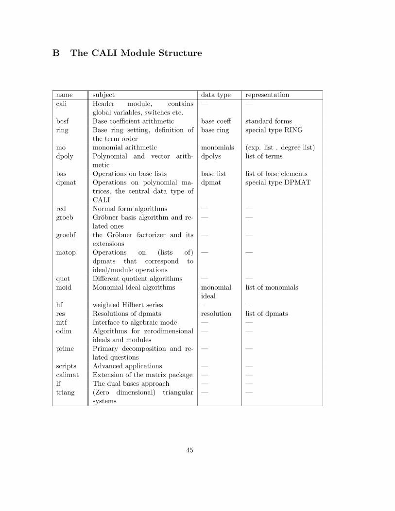
B The CALI Module Structure
name subject data type representationcali Header module, contains
global variables, switches etc.— —
bcsf Base coefficient arithmetic base coeff. standard formsring Base ring setting, definition of
the term orderbase ring special type RING
mo monomial arithmetic monomials (exp. list . degree list)dpoly Polynomial and vector arith-
meticdpolys list of terms
bas Operations on base lists base list list of base elementsdpmat Operations on polynomial ma-
trices, the central data type ofCALI
dpmat special type DPMAT
red Normal form algorithms — —groeb Grobner basis algorithm and re-
lated ones— —
groebf the Grobner factorizer and itsextensions
— —
matop Operations on (lists of)dpmats that correspond toideal/module operations
— —
quot Different quotient algorithms — —moid Monomial ideal algorithms monomial
ideallist of monomials
hf weighted Hilbert series – –res Resolutions of dpmats resolution list of dpmatsintf Interface to algebraic mode — —odim Algorithms for zerodimensional
ideals and modules— —
prime Primary decomposition and re-lated questions
— —
scripts Advanced applications — —calimat Extension of the matrix package — —lf The dual bases approach — —triang (Zero dimensional) triangular
systems— —
45
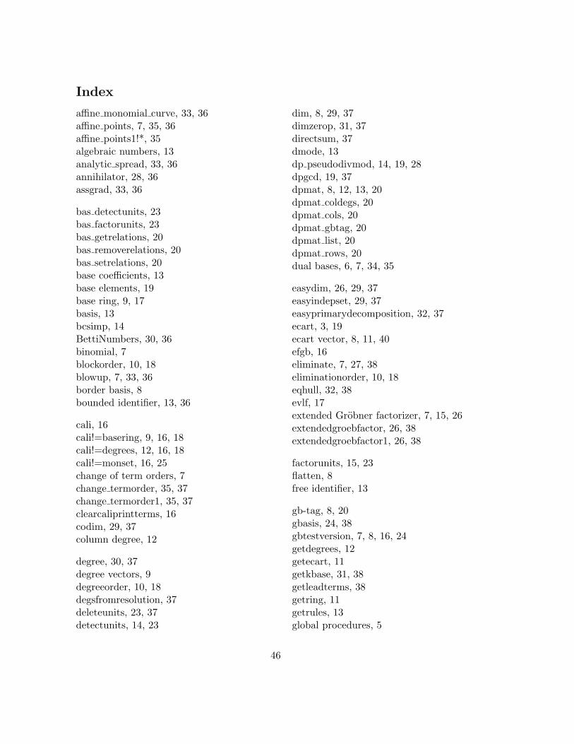
Index
affine monomial curve, 33, 36affine points, 7, 35, 36affine points1!*, 35algebraic numbers, 13analytic spread, 33, 36annihilator, 28, 36assgrad, 33, 36
bas detectunits, 23bas factorunits, 23bas getrelations, 20bas removerelations, 20bas setrelations, 20base coefficients, 13base elements, 19base ring, 9, 17basis, 13bcsimp, 14BettiNumbers, 30, 36binomial, 7blockorder, 10, 18blowup, 7, 33, 36border basis, 8bounded identifier, 13, 36
cali, 16cali!=basering, 9, 16, 18cali!=degrees, 12, 16, 18cali!=monset, 16, 25change of term orders, 7change termorder, 35, 37change termorder1, 35, 37clearcaliprintterms, 16codim, 29, 37column degree, 12
degree, 30, 37degree vectors, 9degreeorder, 10, 18degsfromresolution, 37deleteunits, 23, 37detectunits, 14, 23
dim, 8, 29, 37dimzerop, 31, 37directsum, 37dmode, 13dp pseudodivmod, 14, 19, 28dpgcd, 19, 37dpmat, 8, 12, 13, 20dpmat coldegs, 20dpmat cols, 20dpmat gbtag, 20dpmat list, 20dpmat rows, 20dual bases, 6, 7, 34, 35
easydim, 26, 29, 37easyindepset, 29, 37easyprimarydecomposition, 32, 37ecart, 3, 19ecart vector, 8, 11, 40efgb, 16eliminate, 7, 27, 38eliminationorder, 10, 18eqhull, 32, 38evlf, 17extended Grobner factorizer, 7, 15, 26extendedgroebfactor, 26, 38extendedgroebfactor1, 26, 38
factorunits, 15, 23flatten, 8free identifier, 13
gb-tag, 8, 20gbasis, 24, 38gbtestversion, 7, 8, 16, 24getdegrees, 12getecart, 11getkbase, 31, 38getleadterms, 38getring, 11getrules, 13global procedures, 5
46
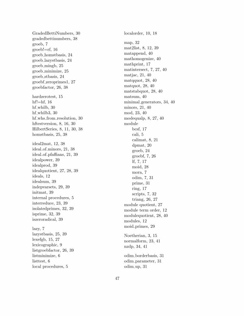
GradedBettiNumbers, 30gradedbettinumbers, 38groeb, 7groeb!=rf, 16groeb homstbasis, 24groeb lazystbasis, 24groeb mingb, 25groeb minimize, 25groeb stbasis, 24groebf zeroprimes1, 27groebfactor, 26, 38
hardzerotest, 15hf!=hf, 16hf whilb, 30hf whilb3, 30hf whs from resolution, 30hftestversion, 8, 16, 30HilbertSeries, 8, 11, 30, 38homstbasis, 25, 38
ideal2mat, 12, 38ideal of minors, 21, 38ideal of pfaffians, 21, 39idealpower, 39idealprod, 39idealquotient, 27, 28, 39ideals, 12idealsum, 39indepvarsets, 29, 39initmat, 39internal procedures, 5interreduce, 23, 39isolatedprimes, 32, 39isprime, 32, 39iszeroradical, 39
lazy, 7lazystbasis, 25, 39lexefgb, 15, 27lexicographic, 9listgroebfactor, 26, 39listminimize, 6listtest, 6local procedures, 5
localorder, 10, 18
map, 32mat2list, 8, 12, 39matappend, 40mathomogenize, 40mathprint, 17matintersect, 7, 27, 40matjac, 21, 40matqquot, 28, 40matquot, 28, 40matstabquot, 28, 40matsum, 40minimal generators, 34, 40minors, 21, 40mod, 23, 40modequalp, 8, 27, 40module
bcsf, 17cali, 5calimat, 8, 21dpmat, 20groeb, 24groebf, 7, 26lf, 7, 17moid, 28mora, 7odim, 7, 31prime, 31ring, 17scripts, 7, 32triang, 26, 27
module quotient, 27module term order, 12modulequotient, 28, 40modules, 12moid primes, 29
Noetherian, 3, 15normalform, 23, 41nzdp, 34, 41
odim borderbasis, 31odim parameter, 31odim up, 31
47
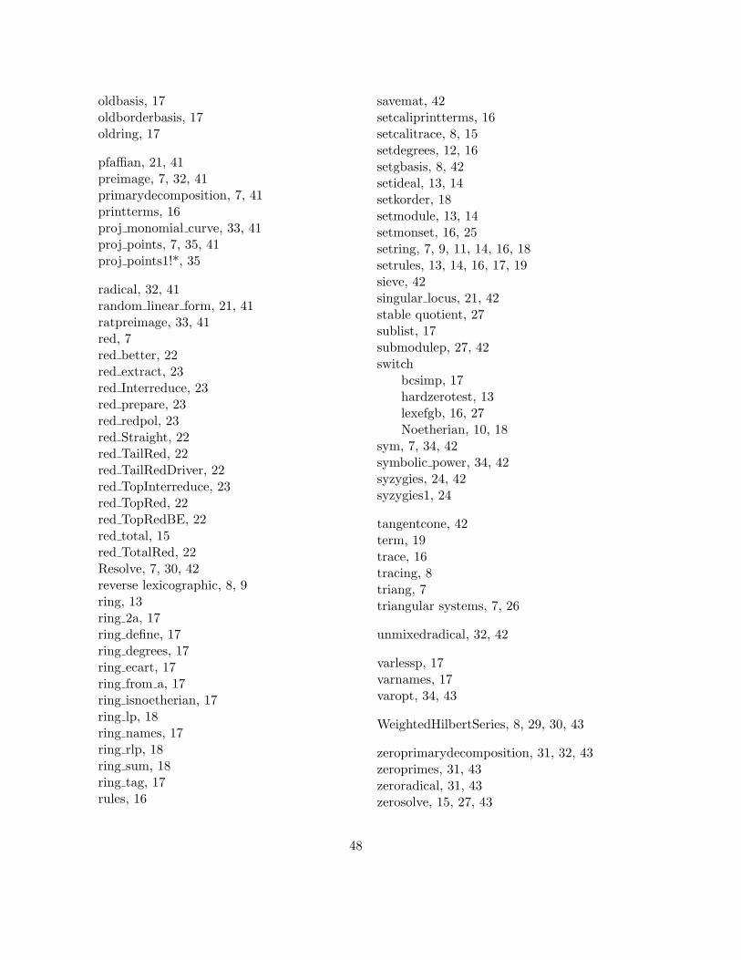
oldbasis, 17oldborderbasis, 17oldring, 17
pfaffian, 21, 41preimage, 7, 32, 41primarydecomposition, 7, 41printterms, 16proj monomial curve, 33, 41proj points, 7, 35, 41proj points1!*, 35
radical, 32, 41random linear form, 21, 41ratpreimage, 33, 41red, 7red better, 22red extract, 23red Interreduce, 23red prepare, 23red redpol, 23red Straight, 22red TailRed, 22red TailRedDriver, 22red TopInterreduce, 23red TopRed, 22red TopRedBE, 22red total, 15red TotalRed, 22Resolve, 7, 30, 42reverse lexicographic, 8, 9ring, 13ring 2a, 17ring define, 17ring degrees, 17ring ecart, 17ring from a, 17ring isnoetherian, 17ring lp, 18ring names, 17ring rlp, 18ring sum, 18ring tag, 17rules, 16
savemat, 42setcaliprintterms, 16setcalitrace, 8, 15setdegrees, 12, 16setgbasis, 8, 42setideal, 13, 14setkorder, 18setmodule, 13, 14setmonset, 16, 25setring, 7, 9, 11, 14, 16, 18setrules, 13, 14, 16, 17, 19sieve, 42singular locus, 21, 42stable quotient, 27sublist, 17submodulep, 27, 42switch
bcsimp, 17hardzerotest, 13lexefgb, 16, 27Noetherian, 10, 18
sym, 7, 34, 42symbolic power, 34, 42syzygies, 24, 42syzygies1, 24
tangentcone, 42term, 19trace, 16tracing, 8triang, 7triangular systems, 7, 26
unmixedradical, 32, 42
varlessp, 17varnames, 17varopt, 34, 43
WeightedHilbertSeries, 8, 29, 30, 43
zeroprimarydecomposition, 31, 32, 43zeroprimes, 31, 43zeroradical, 31, 43zerosolve, 15, 27, 43
48

zerosolve1, 15, 27, 43zerosolve2, 27, 43
49
References
[1] D. Bayer, M. Stillman: Computation of Hilbert functions. J. Symb. Comp. 14(1992), 31 - 50.
[2] T. Becker, H. Kredel, V. Weispfenning: Grobner bases. A computational approachto commutative algebra. Grad. Texts in Math. 141, Springer, New York 1993.
[3] A. M. Bigatti, P. Conti, L. Robbiano, C. Traverso: A “divide and conquer” algorithmfor Hilbert-Poincare series, multiplicity and dimension of monomial ideals. In: Proc.AAECC-10, LNCS 673 (1993), 76 - 88.
[4] W. Boege, R. Gebauer, H. Kredel: Some examples for solving systems of algebraicequations by calculating Grobner bases. J. Symb. Comp. 2 (1986), 83 - 98.
[5] B. Buchberger: Grobner bases: An algorithmic method in polynomial ideal the-ory. In: Recent trends in multidimensional system theory (N. K. Bose ed), Reidel,Dortrecht 1985, 184 - 232.
[6] B. Buchberger: Applications of Grobner bases in non-linear computational geometry.LNCS 296 (1988), 52 - 80.
[7] D. Cox, J. Little, D. O’Shea: Ideals, varieties, and algorithms. Undergraduate Textsin Math., Springer, New York 1992.
[8] D. Eisenbud: Commutative algebra with a view toward algebraic geometry. Springer,1995.
[9] Faugere, Gianni, Lazard, Mora: Efficient computations of zerodimensional Grobnerbases by change of ordering. J. Symb. Comp. 16 (1993), 329 - 344.
[10] P. Gianni, B. Trager, G. Zacharias: Grobner bases and primary decomposition ofpolynomial ideals. J. Symb. Comp. 6 (1988), 149 - 167.
[11] A. Giovini, T. Mora, G. Niesi, L. Robbiano, C. Traverso: ”One sugar cube, please” orSelection strategies in the Buchberger algorithm. In: Proceedings of the ISSAC’91,ACM Press 1991, 49 - 54.
[12] H.-G. Grabe: Two remarks on independent sets. J. Alg. Comb. 2 (1993), 137 - 145.
[13] H.-G. Grabe: The tangent cone algorithm and homogenization. J. Pure AppliedAlg.97 (1994), 303 - 312.
[14] H.-G. Grabe: Algorithms in local algebra. To appear
[15] H.-G. Grabe: On factorized Grobner bases. Report Nr. 6 (1994), Inst. f. Informatik,Univ. Leipzig.
To appear in: Proc. “Computer Algebra in Science and Engineering”, Bielefeld 1994.
50
[16] H.-G. Grabe: Triangular systems and factorized Grobner bases. Report Nr. 7 (1995),Inst. f. Informatik, Univ. Leipzig.
[17] H.-G. Grabe: Factorized Grobner bases and primary decomposition. To appear.
[18] H. Kredel: Primary ideal decomposition. In: Proc. EUROCAL’87, Lecture Notes inComp. Sci. 378 (1986), 270 - 281.
[19] H. Kredel, V. Weispfenning: Computing dimension and independent sets for poly-nomial ideals. J. Symb. Comp. 6 (1988), 231 - 247.
[20] M. Marinari, H.-M. Moller, T. Mora: Grobner bases of ideals given by dual bases.In: Proc. ISSAC’91, ACM Press 1991, 55 - 63.
[21] B. Mishra: Algorithmic Algebra. Springer, New York 1993.
[22] H.-M. Moller, F. Mora: New constructive methods in classical ideal theory. J. Alg.100 (1986), 138 -178.
[23] H.-M. Moller: On decomposing systems of polynomial equations with finitely manysolutions. J. AAECC 4 (1993), 217 - 230.
[24] T. Mora, L. Robbiano: The Grobner fan of an ideal. J. Symb. Comp. 6 (1988), 183- 208.
[25] T. Mora: Seven variations on standard bases. Preprint, Univ. Genova, 1988.
[26] T. Mora, G. Pfister, C. Traverso: An introduction to the tangent cone algorithm.In: Issues in non-linear geometry and robotics, C.M. Hoffman ed., JAI Press.
[27] L. Robbiano: Computer algebra and commutative algebra. LNCS 357 (1989), 31 -44.
[28] E. W. Rutman: Grobner bases and primary decomposition of modules. J. Symb.Comp. 14 (1992), 483 - 503.
51


![Commutative Algebra - Cornell Universitypi.math.cornell.edu/.../partiii/files/commalgnotes.pdf · 2018-08-23 · Commutative algebra is about commutative rings: Z, k[x1,...,xn], etc](https://img.pdfslide.us/doc/110x75/5f157dcc3ba58c0b6a7eac81/commutative-algebra-cornell-2018-08-23-commutative-algebra-is-about-commutative.jpg)