Embed Size (px)
Citation preview
Calculus

This work is licensed under the Creative Commons Attribution-NonCommercial-ShareAlike License. Toview a copy of this license, visit http://creativecommons.org/licenses/by-nc-sa/3.0/ or send a letter toCreative Commons, 543 Howard Street, 5th Floor, San Francisco, California, 94105, USA. If you distributethis work or a derivative, include the history of the document.
This text was initially written by David Guichard. The single variable material (not including infiniteseries) was originally a modification and expansion of notes written by Neal Koblitz at the Universityof Washington, who generously gave permission to use, modify, and distribute his work. New materialhas been added, and old material has been modified, so some portions now bear little resemblance to theoriginal.
The book includes some exercises from Elementary Calculus: An Approach Using Infinitesimals, byH. Jerome Keisler, available at http://www.math.wisc.edu/~keisler/calc.html under a Creative Com-mons license. Albert Schueller, Barry Balof, and Mike Wills have contributed additional material.
This copy of the text was produced at 16:02 on 5/31/2009.
I will be glad to receive corrections and suggestions for improvement at [email protected].


Contents
1Analytic Geometry 1
1.1 Lines . . . . . . . . . . . . . . . . . . . . . . . . . . . . . . . . 21.2 Distance Between Two Points; Circles . . . . . . . . . . . . . . . . 71.3 Functions . . . . . . . . . . . . . . . . . . . . . . . . . . . . . . 81.4 Shifts and Dilations . . . . . . . . . . . . . . . . . . . . . . . . 14
2Instantaneous Rate Of Change: The Derivative 19
2.1 The slope of a function . . . . . . . . . . . . . . . . . . . . . . 192.2 An example . . . . . . . . . . . . . . . . . . . . . . . . . . . . 242.3 Limits . . . . . . . . . . . . . . . . . . . . . . . . . . . . . . 262.4 The Derivative Function . . . . . . . . . . . . . . . . . . . . . 352.5 Adjectives For Functions . . . . . . . . . . . . . . . . . . . . . 40
v
vi Contents
3Rules For Finding Derivatives 45
3.1 The Power Rule . . . . . . . . . . . . . . . . . . . . . . . . . 453.2 Linearity of the Derivative . . . . . . . . . . . . . . . . . . . . 483.3 The Product Rule . . . . . . . . . . . . . . . . . . . . . . . . 503.4 The Quotient Rule . . . . . . . . . . . . . . . . . . . . . . . . 533.5 The Chain Rule . . . . . . . . . . . . . . . . . . . . . . . . . . 56
4Transcendental Functions 63
4.1 Trigonometric Functions . . . . . . . . . . . . . . . . . . . . . 634.2 The Derivative of sin x . . . . . . . . . . . . . . . . . . . . . . 664.3 A hard limit . . . . . . . . . . . . . . . . . . . . . . . . . . . 674.4 The Derivative of sin x, continued . . . . . . . . . . . . . . . . . 704.5 Derivatives of the Trigonometric Functions . . . . . . . . . . . . 714.6 Exponential and Logarithmic functions . . . . . . . . . . . . . . 724.7 Derivatives of the exponential and logarithmic functions . . . . . 754.8 Limits revisited . . . . . . . . . . . . . . . . . . . . . . . . . . 804.9 Implicit Differentiation . . . . . . . . . . . . . . . . . . . . . . 844.10 Inverse Trigonometric Functions . . . . . . . . . . . . . . . . . 89
5Curve Sketching 93
5.1 Maxima and Minima . . . . . . . . . . . . . . . . . . . . . . . 935.2 The first derivative test . . . . . . . . . . . . . . . . . . . . . . 975.3 The second derivative test . . . . . . . . . . . . . . . . . . . . 995.4 Concavity and inflection points . . . . . . . . . . . . . . . . . 1005.5 Asymptotes and Other Things to Look For . . . . . . . . . . . 102

Contents vii
6Applications of the Derivative 105
6.1 Optimization . . . . . . . . . . . . . . . . . . . . . . . . . . 1056.2 Related Rates . . . . . . . . . . . . . . . . . . . . . . . . . 1186.3 Newton’s Method . . . . . . . . . . . . . . . . . . . . . . . . 1276.4 Linear Approximations . . . . . . . . . . . . . . . . . . . . . 1316.5 The Mean Value Theorem . . . . . . . . . . . . . . . . . . . 133
7Integration 139
7.1 Two examples . . . . . . . . . . . . . . . . . . . . . . . . . 1397.2 The Fundamental Theorem of Calculus . . . . . . . . . . . . . 1437.3 Some Properties of Integrals . . . . . . . . . . . . . . . . . . 150
8Techniques of Integration 155
8.1 Substitution . . . . . . . . . . . . . . . . . . . . . . . . . . 1568.2 Powers of sine and cosine . . . . . . . . . . . . . . . . . . . . 1608.3 Trigonometric Substitutions . . . . . . . . . . . . . . . . . . . 1628.4 Integration by Parts . . . . . . . . . . . . . . . . . . . . . . 1668.5 Rational Functions . . . . . . . . . . . . . . . . . . . . . . . 1708.6 Additional exercises . . . . . . . . . . . . . . . . . . . . . . . 176
viii Contents
9Applications of Integration 177
9.1 Area between curves . . . . . . . . . . . . . . . . . . . . . . 1779.2 Distance, Velocity, Acceleration . . . . . . . . . . . . . . . . . 1829.3 Volume . . . . . . . . . . . . . . . . . . . . . . . . . . . . . 1859.4 Average value of a function . . . . . . . . . . . . . . . . . . . 1929.5 Work . . . . . . . . . . . . . . . . . . . . . . . . . . . . . . 1959.6 Center of Mass . . . . . . . . . . . . . . . . . . . . . . . . . 2009.7 Kinetic energy; improper integrals . . . . . . . . . . . . . . . 2059.8 Probability . . . . . . . . . . . . . . . . . . . . . . . . . . . 2109.9 Arc Length . . . . . . . . . . . . . . . . . . . . . . . . . . . 2209.10 Surface Area . . . . . . . . . . . . . . . . . . . . . . . . . . 2229.11 Differential equations . . . . . . . . . . . . . . . . . . . . . . 227
10Sequences and Series 233
10.1 Sequences . . . . . . . . . . . . . . . . . . . . . . . . . . . . 23410.2 Series . . . . . . . . . . . . . . . . . . . . . . . . . . . . . . 24010.3 The Integral Test . . . . . . . . . . . . . . . . . . . . . . . . 24410.4 Alternating Series . . . . . . . . . . . . . . . . . . . . . . . . 24910.5 Comparison Tests . . . . . . . . . . . . . . . . . . . . . . . . 25110.6 Absolute Convergence . . . . . . . . . . . . . . . . . . . . . 25410.7 The Ratio and Root Tests . . . . . . . . . . . . . . . . . . . 25610.8 Power Series . . . . . . . . . . . . . . . . . . . . . . . . . . 25910.9 Calculus with Power Series . . . . . . . . . . . . . . . . . . . 26110.10 Taylor Series . . . . . . . . . . . . . . . . . . . . . . . . . . 26310.11 Taylor’s Theorem . . . . . . . . . . . . . . . . . . . . . . . . 26710.12 Additional exercises . . . . . . . . . . . . . . . . . . . . . . . 271
Contents ix
AIntroduction to Maple 275
A.1 Getting Started . . . . . . . . . . . . . . . . . . . . . . . . . 275A.2 Algebra . . . . . . . . . . . . . . . . . . . . . . . . . . . . . 276
A.2.1 Numbers . . . . . . . . . . . . . . . . . . . . . . . . . 276A.2.2 Variables and Expressions . . . . . . . . . . . . . . . . . 277A.2.3 Evaluation and Substitution . . . . . . . . . . . . . . . 279A.2.4 Solving Equations . . . . . . . . . . . . . . . . . . . . 280
A.3 Plotting . . . . . . . . . . . . . . . . . . . . . . . . . . . . 282A.4 Calculus . . . . . . . . . . . . . . . . . . . . . . . . . . . . 284
A.4.1 Limits . . . . . . . . . . . . . . . . . . . . . . . . . . 284A.4.2 Differentiation . . . . . . . . . . . . . . . . . . . . . . 284A.4.3 Implicit Differentiation . . . . . . . . . . . . . . . . . . 285A.4.4 Integration . . . . . . . . . . . . . . . . . . . . . . . . 285
A.5 Adding text to a Maple session . . . . . . . . . . . . . . . . . 286A.6 Printing . . . . . . . . . . . . . . . . . . . . . . . . . . . . 286A.7 Saving your work . . . . . . . . . . . . . . . . . . . . . . . . 286A.8 Getting Help . . . . . . . . . . . . . . . . . . . . . . . . . . 287
BSelected Answers 289
Index 303

Introduction
The emphasis in this course is on problems—doing calculations and story problems. Tomaster problem solving one needs a tremendous amount of practice doing problems. Themore problems you do the better you will be at doing them, as patterns will start to emergein both the problems and in successful approaches to them. You will learn fastest and bestif you devote some time to doing problems every day.
Typically the most difficult problems are story problems, since they require some effortbefore you can begin calculating. Here are some pointers for doing story problems:
1. Carefully read each problem twice before writing anything.
2. Assign letters to quantities that are described only in words; draw a diagram ifappropriate.
3. Decide which letters are constants and which are variables. A letter stands for aconstant if its value remains the same throughout the problem.
4. Using mathematical notation, write down what you know and then write downwhat you want to find.
5. Decide what category of problem it is (this might be obvious if the problem comesat the end of a particular chapter, but will not necessarily be so obvious if it comeson an exam covering several chapters).
6. Double check each step as you go along; don’t wait until the end to check yourwork.
xi
xii Introduction
7. Use common sense; if an answer is out of the range of practical possibilities, thencheck your work to see where you went wrong.
Suggestions for Using This Text
1. Read the example problems carefully, filling in any steps that are left out (asksomeone if you can’t follow the solution to a worked example).
2. Later use the worked examples to study by covering the solutions, and seeing ifyou can solve the problems on your own.
3. Most exercises have answers in Appendix B; the availability of an answer is markedby “⇒” at the end of the exercise. In the pdf version of the full text, clickingon the arrow will take you to the answer. The answers should be used only asa final check on your work, not as a crutch. Keep in mind that sometimes ananswer could be expressed in various ways that are algebraically equivalent, sodon’t assume that your answer is wrong just because it doesn’t have exactly thesame form as the answer in the back.
4. A few figures in the book are marked with “(JA)” at the end of the caption.Clicking on this should open a related Java applet in your web browser.
Some Useful Formulas
AlgebraRemember that the common algebraic operations have precedences relative to eachother: for example, mulitplication and division take precedence over addition andsubtraction, but are “tied” with each other. In the case of ties, work left to right. Thismeans, for example, that 1/2x means (1/2)x: do the division, then the multiplicationin left to right order. It sometimes is a good idea to use more parentheses than strictlynecessary, for clarity, but it is also a bad idea to use too many parentheses.
Completing the square: x2 + bx + c = (x + b2 )2 − b2
4 + c.
Quadratic formula: the roots of ax2 + bx + c are−b±√b2 − 4ac
2a.
Exponent rules:ab · ac = ab+c
ab
ac= ab−c
(ab)c = abc
a1/b = b√
a
Introduction xiii
Geometry
Circle: circumference = 2πr, area = πr2.
Sphere: vol = 4πr3/3, surface area = 4πr2.
Cylinder: vol = πr2h, lateral area = 2πrh, total surface area = 2πrh + 2πr2.
Cone: vol = πr2h/3, lateral area = πr√
r2 + h2, total surface area = πr√
r2 + h2 +πr2.
Analytic geometry
Point-slope formula for straight line through the point (x0, y0) with slope m: y =y0 + m(x− x0).
Circle with radius r centered at (h, k): (x− h)2 + (y − k)2 = r2.
Ellipse with axes on the x-axis and y-axis:x2
a2+
y2
b2= 1.
Trigonometry
sin(θ) = opposite/hypotenuse
cos(θ) = adjacent/hypotenuse
tan(θ) = opposite/adjacent
sec(θ) = 1/ cos(θ)
csc(θ) = 1/ sin(θ)
cot(θ) = 1/ tan(θ)
tan(θ) = sin(θ)/ cos(θ)
cot(θ) = cos(θ)/ sin(θ)
sin(θ) = cos(
π2 − θ
)
cos(θ) = sin(
π2 − θ
)
sin(θ + π) = − sin(θ)
cos(θ + π) = − cos(θ)
Law of cosines: a2 = b2 + c2 − 2bc cosA
Law of sines:a
sin A=
b
sin B=
c
sin C

xiv Introduction
Sine of sum of angles: sin(x + y) = sin x cos y + cosx sin y
sin2(θ) and cos2(θ) formulas:
sin2(θ) + cos2(θ) = 1
sin2(θ) =1− cos(2θ)
2
cos2(θ) =1 + cos(2θ)
2
Cosine of sum of angles: cos(x + y) = cos x cos y − sin x sin y
Tangent of sum of angles: tan(x + y) =tanx + tan y
1− tanx tan y

1Analytic Geometry
Much of the mathematics in this chapter will be review for you. However, the exampleswill be oriented toward applications and so will take some thought.
In the (x, y) coordinate system we normally write the x-axis horizontally, with positivenumbers to the right of the origin, and the y-axis vertically, with positive numbers abovethe origin. That is, unless stated otherwise, we take “rightward” to be the positive x-direction and “upward” to be the positive y-direction. In a purely mathematical situation,we normally choose the same scale for the x- and y-axes. For example, the line joining theorigin to the point (a, a) makes an angle of 45◦ with the x-axis (and also with the y-axis).
But in applications, often letters other than x and y are used, and often different scalesare chosen in the x and y directions. For example, suppose you drop something from awindow, and you want to study how its height above the ground changes from second tosecond. It is natural to let the letter t denote the time (the number of seconds since theobject was released) and to let the letter h denote the height. For each t (say, at one-secondintervals) you have a corresponding height h. This information can be tabulated, and thenplotted on the (t, h) coordinate plane, as shown in figure 1.1.
We use the word “quadrant” for each of the four regions the plane is divided into: thefirst quadrant is where points have both coordinates positive, or the “northeast” portionof the plot, and the second, third, and fourth quadrants are counted off counterclockwise,so the second quadrant is the northwest, the third is the southwest, and the fourth is thesoutheast.
1

2 Chapter 1 Analytic Geometry
seconds 0 1 2 3 4
meters 80 75.1 60.4 35.9 1.6
20
40
60
80
0 1 2 3 4
t
h..............................................................................................................................................................................................................................................................................................................................................................................................................................................................................................................................................................
• ••
•
•
Figure 1.1 A data plot.
Suppose we have two points A(2, 1) and B(3, 3) in the (x, y)-plane. We often wantto know the change in x-coordinate (also called the “horizontal distance”) in going fromA to B. This is often written ∆x, where the meaning of ∆ (a capital delta in the Greekalphabet) is “change in”. (Thus, ∆x can be read as “change in x” although it usuallyis read as “delta x”. The point is that ∆x denotes a single number, and should not beinterpreted as “delta times x”.) In our example, ∆x = 3−2 = 1. Similarly, the “change iny” is written ∆y. In our example, ∆y = 3−1 = 2, the difference between the y-coordinatesof the two points. It is the vertical distance you have to move in going from A to B. Thegeneral formulas for the change in x and the change in y between a point (x1, y1) and apoint (x2, y2) is:
∆x = x2 − x1, ∆y = y2 − y1.
Note that either or both of these might be negative.
1.1 Lines
If we have two points A(x1, y1) and B(x2, y2), then we can draw one and only one linethrough both points. By the slope of this line we mean the ratio of ∆y to ∆x. The slopeis often denoted m: m = ∆y/∆x = (y2 − y1)/(x2 − x1). For example, the line joining thepoints A and B in the last paragraph has slope 2.

1.1 Lines 3
EXAMPLE 1.1 According to the 1990 U.S. federal income tax schedules, a head ofhousehold paid 15% on taxable income up to $26050. If taxable income was between$26050 and $134930, then, in addition, 28% was to be paid on the amount between $26050and $67200, and 33% paid on the amount over $67200 (if any). Interpret the tax bracketinformation (15%, 28%, or 33%) using mathematical terminology, and graph the tax onthe y-axis against the taxable income on the x-axis.
The percentages, when converted to decimal values 0.15, 0.28, and 0.33, are the slopesof the straight lines which form the graph of the tax for the corresponding tax brackets.The tax graph is what’s called a polygonal line, i.e., it’s made up of several straight linesegments of different slopes. The first line starts at the point (0,0) and heads upwardwith slope 0.15 (i.e., it goes upward 15 for every increase of 100 in the x-direction), untilit reaches the point above x = 26050. Then the graph “bends upward,” i.e., the slopechanges to 0.28. As the horizontal coordinate goes from x = 26050 to x = 67200, the linegoes upward 28 for each 100 in the x-direction. At x = 67200 the line turns upward againand continues with slope 0.33. See figure 1.2.
10000
20000
30000
50000 100000
......................................................................
......................................................................
.................................................
........................................
........................................
........................................
........................................
........................................
........................................
....................................
....................................
....................................
....................................
....................................
................................
•
•
Figure 1.2 Tax vs. income.
The most familiar form of the equation of a straight line is: y = mx+ b. Here m is theslope of the line: if you increase x by 1, the equation tells you that you have to increase y
by m. If you increase x by ∆x, then y increases by ∆y = m∆x. The number b is calledthe y-intercept, because it is where the line crosses the y-axis. If you know two points ona line, the formula m = (y2 − y1)/(x2 − x1) gives you the slope. Once you know a pointand the slope, then the y-intercept can be found by substituting the coordinates of eitherpoint in the equation: y1 = mx1 + b, i.e., b = y1 −mx1. Alternatively, one can use the“point-slope” form of the equation of a straight line, which is: (y−y1)/(x−x1) = m. This
4 Chapter 1 Analytic Geometry
relation says that “between the point (x1, y1) and any other point (x, y) on the line, thechange in y divided by the change in x is the slope m of the line.”
It is possible to find the equation of a line between two points directly from the relation(y− y1)/(x−x1) = (y2− y1)/(x2−x1), which says “the slope measured between the point(x1, y1) and the point (x2, y2) is the same as the slope measured between the point (x1, y1)and any other point (x, y) on the line.” For example, if we want to find the equation ofthe line joining our earlier points A(2, 1) and B(3, 3), we can use this formula:
y − 1x− 2
=3− 13− 2
= 2, so that y − 1 = 2(x− 2), i.e., y = 2x− 3.
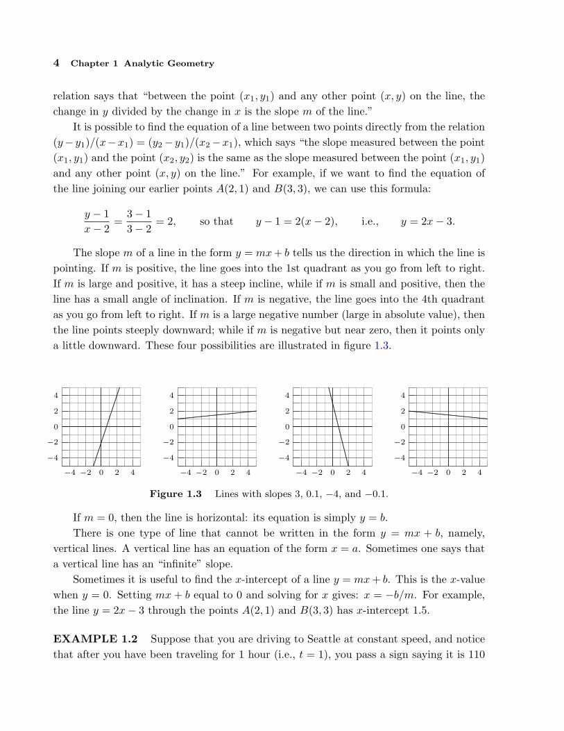
The slope m of a line in the form y = mx + b tells us the direction in which the line ispointing. If m is positive, the line goes into the 1st quadrant as you go from left to right.If m is large and positive, it has a steep incline, while if m is small and positive, then theline has a small angle of inclination. If m is negative, the line goes into the 4th quadrantas you go from left to right. If m is a large negative number (large in absolute value), thenthe line points steeply downward; while if m is negative but near zero, then it points onlya little downward. These four possibilities are illustrated in figure 1.3.
............................................................................................................................................................................................
−4
−2
0
2
4
−4 −2 0 2 4
.........................................................................................................................................................
..........................
−4
−2
0
2
4
−4 −2 0 2 4
........................................................................................................................................................................................−4
−2
0
2
4
−4 −2 0 2 4
...................................................................................................................................................................................
−4
−2
0
2
4
−4 −2 0 2 4
Figure 1.3 Lines with slopes 3, 0.1, −4, and −0.1.
If m = 0, then the line is horizontal: its equation is simply y = b.There is one type of line that cannot be written in the form y = mx + b, namely,
vertical lines. A vertical line has an equation of the form x = a. Sometimes one says thata vertical line has an “infinite” slope.
Sometimes it is useful to find the x-intercept of a line y = mx + b. This is the x-valuewhen y = 0. Setting mx + b equal to 0 and solving for x gives: x = −b/m. For example,the line y = 2x− 3 through the points A(2, 1) and B(3, 3) has x-intercept 1.5.
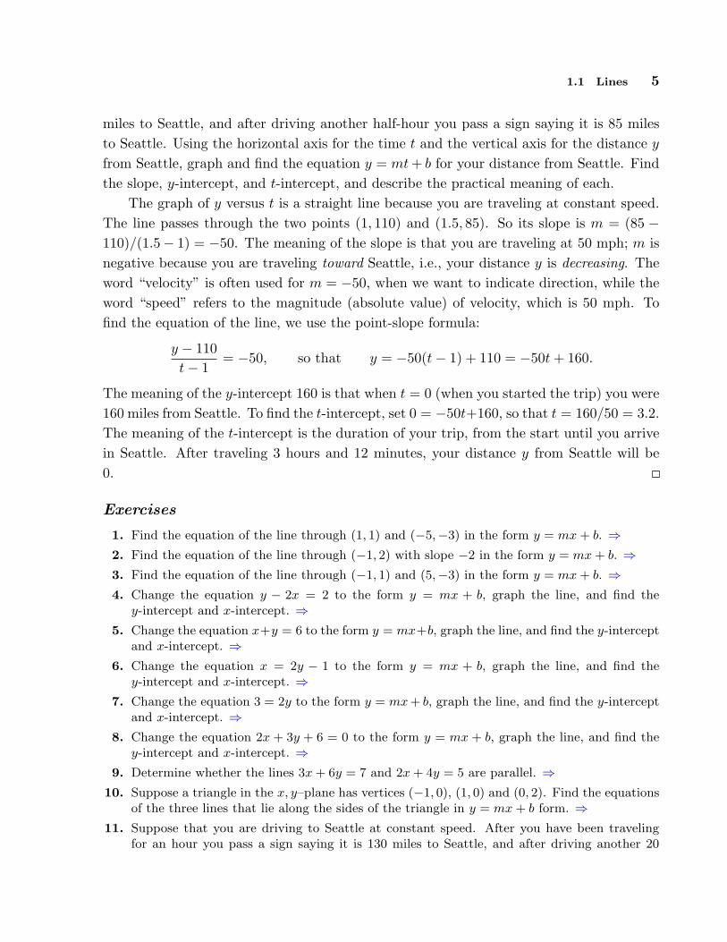
EXAMPLE 1.2 Suppose that you are driving to Seattle at constant speed, and noticethat after you have been traveling for 1 hour (i.e., t = 1), you pass a sign saying it is 110
1.1 Lines 5
miles to Seattle, and after driving another half-hour you pass a sign saying it is 85 milesto Seattle. Using the horizontal axis for the time t and the vertical axis for the distance y
from Seattle, graph and find the equation y = mt + b for your distance from Seattle. Findthe slope, y-intercept, and t-intercept, and describe the practical meaning of each.
The graph of y versus t is a straight line because you are traveling at constant speed.The line passes through the two points (1, 110) and (1.5, 85). So its slope is m = (85 −110)/(1.5− 1) = −50. The meaning of the slope is that you are traveling at 50 mph; m isnegative because you are traveling toward Seattle, i.e., your distance y is decreasing. Theword “velocity” is often used for m = −50, when we want to indicate direction, while theword “speed” refers to the magnitude (absolute value) of velocity, which is 50 mph. Tofind the equation of the line, we use the point-slope formula:
y − 110t− 1
= −50, so that y = −50(t− 1) + 110 = −50t + 160.
The meaning of the y-intercept 160 is that when t = 0 (when you started the trip) you were160 miles from Seattle. To find the t-intercept, set 0 = −50t+160, so that t = 160/50 = 3.2.The meaning of the t-intercept is the duration of your trip, from the start until you arrivein Seattle. After traveling 3 hours and 12 minutes, your distance y from Seattle will be0.
Exercises
1. Find the equation of the line through (1, 1) and (−5,−3) in the form y = mx + b. ⇒2. Find the equation of the line through (−1, 2) with slope −2 in the form y = mx + b. ⇒3. Find the equation of the line through (−1, 1) and (5,−3) in the form y = mx + b. ⇒4. Change the equation y − 2x = 2 to the form y = mx + b, graph the line, and find the
y-intercept and x-intercept. ⇒5. Change the equation x+y = 6 to the form y = mx+b, graph the line, and find the y-intercept
and x-intercept. ⇒6. Change the equation x = 2y − 1 to the form y = mx + b, graph the line, and find the
y-intercept and x-intercept. ⇒7. Change the equation 3 = 2y to the form y = mx + b, graph the line, and find the y-intercept
and x-intercept. ⇒8. Change the equation 2x + 3y + 6 = 0 to the form y = mx + b, graph the line, and find the
y-intercept and x-intercept. ⇒9. Determine whether the lines 3x + 6y = 7 and 2x + 4y = 5 are parallel. ⇒
10. Suppose a triangle in the x, y–plane has vertices (−1, 0), (1, 0) and (0, 2). Find the equationsof the three lines that lie along the sides of the triangle in y = mx + b form. ⇒
11. Suppose that you are driving to Seattle at constant speed. After you have been travelingfor an hour you pass a sign saying it is 130 miles to Seattle, and after driving another 20

6 Chapter 1 Analytic Geometry
minutes you pass a sign saying it is 105 miles to Seattle. Using the horizontal axis for thetime t and the vertical axis for the distance y from your starting point, graph and find theequation y = mt + b for your distance from your starting point. How long does the trip toSeattle take? ⇒
12. Let x stand for temperature in degrees Celsius (centigrade), and let y stand for temperature indegrees Fahrenheit. A temperature of 0◦C corresponds to 32◦F, and a temperature of 100◦Ccorresponds to 212◦F. Find the equation of the line that relates temperature Fahrenheit y totemperature Celsius x in the form y = mx + b. Graph the line, and find the point at whichthis line intersects y = x. What is the practical meaning of this point? ⇒
13. A car rental firm has the following charges for a certain type of car: $25 per day with 100free miles included, $0.15 per mile for more than 100 miles. Suppose you want to rent acar for one day, and you know you’ll use it for more than 100 miles. What is the equationrelating the cost y to the number of miles x that you drive the car? ⇒
14. A photocopy store advertises the following prices: 5/c per copy for the first 20 copies, 4/c percopy for the 21st through 100th copy, and 3/c per copy after the 100th copy. Let x be thenumber of copies, and let y be the total cost of photocopying. (a) Graph the cost as x goesfrom 0 to 200 copies. (b) Find the equation in the form y = mx + b that tells you the costof making x copies when x is more than 100. ⇒
15. In the Kingdom of Xyg the tax system works as follows. Someone who earns less than 100gold coins per month pays no tax. Someone who earns between 100 and 1000 golds coinspays tax equal to 10% of the amount over 100 gold coins that he or she earns. Someonewho earns over 1000 gold coins must hand over to the King all of the money earned over1000 in addition to the tax on the first 1000. (a) Draw a graph of the tax paid y versus themoney earned x, and give formulas for y in terms of x in each of the regions 0 ≤ x ≤ 100,100 ≤ x ≤ 1000, and x ≥ 1000. (b) Suppose that the King of Xyg decides to use the secondof these line segments (for 100 ≤ x ≤ 1000) for x ≤ 100 as well. Explain in practical termswhat the King is doing, and what the meaning is of the y-intercept. ⇒
16. The tax for a single taxpayer is described in the figure below. Use this information to graphtax versus taxable income (i.e., x is the amount on Form 1040, line 37, and y is the amount onForm 1040, line 38). Find the slope and y-intercept of each line that makes up the polygonalgraph, up to x = 97620. ⇒
1990 Tax Rate SchedulesSchedule X—Use if your filing status is
Single
If the amount Enter on of the
on Form 1040 But not Form 1040 amount
line 37 is over: over: line 38 over:
$0 $19,450 15% $0
19,450 47,050 $2,917.50+28% 19,450
47,050 97,620 $10,645.50+33% 47,050
Use Worksheet
97,620 ............ below to figure
your tax
Schedule Z—Use if your filing status isHead of household
If the amount Enter on of the
on Form 1040 But not Form 1040 amount
line 37 is over: over: line 38 over:
$0 $26,050 15% $0
26,050 67,200 $3,907.50+28% 26,050
67,200 134,930 $15,429.50+33% 67,200
Use Worksheet
134,930 ............ below to figure
your tax
1.2 Distance Between Two Points; Circles 7
17. Market research tells you that if you set the price of an item at $1.50, you will be able to sell5000 items; and for every 10 cents you lower the price below $1.50 you will be able to sellanother 1000 items. Let x be the number of items you can sell, and let P be the price of anitem. (a) Express P linearly in terms of x, in other words, express P in the form P = mx+b.(b) Express x linearly in terms of P . ⇒
18. An instructor gives a 100-point final exam, and decides that a score 90 or above will be agrade of 4.0, a score of 40 or below will be a grade of 0.0, and between 40 and 90 the gradingwill be linear. Let x be the exam score, and let y be the corresponding grade. Find a formulaof the form y = mx + b which applies to scores x between 40 and 90. ⇒
1.2 Distance Between Two Points; Circles
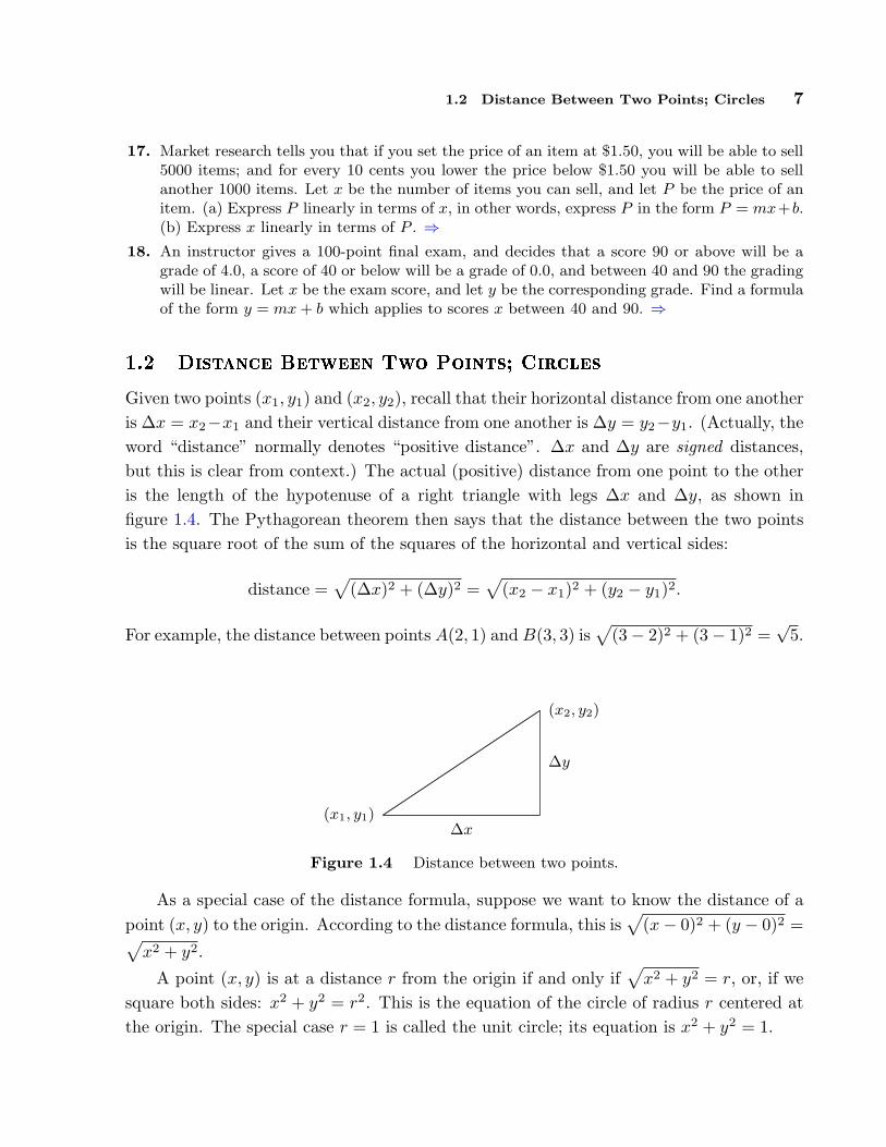
Given two points (x1, y1) and (x2, y2), recall that their horizontal distance from one anotheris ∆x = x2−x1 and their vertical distance from one another is ∆y = y2−y1. (Actually, theword “distance” normally denotes “positive distance”. ∆x and ∆y are signed distances,but this is clear from context.) The actual (positive) distance from one point to the otheris the length of the hypotenuse of a right triangle with legs ∆x and ∆y, as shown infigure 1.4. The Pythagorean theorem then says that the distance between the two pointsis the square root of the sum of the squares of the horizontal and vertical sides:
distance =√
(∆x)2 + (∆y)2 =√
(x2 − x1)2 + (y2 − y1)2.
For example, the distance between points A(2, 1) and B(3, 3) is√
(3− 2)2 + (3− 1)2 =√
5.
................................................................................................................................................................................................................................................................................
(x1, y1)
(x2, y2)
∆x
∆y
Figure 1.4 Distance between two points.
As a special case of the distance formula, suppose we want to know the distance of apoint (x, y) to the origin. According to the distance formula, this is
√(x− 0)2 + (y − 0)2 =√
x2 + y2.
A point (x, y) is at a distance r from the origin if and only if√
x2 + y2 = r, or, if wesquare both sides: x2 + y2 = r2. This is the equation of the circle of radius r centered atthe origin. The special case r = 1 is called the unit circle; its equation is x2 + y2 = 1.

8 Chapter 1 Analytic Geometry
Similarly, if C(h, k) is any fixed point, then a point (x, y) is at a distance r from thepoint C if and only if
√(x− h)2 + (y − k)2 = r, i.e., if and only if
(x− h)2 + (y − k)2 = r2.
This is the equation of the circle of radius r centered at the point (h, k). For example, thecircle of radius 5 centered at the point (0, 5) on the y-axis has equation (x−0)2+(y−5)2 =25. If we expand (y− 5)2 = y2 − 10y + 25 and cancel the 25 on both sides, we can rewritethis as: x2 + y2 − 10y = 0.
Exercises
1. Find the equation of the circle of radius 3 centered at:
a) (0, 0) d) (0, 3)
b) (5, 6) e) (0,−3)
c) (−5,−6) f) (3, 0)
⇒2. For each pair of points A(x1, y1) and B(x2, y2) find (i) ∆x and ∆y in going from A to B,
(ii) the slope of the line joining A and B, (iii) the equation of the line joining A and B inthe form y = mx + b, (iv) the distance from A to B, and (v) an equation of the circle withcenter at A that goes through B.
a) A(2, 0), B(4, 3) d) A(−2, 3), B(4, 3)
b) A(1,−1), B(0, 2) e) A(−3,−2), B(0, 0)
c) A(0, 0), B(−2,−2) f) A(0.01,−0.01), B(−0.01, 0.05)
⇒3. Graph the circle x2 + y2 + 10y = 0.
4. Graph the circle x2 − 10x + y2 = 24.
5. Graph the circle x2 − 6x + y2 − 8y = 0.
6. Find the standard equation of the circle passing through (−2, 1) and tangent to the line3x− 2y = 6 at the point (4, 3). Sketch. (Hint: The line through the center of the circle andthe point of tangency is perpendicular to the tangent line.) ⇒
1.3 Functions
A function y = f(x) is a rule for determining y when you’re given a value of x. Forexample, the rule y = f(x) = 2x + 1 is a function. Any line y = mx + b is called a linearfunction. The graph of a function looks like a curve above (or below) the x-axis, wherefor any value of x the rule y = f(x) tells you how far to go above (or below) the x-axis toreach the curve.
1.3 Functions 9
Functions can be defined in various ways: by an algebraic formula or several algebraicformulas, by a graph, or by an experimentally determined table of values. (In the lattercase, the table gives a bunch of points in the plane, which we then interpolate with asmooth curve.)
Given a value of x, a function must give you at most one value of y. Thus, verticallines are not functions. For example, the line x = 1 has infinitely many values of y if x = 1.It is also true that if x is any number not 1 there is no y which corresponds to x, but thatis not a problem—only multiple y values is a problem.
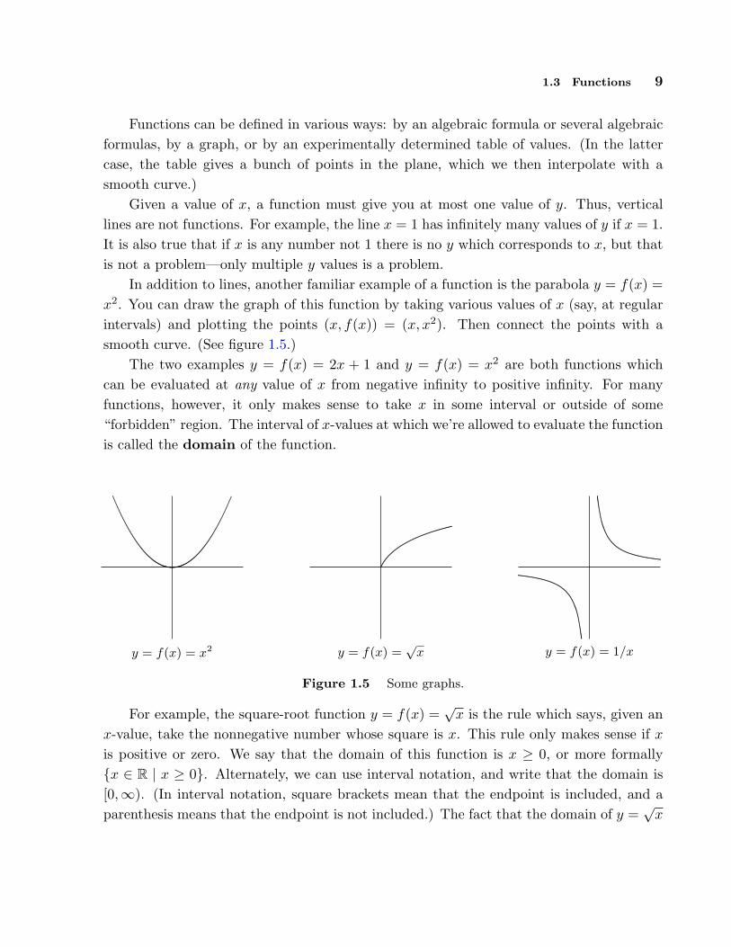
In addition to lines, another familiar example of a function is the parabola y = f(x) =x2. You can draw the graph of this function by taking various values of x (say, at regularintervals) and plotting the points (x, f(x)) = (x, x2). Then connect the points with asmooth curve. (See figure 1.5.)
The two examples y = f(x) = 2x + 1 and y = f(x) = x2 are both functions whichcan be evaluated at any value of x from negative infinity to positive infinity. For manyfunctions, however, it only makes sense to take x in some interval or outside of some“forbidden” region. The interval of x-values at which we’re allowed to evaluate the functionis called the domain of the function.
.....................................................................................................................................................................................................................................................................................................................................................
y = f(x) = x2
........................................................
..................................
.....................................................
......
y = f(x) =√
x
...................................................................................................................................................................................
...................................................................................................................................................................................
y = f(x) = 1/x
Figure 1.5 Some graphs.
For example, the square-root function y = f(x) =√
x is the rule which says, given anx-value, take the nonnegative number whose square is x. This rule only makes sense if x
is positive or zero. We say that the domain of this function is x ≥ 0, or more formally{x ∈ R | x ≥ 0}. Alternately, we can use interval notation, and write that the domain is[0,∞). (In interval notation, square brackets mean that the endpoint is included, and aparenthesis means that the endpoint is not included.) The fact that the domain of y =
√x
10 Chapter 1 Analytic Geometry
is x ≥ 0 means that in the graph of this function ((see figure 1.5) we have points (x, y)only above x-values on the right side of the x-axis.
Another example of a function whose domain is not the entire x-axis is: y = f(x) =1/x, the reciprocal function. We cannot substitute x = 0 in this formula. The functionmakes sense, however, for any nonzero x, so we take the domain to be: x 6= 0. The graphof this function does not have any point (x, y) with x = 0. As x gets close to 0 from eitherside, the graph goes off toward infinity. We call the vertical line x = 0 an asymptote.
To summarize, two reasons why certain x-values are excluded from the domain of afunction are that (i) we cannot divide by zero, and (ii) we cannot take the square rootof a negative number. We will encounter some other ways in which functions might beundefined later.
Another reason why the domain of a function might be restricted is that in a givensituation the x-values outside of some range might have no practical meaning. For example,if y is the area of a square of side x, then we can write y = f(x) = x2. In a purelymathematical context the domain of the function y = x2 is all x. But in the story-problemcontext of finding areas of squares, we restrict the domain to x > 0, because a square withnegative or zero side makes no sense.
In a problem in pure mathematics, we usually take the domain to be all values of x
at which the formulas can be evaluated. But in a story problem there might be furtherrestrictions on the domain because only certain values of x are of interest or make practicalsense.
In a story problem, often letters different from x and y are used. For example, thevolume V of a sphere is a function of the radius r, given by the formula V = f(r) = 4/3πr3.Also, letters different from f may be used. For example, if y is the velocity of something attime t, we write y = v(t) with the letter v (instead of f) standing for the velocity function(and t playing the role of x).
The letter playing the role of x is called the independent variable, and the letterplaying the role of y is called the dependent variable (because its value “depends on”the value of the independent variable). In story problems, when one has to translate fromEnglish into mathematics, a crucial step is to determine what letters stand for variables.If only words and no letters are given, then you have to decide which letters to use. Someletters are traditional. For example, almost always, t stands for time.
EXAMPLE 1.3 An open-top box is made from an a×b rectangular piece of cardboardby cutting out a square of side x from each of the four corners, and then folding the sidesup and sealing them with duct tape. Find a formula for the volume V of the box as afunction of x, and find the domain of this function.

1.3 Functions 11
Here the box we get will have height x and rectangular base of dimensions a− 2x byb− 2x. Thus,
V = f(x) = x(a− 2x)(b− 2x).
Here a and b are constants, and V is the variable that depends on x, i.e., V is playing therole of y.
This formula makes mathematical sense for any x, but in the story problem the domainis much less. In the first place, x must be positive. In the second place, it must be lessthan half the length of either of the sides of the cardboard. Thus, the domain is
0 < x <12(minimum of a and b).
In interval notation we write: the domain is the interval (0, min(a, b)/2).
EXAMPLE 1.4 Circle of radius r centered at the origin The equation forthis circle is usually given in the form x2 + y2 = r2. To write the equation in the formy = f(x) we solve for y, obtaining y = ±√r2 − x2. But this is not a function, becausewhen we substitute a value in (−r, r) for x there are two corresponding values of y. Toget a function, we must choose one of the two signs in front of the square root. If wechoose the positive sign, for example, we get the upper semicircle y = f(x) =
√r2 − x2
(see figure 1.6). The domain of this function is the interval [−r, r], i.e., x must be between−r and r (including the endpoints). If x is outside of that interval, then r2−x2 is negative,and we cannot take the square root. In terms of the graph, this just means that there areno points on the curve whose x-coordinate is greater than r or less than −r.
−r r
........
........
........
........
............................................................................................................................
......................
........................
...........................
..................................
.......................................................
........................................................................................................................................................................................................................................................................................................................................................................................................
Figure 1.6 Upper semicircle y =√
r2 − x2
12 Chapter 1 Analytic Geometry
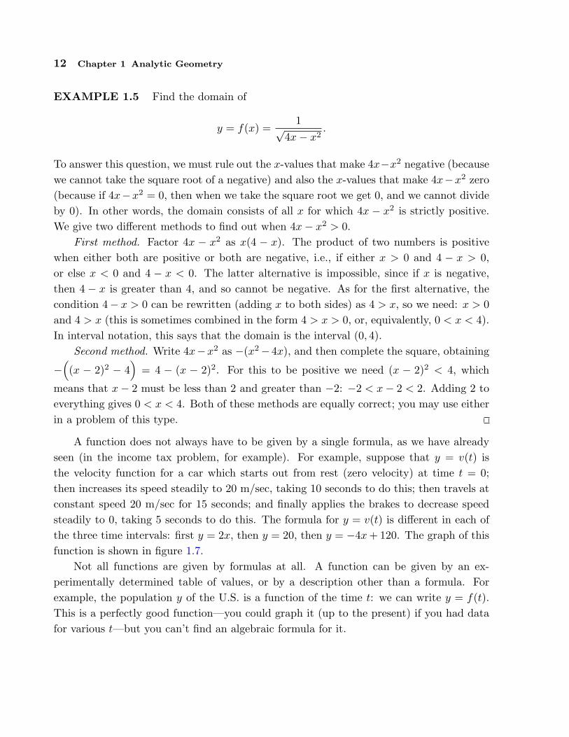
EXAMPLE 1.5 Find the domain of
y = f(x) =1√
4x− x2.
To answer this question, we must rule out the x-values that make 4x−x2 negative (becausewe cannot take the square root of a negative) and also the x-values that make 4x−x2 zero(because if 4x−x2 = 0, then when we take the square root we get 0, and we cannot divideby 0). In other words, the domain consists of all x for which 4x − x2 is strictly positive.We give two different methods to find out when 4x− x2 > 0.
First method. Factor 4x − x2 as x(4 − x). The product of two numbers is positivewhen either both are positive or both are negative, i.e., if either x > 0 and 4 − x > 0,or else x < 0 and 4 − x < 0. The latter alternative is impossible, since if x is negative,then 4 − x is greater than 4, and so cannot be negative. As for the first alternative, thecondition 4− x > 0 can be rewritten (adding x to both sides) as 4 > x, so we need: x > 0and 4 > x (this is sometimes combined in the form 4 > x > 0, or, equivalently, 0 < x < 4).In interval notation, this says that the domain is the interval (0, 4).
Second method. Write 4x−x2 as −(x2−4x), and then complete the square, obtaining
−((x − 2)2 − 4
)= 4 − (x − 2)2. For this to be positive we need (x − 2)2 < 4, which
means that x− 2 must be less than 2 and greater than −2: −2 < x− 2 < 2. Adding 2 toeverything gives 0 < x < 4. Both of these methods are equally correct; you may use eitherin a problem of this type.
A function does not always have to be given by a single formula, as we have alreadyseen (in the income tax problem, for example). For example, suppose that y = v(t) isthe velocity function for a car which starts out from rest (zero velocity) at time t = 0;then increases its speed steadily to 20 m/sec, taking 10 seconds to do this; then travels atconstant speed 20 m/sec for 15 seconds; and finally applies the brakes to decrease speedsteadily to 0, taking 5 seconds to do this. The formula for y = v(t) is different in each ofthe three time intervals: first y = 2x, then y = 20, then y = −4x + 120. The graph of thisfunction is shown in figure 1.7.
Not all functions are given by formulas at all. A function can be given by an ex-perimentally determined table of values, or by a description other than a formula. Forexample, the population y of the U.S. is a function of the time t: we can write y = f(t).This is a perfectly good function—you could graph it (up to the present) if you had datafor various t—but you can’t find an algebraic formula for it.

1.3 Functions 13
10 25 30
0
10
20
.............................................................................................................................................................................................................................................................................................................................................................................................................................................................................................................................................................................................................................................................................................................................................................................................................................................................................................................................................................................................. t
v
Figure 1.7 A velocity function.
Exercises
Find the domain of each of the following functions:
1. y = f(x) =√
2x− 3 ⇒2. y = f(x) = 1/(x + 1) ⇒3. y = f(x) = 1/(x2 − 1) ⇒4. y = f(x) =
p−1/x ⇒
5. y = f(x) = 3√
x ⇒6. y = f(x) = 4
√x ⇒
7. y = f(x) =p
r2 − (x− h)2 , where r and h are positive constants. ⇒8. y = f(x) =
p1− (1/x) ⇒
9. y = f(x) = 1/p
1− (3x)2 ⇒10. y = f(x) =
√x + 1/(x− 1) ⇒
11. y = f(x) = 1/(√
x− 1) ⇒
12. Find the domain of h(x) =
(x2 − 9)/(x− 3) x 6= 36 if x = 3.
⇒
13. Suppose f(x) = 3x − 9 and g(x) =√
x. What is the domain of the composition (g ◦ f)(x)?(Recall that composition is defined as (g ◦ f)(x) = g(f(x)).) What is the domain of(f ◦ g)(x)? ⇒
14. A farmer wants to build a fence along a river. He has 500 feet of fencing and wants to enclosea rectangular pen on three sides (with the river providing the fourth side). If x is the lengthof the side perpendicular to the river, determine the area of the pen as a function of x. Whatis the domain of this function? ⇒
15. A can in the shape of a cylinder is to be made with a total of 100 square centimeters ofmaterial in the side, top, and bottom; the manufacturer wants the can to hold the maximumpossible volume. Write the volume as a function of the radius r of the can; find the domainof the function. ⇒

14 Chapter 1 Analytic Geometry
16. A can in the shape of a cylinder is to be made to hold a volume of one liter (1000 cubiccentimeters). The manufacturer wants to use the least possible material for the can. Writethe surface area of the can (total of the top, bottom, and side) as a function of the radius rof the can; find the domain of the function. ⇒
1.4 Shifts and Dilations
Many functions in applications are built up from simple functions by inserting constantsin various places. It is important to understand the effect such constants have on theappearance of the graph.
Horizontal shifts. If you replace x by x − C everywhere it occurs in the formula forf(x), then the graph shifts over C to the right. (If C is negative, then this means that thegraph shifts over |C| to the left.) For example, the graph of y = (x−2)2 is the x2-parabolashifted over to have its vertex at the point 2 on the x-axis. The graph of y = (x + 1)2 isthe same parabola shifted over to the left so as to have its vertex at −1 on the x-axis.
Vertical shifts. If you replace y by y − D, then the graph moves up D units. (If D isnegative, then this means that the graph moves down |D| units.) If the formula is writtenin the form y = f(x) and if y is replaced by y−D to get y−D = f(x), we can equivalentlymove D to the other side of the equation and write y = f(x) + D. Thus, this principalcan be stated: to get the graph of y = f(x) + D, take the graph of y = f(x) and move itD units up. For example, the function y = x2 − 4x = (x − 2)2 − 4 can be obtained fromy = (x− 2)2 (see the last paragraph) by moving the graph 4 units down. The result is thex2-parabola shifted 2 units to the right and 4 units down so as to have its vertex at thepoint (2,−4).
Warning. Do not confuse f(x)+D and f(x+D). For example, if f(x) is the function x2,then f(x) + 2 is the function x2 + 2, while f(x + 2) is the function (x + 2)2 = x2 + 4x + 4.
EXAMPLE 1.6 Circles An important example of the above two principles startswith the circle x2 + y2 = r2. This is the circle of radius r centered at the origin. (As wesaw, this is not a single function y = f(x), but rather two functions y = ±√r2 − x2 puttogether; in any case, the two shifting principles apply to equations like this one that arenot in the form y = f(x).) If we replace x by x− C and replace y by y −D—getting theequation (x − C)2 + (y − D)2 = r2—the effect on the circle is to move it C to the rightand D up, thereby obtaining the circle of radius r centered at the point (C, D). This tellsus how to write the equation of any circle, not necessarily centered at the origin.
We will later want to use two more principles concerning the effects of constants onthe appearance of the graph of a function.

1.4 Shifts and Dilations 15
Horizontal dilation. If x is replaced by x/A in a formula and A > 1, then the effect onthe graph is to expand it by a factor of A in the x-direction (away from the y-axis). If A
is between 0 and 1 then the effect on the graph is to contract by a factor of 1/A (towardsthe y-axis). We use the word “dilate” in both cases.
For example, replacing x by x/0.5 = 2x has the effect of contracting toward the y-axisby a factor of 2. If A is negative, we dilate by a factor of |A| and then flip about they-axis. Thus, replacing x by −x has the effect of taking the mirror image of the graphwith respect to the y-axis. For example, the function y =
√−x, which has domain x ≤ 0,is obtained by taking the graph of
√x and flipping it around the y-axis into the second
quadrant.
Vertical dilation. If y is replaced by y/B in a formula and B > 0, then the effect onthe graph is to dilate it by a factor of B in the vertical direction. Note that if we havea function y = f(x), replacing y by y/B is equivalent to multiplying the function on theright by B: y = Bf(x). The effect on the graph is to expand the picture away from thex-axis by a factor of B if B > 1, to contract it toward the x-axis by a factor of 1/B if0 < B < 1, and to dilate by |B| and then flip about the x-axis if B is negative.
EXAMPLE 1.7 Ellipses A basic example of the two expansion principles is givenby an ellipse of semimajor axis a and semiminor axis b. We get such an ellipse bystarting with the unit circle—the circle of radius 1 centered at the origin, the equationof which is x2 + y2 = 1—and dilating by a factor of a horizontally and by a factor of b
vertically. To get the equation of the resulting ellipse, which crosses the x-axis at ±a andcrosses the y-axis at ±b, we replace x by x/a and y by y/b in the equation for the unitcircle. This gives (x
a
)2
+(y
b
)2
= 1.
Finally, if you want to analyze a function that involves both shifts and dilations, itis usually simplest to work with the dilations first, and then the shifts. For instance, ifyou want to dilate a function by a factor of A in the x-direction and then shift C to theright, you do this by replacing x first by x/A and then by (x− C) in the formula. As anexample, suppose that, after dilating our unit circle by a in the x-direction and by b in they-direction to get the ellipse in the last paragraph, we then wanted to shift it a distanceh to the right and a distance k upward, so as to be centered at the point (h, k). The new
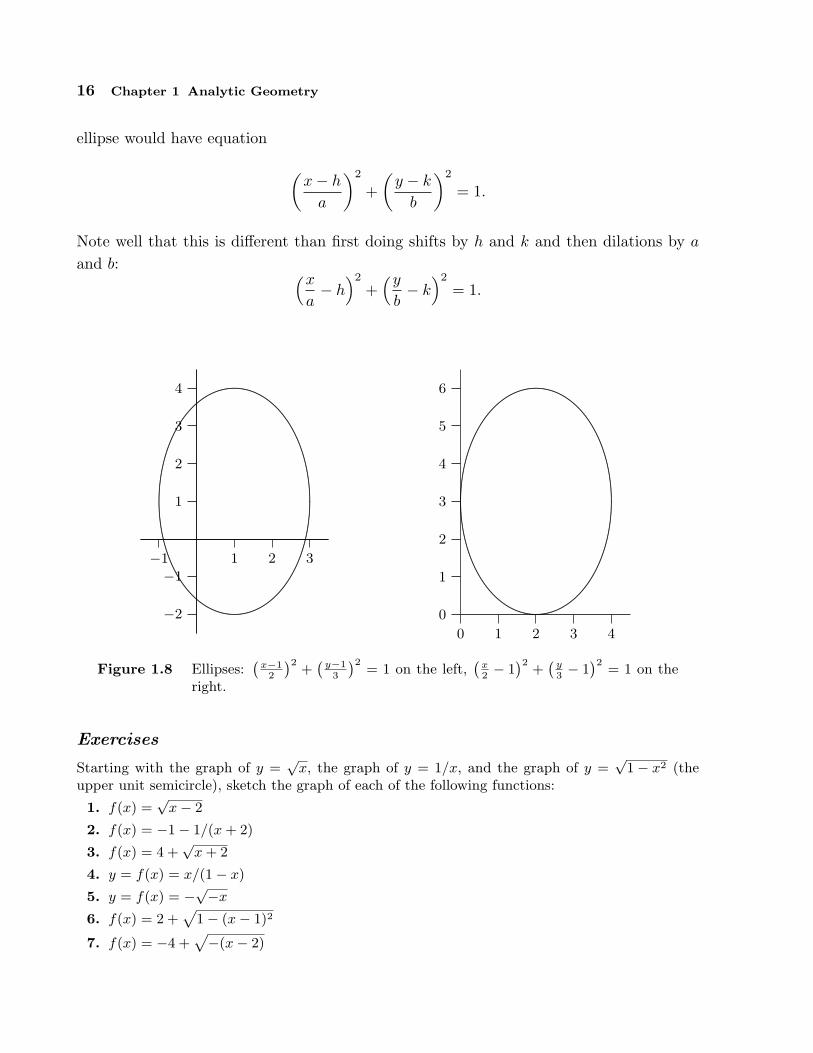
16 Chapter 1 Analytic Geometry
ellipse would have equation
(x− h
a
)2
+(
y − k
b
)2
= 1.
Note well that this is different than first doing shifts by h and k and then dilations by a
and b: (x
a− h
)2
+(y
b− k
)2
= 1.
1 2 3−1
1
2
3
4
−2
−1
........
........
........
........
........
.........................................................................................................
.....................
..........................
.....................................................................................................................................................................................................................................................................................................................................................................................................................................................................................................................................................................................
........................................................................................................................................................................................
0 1 2 3 4
0
1
2
3
4
5
6
........
........
........
........
........
.........................................................................................................
.....................
..........................
.....................................................................................................................................................................................................................................................................................................................................................................................................................................................................................................................................................................................
........................................................................................................................................................................................
Figure 1.8 Ellipses:`
x−12
´2+`
y−13
´2= 1 on the left,
`x2− 1´2
+`
y3− 1´2
= 1 on theright.
Exercises
Starting with the graph of y =√
x, the graph of y = 1/x, and the graph of y =√
1− x2 (theupper unit semicircle), sketch the graph of each of the following functions:
1. f(x) =√
x− 2
2. f(x) = −1− 1/(x + 2)
3. f(x) = 4 +√
x + 2
4. y = f(x) = x/(1− x)
5. y = f(x) = −√−x
6. f(x) = 2 +p
1− (x− 1)2
7. f(x) = −4 +p−(x− 2)

1.4 Shifts and Dilations 17
8. f(x) = 2p
1− (x/3)2
9. f(x) = 1/(x + 1)
10. f(x) = 4 + 2p
1− (x− 5)2/9
11. f(x) = 1 + 1/(x− 1)
12. f(x) =p
100− 25(x− 1)2 + 2
The graph of f(x) is shown below. Sketch the graphs of the following functions.
13. y = f(x− 1)
1 2 3
−1
0
1
2
........
........
........
........
........
........
........
........
........
........
........
........
........
........
........
........
........
........................................................................................................................................................................................................
........................................................................................................................................................................
14. y = 1 + f(x + 2)
15. y = 1 + 2f(x)
16. y = 2f(3x)
17. y = 2f(3(x− 2)) + 1
18. y = (1/2)f(3x− 3)
19. y = f(1 + x/3) + 2


2Instantaneous Rate Of Change:
The Derivative
2.1 The slope of a function
Suppose that y is a function of x, say y = f(x). It is often necessary to know how sensitivethe value of y is to small changes in x.
EXAMPLE 2.1 Take, for example, y = f(x) =√
625− x2 (the upper semicircle ofradius 25 centered at the origin). When x = 7, we find that y =
√625− 49 = 24. Suppose
we want to know how much y changes when x increases a little, say to 7.1 or 7.01.In the case of a straight line y = mx+b, the slope m = ∆y/∆x measures the change in
y per unit change in x. This can be interpreted as a measure of “sensitivity”; for example,if y = 100x + 5, a small change in x corresponds to a change one hundred times as largein y, so y is quite sensitive to changes in x.
Let us look at the same ratio ∆y/∆x for our function y = f(x) =√
625− x2 when x
changes from 7 to 7.1. Here ∆x = 7.1− 7 = 0.1 is the change in x, and
∆y = f(x + ∆x)− f(x) = f(7.1)− f(7)
=√
625− 7.12 −√
625− 72 ≈ 23.9706− 24 = −0.0294.
Thus, ∆y/∆x ≈ −0.0294/0.1 = −0.294. This means that y changes by less than onethird the change in x, so apparently y is not very sensitive to changes in x at x = 7.We say “apparently” here because we don’t really know what happens between 7 and 7.1.Perhaps y changes dramatically as x runs through the values from 7 to 7.1, but at 7.1 y
19

20 Chapter 2 Instantaneous Rate Of Change: The Derivative
just happens to be close to its value at 7. This is not in fact the case for this particularfunction, but we don’t yet know why.
One way to interpret the above calculation is by reference to a line. We have computedthe slope of the line through (7, 24) and (7.1, 23.9706), called a chord of the circle. Ingeneral, if we draw the chord from the point (7, 24) to a nearby point on the semicircle(7 + ∆x, f(7 + ∆x)), the slope of this chord is the so-called difference quotient
slope of chord =f(7 + ∆x)− f(7)
∆x=
√625− (7 + ∆x)2 − 24
∆x.
For example, if x changes only from 7 to 7.01, then the difference quotient (slope of thechord) is approximately equal to (23.997081 − 24)/0.01 = −0.2919. This is slightly lesssteep than the chord from (7, 24) to (7.1, 23.9706).
As the second value 7 + ∆x moves in towards 7, the chord joining (7, f(7)) to (7 +∆x, f(7 + ∆x)) shifts slightly. As indicated in figure 2.1, as ∆x gets smaller and smaller,the chord joining (7, 24) to (7+∆x, f(7+∆x)) gets closer and closer to the tangent lineto the circle at the point (7, 24). (Recall that the tangent line is the line that just grazesthe circle at that point, i.e., it doesn’t meet the circle at any second point.) Thus, as ∆x
gets smaller and smaller, the slope ∆y/∆x of the chord gets closer and closer to the slopeof the tangent line. This is actually quite difficult to see when ∆x is small, because of thescale of the graph. The values of ∆x used for the figure are 1, 5, 10 and 15, not really verysmall values. The tangent line is the one that is uppermost at the right hand endpoint.
........
........
........
........
........
........
......................................................................................................................................................
.....................
......................
........................
...........................
...............................
.......................................
..................................................................
......................................
5
10
15
20
25
5 10 15 20 25
.....................................................................................................................................................................................................................................................................................................................
.......................................................................................................................................................................................................................................................................................................................
.................................................................................................................................................................................................................................................................................................................................
.....................................................................................................................................................................................................................................................................................................................................................
.............................................................................................................................................................................................................................................................................................................................................................................................................
Figure 2.1 Chords approximating the tangent line.
So far we have found the slopes of two chords that should be close to the slope ofthe tangent line, but what is the slope of the tangent line exactly? Since the tangent line
2.1 The slope of a function 21
touches the circle at just one point, we will never be able to calculate its slope directly,using two “known” points on the line. What we need is a way to capture what happensto the slopes of the chords as they get “closer and closer” to the tangent line.
Instead of looking at more particular values of ∆x, let’s see what happens if we dosome algebra with the difference quotient using just ∆x. The slope of a chord from (7, 24)to a nearby point is given by
√625− (7 + ∆x)2 − 24
∆x=
√625− (7 + ∆x)2 − 24
∆x
√625− (7 + ∆x)2 + 24√625− (7 + ∆x)2 + 24
=625− (7 + ∆x)2 − 242
∆x(√
625− (7 + ∆x)2 + 24)
=49− 49− 14∆x−∆x2
∆x(√
625− (7 + ∆x)2 + 24)
=∆x(−14−∆x)
∆x(√
625− (7 + ∆x)2 + 24)
=−14−∆x√
625− (7 + ∆x)2 + 24
Now, can we tell by looking at this last formula what happens when ∆x gets very close tozero? The numerator clearly gets very close to −14 while the denominator gets very close to√
625− 72 +24 = 48. Is the fraction therefore very close to −14/48 = −7/24 ∼= −0.29167?It certainly seems reasonable, and in fact it is true: as ∆x gets closer and closer to zero,the difference quotient does in fact get closer and closer to −7/24, and so the slope of thetangent line is exactly −7/24.
What about the slope of the tangent line at x = 12? Well, 12 can’t be all that differentfrom 7; we just have to redo the calculation with 12 instead of 7. This won’t be hard, butit will be a bit tedious. What if we try to do all the algebra without using a specific valuefor x? Let’s copy from above, replacing 7 by x. We’ll have to do a bit more than that—for

22 Chapter 2 Instantaneous Rate Of Change: The Derivative
example, the “24” in the calculation came from√
625− 72, so we’ll need to fix that too.√
625− (x + ∆x)2 −√625− x2
∆x=
=
√625− (x + ∆x)2 −√625− x2
∆x
√625− (x + ∆x)2 +
√625− x2
√625− (x + ∆x)2 +
√625− x2
=625− (x + ∆x)2 − 625 + x2
∆x(√
625− (x + ∆x)2 +√
625− x2)
=625− x2 − 2x∆x−∆x2 − 625 + x2
∆x(√
625− (x + ∆x)2 +√
625− x2)
=∆x(−2x−∆x)
∆x(√
625− (x + ∆x)2 +√
625− x2)
=−2x−∆x√
625− (x + ∆x)2 +√
625− x2
Now what happens when ∆x is very close to zero? Again it seems apparent that thequotient will be very close to
−2x√625− x2 +
√625− x2
=−2x
2√
625− x2=
−x√625− x2
.
Replacing x by 7 gives −7/24, as before, and now we can easily do the computation for 12or any other value of x between −25 and 25.
So now we have a single, simple formula, −x/√
625− x2, that tells us the slope of thetangent line for any value of x. This slope, in turn, tells us how sensitive the value of y isto changes in the value of x.
What do we call such a formula? That is, a formula with one variable, so that substi-tuting an “input” value for the variable produces a new “output” value? This is a function.Starting with one function,
√625− x2, we have derived, by means of some slightly nasty
algebra, a new function, −x/√
625− x2, that gives us important information about theoriginal function. This new function in fact is called the derivative of the original func-tion. If the original is referred to as f or y then the derivative is often written f ′ or y′ andpronounced “f prime” or “y prime”, so in this case we might write f ′(x) = −x/
√625− x2.
At a particular point, say x = 7, we say that f ′(7) = −7/24 or “f prime of 7 is −7/24” or“the derivative of f at 7 is −7/24.”
To summarize, we compute the derivative of f(x) by forming the difference quotient
f(x + ∆x)− f(x)∆x
,

2.1 The slope of a function 23
which is the slope of a line, then we figure out what happens when ∆x gets very close to0.
We should note that in the particular case of a circle, there’s a simple way to find thederivative. Since the tangent to a circle at a point is perpendicular to the radius drawnto the point of contact, its slope is the negative reciprocal of the slope of the radius. Theradius joining (0, 0) to (7, 24) has slope 24/7. Hence, the tangent line has slope −7/24. Ingeneral, a radius to the point (x,
√625− x2) has slope
√625− x2/x, so the slope of the
tangent line is −x/√
625− x2, as before. It is NOT always true that a tangent line isperpendicular to a line from the origin—don’t use this shortcut in any other circumstance.
As above, and as you might expect, for different values of x we generally get differentvalues of the derivative f ′(x). Could it be that the derivative always has the same value?This would mean that the slope of f , or the slope of its tangent line, is the same everywhere.One curve that always has the same slope is a line; it seems odd to talk about the tangentline to a line, but if it makes sense at all the tangent line must be the line itself. It is nothard to see that the derivative of f(x) = mx + b is f ′(x) = m; see exercise 6.
Exercises
1. Draw the graph of the function y = f(x) =√
169− x2 between x = 0 and x = 13. Find theslope ∆y/∆x of the chord between the points of the circle lying over (a) x = 12 and x = 13,(b) x = 12 and x = 12.1, (c) x = 12 and x = 12.01, (d) x = 12 and x = 12.001. Now usethe geometry of tangent lines on a circle to find (e) the exact value of the derivative f ′(12).Your answers to (a)–(d) should be getting closer and closer to your answer to (e). ⇒
2. Use geometry to find the derivative f ′(x) of the function f(x) =√
625− x2 in the text foreach of the following x: (a) 20, (b) 24, (c) −7, (d) −15. Draw a graph of the upper semicircle,and draw the tangent line at each of these four points. ⇒
3. Draw the graph of the function y = f(x) = 1/x between x = 1/2 and x = 4. Find the slopeof the chord between (a) x = 3 and x = 3.1, (b) x = 3 and x = 3.01, (c) x = 3 and x = 3.001.Now use algebra to find a simple formula for the slope of the chord between (3, f(3)) and(3 + ∆x, f(3 + ∆x)). Determine what happens when ∆x approaches 0. In your graph ofy = 1/x, draw the straight line through the point (3, 1/3) whose slope is this limiting valueof the difference quotient as ∆x approaches 0. ⇒
4. Find an algebraic expression for the difference quotient“f(1+∆x)−f(1)
”/∆x when f(x) =
x2 − (1/x). Simplify the expression as much as possible. Then determine what happens as∆x approaches 0. That value is f ′(1). ⇒
5. Draw the graph of y = f(x) = x3 between x = 0 and x = 1.5. Find the slope of the chordbetween (a) x = 1 and x = 1.1, (b) x = 1 and x = 1.001, (c) x = 1 and x = 1.00001.Then use algebra to find a simple formula for the slope of the chord between 1 and 1 + ∆x.(Use the expansion (A + B)3 = A3 + 3A2B + 3AB2 + B3.) Determine what happens as ∆xapproaches 0, and in your graph of y = x3 draw the straight line through the point (1, 1)whose slope is equal to the value you just found. ⇒
24 Chapter 2 Instantaneous Rate Of Change: The Derivative
6. Find an algebraic expression for the difference quotient (f(x+∆x)− f(x))/∆x when f(x) =mx + b. Simplify the expression as much as possible. Then determine what happens as ∆xapproaches 0. That value is f ′(x). ⇒
7. Sketch the unit circle. Discuss the behavior of the slope of the tangent line at various anglesaround the circle. Which trigonometric function gives the slope of the tangent line at anangle θ? Why? Hint: think in terms of ratios of sides of triangles.
8. Sketch the parabola y = x2. For what values of x on the parabola is the slope of the tangentline positive? Negative? What do you notice about the graph at the point(s) where the signof the slope changes from positive to negative and vice versa?
2.2 An example
We started the last section by saying, “It is often necessary to know how sensitive thevalue of y is to small changes in x.” We have seen one purely mathematical example ofthis: finding the “steepness” of a curve at a point is precisely this problem. Here is a moreapplied example.
With careful measurement it might be possible to discover that a dropped ball hasheight h(t) = h0−kt2, t seconds after it is released. (Here h0 is the initial height of the ball,when t = 0, and k is some number determined by the experiment.) A natural question isthen, “How fast is the ball going at time t?” We can certainly get a pretty good idea with alittle simple arithmetic. To make the calculation more concrete, let’s say h0 = 100 metersand k = 4.9 and suppose we’re interested in the speed at t = 2. We know that when t = 2the height is 100−4 ·4.9 = 80.4. A second later, at t = 3, the height is 100−9 ·4.9 = 55.9,so in that second the ball has traveled 80.4 − 55.9 = 24.5 meters. This means that theaverage speed during that time was 24.5 meters per second. So we might guess that 24.5meters per second is not a terrible estimate of the speed at t = 2. But certainly we cando better. At t = 2.5 the height is 100− 4.9(2.5)2 = 69.375. During the half second fromt = 2 to t = 2.5 the ball dropped 80.4 − 69.375 = 11.025 meters, at an average speed of11.025/(1/2) = 22.05 meters per second; this should be a better estimate of the speed att = 2. So it’s clear now how to get better and better approximations: compute averagespeeds over shorter and shorter time intervals. Between t = 2 and t = 2.01, for example,the ball drops 0.19649 meters in one hundredth of a second, at an average speed of 19.649meters per second.
We can’t do this forever, and we still might reasonably ask what the actual speedprecisely at t = 2 is. If ∆t is some tiny amount of time, what we want to know is whathappens to the average speed (h(2)−h(2+∆t))/∆t as ∆t gets smaller and smaller. Doing

2.2 An example 25
a bit of algebra:
h(2)− h(2 + ∆t)∆t
=80.4− (100− 4.9(2 + ∆t)2)
∆t
=80.4− 100 + 19.6 + 19.6∆t + 4.9∆t2
∆t
=19.6∆t + 4.9∆t2
∆t
= 19.6 + 4.9∆t
When ∆t is very small, this is very close to 19.6, and indeed it seems clear that as ∆t
goes to zero, the average speed goes to 19.6, so the exact speed at t = 2 is 19.6 meters persecond. This calculation should look very familiar. In the language of the previous section,we might have started with f(x) = 100− 4.9x2 and asked for the slope of the tangent lineat x = 2. We would have answered that question by computing
f(2 + ∆x)− f(2)∆x
=−19.6∆x− 4.9∆x2
∆x= −19.6− 4.9∆x
The algebra is the same, except that following the pattern of the previous section thesubtraction would be reversed, and we would say that the slope of the tangent line is−19.6. Indeed, in hindsight, perhaps we should have subtracted the other way even forthe dropping ball. At t = 2 the height is 80.4; one second later the height is 55.9. Theusual way to compute a “distance traveled” is to subtract the earlier position from thelater one, or 55.9 − 80.4 = −24.5. This tells us that the distance traveled is 24.5 meters,and the negative sign tells us that the height went down during the second. If we continuethe original calculation we then get −19.4 meters per second as the exact speed at t = 2.If we interpret the negative sign as meaning that the motion is downward, which seemsreasonable, then in fact this is the same answer as before, but with even more information,since the numerical answer contains the direction of motion as well as the speed. Thus,the speed of the ball is the value of the derivative of a certain function, namely, of thefunction that gives the position of the ball.
The upshot is that this problem, finding the speed of the ball, is exactly the sameproblem mathematically as finding the slope of a curve. This may already be enoughevidence to convince you that whenever some quantity is changing (the height of a curveor the height of a ball or the size of the economy or the distance of a space probe fromearth or the population of the world) the rate at which the quantity is changing can, inprinciple, be computed in exactly the same way, by finding a derivative.

26 Chapter 2 Instantaneous Rate Of Change: The Derivative
Exercises
1. An object is traveling in a straight line so that its position (that is, distance from some fixedpoint) is given by this table:
time (seconds) 0 1 2 3
distance (meters) 0 10 25 60
Find the average speed of the object during the following time intervals: [0, 1], [0, 2], [0, 3],[1, 2], [1, 3], [2, 3]. If you had to guess the speed at t = 2 just on the basis of these, whatwould you guess? ⇒
2. Let y = f(t) = t2, where t is the time in seconds and y is the distance in meters that anobject falls on a certain airless planet. Draw a graph of this function between t = 0 andt = 3. Make a table of the average speed of the falling object between (a) 2 sec and 3 sec,(b) 2 sec and 2.1 sec, (c) 2 sec and 2.01 sec, (d) 2 sec and 2.001 sec. Then use algebra to finda simple formula for the average speed between time 2 and time 2 + ∆t. (If you substitute∆t = 1, 0.1, 0.01, 0.001 in this formula you should again get the answers to parts (a)–(d).)Next, in your formula for average speed (which should be in simplified form) determine whathappens as ∆t approaches zero. This is the instantaneous speed. Finally, in your graphof y = t2 draw the straight line through the point (2, 4) whose slope is the instantaneousvelocity you just computed; it should of course be the tangent line. ⇒
3. If an object is dropped from an 80-meter high window, its height y above the ground at timet seconds is given by the formula y = f(t) = 80−4.9t2. (Here we are neglecting air resistance;the graph of this function was shown in figure 1.1.) Find the average velocity of the fallingobject between (a) 1 sec and 1.1 sec, (b) 1 sec and 1.01 sec, (c) 1 sec and 1.001 sec. Now usealgebra to find a simple formula for the average velocity of the falling object between 1 secand 1 + ∆t sec. Determine what happens to this average velocity as ∆t approaches 0. Thatis the instantaneous velocity at time t = 1 second (it will be negative, because the object isfalling). ⇒
2.3 Limits
In the previous two sections we computed some quantities of interest (slope, speed) byseeing that some expression “goes to” or “approaches” or “gets really close to” a particularvalue. In the examples we saw, this idea may have been clear enough, but it is too fuzzyto rely on in more difficult circumstances. In this section we will see how to make the ideamore precise.
There is an important feature of the examples we have seen. Consider again theformula
−19.6∆x− 4.9∆x2
∆x.
We wanted to know what happens to this fraction as “∆x goes to zero.” Because we wereable to simplify the fraction, it was easy to see the answer, but it was not quite as simple
2.3 Limits 27
as “substituting zero for ∆x,” as that would give
−19.6 · 0− 4.9 · 00
,
which is meaningless. The quantity we are really interested in does not make sense “atzero,” and this is why the answer to the original problem (finding a speed or a slope) wasnot immediately obvious. In other words, we are generally going to want to figure out whata quantity “approaches” in situations where we can’t merely plug in a value. If you wouldlike to think about a hard example (which we will analyze later) consider what happensto (sin x)/x as x approaches zero.
EXAMPLE 2.2 Does√
x approach 1.41 as x approaches 2? In this case it is possibleto compute the actual value
√2 to a high precision to answer the question. But since
in general we won’t be able to do that, let’s not. We might start by computing√
x forvalues of x close to 2, as we did in the previous sections. Here are some values:
√2.05 =
1.431782106,√
2.04 = 1.428285686,√
2.03 = 1.424780685,√
2.02 = 1.421267040,√
2.01 =1.417744688,
√2.005 = 1.415980226,
√2.004 = 1.415627070,
√2.003 = 1.415273825,√
2.002 = 1.414920492,√
2.001 = 1.414567072. So it looks at least possible that indeedthese values “approach” 1.41—already
√2.001 is quite close. If we continue this process,
however, at some point we will appear to “stall.” In fact,√
2 = 1.414213562 . . ., so we willnever even get as far as 1.4142, no matter how long we continue the sequence.
So in a fuzzy, everyday sort of sense, it is true that√
x “gets close to” 1.41, but itdoes not “approach” 1.41 in the sense we want. To compute an exact slope or an exactspeed, what we want to know is that a given quantity becomes “arbitrarily close” to afixed value, meaning that the first quantity can be made “as close as we like” to the fixedvalue. Consider again the quantities
−19.6∆x− 4.9∆x2
∆x= −19.6− 4.9∆x.
These two quantities are equal as long as ∆x is not zero; if ∆x is zero, the left handquantity is meaningless, while the right hand one is −19.6. Can we say more than wedid before about why the right hand side “approaches” −19.6, in the desired sense? Canwe really make it “as close as we want” to −19.6? Let’s try a test case. Can we make−19.6− 4.9∆x within one millionth (0.000001) of −19.6? The values within a millionth of−19.6 are those in the interval (−19.600001,−19.599999). As ∆x approaches zero, does−19.6− 4.9∆x eventually reside inside this interval? If ∆x is positive, this would require

28 Chapter 2 Instantaneous Rate Of Change: The Derivative
that −19.6 − 4.9∆x > −19.600001. This is something we can manipulate with a littlealgebra:
−19.6− 4.9∆x > −19.600001
−4.9∆x > −0.000001
∆x < −0.000001/− 4.9
∆x < 0.0000002040816327 . . .
Thus, we can say with certainty that if ∆x is positive and less than 0.0000002, then∆x < 0.0000002040816327 . . . and so −19.6− 4.9∆x > −19.600001. We could do a similarcalculation if ∆x is negative.
So now we know that we can make −19.6− 4.9∆x within one millionth of −19.6. Butcan we make it “as close as we want”? In this case, it is quite simple to see that the answeris yes, by modifying the calculation we’ve just done. It may be helpful to think of this asa game. I claim that I can make −19.6− 4.9∆x as close as you desire to −19.6 by making∆x “close enough” to zero. So the game is: you give me a number, like 10−6, and I haveto come up with a number representing how close ∆x must be to zero to guarantee that−19.6− 4.9∆x is at least as close to −19.6 as you have requested.
Now if we actually play this game, I could redo the calculation above for each newnumber you provide. What I’d like to do is somehow see that I will always succeed, andeven more, I’d like to have a simple strategy so that I don’t have to do all that algebraevery time. A strategy in this case would be a formula that gives me a correct answer nomatter what you specify. So suppose the number you give me is ε. How close does ∆x
have to be to zero to guarantee that −19.6− 4.9∆x is in (−19.6− ε,−19.6 + ε)? If ∆x ispositive, we need:
−19.6− 4.9∆x > −19.6− ε
−4.9∆x > −ε
∆x < −ε/− 4.9
∆x < ε/4.9
So if I pick any number δ that is less than ε/4.9, the algebra tells me that whenever ∆x < δ
then ∆x < ε/4.9 and so −19.6 − 4.9∆x is within ε of −19.6. (This is exactly what I didin the example: I picked δ = 0.0000002 < 0.0000002040816327 . . ..) A similar calculationagain works for negative ∆x. The important fact is that this is now a completely generalresult—it shows that I can always win, no matter what “move” you make.
Now we can codify this by giving a precise definition to replace the fuzzy, “gets closerand closer” language we have used so far. Henceforward, we will say something like “the
2.3 Limits 29
limit of (−19.6∆x−4.9∆x2)/∆x as ∆x goes to zero is −19.6,” and abbreviate this mouthfulas
lim∆x→0
−19.6∆x− 4.9∆x2
∆x= −19.6.
Here is the actual, official definition of “limit”.
DEFINITION 2.3 Limit Suppose f is a function. We say that limx→a f(x) = L iffor every ε > 0 there is a δ > 0 so that whenever 0 < |x− a| < δ, |f(x)− L| < ε.
The ε and δ here play exactly the role they did in the preceding discussion. Thedefinition says, in a very precise way, that f(x) can be made as close as desired to L
(that’s the |f(x) − L| < ε part) by making x close enough to a (the 0 < |x − a| < δ
part). Note that we specifically make no mention of what must happen if x = a, that is,if |x− a| = 0. This is because in the cases we are most interested in, substituting a for x
doesn’t even make sense.Make sure you are not confused by the names of important quantities. The generic
definition talks about f(x), but the function and the variable might have other names. Inthe discussion above, the function we analyzed was
−19.6∆x− 4.9∆x2
∆x.
and the variable of the limit was not x but ∆x. The x was the variable of the originalfunction; when we were trying to compute a slope or a speed, x was essentially a fixedquantity, telling us at what point we wanted the slope. (In the speed problem, it wasliterally a fixed quantity, as we focused on the time 2.) The quantity a of the definitionin all the examples was zero: we were always interested in what happened as ∆x becamevery close to zero.
Armed with a precise definition, we can now prove that certain quantities behave in aparticular way. The bad news is that even proofs for simple quantities can be quite tediousand complicated; the good news is that we rarely need to do such proofs, because mostexpressions act the way you would expect, and this can be proved once and for all.
EXAMPLE 2.4 Let’s show carefully that limx→2 x + 4 = 6. This is not something we“need” to prove, since it is “obviously” true. But if we couldn’t prove it using our officialdefinition there would be something very wrong with the definition.
As is often the case in mathematical proofs, it helps to work backwards. We want toend up showing that under certain circumstances x + 4 is close to 6; precisely, we want toshow that |x + 4− 6| < ε, or |x− 2| < ε. Under what circumstances? We want this to be

30 Chapter 2 Instantaneous Rate Of Change: The Derivative
true whenever 0 < |x− 2| < δ. So the question becomes: can we choose a value for δ thatguarantees that 0 < |x− 2| < δ implies |x− 2| < ε? Of course: no matter what ε is, δ = ε
works.
So it turns out to be very easy to prove something “obvious,” which is nice. It doesn’ttake long before things get trickier, however.
EXAMPLE 2.5 It seems clear that limx→2 x2 = 4. Let’s try to prove it. We will wantto be able to show that |x2 − 4| < ε whenever 0 < |x− 2| < δ, by choosing δ carefully. Isthere any connection between |x− 2| and |x2− 4|? Yes, and it’s not hard to spot, but it isnot so simple as the previous example. We can write |x2−4| = |(x+2)(x−2)|. Now when|x−2| is small, part of |(x+2)(x−2)| is small, namely (x−2). What about (x+2)? If x isclose to 2, (x + 2) certainly can’t be too big, but we need to somehow be precise about it.Let’s recall the “game” version of what is going on here. You get to pick an ε and I have topick a δ that makes things work out. Presumably it is the really tiny values of ε I need toworry about, but I have to be prepared for anything, even an apparently “bad” move likeε = 1000. I expect that ε is going to be small, and that the corresponding δ will be small,certainly less than 1. If δ ≤ 1 then |x + 2| < 5 when |x− 2| < δ (because if x is within 1 of2, then x is between 1 and 3 and x + 2 is between 3 and 5). So then I’d be trying to showthat |(x + 2)(x − 2)| < 5|x − 2| < ε. So now how can I pick δ so that |x − 2| < δ implies5|x − 2| < ε? This is easy: use δ = ε/5, so 5|x − 2| < 5(ε/5) = ε. But what if the ε youchoose is not small? If you choose ε = 1000, should I pick δ = 200? No, to keep things“sane” I will never pick a δ bigger than 1. Here’s the final “game strategy:” When youpick a value for ε I will pick δ = ε/5 or δ = 1, whichever is smaller. Now when |x− 2| < δ,I know both that |x + 2| < 5 and that |x− 2| < ε/5. Thus |(x + 2)(x− 2)| < 5(ε/5) = ε.
This has been a long discussion, but most of it was explanation and scratch work. Ifthis were written down as a proof, it would be quite short, like this:
Proof that limx→2 x2 = 4. Given any ε, pick δ = ε/5 or δ = 1, whichever is smaller.Then when |x− 2| < δ, |x + 2| < 5 and |x− 2| < ε/5. Hence |x2 − 4| = |(x + 2)(x− 2)| <5(ε/5) = ε.
It probably seems obvious that limx→2 x2 = 4, and it is worth examining more closelywhy it seems obvious. If we write x2 = x · x, and ask what happens when x approaches 2,we might say something like, “Well, the first x approaches 2, and the second x approaches2, so the product must approach 2 · 2.” In fact this is pretty much right on the money,except for that word “must.” Is it really true that if x approaches a and y approaches b
then xy approaches ab? It is, but it is not really obvious, since x and y might be quitecomplicated. The good news is that we can see that this is true once and for all, and then

2.3 Limits 31
we don’t have to worry about it ever again. When we say that x might be “complicated”we really mean that in practice it might be a function. Here is then what we want to know:
THEOREM 2.6 Suppose limx→a f(x) = L and limx→a g(x) = M . Thenlimx→a f(x)g(x) = LM .
Proof. We have to use the official definition of limit to make sense of this. So given anyε we need to find a δ so that 0 < |x − a| < δ implies |f(x)g(x) − LM | < ε. What do wehave to work with? We know that we can make f(x) close to L and g(x) close to M , andwe have to somehow connect these facts to make f(x)g(x) close to LM .
We use, as is so often the case, a little algebraic trick:
|f(x)g(x)− LM | = |f(x)g(x)− f(x)M + f(x)M − LM |= |f(x)(g(x)−M) + (f(x)− L)M |≤ |f(x)(g(x)−M)|+ |(f(x)− L)M |= |f(x)||g(x)−M |+ |f(x)− L||M |.
This is all straightforward except perhaps for the “≤”. That is an example of the triangleinequality, which says that if a and b are any real numbers then |a + b| ≤ |a|+ |b|. If youlook at a few examples, using positive and negative numbers in various combinations fora and b, you should quickly understand why this is true.
Since limx→a = L, there is a value δ1 so that 0 < |x − a| < δ1 implies |f(x) − L| <
|ε/(2M)|, This means that 0 < |x − a| < δ1 implies |f(x) − L||M | < ε/2. You can seewhere this is going: if we can make |f(x)||g(x)−M | < ε/2 also, then we’ll be done.
We can make |g(x) − M | smaller than any fixed number by making x close enoughto a; unfortunately, ε/(2f(x)) is not a fixed number, since x is a variable. Here we needanother little trick, just like the one we used in analyzing x2. We can find a δ2 so that|x− a| < δ2 implies that |f(x)− L| < 1, meaning that L− 1 < f(x) < L + 1. This meansthat |f(x)| < N , where N is either |L− 1| or |L + 1|, depending on whether L is negativeor positive. The important point is that N doesn’t depend on x. Finally, we know thatthere is a δ3 so that 0 < |x − a| < δ3 implies |g(x) −M | < ε/(2N). Now we’re ready toput everything together. Let δ be the smallest of δ1, δ2, and δ3. Then |x− a| < δ impliesthat |f(x)− L| < |ε/(2M)|, |f(x)| < N , and |g(x)−M | < ε/(2N). Then
|f(x)g(x)− LM | ≤ |f(x)||g(x)−M |+ |f(x)− L||M |< N(ε/(2N)) + |ε/(2M)||M |= ε/2 + ε/2 = ε.
32 Chapter 2 Instantaneous Rate Of Change: The Derivative
This is just what we needed, so by the official definition, limx→a f(x)g(x) = LM .
A handful of such theorems give us the tools to compute many limits without explicitlyworking with the definition of limit.
THEOREM 2.7 Suppose that limx→a f(x) = L and limx→a g(x) = M and k is someconstant. Then
limx→a
kf(x) = k limx→a
f(x) = kL
limx→a
(f(x) + g(x)) = limx→a
f(x) + limx→a
g(x) = L + M
limx→a
(f(x)− g(x)) = limx→a
f(x)− limx→a
g(x) = L−M
limx→a
(f(x)g(x)) = limx→a
f(x) · limx→a
g(x) = LM
limx→a
f(x)g(x)
=limx→a f(x)limx→a g(x)
=L
M, if M is not 0
Roughly speaking, these rules say that to compute the limit of an algebraic expression,it is enough to compute the limits of the “innermost bits” and then combine these limits.This often means that it is possible to simply plug in a value for the variable, sincelimx→a x = a.
EXAMPLE 2.8 Compute limx→1
x2 − 3x + 5x− 2
. If we apply the theorem in all its gory
detail, we get
limx→1
x2 − 3x + 5x− 2
=limx→1(x2 − 3x + 5)
limx→1(x− 2)
=(limx→1 x2)− (limx→1 3x) + (limx→1 5)
(limx→1 x)− (limx→1 2)
=(limx→1 x)2 − 3(limx→1 x) + 5
(limx→1 x)− 2
=12 − 3 · 1 + 5
1− 2
=1− 3 + 5−1
= −3

2.3 Limits 33
It is worth commenting on the trivial limit limx→1 5. From one point of view thismight seem meaningless, as the number 5 can’t “approach” any value, since it is simply afixed number. But 5 can, and should, be interpreted here as the function that has value 5everywhere, f(x) = 5, with graph a horizontal line. From this point of view it makes senseto ask what happens to the height of the function as x approaches 1.
Of course, as we’ve already seen, we’re primarily interested in limits that aren’t so easy,namely, limits in which a denominator approaches zero. There are a handful of algebraictricks that work on many of these limits.
EXAMPLE 2.9 Compute limx→1
x2 + 2x− 3x− 1
. We can’t simply plug in x = 1 because
that makes the denominator zero. We can note that if x 6= 1,
limx→1
x2 + 2x− 3x− 1
= limx→1
(x− 1)(x + 3)x− 1
= limx→1
(x + 3) = 4
Another of the most common algebraic tricks was used in section 2.1. Here’s anotherexample:
EXAMPLE 2.10 Compute limx→−1
√x + 5− 2x + 1
.
limx→−1
√x + 5− 2x + 1
= limx→−1
√x + 5− 2x + 1
√x + 5 + 2√x + 5 + 2
= limx→−1
x + 5− 4(x + 1)(
√x + 5 + 2)
= limx→−1
x + 1(x + 1)(
√x + 5 + 2)
= limx→−1
1√x + 5 + 2
=14
Occasionally we will need a slightly modified version of the limit definition. Considerthe function f(x) =
√1− x2, the upper half of the unit circle. What can we say about
limx→1 f(x)? It is apparent from the graph of this familiar function that as x gets closeto 1 from the left, the value of f(x) gets close to zero. It does not even make sense to

34 Chapter 2 Instantaneous Rate Of Change: The Derivative
ask what happens as x approaches 1 from the right, since f(x) is not defined there. Thedefinition of the limit, however, demands that f(1 + ∆x) be close to f(1) whether ∆x ispositive or negative. Sometimes the limit of a function exists from one side or the other(or both) even though the limit does not exist. Since it is useful to be able to talk aboutthis situation, we introduce the concept of one sided limit:
DEFINITION 2.11 One-sided limit Suppose that f(x) is a function. We say thatlimx→a− f(x) = L if for every ε > 0 there is a δ > 0 so that whenever 0 < a − x < δ,|f(x) − L| < ε. We say that limx→a+ f(x) = L if for every ε > 0 there is a δ > 0 so thatwhenever 0 < x− a < δ, |f(x)− L| < ε.
Usually limx→a− f(x) is read “the limit of f(x) from the left” and limx→a+ f(x) isread “the limit of f(x) from the right”.
EXAMPLE 2.12 Discuss limx→0
x
|x| , limx→0−
x
|x| , and limx→0+
x
|x| .The function f(x) = x/|x| is undefined at 0; when x > 0, |x| = x and so f(x) = 1;
when x < 0, |x| = −x and f(x) = −1. Thus limx→0−x|x| = limx→0− −1 = −1 while
limx→0+x|x| = limx→0+ 1 = 1. The limit of f(x) must be equal to both the left and right
limits; since they are different, the limit limx→0x|x| does not exist.
Exercises
Compute the limits. If a limit does not exist, explain why.
1. limx→3
x2 + x− 12
x− 3⇒
2. limx→1
x2 + x− 12
x− 3⇒
3. limx→−4
x2 + x− 12
x− 3⇒
4. limx→2
x2 + x− 12
x− 2⇒
5. limx→1
√x + 8− 3
x− 1⇒
6. limx→0
r1
x+ 2−
r1
x. ⇒
7. limx→2
3 ⇒8. lim
x→43x3 − 5x ⇒
9. limx→0
4x− 5x2
x− 1⇒
10. limx→1
x2 − 1
x− 1⇒
11. limx→0+
√2− x2
x⇒
12. limx→0+
√2− x2
x + 1⇒
13. limx→a
x3 − a3
x− a⇒
14. limx→2
(x2 + 4)3 ⇒
15. limx→1
nx− 5 x 6= 1,7 x = 1.
⇒

2.4 The Derivative Function 35
16. limx→0
x sin
„1
x
«(Hint: Use the fact that | sin a| < 1 for any real number a. You should
probably use the definition of a limit here.) ⇒17. Give an ε–δ proof, similar to example 2.4, of the fact that limx→4(2x− 5) = 3.
18. Evaluate the expressions by reference to this graph:
xK4 K2 0 2 4 6
K2
2
4
6
8
10
(a) limx→4
f(x) (b) limx→−3
f(x) (c) limx→0
f(x)
(d) limx→0−
f(x) (e) limx→0+
f(x) (f) f(−2)
(g) limx→2−
f(x) (h) limx→−2−
f(x) (i) limx→0
f(x + 1)
(j) f(0) (k) limx→1−
f(x− 4) (l) limx→0+
f(x− 2)
⇒19. Use a calculator to estimate lim
x→0
sin x
x.
20. Use a calculator to estimate limx→0
tan(3x)
tan(5x).
2.4 The Derivative Function
We have seen how to create, or derive, a new function f ′(x) from a function f(x), andthat this new function carries important information. In one example we saw that f ′(x)tells us how steep the graph of f(x) is; in another we saw that f ′(x) tells us the speedof an object if f(x) tells us the position of the object at time x. As we said earlier, thissame mathematical idea is useful whenever f(x) represents some changing quantity and we

36 Chapter 2 Instantaneous Rate Of Change: The Derivative
want to know something about how it changes, or roughly, the “rate” at which it changes.Most functions encountered in practice are built up from a small collection of “primitive”functions in a few simple ways, for example, by adding or multiplying functions togetherto get new, more complicated functions. To make good use of the information providedby f ′(x) we need to be able to compute it for a variety of such functions.
We will begin to use different notations for the derivative of a function. While initiallyconfusing, each is often useful so it is worth maintaining multiple versions of the samething.
Consider again the function f(x) =√
625− x2. We have computed the derivativef ′(x) = −x/
√625− x2, and have already noted that if we use the alternate notation
y =√
625− x2 then we might write y′ = −x/√
625− x2. Another notation is quitedifferent, and in time it will become clear why it is often a useful one. Recall that tocompute the the derivative of f we computed
lim∆x→0
√625− (7 + ∆x)2 − 24
∆x.
The denominator here measures a distance in the x direction, sometimes called the “run”,and the numerator measures a distance in the y direction, sometimes called the “rise,” and“rise over run” is the slope of a line. Recall that sometimes such a numerator is abbreviated∆y, exchanging brevity for a more detailed expression. So in general, a derivative is givenby
y′ = lim∆x→0
∆y
∆x.
To recall the form of the limit, we sometimes say instead that
dy
dx= lim
∆x→0
∆y
∆x.
In other words, dy/dx is another notation for the derivative, and it reminds us that it isrelated to an actual slope between two points. This notation is called Leibniz notation,after Gottfried Leibniz, who developed the fundamentals of calculus independently, atabout the same time that Isaac Newton did. Again, since we often use f and f(x) to meanthe original function, we sometimes use df/dx and df(x)/dx to refer to the derivative. Ifthe function f(x) is written out in full we often write the last of these something like this
f ′(x) =d
dx
√625− x2
with the function written to the side, instead of trying to fit it into the numerator.

2.4 The Derivative Function 37
EXAMPLE 2.13 Find the derivative of y = f(t) = t2.We compute
y′ = lim∆t→0
∆y
∆t= lim
∆t→0
(t + ∆t)2 − t2
∆t
= lim∆t→0
t2 + 2t∆t + ∆t2 − t2
∆t
= lim∆t→0
2t∆t + ∆t2
∆t
= lim∆t→0
2t + ∆t = 2t.
Remember that ∆t is a single quantity, not a “∆” times a “t”, and so ∆t2 is (∆t)2 not∆(t2).
EXAMPLE 2.14 Find the derivative of y = f(x) = 1/x.The computation:
y′ = lim∆x→0
∆y
∆x= lim
∆x→0
1x+∆x − 1
x
∆x
= lim∆x→0
xx(x+∆x) − x+∆x
x(x+∆x)
∆x
= lim∆x→0
x−(x+∆x)x(x+∆x)
∆x
= lim∆x→0
x− x−∆x
x(x + ∆x)∆x
= lim∆x→0
−∆x
x(x + ∆x)∆x
= lim∆x→0
−1x(x + ∆x)
=−1x2
Note. If you happen to know some “derivative formulas” from an earlier course, forthe time being you should pretend that you do not know them. In examples like theones above and the homework below, you are required to know how to find the derivativeformula starting from basic principles. We will later develop some formulas so that we donot always need to do such computations, but we will continue to need to know how to dothe more involved computations.
38 Chapter 2 Instantaneous Rate Of Change: The Derivative
Sometimes one encounters a point in the domain of a function y = f(x) where thereis no derivative, because there is no tangent line. In order for the notion of the tangentline at a point to make sense, the curve must be “smooth” at that point. This means thatif you imagine a particle traveling at some steady speed along the curve, then the particledoes not experience an abrupt change of direction. There are two types of situations youshould be aware of—corners and cusps—where there’s a sudden change of direction andhence no derivative.
EXAMPLE 2.15 Discuss the derivative of the absolute value function y = f(x) = |x|.If x is positive, then this is the function y = x, whose derivative is the constant 1.
(Recall that when y = f(x) = mx+ b, the derivative is the slope m.) If x is negative, thenwe’re dealing with the function y = −x, whose derivative is the constant −1. If x = 0,then the function has a corner, i.e., there is no tangent line. A tangent line would haveto point in the direction of the curve—but there are two directions of the curve that cometogether at the origin. We can summarize this as
y′ =
{ 1 if x > 0;−1 if x < 0;undefined if x = 0.
EXAMPLE 2.16 Discuss the derivative of the function y = x2/3, shown in figure 2.2.We will later see how to compute this derivative; for now we use the fact that y′ =(2/3)x−1/3. Visually this looks much like the absolute value function, but it technicallyhas a cusp, not a corner. The absolute value function has no tangent line at 0 becausethere are (at least) two obvious contenders—the tangent line of the left side of the curveand the tangent line of the right side. The function y = x2/3 does have a tangent line at 0,the y-axis, a line with no slope (sometimes called “infinite” slope, though this is hard tomake precise). But the slope of x2/3 just to the right of 0 is very large and positive, whilethe slope to the left is very large and negative, so in fact there is no “single slope” at 0.
In practice we won’t worry much about the distinction between these examples; in bothcases the function has a “sharp point” where there is no tangent line and no derivative.

2.4 The Derivative Function 39
0
1
−2 −1 0 1 2
...........................................................................................................................................................................................................................................................................................................................................................................................................................................................................................................................
..............................
...............................
................................
.................
Figure 2.2 A cusp on x2/3.
Exercises
1. Find the derivative of y = f(x) =√
169− x2. ⇒2. Find the derivative of y = f(t) = 80− 4.9t2. ⇒3. Find the derivative of y = f(x) = x2 − (1/x). ⇒4. Find the derivative of y = f(x) = ax2 + bx + c (where a, b, and c are constants). ⇒5. Find the derivative of y = f(x) = x3. ⇒6. Shown is the graph of a function f(x). Sketch the graph of f ′(x) by estimating the derivative
at a number of points in the interval: estimate the derivative at regular intervals from oneend of the interval to the other, and also at “special” points, as when the derivative is zero.Make sure you indicate any places where the derivative does not exist.
0.2
0.4
0.6
0.8
1.0
1.2
1.4
1.6
−1.0 −0.8 −0.6 −0.4 −0.2 0.0 0.2 0.4 0.6 0.8 1.0
................................................................................................................................................................
......................................................................................................................................................................................................................................................................................................................................................................................................................................................................................................................................
7. Shown is the graph of a function f(x). Sketch the graph of f ′(x) by estimating the derivativeat a number of points in the interval: estimate the derivative at regular intervals from oneend of the interval to the other, and also at “special” points, as when the derivative is zero.

40 Chapter 2 Instantaneous Rate Of Change: The Derivative
Make sure you indicate any places where the derivative does not exist.
0
1
2
3
4
0 1 2 3 4 5
.........................................................................................................................................................................................................................................................................................................................................................................................................................................................................................................
..............................................................................................................................................................................................................................................................................................................................................................
2.5 Adjectives For Functions
As we have defined it in Section 1.3, a function is a very general object. At this point,it is useful to introduce a collection of adjectives to describe certain kinds of functions.Consider the graphs of the functions in Figure 2.3. It would clearly be useful to have wordsto help us describe the distinct features of each of them. We will point out and define afew adjectives (there are many more) for the functions pictured here. For the sake of thediscussion, we will assume that the graphs do not exhibit any unusual behavior off-stage(i.e., outside the view of the graphs).Functions. Each graph in Figure 2.3 certainly represents a function—since each passesthe vertical line test. In other words, as you sweep a vertical line across the graph of eachfunction, the line never intersects the graph more than once. If it did, then the graphwould not represent a function.Bounded. The graph in (c) appears to approach zero as x goes to both positive andnegative infinity. It also never exceeds the value 1 or drops below the value 0. Because thegraph never increases or decreases without bound, we say that the function represented bythe graph in (c) is a bounded function.
DEFINITION 2.17 Bounded A function f is bounded if there is a number M suchthat |f(x)| < M for every x in the domain of f .

2.5 Adjectives For Functions 41
−3
−2
−1
1
2
3
−3 −2 −1 1 2 3
................................................................................................................
.....................................................................................................................................................................................................................................................................................
(c)
−3
−2
−1
1
2
3
−3 −2 −1 1 2 3
....................................................................................
................................................................................................................................
................................................................................................................................
(a)
−3
−2
−1
1
2
3
−3 −2 −1 1 2 3
..........................................................................................................................................................................................................................................................................................................................................................................
..........................................................................
.........
(b)
−3
−2
−1
1
2
3
−3 −2 −1 1 2 3
...............................................................................................................................................................................................................................................................
...............................................................................................................................................................................................................................................................
(d)
Figure 2.3 Function Types: (a) a discontinuous function, (b) a continuous function, (c)a bounded, differentiable function, (d) an unbounded, differentiable function
For the function in (c), one such choice for M would be 10. However, the smallest(optimal) choice would be M = 1. In either case, simply finding an M is enough toestablish boundedness. No such M exists for the hyperbola in (d) and hence we can saythat it is unbounded.Continuity. The graphs shown in (b) and (c) both represent continuous functions.Geometrically, this is because there are no jumps in the graphs. That is, if you pick apoint on the graph and approach it from the left and right, the values of the functionapproach the value of the function at that point. For example, we can see that this is not

42 Chapter 2 Instantaneous Rate Of Change: The Derivative
true for function values near x = −1 on the graph in (a) which is not continuous at thatlocation.
DEFINITION 2.18 Continuity at a Point A function f is continuous at a pointa if limx→a f(x) = f(a).
DEFINITION 2.19 Continuous A function f is continuous if it is continuous atevery point in its domain.
Strangely, we can also say that (d) is continuous even though there is a vertical asymp-tote. A careful reading of the definition of continuous reveals the phrase “at every pointin its domain.” Because the location of the asymptote, x = 0, is not in the domain ofthe function, and because the rest of the function is well-behaved, we can say that (d) iscontinuous.Differentiability. Now that we have introduced the derivative of a function at a point,we can begin to use the adjective differentiable. We can see that the tangent line is well-defined at every point on the graph in (c). Therefore, we can say that (c) is a differentiablefunction.
DEFINITION 2.20 Differentiable at a Point A function f is differentiable atpoint a (excluding endpoints and isolated points in the domain of f) if f ′(a) exists.
DEFINITION 2.21 Differentiable A function f is differentiable if is differentiableat every point (excluding endpoints and isolated points in the domain of f) in the domainof f .
Take note that, for technical reasons not discussed here, both of these definitionsexclude endpoints and isolated points in the domain from consideration.
We now have a collection of adjectives to describe the very rich and complex set ofobjects known as functions.
We close with a useful theorem about continuous functions:
THEOREM 2.22 Intermediate Value Theorem If f is continuous on the interval[a, b] and d is between f(a) and f(b), then there is a number c in [a, b] such that f(c) = d.
This is most frequently used when d = 0.
EXAMPLE 2.23 Explain why the function f = x3 + 3x2 + x− 2 has a root between 0and 1.

2.5 Adjectives For Functions 43
Since f(0) = −2 and f(1) = 3, and 0 is between −2 and 3, there is a c ∈ [0, 1] suchthat f(c) = 0.
This example also points the way to a simple method for approximating roots.
EXAMPLE 2.24 Approximate the root of the previous example to one decimal place.If we compute f(0.1), f(0.2), and so on, we find that f(0.6) < 0 and f(0.7) > 0, so by
the Intermediate Value Theorem, f has a root between 0.6 and 0.7. Repeating the processwith f(0.61), f(0.62), and so on, we find that f(0.61) < 0 and f(0.62) > 0, so f has a rootbetween 0.61 and 0.62, and the root is 0.6 rounded to one decimal place.
Exercises
1. Along the lines of Figure 2.3, for each part below sketch the graph of a function that is:
a. bounded, but not continuous.
b. differentiable and unbounded.
c. continuous at x = 0, not continuous at x = 1, and bounded.
d. differentiable everywhere except at x = −1, continuous, and unbounded.
2. Is f(x) = sin(x) a bounded function? If so, find the smallest M .
3. Is s(t) = 1/(1 + t2) a bounded function? If so, find the smallest M .
4. Is v(u) = 2 ln |u| a bounded function? If so, find the smallest M .
5. Consider the function
h(x) =
2x− 3, if x < 10, if x ≥ 1.
Show that it is continuous at the point x = 0. Is h a continuous function?
6. Approximate a root of f = x3 − 4x2 + 2x + 2 to one decimal place.
7. Approximate a root of f = x4 + x3 − 5x + 1 to one decimal place.

3Rules For Finding Derivatives
It is tedious to compute a limit every time we need to know the derivative of a function.Fortunately, we can develop a small collection of examples and rules that allow us tocompute the derivative of almost any function we are likely to encounter. Many functionsinvolve quantities raised to a constant power, such as polynomials and more complicatedcombinations like y = (sin x)4. So we start by examining powers of a single variable; thisgives us a building block for more complicated examples.
3.1 The Power Rule
We start with the derivative of a power function, f(x) = xn. Here n is a number ofany kind: integer, rational, positive, negative, even irrational, as in xπ. We have alreadycomputed some simple examples, so the formula should not be a complete surprise:
d
dxxn = nxn−1.
It is not easy to show this is true for any n. We will do some of the easier cases now, anddiscuss the rest later.
The easiest, and most common, is the case that n is a positive integer. To computethe derivative we need to compute the following limit:
d
dxxn = lim
∆x→0
(x + ∆x)n − xn
∆x.
45

46 Chapter 3 Rules For Finding Derivatives
For a specific, fairly small value of n, we could do this by straightforward algebra.
EXAMPLE 3.1 Find the derivative of f(x) = x3.
d
dxx3 = lim
∆x→0
(x + ∆x)3 − x3
∆x.
= lim∆x→0
x3 + 3x2∆x + 3x∆x2 + ∆x3 − x3
∆x.
= lim∆x→0
3x2∆x + 3x∆x2 + ∆x3
∆x.
= lim∆x→0
3x2 + 3x∆x + ∆x2 = 3x2.
The general case is really not much harder as long as we don’t try to do too much.The key is understanding what happens when (x + ∆x)n is multiplied out:
(x + ∆x)n = xn + nxn−1∆x + a2xn−2∆x2 + · · ·+ +an−1x∆xn−1 + ∆xn.
We know that multiplying out will give a large number of terms all of the form xi∆xj , andin fact that i+ j = n in every term. One way to see this is to understand that one methodfor mulitplying out (x + ∆x)n is the following: In every (x + ∆x) factor, pick either the x
or the ∆x, then multiply the n choices together; do this in all possible ways. For example,for (x + ∆x)3, there are eight possible ways to do this:
(x + ∆x)(x + ∆x)(x + ∆x) = xxx + xx∆x + x∆xx + x∆x∆x
+ ∆xxx + ∆xx∆x + ∆x∆xx + ∆x∆x∆x
= x3 + x2∆x + x2∆x + x∆x2
+ x2∆x + x∆x2 + x∆x2 + ∆x3
= x3 + 3x2∆x + 3x∆x2 + ∆x3
No matter what n is, there are n ways to pick ∆x in one factor and x in the remainingn−1 factors; this means one term is nxn−1∆x. The other coefficients are somewhat harderto understand, but we don’t really need them, so in the formula above they have simplybeen called a2, a3, and so on. We know that every one of these terms contains ∆x to at
3.1 The Power Rule 47
least the power 2. Now let’s look at the limit:
d
dxxn = lim
∆x→0
(x + ∆x)n − xn
∆x
= lim∆x→0
xn + nxn−1∆x + a2xn−2∆x2 + · · ·+ an−1x∆xn−1 + ∆xn − xn
∆x
= lim∆x→0
nxn−1∆x + a2xn−2∆x2 + · · ·+ an−1x∆xn−1 + ∆xn
∆x
= lim∆x→0
nxn−1 + a2xn−2∆x + · · ·+ an−1x∆xn−2 + ∆xn−1 = nxn−1.
Now without much trouble we can verify the formula for negative integers. First let’slook at an example:
EXAMPLE 3.2 Find the derivative of y = x−3. Using the formula, y′ = −3x−3−1 =−3x−4.
Here is the general computation. Suppose n is a negative integer; the algebra is easierto follow if we use n = −m in the computation, where m is a positive integer.
d
dxxn =
d
dxx−m = lim
∆x→0
(x + ∆x)−m − x−m
∆x
= lim∆x→0
1(x+∆x)m − 1
xm
∆x
= lim∆x→0
xm − (x + ∆x)m
(x + ∆x)mxm∆x
= lim∆x→0
xm − (xm + mxm−1∆x + a2xm−2∆x2 + · · ·+ am−1x∆xm−1 + ∆xm)
(x + ∆x)mxm∆x
= lim∆x→0
−mxm−1 − a2xm−2∆x− · · · − am−1x∆xm−2 −∆xm−1)
(x + ∆x)mxm
=−mxm−1
xmxm=−mxm−1
x2m= −mxm−1−2m = nx−m−1 = nxn−1.
We will later see why the other cases of the power rule work, but from now on we willuse the power rule whenever n is any real number. Let’s note here a simple case in whichthe power rule applies, or almost applies, but is not really needed. Suppose that f(x) = 1;remember that this “1” is a function, not “merely” a number, and that f(x) = 1 has agraph that is a horizontal line, with slope zero everywhere. So we know that f ′(x) = 0.
48 Chapter 3 Rules For Finding Derivatives
We might also write f(x) = x0, though there is some question about just what this meansat x = 0. If we apply the power rule, we get f ′(x) = 0x−1 = 0/x = 0, again noting thatthere is a problem at x = 0. So the power rule “works” in this case, but it’s really best tojust remember that the derivative of any constant function is zero.
Exercises
Find the derivatives of the given functions.
1. x100 ⇒2. x−100 ⇒3.
1
x5⇒
4. xπ ⇒5. x3/4 ⇒6. x−9/7 ⇒
7. Suppose the position of an object at time t is given by f(t) = −49t2/10. Find a functiongiving the speed of the object at time t. The acceleration of an object is the rate at whichits speed is changing, which means it is given by the deriviative of the speed function. Findthe acceleration of the object at time t. ⇒
3.2 Linearity of the Derivative
An operation is linear if it behaves “nicely” with respect to multiplication by a constantand addition. The name comes from the equation of a line through the origin, f(x) = mx,and the following two properties of this equation. First, f(cx) = m(cx) = c(mx) = cf(x),so the constant c can be “moved outside” or “moved through” the function f . Second,f(x + y) = m(x + y) = mx + my = f(x) + f(y), so the addition symbol likewise can bemoved through the function.
The corresponding properties for the derivative are:
(cf(x))′ =d
dxcf(x) = c
d
dxf(x) = cf ′(x),
and
(f(x) + g(x))′ =d
dx(f(x) + g(x)) =
d
dxf(x) +
d
dxg(x) = f ′(x) + g′(x).
It is easy to see, or at least to believe, that these are true by thinking of the dis-tance/speed interpretation of derivatives. If one object is at position f(t) at time t, weknow its speed is given by f ′(t). Suppose another object is at position 5f(t) at time t,namely, that it is always 5 times as far along the route as the first object. Then it “must”be going 5 times as fast at all times.
The second rule is somewhat more complicated, but here is one way to picture it.Suppose a flat bed railroad car is at position f(t) at time t, so the car is traveling at a
3.2 Linearity of the Derivative 49
speed of f ′(t) (to be specific, let’s say that f(t) gives the position on the track of the rearend of the car). Suppose that an ant is crawling from the back of the car to the front sothat its position on the car is g(t) and its speed relative to the car is g′(t). Then in reality,at time t, the ant is at position f(t) + g(t) along the track, and its speed is “obviously”f ′(t) + g′(t).
We don’t want to rely on some more-or-less obvious physical interpretation to deter-mine what is true mathematically, so let’s see how to verify these rules by computation.We’ll do one and leave the other for the exercises.
d
dx(f(x) + g(x)) = lim
∆x→0
f(x + ∆x) + g(x + ∆x)− (f(x) + g(x))∆x
= lim∆x→0
f(x + ∆x) + g(x + ∆x)− f(x)− g(x)∆x
= lim∆x→0
f(x + ∆x)− f(x) + g(x + ∆x)− g(x)∆x
= lim∆x→0
(f(x + ∆x)− f(x)
∆x+
g(x + ∆x)− g(x)∆x
)
= lim∆x→0
f(x + ∆x)− f(x)∆x
+ lim∆x→0
g(x + ∆x)− g(x)∆x
= f ′(x) + g′(x)
This is sometimes called the sum rule for derivatives.
EXAMPLE 3.3 Find the derivative of f(x) = x5 + 5x2. We have to invoke linearitytwice here:
f ′(x) =d
dx(x5 + 5x2) =
d
dxx5 +
d
dx(5x2) = 5x4 + 5
d
dx(x2) = 5x4 + 5 · 2x1 = 5x4 + 10x.
Because it is so easy with a little practice, we can usually combine all uses of linearityinto a single step. The following example shows an acceptably detailed computation.
EXAMPLE 3.4 Find the derivative of f(x) = 3/x4 − 2x2 + 6x− 7.
f ′(x) =d
dx
(3x4− 2x2 + 6x− 7
)=
d
dx(3x−4 − 2x2 + 6x− 7) = −12x−5 − 4x + 6.

50 Chapter 3 Rules For Finding Derivatives
Exercises
Find the derivatives of the functions in 1–6.
1. 5x3 + 12x2 − 15 ⇒2. −4x5 + 3x2 − 5/x2 ⇒3. 5(−3x2 + 5x + 1) ⇒4. f(x) + g(x), where f(x) = x2 − 3x + 2 and g(x) = 2x3 − 5x ⇒5. (x + 1)(x2 + 2x− 3) ⇒6.√
625− x2 + 3x3 + 12 (See section 2.1.) ⇒7. Find an equation for the tangent line to f(x) = x3/4− 1/x at x = −2. ⇒8. Find an equation for the tangent line to f(x) = 3x2 − π3 at x = 4. ⇒9. Suppose the position of an object at time t is given by f(t) = −49t2/10 + 5t + 10. Find a
function giving the speed of the object at time t. The acceleration of an object is the rate atwhich its speed is changing, which means it is given by the deriviative of the speed function.Find the acceleration of the object at time t. ⇒
10. Let f(x) = x3 and c = 3. Sketch the graphs of f , cf , f ′, and (cf)′ on the same diagram.
11. Suppose that f and g are differentiable at x. Show that f − g is differentiable at x using thetwo linearity properties from this section.
12. The general polynomial P of degree n in the variable x has the form P (x) =
nX
k=0
akxk =
a0 + a1x + . . . + anxn. What is the derivative (with respect to x) of P? ⇒13. Find a cubic polynomial whose graph has horizontal tangents at (−2, 5) and (2, 3). ⇒
3.3 The Product Rule
Consider the product of two simple functions, say f(x) = (x2 + 1)(x3 − 3x). An obviousguess for the derivative of f is the product of the derivatives of the constituent functions:(2x)(3x2−3) = 6x3−6x. Is this correct? We can easily check, by rewriting f and doing thecalculation in a way that is known to work. First, f(x) = x5−3x3+x3−3x = x5−2x3−3x,and then f ′(x) = 5x4−6x2−3. Not even close! What went “wrong”? Well, nothing really,except the guess was wrong.
So the derivative of f(x)g(x) is NOT as simple as f ′(x)g′(x). Surely there is somerule for such a situation? There is, and it is instructive to “discover” it by trying to do

3.3 The Product Rule 51
the general calculation even without knowing the answer in advance.
d
dx(f(x)g(x)) = lim
∆x→0
f(x + ∆x)g(x + ∆x)− f(x)g(x)∆x
= lim∆x→0
f(x + ∆x)g(x + ∆x)− f(x + ∆x)g(x) + f(x + ∆x)g(x)− f(x)g(x)∆x
= lim∆x→0
f(x + ∆x)g(x + ∆x)− f(x + ∆x)g(x)∆x
+ lim∆x→0
f(x + ∆x)g(x)− f(x)g(x)∆x
= lim∆x→0
f(x + ∆x)g(x + ∆x)− g(x)
∆x+ lim
∆x→0
f(x + ∆x)− f(x)∆x
g(x)
= f(x)g′(x) + f ′(x)g(x)
A couple of items here need discussion. First, we used a standard trick, “add and subtractthe same thing”, to transform what we had into a more useful form. After some rewriting,we realize that we have two limits that produce f ′(x) and g′(x). Of course, f ′(x) andg′(x) must actually exist for this to make sense. We also replaced lim∆x→0 f(x+∆x) withf(x)—why is this justified?
What we really need to know here is that limx→a f(x) = f(a), that is, the values off(x) get close to f(a) as x gets close to a. This is certainly not always true, as in the“greatest integer” or “floor” function, for example. The value of the function f(x) = bxc is“x rounded down” or “the greatest integer less than or equal to x.” For example, b4.5c = 4,b47c = 47. The graph of this function is indicated in figure 3.1. As x gets close to 1 fromthe left, f(x) gets close to 0 (it actually is 0) but f(1) = 1. If limx→a f(x) = f(a) we saythat f is continuous at a. What we need to know above is that f(x) is continuous, at leastat some point that we’re interested in. We already know that f ′(x) exists (or the wholeapproach, writing the derivative of fg in terms of f ′ and g′, doesn’t make sense). Thisturns out to imply that f is continuous as well. Here’s why:
lim∆x→0
f(x + ∆x) = lim∆x→0
(f(x + ∆x)− f(x) + f(x))
= lim∆x→0
f(x + ∆x)− f(x)∆x
∆x + lim∆x→0
f(x)
= f ′(x) · 0 + f(x) = f(x)
To summarize: the product rule says that
d
dx(f(x)g(x)) = f(x)g′(x) + f ′(x)g(x).
Returning to the example we started with, let f(x) = (x2 +1)(x3−3x). Then f ′(x) =(x2 + 1)(3x2 − 3) + (2x)(x3 − 3x) = 3x4 − 3x2 + 3x2 − 3 + 2x4 − 6x2 = 5x4 − 6x2 − 3,

52 Chapter 3 Rules For Finding Derivatives
•
•
•
•
•
◦
◦
◦
◦
Figure 3.1 The greatest integer function.
as before. In this case it is probably simpler to multiply f(x) out first, then compute thederivative; here’s an example for which we really need the product rule.
EXAMPLE 3.5 Compute the derivative of f(x) = x2√
625− x2. We have alreadycomputed d
dx
√625− x2 = −x/
√625− x2. Now
f ′(x) = x2 −x√625− x2
+ 2x√
625− x2 =−x3 + 2x(625− x2)√
625− x2=−3x3 + 1250x√
625− x2.
Exercises
In 1–4, find the derivatives of the functions using the product rule.
1. x3(x3 − 5x + 10) ⇒2. (x2 + 5x− 3)(x5 − 6x3 + 3x2 − 7x + 1) ⇒3.√
x√
625− x2 ⇒
4.
√625− x2
x20⇒
5. Use the product rule to compute the derivative of f(x) = (2x − 3)2. Sketch the function.Find an equation of the tangent line to the curve at x = 2. Sketch the tangent line at x = 2.⇒
6. Suppose that f , g, and h are differentiable functions. Show that (fgh)′(x) = f ′(x)g(x)h(x)+f(x)g′(x)h(x) + f(x)g(x)h′(x).
7. State and prove a rule to compute (fghi)′(x), similar to the rule in the previous problem.
Product notation. Suppose f1, f2, . . . fn are functions. The product of all these functions canbe written
nY
k=1
fk.
3.4 The Quotient Rule 53
This is similar to the use ofP
to denote a sum. For example,
5Y
k=1
fk = f1f2f3f4f5
andnY
k=1
k = 1 · 2 · . . . · n = n!.
We sometimes use somewhat more complicated conditions; for examplenY
k=1,k 6=j
fk
denotes the product of f1 through fn except for fj . For example,
5Y
k=1,k 6=4
xk = x · x2 · x3 · x5 = x11.
8. The generalized product rule says that if f1, f2, . . . , fn are differentiable functions at xthen
d
dx
nY
k=1
fk(x) =nX
j=1
0@f ′j(x)
nY
k=1,k 6=j
fk(x)
1A .
Verify that this is the same as your answer to the previous problem when n = 4, and writeout what this says when n = 5.
3.4 The Quotient Rule
What is the derivative of (x2 + 1)/(x3 − 3x)? More generally, we’d like to have a formulato compute the derivative of f(x)/g(x) if we already know f ′(x) and g′(x). Instead ofattacking this problem head-on, let’s notice that we’ve already done part of the problem:f(x)/g(x) = f(x) · (1/g(x)), that is, this is “really” a product, and we can compute thederivative if we know f ′(x) and (1/g(x))′. So really the only new bit of information weneed is (1/g(x))′ in terms of g′(x). As with the product rule, let’s set this up and see how

54 Chapter 3 Rules For Finding Derivatives
far we can get:
d
dx
1g(x)
= lim∆x→0
1g(x+∆x) − 1
g(x)
∆x
= lim∆x→0
g(x)−g(x+∆x)g(x+∆x)g(x)
∆x
= lim∆x→0
g(x)− g(x + ∆x)g(x + ∆x)g(x)∆x
= lim∆x→0
−g(x + ∆x)− g(x)∆x
1g(x + ∆x)g(x)
= − g′(x)g(x)2
Now we can put this together with the product rule:
d
dx
f(x)g(x)
= f(x)−g′(x)g(x)2
+ f ′(x)1
g(x)=−f(x)g′(x) + f ′(x)g(x)
g(x)2=
f ′(x)g(x)− f(x)g′(x)g(x)2
.
EXAMPLE 3.6 Compute the derivative of (x2 + 1)/(x3 − 3x).
d
dx
x2 + 1x3 − 3x
=2x(x3 − 3x)− (x2 + 1)(3x2 − 3)
(x3 − 3x)2=−x4 − 6x2 + 3
(x3 − 3x)2.
It is often possible to calculate derivatives in more than one way, as we have alreadyseen. Since every quotient can be written as a product, it is always possible to use theproduct rule to compute the derivative, though it is not always simpler.
EXAMPLE 3.7 Find the derivative of√
625− x2/√
x in two ways: using the quotientrule, and using the product rule.
Quotient rule:
d
dx
√625− x2
√x
=√
x(−x/√
625− x2)−√625− x2 · 1/(2√
x)x
.
Note that we have used√
x = x1/2 to compute the derivative of√
x by the power rule.Product rule:
d
dx
√625− x2x−1/2 =
√625− x2
−12
x−3/2 +−x√
625− x2x−1/2.

3.4 The Quotient Rule 55
With a bit of algebra, both of these simplify to
− x2 + 6252√
625− x2x3/2.
Occasionally you will need to compute the derivative of a quotient with a constantnumerator, like 10/x2. Of course you can use the quotient rule, but it is usually not theeasiest method. If we do use it here, we get
d
dx
10x2
=x2 · 0− 10 · 2x
x4=−20x3
,
since the derivative of 10 is 0. But it is simpler to do this:
d
dx
10x2
=d
dx10x−2 = −20x−3.
Admittedly, x2 is a particularly simple denominator, but we will see that a similar calcu-lation is usually possible. Another approach is to remember that
d
dx
1g(x)
=−g′(x)g(x)2
,
but this requires extra memorization. Using this formula,
d
dx
10x2
= 10−2x
x4.
Note that we first use linearity of the derivative to pull the 10 out in front.

56 Chapter 3 Rules For Finding Derivatives
Exercises
Find the derivatives of the functions in 1–4 using the quotient rule.
1.x3
x3 − 5x + 10⇒
2.x2 + 5x− 3
x5 − 6x3 + 3x2 − 7x + 1⇒
3.
√x√
625− x2⇒
4.
√625− x2
x20⇒
5. Find an equation for the tangent line to f(x) = (x2 − 4)/(5− x) at x = 3. ⇒6. Find an equation for the tangent line to f(x) = (x− 2)/(x3 + 4x− 1) at x = 1. ⇒7. Let P be a polynomial of degree n and let Q be a polynomial of degree m (with Q not the
zero polynomial). Using sigma notation we can write
P =nX
k=0
akxk, Q =mX
k=0
bkxk.
Use sigma notation to write the derivative of the rational function P/Q.
8. The curve y = 1/(1 + x2) is an example of a class of curves each of which is called a witchof Agnesi. Sketch the curve and find the tangent line to the curve at x = 5. (The wordwitch here is a mistranslation of the original Italian, as described at
http://mathworld.wolfram.com/WitchofAgnesi.html
andhttp://instructional1.calstatela.edu/sgray/Agnesi/
WitchHistory/Historynamewitch.html.)
⇒9. If f ′(4) = 5, g′(4) = 12, (fg)(4) = f(4)g(4) = 2, and g(4) = 6, compute f(4) and
d
dx
f
gat 4.
⇒
3.5 The Chain Rule
So far we have seen how to compute the derivative of a function built up from otherfunctions by addition, subtraction, multiplication and division. But there is another veryimportant way that we combine simple functions to make more complicated functions. Forexample, how is
√625− x2 “built”? It has many simpler components, like 625 and x2,
and then there is that square root symbol, so in a way the square root function√
x = x1/2
is involved. One way to view this is that we have taken a simple function, 625 − x2, andput it “inside” the function
√x—that is, we have replaced the variable x in
√x by another
function. The obvious question is: can we compute the derivative using the derivativesof the constituents 625 − x2 and
√x? We can indeed. In general, if f(x) and g(x) are
functions, we can compose them to get a new function by replacing the variable in one withthe other function. There are two ways to do this, and they are generally quite different.
3.5 The Chain Rule 57
EXAMPLE 3.8 Form the two possible compositions of f(x) =√
x and g(x) = 625−x2.First, f(g(x)) =
√625− x2; second g(f(x)) = 625− (
√x)2 = 625− x.
Suppose we want the derivative of f(g(x)). Again, let’s set up the derivative and playsome algebraic tricks:
d
dxf(g(x)) = lim
∆x→0
f(g(x + ∆x))− f(g(x))∆x
= lim∆x→0
f(g(x + ∆x))− f(g(x))g(x + ∆x))− g(x)
g(x + ∆x))− g(x)∆x
Now we see immediately that the second fraction turns into g′(x) when we take the limit.The first fraction is more complicated, but it too looks something like a derivative. Thedenominator, g(x + ∆x)) − g(x), is a change in the value of g, so let’s abbreviate it as∆g = g(x + ∆x))− g(x), which also means g(x + ∆x) = g(x) + ∆g. This gives us
lim∆x→0
f(g(x) + ∆g)− f(g(x))∆g
.
As ∆x goes to 0, it is also true that ∆g goes to 0, because g(x + ∆x) goes to g(x). So wecan rewrite this limit as
lim∆g→0
f(g(x) + ∆g)− f(g(x))∆g
.
Now this looks exactly like a derivative, namely f ′(g(x)), that is, the function f ′(x) withx replaced by g(x). If this all withstands scrutiny, we then get
d
dxf(g(x)) = f ′(g(x))g′(x).
Unfortunately, there is a small flaw in the argument. Recall that what we mean by lim∆x→0
involves what happens when ∆x is close to 0 but not equal to 0. The qualification is veryimportant, since we must be able to divide by ∆x. But when ∆x is close to 0 but not equalto 0, ∆g = g(x + ∆x)) − g(x) is close to 0 but possibly equal to 0. This means it doesn’treally make sense to divide by ∆g. Fortunately, it is possible to recast the argument toavoid this difficulty, but it is a bit tricky; we will not include the details, which can befound in many calculus books.
The chain rule has a particularly simple expression if we use the Leibniz notation forthe derivative. The quantity f ′(g(x)) is the derivative of f with x replaced by g; this canbe written df/dg. As usual, g′(x) = dg/dx. Then the chain rule becomes
df
dx=
df
dg
dg
dx.

58 Chapter 3 Rules For Finding Derivatives
This looks like trivial arithmetic, but it is not: dg/dx is not a fraction, that is, not literaldivision, but a single symbol that means g′(x). Nevertheless, it turns out that what lookslike trivial arithmetic, and is therefore easy to remember, is really true.
It will take a bit of practice to make the use of the chain rule come naturally—it ismore complicated than the earlier differentiation rules we have seen.
EXAMPLE 3.9 Compute the derivative of√
625− x2. We already know that theanswer is −x/
√625− x2, computed directly from the limit. In the context of the chain
rule, we have f(x) =√
x, g(x) = 625 − x2. We know that f ′(x) = (1/2)x−1/2, sof ′(g(x)) = (1/2)(625 − x2)−1/2. Note that this is a two step computation: first computef ′(x), then replace x by g(x). Since g′(x) = −2x we have
f ′(g(x))g′(x) =1
2√
625− x2(−2x) =
−x√625− x2
.
EXAMPLE 3.10 Compute the derivative of 1/√
625− x2. This is a quotient with aconstant numerator, so we could use the quotient rule, but it is simpler to use the chainrule. The function is (625−x2)−1/2, the composition of f(x) = x−1/2 and g(x) = 625−x2.We compute f ′(x) = (−1/2)x−3/2 using the power rule, and then
f ′(g(x))g′(x) =−1
2(625− x2)3/2(−2x) =
x
(625− x2)3/2.
In practice, of course, you will need to use more than one of the rules we have developedto compute the derivative of a complicated function.
EXAMPLE 3.11 Compute the derivative of
f(x) =x2 − 1
x√
x2 + 1.
The “last” operation here is division, so to get started we need to use the quotient rulefirst. This gives
f ′(x) =(x2 − 1)′x
√x2 + 1− (x2 − 1)(x
√x2 + 1)′
x2(x2 + 1)
=2x2
√x2 + 1− (x2 − 1)(x
√x2 + 1)′
x2(x2 + 1).

3.5 The Chain Rule 59
Now we need to compute the derivative of x√
x2 + 1. This is a product, so we use theproduct rule:
d
dxx√
x2 + 1 = xd
dx
√x2 + 1 +
√x2 + 1.
Finally, we use the chain rule:
d
dx
√x2 + 1 =
d
dx(x2 + 1)1/2 =
12(x2 + 1)−1/2(2x) =
x√x2 + 1
.
And putting it all together:
f ′(x) =2x2
√x2 + 1− (x2 − 1)(x
√x2 + 1)′
x2(x2 + 1).
=2x2
√x2 + 1− (x2 − 1)
(x
x√x2 + 1
+√
x2 + 1)
x2(x2 + 1).
This can be simplified of course, but we have done all the calculus, so that only algebra isleft.
EXAMPLE 3.12 Compute the derivative of√
1 +√
1 +√
x. Here we have a morecomplicated chain of compositions, so we use the chain rule twice. At the outermost“layer” we have the function g(x) = 1 +
√1 +
√x plugged into f(x) =
√x, so applying
the chain rule once gives
d
dx
√1 +
√1 +
√x =
12
(1 +
√1 +
√x
)−1/2d
dx
(1 +
√1 +
√x
).
Now we need the derivative of√
1 +√
x. Using the chain rule again:
d
dx
√1 +
√x =
12
(1 +
√x)−1/2 1
2x−1/2.
So the original derivative is
d
dx
√1 +
√1 +
√x =
12
(1 +
√1 +
√x
)−1/2 12
(1 +
√x)−1/2 1
2x−1/2.
=1
8√
x√
1 +√
x
√1 +
√1 +
√x
60 Chapter 3 Rules For Finding Derivatives
Using the chain rule, the power rule, and the product rule, it is possible to avoid usingthe quotient rule entirely.
EXAMPLE 3.13 Compute the derivative of f(x) = x3
x2+1 . Write f(x) = x3(x2 + 1)−1,then
f ′(x) = x3 d
dx(x2 + 1)−1 + 3x2(x2 + 1)−1
= x3(−1)(x2 + 1)−2(2x) + 3x2(x2 + 1)−1
= −2x4(x2 + 1)−2 + 3x2(x2 + 1)−1
=−2x4
(x2 + 1)2+
3x2
x2 + 1
=−2x4
(x2 + 1)2+
3x2(x2 + 1)(x2 + 1)2
=−2x4 + 3x4 + 3x2
(x2 + 1)2=
x4 + 3x2
(x2 + 1)2
Note that we already had the derivative on the second line; all the rest is simplification. Itis easier to get to this answer by using the quotient rule, so there’s a trade off: more workfor fewer memorized formulas.
Exercises
Find the derivatives of the functions. For extra practice, and to check your answers, do some ofthese in more than one way if possible.
1. x4 − 3x3 + (1/2)x2 + 7x− π ⇒2. x3 − 2x2 + 4
√x ⇒
3. (x2 + 1)3 ⇒4. x
√169− x2 ⇒
5. (x2 − 4x + 5)√
25− x2 ⇒6.√
r2 − x2, r is a constant ⇒7.√
1 + x4 ⇒8.
1p5−√x
. ⇒
9. (1 + 3x)2 ⇒
10.(x2 + x + 1)
(1− x)⇒
11.
√25− x2
x⇒
12.
r169
x− x ⇒
13.p
x3 − x2 − (1/x) ⇒14. 100/(100− x2)3/2 ⇒15. 3
√x + x3 ⇒
16.q
(x2 + 1)2 +p
1 + (x2 + 1)2 ⇒17. (x + 8)5 ⇒18. (4− x)3 ⇒19. (x2 + 5)3 ⇒20. (6− 2x2)3 ⇒21. (1− 4x3)−2 ⇒22. 5(x + 1− 1/x) ⇒

3.5 The Chain Rule 61
23. 4(2x2 − x + 3)−2 ⇒24.
1
1 + 1/x⇒
25.−3
4x2 − 2x + 1⇒
26. (x2 + 1)(5− 2x)/2 ⇒27. (3x2 + 1)(2x− 4)3 ⇒28.
x + 1
x− 1⇒
29.x2 − 1
x2 + 1⇒
30.(x− 1)(x− 2)
x− 3⇒
31.2x−1 − x−2
3x−1 − 4x−2⇒
32. 3(x2 + 1)(2x2 − 1)(2x + 3) ⇒33.
1
(2x + 1)(x− 3)⇒
34. ((2x + 1)−1 + 3)−1 ⇒35. (2x + 1)3(x2 + 1)2 ⇒
36. Find an equation for the tangent line to f(x) = (x− 2)1/3/(x3 + 4x− 1)2 at x = 1. ⇒37. Find an equation for the tangent line to y = 9x−2 at (3, 1). ⇒38. Find an equation for the tangent line to (x2 − 4x + 5)
√25− x2 at (3, 8). ⇒
39. Find an equation for the tangent line to(x2 + x + 1)
(1− x)at (2,−7). ⇒
40. Find an equation for the tangent line toq
(x2 + 1)2 +p
1 + (x2 + 1)2 at (1,p
4 +√
5). ⇒


4Transcendental Functions
So far we have used only algebraic functions as examples when finding derivatives, that is,functions that can be built up by the usual algebraic operations of addition, subtraction,multiplication, division, and raising to constant powers. Both in theory and practice thereare other functions, called transcendental, that are very useful. Most important amongthese are the trigonometric functions, the inverse trigonometric functions, exponentialfunctions, and logarithms.
4.1 Trigonometric Functions
When you first encountered the trigonometric functions it was probably in the context of“triangle trigonometry,” defining, for example, the sine of an angle as the “side oppositeover the hypotenuse.” While this will still be useful in an informal way, we need to use amore expansive definition of the trigonometric functions. First an important note: whiledegree measure of angles is sometimes convenient because it is so familiar, it turns out tobe ill-suited to mathematical calculation, so (almost) everything we do will be in terms ofradian measure of angles.
63

64 Chapter 4 Transcendental Functions
To define the radian measurement system, we consider the unit circle in the xy-plane:
........
........
........
........
.........................................................................................
.....................
.........................
..............................
.................................................
...........................................................................................................................................................................................................................................................................................................................................................................................................................................................................................................................................................................................................................................................................................
................................
.............................................................................................................................................................................................
................................
................................
................................
................................
................................
..
..................................................................................................................................................................................
x
(cos x, sin x)
y
A
B
An angle, x, at the center of the circle is associated with an arc of the circle which it issaid to subtend. In the figure, this arc is the portion of the circle from point (1, 0) topoint A. The length of this arc is the radian measure of the angle x; the fact that theradian measure is an actual geometric length is largely responsible for the usefulness ofradian measure. The circumference of the unit circle is 2πr = 2π(1) = 2π, so the radianmeasure of the full circular angle (that is, of the 360 degree angle) is 2π.
While an angle with a particular measure can appear anywhere around the circle, weneed a fixed, conventional location so that we can use the coordinate system to defineproperties of the angle. The standard convention is to place the starting radius for theangle on the positive x-axis, and to measure positive angles counterclockwise around thecircle. In the figure, x is the standard location of the angle π/6, that is, the length of thearc from (1, 0) to A is π/6. The angle y in the picture is −π/6, because the distance from(1, 0) to B along the circle is also π/6, but in a clockwise direction.
Now the fundamental trigonometric definitions are: the cosine of x and the sine of x
are the first and second coordinates of the point A, as indicated in the figure. The angle x
shown can be viewed as an angle of a right triangle, meaning the usual triangle definitionsof the sine and cosine also make sense. Since the hypotenuse of the triangle is 1, the “sideopposite over hypotenuse” definition of the sine is the second coordinate of point A over1, which is just the second coordinate; in other words, both methods give the same valuefor the sine.
The simple triangle definitions work only for angles that can “fit” in a right triangle,namely, angles between 0 and π/2. The coordinate definitions, on the other hand, apply

4.1 Trigonometric Functions 65
to any angles, as indicated in this figure:
........
........
........
........
.........................................................................................
......................
.........................
..............................
..................................................
.........................................................................................................................................................................................................................................................................................................................................................................................................................................................................................................................................................................................................................................................................................
................................
...............................................................................................................................................................................................................................................................................................................................................................
................
....................................................................................
........................................
.....................................................
...........................................................................................................................................................................................................................................................................................................................................................................................................................................................................
x
A
(cos x, sin x)
The angle x subtends the heavy arc in the figure, that is, x = 7π/6. Both coordinates ofpoint A in this figure are negative, so the sine and cosine of 7π/6 are both negative.
The remaining trigonometric functions can be most easily defined in terms of the sineand cosine, as usual:
tan x =sin x
cosx
cot x =cosx
sin x
sec x =1
cosx
csc x =1
sin x
and they can also be defined as the corresponding ratios of coordinates.Although the trigonometric functions are defined in terms of the unit circle, the unit
circle diagram is not what we normally consider the graph of a trigonometric function.(The unit circle is the graph of, well, the circle.) We can easily get a qualitatively correctidea of the graphs of the trigonometric functions from the unit circle diagram. Considerthe sine function, y = sinx. As x increases from 0 in the unit circle diagram, the secondcoordinate of the point A goes from 0 to a maximum of 1, then back to 0, then to aminimum of −1, then back to 0, and then it obviously repeats itself. So the graph ofy = sinx must look something like this:
−1
1
π/2 π 3π/2 2π−π/2−π−3π/2−2π
...........................................................................................
........................................................................................................................................................................................................................................................................................................
................................................................................................................................................
......................................................................................................................................................................................................................................................................................................
.................................................................................
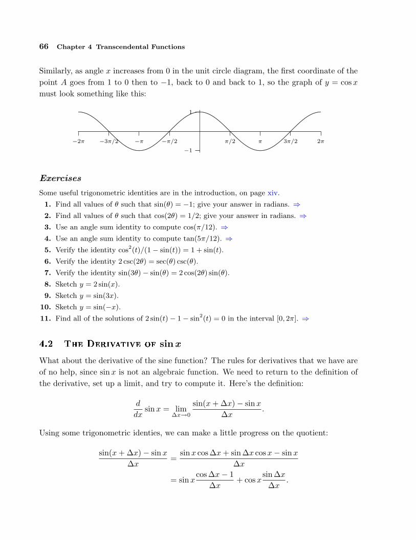
66 Chapter 4 Transcendental Functions
Similarly, as angle x increases from 0 in the unit circle diagram, the first coordinate of thepoint A goes from 1 to 0 then to −1, back to 0 and back to 1, so the graph of y = cos x
must look something like this:
−1
1
π/2 π 3π/2 2π−π/2−π−3π/2−2π
..................................................................................................................................................................................................................................................................................
................................................................................................................................................
.....................................................................................................................................................................................................................................................................................................
................................................................................................................................................................
...................................
Exercises
Some useful trigonometric identities are in the introduction, on page xiv.
1. Find all values of θ such that sin(θ) = −1; give your answer in radians. ⇒2. Find all values of θ such that cos(2θ) = 1/2; give your answer in radians. ⇒3. Use an angle sum identity to compute cos(π/12). ⇒4. Use an angle sum identity to compute tan(5π/12). ⇒5. Verify the identity cos2(t)/(1− sin(t)) = 1 + sin(t).
6. Verify the identity 2 csc(2θ) = sec(θ) csc(θ).
7. Verify the identity sin(3θ)− sin(θ) = 2 cos(2θ) sin(θ).
8. Sketch y = 2 sin(x).
9. Sketch y = sin(3x).
10. Sketch y = sin(−x).
11. Find all of the solutions of 2 sin(t)− 1− sin2(t) = 0 in the interval [0, 2π]. ⇒
4.2 The Derivative of sinx
What about the derivative of the sine function? The rules for derivatives that we have areof no help, since sin x is not an algebraic function. We need to return to the definition ofthe derivative, set up a limit, and try to compute it. Here’s the definition:
d
dxsinx = lim
∆x→0
sin(x + ∆x)− sin x
∆x.
Using some trigonometric identies, we can make a little progress on the quotient:
sin(x + ∆x)− sinx
∆x=
sinx cos∆x + sin∆x cosx− sin x
∆x
= sin xcos∆x− 1
∆x+ cos x
sin∆x
∆x.

4.3 A hard limit 67
This isolates the difficult bits in the two limits
lim∆x→0
cos∆x− 1∆x
and lim∆x→0
sin∆x
∆x.
Here we get a little lucky: it turns out that once we know the second limit the first is quiteeasy. The second is quite tricky, however. Indeed, it is the hardest limit we will actuallycompute, and we devote a section to it.
4.3 A hard limit
We want to compute this limit:
lim∆x→0
sin∆x
∆x.
Equivalently, to make the notation a bit simpler, we can compute
limx→0
sin x
x.
In the original context we need to keep x and ∆x separate, but here it doesn’t hurt torename ∆x to something more convenient.
To do this we need to be quite clever, and to employ some indirect reasoning. Theindirect reasoning is embodied in a theorem, frequently called the squeeze theorem.
THEOREM 4.1 Squeeze Theorem Suppose that g(x) ≤ f(x) ≤ h(x) for all x
close to a but not equal to a. If limx→a g(x) = L = limx→a h(x), then limx→a f(x) = L.
This theorem can be proved using the official definition of limit. We won’t prove ithere, but point out that it is easy to understand and believe graphically. The conditionsays that f(x) is trapped between g(x) below and h(x) above, and that at x = a, both g
and h approach the same value. This means the situation looks something like figure 4.1.The wiggly curve is x2 sin(π/x), the upper and lower curves are x2 and −x2. Since thesine function is always between −1 and 1, −x2 ≤ x2 sin(π/x) ≤ x2, and it is easy to seethat limx→0−x2 = 0 = limx→0 x2. It is not so easy to see directly, that is algebraically,that limx→0 x2 sin(π/x) = 0, because the π/x prevents us from simply plugging in x = 0.The squeeze theorem makes this “hard limit” as easy as the trivial limits involving x2.
To do the really hard limit that we want, limx→0(sinx)/x, we will find two simpler func-tions g and h so that g(x) ≤ (sinx)/x ≤ h(x), and so that limx→0 g(x) = limx→0 h(x). Nottoo surprisingly, this will require some trigonometry and geometry. Refering to figure 4.2,x is the measure of the angle in radians. Since the circle has radius 1, the coordinates of

68 Chapter 4 Transcendental Functions
...............................................................................................................................................................................................................................................................................................................................
......................................................................................................
.................................................................................................
.......................................................................................
............................................................................................................................................................................................................................................................
........................................................................................................................
.........................................................................................................................................................................................................................................................................................................................................................................................................................................................
......................................................................................................................................................................................................................................................................
.........................................................................................................................................................................................................................................................
.....................................................
.................................................................................................................................................................................................................................................................................................................................................................................................................
Figure 4.1 The squeeze theorem.
point A are (cos x, sin x), and the area of the small triangle is (cos x sinx)/2. This triangleis completely contained within the circular wedge-shaped region bordered by two lines andthe circle from (1, 0) to point A. Comparing the areas of the triangle and the wedge wesee (cos x sin x)/2 ≤ x/2, since the area of a circular region with angle θ and radius r isθr2/2. With a little algebra this turns into (sin x)/x ≤ 1/ cos x, giving us the h we seek.
To find g, we note that the circular wedge is completely contained inside the largertriangle. The height of the triangle, from (1, 0) to point B, is tan x, so comparing areas weget x/2 ≤ (tan x)/2 = sin x/(2 cos x). With a little algebra this becomes cos x ≤ (sinx)/x.So now we have
cosx ≤ sin x
x≤ 1
cos x.
Finally, the two limits limx→0 cos x and limx→0 1/ cos x are easy, because cos(0) = 1.By the squeeze theorem, limx→0(sinx)/x = 1 as well.
Before we can complete the calculation of the derivative of the sine, we need one otherlimit:
limx→0
cosx− 1x
.
This limit is just as hard as sin x/x, but closely related to it, so that we don’t have to asimilar calculation; instead we can do a bit of tricky algebra.
cos x− 1x
=cos x− 1
x
cos x + 1cos x + 1
=cos2 x− 1
x(cosx + 1)=
− sin2 x
x(cosx + 1)= − sin x
x
sin x
cos x + 1.
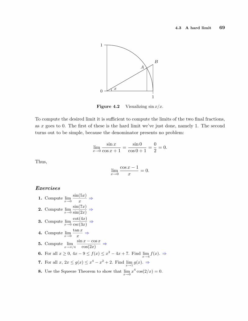
4.3 A hard limit 69
........
........
........
........
........
............................................................................................................................
......................
.......................
...........................
................................
..............................................
...........................................................
0
1
1
................................
................................
................................
................................
................................
................................
................................
................................
..................
x
A
B
.............
Figure 4.2 Visualizing sin x/x.
To compute the desired limit it is sufficient to compute the limits of the two final fractions,as x goes to 0. The first of these is the hard limit we’ve just done, namely 1. The secondturns out to be simple, because the denominator presents no problem:
limx→0
sin x
cosx + 1=
sin 0cos 0 + 1
=02
= 0.
Thus,
limx→0
cos x− 1x
= 0.
Exercises
1. Compute limx→0
sin(5x)
x⇒
2. Compute limx→0
sin(7x)
sin(2x)⇒
3. Compute limx→0
cot(4x)
csc(3x)⇒
4. Compute limx→0
tan x
x⇒
5. Compute limx→π/4
sin x− cos x
cos(2x)⇒
6. For all x ≥ 0, 4x− 9 ≤ f(x) ≤ x2 − 4x + 7. Find limx→4
f(x). ⇒7. For all x, 2x ≤ g(x) ≤ x4 − x2 + 2. Find lim
x→1g(x). ⇒
8. Use the Squeeze Theorem to show that limx→0
x4 cos(2/x) = 0.

70 Chapter 4 Transcendental Functions
4.4 The Derivative of sinx , continued
Now we can complete the calculation of the derivative of the sine:
d
dxsinx = lim
∆x→0
sin(x + ∆x)− sin x
∆x
= lim∆x→0
sin xcos∆x− 1
∆x+ cos x
sin ∆x
∆x
= sin x · 0 + cos x · 1 = cos x.
The derivative of a function measures the slope or steepness of the function; if weexamine the graphs of the sine and cosine side by side, it should be that the latter appearsto accurately describe the slope of the former, and indeed this is true:
−1
1
π/2 π 3π/2 2π
...........................................................................................
.........................................................................................................................................................................................................................................................................................................
.................................................................
sin x−1
1
π/2 π 3π/2 2π
..................................................................................................................................................................................................................................................................................
................................................................................................................................................
...................................
cos x
Notice that where the cosine is zero the sine does appear to have a horizontal tangent line,and that the sine appears to be steepest where the cosine takes on its extreme values of 1and −1.
Of course, now that we know the derivative of the sine, we can compute derivatives ofmore complicated functions involving the sine.
EXAMPLE 4.2 Compute the derivative of sin(x2).
d
dxsin(x2) = cos(x2) · 2x = 2x cos(x2).
EXAMPLE 4.3 Compute the derivative of sin2(x3 − 5x).
d
dxsin2(x3 − 5x) =
d
dx(sin(x3 − 5x))2
= 2(sin(x3 − 5x))1 cos(x3 − 5x)(3x2 − 5)
= 2(3x2 − 5) cos(x3 − 5x) sin(x3 − 5x).
Exercises
Find the derivatives of the following functions.
1. sin2(√
x) ⇒

4.5 Derivatives of the Trigonometric Functions 71
2.√
x sin x ⇒3.
1
sin x⇒
4.x2 + x
sin x⇒
5.p
1− sin2 x ⇒
4.5 Derivatives of the Trigonometric Functions
All of the other trigonometric functions can be expressed in terms of the sine, and so theirderivatives can easily be calculated using the rules we already have. For the cosine weneed to use two identities,
cosx = sin(x +π
2),
sin x = − cos(x +π
2).
Now:d
dxcosx =
d
dxsin(x +
π
2) = cos(x +
π
2) · 1 = − sin x
d
dxtanx =
d
dx
sin x
cosx=
cos2 x + sin2 x
cos2 x=
1cos2 x
= sec2 x
d
dxsec x =
d
dx(cos x)−1 = −1(cos x)−2(− sin x) =
sin x
cos2 x= sec x tanx
The derivatives of the cotangent and cosecant are similar and left as exercises.
Exercises
Find the derivatives of the following functions.
1. sin x cos x ⇒2. sin(cos x) ⇒3.√
x tan x ⇒4. tan x/(1 + sin x) ⇒5. cot x ⇒
6. csc x ⇒7. x3 sin(23x2) ⇒8. sin2 x + cos2 x ⇒9. sin(cos(6x)) ⇒
10. Computed
dθ
sec θ
1 + sec θ. ⇒
11. Computed
dtt5 cos(6t). ⇒
12. Computed
dt
t3 sin(3t)
cos(2t). ⇒
13. Find all points on the graph of f(x) = sin2(x) at which the tangent line is horizontal. ⇒14. Find all points on the graph of f(x) = 2 sin(x)−sin2(x) at which the tangent line is horizontal.
⇒

72 Chapter 4 Transcendental Functions
15. Find an equation for the tangent line to sin2(x) at x = π/3. ⇒16. Find an equation for the tangent line to sec2 x at x = π/3. ⇒17. Find an equation for the tangent line to cos2 x− sin2(4x) at x = π/6. ⇒18. Find the points on the curve y = x + 2 cos x that have a horizontal tangent line. ⇒19. Let C be a circle of radius r. Let A be an arc on C subtended by a central angle θ. Let B be
the the chord of C whose endpoints are the endpoints of A. (Hence, B is also subtended bya central angle θ.) Let s be the length of A and let d be the length of B. Sketch a diagramof the situation and compute limθ→0+ s/d.
4.6 Exponential and Logarithmic functions
An exponential function has the form ax, where a is a constant; examples are 2x, 10x, ex.The logarithmic functions are the inverses of the exponential functions, that is, functionsthat “undo” the exponential functions, just as, for example, the cube root function “un-does” the cube function: 3
√23 = 2. Note that the original function also undoes the inverse
function: ( 3√
8)3 = 8.Let f(x) = 2x. The inverse of this function is called the logarithm base 2, denoted
log2(x) or (especially in computer science circles) lg(x). What does this really mean? Thelogarithm must undo the action of the exponential function, so for example it must be thatlg(23) = 3—starting with 3, the exponential function produces 23 = 8, and the logarithmof 8 must get us back to 3. A little thought shows that it is not a coincidence that lg(23)simply gives the exponent—the exponent is the original value that we must get back to.In other words, the logarithm is the exponent. Remember this catchphrase, and what itmeans, and you won’t go wrong. (You do have to remember what it means. Like anygood mnemonic, “the logarithm is the exponent” leaves out a lot of detail, like “Whichexponent?” and “Exponent of what?”)
EXAMPLE 4.4 What is the value of log10(1000)? The “10” tells us the appropriatenumber to use for the base of the exponential function. The logarithm is the exponent,so the question is, what exponent E makes 10E = 1000? If we can find such an E, thenlog10(1000) = log10(10E) = E; finding the appropriate exponent is the same as finding thelogarithm. In this case, of course, it is easy: E = 3 so log10(1000) = 3.
Let’s review some laws of exponents and logarithms. Since a5 = a ·a ·a ·a ·a and a3 =a·a·a, it’s clear that a5·a3 = a·a·a·a·a·a·a·a = a8 = a5+3, and in general that aman = am+n.Since “the logarithm is the exponent,” it’s no surprise that this translates directly into afact about the logarithm function. Here are three facts from the example: loga(a5) = 5,loga(a3) = 3, loga(a8) = 8. So loga(a5a3) = loga(a8) = 8 = 5 + 3 = loga(a5) + loga(a3).
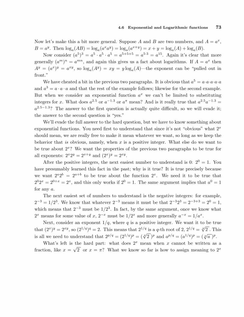
4.6 Exponential and Logarithmic functions 73
Now let’s make this a bit more general. Suppose A and B are two numbers, and A = ax,B = ay. Then loga(AB) = loga(axay) = loga(ax+y) = x + y = loga(A) + loga(B).
Now consider (a5)3 = a5 · a5 · a5 = a5+5+5 = a5·3 = a15. Again it’s clear that moregenerally (am)n = amn, and again this gives us a fact about logarithms. If A = ax thenAy = (ax)y = axy, so loga(Ay) = xy = y loga(A)—the exponent can be “pulled out infront.”
We have cheated a bit in the previous two paragraphs. It is obvious that a5 = a·a·a·a·aand a3 = a · a · a and that the rest of the example follows; likewise for the second example.But when we consider an exponential function ax we can’t be limited to substitutingintegers for x. What does a2.5 or a−1.3 or aπ mean? And is it really true that a2.5a−1.3 =a2.5−1.3? The answer to the first question is actually quite difficult, so we will evade it;the answer to the second question is “yes.”
We’ll evade the full answer to the hard question, but we have to know something aboutexponential functions. You need first to understand that since it’s not “obvious” what 2x
should mean, we are really free to make it mean whatever we want, so long as we keep thebehavior that is obvious, namely, when x is a positive integer. What else do we want tobe true about 2x? We want the properties of the previous two paragraphs to be true forall exponents: 2x2y = 2x+y and (2x)y = 2xy.
After the positive integers, the next easiest number to understand is 0: 20 = 1. Youhave presumably learned this fact in the past; why is it true? It is true precisely becausewe want 2a2b = 2a+b to be true about the function 2x. We need it to be true that202x = 20+x = 2x, and this only works if 20 = 1. The same argument implies that a0 = 1for any a.
The next easiest set of numbers to understand is the negative integers: for example,2−3 = 1/23. We know that whatever 2−3 means it must be that 2−323 = 2−3+3 = 20 = 1,which means that 2−3 must be 1/23. In fact, by the same argument, once we know what2x means for some value of x, 2−x must be 1/2x and more generally a−x = 1/ax.
Next, consider an exponent 1/q, where q is a positive integer. We want it to be truethat (2x)y = 2xy, so (21/q)q = 2. This means that 21/q is a q-th root of 2, 21/q = q
√2 . This
is all we need to understand that 2p/q = (21/q)p = ( q√
2 )p and ap/q = (a1/q)p = ( q√
a )p.What’s left is the hard part: what does 2x mean when x cannot be written as a
fraction, like x =√
2 or x = π? What we know so far is how to assign meaning to 2x
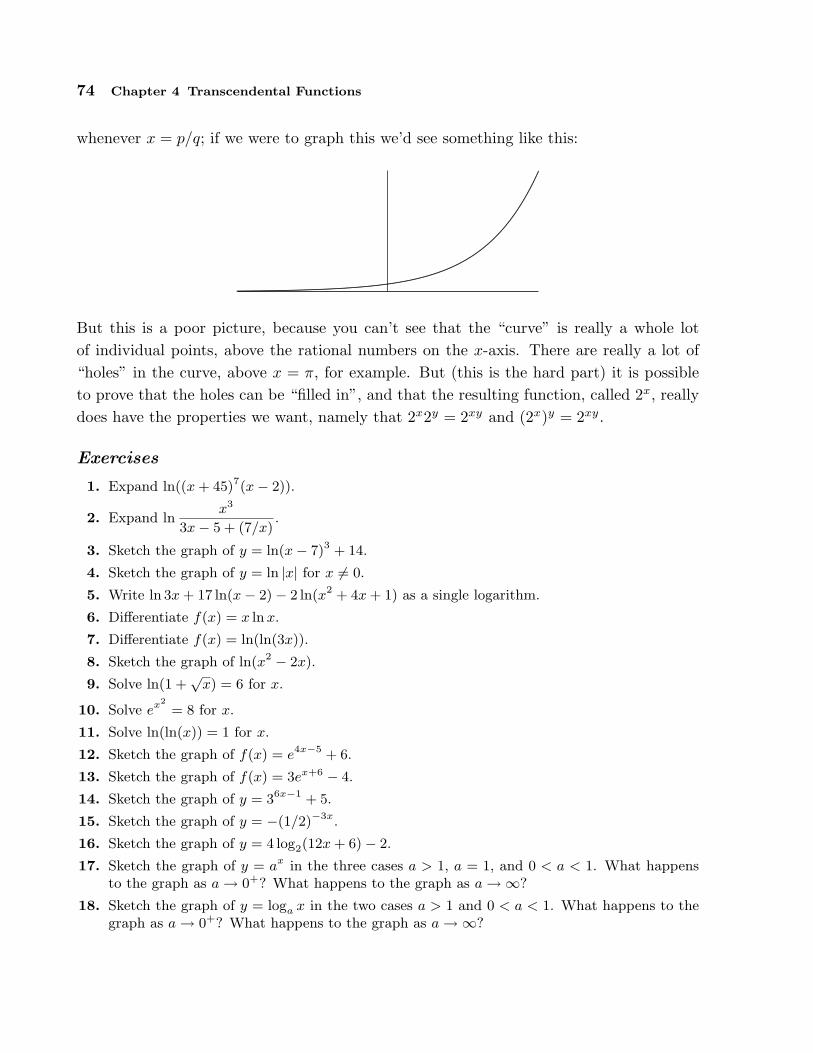
74 Chapter 4 Transcendental Functions
whenever x = p/q; if we were to graph this we’d see something like this:
........................................................................................................................................................................................................................................................................
...........................................................
......................................
..............................................................................................................................................................................................
But this is a poor picture, because you can’t see that the “curve” is really a whole lotof individual points, above the rational numbers on the x-axis. There are really a lot of“holes” in the curve, above x = π, for example. But (this is the hard part) it is possibleto prove that the holes can be “filled in”, and that the resulting function, called 2x, reallydoes have the properties we want, namely that 2x2y = 2xy and (2x)y = 2xy.
Exercises
1. Expand ln((x + 45)7(x− 2)).
2. Expand lnx3
3x− 5 + (7/x).
3. Sketch the graph of y = ln(x− 7)3 + 14.
4. Sketch the graph of y = ln |x| for x 6= 0.
5. Write ln 3x + 17 ln(x− 2)− 2 ln(x2 + 4x + 1) as a single logarithm.
6. Differentiate f(x) = x ln x.
7. Differentiate f(x) = ln(ln(3x)).
8. Sketch the graph of ln(x2 − 2x).
9. Solve ln(1 +√
x) = 6 for x.
10. Solve ex2= 8 for x.
11. Solve ln(ln(x)) = 1 for x.
12. Sketch the graph of f(x) = e4x−5 + 6.
13. Sketch the graph of f(x) = 3ex+6 − 4.
14. Sketch the graph of y = 36x−1 + 5.
15. Sketch the graph of y = −(1/2)−3x.
16. Sketch the graph of y = 4 log2(12x + 6)− 2.
17. Sketch the graph of y = ax in the three cases a > 1, a = 1, and 0 < a < 1. What happensto the graph as a→ 0+? What happens to the graph as a→∞?
18. Sketch the graph of y = loga x in the two cases a > 1 and 0 < a < 1. What happens to thegraph as a→ 0+? What happens to the graph as a→∞?

4.7 Derivatives of the exponential and logarithmic functions 75
4.7 Derivatives of the exponential and logarithmic functions
As with the sine, we don’t know anything about derivatives that allows us to computethe derivatives of the exponential and logarithmic functions without going back to basics.Let’s do a little work with the definition again:
d
dxax = lim
∆x→0
ax+∆x − ax
∆x
= lim∆x→0
axa∆x − ax
∆x
= lim∆x→0
ax a∆x − 1∆x
= ax lim∆x→0
a∆x − 1∆x
There are two interesting things to note here: As in the case of the sine function we are leftwith a limit that involves ∆x but not x, which means that whatever lim∆x→0(a∆x−1)/∆x
is, we know that it is a number, that is, a constant. This means that ax has a remarkableproperty: its derivative is a constant times itself.
We earlier remarked that the hardest limit we would compute was limx→0 sin x/x = 1;we now have a limit that is just a bit too hard to include here. In fact the hard part is tosee that lim∆x→0(a∆x − 1)/∆x even exists—does this fraction really get closer and closerto some fixed value? Yes it does, but we will not prove this fact.
We can look at some examples. Consider (2x − 1)/x for some small values of x: 1,0.828427124, 0.756828460, 0.724061864, 0.70838051, 0.70070877 when x is 1, 1/2, 1/4, 1/8,1/16, 1/32, respectively. It looks like this is settling in around 0.7, which turns out to betrue. Consider next (3x − 1)/x: 2, 1.464101616, 1.264296052, 1.177621520, 1.13720773,1.11768854, at the same values of x. It turns out to be true that in the limit this is about1.1. Two examples don’t establish a pattern, but if you do more examples you will findthat the limit varies directly with the value of a: bigger a, bigger limit; smaller a, smallerlimit. As we can already see, some of these limits will be less than 1 and some larger than1. Somewhere between a = 2 and a = 3 the limit will be exactly 1; the value at which thishappens is called e, so that
lim∆x→0
e∆x − 1∆x
= 1.
As you might guess from our two examples, e is closer to 3 than to 2, and in fact e ≈ 2.718.

76 Chapter 4 Transcendental Functions
Now we see that the function ex has a truly remarkable property:
d
dxex = lim
∆x→0
ex+∆x − ex
∆x
= lim∆x→0
exe∆x − ex
∆x
= lim∆x→0
ex e∆x − 1∆x
= ex lim∆x→0
e∆x − 1∆x
= ex
That is, ex is its own derivative, or in other words, the slope of ex is the same as its height,or the same as its second coordinate: The function f(x) = ex goes through the point (z, ez)and has slope ez there, no matter what z is.
What about the logarithm function? This too is hard, but as the cosine function waseasier to do once the sine was done, so the logarithm is easier to do now that we knowthe derivative of the exponential function. Let’s start with loge x, which as you probablyknow is often abbreviated ln x and called the “natural logarithm” function.
Consider the relationship between the two functions, namely, that they are inverses,that one “undoes” the other. Graphically this means that they have the same graph exceptthat one is “flipped” or “reflected” through the line y = x:
...............................................................
.......................................
...................................................................................................................................................................................................................................................
...............................................................................................................................................................................................................................................
.................................
.....................................
....................................
Figure 4.3 The exponential and logarithmic functions.
This means that the slopes of these two functions are closely related as well: For example,the slope of ex is e at x = 1; at the corresponding point on the ln(x) curve, the slope mustbe 1/e, because the “rise” and the “run” have been interchanged. Since the slope of ex ise at the point (1, e), the slope of ln(x) is 1/e at the point (e, 1).
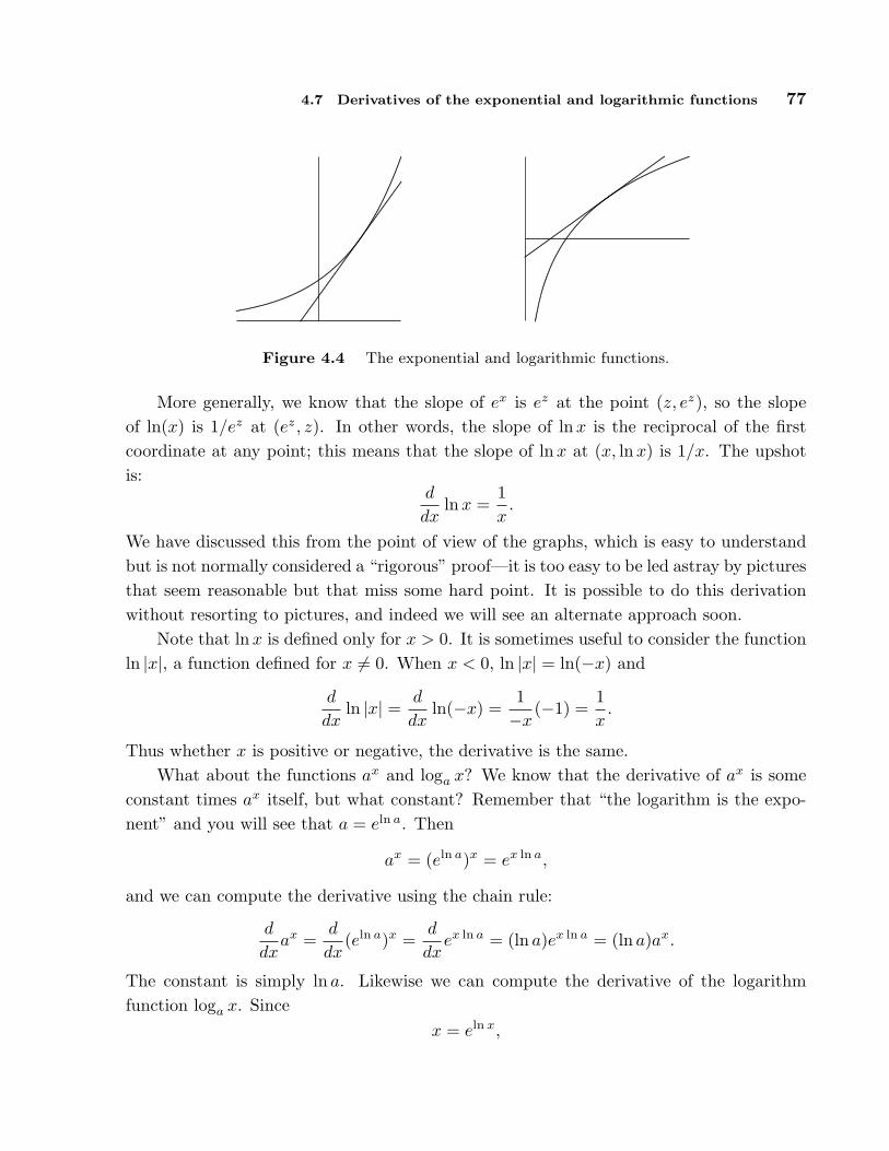
4.7 Derivatives of the exponential and logarithmic functions 77
...............................................................
.......................................
...................................................................................................................................................................................................................................................
........................................................................................................................................................................................................................................................
...............................................................................................................................................................................................................................................
.................................
.....................................
....................................
........................................................................................................................................................................................................................................................
Figure 4.4 The exponential and logarithmic functions.
More generally, we know that the slope of ex is ez at the point (z, ez), so the slopeof ln(x) is 1/ez at (ez, z). In other words, the slope of ln x is the reciprocal of the firstcoordinate at any point; this means that the slope of lnx at (x, ln x) is 1/x. The upshotis:
d
dxln x =
1x
.
We have discussed this from the point of view of the graphs, which is easy to understandbut is not normally considered a “rigorous” proof—it is too easy to be led astray by picturesthat seem reasonable but that miss some hard point. It is possible to do this derivationwithout resorting to pictures, and indeed we will see an alternate approach soon.
Note that ln x is defined only for x > 0. It is sometimes useful to consider the functionln |x|, a function defined for x 6= 0. When x < 0, ln |x| = ln(−x) and
d
dxln |x| = d
dxln(−x) =
1−x
(−1) =1x
.
Thus whether x is positive or negative, the derivative is the same.What about the functions ax and loga x? We know that the derivative of ax is some
constant times ax itself, but what constant? Remember that “the logarithm is the expo-nent” and you will see that a = eln a. Then
ax = (eln a)x = ex ln a,
and we can compute the derivative using the chain rule:
d
dxax =
d
dx(eln a)x =
d
dxex ln a = (ln a)ex ln a = (ln a)ax.
The constant is simply ln a. Likewise we can compute the derivative of the logarithmfunction loga x. Since
x = eln x,

78 Chapter 4 Transcendental Functions
we can take the logarithm base a of both sides to get
loga(x) = loga(eln x) = ln x loga e.
Thend
dxloga x =
1x
loga e.
Finally, sincea = eln a
loga(a) = loga(eln a) = ln a loga e
1 = ln a loga e
1ln a
= loga e,
we can replace loga e to getd
dxloga x =
1x ln a
.
You may if you wish memorize the formulas
d
dxax = (ln a)ax and
d
dxloga x =
1x ln a
.
Because the “trick” a = eln a is often useful, and sometimes essential, it may be better toremember the trick, not the formula.
EXAMPLE 4.5 Compute the derivative of f(x) = 2x.
d
dx2x =
d
dx(eln 2)x
=d
dxex ln 2
=(
d
dxx ln 2
)ex ln 2
= (ln 2)ex ln 2
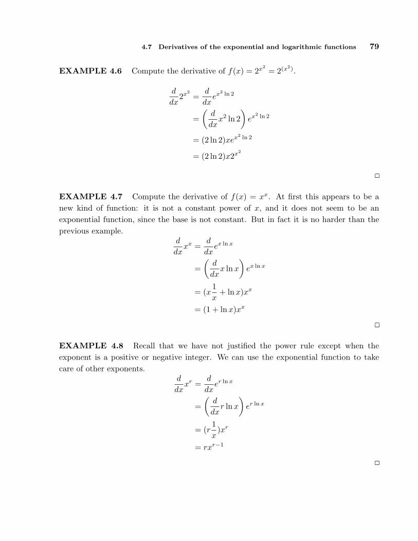
4.7 Derivatives of the exponential and logarithmic functions 79
EXAMPLE 4.6 Compute the derivative of f(x) = 2x2= 2(x2).
d
dx2x2
=d
dxex2 ln 2
=(
d
dxx2 ln 2
)ex2 ln 2
= (2 ln 2)xex2 ln 2
= (2 ln 2)x2x2
EXAMPLE 4.7 Compute the derivative of f(x) = xx. At first this appears to be anew kind of function: it is not a constant power of x, and it does not seem to be anexponential function, since the base is not constant. But in fact it is no harder than theprevious example.
d
dxxx =
d
dxex ln x
=(
d
dxx ln x
)ex ln x
= (x1x
+ ln x)xx
= (1 + ln x)xx
EXAMPLE 4.8 Recall that we have not justified the power rule except when theexponent is a positive or negative integer. We can use the exponential function to takecare of other exponents.
d
dxxr =
d
dxer ln x
=(
d
dxr ln x
)er ln x
= (r1x
)xr
= rxr−1
80 Chapter 4 Transcendental Functions
Exercises
In 1–19, find the derivatives of the functions.
1. 3x2 ⇒2.
sin x
ex⇒
3. (ex)2 ⇒4. sin(ex) ⇒5. esin x ⇒6. xsin x ⇒7. x3ex ⇒8. x + 2x ⇒9. (1/3)x2 ⇒
10. e4x/x ⇒
11. ln(x3 + 3x) ⇒12. ln(cos(x)) ⇒13.
pln(x2)/x ⇒
14. ln(sec(x) + tan(x)) ⇒15. xsin(x) ⇒16. x ln x
17. ln(ln(3x))
18.1 + ln(3x2)
1 + ln(4x)
19.x8(x− 23)1/2
27x6(4x− 6)8
20. Find the value of a so that the tangent line to y = ln(x) at x = a is a line through the origin.Sketch the resulting situation. ⇒
21. If f(x) = ln(x3 + 2) compute f ′(e1/3).
4.8 Limits revisited
We have defined and used the concept of limit, primarily in our development of the deriva-tive. Recall that limx→a f(x) = L is true if, in a precise sense, f(x) gets closer and closerto L as x gets closer and closer to a. While some limits are easy to see, others take someingenuity; in particular, the limits that define derivatives are always difficult on their face,since in
lim∆x→0
f(x + ∆x)− f(x)∆x
both the numerator and denominator approach zero. Typically this difficulty can be re-solved when f is a “nice” function and we are trying to compute a derivative. Occasionallysuch limits are interesting for other reasons, and the limit of a fraction in which both nu-merator and denominator approach zero can be difficult to analyse. Now that we havethe derivative available, there is another technique that can sometimes be helpful in suchcircumstances.
Before we introduce the technique, we will also expand our concept of limit. We willoccasionally want to know what happens to some quantity when a variable gets very largeor “goes to infinity”.

4.8 Limits revisited 81
EXAMPLE 4.9 What happens to the function cos(1/x) as x goes to infinity? It seemsclear that as x gets larger and larger, 1/x gets closer and closer to zero, so cos(1/x) shouldbe getting closer and closer to cos(0) = 1.
As with ordinary limits, this concept of “limit at infinity” can be made precise.Roughly, we want limx→∞ f(x) = L to mean that we can make f(x) as close as wewant to L by making x large enough. Compare this definition to the definition of limit insection 2.3.
DEFINITION 4.10 Limit at infinity Suppose f is a function. We say thatlimx→∞ f(x) = L if for every ε > 0 there is an N > 0 so that whenever x > N ,|f(x)− L| < ε.
We include this definition for completeness, but we will not explore it in detail. Sufficeit to say that such limits behave in much the same way that ordinary limits do; in particularthere is a direct analog of theorem 2.7.
Now consider this limit:
limx→π
x2 − π2
sin x.
As x approaches π, both the numerator and denominator approach zero, so it is notobvious what, if anything, the quotient approaches. We can often compute such limits byapplication of the following theorem.
THEOREM 4.11 L’Hopital’s Rule For “sufficiently nice” functions f(x) and g(x),
if limx→a
f(x) = 0 = limx→a
g(x) or limx→a
f(x) = ±∞ = limx→a
g(x), and if limx→a
f ′(x)g′(x)
exists, then
limx→a
f(x)g(x)
= limx→a
f ′(x)g′(x)
. This remains true if “x → a” is replaced by “x →∞”.
This theorem is somewhat difficult to prove, in part because it incorportates so manydifferent possibilities, so we will not prove it here. We also will not need to worry aboutthe precise definition of “sufficiently nice”, as the functions we encounter will be suitable.
EXAMPLE 4.12 Compute limx→π
x2 − π2
sinxin two ways.
First we use L’Hopital’s Rule: Since the numerator and denominator both approachzero,
limx→π
x2 − π2
sin x= lim
x→π
2x
cos x,
82 Chapter 4 Transcendental Functions
provided the latter exists. But in fact this is an easy limit, since the denominator nowapproaches −1, so
limx→π
x2 − π2
sin x=
2π
−1= −2π.
We don’t really need L’Hopital’s Rule to do this limit. Rewrite it as
limx→π
(x + π)x− π
sin x
and note that
limx→π
x− π
sin x= lim
x→π
x− π
− sin(x− π)= lim
x→0− x
sin x
since x− π approaches zero as x approaches π. Now
limx→π
(x + π)x− π
sin x= lim
x→π(x + π) lim
x→0− x
sin x= 2π(−1) = −2π
as before.
EXAMPLE 4.13 Compute limx→∞
2x2 − 3x + 7x2 + 47x + 1
in two ways.
As x goes to infinity both the numerator and denominator go to infinity, so we mayapply L’Hopital’s Rule:
limx→∞
2x2 − 3x + 7x2 + 47x + 1
= limx→∞
4x− 32x + 47
.
In the second quotient, it is still the case that the numerator and denominator both go toinfinity, so we are allowed to use L’Hopital’s Rule again:
limx→∞
4x− 32x + 47
= limx→∞
42
= 2.
So the original limit is 2 as well.Again, we don’t really need L’Hopital’s Rule, and in fact a more elementary approach
is easier—we divide the numerator and denominator by x2:
limx→∞
2x2 − 3x + 7x2 + 47x + 1
= limx→∞
2x2 − 3x + 7x2 + 47x + 1
1x2
1x2
= limx→∞
2− 3x + 7
x2
1 + 47x + 1
x2
.
Now as x approaches infinity, all the quotients with some power of x in the denominatorapproach zero, leaving 2 in the numerator and 1 in the denominator, so the limit again is2.

4.8 Limits revisited 83
EXAMPLE 4.14 Compute limx→0
sec x− 1sin x
.
Both the numerator and denominator approach zero, so applying L’Hopital’s Rule:
limx→0
sec x− 1sin x
= limx→0
sec x tan x
cosx=
1 · 01
= 0.
EXAMPLE 4.15 Compute limx→0+
x ln x.
This doesn’t appear to be suitable for L’Hopital’s Rule, but it also is not “obvious”.As x approaches zero, ln x goes to −∞, so the product looks like (something very small) ·(something very large and negative). But this could be anything: it depends on how smalland how large. For example, consider (x2)(1/x), (x)(1/x), and (x)(1/x2). As x approacheszero, each of these is (something very small) · (something very large), yet the limits arerespectively zero, 1, and ∞.
We can in fact turn this into a L’Hopital’s Rule problem:
x ln x =ln x
1/x=
ln x
x−1.
Now as x approaches zero, both the numerator and denominator approach infinity (one−∞ and one +∞, but only the size is important). Using L’Hopital’s Rule:
limx→0+
ln x
x−1= lim
x→0+
1/x
−x−2= lim
x→0+
1x
(−x2) = limx→0+
−x = 0.
One way to interpret this is that since limx→0+
x ln x = 0, the x approaches zero much faster
than the ln x approaches −∞.

84 Chapter 4 Transcendental Functions
Exercises
Compute the limits.
1. limx→0
cos x− 1
sin x⇒
2. limx→∞
ex
x3⇒
3. limx→∞
px2 + x−
px2 − x ⇒
4. limx→∞
ln x
x⇒
5. limx→∞
ln x√x⇒
6. limx→∞
ex + e−x
ex − e−x
7. The function f(x) =x√
x2 + 1has two horizontal asymptotes. Find them and give a rough
sketch of f with its horizontal asymptotes. ⇒
4.9 Implicit Differentiation
As we have seen, there is a close relationship between the derivatives of ex and ln x becausethese functions are inverses. Rather than relying on pictures for our understanding, wewould like to be able to exploit this relationship computationally. In fact this techniquecan help us find derivatives in many situations, not just when we seek the derivative of aninverse function.
We will begin by illustrating the technique to find what we already know, the derivativeof ln x. Let’s write y = ln x and then x = eln x = ey, or more simply x = ey. We say thatthis equation defines the function y = ln x implicitly because while it is not an explicitexpression y = . . ., it is true that if x = ey then y is in fact the natural logarithm function.Now, for the time being, pretend that all we know of y is that x = ey; what can we sayabout derivatives? We can take the derivative of both sides of the equation:
d
dxx =
d
dxey.
Then using the chain rule on the right hand side:
1 =(
d
dxy
)ey = y′ey.
Then we can solve for y′:
y′ =1ey
=1x
.
There is one little difficulty here. To use the chain rule to compute d/dx(ey) = y′ey weneed to know that the function y has a derivative. All we have shown is that if it has aderivative then that derivative must be 1/x. When using this method we will always have

4.9 Implicit Differentiation 85
to assume that the desired derivative exists, but fortunately this is a safe assumption formost such problems.
The example y = lnx involved an inverse function defined implicitly, but other func-tions can be defined implicitly, and sometimes a single equation can be used to implicitlydefine more than one function. Here’s a familiar example. The equation r2 = x2 + y2
describes a circle of radius r. The circle is not a function y = f(x) because for some valuesof x there are two corresponding values of y. If we want to work with a function, we canbreak the circle into two pieces, the upper and lower semicircles, each of which is a function.Let’s call these y = U(x) and y = L(x); in fact this is a fairly simple example, and it’spossible to give explicit expressions for these: U(x) =
√r2 − x2 and L(x) = −√r2 − x2 .
But it’s somewhat easier, and quite useful, to view both functions as given implicitly byr2 = x2 + y2: both r2 = x2 + U(x)2 and r2 = x2 + L(x)2 are true, and we can think ofr2 = x2 + y2 as defining both U(x) and L(x).
Now we can take the derivative of both sides as before, remembering that y is notsimply a variable but a function—in this case, y is either U(x) or L(x) but we’re not yetspecifying which one. When we take the derivative we just have to remember to apply thechain rule where y appears.
d
dxr2 =
d
dx(x2 + y2)
0 = 2x + 2yy′
y′ =−2x
2y= −x
y
Now we have an expression for y′, but it contains y as well as x. This means that if wewant to compute y′ for some particular value of x we’ll have to know or compute y at thatvalue of x as well. It is at this point that we will need to know whether y is U(x) or L(x).Occasionally it will turn out that we can avoid explicit use of U(x) or L(x) by the natureof the problem
EXAMPLE 4.16 Find the slope of the circle 4 = x2 + y2 at the point (1,−√3). Sincewe know both the x and y coordinates of the point of interest, we do not need to explicitlyrecognize that this point is on L(x), and we do not need to use L(x) to compute y—butwe could. Using the calculation of y′ from above,
y′ = −x
y= − 1
−√3=
1√3.
It is instructive to compare this approach to others.

86 Chapter 4 Transcendental Functions
We might have recognized at the start that (1,−√3) is on the function y = L(x) =−√4− x2. We could then take the derivative of L(x), using the power rule and the chainrule, to get
L′(x) = −12(4− x2)−1/2(−2x) =
x√4− x2
.
Then we could compute L′(1) = 1/√
3 by substituting x = 1.Alternately, we could realize that the point is on L(x), but use the fact that y′ = −x/y.
Since the point is on L(x) we can replace y by L(x) to get
y′ = − x
L(x)= − x√
4− x2,
without computing the derivative of L(x) explicitly. Then we substitute x = 1 and get thesame answer as before.
In the case of the circle it is possible to find the functions U(x) and L(x) explicitly, butthere are potential advantages to using implicit differentiation anyway. In some cases it ismore difficult or impossible to find an explicit formula for y and implicit differentiation isthe only way to find the derivative.
EXAMPLE 4.17 Find the derivative of any function defined implicitly by yx2+ey = x.We treat y as an unspecified function and use the chain rule:
d
dx(yx2 + ey) =
d
dxx
(y · 2x + y′ · x2) + y′ey = 1
y′x2 + y′ey = 1− 2xy
y′(x2 + ey) = 1− 2xy
y′ =1− 2xy
x2 + ey
You might think that the step in which we solve for y′ could sometimes be difficult—after all, we’re using implicit differentiation here because we can’t solve the equationyx2 + ey = x for y, so maybe after taking the derivative we get something that is hard tosolve for y′. In fact, this never happens. All occurrences y′ come from applying the chainrule, and whenever the chain rule is used it deposits a single y′ multiplied by some otherexpression. So it will always be possible to group the terms containing y′ together and

4.9 Implicit Differentiation 87
factor out the y′, just as in the previous example. If you ever get anything more difficultyou have made a mistake and should fix it before trying to continue.
It is sometimes the case that a situation leads naturally to an equation that defines afunction implicitly.
EXAMPLE 4.18 Consider all the points (x, y) that have the property that the distancefrom (x, y) to (x1, y1) plus the distance from (x, y) to (x2, y2) is 2a (a is some constant).These points form an ellipse, which like a circle is not a function but can viewed as twofunctions pasted together. Because we know how to write down the distance between twopoints, we can write down an implicit equation for the ellipse:
√(x− x1)2 + (y − y1)2 +
√(x− x2)2 + (y − y2)2 = 2a.
Then we can use implicit differentiation to find the slope of the ellipse at any point.
EXAMPLE 4.19 We have already justified the power rule by using the exponentialfunction, but we could also do it for rational exponents by using implicit differentiation.Suppose that y = xm/n, where m and n are positive integers. We can write this implicitlyas yn = xm, then because we justified the power rule for integers, we can take the derivativeof each side:
nyn−1y′ = mxm−1
y′ =m
n
xm−1
yn−1
y′ =m
n
xm−1
(xm/n)n−1
y′ =m
nxm−1−(m/n)(n−1)
y′ =m
nxm−1−m+(m/n)
y′ =m
nx(m/n)−1

88 Chapter 4 Transcendental Functions
Exercises
In exercises 1–8, find a formula for the derivative y′ at the point (x, y):
1. y2 = 1 + x2 ⇒2. x2 + xy + y2 = 7 ⇒3. x3 + xy2 = y3 + yx2 ⇒4. 4 cos x sin y = 1 ⇒5.√
x +√
y = 9 ⇒6. tan(x/y) = x + y ⇒7. sin(x + y) = xy ⇒8.
1
x+
1
y= 7 ⇒
9. A hyperbola passing through (8, 6) consists of all points whose distance from the origin is aconstant more than its distance from the point (5,2). Find the slope of the tangent line tothe hyperbola at (8, 6). ⇒
10. Compute y′ for the ellipse of example 4.18.
11. The graph of the equation x2−xy + y2 = 9 is an ellipse. Find the lines tangent to this curveat the two points where it intersects the x-axis. Show that these lines are parallel. ⇒
12. Repeat the previous problem for the points at which the ellipse intersects the y-axis. ⇒13. Find the points on the ellipse from the previous two problems where the slope is horizontal
and where it is vertical. ⇒14. Find an equation for the tangent line to x4 = y2+x2 at (2,
√12). (This curve is the kampyle
of Eudoxus.) ⇒15. Find an equation for the tangent line to x2/3 + y2/3 = a2/3 at a point (x1, y1) on the curve,
with x1 6= 0 and y1 6= 0. (This curve is an astroid.) ⇒16. Find an equation for the tangent line to (x2 +y2)2 = x2−y2 at a point (x1, y1) on the curve,
with x1 6= 0,−1, 1. (This curve is a lemniscate.) ⇒Definition. Two curves are orthogonal if at each point of intersection, the angle betweentheir tangent lines is π/2 . Two families of curves, A and B, are orthogonal trajectories ofeach other if given any curve C in A and any curve D in B the curves C and D are orthogonal.For example, the family of horizontal lines in the plane is orthogonal to the family of vertical linesin the plane.
17. Show that x2 − y2 = 5 is orthogonal to 4x2 + 9y2 = 72. (Hint: You need to find theintersection points of the two curves and then show that the product of the derivatives ateach intersection point is −1.)
18. Show that x2 +y2 = r2 is orthogonal to y = mx. Conclude that the family of circles centeredat the origin is an orthogonal trajectory of the family of lines that pass through the origin.
Note that there is a technical issue when m = 0. The circles fail to be differentiable whenthey cross the x-axis. However, the circles are orthogonal to the x-axis. Explain why.

4.10 Inverse Trigonometric Functions 89
19. For k, c 6= 0 show that y2 − x2 = k is orthogonal to yx = c. In the case where k and care both zero, the curves intersect at the origin. Are the curves y2 − x2 = 0 and yx = 0orthogonal to each other?
20. Suppose that m 6= 0. Show that the family of curves {y = mx + b | b ∈ R} is orthogonal tothe family of curves {y = −(x/m) + c | c ∈ R}.
4.10 Inverse Trigonometric Functions
The trigonometric functions frequently arise in problems, and often it is necessary toinvert the functions, for example, to find an angle with a specified sine. Of course, thereare many angles with the same sine, so the sine function doesn’t actually have an inversethat reliably “undoes” the sine function. If you know that sinx = 0.5, you can’t reversethis to discover x, that is, you can’t solve for x, as there are infinitely many angles withsine 0.5. Nevertheless, it is useful to have something like an inverse to the sine, howeverimperfect. The usual approach is to pick out some collection of angles that produce allpossible values of the sine exactly once. If we “discard” all other angles, the resultingfunction does have a proper inverse.
The sine takes on all values between −1 and 1 exactly once on the interval [−π/2, π/2].If we truncate the sine, keeping only the interval [−π/2, π/2], as shown in figure 4.5, thenthis truncated sine has an inverse function. We call this the inverse sine or the arcsine,and write y = arcsin(x).
−1
1
π/2 π 3π/2 2π−π/2−π−3π/2−2π
...........................................................................................
........................................................................................................................................................................................................................................................................................................
................................................................................................................................................
......................................................................................................................................................................................................................................................................................................
.................................................................................
−1
1
π/2−π/2
...............................................
................................................................................................................................................
....................................
−π/2
π/2
−1 1
.....
.........
.....................................................................................................................................................................................................................
Figure 4.5 The sine, the truncated sine, the inverse sine.
90 Chapter 4 Transcendental Functions
Recall that a function and its inverse undo each other in either order, for example,( 3√
x)3 = x and 3√
x3 = x. This does not work with the sine and the “inverse sine” becausethe inverse sine is the inverse of the truncated sine function, not the real sine function.It is true that sin(arcsin(x)) = x, that is, the sine undoes the arcsine. It is not true thatthe arcsine undoes the sine, for example, sin(5π/6) = 1/2 and arcsin(1/2) = π/6, so doingfirst the sine then the arcsine does not get us back where we started. This is because 5π/6is not in the domain of the truncated sine. If we start with an angle between −π/2 andπ/2 then the arcsine does reverse the sine: sin(π/6) = 1/2 and arcsin(1/2) = π/6.
What is the derivative of the arcsine? Since this is an inverse function, we can discoverthe derivative by using implicit differentiation. Suppose y = arcsin(x). Then
sin(y) = sin(arcsin(x)) = x.
Now taking the derivative of both sides, we get
y′ cos y = 1
y′ =1
cos y
As we expect when using implicit differentiation, y appears on the right hand side here.We would certainly prefer to have y′ written in terms of x, and as in the case of ln x wecan actually do that here. Since sin2 y + cos2 y = 1, cos2 y = 1 − sin2 y = 1 − x2. Socos y = ±√1− x2 , but which is it—plus or minus? It could in general be either, but thisisn’t “in general”: since y = arcsin(x) we know that −π/2 ≤ y ≤ π/2, and the cosine ofan angle in this interval is always positive. Thus cos y =
√1− x2 and
d
dxarcsin(x) =
1√1− x2
.
Note that this agrees with figure 4.5: the graph of the arcsine has positive slope everywhere.We can do something similar for the cosine. As with the sine, we must first truncate the
cosine so that it can be inverted, as shown in figure 4.6. Then we use implicit differentiationto find that
d
dxarccos(x) =
−1√1− x2
.
Note that the truncated cosine uses a different interval than the truncated sine, so that ify = arccos(x) we know that 0 ≤ y ≤ π. The computation of the derivative of the arccosineis left as an exercise.

4.10 Inverse Trigonometric Functions 91
−1
1
π/2 π
...................................................................................................................................................................................................................................
π/2
π
−1 1
...................................................................................................................................................................................................................................
Figure 4.6 The truncated cosine, the inverse cosine.
−π/2 π/2
....
.....
.....
.....
.....
.....
......
......
.......
........
.........
...........
................
............................................................................................
..........................................................................................................................................................................................
....
....
.....
.....
.....
.....
......
......
.......
.......
........
..........
.............
...............................
.............................................................
....................................
.................................................................................................................................................................
....
....
.....
.....
.....
.....
......
......
.......
.......
........
..........
.............
...............................
.........
....................................................
....................................
.............................................................................................................................................................
−π/2 π/2
....
....
.....
.....
.....
.....
......
......
.......
.......
........
..........
.............
...............................
.............................................................
....................................
.................................................................................................................................................................
−π/2
π/2
...........................................................................................................................................................
.................................................................................................
......................................................................................................................................
Figure 4.7 The tangent, the truncated tangent, the inverse tangent.
Finally we look at the tangent; the other trigonometric functions also have “partialinverses” but the sine, cosine and tangent are enough for most purposes. The tangent,truncated tangent and inverse tangent are shown in figure 4.7; the derivative of the arct-angent is left as an exercise.
Exercises
1. Show that the derivative of arccos x is − 1√1− x2
.
2. Show that the derivative of arctan x is1
1 + x2.
3. Find the derivative of arccot x, the inverse cotangent. ⇒4. Find the derivative of arcsin(x2). ⇒5. Find the derivative of arctan(ex). ⇒6. The inverse of cot is usually defined so that the range of arccot is (0, π). Sketch the graph
of y = arccot x. In the process you will make it clear what the domain of arccot is.

92 Chapter 4 Transcendental Functions
7. Use the preceding exercise to show that arccot x + arctan x = π/2.
8. Find the derivative of arccos(sin x3)
9. Find the derivative of ln((arcsin x)2)
10. Find the derivative of arccos ex
11. Find the derivative of arcsin x + arccos x
12. Find the derivative of log5(arctan(xx))
5Curve Sketching
Whether we are interested in a function as a purely mathematical object or in connectionwith some application to the real world, it is often useful to know what the graph ofthe function looks like. We can obtain a good picture of the graph using certain crucialinformation provided by derivatives of the function and certain limits.
5.1 Maxima and Minima
A local maximum point on a function is a point (x, y) on the graph of the functionwhose y coordinate is larger than all other y coordinates on the graph at points “closeto” (x, y). More precisely, (x, f(x)) is a local maximum if there is an interval (a, b) witha < x < b and f(x) ≥ f(z) for every z in (a, b). Similarly, (x, y) is a local minimumpoint if it has locally the smallest y coordinate. Again being more precise: (x, f(x)) is alocal minimum if there is an interval (a, b) with a < x < b and f(x) ≤ f(z) for every z in(a, b). A local extremum is either a local minimum or a local maximum.
Local maximum and minimum points are quite distinctive on the graph of a function,and are therefore useful in understanding the shape of the graph. In many applied problemswe want to find the largest or smallest value that a function achieves (for example, we mightwant to find the minimum cost at which some task can be performed) and so identifyingmaximum and minimum points will be useful for applied problems as well. Some examplesof local maximum and minimum points are shown in figure 5.1.
93

94 Chapter 5 Curve Sketching
......................................................................................................................................................................................................................................................................................................................................
..............................................................................................................................................................
•
•
A
B
.....................................................................................................................................................................................................................................................
........................................................................................................................................................................................................................................................................................................................................................
•
•
•
A
A
B
Figure 5.1 Some local maximum points (A) and minimum points (B).
If (x, f(x)) is a point where f(x) reaches a local maximum or minimum, and if thederivative of f exists at x, then the graph has a tangent line and the tangent line must behorizontal. This is important enough to state as a theorem:
THEOREM 5.1 Fermat’s Theorem If f(x) has a local extremum at x = a and f
is differentiable at a, then f ′(a) = 0.
Thus, the only points at which a function can have a local maximum or minimumare points at which the derivative is zero, as in the left hand graph in figure 5.1, or thederivative is undefined, as in the right hand graph. Any value of x for which f ′(x) is zero orundefined is called a critical value for f . When looking for local maximum and minimumpoints, you are likely to make two sorts of mistakes: You may forget that a maximum orminimum can occur where the derivative does not exist, and so forget to check whetherthe derivative exists everywhere. You might also assume that any place that the derivativeis zero is a local maximum or minimum point, but this is not true. A portion of the graphof f(x) = x3 is shown in figure 5.2. The derivative of f is f ′(x) = 3x2, and f ′(0) = 0, butthere is neither a maximum nor minimum at (0, 0).
Since the derivative is zero or undefined at both local maximum and local minimumpoints, we need a way to determine which, if either, actually occurs. The most elementaryapproach, but one that is often tedious or difficult, is to test directly whether the y coor-dinates “near” the potential maximum or minimum are above or below the y coordinateat the point of interest. Of course, there are too many points “near” the point to test, buta little thought shows we need only test two provided we know that f is continuous (recallthat this means that the graph of f has no jumps or gaps).
Suppose, for example, that we have identified three points at which f ′ is zero ornonexistent: (x1, y1), (x2, y2), (x3, y3), and x1 < x2 < x3 (see figure 5.3). Suppose that

5.1 Maxima and Minima 95
............................................................................................................................................................................
.....................................................................................................
........................................................................................................................................................................
Figure 5.2 No maximum or minimum even though the derivative is zero.
we compute the value of f(a) for x1 < a < x2, and that f(a) < f(x2). What can we sayabout the graph between a and x2? Could there be a point (b, f(b)), a < b < x2 withf(b) > f(x2)? No: if there were, the graph would go up from (a, f(a)) to (b, f(b)) thendown to (x2, f(x2)) and somewhere in between would have a local maximum point. But atthat local maximum point the derivative of f would be zero or nonexistent, yet we alreadyknow that the derivative is zero or nonexistent only at x1, x2, and x3. The upshot is thatone computation tells us that (x2, f(x2)) has the largest y coordinate of any point on thegraph near x2 and to the left of x2. We can perform the same test on the right. If we findthat on both sides of x2 the values are smaller, then there must be a local maximum at(x2, f(x2)); if we find that on both sides of x2 the values are larger, then there must be alocal minimum at (x2, f(x2)); if we find one of each, then there is neither a local maximumor minimum at x2.
x1 a b x2 x3
• ••
•
Figure 5.3 Testing for a maximum or minimum.
It is not always easy to compute the value of a function at a particular point. Thetask is made easier by the availability of calculators and computers, but they have theirown drawbacks—they do not always allow us to distinguish between values that are very

96 Chapter 5 Curve Sketching
close together. Nevertheless, because this method is conceptually simple and sometimeseasy to perform, you should always consider it.
EXAMPLE 5.2 Find all local maximum and minimum points for the function f(x) =x3 − x. The derivative is f ′(x) = 3x2 − 1. This is defined everywhere and is zero atx = ±√3/3. Looking first at x =
√3/3, we see that f(
√3/3) = −2
√3/9. Now we test
two points on either side of x =√
3/3, making sure that neither is farther away thanthe nearest critical value; since
√3 < 3,
√3/3 < 1 and we can use x = 0 and x = 1.
Since f(0) = 0 > −2√
3/9 and f(1) = 0 > −2√
3/9, there must be a local minimum atx =
√3/3. For x = −√3/3, we see that f(
√3/3) = 2
√3/9. This time we can use x = 0
and x = −1, and we find that f(−1) = f(0) = 0 < 2√
3/9, so there must be a localmaximum at x = −√3/3.
Of course this example is made very simple by our choice of points to test, namelyx = −1, 0, 1. We could have used other values, say −5/4, 1/3, and 3/4, but this wouldhave made the calculations considerably more tedious.
EXAMPLE 5.3 Find all local maximum and minimum points for f(x) = sin x + cos x.The derivative is f ′(x) = cos x − sinx. This is always defined and is zero whenevercos x = sin x. Recalling that the cos x and sinx are the x and y coordinates of points on aunit circle, we see that cos x = sin x when x is π/4, π/4±π, π/4±2π, π/4±3π, etc. Sinceboth sine and cosine have a period of 2π, we need only determine the status of x = π/4and x = 5π/4. We can use 0 and π/2 to test the critical value x = π/4. We find thatf(π/4) =
√2, f(0) = 1 <
√2 and f(π/2) = 1, so there is a local maximum when x = π/4
and also when x = π/4± 2π, π/4± 4π, etc.We use π and 2π to test the critical value x = 5π/4. The relevant values are f(5π/4) =
−√2, f(π) = −1 > −√2, f(2π) = 1 > −√2, so there is a local minimum at x = 5π/4,5π/4± 2π, 5π/4± 4π, etc.
5.2 The first derivative test 97
Exercises
In problems 1–12, find all local maximum and minimum points (x, y) by the method of this section.
1. y = x2 − x ⇒2. y = 2 + 3x− x3 ⇒3. y = x3 − 9x2 + 24x ⇒4. y = x4 − 2x2 + 3 ⇒5. y = 3x4 − 4x3 ⇒6. y = (x2 − 1)/x ⇒7. y = 3x2 − (1/x2) ⇒
8. y = cos(2x)− x ⇒
9. f(x) =
x− 1 x < 2x2 x ≥ 2
⇒
10. f(x) =
8<:
x− 3 x < 3x3 3 ≤ x ≤ 51/x x > 5
⇒
11. f(x) = x2 − 98x + 4 ⇒
12. f(x) =
−2 x = 01/x2 x 6= 0
⇒
13. Recall that for any real number x there is a unique integer n such that n ≤ x < n + 1, andthe greatest integer function is given by bxc = n, as shown in figure 3.1. Where are thecritical values of the greatest integer function? Which are local maxima and which are localminima?
14. Explain why the function f(x) = 1/x has no local maxima or minima.
15. How many critical points can a quadratic polynomial function have? ⇒16. Show that a cubic polynomial can have at most two critical points. Give examples to show
that a cubic polynomial can have zero, one, or two critical points.
17. Explore the family of functions f(x) = x3 + cx + 1 where c is a constant. How many andwhat types of local extremes are there? Your answer should depend on the value of c, thatis, different values of c will give different answers.
18. We generalize the preceding two questions. Let n be a positive integer and let f be a poly-nomial of degree n. How many critical points can f have? (Hint: Recall the FundamentalTheorem of Algebra, which says that a polynomial of degree n has at most n roots.)
5.2 The first derivative test
The method of the previous section for deciding whether there is a local maximum orminimum at a critical value is not always convenient. We can instead use informationabout the derivative f ′(x) to decide; since we have already had to compute the derivativeto find the critical values, there is often relatively little extra work involved in this method.
How can the derivative tell us whether there is a maximum, minimum, or neither ata point? Suppose that f ′(a) = 0. If there is a local maximum when x = a, the functionmust be lower near x = a than it is right at x = a. If the derivative exists near x = a, thismeans f ′(x) > 0 when x is near a and x < a, because the function must “slope up” justto the left of a. Similarly, f ′(x) < 0 when x is near a and x > a, because f slopes downfrom the local maximum as we move to the right. Using the same reasoning, if there isa local minimum at x = a, the derivative of f must be negative just to the left of a and

98 Chapter 5 Curve Sketching
positive just to the right. If the derivative exists near a but does not change from positiveto negative or negative to positive, that is, it is postive on both sides or negative on bothsides, then there is neither a maximum nor minimum when x = a. See the first graph infigure 5.1 and the graph in figure 5.2 for examples.
EXAMPLE 5.4 Find all local maximum and minimum points for f(x) = sin x + cosx
using the first derivative test. The derivative is f ′(x) = cos x− sin x and from example 5.3the critical values we need to consider are π/4 and 5π/4.
The graphs of sin x and cos x are shown in figure 5.4. Just to the left of π/4 the cosineis larger than the sine, so f ′(x) is positive; just to the right the cosine is smaller than thesine, so f ′(x) is negative. This means there is a local maximum at π/4. Just to the leftof 5π/4 the cosine is smaller than the sine, and to the right the cosine is larger than thesine. This means that the derivative f ′(x) is negative to the left and positive to the right,so f has a local minimum at 5π/4.
π4
5π4
..............................................................................................................................
......................................................................................................................................................................................................................................................................................................................................................................................................................................
.................................
...................................................................................................
............................................................................................................................................................................................................................................................................................................................................................................................................
.........................................................................................................................................................................................................................................
...................................................
Figure 5.4 The sine and cosine.
Exercises
In 1–13, find all critical points and identify them as local maximum points, local minimum points,or neither.
1. y = x2 − x ⇒2. y = 2 + 3x− x3 ⇒3. y = x3 − 9x2 + 24x ⇒4. y = x4 − 2x2 + 3 ⇒5. y = 3x4 − 4x3 ⇒6. y = (x2 − 1)/x ⇒7. y = 3x2 − (1/x2) ⇒
8. y = cos(2x)− x ⇒9. f(x) = (5− x)/(x + 2) ⇒
10. f(x) = |x2 − 121| ⇒11. f(x) = x3/(x + 1) ⇒
12. f(x) =
x2 sin(1/x) x 6= 00 x = 0
13. f(x) = sin2 x ⇒
14. Find the maxima and minima of f(x) = sec x. ⇒

5.3 The second derivative test 99
15. Let f(θ) = cos2(θ)−2 sin(θ). Find the intervals where f is increasing and the intervals wheref is decreasing inside of [0, 2π]. Use this information to classify the critical points of f aseither local maximums, local minimums, or neither. ⇒
16. Let r > 0. Find the local maxima and minima of the function f(x) =√
r2 − x2 on its domain(−r, r). Sketch the curve and explain why the result is unsurprising.
17. Let f(x) = ax2 + bx + c with a 6= 0. Show that f has exactly one critical point using thefirst derivative test. Give conditions on a and b which guarantee that the critical point willbe a maximum. It is possible to see this without using calculus at all; explain.
5.3 The second derivative test
The basis of the first derivative test is that if the derivative changes from positive tonegative at a point at which the derivative is zero then there is a local maximum at thepoint, and similarly for a local minimum. If f ′ changes from positive to negative it isdecreasing; this means that the derivative of f ′, f ′′, might be negative, and if in fact f ′′
is negative then f ′ is definitely decreasing, so there is a local maximum at the point inquestion. Note well that f ′ might change from positive to negative while f ′′ is zero, inwhich case f ′′ gives us no information about the critical value. Similarly, if f ′ changesfrom negative to positive there is a local minimum at the point, and f ′ is increasing. Iff ′′ > 0 at the point, this tells us that f ′ is increasing, and so there is a local minimum.
EXAMPLE 5.5 Consider again f(x) = sin x + cos x, with f ′(x) = cos x − sin x andf ′′(x) = − sin x− cosx. Since f ′′(π/4) = −√2/2−√2/2 = −√2 < 0, we know there is alocal maximum at π/4. Since f ′′(5π/4) = − −√2/2 − −√2/2 =
√2 > 0, there is a local
minimum at 5π/4.
When it works, the second derivative test is often the easiest way to identify local max-imum and minimum points. Sometimes the test fails, and sometimes the second derivativeis quite difficult to evaluate; in such cases we must fall back on one of the previous tests.
EXAMPLE 5.6 Let f(x) = x4. The derivatives are f ′(x) = 4x3 and f ′′(x) = 12x2.Zero is the only critical value, but f ′′(0) = 0, so the second derivative test tells us nothing.However, f(x) is positive everywhere except at zero, so clearly f(x) has a local minimumat zero. On the other hand, f(x) = −x4 also has zero as its only critical value, and thesecond derivative is again zero, but −x4 has a local maximum at zero.
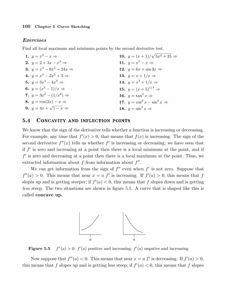
100 Chapter 5 Curve Sketching
Exercises
Find all local maximum and minimum points by the second derivative test.
1. y = x2 − x ⇒2. y = 2 + 3x− x3 ⇒3. y = x3 − 9x2 + 24x ⇒4. y = x4 − 2x2 + 3 ⇒5. y = 3x4 − 4x3 ⇒6. y = (x2 − 1)/x ⇒7. y = 3x2 − (1/x2) ⇒8. y = cos(2x)− x ⇒9. y = 4x +
√1− x ⇒
10. y = (x + 1)/p
5x2 + 35 ⇒11. y = x5 − x ⇒12. y = 6x + sin 3x ⇒13. y = x + 1/x ⇒14. y = x2 + 1/x ⇒15. y = (x + 5)1/4 ⇒16. y = tan2 x ⇒17. y = cos2 x− sin2 x ⇒18. y = sin3 x ⇒
5.4 Concavity and inflection points
We know that the sign of the derivative tells whether a function is increasing or decreasing.For example, any time that f ′(x) > 0, that means that f(x) is increasing. The sign of thesecond derivative f ′′(x) tells us whether f ′ is increasing or decreasing; we have seen thatif f ′ is zero and increasing at a point then there is a local minimum at the point, and iff ′ is zero and decreasing at a point then there is a local maximum at the point. Thus, weextracted information about f from information about f ′′.
We can get information from the sign of f ′′ even when f ′ is not zero. Suppose thatf ′′(a) > 0. This means that near x = a f ′ is increasing. If f ′(a) > 0, this means that f
slopes up and is getting steeper; if f ′(a) < 0, this means that f slopes down and is gettingless steep. The two situations are shown in figure 5.5. A curve that is shaped like this iscalled concave up.
a
.........................................
..........................................................................................
a
.............................................................................................................................................
Figure 5.5 f ′′(a) > 0: f ′(a) positive and increasing, f ′(a) negative and increasing.
Now suppose that f ′′(a) < 0. This means that near x = a f ′ is decreasing. If f ′(a) > 0,this means that f slopes up and is getting less steep; if f ′(a) < 0, this means that f slopes
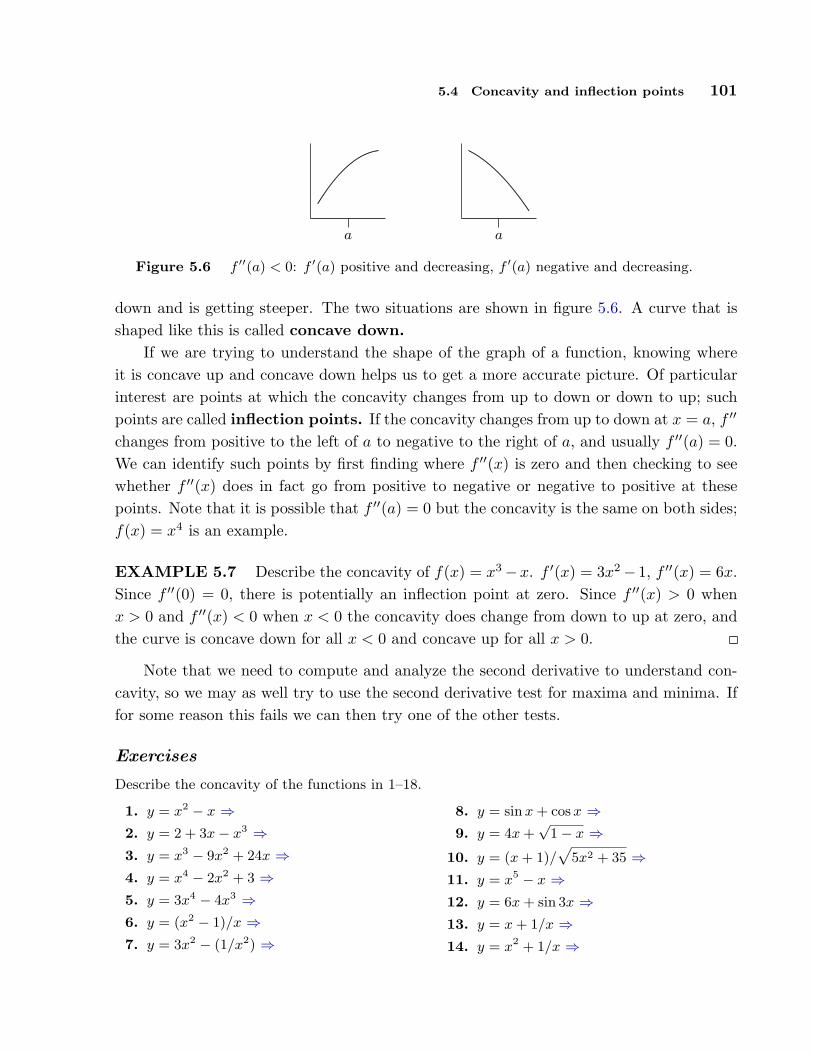
5.4 Concavity and inflection points 101
a
...................................................................................................................
................
a
........................................................................................................................................
Figure 5.6 f ′′(a) < 0: f ′(a) positive and decreasing, f ′(a) negative and decreasing.
down and is getting steeper. The two situations are shown in figure 5.6. A curve that isshaped like this is called concave down.
If we are trying to understand the shape of the graph of a function, knowing whereit is concave up and concave down helps us to get a more accurate picture. Of particularinterest are points at which the concavity changes from up to down or down to up; suchpoints are called inflection points. If the concavity changes from up to down at x = a, f ′′
changes from positive to the left of a to negative to the right of a, and usually f ′′(a) = 0.We can identify such points by first finding where f ′′(x) is zero and then checking to seewhether f ′′(x) does in fact go from positive to negative or negative to positive at thesepoints. Note that it is possible that f ′′(a) = 0 but the concavity is the same on both sides;f(x) = x4 is an example.
EXAMPLE 5.7 Describe the concavity of f(x) = x3−x. f ′(x) = 3x2− 1, f ′′(x) = 6x.Since f ′′(0) = 0, there is potentially an inflection point at zero. Since f ′′(x) > 0 whenx > 0 and f ′′(x) < 0 when x < 0 the concavity does change from down to up at zero, andthe curve is concave down for all x < 0 and concave up for all x > 0.
Note that we need to compute and analyze the second derivative to understand con-cavity, so we may as well try to use the second derivative test for maxima and minima. Iffor some reason this fails we can then try one of the other tests.
Exercises
Describe the concavity of the functions in 1–18.
1. y = x2 − x ⇒2. y = 2 + 3x− x3 ⇒3. y = x3 − 9x2 + 24x ⇒4. y = x4 − 2x2 + 3 ⇒5. y = 3x4 − 4x3 ⇒6. y = (x2 − 1)/x ⇒7. y = 3x2 − (1/x2) ⇒
8. y = sin x + cos x ⇒9. y = 4x +
√1− x ⇒
10. y = (x + 1)/p
5x2 + 35 ⇒11. y = x5 − x ⇒12. y = 6x + sin 3x ⇒13. y = x + 1/x ⇒14. y = x2 + 1/x ⇒

102 Chapter 5 Curve Sketching
15. y = (x + 5)1/4 ⇒16. y = tan2 x ⇒
17. y = cos2 x− sin2 x ⇒18. y = sin3 x ⇒
19. Identify the intervals on which the graph of the function f(x) = x4 − 4x3 + 10 is of one ofthese four shapes: concave up and increasing; concave up and decreasing; concave down andincreasing; concave down and decreasing. ⇒
20. Describe the concavity of y = x3 + bx2 + cx + d. You will need to consider different cases,depending on the values of the coefficients.
21. Let n be an integer greater than or equal to two, and suppose f is a polynomial of degreen. How many inflection points can f have? Hint: Use the second derivative test and thefundamental theorem of algebra.
5.5 Asymptotes and Other Things to Look For
A vertical asymptote is a place where the function becomes infinite, typically because theformula for the function has a denominator that becomes zero. For example, the reciprocalfunction f(x) = 1/x has a vertical asymptote at x = 0, and the function tan x has a verticalasymptote at x = π/2 (and also at x = −π/2, x = 3π/2, etc.). Whenever the formula for afunction contains a denominator it is worth looking for a vertical asymptote by checking tosee if the denominator can ever be zero, and then checking the limit at such points. Notethat there is not always a vertical asymptote where the derivative is zero: f(x) = (sin x)/x
has a zero denominator at x = 0, but since limx→0(sinx)/x = 1 there is no asymptotethere.
A horizontal asymptote is a horizontal line to which f(x) gets closer and closer as x
approaches ∞ (or as x approaches −∞). For example, the reciprocal function has thex-axis for a horizontal asymptote. Horizontal asymptotes can be identified by computingthe limits limx→∞ f(x) and limx→−∞ f(x). Since limx→∞ 1/x = limx→−∞ 1/x = 0, theline y = 0 (that is, the x-axis) is a horizontal asymptote in both directions.
Some functions have asymptotes that are neither horizontal nor vertical, but someother line. Such asymptotes are somewhat more difficult to identify and we will ignorethem.
If the domain of the function does not extend out to infinity, we should also askwhat happens as x approaches the boundary of the domain. For example, the functiony = f(x) = 1/
√r2 − x2 has domain −r < x < r, and y becomes infinite as x approaches
either r or −r. In this case we might also identify this behavior because when x = ±r thedenominator of the function is zero.
5.5 Asymptotes and Other Things to Look For 103
If there are any points where the derivative fails to exist (a cusp or corner), then weshould take special note of what the function does at such a point.
Finally, it is worthwhile to notice any symmetry. A function f(x) that has the samevalue for −x as for x, i.e., f(−x) = f(x), is called an “even function.” Its graph issymmetric with respect to the y-axis. Some examples of even functions are: xn when n
is an even number, cos x, and sin2 x. On the other hand, a function that satisfies theproperty f(−x) = −f(x) is called an “odd function.” Its graph is symmetric with respectto the origin. Some examples of odd functions are: xn when n is an odd number, sin x, andtanx. Of course, most functions are neither even nor odd, and do not have any particularsymmetry.
Exercises
Sketch the curves. Identify clearly any interesting features, including local maximum and mini-mum points, inflection points, asymptotes, and intercepts.
1. y = x5 − 5x4 + 5x3
2. y = x3 − 3x2 − 9x + 5
3. y = (x− 1)2(x + 3)2/3
4. x2 + x2y2 = a2y2, a > 0.
5. y = xex
6. y = (ex + e−x)/2
7. y = e−x cos x
8. y = ex − sin x
9. y = ex/x
10. y = 4x +√
1− x
11. y = (x + 1)/p
5x2 + 35
12. y = x5 − x
13. y = 6x + sin 3x
14. y = x + 1/x
15. y = x2 + 1/x
16. y = (x + 5)1/4
17. y = tan2 x
18. y = cos2 x− sin2 x
19. y = sin3 x
20. y = x(x2 + 1)
21. y = x3 + 6x2 + 9x
22. y = x/(x2 − 9)
23. y = x2/(x2 + 9
24. y = 2√
x− x
25. y = 3 sin(x)− sin3(x), for x ∈ [0, 2π]
26. y = (x− 1)/(x2)
For each of the following five functions, identify any vertical and horizontal asymptotes, andidentify intervals on which the function is concave up and increasing; concave up and decreasing;concave down and increasing; concave down and decreasing.
27. f(θ) = sec(θ)
28. f(x) = 1/(1 + x2)
29. f(x) = (x− 3)/(2x− 2)
30. f(x) = 1/(1− x2)
31. f(x) = 1 + 1/(x2)
32. Let f(x) = 1/(x2 − a2), where a ≥ 0. Find any vertical and horizontal asymptotes andthe intervals upon which the given function is concave up and increasing; concave up and
104 Chapter 5 Curve Sketching
decreasing; concave down and increasing; concave down and decreasing. Discuss how thevalue of a affects these features.
6Applications of the Derivative
6.1 Optimization
Many important applied problems involve finding the best way to accomplish some task.Often this involves finding the maximum or minimum value of some function: the minimumtime to make a certain journey, the minimum cost for doing a task, the maximum powerthat can be generated by a device, and so on. Many of these problems can be solved byfinding the appropriate function and then using techniques of calculus to find the maximumor the minimum value required.
Generally such a problem will have the following mathematical form: Find the largest(or smallest) value of f(x) when a ≤ x ≤ b. Sometimes a or b are infinite, but frequentlythe real world imposes some constraint on the values that x may have.
Such a problem differs in two ways from the local maximum and minimum problemswe encountered when graphing functions: We are interested only in the function betweena and b, and we want to know the largest or smallest value that f(x) takes on, not merelyvalues that are the largest or smallest in a small interval. That is, we seek not a localmaximum or minimum but a global maximum or minimum, sometimes also called anabsolute maximum or minimum.
Any global maximum or minimum must of course be a local maximum or minimum.If we find all possible local extrema, then the global maximum, if it exists, must be thelargest of the local maxima and the global minimum, if it exists, must be the smallest ofthe local minima. We already know where local extrema can occur: only at those pointsat which f ′(x) is zero or undefined. Actually, there are two additional points at which a
105

106 Chapter 6 Applications of the Derivative
maximum or minimum can occur if the endpoints a and b are not infinite, namely, at a
and b. We have not previously considered such points because we have not been interestedin limiting a function to a small interval. An example should make this clear.
−2 1
....................................................................................................................................................................................................................................................................................................................................................................................................................................................
Figure 6.1 The function g(x) or f(x) = x2 truncated to [−2, 1]
EXAMPLE 6.1 Find the maximum and minimum values of f(x) = x2 on the interval[−2, 1], shown in figure 6.1. We compute f ′(x) = 2x, which is zero at x = 0 and is alwaysdefined.
Since f ′(1) = 2 we would not normally flag x = 1 as a point of interest, but it is clearfrom the graph that when f(x) is restricted to [−2, 1] there is a local maximum at x = 1.Likewise we would not normally pay attention to x = −2, but since we have truncated f
at −2 we have introduced a new local maximum there as well. In a technical sense nothingnew is going on here: When we truncate f we actually create a new function, let’s call itg, that is defined only on the interval [−2, 1]. If we try to compute the derivative of thisnew function we actually find that it does not have a derivative at −2 or 1. Why? Becauseto compute the derivative at 1 we must compute the limit
lim∆x→0
g(1 + ∆x)− g(1)∆x
.
This limit does not exist because when ∆x > 0, g(1 + ∆x) is not defined. It is simpler,however, simply to remember that we must always check the endpoints.
So the function g, that is, f restricted to [−2, 1], has one critical value and two finiteendpoints, any of which might be the global maximum or minimum. We could first deter-mine which of these are local maximum or minimum points (or neither); then the largest

6.1 Optimization 107
local maximum must be the global maximum and the smallest local minimum must be theglobal minimum. It is usually easier, however, to compute the value of f at every pointat which the global maximum or minimum might occur; the largest of these is the globalmaximum, the smallest is the global minimum.
So we compute f(−2) = 4, f(0) = 0, f(1) = 1. The global maximum is 4 at x = −2and the global minimum is 0 at x = 0.
It is possible that there is no global maximum or minimum. It is difficult, and notparticularly useful, to express a set procedure for determining whether this is the case.Generally, the best approach is to gain enough understanding of the shape of the graph todecide. Fortunately, only a rough idea of the shape is usually needed.
There are some particularly nice cases that are easy. If you have a continuous functionon a closed interval [a, b], there is always both a global maximum and a global minimum,so examining the critical values and the endpoints is enough:
THEOREM 6.2 Extreme value theorem If f is continuous on a closed interval[a, b], then it has both a minimum and a maximum point. That is, there are real numbersc and d in [a, b] so that for every x in [a, b], f(x) ≤ f(c) and f(x) ≥ f(d).
Another easy case: If a function is continuous and has a single critical value, then ifthere is a local maximum at the critical value it is a global maximum, and if it is a localminimum it is a global minimum. There may also be a global minimum in the first case,or a global maximum in the second case, but that will generally require more effort todetermine.
EXAMPLE 6.3 Let f(x) = −x2 + 4x − 3. Find the maximum value of f(x) on theinterval [0, 4]. First note that f ′(x) = −2x+4 = 0 when x = 2, and f(2) = 1. Next observethat f ′(x) is defined for all x, so there are no other critical values. Finally, f(0) = −3 andf(4) = −3. The largest value of f(x) on the interval [0, 4] is f(2) = 1.
EXAMPLE 6.4 Let f(x) = −x2 + 4x − 3. Find the maximum value of f(x) on theinterval [−1, 1].
First note that f ′(x) = −2x + 4 = 0 when x = 2. But x = 2 is not in the interval, sowe don’t use it. Thus the only two points to be checked are the endpoints; f(−1) = −8and f(1) = 0. So the largest value of f(x) on [−1, 1] is f(1) = 0.
EXAMPLE 6.5 Find the maximum and minimum values of the function f(x) = 7 +|x − 2| for x between 1 and 4 inclusive. The derivative f ′(x) is never zero, but f ′(x) is

108 Chapter 6 Applications of the Derivative
undefined at x = 2, so we compute f(2) = 7. Checking the end points we get f(1) = 8 andf(4) = 9. The smallest of these numbers is f(2) = 7, which is, therefore, the minimumvalue of f(x) on the interval 1 ≤ x ≤ 4, and the maximum is f(4) = 9.
−2 −1 21
....................................................................................................................................................................................
..........................................................................................................................................................................................
................................................................................................................................................................
Figure 6.2 f(x) = x3 − x
EXAMPLE 6.6 Find all local maxima and minima for f(x) = x3 − x, and deter-mine whether there is a global maximum or minimum on the open interval (−2, 2). Inexample 5.2 we found a local maximum at (−√3/3, 2
√3/9) and a local minimum at
(√
3/3,−2√
3/9). Since the endpoints are not in the interval (−2, 2) they cannot be con-sidered. Is the lone local maximum a global maximum? Here we must look more closely atthe graph. We know that on the closed interval [−√3/3,
√3/3] there is a global maximum
at x = −√3/3 and a global minimum at x =√
3/3. So the question becomes: what hap-pens between −2 and −√3/3, and between
√3/3 and 2? Since there is a local minimum
at x =√
3/3, the graph must continue up to the right, since there are no more criticalvalues. This means no value of f will be less than −2
√3/9 between
√3/3 and 2, but it
says nothing about whether we might find a value larger than the local maximum 2√
3/9.How can we tell? Since the function increases to the right of
√3/3, we need to know what
the function values do “close to” 2. Here the easiest test is to pick a number and do acomputation to get some idea of what’s going on. Since f(1.9) = 4.959 > 2
√3/9, there
is no global maximum at −√3/3, and hence no global maximum at all. (How can we tellthat 4.959 > 2
√3/9? We can use a calculator to approximate the right hand side; if it is
not even close to 4.959 we can take this as decisive. Since 2√
3/9 ≈ 0.3849, there’s reallyno question. Funny things can happen in the rounding done by computers and calculators,however, so we might be a little more careful, especially if the values come out quite close.In this case we can convert the relation 4.959 > 2
√3/9 into (9/2)4.959 >
√3 and ask
6.1 Optimization 109
whether this is true. Since the left side is clearly larger than 4 · 4 which is clearly largerthan
√3, this settles the question.)
A similar analysis shows that there is also no global minimum. The graph of f(x) on(−2, 2) is shown in figure 6.2.
EXAMPLE 6.7 Of all rectangles of area 100, which has the smallest perimeter?First we must translate this into a purely mathematical problem in which we want to
find the minimum value of a function. If x denotes one of the sides of the rectangle, thenthe adjacent side must be 100/x (in order that the area be 100). So the function we wantto minimize is
f(x) = 2x + 2100x
since the perimeter is twice the length plus twice the width of the rectangle. Not all valuesof x make sense in this problem: lengths of sides of rectangles must be positive, so x > 0.If x > 0 then so is 100/x, so we need no second condition on x.
We next find f ′(x) and set it equal to zero: 0 = f ′(x) = 2− 200/x2. Solving f ′(x) = 0for x gives us x = ±10. We are interested only in x > 0, so only the value x = 10 is ofinterest. Since f ′(x) is defined everywhere on the interval (0,∞), there are no more criticalvalues, and there are no endpoints. Is there a local maximum, minimum, or neither atx = 10? The second derivative is f ′′(x) = 400/x3, and f ′′(10) > 0, so there is a localminimum. Since there is only one critical value, this is also the global minimum, so therectangle with smallest perimeter is the 10× 10 square.
EXAMPLE 6.8 You want to sell a certain number n of items in order to maximizeyour profit. Market research tells you that if you set the price at $1.50, you will be ableto sell 5000 items, and for every 10 cents you lower the price below $1.50 you will be ableto sell another 1000 items. Suppose that your fixed costs (“start-up costs”) total $2000,and the per item cost of production (“marginal cost”) is $0.50. Find the price to set peritem and the number of items sold in order to maximize profit, and also determine themaximum profit you can get.
The first step is to convert the problem into a function maximization problem. Sincewe want to maximize profit by setting the price per item, we should look for a functionP (x) representing the profit when the price per item is x. Profit is revenue minus costs, andrevenue is number of items sold times the price per item, so we get P = nx−2000−0.50n.The number of items sold is itself a function of x, n = 5000 + 1000(1.5− x)/0.10, because(1.5 − x)/0.10 is the number of multiples of 10 cents that the price is below $1.50. Now

110 Chapter 6 Applications of the Derivative
we substitute for n in the profit function:
P (x) = (5000 + 1000(1.5− x)/0.10)x− 2000− 0.5(5000 + 1000(1.5− x)/0.10)
= −10000x2 + 25000x− 12000
We want to know the maximum value of this function when x is between 0 and 1.5.The derivative is P ′(x) = −20000 ∗ x + 25000, which is zero when x = 1.25. SinceP ′′(x) = −20000 < 0, there must be a local maximum at x = 1.25, and since this is theonly critical value it must be a global maximum as well. (Alternately, we could computeP (0) = −12000, P (1.25) = 3625, and P (1.5) = 3000 and note that P (1.25) is the maximumof these.) Thus the maximum profit is $3625, attained when we set the price at $1.25 andsell 7500 items.
....................................................................................................................................................................................................................................................................................................................................................................................................................................................................................................................
................................................................................................................................................................................................................................................................................................................................
y = a
(x, x2)•
............. ............. ............. ............. ............. ............. ............. ............. ............. ............. ............. ............. ............. ............. ............. ............. ............. .............
Figure 6.3 Rectangle in a parabola.
EXAMPLE 6.9 Find the largest rectangle (that is, the rectangle with largest area)that fits inside the graph of the parabola y = x2 below the line y = a (a is an unspecifiedconstant value). (The top side of the rectangle should be on the horizontal line y = a; seefigure 6.3.)
We want to find the maximum value of some function A(x) representing area. Perhapsthe hardest part of this problem is deciding what x should represent. The lower rightcorner of the rectangle is at (x, x2), and once this is chosen the rectangle is completelydetermined. So we can let the x in A(x) be the x of the parabola f(x) = x2. Then thearea is A(x) = (2x)(a−x2) = −2x3 +2ax. We want the maximum value of A(x) when x isin [0,
√a]. (You might object to allowing x = 0 or x =
√a, since then the “rectangle” has

6.1 Optimization 111
either no width or no height, so is not “really” a rectangle. But the problem is somewhateasier if we simply allow such rectangles, which have zero area.)
Setting 0 = A′(x) = 6x2 + 2a we get x =√
a/3 as the only critical value. Testing this
and the two endpoints, we have A(0) = A(√
a) = 0 and A(√
a/3) = (4/9)√
3a3/2. The
maximum area thus occurs when the rectangle has dimensions 2√
a/3× (2/3)a.
........
........
........
................................................................................
.......................
............................
.....................................................
..................................................................................................................................................................................................................................................................................................................................................................................................................................................................................................................................................
............................................................................................................................................................
................................
................................
................................
................................
................................
................................
................................
..............................................................................................................................................................................................................................................................................................
................................
................................
................................
................................
................................
................................
................................
.......
(h−R, r)
Figure 6.4 Cone in a sphere.
EXAMPLE 6.10 If you fit the largest possible cone inside a sphere, what fraction ofthe volume of the sphere is occupied by the cone? (Here by “cone” we mean a right circularcone, i.e., a cone for which the base is perpendicular to the axis of symmetry, and for whichthe cross-section cut perpendicular to the axis of symmetry at any point is a circle.)
Let R be the radius of the sphere, and let r and h be the base radius and height ofthe cone inside the sphere. What we want to maximize is the volume of the cone: πr2h/3.Here R is a fixed value, but r and h can vary. Namely, we could choose r to be as largeas possible—equal to R—by taking the height equal to R; or we could make the cone’sheight h larger at the expense of making r a little less than R. See the side view depictedin figure 6.4. We have situated the picture in a convenient way relative to the x and y
axes, namely, with the center of the sphere at the origin and the vertex of the cone at thefar left on the x-axis.
Notice that the function we want to maximize, πr2h/3, depends on two variables. Thisis frequently the case, but often the two variables are related in some way so that “really”there is only one variable. So our next step is to find the relationship and use it to solvefor one of the variables in terms of the other, so as to have a function of only one variable

112 Chapter 6 Applications of the Derivative
to maximize. In this problem, the condition can be read off the above drawing: the uppercorner of the triangle, whose coordinates are (h−R, r), must be on the circle of radius R.That is,
(h−R)2 + r2 = R2.
We can solve for h in terms of r or for r in terms of h. Either involves taking a squareroot, but we notice that the volume function contains r2, not r by itself, so it is easiest tosolve for r2 directly: r2 = R2 − (h−R)2. Then we substitute the result into πr2h/3:
V (h) = π(R2 − (h−R)2)h/3
= −π
3h3 +
23πh2R
We want to maximize V (h) when h is between 0 and 2R. Now we solve 0 = f ′(h) =−πh2 + (4/3)πhR, getting h = 0 or h = 4R/3. We compute V (0) = V (2R) = 0 andV (4R/3) = (32/81)πR3. The maximum is the latter; since the volume of the sphere is(4/3)πR3, the fraction of the sphere occupied by the cone is
(32/81)πR3
(4/3)πR3=
827≈ 30%.
EXAMPLE 6.11 You are making cylindrical containers to contain a given volume.Suppose that the top and bottom are made of a material that is N times as expensive(cost per unit area) as the material used for the lateral side of the cylinder. Find (in termsof N) the ratio of height to base radius of the cylinder that minimizes the cost of makingthe containers.
Let us first choose letters to represent various things: h for the height, r for the baseradius, V for the volume of the cylinder, and c for the cost per unit area of the lateral sideof the cylinder; V and c are constants, h and r are variables. Now we can write the costof materials:
c(2πrh) + Nc(2πr2).
Again we have two variables; the relationship is provided by the fixed volume of thecylinder: V = πr2h. We use this relation to eliminate h (we could eliminate r, but it’sa little easier if we eliminate h, which appears in only one place in the above formula forcost). The result is
f(r) = 2cπrV
πr2+ 2Ncπr2 =
2cV
r+ 2Ncπr2.

6.1 Optimization 113
We want to know the minimum value of this function when r is in (0,∞). We now set0 = f ′(r) = −2cV/r2 + 4Ncπr, giving r = 3
√V/(2Nπ). Since f ′′(r) = 4cV/r3 + 4Ncπ
is positive when r is positive, there is a local minimum at the critical value, and hence aglobal minimum since there is only one critical value.
Finally, since h = V/(πr2),
h
r=
V
πr3=
V
π(V/(2Nπ))= 2N,
so the minimum cost occurs when the height h is 2N times the radius. If, for example,there is no difference in the cost of materials, the height is twice the radius (or the heightis equal to the diameter).
..........................................................................................................................................................................................................................................................................................................................................................
• •
•
•xa− x
A
D B C
b
Figure 6.5 Minimizing travel time.
EXAMPLE 6.12 Suppose you want to reach a point A that is located across the sandfrom a nearby road (see figure 6.5). Suppose that the road is straight, and b is the distancefrom A to the closest point C on the road. Let v be your speed on the road, and let w,which is less than v, be your speed on the sand. Right now you are at the point D, whichis a distance a from C. At what point B should you turn off the road and head across thesand in order to minimize your travel time to A?
Let x be the distance short of C where you turn off, i.e., the distance from B to C. Wewant to minimize the total travel time. Recall that when traveling at constant velocity,time=distance/velocity.
You travel the distance DB at speed v, and then the distance BA at speed w. SinceDB = a−x and, by the Pythagorean theorem, BA =
√x2 + b2, the total time for the trip
is
f(x) =a− x
v+√
x2 + b2
w.

114 Chapter 6 Applications of the Derivative
We want to find the minimum value of f when x is between 0 and a. As usual we setf ′(x) = 0 and solve for x:
0 = f ′(x) = −1v
+x
w√
x2 + b2
w√
x2 + b2 = vx
w2(x2 + b2) = v2x2
w2b2 = (v2 − w2)x2
x =wb√
v2 − w2
Notice that a does not appear in the last expression, but a is not irrelevant, since we areinterested only in critical values that are in [0, a], and wb/
√v2 − w2 is either in this interval
or not. If it is, we can use the second derivative to test it:
f ′′(x) =b2
(x2 + b2)3/2w.
Since this is always positive there is a local minimum at the critical point, and so it is aglobal minimum as well.
If the critical value is not in [0, a] it is larger than a. In this case the minimum mustoccur at one of the endpoints. We can compute
f(0) =a
v+
b
w
f(a) =√
a2 + b2
w
but it is difficult to determine which of these is smaller by direct comparison. If, as islikely in practice, we know the values of v, w, a, and b, then it is easy to determine this.With a little cleverness, however, we can determine the minimum in general. We have seenthat f ′′(x) is always positive, so the derivative f ′(x) is always increasing. We know thatat wb/
√v2 − w2 the derivative is zero, so for values of x less than that critical value, the
derivative is negative. This means that f(0) > f(a), so the minimum occurs when x = a.So the upshot is this: If you start farther away from C than wb/
√v2 − w2 then you
always want to cut across the sand when you are a distance wb/√
v2 − w2 from point C.If you start closer than this to C, you should cut directly across the sand.
6.1 Optimization 115
Summary—Steps to solve an optimization problem.
1. Decide what the variables are and what the constants are, draw a diagram ifappropriate, understand clearly what it is that is to be maximized or minimized.
2. Write a formula for the function for which you wish to find the maximum orminimum.
3. Express that formula in terms of only one variable, that is, in the form f(x).
4. Set f ′(x) = 0 and solve. Check all critical values and endpoints to determine theextreme value.
Exercises
1. Let f(x) =
1 + 4x− x2 for x ≤ 3(x + 5)/2 for x > 3
Find the maximum value and minimum values of f(x) for x in [0, 4]. Graph f(x) to checkyour answers. ⇒
2. Find the dimensions of the rectangle of largest area having fixed perimeter 100. ⇒3. Find the dimensions of the rectangle of largest area having fixed perimeter P . ⇒4. A box with square base and no top is to hold a volume 100. Find the dimensions of the box
that requires the least material for the five sides. Also find the ratio of height to side of thebase. ⇒
5. A box with square base is to hold a volume 200. The bottom and top are formed by foldingin flaps from all four sides, so that the bottom and top consist of two layers of cardboard.Find the dimensions of the box that requires the least material. Also find the ratio of heightto side of the base. ⇒
6. A box with square base and no top is to hold a volume V . Find (in terms of V ) the dimensionsof the box that requires the least material for the five sides. Also find the ratio of height toside of the base. (This ratio will not involve V .) ⇒
7. You have 100 feet of fence to make a rectangular play area alongside the wall of your house.The wall of the house bounds one side. What is the largest size possible (in square feet) forthe play area? ⇒
8. You have l feet of fence to make a rectangular play area alongside the wall of your house.The wall of the house bounds one side. What is the largest size possible (in square feet) forthe play area? ⇒
9. Marketing tells you that if you set the price of an item at $10 then you will be unable to sellit, but that you can sell 500 items for each dollar below $10 that you set the price. Supposeyour fixed costs total $3000, and your marginal cost is $2 per item. What is the most profityou can make? ⇒
10. Find the area of the largest rectangle that fits inside a semicircle of radius 10 (one side ofthe rectangle is along the diameter of the semicircle). ⇒
11. Find the area of the largest rectangle that fits inside a semicircle of radius r (one side of therectangle is along the diameter of the semicircle). ⇒

116 Chapter 6 Applications of the Derivative
12. For a cylinder with surface area 50, including the top and the bottom, find the ratio of heightto base radius that maximizes the volume. ⇒
13. For a cylinder with given surface area S, including the top and the bottom, find the ratio ofheight to base radius that maximizes the volume. ⇒
14. You want to make cylindrical containers to hold 1 liter using the least amount of constructionmaterial. The side is made from a rectangular piece of material, and this can be done withno material wasted. However, the top and bottom are cut from squares of side 2r, so that2(2r)2 = 8r2 of material is needed (rather than 2πr2, which is the total area of the top andbottom). Find the dimensions of the container using the least amount of material, and alsofind the ratio of height to radius for this container. ⇒
15. You want to make cylindrical containers of a given volume V using the least amount ofconstruction material. The side is made from a rectangular piece of material, and this canbe done with no material wasted. However, the top and bottom are cut from squares of side2r, so that 2(2r)2 = 8r2 of material is needed (rather than 2πr2, which is the total area ofthe top and bottom). Find the optimal ratio of height to radius. ⇒
16. Given a right circular cone, you put an upside-down cone inside it so that its vertex is at thecenter of the base of the larger cone and its base is parallel to the base of the larger cone. Ifyou choose the upside-down cone to have the largest possible volume, what fraction of thevolume of the larger cone does it occupy? (Let H and R be the height and base radius ofthe larger cone, and let h and r be the height and base radius of the smaller cone. Hint: Usesimilar triangles to get an equation relating h and r.) ⇒
17. In example 6.12, what happens if w ≥ v (i.e., your speed on sand is at least your speed onthe road)? ⇒
18. A container holding a fixed volume is being made in the shape of a cylinder with a hemi-spherical top. (The hemispherical top has the same radius as the cylinder.) Find the ratio ofheight to radius of the cylinder which minimizes the cost of the container if (a) the cost perunit area of the top is twice as great as the cost per unit area of the side, and the containeris made with no bottom; (b) the same as in (a), except that the container is made with acircular bottom, for which the cost per unit area is 1.5 times the cost per unit area of theside. ⇒
19. A piece of carboard is 1 meter by 1/2 meter. A square is to be cut from each corner andthe sides folded up to make an open-top box. What are the dimensions of the box withmaximum possible volume? ⇒
20. (a) A square piece of cardboard of side a is used to make an open-top box by cutting outa small square from each corner and bending up the sides. How large a square should becut from each corner in order that the box have maximum volume? (b) What if the piece ofcardboard used to make the box is a rectangle of sides a and b? ⇒
21. A window consists of a rectangular piece of clear glass with a semicircular piece of coloredglass on top; the colored glass transmits only 1/2 as much light per unit area as the the clearglass. If the distance from top to bottom (across both the rectangle and the semicircle) is2 meters and the window may be no more than 1.5 meters wide, find the dimensions of therectangular portion of the window that lets through the most light. ⇒
22. A window consists of a rectangular piece of clear glass with a semicircular piece of coloredglass on top. Suppose that the colored glass transmits only k times as much light per unit

6.1 Optimization 117
area as the clear glass (k is between 0 and 1). If the distance from top to bottom (acrossboth the rectangle and the semicircle) is a fixed distance H, find (in terms of k) the ratio ofvertical side to horizontal side of the rectangle for which the window lets through the mostlight. ⇒
23. You are designing a poster to contain a fixed amount A of printing (measured in squarecentimeters) and have margins of a centimeters at the top and bottom and b centimeters atthe sides. Find the ratio of vertical dimension to horizontal dimension of the printed area onthe poster if you want to minimize the amount of posterboard needed. ⇒
24. The strength of a rectangular beam is proportional to the product of its width w times thesquare of its depth d. Find the dimensions of the strongest beam that can be cut from acylindrical log of radius r. ⇒
........
........
.......................................................
...........................
.......................................................................................................................................................................................................................................................................................................................................................................
......................................................................................................
.....................................................................................................................................................................................................................................................................................................................................................
........
........
........
........
........
........
........
........
........
........
........
........
........
........
........
........
........
........
...↑||d||↓←− w −→
Figure 6.6 Cutting a beam.
25. What fraction of the volume of a sphere is taken up by the largest cylinder that can be fitinside the sphere? ⇒
26. The U.S. post office will accept a box for shipment only if the sum of the length and girth(distance around) is at most 108 in. Find the dimensions of the largest acceptable box withsquare front and back. ⇒
27. Find the dimensions of the lightest cylindrical can containing 0.25 liter (=250 cm3) if thetop and bottom are made of a material that is twice as heavy (per unit area) as the materialused for the side. ⇒
28. A conical paper cup is to hold 1/4 of a liter. Find the height and radius of the cone whichminimizes the amount of paper needed to make the cup. Use the formula πr
√r2 + h2 for
the area of the side of a cone. ⇒29. A conical paper cup is to hold a fixed volume of water. Find the ratio of height to base radius
of the cone which minimizes the amount of paper needed to make the cup. Use the formulaπr√
r2 + h2 for the area of the side of a cone, called the lateral area of the cone. ⇒30. If you fit the cone with the largest possible surface area (lateral area plus area of base) into
a sphere, what percent of the volume of the sphere is occupied by the cone? ⇒31. Two electrical charges, one a positive charge A of magnitude a and the other a negative
charge B of magnitude b, are located a distance c apart. A positively charged particle P issituated on the line between A and B. Find where P should be put so that the pull awayfrom A towards B is minimal. Here assume that the force from each charge is proportional
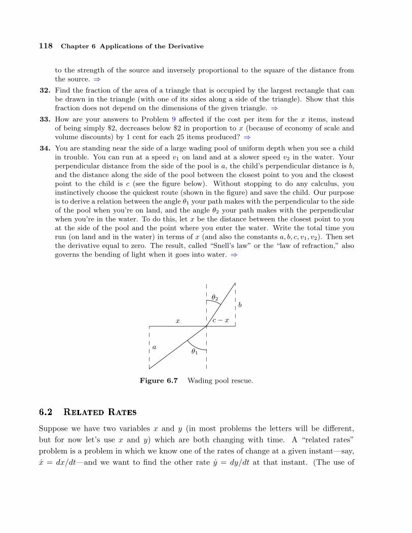
118 Chapter 6 Applications of the Derivative
to the strength of the source and inversely proportional to the square of the distance fromthe source. ⇒
32. Find the fraction of the area of a triangle that is occupied by the largest rectangle that canbe drawn in the triangle (with one of its sides along a side of the triangle). Show that thisfraction does not depend on the dimensions of the given triangle. ⇒
33. How are your answers to Problem 9 affected if the cost per item for the x items, insteadof being simply $2, decreases below $2 in proportion to x (because of economy of scale andvolume discounts) by 1 cent for each 25 items produced? ⇒
34. You are standing near the side of a large wading pool of uniform depth when you see a childin trouble. You can run at a speed v1 on land and at a slower speed v2 in the water. Yourperpendicular distance from the side of the pool is a, the child’s perpendicular distance is b,and the distance along the side of the pool between the closest point to you and the closestpoint to the child is c (see the figure below). Without stopping to do any calculus, youinstinctively choose the quickest route (shown in the figure) and save the child. Our purposeis to derive a relation between the angle θ1 your path makes with the perpendicular to the sideof the pool when you’re on land, and the angle θ2 your path makes with the perpendicularwhen you’re in the water. To do this, let x be the distance between the closest point to youat the side of the pool and the point where you enter the water. Write the total time yourun (on land and in the water) in terms of x (and also the constants a, b, c, v1, v2). Then setthe derivative equal to zero. The result, called “Snell’s law” or the “law of refraction,” alsogoverns the bending of light when it goes into water. ⇒
.....................................................................θ1
................................................
θ2
................................................................................................................................................................................................................................................................................................................................................................................................
x c− x
a
b
Figure 6.7 Wading pool rescue.
6.2 Related Rates
Suppose we have two variables x and y (in most problems the letters will be different,but for now let’s use x and y) which are both changing with time. A “related rates”problem is a problem in which we know one of the rates of change at a given instant—say,x = dx/dt—and we want to find the other rate y = dy/dt at that instant. (The use of

6.2 Related Rates 119
x to mean dx/dt goes back to Newton and is still used for this purpose, especially byphysicists.)
If y is written in terms of x, i.e., y = f(x), then this is easy to do using the chain rule:
y =dy
dt=
dy
dx· dx
dt=
dy
dxx.
That is, find the derivative of f(x), plug in the value of x at the instant in question, andmultiply by the given value of x = dx/dt to get y = dy/dt.
EXAMPLE 6.13 Suppose an object is moving along a path described by y = x2, thatis, it is moving on a parabolic path. At a particular time, say t = 5, the x coordinate is6 and we measure the speed at which the x coordinate of the object is changing and findthat dx/dt = 3. At the same time, how fast is the y coordinate changing?
Using the chain rule, dy/dt = 2x · dx/dt. At t = 5 we know that x = 6 and dx/dt = 3,so dy/dt = 2 · 6 · 3 = 36.
In many cases, particularly interesting ones, x and y will be related in some other way,for example x = f(y), or F (x, y) = k, or perhaps F (x, y) = G(x, y), where F (x, y) andG(x, y) are expressions involving both variables. In all cases, you can solve the relatedrates problem by taking the derivative of both sides, plugging in all the known values(namely, x, y, and x), and then solving for y.
To summarize, here are the steps in doing a related rates problem:
1. Decide what the two variables are.
2. Find an equation relating them.
3. Take d/dt of both sides.
4. Plug in all known values at the instant in question.
5. Solve for the unknown rate.
EXAMPLE 6.14 A plane is flying directly away from you at 500 mph at an altitudeof 3 miles. How fast is the plane’s distance from you increasing at the moment when theplane is flying over a point on the ground 4 miles from you?
To see what’s going on, we first draw a schematic representation of the situation.Because the plane is in level flight directly away from you, the rate at which x changes
is the speed of the plane, dx/dt = 500. The distance between you and the plane is y; itis dy/dt that we wish to know. By the Pythagorean Theorem we know that x2 + 9 = y2.Taking the derivative:
2xx = 2yy.
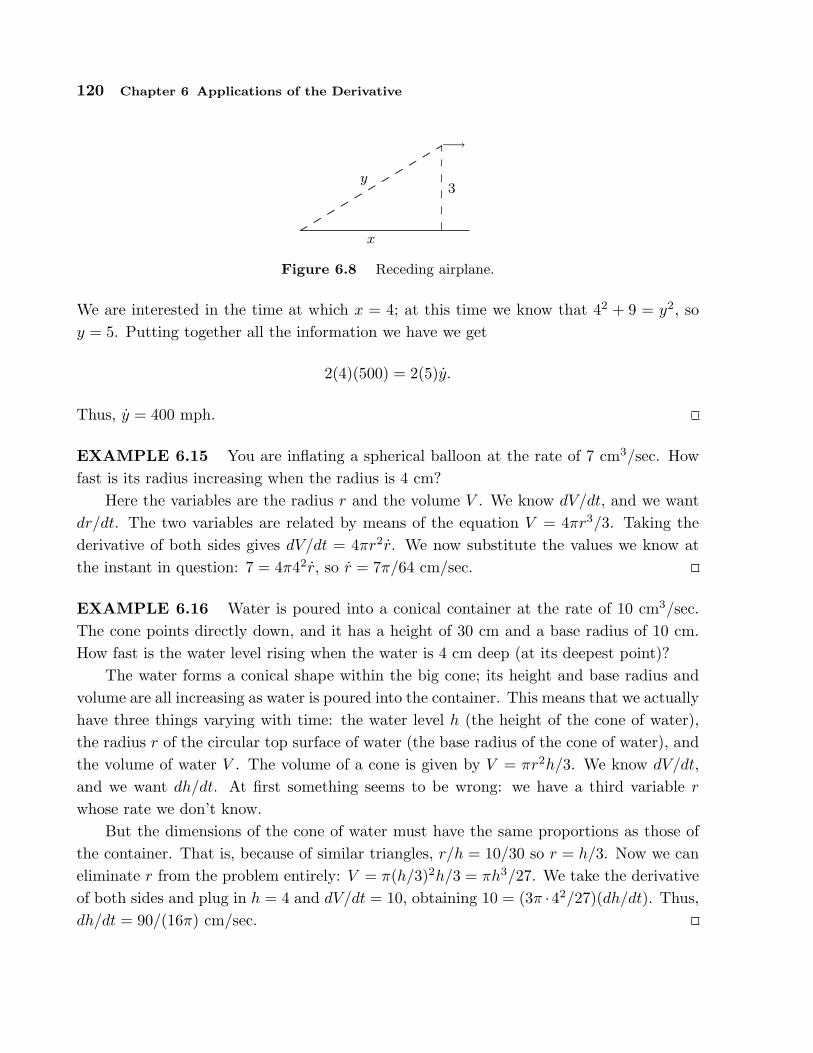
120 Chapter 6 Applications of the Derivative
..........................
..........................
..........................
..........................
..........................
..........−→
x
y3
Figure 6.8 Receding airplane.
We are interested in the time at which x = 4; at this time we know that 42 + 9 = y2, soy = 5. Putting together all the information we have we get
2(4)(500) = 2(5)y.
Thus, y = 400 mph.
EXAMPLE 6.15 You are inflating a spherical balloon at the rate of 7 cm3/sec. Howfast is its radius increasing when the radius is 4 cm?
Here the variables are the radius r and the volume V . We know dV/dt, and we wantdr/dt. The two variables are related by means of the equation V = 4πr3/3. Taking thederivative of both sides gives dV/dt = 4πr2r. We now substitute the values we know atthe instant in question: 7 = 4π42r, so r = 7π/64 cm/sec.
EXAMPLE 6.16 Water is poured into a conical container at the rate of 10 cm3/sec.The cone points directly down, and it has a height of 30 cm and a base radius of 10 cm.How fast is the water level rising when the water is 4 cm deep (at its deepest point)?
The water forms a conical shape within the big cone; its height and base radius andvolume are all increasing as water is poured into the container. This means that we actuallyhave three things varying with time: the water level h (the height of the cone of water),the radius r of the circular top surface of water (the base radius of the cone of water), andthe volume of water V . The volume of a cone is given by V = πr2h/3. We know dV/dt,and we want dh/dt. At first something seems to be wrong: we have a third variable r
whose rate we don’t know.But the dimensions of the cone of water must have the same proportions as those of
the container. That is, because of similar triangles, r/h = 10/30 so r = h/3. Now we caneliminate r from the problem entirely: V = π(h/3)2h/3 = πh3/27. We take the derivativeof both sides and plug in h = 4 and dV/dt = 10, obtaining 10 = (3π ·42/27)(dh/dt). Thus,dh/dt = 90/(16π) cm/sec.

6.2 Related Rates 121
......................
....................................................................................................................................................................................................................................................................................................................................................................
...................
.......................................................................................................................................................................................................
←− 10 −→
↑|30|↓
↑|h|↓
r
............................................................................................................................................................................................................................................................................................................................................................................................................................................................................................................................................................................................................................................
............................................................ ............................................. ...............
Figure 6.9 Conical water tank.
EXAMPLE 6.17 A swing consists of a board at the end of a 10 ft long rope. Think ofthe board as a point P at the end of the rope, and let Q be the point of attachment at theother end. Suppose that the swing is directly below Q at time t = 0, and is being pushedby someone who walks at 6 ft/sec from left to right. Find (a) how fast the swing is risingafter 1 sec; (b) the angular speed of the rope in deg/sec after 1 sec.
We start out by asking: What is the geometric quantity whose rate of change we know,and what is the geometric quantity whose rate of change we’re being asked about? Notethat the person pushing the swing is moving horizontally at a rate we know. In otherwords, the horizontal coordinate of P is increasing at 6 ft/sec. In the xy-plane let usmake the convenient choice of putting the origin at the location of P at time t = 0, i.e., adistance 10 directly below the point of attachment. Then the rate we know is dx/dt, andin part (a) the rate we want is dy/dt (the rate at which P is rising). In part (b) the ratewe want is θ = dθ/dt, where θ stands for the angle in radians through which the swing hasswung from the vertical. (Actually, since we want our answer in deg/sec, at the end wemust convert dθ/dt from rad/sec by multiplying by 180/π.)(a) From the diagram we see that we have a right triangle whose legs are x and 10 − y,and whose hypotenuse is 10. Hence x2 + (10 − y)2 = 100. Taking the derivative of bothsides we obtain: 2xx+2(10− y)(0− y) = 0. We now look at what we know after 1 second,namely x = 6 (because x started at 0 and has been increasing at the rate of 6 ft/secfor 1 sec), y = 2 (because we get 10 − y = 8 from the Pythagorean theorem applied tothe triangle with hypotenuse 10 and leg 6), and x = 6. Putting in these values gives us2 · 6 · 6− 2 · 8y = 0, from which we can easily solve for y: y = 4.5 ft/sec.
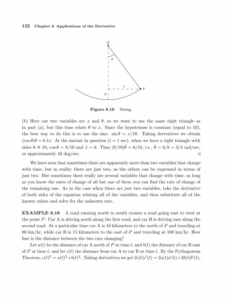
122 Chapter 6 Applications of the Derivative
...............................................................................................................................................................................................................................................................................................
.........................................
................................
......................
.......................................
.........................................................................................................................................................................................................................................................................................................
•
• P
Q
x
y
θ
Figure 6.10 Swing.
(b) Here our two variables are x and θ, so we want to use the same right triangle asin part (a), but this time relate θ to x. Since the hypotenuse is constant (equal to 10),the best way to do this is to use the sine: sin θ = x/10. Taking derivatives we obtain(cos θ)θ = 0.1x. At the instant in question (t = 1 sec), when we have a right triangle withsides 6–8–10, cos θ = 8/10 and x = 6. Thus (8/10)θ = 6/10, i.e., θ = 6/8 = 3/4 rad/sec,or approximately 43 deg/sec.
We have seen that sometimes there are apparently more than two variables that changewith time, but in reality there are just two, as the others can be expressed in terms ofjust two. But sometimes there really are several variables that change with time; as longas you know the rates of change of all but one of them you can find the rate of change ofthe remaining one. As in the case when there are just two variables, take the derivativeof both sides of the equation relating all of the variables, and then substitute all of theknown values and solve for the unknown rate.
EXAMPLE 6.18 A road running north to south crosses a road going east to west atthe point P . Car A is driving north along the first road, and car B is driving east along thesecond road. At a particular time car A is 10 kilometers to the north of P and traveling at80 km/hr, while car B is 15 kilometers to the east of P and traveling at 100 km/hr. Howfast is the distance between the two cars changing?
Let a(t) be the distance of car A north of P at time t, and b(t) the distance of car B eastof P at time t, and let c(t) the distance from car A to car B at time t. By the PythagoreanTheorem, c(t)2 = a(t)2+b(t)2. Taking derivatives we get 2c(t)c′(t) = 2a(t)a′(t)+2b(t)b′(t),

6.2 Related Rates 123
•
•
•
............. ............. ............. ............. ............. ............. ............. ............. ............. .............
(0, a(t))
(b(t), 0)
c(t)
P
...............
.............................................
............................................. ...............
Figure 6.11 Cars moving apart.
so
c =aa + bb
c=
aa + bb√a2 + b2
.
Substituting known values we get:
c =10 · 80 + 15 · 100√
102 + 152=
460√13≈ 127.6km/hr
at the time of interest.
Notice how this problem differs from example 6.14. In both cases we started with thePythagorean Theorem and took derivatives on both sides. However, in example 6.14 oneof the sides was a constant (the altitude of the plane), and so the derivative of the squareof that side of the triangle was simply zero. In this example, on the other hand, all threesides of the right triangle are variables, even though we are interested in a specific valueof each side of the triangle (namely, when the sides have lengths 10 and 15). Make surethat you understand at the start of the problem what are the variables and what are theconstants.

124 Chapter 6 Applications of the Derivative
Exercises
1. A cylindrical tank standing upright (with one circular base on the ground) has radius 20cm. How fast does the water level in the tank drop when the water is being drained at 25cm3/sec? ⇒
2. A cylindrical tank standing upright (with one circular base on the ground) has radius 1meter. How fast does the water level in the tank drop when the water is being drained at 3liters per second? ⇒
3. A ladder 13 meters long rests on horizontal ground and leans against a vertical wall. Thefoot of the ladder is pulled away from the wall at the rate of 0.6 m/sec. How fast is the topsliding down the wall when the foot of the ladder is 5 m from the wall? ⇒
4. A ladder 13 meters long rests on horizontal ground and leans against a vertical wall. Thetop of the ladder is being pulled up the wall at 0.1 meters per second. How fast is the footof the ladder approaching the wall when the foot of the ladder is 5 m from the wall? ⇒
5. A rotating beacon is located 2 miles out in the water. Let A be the point on the shore thatis closest to the beacon. As the beacon rotates at 10 rev/min, the beam of light sweeps downthe shore once each time it revolves. Assume that the shore is straight. How fast is the pointwhere the beam hits the shore moving at an instant when the beam is lighting up a point 2miles along the shore from the point A? ⇒
6. A baseball diamond is a square 90 ft on a side. A player runs from first base to second baseat 15 ft/sec. At what rate is the player’s distance from third base decreasing when she ishalf way from first to second base? ⇒
7. Sand is poured onto a surface at 15 cm3/sec, forming a conical pile whose base diameter isalways equal to its altitude. How fast is the altitude of the pile increasing when the pile is 3cm high? ⇒
8. A boat is pulled in to a dock by a rope with one end attached to the front of the boat andthe other end passing through a ring attached to the dock at a point 5 ft higher than thefront of the boat. The rope is being pulled through the ring at the rate of 0.6 ft/sec. Howfast is the boat approaching the dock when 13 ft of rope are out? ⇒
9. A balloon is at a height of 50 meters, and is rising at the constant rate of 5 m/sec. A bicyclistpasses beneath it, traveling in a straight line at the constant speed of 10 m/sec. How fast isthe distance between the bicylist and the balloon increasing 2 seconds later? ⇒
10. A pyramid-shaped vat has square cross-section and stands on its tip. The dimensions at thetop are 2 m × 2 m, and the depth is 5 m. If water is flowing into the vat at 3 m3/min, howfast is the water level rising when the depth of water (at the deepest point) is 4 m? Note:the volume of any “conical” shape (including pyramids) is (1/3)(height)(area of base). ⇒
11. The sun is rising at the rate of 1/4 deg/min, and appears to be climbing into the skyperpendicular to the horizon. How fast is the shadow of a 200 meter building shrinking atthe moment when the shadow is 500 meters long? ⇒
12. The sun is setting at the rate of 1/4 deg/min, and appears to be climbing into the skyperpendicular to the horizon. How fast is the shadow of a 25 meter wall lengthening at themoment when the shadow is 50 meters? ⇒
13. The trough shown in figure 6.13 is constructed by fastening together three slabs of wood ofdimensions 10 ft × 1 ft, and then attaching the construction to a wooden wall at each end.
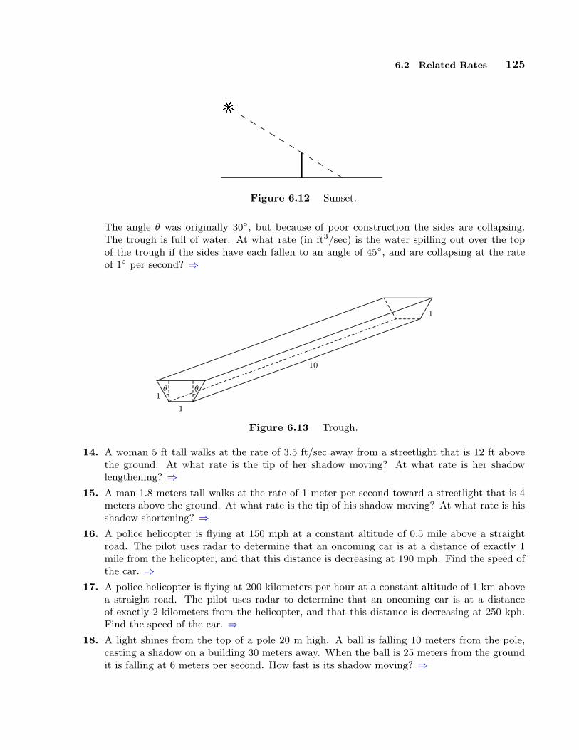
6.2 Related Rates 125
..........................
..........................
..........................
..........................
..........................
.............
................
................
................
......
k
Figure 6.12 Sunset.
The angle θ was originally 30◦, but because of poor construction the sides are collapsing.The trough is full of water. At what rate (in ft3/sec) is the water spilling out over the topof the trough if the sides have each fallen to an angle of 45◦, and are collapsing at the rateof 1◦ per second? ⇒
.............................................................................................................................................................................................................................................................................
..............................................
..............................................
..............................................
..............................................
..............................................
..............................................
..............................................
..............................................
..............................................
..............................................
..............................................
...................................................................................................................................................................................................................................................................................................................................................................................................................................................................................................................................................................................................................................................................................................................................................
......................................................................................................................................................................................................................................................................................................................................................................................................................................................................................................................................................
θ θ
1
1
1
10
......... .........
..............................
..............................
..............................
..............................
..............................
..............................
..............................
..............................
..............................
..............................
........................................................................................
......
......
......
......
......
......
......
......
......
......
Figure 6.13 Trough.
14. A woman 5 ft tall walks at the rate of 3.5 ft/sec away from a streetlight that is 12 ft abovethe ground. At what rate is the tip of her shadow moving? At what rate is her shadowlengthening? ⇒
15. A man 1.8 meters tall walks at the rate of 1 meter per second toward a streetlight that is 4meters above the ground. At what rate is the tip of his shadow moving? At what rate is hisshadow shortening? ⇒
16. A police helicopter is flying at 150 mph at a constant altitude of 0.5 mile above a straightroad. The pilot uses radar to determine that an oncoming car is at a distance of exactly 1mile from the helicopter, and that this distance is decreasing at 190 mph. Find the speed ofthe car. ⇒
17. A police helicopter is flying at 200 kilometers per hour at a constant altitude of 1 km abovea straight road. The pilot uses radar to determine that an oncoming car is at a distanceof exactly 2 kilometers from the helicopter, and that this distance is decreasing at 250 kph.Find the speed of the car. ⇒
18. A light shines from the top of a pole 20 m high. A ball is falling 10 meters from the pole,casting a shadow on a building 30 meters away. When the ball is 25 meters from the groundit is falling at 6 meters per second. How fast is its shadow moving? ⇒

126 Chapter 6 Applications of the Derivative
•k....................................................................................
Figure 6.14 Falling ball.
19. Do example 6.18 assuming that the angle between the two roads is 120◦ instead of 90◦ (thatis, the “north–south” road actually goes in a somewhat northwesterly direction from P ).Recall the law of cosines: c2 = a2 + b2 − 2ab cos θ. ⇒
20. Do example 6.18 assuming that car A is 300 meters north of P , car B is 400 meters east of P ,both cars are going at constant speed toward P , and the two cars will collide in 10 seconds.⇒
21. Do example 6.18 assuming that 8 seconds ago car A started from rest at P and has beenpicking up speed at the steady rate of 5 m/sec2, and 6 seconds after car A started car Bpassed P moving east at constant speed 60 m/sec. ⇒
22. Referring again to example 6.18, suppose that instead of car B an airplane is flying at speed200 km/hr to the east of P at an altitude of 2 km, as depicted in figure 6.15. How fast is thedistance between car and airplane changing? ⇒
...........................................................................................................................................................................................................................................................................
.....................................................................................
......
......
......
......
......
......
......
......
......
......
......
......
......
......
......
......
......
......
•
•
A
B
c(t)
............................................................
.................................................... ...............
Figure 6.15 Car and airplane.
23. Referring again to example 6.18, suppose that instead of car B an airplane is flying at speed200 km/hr to the east of P at an altitude of 2 km, and that it is gaining altitude at 10 km/hr.How fast is the distance between car and airplane changing? ⇒
24. A light shines from the top of a pole 20 m high. An object is dropped from the same heightfrom a point 10 m away, so that its height at time t seconds is h(t) = 20− 9.8t2/2. How fastis the object’s shadow moving on the ground one second later? ⇒
25. The two blades of a pair of scissors are fastened at the point A. Let a denote the distancefrom A to the tip of the blade (the point B). Let β denote the angle at the tip of the bladethat is formed by the line AB and the bottom edge of the blade, line BC, and let θ denotethe angle between AB and the horizontal. Suppose that a piece of paper is cut in such a
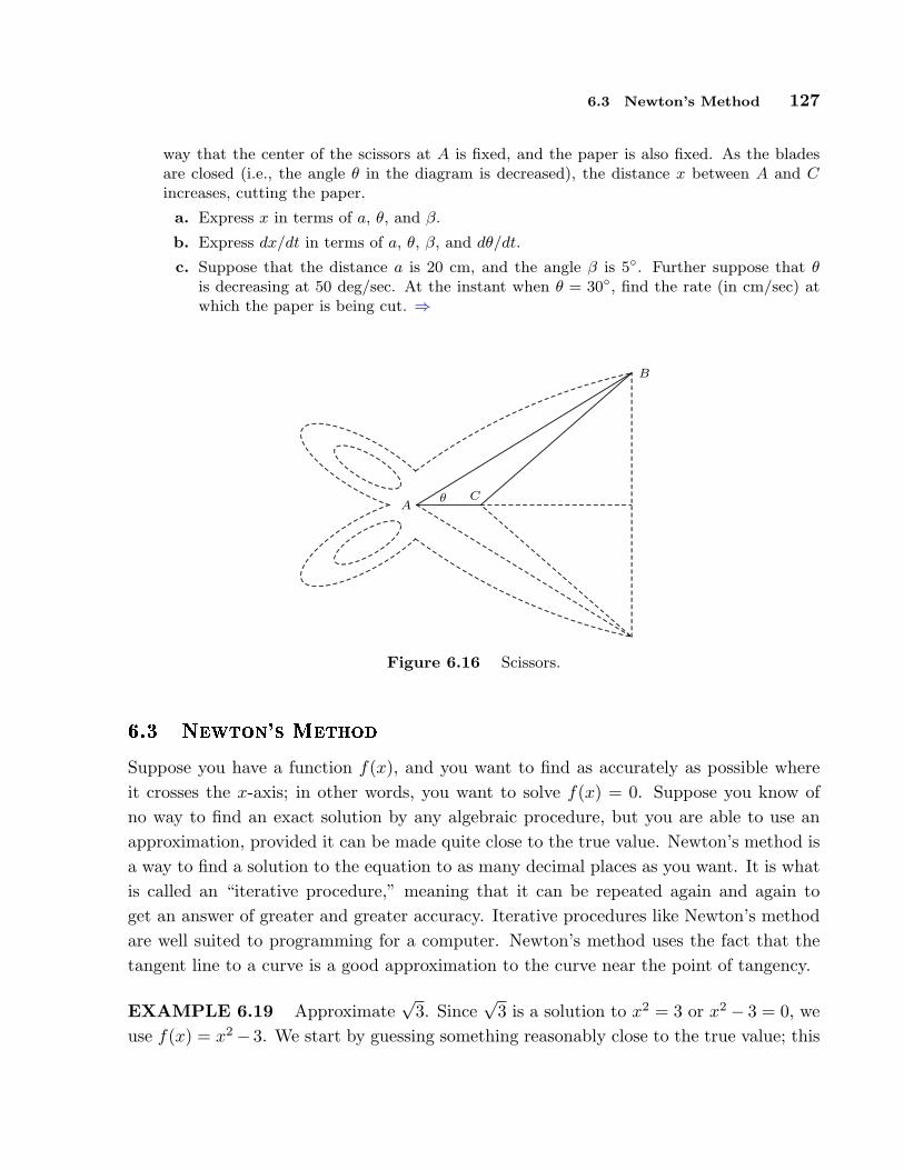
6.3 Newton’s Method 127
way that the center of the scissors at A is fixed, and the paper is also fixed. As the bladesare closed (i.e., the angle θ in the diagram is decreased), the distance x between A and Cincreases, cutting the paper.
a. Express x in terms of a, θ, and β.
b. Express dx/dt in terms of a, θ, β, and dθ/dt.
c. Suppose that the distance a is 20 cm, and the angle β is 5◦. Further suppose that θis decreasing at 50 deg/sec. At the instant when θ = 30◦, find the rate (in cm/sec) atwhich the paper is being cut. ⇒
..............................
..............................
..............................
..............................
..............................
..............................
..............................
..............................
..............................
..............................
..............................
..................................................................................................................................................................................................................................................................................................................................................................................................................
......
.............
.................
............................................................................................................
............................................................................................................
..................
..................
.............................................................................................................................................................
.......................
..................
.................
........................
.......................
................
...............
..................................................................................................................................................
...........................
..................
........................
........................
.........................
.............................
....................................
............
............................................................................................................................................................................................................
......................................................................................................................................................................................................................................
................
................
................
................
................
................
................
................
................
...........
......
......
......
......
......
......
......
......
......
......
......
......
......
......
......
......
......
......
......
......
......
......
......
......
......
......
......
......
......
......
......
......
......
......
......
......
......
....
..................................................................................................................................
B
ACθ
Figure 6.16 Scissors.
6.3 Newton's Method
Suppose you have a function f(x), and you want to find as accurately as possible whereit crosses the x-axis; in other words, you want to solve f(x) = 0. Suppose you know ofno way to find an exact solution by any algebraic procedure, but you are able to use anapproximation, provided it can be made quite close to the true value. Newton’s method isa way to find a solution to the equation to as many decimal places as you want. It is whatis called an “iterative procedure,” meaning that it can be repeated again and again toget an answer of greater and greater accuracy. Iterative procedures like Newton’s methodare well suited to programming for a computer. Newton’s method uses the fact that thetangent line to a curve is a good approximation to the curve near the point of tangency.
EXAMPLE 6.19 Approximate√
3. Since√
3 is a solution to x2 = 3 or x2 − 3 = 0, weuse f(x) = x2− 3. We start by guessing something reasonably close to the true value; this
128 Chapter 6 Applications of the Derivative
is usually easy to do. Let’s use√
3 ≈ 2. Now use the tangent line to the curve when x = 2as an approximation to the curve, as shown in figure 6.17. Since f ′(x) = 2x, the slope ofthis tangent line is 4 and its equation is y = 4x−7. The tangent line is quite close to f(x),so it crosses the x-axis near the point at which f(x) crosses, that is, near
√3. It is easy
to find where the tangent line crosses the x-axis: solve 0 = 4x− 7 to get x = 7/4 = 1.75.This is certainly a better approximation than 2, but let us say not close enough. We canimprove it by doing the same thing again: find the tangent line at x = 1.75, find wherethis new tangent line crosses the x-axis, and use that value as a better approximation. Wecan continue this indefinitely, though it gets a bit tedious. Lets see if we can shortcut theprocess. Suppose the best approximation to the intercept we have so far is xi. To find abetter approximation we will always do the same thing: find the slope of the tangent lineat xi, find the equation of the tangent line, find the x-intercept. The slope will be 2xi. Thetangent line will be y = (2xi)(x− xi) + (x2
i − 3), using the point-slope formula for a line.Finally, the intercept is found by solving 0 = (2xi)(x−xi)+(x2
i −3). With a little algebrathis turns into x = (x2
i + 3)/(2xi); this is the next approximation, which we naturally callxi+1. Instead of doing the whole tangent line computation every time we can simply usethis formula to get as many approximations as we want. Starting with x0 = 2, we getx1 = (x2
0 +3)/(2x0) = (22 +3)/4 = 7/4 (the same approximation we got above, of course),x2 = (x2
1 + 3)/(2x1) = ((7/4)2 + 3)/(7/2) = 97/56 ≈ 1.73214, x3 ≈ 1.73205, and so on.This is still a bit tedious by hand, but with a calculator or, even better, a good computerprogram, it is quite easy to get many, many approximations. We might guess already that1.73205 is accurate to two decimal places, and in fact it turns out that it is accurate to 5places.
Let’s think about this process in more general terms. We want to approximate asolution to f(x) = 0. We start with a rough guess, which we call x0. We use the tangentline to f(x) to get a new approximation that we hope will be closer to the true value.What is the equation of the tangent line when x = x0? The slope is f ′(x0) and the linegoes through (x0, f(x0)), so the equation of the line is
y = f ′(x0)(x− x0) + f(x0).
Now we find where this crosses the x-axis by substituting y = 0 and solving for x:
x =x0f
′(x0)− f(x0)f ′(x0)
= x0 − f(x0)f ′(x0)
.
We will typically want to compute more than one of these improved approximations, sowe number them consecutively; from x0 we have computed x1:
x1 =x0f
′(x0)− f(x0)f ′(x0)
= x0 − f(x0)f ′(x0)
,

6.3 Newton’s Method 129
1 2
..............................................................
................................................................................................................................................................................................................................................................................................................................................................................................
....................................................................................................................................................................................................................................................................................................................................................................................................................................
Figure 6.17 Newton’s method.
and in general from xi we compute xi+1:
xi+1 =xif′(xi)− f(xi)
f ′(xi)= xi − f(xi)
f ′(xi).
EXAMPLE 6.20 Returning to the previous example, f(x) = x2 − 3, f ′(x) = 2x, andthe formula becomes xi+1 = xi − (x2
i − 3)/(2xi) = (x2i + 3)/(2xi), as before.
In practice, which is to say, if you need to approximate a value in the course ofdesigning a bridge or a building or an airframe, you will need to have some confidence thatthe approximation you settle on is accurate enough. As a rule of thumb, once a certainnumber of decimal places stop changing from one approximation to the next it is likelythat those decimal places are correct. Still, this may not be enough assurance, in whichcase we can test the result for accuracy.
EXAMPLE 6.21 Find the x coordinate of the intersection of the curves y = 2x andy = tan x, accurate to three decimal places. To put this in the context of Newton’smethod, we note that we want to know where 2x = tanx or tan x− 2x = 0. We computef ′(x) = sec2 x− 2 and set up the formula:
xi+1 = xi − tanxi − 2xi
sec2 xi − 2.
From the graph in figure 6.18 we guess x0 = 1 as a starting point, then using the formulawe compute x1 = 1.310478030, x2 = 1.223929096, x3 = 1.176050900, x4 = 1.165926508,

130 Chapter 6 Applications of the Derivative
x5 = 1.165561636. So we guess that the first three places are correct, but that is notthe same as saying 1.165 is correct to three decimal places—1.166 might be the correct,rounded approximation. How can we tell? We can substitute 1.165, 1.1655 and 1.166into the original function tanx−2x; this gives −0.002483652, −0.000271247, 0.001948654.Since the first two are negative and the third is positive, tan x − 2x crosses the x axisbetween 1.1655 and 1.166, so the correct value to three places is 1.166.
0
5
10
15
1 1.5
.................................................................................................................................................................................
..........................................................................................................................
.........................................................................
.................................................
...................................
...................................................................................................................................................................................................................................................................................................................................................................................
..............................................................................................
..............................................................................................
..............................................................................................
..............................................................................................
..............................................................................................
.......................................................................
Figure 6.18 y = tan x and y = 2x.
Exercises
1. Approximate the fifth root of 7, using x0 = 1.5 as a first guess. Use Newton’s method to findx3 as your approximation. ⇒
2. Use Newton’s Method to approximate the cube root of 10 to two decimal places. ⇒3. The function f(x) = x3 − 3x2 − 3x + 6 has a root between 3 and 4, because f(3) = −3 and
f(4) = 10. Approximate the root to two decimal places. ⇒4. A rectangular piece of cardboard of dimensions 8 × 17 is used to make an open-top box
by cutting out a small square of side x from each corner and bending up the sides. (Seeexercise 6.1.20.) If x = 2, then the volume of the box is 2 ·4 ·13 = 104. Use Newton’s methodto find a value of x for which the box has volume 100, accurate to 3 significant figures. ⇒
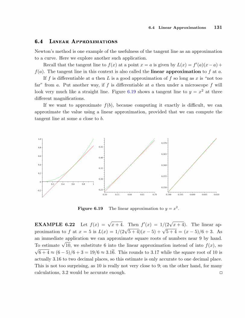
6.4 Linear Approximations 131
6.4 Linear Approximations
Newton’s method is one example of the usefulness of the tangent line as an approximationto a curve. Here we explore another such application.
Recall that the tangent line to f(x) at a point x = a is given by L(x) = f ′(a)(x−a)+f(a). The tangent line in this context is also called the linear approximation to f at a.
If f is differentiable at a then L is a good approximation of f so long as x is “not toofar” from a. Put another way, if f is differentiable at a then under a microscope f willlook very much like a straight line. Figure 6.19 shows a tangent line to y = x2 at threedifferent magnifications.
If we want to approximate f(b), because computing it exactly is difficult, we canapproximate the value using a linear approximation, provided that we can compute thetangent line at some a close to b.
Figure 6.19 The linear approximation to y = x2.
EXAMPLE 6.22 Let f(x) =√
x + 4. Then f ′(x) = 1/(2√
x + 4). The linear ap-proximation to f at x = 5 is L(x) = 1/(2
√5 + 4)(x − 5) +
√5 + 4 = (x − 5)/6 + 3. As
an immediate application we can approximate square roots of numbers near 9 by hand.To estimate
√10, we substitute 6 into the linear approximation instead of into f(x), so√
6 + 4 ≈ (6− 5)/6 + 3 = 19/6 ≈ 3.16. This rounds to 3.17 while the square root of 10 isactually 3.16 to two decimal places, so this estimate is only accurate to one decimal place.This is not too surprising, as 10 is really not very close to 9; on the other hand, for manycalculations, 3.2 would be accurate enough.

132 Chapter 6 Applications of the Derivative
With modern calculators and computing software it may not appear necessary to uselinear approximations. But in fact they are quite useful. In cases requiring an explicitnumerical approximation, they allow us to get a quick rough estimate which can be usedas a “reality check” on a more complex calculation. In some complex calculations involvingfunctions, the linear approximation makes an otherwise intractable calculation possible,without serious loss of accuracy.
EXAMPLE 6.23 Consider the trigonometric function sin x. Its linear approximationat x = 0 is simply L(x) = x. When x is small this is quite a good approximation and isused frequently by engineers and scientists to simplify some calculations.
DEFINITION 6.24 Let y = f(x) be a differentiable function. We define a new in-dependent variable dx, and a new dependent variable dy = f ′(x) dx. Notice that dy is afunction both of x (since f ′(x) is a function of x) and of dx. We say that dx and dy aredifferentials.
Let ∆x = x − a and ∆y = f(x) − f(a). If x is near a then ∆x is small. If we setdx = ∆x then
dy = f ′(a) dx ≈ ∆y
∆x∆x = ∆y.
Thus, dy can be used to approximate ∆y, the actual change in the function f between a
and x. This is exactly the approximation given by the tangent line:
dy = f ′(a)(x− a) = f ′(a)(x− a) + f(a)− f(a) = L(x)− f(a).
While L(x) approximates f(x), dy approximates how f(x) has changed from f(a). Fig-ure 6.20 illustrates the relationships.
a x
...............................
...................................
.........................................
.................................................
......................................................
...........................................................
...................................................................
.........................
..................................
..................................
..................................
..................................
..................................
........................................................................................................................................................................................................................................................................................................
←−− dx = ∆x −−→
↑|∆y
|↓
↑|dy
|↓
Figure 6.20 Differentials.
6.5 The Mean Value Theorem 133
Exercises
1. Let f(x) = x4. If a = 1 and dx = ∆x = 1/2, what are ∆y and dy? ⇒2. Let f(x) =
√x. If a = 1 and dx = ∆x = 1/10, what are ∆y and dy? ⇒
3. Let f(x) = sin(2x). If a = π and dx = ∆x = π/100, what are ∆y and dy?
4. Use differentials to estimate the amount of paint needed to apply a coat of paint 0.02 cmthick to a sphere with diameter 40 meters. (Recall that the volume of a sphere of radius r isV = (4/3)πr3. Notice that you are given that dr = 0.02.) ⇒
5. Show in detail that the linear approximation of sin x at x = 0 is L(x) = x and the linearapproximation of cos x at x = 0 is L(x) = 1.
6.5 The Mean Value Theorem
Here are two interesting questions involving derivatives:
1. Suppose two different functions have the same derivative; what can you say aboutthe relationship between the two functions?
2. Suppose you drive a car from toll booth on a toll road to another toll booth atan average speed of 70 miles per hour. What can be concluded about your actualspeed during the trip? In particular, did you exceed the 65 mile per hour speedlimit?
While these sound very different, it turns out that the two problems are very closelyrelated. We know that “speed” is really the derivative by a different name; let’s start bytranslating the second question into something that may be easier to visualize. Supposethat the function f(t) gives the position of your car on the toll road at time t. Your changein position between one toll booth and the next is given by f(t1) − f(t0), assuming thatat time t0 you were at the first booth and at time t1 you arrived at the second booth.Your average speed for the trip is (f(t1) − f(t0))/(t1 − t0). If we think about the graphof f(t), the average speed is the slope of the line that connects the two points (t0, f(t0))and (t1, f(t1)). Your speed at any particular time t between t0 and t1 is f ′(t), the slopeof the curve. Now question (2) becomes a question about slope. In particular, if the slopebetween endpoints is 70, what can be said of the slopes at points between the endpoints?
As a general rule, when faced with a new problem it is often a good idea to examineone or more simplified versions of the problem, in the hope that this will lead to anunderstanding of the original problem. In this case, the problem in its “slope” form issomewhat easier to simplify than the original, but equivalent, problem.
Here is a special instance of the problem. Suppose that f(t0) = f(t1). Then thetwo endpoints have the same height and the slope of the line connecting the endpointsis zero. What can we say about the slope between the endpoints? It shouldn’t take

134 Chapter 6 Applications of the Derivative
much experimentation before you are convinced of the truth of this statement: Somewherebetween t0 and t1 the slope is exactly zero, that is, somewhere between t0 and t1 the slopeis equal to the slope of the line between the endpoints. This suggests that perhaps the sameis true even if the endpoints are at different heights, and again a bit of experimentation willprobably convince you that this is so. But we can do better than “experimentation”—wecan prove that this is so.
We start with the simplified version:
THEOREM 6.25 Rolle’s Theorem Suppose that f(x) has a derivative on theinterval (a, b), is continuous on the interval [a, b], and f(a) = f(b). Then at some valuec ∈ (a, b), f ′(c) = 0.
Proof. We know that f(x) has a maximum and minimum value on [a, b] (because itis continuous), and we also know that the maximum and minimum must occur at anendpoint, at a point at which the derivative is zero, or at a point where the derivative isundefined. Since the derivative is never undefined, that possibility is removed.
If the maximum or minimum occurs at a point c, other than an endpoint, wheref ′(c) = 0, then we have found the point we seek. Otherwise, the maximum and minimumboth occur at an endpoint, and since the endpoints have the same height, the maximumand minimum are the same. This means that f(x) = f(a) = f(b) at every x ∈ [a, b], sothe function is a horizontal line, and it has derivative zero everywhere in (a, b). Then wemay choose any c at all to get f ′(c) = 0.
Perhaps remarkably, this special case is all we need to prove the more general one aswell.
THEOREM 6.26 Mean Value Theorem Suppose that f(x) has a derivative onthe interval (a, b) and is continuous on the interval [a, b]. Then at some value c ∈ (a, b),
f ′(c) =f(b)− f(a)
b− a.
Proof. Let m =f(b)− f(a)
b− a, and consider a new function g(x) = f(x)−m(x−a)−f(a).
We know that g(x) has a derivative everywhere, since g′(x) = f ′(x)−m. We can computeg(a) = f(a)−m(a− a)− f(a) = 0 and
g(b) = f(b)−m(b− a)− f(a) = f(b)− f(b)− f(a)b− a
(b− a)− f(a)
= f(b)− (f(b)− f(a))− f(a) = 0.

6.5 The Mean Value Theorem 135
So the height of g(x) is the same at both endpoints. This means, by Rolle’s Theorem, thatat some c, g′(c) = 0. But we know that g′(c) = f ′(c)−m, so
0 = f ′(c)−m = f ′(c)− f(b)− f(a)b− a
,
which turns into
f ′(c) =f(b)− f(a)
b− a,
exactly what we want.
Returning to the original formulation of question (2), we see that if f(t) gives theposition of your car at time t, then the Mean Value Theorem says that at some time c,f ′(c) = 70, that is, at some time you must have been traveling at exactly your averagespeed for the trip, and that indeed you exceeded the speed limit.
Now let’s return to question (1). Suppose, for example, that two functions are known tohave derivative equal to 5 everywhere, f ′(x) = g′(x) = 5. It is easy to find such functions:5x, 5x + 47, 5x − 132, etc. Are there other, more complicated, examples? No—the onlyfunctions that work are the “obvious” ones, namely, 5x plus some constant. How can wesee that this is true?
Although “5” is a very simple derivative, let’s look at an even simpler one. Supposethat f ′(x) = g′(x) = 0. Again we can find examples: f(x) = 0, f(x) = 47, f(x) = −511all have f ′(x) = 0. Are there non-constant functions f with derivative 0? No, and here’swhy: Suppose that f(x) is not a constant function. This means that there are two pointson the function with different heights, say f(a) 6= f(b). The Mean Value Theorem tellsus that at some point c, f ′(c) = (f(b)− f(a))/(b− a) 6= 0. So any non-constant functiondoes not have a derivative that is zero everywhere; this is the same as saying that the onlyfunctions with zero derivative are the constant functions.
Let’s go back to the slightly less easy example: suppose that f ′(x) = g′(x) = 5. Then(f(x) − g(x))′ = f ′(x) − g′(x) = 5 − 5 = 0. So using what we discovered in the previousparagraph, we know that f(x)− g(x) = k, for some constant k. So any two functions withderivative 5 must differ by a constant; since 5x is known to work, the only other examplesmust look like 5x + k.
Now we can extend this to more complicated functions, without any extra work.Suppose that f ′(x) = g′(x). Then as before (f(x) − g(x))′ = f ′(x) − g′(x) = 0, sof(x)−g(x) = k. Again this means that if we find just a single function g(x) with a certainderivative, then every other function with the same derivative must be of the form g(x)+k.
136 Chapter 6 Applications of the Derivative
EXAMPLE 6.27 Describe all functions that have derivative 5x − 3. It’s easy to findone: g(x) = (5/2)x2 − 3x has g′(x) = 5x − 3. The only other functions with the samederivative are therefore of the form f(x) = (5/2)x2 − 3x + k.
Alternately, though not obviously, you might have first noticed that g(x) = (5/2)x2 −3x + 47 has g′(x) = 5x − 3. Then every other function with the same derivative musthave the form f(x) = (5/2)x2 − 3x + 47 + k. This looks different, but it really isn’t.The functions of the form f(x) = (5/2)x2 − 3x + k are exactly the same as the ones ofthe form f(x) = (5/2)x2 − 3x + 47 + k. For example, (5/2)x2 − 3x + 10 is the same as(5/2)x2 − 3x + 47 + (−37), and the first is of the first “form” while the second has thesecond form.
This is worth calling a theorem:
THEOREM 6.28 If f ′(x) = g′(x) for every x ∈ (a, b), then for some constant k,f(x) = g(x) + k on the interval (a, b).
EXAMPLE 6.29 Describe all functions with derivative sin x + ex. One such functionis − cosx + ex, so all such functions have the form − cosx + ex + k.
Exercises
1. Let f(x) = x2. Find a value c ∈ (−1, 2) so that f ′(c) equals the slope between the endpointsof f(x) on [−1, 2]. ⇒
2. Verify that f(x) = x/(x + 2) satisfies the hypotheses of the Mean Value Theorem on theinterval [1, 4] and then find all of the values, c, that satisfy the conclusion of the theorem.⇒
3. Verify that f(x) = 3x/(x + 7) satisfies the hypotheses of the Mean Value Theorem on theinterval [−2, 6] and then find all of the values, c, that satisfy the conclusion of the theorem.
4. Let f(x) = tan x. Show that f(π) = f(2π) = 0 but there is no number c ∈ (0, 2π) such thatf ′(c) = 0. Why does this not contradict Rolle’s theorem?
5. Let f(x) = (x − 3)−2. Show that there is no value c in the interval (1, 4) such that f ′(c) =(f(4)− f(1))/(4− 1). Why is this not a contradiction of the Mean Value Theorem?
6. Describe all functions with derivative x2 + 47x− 5. ⇒7. Describe all functions with derivative
1
1 + x2. ⇒
8. Describe all functions with derivative x3 − 1
x. ⇒
9. Describe all functions with derivative sin(2x). ⇒10. Show that the equation
6x4 − 7x + 1 = 0
does not have more than two distinct real roots.

6.5 The Mean Value Theorem 137
11. Let f be differentiable on R. Suppose that f ′(x) 6= 0 for every x. Prove that f has at mostone root.
12. Prove that for all real x and y | cos x− cos y| ≤ |x− y|. State and prove an analogous resultinvolving sine.
13. Show that√
1 + x > 1 + (x/2) if −1 < x < 1.

7Integration
7.1 Two examples
Up to now we have been concerned with extracting information about how a functionchanges from the function itself. Given knowledge about an object’s position, for example,we want to know the object’s speed. Given information about the height of a curve wewant to know its slope. We now consider problems that are, whether obviously or not, thereverse of such problems.
EXAMPLE 7.1 An object moves in a straight line so that its speed at time t is givenby v(t) = 3t in, say, cm/sec. If the object is at position 10 on the straight line when t = 0,where is the object at any time t?
There are two reasonable ways to approach this problem. If s(t) is the position of theobject at time t, we know that s′(t) = v(t). Because of our knowledge of derivatives, weknow therefore that s(t) = 3t2/2+k, and because s(0) = 10 we easily discover that k = 10,so s(t) = 3t2/2 + 10. For example, at t = 1 the object is at position 3/2 + 10 = 11.5. Thisis certainly the easiest way to deal with this problem. Not all similar problems are so easy,as we will see; the second approach to the problem is more difficult but also more general.
We start by considering how we might approximate a solution. We know that at t = 0the object is at position 10. How might we approximate its position at, say, t = 1? Weknow that the speed of the object at time t = 0 is 0; if its speed were constant then in thefirst second the object would not move and its position would still be 10 when t = 1. Infact, the object will not be too far from 10 at t = 1, but certainly we can do better. Let’s
139
140 Chapter 7 Integration
look at the times 0.1, 0.2, 0.3, . . . , 1.0, and try approximating the location of the objectat each, by supposing that during each tenth of a second the object is going at a constantspeed. Since the object initially has speed 0, we again suppose it maintains this speed, butonly for a tenth of second; during that time the object would not move. During the tenthof a second from t = 0.1 to t = 0.2, we suppose that the object is traveling at 0.3 cm/sec,namely, its actual speed at t = 0.1. In this case the object would travel (0.3)(0.1) = 0.03centimeters: 0.3 cm/sec times 0.1 seconds. Similarly, between t = 0.2 and t = 0.3 theobject would travel (0.6)(0.1) = 0.06 centimeters. Continuing, we get as an approximationthat the object travels
(0.0)(0.1) + (0.3)(0.1) + (0.6)(0.1) + · · ·+ (2.7)(0.1) = 1.35
centimeters, ending up at position 11.35. This is a better approximation than 10, certainly,but is still just an approximation. (We know in fact that the object ends up at position11.5, because we’ve already done the problem using the first approach.) Presumably,we will get a better approximation if we divide the time into one hundred intervals of ahundredth of a second each, and repeat the process:
(0.0)(0.01) + (0.03)(0.01) + (0.06)(0.01) + · · ·+ (2.97)(0.01) = 1.485.
We thus approximate the position as 11.485. Since we know the exact answer, we can seethat this is much closer, but if we did not already know the answer, we wouldn’t reallyknow how close.
We can keep this up, but we’ll never really know the exact answer if we simply computemore and more examples. Let’s instead look at a “typical” approximation. Suppose wedivide the time into n equal intervals, and imagine that on each of these the object travelsat a constant speed. Over the first time interval we approximate the distance traveledas (0.0)(1/n) = 0, as before. During the second time interval, from t = 1/n to t = 2/n,the object travels approximately 3(1/n)(1/n) = 3/n2 centimeters. During time intervalnumber i, the object travels approximately (3(i − 1)/n)(1/n) = 3(i − 1)/n2 centimeters.Adding these up as before, we approximate the distance traveled as
(0)1n
+ 31n2
+ 3(2)1n2
+ 3(3)1n2
+ · · ·+ 3(n− 1)1n2
centimeters. What can we say about this? At first it looks rather less useful than theconcrete calculations we’ve already done. But in fact a bit of algebra reveals it to be muchmore useful. We can factor out a 3 and 1/n2 to get
3n2
(0 + 1 + 2 + 3 + · · ·+ (n− 1)),
7.1 Two examples 141
that is, 3/n2 times the sum of the first n− 1 positive integers. Now we make use of a factyou may have run across before:
1 + 2 + 3 + · · ·+ k =k(k + 1)
2.
In our case we’re interested in k = n− 1, so
1 + 2 + 3 + · · ·+ (n− 1) =(n− 1)(n)
2=
n2 − n
2.
This simplifies the approximate distance traveled to
3n2
n2 − n
2=
32
n2 − n
n2=
32
(n2
n2− n
n2
)=
32
(1− 1
n
).
Now this is quite easy to understand: as n gets larger and larger this approximation getscloser and closer to (3/2)(1 − 0) = 3/2, so that 3/2 is the exact distance traveled duringone second, and the final position is 11.5.
So for t = 1, at least, this rather cumbersome approach gives the same answer asthe first approach. But really there’s nothing special about t = 1; let’s just call it t
instead. In this case the approximate distance traveled during time interval number i is3(i− 1)(t/n)(t/n) = 3(i− 1)t2/n2 and the total distance traveled is approximately
(0)t
n+ 3(1)
t2
n2+ 3(2)
t2
n2+ 3(3)
t2
n2+ · · ·+ 3(n− 1)
t2
n2.
As before we can simplify this to
3t2
n2(0 + 1 + 2 + · · ·+ (n− 1)) =
3t2
n2
n2 − n
2=
32t2
(1− 1
n
).
In the limit, as n gets larger, this gets closer and closer to (3/2)t2 and the approximatedposition of the object gets closer and closer to (3/2)t2 + 10, so the actual position is(3/2)t2 + 10, exactly the answer given by the first approach to the problem.
EXAMPLE 7.2 Find the area under the curve y = 3x between x = 0 and any positivevalue x. There is here no obvious analogue to the first approach in the previous example,but the second approach works fine. (Because the function y = 3x is so simple, thereis another approach that works here, but it is even more limited in potential applicationthan is approach number one.) How might we approximate the desired area? We know
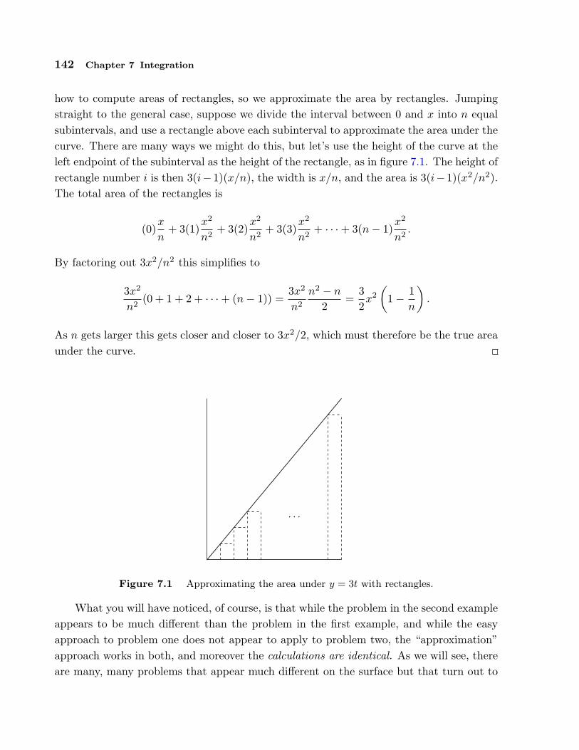
142 Chapter 7 Integration
how to compute areas of rectangles, so we approximate the area by rectangles. Jumpingstraight to the general case, suppose we divide the interval between 0 and x into n equalsubintervals, and use a rectangle above each subinterval to approximate the area under thecurve. There are many ways we might do this, but let’s use the height of the curve at theleft endpoint of the subinterval as the height of the rectangle, as in figure 7.1. The height ofrectangle number i is then 3(i−1)(x/n), the width is x/n, and the area is 3(i−1)(x2/n2).The total area of the rectangles is
(0)x
n+ 3(1)
x2
n2+ 3(2)
x2
n2+ 3(3)
x2
n2+ · · ·+ 3(n− 1)
x2
n2.
By factoring out 3x2/n2 this simplifies to
3x2
n2(0 + 1 + 2 + · · ·+ (n− 1)) =
3x2
n2
n2 − n
2=
32x2
(1− 1
n
).
As n gets larger this gets closer and closer to 3x2/2, which must therefore be the true areaunder the curve.
. . .
...............................................................................................................................................................................................................................................................................................................................................................................................................................................................................
Figure 7.1 Approximating the area under y = 3t with rectangles.
What you will have noticed, of course, is that while the problem in the second exampleappears to be much different than the problem in the first example, and while the easyapproach to problem one does not appear to apply to problem two, the “approximation”approach works in both, and moreover the calculations are identical. As we will see, thereare many, many problems that appear much different on the surface but that turn out to

7.2 The Fundamental Theorem of Calculus 143
be the same as these problems, in the sense that when we try to approximate solutions weend up with mathematics that looks like the two examples, though of course the functioninvolved will not always be so simple.
Even better, we now see that while the second problem did not appear to be amenableto approach one, it can in fact be solved in the same way. The reasoning is this: we knowthat problem one can be solved easily by finding a function whose derivative is 3t. Wealso know that mathematically the two problems are the same, because both can be solvedby taking a limit of a sum, and the sums are identical. Therefore, we don’t really needto compute the limit of either sum because we know that we will get the same answer bycomputing a function with the derivative 3t or, which is the same thing, 3x.
It’s true that the first problem had the added complication of the “10”, and we certainlyneed to be able to deal with such minor variations, but that turns out to be quite simple.The lesson then is this: whenever we can solve a problem by taking the limit of a sum ofa certain form, we can instead of computing the (often nasty) limit find a new functionwith a certain derivative.
Exercises
1. Suppose an object moves in a straight line so that its speed at time t is given by v(t) = 2t+2,and that at t = 1 the object is at position 5. Find the position of the object at t = 2. ⇒
2. Suppose an object moves in a straight line so that its speed at time t is given by v(t) = t2 +2,and that at t = 0 the object is at position 5. Find the position of the object at t = 2. ⇒
3. By a method similar to that in example 7.2, find the area under y = 2x between x = 0 andany positive value for x. ⇒
4. By a method similar to that in example 7.2, find the area under y = 4x between x = 0 andany positive value for x. ⇒
5. By a method similar to that in example 7.2, find the area under y = 4x between x = 2 andany positive value for x bigger than 2. ⇒
6. By a method similar to that in example 7.2, find the area under y = 4x between any twopositive values for x, say a < b. ⇒
7. Let f(x) = x2 + 3x + 2. Approximate the area under the curve between x = 0 and x = 2using 4 rectangles and also using 8 rectangles. ⇒
8. Let f(x) = x2 − 2x + 3. Approximate the area under the curve between x = 1 and x = 3using 4 rectangles. ⇒
7.2 The Fundamental Theorem of Calculus
Let’s recast the first example from the previous section. Suppose that the speed of theobject is 3t at time t. How far does the object travel between time t = a and time t = b?We are no longer assuming that we know where the object is at time t = 0 or at any other

144 Chapter 7 Integration
time. It is certainly true that it is somewhere, so let’s suppose that at t = 0 the position is k.Then just as in the example, we know that the position of the object at any time is 3t2/2+k.This means that at time t = a the position is 3a2/2 + k and at time t = b the position is3b2/2 + k. Therefore the change in position is 3b2/2 + k − (3a2/2 + k) = 3b2/2 − 3a2/2.Notice that the k drops out; this means that it doesn’t matter that we don’t know k, itdoesn’t even matter if we use the wrong k, we get the correct answer. In other words, tofind the change in position between time a and time b we can use any antiderivative of thespeed function 3t—it need not be the one antiderivative that actually gives the location ofthe object.
What about the second approach to this problem, in the new form? We now want toapproximate the change in position between time a and time b. We take the interval oftime between a and b, divide it into n subintervals, and approximate the distance traveledduring each. The starting time of subinterval number i is now a + (i− 1)(b− a)/n, whichwe abbreviate as ti−1, so that t0 = a, t1 = a + (b − a)/n, and so on. The speed of theobject is f(t) = 3t, and each subinterval is (b − a)/n = ∆t seconds long. The distancetraveled during subinterval number i is approximately f(ti−1)∆t, and the total change indistance is approximately
f(t0)∆t + f(t1)∆t + · · ·+ f(tn−1)∆t.
The exact change in position is the limit of this sum as n goes to infinity. We abbreviatethis sum using sigma notation:
n−1∑
i=0
f(ti)∆t = f(t0)∆t + f(t1)∆t + · · ·+ f(tn−1)∆t.
The notation on the left side of the equal sign uses a large capital sigma, a Greek letter,and the left side is an abbreviation for the right side. The answer we seek is
limn→∞
n−1∑
i=0
f(ti)∆t.
Since this must be the same as the answer we have already obtained, we know that
limn→∞
n−1∑
i=0
f(ti)∆t =3b2
2− 3a2
2.
The significance of 3t2/2, into which we substitute t = b and t = a, is of course that it isa function whose derivative is f(t). As we have discussed, by the time we know that we

7.2 The Fundamental Theorem of Calculus 145
want to compute
limn→∞
n−1∑
i=0
f(ti)∆t,
it no longer matters what f(t) stands for—it could be a speed, or the height of a curve,or something else entirely. We know that the limit can be computed by finding anyfunction with derivative f(t), substituting a and b, and subtracting. We summarize thisin a theorem. First, we introduce some new notation and terms.
We write ∫ b
a
f(t) dt = limn→∞
n−1∑
i=0
f(ti)∆t
if the limit exists. That is, the left hand side means, or is an abbreviation for, the righthand side. The symbol
∫is called an integral sign, and the whole expression is read
as “the integral of f(t) from a to b.” What we have learned is that this integral can becomputed by finding a function, say F (t), with the property that F ′(t) = f(t), and thencomputing F (b)− F (a). The function F (t) is called an antiderivative of f(t). Now thetheorem:
THEOREM 7.3 Fundamental Theorem of Calculus Suppose that f(x) is con-tinuous on the interval [a, b]. If F (x) is any antiderivative of f(x), then
∫ b
a
f(x) dx = F (b)− F (a).
Let’s rewrite this slightly:∫ x
a
f(t) dt = F (x)− F (a).
We’ve replaced the variable x by t and b by x. These are just different names for quantities,so the substitution doesn’t change the meaning. It does make it easier to think of the twosides of the equation as functions. The expression
∫ x
a
f(t) dt
is a function: plug in a value for x, get out some other value. The expression F (x)−F (a)is of course also a function, and it has a nice property:
d
dx(F (x)− F (a)) = F ′(x) = f(x),
146 Chapter 7 Integration
since F (a) is a constant and has derivative zero. In other words, by shifting our point ofview slightly, we see that the odd looking function
G(x) =∫ x
a
f(t) dt
has a derivative, and that in fact G′(x) = f(x). This is really just a restatement of theFundamental Theorem of Calculus, and indeed is often called the Fundamental Theoremof Calculus. To avoid confusion, some people call the two versions of the theorem “TheFundamental Theorem of Calculus, part I” and “The Fundamental Theorem of Calculus,part II”, although unfortunately there is no universal agreement as to which is part I andwhich part II. Since it really is the same theorem, differently stated, some people simplycall them both “The Fundamental Theorem of Calculus.”
THEOREM 7.4 Fundamental Theorem of Calculus Suppose that f(x) is con-tinuous on the interval [a, b] and let
G(x) =∫ x
a
f(t) dt.
Then G′(x) = f(x).
We have not really proved the Fundamental Theorem. In a nutshell, we gave thefollowing argument to justify it: Suppose we want to know the value of
∫ b
a
f(t) dt = limn→∞
n−1∑
i=0
f(ti)∆t.
We can interpret the right hand side as the distance traveled by an object whose speedis given by f(t). We know another way to compute the answer to such a problem: findthe position of the object by finding an antiderivative of f(t), then substitute t = a andt = b and subtract to find the distance traveled. This must be the answer to the originalproblem as well, even if f(t) does not represent a speed.
What’s wrong with this? In some sense, nothing. As a practical matter it is a veryconvincing arguement, because our understanding of the relationship between speed anddistance seems to be quite solid. From the point of view of mathematics, however, itis unsatisfactory to justify a purely mathematical relationship by appealing to our un-derstanding of the physical universe, which could, however unlikely it is in this case, bewrong.
7.2 The Fundamental Theorem of Calculus 147
A complete proof is a bit too involved to include here, but we will indicate how it goes.First, if we can prove the second version of the Fundamental Theorem, theorem 7.4, thenwe can prove the first version from that:
Proof of Theorem 7.3. We know from theorem 7.4 that
G(x) =∫ x
a
f(t) dt
is an antiderivative of f(x), and therefore any antiderivative F (x) of f(x) is of the formF (x) = G(x) + k. Then
F (b)− F (a) = G(b) + k − (G(a) + k) = G(b)−G(a)
=∫ b
a
f(t) dt−∫ a
a
f(t) dt.
It is not hard to see that∫ a
af(t) dt = 0, so this means that
F (b)− F (a) =∫ b
a
f(t) dt,
which is exactly what theorem 7.3 says.
So the real job is to prove theorem 7.4. We will sketch the proof, using some facts thatwe do not prove. First, the following identity is true of integrals:
∫ b
a
f(t) dt =∫ c
a
f(t) dt +∫ b
c
f(t) dt.
This can be proved directly from the definition of the integral, that is, using the limitsof sums. It is quite easy to see that it must be true by thinking of either of the twoapplications of integrals that we have seen. It turns out that the identity is true no matterwhat c is, but it is easiest to think about the meaning when a ≤ c ≤ b.
First, if f(t) represents a speed, then we know that the three integrals represent thedistance traveled between time a and time b; the distance traveled between time a andtime c; and the distance traveled between time c and time b. Clearly the sum of the lattertwo is equal to the first of these.
Second, if f(t) represents the height of a curve, the three integrals represent the areaunder the curve between a and b; the area under the curve between a and c; and the areaunder the curve between c and b. Again it is clear from the geometry that the first is equalto the sum of the second and third.
148 Chapter 7 Integration
Proof sketch for Theorem 7.4. We want to compute G′(x), so we start with thedefinition of the derivative in terms of a limit:
G′(x) = lim∆x→0
G(x + ∆x)−G(x)∆x
= lim∆x→0
1∆x
(∫ x+∆x
a
f(t) dt−∫ x
a
f(t) dt
)
= lim∆x→0
1∆x
(∫ x
a
f(t) dt +∫ x+∆x
x
f(t) dt−∫ x
a
f(t) dt
)
= lim∆x→0
1∆x
∫ x+∆x
x
f(t) dt.
Now we need to know something about
∫ x+∆x
x
f(t) dt
when ∆x is small; in fact, it is very close to ∆xf(x), but we will not prove this. Onceagain, it is easy to believe this is true by thinking of our two applications: The integral
∫ x+∆x
x
f(t) dt
can be interpreted as the distance traveled by an object over a very short interval of time.Over a sufficiently short period of time, the speed of the object will not change very much,so the distance traveled will be approximately the length of time multiplied by the speed atthe beginning of the interval, namely, ∆xf(x). Alternately, the integral may be interpretedas the area under the curve between x and x + ∆x. When ∆x is very small, this will bevery close to the area of the rectangle with base ∆x and height f(x); again this is ∆xf(x).If we accept this, we may proceed:
lim∆x→0
1∆x
∫ x+∆x
x
f(t) dt = lim∆x→0
∆xf(x)∆x
= f(x),
which is what we wanted to show.
It is still true that we are depending on an interpretation of the integral to justify theargument, but we have isolated this part of the argument into two facts that are not too
7.2 The Fundamental Theorem of Calculus 149
hard to prove. Once the last reference to interpretation has been removed from the proofsof these facts, we will have a real proof of the Fundamental Theorem.
Now we know that to solve certain kinds of problems, those that lead to a sum of acertain form, we “merely” find an antiderivative and substitute two values and subtract.Unfortunately, finding antiderivatives can be quite difficult. While there are a small numberof rules that allow us to compute the derivative of any common function, there are no suchrules for antiderivatives. There are some techniques that frequently prove useful, but wewill never be able to reduce the problem to a completely mechanical process.
Because of the close relationship between an integral and an antiderivative, the integralsign is also used to mean “antiderivative”. You can tell which is intended by whether thelimits of integration are included: ∫ 2
1
x2 dx
is an ordinary integral, also called a definite integral, because it has a definite value,namely ∫ 2
1
x2 dx =23
3− 13
3=
73.
We use ∫x2 dx
to denote the antiderivative of x2, also called an indefinite integral. So this is evaluatedas ∫
x2 dx =x3
3+ C.
It is customary to include the constant C to indicate that there are really an infinitenumber of antiderivatives. We do not need this C to compute definite integrals, but inother circumstances we will need to remember that the C is there, so it is best to getinto the habit of writing the C. When we compute a definite integral, we first find anantiderivative and then substitute. It is convenient to first display the antiderivative andthen do the substitution; we need a notation indicating that the substitution is yet to bedone. A typical solution would look like this:
∫ 2
1
x2 dx =x3
3
∣∣∣∣2
1
=23
3− 13
3=
73.
The vertical line with subscript and superscript is used to indicate the operation “substituteand subtract” that is needed to finish the evaluation.

150 Chapter 7 Integration
Exercises
Find the antiderivatives of the functions:
1. 8√
x ⇒2. 3t2 + 1 ⇒3. 4/
√x ⇒
4. 2/z2 ⇒5. 7s−1 ⇒
6. (5x + 1)2 ⇒7. (x− 6)2 ⇒8. x3/2 ⇒9.
2
x√
x⇒
10. |2t− 4| ⇒Compute the values of the integrals:
11.
Z 4
1
t2 + 3t dt ⇒
12.
Z π
0
sin t dt ⇒
13.
Z 10
1
1
xdx ⇒
14.
Z 5
0
ex dx ⇒
15.
Z 3
0
x3 dx ⇒
16.
Z 2
1
x5 dx ⇒
17. Find the derivative of G(x) =
Z x
1
t2 − 3t dt ⇒
18. Find the derivative of G(x) =
Z x2
1
t2 − 3t dt ⇒
19. Find the derivative of G(x) =
Z x
1
et2 dt ⇒
20. Find the derivative of G(x) =
Z x2
1
et2 dt ⇒
7.3 Some Properties of Integrals
Suppose an object moves so that its speed, or more properly velocity, is given by v(t) =−t2+5t, as shown in figure 7.2. Let’s examine the motion of this object carefully. We knowthat the velocity is the derivative of position, so position is given by s(t) = −t3/3+5t2/2+C. Let’s suppose that at time t = 0 the object is at position 0, so s(t) = −t3/3 + 5t2/2;this function is also pictured in figure 7.2.
Between t = 0 and t = 5 the velocity is positive, so the object moves away from thestarting point, until it is a bit past position 20. Then the velocity becomes negative andthe object moves back toward its starting point. The position of the object at t = 5 isexactly s(5) = 125/6, and at t = 6 it is s(6) = 18. The total distance traveled by theobject is therefore 125/6 + (125/6− 18) = 71/3 ≈ 23.7.
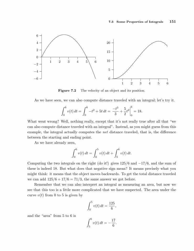
7.3 Some Properties of Integrals 151
−6
−4
−2
0
2
4
6
1 2 3 4 5 6
................................................................................................................................................................................................
................................................................................................................................................................................................................................................................................................................................................................................................................. 0
5
10
15
20
1 2 3 4 5 6
.................................................
.....................................................................................................................................................................................................................................................................................................................
.............................................................................................................
Figure 7.2 The velocity of an object and its position.
As we have seen, we can also compute distance traveled with an integral; let’s try it.
∫ 6
0
v(t) dt =∫ 6
0
−t2 + 5t dt =−t3
3+
52t2
∣∣∣∣6
0
= 18.
What went wrong? Well, nothing really, except that it’s not really true after all that “wecan also compute distance traveled with an integral”. Instead, as you might guess from thisexample, the integral actually computes the net distance traveled, that is, the differencebetween the starting and ending point.
As we have already seen,∫ 6
0
v(t) dt =∫ 5
0
v(t) dt +∫ 6
5
v(t) dt.
Computing the two integrals on the right (do it!) gives 125/6 and −17/6, and the sum ofthese is indeed 18. But what does that negative sign mean? It means precisely what youmight think: it means that the object moves backwards. To get the total distance traveledwe can add 125/6 + 17/6 = 71/3, the same answer we got before.
Remember that we can also interpret an integral as measuring an area, but now wesee that this too is a little more complicated that we have suspected. The area under thecurve v(t) from 0 to 5 is given by
∫ 5
0
v(t) dt =1256
,
and the “area” from 5 to 6 is ∫ 6
5
v(t) dt = −176
.

152 Chapter 7 Integration
In other words, the area between the x-axis and the curve, but under the x-axis, “countsas negative area”. So the integral
∫ 6
0
v(t) dt = 18
measures “net area”, the area above the axis minus the (positive) area below the axis.If we recall that the integral is the limit of a certain kind of sum, this behavior is not
surprising. Recall the sort of sum involved:
n−1∑
i=0
v(ti)∆t.
In each term v(t)∆t the ∆t is positive, but if v(ti) is negative then the term is negative. Ifover an entire interval, like 5 to 6, the function is always negative, then the entire sum isnegative. In terms of area, v(t)∆t is then a negative height times a positive width, givinga negative rectangle “area”.
So now we see that when evaluating
∫ 6
5
v(t) dt = −176
by finding an antiderivative, substituting, and subtracting, we get a surprising answer, butone that turns out to make sense.
Let’s now try something a bit different:
∫ 5
6
v(t) dt =−t3
3+
52t2
∣∣∣∣5
6
=−53
3+
5252 − −63
3− 5
262 =
176
.
Here we simply interchanged the limits 5 and 6, so of course when we substitute andsubtract we’re subtracting in the opposite order and we end up multiplying the answerby −1. This too makes sense in terms of the underlying sum, though it takes a bit morethought. Recall that in the sum
n−1∑
i=0
v(ti)∆t,
the ∆t is the “length” of each little subinterval, but more precisely we could say that∆t = ti+1 − ti, the difference between two endpoints of a subinterval. We have until now
7.3 Some Properties of Integrals 153
assumed that we were working left to right, but could as well number the subintervals fromright to left, so that t0 = b and tn = a. Then ∆t = ti+1 − ti is negative and in
∫ 5
6
v(t) dt =n−1∑
i=0
v(ti)∆t,
the values v(ti) are negative but also ∆t is negative, so all terms are positive again. Onthe other hand, in
∫ 0
5
v(t) dt =n−1∑
i=0
v(ti)∆t,
the values v(ti) are positive but ∆t is negative,and we get a negative result:
∫ 0
5
v(t) dt =−t3
3+
52t2
∣∣∣∣0
5
= 0− −53
3− 5
252 = −125
6.
Finally we note one simple property of integrals:∫ b
a
f(x) + g(x) dx =∫ b
a
f(x) dx +∫ b
a
g(x) dx.
This is easy to understand once you recall that (F (x) + G(x))′ = F ′(x) + G′(x). Hence, ifF ′(x) = f(x) and G′(x) = g(x), then
∫ b
a
f(x) + g(x) dx = (F (x) + G(x))|ba= F (b) + G(b)− F (a)−G(a)
= F (b)− F (a) + G(b)−G(a)
= F (x)|ba + G(x)|ba
=∫ b
a
f(x) dx +∫ b
a
g(x) dx.
In summary, we will frequently use these properties of integrals:∫ b
a
f(x) dx =∫ c
a
f(x) dx +∫ b
c
f(x) dx
∫ b
a
f(x) + g(x) dx =∫ b
a
f(x) dx +∫ b
a
g(x) dx
∫ b
a
f(x) dx = −∫ a
b
f(x) dx
154 Chapter 7 Integration
and if a < b and f(x) ≤ 0 on [a, b] then
∫ b
a
f(x) dx ≤ 0
and in fact ∫ b
a
f(x) dx = −∫ b
a
|f(x)| dx.
Exercises
1. An object moves so that its velocity at time t is v(t) = −9.8t + 20 m/s. Describe the motionof the object between t = 0 and t = 5, find the total distance traveled by the object duringthat time, and find the net distance traveled. ⇒
2. An object moves so that its velocity at time t is v(t) = sin t. Set up and evaluate a singledefinite integral to compute the net distance traveled between t = 0 and t = 2π. ⇒
3. An object moves so that its velocity at time t is v(t) = 1 + 2 sin t m/s. Find the net distancetraveled by the object between t = 0 and t = 2π, and find the total distance traveled duringthe same period. ⇒
4. Consider the function f(x) = (x + 2)(x + 1)(x − 1)(x − 2) on [−2, 2]. Find the total areabetween the curve and the x-axis (measuring all area as positive). ⇒
5. Consider the function f(x) = x2 − 3x + 2 on [0, 4]. Find the total area between the curveand the x-axis (measuring all area as positive). ⇒
6. Evaluate the three integrals:
A =
Z 3
0
−x2 + 9 dx B =
Z 4
0
−x2 + 9 dx C =
Z 3
4
−x2 + 9 dx,
and verify that A = B + C. ⇒

8Techniques of Integration
Over the next few sections we examine some techniques that are frequently successful whenseeking antiderivatives of functions. Sometimes this is a simple problem, since it will beapparent that the function you wish to integrate is a derivative in some straightforwardway. For example, faced with ∫
x10 dx
you realize immediately that the derivative of x11 will supply an x10: (x11)′ = 11x10. Wedon’t want the “11”, but constants are easy to alter, because differentiation “ignores” themin certain circumstances, so
d
dx
111
x11 =111
11x10 = x10.
From our knowledge of derivatives, we can immediately write down a number of an-tiderivatives. Here is a list of those most often used:
∫xn dx =
xn+1
n + 1+ C, if n 6= −1
∫x−1 dx = ln |x|+ C
∫ex dx = ex + C
155
156 Chapter 8 Techniques of Integration
∫sin x dx = − cosx + C
∫cosx dx = sin x + C
∫sec2 x dx = tanx + C
∫sec x tan x dx = sec x + C
∫1
1 + x2dx = arctan x + C
∫1√
1− x2dx = arcsin x + C
8.1 Substitution
Needless to say, most problems we encounter will not be so simple. Here’s a slightly morecomplicated example: find ∫
2x cos(x2) dx.
This is not a “simple” derivative, but a little thought reveals that it must have come froman application of the chain rule. Multiplied on the “outside” is 2x, which is the derivativeof the “inside” function x2. Checking:
d
dxsin(x2) = cos(x2)
d
dxx2 = 2x cos(x2),
so ∫2x cos(x2) dx = sin(x2) + C.
Even when the chain rule has “produced” a certain derivative, it is not always easy tosee. Consider this problem: ∫
x3√
1− x2 dx.
There are two factors in this expression, x3 and√
1− x2, but it is not apparent that thechain rule is involved. Some clever rearrangement reveals that it is:
∫x3
√1− x2 dx =
∫(−2x)
(−1
2
)(1− (1− x2))
√1− x2 dx.
8.1 Substitution 157
This looks messy, but we do now have something that looks like the result of the chainrule: the function 1 − x2 has been substituted into −(1/2)(1 − x)
√x, and the derivative
of 1− x2, −2x, multiplied on the outside. If we can find a function F (x) whose derivativeis −(1/2)(1− x)
√x we’ll be done, since then
d
dxF (1− x2) = −2xF ′(1− x2) = (−2x)
(−1
2
)(1− (1− x2))
√1− x2
= x3√
1− x2
But this isn’t hard:∫−1
2(1− x)
√x dx =
∫−1
2(x1/2 − x3/2) dx (8.1)
= −12
(23x3/2 − 2
5x5/2
)+ C
=(
15x− 1
3
)x3/2 + C.
So finally we have
∫x3
√1− x2 dx =
(15(1− x2)− 1
3
)(1− x2)3/2 + C.
So we succeeded, but it required a clever first step, rewriting the original function sothat it looked like the result of using the chain rule. Fortunately, there is a technique thatmakes such problems simpler, without requiring cleverness to rewrite a function in just theright way. It does sometimes not work, or may require more than one attempt, but theidea is simple: guess at the most likely candidate for the “inside function”, then do somealgebra to see what this requires the rest of the function to look like.
One frequently good guess is any complicated expression inside a square root, so westart by trying u = 1−x2. We use a new variable, u, for convenience in the manipulationsthat follow. Now we know that the chain rule will multiply by the derivative of this innerfunction:
du
dx= −2x,
so we need to rewrite the original function to include this:
∫x3
√1− x2 =
∫x3√
u−2x
−2xdx =
∫x2
−2√
udu
dxdx.

158 Chapter 8 Techniques of Integration
Recall that one benefit of the Leibniz notation is that it turns out that what looks likeordinary arithmetic gives the correct answer, even if something more complicated is goingon. For example, in Leibniz notation the chain rule is
dy
dx=
dy
dt
dt
dx.
The same is true of our current expression:∫
x2
−2√
udu
dxdx =
∫x2
−2√
u du.
Now we’re almost there: since u = 1− x2, x2 = 1− u and the integral is∫−1
2(1− u)
√u du.
It’s no coincidence that this is exactly the integral we computed in (8.1), we have simplyrenamed the variable u to make the calculations less confusing. Just as before:
∫−1
2(1− u)
√u du =
(15u− 1
3
)u3/2 + C.
Then since u = 1− x2:∫
x3√
1− x2 dx =(
15(1− x2)− 1
3
)(1− x2)3/2 + C.
To summarize: if we suspect that a given function is the derivative of another via thechain rule, we let u denote a likely candidate for the inner function, then translate thegiven function so that it is written entirely in terms of u, with no x remaining in theexpression. If we can integrate this new function of u, then the antiderivative of theoriginal function is obtained by replacing u by the equivalent expression in x.
Even in simple cases you may prefer to use this mechanical procedure, since it oftenhelps to avoid silly mistakes. For example, consider again this simple problem:
∫2x cos(x2) dx.
Let u = x2, then du/dx = 2x or du = 2x dx. Since we have exactly 2x dx in the originalintegral, we can replace it by du:
∫2x cos(x2) dx =
∫cos u du = sin u + C = sin(x2) + C.
8.1 Substitution 159
This is not the only way to do the algebra, and typically there are many paths to thecorrect answer. Another possibility, for example, is: Since du/dx = 2x, dx = du/2x, andthen the integral becomes
∫2x cos(x2) dx =
∫2x cos u
du
2x=
∫cos u du.
The important thing to remember is that you must eliminate all instances of the originalvariable x.
EXAMPLE 8.1 Evaluate∫
(ax + b)n dx, assuming that a and b are constants, a 6= 0,
and n is a positive integer. We let u = ax + b so du = a dx or dx = du/a. Then
∫(ax + b)n dx =
∫1aun du =
1a(n + 1)
un+1 + C =1
a(n + 1)(ax + b)n+1 + C.
EXAMPLE 8.2 Evaluate∫
sin(ax + b) dx, assuming that a and b are constants and
a 6= 0. Again we let u = ax + b so du = a dx or dx = du/a. Then
∫sin(ax + b) dx =
∫1a
sin u du =1a(− cos u) + C = −1
acos(ax + b) + C.
EXAMPLE 8.3 Evaluate∫
x sin(x2) dx. Let u = x2 so du = 2x dx or x dx = du/2.
Then ∫x sin(x2) dx =
∫12
sin u du =12(− cosu) + C = −1
2cos(x2) + C.
EXAMPLE 8.4 Evaluate∫
cos(πt)sin2(πt)
dt. Let u = sin(πt) so du = π cos(πt) dt or
du/π = cos(πt) dt. Then
∫cos(πt)sin2(πt)
dt =∫
1π
1u2
du =∫
1π
u−2 du =1π
u−1
−1+ C = − 1
uπ+ C = − 1
π sin(πt)+ C.

160 Chapter 8 Techniques of Integration
Exercises
Find the antiderivatives.
1.
Z(1− t)9 dt ⇒
2.
Z(x2 + 1)2 dx ⇒
3.
Zx(x2 + 1)100 dx ⇒
4.
Z1
3√
1− 5tdt ⇒
5.
Zsin3 x cos x dx ⇒
6.
Zxp
100− x2 dx ⇒
7.
Zx2
√1− x3
dx ⇒
8.
Zcos(πt) cos
“sin(πt)
”dt ⇒
9.
Zsin x
cos3 xdx ⇒
10.
Ztan x dx ⇒
11.
Z π
0
sin5(3x) cos(3x) dx ⇒
12.
Zsec2 x tan x dx ⇒
13.
Z √π/2
0
x sec2(x2) tan(x2) dx ⇒
14.
Zsin(tan x)
cos2 xdx ⇒
15.
Z 4
3
1
(3x− 7)2dx ⇒
16.
Z π/6
0
(cos2 x− sin2 x) dx ⇒
17.
Z6x
(x2 − 7)1/9dx ⇒
18.
Z 1
−1
(2x3 − 1)(x4 − 2x)6 dx ⇒
19.
Z 1
−1
sin7 x dx ⇒
20.
Zf(x)f ′(x) dx ⇒
8.2 Powers of sine and cosine
Functions consisting of products of the sine and cosine can be integrated by using substi-tution and trigonometric identities. These can sometimes be tedious, but the technique isstraightforward. Some examples will suffice to explain the approach.
EXAMPLE 8.5 Evaluate∫
sin5 x dx. Rewrite the function:
∫sin5 x dx =
∫sinx sin4 x dx =
∫sin x(sin2 x)2 dx =
∫sin x(1− cos2 x)2 dx.
8.2 Powers of sine and cosine 161
Now use u = cos x, du = − sin x dx:∫
sin x(1− cos2 x)2 dx =∫−(1− u2)2 du
=∫−(1− 2u2 + u4) du
= −u +23u3 − 1
5u5 + C
= − cos x +23
cos3 x− 15
cos5 x + C.
EXAMPLE 8.6 Evaluate∫
sin6 x dx. Use sin2 x = (1 − cos(2x))/2 to rewrite the
function:∫
sin6 x dx =∫
(sin2 x)3 dx =∫
(1− cos 2x)3
8dx
=18
∫1− 3 cos 2x + 3 cos2 2x− cos3 2x dx.
Now we have four integrals to evaluate:∫
1 dx = x
and ∫−3 cos 2x dx = −3
2sin 2x
are easy. The cos3 2x integral is like the previous example:∫− cos3 2x dx =
∫− cos 2x cos2 2x dx
=∫− cos 2x(1− sin2 2x) dx
=∫−1
2(1− u2) du
= −12
(u− u3
3
)
= −12
(sin 2x− sin3 2x
3
).
162 Chapter 8 Techniques of Integration
And finally we use another trigonometric identity, cos2 x = (1 + cos(2x))/2:
∫3 cos2 2x dx = 3
∫1 + cos 4x
2dx =
32
(x +
sin 4x
4
).
So at long last we get
∫sin6 x dx =
x
8− 3
16sin 2x− 1
16
(sin 2x− sin3 2x
3
)+
316
(x +
sin 4x
4
)+ C.
EXAMPLE 8.7 Evaluate∫
sin2 x cos2 x dx. Use the double angle formulas sin2 x =
(1− cos(2x))/2 and cos2 x = (1 + cos(2x))/2 to get:
∫sin2 x cos2 x dx =
14
∫1− cos2(2x) dx =
14
∫sin2(2x) dx
=18
∫1− cos(4x) dx =
18
(x− sin(4x)
4
)+ C.
Exercises
Find the antiderivatives.
1.
Zsin2 x dx ⇒
2.
Zsin3 x dx ⇒
3.
Zsin4 x dx ⇒
4.
Zcos2 x sin3 x dx ⇒
5.
Zcos3 x dx ⇒
6.
Zsin2 x cos2 x dx ⇒
7.
Zcos3 x sin2 x dx ⇒
8.
Zsin x(cos x)3/2 dx ⇒
9.
Zsec2 x csc2 x dx ⇒
10.
Ztan3 x sec x dx ⇒
8.3 Trigonometric Substitutions
So far we have seen that it sometimes helps to replace a subexpression of a function bya single variable. Occasionally it can help to replace the original variable by somethingmore complicated. This seems like a “reverse” substitution, but it is really no different inprinciple than ordinary substitution.
8.3 Trigonometric Substitutions 163
EXAMPLE 8.8 Evaluate∫ √
1− x2 dx. Let x = sin u so dx = cos u du. Then
∫ √1− x2 dx =
∫ √1− sin2 u cos u du =
∫ √cos2 u cos u du.
We would like to replace√
cos2 u by cos u, but this is valid only if cos u is positive, since√cos2 u is positive. Consider again the substitution x = sin u. We could just as well think
of this as u = arcsin x. If we do, then by the definition of the arcsine, −π/2 ≤ u ≤ π/2, socosu ≥ 0. Then we continue:
∫ √cos2 u cos u du =
∫cos2 u du =
∫1 + cos 2u
2du =
u
2+
sin 2u
4+ C
=arcsinx
2+
sin(2 arcsin x)4
+ C.
This is a perfectly good answer, though the term sin(2 arcsinx) is a bit unpleasant. It ispossible to simplify this. Using the identity sin 2x = 2 sinx cosx, we can write sin 2u =
2 sinu cosu = 2 sin(arcsin x)√
1− sin2 u = 2x√
1− sin2(arcsin x) = 2x√
1− x2. Then the
full antiderivative is
arcsin x
2+
2x√
1− x2
4=
arcsinx
2+
x√
1− x2
2+ C.
This type of substitution is usually indicated when the function you wish to integratecontains a polynomial expression that might allow you to use the fundamental identitysin2 x + cos2 x = 1 in one of three forms:
cos2 x = 1− sin2 x sec2 x = 1 + tan2 x tan2 x = sec2 x− 1.
If your function contains 1−x2, as in the example above, try x = sin u; if it contains 1+x2
try x = tan u; and if it contains x2 − 1, try x = sec u. Sometimes you will need to trysomething a bit different to handle constants other than one.
EXAMPLE 8.9 Evaluate∫ √
4− 9x2 dx. We start by rewriting this so that it looks
more like the previous example:
∫ √4− 9x2 dx =
∫ √4(1− (3x/2)2) dx =
∫2√
1− (3x/2)2 dx.
164 Chapter 8 Techniques of Integration
Now let 3x/2 = sin u so (3/2) dx = cos u du or dx = (2/3) cos u du. Then∫
2√
1− (3x/2)2 dx =∫
2√
1− sin2 u(2/3) cos u du =43
∫cos2 u du
=4u
6+
4 sin 2u
12+ C
=2arcsin(3x/2)
3+
2 sin u cos u
3+ C
=2arcsin(3x/2)
3+
2 sin(arcsin(3x/2)) cos(arcsin(3x/2))3
+ C
=2arcsin(3x/2)
3+
2(3x/2)√
1− (3x/2)2
3+ C
=2arcsin(3x/2)
3+
x√
4− 9x2
2+ C,
using some of the work from example 8.8.
EXAMPLE 8.10 Evaluate∫ √
1 + x2 dx. Let x = tanu, dx = sec2 u du, so
∫ √1 + x2 dx =
∫ √1 + tan2 u sec2 u du =
∫ √sec2 u sec2 u du.
Since u = arctan(x), −π/2 ≤ u ≤ π/2 and sec u ≥ 0, so√
sec2 u = sec u. Then∫ √
sec2 u sec2 u du =∫
sec3 u du.
In problems of this type, two integrals come up frequently:∫
sec3 u du and∫
sec u du. Bothhave relatively nice expressions but they are a bit tricky to discover.
First we do∫
sec u du:∫
sec u du =∫
sec usec u + tan u
sec u + tan udu
=∫
sec2 u + sec u tanu
sec u + tan udu.
Now let w = sec u + tanu, dw = sec u tan u + sec2 u du, exactly the numerator of thefunction we are integrating. Thus
∫sec u du =
∫sec2 u + sec u tan u
sec u + tanudu =
∫1w
dw = ln |w|+ C
= ln | sec u + tan u|+ C.
8.3 Trigonometric Substitutions 165
Now for∫
sec3 u du:
sec3 u =sec3 u
2+
sec3 u
2=
sec3 u
2+
(tan2 u + 1) sec u
2
=sec3 u
2+
sec u tan2 u
2+
sec u
2=
sec3 u + sec u tan2 u
2+
sec u
2.
We already know how to integrate sec u, so we just need the first quotient. This is “simply”a matter of recognizing the product rule in action:
∫sec3 u + sec u tan2 u du = sec u tan u.
So putting these together we get
∫sec3 u du =
sec u tanu
2+
ln | sec u + tan u|2
+ C,
and reverting to the original variable x:
∫ √1 + x2 dx =
sec u tanu
2+
ln | sec u + tan u|2
+ C
=sec(arctanx) tan(arctanx)
2+
ln | sec(arctan x) + tan(arctan x)|2
+ C
=x√
1 + x2
2+
ln |√1 + x2 + x|2
+ C,
using tan(arctan x) = x and sec(arctanx) =√
1 + tan2(arctan x) =√
1 + x2.

166 Chapter 8 Techniques of Integration
Exercises
Find the antiderivatives.
1.
Zcsc x dx ⇒
2.
Zcsc3 x dx ⇒
3.
Z px2 − 1 dx ⇒
4.
Z p9 + 4x2 dx ⇒
5.
Zxp
1− x2 dx ⇒
6.
Zx2p
1− x2 dx ⇒
7.
Z1√
1 + x2dx ⇒
8.
Z px2 + 2x dx ⇒
9.
Z1
x2(1 + x2)dx ⇒
10.
Zx2
√4− x2
dx ⇒
11.
Z √x√
1− xdx ⇒
12.
Zx3
√4x2 − 1
dx ⇒
8.4 Integration by Parts
We have already seen that recognizing the product rule can be useful, when we noticedthat ∫
sec3 u + sec u tan2 u du = sec u tan u.
As with substitution, we do not have to rely on insight or cleverness to discover suchantiderivatives; there is a technique that will often help to uncover the product rule.
Start with the product rule:
d
dxf(x)g(x) = f ′(x)g(x) + f(x)g′(x).
We can rewrite this as
f(x)g(x) =∫
f ′(x)g(x) dx +∫
f(x)g′(x) dx,
and then ∫f(x)g′(x) dx = f(x)g(x)−
∫f ′(x)g(x) dx.
This may not seem particularly useful at first glance, but it turns out that in many caseswe have an integral of the form ∫
f(x)g′(x) dx

8.4 Integration by Parts 167
but that ∫f ′(x)g(x) dx
is easier. This technique for turning one integral into another is called integration byparts, and is usually written in more compact form. If we let u = f(x) and v = g(x) thendu = f ′(x) dx and dv = g′(x) dx and
∫u dv = uv −
∫v du.
To use this technique we need to identify likely candidates for u = f(x) and dv = g′(x) dx.
EXAMPLE 8.11 Evaluate∫
x ln x dx. Let u = ln x so du = 1/x dx. Then we must
let dv = x dx so v = x2/2 and
∫x ln x dx =
x2 ln x
2−
∫x2
21x
dx =x2 ln x
2−
∫x
2dx =
x2 ln x
2− x2
4+ C.
EXAMPLE 8.12 Evaluate∫
x sin x dx. Let u = x so du = dx. Then we must let
dv = sin x dx so v = − cos x and
∫x sin x dx = −x cos x−
∫− cosx dx = −x cosx +
∫cosx dx = −x cos x + sin x + C.
EXAMPLE 8.13 Evaluate∫
sec3 x dx. Of course we already know the answer to this,
but we needed to be clever to discover it. Here we’ll use the new technique to discover theantiderivative. Let u = sec x and dv = sec2 x dx. Then du = sec x tan x and v = tanx and
∫sec3 x dx = sec x tanx−
∫tan2 x sec x dx
= sec x tanx−∫
(sec2 x− 1) sec x dx
= sec x tanx−∫
sec3 x dx +∫
sec x dx.
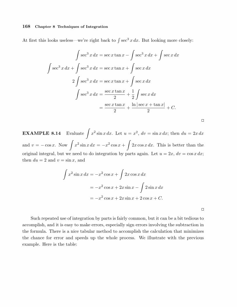
168 Chapter 8 Techniques of Integration
At first this looks useless—we’re right back to∫
sec3 x dx. But looking more closely:
∫sec3 x dx = sec x tan x−
∫sec3 x dx +
∫sec x dx
∫sec3 x dx +
∫sec3 x dx = sec x tan x +
∫sec x dx
2∫
sec3 x dx = sec x tan x +∫
sec x dx
∫sec3 x dx =
sec x tan x
2+
12
∫sec x dx
=sec x tan x
2+
ln | sec x + tan x|2
+ C.
EXAMPLE 8.14 Evaluate∫
x2 sin x dx. Let u = x2, dv = sin x dx; then du = 2x dx
and v = − cosx. Now∫
x2 sin x dx = −x2 cos x +∫
2x cos x dx. This is better than the
original integral, but we need to do integration by parts again. Let u = 2x, dv = cos x dx;then du = 2 and v = sin x, and
∫x2 sinx dx = −x2 cos x +
∫2x cos x dx
= −x2 cos x + 2x sin x−∫
2 sinx dx
= −x2 cos x + 2x sin x + 2 cos x + C.
Such repeated use of integration by parts is fairly common, but it can be a bit tedious toaccomplish, and it is easy to make errors, especially sign errors involving the subtraction inthe formula. There is a nice tabular method to accomplish the calculation that minimizesthe chance for error and speeds up the whole process. We illustrate with the previousexample. Here is the table:

8.4 Integration by Parts 169
sign u dv
x2 sin x
− 2x − cos x
2 − sin x
− 0 cosx
or
u dv
x2 sin x
−2x − cosx
2 − sin x
0 cos x
To form the first table, we start with u at the top of the second column and repeatedlycompute the derivative; starting with dv at the top of the third column, we repeatedlycompute the antiderivative. In the first column, we place a “−” in every second row. Toform the second table we combine the first and second columns by ignoring the boundary;if you do this by hand, you may simply start with two columns and add a “−” to everysecond row.
To compute with this second table we begin at the top. Multiply the first entry incolumn u by the second entry in column dv to get −x2 cos x, and add this to the integralof the product of the second entry in column u and second entry in column dv. This gives:
−x2 cos x +∫
2x cosx dx,
or exactly the result of the first application of integration by parts. Since this integral isnot yet easy, we return to the table. Now we multiply twice on the diagonal, (x2)(− cosx)and (−2x)(− sin x) and then once straight across, (2)(− sin x), and combine these as
−x2 cos x + 2x sin x−∫
2 sinx dx,
giving the same result as the second application of integration by parts. While this integralis easy, we may return yet once more to the table. Now multiply three times on the diagonalto get (x2)(− cosx), (−2x)(− sin x), and (2)(cos x), and once straight across, (0)(cos x).We combine these as before to get
−x2 cos x + 2x sin x + 2 cos x +∫
0 dx = −x2 cos x + 2x sin x + 2 cos x + C.
Typically we would fill in the table one line at a time, until the “straight across” multipli-cation gives an easy integral. If we can see that the u column will eventually become zero,we can instead fill in the whole table; computing the products as indicated will then givethe entire integral, including the “+C”, as above.

170 Chapter 8 Techniques of Integration
Exercises
Find the antiderivatives.
1.
Zx cos x dx ⇒
2.
Zx2 cos x dx ⇒
3.
Zxex dx ⇒
4.
Zxex2
dx ⇒
5.
Zsin2 x dx ⇒
6.
Zln x dx ⇒
7.
Zx arctan x dx ⇒
8.
Zx2 sin x dx ⇒
9.
Zx sin2 x dx ⇒
10.
Zx sin x cos x dx ⇒
11.
Zarctan(
√x) dx ⇒
12.
Zsin(√
x) dx ⇒
13.
Zsec2 x csc2 x dx ⇒
8.5 Rational Functions
A rational function is a fraction with polynomials in the numerator and denominator.For example,
x3
x2 + x− 6,
1(x− 3)2
,x2 + 1x2 − 1
,
are all rational functions of x. There is a general technique called “partial fractions”that, in principle, allows us to integrate any rational function. The algebraic steps in thattechnique are rather cumbersome if the polynomial in the denominator has degree morethan 2, and the technique requires that we factor the denominator, something that is notalways possible. However, in practice one does not often run across rational functions withhigh degree polynomials in the denominator for which one has to find the antiderivativefunction. So we shall explain how to find the antiderivative of a rational function onlywhen the denominator is a quadratic polynomial ax2 + bx + c.
We should mention a special type of rational function that we already know how tointegrate: If the denominator has the form (ax + b)n, the substitution u = ax + b willalways work. The denominator becomes un, and each x in the numerator is replaced by(u − b)/a, and dx = du/a. While it may be tedious to complete the integration if thenumerator has high degree, it is merely a matter of algebra.
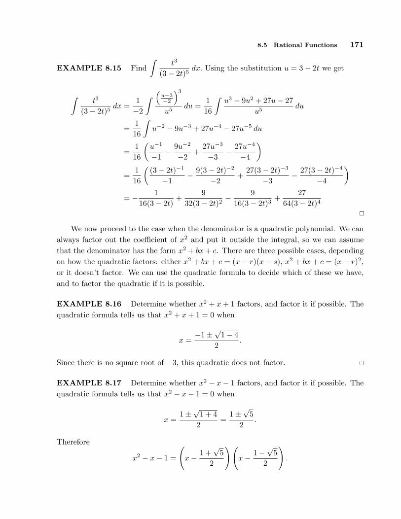
8.5 Rational Functions 171
EXAMPLE 8.15 Find∫
t3
(3− 2t)5dx. Using the substitution u = 3− 2t we get
∫t3
(3− 2t)5dx =
1−2
∫ (u−3−2
)3
u5du =
116
∫u3 − 9u2 + 27u− 27
u5du
=116
∫u−2 − 9u−3 + 27u−4 − 27u−5 du
=116
(u−1
−1− 9u−2
−2+
27u−3
−3− 27u−4
−4
)
=116
((3− 2t)−1
−1− 9(3− 2t)−2
−2+
27(3− 2t)−3
−3− 27(3− 2t)−4
−4
)
= − 116(3− 2t)
+9
32(3− 2t)2− 9
16(3− 2t)3+
2764(3− 2t)4
We now proceed to the case when the denominator is a quadratic polynomial. We canalways factor out the coefficient of x2 and put it outside the integral, so we can assumethat the denominator has the form x2 + bx + c. There are three possible cases, dependingon how the quadratic factors: either x2 + bx + c = (x− r)(x− s), x2 + bx + c = (x− r)2,or it doesn’t factor. We can use the quadratic formula to decide which of these we have,and to factor the quadratic if it is possible.
EXAMPLE 8.16 Determine whether x2 + x + 1 factors, and factor it if possible. Thequadratic formula tells us that x2 + x + 1 = 0 when
x =−1±√1− 4
2.
Since there is no square root of −3, this quadratic does not factor.
EXAMPLE 8.17 Determine whether x2 − x− 1 factors, and factor it if possible. Thequadratic formula tells us that x2 − x− 1 = 0 when
x =1±√1 + 4
2=
1±√52
.
Therefore
x2 − x− 1 =
(x− 1 +
√5
2
)(x− 1−√5
2
).

172 Chapter 8 Techniques of Integration
If x2 + bx + c = (x− r)2 then we have the special case we have already seen, that canbe handled with a substitution. The other two cases require different approaches.
If x2 + bx + c = (x− r)(x− s), we have an integral of the form
∫p(x)
(x− r)(x− s)dx
where p(x) is a polynomial. The first step is to make sure that p(x) has degree less than2.
EXAMPLE 8.18 Rewrite∫
x3
(x− 2)(x + 3)dx in terms of an integral with a numerator
that has degree less than 2. To do this we use “long division of polynomials” to discoverthat
x3
(x− 2)(x + 3)=
x3
x2 + x− 6= x− 1 +
7x− 6x2 + x− 6
= x− 1 +7x− 6
(x− 2)(x + 3),
so ∫x3
(x− 2)(x + 3)dx =
∫x− 1 dx +
∫7x− 6
(x− 2)(x + 3)dx.
The first integral is easy, so only the second requires some work.
Now consider the following simple algebra of fractions:
A
x− r+
B
x− s=
A(x− s) + B(x− r)(x− r)(x− s)
=(A + B)x−As−Br
(x− r)(x− s).
That is, adding two fractions with constant numerator and denominators (x−r) and (x−s)produces a fraction with denominator (x− r)(x− s) and a polynomial of degree less than2 for the numerator. We want to reverse this process: starting with a single fraction, wewant to write it as a sum of two simpler fractions. An example should make it clear howto proceed.
EXAMPLE 8.19 Evaluate∫
x3
(x− 2)(x + 3)dx. We start by writing
7x− 6(x− 2)(x + 3)
as the sum of two fractions. We want to end up with
7x− 6(x− 2)(x + 3)
=A
x− 2+
B
x + 3.
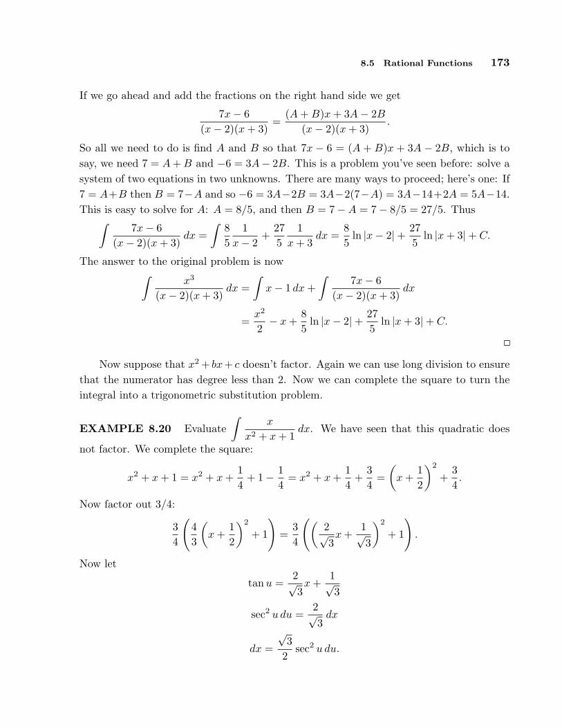
8.5 Rational Functions 173
If we go ahead and add the fractions on the right hand side we get
7x− 6(x− 2)(x + 3)
=(A + B)x + 3A− 2B
(x− 2)(x + 3).
So all we need to do is find A and B so that 7x − 6 = (A + B)x + 3A − 2B, which is tosay, we need 7 = A + B and −6 = 3A− 2B. This is a problem you’ve seen before: solve asystem of two equations in two unknowns. There are many ways to proceed; here’s one: If7 = A+B then B = 7−A and so −6 = 3A−2B = 3A−2(7−A) = 3A−14+2A = 5A−14.This is easy to solve for A: A = 8/5, and then B = 7−A = 7− 8/5 = 27/5. Thus
∫7x− 6
(x− 2)(x + 3)dx =
∫85
1x− 2
+275
1x + 3
dx =85
ln |x− 2|+ 275
ln |x + 3|+ C.
The answer to the original problem is now∫
x3
(x− 2)(x + 3)dx =
∫x− 1 dx +
∫7x− 6
(x− 2)(x + 3)dx
=x2
2− x +
85
ln |x− 2|+ 275
ln |x + 3|+ C.
Now suppose that x2 + bx+ c doesn’t factor. Again we can use long division to ensurethat the numerator has degree less than 2. Now we can complete the square to turn theintegral into a trigonometric substitution problem.
EXAMPLE 8.20 Evaluate∫
x
x2 + x + 1dx. We have seen that this quadratic does
not factor. We complete the square:
x2 + x + 1 = x2 + x +14
+ 1− 14
= x2 + x +14
+34
=(
x +12
)2
+34.
Now factor out 3/4:
34
(43
(x +
12
)2
+ 1
)=
34
((2√3x +
1√3
)2
+ 1
).
Now let
tan u =2√3x +
1√3
sec2 u du =2√3
dx
dx =√
32
sec2 u du.

174 Chapter 8 Techniques of Integration
Now we can substitute in the original integral, using x = (√
3/2)(tanu − 1/√
3) in thenumerator.
∫x
x2 + x + 1dx =
43
∫(√
3/2)(tanu− 1/√
3)tan2 u + 1
√3
2sec2 u du
=43
∫(√
3/2)(tanu− 1/√
3)sec2 u
√3
2sec2 u du
=43
∫ √3
2
(tan u− 1√
3
) √3
2du
=∫
tan u− 1√3
du
= − ln | cos u| − u√3
+ C.
= ln | sec u| − u√3
+ C.
Finally, we can substitute
u = arctan(
2√3x +
1√3
)
and
sec u =√
tan2 u + 1 =
√(2√3x +
1√3
)2
+ 1
to get
ln
∣∣∣∣∣∣
√(2√3x +
1√3
)2
+ 1
∣∣∣∣∣∣− 1√
3arctan
(2√3x +
1√3
)+ C.
The details here are admittedly a bit unpleasant, but the whole process is fairly me-chanical and “easy” in principle.
Exercises
Find the antiderivatives.
1.
Z1
4− x2dx ⇒
2.
Zx4
4− x2dx ⇒
3.
Z1
x2 + 10x + 25dx ⇒
4.
Zx2
4− x2dx ⇒
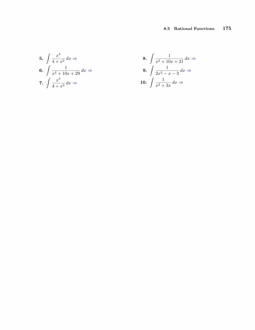
8.5 Rational Functions 175
5.
Zx4
4 + x2dx ⇒
6.
Z1
x2 + 10x + 29dx ⇒
7.
Zx3
4 + x2dx ⇒
8.
Z1
x2 + 10x + 21dx ⇒
9.
Z1
2x2 − x− 3dx ⇒
10.
Z1
x2 + 3xdx ⇒
176 Chapter 8 Techniques of Integration
8.6 Additional exercises
These problems require the techniques of this chapter, and are in no particular order. Someproblems may be done in more than one way.
Exercises
1.
Z(t + 4)3 dt ⇒
2.
Zt(t2 − 9)3/2 dt ⇒
3.
Z(et2 + 16)tet2 dt ⇒
4.
Zsin t cos 2t dt ⇒
5.
Ztan t sec2 t dt ⇒
6.
Z2t + 1
t2 + t + 3dt ⇒
7.
Z1
t(t2 − 4)dt ⇒
8.
Z1
(25− t2)3/2dt ⇒
9.
Zcos 3t√sin 3t
dt ⇒
10.
Zt sec2 t dt ⇒
11.
Zet
√et + 1
dt ⇒
12.
Zcos4 t dt ⇒
13.
Z1
t2 + 3tdt ⇒
14.
Z1
t2√
1 + t2dt ⇒
15.
Zsec2 t
(1 + tan t)3dt ⇒
16.
Zt3p
t2 + 1 dt ⇒
17.
Zet sin t dt ⇒
18.
Z(t3/2 + 47)3
√t dt ⇒
19.
Zt3
(2− t2)5/2dt ⇒
20.
Z1
t(9 + 4t2)dt ⇒
21.
Zarctan 2t
1 + 4t2dt ⇒
22.
Zt
t2 + 2t− 3dt ⇒
23.
Zsin3 t cos4 t dt ⇒
24.
Z1
t2 − 6t + 9dt ⇒
25.
Z1
t(ln t)2dt ⇒
26.
Zt(ln t)2 dt ⇒
27.
Zt3et dt ⇒
28.
Zt + 1
t2 + t− 1dt ⇒

9Applications of Integration
9.1 Area between curves
We have seen how integration can be used to find an area between a curve and the x-axis.With very little change we can find some areas between curves; indeed, the area betweena curve and the x-axis may be interpreted as the area between the curve and a second“curve” with equation y = 0. In the simplest of cases, the idea is quite easy to understand.
EXAMPLE 9.1 Find the area below f(x) = −x2 + 4x + 3 and above g(x) = −x3 +7x2 − 10x + 5 over the interval 1 ≤ x ≤ 2. In figure 9.1 we show the two curves together,with the desired area shaded, then f alone with the area under f shaded, and then g alonewith the area under g shaded.
It is clear from the figure that the area we want is the area under f minus the areaunder g, which is to say
∫ 2
1
f(x) dx−∫ 2
1
g(x) dx =∫ 2
1
f(x)− g(x) dx.
177

178 Chapter 9 Applications of Integration
..
..
..
..
..
..
..
..
..
..
..
..
..
..
..
..
..
..
..
.
..
..
..
..
..
..
..
..
..
..
..
..
..
..
..
..
..
..
..
..
..
..
..
..
..
..
..
..
..
..
..
..
..
..
..
..
..
..
..
..
..
..
..
..
..
..
..
..
..
..
..
..
..
..
..
..
..
..
..
..
..
..
..
..
..
..
..
..
..
..
..
..
..
..
..
..
..
..
..
..
..
..
..
..
..
..
..
..
..
..
..
..
..
..
..
..
..
..
..
.
..
..
..
..
..
..
..
..
..
..
..
..
..
..
..
..
..
..
..
.
..
..
..
..
..
..
..
..
..
..
..
..
..
..
..
..
..
..
..
..
..
..
..
..
..
..
..
..
..
..
..
..
..
..
..
..
..
..
..
.
..
..
..
..
..
..
..
..
..
..
..
..
..
..
..
..
..
..
..
.
..
..
..
..
..
..
..
..
..
..
..
..
..
..
..
..
..
..
..
..
..
..
..
..
..
..
..
..
..
..
..
..
..
..
..
..
..
..
..
..
..
..
..
..
..
..
..
..
..
..
..
..
..
..
..
..
..
..
..
..
..
..
..
..
..
..
..
..
..
..
..
..
..
..
..
..
..
..
..
..
..
..
..
..
..
..
..
..
..
..
..
..
..
..
..
..
..
..
..
..
..
..
..
..
..
..
..
..
..
..
..
..
..
..
..
..
..
..
..
..
..
..
..
..
..
..
..
..
..
..
..
..
..
..
..
..
..
..
..
..
..
..
..
..
..
..
..
..
..
..
..
..
.
..
..
..
..
..
..
..
..
..
..
..
..
..
..
..
..
..
..
..
..
..
..
..
..
..
..
..
..
..
.
..
..
..
..
..
..
..
..
..
..
..
..
..
..
.
..
..
..
..
..
..
..
..
..
..
..
..
..
.
..
..
..
..
..
..
..
..
..
..
..
..
..
.
..
..
..
..
..
..
..
..
..
..
..
..
.
..
..
..
..
..
..
..
..
..
..
..
..
.
..
..
..
..
..
..
..
..
..
..
..
.
..
..
..
..
..
..
..
..
..
..
..
..
..
..
..
..
..
..
..
..
..
..
..
..
..
..
..
..
..
..
..
..
..
..
..
..
..
..
..
..
..
..
..
..
..
..
..
..
..
..
..
..
..
..
..
..
..
..
..
.
0
5
10
0 1 2 3
...............................................................................................................................
.................................................................................................
......................................................................................................................................................................................................................................................................................................................................................................................................
..
..
..
..
..
..
..
..
..
..
..
..
..
..
..
..
..
..
..
..
..
..
..
..
..
..
..
..
..
..
..
..
..
..
..
..
..
..
..
..
..
..
..
..
..
..
..
..
..
..
..
..
..
..
..
..
..
..
..
..
..
..
..
..
..
..
..
..
..
..
..
..
.
..
..
..
..
..
..
..
..
..
..
..
..
..
..
..
..
..
..
..
..
..
..
..
..
.
..
..
..
..
..
..
..
..
..
..
..
..
..
..
..
..
..
..
..
..
..
..
..
..
..
..
..
..
..
..
..
..
..
..
..
..
..
..
..
..
..
..
..
..
..
..
..
..
..
.
..
..
..
..
..
..
..
..
..
..
..
..
..
..
..
..
..
..
..
..
..
..
..
..
..
..
..
..
..
..
..
..
..
..
..
..
..
..
..
..
..
..
..
..
..
..
..
..
..
..
..
..
..
..
..
..
..
..
..
..
..
..
..
..
..
..
..
..
..
..
..
..
..
..
..
.
..
..
..
..
..
..
..
..
..
..
..
..
..
..
..
..
..
..
..
..
..
..
..
..
..
.
..
..
..
..
..
..
..
..
..
..
..
..
..
..
..
..
..
..
..
..
..
..
..
..
..
..
..
..
..
..
..
..
..
..
..
..
..
..
..
..
..
..
..
..
..
..
..
..
..
..
..
.
..
..
..
..
..
..
..
..
..
..
..
..
..
..
..
..
..
..
..
..
..
..
..
..
..
..
..
..
..
..
..
..
..
..
..
..
..
..
..
..
..
..
..
..
..
..
..
..
..
..
..
..
..
..
..
..
..
..
..
..
..
..
..
..
..
..
..
..
..
..
..
..
..
..
..
..
..
..
.
..
..
..
..
..
..
..
..
..
..
..
..
..
..
..
..
..
..
..
..
..
..
..
..
..
..
..
..
..
..
..
..
..
..
..
..
..
..
..
..
..
..
..
..
..
..
..
..
..
..
..
..
.
..
..
..
..
..
..
..
..
..
..
..
..
..
..
..
..
..
..
..
..
..
..
..
..
..
..
.
..
..
..
..
..
..
..
..
..
..
..
..
..
..
..
..
..
..
..
..
..
..
..
..
..
..
..
..
..
..
..
..
..
..
..
..
..
..
..
..
..
..
..
..
..
..
..
..
..
..
..
..
..
.
..
..
..
..
..
..
..
..
..
..
..
..
..
..
..
..
..
..
..
..
..
..
..
..
..
..
..
..
..
..
..
..
..
..
..
..
..
..
..
..
..
..
..
..
..
..
..
..
..
..
..
..
..
..
..
..
..
..
..
..
..
..
..
..
..
..
..
..
..
..
..
..
..
..
..
..
..
..
..
..
..
..
..
..
..
..
..
..
..
..
..
..
..
..
..
..
..
..
..
..
..
..
..
..
..
..
..
..
..
..
..
..
..
..
..
..
..
..
..
..
..
..
..
..
..
..
..
..
..
..
..
..
..
..
..
.
..
..
..
..
..
..
..
..
..
..
..
..
..
..
..
..
..
..
..
..
..
..
..
..
..
..
..
..
..
..
..
..
..
..
..
..
..
..
..
..
..
..
..
..
..
..
..
..
..
..
..
..
..
..
.
..
..
..
..
..
..
..
..
..
..
..
..
..
..
..
..
..
..
..
..
..
..
..
..
..
..
..
.
..
..
..
..
..
..
..
..
..
..
..
..
..
..
..
..
..
..
..
..
..
..
..
..
..
..
..
.
..
..
..
..
..
..
..
..
..
..
..
..
..
..
..
..
..
..
..
..
..
..
..
..
..
..
..
.
..
..
..
..
..
..
..
..
..
..
..
..
..
..
..
..
..
..
..
..
..
..
..
..
..
..
..
.
..
..
..
..
..
..
..
..
..
..
..
..
..
..
..
..
..
..
..
..
..
..
..
..
..
..
..
.
..
..
..
..
..
..
..
..
..
..
..
..
..
..
..
..
..
..
..
..
..
..
..
..
..
..
..
.
..
..
..
..
..
..
..
..
..
..
..
..
..
..
..
..
..
..
..
..
..
..
..
..
..
..
..
.
..
..
..
..
..
..
..
..
..
..
..
..
..
..
..
..
..
..
..
..
..
..
..
..
..
..
..
..
..
..
..
..
..
..
..
..
..
..
..
..
..
..
..
..
..
..
..
..
..
..
..
..
..
..
..
.
..
..
..
..
..
..
..
..
..
..
..
..
..
..
..
..
..
..
..
..
..
..
..
..
..
..
..
..
..
..
..
..
..
..
..
..
..
..
..
..
..
..
..
..
..
..
..
..
..
..
..
..
..
..
..
.
..
..
..
..
..
..
..
..
..
..
..
..
..
..
..
..
..
..
..
..
..
..
..
..
..
..
..
..
0
5
10
0 1 2 3
...............................................................................................................................
.................................................................................................
..
..
..
..
.
..
..
..
..
..
..
..
..
.
..
..
..
..
.
..
..
..
..
..
..
..
..
..
..
..
..
..
..
..
.
..
..
..
..
..
..
..
..
..
..
.
..
..
..
..
..
..
..
..
..
..
..
..
.
..
..
..
..
..
..
.
..
..
..
..
..
..
..
..
..
..
..
..
..
..
..
..
..
..
..
..
..
.
..
..
..
..
..
..
..
.
..
..
..
..
..
..
..
..
.
..
..
..
..
..
..
..
..
.
..
..
..
..
..
..
..
..
..
..
..
..
..
..
..
..
..
..
.
..
..
..
..
..
..
..
..
..
..
..
..
..
..
..
..
..
..
..
..
..
..
..
..
..
..
..
..
..
..
..
..
..
..
..
..
..
..
..
..
..
..
..
..
..
..
..
..
..
..
..
..
..
..
..
..
..
..
..
..
..
..
..
..
..
..
..
..
..
..
..
..
..
..
..
..
..
..
..
..
..
..
..
..
..
..
..
..
..
..
..
..
..
..
..
..
..
..
..
..
..
..
..
..
..
..
..
..
..
..
..
..
..
..
..
..
..
..
..
..
..
..
..
..
..
..
..
..
..
..
..
..
..
..
..
..
..
..
..
..
..
..
..
..
..
..
..
..
..
..
..
..
..
..
..
..
..
..
..
..
..
..
..
..
..
..
..
..
..
..
..
..
..
..
..
..
..
..
..
..
..
..
.
..
..
..
..
..
..
..
..
..
..
..
..
..
..
..
..
..
..
..
..
..
..
..
..
..
..
..
..
..
..
..
..
..
..
.
..
..
..
..
..
..
..
..
..
..
..
..
..
..
..
..
..
..
..
..
..
..
..
..
..
..
..
..
..
..
..
..
..
..
..
..
.
..
..
..
..
..
..
..
..
..
..
..
..
..
..
..
..
..
..
..
.
0
5
10
0 1 2 3
......................................................................................................................................................................................................................................................................................................................................................................................................
Figure 9.1 Area between curves as a difference of areas.
It doesn’t matter whether we compute the two integrals on the left and then subtract orcompute the single integral on the right. In this case, the latter is perhaps a bit easier:
∫ 2
1
f(x)− g(x) dx =∫ 2
1
−x2 + 4x + 3− (−x3 + 7x2 − 10x + 5) dx
=∫ 2
1
x3 − 8x2 + 14x− 2 dx
=x4
4− 8x3
3+ 7x2 − 2x
∣∣∣∣2
1
=164− 64
3+ 28− 4− (
14− 8
3+ 7− 2)
= 23− 563− 1
4=
4912
.
It is worth examining this problem a bit more. We have seen one way to look at it,by viewing the desired area as a big area minus a small area, which leads naturally to thedifference between two integrals. But it is instructive to consider how we might find thedesired area directly. We can approximate the area by dividing the area into thin sectionsand approximating the area of each section by a rectangle, as indicated in figure 9.2. Thearea of a typical rectangle is ∆x(f(xi)− g(xi)), so the total area is approximately
n−1∑
i=0
(f(xi)− g(xi))∆x.
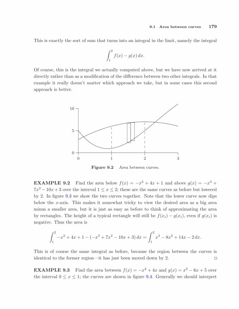
9.1 Area between curves 179
This is exactly the sort of sum that turns into an integral in the limit, namely the integral
∫ 2
1
f(x)− g(x) dx.
Of course, this is the integral we actually computed above, but we have now arrived at itdirectly rather than as a modification of the difference between two other integrals. In thatexample it really doesn’t matter which approach we take, but in some cases this secondapproach is better.
0
5
10
0 1 2 3
..................................
.....................................
.........................................
................................................
............................................................
.........................................................................................................
...................................................................................................................................................................................................................................
.........................................................................................................................................................................................................................................................................
....................................
...............................
.........................................................................................................................................................................................................................................................................................................................
Figure 9.2 Area between curves.
EXAMPLE 9.2 Find the area below f(x) = −x2 + 4x + 1 and above g(x) = −x3 +7x2− 10x + 3 over the interval 1 ≤ x ≤ 2; these are the same curves as before but loweredby 2. In figure 9.3 we show the two curves together. Note that the lower curve now dipsbelow the x-axis. This makes it somewhat tricky to view the desired area as a big areaminus a smaller area, but it is just as easy as before to think of approximating the areaby rectangles. The height of a typical rectangle will still be f(xi)− g(xi), even if g(xi) isnegative. Thus the area is
∫ 2
1
−x2 + 4x + 1− (−x3 + 7x2 − 10x + 3) dx =∫ 2
1
x3 − 8x2 + 14x− 2 dx.
This is of course the same integral as before, because the region between the curves isidentical to the former region—it has just been moved down by 2.
EXAMPLE 9.3 Find the area between f(x) = −x2 + 4x and g(x) = x2 − 6x + 5 overthe interval 0 ≤ x ≤ 1; the curves are shown in figure 9.4. Generally we should interpret
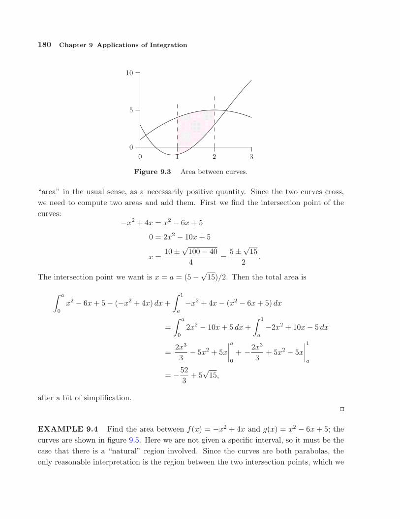
180 Chapter 9 Applications of Integration
..
..
..
..
..
..
..
..
..
..
..
..
..
..
..
..
..
..
..
..
..
..
..
..
..
..
..
..
..
..
..
..
..
..
..
..
..
..
..
.
..
..
..
..
..
..
..
..
..
..
..
..
..
..
..
..
..
..
..
..
..
..
..
..
..
..
..
..
..
..
..
..
..
..
..
..
..
..
..
..
..
..
..
..
..
..
..
..
..
..
..
..
..
..
..
..
..
..
..
.
..
..
..
..
..
..
..
..
..
..
..
..
..
..
..
..
..
..
..
..
..
..
..
..
..
..
..
..
..
..
..
..
..
..
..
..
..
..
..
..
..
..
..
..
..
..
..
..
..
..
..
..
..
..
..
..
..
..
..
.
..
..
..
..
..
..
..
..
..
..
..
..
..
..
..
..
..
..
..
..
..
..
..
..
..
..
..
..
..
..
..
..
..
..
..
..
..
..
..
..
..
..
..
..
..
..
..
..
..
..
..
..
..
..
..
..
..
..
..
.
..
..
..
..
..
..
..
..
..
..
..
..
..
..
..
..
..
..
..
..
..
..
..
..
..
..
..
..
..
..
..
..
..
..
..
..
..
..
..
..
..
..
..
..
..
..
..
..
..
..
..
..
..
..
..
..
..
..
..
.
..
..
..
..
..
..
..
..
..
..
..
..
..
..
..
..
..
..
..
.
..
..
..
..
..
..
..
..
..
..
..
..
..
..
..
..
..
..
..
..
..
..
..
..
..
..
..
..
..
..
..
..
..
..
..
..
..
..
..
.
..
..
..
..
..
..
..
..
..
..
..
..
..
..
..
..
..
..
..
.
..
..
..
..
..
..
..
..
..
..
..
..
..
..
..
..
..
..
..
.
..
..
..
..
..
..
..
..
..
..
..
..
..
..
..
..
..
..
..
.
..
..
..
..
..
..
..
..
..
..
..
..
..
..
..
..
..
..
..
.
..
..
..
..
..
..
..
..
..
..
..
..
..
..
..
..
..
..
..
.
..
..
..
..
..
..
..
..
..
..
..
..
..
..
..
..
..
..
..
..
..
..
..
..
..
..
..
..
..
..
..
..
..
..
..
..
..
..
.
..
..
..
..
..
..
..
..
..
..
..
..
..
..
..
..
..
..
..
.
..
..
..
..
..
..
..
..
..
..
..
..
..
..
..
..
..
..
..
..
..
..
..
..
..
..
..
..
..
..
..
..
..
..
..
..
..
..
..
..
..
..
..
..
..
..
..
..
..
..
..
..
..
..
..
..
..
..
..
..
..
..
..
..
..
..
..
..
..
..
..
..
..
..
..
.
..
..
..
..
..
..
..
..
..
..
..
..
..
..
..
..
..
..
..
..
..
..
..
..
..
..
..
..
..
..
..
..
..
..
..
..
..
.
..
..
..
..
..
..
..
..
..
..
..
..
..
..
..
..
..
..
.
..
..
..
..
..
..
..
..
..
..
..
..
..
..
..
..
..
..
.
..
..
..
..
..
..
..
..
..
..
..
..
..
..
..
..
..
..
..
..
..
..
..
..
..
..
..
..
..
..
..
..
..
..
..
..
..
..
..
..
..
..
..
..
..
..
..
..
..
..
..
..
..
..
..
..
..
..
..
..
..
..
..
..
..
..
..
..
..
..
..
.
..
..
..
..
..
..
..
..
..
..
..
..
..
..
..
..
..
.
..
..
..
..
..
..
..
..
..
..
..
..
..
..
..
..
..
.
..
..
..
..
..
..
..
..
..
..
..
..
..
..
..
..
..
.
..
..
..
..
..
..
..
..
..
..
..
..
..
..
..
..
..
.
..
..
..
..
..
..
..
..
..
..
..
..
..
..
..
..
..
..
..
..
..
..
..
..
..
..
..
..
..
..
..
..
..
..
..
..
..
..
..
..
..
..
..
..
..
..
..
..
..
..
.
..
..
..
..
..
..
..
..
..
..
..
..
..
..
..
..
.
..
..
..
..
..
..
..
..
..
..
..
..
..
..
..
..
..
..
..
..
..
..
..
..
..
..
..
..
..
..
..
..
..
..
..
..
..
..
..
..
..
..
..
..
..
..
..
..
..
..
..
..
..
..
..
..
..
..
..
..
..
..
..
.
..
..
..
..
..
..
..
..
..
..
..
..
..
..
..
.
..
..
..
..
..
..
..
..
..
..
..
..
..
..
..
..
..
..
..
..
..
..
..
..
..
..
..
..
..
..
..
..
..
..
..
..
..
..
..
..
..
..
..
..
..
..
..
..
..
..
..
..
..
..
..
..
..
..
..
.
..
..
..
..
..
..
..
..
..
..
..
..
..
..
.
..
..
..
..
..
..
..
..
..
..
..
..
..
..
..
..
..
..
..
..
..
..
..
..
..
..
..
..
..
..
..
..
..
..
..
..
..
..
..
..
..
.
..
..
..
..
..
..
..
..
..
..
..
..
..
.
..
..
..
..
..
..
..
..
..
..
..
..
..
..
..
..
..
..
..
..
..
..
..
..
..
..
..
..
..
..
..
..
..
..
..
..
..
..
..
..
..
..
..
..
..
..
..
..
..
..
..
.
..
..
..
..
..
..
..
..
..
..
..
..
.
..
..
..
..
..
..
..
..
..
..
..
..
..
..
..
..
..
..
..
..
..
..
..
..
..
..
..
..
..
..
..
..
..
..
..
.
..
..
..
..
..
..
..
..
..
..
..
.
..
..
..
..
..
..
..
..
..
..
..
..
..
..
..
..
..
..
..
..
..
..
..
..
..
..
..
..
..
..
..
..
..
..
..
..
..
..
..
..
..
..
..
..
..
..
..
..
..
..
..
.
..
..
..
..
..
..
..
..
..
.
..
..
..
..
..
..
..
..
..
..
..
..
..
..
..
..
..
..
..
..
..
..
..
..
..
..
.
..
..
..
..
..
..
..
..
.
..
..
..
..
..
..
..
..
0
5
10
0 1 2 3
.....................................................................
...............................
......................................
...................................................
..................................................................................................................................................................................................
.........................................................................................................................................................................................................
...............................................................................................................................................................................................................................................................................................................
Figure 9.3 Area between curves.
“area” in the usual sense, as a necessarily positive quantity. Since the two curves cross,we need to compute two areas and add them. First we find the intersection point of thecurves:
−x2 + 4x = x2 − 6x + 5
0 = 2x2 − 10x + 5
x =10±√100− 40
4=
5±√152
.
The intersection point we want is x = a = (5−√15)/2. Then the total area is
∫ a
0
x2 − 6x + 5− (−x2 + 4x) dx +∫ 1
a
−x2 + 4x− (x2 − 6x + 5) dx
=∫ a
0
2x2 − 10x + 5 dx +∫ 1
a
−2x2 + 10x− 5 dx
=2x3
3− 5x2 + 5x
∣∣∣∣a
0
+ −2x3
3+ 5x2 − 5x
∣∣∣∣1
a
= −523
+ 5√
15,
after a bit of simplification.
EXAMPLE 9.4 Find the area between f(x) = −x2 + 4x and g(x) = x2 − 6x + 5; thecurves are shown in figure 9.5. Here we are not given a specific interval, so it must be thecase that there is a “natural” region involved. Since the curves are both parabolas, theonly reasonable interpretation is the region between the two intersection points, which we
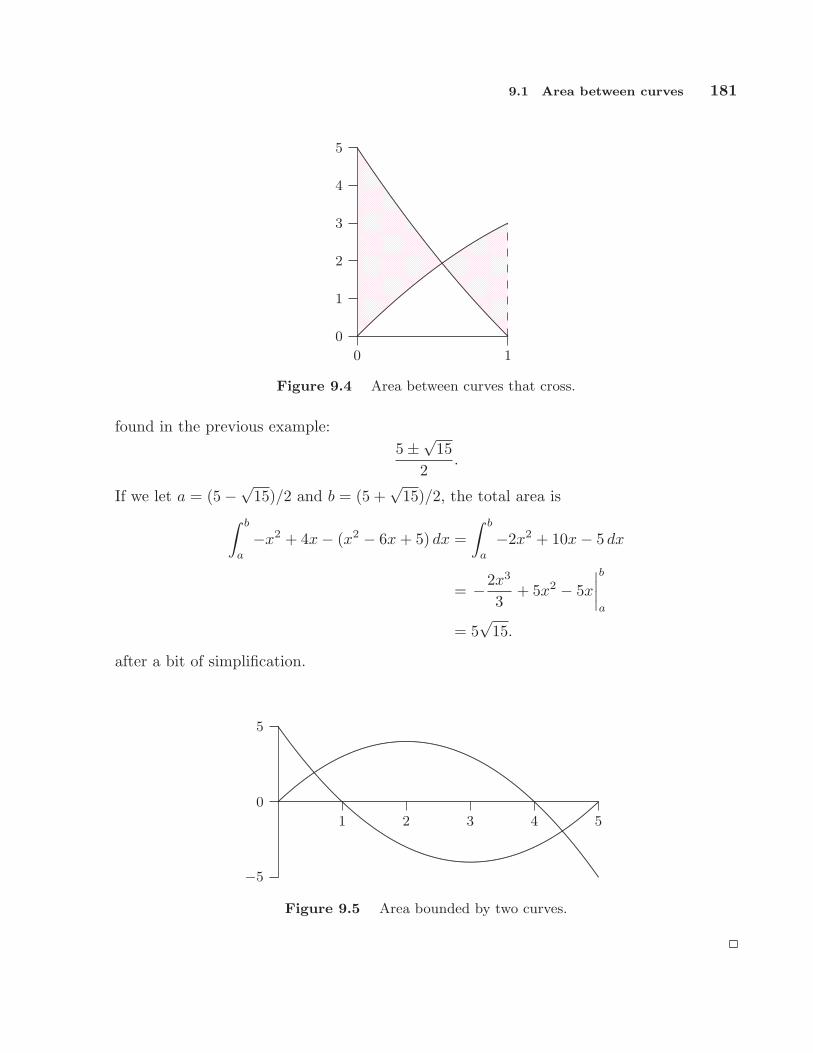
9.1 Area between curves 181
..
..
..
..
..
..
..
..
..
..
..
..
..
..
..
..
..
..
..
..
..
..
..
..
..
..
..
..
..
..
..
..
..
..
..
..
..
..
..
..
..
..
..
..
..
..
..
..
..
.
..
..
..
..
..
..
..
..
..
..
..
..
..
..
..
..
..
..
..
..
..
..
..
..
..
..
..
..
..
..
..
..
..
..
..
..
..
..
..
..
..
..
..
..
..
..
..
..
..
..
..
..
..
..
..
..
..
..
..
..
..
..
..
..
..
..
..
..
..
..
..
..
..
..
..
..
..
..
..
..
..
..
..
..
..
..
..
..
..
..
..
..
..
..
..
..
..
.
..
..
..
..
..
..
..
..
..
..
..
..
..
..
..
..
..
..
..
..
..
..
..
..
..
..
..
..
..
..
..
..
..
..
..
..
..
..
..
..
..
..
..
..
..
..
..
.
..
..
..
..
..
..
..
..
..
..
..
..
..
..
..
..
..
..
..
..
..
..
..
..
..
..
..
..
..
..
..
..
..
..
..
..
..
..
..
..
..
..
..
..
..
..
..
..
..
..
..
..
..
..
..
..
..
..
..
..
..
..
..
..
..
..
..
..
..
..
..
..
..
..
..
..
..
..
..
..
..
..
..
..
..
..
..
..
..
..
..
..
..
.
..
..
..
..
..
..
..
..
..
..
..
..
..
..
..
..
..
..
..
..
..
..
..
..
..
..
..
..
..
..
..
..
..
..
..
..
..
..
..
..
..
..
..
..
..
..
..
..
..
..
..
..
..
..
..
..
..
..
..
..
..
..
..
..
..
..
..
..
..
..
..
..
..
..
..
..
..
..
..
..
..
..
..
..
..
..
..
..
..
..
..
..
..
..
..
..
..
..
..
..
..
..
..
..
..
..
..
..
..
..
..
..
..
..
..
..
..
..
..
..
..
..
..
..
..
..
..
..
..
..
..
..
..
..
..
.
..
..
..
..
..
..
..
..
..
..
..
..
..
..
..
..
..
..
..
..
..
..
..
..
..
..
..
..
..
..
..
..
..
..
..
..
..
..
..
..
..
..
..
..
..
..
..
..
..
..
..
..
..
..
..
..
..
..
..
..
..
..
..
..
..
..
..
..
..
..
..
..
..
..
..
..
..
..
..
..
..
..
..
..
..
..
..
.
..
..
..
..
..
..
..
..
..
..
..
..
..
..
..
..
..
..
..
..
..
..
..
..
..
..
..
..
..
..
..
..
..
..
..
..
..
..
..
..
..
..
.
..
..
..
..
..
..
..
..
..
..
..
..
..
..
..
..
..
..
..
..
..
..
..
..
..
..
..
..
..
..
..
..
..
..
..
..
..
..
..
..
..
..
..
..
..
..
..
..
..
..
..
..
..
..
..
..
..
..
..
..
..
..
..
..
..
..
..
..
..
..
..
..
..
..
..
..
..
..
..
..
..
..
..
.
..
..
..
..
..
..
..
..
..
..
..
..
..
..
..
..
..
..
..
..
..
..
..
..
..
..
..
..
..
..
..
..
..
..
..
..
..
..
..
..
..
..
..
..
..
..
..
..
..
..
..
..
..
..
..
..
..
..
..
..
..
..
..
..
..
..
..
..
..
..
..
..
..
..
..
..
..
..
..
..
..
.
..
..
..
..
..
..
..
..
..
..
..
..
..
..
..
..
..
..
..
..
..
..
..
..
..
..
..
..
..
..
..
..
..
..
..
..
..
..
..
.
..
..
..
..
..
..
..
..
..
..
..
..
..
..
..
..
..
..
..
..
..
..
..
..
..
..
..
..
..
..
..
..
..
..
..
..
..
..
..
..
..
..
..
..
..
..
..
..
..
..
..
..
..
..
..
..
..
..
..
..
..
..
..
..
..
..
..
..
..
..
..
..
..
..
..
..
..
.
..
..
..
..
..
..
..
..
..
..
..
..
..
..
..
..
..
..
..
..
..
..
..
..
..
..
..
..
..
..
..
..
..
..
..
..
..
..
..
..
..
..
..
..
..
..
..
..
..
..
..
..
..
..
..
..
..
..
..
..
..
..
..
..
..
..
..
..
..
..
..
..
..
..
..
..
..
..
..
..
..
..
..
..
..
..
..
..
..
..
..
..
..
..
..
..
..
..
..
..
..
..
..
..
..
..
..
..
..
..
..
.
..
..
..
..
..
..
..
..
..
..
..
..
..
..
..
..
..
..
..
..
..
..
..
..
..
..
..
..
..
..
..
..
..
..
..
..
..
..
..
..
..
..
..
..
..
..
..
..
..
..
..
..
..
..
..
..
..
..
..
..
..
..
..
..
..
..
..
..
..
..
..
.
..
..
..
..
..
..
..
..
..
..
..
..
..
..
..
..
..
..
..
..
..
..
..
..
..
..
..
..
..
..
..
..
..
..
..
..
..
..
..
..
..
..
..
..
..
..
..
..
..
..
..
..
..
..
..
..
..
..
..
..
..
..
..
..
..
..
..
..
..
..
..
..
..
..
..
..
..
..
..
..
..
..
..
..
..
..
..
..
..
..
..
..
..
..
..
..
..
..
..
..
..
..
.
..
..
..
..
..
..
..
..
..
..
..
..
..
..
..
..
..
..
..
..
..
..
..
..
..
..
..
..
..
..
..
..
..
..
..
..
..
..
..
..
..
..
..
..
..
..
..
..
..
..
..
..
..
..
..
..
..
..
..
..
..
..
..
..
..
.
..
..
..
..
..
..
..
..
..
..
..
..
..
..
..
..
..
..
..
..
..
..
..
..
..
..
..
..
..
..
..
..
..
..
..
..
..
..
..
..
..
..
..
..
..
..
..
..
..
..
..
..
..
..
..
..
..
..
..
..
..
..
..
..
..
..
..
..
..
..
..
..
..
..
..
..
..
..
..
..
..
..
..
..
..
..
..
..
..
..
..
..
..
.
..
..
..
..
..
..
..
..
..
..
..
..
..
..
..
..
..
..
..
..
..
..
..
..
..
..
..
..
..
..
..
..
..
..
..
..
..
..
..
..
..
..
..
..
..
..
..
..
..
..
..
..
..
..
..
..
..
..
..
.
..
..
..
..
..
..
..
..
..
..
..
..
..
..
..
..
..
..
..
..
..
..
..
..
..
..
..
..
..
..
..
..
..
..
..
..
..
..
..
..
..
..
..
..
..
..
..
..
..
..
..
..
..
..
..
..
..
..
..
..
..
..
..
..
..
..
..
..
..
..
..
..
..
..
..
..
..
..
..
..
..
..
..
..
..
..
..
..
..
..
..
..
..
..
..
..
..
..
..
..
..
..
..
..
..
..
..
..
..
..
..
..
.
..
..
..
..
..
..
..
..
..
..
..
..
..
..
..
..
..
..
..
..
..
..
..
..
..
..
..
..
..
..
..
..
..
..
..
..
..
..
..
..
..
..
..
..
..
..
..
..
..
..
..
..
..
.
..
..
..
..
..
..
..
..
..
..
..
..
..
..
..
..
..
..
..
..
..
..
..
..
..
.
..
..
..
..
..
..
..
..
..
..
..
..
..
..
..
..
..
..
..
..
..
..
..
..
..
..
..
..
..
..
..
..
..
..
..
..
..
..
..
..
..
..
..
..
..
..
..
..
..
.
..
..
..
..
..
..
..
..
..
..
..
..
..
..
..
..
..
..
..
..
..
..
..
..
..
..
..
..
..
..
..
..
..
..
..
..
..
..
..
..
..
..
..
..
..
..
..
.
..
..
..
..
..
..
..
..
..
..
..
..
..
..
..
..
..
..
..
..
..
..
..
..
..
..
..
..
..
..
..
..
..
..
..
..
..
..
..
..
..
..
..
..
..
..
..
..
..
..
..
..
..
..
..
..
..
..
..
..
..
..
..
..
..
..
.
..
..
..
..
..
..
..
..
..
..
..
..
..
..
..
..
..
..
..
..
..
..
..
..
..
..
..
..
..
..
..
..
..
..
..
..
..
..
..
..
..
.
..
..
..
..
..
..
..
..
..
..
..
..
..
..
..
..
..
..
..
..
..
..
..
..
..
..
..
..
..
..
..
..
..
..
..
..
..
..
..
.
..
..
..
..
..
..
..
..
..
..
..
..
..
..
..
..
..
..
..
..
..
..
..
..
..
..
..
..
..
..
..
..
..
..
..
..
..
.
..
..
..
..
..
..
..
..
..
..
..
..
..
..
..
..
..
..
..
..
..
..
..
..
..
..
..
..
..
..
..
..
..
..
..
.
..
..
..
..
..
..
..
..
..
..
..
..
..
..
..
..
..
..
..
..
..
..
..
..
..
..
..
..
..
..
..
..
..
..
..
..
..
..
..
..
..
..
..
..
..
..
..
..
.
..
..
..
..
..
..
..
..
..
..
..
..
..
..
..
..
..
..
..
..
..
..
..
..
..
..
..
..
..
.
..
..
..
..
..
..
..
..
..
..
..
..
..
..
..
..
..
..
..
..
..
..
..
..
..
..
..
..
..
..
..
..
..
..
..
..
..
..
..
..
..
..
..
..
..
..
..
..
..
..
..
..
..
.
..
..
..
..
..
..
..
..
..
..
..
..
..
..
..
..
..
..
..
..
..
..
..
.
..
..
..
..
..
..
..
..
..
..
..
..
..
..
..
..
..
..
..
..
..
.
..
..
..
..
..
..
..
..
..
..
..
..
..
..
..
..
..
..
..
.
..
..
..
..
..
..
..
..
..
..
..
..
..
..
..
..
..
.
..
..
..
..
..
..
..
..
..
..
..
..
..
..
..
.
..
..
..
..
..
..
..
..
..
..
..
..
..
.
..
..
..
..
..
..
..
..
..
..
..
..
..
..
..
.
..
..
..
..
.
..
..
..
..
..
..
..
.
..
..
..
..
..
.
..
........ ....
.....
..
..
..
..
.
..
..
..
.
..
..
..
..
..
..
..
..
.
..
..
..
..
..
..
..
..
..
..
.
..
..
..
..
..
.
..
..
..
..
..
..
..
..
..
..
..
..
.
..
..
..
..
..
..
..
..
..
..
..
..
..
..
.
..
..
..
..
..
..
..
..
..
..
..
..
..
..
..
..
.
..
..
..
..
..
..
..
..
..
..
..
..
..
..
..
..
..
..
.
..
..
..
..
..
..
..
..
..
..
..
..
..
..
..
..
..
..
..
..
.
..
..
..
..
..
..
..
..
..
..
..
..
..
..
..
..
..
..
..
..
..
..
..
..
..
..
..
..
..
..
..
..
..
.
..
..
..
..
..
..
..
..
..
..
..
..
..
..
..
..
..
..
..
..
..
..
..
..
.
..
..
..
..
..
..
..
..
..
..
..
..
..
..
..
..
..
..
..
..
..
..
..
..
..
..
..
..
..
..
..
..
..
..
..
..
..
..
..
.
..
..
..
..
..
..
..
..
..
..
..
..
..
..
..
..
..
..
..
..
..
..
..
..
..
..
..
..
.
..
..
..
..
..
..
..
..
..
..
..
..
..
..
..
.
..
..
..
..
..
..
..
..
..
..
..
..
..
..
..
..
..
..
..
..
..
..
..
..
..
..
..
..
..
..
..
..
..
..
..
..
..
..
..
..
..
..
..
..
..
..
..
..
.
..
..
..
..
..
..
..
..
..
..
..
..
..
..
..
..
..
..
..
..
..
..
..
..
..
..
..
..
..
..
..
..
..
..
.
..
..
..
..
..
..
..
..
..
..
..
..
..
..
..
..
..
..
..
..
..
..
..
..
..
..
..
..
..
..
..
..
..
..
..
..
..
..
..
..
..
..
..
..
..
..
..
..
..
..
..
..
..
..
.
..
..
..
..
..
..
..
..
..
..
..
..
..
..
..
..
..
..
..
..
..
..
..
..
..
..
..
..
..
..
..
..
..
..
..
..
..
..
.
..
..
..
..
..
..
..
..
..
..
..
..
..
..
..
..
..
..
..
.
..
..
..
..
..
..
..
..
..
..
..
..
..
..
..
..
..
..
..
..
..
..
..
..
..
..
..
..
..
..
..
..
..
..
..
..
..
..
..
..
.
..
..
..
..
..
..
..
..
..
..
..
..
..
..
..
..
..
..
..
..
..
..
..
..
..
..
..
..
..
..
..
..
..
..
..
..
..
..
..
..
..
..
.
..
..
..
..
..
..
..
..
..
..
..
..
..
..
..
..
..
..
..
..
..
.
..
..
..
..
..
..
..
..
..
..
..
..
..
..
..
..
..
..
..
..
..
..
..
..
..
..
..
..
..
..
..
..
..
..
..
..
..
..
..
..
..
..
..
..
.
..
..
..
..
..
..
..
..
..
..
..
..
..
..
..
..
..
..
..
..
..
..
..
..
..
..
..
..
..
..
..
..
..
..
..
..
..
..
..
..
..
..
..
..
..
..
.
..
..
..
..
..
..
..
..
..
..
..
..
..
..
..
..
..
..
..
..
..
..
..
.
..
..
..
..
..
..
..
..
..
..
..
..
..
..
..
..
..
..
..
..
..
..
..
..
..
..
..
..
..
..
..
..
..
..
..
..
..
..
..
..
..
..
..
..
..
..
..
..
.
..
..
..
..
..
..
..
..
..
..
..
..
..
..
..
..
..
..
..
..
..
..
..
..
..
..
..
..
..
..
..
..
..
..
..
..
..
..
..
..
..
..
..
..
..
..
..
..
..
..
..
..
..
..
..
..
..
..
..
..
..
..
..
..
..
..
..
..
..
..
..
..
..
..
..
..
..
..
..
..
..
..
..
..
..
..
..
..
..
..
..
..
..
..
..
..
..
..
..
..
..
..
.
..
..
..
..
..
..
..
..
..
..
..
..
..
..
..
..
..
..
..
..
..
..
..
..
..
..
..
..
..
..
..
..
..
..
..
..
..
..
..
..
..
..
..
..
..
..
..
..
..
..
..
..
..
..
..
..
..
..
..
..
..
..
..
..
..
..
..
..
..
..
..
..
..
..
..
..
..
..
..
..
..
.
..
..
..
..
..
..
..
..
..
..
..
..
..
..
..
..
..
..
..
..
..
..
..
..
..
..
..
..
..
..
..
..
..
..
..
..
..
..
..
..
..
..
..
..
..
..
..
..
..
..
..
..
..
..
..
..
.
..
..
..
..
..
..
..
..
..
..
..
..
..
..
..
..
..
..
..
..
..
..
..
..
..
..
..
..
.
..
..
..
..
..
..
..
..
..
..
..
..
..
..
..
..
..
..
..
..
..
..
..
..
..
..
..
..
..
..
..
..
..
..
..
..
..
..
..
..
..
..
..
..
..
..
..
..
..
..
..
..
..
..
..
..
..
..
.
0
1
2
3
4
5
0 1
................................................................................................................................................................................................................................................
...............................
...........................
.............................................................................................................................................................................................................................................................................................................................................................................................
Figure 9.4 Area between curves that cross.
found in the previous example:5±√15
2.
If we let a = (5−√15)/2 and b = (5 +√
15)/2, the total area is∫ b
a
−x2 + 4x− (x2 − 6x + 5) dx =∫ b
a
−2x2 + 10x− 5 dx
= −2x3
3+ 5x2 − 5x
∣∣∣∣b
a
= 5√
15.
after a bit of simplification.
−5
0
5
1 2 3 4 5
...........................................................................................
.................................
.............................................
............................................................................................................................................................................................................................................................................................................................................................................................................................................................
...................................................................................................................................................................................................................................................................................................................................................................................................................................................................................
......................................
...............................
.............................................................................
Figure 9.5 Area bounded by two curves.
182 Chapter 9 Applications of Integration
Exercises
Find the area bounded by the curves.
1. y = x4 − x2 and y = x2 (the part to the right of the y-axis) ⇒2. x = y3 and x = y2 ⇒3. x = 1− y2 and y = −x− 1 ⇒4. x = 3y − y2 and x + y = 3 ⇒5. y = cos(πx/2) and y = 1− x2 (in the first quadrant) ⇒6. y = sin(πx/3) and y = x (in the first quadrant) ⇒7. y =
√x and y = x2 ⇒
8. y =√
x and y =√
x + 1, 0 ≤ x ≤ 4 ⇒9. x = 0 and x = 25− y2 ⇒
10. y = sin x cos x and y = sin x, 0 ≤ x ≤ π ⇒11. y = x3/2 and y = x2/3 ⇒12. y = x2 − 2x and y = x− 2 ⇒
9.2 Distance, Velocity, Acceleration
We next recall a general principle that will later be applied to distance-velocity-acceleration
problems, among other things. If F (u) is an anti-derivative of f(u), then∫ b
af(u) du =
F (b) − F (a). Suppose that we want to let the upper limit of integration vary, i.e., wereplace b by some variable x. We think of a as a fixed starting value x0. In this newnotation the last equation (after adding F (a) to both sides) becomes:
F (x) = F (x0) +∫ x
x0
f(u) du.
(Here u is the variable of integration, called a “dummy variable,” since it is not the variablein the function F (x). In general, it is not a good idea to use the same letter as a variableof integration and as a limit of integration. That is,
∫ x
x0f(x)dx is bad notation, and can
lead to errors and confusion.)An important application of this principle occurs when we are interested in the position
of an object at time t (say, on the x-axis) and we know its position at time t0. Let s(t)denote the position of the object at time t (its distance from a reference point, such asthe origin on the x-axis). Then the net change in position between t0 and t is s(t)− s(t0).Since s(t) is an anti-derivative of the velocity function v(t), we can write
s(t) = s(t0) +∫ t
t0
v(u)du.
9.2 Distance, Velocity, Acceleration 183
Similarly, since the velocity is an anti-derivative of the acceleration function a(t), we have
v(t) = v(t0) +∫ t
t0
a(u)du.
EXAMPLE 9.5 Suppose an object is acted upon by a constant force F . Find v(t) ands(t). By Newton’s law F = ma, so the acceleration is F/m, where m is the mass of theobject. Then we first have
v(t) = v(t0) +∫ t
t0
F
mdu = v0 +
F
mu
∣∣∣∣t
t0
= v0 +F
m(t− t0),
using the usual convention v0 = v(t0). Then
s(t) = s(t0) +∫ t
t0
(v0 +
F
m(u− t0)
)du = s0 + (v0u +
F
2m(u− t0)2)
∣∣∣∣t
t0
= s0 + v0(t− t0) +F
2m(t− t0)2.
For instance, when F/m = −g is the constant of gravitational acceleration, then this isthe falling body formula (if we neglect air resistance) familiar from elementary physics:
s0 + v0(t− t0)− g
2(t− t0)2,
or in the common case that t0 = 0,
s0 + v0t− g
2t2.
Recall that the integral of the velocity function gives the net distance traveled. If youwant to know the total distance traveled, you must find out where the velocity functioncrosses the t-axis, integrate separately over the time intervals when v(t) is positive andwhen v(t) is negative, and add up the absolute values of the different integrals. Forexample, if an object is thrown straight upward at 19.6 m/sec, its velocity function isv(t) = −9.8t + 19.6, using g = 9.8 m/sec for the force of gravity. This is a straight linewhich is positive for t < 2 and negative for t > 2. The net distance traveled in the first 4seconds is thus ∫ 4
0
(−9.8t + 19.6)dt = 0,

184 Chapter 9 Applications of Integration
while the total distance traveled in the first 4 seconds is∫ 2
0
(−9.8t + 19.6)dt +∣∣∣∣∫ 4
2
(−9.8t + 19.6)dt
∣∣∣∣ = 19.6 + | − 19.6| = 39.2
meters, 19.6 meters up and 19.6 meters down.
EXAMPLE 9.6 The acceleration of an object is given by a(t) = cos(πt), and its velocityat time t = 0 is 1/(2π). Find both the net and the total distance traveled in the first 1.5seconds.
We compute
v(t) = v(0) +∫ t
0
cos(πu)du =12π
+1π
sin(πu)∣∣∣∣t
0
=1π
(12
+ sin(πt)).
The net distance traveled is then
s(3/2)− s(0) =∫ 3/2
0
1π
(12
+ sin(πt))
dt
=1π
(t
2− 1
πcos(πt)
)∣∣∣∣3/2
0
=34π
+1π2
≈ 0.340 meters.
To find the total distance traveled, we need to know when (0.5 + sin(πt)) is positive andwhen it is negative. This function is 0 when sin(πt) is −0.5, i.e., when πt = 7π/6, 11π/6,etc. The value πt = 7π/6, i.e., t = 7/6, is the only value in the range 0 ≤ t ≤ 1.5. Sincev(t) > 0 for t < 7/6 and v(t) < 0 for t > 7/6, the total distance traveled is
∫ 7/6
0
1π
(12
+ sin(πt))
dt +∣∣∣∫ 3/2
7/6
1π
(12
+ sin(πt))
dt∣∣∣
=1π
(712
+1π
cos(7π/6) +1π
)+
1π
∣∣∣34− 7
12+
1π
cos(7π/6)∣∣∣
=1π
(712
+1π
√3
2+
1π
)+
1π
∣∣∣34− 7
12+
1π
√3
2.∣∣∣ ≈ 0.409 meters.

9.3 Volume 185
Exercises
For each velocity function find both the net distance and the total distance traveled during theindicated time interval (graph v(t) to determine when it’s positive and when it’s negative):
1. v = cos(πt), 0 ≤ t ≤ 2.5 ⇒2. v = −9.8t + 49, 0 ≤ t ≤ 10 ⇒3. v = 3(t− 3)(t− 1), 0 ≤ t ≤ 5 ⇒4. v = sin(πt/3)− t, 0 ≤ t ≤ 1 ⇒5. An object is shot upwards from ground level with an initial velocity of 2 meters per second;
it is subject only to the force of gravity (no air resistance). Find its maximum altitude andthe time at which it hits the ground. ⇒
6. An object is shot upwards from ground level with an initial velocity of 3 meters per second;it is subject only to the force of gravity (no air resistance). Find its maximum altitude andthe time at which it hits the ground. ⇒
7. An object is shot upwards from ground level with an initial velocity of 100 meters per second;it is subject only to the force of gravity (no air resistance). Find its maximum altitude andthe time at which it hits the ground. ⇒
8. An object moves along a straight line with acceleration given by a(t) = − cos(t), and s(0) = 1and v(0) = 0. Find the maximum distance the object travels from zero, and find its maximumspeed. Describe the motion of the object. ⇒
9. An object moves along a straight line with acceleration given by a(t) = sin(πt). Assume thatwhen t = 0, s(t) = v(t) = 0. Find s(t), v(t), and the maximum speed of the object. Describethe motion of the object. ⇒
10. An object moves along a straight line with acceleration given by a(t) = 1 + sin(πt). Assumethat when t = 0, s(t) = v(t) = 0. Find s(t) and v(t). ⇒
11. An object moves along a straight line with acceleration given by a(t) = 1− sin(πt). Assumethat when t = 0, s(t) = v(t) = 0. Find s(t) and v(t). ⇒
9.3 Volume
We have seen how to compute certain areas by using integration; some volumes may alsobe computed by evaluating an integral. Generally, the volumes that we can compute thisway have cross-sections that are easy to describe.
EXAMPLE 9.7 Find the volume of a pyramid with a square base that is 20 meters talland 20 meters on a side at the base. As with most of our applications of integration, webegin by asking how we might approximate the volume. Since we can easily compute thevolume of a rectangular prism (that is, a “box”), we will use some boxes to approximatethe volume of the pyramid, as shown in figure 9.6: on the left is a cross-sectional view, onthe right is a 3D view of part of the pyramid with some of the boxes used to approximatethe volume.
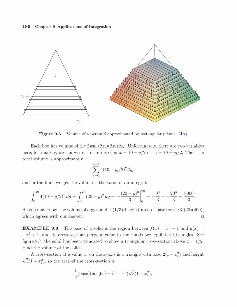
186 Chapter 9 Applications of Integration
xi
yi →
............................................................................................................................................................................................................................................................................................................................................................................................................................................................................................................................................................................................................................................................................................................................................................................................................................
...
Figure 9.6 Volume of a pyramid approximated by rectangular prisms. (JA)
Each box has volume of the form (2xi)(2xi)∆y. Unfortunately, there are two variableshere; fortunately, we can write x in terms of y: x = 10− y/2 or xi = 10− yi/2. Then thetotal volume is approximately
n−1∑
i=0
4(10− yi/2)2∆y
and in the limit we get the volume is the value of an integral:
∫ 20
0
4(10− y/2)2 dy =∫ 20
0
(20− y)2 dy = − (20− y)3
3
∣∣∣∣20
0
= −03
3−−203
3=
80003
.
As you may know, the volume of a pyramid is (1/3)(height)(area of base) = (1/3)(20)(400),which agrees with our answer.
EXAMPLE 9.8 The base of a solid is the region between f(x) = x2 − 1 and g(x) =−x2 + 1, and its cross-sections perpendicular to the x-axis are equilateral triangles. Seefigure 9.7; the solid has been truncated to show a triangular cross-section above x = 1/2.Find the volume of the solid.
A cross-section at a value xi on the x-axis is a triangle with base 2(1− x2i ) and height√
3(1− x2i ), so the area of the cross-section is
12(base)(height) = (1− x2
i )√
3(1− x2i ),
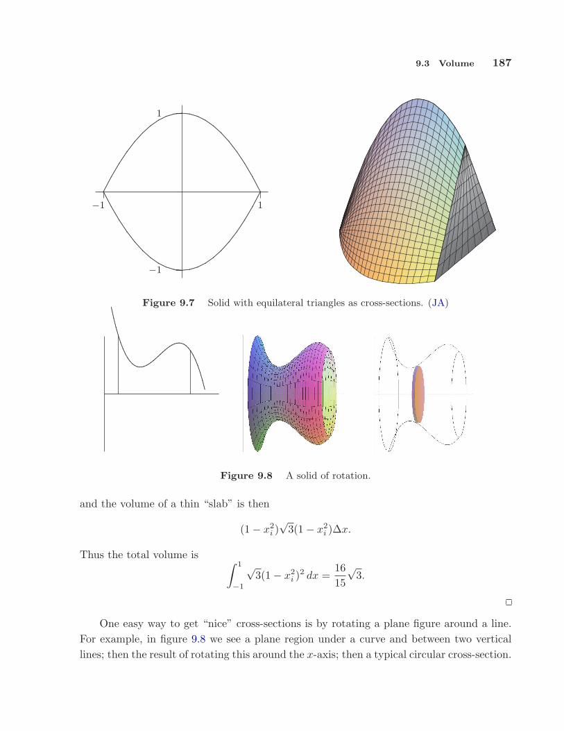
9.3 Volume 187
−1 1
−1
1
....................................................................................................................................................................................................................................................................................................................................
.............................................................................................................................................................................................................................
......................................................................................................................................................................................................................
.........................................................................................................................................................................................................................................................................................................................
Figure 9.7 Solid with equilateral triangles as cross-sections. (JA)...........................................................................................................................................................................................................................................................................................................................................................................................................................
Figure 9.8 A solid of rotation.
and the volume of a thin “slab” is then
(1− x2i )√
3(1− x2i )∆x.
Thus the total volume is ∫ 1
−1
√3(1− x2
i )2 dx =
1615
√3.
One easy way to get “nice” cross-sections is by rotating a plane figure around a line.For example, in figure 9.8 we see a plane region under a curve and between two verticallines; then the result of rotating this around the x-axis; then a typical circular cross-section.
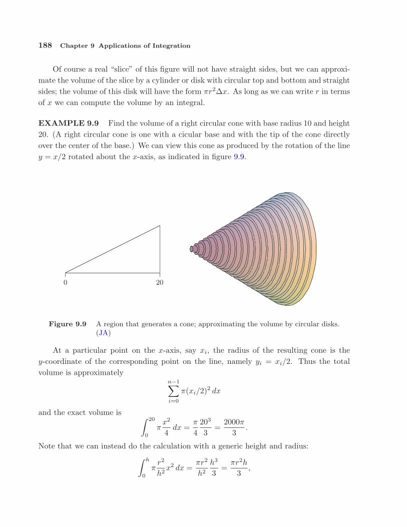
188 Chapter 9 Applications of Integration
Of course a real “slice” of this figure will not have straight sides, but we can approxi-mate the volume of the slice by a cylinder or disk with circular top and bottom and straightsides; the volume of this disk will have the form πr2∆x. As long as we can write r in termsof x we can compute the volume by an integral.
EXAMPLE 9.9 Find the volume of a right circular cone with base radius 10 and height20. (A right circular cone is one with a cicular base and with the tip of the cone directlyover the center of the base.) We can view this cone as produced by the rotation of the liney = x/2 rotated about the x-axis, as indicated in figure 9.9.
0 20
..................................
..................................
..................................
..................................
..................................
..................................
..................................
..................................
..................................
..........................
Figure 9.9 A region that generates a cone; approximating the volume by circular disks.(JA)
At a particular point on the x-axis, say xi, the radius of the resulting cone is they-coordinate of the corresponding point on the line, namely yi = xi/2. Thus the totalvolume is approximately
n−1∑
i=0
π(xi/2)2 dx
and the exact volume is ∫ 20
0
πx2
4dx =
π
4203
3=
2000π
3.
Note that we can instead do the calculation with a generic height and radius:∫ h
0
πr2
h2x2 dx =
πr2
h2
h3
3=
πr2h
3,

9.3 Volume 189
giving us the usual formula for the volume of a cone.
EXAMPLE 9.10 Find the volume of the object generated when the area betweeny = x2 and y = x is rotated around the x-axis. This solid has a “hole” in the middle; wecan compute the volume by subtracting the volume of the hole from the volume enclosedby the outer surface of the solid. In figure 9.10 we show the region that is rotated, theresulting solid with the front half cut away, the cone that forms the outer surface, thehorn-shaped hole, and a cross-section perpendicular to the x-axis.
0 1
0
1
............................................................................................................................................................................................................................................................
.......................................................
.................................................................................................................................................................................................................
Figure 9.10 Solid with a hole, showing the outer cone and the shape to be removed toform the hole. (JA)
We have already computed the volume of a cone; in this case it is π/3. At a particularvalue of x, say xi, the cross-section of the horn is a circle with radius x2
i , so the volume of
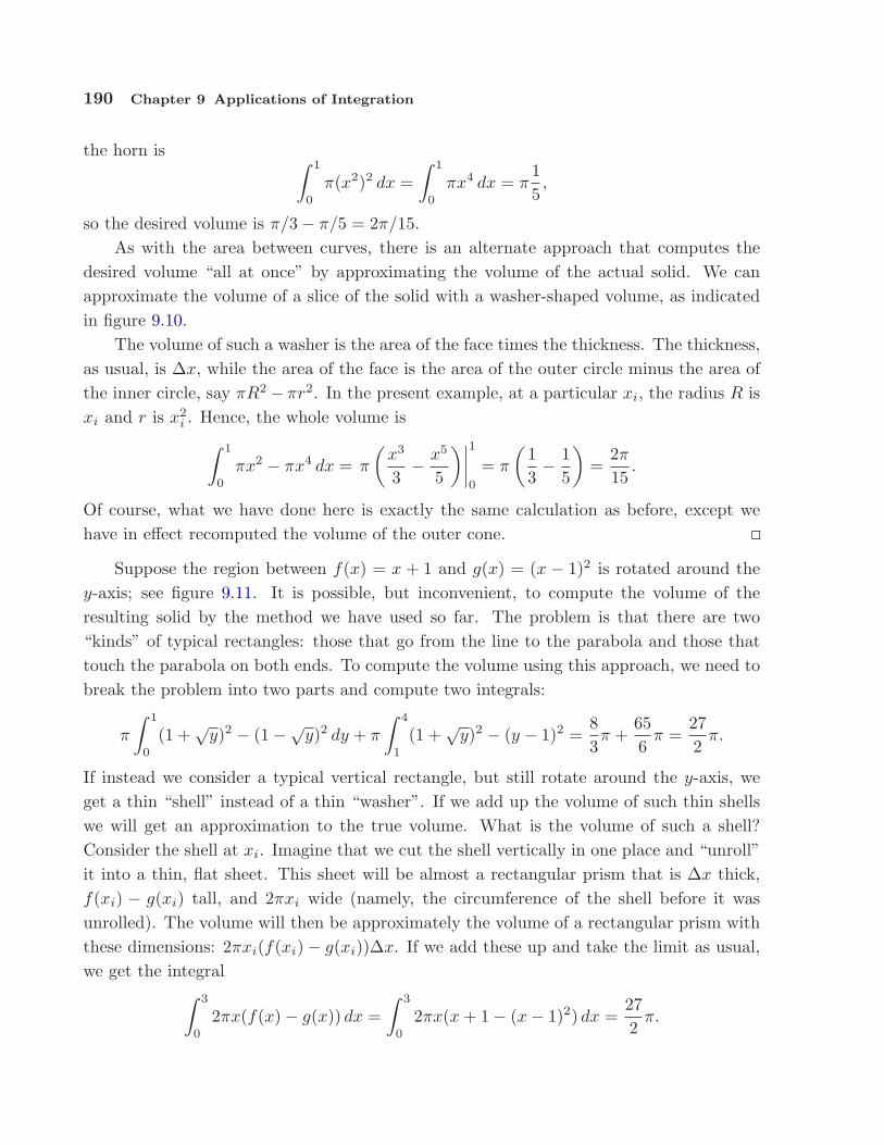
190 Chapter 9 Applications of Integration
the horn is ∫ 1
0
π(x2)2 dx =∫ 1
0
πx4 dx = π15,
so the desired volume is π/3− π/5 = 2π/15.As with the area between curves, there is an alternate approach that computes the
desired volume “all at once” by approximating the volume of the actual solid. We canapproximate the volume of a slice of the solid with a washer-shaped volume, as indicatedin figure 9.10.
The volume of such a washer is the area of the face times the thickness. The thickness,as usual, is ∆x, while the area of the face is the area of the outer circle minus the area ofthe inner circle, say πR2− πr2. In the present example, at a particular xi, the radius R isxi and r is x2
i . Hence, the whole volume is∫ 1
0
πx2 − πx4 dx = π
(x3
3− x5
5
)∣∣∣∣1
0
= π
(13− 1
5
)=
2π
15.
Of course, what we have done here is exactly the same calculation as before, except wehave in effect recomputed the volume of the outer cone.
Suppose the region between f(x) = x + 1 and g(x) = (x − 1)2 is rotated around they-axis; see figure 9.11. It is possible, but inconvenient, to compute the volume of theresulting solid by the method we have used so far. The problem is that there are two“kinds” of typical rectangles: those that go from the line to the parabola and those thattouch the parabola on both ends. To compute the volume using this approach, we need tobreak the problem into two parts and compute two integrals:
π
∫ 1
0
(1 +√
y)2 − (1−√y)2 dy + π
∫ 4
1
(1 +√
y)2 − (y − 1)2 =83π +
656
π =272
π.
If instead we consider a typical vertical rectangle, but still rotate around the y-axis, weget a thin “shell” instead of a thin “washer”. If we add up the volume of such thin shellswe will get an approximation to the true volume. What is the volume of such a shell?Consider the shell at xi. Imagine that we cut the shell vertically in one place and “unroll”it into a thin, flat sheet. This sheet will be almost a rectangular prism that is ∆x thick,f(xi) − g(xi) tall, and 2πxi wide (namely, the circumference of the shell before it wasunrolled). The volume will then be approximately the volume of a rectangular prism withthese dimensions: 2πxi(f(xi)− g(xi))∆x. If we add these up and take the limit as usual,we get the integral
∫ 3
0
2πx(f(x)− g(x)) dx =∫ 3
0
2πx(x + 1− (x− 1)2) dx =272
π.
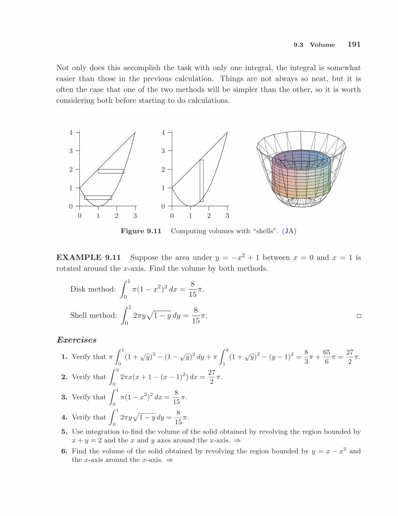
9.3 Volume 191
Not only does this accomplish the task with only one integral, the integral is somewhateasier than those in the previous calculation. Things are not always so neat, but it isoften the case that one of the two methods will be simpler than the other, so it is worthconsidering both before starting to do calculations.
0 1 2 3
0
1
2
3
4
............................................................................................................................................................................................................................................................
............................................................................................................................................................................................................................................................................................................................................................................
Figure 9.11 Computing volumes with “shells”. (JA)
EXAMPLE 9.11 Suppose the area under y = −x2 + 1 between x = 0 and x = 1 isrotated around the x-axis. Find the volume by both methods.
Disk method:∫ 1
0
π(1− x2)2 dx =815
π.
Shell method:∫ 1
0
2πy√
1− y dy =815
π.
Exercises
1. Verify that π
Z 1
0
(1 +√
y)2 − (1−√y)2 dy + π
Z 4
1
(1 +√
y)2 − (y − 1)2 =8
3π +
65
6π =
27
2π.
2. Verify that
Z 3
0
2πx(x + 1− (x− 1)2) dx =27
2π.
3. Verify that
Z 1
0
π(1− x2)2 dx =8
15π.
4. Verify that
Z 1
0
2πyp
1− y dy =8
15π.
5. Use integration to find the volume of the solid obtained by revolving the region bounded byx + y = 2 and the x and y axes around the x-axis. ⇒
6. Find the volume of the solid obtained by revolving the region bounded by y = x − x2 andthe x-axis around the x-axis. ⇒

192 Chapter 9 Applications of Integration
7. Find the volume of the solid obtained by revolving the region bounded by y =√
sin x, they-axis, and the lines y = 1 and x = π/2 around the x-axis. ⇒
8. Let S be the region of the xy-plane bounded above by the curve x3y = 64, below by the liney = 1, on the left by the line x = 2, and on the right by the line x = 4. Find the volume ofthe solid obtained by rotating S around (a) the x-axis, (b) the line y = 1, (c) the y-axis, (d)the line x = 2. ⇒
9. The equation x2/9 + y2/4 = 1 describes an ellipse. Find the volume of the solid obtainedby rotating the ellipse around the x-axis and also around the y-axis. These solids are calledellipsoids; one is vaguely rugby-ball shaped, one is sort of flying-saucer shaped, or perhapssquished-beach-ball-shaped. ⇒
Figure 9.12 Ellipsoids. (JA)
10. Use integration to compute the volume of a sphere of radius r. You should of course get thewell-known formula 4πr3/3.
11. A hemispheric bowl of radius r contains water to a depth h. Find the volume of water in thebowl. ⇒
12. The base of a tetrahedron (a triangular pyramid) of height h is an equilateral triangle of sides. Its cross-sections perpendicular to an altitude are equilateral triangles. Express its volumeV as an integral, and find a formula for V in terms of h and s. Verify that your answer is(1/3)(area of base)(height).
13. The base of a solid is the region between f(x) = cos x and g(x) = − cos x, −π/2 ≤ x ≤ π/2,and its cross-sections perpendicular to the x-axis are squares. Find the volume of the solid.⇒
9.4 Average value of a function
The average of some finite set of values is a familiar concept. If, for example, the classscores on a quiz are 10, 9, 10, 8, 7, 5, 7, 6, 3, 2, 7, 8, then the average score is the sum ofthese numbers divided by the size of the class:
average score =10 + 9 + 10 + 8 + 7 + 5 + 7 + 6 + 3 + 2 + 7 + 8
12=
8212≈ 6.83.
Suppose that between t = 0 and t = 1 the speed of an object is sin(πt). What is theaverage speed of the object over that time? The question sounds as if it must make sense,

9.4 Average value of a function 193
yet we can’t merely add up some number of speeds and divide, since the speed is changingcontinuously over the time interval.
To make sense of “average” in this context, we fall back on the idea of approximation.Consider the speed of the object at tenth of a second intervals: sin 0, sin(0.1π), sin(0.2π),sin(0.3π),. . . , sin(0.9π). The average speed “should” be fairly close to the average of theseten speeds:
110
9∑
i=0
sin(πi/10) ≈ 110
6.3 = 0.63.
Of course, if we compute more speeds at more times, the average of these speeds shouldbe closer to the “real” average. If we take the average of n speeds at evenly spaced times,we get:
1n
n−1∑
i=0
sin(πi/n).
Here the individual times are ti = i/n, so rewriting slightly we have
1n
n−1∑
i=0
sin(πti).
This is almost the sort of sum that we know turns into an integral; what’s apparentlymissing is ∆t—but in fact, ∆t = 1/n, the length of each subinterval. So rewriting again:
n−1∑
i=0
sin(πti)1n
=n−1∑
i=0
sin(πti)∆t.
Now this has exactly the right form, so that in the limit we get
average speed =∫ 1
0
sin(πt) dt = −cos(πt)π
∣∣∣∣1
0
= −cos(π)π
+cos(0)
π=
2π≈ 0.6366 ≈ 0.64.
It’s not entirely obvious from this one simple example how to compute such an averagein general. Let’s look at a somewhat more complicated case. Suppose that the velocityof an object is 16t2 + 5 feet per second. What is the average velocity between t = 1 andt = 3? Again we set up an approximation to the average:
1n
n−1∑
i=0
16t2i + 5,

194 Chapter 9 Applications of Integration
where the values ti are evenly spaced times between 1 and 3. Once again we are “missing”∆t, and this time 1/n is not the correct value. What is ∆t in general? It is the length ofa subinterval; in this case we take the interval [1, 3] and divide it into n subintervals, soeach has length (3 − 1)/n = 2/n = ∆t. Now with the usual “multiply and divide by thesame thing” trick we can rewrite the sum:
1n
n−1∑
i=0
16t2i + 5 =1
3− 1
n−1∑
i=0
(16t2i + 5)3− 1
n=
12
n−1∑
i=0
(16t2i + 5)2n
=12
n−1∑
i=0
(16t2i + 5)∆t.
In the limit this becomes
12
∫ 3
1
16t2 + 5 dt =12
4463
=2233
.
Does this seem reasonable? Let’s picture it: in figure 9.13 is the velocity function togetherwith the horizontal line y = 223/3 ≈ 74.3. Certainly the height of the horizontal line looksat least plausible for the average height of the curve.
0 1 2 3
0
25
50
75
100
125
150
...................................................................................................................
..................................................
........................................
...................................
...............................
.................................................................................................................................................................................................................................................................................................................................................................................................
Figure 9.13 Average velocity.
Here’s another way to interpret “average” that may make our computation appeareven more reasonable. The object of our example goes a certain distance between t = 1and t = 3. If instead the object were to travel at the average speed over the same time, itwould go the same distance. At an average speed of 223/3 feet per second for two secondsthe object would go 446/3 feet. How far does it actually go? We know how to compute

9.5 Work 195
this: ∫ 3
1
v(t) dt =∫ 3
1
16t2 + 5 dt =4463
.
So now we see that another interpretation of the calculation
12
∫ 3
1
16t2 + 5 dt =12
4463
=2233
is: total distance traveled divided by the time in transit, namely, average speed.It may also be helpful to interpret the average geometrically. The area under the
velocity curve is ∫ 3
1
16t2 + 5 dt =4463
.
The area under y = 223/3 over the same interval [1, 3] is simply the area of a rectanglethat is 2 by 223/3 with area 446/3. So the average height of a function is the height of thehorizontal line that produces the same area over the given interval.
Exercises
1. Find the average height of cos x over the intervals [0, π/2], [−π/2, π/2], and [0, 2π]. ⇒2. Find the average height of x2 over the interval [−2, 2]. ⇒3. Find the average height of 1/x2 over the interval [1, A]. ⇒4. Find the average height of
√1− x2 over the interval [−1, 1]. ⇒
5. An object moves with velocity v(t) = −t2 + 1 feet per second between t = 0 and t = 2. Findthe average velocity and the average speed of the object between t = 0 and t = 2. ⇒
6. The observation deck on the 102nd floor of the Empire State Building is 1,224 feet abovethe ground. If a steel ball is dropped from the observation deck its velocity at time t isapproximately v(t) = −32t feet per second. Find the average speed between the time it isdropped and the time it hits the ground, and find its speed when it hits the ground. ⇒
9.5 Work
A fundamental concept in classical physics is work: If an object is moved in a straightline against a force F for a distance s the work done is W = Fs.
EXAMPLE 9.12 How much work is done in lifting a 10 pound weight vertically adistance of 5 feet? The force due to gravity on a 10 pound weight is 10 pounds at thesurface of the earth, and it does not change appreciably over 5 feet. The work done isW = 10 · 5 = 50 foot-pounds.

196 Chapter 9 Applications of Integration
In reality few situations are so simple. The force might not be constant over the rangeof motion, as in the next example.
EXAMPLE 9.13 How much work is done in lifting a 10 pound weight from the surfaceof the earth to an orbit 100 miles above the surface? Over 100 miles the force due togravity does change significantly, so we need to take this into account. The force exertedon a 10 pound weight at a distance r from the center of the earth is F = k/r2 and bydefinition it is 10 when r is the radius of the earth (we assume the earth is a sphere). Howcan we approximate the work done? We divide the path from the surface to orbit into n
small subpaths. On each subpath the force due to gravity is roughly constant, with valuek/r2
i at distance ri. The work to raise the object from ri to ri+1 is thus approximatelyk/r2
i ∆r and the total work is approximately
n−1∑
i=0
k
r2i
∆r,
or in the limit
W =∫ r1
r0
k
r2dr,
where r0 is the radius of the earth and r1 is r0 plus 100 miles. The work is
W =∫ r1
r0
k
r2dr = − k
r
∣∣∣∣r1
r0
= − k
r1+
k
r0.
Using r0 = 20925525 feet we have r1 = 21453525. The force on the 10 pound weight atthe surface of the earth is 10 pounds, so 10 = k/209255252, giving k = 4378775965256250.Then
− k
r1+
k
r0=
49105232000095349
≈ 5150052 foot-pounds.
Note that if we assume the force due to gravity is 10 pounds over the whole distance wewould calculate the work as 10(r1− r0) = 10 · 100 · 5280 = 5280000, somewhat higher sincewe don’t account for the weakening of the gravitational force.
EXAMPLE 9.14 How much work is done in lifting a 10 kilogram object from thesurface of the earth to a distance D from the center of the earth? This is the sameproblem as before in different units, and we are not specifying a value for D. As before
W =∫ D
r0
k
r2dr = − k
r
∣∣∣∣D
r0
= − k
D+
k
r0.
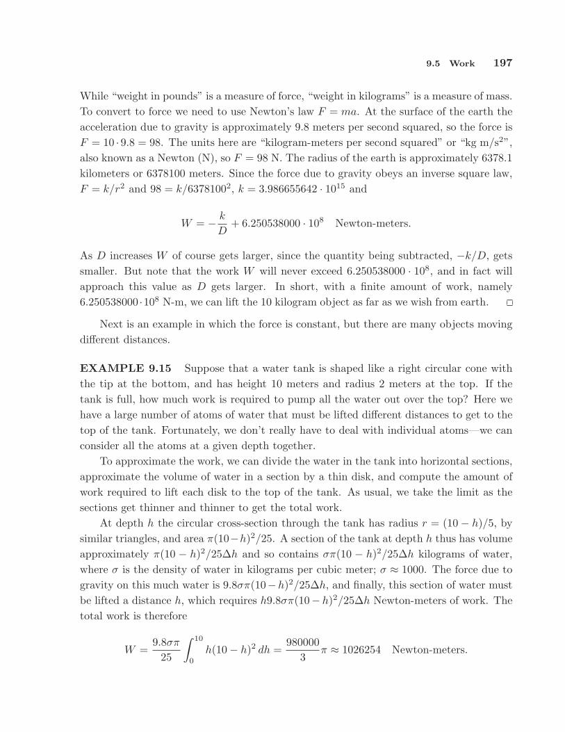
9.5 Work 197
While “weight in pounds” is a measure of force, “weight in kilograms” is a measure of mass.To convert to force we need to use Newton’s law F = ma. At the surface of the earth theacceleration due to gravity is approximately 9.8 meters per second squared, so the force isF = 10 ·9.8 = 98. The units here are “kilogram-meters per second squared” or “kg m/s2”,also known as a Newton (N), so F = 98 N. The radius of the earth is approximately 6378.1kilometers or 6378100 meters. Since the force due to gravity obeys an inverse square law,F = k/r2 and 98 = k/63781002, k = 3.986655642 · 1015 and
W = − k
D+ 6.250538000 · 108 Newton-meters.
As D increases W of course gets larger, since the quantity being subtracted, −k/D, getssmaller. But note that the work W will never exceed 6.250538000 · 108, and in fact willapproach this value as D gets larger. In short, with a finite amount of work, namely6.250538000 ·108 N-m, we can lift the 10 kilogram object as far as we wish from earth.
Next is an example in which the force is constant, but there are many objects movingdifferent distances.
EXAMPLE 9.15 Suppose that a water tank is shaped like a right circular cone withthe tip at the bottom, and has height 10 meters and radius 2 meters at the top. If thetank is full, how much work is required to pump all the water out over the top? Here wehave a large number of atoms of water that must be lifted different distances to get to thetop of the tank. Fortunately, we don’t really have to deal with individual atoms—we canconsider all the atoms at a given depth together.
To approximate the work, we can divide the water in the tank into horizontal sections,approximate the volume of water in a section by a thin disk, and compute the amount ofwork required to lift each disk to the top of the tank. As usual, we take the limit as thesections get thinner and thinner to get the total work.
At depth h the circular cross-section through the tank has radius r = (10 − h)/5, bysimilar triangles, and area π(10−h)2/25. A section of the tank at depth h thus has volumeapproximately π(10 − h)2/25∆h and so contains σπ(10 − h)2/25∆h kilograms of water,where σ is the density of water in kilograms per cubic meter; σ ≈ 1000. The force due togravity on this much water is 9.8σπ(10−h)2/25∆h, and finally, this section of water mustbe lifted a distance h, which requires h9.8σπ(10− h)2/25∆h Newton-meters of work. Thetotal work is therefore
W =9.8σπ
25
∫ 10
0
h(10− h)2 dh =980000
3π ≈ 1026254 Newton-meters.

198 Chapter 9 Applications of Integration
..................................................................................................................................................................................................................................................................................................................................................................................................................................................................................................................................................................................................................................................................................................................................................... ↑
|h|↓
↑|||||
10|||||↓
2........................................................ ......................................... ...............
Figure 9.14 Cross-section of a conical water tank.
A spring has a “natural length,” its length if nothing is stretching or compressingit. If the spring is either stretched or compressed the spring provides an opposing force;according to Hooke’s Law the magnitude of this force is proportional to the distance thespring has been stretched or compressed: F = kx. The constant of proportionality, k, ofcourse depends on the spring. Note that x here represents the change in length from thenatural length.
EXAMPLE 9.16 Suppose k = 5 for a given spring that has a natural length of 0.1meters. Suppose a force is applied that compresses the spring to length 0.08. What isthe magnitude of the force? Assuming that the constant k has appropriate dimensions(namely, kg/s2), the force is 5(0.1− 0.08) = 5(0.02) = 0.1 Newtons.
EXAMPLE 9.17 How much work is done in compressing the spring in the previous ex-ample from its natural length to 0.08 meters? From 0.08 meters to 0.05 meters? How muchwork is done to stretch the spring from 0.1 meters to 0.15 meters? We can approximatethe work by dividing the distance that the spring is compressed into small subintervals.Then the force exerted by the spring is approximately constant over the subinterval, sothe work required to compress the spring from xi to xi+1 is approximately 5(xi − 0.1)∆x.The total work is approximately
n−1∑
i=0
5(xi − 0.1)∆x

9.5 Work 199
and in the limit
W =∫ 0.08
0.1
5(x−0.1) dx =5(x− 0.1)2
2
∣∣∣∣0.08
0.1
=5(0.08− 0.1)2
2− 5(0.1− 0.1)2
2=
11000
N-m.
The other values we seek simply use different limits. To compress the spring from 0.08meters to 0.05 meters takes
W =∫ 0.05
0.08
5(x− 0.1) dx =5x2
2
∣∣∣∣0.05
0.08
=5(0.05− 0.1)2
2− 5(0.08− 0.1)2
2=
214000
N-m
and to stretch the spring from 0.1 meters to 0.15 meters requires
W =∫ 0.15
0.1
5(x− 0.1) dx =5x2
2
∣∣∣∣0.15
0.1
=5(0.15− 0.1)2
2− 5(0.1− 0.1)2
2=
1160
N-m.
Exercises
1. How much work is done in lifting a 100 kilogram weight from the surface of the earth to anorbit 35,786 kilometers above the surface of the earth? ⇒
2. How much work is done in lifting a 100 kilogram weight from an orbit 1000 kilometers abovethe surface of the earth to an orbit 35,786 kilometers above the surface of the earth? ⇒
3. A water tank has the shape of a cylinder with radius r = 1 meter and height 10 meters. Ifthe depth of the water is 5 meters, how much work is required to pump all the water out thetop of the tank? ⇒
4. Suppose the tank of the previous problem is lying on its side, so that the circular ends arevertical, and that it has the same amount of water as before. How much work is requiredto pump the water out the top of the tank (which is now 2 meters above the bottom of thetank)? ⇒
5. A water tank has the shape of the bottom half of a sphere with radius r = 1 meter. If thetank is full, how much work is required to pump all the water out the top of the tank? ⇒
6. A spring has constant k = 10 kg/s2. How much work is done in compressing it 1/10 meterfrom its natural length? ⇒
7. A force of 2 Newtons will compress a spring from 1 meter (its natural length) to 0.8 meters.How much work is required to stretch the spring from 1.1 meters to 1.5 meters? ⇒
8. A 20 meter long steel cable has density 2 kilograms per meter, and is hanging straight down.How much work is required to lift the entire cable to the height of its top end? ⇒
9. The cable in the previous problem has a 100 kilogram bucket of concrete attached to its lowerend. How much work is required to lift the entire cable and bucket to the height of its topend? ⇒

200 Chapter 9 Applications of Integration
9.6 Center of Mass
Suppose a beam is 10 meters long, and that there are three weights on the beam: a 10kilogram weight 3 meters from the left end, a 5 kilogram weight 6 meters from the left end,and a 4 kilogram weight 8 meters from the left end. Where should a fulcrum be placedso that the beam balances? Let’s assign a scale to the beam, from 0 at the left end to 10at the right, so that we can denote locations on the beam simply as x coordinates; theweights are at x = 3, x = 6, and x = 8.
Suppose to begin with that the fulcrum is placed at x = 5. What will happen? Eachweight applies a force to the beam that tends to rotate it around the fulcrum; this effectis measured by a quantity called torque, proportional to the mass times the distancefrom the fulcrum. Of course, weights on different sides of the fulcrum rotate the beamin opposite directions. We can distinguish this by using a signed distance in the formulafor torque. So with the fulcrum at 5, the torques induced by the three weights will beproportional to (3 − 5)10 = −20, (6 − 5)5 = 5, and (8 − 5)4 = 12. For the beam tobalance, the sum of the torques must be zero; since the sum is −20 + 5 + 12 = −3, thebeam rotates counter-clockwise, and to get the beam to balance we need to move thefulcrum to the left. To calculate exactly where the fulcrum should be, we let x denote thelocation of the fulcrum when the beam is in balance. The total torque on the beam is then(3− x)10 + (6− x)5 + (8− x)4 = 92− 19x. Since the beam balances at x it must be that92 − 19x = 0 or x = 92/19 ≈ 4.84, that is, the fulcrum should be placed at x = 92/19 tobalance the beam.
Now suppose that we have a beam with varying density—some portions of the beamcontain more mass than other portions of the same size. We want to figure out where toput the fulcrum so that the beam balances.
EXAMPLE 9.18 Suppose the beam is 10 meters long and that the density is 1 + x
kilograms per meter at location x on the beam. To approximate the solution, we can thinkof the beam as a sequence of weights “on” a beam. For example, we can think of theportion of the beam between x = 0 and x = 1 as a weight sitting at x = 0, the portionbetween x = 1 and x = 2 as a weight sitting at x = 1, and so on. We then approximatethe mass of the weights by assuming that each portion of the beam has constant density.So the mass of the first weight is approximated as m0 = (1 + 0)1 = 1 kilograms, namely,(1 + 0) kilograms per meter times 1 meter. The second weight is m1 = (1 + 1)1 = 2kilograms, and so on to the tenth weight with m9 = (1 + 9)1 = 9 kilograms. So in thiscase the total torque is
(0− x)m0 + (1− x)m1 + · · ·+ (9− x)m9 = (0− x)1 + (1− x)2 + · · ·+ (9− x)9.
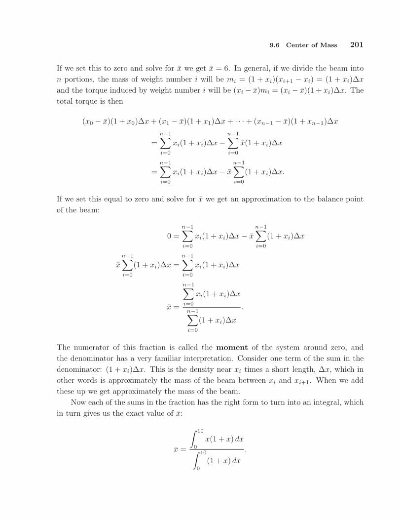
9.6 Center of Mass 201
If we set this to zero and solve for x we get x = 6. In general, if we divide the beam inton portions, the mass of weight number i will be mi = (1 + xi)(xi+1 − xi) = (1 + xi)∆x
and the torque induced by weight number i will be (xi − x)mi = (xi − x)(1 + xi)∆x. Thetotal torque is then
(x0 − x)(1 + x0)∆x + (x1 − x)(1 + x1)∆x + · · ·+ (xn−1 − x)(1 + xn−1)∆x
=n−1∑
i=0
xi(1 + xi)∆x−n−1∑
i=0
x(1 + xi)∆x
=n−1∑
i=0
xi(1 + xi)∆x− x
n−1∑
i=0
(1 + xi)∆x.
If we set this equal to zero and solve for x we get an approximation to the balance pointof the beam:
0 =n−1∑
i=0
xi(1 + xi)∆x− x
n−1∑
i=0
(1 + xi)∆x
x
n−1∑
i=0
(1 + xi)∆x =n−1∑
i=0
xi(1 + xi)∆x
x =
n−1∑
i=0
xi(1 + xi)∆x
n−1∑
i=0
(1 + xi)∆x
.
The numerator of this fraction is called the moment of the system around zero, andthe denominator has a very familiar interpretation. Consider one term of the sum in thedenominator: (1 + xi)∆x. This is the density near xi times a short length, ∆x, which inother words is approximately the mass of the beam between xi and xi+1. When we addthese up we get approximately the mass of the beam.
Now each of the sums in the fraction has the right form to turn into an integral, whichin turn gives us the exact value of x:
x =
∫ 10
0
x(1 + x) dx
∫ 10
0
(1 + x) dx
.
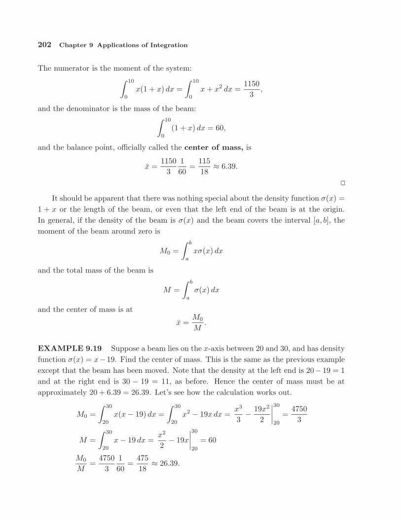
202 Chapter 9 Applications of Integration
The numerator is the moment of the system:∫ 10
0
x(1 + x) dx =∫ 10
0
x + x2 dx =1150
3,
and the denominator is the mass of the beam:∫ 10
0
(1 + x) dx = 60,
and the balance point, officially called the center of mass, is
x =1150
3160
=11518
≈ 6.39.
It should be apparent that there was nothing special about the density function σ(x) =1 + x or the length of the beam, or even that the left end of the beam is at the origin.In general, if the density of the beam is σ(x) and the beam covers the interval [a, b], themoment of the beam around zero is
M0 =∫ b
a
xσ(x) dx
and the total mass of the beam is
M =∫ b
a
σ(x) dx
and the center of mass is at
x =M0
M.
EXAMPLE 9.19 Suppose a beam lies on the x-axis between 20 and 30, and has densityfunction σ(x) = x−19. Find the center of mass. This is the same as the previous exampleexcept that the beam has been moved. Note that the density at the left end is 20− 19 = 1and at the right end is 30 − 19 = 11, as before. Hence the center of mass must be atapproximately 20 + 6.39 = 26.39. Let’s see how the calculation works out.
M0 =∫ 30
20
x(x− 19) dx =∫ 30
20
x2 − 19x dx =x3
3− 19x2
2
∣∣∣∣30
20
=4750
3
M =∫ 30
20
x− 19 dx =x2
2− 19x
∣∣∣∣30
20
= 60
M0
M=
47503
160
=47518
≈ 26.39.
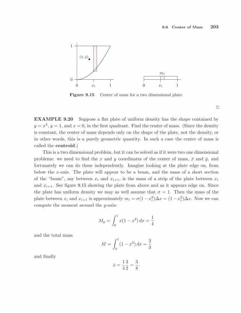
9.6 Center of Mass 203
..
..
..
..
..
..
..
..
..
..
..
..
..
..
..
..
..
..
..
..
..
..
.
..
..
..
..
..
..
..
..
..
..
..
..
..
..
..
..
..
..
..
..
..
..
..
..
..
..
..
..
..
..
..
..
..
..
..
..
..
..
..
..
..
..
..
..
.
..
..
..
..
..
..
..
..
..
..
..
..
..
..
..
..
..
..
..
..
..
..
..
..
..
..
..
..
..
..
..
..
..
..
..
..
..
..
..
..
..
..
..
..
.
..
..
..
..
..
..
..
..
..
..
..
..
..
..
..
..
..
..
..
..
..
..
..
..
..
..
..
..
..
..
..
..
..
..
..
..
..
..
..
..
..
..
..
..
.
..
..
..
..
..
..
..
..
..
..
..
..
..
..
..
..
..
..
..
..
..
..
..
..
..
..
..
..
..
..
..
..
..
..
..
..
..
..
..
..
..
..
..
..
.
..
..
..
..
..
..
..
..
..
..
..
..
..
..
..
..
..
..
..
..
..
..
..
..
..
..
..
..
..
..
..
..
..
..
..
..
..
..
..
..
..
..
..
..
.
..
..
..
..
..
..
..
..
..
..
..
..
..
..
..
..
..
..
..
..
..
..
0
1
0 1xi
.......................................................
.................................................................................................................................................................................................................
•(x, y)
..
..
..
..
..
..
..
..
..
..
..
..
..
..
..
..
..
..
..
..
..
..
..
..
..
..
..
..
..
..
..
..
..
0 1xi
mi
Figure 9.15 Center of mass for a two dimensional plate.
EXAMPLE 9.20 Suppose a flat plate of uniform density has the shape contained byy = x2, y = 1, and x = 0, in the first quadrant. Find the center of mass. (Since the densityis constant, the center of mass depends only on the shape of the plate, not the density, orin other words, this is a purely geometric quantity. In such a case the center of mass iscalled the centroid.)
This is a two dimensional problem, but it can be solved as if it were two one dimensionalproblems: we need to find the x and y coordinates of the center of mass, x and y, andfortunately we can do these independently. Imagine looking at the plate edge on, frombelow the x-axis. The plate will appear to be a beam, and the mass of a short sectionof the “beam”, say between xi and xi+1, is the mass of a strip of the plate between xi
and xi+1. See figure 9.15 showing the plate from above and as it appears edge on. Sincethe plate has uniform density we may as well assume that σ = 1. Then the mass of theplate between xi and xi+1 is approximately mi = σ(1−x2
i )∆x = (1−x2i )∆x. Now we can
compute the moment around the y-axis:
My =∫ 1
0
x(1− x2) dx =14
and the total mass
M =∫ 1
0
(1− x2) dx =23
and finally
x =14
32
=38.
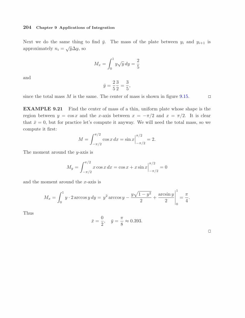
204 Chapter 9 Applications of Integration
Next we do the same thing to find y. The mass of the plate between yi and yi+1 isapproximately ni =
√y∆y, so
Mx =∫ 1
0
y√
y dy =25
and
y =25
32
=35,
since the total mass M is the same. The center of mass is shown in figure 9.15.
EXAMPLE 9.21 Find the center of mass of a thin, uniform plate whose shape is theregion between y = cos x and the x-axis between x = −π/2 and x = π/2. It is clearthat x = 0, but for practice let’s compute it anyway. We will need the total mass, so wecompute it first:
M =∫ π/2
−π/2
cosx dx = sin x∣∣∣π/2
−π/2= 2.
The moment around the y-axis is
My =∫ π/2
−π/2
x cosx dx = cos x + x sinx∣∣∣π/2
−π/2= 0
and the moment around the x-axis is
Mx =∫ 1
0
y · 2 arccos y dy = y2 arccos y − y√
1− y2
2+
arcsin y
2
∣∣∣∣∣
1
0
=π
4.
Thus
x =02, y =
π
8≈ 0.393.

9.7 Kinetic energy; improper integrals 205
Exercises
1. A beam 10 meters long has density σ(x) = x2 at distance x from the left end of the beam.Find the center of mass x. ⇒
2. A beam 10 meters long has density σ(x) = sin(πx/10) at distance x from the left end of thebeam. Find the center of mass x. ⇒
3. A beam 4 meters long has density σ(x) = x3 at distance x from the left end of the beam.Find the center of mass x. ⇒
4. Verify that
Z2x arccos x dx = x2 arccos x− x
√1− x2
2+
arcsin x
2+ C.
5. A thin plate lies in the region between y = x2 and the x-axis between x = 1 and x = 2. Findthe centroid. ⇒
6. A thin plate fills the upper half of the unit circle x2 + y2 = 1. Find the centroid. ⇒7. A thin plate lies in the region contained by y = x and y = x2. Find the centroid. ⇒8. A thin plate lies in the region contained by y = 4−x2 and the x-axis. Find the centroid. ⇒9. A thin plate lies in the region contained by y = x1/3 and the x-axis between x = 0 and x = 1.
Find the centroid. ⇒10. A thin plate lies in the region contained by
√x +√
y = 1 and the axes in the first quadrant.Find the centroid. ⇒
11. A thin plate lies in the region between the circle x2 + y2 = 4 and the circle x2 + y2 = 1,above the x-axis. Find the centroid. ⇒
12. A thin plate lies in the region between the circle x2 + y2 = 4 and the circle x2 + y2 = 1 inthe first quadrant. Find the centroid. ⇒
9.7 Kinetic energy; improper integrals
Recall example 9.14 in which we computed the work required to lift an object from thesurface of the earth to some large distance D away. Since F = k/x2 we computed
∫ D
r0
k
x2dx = − k
D+
k
r0.
We noticed that as D increases, k/D decreases to zero so that the amount of work increasesto k/r0. More precisely,
limD→∞
∫ D
r0
k
x2dx = lim
D→∞− k
D+
k
r0=
k
r0.
We might reasonably describe this calculuation as computing the amount of work requiredto lift the object “to infinity,” and abbreviate the limit as
limD→∞
∫ D
r0
k
x2dx =
∫ ∞r0
k
x2dx.
206 Chapter 9 Applications of Integration
Such an integral, with a limit of infinity, is called an improper integral. This is a bitunfortunate, since it’s not really “improper” to do this, nor is it really “an integral”—it isan abbreviation for the limit of a particular sort of integral. Nevertheless, we’re stuck withthe term, and the operation itself is perfectly legitimate. It may at first seem odd that afinite amount of work is sufficient to lift an object to “infinity”, but sometimes surprisingthings are nevertheless true, and this is such a case. If the value of an improper integralis a finite number, as in this example, we say that the integral converges, and if not wesay that the integral diverges.
Here’s another way, perhaps even more surprising, to interpret this calculation. Weknow that one interpretation of ∫ D
1
1x2
dx
is the area under y = 1/x2 from x = 1 to x = D. Of course, as D increases this areaincreases. But since ∫ D
1
1x2
dx = − 1D
+11,
while the area increases, it never exceeds 1, that is
∫ ∞1
1x2
dx = 1.
The area of the infinite region under y = 1/x2 from x = 1 to infinity is finite.
Consider a slightly different sort of improper integral:∫ ∞−∞
xe−x2dx. There are two
ways we might try to compute this. First, we could break it up into two more familiarintegrals: ∫ ∞
−∞xe−x2
dx =∫ 0
−∞xe−x2
dx +∫ ∞
0
xe−x2dx.
Now we do these as before:
∫ 0
−∞xe−x2
dx = limD→∞
−e−x2
2
∣∣∣∣∣
0
D
= −12,
and∫ ∞
0
xe−x2dx = lim
D→∞−e−x2
2
∣∣∣∣∣
D
0
=12,
9.7 Kinetic energy; improper integrals 207
so ∫ ∞−∞
xe−x2dx = −1
2+
12
= 0.
Alternately, we might try
∫ ∞−∞
xe−x2dx = lim
D→∞
∫ D
−D
xe−x2dx = lim
D→∞−e−x2
2
∣∣∣∣∣
D
−D
= limD→∞
−e−D2
2+
e−D2
2= 0.
So we get the same answer either way. This does not always happen; sometimes the secondapproach gives a finite number, while the first approach does not; the exercises provide
examples. In general, we interpret the integral∫ ∞−∞
f(x) dx according to the first method:
both integrals∫ a
−∞f(x) dx and
∫ ∞a
f(x) dx must converge for the original integral to
converge. The second approach does turn out to be useful; when limD→∞
∫ D
−D
f(x) dx = L,
and L is finite, then L is called the Cauchy Principal Value of∫ ∞−∞
f(x) dx.
Here’s a more concrete application of these ideas. We know that in general
W =∫ x1
x0
F dx
is the work done against the force F in moving from x0 to x1. In the case that F is theforce of gravity exerted by the earth, it is customary to make F < 0 since the force is“downward.” This makes the work W negative when it should be positive, so typically thework in this case is defined as
W = −∫ x1
x0
F dx.
Also, by Newton’s Law, F = ma(t). This means that
W = −∫ x1
x0
ma(t) dx.
Unfortunately this integral is a bit problematic: a(t) is in terms of t, while the limits andthe “dx” are in terms of x. But x and t are certainly related here: x = x(t) is the functionthat gives the position of the object at time t, so v = v(t) = dx/dt = x′(t) is its velocity
208 Chapter 9 Applications of Integration
and a(t) = v′(t) = x′′(t). We can use v = x′(t) as a substitution to convert the integralfrom “dx” to “dv” in the usual way, with a bit of cleverness along the way:
dv = x′′(t) dt = a(t) dt = a(t)dt
dxdx
dx
dtdv = a(t) dx
v dv = a(t) dx.
Substituting in the integral:
W = −∫ x1
x0
ma(t) dx = −∫ v1
v0
mv dv = − mv2
2
∣∣∣∣v1
v0
= −mv21
2+
mv20
2.
You may recall seeing the expression mv2/2 in a physics course—it is called the kineticenergy of the object. We have shown here that the work done in moving the object fromone place to another is the same as the change in kinetic energy.
We know that the work required to move an object from the surface of the earth toinfinity is
W =∫ ∞
r0
k
r2dr =
k
r0.
At the surface of the earth the acceleration due to gravity is approximately 9.8 metersper second squared, so the force on an object of mass m is F = 9.8m. The radius of theearth is approximately 6378.1 kilometers or 6378100 meters. Since the force due to gravityobeys an inverse square law, F = k/r2 and 9.8m = k/63781002, k = 398665564178000m
and W = 62505380m.Now suppose that the initial velocity of the object, v0, is just enough to get it to
infinity, that is, just enough so that the object never slows to a stop, but so that its speeddecreases to zero, i.e., so that v1 = 0. Then
62505380m = W = −mv21
2+
mv20
2=
mv20
2
sov0 =
√125010760 ≈ 11181 meters per second,
or about 40251 kilometers per hour. This speed is called the escape velocity. Notice thatthe mass of the object, m, cancelled out at the last step; the escape velocity is the samefor all objects. Of course, it takes considerably more energy to get a large object up to

9.7 Kinetic energy; improper integrals 209
40251 kph than a small one, so it is certainly more difficult to get a large object into deepspace than a small one. Also, note that while we have computed the escape velocity forthe earth, this speed would not in fact get an object “to infinity” because of the large massin our neighborhood called the sun. Escape velocity for the sun starting at the distance ofthe earth from the sun is nearly 4 times the escape velocity we have calculated.
Exercises
1. Is the area under y = 1/x from 1 to infinity finite or infinite? If finite, compute the area. ⇒2. Is the area under y = 1/x3 from 1 to infinity finite or infinite? If finite, compute the area.⇒
3. Does
Z ∞
0
x2 + 2x− 1 dx converge or diverge? If it converges, find the value. ⇒
4. Does
Z ∞
1
1/√
x dx converge or diverge? If it converges, find the value. ⇒
5. Does
Z ∞
0
e−x dx converge or diverge? If it converges, find the value. ⇒
6.
Z 1/2
0
(2x − 1)−3 dx is an improper integral of a slightly different sort. Express it as a limit
and determine whether it converges or diverges; if it converges, find the value. ⇒
7. Does
Z 1
0
1/√
x dx converge or diverge? If it converges, find the value. ⇒
8. Does
Z π/2
0
sec2 x dx converge or diverge? If it converges, find the value. ⇒
9. Does
Z ∞
−∞
x2
4 + x6dx converge or diverge? If it converges, find the value. ⇒
10. Does
Z ∞
−∞x dx converge or diverge? If it converges, find the value. Also find the Cauchy
Principal Value, if it exists. ⇒11. Does
Z ∞
−∞sin x dx converge or diverge? If it converges, find the value. Also find the Cauchy
Principal Value, if it exists. ⇒12. Does
Z ∞
−∞cos x dx converge or diverge? If it converges, find the value. Also find the Cauchy
Principal Value, if it exists. ⇒13. Suppose the curve y = 1/x is rotated around the x-axis generating a sort of funnel or horn
shape, called Gabriel’s horn or Toricelli’s trumpet. Is the volume of this funnel fromx = 1 to infinity finite or infinite? If finite, compute the volume. ⇒
14. An officially sanctioned baseball must be between 142 and 149 grams. How much work,in Newton-meters, does it take to throw a ball at 80 miles per hour? At 90 mph? At100.9 mph? (According to the Guinness Book of World Records, at http://www.baseball-
almanac.com/recbooks/rb_guin.shtml, “The greatest reliably recorded speed at which a
210 Chapter 9 Applications of Integration
baseball has been pitched is 100.9 mph by Lynn Nolan Ryan (California Angels) at AnaheimStadium in California on August 20, 1974.”) ⇒
9.8 Probability
You perhaps have at least a rudimentary understanding of discrete probability, whichmeasures the likelihood of an “event” when there are a finite number of possibilities. Forexample, when an ordinary six-sided die is rolled, the probability of getting any particularnumber is 1/6. In general, the probability of an event is the number of ways the event canhappen divided by the number of ways that “anything” can happen.
For a slightly more complicated example, consider the case of two six-sided dice. Thedice are physically distinct, which means that rolling a 2–5 is different than rolling a 5–2;each is an equally likely event out of a total of 36 ways the dice can land, so each has aprobability of 1/36.
Most interesting events are not so simple. More interesting is the probability of rollinga certain sum out of the possibilities 2 through 12. It is clearly not true that all sums areequally likely: the only way to roll a 2 is to roll 1–1, while there are many ways to roll a 7.Because the number of possibilities is quite small, and because a pattern quickly becomesevident, it is easy to see that the probabilities of the various sums are:
P (2) = P (12) = 1/36
P (3) = P (11) = 2/36
P (4) = P (10) = 3/36
P (5) = P (9) = 4/36
P (6) = P (8) = 5/36
P (7) = 6/36
Here we use P (n) to mean “the probability of rolling an n.” Since we have correctlyaccounted for all possibilities, the sum of all these probabilities is 36/36 = 1; the probabilitythat the sum is one of 2 through 12 is 1, because there are no other possibilities.
The study of probability is concerned with more difficult questions as well; for example,suppose the two dice are rolled many times. On the average, what sum will come up? Inthe language of probability, this average is called the expected value of the sum. This isat first a little misleading, as it does not tell us what to “expect” when the two dice arerolled, but what we expect the long term average will be.
Suppose that two dice are rolled 36 million times. Based on the probabilities, we wouldexpect about 1 million rolls to be 2, about 2 million to be 3, and so on, with a roll of 7
9.8 Probability 211
topping the list at about 6 million. The sum of all rolls would be 1 million times 2 plus 2million times 3, and so on, and dividing by 36 million we would get the average:
x = (2 · 106 + 3(2 · 106) + · · ·+ 7(6 · 106) + · · ·+ 12 · 106)1
36 · 106
= 2106
36 · 106+ 3
2 · 106
36 · 106+ · · ·+ 7
6 · 106
36 · 106+ · · ·+ 12
106
36 · 106
= 2P (2) + 3P (3) + · · ·+ 7P (7) + · · ·+ 12P (12)
=12∑
i=2
iP (i) = 7.
It is apparent that there is nothing special about the 36 million in this calculation. No
matter what the number of rolls, once we simplify the average, we get the same12∑
i=2
iP (i).
A variable, say X, that can take certain values, each with a corresponding probability,is called a random variable; in the example above, the random variable was the sum ofthe two dice. If the possible values for X are x1, x2,. . . ,xn, then the expected value of the
random variable is E(X) =n∑
i=1
xiP (xi).
In many applications of probability, the number of possible values of a random vari-able is very large, perhaps even infinite. To deal with the infinite case we need a differentapproach, and since there is a sum involved, it should not be wholly surprising that in-tegration turns out to be a useful tool. It then turns out that even when the number ofpossibilities is large but finite, it is easier to pretend that the number is infinite. Suppose,for example, that a dart is thrown at a dart board. Since the dart board consists of a finitenumber of atoms, there are in some sense only a finite number of places for the dart toland, but it is easier to explore the probabilities involved by pretending that the dart canland on any point in the usual x-y plane.
DEFINITION 9.22 Let f : R → R be a function. If f(x) ≥ 0 for every x and∫ ∞−∞
f(x) dx = 1 then f is a probability density function.
We associate a probability density function with a random variable X by stipulating
that the probability that X is between a and b is∫ b
a
f(x) dx. Because of the requirement
that the integral from −∞ to ∞ be 1, all probabilities are less than or equal to 1, and theprobability that X takes on some value between −∞ and ∞ is 1, as it should be.

212 Chapter 9 Applications of Integration
EXAMPLE 9.23 Consider again the two dice example; we can view it in a way morethat resembles the probability density function approach. Consider a random variable X
that takes on any real value with probabilities given by the probability density function infigure 9.16. The function f consists of just the top edges of the rectangles, with verticalsides drawn for clarity; the function is zero below 1.5 and above 12.5. The area of eachrectangle is the probability of rolling the sum in the middle of the bottom of the rectangle,or
P (n) =∫ n+1/2
n−1/2
f(x) dx.
The probability of rolling a 4, 5, or 6 is
P (n) =∫ 13/2
7/2
f(x) dx.
Of course, we could also compute probabilities that don’t make sense in the context of thedice, such as the probability that X is between 4 and 5.8.
1 2 3 4 5 6 7 8 9 10 11 12
1
2
3
4
5
6
Figure 9.16 A probability density function for two dice.
As this example illustrates, we do not require that f be continuous, but we will assumethat f has only finitely many discontinuities (possibly zero), and that the discontinuitiesare either jump discontinuities or removable (a “hole” in the function). This guarantees
9.8 Probability 213
that the cumulative distribution function,
F (x) = P (X ≤ x) =∫ x
−∞f(t)dt,
is continuous. Hence, we say that X is a continuous random variable. Note that becausethe area does not decrease as x increases, the function F (x) is non-decreasing. The entirecollection of probabilities for a random variable X, namely P (X ≤ x) for all x, is called aprobability distribution.
EXAMPLE 9.24 Suppose that a < b and
f(x) =
{1
b− aif a ≤ x ≤ b
0 otherwise.
Then f(x) is the uniform probability density function on [a, b]. and the correspondingdistribution is the uniform distribution on [a, b].
The next theorem is not hard to prove; if I is an interval [a, b], we write∫
I
f(x) dx for∫ b
a
f(x) dx.
THEOREM 9.25 Let I be an interval. If 0 ≤ f(x) ≤ g(x) for x ∈ I and f and g are
integrable on I then 0 ≤∫
I
f(x) dx ≤∫
I
g(x) dx ≤ ∞. In particular, if∫
I
f(x) dx diverges,
then so does∫
I
g(x) dx while if∫
I
g(x) dx converges, then so does∫
I
f(x) dx.
Note that the theorem applies to infinite intervals, in which case the integrals areimproper integrals.
EXAMPLE 9.26 Notice that 0 ≤ f(x) = e−x2/2 ≤ e−x/2 for |x| > 1. It is easy to check
that∫ ∞
1
e−x/2 dx < ∞, so by the theorem∫ ∞
1
e−x2/2 dx is finite. Since f is symmetric
around the y-axis,∫ −1
−∞e−x2/2 dx is also finite, and so finally
A =∫ ∞−∞
e−x2/2 dx =∫ −1
−∞e−x2/2 dx +
∫ 1
−1
e−x2/2 dx +∫ ∞
1
e−x2/2 dx

214 Chapter 9 Applications of Integration
is finite and positive. If we let g(x) = f(x)/A, then g is a probability density function.It turns out to be very useful, and is called the standard normal probability den-sity function or more informally the bell curve, giving rise to the standard normaldistribution. See figure 9.17 for the graph of the bell curve.
−4 −3 −2 −1 0 1 2 3 4
0.5
......................................................................................................................................................
......................................
...............................................
................................................................................................................................................................................................................................................................
Figure 9.17 The bell curve.
We have shown that A is some finite number without computing it; we cannot computeit with the techniques we have available. By using some techniques from multivariablecalculus, we can show that A =
√2π.
EXAMPLE 9.27 The exponential distribution has probability density function
f(x) ={ 0 x < 0
ce−cx x ≥ 0
where c is a positive constant.
DEFINITION 9.28 Let f be a probability density function. Since we are assuming
that the function F (x) =∫ x
−∞f(t) dt is continuous and ranges from 0 to 1 it follows by the
intermediate value theorem that there is at least one number m such that F (m) = 1/2; m
is called a median of the random variable X. Note that P (X ≤ m) = P (X ≥ m) = 1/2.
EXAMPLE 9.29 The median of the uniform distribution on [a, b] is (a + b)/2.
EXAMPLE 9.30 Let
f(x) =
0 x < 01 0 ≤ x ≤ 1/20 1/2 < x < 11 1 ≤ x ≤ 3/20 3/2 < x.
Any value in the interval [1/2, 1 qualifies as a median, although convention would usuallytake ‘the’ median to be 3/4.
9.8 Probability 215
An even function is one that is symmetric around the y axis.
EXAMPLE 9.31 If f is an even probability density function then one of the mediansis 0. If f(x) > 0 on [−δ, δ] for some δ > 0, then 0 is the only median. In particular, themedian of the standard normal distribution is 0.
DEFINITION 9.32 If a probability density function f has a global maximum at x = c
then c is a mode of the random variable X.
There need not be a single mode; for example, in the uniform distribution every numberbetween a and b is a mode. The mode may not even exist, though it is a bit tricky to comeup with an example.
EXAMPLE 9.33 It is somewhat difficult to devise a continuous probability densityfunction for which there is no mode, but easy if we give up continuity. Consider
f(x) =
0 x < −1x + 1 −1 ≤ x < 00 x = 0−x + 1 0 < x ≤ 10 1 < x.
Sketch this graph; it is then apparent that f has no global maximum and hence nomode.
In practice, both the mode and the median are useful, but the expected value, alsocalled the mean, is generally most useful. Following our discussion of discrete probability,the definition should not be surprising.
DEFINITION 9.34 The mean of a continuous random variable X with probability
density function f is µ = E(X) =∫ ∞−∞
xf(x) dx, provided the integral converges.
When the mean exists it is unique, since it is the result of an explicit calculation. Themean does not always exist.
Let us look more closely at the definition of the mean. It is in fact essentially identicalto the definition of the center of mass of a one-dimensional beam. The probability densityfunction f plays the role of the physical density function, but now the “beam” has infinitelength. If we consider only a finite portion of the beam, say between a and b, then the

216 Chapter 9 Applications of Integration
center of mass is
x =
∫ b
a
xf(x) dx
∫ b
a
f(x) dx
.
If we extend the beam to infinity, we get
x =
∫ ∞−∞
xf(x) dx
∫ ∞−∞
f(x) dx
=∫ ∞−∞
xf(x) dx,
because∫∞−∞ f(x) dx = 1. In the center of mass interpretation, this integral is the total
mass of the beam, which is always 1 when f is a probability density function.
EXAMPLE 9.35 The mean of the standard normal distribution is∫ ∞−∞
xe−x2/2
√2π
dx.
We compute the two halves:
∫ 0
−∞x
e−x2/2
√2π
dx = limD→−∞
−e−x2/2
√2π
∣∣∣∣∣
0
D
= − 1√2π
and∫ ∞
0
xe−x2/2
√2π
dx = limD→∞
−e−x2/2
√2π
∣∣∣∣∣
D
0
=1√2π
.
The sum of these is 0, which is the mean.
Suppose that f : R→ R is the probability density function for the continuous randomvariable X, and that the mean µ, exists (and is finite). We would like to measure howfar a “typical” value of X is from µ. One way to measure this distance is (X − µ)2; wesquare the difference so as to measure all distances as positive. The expected value of thisquantity is
V (X) =∫ ∞−∞
(x− µ)2f(x) dx.
This quantity is called the variance, and is the expected value of the squared distance toµ. The standard deviation, denoted σ, is the square root of the variance. By taking

9.8 Probability 217
the square root we “correct for” the original square, so that the units of σ are the same asthe units of X, and σ measures a “typical distance from µ” instead of a typical squareddistance. The standard deviation is very useful in statistical analysis.
EXAMPLE 9.36 We compute the standard deviation of the standard normal distru-bution. The variance is
1√2π
∫ ∞−∞
x2e−x2/2 dx.
To compute the antiderivative, use integration by parts, with u = x and dv = xe−x2/2 dx.This gives ∫
x2e−x2/2 dx = −xe−x2/2 +∫
e−x2/2 dx.
We cannot do the new integral, but we know its value when the limits are −∞ to ∞, fromour discussion of the standard normal distribution. Thus
1√2π
∫ ∞−∞
x2e−x2/2 dx = − 1√2π
xe−x2/2
∣∣∣∣∞
−∞+
1√2π
∫ ∞−∞
e−x2/2 dx = 0 +1√2π
√2π = 1.
The standard deviation is then√
1 = 1.
Here is a simple example of the use of these ideas. Suppose it is known that, in thelong run, 1 out of every 100 computer memory chips produced by a certain manufacturingplant is defective. Suppose 1000 chips are selected at random and 15 of them are defective.This is more than the ‘expected’ number (10), but is it so many that we should suspectthat something has gone wrong in the manufacturing process? We are interested in theprobability that various numbers of defective chips arise; the probability distribution isdiscrete: there can only be a whole number of defective chips. But (under reasonableassumptions) the distribution is very close to a normal distribution. By methods morecomplicated than we can explore here, it turns out that the appropriate density functionis
f(x) =1√
2π√
1000(.01)(.99)exp
( −(x− 10)2
2(1000)(.01)(.99)
),
which is pictured in figure 9.18 (exp(x) = ex).Now how do we measure how unlikely it is that under normal circumstances we would
see 15 defective chips? We can’t compute the probability of exactly 15 defective chips, as
this would be∫ 15
15
f(x) dx = 0. We could compute∫ 15.5
14.5
f(x) dx ≈ 0.036; this means there
is only a 3.6% chance that the number of defective chips is 15. (We cannot compute these

218 Chapter 9 Applications of Integration
0 5 10 15 20 25
0.05
0.10
0.15
.................................................................................
..................................................................................................
..................................................................................................................................................................................................................................................................................................................
Figure 9.18 Normal density function for the defective chips example.
integrals exactly; computer software has been used to approximate the integral values in
this discussion.) But this is misleading:∫ 10.5
9.5
f(x) dx ≈ 0.126, which is larger, certainly,
but still small, even for the “most likely” outcome. The most useful question, in mostcircumstances, is this: how likely is it that the number of defective chips is “far from”the mean? For example, how likely, or unlikely, is it that the number of defective chipsis different by 3 or more from the expected value of 10? This is the probability that thenumber of defective chips is less than 7 or larger than 13, namely
∫ 7
−∞f(x) dx +
∫ ∞13
f(x) dx ≈ 0.34.
So there is a 34% chance that this happens—not small at all. Hence the 15 defective chipsdoes not appear to be cause for alarm. How about 20? Here we compute
∫ 0
−∞f(x) dx +
∫ ∞20
f(x) dx ≈ 0.0015.
So there is only a 0.15% chance that the number of defective chips is more than 10 awayfrom the mean; this would typically be interpreted as too suspicious to ignore—it shouldn’thappen if the process is running normally.
The big question, of course, is what level of improbability should trigger concern?It depends to some degree on the application, and in particular on the consequences ofgetting it wrong in one direction or the other. If we’re wrong, do we lose a little money?A lot of money? Do people die? In general, the standard choices are 5% and 1%. So whatwe should do is find the number of defective chips that has only, let us say, a 1% chanceof occurring under normal circumstances, and use that as the relevant number. In otherwords, we want to know when
∫ 10−r
−∞f(x) dx +
∫ ∞10+r
f(x) dx < 0.01.

9.8 Probability 219
A bit of trial and error shows that with r = 8 the probability is about 1.1%, and withr = 9 it is about 0.4%, so if the number of defective chips is 19 or more, or 1 or fewer, weshould look for problems. If the number is high, we worry that the manufacturing processhas a problem, or conceivably that the process that tests for defective chips is not workingcorrectly. If the number is too low, the obvious culprit is that the testing procedure isbroken, and is not detecting defective chips.
It is sometimes convenient to view the situation from the point of view of what is“good” rather than what is “bad”. Again by trial and error, we can discover that
∫ 10+r
10−r
f(x) dx ≈ 0.9908
when r = 8.2. So there is just over a 99% chance that under normal operation the numberof defective chips is between 2 and 18; in such circumstances we assume the process isworking normally.
Exercises
1. ComputeR∞1
e−x/2 dx.
2. Show that the function
f(x) =
0 x < 0ce−cx x ≥ 0
is a probability density function, where c is a positive constant. Compute the median, mode,and mean.
3. Find the mode of the standard normal distribution.
4. Let µ and σ be real numbers with σ > 0. Show that
N(x) =1√2πσ
e− (x−µ)2
2σ2
is a probability density function. You will not be able to compute this integral directly; usea substitution to convert the integral into the one from example 9.26. The function N isthe probability density function of the normal distribution with mean µ and standarddeviation σ. Show that the mean of the normal distribution is µ and the standard deviationis σ.
5. Let
f(x) =
(1
2x2|x| ≥ 1
0 |x| < 1
Show that f is a probability density function, and that the distribution has no mean.
6. Let
f(x) =
(x −1 ≤ x ≤ 11 1 < x ≤ 20 otherwise.

220 Chapter 9 Applications of Integration
Show thatR∞−∞ f(x) dx = 1. Is f a probability density function? Justify your answer.
7. Find all the modes and the mean for the distribution in example 9.30.
8. What is the expected value of one roll of a fair die?
9. what is the expected sum of one roll of three fair dice?
10. What is the mean of the uniform distribution on [a, b]? (See example 9.24.)
11. Compute the variance and standard deviation of the exponential distribution from exam-ple 9.27.
12. Compute the mean of the distribution from example 9.33.
13. If you have access to appropriate software, compute the range of “good” values for the chip
manufacturing process “at the 5% level.” That is, find r so that
Z 10+r
10−r
f(x) dx ≈ 0.95 and
interpret this as a range of values for the number of defective chips that should cause noalarm. You might think about circumstances that would make the 5% or the 1% thresholdmore appropriate. ⇒
9.9 Arc Length
Here is another geometric application of the integral: find the length of a portion of acurve. As usual, we need to think about how we might approximate the length, and turnthe approximation into an integral.
We already know how to compute one simple arc length, that of a line segment. If theendpoints are P0(x0, y0) and P1(x1, y1) then the length of the segment is the distance be-tween the points,
√(x1 − x0)2 + (y1 − y0)2, from the Pythagorean theorem, as illustrated
in figure 9.19.
..............................
..............................
..............................
..............................
..............................
..............................
..............................
..............................
....................
(x1, y1)
(x0, y0) x1 − x0
y1 − y0
√(x1 − x0)2 + (y1 − y0)2
Figure 9.19 The length of a line segment.
Now if the graph of f is “nice” (say, differentiable) it appears that we can approximatethe length of a portion of the curve with line segments, and that as the number of segments
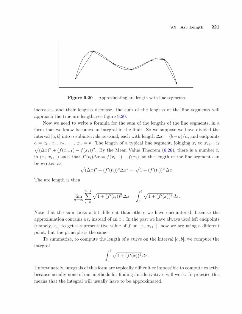
9.9 Arc Length 221
..........................................................................................................................................................................
.................................................................................................................................................................................................................................................................................................
.................................
...............................
..............................................................................................................................................................................................................................
•
•
••
• •
•...............................................................................................................................................................................................................................................................................................................................................................................................................................
....................................
....................................
.................................................................................
............................................................................................................................................................
Figure 9.20 Approximating arc length with line segments.
increases, and their lengths decrease, the sum of the lengths of the line segments willapproach the true arc length; see figure 9.20.
Now we need to write a formula for the sum of the lengths of the line segments, in aform that we know becomes an integral in the limit. So we suppose we have divided theinterval [a, b] into n subintervals as usual, each with length ∆x = (b−a)/n, and endpointsa = x0, x1, x2, . . . , xn = b. The length of a typical line segment, joinging xi to xi+1, is√
(∆x)2 + (f(xi+1)− f(xi))2. By the Mean Value Theorem (6.26), there is a number ti
in (xi, xi+1) such that f ′(ti)∆x = f(xi+1) − f(xi), so the length of the line segment canbe written as √
(∆x)2 + (f ′(ti))2∆x2 =√
1 + (f ′(ti))2 ∆x.
The arc length is then
limn→∞
n−1∑
i=0
√1 + (f ′(ti))2 ∆x =
∫ b
a
√1 + (f ′(x))2 dx.
Note that the sum looks a bit different than others we have encountered, because theapproximation contains a ti instead of an xi. In the past we have always used left endpoints(namely, xi) to get a representative value of f on [xi, xi+1]; now we are using a differentpoint, but the principle is the same.
To summarize, to compute the length of a curve on the interval [a, b], we compute theintegral ∫ b
a
√1 + (f ′(x))2 dx.
Unfortunately, integrals of this form are typically difficult or impossible to compute exactly,because usually none of our methods for finding antiderivatives will work. In practice thismeans that the integral will usually have to be approximated.
222 Chapter 9 Applications of Integration
EXAMPLE 9.37 Let f(x) =√
r2 − x2, the upper half circle of radius r. The lengthof this curve is half the circumference, namely πr. Let’s compute this with the arc length
formula. The derivative f ′ is −x/√
r2 − x2 so the integral is
∫ r
−r
√1 +
x2
r2 − x2dx =
∫ r
−r
√r2
r2 − x2dx = r
∫ r
−r
√1
r2 − x2dx.
Using a trigonometric substitution, we find the antiderivative, namely arcsin(x/r). Notice
that the integral is improper at both endpoints, as the function√
1/(r2 − x2) is undefinedwhen x = ±r. So we need to compute
limD→−r+
∫ 0
D
√1
r2 − x2dx + lim
D→r−
∫ D
0
√1
r2 − x2dx.
This is not difficult, and has value π, so the original integral, with the extra r in front, hasvalue πr as expected.
Exercises
1. Find the arc length of f(x) = x3/2 on [0, 2]. ⇒2. Find the arc length of f(x) = x2/8− ln x on [1, 2]. ⇒3. Find the arc length of f(x) = (1/3)(x2 + 2)3/2 on the interval [0, a]. ⇒4. Find the arc length of f(x) = ln(sin x) on the interval [π/4, π/3]. ⇒5. Set up the integral to find the arc length of sin x on the interval [0, π]; do not evaluate the
integral.
6. Set up the integral to find the arc length of y = xe−x on the interval [2, 3]; do not evaluatethe integral.
7. Find the arc length of y = ex on the interval [0, 1]. (This can be done exactly; it is a bittricky and a bit long.)
9.10 Surface Area
Another geometric question that arises naturally is: “What is the surface area of a vol-ume?” For example, what is the surface area of a sphere? More advanced techniquesare required to approach this question in general, but we can compute the areas of somevolumes generated by revolution.
As usual, the question is: how might we approximate the surface area? For a surfaceobtained by rotating a curve around an axis, we can take a polygonal approximation tothe curve, as in the last section, and rotate it around the same axis. This gives a surface

9.10 Surface Area 223
Figure 9.21 Approximating a surface (left) by portions of cones (right).
composed of many “truncated cones;” a truncated cone is called a frustum of a cone.Figure 9.21 illustrates this approximation.
So we need to be able to compute the area of a frustum of a cone. Since the frustumcan be formed by removing a small cone from the top of a larger one, we can computethe desired area if we know the surface area of a cone. Suppose a right circular cone hasbase radius r and slant height h. If we cut the cone from the vertex to the base circleand flatten it out, we obtain a sector of a circle with radius h and arc length 2πr, as infigure 9.22. The angle at the center, in radians, is then 2πr/h, and the area of the cone isequal to the area of the sector of the circle. Let A be the area of the sector; since the areaof the entire circle is πh2, we have
A
πh2=
2πr/h
2π
A = πrh.
Now suppose we have a frustum of a cone with slant height h and radii r0 and r1, asin figure 9.23. The area of the entire cone is πr1(h0 + h), and the area of the small coneis πr0h0; thus, the area of the frustum is πr1(h0 + h)− πr0h0 = π((r1 − r0)h0 + r1h). Bysimilar triangles,
h0
r0=
h0 + h
r1.
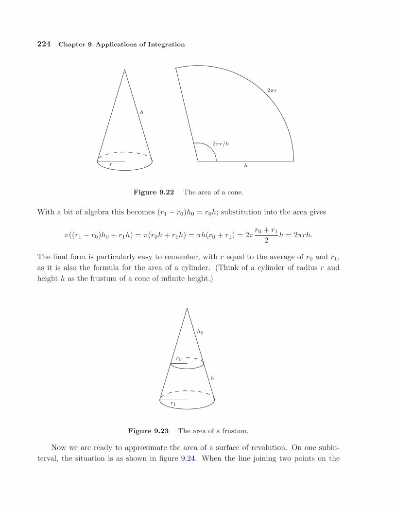
224 Chapter 9 Applications of Integration
....................................................................................................................................................................................
...............................................................................................................................................................................................................................................................................................................................................................................................................................................................................................................................................................................................................................................................
r
h
.............
...........................................................................................
........
........
........
........
........
........
...............................................................................................................................................................
.....................
......................
........................
...........................
.............................
....................................
....................................................
................................................................................................................................................
........
....................................
.............................
...................................
............................................................................................................................................................................................................................................................................................................................................................................................................................................................................................................................................................................................................................................
h
2πr
2πr/h
Figure 9.22 The area of a cone.
With a bit of algebra this becomes (r1 − r0)h0 = r0h; substitution into the area gives
π((r1 − r0)h0 + r1h) = π(r0h + r1h) = πh(r0 + r1) = 2πr0 + r1
2h = 2πrh.
The final form is particularly easy to remember, with r equal to the average of r0 and r1,as it is also the formula for the area of a cylinder. (Think of a cylinder of radius r andheight h as the frustum of a cone of infinite height.)
....................................................................................................................................................................................
...............................................................................................................................................................................................................................................................................................................................................................................................................................................................................................................................................................................................................................................................
r1
h0
.......................................................................................................................
r0
h
.............
...........................................................................................
..........................................
Figure 9.23 The area of a frustum.
Now we are ready to approximate the area of a surface of revolution. On one subin-terval, the situation is as shown in figure 9.24. When the line joining two points on the
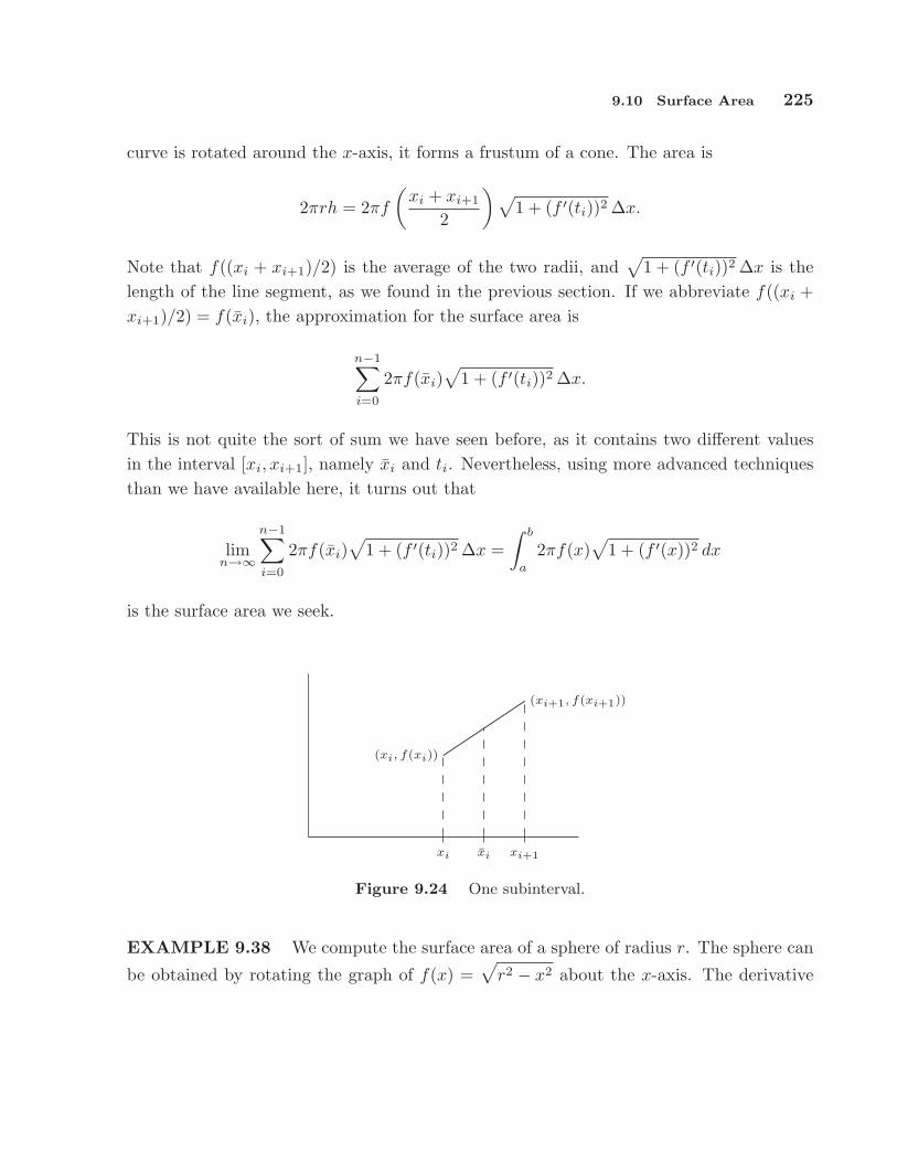
9.10 Surface Area 225
curve is rotated around the x-axis, it forms a frustum of a cone. The area is
2πrh = 2πf
(xi + xi+1
2
) √1 + (f ′(ti))2 ∆x.
Note that f((xi + xi+1)/2) is the average of the two radii, and√
1 + (f ′(ti))2 ∆x is thelength of the line segment, as we found in the previous section. If we abbreviate f((xi +xi+1)/2) = f(xi), the approximation for the surface area is
n−1∑
i=0
2πf(xi)√
1 + (f ′(ti))2 ∆x.
This is not quite the sort of sum we have seen before, as it contains two different valuesin the interval [xi, xi+1], namely xi and ti. Nevertheless, using more advanced techniquesthan we have available here, it turns out that
limn→∞
n−1∑
i=0
2πf(xi)√
1 + (f ′(ti))2 ∆x =∫ b
a
2πf(x)√
1 + (f ′(x))2 dx
is the surface area we seek.
xi xi xi+1
...........................................................................................................................................
(xi, f(xi))
(xi+1, f(xi+1))
Figure 9.24 One subinterval.
EXAMPLE 9.38 We compute the surface area of a sphere of radius r. The sphere can
be obtained by rotating the graph of f(x) =√
r2 − x2 about the x-axis. The derivative

226 Chapter 9 Applications of Integration
f ′ is −x/√
r2 − x2, so the surface area is given by
A = 2π
∫ r
−r
√r2 − x2
√1 +
x2
r2 − x2dx
= 2π
∫ r
−r
√r2 − x2
√r2
r2 − x2dx
= 2π
∫ r
−r
r dx = 2πr
∫ r
−r
1 dx = 4πr2
If the curve is rotated around the y axis, the formula is nearly identical, because thelength of the line segment we use to approximate a portion of the curve doesn’t change.Instead of the radius f(xi), we use the new radius xi, and the surface area integral becomes
∫ b
a
2πx√
1 + (f ′(x))2 dx.
EXAMPLE 9.39 Compute the area of the surface formed when f(x) = x2 between 0and 2 is rotated around the y-axis.
We compute f ′(x) = 2x, and then
2π
∫ 2
0
x√
1 + 4x2 dx =π
6(173/2 − 1),
by a simple substitution.
9.11 Differential equations 227
Exercises
1. Compute the area of the surface formed when f(x) = 2√
1− x between −1 and 0 is rotatedaround the x-axis.
2. Compute the surface area of example 9.39 by rotating f(x) =√
x around the x-axis.
3. Compute the area of the surface formed when f(x) = x3 between 1 and 3 is rotated aroundthe x-axis.
4. Consider the surface obtained by rotating the graph of f(x) = 1/x, x ≥ 1, around the x-axis.This surface is called Gabriel’s horn or Toricelli’s trumpet. Show that Gabriel’s hornhas finite volume and infinite surface area.
5. Consider the circle (x − 2)2 + y2 = 1. Sketch the surface obtained by rotating this circleabout the y-axis. (The surface is called a torus.) What is the surface area?
6. Consider the ellipse with equation x2/4 + y2 = 1. If the ellipse is rotated around the x-axisit forms an ellipsoid. Compute the surface area.
7. Generalize the preceding result: rotate the ellipse given by x2/a2 + y2/b2 = 1 about thex-axis and find the surface area of the resulting ellipsoid. You should consider two cases,when a > b and when a < b. Compare to the area of a sphere.
9.11 Differential equations
Many physical phenomena can be modeled using the language of calculus. For example,observational evidence suggests that the temperature of a cup of tea (or some other liquid)in a room of constant temperature will cool over time at a rate proportional to the differencebetween the room temperature and the temperature of the tea.
In symbols, if t is the time variable, M is the room temperature, and f(t) is thetemperature of the tea at time t then f ′(t) = k(M − f(t)) where k > 0 is a constantwhich will depend on the kind of tea (or more generally the kind of liquid) but not on theroom temperature or the temperature of the tea. This is Newton’s law of cooling andthe equation that we just wrote down is an example of a differential equation. Ideallywe would like to solve this equation, namely, find the function f(t) that describes thetemperature over time, though this often turns out to be impossible, in which case variousapproximation techniques must be used. The use and solution of differential equations isan important field of mathematics; here we give a few examples to illustrate their use.
Informally, a differential equation is an equation in which one or more of the derivativesof some function appear. Typically, a scientific theory will produce a differential equation(or a system of differential equations) that describes or governs some physical process, butthe theory will not produce the desired function or functions directly.

228 Chapter 9 Applications of Integration
Recall from section 6.2 that when the variable is time the derivative of a function y(t)is sometimes written as y instead of y′; this is quite common in the study of differentialequations.
DEFINITION 9.40 A first order differential equation is an equation of the formF (t, y, y) = 0. A solution of a first order differential equation is a function f(t) that makesF (t, f(t), f ′(t)) = 0 for every value of t.
Here, F is a function of three variables which we label t, y, and y. It is understoodthat y will explicitly appear in the equation although t and y need not. The term “firstorder” means that the first derivative of y appears, but no higher order derivatives do.
EXAMPLE 9.41 y = t2 +1 is a first order differential equation; F (t, y, y) = y− t2− 1.All solutions to this equation are of the form t3/3 + t + C.
EXAMPLE 9.42 The equation from Newton’s law of cooling, y = k(M − y) is a firstorder differential equation; F (t, y, y) = k(M − y)− y.
DEFINITION 9.43 A first order initial value problem is a system of equations ofthe form F (t, y, y) = 0, y(t0) = y0. Here t0 is a fixed time and y0 is a number. A solutionof an initial value problem is a solution f(t) of the differential equation that also satisfiesthe initial condition f(t0) = y0.
EXAMPLE 9.44 The initial value problem y = t2 + 1, y(1) = 4 has solution f(t) =t3/3 + t + 8/3.
The general first order equation is rather too general, that is, we can’t describe methodsthat will work on them all, or even a large portion of them. We can make progess withspecific kinds of differential equations. For example, much can be said about equations ofthe form y = φ(t, y) where φ is a function of the two variables t and y. Under reasonableconditions on φ, such an equation has a solution and that the corresponding initial valueproblem will have a unique solution. The precise statement of the result is known asPicard’s existence and uniqueness theorem.
This is still a bit to general for a first introduction.
DEFINITION 9.45 A first order differential equation is separable if it can be writtenin the form y = f(t)g(y).
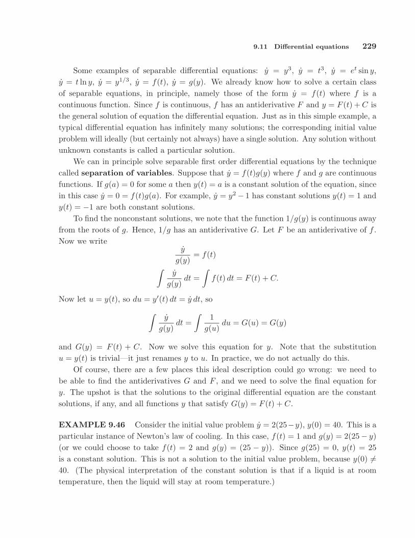
9.11 Differential equations 229
Some examples of separable differential equations: y = y3, y = t3, y = et sin y,y = t ln y, y = y1/3, y = f(t), y = g(y). We already know how to solve a certain classof separable equations, in principle, namely those of the form y = f(t) where f is acontinuous function. Since f is continuous, f has an antiderivative F and y = F (t) + C isthe general solution of equation the differential equation. Just as in this simple example, atypical differential equation has infinitely many solutions; the corresponding initial valueproblem will ideally (but certainly not always) have a single solution. Any solution withoutunknown constants is called a particular solution.
We can in principle solve separable first order differential equations by the techniquecalled separation of variables. Suppose that y = f(t)g(y) where f and g are continuousfunctions. If g(a) = 0 for some a then y(t) = a is a constant solution of the equation, sincein this case y = 0 = f(t)g(a). For example, y = y2− 1 has constant solutions y(t) = 1 andy(t) = −1 are both constant solutions.
To find the nonconstant solutions, we note that the function 1/g(y) is continuous awayfrom the roots of g. Hence, 1/g has an antiderivative G. Let F be an antiderivative of f .Now we write
y
g(y)= f(t)
∫y
g(y)dt =
∫f(t) dt = F (t) + C.
Now let u = y(t), so du = y′(t) dt = y dt, so
∫y
g(y)dt =
∫1
g(u)du = G(u) = G(y)
and G(y) = F (t) + C. Now we solve this equation for y. Note that the substitutionu = y(t) is trivial—it just renames y to u. In practice, we do not actually do this.
Of course, there are a few places this ideal description could go wrong: we need tobe able to find the antiderivatives G and F , and we need to solve the final equation fory. The upshot is that the solutions to the original differential equation are the constantsolutions, if any, and all functions y that satisfy G(y) = F (t) + C.
EXAMPLE 9.46 Consider the initial value problem y = 2(25−y), y(0) = 40. This is aparticular instance of Newton’s law of cooling. In this case, f(t) = 1 and g(y) = 2(25− y)(or we could choose to take f(t) = 2 and g(y) = (25 − y)). Since g(25) = 0, y(t) = 25is a constant solution. This is not a solution to the initial value problem, because y(0) 6=40. (The physical interpretation of the constant solution is that if a liquid is at roomtemperature, then the liquid will stay at room temperature.)
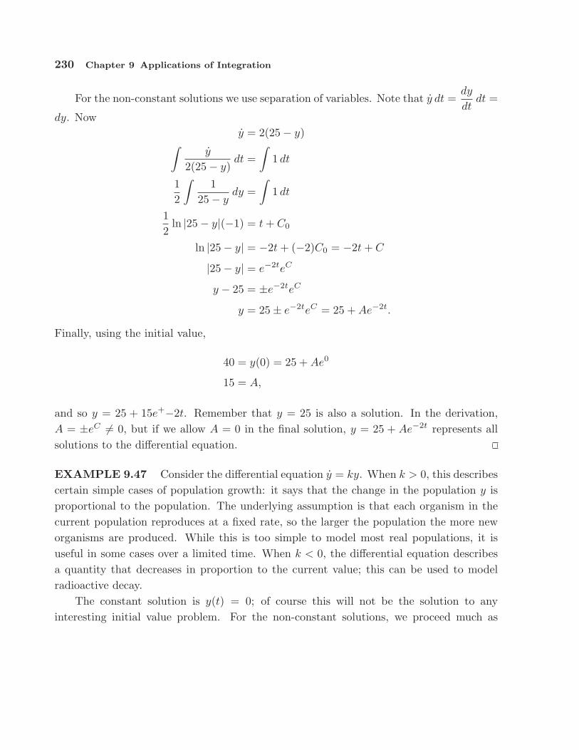
230 Chapter 9 Applications of Integration
For the non-constant solutions we use separation of variables. Note that y dt =dy
dtdt =
dy. Nowy = 2(25− y)
∫y
2(25− y)dt =
∫1 dt
12
∫1
25− ydy =
∫1 dt
12
ln |25− y|(−1) = t + C0
ln |25− y| = −2t + (−2)C0 = −2t + C
|25− y| = e−2teC
y − 25 = ±e−2teC
y = 25± e−2teC = 25 + Ae−2t.
Finally, using the initial value,
40 = y(0) = 25 + Ae0
15 = A,
and so y = 25 + 15e+−2t. Remember that y = 25 is also a solution. In the derivation,A = ±eC 6= 0, but if we allow A = 0 in the final solution, y = 25 + Ae−2t represents allsolutions to the differential equation.
EXAMPLE 9.47 Consider the differential equation y = ky. When k > 0, this describescertain simple cases of population growth: it says that the change in the population y isproportional to the population. The underlying assumption is that each organism in thecurrent population reproduces at a fixed rate, so the larger the population the more neworganisms are produced. While this is too simple to model most real populations, it isuseful in some cases over a limited time. When k < 0, the differential equation describesa quantity that decreases in proportion to the current value; this can be used to modelradioactive decay.
The constant solution is y(t) = 0; of course this will not be the solution to anyinteresting initial value problem. For the non-constant solutions, we proceed much as
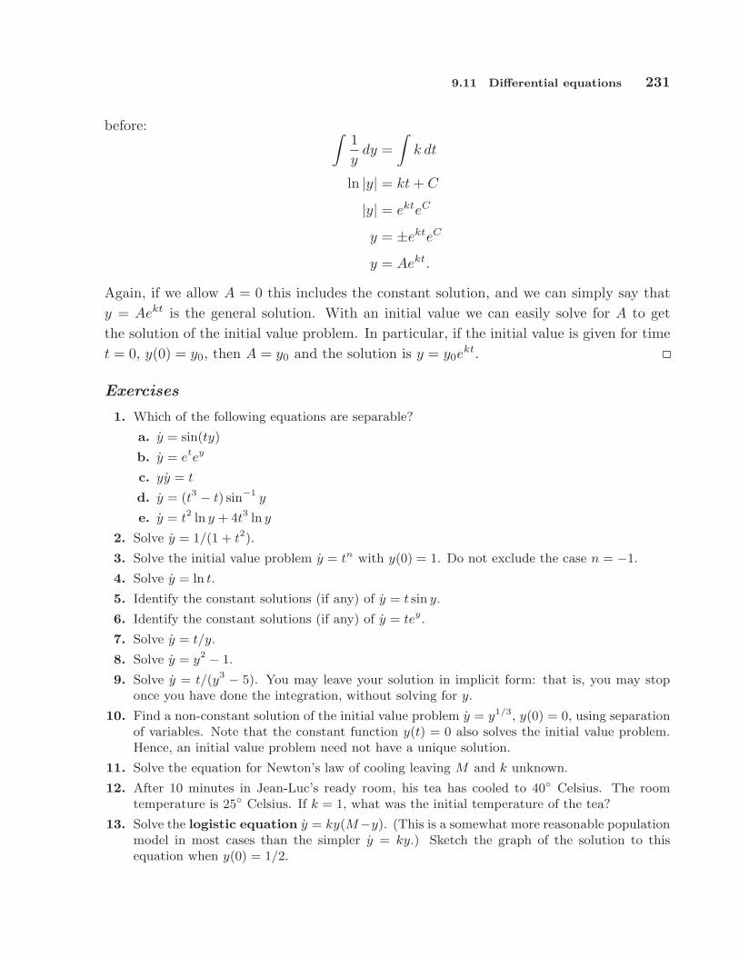
9.11 Differential equations 231
before: ∫1y
dy =∫
k dt
ln |y| = kt + C
|y| = ekteC
y = ±ekteC
y = Aekt.
Again, if we allow A = 0 this includes the constant solution, and we can simply say thaty = Aekt is the general solution. With an initial value we can easily solve for A to getthe solution of the initial value problem. In particular, if the initial value is given for timet = 0, y(0) = y0, then A = y0 and the solution is y = y0e
kt.
Exercises
1. Which of the following equations are separable?
a. y = sin(ty)
b. y = etey
c. yy = t
d. y = (t3 − t) sin−1 y
e. y = t2 ln y + 4t3 ln y
2. Solve y = 1/(1 + t2).
3. Solve the initial value problem y = tn with y(0) = 1. Do not exclude the case n = −1.
4. Solve y = ln t.
5. Identify the constant solutions (if any) of y = t sin y.
6. Identify the constant solutions (if any) of y = tey.
7. Solve y = t/y.
8. Solve y = y2 − 1.
9. Solve y = t/(y3 − 5). You may leave your solution in implicit form: that is, you may stoponce you have done the integration, without solving for y.
10. Find a non-constant solution of the initial value problem y = y1/3, y(0) = 0, using separationof variables. Note that the constant function y(t) = 0 also solves the initial value problem.Hence, an initial value problem need not have a unique solution.
11. Solve the equation for Newton’s law of cooling leaving M and k unknown.
12. After 10 minutes in Jean-Luc’s ready room, his tea has cooled to 40◦ Celsius. The roomtemperature is 25◦ Celsius. If k = 1, what was the initial temperature of the tea?
13. Solve the logistic equation y = ky(M−y). (This is a somewhat more reasonable populationmodel in most cases than the simpler y = ky.) Sketch the graph of the solution to thisequation when y(0) = 1/2.
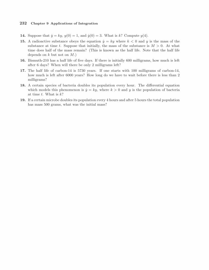
232 Chapter 9 Applications of Integration
14. Suppose that y = ky, y(0) = 1, and y(0) = 3. What is k? Compute y(4).
15. A radioactive substance obeys the equation y = ky where k < 0 and y is the mass of thesubstance at time t. Suppose that initially, the mass of the substance is M > 0. At whattime does half of the mass remain? (This is known as the half life. Note that the half lifedepends on k but not on M .)
16. Bismuth-210 has a half life of five days. If there is initially 600 milligrams, how much is leftafter 6 days? When will there be only 2 milligrams left?
17. The half life of carbon-14 is 5730 years. If one starts with 100 milligrams of carbon-14,how much is left after 6000 years? How long do we have to wait before there is less than 2milligrams?
18. A certain species of bacteria doubles its population every hour. The differential equationwhich models this phenomenon is y = ky, where k > 0 and y is the population of bacteriaat time t. What is k?
19. If a certain microbe doubles its population every 4 hours and after 5 hours the total populationhas mass 500 grams, what was the initial mass?

10Sequences and Series
Consider the following sum:
12
+14
+18
+116
+ · · ·+ 12i
+ · · ·
The dots at the end indicate that the sum goes on forever. Does this make sense? Canwe assign a numerical value to an infinite sum? While at first it may seem difficult orimpossible, we have certainly done something similar when we talked about one quantitygetting “closer and closer” to a fixed quantity. Here we could ask whether, as we add moreand more terms, the sum gets closer and closer to some fixed value. That is, look at
12
=12
34
=12
+14
78
=12
+14
+18
1516
=12
+14
+18
+116
and so on, and ask whether these values have a limit. It seems pretty clear that they do,namely 1. In fact, as we will see, it’s not hard to show that
12
+14
+18
+116
+ · · ·+ 12i
=2i − 1
2i= 1− 1
2i
233
234 Chapter 10 Sequences and Series
and then
limi→∞
1− 12i
= 1− 0 = 1.
There is one place that you have long accepted this notion of infinite sum without reallythinking of it as a sum:
0.33333 =310
+3
100+
31000
+3
10000+ · · · = 1
3,
for example, or
3.14159 . . . = 3 +110
+4
100+
11000
+5
10000+
9100000
+ · · · = π.
Our first task, then, to investigate infinite sums, called series, is to investigate limits ofsequences of numbers. That is, we officially call
∞∑
i=1
12i
=12
+14
+18
+116
+ · · ·+ 12i
+ · · ·
a series, while12,34,78,1516
, . . . ,2i − 1
2i, . . .
is a sequence, and∞∑
i=1
12i
= limi→∞
2i − 12i
,
that is, the value of a series is the limit of a particular sequence.
10.1 Sequences
While the idea of a sequence of numbers, a1, a2, a3, . . . is straightforward, it is useful tothink of a sequence as a function. We have up until now dealt with functions whose domainsare the real numbers, or a subset of the real numbers, like f(x) = sin x. A sequence is afunction with domain the natural numbers N = {1, 2, 3, . . .} or the non-negative integers,Z≥0 = {0, 1, 2, 3, . . .}. The range of the function is still allowed to be the real numbers; insymbols, we say that a sequence is a function f :N → R. Sequences are written in a fewdifferent ways, all equivalent; these all mean the same thing:
a1, a2, a3, . . .
{an}∞n=1
{f(n)}∞n=1
{an | n ∈ N}{f(n) | n ∈ N}
10.1 Sequences 235
As with functions on the real numbers, we will most often encounter sequences thatcan be expressed by a formula. We have already seen the sequence ai = f(i) = 1 − 1/2i,and others are easy to come by:
f(i) =i
i + 1
f(n) =12n
f(n) = sin(nπ/6)
f(i) =(i− 1)(i + 2)
2i
Frequently these formulas will make sense if thought of either as functions with domain Ror N, though occasionally one will make sense only for integer values.
Faced with a sequence we are interested in the limit
limi→∞
f(i) = limi→∞
ai.
We already understandlim
x→∞f(x)
when x is a real valued variable; now we simply want to restrict the “input” values to beintegers. No real difference is required in the definition of limit, except that we specify, per-haps implicitly, that the variable is an integer. Compare this definition to definition 4.10.
DEFINITION 10.1 Suppose that {an}∞n=1 is a sequence. We say that limn→∞ an = L
if for every ε > 0 there is an N > 0 so that whenever n > N , |an−L| < ε. If limn→∞ an = L
we say that the sequence converges, otherwise it diverges.
If f(i) defines a sequence, and f(x) makes sense, and limx→∞ f(x) = L, then it is clearthat limi→∞ f(i) = L as well, but it is important to note that the converse of this statementis not true. For example, since limx→∞(1/x) = 0, it is clear that also limi→∞(1/i) = 0,that is, the numbers
11,12,13,14,15,16, . . .
get closer and closer to 0. Consider this, however: Let f(n) = sin(nπ). This is the sequence
sin(0π), sin(1π), sin(2π), sin(3π), . . . = 0, 0, 0, 0, . . .
since sin(nπ) = 0 when n is an integer. Thus limn→∞ f(n) = 0. But limx→∞ f(x), whenx is real, does not exist: as x gets bigger and bigger, the values sin(xπ) do not get closer
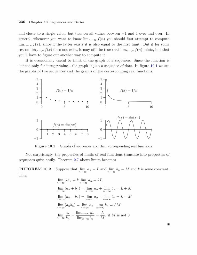
236 Chapter 10 Sequences and Series
and closer to a single value, but take on all values between −1 and 1 over and over. Ingeneral, whenever you want to know limn→∞ f(n) you should first attempt to computelimx→∞ f(x), since if the latter exists it is also equal to the first limit. But if for somereason limx→∞ f(x) does not exist, it may still be true that limn→∞ f(n) exists, but thatyou’ll have to figure out another way to compute it.
It is occasionally useful to think of the graph of a sequence. Since the function isdefined only for integer values, the graph is just a sequence of dots. In figure 10.1 we seethe graphs of two sequences and the graphs of the corresponding real functions.
0
1
2
3
4
5
0 5 10
.............................................................................................................................................................................................................................................................................................................................................................................................................
f(x) = 1/x
0
1
2
3
4
5
0 5 10
•• • • • • • • • •
f(n) = 1/n
−1
0
1
.........................................................................................................................................................................................................
.............................................................................................................................................................................................................................................................
..............................................................................................................................................................................................................................................................
..............................................................................................................................................................................................................................................................
.....................................................
f(x) = sin(xπ)
−1
0
1
1 2 3 4 5 6 7 8
• • • • • • • • •
f(n) = sin(nπ)
Figure 10.1 Graphs of sequences and their corresponding real functions.
Not surprisingly, the properties of limits of real functions translate into properties ofsequences quite easily. Theorem 2.7 about limits becomes
THEOREM 10.2 Suppose that limn→∞
an = L and limn→∞
bn = M and k is some constant.
Thenlim
n→∞kan = k lim
n→∞an = kL
limn→∞
(an + bn) = limn→∞
an + limn→∞
bn = L + M
limn→∞
(an − bn) = limn→∞
an − limn→∞
bn = L−M
limn→∞
(anbn) = limn→∞
an · limn→∞
bn = LM
limn→∞
an
bn=
limn→∞ an
limx→a bn=
L
M, if M is not 0
10.1 Sequences 237
Likewise the Squeeze Theorem (4.1) becomes
THEOREM 10.3 Suppose that an ≤ bn ≤ cn for all n > N , for some N . If limn→∞
an =
limn→∞
cn = L, then limn→∞
bn = L.
And a final useful fact:
THEOREM 10.4 If limn→∞
|an| = 0 then limn→∞
an = 0.
This says simply that if the size of an gets close to zero then in fact an gets close tozero.
Here are some alternate notations for sequences that are frequently used:
a0, a1, a2, a3, . . . = {ai | i = 0, 1, 2, 3 . . .}= {ai | i ∈ Z≥0}= {ai}∞i=0
EXAMPLE 10.5 Determine whether{
n
n + 1
}∞
n=0
converges or diverges. If it con-
verges, compute the limit. Since this makes sense for real numbers we consider
limx→∞
x
x + 1= lim
x→∞1− 1
x + 1= 1− 0 = 1.
Thus the sequence converges to 1.
EXAMPLE 10.6 Determine whether{
ln n
n
}∞
n=1
converges or diverges. If it converges,
compute the limit. We compute
limx→∞
ln x
x= lim
x→∞1/x
1= 0,
using L’Hopital’s Rule. Thus the sequence converges to 0.
EXAMPLE 10.7 Determine whether {(−1)n}∞n=0 converges or diverges. If it converges,compute the limit. This does not make sense for all real exponents, but the sequence iseasy to understand: it is
1,−1, 1,−1, 1 . . .

238 Chapter 10 Sequences and Series
and clearly diverges.
EXAMPLE 10.8 Determine whether {(−1/2)n}∞n=0 converges or diverges. If it con-verges, compute the limit. We consider the sequence {|(−1/2)n|} = {(1/2)n}. Then
limx→∞
(12
)x
= limx→∞
12x
= 0,
so by theorem 10.4 the sequence converges to 0.
EXAMPLE 10.9 Determine whether {(sinn)/√
n}∞n=1 converges or diverges. If it con-verges, compute the limit. Since | sin n| ≤ 1, 0 ≤ | sin n/
√n| ≤ 1/
√n and we can use the-
orem 10.3 with an = 0 and cn = 1/√
n. Since limn→∞
an = limn→∞
cn = 0, limn→∞
sin n/√
n = 0
and the sequence converges to 0.
EXAMPLE 10.10 A particularly common and useful sequence is {rn}∞n=0, for variousvalues of r. Some are quite easy to understand: If r = 1 the sequence converges to 1since every term is 1, and likewise if r = 0 the sequence converges to 0. If r = −1 thisis the sequence of example 10.7 and diverges. If r > 1 or r < −1 the terms rn get largewithout limit, so the sequence diverges. If 0 < r < 1 then the sequence converges to 0. If−1 < r < 0 then |rn| = |r|n and 0 < |r| < 1, so the sequence converges. In summary, {rn}converges precisely when −1 < r ≤ 1 in which case
limn→∞
rn ={ 0 if −1 < r < 1
1 if r = 1
Sometimes we will not be able to determine the limit of a sequence, but we need toknow whether it converges. In some cases we can determine this without being able tocompute the limit.
A sequence is called increasing or sometimes strictly increasing if ai < ai+1 forall i. It is called non-decreasing or sometimes (unfortunately) increasing if ai ≤ ai+1
for all i. Similarly a sequence is decreasing if ai > ai+1 for all i and non-increasing ifai ≥ ai+1 for all i. If a sequence has any of these properties it is called monotonic.
EXAMPLE 10.11 The sequence
{2i − 1
2i
}∞
i=1
=12,34,78,1516
, . . . ,

10.1 Sequences 239
is increasing, and {n + 1
n
}∞
i=1
=21,32,43,54, . . .
is decreasing.
A sequence is bounded above if there is some number N such that an ≤ N for everyn, and bounded below if there is some number N such that an ≥ N for every n. If asequence is bounded above and bounded below it is bounded. If a sequence {an}∞n=0 isincreasing or non-decreasing it is bounded below (by a0), and if it is decreasing or non-increasing it is bounded above (by a0). Finally, with all this new terminology we can statean important theorem.
THEOREM 10.12 If a sequence is bounded and monotonic then it converges.
We will not prove this; the proof appears in many calculus books. It is not hard tobelieve: suppose that a sequence is increasing and bounded, so each term is larger thanthe one before, yet never larger than some fixed value N . The terms must then get closerand closer to some value between a0 and N . It need not be N , since N may be a “too-generous” upper bound, but rather the limit will be the smallest number that is above allof the terms ai.
EXAMPLE 10.13 All of the terms (2i − 1)/2i are less than 2, and the sequence isincreasing. As we have seen, the limit of the sequence is 1—1 is the smallest number thatis bigger than all the terms in the sequence. Similarly, all of the terms (n+1)/n are biggerthan 1/2, and the limit is 1—1 is the largest number that is smaller than the terms of thesequence.
We don’t actually need to know that a sequence is monotonic to apply this theorem—it is enough to know that the sequence is “eventually” monotonic, that is, that at somepoint it becomes increasing or decreasing. For example, the sequence 10, 9, 8, 15, 3, 21, 4,3/4, 7/8, 15/16, 31/32, . . . is not increasing, because among the first few terms it is not.But starting with the term 3/4 it is increasing, so the theorem tells us that the sequence3/4, 7/8, 15/16, 31/32, . . . converges. Since convergence depends only on what happens asn gets large, adding a few random terms at the beginning can’t turn a convergent sequenceinto a divergent one.
240 Chapter 10 Sequences and Series
EXAMPLE 10.14 Show that {n1/n} converges.
We first show that this sequence is decreasing, that is, that n1/n ≥ (n+1)1/(n+1). Considerthe real function f(x) = x1/x when x ≥ 1. We can compute the derivative, f ′(x) =x1/x(1−ln x)/x2, and note that when x ≥ 3 this is negative. Since the function has negativeslope, n1/n ≥ (n + 1)1/(n+1) when n ≥ 3. Since all terms of the sequence are positive, thesequence is decreasing and bounded when n ≥ 3, and so the sequence converges. (As ithappens, we can compute the limit in this case, but we know it converges even withoutknowing the limit; see exercise 1.)
EXAMPLE 10.15 Show that {n!/nn} converges.
Again we show that the sequence is decreasing, and since each term is positive the sequenceconverges. We can’t take the derivative this time, as x! doesn’t make sense for x real. Butwe note that if an+1/an ≤ 1 then an+1 ≤ an, which is what we want to know. So we lookat an+1/an:
an+1
an=
(n + 1)!(n + 1)n+1
nn
n!=
(n + 1)!n!
nn
(n + 1)n+1=
n + 1n + 1
(n
n + 1
)n
=(
n
n + 1
)n
< 1.
(Again it is possible to compute the limit; see exercise 2.)
Exercises
1. Compute limx→∞
x1/x. ⇒
2. Use the squeeze theorem to show that limn→∞
n!
nn= 0.
3. Determine whether {√n + 47−√n}∞n=0 converges or diverges. If it converges, compute thelimit. ⇒
4. Determine whether
n2 + 1
(n + 1)2
ff∞
n=0
converges or diverges. If it converges, compute the limit.
⇒5. Determine whether
n + 47√n2 + 3n
ff∞
n=1
converges or diverges. If it converges, compute the
limit. ⇒6. Determine whether
2n
n!
ff∞
n=0
converges or diverges. ⇒
10.2 Series
While much more can be said about sequences, we now turn to our principal interest,series. Recall that a series, roughly speaking, is the sum of a sequence: if {an | n ∈ Z≥0}
10.2 Series 241
is a sequence then the associated series is
∞∑
i=0
an = a0 + a1 + a2 + · · ·
Associated with a series is a second sequence, called the sequence of partial sums{sn | n ∈ Z≥0}:
sn =n∑
i=0
an.
Sos0 = a0, s1 = a0 + a1, s2 = a0 + a1 + a2, . . .
A series converges if the sequence of partial sums converges, and otherwise the seriesdiverges.
EXAMPLE 10.16 If an = kxn,∞∑
n=0
an is called a geometric series. A typical partial
sum is
sn = k + kx + kx2 + kx3 + · · ·+ kxn = k(1 + x + x2 + x3 + · · ·+ xn).
We note that
sn(1− x) = k(1 + x + x2 + x3 + · · ·+ xn)(1− x)
= k(1 + x + x2 + x3 + · · ·+ xn)1− k(1 + x + x2 + x3 + · · ·+ xn−1 + xn)x
= k(1 + x + x2 + x3 + · · ·+ xn − x− x2 − x3 − · · · − xn − xn+1)
= k(1− xn+1)
sosn(1− x) = k(1− xn+1)
sn = k1− xn+1
1− x.
If |x| < 1, limn→∞
xn = 0 so
limn→∞
sn = limn→∞
k1− xn+1
1− x= k
11− x
.
242 Chapter 10 Sequences and Series
So when |x| < 1 the geometric series converges to k/(1 − x). When, for example, k = 1and x = 1/2:
sn =1− (1/2)n+1
1− 1/2=
2n+1 − 12n
= 2− 12n
and∞∑
n=0
12n
=1
1− 1/2= 2.
We began the chapter with the series
∞∑n=1
12n
,
namely, the geometric series without the first term 1. Each partial sum of this series is 1less than the corresponding partial sum for the geometric series, so of course the limit isalso one less than the value of the geometric series, that is,
∞∑n=1
12n
= 1.
It is not hard to see that the following theorem follows from theorem 10.2.
THEOREM 10.17 Suppose that∑
an and∑
bn are convergent sequences, and c is aconstant. Then
1.∑
can is convergent and∑
can = c∑
an
2.∑
(an + bn) is convergent and∑
(an + bn) =∑
an +∑
bn.
In general, the sequence of partial sums sn is harder to understand and analyze thanthe sequence of terms an, and it is difficult to determine whether series converge and if soto what. Sometimes things are relatively simple, starting with the following.
THEOREM 10.18 If∑
an converges then limn→∞
an = 0.
Proof. Since∑
an converges, limn→∞
sn = L and limn→∞
sn−1 = L, because this really says
the same thing but “renumbers” the terms. By theorem 10.2,
limn→∞
(sn − sn−1) = limn→∞
sn − limn→∞
sn−1 = L− L = 0.

10.2 Series 243
But
sn − sn−1 = (a0 + a1 + a2 + · · ·+ an)− (a0 + a1 + a2 + · · ·+ an−1) = an,
so as desired limn→∞
an = 0.
This theorem presents an easy divergence test: if given a series∑
an the limit limn→∞
an
does not exist or has a value other than zero, the series diverges. Note well that theconverse is not true: If lim
n→∞an = 0 then the series does not necessarily converge.
EXAMPLE 10.19 Show that∞∑
n=1
n
n + 1diverges.
We compute the limit:
limn→∞
n
n + 1= 1 6= 0.
Looking at the first few terms perhaps makes it clear that the series has no chance ofconverging:
12
+23
+34
+45
+ · · ·
will just get larger and larger; indeed, after a bit longer the series starts to look very muchlike · · ·+ 1 + 1 + 1 + 1 + · · ·, and of course if we add up enough 1’s we can make the sumas large as we desire.
EXAMPLE 10.20 Show that∞∑
n=1
1n
diverges.
Here the theorem does not apply: limn→∞
1/n = 0, so it looks like perhaps the series con-
verges. Indeed, if you have the fortitude (or the software) to add up the first 1000 termsyou will find that
1000∑n=1
1n≈ 7.49,
so it might be reasonable to speculate that the series converges to something in the neigh-borhood of 10. But in fact the partial sums do go to infinity; they just get big very, veryslowly. Consider the following:
1 +12
+13
+14
> 1 +12
+14
+14
= 1 +12
+12

244 Chapter 10 Sequences and Series
1 +12
+13
+14
+15
+16
+17
+18
> 1 +12
+14
+14
+18
+18
+18
+18
= 1 +12
+12
+12
1 +12
+13
+ · · ·+ 116
> 1 +12
+14
+14
+18
+ · · ·+ 18
+116
+ · · ·+ 116
= 1 +12
+12
+12
+12
and so on. By swallowing up more and more terms we can always manage to add at leastanother 1/2 to the sum, and by adding enough of these we can make the partial sums asbig as we like. In fact, it’s not hard to see from this pattern that
1 +12
+13
+ · · ·+ 12n
> 1 +n
2,
so to make sure the sum is over 100, for example, we’d add up terms until we get toaround 1/2198, that is, about 4 · 1059 terms. This series,
∑(1/n), is called the harmonic
series.
Exercises
1. Explain why∞X
n=1
n2
2n2 + 1diverges. ⇒
2. Explain why
∞Xn=1
5
21/n + 14diverges. ⇒
3. Explain why
∞Xn=1
3
ndiverges. ⇒
4. Compute∞X
n=0
4
(−3)n− 3
3n. ⇒
5. Compute
∞Xn=0
3
2n+
4
5n. ⇒
10.3 The Integral Test
It is generally quite difficult, often impossible, to determine the value of a series exactly.In many cases it is possible at least to determine whether or not the series converges, andso we will spend most of our time on this problem.
If all of the terms an in a series are non-negative, then clearly the sequence of partialsums sn is non-decreasing. This means that if we can show that the sequence of partialsums is bounded, the series must converge. We know that if the series converges, theterms an approach zero, but this does not mean that an ≥ an+1 for every n. Many usefuland interesting series do have this property, however, and they are among the easiest tounderstand. Let’s look at an example.

10.3 The Integral Test 245
EXAMPLE 10.21 Show that∞∑
n=1
1n2
converges.
The terms 1/n2 are positive and decreasing, and since limx→∞
1/x2 = 0, the terms 1/n2
approach zero. We seek an upper bound for all the partial sums, that is, we want to find anumber N so that sn ≤ N for ever n. The upper bound is provided courtesy of integration,and is inherent in figure 10.2.
0
1
2
0 1 2 3 4 5
.................................................................................................................................................................................................................................................................................................................................................................................................................................................................................................................................................................................................................................
A = 1
A = 1/4
Figure 10.2 Graph of y = 1/x2 with rectangles.
The figure shows the graph of y = 1/x2 together with some rectangles that lie com-pletely below the curve and that all have base length one. Because the heights of therectangles are determined by the height of the curve, the areas of the rectangles are 1/12,1/22, 1/32, and so on—in other words, exactly the terms of the series. The partial sumsn is simply the sum of the areas of the first n rectangles. Because the rectangles all liebetween the curve and the x-axis, any sum of rectangle areas is less than the correspondingarea under the curve, and so of course any sum of rectangle areas is less than the areaunder the entire curve, that is, all the way to infinity. There is a bit of trouble at the leftend, where there is an asymptote, but we can work around that easily. Here it is:
sn =112
+122
+132
+ · · ·+ 1n2
< 1 +∫ n
1
1x2
dx < 1 +∫ ∞
1
1x2
dx = 1 + 1 = 2,
recalling that we computed this improper integral in section 9.7. Since the sequence ofpartial sums sn is increasing and bounded above by 2, we know that lim
n→∞sn = L < 2, and
so the series converges to some number less than 2. In fact, it is possible, though difficult,to show that L = π2/6 ≈ 1.6.
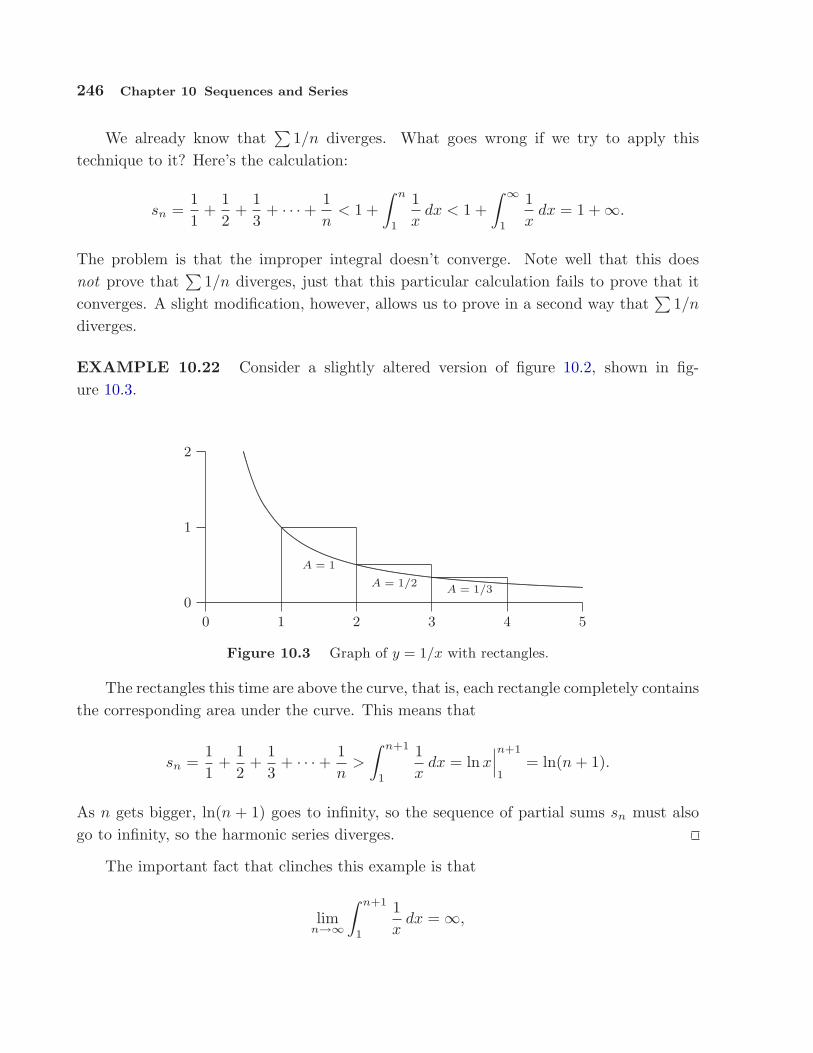
246 Chapter 10 Sequences and Series
We already know that∑
1/n diverges. What goes wrong if we try to apply thistechnique to it? Here’s the calculation:
sn =11
+12
+13
+ · · ·+ 1n
< 1 +∫ n
1
1x
dx < 1 +∫ ∞
1
1x
dx = 1 +∞.
The problem is that the improper integral doesn’t converge. Note well that this doesnot prove that
∑1/n diverges, just that this particular calculation fails to prove that it
converges. A slight modification, however, allows us to prove in a second way that∑
1/n
diverges.
EXAMPLE 10.22 Consider a slightly altered version of figure 10.2, shown in fig-ure 10.3.
0
1
2
0 1 2 3 4 5
...................................................................................................................................................................................................................................................................................................................................................................................................................................................................................................................................................................................................................................................
A = 1
A = 1/2A = 1/3
Figure 10.3 Graph of y = 1/x with rectangles.
The rectangles this time are above the curve, that is, each rectangle completely containsthe corresponding area under the curve. This means that
sn =11
+12
+13
+ · · ·+ 1n
>
∫ n+1
1
1x
dx = ln x∣∣∣n+1
1= ln(n + 1).
As n gets bigger, ln(n + 1) goes to infinity, so the sequence of partial sums sn must alsogo to infinity, so the harmonic series diverges.
The important fact that clinches this example is that
limn→∞
∫ n+1
1
1x
dx = ∞,
10.3 The Integral Test 247
which we can rewrite as ∫ ∞1
1x
dx = ∞.
So these two examples taken together indicate that we can prove that a series convergesor prove that it diverges with a single calculation of an improper integral. This is knownas the integral test, which we state as a theorem.
THEOREM 10.23 Suppose that f(x) > 0 and is decreasing on the infinite interval
[k,∞) (for some k ≥ 1) and that an = f(n). Then the series∞∑
n=1
an converges if and only
if the improper integral∫ ∞
1
f(x) dx converges.
The two examples we have seen are called p-series; a p-series is any series of the form∑1/np. If p ≤ 0, lim
n→∞1/np 6= 0, so the series diverges. For positive values of p we can
determine precisely which series converge.
THEOREM 10.24 A p-series with p > 0 converges if and only if p > 1.
Proof. We use the integral test; we have already done p = 1, so assume that p 6= 1.
∫ ∞1
1xp
dx = limD→∞
x1−p
1− p
∣∣∣∣D
1
= limD→∞
D1−p
1− p− 1
1− p.
If p > 1 then 1 − p < 0 and limD→∞
D1−p = 0, so the integral converges. If 0 < p < 1 then
1− p > 0 and limD→∞
D1−p = ∞, so the integral diverges.
EXAMPLE 10.25 Show that∞∑
n=1
1n3
converges.
We could of course use the integral test, but now that we have the theorem we may simplynote that this is a p-series with p > 1.
EXAMPLE 10.26 Show that∞∑
n=1
5n4
converges.
We know that if∑∞
n=1 1/n4 converges then∑∞
n=1 5/n4 also converges, by theorem 10.17.Since
∑∞n=1 1/n4 is a convergent p-series,
∑∞n=1 5/n4 converges also.

248 Chapter 10 Sequences and Series
EXAMPLE 10.27 Show that∞∑
n=1
5√n
diverges.
This is almost as easy but the logic has a little twist. If∑∞
n=1 5/n1/2 converges thentheorem 10.17 implies that
∑∞n=1(1/5)5/n1/2 =
∑∞n=1 1/n1/2 also converges, but since
this is a p-series with p < 1 we know that in fact it does not converge. Therefore the series∑∞n=1 5/n1/2 can’t converge.
Since it is typically difficult to compute the value of a series exactly, a good approx-imation is frequently required. In a real sense, a good approximation is only as good aswe know it is, that is, while an approximation may in fact be good, it is only valuable inpractice if we can guarantee its accuracy to some degree. This guarantee is usually easyto come by for series with decreasing positive terms.
EXAMPLE 10.28 Approximate∑
1/n2 to two decimal places.
Referring to figure 10.2, if we approximate the sum by∑N
n=1 1/n2, the error we make isthe total area of the remaining rectangles, all of which lie under the curve 1/x2 from x = N
out to infinity. So we know the true value of the series is larger than the approximation,and no bigger than the approximation plus the area under the curve from N to infinity.Roughly, then, we need to find N so that
∫ ∞N
1x2
dx < 1/100.
We can compute the integral: ∫ ∞N
1x2
dx =1N
,
so N = 100 is a good starting point. Adding up the first 100 terms gives approximately1.634983900, and that plus 1/100 is 1.644983900, so approximating the series by the valuehalfway between these will be at most 1/200 = 0.005 in error. The midpoint is 1.639983900,but while this is correct to ±0.005, we can’t tell if the correct two-decimal approximationis 1.63 or 1.64. We need to make N big enough to reduce the guaranteed error, perhaps toaround 0.004 to be safe, so we would need 1/N ≈ 0.008, or N = 125. Now the sum of thefirst 125 terms is approximately 1.636965982, and that plus 8/1000 is 1.644965982 and thepoint halfway between them is 1.640965982. The true value is then 1.640965982 ± 0.004which rounds to 1.64. We have mentioned that the true value of this series can be shownto be π2/6 ≈ 1.644934068 which rounds down to 1.64 (just barely) and is indeed below theupper bound of 1.644965982, again just barely. Frequently approximations will be evenbetter than the “guaranteed” accuracy, but not always, as this example demonstrates.

10.4 Alternating Series 249
Exercises
Determine whether each series converges or diverges.
1.
∞Xn=1
1
nπ/4⇒
2.∞X
n=1
n
n2 + 1⇒
3.
∞Xn=1
ln n
n2⇒
4.
∞Xn=1
1
n2 + 1⇒
5.
∞Xn=1
1
en⇒
6.∞X
n=1
n
en⇒
7.
∞Xn=2
1
n ln n⇒
8.
∞Xn=2
1
n(ln n)2⇒
9. Find an N so that∞X
n=1
1
n4=
NXn=1
1
n4± 0.005. ⇒
10. Find an N so that
∞Xn=0
1
en=
NXn=0
1
en± 10−4. ⇒
11. Find an N so that∞X
n=1
ln n
n2=
NXn=1
ln n
n2± 0.005. ⇒
12. Find an N so that∞X
n=2
1
n(ln n)2=
NXn=2
1
n(ln n)2± 0.005. ⇒
10.4 Alternating Series
Next we consider series with both positive and negative terms, but in a regular pattern:they alternate, as in the alternating harmonic series for example:
∞∑n=1
(−1)n−1
n=
11
+−12
+13
+−14
+ · · · = 11− 1
2+
13− 1
4+ · · · .
In this series the sizes of the terms decrease, that is, |an| forms a decreasing sequence,but this is not required in an alternating series. As with positive term series, however,when the terms do have decreasing sizes it is easier to analyze the series, much easier, infact, than positive term series. Consider pictorially what is going on in the alternatingharmonic series, shown in figure 10.4. Because the sizes of the terms an are decreasing,the partial sums s1, s3, s5, and so on, form a decreasing sequence that is bounded belowby s2, so this sequence must converge. Likewise, the partial sums s2, s4, s6, and so on,form an increasing sequence that is bounded above by s1, so this sequence also converges.Since all the even numbered partial sums are less than all the odd numbered ones, and

250 Chapter 10 Sequences and Series
14
1 = s1 = a1
a2 = − 12
s2 = 12
a3
s3
a4
s4
a5
s5
a6
s6
.....................................................................................................................................................................................................................................................................................................................................................................................................................................................................................
..................................................................................................................................................................................................................................................................................................................... ............
.......................................................................................................................................................................................................................................................
.............................................................................................................................................................................................. ............
............................................................................................................................................................................
Figure 10.4 The alternating harmonic series.
since the “jumps” (that is, the ai terms) are getting smaller and smaller, the two sequencesmust converge to the same value, meaning the entire sequence of partial sums s1, s2, s3, . . .
converges as well.There’s nothing special about the alternating harmonic series—the same argument
works for any alternating sequence with decreasing size terms. The alternating series testis worth calling a theorem.
THEOREM 10.29 Suppose that {an}∞n=0 is a non-increasing sequence of positive num-
bers and limn→∞
an = 0. Then the alternating series∞∑
n=0
(−1)nan converges.
Proof. The odd numbered partial sums, s1, s3, s5, and so on, form a non-increasingsequence, because s2k+3 = s2k+1 − a2k+2 + a2k+3 ≤ s2k+1, since a2k+2 ≥ a2k+3. Thissequence is bounded below by s2, so it must converge, say lim
k→∞s2k+1 = L. Likewise,
the partial sums s2, s4, s6, and so on, form a non-decreasing sequence that is boundedabove by s1, so this sequence also converges, say lim
k→∞s2k = M . Since lim
n→∞an = 0 and
s2k+1 = s2k + a2k+1,
L = limk→∞
s2k+1 = limk→∞
(s2k + a2k+1) = limk→∞
s2k + limk→∞
a2k+1 = M + 0 = M,
so L = M , the two sequences of partial sums converge to the same limit, and this meansthe entire sequence of partial sums also converges to L.
Another useful fact is implicit in this discussion. Suppose that
L =∞∑
n=0
(−1)nan
10.5 Comparison Tests 251
and that we approximate L by a finite part of this sum, say
L ≈N∑
n=0
(−1)nan.
Because the terms are decreasing in size, we know that the true value of L must be betweenthis approximation and the next one, that is, between
N∑n=0
(−1)nan andN+1∑n=0
(−1)nan.
Depending on whether N is odd or even, the second will be larger or smaller than the first.
EXAMPLE 10.30 Approximate the alternating harmonic series to one decimal place.We need to go roughly to the point at which the next term to be added or subtracted
is 1/10. Adding up the first nine and the first ten terms we get approximately 0.746 and0.646. These are 1/10 apart, but it is not clear how the correct value would be rounded. Itturns out that we are able to settle the question by computing the sums of the first elevenand twelve terms, which give 0.737 and 0.653, so correct to one place the value is 0.7.
Exercises
Determine whether the following series converge or diverge.
1.
∞Xn=1
(−1)n−1
2n + 5⇒
2.
∞Xn=4
(−1)n−1
√n− 3
⇒
3.
∞Xn=1
(−1)n−1 n
3n− 2⇒
4.
∞Xn=1
(−1)n−1 ln n
n⇒
5. Approximate∞X
n=1
(−1)n−1 1
n3to two decimal places. ⇒
6. Approximate
∞Xn=1
(−1)n−1 1
n4to two decimal places. ⇒
10.5 Comparison Tests
As we begin to compile a list of convergent and divergent series, new ones can sometimesbe analyzed.
EXAMPLE 10.31 Does∞∑
n=2
1n2 lnn
converge?

252 Chapter 10 Sequences and Series
The obvious first approach, based on what we know, is the integral test. Unfortunately,we can’t compute the required antiderivative. But looking at the series, it would appearthat it must converge, because the terms we are adding are smaller than the terms of ap-series, that is,
1n2 ln n
<1n2
,
when n ≥ 3. Since adding up the terms 1/n2 doesn’t get “too big”, the new series “should”also converge. Let’s make this more precise.
The series∞∑
n=2
1n2 ln n
converges if and only if∞∑
n=3
1n2 ln n
converges—all we’ve done is
dropped the initial term. We know that∞∑
n=3
1n2
converges. Looking at two typical partial
sums:
sn =1
32 ln 3+
142 ln 4
+1
52 ln 5+ · · ·+ 1
n2 ln n<
132
+142
+152
+ · · ·+ 1n2
= tn.
Since the p-series converges, say to L, and since the terms are positive, tn < L. Since theterms of the new series are positive, the sn form an increasing sequence and sn < tn < L
for all n. Hence the sequence {sn} is bounded and so converges.
Sometimes, even when the integral test applies, comparison to a known series is easier,so it’s generally a good idea to think about doing a comparison before doing the integraltest.
EXAMPLE 10.32 Does∞∑
n=2
| sin n|n2
converge?
We can’t apply the integral test here, because the terms of this series are not decreasing.Just as in the previous example, however,
| sin n|n2
≤ 1n2
,
because | sin n| ≤ 1. Once again the partial sums are non-decreasing and bounded aboveby
∑1/n2 = L, so the new series converges.
Like the integral test, the comparison test can be used to show both convergence anddivergence. In the case of the integral test, a single calculation will confirm whichever isthe case. To use the comparison test we must first have a good idea as to convergence ordivergence and pick the sequence for comparison accordingly.
10.5 Comparison Tests 253
EXAMPLE 10.33 Does∞∑
n=2
1√n2 − 3
converge?
We observe that the −3 should have little effect compared to the n2 inside the squareroot, and therefore guess that the terms are enough like 1/
√n2 = 1/n that the series
should diverge. We attempt to show this by comparison to the harmonic series. We notethat
1√n2 − 3
>1√n2
=1n
,
so that
sn =1√
22 − 3+
1√32 − 3
+ · · ·+ 1√n2 − 3
>12
+13
+ · · ·+ 1n
= tn,
where tn is 1 less than the corresponding partial sum of the harmonic series (because westart at n = 2 instead of n = 1). Since lim
n→∞tn = ∞, lim
n→∞sn = ∞ as well.
So the general approach is this: If you believe that a new series is convergent, attemptto find a convergent series whose terms are larger than the terms of the new series; if youbelieve that a new series is divergent, attempt to find a divergent series whose terms aresmaller than the terms of the new series.
EXAMPLE 10.34 Does∞∑
n=1
1√n2 + 3
converge?
Just as in the last example, we guess that this is very much like the harmonic seriesand so diverges. Unfortunately,
1√n2 + 3
<1n
,
so we can’t compare the series directly to the harmonic series. A little thought leads us to
1√n2 + 3
>1√
n2 + 3n2=
12n
,
so if∑
1/(2n) diverges then the given series diverges. But since∑
1/(2n) = (1/2)∑
1/n,theorem 10.17 implies that it does indeed diverge.
For reference we summarize the comparison test in a theorem.
THEOREM 10.35 Suppose that an and bn are non-negative for all n and that an ≤ bn
when n ≥ N , for some N .
If∞∑
n=0
bn converges, so does∞∑
n=0
an.
254 Chapter 10 Sequences and Series
If∞∑
n=0
an diverges, so does∞∑
n=0
bn.
Exercises
Determine whether the series converge or diverge.
1.∞X
n=1
1
2n2 + 3n + 5⇒
2.∞X
n=2
1
2n2 + 3n− 5⇒
3.
∞Xn=1
1
2n2 − 3n− 5⇒
4.∞X
n=1
3n + 4
2n2 + 3n + 5⇒
5.∞X
n=1
3n2 + 4
2n2 + 3n + 5⇒
6.∞X
n=1
ln n
n⇒
7.∞X
n=1
ln n
n3⇒
8.
∞Xn=2
1
ln n⇒
9.∞X
n=1
3n
2n + 5n⇒
10.∞X
n=1
3n
2n + 3n⇒
10.6 Absolute Convergence
Roughly speaking there are two ways for a series to converge: As in the case of∑
1/n2,the individual terms get small very quickly, so that the sum of all of them stays finite, or,as in the case of
∑(−1)n−1/n, the terms don’t get small fast enough (
∑1/n diverges),
but a mixture of positive and negative terms provides enough cancellation to keep thesum finite. You might guess from what we’ve seen that if the terms get small fast enoughto do the job, then whether or not some terms are negative and some positive the seriesconverges.
THEOREM 10.36 If∞∑
n=0
|an| converges, then∞∑
n=0
an converges.
Proof. Note that 0 ≤ an+|an| ≤ 2|an| so by the comparison test∞∑
n=0
(an+|an|) converges.
Now∞∑
n=0
(an + |an|)−∞∑
n=0
|an| =∞∑
n=0
an + |an| − |an| =∞∑
n=0
an
converges by theorem 10.17.

10.6 Absolute Convergence 255
So given a series∑
an with both positive and negative terms, you should first askwhether
∑ |an| converges. This may be an easier question to answer, because we havetests that apply specifically to terms with non-negative terms. If
∑ |an| converges thenyou know that
∑an converges as well. If
∑ |an| diverges then it still may be true that∑an converges—you will have to do more work to decide the question. Another way to
think of this result is: it is (potentially) easier for∑
an to converge than for∑ |an| to
converge, because the latter series cannot take advantage of cancellation.If
∑ |an| converges we say that∑
an converges absolutely; to say that∑
an convergesabsolutely is to say that any cancellation that happens to come along is not really needed,as the terms already get small so fast that convergence is guaranteed by that alone. If∑
an converges but∑ |an| does not, we say that
∑an converges conditionally. For
example∞∑
n=1
(−1)n−1 1n2
converges absolutely, while∞∑
n=1
(−1)n−1 1n
converges conditionally.
EXAMPLE 10.37 Does∞∑
n=2
sin n
n2converge?
In example 10.32 we saw that∞∑
n=2
| sin n|n2
converges, so the given series converges abso-
lutely.
EXAMPLE 10.38 Does∞∑
n=0
(−1)n 3n + 42n2 + 3n + 5
converge?
Taking the absolute value,∞∑
n=0
3n + 42n2 + 3n + 5
diverges by comparison to∞∑
n=1
310n
, so if the
series converges it does so conditionally. It is true that limn→∞
(3n + 4)/(2n2 + 3n + 5) = 0,
so to apply the alternating series test we need to know whether the terms are decreasing.If we let f(x) = (3x + 4)/(2x2 + 3x + 5) then f ′(x) = −(6x2 + 16x− 3)/(2x2 + 3x + 5)2,and it is not hard to see that this is negative for x ≥ 1, so the series is decreasing and bythe alternating series test it converges.
256 Chapter 10 Sequences and Series
Exercises
Determine whether each series converges absolutely, converges conditionally, or diverges.
1.
∞Xn=1
(−1)n−1 1
2n2 + 3n + 5⇒
2.∞X
n=1
(−1)n−1 3n2 + 4
2n2 + 3n + 5⇒
3.
∞Xn=1
(−1)n−1 ln n
n⇒
4.
∞Xn=1
(−1)n−1 ln n
n3⇒
5.
∞Xn=2
(−1)n 1
ln n⇒
6.∞X
n=0
(−1)n 3n
2n + 5n⇒
7.
∞Xn=0
(−1)n 3n
2n + 3n⇒
8.
∞Xn=1
(−1)n−1 arctan n
n⇒
10.7 The Ratio and Root Tests
Does the series∞∑
n=0
n5
5nconverge? It is possible, but a bit unpleasant, to approach this
with the integral test or the comparison test, but there is an easier way. Consider whathappens as we move from one term to the next in this series:
· · ·+ n5
5n+
(n + 1)5
5n+1+ · · ·
The denominator goes up by a factor of 5, 5n+1 = 5 · 5n, but the numerator goes up bymuch less: (n + 1)5 = n5 + 5n4 + 10n3 + 10n2 + 5n + 1, which is much less than 5n5 whenn is large, because 5n4 is much less than n5. So we might guess that in the long run itbegins to look as if each term is 1/5 of the previous term. We have seen series that behavelike this:
∞∑n=0
15n
=54,
a geometric series. So we might try comparing the given series to some variation of thisgeometric series. This is possible, but a bit messy. We can in effect do the same thing,but bypass most of the unpleasant work.
The key is to notice that
limn→∞
an+1
an= lim
n→∞(n + 1)5
5n+1
5n
n5= lim
n→∞(n + 1)5
n5
15
= 1 · 15
=15.
This is really just what we noticed above, done a bit more officially: in the long run, eachterm is one fifth of the previous term. Now pick some number between 1/5 and 1, say 1/2.
10.7 The Ratio and Root Tests 257
Because
limn→∞
an+1
an=
15,
then when n is big enough, say n ≥ N for some N ,
an+1
an<
12
and an+1 <an
2.
So aN+1 < aN/2, aN+2 < aN+1/2 < aN/4, aN+3 < aN+2/2 < aN+1/4 < aN/8, and soon. The general form is aN+k < aN/2k. So if we look at the series
aN + aN+1 + aN+2 + aN+3 + · · ·+ aN+k + · · · ,
its terms are less than or equal to the terms of the sequence
aN +aN
2+
aN
4+
aN
8+ · · ·+ aN
2k+ · · · =
∞∑
k=0
aN
2k= 2aN .
So by the comparison test,∞∑
k=0
aN+k converges, and this means that∞∑
n=0
an converges,
since we’ve just added the fixed number a0 + a1 + · · ·+ aN−1.Under what circumstances could we do this? What was crucial was that the limit of
an+1/an, say L, was less than 1 so that we could pick a value r so that L < r < 1. Thefact that L < r (1/5 < 1/2 in our example) means that we can compare the series
∑an
to∑
rn, and the fact that r < 1 guarantees that∑
rn converges. That’s really all that isrequired to make the argument work. We also made use of the fact that the terms of theseries were positive; in general we simply consider the absolute values of the terms and weend up testing for absolute convergence.
THEOREM 10.39 The Ratio Test Suppose that limn→∞
|an+1/an| = L. If L < 1
the series∑
an converges absolutely, if L > 1 the series diverges, and if L = 1 this testgives no information.
Proof. The example above essentially proves the first part of this, if we simply replace1/5 by L and 1/2 by r. Suppose that L > 1, and pick r so that 1 < r < L. Then forn ≥ N , for some N ,
|an+1||an| > r and |an+1| > r|an|.

258 Chapter 10 Sequences and Series
This implies that |aN+k| > rk|aN |, but since r > 1 this means that limk→∞
|aN+k| 6= 0, which
means also that limn→∞
an 6= 0. By the divergence test, the series diverges.
To see that we get no information when L = 1, we need to exhibit two series withL = 1, one that converges and one that diverges. It is easy to see that
∑1/n2 and
∑1/n
do the job.
EXAMPLE 10.40 The ratio test is particularly useful for series involving the factorial
function. Consider∞∑
n=0
5n/n!.
limn→∞
5n+1
(n + 1)!n!5n
= limn→∞
5n+1
5n
n!(n + 1)!
= limn→∞
51
(n + 1)= 0.
Since 0 < 1, the series converges.
A similar argument, which we will not do, justifies a similar test that is occasionallyeasier to apply.
THEOREM 10.41 The Root Test Suppose that limn→∞
|an|1/n = L. If L < 1 the
series∑
an converges absolutely, if L > 1 the series diverges, and if L = 1 this test givesno information.
The proof of the root test is actually easier than that of the ratio test, and is a goodexercise.
EXAMPLE 10.42 Analyze∞∑
n=0
5n
nn.
The ratio test turns out to be a bit difficult on this series (try it). Using the root test:
limn→∞
(5n
nn
)1/n
= limn→∞
(5n)1/n
(nn)1/n= lim
n→∞5n
= 0.
Since 0 < 1, the series converges.
The root test is frequently useful when n appears as an exponent in the general termof the series.
10.8 Power Series 259
Exercises
1. Compute limn→∞
|an+1/an| for the seriesP
1/n2.
2. Compute limn→∞
|an+1/an| for the seriesP
1/n.
3. Compute limn→∞
|an|1/n for the seriesP
1/n2.
4. Compute limn→∞
|an|1/n for the seriesP
1/n.
Determine whether the series converge.
5.∞X
n=0
(−1)n 3n
5n⇒
6.
∞Xn=1
n!
nn⇒
7.∞X
n=1
n5
nn⇒
8.
∞Xn=1
(n!)2
nn⇒
10.8 Power Series
Recall that we were able to analyze all geometric series “simultaneously” to discover that
∞∑n=0
kxn =k
1− x,
if |x| < 1, and that the series diverges when |x| ≥ 1. At the time, we thought of x as anunspecified constant, but we could just as well think of it as a variable, in which case theseries
∞∑n=0
kxn
is a function, namely, the function k/(1− x), as long as |x| < 1. While k/(1− x) is a rea-sonably easy function to deal with, the more complicated
∑kxn does have its attractions:
it appears to be an infinite version of one of the simplest function types—a polynomial.This leads naturally to the questions: Do other functions have representations as series?Is there an advantage to viewing them in this way?
The geometric series has a special feature that makes it unlike a typical polynomial—the coefficients of the powers of x are the same, namely k. We will need to allow moregeneral coefficients if we are to get anything other than the geometric series.
DEFINITION 10.43 A power series has the form
∞∑n=0
anxn,

260 Chapter 10 Sequences and Series
with the understanding that an may depend on n but not on x.
EXAMPLE 10.44∞∑
n=1
xn
nis a power series. We can investigate convergence using the
ratio test:
limn→∞
|x|n+1
n + 1n
|x|n = limn→∞
|x| n
n + 1= |x|.
Thus when |x| < 1 the series converges and when |x| > 1 it diverges, leaving only two valuesin doubt. When x = 1 the series is the harmonic series and diverges; when x = −1 it is thealternating harmonic series (actually the negative of the usual alternating harmonic series)
and converges. Thus, we may think of∞∑
n=1
xn
nas a function from the interval [−1, 1) to
the real numbers.
A bit of thought reveals that the ratio test applied to a power series will always havethe same nice form. In general, we will compute
limn→∞
|an+1||x|n+1
|an||x|n = limn→∞
|x| |an+1||an| = |x| lim
n→∞|an+1||an| = L|x|,
assuming that lim |an+1|/|an| exists. Then the series converges if L|x| < 1, that is, if|x| < 1/L, and diverges if |x| > 1/L. Only the two values x = ±1/L require furtherinvestigation. Thus the series will definitely define a function on the interval (−1/L, 1/L),and perhaps will extend to one or both endpoints as well. Two special cases deservemention: if L = 0 the limit is 0 no matter what value x takes, so the series converges forall x and the function is defined for all real numbers. If L = ∞, then no matter whatvalue x takes the limit is infinite and the series converges only when x = 0. The value 1/L
is called the radius of convergence of the series, and the interval on which the seriesconverges is the interval of convergence.
Consider again the geometric series,
∞∑n=0
xn =1
1− x.
Whatever benefits there might be in using the series form of this function are only avail-able to us when x is between −1 and 1. Frequently we can address this shortcoming bymodifying the power series slightly. Consider this series:
∞∑n=0
(x + 2)n
3n=∞∑
n=0
(x + 2
3
)n
=1
1− x+23
=3
1− x,

10.9 Calculus with Power Series 261
because this is just a geometric series with x replaced by (x+2)/3. Multiplying both sidesby 1/3 gives
∞∑n=0
(x + 2)n
3n+1=
11− x
,
the same function as before. For what values of x does this series converge? Since it is ageometric series, we know that it converges when
|x + 2|/3 < 1
|x + 2| < 3
−3 < x + 2 < 3
−5 < x < 1.
So we have a series representation for 1/(1−x) that works on a larger interval than before,at the expense of a somewhat more complicated series. The endpoints of the interval ofconvergence now are −5 and 1, but note that they can be more compactly described as−2± 3. Again we say that 3 is the radius of convergence, and we now say that the seriesis centered at −2.
DEFINITION 10.45 A power series centered at a has the form
∞∑n=0
an(x− a)n,
with the understanding that an may depend on n but not on x.
Exercises
Find the radius and interval of convergence for each series.
1.∞X
n=0
nxn ⇒
2.∞X
n=0
xn
n!⇒
3.
∞Xn=1
n!
nnxn ⇒
4.∞X
n=1
n!
nn(x− 2)n ⇒
5.∞X
n=1
(n!)2
nn(x− 2)n ⇒
6.
∞Xn=1
(x + 5)n
n(n + 1)⇒
10.9 Calculus with Power Series
Now we know that some functions can be expressed as power series, which look like infinitepolynomials. Since calculus, that is, computation of derivatives and antiderivatives, is easy

262 Chapter 10 Sequences and Series
for polynomials, the obvious question is whether the same is true for infinite series. Theanswer is yes:
THEOREM 10.46 Suppose the power series f(x) =∞∑
n=0
an(x − a)n has radius of
convergence R. Then
f ′(x) =∞∑
n=0
nan(x− a)n−1,
∫f(x) dx = C +
∞∑n=0
an
n + 1(x− a)n+1,
and these two series have radius of convergence R as well.
EXAMPLE 10.47 Starting with the geometric series:
11− x
=∞∑
n=0
xn
∫1
1− xdx = − ln |1− x| =
∞∑n=0
1n + 1
xn+1
ln |1− x| =∞∑
n=0
− 1n + 1
xn+1
when |x| < 1. The series does not converge when x = 1 but does converge when x = −1or 1 − x = 2. The interval of convergence is [−1, 1), or 0 < 1 − x ≤ 2, so we can use theseries to represent ln(x) when 0 < x ≤ 2. For example
ln(3/2) = ln(1−−1/2) =∞∑
n=0
(−1)n 1n + 1
12n+1
and so
ln(3/2) ≈ 12− 1
8+
124− 1
64+
1160
− 1384
+1
896=
9092240
≈ 0.406.
Because this is an alternating series with decreasing terms, we know that the true valueis between 909/2240 and 909/2240 − 1/2048 = 29053/71680 ≈ .4053, so correct to twodecimal places the value is 0.41.
10.10 Taylor Series 263
What about ln(9/4)? Since 9/4 is larger than 2 we cannot use the series directly, but
ln(9/4) = ln((3/2)2) = 2 ln(3/2) ≈ 0.82,
so in fact we get a lot more from this one calculation than first meets the eye. To estimatethe true value accurately we actually need to be a bit more careful. When we multiply bytwo we know that the true value is between 0.8106 and 0.812, so rounded to two decimalplaces the true value is 0.81.
Exercises
1. Find a series representation for ln 2. ⇒2. Find a power series representation for 1/(1− x)2. ⇒3. Find a power series representation for 2/(1− x)3. ⇒4. Find a power series representation for 1/(1− x)3. What is the radius of convergence? ⇒5. Find a power series representation for
Zln(1− x) dx. ⇒
10.10 Taylor Series
We have seen that some functions can be represented as series, which may give valuableinformation about the function. So far, we have seen only those examples that result frommanipulation of our one fundamental example, the geometric series. We would like to startwith a given function and produce a series to represent it, if possible.
Suppose that f(x) =∞∑
n=0
anxn on some interval of convergence. Then we know that
we can compute derivatives of f by taking derivatives of the terms of the series. Let’s lookat the first few in general:
f ′(x) =∞∑
n=1
nanxn−1 = a1 + 2a2x + 3a3x2 + 4a4x
3 + · · ·
f ′′(x) =∞∑
n=2
n(n− 1)anxn−2 = 2a2 + 3 · 2a3x + 4 · 3a4x2 + · · ·
f ′′′(x) =∞∑
n=3
n(n− 1)(n− 2)anxn−3 = 3 · 2a3 + 4 · 3 · 2a4x + · · ·

264 Chapter 10 Sequences and Series
By examining these it’s not hard to discern the general pattern. The kth derivative mustbe
f (k)(x) =∞∑
n=k
n(n− 1)(n− 2) · · · (n− k + 1)anxn−k
= k(k − 1)(k − 2) · · · (2)ak + (k + 1)(k) · · · (2)ak+1x +
+ (k + 2)(k + 1) · · · (3)ak+2x2 + · · ·
We can shrink this quite a bit by using factorial notation:
f (k)(x) =∞∑
n=k
n!(n− k)!
anxn−k = k!ak + (k + 1)!ak+1x +(k + 2)!
2!ak+2x
2 + · · ·
Now substitute x = 0:
f (k)(0) = k!ak +∞∑
n=k+1
n!(n− k)!
an0n−k = k!ak,
and solve for ak:
ak =f (k)(0)
k!.
Note the special case, obtained from the series for f itself, that gives f(0) = a0.So if a function f can be represented by a series, we know just what series it is. Given
a function f , the series∞∑
n=0
f (n)(0)n!
xn
is called the Maclaurin series for f .
EXAMPLE 10.48 Find the Maclaurin series for f(x) = 1/(1−x). We need to computethe derivatives of f (and hope to spot a pattern).
f(x) = (1− x)−1
f ′(x) = (1− x)−2
f ′′(x) = 2(1− x)−3
f ′′′(x) = 6(1− x)−4
f (4) = 4!(1− x)−5
...
f (n) = n!(1− x)−n−1

10.10 Taylor Series 265
Sof (n)(0)
n!=
n!(1− 0)−n−1
n!= 1
and the Maclaurin series is∞∑
n=0
1 · xn =∞∑
n=0
xn,
the geometric series.
A warning is in order here. Given a function f we may be able to compute theMaclaurin series, but that does not mean we have found a series representation for f . Westill need to know where the series converges, and if, where it converges, it converges tof(x). While for most commonly encountered functions the Maclaurin series does indeedconverge to f on some interval, this is not true of all functions, so care is required.
As a practical matter, if we are interested in using a series to approximate a function,we will need some finite number of terms of the series. Even for functions with messyderivatives we can compute these using computer software like Maple or Mathematica. Ifwe want to know the whole series, that is, a typical term in the series, we need a functionwhose derivatives fall into a pattern that we can discern. A few of the most importantfunctions are fortunately very easy.
EXAMPLE 10.49 Find the Maclaurin series for sinx.The derivatives are quite easy: f ′(x) = cosx, f ′′(x) = − sinx, f ′′′(x) = − cos x,
f (4)(x) = sin x, and then the pattern repeats. We want to know the derivatives at zero: 1,0, −1, 0, 1, 0, −1, 0,. . . , and so the Maclaurin series is
x− x3
3!+
x5
5!− · · · =
∞∑n=0
(−1)n x2n+1
(2n + 1)!.
We should always determine the radius of convergence:
limn→∞
|x|2n+3
(2n + 3)!(2n + 1)!|x|2n+1
= limn→∞
|x|2(2n + 3)(2n + 2)
= 0,
so the series converges for every x. Since it turns out that this series does indeed convergeto sin x everywhere, we have a series representation for sin x for every x.
Sometimes the formula for the nth derivative of a function f is difficult to discover,but a combination of a known Maclaurin series and some algebraic manipulation leadseasily to the Maclaurin series for f .

266 Chapter 10 Sequences and Series
EXAMPLE 10.50 Find the Maclaurin series for x sin(−x).To get from sinx to x sin(−x) we substitute −x for x and then multiply by x. We can
do the same thing to the series for sin x:
x
∞∑n=0
(−1)n (−x)2n+1
(2n + 1)!= x
∞∑n=0
(−1)n(−1)2n+1 x2n+1
(2n + 1)!=∞∑
n=0
(−1)n+1 x2n+2
(2n + 1)!.
As we have seen, a general power series can be centered at a point other than zero,and the method that produces the Maclaurin series can also produce such series.
EXAMPLE 10.51 Find a series centered at −2 for 1/(1− x).
If the series is∞∑
n=0
an(x + 2)n then looking at the kth derivative:
k!(1− x)−k−1 =∞∑
n=k
n!(n− k)!
an(x + 2)n−k
and substituting x = −2 we get k!3−k−1 = k!ak and ak = 3−k−1 = 1/3k+1, so the series is
∞∑n=0
(x + 2)n
3n+1.
We’ve already seen this, on page 261.
Such a series is called the Taylor series for the function, and the general term hasthe form
f (n)(a)n!
(x− a)n.
A Maclaurin series is simply a Taylor series with a = 0.
10.11 Taylor’s Theorem 267
Exercises
For each function, find the Maclaurin series or Taylor series centered at a, and the radius ofconvergence.
1. cos x ⇒2. ex ⇒3. 1/x, a = 5 ⇒4. ln x, a = 1 ⇒5. ln x, a = 2 ⇒6. 1/x2, a = 1 ⇒7. 1/
√1− x ⇒
8. Find the first four terms of the Maclaurin series for tan x (up to and including the x3 term).⇒
9. Use a combination of Maclaurin series and algebraic manipulation to find a series centeredat zero for x cos(x2). ⇒
10. Use a combination of Maclaurin series and algebraic manipulation to find a series centeredat zero for xe−x. ⇒
10.11 Taylor's Theorem
One of the most important uses of infinite series is the potential for using an initial portionof the series for f to approximate f . We have seen, for example, that when we add up thefirst n terms of an alternating series with decreasing terms that the difference between thisand the true value is at most the size of the next term. A similar result is true of manyTaylor series.
THEOREM 10.52 Suppose that f is defined on some open interval I around a andsuppose f (N+1)(x) exists on this interval. Then for each x 6= a in I there is a value z
between x and a so that
f(x) =N∑
n=0
f (n)(a)n!
(x− a)n +f (N+1)(z)(N + 1)!
(x− a)N+1.
Proof. The proof requires some cleverness to set up, but then the details are quiteelementary. We want to define a function F (t). Start with the equation
F (t) =N∑
n=0
f (n)(t)n!
(x− t)n + B(x− t)N+1.
268 Chapter 10 Sequences and Series
Here we have replaced a by t in the first N + 1 terms of the Taylor series, and added acarefully chosen term on the end, with B to be determined. Note that we are temporarilykeeping x fixed, so the only variable in this equation is t, and we will be interested only int between a and x. Now substitute t = a:
F (a) =N∑
n=0
f (n)(a)n!
(x− a)n + B(x− a)N+1.
Set this equal to f(x):
f(x) =N∑
n=0
f (n)(a)n!
(x− a)n + B(x− a)N+1.
Since x 6= a, we can solve this for B, which is a “constant”—it depends on x and a butthose are temporarily fixed. Now we have defined a function F (t) with the property thatF (a) = f(x). Consider also F (x): all terms with a positive power of (x − t) become zerowhen we substitute x for t, so we are left with F (x) = f (0)(x)/0! = f(x). So F (t) is afunction with the same value on the endpoints of the interval [a, x]. By Rolle’s theorem(6.25), we know that there is a value z ∈ (a, x) such that F ′(z) = 0. Let’s look at F ′(t).Each term in F (t), except the first term and the extra term involving B, is a product, soto take the derivative we use the product rule on each of these terms. It will help to writeout the first few terms of the definition:
F (t) = f(t) +f (1)(t)
1!(x− t)1 +
f (2)(t)2!
(x− t)2 +f (3)(t)
3!(x− t)3 + · · ·
+f (N)(t)
N !(x− t)N + B(x− t)N+1.
Now take the derivative:
F ′(t) = f ′(t) +(
f (1)(t)1!
(x− t)0(−1) +f (2)(t)
1!(x− t)1
)
+(
f (2)(t)1!
(x− t)1(−1) +f (3)(t)
2!(x− t)2
)
+(
f (3)(t)2!
(x− t)2(−1) +f (4)(t)
3!(x− t)3
)+ . . . +
+(
f (N)(t)(N − 1)!
(x− t)N−1(−1) +f (N+1)(t)
N !(x− t)N
)
+ B(N + 1)(x− t)N (−1).

10.11 Taylor’s Theorem 269
Now most of the terms in this expression cancel out, leaving just
F ′(t) =f (N+1)(t)
N !(x− t)N + B(N + 1)(x− t)N (−1).
At some z, F ′(z) = 0 so
0 =f (N+1)(z)
N !(x− z)N + B(N + 1)(x− z)N (−1)
B(N + 1)(x− z)N =f (N+1)(z)
N !(x− z)N
B =f (N+1)(z)(N + 1)!
.
Now we can write
F (t) =N∑
n=0
f (n)(t)n!
(x− t)n +f (N+1)(z)(N + 1)!
(x− t)N+1.
Recalling that F (a) = f(x) we get
f(x) =N∑
n=0
f (n)(a)n!
(x− a)n +f (N+1)(z)(N + 1)!
(x− a)N+1,
which is what we wanted to show.
It may not be immediately obvious that this is particularly useful; let’s look at someexamples.
EXAMPLE 10.53 Find a polynomial approximation for sinx accurate to ±0.005.From Taylor’s theorem:
sin x =N∑
n=0
f (n)(a)n!
(x− a)n +f (N+1)(z)(N + 1)!
(x− a)N+1.
What can we say about the size of the term
f (N+1)(z)(N + 1)!
(x− a)N+1?
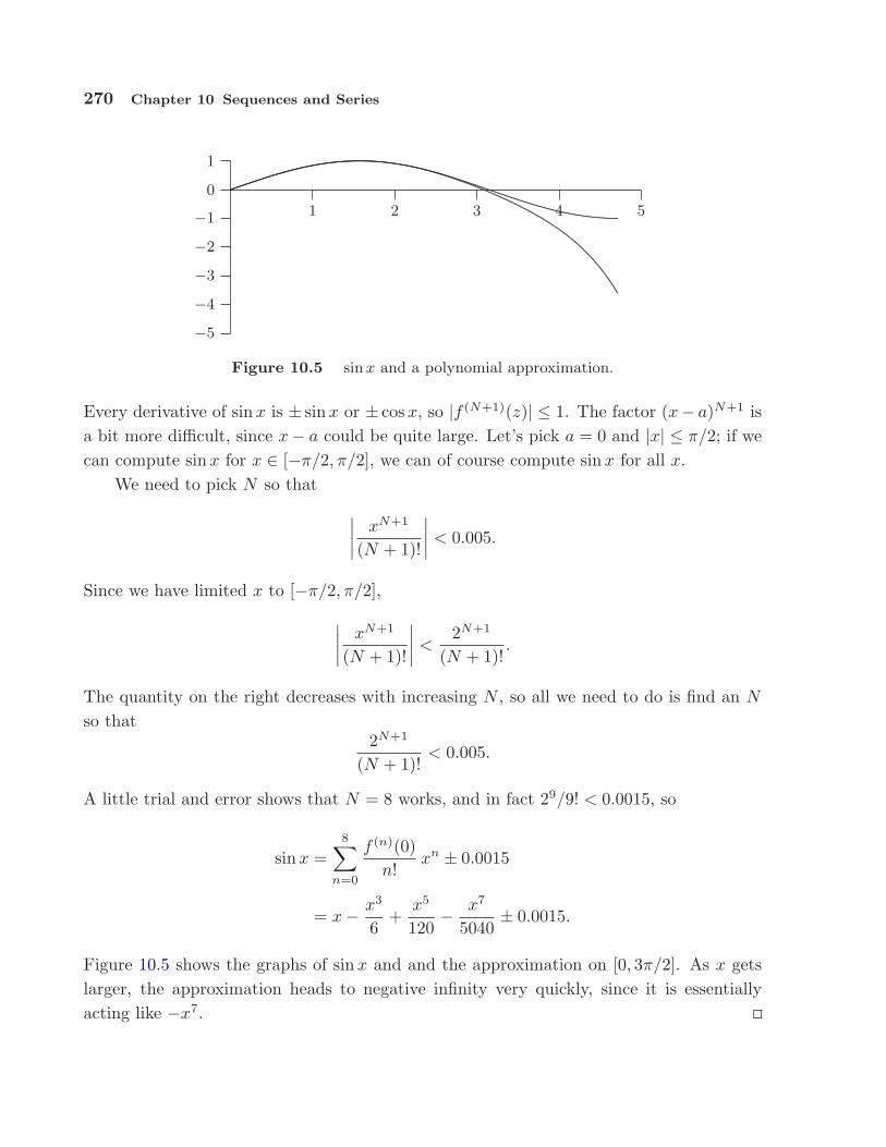
270 Chapter 10 Sequences and Series
−5
−4
−3
−2
−1
0
1
1 2 3 4 5
................................................
........................................................
...........................................................................................................................................................................................................................................................................................................................................................................................................................................................................................................................................
................................................
........................................................
........................................................................................................................................................................................................................................................................................................................................................................................................................................................................................
Figure 10.5 sin x and a polynomial approximation.
Every derivative of sin x is ± sin x or ± cosx, so |f (N+1)(z)| ≤ 1. The factor (x− a)N+1 isa bit more difficult, since x− a could be quite large. Let’s pick a = 0 and |x| ≤ π/2; if wecan compute sin x for x ∈ [−π/2, π/2], we can of course compute sin x for all x.
We need to pick N so that
∣∣∣∣xN+1
(N + 1)!
∣∣∣∣ < 0.005.
Since we have limited x to [−π/2, π/2],
∣∣∣∣xN+1
(N + 1)!
∣∣∣∣ <2N+1
(N + 1)!.
The quantity on the right decreases with increasing N , so all we need to do is find an N
so that2N+1
(N + 1)!< 0.005.
A little trial and error shows that N = 8 works, and in fact 29/9! < 0.0015, so
sin x =8∑
n=0
f (n)(0)n!
xn ± 0.0015
= x− x3
6+
x5
120− x7
5040± 0.0015.
Figure 10.5 shows the graphs of sin x and and the approximation on [0, 3π/2]. As x getslarger, the approximation heads to negative infinity very quickly, since it is essentiallyacting like −x7.
10.12 Additional exercises 271
EXAMPLE 10.54 Find a polynomial approximation for ex near x = 2 accurate to±0.005.
From Taylor’s theorem:
ex =N∑
n=0
e2
n!(x− 2)n +
ez
(N + 1)!(x− 2)N+1,
since f (n)(x) = ex for all n. We are interested in x near 2, and we need to keep |(x−2)N+1|in check, so we may as well specify that |x− 2| ≤ 1, so x ∈ [1, 3]. Also
∣∣∣∣ez
(N + 1)!
∣∣∣∣ ≤e3
(N + 1)!,
so we need to find an N that makes e3/(N + 1)! ≤ 0.005. This time N = 5 makese3/(N + 1)! < 0.0015, so the approximating polynomial is
ex = e2 + e2(x− 2) +e2
2(x− 2)2 +
e2
6(x− 2)3 +
e2
24(x− 2)4 +
e2
120(x− 2)5 ± 0.0015.
This presents an additional problem for approximation, since we also need to approximatee2, and any approximation we use will increase the error, but we will not pursue thiscomplication.
Exercises
1. Find a polynomial approximation for cos x on [0, π], accurate to ±10−3 ⇒2. How many terms of the series for ln x centered at 1 are required so that the guaranteed error
on [1/2, 3/2] is at most 10−3? What if the interval is instead [1, 3/2]? ⇒3. Find the first three nonzero terms in the Taylor series for tan x on [−π/4, π/4], and compute
the guaranteed error term as given by Taylor’s theorem. (You may want to use Maple or asimilar aid.) ⇒
4. Show that cos x is equal to its Taylor series for all x by showing that the limit of the errorterm is zero, as N approaches infinity.
5. Show that ex is equal to its Taylor series for all x by showing that the limit of the error termis zero, as N approaches infinity.
10.12 Additional exercises
These problems require the techniques of this chapter, and are in no particular order. Someproblems may be done in more than one way.
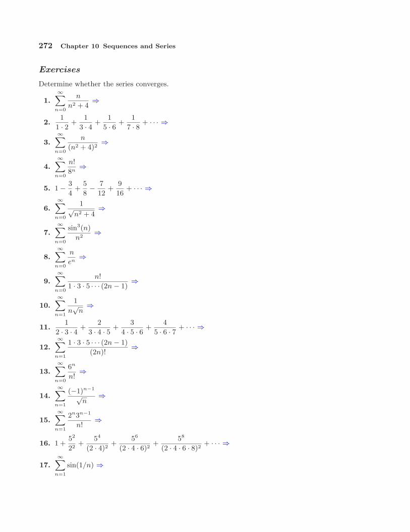
272 Chapter 10 Sequences and Series
Exercises
Determine whether the series converges.
1.∞X
n=0
n
n2 + 4⇒
2.1
1 · 2 +1
3 · 4 +1
5 · 6 +1
7 · 8 + · · · ⇒
3.
∞Xn=0
n
(n2 + 4)2⇒
4.∞X
n=0
n!
8n⇒
5. 1− 3
4+
5
8− 7
12+
9
16+ · · · ⇒
6.
∞Xn=0
1√n2 + 4
⇒
7.
∞Xn=0
sin3(n)
n2⇒
8.∞X
n=0
n
en⇒
9.
∞Xn=0
n!
1 · 3 · 5 · · · (2n− 1)⇒
10.∞X
n=1
1
n√
n⇒
11.1
2 · 3 · 4 +2
3 · 4 · 5 +3
4 · 5 · 6 +4
5 · 6 · 7 + · · · ⇒
12.
∞Xn=1
1 · 3 · 5 · · · (2n− 1)
(2n)!⇒
13.
∞Xn=0
6n
n!⇒
14.∞X
n=1
(−1)n−1
√n
⇒
15.
∞Xn=1
2n3n−1
n!⇒
16. 1 +52
22+
54
(2 · 4)2+
56
(2 · 4 · 6)2+
58
(2 · 4 · 6 · 8)2+ · · · ⇒
17.
∞Xn=1
sin(1/n) ⇒

10.12 Additional exercises 273
Find the interval and radius of convergence; you need not check the endpoints of the intervals.
18.∞X
n=0
2n
n!xn ⇒
19.
∞Xn=0
xn
1 + 3n⇒
20.∞X
n=1
xn
n3n⇒
21. x +1
2
x3
3+
1 · 32 · 4
x5
5+
1 · 3 · 52 · 4 · 6
x7
7+ · · · ⇒
22.
∞Xn=1
n!
n2xn ⇒
23.
∞Xn=1
(−1)n
n23nx2n ⇒
24.∞X
n=0
(x− 1)n
n!⇒
Find a series for each function, using the formula for Maclaurin series and algebraic manipulationas appropriate.
25. 2x ⇒26. ln(1 + x) ⇒
27. ln
„1 + x
1− x
«⇒
28.√
1 + x ⇒29.
1
1 + x2⇒
30. arctan(x) ⇒31. Use the answer to the previous problem to discover a series for a well-known mathematical
constant. ⇒


AIntroduction to Maple
A.1 Getting Started
Maple is a powerful mathematical calculator, often called a computer algebra system(CAS) or symbolic mathematics program, because unlike most calculators it can do alge-bra and calculus symbolically. For example, it can expand the product (x + 1)30 into thenormal representation of this polynomial, and it can factor the result back into the originalform. It can compute the derivative or antiderivative of 3x/
√x2 + 2x + 47. It can also
serve as a numerical calculator, but again unlike most calculators it can do integer andrational number arithmetic exactly, no matter how many digits are involved. If it is unde-sirable or impossible to express a result exactly, Maple can do numerical approximation.Finally, Maple can do some quite sophisticated graphing in both 2 and 3 dimensions.
To learn how to use some of Maple’s features, you should work through this tutorialstep by step. What you should type will be shown in the left hand column in typewriter
style; comments and explanations will appear at the right. You should do everythinglisted here, but you should feel free to experiment too. If you leave something out or dosomething extra it may change the results of some later computations. (If you want toexperiment along the way, try using different names for functions and variables than theones in the examples.)
To start Maple, log in on one of the workstations in the math lab. Click on the Maplebutton on the bar at the bottom of the screen. When the Maple window comes up, youare ready to give commands to Maple.
275

276 Appendix A Introduction to Maple
For the most part, the commands you give will be typed in the main Maple window.Some commands can be given by making selections from menus, or by clicking on buttonson the top bar. For example, to leave Maple, you may move the mouse pointer to thebutton titled ‘File’ and click on the left mouse button. When you do, a list of furthercommands appears. If you click on the last command, ‘Exit’, Maple will quit and thewindow will disappear.
The instructions given here are for Maple version 9. To make Maple 10 act like Maple9, choose Options from the Tools menu; choose the Display tab; change Input displayto Maple Notation; click on Apply Globally. You should only have to do this the firsttime you use Maple.
A.2 Algebra
A.2.1 Numbers
2+3;
123456789* 987654321;
You must type the semicolon at the end ofthe line to signal the end of your expression.
2+3
34*98
-45;
Type this as is, without the semicolon onthe first line. Maple will warn you aboutthe missing semicolon, but will usually dothe calculation anyway. Sometimes you maywant to start a new line as part of the sameexpression; you can do this by holding theshift key while you press return. Do thisafter the “98”.
2/5 + 1/3;
23/45-167/345*2/3;
All rational arithmetic is done exactly.
2^5;
2**5;
3^27;
ifactor(%);
Maple knows standard mathematical no-tation, including these two symbols for ex-ponentiation. The percent sign (%) denotesthe previous result (it’s called the ‘ditto’ op-erator). The command ifactor does inte-ger factoring; the command factor factorspolynomials.

A.2 Algebra 277
12345/98765;
evalf(%);
You can force Maple to approximate valuesas ‘floating point numbers’ (i.e., using deci-mal notation). Some of Maple’s commandsdo this automatically, as we will see later.
I^2;
evalf(Pi);
evalf(exp(1));
The number i =√−1 is denoted by I; the
case is significant—a lower case ‘i’ is differ-ent. Pi denotes π; again case is significant.It is very easy to mistakenly type ‘pi’ in-stead of ‘Pi’. When you do, things will al-most certainly not work properly, but youwill probably get no error messages—youjust have to watch out for this. There is nobuilt-in symbol for e ≈ 2.71828; use thefunction exp(x) whenever you need ex.
A.2.2 Variables and Expressions
Maple can manipulate expressions involving variables as well as numbers. Variables canbe assigned values, either actual numeric values or entire expressions.
(x+5)^2;
f:=%;
x:=5;
f;
x^2;
Maple simply repeats the first line since x
has no value. The second line saves the ex-pression (x + 5)2 with name f ; the “:=”symbol acts like an equal sign in normalmathematics or in the programming lan-guage C. The third line assigns x the value5.
x:=’x’;
x;
f;
This clears the value of x—this is not thesame as setting it to zero! Note that Mapleremembers the ‘real’ definition of f—it isstill an expression involving x, not the fixedvalue 100.

278 Appendix A Introduction to Maple
2x;
2*x;
You must always type the multiplicationsymbol—Maple will not accept the first lineeven though it is standard notation. If youmake a simple typing mistake like this, youcan fix it without retyping the command.In this case, Maple should correctly guesswhere the problem is and place the cursorbetween the 2 and the x; simply type the* and press return. In any case, you canalways move the mouse pointer to the po-sition of the mistake and click the left but-ton, then make your corrections. You canadjust your position in the line using the ar-row keys to the right of the main keyboard.When you press the return key, the com-mand will be re-evaluated.
expand(f);
factor(%);
factor(x^2+4*x+5);
If a polynomial doesn’t factor, Maple leavesit alone. (As a general rule, if Maple cannotperform a calculation it will simply restatethe command.)
WARNING: You can go back anywhere in your Maple session and change a command.When you do this you change only the result of that command—you do not change anysubsequent commands that depend on the result. If you want to re-execute subsequentcommands, you must move the cursor to each command in turn and press the return key.Do not overuse this editing ability—it can make the chain of events very difficult to follow.It often is better to copy the command, paste it in at the end of the session, modify itthere, and execute it as a new command. To copy and paste a command, do this: Positionthe mouse pointer at the beginning of the command you want to copy, press the left mousebutton and hold it down, move the mouse cursor to the end of the command, and releasethe mouse button. (If the command is on a single line, you may also select the wholecommand by positioning the cursor in the line, and clicking the left mouse button threetimes quickly—this is a “triple click”.) The command should now be highlighted. Positionthe mouse pointer where you want to paste and click the middle button.
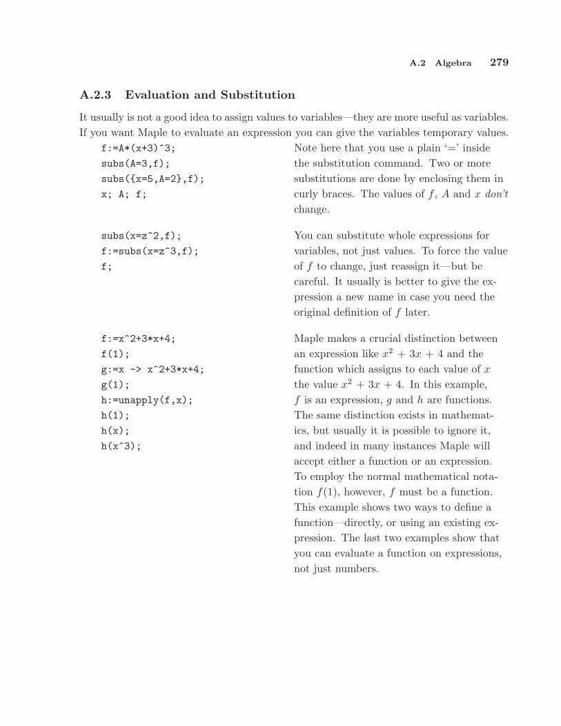
A.2 Algebra 279
A.2.3 Evaluation and Substitution
It usually is not a good idea to assign values to variables—they are more useful as variables.If you want Maple to evaluate an expression you can give the variables temporary values.
f:=A*(x+3)^3;
subs(A=3,f);
subs({x=5,A=2},f);
x; A; f;
Note here that you use a plain ‘=’ insidethe substitution command. Two or moresubstitutions are done by enclosing them incurly braces. The values of f , A and x don’tchange.
subs(x=z^2,f);
f:=subs(x=z^3,f);
f;
You can substitute whole expressions forvariables, not just values. To force the valueof f to change, just reassign it—but becareful. It usually is better to give the ex-pression a new name in case you need theoriginal definition of f later.
f:=x^2+3*x+4;
f(1);
g:=x -> x^2+3*x+4;
g(1);
h:=unapply(f,x);
h(1);
h(x);
h(x^3);
Maple makes a crucial distinction betweenan expression like x2 + 3x + 4 and thefunction which assigns to each value of x
the value x2 + 3x + 4. In this example,f is an expression, g and h are functions.The same distinction exists in mathemat-ics, but usually it is possible to ignore it,and indeed in many instances Maple willaccept either a function or an expression.To employ the normal mathematical nota-tion f(1), however, f must be a function.This example shows two ways to define afunction—directly, or using an existing ex-pression. The last two examples show thatyou can evaluate a function on expressions,not just numbers.

280 Appendix A Introduction to Maple
map(g,[-3,-2,-1,0,1,2,3]);
map(g,{-3,-2,-1,0,1,2,3});
Using the ‘map’ operation and a function(not an expression) you can evaluate a func-tion on a list of values. The list can be en-closed in square brackets or in set braces—but notice the difference! The set bracesproduce a set as a result, meaning that re-peated values are shown only once, and theorder does not necessarily correspond to theorder of the input values. In general, thesquare bracket form is more useful.
A.2.4 Solving Equations
Maple will solve a limited class of equations exactly and a broader class approximately.solve(x^2-x-10=10,x);
solve(x^2-x-20,x);
solutions:=solve(g(x),x);
solve(x^5+4*x^3-3*x^2+10,x);
solve(tan(x)=x+1,x);
allvalues(%);
solve(tan(x)=x,x);
allvalues(%);
solve(sin(x)=cos(x)-1,x);
The solve command will give exact answersif possible, including complex answers. IfMaple can’t solve an equation it may printnothing, or it may display the equation in astandard form, preceded by ‘RootOf’. Youcan ask Maple to attempt to evaluate rootsdisplayed as a RootOf using allvalues.Maple will attempt to find all solutions foran equation or a RootOf, but often will notsucceed.
Do not rely on the solve command alonewhen looking for solutions to equations—atthe very least, you should graph your func-tions so that you know where roots appearto be. Note that if you give an expressioninstead of an equation Maple assumes thatyou mean ‘= 0’.

A.2 Algebra 281
map(g,[solutions]);
simplify(%);
In some cases, Maple will not automaticallysimplify as much as it can, so you need tonudge it a bit. In this case, of course, weknew that the values should be zero. If theresult had not simplified to zero, carefulscrutiny of the problem would be called for.
f:=x^3+3*x^2+x+5:
solve(f,x);
fsolve(f,x);
fsolve(f,x,complex);
You can end a line with a colon instead ofa semicolon—it tells Maple not to displaythe result. This can be particularly handywhen the result is very long, or simply whenyou either know what it is or do not needto know (as when you will be using the re-sult to compute a further result). The fsolveoperation tells Maple to approximate theroots. In this example, Maple can computethe roots exactly, but it may be more in-formative to see approximations. Note thatMaple only computes real roots unless the‘complex’ option is present. If the functionis not a polynomial, fsolve will find at mostone solution, but for polynomials it will findall solutions.
g:=x -> exp(x)+x^2-10*x;
fsolve(g(x),x);
fsolve(g(x),x,-2..2);
g(%);
fsolve(g(x),x,2..4);
g(%);
You can specify a range in fsolve—youwould normally do this when you knowthere are multiple roots and you want toapproximate a particular one. In this case,a graph of the function clearly indicates aroot near 0 and a root near 3. Because g
is a function, and fsolve expects an expres-sion, it is necessary to use g(x) in fsolve. (Imade g a function so that it would be easyto check the answers.)

282 Appendix A Introduction to Maple
solve({3*x+5*y=6,4*x-6*y=-8},
{x,y});
h1:=3*x-6*y-5;
h2:=-4*x*y+7;
solve({h1,h2},{x,y});
evalf(%);
fsolve({h1,h2},{x,y});
fsolve({h1,h2},{x,y},{x=-2..0,y=-2..0});
Maple can solve equations simultaneously,with either solve or fsolve. As with singleequations, fsolve may not find all solutions,but you can specify ranges for x and y toforce fsolve to find particular solutions.
A.3 Plotting
Maple can do two and three dimensional graphing. There are many ways to adjust theplots that Maple produces; we’ll cover just the basics here.
plot(f,x=-10..10);
plot(g(x),x=-5..5);
plot(g,-10..10);
plot(g,-10..10,y=-10..10);
Maple will accept either an expression or afunction to plot, but notice that the form ofthe range is a bit different in the two cases.For an expression, use ‘x=’ before the range,but for a function leave it out. You can alsospecify the range for y explicitly. This isoften useful if the function gets very largeon the interval.
You can change the appearance of the plotin a variety of ways. Click in the plot andyou should see a border appear around it;then you can explore the items on the plotmenu. If you prefer, you can have plotscome up in separate windows; use the Op-tions item on the Tools menu in the mainMaple window, then open the Display taband change the plot display.

A.3 Plotting 283
plot([1+2*sin(t),t,t=-Pi..Pi],
coords=polar);
You can do plots in polar coordinates. In-side the square brackets, the first expressionis the radius, the second is the angle, andthe third is the range of the variable. Inthis case, the angle and the variable are thesame, but in general the angle could be amore complicated function of the variable.
plot({x^2,x^3},x=-5..5);
plot({
[1+2*sin(t),t,t=-Pi..Pi],
[cos(4*t),t,t=-Pi..Pi]},
coords=polar);
You can put more than one curve in thesame plot by enclosing a list of expressionsin curly braces.
r:=sqrt(x^2+y^2);
f:=sin(r)/r;
plot3d(f,x=-10..10,
y=-10..10);
Try changing the appearance of a 3D plotby using the Style, Color, Axes and Pro-jection menus. If you position the cursor inthe drawing area and press and hold the leftmouse button, you can move the mouse tochange the orientation of the plot—try it.
with(plots):
polarplot(1+sin(t));
polarplot(sin(t/3));
polarplot(sin(t/3),
t=0..3*Pi);
When you start Maple, only the most ba-sic plotting commands are available. Bytyping “with(plots)” you tell Maple toload a number of special purpose plot-ting functions. One of the most useful isthe polarplot routine shown here. By de-fault, Maple uses the range [−π, π]; the lastcommand shows how to specify a differentrange.
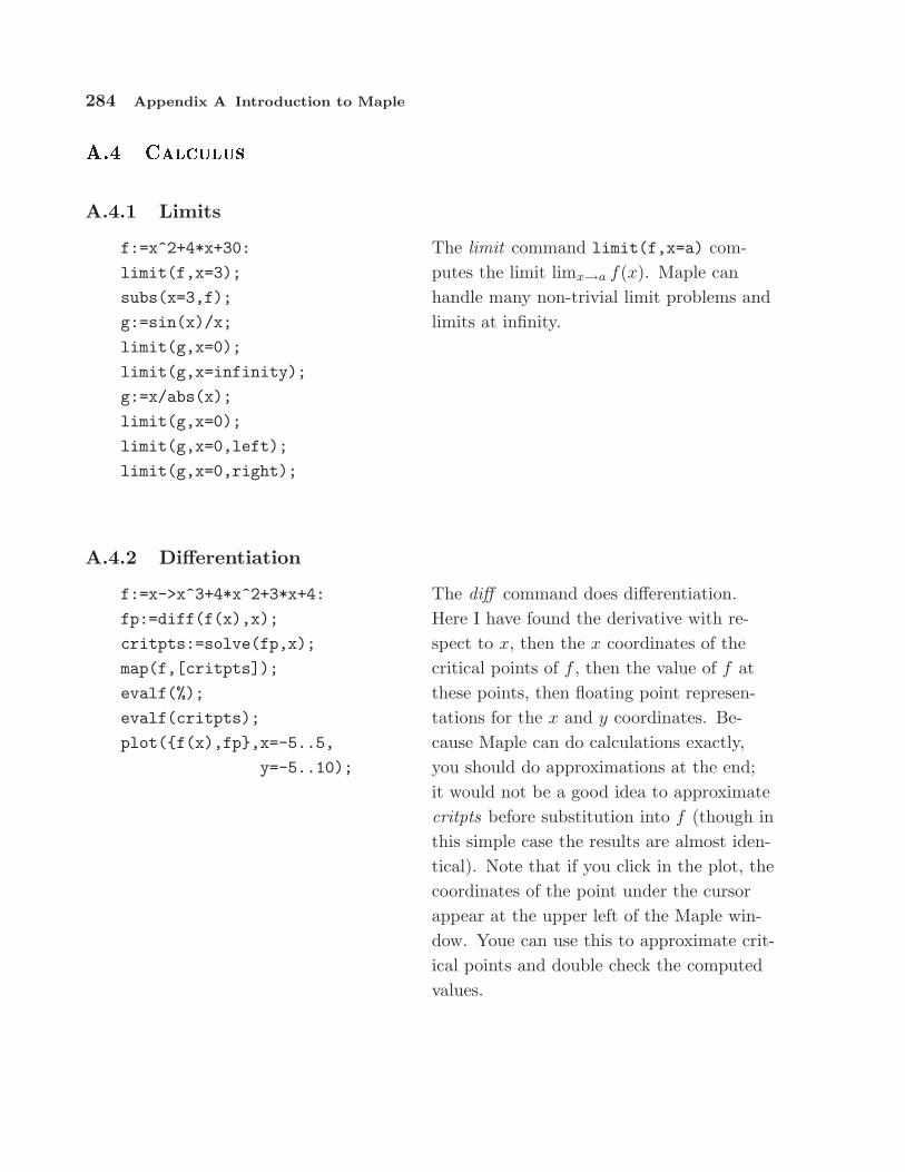
284 Appendix A Introduction to Maple
A.4 Calculus
A.4.1 Limits
f:=x^2+4*x+30:
limit(f,x=3);
subs(x=3,f);
g:=sin(x)/x;
limit(g,x=0);
limit(g,x=infinity);
g:=x/abs(x);
limit(g,x=0);
limit(g,x=0,left);
limit(g,x=0,right);
The limit command limit(f,x=a) com-putes the limit limx→a f(x). Maple canhandle many non-trivial limit problems andlimits at infinity.
A.4.2 Differentiation
f:=x->x^3+4*x^2+3*x+4:
fp:=diff(f(x),x);
critpts:=solve(fp,x);
map(f,[critpts]);
evalf(%);
evalf(critpts);
plot({f(x),fp},x=-5..5,
y=-5..10);
The diff command does differentiation.Here I have found the derivative with re-spect to x, then the x coordinates of thecritical points of f , then the value of f atthese points, then floating point represen-tations for the x and y coordinates. Be-cause Maple can do calculations exactly,you should do approximations at the end;it would not be a good idea to approximatecritpts before substitution into f (though inthis simple case the results are almost iden-tical). Note that if you click in the plot, thecoordinates of the point under the cursorappear at the upper left of the Maple win-dow. Youe can use this to approximate crit-ical points and double check the computedvalues.

A.4 Calculus 285
A.4.3 Implicit Differentiation
eqn:=x^2+y^2=1;
xp:=implicitdiff(eqn,x,y);
yp:=implicitdiff(eqn,y,x);
subs({x=1/2,y=sqrt(3/4)},yp);
Notice that the order of the second two ar-guments to the implicitdiff function isimportant—xp is dx/dy and yp is dy/dx.The last line computes y′ at a specific point,(1/2,
√3/2).
A.4.4 Integration
f:=(2*z-3)*sqrt(z-3);
g:=int(f,z);
diff(g,z);
factor(%);
The int command shown here will computean antiderivative. The computer is not in-fallible, and you may not notice a typingmistake, so it’s not a bad idea to use Mapleto check your work. Here, I’ve taken thederivative to check the antiderivative.
int(f,z=5..10);
simplify(%);
evalf(%);
subs(z=10,g)-subs(z=5,g);
To do definite integration give the limits af-ter the variable. Of course, you can also doit yourself using the antiderivative. Noticethat the answer can look quite different be-fore simplification.
f:=1/sqrt(x):
int(f,x=0..1);
f:=1/x^2:
int(f,x=0..1);
int(f,x=1..infinity);
f:=exp(-x^2):
int(f,x=-infinity..infinity);
int(sin(x),x=0..infinity);
Maple can do many improper integrals ex-actly. If the integral does not converge,Maple may answer with ‘∞’ if appropriate,or it may give an error message.
f:=tan(x^2):
int(f,x);
int(f,x=0..1);
evalf(%);
Int(f,x=0..1);
evalf(%);
Maple can’t find antiderivatives of somefunctions. In such cases you can use evalfto approximate the value of a definite inte-gral. If you don’t want Maple to even try tofind an antiderivative, use the capital I formof the integration operator.

286 Appendix A Introduction to Maple
A.5 Adding text to a Maple session
You can add plain text to a Maple session. This is especially useful if you are going to givea printed or electronic version of a session to someone else, since it lets you explain whatis going on. It is also a good idea to add text to remind yourself at a later date what youwere doing and why.
To add text above a command, position the cursor anywhere in the command. Thenopen the Insert menu, and then the Paragraph submenu, and choose Before Cursor. Whenyou type you will get ordinary text that will not be interpreted as part of the command.
A.6 Printing
BEFORE YOU PRINT: You should clean up your session before you print, so that you donot waste paper and so that the printed copy is attractive and easy to read. If you wantto print only part of the session, first save the session (see the section Saving your work)and then cut out the portions of the session that you do not want to print. You mightwant to save the trimmed version using a different name.
To print your worksheet, choose Print from the File menu, or click on the print button(the fourth little button from the left in the menu bar).
If you would like to print just a plot, you need to display it in a window of its own.You can do this by changing the plot display option, as described in the Plotting section.Then position the cursor in the plot command and press return. The plot should open ina new window, and you can use the Print menu in that window to print the plot.
A.7 Saving your work
You can save your Maple worksheet so that you can come back to it at a later time. Choosethe Save or Save As. . . item from the File menu in Maple; a new window will pop up.(Use Save As if you want to save your worksheet under a new name.) You may also savea worksheet using the third button from the left in the menu bar.
When you reload a worksheet (with the Open item on the File menu or with thesecond button from the left) Maple will not automatically recreate all the values createdin the worksheet. You may selectively re-execute commands in the worksheet, or you mayuse the Execute item on the Edit menu to execute the entire worksheet.

A.8 Getting Help 287
A.8 Getting Help
There are (somewhat out of date) manuals for Maple in the lab. You can also get help ‘online’ from the Maple program. The help system is very good and always available as youwork in Maple.
?int If you know the command you need help on,just type its name after a question mark.
You can browse through the entire help system or search it using the Help menu.

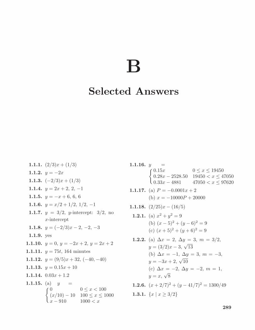
BSelected Answers
1.1.1. (2/3)x + (1/3)
1.1.2. y = −2x
1.1.3. (−2/3)x + (1/3)
1.1.4. y = 2x + 2, 2, −1
1.1.5. y = −x + 6, 6, 6
1.1.6. y = x/2 + 1/2, 1/2, −1
1.1.7. y = 3/2, y-intercept: 3/2, nox-intercept
1.1.8. y = (−2/3)x− 2, −2, −3
1.1.9. yes
1.1.10. y = 0, y = −2x + 2, y = 2x + 2
1.1.11. y = 75t, 164 minutes
1.1.12. y = (9/5)x + 32, (−40,−40)
1.1.13. y = 0.15x + 10
1.1.14. 0.03x + 1.2
1.1.15. (a) y ={ 0 0 ≤ x < 100(x/10)− 10 100 ≤ x ≤ 1000x− 910 1000 < x
1.1.16. y ={ 0.15x 0 ≤ x ≤ 194500.28x− 2528.50 19450 < x ≤ 470500.33x− 4881 47050 < x ≤ 97620
1.1.17. (a) P = −0.0001x + 2(b) x = −10000P + 20000
1.1.18. (2/25)x− (16/5)
1.2.1. (a) x2 + y2 = 9(b) (x− 5)2 + (y − 6)2 = 9(c) (x + 5)2 + (y + 6)2 = 9
1.2.2. (a) ∆x = 2, ∆y = 3, m = 3/2,y = (3/2)x− 3,
√13
(b) ∆x = −1, ∆y = 3, m = −3,y = −3x + 2,
√10
(c) ∆x = −2, ∆y = −2, m = 1,y = x,
√8
1.2.6. (x + 2/7)2 + (y − 41/7)2 = 1300/49
1.3.1. {x | x ≥ 3/2}
289

290 Appendix B Selected Answers
1.3.2. {x | x 6= −1}1.3.3. {x | x 6= 1 and x 6= −1}1.3.4. {x | x < 0}1.3.5. {x | x ∈ R}, i.e., all x
1.3.6. {x | x ≥ 0}1.3.7. {x | h− r ≤ x ≤ h + r}1.3.8. {x | x ≥ 1}1.3.9. {x | −1/3 < x < 1/3}
1.3.10. {x | x ≥ 0 and x 6= 1}1.3.11. {x | x ≥ 0 and x 6= 1}1.3.12. R
1.3.13. {x | x ≥ 3}, {x | x ≥ 0}1.3.14. A = x(500− 2x), {x | 0 ≤ x ≤ 250}1.3.15. V = r(50 − πr2), {r | 0 < r ≤√
50/π}1.3.16. A = 2πr2+2000/r, {r | 0 < r < ∞}2.1.1. −5, −2.47106145, −2.4067927,
−2.400676, −2.4
2.1.2. −4/3, −24/7, 7/24, 3/4
2.1.3. −0.107526881, −0.11074197,
−0.1110741,−1
3(3 + ∆x)→ −1
9
2.1.4.3 + 3∆x + ∆x2
1 + ∆x→ 3
2.1.5. 3.31, 3.003001, 3.0000,3 + 3∆x + ∆x2 → 3
2.1.6. m
2.2.1. 10, 25/2, 20, 15, 25, 35.
2.2.2. 5, 4.1, 4.01, 4.001, 4 + ∆t → 4
2.2.3. −10.29, −9.849, −9.8049,−9.8− 4.9∆t → −9.8
2.3.1. 7
2.3.2. 5
2.3.3. 0
2.3.4. undefined
2.3.5. 1/6
2.3.6. 0
2.3.7. 3
2.3.8. 172
2.3.9. 0
2.3.10. 2
2.3.11. does not exist
2.3.12.√
2
2.3.13. 3a2
2.3.14. 512
2.3.15. −4
2.3.16. 0
2.3.18. (a) 8, (b) 6, (c) dne, (d) −2, (e) −1,(f) 8, (g) 7, (h) 6, (i) 3, (j) −3/2,(k) 6, (l) 2
2.4.1. −x/√
169− x2
2.4.2. −9.8t
2.4.3. 2x + 1/x2
2.4.4. 2ax + b
2.4.5. 3x2
3.1.1. 100x99
3.1.2. −100x−101
3.1.3. −5x−6
3.1.4. πxπ−1
3.1.5. (3/4)x−1/4
3.1.6. −(9/7)x−16/7
3.1.7. −98t/10, −98/10
3.2.1. 15x2 + 24x
3.2.2. −20x4 + 6x + 10/x3
Appendix B Selected Answers 291
3.2.3. −30x + 25
3.2.4. 6x2 + 2x− 8
3.2.5. 3x2 + 6x− 1
3.2.6. 9x2 − x/√
625− x2
3.2.7. y = 13x/4 + 5
3.2.8. y = 24x− 48− π3
3.2.9. −49t/5 + 5, −49/5
3.2.12.n∑
k=1
kakxk−1
3.2.13. x3/16− 3x/4 + 4
3.3.1. 3x2(x3 − 5x + 10) + x3(3x2 − 5)
3.3.2. (x2 +5x−3)(5x4−18x2 +6x−7)+(2x + 5)(x5 − 6x3 + 3x2 − 7x + 1)
3.3.3.
√625− x2
2√
x− x
√x√
625− x2
3.3.4.−1
x19√
625− x2− 20
√625− x2
x21
3.3.5. f ′ = 4(2x− 3), y = 4x− 7
3.4.1.3x2
x3 − 5x + 10− x3(3x2 − 5)
(x3 − 5x + 10)2
3.4.2.2x + 5
x5 − 6x3 + 3x2 − 7x + 1−
(x2 + 5x− 3)(5x4 − 18x2 + 6x− 7)(x5 − 6x3 + 3x2 − 7x + 1)2
3.4.3.1
2√
x√
625− x2+
x3/2
(625− x2)3/2
3.4.4.−1
x19√
625− x2− 20
√625− x2
x21
3.4.5. y = 17x/4− 41/4
3.4.6. y = 11x/16− 15/16
3.4.8. y = 19/169− 5x/338
3.4.9. 13/18
3.5.1. 4x3 − 9x2 + x + 7
3.5.2. 3x2 − 4x + 2/√
x
3.5.3. 6(x2 + 1)2x
3.5.4.√
169− x2 − x2/√
169− x2
3.5.5. (2x− 4)√
25− x2−(x2 − 4x + 5)x/
√25− x2
3.5.6. −x/√
r2 − x2
3.5.7. 2x3/√
1 + x4
3.5.8.1
4√
x(5−√x)3/2
3.5.9. 6 + 18x
3.5.10.2x + 11− x
+x2 + x + 1(1− x)2
3.5.11. −1/√
25− x2 −√25− x2/x2
3.5.12.12
(−169x2
− 1) /√
169x− x
3.5.13.3x2 − 2x + 1/x2
2√
x3 − x2 − (1/x)
3.5.14.300x
(100− x2)5/2
3.5.15.1 + 3x2
3(x + x3)2/3
3.5.16.
(4x(x2 + 1) +
4x3 + 4x
2√
1 + (x2 + 1)2
) /
2√
(x2 + 1)2 +√
1 + (x2 + 1)2
3.5.17. 5(x + 8)4
3.5.18. −3(4− x)2
3.5.19. 6x(x2 + 5)2
3.5.20. −12x(6− 2x2)2
3.5.21. 24x2(1− 4x3)−3
3.5.22. 5 + 5/x2
3.5.23. −8(4x− 1)(2x2 − x + 3)−3
3.5.24. 1/(x + 1)2

292 Appendix B Selected Answers
3.5.25. 3(8x− 2)/(4x2 − 2x + 1)2
3.5.26. −3x2 + 5x− 1
3.5.27. 120x4 − 576x3 + 888x2 − 480x + 96
3.5.28. −2/(x− 1)2
3.5.29. 4x/(x2 + 1)2
3.5.30. (x2 − 6x + 7)/(x− 3)2
3.5.31. −5/(3x− 4)2
3.5.32. 60x4 + 72x3 + 18x2 + 18x− 6
3.5.33. (5− 4x)/((2x + 1)2(x− 3)2)
3.5.34. 1/(2(2 + 3x)2)
3.5.35. 56x6 + 72x5 + 110x4 + 100x3 +60x2 + 28x + 6
3.5.36. y = 23x/96− 29/96
3.5.37. y = 3− 2x/3
3.5.38. y = 13x/2− 23/2
3.5.39. y = 2x− 11
3.5.40. y =20 + 2
√5
5√
4 +√
5x +
3√
5
5√
4 +√
54.1.1. 2nπ − π/2, any integer n
4.1.2. nπ ± π/6, any integer n
4.1.3. (√
2 +√
6)/2
4.1.4. −(1 +√
3)/(1−√3)
4.1.11. t = π/2
4.3.1. 5
4.3.2. 7/2
4.3.3. 3/4
4.3.4. 1
4.3.5. −√2/2
4.3.6. 7
4.3.7. 2
4.4.1. sin(√
x) cos(√
x)/√
x
4.4.2.sin x
2√
x+√
x cosx
4.4.3. − cos x
sin2 x
4.4.4.(2x + 1) sinx− (x2 + x) cos x
sin2 x
4.4.5.− sin x cosx√
1− sin2 x
4.5.1. cos2 x− sin2 x
4.5.2. − sinx cos(cosx)
4.5.3.tan x + x sec2 x
2√
x tan x
4.5.4.sec2 x(1 + sin x)− tan x cosx
(1 + sin x)2
4.5.5. − csc2 x
4.5.6. − csc x cot x
4.5.7. 3x2 sin(23x2) + 46x4 cos(23x2)
4.5.8. 0
4.5.9. −6 cos(cos(6x)) sin(6x)
4.5.10. sin θ/(cos θ + 1)2
4.5.11. 5t4 cos(6t)− 6t5 sin(6t)
4.5.12. 3t2(sin(3t) + t cos(3t))/ cos(2t) +2t3 sin(3t) sin(2t)/ cos2(2t)
4.5.13. nπ/2, any integer n
4.5.14. π/2 + nπ, any integer n
4.5.15.√
3x/2 + 3/4−√3π/6
4.5.16. 8√
3x + 4− 8√
3π/3
4.5.17. 3√
3x/2−√3π/4
4.5.18. π/6 + 2nπ, 5π/6 + 2nπ, any integern
4.7.1. 2 ln(3)x3x2
4.7.2.cos x− sinx
ex
4.7.3. 2e2x

Appendix B Selected Answers 293
4.7.4. ex cos(ex)
4.7.5. cos(x)esin x
4.7.6. xsin x
(cos x ln x +
sin x
x
)
4.7.7. 3x2ex + x3ex
4.7.8. 1 + 2x ln(2)
4.7.9. −2x ln(3)(1/3)x2
4.7.10. e4x(4x− 1)/x2
4.7.11. (3x2 + 3)/(x3 + 3x)
4.7.12. − tan(x)
4.7.13. (1− ln(x2))/(x2√
ln(x2))
4.7.14. sec(x)
4.7.15. xsin(x)(cos(x) ln(x) + sin(x)/x)
4.7.20. e
4.8.1. 0
4.8.2. ∞4.8.3. 1
4.8.4. 0
4.8.5. 0
4.8.7. y = 1 and y = −1
4.9.1. x/y
4.9.2. −(2x + y)/(x + 2y)
4.9.3. −(3x2 + y2− 2xy)/(2xy− 3y2− x2)
4.9.4. sin(x) sin(y)/(cos(x) cos(y))
4.9.5. −√y/√
x
4.9.6. (y sec2(x/y)−y2)/(x sec2(x/y)+y2)
4.9.7. (y − cos(x + y))/(cos(x + y)− x)
4.9.8. −y2/x2
4.9.9. 1
4.9.11. y = 2x± 6
4.9.12. y = x/2± 3
4.9.13. (√
3, 2√
3), (−√3,−2√
3),(2√
3,√
3), (−2√
3,−√3)
4.9.14. y = 7x/√
3− 8/√
3
4.9.15. y = (−y1/31 x+y
1/31 x1+x
1/31 y1)/x
1/31
4.9.16. (y − y1)/(x− x1) = (2x31 + 2x1y
21 −
x1)/(2y31 + 2y1x
21 + y1)
4.10.3. −1/(1 + x2)
4.10.4.2x√
1− x4
4.10.5.ex
1 + e2x
5.1.1. min at x = 1/2
5.1.2. min at x = −1, max at x = 1
5.1.3. max at x = 2, min at x = 4
5.1.4. min at x = ±1, max at x = 0.
5.1.5. min at x = 1
5.1.6. none
5.1.7. none
5.1.8. min at x = 7π/12 + kπ, max atx = −π/12 + kπ, for integer k.
5.1.9. none
5.1.10. local max at x = 5
5.1.11. local min at x = 49
5.1.12. local min at x = 0
5.1.15. one
5.2.1. min at x = 1/2
5.2.2. min at x = −1, max at x = 1
5.2.3. max at x = 2, min at x = 4
5.2.4. min at x = ±1, max at x = 0.
5.2.5. min at x = 1
5.2.6. none
5.2.7. none

294 Appendix B Selected Answers
5.2.8. min at x = 7π/12 + kπ, max atx = −π/12 + kπ, for integer k.
5.2.9. none
5.2.10. max at x = 0, min at x = ±11
5.2.11. min at x = −3/2, neither at x = 0
5.2.13. min at nπ, max at π/2 + nπ
5.2.14. min at 2nπ, max at (2n + 1)π
5.2.15. min at π/2+2nπ, max at 3π/2+2nπ
5.3.1. min at x = 1/2
5.3.2. min at x = −1, max at x = 1
5.3.3. max at x = 2, min at x = 4
5.3.4. min at x = ±1, max at x = 0.
5.3.5. min at x = 1
5.3.6. none
5.3.7. none
5.3.8. min at x = 7π/12 + nπ, max atx = −π/12 + nπ, for integer n.
5.3.9. max at x = 63/64
5.3.10. max at x = 7
5.3.11. max at −5−1/4, min at 5−1/4
5.3.12. none
5.3.13. max at −1, min at 1
5.3.14. min at 2−1/3
5.3.15. none
5.3.16. min at nπ
5.3.17. max at nπ, min at π/2 + nπ
5.3.18. max at π/2+2nπ, min at 3π/2+2nπ
5.4.1. concave up everywhere
5.4.2. concave up when x < 0, concavedown when x > 0
5.4.3. concave down when x < 3, concaveup when x > 3
5.4.4. concave up when x < −1/√
3 orx > 1/
√3, concave down when
−1/√
3 < x < 1/√
3
5.4.5. concave up when x < 0 or x > 2/3,concave down when 0 < x < 2/3
5.4.6. concave up when x < 0, concavedown when x > 0
5.4.7. concave up when x < −1 or x > 1,concave down when −1 < x < 0 or0 < x < 1
5.4.8. concave down on ((8n−1)π/4, (8n+3)π/4), concave up on ((8n +3)π/4, (8n + 7)π/4), for integer n
5.4.9. concave down everywhere
5.4.10. concave up on (−∞, (21−√497)/4)and (21 +
√497)/4,∞)
5.4.11. concave up on (0,∞)
5.4.12. concave down on (2nπ/3, (2n +1)π/3)
5.4.13. concave up on (0,∞)
5.4.14. concave up on (−∞,−1) and (0,∞)
5.4.15. concave down everywhere
5.4.16. concave up everywhere
5.4.17. concave up on (π/4+nπ, 3π/4+nπ)
5.4.18. inflection points at nπ,± arcsin(
√2/3) + nπ
5.4.19. up/incr: (3,∞), up/decr: (−∞, 0),(2, 3), down/decr: (0, 2)
6.1.1. max at (2, 5), min at (0, 1)
6.1.2. 25× 25
6.1.3. P/4× P/4
6.1.4. w = l = 2 · 52/3, h = 52/3, h/w =1/2
Appendix B Selected Answers 295
6.1.5. 3√
100× 3√
100× 2 3√
100, h/s = 2
6.1.6. w = l = 21/3V 1/3, h = V 1/3/22/3,h/w = 1/2
6.1.7. 1250 square feet
6.1.8. l2/8 square feet
6.1.9. $5000
6.1.10. 100
6.1.11. r2
6.1.12. h/r = 2
6.1.13. h/r = 2
6.1.14. r = 5, h = 40/π, h/r = 8/π
6.1.15. 8/π
6.1.16. 4/27
6.1.17. Go direct from A to D.
6.1.18. (a) 2, (b) 7/2
6.1.19.
√3
6×√
36
+12× 1
4−√
312
6.1.20. (a) a/6, (b) (a+b−√a2 − ab + b2)/6
6.1.21. 1.5 meters wide by 1.25 meters tall
6.1.22. If k ≤ 2/π the ratio is (2 − kπ)/4;if k ≥ 2/π, the ratio is zero: thewindow should be semicircular withno rectangular part.
6.1.23. a/b
6.1.24. w = 2r/√
3, h = 2√
2r/√
3
6.1.25. 1/√
3 ≈ 58%
6.1.26. 18× 18× 36
6.1.27. r = 5/(2π)1/3 ≈ 2.7 cm,h = 5 · 25/3/π1/3 = 4r ≈ 10.8 cm
6.1.28. h =750π
(2π2
7502
)1/3
, r =
(7502
2π2
)1/6
6.1.29. h/r =√
2
6.1.30. The ratio of the volume of thesphere to the volume of the cone is1033/4096 + 33/4096
√17 ≈ 0.2854,
so the cone occupies approximately28.54% of the sphere.
6.1.31. P should be at distance c 3√
a/( 3√
a+3√
b) from charge A.
6.1.32. 1/2
6.1.33. $7000
6.1.34. There is a critical point whensin θ1/v1 = sin θ2/v2, and thesecond derivative is positive, sothere is a minimum at the criticalpoint.
6.2.1. 1/(16π) cm/s
6.2.2. 3/(1000π) meters/second
6.2.3. 1/4 m/s
6.2.4. −6/25 m/s
6.2.5. 80π mi/min
6.2.6. 3√
5 ft/s
6.2.7. 20/(3π) cm/s
6.2.8. 13/20 ft/s
6.2.9. 5√
10/2 m/s
6.2.10. 75/64 m/min
6.2.11. 145π/72 m/s
6.2.12. 25π/144 m/min
6.2.13. π√
2/36 ft3/s
6.2.14. tip: 6 ft/s, length: 5/2 ft/s
6.2.15. tip: 20/11 m/s, length: 9/11 m/s
6.2.16. 380/√
3− 150 ≈ 69.4 mph
6.2.17. 81 km/hr

296 Appendix B Selected Answers
6.2.18. 18 m/s
6.2.19. 136√
475/19 ≈ 156 km/hr
6.2.20. −50 m/s
6.2.21. 68 m/s
6.2.22. 3800/√
329 ≈ 210 km/hr
6.2.23. 820/√
329 + 150√
57/√
47 ≈ 210 km/hr
6.2.24. 4000/49 m/s
6.2.25. (a) x = a cos θ− a sin θ cot(θ + β) =a sinβ/ sin(θ + β), (c) x ≈ 3.79 cm/s
6.3.1. x3 = 1.475773162
6.3.2. 2.15
6.3.3. 3.36
6.3.4. 2.19 or 1.26
6.4.1. ∆y = 65/16, dy = 2
6.4.2. ∆y =√
11/10− 1, dy = 0.05
6.4.4. dV = 32π/25
6.5.1. c = 1/2
6.5.2. c =√
18− 2
6.5.6. x3/3 + 47x2/2− 5x + k
6.5.7. arctan x + k
6.5.8. x4/4− ln x + k
6.5.9. − cos(2x)/2 + k
7.1.1. 10
7.1.2. 35/3
7.1.3. x2
7.1.4. 2x2
7.1.5. 2x2 − 8
7.1.6. 2b2 − 2a2
7.1.7. 4 rectangles: 41/4 = 10.25,8 rectangles: 183/16 = 11.4375
7.1.8. 23/4
7.2.1. (16/3)x3/2 + C
7.2.2. t3 + t + C
7.2.3. 8√
x + C
7.2.4. −2/z + C
7.2.5. 7 ln s + C
7.2.6. (5x + 1)3/15 + C
7.2.7. (x− 6)3/3 + C
7.2.8. 2x5/2/5 + C
7.2.9. −4/√
x + C
7.2.10. 4t− t2 + C, t < 2; t2 − 4t + 8 + C,t ≥ 2
7.2.11. 87/2
7.2.12. 2
7.2.13. ln(10)
7.2.14. e5 − 1
7.2.15. 34/4
7.2.16. 26/6− 1/6
7.2.17. x2 − 3x
7.2.18. 2x(x4 − 3x2)
7.2.19. ex2
7.2.20. 2xex4
7.3.1. It rises until t = 100/49, then falls.The position of the object at timet is s(t) = −4.9t2 + 20t + k. Thenet distance traveled is −45/2, thatis, it ends up 45/2 meters belowwhere it started. The total distancetraveled is 6205/98 meters.
7.3.2.∫ 2π
0
sin t dt = 0
7.3.3. net: 2π, total: 2π/3 + 4√
3
7.3.4. 8
7.3.5. 17/3
Appendix B Selected Answers 297
7.3.6. A = 18, B = 44/3, C = 10/3
8.1.1. −(1− t)10/10 + C
8.1.2. x5/5 + 2x3/3 + x + C
8.1.3. (x2 + 1)101/202 + C
8.1.4. −3(1− 5t)2/3/10 + C
8.1.5. (sin4 x)/4 + C
8.1.6. −(100− x2)3/2/3 + C
8.1.7. −2√
1− x3/3 + C
8.1.8. sin(sin πt)/π + C
8.1.9. 1/(2 cos2 x) = (1/2) sec2 x + C
8.1.10. − ln | cosx|+ C
8.1.11. 0
8.1.12. tan2(x)/2 + C
8.1.13. 1/4
8.1.14. − cos(tan x) + C
8.1.15. 1/10
8.1.16.√
3/4
8.1.17. (27/8)(x2 − 7)8/9
8.1.18. −(37 + 1)/14
8.1.19. 0
8.1.20. f(x)2/2
8.2.1. x/2− sin(2x)/4 + C
8.2.2. − cos x + (cos3 x)/3 + C
8.2.3. 3x/8− (sin 2x)/4 + (sin 4x)/32 + C
8.2.4. (cos5 x)/5− (cos3 x)/3 + C
8.2.5. sin x− (sin3 x)/3 + C
8.2.6. x/8− (sin 4x)/32 + C
8.2.7. (sin3 x)/3− (sin5 x)/5 + C
8.2.8. −2(cos x)5/2/5 + C
8.2.9. tan x− cot x + C
8.2.10. (sec3 x)/3− sec x + C
8.3.1. − ln | csc x + cot x|+ C
8.3.2. − csc x cot x/2 − (1/2) ln | csc x +cot x|+ C
8.3.3. x√
x2 − 1/2− ln |x+√
x2 − 1|/2+C
8.3.4. x√
9 + 4x2/2 +(9/4) ln |2x +
√9 + 4x2|+ C
8.3.5. −(1− x2)3/2/3 + C
8.3.6. arcsin(x)/8− sin(4 arcsinx)/32 + C
8.3.7. ln |x +√
1 + x2|+ C
8.3.8. (x + 1)√
x2 + 2x/2 −ln |x + 1 +
√x2 + 2x|/2 + C
8.3.9. − arctanx− 1/x + C
8.3.10. 2 arcsin(x/2)− x√
4− x2/2 + C
8.3.11. arcsin(√
x)−√x√
1− x + C
8.3.12. (2x2 + 1)√
4x2 − 1/24 + C
8.4.1. cos x + x sin x + C
8.4.2. x2 sin x− 2 sinx + 2x cos x + C
8.4.3. (x− 1)ex + C
8.4.4. (1/2)ex2+ C
8.4.5. (x/2)− sin(2x)/4 + C =(x/2)− (sinx cosx)/2 + C
8.4.6. x ln x− x + C
8.4.7. (x2 arctan x + arctan x− x)/2 + C
8.4.8. −x2 cosx + 2x sin x + 2 cos x + C
8.4.9. x2/4−(cos2 x)/4−(x sin x cos x)/2+C
8.4.10. x/4− (x cos2 x)/2+(cos x sin x)/4+C
8.4.11. x arctan(√
x)+arctan(√
x)−√x+C
8.4.12. 2 sin(√
x)− 2√
x cos(√
x) + C
8.4.13. sec x csc x− 2 cot x + C
8.5.1. − ln |x− 2|/4 + ln |x + 2|/4 + C
298 Appendix B Selected Answers
8.5.2. −x3/3− 4x− 4 ln |x− 2|+4 ln |x + 2|+ C
8.5.3. −1/(x + 5) + C
8.5.4. −x− ln |x− 2|+ ln |x + 2|+ C
8.5.5. −4x + x3/3 + 8 arctan(x/2) + C
8.5.6. (1/2) arctan(x/2 + 5/2) + C
8.5.7. x2/2− 2 ln(4 + x2) + C
8.5.8. (1/4) ln |x + 3| − (1/4) ln |x + 7|+ C
8.5.9. (1/5) ln |2x−3|− (1/5) ln |1+x|+C
8.5.10. (1/3) ln |x| − (1/3) ln |x + 3|+ C
8.6.1.(t + 4)4
4+ C
8.6.2.(t2 − 9)5/2
5+ C
8.6.3.(et2 + 16)2
4+ C
8.6.4. cos t− 23
cos3 t + C
8.6.5.tan2 t
2+ C
8.6.6. ln |t2 + t + 3|+ C
8.6.7.18
ln |1− 4/t2|+ C
8.6.8.125
tan(arcsin(t/5)) + C =
t
25√
25− t2+ C
8.6.9.23
√sin 3t + C
8.6.10. t tan t + ln | cos t|+ C
8.6.11. 2√
et + 1 + C
8.6.12.3t
8+
sin 2t
4+
sin 4t
32+ C
8.6.13.ln |t|
3− ln |t + 3|
3+ C
8.6.14.−1
sin arctan t+ C = −
√1 + t2/t + C
8.6.15.−1
2(1 + tan t)2+ C
8.6.16.(t2 + 1)5/2
5− (t2 + 1)3/2
3+ C
8.6.17.et sin t− et cos t
2+ C
8.6.18.(t3/2 + 47)4
6+ C
8.6.19.2
3(2− t2)3/2− 1
(2− t2)1/2+ C
8.6.20.ln | sin(arctan(2t/3))|
9+ C =
(ln(4t2)− ln(9 + 4t2))/18 + C
8.6.21.(arctan(2t))2
4+ C
8.6.22.3 ln |t + 3|
4+
ln |t− 1|4
+ C
8.6.23.cos7 t
7− cos5 t
5+ C
8.6.24.−1
t− 3+ C
8.6.25.−1ln t
+ C
8.6.26.t2(ln t)2
2− t2 ln t
2+
t2
4+ C
8.6.27. (t3 − 3t2 + 6t− 6)et + C
8.6.28.5 +
√5
10ln(2t + 1 −
√5) +
5−√510
ln(2t + 1 +√
5) + C
9.1.1. 8√
2/15
9.1.2. 1/12
9.1.3. 9/2
9.1.4. 4/3
9.1.5. 2/3− 2/π
9.1.6. 3/π − 3√
3/(2π)− 1/8

Appendix B Selected Answers 299
9.1.7. 1/3
9.1.8. 10√
5/3− 6
9.1.9. 500/3
9.1.10. 2
9.1.11. 1/5
9.1.12. 1/6
9.2.1. 1/π, 5/π
9.2.2. 0, 245
9.2.3. 20, 28
9.2.4. (3− π)/(2π), (18− 12√
3 + π)/(4π)
9.2.5. 10/49 meters, 20/49 seconds
9.2.6. 45/98 meters, 30/49 seconds
9.2.7. 25000/49 meters, 1000/49 seconds
9.2.8. s(t) = cos t, v(t) = − sin t,maximum distance is 1,maximum speed is 1
9.2.9. s(t) = − sin(πt)/π2 + t/π,v(t) = − cos(πt)/π + 1/π,maximum speed is 2/π
9.2.10. s(t) = t2/2− sin(πt)/π2 + t/π,v(t) = t− cos(πt)/π + 1/π
9.2.11. s(t) = t2/2 + sin(πt)/π2 − t/π,v(t) = t + cos(πt)/π − 1/π
9.3.5. 8π/3
9.3.6. π/30
9.3.7. π(π/2− 1)
9.3.8. (a) 114π/5 (b) 74π/5 (c) 20π
(d) 4π
9.3.9. 16π, 24π
9.3.11. πh2(3r − h)/3
9.3.13. 2π
9.4.1. 2/π; 2/π; 0
9.4.2. 4/3
9.4.3. 1/A
9.4.4. π/4
9.4.5. −1/3, 1
9.4.6. −4√
1224 ft/s; −8√
1224 ft/s
9.5.1. ≈ 5, 305, 028, 517 N-m
9.5.2. ≈ 4, 457, 854, 041 N-m
9.5.3. 367, 500π N-m
9.5.4. 49000π + 196000/3
9.5.5. 2450π N-m
9.5.6. 0.05 N-m
9.5.7. 6/5 N-m
9.5.8. 3920 N-m
9.5.9. 23520 N-m
9.6.1. 15/2
9.6.2. 5
9.6.3. 16/5
9.6.5. x = 45/28, y = 93/70
9.6.6. x = 0, y = 4/(3π)
9.6.7. x = 1/2, y = 2/5
9.6.8. x = 0, y = 8/5
9.6.9. x = 4/7, y = 2/5
9.6.10. x = y = 1/5
9.6.11. x = 0, y = 28/(9π)
9.6.12. x = y = 28/(9π)
9.7.1. ∞9.7.2. 1/2
9.7.3. diverges
9.7.4. diverges
9.7.5. 1
9.7.6. diverges
9.7.7. 2

300 Appendix B Selected Answers
9.7.8. diverges
9.7.9. π/6
9.7.10. diverges, 0
9.7.11. diverges, 0
9.7.12. diverges, no CPV
9.7.13. π
9.7.14. 80 mph: 90.8 to 95.3 N90 mph: 114.9 to 120.6 N100.9 mph: 144.5 to 151.6 N
9.8.13. 4 through 16
9.9.1. (22√
22− 8)/27
9.9.2. ln(2) + 3/8
9.9.3. a + a3/3
9.9.4. ln((√
2 + 1)/√
3)
10.1.1. 1
10.1.3. 0
10.1.4. 1
10.1.5. 1
10.1.6. 0
10.2.1. limn→∞
n2/(2n2 + 1) = 1/2
10.2.2. limn→∞
5/(21/n + 14) = 1/3
10.2.3. If∞∑
n=1
3n
converges so does
13
∞∑n=1
3n
=∞∑
n=1
1n
, but the latter
in fact diverges.
10.2.4. −3/2
10.2.5. 11
10.3.1. diverges
10.3.2. diverges
10.3.3. converges
10.3.4. converges
10.3.5. converges
10.3.6. converges
10.3.7. diverges
10.3.8. converges
10.3.9. N = 5
10.3.10. N = 10
10.3.11. N = 1687
10.3.12. any integer greater than e200
10.4.1. converges
10.4.2. converges
10.4.3. diverges
10.4.4. converges
10.4.5. 0.90
10.4.6. 0.95
10.5.1. converges
10.5.2. converges
10.5.3. converges
10.5.4. diverges
10.5.5. diverges
10.5.6. diverges
10.5.7. converges
10.5.8. diverges
10.5.9. converges
10.5.10. diverges
10.6.1. converges absolutely
10.6.2. diverges
10.6.3. converges conditionally
10.6.4. converges absolutely
10.6.5. converges conditionally
10.6.6. converges absolutely

Appendix B Selected Answers 301
10.6.7. diverges
10.6.8. converges conditionally
10.7.5. converges
10.7.6. converges
10.7.7. converges
10.7.8. diverges
10.8.1. R = 1, I = (−1, 1)
10.8.2. R = ∞, I = (−∞,∞)
10.8.3. R = e, I = (−e, e)
10.8.4. R = e, I = (2− e, 2 + e)
10.8.5. R = 0, converges only when x = 2
10.8.6. R = 1, I = (−6,−4)
10.9.1. the alternating harmonic series
10.9.2.∞∑
n=0
(n + 1)xn
10.9.3.∞∑
n=0
(n + 1)(n + 2)xn
10.9.4.∞∑
n=0
(n + 1)(n + 2)2
xn, R = 1
10.9.5. C +∞∑
n=0
−1(n + 1)(n + 2)
xn+2
10.10.1.∞∑
n=0
(−1)nx2n/(2n)!, R = ∞
10.10.2.∞∑
n=0
xn/n!, R = ∞
10.10.3.∞∑
n=0
(−1)n (x− 5)n
5n+1, R = 5
10.10.4.∞∑
n=1
(−1)n−1 (x− 1)n
n, R = 1
10.10.5. ln(2) +∞∑
n=1
(−1)n−1 (x− 2)n
n2n, R = 2
10.10.6.∞∑
n=0
(−1)n(n + 1)(x− 1)n, R = 1
10.10.7. 1 +∞∑
n=1
1 · 3 · 5 · · · (2n− 1)n!2n
xn =
1 +∞∑
n=1
(2n− 1)!22n−1(n− 1)! n!
xn, R = 1
10.10.8. x + x3/3
10.10.9.∞∑
n=0
(−1)nx4n+1/(2n)!
10.10.10.∞∑
n=0
(−1)nxn+1/n!
10.11.1. 1− x2
2+
x4
24− x6
720+ · · ·+ x12
12!10.11.2. 1000; 8
10.11.3. x +x3
3+
2x5
15, error ±4.26.
10.12.1. diverges
10.12.2. converges
10.12.3. converges
10.12.4. diverges
10.12.5. diverges
10.12.6. diverges
10.12.7. converges
10.12.8. converges
10.12.9. converges
10.12.10. converges
10.12.11. converges
10.12.12. converges
10.12.13. converges
10.12.14. converges
10.12.15. converges

302 Appendix B Selected Answers
10.12.16. converges
10.12.17. diverges
10.12.18. (−∞,∞)
10.12.19. (−3, 3)
10.12.20. (−3, 3)
10.12.21. (−1, 1)
10.12.22. radius is 0—it converges only whenx = 0
10.12.23. (−√3,√
3)
10.12.24. (−∞,∞)
10.12.25.∞∑
n=0
(ln(2))n
n!xn
10.12.26.∞∑
n=0
(−1)n
n + 1xn+1
10.12.27.∞∑
n=0
22n + 1
x2n+1
10.12.28. 1 + x/2 +∞∑
n=2
(−1)n+1 1 · 3 · 5 · · · (2n− 3)2nn!
xn
10.12.29.∞∑
n=0
(−1)nx2n
10.12.30.∞∑
n=0
(−1)n
2n + 1x2n+1
10.12.31. π =∞∑
n=0
(−1)n 42n + 1
Index
A
absolute extremum, 105algebraic precedence, xiialternating harmonic series, 249antiderivative, 145arccosine, 90arcsine, 89asymptote, 10, 102
B
bell curve, 214bounded function, 40
C
Cauchy Principal Value, 207center of mass, 202centroid, 203chain rule, 56chord, 20circle
area, xiiicircumference, xiiiequation of, xiii, 7, 8unit, 7
completing the square, xiicomposition of functions, 13concave down, 101
concave up, 100cone
lateral area, xiiisurface area, xiiivolume, xiii
continuous, 42, 51convergent sequence, 235convergent series, 241cosines
law of, xiiicritical value, 94cumulative distribution function, 213cylinder
lateral area, xiiisurface area, xiiivolume, xiii
D
definite integral, 149dependent variable, 10derivative, 22
dot notation, 119Leibniz notation, 36
difference quotient, 20differentiable, 42differential, 132differential equation, 227
first order, 228separable, 228
303

304 Index
discrete probability, 210divergence test, 243divergent sequence, 235divergent series, 241domain, 9dot notation, 119
E
ellipseequation of, xiii
ellipsoid, 227escape velocity, 208even function, 215expected value, 210exponential distribution, 214exponential function, 72Extreme Value Theorem, 107
F
Fermat’s Theorem, 94floor, 51frustum, 223function, 8
bounded, 40differentiable, 42even, 215implicit, 84linear, 8rational, 170unbounded, 41
function composition, 13Fundamental Theorem of Algebra, 97Fundamental Theorem of Calculus, 143
G
Gabriel’s horn, 209, 227geometric series, 241global extremum, 105greatest integer, 51, 97
H
harmonic series, 244alternating, 249
Hooke’s Law, 198
I
implicit differentiation, 84
implicit function, 84improper integral, 206
convergent, 206diverges, 206
indefinite integral, 149independent variable, 10inflection point, 101initial value problem
first order, 228integral
improper, 206of sec x, 164of sec3 x, 165properties of, 153
integral sign, 145integral test, 247integration
by parts, 167Intermediate Value Theorem, 42interval of convergence, 260inverse function, 72inverse sine, 89
K
kinetic energy, 208
L
L’Hopital’s Rule, 81lateral area, 117law of cosines, xiiilaw of sines, xiiiLeibniz notation, 36limit, 29limit at infinity, 81limit of a sequence, 235linear approximation, 131linearity of the derivative, 48local extremum, 93local maximum, 93local minimum, 93logarithm, 72logarithmic function, 72logistic equation, 231
M
Maclaurin series, 264mean, 215Mean Value Theorem, 134

Index 305
median, 214mode, 215moment, 201
N
Newton, 197Newton’s law of cooling, 227normal distribution, 219
O
one sided limit, 34optimization, 105
P
p-series, 247physicists, 119point-slope formula, xiiipower function, 45power rule, 45, 79, 87precedence
of algebraic operations, xiiprobability density function, 211probability distribution, 213product rule, 50, 51
generalized, 53properties of integrals, 153
Q
quadratic formula, xiiquotient rule, 53
R
radian measure, 63radius of convergence, 260random variable, 211rational function, 56, 170related rates, 118Rolle’s Theorem, 134
S
separation of variables, 229sequence, 234
bounded, 239bounded above, 239bounded below, 239
convergent, 235decreasing, 238divergent, 235increasing, 238monotonic, 238non-decreasing, 238non-increasing, 238of partial sums, 241
series, 234p-series, 247absolute convergence, 255alternating harmonic, 249conditional convergence, 255convergent, 241divergent, 241geometric, 241harmonic, 244integral test, 247interval of convergence, 260Maclaurin, 264radius of convergence, 260Taylor, 266
sineslaw of, xiii
spheresurface area, xiiivolume, xiii
squeeze theorem, 67standard deviation, 216standard normal distribution, 214standard normal probability density
function, 214subtend, 64sum rule, 49
T
tangent line, 20Taylor series, 266Toricelli’s trumpet, 209, 227torque, 200torus, 227transcendental function, 63triangle inequality, 31trigonometric identities, xiii
U
unbounded function, 41uniform distribution, 213uniform probability density function, 213unit circle, 7

306 Index
W
witch of Agnesi, 56work, 195