Embed Size (px)
Citation preview
Calculus: Rates of ChangeMathematics 15: Lecture 21
Dan Sloughter
Furman University
November 8, 2006
Dan Sloughter (Furman University) Calculus: Rates of Change November 8, 2006 1 / 20
Newton and Leibniz
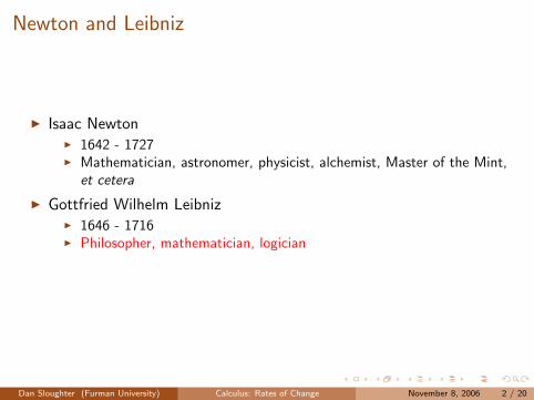
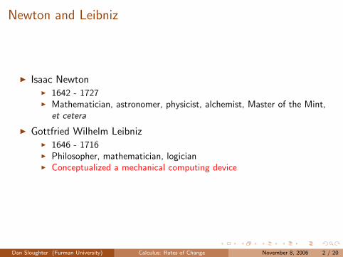
I Isaac Newton
I 1642 - 1727I Mathematician, astronomer, physicist, alchemist, Master of the Mint,
et cetera
I Gottfried Wilhelm Leibniz
I 1646 - 1716I Philosopher, mathematician, logicianI Conceptualized a mechanical computing device
Dan Sloughter (Furman University) Calculus: Rates of Change November 8, 2006 2 / 20
Newton and Leibniz
I Isaac NewtonI 1642 - 1727
I Mathematician, astronomer, physicist, alchemist, Master of the Mint,et cetera
I Gottfried Wilhelm Leibniz
I 1646 - 1716I Philosopher, mathematician, logicianI Conceptualized a mechanical computing device
Dan Sloughter (Furman University) Calculus: Rates of Change November 8, 2006 2 / 20
Newton and Leibniz
I Isaac NewtonI 1642 - 1727I Mathematician, astronomer, physicist, alchemist, Master of the Mint,
et cetera
I Gottfried Wilhelm Leibniz
I 1646 - 1716I Philosopher, mathematician, logicianI Conceptualized a mechanical computing device
Dan Sloughter (Furman University) Calculus: Rates of Change November 8, 2006 2 / 20
Newton and Leibniz
I Isaac NewtonI 1642 - 1727I Mathematician, astronomer, physicist, alchemist, Master of the Mint,
et cetera
I Gottfried Wilhelm LeibnizI 1646 - 1716
I Philosopher, mathematician, logicianI Conceptualized a mechanical computing device
Dan Sloughter (Furman University) Calculus: Rates of Change November 8, 2006 2 / 20
Newton and Leibniz
I Isaac NewtonI 1642 - 1727I Mathematician, astronomer, physicist, alchemist, Master of the Mint,
et cetera
I Gottfried Wilhelm LeibnizI 1646 - 1716I Philosopher, mathematician, logician
I Conceptualized a mechanical computing device
Dan Sloughter (Furman University) Calculus: Rates of Change November 8, 2006 2 / 20
Newton and Leibniz
I Isaac NewtonI 1642 - 1727I Mathematician, astronomer, physicist, alchemist, Master of the Mint,
et cetera
I Gottfried Wilhelm LeibnizI 1646 - 1716I Philosopher, mathematician, logicianI Conceptualized a mechanical computing device
Dan Sloughter (Furman University) Calculus: Rates of Change November 8, 2006 2 / 20
The calculus
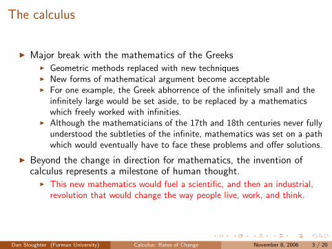
I Major break with the mathematics of the Greeks
I Geometric methods replaced with new techniquesI New forms of mathematical argument become acceptableI For one example, the Greek abhorrence of the infinitely small and the
infinitely large would be set aside, to be replaced by a mathematicswhich freely worked with infinities.
I Although the mathematicians of the 17th and 18th centuries never fullyunderstood the subtleties of the infinite, mathematics was set on a pathwhich would eventually have to face these problems and offer solutions.
I Beyond the change in direction for mathematics, the invention ofcalculus represents a milestone of human thought.
I This new mathematics would fuel a scientific, and then an industrial,revolution that would change the way people live, work, and think.
Dan Sloughter (Furman University) Calculus: Rates of Change November 8, 2006 3 / 20
The calculus
I Major break with the mathematics of the GreeksI Geometric methods replaced with new techniques
I New forms of mathematical argument become acceptableI For one example, the Greek abhorrence of the infinitely small and the
infinitely large would be set aside, to be replaced by a mathematicswhich freely worked with infinities.
I Although the mathematicians of the 17th and 18th centuries never fullyunderstood the subtleties of the infinite, mathematics was set on a pathwhich would eventually have to face these problems and offer solutions.
I Beyond the change in direction for mathematics, the invention ofcalculus represents a milestone of human thought.
I This new mathematics would fuel a scientific, and then an industrial,revolution that would change the way people live, work, and think.
Dan Sloughter (Furman University) Calculus: Rates of Change November 8, 2006 3 / 20
The calculus
I Major break with the mathematics of the GreeksI Geometric methods replaced with new techniquesI New forms of mathematical argument become acceptable
I For one example, the Greek abhorrence of the infinitely small and theinfinitely large would be set aside, to be replaced by a mathematicswhich freely worked with infinities.
I Although the mathematicians of the 17th and 18th centuries never fullyunderstood the subtleties of the infinite, mathematics was set on a pathwhich would eventually have to face these problems and offer solutions.
I Beyond the change in direction for mathematics, the invention ofcalculus represents a milestone of human thought.
I This new mathematics would fuel a scientific, and then an industrial,revolution that would change the way people live, work, and think.
Dan Sloughter (Furman University) Calculus: Rates of Change November 8, 2006 3 / 20
The calculus
I Major break with the mathematics of the GreeksI Geometric methods replaced with new techniquesI New forms of mathematical argument become acceptableI For one example, the Greek abhorrence of the infinitely small and the
infinitely large would be set aside, to be replaced by a mathematicswhich freely worked with infinities.
I Although the mathematicians of the 17th and 18th centuries never fullyunderstood the subtleties of the infinite, mathematics was set on a pathwhich would eventually have to face these problems and offer solutions.
I Beyond the change in direction for mathematics, the invention ofcalculus represents a milestone of human thought.
I This new mathematics would fuel a scientific, and then an industrial,revolution that would change the way people live, work, and think.
Dan Sloughter (Furman University) Calculus: Rates of Change November 8, 2006 3 / 20
The calculus
I Major break with the mathematics of the GreeksI Geometric methods replaced with new techniquesI New forms of mathematical argument become acceptableI For one example, the Greek abhorrence of the infinitely small and the
infinitely large would be set aside, to be replaced by a mathematicswhich freely worked with infinities.
I Although the mathematicians of the 17th and 18th centuries never fullyunderstood the subtleties of the infinite, mathematics was set on a pathwhich would eventually have to face these problems and offer solutions.
I Beyond the change in direction for mathematics, the invention ofcalculus represents a milestone of human thought.
I This new mathematics would fuel a scientific, and then an industrial,revolution that would change the way people live, work, and think.
Dan Sloughter (Furman University) Calculus: Rates of Change November 8, 2006 3 / 20
An example
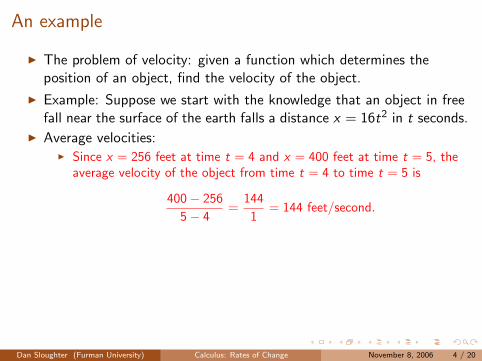
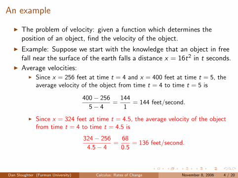
I The problem of velocity: given a function which determines theposition of an object, find the velocity of the object.
I Example: Suppose we start with the knowledge that an object in freefall near the surface of the earth falls a distance x = 16t2 in t seconds.
I Average velocities:
I Since x = 256 feet at time t = 4 and x = 400 feet at time t = 5, theaverage velocity of the object from time t = 4 to time t = 5 is
400− 256
5− 4=
144
1= 144 feet/second.
I Since x = 324 feet at time t = 4.5, the average velocity of the objectfrom time t = 4 to time t = 4.5 is
324− 256
4.5− 4=
68
0.5= 136 feet/second.
Dan Sloughter (Furman University) Calculus: Rates of Change November 8, 2006 4 / 20
An example
I The problem of velocity: given a function which determines theposition of an object, find the velocity of the object.
I Example: Suppose we start with the knowledge that an object in freefall near the surface of the earth falls a distance x = 16t2 in t seconds.
I Average velocities:I Since x = 256 feet at time t = 4 and x = 400 feet at time t = 5, the
average velocity of the object from time t = 4 to time t = 5 is
400− 256
5− 4=
144
1= 144 feet/second.
I Since x = 324 feet at time t = 4.5, the average velocity of the objectfrom time t = 4 to time t = 4.5 is
324− 256
4.5− 4=
68
0.5= 136 feet/second.
Dan Sloughter (Furman University) Calculus: Rates of Change November 8, 2006 4 / 20
An example (cont’d)
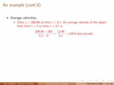
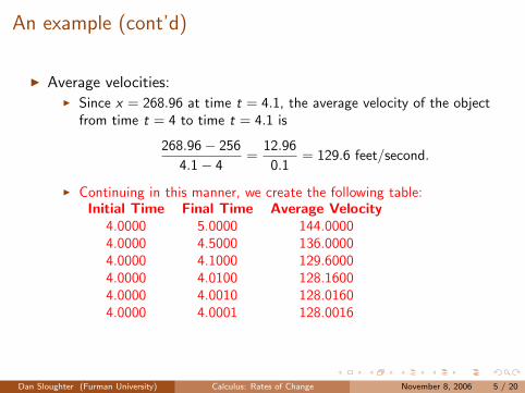
I Average velocities:
I Since x = 268.96 at time t = 4.1, the average velocity of the objectfrom time t = 4 to time t = 4.1 is
268.96− 256
4.1− 4=
12.96
0.1= 129.6 feet/second.
I Continuing in this manner, we create the following table:Initial Time Final Time Average Velocity
4.0000 5.0000 144.00004.0000 4.5000 136.00004.0000 4.1000 129.60004.0000 4.0100 128.16004.0000 4.0010 128.01604.0000 4.0001 128.0016
Dan Sloughter (Furman University) Calculus: Rates of Change November 8, 2006 5 / 20
An example (cont’d)
I Average velocities:I Since x = 268.96 at time t = 4.1, the average velocity of the object
from time t = 4 to time t = 4.1 is
268.96− 256
4.1− 4=
12.96
0.1= 129.6 feet/second.
I Continuing in this manner, we create the following table:Initial Time Final Time Average Velocity
4.0000 5.0000 144.00004.0000 4.5000 136.00004.0000 4.1000 129.60004.0000 4.0100 128.16004.0000 4.0010 128.01604.0000 4.0001 128.0016
Dan Sloughter (Furman University) Calculus: Rates of Change November 8, 2006 5 / 20
An example (cont’d)
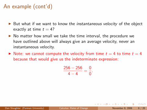
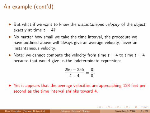
I But what if we want to know the instantaneous velocity of the objectexactly at time t = 4?
I No matter how small we take the time interval, the procedure wehave outlined above will always give an average velocity, never aninstantaneous velocity.
I Note: we cannot compute the velocity from time t = 4 to time t = 4because that would give us the indeterminate expression:
256− 256
4− 4=
0
0.
I Yet it appears that the average velocities are approaching 128 feet persecond as the time interval shrinks toward 4.
Dan Sloughter (Furman University) Calculus: Rates of Change November 8, 2006 6 / 20
An example (cont’d)
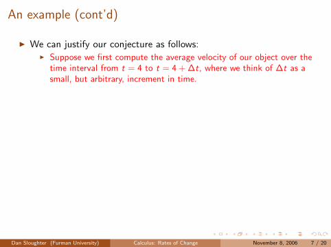
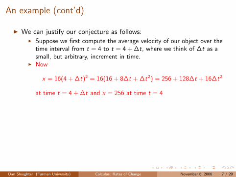
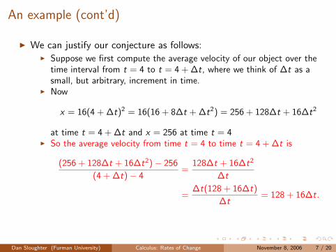
I We can justify our conjecture as follows:
I Suppose we first compute the average velocity of our object over thetime interval from t = 4 to t = 4 + ∆t, where we think of ∆t as asmall, but arbitrary, increment in time.
I Now
x = 16(4 + ∆t)2 = 16(16 + 8∆t + ∆t2) = 256 + 128∆t + 16∆t2
at time t = 4 + ∆t and x = 256 at time t = 4I So the average velocity from time t = 4 to time t = 4 + ∆t is
(256 + 128∆t + 16∆t2)− 256
(4 + ∆t)− 4=
128∆t + 16∆t2
∆t
=∆t(128 + 16∆t)
∆t= 128 + 16∆t.
Dan Sloughter (Furman University) Calculus: Rates of Change November 8, 2006 7 / 20
An example (cont’d)
I We can justify our conjecture as follows:I Suppose we first compute the average velocity of our object over the
time interval from t = 4 to t = 4 + ∆t, where we think of ∆t as asmall, but arbitrary, increment in time.
I Now
x = 16(4 + ∆t)2 = 16(16 + 8∆t + ∆t2) = 256 + 128∆t + 16∆t2
at time t = 4 + ∆t and x = 256 at time t = 4
I So the average velocity from time t = 4 to time t = 4 + ∆t is
(256 + 128∆t + 16∆t2)− 256
(4 + ∆t)− 4=
128∆t + 16∆t2
∆t
=∆t(128 + 16∆t)
∆t= 128 + 16∆t.
Dan Sloughter (Furman University) Calculus: Rates of Change November 8, 2006 7 / 20
An example (cont’d)
I We can justify our conjecture as follows:I Suppose we first compute the average velocity of our object over the
time interval from t = 4 to t = 4 + ∆t, where we think of ∆t as asmall, but arbitrary, increment in time.
I Now
x = 16(4 + ∆t)2 = 16(16 + 8∆t + ∆t2) = 256 + 128∆t + 16∆t2
at time t = 4 + ∆t and x = 256 at time t = 4I So the average velocity from time t = 4 to time t = 4 + ∆t is
(256 + 128∆t + 16∆t2)− 256
(4 + ∆t)− 4=
128∆t + 16∆t2
∆t
=∆t(128 + 16∆t)
∆t= 128 + 16∆t.
Dan Sloughter (Furman University) Calculus: Rates of Change November 8, 2006 7 / 20
An example (cont’d)
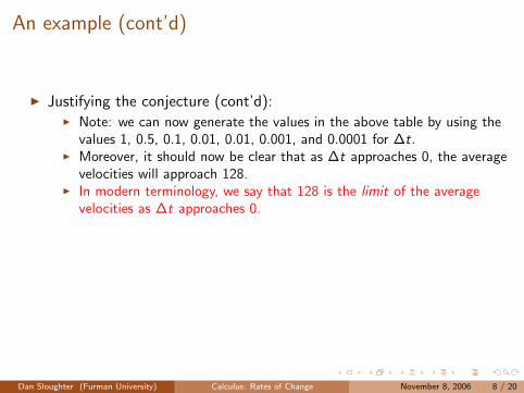
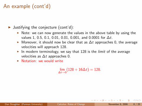
I Justifying the conjecture (cont’d):
I Note: we can now generate the values in the above table by using thevalues 1, 0.5, 0.1, 0.01, 0.01, 0.001, and 0.0001 for ∆t.
I Moreover, it should now be clear that as ∆t approaches 0, the averagevelocities will approach 128.
I In modern terminology, we say that 128 is the limit of the averagevelocities as ∆t approaches 0.
I Notation: we would write
lim∆t→0
(128 + 16∆t) = 128.
Dan Sloughter (Furman University) Calculus: Rates of Change November 8, 2006 8 / 20
An example (cont’d)
I Justifying the conjecture (cont’d):I Note: we can now generate the values in the above table by using the
values 1, 0.5, 0.1, 0.01, 0.01, 0.001, and 0.0001 for ∆t.
I Moreover, it should now be clear that as ∆t approaches 0, the averagevelocities will approach 128.
I In modern terminology, we say that 128 is the limit of the averagevelocities as ∆t approaches 0.
I Notation: we would write
lim∆t→0
(128 + 16∆t) = 128.
Dan Sloughter (Furman University) Calculus: Rates of Change November 8, 2006 8 / 20
An example (cont’d)
I Justifying the conjecture (cont’d):I Note: we can now generate the values in the above table by using the
values 1, 0.5, 0.1, 0.01, 0.01, 0.001, and 0.0001 for ∆t.I Moreover, it should now be clear that as ∆t approaches 0, the average
velocities will approach 128.
I In modern terminology, we say that 128 is the limit of the averagevelocities as ∆t approaches 0.
I Notation: we would write
lim∆t→0
(128 + 16∆t) = 128.
Dan Sloughter (Furman University) Calculus: Rates of Change November 8, 2006 8 / 20
An example (cont’d)
I Justifying the conjecture (cont’d):I Note: we can now generate the values in the above table by using the
values 1, 0.5, 0.1, 0.01, 0.01, 0.001, and 0.0001 for ∆t.I Moreover, it should now be clear that as ∆t approaches 0, the average
velocities will approach 128.I In modern terminology, we say that 128 is the limit of the average
velocities as ∆t approaches 0.
I Notation: we would write
lim∆t→0
(128 + 16∆t) = 128.
Dan Sloughter (Furman University) Calculus: Rates of Change November 8, 2006 8 / 20
An example (cont’d)
I Justifying the conjecture (cont’d):I Note: we can now generate the values in the above table by using the
values 1, 0.5, 0.1, 0.01, 0.01, 0.001, and 0.0001 for ∆t.I Moreover, it should now be clear that as ∆t approaches 0, the average
velocities will approach 128.I In modern terminology, we say that 128 is the limit of the average
velocities as ∆t approaches 0.I Notation: we would write
lim∆t→0
(128 + 16∆t) = 128.
Dan Sloughter (Furman University) Calculus: Rates of Change November 8, 2006 8 / 20
An example (cont’d)
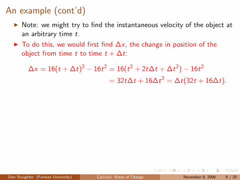
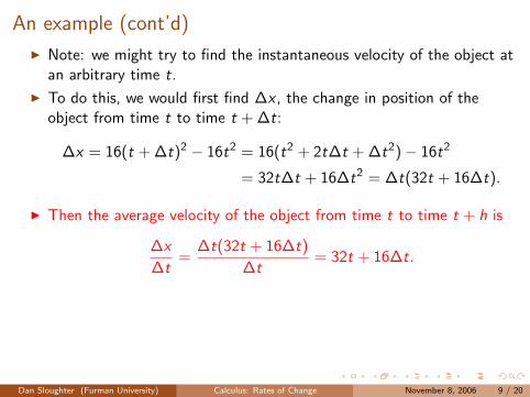
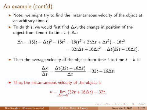
I Note: we might try to find the instantaneous velocity of the object atan arbitrary time t.
I To do this, we would first find ∆x , the change in position of theobject from time t to time t + ∆t:
∆x = 16(t + ∆t)2 − 16t2 = 16(t2 + 2t∆t + ∆t2)− 16t2
= 32t∆t + 16∆t2 = ∆t(32t + 16∆t).
I Then the average velocity of the object from time t to time t + h is
∆x
∆t=
∆t(32t + 16∆t)
∆t= 32t + 16∆t.
I Thus the instantaneous velocity of the object is
v = lim∆t→0
(32t + 16∆t) = 32t.
Dan Sloughter (Furman University) Calculus: Rates of Change November 8, 2006 9 / 20
An example (cont’d)
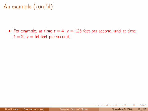
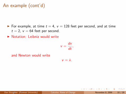
I For example, at time t = 4, v = 128 feet per second, and at timet = 2, v = 64 feet per second.
I Notation: Leibniz would write
v =dx
dt,
and Newton would writev = x .
Dan Sloughter (Furman University) Calculus: Rates of Change November 8, 2006 10 / 20
An example (cont’d)
I For example, at time t = 4, v = 128 feet per second, and at timet = 2, v = 64 feet per second.
I Notation: Leibniz would write
v =dx
dt,
and Newton would writev = x .
Dan Sloughter (Furman University) Calculus: Rates of Change November 8, 2006 10 / 20
Rates of change
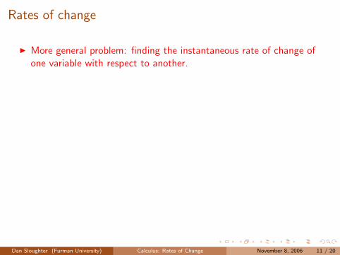
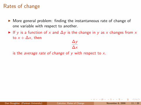
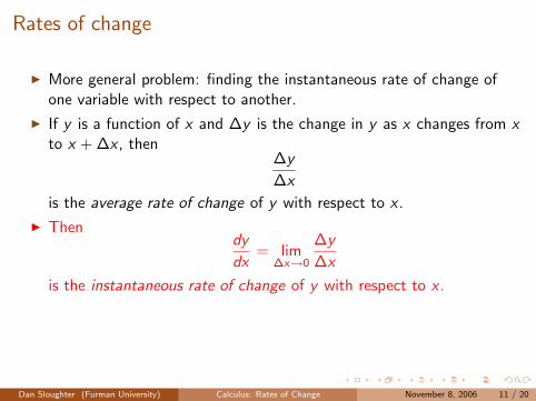
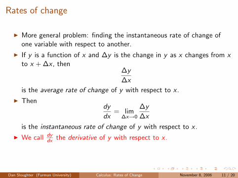
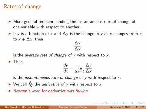
I More general problem: finding the instantaneous rate of change ofone variable with respect to another.
I If y is a function of x and ∆y is the change in y as x changes from xto x + ∆x , then
∆y
∆x
is the average rate of change of y with respect to x .
I Thendy
dx= lim
∆x→0
∆y
∆x
is the instantaneous rate of change of y with respect to x .
I We call dydx the derivative of y with respect to x .
I Newton’s word for derivative was fluxion.
Dan Sloughter (Furman University) Calculus: Rates of Change November 8, 2006 11 / 20
Rates of change
I More general problem: finding the instantaneous rate of change ofone variable with respect to another.
I If y is a function of x and ∆y is the change in y as x changes from xto x + ∆x , then
∆y
∆x
is the average rate of change of y with respect to x .
I Thendy
dx= lim
∆x→0
∆y
∆x
is the instantaneous rate of change of y with respect to x .
I We call dydx the derivative of y with respect to x .
I Newton’s word for derivative was fluxion.
Dan Sloughter (Furman University) Calculus: Rates of Change November 8, 2006 11 / 20
Interpretation
I The interpretation of an instantaneous rate of change depends onwhat the variables represent in the particular situation.
I Example: If x is position and t is time, then dxdt is velocity.
I Example: If v is velocity and t is time, then dvdt is acceleration.
Dan Sloughter (Furman University) Calculus: Rates of Change November 8, 2006 12 / 20
Interpretation (cont’d)
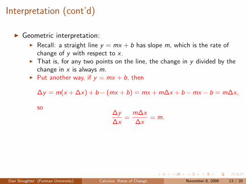
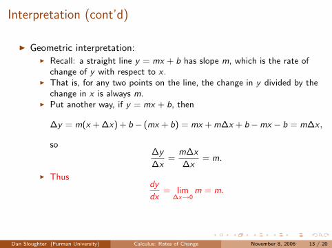
I Geometric interpretation:
I Recall: a straight line y = mx + b has slope m, which is the rate ofchange of y with respect to x .
I That is, for any two points on the line, the change in y divided by thechange in x is always m.
I Put another way, if y = mx + b, then
∆y = m(x + ∆x) + b− (mx + b) = mx + m∆x + b−mx − b = m∆x ,
so∆y
∆x=
m∆x
∆x= m.
I Thusdy
dx= lim
∆x→0m = m.
Dan Sloughter (Furman University) Calculus: Rates of Change November 8, 2006 13 / 20
Interpretation (cont’d)
I Geometric interpretation:I Recall: a straight line y = mx + b has slope m, which is the rate of
change of y with respect to x .
I That is, for any two points on the line, the change in y divided by thechange in x is always m.
I Put another way, if y = mx + b, then
∆y = m(x + ∆x) + b− (mx + b) = mx + m∆x + b−mx − b = m∆x ,
so∆y
∆x=
m∆x
∆x= m.
I Thusdy
dx= lim
∆x→0m = m.
Dan Sloughter (Furman University) Calculus: Rates of Change November 8, 2006 13 / 20
Interpretation (cont’d)
I Geometric interpretation:I Recall: a straight line y = mx + b has slope m, which is the rate of
change of y with respect to x .I That is, for any two points on the line, the change in y divided by the
change in x is always m.
I Put another way, if y = mx + b, then
∆y = m(x + ∆x) + b− (mx + b) = mx + m∆x + b−mx − b = m∆x ,
so∆y
∆x=
m∆x
∆x= m.
I Thusdy
dx= lim
∆x→0m = m.
Dan Sloughter (Furman University) Calculus: Rates of Change November 8, 2006 13 / 20
Interpretation (cont’d)
I Geometric interpretation:I Recall: a straight line y = mx + b has slope m, which is the rate of
change of y with respect to x .I That is, for any two points on the line, the change in y divided by the
change in x is always m.I Put another way, if y = mx + b, then
∆y = m(x + ∆x) + b− (mx + b) = mx + m∆x + b−mx − b = m∆x ,
so∆y
∆x=
m∆x
∆x= m.
I Thusdy
dx= lim
∆x→0m = m.
Dan Sloughter (Furman University) Calculus: Rates of Change November 8, 2006 13 / 20
Interpretation (cont’d)
I Geometric interpretation (cont’d):
I For a curve given by an equation relating y with x , dydx represents the
slope of the curve at the point (x , y) on the curve.I This is also the slope of the line tangent to the curve at (x , y).I Note: unlike the slope of a line, in general the slope of a curve will
change from point to point on the curve.
Dan Sloughter (Furman University) Calculus: Rates of Change November 8, 2006 14 / 20
Interpretation (cont’d)
I Geometric interpretation (cont’d):I For a curve given by an equation relating y with x , dy
dx represents theslope of the curve at the point (x , y) on the curve.
I This is also the slope of the line tangent to the curve at (x , y).I Note: unlike the slope of a line, in general the slope of a curve will
change from point to point on the curve.
Dan Sloughter (Furman University) Calculus: Rates of Change November 8, 2006 14 / 20
Interpretation (cont’d)
I Geometric interpretation (cont’d):I For a curve given by an equation relating y with x , dy
dx represents theslope of the curve at the point (x , y) on the curve.
I This is also the slope of the line tangent to the curve at (x , y).
I Note: unlike the slope of a line, in general the slope of a curve willchange from point to point on the curve.
Dan Sloughter (Furman University) Calculus: Rates of Change November 8, 2006 14 / 20
Interpretation (cont’d)
I Geometric interpretation (cont’d):I For a curve given by an equation relating y with x , dy
dx represents theslope of the curve at the point (x , y) on the curve.
I This is also the slope of the line tangent to the curve at (x , y).I Note: unlike the slope of a line, in general the slope of a curve will
change from point to point on the curve.
Dan Sloughter (Furman University) Calculus: Rates of Change November 8, 2006 14 / 20
Example
I For the parabola y = x2,
∆y = (x + ∆x)2 − x2 = x2 + 2x∆x + ∆x2 − x2 = ∆x(2x + ∆x),
so∆y
∆x=
∆x(2x + ∆x)
∆x= 2x + ∆x .
I Hencedy
dx= lim
∆x→0(2x + ∆x) = 2x .
I For example: The curve y = x2 has slope 0 at x = 0, slope 4 atx = 2, and slope −2 at x = −1.
Dan Sloughter (Furman University) Calculus: Rates of Change November 8, 2006 15 / 20
Example (cont’d)
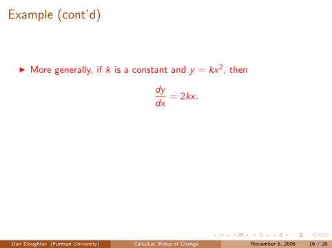
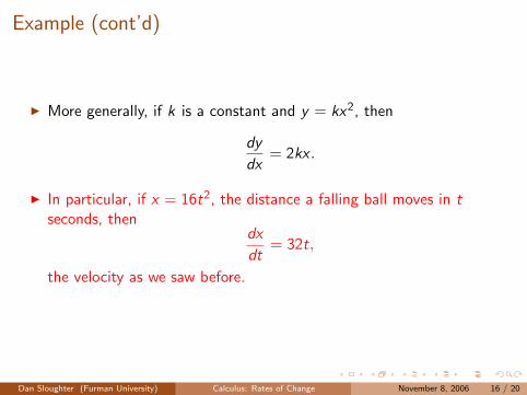
I More generally, if k is a constant and y = kx2, then
dy
dx= 2kx .
I In particular, if x = 16t2, the distance a falling ball moves in tseconds, then
dx
dt= 32t,
the velocity as we saw before.
Dan Sloughter (Furman University) Calculus: Rates of Change November 8, 2006 16 / 20
Example (cont’d)
I More generally, if k is a constant and y = kx2, then
dy
dx= 2kx .
I In particular, if x = 16t2, the distance a falling ball moves in tseconds, then
dx
dt= 32t,
the velocity as we saw before.
Dan Sloughter (Furman University) Calculus: Rates of Change November 8, 2006 16 / 20
Example
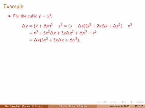
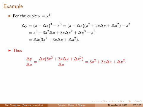
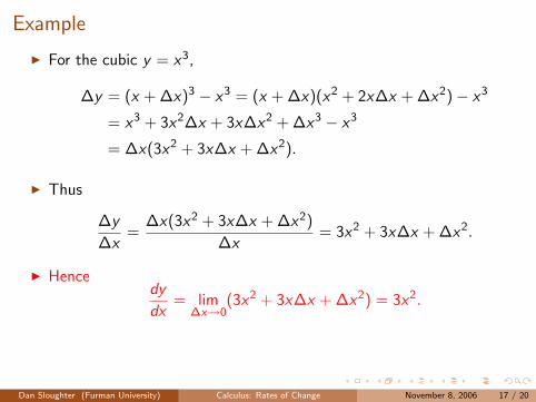
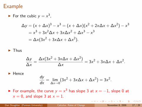
I For the cubic y = x3,
∆y = (x + ∆x)3 − x3 = (x + ∆x)(x2 + 2x∆x + ∆x2)− x3
= x3 + 3x2∆x + 3x∆x2 + ∆x3 − x3
= ∆x(3x2 + 3x∆x + ∆x2).
I Thus
∆y
∆x=
∆x(3x2 + 3x∆x + ∆x2)
∆x= 3x2 + 3x∆x + ∆x2.
I Hencedy
dx= lim
∆x→0(3x2 + 3x∆x + ∆x2) = 3x2.
I For example, the curve y = x3 has slope 3 at x = −1, slope 0 atx = 0, and slope 3 at x = 1.
Dan Sloughter (Furman University) Calculus: Rates of Change November 8, 2006 17 / 20
Example
I For the cubic y = x3,
∆y = (x + ∆x)3 − x3 = (x + ∆x)(x2 + 2x∆x + ∆x2)− x3
= x3 + 3x2∆x + 3x∆x2 + ∆x3 − x3
= ∆x(3x2 + 3x∆x + ∆x2).
I Thus
∆y
∆x=
∆x(3x2 + 3x∆x + ∆x2)
∆x= 3x2 + 3x∆x + ∆x2.
I Hencedy
dx= lim
∆x→0(3x2 + 3x∆x + ∆x2) = 3x2.
I For example, the curve y = x3 has slope 3 at x = −1, slope 0 atx = 0, and slope 3 at x = 1.
Dan Sloughter (Furman University) Calculus: Rates of Change November 8, 2006 17 / 20
Example (cont’d)
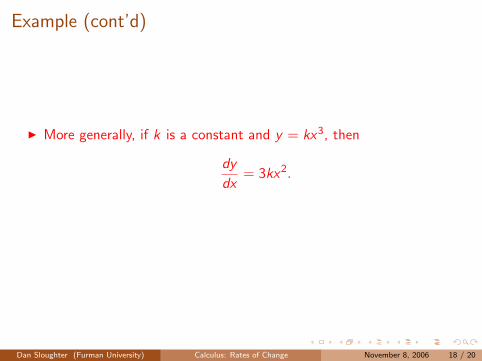
I More generally, if k is a constant and y = kx3, then
dy
dx= 3kx2.
Dan Sloughter (Furman University) Calculus: Rates of Change November 8, 2006 18 / 20
Problems
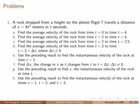
1. A rock dropped from a height on the planet Rigel 7 travels a distanceof x = 4t2 meters in t seconds.
a. Find the average velocity of the rock from time t = 0 to time t = 4.b. Find the average velocity of the rock from time t = 2 to time t = 4.c. Find the average velocity of the rock from time t = 2 to time t = 2.5.d. Find the average velocity of the rock from time t = 2 to time
t = 2 + ∆t, where ∆t 6= 0.e. Use the preceding result to find the instantaneous velocity of the rock at
time t = 2.f. Find ∆x , the change in x as t changes from t to t + ∆t, ∆t 6= 0.g. Use the preceding result to find v , the instantaneous velocity of the rock
at time t.h. Use the preceding result to find the instantaneous velocity of the rock at
times t = 1, t = 2, and t = 3.
Dan Sloughter (Furman University) Calculus: Rates of Change November 8, 2006 19 / 20
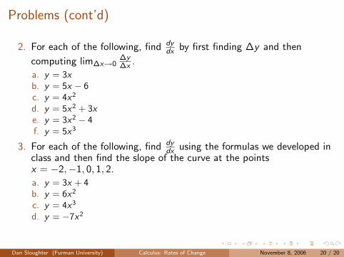
Problems (cont’d)
2. For each of the following, find dydx by first finding ∆y and then
computing lim∆x→0∆y∆x .
a. y = 3xb. y = 5x − 6c. y = 4x2
d. y = 5x2 + 3xe. y = 3x2 − 4f. y = 5x3
3. For each of the following, find dydx using the formulas we developed in
class and then find the slope of the curve at the pointsx = −2,−1, 0, 1, 2.
a. y = 3x + 4b. y = 6x2
c. y = 4x3
d. y = −7x2
Dan Sloughter (Furman University) Calculus: Rates of Change November 8, 2006 20 / 20