Calculus Maximus Notes 12.2: Newton’s Method

Page 1 of 4

§12.2—Newton’s Method

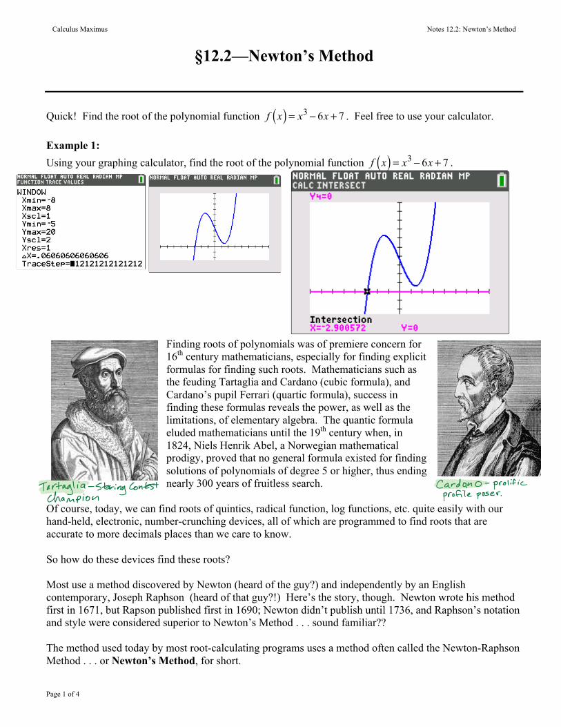
Quick! Find the root of the polynomial function f x( ) = x3 − 6x + 7 . Feel free to use your calculator. Example 1: Using your graphing calculator, find the root of the polynomial function f x( ) = x3 − 6x + 7 .

Finding roots of polynomials was of premiere concern for 16th century mathematicians, especially for finding explicit formulas for finding such roots. Mathematicians such as the feuding Tartaglia and Cardano (cubic formula), and Cardano’s pupil Ferrari (quartic formula), success in finding these formulas reveals the power, as well as the limitations, of elementary algebra. The quantic formula eluded mathematicians until the 19th century when, in 1824, Niels Henrik Abel, a Norwegian mathematical prodigy, proved that no general formula existed for finding solutions of polynomials of degree 5 or higher, thus ending nearly 300 years of fruitless search.

Of course, today, we can find roots of quintics, radical function, log functions, etc. quite easily with our hand-held, electronic, number-crunching devices, all of which are programmed to find roots that are accurate to more decimals places than we care to know. So how do these devices find these roots? Most use a method discovered by Newton (heard of the guy?) and independently by an English contemporary, Joseph Raphson (heard of that guy?!) Here’s the story, though. Newton wrote his method first in 1671, but Rapson published first in 1690; Newton didn’t publish until 1736, and Raphson’s notation and style were considered superior to Newton’s Method . . . sound familiar?? The method used today by most root-calculating programs uses a method often called the Newton-Raphson Method . . . or Newton’s Method, for short.

Calculus Maximus Notes 12.2: Newton’s Method

Page 2 of 4

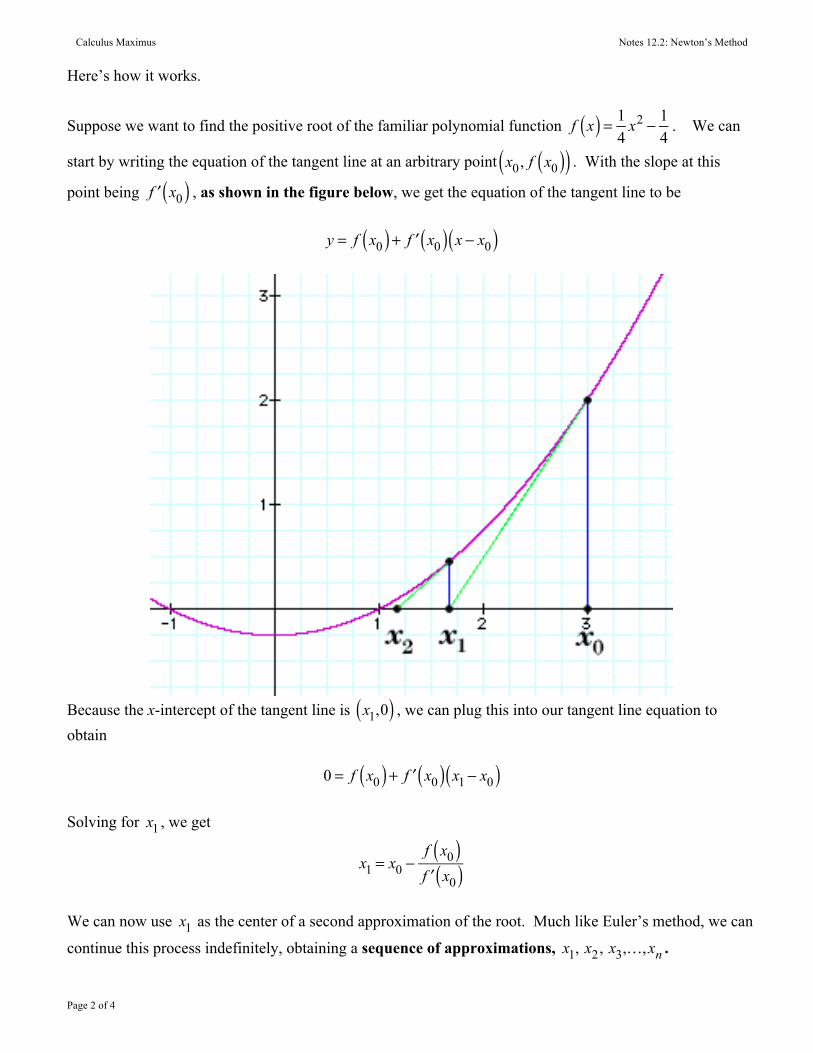
Here’s how it works.

Suppose we want to find the positive root of the familiar polynomial function f x( ) = 1

4x2 − 1

4. We can

start by writing the equation of the tangent line at an arbitrary point

x0, f x0( )( ) . With the slope at this

point being ′f x0( ) , as shown in the figure below, we get the equation of the tangent line to be

y = f x0( ) + ′f x0( ) x − x0( )

Because the x-intercept of the tangent line is

x1,0( ) , we can plug this into our tangent line equation to

obtain

0 = f x0( ) + ′f x0( ) x1 − x0( )

Solving for x1 , we get

x1 = x0 −

f x0( )′f x0( )

We can now use x1 as the center of a second approximation of the root. Much like Euler’s method, we can

continue this process indefinitely, obtaining a sequence of approximations, x1, x2, x3,…,xn .

Calculus Maximus Notes 12.2: Newton’s Method

Page 3 of 4

If we let xn be the nth approximation, and if

′f xn( ) ≠ 0 , then the NEXT approximation will be

xn+1 = xn −

f xn( )′f xn( )

If this sequence converges, then it converges to the root, r, and we say

lim

n→∞xn = r

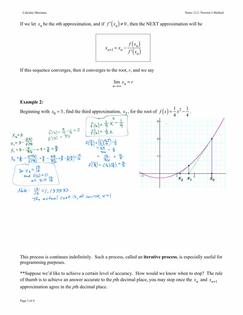
Example 2:

Beginning with x0 = 3 , find the third approximation, x2 , for the root of f x( ) = 1

4x2 − 1

4.

This process is continues indefinitely. Such a process, called an iterative process, is especially useful for programming purposes. **Suppose we’d like to achieve a certain level of accuracy. How would we know when to stop? The rule of thumb is to achieve an answer accurate to the pth decimal place, you may stop once the xn and xn+1 approximation agree in the pth decimal place.

Calculus Maximus Notes 12.2: Newton’s Method

Page 4 of 4

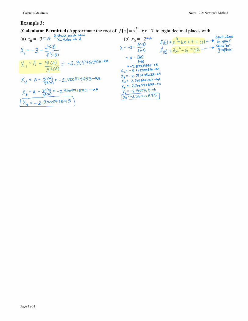
Example 3: (Calculator Permitted) Approximate the root of f x( ) = x3 − 6x + 7 to eight decimal places with

(a) x0 = −3 (b) x0 = −2