CALCULUSTable of Contents

Calculus I, First Semester

Chapter 1. Rates of Change, Tangent Lines and Differentiation 11.1. Newton’s Calculus 11.2. Liebniz’ Calculus of Differentials 131.3. The Chain Rule 141.4. Trigonometric Functions 161.5. Implicit Differentiation and Related Rates 19

Chapter 2. Theoretical Considerations 242.1. Limit Operations 242.2. Limits at Infinity 292.3. Some Basic Theorems 342.4. l’Hopitals Rule 36

Chapter 3. Extrema, Concavity and Graphs 403.1. Monotonicity and the First Derivative 403.2. Optimization 423.3. Concavity and the Second Derivative 453.4. Graphing Functions 47

Rational Functions 47Other Sketches 51

Chapter 4. Integration: A Differential Equations Approach 554.1. Antiderivatives 554.2. Area 594.3 Separation of Variables 644.4. The Exponential Function 694.5 The Logarithm 754.6 Growth and Decay 79

Inhibited Growth 80

Chapter 5. Integration: The Accumulation Method 865.1. The Definite Integral he Fundamental Theorem of the Calculus 865.2. Summation and the Definition of Area 925.3. Volume 95

Volumes of Revolution 995.4. Arc Length 1045.5. Work 1095.6 Mass and Moments 113

Centroids 118

i

Calculus II, Second Semester

Chapter 6. Transcendental Functions 1226.1. Inverse Functions 1226.2. The Inverse Trigonometric Functions 1276.3 First Order Differential Equations 130

Chapter 7. Techniques of Integration 1367.1. Substitution 1367.2. Integration by Parts 1397.3. Partial Fractions 1437.4. Trigonometric Methods 149

Chapter 8. Indeterminate Forms and Improper Integrals 1538.1. L’Hopital’s Rule 1538.2 Other Indeterminate Forms 1568.3 Improper Integrals: Infinite Intervals 1588.4 Improper Integrals: Finite Asymptotes 161

Chapter 9. Sequences and Series 1649.1. Sequences 1649.2. Series 1349.3. Tests for Convergence 1759.4. Power Series 1809.5. Taylor Series 184

Chapter 10 Numerical Methods 19110.1. Taylor Approximation 19110.2. Newton’s Method 19510.3. Numerical Integration 198

Chapter 11. Conics and Polar Coordinates 20311.1. Quadratic Relations 20311.2. Eccentricity and Foci 21011.3. String and Optical Properties of the Conics 21511.4. Polar Coordinates 21911.5. Calculus in Polar Corrdinates 225

Chapter 12. Second Order Linear Differential Equations 22812.1. Homogeneous Equations 22812.2. Behavior of the Solutions 23312.3. Applications 23512.4. The Inhomogeneous equation 238

ii

Calculus III, Third Semester

Chapter 13. Vector Algebra 24113.1 Basic Concepts 24113. 2. Vectors in the Plane 24313.3. Vectors in Space 25313.4. Lines and Planes in Space 259

Chapter 14. Particles in Motion; Kepler’s Laws 26514.1 Vector Functions 26514.2 Planar Particle Motion 26914.3 Particle Motion in Space 27314.4 Derivation of Kepler’s Laws of Planetary Motion from Newton’s Laws 276

Chapter 15. Coordinates and Surfaces 28115.1 Change of Coordinates in Two Dimensions 28115.2 Special Coordinate Systems 28715.3 Surfaces; Graphs and Level Curves 29215.4 Cylinders and Surfaces of Revolution 29515.5. Quadric Surfaces 296

Chapter 16. Differentiable Functions of Several Variables 30216.1 The Differential and Partial Derivatives 30216.2 Gradients and Vector Methods 30916. 3 Theoretical Considerations 31516.4 Optimization 317

The Method of Lagrange Multipliers 320

Chapter 17. Multiple Integration 32417.1 Integration on Planar Regions 32417.2. Applications 33117.3. Theoretical Considerations 33417.4. Integration in Other Coordinates 33717.5 Triple Interals 347

Integration in Other Coordinates 350

Chapter 18. Vector Calculus 35418.1 Vector Fields 35418.2 Line Integrals and Work 36018.3 Independence of Path 36418.4. Green’s Theorem in the Plane 36718.5 Stokes’ and Gauss’ Theorems in Three Dimensions 370

iii

Preface

As I neared the end of a second decade of teaching Calculus at the University of Utah, I becameaware of a student type that persisted in all my classes, comprising between 10 and 20 percent ofthe class. These students came to class irregularly, often just to ask a question about one of themore demanding problems. They took all the exams, and, almost uniformly ended up with gradesin the top quartile. Looking at their transcripts, and talking with several of them, I discoveredthat they were among the better prepared of the Calculus students, having taken Calculus in highschool, either in an AP class, or from another country. Now, the University of Utah has an APCalculus course for such students, but as that course emphasizes theory, these students preferredto be in the regular engineering sequence. As these students were well grounded in Algebra, andhad already seen some of the basics of Calculus, I concluded that what was appropriate for themwas a course in Calculus that emphasized a deep intuitive understanding of Calculus and problemssets that depended on, and extended that understanding.

So, with the collusion of my chair, I started an intensive summer calculus course: all three semestersin ten weeks. After all, if this population was ten percent of the total Calculus cohort, and if half ofthose took the summer course, that would provide a class of about 50 students enough to make theexperiment economically feasible. We met in this class for five hours a day, five days a week. Forabout half the time the instructor developed the basic ideas, illustrating them through problems,and for the rest of the time, the students do their homework in the presence of graduate assistants.This worked, and that course continues still with about the same numbers of students.

I taught that course for three years, and then turned to developing an online course, based onthe same approach. The first few semesters were difficult: there was not a good fit between thetext and the online problem sets I had created. I spent many hours responding to email inquiries,started to write and post supplementary notes, and decided that it was a good idea to keep pastyears’ problems with solutions posted. As new email inquiries and responses were integrated intothe supplementary notes, it occurred to me that I had almost a complete first draft of a text onCalculus. I spent about a semester organizing the material and completing it to a full text thatstill exists as a supplementary text for the online course.

That is the genesis of this text. As a result, it is thin on drill exercises, informal and intuitive ontheoretical issues, approaches the ideas of the subject in the context of the problems they solve,and is rich in examples that illustrate those ideas. As such, it has served well that class of studentswith sufficient technical competence to follow the ideas in an argument.

Conceptual Apporach of the Text

There is no chapter 0: survey of algebra, trigonometry and pre-calculus. It is assumed that studentshave sufficient grasp of the concept of function to be able to get right into that which the Calculusis about. Ideas and techniques from the pre-calculus are reviewed in context as the need for themarises.

The approach in Chapter 1 is intuitive and informal: the fundamental issue is to see how un-derstanding of rules of change leads to qualitative comprehension of processes and predictions offuture behavior. The first two sections start with the Newton and Liebniz approaches to Differen-tial Calculus. The Newtonian approach is presented as one focusing on rates of change of functionsof a given independent variable (usually time), while that of Liebniz deals with variables and how

iv

they change with respect to each other. In this way, the two threads of derivatives (Newton) anddifferentials (Liebniz) are introduced and used throughout the text to develop the various ways oflooking at a particular process.

I’ve always been of two minds concerning theoretical issues. I feel that they are too deep for thefirst calculus course, but find it difficult to be vague and intuitive about them. So, the approachI’ve adopted in this text is that of Newton: position and velocity are measurable attributes ofmoving bodies, and the limit idea of calculus is the tool for solving problems about movement.Similarly, area is a measurable attribute of planar figures, and the idea of accumulation of theCalculus is the tool for calculating area from the algebraic expressions delimiting the figure. Theproblems of existence of limits and area are thus avoided.

On the other hand, there are real issues in relating velocity with change in position, and in definingarea, and I can’t allow myself to sneak through the calculus without pointing it out. Thesediscussions are collected in sections entitled something like ”theoretical considerations.”

As a result this text has no preliminary section on limits. I feel that this would be misplaced:students get the erroneous impression that a limit is calculated by substitution if the function isgiven by a formula, and otherwise one should look at the graph. So, at the beginning, the calculusof polynomials is developed, and the calculation of the derivative is done algebraically. Derivationof the trigonometric functions is presented using Pascal’s idea. Here the issue of existence of limitsis joined: we must know that lim sinx/x = 1 as x approaches zero. This is discussed in chapter2, in which a wide variety of questions of limits is discussed, including l’Hopital’s rule, which isusually postponed to second semester.

Similarly, integration is introduced as the problem of finding functions with given derivatives usingthe idea of differentials. It is essential that students understand that it is a differential, not afunction, that is integrated. By showing that the differential of the area underneath a curvey = f(x) is f(x)dx, we see that that area is given by integration. The technigue of integration bysubstitution is a direct consequence of the chain rule. From there, we move directly into solvingseparable differential equations (of the type f(x)dx = g(y)dy) and from there to the introductionof the exponential function as the solution of dy/y = rdx. Then, in the subsequent chapter theissue of existence of area is taken up; we turn to the integral as a limit of an accumulation processand the Fundamental Theorem of the Calculus is now seen as the binding together of the Newtonand Liebniz approaches.

New techniques and ideas are introduced (where ever possible) in the context of a problem tobe solved. Thus the chapter on sequences and series is viewed as developing a technique forapproximating values of transcendental functions. Conics are introduced as a tool for understandingquadratic relations, and this leads directly into the study of second order equations.

The Chapter on Vector Calculus is based on intuition provided by fluid flows. The motivationis that it is better to emphasize the understanding of the physical content of the fundamentaltheorems of vector calculus, rather than providing proofs of these theorems. After all, the correcrtproofs of these theorems reduce them to the one-variable fundamental theorem of the calculus byjudicious choice of coordinates. The hard part, best deferred to the course in Advanced Calculus,is to show that the statement of the theorems is independent of the coordinates in which they arecalculated.

v

Outline of the Text

First Semester

In Chapter 1 the basics of the differential calculus are introduced, mostly in the context of poly-nomial functions and relations. In section four the derivatives of the trigonometric functions arefound using the differential triangle of Pascal.

Chapter 2 discusses the concept of limit, techniques for calculating limits, including l’Hopital’srule. We show that the sine function is differentiable (a fact postponed from chapter 1). Limitsat infinity and asymptotes are discussed. The point of the last section is the affirmation that afunction with derivative 0 everywhere in an interval is constant. This is always a difficult passagein the first calculus course, for the students see this as the tautology that a function with no changethroughout an interval ends up at the same value with which it started. So, the instructor hasto first convince the student that there is a real issue here. In class, I’ll do that by exhibitingthe Cantor function, which is almost always constant, but somehow gets from 0 to 1. Thenthe instructor must confess that the issue will not be joined, and instead this fundamental factwill be shown to follow from statements (intermediate value, existence of maxima for continuousfunctions) that, for some reason, are more intuitively obvious. I leave the strategy for doing thisto the instructor, and instead just lay down the minimal exposition.

Chapter 3 covers the geometric significance of the first and second derivatives, optimization andgraph sketching,

Chapter 4 introduces integration as the process reverse to differentiation, and extends this toseparable differential equations. This leads to the introduction of the exponential function as thesolution of dy/y = rdx. I do not feel that it is necessary to discuss the general concept of inversefunctions to get from the exponential to the logarithm; the logarithm is simply what we use to finda if we know ea.

Chapter 5 turns to Liebniz’ concept of integration as a method of accumulation, and shows (throughthe Fundamental theorem) that the Calculi of Newton and Liebniz are the same subject. This isfollowed by the application of integration to a variety of accumulation processes.

Covering these first 5 chapters in one semester is a tall order. It may be that the course willend with the fundamental theorem, and that the second semester starts with the applications ofintegration. Alternatively, some sections of these first five chapters may be omitted.

Second Semester

We are now in a position to abstractly discuss inverse functions and the fact that a function withnonzero derivative in an interval has an inverse, leading to the introduction of many useful tran-scendental functions. This, together with the solution of general first order differential equations,is covered in Chapter 6.

Chapter 7 covers the techniques of integration necessary to make use of a table of integrals: substi-tution, integration by parts and partial fractions. It is the intent of this text that from this pointon, students will use a table of integrals.

vi

Chapter 8 begins with a brief review of l’Hopital’s rule, as some instructors may prefer to coverthis in the second semester. Then Improper Integrals are covered as this material will be necessaryfor the next chapter.

We begin Chapter 9 (Sequences and Series) with a more formal discussion of the Principle ofMathematical Induction (although it has already been used informally in several places in thetext), in connection with the definition of sequences by recursion. As the point of this chapter isto develop ways to approximate values of transcendental functions, the focus is to get to Taylorseries quickly. It also works to cover section 10.1 (on the Taylor formula with estimate) beforeChapter 9, to better motivate the discussion of series. The important thing is to emphasize that acalculation is not an approximation without some estimate of the error.

Chapter 10 is a brief introduction to the simplest numerical methods; enough to give an idea ofhow the basic computer algorithms work.

Chapter 11 covers materials on the conics and polar coordinates. Although this material is tradi-tionally pre-calculus, it is necessary to review it before launching into mulit-variate calculus. Thestring properties of the conics are derived, and their optical properties are derived as differentialversions of the string properties.

Chapter 12 covers the usual material on second order differential equations and basic harmon-ics. Many students will have already covered this in the physics classes, and in many cases this isdone at the beginning of the course on differential equations. Thus, this chapter may be omitted,particularly if Calculus is three quarters rather than three semesters.

Third Semester

The introduction to Vector Algebra (chapter 13) is motivated by geometry, the point being tocharacterize linear subspaces in two and three dimensions in a variety of ways.

One of the central themes of this text is the study of particles in motion; we discuss the calculus ofvector-valued functions of a single variable (Chapter 14)in this context. Sections 2 and three coverthe differential geometry of curves in two and three dimensions, and section 4 provides a derivationof Kepler’s Laws of Planetary Motion from Newton’s Laws of Motion.

Chapter 15 (Coordinates and Surfaces) covers the basic geometric tools of the several variablecalculus: change of coordinates in two and three variables, surfaces, and in particular, the normalforms of quadrics.

Chapters 16 and 17 cover differentiation and integration in several variables. The differential of afunction is introduced as the linear function which best fits the given function near a base point.Applications of integrals are discussed in detail in two dimensions.

Chapter 18 (Vector Calculus) is motivated as the study of fluids in motion, paralleling the themeof particles in motion for the single variable calculus. The basic forms (curl and divergence) areintroduced in this context. This leads to an interpretation that makes the fundamental theorems(Green, Stokes, Gauss) plausible. Here the emphasis is on the examples which show how to useand apply these theorems.

vii

CALCULUS I, First Semester

I. Rate of Change, Tangent Line and Differentiation

1.1 Newton’s Calculus

Early in his career, Isaac Newton wrote, but did not publish, a paper referred to as the tractof october 1666. This was his sole work purely on mathematics, and contained the fundamentalideas and techniques of the calculus. While writing (1684-87) the Principia Mathematica, thefundamental exposition of his mathematical physics of “the system of the world”, he reworkedand expanded these ideas and included them as part of this treatise. Newton’s central conceptionwas that of objects in motion. To Newton motion is described by the position and velocity of theparticle relative to a fixed coordinate system, as functions of time. These then are the fundamentalvariables: x, y, z, etc., and their velocities are denoted by x, y, z, etc. Now, velocity is a measureof the rate of change of position (and acceleration, denoted x, etc., is a rate of change of velocity),and what was needed was a means to express this relationship, and a process of deriving relationsamong the various velocities and accelerations from given relations among the variables. This isthe Calculus of Newton.

Calculus, as it is presented today starts in the context of two variables, or measurable quantities,x, y, which are related in the sense that values of one of the variables determine values of the other.A function y = f(x) is a rule which specifies this relation between the input or independent variablex and the output or dependent variable y. This may be given by a formula, a table, or a computeralgorithm; in fact, any set of rules which uniquely determine outputs for given inputs. The set ofallowable values for the input variable is called the domain of the function, and the set of outputs,the range. In our context both the domain and the range are sets of real numbers.

An interval is the set of all real numbers between specified real numbers c and d. This is denotedby

(1.1) (c, d) = {x : c < x < d}

if neither endpoint is included, and by

(1.2) [c, d] = {x : c ≤ x ≤ d}

if both are included. We shall say “I is an interval about a” to mean that a is between theendpoints of the interval I.

Now, suppose that y = f(x) is a function defined for all x in an interval I = (c, d). The graph off is the set of all points (x, y) in the plane where x is in the interval (c, d) and y = f(x). Calculusstudies the behavior of y as a function of x in terms of the way y changes as x changes. For x0, x1

points in the interval, and y0 = f(x0), y1 = f(x1), the ratio

(1.3)∆y

∆x=

y1 − y0

x1 − x0

is called the average rate of change of y with respect to x in the interval between x0 and x1. Thisis the ratio of the change in y (denoted ∆y) with the change in x (denoted ∆x).

1

Linear Functions

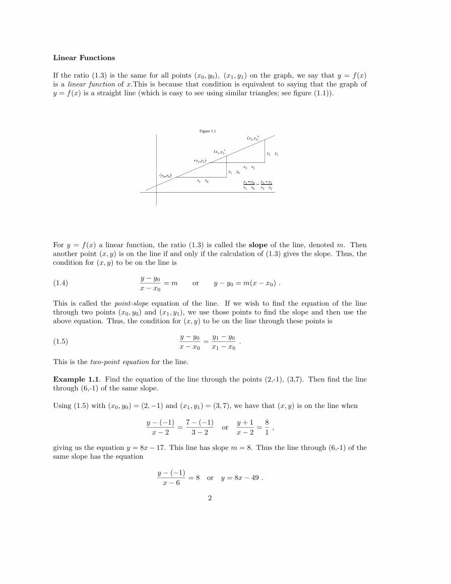
If the ratio (1.3) is the same for all points (x0, y0), (x1, y1) on the graph, we say that y = f(x)is a linear function of x.This is because that condition is equivalent to saying that the graph ofy = f(x) is a straight line (which is easy to see using similar triangles; see figure (1.1)).

Figure 1.1

�x0 � y0 �

�x2 � y2 �

�x3 � y3 �

x1 � x0

y1 � y0

x3 � x2

y3 � y2

y1 � y0x1 � x0 �

y3 � y2x3 � x2

�x1 � y1 �

For y = f(x) a linear function, the ratio (1.3) is called the slope of the line, denoted m. Thenanother point (x, y) is on the line if and only if the calculation of (1.3) gives the slope. Thus, thecondition for (x, y) to be on the line is

(1.4)y − y0

x− x0= m or y − y0 = m(x− x0) .

This is called the point-slope equation of the line. If we wish to find the equation of the linethrough two points (x0, y0) and (x1, y1), we use those points to find the slope and then use theabove equation. Thus, the condition for (x, y) to be on the line through these points is

(1.5)y − y0

x− x0=

y1 − y0

x1 − x0.

This is the two-point equation for the line.

Example 1.1. Find the equation of the line through the points (2,-1), (3,7). Then find the linethrough (6,-1) of the same slope.

Using (1.5) with (x0, y0) = (2,−1) and (x1, y1) = (3, 7), we have that (x, y) is on the line when

y − (−1)x− 2

=7− (−1)

3− 2or

y + 1x− 2

=81

,

giving us the equation y = 8x− 17. This line has slope m = 8. Thus the line through (6,-1) of thesame slope has the equation

y − (−1)x− 6

= 8 or y = 8x− 49 .

2

Example 1.2. Is P (5,12) on the line joining Q(2,7) and R(8,15)?

The slope of the line through Q and R is (15− 7)/(8− 2) = 4/3. The slope of the line through Pand Q is (12− 7)/(5− 2) = 5/3. Since these two lines do not have the same slope, they cannot bethe same line. Thus P is not on the line through Q and R.

Here are some facts about lines which will be useful when studying more general curves.

a. If L is a line of slope m, then

(1.6) m = tan θ

where θ is the angle that L makes with a horizontal line. If the line is vertical, then L has infiniteslope.

Suppose we are given two lines: L1 of slope m1, and L2 of slope m2. Then

b. L1 and L2 are parallel if and only if m1 = m2.

c. L1 and L2 are perpendicular if and only if m1m2 = −1.

d. The length of of the line segment between two points P (x1, y1) and Q(x2, y2) (the distancebetween the two points) is

(1.7) |PQ| =√

(x1 − x2)2 + (y1 − y2)2 .

Example 1.3 Find the equation of the line through (2,3) which is perpendicular to the lineL : 2x + 3y = 11.

The line L has slope m = −2/3. Thus the line perpendicular to L has slope −1/(−2/3) = 3/2.Thus the equation of the line we seek is

y − 3x− 2

=32

or y =32x .

Polynomial functions

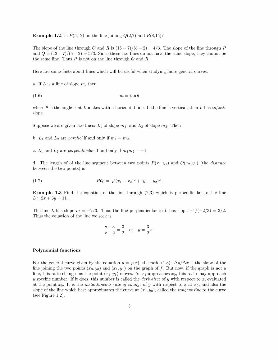
For the general curve given by the equation y = f(x), the ratio (1.3): ∆y/∆x is the slope of theline joining the two points (x0, y0) and (x1, y1) on the graph of f . But now, if the graph is not aline, this ratio changes as the point (x1, y1) moves. As x1 approaches x0, this ratio may approacha specific number. If it does, this number is called the derivative of y with respect to x, evaluatedat the point x0. It is the instantaneous rate of change of y with respect to x at x0, and also theslope of the line which best approximates the curve at (x0, y0), called the tangent line to the curve(see Figure 1.2).

3

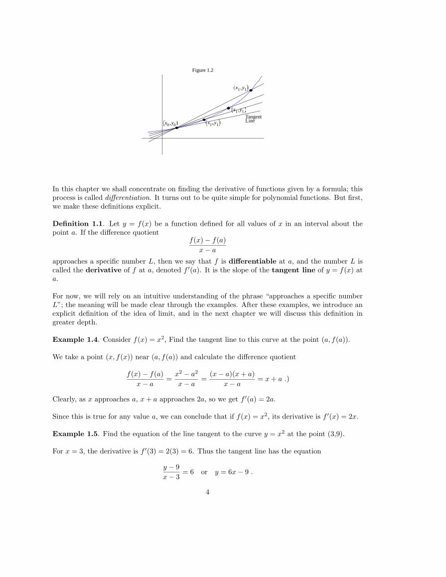
Figure 1.2

�x0 � y0 �

�x1 � y1 �

�x1 � y1 �

�x1 � y1 �

TangentLine

In this chapter we shall concentrate on finding the derivative of functions given by a formula; thisprocess is called differentiation. It turns out to be quite simple for polynomial functions. But first,we make these definitions explicit.

Definition 1.1. Let y = f(x) be a function defined for all values of x in an interval about thepoint a. If the difference quotient

f(x)− f(a)x− a

approaches a specific number L, then we say that f is differentiable at a, and the number L iscalled the derivative of f at a, denoted f ′(a). It is the slope of the tangent line of y = f(x) ata.

For now, we will rely on an intuitive understanding of the phrase “approaches a specific numberL”; the meaning will be made clear through the examples. After these examples, we introduce anexplicit definition of the idea of limit, and in the next chapter we will discuss this definition ingreater depth.

Example 1.4. Consider f(x) = x2, Find the tangent line to this curve at the point (a, f(a)).

We take a point (x, f(x)) near (a, f(a)) and calculate the difference quotient

f(x)− f(a)x− a

=x2 − a2

x− a=

(x− a)(x + a)x− a

= x + a .)

Clearly, as x approaches a, x + a approaches 2a, so we get f ′(a) = 2a.

Since this is true for any value a, we can conclude that if f(x) = x2, its derivative is f ′(x) = 2x.

Example 1.5. Find the equation of the line tangent to the curve y = x2 at the point (3,9).

For x = 3, the derivative is f ′(3) = 2(3) = 6. Thus the tangent line has the equation

y − 9x− 3

= 6 or y = 6x− 9 .

4

The ease with which we calculated the derivative for y = x2 followed from simple algebraic facts.We shall see that this works in general for polynomials; but first, one more example:

Example 1.6. If f(x) = x3, f ′(x) = 3x2. Fix a point (a, a3) on the graph, and let (x, x3) be anearby point. We look at the slope of the line joining these points:

∆y

∆x=

x3 − a3

x− a.

Since the quotient of x3 − a3 by x− a is x2 + ax + a2 this can be rewritten as

x3 − a3

x− a=

(x− a)(x2 + ax + a2)x− a

= x2 + ax + a2 ,

and evaluating this at a, we get f ′(a) = 3a2.

Now, for any polynomial y = f(x), this process will work: divide f(x)−f(a) by x−a, and evaluatethe quotient at x = a to calculate the derivative. Let’s spell this out, starting with the divisiontheorem of algebra:

Theorem 1.2. Let f be a polynomial of degree d. Then, for any number a when we divide f(x)by x− a, we get a quotient which is a polynomial of degree d− 1 and a remainder of f(a):

(1.8)f(x)x− a

= q(x) +f(a)x− a

.

Now, to apply this to the calculation of instantaneous rate of change, move the second term onthe right to the left:

f(x)− f(a)x− a

= q(x) .

Aas we let x approach a, the difference quotient q(x) approaches q(a), so the polynomial is differ-entiable at a, and its derivative is q′(a).

Theorem 1.3. A polynomial y = f(x) is everywhere differentiable. Its derivative at x = a is q(a),where q is the quotient of f(x)− f(a) by x− a.

Newton realized that using long division would be a tedious way to calculate derivatives, and withthem instantaneous rates of change, so he had the genius to take a slightly more abstract approachto lead to an automatic way of calculating derivatives. First, we must make explicit what we meanby the phrase ”the expression approaches a specific number” by introducing the notion of limit.Suppose that y = g(x) defines a function in an interval about x0. We say that g has the limit Las x approaches x0 if we can make the difference |g(x)−L| as small as we need it to be by takingx as close to x0 as we have to. More precisely, but less intuitively,

Definition 1.4. limx→x0 g(x) = L if, for any ε > 0 there is a δ > 0 such that |x− x0| < δ implies|g(x)− L| < ε.

We now observe that limits behave well under algebraic operations.

5

Proposition 1.5. Suppose that f and g are functions defined in an interval about x0 and that

limx→x0

f(x) = L , limx→x0

g(x) = M .

Then

a) limx→x0

(f(x) + g(x)) = L + M

b) limx→x0

(f(x) · g(x)) = L ·M

c) If M 6= 0, then

limx→x0

f(x)g(x)

=L

M.

Applying this proposition to the calculation of derivatives, we see how differentiation behaves underalgebraic operations:

Proposition 1.6. Suppose that f and g are functions defined and differentiable in an interval I.Then

a) f + g is differentiable in I, and (f + g)′ = f ′ + g′.

b) fg is differentiable in I, and (fg)′ = f ′g + fg′.

We give a brief justification of these rules, which follow from the corresponding rules for limits(proposition 1.5). This is straighforward for part a), but for the product, the argument requiressome preliminary algebraic manipulation. Suppose then, that f and g are differentiable at a, andlet h = fg. Then to see that h is differentiable, we must take the limit, as x approaches a of

h(x)− h(a)x− a

=f(x)g(x)− f(a)g(a)

x− a.)

The product rule for limits does not apply directly, for this is not a product. However, if we addand multiply f(a)g(x), we get

f(x)g(x)− f(a)g(a) = [(f(x)− f(a))g(x)] + [f(a)(g(x)− g(a))] ,

which leads to a sum of products

f(x)g(x)− f(a)g(a)x− a

= g(x)f(x)− f(a)

x− a+ f(a)

g(x)− g(a)x− a

.

Now, we can take the limits using proposition 1.5. We have to note that, since g is differentiable,we also have limx→a g(x) = g(a).

This brings us to the rule for differentiating polynomials.

6

Proposition 1.7.

a) If f is constant, then f ′ = 0.

b) If f(x) = axn for some positive integer n, then f ′(x) = anxn−1.

c) A polynomial is differentiated term by term, using b) for each term.

To verify a), we only have to note that a constant function is unchanging; its graph is a horizontalline, so has slope 0. c) follows from the fact that the limit of a sum is the sum of the limits. b)follows by a bootstrap method. We have already seen this for n = 0, 1, 2, 3. To proceed, we usethe product rule. For example, take n = 4:

(x4)′ = (x3x)′ = (x3)′x + x3x′ = (3x2)x + x3(1) = 4x3 .

If we have the proposition for all integers up to n− 1, then we have it for n by the same method:

(xn)′ = (xn−1x)′ = ((n− 1)xn−2)x + xn−1(1) = nxn−1 .

Example 1.7. Let f(x) = 2x2 − 3x + 3. Find f ′(x). What is the equation of the line tangent tothe curve given by y = f(x), at the point (1,2)?

Using proposition 1.7, we have

f ′(x) = 2(2x)− 3(1) + 0 = 4x− 3 .

This gives the slope of the tangent line at (1,2) by evaluating at x = 1 : f ′(1) = 4(1) − 3 = 1.Thus the equation of the tangent line is

y − 2x− 1

= 1 or y = x + 1

Example 1.8. Iff(x) = 2x5 − x4 + 8x3 + 2x− 5 ,

thenf ′(x) = 2(5x4)− 4x3 + 8(3x2) + 2x0 − 0 = 10x4 − 4x3 + 24x2 + 2 .

If a function f is differentiable at every point of an interval I, then the derivative is defined atevery point in the interval I, and thus is a function on I. This function, denoted f ′, is defined bythe rule: for all x in I,

(1.9) f ′(x) = limh→0

f(x + h)− f(x)h

.

In particular, since f ′ is now a function on I, it too may be differentiable. If so, its derivativeis denoted f ′′(x), and is called the second derivative of f with respect to x. Proceeding, we candefine third and fourth derivatives and so forth.

7

So far, we have been interpreting the derivative as the instantaneous rate of change of y withrespect to x, or the slope of the tangent line. Another fundamental interpretation is in terms ofmotion. Consider an object moving along a straight line. Let the variable t represent time, and xthe displacement of the object from a fixed point, 0, on the line. Then the position of the objectat time t is given by a function x = x(t). The velocity (denoted at time t as v(t)) of the object isthe instantaneous rate of change of x with respect to t. The acceleration of this object (denoteda(t)) is the instantaneous rate of change of v with respect to t. Thus, if v(t) is the velocity of theobject at time t, and a(t) its acceleration, we have

(1.10) v(t) = x′(t) , a(t) = v′(t) = x′′(t) .

Example 1.9 Suppose an object is moving in a straight line so that its displacement at time t isgiven by x(t) = 4t2 +12t. Find the formulas for the velocity and acceleration of this object. Whatare the velocity and acceleration at time t = 5?

Differentiating, we find that v(t) = x′(t) = 8t + 12, a(t) = x′′(t) = 8. Thus the velocity at timet = 5 is v(5) = 8(5) + 12 = 52, and the acceleration is a(5) = 8.

In many dynamical problems, an object is moving at constant acceleration. For example, anobject falls near the surface of the earth at an acceleration of 32 ft/sec2 downward (or 9.8 m/sec2

downward, in the metric system). If the acceleration is constant, that tells us that ratio of thechange in velocity over the change in time is constant: that is, the velocity is a linear function oftime. Similarly, since the velocity is a linear function, the distance travelled must be given by aquadratic function; all we have to do is to use the given data to find the coefficients. We conclude:

Proposition 1.8. Suppose an object moves at constant acceleration a. If at time t = 0 the objectis at position x0 and has velocity v0, then at any time we have

(1.11) x(t) =a

2t2 + v0t + x0 , v(t) = at + v0 .

It is easy to check that these functions do have the desired properties, that is, that x′(t) = v(t)and v′(t) = a, and that their values at t = 0 are as given. Furthermore, we can argue intuitively,as we have done above, that these are the precise formulas for distance and velocity. For, sincethe rate of change of velocity is constant, velocity must be linear, and since the rate of change ofdistance is linear, it must be quadratic. This was the way Newton argued; but there are loose endsas was pointed out very articulately by Newton’s contemporary, George Berkeley. Why indeed,are these the only formulas with the desired properties? How do we know that there does notexist some as yet unknown mysterious functions which have the same values at t = 0, and thegiven acceleration? The third book of Newton’s Principia gives formidable evidence that no suchmysteries exist, and that work, together with much subsequent experimental evidence, carried theday. But Berkeley’s objections were valid on logical grounds, and the issue was not satisfactorilyresolved until the nineteenth century.

Example 1.10. An object is projected upward at an initial velocity of 48 ft/sec. How high doesit go?

We measure distance upward from the starting point, so that x0 = 0 and v0 = 48. The accelerationdue to gravity is a = -32 ft/sec, so (by proposition 1.8), the equations of motion (1.11) are

x(t) = −16t2 + 48t , v(t) = −32t + 48 .

8

If we complete the square for x(t), we have

x(t) = −16(t− 3/2)2 + 36 .

Thus the greatest value of x is achieved at t = 3/2, and is x(3/2) = 36 feet. Note that at thishighest point, v(3/2) = 0, confirming our intuition that at the moment the object turns around itsvelocity must be zero.

Example 1.11. An automobile is traveling at 60 mph. At what rate must it decelerate so as tostop in 100 yards?

Converting everything to feet and seconds, we have an initial velocity of 88 ft/sec, and we can takes(0) = 0. At some future time T , we have s(T ) = 300 feet, v(T ) = 0. Call the rate of decelerationa. The equations of motion (1.11) are

x(t) = −a

2t2 + 88t , v(t) = −at + 88 .

At time T we have 300 = −(a/2)T 2 + 88T, 0 = −aT + 88. From the second we get T = 88/a;putting that in the first we get

300 = −a

288a

2

+ 8888a

or 300 = 882(− 12a

+1a) or 300 =

882

2a,

so a = 12.91 ft/sec2.

More rules of differentiation

Eventually we will develop a full set of rules for finding the derivative of any function given bya formula. We turn now to the quotient rule to handle quotients of polynomials (called rationalfunctions).

Proposition 1.9. Suppose that f and g are differentiable at a point a, and g(a) 6= 0. Then 1/gand h = f/g are differentiable at a, and

(1.12)(1g

)′ = − g′

g2, h′ =

gf ′ − fg′

g2.

To show that 1/g is differentiable, we must calculate the limit as x → a of

1g(x) −

1g(a)

x− a.)

Once again, a little algebra helps us. Simplifying the compound fraction, we get

1x− a

· g(a)− g(x)g(x)g(a)

=−1

g(x)g(a)g(x)− g(a)

x− a,

which has as its limit (1g

)′(a) = − g′(a)(g(a))2

.

9

Now the second equation of (1.38) follows from this and the product rule appied to f/g consideredas f · (1/g). (f

g

)′ = f(1g

)′ + f ′(1g

)= f

(−g′

g2

)+ f ′

(1g

)=

gf ′ − fg′

g2.

In particular, we haved

dx(1x

) = − 1x2

.

Proposition 1.10. Let n be any integer, positive, zero, or negative. Then

(1.13) for f(x) = xn we have f ′(x) = nxn−1 .

By proposition 1.7b, this is true for n positive or zero. For negative exponents, we apply thequotient rule to f(x) = 1/xn with n positive:

f ′(x) = −nxn−1

(xn)2= (−n)x−n−1 ,

which is just (1.13) for the negative exponent −n.

Example 1.12. Find the derivative of

f(x) = x2 − 2x +3x− 5

x2.

Rewrite the function in exponential notation: f(x) = x2 − 2x + 3x−1 − 5x−2. Now use (1.13):f ′(x) = 2x− 2 + 3(−x−2)− 5(−2x−3), which can be rewritten as

f(x) = 2x− 2− 3x2

+10x3

.

Example 1.13. Let f(x) = 30x + 2x−1. For what value of x is f ′(x) = 0?

Differentiate: f ′(x) = 30− 2x−2. Now solve f ′(x) = 0:

0 = 30− 2x2

so that x2 = 15

and the answer is x = ±√

15.

As a last observation, we return to the definition of the derivative to differentiate the square rootfunction:

Proposition 1.11. If f(x) =√

x for x > 0, then f ′(x) = 1/(2√

x).

Here we use the fact that x− a = (√

x−√

a)(√

x +√

a). Thus

√x−

√a

x− a=

√x−

√a

(√

x−√

a)(√

x +√

a)=

1√x +

√a→ 1

2√

a

10

as x → a, for a 6= 0.

Problems 1.1

1. Find the equation of the line which goes through the point (2,-1) and is perpendicular to theline given by the equation 2x− y = 1.

2. a) Let f(x) = x2+3x−1. Find the slope of the secant line joining the points (2, 9) and (x, f(x)).b) Find the slope of the tangent line to the curve y = f(x) at the point (2, 9).c) What is the equation of this tangent line?

3. Letf(x) =

1x2

.

a) Find the slope of the secant line through the points (x, 1x2 ) and (x + h, 1

(x+h)2 ).

b) Find the slope of the line tangent to the graph of y = f(x) at the point (3, 19 ).

4. Find the derivatives of the following functions:

a) f(x) = x3 − x2 + 1

b) g(x) = x2 +1x3

c) h(x) = (x2 +1x3

)(x3 − x2 + 1)

5. Find the derivatives of the given functions:

a) f(x) = 3x−1 + x3

b) f(x) = (x2 +1x3

)(x3 − x2 + 1)

6. Find the derivative of the given functions:

a) f(x) =x2 + 1x + 1

b) f(x) = x2 +1x3

7. Find the derivative of

f(x) =x2 + 1x + 1

11

8. Differentiate : h(t) =1− t2

1 + t3

10. Sketch the graph of a function with these properties:a) f(0) = 2 and f(1) = 0;b) f ′(x) < 0 for 0 < x < 2;c) f ′(x) > 0 for x < 0 or x > 2.

11. Sketch the graph of a function with these properties:a) f(0) = 1 and f ′(0) = 0;b) f(−1) = 0, f(1) = 0,c) f ′(x) < 0 for 0x < −1 and 0 < x < 1,c) otherwise, f ′(x) > 0.

12. Find the value of x where the graphs of these two functions have parallel tangent lines:

f(x) = x2 − 3x + 2 , g(x) = 5x2 − 11x− 17 .

13. Find the points on the curve y = 3x2 − 3x + 1 whose tangent line is perpendicular to the linex + 2y = 7.

14. Let C1 and C2 be curves given by the equations C1 : y = x3 + x2, C2 : y = x2 + x. For whatvalues of x do these curves have parallel tangent lines?

15. Find the derivative of f(x) = (x + 1)( 1x + 1).

16. Find the slope of the line tangent to the curve

y = x2 − 3x + 1/x

at the point (3,1/3).

17. Let y = x3 − 48x + 1. Find the x coordinate of the points at which the graph has a horizontaltangent line.

18. A man standing at the edge of the roof of a building 120 feet high throws a ball directlyupwards at a velocity of 48 ft/sec. a) How high does the ball go? b) Assuming that it proceeds tofall along the side of the building, how long does it take to hit ground level?

19. Another man standing on ground level throws the ball back to his friend on the roof. At whatinitial velocity must he throw it in order to reach the roof?

20. On the planet Garbanzo in the Weirdoxus solar system, the equation of motion of a fallingbody is

s = s0 + v0t− 10t3

where s0 is the initial height above ground level and v0 is the initial velocity. Distance is mea-sured in garbanzofeet. If a ball is thrown upwards from ground level at an initial velocity of 120garbanzofeet/second, how high does the ball rise?

12

1.2 Liebniz’ Calculus of Differentials

Up to this point we have been following the development of the Calculus according to Newton.We have been considering variables y, z, u, v, etc. as functions of a particular variable (called the“independent variable”) x, and discovering how to find rates of change of the dependent variablesrelative to the independent variable.

The ideas of Liebniz follow a different, but equivalent, set of ideas. Liebniz is concerned with acollection of variables x, y, z, u, v, etc. and their “infinitesimal increments”. This is a hard conceptto get a hold on, but we can think of it this way. When we actually make measurements, wealways have in mind, even if unspecified, an “error bar”; that is, a largest allowable error. Thus,our calculators display numbers to 8 decimal points, allowing for a “negligible” error of at most10−8. A more efficient computer has a smaller error bar, perhaps 10−32, or 2−128. Instruments ofmeasurement, no matter how delicate, have to allow for such an error bar. So, if u is a measurablevariable, it comes equipped with an error bar: an allowable increment in a measurement which doesnot change the accepted value of the measurement. It is this which we should call the “infintesimalincrement” in u, called by Liebniz the differential of u, denoted du. However, the important featureof this concept is that it is not tied down to the level of accuracy of today’s instruments, but itrepresents the error bar for all time: du stands for the smallest measurable increment for all waysof measuring ever to come.

We get a more concrete interpretation of the differential by relating it to the linear approximationto the variables. More precisely, suppose the variables x, y are related by y = f(x). The tangentline at a point (x0, y0) is the line which best approximates the curve. We have used the symbols∆x, ∆y to represent changes in the variables x and y along the curve; now we let dx, dy representchanges in the variables along the tangent line. Since the slope of the tangent line at (x0, y0) isf ′(x0), we obtain this important relationship between the differentials: at the point (x0, f(x0)),

(1.14)dy

dx= lim

∆x→0

∆y

∆x= f ′(x0) ,

or, without specifying the particular point, dy = f ′(x)dx. This we can interpret as the equationof the tangent line by replacing dx and dy by x− x0, y − y0.

Example 1.14. Find the equation of the tangent line to the curve y = x3 − 2x + 5 at the point(2, 9). First we calculate the relation between the differentials:

dy = (3x2 − 2)dx .

At x = 2, this gives dy = 10dx. Now we interpret this as the equation of the tangent line byreplacing dy by y − 9 and dx by x− 2. The equation of the tangent line is thus

y − 9 = 10(x− 2) or y = 10x− 11 .

Finally, considering the equation dy = f ′(x)dx as the linear approximation to the equation y = f(x)(at a particular point), we can make preliminary estimates of the change in y, given a change in x.

Example 1.15. The volume of a sphere of radius r is V = (4/3)πr3. Suppose the surface of asphere of radius 6 feet is covered by a 1 inch coat of paint. About how much paint will be needed?

13

From the defining equation we have dV = 4πr2dr; so letting r = 6 feet and dr = 1/12 feet, we canestimate the change in volume to be

dV = 4π(6)2(112

) = 37.7 cu. ft.

Thinking of the derivative as the ratio of two quantities which eventually become zero has itsphilosophical problems and was also subjected to the scathing criticism of Berkeley. This conceptof “evanescent quantities” (as Berkeley sarcastically identified them) was controversial in the daysof Newton and Liebniz and remained so for the following 200 years. Note, by the way, that onecan object to Newton’s methods on the same ground: when we write

f(x)− f(a)x− a

=x2 − a2

x− a=

(x− a)(x + a)x− a

= x + a ,

by what right are we now able to let x become a? If we did so one step sooner, we’d be dividingby zero, which is forbidden. So, in this set of equations x cannot be a. But in the next line we say,“let x be a”! These philosophical obstacles were eventually overcome; we shall proceed withoutresolution, as did Newton, Liebniz and their successors to enormous effect. Suffice it to say that thiscan all be put on a logical footing, while at the same time, the concept of differential as “smallestpossible increment” is a powerful intuitive tool throughout mathematics and its applications. Toillustrate, in the next section, we shall give a heuristic derivation of the law of differentiation forcomposite functions.

Problems 1.2

1. Let y =x

x2 + 1.

Find the equation of the tangent line to the graph at the point (2,0.4).

2. Find the equation of the tangent line to y = x2(x3 − 1) at (2,28).

3. Find the equation of the tangent line to the curve y = x cos x at (π/4, π√

2/8).

4. Find the the equation of the tangent line to the curve y = x− x−2 at (2,7/4).

5. Let y = x + 25x−1. Find an approximate value of y when x = 3.2.

1.3 The Chain Rule

Suppose that y, u and x are variables such that u is a function of x: u = f(x), and y is a functionof u: y = g(u). Then y can be viewed as a function of x by writing y = h(x) = f(g(x)). Howdo we find the rate of change of y with respect to x? Using differentials, we have: dy = f ′(u)du,and du = g′(x)dx, so that dy = f ′(u)g′(x)dx, it being understood that in this formula u is to beexpressed in terms of x. A shorthand for this is

dy

dx=

dy

du· du

dx.

14

Example 1.16. Let y = (4x + 1)3. We introduce the intermediate variable u = 4x + 1, so thaty = u3. Then dy = 3u2du, and du = 4dx, so that

dy

dx= 3u2(4) = 12(4x + 1)2 .

Example 1.17. If y = x−n with n positive , we introduce u = xn, so that y = u−1. Then

d

dx(x−n) =

dy

dx=

dy

du

du

dx= − 1

u2nxn−1 = −nxn−1

(xn)2= −nx−n−1 ,

giving another derivation of proposition 1.11.

Example 1.18. Let y = ((2x + 1)3 + 5)2. Here we need to use the chain rule more than once. Wethink of y = v2, where v = u3 + 5, and u = 2x + 1. Then

dy

dx=

dy

dv

dv

du

du

dx= 2v(3u2)(2) .

Now replace v and u by their expressions in x:

dy

dx== 12((2x + 1)3 + 5)(2x + 1)2 .

The statement of the chain rule is as follows.

Proposition 1.12. Suppose that g is differentiable at the point a, and f is differentiable at g(a).Then the composed function h(x) = f(g(x)) is differentiable at a and

(1.15) h′(a) = f ′(g(a))g′(a) .

In particular,

Proposition 1.13. If f is differentiable at a, and n is any positive or negative integer, h(x) =(f(x))n is also differentiable at a and

(1.16) h′(x) = n(f(x))n−1f ′(x) .

Of course, the Liebniz formulation (1.55) is easier to remember and apply than proposition 1.12.For that reason we shall begin to adopt the Liebniz notation for differentiation: if y = f(x) isdifferentiable in an interval I, we write

(1.17) f ′(x) =dy

dx

and use f ′(x) and dy/dx interchangeably. The notation for higher derivatives is:

(1.18) f ′′(x) =d2y

dx2, f ′′′(x) =

d3y

dx3, etc.

15

In this notation, Proposition I.13 becomes simply

d

dx(yn) = nyn−1 dy

dx.

Problems 1.3

1. Find the derivative of g(x) = (x3 + 1)4.

2. Find the first and second derivatives of f(x) = x√

1− x2

3. Differentiate: f(x) =√

2x2 − 3x + 1.

4. Find f ′(x) : f(x) =(x + 1)2

(x− 1)2

5. Find g′(x), g′′(x) : g(x) = (x3 + 1)4.

1.4 Trigonometric Functions

Consider a particle moving in the counterclockwise direction around the circle of radius 1 withconstant angular velocity of 1 radian/second such that at time t = 0 it is at the point (1, 0). Thenits position at time t is (cos t, sin t). These functions are defined for all values of t, and are periodicof period 2π since in time 2π the particle will make one full circuit of the circle.

There are four other trigonometric functions defined by the equations

tan t =sin t

cos t, cot t =

cos t

sin t, sec t =

1cos t

, csc t =1

sin t.

Assuming that these functions are differentiable, we can calculate the derivatives by an argumentusing differentials due to Blaise Pascal.

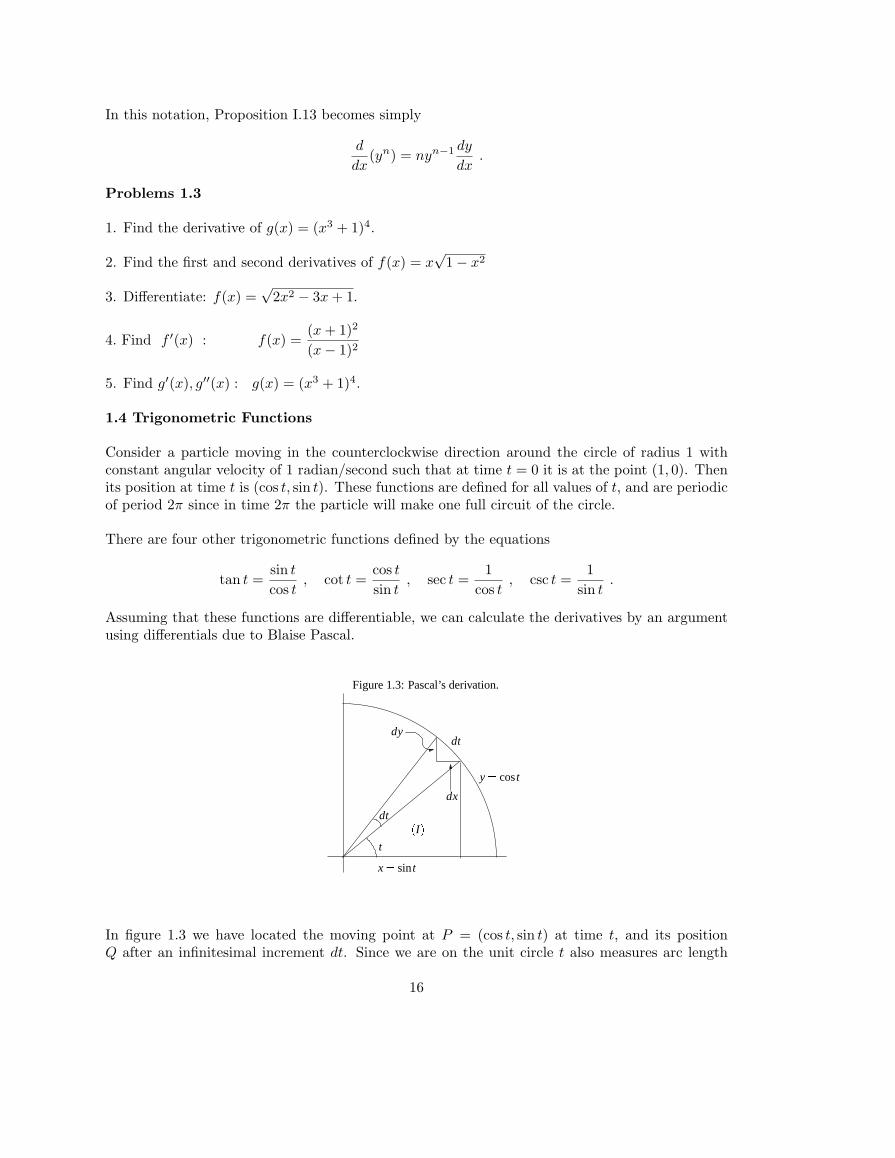
Figure 1.3: Pascal’s derivation.

dydt

dt� dx

x � sin t

y � cos t

�I �

t

In figure 1.3 we have located the moving point at P = (cos t, sin t) at time t, and its positionQ after an infinitesimal increment dt. Since we are on the unit circle t also measures arc length

16

along the circle. The triangle with sides dx, dy, dt is called the “differential triangle”. It may beof concern that dt represents an arc of the circle, but, remember - at the differential level an arcand a straight line are indistinguishable. Since the tangent line to the circle is perpendicular tothe radius at the point P , the differential triangle is similar to the triangle (I) . Thus

−dx

sin t=

dt

1,

dy

cos t=

dt

1,

sodx

dt= − sin t ,

dy

dt= cos t .

Since x = cos t, y = sin t, we obtain the first part of the following.

Proposition 1.14.

a)d

dt(sin t) = cos t ,

d

dt(cos t) = − sin t ,

b)d

dt(tan t) = sec2 t ,

d

dt(cot t) = − csc2 t ,

c)d

dt(sec t) = sec t tan t ,

d

dt(csc t) = − csc t cot t .

b) anc c) follow from the quotient rule. For example, b):

d

dt(tan t) =

d

dt

sin t

cos t=

cos t cos t− sin t(− sin t)cos2 t

=1

cos2 t= sec2 t .

Remember: in the the above discussion we have assumed that the trigonometric functions weredifferentiable, and it was that assumption that allowed us to consider an arc of a (differential)circle as a straight line. These formulae imply the following limit results, just by the definition ofthe derivative.

Proposition 1.15.

(1.19) limx→0

sinx

x= 1 , lim

x→0

cos x− 1x

= 0 .

We remind the reader that we started out assuming that the functions sin x and cos x are differen-tiable, so this problem tells us what the derivatives are at x = 0 under those assumptions. In thenext chapter we wil prove proposition 1.15 directly by geometric methods, from which we concludethat the sine and cosine functions are indeed differentiable.

Problems 1.4

1. From a point 1000 feet away from the base of a building, the angle of elevation of its roof is 17degrees. How tall is the building?

17

2. A marker is rotating counterclockwise around a circle of radius 4 centered at the origin at therate of 7 revolutions per minute. a) What is its position after 2.3 minutes? b) How soon after 2.3minutes will it cross the x-axis again?

3. If tanα = −√

3, what are the possible values of sinα?

4. Express as a function of 2x:sinx− cos x

sinx + cos x

5. Find the derivative:f(x) = sin x cos x

6. Find the derivatives of the following functions:

a) f(x) = cos2 x

b) g(x) =sin2 x

cos x

7. Find the derivative:g(x) =

sinx

cos x

8. Differentiate: y = (x2 − 1) sin(x2 + 1).

9. Find the derivative:h(x) = (cos(2x) + 1) sin(3x)

10. Differentiate: g(x) = (sin(3x) + 1)3.

11. A point moves around the unit circle so that the angle it makes with the x-axis at time t isθ(t) = (t2 + t)π. Let (x(t), y(t)) be the cartesian coordinates of the point at time t. What is dy/dtwhen t = 3?

12. Let f(x) = x sinx. Find the equation of the tangent line to the graph y = f(x) at the pointsx = (2n + 1/2)π for any integer n.

13. Find the derivatives of these functions:

(a) h(x) = (cos(2x) + 1) sin(3x)

b) g(x) = (tan(3x)− 1)2

14. Consider the curves C1 : y = sinx and C2 : y = cos x.a) At which points x between −π/2 and π/2 do the curves have parallel tangent lines?b) At which such points do they have perpendicular tangent lines?

15. Differentiate:f(x) =

1 + tanx

1− tanx

18

1.5 Implicit Differentiation and Related Rates

Suppose that x and y are variables which are related by a functional equation: F (x, y) = c, aconstant. We say that this relation defines y implicitly as a function of x. For, in principle, givena value of x, say x = a, we can solve the equation F (a, y) = c for y, giving the “rule” defining y interms of x. However, to find dy/dx we need not solve this equation. When y and x are so related,their differentials are related as well, and the chain rule can be used to find that relationship, as afunction of both x and y. The idea is to think of z = F (x, y) as another variable which, because ofthe relation F (x, y) = c is constant, so dz = 0. Now, apply the chain rule to the expression for z.

Example 1.19. Suppose that the variables x and y satisfy the relation

(1.20) x2 − xy + 2y2 = 4 .

Letting z represent this defining relation, we have dz = 0. Now, using (1.15) and the rules fordifferentiation,

dz = 2xdx− (xdy + ydx) + 4ydy = 0 ,

giving us

(1.21) (−x + 4y)dy = (−2x + y)dx ,

leading to this expression for the derivative:

dy

dx=

2x− y

4y − x.

Example 1.20. What is the equation of the tangent line to the curve given by (1.68) at the point(2,1)? We find the slope by substituting the values x = 2, y = 1 in equation (1.21):

m =dy

dx=

2(2)− 14(1)− 2

=32

.

Then the equation of the line is

y − 1 =32(x− 2) or y =

32x− 2 .

Notice that, if we substitute x = 2, y = 1, dy = y − 1, dx = x − 2 into equation (1.21) we get thesame result. That is because equation (1.21) is the linear approximation to the relation between xand y, which is of course the same as the equation of the tangent line.

Example 1.21 . Find the equation of the tangent line to the curve y3 + 2 cos2 x = 0 at the point(π/4,−1). We differentiate implicitly:

3y2dy − 2 cos x sinxdx = 0 .

Now, at the point (π/4,−1), y2 = 1, cos x = sinx =√

2/2, so this becomes 3dy − dx = 0.Replacing dx by x− π/4 and dy by y − (−1) gives the equation of the tangent line:

3(y + 1)− (x− π

4) = 0 , or 3y − x =

π

4− 3 .

19

Related Rates

Suppose we are in a situation where one or more variables are related, and the variables arefunctions of time. For example, if a spherical balloon is being inflated, then during this processthe volume (V ), area (A) and radius (r) are increasing with time. Since these are all related, weare able, by differentiation to relate the rates of growth. For example, suppose the balloon is beinginflated by putting gas in at a steady rate of 3 cc/sec. We may ask “at what rate is the radiuschanging?” We start with the formula relating volume with radius: V = (4/3)πr3. V and r arefunctions of time, so, differentiating with respect to time we obtain

dV

dt=

43π(3r2 dr

dt) = 4πr2 dr

dt.

Putting in the datum dV/dt = 3 , we find

dr

dt=

34πr2

cm/sec ,

so depends upon the radius at the time.

Here is a protocol for attacking such problems.

Step 1. Draw a picture (if appropriate), and identify the relevant variables: those things whichcan change. State the problem in terms of the variables.

Step 2. Find a relationship among the variables.

Step 3. Differentiate, to obtain a relationship among the variables and their rates of change.

Step 4. Put in the values of the variables at the time in question, and solve the resultingequation.

Example 1.22. Suppose as above a balloon is being inflated with gas at a rate of 3 cc/sec. Atwhat rate is the area increasing when the radius is 14 cm?

First, we identify the variables as volume: V , area: A, and radius: r. Now, these are relatedby the equations

V =43πr3 , A = 4πr2 .

Now, we differentiate these equations:

dV

dt= 4πr2 dr

dt,

dA

dt= 8πr

dr

dt.

Now, at the specific time of interest, r = 14 cm, and dV/dt = 3 cc/sec. Substituting these values,we have:

3 = 4π(14)2dr

dt,

dA

dt= 8π(14)

dr

dt.

Then dr/dt = 3/[4(14)2π], so the second equation gives

dA

dt= 8π(14)

34(14)2π

=37

cm2/sec .

20

Example 1.23. A ship leaves port at noon heading north at 25 knots (nautical miles per hour),and 2 hours later another ship leaves heading west at 30 knots. Assuming the ships travel in straightlines, at what rate is the distance between the ships increasing after an additional 3 hours?

First, the variables are: t, the time elapsed since noon, N , the distance travelled in that time bythe ship heading north, W , the distance travelled by the ship heading west, and Z, the distancebetween them. The relations among these variables are:

Z2 = N2 + W 2 ,

from the Pythagorean theorem. In t hours after noon, the first ship has travelled 25t nautical miles:N = 25t, and, since the second ship started two hours later, it has travelled 30(t−2) nautical miles(notice, we are assuming that t ≥ 2). Now since we have been given the rates of change of N andW , and want to find that of Z, we differentiate the first equation with respect to t to relate theserates:

2ZdZ

dt= 2N

dN

dt+ 2W

dW

dt.

Now, at t = 5, we have N = 125, W = 75, dN/dt = 25, dW/dt = 30, giving

ZdZ

dt= 125(25) + 75(30) = 5375 .

We find Z by the first relation Z2 = 1252 + 752 = (25)2(34), so Z = 25√

34. Finally,

dZ

dt=

537525√

34= 36.87 nautical miles/hour .

Example 1.24. Suppose that x and y are functions of t which satisfy the relation x3y2 + 2y =8. Suppose that at the point (1, 2), the velocity of x is 3 in/sec. What is the velocity of y?Differentiating the relation implicitly, we get

3x2 dx

dty2 + x3(2y

dy

dt) + 2

dy

dt= 0 .

Now substituting x = 1, y = 2, dx/dt = 3, in this equation:

3(1)2(3)(22) + (1)3(2(2)dy

dt) + 2

dy

dt= 0 .

Solving for dy/dt, we find 36 + 6dy/dt = 0, or, the velocity of y is -6 in/sec.

Definition 1.16. For integers p and q, the function

(1.23) y = xp/q

is defined, for all positive x, as the positive solution of the equation yq = xp.

So, for example,√

x can be written as x1/2, the cube root of x as x1/3, etc. Using implicitdifferentiation we verify:

21

Proposition 1.17.

(1.24)d

dxxn = nxn−1 for all rational numbers n .

A rational number is a quotient p/q of integers. Differentiate the equation yq = xp implicitly:

qyq−1dy = pxp−1dx ordy

dx=

p

q

xp−1

yq−1.)

Replacing y by xp/q, we get

dy

dx=

p

q

xp−1

xp−p/q=

p

qxp−1−p+p/q =

p

qx(p/q)−1

which is the desired result, since n = p/q.

Problems 1.5

1. A curve is given by the equation x2− xy + y2 = 7. Find the equation of the line tangent to thiscurve at the point (2,-1).

2. Find the slope of the curve defined by the relation

4(x2 + xy) = 2y3 − y2

at the point (1, 2).

3. Variables x and y are related by the formula

x sin y + y sinx = π .

If dy/dt = 3 when x = 3π/2 and y = π/2, what is dx/dt?

4. The relation cos y + x = sin y determines a curve in the x-y plane. Find the slope of the linetangent to the curve at the point (1, π/2).

5. Consider the curve given by the equation: y2 + xy + x2 = 1. At what points does this curvehave a horizontal tangent line?

6. Consider the curve given by the equation: x2y − y3 = 1. At what points does this curve have avertical tangent line?

7. A ship is travelling in a circle of radius 6 nautical miles around an island at a speed of 10 knots(nautical miles per hour). A lighthouse is 10 miles due east of the island. At what rate is thedistance between ship and lighthouse increasing when the ship is exactly due north of the island?

8. A new stadium, built like a cylinder capped with a hemispherical dome is proposed to have adiameter of 500 feet. To include another 2000 seats, the diameter must be increased by 10 feet.By approximately how much will the area of the dome be increased? (Note: the area of a sphereof radius r is 4πr2.)

22

9. A cat is walking toward a telelphone pole of height 30 feet. She is walking at a steady rate of 4ft/sec. A bird is perched on top of the tellephone pole. When the cat is 45 feet from the base ofthe pole, at what rate is the distance between bird and cat decreasing?

10. Water is flowing into a conical tank through an opening at the vertex at the top at the rate of12 cu. ft./min. The base of the tank is a circle of radius 12 ft. and the height of the cone is 20 ft.At what rate is the water level rising when the water level is 4 ft. from the top? The formula forthe volume of a cone of base radius r and height h is V = (1/3)πr2h.

11. Let P be an upward-opening parabola whose axis is the y-axis and whose vertex is the origin.Suppose the line y = C intersects the parabola in two points. Show that the tangent lines at thesepoints intersect on the y-axis of the parabola.

12. Suppose that a point moves along the x-axis according to the formula x(t) = 1/(t2 + 1). LetA(t) be the area of the circle with diameter joining the origin to the point x(t). Find A′(t) whent = 3.

23

II. Theoretical Considerations

2.1 Limit Operations

In this section we shall go more deeply into the concept of limits than we did in chapter 1. Supposethat y = f(x) is a function defined in an interval about the point x0. Each value of x determinesa value y using the rule represented by the function f . We say that y approaches a number L as xapproaches x0 if we can be sure that y is as close as we please to L just by taking x close enoughto x0. A little more precisely, if we allow an error ε > 0 in the calculation of L, we can find anerror δ > 0 for x0 such that if x is within δ of x0, then y is within ε of L. If the limit L is thenumber y0 calculated from x0 by f , then we say that f is continuous at x0. That is the content ofthe following two definitions.

Definition 2.1. limx→x0 f(x) = L if, for any ε > 0 there is a δ > 0 such that |x− x0| < δ implies|f(x)− L| < ε.

If the limit L is f(x0), then we say that f is continuous at x0:

Definition 2.2. A function f , defined in an interval about x0 is continuous at x0 if limx→x0 f(x) =f(x0). A function is said to be continuous if it is continuous at every point where it is defined.

Example 2.1. Let f(x) = x/|x|. Then, f(0) = 0, for x > 0, f(x) = 1, and for x < 0, f(x) = −1.Thus, in any interval about 0, there are values of x for which f(x) = 1 and other values of x forwhich f(x) = −1. There is thus no number L such that both 1 and -1 are within .5 of L, so therecan be no limx→0 f(x).

Example 2.2. Let f(x) = cos(1/x) for x 6= 0. There is no value to assign to f(0) to make thisfunction continuous. For if x = (2πn)−1, f(x) = 1 for n even, and f(x) = −1 for n odd, so weare in the same situation as that of example 1. However, for the function g(x) = x cos(1/x), wecan define g(0) = 0 to get a continuous function. For |g(x)| ≤ |x| for every x, since the cosine isbounded by 1. Thus, for any ε > 0, if |x| < ε, we also have |g(x)| < ε.

Now we state the basic facts describing how limits behave under algebraic operations.

Proposition 2.1. Suppose that f and g are functions defined in an interval about x0 and that

limx→x0

f(x) = L , limx→x0

g(x) = M .

Then

a) limx→x0

(f(x) + g(x)) = L + M

b) limx→x0

(f(x) · g(x)) = L ·M

c) If M 6= 0, then

limx→x0

f(x)g(x)

=L

M.

24

This proposition then tells us the following about continuous functions:

Proposition 2.2 Suppose that f and g are defined in an interval about x0, and are continuous atx0. Then the sum f + g and product f · g are also continuous at x0. If g(x0) 6= 0, the quotient f/gis also continuous at x0.

Now it is clear that a constant function is continuous: if f(x) = C for all x, then the difference|f(x)−C| = 0 no matter what x is. Also, the function f(x) = x is continuous everywhere: we canmake |f(x)− f(x0)| < ε just by taking |x−x0| < ε. Thus, by proposition 2.2, any function formedfrom constants and tne function f(x) = x by taking products and sums is continuous. But theseare the polynomials.

Proposition 2.3. All polynomials are continuous everywhere. A rational function (that is, aquotient of polynomials) is continuous everywhere where its denominator is non-zero.

Example 2.3. That is not to say that a rational function is not continuous where the denominatoris zero; perhaps it can be defined at those points so as to be continuous, For example, consider

f(x) =x2 − 4x− 5

x− 5.

Since we cannot divide by zero, f(x) is not defined for x = 5. But, can we define f(5) so thatthe function is continuous? Noting that x2 − 4x − 5 = (x − 5)(x + 1), we see that for x 6= 5,f(x) = x + 1. Thus by defining f(5) = 6, we get a continuous function.

Suppose now that g is defined in an interval around x0 and f is a function defined on the range(set of values) of g. Then we can form the composition of the two functions, f ◦ g, just by applyingthe rule defining f to the value of g : f ◦ g(x) = f(g(x)).

Proposition 2.4. Suppose that g is defined in an interval about the point x0, g(x0) = y0 and f isdefined in an interval about y0. If g is continuous at x0, and f is continuous at y0, then h = f ◦ gis also continuous at x0.

To show this, we have to show that we can insure that h(x) is within ε of h(x0) by taking x closeenough to x0. By the continuity of f we can be sure that f(y) is within ε of f(y0) by taking ywithin some small number, η of y0. But then, by the continuity of g, there is a δ such that, if x iswithin δ of x0, g(x) is within η of g(x0) = y0, and finally, f(g(x)) is within ε of f(y0) = f(g(x0)).

A useful technique is what is called the squeeze theorem. Suppose, in some interval containing thepoint a, the values of f lie between those of two other functions g and h. Suppose also that g andh have the same limit as x approaches a, then f also has that limit.

Proposition 2.5 (Squeeze Theorem). Suppose that f, g, h are defined in a interval containinga and that g(x) ≤ f(x) ≤ h(x). If

limx→a

g(x) = limx→a

h(x) = L ,

we also have limx→a f(x) = L.

25

Suppose an allowable error ε > 0 is specified. From the hypothesis, we know that there is a δ1 > 0such that if x is within δ1 of x0, then g(x) ≥ L − ε, and there is a δ2 > 0 such that if x is withinδ2 of x0, then h(x) ≤ L + ε. Then, so long as δ is less than both δ1 and δ2, we have

L− ε ≤ g(x) ≤ f(x) ≤ h(x) ≤ L + ε

which is to say that f(x) is within ε of L.

Now suppose again that f is defined in a neighborhood of x0 and continuous there. We now turnto the question of the differentiability of f at x0.

Definition 2.3. Let f be defined in a neighborhood of x0. If the limit

limx→x0

f(x)− f(x0)x− x0

exists, it is denoted f ′(x0), and is called the derivative of f at x0. f is said to be differentiableat x0.

Proposition 2.1c suggests that the limit does not exist since the denominator approaches 0. Butwe have to be careful: the numerator is also going to zero (as in example 2.3). In fact, as wesaw by the division theorem of chapter 1, If f is a polynomial, then so is this difference quotient,and the limit is the value of that quotient at x0. In fact, in general it is a necessary condition fordifferentiability that the limit of the numerator is zero - a fact we already used several times inchapter 1.

Proposition 2.6. Let f be defined in a neighborhood of x0. If f is differentiable at x0, then it iscontinuous at x0.

Let L = f ′(x0). The hypothesis tells us that we can be sure the difference quotient is within ε ofL by taking x close enough to x0. So, taking, for example, ε = 1, then if x is close enough to x0,

−1 <f(x)− f(x0)

x− x0− L < +1,

from which we conclude that

(L− 1)(x− x0) < f(x)− f(x0) < (L + 1)(x− x0) .

Now, the left and right hand sides tend to 0 as x approaches x0, so, by the squeeze theorem,lim(f(x)− f(x0)) = 0. But that is the same as lim f(x) = f(x0); that is, f is continuous at x0.

Now, in section 1 of chapter 1, no problems arose in calculating limits, since we were there dealingwith polynomials (even in calculating derivatives). However, more generally questions about limitscan become real issues. For example, when we turned to trigonometric functions and the squareroot function, we tacitly assumed their continuity. Since the continuity is intuitively clear (if weenvision the graph of these functions), this was not an obstacle to finding derivatives. However,in more general contexts, the continuity is not at all clear. As preparation for this, we shall herereconsider the assumptions of continuity made in chapter 1. First, the square root.

26

Example 2.4. For a ≥ 0,limx→a

√x =

√a .

We have to distinguish the cases a 6= 0 and a = 0. First, the case a 6= 0. We start with the identity

(√

x−√

a)(√

x +√

a) = x− a ,

which, for our purposes should be written as√

x−√

a =x− a√x +

√a

,

since it is the expression on the left we need to make small. Given ε > 0, choose δ > 0 so thatδ/√

a < ε. Then if |x− a| < δ,

|√

x−√

a| = |x− a|√x +

√a

<|x− a|√

a<

δ√a

< ε .

Since this argument fails if a = 0, we need another idea.

Proposition 2.7 (Archimedean principle). For any positive real number M , there is an integern such that n > M .

Now, given ε > 0, choose the integer n so that n > 1/ε2. Then√

n > 1/ε, so 1/√

n < ε which iswhat we need. For x < 1/n,

√x <

1√n

< ε .

Now, in section section 1.4 we derived the formulae for the derivatives of the sine and cosinefunctions, assuming that they were differentiable. Here we would like to justify that assumption.The crux of the matter is the following proposition (which we derived in section 1.4 from theformulae for differentiation).

Proposition 2.8.

limx→0

sinx

x= 1 , lim

x→0

cos x− 1x

= 0 .

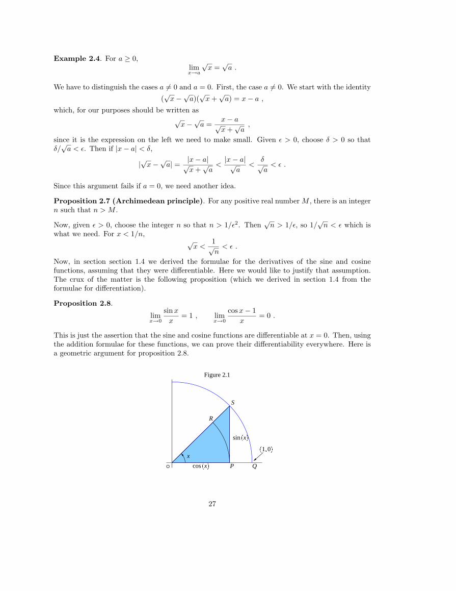
This is just the assertion that the sine and cosine functions are differentiable at x = 0. Then, usingthe addition formulae for these functions, we can prove their differentiability everywhere. Here isa geometric argument for proposition 2.8.

Figure 2.1

O

S

R

sin � x �

cos � x �x

P Q

� 1 � 0 �

27

In figure 2.1, let A be the area of the sector OPR, B the area of triangle OPS, and C the areaof sector OQS. Then A ≤ B ≤ C. Using the formulae for these areas (measuring the angle x inradians), this gives us

12x cos2 x ≤ 1

2cos x sinx ≤ 1

2x(1)2 .

Dividing by x cos x/2, this gives us

cos x ≤ sinx

x≤ 1

cos x.

But now, since limx→0 cos x = 1, as is obvious from the figure, the first part of proposition I.12follows from the squeeze theorem. The second now follows from the first using the equalities:

cos x− 1x

=cos x− 1

x

cos x + 1cos x + 1

=cos2−1

x(cos x + 1)=

sinx

xsinx

11 + cos x

→ 0 ,

since limx→0 sinx = 0, as is clear from the figure.

Example 2.5. Find the limit as x → 0 of sin(3x)/ sin(4x).

limx→0

sin(3x)sin(4x)

=34

limx→0

sin(3x)3x

4x

sin(4x)=

34

lim3x→0

sin(3x)3x

lim4x→0

4x

sin(4x)=

34(1)(1) =

34

Example 2.6. Find the limit as x → π/2 of cos x/(x − π/2). Let t = x − π/2. Then cos x =sin(π/2− x) = − sin(x− π/2) = − sin t, and t → 0 as x → π/2. Thus

limx→π/2

cos x

x− π/2= − lim

t→0

sin t

t= −1 .

Problems 2.1

1. If, in definition 2.1 we just restrict attention to those x > x0, we call the limit the limit fromthe right, denoted limx→x+

0f(x), and if we restrict to those x < x0 we call it the limit from the

left, denoted limx→x−0f(x). Suppose that f is defined in an interval about x0, and both the limit

from the left and the limit from the right exist. Show that if they are both equal to L, then

limx→x0

f(x) = L .

2. Show that if f and g are functions defined in an interval near x0 and

limx→x0

f(x) = L , limx→x0

g(x) = M ,

thenlim

x→x0f(x)g(x) = LM .

Hint: Write f(x) = L + a(x), g(x) = M + b(x), noting that by the hypothesis we can ensure thata(x), b(x) can be made as small as we please by taking x sufficiently close to x0.

3. limx→2

x2 − 4x2 − 3x + 2

=

28

Hint: Factor numerator and denominator.

4. limx→0

cos x− 1x sinx

=

Hint: multiply and divide by cos x + 1.

5. Suppose that f is defined in an interval about 0, and that |f(x)| ≤ |x|2 in that interval. Showthat f is differentiable at 0 and f ′(0) = 0.

6. Show that the function f defined by f(0) = 0 and for x 6= 0, f(x) = x2 sin(1/x) is differentiableat 0 and has derivative zero.

7. Show that the function f defined by f(0) = 0 and for x 6= 0, f(x) = x sin(1/x) is notdifferentiable at 0.

2.2 Limits at Infinity

Suppose that f is defined for all positive numbers. We say that f has the limit L as x → +∞ ifwe can make f as close as we please to L by taking x large enough. For example

limx→+∞

1x

= 0 ,

since we can make 1/x < ε just by taking x > 1/ε.

Definition 2.4. Suppose that f(x) is defined for all x > M0. We say that

limx→+∞

f(x) = L

if, for every ε > 0, we can find an M ≥ M0 such that if x > M , then |f(x)− L| < ε.

Suppose that f(x) is defined for all x < M0. We say that

limx→−∞

f(x) = L

if, for every ε > 0, we can find an M ≤ M0 such that if x < M , then |f(x)− L| < ε.

Example 2.7.lim

x→+∞

x

x + 1= 1 .

For, given ε > 0, choose M = 1/ε. Then, for x > M , we have

∣∣ x

x + 1− 1

∣∣ =∣∣x− (x + 1)

x + 1

∣∣ =∣∣ 1x + 1

∣∣ <∣∣ 1x

∣∣ <1M

= ε .

Now, we define what it means to have ±∞ as a limit.

Definition 2.5. Let f be defined for all x in an interval about a, except perhaps at a. We write

limx→a

f(x) = +∞

29

if, for any M > 0, there is an ε > 0 such that for |x− a| < ε, we have f(x) > M .

Similarly,limx→a

f(x) = −∞

if, for any M > 0, there is an ε > 0 such that for |x− a| < ε, we have f(x) < −M .

We will also say that limx→+∞ f(x) = +∞ if we can make f(x) as large as we please by takingx sufficiently large, and similarly, we define limx→+∞ f(x) = −∞, limx→−∞ f(x) = +∞, and soforth.

Proposition 2.9. Let p be a polynomial of degree n > 1, with leading coefficient 1 .a) If n is even,

limx→±∞

p(x) = +∞ .

b) If n is oddlim

x→+∞p(x) = +∞ , lim

x→−∞p(x) = −∞ .

To see this, write p(x) = xn +an−1xn−1 + · · ·+a1x+a0. Then, by factoring out the highest power

of x:p(x) = xn

(1 +

an−1

x+ · · ·+ a1

xn−1+

a0

xn

).

The term in parenthesis goes to 1 as |x| becomes infinite. Now, since |xn| ≥ |x| so long as |x| ≥ 1,The term xn approaches +∞ as |x| becomes large, except when n is odd, and x → −∞, in whichcase xn → −∞.

Now, we can make the same kind of qualitative statements about quotients of polynomials (rationalfunctions). Let f(x) = p(x)/q(x) where p and q are polynomials with no common factors. Then fis defined and continuous at all points except those points a such that q(a) = 0. At such an a, thegraph of y = f(x) will go off the graph paper, either upwards or downwards, since the denominatoris 0 at a. In this case we say that the graph has a vertical asymptote at x = a. To determine thebehavior, we write q(x) = (x− a)nq0(x) for some positive integer n and some polynomial q0 suchthat q0(a) 6= 0. Since p has no factor in common with q, p(a) 6= 0. Then

limx→a

p(x)q(x)

= limx→a

1(x− a)n

p(x)q0(x)

.

Since the second factor converges to p(a)/q0(a), the behavior of p/q near a is determined by thebehavior of the first factor. For this, if n is odd, it depends upon whether we approach a from theright or the left, since (x − a)n is negative if x < a, and is positive if x > a. We summarize theresult as

Proposition 2.10. a) If n is even,

limx→a

1(x− a)n

= +∞ .

b) If n is odd,

limx→a−

1(x− a)n

= −∞ , limx→a+

1(x− a)n

= +∞ .

30

Finally, we summarize the limits for rational functions as x → ±∞.

Proposition 2.11. Let f(x) = p(x)/q(x), where p and q are polynomials of degree n and mrespectively.

a) If n < m,lim

x→±∞f(x) = 0 .

b) If n = m,lim

x→±∞f(x) =

an

bn,

where an, bn are the leading coefficients of p and q respectively.

c) If n = m + d,lim

x→±∞|f(x)−Q(x)| = 0

where Q is the polynomial of degree d obtained by dividing the polynomial p by the polynomial q.

The conclusion of part c) is to be understood this way: the graph of y = f(x) approaches thegraph of y = Q(x) as x → ±∞ so that for |x| large enough the curves are indistinguishable. Wesay that he latter curve is an asymptote for y = f(x).

Example 2.8. Let f(x) = (x2 + x)/((x + 2). f is not defined at x = −2. To see how f behavesat -2 and at infinity, we do the division:

x2 + x

x + 2= x− 1 +

2x + 2

Thus, for x very close to, but to the left of −2, f(x) is negative; but for x very close to, but to theright of −2, f(x) is positive. Thus

limx→−2−

x2 + x

x + 2= −∞ , lim

x→−2+

x2 + x

x + 2= ∞ .

Finally, y = f(x)has the asymptote y = x− 1 as x goes to infinity, since the difference

∣∣x2 + x

x + 2− (x− 1)

∣∣ =∣∣ 2x + 2

∣∣goes to zero as |x| goes to infinity.

Example 2.9. Let f(x) =x

x− 1

If we writef(x) = x

1x− 1

31

after observing that x is positive near 1, we see from proposition 2.10 that

limx→1−

f(x) = −∞ , limx→1+

f(x) = ∞ .

Finally, to see what happens as x goes to infinity, write

f(x) =1

1− 1x

or f(x) = 1 +1

x− 1

so that y = 1 is the asymptote.

Example 2.10. Let f(x) =x

(x− 1)2

If we writef(x) = x

1(x− 1)2

after observing that x is positive near 1, we see from proposition 2.10 that limx→1 f(x) = ∞ fromboth sides. Since the degree of the denominator is greater than the degree of the numerator, theasymptote is y = 0, with y = f(x) below the x-axis to the left, and above the x-axis to the right.

Example 2.11. Let

f(x) =x3 + 2x2

x2 − 3x + 2.

First, we factor numerator and denominator as much as possible:

f(x) =x2(x + 2)

(x− 1)(x− 2).

From this we see that f is defined except for the points x = 1, 2. We know that at these pointsf(x) becomes infinite; we need only to determine whether the limit is +∞ or −∞.

First we look near x = 1. To the left of 1, the negative terms are x− 1 and x− 2; since all othersare positive, f(x) > 0. We conclude

limx→1−

f(x) = +∞ .

But to the right of x = 1, the term x− 1 changes sign, so now f(x) < 0, and we conclude

limx→1+

f(x) = −∞ .

As we pass through x = 2, the only change is in from x− 2 < 0 to x− 2 > 0, so we conclude

limx→2−

f(x) = −∞ ,

limx→2+

f(x) = +∞ .

32

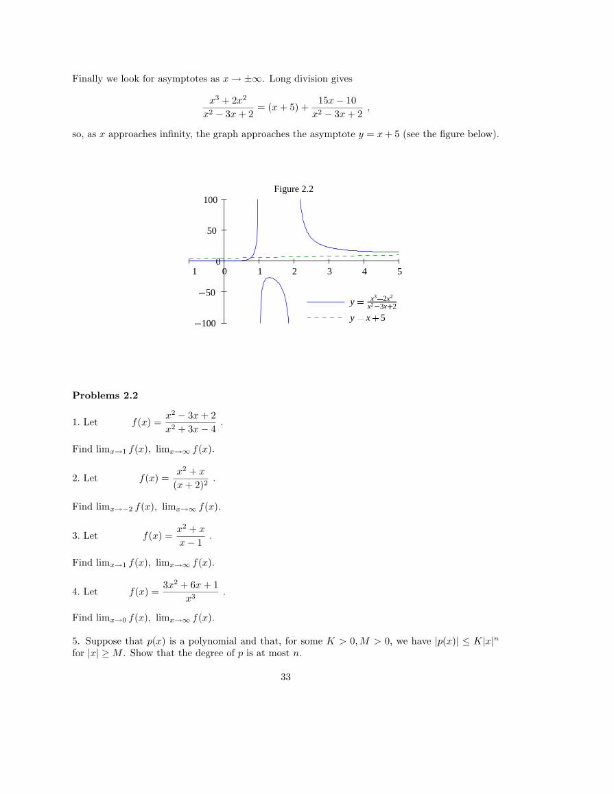
Finally we look for asymptotes as x → ±∞. Long division gives

x3 + 2x2

x2 − 3x + 2= (x + 5) +

15x− 10x2 − 3x + 2

,

so, as x approaches infinity, the graph approaches the asymptote y = x + 5 (see the figure below).

Figure 2.2

y � x3 � 2x2

x2 � 3x � 2

y � x � 5

100

50

� 50

� 100

1 2 3 4 500� 1

Problems 2.2

1. Let f(x) =x2 − 3x + 2x2 + 3x− 4

.

Find limx→1 f(x), limx→∞ f(x).

2. Let f(x) =x2 + x

(x + 2)2.

Find limx→−2 f(x), limx→∞ f(x).

3. Let f(x) =x2 + x

x− 1.

Find limx→1 f(x), limx→∞ f(x).

4. Let f(x) =3x2 + 6x + 1

x3.

Find limx→0 f(x), limx→∞ f(x).

5. Suppose that p(x) is a polynomial and that, for some K > 0,M > 0, we have |p(x)| ≤ K|x|nfor |x| ≥ M . Show that the degree of p is at most n.

33

6. Suppose that p(x) is a polynomial and that, for some K > 0,M > 0, we have |p(x)| ≤ K|x|2for |x| ≤ M . Show that x2 divides p(x).

2.3 Some Basic Theorems

The preceding sections discussed the behavior of functions locally, that is, for x varying in aneighborhood of a particular point a. In this section we summarize more global results; that isthe behavior of the function as x varies over an interval [a, b]. Most of these results are intuitivelyclear, and were taken as such by the founders of the Calculus.

Theorem 2.1 (Intermediate Value Theorem). Suppose that f is a continuous function onthe interval [a.b]. Then, for every number w between f(a) nd f(b), there is a c between a and bsuch that f(c) = w.

Intuitively, this says that as you draw the graph of the function y = f(x), your pencil point neverleaves the paper.

Theorem 2.2 (Maxima and Minima). Suppose that f is a continuous function on the interval[a.b]. There are points c, C in [a, b] such that f(c) is the minimum value of f on the interval, andf(C) is the maximum value of f on the interval.

Theorem 2.3 (Rolle’s theorem). Let f be continuous on [a, b] and differentiable in (a, b), andsuppose that f(a) = f(b). Then there is a point c in (a, b) at which f ′(c) = 0.

We can derive Rolle’s theorem from theorems 2.1 and 2.2. First of all, if f is constant, thenf ′(c) = 0 for all c. If f is nonconstant, there is a point c in the interval (a, b) at which f has eithera maximum or a minimum. Suppose it is a maximum. Then, for all other x in (a, b), f(x) ≤ f(c).In particular, for x < c, f(x)− f(c) and x− c have the same sign, so

f(x)− f(c)x− c

≥ 0 .

Taking the limit as x → c, we conclude f ′(c) ≥ 0. But now if x > c, the denominator changes sign,but the numerator doesn’t, so, in this case

f(x)− f(c)x− c

≤ 0 ,

from which we conclude f ′(c) ≤ 0.Thus f ′(c) = 0.

Notice, that the above argument incidentally shows that at a maximum or minimum point x0 of adifferentiable function, we must have f ′(x0) = 0. In the next chapter we shall see that this providesa method for finding maxima and minima.

Theorem 2.4 (The Mean Value Theorem). Let f be continuous on [a, b] and differentiable in(a, b). There is a c in (a, b) such that

(2.1) f ′(c) =f(b)− f(a)

b− a.

34

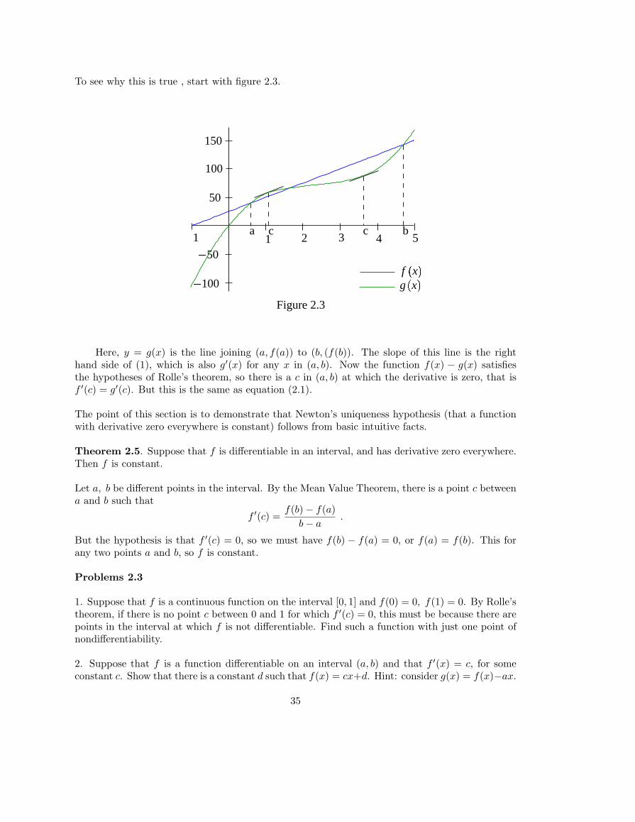
To see why this is true , start with figure 2.3. � ���

f � x �g � x �

150

100

50

� 50

� 100

1 2 3 4 5� 1a bcc

Figure 2.3

Here, y = g(x) is the line joining (a, f(a)) to (b, (f(b)). The slope of this line is the righthand side of (1), which is also g′(x) for any x in (a, b). Now the function f(x) − g(x) satisfiesthe hypotheses of Rolle’s theorem, so there is a c in (a, b) at which the derivative is zero, that isf ′(c) = g′(c). But this is the same as equation (2.1).

The point of this section is to demonstrate that Newton’s uniqueness hypothesis (that a functionwith derivative zero everywhere is constant) follows from basic intuitive facts.

Theorem 2.5. Suppose that f is differentiable in an interval, and has derivative zero everywhere.Then f is constant.

Let a, b be different points in the interval. By the Mean Value Theorem, there is a point c betweena and b such that

f ′(c) =f(b)− f(a)

b− a.

But the hypothesis is that f ′(c) = 0, so we must have f(b) − f(a) = 0, or f(a) = f(b). This forany two points a and b, so f is constant.

Problems 2.3

1. Suppose that f is a continuous function on the interval [0, 1] and f(0) = 0, f(1) = 0. By Rolle’stheorem, if there is no point c between 0 and 1 for which f ′(c) = 0, this must be because there arepoints in the interval at which f is not differentiable. Find such a function with just one point ofnondifferentiability.

2. Suppose that f is a function differentiable on an interval (a, b) and that f ′(x) = c, for someconstant c. Show that there is a constant d such that f(x) = cx+d. Hint: consider g(x) = f(x)−ax.

35

3. Suppose that f is twice differentiable in an interval containing 0, and that f(0) = 3, f ′(0) = 4and f ′′(x) = 2 for all x in the interval. Show that f(x) = x2 + 4x + 3.

4. Show by example that Theorem 2.1 is false for a discontinuous function.

5. Show by example that a function defined on an open interval (a, b) and continuous there neednot have a maximum on the interval.

2.4 L’Hopital’s Rule

The student may have noticed that in almost all of the examples involving limits, the given expres-sion was a quotient. Indeed, the very definition of the derivative is that of a limit of a quotient:

(2.2) f ′(x) = limx→a

f(x)− f(a)x− a

.

In this section we introduce a quick way of calculating the limit of a quotient f(x)/g(x) as xapproaches a in the case where both f(a) = 0 and g(a) = 0. This is, of course, the interesting case;otherwise we can obtain the limit by substitution. This technique, called l’Hopital’s rule, will notwork if either f(a) 6= 0 or g(a) 6= 0 as we shall see. So it is important to verify those conditions.l’Hopital’s rule also should not be confused with the rule for differentiating a quotient, which isquite a bit more complicated.

Proposition 2.12 (l’Hopital’s Rule). If f and g have continuous derivatives at a and f(a) = 0and g(a) = 0, then

limx→a

f(x)g(x)

= limx→a

f ′(x)g′(x)

.

To see this we use the Mean Value Theorem, theorem 2.4. According to that theorem, we canwrite f(x) − f(a) = f ′(c)(x − a) for some c between x and a, and gx) − g(a) = g′(d)(x − a) forsome d between x and a. Since f(a) = 0 and g(a) = 0, we have

limx→a

f(x)g(x)

= limx→a

f ′(c)(x− a)g′(d)(x− a)

= limx→a

f ′(c)g′(d)

.

But now, by assumption the derivatives f ′ and g′ are continuous. So, since c and d lie between xand a, f ′(c) and g′(d) have the same limits as f ′(x) and g′(x) as x → a.

Example 2.12. limx→0

sinx

x=

Here the functions are differentiable and both zero at x = 0, so l’Hopital’s rule applies:

limx→0

sinx

x= lim

x→0

cos x

1= cos(0) = 1 .

Of course this example is a fake, since we needed to validate this limit just to show the differen-tiability of sinx.

Example 2.13. limx→0

sin(3x)4x

=

36

Both numerator and denominator are 0 at x = 0, so we can apply l’H (a convenient abbreviationfor l’Hopital’s rule):

limx→0

sin(3x)4x

=l′H limx→0

3 cos(3x)4

=34

.

Example 2.14. limx→5

x2 − 4x + 5x− 5

=

Here both numerator and denominator are zero, so l’H applies:

limx→5

x2 − 4x + 5x− 5

=l′H limx→5

2x− 41

= 6 .

Note that we could also have divided the numerator by the denominator, getting

x2 − 4x + 5x− 5

= x + 1

whose value at x = 5 is 6.

Example 2.15. limx→0

x + 23x + 1

=

Since neither the numerator nor denominator is zero at x = 0, we can just substitute 0 for x,obtaining 2 as the limit. Note that if we blindly apply l’Hopital’s rule, we get the wrong answer,1/3.

Example 2.16. limx→2

x3 − 3x + 2tan(πx)

=

After checking that the hypotheses are satisfied, we get

limx→2

x3 − 3x + 2tan(πx)

=l′H limx→2

3x2 − 3π sec2(πx)

=12− 3

π=

9π

.

The second limit can be evaluated since both functions are continuous and the denominatornonzero.

Example 2.17. limx→0

sin2(2x)cos x− 1

=

Both numerator and denominator are zero at x = 0, so l’Hopital’s rule applies:

limx→0

sin2(2x)cos x− 1

=l′H limx→0

4 sin(2x) cos(2x)− sinx

.

Now, numerator and denominator are still zero at x = 0, so we can apply l’Hopital’s rule again:

=l′H limx→0

8 cos2(2x)− 8 sin2(2x)− cos x

= −8 ,

for now we can take the limit by evaluating the functions.

37

l’Hopital’s rule also works when taking the limit as x goes to infinity.

Proposition 2.13. If f and g are differentiable functions, and

limx→∞

f(x) = 0 limx→∞

g(x) = 0 ,

then

limx→∞

f(x)g(x)

= limx→∞

f ′(x)g′(x)

.

We see that this is true by the substitution t = 1/x, which leads us back to proposition 8.1:

limx→∞

f(x)g(x)

= limt→0

f(1/t)g(1/t)

=l′H limt→0

−1t2 f ′(1/t)−1t2 g′(1/t)

,

by l’Hopital’s rule and the chain rule. But the factors introduced cancel, so, changing back tox = 1/t, we get the proposition.

Finally, we remark, without verification, that l’Hopital’s rule also works if the limits are infinite:

Proposition 2.14. If f and g are differentiable functions, and limx→a f(x) = ∞ and limx→a g(x) =a, then

limx→∞

f(x)g(x)

= limx→a

f ′(x)g′(x)

.

Here the limit point a may also be infinity.

Example 2.18. limx→∞

2x2 − x + 3x2 + 5x

=

By proposition 2.14, we can replace the numerator and denominator by their derivatives:

limx→∞

2x2 − x + 3)x2 + 5x

=l′H limx→∞

4x− 12x + 5

=l′H limx→∞

42

= 2 .

Of course, this could also be shown by direct application of proposition 2.11.

Problems 2.4

1. Find the limit of example 2.5 using l’Hopital’s rule.

2. Find the limit of example 2.6 using l’Hopital’s rule.

3. limx→2

x2 − 4x2 − 3x + 2

=

4. limx→3

x2 − 3x

x2 + 2x− 15=

5. limx→1−

x− 1√1− x2

=

38

6. limx→0

x√x2

=

7. limx→∞

√1 + x2

x=

8. limx→π

sin2 x

x2 − 2πx + π2=

9. limx→π

sin2 x

x2 − 3πx + 2π2=

10. limx→π

sin2 x

(x− π)2=

11. limx→π/3

2 cos x− 13x− π

=

39

III. Extrema, Concavity, and Graphs

3.1 Monotonicity and the First Derivative

In this chaqpter we will be studying the behavior of differentiable functions in terms of theirderivatives. Thus, whenever a function f is introduced, it is to be understood that it is definedand has first and second derivatives on an interval I.

Definition 3.1. We saya) f is increasing on the interval I if, for a ≤ b, we have f(a) ≤ f(b).b) f is strictly increasing on the interval I if, for a < b, we have f(a) < f(b).c) f is decreasing on the interval I if, for a ≤ b, we have f(a) ≥ f(b).b) f is strictly decreasing on the interval I if, for a < b, we have f(a) > f(b).

Proposition 3.1a) If f ′ is always positive on I, then f is strictly increasing on the interval I.b) If f ′ is always negative on I, then f is strictly decreasing on the interval I.

For a < b, we have b− a > 0. By the mean value theorem (see theorem 2.4 of chapter 2), there isa c between a and b such that

f(b)− f(a)b− a

= f ′(c) .

Now in case the hypothesis of a) holds, this is positive. Since the denominator of the expression onthe left is positive, that implies that f(b)− f(a) > 0. On the other hand, if b) holds, so f ′(c) < 0,we conclude that the numerator is negative, so f(b)− f(a) < 0.

Definition 3.2. a) Let a be a point in I. We say that f has a local maximum at a if, for all xsufficiently close to a, f(a) ≤ f(x).b) We say that f has a local minimum at a if, for all x sufficiently close to a, f(a) ≥ f(x).

If we want to graph the function y = f(x), it is important to calculate f ′, and determine theintervals in which it is positive or negative. Then we know that the graph must “go up” in aninterval where f ′ is positive, and “go down” where f ′ is negative. Clearly, at points at which thesign of of f ′ changes, there must be either a local maximum or a minimum. For example, if f ′ isnegative to the left of a, and positive to the right of a, then f is decreasing to the left of a andincreasing to the right of a, so has a local minimum at a.

Proposition 3.2 (First Derivative Test). a) If f ′(x) > 0 for x < a and f ′(x) < 0 for x > a,then f has a local maximum at a.b) If f ′(x) < 0 for x < a and f ′(x) > 0 for x > a, then f has a local minimum at a.

If the function has a continuous second derivative, the following test may be computationally easier:

Proposition 3.3 (Second Derivative Test). a) If f ′(a) = 0 and f ′′(a) < 0, then f has a localmaximum at a.b) If f ′(a) = 0 and f ′′(a) > 0, then f has a local minimum at a.

Take case (a). We must have f ′′ negative in a neighborhood of a, so f ′ is decreasing in thatneighborhood. Since f ′(a) = 0, we must have f ′ positive to the left of a and negative to the right.So, by the first derivative test, f has a local maximum at a.

40

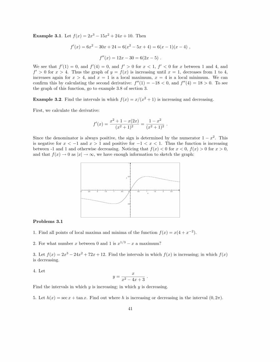
Example 3.1. Let f(x) = 2x3 − 15x2 + 24x + 10. Then

f ′(x) = 6x2 − 30x + 24 = 6(x2 − 5x + 4) = 6(x− 1)(x− 4) ,

f ′′(x) = 12x− 30 = 6(2x− 5) .

We see that f ′(1) = 0, and f ′(4) = 0, and f ′ > 0 for x < 1, f ′ < 0 for x between 1 and 4, andf ′ > 0 for x > 4. Thus the graph of y = f(x) is increasing until x = 1, decreases from 1 to 4,increases again for x > 4, and x = 1 is a local maximum, x = 4 is a local minimum. We canconfirm this by calculating the second derivative: f ′′(1) = −18 < 0, and f ′′(4) = 18 > 0. To seethe graph of this function, go to example 3.8 of section 3.

Example 3.2. Find the intervals in which f(x) = x/(x2 + 1) is increasing and decreasing.

First, we calculate the derivative:

f ′(x) =x2 + 1− x(2x)

(x2 + 1)2=

1− x2

(x2 + 1)2.

Since the denominator is always positive, the sign is determined by the numerator 1 − x2. Thisis negative for x < −1 and x > 1 and positive for −1 < x < 1. Thus the function is increasingbetween -1 and 1 and otherwise decreasing. Noticing that f(x) < 0 for x < 0, f(x) > 0 for x > 0,and that f(x) → 0 as |x| → ∞, we have enough information to sketch the graph:

-3 -2.5 -2 -1.5 -1 -0.5 0 0.5 1 1.5 2 2.5 3

-1

-0.5

0.5

1

Problems 3.1

1. Find all points of local maxima and minima of the function f(x) = x(4 + x−2).

2. For what number x between 0 and 1 is x1/3 − x a maximum?

3. Let f(x) = 2x3 − 24x2 + 72x + 12. Find the intervals in which f(x) is increasing; in which f(x)is decreasing.

4. Lety =

x

x2 − 4x + 3.

Find the intervals in which y is increasing; in which y is decreasing.

5. Let h(x) = sec x + tanx. Find out where h is increasing or decreasing in the interval (0, 2π).

41

6. Let y = x4 − x3 − x + 1. Find the value of x where y has its minimum.

7. Graph a function with these conditions: a) f(0) = 2, b) f(2) = 4, c) f ′(x) < 0 for x < 0, d) fhas a local maximum between x = 0 and x = 2, e) f has a local minimum at some point c withc > 2.

8. Show that the equation 2x12 − 3x6 + x = 0 has a root strictly between 0 and 1.

3.2 Optimization

The knowledge about a function that we obtain from the first derivative often suffices to solvepractical optimization problems. Typically, the given situation leads to a function y = f(x)defined on a closed interval a ≤ x ≤ b, and the problem is to find the maximum or minimum valueof the function on the interval. This can occur only at one of the following points: the endpoints,a, b, any point in the interval at which f does not have a derivative, or any point c on the intervalat which f ′(c) = 0. These are the critical points of the function. Evaluate the function at all ofthe critical points; the largest of these values is the maximum on the interval, and the smallest,the minimum.

Example 3.3. Find the maximum and the minimum of y = x√

1− x2 on the interval −1 ≤ x ≤ 1.

Differentiate:dy

dx=

√1− x2 + x

−2x

2√

1− x2=

1− 2x2

(1− x2)3/2

This is zero when x = ±1/√

2. The critical values are −1,−1/√

2, 1/√

2, 1, and the correspondingvalues of y are 0, −[(1/2)

√3/2], [(1/2)

√3/2], 0, so the nonzero values are the minimum and

maximum repsectively.

Example 3.4. Let y = sin2 x + cos x, for x in the interval [−π, π]. Find the absolute maximumand minimum of y.

Differentiate:y′ = 2 sin x cos x− sinx = sinx(2 cos x− 1) .

This is zero at x = −π, 0, π and x = ±π/3. The values of y at these points are

x −π −π/3 0 π/3 πy −1 5

4 1 54 −1

Thus the absolute maximum is 5/4, and the absolute minimum is -1. Note that at x = 0 we havea local minimum.

Many problems involve finding the values of certain variables which make a related variable amaximum or a minimum. The method of attack on such probems is as follows:

Step 1. Draw a picture (if appropriate), and identify the relevant variables: those things whichcan change. State the problem in terms of the variables. Here it is important to distinguish thevariable to be optimized: call it the objective variable.

42

Step 2. Express the objective variable in terms of the other relevant variables. If there is morethan one such variable, look for relations among them: these are called the constraints.

Step 3. Use the constraints to express the objective as a function of only one of the othervariables.

Step 4. Differentiate and set the derivative equal to zero.

Step 5. Calculate the values of the objective variable at each of the points found in step 4(as well as the endpoints of the range of that variable), and choose the one which is the desiredmaximum (or minimum).

Example 3.5. A triangle in the first quadrant has vertices at the points (0, 0), (t, 0), (t, 9 − t2).Find the triangle of of maximum area.

Here the variables are area, A, and value t determining the triangle. Area is the objective variable;in terms of t this area is

A(t) =12t(9− t2) =

12(9t− t3) .

Since the triangle is in the first quadrant, we must have t ≥ 0 and 9 − t2 ≥ 0, so the interval onwhich the area is defined is 0 ≤ t ≤ 3. Now

f ′(t) =9− 3t2

2

so f ′(t) = 0 when t = ±√

3. The critical points on the interval in question are 0,√

3, 3. The valuesof f at these points are 0, 3

√3, 0, so the maximum value is 3

√3.

Example 3.6. A box with a square bottom is to be made so as to contain 150 in3.The cost ofthe material to make the sides is $2 per in2 and the material for the top and bottom is $3 per in2.What are the dimensions of the box of minimal cost?

Here the variables are: x, the length of a side of the base of the box, h, the height, the area Ab ofthe base (which is the same as the area of the top), the area As of a side (of which there are 4),and the cost, C. Since we want to minimize C, this is the objective variable.

According to our data, the cost is given by C = 3(2Ab) + 2(4As). Now Ab = x2, and As = xh, sowe obtain

C = 6x2 + 8xh .

Now, we need a relationship between x and h: that is provided by the constraint that the boxmust contain 150 in3. Thus x2h = 150, or h = 150x−2. The objective equation becomes

(3.1) C = 6x2 + 8x(150x−2) = 6x2 + 1200x−1 .

In principle, the variable x ranges over all positive numbers, but we note from equation (3.1) thatC becomes arbitrarily large as x becomes very large or very small. Thus there is a minimumsomewhere between: at a place where C ′(x) = 0. Differentiating:

C ′(x) = 12x− 1200x−2 ,

43

so C ′(x) = 0 when 12x3 = 1200, or x = 4.64 in. Since this is the only point at which C ′ = 0, itis the value of x which minimizes the cost. Using x2h = 150, we find h = 6.96 in. Thus the boxshould be (approximately) 4.5 in square on the base, and of height 7 in.

Example 3.7. An automobile maufacturer sells, on average, 8000 cars per month at twenty-fivethousand dollars. The marketing department has determined that for every one thousand dollarreduction in price, the company can sell an additional 500 cars per month. At what price shouldthe car be sold so as to maximize revenue?

Let p be the price reduction (in thousands of dollars) at which the automobile is to be sold. Withthis reduction, the manufacturer sells 8 + p/2 thousand cars, and the price is 25 − p thousand.Thus the total revenue is R = (8+ p/2)(25− p). To maximize revenue we differentiate, and set thederivative equal to zero:

R′ =12(25− p)− (8 + p/2) = 4.5− p .

The desired reduction is p = $4500 and the selling price should be $20,500.

Problems 3.2

1. Find the absolute maxima and minima of the function

f(w) = w√

w + 1

on the interval [-1.4].

2. Find the maximum and the minimum of y = x√

1− x2 on the interval −1 ≤ x ≤ 1.

3. Let y = sinx + cos2 x, for x in the interval [−π, π]. Find the absolute maximum and minimumof y.

4. Find the dimensions of the right triangle with one vertex at the origin, another on the positivex-axis, and the third on the curve y = 4 + x−2 which is of minimum area.

5. We are asked to make an open-topped box out of a rectangular sheet of tin 24 in. wide and 45.in long. This is to be done by cutting congruent squares out of each corner of the sheet and thenbending sides upward to from the sides of the box. What are the dimensions of the box of greatestvolume?

6. A particle travels at 2 ft/sec in the upper half-plane, and at 3 ft/sec on the x-axis. The objectstarts at one foot up the y-axis (at (0,1)), and will travel to a point 3 ft down the x axis (at (3,0))by heading straight for some point (x,0) and then along the x axis. Find the value of x whichminimizes the time it takes.

7. A commuter train carries 600 passengers each day from a suburb to a city. It costs $ 1.50 perperson to ride the train. It is found that 40 more people will ride the train for each 5 cent decreasein the fare. What fare should be charged to make the largest possible revenue?

8. A rectangular racecourse is to be made so the diagonal measures 5 furlongs, and so we canplace 20 spectators per furlong along the horizontal sides, and 30 spectators per furlong along the

44

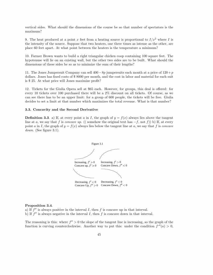
vertical sides. What should the dimensions of the course be so that number of spectators is themaximum?

9. The heat produced at a point x feet from a heating source is proportional to I/x2 where I isthe intensity of the source. Suppose that two heaters, one three times as intense as the other, areplace 60 feet apart. At what point between the heaters is the temperature a minimum?

10. Farmer Brown wants to build a right triangular chicken coop containing 100 square feet. Thehypotenuse will lie on an existing wall, but the other two sides are to be built. What should thedimensions of these sides be so as to minimize the sum of their lengths?

11. The Jones Jumpersuit Company can sell 400−8p jumpersuits each month at a price of 120+pdollars. Jones has fixed costs of $ 8000 per month, and the cost in labor and material for each suitis $ 25. At what price will Jones maximize profit?

12. Tickets for the Giulia Opera sell at $65 each. However, for groups, this deal is offered: forevery 10 tickets over 100 purchased there will be a 2% discount on all tickets. Of course, as wecan see there has to be an upper limit: for a group of 600 people, the tickets will be free. Giuliadecides to set a limit at that number which maximizes the total revenue. What is that number?

3.3. Concavity and the Second Derivative

Definition 3.3. a) If, at every point a in I, the graph of y = f(x) always lies above the tangentline at a, we say that f is concave up. (( somehow the original text has −f , not f)) b) If, at everypoint a in I, the graph of y = f(x) always lies below the tangent line at a, we say that f is concavedown. (See figure 3.1).

Figure 3.1

Increasing, f � � 0Concave up, f � � 0

Increasing, f � � 0Concave Down, f � ��� 0

Decreasing, f � � 0Concave Up, f � � � 0

Decreasing, f ��� 0Concave Down, f � ��� 0

Proposition 3.4.a) If f ′′ is always positive in the interval I, then f is concave up in that interval.b) If f ′′ is always negative in the interval I, then f is concave down in that interval.

The reasoning is this: where f ′′ > 0 the slope of the tangent line is increasing, so the graph of thefunction is curving counterclockwise. Another way to put this: under the condition f ‘′′(a) > 0,

45

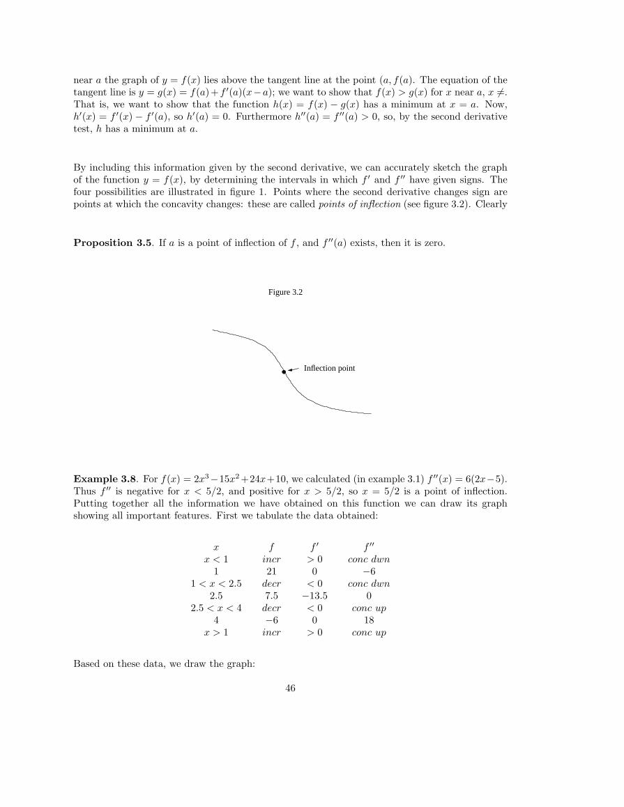
near a the graph of y = f(x) lies above the tangent line at the point (a, f(a). The equation of thetangent line is y = g(x) = f(a)+f ′(a)(x−a); we want to show that f(x) > g(x) for x near a, x 6=.That is, we want to show that the function h(x) = f(x) − g(x) has a minimum at x = a. Now,h′(x) = f ′(x) − f ′(a), so h′(a) = 0. Furthermore h′′(a) = f ′′(a) > 0, so, by the second derivativetest, h has a minimum at a.

By including this information given by the second derivative, we can accurately sketch the graphof the function y = f(x), by determining the intervals in which f ′ and f ′′ have given signs. Thefour possibilities are illustrated in figure 1. Points where the second derivative changes sign arepoints at which the concavity changes: these are called points of inflection (see figure 3.2). Clearly

Proposition 3.5. If a is a point of inflection of f , and f ′′(a) exists, then it is zero.

Figure 3.2

Inflection point

Example 3.8. For f(x) = 2x3−15x2+24x+10, we calculated (in example 3.1) f ′′(x) = 6(2x−5).Thus f ′′ is negative for x < 5/2, and positive for x > 5/2, so x = 5/2 is a point of inflection.Putting together all the information we have obtained on this function we can draw its graphshowing all important features. First we tabulate the data obtained:

x f f ′ f ′′

x < 1 incr > 0 conc dwn1 21 0 −6

1 < x < 2.5 decr < 0 conc dwn2.5 7.5 −13.5 0

2.5 < x < 4 decr < 0 conc up4 −6 0 18

x > 1 incr > 0 conc up

Based on these data, we draw the graph:

46

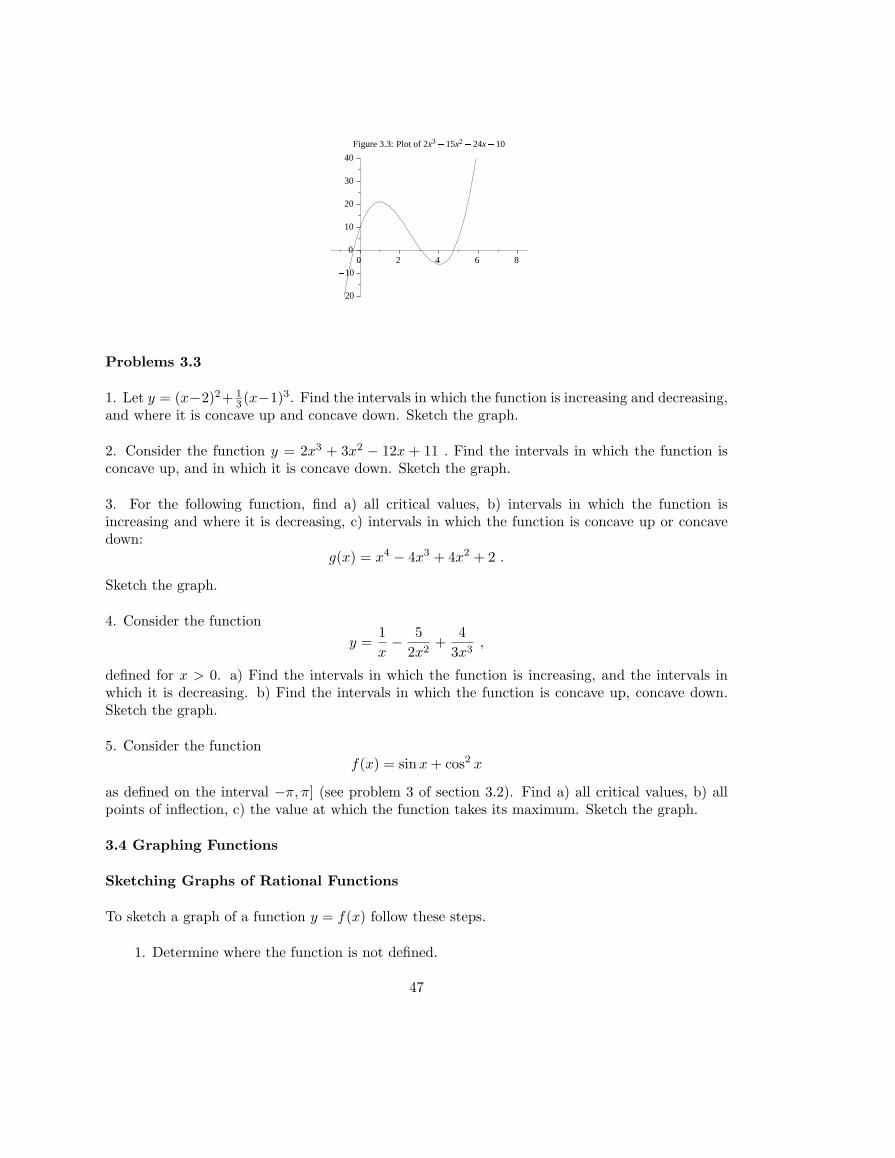
Figure 3.3: Plot of 2x3 � 15x2 �24x

�10

40

30

20

10

� 10

� 20

2 4 6 800

Problems 3.3

1. Let y = (x−2)2+ 13 (x−1)3. Find the intervals in which the function is increasing and decreasing,

and where it is concave up and concave down. Sketch the graph.

2. Consider the function y = 2x3 + 3x2 − 12x + 11 . Find the intervals in which the function isconcave up, and in which it is concave down. Sketch the graph.

3. For the following function, find a) all critical values, b) intervals in which the function isincreasing and where it is decreasing, c) intervals in which the function is concave up or concavedown:

g(x) = x4 − 4x3 + 4x2 + 2 .

Sketch the graph.

4. Consider the functiony =

1x− 5

2x2+

43x3

,

defined for x > 0. a) Find the intervals in which the function is increasing, and the intervals inwhich it is decreasing. b) Find the intervals in which the function is concave up, concave down.Sketch the graph.

5. Consider the functionf(x) = sin x + cos2 x

as defined on the interval −π, π] (see problem 3 of section 3.2). Find a) all critical values, b) allpoints of inflection, c) the value at which the function takes its maximum. Sketch the graph.

3.4 Graphing Functions

Sketching Graphs of Rational Functions

To sketch a graph of a function y = f(x) follow these steps.

1. Determine where the function is not defined.

47

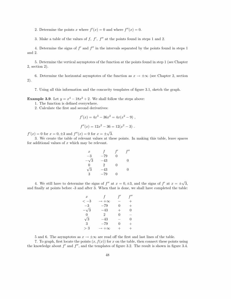
2. Determine the points x where f ′(x) = 0 and where f ′′(x) = 0.

3. Make a table of the values of f, f ′, f ′′ at the points found in steps 1 and 2.

4. Determine the signs of f ′ and f ′′ in the intervals separated by the points found in steps 1and 2.

5. Determine the vertical asymptotes of the function at the points found in step 1 (see Chapter2, section 2).

6. Determine the horizontal asymptotes of the function as x → ±∞ (see Chapter 2, section2).

7. Using all this information and the concavity templates of figure 3.1, sketch the graph.

Example 3.9. Let y = x4 − 18x2 + 2. We shall follow the steps above:1. The function is defined everywhere.2. Calculate the first and second derivatives:

f ′(x) = 4x3 − 36x2 = 4x(x2 − 9) ,

f ′′(x) = 12x2 − 36 = 12(x2 − 3) .

f ′(x) = 0 for x = 0,±3 and f ′′(x) = 0 for x = ±√

3.3. We create the table of relevant values at these points. In making this table, leave spaces

for additional values of x which may be relevant.

x f f ′ f ′′

−3 −79 0−√

3 −43 00 2 0√3 −43 0

3 −79 0

4. We still have to determine the signs of f ′′ at x = 0,±3, and the signs of f ′ at x = ±√

3,and finally at points before -3 and after 3. When that is done, we shall have completed the table:

x f f ′ f ′′

< −3 → +∞ − +−3 −79 0 +−√

3 −43 + 00 2 0 −√3 −43 − 0

3 −79 0 +> 3 → +∞ + +

5 and 6. The asymptotes as x → ±∞ are read off the first and last lines of the table.7. To graph, first locate the points (x, f(x)) for x on the table, then connect these points using

the knowledge about f ′ and f ′′, and the templates of figure 3.2. The result is shown in figure 3.4.

48

� �

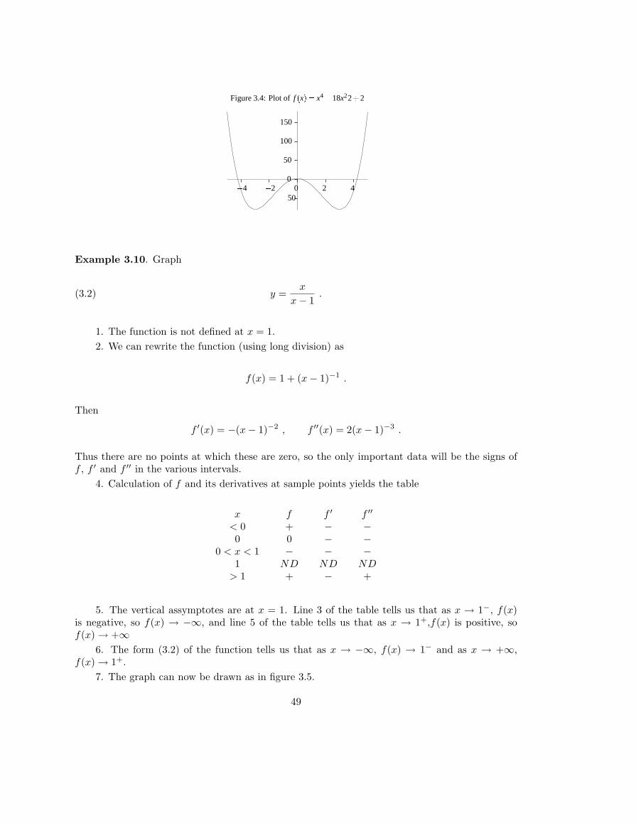
Figure 3.4: Plot of f � x ��� x4 � 18x22�

2

150

100

50

� 50

0� 2� 4 2 40

Example 3.10. Graph

(3.2) y =x

x− 1.

1. The function is not defined at x = 1.2. We can rewrite the function (using long division) as

f(x) = 1 + (x− 1)−1 .

Then

f ′(x) = −(x− 1)−2 , f ′′(x) = 2(x− 1)−3 .

Thus there are no points at which these are zero, so the only important data will be the signs off , f ′ and f ′′ in the various intervals.

4. Calculation of f and its derivatives at sample points yields the table

x f f ′ f ′′

< 0 + − −0 0 − −

0 < x < 1 − − −1 ND ND ND

> 1 + − +

5. The vertical assymptotes are at x = 1. Line 3 of the table tells us that as x → 1−, f(x)is negative, so f(x) → −∞, and line 5 of the table tells us that as x → 1+,f(x) is positive, sof(x) → +∞

6. The form (3.2) of the function tells us that as x → −∞, f(x) → 1− and as x → +∞,f(x) → 1+.

7. The graph can now be drawn as in figure 3.5.

49

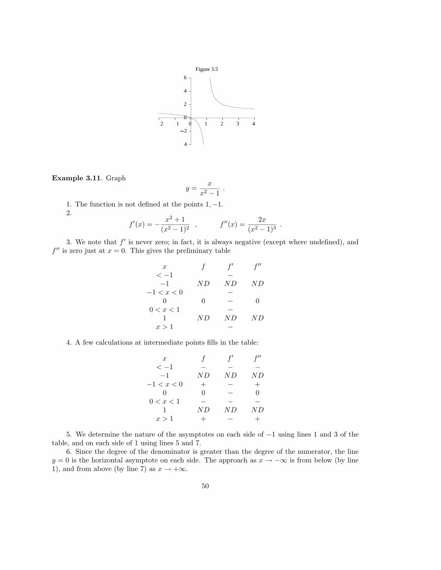
Figure 3.5

� 4

� 2

0

2

4

6

� 2 � 1 1 2 3 40

x

Example 3.11. Graphy =

x

x2 − 1.

1. The function is not defined at the points 1,−1.2.

f ′(x) = − x2 + 1(x2 − 1)2

, f ′′(x) =2x

(x2 − 1)3.

3. We note that f ′ is never zero; in fact, it is always negative (except where undefined), andf ′′ is zero just at x = 0. This gives the preliminary table

x f f ′ f ′′

< −1 −−1 ND ND ND

−1 < x < 0 −0 0 − 0

0 < x < 1 −1 ND ND ND

x > 1 −

4. A few calculations at intermediate points fills in the table:

x f f ′ f ′′

< −1 − − −−1 ND ND ND

−1 < x < 0 + − +0 0 − 0

0 < x < 1 − − −1 ND ND ND

x > 1 + − +

5. We determine the nature of the asymptotes on each side of −1 using lines 1 and 3 of thetable, and on each side of 1 using lines 5 and 7.

6. Since the degree of the denominator is greater than the degree of the numerator, the liney = 0 is the horizontal asymptote on each side. The approach as x → −∞ is from below (by line1), and from above (by line 7) as x → +∞.

50

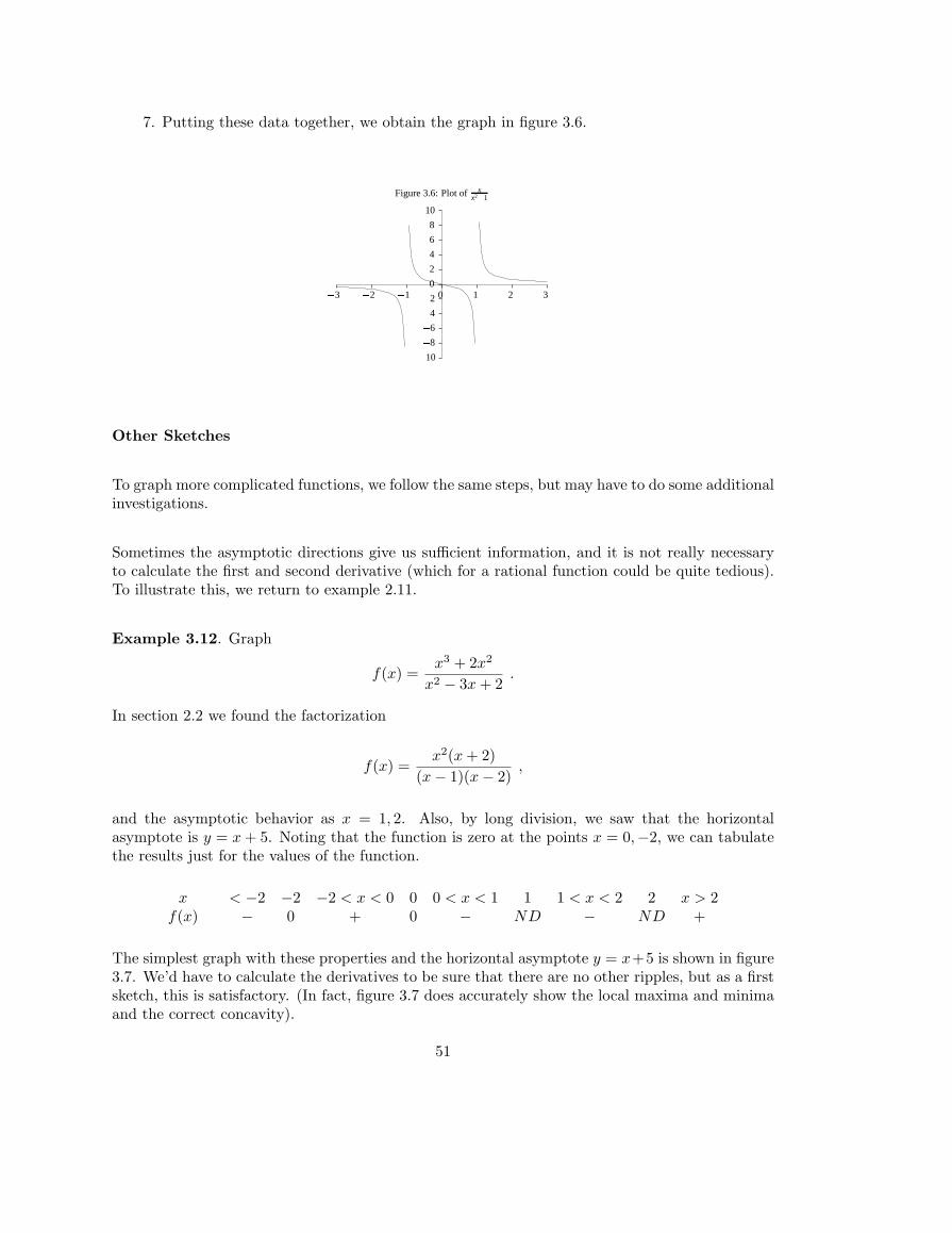
7. Putting these data together, we obtain the graph in figure 3.6.

Figure 3.6: Plot of xx2 � 1

� 10

� 8

� 6

� 4

� 2

0

2

4

6

8

10

� 3 � 2 � 1 0 1 2 3

Other Sketches

To graph more complicated functions, we follow the same steps, but may have to do some additionalinvestigations.

Sometimes the asymptotic directions give us sufficient information, and it is not really necessaryto calculate the first and second derivative (which for a rational function could be quite tedious).To illustrate this, we return to example 2.11.

Example 3.12. Graph

f(x) =x3 + 2x2

x2 − 3x + 2.

In section 2.2 we found the factorization

f(x) =x2(x + 2)

(x− 1)(x− 2),

and the asymptotic behavior as x = 1, 2. Also, by long division, we saw that the horizontalasymptote is y = x + 5. Noting that the function is zero at the points x = 0,−2, we can tabulatethe results just for the values of the function.

x < −2 −2 −2 < x < 0 0 0 < x < 1 1 1 < x < 2 2 x > 2f(x) − 0 + 0 − ND − ND +

The simplest graph with these properties and the horizontal asymptote y = x+5 is shown in figure3.7. We’d have to calculate the derivatives to be sure that there are no other ripples, but as a firstsketch, this is satisfactory. (In fact, figure 3.7 does accurately show the local maxima and minimaand the correct concavity).

51

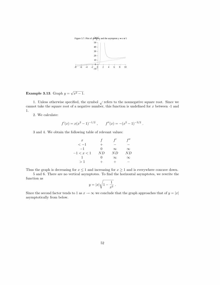
Figure 3.7: Plot of x3 � 2x2

x2 � 3x � 2 and the asymptote y � x�

5

50

40

30

20

10

-10

0-8 -6 -4 -2 2 4 6 8 100

Example 3.13. Graph y =√

x2 − 1.

1. Unless otherwise specified, the symbol √ refers to the nonnegative square root. Since wecannot take the square root of a negative number, this function is undefined for x between -1 and1.

2. We calculate:

f ′(x) = x(x2 − 1)−1/2 , f ′′(x) = −(x2 − 1)−3/2 .

3 and 4. We obtain the following table of relevant values:

x f f ′ f ′′

< −1 + − −−1 0 ∞ ∞

−1 < x < 1 ND ND ND1 0 ∞ ∞

> 1 + + −

Thus the graph is decreasing for x ≤ 1 and increasing for x ≥ 1 and is everywhere concave down.5 and 6. There are no vertical asymptotes. To find the horizontal asymptotes, we rewrite the

function as

y = |x|√

1− 1x2

.

Since the second factor tends to 1 as x →∞ we conclude that the graph approaches that of y = |x|asymptotically from below.

52

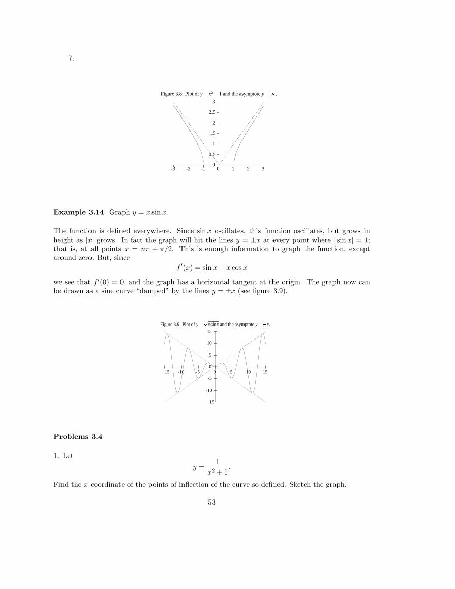
7.

Figure 3.8: Plot of y � x2 � 1 and the asymptote y ��� x � .3

2.5

2

1.5

1

0.5

0-3 -2 -1 1 2 30

Example 3.14. Graph y = x sinx.

The function is defined everywhere. Since sinx oscillates, this function oscillates, but grows inheight as |x| grows. In fact the graph will hit the lines y = ±x at every point where | sinx| = 1;that is, at all points x = nπ + π/2. This is enough information to graph the function, exceptaround zero. But, since

f ′(x) = sin x + x cos x

we see that f ′(0) = 0, and the graph has a horizontal tangent at the origin. The graph now canbe drawn as a sine curve “damped” by the lines y = ±x (see figure 3.9).

�

Figure 3.9: Plot of y ��� x sinx and the asymptote y ��� x.

� 15

-10

-5

5

10

15

0� 15 -10 -5 5 10 150

Problems 3.4

1. Lety =

1x2 + 1

.

Find the x coordinate of the points of inflection of the curve so defined. Sketch the graph.

53

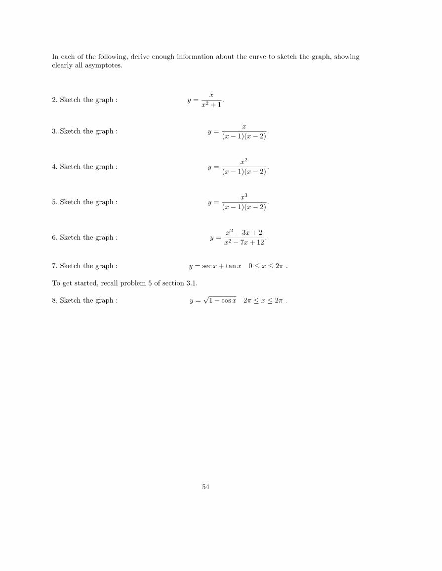
In each of the following, derive enough information about the curve to sketch the graph, showingclearly all asymptotes.

2. Sketch the graph : y =x

x2 + 1.

3. Sketch the graph : y =x

(x− 1)(x− 2).

4. Sketch the graph : y =x2

(x− 1)(x− 2).

5. Sketch the graph : y =x3

(x− 1)(x− 2).

6. Sketch the graph : y =x2 − 3x + 2x2 − 7x + 12

.

7. Sketch the graph : y = sec x + tanx 0 ≤ x ≤ 2π .

To get started, recall problem 5 of section 3.1.

8. Sketch the graph : y =√

1− cos x 2π ≤ x ≤ 2π .

54

IV. Integration: A Differential Equations Approach

4.1 Antiderivatives

Newton’s basic idea of dynamics is this: if we know the state of a system at a particular time,and we know the law of change, then we can predict the state at any future time. The law ofchange will ordinarily be an equation involving the function, its derivative, and the independentvariable: this is called a differential equation. Newton’s first law of motion expresses this idea: inthe absence of external forces, an object in motion will continue its motion in the same directionwith the same speed. Put another way, if acceleration is zero, then velocity is constant; and yetanother way: if dv/dt = 0, then v(t) = v(0) for all t. We have already seen this in Chapter II (astheorem 2.5):

Proposition 4.1. Suppose that f is differentiable in an interval, and has derivative zero every-where. Then f is constant.

As a consequence, we have

Proposition 4.2. If two functions have the same derivative, they differ by a constant.

For suppose f and g are the two functions, and f ′ = g′. We can apply proposition 4.1 to h = f−g:h′ = f ′ − g′ = 0, so h(x) = C, some constant. Then f(x) = g(x) + C.

Definition 4.1. Given a function f , any function F such that F ′ = f is an antiderivative orindefinite integral, or just integral of f . Any integral is denoted∫

f(x)dx .

We emphasize that any two integrals of a given function differ by a constant. So, for example, weknow that if f(x) = x2, then f ′(x) = 2x, so x2 is an integral of 2x, and therefore any integral of2x is of the form x2 +C, for some constant C. We indicate this by writing

∫2xdx = x2 +C . This

process of finding integrals is called integration. Now, the formulas of the differential calculus leadto the formulas for finding integrals, although not always so easily, as we shall see. For example,since the derivative of a sum is the sum of the derivatives, then the integral of a sum is the sum ofthe integrals. Since we differentiate xn by multiplying by the exponent and reducing the exponentby 1, we integrate xn by reversing the process: increase the exponent by 1, and divide by the newexponent. To summarize:

Proposition 4.3.a) Let f be a given function, and a a number. Then

∫af(x)dx = a

∫f(x)dx.

b) Let f and g be given functions. Then∫

(f(x) + g(x))dx =∫

f(x)dx +∫

g(x)dx.

c)∫

xndx = 1n+1xn+1 + C, n 6= −1.

Of course, the exclusion n = −1 is necessary, for in this case the right hand side doesn’t makesense. However, as we’ll see in section 4.5,

∫x−1dx does make sense and defines an important

function.

55

Example 4.1. Find the integral of f(x) = x4 − 3x2 + x − 1. We integrate term by term, usingProposition 4.3c for each term:∫

f(x)dx =x5

5− 3

x3

3+

x2

2− x + C

=15x5 − x3 +

12x2 − x + C

Example 4.2. ∫(4x−3 + x2)dx = 4(

x−2

−2) +

x3

3+ C = −2x−2 +

x3

3+ C

Example 4.3. A function f(x) has the derivative f ′(x) = x2 + x−2, and the value at x = 2 is 5.What is the function?

First we find the general function with the given derivative by integrating term by term:

f(x) =13x3 − x−1 + C

Now we substitute the given values, and solve for C:

5 =1323 − 1

2+ C

giving C = 17/6. Thus the desired function is

f(x) =13x3 − x−1 +

176

Proposition 4.3 shows us how to find integrals of polynomials. The differentiation formulas for thetrigonometric functions also lead to integration formulas for these functions.

Proposition 4.4.

a)∫

cos xdx = sinx + C

b)∫

sinxdx = − cos x + C

since the derivative of sinx is cos x, and the derivative of − cos x is sinx.

So far, we can only integrate functions by, so to speak, reading a table of derivatives in the reversedirection. For example, we also know from these tables that∫

sec2 dx = tan x + C and∫

sec x tanxdx = sec x + C ,

56

but we don’t yet know the integral of sec x, or for that matter, tanx or x−1. Finding integralsin general is a quite complicated process, and as this course proceeds we will study the varioustechniques of integration.

The first, and most useful of these techniques is that of substitution. This is the integration formof the chain rule. It is most conveniently stated in terms of differentials.

Proposition 4.5. Given variables u and x; suppose we know that u = u(x) is a function of x.Suppose their differentials are related by

(4.1) f(x)dx = g(u)du

for some functions f and g. Then ∫f(x)dx =

∫g(u)du + C .

To see this, let G(u) =∫

g(u)du. Then, treating G as a function of x by the substitution u = u(x),we have

dG

dx=

dG

du

du

dx

by the chain rule. But dG/du = g(u), so

dG

dx= g(u)

du

dx= f(x)

by the relation (4.1). Thus G(u(x)) is an integral of f(x).

This explains in part the notation for the integral: we should be thinking that it is the differentialf(x)dx which we are integrating, rather than the function. For when we change variables bysubstitution, it is the entire differential which we must consider.

Example 4.4.∫

(5x− 3)5dx = ?

Since we would rather not multiply 5x − 3 by itself 5 times so we can use Proposition 4.3, weinstead introduce the variable u = 5x− 3. Then du = 5dx, or dx = (1/5)du, so

(5x− 3)5dx =15u5du .

We now apply the power rule to the right hand side:∫15u5du =

15· 16u6 + C

and then replace u by its expression 5x− 3 as a function of x:∫(5x− 3)5dx =

130

(5x− 3)6 + C .

57

Example 4.5.∫

x(x2 + 1)3dx = ?

To integrate by substitution, always let u be what is inside the most complicated part. Here wewant to let u = x2 + 1. Then du = 2xdx, so xdx = 1

2du and we can replace the differential to beintegrated as follows:

x(x2 + 1)3dx = (x2 + 1)3(xdx) = u3(12du) =

12u3du .

Then ∫x(x2 + 1)3dx =

12

∫u3du =

12· 14u4 + C =

18(x2 + 1)4 + C .

Example 4.6.∫

cos2(2x + 1) sin(2x + 1)dx = ?

Let u = cos(2x + 1). Then du = −2 sin(2x + 1)dx or sin(2x + 1)dx = − 12du so that

cos2(2x + 1) sin(2x + 1)dx = −12u2du .

This substitution is effective:∫cos2(2x + 1) sin(2x + 1)dx = −1

2

∫u2du = −1

2u3

3+ C = −1

6cos3(2x + 1) + C .

Problem 4.1

1. Find the indefinite integral of f(x) = (x2 + 1)2x.

2. Integrate :∫

(x3 + 3x + 5)3(x2 + 1)dx =

3. Integrate : h(x) = x(x2 − 1)−3

4. Integrate : g(x) = (x2 − 1)(x3 − 3x)3

5. Integrate :∫

(sin2 x + 1) cos xdx =

6. Find the indefinite integral of f(x) = x2 − 3x + x−2.

7. Find the indefinite integral of

g(x) = sin x +1

cos2 x.

8. Find the indefinite integral of h(x) = tanx sec2 x.

9. Find the indefinite integral of g(x) = sin3 x.

58

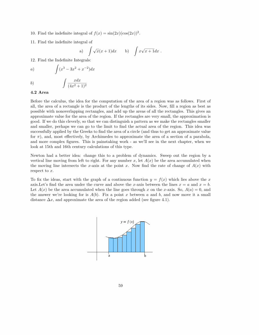
10. Find the indefinite integral of f(x) = sin(2x)(cos(2x))2.

11. Find the indefinite integral of

a)∫ √

x(x + 1)dx b)∫

x√

x + 1dx .

12. Find the Indefinite Integrals:

a)∫

(x3 − 3x2 + x−2)dx

b)∫

xdx

(4x2 + 1)2

4.2 Area

Before the calculus, the idea for the computation of the area of a region was as follows. First ofall, the area of a rectangle is the product of the lengths of its sides. Now, fill a region as best aspossible with nonoverlapping rectangles, and add up the areas of all the rectangles. This gives anapproximate value for the area of the region. If the rectangles are very small, the approximation isgood. If we do this cleverly, so that we can distinguish a pattern as we make the rectangles smallerand smaller, perhaps we can go to the limit to find the actual area of the region. This idea wassuccessfully applied by the Greeks to find the area of a circle (and thus to get an approximate valuefor π), and, most effectively, by Archimedes to approximate the area of a section of a parabola,and more complex figures. This is painstaking work - as we’ll see in the next chapter, when welook at 15th and 16th century calculations of this type.

Newton had a better idea: change this to a problem of dynamics. Sweep out the region by avertical line moving from left to right. For any number x, let A(x) be the area accumulated whenthe moving line intersects the x-axis at the point x. Now find the rate of change of A(x) withrespect to x.

To fix the ideas, start with the graph of a continuous function y = f(x) which lies above the xaxis.Let’s find the area under the curve and above the x-axis between the lines x = a and x = b.Let A(x) be the area accumulated when the line goes through x on the x-axis. So, A(a) = 0, andthe answer we’re looking for is A(b). Fix a point x between a and b, and now move it a smalldistance ∆x, and approximate the area of the region added (see figure 4.1).

y � f�x �

a b

59

Since the curve is almost a straight line over the interval of base length ∆x, we can approximatethat piece of area by the area of the trapezoid:

∆A =12(f(x) + f(x + ∆x))∆x or

∆A

∆x=

12(f(x) + f(x + ∆x)) .

Taking the limit as ∆x → 0, we getdA = f(x)dx .

so that area under a curve is found by finding the integral∫

f(x)dx that has the value 0 at x = a.

Example 4.7. Find the area under the curve y = 4x between x = 1 and x = 4.

This is a trapezoid of side lengths 4,16 and base length 3, so that its area is (1/2)(4 + 16)(3) = 30.But let’s use Newton’s idea. We first calculate the integral of the defining function:

A(x) =∫

4xdx = 2x2 + C .

We want the particular function A(x) whose value at x = 1 is zero; use that condition to solve forC:

0 = 2(12) + C

so that the precise function for area is A(x) = 2x2−2. Finally, the answer is A(4) = 2(42)−2 = 30.

Clearly our technique is not so simple as the formula from geometry. The powerful point here isthat this works for all continuous functions y = f(x).

Example 4.8. Find the area under the curve y = 6x2 + 4x between x = 2 and x = 5.

First, we calculate the indefinite integral:∫(6x2 + 4x)dx = 2x3 + 2x2 + C .

Now we find the particular integral whose value at x = 2 is zero:

0 = 2(2)3 + 2(2)2 + C , so that C = −24 ,

and the area function is A(x) = 2x3 + 2x2 − 24. The answer is

A(5) = 2(5)3 + 2(5)2 − 24 = 276 .

We now introduce a standard way for codifying these computations, which helps us to make thecomputations automatic. This starts with the following observation:

Proposition 4.6. Given a positive continuous function y = f(x), the area between the curve andthe x-axis from x = a to x = b is given by F (b)− F (a) where F is any indefinite integral of f .

To see this, let F be any indefinite integral of f . If F (a) = 0, it is the function we’re looking for.If not, then F (x) − F (a) is an indefinite integral whose value at a is 0, so is the function we’relooking for, and the area is its value at b: F (b)− F (a).

60

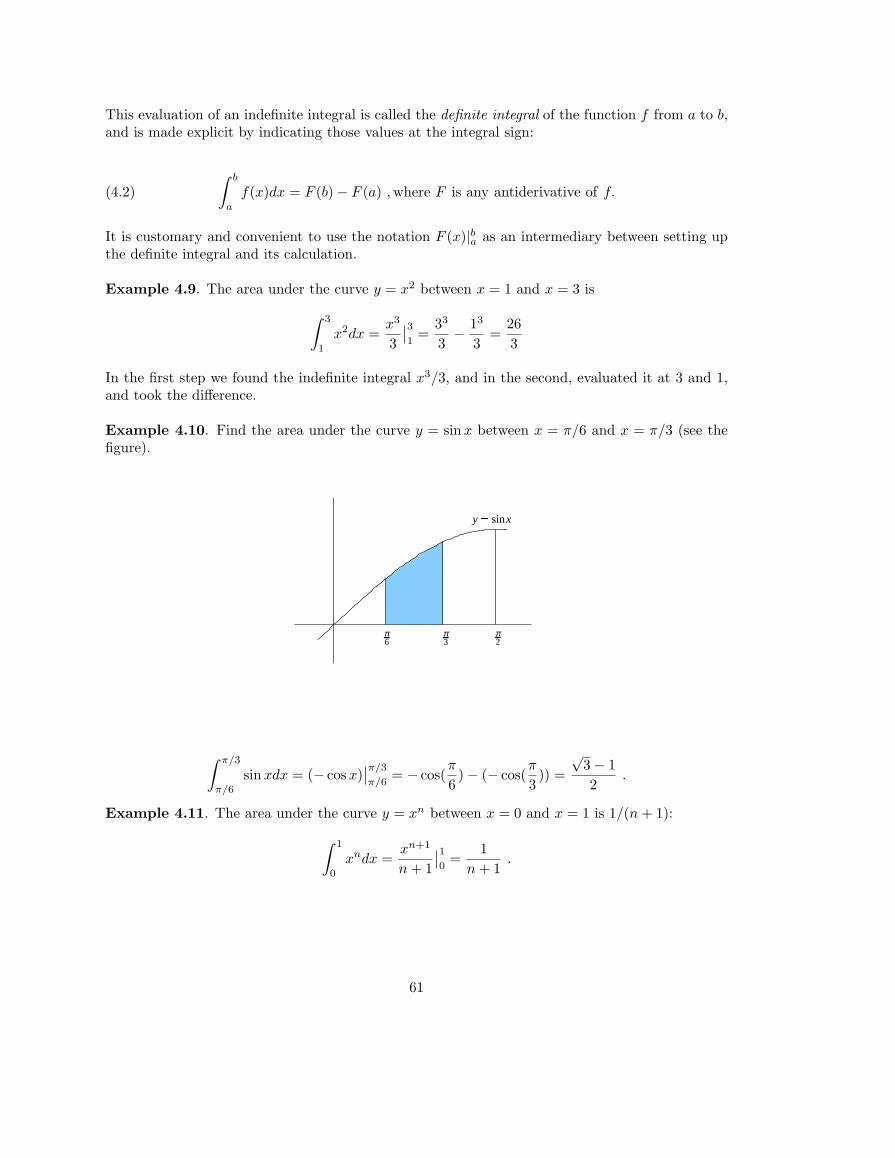
This evaluation of an indefinite integral is called the definite integral of the function f from a to b,and is made explicit by indicating those values at the integral sign:

(4.2)∫ b

a

f(x)dx = F (b)− F (a) ,where F is any antiderivative of f.

It is customary and convenient to use the notation F (x)|ba as an intermediary between setting upthe definite integral and its calculation.

Example 4.9. The area under the curve y = x2 between x = 1 and x = 3 is∫ 3

1

x2dx =x3

3

∣∣31

=33

3− 13

3=

263

In the first step we found the indefinite integral x3/3, and in the second, evaluated it at 3 and 1,and took the difference.

Example 4.10. Find the area under the curve y = sinx between x = π/6 and x = π/3 (see thefigure). � � � � �

y � sinx

π6

π3

π2

∫ π/3

π/6

sinxdx = (− cos x)∣∣π/3

π/6= − cos(

π

6)− (− cos(

π

3)) =

√3− 12

.

Example 4.11. The area under the curve y = xn between x = 0 and x = 1 is 1/(n + 1):∫ 1

0

xndx =xn+1

n + 1

∣∣10

=1

n + 1.

61

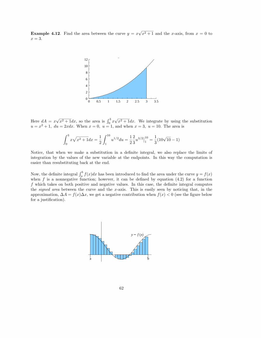
Example 4.12. Find the area between the curve y = x√

x2 + 1 and the x-axis, from x = 0 tox = 3.

�Figure 4.6

12

10

8

6

4

2

2

00

0 � 5 1 1 � 5 2 � 5 3 3 � 5

Here dA = x√

x2 + 1dx, so the area is∫ 3

0x√

x2 + 1dx. We integrate by using the substitutionu = x2 + 1, du = 2xdx. When x = 0, u = 1, and when x = 3, u = 10. The area is∫ 3

0

x√

x2 + 1dx =12

∫ 10

1

u1/2du =12

23u3/2

∣∣101

=13(10

√10− 1)

Notice, that when we make a substitution in a definite integral, we also replace the limits ofintegration by the values of the new variable at the endpoints. In this way the computation iseasier than resubstituting back at the end.

Now, the definite integral∫ b

af(x)dx has been introduced to find the area under the curve y = f(x)

when f is a nonnegative function; however, it can be defined by equation (4.2) for a functionf which takes on both positive and negative values. In this case, the definite integral computesthe signed area between the curve and the x-axis. This is easily seen by noticing that, in theapproximation, ∆A = f(x)∆x, we get a negative contribution when f(x) < 0 (see the figure belowfor a justification).

a b

y � f�x �

62

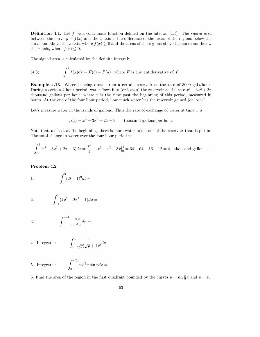
Definition 4.1. Let f be a continuous function defined on the interval [a, b]. The signed areabetween the curve y = f(x) and the x-axis is the difference of the areas of the regions below thecurve and above the x-axis, where f(x) ≥ 0 and the areas of the regions above the curve and belowthe x-axis, where f(x) ≤ 0.

The signed area is calculated by the definite integral:

(4.3)∫ b

a

f(x)dx = F (b)− F (a) ,where F is any antiderivative of f.

Example 4.13. Water is being drawn from a certain reservoir at the rate of 3000 gals/hour.During a certain 4 hour period, water flows into (or leaves) the reservoir at the rate x3 − 3x2 + 2xthousand gallons per hour, where x is the time past the beginning of this period, measured inhours. At the end of the four hour period, how much water has the reservoir gained (or lost)?

Let’s measure water in thousands of gallons. Thus the rate of exchange of water at time x is

f(x) = x3 − 3x2 + 2x− 3 thousand gallons per hour.

Note that, at least at the beginning, there is more water taken out of the reservoir than is put in.The total change in water over the four hour period is∫ 4

0

(x3 − 3x2 + 2x− 3)dx =x4

4− x3 + x2 − 3x

∣∣40

= 64− 64 + 16− 12 = 4 thousand gallons .

Problem 4.2

1.

∫ 3

1

(2t + 1)3dt =

2.

∫ 1

−1

(4x3 − 2x2 + 1)dx =

3.

∫ π/4

0

sinx

cos3 xdx =

4. Integrate :∫ 4

1

1√

y(√

y + 1)2dy

5. Integrate :∫ π/2

0

cos2 x sinxdx =

6. Find the area of the region in the first quadrant bounded by the curves y = sin π2 x and y = x.

63

7. Find the area of the region under the curve y = x2√

x3 + 1, above the x-axis and bounded bythe lines x = 0 and x = 4.

8. Find the area under the curve y = x2 + x−2, above the x-axis and between the lines x = 1 andx = 2.

9. Find the definite Integral:∫ 2

1(x2 + x−2)dx.

10. Find the area of the region above the x-axis and below the curve y = sec2 x lying between thelines x = −π/4 and x = π/4,

11. Find the definite integral:∫ 3

0(4x + 1)2dx.

12. Calculate the definite integrals:∫ 4

−4(x2 − 3 + cos x)dx.

4.3 Separation of Variables

A first order differential equation is a relation among the variables y, y′, x. For example:

y′ = x2 + 1 , (y′)2 + sin2 x = 1 , xy′ = y + 2x3 .

A solution of a differential equation is a function f(x) such that, if we let y = f(x), y′ = f ′(x)in the equation, we get an identity. So, for the above examples, we check that the following aresolutions, respectively:

f(x) =13x3 + x + 5 , g(x) = sin x , h(x) = x3 + 2x .

For the first, we just differentiate: f ′(x) = x2 + 1, and for the second we have g′(x) = cos x,and of course cos2 x + sin2 x = 1. The third takes a little calculation. First, h′(x) = 3x2 + 2, soxh′(x) = 3x3 + 2x = x3 + 2x + 2x3 = h(x) + 2x3, and the identity is verified.

In general, it is difficult to find solutions to differential equations, but in one special case, thanksto Proposition 4.5, it is not so hard. That proposition says that if we know that the differentialsf(y)dy and g(x)dx are equal, then their integrals differ by constant. In that proposition we assumedthe prior knowledge of y as a function of x, but the technique still works without that assumption.In fact, it comes out as a conclusion!

So, suppose that, upon replacing y′ by dy/dx, we can rewrite the differential equation as anequation of differentials:

f(y)dy = g(x)dx ,

so that all factors involving y are on one side of the equation, and all those involving x are on theother. In this case we say that “the variables can be separated.” Then we can solve by integratingboth sides.

Example 4.14. Solve the differential equation y′ = x2/y. We rewrite this as dy/dx = x2/y, whichcan be rewritten in differential form as ydy = x2dx. Now, integrate both sides:

12y2 =

13x3 + C

64

ory2 =

23x3 + C

(since C represents a generic constant, so does 2C, so we can again call it C). Thus the solution is

y =

√23x3 + C ,

and this is the general solution.

Example 4.15. Find the particular soluton of the differential equation y′ = x2/y such that y = 7when x = 3.

We follow the above argument to the equation

y2 =23x3 + C

Now we use the condition y = 7 when x = 3 to identify C:

72 =2333 + C or 49 = 18 + C

so that C = 31. Then the solution is

y =

√23x3 + 31 .

Example 4.16. An object moves along the x-axis so that its velocity at time t is v(t) = t(t2−1)5.If the object is at the origin at time t = 0, at what point is it at time t = 1? At time t = 2?

Notice that the velocity is negative until t = 1, so the object starts moving to the left, but at t = 1turns around and moves to the right. No matter; its position at time T , x(T ), is still given by thedefinite integral:

x(T ) =∫ T

0

vdt =∫ T

0

t(t2 − 1)5dt

Make the substitution u = t2 − 1, du = 2dt to obtain the integrand 12u5du. When t = 0, u = −1,

and when t = 1, u = 0, so

x(1) =12

∫ 0

−1

u5du =112

u6∣∣0−1

= − 112

.

For t = 2, we have u = 3, so

x(2) =12

∫ 3

−1

u5du =112

u6∣∣3−1

=112

(36 − 1) .

Example 4.17. Suppose a ball is thrown upward at an initial velocity of 128 ft/sec. How highdoes it go?

65

Let s, v, a represent position (measured upwards, with the surface of the earth at s = 0), velocity,acceleration. The acceleration due to gravity is

dv

dt= a = −32 ft/sec2

.

We integrate and conclude that v = −32t + C, for some constant C. Now, since v = 128 at timet = 0, we have

(4.4)ds

dt= v = −32t + 128

and integrating again we obtain s = −16t2 + 128t + C. Since s = 0 when t = 0, we must haveC = 0, so

(4.5) s = −16t2 + 128t

Now, at the maximum height, the velocity is zero. Solving (4.4) for v = 0, we have t = 128/32 = 4seconds at the high point. Putting this value of t in (4.5), we obtain the answer

s = −16 · 42 + 128(4) = 256 .

Example 4.18. In the above problem, the time it takes to attain maximum height is calculated inorder to find that height, but is otherwise irrelevant. In fact, by eliminating the variable t, we canfind a more direct relation between position and velocity. Once again, we consider the variabless, v, a, t , and relate their differentials by

ds = vdt , dv = adt .

But now, we eliminate dt by multiplying the second equation by v:

vdv = avdt = ads

from which we conclude, by integrating the differential equation vdv = ads:

(4.6)12v2 =

∫ads

which is useful if a is constant, or a function of position alone. In the case of the above problem ais constant, so (4.6) becomes (1/2)v2 = as + C. Setting s = 0 as the initial position, and v0 theinitial velocity, we find C = (1/2)v2

0 , giving the relation

(4.7)12v2 − 1

2v20 = as

Now, in the preceding problem a = −32, v0 = 128 and v = 0 at the maximum height, so we get−(1/2)(128)2 = −32s; solving for s gives s = 256.

Example 4.19. An automobile travelling at a speed of 60 mph (88 ft/sec) decelerates at a rateof 12 ft/sec2. How far does it travel before it stops?

66

Here a = −12, v0 = 88 and v = 0 when it stops. Putting these data into (4.7):

−12(88)2 = −12s

giving s = 322.67 ft.

Example 4.20. Now, Newton’s second law, F = ma, says that the acceleration of a body ofmass m in motion is proportional to the force F applied to it. If those forces are spacial; that is,functions of s alone, then, by multiplying equation (4.6) by m we get

(4.8)12mv2 =

∫F (s)ds

up to a constant, which is a way of stating the law of conservation of energy: the change in kineticenergy of the moving object (the left hand side) is equal to the work done by the force (the righthand side).

Example 4.21. To illustrate this observation, consider a rocket sitting on the surface of a planetof mass M and radius R. With what initial velocity v0 should the rocket be propelled so as toescape the gravitational field of the planet?

According to Newton’s law of universal gravitation, the force F of gravity is given by

F = −GmM

s2

where G is a universal constant, m is the mass of the rocket, and s is the distance of the rocketfrom the center of the planet. In particular, from F = ma, we obtain

a = −GM

s2,

and equation (4.6) becomes

12v2 = −GM

∫s−2ds = GMs−1 + C .

At liftoff, s = R and v = v0, and we find

C =12v20 −GMR−1 ,

and thus the velocity and distance of the rocket at any future time satisfy the relation

v2 =2GM

s+ v2

0 −2GM

R.

The rocket will escape the planet if this is never zero. As s increases, the first term gets smallerand smaller, so the only way we can insure this is to take v0 ≥

√2GM/R.

67

In particular, if the planet is earth, then GM/R2 = g = 32 ft/sec2, and R = 3900 miles. First, weconvert g to miles per hour per hour:

g = 32ft

sec2· (3600)2sec2

hr2· mile5280 ft

=32(3600)))2

5280mihr2

= 78545mihr2

.

Then, to escape earth’s gravitational pull, we must have

v0 ≥√

2GM

R=

√2gR = 24, 751 miles per hour .

Problems 4.3

1. Givendy

dx= x2√y, y = 4 when x = 0

find y as a function of x.

2. Find y as a function of x, given

dy

dx=

sinx

y, y = 5 when x = 0 .

3. Find the solution to the differential equation y′ = y2x2 + y2 such that y(1) = 2.

4. Find f(x) given that f(2) = 1, f ′(1) = −1 and f ′′(x) = x− x−3.

5. Find the function y = f(x) which satisfies the differential equation x2y′ + (1 + x2)y2 = 0 suchthat f(1) = 2.

6. Find the function y = f(x) which satisfies the differential equation

dy

dx=

1yx2

such that f(1) = 1.

7. Solve the differential equation:

dy

dx= (1 + x)y2, y(1) = 2.

8. Find the function whose value at 0 is 0 and whose derivative is

x

(2x2 + 1)2.

9. Find the function whose value at 0 is 0 and whose derivative is sinx/ cos4 x.

68

10. Find y as a function of x, given that y = 4 when x = 0 and

dy

dx= x + sinx .

11. Find the solution to the differential equation

dy

dx=

x

y2

such that y(1) = 2.

12. An automobile is travelling down the road a speed of 100 ft/sec. a) At what constant ratemust the automobile decelerate in order to stop in 300 ft.? b) How long does that take?

13. A ball is thrown from ground level so as to just reach the top of a building 150 ft. high. Atwhat initial velocity must the ball be thrown?

14. A 10 g object enters a straight track at a velocity of 12 cm/sec. On the track a force of −2sdynes is applied to this object , where s is distance from the start of the track measured in cm.What is the speed of the object when it is 10 cm down the track?How far does it go before it turnsaround?

4.4 The Exponential Function

In many dynamical processes we are interested in studying the development of the quantity ofa certain material as time progresses where the laws governing the process depend only on theproperties of the material. For example: (1) growth of a bacteria culture, (2) decay of a radioactivematerial, (3) cooling of a hot metal thrust into water, (4) growth of an interest bearing investmentfund, (5) spread of an epidemic. Let x = x(t) be the variable in such a process, where t representstime. In the above examples x would be (1) the mass of the bacteria, (2) the remaining mass ofthe original material, (3) the difference between the temperature of the metal and the ambienttemperature, (4) the value of the fund, (5) the number of infected people. These are examples ofgrowth (or decay) processes. In studying such processes we consider the per unit rate of growth:

(4.9) r =x′(t)x(t)

,

which can be written as the differential equation

(4.10)dx

dt= rx .

In many of these processes, the per unit rate of growth r is constant. For our examples: (1) solong as the source of nourishment is plentiful, we can expect the rate at which the bacteria devleopto remain unchanged, (2) the physical process of fission depends only on the nature of the atomand is the same throughout the material and remains unchanged over time, (3) the rate at whichheat is lost depends only on the temperature difference at the interface and the thermal propertiesof the material, (4) the growth of an investment account is the interest rate, set periodically bythe bank. As for (5), the rate of spread of an epidemic depends upon the nature of the disease,

69

and may depend on time, mortality rate as well as the rate of interaction between infected andnoninfected people. We will return to this case in section 6.

In case r is constant, equation (4.10) leads to a separable differential equation:

(4.11)dx

x= rdt .

The integral on the right is rt + C, and the integral on the left is given by sweeping out the areaunder the curve y = x−1. Although we do not know this function in any explicit sense, we canconclude that the differential equation (4.10) (or (4.11)) has a solution, and we proceed with thatknowledge.

Definition 4.2. The exponential function, written x(t) = ert, is the solution of the differentialequation

dx

dt= rx

with value x(0) = 1. If r > 0, r is called the growth rate; if r < 0, it is the decay rate. Moreprecisely, the function ert is defined by the conditions

(4.12)d

dxert = rert , er0 = 1 .

The exponential function, like the trigonometric functions, is a transcendental function. These arefunctions which cannot be expressed as a quotient of polynomials; in this sense they transcendrational functions. In due course, we shall find ways to calculate approximate values of the tran-scendental functions; for us now it suffices to know that these calculations have been done and areincorporated into our calculators.

Proposition 4.7. The solution of the differential equation x′(t) = rx(t), with initial value x(0) =x0 is

(4.12) x(t) = x0ert .

To verify this, we show that the function defined by (4.12) solves this initial value problem. First,x(0) = x0e

r0 = x0. Differentiating:

x′(t) = x0d

dxert = x0re

rt = rx(t) .

Example 4.22. $500 is deposited in an account, continuously compounded at an interest rate of5% per year. What is the value of the account after 5 years?

Let x(t) be the value of the fund at time t. Then x(0) = 500. The phrase continuously compoundedtells us that the fund grows continuously at the given rate, so x satisfies the differential equation(2) with r = .05. The solution then is

x(t) = 500e.05t .

At t = 5, we calculate: e.05(5) = e.25 = 1.284, so x(5) = 500(1.284) = 642.01 dollars.

70

Example 4.23. According to the census, the US population in 2000 was 281.4 million. Thegrowth rate over the preceding decade was .1235. Assuming that growth rate continues during thepresent century, what will be the US population in 2050 ?

Let x(t) be the population of the US in millions, where t is the number of decades after 2000. Thenx(0) = 281.4, and Proposition 4.6 tells us

x(t) = 281.4e(.1235)t

At 2050, t = 5, so the answer is x(5) = 281.4e.1235(5) = 521.8 million.

Example 4.24. The radioactive isotope 128I has a decay rate of .0279 per minute. How manygrams of an initial 100g suppy of 128I remain after 20 minutes?

Let x(t) be the amount of 128I present after t minutes. The information we are given is thatx(0) = 100 g and x(t) satisfies the differential equation

dx

dt= −.0279x(t) .

We have the negative sign since the given per unit rate is that of decay. Thus, by Proposition 4.7,x(t) = 100e(−.0279)t, and the answer is

x(20) = 100e−.0279(20) = 57.23 g.

We can come upon a way to calculate the exponential function by starting with a comparison ofcontinuously compounded interest with other ways of compounding interest. Suppose I depositone dollar in a bank account with an interest rate of 10% per year. If the rate is simple, that is, itis paid out once only at the end of the year, then at that time the account will have $1.10. This isconsidered unfair of the bank, since they have had the use of my dollar throughout the year andhave been investing it over and over, but they have transfered my share of the earning only at theend of the year. Suppose instead the bank paid me twice a year, and the amount added to myaccount after six months were reinvested. Then, after 6 months, I have $1.05. This is reinvested foranother half year, so now, at the end of the year I accrue another 1.05(.05) = .0525, so I will have$1.1025. We now build on this model by increasing the frequency of recomputation of interest.

So, suppose that the interest rate is r per year, and is paid in n periods per year. Then, in eachperiod I gain r/n of the amount I had at the beginning of the period. Let P (k) represent theamount I have at the end of k periods. I start with P (0) dollars. The law of change here isP (k) = P (k − 1) + (r/n)P (k − 1): my increment in any period is r/n times the amount at thebeginning of the period. Thus

P (1) = P (0) + P (0)(r/n) = P (0)(1 +r

n) , P (2) = P (1)(1 +

r

n) = P (0)(1 +

r

n)2 ,

and after k periods,

(4.13) P (k) = P (0)(1 +r

n)k .

71

Now, let t be the time (in years) the fund is allowed to grow at this interest rate. The number ofperiods is k = nt, so we can rewrite (4.13) as

(4.14) P (t) = P (0)(1 +r

n)nt .

As we let the number of periods get larger and larger, this approaches continuous compounding inthe limit; that is, formula (4.14) approaches the formula

(4.15) P (t) = P (0)ert .

We conclude, taking P (0) = 1:

Proposition 4.8. ert = limn→∞

(1 +r

n)nt .

Note that e0 = 1, that is, there is no change in zero time. The number

(4.16) e = e1 = limn→∞

(1 +1n

)n ,

denoted by e, and called Euler’s number, is approximately 2.71828 . . ..

Example 4.25. $500 is invested at 5% per year, compounded quarterly. What is the value of thefund at the end of 5 years? We use formula (4.15) with P (0) = 500, r = .05, n = 4, t = 5:

P (5) = 500(1 +.054

)20 = 641.01 .

Notice that this is close to, but less than the answer to example 4.22: 642.01. If the compounding isdone only annually, then the answer would be 500(1+ .05)5 = 638.14. Since the result using simpleinterest is just 625, clearly any kind of compounding is preferable, and quarterly compounding isalready very close to continuous compounding.

Now, we turn to the study of the properties of the exponential function given by a growth rate of1 = 100%:

Definition 4.3. The exponential function, y = ex, is the solution of the differential equation

dy

dx= y

with value y(0) = 1. It can be computed by

(4.17) ex = limn→∞

(1 +1n

)nx .

We use exponential notation to denote the exponential function because it obeys the rules ofexponents:

Propostion 4.9. For any two numbers A and B:

a) eA+B = eA · eB , b) eAB = (eA)B , c) e−A =1eA

72

Let’s start with c). Let u = 1/ex. Then, by the chain rule:

du

dx=

−1(ex)2

d

dxex =

−1(ex)2

ex =−1ex

= −u .

Since u(0) = 1, u is the function described in Proposition 4.7 with r = −1, so u = e−x; that is,1/ex = e−x.

To show a), let B be a number, and consider v = ex+Be−x. By the product rule for differentiation:

dv

dx= ex+B(−e−x) + ex+Be−x = 0 ,

so v is constant. But at x = 0, v = eB , so

ex+Be−x = eB .

Now, replacing x by A, and using c), this says eA+B/eA = eB , which is a).

b) is shown similarly: differentiate the function w = (ex)B :

dw

dx= B(ex)B−1 · ex = B(ex)B = Bw ,

and w(0) = 1, so w is the solution function of Proposition 4.6 with r = B. Thus (ex)B = eBx, andwe get b) by evaluating at x = A.

In particular, since ex = (e1)x, we can think of the exponential function as raising Euler’s numbere to the xth power.

Proposition 4.10. a) The exponential function y = ex is a strictly increasing function.b) limx→∞ ex = +∞; in particular en ≥ 2n for all n.c) limx→−∞ ex = 0.

a) follows from the fact that ex > 0 for all x, so the derivative of ex is always positive. To see b),we first observe, from the binomial expansion,

(1 +1n

)n = 1 + n1n

+ · · · > 2 ,

so in the limit e ≥ 2. Thus en ≥ 2n for all n. Now, for c):

limx→−∞

ex = limx→∞

e−x = limx→∞

1ex

= 0 .

73

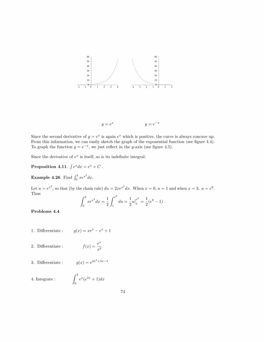
� 2 � 1 0 1 2 3 40

10

20

30

40

50

60

� 2 � 1� 3� 4 0 1 20

10

20

30

40

50

60

y = ex y = e−x

Since the second derivative of y = ex is again ex which is positive, the curve is always concave up.From this information, we can easily sketch the graph of the exponential function (see figure 4.4).To graph the function y = e−x, we just reflect in the y-axis (see figure 4.5).

Since the derivative of ex is itself, so is its indefinite integral:

Proposition 4.11.∫

exdx = ex + C .

Example 4.26. Find∫ 3

0xex2

dx.

Let u = ex2, so that (by the chain rule) du = 2xex2

dx. When x = 0, u = 1 and when x = 3, u = e9.Thus ∫ 3

0

xex2dx =

12

∫ e9

1

du =12u∣∣e9

1=

12(e9 − 1) .

Problems 4.4

1. Differentiate : g(x) = xex − ex + 1

2. Differentiate : f(x) =ex

x2

3. Differentiate : g(x) = e2x2+3x−1

4. Integrate :∫ 3

0

ex(e2x + 1)dx

74

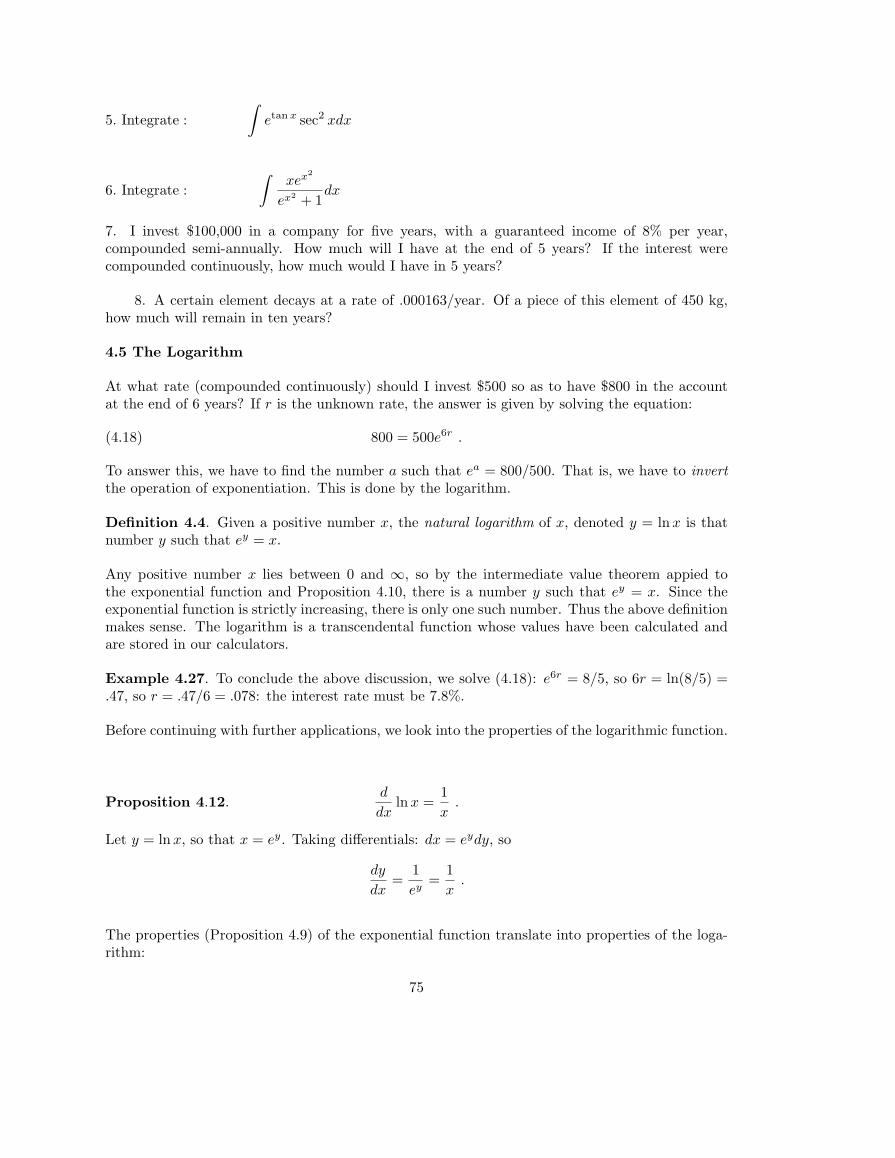
5. Integrate :∫

etan x sec2 xdx

6. Integrate :∫

xex2

ex2 + 1dx

7. I invest $100,000 in a company for five years, with a guaranteed income of 8% per year,compounded semi-annually. How much will I have at the end of 5 years? If the interest werecompounded continuously, how much would I have in 5 years?

8. A certain element decays at a rate of .000163/year. Of a piece of this element of 450 kg,how much will remain in ten years?

4.5 The Logarithm

At what rate (compounded continuously) should I invest $500 so as to have $800 in the accountat the end of 6 years? If r is the unknown rate, the answer is given by solving the equation:

(4.18) 800 = 500e6r .

To answer this, we have to find the number a such that ea = 800/500. That is, we have to invertthe operation of exponentiation. This is done by the logarithm.

Definition 4.4. Given a positive number x, the natural logarithm of x, denoted y = lnx is thatnumber y such that ey = x.

Any positive number x lies between 0 and ∞, so by the intermediate value theorem appied tothe exponential function and Proposition 4.10, there is a number y such that ey = x. Since theexponential function is strictly increasing, there is only one such number. Thus the above definitionmakes sense. The logarithm is a transcendental function whose values have been calculated andare stored in our calculators.

Example 4.27. To conclude the above discussion, we solve (4.18): e6r = 8/5, so 6r = ln(8/5) =.47, so r = .47/6 = .078: the interest rate must be 7.8%.

Before continuing with further applications, we look into the properties of the logarithmic function.

Proposition 4.12.d

dxlnx =

1x

.

Let y = ln x, so that x = ey. Taking differentials: dx = eydy, so

dy

dx=

1ey

=1x

.

The properties (Proposition 4.9) of the exponential function translate into properties of the loga-rithm:

75

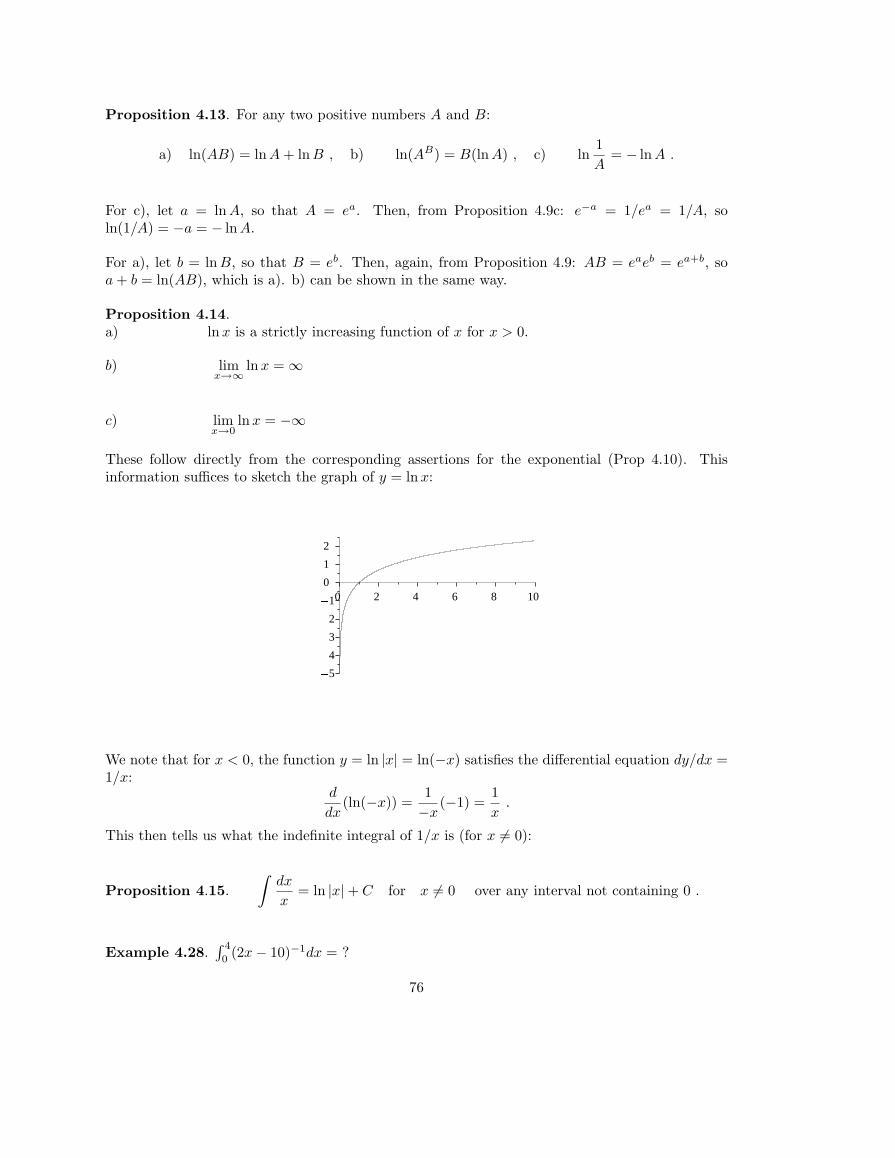
Proposition 4.13. For any two positive numbers A and B:

a) ln(AB) = lnA + lnB , b) ln(AB) = B(lnA) , c) ln1A

= − lnA .

For c), let a = lnA, so that A = ea. Then, from Proposition 4.9c: e−a = 1/ea = 1/A, soln(1/A) = −a = − lnA.

For a), let b = lnB, so that B = eb. Then, again, from Proposition 4.9: AB = eaeb = ea+b, soa + b = ln(AB), which is a). b) can be shown in the same way.

Proposition 4.14.a) ln x is a strictly increasing function of x for x > 0.

b) limx→∞

lnx = ∞

c) limx→0

lnx = −∞

These follow directly from the corresponding assertions for the exponential (Prop 4.10). Thisinformation suffices to sketch the graph of y = ln x:

�

� 5

� 4

� 3

� 2

� 1

0

1

2

0 2 4 6 8 10

We note that for x < 0, the function y = ln |x| = ln(−x) satisfies the differential equation dy/dx =1/x:

d

dx(ln(−x)) =

1−x

(−1) =1x

.

This then tells us what the indefinite integral of 1/x is (for x 6= 0):

Proposition 4.15.

∫dx

x= ln |x|+ C for x 6= 0 over any interval not containing 0 .

Example 4.28.∫ 4

0(2x− 10)−1dx = ?

76

Let u = 2x− 10, du = 2dx. At x = 0, u = −10, and at x = 4, u = −2. Thus∫ 4

0

(2x + 1)−1dx =12

∫ −2

−10

du

u=

12

ln |u|∣∣−2

−10=

12(ln 2− ln 10) = ln

15

.

Example 4.29.

∫ex

ex + 1dx = ?

Let u = ex, du = exdx. Then∫ex

ex + 1dx =

∫du

u= lnu = ln(ex + 1) + C .

Example 4.30. Find the solution of the differential equation dy/dx = xy, y(0) = 1.

The equation is separable and becomes: dy/y = xdx. Integrating both sides gives ln y = x2/2+C.Substituting x = 1, y = 0 we find ln 1 = 0 = C, so C = 0. Thus the solution is given by

ln y = x2/2 , or y = ex2/2 .

General Exponentials and Logarithms

We can raise any positive number a to any power p: since a = eln a, ap = (eln a)p = ep(ln a). Thisobservation allows us to introduce the general exponential and logarithmic functions.

Definition 4.5. For a any positive number, we define the exponential function with base a by

ax = e(ln a)x

and the logarithmic function with base a as its inverse function:

y = loga x if and only if x = ay .

To find a formula for loga, we note that if if x = ay, then x = e(ln a)y, so ln x = (ln a)y. Replacingy by loga x, we have

loga x =lnx

ln a.

From the chain rule, we obtain the following formulas for the derivatives and integrals of these newfunctions:

Proposition 4.16.d

dxax = (ln a)ax ,

d

dxloga x =

1(ln a)x

,∫axdx =

ax

ln a.

77

Problems 4.5

1. Solve for x: 2x = 3(5x).

2. Solve for x: (ex)5 = exe3.

3. Solve for x: 6x = 362−x.

4. Solve for x: ln3 x = 5.

5. Solve for x: ln2(x + 1)− ln2(x− 1) = ln2 8.

6. Solve:√

lnx = ln(√

x).

7. Differentiate : f(x) = e2 ln x

8. Differentiate : y = ln(ln x)

9. Differentiate : y = log2(x2 + 1)

10. Differentiate : y =ex2

x

11. Differentiate : f(x) = ex lnx

12. Differentiate : f(x) = ln(x + 1x− 1

)

13. Differentiate : g(x) = 5x log5 x

14. Differentiate : h(x) = 5log2(x2+1)

15. Integrate :∫

(lnx)2 + 1x

dx =

16. Integrate :∫

esin x cos xdx =

17. Integrate :∫

xdx

3x2 + 1=

78

18. Integrate :∫

eln x+1dx

19. Integrate :∫ 3

0

2x2xdx

20. Two variables are related by the equation 2 ln x + ln y = x − y. What is the equation of thetangent line to the graph of this relation at the point (1,1)?

4.6 Growth and Decay

We have already looked at several growth/decay problems in the course of discussing the exponen-tial and logarithmic functions. In this section we look at growth processes in greater depth, andat more general processes.

Example 4.31. How long does it take for a quantity of 128I to be reduced to half its size?

Referring to example 4.23, if we start with an amount P (0) of 128I , the amount we have after tminutes is P (t) = P (0)e−(.0279)t. To solve our problem we find t such that

12P (0) = P (0)e−(.0279)t .

Factor out P (0) and take the logarithm of both sides:

ln(1/2) = −(.0279)t or t =ln 2

.0279= 24.84 minutes .

This time is called the half-life of 128I.

The general exponential function allows us to replace the rate of decay of a radioactive elementby its half life. For suppose that a certain element has a rate of decay r, and a half-life T . Then1/2 = e−rT . Taking logarithms, this gives us ln 2 = rT , giving this relation between the half-lifeand the growth rate:

r =ln 2T

.

Now, if an amount A of the element decays for t years, then the amount remaining is

(4.19) A(t) = Ae−rt = Ae− ln 2(t/T ) = 2−t/T A .

Example 4.32. Suppose that the half-life of a certain element is 40 years. How much will remainof a 1 kg sample after 200 years? After 50 years?

In 200 years the sample will have halved 5 times, so what will remain is 1/25 of a kilogram, or31.25 g. After 50 years, we have A(t) = 1000(2−50/40) = 435 grams.

Example 4.33. The rate of decay of the radioactive isotope of carbon (14C) is 1.211× 10−4 peryear. In how many years will it take a certain amount of 14C to be reduced by 10%?

79

Let C(t) represent the amount of 14C in t years. We can take C(0) = 1, and the question is: forwhat t is C(t) = .9? Since C(t) satisfies the differential equation

C ′(t) = −1.211× 10−4C(t) .

We conclude (using definition 4.2)

C(t) = e−1.211×10−4t

so we must solve.9 = e−1.211×10−4t

Then

t =ln(.9)

−1.211× 10−4=−.1054−1.211

× 104 = 870 years .

Example 4.34. At the time an organic material is buried, its 14C content ceases to be replenishedby cosmic radiation, so is subject only to the radioactive decay, as described in example 8. Supposethe carbon content of a fossil is discovered to contain 84% of the amount of 14C had it not beenburied. How old is it?

Let time t = 0 represent the time the fossil was buried, and t the number of years since then. Ifwe take P (0) = 1, then P (t) = .84, so we must solve the equation

.84 = e−1.211×10−4t ,

or

t =ln(.84)

−1.211× 10−4=−.1744−1.211

× 104 = 1440 years .

Example 4.35. To find the half-life T of 14C, we solve

12

= e−1.211×10−4T .

The answer is T = ln 2/(1.211× 10−4) = 5724 years.

Inhibited growth

The growth equation dx/dt = rx does not really work for many biological populations, since theydo not appear to continue to grow exponentialy without bound. In fact, one should expect thatthere are factors present which cause the growth rate to decrease as the population increases. Onesuch is the competition over nutrient: the growth rate of a bacterium in an agar dish diminishesas the population increases and nutrient becomes less accessible. A good model for this is to letthe growth rate r decrease linearly as a function of x: r = a − bx, where a is the genetic growthfactor, and b is the inhibiting factor. In this model, the growth equation is replaced by

(4.20)dx

dt= (a− bx)x .

80

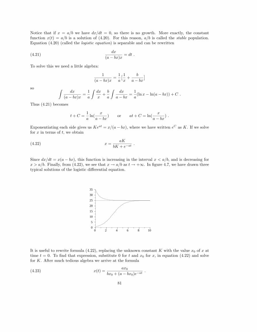
Notice that if x = a/b we have dx/dt = 0, so there is no growth. More exactly, the constantfunction x(t) = a/b is a solution of (4.20). For this reason, a/b is called the stable population.Equation (4.20) (called the logistic equation) is separable and can be rewritten

(4.21)dx

(a− bx)x= dt .

To solve this we need a little algebra:

1(a− bx)x

=1a

[ 1x

+b

a− bx

]so ∫

dx

(a− bx)x=

1a

∫dx

x+

b

a

∫dx

a− bx=

1a(lnx− ln(a− bx)) + C .

Thus (4.21) becomes

t + C =1a

ln(x

a− bx) or at + C = ln(

x

a− bx) .

Exponentiating each side gives us Keat = x/(a− bx), where we have written eC as K. If we solvefor x in terms of t, we obtain

(4.22) x =aK

bK + e−at.

Since dx/dt = x(a − bx), this function is increasing in the interval x < a/b, and is decreasing forx > a/b. Finally, from (4.22), we see that x → a/b as t → +∞. In figure 4.7, we have drawn threetypical solutions of the logistic differential equation.� �

0

5

10

15

20

25

30

35

0 2 4 6 8 10

It is useful to rewrite formula (4.22), replacing the unknown constant K with the value x0 of x attime t = 0. To find that expression, substitute 0 for t and x0 for x, in equation (4.22) and solvefor K. After much tedious algebra we arrive at the formula

(4.23) x(t) =ax0

bx0 + (a− bx0)e−at.

81

Example 4.36. A certain bacterium grows at the growth rate of 80% per hour. In a particularagar dish, the inhibiting factor is .002. What is the stable population? If 100 g of the bacteriumis put in the dish, what will be the size of the population after 2 hours?

Here a = .8, and b = .002, and the growth equation is

x′ = (.8− .002x)x .

The stable populations is .8/.002 = 400 g. To find the population after 2 hours, we use equation(4.23), with x0 = 100 and t = 2:

x(2) =.8(100)

.002(100) + (.8− .002(100))e−.8(2)=

8.2 + .6e−.16

= 249.25

If there were no inhibition to the growth the population woud be 100e1.6 = 495 g.

Example 4.37. In Example 4.23, we saw that the growth rate of the US population over thedecade 1990-2000 was .1235. However, if we looked at the census over the previous few decades,we would find that the growth rate was decreasing. If we attribute that to an inhibiting factor,we would be able to estimate that factor to be about .00032. Given these data, what is the stablepopulation of the US, and what will the population be in 2050 according to this model?

Let P (t) be the US population (in millions) t decades after 2000. We start with the differentialequation P ′ = (.1235 − .00032P )P . The stable population is P = .1235/.00032 = 385.93 million.Now, to estimate the actual population in 2050, let’s use equation (4.21) and evaluate the constantK in the general solution

P (t) =.1235K

.00032K + e−.1235t.

At t = 0, P = 281.4: this gives K = 8400. Then, the population in 2050 is estimated to be

P (5) =.1235(8400)

.00032(8400) + e−.1235(5)= 321.45

million; a much more realistic estimate than the 521.8 million estimate of example 4.22.

Example 4.38. A certain disease is transmitted by direct contact of an infected person withan infected person. This suggest that the rate of change of the number of infected people isproportional both to the number of infected people and the number of uninfected people. If we letN represent the total population, and P (t) the number of infected people, this assumption can bewritten as

P ′(t) = kP (t)(N − P (t))

where k represents the probability of direct contact of an infected person with one not infected.This is the logistic equation with a = kN and b = k. With these values equation (4.23) becomes

(4.24) P (t) =NP0

P0 + (N − P0)e−kNt.

Notice that the stable population is a/b = N ; alas, without intervention everyone eventually isinfected in this model.

82

Example 4.39. For a certain transmittable disease, it has been determined that the rate oftransmission is .1 percent per day, that is k = .001. In a certain community of 500 people it hasbeen found that 5 people have the disease. Assuming that there is no intervention, how manypeople will have the disease in 4 days? How long before half the population is infected?

Here N = 500 and P0 = 5, so NP0 = 2500 and kn = .5 and (4.24) becomes

P (t) =2500

5 + (495)e−.5t.

To answer the first question, calculate

P (4) =2500

5 + (495)e−.5(4)= 34 .

For the second question, solve for t:

12(500) =

25005 + (495)e−.5t

.

This gives us 5 + 495e−.5t = 10, which results in the value t = 9.19.

Example 4.40. In the study of an epidemic of an airborne disease which is reinforced by interactionamong those infected, a first working hypothesis may be that the rate of spread of the disease isproportional to that amount of interaction, which is in turn proportional to the square of thepopulation of infected. If we let P (t) represent the number of people infected at time t, we haveP ′ = kP 2 for some constant k. We are interested in knowing how long it will take, unless someaction is taken, for the entire population to be infected. To work through an example, let’s supposethat k = .001 and that at time t = 0, 100 people are infected.

The given law of change isdP

dt= .001P 2

We can rewrite this in the formP−2dP = .001dt

Integrating, we find−P−1 = .001t + C .

Now when t = 0, P = 100, so C = −.01, so we have

−P−1 = .001t− .01 ,

or P (t) = (.01− .001t)−1. So, for example, after 5 days the infected population is (.01− .005)−1 =200, and after 8 days it is 500. Worst of all, in ten days, P is infinite: everyone is infected, nomatter how large the original healthy population was.

Problems 4.6

1. If I invest $ 8,000 at 12.5 percent per year (compounded continuously) in how many years willmy investment be worth $ 30,000 ?

83

2. I want to invest $5000 in a growth fund so that in 5 years i will have $8000. What interest rate,compounded continuously will produce that growth?

3. If I invest $4000 in a fund, with an interest rate of 8%, compounded continuously, how longwill it take for the fund to be worth $10,000? 4. At what rate (continuously compounded) shouldI invest $10,000 so as to have $14,000 in five years?

5. The Zombie National Bank offers accounts which pay 10.5% annually, compounded continuously.How much should I invest today so as to have $12,000 in 6 years?

6. Carbon14 has a half life of 5801 years. How long does it take for a sample to be reduced to 80%its original size?

7. A certain radioactive element decays so that in 100 years it has decreased to 82% its originalsize. What is its half-life?

8. The half-life of Rossidium312 is 4,801 years. How long will it take for a mass of Rossidium312 todecay to 98 % of its original size?

9. A certain autocatalytic chemical reaction proceeds according to the differential equation

dx

dt= .01

1− x2

x

where x(t) is the fraction of the sample which is the resulting compound at time t, in seconds. Ifwe start with x(0) = .2, how long does it take for x to reach .9?

10. According to Newton’s Law of Cooling, if a hot object is immersed into a cool environment, therate of decrease of the temperature of the oject is proportional to the difference in the temperatureof the object and its environment. If, then, h(t) is the temperature of the object at time t, and T0

is the temperature of the environment, Newton’s law says

(1)dh

dt= −k(h(t)− T0) ,

where k is the coeffiecient of cooling. Suppose that a body at 95◦ Celsius is immersed in a waterbath held at 5◦ Celsius, and the coefficient of cooling is k = .08. What will be the temperature ofthe body in 10 minutes?

11. Suppose that I wish to make iced tea of tea at the boiling point, to be consumed in threeminutes. To get the tea as cold as possible, should I put in an ice cube immediately, or just beforethe three minutes are up?

12. A lake containing 300,000 acre-feet of water has 20% salinity. Clear water flows in from rivers,and out at a dam, both at the rate of 4,000 acre-feet per day. In how may days will the salinitybe reduced to 10%?

13. A pond is in the form of a cylinder of radius 100 ft. and depth 8 ft. Water flows into thepond at the rate of 100 cu. ft./hr and seeps into the ground through the porous bottom at a rateproportional to the volume, where the constant of proportionality is .0005. What is the maximum

84

height of water in the pond that can be achieved? If the water level in the pond is 2 feet at timet= 0, what is the height after 1000 days?

14. Water flows into an elastic ball at a rate of 4 cu. in/minute. The ball has a puncture out ofwhich water flows at a rate proportional to the volume of water in the ball, where the constant ofproportionality is .02. Assuming the ball is empty at the beginning, how much water is in the ballafter 20 minutes?

85

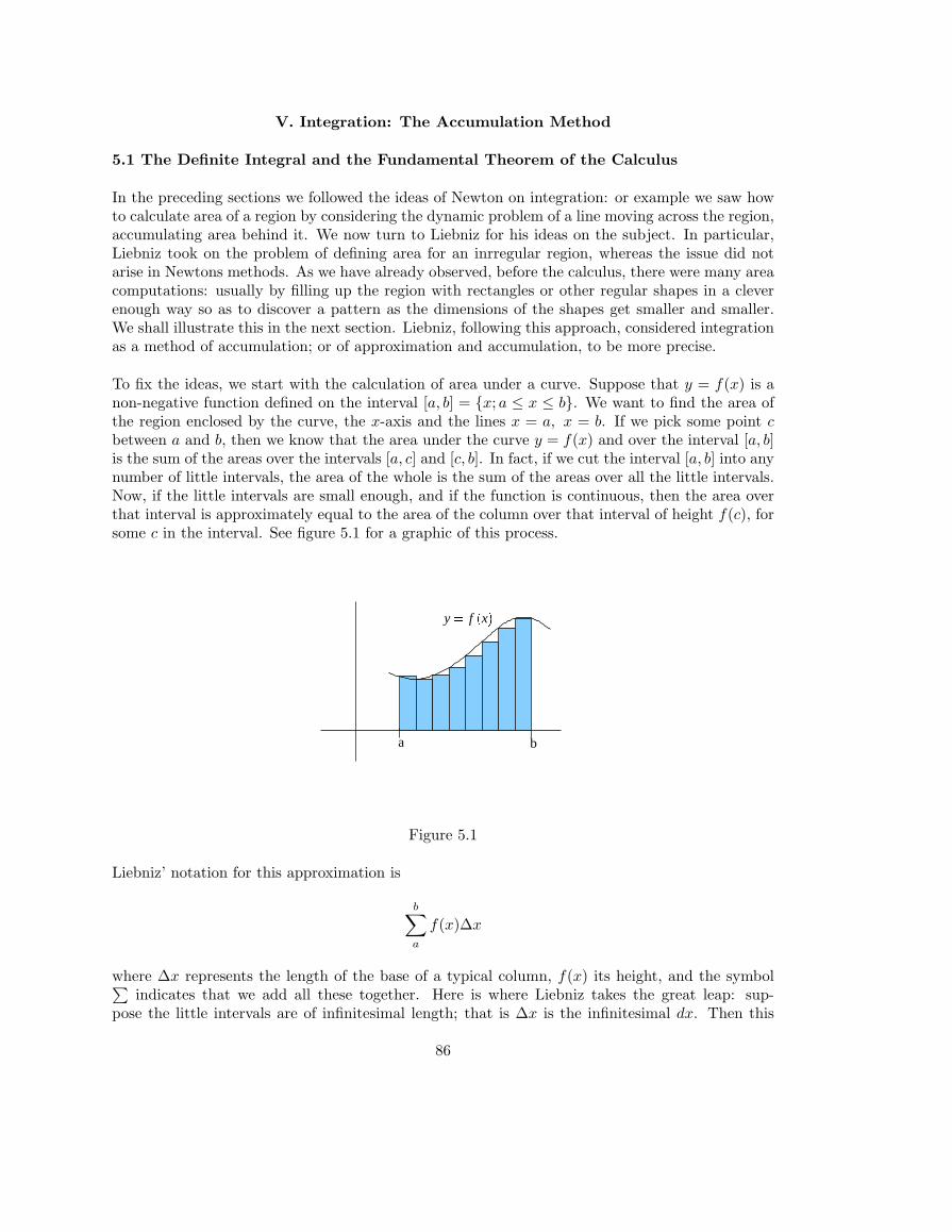
V. Integration: The Accumulation Method

5.1 The Definite Integral and the Fundamental Theorem of the Calculus

In the preceding sections we followed the ideas of Newton on integration: or example we saw howto calculate area of a region by considering the dynamic problem of a line moving across the region,accumulating area behind it. We now turn to Liebniz for his ideas on the subject. In particular,Liebniz took on the problem of defining area for an inrregular region, whereas the issue did notarise in Newtons methods. As we have already observed, before the calculus, there were many areacomputations: usually by filling up the region with rectangles or other regular shapes in a cleverenough way so as to discover a pattern as the dimensions of the shapes get smaller and smaller.We shall illustrate this in the next section. Liebniz, following this approach, considered integrationas a method of accumulation; or of approximation and accumulation, to be more precise.

To fix the ideas, we start with the calculation of area under a curve. Suppose that y = f(x) is anon-negative function defined on the interval [a, b] = {x; a ≤ x ≤ b}. We want to find the area ofthe region enclosed by the curve, the x-axis and the lines x = a, x = b. If we pick some point cbetween a and b, then we know that the area under the curve y = f(x) and over the interval [a, b]is the sum of the areas over the intervals [a, c] and [c, b]. In fact, if we cut the interval [a, b] into anynumber of little intervals, the area of the whole is the sum of the areas over all the little intervals.Now, if the little intervals are small enough, and if the function is continuous, then the area overthat interval is approximately equal to the area of the column over that interval of height f(c), forsome c in the interval. See figure 5.1 for a graphic of this process.

y � f�x �

a b

Figure 5.1

Liebniz’ notation for this approximation is

b∑a

f(x)∆x

where ∆x represents the length of the base of a typical column, f(x) its height, and the symbol∑indicates that we add all these together. Here is where Liebniz takes the great leap: sup-

pose the little intervals are of infinitesimal length; that is ∆x is the infinitesimal dx. Then this

86

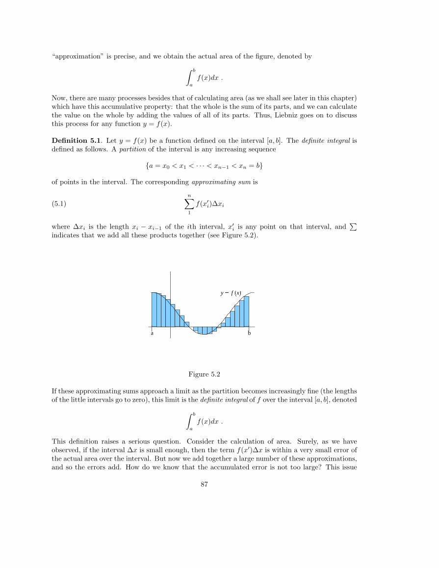
“approximation” is precise, and we obtain the actual area of the figure, denoted by∫ b

a

f(x)dx .

Now, there are many processes besides that of calculating area (as we shall see later in this chapter)which have this accumulative property: that the whole is the sum of its parts, and we can calculatethe value on the whole by adding the values of all of its parts. Thus, Liebniz goes on to discussthis process for any function y = f(x).

Definition 5.1. Let y = f(x) be a function defined on the interval [a, b]. The definite integral isdefined as follows. A partition of the interval is any increasing sequence

{a = x0 < x1 < · · · < xn−1 < xn = b}

of points in the interval. The corresponding approximating sum is

(5.1)n∑1

f(x′i)∆xi

where ∆xi is the length xi − xi−1 of the ith interval, x′i is any point on that interval, and∑

indicates that we add all these products together (see Figure 5.2).

a b

y � f�x �

Figure 5.2

If these approximating sums approach a limit as the partition becomes increasingly fine (the lengthsof the little intervals go to zero), this limit is the definite integral of f over the interval [a, b], denoted∫ b

a

f(x)dx .

This definition raises a serious question. Consider the calculation of area. Surely, as we haveobserved, if the interval ∆x is small enough, then the term f(x′)∆x is within a very small error ofthe actual area over the interval. But now we add together a large number of these approximations,and so the errors add. How do we know that the accumulated error is not too large? This issue

87

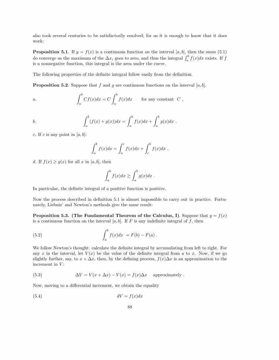
also took several centuries to be satisfactorily resolved; for us it is enough to know that it doeswork:

Proposition 5.1. If y = f(x) is a continuous function on the interval [a, b], then the sums (5.1)do converge as the maximum of the ∆xi goes to zero, and thus the integral

∫ b

af(x)dx exists. If f

is a nonnegative function, this integral is the area under the curve.

The following properties of the definite integral follow easily from the definition.

Proposition 5.2. Suppose that f and g are continuous functions on the interval [a, b].

a.

∫ b

a

Cf(x)dx = C

∫ b

a

f(x)dx for any constant C ,

b.

∫ b

a

(f(x) + g(x))dx =∫ b

a

f(x)dx +∫ b

a

g(x)dx .

c. If c is any point in [a, b]: ∫ b

a

f(x)dx =∫ c

a

f(x)dx +∫ b

c

f(x)dx .

d. If f(x) ≥ g(x) for all x in [a, b], then∫ b

a

f(x)dx ≥∫ b

a

g(x)dx .

In particular, the definite integral of a positive function is positive.

Now the process described in definition 5.1 is almost impossible to carry out in practice. Fortu-nately, Liebniz’ and Newton’s methods give the same result:

Proposition 5.3. (The Fundamental Theorem of the Calculus, I). Suppose that y = f(x)is a continuous function on the interval [a, b]. If F is any indefinite integral of f , then

(5.2)∫ b

a

f(x)dx = F (b)− F (a) .

We follow Newton’s thought: calculate the definite integral by accumulating from left to right. Forany x in the interval, let V (x) be the value of the definite integral from a to x. Now, if we goslightly further, say, to x + ∆x, then, by the defining process, f(x)∆x is an approximation to theincrement in V :

(5.3) ∆V = V (x + ∆x)− V (x) = f(x)∆x approximately .

Now, moving to a differential increment, we obtain the equality

(5.4) dV = f(x)dx

88

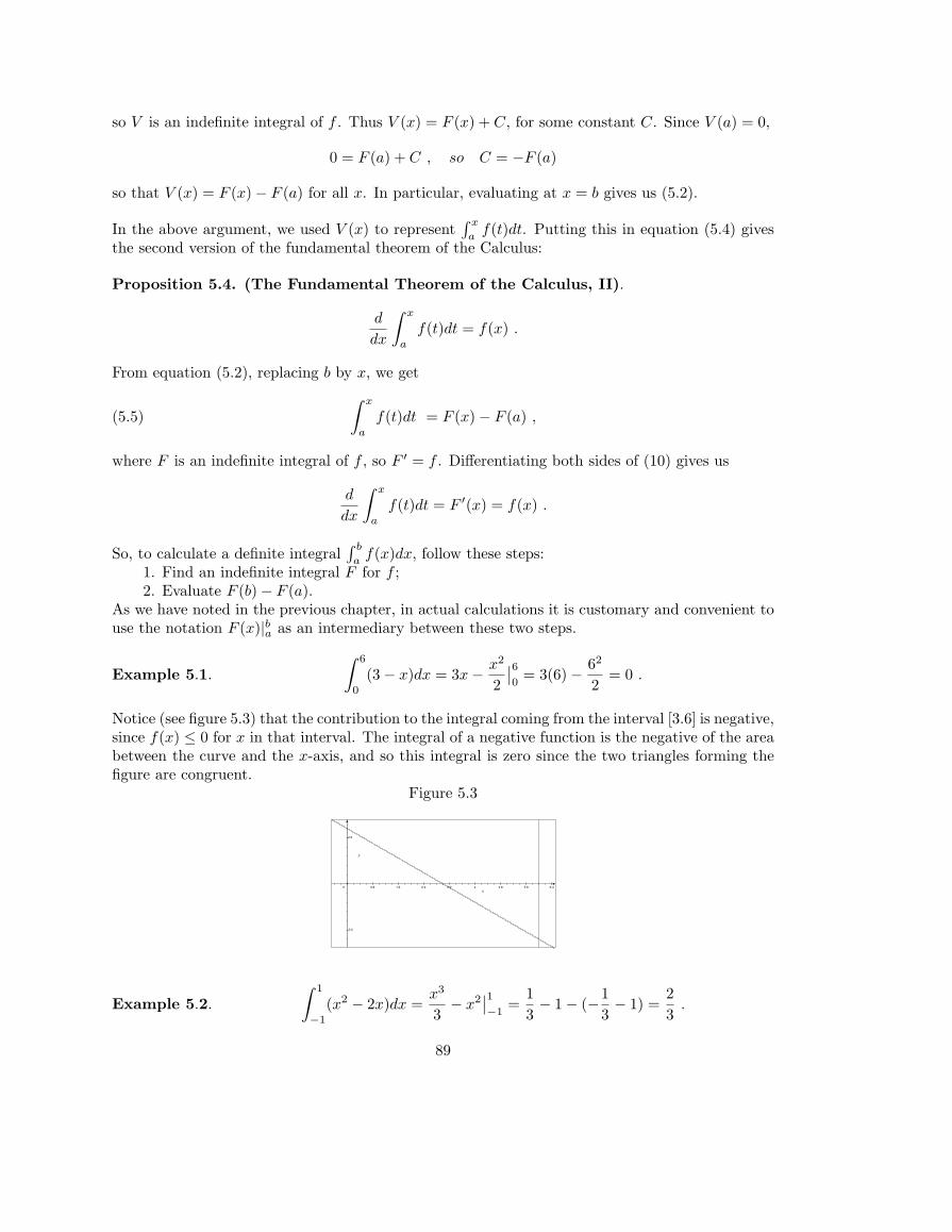
so V is an indefinite integral of f . Thus V (x) = F (x) + C, for some constant C. Since V (a) = 0,

0 = F (a) + C , so C = −F (a)

so that V (x) = F (x)− F (a) for all x. In particular, evaluating at x = b gives us (5.2).

In the above argument, we used V (x) to represent∫ x

af(t)dt. Putting this in equation (5.4) gives

the second version of the fundamental theorem of the Calculus:

Proposition 5.4. (The Fundamental Theorem of the Calculus, II).

d

dx

∫ x

a

f(t)dt = f(x) .

From equation (5.2), replacing b by x, we get

(5.5)∫ x

a

f(t)dt = F (x)− F (a) ,

where F is an indefinite integral of f , so F ′ = f . Differentiating both sides of (10) gives us

d

dx

∫ x

a

f(t)dt = F ′(x) = f(x) .

So, to calculate a definite integral∫ b

af(x)dx, follow these steps:

1. Find an indefinite integral F for f ;2. Evaluate F (b)− F (a).

As we have noted in the previous chapter, in actual calculations it is customary and convenient touse the notation F (x)|ba as an intermediary between these two steps.

Example 5.1.

∫ 6

0

(3− x)dx = 3x− x2

2

∣∣60

= 3(6)− 62

2= 0 .

Notice (see figure 5.3) that the contribution to the integral coming from the interval [3.6] is negative,since f(x) ≤ 0 for x in that interval. The integral of a negative function is the negative of the areabetween the curve and the x-axis, and so this integral is zero since the two triangles forming thefigure are congruent.

Figure 5.3

0 0.8 1.6 2.4 3.2 4 4.8 5.6 6.4

-2.5

2.5

Example 5.2.

∫ 1

−1

(x2 − 2x)dx =x3

3− x2

∣∣1−1

=13− 1− (−1

3− 1) =

23

.

89

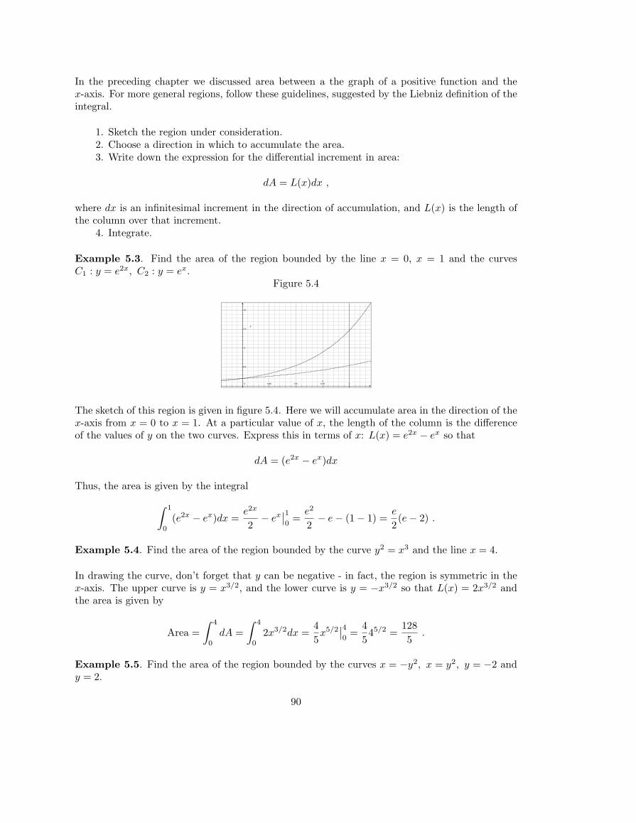
In the preceding chapter we discussed area between a the graph of a positive function and thex-axis. For more general regions, follow these guidelines, suggested by the Liebniz definition of theintegral.

1. Sketch the region under consideration.2. Choose a direction in which to accumulate the area.3. Write down the expression for the differential increment in area:

dA = L(x)dx ,

where dx is an infinitesimal increment in the direction of accumulation, and L(x) is the length ofthe column over that increment.

4. Integrate.

Example 5.3. Find the area of the region bounded by the line x = 0, x = 1 and the curvesC1 : y = e2x, C2 : y = ex.

Figure 5.4

0 0.25 0.5 0.75 1

2.5

5

7.5

10

The sketch of this region is given in figure 5.4. Here we will accumulate area in the direction of thex-axis from x = 0 to x = 1. At a particular value of x, the length of the column is the differenceof the values of y on the two curves. Express this in terms of x: L(x) = e2x − ex so that

dA = (e2x − ex)dx

Thus, the area is given by the integral∫ 1

0

(e2x − ex)dx =e2x

2− ex

∣∣10

=e2

2− e− (1− 1) =

e

2(e− 2) .

Example 5.4. Find the area of the region bounded by the curve y2 = x3 and the line x = 4.

In drawing the curve, don’t forget that y can be negative - in fact, the region is symmetric in thex-axis. The upper curve is y = x3/2, and the lower curve is y = −x3/2 so that L(x) = 2x3/2 andthe area is given by

Area =∫ 4

0

dA =∫ 4

0

2x3/2dx =45x5/2

∣∣40

=4545/2 =

1285

.

Example 5.5. Find the area of the region bounded by the curves x = −y2, x = y2, y = −2 andy = 2.

90

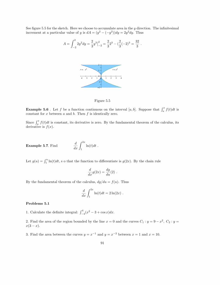
See figure 5.5 for the sketch. Here we choose to accumulate area in the y direction. The infinitesimalincrement at a particular value of y is dA = (y2 − (−y2))dy = 2y2dy. Thus

A =∫ 2

−2

2y2dy =23y3

∣∣2−2

=2323 − (

23(−2)3 =

323

.

� 2

� 1

0

1

2

� 4 � 3 � 2 � 1 0 1 2 3 4

x � � y2 x � y2

Figure 5.5

Example 5.6 . Let f be a function continuous on the interval [a, b]. Suppose that∫ x

af(t)dt is

constant for x between a and b. Then f is identically zero.

Since∫ x

af(t)dt is constant, its derivative is zero. By the fundamental theorem of the calculus, its

derivative is f(x).

Example 5.7. Findd

dx

∫ 2x

1

ln(t)dt .

Let g(u) =∫ u

1ln(t)dt, s o that the function to differentiate is g(2x). By the chain rule

d

dxg(2x) =

dg

du(2) .

By the fundamental theorem of the calculus, dg/du = f(u). Thus

d

dx

∫ 2x

1

ln(t)dt = 2 ln(2x) .

Problems 5.1

1. Calculate the definite integral:∫ 4

−4(x2 − 3 + cos x)dx.

2. Find the area of the region bounded by the line x = 0 and the curves C1 : y = 9− x2, C2 : y =x(3− x).

3. Find the area between the curves y = x−1 and y = x−2 between x = 1 and x = 10.

91

4. Find the area of the region in the first quadrant bounded by the curves y = sin π2 x and y = x.

5. Find the area of the region in the right half plane (x > 0) bounded by the curves y = x − x3

and y = x2 − x.

6. What is the area of the region bounded by the curves y = x3 − 3x and y = 3x.

7. The average value of a function y = f(x) defined over an interval [a, b] is defined to be

yave =1

b− a

∫ b

a

f(x)dx .

Find the average of y = sinx over the interval [0, π].

8. Let g(x) = x2 + x3 for x in the interval 0 ≤ x ≤ 10. Find the average, or mean, value of g onthe interval. Find the average slope of the graph of y = g(x) on the interval.

9. Let f be a function continuous on the interval [a, b]. Suppose that∫ x

af(t)dt is a linear function.

Show that f is constant.

10. Let f be a function continuous on the interval [a, b]. Suppose that∫ x

af(t)dt =

∫ b

xf(t)dt for all

x between a and b. Show that f(x) = 0 for all x in the interval.

11.d

dx

∫ 2x+1

0

cos tdt =

12.d

dx

∫ x2

0

t3dt =

13.d

dx

∫ 2x

0

ln tdt =

14.d

dx

∫ x2+1

0

et+1dt =

5. 2 Summation and the Definite Integral

In this section we shall make the definition of the definite integral precise, and shall do somecomputations directly from the definition. The purpose here is to emphasize that the definiteintegral represents a process of accumulation, as well as to introduce and work with the notationfor summation.

Let n be a positive integer, and a(k) a rule that assigns a number to each integer between 1 andn. For example:

a(k) = 1 for all k ; or a(k) = 2k + 3 ; or a(k) = k2 ; or a(k) =3k

,

92

for k running from 1 to n = 100. The sum of all these numbers is denoted

n∑k=1

a(k) = a(1) + a(2) + · · ·+ a(n) .

This sum can sometimes be easily expressed as a formula in n; more often this is difficult, orimpossible. For example, the sums in the first three cases are, respectively

n ; n(n + 4) ;n(n + 1)(2n + 1)

6,

whereas a formula for the sum in the fourth case is not known. These formulas are not easy to comeby, and usually rely on clever tricks. Here are the cases we will need for application to integration.

Proposition 5.5.

a) Z(n) =n∑1

1 = 1 + 1 + · · ·+ 1 = n

b) U(n) =n∑1

k = 1 + 2 + · · ·+ n =n(n + 1)

2

c) S(n) =n∑1

k2 = 12 + 22 + · · ·+ n2 =n(n + 1)(2n + 1)

6

d) K(n) =n∑1

k3 = 13 + 23 + · · ·+ n3 =[n(n + 1)

2]2

a) just says that the sum of n ones is n. To show b) we start with the observation that

(k + 1)2 = k2 + 2k + 1

Now add these all together from k = 1 to k = n − 1. On the left hand side we get the sum ofall the squares from 22 to n2, or S(n) − 12. The sum of the first terms on the right hand side isS(n− 1), of the second is 2U(n− 1) and the last contributes n− 1. Thus

S(n)− 1 = S(n− 1) + 2U(n− 1) + n− 1 or 2U(n− 1) = S(n)− S(n− 1)− n .

Now add 2n to both sides, and remember that S(n)− S(n− 1) = n2:

2U(n) = n2 + n ,

which gives b). For c) we use the same idea. Start with

(k + 1)3 = k3 + 3k2 + 3k + 1

93

Add these all together from k = 1 to k = n− 1, and calculate each term as above to get:

K(n)− 1 = K(n− 1) + 3S(n− 1) + 3U(n− 1) + n− 1 .

We know U(n− 1) from a), and K(n)−K(n− 1) = n3, so we get:

3S(n− 1) = n3 − 3(n− 1)n

2− n

Now add 3n2 to both sides, to get

3S(n) = n3 − 32n2 +

32n− n + 3n2

from which c) follows. To derive d) we must employ the fourth powers in the same way.

Example 5.6. The sum of the first n odd integers is n2. We see this using a). The first n oddintegers are the numbers 1, 3, 5, . . . , 2n − 1. The kth odd integer is 2k − 1. Thus the sum of thefirst n odd integers is

n∑1

(2k − 1) = 2(n∑1

k)−n∑1

1 = (n + 1)n− n = n2 .

Sometimes to find the sum of a collection of numbers it helps to write out the first few terms.

Example 5.9. Find∑15

3 (k−1 − (k + 1)−1).

The sum of the first two terms is (1/3− 1/4)− (1/4− 1/5) = 1/3− 1/5 Then the sum of the firstthree terms is (1/3− 1/5) + (1/5− 1/6) = 1/3− 1/6. Notice the cancellation. This will happen ateach stage, because each time the first term added is the same as the last subtracted. We conclude

15∑3

(k−1 − (k + 1)−1) = 1/3− 1/16 .

Now let us return to the definition of the definite integral. Let y = f(x) be a continuous functionon the interval [a, b]. Select n + 1 points between a and b: a = x0 < x1 < · · · < xn−1 < xn = b.This is a partition P of the interval [a, b]. The size of the partition is the maximum differencebetween consecutive points, denoted |P |. Form the sum (called the Riemann sum of the functionover the partition) ∑

P

f(x)∆x =n∑1

f(x′k)(xk − xk−1)

where x′k is any point in the interval between xk−1 and xk.

Definition 5.2. The function f is integrable over the interval [a, b] if the Riemann sums converge.That is, there is a number L for which the following condition can be verified. Given any ε > 0,there is a δ > 0 such that if the partition satisfies |P | < δ, then

|∑P

f(x)∆x− L| < ε .

94

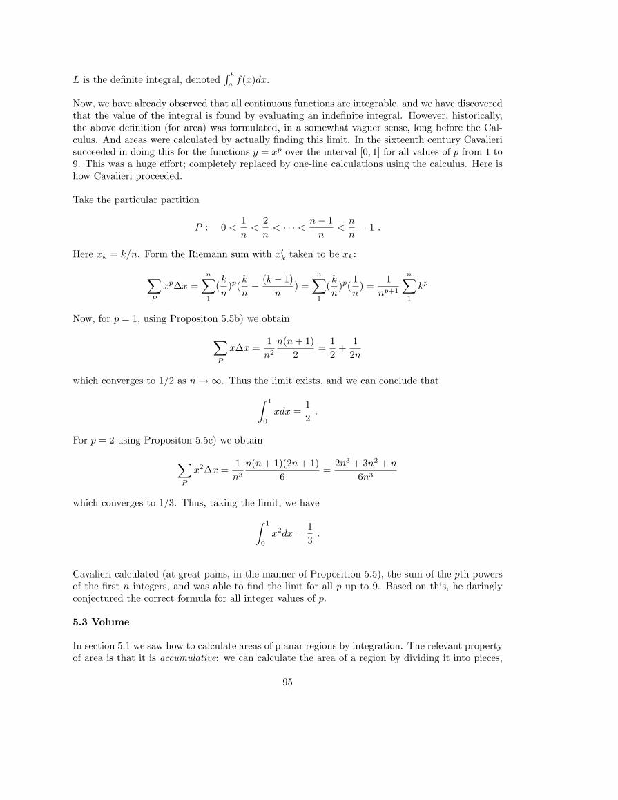
L is the definite integral, denoted∫ b

af(x)dx.

Now, we have already observed that all continuous functions are integrable, and we have discoveredthat the value of the integral is found by evaluating an indefinite integral. However, historically,the above definition (for area) was formulated, in a somewhat vaguer sense, long before the Cal-culus. And areas were calculated by actually finding this limit. In the sixteenth century Cavalierisucceeded in doing this for the functions y = xp over the interval [0, 1] for all values of p from 1 to9. This was a huge effort; completely replaced by one-line calculations using the calculus. Here ishow Cavalieri proceeded.

Take the particular partition

P : 0 <1n

<2n

< · · · < n− 1n

<n

n= 1 .

Here xk = k/n. Form the Riemann sum with x′k taken to be xk:

∑P

xp∆x =n∑1

(k

n)p(

k

n− (k − 1)

n) =

n∑1

(k

n)p(

1n

) =1

np+1

n∑1

kp

Now, for p = 1, using Propositon 5.5b) we obtain

∑P

x∆x =1n2

n(n + 1)2

=12

+12n

which converges to 1/2 as n →∞. Thus the limit exists, and we can conclude that∫ 1

0

xdx =12

.

For p = 2 using Propositon 5.5c) we obtain

∑P

x2∆x =1n3

n(n + 1)(2n + 1)6

=2n3 + 3n2 + n

6n3

which converges to 1/3. Thus, taking the limit, we have∫ 1

0

x2dx =13

.

Cavalieri calculated (at great pains, in the manner of Proposition 5.5), the sum of the pth powersof the first n integers, and was able to find the limt for all p up to 9. Based on this, he daringlyconjectured the correct formula for all integer values of p.

5.3 Volume

In section 5.1 we saw how to calculate areas of planar regions by integration. The relevant propertyof area is that it is accumulative: we can calculate the area of a region by dividing it into pieces,

95

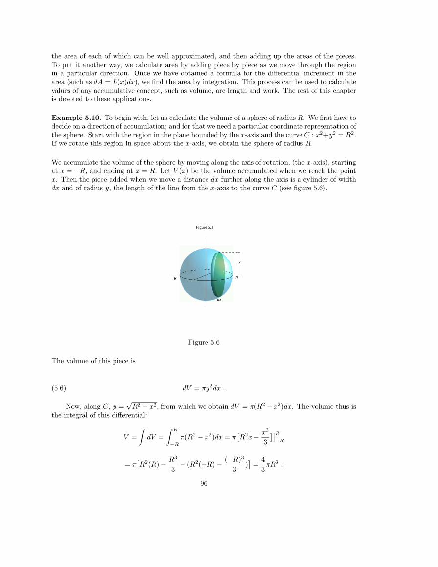
the area of each of which can be well approximated, and then adding up the areas of the pieces.To put it another way, we calculate area by adding piece by piece as we move through the regionin a particular direction. Once we have obtained a formula for the differential increment in thearea (such as dA = L(x)dx), we find the area by integration. This process can be used to calculatevalues of any accumulative concept, such as volume, arc length and work. The rest of this chapteris devoted to these applications.

Example 5.10. To begin with, let us calculate the volume of a sphere of radius R. We first have todecide on a direction of accumulation; and for that we need a particular coordinate representation ofthe sphere. Start with the region in the plane bounded by the x-axis and the curve C : x2+y2 = R2.If we rotate this region in space about the x-axis, we obtain the sphere of radius R.

We accumulate the volume of the sphere by moving along the axis of rotation, (the x-axis), startingat x = −R, and ending at x = R. Let V (x) be the volume accumulated when we reach the pointx. Then the piece added when we move a distance dx further along the axis is a cylinder of widthdx and of radius y, the length of the line from the x-axis to the curve C (see figure 5.6).

Figure 5.1

� R

y

R

dx

Figure 5.6

The volume of this piece is

(5.6) dV = πy2dx .

Now, along C, y =√

R2 − x2, from which we obtain dV = π(R2 − x2)dx. The volume thus isthe integral of this differential:

V =∫

dV =∫ R

−R

π(R2 − x2)dx = π[R2x− x3

3]∣∣R−R

= π[R2(R)− R3

3− (R2(−R)− (−R)3

3)]

=43πR3 .

96

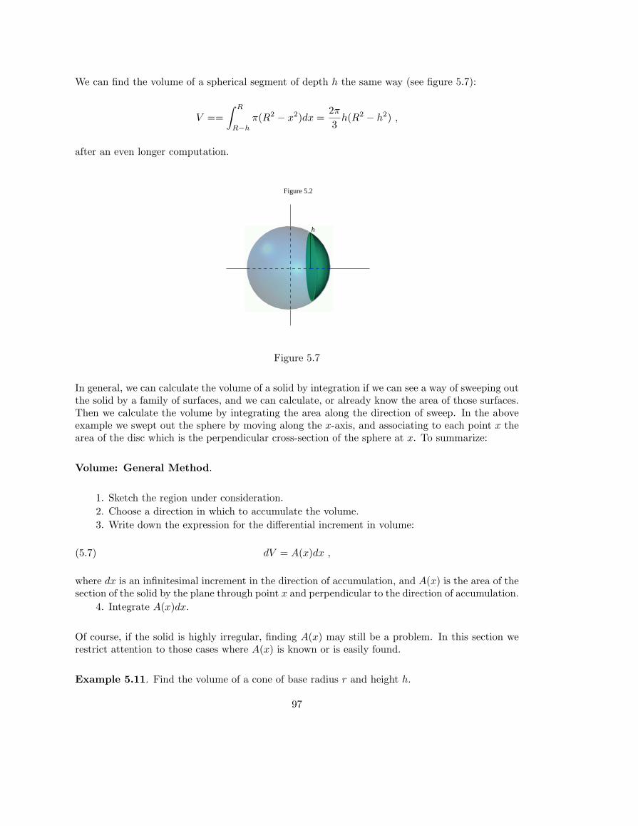
We can find the volume of a spherical segment of depth h the same way (see figure 5.7):

V ==∫ R

R−h

π(R2 − x2)dx =2π

3h(R2 − h2) ,

after an even longer computation.

Figure 5.2

h

Figure 5.7

In general, we can calculate the volume of a solid by integration if we can see a way of sweeping outthe solid by a family of surfaces, and we can calculate, or already know the area of those surfaces.Then we calculate the volume by integrating the area along the direction of sweep. In the aboveexample we swept out the sphere by moving along the x-axis, and associating to each point x thearea of the disc which is the perpendicular cross-section of the sphere at x. To summarize:

Volume: General Method.

1. Sketch the region under consideration.2. Choose a direction in which to accumulate the volume.3. Write down the expression for the differential increment in volume:

(5.7) dV = A(x)dx ,

where dx is an infinitesimal increment in the direction of accumulation, and A(x) is the area of thesection of the solid by the plane through point x and perpendicular to the direction of accumulation.

4. Integrate A(x)dx.

Of course, if the solid is highly irregular, finding A(x) may still be a problem. In this section werestrict attention to those cases where A(x) is known or is easily found.

Example 5.11. Find the volume of a cone of base radius r and height h.

97

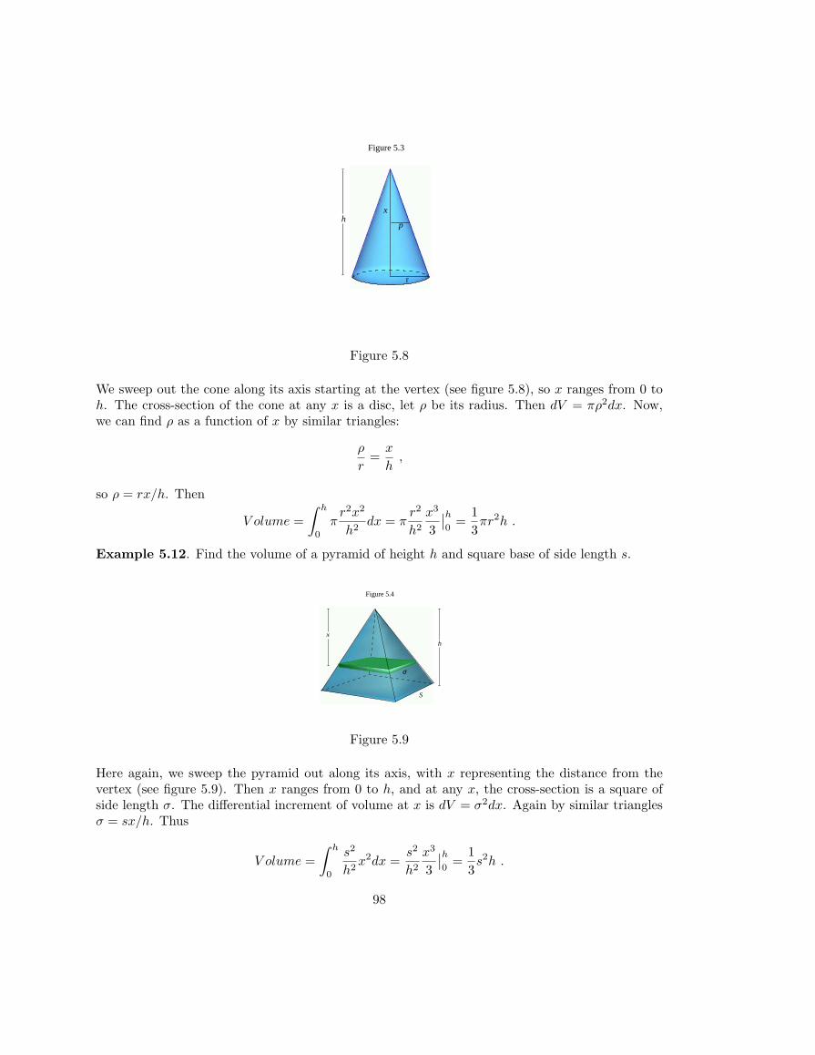
Figure 5.3

r

hx

p

Figure 5.8

We sweep out the cone along its axis starting at the vertex (see figure 5.8), so x ranges from 0 toh. The cross-section of the cone at any x is a disc, let ρ be its radius. Then dV = πρ2dx. Now,we can find ρ as a function of x by similar triangles:

ρ

r=

x

h,

so ρ = rx/h. Then

V olume =∫ h

0

πr2x2

h2dx = π

r2

h2

x3

3

∣∣h0

=13πr2h .

Example 5.12. Find the volume of a pyramid of height h and square base of side length s.

Figure 5.4

h

σ

S

x

Figure 5.9

Here again, we sweep the pyramid out along its axis, with x representing the distance from thevertex (see figure 5.9). Then x ranges from 0 to h, and at any x, the cross-section is a square ofside length σ. The differential increment of volume at x is dV = σ2dx. Again by similar trianglesσ = sx/h. Thus

V olume =∫ h

0

s2

h2x2dx =

s2

h2

x3

3

∣∣h0

=13s2h .

98

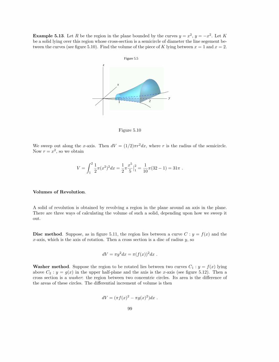
Example 5.13. Let R be the region in the plane bounded by the curves y = x2, y = −x2. Let Kbe a solid lying over this region whose cross-section is a semicircle of diameter the line segement be-tween the curves (see figure 5.10). Find the volume of the piece of K lying between x = 1 and x = 2.

Figure 5.5

z

1 2

x

y

Figure 5.10

We sweep out along the x-axis. Then dV = (1/2)πr2dx, where r is the radius of the semicircle.Now r = x2, so we obtain

V =∫ 2

1

12π(x2)2dx =

12π

x5

5

∣∣21

=110

π(32− 1) = 31π .

Volumes of Revolution.

A solid of revolution is obtained by revolving a region in the plane around an axis in the plane.There are three ways of calculating the volume of such a solid, depending upon how we sweep itout.

Disc method. Suppose, as in figure 5.11, the region lies between a curve C : y = f(x) and thex-axis, which is the axis of rotation. Then a cross section is a disc of radius y, so

dV = πy2dx = π(f(x))2dx .

Washer method. Suppose the region to be rotated lies between two curves C1 : y = f(x) lyingabove C2 : y = g(x) in the upper half-plane and the axis is the x-axis (see figure 5.12). Then across section is a washer: the region between two concentric circles. Its area is the difference ofthe areas of these circles. The differential increment of volume is then

dV = (πf(x)2 − πg(x)2)dx .

99

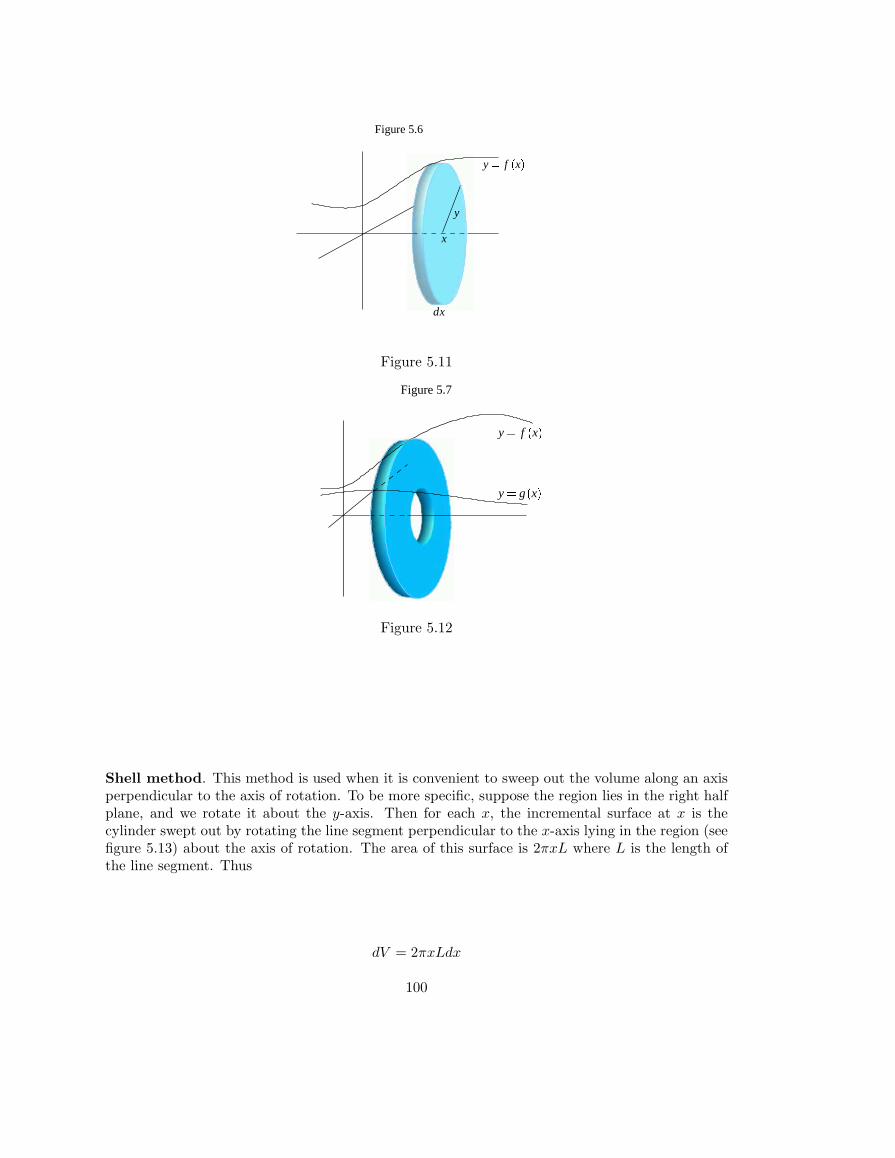
Figure 5.6

x

y

dx

y � f�x �

Figure 5.11� � �

Figure 5.7

y � g�x �

y � f�x �

Figure 5.12

Shell method. This method is used when it is convenient to sweep out the volume along an axisperpendicular to the axis of rotation. To be more specific, suppose the region lies in the right halfplane, and we rotate it about the y-axis. Then for each x, the incremental surface at x is thecylinder swept out by rotating the line segment perpendicular to the x-axis lying in the region (seefigure 5.13) about the axis of rotation. The area of this surface is 2πxL where L is the length ofthe line segment. Thus

dV = 2πxLdx

100

.

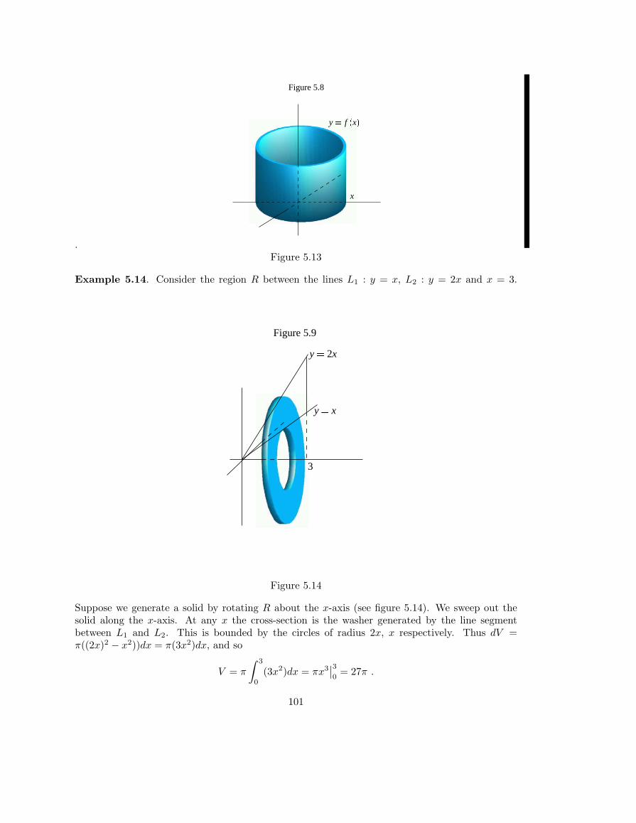
� � � � �Figure 5.8

y � f�x �

x

Figure 5.13

Example 5.14. Consider the region R between the lines L1 : y = x, L2 : y = 2x and x = 3.

Figure 5.9

y � x

y � 2x

3

Figure 5.14

Suppose we generate a solid by rotating R about the x-axis (see figure 5.14). We sweep out thesolid along the x-axis. At any x the cross-section is the washer generated by the line segmentbetween L1 and L2. This is bounded by the circles of radius 2x, x respectively. Thus dV =π((2x)2 − x2))dx = π(3x2)dx, and so

V = π

∫ 3

0

(3x2)dx = πx3∣∣30

= 27π .

101

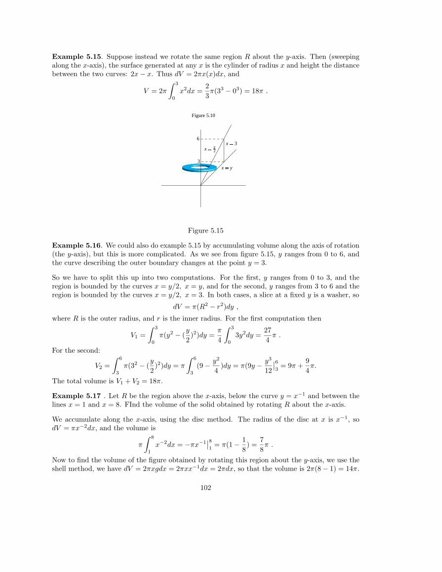
Example 5.15. Suppose instead we rotate the same region R about the y-axis. Then (sweepingalong the x-axis), the surface generated at any x is the cylinder of radius x and height the distancebetween the two curves: 2x− x. Thus dV = 2πx(x)dx, and

V = 2π

∫ 3

0

x2dx =23π(33 − 03) = 18π .

Figure 5.10

x � y2

x � 3

x � y3

6

Figure 5.15

Example 5.16. We could also do example 5.15 by accumulating volume along the axis of rotation(the y-axis), but this is more complicated. As we see from figure 5.15, y ranges from 0 to 6, andthe curve describing the outer boundary changes at the point y = 3.

So we have to split this up into two computations. For the first, y ranges from 0 to 3, and theregion is bounded by the curves x = y/2, x = y, and for the second, y ranges from 3 to 6 and theregion is bounded by the curves x = y/2, x = 3. In both cases, a slice at a fixed y is a washer, so

dV = π(R2 − r2)dy ,

where R is the outer radius, and r is the inner radius. For the first computation then

V1 =∫ 3

0

π(y2 − (y

2)2)dy =

π

4

∫ 3

0

3y2dy =274

π .

For the second:

V2 =∫ 6

3

π(32 − (y

2)2)dy = π

∫ 6

3

(9− y2

4)dy = π(9y − y3

12

∣∣63

= 9π +94π.

The total volume is V1 + V2 = 18π.

Example 5.17 . Let R be the region above the x-axis, below the curve y = x−1 and between thelines x = 1 and x = 8. FInd the volume of the solid obtained by rotating R about the x-axis.

We accumulate along the x-axis, using the disc method. The radius of the disc at x is x−1, sodV = πx−2dx, and the volume is

π

∫ 8

1

x−2dx = −πx−1∣∣81

= π(1− 18) =

78π .

Now to find the volume of the figure obtained by rotating this region about the y-axis, we use theshell method, we have dV = 2πxgdx = 2πxx−1dx = 2πdx, so that the volume is 2π(8− 1) = 14π.

102

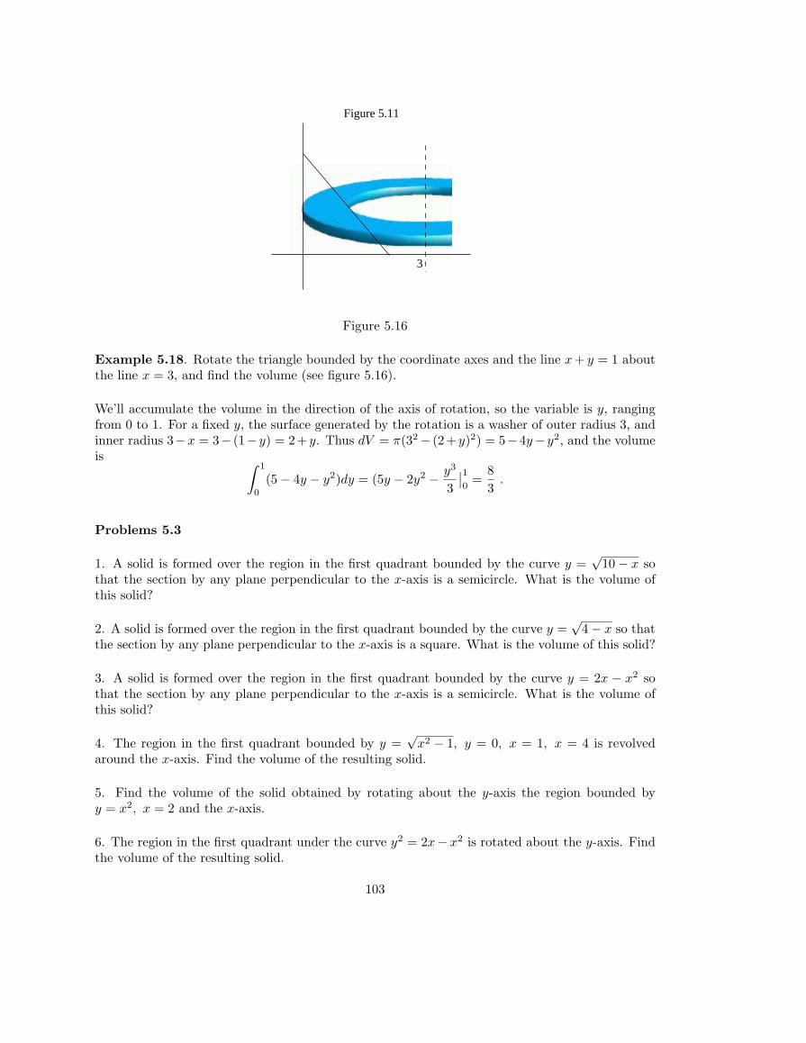
�Figure 5.11

3

volume in the direction of the axis of rotation, so the vFigure 5.16

Example 5.18. Rotate the triangle bounded by the coordinate axes and the line x + y = 1 aboutthe line x = 3, and find the volume (see figure 5.16).

We’ll accumulate the volume in the direction of the axis of rotation, so the variable is y, rangingfrom 0 to 1. For a fixed y, the surface generated by the rotation is a washer of outer radius 3, andinner radius 3−x = 3− (1−y) = 2+ y. Thus dV = π(32− (2+y)2) = 5−4y−y2, and the volumeis ∫ 1

0

(5− 4y − y2)dy = (5y − 2y2 − y3

3

∣∣10

=83

.

Problems 5.3

1. A solid is formed over the region in the first quadrant bounded by the curve y =√

10− x sothat the section by any plane perpendicular to the x-axis is a semicircle. What is the volume ofthis solid?

2. A solid is formed over the region in the first quadrant bounded by the curve y =√

4− x so thatthe section by any plane perpendicular to the x-axis is a square. What is the volume of this solid?

3. A solid is formed over the region in the first quadrant bounded by the curve y = 2x − x2 sothat the section by any plane perpendicular to the x-axis is a semicircle. What is the volume ofthis solid?

4. The region in the first quadrant bounded by y =√

x2 − 1, y = 0, x = 1, x = 4 is revolvedaround the x-axis. Find the volume of the resulting solid.

5. Find the volume of the solid obtained by rotating about the y-axis the region bounded byy = x2, x = 2 and the x-axis.

6. The region in the first quadrant under the curve y2 = 2x− x2 is rotated about the y-axis. Findthe volume of the resulting solid.

103

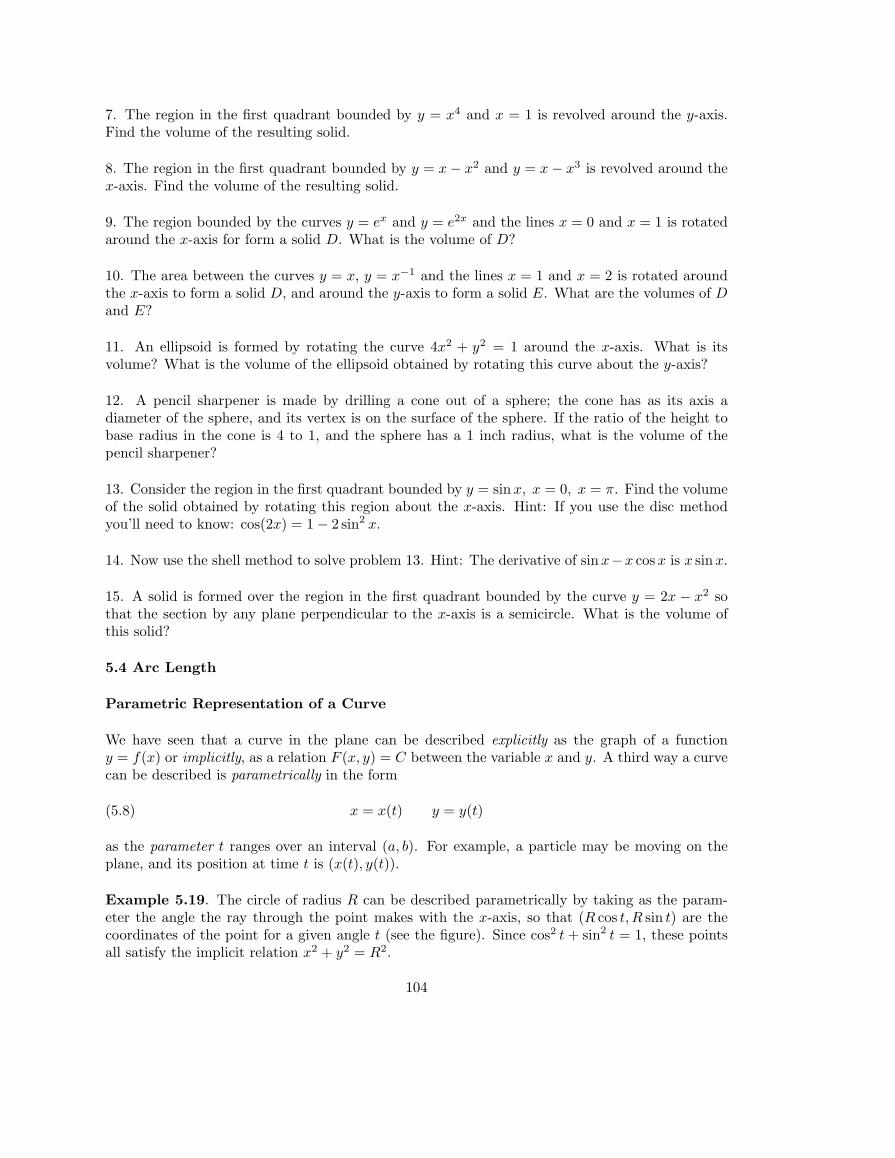
7. The region in the first quadrant bounded by y = x4 and x = 1 is revolved around the y-axis.Find the volume of the resulting solid.

8. The region in the first quadrant bounded by y = x− x2 and y = x− x3 is revolved around thex-axis. Find the volume of the resulting solid.

9. The region bounded by the curves y = ex and y = e2x and the lines x = 0 and x = 1 is rotatedaround the x-axis for form a solid D. What is the volume of D?

10. The area between the curves y = x, y = x−1 and the lines x = 1 and x = 2 is rotated aroundthe x-axis to form a solid D, and around the y-axis to form a solid E. What are the volumes of Dand E?

11. An ellipsoid is formed by rotating the curve 4x2 + y2 = 1 around the x-axis. What is itsvolume? What is the volume of the ellipsoid obtained by rotating this curve about the y-axis?

12. A pencil sharpener is made by drilling a cone out of a sphere; the cone has as its axis adiameter of the sphere, and its vertex is on the surface of the sphere. If the ratio of the height tobase radius in the cone is 4 to 1, and the sphere has a 1 inch radius, what is the volume of thepencil sharpener?

13. Consider the region in the first quadrant bounded by y = sinx, x = 0, x = π. Find the volumeof the solid obtained by rotating this region about the x-axis. Hint: If you use the disc methodyou’ll need to know: cos(2x) = 1− 2 sin2 x.

14. Now use the shell method to solve problem 13. Hint: The derivative of sinx−x cos x is x sinx.

15. A solid is formed over the region in the first quadrant bounded by the curve y = 2x − x2 sothat the section by any plane perpendicular to the x-axis is a semicircle. What is the volume ofthis solid?

5.4 Arc Length

Parametric Representation of a Curve

We have seen that a curve in the plane can be described explicitly as the graph of a functiony = f(x) or implicitly, as a relation F (x, y) = C between the variable x and y. A third way a curvecan be described is parametrically in the form

(5.8) x = x(t) y = y(t)

as the parameter t ranges over an interval (a, b). For example, a particle may be moving on theplane, and its position at time t is (x(t), y(t)).

Example 5.19. The circle of radius R can be described parametrically by taking as the param-eter the angle the ray through the point makes with the x-axis, so that (R cos t, R sin t) are thecoordinates of the point for a given angle t (see the figure). Since cos2 t + sin2 t = 1, these pointsall satisfy the implicit relation x2 + y2 = R2.

104

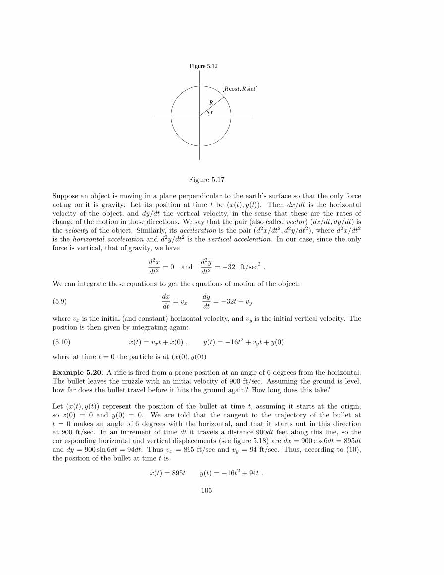
� �Figure 5.12

�Rcos t � Rsint �

R

t

Figure 5.17

Suppose an object is moving in a plane perpendicular to the earth’s surface so that the only forceacting on it is gravity. Let its position at time t be (x(t), y(t)). Then dx/dt is the horizontalvelocity of the object, and dy/dt the vertical velocity, in the sense that these are the rates ofchange of the motion in those directions. We say that the pair (also called vector) (dx/dt, dy/dt) isthe velocity of the object. Similarly, its acceleration is the pair (d2x/dt2, d2y/dt2), where d2x/dt2

is the horizontal acceleration and d2y/dt2 is the vertical acceleration. In our case, since the onlyforce is vertical, that of gravity, we have

d2x

dt2= 0 and

d2y

dt2= −32 ft/sec2

.

We can integrate these equations to get the equations of motion of the object:

(5.9)dx

dt= vx

dy

dt= −32t + vy

where vx is the initial (and constant) horizontal velocity, and vy is the initial vertical velocity. Theposition is then given by integrating again:

(5.10) x(t) = vxt + x(0) , y(t) = −16t2 + vyt + y(0)

where at time t = 0 the particle is at (x(0), y(0))

Example 5.20. A rifle is fired from a prone position at an angle of 6 degrees from the horizontal.The bullet leaves the muzzle with an initial velocity of 900 ft/sec. Assuming the ground is level,how far does the bullet travel before it hits the ground again? How long does this take?

Let (x(t), y(t)) represent the position of the bullet at time t, assuming it starts at the origin,so x(0) = 0 and y(0) = 0. We are told that the tangent to the trajectory of the bullet att = 0 makes an angle of 6 degrees with the horizontal, and that it starts out in this directionat 900 ft/sec. In an increment of time dt it travels a distance 900dt feet along this line, so thecorresponding horizontal and vertical displacements (see figure 5.18) are dx = 900 cos 6dt = 895dtand dy = 900 sin 6dt = 94dt. Thus vx = 895 ft/sec and vy = 94 ft/sec. Thus, according to (10),the position of the bullet at time t is

x(t) = 895t y(t) = −16t2 + 94t .

105

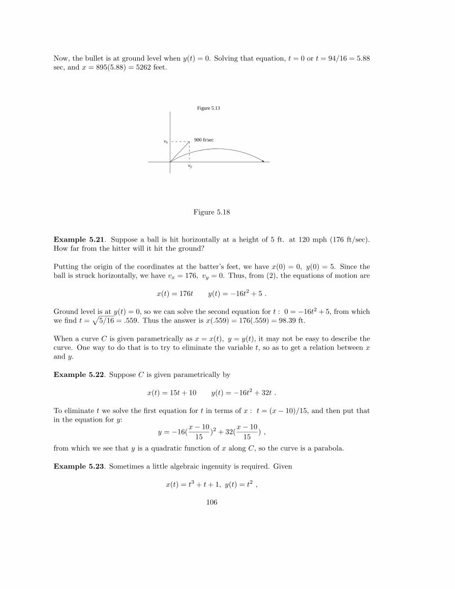
Now, the bullet is at ground level when y(t) = 0. Solving that equation, t = 0 or t = 94/16 = 5.88sec, and x = 895(5.88) = 5262 feet.

Figure 5.13

900 ft/secvx

vy

Figure 5.18

Example 5.21. Suppose a ball is hit horizontally at a height of 5 ft. at 120 mph (176 ft/sec).How far from the hitter will it hit the ground?

Putting the origin of the coordinates at the batter’s feet, we have x(0) = 0, y(0) = 5. Since theball is struck horizontally, we have vx = 176, vy = 0. Thus, from (2), the equations of motion are

x(t) = 176t y(t) = −16t2 + 5 .

Ground level is at y(t) = 0, so we can solve the second equation for t : 0 = −16t2 + 5, from whichwe find t =

√5/16 = .559. Thus the answer is x(.559) = 176(.559) = 98.39 ft.

When a curve C is given parametrically as x = x(t), y = y(t), it may not be easy to describe thecurve. One way to do that is to try to eliminate the variable t, so as to get a relation between xand y.

Example 5.22. Suppose C is given parametrically by

x(t) = 15t + 10 y(t) = −16t2 + 32t .

To eliminate t we solve the first equation for t in terms of x : t = (x− 10)/15, and then put thatin the equation for y:

y = −16(x− 10

15)2 + 32(

x− 1015

) ,

from which we see that y is a quadratic function of x along C, so the curve is a parabola.

Example 5.23. Sometimes a little algebraic ingenuity is required. Given

x(t) = t3 + t + 1, y(t) = t2 ,

106

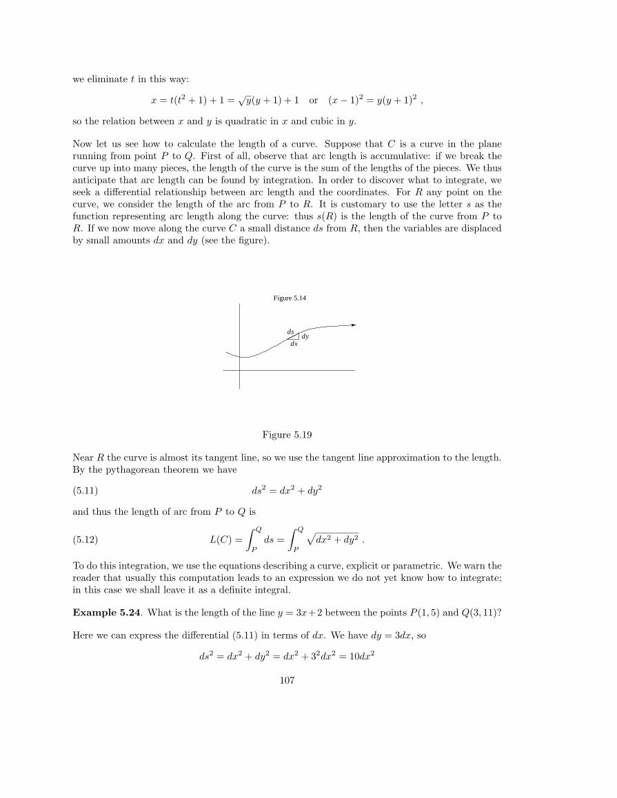
we eliminate t in this way:

x = t(t2 + 1) + 1 =√

y(y + 1) + 1 or (x− 1)2 = y(y + 1)2 ,

so the relation between x and y is quadratic in x and cubic in y.

Now let us see how to calculate the length of a curve. Suppose that C is a curve in the planerunning from point P to Q. First of all, observe that arc length is accumulative: if we break thecurve up into many pieces, the length of the curve is the sum of the lengths of the pieces. We thusanticipate that arc length can be found by integration. In order to discover what to integrate, weseek a differential relationship between arc length and the coordinates. For R any point on thecurve, we consider the length of the arc from P to R. It is customary to use the letter s as thefunction representing arc length along the curve: thus s(R) is the length of the curve from P toR. If we now move along the curve C a small distance ds from R, then the variables are displacedby small amounts dx and dy (see the figure).

� �Figure 5.14

dxdy

ds

Figure 5.19

Near R the curve is almost its tangent line, so we use the tangent line approximation to the length.By the pythagorean theorem we have

(5.11) ds2 = dx2 + dy2

and thus the length of arc from P to Q is

(5.12) L(C) =∫ Q

P

ds =∫ Q

P

√dx2 + dy2 .

To do this integration, we use the equations describing a curve, explicit or parametric. We warn thereader that usually this computation leads to an expression we do not yet know how to integrate;in this case we shall leave it as a definite integral.

Example 5.24. What is the length of the line y = 3x+2 between the points P (1, 5) and Q(3, 11)?

Here we can express the differential (5.11) in terms of dx. We have dy = 3dx, so

ds2 = dx2 + dy2 = dx2 + 32dx2 = 10dx2

107

so ds =√

10dx. Then

L =∫ Q

P

ds =∫ 3

1

√10dx =

√10(3− 1) = 2

√10

which is, of course, the same answer we would have gotten from the distance formula of chapter I.

Example 5.25. Find the length of the arc of a circle of radius R subtended by an angle α.

Here we parametrize the circle as in example 5.18 (see figure 5.18): x = R cos t, y = R sin t. Thendx = −R sin tdt, dy = R cos tdt and

ds2 = dx2 + dy2 = (−R sin t)2dt2 + (R cos t)2dt2 = R2(sin2 t + cos2 t)dt2 = R2dt2 .

Our length is thus

L =∫

ds =∫ α

0

Rdt = Rα ,

another standard formula.

Example 5.26. Find the length of the curve x2 = y3 from (0,0) to (27,9).

First we have to find a suitable parametrization of the curve. Since the variables are positive inthis range, we can write y = t2, and then x2 = y3 = (t2)3 = (t3)2, so we can take x = t3, as tranges from 0 to 3. Now dy = 2tdt and dx = 3t2dt, so

ds2 = dx2 + dy2 = 9t4dt2 + 4t2dt2 = t2(9t2 + 4)dt2 ;

that is, ds = t√

9t2 + 4dt. Then the length is

L =∫

ds =∫ 3

0

t√

9t2 + 4dt ==118

∫ 85

4

u1/2du

using the substitution u = 9t2+4, du = 18tdt. The limits of integration in u are found by evaluatingu at t = 0 and t = 3. The length is

L =118

23u3/2

∣∣854

=127

(853/2 − 8) .

Example 5.27. Find the length of the parabolic segment y = 5x− x2 from x = 0 to x = 5.

We have dy = (5− 2x)dx, so ds2 = (1 + (5− 2x)2)dx2, and the length is

L =∫ 5

0

√1 + (5− 2x)2dx =

12

∫ 5

−5

√1 + u2du ,

making the substitution u = 2x − 5, du = 2dx. But that didn’t help; we still end up with anintegral we have yet to learn how to integrate.

108

Problems 5.4

1. Find the length of the curve y = t3, x = t2, 0 ≤ t ≤ 1.

2. The equations x = eat cos t, y = eat sin t define the logarithmic spiral. Find the length of thiscurve for 0 ≤ t ≤ 2π.

3. Find the integral giving the length of the curve y =√

1 + x2 for 0 ≤ x ≤ 1.

4. Find the area of the surface obtained by rotating the line segment y = 3x− 3, 3 ≤ x ≤ 5 aboutthe x-axis.

5. Find the area of the bowl obtained by rotating the parabola y = x2, 0 ≤ x ≤ a about thex-axis.

5.5 Work

Work is the product of force and distance. The unit of force in the British system is the foot-pound;in the metric system it is the joule, or newton-meter. For example, to move a box a distance of 12feet against a force of friction of 40 lbs takes 40·12 = 480 foot-pounds. To lift a weight of 25 poundsa distance of 8 feet takes 25·8 = 200 foot-pounds. Remember that the weight (at the surface of theearth) of an object is a measure of its gravitational force, and is equal to mg, where m is the massof the object and g is the acceleration of gravity. In the metric system, the gram and the kilogramare measures of mass, so to find the weight (in joules) we must multiply the mass (in kilograms)by g = 9.8 m/sec2.

Example 5.28. How much work is done in lifting a mass of 1.2 kg a distance of 12 meters? Theweight of the mass is (1.2)(9.8) newtons, so the work is (1.2)(9.8)(12) = 141.12 joules.

Now, suppose that the force is not constant, but varies over the distance traversed. For example,to put a rocket in orbit, we must calculate the energy (work) required. But the force on the rocket(its effective weight) decreases as it leaves the surface of the earth.

So, suppose we have a force acting along a line; denote the value of the force at the point x asF (x). If F (x) is positive, it works in the direction of increasing x, and if negative, it works oppositeto that direction. That is, if the force is positive, it does work as we progress, and if negative, itcauses work as we progress. The question we ask is this: what work is done by the force througha given distance on the line. Work is accumulative: If we break the interval up into pieces, thetotal work done is the sum of the work done over each piece. We set up a work calculation byintegration, once we know the differential relation. Let W (x) be the work done to get from a tox. If we move a small distance dx further, we may assume the force to be constant, and equal toF (x) over this interval. Then the increment in work is dW = F (x)dx. We now find the total workby integrating:

W =∫ b

a

F (x)dx .

In particular, if this is positive, the force is doing work over the interval, and if negative, we mustsupply the work to overcome it.

109

Definition 5.3. Let F (x) be a force acting along the real axis, such that F (x) > 0 when F isacting in the direction of increasing x. Let a < b. The work done by the force over the interval[a, b] is W =

∫ b

aF (x)dx.

Example 5.29. Let F (x) = x(1− x2) be a force acting on the x axis. How much work is done bythe force a) between the points 0, 1? b) between the points 0, 2?

a) W =∫ 1

0

(x− x3)dx =x2

2− x4

4

∣∣10

= 1/2

b) W =∫ 2

0

(x− x3)dx =x2

2− x4

4

∣∣20

= −2

Thus the force does work for us between 0 and 1, but against us between 1 and 2.

Springs

Consider a spring hanging vertically. If the spring is extended or compressed, a force will beexerted, called the restoring force, directed toward the inital rest position. If a weight is carefullyattached to the spring, it will extend to a new rest position, at which the weight exactly balancesthe restoring force. This is the equilibrium position for that weight. According to Hooke’s Law, themagnitude of the restoring force and the displacement from rest are proportional. That is, if welet x represent the displacement from the equilibrium position, and F (x) the force in the spring,then we have

(5.13) F (x) = −kx

for some constant k, called the spring constant. The negative sign indicates that the force acts inthe direction opposite to the displacement.

Example 5.30. Suppose a 5 lb weight extends a spring by 1.5 inches. a) What is the springconstant? b) How far will a 12 lb. weight extend the spring?

The force in the spring at 1.5 inches, or .125 feet is -5 lbs, so by (13), −5 = −k(.125), so k = 40lb/ft, and Hooke’s law for this spring is F (x) = −40x. When the 12 lb weight is attached, therestoring force is F (x) = −12, so we find x by solving −12 = −40x, or x = .3 ft or 3.6 inches.

Example 5.31. Suppose a 3 pound weight displaces a spring 2 inches. How much work is requiredto displace the spring two feet?

First we use Hooke’s law with the given information to find the spring constant. In our situation,when x = 1/6 foot, F = −3 pounds. From Hooke’s law, −3 = −k(1/6), so the spring constant isk = 18, and Hooke’s law for this spring is F (x) = −18x. Now, for work, we have dW = F (x)dx,so to extend the spring 2 feet, we calculate the work done by the spring over this distance:

W =∫ 2

0

−18xdx = −9x2∣∣20

= −36

110

ft-lbs. Thus the work needed to extend the spring 2 feet must counterbalance this, so is 36 foot-pounds.

Now if a spring with an object at its end is extended a certain distance and then released, it willvibrate. To understand this motion, we recall the discussion of Example 4.18. There we saw thatfor a body in motion vdv = adx, where x is the displacement, v the velocity and a the acceleration.If we multiply by the mass m and use Newton’s law, F = ma, we get

(5.14) mvdv = Fdx .

The expression on the right is dW , the differential of work, and the expression on the left is thedifferential of (1/2)mv2, the kinetic energy: the change in kinetic energy is equal to the work done.This is then the differential expression of the law of conservation of energy. Now, for a spring,F (x) = −kx, so (5.14) becomes

mvdv + kxdx = 0

which integrates to

(5.15) mv2 + kx2 = constant

during the motion of a vibrating spring of spring constant k and a mass m at its end.

Example 5.32. A spring of spring constant k = 4 ft/lb with an object of weight 3 lbs attached toits end is at rest. The object is extended a distance of 2 feet and then released. At what velocitydoes the object pass its equilibrium position?

The mass of the object is m = w/g = 3/(32) = .0938. Thus, in this situation, (15) tells us that.0938v2 + 4x2 is constant during the motion. At the moment of release, v = 0 and x = 2, so thisconstant is .0938(0)2 + 4(2)2 = 16. At the moment the object passes the equilibrium point, x = 0,so we can solve:.0938v2 = 16, for v = 18.48 ft/sec.

Example 5.33. A 1 kg mass extends a spring 8 cm. Suppose that a mass of 3 kg is attached tothe spring, then extended 20 cm. beyond equilibrium and released. What will be the velocity ofthe mass as it passes the 10 cm. point?

First we must find the spring constant. The weight of a 1 kg mass is w = mg = (1)(9.8) = 9.8newtons. From Hooke’s law we have −9.8 = −k(.08), so k = 9.8/.08 = 122.5 newtons/meter. Forour 3 kg mass in motion, equation (7) is 3v2 +122.5x2 = constant. At the moment of release, v = 0and x = .2, so the constant is 122.5(.2)2 = 4.9. At the 10 cm point, we solve 3v2 +122.5(.1)2 = 4.9,giving v = 1.107 meters/second.

Example 5.34. What is the energy required to lift a payload of 1000 lbs a distance of 250 milesfrom the surface of the earth?

We have to calculate the work required to move the payload 250 miles vertically from the earth’ssurface. Let s represent distance from the center of the earth, and let R be the radius of the earth.According to Newton’s law of gravitation, the force of gravity is

F (s) = − k

s2

111

for some constant k. Now, when s = R, for our payload, F (R) = −103 lbs, so k = 103R2, andF (s) = −103R2/s2. Thus the work “done by” gravity is

W = −∫ R+250

R

103R2

s2ds = −103R2(−1

s)∣∣R+250

R= −103R2(

250R(R + 250)

) .

Taking R = 3900 miles, we see that the energy required to lift this payload to 250 miles is

103(3900)2504150

= 2.34(105) mi · lbs = 12.4(109) ft · lbs

Example 5.35. A cistern is a hole in the ground (usually lined with steel or cement) used tocollect water. Suppose that we have a cylindrical cistern of radius 8 feet and of depth 20 feet. Ifit is full of water, how much work is required to empty the cistern?

In this problem, the force is the weight of the water (one cubic foot of water weighs 62.5 lbs), butthe distance the water has to be moved depends upon how deep into the cistern we have gotten.So, we again approach the problem dynamically, where the dynamic variable is the distance ybetween the top of the cistern and the surface of the water. At this depth, the work required tolift the next slab of water (of thickness dy) is y× (weight of that slab). The weight of that slab is62.5×(volume). The slab is a cylinder of radius 8 feet and thickness dx. Thus

dW = (62.5)π(8)2ydy .

Since the cistern is 20 feet deep, the total work then is the integral∫ 20

0

62.5π(8)2ydy = 4000πy2

2

∣∣200

= 8× 105π ft · lbs .

Example 5.36. Suppose instead that the cistern, of the same depth, has a parabolic profile,following the curve y = (5/16)x2. Now, to lift the slab of thickness dy at a depth y takes theamount of work

dW = (62.5)πx2ydy ,

because the radius at this level is now x. Since x2 = (16/5)y, the total work is given by∫ 20

0

62.5π165

y2dy = 200πy3

3

∣∣200

= 5.33× 105π

Problems 5.5

1. Find the work done in pumping all the oil (whose density is 50 lbs. per cubic foot) over theedge of a cylindrical tank which stands on end. Assume that the radius of the base is 4 feet, theheight is 10 feet and the tank is full of oil.

2. John Brown has a parabolic cistern in the ground with a depth of 12 feet and a diameter atthe top of 4 feet. This can be viewed as formed by revolving the curve y = 3x2 around the y-axis,where the line y = 12 represents ground level. How much work does it take to pump out the cisternwhen it is full of water (the density of water is 62.5 lb/ft3)?

112

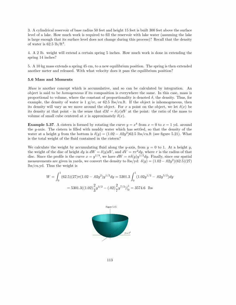
3. A cylindrical reservoir of base radius 50 feet and height 15 feet is built 300 feet above the surfacelevel of a lake. How much work is required to fill the reservoir with lake water (assuming the lakeis large enough that its surface level does not change during this process)? Recall that the densityof water is 62.5 lb/ft3.

4. A 2 lb. weight will extend a certain spring 5 inches. How much work is done in extending thespring 14 inches?

5. A 10 kg mass extends a spring 45 cm, to a new equilibrium position. The spring is then extendedanother meter and released. With what velocity does it pass the equilibrium position?

5.6 Mass and Moments

Mass is another concept which is accumulative, and so can be calculated by integration. Anobject is said to be homogeneous if its composition is everywhere the same. In this case, mass isproportional to volume, where the constant of proportionality is denoted δ, the density. Thus, forexample, the density of water is 1 g/cc, or 62.5 lbs/cu.ft. If the object is inhomogeneous, thenits density will vary as we move around the object. For x a point on the object, we let δ(x) beits density at that point - in the sense that dM = δ(x)dV at the point: the ratio of the mass tovolume of small cube centered at x is approximately δ(x).

Example 5.37. A cistern is formed by rotating the curve y = x4 from x = 0 to x = 1 yd. aroundthe y-axis. The cistern is filled with muddy water which has settled, so that the density of thewater at a height y from the bottom is δ(y) = (1.02− .02y2)62.5 lbs/cu.ft (see figure 5.21). Whatis the total weight of the fluid contained in the cistern?

We calculate the weight by accumulating fluid along the y-axis, from y = 0 to 1. At a height y,the weight of the disc of height dy is dW = δ(y)dV , and dV = πr2dy, where r is the radius of thatdisc. Since the profile is the curve x = y1/4, we have dW = πδ(y)y1/2dy. Finally, since our spatialmeasurements are given in yards, we convert the density to lbs/yd: δ(y) = (1.02− .02y2)(62.5)(27)lbs/cu.yd. Thus the weight is

W =∫ 1

0

(62.5)(27)π(1.02− .02y2)y1/2dy = 5301.3∫ 1

0

(1.02y1/2 − .02y5/2)dy

= 5301.3((1.02)23y3/2 − (.02)

27y7/2)

∣∣10

= 3574.6 lbs

Figure 5.15

y � x4

113

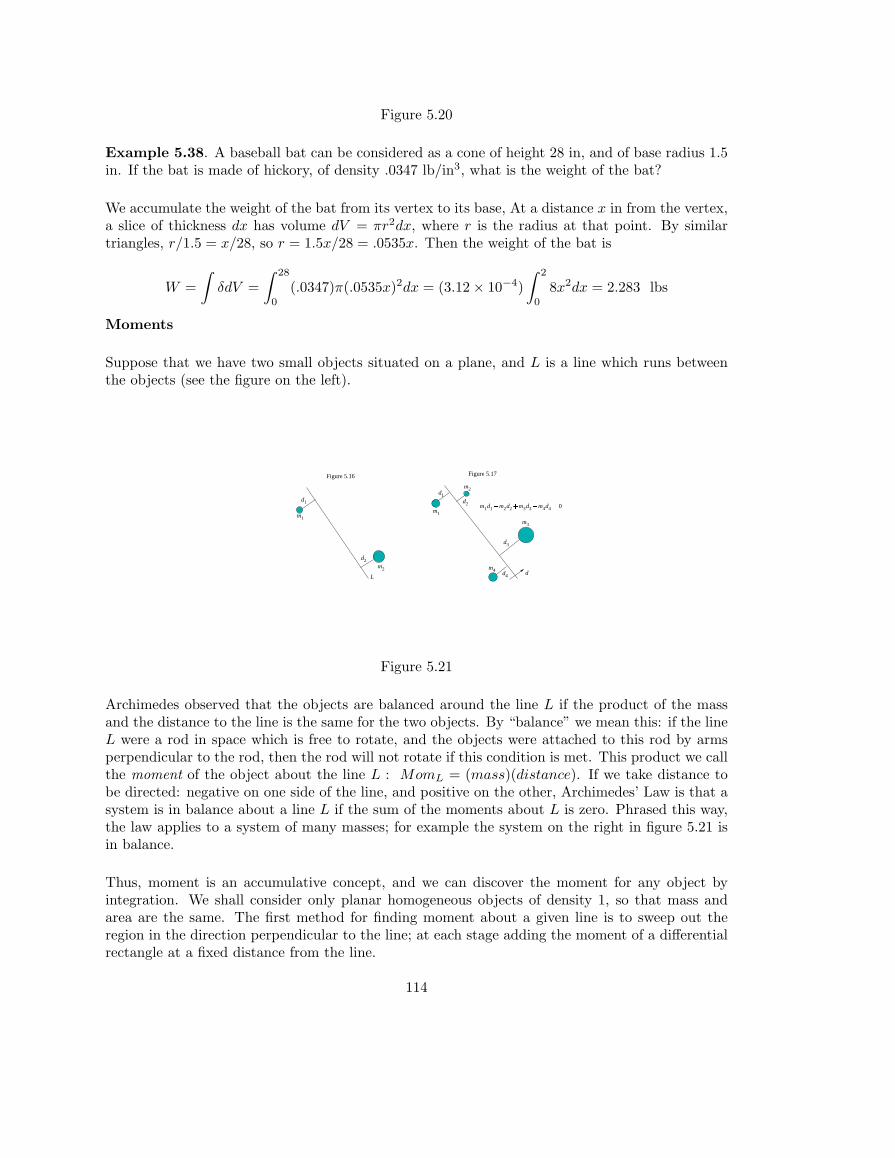
Figure 5.20

Example 5.38. A baseball bat can be considered as a cone of height 28 in, and of base radius 1.5in. If the bat is made of hickory, of density .0347 lb/in3, what is the weight of the bat?

We accumulate the weight of the bat from its vertex to its base, At a distance x in from the vertex,a slice of thickness dx has volume dV = πr2dx, where r is the radius at that point. By similartriangles, r/1.5 = x/28, so r = 1.5x/28 = .0535x. Then the weight of the bat is

W =∫

δdV =∫ 28

0

(.0347)π(.0535x)2dx = (3.12× 10−4)∫ 2

0

8x2dx = 2.283 lbs

Moments

Suppose that we have two small objects situated on a plane, and L is a line which runs betweenthe objects (see the figure on the left).

Figure 5.16

L

d1

d2

m1

m2

Figure 5.17

d1d2

d3

d4

m1

m2

m3

m4 d

m1d1 � m2d2 � m3d3 � m4d4 � 0

Figure 5.21

Archimedes observed that the objects are balanced around the line L if the product of the massand the distance to the line is the same for the two objects. By “balance” we mean this: if the lineL were a rod in space which is free to rotate, and the objects were attached to this rod by armsperpendicular to the rod, then the rod will not rotate if this condition is met. This product we callthe moment of the object about the line L : MomL = (mass)(distance). If we take distance tobe directed: negative on one side of the line, and positive on the other, Archimedes’ Law is that asystem is in balance about a line L if the sum of the moments about L is zero. Phrased this way,the law applies to a system of many masses; for example the system on the right in figure 5.21 isin balance.

Thus, moment is an accumulative concept, and we can discover the moment for any object byintegration. We shall consider only planar homogeneous objects of density 1, so that mass andarea are the same. The first method for finding moment about a given line is to sweep out theregion in the direction perpendicular to the line; at each stage adding the moment of a differentialrectangle at a fixed distance from the line.

114

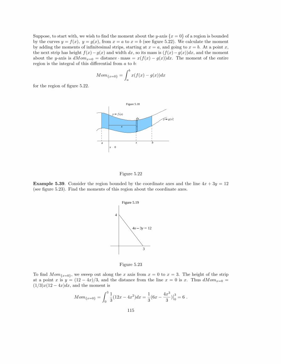
Suppose, to start with, we wish to find the moment about the y-axis {x = 0} of a region is boundedby the curves y = f(x), y = g(x), from x = a to x = b (see figure 5.22). We calculate the momentby adding the moments of infinitesimal strips, starting at x = a, and going to x = b. At a point x,the next strip has height f(x)−g(x) and width dx, so its mass is (f(x)−g(x))dx, and the momentabout the y-axis is dMomx=0 = distance · mass = x(f(x) − g(x))dx. The moment of the entireregion is the integral of this differential from a to b:

Mom{x=0} =∫ b

a

x(f(x)− g(x))dx

for the region of figure 5.22. � � � � � � � �Figure 5.18

�����

�����

y � f�x �

y � g�x �

x

x

dx

a b

x � 0

Figure 5.22

Example 5.39. Consider the region bounded by the coordinate axes and the line 4x + 3y = 12(see figure 5.23). Find the moments of this region about the coordinate axes.

Figure 5.19

3

4

4x � 3y � 12

Figure 5.23

To find Mom{x=0}, we sweep out along the x axis from x = 0 to x = 3. The height of the stripat a point x is y = (12 − 4x)/3, and the distance from the line x = 0 is x. Thus dMomx=0 =(1/3)x(12− 4x)dx, and the moment is

Mom{x=0} =∫ 3

0

13(12x− 4x2)dx =

13(6x− 4x3

3)∣∣30

= 6 .

115

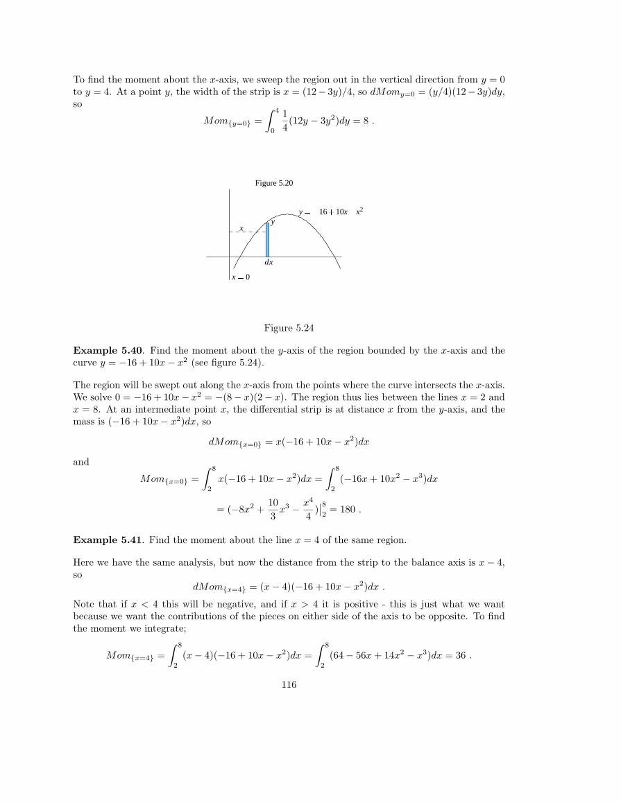
To find the moment about the x-axis, we sweep the region out in the vertical direction from y = 0to y = 4. At a point y, the width of the strip is x = (12− 3y)/4, so dMomy=0 = (y/4)(12− 3y)dy,so

Mom{y=0} =∫ 4

0

14(12y − 3y2)dy = 8 .

Figure 5.20

x � 0

dx

xy

y � � 16 � 10x � x2

swept out along the x-axis from the points where the curve intersects

Figure 5.24

Example 5.40. Find the moment about the y-axis of the region bounded by the x-axis and thecurve y = −16 + 10x− x2 (see figure 5.24).

The region will be swept out along the x-axis from the points where the curve intersects the x-axis.We solve 0 = −16 + 10x− x2 = −(8− x)(2− x). The region thus lies between the lines x = 2 andx = 8. At an intermediate point x, the differential strip is at distance x from the y-axis, and themass is (−16 + 10x− x2)dx, so

dMom{x=0} = x(−16 + 10x− x2)dx

and

Mom{x=0} =∫ 8

2

x(−16 + 10x− x2)dx =∫ 8

2

(−16x + 10x2 − x3)dx

= (−8x2 +103

x3 − x4

4)∣∣82

= 180 .

Example 5.41. Find the moment about the line x = 4 of the same region.

Here we have the same analysis, but now the distance from the strip to the balance axis is x− 4,so

dMom{x=4} = (x− 4)(−16 + 10x− x2)dx .

Note that if x < 4 this will be negative, and if x > 4 it is positive - this is just what we wantbecause we want the contributions of the pieces on either side of the axis to be opposite. To findthe moment we integrate;

Mom{x=4} =∫ 8

2

(x− 4)(−16 + 10x− x2)dx =∫ 8

2

(64− 56x + 14x2 − x3)dx = 36 .

116

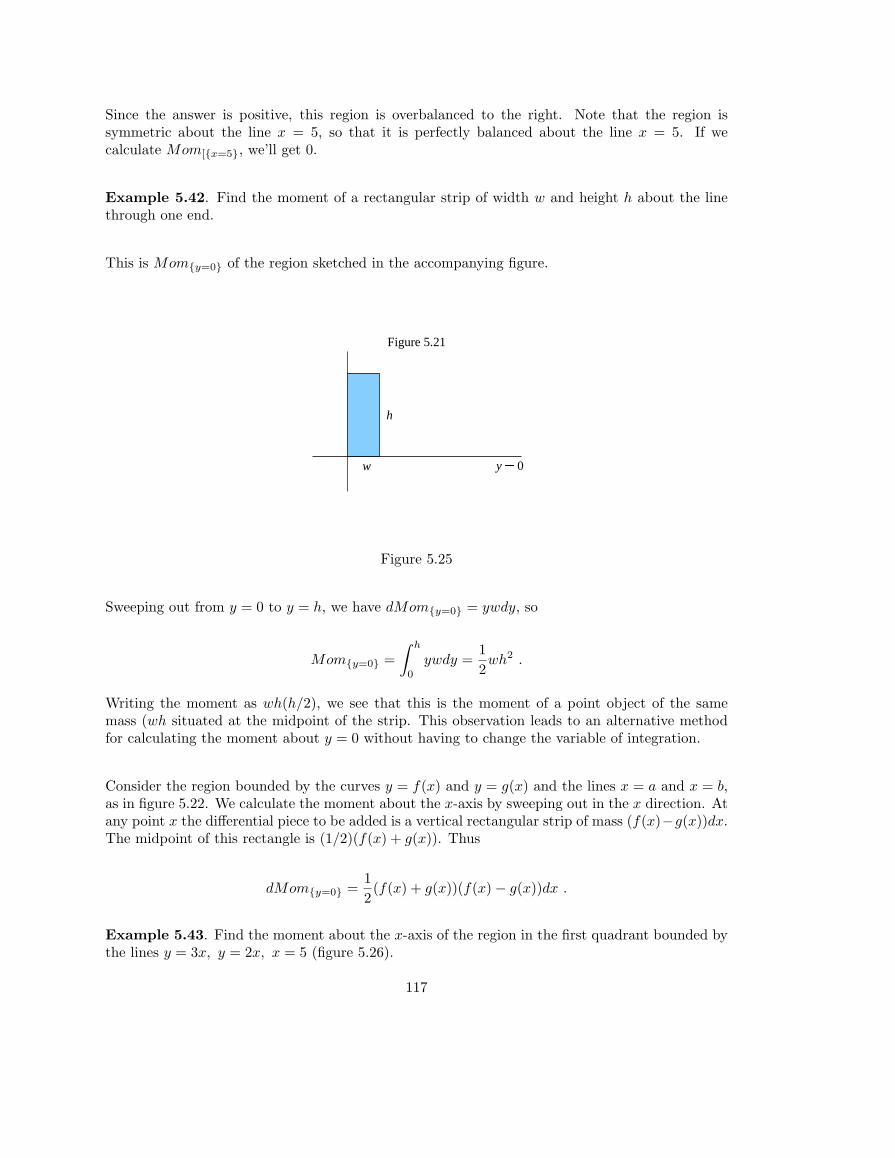
Since the answer is positive, this region is overbalanced to the right. Note that the region issymmetric about the line x = 5, so that it is perfectly balanced about the line x = 5. If wecalculate Mom[{x=5}, we’ll get 0.

Example 5.42. Find the moment of a rectangular strip of width w and height h about the linethrough one end.

This is Mom{y=0} of the region sketched in the accompanying figure.

� � � �� � �Figure 5.21

y � 0

h

w

Figure 5.25

Sweeping out from y = 0 to y = h, we have dMom{y=0} = ywdy, so

Mom{y=0} =∫ h

0

ywdy =12wh2 .

Writing the moment as wh(h/2), we see that this is the moment of a point object of the samemass (wh situated at the midpoint of the strip. This observation leads to an alternative methodfor calculating the moment about y = 0 without having to change the variable of integration.

Consider the region bounded by the curves y = f(x) and y = g(x) and the lines x = a and x = b,as in figure 5.22. We calculate the moment about the x-axis by sweeping out in the x direction. Atany point x the differential piece to be added is a vertical rectangular strip of mass (f(x)−g(x))dx.The midpoint of this rectangle is (1/2)(f(x) + g(x)). Thus

dMom{y=0} =12(f(x) + g(x))(f(x)− g(x))dx .

Example 5.43. Find the moment about the x-axis of the region in the first quadrant bounded bythe lines y = 3x, y = 2x, x = 5 (figure 5.26).

117

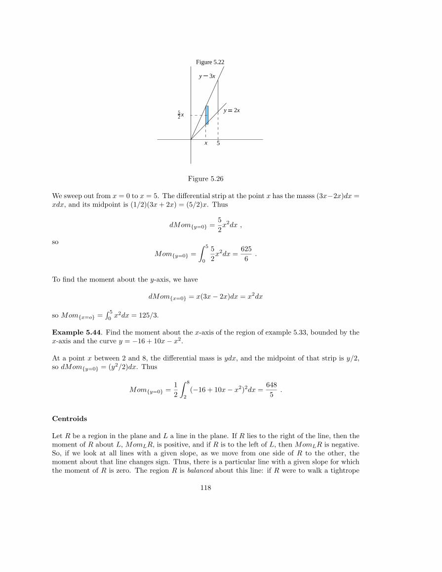
Figure 5.22

52 x

x 5

y � 3x

y � 2x

Figure 5.26

We sweep out from x = 0 to x = 5. The differential strip at the point x has the masss (3x−2x)dx =xdx, and its midpoint is (1/2)(3x + 2x) = (5/2)x. Thus

dMom{y=0} =52x2dx ,

so

Mom{y=0} =∫ 5

0

52x2dx =

6256

.

To find the moment about the y-axis, we have

dMom{x=0} = x(3x− 2x)dx = x2dx

so Mom{x=o} =∫ 5

0x2dx = 125/3.

Example 5.44. Find the moment about the x-axis of the region of example 5.33, bounded by thex-axis and the curve y = −16 + 10x− x2.

At a point x between 2 and 8, the differential mass is ydx, and the midpoint of that strip is y/2,so dMom{y=0} = (y2/2)dx. Thus

Mom{y=0} =12

∫ 8

2

(−16 + 10x− x2)2dx =6485

.

Centroids

Let R be a region in the plane and L a line in the plane. If R lies to the right of the line, then themoment of R about L, MomLR, is positive, and if R is to the left of L, then MomLR is negative.So, if we look at all lines with a given slope, as we move from one side of R to the other, themoment about that line changes sign. Thus, there is a particular line with a given slope for whichthe moment of R is zero. The region R is balanced about this line: if R were to walk a tightrope

118

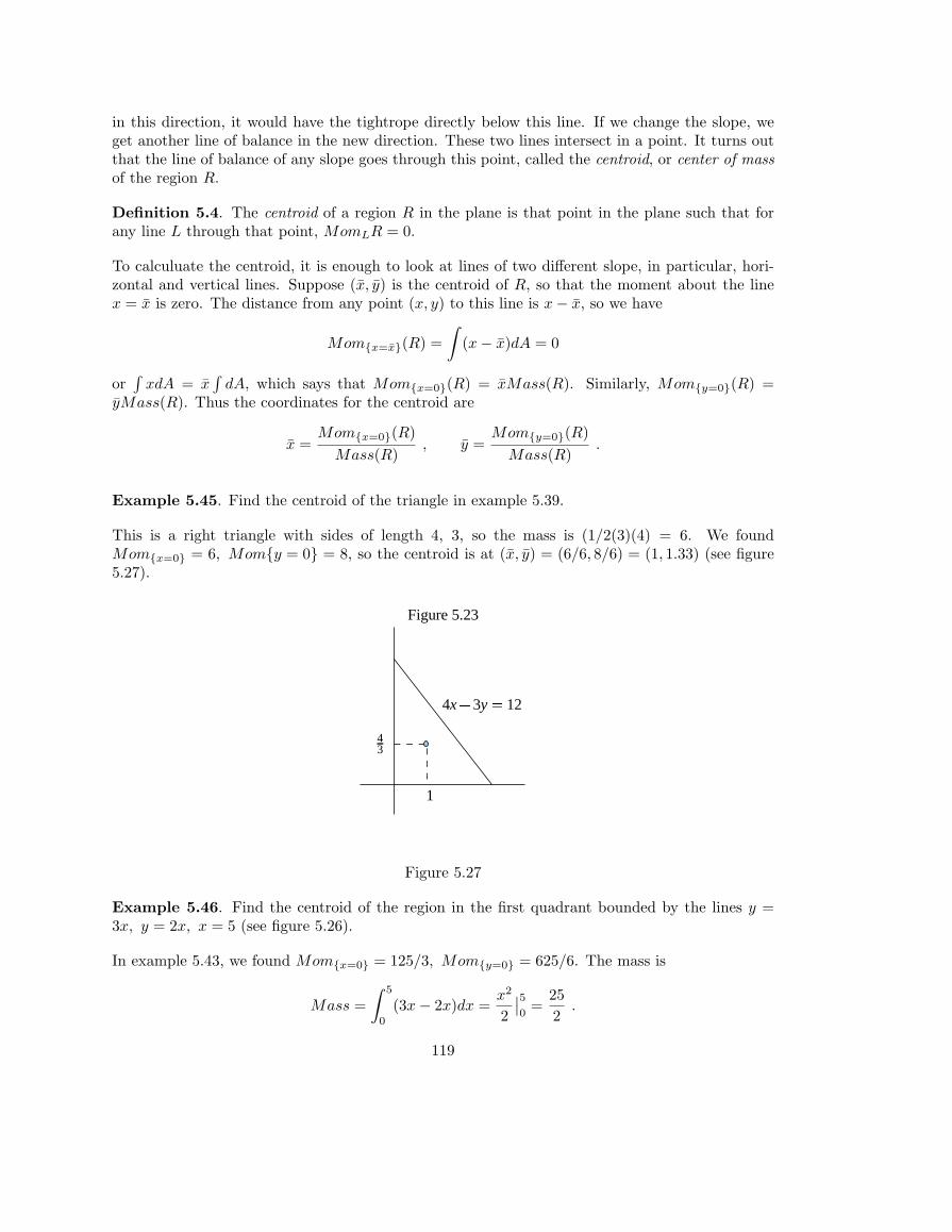
in this direction, it would have the tightrope directly below this line. If we change the slope, weget another line of balance in the new direction. These two lines intersect in a point. It turns outthat the line of balance of any slope goes through this point, called the centroid, or center of massof the region R.

Definition 5.4. The centroid of a region R in the plane is that point in the plane such that forany line L through that point, MomLR = 0.

To calculuate the centroid, it is enough to look at lines of two different slope, in particular, hori-zontal and vertical lines. Suppose (x, y) is the centroid of R, so that the moment about the linex = x is zero. The distance from any point (x, y) to this line is x− x, so we have

Mom{x=x}(R) =∫

(x− x)dA = 0

or∫

xdA = x∫

dA, which says that Mom{x=0}(R) = xMass(R). Similarly, Mom{y=0}(R) =yMass(R). Thus the coordinates for the centroid are

x =Mom{x=0}(R)

Mass(R), y =

Mom{y=0}(R)Mass(R)

.

Example 5.45. Find the centroid of the triangle in example 5.39.

This is a right triangle with sides of length 4, 3, so the mass is (1/2(3)(4) = 6. We foundMom{x=0} = 6, Mom{y = 0} = 8, so the centroid is at (x, y) = (6/6, 8/6) = (1, 1.33) (see figure5.27).

� � � �� � � � � � � � � � � � � �Figure 5.23

4x � 3y � 12

43

1

Figure 5.27

Example 5.46. Find the centroid of the region in the first quadrant bounded by the lines y =3x, y = 2x, x = 5 (see figure 5.26).

In example 5.43, we found Mom{x=0} = 125/3, Mom{y=0} = 625/6. The mass is

Mass =∫ 5

0

(3x− 2x)dx =x2

2

∣∣50

=252

.

119

Thus x = (125/3)/(25/2) = 10/3 and y = (625/6)/(25/2) = 25/3.

Example 5.47. Find the centroid of the region bounded by the y axis and the curve y = −16 +10x− x2 (see figure 5.24).

First of all, since the region is symmetric about the line x = 5, we have x = 5. In example 5.40,we found Mom{y=0} = 648/5. It remains to calculate the mass of the region which is∫ 8

2

(−16 + 10x− x2)dx = (−16x + 5x2 +x3

3)∣∣82

= 36 .

Thus y = (648/5)/36 = 3.6. The centroid is at (5, 3.6).

As a final application of moments, we derive

Pappus’ Theorem. Let R be a region in the right half plane, and consider the solid obtainedby rotating R about the y-axis. The volume of this solid is the product of the area of R and thedistance traveled by the centroid of R.

This is easy to see using the shell method for finding the volume. By that method,

V olume = 2π∫

xdA

where the integration is taken in the x direction between the bounding lines. But∫

xdA =Mom{x=0} and this is x (Area) , where the centroid has coordinates (x, y). So

V olume = 2πx(Area) ,

which is what is asserted by by Pappus’ theorem, since, in the rotation, the centroid travels aroundthe circle of radius x. Although at Pappus’ time the calculus didn’t even exist (in fact, neitherdid algebra), he demonstrated this result in essentially the same way, using Archimedes’ theory ofmoments.

Example 5.48. Find the volume of the solid ring obtained by rotating the disc (x− 5)2 + y2 = 16about the y-axis.

The region being rotated is the circle centered at (5, 0) and of radius 4. Clearly the centroid of adisc is its center, so x = 5. Thus the volume is 2π(5)π(4)2 = 160π2 .

Problems 5.6

1. Kansas can be modelled as a rectangle of length 500 miles and of height 300 miles. Thepopulation density decreases as one moves west through the state; in fact the density x miles westof the eastern border is about

δ(x) = 40− 35( x

500)2

people per square mile. About what is the population of Kansas? Where is the geographical centerof Kansas?

120

2. Find the center of mass of the region bounded by the curves y = x− x3 and y = x− x2.

3. Find the center of mass of the homogeneous region in the first quadrant bounded by the curvex4 + y = 1.

4. Find the centroid of the region bounded by the parabola y2 = 16x and the line x = 9.

5. Let P be the region obtained by rotating the curve y = x3 : 0 ≤ x ≤ 1 about th y-axis. Thisbowl is filled with a fluid whose density along the disc y = h is 1 − h g/cm3. What is the totalmass of this fluid? 6. Find the centroid of the region above the x-axis, under the curve y = x−2

and between the lines x = 1 and x = 8.

121