1

Calculus BC Bible

(3rd most important book in the world) (To be used in conjunction with the Calculus AB Bible)PG. Topic 2 Rectangular and Parametric Equations (Arclength, Speed)3− 4 Polar (Polar Area)4−5 Integration by Parts5−6 Trigonometric Integrals6− 7 Trigonometric Substitutions8−9 Integration Techniques (Long Division, Partial Fractions) 9 Improper Integrals10−12 Convergence/Divergence Tests 13 Taylor/MacLaurin Series 14 Radius and Interval of Convergence 15 Writing Taylor series using known series 15 Separating Variables 16 L'Hopital's Rule 16 Work 16 Hooke's Law16−17 Logistical/Exponential Growth 18 Euler's Method 18 Slope Fields 19 Lagrange Error Bound 19 Area as a Limit 20 Summary of Tests for Convergence 21 Power Series for Elementary Functions 22 Special Integration Techniques23-24 After Calculus BC (Vector Calculus and Calculus III)

2

APPLICATIONS OF THE INTEGRALRectangular Equations y = f (x)( )Length of a Curve (Arclength) Surface Area

L = 1+ ′f x( )( )2

a

b

∫ dx S.A.= 2 π f x( ) 1+ f ' x( )( )2 dxa

b

∫

Parametric Equations Parametric equations are set of equations, both functions of t such that: x = f t( ) y = g t( )

Length of a Curve Surface Area

L = f ' t( )( )2 + g ' t( )( )2 dta

b

∫ or dxdt

⎛⎝⎜

⎞⎠⎟

2

+ dydt

⎛⎝⎜

⎞⎠⎟

2

dta

b

∫ S.A.= 2π g t( )a

b

∫ f ' t( )( )2 + g ' t( )( )2 dt

Speed Equation :

speed = dydt

⎛⎝⎜

⎞⎠⎟2

+dxdt

⎛⎝⎜

⎞⎠⎟2

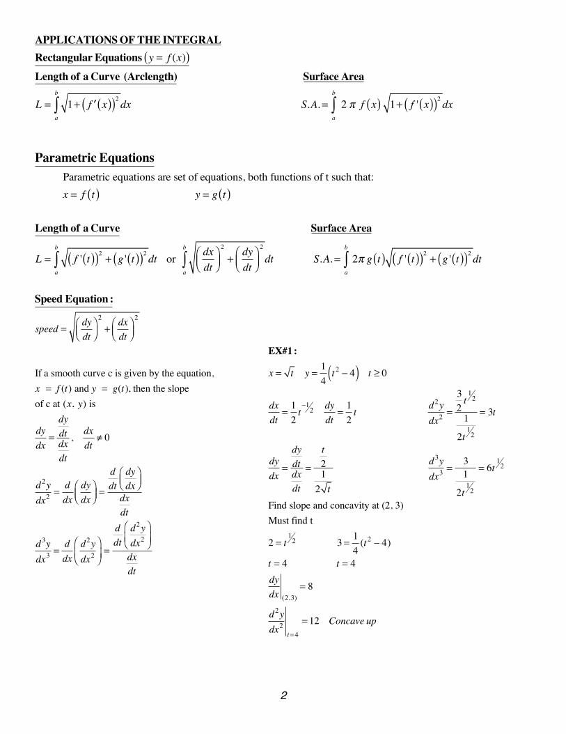
If a smooth curve c is given by the equation, x = f (t) and y = g(t), then the slope of c at (x, y) is

dydx

=

dydtdxdt

, dxdt

≠ 0

d2ydx2 =

ddx

dydx

⎛⎝⎜

⎞⎠⎟=

ddt

dydx

⎛⎝⎜

⎞⎠⎟

dxdt

d3ydx3 =

ddx

d2ydx2

⎛

⎝⎜⎞

⎠⎟=

ddt

d2ydx2

⎛

⎝⎜⎞

⎠⎟

dxdt

EX#1:

x = t y = 14t2 − 4( ) t ≥ 0

dxdt

=12t−1

2 dydt

=12t d

2ydx2 =

32t

12

1

2t1

2

= 3t

dydx

=

dydtdxdt

=

t21

2 t

d3ydx3 =

31

2t1

2

= 6t1

2

Find slope and concavity at (2, 3)Must find t

2 = t1

2 3 = 14

(t2 − 4)

t = 4 t = 4dydx (2,3)

= 8

d2ydx2

t=4

= 12 Concave up

3

Polar CoordinatesPolar coordinates are defined as such:x = r cosθ y = r sinθ

r2 = x2 + y2 θ = tan−1 yx

Area Under a Curve Area Between Two Curves

A =12a

b

∫ ( f θ( ))2dθ A =12a

b

∫ f θ( )( )2 − g θ( )( )2⎡⎣

⎤⎦ dθ

or or

A =12a

b

∫ r2dθ A =12a

b

∫ R( )2 − r( )2⎡⎣ ⎤⎦ dθ

EX#1 : Find the Area of one leaf of the three-leaf rose r = 3cos 3θ. (One leaf is formed from -π6 to π 6)

A = 12 −π

6

π6

∫ (3cos 3θ)2 dθ = 92 −π

6

π6

∫ cos2 3θ dθ = 92 −π

6

π6

∫1− cos6θ

2dθ = 9

4θ − 3sin 6θ

8 −π6

π6

= 3π8

− 0⎛⎝⎜

⎞⎠⎟ −

−3π8

− 0⎛⎝⎜

⎞⎠⎟ =

3π4

EX#2 : Find the Inner Loop of r = 1− 2sinθ. (sinθ =12

at π6 and 5π

6 to form the inner loop)

A =12 π

6

5π6

∫ (1− 2sinθ)2dθ =12 π

6

5π6

∫ 1− 4sinθ + 4sin2θ( ) dθ =12 −π

6

π6

∫ 1− 4sinθ + 4 ⋅1− cos2θ2

⎛⎝⎜

⎞⎠⎟dθ

=12 −π

6

π6

∫ 3− 4sinθ − 2cos2θ( ) dθ =32θ + 2cosθ −

sin2θ2

π6

5π6

=5π4

− 3 +3

4⎛

⎝⎜⎞

⎠⎟−

π4+ 3 −

34

⎛

⎝⎜⎞

⎠⎟

= π − 2 3 +3

2= 0.543516

EX#3 : Find the Total Area of r = 1− 2sinθ. (Half the figure is between 5π

6 and 3π2 , so we double that area)

A = 2 ⋅ 12 5π

6

3π2

∫ (1− 2sinθ)2dθ =5π

6

3π2

∫ 1− 4sinθ + 4 sin2θ( ) dθ =5π

6

3π2

∫ 1− 4 sinθ + 4 ⋅1− cos2θ2

⎛⎝⎜

⎞⎠⎟dθ

=5π

6

3π2

∫ 3− 4 sinθ − 2cos2θ( ) dθ = 3θ + 4 cosθ − sin 2θ5π

6

3π2

=9π2

− 0 + 0⎛⎝⎜

⎞⎠⎟−

5π2

− 2 3 +3

2⎛

⎝⎜⎞

⎠⎟

= 2π + 2 3 −3

2= 8.8812614

EX#4 : Find the Area of the Outer Loop of r = 1− 2sinθ. (Whole figure − Inner Loop)A = 8.881261− 0.543516 = 8.337745

4

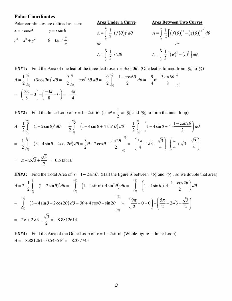
EX#5 : Find the Area of the enclosed region between r1 = 2 − 2 cosθ and r2 = 2 cosθ .

2 − 2 cosθ = 2 cosθ when cosθ = 12

which is θ = π3

and θ = 5π3

.

They form two identical enclosures. Find the Area of one enclosure and double it. They meet at θ = π3

in the first enclosure. You have to figure out which equation outlines your encosure. r1 outlines the enclosure

from θ = 0 to θ = π3

and r2 outlines the enclosure from θ = π3

to θ = π2

.

A = 2 ⋅ 12 0

π3

∫ (2 − 2 cosθ)2 dθ + 12 π

3

π2

∫ 2 cosθ( )2 dθ⎡

⎣⎢⎢

⎤

⎦⎥⎥= 0.402180 π

3

5π

3

INTEGRATION TECHNIQUES Integration by Parts

Integration by Parts is done when taking the integral of a product in which the terms have nothing to do with each other.

u dv = uv − v du∫∫

Refer to the Calculus AB Bible for the general technique.If the derivative of one product will eventually reach zero, use the tabular method.

Tabular method :List the term that will reach zero on the left and keep taking the derivative of that term until it reaches zero. List the other term on the right and take the integral for as many times as it takes for the left side to reach zero.

EX : x cos x dx∫x + cos x1 − sin x 0 − cos x

Multiply the terms as shown. The first one on the left multiplies with the second one on the right and the sign is positive, the second term on the left matches with the third one on the right and is negative, and continue on until the last term on the right is matched up, alternating signs as you go.

∴ x cos x dx = x sin x + cos x∫ + C

5

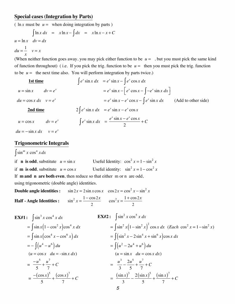
Special cases (Integration by Parts)( ln x must be u = when doing integration by parts )

ln x dx∫ = x ln x − dx∫ = x ln x − x +C

u = ln x dv = dx

du = 1x

v = x

(When neither function goes away, you may pick either function to be u = , but you must pick the same kind of function throughout) ( i.e. If you pick the trig. function to be u = then you must pick the trig. function to be u = the next time also. You will perform integration by parts twice.)

1st time ex sin x dx =∫ ex sin x − ex∫ cos x dx

u = sin x dv = ex = ex sin x − ex cos x − −ex sin x dx∫⎡⎣

⎤⎦

du = cos x dx v = ex = ex sin x − ex cos x − ex sin x∫ dx (Add to other side)

2nd time 2 ex sin x dx =∫ ex sin x − ex cos x

u = cos x dv = ex ex sin x dx =∫ex sin x − ex cos x

2+ C

du = − sin x dx v = ex

Trigonometric Integrals

sinm x cosn x dx∫if n is odd, substitute u = sin x Useful Identity: cos2 x = 1− sin2 x

if m is odd, substitute u = cos x Useful identity: sin2 x = 1− cos2 xIf m and n are both even, then reduce so that either m or n are odd, using trigonometric (double angle) identities.

Double angle identities : sin 2x = 2sin x cos x cos2x = cos2 x − sin2 x

Half - Angle Identities : sin2 x = 1− cos2x2

cos2x = 1+ cos2x2

EX#1 : sin3 x cos4 x dx∫ = sin x 1− cos2 x( )cos4 x dx∫ = sin x cos4 x − cos6 x( ) dx∫ = − u4 − u6( )∫ du

(u = cos x du = -sin x dx)

= −u5

5+u7

7+ C

= − cos x( )5

5+

cos x( )7

7+ C

EX#2 : sin2 x cos5 x dx∫ = sin2 x 1− sin2 x( )2

cos x dx∫ (Each cos2 x = 1− sin2 x)

= sin2 x − 2sin4 x + sin6 x( )cos x dx∫ = u2 − 2u4 + u6( )∫ du

(u = sin x du = cos x dx)

= u3

3−

2u5

5+u7

7+ C

= sin x( )3

3−

2 sin x( )5

5+

sin x( )7

7+ C

6

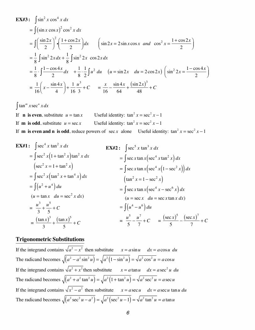
EX#3 : sin2 x cos4 x dx∫ = sin x cos x( )2 cos2 x dx∫

= sin2x2

⎛⎝⎜

⎞⎠⎟

2

∫ i1+ cos2x

2⎛⎝⎜

⎞⎠⎟dx sin2x = 2sin x cos x and cos2 x = 1+ cos2x

2⎛⎝⎜

⎞⎠⎟

= 18

sin2 2x∫ dx + 18

sin2 2x cos2xdx∫ = 1

8⋅

1− cos 4x2∫ dx + 1

8⋅12

u2 du∫ u = sin2x du = 2cos2x( ) sin2 2x = 1− cos 4x2

⎛⎝⎜

⎞⎠⎟

= 116

x − sin 4x4

⎛⎝⎜

⎞⎠⎟+

116

u3

3+ C = x

16−

sin 4x64

+sin 2x( )3

48+ C

tanm x secn x dx∫

If n is even, substitute u = tan x Useful identity: tan2 x = sec2 x −1If m is odd, substitute u = sec x Useful identity: tan2 x = sec2 x −1If m is even and n is odd, reduce powers of sec x alone Useful identity: tan2 x = sec2 x −1

EX#1 : sec4 x tan2 x dx∫ = sec2 x 1+ tan2 x( ) tan2 x dx∫

sec2 x = 1+ tan2 x( ) = sec2 x tan2 x + tan4 x( ) dx∫ = u2 + u4( )∫ du

(u = tan x du = sec2 x dx)

= u3

3+u5

5+ C

= tan x( )3

3+

tan x( )5

5+ C

EX#2 : sec5 x tan3 x dx∫ = sec x tan x sec4 x tan2 x( ) dx∫

= sec x tan x sec4 x 1− sec2 x( )( ) dx∫ tan2 x = 1− sec2 x( ) = sec x tan x sec4 x − sec6 x( ) dx∫

(u = sec x du = sec x tan x dx)

= u4 − u6( )∫ du

= u5

5−u7

7+ C =

sec x( )5

5−

sec x( )7

7+ C

Trigonometric Substitutions

If the integrand contains a2 − x2 then substitute x = asinu dx = acosu du

The radicand becomes a2 − a2 sin2 u( ) = a2 1− sin2 u( ) = a2 cos2 u = acosu

If the integrand contains a2 + x2 then substitute x = a tanu dx = asec2 u du

The radicand becomes a2 + a2 tan2 u( ) = a2 1+ tan2 u( ) = a2 sec2 u = asecu

If the integrand contains x2 − a2 then substitute x = asecu dx = asecu tanu du

The radicand becomes a2 sec2 u − a2( ) = a2 sec2 u −1( ) = a2 tan2 u = a tanu

7

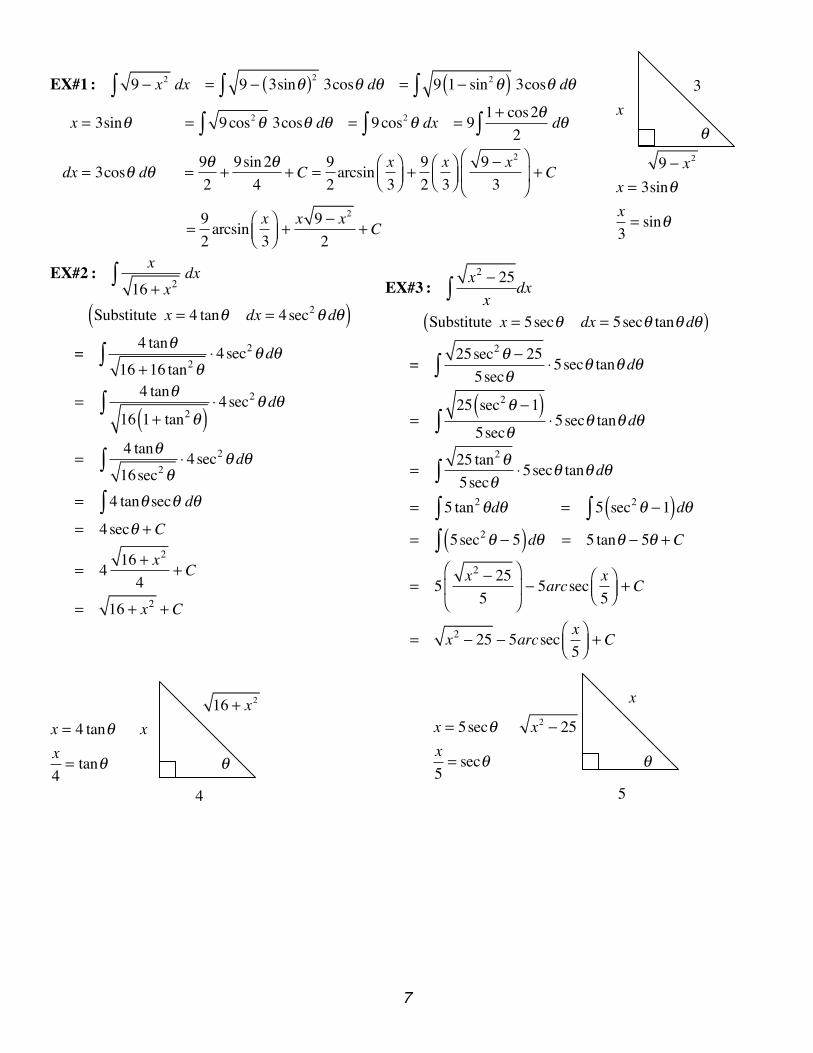
EX#1 : 9 − x2∫ dx = 9 − 3sinθ( )2∫ 3cosθ dθ = 9 1− sin2θ( )∫ 3cosθ dθ

x = 3sinθ = 9cos2θ∫ 3cosθ dθ = 9cos2θ dx∫ = 9 1+ cos2θ2∫ dθ

dx = 3cosθ dθ = 9θ2

+9sin2θ

4+ C =

92

arcsin x3

⎛⎝⎜

⎞⎠⎟+

92

x3

⎛⎝⎜

⎞⎠⎟

9 − x2

3

⎛

⎝⎜

⎞

⎠⎟ + C

= 92

arcsin x3

⎛⎝⎜

⎞⎠⎟+x 9 − x2

2+ C

3x θ

9 − x2

x = 3sinθ x3= sinθ

EX#2 : x

16 + x2∫ dx

Substitute x = 4 tanθ dx = 4sec2θ dθ( ) = 4 tanθ

16 +16 tan2θ∫ ⋅ 4sec2θ dθ

= 4 tanθ

16 1+ tan2θ( )∫ ⋅ 4sec2θ dθ

= 4 tanθ16sec2θ

∫ ⋅ 4sec2θ dθ

= 4 tanθ secθ dθ∫ = 4secθ + C

= 4 16 + x2

4+ C

= 16 + x2 + C

EX#3 : x2 − 25x∫ dx

Substitute x = 5secθ dx = 5secθ tanθ dθ( )

= 25sec2θ − 255secθ∫ ⋅5secθ tanθ dθ

=25 sec2θ −1( )

5secθ∫ ⋅5secθ tanθ dθ

= 25 tan2θ5secθ∫ ⋅5secθ tanθ dθ

= 5 tan2θdθ∫ = 5 sec2θ −1( )dθ∫ = 5sec2θ − 5( )dθ ∫ = 5 tanθ − 5θ + C

= 5 x2 − 255

⎛

⎝⎜

⎞

⎠⎟ − 5arcsec x

5⎛⎝⎜

⎞⎠⎟+ C

= x2 − 25 − 5arcsec x5

⎛⎝⎜

⎞⎠⎟+ C

16 + x2

x = 4 tanθ xx4= tanθ θ

4

x

x = 5secθ x2 − 25x5= secθ θ

5

8

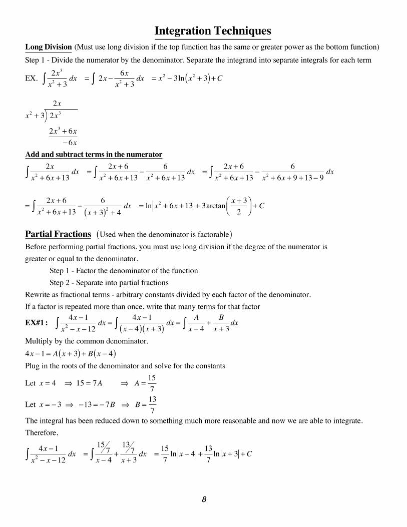
Integration TechniquesLong Division (Must use long division if the top function has the same or greater power as the bottom function)Step 1 - Divide the numerator by the denominator. Separate the integrand into separate integrals for each term

EX. 2x3

x2 + 3dx∫ = 2x − 6x

x2 + 3dx∫ = x2 − 3ln x2 + 3( ) +C

x2 + 3 2x3

2x

2x3 + 6x −6x

Add and subtract terms in the numerator2x

x2 + 6x +13∫ dx =2x + 6

x2 + 6x +13∫ −6

x2 + 6x +13dx =

2x + 6x2 + 6x +13∫ −

6x2 + 6x + 9 +13− 9

dx

=2x + 6

x2 + 6x +13∫ −6

x + 3( )2 + 4dx = ln x2 + 6x +13 + 3arctan x + 3

2⎛⎝⎜

⎞⎠⎟+ C

Partial Fractions Used when the denominator is factorable( ) Before performing partial fractions, you must use long division if the degree of the numerator is greater or equal to the denominator.

Step 1 - Factor the denominator of the functionStep 2 - Separate into partial fractions

Rewrite as fractional terms - arbitrary constants divided by each factor of the denominator. If a factor is repeated more than once, write that many terms for that factor

EX#1 : 4x −1x2 − x −12

dx∫ =4x −1

x − 4( ) x + 3( )∫ dx = Ax − 4∫ +

Bx + 3

dx

Multiply by the common denominator. 4x −1 = A x + 3( ) + B x − 4( ) Plug in the roots of the denominator and solve for the constants

Let x = 4 ⇒ 15 = 7A ⇒ A =157

Let x = − 3 ⇒ −13 = − 7B ⇒ B =137

The integral has been reduced down to something much more reasonable and now we are able to integrate. Therefore,

4x −1x2 − x −12

dx∫ =15

7x − 4∫ +

137

x + 3dx =

157

ln x − 4 +137

ln x + 3 + C

9

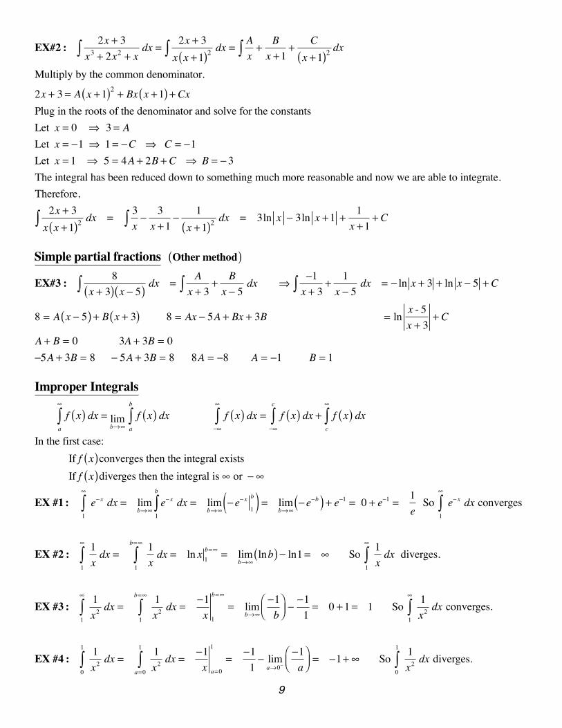
EX#2 : 2x + 3x3 + 2x2 + x

dx∫ =2x + 3x x +1( )2∫ dx = A

x∫ +Bx +1

+C

x +1( )2 dx

Multiply by the common denominator.

2x + 3 = A x +1( )2 + Bx x +1( ) + Cx Plug in the roots of the denominator and solve for the constants Let x = 0 ⇒ 3 = A Let x = −1 ⇒ 1 = −C ⇒ C = −1Let x = 1 ⇒ 5 = 4A + 2B + C ⇒ B = − 3The integral has been reduced down to something much more reasonable and now we are able to integrate. Therefore,

2x + 3x x +1( )2∫ dx =

3x−

3x +1

−1

x +1( )2∫ dx = 3ln x − 3ln x +1 +1

x +1+ C

Simple partial fractions Other method( )

EX#3 : 8x + 3( ) x − 5( ) dx∫ =

Ax + 3∫ +

Bx − 5

dx ⇒−1x + 3∫ +

1x − 5

dx = − ln x + 3 + ln x − 5 + C

8 = A x − 5( ) + B x + 3( ) 8 = Ax − 5A + Bx + 3B = ln x - 5x + 3

+ C

A + B = 0 3A + 3B = 0 −5A + 3B = 8 − 5A + 3B = 8 8A = −8 A = −1 B = 1

Improper Integrals

f x( ) dx =b→∞lim

a

∞

∫ f x( ) dxa

b

∫ f x( ) dx = f x( ) dx + f x( )c

∞

∫−∞

c

∫−∞

∞

∫ dx

In the first case:If f x( )converges then the integral existsIf f x( )diverges then the integral is ∞ or − ∞

EX #1 : e− x dx1

∞

∫ = limb→∞

e− x dx1

b

∫ = limb→∞

− e− x1

b( ) = limb→∞

− e−b( ) + e−1 = 0 + e−1 =1e

So e− x dx 1

∞

∫ converges

EX #2 : 1xdx

1

∞

∫ =1xdx

1

b=∞

∫ = ln x 1b=∞ = lim

b→∞lnb( ) − ln1 = ∞ So 1

xdx

1

∞

∫ diverges.

EX #3 : 1x2 dx

1

∞

∫ =1x2 dx

1

b=∞

∫ =−1 x 1

b=∞

= limb→∞

−1 b

⎛⎝⎜

⎞⎠⎟−−1 1

= 0 +1 = 1 So 1x2 dx

1

∞

∫ converges.

EX #4 : 1x2 dx

0

1

∫ =1x2 dx

a=0

1

∫ =−1 x a=0

1

=−1 1

− lima→0−

−1 a

⎛⎝⎜

⎞⎠⎟= −1+ ∞ So 1

x2 dx0

1

∫ diverges.

10

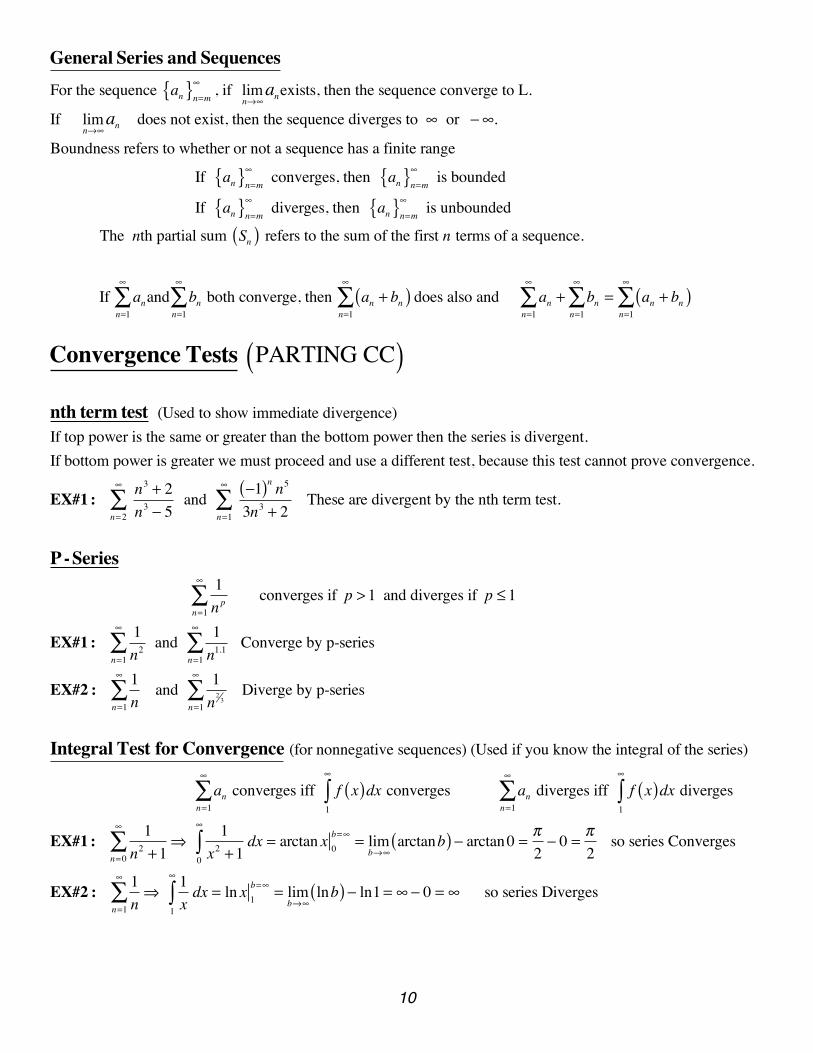
General Series and SequencesFor the sequence an{ }n=m

∞ , if limn→∞

anexists, then the sequence converge to L.

If limn→∞

an does not exist, then the sequence diverges to ∞ or − ∞.

Boundness refers to whether or not a sequence has a finite range

If an{ }n=m∞ converges, then an{ }n=m

∞ is bounded

If an{ }n=m∞ diverges, then an{ }n=m

∞ is unbounded

The nth partial sum Sn( ) refers to the sum of the first n terms of a sequence.

If ann=1

∞

∑ and bnn=1

∞

∑ both converge, then an + bn( )n=1

∞

∑ does also and ann=1

∞

∑ + bnn=1

∞

∑ = an + bn( )n=1

∞

∑

Convergence Tests PARTING CC( )nth term test (Used to show immediate divergence)If top power is the same or greater than the bottom power then the series is divergent.If bottom power is greater we must proceed and use a different test, because this test cannot prove convergence.

EX#1 : n3 + 2n3 − 5

n=2

∞

∑ and −1( )n n5

3n3 + 2

n=1

∞

∑ These are divergent by the nth term test.

P -Series

1np

n=1

∞

∑ converges if p > 1 and diverges if p ≤ 1

EX#1 : 1n2

n=1

∞

∑ and 1n1.1

n=1

∞

∑ Converge by p-series

EX#2 : 1n

n=1

∞

∑ and 1n2

3

n=1

∞

∑ Diverge by p-series

Integral Test for Convergence (for nonnegative sequences) (Used if you know the integral of the series)

an n=1

∞

∑ converges iff f x( )dx1

∞

∫ converges an n=1

∞

∑ diverges iff f x( )dx1

∞

∫ diverges

EX#1 : 1n2 +1n=0

∞

∑ ⇒ 1x2 +10

∞

∫ dx = arctan x 0b=∞ = lim

b→∞arctanb( ) − arctan 0 =

π2− 0 =

π2

so series Converges

EX#2 : 1nn=1

∞

∑ ⇒ 1x1

∞

∫ dx = ln x 1b=∞ = lim

b→∞lnb( ) − ln1 = ∞ − 0 = ∞ so series Diverges

11

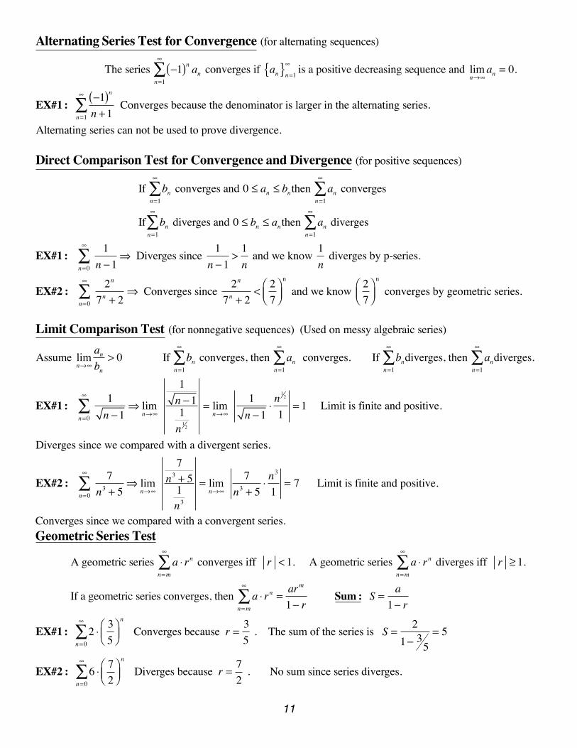
Alternating Series Test for Convergence (for alternating sequences)

The series −1( )n ann=1

∞

∑ converges if an{ }n=1

∞ is a positive decreasing sequence and limn→∞

an = 0.

EX#1 : −1( )nn +1n=1

∞

∑ Converges because the denominator is larger in the alternating series.

Alternating series can not be used to prove divergence.

Direct Comparison Test for Convergence and Divergence (for positive sequences)

If bnn=1

∞

∑ converges and 0 ≤ an ≤ bnthen ann=1

∞

∑ converges

If bnn=1

∞

∑ diverges and 0 ≤ bn ≤ anthen an n=1

∞

∑ diverges

EX#1 : 1n −1n=0

∞

∑ ⇒ Diverges since 1n −1

>1n

and we know 1n

diverges by p-series.

EX#2 : 2n

7n + 2n=0

∞

∑ ⇒ Converges since 2n

7n + 2<

27

⎛⎝⎜

⎞⎠⎟

n

and we know 27

⎛⎝⎜

⎞⎠⎟

n

converges by geometric series.

Limit Comparison Test (for nonnegative sequences) (Used on messy algebraic series)

Assume limn→∞

anbn

> 0 If bnn=1

∞

∑ converges, then ann=1

∞

∑ converges. If bnn=1

∞

∑ diverges, then ann=1

∞

∑ diverges.

EX#1 : 1n −1n=0

∞

∑ ⇒ limn→∞

1n −11n 1

2

= limn→∞

1n −1

⋅n 1

2

1= 1 Limit is finite and positive.

Diverges since we compared with a divergent series.

EX#2 : 7n3 + 5n=0

∞

∑ ⇒ limn→∞

7n3 + 5

1n3

= limn→∞

7n3 + 5

⋅n3

1= 7 Limit is finite and positive.

Converges since we compared with a convergent series.

Geometric Series Test

A geometric series a ⋅ rnn=m

∞

∑ converges iff r < 1. A geometric series a ⋅ rnn=m

∞

∑ diverges iff r ≥ 1.

If a geometric series converges, then a ⋅ rn = arm

1− rn=m

∞

∑ Sum : S = a1− r

EX#1 : 2 ⋅ 35

⎛⎝⎜

⎞⎠⎟n

n=0

∞

∑ Converges because r = 35

. The sum of the series is S = 21− 3

5= 5

EX#2 : 6 ⋅ 72

⎛⎝⎜

⎞⎠⎟n

n=0

∞

∑ Diverges because r = 72

. No sum since series diverges.

12

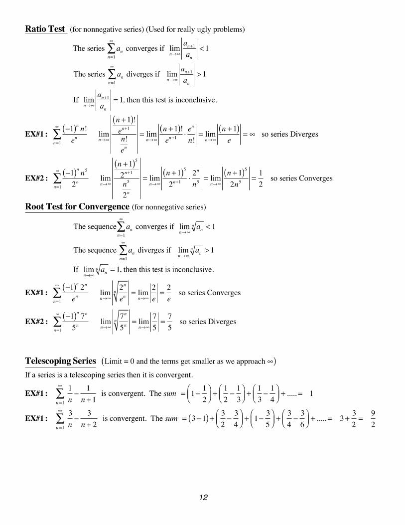
Ratio Test (for nonnegative series) (Used for really ugly problems)

The series ann=1

∞

∑ converges if limn→∞

an+1

an< 1

The series ann=1

∞

∑ diverges if limn→∞

an+1

an> 1

If limn→∞

an+1

an= 1, then this test is inconclusive.

EX#1 : −1( )n n!enn=1

∞

∑ limn→∞

n +1( )!en+1

n!en

= limn→∞

n +1( )!en+1 ⋅

en

n!= lim

n→∞

n +1( )e

= ∞ so series Diverges

EX#2 : −1( )n n5

2nn=1

∞

∑ limn→∞

n +1( )5

2n+1

n5

2n

= limn→∞

n +1( )5

2n+1 ⋅2n

n5 = limn→∞

n +1( )5

2n5 =12

so series Converges

Root Test for Convergence (for nonnegative series)

The sequence ann=1

∞

∑ converges if limn→∞

ann < 1

The sequence ann=1

∞

∑ diverges if limn→∞

ann > 1

If limn→∞

ann = 1, then this test is inconclusive.

EX#1 : −1( )n 2n

enn=1

∞

∑ limn→∞

2n

enn = lim

n→∞

2e=

2e

so series Converges

EX#2 : −1( )n 7n

5nn=1

∞

∑ limn→∞

7n

5nn = lim

n→∞

75

=75

so series Diverges

Telescoping Series Limit = 0 and the terms get smaller as we approach ∞( )If a series is a telescoping series then it is convergent.

EX#1 : 1nn=1

∞

∑ −1

n +1 is convergent. The sum = 1− 1

2⎛⎝⎜

⎞⎠⎟+

12−

13

⎛⎝⎜

⎞⎠⎟+

13−

14

⎛⎝⎜

⎞⎠⎟+ ..... = 1

EX#1 : 3nn=1

∞

∑ −3

n + 2 is convergent. The sum = 3−1( ) + 3

2−

34

⎛⎝⎜

⎞⎠⎟+ 1− 3

5⎛⎝⎜

⎞⎠⎟+

34−

36

⎛⎝⎜

⎞⎠⎟+ ..... = 3+ 3

2=

92

13

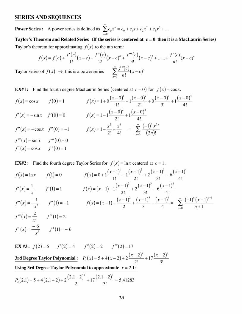
SERIES AND SEQUENCES

Power Series : A power series is defined as caxn = c0 + c1x + c2x

2 + c3x3 + ...

n=0

∞

∑Taylor’s Theorem and Related Series (If the series is centered at c = 0 then it is a MacLaurin Series)Taylor’s theorem for approximating f x( ) to the nth term:

f x( ) = f c( ) + ′f c( )1!

x − c( ) + ′′f c( )2!

x − c( )2 +′′′f c( )3!

x − c( )3 + ......+ f n (c)n!

(x − c)n

Taylor series of f x( ) → this is a power series f n c( )n!n=0

∞

∑ x − c( )n

EX#1 : Find the fourth degree MacLaurin Series centered at c = 0( ) for f x( ) = cos x.

f x( ) = cos x f 0( ) = 1 f x( ) = 1+ 0x − 0( )1

1!−1

x − 0( )2

2!+ 0

x − 0( )3

3!+1

x − 0( )4

4!

′f x( ) = − sin x ′f 0( ) = 0 f x( ) = 1−1x − 0( )2

2!+1

x − 0( )4

4!

′′f x( ) = − cos x ′′f 0( ) = −1 f x( ) = 1− x2

2!+x4

4! =

−1( )n x2n

2n( )!n=0

∞

∑′′′f x( ) = sin x ′′′f 0( ) = 0f 4 x( ) = cos x f 4 0( ) = 1

EX#2 : Find the fourth degree Taylor Series for f x( ) = ln x centered at c = 1.

f x( ) = ln x f 1( ) = 0 f x( ) = 0 +1x −1( )1

1!−1

x −1( )2

2!+ 2

x −1( )3

3!− 6

x −1( )4

4!

′f x( ) = 1x

′f 1( ) = 1 f x( ) = x −1( ) −1x −1( )2

2!+ 2

x −1( )3

3!− 6

x −1( )4

4!

′′f x( ) = −1 x2 ′′f 1( ) = −1 f x( ) = x −1( ) − x −1( )2

2+

x −1( )3

3−

x −1( )4

4=

−1( )n x −1( )n+1

n +1n=0

∞

∑

′′′f x( ) = 2x3 ′′′f 1( ) = 2

f 4 x( ) = − 6 x4 f 4 1( ) = − 6

EX #3 : f 2( ) = 5 ′f 2( ) = 4 ′′f 2( ) = 2 ′′′f 2( ) = 17

3rd Degree Taylor Polynomial : P3 x( ) = 5 + 4 x − 2( ) + 2x − 2( )2

2!+17

x − 2( )3

3!Using 3rd Degree Taylor Polynomial to approximate x = 2.1 :

P3 2.1( ) = 5 + 4 2.1− 2( ) + 22.1− 2( )2

2!+17

2.1− 2( )3

3!= 5.41283

14

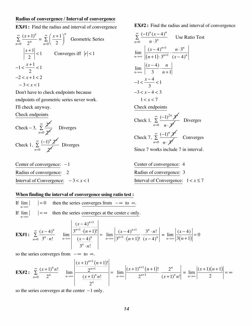
Radius of convergence / Interval of convergenceEX#1 : Find the radius and interval of convergence

(x +1)n

2nn=0

∞∑ = x +1

2⎛⎝⎜

⎞⎠⎟n

n=0

∞∑ Geometric Series

x +12

< 1 Converges iff r < 1

−1< x +12

< 1

−2 < x +1< 2 − 3 < x < 1 Don't have to check endpoints because endpoints of geometric series never work.I'll check anyway.Check endpoints

Check − 3, 2n

2nn=0

∞∑ Diverges

Check 1, (−1)n 2n

2nn=0

∞∑ Diverges

Center of convergence: −1Radius of convergence: 2 Interval of Convergence: − 3 < x < 1

EX#2 : Find the radius and interval of convergence

(−1)n (x − 4)n

n ⋅3nn=0

∞∑ Use Ratio Test

limn→∞

(x − 4)n+1

n +1( ) ⋅3n+1 ⋅n ⋅3n

(x − 4)n

limn→∞

(x − 4)3

⋅ nn +1

−1< x − 43

< 1

−3 < x − 4 < 3 1< x < 7 Check endpoints

Check 1, (−1)2n 3n

n ⋅ 3nn=0

∞∑ Diverges

Check 7, (−1)n 3n

n ⋅ 3nn=0

∞∑ Converges

Since 7 works include 7 in interval.

Center of convergence: 4Radius of convergence: 3 Interval of Convergence: 1< x ≤ 7

When finding the interval of convergence using ratio test :If lim

n→∞ = 0 then the series converges from − ∞ to ∞.

If limn→∞

= ∞ then the series converges at the center c only.

EX#1 : (x − 4)n

3n ⋅n!n=0

∞∑ lim

n→∞

(x − 4)n+1

3n+1 ⋅ n +1( )!(x − 4)n

3n ⋅n!

= limn→∞

(x − 4)n+1

3n+1 ⋅ n +1( )!⋅ 3n ⋅n!(x − 4)n

= limn→∞

(x − 4)3 n +1( ) = 0

so the series converges from − ∞ to ∞.

EX#2 : (x +1)n n!2nn=0

∞∑ lim

n→∞

(x +1)n+1 n +1( )!2n+1

(x +1)n n!2n

= limn→∞

(x +1)n+1 n +1( )!2n+1 ⋅ 2n

(x +1)n n! = lim

n→∞

(x +1) n +1( )2

= ∞

so the series converges at the center −1 only.

15

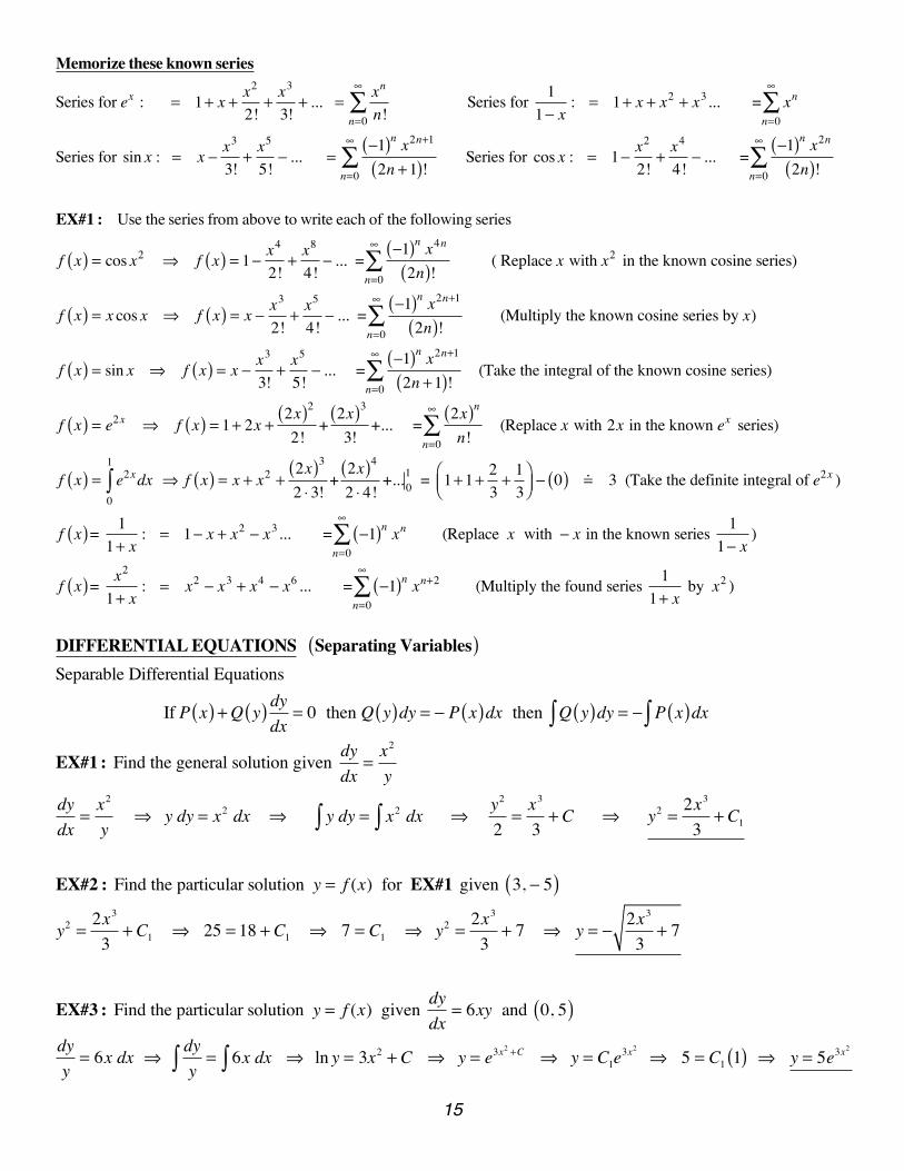
Memorize these known series

Series for ex : = 1+ x + x2

2!+ x3

3!+ ... = xn

n!n=0

∞

∑ Series for 11− x

: = 1+ x + x2 + x3... = xnn=0

∞

∑

Series for sin x : = x − x3

3!+ x5

5!− ... =

−1( )n x2n+1

2n +1( )!n=0

∞

∑ Series for cos x : = 1− x2

2!+ x4

4!− ... =

−1( )n x2n

2n( )!n=0

∞

∑

EX#1 : Use the series from above to write each of the following series

f x( ) = cos x2 ⇒ f x( ) = 1− x4

2!+ x8

4!− ... =

−1( )n x4n

2n( )!n=0

∞

∑ ( Replace x with x2 in the known cosine series)

f x( ) = x cos x ⇒ f x( ) = x − x3

2!+ x5

4!− ... =

−1( )n x2n+1

2n( )!n=0

∞

∑ (Multiply the known cosine series by x)

f x( ) = sin x ⇒ f x( ) = x − x3

3!+ x5

5!− ... =

−1( )n x2n+1

2n +1( )!n=0

∞

∑ (Take the integral of the known cosine series)

f x( ) = e2x ⇒ f x( ) = 1+ 2x +2x( )22!

+2x( )3

3!+... =

2x( )nn!n=0

∞

∑ (Replace x with 2x in the known ex series)

f x( ) = e2x

0

1

∫ dx ⇒ f x( ) = x + x2 +2x( )3

2 ⋅ 3!+

2x( )4

2 ⋅ 4!+... 0

1 = 1+1+ 23+ 1

3⎛⎝⎜

⎞⎠⎟ − 0( ) 3 (Take the definite integral of e2x )

f x( )= 11+ x

: = 1− x + x2 − x3... = −1( )n xn n=0

∞

∑ (Replace x with − x in the known series 11− x

)

f x( )= x2

1+ x: = x2 − x3 + x4 − x6 ... = −1( )n xn+2

n=0

∞

∑ (Multiply the found series 11+ x

by x2 )

DIFFERENTIAL EQUATIONS Separating Variables( )Separable Differential Equations

If P x( ) +Q y( ) dydx

= 0 then Q y( )dy = − P x( )dx then Q y( )dy = − P x( )dx∫∫

EX#1 : Find the general solution given dydx

=x2

ydydx

=x2

y ⇒ y dy = x2 dx ⇒ y dy∫ = x2 dx∫ ⇒ y

2

2=x3

3+ C ⇒ y2 =

2x3

3+ C1

EX#2 : Find the particular solution y = f (x) for EX#1 given 3, − 5( )

y2 =2x3

3+ C1 ⇒ 25 = 18 + C1 ⇒ 7 = C1 ⇒ y2 =

2x3

3+ 7 ⇒ y = −

2x3

3+ 7

EX#3 : Find the particular solution y = f (x) given dydx

= 6xy and 0, 5( )

dyy= 6x dx ⇒ dy

y∫ = 6x dx∫ ⇒ ln y = 3x2 + C ⇒ y = e3x2 +C ⇒ y = C1e3x2

⇒ 5 = C1 1( ) ⇒ y = 5e3x2

16

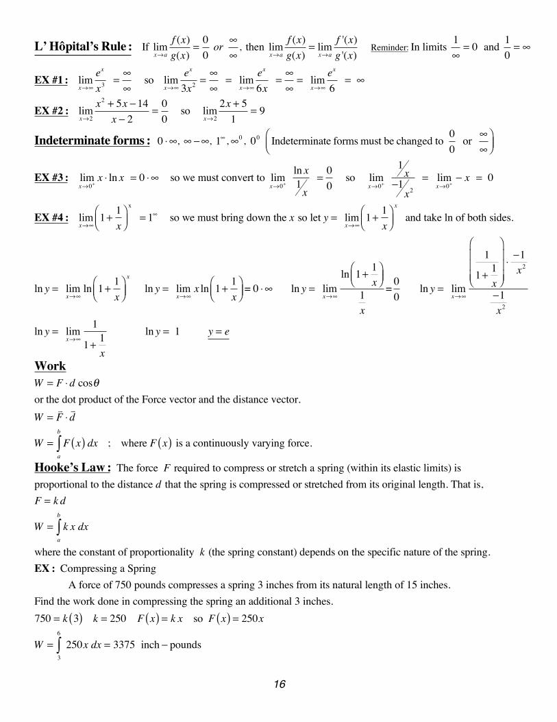
L’ Hôpital’s Rule : If limx→a

f (x)g(x)

=00

or ∞∞

, then limx→a

f (x)g(x)

= limx→a

f '(x)g '(x)

Reminder: In limits 1∞

= 0 and 10= ∞

EX #1 : limx→∞

ex

x3 = ∞∞

so limx→∞

ex

3x2 =∞∞

= limx→∞

ex

6x = ∞

∞= lim

x→∞

ex

6 = ∞

EX #2 : limx→2

x2 + 5x −14x − 2

=00

so limx→2

2x + 51

= 9

Indeterminate forms : 0 ⋅ ∞, ∞ −∞, 1∞ , ∞0 , 00 Indeterminate forms must be changed to 00

or ∞∞

⎛⎝⎜

⎞⎠⎟

EX #3 : limx→0+

x ⋅ ln x = 0 ⋅ ∞ so we must convert to limx→0+

ln x1x

= 00

so limx→0+

1x

−1x2

= limx→0+

− x = 0

EX #4 : limx→∞

1+ 1x

⎛⎝⎜

⎞⎠⎟

x

= 1∞ so we must bring down the x so let y = limx→∞

1+ 1x

⎛⎝⎜

⎞⎠⎟x

and take ln of both sides.

ln y = limx→∞

ln 1+ 1x

⎛⎝⎜

⎞⎠⎟x

ln y = limx→∞

x ln 1+ 1x

⎛⎝⎜

⎞⎠⎟

= 0 ⋅ ∞ ln y = limx→∞

ln 1+ 1x

⎛⎝⎜

⎞⎠⎟

1x

= 00

ln y = limx→∞

1

1+ 1x

⎛

⎝

⎜⎜⎜

⎞

⎠

⎟⎟⎟⋅ −1 x2

−1 x2

ln y = limx→∞

1

1+ 1x

ln y = 1 y = e

WorkW = F ⋅d cosθor the dot product of the Force vector and the distance vector.W =

F ⋅d

W = F x( )a

b

∫ dx ; where F x( ) is a continuously varying force.

Hooke’s Law : The force F required to compress or stretch a spring (within its elastic limits) is proportional to the distance d that the spring is compressed or stretched from its original length. That is, F = k d

W = k x dxa

b

∫where the constant of proportionality k (the spring constant) depends on the specific nature of the spring. EX : Compressing a Spring

A force of 750 pounds compresses a spring 3 inches from its natural length of 15 inches. Find the work done in compressing the spring an additional 3 inches. 750 = k 3( ) k = 250 F x( ) = k x so F x( ) = 250x

W = 250x dx3

6

∫ = 3375 inch − pounds

17

Logistical Growth Exponential Growthdydt

= ky 1− yL

⎛⎝⎜

⎞⎠⎟ ; y = L

1+ be− k t; b = L −Y0

Y0

dydt

= ky ; y = Cekt

k = constant of proportionality k = growth constantL = carrying capacity C = initial amountY0 = initial amount

Logistic Growth dydt

= ky(1− yL

)

where L is the carrying capacity (upper bound) and k is the constant of proportionality. If you solve the differential equation using very tricky separation of variables, you get the general solution:

y = L1+ be−kt

; b = L −Y0

Y0

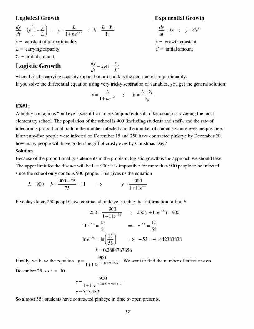
EX#1 :A highly contagious “pinkeye” (scientific name: Conjunctivitus itchlikecrazius) is ravaging the localelementary school. The population of the school is 900 (including students and staff), and the rate of infection is proportional both to the number infected and the number of students whose eyes are pus-free. If seventy-five people were infected on December 15 and 250 have contracted pinkeye by December 20, how many people will have gotten the gift of crusty eyes by Christmas Day?SolutionBecause of the proportionality statements in the problem, logistic growth is the approach we should take. The upper limit for the disease will be L = 900; it is impossible for more than 900 people to be infected since the school only contains 900 people. This gives us the equation

L = 900 b = 900 − 7575

= 11 ⇒ y = 9001+11e−kt

Five days later, 250 people have contracted pinkeye, so plug that information to find k:

250 = 9001+11e− k⋅5

⇒ 250(1+11e− 5k ) = 900

11e− 5k = 135

⇒ e− 5k = 1355

lne− 5k = ln 1355

⎛⎝⎜

⎞⎠⎟ ⇒ − 5k = −1.442383838

k = 0.2884767656

Finally, we have the equation y = 9001+11e− 0.2884767656t . We want to find the number of infections on

December 25, so t = 10.

y = 9001+11e− (0.2884767656)(10)

y ≈ 557.432 So almost 558 students have contracted pinkeye in time to open presents.

18

Euler’s MethodUses tangent lines to approximate points on the curve.

New y = Old y + dx ⋅ dydx

dx : change in x dydx

= Derivative (slope) at the point.

EX#1 :

Given: f (0) = 3 dydx

= xy2

Use step of h = 0.1 to find f (0.3)

Original (0, 3)

New y = 3+ (0.1)(0) = 3 f 0.1( ) 3 At (0, 3) dydx

= 0 ⋅32

= 0

New y = 3+ (0.1)(0.15) = 3.015 f 0.2( ) 3.015 At (0.1, 3) dydx

= 0.1⋅32

= 0.15

New y = 3.015 + (0.1)(0.3015) = 3.04515 f 0.3( ) 3.04515 At (0.2, 3.015) dydx

=0.2 ⋅3.015

2= 0.3015

Slope Fields

Draw the slope field for dydx

= xy

Plug each point into dydx

and graph the tangent line at the point

At 1, 1( ) dydx

= 1. At −1, 1( ) dydx

= −1. At 0, 1( ) dydx

= 0

• • •

• • •

−1• 0• 1•

• • •

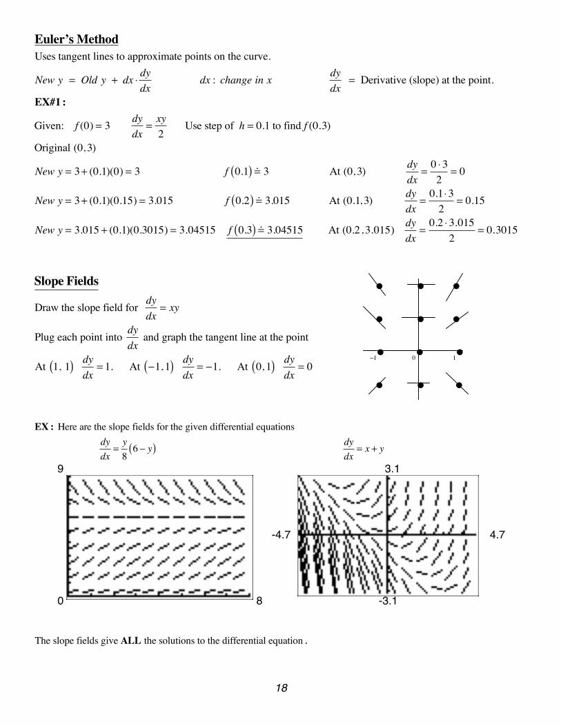
EX : Here are the slope fields for the given differential equations

dydx

=y8

6 − y( ) dydx

= x + y

9 3.1

-4.7 4.7 0 8 -3.1 The slope fields give ALL the solutions to the differential equation .

19

Lagrange Error Bound

Error = f x( )− Pn x( ) ≤ Rn x( ) where Rn x( ) ≤ f n+1 z( ) x − c( )n+1

n +1( )!

f n+1 z( ) = the maximum of the n +1( ) th derivative of the function

EX #1 : cos x = 1− x2

2!+x4

4!− .... cos 0.1( ) 0.99500416667

R4 x( ) = f 5 z( ) x − c( )55!

f 5 z( ) = − sin z We need − sin z to be as large as possible (which is 1 because −1≤ sin z ≤1)

R4 0.1( ) < 1⋅ 0.1( )55!

= 0.0000000833

EX #2 : f 1( ) = 2 ′f 1( ) = 5 ′′f 1( ) = 7 ′′′f 1( ) = 12

2nd Degree Taylor Polynomial : P2 x( ) = 2 + 5 x −1( ) + 7 x −1( )2

Using 2nd Degree Taylor Polynomial to approximate x = 1.1: P2 1.1( ) = 2 + 51.1−1( )1

1!+ 7

1.1−1( )22!

= 2.535

Lagrange Error Bound : R3 x( ) = f 3 z( ) x − c( )3

3!=

12 1.1−1( )3

3!= 0.002 = Error

Area as a limit

Area = limn→∞

f a + b − an

i⎛⎝⎜

⎞⎠⎟i=1

n

∑ b − an

⎛⎝⎜

⎞⎠⎟

i = interval

height width

Summation formulas and properties

1) c = cni

n

∑ 2) i =n n +1( )

2i

n

∑ 3) i2 =n n +1( ) 2n +1( )

6i

n

∑

4) i3 =n2 n +1( )2

4i

n

∑ 5) ai ± bi( )i

n

∑ = ai ± bii

n

∑i

n

∑ 6) k ⋅ai = k aii=1

n

∑i

n

∑ , k is a constant

EX#1: f x( ) = x3 0, 1[ ] n subdivisions Find Area under curve.

Area = limn→∞

f 0 + 1− 0n

i⎛⎝⎜

⎞⎠⎟

1− 0n

⎛⎝⎜

⎞⎠⎟i=1

n

∑ = limn→∞

in

⎛⎝⎜

⎞⎠⎟

3

i=1

n

∑ 1n

= limn→∞

1n4 i3

i=1

n

∑ = limn→∞

1n4

n2 n +1( )24

=14

EX#2 : limn→∞

1n

1n+

2n+ .........+ n

n⎡

⎣⎢

⎤

⎦⎥ =

Answer : x0

1

∫ dx (You have to recognize that the problem is asking for Area from 0,1[ ] with n subdivisions)

20

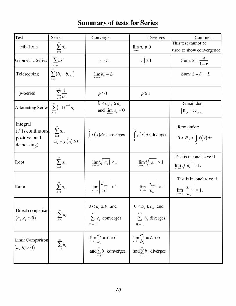
Summary of tests for Series

Test Series Converges Diverges Comment

nth-Term ann=1

∞

∑ limn→∞

an ≠ 0 This test cannot beused to show convergence.

Geometric Series arnn=0

∞

∑ r < 1 r ≥ 1 Sum: S = a1− r

Telescoping bn − bn+1( )n=1

∞

∑ limn→∞

bn = L Sum: S = b1 − L

p-Series 1np

n=1

∞

∑ p > 1 p ≤ 1

Alternating Series −1( ) n−1 ann=1

∞

∑ 0 < an+1 ≤ anand lim

n→∞an = 0

Remainder:RN ≤ aN +1

Integral( f is continuous,positive, anddecreasing)

an

n=1

∞

∑ ,

an = f n( ) ≥ 0 f x( )dx converges

1

∞

∫ f x( )dx diverges1

∞

∫

Remainder:

0 < RN < f x( )dxN

∞

∫

Root ann=1

∞

∑ limn→∞

ann < 1 limn→∞

ann > 1 Test is inconclusive if

limn→∞

ann = 1.

Ratio ann=1

∞

∑ limn→∞

an+1an

< 1 limn→∞

an+1an

> 1

Test is inconclusive if

limn→∞

an+1

an= 1.

Direct comparisonan ,bn > 0( ) an

n=1

∞

∑

0 < an ≤ bn and

bnn = 1

∞∑ converges

0 < bn ≤ an and

bnn = 1

∞∑ diverges

Limit Comparisonan ,bn > 0( ) an

n=1

∞

∑ limn→∞

anbn

= L > 0

and bnn=1

∞

∑ converges

limn→∞

anbn

= L > 0

and bnn=1

∞

∑ diverges

21

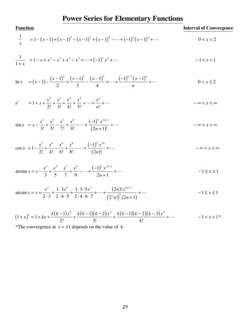
Power Series for Elementary FunctionsFunction Interval of Convergence

1x

= 1− x −1( ) + x −1( )2 − x −1( )3 + x −1( )4 −+ −1( )n x −1( )n + 0 < x < 2

11+ x

= 1− x + x2 − x3 + x4 − x5 ++ −1( )n xn + −1 < x < 1

ln x = x −1( ) − x −1( )2

2+

x −1( )3

3−

x −1( )4

4++

−1( )n−1 x −1( )nn

+ 0 < x ≤ 2

ex = 1+ x + x2

2!+x3

3!+x4

4!+x5

5!++

xn

n!+ − ∞ < x < ∞

sin x = x − x3

3!+x5

5!−x7

7!+x9

9!−+

−1( )n x2n+1

2n +1( )! + − ∞ < x < ∞

cos x = 1− x2

2!+x4

4!−x6

6!+x8

8!−+

−1( )n x2n

2n( )! + − ∞ < x < ∞

arctan x = x − x3

3+x5

5−x7

7+x9

9−+

−1( )n x2n+1

2n +1+ −1 ≤ x ≤ 1

arcsin x = x + x3

2 ⋅ 3+

1 ⋅ 3x5

2 ⋅ 4 ⋅5+

1 ⋅ 3 ⋅5x7

2 ⋅ 4 ⋅6 ⋅ 7++

2n( )!x2n+1

2n n!( )22n +1( )

+ −1 ≤ x ≤ 1

1+ x( )k = 1+ kx +k k −1( )x2

2!+k k −1( ) k − 2( )x3

3!+k k −1( ) k − 2( ) k − 3( )x4

4!+ −1 < x < 1*

*The convergence at x = ±1 depends on the value of k.

22

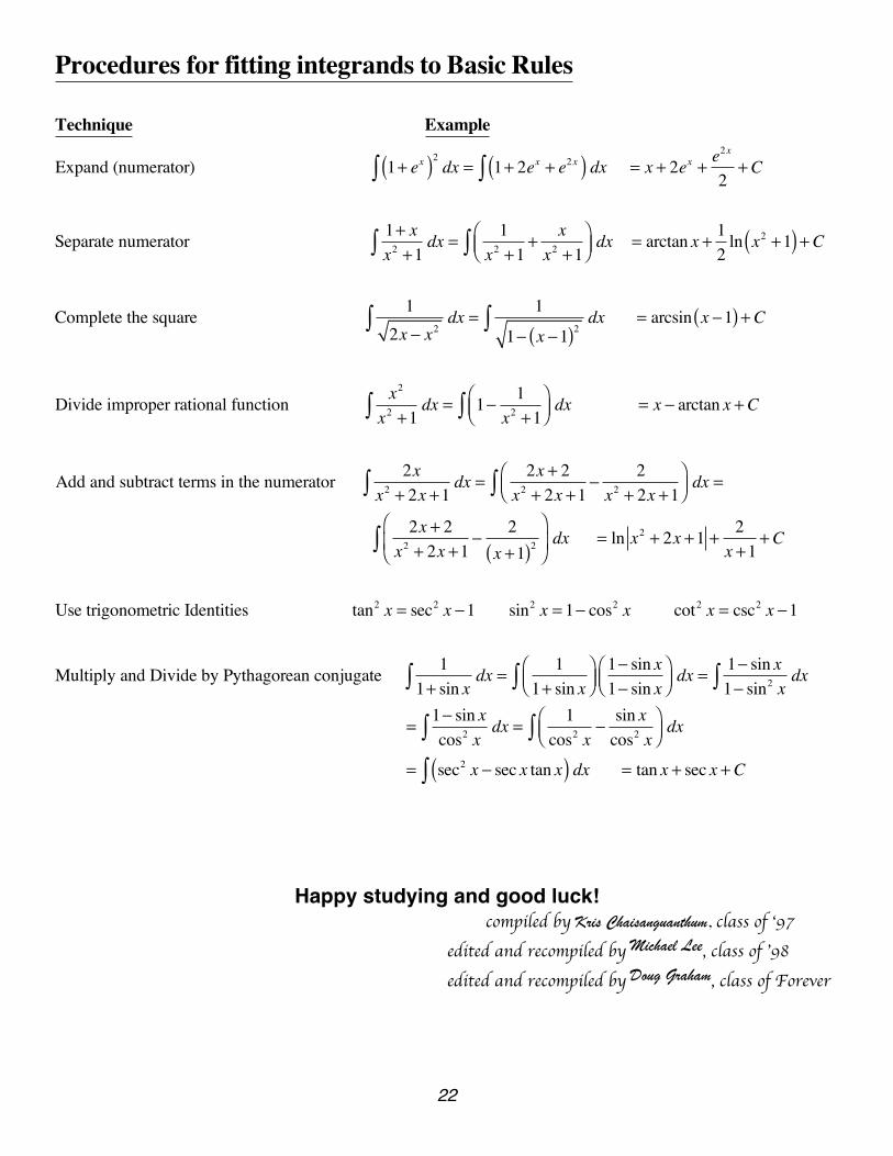
Procedures for fitting integrands to Basic Rules

Technique Example

Expand (numerator) 1+ ex( )2dx∫ = 1+ 2ex + e2x( )∫ dx = x + 2ex + e

2x

2+C

Separate numerator 1+ xx2 +1∫ dx = 1

x2 +1+ xx2 +1

⎛⎝⎜

⎞⎠⎟∫ dx = arctan x + 1

2ln x2 +1( ) +C

Complete the square 12x − x2∫ dx = 1

1− x −1( )2∫ dx = arcsin x −1( ) +C

Divide improper rational function x2

x2 +1∫ dx = 1− 1x2 +1

⎛⎝⎜

⎞⎠⎟∫ dx = x − arctan x +C

Add and subtract terms in the numerator 2xx2 + 2x +1∫ dx = 2x + 2

x2 + 2x +1− 2x2 + 2x +1

⎛⎝⎜

⎞⎠⎟∫ dx =

2x + 2x2 + 2x +1

− 2x +1( )2

⎛

⎝⎜

⎞

⎠⎟∫ dx = ln x2 + 2x +1 + 2

x +1+C

Use trigonometric Identities tan2 x = sec2 x −1 sin2 x = 1− cos2 x cot2 x = csc2 x −1

Multiply and Divide by Pythagorean conjugate 11+ sin x∫ dx = 1

1+ sin x⎛⎝⎜

⎞⎠⎟

1− sin x1− sin x

⎛⎝⎜

⎞⎠⎟∫ dx = 1− sin x

1− sin2 x∫ dx

= 1− sin xcos2 x

dx∫ = 1cos2 x

− sin xcos2 x

⎛⎝⎜

⎞⎠⎟∫ dx

= sec2 x − sec x tan x( ) dx∫ = tan x + sec x +C

Happy studying and good luck! compiled by Kris Chaisanguanthum, class of ‘97

edited and recompiled by Michael Lee, class of ’98 edited and recompiled by Doug Graham, class of Forever

23

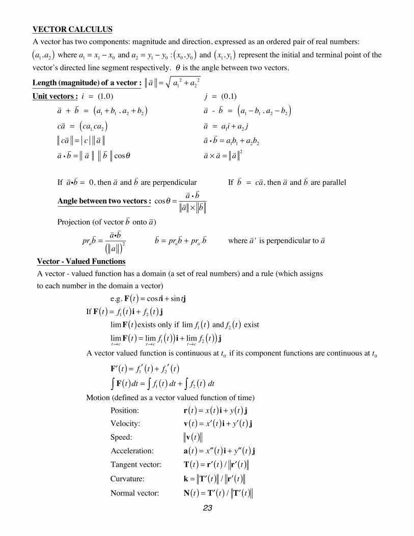
VECTOR CALCULUSA vector has two components: magnitude and direction, expressed as an ordered pair of real numbers: a1,a2( ) where a1 = x1 − x0 and a2 = y1 − y0 : x0 , y0( ) and x1, y1( ) represent the initial and terminal point of the

vector’s directed line segment respectively. θ is the angle between two vectors.

Length (magnitude) of a vector : a = a12 + a2

2

Unit vectors : i = (1,0) j = (0,1)a +

b = a1 + b1 , a2 + b2( ) a -

b = a1 − b1 , a2 − b2( )

ca = ca1,ca2( ) a = a1i + a2 j

ca = c a a •b = a1b1 + a2b2

a •b = a

b cosθ a × a = a 2

If aib = 0, then a and

b are perpendicular If

b = ca, then a and

b are parallel

Angle between two vectors : cosθ =a •b

a ×b

Projection (of vector b onto a)

prab =

aib

a( )2

b = pra

b + pra '

b where a ' is perpendicular to a

Vector - Valued FunctionsA vector - valued function has a domain (a set of real numbers) and a rule (which assigns to each number in the domain a vector)

e.g. F t( ) = cos ti + sin tjIf F t( ) = f1 t( ) i + f2 t( ) j

lim F t( )exists only if lim f1 t( ) and f2 t( ) existlimt→c

F t( ) = limt→c

f1 t )( ) i + limt→c

f2 t )( ) j

A vector valued function is continuous at t0 if its component functions are continuous at t0′F t( ) = f1′ t( ) + f2′ t( )F t( )dt = f1 t( ) dt + f2 t( ) dt∫∫∫

Motion (defined as a vector valued function of time)Position: r t( ) = x t( ) i + y t( ) jVelocity: v t( ) = ′x t( ) i + ′y t( ) jSpeed: v t( )Acceleration: a t( ) = ′′x t( ) i + ′′y t( ) jTangent vector: T t( ) = ′r t( ) / ′r t( )Curvature: k = ′T t( ) / ′r t( )Normal vector: N t( ) = ′T t( ) / ′T t( )

24

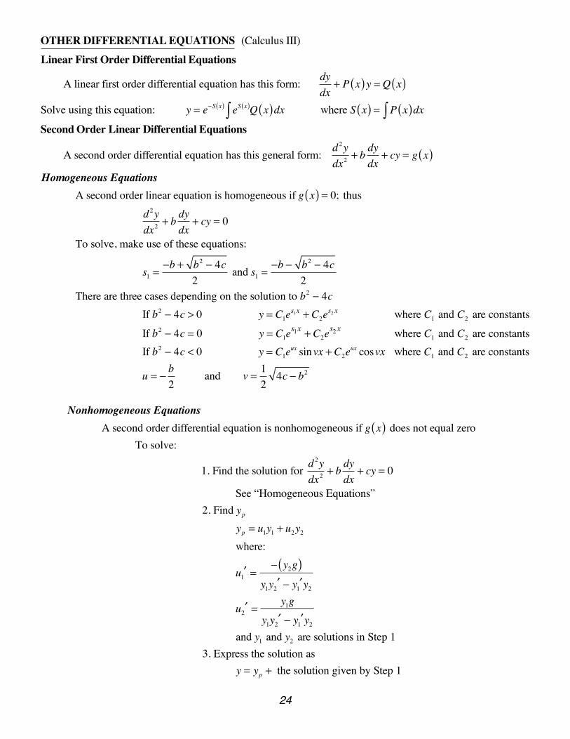
OTHER DIFFERENTIAL EQUATIONS (Calculus III)

Linear First Order Differential Equations

A linear first order differential equation has this form: dydx

+ P x( )y = Q x( )

Solve using this equation: y = e−S x( ) eS x( )Q x( )dx∫ where S x( ) = P x( )dx∫Second Order Linear Differential Equations

A second order differential equation has this general form: d2ydx2 + b dy

dx+ cy = g x( )

Homogeneous EquationsA second order linear equation is homogeneous if g x( ) = 0; thus

d 2ydx2 + b dy

dx+ cy = 0

To solve, make use of these equations:

s1 =−b + b2 − 4c

2 and s1 =

−b − b2 − 4c2

There are three cases depending on the solution to b2 − 4cIf b2 − 4c > 0 y = C1e

s1x + C2es2x where C1 and C2 are constants

If b2 − 4c = 0 y = C1es1x + C2e

s2x where C1 and C2 are constantsIf b2 − 4c < 0 y = C1e

ux sinvx + C2eux cosvx where C1 and C2 are constants

u = −b2

and v = 12

4c − b2

Nonhomogeneous EquationsA second order differential equation is nonhomogeneous if g x( ) does not equal zero

To solve:

1. Find the solution for d2ydx2 + b dy

dx+ cy = 0

See “Homogeneous Equations”2. Find yp

yp = u1y1 + u2y2

where:

u1′ =

− y2g( )y1y2

′ − y1′y2

u2′ =

y1g

y1y2′ − y1

′y2

and y1 and y2 are solutions in Step 13. Express the solution as

y = yp + the solution given by Step 1