Calculus and Differentiation Primer - Dr. Sebastian … · Calculus is a discipline of mathematics that provides us with tools to ana-lyze rates of change, or decay, or motion. Both

SEBASTIAN RASCHKA

Introduction to Artificial Neural Networks and Deep Learning

with Applications in Python

Introduction to ArtificialNeural Networkswith Applications in Python

Sebastian Raschka

DRAFT

Last updated: June 14, 2018

This book will be available at http://leanpub.com/ann-and-deeplearning.

Please visit https://github.com/rasbt/deep-learning-book for moreinformation, supporting material, and code examples.

© 2016-2018 Sebastian Raschka

http://leanpub.com/ann-and-deeplearning

https://github.com/rasbt/deep-learning-book

Contents

D Calculus and Differentiation Primer 4D.1 Intuition . . . . . . . . . . . . . . . . . . . . . . . . . . . . . . 4D.2 Derivatives of Common Functions . . . . . . . . . . . . . . . 8D.3 Common Differentiation Rules . . . . . . . . . . . . . . . . . 9D.4 The Chain Rule – Computing the Derivative of a Composi-

tion of Functions . . . . . . . . . . . . . . . . . . . . . . . . . 10D.4.1 A Chain Rule Example . . . . . . . . . . . . . . . . . . 11

D.5 Arbitrarily Long Function Compositions . . . . . . . . . . . . 13D.6 When a Function is Not Differentiable . . . . . . . . . . . . . 13D.7 Partial Derivatives and Gradients . . . . . . . . . . . . . . . . 18D.8 Second Order Partial Derivatives . . . . . . . . . . . . . . . . 21D.9 The Multivariable Chain Rule . . . . . . . . . . . . . . . . . . 21D.10 The Multivariable Chain Rule in Vector Form . . . . . . . . . 22D.11 The Hessian Matrix . . . . . . . . . . . . . . . . . . . . . . . . 23D.12 The Laplacian Operator . . . . . . . . . . . . . . . . . . . . . 24

i

Website

Please visit the GitHub repository to download the code examples accom-panying this book and other supplementary material.

If you like the content, please consider supporting the work by buy-ing a copy of the book on Leanpub. Also, I would appreciate hearingyour opinion and feedback about the book, and if you have any ques-tions about the contents, please don’t hesitate to get in touch with me [email protected]. Happy learning!

Sebastian Raschka

1

About the Author

Sebastian Raschka received his doctorate from Michigan State Universitydeveloping novel computational methods in the field of computational bi-ology. In summer 2018, he joined the University of Wisconsin–Madisonas Assistant Professor of Statistics. Among others, his research activitiesinclude the development of new deep learning architectures to solve prob-lems in the field of biometrics. Among his other works is his book "PythonMachine Learning," a bestselling title at Packt and on Amazon.com, whichreceived the ACM Best of Computing award in 2016 and was translatedinto many different languages, including German, Korean, Italian, tradi-tional Chinese, simplified Chinese, Russian, Polish, and Japanese.

Sebastian is also an avid open-source contributor and likes to contributeto the scientific Python ecosystem in his free-time. If you like to find moreabout what Sebastian is currently up to or like to get in touch, you can findhis personal website at https://sebastianraschka.com.

2

https://sebastianraschka.com

DRAFT

Acknowledgements

I would like to give my special thanks to the readers, who provided feed-back, caught various typos and errors, and offered suggestions for clarify-ing my writing.

• Appendix A: Artem Sobolev, Ryan Sun

• Appendix B: Brett Miller, Ryan Sun

• Appendix D: Marcel Blattner, Ignacio Campabadal, Ryan Sun, DenisParra Santander

• Appendix F: Guillermo Monecchi, Ged Ridgway, Ryan Sun, PatricHindenberger

• Appendix H: Brett Miller, Ryan Sun, Nicolas Palopoli, Kevin Zakka

3

DRAFT

Appendix D

Calculus and DifferentiationPrimer

Calculus is a discipline of mathematics that provides us with tools to ana-lyze rates of change, or decay, or motion. Both Isaac Newton and GottfriedLeibniz developed the foundations of calculus independently in the 17thcentury. Although we recognize Gottfried and Leibniz as the founding fa-thers of calculus, this field, however, has a very long series of contributors,which dates back to the ancient period and includes Archimedes, Galileo,Plato, Pythagoras, just to name a few [Boyer, 1970].

In this appendix we will only concentrate on the subfield of calculusthat is of most relevance to machine and deep learning: differential calcu-lus. In simple terms, differential calculus is focused on instantaneous ratesof change or computing the slope of a linear function. We will review thebasic concepts of computing the derivatives of functions that take on oneor more parameters. Also, we will refresh the concepts of the chain rule, arule that we use to compute the derivatives of composite functions, whichwe so often deal with in machine learning.

D.1 Intuition

So, what is the derivative of a function? In simple terms, the derivative afunction is a function’s instantaneous rate of change. Now, let us start thissection with a visual explanation, where we consider the function

f(x) = 2x (D.1)

4

DRAFT

APPENDIX D. CALCULUS AND DIFFERENTIATION PRIMER 5

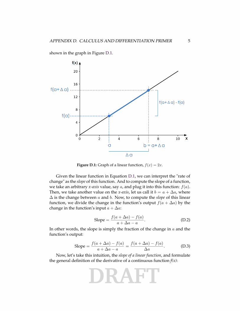
shown in the graph in Figure D.1.

Figure D.1: Graph of a linear function, f(x) = 2x.

Given the linear function in Equation D.1, we can interpret the "rate ofchange" as the slope of this function. And to compute the slope of a function,we take an arbitrary x-axis value, say a, and plug it into this function: f(a).Then, we take another value on the x-axis, let us call it b = a + ∆a, where∆ is the change between a and b. Now, to compute the slope of this linearfunction, we divide the change in the function’s output f(a + ∆a) by thechange in the function’s input a + ∆a:

Slope = f(a + ∆a)− f(a)a + ∆a− a

. (D.2)

In other words, the slope is simply the fraction of the change in a and thefunction’s output:

Slope = f(a + ∆a)− f(a)a + ∆a− a

= f(a + ∆a)− f(a)∆a

. (D.3)

Now, let’s take this intuition, the slope of a linear function, and formulatethe general definition of the derivative of a continuous function f(x):

DRAFT


f ′(x) = df

dx= lim

∆x→0

f(x + ∆x)− f(x)∆x

, (D.4)

where lim∆x→0 means "as the change in x becomes infinitely small (forinstance, ∆x approaches zero)." Since this appendix is merely a refresherrather than a comprehensive calculus resource, we have to skip over someimportant concepts such as Limit Theory. So, if this is the first time youencounter calculus, I recommend consulting additional resources such as"Calculus I, II, and III" by Jerrold E. Marsden and Alan Weinstein 1.

Infobox D.1.1 Derivative Notations

The two different notations dfdx and f ′(x) both refer to the derivative

of a function f(x). The former is the "Lagrange notation," and the lat-ter is called "Leibniz notation," respectively. In Leibniz notation, df

dx issometimes also written as d

dxf(x), and ddx is an operator that we read as

"differentiation with respect to x." Although the Leibniz notation looksa bit verbose at first, it plays nicely into our intuition by regarding df asa small change in the output of a function f and dx as a small change ofits input x. Hence, we can interpret the ratio df

dx as the slope of a pointin a function graph.

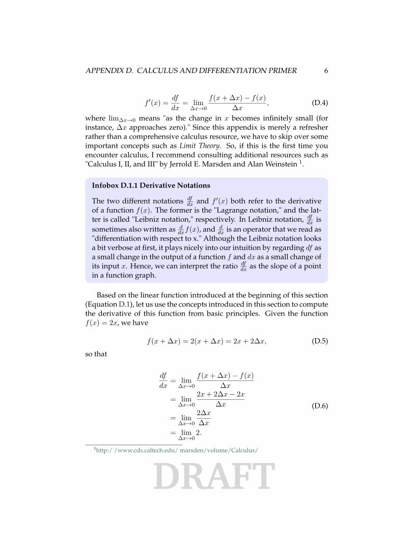
Based on the linear function introduced at the beginning of this section(Equation D.1), let us use the concepts introduced in this section to computethe derivative of this function from basic principles. Given the functionf(x) = 2x, we have

f(x + ∆x) = 2(x + ∆x) = 2x + 2∆x, (D.5)

so that

df

dx= lim

∆x→0

f(x + ∆x)− f(x)∆x

= lim∆x→0

2x + 2∆x− 2x

∆x

= lim∆x→0

2∆x

∆x

= lim∆x→0

2.

(D.6)

1http:/ /www.cds.caltech.edu/ marsden/volume/Calculus/

http://www.cds.caltech.edu/~marsden/volume/Calculus/

DRAFT


We conclude that the derivative of f(x) = 2x is simply a constant, namelyf ′(x) = 2.

Applying these same principles, let us take a look at a slightly moreinteresting example, a quadratic function,

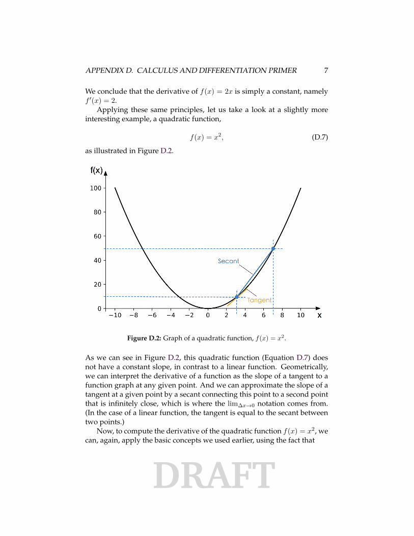
f(x) = x2, (D.7)

as illustrated in Figure D.2.

Figure D.2: Graph of a quadratic function, f(x) = x2.

As we can see in Figure D.2, this quadratic function (Equation D.7) doesnot have a constant slope, in contrast to a linear function. Geometrically,we can interpret the derivative of a function as the slope of a tangent to afunction graph at any given point. And we can approximate the slope of atangent at a given point by a secant connecting this point to a second pointthat is infinitely close, which is where the lim∆x→0 notation comes from.(In the case of a linear function, the tangent is equal to the secant betweentwo points.)

Now, to compute the derivative of the quadratic function f(x) = x2, wecan, again, apply the basic concepts we used earlier, using the fact that

DRAFT


f(x + ∆x) = (x + ∆x)2 = x2 + 2x∆x + (∆x)2. (D.8)

Now, computing the derivative, we get

df

dx= lim

∆x→0

f(x + ∆x)− f(x)∆x

= lim∆x→0

x2 + 2x∆x + (∆x)2 − x2

∆x

= lim∆x→0

2x∆x + (∆x)2

∆x

= lim∆x→0

2x + ∆x.

(D.9)

And since ∆x approaches zero due to the limit, we arrive at f ′(x) = 2x,which is the derivative of f(x) = x2.

D.2 Derivatives of Common Functions

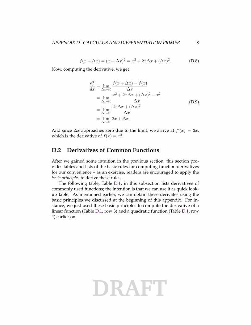
After we gained some intuition in the previous section, this section pro-vides tables and lists of the basic rules for computing function derivativesfor our convenience – as an exercise, readers are encouraged to apply thebasic principles to derive these rules.

The following table, Table D.1, in this subsection lists derivatives ofcommonly used functions; the intention is that we can use it as quick look-up table. As mentioned earlier, we can obtain these derivates using thebasic principles we discussed at the beginning of this appendix. For in-stance, we just used these basic principles to compute the derivative of alinear function (Table D.1, row 3) and a quadratic function (Table D.1, row4) earlier on.

DRAFT


Function f(x) Derivative with respect to x1 a 0

2 x 1

3 ax a

4 x2 2x

5 xa axa−1

6 ax log(a)ax

7 log(x) 1/x

8 loga(x) 1/(x log(a))

9 sin(x) cos(x)

10 cos(x) − sin(x)

11 tan(x) sec2(x)

Table D.1: Derivatives of common functions.

D.3 Common Differentiation Rules

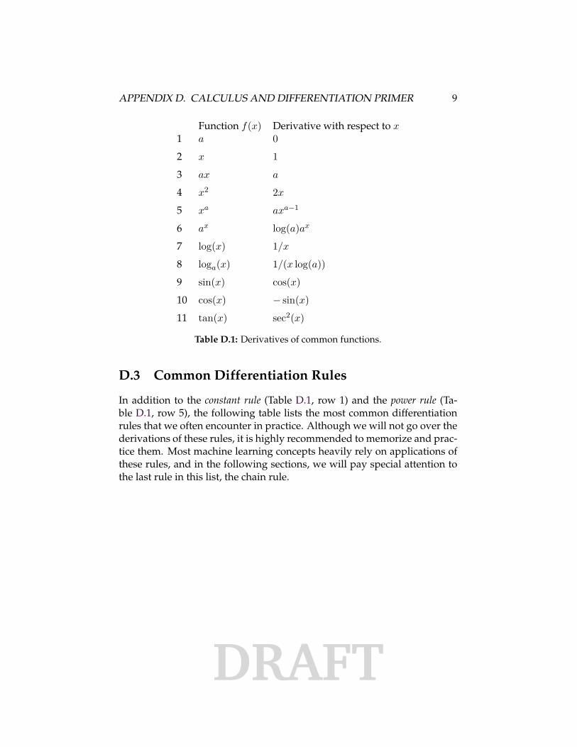
In addition to the constant rule (Table D.1, row 1) and the power rule (Ta-ble D.1, row 5), the following table lists the most common differentiationrules that we often encounter in practice. Although we will not go over thederivations of these rules, it is highly recommended to memorize and prac-tice them. Most machine learning concepts heavily rely on applications ofthese rules, and in the following sections, we will pay special attention tothe last rule in this list, the chain rule.

DRAFT


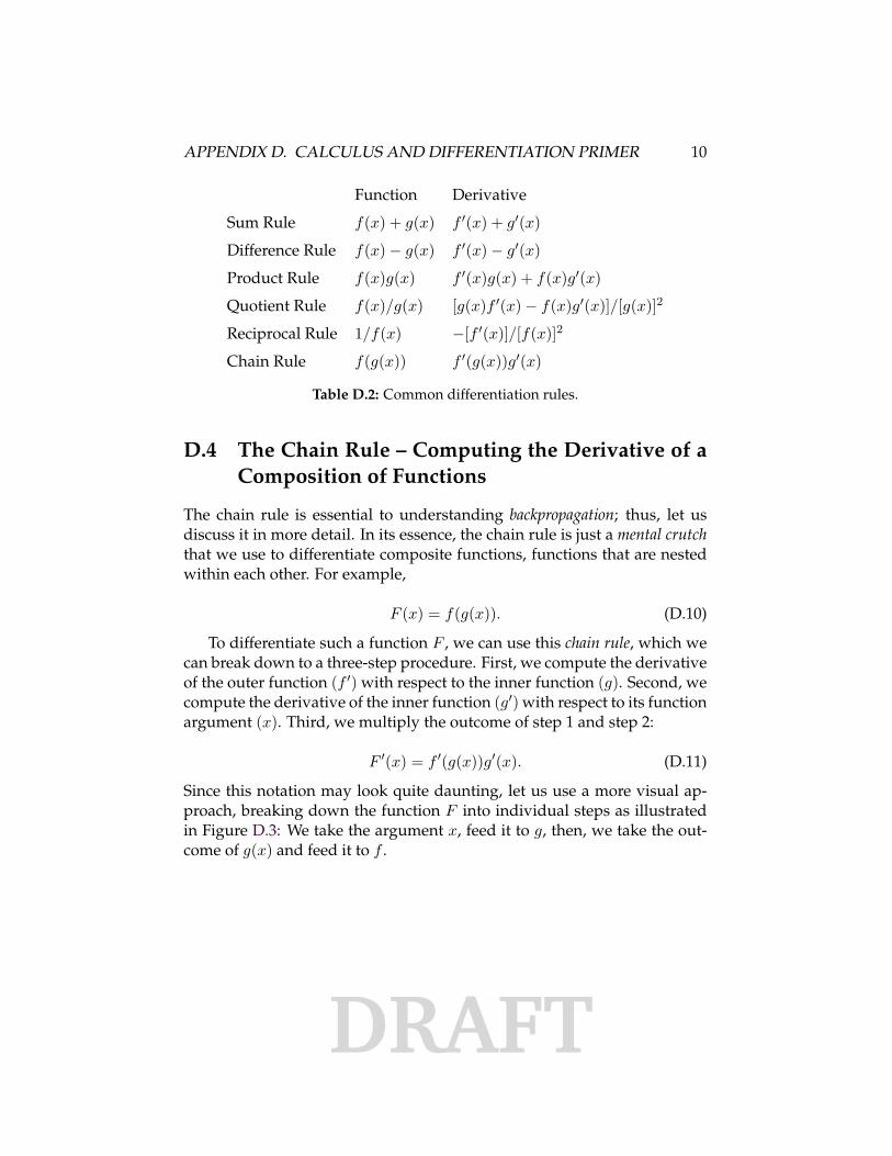
Function Derivative

Sum Rule f(x) + g(x) f ′(x) + g′(x)

Difference Rule f(x)− g(x) f ′(x)− g′(x)

Product Rule f(x)g(x) f ′(x)g(x) + f(x)g′(x)

Quotient Rule f(x)/g(x) [g(x)f ′(x)− f(x)g′(x)]/[g(x)]2

Reciprocal Rule 1/f(x) −[f ′(x)]/[f(x)]2

Chain Rule f(g(x)) f ′(g(x))g′(x)

Table D.2: Common differentiation rules.

D.4 The Chain Rule – Computing the Derivative of aComposition of Functions

The chain rule is essential to understanding backpropagation; thus, let usdiscuss it in more detail. In its essence, the chain rule is just a mental crutchthat we use to differentiate composite functions, functions that are nestedwithin each other. For example,

F (x) = f(g(x)). (D.10)

To differentiate such a function F , we can use this chain rule, which wecan break down to a three-step procedure. First, we compute the derivativeof the outer function (f ′) with respect to the inner function (g). Second, wecompute the derivative of the inner function (g′) with respect to its functionargument (x). Third, we multiply the outcome of step 1 and step 2:

F ′(x) = f ′(g(x))g′(x). (D.11)

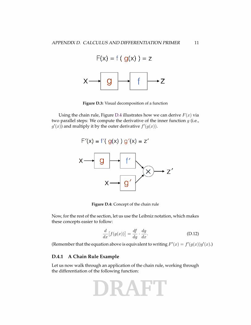
Since this notation may look quite daunting, let us use a more visual ap-proach, breaking down the function F into individual steps as illustratedin Figure D.3: We take the argument x, feed it to g, then, we take the out-come of g(x) and feed it to f .

DRAFT


Figure D.3: Visual decomposition of a function

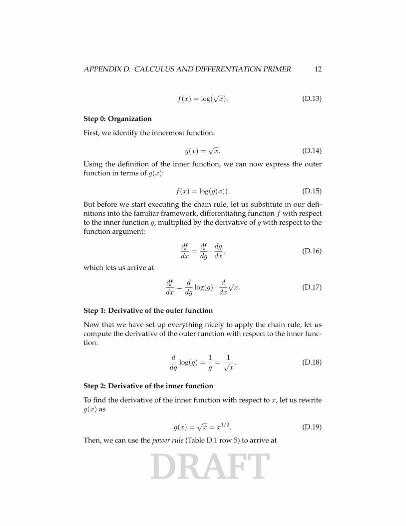
Using the chain rule, Figure D.4 illustrates how we can derive F (x) viatwo parallel steps: We compute the derivative of the inner function g (i.e.,g′(x)) and multiply it by the outer derivative f ′(g(x)).

Figure D.4: Concept of the chain rule

Now, for the rest of the section, let us use the Leibniz notation, which makesthese concepts easier to follow:

d

dx

[f(g(x))

]= df

dg· dg

dx. (D.12)

(Remember that the equation above is equivalent to writing F ′(x) = f ′(g(x))g′(x).)

D.4.1 A Chain Rule Example

Let us now walk through an application of the chain rule, working throughthe differentiation of the following function:

DRAFT


f(x) = log(√

x). (D.13)

Step 0: Organization

First, we identify the innermost function:

g(x) =√

x. (D.14)

Using the definition of the inner function, we can now express the outerfunction in terms of g(x):

f(x) = log(g(x)). (D.15)

But before we start executing the chain rule, let us substitute in our defi-nitions into the familiar framework, differentiating function f with respectto the inner function g, multiplied by the derivative of g with respect to thefunction argument:

df

dx= df

dg· dg

dx, (D.16)

which lets us arrive at

df

dx= d

dglog(g) · d

dx

√x. (D.17)

Step 1: Derivative of the outer function

Now that we have set up everything nicely to apply the chain rule, let uscompute the derivative of the outer function with respect to the inner func-tion:

d

dglog(g) = 1

g= 1√

x. (D.18)

Step 2: Derivative of the inner function

To find the derivative of the inner function with respect to x, let us rewriteg(x) as

g(x) =√

x = x1/2. (D.19)

Then, we can use the power rule (Table D.1 row 5) to arrive at

DRAFT


d

dxx1/2 = 1

2x−1/2 = 12√

x. (D.20)

Step 3: Multiplying inner and outer derivatives

Finally, we multiply the derivatives of the outer (step 1) and inner function(step 2), to get the derivative of the function f(x) = log(

√x):

df

dx= 1√

x· 1

2√

x= 1

2x. (D.21)

D.5 Arbitrarily Long Function Compositions

In the previous sections, we introduced the chain rule in context of twonested functions. However, the chain rule can also be used for an arbitrar-ily long function composition. For example, suppose we have five differentfunctions, f(x), g(x), h(x), u(x), and v(x), and let F be the function compo-sition:

F (x) = f(g(h(u(v(x))))). (D.22)

Then, we compute the derivative as

dF

dx= d

dxF (x) = d

dxf(g(h(u(v(x)))))

= df

dg· dg

dh· dh

du· du

dv· dv

dx.

(D.23)

As we can see in Equation D.23, composing multiple function is similarto the previous two-function example; here, we create a chain of deriva-tives of functions with respect to their inner function until we arrive at theinnermost function, which we then differentiate with respect to the func-tion parameter x.

D.6 When a Function is Not Differentiable

A function is only differentiable if the derivative exists for each value in thefunction’s domain (for instance, at each point). Non-differentiable func-tions may be a bit cumbersome to deal with mathematically; however, they

DRAFT


can still be useful in practical contexts such as deep learning. A popular ex-ample of a non-differentiable function that is widely used in deep learningis the Rectified Linear Unit (ReLU) function. The ReLU function f(x) is notdifferentiable because its derivative does not exist at x = 0, but more aboutthat later in this section.

One criterion for the derivative to exist at a given point is continuity atthat point. However, continuity is not sufficient for the derivative to exist.For the derivative to exist, we require the left-hand and the right-hand limitto exist and to be equal.

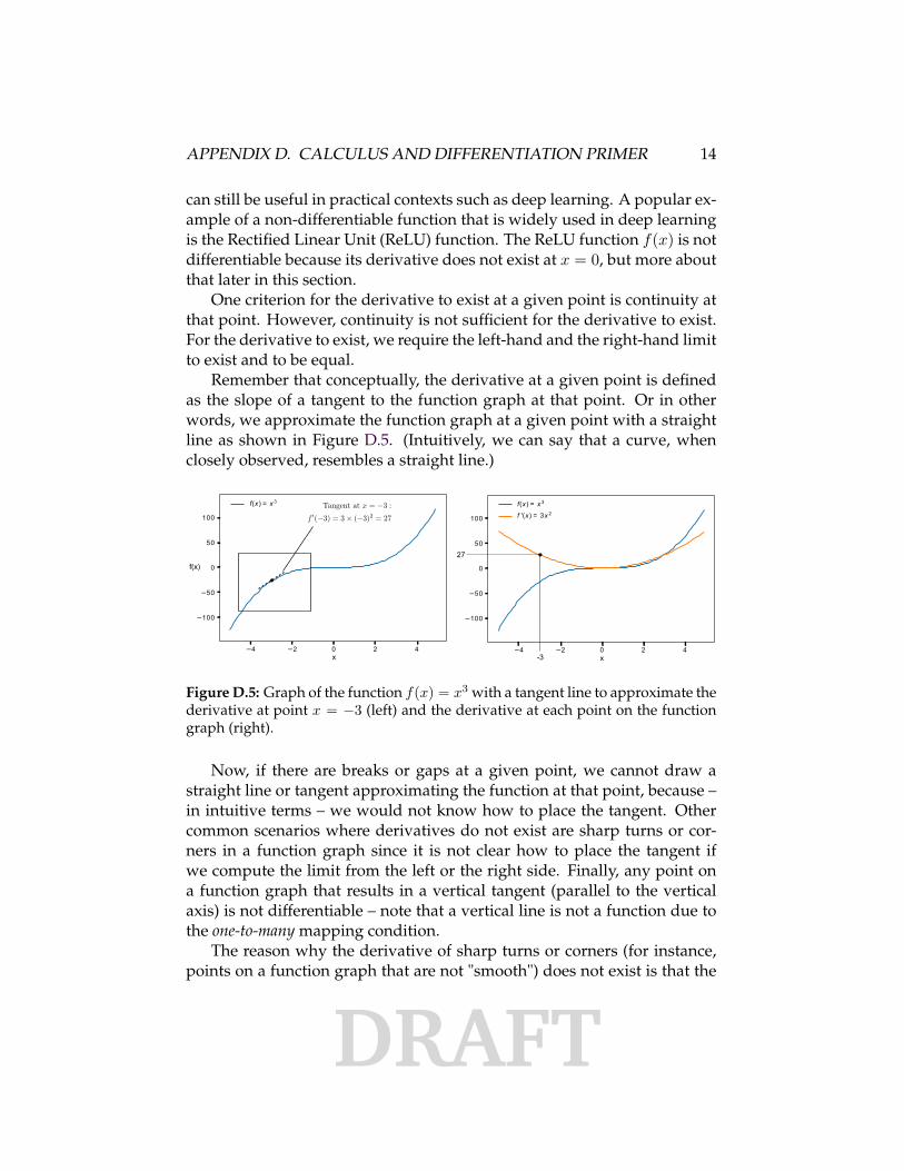
Remember that conceptually, the derivative at a given point is definedas the slope of a tangent to the function graph at that point. Or in otherwords, we approximate the function graph at a given point with a straightline as shown in Figure D.5. (Intuitively, we can say that a curve, whenclosely observed, resembles a straight line.)

4 2 0 2 4

100

50

0

50

100

f(x) = x 3

4 2 0 2 4

100

50

0

50

100

f(x) = x 3

f '(x) = 3x 2

xx

f(x)27

-3

Figure D.5: Graph of the function f(x) = x3 with a tangent line to approximate thederivative at point x = −3 (left) and the derivative at each point on the functiongraph (right).

Now, if there are breaks or gaps at a given point, we cannot draw astraight line or tangent approximating the function at that point, because –in intuitive terms – we would not know how to place the tangent. Othercommon scenarios where derivatives do not exist are sharp turns or cor-ners in a function graph since it is not clear how to place the tangent ifwe compute the limit from the left or the right side. Finally, any point ona function graph that results in a vertical tangent (parallel to the verticalaxis) is not differentiable – note that a vertical line is not a function due tothe one-to-many mapping condition.

The reason why the derivative of sharp turns or corners (for instance,points on a function graph that are not "smooth") does not exist is that the

DRAFT


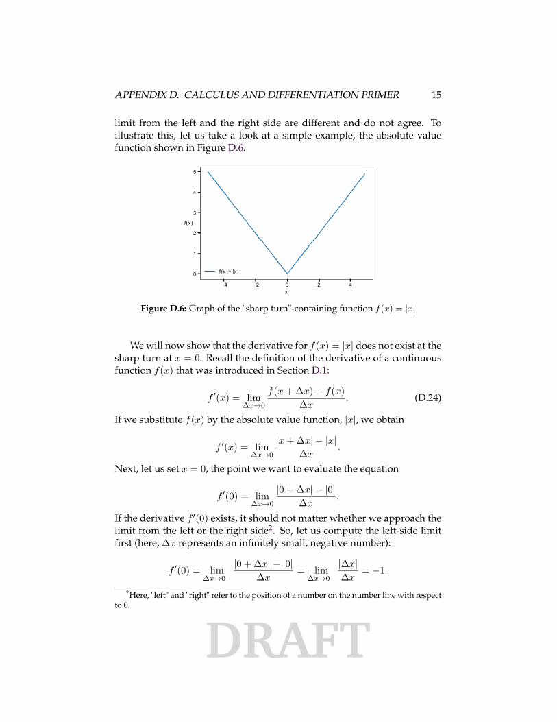
limit from the left and the right side are different and do not agree. Toillustrate this, let us take a look at a simple example, the absolute valuefunction shown in Figure D.6.

4 2 0 2 4x

0

1

2

3

4

5

f(x)

f(x)= |x|

Figure D.6: Graph of the "sharp turn"-containing function f(x) = |x|

We will now show that the derivative for f(x) = |x| does not exist at thesharp turn at x = 0. Recall the definition of the derivative of a continuousfunction f(x) that was introduced in Section D.1:

f ′(x) = lim∆x→0

f(x + ∆x)− f(x)∆x

. (D.24)

If we substitute f(x) by the absolute value function, |x|, we obtain

f ′(x) = lim∆x→0

|x + ∆x| − |x|∆x

.

Next, let us set x = 0, the point we want to evaluate the equation

f ′(0) = lim∆x→0

|0 + ∆x| − |0|∆x

.

If the derivative f ′(0) exists, it should not matter whether we approach thelimit from the left or the right side2. So, let us compute the left-side limitfirst (here, ∆x represents an infinitely small, negative number):

f ′(0) = lim∆x→0−

|0 + ∆x| − |0|∆x

= lim∆x→0−

|∆x|∆x

= −1.

2Here, "left" and "right" refer to the position of a number on the number line with respectto 0.

DRAFT


As shown above, the left-hand limit evaluates to −1 because dividing apositive number be a negative number yields a negative number. We cannow do the same calculation by approaching the limit from the right, where∆x is an infinitely small, non-negative number:

f ′(0) = lim∆x→0+

|0 + ∆x| − |0|∆x

= lim∆x→0+

|∆x|∆x

= 1.

We can see that the limits are not equal (1 6= −1), and because they donot agree, we have no formal notion of how to draw the tangent line to thefunction graph at the point x = 0. Hence, we say that the derivative of thefunction f(x) = |x| does not exist (DNE) at point x = 0:

f ′(0) = DNE.

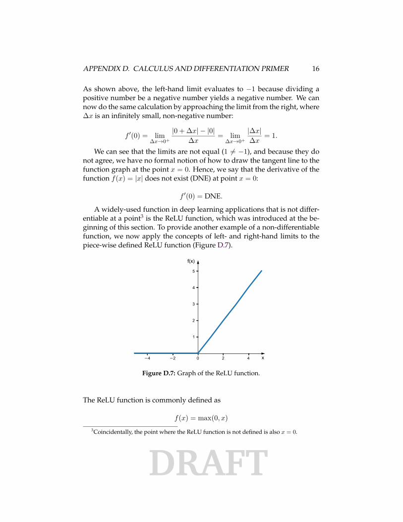
A widely-used function in deep learning applications that is not differ-entiable at a point3 is the ReLU function, which was introduced at the be-ginning of this section. To provide another example of a non-differentiablefunction, we now apply the concepts of left- and right-hand limits to thepiece-wise defined ReLU function (Figure D.7).

4 2 0 2 4

1

2

3

4

5

f(x)

x

Figure D.7: Graph of the ReLU function.

The ReLU function is commonly defined as

f(x) = max(0, x)3Coincidentally, the point where the ReLU function is not defined is also x = 0.

DRAFT


or

f(x) ={

0 if x < 0x if x ≥ 0

(These two function definitions are equivalent.) If we substitute the ReLUequation into Equation D.24, we then obtain

f ′(x) = limx→0

max(0, x + ∆x)−max(0, x)∆x

.

Next, let us compute the left- and right-side limits. Starting from theleft side, where ∆x is an infinitely small, negative number, we get

f ′(0) = limx→0−

0− 0∆x

= 0.

And for the right-hand limit, where ∆x is an infinitely small, positive num-ber, we get

f ′(0) = limx→0+

0 + ∆x− 0∆x

= 1.

Again, the left- and right-hand limits are not equal at x = 0; hence, thederivative of the ReLU function at x = 0 is not defined.

For completeness’ sake, the derivative of the ReLU function for x > 0 is

f ′(x) = limx→0

x + ∆x− x

∆x= ∆x

∆x= 1.

And for x < 0, the ReLU derivative is

f ′(x) = limx→0

0− 0∆x

= 0

To summarize, the derivative of the ReLU function is defined as follows:

f ′(x) =

0 if x < 01 if x > 0DNE if x = 0

.

Infobox D.6.1 ReLU Derivative in Deep Learning

In practical deep learning applications, the ReLU derivative for x = 0 istypically set to 0, 1, or 0.5. However, it is extremely rare that x is exactly

DRAFT


zero, which is why the decision whether we set the ReLU derivative to0, 1, or 0.5 has little impact on the parameterization of a neural networkwith ReLU activation functions.

D.7 Partial Derivatives and Gradients

Throughout the previous sections, we only looked at univariate functions,functions that only take one input variable, for example, f(x). In this sec-tion, we will compute the derivatives of multivariable functions f(x, y, z, ...).Note that we still consider scalar-valued functions, which return a scalar orsingle value.

While the derivative of a univariate function is a scalar, the derivativeof a multivariable function is a vector, the so-called gradient. We denotethe derivative of a multivariable function f using the gradient symbol ∇(pronounced "nabla" or "del"):

∇f =

∂f/∂x∂f/∂y∂f/∂z

...

. (D.25)

As we can see, the gradient is simply a vector listing the derivatives of afunction with respect to each argument of the function. In Leibniz notation,we use the symbol ∂ instead of d to distinguish partial from ordinary deriva-tives. The adjective "partial" is based on the idea that a partial derivativewith respect to a function argument does not tell the whole story about afunction f . For instance, given a function f , the partial derivative ∂

∂xf(x, y)only considers the change in f if x changes while treating y as a constant.

To illustrate the concept of partial derivatives, let us walk through aconcrete example, where we will compute the gradient of the function

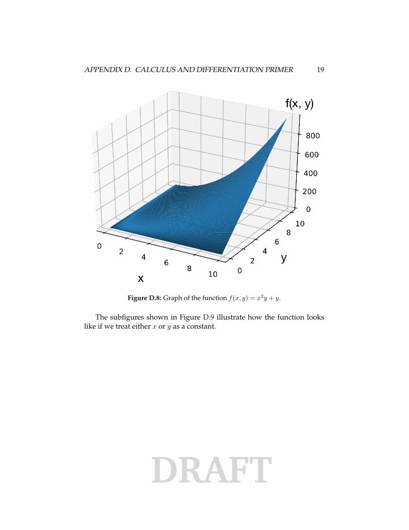
f(x, y) = x2y + y. (D.26)

The plot in Figure D.8 shows a graph of this function for different values ofx and y.

DRAFT


Figure D.8: Graph of the function f(x, y) = x2y + y.

The subfigures shown in Figure D.9 illustrate how the function lookslike if we treat either x or y as a constant.

DRAFT


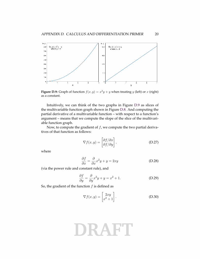
Figure D.9: Graph of function f(x, y) = x2y + y when treating y (left) or x (right)as a constant.

Intuitively, we can think of the two graphs in Figure D.9 as slices ofthe multivariable function graph shown in Figure D.8. And computing thepartial derivative of a multivariable function – with respect to a function’sargument – means that we compute the slope of the slice of the multivari-able function graph.

Now, to compute the gradient of f , we compute the two partial deriva-tives of that function as follows:

∇f(x, y) =[∂f/∂x∂f/∂y

], (D.27)

where

∂f

∂x= ∂

∂xx2y + y = 2xy (D.28)

(via the power rule and constant rule), and

∂f

∂y= ∂

∂yx2y + y = x2 + 1. (D.29)

So, the gradient of the function f is defined as

∇f(x, y) =[

2xyx2 + 1

]. (D.30)

DRAFT


D.8 Second Order Partial Derivatives

Let us briefly go over the notation of second order partial derivatives, sincethe notation may look a bit strange at first. In a nutshell, the second or-der partial derivative of a function is the partial derivative of the partialderivative. For instance, we write the second derivative of a function fwith respect to x as

∂

∂x

(∂f

∂x

)= ∂2f

∂x2 . (D.31)

For example, we compute the second partial derivative of a function f(x, y) =x2y + y as follows:

∂2f

∂x2 = ∂

∂x

(∂

∂xx2y + y

)= ∂

∂x2xy = ∂

∂x= 2y. (D.32)

Note that in the initial definition (Equation D.31) and the example (Equa-tion D.32) both the first and second order partial derivatives were com-puted with respect to the same input argument, x. However, depending onwhat measurement we are interested in, the second order partial derivativecan involve a different input argument. For instance, given a multivariablefunction with two input arguments, we can in fact compute four distinctsecond order partial derivatives:

∂2f

∂x2 ,∂2f

∂y2 ,∂2f

∂x∂y, and

∂2f

∂y∂x, (D.33)

where, for example, ∂2f∂y∂x is defined as

∂2f

∂y∂x= ∂

∂y

(∂f

∂x

). (D.34)

D.9 The Multivariable Chain Rule

In this section, we will take a look at how to apply the chain rule to func-tions that take multiple arguments. For instance, let us consider the follow-ing function:

f(g, h

)= g2h + h, (D.35)

where g(x) = 3x, and h(x) = x2. So, as it turns out, our function is acomposition of two functions:

DRAFT


f(g(x), h(x)

)(D.36)

Previously, in Section D.4, we defined the chain rule for the univariate caseas follows:

d

dx

[f(g(x))

]= df

dg· dg

dx. (D.37)

To extend apply this concept to multivariable functions, we simply extendthe notation above using the product rule. Hence, we can define the multi-variable chain rule as follows:

d

dx

[f(g(x), h(x))

]= ∂f

∂g· dg

dx+ ∂f

∂h· dh

dx. (D.38)

Applying the multivariable chain rule to our multivariable function exam-ple f

(g, h

)= g2h + h, let us start with the partial derivatives:

∂f

∂g= 2gh (D.39)

and

∂f

∂h= g2 + 1. (D.40)

Next, we take the ordinary derivatives of the two functions g and h:

dg

dx= d

dx3x = 3 (D.41)

dh

dx= d

dxx2 = 2x. (D.42)

And finally, plugging everything into our multivariable chain rule definition,we arrive at

d

dx

[f(g(x))

]= [2gh · 3] + [g2 + 1 + 2x] = g(g + 6h) + 2x + 1. (D.43)

D.10 The Multivariable Chain Rule in Vector Form

After we introduced the general concept of the multivariable chain rule, weoften prefer a more compact notation in practice: the multivariable chainrule in vector form.

DRAFT


Infobox D.10.1 Dot Products

As we remember from the linear algebra appendix, we compute the dotproduct between two vectors, a and b , as follows:

a · b =[ab

]·[xy

]= ax + by

In vector form, we write the multivariable chain rule

d

dx

[f(g(x), h(x))

]= ∂f

∂g· dg

dx+ ∂f

∂h· dh

dx(D.44)

as follows:

d

dx

[f(g(x), h(x))

]= ∇f · v′(x). (D.45)

Here, v is a vector listing the function arguments:

v(x) =[

g(x)h(x)

]. (D.46)

And the derivative ("v-prime" in Lagrange notation) is defined as follows:

v′(x) = d

dx

[g(x)h(x)

]=[

dg/dxdh/dx

]. (D.47)

So, putting everything together, we have

∇f · v′(x) =[

∂f/∂g∂f/∂h

]·[

dg/dxdh/dx

]= ∂f

∂g· dg

dx+ ∂f

∂h· dh

dx. (D.48)

D.11 The Hessian Matrix

As mentioned earlier in Section D.8 Second Order Partial Derivatives, we cancompute four distinct partial derivatives for a two-variable function:

f(x, y). (D.49)

The Hessian matrix is simply a matrix that packages them up:

DRAFT


Hf =[

∂2f/∂x2 ∂2f/∂x∂y∂2f/∂y∂x ∂2f/∂y2

]. (D.50)

To formulate the Hessian for a multivariable function that takes n argu-ments,

f(x1, x2, ..., xn), (D.51)

we write the Hessian as

Hf =

∂2f

∂x1∂x1∂2f

∂x1∂x2. . . ∂2f

∂x1∂xn∂2f

∂x2∂x1∂2f

∂x2∂x2. . . ∂2f

∂x2∂xn...

.... . .

...∂2f

∂xn∂x1∂2f

∂xn∂x2. . . ∂2f

∂xn∂xn

. (D.52)

D.12 The Laplacian Operator

At its core, the Laplacian operator (∆) is an operator that takes in a func-tion and returns another function. In particular, it is the divergence of thegradient of a function f – a kind of second order partial derivative, or "thedircection that increases the direction most rapidly:"

∆f(g(x), h(x)) = ∇ · ∇f. (D.53)

Remember, we compute the gradient of a function f(g, h) as follows:

∇f(g, h) =[

∂f/∂g∂f/∂h

]. (D.54)

Plugging it into the definition of the Laplacian, we arrive at

∆f(g(x), h(x)) =[

∂f/∂g∂f/∂h

]·[

∂f/∂g∂f/∂h

]f = ∂2f

∂g2 + ∂2f

∂h2 . (D.55)

And in more general terms, we can define the Laplacian of a function

f(x1, x2, ..., xn) (D.56)

as

DRAFT


∆f =n∑

i=1

∂2f

∂x2i

. (D.57)

DRAFT

Bibliography

[Boyer, 1970] Boyer, C. B. (1970). The history of the calculus. The Two-YearCollege Mathematics Journal, 1(1):60–86.

26

DRAFT

Abbreviations and Terms

AMI [Amazon Machine Image]API [Application Programming Interface]CNN [Convolutional Neural Network]DNE [Does Not Exist]

27

DRAFT

Index

28

Documents

Calculus and Differentiation Primer - Dr. Sebastian … · Calculus is a discipline of mathematics that provides us with tools to ana-lyze rates of change, or decay, or motion. Both