Embed Size (px)
Citation preview

885
13 Functions of SeveralVariables
Many real-life quantities are functions of two or more variables. In Section 13.1, you will learn how to graph a functionof two variables, like the one shown above. The first three graphs show cut-away views of the surface at varioustraces. Another way to visualize this surface is to project the traces onto the xy-plane, as shown in the fourth graph.
x
y
z
x
y
z
x
y
z
x
y
NOAA
In this chapter, you will study functions ofmore than one independent variable. Manyof the concepts presented are extensions offamiliar ideas from earlier chapters.
In this chapter, you should learn the following.
n How to sketch a graph, level curves,and level surfaces. (13.1)
n How to find a limit and determine continuity. (13.2)
n How to find and use a partial derivative.(13.3)
n How to find and use a total differentialand determine differentiability. (13.4)
n How to use the Chain Rules and find apartial derivative implicitly. (13.5)
n How to find and use a directional derivative and a gradient. (13.6)
n How to find an equation of a tangentplane and an equation of a normal line to a surface, and how to find the angle of inclination of a plane. (13.7)
n How to find absolute and relative extrema. (13.8)
n How to solve an optimization problem,including constrained optimization using a Lagrange multiplier, and how to use themethod of least squares. (13.9, 13.10)
Meteorologists use maps that show curves of equal atmospheric pressure, calledisobars, to predict weather patterns. How can you use pressure gradients to determine the area of the country that has the greatest wind speed? (See Section13.6, Exercise 68.)
n
n
1053714_cop13.qxd 10/27/08 12:04 PM Page 885
13 Funciones de variasvariables
En este capítulo se estudiarán funcionesde más de una variable independiente.Muchos de los conceptos presentadosson extensiones de ideas familiares decapítulos recientes.En este capítulo, se aprenderá:
n Cómo trazar una gráfica, curvas denivel y superficies de nivel. (13.1)
n Cómo encontrar un límite y determi-nar la continuidad. (13.2)
n Cómo encontrar y usar una derivadaparcial. (13.3)
n Cómo encontrar y usar una diferen-cial total y determinar diferenciabili-dad. (13.4)
n Cómo usar la regla de la cadena yencontrar una derivada parcial implí-cita. (13.5)
n Cómo encontrar y usar una derivadadireccional y un gradiente. (13.6)
n Cómo encontrar una ecuación de unplano tangente y una ecuación de unarecta normal a una superficie, y cómoencontrar el ángulo de inclinación deun plano. (13.7)
n Cómo encontrar los extremos absolu-tos y relativos. (13.8)
n Cómo resolver un problema de opti-mización, incluida optimización res-tringida usando un multiplicador deLagrange, y cómo usar el método demínimos cuadrados. (13.9, 13.10)
885885
13 Functions of SeveralVariables
Many real-life quantities are functions of two or more variables. In Section 13.1, you will learn how to graph a functionof two variables, like the one shown above. The first three graphs show cut-away views of the surface at varioustraces. Another way to visualize this surface is to project the traces onto the xy-plane, as shown in the fourth graph.
x
y
z
x
y
z
x
y
z
x
y
NOAA
In this chapter, you will study functions ofmore than one independent variable. Manyof the concepts presented are extensions offamiliar ideas from earlier chapters.
In this chapter, you should learn the following.
n How to sketch a graph, level curves,and level surfaces. (13.1)
n How to find a limit and determine continuity. (13.2)
n How to find and use a partial derivative.(13.3)
n How to find and use a total differentialand determine differentiability. (13.4)
n How to use the Chain Rules and find apartial derivative implicitly. (13.5)
n How to find and use a directional derivative and a gradient. (13.6)
n How to find an equation of a tangentplane and an equation of a normal line to a surface, and how to find the angle of inclination of a plane. (13.7)
n How to find absolute and relative extrema. (13.8)
n How to solve an optimization problem,including constrained optimization using a Lagrange multiplier, and how to use themethod of least squares. (13.9, 13.10)
Meteorologists use maps that show curves of equal atmospheric pressure, calledisobars, to predict weather patterns. How can you use pressure gradients to determine the area of the country that has the greatest wind speed? (See Section13.6, Exercise 68.)
n
n
1053714_cop13.qxd 10/27/08 12:04 PM Page 885
Los meteorólogos usan mapas que muestran curvas de presión atmosférica igual,llamadas isobaras, para predecir los patrones del clima. ¿Cómo se pueden usar losgradientes de presión para determinar el área del país que tiene las mayoresvelocidades de viento? (Ver la sección 13.6, ejercicio 68.)
Muchas cantidades de la vida real son funciones de dos o más variables. En la sección 13.1 se aprenderá cómograficar una función de dos variables, tal como la que se muestra arriba. Las primeras tres gráficas muestran vis-tas cortadas de la superficie en varios trazos. Otra forma de visualizar estas superficies es proyectar los trazoshacia el plano xy, tal como se muestra en la cuarta gráfica.
885885
13 Functions of SeveralVariables
Many real-life quantities are functions of two or more variables. In Section 13.1, you will learn how to graph a functionof two variables, like the one shown above. The first three graphs show cut-away views of the surface at varioustraces. Another way to visualize this surface is to project the traces onto the xy-plane, as shown in the fourth graph.
x
y
z
x
y
z
x
y
z
x
y
NOAA
In this chapter, you will study functions ofmore than one independent variable. Manyof the concepts presented are extensions offamiliar ideas from earlier chapters.
In this chapter, you should learn the following.
n How to sketch a graph, level curves,and level surfaces. (13.1)
n How to find a limit and determine continuity. (13.2)
n How to find and use a partial derivative.(13.3)
n How to find and use a total differentialand determine differentiability. (13.4)
n How to use the Chain Rules and find apartial derivative implicitly. (13.5)
n How to find and use a directional derivative and a gradient. (13.6)
n How to find an equation of a tangentplane and an equation of a normal line to a surface, and how to find the angle of inclination of a plane. (13.7)
n How to find absolute and relative extrema. (13.8)
n How to solve an optimization problem,including constrained optimization using a Lagrange multiplier, and how to use themethod of least squares. (13.9, 13.10)
Meteorologists use maps that show curves of equal atmospheric pressure, calledisobars, to predict weather patterns. How can you use pressure gradients to determine the area of the country that has the greatest wind speed? (See Section13.6, Exercise 68.)
n
n
1053714_cop13.qxd 10/27/08 12:04 PM Page 885
Larson-13-01.qxd 3/12/09 18:39 Page 885

886 CAPÍTULO 13 Funciones de varias variables
13.1 Introducción a las funciones de varias variables
n Entender la notación para una función de varias variables.n Dibujar la gráfica de una función de dos variables.n Dibujar las curvas de nivel de una función de dos variables.n Dibujar las superficies de nivel de una función de tres variables.n Utilizar gráficos por computadora para representar una función de dos
variables.
Funciones de varias variables
Hasta ahora en este texto, sólo se han visto funciones de una sola variable (independiente).Sin embargo, muchos problemas comunes son funciones de dos o más variables. Por ejem-plo, el trabajo realizado por una fuerza y el volumen de un cilindro circular recto
son funciones de dos variables. El volumen de un sólido rectangular es una función de tres variables. La notación para una función de dos o más variables es si-milar a la utilizada para una función de una sola variable. Aquí se presentan dos ejemplos.
Función de 2 variables.
2 variables
y
Función de 3 variables.
3 variables
En la función dada por y son las variables independientes y z es lavariable dependiente.
Pueden darse definiciones similares para las funciones de tres, cuatro o n variablesdonde los dominios consisten en tríadas (x1, x2, x3), tétradas (x1, x2, x3, x4) y
adas (x1, x2, . . ., xn). En todos los casos, rango es un conjunto de números reales. En estecapítulo, sólo se estudian funciones de dos o tres variables.
Como ocurre con las funciones de una variable, la manera más común para describiruna función de varias variables es por medio de una ecuación, y a menos que se digaexplícitamente lo contrario, se puede suponer que el dominio es el conjunto de todos lospuntos para los que la ecuación está definida. Por ejemplo, el dominio de la función dadapor
se supone que es todo el plano xy. Similarmente, el dominio de
es el conjunto de todos los puntos en el plano para los que Esto consiste entodos los puntos del primer y tercer cuadrantes.
xy > 0.sx, yd
f sx, yd 5 ln xy
f sx, yd 5 x2 1 y2
n-
yxz 5 f sx, yd,
w 5 f sx, y, zd 5 x 1 2y 2 3z
z 5 f sx, yd 5 x2 1 xy
sV 5 lwhdsV 5 p r2hdsW 5 FDd
MARY FAIRFAX SOMERVILLE (1780-1872)
Somerville se interesó por el problema decrear modelos geométricos de funciones devarias variables. Su libro más conocido, The Mechanics of the Heavens, se publicó en 1831.
Arc
hive
Pho
tos
E X P L O R A C I Ó N
Comparación de dimensionesSin usar una herramienta de grafi-cación, describir la gráfica de cadafunción de dos variables.
a)
b)
c)
d)
e) z 5 !1 2 x2 1 y2
z 5 !x2 1 y2
z 5 x2 1 y
z 5 x 1 y
z 5 x2 1 y2
DEFINICIÓN DE UNA FUNCIÓN DE DOS VARIABLES
Sea D un conjunto de pares ordenados de números reales. Si a cada par ordenado(x, y) de D le corresponde un único número real f(x, y), entonces se dice que f esuna función de x y y. El conjunto D es el dominio de f, y el correspondienteconjunto de valores f(x, y) es el rango de f.
Larson-13-01.qxd 3/12/09 18:39 Page 886
gsud 5 !u.16 2 4x2 2 y2
SECCIÓN 13.1 Introducción a las funciones de varias variables 887
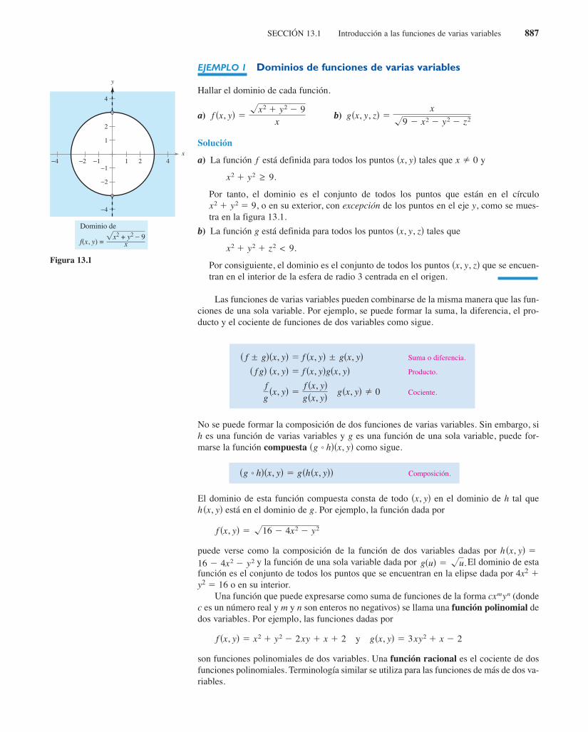
EJEMPLO 1 Dominios de funciones de varias variables
Hallar el dominio de cada función.
a) b)
Solución
a) La función está definida para todos los puntos tales que y
Por tanto, el dominio es el conjunto de todos los puntos que están en el círculoo en su exterior, con excepción de los puntos en el eje y, como se mues-
tra en la figura 13.1.
b) La función g está definida para todos los puntos tales que
Por consiguiente, el dominio es el conjunto de todos los puntos que se encuen-tran en el interior de la esfera de radio 3 centrada en el origen.
Las funciones de varias variables pueden combinarse de la misma manera que las fun-ciones de una sola variable. Por ejemplo, se puede formar la suma, la diferencia, el pro-ducto y el cociente de funciones de dos variables como sigue.
No se puede formar la composición de dos funciones de varias variables. Sin embargo, sies una función de varias variables y es una función de una sola variable, puede for-
marse la función compuesta como sigue.
El dominio de esta función compuesta consta de todo en el dominio de tal queestá en el dominio de Por ejemplo, la función dada por
puede verse como la composición de la función de dos variables dadas por y la función de una sola variable dada por El dominio de esta
función es el conjunto de todos los puntos que se encuentran en la elipse dada por 4x2 1y2 5 16 o en su interior.
Una función que puede expresarse como suma de funciones de la forma (dondec es un número real y m y n son enteros no negativos) se llama una función polinomial dedos variables. Por ejemplo, las funciones dadas por
y
son funciones polinomiales de dos variables. Una función racional es el cociente de dosfunciones polinomiales. Terminología similar se utiliza para las funciones de más de dos va-riables.
gsx, yd 5 3xy2 1 x 2 2f sx, yd 5 x2 1 y2 2 2xy 1 x 1 2
cxmyn
h sx, yd 5
f sx, yd 5 !16 2 4x2 2 y2
g.h sx, ydhsx, yd
sg 8 hdsx, ydgh
sx, y, zd
x2 1 y2 1 z2 < 9.
sx, y, zd
x2 1 y2 5 9,
x2 1 y2 ≥ 9.
x Þ 0sx, ydf
gsx, y, zd 5x
!9 2 x2 2 y2 2 z2f sx, yd 5!x2 1 y2 2 9
x
y
x2 + y2 − 9xf(x, y) =
Dominio de
x1
1
2
2
4
4
−1−1
−2
−2
−4
−4
Figura 13.1
Composición.sg 8 hdsx, yd 5 gshsx, ydd
Suma o diferencia.
Producto.
Cociente. fg
sx, yd 5f sx, ydgsx, yd gsx, yd Þ 0
s f gd sx, yd 5 f sx, ydgsx, yd s f ± gdsx, yd 5 f sx, yd ± gsx, yd
Larson-13-01.qxd 3/12/09 18:39 Page 887
888 CAPÍTULO 13 Funciones de varias variables
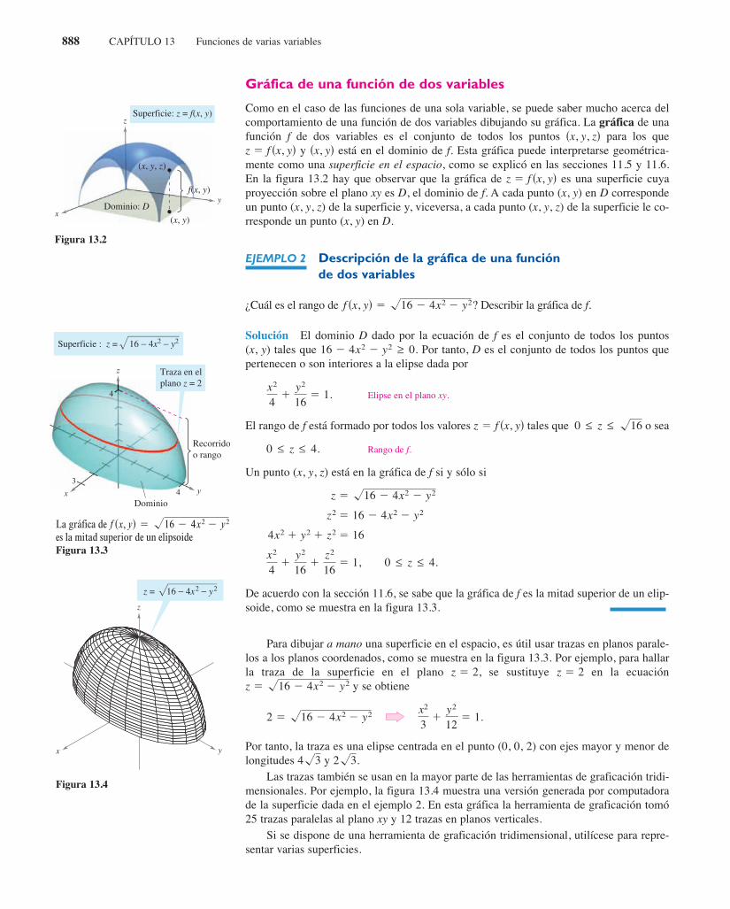
Gráfica de una función de dos variables
Como en el caso de las funciones de una sola variable, se puede saber mucho acerca delcomportamiento de una función de dos variables dibujando su gráfica. La gráfica de unafunción f de dos variables es el conjunto de todos los puntos para los que
y está en el dominio de f. Esta gráfica puede interpretarse geométrica-mente como una superficie en el espacio, como se explicó en las secciones 11.5 y 11.6.En la figura 13.2 hay que observar que la gráfica de es una superficie cuyaproyección sobre el plano xy es D, el dominio de f. A cada punto (x, y) en D correspondeun punto (x, y, z) de la superficie y, viceversa, a cada punto (x, y, z) de la superficie le co-rresponde un punto (x, y) en D.
EJEMPLO 2 Descripción de la gráfica de una funciónde dos variables
¿Cuál es el rango de Describir la gráfica de f.
Solución El dominio D dado por la ecuación de f es el conjunto de todos los puntos(x, y) tales que Por tanto, D es el conjunto de todos los puntos quepertenecen o son interiores a la elipse dada por
Elipse en el plano xy.
El rango de f está formado por todos los valores tales que o sea
Rango de f.
Un punto (x, y, z) está en la gráfica de f si y sólo si
De acuerdo con la sección 11.6, se sabe que la gráfica de f es la mitad superior de un elip-soide, como se muestra en la figura 13.3.
Para dibujar a mano una superficie en el espacio, es útil usar trazas en planos parale-los a los planos coordenados, como se muestra en la figura 13.3. Por ejemplo, para hallarla traza de la superficie en el plano se sustituye en la ecuación
y se obtiene
Por tanto, la traza es una elipse centrada en el punto (0, 0, 2) con ejes mayor y menor delongitudes y
Las trazas también se usan en la mayor parte de las herramientas de graficación tridi-mensionales. Por ejemplo, la figura 13.4 muestra una versión generada por computadorade la superficie dada en el ejemplo 2. En esta gráfica la herramienta de graficación tomó25 trazas paralelas al plano xy y 12 trazas en planos verticales.
Si se dispone de una herramienta de graficación tridimensional, utilícese para repre-sentar varias superficies.
2!3.4!3
x2
31
y2
125 1.2 5 !16 2 4x2 2 y2
z 5 !16 2 4x2 2 y2z 5 2z 5 2,
x2
41
y2
161
z2
165 1, 0 ≤ z ≤ 4.
4x2 1 y2 1 z2 5 16
z2 5 16 2 4x2 2 y2
z 5 !16 2 4x2 2 y2
0 ≤ z ≤ 4.
0 ≤ z ≤ !16z 5 f sx, yd
x2
41
y2
165 1.
16 2 4x2 2 y2 ≥ 0.
f sx, yd 5 !16 2 4x2 2 y2?
z 5 f sx, yd
sx, ydz 5 f sx, ydsx, y, zd
Figura 13.2
La gráfica dees la mitad superior de un elipsoideFigura 13.3
f sx, yd 5 !16 2 4x2 2 y2
z
yx
z = 16 − 4x2 − y2
Figura 13.4
Larson-13-01.qxd 3/12/09 18:39 Page 888

SECCIÓN 13.1 Introducción a las funciones de varias variables 889
Curvas de nivel
Una segunda manera de visualizar una función de dos variables es usar un campo escalaren el que el escalar se asigna al punto Un campo escalar puede carac-terizarse por sus curvas de nivel (o líneas de contorno) a lo largo de las cuales el valorde es constante. Por ejemplo, el mapa climático en la figura 13.5 muestra las cur-vas de nivel de igual presión, llamadas isobaras. Las curvas de nivel que representan pun-tos de igual temperatura en mapas climáticos, se llaman isotermas, como se muestra en lafigura 13.6. Otro uso común de curvas de nivel es la representación de campos de poten-cial eléctrico. En este tipo de mapa, las curvas de nivel se llaman líneas equipotenciales.
Los mapas de contorno suelen usarse para representar regiones de la superficie de laTierra, donde las curvas de nivel representan la altura sobre el nivel del mar. Este tipo demapas se llama mapa topográfico. Por ejemplo, la montaña mostrada en la figura 13.7 serepresenta por el mapa topográfico de la figura 13.8.
Un mapa de contorno representa la variación de z respecto a x y y mediante espacio entrelas curvas de nivel. Una separación grande entre las curvas de nivel indica que z cambia lenta-mente, mientras que un espacio pequeño indica un cambio rápido en z. Además, en un mapade contorno, es importante elegir valores de c uniformemente espaciados, para dar una mejorilusión tridimensional.
f sx, yd
sx, yd.z 5 f sx, yd
Figura 13.7
001 8
021
1004
1
001 4
1012
1061
8010
8100
0010
1100
0 48001 010 4
100
2110
008
14001
008
1000
10
08
Las curvas de nivel muestran las líneas deigual presión (isobaras) medidas en milibaresFigura 13.5
0403
02
03
20
3003
02
40
05
06
09
8008
07
Las curvas de nivel muestran líneas de igualtemperatura (isotermas) medidas en gradosFahrenheitFigura 13.6
Figura 13.8
USG
S
Alf
red
B. T
hom
as/E
arth
Sce
nes
Larson-13-01.qxd 3/12/09 18:39 Page 889

890 CAPÍTULO 13 Funciones de varias variables
y
z
f(x, y) = 64 − x2 − y2
Superficie:
x
8
8
8
HemisferioFigura 13.9
x4
4
8
8
−4
−4
−8
−8
yc1 = 0c2 = 1c3 = 2c4 = 3 c8 = 7
c7 = 6c6 = 5c5 = 4
c9 = 8
Mapa de contornoFigura 13.10
xy
Superficie:z = y2 − x2
4 4
10
12
8
6
4
2
z
Paraboloide hiperbólicoFigura 13.11
4
4
−4
−4
x
c = −2c = −4
c = −8c = −10
c = −6
c = −12
c = 12c = 2 y
c = 0
Curvas de nivel hiperbólicas (con incrementos de 2) Figura 13.12
EJEMPLO 3 Dibujo de un mapa de contorno
El hemisferio dado por se muestra en la figura 13.9. Dibujar unmapa de contorno de esta superficie utilizando curvas de nivel que correspondan a
Solución Para cada c, la ecuación dada por es un círculo (o un punto) en elplano xy. Por ejemplo, para la curva de nivel es
Círculo de radio 8.
la cual es un círculo de radio 8. La figura 13.10 muestra las nueve curvas de nivel del he-misferio.
EJEMPLO 4 Dibujo de un mapa de contorno
El paraboloide hiperbólico dado por
se muestra en la figura 13.11. Dibujar un mapa de contorno de esta superficie.
Solución Para cada valor de c, sea y dibújese la curva de nivel resultante enel plano xy. Para esta función, cada una de las curvas de nivel es una hipérbolacuyas asíntotas son las rectas Si el eje transversal es horizontal. Por ejem-plo, la curva de nivel para está dada por
Hipérbola con eje transversal horizontal.
Si el eje transversal es vertical. Por ejemplo, la curva de nivel para está dadapor
Hipérbola con eje transversal vertical.
Si la curva de nivel es la cónica degenerada representada por las asíntotas que secortan, como se muestra en la figura 13.12.
c 5 0,
y2
22 2x2
22 5 1.
c 5 4c > 0,
x2
22 2y2
22 5 1.
c 5 24c < 0,y 5 ±x.
sc Þ 0df sx, yd 5 c
z 5 y2 2 x2
x2 1 y2 5 64
c1 5 0,f sx, yd 5 c
c 5 0, 1, 2, . . . , 8.
f sx, yd 5 !64 2 x2 2 y2
Larson-13-01.qxd 3/12/09 18:39 Page 890

SECCIÓN 13.1 Introducción a las funciones de varias variables 891
Un ejemplo de función de dos variables utilizada en economía es la función de pro-ducción de Cobb-Douglas. Esta función se utiliza como un modelo para representar elnúmero de unidades producidas al variar las cantidades de trabajo y capital. Si x mide lasunidades de trabajo y y mide las unidades de capital, el número de unidades producidasestá dado por
donde y son constantes, con
EJEMPLO 5 La función de producción de Cobb-Douglas
Un fabricante de juguetes estima que su función de producción es donde x es el número de unidades de trabajo y y es el número de unidades de capital.Comparar el nivel de producción cuando x 5 1 000 y y 5 500 con el nivel de produccióncuando x 5 2 000 y y 5 1 000.
Solución Cuando x 5 1 000 y y 5 500, el nivel de producción es
ƒ(1 000, 500) 5 100(1 0000.6)(5000.4) ø 75 786.
Cuando x 5 2 000 y y 5 1 000, el nivel de producción es
ƒ(2 000, 1 000) 5 100(2 0000.6)(1 0000.4) 5 151 572.
Las curvas de nivel de se muestran en la figura 13.13. Nótese que al doblarambas x y y, se duplica el nivel de producción (ver ejercicio 79).
Superficies de nivel
El concepto de curva de nivel puede extenderse una dimensión para definir una superficiede nivel. Si f es una función de tres variables y c es una constante, la gráfica de la ecuación
es una superficie de nivel de la función f, como se muestra en la figura13.14.
Ingenieros y científicos han desarrollado mediante computadoras otras formas de verfunciones de tres variables. Por ejemplo, la figura 13.15 muestra una simulación compu-tacional que usa colores para representar la distribución de temperaturas del fluido queentra en el tubo.
f sx, y, zd 5 c
z 5 f sx, yd
f sx, yd 5 100x0.6y0.4,
0 < a < 1.aC
f sx, yd 5 Cxa y12a
2 000
2 000
1 500
1 500
1 000
1 000
500
500x
(1 000, 500)
(2 000, 1 000)
c = 80 000 c = 160 000yz = 100x0.6y0.4
Curvas de nivel (con incrementos de 10 000)Figura 13.13
y
zf (x, y, z) = c2 f (x, y, z) = c1
x
f (x, y, z) = c3
Superficies de nivel deFigura 13.14
f
One example of a function of two variables used in economics is the Cobb-Douglas production function. This function is used as a model to represent thenumbers of units produced by varying amounts of labor and capital. If measures theunits of labor and measures the units of capital, the number of units produced isgiven by
where and are constants with
EXAMPLE 5 The Cobb-Douglas Production Function
A toy manufacturer estimates a production function to be whereis the number of units of labor and is the number of units of capital. Compare the
production level when and with the production level whenand
Solution When and the production level is
When and the production level is
The level curves of are shown in Figure 13.13. Note that by doubling bothand you double the production level (see Exercise 79).
Level SurfacesThe concept of a level curve can be extended by one dimension to define a levelsurface. If is a function of three variables and is a constant, the graph of theequation is a level surface of the function as shown in Figure 13.14.
With computers, engineers and scientists have developed other ways to viewfunctions of three variables. For instance, Figure 13.15 shows a computer simulationthat uses color to represent the temperature distribution of fluid inside a pipe fitting.
f,f x, y, z ccf
y,xz f x, y
f 2000, 1000 100 20000.6 10000.4 151,572.
y 1000,x 2000
f 1000, 500 100 10000.6 5000.4 75,786.
y 500,x 1000
y 1000.x 2000y 500x 1000
yxf x, y 100x0.6y0.4,
0 < a < 1.aC
f x, y Cxa y1 a
yx
13.1 Introduction to Functions of Several Variables 891
One-way coupling of ANSYS CFX™ and ANSYS Mechanical™for thermal stress analysisFigure 13.15
Imag
en c
orte
sía d
eCA
DFE
M G
mbH
2000
2000
1500
1500
1000
1000
500
500x
(1000, 500)
(2000, 1000)
c = 80,000 c = 160,000yz = 100x0.6y0.4
Level curves (at increments of 10,000)Figure 13.13
y
zf (x, y, z) = c2
f (x, y, z) = c1
x
f (x, y, z) = c3
Level surfaces of fFigure 13.14
1053714_1301.qxp 10/27/08 12:05 PM Page 891
Una forma común de ANSYS CFXTM y ANSYSMechanicalTM para análisis de esfuerzos térmicos. Figura 13.15
Larson-13-01.qxd 3/12/09 18:39 Page 891

892 CAPÍTULO 13 Funciones de varias variables
EJEMPLO 6 Superficies de nivel
Describir las superficies de nivel de la función
Solución Cada superficie de nivel tiene una ecuación de la forma
Ecuación de una superficie de nivel.
Por tanto, las superficies de nivel son elipsoides (cuyas secciones transversales paralelas alplano yz son círculos). A medida que c aumenta, los radios de las secciones transversalescirculares aumentan según la raíz cuadrada de c. Por ejemplo, las superficies de nivel co-rrespondientes a los valores c 5 0, c 5 4 y c 5 16 son como sigue.
Superficie de nivel para (un solo punto).
Superficie de nivel para (elipsoide).
Superficie de nivel para (elipsoide).
Estas superficies de nivel se muestran en la figura 13.16.
Si la función del ejemplo 6 representara la temperatura en el punto (x, y, z), las superficiesde nivel mostradas en la figura 13.16 se llamarían superficies isotermas. n
Gráficas por computadora
El problema de dibujar la gráfica de una superficie en el espacio puede simplificarse usan-do una computadora. Aunque hay varios tipos de herramientas de graficación tridimen-sionales, la mayoría utiliza alguna forma de análisis de trazas para dar la impresión de tresdimensiones. Para usar tales herramientas de graficación, por lo general se necesita dar laecuación de la superficie, la región del plano xy sobre la cual la superficie ha de visua-lizarse y el número de trazas a considerar. Por ejemplo, para representar gráficamente lasuperficie dada por
se podrían elegir los límites siguientes para x, y y z.
Límites para .
Límites para .
Límites para .
La figura 13.17 muestra una gráfica de esta superficie generada por computadora utilizan-do 26 trazas paralelas al plano yz. Para realizar el efecto tridimensional, el programa uti-liza una rutina de “línea oculta”. Es decir, comienza dibujando las trazas en primer plano(las correspondientes a los valores mayores de x), y después, a medida que se dibuja unanueva traza, el programa determina si mostrará toda o sólo parte de la traza siguiente.
Las gráficas en la página siguiente muestran una variedad de superficies que fuerondibujadas por una computadora. Si se dispone de un programa de computadora para dibu-jo, podrán reproducirse estas superficies.
z 0 ≤ z ≤ 3
y 23 ≤ y ≤ 3
x 23 ≤ x ≤ 3
f sx, yd 5 sx2 1 y2de12x22y2
NOTA
c 5 16 x2
41
y2
161
z2
165 1
c 5 4 x2
11
y2
41
z2
45 1
c 5 0 4x2 1 y2 1 z2 5 0
4x2 1 y2 1 z2 5 c.
f sx, y, zd 5 4x2 1 y2 1 z2.
y
c = 16
c = 0
c = 4
x
z
4x2 + y2 + z2 = cSuperficies de nivel:
Figura 13.16
x y
z
f (x, y) = (x2 + y2)e1 − x2 − y2
Figura 13.17
Larson-13-01.qxd 3/12/09 18:39 Page 892

SECCIÓN 13.1 Introducción a las funciones de varias variables 893
xy
z
z
x
y
f(x, y) = sen x sen y
y
x
z
x
y
z
x y
f (x, y) = −x2 + y2
1
z
x y
f (x, y) =1− x2 − y2
1− x2 − y2
z
Tres vistas diferentes de la gráfica de fsx, yd 5 s2 2 y2 1 x2d e12 x22 sy2y4d
Trazas y curvas de nivel de la gráfica de fsx, yd 524x
x2 1 y 2 1 1
x y
z
x y
z
x
y
Trazas simples Trazas dobles Curvas de nivel
Larson-13-01.qxd 3/12/09 18:39 Page 893

894 CAPÍTULO 13 Funciones de varias variables
1133..11 EjerciciosEn los ejercicios 1 y 2, usar la gráfica para determinar si z es unafunción de x y y. Explicar.
En los ejercicios 3 a 6, determinar si z es una función de x y y.
En los ejercicios 7 a 18, hallar y simplificar los valores de la fun-ción.
En los ejercicios 19 a 30, describir el dominio y rango de la fun-ción.
31. Para pensar Las gráficas marcadas a), b), c) y d) son gráficasde la función Asociar cada gráfi-ca con el punto en el espacio desde el que la superficie es vi-sualizada. Los cuatro puntos son (20, 15, 25), (215, 10, 20),(20, 20, 0) y (20, 0, 0)
a) b)
c) d)
f sx, yd 5 24xysx2 1 y2 1 1d.
Generada con Maple
yx
z
x
y
Generada con Maple
z
y
Generada con Maple
z
y
x
Generada con Maple
z
Generated by Maple
yx
z
y
x
Generated by Maple
z
x
y
Generated by Maple
z
y
Generated by Maple
z
In Exercises 1 and 2, use the graph to determine whether is afunction of and Explain.
1.
2.
In Exercises 3–6, determine whether is a function of and
3. 4.
5. 6.
In Exercises 7–18, find and simplify the function values.
7.
a) b) c)
d) e) f )
8.
a) b) c)
d)
9.
a) b) c)
d)
10.
a) b) c)
d)
11.
a) b) c) d)
12.
a) b)
c) d)
13.
a) b) c) d)
14.
a) b) c) d)
15.
a) b) c) d)
16.
a) b) c) d)
17. 18.
a) a)
b) b)
In Exercises 19–30, describe the domain and range of thefunction.
19. 20.
21. 22.
23. 24.
25. 26.
27. 28.
29. 30.
31. Think About It The graphs labeled a), b), c), and (d) aregraphs of the function Matchthe four graphs with the points in space from which the surfaceis viewed. The four points are
and
a) b)
c) d)
20, 0, 0 .20, 20, 0 ,15, 10, 20 ,20, 15, 25 ,
f x, y 4x x2 y2 1 .
f x, y ln xy 6f x, y ln 4 x y
f x, y arcsen y xf x, y arccos x y
f x, y 4 x2 4y2f x, y 4 x2 y2
zxy
x yz
x yxy
g x, yy
xg x, y x y
f x, y exyf x, y x2 y2
f x, y y f x, yy
f x, y y f x, yy
f x x, y f x, yx
f x x, y f x, yx
f x, y 3x2 2yf x, y 2x y2
12, 72, 56, 34, 1
g x, yy
x
1t dt
32, 04, 324, 14, 0
g x, yy
x
2t 3 dt
6, 44, 85, 23, 10
V r, h r2h
4, 23, 33, 12, 4
f x, y x sen y
10, 4, 34, 6, 2
6, 8, 30, 5, 4
f x, y, z x y z
5, 4, 62, 3, 41, 0, 12, 3, 9
h x, y, zxyz
2, 5e, e 21, 1
0, e0, 11, 0
g x, y ln x y
t, tx, 25, y
2, 13, 25, 0
f x, y xey
t, 1x, 01, y
2, 30, 10, 0
f x, y 4 x2 4y2
5, tx, 25, y
30, 51, 43, 2
f x, y xy
z x ln y 8yz 0x2
4y2
9z2 1
xz2 2xy y2 4x2z 3y2 xy 10
y.xz
x
5
5
3
y
z
y
x
44
3
2
z
y.xz
894 Chapter 13 Functions of Several Variables
13.1 Exercises See www.CalcChat.com for worked-out solutions to odd-numbered exercises.
1053714_1301.qxp 10/27/08 12:05 PM Page 894
e) f )
e) f )
e) f )
Generated by Maple
yx
z
y
x
Generated by Maple
z
x
y
Generated by Maple
z
y
Generated by Maple
z
In Exercises 1 and 2, use the graph to determine whether is afunction of and Explain.
1.
2.
In Exercises 3–6, determine whether is a function of and
3. 4.
5. 6.
In Exercises 7–18, find and simplify the function values.
7.
a) b) c)
d) e) f )
8.
a) b) c)
d)
9.
a) b) c)
d)
10.
a) b) c)
d)
11.
a) b) c) d)
12.
a) b)
c) d)
13.
a) b) c) d)
14.
a) b) c) d)
15.
a) b) c) d)
16.
a) b) c) d)
17. 18.
a) a)
b) b)
In Exercises 19–30, describe the domain and range of thefunction.
19. 20.
21. 22.
23. 24.
25. 26.
27. 28.
29. 30.
31. Think About It The graphs labeled a), b), c), and (d) aregraphs of the function Matchthe four graphs with the points in space from which the surfaceis viewed. The four points are
and
a) b)
c) d)
20, 0, 0 .20, 20, 0 ,15, 10, 20 ,20, 15, 25 ,
f x, y 4x x2 y2 1 .
f x, y ln xy 6f x, y ln 4 x y
f x, y arcsen y xf x, y arccos x y
f x, y 4 x2 4y2f x, y 4 x2 y2
zxy
x yz
x yxy
g x, yy
xg x, y x y
f x, y exyf x, y x2 y2
f x, y y f x, yy
f x, y y f x, yy
f x x, y f x, yx
f x x, y f x, yx
f x, y 3x2 2yf x, y 2x y2
12, 72, 56, 34, 1
g x, yy
x
1t dt
32, 04, 324, 14, 0
g x, yy
x
2t 3 dt
6, 44, 85, 23, 10
V r, h r2h
4, 23, 33, 12, 4
f x, y x sen y
10, 4, 34, 6, 2
6, 8, 30, 5, 4
f x, y, z x y z
5, 4, 62, 3, 41, 0, 12, 3, 9
h x, y, zxyz
2, 5e, e 21, 1
0, e0, 11, 0
g x, y ln x y
t, tx, 25, y
2, 13, 25, 0
f x, y xey
t, 1x, 01, y
2, 30, 10, 0
f x, y 4 x2 4y2
5, tx, 25, y
30, 51, 43, 2
f x, y xy
z x ln y 8yz 0x2
4y2
9z2 1
xz2 2xy y2 4x2z 3y2 xy 10
y.xz
x
5
5
3
y
z
y
x
44
3
2
z
y.xz
894 Chapter 13 Functions of Several Variables
13.1 Exercises See www.CalcChat.com for worked-out solutions to odd-numbered exercises.
1053714_1301.qxp 10/27/08 12:05 PM Page 894
e) f )
e) f )
e) f )
32. Think About It Use the function given in Exercise 31.
(a) Find the domain and range of the function.
(b) Identify the points in the plane at which the functionvalue is 0.
(c) Does the surface pass through all the octants of the rectan-gular coordinate system? Give reasons for your answer.
In Exercises 33– 40, sketch the surface given by the function.
33. 34.
35. 36.
37. 38.
39.
40.
In Exercises 41–44, use a computer algebra system to graph thefunction.
41. 42.
43. 44.
In Exercises 45–48, match the graph of the surface with one ofthe contour maps. [The contour maps are labeled (a), (b), (c),and (d).]
(a) (b)
(c) (d)
45. 46.
47. 48.
In Exercises 49–56, describe the level curves of the function.Sketch the level curves for the given -values.
49.
50.
51.
52.
53.
54.
55.
56.
In Exercises 57–60, use a graphing utility to graph six levelcurves of the function.
57. 58.
59. 60. h x, y 3 sin x yg x, y8
1 x2 y2
f x, y xyf x, y x2 y2 2
c 0, ±12, ±1, ±3
2, ±2f x, y ln x y ,
c ±12, ±1, ±3
2, ±2f x, y x x2 y2 ,
c 2, 3, 4, 12, 13, 14f x, y exy 2,
c ±1, ±2, . . . , ±6f x, y xy,
c 0, 1, 2, 3f x, y 9 x2 y2,
c 0, 1, 2, 3, 4z x2 4y2,
c 0, 2, 4, 6, 8, 10z 6 2x 3y,
c 1, 0, 2, 4z x y,
c
y
x
−6
4
10
z
465
453 2
5
−2x
y
z
f x, y cos x2 2y2
4f x, y ln y x2
y
x
3
6
44
z
y
x
33
3
z
f x, y e1 x2 y2f x, y e1 x2 y2
x
y
x
y
y
x
y
f x, y x sin yf x, y x2e xy 2
z 112 144 16x2 9y2z y2 x2 1
f x, yxy,0,
x 0, y 0x < 0 o y < 0
f x, y e x
z 12 x2 y2z x2 y2
g x, y 12 yf x, y y2
f x, y 6 2x 3yf x, y 4
xy-
13.1 Introduction to Functions of Several Variables 895
CAS
61. What is a graph of a function of two variables? How is itinterpreted geometrically? Describe level curves.
62. All of the level curves of the surface given by are concentric circles. Does this imply that the graph of isa hemisphere? Illustrate your answer with an example.
63. Construct a function whose level curves are lines passingthrough the origin.
fz f x, y
WRITING ABOUT CONCEPTS
64. Considere la función para y
(a) Sketch the graph of the surface given by
(b) Make a conjecture about the relationship between thegraphs of y Explain your reasoning.
(c) Make a conjecture about the relationship between thegraphs of y Explain your reasoning.
(d) Make a conjecture about the relationship between the graphs of y Explain your reasoning.
(e) On the surface in part (a), sketch the graph ofz f x, x .
g x, y 12 f x, y .f
g x, y f x, y .f
g x, y f x, y 3.f
f.
y 0.x 0f x, y xy,
1053714_1301.qxp 10/27/08 12:05 PM Page 895
Larson-13-01.qxd 3/12/09 18:40 Page 894

SECCIÓN 13.1 Introducción a las funciones de varias variables 895
32. Para pensar Usar la función dada en el ejercicio 31.
a) Hallar el dominio y rango de la función.b) Identificar los puntos en el plano xy donde el valor de la fun-
ción es 0.c) ¿Pasa la superficie por todos los octantes del sistema de coor-
denadas rectangular? Dar las razones de la respuesta.
En los ejercicios 33 a 40, dibujar la superficie dada por la función.
En los ejercicios 41 a 44, utilizar un sistema algebraico por compu-tadora para álgebra y representar gráficamente la función.
41. 42.
43. 44. f(x, y) 5 x sen y
En los ejercicios 45 a 48, asociar la gráfica de la superficie conuno de los mapas de contorno. [Los mapas de contorno estánmarcados a), b), c) y d).]
a) b)
c) d)
45. 46.
47. 48.
En los ejercicios 49 a 56, describir las curvas de nivel de la fun-ción. Dibujar las curvas de nivel para los valores dados de c.
En los ejercicios 57 a 60, utilizar una herramienta de graficaciónpara representar seis curvas de nivel de la función.
57. 58.
59. 60. h(x, y) 5 3 sen()x ) 1 )y ))gsx, yd 58
1 1 x2 1 y2
f sx, yd 5 |xy|f sx, yd 5 x2 2 y2 1 2
y
x
−6
4
10
z
465
453 2
5
−2x
y
z
f sx, yd 5 cos 1x2 1 2y2
4 2f sx, yd 5 ln|y 2 x2|
y
x
3
6
4 4
z
y
x
33
3
z
f sx, yd 5 e12x21y2f sx, yd 5 e12x22y2
x
y
x
y
x
y
x
y
f sx, yd 5 x2es2xyy2d
z 5112!144 2 16x2 2 9y2z 5 y2 2 x2 1 1
Desarrollo de conceptos61. ¿Qué es una gráfica de una función de dos variables? ¿Cómo
se interpreta geométricamente? Describir las curvas de nivel.
62. Todas las curvas de nivel de la superficie dada por son círculos concéntricos. ¿Implica esto que la gráfica de f es unhemisferio? Ilustrar la respuesta con un ejemplo.
63. Construir una función cuyas curvas de nivel sean rectas quepasen por el origen.
z 5 f sx, yd
32. Think About It Use the function given in Exercise 31.
(a) Find the domain and range of the function.
(b) Identify the points in the plane at which the functionvalue is 0.
(c) Does the surface pass through all the octants of the rectan-gular coordinate system? Give reasons for your answer.
In Exercises 33– 40, sketch the surface given by the function.
33. 34.
35. 36.
37. 38.
39.
40.
In Exercises 41–44, use a computer algebra system to graph thefunction.
41. 42.
43. 44.
In Exercises 45–48, match the graph of the surface with one ofthe contour maps. [The contour maps are labeled (a), (b), (c),and (d).]
(a) (b)
(c) (d)
45. 46.
47. 48.
In Exercises 49–56, describe the level curves of the function.Sketch the level curves for the given -values.
49.
50.
51.
52.
53.
54.
55.
56.
In Exercises 57–60, use a graphing utility to graph six levelcurves of the function.
57. 58.
59. 60. h x, y 3 sin x yg x, y8
1 x2 y2
f x, y xyf x, y x2 y2 2
c 0, ±12, ±1, ±3
2, ±2f x, y ln x y ,
c ±12, ±1, ±3
2, ±2f x, y x x2 y2 ,
c 2, 3, 4, 12, 13, 14f x, y exy 2,
c ±1, ±2, . . . , ±6f x, y xy,
c 0, 1, 2, 3f x, y 9 x2 y2,
c 0, 1, 2, 3, 4z x2 4y2,
c 0, 2, 4, 6, 8, 10z 6 2x 3y,
c 1, 0, 2, 4z x y,
c
y
x
−6
4
10
z
465
453 2
5
−2x
y
z
f x, y cos x2 2y2
4f x, y ln y x2
y
x
3
6
44
z
y
x
33
3
z
f x, y e1 x2 y2f x, y e1 x2 y2
x
y
x
y
y
x
y
f x, y x sin yf x, y x2e xy 2
z 112 144 16x2 9y2z y2 x2 1
f x, yxy,0,
x 0, y 0x < 0 o y < 0
f x, y e x
z 12 x2 y2z x2 y2
g x, y 12 yf x, y y2
f x, y 6 2x 3yf x, y 4
xy-
13.1 Introduction to Functions of Several Variables 895
CAS
61. What is a graph of a function of two variables? How is itinterpreted geometrically? Describe level curves.
62. All of the level curves of the surface given by are concentric circles. Does this imply that the graph of isa hemisphere? Illustrate your answer with an example.
63. Construct a function whose level curves are lines passingthrough the origin.
fz f x, y
WRITING ABOUT CONCEPTS
64. Considere la función para y
(a) Sketch the graph of the surface given by
(b) Make a conjecture about the relationship between thegraphs of y Explain your reasoning.
(c) Make a conjecture about the relationship between thegraphs of y Explain your reasoning.
(d) Make a conjecture about the relationship between the graphs of y Explain your reasoning.
(e) On the surface in part (a), sketch the graph ofz f x, x .
g x, y 12 f x, y .f
g x, y f x, y .f
g x, y f x, y 3.f
f.
y 0.x 0f x, y xy,
1053714_1301.qxp 10/27/08 12:05 PM Page 895
Para discusión64. Considerar la función
a) Trazar la gráfica de la superficie dada por f.
b) Conjeturar acerca de la relación entre las gráficas de f yExplicar el razonamiento.
c) Conjeturar acerca de la relación entre las gráficas de f yExplicar el razonamiento.
d) Conjeturar acerca de la relación entre las gráficas de f yExplicar el razonamiento.
e) Sobre la superficie en el inciso a), trazar la gráfica de
32. Think About It Use the function given in Exercise 31.
(a) Find the domain and range of the function.
(b) Identify the points in the plane at which the functionvalue is 0.
(c) Does the surface pass through all the octants of the rectan-gular coordinate system? Give reasons for your answer.
In Exercises 33– 40, sketch the surface given by the function.
33. 34.
35. 36.
37. 38.
39.
40.
In Exercises 41–44, use a computer algebra system to graph thefunction.
41. 42.
43. 44.
In Exercises 45–48, match the graph of the surface with one ofthe contour maps. [The contour maps are labeled (a), (b), (c),and (d).]
(a) (b)
(c) (d)
45. 46.
47. 48.
In Exercises 49–56, describe the level curves of the function.Sketch the level curves for the given -values.
49.
50.
51.
52.
53.
54.
55.
56.
In Exercises 57–60, use a graphing utility to graph six levelcurves of the function.
57. 58.
59. 60. h x, y 3 sin x yg x, y8
1 x2 y2
f x, y xyf x, y x2 y2 2
c 0, ±12, ±1, ±3
2, ±2f x, y ln x y ,
c ±12, ±1, ±3
2, ±2f x, y x x2 y2 ,
c 2, 3, 4, 12, 13, 14f x, y exy 2,
c ±1, ±2, . . . , ±6f x, y xy,
c 0, 1, 2, 3f x, y 9 x2 y2,
c 0, 1, 2, 3, 4z x2 4y2,
c 0, 2, 4, 6, 8, 10z 6 2x 3y,
c 1, 0, 2, 4z x y,
c
y
x
−6
4
10
z
465
453 2
5
−2x
y
z
f x, y cos x2 2y2
4f x, y ln y x2
y
x
3
6
44
z
y
x
33
3
z
f x, y e1 x2 y2f x, y e1 x2 y2
x
y
x
y
y
x
y
f x, y x sin yf x, y x2e xy 2
z 112 144 16x2 9y2z y2 x2 1
f x, yxy,0,
x 0, y 0x < 0 o y < 0
f x, y e x
z 12 x2 y2z x2 y2
g x, y 12 yf x, y y2
f x, y 6 2x 3yf x, y 4
xy-
13.1 Introduction to Functions of Several Variables 895
CAS
61. What is a graph of a function of two variables? How is itinterpreted geometrically? Describe level curves.
62. All of the level curves of the surface given by are concentric circles. Does this imply that the graph of isa hemisphere? Illustrate your answer with an example.
63. Construct a function whose level curves are lines passingthrough the origin.
fz f x, y
WRITING ABOUT CONCEPTS
64. Considere la función para y
(a) Sketch the graph of the surface given by
(b) Make a conjecture about the relationship between thegraphs of y Explain your reasoning.
(c) Make a conjecture about the relationship between thegraphs of y Explain your reasoning.
(d) Make a conjecture about the relationship between the graphs of y Explain your reasoning.
(e) On the surface in part (a), sketch the graph ofz f x, x .
g x, y 12 f x, y .f
g x, y f x, y .f
g x, y f x, y 3.f
f.
y 0.x 0f x, y xy,
1053714_1301.qxp 10/27/08 12:05 PM Page 895
Larson-13-01.qxd 3/12/09 18:40 Page 895

896 CAPÍTULO 13 Funciones de varias variables
Redacción En los ejercicios 65 y 66, utilizar las gráficas de lascurvas de nivel (valores de c uniformemente espaciados) de lafunción f para dar una descripción de una posible gráfica de f.¿Es única la gráfica de f ? Explicar la respuesta.
65. 66.
67. Inversión En el 2009 se efectuó una inversión de $1 000 al6% de interés compuesto anual. Suponemos que el inversor pagauna tasa de impuesto R y que la tasa de inflación anual es I. Enel año 2019, el valor V de la inversión en dólares constantes de2009 es
Utilizar esta función de dos variables para completar la tabla.
68. Inversión Se depositan $5 000 en una cuenta de ahorro a unatasa de interés compuesto continuo r (expresado en forma de-cimal). La cantidad A(r, t) después de t años es A(r, t) 55 000ert. Utilizar esta función de dos variables para completar latabla.
En los ejercicios 69 a 74, dibujar la gráfica de la superficie denivel para el valor de c que se especifica.
75. Explotación forestal La regla de los troncos de Doyle es unode varios métodos para determinar el rendimiento en madera ase-rrada (en tablones-pie) en términos de su diámetro d (en pulgadas)y su longitud L (en pies). El número de tablones-pie es
a) Hallar el número de tablones-pie de madera aserrada pro-ducida por un tronco de 22 pulgadas de diámetro y 12 pies delongitud.
b) Evaluar
76. Modelo de filas La cantidad de tiempo promedio que uncliente espera en una fila para recibir un servicio es
donde y es el ritmo o tasa media de llegadas, expresada comonúmero de clientes por unidad de tiempo, y x es el ritmo o tasamedia de servicio, expresada en las mismas unidades. Evaluarcada una de las siguientes cantidades.
77. Distribución de temperaturas La temperatura T (en gradosCelsius) en cualquier punto (x, y) de una placa circular de acerode 10 metros de radio es , donde xy y se miden en metros. Dibujar algunas de las curvas isotermas.
78. Potencial eléctrico El potencial eléctrico V en cualquier punto(x, y) es
Dibujar las curvas equipotenciales de y
79. Función de producción de Cobb-Douglas Utilizar la funciónde producción de Cobb-Douglas (ver ejemplo 5) para mostrar quesi el número de unidades de trabajo y el número de unidades decapital se duplican, el nivel de producción también se duplica.
80. Función de producción de Cobb-Douglas Mostrar que la fun-ción de producción de Cobb-Douglas puede rees-
cribirse como
81. Costo* de construcción Una caja rectangular abierta por arri-ba tiene x pies de longitud, y pies de ancho y z pies de alto.Construir la base cuesta $1.20 por pie cuadrado y construir loslados $0.75 por pie cuadrado. Expresar el costo C de construc-ción de la caja en función de x, y y z.
82. Volumen Un tanque de propano se construye soldando hemisfe-rios a los extremos de un cilindro circular recto. Expresar el volu-men V del tanque en función de r y l, donde r es el radio del cilin-dro y de los hemisferios, y l es la longitud del cilindro.
83. Ley de los gases ideales De acuerdo con la ley de los gasesideales, donde es la presión, es el volumen, esla temperatura (en kelvins) y k es una constante de propor-cionalidad. Un tanque contiene 2 000 pulgadas cúbicas denitrógeno a una presión de 26 libras por pulgada cuadrada y unatemperatura de 300 K.
a) Determinar
b) Expresar P como función de V y T y describir las curvas denivel.
k.
TVPPV 5 kT,
ln zy
5 ln C 1 a ln xy.
z 5 Cxay12a
V 514.V 5
13,V 5
12,
Vsx, yd 55
!25 1 x2 1 y2.
T 5 600 2 0.75x2 2 0.75y2
Wsx, yd 51
x 2 y, x > y
Ns30, 12d.
Nsd, Ld 5 1d 2 44 2
2 L.
f xx, y, zc 5 c
x
y
x
y
Writing In Exercises 65 and 66, use the graphs of the levelcurves ( -values evenly spaced) of the function to write adescription of a possible graph of Is the graph of unique?Explain.
65. 66.
67. Investment In 2009, an investment of $1000 was made in abond earning 6% compounded annually. Assume that the buyerpays tax at rate and the annual rate of inflation is In the year2019, the value of the investment in constant 2009 dollars is
Use this function of two variables to complete the table.
68. Investment A principal of $5000 is deposited in a savingsaccount that earns interest at a rate of (written as a decimal),compounded continuously. The amount after years is
Use this function of two variables to complete the table.
In Exercises 69–74, sketch the graph of the level surfaceat the given value of
69.
70.
71.
72.
73.
74.
75. Forestry The Doyle Log Rule is one of several methods usedto determine the lumber yield of a log (in board-feet) in termsof its diameter (in inches) and its length (in feet). Thenumber of board-feet is
(a) Find the number of board-feet of lumber in a log 22 inchesin diameter and 12 feet in length.
(b) Find
76. Queuing Model The average length of time that a customerwaits in line for service is
where is the average arrival rate, written as the number ofcustomers per unit of time, and is the average service rate,written in the same units. Evaluate each of the following.
a) b) c) d)
77. Temperature Distribution The temperature (in degreesCelsius) at any point in a circular steel plate of radius 10 meters is where and aremeasured in meters. Sketch some of the isothermal curves.
78. Electric Potential The electric potential at any point is
Sketch the equipotential curves for and
79. Cobb-Douglas Production Function Use the Cobb-Douglasproduction function (see Example 5) to show that if the numberof units of labor and the number of units of capital are doubled,the production level is also doubled.
80. Cobb-Douglas Production Function Show that the Cobb-Douglas production function can be rewritten as
81. Construction Cost A rectangular box with an open top has alength of feet, a width of feet, and a height of feet. It costs$1.20 per square foot to build the base and $0.75 per squarefoot to build the sides. Write the cost of constructing the boxas a function of and
82. Volume A propane tank is constructed by welding hemispheres to the ends of a right circular cylinder. Write thevolume of the tank as a function of and where isthe radius of the cylinder and hemispheres, and is the lengthof the cylinder.
83. Ideal Gas Law According to the Ideal Gas Law,where is pressure, is volume, is temperature (in Kelvins),and is a constant of proportionality. A tank contains 2000cubic inches of nitrogen at a pressure of 26 pounds per squareinch and a temperature of 300 K.
(a) Determine
(b) Write as a function of and and describe the levelcurves.
TVP
k.
kTVP
PV kT,
lrl,rV
z.y,x,C
zyx
ln zy
ln C a ln xy.
z Cxay1 a
V 14.V 1
3,V 12,
V x, y5
25 x2 y2.
x, yV
yxT 600 0.75x2 0.75y2,x, y
T
W 5, 2W 12, 7W 15, 13W 15, 9
xy
W x, y1
x y, x > y
N 30, 12 .
N d, Ld 4
4
2 L.
Ld
c 0f x, y, z sen x z,
c 0f x, y, z 4x2 4y2 z2,
c 1f x, y, z x2 14y2 z,
c 9f x, y, z x2 y2 z2,
c 4f x, y, z 4x y 2z,
c 1f x, y, z x y z,
c.f x, y, z c
A r, t 5000ert.tA r, t
r
V I, R 1 0001 0.06 1 R
1 I
10
.
VI.R
x
y
x
y
ff.fc
896 Chapter 13 Functions of Several Variables
Tasa de inflaciónTasa de
0 0.03 0.05
0
0.28
0.35
Número de años
Tasa 5 10 15 20
0.02
0.03
0.04
0.05
1053714_1301.qxp 10/27/08 12:05 PM Page 896
impuestos
* En España se le denomina coste.
Larson-13-01.qxd 3/12/09 18:40 Page 896

SECCIÓN 13.1 Introducción a las funciones de varias variables 897
84. Modelo matemático La tabla muestra las ventas netas x (enmiles de millones de dólares), los activos totales y (en miles demillones de dólares) y los derechos de los accionistas z (en milesde millones de dólares) de Wal-Mart desde 2002 hasta el 2007.(Fuente: 2007 Annual Report for Wal-Mart)
Un modelo para estos datos es
a) Utilizar una herramienta de graficación y el modelo paraaproximar z para los valores dados de x y y.
b) ¿Cuál de las dos variables en este modelo tiene mayor in-fluencia sobre los derechos de los accionistas?
c) Simplificar la expresión de f (x, 95) e interpretar su signifi-cado en el contexto del problema.
85. Meteorología Los meteorólogos miden la presión atmosféricaen milibares. A partir de estas observaciones elaboran mapasclimáticos en los que se muestran las curvas de presión atmos-férica constante (isobaras) (ver la figura). En el mapa, cuantomás juntas están las isobaras mayor es la velocidad del viento.Asociar los puntos A, B y C con a) la mayor presión, b) la menorpresión y c) la mayor velocidad del viento.
Figura para 85 Figura para 86
86. Lluvia ácida La acidez del agua de lluvia se mide en uni-dades llamadas pH. Un pH de 7 es neutro, valores menores co-rresponden a acidez creciente, y valores mayores a alcalinidadcreciente. El mapa muestra las curvas de pH constante y da evi-dencia de que en la dirección en la que sopla el viento de áreasmuy industrializadas la acidez ha ido aumentando. Utilizar lascurvas de nivel en el mapa, para determinar la dirección de losvientos dominantes en el noreste de Estados Unidos.
87. Atmósfera El contorno del mapa mostrado en la figura fue ge-nerado por computadora usando una colección de datos medianteinstrumentación del satélite. El color se usa para mostrar el “agu-jero de ozono” en la atmósfera de la Tierra. Las áreas púrpura yazul representan los más bajos niveles de ozono y las áreasverdes representan los niveles más altos. (Fuente: NationalAeronautics and Space Administration)
Figura para 87
a) ¿Corresponden las curvas de nivel a los mismos niveles deozono espaciados? Explicar.
b) Describir cómo obtener un contorno de mapa más detallado.
88. Geología El mapa de contorno de la figura representa ampli-tudes sísmicas en código de color de una falla horizontal y unmapa de contorno proyectado que se usa en los estudios de te-rremotos. (Fuente: Adaptado de Shipman/Wilson/Todd, An In-troduction to Physical Science, 10a. ed.)
a) Analizar el uso de colores para representar las curvas de nivel.
b) ¿Corresponden las curvas de nivel a amplitudes uniforme-mente espaciadas? Explicar.
¿Verdadero o falso? En los ejercicios 89 a 92, determinar si ladeclaración es verdadera o falsa. Si es falsa, explicar por qué odar un ejemplo que demuestre que es falsa.
89. Si entonces y
90. Si es una función, entonces
91. Una recta vertical puede cortar la gráfica de a losumo una vez.
92. Dos diferentes curvas de nivel de la gráfica de pueden intersecarse.
z 5 f sx, yd
z 5 f sx, ydf sax, ayd 5 a2f sx, yd.f
y0 5 y1.x0 5 x1f sx0, y0d 5 f sx1, y1d,
4.22
4.304.40
4.52
4.70
4.705.00 4.52
5.60
4.22
4.304.40
4.52
4.70
4.705.00 4.52
5.60
10241024
10241028
10121016
10201024
1032
10281032
1036
1036
10241028
10121016
10201024
1032
10281032
1036
1036
B
AC
Geo
Que
st S
yste
ms,
Inc.
84. Modeling Data The table shows the net sales (in billions ofdollars), the total assets (in billions of dollars), and theshareholder’s equity (in billions of dollars) for Wal-Mart forthe years 2002 through 2007. (Source: 2007 Annual Reportfor Wal-Mart)
A model for these data is
(a) Use a graphing utility and the model to approximate forthe given values of and
(b) Which of the two variables in this model has the greaterinfluence on shareholder’s equity?
(c) Simplify the expression for and interpret itsmeaning in the context of the problem.
85. Meteorology Meteorologists measure the atmosphericpressure in millibars. From these observations they createweather maps on which the curves of equal atmosphericpressure (isobars) are drawn (see figure). On the map, the closerthe isobars the higher the wind speed. Match points and with (a) highest pressure, (b) lowest pressure, and (c) highestwind velocity.
Figure for 85 Figure for 86
86. Acid Rain The acidity of rainwater is measured in unitscalled pH. A pH of 7 is neutral, smaller values are increasinglyacidic, and larger values are increasingly alkaline. The mapshows curves of equal pH and gives evidence that downwind ofheavily industrialized areas the acidity has been increasing.Using the level curves on the map, determine the direction ofthe prevailing winds in the northeastern United States.
87. Atmosphere The contour map shown in the figure was computer generated using data collected by satellite instrumen-tation. Color is used to show the “ozone hole” in Earth’s atmosphere. The purple and blue areas represent the lowest levels of ozone and the green areas represent the highest levels.(Source: National Aeronautics and Space Administration)
Figure for 87
(a) Do the level curves correspond to equally spaced ozone levels? Explain.
(b) Describe how to obtain a more detailed contour map.
88. Geology The contour map in the figure represents color-coded seismic amplitudes of a fault horizon and a projectedcontour map, which is used in earthquake studies. (Source:Adapted from Shipman/Wilson/Todd, An Introduction toPhysical Science, Tenth Edition)
(a) Discuss the use of color to represent the level curves.
(b) Do the level curves correspond to equally spaced amplitudes?Explain.
True or False? In Exercises 89–92, determine whether thestatement is true or false. If it is false, explain why or give anexample that shows it is false.
89. If then and
90. If is a function, then
91. A vertical line can intersect the graph of at mostonce.
92. Two different level curves of the graph of can intersect.
z f x, y
z f x, y
f ax, ay a2f x, y .f
y0 y1.x0 x1f x0, y0 f x1, y1 ,
4.22
4.304.404.52
4.7 0
4.7 05.00 4.52
5.60
4.22
4.304.404.52
4.7 0
4.7 05.00 4.52
5.60
10241024
10241028
1012101610201024
1032
10281032
1036
1036
10241028
1012101610201024
1032
10281032
1036
1036
B
AC
CB,A,
f x, 95
y.xz
z f x, y 0.026x 0.316y 5.04.
zy
x
13.1 Introduction to Functions of Several Variables 897
NA
SAG
eoQ
uest
Sys
tem
s,In
c.
Año 2002 2003 2004 2005 2006 2007
x 201.2 226.5 252.8 281.5 208.9 345.0
y 79.3 90.2 102.5 117.1 135.6 151.2
z 35.2 39.5 43.6 49.4 53.2 61.6
1053714_1301.qxp 10/27/08 12:05 PM Page 897
84. Modeling Data The table shows the net sales (in billions ofdollars), the total assets (in billions of dollars), and theshareholder’s equity (in billions of dollars) for Wal-Mart forthe years 2002 through 2007. (Source: 2007 Annual Reportfor Wal-Mart)
A model for these data is
(a) Use a graphing utility and the model to approximate forthe given values of and
(b) Which of the two variables in this model has the greaterinfluence on shareholder’s equity?
(c) Simplify the expression for and interpret itsmeaning in the context of the problem.
85. Meteorology Meteorologists measure the atmosphericpressure in millibars. From these observations they createweather maps on which the curves of equal atmosphericpressure (isobars) are drawn (see figure). On the map, the closerthe isobars the higher the wind speed. Match points and with (a) highest pressure, (b) lowest pressure, and (c) highestwind velocity.
Figure for 85 Figure for 86
86. Acid Rain The acidity of rainwater is measured in unitscalled pH. A pH of 7 is neutral, smaller values are increasinglyacidic, and larger values are increasingly alkaline. The mapshows curves of equal pH and gives evidence that downwind ofheavily industrialized areas the acidity has been increasing.Using the level curves on the map, determine the direction ofthe prevailing winds in the northeastern United States.
87. Atmosphere The contour map shown in the figure was computer generated using data collected by satellite instrumen-tation. Color is used to show the “ozone hole” in Earth’s atmosphere. The purple and blue areas represent the lowest levels of ozone and the green areas represent the highest levels.(Source: National Aeronautics and Space Administration)
Figure for 87
(a) Do the level curves correspond to equally spaced ozone levels? Explain.
(b) Describe how to obtain a more detailed contour map.
88. Geology The contour map in the figure represents color-coded seismic amplitudes of a fault horizon and a projectedcontour map, which is used in earthquake studies. (Source:Adapted from Shipman/Wilson/Todd, An Introduction toPhysical Science, Tenth Edition)
(a) Discuss the use of color to represent the level curves.
(b) Do the level curves correspond to equally spaced amplitudes?Explain.
True or False? In Exercises 89–92, determine whether thestatement is true or false. If it is false, explain why or give anexample that shows it is false.
89. If then and
90. If is a function, then
91. A vertical line can intersect the graph of at mostonce.
92. Two different level curves of the graph of can intersect.
z f x, y
z f x, y
f ax, ay a2f x, y .f
y0 y1.x0 x1f x0, y0 f x1, y1 ,
4.22
4.304.404.52
4.7 0
4.7 05.00 4.52
5.60
4.22
4.304.404.52
4.7 0
4.7 05.00 4.52
5.60
10241024
10241028
1012101610201024
1032
10281032
1036
1036
10241028
1012101610201024
1032
10281032
1036
1036
B
AC
CB,A,
f x, 95
y.xz
z f x, y 0.026x 0.316y 5.04.
zy
x
13.1 Introduction to Functions of Several Variables 897
NA
SAG
eoQ
uest
Sys
tem
s,In
c.
Año 2002 2003 2004 2005 2006 2007
x 201.2 226.5 252.8 281.5 208.9 345.0
y 79.3 90.2 102.5 117.1 135.6 151.2
z 35.2 39.5 43.6 49.4 53.2 61.6
1053714_1301.qxp 10/27/08 12:05 PM Page 897Larson-13-01.qxd 3/12/09 18:40 Page 897

898 CAPÍTULO 13 Funciones de varias variables
13.2 Límites y continuidad
n Entender la definición de un entorno en el plano.n Entender y utilizar la definición de límite de una función de dos variables.n Extender el concepto de continuidad a una función de dos variables.n Extender el concepto de continuidad a una función de tres variables.
Entornos en el plano
En esta sección se estudiarán límites y continuidad de funciones de dos o tres variables. Lasección comienza con funciones de dos variables. Al final de la sección, los conceptos seextienden a funciones de tres variables.
El estudio del límite de una función de dos variables inicia definiendo el análogo bidi-mensional de un intervalo en la recta real. Utilizando la fórmula para la distancia entre dospuntos y en el plano, se puede definir el entorno de como el discocon radio centrado en
como se muestra en la figura 13.18. Cuando esta fórmula contiene el signo de desigualdadmenor que, al disco se le llama abierto, y cuando contiene el signo de desigual-dad menor o igual que, al disco se le llama cerrado. Esto corresponde al uso del ydel al definir intervalos abiertos y cerrados.
Un punto en una región del plano es un punto interior de si existe unentorno d de que esté contenido completamente en como se muestra en la figura13.19. Si todo punto de es un punto interior, entonces es una región abierta. Un punto
es un punto frontera de si todo disco abierto centrado en contiene puntosdentro de y puntos fuera de Por definición, una región debe contener sus puntos inte-riores, pero no necesita contener sus puntos frontera. Si una región contiene todos sus pun-tos frontera, la región es cerrada. Una región que contiene algunos pero no todos sus puntosfrontera no es ni abierta ni cerrada.
PARA MAYOR INFORMACIÓN Para más información acerca de Sonya Kovalevsky, ver elartículo “S. Kovalevsky: A Mathematical Lesson” de Karen D. Rappaport en The AmericanMathematical Monthly.
R.Rsx0, y0dRsx0, y0d
RRR,sx0, y0d
RRsx0, y0d
≤<≤,
<,
sx0, y0dd > 0sx0, y0ddsx0, y0dsx, yd
Disco abierto.Hsx, yd: !sx 2 x0d2 1 s y 2 y0d2 < dJ
x
(x0, y0)
δ
y
Un disco abiertoFigura 13.18
x
Puntofrontera
Puntointerior
R
Frontera de R
y
La frontera y los puntos interiores de una región Figura 13.19
R
SONYA KOVALEVSKY (1850-1891)
Gran parte de la terminología usada paradefinir límites y continuidad de una funciónde dos o tres variables la introdujo elmatemático alemán Karl Weierstrass (1815-1897). El enfoque riguroso deWeierstrass a los límites y a otros temas en cálculo le valió la reputación de “padre delanálisis moderno”. Weierstrass era un ma-estro excelente. Una de sus alumnas másconocidas fue la matemática rusa SonyaKovalevsky, quien aplicó muchas de las téc-nicas de Weierstrass a problemas de la físicamatemática y se convirtió en una de lasprimeras mujeres aceptada como investi-gadora matemática.
The
Gra
nger
Col
lect
ion
Larson-13-02.qxd 3/12/09 18:46 Page 898

SECCIÓN 13.2 Límites y continuidad 899
Límite de una función de dos variables
Gráficamente, esta definición del límite implica que para todo punto en eldisco de radio el valor está entre y como se muestra en la figura 13.20. n
La definición del límite de una función en dos variables es similar a la definición dellímite de una función en una sola variable, pero existe una diferencia importante. Para deter-minar si una función en una sola variable tiene límite, sólo se necesita ver que se aproxime allímite por ambas direcciones: por la derecha y por la izquierda. Si la función se aproxima almismo límite por la derecha y por la izquierda, se puede concluir que el límite existe. Sinembargo, en el caso de una función de dos variables, la expresión
significa que el punto puede aproximarse al punto por cualquier dirección. Siel valor de
no es el mismo al aproximarse por cualquier dirección, o trayectoria o camino a ellímite no existe.
EJEMPLO 1 Verificar un límite a partir de la definición
Mostrar que
Solución Sea y Se necesita mostrar que para cada existe unentorno de tal que
siempre que se encuentre en el entorno. Primero se puede observar que
implica que
Así que se puede elegir d = e y el límite queda verificado.
< d.
≤ !sx 2 ad2 1 sy 2 bd2
5 !sx 2 ad2
| fsx, yd 2 a| 5 |x 2 a|
0 < !sx 2 ad2 1 sy 2 bd2 < d
sx, yd Þ sa, bd
| fsx, yd 2 L| 5 |x 2 a| < «
sa, bdd« > 0,L 5 a.fsx, yd 5 x
limsx, yd→sa, bd
x 5 a.
sx0, y0d,
limsx, yd→sx0, y0d
f sx, yd
sx0, y0dsx, yd
sx, yd → sx0, y0d
L 2 «,L 1 «f sx, ydd,sx, yd Þ sx0, y0dNOTA
(x0, y0)x (x1, y1)
y
L + ε
L − ε
L
z
Disco de radio δ
Para todo en el círculo de radio elvalor de se encuentra entre y
Figura 13.20L 2 «.
L 1 «fsx, ydd,sx, yd
DEFINICIÓN DEL LÍMITE DE UNA FUNCIÓN DE DOS VARIABLES
Sea una función de dos variables definida en un disco abierto centrado en excepto posiblemente en y sea L un número real. Entonces
si para cada existe un tal que
siempre que 0 < !sx 2 x0d2 1 sy 2 y0d2 < d.| fsx, yd 2 L| < «
d > 0« > 0
limsx, yd→sx0, y0d
fsx, yd 5 L
sx0, y0d,sx0, y0d,f
lím
lím
lím
Larson-13-02.qxd 3/12/09 18:46 Page 899

900 CAPÍTULO 13 Funciones de varias variables
Los límites de funciones de varias variables tienen las mismas propiedades respecto ala suma, diferencia, producto y cociente que los límites de funciones de una sola variable.(Ver teorema 1.2 en la sección 1.3.) Algunas de estas propiedades se utilizan en el ejem-plo siguiente.
EJEMPLO 2 Cálculo de un límite
Calcular
Solución Usando las propiedades de los límites de productos y de sumas, se obtiene
y
Como el límite de un cociente es igual al cociente de los límites (y el denominador no es0), se tiene
EJEMPLO 3 Verificar un límite
Calcular
Solución En este caso, los límites del numerador y del denominador son ambos 0, portanto no se puede determinar la existencia (o inexistencia) del límite tomando los límitesdel numerador y del denominador por separado y dividiendo después. Sin embargo, por lagráfica de ƒ (figura 13.21), parece razonable pensar que el límite pueda ser 0. En conse-cuencia, se puede intentar aplicar la definición de límite a Primero, hay que obser-var que
y
Entonces, en un entorno de (0, 0), se tiene lo que, para (x, y) ≠(0, 0) implica
Por tanto, se puede elegir y concluir que
limsx, yd→s0, 0d
5x2yx2 1 y2 5 0.
d 5 «y5
< 5d.
≤ 5!x2 1 y2
≤ 5|y|5 5|y|1 x2
x2 1 y22| fsx, yd 2 0| 5 | 5x2y
x2 1 y2|0 < !x2 1 y2 < d,d
x2
x2 1 y2 ≤ 1.|y| ≤ !x2 1 y2
L 5 0.
limsx, yd→s0, 0d
5x2yx2 1 y2.
5 2.
limsx, yd→s1, 2d
5x2yx2 1 y2 5
105
5 5.
limsx, yd→s1, 2d
sx2 1 y2d 5 s12 1 22d
5 10
limsx, yd→s1, 2d
5x2y 5 5s12ds2d
limsx, yd→s1, 2d
5x2yx2 1 y2.
Superficie:
f(x, y) =x2 + y2
5x2y
y324 5
−5 −4
7
6
5
x5
z
Figura 13.21
lím
lím
lím
lím
lím
lím
Larson-13-02.qxd 3/12/09 18:46 Page 900

SECCIÓN 13.2 Límites y continuidad 901
Con algunas funciones es fácil reconocer que el límite no existe. Por ejemplo, estáclaro que el límite
no existe porque el valor de crece sin tope cuando se aproxima a a lo largode cualquier trayectoria (ver la figura 13.22).
Con otras funciones no es tan fácil reconocer que un límite no existe. Así, el siguienteejemplo describe un caso en el que el límite no existe ya que la función se aproxima a va-lores diferentes a lo largo de trayectorias diferentes.
EJEMPLO 4 Un límite que no existe
Mostrar que el siguiente límite no existe.
Solución El dominio de la función
consta de todos los puntos en el plano xy con excepción del punto (0, 0). Para mostrar queel límite no existe cuando (x, y) se aproxima a (0, 0), considérense aproximaciones a (0, 0)a lo largo de dos “trayectorias” diferentes, como se muestra en la figura 13.23. A lo largodel eje x, todo punto es de la forma (x, 0) y el límite a lo largo de esta trayectoria es
Límite a lo largo del eje x.
Sin embargo, si se aproxima a a lo largo de la recta se obtiene
Límite a lo largo de la recta .
Esto significa que en cualquier disco abierto centrado en existen puntos en losque toma el valor 1 y otros puntos en los que asume el valor 0. Por ejemplo,
en los puntos y y en los puntos(0.01, 0.01) y Por tanto, no tiene límite cuando
sx, yd → s0, 0d.fs0.001, 0.001d.s0.1, 0.1d,s1, 1d,
fsx, yd 5 0s0.001, 0ds0.01, 0d,s0.1, 0d,s1, 0d,fsx, yd 5 1ff
sx, yds0, 0d
y 5 x5 0.limsx, xd→s0, 0d 1
x2 2 x2
x2 1 x222
5 limsx, xd→s0, 0d1
02x22
2
y 5 x,s0, 0dsx, yd
5 1.limsx, 0d→s0, 0d 1
x2 2 02
x2 1 0222
5 limsx, 0d→s0, 0d
12
fsx, yd 5 1x2 2 y2
x2 1 y222
limsx, yd→s0, 0d 1
x2 2 y2
x2 1 y222
s0, 0dsx, ydfsx, yd
limsx, yd→s0, 0d
1x2 1 y2
y
x
33
4
z
no existe
Figura 13.22
limsx, yd→s0, 0d
1x2 1 y 2
En el ejemplo 4 se puede concluir que el límite no existe ya quese encuentran dos trayectorias que danlímites diferentes. Sin embargo, si dostrayectorias hubieran dado el mismolímite, no se podría concluir que ellímite existe. Para llegar a tal con-clusión, se debe mostrar que el límitees el mismo para todas las aproxima-ciones posibles. n
NOTA
3
2
3
A lo largo del eje y = x: (x, x) → (0, 0)El límite es 0.
yx
El límite es 1.z A lo largo del eje x: (x, 0) → (0, 0)
no existe
Figura 13.23
limsx, yd→s0, 0d 1
x2 2 y 2
x2 1 y 222
lím
lím
lím lím
lím lím
lím
lím
Larson-13-02.qxd 3/12/09 18:46 Page 901

902 CAPÍTULO 13 Funciones de varias variables
Continuidad de una función de dos variables
En el ejemplo 2 hay que observar que el límite de cuandopuede calcularse por sustitución directa. Es decir, el límite es
En tales casos se dice que la función es continua en el punto
En el ejemplo 3 se mostró que la función
no es continua en (0, 0). Sin embargo, como el límite en este punto existe, se puede eliminarla discontinuidad definiendo el valor de f en (0, 0) igual a su límite. Tales discontinuidadesse llaman removibles o evitables. En el ejemplo 4 se mostró que la función
tampoco es continua en (0, 0), pero esta discontinuidad es inevitable o no removible.
El teorema 13.1 establece la continuidad de las funciones polinomiales y racionales entodo punto de su dominio. La continuidad de otros tipos de funciones puede extenderse demanera natural de una a dos variables. Por ejemplo, las funciones cuyas gráficas se mues-tran en las figuras 13.24 y 13.25 son continuas en todo punto del plano.
fsx, yd 5 1x2 2 y2
x2 1 y222
fsx, yd 55x2y
x2 1 y2
s1, 2d.ffs1, 2d 5 2.sx, yd → s1, 2d
fsx, yd 5 5x2yysx2 1 y2d
Esta definición de con-tinuidad puede extenderse a puntosfrontera de la región abierta con-siderando un tipo especial de límite enel que sólo se permite a tenderhacia a lo largo de trayectoriasque están en la región Esta noción essimilar a la de límites unilaterales,tratada en el capítulo 1. n
R.sx0, y0d
sx, yd
R
NOTA
Superficie: f(x, y) = sen(x2 + y2)12
x y
z
La función f es continua en todo punto del planoFigura 13.24
y2
2
2x
z
f(x, y) = cos(y2)e− x2 + y2Superficie:
La función f es continua en todo punto en el planoFigura 13.25
DEFINICIÓN DE CONTINUIDAD DE UNA FUNCIÓN DE DOS VARIABLES
Una función de dos variables es continua en un punto de una regiónabierta si es igual al límite de cuando Æ Es decir,
La función es continua en la región abierta si es continua en todo punto de R.Rf
limsx, yd→sx0, y0d
f sx, yd 5 fsx0, y0d.
sx0, y0d.sx, ydf sx, ydfsx0, y0dRsx0, y0df
TEOREMA 13.1 FUNCIONES CONTINUAS DE DOS VARIABLES
Si k es un número real y f y g son funciones continuas en entonces las fun-ciones siguientes son continuas en
1. Múltiplo escalar: 3. Producto:
2. Suma y diferencia: 4. Cociente: si gsx0, y0d Þ 0fyg,f ± g
fgkf
sx0, y0d.sx0, y0d,
lím
Larson-13-02.qxd 3/12/09 18:46 Page 902

SECCIÓN 13.2 Límites y continuidad 903
El siguiente teorema establece las condiciones bajo las cuales una función compuestaes continua.
En el teorema 13.2 hay que observar que h es una función de dos variables mientras queg es una función de una variable. n
EJEMPLO 5 Análisis de la continuidad
Analizar la continuidad de cada función.
a) b)
Solución
a) Como una función racional es continua en todo punto de su dominio, se puede concluirque es continua en todo punto del plano xy excepto en (0, 0), como se muestra en lafigura 13.26.
b) La función dada por es continua excepto en los puntos en loscuales el denominador es 0, Por tanto, se puede concluir que la función escontinua en todos los puntos excepto en los puntos en que se encuentra la parábola
En el interior de esta parábola se tiene y la superficie representada porla función se encuentra sobre el plano xy, como se muestra en la figura 13.27. En elexterior de la parábola, y la superficie se encuentra debajo del plano xy.y < x2,
y > x2,y 5 x2.
y 2 x2 5 0.gsx, yd 5 2ysy 2 x2d
f
gsx, yd 52
y 2 x2fsx, yd 5x 2 2yx2 1 y2
NOTA
xy
f (x, y) =x2 + y2
x − 2y
43
5
z
La función no es continua en (0, 0)Figura 13.26
f
g(x, y) =y − x2
y = x2
2
y
x
5
5
4
4
3
2
z
La función g no es continua en la parábola y 5 x2
Figura 13.27
TEOREMA 13.2 CONTINUIDAD DE UNA FUNCIÓN COMPUESTA
Si es continua en y es continua en entonces la función com-puesta es continua en Es decir,
limsx, yd→sx0, y0d
gshsx, ydd 5 gshsx0, y0dd.
sx0, y0d.sg 8 hdsx, yd 5 gshsx, yddhsx0, y0d,gsx0, y0dh
E X P L O R A C I Ó N
Sostener una cuchara a un palmo dedistancia y mirar la propia imagenen la cuchara. La imagen estaráinvertida. Ahora, mover la cucharamás y más cerca a uno de los ojos.En algún punto, la imagen dejará deestar invertida. ¿Podría ser que laimagen ha sido deformada conti-nuamente? Hablar sobre estacuestión y sobre el significado gen-eral de continuidad con otros miem-bros de la clase. (Esta exploraciónla sugirió Irvin Roy Hentzel, IowaState University.)
lím
Larson-13-02.qxd 3/12/09 18:46 Page 903

904 CAPÍTULO 13 Funciones de varias variables
En los ejercicios 1 a 4, utilizar la definición de límite de una fun-ción de dos variables para verificar el límite.
En los ejercicios 5 a 8, hallar el límite indicado utilizando loslímites
En los ejercicios 9 a 22, calcular el límite y analizar la con-tinuidad de la función.
Continuidad de una función de tres variables
Las definiciones anteriores de límites y continuidad pueden extenderse a funciones de tresvariables considerando los puntos dentro de la esfera abierta
El radio de esta esfera es d, y la esfera está centrada en como se muestra en lafigura 13.28. Un punto en una región en el espacio es un punto interior de si existe una -esfera centrada en que está contenida completamente en Sitodo punto de es un punto interior, entonces se dice que es una región abierta.
EJEMPLO 6 Continuidad de una función de tres variables
La función
es continua en todo punto en el espacio excepto en los puntos sobre el paraboloide dadopor z 5 x2 1 y2.
fsx, y, zd 51
x2 1 y2 2 z
RRR.sx0, y0, z0dd
RRsx0, y0, z0dsx0, y0, z0d,
sx, y, zd
xy
(x0, y0, z0)
z
δ
Esfera abierta en el espacioFigura 13.28
Esfera abierta.sx 2 x0d2 1 sy 2 y0d2 1 sz 2 z0d2 < d2.
DEFINICIÓN DE CONTINUIDAD DE UNA FUNCIÓN DE TRES VARIABLES
Una función de tres variables es continua en un punto de una regiónabierta si está definido y es igual al límite de cuando se aproxima a Es decir,
La función es continua en una región abierta si es continua en todo puntode R.
Rf
limsx, y, zd→sx0, y0, z0d
fsx, y, zd 5 fsx0, y0, z0d.
sx0, y0, z0d.sx, y, zdfsx, y, zdfsx0, y0, z0dR
sx0, y0, z0df
lím
1133..22 Ejercicios
Continuity of a Function of Three VariablesThe preceding definitions of limits and continuity can be extended to functions ofthree variables by considering points within the open sphere
The radius of this sphere is and the sphere is centered at as shown inFigure 13.28. A point in a region in space is an interior point of if thereexists a -sphere about that lies entirely in If every point in is aninterior point, then is called open.
EXAMPLE 6 Testing Continuity of a Function of Three Variables
The function
is continuous at each point in space except at the points on the paraboloid given byz x2 y2.
f x, y, z1
x2 y2 z
RRR.x0, y0, z0
RRx0, y0, z0
x0, y0, z0 ,,
x, y, z
904 Chapter 13 Functions of Several Variables
In Exercises 1–4, use the definition of the limit of a function oftwo variables to verify the limit.
1. 2.
3. 4.
In Exercises 5–8, find the indicated limit by using the limits
y
5.
6.
7.
8.
In Exercises 9–22, find the limit and discuss the continuity ofthe function.
9. 10.
11. 12.
13. 14.
15. 16.
17. 18.
19. 20.
21. 22. límx, y, z → 2, 1, 0
xeyzlímx, y, z → 1, 3, 4
x y z
límx, y → 0, 1
arccos x y
1 xylím
x, y → 0, 1 arcsen xy1 xy
límx, y → 2 , 4
sen xy
límx, y → 4, 2
y cos xy
límx, y → 1, 1
x
x ylím
x, y → 1, 1
xyx2 y2
límx, y → 1, 2
x yx y
límx, y → 0, 2
xy
límx, y → 2, 4
x yx2 1
límx, y → 1, 2
exy
límx, y → 0, 0
x 4y 1límx, y → 2,
1
2x2 y
límx, y → a, b
f x, y g x, y
f x, y
límx, y → a, b
f x, y g x, y
límx, y → a, b
5 f x, yg x, y
límx, y → a, b
f x, y g x, y
límx, y → a, b
g x, y 3.límx, y → a, b
f x, y 4
límx, y → a,
b
y blímx, y → 1, 3
y 3
límx, y → 4, 1
x 4límx, y → 1, 0
x 1
13.2 Exercises See www.CalcChat.com for worked-out solutions to odd-numbered exercises.
Open spherex x02 y y0
2 z z02 < 2.
DEFINITION OF CONTINUITY OF A FUNCTION OF THREE VARIABLES
A function of three variables is continuous at a point in an openregion if is defined and is equal to the limit of as
approaches That is,
The function is continuous in the open region if it is continuous at everypoint in R.
Rf
límx, y, z → x0, y0, z0
f x, y, z f x0, y0, z0 .
x0, y0, z0 .x, y, zf x, y, zf x0, y0, z0R
x0, y0, z0f
xy
(x0, y0, z0)
z
δ
Open sphere in spaceFigure 13.28
1053714_1302.qxp 10/27/08 12:06 PM Page 904
Continuity of a Function of Three VariablesThe preceding definitions of limits and continuity can be extended to functions ofthree variables by considering points within the open sphere
The radius of this sphere is and the sphere is centered at as shown inFigure 13.28. A point in a region in space is an interior point of if thereexists a -sphere about that lies entirely in If every point in is aninterior point, then is called open.
EXAMPLE 6 Testing Continuity of a Function of Three Variables
The function
is continuous at each point in space except at the points on the paraboloid given byz x2 y2.
f x, y, z1
x2 y2 z
RRR.x0, y0, z0
RRx0, y0, z0
x0, y0, z0 ,,
x, y, z
904 Chapter 13 Functions of Several Variables
In Exercises 1–4, use the definition of the limit of a function oftwo variables to verify the limit.
1. 2.
3. 4.
In Exercises 5–8, find the indicated limit by using the limits
y
5.
6.
7.
8.
In Exercises 9–22, find the limit and discuss the continuity ofthe function.
9. 10.
11. 12.
13. 14.
15. 16.
17. 18.
19. 20.
21. 22. límx, y, z → 2, 1, 0
xeyzlímx, y, z → 1, 3, 4
x y z
límx, y → 0, 1
arccos x y
1 xylím
x, y → 0, 1 arcsen xy1 xy
límx, y → 2 , 4
sen xy
límx, y → 4, 2
y cos xy
límx, y → 1, 1
x
x ylím
x, y → 1, 1
xyx2 y2
límx, y → 1, 2
x yx y
límx, y → 0, 2
xy
límx, y → 2, 4
x yx2 1
límx, y → 1, 2
exy
límx, y → 0, 0
x 4y 1límx, y → 2,
1
2x2 y
límx, y → a, b
f x, y g x, y
f x, y
límx, y → a, b
f x, y g x, y
límx, y → a, b
5 f x, yg x, y
límx, y → a, b
f x, y g x, y
límx, y → a, b
g x, y 3.límx, y → a, b
f x, y 4
límx, y → a,
b
y blímx, y → 1, 3
y 3
límx, y → 4, 1
x 4límx, y → 1, 0
x 1
13.2 Exercises See www.CalcChat.com for worked-out solutions to odd-numbered exercises.
Open spherex x02 y y0
2 z z02 < 2.
DEFINITION OF CONTINUITY OF A FUNCTION OF THREE VARIABLES
A function of three variables is continuous at a point in an openregion if is defined and is equal to the limit of as
approaches That is,
The function is continuous in the open region if it is continuous at everypoint in R.
Rf
límx, y, z → x0, y0, z0
f x, y, z f x0, y0, z0 .
x0, y0, z0 .x, y, zf x, y, zf x0, y0, z0R
x0, y0, z0f
xy
(x0, y0, z0)
z
δ
Open sphere in spaceFigure 13.28
1053714_1302.qxp 10/27/08 12:06 PM Page 904Larson-13-02.qxd 3/12/09 18:46 Page 904

SECCIÓN 13.2 Límites y continuidad 905
En los ejercicios 23 a 36, hallar el límite (si existe). Si el límite noexiste, explicar por qué.
En los ejercicios 37 y 38, analizar la continuidad de la función yevaluar el límite de (si existe) cuando
En los ejercicios 39 a 42, utilizar una herramienta de graficaciónpara elaborar una tabla que muestre los valores de en lospuntos que se especifican. Utilizar el resultado para formular unaconjetura sobre el límite de cuando Determinar analíticamente si el límite existe y discutir la con-tinuidad de la función.
39.
Trayectoria:
Puntos:
Trayectoria:
Puntos:
40.
Trayectoria:
Puntos:
Trayectoria:
Puntos:
41.
Trayectoria:
Puntos:
Trayectoria:
Puntos:
s20.000001, 0.001ds20.0001, 0.01d,
s20.01, 0.1d,s20.25, 0.5d,s21, 1d,
x 5 2y2
s0.000001, 0.001ds0.0001, 0.01d,
s0.01, 0.1d,s0.25, 0.5d,s1, 1d,
x 5 y2
y
x
4
2
3
zf sx, yd 5 2xy2
x2 1 y4
s0.001, 0.001ds0.01, 0.01d,s0.1, 0.1d,s0.5, 0.5d,
s1, 1d,y 5 x
s0.001, 0ds0.01, 0d,s0.1, 0d,s0.5, 0d,s1, 0d,
y 5 0
y3
4
3
2
x 3
zf sx, yd 5y
x2 1 y2
s0.001, 0.001ds0.01, 0.01d,s0.1, 0.1d,s0.5, 0.5d,
s1, 1d,y 5 x
s0.001, 0ds0.01, 0d,s0.1, 0d,s0.5, 0d,s1, 0d,
y 5 02
2
2
y
x
zf sx, yd 5xy
x2 1 y2
xx, yc → x0, 0c.f xx, yc
f xx, yc
xx, yc → x0, 0c.f xx, yc
In Exercises 23–36, find the limit (if it exists). If the limit doesnot exist, explain why.
23. 24.
25. 26.
27. 28.
29. 30.
31. 32.
33. 34.
35.
36.
In Exercises 37 and 38, discuss the continuity of the functionand evaluate the limit of (if it exists) as
37.
38.
In Exercises 39–42, use a graphing utility to make a table showingthe values of at the given points for each path. Use theresult to make a conjecture about the limit of as
Determine whether the limit exists analyticallyand discuss the continuity of the function.
39.
Path:
Points:
Path:
Points:
40.
Path:
Points:
Path:
Points:
41.
Path:
Points:
Path:
Points:
0.000001, 0.001
0.0001, 0.01 ,
0.01, 0.1 ,0.25, 0.5 ,
1, 1 ,
x y2
0.000001, 0.001
0.0001, 0.01 ,
0.01, 0.1 ,0.25, 0.5 ,
1, 1 ,
x y2
y
x
4
2
3
zf x, yxy2
x2 y4
0.001, 0.0010.01, 0.01 ,
0.1, 0.1 ,0.5, 0.5 ,
1, 1 ,
y x
0.001, 00.01, 0 ,
0.1, 0 ,0.5, 0 ,
1, 0 ,
y 0
y3
4
3
2
x 3
zf x, yy
x2 y2
0.001, 0.0010.01, 0.01 ,
0.1, 0.1 ,0.5, 0.5 ,
1, 1 ,
y x
0.001, 00.01, 0 ,
0.1, 0 ,0.5, 0 ,
1, 0 ,
y 02
2
2
y
x
zf x, yxy
x2 y2
x, y → 0, 0 .f x, y
f x, y
f x, y 1cos x2 y2
x2 y2
x
1 2 33
7
y
zf x, y exy
x, y → 0, 0 .f x, y
límx, y, z → 0, 0, 0
xy yz2 xz2
x2 y2 z2
límx, y, z → 0, 0, 0
xy yz xzx2 y2 z2
límx, y → 0, 0
ln x2 y2límx, y → 0, 0
x2
x2 1 y2 1
límx, y → 0, 0
x
x2 y2límx, y → 0, 0
x yx2 y
límx, y → 2, 1
x y 1
x y 1lím
x, y → 0, 0
x y
x y
límx, y → 0, 0
x4 4y4
x2 2y2límx, y → 2, 2
x2 y2
x y
límx, y → 0, 0
1
x2y2límx, y → 0, 0
1
x y
límx, y → 1, 1
x2y
1 xy2límx, y → 1, 1
xy 11 xy
13.2 Limits and Continuity 905
1053714_1302.qxp 10/27/08 12:06 PM Page 905
In Exercises 23–36, find the limit (if it exists). If the limit doesnot exist, explain why.
23. 24.
25. 26.
27. 28.
29. 30.
31. 32.
33. 34.
35.
36.
In Exercises 37 and 38, discuss the continuity of the functionand evaluate the limit of (if it exists) as
37.
38.
In Exercises 39–42, use a graphing utility to make a table showingthe values of at the given points for each path. Use theresult to make a conjecture about the limit of as
Determine whether the limit exists analyticallyand discuss the continuity of the function.
39.
Path:
Points:
Path:
Points:
40.
Path:
Points:
Path:
Points:
41.
Path:
Points:
Path:
Points:
0.000001, 0.001
0.0001, 0.01 ,
0.01, 0.1 ,0.25, 0.5 ,
1, 1 ,
x y2
0.000001, 0.001
0.0001, 0.01 ,
0.01, 0.1 ,0.25, 0.5 ,
1, 1 ,
x y2
y
x
4
2
3
zf x, yxy2
x2 y4
0.001, 0.0010.01, 0.01 ,
0.1, 0.1 ,0.5, 0.5 ,
1, 1 ,
y x
0.001, 00.01, 0 ,
0.1, 0 ,0.5, 0 ,
1, 0 ,
y 0
y3
4
3
2
x 3
zf x, yy
x2 y2
0.001, 0.0010.01, 0.01 ,
0.1, 0.1 ,0.5, 0.5 ,
1, 1 ,
y x
0.001, 00.01, 0 ,
0.1, 0 ,0.5, 0 ,
1, 0 ,
y 02
2
2
y
x
zf x, yxy
x2 y2
x, y → 0, 0 .f x, y
f x, y
f x, y 1cos x2 y2
x2 y2
x
1 2 33
7
y
zf x, y exy
x, y → 0, 0 .f x, y
límx, y, z → 0, 0, 0
xy yz2 xz2
x2 y2 z2
límx, y, z → 0, 0, 0
xy yz xzx2 y2 z2
límx, y → 0, 0
ln x2 y2límx, y → 0, 0
x2
x2 1 y2 1
límx, y → 0, 0
x
x2 y2límx, y → 0, 0
x yx2 y
límx, y → 2, 1
x y 1
x y 1lím
x, y → 0, 0
x y
x y
límx, y → 0, 0
x4 4y4
x2 2y2límx, y → 2, 2
x2 y2
x y
límx, y → 0, 0
1
x2y2límx, y → 0, 0
1
x y
límx, y → 1, 1
x2y
1 xy2límx, y → 1, 1
xy 11 xy
13.2 Limits and Continuity 905
y4354
5x
1
2
z
1053714_1302.qxp 10/27/08 12:06 PM Page 905Larson-13-02.qxd 3/12/09 18:46 Page 905

906 CAPÍTULO 13 Funciones de varias variables
42.
Trayectoria:
Puntos:
Trayectoria:
Puntos:
En los ejercicios 43 a 46, analizar la continuidad de las funcionesf y g. Explicar cualquier diferencia.
En los ejercicios 47 a 52, utilizar un sistema algebraico porcomputadora para representar gráficamente la función y hallar
(si existe).
En los ejercicios 53 a 58, utilizar las coordenadas polares parahallar el límite. [Sugerencia: Tomar y yobservar que implica
En los ejercicios 59 a 62, usar las coordenadas polares y la reglade L’Hôpital para encontrar el límite.
En los ejercicios 63 a 68, analizar la continuidad de la función.
En los ejercicios 69 a 72, analizar la continuidad de la funcióncompuesta
En los ejercicios 73 a 78, hallar cada límite.
f 8 g.
r → 0.]xx, yc→x0, 0cy 5 r sin u,x 5 r cos u
42.
Path:
Points:
Path:
Points:
In Exercises 43– 46, discuss the continuity of the functions andExplain any differences.
43.
44.
45.
46.
In Exercises 47–52, use a computer algebra system to graph thefunction and find (if it exists).
47. 48.
49. 50.
51.
52.
In Exercises 53–58, use polar coordinates to find the limit. Hint: Let and and note that
implies
53. 54.
55. 56.
57. 58.
In Exercises 59– 62, use polar coordinates and L’Hôpital’s Ruleto find the limit.
59. 60.
61.
62.
In Exercises 63– 68, discuss the continuity of the function.
63. 64.
65. 66.
67.
68.
In Exercises 69–72, discuss the continuity of the composite function
69.
70.
71. 72.
In Exercises 73–78, find each limit.
a)
b)
73. 74.
75. 76.
77. 78. f x, y y y 1f x, y 3x xy 2y
f x, y1
x yf x, y
xy
f x, y x2 y2f x, y x2 4y
límy→0
f x, y 1 y f x, yy
límx→0
f x 1 x, y f x, y
x
g x, y x2 y2g x, y 2x 3y
f t1
1 tf t
1t
g x, y x2 y2
f t1t
g x, y 2x 3y
f t t2
f g.
f x, y
sen x2 y2
x2 y2 , x2 y2
1, x2 y2
f x, y
sen xyxy
, xy 0
1, xy 0
f x, y, z xy sen zf x, y, zsen z
ex ey
f x, y, zz
x2 y2 4f x, y, z
1
x2 y2 z2
límx, y → 0, 0
x2 y2 ln x2 y2
límx, y → 0, 0
1 cos x2 y2
x2 y2
límx, y → 0, 0
sen x2 y2
x2 y2límx, y → 0, 0
sen x2 y2
x2 y2
límx, y → 0, 0
sen x2 y2límx, y → 0, 0
cos x2 y2
límx, y → 0, 0
x2 y2
x2 y2lím
x, y → 0, 0
x2y2
x2 y2
límx, y → 0, 0
x3 y3
x2 y2límx, y → 0, 0
xy2
x2 y2
r → 0.]x, y → 0, 0y r sen ,x r cos [
f x, y6xy
x2 y2 1
f x, y5xy
x2 2y2
f x, yx2 y2
x2yf x, y
x2yx4 2y2
f x, y sen 1x
cos 1x
f x, y sen x sen y
límx, y → 0, 0
f x, y
g x, yx2 2xy2 y2
, x2 y2
1,
x, y 0, 0
x, y 0, 0
f x, yx2 2xy2 y2
, x2 y2
0,
x, y 0, 0
x, y 0, 0
g x, y 4x2y2
x2 y2,
2,
x, y 0, 0
x, y 0, 0
f x, y 4x2y2
x2 y2,
0,
x, y 0, 0
x, y 0, 0
g x, y
4x4 y4
2x2 y2,
0,
x, y 0, 0
x, y 0, 0
f x, y4x4 y4
2x2 y2,
1,
x, y 0, 0
x, y 0, 0
g x, y
x4 y4
x2 y2,
1,
x, y 0, 0
x, y 0, 0
f x, y
x4 y4
x2 y2,
0,
x, y 0, 0
x, y 0, 0
g.f
0.0001, 0.0001
0.001, 0.001 ,
0.01, 0.01 ,0.25, 0.25 ,
1, 1 ,
y x
0.000001, 0
0.001, 0 ,
0.01, 0 ,0.25, 0 ,
1, 0 ,
y 0
y
x
−3
−4
4
−2−3
32
zf x, y2x y2
2x2 y
906 Chapter 13 Functions of Several Variables
CAS
1053714_1302.qxp 10/27/08 12:06 PM Page 906
s0.0001, 0.0001ds0.001, 0.001d,
s0.01, 0.01d,s0.25, 0.25d,s1, 1d,
y 5 x
s0.000001, 0ds0.001, 0d,
s0.01, 0d,s0.25, 0d,s1, 0d,
y 5 0
y
x
−3
−4
4
−2−3
32
zf sx, yd 52x 2 y2
2x2 1 y42.
Path:
Points:
Path:
Points:
In Exercises 43– 46, discuss the continuity of the functions andExplain any differences.
43.
44.
45.
46.
In Exercises 47–52, use a computer algebra system to graph thefunction and find (if it exists).
47. 48.
49. 50.
51.
52.
In Exercises 53–58, use polar coordinates to find the limit. Hint: Let and and note that
implies
53. 54.
55. 56.
57. 58.
In Exercises 59– 62, use polar coordinates and L’Hôpital’s Ruleto find the limit.
59. 60.
61.
62.
In Exercises 63– 68, discuss the continuity of the function.
63. 64.
65. 66.
67.
68.
In Exercises 69–72, discuss the continuity of the composite function
69.
70.
71. 72.
In Exercises 73–78, find each limit.
a)
b)
73. 74.
75. 76.
77. 78. f x, y y y 1f x, y 3x xy 2y
f x, y1
x yf x, y
xy
f x, y x2 y2f x, y x2 4y
límy→0
f x, y 1 y f x, yy
límx→0
f x 1 x, y f x, y
x
g x, y x2 y2g x, y 2x 3y
f t1
1 tf t
1t
g x, y x2 y2
f t1t
g x, y 2x 3y
f t t2
f g.
f x, y
sen x2 y2
x2 y2 , x2 y2
1, x2 y2
f x, y
sen xyxy
, xy 0
1, xy 0
f x, y, z xy sen zf x, y, zsen z
ex ey
f x, y, zz
x2 y2 4f x, y, z
1
x2 y2 z2
límx, y → 0, 0
x2 y2 ln x2 y2
límx, y → 0, 0
1 cos x2 y2
x2 y2
límx, y → 0, 0
sen x2 y2
x2 y2límx, y → 0, 0
sen x2 y2
x2 y2
límx, y → 0, 0
sen x2 y2límx, y → 0, 0
cos x2 y2
límx, y → 0, 0
x2 y2
x2 y2lím
x, y → 0, 0
x2y2
x2 y2
límx, y → 0, 0
x3 y3
x2 y2límx, y → 0, 0
xy2
x2 y2
r → 0.]x, y → 0, 0y r sen ,x r cos [
f x, y6xy
x2 y2 1
f x, y5xy
x2 2y2
f x, yx2 y2
x2yf x, y
x2yx4 2y2
f x, y sen 1x
cos 1x
f x, y sen x sen y
límx, y → 0, 0
f x, y
g x, yx2 2xy2 y2
, x2 y2
1,
x, y 0, 0
x, y 0, 0
f x, yx2 2xy2 y2
, x2 y2
0,
x, y 0, 0
x, y 0, 0
g x, y 4x2y2
x2 y2,
2,
x, y 0, 0
x, y 0, 0
f x, y 4x2y2
x2 y2,
0,
x, y 0, 0
x, y 0, 0
g x, y
4x4 y4
2x2 y2,
0,
x, y 0, 0
x, y 0, 0
f x, y4x4 y4
2x2 y2,
1,
x, y 0, 0
x, y 0, 0
g x, y
x4 y4
x2 y2,
1,
x, y 0, 0
x, y 0, 0
f x, y
x4 y4
x2 y2,
0,
x, y 0, 0
x, y 0, 0
g.f
0.0001, 0.0001
0.001, 0.001 ,
0.01, 0.01 ,0.25, 0.25 ,
1, 1 ,
y x
0.000001, 0
0.001, 0 ,
0.01, 0 ,0.25, 0 ,
1, 0 ,
y 0
y
x
−3
−4
4
−2−3
32
zf x, y2x y2
2x2 y
906 Chapter 13 Functions of Several Variables
CAS
1053714_1302.qxp 10/27/08 12:06 PM Page 906
42.
Path:
Points:
Path:
Points:
In Exercises 43– 46, discuss the continuity of the functions andExplain any differences.
43.
44.
45.
46.
In Exercises 47–52, use a computer algebra system to graph thefunction and find (if it exists).
47. 48.
49. 50.
51.
52.
In Exercises 53–58, use polar coordinates to find the limit. Hint: Let and and note that
implies
53. 54.
55. 56.
57. 58.
In Exercises 59– 62, use polar coordinates and L’Hôpital’s Ruleto find the limit.
59. 60.
61.
62.
In Exercises 63– 68, discuss the continuity of the function.
63. 64.
65. 66.
67.
68.
In Exercises 69–72, discuss the continuity of the composite function
69.
70.
71. 72.
In Exercises 73–78, find each limit.
a)
b)
73. 74.
75. 76.
77. 78. f x, y y y 1f x, y 3x xy 2y
f x, y1
x yf x, y
xy
f x, y x2 y2f x, y x2 4y
límy→0
f x, y 1 y f x, yy
límx→0
f x 1 x, y f x, y
x
g x, y x2 y2g x, y 2x 3y
f t1
1 tf t
1t
g x, y x2 y2
f t1t
g x, y 2x 3y
f t t2
f g.
f x, y
sen x2 y2
x2 y2 , x2 y2
1, x2 y2
f x, y
sen xyxy
, xy 0
1, xy 0
f x, y, z xy sen zf x, y, zsen z
ex ey
f x, y, zz
x2 y2 4f x, y, z
1
x2 y2 z2
límx, y → 0, 0
x2 y2 ln x2 y2
límx, y → 0, 0
1 cos x2 y2
x2 y2
límx, y → 0, 0
sen x2 y2
x2 y2límx, y → 0, 0
sen x2 y2
x2 y2
límx, y → 0, 0
sen x2 y2límx, y → 0, 0
cos x2 y2
límx, y → 0, 0
x2 y2
x2 y2lím
x, y → 0, 0
x2y2
x2 y2
límx, y → 0, 0
x3 y3
x2 y2límx, y → 0, 0
xy2
x2 y2
r → 0.]x, y → 0, 0y r sen ,x r cos [
f x, y6xy
x2 y2 1
f x, y5xy
x2 2y2
f x, yx2 y2
x2yf x, y
x2yx4 2y2
f x, y sen 1x
cos 1x
f x, y sen x sen y
límx, y → 0, 0
f x, y
g x, yx2 2xy2 y2
, x2 y2
1,
x, y 0, 0
x, y 0, 0
f x, yx2 2xy2 y2
, x2 y2
0,
x, y 0, 0
x, y 0, 0
g x, y 4x2y2
x2 y2,
2,
x, y 0, 0
x, y 0, 0
f x, y 4x2y2
x2 y2,
0,
x, y 0, 0
x, y 0, 0
g x, y
4x4 y4
2x2 y2,
0,
x, y 0, 0
x, y 0, 0
f x, y4x4 y4
2x2 y2,
1,
x, y 0, 0
x, y 0, 0
g x, y
x4 y4
x2 y2,
1,
x, y 0, 0
x, y 0, 0
f x, y
x4 y4
x2 y2,
0,
x, y 0, 0
x, y 0, 0
g.f
0.0001, 0.0001
0.001, 0.001 ,
0.01, 0.01 ,0.25, 0.25 ,
1, 1 ,
y x
0.000001, 0
0.001, 0 ,
0.01, 0 ,0.25, 0 ,
1, 0 ,
y 0
y
x
−3
−4
4
−2−3
32
zf x, y2x y2
2x2 y
906 Chapter 13 Functions of Several Variables
CAS
1053714_1302.qxp 10/27/08 12:06 PM Page 906
sen
Larson-13-02.qxd 3/12/09 18:46 Page 906

SECCIÓN 13.2 Límites y continuidad 907
¿Verdadero o falso? En los ejercicios 79 a 82, determinar si ladeclaración es verdadera o falsa. Si es falsa, explicar por qué odar un ejemplo que demuestre que es falsa.
79. Si entonces
80. Si entonces
81. Si es continua para todo x y para todo y distintos de cero, yentonces
82. Si y son funciones continuas de y y entonces es continua.
83. Considerar (ver la figura).
a) Determinar el límite (si es posible) a lo largo de toda recta dela forma
b) Determinar el límite (si es posible) a lo largo de la parábola
c) ¿Existe el límite? Explicar la respuesta.
84. Considerar (ver la figura).
a) Determinar el límite (si es posible) a lo largo de toda recta dela forma
b) Determinar el límite (si es posible) a lo largo de la parábola
c) ¿Existe el límite? Explicar la respuesta.
En los ejercicios 85 y 86, utilizar las coordenadas esféricas paraencontrar el límite. [Sugerencia: Tomar x 5 r sen f cos u, y 5r sen f sen u y z 5 r cos f, y observar que esequivalente a ]
85.
86.
87. Hallar el límite siguiente.
88. Dada la función
definir de manera que f sea continua en el origen.
89. Demostrar que
donde tiende a y se aproxima a cuando
90. Demostrar que si es continua y existe un d-en-torno de tal que para todo punto en lavecindad o el entorno.
sx, ydf sx, yd < 0sa, bdf sa, bd < 0,f
sx, yd → sa, bd.L2gsx, ydL1f sx, yd
limsx, yd→sa, bd
f f sx, yd 1 gsx, ydg 5 L1 1 L2
f s0, 0d
f sx, yd 5 xy1x2 2 y2
x2 1 y22
limsx, yd→s0, 1d
tan213 x2 1 1x2 1 sy 2 1d24
limsx, y, zd→s0, 0, 0d
tan213 1x2 1 y2 1 z24
limsx, y, zd→s0, 0, 0d
xyz
x2 1 y2 1 z2
r → 01.xx, y, zc → x0, 0, 0c
y 5 x2.
y 5 ax.
x
y
1
1
−1
−1
z
limsx, yd→s0, 0d
x2y
x4 1 y2
y 5 x2.
y 5 ax.
x
z
y2020
20
limsx, yd→s0, 0d
x2 1 y2
xy
fgsxd 1 hsyd,f sx, yd 5y,xhg
limsx, yd→s0, 0d
f sx, yd 5 0.f s0, 0d 5 0,f
limsx, yd→s0, 0d
f sx, yd 5 0.limsx, yd→s0, 0d
f s0, yd 5 0,
limx→0
f sx, 0d 5 0.limsx, yd→s0, 0d
f sx, yd 5 0,
Para discusión94. a) Si ¿se puede concluir algo acerca de
Dar razones que justifiquen la respuesta.
b) Si ¿se puede concluir algo acerca
de Dar razones que justifiquen la respuesta.f s2, 3d?
limsx, yd→s2, 3d
f sx, yd 5 4,
limsx, yd→s2, 3d
f sx, yd?
f s2, 3d 5 4,
Desarrollo de conceptos91. Definir el límite de una función de dos variables. Describir
un método para probar que
no existe.
92. Dar la definición de continuidad de una función de dos va-riables.
93. Determinar si cada una de las siguientes declaraciones esverdadera o falsa. Explicar el razonamiento.
a) Si entonces
b) Si entonces
c) Si entonces
d) Si entonces para cualquier número
real k,
True or False? In Exercises 79–82, determine whether thestatement is true or false. If it is false, explain why or give anexample that shows it is false.
79. If then
80. If then
81. If is continuous for all nonzero and and then
82. If and are continuous functions of and and then is continuous.
83. Consider (see figure).
(a) Determine (if possible) the limit along any line of the form
(b) Determine (if possible) the limit along the parabola
(c) Does the limit exist? Explain.
84. Consider (see figure).
(a) Determine (if possible) the limit along any line of the form
(b) Determine (if possible) the limit along the parabola
(c) Does the limit exist? Explain.
In Exercises 85 and 86, use spherical coordinates to find thelimit. [Hint: Let and
and note that implies ]
85.
86.
87. Find the following limit.
88. For the function
define such that is continuous at the origin.
89. Prove that
where approaches and approaches as
90. Prove that if is continuous and there exists a -neighborhood about such that for every
point in the neighborhood. x, yf x, y < 0a, b
f a, b < 0,f
x, y → a, b .L2g x, yL1f x, y
límx, y → a, b
f x, y g x, y L1 L2
ff 0, 0
f x, y xyx2 y2
x2 y2
límx, y → 0, 1
tan 1 x2 1x2 y 1 2
límx, y, z → 0, 0, 0
tan 1 1x2 y2 z2
límx, y, z → 0, 0, 0
xyz
x2 y2 z2
→ 01.x, y, z → 0, 0, 0z cos ,y sen sen ,x sen cos ,
y x2.
y ax.
y
1
1
−1
−1
z
límx, y → 0, 0
x2y
x4 y2
y x2.
y ax.
x
z
y2020
20
límx, y → 0, 0
x2 y2
xy
fg x h y ,f x, y y,xhg
límx, y → 0, 0
f x, y 0.f 0, 0 0,y,xf
límx, y → 0, 0
f x, y 0.límx, y → 0, 0
f 0, y 0,
límx→0
f x, 0 0.límx, y → 0, 0
f x, y 0,
13.2 Limits and Continuity 907
91. Define the limit of a function of two variables. Describe amethod for showing that
does not exist.
92. State the definition of continuity of a function of two variables.
93. Determine whether each of the following statements is trueor false. Explain your reasoning.
(a) If then
(b) If then
(c) If then
(d) If then for any real number
límx, y → 0, 0
f kx, y 0.
k,límx, y → 0, 0
f x, y 0,
límx, y → 2, 3
f x, y 4.
límx→2
f x, 3 límy→3
f 2, y 4,
límx, y → 2, 3
f x, y 4.límx→2
f x, 3 4,
límx→2
f x, 3 4.límx, y → 2, 3
f x, y 4,
límx, y → x0,
y0
f x, y
WRITING ABOUT CONCEPTS
94. (a) If can you conclude anything aboutGive reasons for your answer.
(b) If can you conclude anything
about Give reasons for your answer.f 2, 3 ?
límx, y → 2, 3
f x, y 4,
límx, y → 2, 3
f x, y ?f 2, 3 4,
CAPSTONE
1053714_1302.qxp 10/27/08 12:06 PM Page 907
lím lím
lím lím
lím
lím
lím
lím
lím
lím
lím
lím
lím
Larson-13-02.qxd 3/12/09 18:46 Page 907

908 CAPÍTULO 13 Funciones de varias variables
13.3 Derivadas parciales
n Hallar y utilizar las derivadas parciales de una función de dos variables.n Hallar y utilizar las derivadas parciales de una función de tres o más variables.n Hallar derivadas parciales de orden superior de una función de dos o tres
variables.
Derivadas parciales de una función de dos variables
En aplicaciones de funciones de varias variables suele surgir la pregunta: ¿“Cómo afectaríaal valor de una función un cambio en una de sus variables independientes”? Se puede con-testar esta pregunta considerando cada una de las variables independientes por separado.Por ejemplo, para determinar el efecto de un catalizador en un experimento, un químicopodría repetir el experimento varias veces usando cantidades distintas de catalizador,mientras mantiene constantes las otras variables como temperatura y presión. Para deter-minar la velocidad o la razón de cambio de una función f respecto a una de sus variablesindependientes se puede utilizar un procedimiento similar. A este proceso se le llamaderivación parcial y el resultado se llama derivada parcial de f con respecto a la variableindependiente elegida.
Esta definición indica que si entonces para hallar se considera y cons-tante y se deriva con respecto a De manera similar, para calcular se considera xconstante y se deriva con respecto a y.
EJEMPLO 1 Hallar las derivadas parciales
Hallar las derivadas parciales y de la función
Solución Si se considera y como constante y se deriva con respecto a x se obtiene
Escribir la función original.
Derivada parcial con respecto a x.
Si se considera x constante y se deriva con respecto a y obtenemos
Escribir la función original.
Derivada parcial con respecto a .yfysx, yd 5 22x2y 1 2x3.
f sx, yd 5 3x 2 x2y2 1 2x3y
fxsx, yd 5 3 2 2xy2 1 6x2y.
f sx, yd 5 3x 2 x2y2 1 2x3y
fsx, yd 5 3x 2 x2y2 1 2x3y.
fyfx
fy,x.fxz 5 fsx, yd,
DEFINICIÓN DE LAS DERIVADAS PARCIALES DE UNA FUNCIÓN DE DOS VARIABLES
Si las primeras derivadas parciales de con respecto a y son lasfunciones y definidas por
siempre y cuando el límite exista.
fysx, yd 5 limDy→0
f sx, y 1 Dyd 2 fsx, ydDy
fxsx, yd 5 limDx→0
f sx 1 Dx, yd 2 fsx, ydDx
fyfx
yxfz 5 fsx, yd,JEAN LE ROND D’ALEMBERT (1717-1783)
La introducción de las derivadas parcialesocurrió años después del trabajo sobre el cálculo de Newton y Leibniz. Entre 1730 y1760, Leonhard Euler y Jean Le Rondd’Alembert publicaron por separado variosartículos sobre dinámica en los cualesestablecieron gran parte de la teoría de lasderivadas parciales. Estos artículos utiliza-ban funciones de dos o más variables paraestudiar problemas de equilibrio, movimien-to de fluidos y cuerdas vibrantes.
Mar
yE
vans
Pict
ure
Lib
rary
lím
lím
Larson-13-03.qxd 3/12/09 18:48 Page 908

SECCIÓN 13.3 Derivadas parciales 909
EJEMPLO 2 Hallar y evaluar las derivadas parciales
Dada hallar y y evaluar cada una en el punto
Solución Como
Derivada parcial con respecto a .
la derivada parcial de con respecto a en es
Como
Derivada parcial con respecto a .
la derivada parcial de con respecto a en es
Las derivadas parciales de una función de dos variables, tienen una inter-pretación geométrica útil. Si entonces representan la curva intersec-ción de la superficie con el plano como se muestra en la figura 13.29.Por consiguiente,
representa la pendiente de esta curva en el punto Nótese que tanto lacurva como la recta tangente se encuentran en el plano Análogamente,
representa la pendiente de la curva dada por la intersección de y el planoen como se muestra en la figura 13.30.
Informalmente, los valores y en denotan las pendientes de lasuperficie en las direcciones de x y y, respectivamente.
sx0, y0, z0dfyyfyxsx0, y0, fsx0, y0dd,x 5 x0
z 5 fsx, yd
fysx0, y0d 5 limDy→0
fsx0, y0 1 Dyd 2 fsx0, y0dDy
y 5 y0.sx0, y0, fsx0, y0dd.
fxsx0, y0d 5 limDx→0
fsx0 1 Dx, y0d 2 fsx0, y0dDx
y 5 y0,z 5 fsx, ydz 5 fsx, y0dy 5 y0,
z 5 fsx, yd,
5 2.
fys1, ln 2d 5 eln 2
s1, ln 2dyf
y5 x3ex2y
fysx, yd 5 xex2ysx2d
5 4 ln 2 1 2.
fxs1, ln 2d 5 eln 2s2 ln 2d 1 eln 2
s1, ln 2dxf
xfxsx, yd 5 xex2ys2xyd 1 ex2y
s1, ln 2d.fy,fxfsx, yd 5 xex2y,
x
Plano: y = y0
y
(x0, y0, z0)z
pendiente en la dirección x
Figura 13.29
fx
5
(x0, y0, z0)
x y
Plano: x = x0
z
pendiente en la dirección y
Figura 13.30
fy
5
NOTACIÓN PARA LAS PRIMERAS DERIVADAS PARCIALES
Si las derivadas parciales y se denotan por
y
Las primeras derivadas parciales evaluadas en el punto se denotan por
yzy|sa, bd
5 fysa, bd.zx|sa, bd
5 fxsa, bd
sa, bd
yfsx, yd 5 fysx, yd 5 zy 5
zy
.
xfsx, yd 5 fxsx, yd 5 zx 5
zx
fyfxz 5 fsx, yd,
lím
lím
Larson-13-03.qxd 3/12/09 18:48 Page 909

910 CAPÍTULO 13 Funciones de varias variables
EJEMPLO 3 Hallar las pendientes de una superficie en las direcciones de x y de y
Hallar las pendientes en las direcciones de x y de y de la superficie dada por
en el punto
Solución Las derivadas parciales de f con respecto a x y a y son
y Derivadas parciales.
Por tanto, en la dirección de x, la pendiente es
Figura 13.31a.
y en la dirección de y, la pendiente es
Figura 13.31b.
EJEMPLO 4 Hallar las pendientes de una superficie en las direcciones de x y de y
Hallar las pendientes de la superficie dada por
en el punto (1, 2, 1), en las direcciones de x y de y.
Solución Las derivadas parciales de f con respecto a x y y son
y Derivadas parciales.
Por tanto, en el punto (1, 2, 1), las pendientes en las direcciones de x y de y son
y
como se muestra en la figura 13.32.
fys1, 2d 5 22s2 2 2d 5 0fxs1, 2d 5 22s1 2 1d 5 0
fysx, yd 5 22s y 2 2d.fxsx, yd 5 22sx 2 1d
fsx, yd 5 1 2 sx 2 1d2 2 s y 2 2d2
fy112
, 12 5 22.
fx112
, 12 5 212
fysx, yd 5 22y.fxsx, yd 5 2x
s 12, 1, 2d.
fsx, yd 5 2x2
22 y2 1
258
f(x, y) = 1 − (x − 1)2 − (y − 2)2
Superficie:
yx
z
43
21
1
fx(x, y)
fy(x, y)
(1, 2, 1)
Figura 13.32
f(x, y) = − − y2 +
Superficie:
x2
2 825
fx , 1 = −
, 1, 2
1
1
12
2
2( )
( )
Pendiente en la dirección de x:
y23
4
x
z
a)Figura 13.31
, 1, 212( )
x
y23
4
fy , 1 = −212( )
Pendiente en la dirección y:
z
b)
1 1 12 2 21
Larson-13-03.qxd 3/12/09 18:48 Page 910
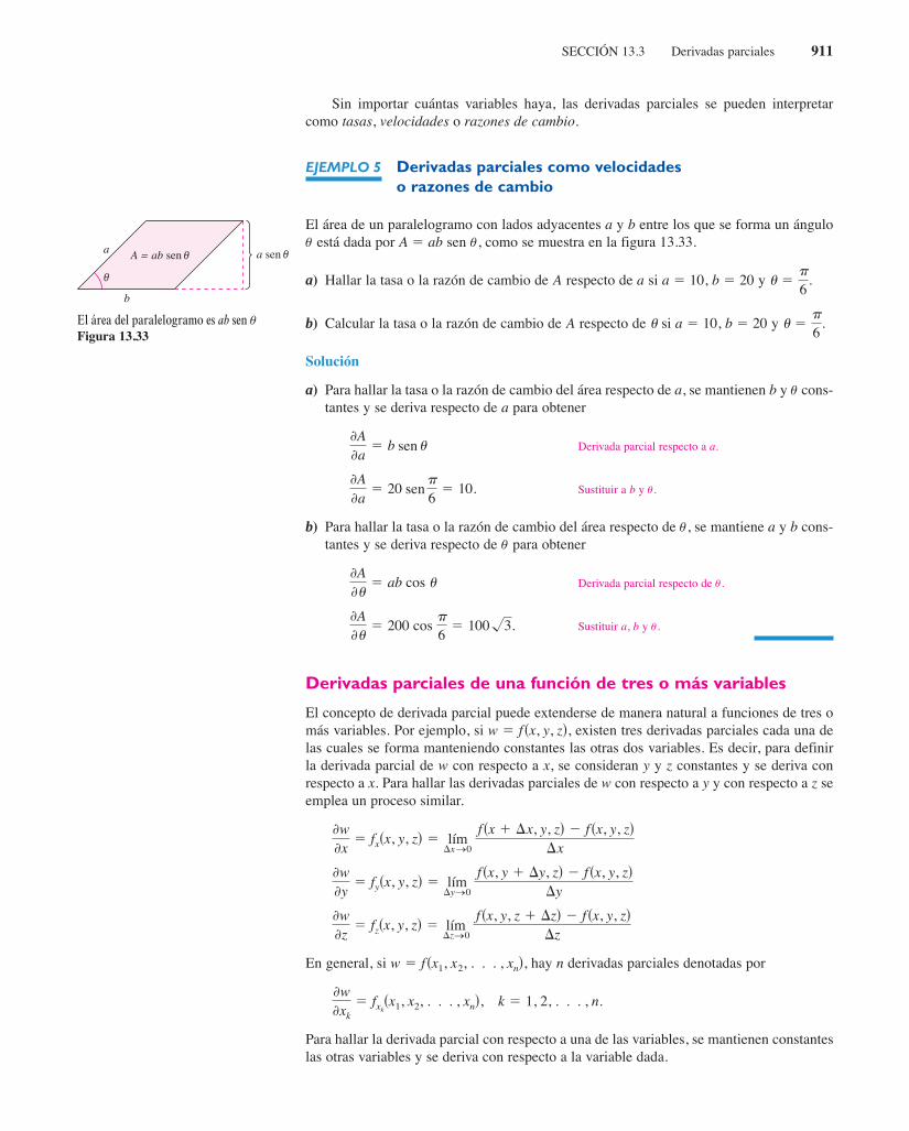
SECCIÓN 13.3 Derivadas parciales 911
Sin importar cuántas variables haya, las derivadas parciales se pueden interpretarcomo tasas, velocidades o razones de cambio.
EJEMPLO 5 Derivadas parciales como velocidadeso razones de cambio
El área de un paralelogramo con lados adyacentes a y b entre los que se forma un ánguloq está dada por A 5 ab sen q, como se muestra en la figura 13.33.
a) Hallar la tasa o la razón de cambio de respecto de si a 5 10, b 5 20 y
b) Calcular la tasa o la razón de cambio de respecto de si a 5 10, b 5 20 y
Solución
a) Para hallar la tasa o la razón de cambio del área respecto de a, se mantienen b y q cons-tantes y se deriva respecto de a para obtener
Derivada parcial respecto a a.
Sustituir a b y q.
b) Para hallar la tasa o la razón de cambio del área respecto de q, se mantiene a y b cons-tantes y se deriva respecto de q para obtener
Derivada parcial respecto de q.
Sustituir a, b y q.
Derivadas parciales de una función de tres o más variables
El concepto de derivada parcial puede extenderse de manera natural a funciones de tres omás variables. Por ejemplo, si existen tres derivadas parciales cada una delas cuales se forma manteniendo constantes las otras dos variables. Es decir, para definirla derivada parcial de w con respecto a x, se consideran y y z constantes y se deriva conrespecto a x. Para hallar las derivadas parciales de w con respecto a y y con respecto a z seemplea un proceso similar.
En general, si hay n derivadas parciales denotadas por
Para hallar la derivada parcial con respecto a una de las variables, se mantienen constanteslas otras variables y se deriva con respecto a la variable dada.
k 5 1, 2, . . . , n.wxk
5 fxksx1, x2, . . . , xnd,
w 5 fsx1, x2, . . . , xnd,
wz
5 fzsx, y, zd 5 limDz→0
f sx, y, z 1 Dzd 2 fsx, y, zdDz
wy
5 fysx, y, zd 5 limDy→0
f sx, y 1 Dy, zd 2 fsx, y, zdDy
wx
5 fxsx, y, zd 5 limDx→0
f sx 1 Dx, y, zd 2 fsx, y, zdDx
w 5 fsx, y, zd,
Au
5 200 cos p
65 100!3.
Au
5 ab cos u
Aa
5 20 sin p
65 10.
Aa
5 b sin u
u 5p
6.uA
u 5p
6.aA
a sena
b
θ
θA = ab sen θ
El área del paralelogramo es ab sen qFigura 13.33
sen
sen
lím
lím
lím
Larson-13-03.qxd 3/12/09 18:48 Page 911

912 CAPÍTULO 13 Funciones de varias variables
EJEMPLO 6 Hallar las derivadas parciales
a) Para hallar la derivada parcial de con respecto a se con-sideran y constantes y se obtiene
b) Para hallar la derivada parcial de f(x, y, z) 5 z sen(xy2 1 2z) con respecto a z, se con-sideran x y y constantes. Entonces, usando la regla del producto, se obtiene
c) Para calcular la derivada parcial de con respecto a seconsideran y y constantes y se obtiene
Derivadas parciales de orden superior
Como sucede con las derivadas ordinarias, es posible hallar las segundas, terceras, etc.,derivadas parciales de una función de varias variables, siempre que tales derivadas existan.Las derivadas de orden superior se denotan por el orden al que se hace la derivación. Porejemplo, la función tiene las siguientes derivadas parciales de segundo orden.
1. Derivar dos veces con respecto a
2. Derivar dos veces con respecto a
3. Derivar primero con respecto a y luego con respecto a
4. Derivar primero con respecto a y luego con respecto a
Los casos tercero y cuarto se llaman derivadas parciales mixtas (cruzadas).
x:y
y:x
y:
x:
z 5 fsx, yd
w3x 1 y 1 zw 4 5 2
x 1 y 1 zw2 .
zx,w,f sx, y, z, wd 5 sx 1 y 1 zdyw
5 2z cossxy2 1 2zd 1 sinsxy2 1 2zd.
5 szdfcossxy2 1 2zdgs2d 1 sinsxy2 1 2zd
zfz sinsxy2 1 2zdg 5 szd
zfsinsxy2 1 2zdg 1 sinsxy2 1 2zd
zfzg
zfxy 1 yz2 1 xzg 5 2yz 1 x.
yxz,fsx, y, zd 5 xy 1 yz2 1 xz
Observar que los dos tipos denotación para las derivadas parciales mixtas tienen convenciones diferentespara indicar el orden de derivación.
Orden de derecha aizquierda.
Orden de izquierda aderecha.
Se puede recordar el orden de ambas notaciones observando que primero sederiva con respecto a la variable más “cercana” a f. n
s fxdy 5 fxy
y 1fx 2 5
2fyx
NOTA
x 1fx 2 5
2fx2 5 fxx.
y 1fy 2 5
2fy2 5 fyy.
y 1fx 2 5
2fyx
5 fxy.
x 1fy 2 5
2fxy
5 fyx.
sen fsen sen
sen
sen
Larson-13-03.qxd 3/12/09 18:48 Page 912

SECCIÓN 13.3 Derivadas parciales 913
EJEMPLO 7 Hallar derivadas parciales de segundo orden
Hallar las derivadas parciales de segundo orden de y deter-minar el valor de
Solución Empezar por hallar las derivadas parciales de primer orden con respecto a x y y.
y
Después, se deriva cada una de éstas con respecto a x y con respecto a y.
y
y
En el valor de es
En el ejemplo 7 las dos derivadas parciales mixtas son iguales. En el teorema 13.3 se dancondiciones suficientes para que esto ocurra. n
El teorema 13.3 también se aplica a una función de tres o más variables siempre ycuando las derivadas parciales de segundo orden sean continuas. Por ejemplo, si
y todas sus derivadas parciales de segundo orden son continuas en unaregión abierta entonces en todo punto en el orden de derivación para obtener lasderivadas parciales mixtas de segundo orden es irrelevante. Si las derivadas parciales detercer orden de también son continuas, el orden de derivación para obtener las derivadasparciales mixtas de tercer orden es irrelevante.
EJEMPLO 8 Hallar derivadas parciales de orden superior
Mostrar que y para la función dada por
Solución
Derivadas parciales de primer orden:
Derivadas parciales de segundo orden (nótese que las dos primeras son iguales):
Derivadas parciales de tercer orden (nótese que las tres son iguales):
fzzxsx, y, zd 5 21z2fzxzsx, y, zd 5 2
1z2,fxzzsx, y, zd 5 2
1z2,
fzzsx, y, zd 5 2xz2fzxsx, y, zd 5
1z,fxzsx, y, zd 5
1z,
fzsx, y, zd 5xz
fxsx, y, zd 5 yex 1 ln z,
fsx, y, zd 5 yex 1 x ln z.
fxzz 5 fzxz 5 fzzxfxz 5 fzx
f
RR,w 5 fsx, y, zd
f
NOTA
fxys21, 2d 5 12 2 40 5 228.fxys21, 2d,
fyxsx, yd 5 6y 1 20xyfxysx, yd 5 6y 1 20xy
fyysx, yd 5 6x 1 10x2fxxsx, yd 5 10y2
fysx, yd 5 6xy 2 2 1 10x2yfxsx, yd 5 3y2 1 10xy2
fxys21, 2d.fsx, yd 5 3xy2 2 2y 1 5x2y2,
TEOREMA 13.3 IGUALDAD DE LAS DERIVADAS PARCIALES MIXTAS
Si es una función de y tal que y son continuas en un disco abierto entonces, para todo en
fxysx, yd 5 fyxsx, yd.
R,sx, ydR,fyxfxyyxf
Larson-13-03.qxd 3/12/09 18:48 Page 913
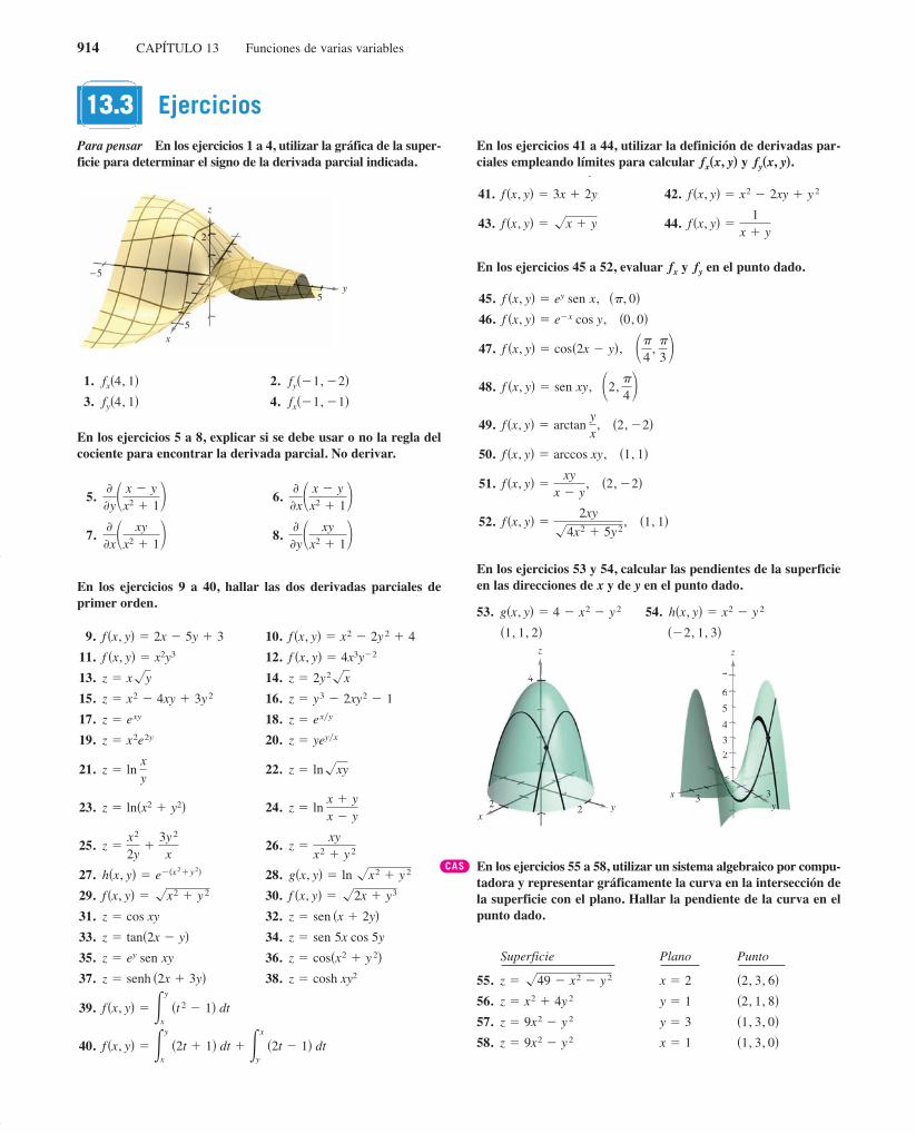
914 CAPÍTULO 13 Funciones de varias variables
Para pensar En los ejercicios 1 a 4, utilizar la gráfica de la super-ficie para determinar el signo de la derivada parcial indicada.
1. 2.
3. 4.
En los ejercicios 5 a 8, explicar si se debe usar o no la regla delcociente para encontrar la derivada parcial. No derivar.
En los ejercicios 9 a 40, hallar las dos derivadas parciales deprimer orden.
En los ejercicios 41 a 44, utilizar la definición de derivadas par-ciales empleando límites para calcular y
En los ejercicios 45 a 52, evaluar y en el punto dado.
En los ejercicios 53 y 54, calcular las pendientes de la superficieen las direcciones de x y de y en el punto dado.
53. 54.
En los ejercicios 55 a 58, utilizar un sistema algebraico por compu-tadora y representar gráficamente la curva en la intersección dela superficie con el plano. Hallar la pendiente de la curva en elpunto dado.
Superficie Plano Punto
55.
56.
57.
58. �1, 3, 0�x � 1z � 9x2 � y 2
�1, 3, 0�y � 3z � 9x2 � y 2
�2, 1, 8�y � 1z � x2 � 4y 2
�2, 3, 6�x � 2z � �49 � x2 � y 2
yx 3 3
7
6
4
3
5
2
z
yx
2
4
2
z
��2, 1, 3��1, 1, 2�h�x, y� � x2 � y 2g�x, y� � 4 � x2 � y 2
fyfx
fy�x, y�.fx�x, y�
fx��1, �1�fy�4, 1�fy��1, �2�fx�4, 1�
y
x
5
5
2
−5
z
1133..33 Ejercicios
5. 6.
7. 8.y
xyx2 1x
xyx2 1
xx yx2 1y
x yx2 1
9. 10.
11. 12.
13. 14.
15. 16.
17. 18.
19. 20.
21. 22.
23. 24.
25. 26.
27. 28.
29. 30.
31. 32.
33. 34.
35. 36.
37. 38.
39.
40. f x, yy
x
2t 1 dtx
y
2t 1 dt
f x, yy
x
t 2 1 dt
z cosh xy2z senh 2x 3y
z cos x2 y 2z ey sen xy
z sen 5x cos 5yz tan 2x y
z sen x 2yz cos xy
f x, y 2x y3f x, y x2 y 2
g x, y ln x2 y 2h x, y e x2 y2
zxy
x2 y 2zx2
2y3y 2
x
z ln x yx y
z ln x2 y2
z ln xyz ln xy
z yey xz x2e2y
z ex yz exy
z y3 2xy2 1z x2 4xy 3y 2
z 2y2 xz x y
f x, y 4x3y 2f x, y x2y3
f x, y x2 2y 2 4f x, y 2x 5y 3
41. 42.
43. 44. f x, y1
x yf x, y x y
f x, y x2 2xy y 2f x, y 3x 2y
y
45.
46.
47.
48.
49.
50.
51.
52. 1, 1f x, y2xy
4x2 5y 2,
2, 2f x, yxy
x y,
1, 1f x, y arccos xy,
2, 2f x, y arctan yx,
f x, y sen xy, 2, 4
f x, y cos 2x y , 4
, 3
f x, y e x cos y, 0, 0
f x, y ey sen x, , 0
CAS
Larson-13-03.qxd 26/2/10 14:19 Página 914

SECCIÓN 13.3 Derivadas parciales 915
En los ejercicios 59 a 64, calcular las derivadas parciales deprimer orden con respecto a x, y y z.
En los ejercicios 65 a 70, evaluar fx, fy y fz en el punto dado.
En los ejercicios 71 a 80, calcular las cuatro derivadas parcialesde segundo orden. Observar que las derivadas parciales mixtasde segundo orden son iguales.
En los ejercicios 81 a 88, para f(x, y), encontrar todos los valoresde x y y, tal que fx(x, y) = 0 y fy(x, y) = 0 simultáneamente.
En los ejercicios 89 a 92, utilizar un sistema algebraico por compu-tadora y hallar las derivadas parciales de primero y segundoorden de la función. Determinar si existen valores de x y y talesque y simultáneamente.
En los ejercicios 93 a 96, mostrar que las derivadas parcialesmixtas fxyy, fyxy y fyyx son iguales.
Ecuación de Laplace En los ejercicios 97 a 100, mostrar que lafunción satisface la ecuación de Laplace
97. 98.
99. z 5 ex sen y 100.
Ecuación de ondas En los ejercicios 101 a 104, mostrar que lafunción satisface la ecuación de ondas
101. z 5 sen(x 2 ct) 102.
103. 104. z 5 sen wct sen wx
Ecuación del calor En los ejercicios 105 y 106, mostrar que lafunción satisface la ecuación del calor
105. 106.
En los ejercicios 107 y 108, determinar si existe o no una funciónf(x, y) con las derivadas parciales dadas. Explicar el razona-miento. Si tal función existe, dar un ejemplo.
En los ejercicios 109 y 110, encontrar la primera derivada par-cial con respecto a x.
z 5 e2t sin xc
z 5 e2t cos xc
z /t 5 c2x2z /x2c.
z 5 lnsx 1 ctdz 5 coss4x 1 4ctd
2z /t 2 5 c2x2z /x2c.
z 5 arctan yx
z 512sey 2 e2ydsin xz 5 5xy
2z /x2 1 2z /y2 5 0.
fyxx, yc 5 0fxxx, yc 5 0
In Exercises 59–64, find the first partial derivatives with respectto and
59.
60.
61. 62.
63.
64.
In Exercises 65–70, evaluate and at the given point.
65.
66.
67.
68.
69.
70.
In Exercises 71–80, find the four second partial derivatives.Observe that the second mixed partials are equal.
71. 72.
73. 74.
75. 76.
77. 78.
79. 80.
In Exercises 81–88, for find all values of and suchthat and simultaneously.
81.
82.
83.
84.
85.
86.
87.
88.
In Exercises 89–92, use a computer algebra system to find thefirst and second partial derivatives of the function. Determinewhether there exist values of and such that and
simultaneously.
89. 90.
91. 92.
In Exercises 93–96, show that the mixed partial derivatives and are equal.
93.
94.
95.
96.
Laplace’s Equation In Exercises 97–100, show that the functionsatisfies Laplace’s equation
97. 98.
99. 100.
Wave Equation In Exercises 101–104, show that the functionsatisfies the wave equation
101. 102.
103. 104.
Heat Equation In Exercises 105 and 106, show that the functionsatisfies the heat equation
105. 106.
In Exercises 107 and 108, determine whether there exists a function with the given partial derivatives. Explain yourreasoning. If such a function exists, give an example.
107.
108.
In Exercises 109 and 110, find the first partial derivative withrespect to
109.
110. f x, y, z x senh yz
y2 2 y 1 z
f x, y, z tan y2z ez2 y 2 z
x.
fy x, y x 4yfx x, y 2x y,
fy x, y 2 sen 3x 2yfx x, y 3 sen 3x 2y ,
f x, y
z e t sen xc
z e t cos xc
z/ t c2 2z/ x2 .
z sen ct sen xz ln x ct
z cos 4x 4ctz sen x ct
2z/ t 2 c2 2z/ x2 .
z arctan yx
z ex sen y
z 12 ey e y sen xz 5xy
2z/ x2 1 2z/ y2 0.
f x, y, z2z
x y
f x, y, z e x sen yz
f x, y, z x2 3xy 4yz z3
f x, y, z xyz
fyyxfyxy,fxyy,
f x, yxy
x yf x, y ln
xx2 y2
f x, y 25 x2 y 2f x, y x sec y
fy x, y 0fx x, y 0yx
f x, y ln x2 y 2 1
f x, y ex2 xy y2
f x, y 3x3 12xy y3
f x, y1x
1y
xy
f x, y x2 xy y2
f x, y x2 4xy y 2 4x 16y 3
f x, y x2 xy y2 5x y
f x, y x2 xy y2 2x 2y
fy x, y 0fx x, y 0yxf x, y ,
z arctan yx
z cos xy
z 2xey 3ye xz ex tan y
z ln x yz x2 y 2
z x4 3x2y 2 y4z x2 2xy 3y 2
z x2 3y2z 3xy2
1, 2, 1f x, y, z 3x2 y2 2z2,
0, 2
, 4f x, y, z z sen x y ,
3, 1, 1f x, y, zxy
x y z,
f x, y, zxyz
, 1, 1, 1
2, 1, 2f x, y, z x2y3 2xyz 3yz,
f x, y, z x3yz2, 1, 1, 1
fzfy,fx,
G x, y, z1
1 x2 y 2 z 2
F x, y, z ln x2 y 2 z 2
w7xz
x yw x2 y 2 z2
f x, y, z 3x2y 5xyz 10yz 2
H x, y, z sen x 2y 3z
z.y,x,
13.3 Partial Derivatives 915
CAS
111. Let be a function of two variables and Describe theprocedure for finding the first partial derivatives.
112. Sketch a surface representing a function of two variablesand Use the sketch to give geometric interpretations of
and
113. Sketch the graph of a function whose derivativeis always negative and whose derivative is always
positive.
114. Sketch the graph of a function whose deriva-tives and are always positive.
115. If is a function of and such that and arecontinuous, what is the relationship between the mixedpartial derivatives? Explain.
fyxfxyyxf
fyfx
z f x, y
fyfx
z f x, y
f y.f xy.x
f
y.xf
WRITING ABOUT CONCEPTS
1053714_1303_pg 915.qxp 10/30/08 8:30 AM Page 915
Desarrollo de conceptos111. Sea f una función de dos variables x y y. Describir el proce-
dimiento para hallar las derivadas parciales de primer orden.
112. Dibujar una superficie que represente una función f de dosvariables x y y. Utilizar la gráfica para dar una interpre-tación geométrica de y
113. Dibujar la gráfica de una función cuya derivadasea siempre negativa y cuya derivada sea siempre po-
sitiva.
114. Dibujar la gráfica de una función cuyas deri-vadas y sean siempre positivas.
115. Si es una función de y tal que y son continuas,¿qué relación existe entre las derivadas parciales mixtas?Explicar.
fyxfxyyxf
fyfx
z 5 f sx, yd
fyfx
z 5 f sx, ydfyy.fyx
In Exercises 59–64, find the first partial derivatives with respectto and
59.
60.
61. 62.
63.
64.
In Exercises 65–70, evaluate and at the given point.
65.
66.
67.
68.
69.
70.
In Exercises 71–80, find the four second partial derivatives.Observe that the second mixed partials are equal.
71. 72.
73. 74.
75. 76.
77. 78.
79. 80.
In Exercises 81–88, for find all values of and suchthat and simultaneously.
81.
82.
83.
84.
85.
86.
87.
88.
In Exercises 89–92, use a computer algebra system to find thefirst and second partial derivatives of the function. Determinewhether there exist values of and such that and
simultaneously.
89. 90.
91. 92.
In Exercises 93–96, show that the mixed partial derivatives and are equal.
93.
94.
95.
96.
Laplace’s Equation In Exercises 97–100, show that the functionsatisfies Laplace’s equation
97. 98.
99. 100.
Wave Equation In Exercises 101–104, show that the functionsatisfies the wave equation
101. 102.
103. 104.
Heat Equation In Exercises 105 and 106, show that the functionsatisfies the heat equation
105. 106.
In Exercises 107 and 108, determine whether there exists a function with the given partial derivatives. Explain yourreasoning. If such a function exists, give an example.
107.
108.
In Exercises 109 and 110, find the first partial derivative withrespect to
109.
110. f x, y, z x senh yz
y2 2 y 1 z
f x, y, z tan y2z ez2 y 2 z
x.
fy x, y x 4yfx x, y 2x y,
fy x, y 2 sen 3x 2yfx x, y 3 sen 3x 2y ,
f x, y
z e t sen xc
z e t cos xc
z/ t c2 2z/ x2 .
z sen ct sen xz ln x ct
z cos 4x 4ctz sen x ct
2z/ t 2 c2 2z/ x2 .
z arctan yx
z ex sen y
z 12 ey e y sen xz 5xy
2z/ x2 1 2z/ y2 0.
f x, y, z2z
x y
f x, y, z e x sen yz
f x, y, z x2 3xy 4yz z3
f x, y, z xyz
fyyxfyxy,fxyy,
f x, yxy
x yf x, y ln
xx2 y2
f x, y 25 x2 y 2f x, y x sec y
fy x, y 0fx x, y 0yx
f x, y ln x2 y 2 1
f x, y ex2 xy y2
f x, y 3x3 12xy y3
f x, y1x
1y
xy
f x, y x2 xy y2
f x, y x2 4xy y 2 4x 16y 3
f x, y x2 xy y2 5x y
f x, y x2 xy y2 2x 2y
fy x, y 0fx x, y 0yxf x, y ,
z arctan yx
z cos xy
z 2xey 3ye xz ex tan y
z ln x yz x2 y 2
z x4 3x2y 2 y4z x2 2xy 3y 2
z x2 3y2z 3xy2
1, 2, 1f x, y, z 3x2 y2 2z2,
0, 2
, 4f x, y, z z sen x y ,
3, 1, 1f x, y, zxy
x y z,
f x, y, zxyz
, 1, 1, 1
2, 1, 2f x, y, z x2y3 2xyz 3yz,
f x, y, z x3yz2, 1, 1, 1
fzfy,fx,
G x, y, z1
1 x2 y 2 z 2
F x, y, z ln x2 y 2 z 2
w7xz
x yw x2 y 2 z2
f x, y, z 3x2y 5xyz 10yz 2
H x, y, z sen x 2y 3z
z.y,x,
13.3 Partial Derivatives 915
CAS
111. Let be a function of two variables and Describe theprocedure for finding the first partial derivatives.
112. Sketch a surface representing a function of two variablesand Use the sketch to give geometric interpretations of
and
113. Sketch the graph of a function whose derivativeis always negative and whose derivative is always
positive.
114. Sketch the graph of a function whose deriva-tives and are always positive.
115. If is a function of and such that and arecontinuous, what is the relationship between the mixedpartial derivatives? Explain.
fyxfxyyxf
fyfx
z f x, y
fyfx
z f x, y
f y.f xy.x
f
y.xf
WRITING ABOUT CONCEPTS
1053714_1303_pg 915.qxp 10/30/08 8:30 AM Page 915
sen
sen
Larson-13-03.qxd 3/12/09 18:48 Page 915

916 CAPÍTULO 13 Funciones de varias variables
117. Ingreso marginal Una corporación farmacéutica tiene dosplantas que producen la misma medicina. Si x1 y x2 son losnúmeros de unidades producidos en la planta 1 y en la planta 2,respectivamente, entonces el ingreso total del producto estádado por Cuandox1 = 4 y x2 = 12, encontrar a) el ingreso marginal para la plan-ta 1, y b) el ingreso marginal para la planta 2,
118. Costo marginal Una empresa fabrica dos tipos de estufas decombustión de madera: el modelo autoestable y el modelo parainserción en una chimenea. La función de costo para producirx estufas autoestables y y de inserción en una chimenea es
a) Calcular los costos marginales y cuandoy
b) Cuando se requiera producción adicional, ¿qué modelo deestufa hará incrementar el costo con una tasa más alta? ¿Có-mo puede determinarse esto a partir del modelo del costo?
119. Psicología Recientemente en el siglo xx se desarrolló una prue-ba de inteligencia llamada la Prueba de Stanford-Binet (másconocida como la prueba IQ). En esta prueba, una edad mentalindividual M es dividida entre la edad cronológica individual C,y el cociente es multiplicado por 100. El resultado es el IQ indi-vidual.
Encontrar las derivadas parciales de IQ con respecto a M y conrespecto a C. Evaluar las derivadas parciales en el punto (12, 10)e interpretar el resultado. (Fuente: Adaptado de Bernstein/Clark-Steward/Roy/Wickens, Psicología, 4a. ed.)
120. Productividad marginal Considerar la función de producciónde Cobb-Douglas Si x 5 1 000 y y 5 500,hallar a) la productividad marginal del trabajo, y b) laproductividad marginal del capital,
121. Para pensar Sea el número de aspirantes a una universi-dad, p el costo por alimentación y alojamiento en la universi-dad, y t el costo de la matrícula. N es una función de p y t talque y ¿Qué información se obtiene alsaber que ambas derivadas parciales son negativas?
122. Inversión El valor de una inversión de $1 000 al 6% deinterés compuesto anual es
donde I es la tasa anual de inflación y R es la tasa de impuestopara el inversor. Calcular y Determinar si la tasa de impuesto o la tasa de inflación es elmayor factor “negativo” sobre el crecimiento de la inversión.
123. Distribución de temperatura La temperatura en cualquierpunto de una placa de acero es donde y son medidos en metros. En el punto (2, 3), hallar elritmo de cambio de la temperatura respecto a la distancia reco-rrida en la placa en las direcciones del eje x y y.
124. Temperatura aparente Una medida de la percepción delcalor ambiental por unas personas promedio es el Índice detemperatura aparente. Un modelo para este índice es
donde es la temperatura aparente en grados Celsius, es latemperatura del aire y es la humedad relativa dada en formadecimal. (Fuente: The UMAP Journal)
a) Hallar y si y
b) ¿Qué influye más sobre A, la temperatura del aire o lahumedad? Explicar.
125. Ley de los gases ideales La ley de los gases ideales estableceque donde es la presión, es el volumen, es elnúmero de moles de gas, es una constante (la constante de losgases) y T es temperatura absoluta. Mostrar que
126. Utilidad marginal La función de utilidad es unamedida de la utilidad (o satisfacción) que obtiene una personapor el consumo de dos productos y Suponer que la funciónde utilidad es
a) Determinar la utilidad marginal del producto
b) Determinar la utilidad marginal del producto
c) Si y ¿se debe consumir una unidad más deproducto x o una unidad más de producto y? Explicar elrazonamiento.
d) Utilizar un sistema algebraico por computadora y represen-tar gráficamente la función. Interpretar las utilidades mar-ginales de productos x y y con una gráfica.
127. Modelo matemático En la tabla se muestran los consumosper cápita (en galones) de diferentes tipos de leche en EstadosUnidos desde 1999 hasta 2005. El consumo de leche light ydescremada, leche baja en grasa y leche entera se representapor las variables x, y y z, respectivamente. (Fuente: U.S. De-partment of Agriculture)
Un modelo para los datos está dado por
a) Hallar y
b) Interpretar las derivadas parciales en el contexto del problema.
zy
.zx
y 5 3,x 5 2
y.
x.
U 5 25x2 1 xy 2 3y 2.y.x
U 5 f sx, yd
TP
PV
VT
5 21.
RnVPPV 5 nRT,
h 5 0.80.t 5 308AyhAyt
htA
A 5 0.885t 2 22.4h 1 1.20th 2 0.544
yxT 5 500 2 0.6x2 2 1.5y2,sx, yd
VRs0.03, 0.28d.VIs0.03, 0.28d
Nyt < 0.Nyp < 0
N
fyy.
916 Chapter 13 Functions of Several Variables
117. Marginal Revenue A pharmaceutical corporation has twoplants that produce the same over-the-counter medicine. If and are the numbers of units produced at plant 1 and plant 2,respectively, then the total revenue for the product is given by
When and find (a) the marginal revenue for plant 1,and (b) the marginal revenue for plant 2,
118. Marginal Costs A company manufactures two types ofwood-burning stoves: a freestanding model and a fireplace-insert model. The cost function for producing freestandingand fireplace-insert stoves is
(a) Find the marginal costs and when and
(b) When additional production is required, which model ofstove results in the cost increasing at a higher rate? Howcan this be determined from the cost model?
119. Psychology Early in the twentieth century, an intelligence testcalled the Stanford-Binet Test (more commonly known as the IQtest) was developed. In this test, an individual’s mental age isdivided by the individual’s chronological age and the quotientis multiplied by 100. The result is the individual’s
Find the partial derivatives of with respect to and withrespect to Evaluate the partial derivatives at the point
and interpret the result. (Source: Adapted fromBernstein/Clark-Stewart/Roy/Wickens, Psychology, FourthEdition)
120. Marginal Productivity Consider the Cobb-Douglas produc-tion function When and
find (a) the marginal productivity of labor,and (b) the marginal productivity of capital,
121. Think About It Let be the number of applicants to auniversity, the charge for food and housing at the university,and the tuition. is a function of and such that
and What information is gained bynoticing that both partials are negative?
122. Investment The value of an investment of $1000 earning 6%compounded annually is
where is the annual rate of inflation and is the tax rate forthe person making the investment. Calculate and Determine whether the tax rate or the rateof inflation is the greater “negative” factor in the growth of theinvestment.
123. Temperature Distribution The temperature at any pointin a steel plate is where
and are measured in meters. At the point find the ratesof change of the temperature with respect to the distancesmoved along the plate in the directions of the and axes.
124. Apparent Temperature A measure of how hot weather feelsto an average person is the Apparent Temperature Index. Amodel for this index is
where is the apparent temperature in degrees Celsius, is theair temperature, and is the relative humidity in decimalform. (Source: The UMAP Journal)
(a) Find and when and
(b) Which has a greater effect on air temperature orhumidity? Explain.
125. Ideal Gas Law The Ideal Gas Law states that where is pressure, is volume, is the number of moles ofgas, is a fixed constant (the gas constant), and is absolutetemperature. Show that
126. Marginal Utility The utility function is ameasure of the utility (or satisfaction) derived by a personfrom the consumption of two products and Suppose theutility function is
(a) Determine the marginal utility of product
(b) Determine the marginal utility of product
(c) When and should a person consume onemore unit of product or one more unit of product Explain your reasoning.
(d) Use a computer algebra system to graph the function.Interpret the marginal utilities of products and graphically.
127. Modeling Data Per capita consumptions (in gallons) ofdifferent types of milk in the United States from 1999 through2005 are shown in the table. Consumption of flavored milk,plain reduced-fat milk, and plain light and skim milks are represented by the variables and respectively.(Source: U.S. Department of Agriculture)
A model for the data is given by
(a) Find and
(b) Interpret the partial derivatives in the context of the problem.
zy.
zx
z 0.92x 1.03y 0.02.
z,y,x,
yx
y?xy 3,x 2
y.
x.
U 5x2 xy 3y 2.y.x
U f x, y
TP
PV
VT
1.
TRnVP
PV nRT,
A,
h 0.80.t 30A hA t
htA
A 0.885t 22.4h 1.20th 0.544
y-x-
2, 3 ,yxT 500 0.6x2 1.5y2,x, y
VR 0.03, 0.28 .VI 0.03, 0.28
RI
V I, R 1 0001 0.06 1 R
1 I
10
N t < 0.N p < 0tpNt
pN
f y.f x,y 500,
x 1000f x, y 200x0.7y0.3.
12, 10C.
MIQ
IQ M, CMC
100
IQ.C
M
y 20.x 80C yC x
C 32 xy 175x 205y 1 050.
yx
R x2.R x1,x2 12,x1 4R 200x1 200x2 4x1
2 8x1x2 4x22.
x2
x1
116. Find the four second partial derivatives of the functiongiven by Show that the secondmixed partial derivatives and are equal.fyxfxy
f x, y sen x 2y .
CAPSTONE
Año 1999 2000 2001 2002 2003 2004 2005
x 1.4 1.4 1.4 1.6 1.6 1.7 1.7
y 7.3 7.1 7.0 7.0 6.9 6.9 6.9
z 6.2 6.1 5.9 5.8 5.6 5.5 5.6
CAS
1053714_1303.qxp 10/27/08 12:06 PM Page 916
f sx, yd 5 200x0.7y0.3.
y 5 20.x 5 80CyydsCyx
C 5 32!xy 1 175x 1 205y 1 1050.
916 Chapter 13 Functions of Several Variables
117. Marginal Revenue A pharmaceutical corporation has twoplants that produce the same over-the-counter medicine. If and are the numbers of units produced at plant 1 and plant 2,respectively, then the total revenue for the product is given by
When and find (a) the marginal revenue for plant 1,and (b) the marginal revenue for plant 2,
118. Marginal Costs A company manufactures two types ofwood-burning stoves: a freestanding model and a fireplace-insert model. The cost function for producing freestandingand fireplace-insert stoves is
(a) Find the marginal costs and when and
(b) When additional production is required, which model ofstove results in the cost increasing at a higher rate? Howcan this be determined from the cost model?
119. Psychology Early in the twentieth century, an intelligence testcalled the Stanford-Binet Test (more commonly known as the IQtest) was developed. In this test, an individual’s mental age isdivided by the individual’s chronological age and the quotientis multiplied by 100. The result is the individual’s
Find the partial derivatives of with respect to and withrespect to Evaluate the partial derivatives at the point
and interpret the result. (Source: Adapted fromBernstein/Clark-Stewart/Roy/Wickens, Psychology, FourthEdition)
120. Marginal Productivity Consider the Cobb-Douglas produc-tion function When and
find (a) the marginal productivity of labor,and (b) the marginal productivity of capital,
121. Think About It Let be the number of applicants to auniversity, the charge for food and housing at the university,and the tuition. is a function of and such that
and What information is gained bynoticing that both partials are negative?
122. Investment The value of an investment of $1000 earning 6%compounded annually is
where is the annual rate of inflation and is the tax rate forthe person making the investment. Calculate and Determine whether the tax rate or the rateof inflation is the greater “negative” factor in the growth of theinvestment.
123. Temperature Distribution The temperature at any pointin a steel plate is where
and are measured in meters. At the point find the ratesof change of the temperature with respect to the distancesmoved along the plate in the directions of the and axes.
124. Apparent Temperature A measure of how hot weather feelsto an average person is the Apparent Temperature Index. Amodel for this index is
where is the apparent temperature in degrees Celsius, is theair temperature, and is the relative humidity in decimalform. (Source: The UMAP Journal)
(a) Find and when and
(b) Which has a greater effect on air temperature orhumidity? Explain.
125. Ideal Gas Law The Ideal Gas Law states that where is pressure, is volume, is the number of moles ofgas, is a fixed constant (the gas constant), and is absolutetemperature. Show that
126. Marginal Utility The utility function is ameasure of the utility (or satisfaction) derived by a personfrom the consumption of two products and Suppose theutility function is
(a) Determine the marginal utility of product
(b) Determine the marginal utility of product
(c) When and should a person consume onemore unit of product or one more unit of product Explain your reasoning.
(d) Use a computer algebra system to graph the function.Interpret the marginal utilities of products and graphically.
127. Modeling Data Per capita consumptions (in gallons) ofdifferent types of milk in the United States from 1999 through2005 are shown in the table. Consumption of flavored milk,plain reduced-fat milk, and plain light and skim milks are represented by the variables and respectively.(Source: U.S. Department of Agriculture)
A model for the data is given by
(a) Find and
(b) Interpret the partial derivatives in the context of the problem.
zy.
zx
z 0.92x 1.03y 0.02.
z,y,x,
yx
y?xy 3,x 2
y.
x.
U 5x2 xy 3y 2.y.x
U f x, y
TP
PV
VT
1.
TRnVP
PV nRT,
A,
h 0.80.t 30A hA t
htA
A 0.885t 22.4h 1.20th 0.544
y-x-
2, 3 ,yxT 500 0.6x2 1.5y2,x, y
VR 0.03, 0.28 .VI 0.03, 0.28
RI
V I, R 1 0001 0.06 1 R
1 I
10
N t < 0.N p < 0tpNt
pN
f y.f x,y 500,
x 1000f x, y 200x0.7y0.3.
12, 10C.
MIQ
IQ M, CMC
100
IQ.C
M
y 20.x 80C yC x
C 32 xy 175x 205y 1 050.
yx
R x2.R x1,x2 12,x1 4R 200x1 200x2 4x1
2 8x1x2 4x22.
x2
x1
116. Find the four second partial derivatives of the functiongiven by Show that the secondmixed partial derivatives and are equal.fyxfxy
f x, y sen x 2y .
CAPSTONE
Año 1999 2000 2001 2002 2003 2004 2005
x 1.4 1.4 1.4 1.6 1.6 1.7 1.7
y 7.3 7.1 7.0 7.0 6.9 6.9 6.9
z 6.2 6.1 5.9 5.8 5.6 5.5 5.6
CAS
1053714_1303.qxp 10/27/08 12:06 PM Page 916
Para discusión116. Encontrar las cuatro segundas derivadas parciales de la fun-
ción dada por Mostrar que las se-gundas derivadas parciales mixtas fxy y fyx son iguales.
916 Chapter 13 Functions of Several Variables
117. Marginal Revenue A pharmaceutical corporation has twoplants that produce the same over-the-counter medicine. If and are the numbers of units produced at plant 1 and plant 2,respectively, then the total revenue for the product is given by
When and find (a) the marginal revenue for plant 1,and (b) the marginal revenue for plant 2,
118. Marginal Costs A company manufactures two types ofwood-burning stoves: a freestanding model and a fireplace-insert model. The cost function for producing freestandingand fireplace-insert stoves is
(a) Find the marginal costs and when and
(b) When additional production is required, which model ofstove results in the cost increasing at a higher rate? Howcan this be determined from the cost model?
119. Psychology Early in the twentieth century, an intelligence testcalled the Stanford-Binet Test (more commonly known as the IQtest) was developed. In this test, an individual’s mental age isdivided by the individual’s chronological age and the quotientis multiplied by 100. The result is the individual’s
Find the partial derivatives of with respect to and withrespect to Evaluate the partial derivatives at the point
and interpret the result. (Source: Adapted fromBernstein/Clark-Stewart/Roy/Wickens, Psychology, FourthEdition)
120. Marginal Productivity Consider the Cobb-Douglas produc-tion function When and
find (a) the marginal productivity of labor,and (b) the marginal productivity of capital,
121. Think About It Let be the number of applicants to auniversity, the charge for food and housing at the university,and the tuition. is a function of and such that
and What information is gained bynoticing that both partials are negative?
122. Investment The value of an investment of $1000 earning 6%compounded annually is
where is the annual rate of inflation and is the tax rate forthe person making the investment. Calculate and Determine whether the tax rate or the rateof inflation is the greater “negative” factor in the growth of theinvestment.
123. Temperature Distribution The temperature at any pointin a steel plate is where
and are measured in meters. At the point find the ratesof change of the temperature with respect to the distancesmoved along the plate in the directions of the and axes.
124. Apparent Temperature A measure of how hot weather feelsto an average person is the Apparent Temperature Index. Amodel for this index is
where is the apparent temperature in degrees Celsius, is theair temperature, and is the relative humidity in decimalform. (Source: The UMAP Journal)
(a) Find and when and
(b) Which has a greater effect on air temperature orhumidity? Explain.
125. Ideal Gas Law The Ideal Gas Law states that where is pressure, is volume, is the number of moles ofgas, is a fixed constant (the gas constant), and is absolutetemperature. Show that
126. Marginal Utility The utility function is ameasure of the utility (or satisfaction) derived by a personfrom the consumption of two products and Suppose theutility function is
(a) Determine the marginal utility of product
(b) Determine the marginal utility of product
(c) When and should a person consume onemore unit of product or one more unit of product Explain your reasoning.
(d) Use a computer algebra system to graph the function.Interpret the marginal utilities of products and graphically.
127. Modeling Data Per capita consumptions (in gallons) ofdifferent types of milk in the United States from 1999 through2005 are shown in the table. Consumption of flavored milk,plain reduced-fat milk, and plain light and skim milks are represented by the variables and respectively.(Source: U.S. Department of Agriculture)
A model for the data is given by
(a) Find and
(b) Interpret the partial derivatives in the context of the problem.
zy.
zx
z 0.92x 1.03y 0.02.
z,y,x,
yx
y?xy 3,x 2
y.
x.
U 5x2 xy 3y 2.y.x
U f x, y
TP
PV
VT
1.
TRnVP
PV nRT,
A,
h 0.80.t 30A hA t
htA
A 0.885t 22.4h 1.20th 0.544
y-x-
2, 3 ,yxT 500 0.6x2 1.5y2,x, y
VR 0.03, 0.28 .VI 0.03, 0.28
RI
V I, R 1 0001 0.06 1 R
1 I
10
N t < 0.N p < 0tpNt
pN
f y.f x,y 500,
x 1000f x, y 200x0.7y0.3.
12, 10C.
MIQ
IQ M, CMC
100
IQ.C
M
y 20.x 80C yC x
C 32 xy 175x 205y 1 050.
yx
R x2.R x1,x2 12,x1 4R 200x1 200x2 4x1
2 8x1x2 4x22.
x2
x1
116. Find the four second partial derivatives of the functiongiven by Show that the secondmixed partial derivatives and are equal.fyxfxy
f x, y sen x 2y .
CAPSTONE
Año 1999 2000 2001 2002 2003 2004 2005
x 1.4 1.4 1.4 1.6 1.6 1.7 1.7
y 7.3 7.1 7.0 7.0 6.9 6.9 6.9
z 6.2 6.1 5.9 5.8 5.6 5.5 5.6
CAS
1053714_1303.qxp 10/27/08 12:06 PM Page 916
In Exercises 59–64, find the first partial derivatives with respectto and
59.
60.
61. 62.
63.
64.
In Exercises 65–70, evaluate and at the given point.
65.
66.
67.
68.
69.
70.
In Exercises 71–80, find the four second partial derivatives.Observe that the second mixed partials are equal.
71. 72.
73. 74.
75. 76.
77. 78.
79. 80.
In Exercises 81–88, for find all values of and suchthat and simultaneously.
81.
82.
83.
84.
85.
86.
87.
88.
In Exercises 89–92, use a computer algebra system to find thefirst and second partial derivatives of the function. Determinewhether there exist values of and such that and
simultaneously.
89. 90.
91. 92.
In Exercises 93–96, show that the mixed partial derivatives and are equal.
93.
94.
95.
96.
Laplace’s Equation In Exercises 97–100, show that the functionsatisfies Laplace’s equation
97. 98.
99. 100.
Wave Equation In Exercises 101–104, show that the functionsatisfies the wave equation
101. 102.
103. 104.
Heat Equation In Exercises 105 and 106, show that the functionsatisfies the heat equation
105. 106.
In Exercises 107 and 108, determine whether there exists a function with the given partial derivatives. Explain yourreasoning. If such a function exists, give an example.
107.
108.
In Exercises 109 and 110, find the first partial derivative withrespect to
109.
110. f x, y, z x senh yz
y2 2 y 1 z
f x, y, z tan y2z ez2 y 2 z
x.
fy x, y x 4yfx x, y 2x y,
fy x, y 2 sen 3x 2yfx x, y 3 sen 3x 2y ,
f x, y
z e t sen xc
z e t cos xc
z/ t c2 2z/ x2 .
z sen ct sen xz ln x ct
z cos 4x 4ctz sen x ct
2z/ t 2 c2 2z/ x2 .
z arctan yx
z ex sen y
z 12 ey e y sen xz 5xy
2z/ x2 1 2z/ y2 0.
f x, y, z2z
x y
f x, y, z e x sen yz
f x, y, z x2 3xy 4yz z3
f x, y, z xyz
fyyxfyxy,fxyy,
f x, yxy
x yf x, y ln
xx2 y2
f x, y 25 x2 y 2f x, y x sec y
fy x, y 0fx x, y 0yx
f x, y ln x2 y 2 1
f x, y ex2 xy y2
f x, y 3x3 12xy y3
f x, y1x
1y
xy
f x, y x2 xy y2
f x, y x2 4xy y 2 4x 16y 3
f x, y x2 xy y2 5x y
f x, y x2 xy y2 2x 2y
fy x, y 0fx x, y 0yxf x, y ,
z arctan yx
z cos xy
z 2xey 3ye xz ex tan y
z ln x yz x2 y 2
z x4 3x2y 2 y4z x2 2xy 3y 2
z x2 3y2z 3xy2
1, 2, 1f x, y, z 3x2 y2 2z2,
0, 2
, 4f x, y, z z sen x y ,
3, 1, 1f x, y, zxy
x y z,
f x, y, zxyz
, 1, 1, 1
2, 1, 2f x, y, z x2y3 2xyz 3yz,
f x, y, z x3yz2, 1, 1, 1
fzfy,fx,
G x, y, z1
1 x2 y 2 z 2
F x, y, z ln x2 y 2 z 2
w7xz
x yw x2 y 2 z2
f x, y, z 3x2y 5xyz 10yz 2
H x, y, z sen x 2y 3z
z.y,x,
13.3 Partial Derivatives 915
CAS
111. Let be a function of two variables and Describe theprocedure for finding the first partial derivatives.
112. Sketch a surface representing a function of two variablesand Use the sketch to give geometric interpretations of
and
113. Sketch the graph of a function whose derivativeis always negative and whose derivative is always
positive.
114. Sketch the graph of a function whose deriva-tives and are always positive.
115. If is a function of and such that and arecontinuous, what is the relationship between the mixedpartial derivatives? Explain.
fyxfxyyxf
fyfx
z f x, y
fyfx
z f x, y
f y.f xy.x
f
y.xf
WRITING ABOUT CONCEPTS
1053714_1303_pg 915.qxp 10/30/08 8:30 AM Page 915
916 Chapter 13 Functions of Several Variables
117. Marginal Revenue A pharmaceutical corporation has twoplants that produce the same over-the-counter medicine. If and are the numbers of units produced at plant 1 and plant 2,respectively, then the total revenue for the product is given by
When and find (a) the marginal revenue for plant 1,and (b) the marginal revenue for plant 2,
118. Marginal Costs A company manufactures two types ofwood-burning stoves: a freestanding model and a fireplace-insert model. The cost function for producing freestandingand fireplace-insert stoves is
(a) Find the marginal costs and when and
(b) When additional production is required, which model ofstove results in the cost increasing at a higher rate? Howcan this be determined from the cost model?
119. Psychology Early in the twentieth century, an intelligence testcalled the Stanford-Binet Test (more commonly known as the IQtest) was developed. In this test, an individual’s mental age isdivided by the individual’s chronological age and the quotientis multiplied by 100. The result is the individual’s
Find the partial derivatives of with respect to and withrespect to Evaluate the partial derivatives at the point
and interpret the result. (Source: Adapted fromBernstein/Clark-Stewart/Roy/Wickens, Psychology, FourthEdition)
120. Marginal Productivity Consider the Cobb-Douglas produc-tion function When and
find (a) the marginal productivity of labor,and (b) the marginal productivity of capital,
121. Think About It Let be the number of applicants to auniversity, the charge for food and housing at the university,and the tuition. is a function of and such that
and What information is gained bynoticing that both partials are negative?
122. Investment The value of an investment of $1000 earning 6%compounded annually is
where is the annual rate of inflation and is the tax rate forthe person making the investment. Calculate and Determine whether the tax rate or the rateof inflation is the greater “negative” factor in the growth of theinvestment.
123. Temperature Distribution The temperature at any pointin a steel plate is where
and are measured in meters. At the point find the ratesof change of the temperature with respect to the distancesmoved along the plate in the directions of the and axes.
124. Apparent Temperature A measure of how hot weather feelsto an average person is the Apparent Temperature Index. Amodel for this index is
where is the apparent temperature in degrees Celsius, is theair temperature, and is the relative humidity in decimalform. (Source: The UMAP Journal)
(a) Find and when and
(b) Which has a greater effect on air temperature orhumidity? Explain.
125. Ideal Gas Law The Ideal Gas Law states that where is pressure, is volume, is the number of moles ofgas, is a fixed constant (the gas constant), and is absolutetemperature. Show that
126. Marginal Utility The utility function is ameasure of the utility (or satisfaction) derived by a personfrom the consumption of two products and Suppose theutility function is
(a) Determine the marginal utility of product
(b) Determine the marginal utility of product
(c) When and should a person consume onemore unit of product or one more unit of product Explain your reasoning.
(d) Use a computer algebra system to graph the function.Interpret the marginal utilities of products and graphically.
127. Modeling Data Per capita consumptions (in gallons) ofdifferent types of milk in the United States from 1999 through2005 are shown in the table. Consumption of flavored milk,plain reduced-fat milk, and plain light and skim milks are represented by the variables and respectively.(Source: U.S. Department of Agriculture)
A model for the data is given by
(a) Find and
(b) Interpret the partial derivatives in the context of the problem.
zy.
zx
z 0.92x 1.03y 0.02.
z,y,x,
yx
y?xy 3,x 2
y.
x.
U 5x2 xy 3y 2.y.x
U f x, y
TP
PV
VT
1.
TRnVP
PV nRT,
A,
h 0.80.t 30A hA t
htA
A 0.885t 22.4h 1.20th 0.544
y-x-
2, 3 ,yxT 500 0.6x2 1.5y2,x, y
VR 0.03, 0.28 .VI 0.03, 0.28
RI
V I, R 1 0001 0.06 1 R
1 I
10
N t < 0.N p < 0tpNt
pN
f y.f x,y 500,
x 1000f x, y 200x0.7y0.3.
12, 10C.
MIQ
IQ M, CMC
100
IQ.C
M
y 20.x 80C yC x
C 32 xy 175x 205y 1 050.
yx
R x2.R x1,x2 12,x1 4R 200x1 200x2 4x1
2 8x1x2 4x22.
x2
x1
116. Find the four second partial derivatives of the functiongiven by Show that the secondmixed partial derivatives and are equal.fyxfxy
f x, y sen x 2y .
CAPSTONE
Año 1999 2000 2001 2002 2003 2004 2005
x 1.4 1.4 1.4 1.6 1.6 1.7 1.7
y 7.3 7.1 7.0 7.0 6.9 6.9 6.9
z 6.2 6.1 5.9 5.8 5.6 5.5 5.6
CAS
1053714_1303.qxp 10/27/08 12:06 PM Page 916
1 050.
Larson-13-03.qxd 3/12/09 18:48 Page 916

Franjas de Moiré
SECCIÓN 13.3 Derivadas parciales 917
128. Modelo matemático La tabla muestra el gasto en atenciónpública médica (en miles de millones de dólares) en compen-sación a trabajadores x, asistencia pública y y seguro médico delEstado z, del año 2000 al 2005. (Fuente: Centers for Medicareand Medicaid Services)
Un modelo para los datos está dado por
a) Hallar y
b) Determinar la concavidad de las trazas paralelas al plano xz.Interpretar el resultado en el contexto del problema.
c) Determinar la concavidad de las trazas paralelas al plano yz.Interpretar el resultado en el contexto del problema.
¿Verdadero o falso? En los ejercicios 129 a 132, determinar si ladeclaración es verdadera o falsa. Si es falsa, explicar por qué odar un ejemplo que demuestre que es falsa.
129. Si y entonces
130. Si entonces
131. Si entonces
132. Si una superficie cilíndrica tiene rectas generatricesparalelas al eje y, entonces
133. Considerar la función definida por
a) Hallar y para
b) Utilizar la definición de derivadas parciales para hallary
Sugerencia:
c) Utilizar la definición de derivadas parciales para hallary
d) Utilizando el teorema 13.3 y el resultado del inciso c),indicar qué puede decirse acerca de fxy o fyx.
134. Sea Hallar y
135. Mostrar la función
a) Hallar fx(0, 0) y fy(0, 0).
b) Determinar los puntos (si los hay) en los que fx(x, y) ono existe.
136. Considerar la función Mostrar que
PARA MAYOR INFORMACIÓN Para más información sobre esteproblema, ver el artículo “A Classroom Note on a NaturallyOccurring Piecewise Defined Function” de Don Cohen enMathematics and Computer Education.
fxsx, yd 5 5 4x3sx2 1 y2d1y3,
0,
sx, yd Þ s0, 0d
sx, yd 5 s0, 0d.
f sx, yd 5 sx2 1 y2d2y3.
fysx, yd
f sx, yd 5 sx3 1 y3d1y3.
fysx, yd.fxsx, ydf sx, yd 5 Ey
x
!1 1 t3 dt.
fyxs0, 0d.fxys0, 0d
fxs0, 0d 5 limDx→0
f sDx, 0d 2 f s0, 0d
Dx.43
fys0, 0d.fxs0, 0d
sx, yd Þ s0, 0d.fysx, ydfxsx, yd
f sx, yd 5 5xysx2 2 y2d , x2 1 y2
0,
sx, yd Þ s0, 0d
sx, yd 5 s0, 0d.
zyy 5 0.z 5 f sx, yd
2zyx
5 sxy 1 1de xy.z 5 exy,
szyxd 1 szyyd 5 f9sxdgsyd 1 f sxdg9syd.z 5 f sxdgsyd,
z 5 csx 1 yd.zyx 5 zyy,z 5 f sx, yd
2zy2.
2zx2
Léase el artículo “Moiré Fringes and the Conic Sections” de MikeCullen en The College Mathematics Journal. El artículo describecómo dos familias de curvas de nivel dadas por
y
pueden formar franjas de Moiré. Después de leer el artículo, escribirun documento que explique cómo se relaciona la expresión
con las franjas de Moiré formadas por la intersección de las dosfamilias de curvas de nivel. Utilizar como ejemplo uno de los mo-delos siguientes.
fx
?gx
1fy
?gy
gsx, yd 5 bfsx, yd 5 a
Mik
e C
ulle
nM
ike
Cul
len
lím
13.3 Partial Derivatives 917
128. Modeling Data The table shows the public medical expenditures (in billions of dollars) for worker’s compensation
public assistance and Medicare from 2000 through 2005.(Source: Centers for Medicare and Medicaid Services)
A model for the data is given by
(a) Find and
(b) Determine the concavity of traces parallel to the plane.Interpret the result in the context of the problem.
(c) Determine the concavity of traces parallel to the plane.Interpret the result in the context of the problem.
True or False? In Exercises 129–132, determine whether thestatement is true or false. If it is false, explain why or give anexample that shows it is false.
129. If and then
130. If then
131. If then
132. If a cylindrical surface has rulings parallel to the axis, then
133. Consider the function defined by
(a) Find and for
(b) Use the definition of partial derivatives to find and
Hint:
(c) Use the definition of partial derivatives to find and
(d) Using Theorem 13.3 and the result of part (c), what can besaid about or
134. Let Find and
135. Consider the function
(a) Find and
(b) Determine the points (if any) at which or fails to exist.
136. Consider the function Show that
fx x, y4x
3 x2 y2 1 3,
0,
x, y 0, 0
x, y 0, 0.
f x, y x2 y2 2 3.
fy x, yfx x, y
fy 0, 0 .fx 0, 0
f x, y x3 y3 1 3.
fy x, y .fx x, yf x, yy
x
1 t3 dt.
fyx?fxy
fyx 0, 0 .fxy 0, 0
fx 0, 0 límx→0
f x, 0 f 0, 0
x.
fy 0, 0 .fx 0, 0
x, y 0, 0 .fy x, yfx x, y
f x, yxy x2 y2
, x2 y2
0,
x, y 0, 0
x, y 0, 0.
z y 0.y-z f x, y
2zy x
xy 1 e xy.z exy,
z x z y f x g y f x g y .z f x g y ,
z c x y .z x z y,z f x, y
yz-
xz-
2zy2.
2zx2
z 1.2225x2 0.0096y2 71.381x 4.121y 354.65.
zy,x,
Año 2000 2001 2002 2003 2004 2005
x 24.9 28.1 30.1 31.4 32.1 33.5
y 207.5 233.2 258.4 281.9 303.2 324.9
z 224.3 247.7 265.7 283.5 312.8 342.0
FOR FURTHER INFORMATION For more information about thisproblem, see the article “A Classroom Note on a Naturally OccurringPiecewise Defined Function” by Don Cohen in Mathematics andComputer Education.
Read the article “Moiré Fringes and the Conic Sections” by MikeCullen in The College Mathematics Journal. The article describeshow two families of level curves given by
and
can form Moiré patterns. After reading the article, write a paperexplaining how the expression
is related to the Moiré patterns formed by intersecting the twofamilies of level curves. Use one of the following patterns as anexample in your paper.
fx
gx
fy
gy
g x, y bf x, y a
Moiré Fringes
S E C T I O N P R O J E C T
Mik
e C
ulle
nM
ike
Cul
len
1053714_1303.qxp 10/27/08 12:06 PM Page 917
PROYECTO DE TRABAJO
Larson-13-03.qxd 3/12/09 18:48 Page 917

918 CAPÍTULO 13 Funciones de varias variables
13.4 Diferenciales
n Entender los conceptos de incrementos y diferenciales.n Extender el concepto de diferenciabilidad a funciones de dos variables.n Utilizar una diferencial como aproximación.
Incrementos y diferenciales
En esta sección se generalizan los conceptos de incrementos y diferenciales a funciones dedos o más variables. Recuérdese que en la sección 3.9, dada se definió la dife-rencial de y como
Terminología similar se usa para una función de dos variables, Es decir, yson los incrementos en x y en y, y el incremento en z está dado por
Esta definición puede extenderse a una función de tres o más variables. Por ejemplo,si entonces y la diferencial totalde w es
EJEMPLO 1 Hallar la diferencial total
Hallar la diferencial total de cada función.
a) z 5 2x sen y 2 3x2y2 b)
Solución
a) La diferencial total de z 5 2x sen y 2 3x2y2 es
Diferencial total .
b) La diferencial total de es
Diferencial total .
5 2x dx 1 2y dy 1 2z dz.
dwdw 5wx
dx 1wy
dy 1wz
dz
w 5 x2 1 y2 1 z2dw
5 s2 sin y 2 6xy2d dx 1 s2x cos y 2 6x2yd dy.
dzdz 5zx
dx 1zy
dy
dz
w 5 x2 1 y2 1 z2
dw 5wx
dx 1wy
dy 1wz
dz 1wu
du.
du 5 Du,dz 5 Dz,dy 5 Dy,dx 5 Dx,w 5 f sx, y, z, ud,
DyDxz 5 f sx, yd.
dy 5 f9sxd dx.
y 5 f sxd,
Incremento en .zDz 5 f sx 1 Dx, y 1 Dyd 2 f sx, yd.
DEFINICIÓN DE DIFERENCIAL TOTAL
Si y y son los incrementos en x y en y, entonces las diferencialesde las variables independientes x y y son
y
y la diferencial total de la variable dependiente z es
dz 5zx
dx 1zy
dy 5 fx sx, yd dx 1 fysx, yd dy.
dy 5 Dydx 5 Dx
DyDxz 5 f sx, yd
sen
Larson-13-04.qxd 3/12/09 18:52 Page 918

SECCIÓN 13.4 Diferenciales 919
Diferenciabilidad
En la sección 3.9 se vio que si una función dada por y 5 f(x) es diferenciable, se puede uti-lizar la diferencial como una aproximación (para pequeños) al valor
Cuando es válida una aproximación similar para una función dedos variables, se dice que la función es diferenciable. Esto se expresa explícitamente enla definición siguiente.
EJEMPLO 2 Mostrar que una función es diferenciable
Mostrar que la función dada por
es diferenciable en todo punto del plano.
Solución Haciendo el incremento de z en un punto arbitrario en elplano es
Incremento de .
donde y Como y cuando se sigue que fes diferenciable en todo punto en el plano. La gráfica de f se muestra en la figura 13.34.
Debe tenerse en cuenta que el término “diferenciable” se usa de manera diferente parafunciones de dos variables y para funciones de una variable. Una función de una variablees diferenciable en un punto si su derivada existe en el punto. Sin embargo, en el caso deuna función de dos variables, la existencia de las derivadas parciales y no garantizaque la función sea diferenciable (ver ejemplo 5). El teorema siguiente proporciona unacondición suficiente para la diferenciabilidad de una función de dos variables. En elapéndice A se da una demostración del teorema 13.4.
fyfx
sDx, Dyd → s0, 0d,«2 → 0«1 → 0«2 5 0.«1 5 Dx
5 fxsx, yd Dx 1 fysx, yd Dy 1 «1Dx 1 «2Dy
5 2xsDxd 1 3sDyd 1 DxsDxd 1 0sDyd
5 2xDx 1 Dx2 1 3Dy
5 sx2 1 2xDx 1 Dx2d 1 3sy 1 Dyd 2 sx2 1 3yd
zDz 5 f sx 1 Dx, y 1 Dyd 2 f sx, yd
sx, ydz 5 f sx, yd,
f sx, yd 5 x2 1 3y
Dy 5 f sx 1 Dxd 2 f sxd.Dxdy 5 f9sxd dx
y
x4
−4
4
1
z
Figura 13.34
DEFINICIÓN DE DIFERENCIABILIDAD
Una función dada por es diferenciable en si puede expre-sarse en la forma
donde y cuando La función es diferenciable en unaregión R si es diferenciable en todo punto de R.
fsDx, Dyd → s0, 0d.«2 → 0«1
Dz 5 fxsx0, y0d Dx 1 fysx0, y0d Dy 1 «1Dx 1 «2Dy
Dzsx0, y0dz 5 f sx, ydf
TEOREMA 13.4 CONDICIONES SUFICIENTES PARA LA DIFERENCIABILIDAD
Si es una función de y para la que y son continuas en una región abiertaentonces es diferenciable en R.fR,
fyfxy,xf
Larson-13-04.qxd 3/12/09 18:52 Page 919

sx 1 Dx, y 1 Dyd
920 CAPÍTULO 13 Funciones de varias variables
Aproximación mediante diferenciales
El teorema 13.4 dice que se puede elegir suficientemente cerca de (x, y)para hacer que e1Dx y e2Dy sean insignificantes. En otros términos, para Dx y Dy pequeños,se puede usar la aproximación
Esta aproximación se ilustra gráficamente en la figura 13.35. Hay que recordar que lasderivadas parciales y pueden interpretarse como las pendientes de la superfi-cie en las direcciones de x y de y. Esto significa que
representa el cambio en altura de un plano tangente a la superficie en el punto Como un plano en el espacio se representa mediante una ecuación lineal en las variables x,y y z, la aproximación de mediante se llama aproximación lineal. Se verá más acer-ca de esta interpretación geométrica en la sección 13.7.
EJEMPLO 3 Uso de la diferencial como una aproximación
Utilizar la diferencial dz para aproximar el cambio en cuando se desplaza del punto (1, 1) al punto (1.01, 0.97). Comparar esta aproximación con el cam-bio exacto en
Solución Se hace (x, y) = (1, 1) y (x + Dx, y + Dy) = (1.01, 0.97) y se obtiene dx =Dx = 0.01 y dy = Dy = –0.03. Por tanto, el cambio en z puede aproximarse mediante
Cuando y se tiene
En la figura 13.36 se puede ver que el cambio exacto corresponde a la diferencia entre lasalturas de dos puntos sobre la superficie de un hemisferio. Esta diferencia está dada por
Una función de tres variables se dice que es diferenciable en si
puede expresarse en la forma
donde y cuando Con esta definición de diferencia-bilidad, el teorema 13.4 puede extenderse de la siguiente manera a funciones de tres varia-bles: si es una función de x, y y donde y son continuas en una región abier-ta entonces es diferenciable en
En la sección 3.9 se utilizaron las diferenciales para aproximar el error de propagaciónintroducido por un error en la medida. Esta aplicación de las diferenciales se ilustra en elejemplo 4.
R.fR,fzfy ,fx ,f,z,f
sDx, Dy, Dzd → s0, 0, 0d.«3 → 0«2,«1,
Dw 5 fxDx 1 fyDy 1 fzDz 1 «1Dx 1 «2Dy 1 «3Dz
Dw 5 f sx 1 Dx, y 1 Dy, z 1 Dzd 2 f sx, y, zd
sx, y, zdw 5 f sx, y, zd
< 0.0137.5 !4 2 s1.01d2 2 s0.97d2 2 !4 2 12 2 12
Dz 5 f s1.01, 0.97d 2 f s1, 1d
< 0.0141.5 !2 s0.01d50.02!2
Dz < 21!2
s0.01d 21!2
s20.03d
y 5 1,x 5 1
52x
!4 2 x2 2 y2Dx 1
2y!4 2 x2 2 y2
Dy.5zx
dx 1zy
dyDz < dz
z.
sx, ydz 5 !4 2 x2 2 y2
dzDz
sx, y, f sx, ydd.
dz 5zx
Dx 1zy
Dy
zyyzyx
Dz < dz.
yx
∆z2
∆z1∆z
(x, y) (x + ∆x, y + ∆y)(x + ∆x, y)
dz
∂∂
∂
z
z
x
y∆y
∆x
∂
z
El cambio exacto en z es Este cambio puede aproximarse mediantela diferencial Figura 13.35
dz.
Dz.
x
y
z
(1, 1)(1.01, 0.97)
22
2
z = 4 − x2 − y2
f (x, y)f (x + ∆x, y + ∆y)
Cuando se desplaza de al puntoel valor de cambia
aproximadamente en 0.0137Figura 13.36
f sx, yds1.01, 0.97d,s1, 1dsx, yd
1.01 0.97 1 1
Larson-13-04.qxd 3/12/09 18:52 Page 920

SECCIÓN 13.4 Diferenciales 921
EJEMPLO 4 Análisis de errores
El error producido al medir cada una de las dimensiones de una caja rectangular es milímetros. Las dimensiones de la caja son centímetros, centímetros y
centímetros, como se muestra en la figura 13.37. Utilizar para estimar el errorpropagado y el error relativo en el volumen calculado de la caja.
Solución El volumen de la caja está dado por y por tanto
Utilizando 0.1 milímetros centímetros, se tiene y el errorpropagado es aproximadamente
5 2 050(60.01) 5 620.5 centímetros cúbicos.
Como el volumen medido es
centímetros cúbicos,
el error relativo, es aproximadamente
Como ocurre con una función de una sola variable, si una función de dos o más varia-bles es diferenciable en un punto, también es continua en él.
Sea diferenciable en donde Entonces
donde y cuando Sin embargo, por definición, se sabe que está dada por
Haciendo y se obtiene
Tomando el límite cuando se obtiene
lo cual significa que es continua en sx0, y0d.f
límx, y → x0, y0
f x, y f x0, y0
sx, yd → sx0, y0d,
5 f fxsx0, y0d 1 «1gsx 2 x0d 1 f fysx0, y0d 1 «2gsy 2 y0d.f sx, yd 2 f sx0, y0d 5 f fxsx0, y0d 1 «1g Dx 1 f fysx0, y0d 1 «2g Dy
y 5 y0 1 Dyx 5 x0 1 Dx
Dz 5 f sx0 1 Dx, y0 1 Dyd 2 f sx0, y0d.
DzsDx, Dyd → s0, 0d.«2 → 0«1
Dz 5 f fxsx0, y0d 1 «1g Dx 1 f fysx0, y0d 1 «2g Dy
z 5 f sx, yd.sx0, y0d,fDEMOSTRACIÓN
DVV
<dVV
520.5
15,000< 0.14%.
DVyV,
V 5 s50ds20ds15d 5 15,000
5 300s±0.01d 1 750s±0.01d 1 1000s±0.01d
dV 5 s20ds15ds±0.01d 1 s50ds15ds±0.01d 1 s50ds20ds±0.01d
dx 5 dy 5 dz 5 ±0.01,5 0.01
5 yz dx 1 xz dy 1 xy dz.
dV 5Vx
dx 1Vy
dy 1Vz
dz
V 5 xyz,
dVz 5 15y 5 20x 5 50
±0.1
x
y
50
20
20
x = 50
z = 15
y = 20
z
VolumenFigura 13.37
5 xyz
TEOREMA 13.5 DIFERENCIABILIDAD IMPLICA CONTINUIDAD
Si una función de x y y es diferenciable en entonces es continuaen sx0, y0d.
sx0, y0d,
1 000(±0.01)
Larson-13-04.qxd 3/12/09 18:53 Page 921

922 CAPÍTULO 13 Funciones de varias variables
Hay que recordar que la existencia de y no es suficiente para garantizar la dife-renciabilidad, como se ilustra en el siguiente ejemplo.
EJEMPLO 5 Una función que no es diferenciable
Mostrar que y existen, pero f no es diferenciable en (0, 0), donde f estádefinida como
Solución Para mostrar que f no es diferenciable en (0, 0) basta mostrar que no es con-tinua en este punto. Para ver que f no es continua en (0, 0), se observan los valores de f(x, y)a lo largo de dos trayectorias diferentes que se aproximan a (0, 0), como se muestra en lafigura 13.38. A lo largo de la recta el límite es
mientras que a lo largo de se tiene
Así, el límite de f(x, y) cuando no existe, y se puede concluir que f no escontinua en (0, 0). Por tanto, de acuerdo con el teorema 13.5, f no es diferenciable en (0, 0).Por otro lado, de acuerdo con la definición de las derivadas parciales y se tiene
Por tanto, las derivadas parciales en (0, 0) existen.
y
fy 0, 0 límy→0
f 0, y f 0, 0y
límy→0
0 0y
0.
fx 0, 0 límx→0
f x, 0 f 0, 0x
límx→0
0 0x
0
fy,fx
sx, yd → s0, 0d
límx, x → 0, 0
f x, y límx, x → 0, 0
3x2
2x2
32
.
y 5 2x
límx, x → 0, 0
f x, y límx, x → 0, 0
3x2
2x2
32
y 5 x,
fys0, 0dfxs0, 0d
fyfx
f(x, y) =
−3xy
x2 + y2, (x, y) ≠ (0, 0)
(x, y) = (0, 0)0,
A lo largo de la recta y = x,f(x, y) se aproxima o tiende a −3/2.
y
z
(0, 0, 0)
x
A lo largo de la recta y = −x,f(x, y) se aproxima o tiende a 3/2.
Figura 13.38
TECNOLOGÍA Utilizar unaherramienta de graficación pararepresentar la función del ejemplo 5.La gráfica mostrada abajo fuegenerada con Mathematica.
y
x
z
Generada con Mathematica
f x, y3xy
x2 y2, si x, y 0, 0
0, si x, y 0, 0.
Larson-13-04.qxd 3/12/09 18:53 Page 922

SECCIÓN 13.4 Diferenciales 923
En los ejercicios 1 a 10, hallar la diferencial total.
En los ejercicios 11 a 16, a) evaluar f(2, 1) y f(2.1, 1.05) y calcu-lar y b) usar el diferencial total dz para aproximar
En los ejercicios 17 a 20, hallar y utilizar la diferen-cial total para aproximar la cantidad.
25. Área El área del rectángulo sombreada en la figura es Los posibles errores en la longitud y la altura son y respectivamente. Hallar e identificar las regiones de la figu-ra cuyas áreas están dadas por los términos de ¿Qué regiónrepresenta la diferencia entre y
Figura para 25 Figura para 26
26. Volumen El volumen del cilindro circular recto de color rojo enla figura es Los posibles errores son y en elradio y en la altura, respectivamente. Hallar e identificar lossólidos de la figura cuyos volúmenes están dados por los términosde ¿Qué sólido representa la diferencia entre y
27. Análisis numérico Se construye un cono circular recto dealtura h = 8 y radio r = 4 y durante la medición se cometieronerrores en el radio y en la altura . Completar la tabla paramostrar la relación entre y para los errores indicados.
28. Análisis numérico La altura y radio de un cono circular rectomidieron h = 16 metros y r = 6 metros. En la medición, secometieron errores y . S es el área de la superficie lateralde un cono. Completar la tabla anterior para mostrar la relaciónentre y para los errores indicados.
29. Modelo matemático Los consumos per cápita (en galones) dediferentes tipos de leche en Estados Unidos de 1999 a 2005 semuestran en la tabla. El consumo de leche light y descremada,leche baja en grasas y leche entera se representa por las varia-bles x, y y z, respectivamente. (Fuente: U.S. Department ofAgriculture)
Un modelo para los datos está dado por z 5 20.92x 1 1.03y 10.02.
a) Hallar la diferencial total del modelo.
b) Se prevé en la industria lechera que en años futuros el consu-mo per cápita de leche light y descremada será de 1.9 ± 0.25galones y que el consumo per cápita de leche baja en grasasserá galones. Utilizar dz para estimar los máximoserrores de propagación y relativo en el pronóstico de consumode leche entera.
30. Coordenadas rectangulares a polares Un sistema de coorde-nadas rectangular se coloca sobre un mapa y las coordenadas deun punto de interés son (7.2, 2.5). Existe un posible error de 0.05en cada coordenada. Aproximar el máximo error posible almedir las coordenadas polares del punto.
7.5 ± 0.25
dSDS
DhDr
dVDVDhDr
dV?DVdV.
dVDh,DrV 5 pr 2h.
∆r
∆h∆h
h
l ∆l
dA?DAdA.
dADh,Dl
A 5 lh.
z 5 f xx, yc
Dz.Dz,
Desarrollo de conceptos21. Definir la diferencial total de una función de dos variables.
22. Describir el cambio en la exactitud de dz como aproxi-mación a cuando y aumentan.
23. ¿Qué se quiere decir con una aproximación lineal aen el punto
24. Cuando se usan diferenciales, ¿qué significan los términosde propagación y error relativo?
Psx0, y0d?z 5 f sx, yd
DyDxDz
13.4 Ejercicios
1. 2.
3. 4.
5. 6.
7. 8.
9. 10. w x2yz2 sen yzw 2z3y sen x
w ey cos x z2z ex sen y
z 12 ex2 y2
e x2 y2z x cos y y cos x
wx yz 3y
z1
x2 y2
zx2
yz 2x2y3
11. 12.
13. 14.
15. 16. f x, y x cos yf x, y yex
f x, yyx
f x, y 16 x2 y2
f x, y x2 y2f x, y 2x 3y
17.
18.
19.
20. sen 1.05 2 0.95 2 sen 12 12
1 3.05 2
5.95 2
1 32
62
5.05 2 3.1 2 52 32
2.01 2 9.02 22 9
r h
dVo
dSoS
Vo
S dS
V dV
0.1 0.1
0.1 0.1
0.001 0.002
0.0001 0.0002
Area The area of the shaded rectangle in the figure is The possible errors in the length and height are and respectively. Find and identify the regions in the figurewhose areas are given by the terms of What regionrepresents the difference between and
Figure for 25 Figure for 26
26. Volume The volume of the red right circular cylinder in thefigure is The possible errors in the radius and the height are and respectively. Find and identify thesolids in the figure whose volumes are given by the terms of What solid represents the difference between and
27. Numerical Analysis A right circular cone of height and radius is constructed, and in the process errors and are made in the radius and height, respectively.Complete the table to show the relationship between and for the indicated errors.
28. Numerical Analysis The height and radius of a right circularcone are measured as meters and meters. In theprocess of measuring, errors and are made. is the lateralsurface area of the cone. Complete the table above to show the relationship between and for the indicated errors.
29. Modeling Data Per capita consumptions (in gallons) ofdifferent types of plain milk in the United States from 1999through 2005 are shown in the table. Consumption of flavoredmilk, plain reduced-fat milk, and plain light and skim milks arerepresented by the variables and respectively. (Source:U.S. Department of Agriculture)
A model for the data is given by
(a) Find the total differential of the model.
(b) A dairy industry forecast for a future year is that per capitaconsumption of flavored milk will be gallons andthat per capita consumption of plain reduced-fat milk will be gallons. Use to estimate the maximum possible propagated error and relative error in the predictionfor the consumption of plain light and skim milks.
30. Rectangular to Polar Coordinates A rectangular coordinatesystem is placed over a map, and the coordinates of a point ofinterest are There is a possible error of 0.05 in eachcoordinate. Approximate the maximum possible error inmeasuring the polar coordinates of the point.
7.2, 2.5 .
dz7.5 ± 0.25
1.9 ± 0.25
z 0.92x 1.03y 0.02.
z,y,x,
dSS
Shrr 6h 16
dVVh
rr 4h 8
dV?VdV.
dVh,rV r 2h.
∆r
∆h∆h
h
l ∆l
dA?AdA.
dAh,l
A lh.
sen 1.05 2 0.95 2 sen 12 12
1 3.05 2
5.95 2
1 32
62
5.05 2 3.1 2 52 32
2.01 2 9.02 22 9
z f x, y
f x, y x cos yf x, y yex
f x, yyx
f x, y 16 x2 y2
f x, y x2 y2f x, y 2x 3y
z.dzz,
f 2.1, 1.05f 2, 1
w x2yz2 sen yzw 2z3y sen x
w ey cos x z2z ex sen y
z 12 ex2 y2
e x2 y2z x cos y y cos x
wx yz 3y
z1
x2 y2
zx2
yz 2x2y3
13.4 Differentials 923
13.4 Exercises See www.CalcChat.com for worked-out solutions to odd-numbered exercises.
21. Define the total differential of a function of two variables.
22. Describe the change in accuracy of as an approximationof as and increase.
23. What is meant by a linear approximation of atthe point
24. When using differentials, what is meant by the termspropagated error and relative error?
P x0, y0 ?z f x, y
yxzdz
WRITING ABOUT CONCEPTS
Año 1999 2000 2001 2002 2003 2004 2005
x 1.4 1.4 1.4 1.6 1.6 1.7 1.7
y 7.3 7.1 7.0 7.0 6.9 6.9 6.9
z 6.2 6.1 5.9 5.8 5.6 5.5 5.6
r h
dVo
dSoS
Vo
S dS
V dV
0.1 0.1
0.1 0.1
0.001 0.002
0.0001 0.0002
1053714_1304.qxp 10/27/08 12:07 PM Page 923
Larson-13-04.qxd 3/12/09 18:53 Page 923

r 5 2 ± 116
924 CAPÍTULO 13 Funciones de varias variables
31. Volumen El radio r y la altura h de un cilindro circular recto se miden con posibles errores de 4 y 2%, respectivamente. Apro-ximar el máximo error porcentual posible al medir el volu-men.
32. Área En un triángulo, dos lados adyacentes miden 3 y 4 pul-gadas de longitud, y entre ellos forman un ángulo de Los posibles errores de medición son pulgadas en loslados y 0.02 radianes en el ángulo. Aproximar el máximo errorposible al calcular el área.
33. Viento La fórmula para la frialdad producida por el viento C(en grados Fahrenheit) es
donde es la velocidad del viento en millas por hora y es latemperatura en grados Fahrenheit. La velocidad del viento es
millas por hora y la temperatura es Utilizar dCpara estimar el posible error propagado y el error relativo má-ximos al calcular la frialdad producida por el viento. (Fuente:National Oceanic and Atmospheric Administration)
34. Aceleración La aceleración centrípeta de una partícula que semueve en un círculo es donde es la velocidad y esel radio del círculo. Aproximar el error porcentual máximo almedir la aceleración debida a errores de 3% en y 2% en
35. Volumen Un abrevadero tiene 16 pies de largo (ver la figura).Sus secciones transversales son triángulos isósceles en los que losdos lados iguales miden 18 pulgadas. El ángulo entre los dos ladosiguales es
a) Expresar el volumen del abrevadero en función de y determinar el valor de para el que el volumen es má-ximo.
b) El error máximo en las mediciones lineales es de media pul-gada y el error máximo en la medida del ángulo es 2°.Aproximar el cambio a partir del volumen máximo.
Figura para 35 Figura para 36
36. Deportes Un jugador de béisbol en el jardín central se encuen-tra aproximadamente a 330 pies de una cámara de televisión queestá en la base. Un bateador golpea una pelota que sale hacia unavalla situada a una distancia de 420 pies de la cámara (ver lafigura).
a) La cámara gira 9° para seguir la carrera. Aproximar elnúmero de pies que el jugador central tiene que correr paraatrapar la pelota.
b) La posición del jugador central podría tener un error hasta de6 pies y el error máximo al medir la rotación de la cámarade 1°. Aproximar el máximo error posible en el resultado delinciso a).
37. Potencia La potencia eléctrica P está dada por P = E 2/R,donde E es el voltaje y R es la resistencia. Aproximar el máxi-mo error porcentual al calcular la potencia si se aplican 120volts a una resistencia de 2 000 ohms y los posibles errores por-centuales al medir E y R son 3 y 4%, respectivamente.
38. Resistencia La resistencia total R de dos resistencias conec-tadas en paralelo es
Aproximar el cambio en cuando incrementa de 10 ohms a10.5 ohms y decrece de 15 ohms a 13 ohms.
39. Inductancia La inductancia L (en microhenrys) de un hilorecto no magnético en el vacío es
donde es la longitud del hilo en milímetros y es el radio deuna sección transversal circular. Aproximar L cuando
milímetros y milímetros.40. Péndulo El periodo T de un péndulo de longitud L es
donde es la aceleración de la gravedad. Unpéndulo se lleva de la zona del canal, donde pies/s2,a Groenlandia, donde pies/s2. Debido al cambio en latemperatura, la longitud del péndulo cambia de 2.5 pies a 2.48pies. Aproximar el cambio en el periodo del péndulo.
En los ejercicios 41 a 44, mostrar que la función es diferen-ciable, hallando los valores de y que se dan en la defi-nición de diferenciabilidad y verificar que y cuando
41. 42.
43. 44.
En los ejercicios 45 y 46, utilizar la función para demostrar quea) y existen, y b) no es diferenciable en
45.
46.
47. Mostrar que si f(x, y) es diferenciable en (x0, y0), entonces f(x, y0)es diferenciable en x = x0. Usar este resultado para probar que
no es diferenciable en (0, 0).
31. Volume The radius and height of a right circular cylinderare measured with possible errors of 4% and 2%, respectively.Approximate the maximum possible percent error in measuringthe volume.
32. Area A triangle is measured and two adjacent sides are foundto be 3 inches and 4 inches long, with an included angle of The possible errors in measurement are inch for the sides and0.02 radian for the angle. Approximate the maximum possibleerror in the computation of the area.
33. Wind Chill The formula for wind chill (in degreesFahrenheit) is given by
where is the wind speed in miles per hour and is thetemperature in degrees Fahrenheit. The wind speed is miles per hour and the temperature is Use toestimate the maximum possible propagated error and relativeerror in calculating the wind chill. (Source: NationalOceanic and Atmospheric Administration)
34. Acceleration The centripetal acceleration of a particlemoving in a circle is where is the velocity and isthe radius of the circle. Approximate the maximum percenterror in measuring the acceleration due to errors of 3% in and2% in
35. Volume A trough is 16 feet long (see figure). Its cross sectionsare isosceles triangles with each of the two equal sides measuring18 inches. The angle between the two equal sides is
(a) Write the volume of the trough as a function of and determine the value of such that the volume is a maximum.
(b) The maximum error in the linear measurements is one-halfinch and the maximum error in the angle measure is Approximate the change in the maximum volume.
Figure for 35 Figure for 36
36. Sports A baseball player in center field is playing approxi-mately 330 feet from a television camera that is behind homeplate. A batter hits a fly ball that goes to the wall 420 feet fromthe camera (see figure).
(a) The camera turns to follow the play. Approximate thenumber of feet that the center fielder has to run to make thecatch.
(b) The position of the center fielder could be in error by asmuch as 6 feet and the maximum error in measuring therotation of the camera is Approximate the maximumpossible error in the result of part (a).
37. Power Electrical power is given by where isvoltage and is resistance. Approximate the maximum percenterror in calculating power if 120 volts is applied to a 2000-ohmresistor and the possible percent errors in measuring and are 3% and 4%, respectively.
38. Resistance The total resistance of two resistors connectedin parallel is given by
Approximate the change in as is increased from 10 ohmsto 10.5 ohms and is decreased from 15 ohms to 13 ohms.
39. Inductance The inductance (in microhenrys) of a straightnonmagnetic wire in free space is
where is the length of the wire in millimeters and is theradius of a circular cross section. Approximate when
millimeters and millimeters.
40. Pendulum The period of a pendulum of length iswhere is the acceleration due to gravity. A
pendulum is moved from the Canal Zone, where feetper second per second, to Greenland, where feet persecond per second. Because of the change in temperature, thelength of the pendulum changes from 2.5 feet to 2.48 feet.Approximate the change in the period of the pendulum.
In Exercises 41–44, show that the function is differentiable by finding values of and as designated in the definition of differentiability, and verify that both and as
41. 42.
43. 44.
In Exercises 45 and 46, use the function to show that andboth exist, but that is not differentiable at
45.
46.
47. Show that if is differentiable at then is differentiable at Use this result to prove that
is not differentiable at s0, 0d.f sx, yd 5 !x2 1 y2x 5 x0.
f sx, y0dsx0, y0d,f sx, yd
f sx, yd 5 5 5x2yx3 1 y3
,
0,
sx, yd Þ s0, 0d
sx, yd 5 s0, 0d
f sx, yd 5 5 3x2yx4 1 y2
,
0,
sx, yd Þ s0, 0d
sx, yd 5 s0, 0d
x0, 0c.ffyx0, 0cfxx0, 0c
f sx, yd 5 5x 2 10y 1 y3f sx, yd 5 x2y
f sx, yd 5 x2 1 y2f sx, yd 5 x2 2 2x 1 y
xDx, Dyc → x0, 0c.«2 → 0«1
«2«1
g 5 32.23g 5 32.09
gT 5 2p!Lyg ,LT
h 5 100 ± 1100r 5 2 ± 1
16
Lrh
L 5 0.000211ln 2hr
2 0.752
L
R2
R1R
1R
51R1
11
R2.
R
RE
REP 5 E2yR,P
18.
98
330 ft
420 ft
9°
18 in.
16 ft
θ18 in.
Not drawn to scale
28.
uu
u.
r.v
rva 5 v2yr,
dC88 ± 18.23 ± 3
Tv
C 5 35.74 1 0.6215T 2 35.75v0.16 1 0.4275Tv0.16
C
116
py4.
hr
924 Chapter 13 Functions of Several Variables
48. Consider the function
(a) Evaluate and
(b) Use the results of part (a) to calculate
(c) Use the total differential to approximate Compare your result with that of part (b).
Dz.dz
Dz.
f s3.05, 1.1d.f s3, 1df sx, yd 5 !x2 1 y2.
CAPSTONE
1053714_1304_pg 924.qxp 11/3/08 1:53 PM Page 924
f sx, yd 5 5 5x2yx3 1 y3
,
0,
sx, yd Þ s0, 0d
sx, yd 5 s0, 0d
f sx, yd 5 5 3x2yx4 1 y2
,
0,
sx, yd Þ s0, 0d
sx, yd 5 s0, 0d
x0, 0c.ffyx0, 0cfxx0, 0c
f sx, yd 5 5x 2 10y 1 y3f sx, yd 5 x2y
f sx, yd 5 x2 1 y2f sx, yd 5 x2 2 2x 1 y
xDx, Dyc → x0, 0c.«2 → 0«1
«2«1
g 5 32.23g 5 32.09
gT 5 2p!Lyg ,
h 5 100 ± 1100
rh
L 5 0.000211ln 2hr
2 0.752
R2
R1R
1R
51R1
11
R2.
330 pies
420 pies
9°
18 pulg
16 pies
θ18 pulg
No dibujado a escala
uu
u.
r.v
rva 5 v2yr,
88 ± 18.23 ± 3
Tv
C 5 35.74 1 0.6215T 2 35.75v0.16 1 0.4275Tv0.16
116
py4.
Para discusión48. Considerar la función
a) Evaluar f(3, 1) y f(3.05, 1.1).
b) Usar los resultados del inciso a) para calcular ∆z.
c) Usar la diferencial total dz para aproximar ∆z. Compararlos resultados con los del inciso b).
31. Volume The radius and height of a right circular cylinderare measured with possible errors of 4% and 2%, respectively.Approximate the maximum possible percent error in measuringthe volume.
32. Area A triangle is measured and two adjacent sides are foundto be 3 inches and 4 inches long, with an included angle of The possible errors in measurement are inch for the sides and0.02 radian for the angle. Approximate the maximum possibleerror in the computation of the area.
33. Wind Chill The formula for wind chill (in degreesFahrenheit) is given by
where is the wind speed in miles per hour and is thetemperature in degrees Fahrenheit. The wind speed is miles per hour and the temperature is Use toestimate the maximum possible propagated error and relativeerror in calculating the wind chill. (Source: NationalOceanic and Atmospheric Administration)
34. Acceleration The centripetal acceleration of a particlemoving in a circle is where is the velocity and isthe radius of the circle. Approximate the maximum percenterror in measuring the acceleration due to errors of 3% in and2% in
35. Volume A trough is 16 feet long (see figure). Its cross sectionsare isosceles triangles with each of the two equal sides measuring18 inches. The angle between the two equal sides is
(a) Write the volume of the trough as a function of and determine the value of such that the volume is a maximum.
(b) The maximum error in the linear measurements is one-halfinch and the maximum error in the angle measure is Approximate the change in the maximum volume.
Figure for 35 Figure for 36
36. Sports A baseball player in center field is playing approxi-mately 330 feet from a television camera that is behind homeplate. A batter hits a fly ball that goes to the wall 420 feet fromthe camera (see figure).
(a) The camera turns to follow the play. Approximate thenumber of feet that the center fielder has to run to make thecatch.
(b) The position of the center fielder could be in error by asmuch as 6 feet and the maximum error in measuring therotation of the camera is Approximate the maximumpossible error in the result of part (a).
37. Power Electrical power is given by where isvoltage and is resistance. Approximate the maximum percenterror in calculating power if 120 volts is applied to a 2000-ohmresistor and the possible percent errors in measuring and are 3% and 4%, respectively.
38. Resistance The total resistance of two resistors connectedin parallel is given by
Approximate the change in as is increased from 10 ohmsto 10.5 ohms and is decreased from 15 ohms to 13 ohms.
39. Inductance The inductance (in microhenrys) of a straightnonmagnetic wire in free space is
where is the length of the wire in millimeters and is theradius of a circular cross section. Approximate when
millimeters and millimeters.
40. Pendulum The period of a pendulum of length iswhere is the acceleration due to gravity. A
pendulum is moved from the Canal Zone, where feetper second per second, to Greenland, where feet persecond per second. Because of the change in temperature, thelength of the pendulum changes from 2.5 feet to 2.48 feet.Approximate the change in the period of the pendulum.
In Exercises 41–44, show that the function is differentiable by finding values of and as designated in the definition of differentiability, and verify that both and as
41. 42.
43. 44.
In Exercises 45 and 46, use the function to show that andboth exist, but that is not differentiable at
45.
46.
47. Show that if is differentiable at then is differentiable at Use this result to prove that
is not differentiable at s0, 0d.f sx, yd 5 !x2 1 y2x 5 x0.
f sx, y0dsx0, y0d,f sx, yd
f sx, yd 5 5 5x2yx3 1 y3
,
0,
sx, yd Þ s0, 0d
sx, yd 5 s0, 0d
f sx, yd 5 5 3x2yx4 1 y2
,
0,
sx, yd Þ s0, 0d
sx, yd 5 s0, 0d
x0, 0c.ffyx0, 0cfxx0, 0c
f sx, yd 5 5x 2 10y 1 y3f sx, yd 5 x2y
f sx, yd 5 x2 1 y2f sx, yd 5 x2 2 2x 1 y
xDx, Dyc → x0, 0c.«2 → 0«1
«2«1
g 5 32.23g 5 32.09
gT 5 2p!Lyg ,LT
h 5 100 ± 1100r 5 2 ± 1
16
Lrh
L 5 0.000211ln 2hr
2 0.752
L
R2
R1R
1R
51R1
11
R2.
R
RE
REP 5 E2yR,P
18.
98
330 ft
420 ft
9°
18 in.
16 ft
θ18 in.
Not drawn to scale
28.
uu
u.
r.v
rva 5 v2yr,
dC88 ± 18.23 ± 3
Tv
C 5 35.74 1 0.6215T 2 35.75v0.16 1 0.4275Tv0.16
C
116
py4.
hr
924 Chapter 13 Functions of Several Variables
48. Consider the function
(a) Evaluate and
(b) Use the results of part (a) to calculate
(c) Use the total differential to approximate Compare your result with that of part (b).
Dz.dz
Dz.
f s3.05, 1.1d.f s3, 1df sx, yd 5 !x2 1 y2.
CAPSTONE
1053714_1304_pg 924.qxp 11/3/08 1:53 PM Page 924
r 5 2 ± 116
Larson-13-04.qxd 3/12/09 18:53 Page 924

SECCIÓN 13.5 Regla de la cadena para funciones de varias variables 925
13.5 Regla de la cadena para funciones de varias variables
n Utilizar la regla de la cadena para funciones de varias variables.n Hallar las derivadas parciales implícitamente.
Regla de la cadena para funciones de varias variables
El trabajo con diferenciales de la sección anterior proporciona las bases para la extensiónde la regla de la cadena a funciones de dos variables. Hay dos casos: el primer caso cuan-do w es una función de x y y, donde x y y son funciones de una sola variable indepen-diente t. (La demostración de este teorema se da en el apéndice A.)
EJEMPLO 1 Regla de la cadena con una variable independiente
Sea donde x 5 sen t y Hallar cuando
Solución De acuerdo con la regla de la cadena para una variable independiente, se tiene
Cuando se sigue que
La regla de la cadena presentada en esta sección proporciona técnicas alternativas pararesolver muchos problemas del cálculo de una sola variable. Así, en el ejemplo 1, sepodrían haber usado técnicas para una sola variable para encontrar dw/dt expresandoprimero w como función de t,
y derivando después como de costumbre.
dwdt
5 22.
t 5 0,
t 5 0.dwydty 5 et.w 5 x2y 2 y2,
w
x y
t t
dxdt
∂w∂x
∂w∂y
dydt
Regla de la cadena: una variable depen-diente w, es función de x y y las que a su vezson funciones de t. Este diagrama represen-ta la derivada de w con respecto a tFigura 13.39
TEOREMA 13.6 REGLA DE LA CADENA: UNA VARIABLE INDEPENDIENTE
Sea donde es una función derivable de y Si y donde y son funciones derivables de entonces w es una función diferenciable de
y
Ver figura 13.39.dwdt
5wx
dxdt
1wy
dydt
.
t,t,hg
y 5 hstd,x 5 gstdy.xfw 5 f sx, yd,
2et sen t cos t et sen2 t 2e2t.
2 sen t et cos t sen2 t 2et et
2xy cos t x2 2y et
dwdt
wx
dxdt
wy
dydt
et sen2 t e2t
sen t 2 et et 2
w x2y y2
dwdt
2et sen t cos t et sen2 t 2e2t
Larson-13-05.qxd 3/12/09 18:56 Page 925

926 CAPÍTULO 13 Funciones de varias variables
La regla de la cadena en el teorema 13.6 puede extenderse a cualquier número de va-riables. Por ejemplo, si cada es una función derivable de una sola variable t, entoncespara
se tiene
EJEMPLO 2 Aplicación de la regla de la cadena a velocidades o ritmos de cambio relacionados
Dos objetos recorren trayectorias elípticas dadas por las ecuaciones paramétricas siguientes.
y Primer objeto.
y Segundo objeto.
¿A qué velocidad o ritmo cambia la distancia entre los dos objetos cuando
Solución En la figura 13.40 se puede ver que la distancia s entre los dos objetos está dadapor
y que cuando se tiene y
Cuando las derivadas parciales de s son las siguientes.
Cuando las derivadas de x1, y1, x2 y y2 son
Por tanto, usando la regla de la cadena apropiada, se sabe que la distancia cambia a unavelocidad o ritmo
5225
.
5 12452s0d 1 12
352s22d 1 14
52s4d 1 1352s0d
dsdt
5sx1
dx1
dt1
sy1
dy1
dt1
sx2
dx2
dt1
sy2
dy2
dt
dx2
dt5 4 cos 2t 5 4
dy2
dt5 26 sin 2t 5 0.
dx1
dt5 24 sin t 5 0
dy1
dt5 2 cos t 5 22
t 5 p,
sy2
5sy2 2 y1d
!sx2 2 x1d2 1 sy2 2 y1d25
15
s3 2 0d 535
sx2
5sx2 2 x1d
!sx2 2 x1d2 1 sy2 2 y1d25
15
s0 1 4d 545
sy1
52sy2 2 y1d
!sx2 2 x1d2 1 sy2 2 y1d25 2
15
s3 2 0d 5 235
sx1
52sx2 2 x1d
!sx2 2 x1d2 1 sy2 2 y1d25 2
15
s0 1 4d 5 245
t 5 p,
s 5 !s0 1 4d2 1 s3 2 0d2 5 5.
y2 5 3,x2 5 0,y1 5 0,x1 5 24,t 5 p,
s 5 !sx2 2 x1d2 1 sy2 2 y1d2
t 5 p?
y2 5 3 cos 2tx2 5 2 sin 2t
y1 5 2 sin tx1 5 4 cos t
dwdt
5wx1
dx1
dt1
wx2
dx2
dt1 . . . 1
wxn
dxn
dt.
w 5 f sx1, x2, . . . , xnd
xi
x
2
4
4
−2
−2
−4
−4
s
t = π3
y
x
2
4
4
−2
−2
−4
−4
s
t = π2
y
x
4
4
−2
−4
−4
s
t = π
y
Trayectorias de dos objetos que recorrenórbitas elípticasFigura 13.40
sen
sen
sen
sen
Larson-13-05.qxd 3/12/09 18:56 Page 926

SECCIÓN 13.5 Regla de la cadena para funciones de varias variables 927
En el ejemplo 2, obsérvese que s es función de cuatro variables intermedias, y1, x2y y2, cada una de las cuales es a su vez función de una sola variable Otro tipo de funcióncompuesta es aquella en la que las variables intermedias son, a su vez, funciones de másde una variable. Por ejemplo, si donde y se sigue quew es función de y y se pueden considerar las derivadas parciales de w con respecto a sy t. Una manera de encontrar estas derivadas parciales es expresar w explícitamente comofunción de s y t sustituyendo las ecuaciones y en la ecuación
Así se pueden encontrar las derivadas parciales de la manera usual, como semuestra en el ejemplo siguiente.
EJEMPLO 3 Hallar derivadas parciales por sustitución
Hallar y para donde y
Solución Se comienza por sustituir y en la ecuación paraobtener
Después, para encontrar se mantiene constante y se deriva con respecto a
De manera similar, para hallar , se mantiene constante y se deriva con respecto a para obtener
El teorema 13.7 proporciona un método alternativo para hallar las derivadas parciales delejemplo 3, sin expresar w explícitamente como función de y
Para obtener ∂w/∂s, se mantiene constante t y se aplica el teorema 13.6para obtener el resultado deseado. De manera similar, para obtener ∂w/∂t se mantieneconstante s y se aplica el teorema 13.6.
La regla de la cadena en este teorema se muestra esquemáticamente en la figura 13.41. nNOTA
DEMOSTRACIÓN
t.s
52st2 2 2s3
t2 .
5 212s3 1 st2
t2 2
wt
5 212s3
t2 1 s2
tswyt
56s2 1 2t2
t
ws
5 213s2
t1 t2
s.twys,
5 21s3
t1 st2.5 2ss2 1 t2d1s
t2w 5 2xy
w 5 2xyy 5 sytx 5 s2 1 t2
y 5 syt.x 5 s2 1 t2w 5 2xy,wytwys
w 5 f sx, yd.y 5 hss, tdx 5 gss, td
t,sy 5 hss, td,x 5 gss, tdw 5 f sx, yd,
t.x1,
∂∂y
s
wy∂
y
t∂y∂
∂w
wx∂
∂∂x
s
x
t∂∂x
∂
stst
La regla de la cadena: dos variables independientesFigura 13.41
TEOREMA 13.7 REGLA DE LA CADENA: DOS VARIABLES INDEPENDIENTES
Sea w 5 f(x, y), donde f es una función diferenciable de x y y. Si x 5 g(s, t) yson tales que las derivadas parciales de primer orden ∂x/∂s, ∂x/∂t, ∂y/∂s y ∂y/∂t existen,entonces y existen y están dadas por
ywt
5wx
xt
1wy
yt
.ws
5wx
xs
1wy
ys
wytwys
y 5 hss, td
Larson-13-05.qxd 3/12/09 18:56 Page 927

928 CAPÍTULO 13 Funciones de varias variables
EJEMPLO 4 Regla de la cadena con dos variables independientes
Utilizar la regla de la cadena para encontrar y , dada
donde y
Solución Nótese que estas mismas derivadas parciales fueron calculadas en el ejemplo3. Esta vez, usando el teorema 13.7, se puede mantener constante t y derivar con respectoa s para obtener
Sustituir y por y x por .
De manera similar, manteniendo s constante se obtiene
Sustituir y por y x por .
La regla de la cadena del teorema 13.7 también puede extenderse a cualquier númerode variables. Por ejemplo, si w es una función diferenciable de n variables donde cada es una función diferenciable de m variables entonces para
se obtiene lo siguiente.
wtm
5wx1
x1
tm1
wx2
x2
tm1 . . . 1
wxn
xn
tm
:
wt2
5wx1
x1
t21
wx2
x2
t21 . . . 1
wxn
xn
t2
wt1
5wx1
x1
t11
wx2
x2
t11 . . . 1
wxn
xn
t1
w 5 f sx1, x2, . . . , xnd
t1, t2, . . . , tm,xi
x1, x2, . . . , xn,
52st2 2 2s3
t2.
54st2 2 2s3 2 2st2
t2
5 4s 22s3 1 2st2
t2
s2 1 t2ssytd5 21st2s2td 1 2ss2 1 t2d12s
t2 2
5 2ys2td 1 2x12st2 2
wt
5wx
xt
1wy
yt
56s2 1 2t2
t.
54s2
t1
2s2 1 2t2
t
s2 1 t2ssytd5 21st2s2sd 1 2ss2 1 t2d11
t 2
5 2ys2sd 1 2x11t 2
ws
5wx
xs
1wy
ys
y 5 syt.x 5 s2 1 t2
w 5 2xy
wytwys
st
s2 t2+
st
s2 t2+
Larson-13-05.qxd 3/12/09 18:56 Page 928

SECCIÓN 13.5 Regla de la cadena para funciones de varias variables 929
EJEMPLO 5 Regla de la cadena para una función de tres variables
Hallar y si y , dada la función
donde y 5 s sen t y
Solución Por extensión del teorema 13.7, se tiene
Cuando y se tiene y 5 0 y Así,Y
y si y se sigue que
Derivación o diferenciación parcial implícita
Esta sección concluye con una aplicación de la regla de la cadena para determinar laderivada de una función definida implícitamente. Supóngase que x y y están relacionadaspor la ecuación donde se supone que es función derivable de Parahallar se podría recurrir a las técnicas vistas de la sección 2.5. Sin embargo, se veráque la regla de la cadena proporciona una útil alternativa. Si se considera la función dadapor
se puede aplicar el teorema 13.6 para obtener
Como para toda en el dominio de se sabe que y se tiene
Ahora, si se puede usar el hecho de que para concluir que
Un procedimiento similar puede usarse para encontrar las derivadas parciales de funcionesde varias variables definidas implícitamente.
dydx
5 2Fx sx, ydFy sx, yd
.
dxydx 5 1Fysx, yd Þ 0,
Fxsx, yd dxdx
1 Fy sx, yd dydx
5 0.
dwydx 5 0f,xw 5 Fsx, yd 5 0
dwdx
5 Fxsx, yd dxdx
1 Fy sx, yd dydx
.
w 5 Fsx, yd 5 Fsx, f sxdd
dyydx,x.y 5 f sxdFsx, yd 5 0,
5 2 1 2p.
wt
5 s0 1 2pds0d 1 s1 1 2pds1d 1 s0 1 1ds1d
t 5 2p,s 5 1
5 sy 1 zds2s sin td 1 sx 1 zdss cos td 1 sy 1 xds1d
wt
5wx
xt
1wy
yt
1wz
zt
z 5 2p.x 5 1,t 5 2p,s 5 1
5 sy 1 zdscos td 1 sx 1 zdssin td.
5 sy 1 zdscos td 1 sx 1 zdssin td 1 sy 1 xds0d
ws
5wx
xs
1wy
ys
1wz
zs
z 5 t.x 5 s cos t,
w 5 xy 1 yz 1 xz
t 5 2ps 5 1wytwys
sen
sen
sen
wys 5 s0 1 2pds1d 1s1 1 2pds0d 5 2p.
Larson-13-05.qxd 3/12/09 18:56 Page 929

930 CAPÍTULO 13 Funciones de varias variables
Este teorema puede extenderse a funciones diferenciables definidas implícitamente decualquier número de variables.
EJEMPLO 6 Hallar una derivada implícitamente
Hallar dada la ecuación
Solución Se comienza por definir una función
Después, usando el teorema 13.8, se tiene
y
por lo que
Comparar la solución del ejemplo 6 con la solución del ejemplo 2 en la sección2.5. n
EJEMPLO 7 Hallar derivadas parciales implícitamente
Encontrar y dada la ecuación
Solución Para aplicar el teorema 13.8, sea
Entonces
con lo que
zy
5 2Fysx, y, zdFz sx, y, zd 5
2x2y 2 3z3x2 1 6z2 1 3y
.
zx
5 2Fxsx, y, zdFzsx, y, zd 5
2xy2 2 6xz3x2 1 6z2 1 3y
Fzsx, y, zd 5 3x2 1 6z2 1 3y
Fysx, y, zd 5 22x2y 1 3z
Fxsx, y, zd 5 6xz 2 2xy2
Fsx, y, zd 5 3x2z 2 x2y2 1 2z3 1 3yz 2 5.
3x2z 2 x2y2 1 2z3 1 3yz 2 5 5 0.zyy,zyx
NOTA
dydx
5 2Fxsx, ydFysx, yd 5
2s22xd3y2 1 2y 2 5
52x
3y2 1 2y 2 5.
Fysx, yd 5 3y2 1 2y 2 5Fxsx, yd 5 22x
Fsx, yd 5 y3 1 y2 2 5y 2 x2 1 4.
F
y3 1 y2 2 5y 2 x2 1 4 5 0.dyydx,
TEOREMA 13.8 REGLA DE LA CADENA: DERIVACIÓN IMPLÍCITA
Si la ecuación define a implícitamente como función derivable de x,entonces
Si la ecuación define a implícitamente como función diferenciablede y entonces
y Fzsx, y, zd Þ 0.zy
5 2Fy sx, y, zdFz sx, y, zd,
zx
5 2Fxsx, y, zdFz sx, y, zd
y,xzFsx, y, zd 5 0
Fysx, yd Þ 0.dydx
5 2Fxsx, ydFy sx, yd,
yFsx, yd 5 0
– 2x3y2 + 2y – 5
Larson-13-05.qxd 3/12/09 18:56 Page 930

SECCIÓN 13.5 Regla de la cadena para funciones de varias variables 931
En los ejercicios 1 a 4, hallar dw/dt utilizando la regla de la cade-na apropiada.
En los ejercicios 5 a 10, hallar dw/dt a) utilizando la regla de lacadena apropiada y b) convirtiendo w en función de t antes dederivar.
Movimiento de un proyectil En los ejercicios 11 y 12 se dan lasecuaciones paramétricas de las trayectorias de dos proyectiles.¿A qué velocidad o ritmo cambia la distancia entre los dos obje-tos en el valor de t dado?
Primer objeto.
Segundo objeto.
Primer objeto.
Segundo objeto.
En los ejercicios 13 y 14, hallar utilizando la regla de lacadena apropiada. Evaluar en el valor de t dado.
En los ejercicios 15 a 18, hallar y utilizando la reglade la cadena apropiada y evaluar cada derivada parcial en losvalores de s y t dados.
En los ejercicios 19 a 22, hallar y a) utilizando laregla de la cadena apropiada y b) convirtiendo w en una funciónde r y u antes de derivar
En los ejercicios 23 a 26, hallar y utilizando la reglade la cadena apropiada.
En los ejercicios 27 a 30, hallar dy/dx por derivación implícita.
En los ejercicios 31 a 38, hallar las primeras derivadas parcialesde z por derivación implícita.
En los ejercicios 39 a 42, hallar las primeras derivadas parcialesde w por derivación implícita.
Funciones homogéneas Una función es homogénea de gradosi En los ejercicios 43 a 46, a) mostrar que
la función es homogénea y determinar n, y b) mostrar que
43. 44.
45. 46. f sx, yd 5x2
!x2 1 y2f sx, yd 5 exyy
f sx, yd 5 x3 2 3xy2 1 y3f sx, yd 5xy
!x2 1 y2
f xtx, tyc 5 tnf xx, yc.nf
w/tw/s
w/uw/r
w/tw/s
d2w/dt2d2w/dt2
13.5 Ejercicios
1. 2.
3. 4.
x cos t, y sen tx et, y t
w lnyx
w x sen y
x cos t, y etx 2t, y 3t
w x2 y2w x2 y2
5.
6.
7.
8.
9.
10. w xy2 x2z yz2, x t2, y 2t, z 2
w xy xz yz, x t 1, y t2 1, z t
w xy cos z, x t, y t2, z arccos t
w x2 y2 z2, x cos t, y sen t, z et
w cos x y , x t2, y 1
w xy, x et, y e 2t
11.
12.
t 1
x2 48 3 t, y2 48t 16t2
x1 48 2 t, y1 48 2 t 16t2
t 2
x2 7 cos t, y2 4 sen t
x1 10 cos 2t, y1 6 sen 2t
13.
14. wx2
y, x t2, y t 1, t 1
w ln x y , x et, y e t, t 0
15.
16.
17.
18.
x s cos t, y s sen t
s 3, t4
w x2 y2
x s t, y s t
s 0, t2
w sen 2x 3y
x es, y et
s 1, t 2w y3 3x2y
x s t, y s t
s 1, t 0w x2 y2
PuntoFunción
8.
9.
10.
Projectile Motion In Exercises 11 and 12, the parametricequations for the paths of two projectiles are given. At what rateis the distance between the two objects changing at the givenvalue of
11. First object
Second object
12. First object
Second object
In Exercises 13 and 14, find using the appropriateChain Rule. Evaluate at the given value of
13.
14.
In Exercises 15–18, find and using the appropriateChain Rule, and evaluate each partial derivative at the givenvalues of and
15.
16.
17.
18.
In Exercises 19–22, find and (a) by using theappropriate Chain Rule and (b) by converting to a function of
and before differentiating.
19.
20.
21.
22.
In Exercises 23–26, find and by using the appro-priate Chain Rule.
23.
24.
25.
26.
In Exercises 27–30, differentiate implicitly to find
27.
28.
29.
30.
In Exercises 31–38, differentiate implicitly to find the firstpartial derivatives of
31. 32.
33. 34.
35. 36.
37. 38.
In Exercises 39– 42, differentiate implicitly to find the firstpartial derivatives of
39.
40.
41.
42.
Homogeneous Functions A function is homogeneous ofdegree if In Exercises 43– 46, (a) show thatthe function is homogeneous and determine and (b) showthat
43. 44.
45. 46. f x, yx2
x2 y2f x, y ex y
f x, y x3 3xy2 y3f x, yxy
x2 y2
xfx x, y 1 yfy x, y nf x, y .n,
f tx, ty t nf x, y .nf
w x y y z 0
cos xy sen yz wz 20
x2 y2 z2 5yw 10w2 2
xy yz wz wx 5
w.
x ln y y2z z2 8ex z xy 0
z ex sen y ztan x y tan y z 1
x sen y z 0x2 2yz z2 1
xz yz xy 0x2 y2 z2 1
z.
xx2 y2 y2 6
ln x2 y2 x y 4
sec xy tan xy 5 0
x2 xy y2 x y 0
dy/dx.
w x cos yz, x s2, y t2, z s 2t
w zexy, x s t, y s t, z st
w x2 y2 z2, x t sen s, y t cos s, z st2w xyz, x s t, y s t, z st2
w/ tw/ s
w 25 5x2 5y2, x r cos , y r sen
w arctan yx, x r cos , y r sen
w x2 2xy y2, x r , y r
wyzx
, x 2, y r , z r
rw
w/w/ r
x s cos t, y s sen t
s 3, t4
w x2 y2
x s t, y s t
s 0, t2
w sen 2x 3y
x es, y et
s 1, t 2w y3 3x2y
x s t, y s t
s 1, t 0w x2 y2
Punto Función
t.s
w/ tw/ s
wx2
y, x t2, y t 1, t 1
w ln x y , x et, y e t, t 0
t.d 2w/dt 2
d 2w/dt 2
t 1
x2 48 3 t, y2 48t 16t2
x1 48 2 t, y1 48 2 t 16t2
t 2
x2 7 cos t, y2 4 sen t
x1 10 cos 2t, y1 6 sen 2t
t?
w xy2 x2z yz2, x t2, y 2t, z 2
w xy xz yz, x t 1, y t2 1, z t
w xy cos z, x t, y t2, z arccos t
w x2 y2 z2, x cos t, y sen t, z et
w cos x y , x t2, y 1
w xy, x et, y e 2t
twdw/dt
x cos t, y sen tx et, y t
w ln yx
w x sen y
x cos t, y etx 2t, y 3t
w x2 y2w x2 y2
dw/dt
13.5 Chain Rules for Functions of Several Variables 931
13.5 Exercises See www.CalcChat.com for worked-out solutions to odd-numbered exercises.
1053714_1305.qxp 10/27/08 12:07 PM Page 931
In Exercises 1–4, find using the appropriate Chain Rule.
1. 2.
3. 4.
In Exercises 5–10, find (a) by using the appropriate Chain Rule and (b) by converting to a function of beforedifferentiating.
5.
6.
7.
8.
9.
10.
Projectile Motion In Exercises 11 and 12, the parametricequations for the paths of two projectiles are given. At what rateis the distance between the two objects changing at the givenvalue of
11. First object
Second object
12. First object
Second object
In Exercises 13 and 14, find using the appropriateChain Rule. Evaluate at the given value of
13.
14.
In Exercises 15–18, find and using the appropriateChain Rule, and evaluate each partial derivative at the givenvalues of and
15.
16.
17.
18.
In Exercises 19–22, find and (a) by using theappropriate Chain Rule and (b) by converting to a function of
and before differentiating.
19.
20.
21.
22.
In Exercises 23–26, find and by using the appro-priate Chain Rule.
23.
24.
25.
26.
In Exercises 27–30, differentiate implicitly to find
27.
28.
29.
30.
In Exercises 31–38, differentiate implicitly to find the firstpartial derivatives of
31. 32.
33. 34.
35. 36.
37. 38.
In Exercises 39– 42, differentiate implicitly to find the firstpartial derivatives of
39.
40.
41.
42.
Homogeneous Functions A function is homogeneous ofdegree if In Exercises 43– 46, (a) show thatthe function is homogeneous and determine and (b) showthat
43. 44.
45. 46. f x, yx2
x2 y2f x, y ex y
f x, y x3 3xy2 y3f x, yxy
x2 y2
xfx x, y 1 yfy x, y nf x, y .n,
f tx, ty t nf x, y .nf
w x y y z 0
cos xy sen yz wz 20
x2 y2 z2 5yw 10w2 2
xy yz wz wx 5
w.
x ln y y2z z2 8ex z xy 0
z ex sen y ztan x y tan y z 1
x sen y z 0x2 2yz z2 1
xz yz xy 0x2 y2 z2 1
z.
xx2 y2 y2 6
ln x2 y2 x y 4
sec xy tan xy 5 0
x2 xy y2 x y 0
dy/dx.
w x cos yz, x s2, y t2, z s 2t
w zexy, x s t, y s t, z st
w x2 y2 z2, x t sen s, y t cos s, z st2w xyz, x s t, y s t, z st2
w/ tw/ s
w 25 5x2 5y2, x r cos , y r sen
w arctan yx, x r cos , y r sen
w x2 2xy y2, x r , y r
wyzx
, x 2, y r , z r
rw
w/w/ r
x s cos t, y s sen t
s 3, t4
w x2 y2
x s t, y s t
s 0, t2
w sen 2x 3y
x es, y et
s 1, t 2w y3 3x2y
x s t, y s t
s 1, t 0w x2 y2
Punto Función
t.s
w/ tw/ s
wx2
y, x t2, y t 1, t 1
w ln x y , x et, y e t, t 0
t.d 2w/dt 2
d 2w/dt 2
t 1
x2 48 3 t, y2 48t 16t2
x1 48 2 t, y1 48 2 t 16t2
t 2
x2 7 cos t, y2 4 sen t
x1 10 cos 2t, y1 6 sen 2t
t?
w xy2 x2z yz2, x t2, y 2t, z 2
w xy xz yz, x t 1, y t2 1, z t
w xy cos z, x t, y t2, z arccos t
w x2 y2 z2, x cos t, y sen t, z et
w cos x y , x t2, y 1
w xy, x et, y e 2t
twdw/dt
x cos t, y sen tx et, y t
w ln yx
w x sen y
x cos t, y etx 2t, y 3t
w x2 y2w x2 y2
dw/dt
13.5 Chain Rules for Functions of Several Variables 931
13.5 Exercises See www.CalcChat.com for worked-out solutions to odd-numbered exercises.
1053714_1305.qxp 10/27/08 12:07 PM Page 931
xfxxx, yc 1 yfyxx, yc 5 nf xx, yc.
Larson-13-05.qxd 3/12/09 18:56 Page 931

932 CAPÍTULO 13 Funciones de varias variables
47. Sean w = f(x, y), x = g(t) y y = h(t), donde f, g y h son diferen-ciables. Usar la regla de la cadena apropiada para encontrardw/dt cuando t = 2 dada la siguiente tabla de valores.
48. Sean w = f(x, y), x = g(s, t) y y = h(t), donde f, g y h son dife-renciables. Usar la regla de la cadena apropiada para encontrarws(1, 2) y wt (1, 2) dada la siguiente tabla de valores.
53. Volumen y área superficial El radio de un cilindro circularrecto se incrementa a razón de 6 pulgadas por minuto, y la alturadecrece a razón de 4 pulgadas por minuto. ¿Cuál es la razón decambio del volumen y del área superficial cuando el radio es 12pulgadas y la altura 36 pulgadas?
54. Volumen y área superficial Repetir el ejercicio 53 con uncono circular.
55. Ley de los gases ideales Según la ley de los gases idealesdonde es una constante, es una masa constante
y y son funciones del tiempo. Hallar la velocidad oel ritmo de cambio de la temperatura con respecto al tiempo.
56. Área Sea el ángulo entre los lados iguales de un triánguloisósceles y sea la longitud de estos lados. Si se incrementa arazón de metro por hora y se incrementa a razón de radianes por hora, hallar la tasa de incremento del área cuando
y
57. Momento de inercia Un cilindro anular tiene un radio inte-rior de y un radio exterior de (ver la figura). Su momentode inercia es donde es la masa. Los dosradios se incrementan a razón de 2 centímetros por segundo.Hallar la velocidad al que varía I en el instante en que los radiosson 6 y 8 centímetros. (Suponer que la masa es constante.)
Figura para 57 Figura para 58
58. Volumen y área superficial Los dos radios del tronco de uncono circular recto se incrementan a razón de 4 centímetros porminuto y la altura se incrementa a razón de 12 centímetros porminuto (ver la figura). Hallar a qué velocidad cambian el volu-men y el área superficial cuando los radios son 15 y 25 cen-tímetros, respectivamente, y la altura es de 10 centímetros.
59. Mostrar que para w = f(x, y), x = u – vy
60. Verificar el resultado del ejercicio 59 con
61. Considerar la función en la que yDemostrar:
a)
b)
62. Verificar el resultado del ejercicio 61b con
63. Ecuaciones de Cauchy-Riemann Dadas las funciones y verificar que las ecuaciones diferenciales Cauchy-Riemann
y
pueden escribirse en coordenadas polares como
y
64. Verificar el resultado del ejercicio 63 con las funciones
y
65. Demostrar que si ƒ(x, y) es homogénea de grado n, entonces
[Sugerencia: Sea Hallar ydespués hacer ]t 5 1.
g9stdgstd 5 f stx, tyd 5 tn f sx, yd.
x fxsx, yd 1 yfysx, yd 5 nf sx, yd.
v 5 arctan yx.u 5 ln!x2 1 y2
vr
5 21r uu
.ur
51r vu
uy
5 2vx
ux
5vy
vsx, yd,usx, yd
w 5 arctansyyxd.
1wx 2
2
1 1wy 2
2
5 1wr 2
2
1 1 1r221w
u22
wy
5wr
sin u 1wu
cos u
r
wx
5wr
cos u 2wu
sin u
r
y 5 r sin u.x 5 r cos uw 5 f sx, yd,
47. Let and where and aredifferentiable. Use the appropriate Chain Rule to find when given the following table of values.
48. Let and where and are differentiable. Use the appropriate Chain Rule to find
and given the following table of values.
53. Volume and Surface Area The radius of a right circularcylinder is increasing at a rate of 6 inches per minute, and theheight is decreasing at a rate of 4 inches per minute. What arethe rates of change of the volume and surface area when theradius is 12 inches and the height is 36 inches?
54. Volume and Surface Area Repeat Exercise 53 for a rightcircular cone.
55. Ideal Gas Law The Ideal Gas Law is where isa constant, is a constant mass, and and are functions oftime. Find the rate at which the temperature changeswith respect to time.
56. Area Let be the angle between equal sides of an isoscelestriangle and let be the length of these sides. is increasing at
meter per hour and is increasing at radian per hour.Find the rate of increase of the area when and
57. Moment of Inertia An annular cylinder has an inside radiusof and an outside radius of (see figure). Its momentof inertia is where is the mass. The tworadii are increasing at a rate of 2 centimeters per second. Findthe rate at which is changing at the instant the radii are 6 centimeters and 8 centimeters. (Assume mass is a constant.)
Figure for 57 Figure for 58
58. Volume and Surface Area The two radii of the frustum of aright circular cone are increasing at a rate of 4 centimeters perminute, and the height is increasing at a rate of 12 centimetersper minute (see figure). Find the rates at which the volume andsurface area are changing when the two radii are 15 centimetersand 25 centimeters, and the height is 10 centimeters.
59. Show that for and
60. Demonstrate the result of Exercise 59 for
61. Consider the function where andVerify each of the following.
(a)
(b)
62. Demonstrate the result of Exercise 61(b) for
63. Cauchy-Riemann Equations Given the functions andverify that the Cauchy-Riemann differential equations
and
can be written in polar coordinate form as
and
64. Demonstrate the result of Exercise 63 for the functions
and
65. Show that if is homogeneous of degree then
[Hint: Let Find and then let]t 1.
g tg t f tx, ty tn f x, y .
x fx x, y yfy x, y nf x, y .
n,f x,y
v arctan yx.u ln x2 y2
vr
1r
u.
ur
1r
v
uy
vx
ux
vy
v x, y ,u x, y
w arctan y x .
wx
2 wy
2 wr
2 1r2
w 2
wy
wr
sen w
cos
r
wx
wr
cos w
sen
r
y r sen .x r cos w f x, y ,
sen y x .w x y
y v u.x u v,w f x, y ,w u w v 0
R
h
rr1
r2
I
mI 12m r 2
1 r22 ,
r2r1
4.x 6901
2
xx
dT dt,Vpm
RpV mRT,
wt 1, 2ws 1, 2
hf, g,y h s, t ,w f x, y , x g s, t ,
t 2dw dthf, g,y h t ,w f x, y , x g t ,
932 Chapter 13 Functions of Several Variables
g 2 h 2 g 2 h 2 fx 4, 3 fy 4, 3
4 3 1 6 5 7
g 1, 2 h 1, 2 gs 1, 2 hs 1, 2
4 3 3 5
gt 1, 2 ht 1, 2 fx 4, 3 fy 4, 3
2 8 5 7
52. Consider the function where and
(a) Use the appropriate Chain Rule to find
(b) Write as a function of and then find Explainwhy this result is the same as that of part (a).
df dt.tf
df dt.
z e t.y 2t,x t 2,f x, y, z xyz,
CAPSTONE
49. Let be a function in which and are functionsof a single variable Give the Chain Rule for finding
50. Let be a function in which and are functionsof two variables and Give the Chain Rule for finding
and
51. If give the rule for finding implicitly. Ifgive the rule for finding and
implicitly.z yz xf x, y, z 0,
dy dxf x, y 0,
w t.w st.s
yxw f x, y
dw dt.t.yxw f x, y
WRITING ABOUT CONCEPTS
1053714_1305.qxp 10/27/08 12:07 PM Page 932
y 5 v 2 u.
47. Let and where and aredifferentiable. Use the appropriate Chain Rule to find when given the following table of values.
48. Let and where and are differentiable. Use the appropriate Chain Rule to find
and given the following table of values.
53. Volume and Surface Area The radius of a right circularcylinder is increasing at a rate of 6 inches per minute, and theheight is decreasing at a rate of 4 inches per minute. What arethe rates of change of the volume and surface area when theradius is 12 inches and the height is 36 inches?
54. Volume and Surface Area Repeat Exercise 53 for a rightcircular cone.
55. Ideal Gas Law The Ideal Gas Law is where isa constant, is a constant mass, and and are functions oftime. Find the rate at which the temperature changeswith respect to time.
56. Area Let be the angle between equal sides of an isoscelestriangle and let be the length of these sides. is increasing at
meter per hour and is increasing at radian per hour.Find the rate of increase of the area when and
57. Moment of Inertia An annular cylinder has an inside radiusof and an outside radius of (see figure). Its momentof inertia is where is the mass. The tworadii are increasing at a rate of 2 centimeters per second. Findthe rate at which is changing at the instant the radii are 6 centimeters and 8 centimeters. (Assume mass is a constant.)
Figure for 57 Figure for 58
58. Volume and Surface Area The two radii of the frustum of aright circular cone are increasing at a rate of 4 centimeters perminute, and the height is increasing at a rate of 12 centimetersper minute (see figure). Find the rates at which the volume andsurface area are changing when the two radii are 15 centimetersand 25 centimeters, and the height is 10 centimeters.
59. Show that for and
60. Demonstrate the result of Exercise 59 for
61. Consider the function where andVerify each of the following.
(a)
(b)
62. Demonstrate the result of Exercise 61(b) for
63. Cauchy-Riemann Equations Given the functions andverify that the Cauchy-Riemann differential equations
and
can be written in polar coordinate form as
and
64. Demonstrate the result of Exercise 63 for the functions
and
65. Show that if is homogeneous of degree then
[Hint: Let Find and then let]t 1.
g tg t f tx, ty tn f x, y .
x fx x, y yfy x, y nf x, y .
n,f x,y
v arctan yx.u ln x2 y2
vr
1r
u.
ur
1r
v
uy
vx
ux
vy
v x, y ,u x, y
w arctan y x .
wx
2 wy
2 wr
2 1r2
w 2
wy
wr
sen w
cos
r
wx
wr
cos w
sen
r
y r sen .x r cos w f x, y ,
sen y x .w x y
y v u.x u v,w f x, y ,w u w v 0
R
h
rr1
r2
I
mI 12m r 2
1 r22 ,
r2r1
4.x 6901
2
xx
dT dt,Vpm
RpV mRT,
wt 1, 2ws 1, 2
hf, g,y h s, t ,w f x, y , x g s, t ,
t 2dw dthf, g,y h t ,w f x, y , x g t ,
932 Chapter 13 Functions of Several Variables
g 2 h 2 g 2 h 2 fx 4, 3 fy 4, 3
4 3 1 6 5 7
g 1, 2 h 1, 2 gs 1, 2 hs 1, 2
4 3 3 5
gt 1, 2 ht 1, 2 fx 4, 3 fy 4, 3
2 8 5 7
52. Consider the function where and
(a) Use the appropriate Chain Rule to find
(b) Write as a function of and then find Explainwhy this result is the same as that of part (a).
df dt.tf
df dt.
z e t.y 2t,x t 2,f x, y, z xyz,
CAPSTONE
49. Let be a function in which and are functionsof a single variable Give the Chain Rule for finding
50. Let be a function in which and are functionsof two variables and Give the Chain Rule for finding
and
51. If give the rule for finding implicitly. Ifgive the rule for finding and
implicitly.z yz xf x, y, z 0,
dy dxf x, y 0,
w t.w st.s
yxw f x, y
dw dt.t.yxw f x, y
WRITING ABOUT CONCEPTS
1053714_1305.qxp 10/27/08 12:07 PM Page 932
r1
r2
mI 512msr 2
1 1 r22 d
r2r1
u 5 py4.x 5 6
py90u12
xxu
dTydt,VpmRpV 5 mRT,
Desarrollo de conceptos49. Sea una función donde y son funciones de
una sola variable Dar la regla de la cadena para hallar
50. Sea una función donde y son funciones dedos variables y Dar la regla de la cadena para hallar
y
51. Si dar la regla para hallar implícitamente.Si dar la regla para hallar y implícitamente.
zyyzyxf sx, y, zd 5 0,dyydxf sx, yd 5 0,
wyt.wyst.s
yxw 5 f sx, yddwydt.
t.yxw 5 f sx, yd
R
h
r
sen
47. Let and where and aredifferentiable. Use the appropriate Chain Rule to find when given the following table of values.
48. Let and where and are differentiable. Use the appropriate Chain Rule to find
and given the following table of values.
53. Volume and Surface Area The radius of a right circularcylinder is increasing at a rate of 6 inches per minute, and theheight is decreasing at a rate of 4 inches per minute. What arethe rates of change of the volume and surface area when theradius is 12 inches and the height is 36 inches?
54. Volume and Surface Area Repeat Exercise 53 for a rightcircular cone.
55. Ideal Gas Law The Ideal Gas Law is where isa constant, is a constant mass, and and are functions oftime. Find the rate at which the temperature changeswith respect to time.
56. Area Let be the angle between equal sides of an isoscelestriangle and let be the length of these sides. is increasing at
meter per hour and is increasing at radian per hour.Find the rate of increase of the area when and
57. Moment of Inertia An annular cylinder has an inside radiusof and an outside radius of (see figure). Its momentof inertia is where is the mass. The tworadii are increasing at a rate of 2 centimeters per second. Findthe rate at which is changing at the instant the radii are 6 centimeters and 8 centimeters. (Assume mass is a constant.)
Figure for 57 Figure for 58
58. Volume and Surface Area The two radii of the frustum of aright circular cone are increasing at a rate of 4 centimeters perminute, and the height is increasing at a rate of 12 centimetersper minute (see figure). Find the rates at which the volume andsurface area are changing when the two radii are 15 centimetersand 25 centimeters, and the height is 10 centimeters.
59. Show that for and
60. Demonstrate the result of Exercise 59 for
61. Consider the function where andVerify each of the following.
(a)
(b)
62. Demonstrate the result of Exercise 61(b) for
63. Cauchy-Riemann Equations Given the functions andverify that the Cauchy-Riemann differential equations
and
can be written in polar coordinate form as
and
64. Demonstrate the result of Exercise 63 for the functions
and
65. Show that if is homogeneous of degree then
[Hint: Let Find and then let]t 1.
g tg t f tx, ty tn f x, y .
x fx x, y yfy x, y nf x, y .
n,f x,y
v arctan yx.u ln x2 y2
vr
1r
u.
ur
1r
v
uy
vx
ux
vy
v x, y ,u x, y
w arctan y x .
wx
2 wy
2 wr
2 1r2
w 2
wy
wr
sen w
cos
r
wx
wr
cos w
sen
r
y r sen .x r cos w f x, y ,
sen y x .w x y
y v u.x u v,w f x, y ,w u w v 0
R
h
rr1
r2
I
mI 12m r 2
1 r22 ,
r2r1
4.x 6901
2
xx
dT dt,Vpm
RpV mRT,
wt 1, 2ws 1, 2
hf, g,y h s, t ,w f x, y , x g s, t ,
t 2dw dthf, g,y h t ,w f x, y , x g t ,
932 Chapter 13 Functions of Several Variables
g 2 h 2 g 2 h 2 fx 4, 3 fy 4, 3
4 3 1 6 5 7
g 1, 2 h 1, 2 gs 1, 2 hs 1, 2
4 3 3 5
gt 1, 2 ht 1, 2 fx 4, 3 fy 4, 3
2 8 5 7
52. Consider the function where and
(a) Use the appropriate Chain Rule to find
(b) Write as a function of and then find Explainwhy this result is the same as that of part (a).
df dt.tf
df dt.
z e t.y 2t,x t 2,f x, y, z xyz,
CAPSTONE
49. Let be a function in which and are functionsof a single variable Give the Chain Rule for finding
50. Let be a function in which and are functionsof two variables and Give the Chain Rule for finding
and
51. If give the rule for finding implicitly. Ifgive the rule for finding and
implicitly.z yz xf x, y, z 0,
dy dxf x, y 0,
w t.w st.s
yxw f x, y
dw dt.t.yxw f x, y
WRITING ABOUT CONCEPTS
1053714_1305.qxp 10/27/08 12:07 PM Page 932
Para discusión52. Considerar la función f(x, y, z) = xyz, donde x = t2, y = 2t,
z = e–t.
a) Usar la regla de la cadena apropiada para encontrar df/dt.
b) Escribir f como una función de t y entonces encontrardf/dt. Explicar por qué este resultado es el mismo que eldel inciso a).
sen
sen
Larson-13-05.qxd 3/12/09 18:56 Page 932

SECCIÓN 13.6 Derivadas direccionales y gradientes 933
13.6 Derivadas direccionales y gradientes
n Hallar y usar las derivadas direccionales de una función de dos variables.n Hallar el gradiente de una función de dos variables.n Utilizar el gradiente de una función de dos variables en aplicaciones.n Hallar las derivadas direccionales y el gradiente de funciones de tres variables.
Derivada direccional
Suponer que se está en la colina de la figura 13.42 y se quiere determinar la inclinación dela colina respecto al eje z. Si la colina está representada por se sabe cómo deter-minar la pendiente en dos direcciones diferentes: la pendiente en la dirección de y está dadapor la derivada parcial y la pendiente en la dirección de x está dada por la derivadaparcial En esta sección se verá que estas dos derivadas parciales pueden usarse paracalcular la pendiente en cualquier dirección.
Para determinar la pendiente en un punto de una superficie, se definirá un nuevo tipode derivada llamada derivada direccional. Sea una superficie y unpunto en el dominio de como se muestra en la figura 13.43. La “dirección” de la deriva-da direccional está dada por un vector unitario
donde es el ángulo que forma el vector con el eje x positivo. Para hallar la pendientedeseada, se reduce el problema a dos dimensiones cortando la superficie con un plano ver-tical que pasa por el punto y es paralelo a como se muestra en la figura 13.44. Esteplano vertical corta la superficie formando una curva La pendiente de la superficie en
en la dirección de se define como la pendiente de la curva en esepunto.
De manera informal, se puede expresar la pendiente de la curva C como un límiteanálogo a los usados en el cálculo de una variable. El plano vertical utilizado para formarC corta el plano xy en una recta L, representada por las ecuaciones paramétricas,
y
de manera que para todo valor de el punto se encuentra en la recta Para cadauno de los puntos y hay un punto correspondiente en la superficie.
Punto sobre .
Punto sobre .
Como la distancia entre P y Q es
se puede escribir la pendiente de la recta secante que pasa por ycomo
Por último, haciendo que t se aproxime a 0, se llega a la definición siguiente.
fsx, yd 2 fsx0, y0dt
5f sx0 1 t cos u, y0 1 t sin ud 2 fsx0, y0d
t.
sx, y, fsx, yddsx0, y0, fsx0, y0dd
5 |t|!sx 2 x0d2 1 s y 2 y0d2 5 !st cos ud2 1 st sin ud2
Qsx, y, fsx, yddPsx0, y0, f sx0, y0dd
Q,PL.Qsx, ydt,
y 5 y0 1 t sin u
x 5 x0 1 t cos u
Cusx0, y0, f sx0, y0ddC.
u,P
u
u 5 cos u i 1 sin u j
f,Psx0, y0dz 5 fsx, yd
fxsx, yd.fy sx, yd,
z 5 f sx, yd,
y
x Superficie:z = f(x, y)
z
Figura 13.42
x
P
L
θ yu
z = f (x, y)
z
Figura 13.43
y
x
t
P Q
Curva: C(x0, y0, f(x0, y0))
(x, y, f(x, y))
z Superficie:z = f(x, y)
Figura 13.44
sen
sen
sen
sen
Larson-13-06.qxd 3/12/09 19:00 Page 933

934 CAPÍTULO 13 Funciones de varias variables
Calcular derivadas direccionales empleando esta definición es lo mismo que encontrarla derivada de una función de una variable empleando el proceso del límite (sección 2.1).Una fórmula “de trabajo” más simple para hallar derivadas direccionales emplea lasderivadas parciales y
Dado un punto fijado (x0, y0), sea x 5 x0 1 t cos u y sea y 5 y0 1t sen u. Ahora, se hace Como ƒ es diferenciable, se puede aplicar la regla dela cadena del teorema 13.6 para obtener
Si entonces y por tanto
De acuerdo con la definición de también es verdad que
Por consiguiente,
Hay una cantidad infinita de derivadas direccionales en un punto dado de una super-ficie, una para cada dirección especificada por u, como se muestra en la figura 13.45. Dosde éstas son las derivadas parciales y
1. En la dirección del eje x positivo (q 5 0): u 5 cos 0 i 1 sen 0 j 5 i
2. En la dirección del eje y positivo
Dj f sx, yd 5 fxsx, yd cos p
21 fysx, yd sin
p
25 fysx, yd
su 5 py2d: u 5 cos p
2i 1 sin
p
2j 5 j
Di fsx, yd 5 fxsx, yd cos 0 1 fysx, yd sin 0 5 fxsx, yd
fy.fx
Du fsx0, y0d 5 fxsx0, y0d cos u 1 fysx0, y0d sin u.
5 limt→0
fsx0 1 t cos u, y0 1 t sin ud 2 fsx0, y0dt
.
g9s0d 5 limt→0
gstd 2 gs0dt
g9std,
g9s0d 5 fxsx0, y0d cos u 1 fysx0, y0d sin u.
y 5 y0,x 5 x0t 5 0,
g9std 5 fxsx, ydx9std 1 fysx, ydy9std 5 fxsx, yd cos u 1 fysx, yd sin u.
gstd 5 fsx, yd.DEMOSTRACIÓN
fy.fx
Superficie:z = f(x, y)
y
x(x, y)
El vector u
z
Figura 13.45
DEFINICIÓN DE LA DERIVADA DIRECCIONAL
Sea una función de dos variables y , y sea un vector uni-tario. Entonces la derivada direccional de f en la dirección de u, que se denota
es
siempre que este límite exista.
Du fsx, yd 5 limt→0
fsx 1 t cos u, y 1 t sin ud 2 fsx, ydt
Du f,
u 5 cos u i 1 sin ujyxf
TEOREMA 13.9 DERIVADA DIRECCIONAL
Si es una función diferenciable de y entonces la derivada direccional de enla dirección del vector unitario es
Du fsx, yd 5 fxsx, yd cos u 1 fysx, yd sin u.
u 5 cos u i 1 sin u jfy,xf
sen
senlím
sen
sen
sen
sen
sen
lím
lím
sen
sen
sen
sen
Larson-13-06.qxd 3/12/09 19:00 Page 934

SECCIÓN 13.6 Derivadas direccionales y gradientes 935
EJEMPLO 1 Hallar una derivada direccional
Hallar la derivada direccional de
Superficie.
en (1, 2) en la dirección de
Dirección.
Solución Como y son continuas, es diferenciable, y se puede aplicar el teorema13.9.
Evaluando en y se obtiene
Ver la figura 13.46.
La figura 13.46 muestra que la derivada direccional se puede interpretar como la pendientede la superficie en el punto (1, 2, 2) en la dirección del vector unitario u. n
Se ha especificado la dirección por medio de un vector unitario u. Si la dirección estádada por un vector cuya longitud no es 1, se debe normalizar el vector antes de aplicar lafórmula del teorema 13.9.
EJEMPLO 2 Hallar una derivada direccional
Hallar la derivada direccional de
Superficie.
en en la dirección de
Dirección.
Solución Como y son continuas, es diferenciable, y se puede aplicar el teorema13.9. Se comienza por calcular un vector unitario en la dirección de v.
Usando este vector unitario, se tiene
Ver la figura 13.47.585
.
5 s0d1352 1 s22d12
452
Du f11, p
22 5 s2 sin pd1352 1 s2 cos pd12
452
Du fsx, yd 5 s2x sin 2ydscos ud 1 s2x2 cos 2ydssin ud
u 5v
iv i5
35
i 245
j 5 cos u i 1 sin u j
ffyfx
v 5 3i 2 4j.
s1, py2d
fsx, yd 5 x2 sin 2y
NOTA
< 21.866.
5 21 2!32
Du f s1, 2d 5 s22d1122 1 s21d1!3
2 2y 5 2u 5 py3, x 5 1,
5 s22xd cos u 1 12y22 sin u
Du f sx, yd 5 fxsx, yd cos u 1 fysx, yd sin u
ffyfx
u 5 1cos p
32i 1 1sin p
32j.
fsx, yd 5 4 2 x2 214y2
Superficie:
f(x, y) = 4 − x2 − y214
y
z
3π
(1, 2)
5
4
3 ux
Figura 13.46
Superficie:f(x, y) = x2 sen 2y
yx
/2ππu
2π1,( )
z
25
−25
20
15
10
5
3
Figura 13.47
sen
sen
sen
sen
sensen
sen
sen
Larson-13-06.qxd 3/12/09 19:00 Page 935

936 CAPÍTULO 13 Funciones de varias variables
El gradiente de una función de dos variables
El gradiente de una función de dos variables es una función vectorial de dos variables.Esta función tiene múltiples aplicaciones importantes, algunas de las cuales se describenmás adelante en esta misma sección.
El símbolo no tiene ningún valor. Es un operador de la misma manera que es unoperador. Cuando opera sobre produce el vector n
EJEMPLO 3 Hallar el gradiente de una función
Hallar el gradiente de en el punto (1, 2).
Solución Utilizando
y
se tiene
En el punto (1, 2), el gradiente es
Como el gradiente de f es un vector, se puede expresar la derivada direccional de f enla dirección de u como
En otras palabras, la derivada direccional es el producto escalar del gradiente y el vectordirección. Este útil resultado se resume en el teorema siguiente.
Du fsx, yd 5 f fxsx, ydi 1 fysx, ydjg ? fcos u i 1 sin u jg.
5 6i 1 4j.
=fs1, 2d 5 121
1 222i 1 fln 1 1 2s1ds2dg j
=fsx, yd 5 1yx
1 y22i 1 sln x 1 2xydj.
fysx, yd 5 ln x 1 2xyfxsx, yd 5yx
1 y2
fsx, yd 5 y ln x 1 xy2
=f sx, yd.f sx, yd,=
dydx=NOTA
y
x
(x, y, f(x, y))
(x, y)∇f (x, y)
z
El gradiente de f es un vector en el plano xyFigura 13.48
DEFINICIÓN DE GRADIENTE DE UNA FUNCIÓN DE DOS VARIABLES
Sea una función de y tal que y existen. Entonces el gradientede f, denotado por es el vector
se lee como “nabla ”. Otra notación para el gradiente es grad En lafigura 13.48 hay que observar que para cada el gradiente es un vectoren el plano (no un vector en el espacio).
=fsx, ydsx, yd,fsx, yd.f=f
=fsx, yd 5 fxsx, ydi 1 fysx, ydj.
=fsx, yd,fyfxyxz 5 f (x, yd
TEOREMA 13.10 FORMA ALTERNATIVA DE LA DERIVADA DIRECCIONAL
Si es una función diferenciable de y entonces la derivada direccional de enla dirección del vector unitario u es
Du fsx, yd 5 =f (x, yd ? u.
fy,xf
sen
Larson-13-06.qxd 3/12/09 19:00 Page 936

SECCIÓN 13.6 Derivadas direccionales y gradientes 937
EJEMPLO 4 Hallar una derivada direccional usando
Hallar la derivada direccional de
en , en la dirección de a
Solución Como las derivadas de f son continuas, f es diferenciable y se puede aplicar elteorema 13.10. Un vector en la dirección especificada es
y un vector unitario en esta dirección es
Vector unitario en la dirección de .
Como el gradiente en es
Gradiente en .
Por consiguiente, en la derivada direccional es
Derivada direccional en .
Ver la figura 13.49.
Aplicaciones del gradiente
Se ha visto ya que hay muchas derivadas direccionales en un punto de una superfi-cie. En muchas aplicaciones, se desea saber en qué dirección moverse de manera que
crezca más rápidamente. Esta dirección se llama la dirección de mayor ascenso, yviene dada por el gradiente, como se establece en el teorema siguiente.fsx, yd
sx, yd
s234, 0d5 2
2710
.
5 1292
i 1 0j2 ? 135
i 145
j2
Du f 1234
, 02 5 =f 1234
, 02 ? u
s234, 0d
s234, 0d=f 12
34
, 02 5 292
i 1 0j.
s234, 0d=f sx, yd 5 fxsx, ydi 1 fysx, ydj 5 6xi 2 4yj,
PQ\
u 5v
ivi5
35
i 145
j.
534
i 1 j
PQ\
5 v 5 10 1342i 1 s1 2 0dj
Qs0, 1d.Ps234, 0ds23
4, 0dfsx, yd 5 3x2 2 2y2
=f xx, yc
y
x
z
P
Q
2
3
2
1
1
Superficie:
f(x, y) = 3x2 − 2y2
Figura 13.49
La parte 2 del teorema 13.11dice que en el punto crece másrápidamente en dirección del gradiente,
n=f sx, yd.
fsx, yd,NOTA
TEOREMA 13.11 PROPIEDADES DEL GRADIENTE
Sea diferenciable en el punto
1. Si entonces para todo
2. La dirección de máximo incremento de f está dada por El valor máximode es
3. La dirección de mínimo incremento de f está dada por El valor mínimode es 2i=fsx, ydi.Du f sx, yd
2=f sx, yd.i=f sx, ydi.Du fsx, yd
=fsx, yd.u.Du f sx, yd 5 0=f sx, yd 5 0,
sx, yd.f
Larson-13-06.qxd 3/12/09 19:00 Page 937
Si entonces en cualquier dirección (con cualquier u), setiene
Si sea el ángulo entre y un vector unitario u. Usando el productoescalar se puede aplicar el teorema 11.5 para concluir que
y se sigue que el valor máximo de se presentará cuando Por tanto,y el valor máximo de la derivada direccional se tiene cuando u tiene la misma
dirección que Este valor máximo de es precisamente
De igual forma, el valor mínimo de puede obtenerse haciendo de maneraque u apunte en dirección opuesta a como se muestra en la figura 13.50.
Para visualizar una de las propiedades del gradiente, imaginar a un esquiador quedesciende por una montaña. Si denota la altitud a la que se encuentra el esquiador,entonces indica la dirección de acuerdo con la brújula que debe tomar elesquiador para seguir el camino de descenso más rápido. (Recuérdese que el gradienteindica una dirección en el plano xy y no apunta hacia arriba ni hacia abajo de la ladera dela montaña.)
Otra ilustración del gradiente es la temperatura en cualquier punto de unaplaca metálica plana. En este caso, da la dirección de máximo aumento de tem-peratura en el punto como se ilustra en el ejemplo siguiente.
EJEMPLO 5 Hallar la dirección de máximo incremento
La temperatura en grados Celsius en la superficie de una placa metálica es
donde x y y se miden en centímetros. ¿En qué dirección a partir de (2, 23) aumenta másrápido la temperatura? ¿Cuál es la tasa o ritmo de crecimiento?
Solución El gradiente es
Se sigue que la dirección de máximo incremento está dada por
como se muestra en la figura 13.51, y la tasa de incremento es
< 17.098 per centimeter.
5 !292
i=Ts2, 23di 5 !256 1 36
=Ts2, 23d 5 216i 1 6j
5 28x i 2 2y j.
=Tsx, yd 5 Txsx, ydi 1 Tysx, ydj
Tsx, yd 5 20 2 4x2 2 y2
sx, yd,=Tsx, yd
sx, ydTsx, yd
2=fsx, ydfsx, yd
=fsx, yd,f 5 pDu fsx, yd
i=fsx, ydi cos f 5 i=fsx, ydi.
Du fsx, yd=fsx, yd.f 5 0,
cos f 5 1.Du f sx, yd
5 i=fsx, ydi cos f
5 i=fsx, ydi iui cos f
Du f sx, yd 5 =fsx, yd ? u
=fsx, ydf=fsx, yd Þ 0,
5 0.
5 s0i 1 0jd ? scos ui 1 sin ujdDu fsx, yd 5 =fsx, yd ? u
=fsx, yd 5 0,DEMOSTRACIÓN
y
x
Máximoincremento
(x, y, f(x, y))
(x, y)
∇f(x, y)
z
El gradiente de es un vector en el plano que apunta en dirección del máximo incremen-to sobre la superficie dada por Figura 13.50
z 5 f sx, yd.
xyf
3−3
−5
y
x
T(x, y) = 20 − 4x2 − y2
(2, −3)
5
Curvas de nivel:
La dirección del máximo incremento de latemperatura en está dada por
Figura 13.51216i 1 6j.
s2, 23d
sen
por centímetro.
938 CAPÍTULO 13 Funciones de varias variables
Larson-13-06.qxd 3/12/09 19:00 Page 938

La solución del ejemplo 5 puede entenderse erróneamente. Aunque el gradiente apun-ta en la dirección de máximo incremento de la temperatura, no necesariamente apuntahacia el punto más caliente de la placa. En otras palabras, el gradiente proporciona unasolución local para encontrar un incremento relativo de la temperatura en el punto Una vez que se abandona esa posición, la dirección de máximo incremento puede cam-biar.
EJEMPLO 6 Hallar la trayectoria de un rastreador térmico
Un rastreador térmico se encuentra en el punto sobre una placa metálica cuya tem-peratura en es
Hallar la trayectoria del rastreador, si éste se mueve continuamente en dirección de máxi-mo incremento de temperatura.
Solución Represéntese la trayectoria por la función de posición
Un vector tangente en cada punto está dado por
Como el rastreador busca el máximo incremento de temperatura, las direcciones de yson iguales en todo punto de la trayectoria. Así,
y
donde depende de Despejando en cada ecuación e igualando los resultados, seobtiene
La solución de esta ecuación diferencial es Como el rastreador comienza en elpunto se puede determinar que Por tanto, la trayectoria del rastreadordel calor es
La trayectoria se muestra en la figura 13.52.
En la figura 13.52, la trayectoria del rastreador (determinada por el gradiente en cadapunto) parece ser ortogonal a cada una de las curvas de nivel. Esto resulta claro cuando seconsidera que la temperatura es constante en cada una de las curvas de nivel. Así,en cualquier punto sobre la curva, la velocidad o razón de cambio de en direcciónde un vector unitario tangente u es 0, y se puede escribir
es un vector unitario tangente.
Puesto que el producto escalar de y es 0, se puede concluir que deben ser orto-gonales. Este resultado se establece en el teorema siguiente.
u=f sx, yd
u=fsx, yd ? u 5 DuTsx, yd 5 0.
Tsx, ydTsx, yd
x 52
81y4.
C 5 2y81.s2, 23d,x 5 Cy4.
dx28x
5dy
22y.
dtykt.k
22y 5 kdydt
28x 5 kdxdt
=Tsx, yd 5 28xi 2 2yjr9std
r9std 5dxdt
i 1dydt
j.
sxstd, ystdd
rstd 5 xstdi 1 ystdj.
Tsx, yd 5 20 2 4x2 2 y2.
sx, yds2, 23d
s2, 23d.
−3 3
−5
5
x
y
(2, −3)
T(x, y) = 20 − 4x2 − y2Curvas de nivel:
Trayectoria seguida por un rastreador térmicoFigura 13.52
SECCIÓN 13.6 Derivadas direccionales y gradientes 939
Larson-13-06.qxd 3/12/09 19:00 Page 939

EJEMPLO 7 Hallar un vector normal a una curva de nivel
Dibujar la curva de nivel que corresponde a para la función dada por
y hallar un vector normal a varios puntos de la curva.
Solución La curva de nivel para está dada por
como se muestra en la figura 13.53a. Como el vector gradiente de f en es
se puede utilizar el teorema 13.12 para concluir que es normal a la curva de nivelen el punto (x, y). Algunos vectores gradiente son
Estos vectores se muestran en la figura 13.53b.
=f1p
2, 12 5 j.
=f1p
3,!32 2 5 2
12
i 1 j
=fs0, 0d 5 2i 1 j
=f12p
3, 2
!32 2 5 2
12
i 1 j
=f 12p
2, 212 5 j
=f 122p
3, 2
!32 2 5
12
i 1 j
=fs2p, 0d 5 i 1 j
=fsx, yd
5 2cos xi 1 j
=fsx, yd 5 fxsx, ydi 1 fysx, ydj
sx, yd
y 5 sin x
0 5 y 2 sin x
c 5 0
fsx, yd 5 y 2 sin x
c 5 0
y
x
z
π−π
−4
−4
4
4
a) La superficie está dada por f (x, y) 5 y 2 sen xFigura 13.53
x
y
1
2
3
−2
−3
y − sen x = 0
πππ−2
El gradientees normal a lacurva de nivel
b) La curva de nivel está dada por f sx, yd 5 0.
TEOREMA 13.12 EL GRADIENTE ES NORMAL A LAS CURVAS DE NIVEL
Si es diferenciable en y entonces es normal(ortogonal) a la curva de nivel que pasa por sx0, y0d.
=fsx0, y0d=fsx0, y0d Þ 0,sx0, y0df
sen
sen
sen
940 CAPÍTULO 13 Funciones de varias variables
Larson-13-06.qxd 3/12/09 19:00 Page 940

Funciones de tres variables
Las definiciones de derivada direccional y gradiente se pueden extender de manera natu-ral a funciones de tres o más variables. Como a menudo pasa, algo de la interpretacióngeométrica se pierde al generalizar funciones de dos variables a funciones de tres varia-bles. Por ejemplo, no se puede interpretar la derivada direccional de una función de tresvariables como una pendiente.
Las definiciones y propiedades de la derivada direccional y del gradiente de una fun-ción de tres variables se dan en el resumen siguiente.
El teorema 13.12 se puede generalizar a funciones de tres variables. Bajo las hipótesis ade-cuadas,
es normal a la superficie de nivel a través de n
EJEMPLO 8 Hallar el gradiente para una función de tres variables
Hallar para la función dada por
y hallar la dirección de máximo incremento de f en el punto
Solución El vector gradiente está dado por
Por tanto, la dirección de máximo incremento en es
=fs2, 21, 1d 5 4 i 2 2 j 2 4 k.
s2, 21, 1d
5 2x i 1 2y j 2 4k.
=fsx, y, zd 5 fxsx, y, zdi 1 fysx, y, zdj 1 fzsx, y, zdk
s2, 21, 1d.
fsx, y, zd 5 x2 1 y2 2 4z
=fsx, y, zd
sx0, y0, z0d.
=f sx0, y0, z0d
NOTA
DERIVADA DIRECCIONAL Y GRADIENTE PARA FUNCIONES DE TRES VARIABLES
Sea una función de x, y y z, con derivadas parciales de primer orden continuas. Laderivada direccional de f en dirección de un vector unitario estádada por
El gradiente de f se define como
Las propiedades del gradiente son:
1.
2. Si entonces para toda
3. La dirección de máximo incremento de f está dada por El valor máxi-mo de es
Valor máximo de .
4. La dirección de mínimo incremento de f está dada por El valor míni-mo de es
Valor mínimo de .Du f sx, y, zd2i=fsx, y, zdi.
Du fsx, y, zd2=fsx, y, zd.
Du f sx, y, zdi=fsx, y, zdi.
Du fsx, y, zd=fsx, y, zd.u.Du fsx, y, zd 5 0=fsx, y, zd 5 0,
Du fsx, y, zd 5 =fsx, y, zd ? u
=fsx, y, zd 5 fxsx, y, zdi 1 fysx, y, zdj 1 fzsx, y, zdk.
Du fsx, y, zd 5 afxsx, y, zd 1 bfysx, y, zd 1 cfzsx, y, zd.
u 5 ai 1 bj 1 ckf
Functions of Three VariablesThe definitions of the directional derivative and the gradient can be extended naturallyto functions of three or more variables. As often happens, some of the geometricinterpretation is lost in the generalization from functions of two variables to those ofthree variables. For example, you cannot interpret the directional derivative of afunction of three variables to represent slope.
The definitions and properties of the directional derivative and the gradient of afunction of three variables are given in the following summary.
EXAMPLE 8 Finding the Gradient for a Function of Three Variables
Find for the function given by
and find the direction of maximum increase of at the point
Solution The gradient vector is given by
So, it follows that the direction of maximum increase at is
See Figure 13.54.f 2, 1, 1 4 i 2 j 4 k.
2, 1, 1
2x i 2y j 4k.
f x, y, z fx x, y, z i fy x, y, z j fz x, y, z k
2, 1, 1 .f
f x, y, z x2 y2 4z
f x, y, z
13.6 Directional Derivatives and Gradients 941
NOTE You can generalize Theorem 13.12 to functions of three variables. Under suitablehypotheses,
is normal to the level surface through x0, y0, z0 .
f x0, y0, z0
DIRECTIONAL DERIVATIVE AND GRADIENT FOR THREE VARIABLES
Let be a function of and with continuous first partial derivatives. Thedirectional derivative of f in the direction of a unit vector is given by
The gradient of f is defined as
Properties of the gradient are as follows.
1.
2. If then for all
3. The direction of maximum increase of is given by The maximumvalue of is
Maximum value of
4. The direction of minimum increase of is given by The mini-mum value of is
Minimum value of Du f x, y, zf x, y, z .
Du f x, y, zf x, y, z .f
Du f x, y, zf x, y, z .
Du f x, y, zf x, y, z .f
u.Du f x, y, z 0f x, y, z 0,
Du f x, y, z f x, y, z u
f x, y, z fx x, y, z i fy x, y, z j fz x, y, z k.
Du f x, y, z afx x, y, z bfy x, y, z cfz x, y, z .
u ai bj ckz,y,x,f
y
x
∇f (2, −1, 1) = 4i − 2j − 4k
(2, −1, 1)
z
2 4 6
−2
2
2
4
6
8
−6
−4
−4
Superficie de nivel y vector gradiente enpara
Figura 13.54f x, y, z x2 y2 4z2, 1, 1
1053714_1306.qxp 10/27/08 12:08 PM Page 941
Ver la figura 13.54.
SECCIÓN 13.6 Derivadas direccionales y gradientes 941
Larson-13-06.qxd 3/12/09 19:00 Page 941

En los ejercicios 1 a 12, hallar la derivada direccional de la fun-ción en en dirección de v.
En los ejercicios 13 a 16, hallar la derivada direccional de la fun-ción en dirección de
En los ejercicios 17 a 20, hallar la derivada direccional de la fun-ción en en dirección de
En los ejercicios 21 a 26, hallar el gradiente de la función en elpunto dado.
En los ejercicios 27 a 30, utilizar el gradiente para hallar laderivada direccional de la función en en la dirección de
En los ejercicios 31 a 40, hallar el gradiente de la función y elvalor máximo de la derivada direccional en el punto dado.
En los ejercicios 41 a 46, utilizar la función
41. Dibujar la gráfica de en el primer octante y marcar el punto(3, 2, 1) sobre la superficie.
42. Hallar donde usando cadavalor dado de q.
a) b)
c) d)
43. Hallar donde usando cada vector v dado.
a)
b)
c) es el vector que va de a
d) es el vector que va de a
44. Hallar
45. Hallar el valor máximo de la derivada direccional en (3, 2).
46. Hallar un vector unitario de u ortogonal a y calcularAnalizar el significado geométrico del resultado.Du f s3, 2d.
=f s3, 2d
=f sx, yd.
s4, 5d.s3, 2dv
s22, 6d.s1, 2dv
v 5 23i 2 4j
v 5 i 1 j
In Exercises 1–12, find the directional derivative of the functionat in the direction of v.
1.
2.
3.
4.
5.
6.
7.
8.
9.
10.
11.
12.
In Exercises 13–16, find the directional derivative of thefunction in the direction of the unit vector
13.
14.
15.
16.
In Exercises 17–20, find the directional derivative of thefunction at in the direction of
17.
18.
19.
20.
In Exercises 21–26, find the gradient of the function at the givenpoint.
21.
22.
23.
24.
25.
26.
In Exercises 27–30, use the gradient to find the directionalderivative of the function at in the direction of
27.
28.
29.
30.
In Exercises 31–40, find the gradient of the function and themaximum value of the directional derivative at the given point.
31.
32.
33.
34.
35.
36.
37.
38.
39.
40.
In Exercises 41– 46, consider the function
41. Sketch the graph of in the first octant and plot the pointon the surface.
42. Find where each givenvalue of
(a) (b)
(c) (d)
43. Find where using each given vector
(a)
(b)
(c) is the vector from to
(d) is the vector from to
44. Find
45. Find the maximum value of the directional derivative at
46. Find a unit vector orthogonal to and calculateDiscuss the geometric meaning of the result.Du f 3, 2 .
f 3, 2u
3, 2 .
f x, y .
4, 5 .3, 2v
2, 6 .1, 2v
v 3i 4j
v i j
v.uvv
,Du f 3, 2 ,
643
234
.u cos i sen j,Du f 3, 2 ,
3, 2, 1f
f x, y 3x3
y2
.
2, 0, 4f x, y, z xeyz
2, 1, 1w xy 2z2
0, 0, 0w1
1 x2 y 2 z2
1, 4, 2f x, y, z x2 y 2 z2
1, 2g x, y ln 3 x2 y 2
0, 5g x, y ye x
0, 3
h x, y y cos x y
2, 4
h x, y x tan y
0, 1f x, yx yy 1
1, 0f x, y x2 2xy
Punto Función
P , 0 , Q2
, f x, y sen 2x cos y,
P 0, 0 , Q 2, 1f x, y ey sen x,
P 1, 4 , Q 3, 6f x, y 3x2 y2 4,
P 1, 2 , Q 2, 3g x, y x2 y2 1,
Q.P
4, 3, 1w x tan y z ,
1, 1, 2w 3x2 5y2 2z2,
3, 4z cos x2 y2 ,
2, 3z ln x2 y ,
2, 0g x, y 2xey x,
2, 1f x, y 3x 5y2 1,
P 1, 0, 0 , Q 4, 3, 1h x, y, z ln x y z ,
P 2, 4, 0 , Q 0, 0, 0g x, y, z xyez,
P 0, , Q2
, 0f x, y cos x y ,
P 1, 1 , Q 4, 5f x, y x2 3y 2,
Q.P
23
g x, y xey ,
3f x, y sen 2x y ,
6f x, y
yx y
,
4f x, y x2 y 2,
u cos i + sen j.
P 4, 1, 1 , v 1, 2, 1h x, y, z x arctan yz,
P 2, 1, 1 , v 2, 1, 2h(x, y, z xyz,
P 1, 2, 1 , v 2i j kf x, y, z xy yz xz,
P 1, 1, 1 , v3
3i j kf x, y, z x2 y 2 z2,
P 0, 0 , v i jh x, y e x2 y2,
P 3, 4 , v 3i 4jg x, y x2 y2,
P 1, 0 , v jg x, y arccos xy,
P 1, 2
, v ih x, y ex sen y,
P 1, 1 , v jf x, yxy ,
P 0, 2 , v 12 i 3 jf x, y xy,
P 4, 3 , v2
2 i jf x, y x3 y3,
P 1, 2 , v35
i45
jf x, y 3x 4xy 9y,
P
942 Chapter 13 Functions of Several Variables
13.6 Exercises See www.CalcChat.com for worked-out solutions to odd-numbered exercises.
1053714_1306.qxp 10/27/08 12:08 PM Page 942
Du f s3, 2d,
u 5 2p
6u 5
4p
3
u 52p
3u 5
p
4
In Exercises 1–12, find the directional derivative of the functionat in the direction of v.
1.
2.
3.
4.
5.
6.
7.
8.
9.
10.
11.
12.
In Exercises 13–16, find the directional derivative of thefunction in the direction of the unit vector
13.
14.
15.
16.
In Exercises 17–20, find the directional derivative of thefunction at in the direction of
17.
18.
19.
20.
In Exercises 21–26, find the gradient of the function at the givenpoint.
21.
22.
23.
24.
25.
26.
In Exercises 27–30, use the gradient to find the directionalderivative of the function at in the direction of
27.
28.
29.
30.
In Exercises 31–40, find the gradient of the function and themaximum value of the directional derivative at the given point.
31.
32.
33.
34.
35.
36.
37.
38.
39.
40.
In Exercises 41– 46, consider the function
41. Sketch the graph of in the first octant and plot the pointon the surface.
42. Find where each givenvalue of
(a) (b)
(c) (d)
43. Find where using each given vector
(a)
(b)
(c) is the vector from to
(d) is the vector from to
44. Find
45. Find the maximum value of the directional derivative at
46. Find a unit vector orthogonal to and calculateDiscuss the geometric meaning of the result.Du f 3, 2 .
f 3, 2u
3, 2 .
f x, y .
4, 5 .3, 2v
2, 6 .1, 2v
v 3i 4j
v i j
v.uvv
,Du f 3, 2 ,
643
234
.u cos i sen j,Du f 3, 2 ,
3, 2, 1f
f x, y 3x3
y2
.
2, 0, 4f x, y, z xeyz
2, 1, 1w xy 2z2
0, 0, 0w1
1 x2 y 2 z2
1, 4, 2f x, y, z x2 y 2 z2
1, 2g x, y ln 3 x2 y 2
0, 5g x, y ye x
0, 3
h x, y y cos x y
2, 4
h x, y x tan y
0, 1f x, yx yy 1
1, 0f x, y x2 2xy
Punto Función
P , 0 , Q2
, f x, y sen 2x cos y,
P 0, 0 , Q 2, 1f x, y ey sen x,
P 1, 4 , Q 3, 6f x, y 3x2 y2 4,
P 1, 2 , Q 2, 3g x, y x2 y2 1,
Q.P
4, 3, 1w x tan y z ,
1, 1, 2w 3x2 5y2 2z2,
3, 4z cos x2 y2 ,
2, 3z ln x2 y ,
2, 0g x, y 2xey x,
2, 1f x, y 3x 5y2 1,
P 1, 0, 0 , Q 4, 3, 1h x, y, z ln x y z ,
P 2, 4, 0 , Q 0, 0, 0g x, y, z xyez,
P 0, , Q2
, 0f x, y cos x y ,
P 1, 1 , Q 4, 5f x, y x2 3y 2,
Q.P
23
g x, y xey ,
3f x, y sen 2x y ,
6f x, y
yx y
,
4f x, y x2 y 2,
u cos i + sen j.
P 4, 1, 1 , v 1, 2, 1h x, y, z x arctan yz,
P 2, 1, 1 , v 2, 1, 2h(x, y, z xyz,
P 1, 2, 1 , v 2i j kf x, y, z xy yz xz,
P 1, 1, 1 , v3
3i j kf x, y, z x2 y 2 z2,
P 0, 0 , v i jh x, y e x2 y2,
P 3, 4 , v 3i 4jg x, y x2 y2,
P 1, 0 , v jg x, y arccos xy,
P 1, 2
, v ih x, y ex sen y,
P 1, 1 , v jf x, yxy ,
P 0, 2 , v 12 i 3 jf x, y xy,
P 4, 3 , v2
2 i jf x, y x3 y3,
P 1, 2 , v35
i45
jf x, y 3x 4xy 9y,
P
942 Chapter 13 Functions of Several Variables
13.6 Exercises See www.CalcChat.com for worked-out solutions to odd-numbered exercises.
1053714_1306.qxp 10/27/08 12:08 PM Page 942
Du f s3, 2d,
f
f xx, yc 5 3 2x3
2y2
.
Q.P
Q.P
u 5 cos u i 1 sin u j.
P
13.6 Ejercicios
942 CAPÍTULO 13 Funciones de varias variables
In Exercises 1–12, find the directional derivative of the functionat in the direction of v.
1.
2.
3.
4.
5.
6.
7.
8.
9.
10.
11.
12.
In Exercises 13–16, find the directional derivative of thefunction in the direction of the unit vector
13.
14.
15.
16.
In Exercises 17–20, find the directional derivative of thefunction at in the direction of
17.
18.
19.
20.
In Exercises 21–26, find the gradient of the function at the givenpoint.
21.
22.
23.
24.
25.
26.
In Exercises 27–30, use the gradient to find the directionalderivative of the function at in the direction of
27.
28.
29.
30.
In Exercises 31–40, find the gradient of the function and themaximum value of the directional derivative at the given point.
31.
32.
33.
34.
35.
36.
37.
38.
39.
40.
In Exercises 41– 46, consider the function
41. Sketch the graph of in the first octant and plot the pointon the surface.
42. Find where each givenvalue of
(a) (b)
(c) (d)
43. Find where using each given vector
(a)
(b)
(c) is the vector from to
(d) is the vector from to
44. Find
45. Find the maximum value of the directional derivative at
46. Find a unit vector orthogonal to and calculateDiscuss the geometric meaning of the result.Du f 3, 2 .
f 3, 2u
3, 2 .
f x, y .
4, 5 .3, 2v
2, 6 .1, 2v
v 3i 4j
v i j
v.uvv
,Du f 3, 2 ,
643
234
.u cos i sen j,Du f 3, 2 ,
3, 2, 1f
f x, y 3x3
y2
.
2, 0, 4f x, y, z xeyz
2, 1, 1w xy 2z2
0, 0, 0w1
1 x2 y 2 z2
1, 4, 2f x, y, z x2 y 2 z2
1, 2g x, y ln 3 x2 y 2
0, 5g x, y ye x
0, 3
h x, y y cos x y
2, 4
h x, y x tan y
0, 1f x, yx yy 1
1, 0f x, y x2 2xy
Punto Función
P , 0 , Q2
, f x, y sen 2x cos y,
P 0, 0 , Q 2, 1f x, y ey sen x,
P 1, 4 , Q 3, 6f x, y 3x2 y2 4,
P 1, 2 , Q 2, 3g x, y x2 y2 1,
Q.P
4, 3, 1w x tan y z ,
1, 1, 2w 3x2 5y2 2z2,
3, 4z cos x2 y2 ,
2, 3z ln x2 y ,
2, 0g x, y 2xey x,
2, 1f x, y 3x 5y2 1,
P 1, 0, 0 , Q 4, 3, 1h x, y, z ln x y z ,
P 2, 4, 0 , Q 0, 0, 0g x, y, z xyez,
P 0, , Q2
, 0f x, y cos x y ,
P 1, 1 , Q 4, 5f x, y x2 3y 2,
Q.P
23
g x, y xey ,
3f x, y sen 2x y ,
6f x, y
yx y
,
4f x, y x2 y 2,
u cos i + sen j.
P 4, 1, 1 , v 1, 2, 1h x, y, z x arctan yz,
P 2, 1, 1 , v 2, 1, 2h(x, y, z xyz,
P 1, 2, 1 , v 2i j kf x, y, z xy yz xz,
P 1, 1, 1 , v3
3i j kf x, y, z x2 y 2 z2,
P 0, 0 , v i jh x, y e x2 y2,
P 3, 4 , v 3i 4jg x, y x2 y2,
P 1, 0 , v jg x, y arccos xy,
P 1, 2
, v ih x, y ex sen y,
P 1, 1 , v jf x, yxy ,
P 0, 2 , v 12 i 3 jf x, y xy,
P 4, 3 , v2
2 i jf x, y x3 y3,
P 1, 2 , v35
i45
jf x, y 3x 4xy 9y,
P
942 Chapter 13 Functions of Several Variables
13.6 Exercises See www.CalcChat.com for worked-out solutions to odd-numbered exercises.
1053714_1306.qxp 10/27/08 12:08 PM Page 942
Investigation In Exercises 47 and 48, (a) use the graph toestimate the components of the vector in the direction of themaximum rate of increase in the function at the given point. (b)Find the gradient at the point and compare it with yourestimate in part (a). (c) In what direction would the function bedecreasing at the greatest rate? Explain.
47. 48.
49. Investigation Consider the function
at the point
(a) Use a computer algebra system to graph the surfacerepresented by the function.
(b) Determine the directional derivative as afunction of where Use a computeralgebra system to graph the function on the interval
(c) Approximate the zeros of the function in part (b) andinterpret each in the context of the problem.
(d) Approximate the critical numbers of the function in part (b)and interpret each in the context of the problem.
(e) Find and explain its relationship to youranswers in part (d).
(f) Use a computer algebra system to graph the level curveof the function at the level On this curve, graphthe vector in the direction of and state itsrelationship to the level curve.
50. Investigation Consider the function
(a) Analytically verify that the level curve of at the levelis a circle.
(b) At the point on the level curve for which sketch the vector showing the direction of the greatest rateof increase of the function. (To print an enlarged copy ofthe graph, go to the website www.mathgraphs.com.)
(c) At the point on the level curve, sketch a vectorsuch that the directional derivative is 0.
(d) Use a computer algebra system to graph the surface toverify your answers in parts (a)–(c).
In Exercises 51–54, find a normal vector to the level curveat
51. 52.
53. 54.
In Exercises 55–58, (a) find the gradient of the function at (b) find a unit normal vector to the level curve at (c) find the tangent line to the level curve at and (d) sketch the level curve, the unit normal vector, and thetangent line in the plane.
55. 56.
57. 58.
65. Temperature Distribution The temperature at the point on a metal plate is
Find the direction of greatest increase in heat from the point3, 4 .
Tx
x2 y 2.
x, y
c 40, P 2, 1c 1, P 1, 1
f x, y 9x2 4y2f x, y 3x2 2y2
c 3, P 4, 1c 6, P 2, 10
f x, y x y2f x, y 4x2 y
xy-
P,f x, y cP,f x, y cP,
P 1, 1c 12,P 1, 3c 3,
f x, yx
x2 y 2f x, y xy
P 3, 4c 25,P 0, 0c 6,
f x, y x2 y 2f x, y 6 2x 3y
P.f x, y c
3, 2
c 2,3, 2
c 2f x, y
f x, y8y
1 x2 y 2.
f 4, 3 ,c 7.f
f 4, 3
0, 2 .u cos i sen j.,
Du f 4, 3
4, 3, 7 .
f x, y x2 y 2
3
3
x
y
1
1
2
2
Generated by Maple
z
1
33
x
y
Generated by Maple
z
1, 21, 2
f x, y 12y x,f x, y 1
10 x2 3xy y 2 ,
13.6 Directional Derivatives and Gradients 943
59. Define the derivative of the function in thedirection
60. Write a paragraph describing the directional derivative of the function in the direction when(a) and (b)
61. Define the gradient of a function of two variables. State theproperties of the gradient.
62. Sketch the graph of a surface and select a point on the surface. Sketch a vector in the plane giving the directionof steepest ascent on the surface at
63. Describe the relationship of the gradient to the level curvesof a surface given by z f x, y .
P.xy-
P
90 .0u cos i sen jf
u cos i sen j.z f x, y
WRITING ABOUT CONCEPTS
64. Consider the function
(a) Sketch the graph of in the first octant and plot thepoint on the surface.
(b) Find where for
(c) Repeat part (b) for
(d) Find and
(e) Find a unit vector orthogonal to and calculateDiscuss the geometric meaning of the result.Du f 1, 2 .
f 1, 2u
f 1, 2 .f 1, 2
3.
4.u cos i sen j,Du f 1, 2 ,
1, 2, 4f
f x, y 9 x2 y 2.
CAPSTONE
CAS
CAS
1053714_1306.qxp 10/27/08 12:08 PM Page 943
sen
Larson-13-06.qxd 3/12/09 19:00 Page 942

Investigación En los ejercicios 47 y 48, a) utilizar la gráficapara estimar las componentes del vector en la dirección de latasa máxima de incremento en la función en el punto dado.b) Hallar el gradiente en el punto y compararlo con el estimadodel inciso a). c) ¿En qué dirección decrece más rápido la fun-ción? Explicar.
47. 48.
49. Investigación Considerar la función
en el punto
a) Utilizar un sistema algebraico por computadora para dibujar lasuperficie dada por esa función.
b) Determinar la derivada direccional como fun-ción de donde Utilizar un sistemaalgebraico por computadora para representar gráficamente lafunción en el intervalo
c) Aproximar los ceros de la función del inciso b) e interpretarcada uno en el contexto del problema.
d) Aproximar los números críticos de la función del inciso b) einterpretar cada uno en el contexto del problema.
e) Hallar y explicar su relación con las respuestasdel inciso d).
f ) Utilizar un sistema algebraico por computadora para represen-tar gráficamente la curva de nivel de la función en el nivel
En esta curva, representar gráficamente el vector en ladirección de y establecer su relación con la curvade nivel.
50. Investigación Considerar la función
a) Verificar analíticamente que la curva de nivel de f(x, y) parael nivel c = 2 es un círculo.
b) En el punto sobre la curva de nivel para la cual c = 2,dibujar el vector que apunta en dirección de la mayor tasa oritmo de incremento de la función.
c) En el punto sobre la curva de nivel, dibujar el vectorcuya derivada direccional sea 0.
d) Utilizar un sistema algebraico por computadora para repre-sentar gráficamente la superficie y verificar las respuestas alos incisos a) a c).
En los ejercicios 51 a 54, hallar un vector normal a la curva denivel en
En los ejercicios 55 a 58, a) encontrar el gradiente de la funciónen P, b) encontrar un vector normal unitario para la curva denivel f(x, y) = c en P, c) encontrar la recta tangente a la curva denivel f(x, y) = c en P, y d) trazar la curva de nivel, el vector uni-tario normal y la recta tangente en el plano xy.
65. Distribución de temperatura La temperatura en el punto (x, y)de una placa metálica es
Hallar la dirección de mayor incremento de calor en el punto (3, 4).
T 5x
x2 1 y 2.
P.f xx, yc 5 c
s!3, 2d
s!3, 2d
f sx, yd 58y
1 1 x2 1 y 2
=f s4, 23d,c 5 7.
f
i=f s4, 23di
f0, 2pd.
u 5 cos u i 1 sin u j.u,Du f s4, 23d
s4, 23, 7d.
f sx, yd 5 x2 2 y 2
3
3
x
y
1
1
2
2
Generado con Maple
z
1
33
x
y
Generado con Maple
z
s1, 2ds1, 2df sx, yd 5
12y!x,f sx, yd 5
110sx2 2 3xy 1 y 2d,
SECCIÓN 13.6 Derivadas direccionales y gradientes 943
Investigation In Exercises 47 and 48, (a) use the graph toestimate the components of the vector in the direction of themaximum rate of increase in the function at the given point. (b)Find the gradient at the point and compare it with yourestimate in part (a). (c) In what direction would the function bedecreasing at the greatest rate? Explain.
47. 48.
49. Investigation Consider the function
at the point
(a) Use a computer algebra system to graph the surfacerepresented by the function.
(b) Determine the directional derivative as afunction of where Use a computeralgebra system to graph the function on the interval
(c) Approximate the zeros of the function in part (b) andinterpret each in the context of the problem.
(d) Approximate the critical numbers of the function in part (b)and interpret each in the context of the problem.
(e) Find and explain its relationship to youranswers in part (d).
(f) Use a computer algebra system to graph the level curveof the function at the level On this curve, graphthe vector in the direction of and state itsrelationship to the level curve.
50. Investigation Consider the function
(a) Analytically verify that the level curve of at the levelis a circle.
(b) At the point on the level curve for which sketch the vector showing the direction of the greatest rateof increase of the function. (To print an enlarged copy ofthe graph, go to the website www.mathgraphs.com.)
(c) At the point on the level curve, sketch a vectorsuch that the directional derivative is 0.
(d) Use a computer algebra system to graph the surface toverify your answers in parts (a)–(c).
In Exercises 51–54, find a normal vector to the level curveat
51. 52.
53. 54.
In Exercises 55–58, (a) find the gradient of the function at (b) find a unit normal vector to the level curve at (c) find the tangent line to the level curve at and (d) sketch the level curve, the unit normal vector, and thetangent line in the plane.
55. 56.
57. 58.
65. Temperature Distribution The temperature at the point on a metal plate is
Find the direction of greatest increase in heat from the point3, 4 .
Tx
x2 y 2.
x, y
c 40, P 2, 1c 1, P 1, 1
f x, y 9x2 4y2f x, y 3x2 2y2
c 3, P 4, 1c 6, P 2, 10
f x, y x y2f x, y 4x2 y
xy-
P,f x, y cP,f x, y cP,
P 1, 1c 12,P 1, 3c 3,
f x, yx
x2 y 2f x, y xy
P 3, 4c 25,P 0, 0c 6,
f x, y x2 y 2f x, y 6 2x 3y
P.f x, y c
3, 2
c 2,3, 2
c 2f x, y
f x, y8y
1 x2 y 2.
f 4, 3 ,c 7.f
f 4, 3
0, 2 .u cos i sen j.,
Du f 4, 3
4, 3, 7 .
f x, y x2 y 2
3
3
x
y
1
1
2
2
Generated by Maple
z
1
33
x
y
Generated by Maple
z
1, 21, 2
f x, y 12y x,f x, y 1
10 x2 3xy y 2 ,
13.6 Directional Derivatives and Gradients 943
59. Define the derivative of the function in thedirection
60. Write a paragraph describing the directional derivative of the function in the direction when(a) and (b)
61. Define the gradient of a function of two variables. State theproperties of the gradient.
62. Sketch the graph of a surface and select a point on the surface. Sketch a vector in the plane giving the directionof steepest ascent on the surface at
63. Describe the relationship of the gradient to the level curvesof a surface given by z f x, y .
P.xy-
P
90 .0u cos i sen jf
u cos i sen j.z f x, y
WRITING ABOUT CONCEPTS
64. Consider the function
(a) Sketch the graph of in the first octant and plot thepoint on the surface.
(b) Find where for
(c) Repeat part (b) for
(d) Find and
(e) Find a unit vector orthogonal to and calculateDiscuss the geometric meaning of the result.Du f 1, 2 .
f 1, 2u
f 1, 2 .f 1, 2
3.
4.u cos i sen j,Du f 1, 2 ,
1, 2, 4f
f x, y 9 x2 y 2.
CAPSTONE
CAS
CAS
1053714_1306.qxp 10/27/08 12:08 PM Page 943
Desarrollo de conceptos59. Definir la derivada de la función en la dirección
de
60. Redactar un párrafo que describa la derivada direccional dela función f en la dirección de cuandoa) y b)
61. Definir el gradiente de una función de dos variables. Dar laspropiedades del gradiente.
62. Dibujar la gráfica de una superficie y elegir un punto P sobrela superficie. Dibujar un vector en el plano xy que indique ladirección de mayor ascenso sobre la superficie en P.
63. Describir la relación del gradiente con las curvas de nivel deuna superficie dada por z 5 f sx, yd.
u 5 908.u 5 08u 5 cos ui 1 sin uj
u 5 cos u i 1 sin uj.z 5 f sx, yd
sen
Para discusión64. Considerar la función
a) Trazar la gráfica de f en el primer octante y graficar elpunto (1, 2, 4) sobre la superficie.
b) Encontrar donde paraq = –p/4.
c) Repetir el inciso b) para q = p/3.
d) Encontrar y
e) Encontrar un vector unitario u ortogonal para ycalcular Discutir el significado geométrico delresultado.
Du f s1, 2d.=f s1, 2d
i=f s1, 2di.=f s1, 2d
u 5 cos u i 1 sin u j.Du f s1, 2d,
Investigation In Exercises 47 and 48, (a) use the graph toestimate the components of the vector in the direction of themaximum rate of increase in the function at the given point. (b)Find the gradient at the point and compare it with yourestimate in part (a). (c) In what direction would the function bedecreasing at the greatest rate? Explain.
47. 48.
49. Investigation Consider the function
at the point
(a) Use a computer algebra system to graph the surfacerepresented by the function.
(b) Determine the directional derivative as afunction of where Use a computeralgebra system to graph the function on the interval
(c) Approximate the zeros of the function in part (b) andinterpret each in the context of the problem.
(d) Approximate the critical numbers of the function in part (b)and interpret each in the context of the problem.
(e) Find and explain its relationship to youranswers in part (d).
(f) Use a computer algebra system to graph the level curveof the function at the level On this curve, graphthe vector in the direction of and state itsrelationship to the level curve.
50. Investigation Consider the function
(a) Analytically verify that the level curve of at the levelis a circle.
(b) At the point on the level curve for which sketch the vector showing the direction of the greatest rateof increase of the function. (To print an enlarged copy ofthe graph, go to the website www.mathgraphs.com.)
(c) At the point on the level curve, sketch a vectorsuch that the directional derivative is 0.
(d) Use a computer algebra system to graph the surface toverify your answers in parts (a)–(c).
In Exercises 51–54, find a normal vector to the level curveat
51. 52.
53. 54.
In Exercises 55–58, (a) find the gradient of the function at (b) find a unit normal vector to the level curve at (c) find the tangent line to the level curve at and (d) sketch the level curve, the unit normal vector, and thetangent line in the plane.
55. 56.
57. 58.
65. Temperature Distribution The temperature at the point on a metal plate is
Find the direction of greatest increase in heat from the point3, 4 .
Tx
x2 y 2.
x, y
c 40, P 2, 1c 1, P 1, 1
f x, y 9x2 4y2f x, y 3x2 2y2
c 3, P 4, 1c 6, P 2, 10
f x, y x y2f x, y 4x2 y
xy-
P,f x, y cP,f x, y cP,
P 1, 1c 12,P 1, 3c 3,
f x, yx
x2 y 2f x, y xy
P 3, 4c 25,P 0, 0c 6,
f x, y x2 y 2f x, y 6 2x 3y
P.f x, y c
3, 2
c 2,3, 2
c 2f x, y
f x, y8y
1 x2 y 2.
f 4, 3 ,c 7.f
f 4, 3
0, 2 .u cos i sen j.,
Du f 4, 3
4, 3, 7 .
f x, y x2 y 2
3
3
x
y
1
1
2
2
Generated by Maple
z
1
33
x
y
Generated by Maple
z
1, 21, 2
f x, y 12y x,f x, y 1
10 x2 3xy y 2 ,
13.6 Directional Derivatives and Gradients 943
59. Define the derivative of the function in thedirection
60. Write a paragraph describing the directional derivative of the function in the direction when(a) and (b)
61. Define the gradient of a function of two variables. State theproperties of the gradient.
62. Sketch the graph of a surface and select a point on the surface. Sketch a vector in the plane giving the directionof steepest ascent on the surface at
63. Describe the relationship of the gradient to the level curvesof a surface given by z f x, y .
P.xy-
P
90 .0u cos i sen jf
u cos i sen j.z f x, y
WRITING ABOUT CONCEPTS
64. Consider the function
(a) Sketch the graph of in the first octant and plot thepoint on the surface.
(b) Find where for
(c) Repeat part (b) for
(d) Find and
(e) Find a unit vector orthogonal to and calculateDiscuss the geometric meaning of the result.Du f 1, 2 .
f 1, 2u
f 1, 2 .f 1, 2
3.
4.u cos i sen j,Du f 1, 2 ,
1, 2, 4f
f x, y 9 x2 y 2.
CAPSTONE
CAS
CAS
1053714_1306.qxp 10/27/08 12:08 PM Page 943
sen
sen
sen
Larson-13-06.qxd 3/12/09 19:00 Page 943

66. Topografía La superficie de una montaña se modela median-te la ecuación h(x, y) � 5 000 � 0.001x2 � 0.004y2. Un mon-tañista se encuentra en el punto (500, 300, 4 390). ¿En qué direc-ción debe moverse para ascender con la mayor rapidez?
67. Topografía La figura muestra un mapa topográfico utilizadopor un grupo de excursionistas. Dibujar las trayectorias dedescenso más rápidas si los excursionistas parten del punto A ysi parten del punto B.
68. Meteorología Los meteorólogos miden la presión atmosféricaen milibares. A partir de estas observaciones elaboran mapasclimáticos en los que dibujan las curvas de igual presión atmos-férica (isobaras) (ver la figura). Son curvas de nivel de una fun-ción que dan la presión en cualquier punto. Dibujar losgradientes de las isobaras en los puntos A, B y C. Aunque no seconocen las magnitudes de los gradientes, sus longitudes relati-vas pueden estimarse. ¿En cuál de los tres puntos es la veloci-dad del viento mayor si la velocidad del viento se incrementaconforme el gradiente de presión aumenta?
Rastreador térmico En los ejercicios 69 y 70, hallar la trayecto-ria de un rastreador térmico situado en el punto P de una placametálica con un campo de temperatura T(x, y).
Campo de temperatura Punto
69.
70.
71. Temperatura La temperatura en el punto (x, y) de una placametálica se modela mediante
a) Utilizar un sistema algebraico por computadora para repre-sentar gráficamente la función de distribución de tempe-ratura.
b) Hallar las direcciones, sobre la placa en el punto (3, 5), en lasque no hay cambio en el calor.
c) Hallar la dirección de mayor incremento de calor en el punto(3, 5).
72. Investigación Un equipo de oceanógrafos está elaborando unmapa del fondo del océano para ayudar a recuperar un barcohundido. Utilizando el sonido, desarrollan el modelo
o
donde D es la profundidad en metros, y x y y son las distanciasen kilómetros.
a) Utilizar un sistema algebraico por computadora para repre-sentar gráficamente la superficie.
b) Como la gráfica del inciso a) da la profundidad, no es un mapadel fondo del océano. ¿Cómo podría modificarse el modelo paraque se pudiera obtener una gráfica del fondo del océano?
c) ¿Cuál es la profundidad a la que se encuentra el barco si selocaliza en las coordenadas y
d) Determinar la pendiente del fondo del océano en la direccióndel eje x positivo a partir del punto donde se encuentra elbarco.
e) Determinar la pendiente del fondo del océano en la direccióndel eje y positivo en el punto donde se encuentra el barco.
f ) Determinar la dirección de mayor tasa de cambio de la pro-fundidad a partir del punto donde se encuentra el barco.
¿Verdadero o falso? En los ejercicios 73 a 76, determinar si ladeclaración es verdadera o falsa. Si es falsa, explicar por qué odar un ejemplo que demuestre que es falsa.
73. Si entonces para todovector unitario u.
74. Si entonces
75. Si existe, entonces
76. Si para todo vector unitario u, entonces
77. Hallar una función f tal que
78. Considerar la función
y el vector unitario
¿Existe la derivada direccional de f en P(0, 0) en la direcciónde u? Si f (0, 0) estuviera definido en 2 en vez de 0, ¿existiría laderivada direccional?
79. Considerar la función
a) Demostrar que f es continua en el origen.b) Demostrar que fx y fy existen en el origen, pero que la deriva-
da direccional en el origen en todas las demás direcciones noexiste.
c) Usar un sistema algebraico por computadora para graficar fcerca del origen a fin de verificar las respuestas de los incisosa) y b). Explicar.
f �x, y� � 3�xy.
u �1�2
�i � j�.
�f � e x cos y i � e x sin y j � z k.
c � 0.Du f �x0, y0� � c
Du f �x, y� � �D�u f �x, y�.Du f �x, y��1 ≤ Du f �x, y� ≤ 1.f �x, y� � x � y,
Du f �0, 0� � 0f �x, y� � �1 � x2 � y 2,
y � 0.5?x � 1
D � 250 � 30x2 � 50 sin �y2
,
x ≥ 0, y ≥ 0.T�x, y� � 400e��x2�y��2,
P�4, 3�T�x, y� � 100 � x2 � 2y 2
P�10, 10�T�x, y� � 400 � 2x2 � y 2
AA
BB
CC
P�x, y�
1800
1800
A
B1994
1671
sen
sen
944 CAPÍTULO 13 Funciones de varias variables
CAS
CAS
CAS
f �x, y� � � 4xyx2 � y2
,
0,
�x, y� � �0, 0�
�x, y� � �0, 0�
� x � 2, 0 � y � 2
Larson-13-06.qxd 26/2/10 14:22 Página 944

SECCIÓN 13.7 Planos tangentes y rectas normales 945
13.7 Planos tangentes y rectas normales
n Hallar ecuaciones de planos tangentes y rectas normales a superficies.n Hallar el ángulo de inclinación de una recta en el espacio.n Comparar los gradientes y
Plano tangente y recta normal a una superficie
Hasta ahora las superficies en el espacio se han representado principalmente por medio deecuaciones de la forma
Ecuación de una superficie .
Sin embargo, en el desarrollo que sigue, es conveniente utilizar la representación más ge-neral Una superficie dada por se puede convertir a la formageneral definiendo como
Puesto que se puede considerar S como la superficie de nivel de F dadapor
Ecuación alternativa de la superficie .
EJEMPLO 1 Expresar una ecuación de una superficie
Dada la función
describir la superficie de nivel dada por
Solución La superficie de nivel dada por puede expresarse como
la cual es una esfera de radio 2 centrada en el origen.
Se han visto muchos ejemplos acerca de la utilidad de rectas normales en aplicacionesrelacionadas con curvas. Las rectas normales son igualmente importantes al analizar super-ficies y sólidos. Por ejemplo, considérese la colisión de dos bolas de billar. Cuando una bolaestacionaria es golpeada en un punto de su superficie, se mueve a lo largo de la línea deimpacto determinada por y por el centro de la bola. El impacto puede ser de dos maneras.Si la bola que golpea se mueve a lo largo de la línea de impacto, se detiene y transfiere todosu momento a la bola estacionaria, como se muestra en la figura 13.55. Si la bola que gol-pea no se mueve a lo largo de la línea de impacto, se desvía a un lado o al otro y retieneparte de su momento. La transferencia de parte de su momento a la bola estacionaria ocurrea lo largo de la línea de impacto, sin tener en cuenta la dirección de la bola que golpea,como se muestra en la figura 13.56. A esta línea de impacto se le llama recta normal a lasuperficie de la bola en el punto P.
PP
x2 1 y2 1 z2 5 4
Fsx, y, zd 5 0
Fsx, y, zd 5 0.
Fsx, y, zd 5 x2 1 y2 1 z2 2 4
SFsx, y, zd 5 0.
f sx, yd 2 z 5 0,
Fsx, y, zd 5 f sx, yd 2 z.
Fz 5 f sx, yd,SFsx, y, zd 5 0.
Sz 5 f sx, yd.
=Fxx, y, zc.=f sx, yd
Línea deimpacto
Línea deimpacto
Figura 13.55
Línea deimpacto
Figura 13.56
E X P L O R A C I Ó N
Bolas de billar y rectas normalesEn cada una de las tres figuras labola en movimiento está a punto degolpear una bola estacionaria en elpunto P. Explicar cómo utilizar larecta normal a la bola estacionariaen el punto P para describir elmovimiento resultante en cada unade las bolas. Suponiendo que todaslas bolas en movimiento tengan lamisma velocidad, ¿cuál de las bolasestacionarias adquirirá mayor veloci-dad? ¿Cuál adquirirá menor veloci-dad? Explicar el razonamiento.
Recta normala la bolaestacionariaen el punto P
Bolaestacionaria
Bola enmovimiento
P
Recta normala la bolaestacionariaen el punto P
Bolaestacionaria
Bola enmovimientoP
Recta normala la bolaestacionariaen el punto P
Bolaestacionaria
Bola enmovimiento
P
Larson-13-07.qxd 3/12/09 19:10 Page 945

946 CAPÍTULO 13 Funciones de varias variables
En el proceso de hallar una recta normal a una superficie, se puede también resolverel problema de encontrar un plano tangente a la superficie. Sea S una superficie dada por
y sea un punto en Sea una curva en que pasa por definida por la fun-ción vectorial
Entonces, para todo
Si F es diferenciable y y ¢(t) y existen, se sigue por la regla de la cadena que
En la forma vectorial equivalente es
Gradiente Vectortangente
Este resultado significa que el gradiente en es ortogonal al vector tangente de toda curvaen que pase por Por tanto, todas las rectas tangentes en S se encuentran en un plano quees normal a y contiene a como se muestra en la figura 13.57.
En el resto de esta sección, se supone π 0 a menos que se establezca lo con-trario. n
Para hallar una ecuación para el plano tangente a S en sea un puntoarbitrario en el plano tangente. Entonces el vector
se encuentra en el plano tangente. Como es normal al plano tangente en debe ser ortogonal a todo vector en el plano tangente, y se tiene
lo que demuestra el resultado enunciado en el teorema siguiente.=Fsx0, y0, z0d ? v 5 0,sx0, y0, z0d,
=Fsx0, y0, z0d
v 5 sx 2 x0di 1 sy 2 y0dj 1 sz 2 z0dk
sx, y, zdsx0, y0, z0d,
=Fsx0, y0, z0dNOTA
P,=Fsx0, y0, z0dP.S
P
0 5 =Fsx0, y0, z0d ? r9 st0d.
sx0, y0, z0d,
5 Fxsx, y, zdx9std 1 Fysx, y, zdy9std 1 Fzsx, y, zdz9std.0 5 F9std
z9stdx9std,
Fsxstd, ystd, zstdd 5 0.
t,
rstd 5 xstdi 1 y stdj 1 zstdk.
PSCS.Psx0, y0, z0d
Fsx, y, zd 5 0
F
Superficie S:F(x, y, z) = 0
P(x0, y0, z0)
Plano tangente a la superficie en Figura 13.57
PS
DEFINICIÓN DE PLANO TANGENTE Y RECTA NORMAL
Sea diferenciable en un punto de la superficie dada portal que
1. Al plano que pasa por P y es normal a se le llama plano tangente aS en P.
2. A la recta que pasa por P y tiene la dirección de se le llama rectanormal a S en P.
=Fsx0, y0, z0d
=Fsx0, y0, z0d
=Fsx0, y0, z0d Þ 0.Fsx, y, zd 5 0SPsx0, y0, z0dF
TEOREMA 13.13 ECUACIÓN DEL PLANO TANGENTE
Si es diferenciable en entonces una ecuación del plano tangente a lasuperficie dada por en es
Fxsx0, y0, z0dsx 2 x0d 1 Fysx0, y0, z0dsy 2 y0d 1 Fzsx0, y0, z0dsz 2 z0) 5 0.
sx0, y0, z0dFsx, y, zd 5 0sx0, y0, z0d,F
Larson-13-07.qxd 3/12/09 19:11 Page 946

SECCIÓN 13.7 Planos tangentes y rectas normales 947
EJEMPLO 2 Hallar una ecuación de un plano tangente
Hallar una ecuación del plano tangente al hiperboloide
en el punto
Solución Se comienza por expresar la ecuación de la superficie como
Después, considerando
se tiene
En el punto las derivadas parciales son
Por tanto, una ecuación del plano tangente en es
La figura 13.58 muestra una parte del hiperboloide y el plano tangente.
Para hallar la ecuación del plano tangente en un punto a una superficie dada porse define la función F mediante
Después se da S por medio de la superficie de nivel y por el teorema 13.13una ecuación del plano tangente a S en el punto essx0, y0, z0d
Fsx, y, zd 5 0,
Fsx, y, zd 5 f sx, yd 2 z.
z 5 f sx, yd,
x 2 y 2 2z 1 6 5 0.
24x 1 4y 1 8z 2 24 5 0
24x 1 4 1 4y 1 4 1 8z 2 32 5 0
24sx 2 1d 1 4sy 1 1d 1 8sz 2 4d 5 0
s1, 21, 4d
Fxs1, 21, 4d 5 24, Fys1, 21, 4d 5 4, and Fzs1, 21, 4d 5 8.
s1, 21, 4d
Fxsx, y, zd 5 24x, Fysx, y, zd 5 24y, and Fzsx, y, zd 5 2z.
Fsx, y, zd 5 z2 2 2x2 2 2y2 2 12
z2 2 2x2 2 2y2 2 12 5 0.
s1, 21, 4d.
z2 2 2x2 2 2y2 5 12
y
x
Generado con Mathematica
z
Esfera: x2 1 y 2 1 z2 5 1
x Generado con Mathematica
y
z
Paraboloide: z 5 2 2 x2 2 y 2
fxsx0, y0dsx 2 x0d 1 fysx0, y0dsy 2 y0d 2 sz 2 z0d 5 0.
x
y
z
3
3
6
5
F(1, −1, 4)
Superficie:z2 − 2x2 − 2y2 − 12 = 0
Plano tangente a la superficieFigura 13.58
TECNOLOGÍA Algunas herramientas de graficación tridimensionales pueden repre-sentar planos tangentes a superficies. He aquí dos ejemplos.
y
y
Larson-13-07.qxd 3/12/09 19:11 Page 947

948 CAPÍTULO 13 Funciones de varias variables
EJEMPLO 3 Hallar una ecuación del plano tangente
Hallar la ecuación del plano tangente al paraboloide
en el punto
Solución De se obtiene
y
Así, una ecuación del plano tangente en es
Este plano tangente se muestra en la figura 13.59.
El gradiente proporciona una manera adecuada de obtener ecuaciones derectas normales, como se muestra en el ejemplo 4.
EJEMPLO 4 Hallar una ecuación de una recta normala una superficie
Hallar un conjunto de ecuaciones simétricas para la recta normal a la superficie dada poren el punto
Solución Se comienza por hacer
Entonces, el gradiente está dado por
y en el punto se tiene
La recta normal en tiene números de dirección o directores 6, 26 y y elconjunto correspondiente de ecuaciones simétricas es
Ver la figura 13.60.
x 2 26
5y 1 226
5z 1 324
.
24,s2, 22, 23d
5 6i 2 6j 2 4k.
=Fs2, 22, 23d 5 s22ds23di 1 s2d(23dj 1 s2ds22dk
s2, 22, 23d
5 yz i 1 xz j 1 xyk
=Fsx, y, zd 5 Fxsx, y, zdi 1 Fysx, y, zdj 1 Fzsx, y, zdk
Fsx, y, zd 5 xyz 2 12.
s2, 22, 23d.xyz 5 12
=Fsx, y, zd
215
x 245
y 2 z 132
5 0.
215
sx 2 1d 245
sy 2 1d 2 1z 2122 5 0
fx s1, 1dsx 2 1d 1 fy s1, 1dsy 2 1d 2 1z 2122 5 0
s1, 1, 12d
fy s1, 1d 5 245
.fy sx, yd 5 24y5
fx s1, 1d 5 215
fxsx, yd 5 2x5
z 5 f sx, yd 5 1 21
10sx2 1 4y2d,
s1, 1, 12d.
z 5 1 21
10 sx2 1 4y2d
z
Superficie:
12
z = 1 − (x2 + 4y2)110
y
x
1, 1,( )
2
2
3
−3
6
−6
5
Figura 13.59
y
x
z
2
2
4
4
−6
−4
−2
−2
−4
∇F(2, −2, −3)
Superficie: xyz = 12
Figura 13.60
2, –2, –3 –2 –3 2 – 3 2 – 2
Larson-13-07.qxd 3/12/09 19:11 Page 948

SECCIÓN 13.7 Planos tangentes y rectas normales 949
Saber que el gradiente es normal a la superficie F(x, y, z) 5 0 permiteresolver diversos problemas relacionados con superficies y curvas en el espacio.
EJEMPLO 5 Hallar la ecuación de una recta tangente a una curva
Describir la recta tangente a la curva de intersección de las superficies
Elipsoide.
Paraboloide.
en el punto (0, 1, 3), como se muestra en la figura 13.61.
Solución Para comenzar, se calculan los gradientes de ambas superficies en el punto (0, 1, 3).
Elipsoide Paraboloide
El producto vectorial de estos dos gradientes es un vector tangente a ambas superficies enel punto (0, 1, 3).
Por tanto, la recta tangente a la curva de intersección de las dos superficies en el punto(0, 1, 3) es una recta paralela al eje x y que pasa por el punto (0, 1, 3).
El ángulo de inclinación de un plano
Otro uso del gradiente es determinar el ángulo de inclinación del plano tangentea una superficie. El ángulo de inclinación de un plano se define como el ángulo
entre el plano dado y el plano xy, como se muestra en la figura 13.62.(El ángulo de inclinación de un plano horizontal es por definición cero.) Como el vector kes normal al plano xy, se puede utilizar la fórmula del coseno del ángulo entre dos planos(dado en la sección 11.5) para concluir que el ángulo de inclinación de un plano con vec-tor normal n está dado por
0 2
Tangent line
Figure 13.61
1053714_1307.qxp 10/27/08 12:09 PM Page 949
=Fsx, y, zd
=Fs0, 1, 3d 3 =Gs0, 1, 3d 5 | i00
j42
k121| 5 220i.
=Gs0, 1, 3d 5 2j 1 k =Fs0, 1, 3d 5 4j 1 12k
=Gsx, y, zd 5 2xi 1 2yj 1 k =Fsx, y, zd 5 2xi 1 4yj 1 4zk
Gsx, y, zd 5 x2 1 y2 1 z 2 4 Fsx, y, zd 5 x2 1 2y2 1 2z2 2 20
x2 1 y2 1 z 5 4
x2 1 2y2 1 2z2 5 20
=Fsx, y, zd
Knowing that the gradient is normal to the surface given byallows you to solve a variety of problems dealing with surfaces and
curves in space.
EXAMPLE 5 Finding the Equation of a Tangent Line to a Curve
Describe the tangent line to the curve of intersection of the surfaces
Ellipsoid
Paraboloid
at the point (0, 1, 3), as shown in Figure 13.61.
Solution Begin by finding the gradients to both surfaces at the point (0, 1, 3).
The cross product of these two gradients is a vector that is tangent to both surfaces atthe point
So, the tangent line to the curve of intersection of the two surfaces at the point is a line that is parallel to the axis and passes through the point
The Angle of Inclination of a PlaneAnother use of the gradient is to determine the angle of inclination of thetangent plane to a surface. The angle of inclination of a plane is defined as the angle
between the given plane and the plane, as shown in Figure 13.62.(The angle of inclination of a horizontal plane is defined as zero.) Because the vector
is normal to the plane, you can use the formula for the cosine of the anglebetween two planes (given in Section 11.5) to conclude that the angle of inclinationof a plane with normal vector is given by
The angle of inclinationFigure 13.62
y
xθ
θ
z
n k
n
xy-k
xy- 0 2
F x, y, z
0, 1, 3 .x-0, 1, 3
F 0, 1, 3 G 0, 1, 3i00
j42
k121
20i
0, 1, 3 .
G 0, 1, 3 2j k F 0, 1, 3 4j 12k
G x, y, z 2xi 2yj k F x, y, z 2xi 4yj 4zk
G x, y, z x2 y2 z 4 F x, y, z x2 2y2 2z2 20
Paraboloid Ellipsoid
x2 y2 z 4
x2 2y2 2z2 20
F x, y, z 0F x, y, z
13.7 Tangent Planes and Normal Lines 949
Angle of inclination of a planecos n kn k
n kn
.
xy
z
4 532
4
5
(0, 1, 3)
Ellipsoid: x2 + 2y2 + 2z2 = 20
Paraboloid: x2 + y2 + z = 4
Tangent line
Figure 13.61
1053714_1307.qxp 10/27/08 12:09 PM Page 949
Ángulo de inclinaciónFigura 13.62
Ángulo de inclinación de un plano.cos u 5|n ? k|ini ik i
5|n ? k|
ini.
xy
z
4 532
4
5
(0, 1, 3)
Elipsoide: x2 + 2y2 + 2z2 = 20
Paraboloide: x2 + y2 + z = 4
Recta tangente
Figura 13.61
Larson-13-07.qxd 3/12/09 19:11 Page 949

950 CAPÍTULO 13 Funciones de varias variables
EJEMPLO 6 Hallar el ángulo de inclinación de un plano tangente
Hallar el ángulo de inclinación del plano tangente al elipsoide
en el punto
Solución Si se hace
el gradiente de F en el punto (2, 2, 1) está dado por
Como es normal al plano tangente y k es normal al plano xy, se sigue que elángulo de inclinación del plano tangente está dado por
lo cual implica que
como se muestra en la figura 13.63.
Un caso especial del procedimiento mostrado en el ejemplo 6 merece mención especial. Elángulo de inclinación q del plano tangente a la superficie en está dado por
n
Comparación de los gradientes y —F(x, y, z)
Esta sección concluye con una comparación de los gradientes y En la sección anterior se vio que el gradiente de una función f de dos variables es normala las curvas de nivel de f. Específicamente, el teorema 13.12 establece que si f es diferen-ciable en y entonces es normal a la curva de nivel quepasa por Habiendo desarrollado rectas normales a superficies, ahora se puedeextender este resultado a una función de tres variables. La demostración del teorema 13.14se deja como un ejercicio (ver ejercicio 78).
Al trabajar con los gradientes y hay que recordar que esun vector en el plano xy y es un vector en el espacio.=Fsx, y, zd
=f sx, yd=Fsx, y, zd,=f sx, yd
sx0, y0d.=f sx0, y0d=f sx0, y0d Þ 0,sx0, y0d
=Fsx, y, zd.=f sx, yd
=f xx, yc
Fórmula alternativa para el ángulo de inclinación (ver ejercicio 77).
cos u 51
!f fxsx0, y0dg2 1 f fysx0, y0dg2 1 1.
sx0, y0, z0dz 5 f sx, ydNOTA
u 5 arccos!23
< 35.38,
cos u 5|=Fs2, 2, 1d ? k|
i=Fs2, 2, 1di 52y3
!s1y3d2 1 s1y3d2 1 s2y3d25!2
3
=Fs2, 2, 1d
=Fs2, 2, 1d 513
i 113
j 123
k.
=Fsx, y, zd 5x6
i 1y6
j 12z3
k
Fsx, y, zd 5x2
121
y2
121
z2
32 1
s2, 2, 1d.
x2
121
y2
121
z2
35 1
+ + = 1
y
x
θ∇F(2, 2, 1)k
66
3
Elipsoide:
x2 y2 z2
12 12 3
z
Figura 13.63
TEOREMA 13.14 EL GRADIENTE ES NORMAL A LAS SUPERFICIES DE NIVEL
Si es diferenciable en y entonces esnormal a la superficie de nivel que pasa por sx0, y0, z0d.
=Fsx0, y0, z0d=Fsx0, y0, z0d Þ 0,sx0, y0, z0dF
Larson-13-07.qxd 3/12/09 19:11 Page 950

SECCIÓN 13.7 Planos tangentes y rectas normales 951
13.7 Ejercicios
En los ejercicios 1 a 4, describir la superficie de nivel
En los ejercicios 5 a 16, hallar un vector unitario normal a lasuperficie en el punto dado. [Sugerencia: Normalizar el vectorgradiente
En los ejercicios 17 a 30, hallar una ecuación del plano tangentea la superficie en el punto dado.
En los ejercicios 31 a 40, hallar una ecuación del plano tangentey hallar ecuaciones simétricas para la recta normal a la superfi-cie en el punto dado.
En los ejercicios 41 a 46, a) encontrar ecuaciones simétricas de larecta tangente a la curva de intersección de las superficies en elpunto dado, y b) encontrar el coseno del ángulo entre los vectoresgradiente en este punto. Establecer si son ortogonales o no lassuperficies en el punto de intersección.
En los ejercicios 47 a 50, encontrar el ángulo de inclinación qq delplano tangente a la superficie en el punto dado.
=Fsx, y, zd.]
Fxx, y, zc 5 0.In Exercises 1–4, describe the level surface
1.
2.
3.
4.
In Exercises 5–16, find a unit normal vector to the surface at the given point. [Hint: Normalize the gradient vector
5.
6.
7.
8.
9.
10.
11.
12.
13.
14.
15.
16.
In Exercises 17–30, find an equation of the tangent plane to thesurface at the given point.
17. 18.
19.
20.
21.
22.
23.
24.
25.
26.
27.
28.
29.
30.
In Exercises 31– 40, find an equation of the tangent plane andfind symmetric equations of the normal line to the surface at thegiven point.
31.
32.
33.
34.
35.
36.
37.
38.
39.
40.
In Exercises 41– 46, (a) find symmetric equations of the tangentline to the curve of intersection of the surfaces at the givenpoint, and (b) find the cosine of the angle between the gradientvectors at this point. State whether the surfaces are orthogonalat the point of intersection.
41.
42.
43.
44.
45.
46.
In Exercises 47–50, find the angle of inclination of the tangentplane to the surface at the given point.
47.
48.
49.
50. 2, 1, 3x2 y2 5,
1, 2, 3x2 y2 z 0,
2, 2, 22xy z3 0,
2, 2, 53x2 2y2 z 15,
1, 2, 5z x2 y2, x y 6z 33,
3, 1, 2x2 y2 z2 14, x y z 0,
3, 4, 5z x2 y2, 5x 2y 3z 22,
3, 3, 4x2 z2 25, y2 z2 25,
2, 1, 5z x2 y2, z 4 y,
1, 1, 1x2 y2 2, z x,
e, 2, 1y ln xz2 2,
1, 1, 4
z arctan yx,
0, 2, 2z ye2xy,
1, 2, 5xyz 10,
2, 3, 6xy z 0,
3, 2, 5z x2 y2,
2, 2, 8z 16 x2 y2,
1, 2, 4x2 y2 z 9,
1, 2, 2x2 y2 z2 9,
3, 3, 3x y z 9,
4, 4, 2x y 2z 3 ,
1, 3, 2xy2 3x z2 8,
1, 3, 2x2 2z2 y2,
2, 2, 4x2 4y2 z2 36,
5, 4
, 2
2h x, y cos y,
3, 4, ln 5h x, y ln x2 y2,
0, 2
, 2z ex sen y 1 ,
3, 1, 1z 2 23x y,
1, 2, 1f x, y x2 2xy y2,
1, 1, 2g x, y x2 y2,
1, 0, 0g x, y arctan yx,
3, 4, 5z x2 y2,
x
y
(1, 2, 2)2
4
6
64
2
6
8
10
z
x y
(2, 1, 8)
z
2
2
4
6
10
2
1, 2, 22, 1, 8
f x, yyx
z x2 y2 3
3,
6,
32
sen x y z 2
6, 6
, 7z x sen y 4
2, 2, 3zex 2 y 2 3 0
1, 4, 3lnx
y z0
1, 1, 1x2y3 y2z 2xz3 4
2, 1, 2x2 3y z3 9
1, 2, 16x2y4 z 0
2, 1, 8z x3
3, 4, 5z x2 y2
1, 1, 2x2 y2 z2 6
2, 0, 2x y z 4
0, 0, 03x 4y 12z 0
Punto Superficie
F x, y, z .]
F x, y, z 16x2 9y2 36z
F x, y, z 4x2 9y2 4z2
F x, y, z x2 y2 z2 25
F x, y, z 3x 5y 3z 15
F x, y, z 0.
13.7 Tangent Planes and Normal Lines 951
13.7 Exercises See www.CalcChat.com for worked-out solutions to odd-numbered exercises.
1053714_1307_pg 951.qxp 10/30/08 8:24 AM Page 951
In Exercises 1–4, describe the level surface
1.
2.
3.
4.
In Exercises 5–16, find a unit normal vector to the surface at the given point. [Hint: Normalize the gradient vector
5.
6.
7.
8.
9.
10.
11.
12.
13.
14.
15.
16.
In Exercises 17–30, find an equation of the tangent plane to thesurface at the given point.
17. 18.
19.
20.
21.
22.
23.
24.
25.
26.
27.
28.
29.
30.
In Exercises 31– 40, find an equation of the tangent plane andfind symmetric equations of the normal line to the surface at thegiven point.
31.
32.
33.
34.
35.
36.
37.
38.
39.
40.
In Exercises 41– 46, (a) find symmetric equations of the tangentline to the curve of intersection of the surfaces at the givenpoint, and (b) find the cosine of the angle between the gradientvectors at this point. State whether the surfaces are orthogonalat the point of intersection.
41.
42.
43.
44.
45.
46.
In Exercises 47–50, find the angle of inclination of the tangentplane to the surface at the given point.
47.
48.
49.
50. 2, 1, 3x2 y2 5,
1, 2, 3x2 y2 z 0,
2, 2, 22xy z3 0,
2, 2, 53x2 2y2 z 15,
1, 2, 5z x2 y2, x y 6z 33,
3, 1, 2x2 y2 z2 14, x y z 0,
3, 4, 5z x2 y2, 5x 2y 3z 22,
3, 3, 4x2 z2 25, y2 z2 25,
2, 1, 5z x2 y2, z 4 y,
1, 1, 1x2 y2 2, z x,
e, 2, 1y ln xz2 2,
1, 1, 4
z arctan yx,
0, 2, 2z ye2xy,
1, 2, 5xyz 10,
2, 3, 6xy z 0,
3, 2, 5z x2 y2,
2, 2, 8z 16 x2 y2,
1, 2, 4x2 y2 z 9,
1, 2, 2x2 y2 z2 9,
3, 3, 3x y z 9,
4, 4, 2x y 2z 3 ,
1, 3, 2xy2 3x z2 8,
1, 3, 2x2 2z2 y2,
2, 2, 4x2 4y2 z2 36,
5, 4
, 2
2h x, y cos y,
3, 4, ln 5h x, y ln x2 y2,
0, 2
, 2z ex sen y 1 ,
3, 1, 1z 2 23x y,
1, 2, 1f x, y x2 2xy y2,
1, 1, 2g x, y x2 y2,
1, 0, 0g x, y arctan yx,
3, 4, 5z x2 y2,
x
y
(1, 2, 2)2
4
6
64
2
6
8
10
z
x y
(2, 1, 8)
z
2
2
4
6
10
2
1, 2, 22, 1, 8
f x, yyx
z x2 y2 3
3,
6,
32
sen x y z 2
6, 6
, 7z x sen y 4
2, 2, 3zex 2 y 2 3 0
1, 4, 3lnx
y z0
1, 1, 1x2y3 y2z 2xz3 4
2, 1, 2x2 3y z3 9
1, 2, 16x2y4 z 0
2, 1, 8z x3
3, 4, 5z x2 y2
1, 1, 2x2 y2 z2 6
2, 0, 2x y z 4
0, 0, 03x 4y 12z 0
Punto Superficie
F x, y, z .]
F x, y, z 16x2 9y2 36z
F x, y, z 4x2 9y2 4z2
F x, y, z x2 y2 z2 25
F x, y, z 3x 5y 3z 15
F x, y, z 0.
13.7 Tangent Planes and Normal Lines 951
13.7 Exercises See www.CalcChat.com for worked-out solutions to odd-numbered exercises.
1053714_1307_pg 951.qxp 10/30/08 8:24 AM Page 951Larson-13-07.qxd 3/12/09 19:11 Page 951

952 CAPÍTULO 13 Funciones de varias variables
En los ejercicios 51 a 56, encontrar el (los) punto(s) sobre lasuperficie en la cual el plano tangente es horizontal.
En los ejercicios 57 y 58, demostrar que las superficies son tan-gentes a cada una en el punto dado para demostrar que lassuperficies tienen el mismo plano tangente en este punto.
En los ejercicios 59 y 60, a) demostrar que las superficies inter-secan en el punto dado y b) demostrar que las superficies tienenplanos tangentes perpendiculares en este punto.
61. Encontrar un punto sobre el elipsoide don-de el plano tangente es perpendicular a la recta con ecuacionesparamétricas
62. Encontrar un punto sobre el hiperboloidedonde el plano tangente es paralelo al plano
67. Investigación Considerar la función
en los intervalos
a) Hallar un conjunto de ecuaciones paramétricas de la rectanormal y una ecuación del plano tangente a la superficie enel punto (1, 1, 1).
b) Repetir el inciso a) con el punto
c) Utilizar un sistema algebraico por computadora y representargráficamente la superficie, las rectas normales y los planostangentes encontrados en los incisos a) y b).
68. Investigación Considerar la función
en los intervalos
a) Hallar un conjunto de ecuaciones paramétricas de la rectanormal y una ecuación del plano tangente a la superficie enel punto
b) Repetir el inciso a) con el punto
c) Utilizar un sistema algebraico por computadora y representargráficamente la superficie, las rectas normales y los planostangentes calculados en los incisos a) y b).
69. Considerar las funciones
y
a) Hallar un conjunto de ecuaciones paramétricas de la recta tan-gente a la curva de intersección de las superficies en el punto(1, 2, 4), y hallar el ángulo entre los vectores gradientes.
b) Utilizar un sistema algebraico por computadora y representargráficamente las superficies. Representar gráficamente larecta tangente obtenida en el inciso a).
70. Considerar las funciones
y
a) Utilizar un sistema algebraico por computadora y representargráficamente la porción del primer octante de las superficiesrepresentadas por f y g.
b) Hallar un punto en el primer octante sobre la curva interseccióny mostrar que las superficies son ortogonales en este punto.
c) Estas superficies son ortogonales a lo largo de la curva inter-sección. ¿Demuestra este hecho el inciso b)? Explicar.
En los ejercicios 71 y 72, probar que el plano tangente a la super-ficie cuádrica en el punto puede expresarse en la formadada.
71. Elipsoide:
Plano:x0xa2 1
y0yb2 1
z0zc2 5 1
x2
a2 1y2
b2 1z2
c2 5 1
xx0, y0, z0c
gsx, yd 5!22!1 2 3x2 1 y2 1 6x 1 4y.
f sx, yd 5 !16 2 x2 2 y2 1 2x 2 4y
gsx, yd 5 2x 1 y.f sx, yd 5 6 2 x2 2 y2y4
1223
, 3p
2,
322.
12, p
2,
122.
In Exercises 51–56, find the point(s) on the surface at which thetangent plane is horizontal.
51.
52.
53.
54.
55.
56.
In Exercises 57 and 58, show that the surfaces are tangent toeach other at the given point by showing that the surfaces havethe same tangent plane at this point.
57.
58.
In Exercises 59 and 60, (a) show that the surfaces intersect atthe given point, and (b) show that the surfaces have perpendiculartangent planes at this point.
59.
60.
61. Find a point on the ellipsoid where the tangent plane is perpendicular to the line with parametric equations
y
62. Find a point on the hyperboloid where thetangent plane is parallel to the plane
67. Investigation Consider the function
on the intervals y
(a) Find a set of parametric equations of the normal line and anequation of the tangent plane to the surface at the point
(b) Repeat part (a) for the point
(c) Use a computer algebra system to graph the surface, the nor-mal lines, and the tangent planes found in parts (a) and (b).
68. Investigation Consider the function
on the intervals y
(a) Find a set of parametric equations of the normal line and anequation of the tangent plane to the surface at the point
(b) Repeat part (a) for the point
(c) Use a computer algebra system to graph the surface, the nor-mal lines, and the tangent planes found in parts (a) and (b).
69. Consider the functions
y
(a) Find a set of parametric equations of the tangent line to thecurve of intersection of the surfaces at the point ,and find the angle between the gradient vectors.
(b) Use a computer algebra system to graph the surfaces.Graph the tangent line found in part (a).
70. Consider the functions
y
(a) Use a computer algebra system to graph the first-octantportion of the surfaces represented by and
(b) Find one first-octant point on the curve of intersection andshow that the surfaces are orthogonal at this point.
(c) These surfaces are orthogonal along the curve of intersection.Does part (b) prove this fact? Explain.
In Exercises 71 and 72, show that the tangent plane to thequadric surface at the point can be written in thegiven form.
71. Ellipsoid:
Plane:x0xa2
y0yb2
z0zc2 1
x2
a2
y2
b2
z2
c2 1
x0, y0, z0
g.f
g x, y2
21 3x2 y2 6x 4y.
f x, y 16 x2 y2 2x 4y
1, 2, 4
g x, y 2x y.f x, y 6 x2 y2 4
23
, 32
, 32
.
2, 2
, 12
.
0 y 2 .3 x 3
f x, ysen y
x
1, 2, 45 .
1, 1, 1 .
0 y 3.2 x 2
f x, y4xy
x2 1 y2 1
x 4y z 0.x2 4y2 z2 1
z 3 2t.x 2 4t, y 1 8t
x2 4y2 z2 9
4x2 y2 16z2 24, 1, 2, 1
x2 y2 z2 2x 4y 4z 12 0,
z 2xy2, 8x2 5y2 8z 13, 1, 1, 2
2, 3, 3
x2 y2 2z 7,x2 y2 z2 8x 12y 4z 42 0,
1, 1, 0
x2 y2 z2 6x 10y 14 0,x2 2y2 3z2 3,
z xy1x
1y
z 5xy
z 4x2 4xy 2y2 8x 5y 4
z x2 xy y2 2x 2y
z 3x2 2y2 3x 4y 5
z 3 x2 y2 6y
952 Chapter 13 Functions of Several Variables
63. Give the standard form of the equation of the tangent planeto a surface given by at
64. For some surfaces, the normal lines at any point passthrough the same geometric object. What is the commongeometric object for a sphere? What is the commongeometric object for a right circular cylinder? Explain.
65. Discuss the relationship between the tangent plane to asurface and approximation by differentials.
x0, y0, z0 .F x, y, z 0
WRITING ABOUT CONCEPTS
66. Consider the elliptic cone given by
(a) Find an equation of the tangent plane at the point
(b) Find symmetric equations of the normal line at thepoint 5, 13, 12 .
5, 13, 12 .
x2 y2 z2 0.
CAPSTONE
CAS
CAS
CAS
CAS
1053714_1307.qxp 10/27/08 12:09 PM Page 952
s21, 2, 245d.
In Exercises 51–56, find the point(s) on the surface at which thetangent plane is horizontal.
51.
52.
53.
54.
55.
56.
In Exercises 57 and 58, show that the surfaces are tangent toeach other at the given point by showing that the surfaces havethe same tangent plane at this point.
57.
58.
In Exercises 59 and 60, (a) show that the surfaces intersect atthe given point, and (b) show that the surfaces have perpendiculartangent planes at this point.
59.
60.
61. Find a point on the ellipsoid where the tangent plane is perpendicular to the line with parametric equations
y
62. Find a point on the hyperboloid where thetangent plane is parallel to the plane
67. Investigation Consider the function
on the intervals y
(a) Find a set of parametric equations of the normal line and anequation of the tangent plane to the surface at the point
(b) Repeat part (a) for the point
(c) Use a computer algebra system to graph the surface, the nor-mal lines, and the tangent planes found in parts (a) and (b).
68. Investigation Consider the function
on the intervals y
(a) Find a set of parametric equations of the normal line and anequation of the tangent plane to the surface at the point
(b) Repeat part (a) for the point
(c) Use a computer algebra system to graph the surface, the nor-mal lines, and the tangent planes found in parts (a) and (b).
69. Consider the functions
y
(a) Find a set of parametric equations of the tangent line to thecurve of intersection of the surfaces at the point ,and find the angle between the gradient vectors.
(b) Use a computer algebra system to graph the surfaces.Graph the tangent line found in part (a).
70. Consider the functions
y
(a) Use a computer algebra system to graph the first-octantportion of the surfaces represented by and
(b) Find one first-octant point on the curve of intersection andshow that the surfaces are orthogonal at this point.
(c) These surfaces are orthogonal along the curve of intersection.Does part (b) prove this fact? Explain.
In Exercises 71 and 72, show that the tangent plane to thequadric surface at the point can be written in thegiven form.
71. Ellipsoid:
Plane:x0xa2
y0yb2
z0zc2 1
x2
a2
y2
b2
z2
c2 1
x0, y0, z0
g.f
g x, y2
21 3x2 y2 6x 4y.
f x, y 16 x2 y2 2x 4y
1, 2, 4
g x, y 2x y.f x, y 6 x2 y2 4
23
, 32
, 32
.
2, 2
, 12
.
0 y 2 .3 x 3
f x, ysen y
x
1, 2, 45 .
1, 1, 1 .
0 y 3.2 x 2
f x, y4xy
x2 1 y2 1
x 4y z 0.x2 4y2 z2 1
z 3 2t.x 2 4t, y 1 8t
x2 4y2 z2 9
4x2 y2 16z2 24, 1, 2, 1
x2 y2 z2 2x 4y 4z 12 0,
z 2xy2, 8x2 5y2 8z 13, 1, 1, 2
2, 3, 3
x2 y2 2z 7,x2 y2 z2 8x 12y 4z 42 0,
1, 1, 0
x2 y2 z2 6x 10y 14 0,x2 2y2 3z2 3,
z xy1x
1y
z 5xy
z 4x2 4xy 2y2 8x 5y 4
z x2 xy y2 2x 2y
z 3x2 2y2 3x 4y 5
z 3 x2 y2 6y
952 Chapter 13 Functions of Several Variables
63. Give the standard form of the equation of the tangent planeto a surface given by at
64. For some surfaces, the normal lines at any point passthrough the same geometric object. What is the commongeometric object for a sphere? What is the commongeometric object for a right circular cylinder? Explain.
65. Discuss the relationship between the tangent plane to asurface and approximation by differentials.
x0, y0, z0 .F x, y, z 0
WRITING ABOUT CONCEPTS
66. Consider the elliptic cone given by
(a) Find an equation of the tangent plane at the point
(b) Find symmetric equations of the normal line at thepoint 5, 13, 12 .
5, 13, 12 .
x2 y2 z2 0.
CAPSTONE
CAS
CAS
CAS
CAS
1053714_1307.qxp 10/27/08 12:09 PM Page 952
f sx, yd 54xy
sx2 1 1dsy2 1 1d
In Exercises 51–56, find the point(s) on the surface at which thetangent plane is horizontal.
51.
52.
53.
54.
55.
56.
In Exercises 57 and 58, show that the surfaces are tangent toeach other at the given point by showing that the surfaces havethe same tangent plane at this point.
57.
58.
In Exercises 59 and 60, (a) show that the surfaces intersect atthe given point, and (b) show that the surfaces have perpendiculartangent planes at this point.
59.
60.
61. Find a point on the ellipsoid where the tangent plane is perpendicular to the line with parametric equations
y
62. Find a point on the hyperboloid where thetangent plane is parallel to the plane
67. Investigation Consider the function
on the intervals y
(a) Find a set of parametric equations of the normal line and anequation of the tangent plane to the surface at the point
(b) Repeat part (a) for the point
(c) Use a computer algebra system to graph the surface, the nor-mal lines, and the tangent planes found in parts (a) and (b).
68. Investigation Consider the function
on the intervals y
(a) Find a set of parametric equations of the normal line and anequation of the tangent plane to the surface at the point
(b) Repeat part (a) for the point
(c) Use a computer algebra system to graph the surface, the nor-mal lines, and the tangent planes found in parts (a) and (b).
69. Consider the functions
y
(a) Find a set of parametric equations of the tangent line to thecurve of intersection of the surfaces at the point ,and find the angle between the gradient vectors.
(b) Use a computer algebra system to graph the surfaces.Graph the tangent line found in part (a).
70. Consider the functions
y
(a) Use a computer algebra system to graph the first-octantportion of the surfaces represented by and
(b) Find one first-octant point on the curve of intersection andshow that the surfaces are orthogonal at this point.
(c) These surfaces are orthogonal along the curve of intersection.Does part (b) prove this fact? Explain.
In Exercises 71 and 72, show that the tangent plane to thequadric surface at the point can be written in thegiven form.
71. Ellipsoid:
Plane:x0xa2
y0yb2
z0zc2 1
x2
a2
y2
b2
z2
c2 1
x0, y0, z0
g.f
g x, y2
21 3x2 y2 6x 4y.
f x, y 16 x2 y2 2x 4y
1, 2, 4
g x, y 2x y.f x, y 6 x2 y2 4
23
, 32
, 32
.
2, 2
, 12
.
0 y 2 .3 x 3
f x, ysen y
x
1, 2, 45 .
1, 1, 1 .
0 y 3.2 x 2
f x, y4xy
x2 1 y2 1
x 4y z 0.x2 4y2 z2 1
z 3 2t.x 2 4t, y 1 8t
x2 4y2 z2 9
4x2 y2 16z2 24, 1, 2, 1
x2 y2 z2 2x 4y 4z 12 0,
z 2xy2, 8x2 5y2 8z 13, 1, 1, 2
2, 3, 3
x2 y2 2z 7,x2 y2 z2 8x 12y 4z 42 0,
1, 1, 0
x2 y2 z2 6x 10y 14 0,x2 2y2 3z2 3,
z xy1x
1y
z 5xy
z 4x2 4xy 2y2 8x 5y 4
z x2 xy y2 2x 2y
z 3x2 2y2 3x 4y 5
z 3 x2 y2 6y
952 Chapter 13 Functions of Several Variables
63. Give the standard form of the equation of the tangent planeto a surface given by at
64. For some surfaces, the normal lines at any point passthrough the same geometric object. What is the commongeometric object for a sphere? What is the commongeometric object for a right circular cylinder? Explain.
65. Discuss the relationship between the tangent plane to asurface and approximation by differentials.
x0, y0, z0 .F x, y, z 0
WRITING ABOUT CONCEPTS
66. Consider the elliptic cone given by
(a) Find an equation of the tangent plane at the point
(b) Find symmetric equations of the normal line at thepoint 5, 13, 12 .
5, 13, 12 .
x2 y2 z2 0.
CAPSTONE
CAS
CAS
CAS
CAS
1053714_1307.qxp 10/27/08 12:09 PM Page 952
Desarrollo de conceptos63. Dar la forma estándar de la ecuación del plano tangente a
una superficie dada por en
64. En algunas superficies, las rectas normales en cualquier puntopasan por el mismo objeto geométrico. ¿Cuál es el objetogeométrico común en una esfera? ¿Cuál es el objeto geométri-co común en un cilindro circular recto? Explicar.
65. Analizar la relación entre el plano tangente a una superficiey la aproximación por diferenciales.
sx0, y0, z0d.Fsx, y, zd 5 0
In Exercises 51–56, find the point(s) on the surface at which thetangent plane is horizontal.
51.
52.
53.
54.
55.
56.
In Exercises 57 and 58, show that the surfaces are tangent toeach other at the given point by showing that the surfaces havethe same tangent plane at this point.
57.
58.
In Exercises 59 and 60, (a) show that the surfaces intersect atthe given point, and (b) show that the surfaces have perpendiculartangent planes at this point.
59.
60.
61. Find a point on the ellipsoid where the tangent plane is perpendicular to the line with parametric equations
y
62. Find a point on the hyperboloid where thetangent plane is parallel to the plane
67. Investigation Consider the function
on the intervals y
(a) Find a set of parametric equations of the normal line and anequation of the tangent plane to the surface at the point
(b) Repeat part (a) for the point
(c) Use a computer algebra system to graph the surface, the nor-mal lines, and the tangent planes found in parts (a) and (b).
68. Investigation Consider the function
on the intervals y
(a) Find a set of parametric equations of the normal line and anequation of the tangent plane to the surface at the point
(b) Repeat part (a) for the point
(c) Use a computer algebra system to graph the surface, the nor-mal lines, and the tangent planes found in parts (a) and (b).
69. Consider the functions
y
(a) Find a set of parametric equations of the tangent line to thecurve of intersection of the surfaces at the point ,and find the angle between the gradient vectors.
(b) Use a computer algebra system to graph the surfaces.Graph the tangent line found in part (a).
70. Consider the functions
y
(a) Use a computer algebra system to graph the first-octantportion of the surfaces represented by and
(b) Find one first-octant point on the curve of intersection andshow that the surfaces are orthogonal at this point.
(c) These surfaces are orthogonal along the curve of intersection.Does part (b) prove this fact? Explain.
In Exercises 71 and 72, show that the tangent plane to thequadric surface at the point can be written in thegiven form.
71. Ellipsoid:
Plane:x0xa2
y0yb2
z0zc2 1
x2
a2
y2
b2
z2
c2 1
x0, y0, z0
g.f
g x, y2
21 3x2 y2 6x 4y.
f x, y 16 x2 y2 2x 4y
1, 2, 4
g x, y 2x y.f x, y 6 x2 y2 4
23
, 32
, 32
.
2, 2
, 12
.
0 y 2 .3 x 3
f x, ysen y
x
1, 2, 45 .
1, 1, 1 .
0 y 3.2 x 2
f x, y4xy
x2 1 y2 1
x 4y z 0.x2 4y2 z2 1
z 3 2t.x 2 4t, y 1 8t
x2 4y2 z2 9
4x2 y2 16z2 24, 1, 2, 1
x2 y2 z2 2x 4y 4z 12 0,
z 2xy2, 8x2 5y2 8z 13, 1, 1, 2
2, 3, 3
x2 y2 2z 7,x2 y2 z2 8x 12y 4z 42 0,
1, 1, 0
x2 y2 z2 6x 10y 14 0,x2 2y2 3z2 3,
z xy1x
1y
z 5xy
z 4x2 4xy 2y2 8x 5y 4
z x2 xy y2 2x 2y
z 3x2 2y2 3x 4y 5
z 3 x2 y2 6y
952 Chapter 13 Functions of Several Variables
63. Give the standard form of the equation of the tangent planeto a surface given by at
64. For some surfaces, the normal lines at any point passthrough the same geometric object. What is the commongeometric object for a sphere? What is the commongeometric object for a right circular cylinder? Explain.
65. Discuss the relationship between the tangent plane to asurface and approximation by differentials.
x0, y0, z0 .F x, y, z 0
WRITING ABOUT CONCEPTS
66. Consider the elliptic cone given by
(a) Find an equation of the tangent plane at the point
(b) Find symmetric equations of the normal line at thepoint 5, 13, 12 .
5, 13, 12 .
x2 y2 z2 0.
CAPSTONE
CAS
CAS
CAS
CAS
1053714_1307.qxp 10/27/08 12:09 PM Page 952
Para discusión66. Considerar el cono elíptico dado por
a) Encontrar una ecuación del plano tangente en el punto(5, 13, –12).
b) Encontrar ecuaciones simétricas de la superficie normalen el punto (5, 13, –12).
In Exercises 51–56, find the point(s) on the surface at which thetangent plane is horizontal.
51.
52.
53.
54.
55.
56.
In Exercises 57 and 58, show that the surfaces are tangent toeach other at the given point by showing that the surfaces havethe same tangent plane at this point.
57.
58.
In Exercises 59 and 60, (a) show that the surfaces intersect atthe given point, and (b) show that the surfaces have perpendiculartangent planes at this point.
59.
60.
61. Find a point on the ellipsoid where the tangent plane is perpendicular to the line with parametric equations
y
62. Find a point on the hyperboloid where thetangent plane is parallel to the plane
67. Investigation Consider the function
on the intervals y
(a) Find a set of parametric equations of the normal line and anequation of the tangent plane to the surface at the point
(b) Repeat part (a) for the point
(c) Use a computer algebra system to graph the surface, the nor-mal lines, and the tangent planes found in parts (a) and (b).
68. Investigation Consider the function
on the intervals y
(a) Find a set of parametric equations of the normal line and anequation of the tangent plane to the surface at the point
(b) Repeat part (a) for the point
(c) Use a computer algebra system to graph the surface, the nor-mal lines, and the tangent planes found in parts (a) and (b).
69. Consider the functions
y
(a) Find a set of parametric equations of the tangent line to thecurve of intersection of the surfaces at the point ,and find the angle between the gradient vectors.
(b) Use a computer algebra system to graph the surfaces.Graph the tangent line found in part (a).
70. Consider the functions
y
(a) Use a computer algebra system to graph the first-octantportion of the surfaces represented by and
(b) Find one first-octant point on the curve of intersection andshow that the surfaces are orthogonal at this point.
(c) These surfaces are orthogonal along the curve of intersection.Does part (b) prove this fact? Explain.
In Exercises 71 and 72, show that the tangent plane to thequadric surface at the point can be written in thegiven form.
71. Ellipsoid:
Plane:x0xa2
y0yb2
z0zc2 1
x2
a2
y2
b2
z2
c2 1
x0, y0, z0
g.f
g x, y2
21 3x2 y2 6x 4y.
f x, y 16 x2 y2 2x 4y
1, 2, 4
g x, y 2x y.f x, y 6 x2 y2 4
23
, 32
, 32
.
2, 2
, 12
.
0 y 2 .3 x 3
f x, ysen y
x
1, 2, 45 .
1, 1, 1 .
0 y 3.2 x 2
f x, y4xy
x2 1 y2 1
x 4y z 0.x2 4y2 z2 1
z 3 2t.x 2 4t, y 1 8t
x2 4y2 z2 9
4x2 y2 16z2 24, 1, 2, 1
x2 y2 z2 2x 4y 4z 12 0,
z 2xy2, 8x2 5y2 8z 13, 1, 1, 2
2, 3, 3
x2 y2 2z 7,x2 y2 z2 8x 12y 4z 42 0,
1, 1, 0
x2 y2 z2 6x 10y 14 0,x2 2y2 3z2 3,
z xy1x
1y
z 5xy
z 4x2 4xy 2y2 8x 5y 4
z x2 xy y2 2x 2y
z 3x2 2y2 3x 4y 5
z 3 x2 y2 6y
952 Chapter 13 Functions of Several Variables
63. Give the standard form of the equation of the tangent planeto a surface given by at
64. For some surfaces, the normal lines at any point passthrough the same geometric object. What is the commongeometric object for a sphere? What is the commongeometric object for a right circular cylinder? Explain.
65. Discuss the relationship between the tangent plane to asurface and approximation by differentials.
x0, y0, z0 .F x, y, z 0
WRITING ABOUT CONCEPTS
66. Consider the elliptic cone given by
(a) Find an equation of the tangent plane at the point
(b) Find symmetric equations of the normal line at thepoint 5, 13, 12 .
5, 13, 12 .
x2 y2 z2 0.
CAPSTONE
CAS
CAS
CAS
CAS
1053714_1307.qxp 10/27/08 12:09 PM Page 952
Larson-13-07.qxd 3/12/09 19:11 Page 952

Flora silvestre
SECCIÓN 13.7 Planos tangentes y rectas normales 953
72. Hiperboloide:
Plano:
73. Demostrar que todo plano tangente al cono
pasa por el origen.
74. Sea una función derivable y considérese la superficieMostrar que el plano tangente a cualquier punto
de la superficie pasa por el origen.
75. Aproximación Considerar las aproximaciones siguientes pa-ra una función centrada en
Aproximación lineal:
Aproximación cuadrática:
[Observar que la aproximación lineal es el plano tangente a lasuperficie en (0, 0, f (0, 0)).]
a) Hallar la aproximación lineal a centrada en(0, 0).
b) Hallar la aproximación cuadrática a centra-da en (0, 0).
c) Si en la aproximación cuadrática, ¿para qué función seobtiene el polinomio de Taylor de segundo orden? Responderla misma pregunta para
d) Completar la tabla.
e) Utilizar un sistema algebraico por computadora y representargráficamente las superficies z � ƒ(x, y), z � P1(x, y) y z �P2(x, y).
76. Aproximación Repetir el ejercicio 75 con la función ƒ(x, y) �cos (x + y).
77. Demostrar que el ángulo de inclinación del plano tangente a lasuperficie en el punto está dado por
78. Demostrar el teorema 13.14.
cos � �1
�[ fx�x0, y0�]2 � [ fy�x0, y0�]2 � 1.
�x0, y0, z0�z � f �x, y��
y � 0.
x � 0
f �x, y� � e�x�y�
f �x, y� � e�x�y�
12 fxx�0, 0�x2 � fxy�0, 0�xy �
12 fyy�0, 0�y2
P2�x, y� � f �0, 0� � fx�0, 0�x � fy�0, 0�y �
P1�x, y� � f �0, 0� � fx�0, 0�x � fy�0, 0�y
�0, 0�.f �x, y�
P�x0, y0, z0�z � xf �y�x�.
f
z2 � a2x2 � b2y2
x0xa2 �
y0yb2 �
z0zc2 � 1
x2
a2 �y2
b2 �z2
c2 � 1
La diversidad de la flora silvestre en una pradera se puede medir con-tando el número de margaritas, lirios, amapolas, etc. Si existen ntipos de flores silvestres, cada una en una proporción pi respecto a lapoblación total, se sigue que La medidade diversidad de la población se define como
En esta definición, se entiende que cuando Las tablas muestran las proporciones de flores silvestres en unapradera en mayo, junio, agosto y septiembre.
Mayo
Junio
Agosto
Septiembre
a) Determinar la diversidad de flores silvestres durante cada mes.¿Cómo se interpretaría la diversidad en septiembre? ¿Qué mestiene mayor diversidad?
b) Si la pradera contiene 10 tipos de flores silvestres en propor-ciones aproximadamente iguales, la diversidad de la población¿es mayor o menor que la diversidad de una distribución similarcon 4 tipos de flores? ¿Qué tipo de distribución (de 10 tipos deflores silvestres) produciría la diversidad máxima?
c) Sea la diversidad máxima de n tipos de flores silvestres.¿Tiende a algún límite cuando
PARA MAYOR INFORMACIÓN Los biólogos utilizan el concep-to de diversidad para medir las proporciones de diferentes tipos deorganismos dentro de un medio ambiente. Para más informaciónsobre esta técnica, ver el artículo “Information Theory and BiologicalDiversity” de Steven Kolmes y Kevin Mitchell en la UMAP Modules.
n → �?Hn
Hn
pi � 0.pi log2 pi � 0
H � � �n
i�1pi log2 pi.
p1 � p2 � . . . � pn � 1.
x y f x, y P1 x, y P2 x, y
0 0
0 0.1
0.2 0.1
0.2 0.5
1 0.5
CAS
PROYECTO DE TRABAJO
Tipo de flor 1 2 3 4
Proporción 516
516
516
116
1 2 3 4
14
14
14
14
Tipo de flor
Proporción
1 2 3 4
14
0 14
12
Tipo de flor
Proporción
1 2 3 4
0 0 0 1
Tipo de flor
Proporción
Larson-13-07.qxd 26/2/10 14:25 Página 953

954 CAPÍTULO 13 Funciones de varias variables
13.8 Extremos de funciones de dos variables
n Hallar extremos absolutos y relativos de una función de dos variables.n Utilizar el criterio de las segundas derivadas parciales para hallar un extremo relativo
de una función de dos variables.
Extremos absolutos y extremos relativos
En el capítulo 3 se estudiaron las técnicas para hallar valores extremos de una función deuna (sola) variable. En esta sección se extienden estas técnicas a funciones de dos varia-bles. Por ejemplo, en el teorema 13.15 se extiende el teorema del valor extremo para unafunción de una sola variable a una función de dos variables.
Considérese la función continua de dos variables, definida en una región acotadacerrada Los valores y tales que
y están en
para todo en se conocen como el mínimo y máximo de en la región como semuestra en la figura 13.64. Recuérdese de la sección 13.2 que una región en el plano escerrada si contiene todos sus puntos frontera. El teorema del valor extremo se refiere a unaregión en el plano que es cerrada y acotada. A una región en el plano se le llama acotadasi es una subregión de un disco cerrado en el plano.
A un mínimo también se le llama un mínimo absoluto y a un máximo también se lellama un máximo absoluto. Como en el cálculo de una variable, se hace una distinciónentre extremos absolutos y extremos relativos.
Decir que tiene un máximo relativo en significa que el punto espor lo menos tan alto como todos los puntos cercanos en la gráfica de De ma-nera similar, tiene un mínimo relativo en si es por lo menos tan bajocomo todos los puntos cercanos en la gráfica. (Ver la figura 13.65.)
sx0, y0, z0dsx0, y0dfz 5 f sx, yd.
sx0, y0, z0dsx0, y0df
R,fRsx, yd
R.sc, d dsa, bdf sa, bd ≤ f sx, y) ≤ f sc, dd
f sc, ddf (a, bdR.f
x y
z
Superficie:z = f(x, y)
MáximoMínimo
Región acotadacerrada R
R contiene algún(os) punto(s) dondef (x, y) es un mínimo y algún(os) punto(s)donde f (x, y) es un máximoFigura 13.64
y
x
55
z
Extremos relativosFigura 13.65
TEOREMA 13.15 TEOREMA DEL VALOR EXTREMO
Sea una función continua de dos variables x y y definida en una región acotadacerrada R en el plano xy.
1. Existe por lo menos un punto en , en el que toma un valor mínimo.
2. Existe por lo menos un punto en , en el que toma un valor máximo.fR
fR
f
DEFINICIÓN DE EXTREMOS RELATIVOS
Sea una función definida en una región R que contiene
1. La función tiene un mínimo relativo en si
para todo en un disco abierto que contiene
2. La función tiene un máximo relativo en si
para todo en un disco abierto que contiene sx0, y0d.sx, yd
f sx, yd ≤ f sx0, y0d
sx0, y0df
sx0, y0d.sx, yd
f sx, yd ≥ f sx0, y0d
sx0, y0df
sx0, y0d.f
Larson-13-08.qxd 3/12/09 19:14 Page 954
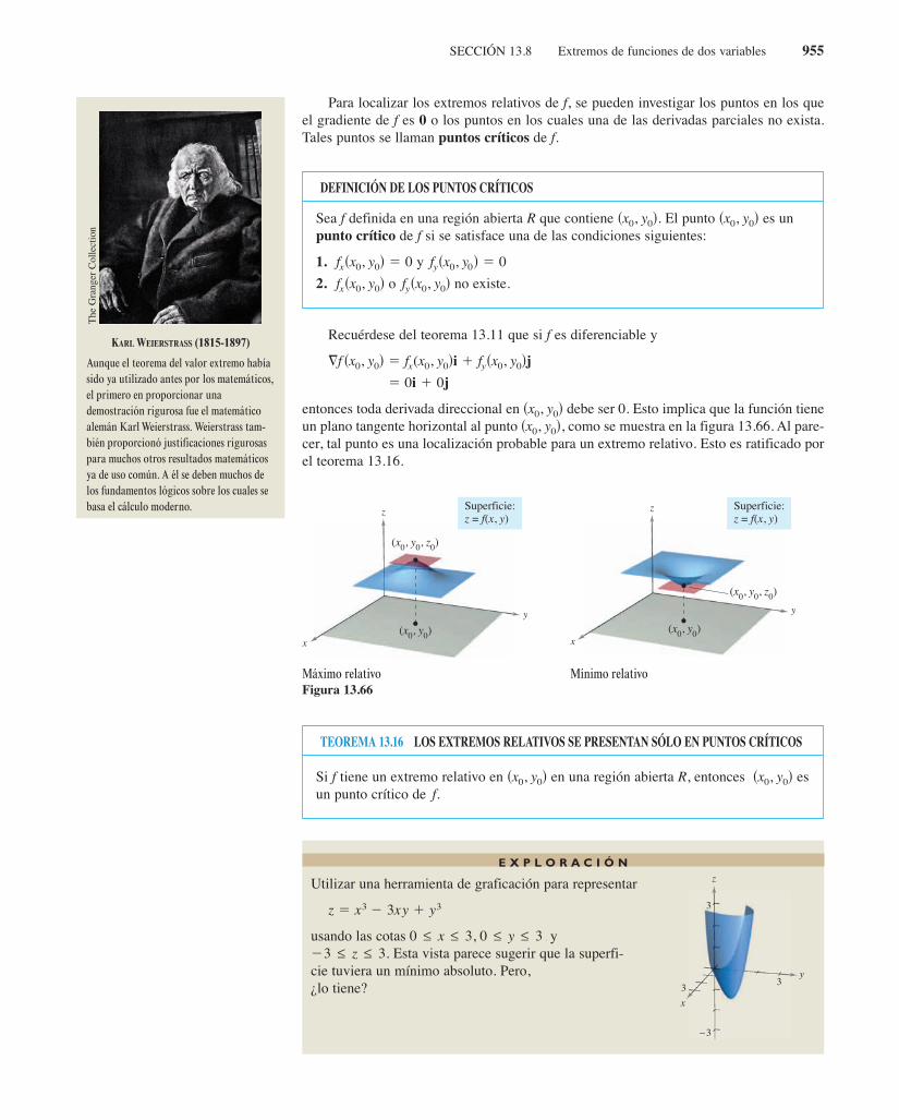
SECCIÓN 13.8 Extremos de funciones de dos variables 955
Para localizar los extremos relativos de f, se pueden investigar los puntos en los queel gradiente de f es 0 o los puntos en los cuales una de las derivadas parciales no exista.Tales puntos se llaman puntos críticos de f.
Recuérdese del teorema 13.11 que si f es diferenciable y
entonces toda derivada direccional en debe ser 0. Esto implica que la función tieneun plano tangente horizontal al punto como se muestra en la figura 13.66. Al pare-cer, tal punto es una localización probable para un extremo relativo. Esto es ratificado porel teorema 13.16.
sx0, y0d,sx0, y0d
5 0i 1 0j
=f sx0, y0d 5 fx(x0, y0di 1 fysx0, y0dj
(x0, y0, z0)
(x0, y0)
y
x
z Superficie:z = f(x, y)
Máximo relativoFigura 13.66
z
y
x
Superficie:z = f(x, y)
(x0, y0, z0)
(x0, y0)
Mínimo relativo
DEFINICIÓN DE LOS PUNTOS CRÍTICOS
Sea f definida en una región abierta R que contiene El punto es unpunto crítico de f si se satisface una de las condiciones siguientes:
1. y
2. o no existe.fysx0, y0dfxsx0, y0dfysx0, y0d 5 0fxsx0, y0d 5 0
sx0, y0dsx0, y0d.
TEOREMA 13.16 LOS EXTREMOS RELATIVOS SE PRESENTAN SÓLO EN PUNTOS CRÍTICOS
Si f tiene un extremo relativo en en una región abierta R, entonces esun punto crítico de f.
sx0, y0dsx0, y0d
E X P L O R A C I Ó N
Utilizar una herramienta de graficación para representar
usando las cotas yEsta vista parece sugerir que la superfi-
cie tuviera un mínimo absoluto. Pero,¿lo tiene?
23 ≤ z ≤ 3.0 ≤ y ≤ 3,0 ≤ x ≤ 3,
z 5 x3 2 3xy 1 y3
y
x
3
−3
3
3
z
KARL WEIERSTRASS (1815-1897)
Aunque el teorema del valor extremo habíasido ya utilizado antes por los matemáticos,el primero en proporcionar unademostración rigurosa fue el matemáticoalemán Karl Weierstrass. Weierstrass tam-bién proporcionó justificaciones rigurosaspara muchos otros resultados matemáticosya de uso común. A él se deben muchos delos fundamentos lógicos sobre los cuales sebasa el cálculo moderno.
The
Gra
nger
Col
lect
ion
Larson-13-08.qxd 3/12/09 19:14 Page 955

956 CAPÍTULO 13 Funciones de varias variables
EJEMPLO 1 Hallar un extremo relativo
Hallar los extremos relativos de
Solución Para comenzar, encontrar los puntos críticos de Como
Derivada parcial con respecto a .
y
Derivada parcial con respecto a .
están definidas para todo y los únicos puntos críticos son aquellos en los cuales lasderivadas parciales de primer orden son 0. Para localizar estos puntos, se hacen y
igual a 0, y se resuelven las ecuaciones
y
para obtener el punto crítico Completando cuadrados, se concluye que para todo
Por tanto, un mínimo relativo de f se encuentra en El valor del mínimo relativo escomo se muestra en la figura 13.67.
El ejemplo 1 muestra un mínimo relativo que se presenta en un tipo de punto crítico;el tipo en el cual ambos y son 0. En el siguiente ejemplo se presenta unmáximo relativo asociado al otro tipo de punto crítico; el tipo en el cual o no existe.
EJEMPLO 2 Hallar un extremo relativo
Determinar los extremos relativos de
Solución Como
Derivada parcial con respecto a .
y
Derivada parcial con respecto a .
se sigue que ambas derivadas parciales existen para todo punto en el plano xy salvo para(0, 0). Como las derivadas parciales no pueden ser ambas 0 a menos que x y y sean 0, seconcluye que (0, 0) es el único punto crítico. En la figura 13.68 se observa que f (0, 0) es1. Para cualquier otro (x, y) es claro que
Por tanto, f tiene un máximo relativo en
En el ejemplo 2, para todo punto distinto de (0, 0) en el eje y. Sin embargo,como no es cero, éstos no son puntos críticos. Recuérdese que una de las derivadas parcialesdebe no existir o las dos deben ser 0 para tener un punto crítico. n
fysx, ydfxsx, yd 5 0NOTA
s0, 0d.
f sx, yd 5 1 2 sx2 1 y2d1y3 < 1.
yfysx, yd 5 22y
3sx2 1 y2d2y3
xfxsx, yd 5 22x
3sx2 1 y2d2y3
f sx, yd 5 1 2 sx2 1 y2d1y3.
fysx, ydfxsx, ydfysx, ydfxsx, yd
f s22, 3d 5 3,s22, 3d.
f sx, yd 5 2sx 1 2d2 1 s y 2 3d2 1 3 > 3.
sx, yd Þ s22, 3ds22, 3d.
2y 2 6 5 04x 1 8 5 0
fysx, ydfxsx, yd
y,x
yfysx, yd 5 2y 2 6
xfxsx, yd 5 4x 1 8
f.
f sx, yd 5 2x2 1 y2 1 8x 2 6y 1 20.
xy
z
−2−3
−4
213 4 5
1
2
3
4
5
6
(−2, 3, 3)
Superficie:f(x, y) = 2x2 + y2 + 8x − 6y + 20
La función tiene un mínimo relativo en Figura 13.67
s22, 3d.z 5 fsx, yd
Superficie:f(x, y) = 1 − (x2 + y2)1/3
y
x
z
443
2
1
(0, 0, 1)
y están indefinidas en
Figura 13.68s0, 0d.
fysx, ydfxsx, yd
Larson-13-08.qxd 3/12/09 19:14 Page 956

SECCIÓN 13.8 Extremos de funciones de dos variables 957
El criterio de las segundas derivadas parciales
El teorema 13.16 afirma que para encontrar extremos relativos sólo se necesita examinarlos valores de en los puntos críticos. Sin embargo, como sucede con una función deuna variable, los puntos críticos de una función de dos variables no siempre son máximoso mínimos relativos. Algunos puntos críticos dan puntos silla que no son ni máximos re-lativos ni mínimos relativos.
Como ejemplo de un punto crítico que no es un extremo relativo, considérese la super-ficie dada por
Paraboloide hiperbólico.
que se muestra en la figura 13.69. En el punto (0, 0), ambas derivadas parciales son 0. Sinembargo, la función f no tiene un extremo relativo en este punto ya que en todo disco abier-to centrado en (0, 0) la función asume valores negativos (a lo largo del eje x) y valores po-sitivos (a lo largo del eje y). Por tanto, el punto (0, 0, 0) es un punto silla de la superficie.(El término “punto silla” viene del hecho de que la superficie mostrada en la figura 13.69se parece a una silla de montar.)
En las funciones de los ejemplos 1 y 2, fue relativamente fácil determinar los extremosrelativos, porque cada una de las funciones estaba dada, o se podía expresar, en forma decuadrado perfecto. Con funciones más complicadas, los argumentos algebraicos sonmenos adecuados y es mejor emplear los medios analíticos presentados en el siguiente cri-terio de las segundas derivadas parciales. Es el análogo, para funciones de dos variables,del criterio de las segundas derivadas para las funciones de una variable. La demostraciónde este teorema se deja para un curso de cálculo avanzado.
Si entonces y deben tener el mismo signo. Esto significa que
puede sustituirse por en las dos primeras partes del criterio. n
Un recurso conveniente para recordar la fórmula de d en el criterio de las segundasderivadas parciales lo da el determinante
donde de acuerdo al teorema 13.3.fxysa, bd 5 fyxsa, bd
d 5 | fxxsa, bdfyxsa, bd
fxysa, bdfyysa, bd|
2 3 2
fyysa, bdfxxsa, bd
fyy sa, bdfxxsa, bdd > 0,NOTA
f sx, yd 5 y2 2 x2
f sx, yd
y
x
z f (x, y) = y2 − x2
Punto silla en
Figura 13.69
fxs0, 0d 5 fys0, 0d 5 0s0, 0, 0d:
TEOREMA 13.17 CRITERIO DE LAS SEGUNDAS DERIVADAS PARCIALES
Sea f una función con segundas derivadas parciales continuas en una región abiertaque contiene un punto (a, b) para el cual
y
Para buscar los extremos relativos de f, considérese la cantidad
1. Si y entonces tiene un mínimo relativo en
2. Si y entonces tiene un máximo relativo en
3. Si entonces es un punto silla.
4. Si d 5 0 el criterio no lleva a ninguna conclusión.
sa, b, f sa, bddd < 0,
sa, bd.ffxxsa, bd < 0,d > 0
sa, bd.ffxxsa, bd > 0,d > 0
d 5 fxxsa, bd fyysa, bd 2 f fxysa, bdg2.
fysa, bd 5 0.fxsa, bd 5 0
Larson-13-08.qxd 3/12/09 19:14 Page 957

958 CAPÍTULO 13 Funciones de varias variables
EJEMPLO 3 Aplicación del criterio de las segundas derivadas parciales
Identificar los extremos relativos de
Solución Para comenzar, se identifican los puntos críticos de f. Como
y
existen para todo x y y, los únicos puntos críticos son aquellos en los que ambas derivadasparciales de primer orden son 0. Para localizar estos puntos, se igualan a 0 y
y se obtiene y De la segunda ecuación se sabe quey por sustitución en la primera ecuación, se obtienen dos soluciones: y
Como
y
se sigue que, para el punto crítico (0, 0),
y, por el criterio de las segundas derivadas parciales, se puede concluir que (0, 0, 1) es unpunto silla. Para el punto crítico
y como se concluye que f tiene un máximo relativo en como semuestra en la figura 13.70.
Con el criterio de las segundas derivadas parciales pueden no hallarse los extremosrelativos por dos razones. Si alguna de las primeras derivadas parciales no existe, no sepuede aplicar el criterio. Si
el criterio no es concluyente. En tales casos, se pueden tratar de hallar los extremos me-diante la gráfica o mediante algún otro método, como se muestra en el siguiente ejemplo.
EJEMPLO 4 Cuando el criterio de las segundas derivadasparciales no es concluyente
Hallar los extremos relativos de
Solución Como y se sabe que ambas derivadas parcialesson igual a 0 si o Es decir, todo punto del eje x o del eje y es un punto críti-co. Como
y
se sabe que si o entonces
Por tanto, el criterio de las segundas derivadas parciales no es concluyente, no funciona. Sinembargo, como para todo punto en los ejes x o y y en todoslos otros puntos, se puede concluir que cada uno de estos puntos críticos son un mínimoabsoluto, como se muestra en la figura 13.71.
f�x, y� � x2y2 > 0f �x, y� � 0
� 4x2y2 � 16x2y2 � �12x2y2 � 0.
d � fxx�x, y�fyy�x, y� � � fxy�x, y��2
y � 0,x � 0
fxy�x, y� � 4xyfyy�x, y� � 2x2,fxx�x, y� � 2y2,
y � 0.x � 0fy�x, y� � 2x2y,fx�x, y� � 2xy2
f �x, y� � x2y2.
d � fxx�a, b� fyy�a, b� � � fxy�a, b��2� 0
�43, 43�,fxx�4
3, 43� � �8 < 0
> 0
� 16
� �8��4� � 16
d � fxx�43, 43� fyy�4
3, 43� � � fxy�43, 43��2
�43, 43�,
d � fxx�0, 0� fyy�0, 0� � � fxy�0, 0��2 � 0 � 16 < 0
fxy�x, y� � 4fyy�x, y� � �4,fxx�x, y� � �6x,
y � x �43.
y � x � 0x � y,4x � 4y � 0.�3x2 � 4y � 0fy�x, y�
fx�x, y�
fy�x, y� � 4x � 4yfx�x, y� � �3x2 � 4y
f �x, y� � �x3 � 4xy � 2y2 � 1.
y
x
4 43 3
,( )
23
4
3
4
5
6
7
8
9
Punto silla(0, 0, 1)Máximo
relativo
f(x, y) = −x3 + 4xy − 2y2 + 1
z
Figura 13.70
x
y
z
22
1
f(x, y) = x2y2
Si y = 0,entonces f (x, y) = 0
Si x = 0,entonces f (x, y) = 0
Figura 13.71
Larson-13-08.qxd 26/2/10 14:26 Página 958

x 5 0,
SECCIÓN 13.8 Extremos de funciones de dos variables 959
Los extremos absolutos de una función se pueden presentar de dos maneras. Primero,algunos extremos relativos también resultan ser extremos absolutos. Así, en el ejemplo 1,
es un mínimo absoluto de la función. (Por otro lado, el máximo relativo encon-trado en el ejemplo 3 no es un máximo absoluto de la función.) Segundo, los extremosabsolutos pueden presentarse en un punto frontera del dominio. Esto se ilustra en el ejem-plo 5.
EJEMPLO 5 Encontrar extremos absolutos
Hallar los extremos absolutos de la función
en la región cerrada dada por y
Solución La expresión de las derivadas parciales
y
permite ver que todo punto en la hipérbola dada por es un punto crítico. Entodos estos puntos el valor de f es
el cual se sabe que es el máximo absoluto, como se muestra en la figura 13.72. El otropunto crítico de que se encuentra en la región dada es Este punto da un mínimoabsoluto de 0, ya que
implica que
Para localizar otros extremos absolutos se deben considerar las cuatro fronteras de laregión formadas por las trazas, de los planos verticales x = p, y = 0 y y = 1. Al ha-cer esto, se encuentra que sen xy 5 0 en todos los puntos del eje x, en todos los puntos deleje y y en el punto Cada uno de estos puntos es un mínimo absoluto de la superfi-cie, como se muestra en la figura 13.72.
Los conceptos de extremos relativos y puntos críticos pueden extenderse a funcionesde tres o más variables. Si todas las primeras derivadas parciales de
existen, puede mostrarse que se presenta un máximo o un mínimo relativo en (x1, x2,x3, . . . , xn) sólo si cada una de las primeras derivadas parciales en ese punto es 0. Esto sig-nifica que los puntos críticos se obtienen al resolver el sistema de ecuaciones siguiente.
La extensión del teorema 13.17 a tres o más variables también es posible, aunque no seconsiderará en este texto.
fxnsx1, x2, x3, . . . , xnd 5 0
:fx2
sx1, x2, x3, . . . , xnd 5 0
fx1sx1, x2, x3, . . . , xnd 5 0
w 5 f sx1, x2, x3, . . . , xnd
sp, 1d.
0 ≤ sin xy ≤ 1.
0 ≤ xy ≤ p
s0, 0d.f
f sx, yd 5 sin p
25 1
xy 5 py2
fysx, yd 5 x cos xyfxsx, yd 5 y cos xy
0 ≤ y ≤ 1.0 ≤ x ≤ p
f sx, yd 5 sin xy
f s22, 3d
y
x
1
1
3
Mínimoabsoluto
Mínimoabsoluto
Máximoabsoluto
( , 1)π
πxy =2
Superficie:f(x, y) = sen xy
Dominio:0 ≤ x ≤0 ≤ y ≤ 1
π
z
Figura 13.72
sen
sen
sen
Larson-13-08.qxd 3/12/09 19:14 Page 959

960 CAPÍTULO 13 Funciones de varias variables
En los ejercicios 1 a 6, identificar los extremos de la funciónreconociendo su forma dada o su forma después de completarcuadrados. Verificar los resultados empleando derivadas par-ciales para localizar los puntos críticos y probar si son extremosrelativos.
En los ejercicios 7 a 16, examinar la función para localizar losextremos relativos.
En los ejercicios 17 a 20, utilizar un sistema algebraico por compu-tadora y representar la superficie y localizar los extremos rela-tivos y los puntos silla.
17.
18.
19.
20.
En los ejercicios 21 a 28, examinar la función para localizar losextremos relativos y los puntos silla.
26.
27.
28.
En los ejercicios 29 y 30, buscar los extremos de la función sinutilizar los criterios de la derivada. Utilizar un sistema alge-braico por computadora y representar gráficamente la superfi-cie. (Sugerencia: Por observación, determinar si es posible que zsea negativo. ¿Cuándo z es igual a 0?)
29. 30.
Para pensar En los ejercicios 31 a 34, determinar si hay unmáximo relativo, un mínimo relativo, un punto silla, o si la infor-mación es insuficiente para determinar la naturaleza de la fun-ción en el punto crítico
31.
32.
33.
34. fxxsx0, y0d 5 25, fyysx0, y0d 5 8, fxysx0, y0d 5 10
fxxsx0, y0d 5 29, fyysx0, y0d 5 6, fxysx0, y0d 5 10
fxx sx0, y0d 5 23, fyysx0, y0d 5 28, fxysx0, y0d 5 2
fxxsx0, y0d 5 9, fyysx0, y0d 5 4, fxysx0, y0d 5 6
xx0 , y0c.f xx, yc
z 5sx2 2 y2d2
x2 1 y2z 5sx 2 yd4
x2 1 y2
y
x
4
4
2
z
z 5 112
2 x2 1 y22e12x22y2
y
x
3
8
4
2
6
6 π
zz 5 e2x sin y
y
x
2
−2
3
z
f sx, yd 5 2xy 212sx4 1 y4d 1 1
z 5 exy
z 5 sx2 1 4y2de12x22y2
f sx, yd 5 y3 2 3yx2 2 3y2 2 3x2 1 1
z 524x
x2 1 y2 1 1
sen
13.8 Ejercicios
1.
2.
3.
4.
5.
6. f x, y x2 y2 10x 12y 64
f x, y x2 y2 2x 6y 6
f x, y 25 x 2 2 y2
f x, y x2 y2 1
g x, y 5 x 3 2 y 2 2
g x, y x 1)2 y 3 2
7.
8.
9.
10.
11.
12.
13.
14.
15. 16. f x, y x y 2g x, y 4 x y
h x, y x2 y2 1 3 2
f x, y x2 y2
z 5x2 4xy y2 16x 10
z x2 xy 12 y2 2x y
f x, y 2x2 2xy y2 2x 3
f x, y x2 5y2 10x 10y 28
f x, y 3x2 2y2 3x 4y 5
f x, y 3x2 2y2 6x 4y 16
21.
22.
23.
24.
25.
y
x
33
4
z
f x, y x2 xy y2 3x y
h x, y x2 3xy y2
g x, y xy
g x, y x2 y2 x y
h x, y 80x 80y x2 y2
CAS
CAS
Think About It In Exercises 31–34, determine whether there isa relative maximum, a relative minimum, a saddle point, orinsufficient information to determine the nature of the function
at the critical point
31.
32.
33.
34. fxx x0, y0 25, fyy x0, y0 8, fxy x0, y0 10
fxx x0, y0 9, fyy x0, y0 6, fxy x0, y0 10
fxx x0, y0 3, fyy x0, y0 8, fxy x0, y0 2
fxx x0, y0 9, fyy x0, y0 4, fxy x0, y0 6
x0 , y0 .f x, y
zx2 y2 2
x2 y2zx y 4
x2 y2
zz
y
x
4
4
2
z
z12
x2 y2 e1 x2 y2
y
x
3
8
4
2
6
6 π
zz e x sin y
y
x
2
−2
3
z
f x, y 2xy 12 x4 y4 1
y
x
33
4
z
f x, y x2 xy y2 3x y
h x, y x2 3xy y2
g x, y xy
g x, y x2 y2 x y
h x, y 80x 80y x2 y2
z exy
z x2 4y2 e1 x2 y2
f x, y y3 3yx2 3y2 3x2 1
z4x
x2 y2 1
f x, y x y 2g x, y 4 x y
h x, y x2 y2 1 3 2
f x, y x2 y2
z 5x2 4xy y2 16x 10
z x2 xy 12 y2 2x y
f x, y 2x2 2xy y2 2x 3
f x, y x2 5y2 10x 10y 28
f x, y 3x2 2y2 3x 4y 5
f x, y 3x2 2y2 6x 4y 16
f x, y x2 y2 10x 12y 64
f x, y x2 y2 2x 6y 6
f x, y 25 x 2 2 y2
f x, y x2 y2 1
g x, y 5 x 3 2 y 2 2
g x, y x 1)2 y 3 2
960 Chapter 13 Functions of Several Variables
13.8 Exercises See www.CalcChat.com for worked-out solutions to odd-numbered exercises.
CAS
CAS
1053714_1308.qxp 10/27/08 12:09 PM Page 960
Larson-13-08.qxd 3/12/09 19:14 Page 960

SECCIÓN 13.8 Extremos de funciones de dos variables 961
35. Una función tiene segundas derivadas parciales continuas enuna región abierta que contiene el punto crítico (3, 7). La fun-ción tiene un mínimo en (3, 7) y para el criterio de lassegundas derivadas parciales. Determinar el intervalo para
si y
36. Una función f tiene segundas derivadas parciales continuas en unaregión abierta que contiene el punto crítico (a, b). Si y
tiene signos opuestos, ¿qué implica esto? Explicar.
En los ejercicios 37 a 42, a) hallar los puntos críticos, b) deter-minar los extremos relativos, c) indicar los puntos críticos en loscuales el criterio de las segundas derivadas parciales no es con-cluyente, y d) usar un sistema algebraico por computadora paratrazar la función, clasificando cualesquiera puntos extremos ypuntos silla.
37.
38.
39.
40.
41. 42.
En los ejercicios 43 y 44, hallar los puntos críticos de la funcióny, por la forma de la función, determinar si se presenta un má-ximo o un mínimo relativo en cada punto.
En los ejercicios 45 a 54, hallar los extremos absolutos de la fun-ción en la región R. (En cada caso, R contiene sus puntos fron-tera.) Utilizar un sistema algebraico por computadora y confir-mar los resultados.
47.
La región triangular en el plano xy con vértices (2, 0), (0, 1)y
48.
La región triangular en el plano xy con vértices (2, 0), (0, 1)y
49.
La región en el plano xy acotada por las gráficas de y
50.
La región en el plano xy acotada por las gráficas de y
51.
52.
53.
54.
¿Verdadero o falso? En los ejercicios 61 a 64, determinar si ladeclaración es verdadera o falsa. Si es falsa, explicar por qué odar un ejemplo que demuestre que es falsa.
61. Si f tiene un máximo relativo en entonces ƒx(x0, y0)5 ƒy(x0, y0) 5 0.
62. Si fx(x0, y0) = fy(x0, y0) = 0, entonces f tiene un máximo relativoen (x0, y0, z0).
63. Entre cualesquiera dos mínimos relativos de f, aquí debe estar almenos un máximo relativo de f.
64. Si f es continua para todo x y y y tiene dos mínimos relativos,entonces f debe tener un máximo relativo por lo menos.
sx0, y0, z0d,
R 5 Hsx, yd : x ≥ 0, y ≥ 0, x2 1 y2 ≤ 1J
f sx, yd 54xy
sx2 1 1dsy2 1 1d
R 5 Hsx, yd : 0 ≤ x ≤ 1, 0 ≤ y ≤ 1J
f sx, yd 54xy
sx2 1 1)sy2 1 1d
f sx, yd 5 x2 1 2xy 1 y2, R 5 Hsx, yd : x2 1 y2 ≤ 8Jf sx, yd 5 x2 1 2xy 1 y2, R 5 Hsx, yd : |x| ≤ 2, |y| ≤ 1J
y 5 1y 5 x2R:
f sx, yd 5 2x 2 2xy 1 y2
y 5 4y 5 x2R:
f sx, yd 5 3x2 1 2y2 2 4y
s1, 2dR:
f sx, yd 5 s2x 2 yd2
s1, 2dR:
f sx, yd 5 12 2 3x 2 2y
f sx, yd 5 sx2 1 y2d2y3f sx, yd 5 x2y3 1 y2y3
f sx, yd 5 !sx 2 1d2 1 sy 1 2d2
f sx, yd 5 sx 2 1d2sy 1 4d2
f sx, yd 5 x3 1 y3 2 6x2 1 9y2 1 12x 1 27y 1 19
f sx, yd 5 x3 1 y3
fyysa, bdfxxsa, bd
fyys3, 7d 5 8.fxxs3, 7d 5 2fxys3, 7d
d > 0
f Desarrollo de conceptos
55. La figura muestra las curvas de nivel de una función descono-cida ¿Qué información, si es que hay alguna, puededarse acerca de f en el punto A? Explicar el razonamiento.
Figura para 55 Figura para 56
56. La figura muestra las curvas de nivel de una función des-conocida f(x, y). ¿Qué información, si es que hay alguna,puede darse acerca de f en los puntos A, B, C y D? Explicarel razonamiento.
En los ejercicios 57 a 59, dibujar la gráfica de una funciónarbitraria f que satisfaga las condiciones dadas. Decir si lafunción tiene extremos o puntos silla. (Hay muchas respues-tas correctas.)
57. y para todo
58. Todas las primeras y segundas derivadas parciales de f son 0.
59.
y para todo sx, yd.fxysx, yd 5 0fyysx, yd < 0,fxxsx, yd > 0,
fxsx, yd5< 0,
> 0,
x < 0
x > 0, fysx, yd5> 0,
< 0,
y < 0
y > 0
fys0, 0d 5 0fxs0, 0d 5 0,
sx, yd.fysx, yd < 0fxsx, yd > 0
xA
BC
D
y
x
A
y
f sx, yd.
In Exercises 1–6, identify any extrema of the function by recog-nizing its given form or its form after completing the square.Verify your results by using the partial derivatives to locate anycritical points and test for relative extrema.
1.
2.
3.
4.
5.
6.
In Exercises 7–16, examine the function for relative extrema.
7.
8.
9.
10.
11.
12.
13.
14.
15. 16.
In Exercises 17–20, use a computer algebra system to graph thesurface and locate any relative extrema and saddle points.
17.
18.
19.
20.
In Exercises 21–28, examine the function for relative extremaand saddle points.
21.
22.
23.
24.
25.
26.
27.
28.
In Exercises 29 and 30, examine the function for extremawithout using the derivative tests, and use a computer algebrasystem to graph the surface. (Hint: By observation, determineif it is possible for to be negative. When is equal to 0?)
29. 30.
Think About It In Exercises 31–34, determine whether there isa relative maximum, a relative minimum, a saddle point, orinsufficient information to determine the nature of the function
at the critical point
31.
32.
33.
34. fxx x0, y0 25, fyy x0, y0 8, fxy x0, y0 10
fxx x0, y0 9, fyy x0, y0 6, fxy x0, y0 10
fxx x0, y0 3, fyy x0, y0 8, fxy x0, y0 2
fxx x0, y0 9, fyy x0, y0 4, fxy x0, y0 6
x0 , y0 .f x, y
zx2 y2 2
x2 y2zx y 4
x2 y2
zz
y
x
4
4
2
z
z12
x2 y2 e1 x2 y2
y
x
3
8
4
2
6
6 π
zz e x sin y
y
x
2
−2
3
z
f x, y 2xy 12 x4 y4 1
y
x
33
4
z
f x, y x2 xy y2 3x y
h x, y x2 3xy y2
g x, y xy
g x, y x2 y2 x y
h x, y 80x 80y x2 y2
z exy
z x2 4y2 e1 x2 y2
f x, y y3 3yx2 3y2 3x2 1
z4x
x2 y2 1
f x, y x y 2g x, y 4 x y
h x, y x2 y2 1 3 2
f x, y x2 y2
z 5x2 4xy y2 16x 10
z x2 xy 12 y2 2x y
f x, y 2x2 2xy y2 2x 3
f x, y x2 5y2 10x 10y 28
f x, y 3x2 2y2 3x 4y 5
f x, y 3x2 2y2 6x 4y 16
f x, y x2 y2 10x 12y 64
f x, y x2 y2 2x 6y 6
f x, y 25 x 2 2 y2
f x, y x2 y2 1
g x, y 5 x 3 2 y 2 2
g x, y x 1)2 y 3 2
960 Chapter 13 Functions of Several Variables
13.8 Exercises See www.CalcChat.com for worked-out solutions to odd-numbered exercises.
CAS
CAS
1053714_1308.qxp 10/27/08 12:09 PM Page 960
35. A function has continuous second partial derivatives on anopen region containing the critical point The functionhas a minimum at and for the Second Partials Test.Determine the interval for if and
36. A function has continuous second partial derivatives on anopen region containing the critical point If and
have opposite signs, what is implied? Explain.
In Exercises 37– 42, (a) find the critical points, (b) test for relative extrema, (c) list the critical points for which the SecondPartials Test fails, and (d) use a computer algebra system tograph the function, labeling any extrema and saddle points.
37.
38.
39.
40.
41. 42.
In Exercises 43 and 44, find the critical points of the functionand, from the form of the function, determine whether a relativemaximum or a relative minimum occurs at each point.
43.
44.
In Exercises 45–54, find the absolute extrema of the functionover the region (In each case, contains the boundaries.) Usea computer algebra system to confirm your results.
45.
46.
47.
The triangular region in the plane with vertices and
48.
The triangular region in the plane with vertices and
49.
The region in the plane bounded by the graphs of and
50.
The region in the plane bounded by the graphs of and
51.
52.
53.
54.
True or False? In Exercises 61–64, determine whether thestatement is true or false. If it is false, explain why or give anexample that shows it is false.
61. If has a relative maximum at then
62. If then has a relative maximum at
63. Between any two relative minima of there must be at least onerelative maximum of
64. If is continuous for all and and has two relative minima,then must have at least one relative maximum.f
yxf
f.f,
x0, y0, z0 .ffx x0, y0 fy x0, y0 0,
fy x0, y0 0.fx x0, y0x0, y0, z0 ,f
R x, y : x 0, y 0, x2 y2 1
f x, y4xy
x2 1 y2 1
R x, y : 0 x 1, 0 y 1
f x, y4xy
x2 1) y2 1
f x, y x2 2xy y2, R x, y : x2 y2 8
f x, y x2 2xy y2, R x, y : x 2, y 1
y 1y x2xy-R:
f x, y 2x 2xy y2
y 4y x2xy-R:
f x, y 3x2 2y2 4y
1, 20, 1 ,2, 0 ,xy-R:
f x, y 2x y 2
1, 20, 1 ,2, 0 ,xy-R:
f x, y 12 3x 2y
f x, y x2 xy, R x, y : x 2, y 1
R x, y : 1 x 4, 0 y 2
f x, y x2 4xy 5
RR.
f x, y, z 9 x y 1 z 2 2
f x, y, z x2 y 3 2 z 1 2
f x, y x2 y2 2 3f x, y x2 3 y2 3
f x, y x 1 2 y 2 2
f x, y x 1 2 y 4 2
f x, y x3 y3 6x2 9y2 12x 27y 19
f x, y x3 y3
fyy a, bfxx a, ba, b .
f
fyy 3, 7 8.fxx 3, 7 2fxy 3, 7
d > 03, 7 ,3, 7 .
f
13.8 Extrema of Functions of Two Variables 961
55. The figure shows the level curves for an unknown functionWhat, if any, information can be given about at the
point Explain your reasoning.
Figure for 55 Figure for 56
56. The figure shows the level curves for an unknown functionWhat, if any, information can be given about at the
points and Explain your reasoning.
In Exercises 57–59, sketch the graph of an arbitraryfunction satisfying the given conditions. State whether thefunction has any extrema or saddle points. (There are manycorrect answers.)
57. and for all
58. All of the first and second partial derivatives of are 0.
59.
and for all x, y .fxy x, y 0fyy x, y < 0,fxx x, y > 0,
fx x, y< 0,
> 0,
x < 0
x > 0, fy x, y
> 0,
< 0,
y < 0
y > 0
fy 0, 0 0fx 0, 0 0,
f
x, y .fy x, y < 0fx x, y > 0
f
D?C,B,A,ff x, y .
A
BC
D
y
A
y
A?ff x, y .
WRITING ABOUT CONCEPTS
CAS
60. Consider the functions
y
(a) Show that both functions have a critical point at
(b) Explain how and behave differently at this criticalpoint.
gf
0, 0 .
g x, y x2 y2.f x, y x2 y2
CAPSTONE
1053714_1308.qxp 10/27/08 12:09 PM Page 961
Para discusión60. Considerar las funciones
a) Demostrar que ambas funciones tienen un punto crítico en(0, 0).
b) Explicar cómo f y g se comportan de manera diferente eneste punto crítico.
35. A function has continuous second partial derivatives on anopen region containing the critical point The functionhas a minimum at and for the Second Partials Test.Determine the interval for if and
36. A function has continuous second partial derivatives on anopen region containing the critical point If and
have opposite signs, what is implied? Explain.
In Exercises 37– 42, (a) find the critical points, (b) test for relative extrema, (c) list the critical points for which the SecondPartials Test fails, and (d) use a computer algebra system tograph the function, labeling any extrema and saddle points.
37.
38.
39.
40.
41. 42.
In Exercises 43 and 44, find the critical points of the functionand, from the form of the function, determine whether a relativemaximum or a relative minimum occurs at each point.
43.
44.
In Exercises 45–54, find the absolute extrema of the functionover the region (In each case, contains the boundaries.) Usea computer algebra system to confirm your results.
45.
46.
47.
The triangular region in the plane with vertices and
48.
The triangular region in the plane with vertices and
49.
The region in the plane bounded by the graphs of and
50.
The region in the plane bounded by the graphs of and
51.
52.
53.
54.
True or False? In Exercises 61–64, determine whether thestatement is true or false. If it is false, explain why or give anexample that shows it is false.
61. If has a relative maximum at then
62. If then has a relative maximum at
63. Between any two relative minima of there must be at least onerelative maximum of
64. If is continuous for all and and has two relative minima,then must have at least one relative maximum.f
yxf
f.f,
x0, y0, z0 .ffx x0, y0 fy x0, y0 0,
fy x0, y0 0.fx x0, y0x0, y0, z0 ,f
R x, y : x 0, y 0, x2 y2 1
f x, y4xy
x2 1 y2 1
R x, y : 0 x 1, 0 y 1
f x, y4xy
x2 1) y2 1
f x, y x2 2xy y2, R x, y : x2 y2 8
f x, y x2 2xy y2, R x, y : x 2, y 1
y 1y x2xy-R:
f x, y 2x 2xy y2
y 4y x2xy-R:
f x, y 3x2 2y2 4y
1, 20, 1 ,2, 0 ,xy-R:
f x, y 2x y 2
1, 20, 1 ,2, 0 ,xy-R:
f x, y 12 3x 2y
f x, y x2 xy, R x, y : x 2, y 1
R x, y : 1 x 4, 0 y 2
f x, y x2 4xy 5
RR.
f x, y, z 9 x y 1 z 2 2
f x, y, z x2 y 3 2 z 1 2
f x, y x2 y2 2 3f x, y x2 3 y2 3
f x, y x 1 2 y 2 2
f x, y x 1 2 y 4 2
f x, y x3 y3 6x2 9y2 12x 27y 19
f x, y x3 y3
fyy a, bfxx a, ba, b .
f
fyy 3, 7 8.fxx 3, 7 2fxy 3, 7
d > 03, 7 ,3, 7 .
f
13.8 Extrema of Functions of Two Variables 961
55. The figure shows the level curves for an unknown functionWhat, if any, information can be given about at the
point Explain your reasoning.
Figure for 55 Figure for 56
56. The figure shows the level curves for an unknown functionWhat, if any, information can be given about at the
points and Explain your reasoning.
In Exercises 57–59, sketch the graph of an arbitraryfunction satisfying the given conditions. State whether thefunction has any extrema or saddle points. (There are manycorrect answers.)
57. and for all
58. All of the first and second partial derivatives of are 0.
59.
and for all x, y .fxy x, y 0fyy x, y < 0,fxx x, y > 0,
fx x, y< 0,
> 0,
x < 0
x > 0, fy x, y
> 0,
< 0,
y < 0
y > 0
fy 0, 0 0fx 0, 0 0,
f
x, y .fy x, y < 0fx x, y > 0
f
D?C,B,A,ff x, y .
A
BC
D
y
A
y
A?ff x, y .
WRITING ABOUT CONCEPTS
CAS
60. Consider the functions
y
(a) Show that both functions have a critical point at
(b) Explain how and behave differently at this criticalpoint.
gf
0, 0 .
g x, y x2 y2.f x, y x2 y2
CAPSTONE
1053714_1308.qxp 10/27/08 12:09 PM Page 961
Larson-13-08.qxd 3/12/09 19:14 Page 961

962 CAPÍTULO 13 Funciones de varias variables
13.9 Aplicaciones de los extremos de funciones de dos variables
n Resolver problemas de optimización con funciones de varias variables.n Utilizar el método de mínimos cuadrados.
Problemas de optimización aplicada
En esta sección se verán algunas de las muchas aplicaciones de los extremos de funcionesde dos (o más) variables.
EJEMPLO 1 Hallar un volumen máximo
Una caja rectangular descansa en el plano xy con uno de sus vértices en el origen. El vér-tice opuesto está en el plano
como se muestra en la figura 13.73. Hallar el volumen máximo de la caja.
Solución Sean x, y y z el largo, ancho y la altura de la caja. Como un vértice de la cajase encuentra en el plano se sabe que z 5 –1
3(24 2 6x 2 4y), y así sepuede expresar el volumen xyz de la caja en función de dos variables.
Igualando a 0 las primeras derivadas parciales
se obtienen los puntos críticos (0, 0) y En (0, 0) el volumen es 0, así que ese punto
no proporciona un volumen máximo. En el punto se puede aplicar el criterio de lassegundas derivadas parciales.
Como
y
se concluye de acuerdo con el criterio de las segundas derivadas parciales que el vo-lumen máximo es
unidades cúbicas.
Nótese que el volumen es 0 en los puntos frontera del dominio triangular de V.
5649
Vs43, 2d 5
13f24s4
3ds2d 2 6s43d2s2d 2 4s4
3ds22dg
Vxxs43, 2d 5 28 < 0
Vxxs43, 2dVyys4
3, 2d 2 fVxys43, 2dg2
5 s28ds2329 d 2 s28
3d25
643 > 0
Vxysx, yd 513s24 2 12x 2 8yd
Vyysx, yd 528x
3
Vxxsx, yd 5 24y
s43, 2d,
s43, 2d.
Vysx, yd 513s24x 2 6x2 2 8xyd 5
x3
s24 2 6x 2 8yd 5 0
Vxsx, yd 513 s24y 2 12xy 2 4y2d 5
y3
s24 2 12x 2 4yd 5 0
513s24xy 2 6x2y 2 4xy2d
Vsx, yd 5 sxdsydf13s24 2 6x 2 4ydg
6x 1 4y 1 3z 5 24,
6x 1 4y 1 3z 5 24
y
x (4, 0, 0)(0, 6, 0)
(0, 0, 8) Plano:6x + 4y + 3z = 24
z
Figura 13.73
En muchos problemas prácti-cos, el dominio de la función a opti-mizar es una región acotada cerrada.Para encontrar los puntos mínimos omáximos, no sólo se deben probar lospuntos críticos, sino también los va-lores de la función en los puntos fron-tera. n
NOTA
Larson-13-09.qxd 3/12/09 19:18 Page 962

SECCIÓN 13.9 Aplicaciones de los extremos de funciones de dos variables 963
En las aplicaciones de los extremos a la economía y a los negocios a menudo se tienemás de una variable independiente. Por ejemplo, una empresa puede producir varios mo-delos de un mismo tipo de producto. El precio por unidad y la ganancia o beneficio porunidad de cada modelo son, por lo general, diferentes. La demanda de cada modelo es, amenudo, función de los precios de los otros modelos (así como su propio precio). El si-guiente ejemplo ilustra una aplicación en la que hay dos productos.
EJEMPLO 2 Beneficio máximo
Un fabricante de artículos electrónicos determina que la ganancia o beneficio P (endólares) obtenido al producir x unidades de un reproductor de DVD y y unidades de ungrabador de DVD se aproxima mediante el modelo
Hallar el nivel de producción que proporciona una ganancia o beneficio máximo. ¿Cuál esla ganancia máxima?
Solución Las derivadas parciales de la función de beneficio son
y
Igualando estas derivadas parciales a 0, se obtiene el sistema de ecuaciones siguiente.
Después de simplificar, este sistema de ecuaciones lineales puede expresarse como
2x 1 2y 5 08 000
2x 1 2y 5 10 000.
Resolviendo el sistema se obtiene x 5 2 000 y y 5 4 000. Las segundas derivadas parcialesde P son
Pxx(2 000, 4 000) 5 20.002
Pyy(2 000, 4 000) 5 20.002
Pxy(2 000, 4 000) 5 20.001.
Como y
Pxx(2 000, 4 000)Pyy(2 000, 4 000) 2 [Pxy(2 000, 4 000)]2 5
se concluye que el nivel de producción con x 5 2 000 unidades y y 5 4 000 unidades pro-porciona el beneficio máximo. El beneficio máximo es
P(2 000, 4 000) 5 8(2 000) 1 10(4 000) 2
(0.001)[2 0002 1 2 000(4 000) 1 4 0002)] 2 10 000
5 $18 000.
En el ejemplo 2 se supuso que la planta industrial puede producir el número requerido deunidades para proporcionar el beneficio máximo. En la práctica, la producción estará limitada porrestricciones físicas. En la sección siguiente se estudiarán tales problemas de optimización. n
NOTA
s20.002d2 2 s20.001d2 > 0
Pxx < 0
10 2 s0.001dsx 1 2yd 5 0
8 2 s0.001ds2x 1 yd 5 0
Pysx, yd 5 10 2 s0.001dsx 1 2yd.Pxsx, yd 5 8 2 s0.001ds2x 1 yd
Psx, yd 5 8x 1 10y 2 s0.001dsx2 1 xy 1 y2d 2 10,000.
PARA MAYOR INFORMACIÓNPara más información sobre el uso dela matemática en la economía, ver elartículo “Mathematical Methods ofEconomics” de Joel Franklin en TheAmerican Mathematical Monthly.
Larson-13-09.qxd 3/12/09 19:18 Page 963

964 CAPÍTULO 13 Funciones de varias variables
El método de mínimos cuadrados
En muchos de los ejemplos en este texto se han empleado modelos matemáticos, comoen el caso del ejemplo 2, donde se utiliza un modelo cuadrático para el beneficio. Hayvarias maneras para desarrollar tales modelos; una es la conocida como el método de mí-nimos cuadrados.
Al construir un modelo para representar un fenómeno particular, los objetivos sonsimplicidad y precisión. Por supuesto, estas metas entran a menudo en conflicto. Por ejem-plo, un modelo lineal simple para los puntos en la figura 13.74 es
Sin embargo, la figura 13.75 muestra que si se elige el modelo cuadrático, ligeramente máscomplicado,* es
se logra mayor precisión.
Como medida de qué tan bien se ajusta el modelo a la colección de puntos
se pueden sumar los cuadrados de las diferencias entre los valores reales y y los valoresdados por el modelo para obtener la suma de los cuadrados de los errores o errorescuadráticos
Gráficamente, S puede interpretarse como la suma de los cuadrados de las distancias ver-ticales entre la gráfica de f y los puntos dados en el plano (los puntos de los datos), comose muestra en la figura 13.76. Si el modelo es perfecto, entonces S = 0. Sin embargo, cuan-do la perfección no es posible, podemos conformarnos con un modelo que haga mínimoel valor de S. Por ejemplo, la suma de los errores cuadráticos en el modelo lineal en la figu-ra 13.74 es En estadística, al modelo lineal que minimiza el valor de S se le llamarecta de regresión o por mínimos cuadrados. La demostración de que esta recta real-mente minimiza S requiere minimizar una función de dos variables.
* En el ejercicio 37 se describe un método para hallar el modelo de mínimos cuadrados para una colección dedatos.
S < 17.
Hsx1, y1d, sx2, y2d, sx3, y3d, . . . , sxn, yndJ
y 5 fsxd
y 5 0.1996x2 2 0.7281x 1 1.3749
y 5 1.8566x 2 5.0246.
Suma de los cuadrados de los errores o errores cuadráticos.S 5 on
i51f fsxid 2 yig2.
x
(x3, y3)
(x2, y2)
(x1, y1)
d1
d2
d3
y = f(x)
y
Suma de los cuadrados de los errores:
Figura 13.76S 5 d1
2 1 d22 1 d3
2
5
105
10
15
y
x
y = 1.8566x − 5.0246
(11, 17)
(9, 12)
(7, 6)
(5, 2)(2, 1)
Figura 13.74
5
105
10
15
y
x
(11, 17)
(9, 12)
(7, 6)
(5, 2)(2, 1)
y = 0.1996x2 − 0.7281x + 1.3749
Figura 13.75
Larson-13-09.qxd 3/12/09 19:18 Page 964

SECCIÓN 13.9 Aplicaciones de los extremos de funciones de dos variables 965
Sea la suma de los cuadrados de los errores para el modeloy el conjunto de puntos dado. Es decir,
donde los puntos representan constantes. Como S es una función de a y b, se puedenusar los métodos de la sección anterior para encontrar el valor mínimo de S. Las primerasderivadas parciales de S son
Igualando estas dos derivadas parciales a 0, se obtienen los valores de a y b que indica el teo-rema. Se deja como ejercicio aplicar el criterio de las segundas derivadas parciales (ver ejer-cicio 47) para verificar que estos valores de a y b dan un mínimo.
Si los valores de x están simétricamente distribuidos respecto al eje y, entoncesy las fórmulas para a y b se simplifican:
y
Esta simplificación es a menudo posible mediante una traslación de los valores x. Porejemplo, si los valores x en una colección de datos son los años 2005, 2006, 2007, 2008 y2009, se puede tomar 2007 como 0.
b 51n o
n
i51yi.
a 5on
i51xiyi
on
i51xi
2
o xi 5 0
5 2aon
i51xi 1 2nb 2 2o
n
i51yi.
Sbsa, bd 5 on
i512saxi 1 b 2 yid
5 2aon
i51xi
2 1 2bon
i51xi 2 2o
n
i51xiyi
Sasa, bd 5 on
i512xisaxi 1 b 2 yid
sxi, yid
5 on
i51saxi 1 b 2 yid2
Ssa, bd 5 on
i51f fsxid 2 yig2
fsxd 5 ax 1 bSsa, bdDEMOSTRACIÓN
TEOREMA 13.18 RECTA DE REGRESIÓN DE MÍNIMOS CUADRADOS
La recta de regresión de mínimos cuadrados para {(x1, y1), (x2, y2), . . . . (xn,yn)} está dada por donde
y b 51n1o
n
i51yi 2 ao
n
i51xi2.a 5
non
i51xiyi 2 o
n
i51xio
n
i51yi
non
i51xi
2 2 1on
i51xi2
2
fsxd 5 ax 1 b,
ADRIEN-MARIE LEGENDRE (1752-1833)
El método de mínimos cuadrados lo intro-dujo el matemático francés Adrien-MarieLegendre. Legendre es mejor conocido porsu trabajo en geometría. De hecho, su texto“Elementos de Geometría” fue tan popularen Estados Unidos que se usó durante unperiodo de más de 100 años y hubo 33 edi-ciones.
The
Gra
nger
Col
lect
ion
Larson-13-09.qxd 3/12/09 19:18 Page 965

966 CAPÍTULO 13 Funciones de varias variables
En los ejercicios 1 y 2, hallar la distancia mínima del punto alplano (Sugerencia: Para simplificar los cálcu-los, minimizar el cuadrado de la distancia.)
1. 2.
En los ejercicios 3 y 4, encontrar la distancia mínima desde elpunto a la superficie (Sugerencia: En elejercicio 4, usar la operación raíz de una herramienta de grafi-cación.)
En los ejercicios 5 a 8, hallar tres números positivos x, y y z quesatisfagan las condiciones dadas.
5. El producto es 27 y la suma es mínima.
6. La suma es 32 y es máxima.
7. La suma es 30 y la suma de los cuadrados es mínima.
8. El producto es 1 y la suma de los cuadrados es mínima.
9. Costos Un contratista de mejorías caseras está pintando lasparedes y el techo de una habitación rectangular. El volumen dela habitación es de 668.25 pies cúbicos. El costo de pintura depared es de $0.06 por pie cuadrado y el costo de pintura de techoes de $0.11 por pie cuadrado. Encontrar las dimensiones de lahabitación que den por resultado un mínimo costo para la pintu-ra. ¿Cuál es el mínimo costo por la pintura?
10. Volumen máximo El material para construir la base de unacaja abierta cuesta 1.5 veces más por unidad de área que el mate-rial para construir los lados. Dada una cantidad fija de dinero C,hallar las dimensiones de la caja de mayor volumen que puedeser fabricada.
11. Volumen máximo El volumen de un elipsoide
es Dada una suma fija mostrar que el elip-soide de volumen máximo es una esfera.
a 1 b 1 c,4pabcy3.
x2
a2 1y 2
b2 1z2
c2 5 1
P � xy2z
z � �1 � 2x � 2y.
s1, 2, 3ds0, 0, 0d
x � y 1 z � 3.
EJEMPLO 3 Hallar la recta de regresión de mínimos cuadrados
Hallar la recta de regresión de mínimos cuadrados para los puntos (23, 0), (21, 1), (0, 2)y (2, 3).
Solución La tabla muestra los cálculos necesarios para hallar la recta de regresión demínimos cuadrados usando
Aplicando el teorema 13.18 se obtiene
y
La recta de regresión de mínimos cuadrados es como se muestra en lafigura 13.77.
f sxd 5813x 1
4726,
b 51n 1o
n
i51yi 2 ao
n
i51xi2 5
1436 2
813
s22d4 54726
.
a 5
non
i51xiyi 2 o
n
i51xi o
n
i51yi
non
i51xi
2 2 1on
i51xi2
2 54s5d 2 s22ds6d4s14d 2 s22d2 5
813
n 5 4.
3
1
2
21−1−2−3x
(0, 2)
(2, 3)
47x + 268f(x) = 13
(−1, 1)(−3, 0)
y
Recta de regresión de mínimos cuadradosFigura 13.77
TECNOLOGÍA Muchas calcu-ladoras tienen “incorporados” pro-gramas de regresión de mínimoscuadrados. Se puede utilizar unacalculadora con estos programaspara reproducir los resultados delejemplo 3.
EXAMPLE 3 Finding the Least Squares Regression Line
Find the least squares regression line for the points and
Solution The table shows the calculations involved in finding the least squaresregression line using
Applying Theorem 13.18 produces
and
The least squares regression line is as shown in Figure 13.77.�
f �x� �813x �
4726,
b �1n
n
i�1yi � a
n
i�1xi� �
14�6 �
813
��2� �4726
.
a �
nn
i�1xiyi �
n
i�1xi
n
i�1yi
nn
i�1xi
2 � n
i�1xi�
2 �4�5� � ��2��6�4�14� � ��2�2 �
813
n � 4.
�2, 3�.��3, 0�, ��1, 1�, �0, 2�,
966 Chapter 13 Functions of Several Variables
In Exercises 1 and 2, find the minimum distance from the pointto the plane (Hint: To simplify the computations,minimize the square of the distance.)
1. 2.
In Exercises 3 and 4, find the minimum distance from the pointto the surface (Hint: In Exercise 4, use theroot feature of a graphing utility.)
3.
4.
In Exercises 5–8, find three positive integers and thatsatisfy the given conditions.
5. The product is 27 and the sum is a minimum.
6. The sum is 32 and is a maximum.
7. The sum is 30 and the sum of the squares is a minimum.
8. The product is 1 and the sum of the squares is a minimum.
9. Cost A home improvement contractor is painting the wallsand ceiling of a rectangular room. The volume of the room is668.25 cubic feet. The cost of wall paint is $0.06 per squarefoot and the cost of ceiling paint is $0.11 per square foot. Findthe room dimensions that result in a minimum cost for thepaint. What is the minimum cost for the paint?
10. Maximum Volume The material for constructing the baseof an open box costs 1.5 times as much per unit area as thematerial for constructing the sides. For a fixed amount ofmoney find the dimensions of the box of largest volume thatcan be made.
11. Maximum Volume The volume of an ellipsoid
is For a fixed sum show that the ellipsoidof maximum volume is a sphere.
a � b � c,4�abc�3.
x2
a2 �y 2
b2 �z2
c2 � 1
C,
P � xy2z
zy,x,
�0, 0, 2���2, �2, 0�
z � �1 � 2x � 2y.
�1, 2, 3��0, 0, 0�
x � y 1 z � 3.
13.9 Exercises See www.CalcChat.com for worked-out solutions to odd-numbered exercises.
Many calculatorshave “built-in” least squares regressionprograms. If your calculator has such aprogram, use it to duplicate the resultsof Example 3.
TECHNOLOGY
3
1
2
21−1−2−3x
(0, 2)
(2, 3)
x +813
f(x) = 4726
(−1, 1)(−3, 0)
y
Least squares regression lineFigure 13.77
x y xy x2
�3 0 0 9
�1 1 �1 1
0 2 0 0
2 3 6 4
n
i�1xi � �2
n
i�1yi � 6
n
i�1xiyi � 5
n
i�1xi
2 � 14
1053714_1309.qxp 10/27/08 12:10 PM Page 966
13.9 Ejercicios
Larson-13-09.qxd 3/12/09 19:18 Page 966

SECCIÓN 13.9 Aplicaciones de los extremos de funciones de dos variables 967
12. Volumen máximo Mostrar que la caja rectangular de volumenmáximo inscrita en una esfera de radio r es un cubo.
13. Volumen y área exterior Mostrar que una caja rectangular devolumen dado y área exterior mínima es un cubo.
14. Área Un comedero de secciones transversales en forma detrapecio se forma doblando los extremos de una lámina de alu-minio de 30 pulgadas de ancho (ver la figura). Hallar la seccióntransversal de área máxima.
15. Ingreso máximo Una empresa fabrica dos tipos de zapatostenis, tenis para correr y tenis para baloncesto. El ingreso total de
unidades de tenis para correr y unidades de tenis de balon-cesto es donde y están en miles de unidades. Hallar las y que maximizanel ingreso.
16. Ganancia o beneficio máximo Una empresa fabrica velas endos lugares. El costo de producción de unidades en el lugar 1es
y el costo de producción de x2 unidades en el lugar 2 es
Las velas se venden a $15 por unidad. Hallar la cantidad quedebe producirse en cada lugar para aumentar al máximo el be-neficio
17. Ley de Hardy-Weinberg Los tipos sanguíneos son genética-mente determinados por tres alelos A, B y O. (Alelo escualquiera de las posibles formas de mutación de un gen.) Unapersona cuyo tipo sanguíneo es AA, BB u OO es homocigótica.Una persona cuyo tipo sanguíneo es AB, AO o BO es hetero-cigótica. La ley Hardy-Weinberg establece que la proporción Pde individuos heterocigótica en cualquier población dada es
donde p representa el porcentaje de alelos A en la población, qrepresenta el porcentaje de alelos B en la población y r repre-senta el porcentaje de alelos O en la población. Utilizar el hechode que para mostrar que la proporción máxi-ma de individuos heterocigóticos en cualquier población es
18. Índice de diversidad de Shannon Una forma de medir diversi-dad de especies es usar el índice de diversidad de Shannon H. Siun hábitat consiste de tres especies, A, B y C, su índice de diver-sidad de Shannon es
donde x es el porcentaje de especies A en el hábitat, y es el por-centaje de especies B en el hábitat y z es el porcentaje deespecies C en el hábitat.
a) Usar el factor de x + y + z = 1 para demostrar que el valormáximo de H ocurre cuando
b) Usar el resultado del inciso a) para demostrar que el valormáximo de H en este hábitat es de ln 3.
19. Costo mínimo Hay que construir un conducto para agua desdeel punto P al punto S y debe atravesar regiones donde los costosde construcción difieren (ver la figura). El costo por kilómetroen dólares es 3k de P a Q, 2k de Q a R y k de R a S. Hallar x y ytales que el costo total C se minimice.
20. Distancia Una empresa tiene tres tiendas de ventas al menudeolocalizadas en los puntos (0, 0), (2, 2) y (22, 2) (ver la figura). Ladirección planea construir un centro de distribución localizado detal manera que la suma S de las distancias del centro a las tiendassea mínimo. Por la simetría del problema es claro que el centro dedistribución se localizará en el eje y, y por consiguiente S es unafunción de una variable y. Utilizando las técnicas presentadas en elcapítulo 3, calcular el valor de y requerido.
Figura para 20 Figura para 21
21. Investigación Las tiendas de ventas al menudeo descritas en elejercicio 20 se localizan en (0, 0), (4, 2) y (22, 2) (ver la figura).La localización del centro de distribución es (x, y), y por consi-guiente la suma S de las distancias es una función de x y y.
a) Escribir la expresión que da la suma S de las distancias.Utilizar un sistema algebraico por computadora y representarS. ¿Tiene esta superficie un mínimo?
b) Utilizar un sistema algebraico por computadora y obtener y Observar que resolver el sistema y es muydifícil. Por tanto, aproximar la localización del centro de dis-tribución.
c) Una estimación inicial del punto crítico es Calcular con componentes y ¿Qué dirección es la dada por el vector
d) La segunda estimación del punto crítico es
Si se sustituyen estas coordenadas en entonces S seconvierte en una función de una variable t. Hallar el valor det que minimiza S. Utilizar este valor de t para estimar
e) Realizar dos iteraciones más del proceso del inciso d) paraobtener Dada esta localización del centro de dis-tribución, ¿cuál es la suma de las distancias a las tiendas almenudeo?
f) Explicar por qué se usó para aproximar el valormínimo de S. ¿En qué tipo de problemas se usaría =Ssx, yd?
2=Ssx, yd
sx4, y4d.
sx2, y2d.
Ssx, yd,sx2, y2d 5 sx1 2 Sxsx1, y1dt, y1 2 Sysx1, y1dtd.
2=Ss1, 1d?2Sys1, 1d.2Sxs1, 1d2=Ss1, 1d
sx1, y1d 5 s1, 1d.
Sy 5 0Sx 5 0Sy.Sx
x2 4
4
−2
−2
(−2, 2) (4, 2)
(0, 0)
(x, y)d1 d2
d3
y
x−3
−2
−2
3
2
21
(2, 2)(−2, 2)
(0, y)d1
d2
d3
(0, 0)
y
1 km
P
Q
R
S
x
y
10 km
2 km
12. Maximum Volume Show that the rectangular box of maxi-mum volume inscribed in a sphere of radius is a cube.
13. Volume and Surface Area Show that a rectangular box ofgiven volume and minimum surface area is a cube.
14. Area A trough with trapezoidal cross sections is formed byturning up the edges of a 30-inch-wide sheet of aluminum (seefigure). Find the cross section of maximum area.
15. Maximum Revenue A company manufactures two types ofsneakers, running shoes and basketball shoes. The total revenuefrom units of running shoes and units of basketball shoesis where and
are in thousands of units. Find and so as to maximizethe revenue.
16. Maximum Profit A corporation manufactures candles at twolocations. The cost of producing units at location 1 is
and the cost of producing units at location 2 is
The candles sell for $15 per unit. Find the quantity that shouldbe produced at each location to maximize the profit
17. Hardy-Weinberg Law Common blood types are determinedgenetically by three alleles A, B, and O. (An allele is any of agroup of possible mutational forms of a gene.) A person whoseblood type is AA, BB, or OO is homozygous. A person whoseblood type is AB, AO, or BO is heterozygous. The Hardy-Weinberg Law states that the proportion of heterozygousindividuals in any given population is
where represents the percent of allele A in the population,represents the percent of allele B in the population, and represents the percent of allele O in the population. Use the factthat to show that the maximum proportion ofheterozygous individuals in any population is
18. Shannon Diversity Index One way to measure species diver-sity is to use the Shannon diversity index If a habitat consistsof three species, A, B, and C, its Shannon diversity index is
where is the percent of species A in the habitat, is the percent of species B in the habitat, and is the percent ofspecies C in the habitat.
(a) Use the fact that to show that the maximumvalue of occurs when
(b) Use the results of part (a) to show that the maximum valueof in this habitat is
19. Minimum Cost A water line is to be built from point topoint and must pass through regions where construction costsdiffer (see figure). The cost per kilometer in dollars is from
to from to and from to Find and suchthat the total cost will be minimized.
20. Distance A company has retail outlets located at the pointsand (see figure). Management plans to
build a distribution center located such that the sum of thedistances from the center to the outlets is minimum. From thesymmetry of the problem it is clear that the distribution centerwill be located on the axis, and therefore is a function of thesingle variable Using techniques presented in Chapter 3, findthe required value of
Figure for 20 Figure for 21
21. Investigation The retail outlets described in Exercise 20 arelocated at and (see figure). The locationof the distribution center is and therefore the sum of thedistances is a function of and
(a) Write the expression giving the sum of the distances Usea computer algebra system to graph Does the surfacehave a minimum?
(b) Use a computer algebra system to obtain and Observethat solving the system and is very difficult.So, approximate the location of the distribution center.
(c) An initial estimate of the critical point is Calculate with components and
What direction is given by the vector
(d) The second estimate of the critical point is
If these coordinates are substituted into then becomes a function of the single variable Find the valueof that minimizes Use this value of to estimate
(e) Complete two more iterations of the process in part (d) toobtain For this location of the distribution center,what is the sum of the distances to the retail outlets?
(f) Explain why was used to approximate theminimum value of In what types of problems would youuse S x, y ?
S.S x, y
x4, y4 .
x2, y2 .tS.tt.
SS x, y ,
x2, y2 x1 Sx x1, y1 t, y1 Sy x1, y1 t .
S 1, 1 ?Sy 1, 1 .Sx 1, 1S 1, 1
x1, y1 1, 1 .
Sy 0Sx 0Sy.Sx
S.S.
y.xSx, y ,
2, 24, 2 ,0, 0 ,
2 4
4
−2
−2
(−2, 2) (4, 2)
(0, 0)
(x, y)d2 d1
d3
y
−3
−2
−2
3
2
21
(2, 2)(−2, 2)
(0, y)d1
d2
d3
(0, 0)
y
y.y.
Sy-
S
2, 22, 2 ,0, 0 ,
1 km
P
Q
R
S
x
y
10 km
2 km
CyxS.RkR,Q2kQ,P
3kS
P
ln 3.H
x y z 13.H
x y z 1
zyx
H x ln x y ln y z ln z
H.
23.
p q r 1
rqp
P p, q, r 2pq 2pr 2qr
P
P 15 x1 x2 C1 C2.
C2 0.05x22 4x2 275.
x2
C1 0.02x12 4x1 500
x1
x2x1x2
x1R 5x12 8x2
2 2x1x2 42x1 102x2,x2x1
30 − 2x
x x
θθ
r
13.9 Applications of Extrema of Functions of Two Variables 967
CAS
1053714_1309.qxp 10/27/08 12:10 PM Page 967
23.
p 1 q 1 r 5 1
Ps p, q, rd 5 2pq 1 2pr 1 2qr
P 5 15sx1 1 x2d 2 C1 2 C2.
C2 5 0.05x22 1 4x2 1 275.
C1 5 0.02x12 1 4x1 1 500
x1
x2x1x2
x1R 5 25x12 2 8x2
2 2 2x1x2 1 42x1 1 102x2,x2x1
30 − 2x
x x
θθ
12. Maximum Volume Show that the rectangular box of maxi-mum volume inscribed in a sphere of radius is a cube.
13. Volume and Surface Area Show that a rectangular box ofgiven volume and minimum surface area is a cube.
14. Area A trough with trapezoidal cross sections is formed byturning up the edges of a 30-inch-wide sheet of aluminum (seefigure). Find the cross section of maximum area.
15. Maximum Revenue A company manufactures two types ofsneakers, running shoes and basketball shoes. The total revenuefrom units of running shoes and units of basketball shoesis where and
are in thousands of units. Find and so as to maximizethe revenue.
16. Maximum Profit A corporation manufactures candles at twolocations. The cost of producing units at location 1 is
and the cost of producing units at location 2 is
The candles sell for $15 per unit. Find the quantity that shouldbe produced at each location to maximize the profit
17. Hardy-Weinberg Law Common blood types are determinedgenetically by three alleles A, B, and O. (An allele is any of agroup of possible mutational forms of a gene.) A person whoseblood type is AA, BB, or OO is homozygous. A person whoseblood type is AB, AO, or BO is heterozygous. The Hardy-Weinberg Law states that the proportion of heterozygousindividuals in any given population is
where represents the percent of allele A in the population,represents the percent of allele B in the population, and represents the percent of allele O in the population. Use the factthat to show that the maximum proportion ofheterozygous individuals in any population is
18. Shannon Diversity Index One way to measure species diver-sity is to use the Shannon diversity index If a habitat consistsof three species, A, B, and C, its Shannon diversity index is
where is the percent of species A in the habitat, is the percent of species B in the habitat, and is the percent ofspecies C in the habitat.
(a) Use the fact that to show that the maximumvalue of occurs when
(b) Use the results of part (a) to show that the maximum valueof in this habitat is
19. Minimum Cost A water line is to be built from point topoint and must pass through regions where construction costsdiffer (see figure). The cost per kilometer in dollars is from
to from to and from to Find and suchthat the total cost will be minimized.
20. Distance A company has retail outlets located at the pointsand (see figure). Management plans to
build a distribution center located such that the sum of thedistances from the center to the outlets is minimum. From thesymmetry of the problem it is clear that the distribution centerwill be located on the axis, and therefore is a function of thesingle variable Using techniques presented in Chapter 3, findthe required value of
Figure for 20 Figure for 21
21. Investigation The retail outlets described in Exercise 20 arelocated at and (see figure). The locationof the distribution center is and therefore the sum of thedistances is a function of and
(a) Write the expression giving the sum of the distances Usea computer algebra system to graph Does the surfacehave a minimum?
(b) Use a computer algebra system to obtain and Observethat solving the system and is very difficult.So, approximate the location of the distribution center.
(c) An initial estimate of the critical point is Calculate with components and
What direction is given by the vector
(d) The second estimate of the critical point is
If these coordinates are substituted into then becomes a function of the single variable Find the valueof that minimizes Use this value of to estimate
(e) Complete two more iterations of the process in part (d) toobtain For this location of the distribution center,what is the sum of the distances to the retail outlets?
(f) Explain why was used to approximate theminimum value of In what types of problems would youuse S x, y ?
S.S x, y
x4, y4 .
x2, y2 .tS.tt.
SS x, y ,
x2, y2 x1 Sx x1, y1 t, y1 Sy x1, y1 t .
S 1, 1 ?Sy 1, 1 .Sx 1, 1S 1, 1
x1, y1 1, 1 .
Sy 0Sx 0Sy.Sx
S.S.
y.xSx, y ,
2, 24, 2 ,0, 0 ,
2 4
4
−2
−2
(−2, 2) (4, 2)
(0, 0)
(x, y)d2 d1
d3
y
−3
−2
−2
3
2
21
(2, 2)(−2, 2)
(0, y)d1
d2
d3
(0, 0)
y
y.y.
Sy-
S
2, 22, 2 ,0, 0 ,
1 km
P
Q
R
S
x
y
10 km
2 km
CyxS.RkR,Q2kQ,P
3kS
P
ln 3.H
x y z 13.H
x y z 1
zyx
H x ln x y ln y z ln z
H.
23.
p q r 1
rqp
P p, q, r 2pq 2pr 2qr
P
P 15 x1 x2 C1 C2.
C2 0.05x22 4x2 275.
x2
C1 0.02x12 4x1 500
x1
x2x1x2
x1R 5x12 8x2
2 2x1x2 42x1 102x2,x2x1
30 − 2x
x x
θθ
r
13.9 Applications of Extrema of Functions of Two Variables 967
CAS
1053714_1309.qxp 10/27/08 12:10 PM Page 967
Larson-13-09.qxd 3/12/09 19:18 Page 967

968 CAPÍTULO 13 Funciones de varias variables
22. Investigación Repetir el ejercicio 21 con tiendas de ventas almenudeo localizadas en los puntos y
En los ejercicios 25 a 28, a) hallar la recta de regresión de mí-nimos cuadrados y b) calcular S, la suma de los errores alcuadrado. Utilizar el programa para regresión de una herra-mienta de graficación para verificar los resultados.
25. 26.
27. 28.
En los ejercicios 29 a 32, hallar la recta de regresión de mínimoscuadrados para los puntos dados. Utilizar el programa de regresiónde una herramienta de graficación para verificar los resultados.Utilizar la herramienta de graficación para trazar los puntos y re-presentar la recta de regresión.
29.
30.
31.
32.
33. Modelo matemático En la tabla se muestran las edades x (enaños) y las presiones arteriales sistólicas y de siete hombres.
a) Utilizar el programa de regresión de una herramienta de grafi-cación para hallar la recta de regresión de mínimos cuadradospara los datos.
b) Utilizar una herramienta de graficación para trazar los datos yrepresentar el modelo.
c) Utilizar el modelo para aproximar la variación en la presiónarterial sistólica por cada incremento de un año en la edad.
34. Modelo matemático El gerente de tienda quiere conocer lademanda y de una barra de energía en función del precio x. Lasventas diarias a tres precios diferentes de la barra de energía semuestran en la tabla.
a) Utilizar el programa de regresión de una herramienta de grafi-cación para hallar la recta de regresión de mínimos cuadra-dos para los datos.
b) Usar el modelo para estimar la demanda cuando el precio es$1.59.
35. Modelo matemático Un agrónomo prueba cuatro fertilizantesen los campos de cultivo para determinar la relación entre laproducción de trigo y (en bushels por acre) y la cantidad de fer-tilizante x (en cientos de libras por acre). Los resultados semuestran en la tabla.
Utilizar el programa de regresión de una herramienta de grafi-cación para hallar la recta de regresión de mínimos cuadradospara los datos, y estimar la producción para una aplicación de160 libras de fertilizante por acre.
36. Modelo matemático La tabla muestra los porcentajes x y losnúmeros y (en millones) de mujeres en la fuerza laboral endeterminados años. (Fuente: U.S. Bureau of Labor Statistics)
a) Utilizar el programa para regresión de una herramienta degraficación para hallar la recta de regresión de mínimoscuadrados para los datos.
b) Según este modelo, ¿aproximadamente cuántas mujeresingresan a la fuerza laboral por cada incremento de un puntoen el porcentaje de mujeres en la fuerza laboral?
37. Hallar un sistema de ecuaciones cuya solución proporcione los coeficientes a, b y c para el modelo cuadrático de regresiónde mínimos cuadrados para los puntos
minimizando la suma
Ssa, b, cd 5 on
i51 syi 2 axi
2 2 bxi 2 cd2.
sx1, y1d, sx2, y2d, . . . , sxn, yndy 5 ax2 1 bx 1 c
s6, 4d, s1, 2d, s3, 3d, s8, 6d, s11, 8d, s13, 8ds0, 6d, s4, 3d, s5, 0d, s8, 24d, s10, 25ds1, 0d, s3, 3d, s5, 6ds0, 0d, s1, 1d, s3, 4d, s4, 2d, s5, 5d
x
1
1
2
2 5 643
(3, 1) (4, 1)
(4, 2)
(5, 2)
(6, 2)
(2, 0)
(3, 0)(1, 0)
y
x
1
1
2
2
3
4
43
(1, 3)
(1, 1)
(0, 4)
(2, 0)
y
x
1
1
2
2
3
4
3
−2
−1−2−3
(1, 1)(3, 2)
(−1, 1)(−3, 0)
y
x
1
1
2
2
3
−1−1−2
(0, 1)
(2, 3)
(−2, 0)
y
s12, 2d.s1, 6d,s24, 0d,
Desarrollo de conceptos23. Con las propias palabras, describir la estrategia para la solu-
ción de problemas de aplicación de mínimos y máximos.
24. Con las propias palabras, describir el método de mínimoscuadrados para elaborar modelos matemáticos.
22. Investigation Repeat Exercise 21 for retail outlets located atthe points and
In Exercises 25–28, (a) find the least squares regression line and(b) calculate the sum of the squared errors. Use the regressioncapabilities of a graphing utility to verify your results.
25. 26.
27. 28.
In Exercises 29–32, find the least squares regression line for thepoints. Use the regression capabilities of a graphing utility toverify your results. Use the graphing utility to plot the pointsand graph the regression line.
29.
30.
31.
32.
33. Modeling Data The ages (in years) and systolic bloodpressures of seven men are shown in the table.
(a) Use the regression capabilities of a graphing utility to findthe least squares regression line for the data.
(b) Use a graphing utility to plot the data and graph the model.
(c) Use the model to approximate the change in systolic bloodpressure for each one-year increase in age.
34. Modeling Data A store manager wants to know the demandfor an energy bar as a function of price The daily sales for
three different prices of the energy bar are shown in the table.
(a) Use the regression capabilities of a graphing utility to findthe least squares regression line for the data.
(b) Use the model to estimate the demand when the price is$1.59.
35. Modeling Data An agronomist used four test plots todetermine the relationship between the wheat yield (inbushels per acre) and the amount of fertilizer (in hundreds ofpounds per acre). The results are shown in the table.
Use the regression capabilities of a graphing utility to find theleast squares regression line for the data, and estimate the yieldfor a fertilizer application of 160 pounds per acre.
36. Modeling Data The table shows the percents and numbers(in millions) of women in the work force for selected years.
(Source: U.S. Bureau of Labor Statistics)
(a) Use the regression capabilities of a graphing utility to findthe least squares regression line for the data.
(b) According to this model, approximately how many womenenter the labor force for each one-point increase in thepercent of women in the labor force?
37. Find a system of equations whose solution yields the coeffi-cients and for the least squares regression quadratic
for the points by minimizing the sum
S a, b, cn
i 1yi axi
2 bxi c 2.
x1, y1 , x2, y2 , . . . , xn, yny ax2 bx ccb,a,
yx
xy
x.y
yx
6, 4 , 1, 2 , 3, 3 , 8, 6 , 11, 8 , 13, 8
0, 6 , 4, 3 , 5, 0 , 8, 4 , 10, 5
1, 0 , 3, 3 , 5, 6
0, 0 , 1, 1 , 3, 4 , 4, 2 , 5, 5
1
1
2
2 5 643
(3, 1) (4, 1)
(4, 2)
(5, 2)
(6, 2)
(2, 0)
(3, 0)(1, 0)
y
1
1
2
2
3
4
43
(1, 3)
(1, 1)
(0, 4)
(2, 0)
y
1
1
2
2
3
4
3
−2
−1−2−3
(1, 1)(3, 2)
(−1, 1)(−3, 0)
y
1
1
2
2
3
−1−1−2
(0, 1)
(2, 3)
(−2, 0)
y
S,
12, 2 .1, 6 ,4, 0 ,
968 Chapter 13 Functions of Several Variables
23. In your own words, state the problem-solving strategy forapplied minimum and maximum problems.
24. In your own words, describe the method of least squares forfinding mathematical models.
WRITING ABOUT CONCEPTS
Edad, x 16 25 39 45 49 64 70
Presiónarterialsistólica, y
109 122 150 165 159 183 199
Precio, x $1.29 $1.49 $1.69
Demanda, y 450 375 330
Fertilizante, x 1.0 1.5 2.0 2.5
Rendimiento, y 32 41 48 53
Año 1970 1975 1980 1985
Porcentaje, x 43.3 46.3 51.5 54.5
Número, y 31.5 37.5 45.5 51.1
1990 1995 2000 2005
57.5 58.9 59.9 59.3
56.8 60.9 66.3 69.3
38. The sum of the length and the girth (perimeter of a crosssection) of a package carried by a delivery service cannotexceed 108 inches. Find the dimensions of the rectangularpackage of largest volume that may be sent.
CAPSTONE
1053714_1309.qxp 10/27/08 12:10 PM Page 968
Año
Porcentaje, x
Número, y
Para discusión38. La suma de las longitudes y el tamaño (perímetro de una sec-
ción transversal) de un paquete llevado por un servicio deentrega a domicilio no puede exceder 108 pulgadas.Encontrar las dimensiones del paquete rectangular de másgrande volumen que puede ser enviado.
Larson-13-09.qxd 3/12/09 19:18 Page 968

SECCIÓN 13.9 Aplicaciones de los extremos de funciones de dos variables 969
En los ejercicios 39 a 42, utilizar el resultado del ejercicio 37para hallar el modelo cuadrático de regresión de mínimos cua-drados para los puntos dados. Usar el programa de regresión deuna herramienta de graficación para confirmar los resultados.Utilizar la herramienta de graficación para trazar los puntos yrepresentar la curva de regresión de mínimos cuadrados.
39.
40.
41. 42.
43. Modelo matemático Después de que fue desarrollado un nue-vo turbopropulsor para un motor de automóvil, se obtuvieron losdatos experimentales siguientes de velocidad y en millas porhora a intervalos x de dos segundos.
a) Hallar un modelo cuadrático de regresión de mínimoscuadrados para los datos. Utilizar una herramienta de grafi-cación para confirmar los resultados.
b) Utilizar una herramienta de graficación para trazar los puntosy representar el modelo.
44. Modelo matemático La tabla muestra la población mundial y(en miles de millones) para cinco diferentes años. Considerar quex = 8 representa el año 2008. (Fuente: U.S. Census Bureau,International Data Base)
a) Utilizar el programa de regresión de una herramienta degraficación para hallar la recta de regresión de mínimoscuadrados para los datos.
b) Utilizar el programa de regresión de una herramienta degraficación para hallar el modelo cuadrático de regresión demínimos cuadrados para los datos.
c) Utilizar una herramienta de graficación para trazar los datosy representar los modelos.
d) Utilizar ambos modelos para estimar la población mundialen el año 2014. ¿Cómo difieren los dos modelos cuando seextrapola hacia el futuro?
45. Modelo matemático Un meteorólogo mide la presión atmos-férica P (en kilogramos por metro cuadrado) a una altitud h (enkilómetros). Los datos se muestran en la tabla.
a) Utilizar el programa de regresión de una herramienta degraficación para hallar una recta de regresión de mínimoscuadrados para los puntos
b) El resultado del inciso a) es una ecuación de la forma Expresar esta forma logarítmica en forma exponencial.
c) Utilizar una herramienta de graficación para trazar los datosoriginales y representar el modelo exponencial del inciso b).
d) Si una herramienta de graficación puede ajustar modelos lo-garítmicos a datos, utilizarla para verificar el resultado delinciso b).
46. Modelo matemático Los puntos terminales del intervalo devisión se llaman punto próximo y punto lejano del ojo. Con laedad, estos puntos cambian. La tabla muestra los puntos próxi-mos y (en pulgadas) a varias edades x (en años). (Fuente:Ophtalmology & Physiological Optics)
a) Hallar un modelo racional para los datos tomando el recí-proco o inverso de los puntos próximos para generar los pun-tos Utilizar el programa para regresión de una he-rramienta de graficación para hallar una recta de regresión demínimos cuadrados para los datos revisados. La recta resul-tante tiene la forma 1/y = ax + b. Despejar
b) Utilizar una herramienta de graficación para trazar los datosy representar el modelo.
c) ¿Puede utilizarse el modelo para predecir el punto próximoen una persona de 70 años? Explicar.
47. Usar el criterio de las segundas derivadas parciales para ve-rificar que las fórmulas para a y b proporcionadas en el teorema13.18 llevan a un mínimo.
Sugerencia: Considerar el hecho que non
i51 xi
2 ≥ 1on
i51 xi2
2
.43
y.
sx, 1yyd.
ah 1 b.ln P 5
sh, ln Pd.s0, 10d, s1, 9d, s2, 6d, s3, 0ds0, 0d, s2, 2d, s3, 6d, s4, 12ds24, 5d, s22, 6d, s2, 6d, s4, 2ds22, 0d, s21, 0d, s0, 1d, s1, 2d, s2, 5d
Una empresa petrolera desea construir un oleoducto desde suplataforma A hasta su refinería B. La plataforma está a 2 millas de lacosta, y la refinería está 1 milla tierra adentro. Además, A y B están a5 millas de distancia una de otra, como se muestra en la figura.
El costo de construcción del oleoducto es $3 millones por millaen el mar, y $4 millones por milla en tierra. Por tanto, el costo deloleoducto depende de la localización del punto P en la orilla. ¿Cuálsería la ruta más económica para el oleoducto?
Imaginar que hay que redactar un informe para la empresapetrolera acerca de este problema. Sea x la distancia mostrada en lafigura. Determinar el costo de construir el oleoducto de A a P, y elcosto de P a B. Analizar alguna trayectoria muestra para el oleoduc-to y sus costos correspondientes. Por ejemplo, ¿cuál es el costo de laruta más directa? Utilizar después el cálculo para determinar la rutadel oleoducto que minimiza el costo. Explicar todos los pasos deldesarrollo e incluir una gráfica pertinente.
1 milla
5 millas
P
A
B
x
2 millas
In Exercises 39–42, use the result of Exercise 37 to find the leastsquares regression quadratic for the given points. Use theregression capabilities of a graphing utility to confirm yourresults. Use the graphing utility to plot the points and graph theleast squares regression quadratic.
39.
40.
41. 42.
43. Modeling Data After a new turbocharger for an automobileengine was developed, the following experimental data wereobtained for speed in miles per hour at two-second timeintervals
(a) Find a least squares regression quadratic for the data. Use agraphing utility to confirm your results.
(b) Use a graphing utility to plot the points and graph the model.
44. Modeling Data The table shows the world populations (inbillions) for five different years. Let represent the year1998. (Source: U.S. Census Bureau, International Data Base)
(a) Use the regression capabilities of a graphing utility to findthe least squares regression line for the data.
(b) Use the regression capabilities of a graphing utility to findthe least squares regression quadratic for the data.
(c) Use a graphing utility to plot the data and graph the models.
(d) Use both models to forecast the world population for theyear 2014. How do the two models differ as you extrapo-late into the future?
45. Modeling Data A meteorologist measures the atmosphericpressure (in kilograms per square meter) at altitude (inkilometers). The data are shown below.
(a) Use the regression capabilities of a graphing utility to finda least squares regression line for the points
(b) The result in part (a) is an equation of the form Write this logarithmic form in exponential form.
(c) Use a graphing utility to plot the original data and graph theexponential model in part (b).
(d) If your graphing utility can fit logarithmic models to data,use it to verify the result in part (b).
46. Modeling Data The endpoints of the interval over whichdistinct vision is possible are called the near point and far pointof the eye. With increasing age, these points normally change.The table shows the approximate near points (in inches) forvarious ages (in years). (Source: Ophthalmology &Physiological Optics)
(a) Find a rational model for the data by taking the reciprocalsof the near points to generate the points Use theregression capabilities of a graphing utility to find a leastsquares regression line for the revised data. The resultingline has the form Solve for
(b) Use a graphing utility to plot the data and graph the model.
(c) Do you think the model can be used to predict the nearpoint for a person who is 70 years old? Explain.
47. Use the Second Partials Test to verify that the formulas for and given in Theorem 13.18 yield a minimum.
Hint: Use the fact that nn
i 1xi
2n
i 1xi
2
.
ba
y.1 y ax b.
x, 1 y .
xy
ah b.ln P
h, ln P .
hP
x 8y
x.y
0, 10 , 1, 9 , 2, 6 , 3, 00, 0 , 2, 2 , 3, 6 , 4, 12
4, 5 , 2, 6 , 2, 6 , 4, 2
2, 0 , 1, 0 , 0, 1 , 1, 2 , 2, 5
13.9 Applications of Extrema of Functions of Two Variables 969
An oil company wishes to construct a pipeline from its offshorefacility to its refinery The offshore facility is 2 miles fromshore, and the refinery is 1 mile inland. Furthermore, and are 5 miles apart, as shown in the figure.
The cost of building the pipeline is $3 million per mile in thewater and $4 million per mile on land. So, the cost of the pipelinedepends on the location of point where it meets the shore. Whatwould be the most economical route of the pipeline?
Imagine that you are to write a report to the oil company aboutthis problem. Let be the distance shown in the figure. Determinethe cost of building the pipeline from to and the cost from to
Analyze some sample pipeline routes and their correspondingcosts. For instance, what is the cost of the most direct route? Thenuse calculus to determine the route of the pipeline that minimizesthe cost. Explain all steps of your development and include anyrelevant graphs.
B.PP,A
x
P,
1 mi
5 mi
P
A
B
x
2 mi
BAB.A
Building a Pipeline
S E C T I O N P R O J E C T
Tiempo, x 0 2 4 6 8 10
Velocidad, y 0 15 30 50 65 70
Altitud, h 0 5 10 15 20
Presión, P 10 332 5 583 2 376 1 240 517
Edad, x 16 32 44 50 60
Punto próximo, y 3.0 4.7 9.8 19.7 39.4Año, x 1998 2000 2002 2004 2006
Población, y 5.9 6.1 6.2 6.4 6.5
1053714_1309.qxp 10/27/08 12:10 PM Page 969
Construcción de un oleoducto
PROYECTO DE TRABAJO
Larson-13-09.qxd 3/12/09 19:18 Page 969

970 CAPÍTULO 13 Funciones de varias variables
13.10 Multiplicadores de Lagrange
n Entender el método de los multiplicadores de Lagrange.n Utilizar los multiplicadores de Lagrange para resolver problemas de optimización con
restricciones.n Utilizar el método de multiplicadores de Lagrange con dos restricciones.
Multiplicadores de Lagrange
Muchos problemas de optimización tienen restricciones, o ligaduras, para los valores quepueden usarse para dar la solución óptima. Tales restricciones tienden a complicar los pro-blemas de optimización porque la solución óptima puede presentarse en un punto fronteradel dominio. En esta sección se estudia una ingeniosa técnica para resolver tales problemas.Es el método de los multiplicadores de Lagrange.
Para ver cómo funciona esta técnica, supóngase que se quiere hallar el rectángulo deárea máxima que puede inscribirse en la elipse dada por
Sea (x, y) el vértice del rectángulo que se encuentra en el primer cuadrante, como se mues-tra en la figura 13.78. Como el rectángulo tiene lados de longitudes 2x y 2y, su área estádada por
Función objetivo.
Se quieren hallar x y y tales que es un máximo. La elección de (x, y) está restringi-da a puntos del primer cuadrante que están en la elipse
Restricción.
Ahora, considérese la ecuación restrictiva o de ligadura como una curva de nivel fija de
Las curvas de nivel de f representan una familia de hipérbolas En estafamilia, las curvas de nivel que satisfacen la restricción dada corresponden a hipérbolas quecortan a la elipse. Es más, para maximizar se quiere hallar la hipérbola que justo sa-tisfaga la restricción. La curva de nivel que hace esto es la que es tangente a la elipse, comose muestra en la figura 13.79.
f sx, yd,
f sx, yd 5 4xy 5 k.
gsx, yd 5x2
32 1y2
42.
x2
32 1y2
42 5 1.
f sx, ydf sx, yd 5 4xy.
x2
32 1y2
42 5 1.
Elipse:x2 y2
= 132 42+
x
y
2
2 4
1
1
3
−2
−2−4−1
−1
−3
(x, y)
Función objetivo: Figura 13.78
f sx, yd 5 4xy
x
y
2
2 4 5 6
5
1
1
3
−2
−2−1
−1
−3
Curvas de nivel f:4xy = k
k = 24k = 40k = 56k = 72
Restricción:
Figura 13.79
gsx, yd 5x2
32 1y2
42 5 1
JOSEPH-LOUIS LAGRANGE (1736-1813)
El método de los multiplicadores deLagrange debe su nombre al matemáticofrancés Joseph Louis Lagrange. Lagrangepresentó el método por primera vez en sufamoso trabajo sobre mecánica, escritocuando tenía apenas 19 años.
Larson-13-10.qxd 3/12/09 19:23 Page 970

r��t0�.
=gsx, yd
SECCIÓN 13.10 Multiplicadores de Lagrange 971
Para encontrar la hipérbola apropiada se usa el hecho de que dos curvas son tangentes enun punto si y sólo si sus vectores gradiente son paralelos. Esto significa que debeser un múltiplo escalar de en el punto de tangencia. En el contexto de los proble-mas de optimización con restricciones, este escalar se denota con la letra griega l (lamb-da minúscula del alfabeto griego).
Al escalar l se le conoce como un multiplicador de Lagrange. El teorema 13.19 da lascondiciones necesarias para la existencia de tales multiplicadores.
Para empezar, se representa la curva suave dada por mediantela función vectorial
donde y son continuas en un intervalo abierto Se define la función comoEntonces, como es un valor extremo de f, se sabe que
es un valor extremo de Esto implica que y, por la regla de la cadena,
Así, es ortogonal a Por el teorema 13.12, también es ortogonala Por consiguiente, los gradientes y son paralelos y debe exis-tir un escalar l tal que
El método de los multiplicadores de Lagrange emplea el teorema 13.19 para encon-trar los valores extremos de una función sujeta a una restricción.f
=f sx0, y0d 5 l=gsx0, y0d.
=gsx0, y0d=f sx0, y0d=gsx0, y0dr9st0d.=f sx0, y0d
h9st0d 5 fxsx0, y0dx9st0d 1 fysx0, y0dy9st0d 5 =f sx0, y0d ? r9st0d 5 0.
h9st0d 5 0,h.
hst0d 5 f sxst0d, yst0dd 5 f sx0, y0d
f sx0, y0dhstd 5 f sxstd, ystdd.hI.y9x9
r9std Þ 0rstd 5 xstdi 1 ystdj,
gsx, yd 5 cDEMOSTRACIÓN
=f sx, yd 5 l=gsx, yd
=f sx, yd
Se puede demostrar que elteorema de Lagrange también es váli-do para funciones de tres variables,usando un argumento similar consuperficies de nivel y con el teorema13.14. n
NOTA
Como se verá en los ejem-plos 1 y 2, el método de los multipli-cadores de Lagrange requiere resolversistemas de ecuaciones no lineales.Esto a menudo requiere de algunamanipulación algebraica ingeniosa. n
NOTA
MÉTODO DE LOS MULTIPLICADORES DE LAGRANGE
Sean y funciones que satisfacen las hipótesis del teorema de Lagrange, ysea una función que tiene un mínimo o un máximo sujeto a la restricción
Para hallar el mínimo o el máximo de seguir los pasos descritos acontinuación.
1. Resolver simultáneamente las ecuaciones y resolviendo el sistema de ecuaciones siguiente.
2. Evaluar en cada punto solución obtenido en el primer paso. El valor mayorda el máximo de sujeto a la restricción y el valor menor da elmínimo de sujeto a la restricción gsx, yd 5 c.f
gsx, yd 5 c,ff
gsx, yd 5 c
fysx, yd 5 lgysx, ydfxsx, yd 5 lgxsx, yd
gsx, yd 5 c=f sx, yd 5 l=gsx, yd
f,gsx, yd 5 c.f
gf
TEOREMA 13.19 TEOREMA DE LAGRANGE
Sean f y g funciones con primeras derivadas parciales continuas, y tales que f tieneun extremo en un punto (x0, y0) sobre la curva suave de restricción Si entonces existe un número real l tal que
=f sx0, y0d 5 l=gsx0, y0d.
=gsx0, y0d Þ 0,gsx, yd 5 c.
Larson-13-10.qxd 3/12/09 19:23 Page 971
972 CAPÍTULO 13 Funciones de varias variables
Problemas de optimización con restricciones o ligaduras
En el problema presentado al principio de esta sección, se quería maximizar el área de unrectángulo inscrito en una elipse. El ejemplo 1 muestra cómo usar los multiplicadores deLagrange para resolver este problema.
EJEMPLO 1 Multiplicador de Lagrange con una restricción o ligadura
Hallar el valor máximo de donde y sujeto a la restricción
Solución Para comenzar, sea
Igualando y se puede obtener elsistema de ecuaciones siguiente.
.
.
Restricción.
De la primera ecuación, se obtiene que sustituido en la segunda ecuación da
Sustituyendo en la tercera ecuación x2 por este valor se tiene
Así, Como se requiere que se elige el valor positivo y se halla que
Por tanto, el valor máximo de es
Nótese que el expresar la restricción como
o
no afecta la solución, la constante se elimina cuando se calcula =g.
gsx, yd 5x2
32 1y2
42 2 1 5 0gsx, yd 5x2
32 1y2
42 5 1
f
x 53!2
.
592
59
16s8d
x2 59
16 y2
y > 0,y 5 ±2!2.
y2 5 8.19 1
916
y22 11
16 y2 5 1
x2 59
16 y2.4x 5
181
18yx 2y
l 5 18yyx,
x2
32 1y2
42 5 1
fysx, yd 5 lgysx, yd4x 518
ly
fxsx, yd 5 lgxsx, yd4y 529
lx
l=gsx, yd 5 s2lxy9d i 1 slyy8dj,=f sx, yd 5 4yi 1 4xj
gsx, yd 5x2
32 1y2
42 5 1.
sx2y32d 1 sy2y42d 5 1.y > 0,x > 0f sx, yd 5 4xy
El ejemplo 1 también puederesolverse utilizando las técnicasaprendidas en el capítulo 3. Para vercómo se hace esto, calcular el valormáximo de dado que
Para empezar, de la segunda ecuaciónse despeja y y se obtiene
Después se sustituye este valor en laprimera ecuación para obtener
Por último, se usan las técnicas delcapítulo 3 para maximizar nA.
A 5 4x s43!9 2 x2 d.
y 543!9 2 x2.
x2
32 1y2
42 5 1.
A 5 4xy
NOTA
f3
2, 2 2 4xy 4
3
22 2 24.
Larson-13-10.qxd 3/12/09 19:23 Page 972

SECCIÓN 13.10 Multiplicadores de Lagrange 973
EJEMPLO 2 Una aplicación a la economía
La función de producción de Cobb-Douglas (ver ejemplo 5, sección 13.1) para un fa-bricante de software está dada por
Función objetivo.
donde x representa las unidades de trabajo (a $150 por unidad) y y representa las unidadesde capital (a $250 por unidad). El costo total de trabajo y capital está limitado a $50 000.Hallar el nivel máximo de producción de este fabricante.
Solución De la función dada, se tiene
El límite para el costo de trabajo y capital se refleja en la restricción o ligadura
Restricción.
Así, Esto da lugar al sistema de ecuaciones siguiente.
.
.
Restricción.
Resolviendo para en la primera ecuación
y despejando l de la segunda ecuación, se obtiene
Multiplicar por
Así, Sustituyendo en la tercera ecuación, se tiene
y 5 50 unidades de capital
x 5 250 unidades de trabajo.
Por tanto, el nivel máximo de producción es
Los economistas llaman al multiplicador de Lagrange obtenido en una función de pro-ducción productividad marginal del capital. Por ejemplo, en el ejemplo 2 la productivi-dad marginal de capital en y es
lo cual significa que por cada dólar adicional gastado en la producción, puede producirse0.334 unidades adicionales del producto.
l 5x21y4y1y4
25
s250d21y4s50d1y4
2< 0.334
y 5 50x 5 250
< 16,719 product units.
1000y 5 50,000
150s5yd 1 250y 5 50,000
x 5 5y.
x1y4y3y4.25x 5 125y.
25x3y4y23y4 5 2501x21y4y1y4
2 2
l 575x21y4y1y4
1505
x21y4y1y4
2
l
150x 1 250y 5 50,000
fysx, yd 5 lgysx, yd25x3y4y23y4 5 250l
fxsx, yd 5 lgxsx, yd75x21y4 y1y4 5 150l
l=gsx, yd 5 150l i 1 250l j.
gsx, yd 5 150x 1 250y 5 50,000.
=f sx, yd 5 75x21y4y1y4 i 1 25x3y4y23y4 j.
f sx, yd 5 100x3y4y1y4
PARA MAYOR INFORMACIÓNPara más información sobre la uti-lización de los multiplicadores deLagrange en economía, ver el artículo“Lagrange Multiplier Problems inEconomics” de John V. Baxley y JohnC. Moorhouse en The AmericanMathematical Monthly.
1 000y
unidades del producto.
f s250, 50d 5 100s250d3y4s50d1y4
Larson-13-10.qxd 3/12/09 19:23 Page 973

974 CAPÍTULO 13 Funciones de varias variables
EJEMPLO 3 Multiplicadores de Lagrange y tres variables
Hallar el valor mínimo de
Función objetivo.
sujeto a la restricción o ligadura
Solución Sea Entonces, como
y
se obtiene el sistema de ecuaciones siguiente.
.
.
.
Restricción.
La solución de este sistema es y 5 29 y Por tanto, el valor óptimo de es
De la función original y de la restricción, resulta claro que no tiene máximo. Portanto, el valor óptimo de determinado arriba es un mínimo.
Al principio de esta sección se dio una interpretación gráfica del problema de opti-mización con restricciones para dos variables. Con tres variables, la interpretación es simi-lar, sólo que se usan superficies de nivel en lugar de curvas de nivel. Así, en el ejemplo 3,las superficies de nivel de son elipsoides centradas en el origen, y la restricción
es un plano. El valor mínimo de está representado por la elipsoide tangente al plano dela restricción, como se muestra en la figura 13.80.
EJEMPLO 4 Optimización en el interior de una región
Hallar los valores extremos de
Función objetivo.
sujeto a la restricción
Solución Para resolver este problema, se puede dividir la restricción en dos casos.
a) Para los puntos en el círculo se pueden usar los multiplicadores deLagrange para hallar que el valor máximo de es 24; este valor se presenta en
y en De manera similar, se puede determinar que el valor mínimode es aproximadamente 6.675; este valor se presenta en
b) Para los puntos interiores al círculo, se pueden usar las técnicas analizadas en la sec-ción 13.8 para concluir que la función tiene un mínimo relativo de 2 en el punto (1, 0).
Combinando estos dos resultados, se puede concluir que tiene un máximo de 24 en
y un mínimo de 2 en (1, 0), como se muestra en la figura 13.81.s21, ±3df
s!10, 0d.f sx, yds21, 23d.s21, 3d
f sx, ydx2 1 y2 5 10,
x2 1 y2 ≤ 10.
f sx, yd 5 x2 1 2y2 2 2x 1 3
f
2x 2 3y 2 4z 5 49
f
ff sx, y, zd
fz 5 24.x 5 3,
2x 2 3y 2 4z 5 49
fzsx, y, zd 5 lgzsx, y, zd6z 5 24l
fysx, y, zd 5 lgysx, y, zd2y 5 23l
fxsx, y, zd 5 lgxsx, y, zd4x 5 2l
l=gsx, y, zd 5 2l i 2 3l j 2 4lk=f sx, y, zd 5 4xi 1 2yj 1 6zk
gsx, y, zd 5 2x 2 3y 2 4z 5 49.
2x 2 3y 2 4z 5 49.
f sx, y, zd 5 2x2 1 y2 1 3z2
z
y
x24
16
−16
8
Punto de tangencia(3, −9, −4)
Elipsoide:2x2 + y2 + 3z2 = 147
Plano:2x − 3y − 4z = 49
Figura 13.80
x
y2
34 4
8
16
24
32
40(−1, −3, 24)
(−1, 3, 24)
10, 0, 6.675( (
Máximorelativo
Mínimorelativo(1, 0, 2)
z
Figura 13.81
Lagrange Multipliers and Three Variables
Find the minimum value of
Objective function
subject to the constraint
Solution Let Then, because
and
you obtain the following system of equations.
Constraint
The solution of this system is and So, the optimum value ofis
From the original function and constraint, it is clear that has no maximum.So, the optimum value of determined above is a minimum. n
A graphical interpretation of constrained optimization problems in two variableswas given at the beginning of this section. In three variables, the interpretation issimilar, except that level surfaces are used instead of level curves. For instance, inExample 3, the level surfaces of are ellipsoids centered at the origin, and the constraint
is a plane. The minimum value of is represented by the ellipsoid that is tangent to theconstraint plane, as shown in Figure 13.80.
EXAMPLE 4 Optimization Inside a Region
Find the extreme values of
Objective function
subject to the constraint
Solution To solve this problem, you can break the constraint into two cases.
a. For points on the circle you can use Lagrange multipliers to findthat the maximum value of is 24—this value occurs at and at
In a similar way, you can determine that the minimum value of is approximately 6.675—this value occurs at
b. For points inside the circle, you can use the techniques discussed in Section 13.8to conclude that the function has a relative minimum of 2 at the point
By combining these two results, you can conclude that has a maximum of 24 atand a minimum of 2 at as shown in Figure 13.81. ns1, 0d,s21, ±3d
f
s1, 0d.
s!10, 0d.f sx, yds21, 23d.
s21, 3df sx, ydx2 1 y2 5 10,
x2 1 y2 # 10.
f sx, yd 5 x2 1 2y2 2 2x 1 3
f
2x 2 3y 2 4z 5 49
f
ff sx, y, zd
5 147.
f s3, 29, 24d 5 2s3d2 1 s29d2 1 3s24d2
fz 5 24.y 5 29,x 5 3,
2x 2 3y 2 4z 5 49
fzsx, y, zd 5 lgzsx, y, zd 6z 5 24l
fysx, y, zd 5 lgysx, y, zd 2y 5 23l
fxsx, y, zd 5 lgxsx, y, zd 4x 5 2l
l=gsx, y, zd 5 2l i 2 3l j 2 4lk=f sx, y, zd 5 4xi 1 2yj 1 6zk
gsx, y, zd 5 2x 2 3y 2 4z 5 49.
2x 2 3y 2 4z 5 49.
f sx, y, zd 5 2x2 1 y2 1 3z2
974 Chapter 13 Functions of Several Variables
z
y
x24
16
−16
8
Point of tangency(3, −9, −4)
Ellipsoid:2x2 + y2 + 3z2 = 147
Plane:2x − 3y − 4z = 49
Figure 13.80
x
y2
34 4
8
16
24
32
40(−1, −3, 24)
(−1, 3, 24)
10, 0, 6.675( (
Relativemaxima
Relativeminimum(1, 0, 2)
z
Figure 13.81
1053714_1310.qxp 10/27/08 12:10 PM Page 974
Larson-13-10.qxd 3/12/09 19:23 Page 974

SECCIÓN 13.10 Multiplicadores de Lagrange 975
El método de multiplicadores de Lagrange con dos restricciones
En problemas de optimización que involucran dos funciones de restricción y se puedeintroducir un segundo multiplicador de Lagrange, (letra minúscula mu del alfabetogriego), y resolver la ecuación
donde los vectores gradiente no son paralelos, como se ilustra en el ejemplo 5.
EJEMPLO 5 Optimización con dos restricciones
Sea la temperatura en cada punto en la esferaHallar las temperaturas extremas en la curva formada por la intersec-
ción del plano y la esfera.
Solución Las dos restricciones son
y
Usando
y
se obtiene el sistema de ecuaciones siguiente.
.
.
.
Restricción 1.
Restricción 2.
Restando la segunda ecuación de la primera, se obtiene el sistema siguiente.
De la primera ecuación, se concluye que o Si se puede demostrar quelos puntos críticos son y (Tratar de hacer esto toma un poco de tra-bajo.) Si entonces y se puede mostrar que los puntos críticos se presentandonde y Por último, para encontrar las solu-ciones óptimas, se deben comparar las temperaturas en los cuatro puntos críticos.
Así, es la temperatura mínima y es la temperatura máxima en la curva.T 5913T 5 25
T13 1 2!33
, 3 1 2!3
3,
3 2 4!33 2 5
913
< 30.33
T13 2 2!33
, 3 2 2!3
3,
3 1 4!33 2 5
913
< 30.33
T s3, 21, 1d 5 Ts21, 3, 1d 5 25
z 5 s3 7 4!3 dy3.x 5 y 5 s3 ± 2!3 dy3x 5 yl Þ 0,
s21, 3, 1d.s3, 21, 1dl 5 0,x 5 y.l 5 0
x 1 y 1 z 5 3
x2 1 y2 1 z2 5 11
2zs1 2 ld 2 m 5 0
lsx 2 yd 5 0
x 1 y 1 z 5 3
x2 1 y2 1 z2 5 11
Tzsx, y, zd 5 lgzsx, y, zd 1 mhzsx, y, zd 2z 5 2lz 1 m
Tysx, y, zd 5 lgysx, y, zd 1 mhysx, y, zd 2 5 2ly 1 m
Txsx, y, zd 5 lgxsx, y, zd 1 mhxsx, y, zd 2 5 2lx 1 m
m=hsx, y, zd 5 m i 1 m j 1 mk
l=gsx, y, zd 5 2lx i 1 2ly j 1 2lz k
=Tsx, y, zd 5 2i 1 2j 1 2zk
hsx, y, zd 5 x 1 y 1 z 5 3.gsx, y, zd 5 x2 1 y2 1 z2 5 11
x 1 y 1 z 5 3x2 1 y2 1 z2 5 11.
Tsx, y, zd 5 20 1 2x 1 2y 1 z2
=f 5 l=g 1 m=h
mh,g
El sistema de ecuaciones que se obtiene en el métodode los multiplicadores de Lagrange noes, en general, un sistema lineal, y amenudo hallar la solución requiere deingenio.
AYUDA DE ESTUDIO
Larson-13-10.qxd 3/12/09 19:23 Page 975

976 CAPÍTULO 13 Funciones de varias variables
En los ejercicios 1 a 4, identificar la restricción o ligadura y lascurvas de nivel de la función objetivo mostradas en la figura.Utilizar la figura para aproximar el extremo indicado, suponien-do que x y y son positivos. Utilizar los multiplicadores deLagrange para verificar el resultado.
1. Maximizar 2. Maximizar
Restricción Restriccióno ligadura: o ligadura:
3. Minimizar 4. Minimizar Restricción o ligadura: Restricción o ligadura:
En los ejercicios 5 a 10, utilizar multiplicadores de Lagrange parahallar el extremo indicado, suponer que x y y son positivos.
5. Minimizar
Restricción:
6. Maximizar
Restricción:
7. Maximizar
Restricción:
8. Minimizar
Restricción:
9. Maximizar
Restricción:
10. Minimizar
Restricción:
En los ejercicios 11 a 14, utilizar los multiplicadores de La-grange para hallar los extremos indicados, suponiendo que x, yy z son positivos.
En los ejercicios 15 y 16, utilizar los multiplicadores de Lagran-ge para hallar todos los extremos de la función sujetos a larestricción
15. 16.
En los ejercicios 17 y 18, utilizar los multiplicadores de La-grange para hallar los extremos de indicados sujetos a dosrestricciones. En cada caso, suponer que x, y y z son no nega-tivos.
17. Maximizar
Restricción:
18. Minimizar
Restricción:
En los ejercicios 19 a 28, usar los multiplicadores de Lagrangepara encontrar la distancia mínima desde la curva o superficieal punto indicado. [Sugerencia: En el ejercicio 19, minimizar
sujeta a la restricción x + y = 1. En el ejercicio25, usar la operación raíz de una herramienta de graficación.]
En los ejercicios 29 y 30, hallar el punto más alto de la curva deintersección de las superficies.
29. Cono: Plano:
30. Esfera: Plano: 2x 1 y 2 z 5 2x2 1 y2 1 z2 5 36,
x 1 2z 5 4x2 1 y2 2 z2 5 0,
f xx, yc 5 x2 1 y2
x 1 y 5 12x 1 2z 5 6,
f sx, y, zd 5 x2 1 y2 1 z2
x 2 y 1 z 5 0x 1 y 1 z 5 32,
f sx, y, zd 5 xyz
f
f sx, yd 5 e2xyy4f sx, yd 5 x2 1 3xy 1 y2
x2 1 y2 ≤ 1.
2x 1 4y 2 15 5 0
f sx, yd 5 !x2 1 y2
x 1 y 2 2 5 0
f sx, yd 5 !6 2 x2 2 y2
x2y 5 6
f sx, yd 5 3x 1 y 1 10
2x 1 y 5 100
f sx, yd 5 2x 1 2xy 1 y
2y 2 x2 5 0
f sx, yd 5 x2 2 y2
976 Chapter 13 Functions of Several Variables
13.10 Exercises See www.CalcChat.com for worked-out solutions to odd-numbered exercises.
31. Explain what is meant by constrained optimizationproblems.
32. Explain the Method of Lagrange Multipliers for solvingconstrained optimization problems.
WRITING ABOUT CONCEPTS
In Exercises 1– 4, identify the constraint and level curves of theobjective function shown in the figure. Use the figure to approx-imate the indicated extrema, assuming that and are positive.Use Lagrange multipliers to verify your result.
1. Maximize 2. Maximize
Constraint: Constraint:
3. Minimize 4. Minimize
Constraint: Constraint:
In Exercises 5–10, use Lagrange multipliers to find the indicated extrema, assuming that and are positive.
5. Minimize
Constraint:
6. Maximize
Constraint:
7. Maximize
Constraint:
8. Minimize
Constraint:
9. Maximize
Constraint:
10. Minimize
Constraint:
In Exercises 11–14, use Lagrange multipliers to find theindicated extrema, assuming that and are positive.
11. Minimizar
Restricción o ligadura:
12. Maximizar
Restricción o ligadura:
13. Minimizar
Restricción:
14. Minimizar
Restricción:
In Exercises 15 and 16, use Lagrange multipliers to find anyextrema of the function subject to the constraint
15.
16.
In Exercises 17 and 18, use Lagrange multipliers to find theindicated extrema of subject to two constraints. In each case,assume that and are nonnegative.
17. Maximize
Constraints:
18. Minimize
Constraints:
In Exercises 19–28, use Lagrange multipliers to find the mini-mum distance from the curve or surface to the indicated point.[Hints: In Exercise 19, minimize subject to theconstraint In Exercise 25, use the root feature of agraphing utility.]
19. Recta:
20. Recta:
21. Recta:
22. Recta:
23. Parábola:
24. Parábola:
25. Parábola:
26. Círculo:
27. Plano:
28. Cono:
In Exercises 29 and 30, find the highest point on the curve ofintersection of the surfaces.
29. Cone: Plane:
30. Sphere: Plane: 2x y z 2x2 y2 z2 36,
x 2z 4x2 y2 z2 0,
4, 0, 0z x2 y2
2, 1, 1x y z 1
PuntoSuperficie
0, 10x 4 2 y2 4
12, 1y x2 1
3, 0y x2
0, 3y x2
1, 0x 4y 3
0, 2x y 4
0, 02x 3y 1
0, 0x y 1
PuntoCurva
x 1 y 1.f x, y x2 1 y2
x y 12x 2z 6,
f x, y, z x2 y2 z2
x y z 0x y z 32,
f x, y, z xyz
zy,x,f
f x, y e xy 4
f x, y x2 3xy y2
x2 1 y2 1.
x y 10
f x, y x2 10x y 2 14y 28
x y z 1
f x, y, z x2 y2 z2
x y z 3 0
f x, y, z xyz
x y z 9 0
f x, y, z x2 y2 z2
zy,x,
2x 4y 15 0
f x, y x2 y2
x y 2 0
f x, y 6 x2 y2
x2y 6
f x, y 3x y 10
2x y 100
f x, y 2x 2xy y
2y x2 0
f x, y x2 y2
x 2y 5 0
f x, y x2 y2
yx
2
2−2
−2
c = 1c = 1
2
y
4
4
c = 2c = 4c = 6c = 8
−4
−4
y
2x 4y 5x y 4 0
z x2 y2z x2 y2
2
2
4
4
6
6
c = 2c = 4
c = 6
y
2
2
4
4
6
6
8
8
10
10
12
12
c = 30c = 40
c = 50
y
2x y 4x y 10
z xyz xy
yx
1053714_1310.qxp 10/27/08 12:10 PM Page 976
x
2
2−2
−2
c = 1c = 1
2
y
x
4
4
c = 2c = 4c = 6c = 8
−4
−4
y
2x 1 4y 5 5x 1 y 2 4 5 0
z 5 x2 1 y2z 5 x2 1 y2
x
2
2
4
4
6
6
c = 2c = 4
c = 6
y
2
2
4
4
6
6
8
8
10
10
12
12
x
c = 30c = 40
c = 50
y2x 1 y 5 4x 1 y 5 10
z 5 xyz 5 xy
Desarrollo de conceptos31. Explicar qué se quiere decir con problemas de optimización
con restricciones.
32. Explicar el método de los multiplicadores de Lagrange pararesolver problemas de optimización con restricciones.
13.10 Ejercicios976 Chapter 13 Functions of Several Variables
13.10 Exercises See www.CalcChat.com for worked-out solutions to odd-numbered exercises.
31. Explain what is meant by constrained optimizationproblems.
32. Explain the Method of Lagrange Multipliers for solvingconstrained optimization problems.
WRITING ABOUT CONCEPTS
In Exercises 1– 4, identify the constraint and level curves of theobjective function shown in the figure. Use the figure to approx-imate the indicated extrema, assuming that and are positive.Use Lagrange multipliers to verify your result.
1. Maximize 2. Maximize
Constraint: Constraint:
3. Minimize 4. Minimize
Constraint: Constraint:
In Exercises 5–10, use Lagrange multipliers to find the indicated extrema, assuming that and are positive.
5. Minimize
Constraint:
6. Maximize
Constraint:
7. Maximize
Constraint:
8. Minimize
Constraint:
9. Maximize
Constraint:
10. Minimize
Constraint:
In Exercises 11–14, use Lagrange multipliers to find theindicated extrema, assuming that and are positive.
11. Minimizar
Restricción o ligadura:
12. Maximizar
Restricción o ligadura:
13. Minimizar
Restricción:
14. Minimizar
Restricción:
In Exercises 15 and 16, use Lagrange multipliers to find anyextrema of the function subject to the constraint
15.
16.
In Exercises 17 and 18, use Lagrange multipliers to find theindicated extrema of subject to two constraints. In each case,assume that and are nonnegative.
17. Maximize
Constraints:
18. Minimize
Constraints:
In Exercises 19–28, use Lagrange multipliers to find the mini-mum distance from the curve or surface to the indicated point.[Hints: In Exercise 19, minimize subject to theconstraint In Exercise 25, use the root feature of agraphing utility.]
19. Recta:
20. Recta:
21. Recta:
22. Recta:
23. Parábola:
24. Parábola:
25. Parábola:
26. Círculo:
27. Plano:
28. Cono:
In Exercises 29 and 30, find the highest point on the curve ofintersection of the surfaces.
29. Cone: Plane:
30. Sphere: Plane: 2x y z 2x2 y2 z2 36,
x 2z 4x2 y2 z2 0,
4, 0, 0z x2 y2
2, 1, 1x y z 1
PuntoSuperficie
0, 10x 4 2 y2 4
12, 1y x2 1
3, 0y x2
0, 3y x2
1, 0x 4y 3
0, 2x y 4
0, 02x 3y 1
0, 0x y 1
PuntoCurva
x 1 y 1.f x, y x2 1 y2
x y 12x 2z 6,
f x, y, z x2 y2 z2
x y z 0x y z 32,
f x, y, z xyz
zy,x,f
f x, y e xy 4
f x, y x2 3xy y2
x2 1 y2 1.
x y 10
f x, y x2 10x y 2 14y 28
x y z 1
f x, y, z x2 y2 z2
x y z 3 0
f x, y, z xyz
x y z 9 0
f x, y, z x2 y2 z2
zy,x,
2x 4y 15 0
f x, y x2 y2
x y 2 0
f x, y 6 x2 y2
x2y 6
f x, y 3x y 10
2x y 100
f x, y 2x 2xy y
2y x2 0
f x, y x2 y2
x 2y 5 0
f x, y x2 y2
yx
2
2−2
−2
c = 1c = 1
2
y
4
4
c = 2c = 4c = 6c = 8
−4
−4
y
2x 4y 5x y 4 0
z x2 y2z x2 y2
2
2
4
4
6
6
c = 2c = 4
c = 6
y
2
2
4
4
6
6
8
8
10
10
12
12
c = 30c = 40
c = 50
y
2x y 4x y 10
z xyz xy
yx
1053714_1310.qxp 10/27/08 12:10 PM Page 976
976 Chapter 13 Functions of Several Variables
13.10 Exercises See www.CalcChat.com for worked-out solutions to odd-numbered exercises.
31. Explain what is meant by constrained optimizationproblems.
32. Explain the Method of Lagrange Multipliers for solvingconstrained optimization problems.
WRITING ABOUT CONCEPTS
In Exercises 1– 4, identify the constraint and level curves of theobjective function shown in the figure. Use the figure to approx-imate the indicated extrema, assuming that and are positive.Use Lagrange multipliers to verify your result.
1. Maximize 2. Maximize
Constraint: Constraint:
3. Minimize 4. Minimize
Constraint: Constraint:
In Exercises 5–10, use Lagrange multipliers to find the indicated extrema, assuming that and are positive.
5. Minimize
Constraint:
6. Maximize
Constraint:
7. Maximize
Constraint:
8. Minimize
Constraint:
9. Maximize
Constraint:
10. Minimize
Constraint:
In Exercises 11–14, use Lagrange multipliers to find theindicated extrema, assuming that and are positive.
11. Minimizar
Restricción o ligadura:
12. Maximizar
Restricción o ligadura:
13. Minimizar
Restricción:
14. Minimizar
Restricción:
In Exercises 15 and 16, use Lagrange multipliers to find anyextrema of the function subject to the constraint
15.
16.
In Exercises 17 and 18, use Lagrange multipliers to find theindicated extrema of subject to two constraints. In each case,assume that and are nonnegative.
17. Maximize
Constraints:
18. Minimize
Constraints:
In Exercises 19–28, use Lagrange multipliers to find the mini-mum distance from the curve or surface to the indicated point.[Hints: In Exercise 19, minimize subject to theconstraint In Exercise 25, use the root feature of agraphing utility.]
19. Recta:
20. Recta:
21. Recta:
22. Recta:
23. Parábola:
24. Parábola:
25. Parábola:
26. Círculo:
27. Plano:
28. Cono:
In Exercises 29 and 30, find the highest point on the curve ofintersection of the surfaces.
29. Cone: Plane:
30. Sphere: Plane: 2x y z 2x2 y2 z2 36,
x 2z 4x2 y2 z2 0,
4, 0, 0z x2 y2
2, 1, 1x y z 1
PuntoSuperficie
0, 10x 4 2 y2 4
12, 1y x2 1
3, 0y x2
0, 3y x2
1, 0x 4y 3
0, 2x y 4
0, 02x 3y 1
0, 0x y 1
PuntoCurva
x 1 y 1.f x, y x2 1 y2
x y 12x 2z 6,
f x, y, z x2 y2 z2
x y z 0x y z 32,
f x, y, z xyz
zy,x,f
f x, y e xy 4
f x, y x2 3xy y2
x2 1 y2 1.
x y 10
f x, y x2 10x y 2 14y 28
x y z 1
f x, y, z x2 y2 z2
x y z 3 0
f x, y, z xyz
x y z 9 0
f x, y, z x2 y2 z2
zy,x,
2x 4y 15 0
f x, y x2 y2
x y 2 0
f x, y 6 x2 y2
x2y 6
f x, y 3x y 10
2x y 100
f x, y 2x 2xy y
2y x2 0
f x, y x2 y2
x 2y 5 0
f x, y x2 y2
yx
2
2−2
−2
c = 1c = 1
2
y
4
4
c = 2c = 4c = 6c = 8
−4
−4
y
2x 4y 5x y 4 0
z x2 y2z x2 y2
2
2
4
4
6
6
c = 2c = 4
c = 6
y
2
2
4
4
6
6
8
8
10
10
12
12
c = 30c = 40
c = 50
y
2x y 4x y 10
z xyz xy
yx
1053714_1310.qxp 10/27/08 12:10 PM Page 976
976 Chapter 13 Functions of Several Variables
13.10 Exercises See www.CalcChat.com for worked-out solutions to odd-numbered exercises.
31. Explain what is meant by constrained optimizationproblems.
32. Explain the Method of Lagrange Multipliers for solvingconstrained optimization problems.
WRITING ABOUT CONCEPTS
In Exercises 1– 4, identify the constraint and level curves of theobjective function shown in the figure. Use the figure to approx-imate the indicated extrema, assuming that and are positive.Use Lagrange multipliers to verify your result.
1. Maximize 2. Maximize
Constraint: Constraint:
3. Minimize 4. Minimize
Constraint: Constraint:
In Exercises 5–10, use Lagrange multipliers to find the indicated extrema, assuming that and are positive.
5. Minimize
Constraint:
6. Maximize
Constraint:
7. Maximize
Constraint:
8. Minimize
Constraint:
9. Maximize
Constraint:
10. Minimize
Constraint:
In Exercises 11–14, use Lagrange multipliers to find theindicated extrema, assuming that and are positive.
11. Minimizar
Restricción o ligadura:
12. Maximizar
Restricción o ligadura:
13. Minimizar
Restricción:
14. Minimizar
Restricción:
In Exercises 15 and 16, use Lagrange multipliers to find anyextrema of the function subject to the constraint
15.
16.
In Exercises 17 and 18, use Lagrange multipliers to find theindicated extrema of subject to two constraints. In each case,assume that and are nonnegative.
17. Maximize
Constraints:
18. Minimize
Constraints:
In Exercises 19–28, use Lagrange multipliers to find the mini-mum distance from the curve or surface to the indicated point.[Hints: In Exercise 19, minimize subject to theconstraint In Exercise 25, use the root feature of agraphing utility.]
19. Recta:
20. Recta:
21. Recta:
22. Recta:
23. Parábola:
24. Parábola:
25. Parábola:
26. Círculo:
27. Plano:
28. Cono:
In Exercises 29 and 30, find the highest point on the curve ofintersection of the surfaces.
29. Cone: Plane:
30. Sphere: Plane: 2x y z 2x2 y2 z2 36,
x 2z 4x2 y2 z2 0,
4, 0, 0z x2 y2
2, 1, 1x y z 1
PuntoSuperficie
0, 10x 4 2 y2 4
12, 1y x2 1
3, 0y x2
0, 3y x2
1, 0x 4y 3
0, 2x y 4
0, 02x 3y 1
0, 0x y 1
PuntoCurva
x 1 y 1.f x, y x2 1 y2
x y 12x 2z 6,
f x, y, z x2 y2 z2
x y z 0x y z 32,
f x, y, z xyz
zy,x,f
f x, y e xy 4
f x, y x2 3xy y2
x2 1 y2 1.
x y 10
f x, y x2 10x y 2 14y 28
x y z 1
f x, y, z x2 y2 z2
x y z 3 0
f x, y, z xyz
x y z 9 0
f x, y, z x2 y2 z2
zy,x,
2x 4y 15 0
f x, y x2 y2
x y 2 0
f x, y 6 x2 y2
x2y 6
f x, y 3x y 10
2x y 100
f x, y 2x 2xy y
2y x2 0
f x, y x2 y2
x 2y 5 0
f x, y x2 y2
yx
2
2−2
−2
c = 1c = 1
2
y
4
4
c = 2c = 4c = 6c = 8
−4
−4
y
2x 4y 5x y 4 0
z x2 y2z x2 y2
2
2
4
4
6
6
c = 2c = 4
c = 6
y
2
2
4
4
6
6
8
8
10
10
12
12
c = 30c = 40
c = 50
y
2x y 4x y 10
z xyz xy
yx
1053714_1310.qxp 10/27/08 12:10 PM Page 976Larson-13-10.qxd 3/12/09 19:23 Page 976
SECCIÓN 13.10 Multiplicadores de Lagrange 977
En los ejercicios 33 a 42, usar los multiplicadores de Lagrangepara resolver el ejercicio indicado en la sección 13.9.
33. Ejercicio 1 34. Ejercicio 2
35. Ejercicio 5 36. Ejercicio 6
37. Ejercicio 9 38. Ejercicio 10
39. Ejercicio 11 40. Ejercicio 12
41. Ejercicio 17 42. Ejercicio 18
43. Volumen máximo Utilizar multiplicadores de Lagrange para de-terminar las dimensiones de la caja rectangular de volumen máxi-mo que puede ser inscrita (con los bordes paralelos a los ejes decoordenadas) en el elipsoide
45. Costo mínimo Un contenedor de carga (en forma de un sólidorectangular) debe tener un volumen de 480 pies cúbicos. Laparte inferior costará $5 por pie cuadrado para construir, y loslados y la parte superior costarán $3 por pie cuadrado para cons-trucción. Usar los multiplicadores de Lagrange para encontrarlas dimensiones del contenedor de este tamaño que tiene costomínimo.
46. Medias geométrica y aritmética
a) Utilizar los multiplicadores de Lagrange para demostrar queel producto de tres números positivos x, y y z cuya suma tieneun valor constante S, es máximo cuando los tres números soniguales. Utilizar este resultado para demostrar que
b) Generalizar el resultado del inciso a) para demostrar que elproducto es máximo cuando
y todo Después, demostrar que
Esto demuestra que la media geométrica nunca es mayorque la media aritmética.
47. Superficie mínima Utilizar multiplicadores de Lagrange paraencontrar las dimensiones de un cilindro circular recto con vo-lumen de V0 unidades cúbicas y superficie mínima.
48. Distribución de temperatura Sea la temperatura en cada punto sobre la esfera x2 1 y2 1 z2
5 50. Hallar la temperatura máxima en la curva formada por laintersección de la esfera y el plano
49. Refracción de la luz Cuando las ondas de luz que viajan en unmedio transparente atraviesan la superficie de un segundo mediotransparente, tienden a “desviarse” para seguir la trayectoria detiempo mínimo. Esta tendencia se llama refracción y está descri-ta por la ley de refracción de Snell, según la cual
donde y son las magnitudes de los ángulos mostrados en lafigura, y y son las velocidades de la luz en los dos medios.Utilizar los multiplicadores de Lagrange para deducir esta leyusando
Figura para 49 Figura para 50
50. Área y perímetro Un semicírculo está sobre un rectángulo (verla figura). Si el área es fija y el perímetro es un mínimo, o si elperímetro es fijo y el área es un máximo, utilizar multiplicadoresde Lagrange para verificar que la longitud del rectángulo es eldoble de su altura.
Nivel de producción En los ejercicios 51 y 52, hallar el máximonivel de producción P si el costo total de trabajo (a $72 porunidad) y capital (a $60 por unidad) está restringido a $250 000,donde x es el número de unidades de trabajo y y es el número deunidades de capital.
51. 52.
Costo En los ejercicios 53 y 54, hallar el costo mínimo para pro-ducir 50 000 unidades de un producto donde x es el número deunidades de trabajo (a $72 por unidad) y y es el número de uni-dades de capital (a $60 por unidad).
53. 54.
55. Investigación Considerar la función objetivo sujeta a la restricción o ligadura de que a, b
y g sean los ángulos de un triángulo.
a) Utilizar los multiplicadores de Lagrange para maximizar
b) Utilizar la restricción o ligadura para reducir la función g auna función de dos variables independientes. Utilizar un sis-tema algebraico por computadora para representar gráfica-mente la superficie definida por g. Identificar en la gráfica losvalores máximos.
g.
In Exercises 33–42, use Lagrange multipliers to solve the indi-cated exercise in Section 13.9.
33. Exercise 1 34. Exercise 2
35. Exercise 5 36. Exercise 6
37. Exercise 9 38. Exercise 10
39. Exercise 11 40. Exercise 12
41. Exercise 17 42. Exercise 18
43. Maximum Volume Use Lagrange multipliers to find thedimensions of a rectangular box of maximum volume that canbe inscribed (with edges parallel to the coordinate axes) in theellipsoid
45. Minimum Cost A cargo container (in the shape of a rectangularsolid) must have a volume of 480 cubic feet. The bottom willcost $5 per square foot to construct and the sides and the topwill cost $3 per square foot to construct. Use Lagrangemultipliers to find the dimensions of the container of this sizethat has minimum cost.
46. Geometric and Arithmetic Means
(a) Use Lagrange multipliers to prove that the product of threepositive numbers and whose sum has the constantvalue is a maximum when the three numbers are equal.Use this result to prove that
(b) Generalize the result of part (a) to prove that the productis a maximum when
and all Then prove that
This shows that the geometric mean is never greater thanthe arithmetic mean.
47. Minimum Surface Area Use Lagrange multipliers to find thedimensions of a right circular cylinder with volume cubicunits and minimum surface area.
48. Temperature Distribution Letrepresent the temperature at each point on the sphere
Find the maximum temperature on thecurve formed by the intersection of the sphere and the plane
49. Refraction of Light When light waves traveling in atransparent medium strike the surface of a second transparentmedium, they tend to “bend” in order to follow the path ofminimum time. This tendency is called refraction and isdescribed by Snell’s Law of Refraction,
where and are the magnitudes of the angles shown in thefigure, and and are the velocities of light in the two media.Use Lagrange multipliers to derive this law using
Figure for 49 Figure for 50
50. Area and Perimeter A semicircle is on top of a rectangle (seefigure). If the area is fixed and the perimeter is a minimum, orif the perimeter is fixed and the area is a maximum, useLagrange multipliers to verify that the length of the rectangle istwice its height.
Production Level In Exercises 51 and 52, find the maximumproduction level if the total cost of labor (at $72 per unit) andcapital (at $60 per unit) is limited to $250,000, where is thenumber of units of labor and is the number of units of capital.
51. 52.
Cost In Exercises 53 and 54, find the minimum cost ofproducing 50,000 units of a product, where is the numberof units of labor (at $72 per unit) and is the number of units ofcapital (at $60 per unit).
53. 54.
55. Investigation Consider the objective function subject to the constraint that , and are
the angles of a triangle.
(a) Use Lagrange multipliers to maximize
(b) Use the constraint to reduce the function to a function oftwo independent variables. Use a computer algebra systemto graph the surface represented by Identify themaximum values on the graph.
g.
g
g.
,cos cos cosg , ,
P x, y 100x0.6y0.4P x, y 100x0.25y0.75
yx
P x, y 100x0.4y0.6P x, y 100x0.25y0.75
yx
P
l
h
a
x
d1
y1θ
2θQ
d2
Medium 1
Medium 2
P
x y a.v2v1
21
sin 1
v1
sin 2
v2
x z 0.
x2 y2 z2 50.
T x, y, z 100 x2 y2
V0
n x1 x2 x3. . . xn
x1 x2 x3. . . xn
n.
xi 0.. . . xn,n
i 1xi S,
x1 x2 x3x1 x2 x3. . . xn
3 xyz x y z 3.S,
z,y,x,
x2 a2 y2 b2 z2 c2 1.
13.10 Lagrange Multipliers 977
44. The sum of the length and the girth (perimeter of a crosssection) of a package carried by a delivery service cannotexceed 108 inches.
(a) Determine whether Lagrange multipliers can be used tofind the dimensions of the rectangular package oflargest volume that may be sent. Explain your reasoning.
(b) If Lagrange multipliers can be used, find the dimen-sions. Compare your answer with that obtained inExercise 38, Section 13.9.
CAPSTONE
CAS
56. A can buoy is to be made of three pieces, namely, a cylinderand two equal cones, the altitude of each cone being equalto the altitude of the cylinder. For a given area of surface, what shape will have the greatest volume?
This problem was composed by the Committee on the Putnam Prize Competition.© The Mathematical Association of America. All rights reserved.
PUTNAM EXAM CHALLENGE
1053714_1310.qxp 10/27/08 12:10 PM Page 977
Psx, yd 5 100x0.6y0.4Psx, yd 5 100x0.25y0.75
Psx, yd 5 100x0.4y0.6Psx, yd 5 100x0.25y0.75
x 1 y 5 a.
v2v1
u2u1
sin u1
v15
sin u2
v2
x 2 z 5 0.
n!x1 x2 x3 . . . xn ≤x1 1 x2 1 x3 1 . . . 1 xn
n.
xi ≥ 0.. . . 5 xn, on
i51xi 5 S,
x1 5 x2 5 x3 5x1 x2 x3 . . . xn
3!xyz ≤x 1 y 1 z
3.
In Exercises 33–42, use Lagrange multipliers to solve the indi-cated exercise in Section 13.9.
33. Exercise 1 34. Exercise 2
35. Exercise 5 36. Exercise 6
37. Exercise 9 38. Exercise 10
39. Exercise 11 40. Exercise 12
41. Exercise 17 42. Exercise 18
43. Maximum Volume Use Lagrange multipliers to find thedimensions of a rectangular box of maximum volume that canbe inscribed (with edges parallel to the coordinate axes) in theellipsoid
45. Minimum Cost A cargo container (in the shape of a rectangularsolid) must have a volume of 480 cubic feet. The bottom willcost $5 per square foot to construct and the sides and the topwill cost $3 per square foot to construct. Use Lagrangemultipliers to find the dimensions of the container of this sizethat has minimum cost.
46. Geometric and Arithmetic Means
(a) Use Lagrange multipliers to prove that the product of threepositive numbers and whose sum has the constantvalue is a maximum when the three numbers are equal.Use this result to prove that
(b) Generalize the result of part (a) to prove that the productis a maximum when
and all Then prove that
This shows that the geometric mean is never greater thanthe arithmetic mean.
47. Minimum Surface Area Use Lagrange multipliers to find thedimensions of a right circular cylinder with volume cubicunits and minimum surface area.
48. Temperature Distribution Letrepresent the temperature at each point on the sphere
Find the maximum temperature on thecurve formed by the intersection of the sphere and the plane
49. Refraction of Light When light waves traveling in atransparent medium strike the surface of a second transparentmedium, they tend to “bend” in order to follow the path ofminimum time. This tendency is called refraction and isdescribed by Snell’s Law of Refraction,
where and are the magnitudes of the angles shown in thefigure, and and are the velocities of light in the two media.Use Lagrange multipliers to derive this law using
Figure for 49 Figure for 50
50. Area and Perimeter A semicircle is on top of a rectangle (seefigure). If the area is fixed and the perimeter is a minimum, orif the perimeter is fixed and the area is a maximum, useLagrange multipliers to verify that the length of the rectangle istwice its height.
Production Level In Exercises 51 and 52, find the maximumproduction level if the total cost of labor (at $72 per unit) andcapital (at $60 per unit) is limited to $250,000, where is thenumber of units of labor and is the number of units of capital.
51. 52.
Cost In Exercises 53 and 54, find the minimum cost ofproducing 50,000 units of a product, where is the numberof units of labor (at $72 per unit) and is the number of units ofcapital (at $60 per unit).
53. 54.
55. Investigation Consider the objective function subject to the constraint that , and are
the angles of a triangle.
(a) Use Lagrange multipliers to maximize
(b) Use the constraint to reduce the function to a function oftwo independent variables. Use a computer algebra systemto graph the surface represented by Identify themaximum values on the graph.
g.
g
g.
,cos cos cosg , ,
P x, y 100x0.6y0.4P x, y 100x0.25y0.75
yx
P x, y 100x0.4y0.6P x, y 100x0.25y0.75
yx
P
l
h
a
x
d1
y1θ
2θQ
d2
Medium 1
Medium 2
P
x y a.v2v1
21
sin 1
v1
sin 2
v2
x z 0.
x2 y2 z2 50.
T x, y, z 100 x2 y2
V0
n x1 x2 x3. . . xn
x1 x2 x3. . . xn
n.
xi 0.. . . xn,n
i 1xi S,
x1 x2 x3x1 x2 x3. . . xn
3 xyz x y z 3.S,
z,y,x,
x2 a2 y2 b2 z2 c2 1.
13.10 Lagrange Multipliers 977
44. The sum of the length and the girth (perimeter of a crosssection) of a package carried by a delivery service cannotexceed 108 inches.
(a) Determine whether Lagrange multipliers can be used tofind the dimensions of the rectangular package oflargest volume that may be sent. Explain your reasoning.
(b) If Lagrange multipliers can be used, find the dimen-sions. Compare your answer with that obtained inExercise 38, Section 13.9.
CAPSTONE
CAS
56. A can buoy is to be made of three pieces, namely, a cylinderand two equal cones, the altitude of each cone being equalto the altitude of the cylinder. For a given area of surface, what shape will have the greatest volume?
This problem was composed by the Committee on the Putnam Prize Competition.© The Mathematical Association of America. All rights reserved.
PUTNAM EXAM CHALLENGE
1053714_1310.qxp 10/27/08 12:10 PM Page 977
Preparación del examen Putman56. Una boya está hecha de tres piezas, a saber, un cilindro y dos
conos iguales, la altura de cada uno de los conos es igual ala altura del cilindro. Para una superficie dada, ¿con quéforma se tendrá el volumen máximo?
Este problema fue preparado por el Committee on the Putnam Prize Competition. © The Mathematical Association of America. Todos los derechos reservados.
Para discusión44. La suma de las longitudes y el tamaño (perímetro de una sec-
ción transversal) de un paquete llevado por un servicio deentrega a domicilio no puede exceder 108 pulgadas.
a) Determinar si los multiplicadores de Lagrange se puedenusar para encontrar las dimensiones del paquete rectangu-lar de más grande volumen que puede ser enviado.Explicar el razonamiento.
b) Si se pueden usar los multiplicadores de Lagrange, encon-trar las dimensiones. Comparar su respuesta con la obteni-da en el ejercicio 38, sección 13.9.
sen sen
In Exercises 33–42, use Lagrange multipliers to solve the indi-cated exercise in Section 13.9.
33. Exercise 1 34. Exercise 2
35. Exercise 5 36. Exercise 6
37. Exercise 9 38. Exercise 10
39. Exercise 11 40. Exercise 12
41. Exercise 17 42. Exercise 18
43. Maximum Volume Use Lagrange multipliers to find thedimensions of a rectangular box of maximum volume that canbe inscribed (with edges parallel to the coordinate axes) in theellipsoid
45. Minimum Cost A cargo container (in the shape of a rectangularsolid) must have a volume of 480 cubic feet. The bottom willcost $5 per square foot to construct and the sides and the topwill cost $3 per square foot to construct. Use Lagrangemultipliers to find the dimensions of the container of this sizethat has minimum cost.
46. Geometric and Arithmetic Means
(a) Use Lagrange multipliers to prove that the product of threepositive numbers and whose sum has the constantvalue is a maximum when the three numbers are equal.Use this result to prove that
(b) Generalize the result of part (a) to prove that the productis a maximum when
and all Then prove that
This shows that the geometric mean is never greater thanthe arithmetic mean.
47. Minimum Surface Area Use Lagrange multipliers to find thedimensions of a right circular cylinder with volume cubicunits and minimum surface area.
48. Temperature Distribution Letrepresent the temperature at each point on the sphere
Find the maximum temperature on thecurve formed by the intersection of the sphere and the plane
49. Refraction of Light When light waves traveling in atransparent medium strike the surface of a second transparentmedium, they tend to “bend” in order to follow the path ofminimum time. This tendency is called refraction and isdescribed by Snell’s Law of Refraction,
where and are the magnitudes of the angles shown in thefigure, and and are the velocities of light in the two media.Use Lagrange multipliers to derive this law using
Figure for 49 Figure for 50
50. Area and Perimeter A semicircle is on top of a rectangle (seefigure). If the area is fixed and the perimeter is a minimum, orif the perimeter is fixed and the area is a maximum, useLagrange multipliers to verify that the length of the rectangle istwice its height.
Production Level In Exercises 51 and 52, find the maximumproduction level if the total cost of labor (at $72 per unit) andcapital (at $60 per unit) is limited to $250,000, where is thenumber of units of labor and is the number of units of capital.
51. 52.
Cost In Exercises 53 and 54, find the minimum cost ofproducing 50,000 units of a product, where is the numberof units of labor (at $72 per unit) and is the number of units ofcapital (at $60 per unit).
53. 54.
55. Investigation Consider the objective function subject to the constraint that , and are
the angles of a triangle.
(a) Use Lagrange multipliers to maximize
(b) Use the constraint to reduce the function to a function oftwo independent variables. Use a computer algebra systemto graph the surface represented by Identify themaximum values on the graph.
g.
g
g.
,cos cos cosg , ,
P x, y 100x0.6y0.4P x, y 100x0.25y0.75
yx
P x, y 100x0.4y0.6P x, y 100x0.25y0.75
yx
P
l
h
a
x
d1
y1θ
2θQ
d2
Medium 1
Medium 2
P
x y a.v2v1
21
sin 1
v1
sin 2
v2
x z 0.
x2 y2 z2 50.
T x, y, z 100 x2 y2
V0
n x1 x2 x3. . . xn
x1 x2 x3. . . xn
n.
xi 0.. . . xn,n
i 1xi S,
x1 x2 x3x1 x2 x3. . . xn
3 xyz x y z 3.S,
z,y,x,
x2 a2 y2 b2 z2 c2 1.
13.10 Lagrange Multipliers 977
44. The sum of the length and the girth (perimeter of a crosssection) of a package carried by a delivery service cannotexceed 108 inches.
(a) Determine whether Lagrange multipliers can be used tofind the dimensions of the rectangular package oflargest volume that may be sent. Explain your reasoning.
(b) If Lagrange multipliers can be used, find the dimen-sions. Compare your answer with that obtained inExercise 38, Section 13.9.
CAPSTONE
CAS
56. A can buoy is to be made of three pieces, namely, a cylinderand two equal cones, the altitude of each cone being equalto the altitude of the cylinder. For a given area of surface, what shape will have the greatest volume?
This problem was composed by the Committee on the Putnam Prize Competition.© The Mathematical Association of America. All rights reserved.
PUTNAM EXAM CHALLENGE
1053714_1310.qxp 10/27/08 12:10 PM Page 977
a
x
d1
y
2θ
1θ
Q
d2
Medio 1
Medio 2
P
l
h
In Exercises 33–42, use Lagrange multipliers to solve the indi-cated exercise in Section 13.9.
33. Exercise 1 34. Exercise 2
35. Exercise 5 36. Exercise 6
37. Exercise 9 38. Exercise 10
39. Exercise 11 40. Exercise 12
41. Exercise 17 42. Exercise 18
43. Maximum Volume Use Lagrange multipliers to find thedimensions of a rectangular box of maximum volume that canbe inscribed (with edges parallel to the coordinate axes) in theellipsoid
45. Minimum Cost A cargo container (in the shape of a rectangularsolid) must have a volume of 480 cubic feet. The bottom willcost $5 per square foot to construct and the sides and the topwill cost $3 per square foot to construct. Use Lagrangemultipliers to find the dimensions of the container of this sizethat has minimum cost.
46. Geometric and Arithmetic Means
(a) Use Lagrange multipliers to prove that the product of threepositive numbers and whose sum has the constantvalue is a maximum when the three numbers are equal.Use this result to prove that
(b) Generalize the result of part (a) to prove that the productis a maximum when
and all Then prove that
This shows that the geometric mean is never greater thanthe arithmetic mean.
47. Minimum Surface Area Use Lagrange multipliers to find thedimensions of a right circular cylinder with volume cubicunits and minimum surface area.
48. Temperature Distribution Letrepresent the temperature at each point on the sphere
Find the maximum temperature on thecurve formed by the intersection of the sphere and the plane
49. Refraction of Light When light waves traveling in atransparent medium strike the surface of a second transparentmedium, they tend to “bend” in order to follow the path ofminimum time. This tendency is called refraction and isdescribed by Snell’s Law of Refraction,
where and are the magnitudes of the angles shown in thefigure, and and are the velocities of light in the two media.Use Lagrange multipliers to derive this law using
Figure for 49 Figure for 50
50. Area and Perimeter A semicircle is on top of a rectangle (seefigure). If the area is fixed and the perimeter is a minimum, orif the perimeter is fixed and the area is a maximum, useLagrange multipliers to verify that the length of the rectangle istwice its height.
Production Level In Exercises 51 and 52, find the maximumproduction level if the total cost of labor (at $72 per unit) andcapital (at $60 per unit) is limited to $250,000, where is thenumber of units of labor and is the number of units of capital.
51. 52.
Cost In Exercises 53 and 54, find the minimum cost ofproducing 50,000 units of a product, where is the numberof units of labor (at $72 per unit) and is the number of units ofcapital (at $60 per unit).
53. 54.
55. Investigation Consider the objective function subject to the constraint that , and are
the angles of a triangle.
(a) Use Lagrange multipliers to maximize
(b) Use the constraint to reduce the function to a function oftwo independent variables. Use a computer algebra systemto graph the surface represented by Identify themaximum values on the graph.
g.
g
g.
,cos cos cosg , ,
P x, y 100x0.6y0.4P x, y 100x0.25y0.75
yx
P x, y 100x0.4y0.6P x, y 100x0.25y0.75
yx
P
l
h
a
x
d1
y1θ
2θQ
d2
Medium 1
Medium 2
P
x y a.v2v1
21
sin 1
v1
sin 2
v2
x z 0.
x2 y2 z2 50.
T x, y, z 100 x2 y2
V0
n x1 x2 x3. . . xn
x1 x2 x3. . . xn
n.
xi 0.. . . xn,n
i 1xi S,
x1 x2 x3x1 x2 x3. . . xn
3 xyz x y z 3.S,
z,y,x,
x2 a2 y2 b2 z2 c2 1.
13.10 Lagrange Multipliers 977
44. The sum of the length and the girth (perimeter of a crosssection) of a package carried by a delivery service cannotexceed 108 inches.
(a) Determine whether Lagrange multipliers can be used tofind the dimensions of the rectangular package oflargest volume that may be sent. Explain your reasoning.
(b) If Lagrange multipliers can be used, find the dimen-sions. Compare your answer with that obtained inExercise 38, Section 13.9.
CAPSTONE
CAS
56. A can buoy is to be made of three pieces, namely, a cylinderand two equal cones, the altitude of each cone being equalto the altitude of the cylinder. For a given area of surface, what shape will have the greatest volume?
This problem was composed by the Committee on the Putnam Prize Competition.© The Mathematical Association of America. All rights reserved.
PUTNAM EXAM CHALLENGE
1053714_1310.qxp 10/27/08 12:10 PM Page 977
Larson-13-10.qxd 3/12/09 19:23 Page 977

13 Ejercicios de repaso
En los ejercicios 1 y 2, trazar la gráfica de la superficie de nivelf(x, y, z) = c en el valor dado de c.
3. Conjetura Considerar la función f(x, y) = x2 + y2.
a) Trazar la gráfica de la superficie dada por f.
b) Conjeturar la relación entre las gráficas de f y g(x, y) =f(x, y) + 2. Explicar el razonamiento.
c) Conjeturar la relación entre las gráficas de f y g(x, y) =f(x, y – 2). Explicar el razonamiento.
d) Sobre la superficie en el inciso a), trazar las gráficas dez = f(1, y) y z = f(x, 1).
4. Conjetura Considerar la función
a) Trazar la gráfica de la superficie dada por f.
b) Conjeturar la relación entre las gráficas de f y g(x, y) = f(x + 2, y).Explicar el razonamiento.
c) Conjeturar la relación entre las gráficas de f y g(x, y) = 4 –f(x, y). Explicar el razonamiento.
d) Sobre la superficie en el inciso a), trazar las gráficas de z =f(0, y) y z = f(x, 0).
En los ejercicios 5 a 8, utilizar un sistema algebraico por compu-tadora y representar gráficamente algunas de las curvas de nivelde la función.
5. 6.
7. 8.
En los ejercicios 9 y 10, utilizar un sistema algebraico por compu-tadora y representar gráficamente la función.
9. 10.
En los ejercicios 11 a 14, hallar el límite y analizar la continuidadde la función (si existe).
En los ejercicios 15 a 24, hallar todas las primeras derivadas par-ciales.
25. Para pensar Dibujar una gráfica de una función cuyas derivadas y sean siempre negativas.
26. Hallar las pendientes de la superficie en lasdirecciones x y y en el punto .
En los ejercicios 27 a 30, hallar todas las segundas derivadas par-ciales y verificar que las segundas derivadas parciales mixtas soniguales.
Ecuación de Laplace En los ejercicios 31 a 34, mostrar que lafunción satisface la ecuación de Laplace
En los ejercicios 35 y 36, hallar la diferencial total.
37. Análisis de errores Al medir los lados de un triángulo rectán-gulo se obtienen los valores de 5 y 12 centímetros, con un posi-ble error de centímetro. Aproximar el error máximo posible alcalcular la longitud de la hipotenusa. Aproximar el error por-centual máximo.
38. Análisis de errores Para determinar la altura de una torre, elángulo de elevación a la parte superior de la torre se midió desdeun punto a 100 pies pie de la base. La medida del ángulo da33°, con un posible error de 1°. Suponer que el suelo es hori-zontal, para aproximar el error máximo al determinar la alturade la torre.
39. Volumen Se mide un cono circular recto. Su radio y su alturason 2 y 5 pulgadas, respectivamente. El posible error demedición es –18 de pulgada. Aproximar el error máximo posible enel cálculo del volumen.
40. Superficie lateral Aproximar el error en el cálculo de la super-ficie lateral del cono del ejercicio 39. (La superficie lateral estádada por A 5 pr!r2 1 h2.d
± 12
12
s2, 0, 0dz 5 x2 lns y 1 1d
fyfx
z 5 f sx, yd
gsx, yd 5 |y|11|x|f sx, yd 5 e2sx21y2d
f sx, yd 5x
x 1 yf sx, yd 5 x2 2 y2
f sx, yd 5 ln xyf sx, yd 5 ex21y2
978 CAPÍTULO 13 Funciones de varias variables
1.
2. c 0f x, y, z 4x2 y2 4z2,
c 2f x, y, z x2 y z2,
f x, y 1 x2 y2.
11. 12.
13. 14. límx, y → 0, 0
x2yx 4 y2lím
x, y → 0, 0
y xe y2
1 x2
límx, y → 1, 1
xyx2 y2lím
x, y → 1, 1
xyx2 y2
15. 16.
17. 18. z ln x2 y2 1z e y e x
f x, yxy
x yf x, y ex cos y
zx2 +
2zy2 0.
g x, y cos x 2yh x, y x sen y y cos x
h x, yx
x yf x, y 3x2 xy 2y3
2, 0, 0y-x-z x2 ln y 1
fyfx
z f x, y
u x, t c sen akx cos ktu x, t ce n2t sen nx
f x, y, z1
1 x2 y2 z2
f x, y, z z arctan yx
w x2 y2 z2g x, yxy
x2 y2
z ln x2 y2 1z e y e x
f x, yxy
x yf x, y ex cos y
límx, y → 0, 0
x2yx 4 y2lím
x, y → 0, 0
y xe y2
1 x2
límx, y → 1, 1
xyx2 y2lím
x, y → 1, 1
xyx2 y2
g x, y y 1 xf x, y e x2 y2
f x, yx
x yf x, y x2 y2
f x, y ln xyf x, y ex2 y2
z f x, 0 .z f 0, y
g x, y 4 f x, y .f
g x, y f x 2, y .f
f.
f x, y 1 x2 y2.
z f x, 1 .z f 1, y
g x, y f x, y 2 .f
g x, y f x, y 2.f
f.
f x, y x2 y2.
c 0f x, y, z 4x2 y2 4z2,
c 2f x, y, z x2 y z2,
c.f x, y, z c
978 Chapter 13 Functions of Several Variables
13 REVIEW EXERCISES See www.CalcChat.com for worked-out solutions to odd-numbered exercises.
CAS
CAS
1053714_130R.qxp 10/27/08 12:11 PM Page 978
In Exercises 1 and 2, sketch the graph of the level surfaceat the given value of
1.
2.
3. Conjecture Consider the function
(a) Sketch the graph of the surface given by
(b) Make a conjecture about the relationship between thegraphs of and Explain your reasoning.
(c) Make a conjecture about the relationship between thegraphs of and Explain your reasoning.
(d) On the surface in part (a), sketch the graphs of and
4. Conjecture Consider the function
(a) Sketch the graph of the surface given by
(b) Make a conjecture about the relationship between thegraphs of and Explain your reasoning.
(c) Make a conjecture about the relationship between thegraphs of and Explain your reasoning.
(d) On the surface in part (a), sketch the graphs of and
In Exercises 5–8, use a computer algebra system to graphseveral level curves of the function.
5. 6.
7. 8.
In Exercises 9 and 10, use a computer algebra system to graphthe function.
9. 10.
In Exercises 11–14, find the limit and discuss the continuity ofthe function (if it exists).
11. 12.
13. 14.
In Exercises 15–24, find all first partial derivatives.
15. 16.
17. 18.
19. 20.
21.
22.
23. 24.
25. Think About It Sketch a graph of a function whose derivative is always negative and whose derivative isalways negative.
26. Find the slopes of the surface in the and directions at the point .
In Exercises 27–30, find all second partial derivatives and verify that the second mixed partials are equal.
27. 28.
29. 30.
Laplace’s Equation In Exercises 31–34, show that the functionsatisfies Laplace’s equation
31. 32.
33. 34.
In Exercises 35 and 36, find the total differential.
35. 36.
37. Error Analysis The legs of a right triangle are measured to be5 centimeters and 12 centimeters, with a possible error of
centimeter. Approximate the maximum possible error in computing the length of the hypotenuse. Approximate the maximum percent error.
38. Error Analysis To determine the height of a tower, the angleof elevation to the top of the tower is measured from a point 100feet foot from the base. The angle is measured at witha possible error of Assuming that the ground is horizontal, approximate the maximum error in determining theheight of the tower.
39. Volume A right circular cone is measured, and the radius andheight are found to be 2 inches and 5 inches, respectively. Thepossible error in measurement is inch. Approximate the maximum possible error in the computation of the volume.
40. Lateral Surface Area Approximate the error in the computa-tion of the lateral surface area of the cone in Exercise 39. Thelateral surface area is given by A r r2 h2.
18
1 .33 ,± 1
2
12
zxy
x2 y2z x sen xy
z ey sen xzy
x2 y2
z x3 3xy2z x2 y2
2zx2 +
2zy2 0.
g x, y cos x 2yh x, y x sen y y cos x
h x, yx
x yf x, y 3x2 xy 2y3
2, 0, 0y-x-z x2 ln y 1
fyfx
z f x, y
u x, t c sen akx cos ktu x, t ce n2t sen nx
f x, y, z1
1 x2 y2 z2
f x, y, z z arctan yx
w x2 y2 z2g x, yxy
x2 y2
z ln x2 y2 1z e y e x
f x, yxy
x yf x, y ex cos y
límx, y → 0, 0
x2yx 4 y2lím
x, y → 0, 0
y xe y2
1 x2
límx, y → 1, 1
xyx2 y2lím
x, y → 1, 1
xyx2 y2
g x, y y 1 xf x, y e x2 y2
f x, yx
x yf x, y x2 y2
f x, y ln xyf x, y ex2 y2
z f x, 0 .z f 0, y
g x, y 4 f x, y .f
g x, y f x 2, y .f
f.
f x, y 1 x2 y2.
z f x, 1 .z f 1, y
g x, y f x, y 2 .f
g x, y f x, y 2.f
f.
f x, y x2 y2.
c 0f x, y, z 4x2 y2 4z2,
c 2f x, y, z x2 y z2,
c.f x, y, z c
978 Chapter 13 Functions of Several Variables
13 REVIEW EXERCISES See www.CalcChat.com for worked-out solutions to odd-numbered exercises.
CAS
CAS
1053714_130R.qxp 10/27/08 12:11 PM Page 978
Larson-13-11-R.qxd 3/12/09 19:28 Page 978

Ejercicios de repaso 979
En los ejercicios 41 a 44, hallar las derivadas indicadas a) uti-lizando la regla de la cadena apropiada y b) por sustitución antesde derivar.
En los ejercicios 45 y 46, derivar implícitamente para encontrarlas primeras derivadas parciales de z.
En los ejercicios 47 a 50, hallar la derivada direccional de la fun-ción en P en la dirección de v.
En los ejercicios 51 a 54, hallar el gradiente de la función y elvalor máximo de la derivada direccional en el punto dado.
En los ejercicios 55 y 56, a) encontrar el gradiente de la funciónen P, b) encontrar un vector normal a la curva de nivel f(x, y) = c enP, c) encontrar la recta tangente a la curva de nivel f(x, y) = cen P, y d) trazar la curva de nivel, el vector unitario normal y larecta tangente en el plano xy.
En los ejercicios 57 a 60, hallar una ecuación del plano tangentey las ecuaciones paramétricas de la recta normal a la superficieen el punto dado.
Superficie Punto
57.
58.
59.
60.
En los ejercicios 61 y 62, hallar las ecuaciones simétricas de larecta tangente a la curva de intersección de las superficies en elpunto dado.
63. Hallar el ángulo de inclinación del plano tangente a la super-ficie en el punto
64. Aproximación Considerar las aproximaciones siguientes auna función centrada en
Aproximación lineal
Aproximación cuadrática
[Observar que la aproximación lineal es el plano tangente a lasuperficie en
a) Hallar la aproximación lineal de cen-trada en
b) Hallar la aproximación cuadrática de centrada en
c) Si en la aproximación cuadrática, ¿para qué función seobtiene el polinomio de Taylor de segundo grado?
d) Completar la tabla.
e) Utilizar un sistema algebraico por computadora para repre-sentar gráficamente las superficies y
¿Cómo varía la exactitud de las aproximacionesa medida que aumenta la distancia para (0, 0)?
En los ejercicios 65 a 68, localizar los extremos relativos de lafunción. Utilizar un sistema algebraico por computadora y re-presentar gráficamente la función y confirmar los resultados.
z 5 P2sx, yd.z 5 P1sx, yd,z 5 f sx, yd,
y 5 0
s0, 0d.f sx, yd 5 cos x 1 sin y
s0, 0d.f sx, yd 5 cos x 1 sin y
s0, 0, f s0, 0dd.g
12 fxxs0, 0dx2 1 fxys0, 0dxy 112 fyys0, 0dy2
P2sx, yd 5 f s0, 0d 1 fxs0, 0dx 1 fys0, 0dy 1
P1sx, yd 5 f s0, 0d 1 fxs0, 0dx 1 fys0, 0dy
s0, 0d.f sx, yd
s2, 1, 3d.x2 1 y2 1 z2 5 14u
s1, 2, 2dz 5 !9 2 x2 2 y 2
s2, 23, 4dz 5 29 1 4x 2 6y 2 x2 2 y2
s2, 3, 4df sx, yd 5 !25 2 y 2
s2, 1, 4df sx, yd 5 x2y
sen
In Exercises 41– 44, find the indicated derivatives (a) usingthe appropriate Chain Rule and (b) using substitution beforedifferentiating.
41.
42.
43.
44.
In Exercises 45 and 46, differentiate implicitly to find the firstpartial derivatives of
45. 46.
In Exercises 47–50, find the directional derivative of the functionat in the direction of v.
47.
48.
49.
50.
In Exercises 51–54, find the gradient of the function and themaximum value of the directional derivative at the given point.
51. 52.
53. 54.
In Exercises 55 and 56, (a) find the gradient of the function at (b) find a unit normal vector to the level curve at (c) find the tangent line to the level curve at and(d) sketch the level curve, the unit normal vector, and the tangent line in the plane.
55. 56.
In Exercises 57–60, find an equation of the tangent plane andparametric equations of the normal line to the surface at thegiven point.
57.
58.
59.
60.
In Exercises 61 and 62, find symmetric equations of the tangentline to the curve of intersection of the surfaces at the givenpoint.
61.
62.
63. Find the angle of inclination of the tangent plane to thesurface at the point
64. Approximation Consider the following approximations for afunction centered at
[Note that the linear approximation is the tangent plane to thesurface at
(a) Find the linear approximation of centered at
(b) Find the quadratic approximation of centered at
(c) If in the quadratic approximation, you obtain thesecond-degree Taylor polynomial for what function?
(d) Complete the table.
(e) Use a computer algebra system to graph the surfacesand How does the
accuracy of the approximations change as the distance fromincreases?
In Exercises 65–68, examine the function for relative extremaand saddle points. Use a computer algebra system to graph thefunction and confirm your results.
65.
66.
67.
68.
0.05y3 20.6y 125
z 50 x y 0.1x3 20x 150
f x, y xy1x
1y
f x, y x2 3xy y2 5x
f x, y 2x2 6xy 9y2 8x 14
0, 0
z P2 x, y .z P1 x, y ,z f x, y ,
y 0
0, 0 .f x, y cos x sen y
0, 0 .f x, y cos x sen y
0, 0, f 0, 0 .
12 fxx 0, 0 x2 fxy 0, 0 xy 1
2 fyy 0, 0 y2
P2 x, y f 0, 0 fx 0, 0 x fy 0, 0 y
Quadratic approximation:
P1 x, y f 0, 0 fx 0, 0 x fy 0, 0 y
Linear approximation:
0, 0 .f x, y
2, 1, 3 .x2 y2 z2 14
2, 1, 3z x2 y2, z 3
2, 2, 5z 9 y2, y x
PuntoSuperficies
1, 2, 2z 9 x2 y 2
2, 3, 4z 9 4x 6y x2 y2
2, 3, 4f x, y 25 y 2
2, 1, 4f x, y x2y
PointSurface
c 3, P2
, 1c 65, P 3, 2
f x, y 4y sen x yf x, y 9x2 4y2
xy-
P,f x, y cP,f x, y cP,
zx2
x y, 2, 1z
yx2 y2 , 1, 1
z e x cos y, 0,4
z x2y, 2, 1
v i j k1, 0, 1 ,w 5x2 2xy 3y2z,
v 2i j 2k1, 2, 2 ,w y2 xz,
v 2i j1, 4 ,f x, y 14 y2 x2,
v 3i 4j5, 5 ,f x, y x2y,
P
xz2 y sen z 0x2 xy y2 yz z2 0
z.
z ty r sen t,x r cos t,
ur
,ut
u x2 y2 z2,
z 2r ty rt,x 2r t,
wr
, wt
wxyz
,
y sen tx cos t,
dudt
u y2 x,
y 4 tx 2t,
dwdt
w ln x2 y ,
Review Exercises 979
x y f x, y P1 x, y P2 x, y
0 0
0 0.1
0.2 0.1
0.5 0.3
1 0.5
SAC
CAS
1053714_130R.qxp 10/27/08 12:11 PM Page 979
sen
In Exercises 41– 44, find the indicated derivatives (a) usingthe appropriate Chain Rule and (b) using substitution beforedifferentiating.
41.
42.
43.
44.
In Exercises 45 and 46, differentiate implicitly to find the firstpartial derivatives of
45. 46.
In Exercises 47–50, find the directional derivative of the functionat in the direction of v.
47.
48.
49.
50.
In Exercises 51–54, find the gradient of the function and themaximum value of the directional derivative at the given point.
51. 52.
53. 54.
In Exercises 55 and 56, (a) find the gradient of the function at (b) find a unit normal vector to the level curve at (c) find the tangent line to the level curve at and(d) sketch the level curve, the unit normal vector, and the tangent line in the plane.
55. 56.
In Exercises 57–60, find an equation of the tangent plane andparametric equations of the normal line to the surface at thegiven point.
57.
58.
59.
60.
In Exercises 61 and 62, find symmetric equations of the tangentline to the curve of intersection of the surfaces at the givenpoint.
61.
62.
63. Find the angle of inclination of the tangent plane to thesurface at the point
64. Approximation Consider the following approximations for afunction centered at
[Note that the linear approximation is the tangent plane to thesurface at
(a) Find the linear approximation of centered at
(b) Find the quadratic approximation of centered at
(c) If in the quadratic approximation, you obtain thesecond-degree Taylor polynomial for what function?
(d) Complete the table.
(e) Use a computer algebra system to graph the surfacesand How does the
accuracy of the approximations change as the distance fromincreases?
In Exercises 65–68, examine the function for relative extremaand saddle points. Use a computer algebra system to graph thefunction and confirm your results.
65.
66.
67.
68.
0.05y3 20.6y 125
z 50 x y 0.1x3 20x 150
f x, y xy1x
1y
f x, y x2 3xy y2 5x
f x, y 2x2 6xy 9y2 8x 14
0, 0
z P2 x, y .z P1 x, y ,z f x, y ,
y 0
0, 0 .f x, y cos x sen y
0, 0 .f x, y cos x sen y
0, 0, f 0, 0 .
12 fxx 0, 0 x2 fxy 0, 0 xy 1
2 fyy 0, 0 y2
P2 x, y f 0, 0 fx 0, 0 x fy 0, 0 y
Quadratic approximation:
P1 x, y f 0, 0 fx 0, 0 x fy 0, 0 y
Linear approximation:
0, 0 .f x, y
2, 1, 3 .x2 y2 z2 14
2, 1, 3z x2 y2, z 3
2, 2, 5z 9 y2, y x
PuntoSuperficies
1, 2, 2z 9 x2 y 2
2, 3, 4z 9 4x 6y x2 y2
2, 3, 4f x, y 25 y 2
2, 1, 4f x, y x2y
PointSurface
c 3, P2
, 1c 65, P 3, 2
f x, y 4y sen x yf x, y 9x2 4y2
xy-
P,f x, y cP,f x, y cP,
zx2
x y, 2, 1z
yx2 y2 , 1, 1
z e x cos y, 0,4
z x2y, 2, 1
v i j k1, 0, 1 ,w 5x2 2xy 3y2z,
v 2i j 2k1, 2, 2 ,w y2 xz,
v 2i j1, 4 ,f x, y 14 y2 x2,
v 3i 4j5, 5 ,f x, y x2y,
P
xz2 y sen z 0x2 xy y2 yz z2 0
z.
z ty r sen t,x r cos t,
ur
,ut
u x2 y2 z2,
z 2r ty rt,x 2r t,
wr
, wt
wxyz
,
y sen tx cos t,
dudt
u y2 x,
y 4 tx 2t,
dwdt
w ln x2 y ,
Review Exercises 979
x y f x, y P1 x, y P2 x, y
0 0
0 0.1
0.2 0.1
0.5 0.3
1 0.5
SAC
CAS
1053714_130R.qxp 10/27/08 12:11 PM Page 979
In Exercises 41– 44, find the indicated derivatives (a) usingthe appropriate Chain Rule and (b) using substitution beforedifferentiating.
41.
42.
43.
44.
In Exercises 45 and 46, differentiate implicitly to find the firstpartial derivatives of
45. 46.
In Exercises 47–50, find the directional derivative of the functionat in the direction of v.
47.
48.
49.
50.
In Exercises 51–54, find the gradient of the function and themaximum value of the directional derivative at the given point.
51. 52.
53. 54.
In Exercises 55 and 56, (a) find the gradient of the function at (b) find a unit normal vector to the level curve at (c) find the tangent line to the level curve at and(d) sketch the level curve, the unit normal vector, and the tangent line in the plane.
55. 56.
In Exercises 57–60, find an equation of the tangent plane andparametric equations of the normal line to the surface at thegiven point.
57.
58.
59.
60.
In Exercises 61 and 62, find symmetric equations of the tangentline to the curve of intersection of the surfaces at the givenpoint.
61.
62.
63. Find the angle of inclination of the tangent plane to thesurface at the point
64. Approximation Consider the following approximations for afunction centered at
[Note that the linear approximation is the tangent plane to thesurface at
(a) Find the linear approximation of centered at
(b) Find the quadratic approximation of centered at
(c) If in the quadratic approximation, you obtain thesecond-degree Taylor polynomial for what function?
(d) Complete the table.
(e) Use a computer algebra system to graph the surfacesand How does the
accuracy of the approximations change as the distance fromincreases?
In Exercises 65–68, examine the function for relative extremaand saddle points. Use a computer algebra system to graph thefunction and confirm your results.
65.
66.
67.
68.
0.05y3 20.6y 125
z 50 x y 0.1x3 20x 150
f x, y xy1x
1y
f x, y x2 3xy y2 5x
f x, y 2x2 6xy 9y2 8x 14
0, 0
z P2 x, y .z P1 x, y ,z f x, y ,
y 0
0, 0 .f x, y cos x sen y
0, 0 .f x, y cos x sen y
0, 0, f 0, 0 .
12 fxx 0, 0 x2 fxy 0, 0 xy 1
2 fyy 0, 0 y2
P2 x, y f 0, 0 fx 0, 0 x fy 0, 0 y
Quadratic approximation:
P1 x, y f 0, 0 fx 0, 0 x fy 0, 0 y
Linear approximation:
0, 0 .f x, y
2, 1, 3 .x2 y2 z2 14
2, 1, 3z x2 y2, z 3
2, 2, 5z 9 y2, y x
PuntoSuperficies
1, 2, 2z 9 x2 y 2
2, 3, 4z 9 4x 6y x2 y2
2, 3, 4f x, y 25 y 2
2, 1, 4f x, y x2y
PointSurface
c 3, P2
, 1c 65, P 3, 2
f x, y 4y sen x yf x, y 9x2 4y2
xy-
P,f x, y cP,f x, y cP,
zx2
x y, 2, 1z
yx2 y2 , 1, 1
z e x cos y, 0,4
z x2y, 2, 1
v i j k1, 0, 1 ,w 5x2 2xy 3y2z,
v 2i j 2k1, 2, 2 ,w y2 xz,
v 2i j1, 4 ,f x, y 14 y2 x2,
v 3i 4j5, 5 ,f x, y x2y,
P
xz2 y sen z 0x2 xy y2 yz z2 0
z.
z ty r sen t,x r cos t,
ur
,ut
u x2 y2 z2,
z 2r ty rt,x 2r t,
wr
, wt
wxyz
,
y sen tx cos t,
dudt
u y2 x,
y 4 tx 2t,
dwdt
w ln x2 y ,
Review Exercises 979
x y f x, y P1 x, y P2 x, y
0 0
0 0.1
0.2 0.1
0.5 0.3
1 0.5
SAC
CAS
1053714_130R.qxp 10/27/08 12:11 PM Page 979
In Exercises 41– 44, find the indicated derivatives (a) usingthe appropriate Chain Rule and (b) using substitution beforedifferentiating.
41.
42.
43.
44.
In Exercises 45 and 46, differentiate implicitly to find the firstpartial derivatives of
45. 46.
In Exercises 47–50, find the directional derivative of the functionat in the direction of v.
47.
48.
49.
50.
In Exercises 51–54, find the gradient of the function and themaximum value of the directional derivative at the given point.
51. 52.
53. 54.
In Exercises 55 and 56, (a) find the gradient of the function at (b) find a unit normal vector to the level curve at (c) find the tangent line to the level curve at and(d) sketch the level curve, the unit normal vector, and the tangent line in the plane.
55. 56.
In Exercises 57–60, find an equation of the tangent plane andparametric equations of the normal line to the surface at thegiven point.
57.
58.
59.
60.
In Exercises 61 and 62, find symmetric equations of the tangentline to the curve of intersection of the surfaces at the givenpoint.
61.
62.
63. Find the angle of inclination of the tangent plane to thesurface at the point
64. Approximation Consider the following approximations for afunction centered at
[Note that the linear approximation is the tangent plane to thesurface at
(a) Find the linear approximation of centered at
(b) Find the quadratic approximation of centered at
(c) If in the quadratic approximation, you obtain thesecond-degree Taylor polynomial for what function?
(d) Complete the table.
(e) Use a computer algebra system to graph the surfacesand How does the
accuracy of the approximations change as the distance fromincreases?
In Exercises 65–68, examine the function for relative extremaand saddle points. Use a computer algebra system to graph thefunction and confirm your results.
65.
66.
67.
68.
0.05y3 20.6y 125
z 50 x y 0.1x3 20x 150
f x, y xy1x
1y
f x, y x2 3xy y2 5x
f x, y 2x2 6xy 9y2 8x 14
0, 0
z P2 x, y .z P1 x, y ,z f x, y ,
y 0
0, 0 .f x, y cos x sen y
0, 0 .f x, y cos x sen y
0, 0, f 0, 0 .
12 fxx 0, 0 x2 fxy 0, 0 xy 1
2 fyy 0, 0 y2
P2 x, y f 0, 0 fx 0, 0 x fy 0, 0 y
Quadratic approximation:
P1 x, y f 0, 0 fx 0, 0 x fy 0, 0 y
Linear approximation:
0, 0 .f x, y
2, 1, 3 .x2 y2 z2 14
2, 1, 3z x2 y2, z 3
2, 2, 5z 9 y2, y x
PuntoSuperficies
1, 2, 2z 9 x2 y 2
2, 3, 4z 9 4x 6y x2 y2
2, 3, 4f x, y 25 y 2
2, 1, 4f x, y x2y
PointSurface
c 3, P2
, 1c 65, P 3, 2
f x, y 4y sen x yf x, y 9x2 4y2
xy-
P,f x, y cP,f x, y cP,
zx2
x y, 2, 1z
yx2 y2 , 1, 1
z e x cos y, 0,4
z x2y, 2, 1
v i j k1, 0, 1 ,w 5x2 2xy 3y2z,
v 2i j 2k1, 2, 2 ,w y2 xz,
v 2i j1, 4 ,f x, y 14 y2 x2,
v 3i 4j5, 5 ,f x, y x2y,
P
xz2 y sen z 0x2 xy y2 yz z2 0
z.
z ty r sen t,x r cos t,
ur
,ut
u x2 y2 z2,
z 2r ty rt,x 2r t,
wr
, wt
wxyz
,
y sen tx cos t,
dudt
u y2 x,
y 4 tx 2t,
dwdt
w ln x2 y ,
Review Exercises 979
x y f x, y P1 x, y P2 x, y
0 0
0 0.1
0.2 0.1
0.5 0.3
1 0.5
SAC
CAS
1053714_130R.qxp 10/27/08 12:11 PM Page 979Larson-13-11-R.qxd 3/12/09 19:28 Page 979

980 CAPÍTULO 13 Funciones de varias variables
Redacción En los ejercicios 69 y 70, redactar un párrafo brevesobre la superficie cuyas curvas de nivel (los valores de c espacia-dos uniformemente) se muestran. Hacer un comentario acerca delos posibles extremos, puntos silla, la magnitud del gradiente,etcétera.
69. 70.
71. Ganancia o beneficio máximo Una corporación fabrica, endos lugares, cámaras digitales. Las funciones de costo para pro-ducir unidades en el lugar 1 y unidades en el lugar 2 son
y la función del ingreso total es
Hallar los niveles de producción en los dos lugares que maxi-mizan el beneficio
72. Costo mínimo Un fabricante recibe una orden para 1 000unidades de bancos de madera que pueden producirse en doslugares. Sean y los números de unidades producidos encada uno de los dos lugares. La función del costo es
Hallar la cantidad que debe producirse en cada lugar para satis-facer la orden y minimizar el costo.
73. Nivel de producción La función de producción de un fabri-cante de dulces es
donde x es el número de unidades de trabajo y y es el número deunidades de capital. Suponer que la cantidad total disponiblepara trabajo y capital es $2 000, y que las unidades de trabajo ycapital cuestan $20 y $4, respectivamente. Hallar el nivel de pro-ducción máximo de este fabricante.
74. Hallar la distancia mínima del punto (2, 2, 0) a la superficie
75. Modelo matemático La tabla muestra la fuerza de fricción y enkilogramos de un vehículo de motor a las velocidades x, enkilómetros por hora, indicadas.
a) Utilizar el programa de regresión de una herramienta degraficación para hallar un modelo cuadrático de regresiónpor mínimos cuadrados para los datos.
b) Utilizar el modelo para estimar la fuerza total de fricción cuan-do el vehículo está en movimiento a 80 kilómetros por hora.
76. Modelo matemático Los datos en la tabla muestran el ren-dimiento y (en miligramos) en una reacción química después det minutos.
a) Utilizar el programa de regresión de una herramienta degraficación para hallar la recta de regresión de mínimoscuadrados para los datos. Después utilizar la herramienta degraficación para representar los datos y el modelo.
b) Utilizar una herramienta de graficación para trazar los pun-tos ¿Parecen seguir estos puntos un modelo linealcon más exactitud que los datos dados en el inciso a)?
c) Utilizar el programa de regresión de una herramienta de grafi-cación para hallar la recta de regresión de mínimos cuadradospara los puntos y obtener el modelo logarítmico
d) Utilizar una herramienta de graficación para representar losdatos y los modelos lineal y logarítmico. ¿Qué modelo esmejor? Explicar.
En los ejercicios 77 y 78, utilizar multiplicadores de Lagrangepara localizar y clasificar todos los extremos de la función.
77.
Restricción:
78.
Restricción:
79. Costo mínimo Se va a construir un conducto para agua que vadel punto P al punto S y que debe atravesar por regiones dondelos costos de construcción difieren (ver la figura). El costo porkilómetro en dólares es 3k de P a Q, 2k de Q a R y k de R a S.Para simplificar, sea k = 1. Utilizar multiplicadores de Lagrangepara localizar x, y y z tales que el costo total C se minimice.
80. Investigación Considerar la función objetivo ƒ(x, y) 5 ax 1by sujeta a la restricción Suponer que y son positivas.
a) Utilizar un sistema algebraico por computadora y representargráficamente la restricción o ligadura. Si y uti-lizar el sistema algebraico por computadora y representargráficamente las curvas de nivel de la función objetivo.Mediante ensayo y error, hallar la curva de nivel que pareceser tangente a la elipse. Utilizar el resultado para aproximarel máximo de f sujeto a la restricción o ligadura.
b) Repetir el inciso a) con y b 5 9.a 5 4
b 5 3,a 5 4
yxx2y64 1 y2y36 5 1.
1 km
P
Q
R Sx y z
10 km
2 km
x 1 2y 5 2
z 5 x2y
x 1 y 1 z 5 1
w 5 xy 1 yz 1 xz
y 5 a 1 b ln t.sln t, yd
sln t, yd.
z 5 x2 1 y2.
f sx, yd 5 4x 1 xy 1 2y
C 5 0.25x12 1 10x1 1 0.15x2
2 1 12x2.
x2x1
Psx1, x2d 5 R 2 C1 2 C2.
R 5 f225 2 0.4sx1 1 x2dgsx1 1 x2d.
C2 5 0.03x22 1 15x2 1 6100
C1 5 0.05x12 1 15x1 1 5400
x2x1
x
y
x
y
Minutos, t 1 2 3 4
Rendimiento, y 1.2 7.1 9.9 13.1
Minutos, t 5 6 7 8
Rendimiento, y 15.5 16.0 17.9 18.0
Velocidad, x 25 50 75 100 125
Fuerza de fricción, y 24 34 50 71 98
5 400
6 100
In Exercises 41– 44, find the indicated derivatives (a) usingthe appropriate Chain Rule and (b) using substitution beforedifferentiating.
41.
42.
43.
44.
In Exercises 45 and 46, differentiate implicitly to find the firstpartial derivatives of
45. 46.
In Exercises 47–50, find the directional derivative of the functionat in the direction of v.
47.
48.
49.
50.
In Exercises 51–54, find the gradient of the function and themaximum value of the directional derivative at the given point.
51. 52.
53. 54.
In Exercises 55 and 56, (a) find the gradient of the function at (b) find a unit normal vector to the level curve at (c) find the tangent line to the level curve at and(d) sketch the level curve, the unit normal vector, and the tangent line in the plane.
55. 56.
In Exercises 57–60, find an equation of the tangent plane andparametric equations of the normal line to the surface at thegiven point.
57.
58.
59.
60.
In Exercises 61 and 62, find symmetric equations of the tangentline to the curve of intersection of the surfaces at the givenpoint.
61.
62.
63. Find the angle of inclination of the tangent plane to thesurface at the point
64. Approximation Consider the following approximations for afunction centered at
[Note that the linear approximation is the tangent plane to thesurface at
(a) Find the linear approximation of centered at
(b) Find the quadratic approximation of centered at
(c) If in the quadratic approximation, you obtain thesecond-degree Taylor polynomial for what function?
(d) Complete the table.
(e) Use a computer algebra system to graph the surfacesand How does the
accuracy of the approximations change as the distance fromincreases?
In Exercises 65–68, examine the function for relative extremaand saddle points. Use a computer algebra system to graph thefunction and confirm your results.
65.
66.
67.
68.
0.05y3 20.6y 125
z 50 x y 0.1x3 20x 150
f x, y xy1x
1y
f x, y x2 3xy y2 5x
f x, y 2x2 6xy 9y2 8x 14
0, 0
z P2 x, y .z P1 x, y ,z f x, y ,
y 0
0, 0 .f x, y cos x sen y
0, 0 .f x, y cos x sen y
0, 0, f 0, 0 .
12 fxx 0, 0 x2 fxy 0, 0 xy 1
2 fyy 0, 0 y2
P2 x, y f 0, 0 fx 0, 0 x fy 0, 0 y
Quadratic approximation:
P1 x, y f 0, 0 fx 0, 0 x fy 0, 0 y
Linear approximation:
0, 0 .f x, y
2, 1, 3 .x2 y2 z2 14
2, 1, 3z x2 y2, z 3
2, 2, 5z 9 y2, y x
PuntoSuperficies
1, 2, 2z 9 x2 y 2
2, 3, 4z 9 4x 6y x2 y2
2, 3, 4f x, y 25 y 2
2, 1, 4f x, y x2y
PointSurface
c 3, P2
, 1c 65, P 3, 2
f x, y 4y sen x yf x, y 9x2 4y2
xy-
P,f x, y cP,f x, y cP,
zx2
x y, 2, 1z
yx2 y2 , 1, 1
z e x cos y, 0,4
z x2y, 2, 1
v i j k1, 0, 1 ,w 5x2 2xy 3y2z,
v 2i j 2k1, 2, 2 ,w y2 xz,
v 2i j1, 4 ,f x, y 14 y2 x2,
v 3i 4j5, 5 ,f x, y x2y,
P
xz2 y sen z 0x2 xy y2 yz z2 0
z.
z ty r sen t,x r cos t,
ur
,ut
u x2 y2 z2,
z 2r ty rt,x 2r t,
wr
, wt
wxyz
,
y sen tx cos t,
dudt
u y2 x,
y 4 tx 2t,
dwdt
w ln x2 y ,
Review Exercises 979
x y f x, y P1 x, y P2 x, y
0 0
0 0.1
0.2 0.1
0.5 0.3
1 0.5
SAC
CAS
1053714_130R.qxp 10/27/08 12:11 PM Page 979Larson-13-11-R.qxd 3/12/09 19:28 Page 980

Solución de problemas 981
SP Solución de problemas
1. La fórmula de Heron establece que el área de un triángulo conlados de longitudes a, b y c está dada por
donde como se muestra en la figura.
a) Utilizar la fórmula de Heron para calcular el área del triángu-lo con vértices y
b) Mostrar que, de todos los triángulos que tienen un mismoperímetro, el triángulo con el área mayor es un triángulo equi-látero.
c) Mostrar que, de todos los triángulos que tienen una mismaárea, el triángulo con el perímetro menor es un triángulo equi-látero.
2. Un tanque industrial tiene forma cilíndrica con extremos he-misféricos, como se muestra en la figura. El depósito debe al-macenar 1 000 litros de fluido. Determinar el radio r y longitud hque minimizan la cantidad de material utilizado para laconstrucción del tanque.
3. Sea un punto en el primer octante en la superficie
a) Hallar la ecuación del plano tangente a la superficie en elpunto
b) Mostrar que el volumen del tetraedro formado en los tresplanos de coordenadas y el plano tangente es constante, inde-pendiente del punto de tangencia (ver la figura).
4. Utilizar un sistema algebraico por computadora y representar lasfunciones y en la misma pantalla.
a) Mostrar que
y
b) Hallar el punto en la gráfica de f que está más alejado de lagráfica de g.
5. a) Sean f(x, y) = x – y y g(x, y) = x2 + y2 = 4. Graficar varias cur-vas de nivel de f y la restricción g en el plano xy. Usar la grá-fica para determinar el valor mayor de f sujeto a la restriccióng = 4. Después, verificar su resultado mediante los multipli-cadores de Lagrange.
b) Sean f(x, y) = x – y y g(x, y) = x2 + y2 = 0. Encontrar los valo-res máximos y mínimos de f sujetos a la restricción g = 0.¿Funcionará el método de los multiplicadores de Lagrange eneste caso? Explicar.
6. Un cuarto caliente de almacenamiento tiene la forma de una cajarectangular y un volumen de 1 000 pies cúbicos, como se mues-tra en la figura. Como el aire caliente sube, la pérdida de calorpor unidad de área a través del techo es cinco veces mayor quela pérdida de calor a través del suelo. La pérdida de calor através de las cuatro paredes es tres veces mayor que la pérdi-da de calor a través del suelo. Determinar las dimensiones delcuarto que minimizan la pérdida de calor y que por consi-guiente minimizan los costos de calefacción.
7. Repetir el ejercicio 6 suponiendo que la pérdida de calor a travésde las paredes y del techo sigue siendo la misma, pero el suelose aísla de manera que no hay ninguna pérdida de calor a travésdel mismo.
8. Considerar una placa circular de radio 1 dada por como se muestra en la figura. La temperatura sobre cualquierpunto de la placa es
a) Dibujar las isotermas
b) Hallar el punto más caliente y el punto más frío de la placa.
9. Considerar la función de producción de Cobb-Douglas
a) Mostrar que satisface la ecuación
b) Mostrar que .
10. Expresar la ecuación de Laplace en coor-
denadas cilíndricas.
2ux2 1
2uy2 1
2uz2 5 0
f stx, tyd 5 t f sx, yd
x fdx
1 y fdy
5 f.f
0 < a < 1.f sx, yd 5 Cxay12a,
Tsx, yd 5 10.
x1−1
−1
1x2 + y2 ≤ 1
y
Tsx, yd 5 2x2 1 y2 2 y 1 10.Psx, yd
x2 1 y2 ≤ 1,
z
xy
V = xyz = 1 000
limx→2`
f f sxd 2 gsxdg 5 0.limx→`
f f sxd 2 gsxdg 5 0
gsxd 5 xf sxd 5 3!x3 2 1
y
x
3
3
3
z
P
P.
xyz 5 1.Psx0, y0, z0d
h
r
s6, 0d.s3, 4d,s0, 0d,
a b
c
s 5a 1 b 1 c
2,
A 5 !sss 2 adss 2 bdss 2 cd
lím lím
Larson-13-11-R.qxd 3/12/09 19:28 Page 981

982 CAPÍTULO 13 Funciones de varias variables
11. Un proyectil es lanzado a un ángulo de 45° respecto a la hori-zontal y con una velocidad inicial de 64 pies por segundo. Unacámara de televisión se localiza en el plano de la trayectoria delproyectil, 50 pies detrás del sitio del lanzamiento (ver la figura).
a) Hallar las ecuaciones paramétricas de la trayectoria delproyectil en términos del parámetro t que representa tiempo.
b) Expresar el ángulo que la cámara forma con la horizontalen términos de x y y y en términos de t.
c) Utilizar los resultados del inciso b) para calcular
d) Utilizar una herramienta de graficación para representar entérminos de ¿Es simétrica la gráfica respecto al eje del arcoparabólico del proyectil? ¿En qué momento es mayor larazón de cambio de ?
e) ¿En qué momento es máximo el ángulo ? ¿Ocurre estocuando el proyectil está a su mayor altura?
12. Considerar la distancia entre el sitio del lanzamiento y elproyectil del ejercicio 11.
a) Expresar la distancia d en términos de x y y y en términos delparámetro t.
b) Utilizar los resultados del inciso a) para hallar la razón decambio de
c) Hallar la razón de cambio de la distancia cuando
d) Durante el vuelo del proyectil, ¿cuándo es mínima la razón ocambio de d? ¿Ocurre esto en el momento en el que elproyectil alcanza su altura máxima?
13. Considerar la función
a) Utilizar un sistema algebraico por computadora y representargráficamente la función empleando y e identi-ficar todos los extremos o puntos silla.
b) Utilizar un sistema algebraico por computadora y representargráficamente la función empleando y e iden-tificar todos los extremos o puntos silla.
c) Generalizar los resultados de los incisos a) y b) para la fun-ción f.
14. Demostrar que si f es una función diferenciable tal que
entonces el plano tangente en es horizontal.
15. La figura muestra un rectángulo que tiene aproximadamentecentímetros de largo y centímetro de altura.
a) Dibujar una franja rectangular a lo largo de la región rectan-gular que muestre un pequeño incremento en la longitud.
b) Dibuje una franja rectangular a lo largo de la región rectan-gular que muestre un pequeño incremento en la altura.
c) Utilizar los resultados en los incisos a) y b) para identificar lamedida que tiene mayor efecto en el área A del rectángulo.
d) Verificar analíticamente la respuesta dada en el inciso c) com-parando los valores de cuando y cuando
16. Considerar convertir un punto en coor-denadas polares a coordenadas rectangulares
a) Utilizar un argumento geométrico para determinar si la exac-titud en x depende más de la exactitud en r o de la exactituden q. Explicar. Verificar analíticamente la respuesta.
b) Utilizar un argumento geométrico para determinar si la exac-titud en y depende más de la exactitud en r o de la exactituden Explicar. Verificar analíticamente la respuesta.
17. Sea una función de una variable derivable. Mostrar que losplanos tangentes a la superficie se cortan en unpunto común.
18. Considerar la elipse
que encierra el círculo Hallar los valores de a y bque minimizan el área de la elipse.
19. Mostrar que
es una solución a la ecuación de ondas unidimensional
20. Mostrar que
es una solución a la ecuación de ondas unidimensional
(Esta ecuación describe la vibración transversal pequeña de unacuerda elástica como las de ciertos instrumentos musicales.)
2ut2 5 c2
2ux2.
usx, td 512
f f sx 2 ctd 1 f sx 1 ctdg
2ut2 5
2ux2.
usx, td 512
fsinsx 2 td 1 sinsx 1 tdg
x2 1 y2 5 2x.
x2
a2 1y2
b2 5 1
z 5 y f sxyydf
u.
sx, yd.py18 ± 0.05ds5 ± 0.05,
dh 5 0.01.dl 5 0.01dA
h = 1 cm
l = 6 cm
h 5 1l 5 6
sx0, y0d
=f sx0, y0d 5 0
b 5 2,a 5 21
b 5 2,a 5 1
f sx, yd 5 sax2 1 by2de2sx21y2d, 0 < |a| < b.
t 5 2.
d.
d
a
a
t.a
daydt.
a
(−50, 0) 45°
(x, y)
α
y
x
[sen sen
In Exercises 41– 44, find the indicated derivatives (a) usingthe appropriate Chain Rule and (b) using substitution beforedifferentiating.
41.
42.
43.
44.
In Exercises 45 and 46, differentiate implicitly to find the firstpartial derivatives of
45. 46.
In Exercises 47–50, find the directional derivative of the functionat in the direction of v.
47.
48.
49.
50.
In Exercises 51–54, find the gradient of the function and themaximum value of the directional derivative at the given point.
51. 52.
53. 54.
In Exercises 55 and 56, (a) find the gradient of the function at (b) find a unit normal vector to the level curve at (c) find the tangent line to the level curve at and(d) sketch the level curve, the unit normal vector, and the tangent line in the plane.
55. 56.
In Exercises 57–60, find an equation of the tangent plane andparametric equations of the normal line to the surface at thegiven point.
57.
58.
59.
60.
In Exercises 61 and 62, find symmetric equations of the tangentline to the curve of intersection of the surfaces at the givenpoint.
61.
62.
63. Find the angle of inclination of the tangent plane to thesurface at the point
64. Approximation Consider the following approximations for afunction centered at
[Note that the linear approximation is the tangent plane to thesurface at
(a) Find the linear approximation of centered at
(b) Find the quadratic approximation of centered at
(c) If in the quadratic approximation, you obtain thesecond-degree Taylor polynomial for what function?
(d) Complete the table.
(e) Use a computer algebra system to graph the surfacesand How does the
accuracy of the approximations change as the distance fromincreases?
In Exercises 65–68, examine the function for relative extremaand saddle points. Use a computer algebra system to graph thefunction and confirm your results.
65.
66.
67.
68.
0.05y3 20.6y 125
z 50 x y 0.1x3 20x 150
f x, y xy1x
1y
f x, y x2 3xy y2 5x
f x, y 2x2 6xy 9y2 8x 14
0, 0
z P2 x, y .z P1 x, y ,z f x, y ,
y 0
0, 0 .f x, y cos x sen y
0, 0 .f x, y cos x sen y
0, 0, f 0, 0 .
12 fxx 0, 0 x2 fxy 0, 0 xy 1
2 fyy 0, 0 y2
P2 x, y f 0, 0 fx 0, 0 x fy 0, 0 y
Quadratic approximation:
P1 x, y f 0, 0 fx 0, 0 x fy 0, 0 y
Linear approximation:
0, 0 .f x, y
2, 1, 3 .x2 y2 z2 14
2, 1, 3z x2 y2, z 3
2, 2, 5z 9 y2, y x
PuntoSuperficies
1, 2, 2z 9 x2 y 2
2, 3, 4z 9 4x 6y x2 y2
2, 3, 4f x, y 25 y 2
2, 1, 4f x, y x2y
PointSurface
c 3, P2
, 1c 65, P 3, 2
f x, y 4y sen x yf x, y 9x2 4y2
xy-
P,f x, y cP,f x, y cP,
zx2
x y, 2, 1z
yx2 y2 , 1, 1
z e x cos y, 0,4
z x2y, 2, 1
v i j k1, 0, 1 ,w 5x2 2xy 3y2z,
v 2i j 2k1, 2, 2 ,w y2 xz,
v 2i j1, 4 ,f x, y 14 y2 x2,
v 3i 4j5, 5 ,f x, y x2y,
P
xz2 y sen z 0x2 xy y2 yz z2 0
z.
z ty r sen t,x r cos t,
ur
,ut
u x2 y2 z2,
z 2r ty rt,x 2r t,
wr
, wt
wxyz
,
y sen tx cos t,
dudt
u y2 x,
y 4 tx 2t,
dwdt
w ln x2 y ,
Review Exercises 979
x y f x, y P1 x, y P2 x, y
0 0
0 0.1
0.2 0.1
0.5 0.3
1 0.5
SAC
CAS
1053714_130R.qxp 10/27/08 12:11 PM Page 979
Larson-13-11-R.qxd 3/12/09 19:28 Page 982

983
14 Integración múltiple
En este capítulo se introduce el conceptode integrales dobles sobre regiones en elplano e integrales triples sobre regionesen el espacio.
En este capítulo, se aprenderá:
n Cómo evaluar una integral iterada yencontrar el área de una región plana.(14.1)
n Cómo usar una integral doble paraencontrar el volumen de una regiónsólida. (14.2)
n Cómo escribir y evaluar integralesdobles en coordenadas polares. (14.3)
n Cómo encontrar la masa de una láminaplana, el centro de masa de unalámina plana y los momentos deinercia usando integrales dobles. (14.4)
n Cómo usar una integral doble paraencontrar el área de una superficie.(14.5)
n Cómo usar una integral triple paraencontrar el volumen, centro de masay momentos de inercia de una regiónsólida. (14.6)
n Cómo escribir y evaluar integralestriples en coordenadas cilíndricas yesféricas. (14.7)
n Cómo usar un jacobiano para cambiarvariables en una integral doble. (14.8)
983983
14 Multiple Integration
You can approximate the volume of a solid region by finding the sum of the volumes of representative rectangularprisms. As you increase the number of rectangular prisms, the approximation tends to become more and more accurate. In Chapter 14, you will learn how to use multiple integrals to find the volume of a solid region.
Langley Photography/Getty Images
This chapter introduces the concepts ofdouble integrals over regions in the planeand triple integrals over regions in space.
In this chapter, you should learn the following.
n How to evaluate an iterated integral and find the area of a plane region.(14.1)
n How to use a double integral to find thevolume of a solid region. (14.2)
n How to write and evaluate double integrals in polar coordinates. (14.3)
n How to find the mass of a planar lamina,the center of mass of a planar lamina,and moments of inertia using doubleintegrals. (14.4)
n How to use a double integral to find thearea of a surface. (14.5)
n How to use a triple integral to find the volume, center of mass, and moments ofinertia of a solid region. (14.6)
n How to write and evaluate triple integralsin cylindrical and spherical coordinates.(14.7)
n How to use a Jacobian to change variablesin a double integral. (14.8) The center of pressure on a sail is that point at which the total aerodynamic force
may be assumed to act. Letting the sail be represented by a plane region, how canyou use double integrals to find the center of pressure on a sail? (See Section14.4, Section Project.)
n
n
1053714_cop14.qxd 10/27/08 12:24 PM Page 983
El centro de presión de una vela es ese punto en el cual la fuerza totalaerodinámica puede considerarse que actúa. Ya que la vela es representada poruna región plana, ¿cómo se pueden usar las integrales dobles para encontrar elcentro de presión sobre una vela? (Ver sección 14.4, sección proyecto.)
Se puede aproximar el volumen de una región sólida encontrando la suma de los volúmenes de prismasrectangulares representativos. Como aumenta el número de prismas rectangulares, la aproximación tiende a sermás y más exacta. En el capítulo 14 se aprenderá a usar integrales múltiples para encontrar el volumen de unaregión sólida.
14-1.qxd 3/12/09 18:25 Page 983

984 CAPÍTULO 14 Integración múltiple
14.1 Integrales iteradas y área en el planon Evaluar una integral iterada.n Utilizar una integral iterada para hallar el área de una región plana.
Integrales iteradas
En el capítulo 13 se vio cómo derivar funciones de varias variables con respecto a unavariable manteniendo constantes las demás variables. Empleando un procedimiento simi-lar se pueden integrar funciones de varias variables. Por ejemplo, dada la derivada parcial
entonces, considerando y constante, se puede integrar con respecto a x para obtener
Integrar con respecto a x.
Mantener y constante.
Sacar y como factor constante.
Una primitiva (o antiderivada) de 2x es
es una función de
La “constante” de integración, C(y), es una función de y. En otras palabras, al integrar conrespecto a x, se puede recobrar ƒ(x, y) sólo parcialmente. Cómo recobrar totalmente unafunción de x y y a partir de sus derivadas parciales es un tema que se estudiará en el capí-tulo 15. Por ahora, lo que interesa es extender las integrales definidas a funciones de variasvariables. Por ejemplo, al considerar y constante, se puede aplicar el teorema fundamentaldel cálculo para evaluar
x es la variable Sustituir x por El resultadode integración los límites es una función y y es fija. de integración. de y.
De manera similar se puede integrar con respecto a y, manteniendo x fija. Ambos procedi-mientos se resumen como sigue.
Nótese que la variable de integración no puede aparecer en ninguno de los límites de inte-gración. Por ejemplo, no tiene ningún sentido escribir
Ex
0 y dx.
y.Csyd 5 x2y 1 Csyd.
x2. 5 ysx2d 1 Csyd
5 yE 2x dx
5 E 2xy dx
fsx, yd 5 E fxsx, yd dx
fxsx, yd 5 2xy
En los capítulos 14 y 15 seestudiarán varias aplicaciones de laintegración de funciones de variasvariables. Este capítulo es muy similaral capítulo 7 ya que ilustra el uso de laintegración para hallar áreas planas,volúmenes, áreas de superficies,momentos y centros de masa. n
NOTA
Con respecto a x.5 fsh2syd, yd 2 fsh1syd, ydEh2s yd
h1s yd fxsx, yd dx 5 fsx, yd4
h2s yd
h1s yd
Con respecto a y.5 fsx, g2sxdd 2 fsx, g1sxddEg2sxd
g1sxd fysx, yd dy 5 fsx, yd4
g2sxd
g1sxd
n Evaluate an iterated integral.n Use an iterated integral to find the area of a plane region.
Iterated IntegralsIn Chapter 13, you saw that it is meaningful to differentiate functions of severalvariables with respect to one variable while holding the other variables constant. Youcan integrate functions of several variables by a similar procedure. For example, ifyou are given the partial derivative
then, by considering constant, you can integrate with respect to to obtain
Integrate with respect to
Hold constant.
Factor out constant
Antiderivative of is
is a function of
The “constant” of integration, is a function of In other words, by integratingwith respect to , you are able to recover only partially. The total recovery of afunction of and from its partial derivatives is a topic you will study in Chapter 15.For now, we are more concerned with extending definite integrals to functions ofseveral variables. For instance, by considering constant, you can apply theFundamental Theorem of Calculus to evaluate
is the variable Replace by The result isof integration the limits of a functionand is fixed. integration. of
Similarly, you can integrate with respect to by holding fixed. Both procedures aresummarized as follows.
Note that the variable of integration cannot appear in either limit of integration. Forinstance, it makes no sense to write
Ex
0 y dx.
xy
y.y
xx
E2y
1 2xy dx 5 x2y4
2y
15 s2yd2y 2 s1d2y 5 4y3 2 y.
y
yxfsx, ydx
y.Csyd,
y.Csyd 5 x2y 1 Csyd.x2.2x 5 ysx2d 1 Csyd
y. 5 yE 2x dx
y 5 E 2xy dx
x. fsx, yd 5 E fxsx, yd dx
xy
fxsx, yd 5 2xy
984 Chapter 14 Multiple Integration
14.1 Iterated Integrals and Area in the Plane
With respect to x5 fsh2syd, yd 2 fsh1syd, ydEh2s yd
h1s yd fxsx, yd dx 5 fsx, yd4
h2s yd
h1s yd
With respect to y5 fsx, g2sxdd 2 fsx, g1sxddEg2sxd
g1sxd fysx, yd dy 5 fsx, yd4
g2sxd
g1sxd
NOTE In Chapters 14 and 15, you willstudy several applications of integrationinvolving functions of several variables.Chapter 14 is much like Chapter 7 inthat it surveys the use of integration tofind plane areas, volumes, surface areas,moments, and centers of mass.
1053714_1401.qxp 10/27/08 1:27 PM Page 984
14-1.qxd 3/12/09 18:25 Page 984

SECCIÓN 14.1 Integrales iteradas y área en el plano 985
EJEMPLO 1 Integrar con respecto a y
Evaluar
Solución Se considera x constante y se integra con respecto a y, con lo que se obtiene
Integrar con respecto a y.
En el ejemplo 1 nótese que la integral define una función de x que puede ser integrada ellamisma, como se muestra en el ejemplo siguiente.
EJEMPLO 2 La integral de una integral
Evaluar
Solución Utilizando el resultado del ejemplo 1, se tiene
Integrar con respecto a x.
La integral del ejemplo 2 es una integral iterada. Los corchetes usados en el ejem-plo 2 normalmente no se escriben. Las integrales iteradas se escriben normalmente como
y
Los límites interiores de integración pueden ser variables con respecto a la variable exte-rior de integración. Sin embargo, los límites exteriores de integración deben ser cons-tantes con respecto a ambas variables de integración. Después de realizar la integracióninterior, se obtiene una integral definida “ordinaria” y la segunda integración produce unnúmero real. Los límites de integración de una integral iterada definen dos intervalos paralas variables. Así, en el ejemplo 2, los límites exteriores indican que x está en el intervalo1 # x # 2 y los límites interiores indican que y está en el intervalo 1 # y # x. Juntos, estosdos intervalos determinan la región de integración R de la integral iterada, como se mues-tra en la figura 14.1.
Como una integral iterada es simplemente un tipo especial de integral definida, en elque el integrando es también una integral, se pueden utilizar las propiedades de las inte-grales definidas para evaluar integrales iteradas.
Ed
cEh
2syd
h1syd f sx, yd dx dy.Eb
aEg
2sxd
g1(xd fsx, yd dy dx
5 3.
5 2 2 s21d
5 3x3 2 x2 2 x42
1
E2
1 3Ex
1s2x2y22 1 2yd dy4 dx 5 E2
1 s3x2 2 2x 2 1d dx
E2
1 3Ex
1s2x2y22 1 2yd dy4 dx.
5 3x2 2 2x 2 1.
5 122x2
x1 x22 2 122x2
11 12
Ex
1 s2x2y22 1 2yd dy 5 322x2
y1 y24
x
1
Ex
1 s2x2y22 1 2yd dy.
1 2
1
2
x
y y = x
R: 1 ≤ x ≤ 21 ≤ y ≤ x
La región de integración para
Figura 14.1
E2
1Ex
1f sx, yd dy dx
14-1.qxd 3/12/09 18:25 Page 985

986 CAPÍTULO 14 Integración múltiple
Área de una región plana
En el resto de esta sección se verá desde una perspectiva nueva un viejo problema, el dehallar el área de una región plana. Considérese la región plana R acotada por a # x # b yg1(x) # y # g2(x), como se muestra en la figura 14.2. El área de R está dada por la inte-gral definida
Área de R.
Usando el teorema fundamental del cálculo, se puede reescribir el integrandocomo una integral definida. Concretamente, si se considera x fija y se deja
que y varíe desde hasta se puede escribir
Combinando estas dos integrales, se puede expresar el área de la región R mediante unaintegral iterada
Área de R.
Colocar un rectángulo representativo en la región R ayuda a determinar el orden y loslímites de integración. Un rectángulo vertical implica el orden donde los límitesinteriores corresponden a los límites o cotas superior e inferior del rectángulo, como semuestra en la figura 14.2. Este tipo de región se llama verticalmente simple, porque loslímites exteriores de integración representan las rectas verticales y
De manera similar, un rectángulo horizontal implica el orden donde los límitesinteriores están determinados por los límites o cotas izquierda y derecha del rectángulo,como se muestra en la figura 14.3. Este tipo de región se llama horizontalmente simple,porque los límites exteriores representan las rectas horizontales y Las inte-grales iteradas utilizadas en estos dos tipos de regiones simples se resumen como sigue.
Hay que observar que en estas dos integrales el orden de integración es diferente; el ordendy dx corresponde a una región verticalmente simple, y el orden dx dy corresponde a una región hori-zontalmente simple. n
NOTA
y 5 d.y 5 c
dx dy,x 5 b.x 5 a
dy dx,
5 Eb
a
fg2sxd 2 g1sxdg dx.
Eb
aEg
2sxd
g1sxd dy dx 5 Eb
a
y4g2sxd
g1sxd dx
Eg2sxd
g1sxd dy 5 y4
g2sxd
g1sxd5 g2sxd 2 g1sxd.
g2sxd,g1sxdg2sxd 2 g1sxd
Eb
a
fg2sxd 2 g1sxdg dx.
y
x
g2
g1
g1(x) ≤ y ≤ g2(x)a ≤ x ≤ b y
R
b
dxdy
∆xa
g2(x)b
a g1(x)
Área =
La región está limitadao acotada por
Región verticalmente simpleFigura 14.2
y
x
∆y
R
d
dydx
h2
h2(y)
h1(y)c
d
h1
Área =
c
h1(y) ≤ x ≤ h2(y)c ≤ y ≤ d y
La región está limitadao acotada por
Región horizontalmente simpleFigura 14.3
ÁREA DE UNA REGIÓN EN EL PLANO
1. Si R está definida por a # x # b y g1(x) # y # g2(x), donde y son continuasen R está dada por
Figura 14.2 (verticalmente simple).
2. Si está definida por c # y # d y h1(y) # x # h2(y), donde y son continuasen entonces el área de R está dada por
Figura 14.3 (horizontalmente simple).A 5 Ed
cEh
2syd
h1syd dx dy.
fc, dg,h2h1R
A 5 Eb
aEg
2sxd
g1sxd dy dx.
fa, bg,g2g1
14-1.qxd 3/12/09 18:25 Page 986

SECCIÓN 14.1 Integrales iteradas y área en el plano 987
Si los cuatro límites de integración son constantes, la región de integración es rectan-gular, como ocurre en el ejemplo 3.
EJEMPLO 3 Área de una región rectangular
Utilizar una integral iterada para representar el área del rectángulo que se muestra en lafigura 14.4.
Solución La región de la figura 14.4 es verticalmente simple y horizontalmente simple,por tanto se puede emplear cualquier orden de integración. Eligiendo el orden dy dx, seobtiene lo siguiente.
Integrar con respecto a y.
Integrar con respecto a x.
Nótese que esta respuesta es consistente con los conocimientos de la geometría.
EJEMPLO 4 Hallar el área por medio de una integral iterada
Utilizar una integral iterada para hallar el área de la región limitada o acotada por las grá-ficas de
La curva seno constituye el límite o cota superior.
La curva coseno constituye el límite o cota inferior.
between y
Solución Como ƒ y g se dan como funciones de x, es conveniente un rectángulo repre-sentativo vertical, y se puede elegir dy dx como orden de integración, como se muestra enla figura 14.5. Los límites exteriores de integración son ��4 � x � 5��4. Dado que el rec-tángulo está limitado o acotado, superiormente por ƒ(x) � sen x e inferiormente por
se tiene
Integrar con respecto a y.
Integrar con respecto a x.
La región de integración en una integral iterada no necesariamente debe estar acotada porrectas. Por ejemplo, la región de integración que se muestra en la figura 14.5 es verticalmente sim-ple aun cuando no tiene rectas verticales como fronteras izquierda y derecha. Lo que hace que laregión sea verticalmente simple es que está limitada o acotada superiormente e inferiormente porgráficas de funciones de x. �
NOTA
� 2�2.
� ��cos x � sin x�5��4
��4
� �5��4
��4 �sin x � cos x� dx
� �5��4
��4 y�
sin x
cos x
dx
Area of R � �5��4
��4�sin x
cos x dy dx
g�x� � cos x,
x � 5��4.x � ��4
g�x� � cos x
f�x� � sin x
� �d � c��b � a�
� ��d � c�x�b
a
� �b
a
�d � c� dx
�b
a�d
c
dy dx � �b
a
y�d
c
dx
x
dRegión rectangular
b
b − a
c
a
Rd − c
y
Figura 14.4
Área =sen x
cos xdy dx
5π /4
π /4
x
y
−1
π π 4
π 2
π 23
y = sen x
y = cos x
Δx
π 4
π 45≤ x ≤R:
cos x ≤ y ≤ sen x
Figura 14.5
sen x
Área de R
sen x
sen x
sen x
sen x
entre
14-1.qxd 25/2/10 14:26 Página 987

988 CAPÍTULO 14 Integración múltiple
Con frecuencia, uno de los órdenes de integración hace que un problema de integra-ción resulte más sencillo de como resulta con el otro orden de integración. Por ejemplo,hacer de nuevo el ejemplo 4 con el orden dx dy; sorprenderá ver que la tarea es formida-ble. Sin embargo, si se llega al resultado, se verá que la respuesta es la misma. En otraspalabras, el orden de integración afecta la complejidad de la integración, pero no el valorde la integral.
EJEMPLO 5 Comparación de diferentes órdenes de integración
Dibujar la región cuya área está representada por la integral
Después hallar otra integral iterada que utilice el orden dy dx para representar la misma áreay mostrar que ambas integrales dan el mismo valor.
Solución De acuerdo con los límites de integración dados, se sabe que
y2 # x # 4 Límites interiores de integración.
lo cual significa que la región R está limitada o acotada a la izquierda por la parábolay a la derecha por la recta Además, como
0 # y # 2 Límites exteriores de integración.
se sabe que R está limitada o acotada inferiormente por el eje x, como se muestra en lafigura 14.6a. El valor de esta integral es
Integrar con respecto a x.
Integrar con respecto a y.
Para cambiar el orden de integración a se coloca un rectángulo vertical en la región,como se muestra en la figura 14.6b. Con esto se puede ver que los límites o cotas cons-tantes 0 # x # 4 sirven como límites exteriores de integración. Despejando y de la ecua-ción se concluye que los límites interiores son Por tanto, el área dela región también se puede representar por
Evaluando esta integral, se ve que tiene el mismo valor que la integral original.
Integrar con respecto a y.
Integrar con respecto a x.5163
523
x3y244
0
5 E4
0 !x dx
E4
0E!x
0 dy dx 5 E4
0 y4!x
0 dx
E4
0E!x
0 dy dx.
One order of integration will often produce a simpler integration problem than theother order. For instance, try reworking Example 4 with the order —you may besurprised to see that the task is formidable. However, if you succeed, you will see thatthe answer is the same. In other words, the order of integration affects the ease ofintegration, but not the value of the integral.
EXAMPLE 5 Comparing Different Orders of Integration
Sketch the region whose area is represented by the integral
Then find another iterated integral using the order to represent the same area andshow that both integrals yield the same value.
Solution From the given limits of integration, you know that
Inner limits of integration
which means that the region is bounded on the left by the parabola and onthe right by the line Furthermore, because
Outer limits of integration
you know that is bounded below by the axis, as shown in Figure 14.6(a). The valueof this integral is
Integrate with respect to
Integrate with respect to
To change the order of integration to place a vertical rectangle in the region, asshown in Figure 14.6(b). From this you can see that the constant bounds serve as the outer limits of integration. By solving for in the equation youcan conclude that the inner bounds are So, the area of the region canalso be represented by
By evaluating this integral, you can see that it has the same value as the originalintegral.
Integrate with respect to
Integrate with respect to nx.5163
523
x3y244
0
5 E4
0 !x dx
y. E4
0E!x
0 dy dx 5 E4
0 y4!x
0 dx
E4
0E!x
0 dy dx.
0 # y # !x.x 5 y2,y0 # x # 4
dy dx,
y.5163
. 5 34y 2y3
3 42
0
5 E2
0 s4 2 y2d dy
x. E2
0E4
y2
dx dy 5 E2
0 x4
4
y2
dy
x-R
0 # y # 2
x 5 4.x 5 y2R
y2 # x # 4
dy dx
E2
0E4
y2
dx dy.
dx dy
988 Chapter 14 Multiple Integration
The icon indicates that you will find a CAS Investigation on the book’s website. The CASInvestigation is a collaborative exploration of this example using the computer algebra systemsMaple and Mathematica.
y2 ≤ x ≤ 4
Area =4
y2dydx
2
0
x
∆y
0 ≤ y ≤ 2R:
1
1
−1
2
2
3
3
4
x = y2 (4, 2)
y
(a)
Area =xdy dx
4
0 0
x∆x
0 ≤ x ≤ 4R:
1
1
−1
2
2
3
3
4
(4, 2)y = x
0 ≤ y ≤ x
y
(b)Figure 14.6
1053714_1401.qxp 10/27/08 1:27 PM Page 988
x 5 y2,
dy dx,
5163
. 5 34y 2y3
3 42
0
5 E2
0 s4 2 y2d dy
E2
0E4
y2
dx dy 5 E2
0 x4
4
y2
dy
x 5 4.x 5 y2
E2
0E4
y2
dx dy.y2 ≤ x ≤ 4
Área =4
y2dydx
2
0
x
∆y
0 ≤ y ≤ 2R:
1
1
−1
2
2
3
3
4
x = y2 (4, 2)
y
a)
Área =xdy dx
4
0 0
x∆x
0 ≤ x ≤ 4R:
1
1
−1
2
2
3
3
4
(4, 2)y = x
0 ≤ y ≤ x
y
b)Figura 14.6
14-1.qxd 3/12/09 18:25 Page 988

SECCIÓN 14.1 Integrales iteradas y área en el plano 989
Algunas veces no es posible calcular el área de una región con una sola integral itera-da. En estos casos se divide la región en subregiones de manera que el área de cada subre-gión pueda calcularse por medio de una integral iterada. El área total es entonces la sumade las integrales iteradas.
EJEMPLO 6 Un área representada por dos integrales iteradas
Hallar el área de la región R que se encuentra bajo la parábola
La parábola forma el límite o cota superior.
sobre el eje x, y sobre la recta
La recta y el eje x forman el límite o cota inferior.
Solución Para empezar se divide R en dos subregiones y como se muestra en la figu-ra 14.7.
En ambas regiones es conveniente usar rectángulos verticales y se tiene
El área de la región es 15/2 unidades cuadradas. Tratar de comprobar el resulta-do usando el procedimiento para hallar el área entre dos curvas, que se presentó en la sec-ción 7.1.
En este punto, uno se puede preguntar para qué se necesitan las integrales iteradas.Después de todo, ya se sabe usar la integración convencional para hallar el área de unaregión en el plano. (Por ejemplo, comparar la solución del ejemplo 4 de esta sección conla del ejemplo 3 en la sección 7.1.) La necesidad de las integrales iteradas será más claraen la sección siguiente. En esta sección se presta especial atención a los procedimientospara determinar los límites de integración de las integrales iteradas, y el conjunto de ejer-cicios siguiente está diseñado para adquirir práctica en este procedimiento importante.
5 114 283
2 12 272
113
1 62 1 132 2643
2 8 1832 5
152
.
5 37x2
22
x3
32 6x4
2
11 32x2 2
x3
3 44
2
5 E2
1 s4x 2 x2 1 3x 2 6d dx 1 E4
2 s4x 2 x2d dx
Area 5 E2
1E4x2x2
23x16 dy dx 1 E4
2E4x2x2
0 dy dx
R2R1
y 5 23x 1 6.
y 5 4x 2 x2
En los ejemplos 3 a 6, hayque observar la ventaja de dibujar laregión de integración. Se recomiendadesarrollar el hábito de hacer dibujoscomo ayuda para determinar los límitesde integración de todas las integralesiteradas de este capítulo. n
NOTA
x1
1
2
2
3
4
4
(1, 3)
∆x
R1
R2
y = −3x + 6
y = 4x − x2
∆x
Área =4x − x2
dy dx2
1 −3x + 6+
4x − x2
dy dx4
2 0
y
Figura 14.7
TECNOLOGÍA Algunos paque-tes de software pueden efectuar inte-gración simbólica de integrales comolas del ejemplo 6. Tales programas sepueden utilizar para evaluar las inte-grales de los ejercicios y ejemplosdados en esta sección.
Área
14-1.qxd 3/12/09 18:25 Page 989
990 CAPÍTULO 14 Integración múltiple
En los ejercicios 1 a 10, evaluar la integral.
1. 2.
3. 4.
5. 6.
7. 8.
9. 10.
En los ejercicios 11 a 30, evaluar la integral iterada.
11. 12.
17.
18.
19. 20.
21.
22.
23. 24.
25. 26.
29.
30.
En los ejercicios 31 a 34, evaluar la integral iterada impropia.
31. 32.
33. 34.
En los ejercicios 35 a 38, utilizar una integral iterada para ha-llar el área de la región.
35. 36.
37. 38.
En los ejercicios 39 a 46, utilizar una integral iterada para calcular el área de la región limitada o acotada por las gráficasde las ecuaciones.
39.
40.
41.
42.
43.
44.
En los ejercicios 47 a 54, dibujar la región R de integración ycambiar el orden de integración.
47. 48.
49. 50.
51. 52.
53. 54.
En los ejercicios 55 a 64, dibujar la región R cuya área está dadapor la integral iterada. Después cambiar el orden de integracióny mostrar que ambos órdenes dan la misma área.
55. 56.
57. 58. �2
�2 ��4�x2
��4�x2
dy dx�1
0��1�y2
��1�y2
dx dy
�2
1�4
2 dx dy�1
0�2
0 dy dx
���2
���2 �cos x
0 f �x, y� dy dx�1
�1�1
x2
f �x, y� dy dx
�2
�1 �e�x
0 f �x, y� dy dx�10
1�ln y
0 f �x, y� dx dy
�2
0�4�x2
0 f �x, y� dy dx�2
�2 ��4�x2
0 f �x, y� dy dx
�4
0�2
�y f �x, y� dx dy�4
0�y
0 f �x, y� dx dy
45.
46. x2 � y2 � 4, x � 0, y � 0
y � 4 � x2, y � x � 2
y � x, y � 2x, x � 2
x2
a2 �y 2
b2 � 1
xy � 9, y � x, y � 0, x � 9
2x � 3y � 0, x � y � 5, y � 0
y � x3�2, y � 2x
�x � �y � 2, x � 0, y � 0
x1
1
2
32 5
5
3
4
4
2 ≤ x ≤ 5
y = 1x − 1
y
x1
1
2
3
3
4
y = 4 − x2
y
x1
1
2
2
3
3(2, 3)
(2, 1)
(1, 3)
(1, 1)
y
x2
2
4
4
6
6
8
8
(8, 3)
y
��
0��
0 xye��x2�y 2� dx dy��
1��
1 1xy
dx dy
�3
0��
0
x2
1 � y 2 dy dx��
1�1�x
0 y dy dx
���4
0�cos �
0 3r 2 sin � dr d�
���2
0�sin �
0 �r dr d�
27. 28. ���4
0��3 cos �
�3r dr d����2
0�2 cos
�
0 r dr d�
�3
1�y
0
4x2 � y2 dx dy�2
0��4�y2
0
2�4 � y 2
dx dy
�2
0�2y�y2
3y2�6y
3y dx dy�1
0��1�y2
0 �x � y� dx dy
�2
0�2y
y
�10 � 2x2 � 2y 2� dx dy
�5
�1�3y
0�3 � x2 �
14
y2� dx dy
�4
�4�x2
0
�64 � x3 dy dx�1
0�x
0 �1 � x2 dy dx
�4
1��x
1 2ye�x dy dx
��
0�sin x
0 �1 � cos x� dy dx
�1
�1�2
�2�x2 � y2� dy dx�1
0�2
0 �x � y� dy dx
���2
y
sin3 x cos y dx�x3
0 ye�y�x dy
��1�y2
��1�y2
�x2 � y 2� dxy > 0�y
ey y ln x
x dx,
��x
x3 �x2 � 3y 2� dy��4�x2
0 x 2y dy
�cos y
0 y dxy > 0�2y
1 yx dx,
�x2
x
yx dy�x
0 �x � 2y� dy
sen
sen x
sen �
sen
14.1 Ejercicios
13. 14. �2
�1�3
1�x � y2� dx dy�2
1�4
0 �x2 � 2y 2� dx dy
15. 16. �ln 4
0�ln 3
0e x�y dy dx���2
0�1
0y cos x dy dx
14-1.qxd 25/2/10 14:31 Página 990

SECCIÓN 14.1 Integrales iteradas y área en el plano 991
59.
60.
61. 62.
63. 64.
65. Para pensar Dar un argumento geométrico para la igual-dad. Verificar la igualdad analíticamente.
En los ejercicios 67 a 72, trazar la región de integración. Despuésevaluar la integral iterada. (Observar que es necesario cambiarel orden de integración.)
67. 68.
69. 70.
71. 72.
En los ejercicios 73 a 76, utilizar un sistema algebraico por compu-tadora y evaluar la integral iterada.
73.
74.
75.
76.
En los ejercicios 77 y 78, a) dibujar la región de integración,b) cambiar el orden de integración y c) usar un sistema alge-braico por computadora y mostrar que ambos órdenes dan elmismo valor.
77.
78.
En los ejercicios 79 a 82, usar un sistema algebraico por compu-tadora y aproximar la integral iterada.
79.
80.
81.
82.
¿Verdadero o falso? En los ejercicios 87 y 88, determinar si ladeclaración es verdadera o falsa. Si es falsa, explicar por qué odar un ejemplo que demuestre que es falsa.
87.
88. E1
0Ex
0 f sx, yd dy dx 5 E1
0Ey
0 f sx, yd dx dy
Eb
aEd
c
f sx, yd dy dx 5 Ed
cEb
a
f sx, yd dx dy
Epy2
0E11sin u
015ur dr du
E2p
0E11cos u
0 6r2 cos u dr du
E2
0E2
x
!16 2 x3 2 y3 dy dx
E2
0E42x2
0 e xy dy dx
E2
0E42x 2y4
!42x2
xyx2 1 y 2 1 1
dy dx
E2
0E4!2y
y3 sx2y 2 xy 2d dx dy
Ea
0Ea2x
0 sx2 1 y 2d dy dx
E4
0Ey
0
2sx 1 1dsy 1 1d dx dy
E1
0E2y
y
sinsx 1 yd dx dy
E2
0E2x
x2
sx3 1 3y 2d dy dx
E2
0E4
y2
!x sin x dx dyE1
0E1
y
sin x2 dx dy
E2
0E2
x
e2y 2 dy dx
59.
60.
61. 62.
63. 64.
65. Think About It Give a geometric argument for the equality.Verify the equality analytically.
In Exercises 67–72, sketch the region of integration. Then evaluate the iterated integral. (Note that it is necessary to switchthe order of integration.)
67. 68.
69. 70.
71. 72.
In Exercises 73–76, use a computer algebra system to evaluatethe iterated integral.
73.
74.
75.
76.
In Exercises 77 and 78, (a) sketch the region of integration,(b) switch the order of integration, and (c) use a computeralgebra system to show that both orders yield the same value.
77.
78.
In Exercises 79–82, use a computer algebra system to approxi-mate the iterated integral.
79.
80.
81.
82.
True or False? In Exercises 87 and 88, determine whether thestatement is true or false. If it is false, explain why or give anexample that shows it is false.
87.
88.1
0
x
0 f x, y dy dx
1
0
y
0 f x, y dx dy
b
a
d
c
f x, y dy dxd
c
b
a
f x, y dx dy
2
0
1 sin
015 r dr d
2
0
1 cos
0 6r2 cos dr d
2
0
2
x
16 x3 y3 dy dx
2
0
4 x2
0 e xy dy dx
2
0
4 x 2 4
4 x2
xyx2 y 2 1
dy dx
2
0
4 2y
y3 x2y xy 2 dx dy
a
0
a x
0 x2 y 2 dy dx
4
0
y
0
2x 1 y 1
dx dy
1
0
2y
y
sin x y dx dy
2
0
2x
x2
x3 3y 2 dy dx
2
0
4
y2
x sin x dx dy1
0
1
y
sin x2 dx dy
2
0
2
x
e y 2 dy dx
1
0
2
2x
4ey 2 dy dx
4
0
2
x
3
2 y3 dy dx2
0
2
x
x 1 y3 dy dx
x5
5 (5, 5)
y
y = x
y = 50 − x2
5 20,( )
5
0
y
0 x2y 2 dx dy
5 2
5
50 y2
0 x2y2 dx dy
5
0
50 x2
x
x2y 2 dy dx
2
2
4 y2
0 dx dy
1
0
3 y
y2
dx dy
9
0
3
x dy dx
2
0
1
x 2 dy dx
4
0
x 2
0 dy dx
6
4
6 x
0 dy dx
2
0
x
0 dy dx
4
2
4 x
0 dy dx
14.1 Iterated Integrals and Area in the Plane 991
66. Think About It Complete the iterated integrals so thateach one represents the area of the region (see figure).Then show that both integrals yield the same area.
a) b)
(4, 2)y = x
y = x2
y
1 2 3 4
1
2
R
Área dy dxÁrea dx dy
R
CAPSTONE
CAS
CAS
CAS
83. Explain what is meant by an iterated integral. How is itevaluated?
84. Describe regions that are vertically simple and regions thatare horizontally simple.
85. Give a geometric description of the region of integration ifthe inside and outside limits of integration are constants.
86. Explain why it is sometimes an advantage to change theorder of integration.
WRITING ABOUT CONCEPTS
1053714_1401.qxp 10/27/08 1:27 PM Page 991
E2
0E2
x
x!1 1 y3 dy dx
x5
5 (5, 5)
y
y = x
y = 50 − x2
5 20,( )
E5
0Ey
0 x2y 2 dx dy 1 E5!2
5E!502y2
0 x2y2 dx dy
E5
0E!502x2
x
x2y 2 dy dx 5
E2
22E42y2
0 dx dyE1
0E 3!y
y2
dx dy
E9
0E3
!x dy dxE2
0E1
xy2 dy dx
E4
0Exy2
0 dy dx 1 E6
4E62x
0 dy dx
E2
0Ex
0 dy dx 1 E4
2E42x
0 dy dx
Desarrollo de conceptos83. Explicar qué se quiere decir con una integral iterada. ¿Có-
mo se evalúa?
84. Describir regiones que sean verticalmente simples y re-giones que sean horizontalmente simples.
85. Dar una descripción geométrica de la región de integraciónsi los límites interiores y exteriores de integración son cons-tantes.
86. Explicar por qué algunas veces es una ventaja cambiar elorden de integración.
sen sen
sen
Para discusión66. Para pensar Completar las integrales iteradas en forma tal
que cada una represente el área de la región R (ver la figu-ra). Entonces demostrar que ambas integrales tienen lamisma área.
59.
60.
61. 62.
63. 64.
65. Think About It Give a geometric argument for the equality.Verify the equality analytically.
In Exercises 67–72, sketch the region of integration. Then evaluate the iterated integral. (Note that it is necessary to switchthe order of integration.)
67. 68.
69. 70.
71. 72.
In Exercises 73–76, use a computer algebra system to evaluatethe iterated integral.
73.
74.
75.
76.
In Exercises 77 and 78, (a) sketch the region of integration,(b) switch the order of integration, and (c) use a computeralgebra system to show that both orders yield the same value.
77.
78.
In Exercises 79–82, use a computer algebra system to approxi-mate the iterated integral.
79.
80.
81.
82.
True or False? In Exercises 87 and 88, determine whether thestatement is true or false. If it is false, explain why or give anexample that shows it is false.
87.
88.1
0
x
0 f x, y dy dx
1
0
y
0 f x, y dx dy
b
a
d
c
f x, y dy dxd
c
b
a
f x, y dx dy
2
0
1 sin
015 r dr d
2
0
1 cos
0 6r2 cos dr d
2
0
2
x
16 x3 y3 dy dx
2
0
4 x2
0 e xy dy dx
2
0
4 x 2 4
4 x2
xyx2 y 2 1
dy dx
2
0
4 2y
y3 x2y xy 2 dx dy
a
0
a x
0 x2 y 2 dy dx
4
0
y
0
2x 1 y 1
dx dy
1
0
2y
y
sin x y dx dy
2
0
2x
x2
x3 3y 2 dy dx
2
0
4
y2
x sin x dx dy1
0
1
y
sin x2 dx dy
2
0
2
x
e y 2 dy dx
1
0
2
2x
4ey 2 dy dx
4
0
2
x
3
2 y3 dy dx2
0
2
x
x 1 y3 dy dx
x5
5 (5, 5)
y
y = x
y = 50 − x2
5 20,( )
5
0
y
0 x2y 2 dx dy
5 2
5
50 y2
0 x2y2 dx dy
5
0
50 x2
x
x2y 2 dy dx
2
2
4 y2
0 dx dy
1
0
3 y
y2
dx dy
9
0
3
x dy dx
2
0
1
x 2 dy dx
4
0
x 2
0 dy dx
6
4
6 x
0 dy dx
2
0
x
0 dy dx
4
2
4 x
0 dy dx
14.1 Iterated Integrals and Area in the Plane 991
66. Think About It Complete the iterated integrals so thateach one represents the area of the region (see figure).Then show that both integrals yield the same area.
a) b)
x
(4, 2)y = x
y = x2
y
1 2 3 4
1
2
R
Área dy dxÁrea dx dy
R
CAPSTONE
CAS
CAS
CAS
83. Explain what is meant by an iterated integral. How is itevaluated?
84. Describe regions that are vertically simple and regions thatare horizontally simple.
85. Give a geometric description of the region of integration ifthe inside and outside limits of integration are constants.
86. Explain why it is sometimes an advantage to change theorder of integration.
WRITING ABOUT CONCEPTS
1053714_1401.qxp 10/27/08 1:27 PM Page 991
CAS
CAS
CAS
14-1.qxd 3/12/09 18:25 Page 991

992 CAPÍTULO 14 Integración múltiple
14.2 Integrales dobles y volumen
n Utilizar una integral doble para representar el volumen de una región sólida.n Utilizar las propiedades de las integrales dobles.n Evaluar una integral doble como una integral iterada.n Hallar el valor promedio de una función sobre una región.
Integrales dobles y volumen de una región sólida
Se sabe que una integral definida sobre un intervalo utiliza un proceso de límite para asig-nar una medida a cantidades como el área, el volumen, la longitud de arco y la masa. Enesta sección, se usará un proceso similar para definir la integral doble de una función dedos variables sobre una región en el plano.
Considérese una función continua tal que para todo en una regiónR del plano xy. El objetivo es hallar el volumen de la región sólida comprendida entre lasuperficie dada por
Superficie sobre el plano xy.
y el plano xy, como se muestra en la figura 14.8. Para empezar se sobrepone una red ocuadrícula rectangular sobre la región, como se muestra en la figura 14.9. Los rectángulosque se encuentran completamente dentro de R forman una partición interior cuyanorma está definida como la longitud de la diagonal más larga de los n rectángulos.Después, se elige un punto en cada rectángulo y se forma el prisma rectangular cuyaaltura es como se muestra en la figura 14.10. Como el área del i-ésimo rectángu-lo es
Área del rectángulo i-ésimo.
se sigue que el volumen del prisma i-ésimo es
Volumen del prisma i-ésimo.
y el volumen de la región sólida se puede aproximar por la suma de Riemann de losvolúmenes de todos los n prismas,
Suma de Riemann.
como se muestra en la figura 14.11. Esta aproximación se puede mejorar tomando redes ocuadrículas con rectángulos más y más pequeños, como se muestra en el ejemplo 1.
on
i51f sxi, yid DAi
f sxi, yid DAi
DAi
f sxi, yid,sxi, yid
iDiD,
z 5 f sx, yd
sx, ydf sx, yd ≥ 0f
x
y
z
Rx
y
Superficie:z = f(x, y)
z
(xi , yi)
x
y
z
f (xi, yi)
Los rectángulos que se encuentran dentro de Rforman una partición interior de RFigura 14.9
Prisma rectangular cuya base tiene un área dey cuya altura es
Figura 14.10f sxi, yidDAi
Volumen aproximado por prismas rectangularesFigura 14.11
x
y
Superficie:z = f(x, y)
R
z
Figura 14.8
14-2.qxd 3/12/09 18:26 Page 992

SECCIÓN 14.2 Integrales dobles y volumen 993
EJEMPLO 1 Aproximar el volumen de un sólido
Aproximar el volumen del sólido comprendido entre el paraboloide
y la región cuadrada R dada por Utilizar una partición for-mada por los cuadrados cuyos lados tengan una longitud de
Solución Para empezar se forma la partición especificada de R. En esta partición, es con-veniente elegir los centros de las subregiones como los puntos en los que se evalúa
Como el área de cada cuadrado es el volumen se puede aproximar por la suma
Esta aproximación se muestra gráficamente en la figura 14.12. El volumen exacto del sóli-do es (ver el ejemplo 2). Se obtiene una mejor aproximación si se usa una parti-ción más fina. Por ejemplo, con una partición con cuadrados con lados de longitud laaproximación es 0.668.
En el ejemplo 1, hay que observar que, usando particiones más finas, se obtienenmejores aproximaciones al volumen. Esta observación sugiere que se podría obtener elvolumen exacto tomando un límite. Es decir,
Volumen
El significado exacto de este límite es que el límite es igual a L si para todo existeun tal que
para toda partición de la región plana R (que satisfaga ) y para toda elecciónposible de y en la región i-ésima.
El uso del límite de una suma de Riemann para definir un volumen es un caso espe-cial del uso del límite para definir una integral doble. Sin embargo, el caso general norequiere que la función sea positiva o continua.
yixi
iDi < dD
|L 2 on
i51f sxi, yid DAi| < «
d > 0« > 0
5 limiDi→0 o
n
i51f sxi, yid DAi .
110,
23
< 0.672.
o16
i51f sxi yid DAi 5 o
16
i5111 2
12
x 2i 2
12
y 2i 21 1
162DAi 5
116,
s78, 1
8d s78, 3
8d s78, 5
8d s78, 7
8ds5
8, 18d s5
8, 38d s5
8, 58d s5
8, 78d
s38, 1
8d s38, 3
8d s38, 5
8d s38, 7
8ds1
8, 18d s1
8, 38d s1
8, 58d s1
8, 78d
f sx, yd.
14.
0 ≤ y ≤ 1.0 ≤ x ≤ 1,
f sx, yd 5 1 212
x2 212
y2
x
y
Superficie:
f (x, y) = 1 − x2 − y21 12 2
1
1
1
z
x
y
z
Figura 14.12
Figura 14.13
TECNOLOGÍA Algunas herramientas de graficación tridimensionales pueden repre-sentar figuras como la mostrada en la figura 14.12. La gráfica mostrada en la figura14.13 se dibujó con una herramienta de graficación. En esta gráfica, obsérvese que cadauno de los prismas rectangulares está dentro de la región sólida.
lím
14-2.qxd 3/12/09 18:26 Page 993

994 CAPÍTULO 14 Integración múltiple
Una vez definidas las integrales dobles, se verá que una integral definida ocasionalmentese llama integral simple. n
Para que la integral doble de ƒ en la región R exista es suficiente que R pueda expre-sarse como la unión de un número finito de subregiones que no se sobrepongan (ver lafigura 14.14) y que sean vertical u horizontalmente simples, y que ƒ sea continua en la región R.
Una integral doble se puede usar para hallar el volumen de una región sólida que seencuentra entre el plano xy y la superficie dada por
Propiedades de las integrales dobles
Las integrales dobles tienen muchas de las propiedades de las integrales simples.
z 5 f sx, yd.
NOTA
x
R2R1
R = R1 ∪ R2
y
Dos regiones no se sobreponen si su intersec-ción es un conjunto de área 0. En esta figura,el área del segmento de la recta común a y
es 0Figura 14.14R2
R1
DEFINICIÓN DE INTEGRAL DOBLE
Si ƒ está definida en una región cerrada y acotada R del plano xy, entonces la inte-gral doble de ƒ sobre R está dada por
siempre que el límite exista. Si existe el límite, entonces ƒ es integrable sobre R.
ERE f sx, yd d A 5 lim
iDi→0 on
i51f sxi, yid DAi
VOLUMEN DE UNA REGIÓN SÓLIDA
Si ƒ es integrable sobre una región plana R y para todo en R,entonces el volumen de la región sólida que se encuentra sobre R y bajo la gráficade ƒ se define como
V 5 ERE f sx, yd dA.
sx, ydf sx, yd ≥ 0
TEOREMA 14.1 PROPIEDADES DE LAS INTEGRALES DOBLES
Sean ƒ y g continuas en una región cerrada y acotada R del plano, y sea c una cons-tante.
1.
2.
3. si
4. si
5. donde es la unión de dos
subregiones R1 y R2 que no se sobreponen.
RERE f sx, yd dA 5 E
R1
E f sx, yd dA 1 ER2
E f sx, yd dA,
f sx, yd ≥ gsx, ydERE f sx, yd dA ≥ E
REgsx, yd dA,
f sx, yd ≥ 0ERE f sx, yd dA ≥ 0,
EREf f sx, yd ± gsx, ydg dA 5 E
RE f sx, yd d A ± E
REgsx, yd dA
ERE cf sx, yd dA 5 cE
RE f sx, yd dA
E X P L O R A C I Ó N
Las cantidades en la tabla represen-tan la profundidad (en unidades de10 yardas) de la tierra en el centrode cada cuadrado de la figura.
Aproximar el número de yardascúbicas de tierra en el primeroctante. (Esta exploración la sugirióRobert Vojack, Ridgewood HighSchool, Ridgewood, NJ.)
1 2 3
1 10 9 7
2 7 7 4
3 5 5 4
4 4 5 3
yx
lím
x
y
40
30
20
z
14-2.qxd 3/12/09 18:26 Page 994

SECCIÓN 14.2 Integrales dobles y volumen 995
Evaluación de integrales dobles
Normalmente, el primer paso para evaluar una integral doble es reescribirla como una inte-gral iterada. Para mostrar cómo se hace esto, se utiliza el modelo geométrico de una in-tegral doble: el volumen de un sólido.
Considérese la región sólida acotada por el plano z 5 ƒ(x, y) 5 2 2 x 2 2y y por lostres planos coordenados, como se muestra en la figura 14.15. Cada sección transversal ver-tical paralela al plano yz es una región triangular cuya base tiene longitud y 5 (2 2 x)/2 ycuya altura es z 5 2 2 x. Esto implica que para un valor fijo de x, el área de la seccióntransversal triangular es
De acuerdo con la fórmula para el volumen de un sólido de secciones transversales cono-cidas (sección 7.2), el volumen del sólido es
Este procedimiento funciona sin importar cómo se obtenga A(x). En particular, A(x) sepuede hallar por integración, como se muestra en la figura 14.16. Es decir, se considera xconstante, y se integra desde 0 hasta para obtener
Combinando estos resultados, se tiene la integral iterada
Para comprender mejor este procedimiento, se puede imaginar la integración como dosbarridos. En la integración interior, una recta vertical barre el área de una sección trans-versal. En la integración exterior, la sección transversal triangular barre el volumen, comose muestra en la figura 14.17.
Volume 5 EREf sx, yd dA 5 E2
0Es22xdy2
0s2 2 x 2 2yd dy dx.
5s2 2 xd2
4.
5 3s2 2 xdy 2 y24s22xdy2
0
Asxd 5 Es22xdy2
0s2 2 x 2 2yd dy
s2 2 xdy2z 5 2 2 x 2 2y
5 2s2 2 xd3
12 42
05
23
.
5 E2
0
s2 2 xd2
4dx
Volume 5 Eb
a
Asxd dx
Asxd 512
sbasedsheightd 5121
2 2 x2 2s2 2 xd 5
s2 2 xd2
4.
x y221
(0, 0, 2)
(2, 0, 0)(0, 1, 0)
Base: y =
Seccióntransversaltriangular
Altura:z = 2 − x
2 − x2
Plano:z = 2 − x − 2y
2
1
z
2
z = 2 − x − 2y
y = 2 − xy = 0
Volumen:
Figura 14.15
E2
0Asxd dx
Sección transversal triangularFigura 14.16
xy
z
xy
z
xy
z
xy
z
Integrar con respecto a y para obtener el área de la sección transversalFigura 14.17
Integrar con respecto a x para obtener el volumen del sólido
(base)(altura)
Volumen
Volumen
14-2.qxd 3/12/09 18:26 Page 995

996 CAPÍTULO 14 Integración múltiple
El teorema siguiente lo demostró el matemático italiano Guido Fubini (1879-1943).El teorema establece que si R es vertical u horizontalmente simple y ƒ es continua en R, laintegral doble de ƒ en R es igual a una integral iterada.
EJEMPLO 2 Evaluación de una integral doble como integral iterada
Evaluar
donde R es la región dada por
Solución Como la región R es un cuadrado, es vertical y horizontalmente simple y sepuede emplear cualquier orden de integración. Se elige dy dx colocando un rectángulorepresentativo vertical en la región, como se muestra en la figura 14.18. Con esto se obtie-ne lo siguiente.
La integral doble evaluada en el ejemplo 2 representa el volumen de la región sólidaque fue aproximado en el ejemplo 1. Nótese que la aproximación obtenida en el ejemplo1 es buena 10.672 contra eW 2 aun cuando se empleó una partición que constaba sólo en 16cuadrados. El error se debe a que se usaron los centros de las subregiones cuadradas comolos puntos para la aproximación. Esto es comparable a la aproximación de una integralsimple con la regla del punto medio.
523
5 356
x 2x3
6 41
0
5 E1
015
62
12
x22 dx
5 E1
0311 2
12
x22 y 2y3
6 41
0dx
ERE11 2
12
x2 212
y22 dA 5 E1
0E1
011 2
12
x2 212
y22 dy dx
0 ≤ y ≤ 1.0 ≤ x ≤ 1,
ERE11 2
12
x2 212
y22 dA
x
R: 0 ≤ x ≤ 10 ≤ y ≤ 1
1
1
f (x, y) dA = f (x, y) dy dx1 1
0 0R
∆x
y
El volumen de la región sólida es Figura 14.18
23.
TEOREMA 14.2 TEOREMA DE FUBINI
Sea ƒ continua en una región plana R.
1. Si R está definida por y donde y son continuasen entonces
2. Si R está definida por y donde y son conti-nuas en entonces
EREf sx, yd dA 5 Ed
cEh2syd
h1sydf sx, yd dx dy.
fc, dg,h2h1h1syd ≤ x ≤ h2syd,c ≤ y ≤ d
EREf sx, yd dA 5 Eb
aEg
2sxd
g1sxd
f sx, yd dy dx.
fa, bg,g2g1g1sxd ≤ y ≤ g2sxd,a ≤ x ≤ b
14-2.qxd 3/12/09 18:26 Page 996

SECCIÓN 14.2 Integrales dobles y volumen 997
La dificultad para evaluar una integral simple depende normalmente de lafunción ƒ, y no del intervalo [a, b]. Ésta es una diferencia importante entre las integralessimples y las integrales dobles. En el ejemplo siguiente se integra una función similar a lade los ejemplos 1 y 2. Nótese que una variación en la región R lleva a un problema de inte-gración mucho más difícil.
EJEMPLO 3 Hallar el volumen por medio de una integral doble
Hallar el volumen de la región sólida acotada por el paraboloide y elplano xy.
Solución Haciendo , se ve que la base de la región, en el plano xy, es la elipsecomo se muestra en la figura 14.19a. Esta región plana es vertical y hori-
zontalmente simple, por tanto el orden dy dx es apropiado.
Límites o cotas variables para y:
Límites o cotas constantes para x:
El volumen está dado por
Ver figura 14.19b.
x 5 2 sen u.
Fórmula de Wallis.
5 4!2p.
5128
3!2 13p
1625
64
3!2s2dEpy2
0cos4 u du
54
3!2Epy2
2py216 cos4 u du
54
3!2E2
22s4 2 x2d3y2 dx
5 E2
223s4 2 x2dy 2
2y3
3 4!s42x2dy2
2!s42x2dy2dx
V 5 E2
22E!s42x2dy2
2!s42x2dy2s4 2 x2 2 2y2d dy dx
22 ≤ x ≤ 2
2!s4 2 x2d2
≤ y ≤ !s4 2 x2d2
x2 1 2y2 5 4,z 5 0
z 5 4 2 x2 2 2y2
eba f sxd dx
En el ejemplo 3, observar lautilidad de la fórmula de Wallis paraevaluar Esta fórmula sepuede consultar en la sección 8.3. n
epy20 cosn u du.
NOTA
a) b)
Figura 14.19
x
y
z Superficie:f(x, y) = 4 − x2 − 2y2
32
4
x
y
1
1
2
−2
−1
−1
∆x
(4 − x2 − 2y2) dy dx2
−2 − (4 − x2)/2
(4 − x2)/2
Volumen:
Base: −2 ≤ x ≤ 2≤ y ≤− (4 − x2)/2 (4 − x2)/2
E X P L O R A C I Ó N
El volumen de un sector de paraboloideEl sólido del ejemplo 3 tiene unabase elíptica (no circular). Consi-derar la región limitada o acotadapor el paraboloide circular
y el plano xy. ¿Cuántas maneras dehallar el volumen de este sólido seconocen ahora? Por ejemplo, sepodría usar el método del disco paraencontrar el volumen como un sóli-do de revolución. ¿Todos los méto-dos emplean integración?
y
x
a
z
a
−a
a2
z 5 a2 2 x2 2 y2, a > 0
14-2.qxd 3/12/09 18:26 Page 997

998 CAPÍTULO 14 Integración múltiple
En los ejemplos 2 y 3, los problemas se podrían haber resuelto empleando cualquierade los órdenes de integración porque las regiones eran vertical y horizontalmente simples.En caso de haber usado el orden dx dy se habrían obtenido integrales con dificultad muyparecida. Sin embargo, hay algunas ocasiones en las que uno de los órdenes de integraciónes mucho más conveniente que otro. El ejemplo 4 muestra uno de estos casos.
EJEMPLO 4 Comparación de diferentes órdenes de integración
Hallar el volumen de la región sólida R acotada por la superficie
Superficie.
y los planos z 5 0, y 5 0, y 5 x y x 5 1, como se muestra en la figura 14.20.
Solución La base de R en el plano xy está acotada por las rectas y 5 0, x 5 1 yy 5 x. Los dos posibles órdenes de integración se muestran en la figura 14.21.
Estableciendo las integrales iteradas correspondientes, se ve que el orden dx dy requiere laprimitiva (o antiderivada) la cual no es una función elemental. Por otro lado conel orden dy dx se obtiene la integral
Tratar de utilizar un integrador simbólico para evaluar la integral del ejemplo 4. nNOTA
< 0.316.
5e 2 1
2e
5 212 1
1e
2 12
5 212
e2x241
0
5 E1
0xe2x2
dx
E1
0Ex
0e2x2
dy dx 5 E1
0e2x2
y4x
0dx
ee2x2 dx,
f sx, yd 5 e2x2
y = 01
11
yx
2xe)y,x)f
Superficie:z
z = 0
y = xx = 1
La base está acotada por y
Figura 14.20x 5 1.
y 5 x,y 5 0,
x
0 ≤ x ≤ 10 ≤ y ≤ x
1
1
e−x2dy dx
1 x
0 0
R:
∆x
(1, 1)
(1, 0)
y
x
0 ≤ y ≤ 1y ≤ x ≤ 1
1
1
e−x2dydx
1 1
y0
R:
(1, 1)
(1, 0)
∆y
y
Figura 14.21
14-2.qxd 3/12/09 18:26 Page 998

SECCIÓN 14.2 Integrales dobles y volumen 999
EJEMPLO 5 Volumen de una región acotada por dos superficies
Hallar el volumen de la región sólida R acotada superiormente por el paraboloidee inferiormente por el plano como se muestra en la figura
14.22.
Solución Igualando los valores z, se determina que la intersección de las dos superficiesse produce en el cilindro circular recto dado por
Como el volumen de R es la diferencia entre el volumen bajo el paraboloide y el volumenbajo el plano, se tiene
2y 2 1 5 sen u.
Fórmula de Wallis.
Valor promedio de una función
Recordar de la sección 4.4 que para una función f en una variable, el valor promedio de fsobre [a, b] es
Dada una función de f en dos variables, se puede encontrar el valor de f sobre la región Rcomo se muestra en la siguiente definición.
EXAMPLE 5 Volume of a Region Bounded by Two Surfaces
Find the volume of the solid region bounded above by the paraboloidand below by the plane as shown in Figure 14.22.
Solution Equating values, you can determine that the intersection of the twosurfaces occurs on the right circular cylinder given by
Because the volume of is the difference between the volume under the paraboloidand the volume under the plane, you have
Wallis’s Formula
n
Average Value of a FunctionRecall from Section 4.4 that for a function in one variable, the average value of on
is
Given a function in two variables, you can find the average value of over the regionas shown in the following definition.R
ff
1b 2 aE
b
a
fsxd dx.
fa, bgff
5p
32.
5 11621
3p
162
516E
py2
0 cos4 du
2y 2 1 5 sin u 516E
py2
2py2 cos4 u
2 du
5 14321
182E
1
0 f1 2 s2y 2 1d2g3y2 dy
543E
1
0 sy 2 y2d3y2 dy
5 E1
03sy 2 y2dx 2
x3
3 4!y2y2
2!y2y2
dy
5 E1
0E!y2y2
2!y2y2
sy 2 y2 2 x2d dx dy
Volume 5 E1
0E!y2y2
2!y2y2 s1 2 x2 2 y2d dx dy 2 E1
0E!y2y2
2!y2y2 s1 2 yd dx dy
R
x2 5 y 2 y2.1 2 y 5 1 2 x2 2 y2
z-
z 5 1 2 y,z 5 1 2 x2 2 y2R
14.2 Double Integrals and Volume 999
DEFINITION OF THE AVERAGE VALUE OF A FUNCTION OVER A REGION
If is integrable over the plane region then the average value of over is
where is the area of R.A
1AER
Efsx, yd dA
RfR,f
x
y
z
1 1
1
Paraboloid:z = 1 − x2 − y2
Plane:z = 1 − y
R:
− ≤ x ≤y − y2 y − y2
0 ≤ y ≤ 1
x12
12
12
−
y
Figure 14.22
1053714_1402.qxp 10/27/08 1:30 PM Page 999
5 11621
3p
162 5p
32.
516E
py2
0 cos4 du
516E
py2
2py2 cos4 u
2 du
5 14321
182E
1
0 f1 2 s2y 2 1d2g3y2 dy
543E
1
0 sy 2 y2d3y2 dy
5 E1
03sy 2 y2dx 2
x3
3 4!y2y2
2!y2y2
dy
5 E1
0E!y2y2
2!y2y2
sy 2 y2 2 x2d dx dy
Volume 5 E1
0E!y2y2
2!y2y2 s1 2 x2 2 y2d dx dy 2 E1
0E!y2y2
2!y2y2 s1 2 yd dx dy
x2 5 y 2 y2.1 2 y 5 1 2 x2 2 y2
z 5 1 2 y,z 5 1 2 x2 2 y2
x
y
z
1 1
1
Paraboloide:z = 1 − x2 − y2
Plano:z = 1 − y
R:
− ≤ x ≤y − y2 y − y2
0 ≤ y ≤ 1
x12
12
12
−
y
Figura 14.22
Volumen
DEFINICIÓN DEL VALOR PROMEDIO DE UNA FUNCIÓN SOBRE UNA REGIÓN
Si f es integrable sobre la región plana R, entonces el valor promedio de f sobre Res
donde A es el área de R.
EXAMPLE 5 Volume of a Region Bounded by Two Surfaces
Find the volume of the solid region bounded above by the paraboloidand below by the plane as shown in Figure 14.22.
Solution Equating values, you can determine that the intersection of the twosurfaces occurs on the right circular cylinder given by
Because the volume of is the difference between the volume under the paraboloidand the volume under the plane, you have
Wallis’s Formula
n
Average Value of a FunctionRecall from Section 4.4 that for a function in one variable, the average value of on
is
Given a function in two variables, you can find the average value of over the regionas shown in the following definition.R
ff
1b 2 aE
b
a
fsxd dx.
fa, bgff
5p
32.
5 11621
3p
162
516E
py2
0 cos4 du
2y 2 1 5 sin u 516E
py2
2py2 cos4 u
2 du
5 14321
182E
1
0 f1 2 s2y 2 1d2g3y2 dy
543E
1
0 sy 2 y2d3y2 dy
5 E1
03sy 2 y2dx 2
x3
3 4!y2y2
2!y2y2
dy
5 E1
0E!y2y2
2!y2y2
sy 2 y2 2 x2d dx dy
Volume 5 E1
0E!y2y2
2!y2y2 s1 2 x2 2 y2d dx dy 2 E1
0E!y2y2
2!y2y2 s1 2 yd dx dy
R
x2 5 y 2 y2.1 2 y 5 1 2 x2 2 y2
z-
z 5 1 2 y,z 5 1 2 x2 2 y2R
14.2 Double Integrals and Volume 999
DEFINITION OF THE AVERAGE VALUE OF A FUNCTION OVER A REGION
If is integrable over the plane region then the average value of over is
where is the area of R.A
1AER
Efsx, yd dA
RfR,f
x
y
z
1 1
1
Paraboloid:z = 1 − x2 − y2
Plane:z = 1 − y
R:
− ≤ x ≤y − y2 y − y2
0 ≤ y ≤ 1
x12
12
12
−
y
Figure 14.22
1053714_1402.qxp 10/27/08 1:30 PM Page 999
14-2.qxd 3/12/09 18:26 Page 999

1000 CAPÍTULO 14 Integración múltiple
Aproximación En los ejercicios 1 a 4, aproximar la integraldividiendo el rectángulo R con vértices (0, 0), (4, 0),
(4, 2) y (0, 2) en ocho cuadrados iguales y hallando la suma
donde es el centro del cuadrado i-ésimo.
Evaluar la integral iterada y compararla con la aproximación.
1. 2.
3. 4.
5. Aproximación La tabla muestra valores de una función ƒ sobreuna región cuadrada R. Dividir la región en 16 cuadrados igualesy elegir como el punto más cercano al origen en el cuadra-do i-ésimo. Comparar esta aproximación con la obtenida usandoel punto más lejano al origen en el cuadrado i-ésimo.
6. Aproximación La figura muestra las curvas de nivel de unafunción ƒ en una región cuadrada R. Aproximar la integral em-pleando cuatro cuadrados y tomando el punto medio de cadacuadrado como
En los ejercicios 7 a 12, dibujar la región R y evaluar la integraliterada
7. 8.
9. 10.
11.
12. E1
0E0
y21 ex1y dx dy 1 E1
0E12y
0 ex1y dx dy
Ea
2aE!a22x2
2!a22x2
sx 1 yd dy dx
E4
0E!y
12 y
x2y2 dx dyE6
0E3
yy2 sx 1 yd dx dy
Ep
0Epy2
0 sin2 x cos2 y dy dxE2
0E1
0 s1 1 2x 1 2yd dy dx
eRe f xx, yc dA.
x
2
1
21
y
24
68
10
E2
0E2
0f sx, yd dy dx
sxi, yi d.
EXAMPLE 6 Finding the Average Value of a Function
Find the average value of over the region where is a rectangle withvertices and
Solution The area of the rectangular region is (see Figure 14.23). Theaverage value is given by
32
.
3
168
316
12
x24
0
1
1294
4
0x dx
112
4
0
14
xy23
0 dx
1A R
f x, y dA112
4
0
3
0
12
xy dy dx
A 12R
0, 3 .0, 0 , 4, 0 , 4, 3 ,RR,f x, y 1
2 xy
1000 Chapter 14 Multiple Integration
1
1
2
3
4
2
3
4
5
6
y
x
f (x, y) = xy
(4, 3)(4, 0)
(0, 3)
R
z
1 2
(0, 0)1
Figure 14.23
Approximation In Exercises 1– 4, approximate the integralby dividing the rectangle with vertices
and into eight equal squares and finding the
sum where is the center of the th square.
Evaluate the iterated integral and compare it with the approxi-mation.
1. 2.
3. 4.
5. Approximation The table shows values of a function over asquare region Divide the region into 16 equal squares andselect to be the point in the square closest to the origin. Compare this approximation with that obtained by usingthe point in the square farthest from the origin.
6. Approximation The figure shows the level curves for a func-tion over a square region Approximate the integral usingfour squares, selecting the midpoint of each square as
In Exercises 7–12, sketch the region and evaluate the iteratedintegral
7. 8.
9.
10.
11.
12.1
0
0
y 1 ex y dx dy
1
0
1 y
0 ex y dx dy
a
a
a2 x2
a2 x2
x y dy dx
4
0
y
12 y
x2y2 dx dy
6
0
3
y 2 x y dx dy
0
2
0 sin2 x cos2 y dy dx
2
0
1
0 1 2x 2y dy dx
R f x, y dA.R
x
2
1
21
y
24
68
10
2
0
2
0f x, y dy dx
xi, yi .R.f
40 4
0 f x, y dy dx
ith
ithxi, yi
R.f
4
0
2
0
1x 1 y 1
dy dx4
0
2
0 x2 y2 dy dx
12
4
0
2
0 x2y dy dx
4
0
2
0 x y dy dx
ixi, yi
8
i 1 f xi, yi Ai
0, 24, 2 ,4, 0 ,0, 0 ,RR f x, y dA
14.2 Exercises See www.CalcChat.com for worked-out solutions to odd-numbered exercises.
0 1 2 3 4
0 32 31 28 23 16
1 31 30 27 22 15
2 28 27 24 19 12
3 23 22 19 14 7
4 16 15 12 7 0
xy
1053714_1402.qxp 10/27/08 1:30 PM Page 1000
sxi, yid
E4
0E2
0
1sx 1 1dsy 1 1d dy dxE4
0E2
0 sx2 1 y2d dy dx
12E
4
0E2
0 x2y dy dxE4
0E2
0 sx 1 yd dy dx
xxi, yico8
i51 f xxi, yic DAi
eRe f xx, yc dA
xy 0 1 2 3 4
0 32 31 28 23 16
1 31 30 27 22 15
2 28 27 24 19 12
3 23 22 19 14 7
4 16 15 12 7 0
EJEMPLO 6 Encontrar el valor promedio de una función
Encontrar el valor promedio de sobre la región R, donde R es un rectángu-lo con vértices (0, 0), (4, 0), (4, 3) y (0, 3).
Solución El área de la región rectangular R es A 5 12 (ver la figura 14.23). El valorpromedio está dado por
EXAMPLE 6 Finding the Average Value of a Function
Find the average value of over the region where is a rectangle withvertices and
Solution The area of the rectangular region is (see Figure 14.23). Theaverage value is given by
32
.
3
168
316
12
x24
0
1
1294
4
0x dx
112
4
0
14
xy23
0 dx
1A R
f x, y dA112
4
0
3
0
12
xy dy dx
A 12R
0, 3 .0, 0 , 4, 0 , 4, 3 ,RR,f x, y 1
2 xy
1000 Chapter 14 Multiple Integration
1
1
2
3
4
2
3
4
5
6
y
x
f (x, y) = xy
(4, 3)(4, 0)
(0, 3)
R
z
1 2
(0, 0)1
Figure 14.23
Approximation In Exercises 1– 4, approximate the integralby dividing the rectangle with vertices
and into eight equal squares and finding the
sum where is the center of the th square.
Evaluate the iterated integral and compare it with the approxi-mation.
1. 2.
3. 4.
5. Approximation The table shows values of a function over asquare region Divide the region into 16 equal squares andselect to be the point in the square closest to the origin. Compare this approximation with that obtained by usingthe point in the square farthest from the origin.
6. Approximation The figure shows the level curves for a func-tion over a square region Approximate the integral usingfour squares, selecting the midpoint of each square as
In Exercises 7–12, sketch the region and evaluate the iteratedintegral
7. 8.
9.
10.
11.
12.1
0
0
y 1 ex y dx dy
1
0
1 y
0 ex y dx dy
a
a
a2 x2
a2 x2
x y dy dx
4
0
y
12 y
x2y2 dx dy
6
0
3
y 2 x y dx dy
0
2
0 sin2 x cos2 y dy dx
2
0
1
0 1 2x 2y dy dx
R f x, y dA.R
x
2
1
21
y
24
68
10
2
0
2
0f x, y dy dx
xi, yi .R.f
40 4
0 f x, y dy dx
ith
ithxi, yi
R.f
4
0
2
0
1x 1 y 1
dy dx4
0
2
0 x2 y2 dy dx
12
4
0
2
0 x2y dy dx
4
0
2
0 x y dy dx
ixi, yi
8
i 1 f xi, yi Ai
0, 24, 2 ,4, 0 ,0, 0 ,RR f x, y dA
14.2 Exercises See www.CalcChat.com for worked-out solutions to odd-numbered exercises.
0 1 2 3 4
0 32 31 28 23 16
1 31 30 27 22 15
2 28 27 24 19 12
3 23 22 19 14 7
4 16 15 12 7 0
xy
1053714_1402.qxp 10/27/08 1:30 PM Page 1000
Figura 14.23
14.2 Ejercicios
sen
14-2.qxd 3/12/09 18:26 Page 1000

SECCIÓN 14.2 Integrales dobles y volumen 1001
En los ejercicios 13 a 20, dar una integral para cada orden deintegración y utilizar el orden más conveniente para evaluar laintegral en la región R.
13.
rectángulo con vértices
14.
rectángulo con vértices
15.
triángulo acotado por y 5 x, y 5 2x, x 5 1, x 5 2
16.
triángulo acotado por
17.
región acotada por
18.
región acotada por
19.
el sector circular en el primer cuadrante acotado por
20.
semicírculo acotado por
En los ejercicios 21 a 30, utilizar una integral doble para hallarel volumen del sólido indicado.
21. 22.
23. 24.
25. 26.
27. 28.
29. Integral impropia 30. Integral impropia
En los ejercicios 31 y 32, utilizar un sistema algebraico por compu-tadora y hallar el volumen del sólido.
31. 32.
En los ejercicios 33 a 40, dar una integral doble para hallar elvolumen del sólido limitado o acotado por las gráficas de lasecuaciones.
33. primer octante
34.
35.
36. x2 1 y2 1 z2 5 r2
z 5 0, z 5 x2, x 5 0, x 5 2, y 5 0, y 5 4
y 5 0, z 5 0, y 5 x, z 5 x, x 5 0, x 5 5
z 5 xy, z 5 0, y 5 x, x 5 1,
y
x1
1
1
x2 + z2 = 1
x = 1y = x
z
In Exercises 13–20, set up integrals for both orders of integration,and use the more convenient order to evaluate the integral overthe region
13.
rectangle with vertices
14.
rectangle with vertices
15.
trapezoid bounded by
16.
triangle bounded by
17.
region bounded by
18.
region bounded by
19.
sector of a circle in the first quadrant bounded by
20.
semicircle bounded by
In Exercises 21–30, use a double integral to find the volume ofthe indicated solid.
21. 22.
23. 24.
25. 26.
27. 28.
29. Improper integral 30. Improper integral
In Exercises 31 and 32, use a computer algebra system to findthe volume of the solid.
31. 32.
In Exercises 33–40, set up and evaluate a double integral to findthe volume of the solid bounded by the graphs of the equations.
33. first octant
34.
35.
36. x2 1 y2 1 z2 5 r2
z 5 0, z 5 x2, x 5 0, x 5 2, y 5 0, y 5 4
y 5 0, z 5 0, y 5 x, z 5 x, x 5 0, x 5 5
z 5 xy, z 5 0, y 5 x, x 5 1,
y1
1
1
x2 + z2 = 1
x = 1y = x
z
z = 8 − x2 − y2
y
x
4
3 3
z
y
0 ≤ x < ∞0 ≤ y < ∞
z e− (x + y)/2=
2 2
1
z
y
z
0 ≤ x < ∞0 ≤ y < ∞
z = 1(x + 1)2(y + 1)2
22
1
x
z = 4 − y2
y
4
3
2
1
221
y = x y = 2
z
z = 1 − xy
y
1
11y = x y = 1
z
y
2
22
x + y + z = 2
z
z2x + 3y + 4z = 12
y
3
4
6
z = 4
y
x
4
22
x = 2
y = x
z
z = 4 − x − y
y
4
3
2
1
221
y = 2y = x
z
0 ≤ x ≤ 40 ≤ y ≤ 2
z = 6 − 2y
y
6
24
z
y
3
1
4
2 2
1
0 ≤ x ≤ 40 ≤ y ≤ 2
z =y2
z
y 5 !4 2 x2, y 5 0R:
EREsx2 1 y2d dA
y 5 !25 2 x2, 3x 2 4y 5 0, y 5 0R:
EREx dA
y 5 0, y 5 !x, x 5 4R:
ERE y
1 1 x2 dA
y 5 4 2 x2, y 5 4 2 xR:
ERE22y dA
x 5 0y 5 4 2 x, y 5 0,R:
ERExey dA
y 5 x, y 5 2x, x 5 1, x 5 2R:
ERE y
x2 1 y2 dA
s2p, py2dsp, py2d,sp, 0d,s2p, 0d,R:
EREsin x sin y dA
s0, 0d, s0, 5d, s3, 5d, s3, 0dR:
ERExy dA
R.
14.2 Double Integrals and Volume 1001
CAS
1053714_1402.qxp 10/27/08 1:30 PM Page 1001
y
0 ≤ x < ∞ 0 ≤ y < ∞
z e− (x + y)/2=
2 2
1
x
z
y
z
0 ≤ x < ∞ 0 ≤ y < ∞
z = 1
(x + 1)2(y + 1)2
22
1
x
z = 4 − y2
y
x
4
3
2
1
221
y = x y = 2
z
z = 1 − xy
y
x
1
11y = x y = 1
z
y
x
2
22
x + y + z = 2
z
z2x + 3y + 4z = 12
y
x
3
4
6
z = 4
y
x
4
22
x = 2
y = x
z
z = 4 − x − y
y
x
4
3
2
1
221
y = 2y = x
z
0 ≤ x ≤ 40 ≤ y ≤ 2
z = 6 − 2y
y
x
6
24
z
y
x
3
1
4
2 2
1
0 ≤ x ≤ 40 ≤ y ≤ 2
z =y2
z
y 5 !4 2 x2, y 5 0R:
EREsx2 1 y2d dA
y 5 !25 2 x2, 3x 2 4y 5 0, y 5 0R:
EREx dA
y 5 0, y 5 !x, x 5 4R:
ERE y
1 1 x2 dA
y 5 4 2 x2, y 5 4 2 xR:
In Exercises 13–20, set up integrals for both orders of integration,and use the more convenient order to evaluate the integral overthe region
13.
rectangle with vertices
14.
rectangle with vertices
15.
trapezoid bounded by
16.
triangle bounded by
17.
region bounded by
18.
region bounded by
19.
sector of a circle in the first quadrant bounded by
20.
semicircle bounded by
In Exercises 21–30, use a double integral to find the volume ofthe indicated solid.
21. 22.
23. 24.
25. 26.
27. 28.
29. Improper integral 30. Improper integral
In Exercises 31 and 32, use a computer algebra system to findthe volume of the solid.
31. 32.
In Exercises 33–40, set up and evaluate a double integral to findthe volume of the solid bounded by the graphs of the equations.
33. first octant
34.
35.
36. x2 1 y2 1 z2 5 r2
z 5 0, z 5 x2, x 5 0, x 5 2, y 5 0, y 5 4
y 5 0, z 5 0, y 5 x, z 5 x, x 5 0, x 5 5
z 5 xy, z 5 0, y 5 x, x 5 1,
y1
1
1
x2 + z2 = 1
x = 1y = x
z
z = 8 − x2 − y2
y
x
4
3 3
z
y
0 ≤ x < ∞0 ≤ y < ∞
z e− (x + y)/2=
2 2
1
z
y
z
0 ≤ x < ∞0 ≤ y < ∞
z = 1(x + 1)2(y + 1)2
22
1
x
z = 4 − y2
y
4
3
2
1
221
y = x y = 2
z
z = 1 − xy
y
1
11y = x y = 1
z
y
2
22
x + y + z = 2
z
z2x + 3y + 4z = 12
y
3
4
6
z = 4
y
x
4
22
x = 2
y = x
z
z = 4 − x − y
y
4
3
2
1
221
y = 2y = x
z
0 ≤ x ≤ 40 ≤ y ≤ 2
z = 6 − 2y
y
6
24
z
y
3
1
4
2 2
1
0 ≤ x ≤ 40 ≤ y ≤ 2
z =y2
z
y 5 !4 2 x2, y 5 0R:
EREsx2 1 y2d dA
y 5 !25 2 x2, 3x 2 4y 5 0, y 5 0R:
EREx dA
y 5 0, y 5 !x, x 5 4R:
ERE y
1 1 x2 dA
y 5 4 2 x2, y 5 4 2 xR:
ERE22y dA
x 5 0y 5 4 2 x, y 5 0,R:
ERExey dA
y 5 x, y 5 2x, x 5 1, x 5 2R:
ERE y
x2 1 y2 dA
s2p, py2dsp, py2d,sp, 0d,s2p, 0d,R:
EREsin x sin y dA
s0, 0d, s0, 5d, s3, 5d, s3, 0dR:
ERExy dA
R.
14.2 Double Integrals and Volume 1001
CAS
1053714_1402.qxp 10/27/08 1:30 PM Page 1001
x 5 0y 5 4 2 x, y 5 0,R:
ERExey dA
R:
ERE y
x2 1 y2 dA
s2p, py2dsp, py2d,sp, 0d,s2p, 0d,R:
EREsin x sin y dA
s0, 0d, s0, 5d, s3, 5d, s3, 0dR:
ERExy dA
CAS
sensen
14-2.qxd 3/12/09 18:26 Page 1001

1002 CAPÍTULO 14 Integración múltiple
37. primer octante
38. primer octante
39. primer octante
40.
En los ejercicios 41 a 46, establecer una integral doble paraencontrar el volumen de una región sólida limitada por las grá-ficas de las ecuaciones. No evaluar la integral.
41. 42.
43.
44.
En los ejercicios 47 a 50, utilizar un sistema algebraico por compu-tadora y hallar el volumen del sólido limitado o acotado por lasgráficas de las ecuaciones.
47.
48. primer octante
49.
50.
51. Si es una función continua tal que en unaregión R de área 1, demostrar que
52. Hallar el volumen del sólido que se encuentra en el primeroctante, acotado por los planos coordenados y el plano
donde y
En los ejercicios 53 a 58, trazar la región de integración. Despuésevaluar la integral iterada y, si es necesario, cambiar el orden deintegración.
53. 54.
57.
Valor promedio En los ejercicios 59 a 64, encontrar el valorpromedio de f (x, y) sobre la región R.
59.rectángulo con vértices
60. f(x, y) 5 2xyrectángulo con vértices (0, 0), (5, 0), (5, 3), (0, 3)
61.cuadrado con vértices
62.
R: triángulo con vértices (0, 0), (1, 0), (1, 1)
63.
R: triángulo con vértices (0, 0), (0, 1), (1, 1)
64.
R: rectángulo con vértices (0, 0), (p, 0), (p, p), (0, p)
65. Producción promedio La función de producción Cobb-Dou-glas para un fabricante de automóviles es donde x es el número de unidades de trabajo y y es el número deunidades de capital. Estimar el nivel promedio de producción siel número x de unidades de trabajo varía entre 200 y 250 y elnúmero y de unidades de capital varía entre 300 y 325.
66. Temperatura promedio La temperatura en grados Celsiussobre la superficie de una placa metálica es T(x, y) 5 20 2 4x2
2 y2, donde x y y están medidas en centímetros. Estimar la tem-peratura promedio si x varía entre 0 y 2 centímetros y y varíaentre 0 y 4 centímetros.
f sx, yd 5 100x0.6y0.4
37. first octant
38. first octant
39. first octant
40.
In Exercises 41–46, set up a double integral to find the volumeof the solid region bounded by the graphs of the equations. Donot evaluate the integral.
41. 42.
43.
44.
45.
46.
In Exercises 47–50, use a computer algebra system to find thevolume of the solid bounded by the graphs of the equations.
47.
48. first octant
49.
50.
51. If is a continuous function such that over aregion of area 1, prove that
52. Find the volume of the solid in the first octant bounded by thecoordinate planes and the plane where and
In Exercises 53–58, sketch the region of integration. Then evaluate the iterated integral, switching the order of integrationif necessary.
53. 54.
55. 56.
57.
58.
Average Value In Exercises 59– 64, find the average value ofover the region
59.
rectangle with vertices
60.
rectangle with vertices
61.
square with vertices
62.
triangle with vertices
63.
triangle with vertices
64.
rectangle with vertices
65. Average Production The Cobb-Douglas production functionfor an automobile manufacturer is where
is the number of units of labor and is the number of units ofcapital. Estimate the average production level if the number ofunits of labor varies between 200 and 250 and the number ofunits of capital varies between 300 and 325.
66. Average Temperature The temperature in degrees Celsius onthe surface of a metal plate is where
and are measured in centimeters. Estimate the average temperature if varies between 0 and 2 centimeters and variesbetween 0 and 4 centimeters.
yxyx
T x, y 20 4x2 y2,
yx
yxf x, y 100x0.6y0.4,
0, 0 , , 0 , , , 0, R:
f x, y sen x y
0, 0 , 0, 1 , 1, 1R:
f x, y ex y
0, 0 , 1, 0 , 1, 1R:
f x, y1
x y
0, 0 , 2, 0 , 2, 2 , 0, 2R:
f x, y x2 y2
0, 0 , 5, 0 , 5, 3 , 0, 3R:
f x, y 2xy
0, 0 , 4, 0 , 4, 2 , 0, 2R:
f x, y x
R.f x, y
2
0
2
1 2 x2 y cos y dy dx
1
0
arccos y
0 sin x 1 sin2 x dx dy
3
0
1
y 3
11 x 4 dx dy
2
2
4 x2
4 x2 4 y2 dy dx
ln 10
0
10
ex
1ln y
dy dx1
0
1 2
y 2 e x2
dx dy
c > 0.b > 0,a > 0,x a y b z c 1,
0 R f x, y dA 1.R0 f x, y 1f
z ln 1 x y , z 0, y 0, x 0, x 4 y
z2
1 x2 y2, z 0, y 0, x 0, y 0.5x 1
x2 9 y, z2 9 y,
z 9 x2 y2, z 0
z x2 y2, z 18 x2 y2
z x2 2y2, z 4y
z sin2 x, z 0, 0 x , 0 y 5
z x2 y2, x2 y2 4, z 0
z = 2x
yx
4
2
−2 −2
12 1
z z = x2 + y2
z = 4 − x2 − y2
z = 4 − 2x
y
x
4
2 2
z
z1
1 y2, x 0, x 2, y 0
z x y, x2 y2 4,
y 4 x2, z 4 x2,
x2 z2 1, y2 z2 1,
1002 Chapter 14 Multiple Integration
CAS
67. State the definition of a double integral. If the integrand isa nonnegative function over the region of integration, givethe geometric interpretation of a double integral.
68. Let be a region in the plane whose area is Iffor every point in what is the value of
Explain.
69. Let represent a county in the northern part of the UnitedStates, and let represent the total annual snowfall atthe point in Interpret each of the following.
(a) (b)
70. Identify the expression that is invalid. Explain your reasoning.
a) b)
c) d)
71. Let the plane region be a unit circle and let the maximumvalue of on be 6. Is the greatest possible value of
equal to 6? Why or why not? If not, whatis the greatest possible value?
R f x, y dy dx
RfR
2
0
x
0f x, y dy dx
2
0
3
x
f x, y dy dx
2
0
y
0f x, y dy dx
2
0
3
0f x, y dy dx
R
f x, y dA
R
dAR
f x, y dA
R.x, yf x, y
RR f x, y dA?
R,x, yf x, y kB.xy-R
WRITING ABOUT CONCEPTS
1053714_1402.qxp 10/27/08 1:30 PM Page 1002
s0, 0d, s2, 0d, s2, 2d, s0, 2dR:f sx, yd 5 x2 1 y2
R:
s0, 0d, s4, 0d, s4, 2d, s0, 2dR:f sx, yd 5 x
E1
0Earccos y
0 sin x!1 1 sin2 x dx dy
Eln 10
0E10
ex
1ln y
dy dxE1
0E1y2
yy2 e2x2
dx dy
c > 0.b > 0,a > 0,sxyad 1 syybd 1 szycd 5 1,
0 ≤ eRe f sx, yd dA ≤ 1.0 ≤ f sx, yd ≤ 1f
z 5 lns1 1 x 1 yd, z 5 0, y 5 0, x 5 0, x 5 4 2 !y
z 52
1 1 x2 1 y2, z 5 0, y 5 0, x 5 0, y 5 20.5x 1 1
x2 5 9 2 y, z2 5 9 2 y,
z 5 9 2 x2 2 y2, z 5 0
37. first octant
38. first octant
39. first octant
40.
In Exercises 41–46, set up a double integral to find the volumeof the solid region bounded by the graphs of the equations. Donot evaluate the integral.
41. 42.
43.
44.
45.
46.
In Exercises 47–50, use a computer algebra system to find thevolume of the solid bounded by the graphs of the equations.
47.
48. first octant
49.
50.
51. If is a continuous function such that over aregion of area 1, prove that
52. Find the volume of the solid in the first octant bounded by thecoordinate planes and the plane where and
In Exercises 53–58, sketch the region of integration. Then evaluate the iterated integral, switching the order of integrationif necessary.
53. 54.
55. 56.
57.
58.
Average Value In Exercises 59– 64, find the average value ofover the region
59.
rectangle with vertices
60.
rectangle with vertices
61.
square with vertices
62.
triangle with vertices
63.
triangle with vertices
64.
rectangle with vertices
65. Average Production The Cobb-Douglas production functionfor an automobile manufacturer is where
is the number of units of labor and is the number of units ofcapital. Estimate the average production level if the number ofunits of labor varies between 200 and 250 and the number ofunits of capital varies between 300 and 325.
66. Average Temperature The temperature in degrees Celsius onthe surface of a metal plate is where
and are measured in centimeters. Estimate the average temperature if varies between 0 and 2 centimeters and variesbetween 0 and 4 centimeters.
yxyx
T x, y 20 4x2 y2,
yx
yxf x, y 100x0.6y0.4,
0, 0 , , 0 , , , 0, R:
f x, y sen x y
0, 0 , 0, 1 , 1, 1R:
f x, y ex y
0, 0 , 1, 0 , 1, 1R:
f x, y1
x y
0, 0 , 2, 0 , 2, 2 , 0, 2R:
f x, y x2 y2
0, 0 , 5, 0 , 5, 3 , 0, 3R:
f x, y 2xy
0, 0 , 4, 0 , 4, 2 , 0, 2R:
f x, y x
R.f x, y
2
0
2
1 2 x2 y cos y dy dx
1
0
arccos y
0 sin x 1 sin2 x dx dy
3
0
1
y 3
11 x 4 dx dy
2
2
4 x2
4 x2 4 y2 dy dx
ln 10
0
10
ex
1ln y
dy dx1
0
1 2
y 2 e x2
dx dy
c > 0.b > 0,a > 0,x a y b z c 1,
0 R f x, y dA 1.R0 f x, y 1f
z ln 1 x y , z 0, y 0, x 0, x 4 y
z2
1 x2 y2, z 0, y 0, x 0, y 0.5x 1
x2 9 y, z2 9 y,
z 9 x2 y2, z 0
z x2 y2, z 18 x2 y2
z x2 2y2, z 4y
z sin2 x, z 0, 0 x , 0 y 5
z x2 y2, x2 y2 4, z 0
z = 2x
yx
4
2
−2 −2
12 1
z z = x2 + y2
z = 4 − x2 − y2
z = 4 − 2x
y
x
4
2 2
z
z1
1 y2, x 0, x 2, y 0
z x y, x2 y2 4,
y 4 x2, z 4 x2,
x2 z2 1, y2 z2 1,
1002 Chapter 14 Multiple Integration
CAS
67. State the definition of a double integral. If the integrand isa nonnegative function over the region of integration, givethe geometric interpretation of a double integral.
68. Let be a region in the plane whose area is Iffor every point in what is the value of
Explain.
69. Let represent a county in the northern part of the UnitedStates, and let represent the total annual snowfall atthe point in Interpret each of the following.
(a) (b)
70. Identify the expression that is invalid. Explain your reasoning.
a) b)
c) d)
71. Let the plane region be a unit circle and let the maximumvalue of on be 6. Is the greatest possible value of
equal to 6? Why or why not? If not, whatis the greatest possible value?
R f x, y dy dx
RfR
2
0
x
0f x, y dy dx
2
0
3
x
f x, y dy dx
2
0
y
0f x, y dy dx
2
0
3
0f x, y dy dx
R
f x, y dA
R
dAR
f x, y dA
R.x, yf x, y
RR f x, y dA?
R,x, yf x, y kB.xy-R
WRITING ABOUT CONCEPTS
1053714_1402.qxp 10/27/08 1:30 PM Page 1002
z 5 sin2 x, z 5 0, 0 ≤ x ≤ p, 0 ≤ y ≤ 5
z 5 x2 1 y2, x2 1 y2 5 4, z 5 0
37. first octant
38. first octant
39. first octant
40.
In Exercises 41–46, set up a double integral to find the volumeof the solid region bounded by the graphs of the equations. Donot evaluate the integral.
41. 42.
43.
44.
45.
46.
In Exercises 47–50, use a computer algebra system to find thevolume of the solid bounded by the graphs of the equations.
47.
48. first octant
49.
50.
51. If is a continuous function such that over aregion of area 1, prove that
52. Find the volume of the solid in the first octant bounded by thecoordinate planes and the plane where and
In Exercises 53–58, sketch the region of integration. Then evaluate the iterated integral, switching the order of integrationif necessary.
53. 54.
55. 56.
57.
58.
Average Value In Exercises 59– 64, find the average value ofover the region
59.
rectangle with vertices
60.
rectangle with vertices
61.
square with vertices
62.
triangle with vertices
63.
triangle with vertices
64.
rectangle with vertices
65. Average Production The Cobb-Douglas production functionfor an automobile manufacturer is where
is the number of units of labor and is the number of units ofcapital. Estimate the average production level if the number ofunits of labor varies between 200 and 250 and the number ofunits of capital varies between 300 and 325.
66. Average Temperature The temperature in degrees Celsius onthe surface of a metal plate is where
and are measured in centimeters. Estimate the average temperature if varies between 0 and 2 centimeters and variesbetween 0 and 4 centimeters.
yxyx
T x, y 20 4x2 y2,
yx
yxf x, y 100x0.6y0.4,
0, 0 , , 0 , , , 0, R:
f x, y sen x y
0, 0 , 0, 1 , 1, 1R:
f x, y ex y
0, 0 , 1, 0 , 1, 1R:
f x, y1
x y
0, 0 , 2, 0 , 2, 2 , 0, 2R:
f x, y x2 y2
0, 0 , 5, 0 , 5, 3 , 0, 3R:
f x, y 2xy
0, 0 , 4, 0 , 4, 2 , 0, 2R:
f x, y x
R.f x, y
2
0
2
1 2 x2 y cos y dy dx
1
0
arccos y
0 sin x 1 sin2 x dx dy
3
0
1
y 3
11 x 4 dx dy
2
2
4 x2
4 x2 4 y2 dy dx
ln 10
0
10
ex
1ln y
dy dx1
0
1 2
y 2 e x2
dx dy
c > 0.b > 0,a > 0,x a y b z c 1,
0 R f x, y dA 1.R0 f x, y 1f
z ln 1 x y , z 0, y 0, x 0, x 4 y
z2
1 x2 y2, z 0, y 0, x 0, y 0.5x 1
x2 9 y, z2 9 y,
z 9 x2 y2, z 0
z x2 y2, z 18 x2 y2
z x2 2y2, z 4y
z sin2 x, z 0, 0 x , 0 y 5
z x2 y2, x2 y2 4, z 0
z = 2x
yx
4
2
−2 −2
12 1
z z = x2 + y2
z = 4 − x2 − y2
z = 4 − 2x
y
x
4
2 2
z
z1
1 y2, x 0, x 2, y 0
z x y, x2 y2 4,
y 4 x2, z 4 x2,
x2 z2 1, y2 z2 1,
1002 Chapter 14 Multiple Integration
CAS
67. State the definition of a double integral. If the integrand isa nonnegative function over the region of integration, givethe geometric interpretation of a double integral.
68. Let be a region in the plane whose area is Iffor every point in what is the value of
Explain.
69. Let represent a county in the northern part of the UnitedStates, and let represent the total annual snowfall atthe point in Interpret each of the following.
(a) (b)
70. Identify the expression that is invalid. Explain your reasoning.
a) b)
c) d)
71. Let the plane region be a unit circle and let the maximumvalue of on be 6. Is the greatest possible value of
equal to 6? Why or why not? If not, whatis the greatest possible value?
R f x, y dy dx
RfR
2
0
x
0f x, y dy dx
2
0
3
x
f x, y dy dx
2
0
y
0f x, y dy dx
2
0
3
0f x, y dy dx
R
f x, y dA
R
dAR
f x, y dA
R.x, yf x, y
RR f x, y dA?
R,x, yf x, y kB.xy-R
WRITING ABOUT CONCEPTS
1053714_1402.qxp 10/27/08 1:30 PM Page 1002
z 51
1 1 y2, x 5 0, x 5 2, y ≥ 0
z 5 x 1 y, x2 1 y2 5 4,
y 5 4 2 x2, z 5 4 2 x2,
x2 1 z2 5 1, y2 1 z2 5 1,
Desarrollo de conceptos67. Enunciar la definición de integral doble. Dar la interpre-
tación geométrica de una integral doble si el integrando esuna función no negativa sobre la región de integración.
68. Sea R una región en el plano xy cuya área es B. Si ƒ(x, y) 5 kpara todo punto (x, y) en R, ¿cuál es el valor de
Explicar.
69. Sea R un condado en la parte norte de Estados Unidos, y seaƒ(x, y) la precipitación anual de nieve en el punto (x, y) de R.Interpretar cada uno de los siguientes.
a) b)
70. Identificar la expresión que es inválida. Explicar el razona-miento.
71. Sea la región plana R un círculo unitario y el máximo valorde f sobre R sea 6. ¿Es el valor más grande posible de
igual a 6? ¿Por qué sí o por qué no? Si esno, ¿cuál es el valor más grande posible?
37. first octant
38. first octant
39. first octant
40.
In Exercises 41–46, set up a double integral to find the volumeof the solid region bounded by the graphs of the equations. Donot evaluate the integral.
41. 42.
43.
44.
45.
46.
In Exercises 47–50, use a computer algebra system to find thevolume of the solid bounded by the graphs of the equations.
47.
48. first octant
49.
50.
51. If is a continuous function such that over aregion of area 1, prove that
52. Find the volume of the solid in the first octant bounded by thecoordinate planes and the plane where and
In Exercises 53–58, sketch the region of integration. Then evaluate the iterated integral, switching the order of integrationif necessary.
53. 54.
55. 56.
57.
58.
Average Value In Exercises 59– 64, find the average value ofover the region
59.
rectangle with vertices
60.
rectangle with vertices
61.
square with vertices
62.
triangle with vertices
63.
triangle with vertices
64.
rectangle with vertices
65. Average Production The Cobb-Douglas production functionfor an automobile manufacturer is where
is the number of units of labor and is the number of units ofcapital. Estimate the average production level if the number ofunits of labor varies between 200 and 250 and the number ofunits of capital varies between 300 and 325.
66. Average Temperature The temperature in degrees Celsius onthe surface of a metal plate is where
and are measured in centimeters. Estimate the average temperature if varies between 0 and 2 centimeters and variesbetween 0 and 4 centimeters.
yxyx
T x, y 20 4x2 y2,
yx
yxf x, y 100x0.6y0.4,
0, 0 , , 0 , , , 0, R:
f x, y sen x y
0, 0 , 0, 1 , 1, 1R:
f x, y ex y
0, 0 , 1, 0 , 1, 1R:
f x, y1
x y
0, 0 , 2, 0 , 2, 2 , 0, 2R:
f x, y x2 y2
0, 0 , 5, 0 , 5, 3 , 0, 3R:
f x, y 2xy
0, 0 , 4, 0 , 4, 2 , 0, 2R:
f x, y x
R.f x, y
2
0
2
1 2 x2 y cos y dy dx
1
0
arccos y
0 sin x 1 sin2 x dx dy
3
0
1
y 3
11 x 4 dx dy
2
2
4 x2
4 x2 4 y2 dy dx
ln 10
0
10
ex
1ln y
dy dx1
0
1 2
y 2 e x2
dx dy
c > 0.b > 0,a > 0,x a y b z c 1,
0 R f x, y dA 1.R0 f x, y 1f
z ln 1 x y , z 0, y 0, x 0, x 4 y
z2
1 x2 y2, z 0, y 0, x 0, y 0.5x 1
x2 9 y, z2 9 y,
z 9 x2 y2, z 0
z x2 y2, z 18 x2 y2
z x2 2y2, z 4y
z sin2 x, z 0, 0 x , 0 y 5
z x2 y2, x2 y2 4, z 0
z = 2x
yx
4
2
−2 −2
12 1
z z = x2 + y2
z = 4 − x2 − y2
z = 4 − 2x
y
x
4
2 2
z
z1
1 y2, x 0, x 2, y 0
z x y, x2 y2 4,
y 4 x2, z 4 x2,
x2 z2 1, y2 z2 1,
1002 Chapter 14 Multiple Integration
CAS
67. State the definition of a double integral. If the integrand isa nonnegative function over the region of integration, givethe geometric interpretation of a double integral.
68. Let be a region in the plane whose area is Iffor every point in what is the value of
Explain.
69. Let represent a county in the northern part of the UnitedStates, and let represent the total annual snowfall atthe point in Interpret each of the following.
(a) (b)
70. Identify the expression that is invalid. Explain your reasoning.
a) b)
c) d)
71. Let the plane region be a unit circle and let the maximumvalue of on be 6. Is the greatest possible value of
equal to 6? Why or why not? If not, whatis the greatest possible value?
R f x, y dy dx
RfR
2
0
x
0f x, y dy dx
2
0
3
x
f x, y dy dx
2
0
y
0f x, y dy dx
2
0
3
0f x, y dy dx
R
f x, y dA
R
dAR
f x, y dA
R.x, yf x, y
RR f x, y dA?
R,x, yf x, y kB.xy-R
WRITING ABOUT CONCEPTS
1053714_1402.qxp 10/27/08 1:30 PM Page 1002
EREf sx, yd dA
EREdA
EREf sx, yd dA
eRe f sx, yd dA?
sen sen
37. first octant
38. first octant
39. first octant
40.
In Exercises 41–46, set up a double integral to find the volumeof the solid region bounded by the graphs of the equations. Donot evaluate the integral.
41. 42.
43.
44.
45.
46.
In Exercises 47–50, use a computer algebra system to find thevolume of the solid bounded by the graphs of the equations.
47.
48. first octant
49.
50.
51. If is a continuous function such that over aregion of area 1, prove that
52. Find the volume of the solid in the first octant bounded by thecoordinate planes and the plane where and
In Exercises 53–58, sketch the region of integration. Then evaluate the iterated integral, switching the order of integrationif necessary.
53. 54.
55. 56.
57.
58.
Average Value In Exercises 59– 64, find the average value ofover the region
59.
rectangle with vertices
60.
rectangle with vertices
61.
square with vertices
62.
triangle with vertices
63.
triangle with vertices
64.
rectangle with vertices
65. Average Production The Cobb-Douglas production functionfor an automobile manufacturer is where
is the number of units of labor and is the number of units ofcapital. Estimate the average production level if the number ofunits of labor varies between 200 and 250 and the number ofunits of capital varies between 300 and 325.
66. Average Temperature The temperature in degrees Celsius onthe surface of a metal plate is where
and are measured in centimeters. Estimate the average temperature if varies between 0 and 2 centimeters and variesbetween 0 and 4 centimeters.
yxyx
T x, y 20 4x2 y2,
yx
yxf x, y 100x0.6y0.4,
0, 0 , , 0 , , , 0, R:
f x, y sen x y
0, 0 , 0, 1 , 1, 1R:
f x, y ex y
0, 0 , 1, 0 , 1, 1R:
f x, y1
x y
0, 0 , 2, 0 , 2, 2 , 0, 2R:
f x, y x2 y2
0, 0 , 5, 0 , 5, 3 , 0, 3R:
f x, y 2xy
0, 0 , 4, 0 , 4, 2 , 0, 2R:
f x, y x
R.f x, y
2
0
2
1 2 x2 y cos y dy dx
1
0
arccos y
0 sin x 1 sin2 x dx dy
3
0
1
y 3
11 x 4 dx dy
2
2
4 x2
4 x2 4 y2 dy dx
ln 10
0
10
ex
1ln y
dy dx1
0
1 2
y 2 e x2
dx dy
c > 0.b > 0,a > 0,x a y b z c 1,
0 R f x, y dA 1.R0 f x, y 1f
z ln 1 x y , z 0, y 0, x 0, x 4 y
z2
1 x2 y2, z 0, y 0, x 0, y 0.5x 1
x2 9 y, z2 9 y,
z 9 x2 y2, z 0
z x2 y2, z 18 x2 y2
z x2 2y2, z 4y
z sin2 x, z 0, 0 x , 0 y 5
z x2 y2, x2 y2 4, z 0
z = 2x
yx
4
2
−2 −2
12 1
z z = x2 + y2
z = 4 − x2 − y2
z = 4 − 2x
y
x
4
2 2
z
z1
1 y2, x 0, x 2, y 0
z x y, x2 y2 4,
y 4 x2, z 4 x2,
x2 z2 1, y2 z2 1,
1002 Chapter 14 Multiple Integration
CAS
67. State the definition of a double integral. If the integrand isa nonnegative function over the region of integration, givethe geometric interpretation of a double integral.
68. Let be a region in the plane whose area is Iffor every point in what is the value of
Explain.
69. Let represent a county in the northern part of the UnitedStates, and let represent the total annual snowfall atthe point in Interpret each of the following.
(a) (b)
70. Identify the expression that is invalid. Explain your reasoning.
a) b)
c) d)
71. Let the plane region be a unit circle and let the maximumvalue of on be 6. Is the greatest possible value of
equal to 6? Why or why not? If not, whatis the greatest possible value?
R f x, y dy dx
RfR
2
0
x
0f x, y dy dx
2
0
3
x
f x, y dy dx
2
0
y
0f x, y dy dx
2
0
3
0f x, y dy dx
R
f x, y dA
R
dAR
f x, y dA
R.x, yf x, y
RR f x, y dA?
R,x, yf x, y kB.xy-R
WRITING ABOUT CONCEPTS
1053714_1402.qxp 10/27/08 1:30 PM Page 1002
CAS
37. first octant
38. first octant
39. first octant
40.
In Exercises 41–46, set up a double integral to find the volumeof the solid region bounded by the graphs of the equations. Donot evaluate the integral.
41. 42.
43.
44.
45.
46.
In Exercises 47–50, use a computer algebra system to find thevolume of the solid bounded by the graphs of the equations.
47.
48. first octant
49.
50.
51. If is a continuous function such that over aregion of area 1, prove that
52. Find the volume of the solid in the first octant bounded by thecoordinate planes and the plane where and
In Exercises 53–58, sketch the region of integration. Then evaluate the iterated integral, switching the order of integrationif necessary.
53. 54.
55. 56.
57.
58.
Average Value In Exercises 59– 64, find the average value ofover the region
59.
rectangle with vertices
60.
rectangle with vertices
61.
square with vertices
62.
triangle with vertices
63.
triangle with vertices
64.
rectangle with vertices
65. Average Production The Cobb-Douglas production functionfor an automobile manufacturer is where
is the number of units of labor and is the number of units ofcapital. Estimate the average production level if the number ofunits of labor varies between 200 and 250 and the number ofunits of capital varies between 300 and 325.
66. Average Temperature The temperature in degrees Celsius onthe surface of a metal plate is where
and are measured in centimeters. Estimate the average temperature if varies between 0 and 2 centimeters and variesbetween 0 and 4 centimeters.
yxyx
T x, y 20 4x2 y2,
yx
yxf x, y 100x0.6y0.4,
0, 0 , , 0 , , , 0, R:
f x, y sen x y
0, 0 , 0, 1 , 1, 1R:
f x, y ex y
0, 0 , 1, 0 , 1, 1R:
f x, y1
x y
0, 0 , 2, 0 , 2, 2 , 0, 2R:
f x, y x2 y2
0, 0 , 5, 0 , 5, 3 , 0, 3R:
f x, y 2xy
0, 0 , 4, 0 , 4, 2 , 0, 2R:
f x, y x
R.f x, y
2
0
2
1 2 x2 y cos y dy dx
1
0
arccos y
0 sin x 1 sin2 x dx dy
3
0
1
y 3
11 x 4 dx dy
2
2
4 x2
4 x2 4 y2 dy dx
ln 10
0
10
ex
1ln y
dy dx1
0
1 2
y 2 e x2
dx dy
c > 0.b > 0,a > 0,x a y b z c 1,
0 R f x, y dA 1.R0 f x, y 1f
z ln 1 x y , z 0, y 0, x 0, x 4 y
z2
1 x2 y2, z 0, y 0, x 0, y 0.5x 1
x2 9 y, z2 9 y,
z 9 x2 y2, z 0
z x2 y2, z 18 x2 y2
z x2 2y2, z 4y
z sin2 x, z 0, 0 x , 0 y 5
z x2 y2, x2 y2 4, z 0
z = 2x
yx
4
2
−2 −2
12 1
z z = x2 + y2
z = 4 − x2 − y2
z = 4 − 2x
y
x
4
2 2
z
z1
1 y2, x 0, x 2, y 0
z x y, x2 y2 4,
y 4 x2, z 4 x2,
x2 z2 1, y2 z2 1,
1002 Chapter 14 Multiple Integration
CAS
67. State the definition of a double integral. If the integrand isa nonnegative function over the region of integration, givethe geometric interpretation of a double integral.
68. Let be a region in the plane whose area is Iffor every point in what is the value of
Explain.
69. Let represent a county in the northern part of the UnitedStates, and let represent the total annual snowfall atthe point in Interpret each of the following.
(a) (b)
70. Identify the expression that is invalid. Explain your reasoning.
a) b)
c) d)
71. Let the plane region be a unit circle and let the maximumvalue of on be 6. Is the greatest possible value of
equal to 6? Why or why not? If not, whatis the greatest possible value?
R f x, y dy dx
RfR
2
0
x
0f x, y dy dx
2
0
3
x
f x, y dy dx
2
0
y
0f x, y dy dx
2
0
3
0f x, y dy dx
R
f x, y dA
R
dAR
f x, y dA
R.x, yf x, y
RR f x, y dA?
R,x, yf x, y kB.xy-R
WRITING ABOUT CONCEPTS
1053714_1402.qxp 10/27/08 1:30 PM Page 1002
sen
37. first octant
38. first octant
39. first octant
40.
In Exercises 41–46, set up a double integral to find the volumeof the solid region bounded by the graphs of the equations. Donot evaluate the integral.
41. 42.
43.
44.
45.
46.
In Exercises 47–50, use a computer algebra system to find thevolume of the solid bounded by the graphs of the equations.
47.
48. first octant
49.
50.
51. If is a continuous function such that over aregion of area 1, prove that
52. Find the volume of the solid in the first octant bounded by thecoordinate planes and the plane where and
In Exercises 53–58, sketch the region of integration. Then evaluate the iterated integral, switching the order of integrationif necessary.
53. 54.
55. 56.
57.
58.
Average Value In Exercises 59– 64, find the average value ofover the region
59.
rectangle with vertices
60.
rectangle with vertices
61.
square with vertices
62.
triangle with vertices
63.
triangle with vertices
64.
rectangle with vertices
65. Average Production The Cobb-Douglas production functionfor an automobile manufacturer is where
is the number of units of labor and is the number of units ofcapital. Estimate the average production level if the number ofunits of labor varies between 200 and 250 and the number ofunits of capital varies between 300 and 325.
66. Average Temperature The temperature in degrees Celsius onthe surface of a metal plate is where
and are measured in centimeters. Estimate the average temperature if varies between 0 and 2 centimeters and variesbetween 0 and 4 centimeters.
yxyx
T x, y 20 4x2 y2,
yx
yxf x, y 100x0.6y0.4,
0, 0 , , 0 , , , 0, R:
f x, y sen x y
0, 0 , 0, 1 , 1, 1R:
f x, y ex y
0, 0 , 1, 0 , 1, 1R:
f x, y1
x y
0, 0 , 2, 0 , 2, 2 , 0, 2R:
f x, y x2 y2
0, 0 , 5, 0 , 5, 3 , 0, 3R:
f x, y 2xy
0, 0 , 4, 0 , 4, 2 , 0, 2R:
f x, y x
R.f x, y
2
0
2
1 2 x2 y cos y dy dx
1
0
arccos y
0 sin x 1 sin2 x dx dy
3
0
1
y 3
11 x 4 dx dy
2
2
4 x2
4 x2 4 y2 dy dx
ln 10
0
10
ex
1ln y
dy dx1
0
1 2
y 2 e x2
dx dy
c > 0.b > 0,a > 0,x a y b z c 1,
0 R f x, y dA 1.R0 f x, y 1f
z ln 1 x y , z 0, y 0, x 0, x 4 y
z2
1 x2 y2, z 0, y 0, x 0, y 0.5x 1
x2 9 y, z2 9 y,
z 9 x2 y2, z 0
z x2 y2, z 18 x2 y2
z x2 2y2, z 4y
z sin2 x, z 0, 0 x , 0 y 5
z x2 y2, x2 y2 4, z 0
z = 2x
yx
4
2
−2 −2
12 1
z z = x2 + y2
z = 4 − x2 − y2
z = 4 − 2x
y
x
4
2 2
z
z1
1 y2, x 0, x 2, y 0
z x y, x2 y2 4,
y 4 x2, z 4 x2,
x2 z2 1, y2 z2 1,
1002 Chapter 14 Multiple Integration
CAS
67. State the definition of a double integral. If the integrand isa nonnegative function over the region of integration, givethe geometric interpretation of a double integral.
68. Let be a region in the plane whose area is Iffor every point in what is the value of
Explain.
69. Let represent a county in the northern part of the UnitedStates, and let represent the total annual snowfall atthe point in Interpret each of the following.
(a) (b)
70. Identify the expression that is invalid. Explain your reasoning.
a) b)
c) d)
71. Let the plane region be a unit circle and let the maximumvalue of on be 6. Is the greatest possible value of
equal to 6? Why or why not? If not, whatis the greatest possible value?
R f x, y dy dx
RfR
2
0
x
0f x, y dy dx
2
0
3
x
f x, y dy dx
2
0
y
0f x, y dy dx
2
0
3
0f x, y dy dx
R
f x, y dA
R
dAR
f x, y dA
R.x, yf x, y
RR f x, y dA?
R,x, yf x, y kB.xy-R
WRITING ABOUT CONCEPTS
1053714_1402.qxp 10/27/08 1:30 PM Page 1002
14-2.qxd 3/12/09 18:26 Page 1002

SECCIÓN 14.2 Integrales dobles y volumen 1003
Probabilidad Una función de densidad de probabilidad conjun-ta de las variables aleatorias continuas x y y es una función ƒ(x, y) que satisface las propiedades siguientes.
a) para todo b)
c)
En los ejercicios 73 a 76, mostrar que la función es una funciónde densidad de probabilidad conjunta y hallar la probabilidadrequerida.
73.
74.
75.
76.
77. Aproximación En una fábrica de cemento la base de un mon-tón de arena es rectangular con dimensiones aproximadas de 20por 30 metros. Si la base se coloca en el plano xy con un vérticeen el origen, las coordenadas de la superficie del montón son (5, 5, 3), (15, 5, 6), (25, 5, 4), (5, 15, 2), (15, 15, 7) y (25, 15, 3).Aproximar el volumen de la arena en el montón.
78. Programación Considerar una función continua sobrela región rectangular R con vértices (a, c), (b, c), (a, d) y (b, d)donde y Dividir los intervalos y en y subintervalos, de modo que los subintervalos en una direc-ción dada sean de igual longitud. Escribir un programa para queuna herramienta de graficación calcule la suma
donde es el centro de un rectángulo representativo en
Aproximación En los ejercicios 79 a 82, a) utilizar un sistemaalgebraico por computadora y aproximar la integral iterada, y b) utilizar el programa del ejercicio 78 para aproximar la inte-gral iterada con los valores dados de m y n.
79. 80.
81. 82.
Aproximación En los ejercicios 83 y 84, determinar qué valoraproxima mejor el volumen del sólido entre el plano xy y la funciónsobre la región. (Hacer la elección con base en un dibujo del sólidoy sin realizar ningún cálculo.)
83.
cuadrado con vértices
a) b) 600 c) 50 d) 125 e) 1 000
84.
círculo acotado por
a) 50 b) 500 c) d) 5 e) 5 000
¿Verdadero o falso? En los ejercicios 85 y 86, determinar si ladeclaración es verdadera o falsa. Si es falsa, explicar por qué odar un ejemplo que demuestre que es falsa.
85. El volumen de la esfera está dado por la inte-gral
86. Si para todo en R, y ƒ y g son continuasen R, entonces
87. Sea Hallar el valor promedio de f en el interva-lo
88. Hallar Sugerencia: Evaluar
89. Determinar la región R en el plano xy que maximiza el valor de
90. Determinar la región R en el plano xy que minimiza el valor de
91. Hallar (Sugerencia: Convertir laintegral en una integral doble.)
92. Utilizar un argumento geométrico para mostrar que
E3
0E!92y2
0 !9 2 x2 2 y2 dx dy 5
9p
2.
e20 farctanspxd 2 arctan xg dx.
Probability A joint density function of the continuous randomvariables and is a function satisfying the followingproperties.
(a) for all (b)
(c)
In Exercises 73–76, show that the function is a joint densityfunction and find the required probability.
73.
74.
75.
76.
77. Approximation The base of a pile of sand at a cement plant isrectangular with approximate dimensions of 20 meters by30 meters. If the base is placed on the plane with one vertexat the origin, the coordinates on the surface of the pile are
andApproximate the volume of sand in the pile.
78. Programming Consider a continuous function overthe rectangular region with vertices and
where and Partition the intervals andinto and subintervals, so that the subintervals in a
given direction are of equal length. Write a program for agraphing utility to compute the sum
where is the center of a representative rectangle in
Approximation In Exercises 79–82, (a) use a computer algebrasystem to approximate the iterated integral, and (b) use theprogram in Exercise 78 to approximate the iterated integral forthe given values of and
79. 80.
81. 82.
Approximation In Exercises 83 and 84, determine which valuebest approximates the volume of the solid between the -planeand the function over the region. (Make your selection on thebasis of a sketch of the solid and not by performing anycalculations.)
83.
square with vertices
(a) (b) 600 (c) 50 (d) 125 (e) 1000
84.
circle bounded by
(a) 50 (b) 500 (c) (d) 5 (e) 5000
True or False? In Exercises 85 and 86, determine whether thestatement is true or false. If it is false, explain why or give anexample that shows it is false.
85. The volume of the sphere is given by theintegral
86. If for all in and both and arecontinuous over then
87. Let Find the average value of on the interval
88. Find Hint: Evaluate
89. Determine the region in the -plane that maximizes thevalue of
90. Determine the region in the -plane that minimizes thevalue of
91. Find (Hint: Convert the integralto a double integral.)
92. Use a geometric argument to show that3
0
9 y2
0 9 x2 y2 dx dy
92
.
20 arctan x arctan x dx.
R x2 y2 4 dA.xyR
R 9 x2 y2 dA.xyR
2
1 e
xy dy.0
e x e 2x
x dx.
0, 1 .ff x x
1 et2 dt.
R f x, y dA R g x, y dA.R,gfR,x, y f x, y g x, y
V 81
0
1
0 1 x2 y2 dx dy.
x2 y2 z2 1
500
x2 y2 9R:
f x, y x2 y2
200
0, 0 , 4, 0 , 4, 4 , 0, 4R:
f x, y 4x
xy
m 6, n 4m 4, n 8
4
1
2
1 x3 y3 dx dy
6
4
2
0 y cos x dx dy
m 10, n 20m 4, n 8
2
0
4
0 20e x3 8dy dx
1
0
2
0 sen x y dy dx
n.m
R.xi, yj
n
i 1
m
j 1f xi, yj Ai
b
a
d
c
f x, y dA
nmc, da, bc < d.a < bb, d ,
a, d ,b, c ,a, c ,Rf x, y
25, 15, 3 .15, 15, 7 ,5, 15, 2 ,25, 5, 4 ,15, 5, 6 ,5, 5, 3 ,
xy-
P 0 x 1, x y 1
f x, ye x y,
0,
x 0, y 0
elsewhere
P 0 x 1, 4 y 6
f x, y127 9 x y ,
0,
0 x 3, 3 y 6
elsewhere
P 0 x 1, 1 y 2
f x, y14 xy,
0,
0 x 2, 0 y 2
elsewhere
P 0 x 2, 1 y 2
f x, y110,
0,
0 x 5, 0 y 2
elsewhere
P [ x, y R]R
f x, y dA
f x, y dA 1x, yf x, y ~ 0
f x, yyx
14.2 Double Integrals and Volume 1003
72. The following iterated integrals represent the solution to thesame problem. Which iterated integral is easier to evaluate?Explain your reasoning.
4
0
2
x 2sen y2 dy dx
2
0
2y
0sen y2 dx dy
CAPSTONE
CAS
93. Evaluate where and are
positive.
94. Show that if there does not exist a real-valued func-tion such that for all in the closed interval
These problems were composed by the Committee on the Putnam PrizeCompetition. © The Mathematical Association of America. All rights reserved.
u x 1 1x u y u y x dy.
0 x 1,xu> 1
2
baa0 b
0 emax b2x2, a2 y2 dy dx,
PUTNAM EXAM CHALLENGE
1053714_1402.qxp 10/27/08 1:30 PM Page 1003
E2
1 e
2xy dy.21E`
0 e2x 2 e22x
x dx.
f0, 1g.f sxd 5 ex
1 et2 dt.
Probability A joint density function of the continuous randomvariables and is a function satisfying the followingproperties.
(a) for all (b)
(c)
In Exercises 73–76, show that the function is a joint densityfunction and find the required probability.
73.
74.
75.
76.
77. Approximation The base of a pile of sand at a cement plant isrectangular with approximate dimensions of 20 meters by30 meters. If the base is placed on the plane with one vertexat the origin, the coordinates on the surface of the pile are
andApproximate the volume of sand in the pile.
78. Programming Consider a continuous function overthe rectangular region with vertices and
where and Partition the intervals andinto and subintervals, so that the subintervals in a
given direction are of equal length. Write a program for agraphing utility to compute the sum
where is the center of a representative rectangle in
Approximation In Exercises 79–82, (a) use a computer algebrasystem to approximate the iterated integral, and (b) use theprogram in Exercise 78 to approximate the iterated integral forthe given values of and
79. 80.
81. 82.
Approximation In Exercises 83 and 84, determine which valuebest approximates the volume of the solid between the -planeand the function over the region. (Make your selection on thebasis of a sketch of the solid and not by performing anycalculations.)
83.
square with vertices
(a) (b) 600 (c) 50 (d) 125 (e) 1000
84.
circle bounded by
(a) 50 (b) 500 (c) (d) 5 (e) 5000
True or False? In Exercises 85 and 86, determine whether thestatement is true or false. If it is false, explain why or give anexample that shows it is false.
85. The volume of the sphere is given by theintegral
86. If for all in and both and arecontinuous over then
87. Let Find the average value of on the interval
88. Find Hint: Evaluate
89. Determine the region in the -plane that maximizes thevalue of
90. Determine the region in the -plane that minimizes thevalue of
91. Find (Hint: Convert the integralto a double integral.)
92. Use a geometric argument to show that3
0
9 y2
0 9 x2 y2 dx dy
92
.
20 arctan x arctan x dx.
R x2 y2 4 dA.xyR
R 9 x2 y2 dA.xyR
2
1 e
xy dy.0
e x e 2x
x dx.
0, 1 .ff x x
1 et2 dt.
R f x, y dA R g x, y dA.R,gfR,x, y f x, y g x, y
V 81
0
1
0 1 x2 y2 dx dy.
x2 y2 z2 1
500
x2 y2 9R:
f x, y x2 y2
200
0, 0 , 4, 0 , 4, 4 , 0, 4R:
f x, y 4x
xy
m 6, n 4m 4, n 8
4
1
2
1 x3 y3 dx dy
6
4
2
0 y cos x dx dy
m 10, n 20m 4, n 8
2
0
4
0 20e x3 8dy dx
1
0
2
0 sen x y dy dx
n.m
R.xi, yj
n
i 1
m
j 1f xi, yj Ai
b
a
d
c
f x, y dA
nmc, da, bc < d.a < bb, d ,
a, d ,b, c ,a, c ,Rf x, y
25, 15, 3 .15, 15, 7 ,5, 15, 2 ,25, 5, 4 ,15, 5, 6 ,5, 5, 3 ,
xy-
P 0 x 1, x y 1
f x, ye x y,
0,
x 0, y 0
elsewhere
P 0 x 1, 4 y 6
f x, y127 9 x y ,
0,
0 x 3, 3 y 6
elsewhere
P 0 x 1, 1 y 2
f x, y14 xy,
0,
0 x 2, 0 y 2
elsewhere
P 0 x 2, 1 y 2
f x, y110,
0,
0 x 5, 0 y 2
elsewhere
P [ x, y R]R
f x, y dA
f x, y dA 1x, yf x, y ~ 0
f x, yyx
14.2 Double Integrals and Volume 1003
72. The following iterated integrals represent the solution to thesame problem. Which iterated integral is easier to evaluate?Explain your reasoning.
4
0
2
x 2sen y2 dy dx
2
0
2y
0sen y2 dx dy
CAPSTONE
CAS
93. Evaluate where and are
positive.
94. Show that if there does not exist a real-valued func-tion such that for all in the closed interval
These problems were composed by the Committee on the Putnam PrizeCompetition. © The Mathematical Association of America. All rights reserved.
u x 1 1x u y u y x dy.
0 x 1,xu> 1
2
baa0 b
0 emax b2x2, a2 y2 dy dx,
PUTNAM EXAM CHALLENGE
1053714_1402.qxp 10/27/08 1:30 PM Page 1003
sx, yd f sx, yd ≤ gsx, yd
V 5 8E1
0E1
0 !1 2 x2 2 y2 dx dy.
x2 1 y2 1 z2 5 1
2500
x2 1 y2 5 9R:
f sx, yd 5 !x2 1 y2
2200
s0, 0d, s4, 0d, s4, 4d, s0, 4dR:
f sx, yd 5 4x
m 5 6, n 5 4m 5 4, n 5 8
E4
1E2
1 !x3 1 y3 dx dyE6
4E2
0 y cos !x dx dy
m 5 10, n 5 20m 5 4, n 5 8
E2
0E4
0 20e2x3y8dy dxE1
0E2
0 sin !x 1 y dy dx
R.sxi, yjd
on
i51om
j51f sxi, yjd DAi < Eb
aEd
c
f sx, yd dA
nmfc, dgfa, bgc < d.a < b
f sx, yd
Ps0 ≤ x ≤ 1, x ≤ y ≤ 1d
f sx, yd 5 5e2x2y,
0,
x ≥ 0, y ≥ 0
elsewhere
Ps0 ≤ x ≤ 1, 4 ≤ y ≤ 6d
f sx, yd 5 51
27s9 2 x 2 yd,0,
0 ≤ x ≤ 3, 3 ≤ y ≤ 6
elsewhere
Ps0 ≤ x ≤ 1, 1 ≤ y ≤ 2d
f sx, yd 5 514 xy,
0,
0 ≤ x ≤ 2, 0 ≤ y ≤ 2
elsewhere
Ps0 ≤ x ≤ 2, 1 ≤ y ≤ 2d
f sx, yd 5 51
10,
0,
0 ≤ x ≤ 5, 0 ≤ y ≤ 2
elsewhere
P[xx, yc [ R] 5 ERE f xx, yc dA
E`
2`E`
2` f xx, yc dA 5 1xx, ycf xx, yc ≥ 0
en cualquier otro punto
en cualquier otro punto
en cualquier otro punto
en cualquier otro punto
Para discusión72. Las siguientes integrales iteradas representan la solución al
mismo problema. ¿Cuál integral iterada es más fácil de eva-luar? Explicar el razonamiento.
Probability A joint density function of the continuous randomvariables and is a function satisfying the followingproperties.
(a) for all (b)
(c)
In Exercises 73–76, show that the function is a joint densityfunction and find the required probability.
73.
74.
75.
76.
77. Approximation The base of a pile of sand at a cement plant isrectangular with approximate dimensions of 20 meters by30 meters. If the base is placed on the plane with one vertexat the origin, the coordinates on the surface of the pile are
andApproximate the volume of sand in the pile.
78. Programming Consider a continuous function overthe rectangular region with vertices and
where and Partition the intervals andinto and subintervals, so that the subintervals in a
given direction are of equal length. Write a program for agraphing utility to compute the sum
where is the center of a representative rectangle in
Approximation In Exercises 79–82, (a) use a computer algebrasystem to approximate the iterated integral, and (b) use theprogram in Exercise 78 to approximate the iterated integral forthe given values of and
79. 80.
81. 82.
Approximation In Exercises 83 and 84, determine which valuebest approximates the volume of the solid between the -planeand the function over the region. (Make your selection on thebasis of a sketch of the solid and not by performing anycalculations.)
83.
square with vertices
(a) (b) 600 (c) 50 (d) 125 (e) 1000
84.
circle bounded by
(a) 50 (b) 500 (c) (d) 5 (e) 5000
True or False? In Exercises 85 and 86, determine whether thestatement is true or false. If it is false, explain why or give anexample that shows it is false.
85. The volume of the sphere is given by theintegral
86. If for all in and both and arecontinuous over then
87. Let Find the average value of on the interval
88. Find Hint: Evaluate
89. Determine the region in the -plane that maximizes thevalue of
90. Determine the region in the -plane that minimizes thevalue of
91. Find (Hint: Convert the integralto a double integral.)
92. Use a geometric argument to show that3
0
9 y2
0 9 x2 y2 dx dy
92
.
20 arctan x arctan x dx.
R x2 y2 4 dA.xyR
R 9 x2 y2 dA.xyR
2
1 e
xy dy.0
e x e 2x
x dx.
0, 1 .ff x x
1 et2 dt.
R f x, y dA R g x, y dA.R,gfR,x, y f x, y g x, y
V 81
0
1
0 1 x2 y2 dx dy.
x2 y2 z2 1
500
x2 y2 9R:
f x, y x2 y2
200
0, 0 , 4, 0 , 4, 4 , 0, 4R:
f x, y 4x
xy
m 6, n 4m 4, n 8
4
1
2
1 x3 y3 dx dy
6
4
2
0 y cos x dx dy
m 10, n 20m 4, n 8
2
0
4
0 20e x3 8dy dx
1
0
2
0 sen x y dy dx
n.m
R.xi, yj
n
i 1
m
j 1f xi, yj Ai
b
a
d
c
f x, y dA
nmc, da, bc < d.a < bb, d ,
a, d ,b, c ,a, c ,Rf x, y
25, 15, 3 .15, 15, 7 ,5, 15, 2 ,25, 5, 4 ,15, 5, 6 ,5, 5, 3 ,
xy-
P 0 x 1, x y 1
f x, ye x y,
0,
x 0, y 0
elsewhere
P 0 x 1, 4 y 6
f x, y127 9 x y ,
0,
0 x 3, 3 y 6
elsewhere
P 0 x 1, 1 y 2
f x, y14 xy,
0,
0 x 2, 0 y 2
elsewhere
P 0 x 2, 1 y 2
f x, y110,
0,
0 x 5, 0 y 2
elsewhere
P [ x, y R]R
f x, y dA
f x, y dA 1x, yf x, y ~ 0
f x, yyx
14.2 Double Integrals and Volume 1003
72. The following iterated integrals represent the solution to thesame problem. Which iterated integral is easier to evaluate?Explain your reasoning.
4
0
2
x 2sen y2 dy dx
2
0
2y
0sen y2 dx dy
CAPSTONE
CAS
93. Evaluate where and are
positive.
94. Show that if there does not exist a real-valued func-tion such that for all in the closed interval
These problems were composed by the Committee on the Putnam PrizeCompetition. © The Mathematical Association of America. All rights reserved.
u x 1 1x u y u y x dy.
0 x 1,xu> 1
2
baa0 b
0 emax b2x2, a2 y2 dy dx,
PUTNAM EXAM CHALLENGE
1053714_1402.qxp 10/27/08 1:30 PM Page 1003
CAS
Preparación del examen Putnam93. Evaluar donde a y b son posi-
tivos.
94. Probar que si no existe una función real u tal que, paratodo x en el intervalo cerrado ,
Estos problemas fueron preparados por el Committee on the Putnam PrizeCompetition. © The Mathematical Association of America. Todos los derechos reser-vados.
Probability A joint density function of the continuous randomvariables and is a function satisfying the followingproperties.
(a) for all (b)
(c)
In Exercises 73–76, show that the function is a joint densityfunction and find the required probability.
73.
74.
75.
76.
77. Approximation The base of a pile of sand at a cement plant isrectangular with approximate dimensions of 20 meters by30 meters. If the base is placed on the plane with one vertexat the origin, the coordinates on the surface of the pile are
andApproximate the volume of sand in the pile.
78. Programming Consider a continuous function overthe rectangular region with vertices and
where and Partition the intervals andinto and subintervals, so that the subintervals in a
given direction are of equal length. Write a program for agraphing utility to compute the sum
where is the center of a representative rectangle in
Approximation In Exercises 79–82, (a) use a computer algebrasystem to approximate the iterated integral, and (b) use theprogram in Exercise 78 to approximate the iterated integral forthe given values of and
79. 80.
81. 82.
Approximation In Exercises 83 and 84, determine which valuebest approximates the volume of the solid between the -planeand the function over the region. (Make your selection on thebasis of a sketch of the solid and not by performing anycalculations.)
83.
square with vertices
(a) (b) 600 (c) 50 (d) 125 (e) 1000
84.
circle bounded by
(a) 50 (b) 500 (c) (d) 5 (e) 5000
True or False? In Exercises 85 and 86, determine whether thestatement is true or false. If it is false, explain why or give anexample that shows it is false.
85. The volume of the sphere is given by theintegral
86. If for all in and both and arecontinuous over then
87. Let Find the average value of on the interval
88. Find Hint: Evaluate
89. Determine the region in the -plane that maximizes thevalue of
90. Determine the region in the -plane that minimizes thevalue of
91. Find (Hint: Convert the integralto a double integral.)
92. Use a geometric argument to show that3
0
9 y2
0 9 x2 y2 dx dy
92
.
20 arctan x arctan x dx.
R x2 y2 4 dA.xyR
R 9 x2 y2 dA.xyR
2
1 e
xy dy.0
e x e 2x
x dx.
0, 1 .ff x x
1 et2 dt.
R f x, y dA R g x, y dA.R,gfR,x, y f x, y g x, y
V 81
0
1
0 1 x2 y2 dx dy.
x2 y2 z2 1
500
x2 y2 9R:
f x, y x2 y2
200
0, 0 , 4, 0 , 4, 4 , 0, 4R:
f x, y 4x
xy
m 6, n 4m 4, n 8
4
1
2
1 x3 y3 dx dy
6
4
2
0 y cos x dx dy
m 10, n 20m 4, n 8
2
0
4
0 20e x3 8dy dx
1
0
2
0 sen x y dy dx
n.m
R.xi, yj
n
i 1
m
j 1f xi, yj Ai
b
a
d
c
f x, y dA
nmc, da, bc < d.a < bb, d ,
a, d ,b, c ,a, c ,Rf x, y
25, 15, 3 .15, 15, 7 ,5, 15, 2 ,25, 5, 4 ,15, 5, 6 ,5, 5, 3 ,
xy-
P 0 x 1, x y 1
f x, ye x y,
0,
x 0, y 0
elsewhere
P 0 x 1, 4 y 6
f x, y127 9 x y ,
0,
0 x 3, 3 y 6
elsewhere
P 0 x 1, 1 y 2
f x, y14 xy,
0,
0 x 2, 0 y 2
elsewhere
P 0 x 2, 1 y 2
f x, y110,
0,
0 x 5, 0 y 2
elsewhere
P [ x, y R]R
f x, y dA
f x, y dA 1x, yf x, y ~ 0
f x, yyx
14.2 Double Integrals and Volume 1003
72. The following iterated integrals represent the solution to thesame problem. Which iterated integral is easier to evaluate?Explain your reasoning.
4
0
2
x 2sen y2 dy dx
2
0
2y
0sen y2 dx dy
CAPSTONE
CAS
93. Evaluate where and are
positive.
94. Show that if there does not exist a real-valued func-tion such that for all in the closed interval
These problems were composed by the Committee on the Putnam PrizeCompetition. © The Mathematical Association of America. All rights reserved.
u x 1 1x u y u y x dy.
0 x 1,xu> 1
2
baa0 b
0 emax b2x2, a2 y2 dy dx,
PUTNAM EXAM CHALLENGE
1053714_1402.qxp 10/27/08 1:30 PM Page 1003
Probability A joint density function of the continuous randomvariables and is a function satisfying the followingproperties.
(a) for all (b)
(c)
In Exercises 73–76, show that the function is a joint densityfunction and find the required probability.
73.
74.
75.
76.
77. Approximation The base of a pile of sand at a cement plant isrectangular with approximate dimensions of 20 meters by30 meters. If the base is placed on the plane with one vertexat the origin, the coordinates on the surface of the pile are
andApproximate the volume of sand in the pile.
78. Programming Consider a continuous function overthe rectangular region with vertices and
where and Partition the intervals andinto and subintervals, so that the subintervals in a
given direction are of equal length. Write a program for agraphing utility to compute the sum
where is the center of a representative rectangle in
Approximation In Exercises 79–82, (a) use a computer algebrasystem to approximate the iterated integral, and (b) use theprogram in Exercise 78 to approximate the iterated integral forthe given values of and
79. 80.
81. 82.
Approximation In Exercises 83 and 84, determine which valuebest approximates the volume of the solid between the -planeand the function over the region. (Make your selection on thebasis of a sketch of the solid and not by performing anycalculations.)
83.
square with vertices
(a) (b) 600 (c) 50 (d) 125 (e) 1000
84.
circle bounded by
(a) 50 (b) 500 (c) (d) 5 (e) 5000
True or False? In Exercises 85 and 86, determine whether thestatement is true or false. If it is false, explain why or give anexample that shows it is false.
85. The volume of the sphere is given by theintegral
86. If for all in and both and arecontinuous over then
87. Let Find the average value of on the interval
88. Find Hint: Evaluate
89. Determine the region in the -plane that maximizes thevalue of
90. Determine the region in the -plane that minimizes thevalue of
91. Find (Hint: Convert the integralto a double integral.)
92. Use a geometric argument to show that3
0
9 y2
0 9 x2 y2 dx dy
92
.
20 arctan x arctan x dx.
R x2 y2 4 dA.xyR
R 9 x2 y2 dA.xyR
2
1 e
xy dy.0
e x e 2x
x dx.
0, 1 .ff x x
1 et2 dt.
R f x, y dA R g x, y dA.R,gfR,x, y f x, y g x, y
V 81
0
1
0 1 x2 y2 dx dy.
x2 y2 z2 1
500
x2 y2 9R:
f x, y x2 y2
200
0, 0 , 4, 0 , 4, 4 , 0, 4R:
f x, y 4x
xy
m 6, n 4m 4, n 8
4
1
2
1 x3 y3 dx dy
6
4
2
0 y cos x dx dy
m 10, n 20m 4, n 8
2
0
4
0 20e x3 8dy dx
1
0
2
0 sen x y dy dx
n.m
R.xi, yj
n
i 1
m
j 1f xi, yj Ai
b
a
d
c
f x, y dA
nmc, da, bc < d.a < bb, d ,
a, d ,b, c ,a, c ,Rf x, y
25, 15, 3 .15, 15, 7 ,5, 15, 2 ,25, 5, 4 ,15, 5, 6 ,5, 5, 3 ,
xy-
P 0 x 1, x y 1
f x, ye x y,
0,
x 0, y 0
elsewhere
P 0 x 1, 4 y 6
f x, y1
27 9 x y ,
0,
0 x 3, 3 y 6
elsewhere
P 0 x 1, 1 y 2
f x, y14 xy,
0,
0 x 2, 0 y 2
elsewhere
P 0 x 2, 1 y 2
f x, y1
10,
0,
0 x 5, 0 y 2
elsewhere
P [ x, y R]R
f x, y dA
f x, y dA 1x, yf x, y ~ 0
f x, yyx
14.2 Double Integrals and Volume 1003
72. The following iterated integrals represent the solution to thesame problem. Which iterated integral is easier to evaluate?Explain your reasoning.
4
0
2
x 2sen y2 dy dx
2
0
2y
0sen y2 dx dy
CAPSTONE
CAS
93. Evaluate where and are
positive.
94. Show that if there does not exist a real-valued func-tion such that for all in the closed interval
These problems were composed by the Committee on the Putnam PrizeCompetition. © The Mathematical Association of America. All rights reserved.
u x 1 1x u y u y x dy.
0 x 1,xu> 1
2
baa0 b
0 emax b2x2, a2 y2 dy dx,
PUTNAM EXAM CHALLENGE
1053714_1402.qxp 10/27/08 1:30 PM Page 1003
0 ≤ x ≤ 1l > 1
2
Probability A joint density function of the continuous randomvariables and is a function satisfying the followingproperties.
(a) for all (b)
(c)
In Exercises 73–76, show that the function is a joint densityfunction and find the required probability.
73.
74.
75.
76.
77. Approximation The base of a pile of sand at a cement plant isrectangular with approximate dimensions of 20 meters by30 meters. If the base is placed on the plane with one vertexat the origin, the coordinates on the surface of the pile are
andApproximate the volume of sand in the pile.
78. Programming Consider a continuous function overthe rectangular region with vertices and
where and Partition the intervals andinto and subintervals, so that the subintervals in a
given direction are of equal length. Write a program for agraphing utility to compute the sum
where is the center of a representative rectangle in
Approximation In Exercises 79–82, (a) use a computer algebrasystem to approximate the iterated integral, and (b) use theprogram in Exercise 78 to approximate the iterated integral forthe given values of and
79. 80.
81. 82.
Approximation In Exercises 83 and 84, determine which valuebest approximates the volume of the solid between the -planeand the function over the region. (Make your selection on thebasis of a sketch of the solid and not by performing anycalculations.)
83.
square with vertices
(a) (b) 600 (c) 50 (d) 125 (e) 1000
84.
circle bounded by
(a) 50 (b) 500 (c) (d) 5 (e) 5000
True or False? In Exercises 85 and 86, determine whether thestatement is true or false. If it is false, explain why or give anexample that shows it is false.
85. The volume of the sphere is given by theintegral
86. If for all in and both and arecontinuous over then
87. Let Find the average value of on the interval
88. Find Hint: Evaluate
89. Determine the region in the -plane that maximizes thevalue of
90. Determine the region in the -plane that minimizes thevalue of
91. Find (Hint: Convert the integralto a double integral.)
92. Use a geometric argument to show that3
0
9 y2
0 9 x2 y2 dx dy
92
.
20 arctan x arctan x dx.
R x2 y2 4 dA.xyR
R 9 x2 y2 dA.xyR
2
1 e
xy dy.0
e x e 2x
x dx.
0, 1 .ff x x
1 et2 dt.
R f x, y dA R g x, y dA.R,gfR,x, y f x, y g x, y
V 81
0
1
0 1 x2 y2 dx dy.
x2 y2 z2 1
500
x2 y2 9R:
f x, y x2 y2
200
0, 0 , 4, 0 , 4, 4 , 0, 4R:
f x, y 4x
xy
m 6, n 4m 4, n 8
4
1
2
1 x3 y3 dx dy
6
4
2
0 y cos x dx dy
m 10, n 20m 4, n 8
2
0
4
0 20e x3 8dy dx
1
0
2
0 sen x y dy dx
n.m
R.xi, yj
n
i 1
m
j 1f xi, yj Ai
b
a
d
c
f x, y dA
nmc, da, bc < d.a < bb, d ,
a, d ,b, c ,a, c ,Rf x, y
25, 15, 3 .15, 15, 7 ,5, 15, 2 ,25, 5, 4 ,15, 5, 6 ,5, 5, 3 ,
xy-
P 0 x 1, x y 1
f x, ye x y,
0,
x 0, y 0
elsewhere
P 0 x 1, 4 y 6
f x, y127 9 x y ,
0,
0 x 3, 3 y 6
elsewhere
P 0 x 1, 1 y 2
f x, y14 xy,
0,
0 x 2, 0 y 2
elsewhere
P 0 x 2, 1 y 2
f x, y110,
0,
0 x 5, 0 y 2
elsewhere
P [ x, y R]R
f x, y dA
f x, y dA 1x, yf x, y ~ 0
f x, yyx
14.2 Double Integrals and Volume 1003
72. The following iterated integrals represent the solution to thesame problem. Which iterated integral is easier to evaluate?Explain your reasoning.
4
0
2
x 2sen y2 dy dx
2
0
2y
0sen y2 dx dy
CAPSTONE
CAS
93. Evaluate where and are
positive.
94. Show that if there does not exist a real-valued func-tion such that for all in the closed interval
These problems were composed by the Committee on the Putnam PrizeCompetition. © The Mathematical Association of America. All rights reserved.
u x 1 1x u y u y x dy.
0 x 1,xu> 1
2
baa0 b
0 emax b2x2, a2 y2 dy dx,
PUTNAM EXAM CHALLENGE
1053714_1402.qxp 10/27/08 1:30 PM Page 1003
emáx
sen
14-2.qxd 3/12/09 18:26 Page 1003
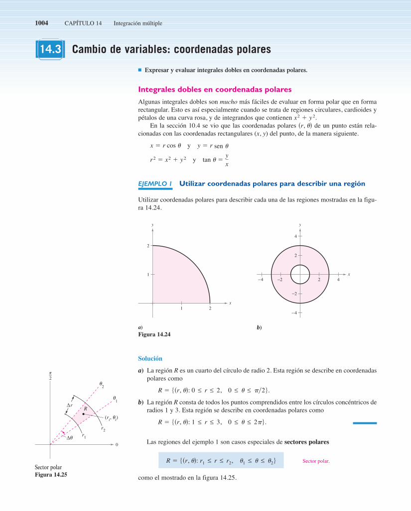
1004 CAPÍTULO 14 Integración múltiple
14.3 Cambio de variables: coordenadas polares
n Expresar y evaluar integrales dobles en coordenadas polares.
Integrales dobles en coordenadas polares
Algunas integrales dobles son mucho más fáciles de evaluar en forma polar que en formarectangular. Esto es así especialmente cuando se trata de regiones circulares, cardioides ypétalos de una curva rosa, y de integrandos que contienen
En la sección 10.4 se vio que las coordenadas polares de un punto están rela-cionadas con las coordenadas rectangulares (x, y) del punto, de la manera siguiente.
y
y
EJEMPLO 1 Utilizar coordenadas polares para describir una región
Utilizar coordenadas polares para describir cada una de las regiones mostradas en la figu-ra 14.24.
Solución
a) La región R es un cuarto del círculo de radio 2. Esta región se describe en coordenadaspolares como
b) La región R consta de todos los puntos comprendidos entre los círculos concéntricos deradios 1 y 3. Esta región se describe en coordenadas polares como
Las regiones del ejemplo 1 son casos especiales de sectores polares
como el mostrado en la figura 14.25.
0 ≤ u ≤ 2pJ.R 5 Hsr, ud: 1 ≤ r ≤ 3,
0 ≤ u ≤ py2J.R 5 Hsr, ud: 0 ≤ r ≤ 2,
tan u 5yx
r2 5 x2 1 y2
y 5 r sin ux 5 r cos u
sr, udx2 1 y2.
0
π2
θ1
θ2
θ∆
∆r
r1
r2
(ri, i)θ
R
Sector polarFigura 14.25
x
1
2
1 2
y
a)Figura 14.24
2
4
x2 4−2
−2
−4
−4
y
b)
Sector polar.u1 ≤ u ≤ u2JR 5 Hsr, ud: r1 ≤ r ≤ r2,
sen u
14-3.qxd 3/12/09 18:28 Page 1004

SECCIÓN 14.3 Cambio de variables: coordenadas polares 1005
Para definir una integral doble de una función continua en coordenadaspolares, considerar una región R limitada o acotada por las gráficas de y
y las rectas y En lugar de hacer una partición de R en rectángulospequeños, se utiliza una partición en sectores polares pequeños. A R se le superpone unared o cuadrícula polar formada por rayos o semirrectas radiales y arcos circulares, comose muestra en la figura 14.26. Los sectores polares Ri que se encuentran completamentedentro de R forman una partición polar interna cuya norma es la longitud de ladiagonal más larga en los n sectores polares.
Considerar un sector polar específico como se muestra en la figura 14.27. Se puedemostrar (ver ejercicio 75) que el área de es
Área de .
donde y Esto implica que el volumen del sólido de alturasobre es aproximadamente
y se tiene
La suma de la derecha se puede interpretar como una suma de Riemann para f(r cos u,r sen u)r. La región R corresponde a una región S horizontalmente simple en el plano ru,como se muestra en la figura 14.28. Los sectores polares corresponden a los rectángu-los y el área de es Por tanto, el lado derecho de la ecuación correspon-de a la integral doble
A partir de esto, se puede aplicar el teorema 14.2 para escribir
Esto sugiere el teorema siguiente, cuya demostración se verá en la sección 14.8.
5 Eb
aEg
2sud
g1sudf sr cos u, r sin udr dr du.
ERE fsx, yd dA 5 E
SE fsr cos u, r sin udr dA
ESE fsr cos u, r sin udr dA.
Dri Dui.SiDAiSi,Ri
ERE fsx, yd dA < o
n
i51fsri cos ui, ri sin ui dri Dri Dui.
fsri cos ui, ri sin uidri Dri Dui
Rifsri cos ui, ri sin uidDui 5 u2 2 u1.Dri 5 r2 2 r1
R iDAi 5 ri Dri Dui
Ri
Ri,
iD iD,
u 5 b.u 5 ar 5 g2sudr 5 g1sud
z 5 fsx, yd
θ∆
∆ri
g2
g1
(ri, i)θ
i
Ri
αβ
0
π2
La red o cuadrícula polar se sobreponesobre la región RFigura 14.26
Ri
r1
r2
θ
θ
θ
2
1
(ri, i)
0
π2
El sector polar es el conjunto de todos lospuntos tal que y
Figura 14.27u1 ≤ u ≤ u2.
r1 ≤ r ≤ r2sr, udRi
r
α
β
Si
θ(ri, i)
θr = g1( )θ r = g2( )θ
Región S horizontalmente simpleFigura 14.28
sen
sen
sen
sen
sen
sen
14-3.qxd 3/12/09 18:28 Page 1005

1006 CAPÍTULO 14 Integración múltiple
Si es no negativa en R, entonces la integral del teorema 14.3 puede interpretar-se como el volumen de la región sólida entre la gráfica de ƒ y la región R. Cuando se usa la integralen el teorema 14.3, asegurarse de no omitir el factor extra de r en el integrando. n
La región R puede ser de dos tipos básicos, regiones r-simples y regiones -simples,como se muestra en la figura 14.29.
EJEMPLO 2 Evaluar una integral usando coordenadas polares doble
Sea R la región anular comprendida entre los dos círculos y Evaluar la integral
Solución Los límites o cotas polares son y como se muestraen la figura 14.30. Además, y Por tanto, se tiene
5 6p.
5 13u 13 sin 2u
22
5!5 2 13
cos u242p
0
5 E2p
013 1 3 cos 2u 1
5!5 2 13
sin u2 du
5 E2p
016 cos2 u 1
5!5 2 13
sin u2 du
5 E2p
01r4
4cos2 u 1
r3
3sin u24
!5
1du
5 E2p
0E!5
1sr3 cos2 u 1 r2 sin ud dr du
ERE sx2 1 yd dA 5 E2p
0E!5
1sr2 cos2 u 1 r sin udr dr du
y 5 r sin u.x2 5 sr cos ud20 ≤ u ≤ 2p,1 ≤ r ≤ !5
eRe sx21 yd dA.
x2 1 y2 5 5.x2 1 y2 5 1
u
z 5 f sx, ydNOTA
2 3
R
R: 1 ≤ r ≤ 50 ≤ ≤ 2θ π
0
π2
Región simple Figura 14.30
r-
g1
g2
∆θ
θ =
αθ =
β
Límites o cotas variables para r:0 ≤ g1( ) ≤ r ≤ g2( )θ θ
α β≤ ≤θLímites o cotas fijas para :θ
0
π2
Región r-simpleFigura 14.29
r = r1
h1
r = r2
h2
∆r
Límites o cotas fijas para r:r1 ≤ r ≤ r2
0 ≤ h1(r) ≤ ≤ h2(r)θLímites o cotas variables para :θ
0
π2
Región u-simple
TEOREMA 14.3 CAMBIO DE VARIABLES A LA FORMA POLAR
Sea R una región plana que consta de todos los puntos (x, y) 5 (r cos u, r sen u) que satis-facen las condiciones 0 # g1(u) # r # g2(u), a # u # b, donde 0 # (b 2 a) # 2p. Sig1 y g2 son continuas en [a, b] y f es continua en R, entonces
ERE fsx, yd dA 5 Eb
aEg
2sud
g1sud
f sr cos u, r sin udr dr du.
E X P L O R A C I Ó N
Volumen de un sector paraboloideEn la exploración de la página 997se pidió resumir los diferentesmétodos hasta ahora estudiadospara calcular el volumen del sólidolimitado o acotado por el parabo-loide
y el plano xy. Ahora se conoce unmétodo más. Utilizarlo para encon-trar el volumen del sólido.
a > 0z 5 a2 2 x2 2 y 2,
sen
sen
sen
sen
sen
sen
sen
sen
14-3.qxd 3/12/09 18:28 Page 1006

SECCIÓN 14.3 Cambio de variables: coordenadas polares 1007
En el ejemplo 2, notar el factor extra de r en el integrando. Esto proviene de la fór-mula para el área de un sector polar. En notación diferencial, se puede escribir
lo que indica que el área de un sector polar aumenta al alejarse del origen.
EJEMPLO 3 Cambio de variables a coordenadas polares
Utilizar las coordenadas polares para hallar el volumen de la región sólida limitada supe-riormente por el hemisferio
Hemisferio que forma la superficie superior.
e inferiormente por la región circular R dada por
Región circular que forma la superficie inferior.
como se muestra en la figura 14.31.
Solución En la figura 14.31 se puede ver que R tiene como límites o cotas
y que En coordenadas polares, las cotas son
y
con altura Por consiguiente, el volumen V está dado por
< 46.979.516p
3s8 2 3!3 d
5 283
s3!3 2 8du42p
0
5 213 E
2p
0s24!3 2 64d du
5 213 E
2p
0s16 2 r2d3y24
2
0du
V 5 ERE fsx, yd dA 5 E2p
0E2
0
!16 2 r2 r dr du
z 5 !16 2 x2 2 y2 5 !16 2 r2.
0 ≤ u ≤ 2p0 ≤ r ≤ 2
0 ≤ z ≤ !16 2 x2 2 y2.
22 ≤ y ≤ 22!4 2 y2 ≤ x ≤ !4 2 y2,
x2 1 y2 ≤ 4
z 5 !16 2 x2 2 y2
dA 5 r dr du
y
x
z
R: x2 + y2 ≤ 4
Superficie: 16 − x2 − y2z =
4
4
4
Figura 14.31
TECNOLOGÍA Todo sistema algebraico por computadora que calcula integralesdobles en coordenadas rectangulares también calcula integrales dobles en coordenadaspolares. La razón es que una vez que se ha formado la integral iterada, su valor no cambiaal usar variables diferentes. En otras palabras, si se usa un sistema algebraico por compu-tadora para evaluar
se deberá obtener el mismo valor que se obtuvo en el ejemplo 3.
.
Así como ocurre con coordenadas rectangulares, la integral doble
puede usarse para calcular el área de una región en el plano.
ERE dA
E2p
0E2
0
!16 2 x2 x dx dy
Para ver la ventaja de lascoordenadas polares en el ejemplo 3,hay que tratar de evaluar la integral ite-rada rectangular correspondiente
n
E2
22E!42y2
2!42y2
!16 2 x2 2 y 2 dx dy.
NOTA
14-3.qxd 3/12/09 18:28 Page 1007

1008 CAPÍTULO 14 Integración múltiple
EJEMPLO 4 Hallar áreas de regiones polares
Utilizar una integral doble para hallar el área encerrada por la gráfica de
Solución Sea R un pétalo de la curva mostrada en la figura 14.32. Esta región es r-simple y los límites son los siguientes.
Límites o cotas fijas para .
Límites o cotas variables para r.
Por tanto, el área de un pétalo es
Así, el área total es
Como se ilustra en el ejemplo 4, el área de una región en el plano puede representarsemediante
Si se obtiene
lo cual concuerda con el teorema 10.13.Hasta ahora en esta sección, todos los ejemplos de integrales iteradas en forma polar
han sido de la forma
en donde el orden de integración es primero con respecto a r. Algunas veces se puede sim-plificar el problema de integración cambiando el orden de integración, como se ilustra enel ejemplo siguiente.
EJEMPLO 5 Cambio del orden de integración
Hallar el área de la región acotada superiormente por la espiral e inferior-mente por el eje polar, entre y
Solución La región se muestra en la figura 14.33. Las cotas o límites polares de la región son
y
Por tanto, el área de la región puede evaluarse como sigue.
5p
35
pr3 4
2
15 E2
1
p
3dr5 E2
1ru4
pys3rd
0drA 5 E2
1Epys3rd
0r du dr
0 ≤ u ≤p
3r.1 ≤ r ≤ 2
r 5 2.r 5 1r 3
Eb
aEg
2sud
g1sudfsr cos u, r sin udr dr du
5 Eb
a
12
sg2sudd2 du5 Eb
a
r2
2 4g
2sud
0duA 5 Eb
aEg
2sud
0r dr du
g1sud 5 0,
A 5 Eb
aEg
2sud
g1sudr dr du.
A 5 9py4.
0 r 3 cos 3
u6 6
r 5 3 cos 3u.
03
R:
0 ≤ r ≤ 3 cos 3
≤ ≤θθ
θr = 3 cos 3
π6
=θ
π6
π6
= −θ
π6
−
π2
Figura 14.32
sen
021
R:
1 ≤ r ≤ 2
0 ≤ ≤θ
π3
=θ
π3r
θπ3
r =
π6
=θ
π2
Región u-simpleFigura 14.33
94
6
61 cos 6 d
94
16
sen 66
6
34
.
92
6
6cos2 3 d
6
6
r2
2
3 cos 3
0d
13
AR
dA6
6
3 cos 3
0r dr d
14-3.qxd 3/12/09 18:28 Page 1008

SECCIÓN 14.3 Cambio de variables: coordenadas polares 1009
En los ejercicios 1 a 4 se muestra la región R para la integral. Decir si serían más convenientes coordenadas rec-
tangulares o polares para evaluar la integral.
1. 2.
3. 4.
En los ejercicios 5 a 8, utilizar las coordenadas polares paradescribir la región mostrada.
5. 6.
7. 8.
En los ejercicios 9 a 16, evaluar la integral doble y dibujar la región R.
11. 12.
13. 14.
15. 16.
En los ejercicios 17 a 26, evaluar la integral iterada pasando acoordenadas polares.
17. 18.
21. 22.
23. 24.
En los ejercicios 27 y 28, combinar la suma de las dos integralesiteradas en una sola integral iterada pasando a coordenadaspolares. Evaluar la integral iterada resultante.
27.
28.
En los ejercicios 29 a 32, utilizar coordenadas polares para es-cribir y evaluar la integral doble
29.
30.
31.
32.
Volumen En los ejercicios 33 a 38, utilizar una integral doble encoordenadas polares para hallar el volumen del sólido limitado oacotado por las gráficas de las ecuaciones.
33.
34.
35.
36.
37. Interior al hemisferio e interior al cilindro
38. Interior al hemisferio y exterior al cilindrox2 1 y 2 5 1
z 5 !16 2 x2 2 y 2
x2 1 y 2 2 4x 5 0z 5 !16 2 x2 2 y 2
z 5 lnsx2 1 y 2d, z 5 0, x2 1 y 2 ≥ 1, x2 1 y 2 ≤ 4
z 5 !x2 1 y 2, z 5 0, x2 1 y 2 5 25
z 5 x2 1 y 2 1 3, z 5 0, x2 1 y 2 5 1
z 5 xy, x2 1 y 2 5 1, first octant
R: x2 1 y 2 ≤ 9, x ≥ 0, y ≥ 0f sx, yd 5 9 2 x 2 2 y 2,
R: x2 1 y 2 ≥ 1, x2 1 y 2 ≤ 4, 0 ≤ y ≤ xf sx, yd 5 arctan yx,
R: x2 1 y2 ≤ 25, x ≥ 0f sx, yd 5 e2sx21y2dy2,
R: x2 1 y 2 ≤ 4, x ≥ 0, y ≥ 0f sx, yd 5 x 1 y,
eRe f xx, yc dA.
E5!2y2
0Ex
0xy dy dx 1 E5
5!2y2E!252x2
0xy dy dx
E2
0Ex
0
!x2 1 y 2 dy dx 1 E2!2
2E!82x2
0
!x2 1 y 2 dy dx
E4
0E!4y2y2
0x2 dx dyE2
0E!2x2x2
0xy dy dx
E2
0E!82y2
y
!x2 1 y2 dx dyE3
0E!92x2
0sx2 1 y 2d3y2 dy dx
Ea
0E!a22x2
0x dy dxEa
0E!a22y2
0y dx dy
Epy2
0E12cos
u
0ssin udr dr duEpy2
0E11sin u
0ur dr du
Epy2
0E3
0re2r2
dr duEpy2
0E3
2
!9 2 r2 r dr du
Epy4
0E4
0r2 sin u cos u dr duE2p
0E6
03r2 sin u dr du
9. 10.0
sen
0r 2 dr d
0
cos
0r dr d
eRe f xr, uc dA,
x−2−4
−4
2
4
4
y
x
−2
−4
2
4
4
y
x
−2
−2−4
2
6
2 4
y
x
−4
−4−8
4
12
4 8
y
x1
1
−1
2
3
2 3 4
R
y
x
−2−4
−4
2
4
2 4
R
y
x
−2
−2−6
−4
2
4
2
R
y
x1
1
2
3
4
2 3 4
R
y
eRe f xx, yc dA
14.3 Ejercicios
19. 20.1
0
x x2
x x2x2 y2 dy dx
2
2
4 x2
0x2 y2 dy dx
sensen θ
25.
26.2
0
4 x2
0sen x2 y2 dy dx
1
1
1 x2
0cos x2 y2 dy dx
primer octante
sen sen
14-3.qxd 3/12/09 18:28 Page 1009

1010 CAPÍTULO 14 Integración múltiple
39. Volumen Hallar a tal que el volumen en el interior del hemis-ferio y en el exterior del cilindro
sea la mitad del volumen del hemisferio.
40. Volumen Utilizar una integral doble en coordenadas polarespara hallar el volumen de una esfera de radio a.
41. Volumen Determinar el diámetro de un orificio cavado verti-calmente a través del centro del sólido limitado o acotado por lasgráficas de las ecuaciones y
si se elimina la décima parte del volumen del sóli-do.
42. Diseño industrial Las superficies de una leva de doble lóbulose representan por las desigualdades y
donde todas las medidas se dan en pulgadas.
a) Utilizar un sistema algebraico por computadora y representargráficamente la leva.
b) Utilizar un sistema algebraico por computadora y aproximarel perímetro de la curva polar
Ésta es la distancia que recorre una pieza en contacto con laleva durante un giro completo de ésta.
c) Utilizar un sistema algebraico por computadora y hallar elvolumen del acero en la leva.
Área En los ejercicios 43 a 48, utilizar una integral doble paracalcular el área de la región sombreada.
43. 44.
45. 46.
47. 48.
Área En los ejercicios 49 a 54, trazar una gráfica de la regiónlimitada por las gráficas de las ecuaciones. Después, usar unaintegral doble para encontrar el área de la región.
49. Dentro del círculo r 5 2 cos u y fuera del círculo r 5 1.
50. Dentro de la cardioide r 5 2 1 2 cos u y fuera del círculo r 5 1.
51. Dentro del círculo r 5 3 cos u y fuera de la cardioide r 5 1 1cos u.
52. Dentro de la cardioide r 5 1 1 cos u y fuera del círculo r 5 3 cos u.
53. Dentro de la curva rosa r 5 4 sen 3u y fuera del círculo r 5 2.
54. Dentro del círculo r 5 2 y fuera de la cardioide r 5 2 2 2 cos u.
03
r = 3 cos 2θπ2
01 2
r = 2 sen 3θ
π2
02 43
r = 2 + senθ
π2
01
r = 1 + cos θπ2
0
r = 4
1 3
π2r = 2
01 2 3 4 75
r = 6 cos θ
π2
r 512s1 1 cos2 ud.
294sx2 1 y 2 1 9d ≤ z ≤
94sx2 1 y 2 1 9d
14 ≤ r ≤ 1
2s1 1 cos2 ud
x2 1 y 2 5 16z 5 25e2sx21y 2dy4, z 5 0,
x2 1 y 2 5 a2z 5 !16 2 x2 2 y 2
Desarrollo de conceptos55. Describir la partición de la región de integración R en el
plano xy cuando se utilizan coordenadas polares para eva-luar una integral doble.
56. Explicar cómo pasar de coordenadas rectangulares a coorde-nadas polares en una integral doble.
57. Con sus propias palabras, describir regiones r-simples yregiones u-simples.
58. Cada figura muestra una región de integración para la integraldoble Para cada región, decir si es más fácilobtener los límites de integración con elementos representa-tivos horizontales, elementos representativos verticales o consectores polares. Explicar el razonamiento.
a) b) c)
59. Sea R la región limitada por el círculo x2 1 y2 5 9.
a) Establecer la integral
b) Convertir la integral en el inciso a) a coordenadas po-lares.
c) ¿Qué integral debería elegirse para evaluar? ¿Por qué?
Rf x, y dA.
x
R
y
x
R
y
x
R
y
eRe f sx, yd dA.
Para discusión60. Para pensar Sin desarrollar cálculos, identificar la integral
doble que represente la integral de f(x) 5 x2 1 y2 sobre uncírculo de radio 4. Explicar el razonamiento.
a) b)
c) d)2
0
4
4r3 dr d
2
0
4
0r3 dr d
4
0
2
0r3 dr d
2
0
4
0r2 dr d
CAS
14-3.qxd 3/12/09 18:28 Page 1010

SECCIÓN 14.3 Cambio de variables: coordenadas polares 1011
61. Para pensar Considerar el programa escrito en el ejercicio 78de la sección 14.2 para aproximar integrales dobles en coorde-nadas rectangulares. Si el programa se usa para aproximar laintegral doble
en coordenadas polares, ¿cómo hay que modificar ƒ para intro-ducirla al programa? Como los límites de integración son cons-tantes, describir la región plana de integración.
62. Aproximación Las secciones transversales horizontales de unbloque de hielo desprendido de un glaciar tienen forma deun cuarto de un círculo con radio aproximado de 50 pies. Labase se divide en 20 subregiones como se muestra en la figura.En el centro de cada subregión, se mide la altura del hielo,dando los puntos siguientes en coordenadas cilíndricas.
a) Aproximar el volumen del sólido.
b) El hielo pesa aproximadamente 57 libras por pie cúbico.Aproximar el peso del sólido.
c) Aproximar el número de galones de agua en el sólido si hay7.48 galones de agua por pie cúbico.
Aproximación En los ejercicios 63 y 64, utilizar un sistemaalgebraico por computadora y aproximar la integral iterada.
63.
64.
Aproximación En los ejercicios 65 y 66, determinar qué valorse aproxima más al volumen del sólido entre el plano xy y la fun-ción sobre la región. (Realizar la elección a la vista de un dibujodel sólido y no efectuando cálculo alguno.)
65. ƒ(x, y) 5 15 2 2y; R: semicírculo: x2 1 y2 5 16, y ≥ 0
a) 100 b) 200 c) 300 d) e) 800
66. ƒ(x, y) 5 xy 1 2; R: cuarto de círculo: x2 1 y2 5 9, x ≥ 0, y ≥ 0
a) 25 b) 8 c) 100 d) 50 e)
¿Verdadero o falso? En los ejercicios 67 y 68, determinar si ladeclaración es verdadera o falsa. Si es falsa, explicar por qué odar un ejemplo que demuestre que es falsa.
67. Si entonces para todo en
68. Si es una función constante y el área de la región S es el dobledel área de la región R, entonces
69. Probabilidad El valor de la integral se re-
quiere en el desarrollo de la función de densidad de probabi-lidad normal.
a) Utilizar coordenadas polares para evaluar la integral im-propia.
b) Utilizar el resultado del inciso a) para calcular I.
PARA MAYOR INFORMACIÓN Para más información sobreeste problema, ver el artículo “Integrating Without Polar Coor-dinates” de William Dunham en Mathematics Teacher.
70. Utilizar el resultado del ejercicio 69 y un cambio de variablespara evaluar cada una de las integrales siguientes. No se re-quiere hacer ninguna integración.
a) b)
71. Población La densidad de población en una ciudad se aproxima mediante el modelo ƒ(x, y) 5 4 000e20.01(x2 1 y2),
donde y se miden en millas. Integrar la fun-ción de densidad sobre la región circular indicada para aproxi-mar la población de la ciudad.
72. Probabilidad Hallar k tal que la función
sea una función de densidad de probabilidad.
73. Para pensar Considerar la región limitada o acotada por lasgráficas de y 5 2, y 5 4, y 5 x y y la integral doble
Determinar los límites de integración si la región R está dividida en a) elementos representativos horizontales,b) elementos representativos verticales y c) sectores polares.
74. Repetir el ejercicio 73 con una región R limitada o acotada porla gráfica de la ecuación
75. Mostrar que el área A del sector polar R (ver la figura) esdonde es el radio promedio de R.
θ∆
∆r
r1
r2
R
r 5 sr1 1 r2dy2A 5 rDrDu,
sx 2 2d2 1 y 2 5 4.
eRe f dA.y 5 !3x
f sx, yd 5 5ke2sx21y2d,0,
x ≥ 0, y ≥ 0elsewhere
yxx2 1 y 2 ≤ 49,
E`
2`e24x 2 dxE`
2`e2x 2 dx
e2x2
5 E`
2`E`
2`e2sx21y2dy2 dA
I 2 5 1E`
2`e2x2y2 dx21E`
2`e2y2y2 dy2
I 5 E`
2`e2x2y2 dx
2 eRe f sr, ud dA 5 eSe f sr, ud dA.f sr, ud
R.sr, udf sr, ud > 0eRe f sr, ud dA > 0,
230
2200
Epy4
0E4
05re!ru dr du
Epy2
py4E5
0r!1 1 r 3 sin !u dr du
010 20 30 40 50
π
π
8
4
8π3
π2
s5, 7p16, 5d, s15, 7p
16, 8d, s25, 7p16, 11d, s35, 7p
16, 16d, s45, 7p16, 12d
s5, 5p16, 9d, s15, 5p
16, 11d, s25, 5p16, 15d, s35, 5p
16, 18d, s45, 5p16, 14d,
s5, 3p16, 9d, s15, 3p
16, 10d, s25, 3p16, 14d, s35, 3p
16, 15d, s45, 3p16, 10d,
s5, p16, 7d, s15, p
16, 8d, s25, p16, 10d, s35, p
16, 12d, s45, p16, 9d,
ERE f sr, ud dA
sen
en el restoCAS
14-3.qxd 3/12/09 18:28 Page 1011

1012 CAPÍTULO 14 Integración múltiple
14.4 Centro de masa y momentos de inercian Hallar la masa de una lámina plana utilizando una integral doble.n Hallar el centro de masa de una lámina plana utilizando integrales dobles.n Hallar los momentos de inercia utilizando integrales dobles.
Masa
En la sección 7.6 se analizaron varias aplicaciones de la integración en las que se tenía unalámina plana de densidad constante Por ejemplo, si la lámina que corresponde a laregión R, que se muestra en la figura 14.34, tiene una densidad constante entoncesla masa de la lámina está dada por
Densidad constante.
Si no se especifica otra cosa, se supone que una lámina tiene densidad constante. En estasección, se extiende la definición del término lámina para abarcar también placas delgadasde densidad variable. Las integrales dobles pueden usarse para calcular la masa de unalámina de densidad variable, donde la densidad en (x, y) está dada por la función de den-sidad r.
La densidad se expresa normalmente como masa por unidad de volumen. Sin embargo, enuna lámina plana la densidad es masa por unidad de área de superficie. n
EJEMPLO 1 Hallar la masa de una lámina plana
Hallar la masa de la lámina triangular con vértices (0, 0), (0, 3) y (2, 3), dado que la den-sidad en es
Solución Como se muestra en la figura 14.35, la región R tiene como fronteras x 5 0,y 5 3 y y 5 3x/2 (o x 5 2y/3). Por consiguiente, la masa de la lámina es
En la figura 14.35, nótese que la lámina plana está sombreada; el sombreado más oscurocorresponde a la parte más densa. n
NOTA
5 10.
5109 3 y3
3 43
0
5109 E
3
0y2 dy
5 E3
03x2 1 xy4
2yy3
0dy
m 5 EREs2x 1 yd dA 5 E3
0E2yy3
0s2x 1 yd dx dy
rsx, yd 5 2x 1 y.sx, yd
NOTA
Mass 5 rA 5 rEREdA 5 E
REr dA.
r,r.
xx = a x = b
g1
g2
R
y
Lámina de densidad constante Figura 14.34
r
x
1
1
2
2
3
3
(0, 3)
(0, 0)
(2, 3)
x = 23
y
y = 3
R
y
Lámina de densidad variable
Figura 14.35rsx, yd 5 2x 1 y
DEFINICIÓN DE MASA DE UNA LÁMINA PLANA DE DENSIDAD VARIABLE
Si r es una función de densidad continua sobre la lámina que corresponde a unaregión plana R, entonces la masa m de la lámina está dada por
Densidad variable.m 5 ERErsx, yd dA.
Masa
14-4.qxd 3/12/09 18:29 Page 1012

SECCIÓN 14.4 Centro de masa y momentos de inercia 1013
EJEMPLO 2 Hallar la masa empleando coordenadas polares
Hallar la masa de la lámina correspondiente a la porción en el primer cuadrante delcírculo
donde la densidad en el punto (x, y) es proporcional a la distancia entre el punto y el ori-gen, como se muestra en la figura 14.36.
Solución En todo punto (x, y), la densidad de la lámina es
Como y la masa está dada por
Para simplificar la integración, se puede convertir a coordenadas polares, utilizando loslímites o cotas y Por tanto, la masa es
54pk
3.
58k3 3u4
py2
0
58k3 Epy2
0du
5 Epy2
0
kr3
3 42
0du
5 Epy2
0E2
0kr2 dr du
m 5 EREk!x2 1 y2 dA 5 Epy2
0E2
0k!r2 r dr du
0 ≤ r ≤ 2.0 ≤ u ≤ py2
5 E2
0E!42x2
0k!x2 1 y2 dy dx.
m 5 EREk!x2 1 y2 dA
0 ≤ y ≤ !4 2 x2,0 ≤ x ≤ 2
5 k!x2 1 y2.
rsx, yd 5 k!sx 2 0d2 1 sy 2 0d2
x2 1 y2 5 4
x
1
1
2
2
(x, y)
x2 + y2 = 4
R
y
Densidad en Figura 14.36
rsx, yd 5 k!x2 1 y2sx, yd:
TECNOLOGÍA En muchas ocasiones, en este texto, se han mencionado las ventajasde utilizar programas de computación que realizan integración simbólica. Aun cuandose utilicen tales programas con regularidad, hay que recordar que sus mejores ventajassólo son aprovechables en manos de un usuario conocedor. Por ejemplo, nótese la sim-plificación de la integral del ejemplo 2 cuando se convierte a la forma polar.
Forma rectangular Forma polar
Si se tiene acceso a programas que realicen integración simbólica, se recomienda utili-zarlos para evaluar ambas integrales. Algunos programas no pueden manejar la primeraintegral, pero cualquier programa que calcule integrales dobles puede evaluar la segun-da integral.
Epy2
0E2
0kr2 dr duE2
0E!42x2
0k!x2 1 y2 dy dx
14-4.qxd 3/12/09 18:29 Page 1013

1014 CAPÍTULO 14 Integración múltiple
Momentos y centros de masa
En láminas de densidad variable, los momentos de masa se definen de manera similar ala empleada en el caso de densidad uniforme. Dada una partición de una lámina, corres-pondiente a una región plana R, considerar el rectángulo i-ésimo de área como semuestra en la figura 14.37. Suponer que la masa de se concentra en uno de sus puntosinteriores El momento de masa de respecto al eje x puede aproximarse pormedio de
De manera similar, el momento de masa con respecto al eje y puede aproximarse pormedio de
Formando la suma de Riemann de todos estos productos y tomando límites cuando lanorma de se aproxima a 0, se obtienen las definiciones siguientes de momentos de masacon respecto a los ejes x y y.
En algunas láminas planas con densidad constante se puede determinar el centro demasa (o una de sus coordenadas) utilizando la simetría en lugar de usar integración. Porejemplo, considerar las láminas de densidad constante mostradas en la figura 14.38.Utilizando la simetría, se puede ver que en la primera lámina y en la segundalámina.
x 5 0y 5 0
r,
D
sMassdsxid < frsxi, yid DAigsxid.
sMassdsyid < frsxi, yid DAigsyid.
Risxi, yid.Ri
DAi,Ri
D
x
Ri
xi
yi
(xi, yi)
y
Mx 5 (masa)(yi)My 5 (masa)(xi)Figura 14.37
Lámina de densidad constante y simétrica conrespecto al eje xFigura 14.38
Lámina de densidad constante y simétrica conrespecto al eje y
x
y
z
1 1
1
−1
−1
−1
R: 0 ≤ x ≤ 1
− 1 − x2 ≤ y ≤ 1 − x2R: 1 − y2 1 − y2− ≤ x ≤
0 ≤ y ≤ 1
x
y
z
1 1
1
−1
−1
−1
MOMENTOS Y CENTRO DE MASA DE UNA LÁMINA PLANA DE DENSIDAD VARIABLE
Sea una función de densidad continua sobre la lámina plana R. Los momentos demasa con respecto a los ejes x y y son
y
Si m es la masa de la lámina, entonces el centro de masa es
Si R representa una región plana simple en lugar de una lámina, el punto sellama el centroide de la región.
sx, yd
sx, yd 5 1My
m,
Mx
m 2.
My 5 ERExr(x, yd dA.Mx 5 E
REyrsx, yd dA
r
(Masa)(yi)
(Masa)(xi)
14-4.qxd 3/12/09 18:29 Page 1014

SECCIÓN 14.4 Centro de masa y momentos de inercia 1015
EJEMPLO 3 Hallar el centro de masa
Hallar el centro de masa de la lámina que corresponde a la región parabólica
Región parabólica.
donde la densidad en el punto es proporcional a la distancia entre y el eje x,como se muestra en la figura 14.39.
Solución Como la lámina es simétrica con respecto al eje y y
el centro de masa está en el eje y. Así, Para hallar primero calcular la masa de lalámina.
Después se halla el momento con respecto al eje x.
Así,
y el centro de masa es
Aunque los momentos y se pueden interpretar como una medida de la tenden-cia a girar en torno a los ejes x o y, el cálculo de los momentos normalmente es un pasointermedio hacia una meta más tangible. El uso de los momentos y es encontrar elcentro de masa. La determinación del centro de masa es útil en muchas aplicaciones, yaque permite tratar una lámina como si su masa se concentrara en un solo punto.Intuitivamente, se puede concebir el centro de masa como el punto de equilibrio de la lámi-na. Por ejemplo, la lámina del ejemplo 3 se mantendrá en equilibrio sobre la punta de unlápiz colocado en como se muestra en la figura 14.40.s0, 16
7 d,
MyMx
MyMx
s0, 167 d.
y 5Mx
m5
4096ky105256ky15
5167
54096k105
5k3364x 2 16x3 1
12x5
52
x7
7 42
22
5k3E
2
22s64 2 48x2 1 12x4 2 x6d dx
Mx 5 E2
22E42x2
0sydskyd dy dx 5
k3E
2
22y34
42x2
0dx
5256k15
5 k132 2643
1325 2
5k2316x 2
8x3
31
x5
5 42
22
5k2E
2
22s16 2 8x2 1 x4d dx
Mass 5 E2
22E42x2
0ky dy dx 5
k2E
2
22y24
42x2
0dx
y,x 5 0.
rsx, yd 5 ky
sx, ydsx, yd
0 ≤ y ≤ 4 2 x2
x
y
1 2−2 −1
3
2
1
y = 4 − x2
Densidad variable:(x, y) = kyρ
(x, y)
Región parabólica de densidad variableFigura 14.39
x
z
y
Centro de masa:
0, 167( )
2
14
−2
R: −2 ≤ x ≤ 20 ≤ y ≤ 4 − x2
Densidadvariable:
(x, y) = kyρ
Figura 14.40
Masa
4 096k
4 096k/105
14-4.qxd 3/12/09 18:29 Page 1015

1016 CAPÍTULO 14 Integración múltiple
Momentos de inercia
Los momentos y utilizados en la determinación del centro de masa de una láminase suelen llamar primeros momentos con respecto a los ejes x y y. En cada uno de loscasos, el momento es el producto de una masa por una distancia.
Distancia Masa Distancia Masaal eje x al eje y
Ahora se introducirá otro tipo de momento, el segundo momento o momento de inerciade una lámina respecto de una recta. Del mismo modo que la masa es una medida de latendencia de la materia a resistirse a cambios en el movimiento rectilíneo, el momento deinercia respecto de una recta es una medida de la tendencia de la materia a resistirse acambios en el movimiento de rotación. Por ejemplo, si una partícula de masa m está a unadistancia d de una recta fija, su momento de inercia respecto de la recta se define como
I 5 md2 5 (masa)(distancia)2.
Igual que ocurre con los momentos de masa, se puede generalizar este concepto paraobtener los momentos de inercia de una lámina de densidad variable respecto de los ejes xy y. Estos segundos momentos se denotan por e y en cada caso el momento es el pro-ducto de una masa por el cuadrado de una distancia.
Cuadrado de Masa Cuadrado de Masala distancia la distanciaal eje x al eje y
A la suma de los momentos e se le llama el momento polar de inercia y se denotapor
EJEMPLO 4 Hallar el momento de inercia
Hallar el momento de inercia respecto del eje x de la lámina del ejemplo 3.
Solución De acuerdo con la definición de momento de inercia, se tiene
532,768k
315.
5k43256x 2
256x3
31
96x5
52
16x7
71
x9
9 42
22
5k4E
2
22s256 2 256x2 1 96x4 2 16x6 1 x8d dx
5k4E
2
22y44
42x2
0dx
Ix 5 E2
22E42x2
0y2skyd dy dx
I0.IyIx
Iy 5 EREsx2drsx, yd dAIx 5 E
REsy2drsx, yd dA
Iy,Ix
My 5 EREsxdrsx, yd dAMx 5 E
REsydrsx, yd dA
MyMx
En el caso de una lámina enel plano xy, representa el momentode inercia de la lámina con respecto aleje z. El término “momento polar deinercia” se debe a que en el cálculo seutiliza el cuadrado de la distanciapolar r.
n
5 EREr2rsx, yd dA
I0 5 EREsx2 1 y2drsx, yd dA
I0
NOTA
14-4.qxd 3/12/09 18:29 Page 1016

SECCIÓN 14.4 Centro de masa y momentos de inercia 1017
El momento de inercia I de una lámina en rotación puede utilizarse para medir suenergía cinética. Por ejemplo, consideremos una lámina plana que gira en torno a una rectacon una velocidad angular de v radianes por segundo, como se muestra en la figura14.41. La energía cinética E de la lámina en rotación es
Energía cinética del movimiento giratorio.
Por otro lado, la energía cinética E de una masa m que se mueve en línea recta a una veloci-dad v es
Energía cinética del movimiento rectilíneo.
Por lo tanto, la energía cinética de una masa que se mueve en línea recta es proporcionala su masa, pero la energía cinética de una masa que gira en torno a un eje es proporcio-nal a su momento de inercia.
El radio de giro de una masa en rotación m con momento de inercia I se definecomo
Radio de giro.
Si toda la masa se localizara a una distancia de su eje de giro o eje de rotación, tendríael mismo momento de inercia y, por consiguiente, la misma energía cinética. Por ejemplo,el radio de giro de la lámina del ejemplo 4 respecto al eje x está dado por
EJEMPLO 5 Cálculo del radio de giro
Hallar el radio de giro con respecto al eje y de la lámina que corresponde a la regióndonde la densidad en está dada por
Solución La región R se muestra en la figura 14.42. Integrando sobre laregión se puede determinar que la masa de la región es El momento de inercia conrespecto al eje y es
Por tanto, el radio de giro con respecto al eje y es
5 !p2 2 6 < 1.967.
5!p3 2 6p
p
x 5!Iy
m
5 p3 2 6p.
5 3s3x2 2 6dssin xd 2 sx3 2 6xdscos xd4p
0
5 Ep
0x3 sin x dx
5 Ep
0x3y4
sin x
0dx
Iy 5 Ep
0Esin x
0x3 dy dx
p.R,rsx, yd 5 x
rsx, yd 5 x.sx, yd0 ≤ x ≤ p,R: 0 ≤ y ≤ sin x,
y 5!Ix
m5!32,768ky315
256ky155!128
21< 2.469.
r
r 5! Im
.
r
E 512
mv2.
E 512
Iv2.
Lámina plana girando a v radianes porsegundoFigura 14.41
x
1
2
2
Densidadvariable: R: 0 ≤ x ≤
0 ≤ y ≤ sen xπ
(x, y)
(x, y) = xρ
ππ
y
Figura 14.42
(sen x)
sen
sen x
sen x
sen
14-4.qxd 3/12/09 18:29 Page 1017

1018 CAPÍTULO 14 Integración múltiple
En los ejercicios 1 a 4, hallar la masa de la lámina descrita porlas desigualdades, dado que su densidad es (Suge-rencia: Algunas de las integrales son más simples en coorde-nadas polares.)
En los ejercicios 5 a 8, hallar la masa y el centro de masa de lalámina con cada densidad.
5. cuadrado con vértices (0, 0), (a, 0), (0, a), (a, a)
a) b) c)
6. rectángulo con vértices
a) b)
7. triángulo con vértices (0, 0), (0, a), (a, a)
a) b) c)
8. triángulo con vértices (0, 0), (a/2, a), (a, 0)
a) b) y
9. Traslaciones en el plano Trasladar la lámina del ejercicio 5cinco unidades a la derecha y determinar el centro de masaresultante.
10. Conjetura Utilizar el resultado del ejercicio 9 para formularuna conjetura acerca del cambio en el centro de masa cuandouna lámina de densidad constante se traslada c unidades hori-zontalmente o d unidades verticalmente. ¿Es la conjetura ver-dadera si la densidad no es constante? Explicar.
En los ejercicios 11 a 22, hallar la masa y el centro de masa de lalámina limitada o acotada por las gráficas de las ecuaciones conla densidad o densidades que se especifican. (Sugerencia: Algunasde las integrales son más sencillas en coordenadas polares.)
En los ejercicios 23 a 26, utilizar un sistema algebraico por compu-tadora para hallar la masa y el centro de masa de la lámina limita-da o acotada por las gráficas de las ecuaciones con la densidad dada.
23.
24.
25.
26.
En los ejercicios 27 a 32, verificar los momentos de inercia dadosy hallar y Suponer que la densidad de cada lámina esr 55 1 gramos por centímetro cuadrado. (Estas regiones son for-mas de uso común empleadas en diseño.)
27. Rectángulo 28. Triángulo rectángulo
29. Círculo 30. Semicírculo
31. Cuarto del círculo 32. Elipse
En los ejercicios 33 a 40, hallar y para la lámina li-mitada o acotada por las gráficas de las ecuaciones. Utilizar un sis-tema algebraico por computadora a fin de evaluar las integralesdobles.
33.
34.
35.
36.
37.
38.
39.
40. y 5 x3, y 5 4x, r 5 k|y|y 5 x2, y2 5 x, r 5 kx
y 5 x2, y2 5 x, r 5 x2 1 y2
y 5 !x, y 5 0, x 5 4, r 5 kxy
y 5 x, y 5 x2, r 5 kxy
y 5 4 2 x2, y 5 0, x > 0, r 5 kx
y 5 !a2 2 x2, y 5 0, r 5 ky
y 5 0, y 5 b, x 5 0, x 5 a, r 5 ky
yx,I0,Iy,Ix,
x
I0 =14
πab(a2 + b2)
ab
y
xa
I0 = 18
π a4
y
x
I0 = 14
π a4
a
y
x
I0 = 12
π a4
a
y
x
Ix = bh3112
Iy = b3h112
h
b
y
x
Ix = bh313
Iy = b3h13
h
b
y
y.x
r 5 1 1 cos u, r 5 k
r 5 2 cos 3u, 2p
6≤ u ≤
p
6, r 5 k
y 5 ln x, y 5 0, x 5 1, x 5 e, r 5 kyx
y 5 e2x, y 5 0, x 5 0, x 5 2, r 5 ky
r 5 kxr 5 k
R:
r 5 kxr 5 kyr 5 k
R:
r 5 ksx2 1 y2dr 5 kxy
s0, 0d, sa, 0d, s0, bd, sa, bdR:
r 5 kxr 5 kyr 5 k
R:
rxx, yc 5 xy.
14.4 Ejercicios
In Exercises 1– 4, find the mass of the lamina described by theinequalities, given that its density is (Hint: Someof the integrals are simpler in polar coordinates.)
1.
2.
3.
4.
In Exercises 5– 8, find the mass and center of mass of the laminafor each density.
5. square with vertices
(a) (b) (c)
6. rectangle with vertices
(a) (b)
7. triangle with vertices
(a) (b) (c)
8. triangle with vertices
(a) (b)
9. Translations in the Plane Translate the lamina in Exercise 5to the right five units and determine the resulting center of mass.
10. Conjecture Use the result of Exercise 9 to make a conjectureabout the change in the center of mass when a lamina ofconstant density is translated units horizontally or unitsvertically. Is the conjecture true if the density is not constant?Explain.
In Exercises 11–22, find the mass and center of mass of thelamina bounded by the graphs of the equations for the givendensity or densities. (Hint: Some of the integrals are simpler inpolar coordinates.)
11.
12.
13.
14.
15.
a) b)
16.
a) b)
17.
18.
19.
20.
21.
22.
In Exercises 23 –26, use a computer algebra system to find themass and center of mass of the lamina bounded by the graphsof the equations for the given density.
23.
24.
25.
26.
In Exercises 27–32, verify the given moment(s) of inertia andfind and Assume that each lamina has a density of gram per square centimeter. (These regions are common shapesused in engineering.)
27. Rectangle 28. Right triangle
29. Circle 30. Semicircle
31. Quarter circle 32. Ellipse
In Exercises 33 – 40, find and for the laminabounded by the graphs of the equations. Use a computeralgebra system to evaluate the double integrals.
33.
34.
35.
36.
37.
38.
39. 40. y x3, y 4x, k yy x2, y2 x, kx
y x2, y2 x, x2 y2
y x, y 0, x 4, kxy
y x, y x2, kxy
y 4 x2, y 0, x > 0, kx
y a2 x2, y 0, ky
y 0, y b, x 0, x a, ky
yIx, Iy, I0, x,
x
I0 =14
π ab(a2 + b2)
ab
y
xa
y
I0 = 18
π a4
a
y
I0 = 14
π a4
x
I0 = 12
π a4
a
y
x
Ix = bh3112
112
Iy = b3h
h
b
y
x
Ix = bh3
Iy = b3h13
13
h
b
y
1y.x
r 1 cos , k
r 2 cos 3 , 6 6, k
y ln x, y 0, x 1, x e, k x
y e x, y 0, x 0, x 2, kxy
x2 y2 a2, 0 x, 0 y, k x2 y2
y a2 x2, 0 y x, k
y cos x
L, y 0, x 0, x
L2
, ky
y sen x
L, y 0, x 0, x L, k
x 9 y2, x 0, kx
y 4 x2, y 0, ky
ky2ky
y e x, y 0, x 0, x 1
kyk
y ex, y 0, x 0, x 1
y1
1 x2, y 0, x 1, x 1, k
y 4 x, y 0, x 1, x 4, kx2
y x2, y 0, x 2, kxy
y x, y 0, x 1, ky
dc
kxyk
0, 0 , a 2, a , a, 0R:
kxkyk
0, 0 , 0, a , a, aR:
k x2 y2kxy
0, 0 , a, 0 , 0, b , a, bR:
kxkyk
0, 0 , a, 0 , 0, a , a, aR:
x 0, 3 y 3 9 x2
0 x 1, 0 y 1 x2
0 x 3, 0 y 9 x2
0 x 2, 0 y 2
x, y xy.
1018 Chapter 14 Multiple Integration
14.4 Exercises See www.CalcChat.com for worked-out solutions to odd-numbered exercises.
CAS
CAS
1053714_1404.qxp 10/27/08 1:33 PM Page 1018
CAS
CAS
kxy
14-4.qxd 3/12/09 18:29 Page 1018

SECCIÓN 14.4 Centro de masa y momentos de inercia 1019
En los ejercicios 41 a 46, dar la integral doble requerida parahallar el momento de inercia I, con respecto a la recta dada, de lalámina limitada o acotada por las gráficas de las ecuaciones.Utilizar un sistema algebraico por computadora y evaluar la inte-gral doble.
41.
42.
43.
44.
45.
46.
Hidráulica En los ejercicios 51 a 54, determinar la posición del ejehorizontal en el que debe situarse una compuerta vertical en unapresa para lograr que no haya momento que ocasione la rotaciónbajo la carga indicada (ver la figura). El modelo para es
donde es la coordenada y del centroide de la compuerta, esel momento de inercia de la compuerta con respecto a la recta
es la profundidad del centroide bajo la superficie y A esel área de la compuerta.
51. 52.
53. 54.
55. Demostrar el teorema de Pappus siguiente: sea R una regiónplana y sea L una recta en el mismo plano tal que L no corta elinterior de R. Si r es la distancia entre el centroide de R y larecta, entonces el volumen V del sólido de revolución generadopor revolución de R en torno a la recta está dado por donde A es el área de R.
V � 2� rA,
x
y = L
a
d
y
x
y = Lb
y
x
y = L
b
a
d
y
x
y = L
b
y
x
h
y L=
y = y
ya = y −Iy
hA
y
hy � y,
Iyy
ya � y �I y
hA
ya
ya
y � 4 � x2, y � 0, � � k, line: y � 2
y � �a2 � x2, y � 0, x ≥ 0, � � k�a � y�, line: y � a
y � �a2 � x2, y � 0, � � ky, line: y � a
y � �x, y � 0, x � 4, � � kx, line: x � 6
y � 0, y � 2, x � 0, x � 4, � � k, line: x � 6
x2 � y2 � b2, � � k, line: x � a �a > b�
Desarrollo de conceptos
47. Dar las fórmulas para hallar los momentos y el centro demasa de una lámina plana de densidad variable.
48. Dar las fórmulas para hallar los momentos de inercia conrespecto a los ejes x y y de una lámina plana de densidadvariable.
49. Con las propias palabras, describir qué mide el radio de giro.
El centro de presión sobre una vela es aquel punto en el cualpuede suponerse que actúa la fuerza aerodinámica total. Si la vela serepresenta mediante una región plana R, el centro de presión es
y
Considerar una vela triangular con vértices en (0, 0), (2, 1) y (0, 5).Verificar los valores de cada integral.
a) b) c)
Calcular las coordenadas del centro de presión. Dibujar unagráfica de la vela e indicar la localización del centro de presión.
�xp, yp�
�R� y
2 dA �155
6�R� xy dA �
356�
R� y dA � 10
yp ��R� y2 dA�R� y dA
.xp ��R� xy dA�R�y dA
�xp, yp�
recta:
Para discusión
50. El centro de masa de la lámina de densidad constantemostrado en la figura es Hacer una conjetura acercade cómo cambiará el centro de masa si la densidadρ(x, y) no es constante. Explicar. (Hacer la conjetura sinrealizar cálculo alguno.)
a) b)
c) d) ��x, y� � k�4 � x��4 � y���x, y� � kxy
��x, y� � k�2 � x���x, y� � ky
x
1
1
2
2
3
3
4
4
85)(2,
y
�x, y��2, 85�.
Centro de presión sobre una vela
PROYECTO DE TRABAJO
CAS
recta:
recta:
recta:
recta:
recta:
14-4.qxd 25/2/10 14:56 Página 1019

1020 CAPÍTULO 14 Integración múltiple
14.5 Área de una superficie
n Utilizar una integral doble para hallar el área de una superficie.
Área de una superficie
En este punto ya se tiene una gran cantidad de conocimientos acerca de la región sólidaque se encuentra entre una superficie y una región R en el plano xy cerrada y limitada oacotada, como se muestra en la figura 14.43. Por ejemplo, se sabe cómo hallar losextremos de ƒ en R (sección 13.8), el área de la base R del sólido (sección 14.1), el volu-men del sólido (sección 14.2) y el centroide de la base de R (sección 14.4).
En esta sección se verá cómo hallar el área de la superficie superior del sólido. Másadelante se aprenderá a calcular el centroide del sólido (sección 14.6) y el área de la super-ficie lateral (sección 15.2).
Para empezar, considerar una superficie S dada por
Superficie definida sobre una región .
definida sobre una región R. Suponer que R es cerrada y acotada y que ƒ tiene primerasderivadas parciales continuas. Para hallar el área de la superficie, se construye una parti-ción interna de R que consiste en n rectángulos donde el área del rectángulo i-ésimo es
como se muestra en la figura 14.44. En cada sea el punto máspróximo al origen. En el punto de la superficie S, se construyeun plano tangente El área de la porción del plano tangente que se encuentra directa-mente sobre es aproximadamente igual al área de la superficie que se encuentra direc-tamente sobre Es decir, Por tanto, el área de la superficie de S está dada por
Para hallar el área del paralelogramo notar que sus lados están dados por los vectores
y
De acuerdo con el teorema 11.8, el área de está dada por donde
Por tanto, el área de es y
Esto sugiere la definición siguiente de área de una superficie.
< on
i51
!1 1 f fxsxi, yidg2 1 f fysxi, yidg2 DAi.
Surface area of S < on
i51DSi
iu 3 v i 5 !f fxsxi, yidg2 1 f fysxi, yi dg2 1 1 DAi,DTi
5 s2fxsxi, yidi 2 fysxi, yidj 1 kd DAi.
5 2fxsxi, yid DxiDyi i 2 fysxi, yi d DxiDyij 1 DxiDyik
u 3 v 5 | iDxi
0
j0
Dyi
kfxsxi, yid Dxi
fysxi, yid Dyi |iu 3 v i,DTi
v 5 Dyij 1 fysxi, yid Dyik.
u 5 Dxi i 1 fxsxi, yid Dxik
DTi,
on
i51DSi < o
n
i51DTi.
DTi < DSi.Ri.Ri
Ti.sxi, yi, zid 5 sxi, yi, fsxi, yidd
sxi, yidRiDAi 5 Dxi Dyi,Ri
Rz 5 fsx, ydx
y
Superficie:z = f(x, y)
Región R en el plano xy
z
Figura 14.43
x
y
zSuperficie:z = f (x, y)
∆Ai
∆Ti
R
∆Si ≈ ∆Ti
Figura 14.44
El área de la superficie de
14-5.qxd 3/12/09 18:30 Page 1020

SECCIÓN 14.5 Área de una superficie 1021
Para memorizar la integral doble para el área de una superficie, es útil notar su seme-janza con la integral de la longitud del arco.
Longitud sobre el eje x:
Longitud de arco en el plano xy:
Área en el plano xy:
Igual que las integrales para la longitud de arco, las integrales para el área de unasuperficie son a menudo muy difíciles de calcular. Sin embargo, en el ejemplo siguiente semuestra un tipo que se evalúa con facilidad.
EJEMPLO 1 El área de la superficie de una región plana
Hallar el área de la superficie de la porción del plano
que se encuentra sobre el círculo en el primer cuadrante, como se muestra enla figura 14.45.
Solución Como y el área de la superficie está dada por
Fórmula para el área de la superficie.
Sustituir.
Observar que la última integral es simplemente por el área de la región es uncuarto del círculo de radio 1, cuya área es o Por tanto, el área de S es
5!3 p
4.
5 !31p
42S 5 !3 sarea of Rd
py4.14p s12d
RR.!3
5 !3 ERE dA.
5 ERE!3 dA
5 ERE!1 1 s21d2 1 s21d2 dA
S 5 ERE!1 1 f fxsx, ydg2 1 f fysx, ydg2 dA
fysx, yd 5 21,fxsx, yd 5 21
x2 1 y2 ≤ 1
z 5 2 2 x 2 y
ERE dS 5 E
RE!1 1 f fxsx, ydg2 1 f fysx, ydg2 dA
ERE dA
Eb
a
ds 5 Eb
a
!1 1 f f9sxdg2 dx
Eb
a
dx
x
y
z
2 2
2
R: x2 + y2 ≤ 1
Plano:z = 2 − x − y
Figura 14.45
DEFINICIÓN DEL ÁREA DE UNA SUPERFICIE
Si ƒ y sus primeras derivadas parciales son continuas en la región cerrada R en elplano xy, entonces el área de la superficie S dada por sobre R está dadapor
5 ERE!1 1 f fxsx, ydg2 1 f fysx, ydg2 dA.
Surface area 5 ERE dS
z 5 fsx, yd
Área de la superficie
Área de una superficieen el espacio:
sárea de Rd
5 ERE!1 1 s21d2 1 s21d2 dA
14-5.qxd 3/12/09 18:30 Page 1021

1022 CAPÍTULO 14 Integración múltiple
EJEMPLO 2 Hallar el área de una superficie
Hallar el área de la porción de la superficie
que se encuentra sobre la región triangular cuyos vértices son s0, 21, 0d ycomo se muestra en la figura 14.46a.
Solución Como y se tiene
En la figura 14.46b se ve que los límites o cotas de R son y Por lo que la integral será
EJEMPLO 3 Cambio de variables a coordenadas polares
Hallar el área de la superficie del paraboloide que se encuentra sobre elcírculo unidad o unitario, como se muestra en la figura 14.47.
Solución Como y se tiene
Se puede pasar a coordenadas polares haciendo y Entonces, comola región R está acotada por y se tiene
< 5.33.
5p s5!5 2 1d
6
55!5 2 1
12u4
2p
0
5 E2p
0
5!5 2 112
du
5 E2p
0
112
s1 1 4r2d3y241
0du
S 5 E2p
0E1
0
!1 1 4r2 r dr du
0 ≤ u ≤ 2p,0 ≤ r ≤ 1y 5 r sin u.x 5 r cos u
S 5 ERE!1 1 f fxsx, ydg2 1 f fysx, ydg2 dA 5 E
RE!1 1 4x2 1 4y2 dA.
fysx, yd 5 2y,fxsx, yd 5 2x
z 5 1 1 x2 1 y2
5 !6 1 lns2 1 !6 d 2 !6 2 ln !2 113!2 < 1.618.
5 3x!2 1 4x2 1 lns2x 1 !2 1 4x2 d 2s2 1 4x2d3y2
6 41
0
5 E1
0s2!2 1 4x2 2 2x!2 1 4x2 d dx
5 E1
03s1 2 xd!2 1 4x2 2 sx 2 1d!2 1 4x24 dx
5 E1
0y!2 1 4x2 4
12x
x21dx
S 5 E1
0E12x
x21
!2 1 4x2 dy dx
y ≤ 1 2 x.x 2 1 ≤0 ≤ x ≤ 1
S 5 ERE!1 1 f fxsx, ydg2 1 f fysx, ydg2 dA 5 E
RE!1 1 4x2 1 1 dA.
fysx, yd 5 1,fxsx, yd 5 22x
s0, 1, 0d,s1, 0, 0d,
fsx, yd 5 1 2 x2 1 y
y
x
z
R: x2 + y2 ≤ 1
R
1 1
2
Paraboloide:
z = 1 + x2 + y2
Figura 14.47
x
y1 1
1
−1
2
Superficie:f(x, y) = 1 − x2 + y
(0, 1, 2)
z
x
−1
1
1 2
y = 1 − x
y = x − 1
R: 0 1≤ ≤xx − 1 ≤ y ≤ 1 − x
y
b)Figura 14.46
a)
Tablas de integración (apéndice B).Fórmula 26 y regla de la potencia.
sen
14-5.qxd 3/12/09 18:30 Page 1022
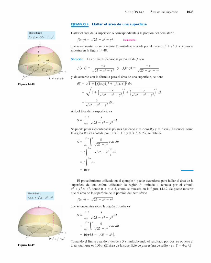
SECCIÓN 14.5 Área de una superficie 1023
EJEMPLO 4 Hallar el área de una superficie
Hallar el área de la superficie S correspondiente a la porción del hemisferio
Hemisferio.
que se encuentra sobre la región R limitada o acotada por el círculo como semuestra en la figura 14.48.
Solución Las primeras derivadas parciales de ƒ son
y
y, de acuerdo con la fórmula para el área de una superficie, se tiene
Así, el área de la superficie es
Se puede pasar a coordenadas polares haciendo y Entonces, comola región R está acotada por y se obtiene
El procedimiento utilizado en el ejemplo 4 puede extenderse para hallar el área de lasuperficie de una esfera utilizando la región R limitada o acotada por el círculo
donde como se muestra en la figura 14.49. Se puede mostrarque el área de la superficie de la porción del hemisferio
que se encuentra sobre la región circular es
Tomando el límite cuando a tiende a 5 y multiplicando el resultado por dos, se obtiene elárea total, que es (El área de la superficie de una esfera de radio r es )S 5 4pr2.100p.
5 10p s5 2 !25 2 a2 d.
5 E2p
0Ea
0
5!25 2 r2
r dr du
S 5 ERE 5!25 2 x2 2 y2
dA
!25 2 x2 2 y2fsx, yd 5
0 < a < 5,x2 1 y2 ≤ a2,
5 10p.
5 5E2p
0du
5 5E2p
02!25 2 r24
3
0du
S 5 E2p
0E3
0
5!25 2 r2
r dr du
0 ≤ u ≤ 2p,0 ≤ r ≤ 3y 5 r sin u.x 5 r cos u
S 5 ERE 5!25 2 x2 2 y2
dA.
55
!25 2 x2 2 y2dA.
5!1 1 1 2x!25 2 x2 2 y22
2
1 1 2y!25 2 x2 2 y22
2
dA
dS 5 !1 1 f fxsx, ydg 2 1 f fysx, ydg2 dA
fysx, yd 52y
!25 2 x2 2 y2fxsx, yd 5
2x!25 2 x2 2 y2
x2 1 y2 ≤ 9,
fsx, yd 5 !25 2 x2 2 y2
x
y
z
−2
−4−6
−41
1
2 2
2
3
3
4 4
4
5
5
6R: x2 + y2 ≤ 9
f(x, y) = 25 − x2 − y2
Hemisferio:
Figura 14.48
x
y
z
5
5
5
R: x2 + y2 ≤ a2
aa
f(x, y) = 25 − x2 − y2
Hemisferio:
Figura 14.49
sen
14-5.qxd 3/12/09 18:30 Page 1023

1024 CAPÍTULO 14 Integración múltiple
La regla de Simpson o la regla del trapecio pueden usarse para aproximar el valor deuna integral doble, siempre que se pueda obtener la primera integral. Esto se ilustra en elejemplo siguiente.
EJEMPLO 5 Aproximación del área de una superficie mediantela regla de Simpson
Hallar el área de la superficie del paraboloide
Paraboloide.
que se encuentra sobre la región cuadrada acotada por y comose muestra en la figura 14.50.
Solución Utilizando las derivadas parciales
y
se tiene que el área de la superficie es
En coordenadas polares, la recta está dada por o y en la figu-ra 14.51 se puede determinar que un cuarto de la región R está limitada o acotada por
y
Haciendo y se obtiene
Por último, usando la regla de Simpson con se aproxima esta integral simple
< 7.450.
S 513E
py4
2py4fs1 1 4 sec2 ud3y2 2 1g du
n 5 10,
51
12Epy4
2py4fs1 1 4 sec2 udg3y2 2 1g du.
5 Epy4
2py4
112
s1 1 4r2d3y24sec u
0du
5 Epy4
2py4Esec u
0
!1 1 4r2 r dr du
14
S 514 ER
E!1 1 4x2 1 4y2 dA
y 5 r sin ux 5 r cos u
2p
4≤ u ≤
p
4.0 ≤ r ≤ sec u
r 5 sec u,r cos u 5 1x 5 1
5 ERE!1 1 4x2 1 4y2 dA.
5 ERE!1 1 s22xd2 1 s22yd2 dA
S 5 ERE!1 1 f fxsx, ydg2 1 f fysx, ydg2 dA
fysx, yd 5 22yfxsx, yd 5 22x
21 ≤ y ≤ 1,21 ≤ x ≤ 1
fsx, yd 5 2 2 x2 2 y2
x1
r = sec θ
π
π
4
4
= −
θ
θ
=1
−1
−1
y
Un cuarto de la región R está acotada por
y
Figura 14.51
2p
4≤ u ≤
p
4.0 ≤ r ≤ sec u
y
x
z
R: 1− ≤ x ≤ 1−1 ≤ y ≤ 1
21
2
Paraboloide:
f(x, y) = 2 − x2 − y2
Figura 14.50
TECNOLOGÍA La mayor parte de los programas de computación que realizan inte-gración simbólica con integrales múltiples también realizan técnicas de aproximaciónnuméricas. Si se dispone de uno de estos programas, se recomienda usarlo para aproxi-mar el valor de la integral del ejemplo 5.
sen
14-5.qxd 3/12/09 18:30 Page 1024

SECCIÓN 14.5 Área de una superficie 1025
En los ejercicios 1 a 14, hallar el área de la superficie dada porsobre la región R. (Sugerencia: Algunas de las inte-
grales son más sencillas en coordenadas polares.)
1.
R: triángulo cuyos vértices son (0, 0), (4, 0), (0, 4)
2.
R: cuadrado cuyos vértices son (0, 0), (3, 0), (0, 3), (3, 3)
3. 4.
5.
R: cuadrado cuyos vértices son (0, 0), (2, 0), (0, 2), (2, 2)
6.
R: cuadrado cuyos vértices son (0, 0), (3, 0), (0, 3), (3, 3)7.
R: rectángulo cuyos vértices son (0, 0), (0, 4), (3, 4), (3, 0)
8.
9.
10. f(x, y) 5 13 1 x2 2 y2
11. ,
12. ,
13.
14.
En los ejercicios 15 a 18, hallar el área de la superficie.
15. Porción del plano en el primer octante
16. Porción del paraboloide en el primer octante
17. Porción de la esfera en el interior del cilin-dro
18. Porción del cono en el interior del cilindro
En los ejercicios 19 a 24, dar una integral doble que representeel área de la superficie sobre la región R. Utilizandoun sistema algebraico por computadora, evaluar la integraldoble.
19.
R: triángulo cuyos vértices son (0, 0), (1, 0), (1, 1)
20.
R: triángulo cuyos vértices son (0, 0), (2, 0), (2, 2)
21. f(x, y) 5 9 2 x2 2 y2 22.
23.
24.
Aproximación En los ejercicios 25 y 26, determinar qué valorse aproxima más al área de la superficie sobre laregión R. (Elegir el valor basándose en un dibujo de la superficiey no mediante la utilización de cálculos.)
25.
R: cuadrado cuyos vértices son (0, 0), (4, 0), (4, 4), (0, 4)a) 16 b) 200 c) d) 72 e) 36
26.
R: círculo limitado o acotado por x2 1 y2 5 9a) b) 150 c) d) 55 e) 500
En los ejercicios 27 y 28, utilizar un sistema algebraico porcomputadora y aproximar la integral doble que representa elárea de la superficie de la gráfica de ƒ sobre la región
27. 28.
En los ejercicios 29 a 34, formular una integral doble que propor-cione el área de la superficie en la gráfica de ƒ sobre la región R.
29.
R: cuadrado cuyos vértices son (1, 1), (21, 1), (21, 21), (1, 21)
30.
31. 32.
33.
34.
R 5 Hsx, yd: 0 ≤ x ≤ 4, 0 ≤ y ≤ xJf sx, yd 5 e2x sin y
R 5 Hsx, yd: 0 ≤ x ≤ 4, 0 ≤ y ≤ 10Jf sx, yd 5 exy
R 5 5sx, yd: x2 1 y2 ≤p
26R 5 Hsx, yd: x2 1 y 2 ≤ 4J
f sx, yd 5 cossx2 1 y 2df sx, yd 5 e2x sin y
R 5 Hsx, yd: 0 ≤ x ≤ 4, 0 ≤ y ≤ xJf sx, yd 5 x2 2 3xy 2 y 2
f sx, yd 5 x3 2 3xy 1 y3
f sx, yd 525 y5y2f sx, yd 5 e x
0 ≤ y ≤ 1}.R 5 {xx, yc: 0 ≤ x ≤ 1,
9p2100
f sx, yd 514!x2 1 y 2
2100
f sx, yd 5 10 212 y 2
z 5 f xx, yc
R 5 Hsx, yd: 0 ≤ x ≤ 1, 0 ≤ y ≤ 1Jf sx, yd 5
23x3y2 1 cos x
R 5 Hsx, yd: 0 ≤ x ≤ 1, 0 ≤ y ≤ 1Jf sx, yd 5 4 2 x2 2 y 2
R 5 Hsx, yd: 0 ≤ f sx, yd ≤ 16JR 5 Hsx, yd: 0 ≤ f sx, ydJf sx, yd 5 x2 1 y 2
f sx, yd 5 2x 1 y 2
f sx, yd 5 2y 1 x2
z 5 f xx, yc
x2 1 y 2 5 4z 5 2!x2 1 y 2
x2 1 y 2 5 9x2 1 y 2 1 z2 5 25
z 5 16 2 x2 2 y2
z 5 24 2 3x 2 2y
R 5 Hsx, yd: x2 1 y 2 ≤ a2Jf sx, yd 5 !a2 2 x2 2 y 2
R 5 Hsx, yd: x2 1 y 2 ≤ b2, 0 < b < aJf sx, yd 5 !a2 2 x2 2 y 2
R 5 Hsx, yd: x2 1 y 2 ≤ 16Jf sx, yd 5 xy
R 5 Hsx, yd: 0 ≤ f sx, yd ≤ 1Jf sx, yd 5 !x2 1 y 2
R 5 Hsx, yd: x2 1 y 2 ≤ 4J
R 5 5sx, yd: 0 ≤ x ≤p
4, 0 ≤ y ≤ tan x6
f sx, yd 5 ln|sec x|R 5 Hsx, yd: 0 ≤ x ≤ 2, 0 ≤ y ≤ 2 2 xJf sx, yd 5 2 1
23 y3y2
f sx, yd 5 3 1 x3y2
f sx, yd 5 y 2
f sx, yd 5 9 2 x2
R 5 Hsx, yd: x2 1 y 2 ≤ 9JR 5 Hsx, yd: x2 1 y 2 ≤ 4Jf sx, yd 5 12 1 2x 2 3yf sx, yd 5 7 1 2x 1 2y
WRITING ABOUT CONCEPTS
1053714_1405.qxp 10/27/08 1:33 PM Page 1025
f sx, yd 5 15 1 2x 2 3y
f sx, yd 5 2x 1 2y
z 5 f xx, yc
Desarrollo de conceptos35. Enunciar la definición, con integral doble, del área de una
superficie S dada por sobre una región R en elplano xy.
36. Considerar la superficie f(x, y) 5 x2 1 y2 y el área de super-ficie de f sobre cada región R. Sin integrar, ordenar las áreasde superficie desde la menor hasta la mayor. Explicar elrazonamiento.
a) R: rectángulo con vértices (0, 0), (2, 0), (2, 2), (0, 2)
b) R: triángulo con vértices (0, 0), (2, 0), (0, 2)
c) R 5 {(x, y): x2 1 y2 # 4 sólo el primer cuadrante}
37. ¿Aumentará el área de superficie de la gráfica de una fun-ción z 5 f(x, y) sobre una región R si la gráfica de f cambiók unidades verticalmente? ¿Por qué sí o por qué no?
z 5 f sx, yd
sen
sen
14.5 Ejercicios
CAS
CAS
14-5.qxd 3/12/09 18:30 Page 1025

1026 CAPÍTULO 14 Integración múltiple
39. Hallar el área de la superficie del sólido intersección de los ci-lindros y (ver la figura).
Figura para 39 Figura para 40
40. Mostrar que el área de la superficie del cono sobre la región circular en el plano xy es
(ver la figura).
41. Diseño industrial Una empresa produce un objeto esférico de25 centímetros de radio. Se hace una perforación de 4 centíme-tros de radio a través del centro del objeto. Calcular a) el volu-men del objeto y b) el área de la superficie exterior del objeto.
42. Modelo matemático Un ranchero construye un granero dedimensiones 30 por 50 pies. En la figura se muestra la formasimétrica y la altura elegidas para el tejado.
a) Utilizar las funciones de regresión de una herramienta degraficación para hallar un modelo de la forma z 5 ay3 1 by2
1 cy 1 d para el perfil del techo.
b) Utilizar las funciones de integración numérica de una herra-mienta de graficación y el modelo del inciso a) para aproxi-mar el volumen del espacio de almacenaje en el granero.
c) Utilizar las funciones de integración numérica de una herra-mienta de graficación y el modelo del inciso a) para aproxi-mar el área de la superficie del techo.
d) Aproximar la longitud de arco de la recta del techo y calcularel área de la superficie del techo multiplicando la longitud dearco por la longitud del granero. Comparar los resultados y lasintegraciones con los encontrados en el inciso c).
y
x50
20
25(0, 25)
(5, 22)
(10, 17)
(15, 0)
z
pr 2!k2 1 1x2 1 y 2 ≤ r 2k > 0
z 5 k!x2 1 y 2,
y
x
z = k x2 + y2, k > 0
rr
z
x
y3
2
−3
−2
3
y2 + z2 = 1
x2 + z2 = 1
z
y 2 1 z2 5 1x2 1 z2 5 1
Una propiedad muy conocida de los líquidos se llama “capilaridad”,y consiste en que ascienden por conductos verticales muy estrechos.La figura muestra dos placas que forman una cuña estrecha dentro deun recipiente con líquido. La superficie superior del líquido tomauna forma hiperbólica dada por
donde x, y y z están medidas en pulgadas. La constante k depende delángulo de la cuña, del tipo de líquido y del material de las placas.
a) Hallar el volumen del líquido que ha ascendido por la cuña.(Tomar )
b) Hallar el área de la superficie horizontal del líquido que ha ascen-dido por la cuña.
Adaptación de un problema sobre capilaridad de “Capillary Phe-nomena” de Thomas B. Greenslade, Jr., Physics Teacher, mayo de1992. Con autorización del autor.
x
y
= 2 arctan (0.01)θ
13 pulg
9 pulg
z
k 5 1.
z 5k
!x2 1 y 2
Para discusión38. Responder las siguientes preguntas acerca del área de super-
ficie S sobre una superficie dada por una función positiva z 5 f (x, y) sobre una región R en el plano xy. Explicar cadarespuesta.
a) ¿Es posible para S igualar el área de R?
b) ¿Puede S ser mayor que el área de R?
c) ¿Puede S ser menor que el área de R?
Capilaridad
PROYECTO DE TRABAJO
14-5.qxd 3/12/09 18:30 Page 1026

SECCIÓN 14.6 Integrales triples y aplicaciones 1027
14.6 Integrales triples y aplicaciones
n Utilizar una integral triple para calcular el volumen de una región sólida.n Hallar el centro de masa y los momentos de inercia de una región sólida.
Integrales triples
El procedimiento utilizado para definir una integral triple es análogo al utilizarlo paraintegrales dobles. Considerar una función f en tres variables que es continua sobre unaregión sólida acotada Q. Entonces, se encierra Q en una red de cubos y se forma una par-tición interna que consta de todos los cubos que quedan completamente dentro de Q,como se muestra en la figura 14.52. El volumen del i-ésimo cubo es
Volumen del i-ésimo cubo.
La norma de la partición es la longitud de la diagonal más larga en los n cubos de lapartición. En cada cubo se elige un punto y se forma la suma de Riemann
Tomando el límite cuando se llega a la siguiente definición.
Algunas de las propiedades de las integrales dobles expuestas en el teorema 14.1pueden replantearse en términos de integrales triples.
1.
2.
3.
En las propiedades dadas arriba, Q es la unión de dos subregiones sólidas que no se sobre-ponen y Si la región sólida es simple, la integral triple puedeevaluarse con una integral iterada utilizando alguno de los seis posibles órdenes de inte-gración:
dz dy dx.dy dz dxdx dz dydz dx dydy dx dzdx dy dz
eee fsx, y, zd dVQQ2.Q1
EEQ
E f sx, y, zd dV 5 EEQ1
E f sx, y, zd dV 1 EEQ2
E f sx, y, zd dV
EEQ
E f f sx, y, zd ± gsx, y, zdg dV 5 EEQ
E f sx, y, zd dV ± EEQ
Egsx, y, zd dV
EEQ
E cf sx, y, zd dV 5 cEEQ
E f sx, y, zd dV
iD i → 0
on
i51f sxi, yi, zid DVi.
sxi, yi, zidiD i
DVi 5 DxiDyiDzi.
Volumen de
Figura 14.52
Q < on
i51
DVi
y
x
z
Región sólida Q
y
x
z
DEFINICIÓN DE INTEGRAL TRIPLE
Si es continua sobre una región sólida acotada , entonces la integral triple de fsobre Q se define como
siempre que el límite exista. El volumen de la región sólida Q está dado por
Volumen de Q 5 EEQ
E dV.
EEQ
E fsx, y, zd dV 5 limiDi→0 o
n
i51fsxi, yi, zid DVi
Qf
lím
14-6.qxd 3/12/09 18:32 Page 1027

1028 CAPÍTULO 14 Integración múltiple
La versión siguiente del teorema de Fubini describe una región que es consideradasimple con respecto al orden Para los otros cinco órdenes pueden formularsedescripciones similares.
Para evaluar una integral iterada triple en el orden se mantienen x y y cons-tantes para la integración más interior. Después, se mantiene x constante para la segundaintegración.
EJEMPLO 1 Evaluar una integral iterada triple
Evaluar la integral iterada triple
Solución Para la primera integración, se mantienen x y y constantes y se integra conrespecto a z.
Para la segunda integración, mantener x constante y se integra con respecto a y.
Por último, se integra con respecto a x.
El ejemplo 1 muestra el orden de integración Con otros órdenes, se puedeseguir un procedimiento similar. Por ejemplo, para evaluar una integral iterada triple en elorden se mantienen y y z constantes para la integración más interior y se integracon respecto a x. Después, para la segunda integración, se mantiene z constante y se inte-gra con respecto a y. Por último, para la tercera integración, se integra con respecto a z.
dx dy dz,
dz dy dx.
< 65.797
5 191e2
31 12
196 E2
0x3ex dx 5
196 3exsx3 2 3x2 1 6x 2 6d4
2
0
5196 E2
0x3ex dx
E2
0Ex
0exsx2 1 3xy 1 2y2d dy dx 5 E2
03ex1x2y 1
3xy2
21
2y3
3 24x
0dx
5 E2
0Ex
0exsx2 1 3xy 1 2y2d dy dx
E2
0Ex
0Ex1y
0exs y 1 2zd dz dy dx 5 E2
0Ex
0exsyz 1 z2d4
x1y
0dy dx
E2
0Ex
0Ex1y
0exs y 1 2zd dz dy dx.
dz dy dx,
dz dy dx.
TEOREMA 14.4 EVALUACIÓN MEDIANTE INTEGRALES ITERADAS
Sea f continua en una región sólida definida por Q
donde h1, h2, g1 y son funciones continuas. Entonces,
EEQ
E fsx, y, zd dV 5 Eb
aEh2sxd
h1sxdEg
2sx, yd
g1sx, ydfsx, y, zd dz dy dx.
g2
g1sx, yd ≤ z ≤ g2sx, ydh1sxd ≤ y ≤ h2sxd,a ≤ x ≤ b,
E X P L O R A C I Ó N
Volumen de un sector paraboloideEn las páginas 997 y 1006, se pidióresumir las diferentes formas estu-diadas hasta ahora para hallar elvolumen del sólido limitado o aco-tado por el paraboloide
y el plano xy. Ahora se conoce unmétodo más. Utilizarse para hallarel volumen del sólido.
y
x
a
z
a
−a
a2
a > 0z 5 a2 2 x2 2 y2,
14-6.qxd 3/12/09 18:32 Page 1028

SECCIÓN 14.6 Integrales triples y aplicaciones 1029
Para hallar los límites dado un orden determinado de integración, por lo general seaconseja determinar primero los límites más interiores, que pueden ser funciones de lasdos variables exteriores. Después, proyectando el sólido Q sobre el plano coordenado delas dos variables exteriores, se pueden determinar sus límites de integración mediante losmétodos usados para las integrales dobles. Por ejemplo, para evaluar
primero se determinan los límites de z, y entonces la integral toma la forma
Proyectando el sólido Q sobre el plano xy, se pueden determinar los límites de x y de y dela misma manera que se hizo en el caso de las integrales dobles, como se muestra en lafigura 14.53.
EJEMPLO 2 Integral triple para hallar un volumen
Hallar el volumen del elipsoide dado por
Solución Como en la ecuación x, y y juegan papeles similares, el orden de integraciónes probablemente irrelevante, y se puede elegir arbitrariamente Además, sepueden simplificar los cálculos considerando sólo la porción del elipsoide que se encuen-tra en el primer octante, como se muestra en la figura 14.54. Para el orden sedeterminan primero los límites o cotas de z.
Los límites o cotas de x y y son, como se ve en la figura 14.55, y y ypor lo que el volumen del elipsoide es
564p
3.
5 4p 34x 2x3
3 42
0
5 8E2
0s4 2 x2d1p
22 dx
5 8E2
0f0 1 s4 2 x2d arcsins1d 2 0 2 0g dx
5 8E2
03y!4 2 x2 2 y2 1 s4 2 x2d arcsin1 y
!4 2 x224!42x2
0dx
5 16E2
0E!42x2
0
!s4 2 x2d 2 y2 dy dx
5 8E2
0E!42x2
0z42!42x22y2
0dy dx
5 8E2
0E!42x2
0E2!42x22y2
0dz dy dx
V 5 EEQ
E dV
0 ≤ y ≤ !4 2 x2,0 ≤ x ≤ 2yx
0 ≤ z ≤ 2!4 2 x2 2 y2
dz dy dx,
dz dy dx.z
4x2 1 4y2 1 z2 5 16.
EE 3Eg2sx, yd
g1sx, ydfsx, y, zd dz4 dy dx.
EEQ
E fsx, y, zd dz dy dx
Figura 14.55
x
0 ≤ y ≤ 4 − x2
1
1
2
2
x2 + y2 = 4
0 ≤ x ≤ 2y
Figura 14.54
2
2
1
4
x
0 ≤ z ≤ 2 4 − x2 − y2
Elipsoide: 4x2 + 4y2 + z2 = 16
z
y
La región sólida Q se encuentra entre dossuperficiesFigura 14.53
x y
Q
Proyección sobre el plano xy
z = g1(x, y)
z = g2(x, y)z
Tablas de integración (apéndiceB), fórmula 37.
arcsen
arcsen
14-6.qxd 3/12/09 18:32 Page 1029

1030 CAPÍTULO 14 Integración múltiple
El ejemplo 2 es poco usual en el sentido de que con los seis posibles órdenes de inte-gración se obtienen integrales de dificultad comparable. Tratar de emplear algún otro delos posibles órdenes de integración para hallar el volumen del elipsoide. Por ejemplo, conel orden dx dy dz se obtiene la integral
Si se resuelve esta integral, se obtiene el mismo volumen que en el ejemplo 2. Esto essiempre así; el orden de integración no afecta el valor de la integral. Sin embargo, el ordende integración a menudo afecta la complejidad de la integral. En el ejemplo 3, el orden deintegración propuesto no es conveniente, por lo que se puede cambiar el orden para sim-plificar el problema.
EJEMPLO 3 Cambiar el orden de integración
Evaluar
Solución Obsérvese que después de una integración en el orden dado, se encontraría laintegral que no es una función elemental. Para evitar este problema, se cam-bia el orden de integración a de manera que y sea la variable exterior. Como semuestra en la figura 14.56, la región sólida Q está dada por
y la proyección de Q en el plano xy proporciona los límites
y
Por tanto, la evaluación de la integral triple usando el orden dz dx dy produce
0 ≤ x ≤ y.0 ≤ y ≤ !p
2
1 ≤ z ≤ 3x ≤ y ≤ !p
2,0 ≤ x ≤ !p
2,
dz dx dy,2e sins y2d dy,
E!py2
0E!py2
xE3
1
sin sy2d dz dy dx.
V 5 8E4
0E!162z2y2
0E!1624y22z2y2
0dx dy dz.
Figura 14.56
x
y
z
1
2
3
y = x
Q: 0 ≤ x ≤
x ≤ y ≤1 ≤ z ≤ 3
π
ππ
π
π
2
2
2
2
2
2
( , , 3)
π π2 2( , , 1)
π
sen
sensy2d dy,
1.
cos y22
0
22
0y sen y2 dy
22
0x sen y2
y
0dy
22
0
y
0sen y2 dx dy
2
0
y
0
3
1
sen y2 dz dx dy2
0
y
0z sen y2
3
1dx dy
14-6.qxd 3/12/09 18:32 Page 1030

SECCIÓN 14.6 Integrales triples y aplicaciones 1031
EJEMPLO 4 Determinación de los límites de integración
Dar una integral triple para el volumen de cada una de las regiones sólidas.
a) La región en el primer octante acotada superiormente por el cilindro y com-prendida entre los planos verticales y
b) El hemisferio superior dado por
c) La región acotada inferiormente por el paraboloide y superiormente por laesfera
Solución
a) En la figura 14.57, obsérvese que el sólido está acotado inferiormente por el plano xyy superiormente por el cilindro Por tanto,
Límites o cotas para z.
Proyectando la región sobre el plano xy se obtiene un paralelogramo. Como dos de loslados del paralelogramo son paralelos al eje x, se tienen las cotas siguientes:
y
Por tanto, el volumen de la región está dado por
b) Para el hemisferio superior dado por se tiene
Cotas para z.
En la figura 14.58, obsérvese que la proyección del hemisferio sobre el plano xy es elcírculo dado por y se puede usar el orden o el orden Eligiendo el primero se obtiene
y
lo cual implica que el volumen de la región está dado por
c) Para la región acotada inferiormente por el paraboloide y superiormentepor la esfera se tiene
Cotas para z.
La esfera y el paraboloide se cortan en Además, en la figura 14.59 se puede verque la proyección de la región sólida sobre el plano xy es el círculo dado por
Utilizando el orden se obtiene
y
lo cual implica que el volumen de la región está dado por
V 5 EEQ
E dV 5 E!2
2!2E!22x2
2!22x2E!62x22y2
x21y2dz dy dx.
2!2 ≤ x ≤ !22!2 2 x2 ≤ y ≤ !2 2 x2
dy dxx2 1 y2 5 2.
z 5 2.
x2 1 y2 ≤ z ≤ !6 2 x2 2 y2.
x2 1 y2 1 z2 5 6,z 5 x2 1 y2
V 5 EEQ
E dV 5 E1
21E!12y2
2!12y2E!12x22y2
0dz dx dy.
21 ≤ y ≤ 12!1 2 y2 ≤ x ≤ !1 2 y2
dy dx.dx dyx2 1 y2 5 1,
0 ≤ z ≤ !1 2 x2 2 y2.
z 5 !1 2 x2 2 y2,
V 5 EEQ
E dV 5 E1
0E32y
12yE12y2
0dz dx dy.
0 ≤ y ≤ 1.1 2 y ≤ x ≤ 3 2 y
0 ≤ z ≤ 1 2 y2.
z 5 1 2 y2.sz 5 0d
x2 1 y2 1 z2 5 6z 5 x2 1 y2
z 5 !1 2 x2 2 y2
x 1 y 5 3x 1 y 5 1z 5 1 2 y2
Figura 14.57
x
y
3
1
1
x = 1 − y
x = 3 − y
z = 1 − y2
∆y
Q: 0 ≤ z ≤ 1 − y2
1 − y ≤ x ≤ 3 − y0 ≤ y ≤ 1
z
Figura 14.58
x
y1 1
1
z = 1 − x2 − y2
Hemisferio:
Base circular:x2 + y2 = 1
−1 ≤ y ≤ 11 − y2 ≤ x ≤ 1 − y2−
0 ≤ z ≤ 1 − x2 − y2
z
Q:
Figura 14.59
y
x2 2
−2
3
Esfera:
x2 + y2 + z2 = 6
Paraboloide:
z = x2 + y2
− 2 − x2 ≤ y ≤ 2 − x2
− ≤ x ≤ 22
x2 + y2 ≤ z ≤ 6 − x2 − y2
z
Q:
14-6.qxd 3/12/09 18:32 Page 1031

1032 CAPÍTULO 14 Integración múltiple
Centro de masa y momentos de inercia
En el resto de esta sección se analizan dos aplicaciones importantes de las integrales triplesa la ingeniería. Considérese una región sólida Q cuya densidad está dada por la funciónde densidad r. El centro de masa de una región sólida Q de masa m está dado por
donde
Masa del sólido.
Primer momento con respecto al plano yz.
Primer momento con respecto al plano xz.
Primer momento con respecto al plano xy.
y
Las cantidades y se conocen como los primeros momentos de la región Qcon respecto a los planos yz, xz y xy, respectivamente.
Los primeros momentos de las regiones sólidas se toman con respecto a un plano,mientras que los segundos momentos de los sólidos se toman con respecto a una recta.Los segundos momentos (o momentos de inercia) con respecto a los ejes x, y y z son lossiguientes.
Momento de inercia con respecto al eje x.
Momento de inercia con respecto al eje y.
Momento de inercia con respecto al eje z.
En problemas que requieren el cálculo de los tres momentos, puede ahorrarse una canti-dad considerable de trabajo empleando la propiedad aditiva de las integrales triples y escri-biendo
e
donde e son
Iyz 5 EEQ
E x2rsx, y, zd dV
Ixz 5 EEQ
E y2rsx, y, zd dV
Ixy 5 EEQ
E z2rsx, y, zd dV
IyzIxy, Ixz,
Iz 5 Iyz 1 IxzIy 5 Iyz 1 Ixy,Ix 5 Ixz 1 Ixy,
Iz 5 EEQ
E sx2 1 y2drsx, y, zd dV
Iy 5 EEQ
E sx2 1 z2drsx, y, zd dV
Ix 5 EEQ
E s y2 1 z2drsx, y, zd dV
MxyMxz,Myz,
z 5Mxy
m.y 5
Mxz
m,x 5
Myz
m,
Mxy 5 EEQ
E zrsx, y, zd dV
Mxz 5 EEQ
E yrsx, y, zd dV
Myz 5 EEQ
E xrsx, y, zd dV
m 5 EEQ
E rsx, y, zd dV
sx, y, zd,
En ingeniería y en física, elmomento de inercia de una masa seusa para hallar el tiempo requeridopara que una masa alcance una veloci-dad de rotación dada con respecto a uneje, como se muestra en la figura14.60. Cuanto mayor es el momento deinercia, mayor es la fuerza que hay queaplicar a la masa para que alcance lavelocidad deseada. n
NOTA
x
y
z
Figura 14.60
E X P L O R A C I Ó N
Dibujar el sólido (de densidad uni-forme) limitado o acotado por
y
donde A partir deldibujo, estimar las coordenadas delcentro de masa del sólido. Ahorautilizar un sistema algebraico porcomputadora y verificar la esti-mación. ¿Qué se observa?
x2 1 y 2 ≤ 1.
z 51
1 1 x2 1 y2
z 5 0
14-6.qxd 3/12/09 18:32 Page 1032

SECCIÓN 14.6 Integrales triples y aplicaciones 1033
EJEMPLO 5 Hallar el centro de masa de una región sólida
Hallar el centro de masa del cubo unidad mostrado en la figura 14.61, dado que la densi-dad en el punto (x, y, z) es proporcional al cuadrado de su distancia al origen.
Solución Como la densidad en (x, y, z) es proporcional al cuadrado de la distancia entre(0, 0, 0) y (x, y, z), se tiene
Esta función de densidad se puede utilizar para hallar la masa del cubo. Debido a lasimetría de la región, cualquier orden de integración producirá integrales de dificultadcomparable.
El primer momento con respecto al plano yz es
Nótese que x puede sacarse como factor fuera de las dos integrales interiores, ya que esconstante con respecto a y y a z. Después de factorizar, las dos integrales interiores soniguales con respecto a la masa m. Por tanto, se tiene
Así,
Por último, por la naturaleza de r y la simetría de x, y y en esta región sólida, se tieney el centro de masa es s 7
12, 712, 7
12d.x 5 y 5 z,z
x 5Myz
m5
7ky12k
57
12.
57k12
.
5 k3x4
41
x2
3 41
0
Myz 5 kE1
0 x1x2 1
232 dx
5 kE1
0 x3E1
0E1
0 sx2 1 y2 1 z2d dz dy4 dx.
Myz 5 kE1
0E1
0E1
0 xsx2 1 y2 1 z2d dz dy dx
5 k3x3
31
2x3 4
1
05 k
5 kE1
0 1x2 1
23
2 dx
5 kE1
0 31x2 1
132y 1
y3
3 41
0 dx
5 kE1
0E1
0 1x2 1 y2 1
13
2 dy dx
5 kE1
0E1
0 3sx2 1 y2dz 1
z3
3 41
0 dy dx
m 5 E1
0E1
0E1
0 ksx2 1 y2 1 z2d dz dy dx
rsx, y, zd 5 ksx2 1 y2 1 z2d.
Densidad variable:
Figura 14.61rsx, y, zd 5 ksx2 1 y2 1 z2d
x
y
1
1 1
(x, y, z)
z
14-6.qxd 3/12/09 18:32 Page 1033

1034 CAPÍTULO 14 Integración múltiple
EJEMPLO 6 Momentos de inercia de una región sólida
Hallar los momentos de inercia con respecto a los ejes x y y de la región sólida compren-dida entre el hemisferio
y el plano xy, dado que la densidad en (x, y, z) es proporcional a la distancia entre (x, y, z) y el plano xy.
Solución La densidad de la región está dada por Considerando lasimetría de este problema, se sabe que y sólo se necesita calcular un momento,digamos De acuerdo con la figura 14.62, se elige el orden dz dy dx y se escribe
.
Fórmula de Wallis.
Por tanto,
En el ejemplo 6, los momentos de inercia con respecto a los ejes x y y son iguales. Sinembargo, el momento con respecto al eje z es diferente. ¿Parece que el momento de iner-cia con respecto al eje z deba ser menor o mayor que los momentos calculados en el ejem-plo 6? Realizando los cálculos, se determina que
Esto indica que el sólido mostrado en la figura 14.62 presenta resistencia mayor a larotación en torno a los ejes x o y que en torno al eje z.
Iz 5163
kp.
Ix 5 8kp 5 Iy.
5 8kp.
5 1256k5 215p
322
54k5 E
py2
0 64 cos6 u du
x 5 2 sin u 54k5 E
2
0 s4 2 x2d5y2 dx
5k4E
2
22 85
s4 2 x2d5y2 dx
5k4E
2
22 3s4 2 x2d2y 2
y5
5 4 !42x2
2!42x2 dx
5k4E
2
22E!42x2
2!42x2
fs4 2 x2d2 2 y4g dy dx
5 kE2
22E!42x2
2!42x2
3y2s4 2 x2 2 y2d2
1s4 2 x2 2 y2d2
4 4 dy dx
5 kE2
22E!42x2
2!42x2
3y2z2
21
z4
4 4!42x22y2
0
dy dx
5 E2
22E!42x2
2!42x2E!42x22y2
0 s y2 1 z2dskzd dz dy dx
Ix 5 EEQ
E sy2 1 z2drsx, y, zd dV
Ix.Ix 5 Iy,
rsx, y, zd 5 kz.
z 5 !4 2 x2 2 y2
Densidad variable: Figura 14.62
rsx, y, zd 5 kz
x
y
z
2
2
2
z = 4 − x2 − y2
Hemisferio:
Base circular:x2 + y2 = 4
−2 ≤ x ≤ 2− 4 − x2 ≤ y ≤ 4 − x2
0 ≤ z ≤ 4 − x2 − y2
sen
14-6.qxd 3/12/09 18:32 Page 1034

SECCIÓN 14.6 Integrales triples y aplicaciones 1035
En los ejercicios 1 a 8, evaluar la integral iterada.
1. 2.
3. 4.
5. 6.
7. 8.
En los ejercicios 9 y 10, utilizar un sistema algebraico por compu-tadora y evaluar la integral iterada.
9.
10.
En los ejercicios 11 y 12, utilizar un sistema algebraico porcomputadora y aproximar la integral iterada.
11.
12.
En los ejercicios 13 a 18, dar una integral triple para el volumendel sólido.
13. El sólido en el primer octante acotado por los planos coordena-dos y el plano z 5 5 2 x 2 y
14. El sólido acotado por y 5 0 y
15. El sólido acotado por el paraboloide z 5 6 2 x2 2 y2 y
16. El sólido limitado por y z 5 0.
17. El sólido que es el interior común bajo de la esfera x2 1 y2 1 z2
5 80 y sobre el paraboloide
18. El sólido limitado arriba por el cilindro z 5 4 2 x2 y abajo por
el paraboloide
Volumen En los ejercicios 19 a 22, utilizar una integral triplepara hallar el volumen del sólido mostrado en la figura.
19. 20.
21. 22.
Volumen En los ejercicios 23 a 26, usar una integral triple paraencontrar el volumen del sólido limitado por las gráficas de lasecuaciones.
En los ejercicios 27 a 32, dibujar el sólido cuyo volumen estádado por la integral iterada y reescribir la integral utilizando elorden de integración indicado.
27.
Reescribir usando el orden dy dz dx.
28.
Reescribir usando el orden dx dz dy.
29.
Reescribir utilizando el orden
30.
Reescribir utilizando el orden
31.
Reescribir utilizando el orden
32.
Reescribir utilizando el orden
En los ejercicios 33 a 36, dar los seis posibles órdenes de inte-gración de la integral triple sobre la región sólida Q,
33.
34.
35.
36. Q 5 Hsx, y, zd: 0 ≤ x ≤ 1, y ≤ 1 2 x2, 0 ≤ z ≤ 6JQ 5 Hsx, y, zd: x2 1 y2 ≤ 9, 0 ≤ z ≤ 4JQ 5 Hsx, y, zd: 0 ≤ x ≤ 2, x2 ≤ y ≤ 4, 0 ≤ z ≤ 2 2 xJQ 5 Hsx, y, zd: 0 ≤ x ≤ 1, 0 ≤ y ≤ x, 0 ≤ z ≤ 3J
In Exercises 1–8, evaluate the iterated integral.
1. 2.
3. 4.
5. 6.
7. 8.
In Exercises 9 and 10, use a computer algebra system toevaluate the iterated integral.
9.
10.
In Exercises 11 and 12, use a computer algebra system toapproximate the iterated integral.
11.
12.
In Exercises 13–18, set up a triple integral for the volume of thesolid.
13. The solid in the first octant bounded by the coordinate planesand the plane
14. The solid bounded by and
15. The solid bounded by and
16. The solid bounded by and
17. The solid that is the common interior below the sphereand above the paraboloid
18. The solid bounded above by the cylinder and belowby the paraboloid
Volume In Exercises 19–22, use a triple integral to find thevolume of the solid shown in the figure.
19. 20.
21. 22.
Volume In Exercises 23–26, use a triple integral to find the volume of the solid bounded by the graphs of the equations.
23. primer octante
24.
25.
26. primer octante
In Exercises 27–32, sketch the solid whose volume is given bythe iterated integral and rewrite the integral using the indicatedorder of integration.
27.
Rewrite using the order
28.
Rewrite using the order
29.
Rewrite using the order
30.
Rewrite using the order
31.
Rewrite using the order
32.
Rewrite using the order
In Exercises 33–36, list the six possible orders of integration forthe triple integral over the solid region
33.
34.
35.
36. Q x, y, z : 0 x 1, y 1 x2, 0 z 6
Q x, y, z : x2 y2 9, 0 z 4
Q x, y, z : 0 x 2, x2 y 4, 0 z 2 x
Q x, y, z : 0 x 1, 0 y x, 0 z 3Q
xyz dV.Q,
dx dy dz.
2
0
4
2x
y2 4x2
0 dz dy dx
dz dy dx.
1
0
1
y
1 y2
0 dz dx dy
dz dx dy.
3
0
9 x2
0
6 x y
0 dz dy dx
dy dx dz.
4
0
4 x 2
0
12 3x 6y 4
0 dz dy dx
dx dz dy.
1
1
1
y2
1 x
0dz dx dy
dy dz dx.
1
0
0
1
y2
0 dz dy dx
z x, y x 2, y x2,
z 2 y, z 4 y2, x 0, x 3, y 0
z 9 x3, y x2 2, y 0, z 0, x ≥ 0
z 4 x2, y 4 x2,
z = 36 − x2 − y2
yx
36
1212
z
z = 0
x2 + y2 + z2 = a2
yx
a
a a
z
0 ≤ x ≤ 2 0 ≤ y ≤ 2
z = 2xy
y
x
12
2
4
6
3
8
z z = x
z = 0
x = 4 − y2
y
x
4
3
2
4
z
z x2 3y2z 4 x2
z 12 x2 y2x2 y2 z2 80
z 0z 16 x2 y2
z 0z 6 x2 y2
y 2xy 0,z 0,z 9 x2,
z 5 x y
3
0
2 2y 3
0
6 2y 3z
0 ze x2y2
dx dz dy
2
0
4 x2
0
4
1 x2 sin y
z dz dy dx
2
0
2 x2
0
4 y2
2x2 y2 y dz dy dx
3
0
9 y2
9 y2
y2
0y dz dx dy
2
0
y 2
0
1 y
0 sin y dz dx dy
4
0
2
0
1 x
0 x cos y dz dy dx
4
1
e2
1
1 xz
0 ln z dy dz dx
4
1
1
0
x
0 2ze x2
dy dx dz
9
0
y 3
0
y2 9x2
0 z dz dx dy
1
0
x
0
xy
0 x dz dy dx
1
1
1
1
1
1 x2y 2z2 dx dy dz
3
0
2
0
1
0 x y z dx dz dy
14.6 Triple Integrals and Applications 1035
14.6 Exercises See www.CalcChat.com for worked-out solutions to odd-numbered exercises.
CAS
CAS
1053714_1406.qxp 10/27/08 1:34 PM Page 1035
dx dy dz.
E2
0E4
2x
E!y224x2
0 dz dy dx
dz dy dx.
E1
0E1
yE!12y2
0 dz dx dy
dz dx dy.
E3
0E!92x2
0E62x2y
0 dz dy dx
dy dx dz.
E4
0Es42xdy2
0Es1223x26ydy4
0 dz dy dx
In Exercises 1–8, evaluate the iterated integral.
1. 2.
3. 4.
5. 6.
7. 8.
In Exercises 9 and 10, use a computer algebra system toevaluate the iterated integral.
9.
10.
In Exercises 11 and 12, use a computer algebra system toapproximate the iterated integral.
11.
12.
In Exercises 13–18, set up a triple integral for the volume of thesolid.
13. The solid in the first octant bounded by the coordinate planesand the plane
14. The solid bounded by and
15. The solid bounded by and
16. The solid bounded by and
17. The solid that is the common interior below the sphereand above the paraboloid
18. The solid bounded above by the cylinder and belowby the paraboloid
Volume In Exercises 19–22, use a triple integral to find thevolume of the solid shown in the figure.
19. 20.
21. 22.
Volume In Exercises 23–26, use a triple integral to find the volume of the solid bounded by the graphs of the equations.
23. primer octante
24.
25.
26. primer octante
In Exercises 27–32, sketch the solid whose volume is given bythe iterated integral and rewrite the integral using the indicatedorder of integration.
27.
Rewrite using the order
28.
Rewrite using the order
29.
Rewrite using the order
30.
Rewrite using the order
31.
Rewrite using the order
32.
Rewrite using the order
In Exercises 33–36, list the six possible orders of integration forthe triple integral over the solid region
33.
34.
35.
36. Q x, y, z : 0 x 1, y 1 x2, 0 z 6
Q x, y, z : x2 y2 9, 0 z 4
Q x, y, z : 0 x 2, x2 y 4, 0 z 2 x
Q x, y, z : 0 x 1, 0 y x, 0 z 3Q
xyz dV.Q,
dx dy dz.
2
0
4
2x
y2 4x2
0 dz dy dx
dz dy dx.
1
0
1
y
1 y2
0 dz dx dy
dz dx dy.
3
0
9 x2
0
6 x y
0 dz dy dx
dy dx dz.
4
0
4 x 2
0
12 3x 6y 4
0 dz dy dx
dx dz dy.
1
1
1
y2
1 x
0dz dx dy
dy dz dx.
1
0
0
1
y2
0 dz dy dx
z x, y x 2, y x2,
z 2 y, z 4 y2, x 0, x 3, y 0
z 9 x3, y x2 2, y 0, z 0, x ≥ 0
z 4 x2, y 4 x2,
z = 36 − x2 − y2
yx
36
1212
z
z = 0
x2 + y2 + z2 = a2
yx
a
a a
z
0 ≤ x ≤ 2 0 ≤ y ≤ 2
z = 2xy
y
x
12
2
4
6
3
8
z z = x
z = 0
x = 4 − y2
y
x
4
3
2
4
z
z x2 3y2z 4 x2
z 12 x2 y2x2 y2 z2 80
z 0z 16 x2 y2
z 0z 6 x2 y2
y 2xy 0,z 0,z 9 x2,
z 5 x y
3
0
2 2y 3
0
6 2y 3z
0 ze x2y2
dx dz dy
2
0
4 x2
0
4
1 x2 sin y
z dz dy dx
2
0
2 x2
0
4 y2
2x2 y2 y dz dy dx
3
0
9 y2
9 y2
y2
0y dz dx dy
2
0
y 2
0
1 y
0 sin y dz dx dy
4
0
2
0
1 x
0 x cos y dz dy dx
4
1
e2
1
1 xz
0 ln z dy dz dx
4
1
1
0
x
0 2ze x2
dy dx dz
9
0
y 3
0
y2 9x2
0 z dz dx dy
1
0
x
0
xy
0 x dz dy dx
1
1
1
1
1
1 x2y 2z2 dx dy dz
3
0
2
0
1
0 x y z dx dz dy
14.6 Triple Integrals and Applications 1035
14.6 Exercises See www.CalcChat.com for worked-out solutions to odd-numbered exercises.
CAS
CAS
1053714_1406.qxp 10/27/08 1:34 PM Page 1035
z = 36 − x2 − y2
yx
36
1212
z
z = 0
x2 + y2 + z2 = a2
yx
a
a a
z
In Exercises 1–8, evaluate the iterated integral.
1. 2.
3. 4.
5. 6.
7. 8.
In Exercises 9 and 10, use a computer algebra system toevaluate the iterated integral.
9.
10.
In Exercises 11 and 12, use a computer algebra system toapproximate the iterated integral.
11.
12.
In Exercises 13–18, set up a triple integral for the volume of thesolid.
13. The solid in the first octant bounded by the coordinate planesand the plane
14. The solid bounded by and
15. The solid bounded by and
16. The solid bounded by and
17. The solid that is the common interior below the sphereand above the paraboloid
18. The solid bounded above by the cylinder and belowby the paraboloid
Volume In Exercises 19–22, use a triple integral to find thevolume of the solid shown in the figure.
19. 20.
21. 22.
Volume In Exercises 23–26, use a triple integral to find the volume of the solid bounded by the graphs of the equations.
23. primer octante
24.
25.
26. primer octante
In Exercises 27–32, sketch the solid whose volume is given bythe iterated integral and rewrite the integral using the indicatedorder of integration.
27.
Rewrite using the order
28.
Rewrite using the order
29.
Rewrite using the order
30.
Rewrite using the order
31.
Rewrite using the order
32.
Rewrite using the order
In Exercises 33–36, list the six possible orders of integration forthe triple integral over the solid region
33.
34.
35.
36. Q x, y, z : 0 x 1, y 1 x2, 0 z 6
Q x, y, z : x2 y2 9, 0 z 4
Q x, y, z : 0 x 2, x2 y 4, 0 z 2 x
Q x, y, z : 0 x 1, 0 y x, 0 z 3Q
xyz dV.Q,
dx dy dz.
2
0
4
2x
y2 4x2
0 dz dy dx
dz dy dx.
1
0
1
y
1 y2
0 dz dx dy
dz dx dy.
3
0
9 x2
0
6 x y
0 dz dy dx
dy dx dz.
4
0
4 x 2
0
12 3x 6y 4
0 dz dy dx
dx dz dy.
1
1
1
y2
1 x
0dz dx dy
dy dz dx.
1
0
0
1
y2
0 dz dy dx
z x, y x 2, y x2,
z 2 y, z 4 y2, x 0, x 3, y 0
z 9 x3, y x2 2, y 0, z 0, x ≥ 0
z 4 x2, y 4 x2,
z = 36 − x2 − y2
yx
36
1212
z
z = 0
x2 + y2 + z2 = a2
yx
a
a a
z
0 ≤ x ≤ 2 0 ≤ y ≤ 2
z = 2xy
y
x
12
2
4
6
3
8
z z = x
z = 0
x = 4 − y2
y
x
4
3
2
4
z
z x2 3y2z 4 x2
z 12 x2 y2x2 y2 z2 80
z 0z 16 x2 y2
z 0z 6 x2 y2
y 2xy 0,z 0,z 9 x2,
z 5 x y
3
0
2 2y 3
0
6 2y 3z
0 ze x2y2
dx dz dy
2
0
4 x2
0
4
1 x2 sin y
z dz dy dx
2
0
2 x2
0
4 y2
2x2 y2 y dz dy dx
3
0
9 y2
9 y2
y2
0y dz dx dy
2
0
y 2
0
1 y
0 sin y dz dx dy
4
0
2
0
1 x
0 x cos y dz dy dx
4
1
e2
1
1 xz
0 ln z dy dz dx
4
1
1
0
x
0 2ze x2
dy dx dz
9
0
y 3
0
y2 9x2
0 z dz dx dy
1
0
x
0
xy
0 x dz dy dx
1
1
1
1
1
1 x2y 2z2 dx dy dz
3
0
2
0
1
0 x y z dx dz dy
14.6 Triple Integrals and Applications 1035
14.6 Exercises See www.CalcChat.com for worked-out solutions to odd-numbered exercises.
CAS
CAS
1053714_1406.qxp 10/27/08 1:34 PM Page 1035
z = x
z = 0
x = 4 − y2
y
x
4
3
2
4
z
In Exercises 1–8, evaluate the iterated integral.
1. 2.
3. 4.
5. 6.
7. 8.
In Exercises 9 and 10, use a computer algebra system toevaluate the iterated integral.
9.
10.
In Exercises 11 and 12, use a computer algebra system toapproximate the iterated integral.
11.
12.
In Exercises 13–18, set up a triple integral for the volume of thesolid.
13. The solid in the first octant bounded by the coordinate planesand the plane
14. The solid bounded by and
15. The solid bounded by and
16. The solid bounded by and
17. The solid that is the common interior below the sphereand above the paraboloid
18. The solid bounded above by the cylinder and belowby the paraboloid
Volume In Exercises 19–22, use a triple integral to find thevolume of the solid shown in the figure.
19. 20.
21. 22.
Volume In Exercises 23–26, use a triple integral to find the volume of the solid bounded by the graphs of the equations.
23. primer octante
24.
25.
26. primer octante
In Exercises 27–32, sketch the solid whose volume is given bythe iterated integral and rewrite the integral using the indicatedorder of integration.
27.
Rewrite using the order
28.
Rewrite using the order
29.
Rewrite using the order
30.
Rewrite using the order
31.
Rewrite using the order
32.
Rewrite using the order
In Exercises 33–36, list the six possible orders of integration forthe triple integral over the solid region
33.
34.
35.
36. Q x, y, z : 0 x 1, y 1 x2, 0 z 6
Q x, y, z : x2 y2 9, 0 z 4
Q x, y, z : 0 x 2, x2 y 4, 0 z 2 x
Q x, y, z : 0 x 1, 0 y x, 0 z 3Q
xyz dV.Q,
dx dy dz.
2
0
4
2x
y2 4x2
0 dz dy dx
dz dy dx.
1
0
1
y
1 y2
0 dz dx dy
dz dx dy.
3
0
9 x2
0
6 x y
0 dz dy dx
dy dx dz.
4
0
4 x 2
0
12 3x 6y 4
0 dz dy dx
dx dz dy.
1
1
1
y2
1 x
0dz dx dy
dy dz dx.
1
0
0
1
y2
0 dz dy dx
z x, y x 2, y x2,
z 2 y, z 4 y2, x 0, x 3, y 0
z 9 x3, y x2 2, y 0, z 0, x ≥ 0
z 4 x2, y 4 x2,
z = 36 − x2 − y2
yx
36
1212
z
z = 0
x2 + y2 + z2 = a2
yx
a
a a
z
0 ≤ x ≤ 2 0 ≤ y ≤ 2
z = 2xy
y
x
12
2
4
6
3
8
z z = x
z = 0
x = 4 − y2
y
x
4
3
2
4
z
z x2 3y2z 4 x2
z 12 x2 y2x2 y2 z2 80
z 0z 16 x2 y2
z 0z 6 x2 y2
y 2xy 0,z 0,z 9 x2,
z 5 x y
3
0
2 2y 3
0
6 2y 3z
0 ze x2y2
dx dz dy
2
0
4 x2
0
4
1 x2 sin y
z dz dy dx
2
0
2 x2
0
4 y2
2x2 y2 y dz dy dx
3
0
9 y2
9 y2
y2
0y dz dx dy
2
0
y 2
0
1 y
0 sin y dz dx dy
4
0
2
0
1 x
0 x cos y dz dy dx
4
1
e2
1
1 xz
0 ln z dy dz dx
4
1
1
0
x
0 2ze x2
dy dx dz
9
0
y 3
0
y2 9x2
0 z dz dx dy
1
0
x
0
xy
0 x dz dy dx
1
1
1
1
1
1 x2y 2z2 dx dy dz
3
0
2
0
1
0 x y z dx dz dy
14.6 Triple Integrals and Applications 1035
14.6 Exercises See www.CalcChat.com for worked-out solutions to odd-numbered exercises.
CAS
CAS
1053714_1406.qxp 10/27/08 1:34 PM Page 1035
z 512sx2 1 y2d
In Exercises 1–8, evaluate the iterated integral.
1. 2.
3. 4.
5. 6.
7. 8.
In Exercises 9 and 10, use a computer algebra system toevaluate the iterated integral.
9.
10.
In Exercises 11 and 12, use a computer algebra system toapproximate the iterated integral.
11.
12.
In Exercises 13–18, set up a triple integral for the volume of thesolid.
13. The solid in the first octant bounded by the coordinate planesand the plane
14. The solid bounded by and
15. The solid bounded by and
16. The solid bounded by and
17. The solid that is the common interior below the sphereand above the paraboloid
18. The solid bounded above by the cylinder and belowby the paraboloid
Volume In Exercises 19–22, use a triple integral to find thevolume of the solid shown in the figure.
19. 20.
21. 22.
Volume In Exercises 23–26, use a triple integral to find the volume of the solid bounded by the graphs of the equations.
23. primer octante
24.
25.
26. primer octante
In Exercises 27–32, sketch the solid whose volume is given bythe iterated integral and rewrite the integral using the indicatedorder of integration.
27.
Rewrite using the order
28.
Rewrite using the order
29.
Rewrite using the order
30.
Rewrite using the order
31.
Rewrite using the order
32.
Rewrite using the order
In Exercises 33–36, list the six possible orders of integration forthe triple integral over the solid region
33.
34.
35.
36. Q x, y, z : 0 x 1, y 1 x2, 0 z 6
Q x, y, z : x2 y2 9, 0 z 4
Q x, y, z : 0 x 2, x2 y 4, 0 z 2 x
Q x, y, z : 0 x 1, 0 y x, 0 z 3Q
xyz dV.Q,
dx dy dz.
2
0
4
2x
y2 4x2
0 dz dy dx
dz dy dx.
1
0
1
y
1 y2
0 dz dx dy
dz dx dy.
3
0
9 x2
0
6 x y
0 dz dy dx
dy dx dz.
4
0
4 x 2
0
12 3x 6y 4
0 dz dy dx
dx dz dy.
1
1
1
y2
1 x
0dz dx dy
dy dz dx.
1
0
0
1
y2
0 dz dy dx
z x, y x 2, y x2,
z 2 y, z 4 y2, x 0, x 3, y 0
z 9 x3, y x2 2, y 0, z 0, x ≥ 0
z 4 x2, y 4 x2,
z = 36 − x2 − y2
yx
36
1212
z
z = 0
x2 + y2 + z2 = a2
yx
a
a a
z
0 ≤ x ≤ 2 0 ≤ y ≤ 2
z = 2xy
y
x
12
2
4
6
3
8
z z = x
z = 0
x = 4 − y2
y
x
4
3
2
4
z
z x2 3y2z 4 x2
z 12 x2 y2x2 y2 z2 80
z 0z 16 x2 y2
z 0z 6 x2 y2
y 2xy 0,z 0,z 9 x2,
z 5 x y
3
0
2 2y 3
0
6 2y 3z
0 ze x2y2
dx dz dy
2
0
4 x2
0
4
1 x2 sin y
z dz dy dx
2
0
2 x2
0
4 y2
2x2 y2 y dz dy dx
3
0
9 y2
9 y2
y2
0y dz dx dy
2
0
y 2
0
1 y
0 sin y dz dx dy
4
0
2
0
1 x
0 x cos y dz dy dx
4
1
e2
1
1 xz
0 ln z dy dz dx
4
1
1
0
x
0 2ze x2
dy dx dz
9
0
y 3
0
y2 9x2
0 z dz dx dy
1
0
x
0
xy
0 x dz dy dx
1
1
1
1
1
1 x2y 2z2 dx dy dz
3
0
2
0
1
0 x y z dx dz dy
14.6 Triple Integrals and Applications 1035
14.6 Exercises See www.CalcChat.com for worked-out solutions to odd-numbered exercises.
CAS
CAS
1053714_1406.qxp 10/27/08 1:34 PM Page 1035
z 5 0
y 5 2xz 5 0,z 5 9 2 x2,
E3
0E22s2yy3d
0E622y23z
0 ze2x2y2
dx dz dy
E2
0E!42x2
0E4
1 x2 sin y
z dz dy dx
E!2
0E!22x2
0E42y2
2x21y2 y dz dy dx
In Exercises 1–8, evaluate the iterated integral.
1. 2.
3. 4.
5. 6.
7. 8.
In Exercises 9 and 10, use a computer algebra system toevaluate the iterated integral.
9.
10.
In Exercises 11 and 12, use a computer algebra system toapproximate the iterated integral.
11.
12.
In Exercises 13–18, set up a triple integral for the volume of thesolid.
13. The solid in the first octant bounded by the coordinate planesand the plane
14. The solid bounded by and
15. The solid bounded by and
16. The solid bounded by and
17. The solid that is the common interior below the sphereand above the paraboloid
18. The solid bounded above by the cylinder and belowby the paraboloid
Volume In Exercises 19–22, use a triple integral to find thevolume of the solid shown in the figure.
19. 20.
21. 22.
Volume In Exercises 23–26, use a triple integral to find the volume of the solid bounded by the graphs of the equations.
23. primer octante
24.
25.
26. primer octante
In Exercises 27–32, sketch the solid whose volume is given bythe iterated integral and rewrite the integral using the indicatedorder of integration.
27.
Rewrite using the order
28.
Rewrite using the order
29.
Rewrite using the order
30.
Rewrite using the order
31.
Rewrite using the order
32.
Rewrite using the order
In Exercises 33–36, list the six possible orders of integration forthe triple integral over the solid region
33.
34.
35.
36. Q x, y, z : 0 x 1, y 1 x2, 0 z 6
Q x, y, z : x2 y2 9, 0 z 4
Q x, y, z : 0 x 2, x2 y 4, 0 z 2 x
Q x, y, z : 0 x 1, 0 y x, 0 z 3Q
xyz dV.Q,
dx dy dz.
2
0
4
2x
y2 4x2
0 dz dy dx
dz dy dx.
1
0
1
y
1 y2
0 dz dx dy
dz dx dy.
3
0
9 x2
0
6 x y
0 dz dy dx
dy dx dz.
4
0
4 x 2
0
12 3x 6y 4
0 dz dy dx
dx dz dy.
1
1
1
y2
1 x
0dz dx dy
dy dz dx.
1
0
0
1
y2
0 dz dy dx
z x, y x 2, y x2,
z 2 y, z 4 y2, x 0, x 3, y 0
z 9 x3, y x2 2, y 0, z 0, x ≥ 0
z 4 x2, y 4 x2,
z = 36 − x2 − y2
yx
36
1212
z
z = 0
x2 + y2 + z2 = a2
yx
a
a a
z
0 ≤ x ≤ 2 0 ≤ y ≤ 2
z = 2xy
y
x
12
2
4
6
3
8
z z = x
z = 0
x = 4 − y2
y
x
4
3
2
4
z
z x2 3y2z 4 x2
z 12 x2 y2x2 y2 z2 80
z 0z 16 x2 y2
z 0z 6 x2 y2
y 2xy 0,z 0,z 9 x2,
z 5 x y
3
0
2 2y 3
0
6 2y 3z
0 ze x2y2
dx dz dy
2
0
4 x2
0
4
1 x2 sin y
z dz dy dx
2
0
2 x2
0
4 y2
2x2 y2 y dz dy dx
3
0
9 y2
9 y2
y2
0y dz dx dy
2
0
y 2
0
1 y
0 sin y dz dx dy
4
0
2
0
1 x
0 x cos y dz dy dx
4
1
e2
1
1 xz
0 ln z dy dz dx
4
1
1
0
x
0 2ze x2
dy dx dz
9
0
y 3
0
y2 9x2
0 z dz dx dy
1
0
x
0
xy
0 x dz dy dx
1
1
1
1
1
1 x2y 2z2 dx dy dz
3
0
2
0
1
0 x y z dx dz dy
14.6 Triple Integrals and Applications 1035
14.6 Exercises See www.CalcChat.com for worked-out solutions to odd-numbered exercises.
CAS
CAS
1053714_1406.qxp 10/27/08 1:34 PM Page 1035
Epy2
0Eyy2
0E1yy
0 sin y dz dx dyE4
0Epy2
0E12x
0 x cos y dz dy dx
E4
1Ee2
1E1yxz
0 ln z dy dz dxE4
1E1
0Ex
0 2ze2x2
dy dx dz
E9
0Eyy3
0E!y229x2
0 z dz dx dyE1
0Ex
0Exy
0 x dz dy dx
E1
21E1
21E1
21 x2y 2z2 dx dy dzE3
0E2
0E1
0 sx 1 y 1 zd dx dy dz
sen
sen
14.6 Ejercicios
CAS
CAS
In Exercises 1–8, evaluate the iterated integral.
1. 2.
3. 4.
5. 6.
7. 8.
In Exercises 9 and 10, use a computer algebra system toevaluate the iterated integral.
9.
10.
In Exercises 11 and 12, use a computer algebra system toapproximate the iterated integral.
11.
12.
In Exercises 13–18, set up a triple integral for the volume of thesolid.
13. The solid in the first octant bounded by the coordinate planesand the plane
14. The solid bounded by and
15. The solid bounded by and
16. The solid bounded by and
17. The solid that is the common interior below the sphereand above the paraboloid
18. The solid bounded above by the cylinder and belowby the paraboloid
Volume In Exercises 19–22, use a triple integral to find thevolume of the solid shown in the figure.
19. 20.
21. 22.
Volume In Exercises 23–26, use a triple integral to find the volume of the solid bounded by the graphs of the equations.
23. primer octante
24.
25.
26. primer octante
In Exercises 27–32, sketch the solid whose volume is given bythe iterated integral and rewrite the integral using the indicatedorder of integration.
27.
Rewrite using the order
28.
Rewrite using the order
29.
Rewrite using the order
30.
Rewrite using the order
31.
Rewrite using the order
32.
Rewrite using the order
In Exercises 33–36, list the six possible orders of integration forthe triple integral over the solid region
33.
34.
35.
36. Q x, y, z : 0 x 1, y 1 x2, 0 z 6
Q x, y, z : x2 y2 9, 0 z 4
Q x, y, z : 0 x 2, x2 y 4, 0 z 2 x
Q x, y, z : 0 x 1, 0 y x, 0 z 3Q
xyz dV.Q,
dx dy dz.
2
0
4
2x
y2 4x2
0 dz dy dx
dz dy dx.
1
0
1
y
1 y2
0 dz dx dy
dz dx dy.
3
0
9 x2
0
6 x y
0 dz dy dx
dy dx dz.
4
0
4 x 2
0
12 3x 6y 4
0 dz dy dx
dx dz dy.
1
1
1
y2
1 x
0dz dx dy
dy dz dx.
1
0
0
1
y2
0 dz dy dx
z x, y x 2, y x2,
z 2 y, z 4 y2, x 0, x 3, y 0
z 9 x3, y x2 2, y 0, z 0, x ≥ 0
z 4 x2, y 4 x2,
z = 36 − x2 − y2
yx
36
1212
z
z = 0
x2 + y2 + z2 = a2
yx
a
a a
z
0 ≤ x ≤ 2 0 ≤ y ≤ 2
z = 2xy
y
x
12
2
4
6
3
8
z z = x
z = 0
x = 4 − y2
y
x
4
3
2
4
z
z x2 3y2z 4 x2
z 12 x2 y2x2 y2 z2 80
z 0z 16 x2 y2
z 0z 6 x2 y2
y 2xy 0,z 0,z 9 x2,
z 5 x y
3
0
2 2y 3
0
6 2y 3z
0 ze x2y2
dx dz dy
2
0
4 x2
0
4
1 x2 sin y
z dz dy dx
2
0
2 x2
0
4 y2
2x2 y2 y dz dy dx
3
0
9 y2
9 y2
y2
0y dz dx dy
2
0
y 2
0
1 y
0 sin y dz dx dy
4
0
2
0
1 x
0 x cos y dz dy dx
4
1
e2
1
1 xz
0 ln z dy dz dx
4
1
1
0
x
0 2ze x2
dy dx dz
9
0
y 3
0
y2 9x2
0 z dz dx dy
1
0
x
0
xy
0 x dz dy dx
1
1
1
1
1
1 x2y 2z2 dx dy dz
3
0
2
0
1
0 x y z dx dz dy
14.6 Triple Integrals and Applications 1035
14.6 Exercises See www.CalcChat.com for worked-out solutions to odd-numbered exercises.
CAS
CAS
1053714_1406.qxp 10/27/08 1:34 PM Page 1035
14-6.qxd 3/12/09 18:32 Page 1035

1036 CAPÍTULO 14 Integración múltiple
En los ejercicios 37 y 38, la figura muestra la región de inte-gración de la integral dada. Reescribir la integral como una inte-gral iterada equivalente con los otros cinco órdenes.
37. 38.
Masa y centro de masaMEn los ejercicios 39 a 42, hallar la masay las coordenadas indicadas del centro de masa del sólido de den-sidad dada acotado por las gráficas de las ecuaciones.
39. Hallar utilizando
40. Hallar utilizando
41. Hallar utilizando
42. Hallar utilizando
Masa y centro de masaMEn los ejercicios 43 y 44, formular lasintegrales triples para hallar la masa y el centro de masa del sóli-do acotado por las gráficas de las ecuaciones.
43.
44.
Para pensarMEn la figura se muestra el centro de masa de unsólido de densidad constante. En los ejercicios 45 a 48, hacer unaconjetura acerca de cómo cambiará el centro de masa con la densidad no constante Explicar.
45.
46.
47.
48.
CentroideMEn los ejercicios 49 a 54, hallar el centroide de laregión sólida acotada por las gráficas de las ecuaciones o descri-ta en la figura. Utilizar un sistema algebraico por computadoray evaluar las integrales triples. (Suponer densidad uniforme yhallar el centro de masa.)
49. 50.
51.
52.
53. 54.
Momentos de inerciaMEn los ejercicios 55 a 58, hallar e para el sólido de densidad dada. Utilizar un sistema algebraicopor computadora y evaluar las integrales triples.
55. a) 56. a)
b) b)
57. a) 58. a)
b) b)
Momentos de inerciaMEn los ejercicios 59 y 60, verificar losmomentos de inercia del sólido de densidad uniforme. Utilizarun sistema algebraico por computadora y evaluar las integralestriples.
59.
Iz 5112ms3a2 1 L2d
Iy 512ma2
xy
a
aL
a
L2
zIx 5
112ms3a2 1 L2d
x
y2
4
4
z = 4 − y2z
x
y4
4
4
z = 4 − xz
r 5 ks4 2 zdr 5 ky
r 5 kzrsx, y, zd 5 k
x
ya2a
2
a2
z
x
ya
a
a
z
rsx, y, zd 5 ksx2 1 y 2dr 5 kxyz
rsx, y, zd 5 kr 5 k
IzIy,Ix,
xy
(0, 0, 4)
(0, 3, 0)(5, 0, 0)
z
x
y5 cm20 cm
12 cm
z
z 51
y 2 1 1, z 5 0, x 5 22, x 5 2, y 5 0, y 5 1
In Exercises 37 and 38, the figure shows the region of integra-tion for the given integral. Rewrite the integral as an equivalentiterated integral in the five other orders.
37. 38.
Mass and Center of Mass In Exercises 39– 42, find the massand the indicated coordinates of the center of mass of the solidof given density bounded by the graphs of the equations.
39. Find using
40. Find using
41. Find using
42. Find using
Mass and Center of Mass In Exercises 43 and 44, set up thetriple integrals for finding the mass and the center of mass ofthe solid bounded by the graphs of the equations.
43.
44.
Think About It The center of mass of a solid of constantdensity is shown in the figure. In Exercises 45–48, make aconjecture about how the center of mass will change forthe nonconstant density Explain.
45.
46.
47.
48.
Centroid In Exercises 49–54, find the centroid of the solidregion bounded by the graphs of the equations or described bythe figure. Use a computer algebra system to evaluate the tripleintegrals. (Assume uniform density and find the center of mass.)
49. 50.
51.
52.
53. 54.
Moments of Inertia In Exercises 55–58, find and forthe solid of given density. Use a computer algebra system toevaluate the triple integrals.
55. (a) 56. (a)
(b) (b)
57. (a) 58. (a)
(b) (b)
Moments of Inertia In Exercises 59 and 60, verify the momentsof inertia for the solid of uniform density. Use a computeralgebra system to evaluate the triple integrals.
59.
Iz 51
12ms3a2 1 L2dIy 5
12ma2
xy
a
aL
aL2
zIx 5
112ms3a2 1 L2d
y2
4
4
z = 4 − y2z
y4
4
4
z = 4 − xz
r 5 ks4 2 zdr 5 ky
r 5 kzrsx, y, zd 5 k
x
ya2
a2
a2
z
ya
a
a
z
rsx, y, zd 5 ksx2 1 y 2dr 5 kxyz
rsx, y, zd 5 kr 5 k
IzIx, Iy,
y
(0, 0, 4)
(0, 3, 0)(5, 0, 0)
z
y5 cm20 cm
12 cm
z
z 51
y 2 1 1, z 5 0, x 5 22, x 5 2, y 5 0, y 5 1
z 5 !16 2 x2 2 y 2, z 5 0
y 5 !9 2 x2, z 5 y, z 5 0z 5hr!x2 1 y 2, z 5 h
rsx, y, zd 5 kxz2sy 1 2d2
rsx, y, zd 5 ksy 1 2drsx, y, zd 5 kz
y
x
21
2
3
4
43
2
z
2, 0, )) 85
rsx, y, zd 5 kx
r xx, y, zc.xx, y, zc
rsx, y, zd 5 kz
x 5 0, x 5 a, y 5 0, y 5 b, z 5 0, z 5 c
rsx, y, zd 5 kxy
x 5 0, x 5 b, y 5 0, y 5 b, z 5 0, z 5 b
Q: xa
1yb
1zc
5 1 sa, b, c > 0d, x 5 0, y 5 0, z 5 0
rsx, y, zd 5 k.y
Q: z 5 4 2 x, z 5 0, y 5 0, y 5 4, x 5 0
rsx, y, zd 5 kx.z
Q: 3x 1 3y 1 5z 5 15, x 5 0, y 5 0, z 5 0
rsx, y, zd 5 ky.y
Q: 2x 1 3y 1 6z 5 12, x 5 0, y 5 0, z 5 0
rsx, y, zd 5 k.x
y = x
y
x
9
6
3
3
3
z
z = 9 − x2
x ≥ 0y ≥ 0z ≥ 0
z = 1 − y
x = 1 − y2
y
1
11
z
x ≥ 0y ≥ 0z ≥ 0
E3
0Ex
0E92x2
0 dz dy dxE1
0E12y2
0E12y
0 dz dx dy
1036 Chapter 14 Multiple Integration
CAS
CAS
CAS
1053714_1406.qxp 10/27/08 1:34 PM Page 1036
z 5hr!x2 1 y 2, z 5 h
rsx, y, zd 5 kxz2sy 1 2d2
rsx, y, zd 5 ksy 1 2drsx, y, zd 5 kz
y
x
21
2
3
4
43
2
z
2, 0,( )85
rsx, y, zd 5 kx
rxx, y, zc.xx, y, zc
rsx, y, zd 5 kz
x 5 0, x 5 a, y 5 0, y 5 b, z 5 0, z 5 c
rsx, y, zd 5 kxy
x 5 0, x 5 b, y 5 0, y 5 b, z 5 0, z 5 b
Q: xa
1yb
1zc
5 1 sa, b, c > 0d, x 5 0, y 5 0, z 5 0
rsx, y, zd 5 k.y
Q: z 5 4 2 x, z 5 0, y 5 0, y 5 4, x 5 0
rsx, y, zd 5 kx.z
Q: 3x 1 3y 1 5z 5 15, x 5 0, y 5 0, z 5 0
rsx, y, zd 5 ky.y
Q: 2x 1 3y 1 6z 5 12, x 5 0, y 5 0, z 5 0
rsx, y, zd 5 k.x
y = x
y
x
9
6
3
3
3
z
z = 9 − x2
x ≥ 0y ≥ 0z ≥ 0
z = 1 − y
x = 1 − y2
yx
1
11
z
x ≥ 0y ≥ 0z ≥ 0
E3
0Ex
0E92x2
0 dz dy dxE1
0E12y2
0E12y
0 dz dx dy
CAS
CAS
CAS
14-6.qxd 3/12/09 18:32 Page 1036

SECCIÓN 14.6 Integrales triples y aplicaciones 1037
60.
Momentos de inerciaMEn los ejercicios 61 y 62, dar una integraltriple que represente el momento de inercia con respecto al eje zde la región sólida Q de densidad r.
61.
62.
En los ejercicios 63 y 64, utilizando la descripción de región só-lida, dar la integral para a) la masa, b) el centro de masa y c) elmomento de inercia con respecto al eje z.
63. El sólido acotado por y con la funciónde densidad
64. El sólido en el primer octante acotado por los planos coordena-dos y con función de densidad
Valor promedioMEn los ejercicios 69 a 72, hallar el valor prome-dio de la función sobre el sólido dado. El valor promedio de unafunción continua f(x, y, z) sobre una región sólida Q es
donde V es el volumen de la región sólida Q.
69. f(x, y, z) 5 z2 1 4 sobre el cubo en el primer octante acotado porlos planos coordenados, y los planos x 5 1, y 5 1 y z 5 1.
70. sobre el cubo en el primer octante acotado porlos planos coordenados y los planos x 5 4, y 5 4 y z 5 4.
71. sobre el tetraedro en el primer octantecuyos vértices son y
72. f(x, y, z) 5 x 1 y sobre el sólido acotado por la esfera x2 1 y2
1 z2 5 3.
73. Hallar la región sólida Q donde la integral triple
es un máximo. Utilizar un sistema algebraico por computadora yaproximar el valor máximo. ¿Cuál es el valor máximo exacto?
74. Hallar la región sólida Q donde la integral triple
es un máximo. Utilizar un sistema algebraico por computadora yaproximar el valor máximo. ¿Cuál es el valor máximo exacto?
75. Encontrar a en la integral triple.
76. Determinar el valor de b de manera que el volumen del elipsoide
60.
Moments of Inertia In Exercises 61 and 62, set up a tripleintegral that gives the moment of inertia about the -axis of thesolid region of density
61.
62.
In Exercises 63 and 64, using the description of the solid region,set up the integral for (a) the mass, (b) the center of mass, and(c) the moment of inertia about the -axis.
63. The solid bounded by and with densityfunction
64. The solid in the first octant bounded by the coordinate planesand with density function
Average Value In Exercises 69–72, find the average value ofthe function over the given solid. The average value of a contin-uous function over a solid region is
where is the volume of the solid region
69. over the cube in the first octant bounded bythe coordinate planes and the planes and
70. over the cube in the first octant bounded by thecoordinate planes and the planes and
71. over the tetrahedron in the first octantwith vertices and
72. over the solid bounded by the sphere
73. Find the solid region where the triple integral
is a maximum. Use a computer algebra system to approximatethe maximum value. What is the exact maximum value?
74. Find the solid region where the triple integral
is a maximum. Use a computer algebra system to approximatethe maximum value. What is the exact maximum value?
75. Solve for in the triple integral.
76. Determine the value of such that the volume of the ellipsoides 16 .x2 y2 b2 z2 9 1
b
1
0
3 a y2
0
4 x y2
a
dz dx dy1415
a
Q
1 x2 y2 z2 dV
Q
Q
1 2x2 y2 3z2 dV
Q
x2 y2 z2 3f x, y, z x y
0, 0, 20, 2, 02, 0, 0 ,0, 0, 0 ,f x, y, z x y z
z 4y 4,x 4,f x, y, z xyz
z 1y 1,x 1,f x, y, z z2 4
Q.V
1V
Q
f x, y, z dV
Qf x, y, z
kxyx2 y2 z2 25
kzz 0z 4 x2 y2
z
kx2
Q x, y, z : x2 y 2 1, 0 z 4 x2 y 2
x2 y 2 z2
Q x, y, z : 1 x 1, 1 y 1, 0 z 1 x
.Qz
Iz112m a2 c2
Iy112m b2 c2
x y
ac
b
z
a2
b2
c2
Ix112m a2 b2
14.6 Triple Integrals and Applications 1037
65. Define a triple integral and describe a method of evaluatinga triple integral.
66. Determine whether the moment of inertia about the axisof the cylinder in Exercise 59 will increase or decrease forthe nonconstant density and
67. Consider two solids, solid and solid of equal weight asshown below.
(a) Because the solids have the same weight, which has thegreater density?
(b) Which solid has the greater moment of inertia? Explain.
(c) The solids are rolled down an inclined plane. They arestarted at the same time and at the same height. Whichwill reach the bottom first? Explain.
Axis ofrevolution
Axis ofrevolution
Solid A Solid B
B,A
a 4.x, y, z x2 z2
y-
WRITING ABOUT CONCEPTS
68. Think About It Of the integrals (a)–(c), which one is
equal to Explain.
a)
b)
c)2
0
3
1
1
1 f x, y, z dy dx dz
1
1
2
0
3
1 f x, y, z dx dy dz
3
1
2
0
1
1 f x, y, z dz dx dy
3
1
2
0
1
1 f x, y, z dz dy dx?
CAPSTONE
CAS
CAS
77. Evaluate
This problem was composed by the Committee on the Putnam Prize Competition.© The Mathematical Association of America. All rights reserved.
límn→
1
0
1
0
. . .1
0 cos2
2nx1 x2
. . . xn dx1 dx2 . . . dxn.
PUTNAM EXAM CHALLENGE
1053714_1406.qxp 10/27/08 1:34 PM Page 1037
E1
0E32a2y2
0E42x2y2
a
dz dx dy 51415
EEQ
Es1 2 x2 2 y2 2 z2d dV
EEQ
Es1 2 2x2 2 y2 2 3z2d dV
s0, 0, 2ds0, 2, 0ds2, 0, 0d,s0, 0, 0d,f sx, y, zd 5 x 1 y 1 z
f sx, y, zd 5 xyz
1VEE
Q
E f xx, y, zc dV
r 5 kxyx2 1 y2 1 z2 5 25
r 5 kzz 5 0z 5 4 2 x2 2 y2
r 5 kx2
Q 5 Hsx, y, zd: x2 1 y 2 ≤ 1, 0 ≤ z ≤ 4 2 x2 2 y 2Jr 5 !x2 1 y 2 1 z2
Q 5 Hsx, y, zd: 21 ≤ x ≤ 1, 21 ≤ y ≤ 1, 0 ≤ z ≤ 1 2 xJ
Iz 5112msa2 1 c2d
Iy 5112msb2 1 c2d
x ya2
c2
b2
ac
b
zIx 5112msa2 1 b2d
Desarrollo de conceptos65. Definir una integral triple y describir un método para eva-
luar una integral triple.
66. Determinar si el momento de inercia con respecto al eje y delcilindro del ejercicio 59 aumentará o disminuirá con la den-sidad no constante y
67. Considerar el sólido A y el sólido B de pesos iguales que semuestran en la figura.
a) Como los sólidos tienen el mismo peso, ¿cuál tiene ladensidad mayor?
b) ¿Cuál sólido tiene el momento de inercia mayor?Explicar.
c) Los sólidos se hacen rodar hacia abajo en un plano incli-nado. Empiezan al mismo tiempo y a la misma altura.¿Cuál llegará abajo primero? Explicar.
Eje derevolución
Eje derevolución
Sólido A Sólido B
a 5 4.rsx, y, zd 5 !x2 1 z2
Para discusión
68. Para pensar De las integrales a) a c), ¿cuál es igual a
Explicar.
60.
Moments of Inertia In Exercises 61 and 62, set up a tripleintegral that gives the moment of inertia about the -axis of thesolid region of density
61.
62.
In Exercises 63 and 64, using the description of the solid region,set up the integral for (a) the mass, (b) the center of mass, and(c) the moment of inertia about the -axis.
63. The solid bounded by and with densityfunction
64. The solid in the first octant bounded by the coordinate planesand with density function
Average Value In Exercises 69–72, find the average value ofthe function over the given solid. The average value of a contin-uous function over a solid region is
where is the volume of the solid region
69. over the cube in the first octant bounded bythe coordinate planes and the planes and
70. over the cube in the first octant bounded by thecoordinate planes and the planes and
71. over the tetrahedron in the first octantwith vertices and
72. over the solid bounded by the sphere
73. Find the solid region where the triple integral
is a maximum. Use a computer algebra system to approximatethe maximum value. What is the exact maximum value?
74. Find the solid region where the triple integral
is a maximum. Use a computer algebra system to approximatethe maximum value. What is the exact maximum value?
75. Solve for in the triple integral.
76. Determine the value of such that the volume of the ellipsoides 16 .x2 y2 b2 z2 9 1
b
1
0
3 a y2
0
4 x y2
a
dz dx dy1415
a
Q
1 x2 y2 z2 dV
Q
Q
1 2x2 y2 3z2 dV
Q
x2 y2 z2 3f x, y, z x y
0, 0, 20, 2, 02, 0, 0 ,0, 0, 0 ,f x, y, z x y z
z 4y 4,x 4,f x, y, z xyz
z 1y 1,x 1,f x, y, z z2 4
Q.V
1V
Q
f x, y, z dV
Qf x, y, z
kxyx2 y2 z2 25
kzz 0z 4 x2 y2
z
kx2
Q x, y, z : x2 y 2 1, 0 z 4 x2 y 2
x2 y 2 z2
Q x, y, z : 1 x 1, 1 y 1, 0 z 1 x
.Qz
Iz112m a2 c2
Iy112m b2 c2
x y
ac
b
z
a2
b2
c2
Ix112m a2 b2
14.6 Triple Integrals and Applications 1037
65. Define a triple integral and describe a method of evaluatinga triple integral.
66. Determine whether the moment of inertia about the axisof the cylinder in Exercise 59 will increase or decrease forthe nonconstant density and
67. Consider two solids, solid and solid of equal weight asshown below.
(a) Because the solids have the same weight, which has thegreater density?
(b) Which solid has the greater moment of inertia? Explain.
(c) The solids are rolled down an inclined plane. They arestarted at the same time and at the same height. Whichwill reach the bottom first? Explain.
Axis ofrevolution
Axis ofrevolution
Solid A Solid B
B,A
a 4.x, y, z x2 z2
y-
WRITING ABOUT CONCEPTS
68. Think About It Of the integrals (a)–(c), which one is
equal to Explain.
a)
b)
c)2
0
3
1
1
1 f x, y, z dy dx dz
1
1
2
0
3
1 f x, y, z dx dy dz
3
1
2
0
1
1 f x, y, z dz dx dy
3
1
2
0
1
1 f x, y, z dz dy dx?
CAPSTONE
CAS
CAS
77. Evaluate
This problem was composed by the Committee on the Putnam Prize Competition.© The Mathematical Association of America. All rights reserved.
límn→
1
0
1
0
. . .1
0 cos2
2nx1 x2
. . . xn dx1 dx2 . . . dxn.
PUTNAM EXAM CHALLENGE
1053714_1406.qxp 10/27/08 1:34 PM Page 1037
CAS
Preparación del examen Putnam77. Evaluar
Este problema fue preparado por el Committee on the Putnam Prize Competition. © The Mathematical Association of America. Todos los derechos reservados.
60.
Moments of Inertia In Exercises 61 and 62, set up a tripleintegral that gives the moment of inertia about the -axis of thesolid region of density
61.
62.
In Exercises 63 and 64, using the description of the solid region,set up the integral for (a) the mass, (b) the center of mass, and(c) the moment of inertia about the -axis.
63. The solid bounded by and with densityfunction
64. The solid in the first octant bounded by the coordinate planesand with density function
Average Value In Exercises 69–72, find the average value ofthe function over the given solid. The average value of a contin-uous function over a solid region is
where is the volume of the solid region
69. over the cube in the first octant bounded bythe coordinate planes and the planes and
70. over the cube in the first octant bounded by thecoordinate planes and the planes and
71. over the tetrahedron in the first octantwith vertices and
72. over the solid bounded by the sphere
73. Find the solid region where the triple integral
is a maximum. Use a computer algebra system to approximatethe maximum value. What is the exact maximum value?
74. Find the solid region where the triple integral
is a maximum. Use a computer algebra system to approximatethe maximum value. What is the exact maximum value?
75. Solve for in the triple integral.
76. Determine the value of such that the volume of the ellipsoides 16 .x2 y2 b2 z2 9 1
b
1
0
3 a y2
0
4 x y2
a
dz dx dy1415
a
Q
1 x2 y2 z2 dV
Q
Q
1 2x2 y2 3z2 dV
Q
x2 y2 z2 3f x, y, z x y
0, 0, 20, 2, 02, 0, 0 ,0, 0, 0 ,f x, y, z x y z
z 4y 4,x 4,f x, y, z xyz
z 1y 1,x 1,f x, y, z z2 4
Q.V
1V
Q
f x, y, z dV
Qf x, y, z
kxyx2 y2 z2 25
kzz 0z 4 x2 y2
z
kx2
Q x, y, z : x2 y 2 1, 0 z 4 x2 y 2
x2 y 2 z2
Q x, y, z : 1 x 1, 1 y 1, 0 z 1 x
.Qz
Iz112m a2 c2
Iy112m b2 c2
x y
ac
b
z
a2
b2
c2
Ix112m a2 b2
14.6 Triple Integrals and Applications 1037
65. Define a triple integral and describe a method of evaluatinga triple integral.
66. Determine whether the moment of inertia about the axisof the cylinder in Exercise 59 will increase or decrease forthe nonconstant density and
67. Consider two solids, solid and solid of equal weight asshown below.
(a) Because the solids have the same weight, which has thegreater density?
(b) Which solid has the greater moment of inertia? Explain.
(c) The solids are rolled down an inclined plane. They arestarted at the same time and at the same height. Whichwill reach the bottom first? Explain.
Axis ofrevolution
Axis ofrevolution
Solid A Solid B
B,A
a 4.x, y, z x2 z2
y-
WRITING ABOUT CONCEPTS
68. Think About It Of the integrals (a)–(c), which one is
equal to Explain.
a)
b)
c)2
0
3
1
1
1 f x, y, z dy dx dz
1
1
2
0
3
1 f x, y, z dx dy dz
3
1
2
0
1
1 f x, y, z dz dx dy
3
1
2
0
1
1 f x, y, z dz dy dx?
CAPSTONE
CAS
CAS
77. Evaluate
This problem was composed by the Committee on the Putnam Prize Competition.© The Mathematical Association of America. All rights reserved.
límn→
1
0
1
0
. . .1
0 cos2
2nx1 x2
. . . xn dx1 dx2 . . . dxn.
PUTNAM EXAM CHALLENGE
1053714_1406.qxp 10/27/08 1:34 PM Page 1037
CAS
14-6.qxd 3/12/09 18:32 Page 1037

1038 CAPÍTULO 14 Integración múltiple
14.7 Integrales triples en coordenadas cilíndricas y esféricas
n Expresar y evaluar una integral triple en coordenadas cilíndricas.n Expresar y evaluar una integral triple en coordenadas esféricas.
Integrales triples en coordenadas cilíndricas
Muchas regiones sólidas comunes como esferas, elipsoides, conos y paraboloides puedendar lugar a integrales triples difíciles de calcular en coordenadas rectangulares. De hecho,fue precisamente esta dificultad la que llevó a la introducción de sistemas de coordenadasno rectangulares. En esta sección se aprenderá a usar coordenadas cilíndricas y esféricaspara evaluar integrales triples.
Recuérdese que en la sección 11.7 se vio que las ecuaciones rectangulares de conver-sión a coordenadas cilíndricas son
Una manera fácil de recordar estas ecuaciones es observar que lasecuaciones para obtener x y y son iguales que en el caso de coordenadas polares y que zno cambia.
En este sistema de coordenadas, la región sólida más simple es un bloque cilíndricodeterminado por
como se muestra en la figura 14.63. Para expresar una integral triple por medio de coor-denadas cilíndricas, supóngase que Q es una región sólida cuya proyección R sobre elplano xy puede describirse en coordenadas polares. Es decir,
está en
y
Si ƒ es una función continua sobre el sólido Q, se puede expresar la integral triple de ƒsobre Q como
donde la integral doble sobre se evalúa en coordenadas polares. Es decir, es una regiónplana que es simple o -simple. Si es simple, la forma iterada de la integral triple enforma cilíndrica es
Éste es sólo uno de los seis posibles órdenes de integración. Los otros cinco son y du dr dz.du dz dr,dr du dz,dr dz du,
dz du dr,NOTA
r-Rur-RR
EEQ
E fsx, y, zd dV 5 ERE 3Eh
2sx, yd
h1sx, ydfsx, y, zd dz4 dA
g1sud ≤ r ≤ g2sudJ.R 5 Hsr, ud: u1 ≤ u ≤ u2,
h1sx, yd ≤ z ≤ h2sx, ydJR,Q 5 Hsx, y, zd: sx, yd
z1 ≤ z ≤ z2u1 ≤ u ≤ u2,r1 ≤ r ≤ r2,
AYUDA DE ESTUDIO
z 5 z.
y 5 r sin u
x 5 r cos u
∆ri
∆zi
= 0θ
=θ
ri ∆θ
π2
z
Volumen del bloque cilíndrico:
Figura 14.63DVi 5 ri D ri Dui Dzi
EEQ
E fsx, y, zd dV 5 Eu2
u1
Eg2sud
g1sudEh2sr cos u, r sin ud
h1sr cos u, r sin udf sr cos u, r sin u, zdr dz dr du.
PIERRE SIMON DE LAPLACE (1749-1827)
Uno de los primeros en utilizar un sistemade coordenadas cilíndricas fue el matemáticofrancés Pierre Simon de Laplace. Laplace hasido llamado el “Newton de Francia”, y pu-blicó muchos trabajos importantes enmecánica, ecuaciones diferenciales y proba-bilidad.
The
Gra
nger
Col
lect
ion
sen
sen
sensen
n
14-7.qxd 3/12/09 18:33 Page 1038
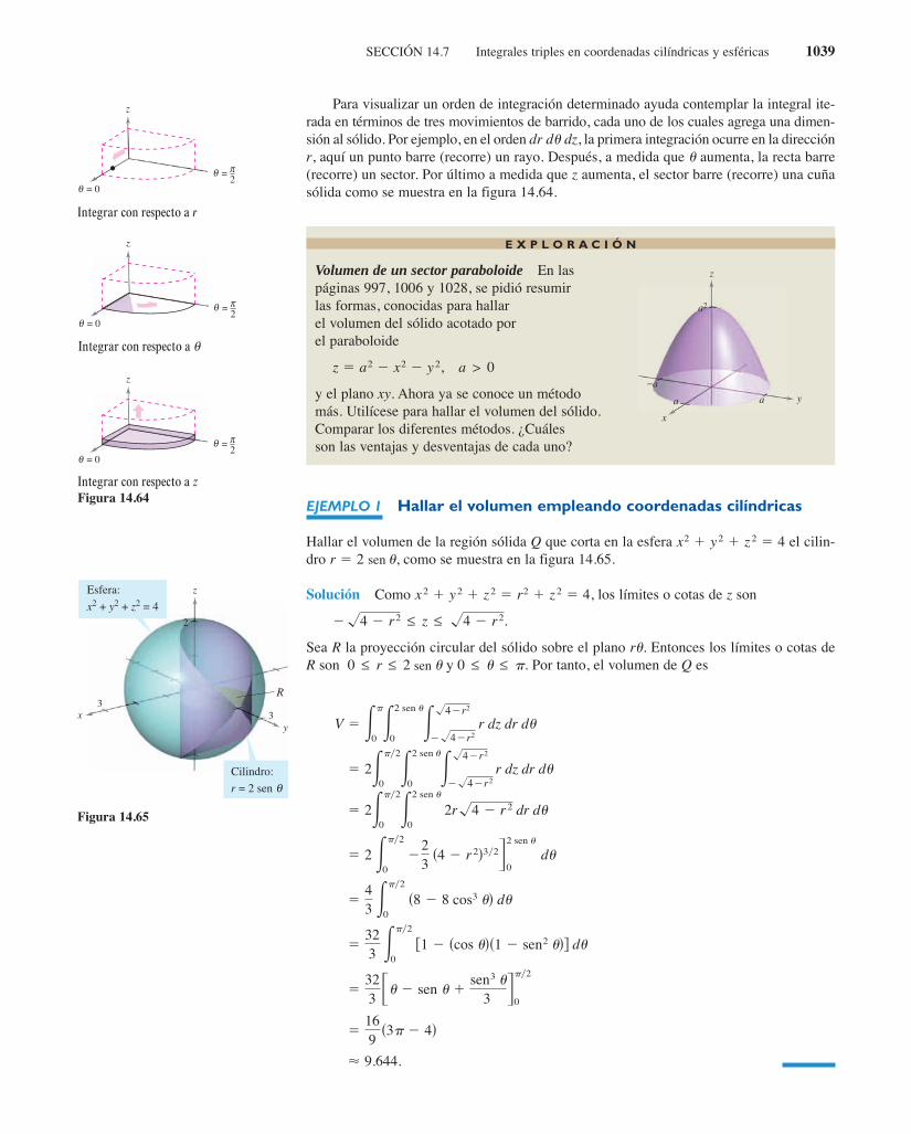
SECCIÓN 14.7 Integrales triples en coordenadas cilíndricas y esféricas 1039
Para visualizar un orden de integración determinado ayuda contemplar la integral ite-rada en términos de tres movimientos de barrido, cada uno de los cuales agrega una dimen-sión al sólido. Por ejemplo, en el orden la primera integración ocurre en la direcciónr, aquí un punto barre (recorre) un rayo. Después, a medida que aumenta, la recta barre(recorre) un sector. Por último a medida que z aumenta, el sector barre (recorre) una cuñasólida como se muestra en la figura 14.64.
EJEMPLO 1 Hallar el volumen empleando coordenadas cilíndricas
Hallar el volumen de la región sólida Q que corta en la esfera el cilin-dro como se muestra en la figura 14.65.
Solución Como los límites o cotas de z son
Sea la proyección circular del sólido sobre el plano . Entonces los límites o cotas deR son y Por tanto, el volumen de Q es0 ≤ u ≤ p.0 ≤ r ≤ 2 sin u
ruR
2!4 2 r2 ≤ z ≤ !4 2 r2.
x2 1 y2 1 z2 5 r2 1 z2 5 4,
r 5 2 sin u,x2 1 y2 1 z2 5 4
udr du dz,
Esfera:
x2 + y2 + z2 = 4
Cilindro:
r = 2 sen θ
xy
z
R3
2
3
Figura 14.65
θ = 0
θ = π2
z
θ = 0
θ = π2
z
θ = 0
θ = π2
z
Integrar con respecto a r
Integrar con respecto a u
Integrar con respecto a zFigura 14.64
E X P L O R A C I Ó N
Volumen de un sector paraboloide En laspáginas 997, 1006 y 1028, se pidió resumirlas formas, conocidas para hallarel volumen del sólido acotado porel paraboloide
y el plano xy. Ahora ya se conoce un método más. Utilícese para hallar el volumen del sólido. Comparar los diferentes métodos. ¿Cuáles son las ventajas y desventajas de cada uno?
a > 0z 5 a2 2 x2 2 y2,
y
x
a
z
a
−a
a2
9.644.
169
3 4
323
sensen3
3
2
0
323
2
01 cos 1 sen2 d
43
2
08 8 cos3 d
22
0
23
4 r2 3 22 sen
0d
22
0
2 sen
02r 4 r2 dr d
22
0
2 sen
0
4 r2
4 r2r dz dr d
V0
2 sen
0
4 r2
4 r2r dz dr d
sen
sen
14-7.qxd 3/12/09 18:33 Page 1039

1040 CAPÍTULO 14 Integración múltiple
EJEMPLO 2 Hallar la masa empleando coordenadas cilíndricas
Hallar la masa de la porción del elipsoide Q dado por situada sobreel plano xy. La densidad en un punto del sólido es proporcional a la distancia entre el puntoy el plano xy.
Solución La función de densidad es Los límites o cotas de z son
donde y como se muestra en la figura 14.66. La masa del sólidoes
La integración en coordenadas cilíndricas es útil cuando en el integrando aparecenfactores con la expresión como se ilustra en el ejemplo 3.
EJEMPLO 3 Hallar el momento de inercia
Hallar el momento de inercia con respecto al eje de simetría del sólido Q limitado o aco-tado por el paraboloide y el plano como se muestra en la figura 14.67.La densidad en cada punto es proporcional a la distancia entre el punto y el eje z.
Solución Como el eje z es el eje de simetría, y sigue que
En coordenadas cilíndricas, Por tanto, se tiene
52pk
5 327
z7y244
05
512kp
35.
5k5 E
4
0z5y2 s2pd dz
5 k E4
0E2p
0
z5y2
5du dz
5 k E4
0E2p
0
r5
5 4!z
0du dz
Iz 5 k E4
0E2p
0E!z
0r2srdr dr du dz
0 ≤ r ≤ !x2 1 y2 5 !z.
Iz 5 EEQ
E ksx2 1 y2d!x2 1 y2 dV.
rsx, y, zd 5 k!x2 1 y2,
z 5 4,z 5 x2 1 y2
x2 1 y2
5 8kE2p
0du 5 16pk.
5k2 E
2p
038r2 2 r44
2
0du
5k2 E
2p
0E2
0s16r 2 4r3d dr du
5k2 E
2p
0E2
0z2r4!1624r2
0dr du
m 5 E2p
0E2
0E!1624r2
0kzr dz dr du
0 ≤ u ≤ 2p,0 ≤ r ≤ 2
0 ≤ z ≤ !16 2 4x2 2 4y2 5 !16 2 4r2
rsr, u, zd 5 kz.
4x2 1 4y2 1 z2 5 16,0 ≤ z ≤ 16 − 4r2
x
y
z
2
2
4
Elipsoide: 4x2 + 4y2 + z2 = 16
Figura 14.66
y
x
2 2
−2
11
5
Limitado o acotado por Q:
z = x2 + y2
z = 4
z
Figura 14.67
14-7.qxd 3/12/09 18:33 Page 1040

SECCIÓN 14.7 Integrales triples en coordenadas cilíndricas y esféricas 1041
Integrales triples en coordenadas esféricas
Las integrales triples que involucran esferas o conos son a menudo más fáciles de calcular mediante la conversión a coordenadas esféricas. Recordar que en la sección 11.7se vieron las ecuaciones rectangulares para conversión a coordenadas esféricas
En este sistema de coordenadas, la región más simple es un bloque esférico determinadopor
donde y como se muestra en la figura 14.68. Sies un punto en el interior de uno de estos bloques, entonces el volumen del bloque
puede ser aproximado por (ver ejercicio 18 en los ejercicios desolución de problemas de este capítulo).
Utilizando el proceso habitual que comprende una partición interior, una suma y unlímite, se desarrolla la versión siguiente de una integral triple en coordenadas esféricaspara una función continua ƒ en la región sólida Q.
Esta fórmula puede modificarse para emplear diferentes órdenes de integración y se puedegeneralizar a regiones con límites o cotas variables.
Como las integrales triples en coordenadas cilíndricas, las integrales triples en coor-denadas esféricas se evalúan empleando integrales iteradas. Como sucede con las coorde-nadas cilíndricas, se puede visualizar un orden determinado de integración contemplandola integral iterada en términos de tres movimientos de barrido, cada uno de los cuales agre-ga una dimensión al sólido. Por ejemplo, la integral iterada
(que se usó en el ejemplo 4) se ilustra en la figura 14.69.
Cuando la letra griega r se emplea en coordenadas esféricas no está relacionada con la den-sidad. Es la análoga tridimensional de la r que se utiliza en coordenadas polares. En este texto, enlos problemas en los que se empleen coordenadas esféricas y una función de densidad, se usará unsímbolo diferente para denotar la densidad. n
NOTA
E2p
0Epy4
0E3
0r2 sin f dr df du
DV < r2 sin f Dr Df Dusr, u, fd
0 ≤ f1 ≤ f2 ≤ p,u2 2 u1 ≤ 2p,r1 ≥ 0,
f1 ≤ f ≤ f2Ju1 ≤ u ≤ u2,Hsr, u, fd: r1 ≤ r ≤ r2,
z 5 r cos f.
y 5 r sin f sin u
x 5 r sin f cos u
x
y
θφρi i isen ∆
ρ∆ i φρi i∆
z
Bloque esférico:
Figura 14.68
Vi i2 sen i i i i
EEQ
E fsx, y, zd dV 5 Eu2
u1
Ef2
f1
Er2
r1
fsr sin f cos u, r sin f sin u, r cos fdr2 sin f dr df du.
z
y
x
2 1
1
−22
ρ
Cono:x2 + y2 = z2 x2 + y2 + z2 = 9
= 3ρ
Esfera:
y
x
2 1−2
2
φ
z
y
x
2 1−2
2
θz
varía desde 0 hasta 3 mientras yse mantienen constantesFigura 14.69
ufr varía desde 0 hasta mientras se mantiene cons-tante
upy4f varía desde 0 hasta 2pu
sen
sen sen
sen sen sen sen
sen
sen
14-7.qxd 3/12/09 18:33 Page 1041

1042 CAPÍTULO 14 Integración múltiple
EJEMPLO 4 Hallar un volumen en coordenadas esféricas
Hallar el volumen de la región sólida Q limitada o acotada inferiormente por la hoja supe-rior del cono y superiormente por la esfera como semuestra en la figura 14.70.
Solución En coordenadas esféricas, la ecuación de la esfera es
La esfera y el cono se cortan cuando
y, como se tiene que
Por consiguiente, se puede utilizar el orden de integración donde 0 ≤ r≤ 3, y El volumen es
EJEMPLO 5 Hallar el centro de masa de una región sólida
Hallar el centro de masa de la región sólida Q de densidad uniforme, limitada o acotadainferiormente por la hoja superior del cono y superiormente por la esfera
Solución Como la densidad es uniforme, se puede considerar que la densidad en el puntoes Por la simetría, el centro de masa se encuentra en el eje z, y sólo se necesita
calcular donde por el ejemplo 4. Como se sigue que
Por tanto,
y el centro de masa es aproximadamente s0, 0, 1.92d.
z 5Mxy
m5
81kpy8
9kp s2 2 !2 d 59s2 1 !2 d
16< 1.920
5k4 E
3
0E2p
0r3 du dr 5
kp
2 E3
0r3 dr 5
81kp
8.
5 kE3
0E2p
0r3 sin2 f
2 4py4
0
du dr
Mxy 5 EEQ
E kz dV 5 k E3
0E2p
0Epy4
0sr cos fdr2 sin f df du dr
z 5 r cos f,m 5 kV 5 9kp s2 2 !2 dz 5 Mxyym,k.sx, y, zd
x2 1 y2 1 z2 5 9.z2 5 x2 1 y2
5 9E2p
011 2
!22 2 du 5 9p s2 2 !2 d < 16.563.
5 9E2p
02cos f4
py4
0du
5 E2p
0Epy4
09 sin f df du
V 5 EEQ
E dV 5 E2p
0Epy4
0E3
0r2 sin f dr df du
0 ≤ u ≤ 2p.0 ≤ f ≤ py4,dr df du,
f 5p
4.1 3
!221132 5 cos f
z 5 r cos f,
z 53!2
sx2 1 y2d 1 z2 5 sz2d 1 z2 5 9
r 5 3.r2 5 x2 1 y2 1 z2 5 9
x2 1 y2 1 z2 5 9,z2 5 x2 1 y2
Esfera:
x2 + y2 + z2 = 9
x
y
z
3
321
32
−2−31
Hoja superiordel cono:z2 = x2 + y2
Figura 14.70
sen
sen
sen
sen2
14-7.qxd 3/12/09 18:33 Page 1042
SECCIÓN 14.7 Integrales triples en coordenadas cilíndricas y esféricas 1043
En los ejercicios 1 a 6, evaluar la integral iterada.
3.
4.
5.
6.
En los ejercicios 7 y 8, utilizar un sistema algebraico por compu-tadora y evaluar la integral iterada.
7.
8.
En los ejercicios 9 a 12, dibujar la región sólida cuyo volumenestá dado por la integral iterada, y evaluar la integral iterada.
11.
12.
En los ejercicios 13 a 16, convertir la integral de coordenadasrectangulares a coordenadas cilíndricas y a coordenadas esféri-cas, y evaluar la integral iterada más sencilla.
13.
14.
15.
Volumen En los ejercicios 17 a 22, utilizar coordenadas cilín-dricas para hallar el volumen del sólido.
17. Sólido interior a y
18. Sólido interior a y exterior a
19. Sólido limitado arriba por z � 2x y abajo por
20. Sólido limitado arriba por z � 2 � x2 � y2 y abajo por z �x2 � y2
21. Sólido limitado o acotado por las gráficas de la esfera r2 �z2 � a2 y del cilindro
22. Sólido interior a la esfera y sobre la hojasuperior del cono
Masa En los ejercicios 23 y 24, utilizar coordenadas cilíndri-cas para hallar la masa del sólido Q.
23.
24.
En los ejercicios 25 a 30, utilizar coordenadas cilíndricas parahallar la característica indicada del cono que se muestra en lafigura.
25. Volumen Hallar el volumen del cono.
26. Centroide Hallar el centroide del cono.
27. Centro de masa Hallar el centro de masa del cono suponiendoque su densidad en cualquier punto es proporcional a la distan-cia entre el punto y el eje del cono. Utilizar un sistema algebrai-co por computadora y evaluar la integral triple.
28. Centro de masa Hallar el centro de masa del cono suponiendoque su densidad en cualquier punto es proporcional a la distan-cia entre el punto y la base. Utilizar un sistema algebraico porcomputadora y evaluar la integral triple.
29. Momento de inercia Suponer que el cono tiene densidad uni-forme y mostrar que el momento de inercia con respecto al eje zes
30. Momento de inercia Suponer que la densidad del cono es
y hallar el momento de inercia conrespecto al eje z.
Momento de inercia En los ejercicios 31 y 32, usar coordenadascilíndricas para verificar la fórmula dada para el momento deinercia del sólido de densidad uniforme.
31. Capa cilíndrica:
0 ≤ z ≤ h0 < a ≤ r ≤ b,
Iz �12m�a2 � b2�
� �x, y, z� � k�x2 � y 2
Iz �3
10mr02.
x
y
h
r0
z = h 1 − rr0( (
z
��x, y, z� � k
y ≥ 0�x2 � y2 ≤ 4, x ≥ 0,Q � ��x, y, z�: 0 ≤ z ≤ 12e��x2�y2�,
��x, y, z� � k�x2 � y2
x2 � y2 ≤ 4�Q � ��x, y, z�: 0 ≤ z ≤ 9 � x � 2y,
z2 � x2 � y 2x2 � y 2 � z2 � 4
r � a cos �
z � 2x2 � 2y2
z � �x2 � y 2x2 � y 2 � z2 � 16
�x � a�2�2 � y2 � �a�2�2x2 � y 2 � z2 � a2
�a
�a
��a2�x2
��a2�x2
�a��a2�x2�y2
a
x dz dy dx
�2
0��4�x2
0 ��16�x2�y2
0 �x2 � y 2 dz dy dx
�2
�2��4�x2
��4�x2
�4
x2�y2
x dz dy dx
�2�
0��
0�5
2 �2 sin � d� d� d�
�2�
0���2
��6�4
0 �2 sin � d� d� d�
���2
0��
0�sin �
0 �2 cos ���2 d� d� d�
�4
0�z
0���2
0 rer d� dr dz
���4
0���4
0�cos �
0 �2 sin � cos � d� d� d�
�2�
0���4
0�cos �
0 �2 sin � d� d� d�
���2
0��
0�2
0 e��3 �2 d� d� d�
���2
0�2 cos2
�
0�4�r2
0 r sin� dz dr d�r sen � dx dr d�
sen
sen
sen
sen
sen
14.7 Ejercicios
CAS
1. 2. ���4
0�6
0�6�r
0 rz dz dr d��5
�1���2
0�3
0 r cos � dr d� dz
9. 10. �2�
0��5
0�5�r 2
0 r dz dr d����2
0�3
0 �e�r 2
0r dz dr d�
16. �3
0��9�x2
0��9�x2�y2
0 �x2 � y 2 � z2 dz dy dx
CAS
CAS
14-7.qxd 25/2/10 16:33 Página 1043

1044 CAPÍTULO 14 Integración múltiple
32. Cilindro circular recto:
Utilizar un sistema algebraico por computadora y calcular laintegral triple.
Volumen En los ejercicios 33 a 36, utilizar coordenadas esféri-cas para calcular el volumen del sólido.
33. Sólido interior x2 1 y2 1 z2 5 9, exterior y arri-ba del plano xy.
34. Sólido limitado arriba por x2 1 y2 1 z2 5 z y abajo por.
35. El toro dado por . (Utilizar un sistema algebraicopor computadora y evaluar la integral triple.)
36. El sólido comprendido entre las esferas ye interior al cono
Masa En los ejercicios 37 y 38, utilizar coordenadas esféricaspara hallar la masa de la esfera de densidadespecificada.
37. La densidad en cualquier punto es proporcional a la distanciaentre el punto y el origen.
38. La densidad en cualquier punto es proporcional a la distancia delpunto al eje z.
Centro de masa En los ejercicios 39 y 40, utilizar coordenadasesféricas para hallar el centro de masa del sólido de densidaduniforme.
39. Sólido hemisférico de radio
40. Sólido comprendido entre dos hemisferios concéntricos de ra-dios y donde
Momento de inercia En los ejercicios 41 y 42, utilizar coorde-nadas esféricas para hallar el momento de inercia con respectoal eje z del sólido de densidad uniforme.
41. Sólido limitado o acotado por el hemisferio py4 #f # py2, y el cono
42. Sólido comprendido entre dos hemisferios concéntricos de ra-dios y donde
49. Hallar el “volumen” de la “esfera en cuatro dimensiones”
evaluando
50. Utilizar las coordenadas esféricas para mostrar que
E`
2`E`
2`E`
2`
!x2 1 y2 1 z2 e2sx21y21z2d dx dy dz 5 2p.
16Ea
0E!a22x2
0 E!a22x22y2
0 E!a22x22y22z2
0
dw dz dy dx.
x2 1 y 2 1 z2 1 w2 5 a2
r < RR,r
f 5 py4r 5 cos f,
r < RR,r
r
x2 1 y 2 1 z2 5 a2
z2 5 x2 1 y 2b > a,x2 1 y 2 1 z2 5 b2,x2 1 y 2 1 z2 5 a2
r 5 4 sin f
32. Right circular cylinder:
Use a computer algebra system to evaluate the triple integral.
Volume In Exercises 33–36, use spherical coordinates to findthe volume of the solid.
33. Solid inside outside andabove the plane
34. Solid bounded above by and below by
35. The torus given by (Use a computer algebra systemto evaluate the triple integral.)
36. The solid between the spheres andand inside the cone
Mass In Exercises 37 and 38, use spherical coordinates to findthe mass of the sphere with the given density.
37. The density at any point is proportional to the distance betweenthe point and the origin.
38. The density at any point is proportional to the distance of thepoint from the axis.
Center of Mass In Exercises 39 and 40, use spherical coordi-nates to find the center of mass of the solid of uniform density.
39. Hemispherical solid of radius
40. Solid lying between two concentric hemispheres of radii andwhere
Moment of Inertia In Exercises 41 and 42, use sphericalcoordinates to find the moment of inertia about the z-axis of thesolid of uniform density.
41. Solid bounded by the hemisphere and the cone
42. Solid lying between two concentric hemispheres of radii andwhere
49. Find the “volume” of the “four-dimensional sphere”
by evaluating
50. Use spherical coordinates to show that
x2 y2 z2 e x2 y2 z2
dx dy dz 2 .
16a
0
a2 x2
0
a2 x2 y2
0
a2 x2 y2 z2
0
dw dz dy dx.
x2 y 2 z2 w2 a2
r < RR,r
44 2,cos ,
r < RR,r
r
z-
x2 1 y 2 1 z2 a2
z2 x2 y 2b > a,x2 y 2 z2 b2,x2 y 2 z2 a2
4 sin
z x2 y2
x2 y2 z2 z
xy-z x2 y2,x2 y2 z2 9,
0 z hr 2a sin ,
Iz32ma2
1044 Chapter 14 Multiple Integration
CAS
CAS
48. Convert the integral from rectangular coordinates to both (a) cylindrical and (b) spherical coordinates. Without calcu-lating, which integral appears to be the simplest to evaluate?Why?
a
0
a2 x2
0
a2 x2 y2
0 x2 y2 z2 dz dy dx
CAPSTONE
43. Give the equations for conversion from rectangular to cylindrical coordinates and vice versa.
44. Give the equations for conversion from rectangular tospherical coordinates and vice versa.
45. Give the iterated form of the triple integral in cylindrical form.
46. Give the iterated form of the triple integral in spherical form.
47. Describe the surface whose equation is a coordinate equal toa constant for each of the coordinates in (a) the cylindricalcoordinate system and (b) the spherical coordinate system.
Q f x, y, z dV
Q f x, y, z dV
WRITING ABOUT CONCEPTS
51. Find the volume of the region of points such that
This problem was composed by the Committee on the Putnam Prize Competition.© The Mathematical Association of America. All rights reserved.
x2 y2 z2 8 2 36 x2 y2 .x, y, z
PUTNAM EXAM CHALLENGE
FOR FURTHER INFORMATION For more information on thesetypes of spheres, see the article “Heat Therapy for Tumors” by LeahEdelstein-Keshet in The UMAP Journal.
In parts (a) and (b), find the volume of the wrinkled sphere orbumpy sphere. These solids are used as models for tumors.
(a) Wrinkled sphere (b) Bumpy sphere
x
Generado con Maple
z
x
y
Generado con Maple
z
0 2 , 00 2 , 0
1 0.2 sin 8 sin 41 0.2 sin 8 sin
Wrinkled and Bumpy Spheres
S E C T I O N P R O J E C T
1053714_1407.qxp 10/27/08 1:34 PM Page 1044
0 ≤ z ≤ hr 5 2a sin u,
Iz 532ma2
Desarrollo de conceptos43. Dar las ecuaciones de conversión de coordenadas rectangu-
lares a coordenadas cilíndricas y viceversa.
44. Dar las ecuaciones de conversión de coordenadas rectangu-lares a coordenadas esféricas y viceversa.
45. Dar la forma iterada de la integral triple enforma cilíndrica.
46. Dar la forma iterada de la integral triple enforma esférica.
47. Describir la superficie cuya ecuación es una coordenada iguala una constante en cada una de las coordenadas en a) el sistemade coordenadas cilíndricas y b) el sistema de coordenadasesféricas.
eeQ
e f sx, y, zd dV
eeQ
e f sx, y, zd dV
En los incisos a) y b), hallar el volumen de las esferas deformadas.Estos sólidos se usan como modelos de tumores.
a) Esfera deformada b) Esfera deformada
PARA MAYOR INFORMACIÓNMPara más información sobreestos tipos de esferas, ver el artículo “Heat Therapy for Tumors” deLeah Edelstein-Keshet en The UMAP Journal.
0 ≤ u ≤ 2p, 0 ≤ f ≤ p0 ≤ u ≤ 2p, 0 ≤ f ≤ p
r 5 1 1 0.2 sin 8u sin 4fr 5 1 1 0.2 sin 8u sin f
senPara discusión48. Convertir la integral desde coordenadas rectangulares a
a) coordenadas cilíndricas y b) esféricas. Sin calcular, ¿quéintegral parece ser más sencilla de evaluar? ¿Por qué?
32. Right circular cylinder:
Use a computer algebra system to evaluate the triple integral.
Volume In Exercises 33–36, use spherical coordinates to findthe volume of the solid.
33. Solid inside outside andabove the plane
34. Solid bounded above by and below by
35. The torus given by (Use a computer algebra systemto evaluate the triple integral.)
36. The solid between the spheres andand inside the cone
Mass In Exercises 37 and 38, use spherical coordinates to findthe mass of the sphere with the given density.
37. The density at any point is proportional to the distance betweenthe point and the origin.
38. The density at any point is proportional to the distance of thepoint from the axis.
Center of Mass In Exercises 39 and 40, use spherical coordi-nates to find the center of mass of the solid of uniform density.
39. Hemispherical solid of radius
40. Solid lying between two concentric hemispheres of radii andwhere
Moment of Inertia In Exercises 41 and 42, use sphericalcoordinates to find the moment of inertia about the z-axis of thesolid of uniform density.
41. Solid bounded by the hemisphere and the cone
42. Solid lying between two concentric hemispheres of radii andwhere
49. Find the “volume” of the “four-dimensional sphere”
by evaluating
50. Use spherical coordinates to show that
x2 y2 z2 e x2 y2 z2
dx dy dz 2 .
16a
0
a2 x2
0
a2 x2 y2
0
a2 x2 y2 z2
0
dw dz dy dx.
x2 y 2 z2 w2 a2
r < RR,r
44 2,cos ,
r < RR,r
r
z-
x2 1 y 2 1 z2 a2
z2 x2 y 2b > a,x2 y 2 z2 b2,x2 y 2 z2 a2
4 sin
z x2 y2
x2 y2 z2 z
xy-z x2 y2,x2 y2 z2 9,
0 z hr 2a sin ,
Iz32ma2
1044 Chapter 14 Multiple Integration
CAS
CAS
48. Convert the integral from rectangular coordinates to both (a) cylindrical and (b) spherical coordinates. Without calcu-lating, which integral appears to be the simplest to evaluate?Why?
a
0
a2 x2
0
a2 x2 y2
0 x2 y2 z2 dz dy dx
CAPSTONE
43. Give the equations for conversion from rectangular to cylindrical coordinates and vice versa.
44. Give the equations for conversion from rectangular tospherical coordinates and vice versa.
45. Give the iterated form of the triple integral in cylindrical form.
46. Give the iterated form of the triple integral in spherical form.
47. Describe the surface whose equation is a coordinate equal toa constant for each of the coordinates in (a) the cylindricalcoordinate system and (b) the spherical coordinate system.
Q f x, y, z dV
Q f x, y, z dV
WRITING ABOUT CONCEPTS
51. Find the volume of the region of points such that
This problem was composed by the Committee on the Putnam Prize Competition.© The Mathematical Association of America. All rights reserved.
x2 y2 z2 8 2 36 x2 y2 .x, y, z
PUTNAM EXAM CHALLENGE
FOR FURTHER INFORMATION For more information on thesetypes of spheres, see the article “Heat Therapy for Tumors” by LeahEdelstein-Keshet in The UMAP Journal.
In parts (a) and (b), find the volume of the wrinkled sphere orbumpy sphere. These solids are used as models for tumors.
(a) Wrinkled sphere (b) Bumpy sphere
x
Generado con Maple
z
x
y
Generado con Maple
z
0 2 , 00 2 , 0
1 0.2 sin 8 sin 41 0.2 sin 8 sin
Wrinkled and Bumpy Spheres
S E C T I O N P R O J E C T
1053714_1407.qxp 10/27/08 1:34 PM Page 1044
Preparación del examen Putnam51. Encontrar el volumen de la región de puntos (x, y, z) en
forma tal que
Este problema fue preparado por el Committee on the Putnam Prize Competition.© The Mathematical Association of America. Todos los derechos reservados.
32. Right circular cylinder:
Use a computer algebra system to evaluate the triple integral.
Volume In Exercises 33–36, use spherical coordinates to findthe volume of the solid.
33. Solid inside outside andabove the plane
34. Solid bounded above by and below by
35. The torus given by (Use a computer algebra systemto evaluate the triple integral.)
36. The solid between the spheres andand inside the cone
Mass In Exercises 37 and 38, use spherical coordinates to findthe mass of the sphere with the given density.
37. The density at any point is proportional to the distance betweenthe point and the origin.
38. The density at any point is proportional to the distance of thepoint from the axis.
Center of Mass In Exercises 39 and 40, use spherical coordi-nates to find the center of mass of the solid of uniform density.
39. Hemispherical solid of radius
40. Solid lying between two concentric hemispheres of radii andwhere
Moment of Inertia In Exercises 41 and 42, use sphericalcoordinates to find the moment of inertia about the z-axis of thesolid of uniform density.
41. Solid bounded by the hemisphere and the cone
42. Solid lying between two concentric hemispheres of radii andwhere
49. Find the “volume” of the “four-dimensional sphere”
by evaluating
50. Use spherical coordinates to show that
x2 y2 z2 e x2 y2 z2
dx dy dz 2 .
16a
0
a2 x2
0
a2 x2 y2
0
a2 x2 y2 z2
0
dw dz dy dx.
x2 y 2 z2 w2 a2
r < RR,r
44 2,cos ,
r < RR,r
r
z-
x2 1 y 2 1 z2 a2
z2 x2 y 2b > a,x2 y 2 z2 b2,x2 y 2 z2 a2
4 sin
z x2 y2
x2 y2 z2 z
xy-z x2 y2,x2 y2 z2 9,
0 z hr 2a sin ,
Iz32ma2
1044 Chapter 14 Multiple Integration
CAS
CAS
48. Convert the integral from rectangular coordinates to both (a) cylindrical and (b) spherical coordinates. Without calcu-lating, which integral appears to be the simplest to evaluate?Why?
a
0
a2 x2
0
a2 x2 y2
0 x2 y2 z2 dz dy dx
CAPSTONE
43. Give the equations for conversion from rectangular to cylindrical coordinates and vice versa.
44. Give the equations for conversion from rectangular tospherical coordinates and vice versa.
45. Give the iterated form of the triple integral in cylindrical form.
46. Give the iterated form of the triple integral in spherical form.
47. Describe the surface whose equation is a coordinate equal toa constant for each of the coordinates in (a) the cylindricalcoordinate system and (b) the spherical coordinate system.
Q f x, y, z dV
Q f x, y, z dV
WRITING ABOUT CONCEPTS
51. Find the volume of the region of points such that
This problem was composed by the Committee on the Putnam Prize Competition.© The Mathematical Association of America. All rights reserved.
x2 y2 z2 8 2 36 x2 y2 .x, y, z
PUTNAM EXAM CHALLENGE
FOR FURTHER INFORMATION For more information on thesetypes of spheres, see the article “Heat Therapy for Tumors” by LeahEdelstein-Keshet in The UMAP Journal.
In parts (a) and (b), find the volume of the wrinkled sphere orbumpy sphere. These solids are used as models for tumors.
(a) Wrinkled sphere (b) Bumpy sphere
x
Generado con Maple
z
x
y
Generado con Maple
z
0 2 , 00 2 , 0
1 0.2 sin 8 sin 41 0.2 sin 8 sin
Wrinkled and Bumpy Spheres
S E C T I O N P R O J E C T
1053714_1407.qxp 10/27/08 1:34 PM Page 1044
Esferas deformadas
PROYECTO DE TRABAJO
32. Right circular cylinder:
Use a computer algebra system to evaluate the triple integral.
Volume In Exercises 33–36, use spherical coordinates to findthe volume of the solid.
33. Solid inside outside andabove the plane
34. Solid bounded above by and below by
35. The torus given by (Use a computer algebra systemto evaluate the triple integral.)
36. The solid between the spheres andand inside the cone
Mass In Exercises 37 and 38, use spherical coordinates to findthe mass of the sphere with the given density.
37. The density at any point is proportional to the distance betweenthe point and the origin.
38. The density at any point is proportional to the distance of thepoint from the axis.
Center of Mass In Exercises 39 and 40, use spherical coordi-nates to find the center of mass of the solid of uniform density.
39. Hemispherical solid of radius
40. Solid lying between two concentric hemispheres of radii andwhere
Moment of Inertia In Exercises 41 and 42, use sphericalcoordinates to find the moment of inertia about the z-axis of thesolid of uniform density.
41. Solid bounded by the hemisphere and the cone
42. Solid lying between two concentric hemispheres of radii andwhere
49. Find the “volume” of the “four-dimensional sphere”
by evaluating
50. Use spherical coordinates to show that
x2 y2 z2 e x2 y2 z2
dx dy dz 2 .
16a
0
a2 x2
0
a2 x2 y2
0
a2 x2 y2 z2
0
dw dz dy dx.
x2 y 2 z2 w2 a2
r < RR,r
44 2,cos ,
r < RR,r
r
z-
x2 1 y 2 1 z2 a2
z2 x2 y 2b > a,x2 y 2 z2 b2,x2 y 2 z2 a2
4 sin
z x2 y2
x2 y2 z2 z
xy-z x2 y2,x2 y2 z2 9,
0 z hr 2a sin ,
Iz32ma2
1044 Chapter 14 Multiple Integration
CAS
CAS
48. Convert the integral from rectangular coordinates to both (a) cylindrical and (b) spherical coordinates. Without calcu-lating, which integral appears to be the simplest to evaluate?Why?
a
0
a2 x2
0
a2 x2 y2
0 x2 y2 z2 dz dy dx
CAPSTONE
43. Give the equations for conversion from rectangular to cylindrical coordinates and vice versa.
44. Give the equations for conversion from rectangular tospherical coordinates and vice versa.
45. Give the iterated form of the triple integral in cylindrical form.
46. Give the iterated form of the triple integral in spherical form.
47. Describe the surface whose equation is a coordinate equal toa constant for each of the coordinates in (a) the cylindricalcoordinate system and (b) the spherical coordinate system.
Q f x, y, z dV
Q f x, y, z dV
WRITING ABOUT CONCEPTS
51. Find the volume of the region of points such that
This problem was composed by the Committee on the Putnam Prize Competition.© The Mathematical Association of America. All rights reserved.
x2 y2 z2 8 2 36 x2 y2 .x, y, z
PUTNAM EXAM CHALLENGE
FOR FURTHER INFORMATION For more information on thesetypes of spheres, see the article “Heat Therapy for Tumors” by LeahEdelstein-Keshet in The UMAP Journal.
In parts (a) and (b), find the volume of the wrinkled sphere orbumpy sphere. These solids are used as models for tumors.
(a) Wrinkled sphere (b) Bumpy sphere
x
y
Generado con Maple
z
x
y
Generado con Maple
z
0 2 , 00 2 , 0
1 0.2 sin 8 sin 41 0.2 sin 8 sin
Wrinkled and Bumpy Spheres
S E C T I O N P R O J E C T
1053714_1407.qxp 10/27/08 1:34 PM Page 1044
CAS
CAS sen
sen sen sen sen
14-7.qxd 3/12/09 18:33 Page 1044

SECCIÓN 14.8 Cambio de variables: jacobianos 1045
14.8 Cambio de variables: jacobianos
n Comprender el concepto de jacobiano.n Utilizar un jacobiano para cambiar variables en una integral doble.
Jacobianos
En una integral simple
se puede tener un cambio de variables haciendo con lo que yobtener
donde y Nótese que el proceso de cambio de variables introduce, en elintegrando, un factor adicional . Esto también ocurre en el caso de las integralesdobles
Jacobiano
donde el cambio de variables y introduce un factor llamado jaco-biano de y con respecto a y Al definir el jacobiano, es conveniente utilizar lanotación siguiente que emplea determinantes.
EJEMPLO 1 El jacobiano de la conversión rectangular-polar
Hallar el jacobiano para el cambio de variables definido por
y
Solución De acuerdo con la definición de un jacobiano, se obtiene
5 r.
5 r cos2 u 1 r sin2 u
5 |cos usin u
2r sin ur cos u |
sx, ydsr, ud 5 | x
rxu
yr
yu |
y 5 r sin u.x 5 r cos u
v.uyxy 5 hsu, vdx 5 gsu, vd
ERE f sx, yd dA 5 E
SE f sgsu, vd, hsu, vdd| x
uyv
2yu
xv | du dv
g9sudb 5 gsdd.a 5 gscd
Eb
a
f sxd dx 5 Ed
c
f sgsuddg9sud du
dx 5 g9sud du,x 5 gsud,
Eb
a
f sxd dx
CARL GUSTAV JACOBI (1804-1851)
El jacobiano recibe su nombre en honor almatemático alemán Carl Gustav Jacobi,conocido por su trabajo en muchas áreas dematemática, pero su interés en integraciónprovenía del problema de hallar la circunfe-rencia de una elipse.
DEFINICIÓN DEL JACOBIANO
Si y entonces el jacobiano de y con respecto a y denotado por es
sx, ydsu, vd 5 | x
uxv
yu
yv | 5
xu
yv
2yu
xv
.
sx, ydysu, vd,v,uyxy 5 hsu, vd,x 5 gsu, vd
sen
sen
sen2
sen
14-8.qxd 3/12/09 18:35 Page 1045

1046 CAPÍTULO 14 Integración múltiple
El ejemplo 1 indica que el cambio de variables de coordenadas rectangulares a polaresen una integral doble se puede escribir como
donde es la región en el plano que corresponde a la región en el plano xy, como semuestra en la figura 14.71. Esta fórmula es semejante a la de la página 1006.
En general, un cambio de variables está dado por una transformación biyectiva (o unoa uno) de una región en el plano uv en una región en el plano xy dada por
donde y tienen primeras derivadas parciales continuas en la región S. Nótese que elpunto se encuentra en S y el punto se encuentra en R. En la mayor parte delas ocasiones, se busca una transformación en la que la región S sea más simple que laregión R.
EJEMPLO 2 Hallar un cambio de variables para simplificaruna región
Sea R la región limitada o acotada por las rectas
y
como se muestra en la figura 14.72. Hallar una transformación T de una región S a R talque S sea una región rectangular (con lados paralelos a los ejes u o v).
Solución Para empezar, sea y Resolviendo este sistema de ecua-ciones para encontrar y se obtiene donde
y
Los cuatro límites de R en el plano xy dan lugar a los límites siguientes de S en el planouv.
Límites en el plano xy Límites en el plano uv
La región S se muestra en la figura 14.73. Nótese que la transformación T
transforma los vértices de la región S en los vértices de la región R. Por ejemplo,
Tsu, vd 5 sx, yd 5 113
f2u 1 vg, 13
fu 2 vg2
v 5 24x 2 2y 5 24
v 5 0x 2 2y 5 0
u 5 4x 1 y 5 4
u 5 1x 1 y 5 1
y 513
su 2 vd.x 513
s2u 1 vd
T su, vd 5 sx, yd,yxv 5 x 2 2y.u 5 x 1 y
x 1 y 5 1x 1 y 5 4,x 2 2y 5 24,x 2 2y 5 0,
sx, ydsu, vdhg
Tsu, vd 5 sx, yd 5 sgsu, vd, hsu, vdd
RST
RruS
5 ESE f sr cos u, r sin ud|sx, yd
sr, ud | dr du
ERE f sx, yd dA 5 E
SE f sr cos u, r sin udr dr du, r > 0
r
α
β
a b
S
αθ
θ
=
β=
r a= r = b
θθ θT(r, ) = (r cos , r sen )θ
x
R
αθ
θ
=
β=
r = a
r = b
y
S es la región en el plano ru que correspon-de a R en el plano xyFigura 14.71
321
3
2
1
−2
−1
−2
x
34
83,,,3
4
x − 2y = −4
3 ,,,8
x − 2y = 0
R
x +y =
4x +
y =1
523,,,3
1,,, 33
2
( )−
( )
( )
( )
y
Región R en el plano xyFigura 14.72
u32−1
−1
−3
−2
−5
u = 4u = 1
(4, 0)
S
v = 0
(1, −4) (4, −4)
v = −4
(1 , 0)
v
Región S en el plano uvFigura 14.73
sen
Ts1, 24d 5 s13f2s1d 2 4g , 1
3 f1 2 s24dg d 5 s223, 5
3d.T s4, 24d 5 s1
3f2s4d 2 4g , 13 f4 2 s24dg d 5 s4
3, 83d
Ts4, 0d 5 s13f2s4d 1 0g , 1
3 f4 2 0g d 5 s83, 4
3dTs1, 0d 5 s1
3f2s1d 1 0g , 13 f1 2 0g d 5 s2
3, 13d
sen
14-8.qxd 3/12/09 18:35 Page 1046

SECCIÓN 14.8 Cambio de variables: jacobianos 1047
Cambio de variables en integrales dobles
Considerar el caso en el que S es una región rectangular en el plano uv convértices y como se muestra en la figura14.74. Las imágenes de estos vértices en el plano xy se muestran en la figura 14.75. Si y
son pequeños, la continuidad de g y de h implica que R es aproximadamente un parale-logramo determinado por los vectores y Así pues, el área de R es
Para y Dv pequeños, las derivadas parciales de g y h con respecto a u pueden ser apro-ximadas por
y
Por consiguiente,
De manera similar, se puede aproximar por lo que implica que
Por tanto, en la notación del jacobiano,
Como esta aproximación mejora cuando y se aproximan a 0, el caso límite puedeescribirse como
Por tanto,
EREf sx, yd dx dy 5 E
SEf sgsu, vd, hsu, vdd|sx, yd
su, vd| du dv.
dA < iMN\
3 MQ\
i < | sx, ydsu, vd | du dv.
DvDu
DA < iMN\
3 MQ\
i < | sx, ydsu, vd | Du Dv.
Du Dvk.|xuxv
yuyv|5MN
\
3 MQ\
< |i
xu Du
xv Dv
j
yu Du
yv
Dv
k
0
0|xv
Dv i 1yv
Dvj,MQ\
5xu
Du i 1yu
Duj.
< fgusu, vd Dug i 1 fhusu, vd Dug j
MN\
5 fgsu 1 Du, vd 2 gsu, vdg i 1 fhsu 1 Du, vd 2 hsu, vdgj
husu, vd <hsu 1 Du, vd 2 hsu, vd
Du.gusu, vd <
gsu 1 Du, vd 2 gsu, vdDu
Du
DA < i MN\
3 MQ\
i .
MQ\
.MN\
DvDu
su, v 1 Dvd,su 1 Du, v 1 Dvd,su 1 Du, vd,su, vd,DEMOSTRACIÓN
u
(u, v + ∆v) (u + ∆u, v + ∆v)
(u, v) (u + ∆u, v)
S
v
x
R
x = g(u, v)y = h(u, v)
M = (x, y)
Q P
N
y
Los vértices en el plano son
y
Figura 14.75hsu, v 1 Dvdd.Qsgsu, v 1 Dvd,
hsu 1 Du, v 1 Dvdd,Psgsu 1 Du, v 1 Dvd,hsu 1 Du, vdd,
Nsgsu 1 Du, vd,Msgsu, vd, hsu, vdd,xy
Área de
Figura 14.74Du > 0, Dv > 0
S 5 Du Dv
TEOREMA 14.5 CAMBIO DE VARIABLES EN INTEGRALES DOBLES
Sea R una región vertical u horizontalmente sencilla en el plano xy y sea S una regiónvertical u horizontalmente sencilla en el plano uv. Sea T desde S hasta R dado por T(u,v) 5 (x, y) 5 (g(u, v), h(u, v)), donde g y h tienen primeras derivadas parciales conti-nuas. Suponer que T es uno a uno excepto posiblemente en la frontera de S. Si f escontinua en R y (x, y)y(u, v) no es cero en S, entonces
ERE f sx, yddx dy 5 E
SE f sgsu, vd, hsu, vdd| sx, yd
su, vd | du dv.
14-8.qxd 3/12/09 18:35 Page 1047

1048 CAPÍTULO 14 Integración múltiple
Los dos ejemplos siguientes muestran cómo un cambio de variables puede simplificarel proceso de integración. La simplificación se puede dar de varias maneras. Se puedehacer un cambio de variables para simplificar la región R o el integrando o ambos.
EJEMPLO 3 Un cambio de variables para simplificar una región
Sea R la región limitada o acotada por las rectas
y
como se muestra en la figura 14.76. Evaluar la integral doble
Solución De acuerdo con el ejemplo 2, se puede usar el cambio siguiente de variables.
y
Las derivadas parciales de y son
y
lo cual implica que el jacobiano es
Por tanto, por el teorema 14.5, se obtiene
51649
.
519 3
8u3
31 4u2 2
643
u44
1
519 E
4
118u2 1 8u 2
643 2 du
519 E
4
132u2v 2
uv2
22
v3
3 40
24du
5 E4
1E0
24
19
s2u2 2 uv 2 v2d dv du
ERE 3xy dA 5 E
SE 331
3s2u 1 vd 1
3su 2 vd4| sx, yd
su, vd | dv du
5 213
.
5 229
219
5 |2313 13
213|
sx, ydsu, vd 5 | x
uxv
yu
yv |
yv
5 213
yu
513
,xv
513
,xu
523
,
yx
y 513
su 2 vdx 513
s2u 1 vd
ERE 3xy dA.
x 1 y 5 1x 1 y 5 4,x 2 2y 5 24,x 2 2y 5 0,
f sx, yd,
321
3
2
1
−2
−1
−2
x
x − 2y = −4
x − 2y = 0
R
x +y =
4x +
y =1
y
Figura 14.76
14-8.qxd 3/12/09 18:35 Page 1048

SECCIÓN 14.8 Cambio de variables: jacobianos 1049
EJEMPLO 4 Un cambio de variables para simplificar un integrando
Sea R la región limitada o acotada por el cuadrado cuyos vértices son s2, 1dy Evaluar la integral
Solución Obsérvese que los lados de R se encuentran sobre las rectas y como se muestra en la figura 14.77. Haciendo
y se tiene que los límites o cotas de la región S en el plano uv son
y
como se muestra en la figura 14.78. Despejando x y y en términos de u y v se obtiene
y
Las derivadas parciales de x y y son
y
lo cual implica que el jacobiano es
Por el teorema 14.5, sigue que
En cada uno de los ejemplos de cambio de variables de esta sección, la región S hasido un rectángulo con lados paralelos a los ejes u o v. En ocasiones, se puede usar un cam-bio de variables para otros tipos de regiones. Por ejemplo, transforma laregión circular en la región elíptica x2 1 sy2y4d 5 1.u2 1 v2 5 1
T su, vd 5 sx, 12 yd
< 2.363.
5136
s2 2 sin 2d
5136 32 2
12
sin 2 112
sins22d4
5136 3v 2
12
sin 2v41
21
5136 E1
21s1 2 cos 2vd dv
5133 E1
21sin2v dv
512 E
1
21ssin2 vd u3
3 43
1dv
ERE sx 1 yd2 sin2sx 2 yd dA 5 E1
21E3
1u2 sin2 v11
22 du dv
5 214
214
5 212
.5 | 12
12
12
212 |sx, yd
su, vd 5 | xu
xv
yu
yv |
yv
5 212
yu
512
,xv
512
,xu
512
,
y 512
su 2 vd.x 512
su 1 vd
21 ≤ v ≤ 11 ≤ u ≤ 3
v 5 x 2 y,u 5 x 1 yx 2 y 5 21,x 1 y 5 3,x 2 y 5 1,
x 1 y 5 1,
ERE sx 1 yd2 sin2sx 2 yd dA.
s1, 0d.s1, 2d,s0, 1d,
u321
1
−1
(3, 1)(1, 1)
S
u = 3
v = 1
v = −1
u = 1
(1, −1) (3, −1)
v
Región S en el plano uvFigura 14.78
2
3
2 3x
(1, 2)
(2, 1)
R
x − y = −1
(1, 0)x +
y =1
(0, 1)
x − y = 1
x +y =
3
y
Región R en el plano xyFigura 14.77
sen2
sen2
sen2
sen2
sen2
sen
sen sen1222
sen
14-8.qxd 3/12/09 18:35 Page 1049

1050 CAPÍTULO 14 Integración múltiple
En los ejercicios 1 a 8, hallar el jacobiano para elcambio de variables indicado.
1.
2.
3.
4.
5.
6.
7.
8.
En los ejercicios 9 a 12, dibujar la imagen S en el plano uv de laregión R en el plano xy utilizando las transformaciones dadas.
9. 10.
En los ejercicios 13 y 14, verificar el resultado del ejemplo indi-cado por establecer la integral usando dy dx o dx dy para dA.Después, usar un sistema algebraico por computadora para eva-luar la integral.
13. Ejemplo 3 14. Ejemplo 4
En los ejercicios 15 a 20, utilizar el cambio de variables indicadopara hallar la integral doble.
15. 16.
Figura para 15 Figura para 16
17. 18.
19. 20.
En los ejercicios 21 a 28, utilizar un cambio de variables parahallar el volumen de la región sólida que se encuentra bajo lasuperficie y sobre la región plana
21.
R: región limitada por el cuadrado con vértices (1, 0), (0, 1),(1, 2), (2, 1)
22.
R: región limitada por el paralelogramo con vértices (0, 0),(22, 3), (2, 5), (4, 2)
23.
región acotada por el cuadrado cuyos vértices son s2, 2ds4, 4d,s6, 2d,
s4, 0d,R:
f sx, yd 5 sx 1 ydex2y
f sx, yd 5 s3x 1 2yd2!2y 2 x
f sx, yd 5 48xy
R.z 5 f xx, yc
x 5uv, y 5 vx 5!v
u, y 5 !uv
ERE y sin xy dAE
REe2xyy2 dA
x1
−1
−1 (0, 0)
(1, 1)(−1, 1)
y
x
4
2
6
6
−28
(3, 3) (7, 3)
(4, 0)(0, 0)
y
y 512su 2 vdy 5 u
x 512su 1 vdx 5 u 1 v
ERE 4sx 1 ydex2y dAE
RE ysx 2 yd dA
x
(0, 1)
1
2
1 2
(1, 2)
(2, 1)
(1, 0)
y
x
1
1
−1
−1
(0, 1)
(1, 0)
(0, −1)
(−1, 0)
y
y 5 212su 2 vdy 5
12su 2 vd
x 512su 1 vdx 5
12su 1 vd
ERE 60xy dAE
RE 4sx2 1 y2d dA
x
R(4, 1)
(0, 0)
6
5
4
3
2
1
(2, 2)
(6, 3)
2 63 4 5
y
x
R
(2, 3)
(3, 0)
(0, 0)
1
2
2
3
3
y
y 513su 2 vdy 5 3v
x 513s4u 2 vdx 5 3u 1 2v
x 5uv, y 5 u 1 v
x 5 eu sin v, y 5 eu cos v
x 5 u 1 a, y 5 v 1 a
x 5 u cos u 2 v sin u, y 5 u sin u 1 v cos u
x 5 uv 2 2u, y 5 uv
x 5 u 2 v2, y 5 u 1 v
x 5 au 1 bv, y 5 cu 1 dv
x 5 212su 2 vd, y 5
12su 1 vd
xx, yc /xu, vc
sensen
sen
sen
14.8 Ejercicios
11. 12.
103
x
y
23
13, ))
43
13,− ))
83
43, ))
23, ))
R
−1−2 1 2 3−1
2
3
4
x
y
1 2
1
2
12
12, ))
32
32, ))
(1, 2)(0, 1)
R
y 513s2v 1 udy 5
12su 2 vd
x 513sv 2 udx 5
12su 1 vd
R
x
y
1 2 3 4
2
3 xy = 4
xy = 1 y = 4
y = 1R
x
y
3
1
2
3
y = 2x
y = x14
y = 4x
y = 1x
CAS
1053714_1408.qxp 10/27/08 1:35 PM Page 1050
CAS
14-8.qxd 3/12/09 18:35 Page 1050

24.
región acotada por el cuadrado cuyos vértices son
25.
región acotada por el paralelogramo cuyos vértices son
26.
región acotada por el paralelogramo cuyos vértices son
27.
región acotada por el triángulo cuyos vértices son donde
28.
región acotada por las gráficas de Sugerencia: Hacer
29. La sustitución u 5 2x 2 y y v 5 x 1 y hacen la región R (ver lafigura) en una simple región S en el plano uv. Determinar elnúmero total de lados de S que son paralelos a cualquiera de losejes u o v.
31. Considerar la región R en el plano xy acotada por la elipse
y las transformaciones y
a) Dibujar la gráfica de la región R y su imagen S bajo la trans-formación dada.
b) Hallar
c) Hallar el área de la elipse.
32. Utilizar el resultado del ejercicio 31 para hallar el volumen decada uno de los sólidos abovedados que se encuentra bajo lasuperficie y sobre la región elíptica R. (Sugerencia:Después de hacer el cambio de variables dado por los resultadosdel ejercicio 31, hacer un segundo cambio de variables a coor-denadas polares.)
a)
b)
En los ejercicios 35 a 40, hallar el jacobiano para el cambio de variables indicado. Si
y entonces el jacobiano de y y con respecto a v y es
.
35.
36.
39. Coordenadas esféricas
40. Coordenadas cilíndricas
x 5 r cos u, y 5 r sin u, z 5 z
x 5 r sin f cos u, y 5 r sin f sin u, z 5 r cos f
x 5 4u 2 v, y 5 4v 2 w, z 5 u 1 w
x 5 us1 2 vd, y 5 uvs1 2 wd, z 5 uvw
xx, y, zcxu, v, wc 5 |x
uyuzu
xvyvzv
xwywzw|
wu,zx,z 5 hxu, v, wc,y 5 gxu, v, wc,
x 5 f xu, v, wc,xx, y, zc/xu, v, wc
R: x2
a2 1y2
b2 ≤ 1
f sx, yd 5 A cos1p2!x2
a2 1y2
b2 2;
R: x2
161
y2
9≤ 1
f sx, yd 5 16 2 x2 2 y2;
z 5 f sx, yd
sx, ydsu, vd.
y 5 bv.x 5 au
x2
a2 1y2
b2 5 1
x 5 u, y 5 vyu.dsx 5 4x 5 1,xy 5 4,xy 5 1,R:
f sx, yd 5xy
1 1 x2y2
a > 0s0, ad,sa, 0d,s0, 0d,R:
f sx, yd 5 !x 1 y
s4, 2ds2, 5d,s22, 3d,s0, 0d,R:
f sx, yd 5 s3x 1 2yds2y 2 xd3y2
s4, 21ds5, 0d,s1, 1d,s0, 0d,R:
f sx, yd 5 !sx 2 ydsx 1 4ydspy2, py2dsp, pd,s3py2, py2d,
sp, 0d,R:
f sx, yd 5 sx 1 yd2 sin2sx 2 yd
SECCIÓN 14.8 Cambio de variables: jacobianos 1051
24.
region bounded by the square with vertices
25.
region bounded by the parallelogram with vertices
26.
region bounded by the parallelogram with vertices
27.
region bounded by the triangle with vertices where
28.
region bounded by the graphs of Hint: Let
29. The substitutions and make the region(see figure) into a simpler region in the plane. Determine
the total number of sides of that are parallel to either the axis or the axis.
31. Consider the region in the plane bounded by the ellipse
and the transformations and
(a) Sketch the graph of the region and its image under thegiven transformation.
(b) Find
(c) Find the area of the ellipse.
32. Use the result of Exercise 31 to find the volume of each dome-shaped solid lying below the surface and above theelliptical region (Hint: After making the change of variablesgiven by the results in Exercise 31, make a second change ofvariables to polar coordinates.)
(a)
(b)
In Exercises 35–40, find the Jacobian for theindicated change of variables. If and then the Jacobian of and with respectto and is
35.
36.
37.
38.
39. Spherical Coordinates
40. Cylindrical Coordinates
x 5 r cos u, y 5 r sin u, z 5 z
x 5 r sin f cos u, y 5 r sin f sin u, z 5 r cos f
x 5 u 2 v 1 w, y 5 2uv, z 5 u 1 v 1 w
x 512su 1 vd, y 5
12su 2 vd, z 5 2uvw
x 5 4u 2 v, y 5 4v 2 w, z 5 u 1 w
x 5 us1 2 vd, y 5 uvs1 2 wd, z 5 uvw
xx, y, zcxu, v, wc 5 |x
uyuzu
xvyvzv
xwywzw|.
wu, v,zx, y,z 5 hxu, v, wc,y 5 gxu, v, wc,x 5 f xu, v, wc,
xx, y, zc/xu, v, wc
R: x2
a2 1y2
b2 # 1
f sx, yd 5 A cos1p2!x2
a2 1y2
b2 2R:
x2
161
y2
9# 1
f sx, yd 5 16 2 x2 2 y2
R.z 5 f sx, yd
sx, ydsu, vd.
SR
y 5 bv.x 5 au
x2
a2 1y2
b2 5 1
xy-R
x
y
2 4 6 8
4
8
2
6
(2, 7)
(6, 3)
(0, 0)
R
v-u-S
uv-SRv 5 x 1 yu 5 2x 2 y
x 5 u, y 5 vyu.dsx 5 4x 5 1,xy 5 4,xy 5 1,R:
f sx, yd 5xy
1 1 x2y2
a > 0s0, ad,sa, 0d,s0, 0d,R:
f sx, yd 5 !x 1 y
s4, 2ds2, 5d,s22, 3d,s0, 0d,R:
f sx, yd 5 s3x 1 2yds2y 2 xd3y2
s4, 21ds5, 0d,s1, 1d,s0, 0d,R:
f sx, yd 5 !sx 2 ydsx 1 4ydspy2, py2dsp, pd,s3py2, py2d,
sp, 0d,R:
f sx, yd 5 sx 1 yd2 sin2sx 2 yd
14.8 Change of Variables: Jacobians 1051
30. Find a transformation that when applied to the region will result in the image (see figure). Explain your reasoning.
u
v
(−2, 6)
(−2, 2) (0, 2)
(0, 6)
S
−1−2−3−4−5 1 2
1
5
3
y
(1, 1)
(4, 2)
(6, 4)(3, 3)
R
1 2 3 4 5 6
1
2
3
4
5
SRsgsu, vd, hsu, vddTsu, vd 5 sx, yd 5
CAPSTONE
33. State the definition of the Jacobian.
34. Describe how to use the Jacobian to change variables indouble integrals.
WRITING ABOUT CONCEPTS
41. Let be the area of the region in the first quadrant boundedby the line the -axis, and the ellipse Find the positive number such that is equal to the areaof the region in the first quadrant bounded by the line
the -axis, and the ellipse This problem was composed by the Committee on the Putnam Prize Competition.© The Mathematical Association of America. All rights reserved.
19 x2 1 y2 5 1.yy 5 mx,
Am
19 x2 1 y2 5 1.xy 5
12 x,
A
PUTNAM EXAM CHALLENGE
1053714_1408.qxp 10/27/08 1:35 PM Page 1051
Para discusión30. Encontrar una transformación
que al aplicar a la región R resultará en la imagen S(ver la figura). Explicar el razonamiento.
24.
region bounded by the square with vertices
25.
region bounded by the parallelogram with vertices
26.
region bounded by the parallelogram with vertices
27.
region bounded by the triangle with vertices where
28.
region bounded by the graphs of Hint: Let
29. The substitutions and make the region(see figure) into a simpler region in the plane. Determine
the total number of sides of that are parallel to either the axis or the axis.
31. Consider the region in the plane bounded by the ellipse
and the transformations and
(a) Sketch the graph of the region and its image under thegiven transformation.
(b) Find
(c) Find the area of the ellipse.
32. Use the result of Exercise 31 to find the volume of each dome-shaped solid lying below the surface and above theelliptical region (Hint: After making the change of variablesgiven by the results in Exercise 31, make a second change ofvariables to polar coordinates.)
(a)
(b)
In Exercises 35–40, find the Jacobian for theindicated change of variables. If and then the Jacobian of and with respectto and is
35.
36.
37.
38.
39. Spherical Coordinates
40. Cylindrical Coordinates
x 5 r cos u, y 5 r sin u, z 5 z
x 5 r sin f cos u, y 5 r sin f sin u, z 5 r cos f
x 5 u 2 v 1 w, y 5 2uv, z 5 u 1 v 1 w
x 512su 1 vd, y 5
12su 2 vd, z 5 2uvw
x 5 4u 2 v, y 5 4v 2 w, z 5 u 1 w
x 5 us1 2 vd, y 5 uvs1 2 wd, z 5 uvw
xx, y, zcxu, v, wc 5 |x
uyuzu
xvyvzv
xwywzw|.
wu, v,zx, y,z 5 hxu, v, wc,y 5 gxu, v, wc,x 5 f xu, v, wc,
xx, y, zc/xu, v, wc
R: x2
a2 1y2
b2 # 1
f sx, yd 5 A cos1p2!x2
a2 1y2
b2 2R:
x2
161
y2
9# 1
f sx, yd 5 16 2 x2 2 y2
R.z 5 f sx, yd
sx, ydsu, vd.
SR
y 5 bv.x 5 au
x2
a2 1y2
b2 5 1
xy-R
y
2 4 6 8
4
8
2
6
(2, 7)
(6, 3)
(0, 0)
R
v-u-S
uv-SRv 5 x 1 yu 5 2x 2 y
x 5 u, y 5 vyu.dsx 5 4x 5 1,xy 5 4,xy 5 1,R:
f sx, yd 5xy
1 1 x2y2
a > 0s0, ad,sa, 0d,s0, 0d,R:
f sx, yd 5 !x 1 y
s4, 2ds2, 5d,s22, 3d,s0, 0d,R:
f sx, yd 5 s3x 1 2yds2y 2 xd3y2
s4, 21ds5, 0d,s1, 1d,s0, 0d,R:
f sx, yd 5 !sx 2 ydsx 1 4ydspy2, py2dsp, pd,s3py2, py2d,
sp, 0d,R:
f sx, yd 5 sx 1 yd2 sin2sx 2 yd
14.8 Change of Variables: Jacobians 1051
30. Find a transformation that when applied to the region will result in the image (see figure). Explain your reasoning.
u
v
(−2, 6)
(−2, 2) (0, 2)
(0, 6)
S
−1−2−3−4−5 1 2
1
5
3
y
(1, 1)
(4, 2)
(6, 4)(3, 3)
R
1 2 3 4 5 6
1
2
3
4
5
SRsgsu, vd, hsu, vddTsu, vd 5 sx, yd 5
CAPSTONE
33. State the definition of the Jacobian.
34. Describe how to use the Jacobian to change variables indouble integrals.
WRITING ABOUT CONCEPTS
41. Let be the area of the region in the first quadrant boundedby the line the -axis, and the ellipse Find the positive number such that is equal to the areaof the region in the first quadrant bounded by the line
the -axis, and the ellipse This problem was composed by the Committee on the Putnam Prize Competition.© The Mathematical Association of America. All rights reserved.
19 x2 1 y2 5 1.yy 5 mx,
Am
19 x2 1 y2 5 1.xy 5
12 x,
A
PUTNAM EXAM CHALLENGE
1053714_1408.qxp 10/27/08 1:35 PM Page 1051
24.
region bounded by the square with vertices
25.
region bounded by the parallelogram with vertices
26.
region bounded by the parallelogram with vertices
27.
region bounded by the triangle with vertices where
28.
region bounded by the graphs of Hint: Let
29. The substitutions and make the region(see figure) into a simpler region in the plane. Determine
the total number of sides of that are parallel to either the axis or the axis.
31. Consider the region in the plane bounded by the ellipse
and the transformations and
(a) Sketch the graph of the region and its image under thegiven transformation.
(b) Find
(c) Find the area of the ellipse.
32. Use the result of Exercise 31 to find the volume of each dome-shaped solid lying below the surface and above theelliptical region (Hint: After making the change of variablesgiven by the results in Exercise 31, make a second change ofvariables to polar coordinates.)
(a)
(b)
In Exercises 35–40, find the Jacobian for theindicated change of variables. If and then the Jacobian of and with respectto and is
35.
36.
37.
38.
39. Spherical Coordinates
40. Cylindrical Coordinates
x 5 r cos u, y 5 r sin u, z 5 z
x 5 r sin f cos u, y 5 r sin f sin u, z 5 r cos f
x 5 u 2 v 1 w, y 5 2uv, z 5 u 1 v 1 w
x 512su 1 vd, y 5
12su 2 vd, z 5 2uvw
x 5 4u 2 v, y 5 4v 2 w, z 5 u 1 w
x 5 us1 2 vd, y 5 uvs1 2 wd, z 5 uvw
xx, y, zcxu, v, wc 5 |x
uyuzu
xvyvzv
xwywzw|.
wu, v,zx, y,z 5 hxu, v, wc,y 5 gxu, v, wc,x 5 f xu, v, wc,
xx, y, zc/xu, v, wc
R: x2
a2 1y2
b2 # 1
f sx, yd 5 A cos1p2!x2
a2 1y2
b2 2R:
x2
161
y2
9# 1
f sx, yd 5 16 2 x2 2 y2
R.z 5 f sx, yd
sx, ydsu, vd.
SR
y 5 bv.x 5 au
x2
a2 1y2
b2 5 1
xy-R
y
2 4 6 8
4
8
2
6
(2, 7)
(6, 3)
(0, 0)
R
v-u-S
uv-SRv 5 x 1 yu 5 2x 2 y
x 5 u, y 5 vyu.dsx 5 4x 5 1,xy 5 4,xy 5 1,R:
f sx, yd 5xy
1 1 x2y2
a > 0s0, ad,sa, 0d,s0, 0d,R:
f sx, yd 5 !x 1 y
s4, 2ds2, 5d,s22, 3d,s0, 0d,R:
f sx, yd 5 s3x 1 2yds2y 2 xd3y2
s4, 21ds5, 0d,s1, 1d,s0, 0d,R:
f sx, yd 5 !sx 2 ydsx 1 4ydspy2, py2dsp, pd,s3py2, py2d,
sp, 0d,R:
f sx, yd 5 sx 1 yd2 sin2sx 2 yd
14.8 Change of Variables: Jacobians 1051
30. Find a transformation that when applied to the region will result in the image (see figure). Explain your reasoning.
u
v
(−2, 6)
(−2, 2) (0, 2)
(0, 6)
S
−1−2−3−4−5 1 2
1
5
3
x
y
(1, 1)
(4, 2)
(6, 4)(3, 3)
R
1 2 3 4 5 6
1
2
3
4
5
SRsgsu, vd, hsu, vddTsu, vd 5 sx, yd 5
CAPSTONE
33. State the definition of the Jacobian.
34. Describe how to use the Jacobian to change variables indouble integrals.
WRITING ABOUT CONCEPTS
41. Let be the area of the region in the first quadrant boundedby the line the -axis, and the ellipse Find the positive number such that is equal to the areaof the region in the first quadrant bounded by the line
the -axis, and the ellipse This problem was composed by the Committee on the Putnam Prize Competition.© The Mathematical Association of America. All rights reserved.
19 x2 1 y2 5 1.yy 5 mx,
Am
19 x2 1 y2 5 1.xy 5
12 x,
A
PUTNAM EXAM CHALLENGE
1053714_1408.qxp 10/27/08 1:35 PM Page 1051
Desarrollo de conceptos33. Enunciar la definición de jacobiano.
34. Describir cómo usar el jacobiano para hacer un cambio devariables en integrales dobles.
24.
region bounded by the square with vertices
25.
region bounded by the parallelogram with vertices
26.
region bounded by the parallelogram with vertices
27.
region bounded by the triangle with vertices where
28.
region bounded by the graphs of Hint: Let
29. The substitutions and make the region(see figure) into a simpler region in the plane. Determine
the total number of sides of that are parallel to either the axis or the axis.
31. Consider the region in the plane bounded by the ellipse
and the transformations and
(a) Sketch the graph of the region and its image under thegiven transformation.
(b) Find
(c) Find the area of the ellipse.
32. Use the result of Exercise 31 to find the volume of each dome-shaped solid lying below the surface and above theelliptical region (Hint: After making the change of variablesgiven by the results in Exercise 31, make a second change ofvariables to polar coordinates.)
(a)
(b)
In Exercises 35–40, find the Jacobian for theindicated change of variables. If and then the Jacobian of and with respectto and is
35.
36.
37.
38.
39. Spherical Coordinates
40. Cylindrical Coordinates
x 5 r cos u, y 5 r sin u, z 5 z
x 5 r sin f cos u, y 5 r sin f sin u, z 5 r cos f
x 5 u 2 v 1 w, y 5 2uv, z 5 u 1 v 1 w
x 512su 1 vd, y 5
12su 2 vd, z 5 2uvw
x 5 4u 2 v, y 5 4v 2 w, z 5 u 1 w
x 5 us1 2 vd, y 5 uvs1 2 wd, z 5 uvw
xx, y, zcxu, v, wc 5 |x
uyuzu
xvyvzv
xwywzw|.
wu, v,zx, y,z 5 hxu, v, wc,y 5 gxu, v, wc,x 5 f xu, v, wc,
xx, y, zc/xu, v, wc
R: x2
a2 1y2
b2 # 1
f sx, yd 5 A cos1p2!x2
a2 1y2
b2 2R:
x2
161
y2
9# 1
f sx, yd 5 16 2 x2 2 y2
R.z 5 f sx, yd
sx, ydsu, vd.
SR
y 5 bv.x 5 au
x2
a2 1y2
b2 5 1
xy-R
y
2 4 6 8
4
8
2
6
(2, 7)
(6, 3)
(0, 0)
R
v-u-S
uv-SRv 5 x 1 yu 5 2x 2 y
x 5 u, y 5 vyu.dsx 5 4x 5 1,xy 5 4,xy 5 1,R:
f sx, yd 5xy
1 1 x2y2
a > 0s0, ad,sa, 0d,s0, 0d,R:
f sx, yd 5 !x 1 y
s4, 2ds2, 5d,s22, 3d,s0, 0d,R:
f sx, yd 5 s3x 1 2yds2y 2 xd3y2
s4, 21ds5, 0d,s1, 1d,s0, 0d,R:
f sx, yd 5 !sx 2 ydsx 1 4ydspy2, py2dsp, pd,s3py2, py2d,
sp, 0d,R:
f sx, yd 5 sx 1 yd2 sin2sx 2 yd
14.8 Change of Variables: Jacobians 1051
30. Find a transformation that when applied to the region will result in the image (see figure). Explain your reasoning.
u
v
(−2, 6)
(−2, 2) (0, 2)
(0, 6)
S
−1−2−3−4−5 1 2
1
5
3
y
(1, 1)
(4, 2)
(6, 4)(3, 3)
R
1 2 3 4 5 6
1
2
3
4
5
SRsgsu, vd, hsu, vddTsu, vd 5 sx, yd 5
CAPSTONE
33. State the definition of the Jacobian.
34. Describe how to use the Jacobian to change variables indouble integrals.
WRITING ABOUT CONCEPTS
41. Let be the area of the region in the first quadrant boundedby the line the -axis, and the ellipse Find the positive number such that is equal to the areaof the region in the first quadrant bounded by the line
the -axis, and the ellipse This problem was composed by the Committee on the Putnam Prize Competition.© The Mathematical Association of America. All rights reserved.
19 x2 1 y2 5 1.yy 5 mx,
Am
19 x2 1 y2 5 1.xy 5
12 x,
A
PUTNAM EXAM CHALLENGE
1053714_1408.qxp 10/27/08 1:35 PM Page 1051
Preparación del examen Putnam41. Sea A el área de la región del primer cuadrante acotada por
la recta el eje x y la elipse Hallar elnúmero positivo m tal que A es igual al área de la región delprimer cuadrante acotada por la recta el eje y y laelipse
Este problema fue preparado por el Committee on the Putnam Prize Competition. © The Mathematical Association of America. Todos los derechos reservados.
19 x2 1 y2 5 1.
y 5 mx,
19 x2 1 y2 5 1.y 5
12 x,
sen sen sen
sen
sen2
14-8.qxd 3/12/09 18:35 Page 1051

1052 CAPÍTULO 14 Integración múltiple
14 Ejercicios de repaso
En los ejercicios 1 y 2, evaluar la integral.
1.
2.
En los ejercicios 3 a 6, trazar la región de integración. Después,evaluar la integral iterada. Cambiar el sistema de coordenadascuando sea conveniente.
3.
4.
5.
6.
Área En los ejercicios 7 a 14, dar los límites para la integral doble
para ambos órdenes de integración. Calcular el área de R ha-ciendo e integrando.
7. Triángulo: vértices
8. Triángulo: vértices
9. El área mayor entre las gráficas de y
10. Región acotada por las gráficas de y 11. Región encerrada por la gráfica de 12. Región acotada por las gráficas de y 5 0 y
13. Región acotada por las gráficas de y 14. Región acotada por las gráficas de y x 5 2y 2 y2
Para pensar En los ejercicios 15 y 16, dar un argumento geo-métrico para la igualdad dada. Verificar la igualdad analítica-mente.
15.
16.
Volumen En los ejercicios 17 y 18, utilizar una integral múlti-ple y un sistema de coordenadas adecuado para hallar el volu-men del sólido.
17. Sólido acotado por las gráficas de x 5 0 y
18. Sólido acotado por las gráficas de y
Valor promedio En los ejercicios 19 y 20, encontrar el promediode f(x, y) sobre la región R.
19. f(x) 5 16 2 x2 2 y2
R: rectángulo con vértices (2, 2), (22, 2), (22, 22), (2, 22)
20. f(x) 5 2x2 1 y2
R: cuadrado con vértices (0, 0), (3, 0), (3, 3), (0, 3)
21. Temperatura promedio La temperatura en grados Celsiussobre la superficie de una placa metálica es
T(x, y) 5 40 2 6x2 2 y2
donde x y y están medidos en centímetros. Estimar la tempera-tura promedio si x varía entre 0 y 3 centímetros y y varía entre 0y 5 centímetros.
22. Ganancia promedio La ganancia para la empresa P gracias almarketing de dos bebidas dietéticas es
P 5 192x 1 576y 2 x2 2 5y2 2 2xy 2 5 000
donde x y y representan el número de unidades de las dos bebi-das dietéticas. Usar un sistema algebraico por computadorapara evaluar la doble integral alcanzando la ganancia promediosemanal si x varía entre 40 y 50 unidades y y varía entre 45 y60 unidades.
Probabilidad En los ejercicios 23 y 24, hallar k tal que la fun-ción sea una función de densidad conjunta y hallar la probabi-lidad requerida, donde
23.
24.
Aproximación En los ejercicios 25 y 26, determinar qué valorse aproxima mejor al volumen del sólido entre el plano xy y lafunción sobre la región. (Hacer la elección a la vista de un dibu-jo del sólido y no realizando cálculo alguno.)
25.
triángulo con vértices
a) b) 5 c) 13 d) 100 e)
26.
círculo limitado o acotado por
a) b) c) d) 3 e) 1523215p
x2 1 y2 5 1R:
f sx, yd 5 10x2y2
210092
s3, 3ds3, 0d,s0, 0d,R:
f sx, yd 5 x 1 y
Ps0 ≤ x ≤ 0.5, 0 ≤ y ≤ 0.25d
f sx, yd 5 5kxy,0,
0 ≤ x ≤ 1, 0 ≤ y ≤ xelsewhere
Ps0 ≤ x ≤ 1, 0 ≤ y ≤ 1d
f sx, yd 5 5kxye2sx1yd,0,
x ≥ 0, y ≥ 0elsewhere
Pxa ≤ x ≤ b, c ≤ y ≤ dc 5 Ed
cEb
af xx, yc dx dy.
y 5 xx 5 3,x 5 0,z 5 0,z 5 x 1 y,
x 5 4y 5 0,z 5 0,z 5 x2 2 y 1 4,
E5
3E52x
0ex1y dy dxE2
0E52y
3yy2ex1y dx dy 5 E3
0E2xy3
0ex1y dy dx 1
E2!2
2E!82x2y2
0sx 1 yd dy dx
E1
0E2!22y2
2y
sx 1 yd dx dy 5 E2
0Exy2
0sx 1 yd dy dx 1
x 5 2yx 5 y2 1 1x 5 y 1 3
y 5 2x 5 0,x 5 y2 1 1,
y2 5 x2 2 x4
y 5 x2 2 2xy 5 6x 2 x2
x 5 3x2 1 y2 5 25
s0, 0d, s3, 0d, s2, 2ds0, 0d, s3, 0d, s0, 1d
f xx, yc 5 1
ERE f xx, yc dA
E!3
0E21!42y2
22!42y2
dx dy
E3
0E!92x2
04x dy dx
E2
0E2x
x2
xx2 1 2yc dy dx
E1
0E11x
0s3x 1 2yd dy dx
E2y
y
sx2 1 y2d dx
Ex2
1x ln y dy
CAS
en el resto
en el resto
14-R.qxd 3/12/09 18:38 Page 1052

Ejercicios de repaso 1053
¿Verdadero o falso? En los ejercicios 27 a 30, determinar si ladeclaración es verdadera o falsa. Si es falsa, explicar por qué odar un ejemplo que demuestre que es falsa.
27.
28. Si ƒ es continua sobre y y
entonces
29.
30.
En los ejercicios 31 y 32, evaluar la integral iterada convirtiendoa coordenadas polares.
31. 32.
Área En los ejercicios 33 y 34, usar la doble integral paraencontrar el área en la región sombreada.
Volumen En los ejercicios 35 y 36, utilizar una integral múlti-ple y un sistema de coordenadas adecuado para hallar el volu-men del sólido.
35. Sólido limitado o acotado por las gráficas de y exterior al cilindro e interior al hiperboloide
36. Sólido restante después de perforar un orificio de radio b através del centro de una esfera de radio
37. Considerar la región R en el plano xy limitada o acotada por lagráfica de la ecuación
a) Convertir la ecuación a coordenadas polares. Utilizar unaherramienta de graficación para representar la ecuación.
b) Utilizar una integral doble para hallar el área de la región
c) Utilizar un sistema algebraico por computadora y determinarel volumen del sólido sobre la región R y bajo el hemisferio
38. Combinar la suma de las dos integrales iteradas en una sola inte-gral iterada convirtiendo a coordenadas polares. Evaluar la inte-gral iterada resultante.
Masa y centro de masa En los ejercicios 39 y 40, hallar la masay el centro de masa de la lámina limitada o acotada por las grá-ficas de las ecuaciones con la densidad o densidades dadas.Utilizar un sistema algebraico por computadora y evaluar lasintegrales múltiples.
39. primer cuadrante
a) b)
40. primer cuadrante
En los ejercicios 41 y 42, hallar y para la láminalimitada o acotada por las gráficas de las ecuaciones. Utilizar unsistema algebraico por computadora y evaluar las integralesdobles.
41.
42.
Área de una superficie En los ejercicios 43 a 46, hallar el áreade la superficie dada por sobre la región
43. f (x, y) 5 25 2 x2 2 y2
R 5 {(x, y): x2 1 y2 # 25}
44.
Utilizar un sistema algebraico por computadora y evaluar laintegral.
45. f(x, y) 5 9 2 y2
R: triángulo limitado por las gráficas de las ecuaciones y 5 x,y 5 2x y y 5 3.
46. f(x, y) 5 4 2 x2
R: triángulo limitado por las gráficas de las ecuaciones y 5 x,y 5 2x y y 5 2.
47. Proyectar construcción Un nuevo auditorio es construido conun cimiento en forma de un cuarto de un círculo de 50 pies deradio. Así, se forma una región R limitada por la gráfica de
x2 1 y2 5 502
con x $ 0 y y $ 0. Las siguientes ecuaciones son modelos parael piso y el techo.
Piso:
Techo:
a) Calcular el volumen del cuarto, el cual es necesario paradeterminar los requisitos de calor y enfriamiento.
b) Encontrar el área de superficie del techo.
z 20xy
100
zx y
5
R 5 Hsx, yd: 0 ≤ x ≤ 2, 0 ≤ y ≤ xJf sx, yd 5 16 2 x 2 y2
R.z 5 f xx, yc
r 5 kyx > 0,y 5 0,y 5 4 2 x2,
r 5 kxx 5 a,x 5 0,y 5 b,y 5 0,
yx,I0,Iy,Ix,
r 5 k,y 5h2 12 2
xL
2x2
L22,
r 5 ksx2 1 y2dr 5 kxy
y 5 2x3,y 5 2x,
E8y!13
0E3xy2
0xy dy dx 1 E4
8y!13E!162x2
0xy dy dx
z 5 !9 2 x2 2 y2 .
R.
sx2 1 y2d2 5 9sx2 2 y2d.
R sb < Rd
x2 1 y2 2 z2 5 1x2 1 y2 5 1
z 5 h,z 5 0
E4
0E!162y2
0sx2 1 y2d dx dyEh
0Ex
0
!x2 1 y 2 dy dx
E1
0E1
0
11 1 x2 1 y2 dx dy <
p
4
E1
21E1
21cossx2 1 y2d dx dy 5 4E1
0E1
0cossx2 1 y2d dx dy
ER1
E f sx, yd dA 5 ER2
E f sx, yd dA.
ER1
E dA 5 ER2
E dA
R2,R1
Eb
aEd
c
f sxdgs yd dy dx 5 3Eb
a
f sxd dx43Ed
c
gsyd dy4
33. 34.π2
0
r = 2 sen 2θ
2
π2
1 2 40
r = 2 + cos θ
CAS
CAS
CAS
CAS
14-R.qxd 3/12/09 18:38 Page 1053

1054 CAPÍTULO 14 Integración múltiple
48. Área de una superficie El techo del escenario de un teatro alaire libre en un parque se modela por
donde el escenario es un semicírculo limitado o acotado por lasgráficas de y
a) Utilizar un sistema algebraico por computadora y representargráficamente la superficie.
b) Utilizar un sistema algebraico por computadora y aproximarla cantidad de pies cuadrados de techo requeridos para cubrirla superficie.
En los ejercicios 49 a 52, evaluar la integral iterada.
49.
50.
51.
52.
En los ejercicios 53 y 54, utilizar un sistema algebraico porcomputadora y evaluar la integral iterada.
53.
54.
Volumen En los ejercicios 55 y 56, utilizar una integral múlti-ple para calcular el volumen del sólido.
55. El sólido interior a las gráficas de y
56. El sólido interior a las gráficas de z � 0 y r � 2sen �
Centro de masa En los ejercicios 57 a 60, hallar el centro demasa del sólido de densidad uniforme limitado o acotado por lasgráficas de las ecuaciones.
57. El sólido interior al hemisferio yexterior al cono
58. La cuña:
59. primer octante
60. (el sólido mayor)
Momento de inercia En los ejercicios 61 y 62, hallar el momen-to de inercia del sólido de densidad dada.
61. El sólido de densidad uniforme interior al paraboloide z � 16 �x2 � y2, y exterior al cilindro
62. densidad proporcional a la distancia alcentro
63. Investigación Considerar un segmento esférico de altura h deuna esfera de radio a, donde h � a y de densidad constante
(ver la figura).
a) Hallar el volumen del sólido.
b) Hallar el centroide del sólido.
c) Utilizar el resultado del inciso b) para localizar el centroidede un hemisferio de radio a.
d) Hallar
e) Hallar
f ) Utilizar el resultado del inciso e) para hallar para un he-misferio.
64. Momento de inercia Hallar el momento de inercia con res-
pecto al eje z del elipsoide donde
En los ejercicios 65 y 66, dar una interpretación geométrica de laintegral iterada.
65.
66.
En los ejercicios 67 y 68, hallar el jacobiano parael cambio de variables indicado.
67.
68.
En los ejercicios 69 y 70, utilizar el cambio de variables indicadopara evaluar la integral doble.
69. 70.
x1
1
6
3
6
54
5
4
2R
xy = 5
x = 5
x = 1
xy = 1
y
x1
1
2
2
3
3
4
4
R(1, 2)
(2, 1)
(3, 2)
(2, 3)
y
y �vu
x � u,y �12
�u � v�x �12
�u � v�,
�R�
x1 � x2y2 dA�
R� ln�x � y� dA
y � u2 � v2x � u2 � v2,
y � 2u � 3vx � u � 3v,
��x, y�/��u, v�
��
0�2
0�1�r2
0r dz dr d�
�2�
0��
0�6 sin �
02 sin � d d� d�
a > 0.x2 � y 2 �z2
a2 � 1,
Iz
Iz.
limh→0
z.
h
�x, y, z� � k
x2 � y2 � z2 � a2,
z ≥ 0.x2 � y2 � 9,
Iz
z � 4x2 � y2 � z2 � 25,
x2 � y2 � z2 � a2,
z ≥ 0y ≥ 0,z � cy �c > 0�,x2 � y2 � a2,
� � ��4��4 ≤ � ≤ ��2, � cos �,
r2 � z � 16,
r2 � z2 � 4r � 2 cos �
�2
0��4�x2
0��4�x2�y2
0 xyz dz dy dx
�1
�1��1�x2
��1�x2��1�x2�y2
��1�x2�y2 �x2 � y2� dz dy dx
�5
0��25�x2
0��25�x2�y2
0
11 � x2 � y2 � z2 dz dy dx
�a
0�b
0�c
0 �x2 � y2 � z2� dx dy dz
�2
�2��4�x2
��4�x2
��x2�y2��2
0 �x2 � y2� dz dy dx
�3
�3��9�x2
��9�x2
�9
x2�y2 �x2 � y2 dz dy dx
y � 0.y � �502 � x2
f �x, y� � 251 � e��x2�y2��1000 cos2x2 � y2
1000 ��
sen
1 0001 000
lím
sen
CAS
CAS
14-R.qxd 25/2/10 16:58 Página 1054

Solución de problemas 1055
1. Hallar el volumen del sólido de intersección de los tres cilindrosy (ver la figura).
2. Sean c y números reales positivos. El primer octante delplano se muestra en la figura. Mostrar que elárea de la superficie de esta porción del plano es igual a
donde es el área de la región triangular R en el plano xy,como se muestra en la figura.
3. Deducir el famoso resultado de Euler que se menciona en la sec-
ción 9.3, completando cada uno de los pasos.
a) Demostrar que
b) Demostrar que
utilizando la sustitución
c) Demostrar que
utilizando la sustitución
d) Demostrar la identidad trigonométrica
e) Demostrar que
ƒ) Utilizar la fórmula para la suma de una serie geométrica infi-
nita para verificar que
g) Utilizar el cambio de variables y para
demostrar que
4. Considerar un césped circular de 10 pies de radio, como se mues-tra en la figura. Supóngase que un rociador distribuye agua demanera radial de acuerdo con la fórmula
(medido en pies cúbicos de agua por hora por pie cuadrado decésped), donde r es la distancia en pies al rociador. Hallar la can-tidad de agua que se distribuye en 1 hora en las dos regiones anu-lares siguientes.
¿Es uniforme la distribución del agua? Determinar la cantidad deagua que recibe todo el césped en 1 hora.
5. La figura muestra la región R limitada o acotada por las curvas
y Utilizar el cambio de
variables y para hallar el área de laregión R.
x
Ry = x
y = 2x
y y = x214y = x21
3
y 5 u2y3 v1y3x 5 u1y3v2y3
y 5x2
4.y 5
x2
3,y 5 !2x,y 5 !x,
4 pies
1 pie
AB
B 5 Hsr, ud: 9 ≤ r ≤ 10, 0 ≤ u ≤ 2p}
A 5 Hsr, ud: 4 ≤ r ≤ 5, 0 ≤ u ≤ 2p}
f srd 5r
162
r2
160
o`
n51
1n2 5 E1
0E1
0
11 2 xy
dx dy 5 I1 1 I2 5p2
6.
v 5y 2 x!2
u 5x 1 y!2
o`
n51
1n2 5 E1
0E1
0
11 2 xy
dx dy.
I2 5 E!2
!2y2E2u1!2
u2!2
22 2 u2 1 v2 dv du 5
p2
9.
12 sin ucos u
5 tan1spy2d 2 u
2 2.
u 5 !2 sin u.
5 4Epy2
py6arctan
1 2 sin ucos u
du
I2 5 E!2
!2y2E2u1!2
u2!2
22 2 u2 1 v2 dv du
u 5 !2 sin u.
I1 5 E!2y2
0Eu
2u
22 2 u2 1 v2 dv du 5
p2
18
E dv2 2 u2 1 v2 5
1!2 2 u2
arctan v
!2 2 u21 C.
o`
n51
1n2 5
p2
6,
xyR
z
AsRd
AsRdc
!a2 1 b2 1 c2
ax 1 by 1 cz 5 ddb,a,
yx
z
yx
z
3
33
−3
−3
3
33
−3
−3
x2 1 y2 5 1y2 1 z2 5 1,x2 1 z2 5 1,
sen
sen
sen
sen
SP Solución de problemas
14-R.qxd 3/12/09 18:38 Page 1055

1056 CAPÍTULO 14 Integración múltiple
6. La figura muestra un sólido acotado inferiormente por el planoy superiormente por la esfera
a) Hallar el volumen del sólido utilizando coordenadas cilín-dricas.
b) Hallar el volumen del sólido utilizando coordenadas esfé-ricas.
7. Dibujar el sólido cuyo volumen está dado por la suma de lasintegrales iteradas
Después, expresar el volumen mediante una integral iteradasimple con el orden
8. Demostrar que
En los ejercicios 9 y 10, evaluar la integral. (Sugerencia: Ver elejercicio 69 de la sección 14.3.)
9.
10.
11. Considerar la función
Hallar la relación entre las constantes positivas a y k de maneraque ƒ sea una función de densidad conjunta de las variablesaleatorias continuas x y y.
12. Encontrar el volumen del sólido generado al girar la región en elprimer cuadrante limitado por y 5 e2x2
alrededor del eje y. Usareste resultado para encontrar
13. De 1963 a 1986, el volumen del lago Great Salt se triplicó, mien-tras que el área de su superficie superior se duplicó. Leer el artícu-lo “Relations between Surface Area and Volume in Lakes” deDaniel Cass y Gerald Wildenberg en The College MathematicsJournal. Después, proporcionar ejemplos de sólidos que tengan“niveles de agua” a y b tales que y(ver la figura), donde V es el volumen y A es el área.
Figura para 13
14. El ángulo entre un plano P y el plano xy es q, donde 0 # u ,py2. La proyección de una región rectangular en P sobre elplano xy es un rectángulo en el que las longitudes de sus ladosson ∆x y ∆y, como se muestra en la figura. Demostrar que elárea de la región rectangular en P es sec u Dx Dy.
15. Utilizar el resultado del ejercicio 14 para ordenar los planos, enorden creciente de sus áreas de superficie, en una región fija Rdel plano xy. Explicar el orden elegido sin hacer ningún cálculo.
a)
b)
c)
d)
16. Evaluar la integral
17. Evaluar las integrales
y
¿Son iguales los resultados? ¿Por qué sí o por qué no?
18. Mostrar que el volumen de un bloque esférico puede ser apro-ximado por
DV < r2 sin f Dr Df Du.
E1
0E1
0
x 2 ysx 1 yd3 dy dx.E1
0E1
0
x 2 ysx 1 yd3 dx dy
E`
0E`
0
1s1 1 x2 1 y2d2 dx dy.
z4 5 3 1 x 2 2y
z3 5 10 2 5x 1 9y
z2 5 5
z1 5 2 1 x
∆x
θ
θÁrea: sec ∆x∆y
Área en el plano xy: ∆x∆y
∆y
P
A(b)
A(a)
V(a)
V(b)
Asbd 5 2AsadVsbd 5 3Vsad
E`
2`
e2x2dx.
f sx, yd 5 5ke2sx1ydya,
0,
x ≥ 0, y ≥ 0
elsewhere.
E1
0!ln
1x
dx
E`
0x2e2x2 dx
limn→`
E1
0E1
0xn yn dx dy 5 0.
dy dz dx.
E6
0E3
zy2Ey
zy2dx dy dz 1E6
0Es122zdy2
3E62y
zy2dx dy dz.
z
x
y22
4
−2
x2 + y2 + z2 = 8
x2 1 y2 1 z2 5 8.z 5 2
en el resto.
sen
lím
14-R.qxd 3/12/09 18:38 Page 1056