Calculation of Transient Motion of Submerged Cables

Calculation of Transient Motion ofSubmerged Cables

By Thomas S. Walton and Harry Polachek

Abstract. The system of nonlinear partial differential equations governing the

transient motion of a cable immersed in a fluid is solved by finite difference

methods. This problem may be considered a generalization of the classical vibrating

string problem in the following respects: a) the motion is two dimensional, b)

large displacements are permitted, c) forces due to the weight of the cable, buoyancy,

drag and virtual inertia of the medium are included, and d) the properties of the

cable need not be uniform. The numerical solution of this system of equations

presents a number of interesting mathematical problems related to: a) the nonlinear

nature of the equations, b) the determination of a stable numerical procedure, and

c) the determination of an effective computational method. The solution of this

problem is of practical significance in the calculation of the transient forces acting

on mooring and towing lines which are subjected to arbitrarily prescribed motions.

1. Introduction. This problem arose as a result of an urgent requirement by the

Navy in connection with a series of nuclear explosion tests which were conducted

in the Pacific. In preparation for these tests a number of ships were instrumented

and moored at specified locations from the explosion point. These positions had

to be maintained intact during the period preceding the explosion. However, the

bobbing up and down of the ships due to ocean waves could excite transient forces

in the mooring lines sufficient to break them and thus result in the loss of informa-

tion from the tests. Several months prior to these tests a request was made to the

Applied Mathematics Laboratory to calculate the magnitude of the forces acting

on the mooring lines for waves of varying amplitude and frequency. The two factors

which made a theoretical solution feasible at this time, whereas it would not have

been possible several years ago, were: a) the availability of a high-speed computer

and b) the recent progress made in the understanding and development of nu-

merical methods for the solution of systems of partial differential equations by

finite-difference methods.

Although this problem was solved to satisfy a specific request, it is more useful

to regard it as the general problem of the two-dimensional motion of a cable or

rope immersed in a fluid, and it becomes immediately apparent that its solution U

applicable to a wide class of engineering problems involving the motion of cables,

such as: a) the laying of submarine telegraph cables, b) the towing of a ship or

other object in water, or c) the snapping of power lines as a result of transient

forces caused by storms. The problem may be stated abstractly as follows: Given

the initial conditions (i.e., position and velocity at any time, i0) and boundary

conditions (positions of end points at all times) of a cable immersed in a fluid,

determine its subsequent motions. The motions are assumed to take place in twodimensions.

Received September 24, 1959. This work was done at the Applied Mathematics Labora-

tory, David Taylor Model Basin, and the paper is a condensation of DTMB Report 1279 [1].

27

License or copyright restrictions may apply to redistribution; see https://www.ams.org/journal-terms-of-use

28 THOMAS S. WALTON AND HARRY POLACHEK

Forces that are assumed acting on the cable are: a) forced motion of the ex-

tremities of the cable, b) damping or drag as it moves through the fluid, c) inertial

reaction of the surrounding fluid, d) weight of the cable, and e) buoyancy. Vari-

ations in the mass as well as other physical properties of the cable along its length

are allowed. However, in the present solution it is assumed that the cable is in-

extensible. The displacements may be large and the motions rapid, provided that

all significant components of the driving motion he in a frequency range well

below the lowest natural frequency of the line for elastic (longitudinal) vibrations.

In other words, the cable must be sufficiently short (or the velocity of propagation

of elastic waves sufficiently great) that the line may be considered to be in equilib-

rium as far as longitudinal waves are concerned. In subsequent work the authors

have carried out solutions for cables with elastic properties.

2. Derivation of Equations of Motion. The problem under consideration is a

generalization of the classical problem of the motion of a vibrating string. We wish

to deduce the approximate motion of a flexible steel cable without becoming in-

volved in the explicit computation of the elastic forces which act on the cable.

However, the formulation of the problem will be more general in several respects,

namely :a) Longitudinal as well as transverse motions of the line must be taken into

consideration.

b) The occurrence of large displacements from the equilibrium configuration

of the line must be permitted.

c) The extremities of the cable may be at different levels with the cable sagging

between the positions of support. This requires that the weight of the line be taken

into account. Thus, even when the line is in stat'<? equilibrium, the tension wül not

be uniform nor will the line be straight.

d) Since the cable is submerged, the static forces must include the buoyancy

of the medium, and the dynamic forces must allow for the virtual inertia of the

medium. Furthermore, it is necessary to make provision for damping forces due

to the drag on the line whenever transverse motion is occurring.

e) Finally, it is desired to suspend concentrated loads at one or more points

along the line and to change the diameter and linear density of the cable at specified

points.

The best approach to the solution of a problem with such general specifications

appears to be a numerical method based on finite-difference approximations.

Inasmuch as we are committing ourselves to the eventual use of differences in both

the time and space dimensions, it will be simpler to introduce the spacewise dis-

creteness into the original formulation of the problem. We therefore proceed at

once to the derivation of the equations of motion of a simplified model in which the

distributed mass of the cable has been replaced by a series of discrete masses m¡

attached to a weightless, inextensible line. This leads to a system of ordinary differ-

ential equations. It may be shown that, in the limit, the resulting equations pass

over into the corresponding Dartial differential equations for the motion of a sub-

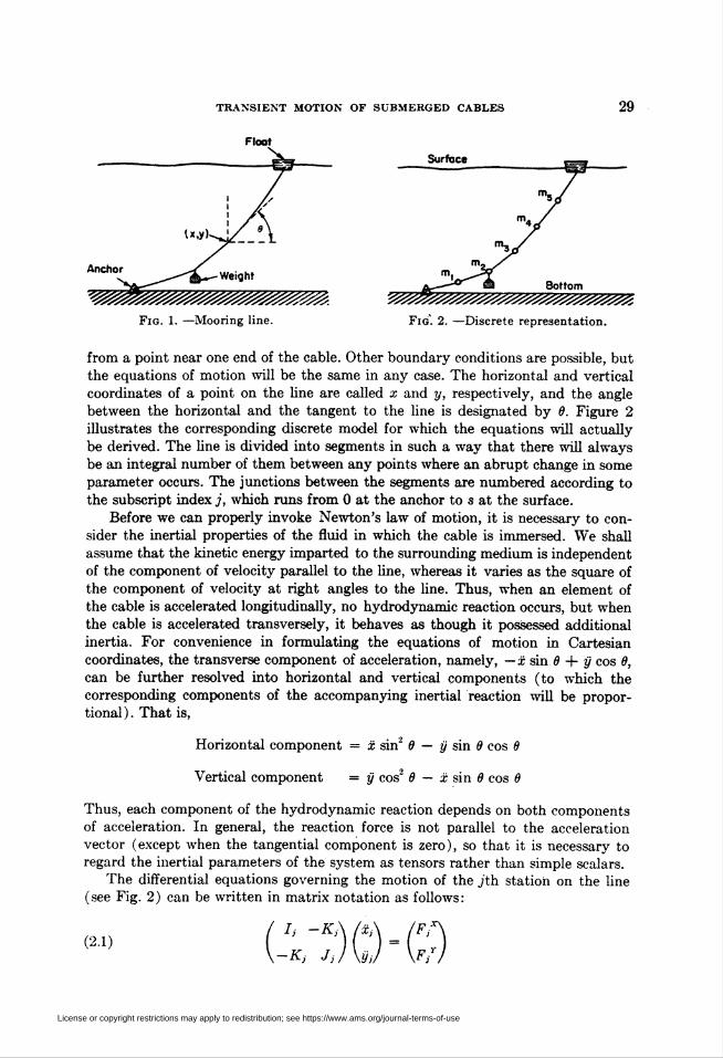
merged cable.Figure 1 shows a typical configuration of the system with the cable attached to

a float at the surface and anchored to the bottom. Also, a heavy load is suspended


TRANSIENT MOTION OF SUBMERGED CABLES 29

Fig. 1. —Mooring line. Fig" 2. —Discrete representation.

from a point near one end of the cable. Other boundary conditions are possible, but

the equations of motion will be the same in any case. The horizontal and vertical

coordinates of a point on the fine are called x and y, respectively, and the angle

between the horizontal and the tangent to the line is designated by 6. Figure 2

illustrates the corresponding discrete model for which the equations will actually

be derived. The Une is divided into segments in such a way that there will always

be an integral number of them between any points where an abrupt change in some

parameter occurs. The junctions between the segments are numbered according to

the subscript index j, which runs from 0 at the anchor to s at the surface.

Before we can properly invoke Newton's law of motion, it is necessary to con-

sider the inertial properties of the fluid in which the cable is immersed. We shall

assume that the kinetic energy imparted to the surrounding medium is independent

of the component of velocity parallel to the line, whereas it varies as the square of

the component of velocity at right angles to the line. Thus, when an element of

the cable is accelerated longitudinally, no hydrodynamic reaction occurs, but when

the cable is accelerated transversely, it behaves as though it possessed additional

inertia. For convenience in formulating the equations of motion in Cartesian

coordinates, the transverse component of acceleration, namely, — x sin d + y cos 0,

can be further resolved into horizontal and vertical components (to which the

corresponding components of the accompanying inertial reaction will be propor-

tional). That is,

Horizontal component = x sin2 9 — y sin 0 cos 6

Vertical component = y cos2 6 — x sin 0 cos 6

Thus, each component of the hydrodynamic reaction depends on both components

of acceleration. In general, the reaction force is not parallel to the acceleration

vector (except when the tangential component is zero), so that it is necessary to

regard the inertial parameters of the system as tensors rather than simple scalars.

The differential equations governing the motion of the jth. station on the line

(see Fig. 2) can be written in matrix notation as follows:


30 THOMAS S. WAI/rON AND HARRY POLACHEK

where

I i - m, + K«y+* sin* öy+i + ey_j sin* 0y_j) + ■»/

// = my + è(ey+j COS* ffy+j + ey_} COS* 0y_j) + Wiy*"

^y ■* K«y+j sin 0y+$ cos 0y+j + ey_j sin 0y_j cos 0y_$)

andf

my = ItMy+^y+l + My-i^y-è]

ei+i = Pkj+ilj+io-j+i

m? - my* + pFyX

m* = my* + pFyr

COS 6j+i = (Xy+1 - Xj)/lj+i

Sin 0y+J = iyj+1 - 2/y)/Zy+1 .

Each lumped mass, my, has been expressed as the average mass of the two seg-

ments of cable which lie on either side of station j. Also, one-half the equivalent

transverse mass, e¡, of the fluid entrained with each of these segments has been

included in the inertia tensor. Furthermore, at those stations from which a weight

is suspended, the effective horizontal and vertical masses, myX and m,r, of the weight

are to be added. For simplicity in allowing for virtual inertia, we have assumed

that any such weights possess a certain degree of symmetry and remain upright

as the line moves about.

The force vector, F¡, on the right side of eq. (2.1) can be expressed as the sum

of internal forces (the tensions acting between adjacent mass elements) and what-

ever external forces are present. Thus, in expanded form the equations of motion

can be written

IjXj - Kjjjj = Ty+i COS 9j+i — Tj-i COS 0y_j + Xj

(2.2)-Ayá-y + Jßi = Tj+i sin 0y+è - Tj-i sin 0y_j + F>

where Ty+j = tension in segment of line between stations j and j + 1

Xj = horizontal component of resultant external force at station j

Yj = vertical component of resultant external force at station j.

There are two sources of external force, namely: 1) gravity, which gives rise to the

weight minus the buoyancy and acts only in the vertical, and 2) fluid resistance,

which gives rise to the damping forces. Thus, we write

Xj = -W>i+\ sin Bj+\ + Dj_i sin 0y_è] + X¡*

Yj - h[Dj+i COS 6i+i + Z>y_| COS 0y_j] + Fy* - Wj - Wj*

where

Wj = m¡g — hpgilj+i.o-j+i + iy_j<ry_§)

Wj* = m¡*g - pgV*

t See Appendix for definitions of the pmameters which appear in the formulas.



and Dj+i — drag on segment of line between stations j and j' + 1

Xj* = horizontal component of damping force on weight at station j

Yj* — vertical component of damping force on weight at station /.

Again, in order to get the best approximation to the continuous case, the net effect

of the drag at station j has been expressed as one-half of each component of the

drag on the segments which lie on either side of this station. The buoyant force of

the displaced fluid has been treated likewise.

We have assumed that the drag, Z)y+j , on a segment of the line acts in a direction

at right angles to the line. This is a good approximation whenever the velocity is

high enough to produce significant forces, since at all but the lowest Reynolds

numbers the tangential component of the hydrodynamic force is very small com-

pared to the normal component. Furthermore, we assume that the drag is pro-

portional to the square of the component of relative velocity normal to the line:

(2.4) Dj+i = -ff+iqj+i | qj+i |

where

fj+i — hpCj-rih+ißi+i

Qi-H = -M(*>+i - c) + i±j - c)] sin $j+i + k[yj+l + yy] cos 6j+i.

The positive normal to the fine has been arbitrarily taken to be directed upward

when 6 equals zero. The use of the minus sign and the introduction of the absolute

value of one of the velocity factors ensures that the drag will always be opposed

to the direction of gy+j and thus act as a dissipative force to remove energy from

the system. Since the velocities of the two endpoints of each segment will, in general,

differ slightly, their mean value (which for a straight line segment is exactly equal

to the velocity of the midpoint) is taken as a representative value in the definition

of qj+\. In addition, the definition allows for the presence of a uniform horizontal

current, c, to incorporate the ability to treat towing fines as well as mooring lines

(or mooring lines subjected to ocean currents).

In addition to the drag on the line itself, there will also be resistance to the

motion of any concentrated loads which may be suspended from the line. These

additional damping forces will vary with the velocity but will not, in general, be

directed exactly opposite to the motion of each weight. However, on account of the

assumed orientation and symmetry of any such weights, the resistance force will

be parallel to the velocity vector whenever the relative motion is either purely

horizontal or purely vertical. Accordingly, the two components of resistance may

be written

Xj* = -fjXUji±j - c)

Yj* = -fjYUjyj

where

ff = kfiC'Sj*hr = yCjrSjr

Uj = [(xy - c)2 + yft



Up to this point an explicit formula has been given for the evaluation of every

term in the equations of motion (2.2) with the exception of the tensions. To de-

termine these we must invoke the inextensibility condition which was assumed

at the outset. This takes the form of a constraint on the motion of the line. It re-

quires that the separation between adjacent stations must not change with time.

Thus, we -write '

(2.6) ixj - Xj-i)2 + iijj - t/y_t)2 m Zy_} = const.

This holds for each segment of the line, and we require that the corresponding

set of tensions, T¡-¡ , take on values such that the resulting solution of the equations

of motion will be consistent with eq. (2.6). Because of the implicit nature of this

condition, we are led to a system of algebraic equations for the determination of

the proper tensions. At the extremities of the line {j = 0 andj =s s) x¡ and y¡ must

be obtained from the boundary conditions, namely:

xo = Xo(<), 2/0 = yoit)

(2.7)x» = x,(i), y, = y.it).

These are given as functions of time, and permit the introduction of any desired

types of driving motions.

Finally, to complete the formulation of the problem a set of initial conditions

must be given for each station on the line. Since the equations of motion are of

the second order, it is necessary to specify both the coordinates and the velocities

at t = 0. That is,

xy(0) = xy°, 2/y(0) = yf if = 1, 2, • • • s - 1)

(2'8 *y(0) = Xy°, t/y(0) - if* if = 1, 2, • • • s - 1)

where the superscript index "0" is used to designate a value at the origin in time.

3. Solution of Equations by Finite Differences.

A. General Description of Computational Procedure. The equations

governing the motion of a cable, as derived in the last section, are summarized

here. The basic equations of motion, (2.2), are repeated for convenience,

ZyXy — A'yjfy = Ty+è COS 0y+è — Ty_| COS 0y_J + Xj

(2.2, cy-i.2....-i),

-KjXj + Jjüj = Tj+i sin 0y+J - Tj-i sin 0y_j + Fy

if = 1, 2, • • • s - 1),

wherea) s is the number of segments into which the cable is divided,

b) Ij, Kj , Jj are given in eq. (2.1) and are functions of the physical properties

of the cable and of position only,

c) Xj, Yj are given by eqs. (2.3), (2.4), and (2.5) and are functions of the

physical properties of the cable and of position and velocity.

In addition, the motion is governed by the condition of êxtensibility of the cable,


transient motion of submerged cables 33

eq. (2.6), namely,

(2.6) (Xy - Xj-.,)2 + (i/y - ¿/y-,)2 = iy-J = COUS«,, (j - 1, 2, • • • S).

The differentiated (with respect to time) forms of this relation,

(3.1) (Xy - Xj-i) (¿y - Xy_i) + (î/y - î/y-j) iyj - yj-i) = 0

if = 1,2, ••*),

(Xy - Xy_i) (Xy - Xy_i) + (*/y - Z/y-i) (¿fy - jfy-i)

+ (xy - xy_02 + {t, - 2/y-i)2 = 0 (j = 1, 2, • • • S),

are also used in the computation.

For numerical solution by finite-difference methods the following finite-difference

equivalents are used,

n+l _ n rt+1 _ n

(3.3) x;+* = Xj M Xi , tln - Vi M Vi if = 1,2, ■■■ s-I),

x;+1-2xy" + xr ,1n_yri-2yjn + y?-1

(3.4) ' ' " (AO2 ' V' (Ai)2

(j = 1,2, ••• s - 1).

It is assumed that the boundary and initial conditions are known. These are given

in eqs. (2.7) and (2.8), respectively. The system of equations summarized above,

consisting of eqs. (2.2), (2.6), (2.7), (2.8), (3.1), (3.2), (3.3), (3.4) with theauxiliary equations (2.1), (2.3), (2.4), (2.5), completely describe the motion of

the cable.

The computational procedure, as developed in detail in the remainder of this

section, consists of an algorithm to determine the values Xy*+\ y"+1, xy*"1"*, yf^

(at time t = tn+l = tn + M and t — tn + JAZ) from known values xy", y/1,

Xj, y1j~>i (at time t = t" and ¿n-i). It is convenient to divide this algorithm in

two phases. The first phase involves the determination of a tentative (but con-

sistent) set of tensions for all segments, and numerical integration of the equations

of motion to predict the coordinates one step ahead; the second phase involves the

evaluation of small discrepancies in the constraint equations from which a set of

first-order corrections to the tensions can be obtained, and integration of the equa-

tions a second time to obtain accurate values of the coordinates.

Phase 1. Using eqs. (2.2) and (3.2), (3s — 2 equations), we compute the (3s — 2)

unknown variables xy", yj" ij = 1, 2, ••• s — 1) and T*-\ (J = 1, 2, • • • s).

We now use eqs. (3.3) and (3.4), (4s — 4 equations), to compute the (4s — 4)

variables at the next time step, x,n+i, y"+i, x?"4, 2/"+* (j = 1, 2 • • • s — 1). These

are considered to be only tentative values (denoted in subsequent text by use ofthe tilde).

Phase 2. To obtain improved values of the tensions 77_j (j = 1, 2, • • • s)

and the quantities x3n, y¡n, x*+l, yî+1, x?"4, y"**1 (a total of (7s — 6) quantities)

we use the system of equations (2.2), (2.6) and (3.3), (3.4), consisting of (7s — 6)

equations. However, since eqs. (2.6) are not linear but quadratic in the unknowns

xy and 2/y, an explicit solution is impractical to obtain. For this reason a computa-

tion algorithm based on the Newton-Raphson method of successive approximations



is developed. A detailed discussion of the computational procedure used in this

problem is given in the sections which follow.

B. Determination of Tentative Values of Tensions. The system of equa-

tions (2.2) may be regarded as a set of (2s — 2) linear equations in the variables

Xy and ti (accelerations) and may be solved directly for these variables. If we

designate

Lj= iU)2Ij/iIjJj-K/)

Mj= iAt)2Jj/HjJj-K/)

Nj = (AZ)2 Kj/iljJj - Kh,

then the equations of motion (2.2) can be reduced to:

xy - [B,TM - PjTj-i + Uj]/iM)2

ti - [SjTj+i - QjTj-i + Vj]/iàt)2(3.5)

where

Pj = Mj cos 0y_} + Nj sin 0y_j

Qj = Nj cos 0y_j + Lj sin 0y_j

Rj = Mj cos 6j+i + Nj sin 0y+$

<Sy = iVy COS 0j+i + Lj Sin 8j+t

Uj = Mj Xj + Nj Yj

Vj = Nj Xj + Lj Yj .

We observe that eq. (3.2) involves positions, velocities, and accelerations. As is

often the case with finite-difference procedures, it proves to be convenient to com-

pute positions and accelerations at the mesh points while velocities are found at

the midpoints in time. For this reason we shall use a modified form obtained by

evaluating eq. (3.2) at t = t" and at Z = ZB_l, and then adding the two results

together, namely,

(Xy" - Xy"_0 (¿y" - xjU) + (t/y" - VU) it* ~ tU)

(3.6) + Í*""1 * *#> i*'""1 - £?-i) + (I/"-1 - y?-í) it?'1 - t?-x)

+ 2(AZ)-2 [(xy" - x,-1) - ix?-i - sH1)]*

+ 2(Azr2 Kv' - y?'1) - iy?-i - y?-?))* - o,

in which we have used the approximations,

(Xy" - X7-02 + (Xy"-* - X^)* « 2(x;~* - *£?>"

« 2[(Xy" - X?-1)/^ - (XU - *#)/*]*,

.its" - tU? + (2/y-1 - yy-i1)2 « 2(2/?-» - tl-i?

« 2[(j/y" - y]-1)/^ - iyU - y?3)/Ut

Note that eqs. (3.6) are linear in the accelerations. Likewise, eqs. (3.5) are linear

in the tensions. Consequently, when these latter expressions are substituted for the


transient motion of submerged cables 35

acceleration components in the constraint equations (3.6), we obtain a set of condi-

tions which are linear in the tensions, namely,

et» /fin jpn As . ¿~,n rfjn

+ E"U TU - FÏÏ Tpi + GUI T7+Í + HU + HU(3"7) + 2[(xy" - xrl) - (*y-i - xU)f

+ 2[(2/y" - yr1)where

iyU - y?-¡)]2 = 0

EU = (*/" - xU)PU + iyjn - yU)QU

FU = (xy" - xU) iPjn + RU) + iy? - vU) iQin + SU)

GU = i*r - *U) R)n + iyr - vU) Sjn

HU = i*r - xU) iUjn - UU) + iyP - vU) (F/ - VU)-

Now assume that the solution is correct up to Z = tn. Then all quantities in (3.7)

can be evaluated at once except for TU > TU an^ TU ■ The tentative values of

the tensions—signified by the tildes—are determined by the following system of

equations:

(3.8)

—Fo.h

E\.i

Go*

1.5 tri.5

771» r,n■E<2.5 ~?2.i G2.S

0.5

Tt»

tit

-*o".

-F,"-,.5 GU* I K-**

EU., -FU.,. ? >-«■>.

where

*;_, = eU tU - fU tU + GU1 tu1 + HU + HU

+ 2[(xy" - x?-1) - ixU - xU)f + 2[(ivy" - yU1) - ivU ~ VÎ-ï)t

In general, we can write (for j = 1, 2, • • • s)

(3.9) EU TU - PU TU + GU TU + * U = 0

with the conditions: El, = GU = 0 for ail n. Also, Po" , Q0n , fio" , So" , and P," ,Q," , R,n, S,n = 0 for all n; and

r/o" = (AZ)V and U." = (AZ)2x,n for ail n,

Von = (AZ)V and V," = (Aí)V for ail n.

The matrix of coefficients of the system of equations is a triple diagonal one, and

it can be easily reduced to a single linear equation by elimination. Thus, we solve

eq. (3.9) for TU .

(3.10) »fr» _ Fj-i ,*„ _ Ej-j *„ ¥*-}Mi? GÜ ' GyL~J GÜ


36 THOMAS S. WALTON AND HARRY POLACHEK.

Now we express each tension as a linear function of tô.i (the tension in the first

segment) as follows:

(3.11) TU = aU tâ.s + ßU

and we arrive at the following recursion formulas for aU and ßU > namely,

«y+l = iFj-i aU - El-i a?-l)/öy-i

ßU - (FU ßU - EU ßU - *U)/Gl-twith the conditions

aô.t = 1, alo., = 0 for ail n,

0?.5 = 0, (Sô.5 = 0 for ail n.

Starting withj = 1, we evaluate aU and ßU recursively up to j = s — 1. We

then find tô.t from the last equation of the system.

(3.13) ?on5 = - jFU ßU - EU ßU - *?-»)iFU<*U-EU<*U)

C. Computation of Tentative Coordinates. In order to solve eqs. (3.5)

numerically, we replace xy" and yf by their simplest central-difference approxima-

tions, eq. (3.4), namely,

*/ = (^+1 - 2xy" + xrV(AZ)2

tin = ivl+1 - 2y? + yrl)/i*t)\

Now we solve for x" +1 and y]+l, considering these as tentative values subject to a

slight modification in order to satisfy a system of constraints. Thus we write

x;+1 = 2xyB - X?-1 - P*tu + R*tu + up

tri = 2yr - yU - Qrtu + srtu + Vf .The quantities Pj", Qy", fiy", Sj", Uj" and Fy" are the same as were used to set

up the coefficient matrix for the tensions, and the values for tU and tU are

obtained from (3.11).

D. Determination of Improved Values of Tensions. Next, we determine

the set of corrections 6TU to be applied to the tensions TU m order that the

values of x"+1 and y"+l should also satisfy the inextensibility condition (2.6). For

this purpose we define the function

(3.16) Otf * hlix?+l - x?_+i1)2 + iy?+l - ytf)2 - £_,]

which measures the discrepancy in the distance between the extrapolated positions

of pairs of adjacent stations. We observe from eqs. (3.15)—with the tildes sup-

pressed—that x"+1 and y"+l are functions of the tensions. Consequently, Q$-} may

also be expressed as a function of the tensions. This enables us to write the

system of constraints to which the tensions are subject as follows:

(3.17) Q£? - A"-!1 {TU , TU . TU\ =0 ij= 1,2, ■■■ s)

since ü"-i vanishes when tne inextensibility condition is obeyed-



Now let

(3.18) T]+i - TU + STU,

and expand fí£íj in a Taylor series about the point {tU » t"-\ » tU) • Thus, we

obtain

n»+i _ rS»+i i dQ,_$ ¡.rpn , dfl,-i _,„

(3.19)

where

dTU dTU

+ -J~* &TU + higher order terms,

= IK*?«" - i"-4"/)2 + W+1 - tël? - lUl

Provided that the tentative values tU are sufficiently close to the correct values

TU > we may neglect the higher order terms in the expansion (3.19), and thereby

obtain a system of s linear equations for the differential corrections 6TU • These

equations have the same form as the previous system (3.8) for determining tU >

namely,

(3.20)

«n+l-ro.i

»+l

»»+•ßl.5

+ 1

0»+0.5

«»+1— ^1.6

»»+1•Ö2.6

Ön+11.5

ff»-t-l— r*2.5

£t»+l■ßt-1.5

U-2.5

ffn+l— f i—1.5

£js— 0.5

Gn+1

ffn+l— i*«-0

s—1.6

+1

5TS.i

57Î.5

¡Tls

5t;_,.5

5T,_o.5

-Oit1

-QÍÍ1

«2.5

_ö"+1— »«-1.6

— Ô"+1««—0.5

the general expression being (for j = 1, 2, • • • s)

(3.21) EU ÖTU - F?-i àTU + GU 6TU + »"-il = 0

where

>r»»+lÄn+1 dßy—J /.n+1 «h+Utji i /.-;n+l „~.»+l\/-i»Ej-i = ^— = Uy - a;y-i )¿y-i + (2/y - J/y-i )Ç,-i

añri1ffif = -^ = (*n+1 - «WfXJV + äh) + (yî+1 - §£¡)(Q" + SU)Öl y_j

,b+i _ dUj-iÖ»+i _¿-i = dTU = (X, — X,_l )Rj + (t/, — i/,-1 )ày

with the conditions: Êôt1 = oílíj1 = 0 for all n, and the quantities P?, Q?, fi," and

S" being the same as in (3.7).

The system (3.20) can be solved in a manner completely analogous to the solu-

tion of the system (3.8). Thus, we write

(3.22) &TU = *"+i 5^0.5 + AyV}



and obtain the following recursion formulas:

„» _ / fl»+l » £¡»+1 » \ //^n+l

Ay+i ■ I^hVi — »y-»*y-l — «y-j )/"*-*

with the conditions

#co.5 = 1, (cT^.j = 0 for all n,

X",5 = 0, Xô.5 = 0 for all n.

Finally, the last equation of the system enables us to solve for dTô.s. The result is

(3.24) an* = - -> *"» ~ -> 'I? ~ -»}•iFUtU - ft-i*U)

We can now obtain the corrected values of the tension in each segment. Thus,

(3 25) TU - TU + >TU _= tj-l + K,_j5To.6 + X"_} .

E. Computation of Improved Coordinates. The corrected values of the

coordinates are found using eqs. (3.15)—but this time with the tildes suppressed—

namely :

xn+l = 2xy" - xU - PfTU + RPTU + UP(3.26) Vl+l = 22/y" - yrl - QPTU + SjnT7+} + Fy".

For solution on an automatic computer, it is more convenient to express eqs. (3.26)

in terms of corrections to be added to the tentative values of the coordinates. That is,

far"+l = -PjnôTU + RfàTU5y'¡+l = -Qjn5TU + SjnôTU ■

Then the corrected coordinates are given by:

xM+1 = x"+1 + 5xr+1

y, = y i + oyj .

F. Special Form of Equations for Computing First Time Step. We assume

that the initial velocity components are zero at each station, and we obtain the

initial coordinates from the equations for static equilibrium of the fine. Since xy°

and yf = 0, eq. (3.2) reduces to

(3.29) (Xy° - Xy_x)(Xy° - Xy_x) + (<// " yU)iti ~ tU) = 0

and, on substituting the expressions (3.5), we find that the tensions are subject

to the constraint

.(3.30) £y-j fy-, - Fy_, fy_j + (fj-i t*m + tfy-, = 0.

Comparing this with eq. (3.9), we see that

(3.31) *y-j = #y-è U = 1, 2, ••••)•

(3.27)



The system of equations (3.8) is then solved in the usual way to get the proper

initial tensions !Ty_}.

To obtain tentative values for the coordinates at Z = t, we make use of their

Taylor series expansions about the point t = Z°, namely:

Xy' = Xy° + (AZ)Xy° + è(AZ)V + • • •

*/-■»/+(*)*/ + *(*)•«?/.+ •••

Taking xy° and t/y° = 0, and substituting eqs. (3.5) for xy° and yf, we find

*/ = Xy° 4- } [- PfTU + Rit"^ + Uf\(3 33")

y/ = Vi + \ [- Q/fy-i + Sj*t*j+i + V¡\

The corrections to the tensions are then determined by the system of equations

(3.20) in the usual manner. Finally, the corrections to the coordinates "are com-

puted as follows:

fa/ = i I- P? «îl-i + fi/ iT*i+l](3 34)

¡¡y/ = i [- Q,° 5TU + s; oTU\

and the corrected coordinates are given by:

Xy* = Xy' 4- ÔXy1

(3.35) •Vi = Vi + 52//.

4. Analysis of Numerical Stability. In order to obtain a valid solution of the

system of partial differential equations governing the generalized motion of a

cable, it is necessary to insure the stability (in the sense discussed in [2], [3], [4])

of the equivalent finite-difference system (2.2), (2.6), (3.3), (3.4). In this section

we will derive the criteria for stability of this system of equations. We will also

show that whereas the system of finite-difference equations (2.2), (2.6), (3.3), (3.4)

is stable for sufficiently small time intervals AZ, the system (2.2), (3.2), (3.3), (3.4)

is always unstable. This characteristic of the latter system has led to the abandon-

ment of this simpler set of equations in favor of the more difficult nonlinear svstem

(2.2), (2.6), (3.3), (3.4).In order to determine the stability of a system of finite-difference equations, we

study the growth of a small disturbance or perturbation. The conditions for sta-

bility are said to be satisfied if the amplitude of a small disturbance, introduced

at any time, t, in any of the dependent variables, does not increase exponentially

with successive time steps. This condition may be stated as follows:

If 5F(s, t) and á/7(s, t -\- AZ) are values of a variation (or perturbation) in any

of the dependent variables x, y, T in the system, then it is said to be stable provided

| SFis, t + At)/ôFis, <) | á 1. We introduce perturbations 5x, Sy, ST in the

dependent variables x, y, T, respectively. To simplify the stability investigation,

we shall omit the terms pertaining to the suspended weights as well as all terms

involving virtual inertia. From eqs. (2.2), (2.6), (3.3), and (3.4) wè obtain the

following variational system of equations:

mjOXj = Ty+j 5 COS dj+i — Ty_i 5 COS 0y_j + COS 0y+j ôTy+j

— cos 0y_j &Tj-x — $[Dj+i S sin 0y+J 4- Dj-i 8 sin 0y_¡

+ sin fly+j 6Dj+i 4- sin 0y_S 5/>y_J,



(4.1) mjStj = Ty+j S sin 0y+| - TVi 5 sin 0y_, + sin 0y+j STj+i

— sin dj-i STj-i + %[Dj+i S cos 0y+à + Dj^ S cos 0y_}

-H COS 0y+i 6Dj+i + COS 0y_} iDy-j],

COS 0y+j 5 COS 0y+» + sin 0y+j 5 sin 0y+} = 0,

where

5öy+} = -2/y+j | 3y+ä | &qj+i,

5«y+ä = -M(*y+J - c) + (x,- - c)] 5 sin 0y+1 + Htm + t¡) « cos 0y+j

- | sin 0y+j(5Xy+1 4- &¿y) + \ COS öy+j (5yy+1 4- otj);

and where

5 COS 0y+j = (5xJ+i - ¿Xy)/Zy+i ,

Sx,"-1 = (fay" - 5xr')/AZ,

5 sin 0y+i = iôyj+1 - ôyj)/lj+i ;

SyU = i&yP - SyUl/U;

Sxj" = (Öx"+I - 25xy" 4- 5xr')/(AZ)J, by? = (ty',n+l

252/y" + ty?-1)/^)'

We will assume in this analysis that within a small region in the is, Z) plane the

coefficients (7'yn, cos 0y", Z>y", etc.) of the variational functions vary only slightly

and hence may be treated as constants. We will denote these simply by T, cos 0,

D, etc., omitting the indices. A solution of the system of equations (4.1) can then

be obtained in the form* noXj = a e

ißj+an&t

Sy"

STj"

beißj+an&t

c eißj+an&t

where a, b, c are real constants and a complex. Substituting in eq. (4.1), we obtain

a system of linear homogeneous equations for the quantities a, b and c which has a

non-trival solution, provided the determinant of the coefficients is identically zero.

After some algebraic simplifications, the determinant of the coefficients may be

written in the form

(4.2)

where

F - A sin 0 D' 4- B sin 0 cos 0

-D' + A cos 9 F - B cos 0 sin 0

cos 0 sin 0 0

= 0

A = / | q | [2iy sin ß - il sin 0/AZ)(l 4- cos /S)(l - X-1)]

B = f\q\ [2¿(x - c) sin ß - il cos 0/AZ)(l -f- cos /3)(1 - X"1)]

D' = iD sin ß

F = mZ£/(AZ)2 + AT sm2iß/2)

and whereX = ea4', 5 - (X - 2 + X"1).

Multiplying the elements of the determinant and simplifying, we obtain

(4.3) A sin 0 + B cos 0 - F = 0



But,

A sin 0-r-ß cos 0 = /1 q | [(2t sin ß) p - (i/AZ)(l 4- cosi8)(l - X~l)l

where

p = (x — c) cos 0 4- y sin 0

i.e., the tangential component of the velocity of the cable (relative to the medium).

Substituting in equation (4.3), we finally obtain the characteristic equation of the

variational system (4.1), namely,

ml\2 + {/1 q | AZ [Z(l + cos ß) - pAZ(2í sin ß)\(4.4)

+ ATiùdY sin iß/2) - 2ml\\ + [ml - /1 q | ZAZ( 1 4- cos ß)\ = 0.

Now, comparing the first and second terms of the coefficient of X, we find that the

second term is negligibly small provided 2pAZ « I, i.e., the tangential distance

traversed by the cable in one time step is very small compared with the length of

the cable segment. Since this is usually the case and, at any rate, can always be

satisfied by taking the time step sufficiently small, we will omit this term from our

subsequent analysis.

For the case of negligible drag, i.e.,/ = 0, approximately, we obtain from eq. (4.4)

(4.5) X2 4- [AT sin2 iß/2) i&t)2/ml - 2]X -f- 1 = 0.

In order for the solution to be stable, the conditions | Xt | ¿ 1 and [ Xî | jg 1 must

both be satisfied. But if M is a solution of (4.5), then X2 = 1/Xi is also a solution.

It follows that the conditions for stability can be satisfied only if | X> | = | 1/XL i =

| Xx | = 1. Now, let \i = cos y + i sin y, \¡ = cos y — i sin y — 1/Xi ; then,

I Xi 4- Xa | = I 2 eos y | ¿ 2. Furthermore, from eq. (4.5) we have

... „ 4T'sin2(/?/2)(AZ)2Al "T A2 = ¿ — -

mi

We thus obtain the inequality

| 2 - AT sin2(/J/2)(AZ)7w/1 ^ 2,or

(4.6) 7,sin2(^/2)(AZ)2/mZ ^ 1.

This requirement is tantamount to the condition

AZ < a M = lT velocity of transverse wave '

In the more general case, allowing for finite drag, eq. (4.4) may be reduced to

(after neglecting the second term of the coefficient of X)

ml\2 4- [2/1 g | ¿AZ cos2 (0/2) 4- 4r(AZ)2 sin2(0/2) - 2mZ]X(4.7)

4- [ml - 2/1 q ! ÏAZ cos' iß/2)] = 0.

This equation is more difficult to analyze. However, it is possible to show that both

| Xi | ^ 1 and | Xj | á 1, provided that we have chosen



(4.8)

AZ £ i/^, and

AZ¿ m

f\q\

These conditions (4.8) are both necessary and sufficient to insure stability, t

We will now show that the replacement of eq. (2.6) by its differentiated form

(3.2) results in an unstable system; and that, furthermore, the use of any time

interval AZ, no matter how small, does not change the unstable character of the

equations. It will suffice to show that this condition exists in the case when the

drag is negligible, i.e.,/ = 0. The variational equation corresponding to eq. (3.2) is,

ix, — Xy_j)(«Xy - OXy_0 + (Xj - Xy_i)(«Xy — ÔXj-i)

+ 2(¿y - Xy_,)(ÔXy - ÔXy_i) 4" (j/y - yj-l)(9gi - ífo-l)

4- (ti - 9i-i)(*yi - tyy-i) 4- 2(£y - tj-i)iSyj - to/y-O = 0.

Substituting appropriate values for Sx and Sy and neglecting terms containing /,

we find that the determinant equation (4.2) is replaced by

(4.9)

F 0 cos 0

0 F sin 0

(Xy - Xy_,)£ 4- (Xy - Xy_,)(AZ)2 G/y ~ 2/y-l)£ 4" (ft - ft-l) (AZ)2 „4- 2(xy - xy_,)(l - X_,)AZ 4- 2(yy - t/y_,)(l - X_1)AZ

= 0.

Multiplying the elements of the determinant, we obtain

F COS 0[(Xy - *y_,)| 4- (Xy - Xy_,)(AZ)2 + 2(iy - Xy_0(l ~ X_1)AZ]

(4.10)4- F sin 0[(//y - !/,_,)£ + iti - yy-i)(AZ)2 -|- 2(yy - tj^)i\ - X l)AZ] = 0.

Equating

cos 0 = (xy - xy_i)/Z, sin 0 = (»y — j/y-i)/Z ;

and using the relations (3.1) and (3.2), we obtain in place of eq. (4.10)

(4.11) F\l2l - [(xy - xy_02 4- itj - ^y-x)2](AZ)2} = 0.

In this case the characteristic equation is a quartic, and it is necessary that the

absolute values of all four roots be á 1 to insure the numerical stability of the

system. Thus, we must examine the roots of both factors of eq. (4.11), namely,

(4.12) F » 0

and

(4.13) l2t - li±i - *y-i)' + iti - 2/y-i)2](AZ)2 = 0.

It can be shown that eq. (4.12) is equivalent to the criterion (4.6) which can

f When the terms for the virtual inertia and suspended weights are included in the stabil-

ity analysis, it is found that the quantity m in eq. (4.8) should be replaced by the expression

m + m* + e + /»(Vîn«» + Vy cos1«).



be satisfied provided

AZ áml

However, the pair of roots associated with the second factor of (4.11) cannot satisfy

the stability condition for any finite AZ because eq. (4.13) requires that

t = [(Xy - Xy_x)2 4- itj - yj-rfyUf/l2,

an inherently positive quantity. This conclusion follows as a result of the definition

t = X — 2 4- X-1. If X3 is a root of equation (4.13), then X4 = 1/X3 is also a root of

this equation. As before it follows that for stability | X3 | ^ 1 and | X4 ] = | 1/X3 | á 1.

Hence, | X31 = | X4 | = 1. Let X3 = cos y + i sin y, X4 = cos y — i sin y — 1/Xj ;

then t = 2(cos7 — 1), or — 4 á f û 0. Thus, to satisfy the stability requirement

£ must lie between 0 and —4, and consequently can never be positive.

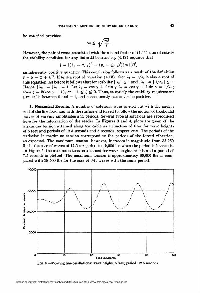
5. Numerical Results. A number of solutions were carried out with the anchor

end of the line fixed and with the surface end forced to follow the motion of trochoidal

waves of varying amplitudes and periods. Several typical solutions are reproduced

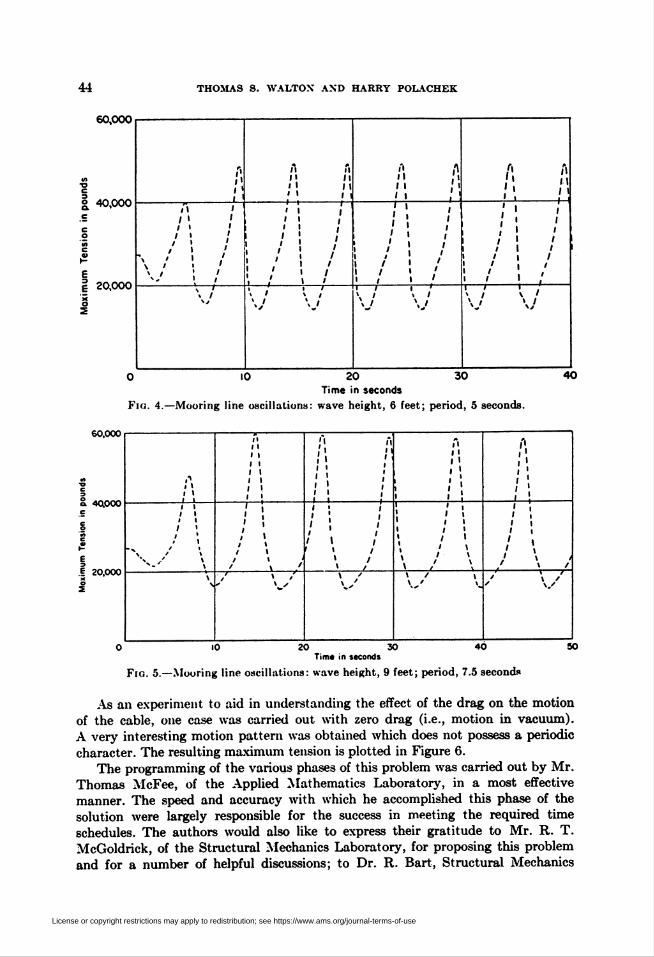
here for the information of the reader. In Figures 3 and 4, plots are given of the

maximum tension attained along the cable as a function of time for wave heights

of 6 feet and periods of 12.5 seconds and 5 seconds, respectively. The periods of the

variation in maximum tension correspond to the periods of the forced vibration,

as expected. The maximum tension, however, increases in magnitude from 33,250

lbs in the case of waves of 12.5 sec period to 49,500 lbs when the period is 5 seconds.

In Figure 5, the maximum tension attained for wave heights of 9 ft and a period of

7.5 seconds is plotted. The maximum tension is approximately 60,000 lbs as com-

pared with 38,500 lbs for the case of 6-ft waves with the same period.

40,000 r

30,000

g 20,000

10,000

0 10 20 30 40Tim« m seconds

Fig. 3.—Mooring line oscillations: wave height, 6 feet; period, 12.5 seconds.

50



60,000 r

-oc

OO.c

40,000

20,000

í'nliIIi i

\ /

MilI II I

-r-r

i

V

AM/ i

» ./

0 10 20 30Time in seconds

Flo. 4.—Mooring line oscillations: wave height, 6 feet; period, 5 seconds.

40

60,000

a. 40,000

§ 20,000

|lI ■I II >

0 10 20 30 40Tim« in seconds

Fio. 5.—Mooring line oscillations: wave height, 9 feet; period, 7.5 second»

50

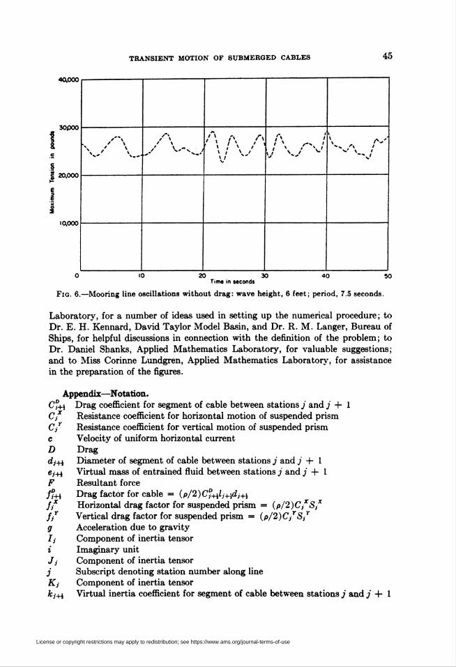
As an experiment to aid in understanding the effect of the drag on the motion

of the cable, one case was carried out with zero drag (i.e., motion in vacuum).

A very interesting motion pattern was obtained which does not possess a periodic

character. The resulting maximum tension is plotted in Figure 6.

The programming of the various phases of this problem was carried out by Mr.

Thomas McFee, of the Applied Mathematics Laboratory, in a most effective

manner. The speed and accuracy with which he accomplished this phase of the

solution were largely responsible for the success in meeting the required time

schedules. The authors would also like to express their gratitude to Mr. R. T.

McGoldrick, of the Structural Mechanics Laboratory, for proposing this problem

and for a number of helpful discussions; to Dr. R. Bart, Structural Mechanics



40,000

30O00

S£ 20,000

10,000

\,'\ I \ ' , i v / \ I

^-'

0 10 20 30 40 50Tim« in seconds

Fig. 6.—Mooring line oscillations without drag: wave height, 6 feet; period, 7.5 seconds.

Laboratory, for a number of ideas used in setting up the numerical procedure; to

Dr. E. H. Kennard, David Taylor Model Basin, and Dr. R. M. Langer, Bureau of

Ships, for helpful discussions in connection with the definition of the problem; to

Dr. Daniel Shanks, Applied Mathematics Laboratory, for valuable suggestions;

and to Miss Corinne Lundgren, Applied Mathematics Laboratory, for assistance

in the preparation of the figures.

Appendix—Notation.CU Drag coefficient for segment of cable between stations / and j 4- 1

Resistance coefficient for horizontal motion of suspended prism

Resistance coefficient for vertical motion of suspended prism

Velocity of uniform horizontal current

Drag

Diameter of segment of cable between stations j and j + I

Virtual mass of entrained fluid between stations j and ¿4-1

Resultant force

Drag factor for cable = ip/2)CUh+î+iHorizontal drag factor for suspended prism = ip/2)CjXSjX

Vertical drag factor for suspended prism = (p/2)CyrSyy

Acceleration due to gravity

Component of inertia tensor

Imaginary unit


Subscript denoting station number along line


Virtual inertia coefficient for segment of cable between stations j and ¿4-1

Cx

Cjr

c

D

dj+hey+i

F

fmfffir

9hiJi

3Kj*y+i



Zy+j Length of line between stations j and ¿4-1

m¡ Mean mass of segments of cable adjoining station j

m/* Mass of prism suspended from station ¿

m, Effective horizontal mass of suspended prism

my Effective vertical mass of suspended prism

n Superscript denoting time-step number

o Superscript denoting initial state (origin in time), or subscript denoting

anchor end of line

p Tangential component of velocity of cable (relative to medium)

q Normal component of velocity of cable (relative to medium)

SjX Projected area of suspended prism along x-axis

SjY Projected area of suspended prism along y-axis

s- Subscript denoting surface end of line

T Tension

Z Time

AZ Time-step interval

u Magnitude of velocity of cable (relative to medium)

Vj* Volume of prism suspended from station j

VjX Equivalent volume of horizontal virtual mass of suspended prism

VjY Equivalent volume of vertical virtual mass of suspended prism

Wj Mean net weight of segments of cable adjoining station j

Wj* Net weight of prism suspended from station j

X Horizontal component of resultant external force

Xj* Horizontal component of damping force on suspended prism

x Horizontal coordinate of cable

Y Vertical component of resultant external force

Fy* Vertical component of damping force on suspended prism

y Vertical coordinate of cable

a Damping coefficient of the perturbation functions

ß Angular wave number of the perturbation functions

5 The variation of

0 Angle between horizontal and tangent to cable

X Eigenvalue (root of characteristic equation)

Pj+l Linear density of segment of cable between stations j and ¿4-1

p Density of fluid medium<7y+< Cross-section area of segment of cable between stations j and ¿4-1

Dot signifies differentiation with respect to time

~ Tilde signifies tentative value of a variable

Applied Mathematics Laboratory

David Taylor Model Basin

Washington 7, District of Columbia.

1. T. S. Walton & H. Polachek, "Calculation of nonlinear transient motion of cables,"David Taylor Model Basin Report 1279, 1959.

2. G. G. O'Brien, M. A. Htmak & S. Kaplan, "A study of the numerical solution ofpartial differential equations," Jn. Math, and Phys., v. 29, 1951, p. 223-251.

3. P. D. Lax & R. D. Richtmeyer, "Stabilitv of difference equations," Com. Pure Appl.

Math., v. 9, 1956, p. 267-293.4. G. Ludford, H. Polachek & R. J. Seeger, "On unsteady flow of compressible viscous

fluids," Jn. Appl. Phys., v. 24, 1953, p. 490-495.


Documents

Calculation of Transient Motion of Submerged Cables