Embed Size (px)
Citation preview
FinalCareerProject
CalculationofradioelectricalcoverageinMedium‐WaveFrequencies
MarcosCregoGarcía
TechnicalIndustrialEngineering
Director:Prof.Dr.ThomasLauterbach
Vic,February2009
Calculation of radio electrical coverage in Medium-Wave Frequencies Marcos Crego García
2
Index of contents:
Resume of the Final Career Project .................................................................................. 5
1 Introduction................................................................................................................. 5
2 Objectives ................................................................................................................... 7
3 Project exposure.......................................................................................................... 9
3.1 Groundwave propagation ................................................................................... 9
3.2 Homogeneous paths ......................................................................................... 10
3.3 Non-Homogeneous paths ................................................................................. 13
3.4 Project description............................................................................................ 14
3.5 Software development...................................................................................... 26
3.5.1 GRWAVE Matlab interface................................................................ 28
3.5.2 Millington Method.............................................................................. 33
3.5.3 Elevation and conductivity database................................................... 39
3.5.4 Code errors returned ........................................................................... 50
3.5.5 Mapping Toolbox ............................................................................... 51
3.6 Practical examples............................................................................................ 60
4 Conclusions............................................................................................................... 65
5 Future guidelines ...................................................................................................... 66
6 Bibliography and references ..................................................................................... 67
Appendix: List of abbreviations .................................................................................... 70
Calculation of radio electrical coverage in Medium-Wave Frequencies Marcos Crego García
3
Index of figures
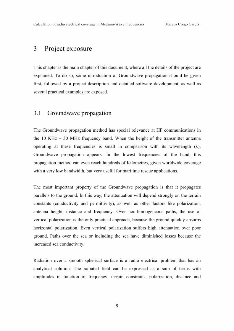
Figure 3.1.1: Examples of the maps obtained................................................................... 8
Figure 3.1.2: Examples of profiles and results printed on screen..................................... 8
Figure 3.2.1: Example of ITU-R P. 368-9 Recommendation......................................... 11
Figure 3.2.2: ITU-R P. 368-9 Rec. Remarkable parameters........................................... 11
Figure 3.3.1: Example of Method of Millington with a path of two conductivities....... 13
Figure 3.4.1: Start Menu Window .................................................................................. 15
Figure 3.4.2: Field Calculation at single points Windows.............................................. 16
Figure 3.4.3: Parameters to configure the simulation..................................................... 16
Figure 3.4.4: Field Calculation – Results offered........................................................... 18
Figure 3.4.5: Coverage calculation window ................................................................... 20
Figure 3.4.6: Configuration parameters.......................................................................... 20
Figure 3.4.7: Example of configuration and waitbar ...................................................... 21
Figure 3.4.8: Coverage results in the area of Nurnberg.................................................. 22
Figure 3.4.9: Elevation map in the area of Nurnberg ..................................................... 23
Figure 3.4.10: Field profile between a Transmitter (TX) and a Receiver (RX) ............. 23
Figure 3.4.11: Elevation profile over the sea between a Transmitter and a Receiver .... 24
Figure 3.4.12: Control code of a waitbar ........................................................................ 25
Figure 3.5.1: Flow chart of the application..................................................................... 28
Figure 3.5.2: Example of GRWAVE input data file, data.inp........................................ 29
Figure 3.5.3: Example of GRWAVE output data file, data.out...................................... 30
Figure 3.5.4: Extract of instructions from grwave.m...................................................... 31
Calculation of radio electrical coverage in Medium-Wave Frequencies Marcos Crego García
4
Figure 3.5.5: GRWAVE result vs. ITU-R graphics result.............................................. 33
Figure 3.5.6: Acquiring the stretches of the path of the same conductivity ................... 34
Figure 3.5.7: Calculation of the effective height ............................................................ 35
Figure 3.5.8: MillingtonH.m source code....................................................................... 36
Figure 3.5.9: Millington example for testing Matlab function ....................................... 37
Figure 3.5.10: GLOBE elevation data for Nurnberg area............................................... 41
Figure 3.5.11: Cleaning the image with an image editor................................................ 42
Figure 3.5.12: Setting latitude and longitude limits. ...................................................... 43
Figure 3.5.13: Converting image to conductivity database (I). ...................................... 44
Figure 3.5.14: Converting image to conductivity database (II)...................................... 45
Figure 3.5.15: Converting image to conductivity database (II)...................................... 45
Figure 3.5.16: Converting image to conductivity database. Sig_ep matrix (III) ............ 46
Figure 3.5.17: High resolution Germany conductivity database. ................................... 48
Figure 3.5.18: High resolution South Korea conductivity database. .............................. 49
Figure 3.5.19: Graphical example of the map variables ................................................. 52
Figure 3.5.20: Example of mapprofile............................................................................ 55
Figure 3.5.21: Example of resizem................................................................................. 56
Figure 3.5.22: Example of maptrims .............................................................................. 57
Figure 3.5.23: loadmap.m partial code ........................................................................... 59
Figure 3.6.1: Example of coverage at 0.909 MHz, Vertical polarization....................... 61
Figure 3.6.2: Example of coverage at 24 MHz, Vertical polarization............................ 62
Figure 3.6.3: Example of coverage at 0.909 MHz, Vertical polarization....................... 63
Figure 3.6.4: Example of coverage at 0.909 MHz, Horizontal polarization................... 64
Calculation of radio electrical coverage in Medium-Wave Frequencies Marcos Crego García
5
Resume of the Final Career Project
Technical Industrial Engineering
Title: Calculation of radio electrical coverage in Medium-Wave Frequencies
Keyword: Groundwave, propagation, coverage, conductivity, field strength, ISI, ITU-R
Author: Marcos Crego García
Director: Prof. Dr. Thomas Lauterbach (Georg-Simon-Ohm-Hochschule. Nurnberg)
Codirector: Moisés Serra
Date: February 2009
Resume
The aim of this project is to accomplish an application software based on Matlab to
calculate the radioelectrical coverage by surface wave of broadcast radiostations in the
band of Medium Wave (MW) all around the world. Also, given the location of a
transmitting and a receiving station, the software should be able to calculate the electric
field that the receiver should receive at that specific site. In case of several transmitters,
the program should search for the existence of Inter-Symbol Interference, and calculate
the field strength accordingly.
The application should ask for the configuration parameters of the transmitter
radiostation within a Graphical User Interface (GUI), and bring back the resulting
coverage above a map of the area under study. For the development of this project, it
has been used several conductivity databases of different countries, and a high-
resolution elevation database (GLOBE). Also, to calculate the field strength due to
groundwave propagation, it has been used ITU GRWAVE program, which must be
integrated into a Matlab interface to be used by the application developed.
Calculation of radio electrical coverage in Medium-Wave Frequencies Marcos Crego García
6
1 Introduction
This project deals with radioelectrical propagation in the frequency band of Medium-
Wave. In this band of frequencies, between 10 KHz and 30 MHz, the main propagation
method is Surface Wave or Ground-Wave Propagation. There are two different ways to
calculate the electric field due to Groundwave propagation:
The set of graphics provided by the ITU-R P.368-9 Recommendation, each one
for different frequencies and terrain conductivity and permittivity.
With ITU-R GRWAVE, a MSDOS based software used by ITU to obtain the
graphics showed at Rec. ITU-R P.368-9, which allows calculating the field at
one point over a path with one conductivity, given a transmitter and a receiver.
Although ITU-R Graphics and GRWAVE are recognized methods by ITU-R, they have
limitations, like:
These methods do not have in account topographical data, very important in this
type of propagation due to its nature (detailed description of groundwave
propagation can be found at chapter 3.1).
Millington method for Non-Homogeneous paths calculations become tedious
and complicated when calculating the field over paths with several different
conductivities.
Calculation of radio electrical coverage in Medium-Wave Frequencies Marcos Crego García
7
2 Objectives
The aim of this project is the development of a software tool based on ITU-R
Recommendation and ITU-R GRWAVE that will eliminate these limitations, by:
Calculating the electric field keeping the ITU-R P.368-9 Recommendations with
ITU-R GRWAVE.
Introducing topographical data of the terrain under study.
Introducing high-resolution conductivity maps.
Performing automatic calculations of radio electrical coverage at one region.
Making calculations at one single point, being able to plot the field profile
between the transmitter and the receiver.
Adapting the system to be able to calculate the effect of the Inter-Symbol
Interference (ISI) and the electric field resulting at one receiver in a scenario of
several transmitters.
And packaging all this calculations into an easy-to-use Graphical User Interface.
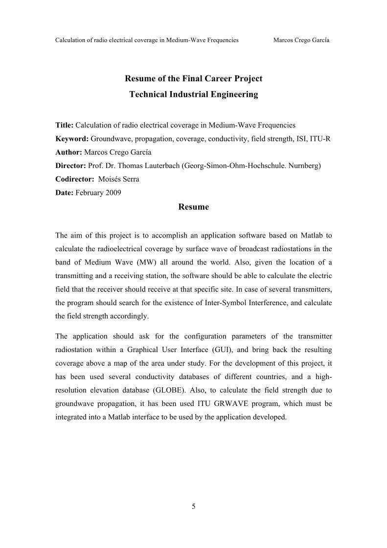
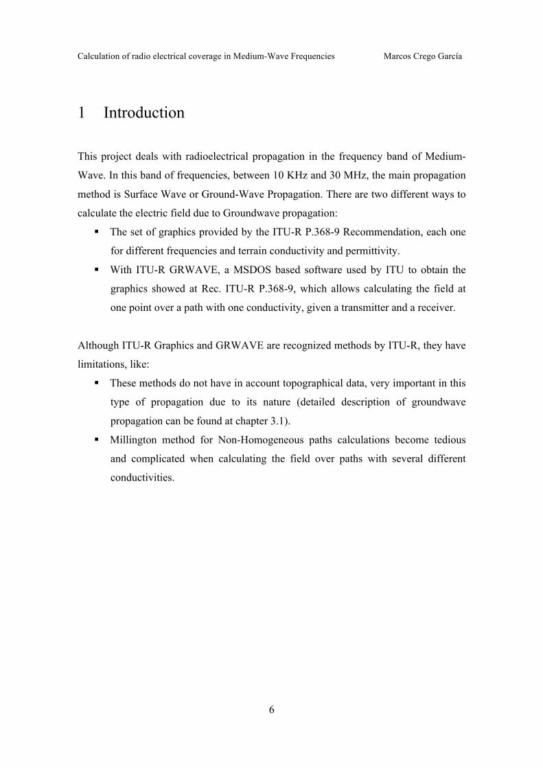
In the figures below, some examples of the results desired are shown:
Calculation of radio electrical coverage in Medium-Wave Frequencies Marcos Crego García
8
(a) Example of Coverage Map (b) Example of field calculating results over an scenario
with several receivers and transmitters
Figure 3.1.1: Examples of the maps obtained.
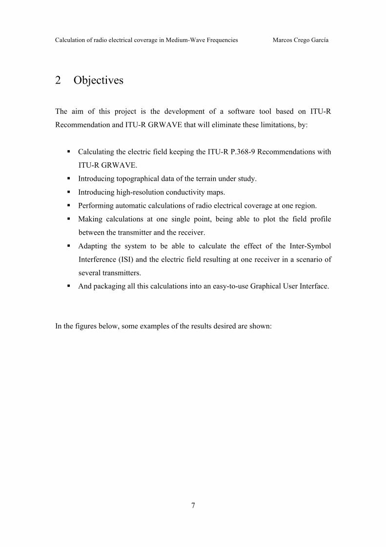
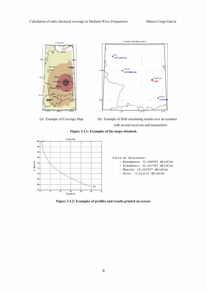
Figure 3.1.2: Examples of profiles and results printed on screen.
Calculation of radio electrical coverage in Medium-Wave Frequencies Marcos Crego García
9
3 Project exposure
This chapter is the main chapter of this document, where all the details of the project are
explained. To do so, some introduction of Groundwave propagation should be given
first, followed by a project description and detailed software development, as well as
several practical examples are exposed.
3.1 Groundwave propagation
The Groundwave propagation method has special relevance at HF communications in
the 10 KHz – 30 MHz frequency band. When the height of the transmitter antenna
operating at these frequencies is small in comparison with its wavelength (λ),
Groundwave propagation appears. In the lowest frequencies of the band, this
propagation method can even reach hundreds of Kilometres, given worldwide coverage
with a very low bandwidth, but very useful for maritime rescue applications.
The most important property of the Groundwave propagation is that it propagates
parallels to the ground. In this way, the attenuation will depend strongly on the terrain
constants (conductivity and permittivity), as well as other factors like polarization,
antenna height, distance and frequency. Over non-homogeneous paths, the use of
vertical polarization is the only practical approach, because the ground quickly absorbs
horizontal polarization. Even vertical polarization suffers high attenuation over poor
ground. Paths over the sea or including the sea have diminished losses because the
increased sea conductivity.
Radiation over a smooth spherical surface is a radio electrical problem that has an
analytical solution. The radiated field can be expressed as a sum of terms with
amplitudes in function of frequency, terrain constrains, polarization, distance and
Calculation of radio electrical coverage in Medium-Wave Frequencies Marcos Crego García
10
antenna height. This is the analytical solution provided by ITU-R GRWAVE
[GRWAVE].
The estimation of the Groundwave field strength given at one point depends on the
nature of the path between transmitter and receiver. In this way, two different methods
are defined by ITU-R Recommendation: Method for homogeneous paths and
Millington’s Method for Non-Homogeneous paths [ITU-R P.368-9].
3.2 Homogeneous paths
The ITU-R Rec. 368-9 defines a homogeneous path as the path between the transmitter
and the receiver when there is only one terrain conductivity between them. In this case,
both ITU-R Graphics or ITU-R GRWAVE can be used directly to calculate the field
strength at the receiver.
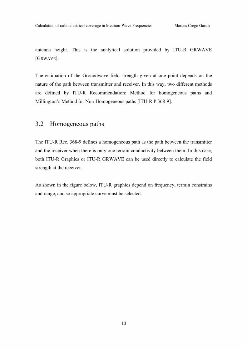
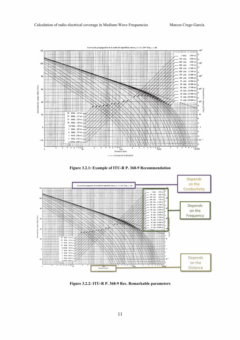
As shown in the figure below, ITU-R graphics depend on frequency, terrain constrains
and range, and so appropriate curve must be selected.
Calculation of radio electrical coverage in Medium-Wave Frequencies Marcos Crego García
11
Figure 3.2.1: Example of ITU-R P. 368-9 Recommendation
Figure 3.2.2: ITU-R P. 368-9 Rec. Remarkable parameters
Calculation of radio electrical coverage in Medium-Wave Frequencies Marcos Crego García
12
As the figure shows, they are only valid over the frequency range from 10 KHz to 30
MHz for vertical polarization and antennas over the ground [ITU-R P.368-9]. Over those
frequencies, GRWAVE still gives an approximation of the field strength, but it is not
accurate and reliable, so it is not recommended using it out of this range.
From the graphics it can be seen that field strength diminish with frequency, so
groundwave propagation is not a relevant propagation mechanism with big distances in
the HF band.
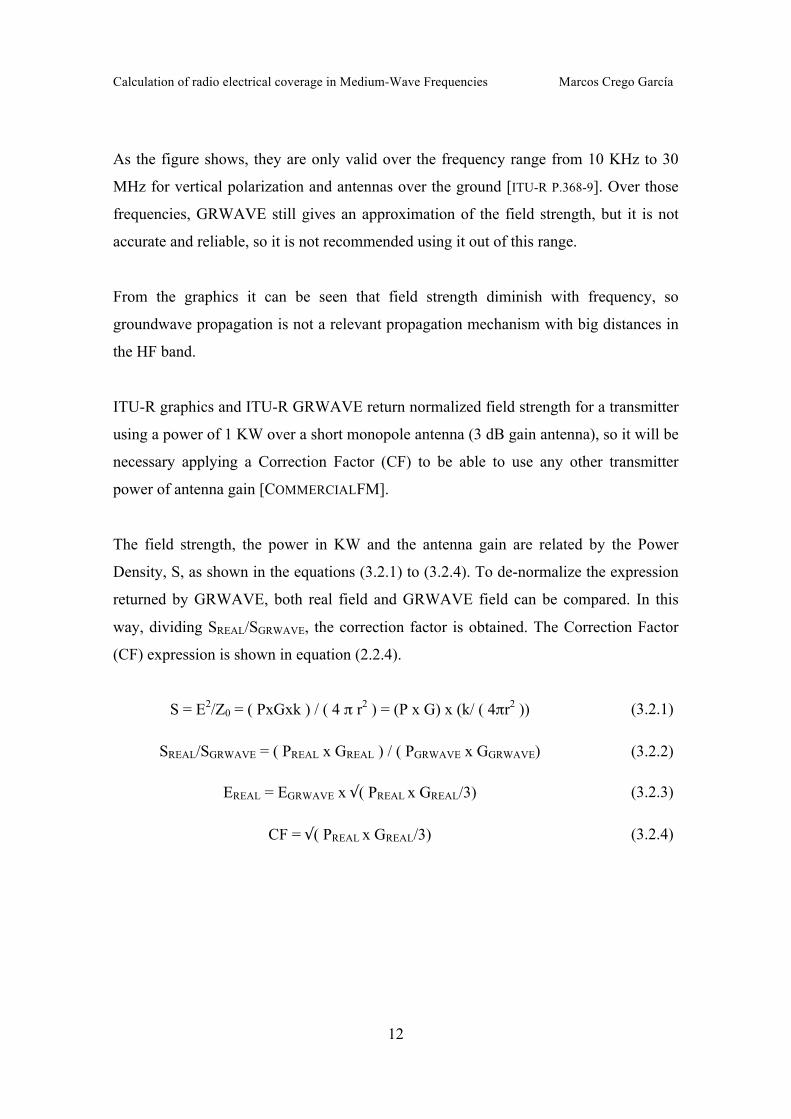
ITU-R graphics and ITU-R GRWAVE return normalized field strength for a transmitter
using a power of 1 KW over a short monopole antenna (3 dB gain antenna), so it will be
necessary applying a Correction Factor (CF) to be able to use any other transmitter
power of antenna gain [COMMERCIALFM].
The field strength, the power in KW and the antenna gain are related by the Power
Density, S, as shown in the equations (3.2.1) to (3.2.4). To de-normalize the expression
returned by GRWAVE, both real field and GRWAVE field can be compared. In this
way, dividing SREAL/SGRWAVE, the correction factor is obtained. The Correction Factor
(CF) expression is shown in equation (2.2.4).
S = E2/Z0 = ( PxGxk ) / ( 4 π r2 ) = (P x G) x (k/ ( 4πr2 )) (3.2.1)
SREAL/SGRWAVE = ( PREAL x GREAL ) / ( PGRWAVE x GGRWAVE) (3.2.2)
EREAL = EGRWAVE x √( PREAL x GREAL/3) (3.2.3)
CF = √( PREAL x GREAL/3) (3.2.4)
Calculation of radio electrical coverage in Medium-Wave Frequencies Marcos Crego García
13
3.3 Non-Homogeneous paths
The ITU-R P.368-9 Recommendation defines a non-homogeneous path as the path
between the transmitter and the receiver with two or more conductivities between them.
In this case, data contained in the graphics must be used following the Method of
Millington described at the Recommendation.
This method implies several calculations over several graphics both in Transmitter-to-
Receiver direction as in the inverse, Receiver-to-Transmitter direction.
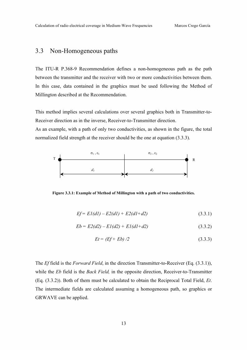
As an example, with a path of only two conductivities, as shown in the figure, the total
normalized field strength at the receiver should be the one at equation (3.3.3).
Figure 3.3.1: Example of Method of Millington with a path of two conductivities.
Ef = E1(d1) – E2(d1) + E2(d1+d2) (3.3.1)
Eb = E2(d2) – E1(d2) + E1(d1+d2) (3.3.2)
Et = (Ef + Eb) /2 (3.3.3)
The Ef field is the Forward Field, in the direction Transmitter-to-Receiver (Eq. (3.3.1)),
while the Eb field is the Back Field, in the opposite direction, Receiver-to-Transmitter
(Eq. (3.3.2)). Both of them must be calculated to obtain the Reciprocal Total Field, Et.
The intermediate fields are calculated assuming a homogeneous path, so graphics or
GRWAVE can be applied.
T R
σ1 , ε1 σ2 , ε2
d1 d2
Calculation of radio electrical coverage in Medium-Wave Frequencies Marcos Crego García
14
As it can be seen in this example, for only two conductivities, six different consults to
ITU-R graphics or six calls to GRWAVE are needed. This means a very tedious process
and it becomes even more tedious because generally there are more than two
conductivities between Transmitter and Receiver, especially when they are far enough.
3.4 Project description
As it was said in the first chapter, the aim of this project is to accomplish next
objectives:
Suit the method of calculation to the ITU-R P.368-9 for groundwave field
strength coverage.
Include topographical data.
Include conductivity maps to be able to process the coverage under one area and
fields profiles automatically.
Extend the GRWAVE to calculate the field in one point (receiver) due to one or
several transmitters, checking if there is ISI or not.
Create an easy-to-use graphical user interface to simplify the methods described
at ITU-R Rec.
To achieve these objectives, it has been chosen Matlab as the programming tool, due to
its Mapping Toolbox, that allows dealing with maps and coordinates data expressed in
latitude and longitude, which are the nature way to express the location of a radio
station. Moreover, the version chosen has been Matlab 7 R14, because the plot of the
coastal line and politics frontiers is more accuracy.
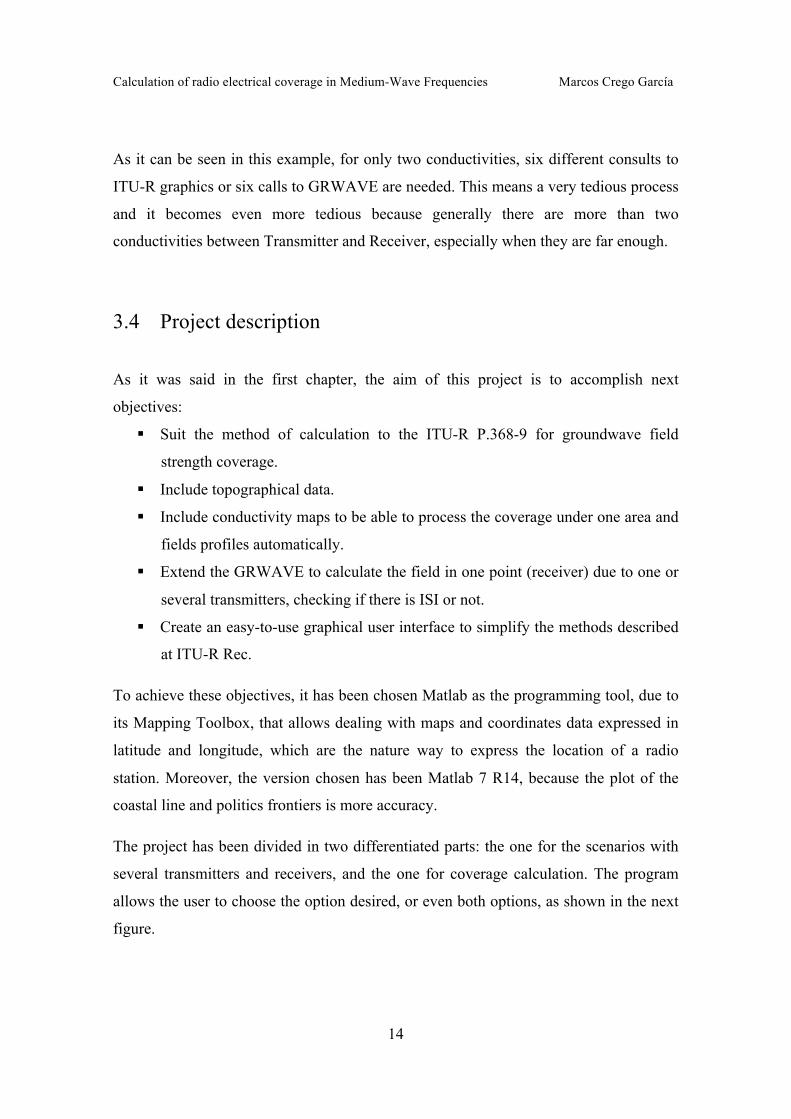
The project has been divided in two differentiated parts: the one for the scenarios with
several transmitters and receivers, and the one for coverage calculation. The program
allows the user to choose the option desired, or even both options, as shown in the next
figure.
Calculation of radio electrical coverage in Medium-Wave Frequencies Marcos Crego García
15
Figure 3.4.1: Start Menu Window
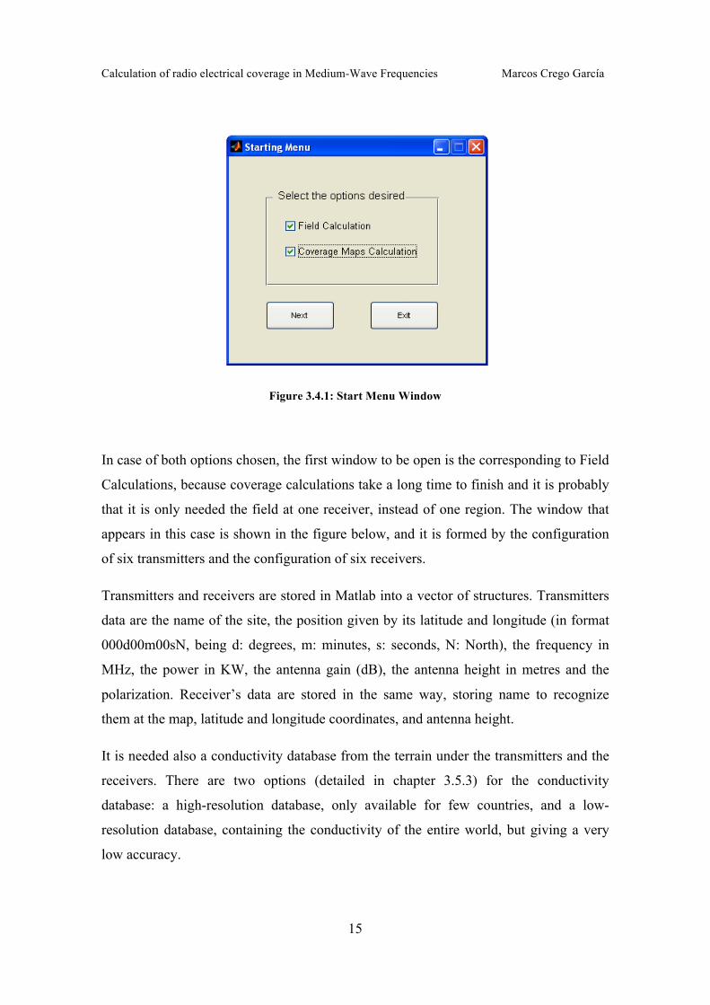
In case of both options chosen, the first window to be open is the corresponding to Field
Calculations, because coverage calculations take a long time to finish and it is probably
that it is only needed the field at one receiver, instead of one region. The window that
appears in this case is shown in the figure below, and it is formed by the configuration
of six transmitters and the configuration of six receivers.
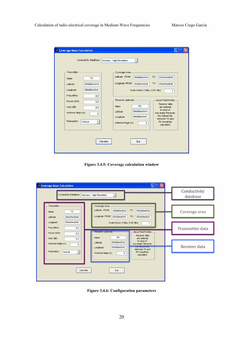
Transmitters and receivers are stored in Matlab into a vector of structures. Transmitters
data are the name of the site, the position given by its latitude and longitude (in format
000d00m00sN, being d: degrees, m: minutes, s: seconds, N: North), the frequency in
MHz, the power in KW, the antenna gain (dB), the antenna height in metres and the
polarization. Receiver’s data are stored in the same way, storing name to recognize
them at the map, latitude and longitude coordinates, and antenna height.
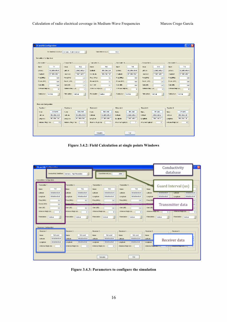
It is needed also a conductivity database from the terrain under the transmitters and the
receivers. There are two options (detailed in chapter 3.5.3) for the conductivity
database: a high-resolution database, only available for few countries, and a low-
resolution database, containing the conductivity of the entire world, but giving a very
low accuracy.
Calculation of radio electrical coverage in Medium-Wave Frequencies Marcos Crego García
16
Figure 3.4.2: Field Calculation at single points Windows
Figure 3.4.3: Parameters to configure the simulation
Calculation of radio electrical coverage in Medium-Wave Frequencies Marcos Crego García
17
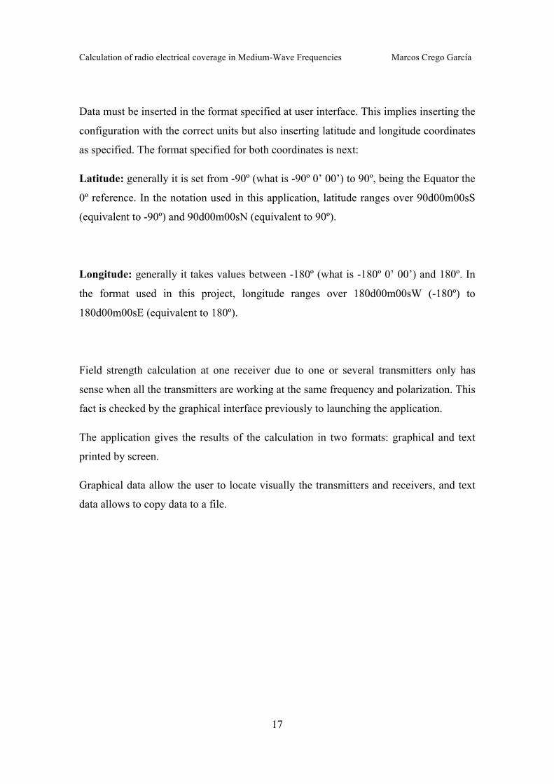
Data must be inserted in the format specified at user interface. This implies inserting the
configuration with the correct units but also inserting latitude and longitude coordinates
as specified. The format specified for both coordinates is next:
Latitude: generally it is set from -90º (what is -90º 0’ 00’) to 90º, being the Equator the
0º reference. In the notation used in this application, latitude ranges over 90d00m00sS
(equivalent to -90º) and 90d00m00sN (equivalent to 90º).
Longitude: generally it takes values between -180º (what is -180º 0’ 00’) and 180º. In
the format used in this project, longitude ranges over 180d00m00sW (-180º) to
180d00m00sE (equivalent to 180º).
Field strength calculation at one receiver due to one or several transmitters only has
sense when all the transmitters are working at the same frequency and polarization. This
fact is checked by the graphical interface previously to launching the application.
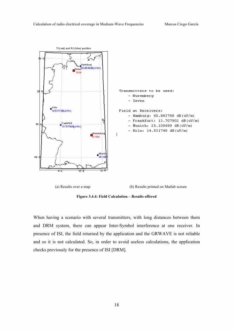
The application gives the results of the calculation in two formats: graphical and text
printed by screen.
Graphical data allow the user to locate visually the transmitters and receivers, and text
data allows to copy data to a file.
Calculation of radio electrical coverage in Medium-Wave Frequencies Marcos Crego García
18
(a) Results over a map (b) Results printed on Matlab screen
Figure 3.4.4: Field Calculation – Results offered
When having a scenario with several transmitters, with long distances between them
and DRM system, there can appear Inter-Symbol interference at one receiver. In
presence of ISI, the field returned by the application and the GRWAVE is not reliable
and so it is not calculated. So, in order to avoid useless calculations, the application
checks previously for the presence of ISI [DRM].
Calculation of radio electrical coverage in Medium-Wave Frequencies Marcos Crego García
19
There will be ISI when:
|d1-d2| > Guard Interval (s) x c (m/s) (3.4.1) Being:
d1: distance between transmitter 1 and receiver d2: distance between transmitter 2 and receiver Guard interval in seconds: Guard interval defined by DRM standard c: speed of light at the vacuum (3x10⁸ m/s)
With a default guard interval of 2666 us, the minimum difference of distance needed to
have ISI is 800 km, far enough to cover a wide region without ISI [DRM].
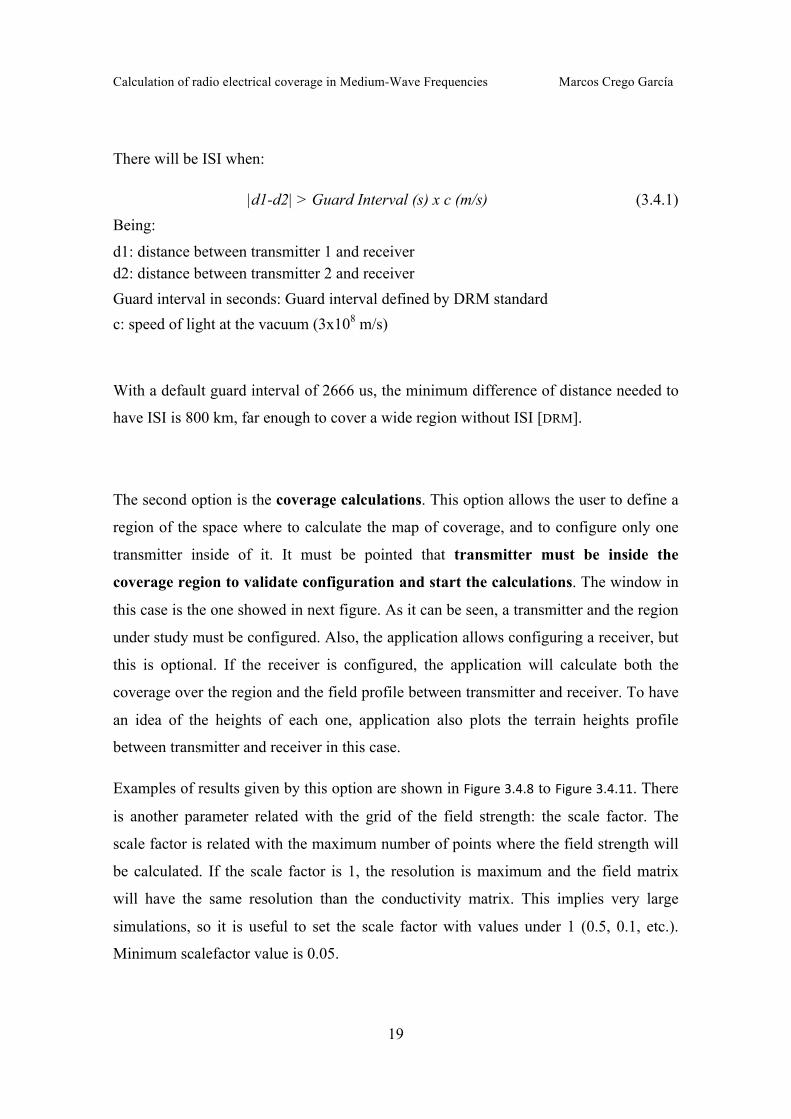
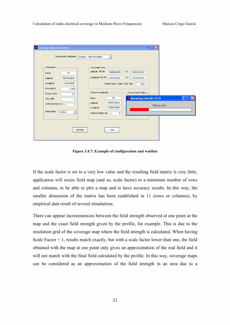
The second option is the coverage calculations. This option allows the user to define a
region of the space where to calculate the map of coverage, and to configure only one
transmitter inside of it. It must be pointed that transmitter must be inside the
coverage region to validate configuration and start the calculations. The window in
this case is the one showed in next figure. As it can be seen, a transmitter and the region
under study must be configured. Also, the application allows configuring a receiver, but
this is optional. If the receiver is configured, the application will calculate both the
coverage over the region and the field profile between transmitter and receiver. To have
an idea of the heights of each one, application also plots the terrain heights profile
between transmitter and receiver in this case.
Examples of results given by this option are shown in Figure3.4.8 to Figure3.4.11. There
is another parameter related with the grid of the field strength: the scale factor. The
scale factor is related with the maximum number of points where the field strength will
be calculated. If the scale factor is 1, the resolution is maximum and the field matrix
will have the same resolution than the conductivity matrix. This implies very large
simulations, so it is useful to set the scale factor with values under 1 (0.5, 0.1, etc.).
Minimum scalefactor value is 0.05.
Calculation of radio electrical coverage in Medium-Wave Frequencies Marcos Crego García
20
Figure 3.4.5: Coverage calculation window
Figure 3.4.6: Configuration parameters
Calculation of radio electrical coverage in Medium-Wave Frequencies Marcos Crego García
21
Figure 3.4.7: Example of configuration and waitbar
If the scale factor is set to a very low value and the resulting field matrix is very little,
application will resize field map (and so, scale factor) to a minimum number of rows
and columns, to be able to plot a map and to have accuracy results. In this way, the
smaller dimension of the matrix has been established in 11 (rows or columns), by
empirical data result of several simulations.
There can appear inconsistencies between the field strength observed at one point at the
map and the exact field strength given by the profile, for example. This is due to the
resolution grid of the coverage map where the field strength is calculated. When having
Scale Factor = 1, results match exactly, but with a scale factor lower than one, the field
obtained with the map at one point only gives an approximation of the real field and it
will not match with the final field calculated by the profile. In this way, coverage maps
can be considered as an approximation of the field strength in an area due to a
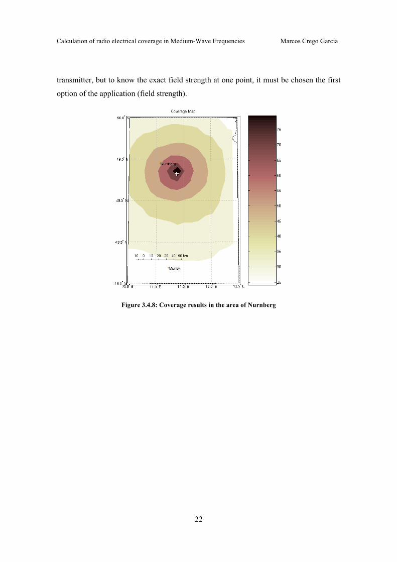
Calculation of radio electrical coverage in Medium-Wave Frequencies Marcos Crego García
22
transmitter, but to know the exact field strength at one point, it must be chosen the first
option of the application (field strength).
Figure 3.4.8: Coverage results in the area of Nurnberg
Calculation of radio electrical coverage in Medium-Wave Frequencies Marcos Crego García
23
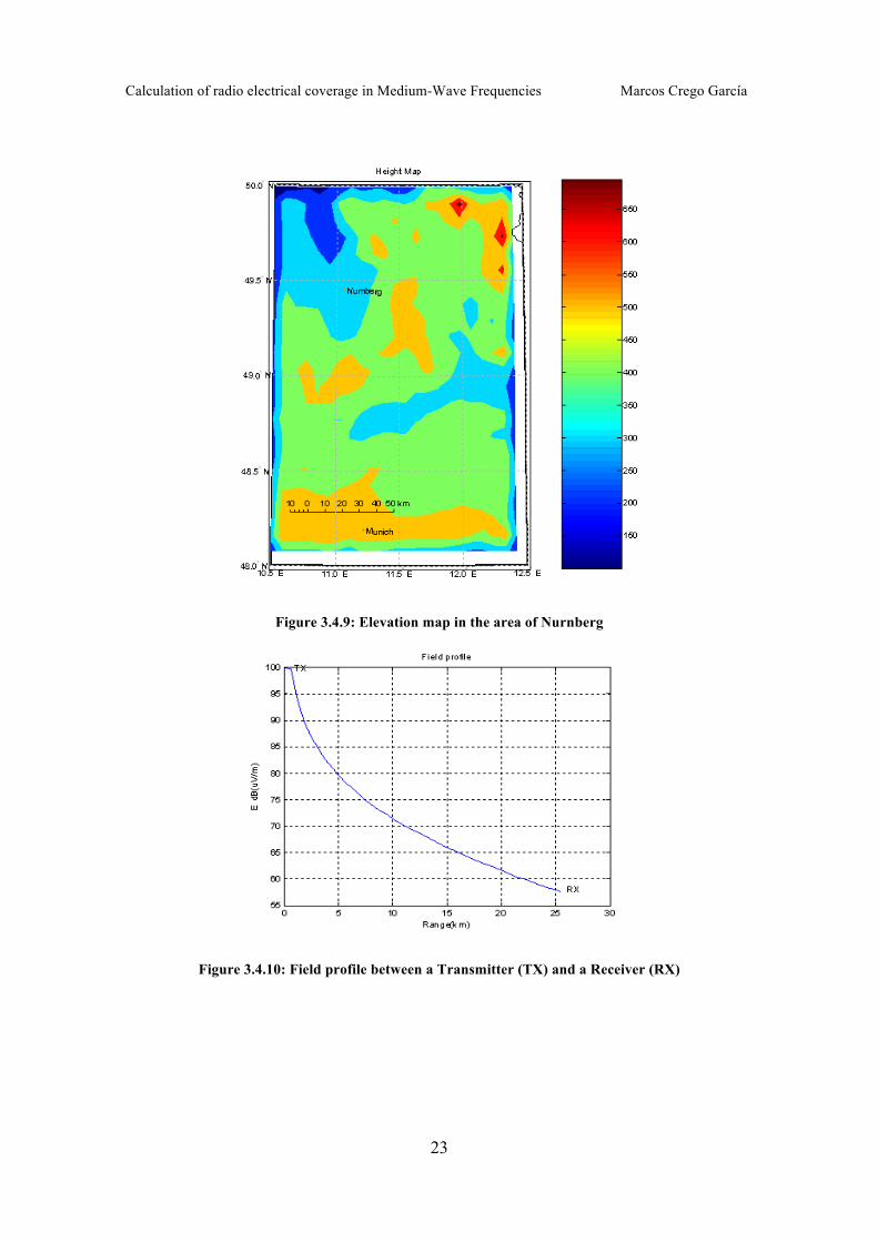
Figure 3.4.9: Elevation map in the area of Nurnberg
Figure 3.4.10: Field profile between a Transmitter (TX) and a Receiver (RX)
Calculation of radio electrical coverage in Medium-Wave Frequencies Marcos Crego García
24
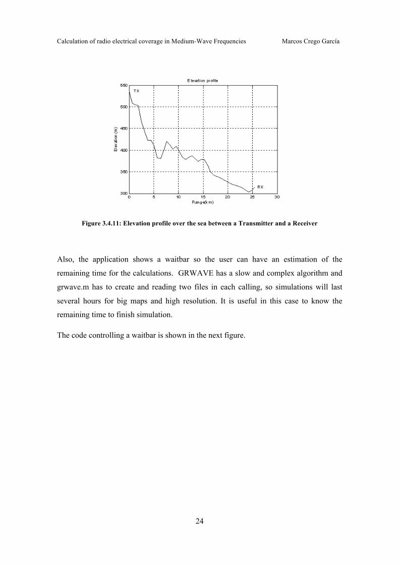
Figure 3.4.11: Elevation profile over the sea between a Transmitter and a Receiver
Also, the application shows a waitbar so the user can have an estimation of the
remaining time for the calculations. GRWAVE has a slow and complex algorithm and
grwave.m has to create and reading two files in each calling, so simulations will last
several hours for big maps and high resolution. It is useful in this case to know the
remaining time to finish simulation.
The code controlling a waitbar is shown in the next figure.
Calculation of radio electrical coverage in Medium-Wave Frequencies Marcos Crego García
25
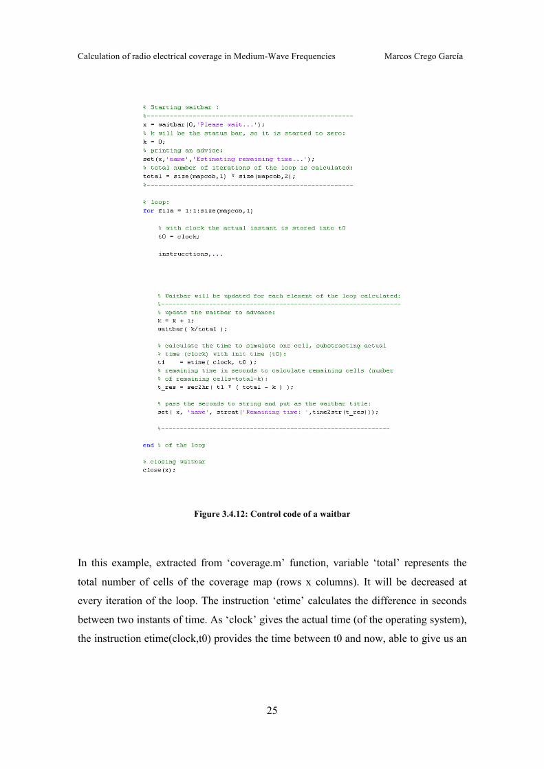
Figure 3.4.12: Control code of a waitbar
In this example, extracted from ‘coverage.m’ function, variable ‘total’ represents the
total number of cells of the coverage map (rows x columns). It will be decreased at
every iteration of the loop. The instruction ‘etime’ calculates the difference in seconds
between two instants of time. As ‘clock’ gives the actual time (of the operating system),
the instruction etime(clock,t0) provides the time between t0 and now, able to give us an
Calculation of radio electrical coverage in Medium-Wave Frequencies Marcos Crego García
26
estimation of the time needed to process one cell, and so on, the time remaining to
process the remaining cells.
Functions ‘etime’ and ‘clock’ are Matlab reference functions, available in the basic
Matlab toolbox. However, the instruction ‘time2str’ is only available in the Mapping
Toolbox, as one of the huge amount of conversion between units function.
Furthermore, to work with the data resulting once the simulation is made, the program
stores the data acquired into three different files in .mat binary format: FieldData.mat,
saves the variables resulting from the simulation of several transmitters and receivers.
CoverageData.mat, saves the coverage maps and data resulting from coverage
simulation. SimulationData.mat, that saves all variables available in the workspace.
To load the data once the simulation is finished, type “load filename.mat” in the Matlab
command windows (or workspace) to access the data.
3.5 Software development
The application consists on several functions developed in Matlab. All of them
converge in two primary functions: loadmap, in charge of loading conductivity and
elevation maps and MillingtonH, the function in charge of the field calculation at one
point, given one transmitter and one receiver. This function implements Millington’s
Method of calculation, which implies the calculation of the paths of different
conductivity between transmitter and receiver and several callings to the Matlab
GRWAVE Interface.
Calculation of radio electrical coverage in Medium-Wave Frequencies Marcos Crego García
27
The main steps followed in the software development of the application were these:
Programming ITU-R P. 368-9 Recommendation for homogeneous paths: Calling
GRWAVE from Matlab.
Programming ITU-R P. 368-9 Recommendation for non-homogeneous paths:
Programming method of Millington. This means the previous obtaining of the
path between two points in a map: conductivity interpolation and effective
heights.
The nature of the project means working with maps, so it is needed to use
Matlab Mapping Toolbox, which will be discussed, in the last place.
This project works with two databases: terrain conductivity and permittivity and
elevation database. Both are necessary data to call GRWAVE following the
instructions from the ITU-R.
Loading conductivity and elevation maps.
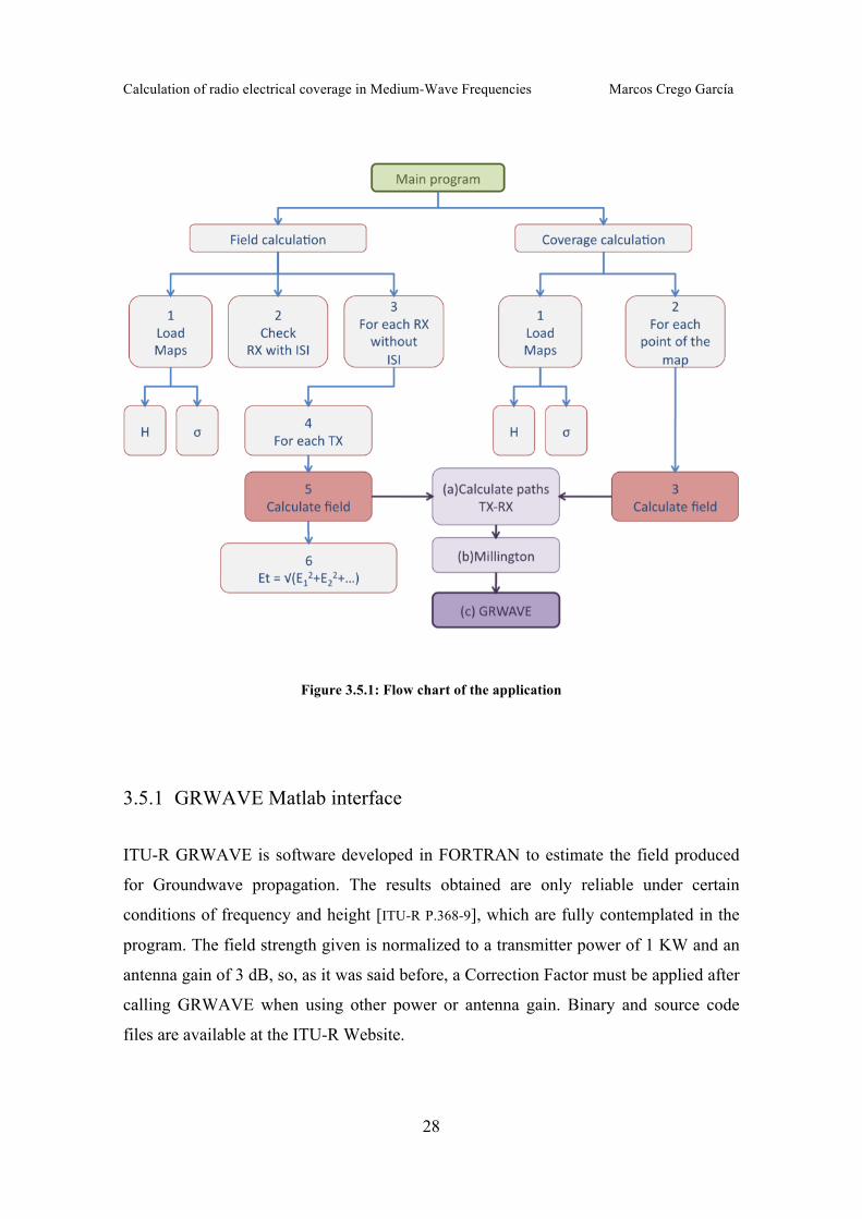
The flow diagram is shown below.
Calculation of radio electrical coverage in Medium-Wave Frequencies Marcos Crego García
28
Figure 3.5.1: Flow chart of the application
3.5.1 GRWAVE Matlab interface
ITU-R GRWAVE is software developed in FORTRAN to estimate the field produced
for Groundwave propagation. The results obtained are only reliable under certain
conditions of frequency and height [ITU-R P.368-9], which are fully contemplated in the
program. The field strength given is normalized to a transmitter power of 1 KW and an
antenna gain of 3 dB, so, as it was said before, a Correction Factor must be applied after
calling GRWAVE when using other power or antenna gain. Binary and source code
files are available at the ITU-R Website.
Calculation of radio electrical coverage in Medium-Wave Frequencies Marcos Crego García
29
GRWAVE has a MSDOS command window interface to insert data needed, but also
allows the user to insert data into a file following a fixed format. In the same way,
results obtained can be printed by GRWAVE either in the screen or into a text file.
The option chosen to communicate Matlab with GRWAVE was using the binary and
the ‘system’ command from Matlab, and input and output text files to insert
configuration and reading data. The full instruction used to call GRWAVE is:
[ ergrw, res ] = system('grwave <data.inp >data.out');
The instruction system(‘command’) execute operating system command and return the
result on success or an explanatory message of error in other case. In this case,
command to execute is GRWAVE, which must be located in the same directory of the
application, and data.inp and data.out are the names of the input and output directory,
respectively. Both input and output files are text files with a format specified by
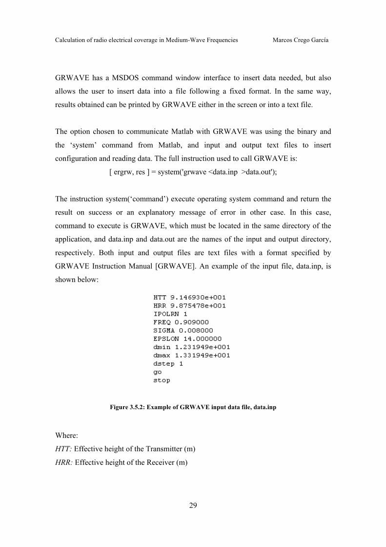
GRWAVE Instruction Manual [GRWAVE]. An example of the input file, data.inp, is
shown below:
Figure 3.5.2: Example of GRWAVE input data file, data.inp
Where:
HTT: Effective height of the Transmitter (m)
HRR: Effective height of the Receiver (m)
Calculation of radio electrical coverage in Medium-Wave Frequencies Marcos Crego García
30
IPOLRN: Polarization (1 for vertical and 2 for horizontal)
FREQ: Frequency in MHz
SIGMA, EPSLON: Condutivity (S/m) and permitivity of the terrain.
dmin: Distance (km) where the field needs to be calculated.
dmax and dstep are required but not used, and take values next to dmin.
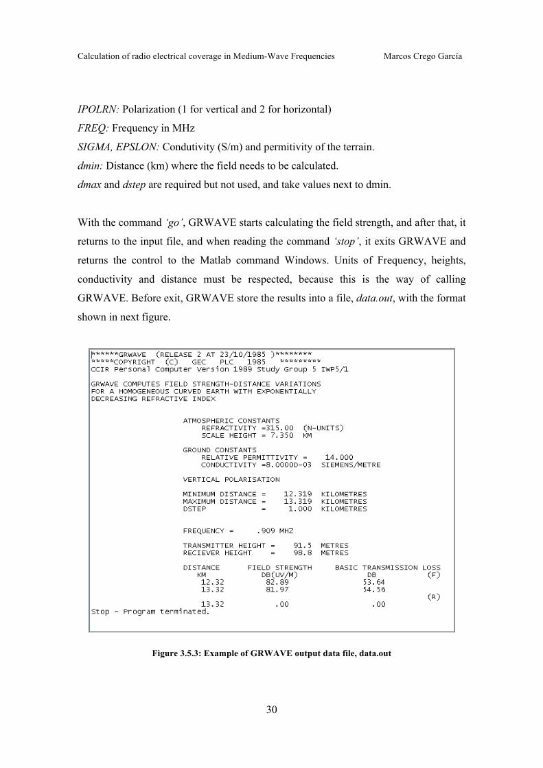
With the command ‘go’, GRWAVE starts calculating the field strength, and after that, it
returns to the input file, and when reading the command ‘stop’, it exits GRWAVE and
returns the control to the Matlab command Windows. Units of Frequency, heights,
conductivity and distance must be respected, because this is the way of calling
GRWAVE. Before exit, GRWAVE store the results into a file, data.out, with the format
shown in next figure.
Figure 3.5.3: Example of GRWAVE output data file, data.out
Calculation of radio electrical coverage in Medium-Wave Frequencies Marcos Crego García
31
This file has all the information of the configuration in the header, and the value desired
is near the bottom of the file, so it means that, to be able to read the data desired, the file
pointer must be located first at the beginning of the corresponding line. GRWAVE
always print two values of field strength, but the only one needed is the first one. In the
example below, data required should be 82.89 dB(uV/m).
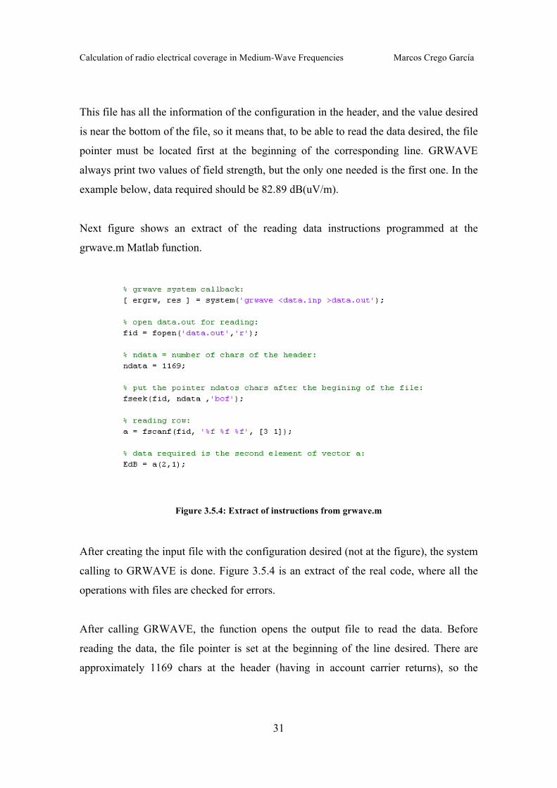
Next figure shows an extract of the reading data instructions programmed at the
grwave.m Matlab function.
Figure 3.5.4: Extract of instructions from grwave.m
After creating the input file with the configuration desired (not at the figure), the system
calling to GRWAVE is done. Figure 3.5.4 is an extract of the real code, where all the
operations with files are checked for errors.
After calling GRWAVE, the function opens the output file to read the data. Before
reading the data, the file pointer is set at the beginning of the line desired. There are
approximately 1169 chars at the header (having in account carrier returns), so the
Calculation of radio electrical coverage in Medium-Wave Frequencies Marcos Crego García
32
pointer is moved 1169 chars from the beginning of the file (bof) with the command
fseek. This is indeed an approximation, and in the real function several validations of
the position are done, because sometimes GRWAVE inserts some more characters, so
an approximation is done.
When the pointer is correctly located, the function reads the file with the command
fscanf, and returns in ‘a’ a vector of tree elements in column format. The field strength
should be the second one, that is the data returned by grwave.m function.
So, Matlab GRWAVE interface is a file (grwave.m) that creates the input file, calls
GRWAVE, and reads the data of the output file. Dealing with text files decreases the
simulation speed.
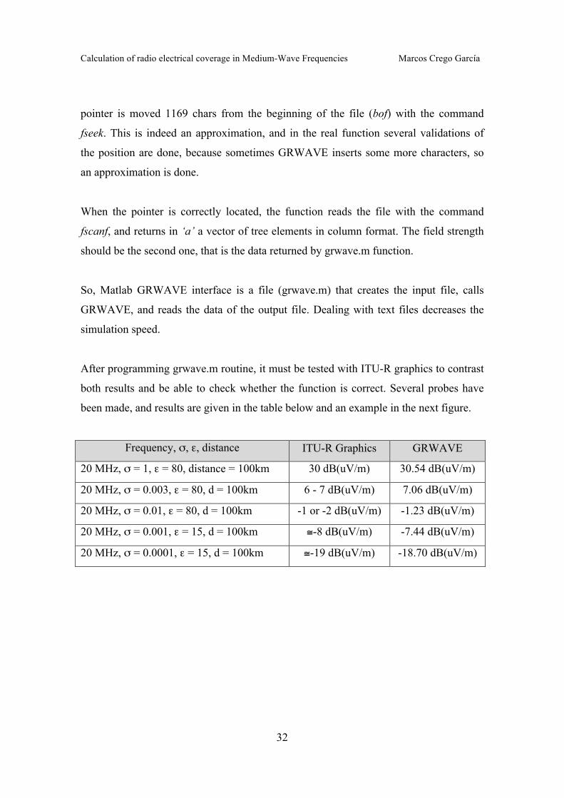
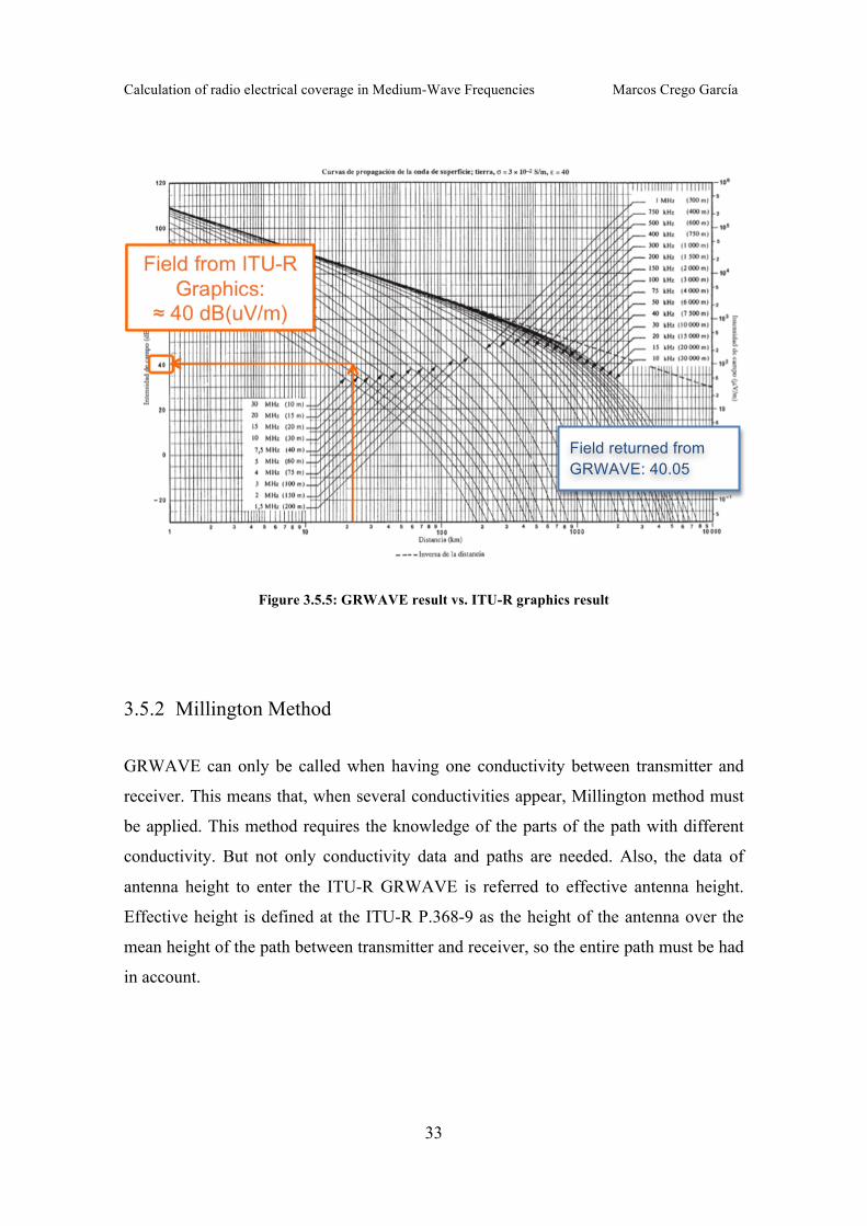
After programming grwave.m routine, it must be tested with ITU-R graphics to contrast
both results and be able to check whether the function is correct. Several probes have
been made, and results are given in the table below and an example in the next figure.
Frequency, σ, ε, distance ITU-R Graphics GRWAVE
20 MHz, σ = 1, ε = 80, distance = 100km 30 dB(uV/m) 30.54 dB(uV/m)
20 MHz, σ = 0.003, ε = 80, d = 100km 6 - 7 dB(uV/m) 7.06 dB(uV/m)
20 MHz, σ = 0.01, ε = 80, d = 100km -1 or -2 dB(uV/m) -1.23 dB(uV/m)
20 MHz, σ = 0.001, ε = 15, d = 100km ≅-8 dB(uV/m) -7.44 dB(uV/m)
20 MHz, σ = 0.0001, ε = 15, d = 100km ≅-19 dB(uV/m) -18.70 dB(uV/m)
Calculation of radio electrical coverage in Medium-Wave Frequencies Marcos Crego García
33
Figure 3.5.5: GRWAVE result vs. ITU-R graphics result
3.5.2 Millington Method
GRWAVE can only be called when having one conductivity between transmitter and
receiver. This means that, when several conductivities appear, Millington method must
be applied. This method requires the knowledge of the parts of the path with different
conductivity. But not only conductivity data and paths are needed. Also, the data of
antenna height to enter the ITU-R GRWAVE is referred to effective antenna height.
Effective height is defined at the ITU-R P.368-9 as the height of the antenna over the
mean height of the path between transmitter and receiver, so the entire path must be had
in account.
Field returned from GRWAVE: 40.05 dB(uV/m)
Calculation of radio electrical coverage in Medium-Wave Frequencies Marcos Crego García
34
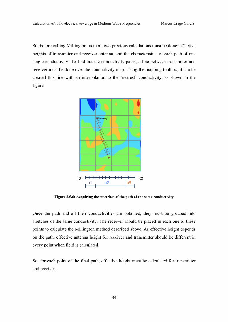
So, before calling Millington method, two previous calculations must be done: effective
heights of transmitter and receiver antenna, and the characteristics of each path of one
single conductivity. To find out the conductivity paths, a line between transmitter and
receiver must be done over the conductivity map. Using the mapping toolbox, it can be
created this line with an interpolation to the ‘nearest’ conductivity, as shown in the
figure.
Figure 3.5.6: Acquiring the stretches of the path of the same conductivity
Once the path and all their conductivities are obtained, they must be grouped into
stretches of the same conductivity. The receiver should be placed in each one of these
points to calculate the Millington method described above. As effective height depends
on the path, effective antenna height for receiver and transmitter should be different in
every point when field is calculated.
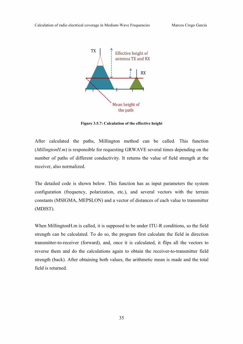
So, for each point of the final path, effective height must be calculated for transmitter
and receiver.
Calculation of radio electrical coverage in Medium-Wave Frequencies Marcos Crego García
35
Figure 3.5.7: Calculation of the effective height
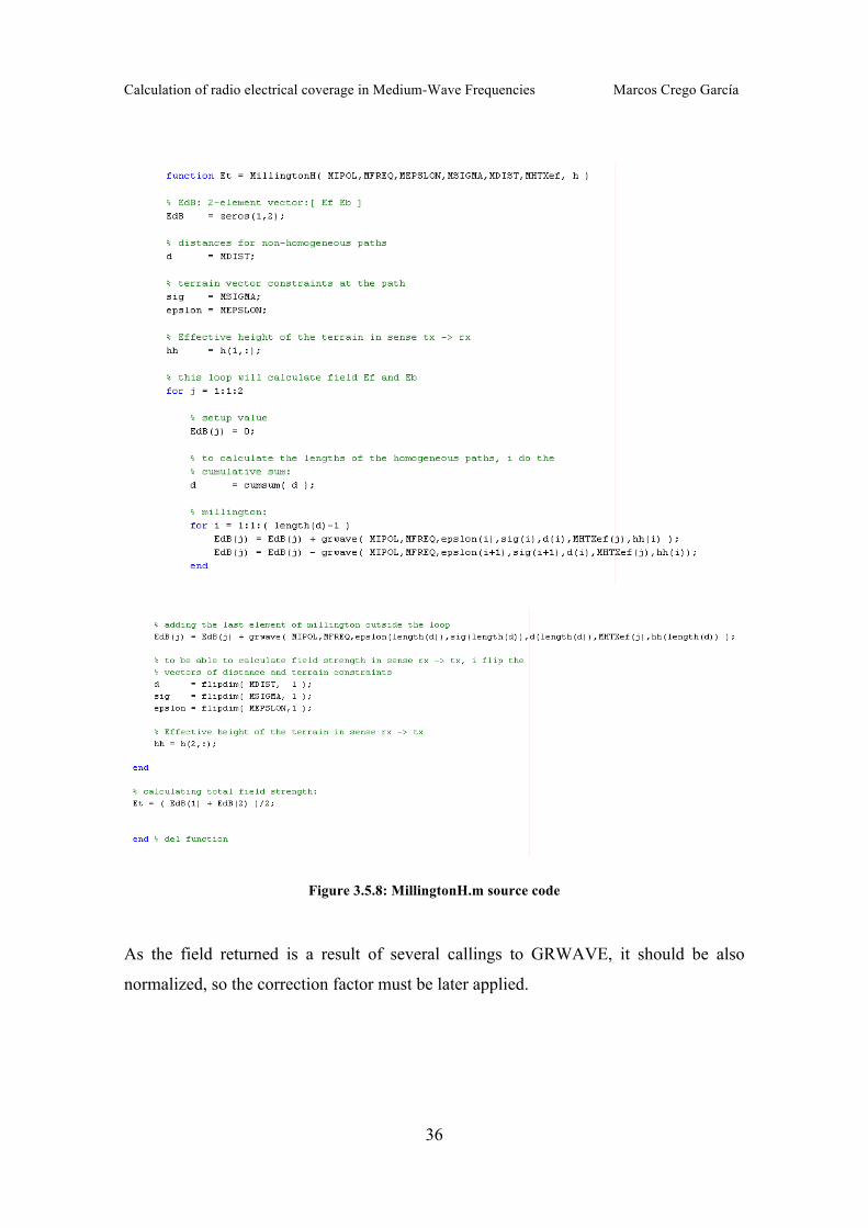
After calculated the paths, Millington method can be called. This function
(MillingtonH.m) is responsible for requesting GRWAVE several times depending on the
number of paths of different conductivity. It returns the value of field strength at the
receiver, also normalized.
The detailed code is shown below. This function has as input parameters the system
configuration (frequency, polarization, etc.), and several vectors with the terrain
constants (MSIGMA, MEPSLON) and a vector of distances of each value to transmitter
(MDIST).
When MillingtonH.m is called, it is supposed to be under ITU-R conditions, so the field
strength can be calculated. To do so, the program first calculate the field in direction
transmitter-to-receiver (forward), and, once it is calculated, it flips all the vectors to
reverse them and do the calculations again to obtain the receiver-to-transmitter field
strength (back). After obtaining both values, the arithmetic mean is made and the total
field is returned.
Calculation of radio electrical coverage in Medium-Wave Frequencies Marcos Crego García
36
Figure 3.5.8: MillingtonH.m source code
As the field returned is a result of several callings to GRWAVE, it should be also
normalized, so the correction factor must be later applied.
Calculation of radio electrical coverage in Medium-Wave Frequencies Marcos Crego García
37
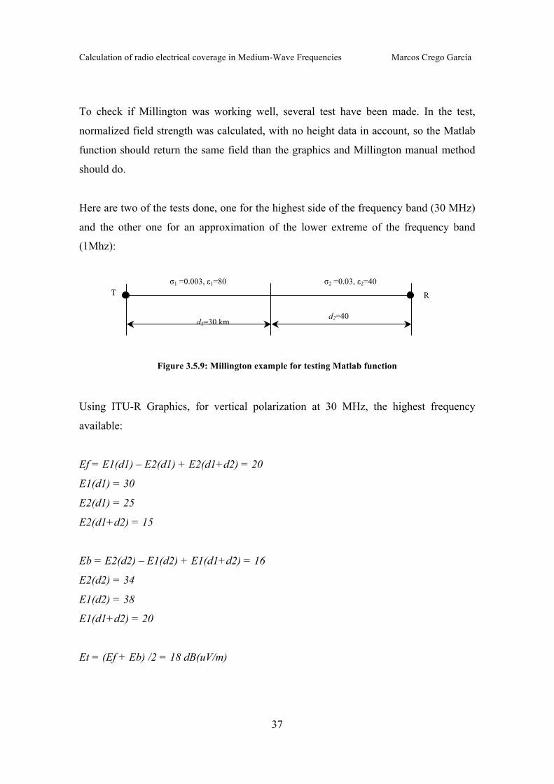
To check if Millington was working well, several test have been made. In the test,
normalized field strength was calculated, with no height data in account, so the Matlab
function should return the same field than the graphics and Millington manual method
should do.
Here are two of the tests done, one for the highest side of the frequency band (30 MHz)
and the other one for an approximation of the lower extreme of the frequency band
(1Mhz):
Figure 3.5.9: Millington example for testing Matlab function
Using ITU-R Graphics, for vertical polarization at 30 MHz, the highest frequency
available:
Ef = E1(d1) – E2(d1) + E2(d1+d2) = 20
E1(d1) = 30
E2(d1) = 25
E2(d1+d2) = 15
Eb = E2(d2) – E1(d2) + E1(d1+d2) = 16
E2(d2) = 34
E1(d2) = 38
E1(d1+d2) = 20
Et = (Ef + Eb) /2 = 18 dB(uV/m)
T R
σ1 =0.003, ε1=80
σ2 =0.03, ε2=40
d1=30 km d2=40
Calculation of radio electrical coverage in Medium-Wave Frequencies Marcos Crego García
38
By Millington programmed Matlab function, the field strength returned is, directly:
Et = 17.70 dB(uV/m) approximately equal to the field strength calculated manually with
two graphics.
The second test, using ITU-R Graphics, for vertical polarization at 1 MHz, low
frequencies:
Ef = E1(d1) – E2(d1) + E2(d1+d2) = 58
E1(d1) = 64
E2(d1) = 77
E2(d1+d2) = 71
Eb = E2(d2) – E1(d2) + E1(d1+d2) = 66
E2(d2) = 81
E1(d2) = 70
E1(d1+d2) = 55
Et = (Ef + Eb) /2 = 62 dB(uV/m)
By Millington, the field strength returned is, directly: Et = 62.14 dB(uV/m)
approximately equal to the field strength calculated manually with two graphics.
Calculation of radio electrical coverage in Medium-Wave Frequencies Marcos Crego García
39
3.5.3 Elevation and conductivity database
Due to the nature of the Groundwave propagation, it is needed to know the terrain
conductivity and the antenna height, and so, digital conductivity and elevation or
topography databases are required. Nowadays there is no digital High Resolution
Conductivity Database available. However, there is available a digital Global Elevation
Terrain database with a resolution of one km available at NOAA’s Project Website
[GLOBE].
GLOBE is an atlas elevation database. World data are separated into several ‘tiles’ to be
able to manage them, each tile representing an area of the world. The limits of latitude
and longitude are specified into headers text files that must be downloaded with the
elevation tiles.
To deal with GLOBE database and being capable of extract a region of the world even
if it is separated in tiles, MATLAB Mapping Toolbox [MATLAB] can be used with the
function ‘globedem’.
[ mapg, mapglegend ] = globedem('c:\globe', ScaleFactor, Latlim, Lonlim );
This command specifies Matlab:
‘c:\globe’: The directory where the files of GLOBE are stored (both elevation tiles and
headers).
ScaleFactor: The Scale Factor, that is, the resolution desired (1 means maximum
resolution, 1 km between points of the matrix returned).
Latlim and Lonlim: These two variables specify the limits of latitude and longitude of
the region desired.
Calculation of radio electrical coverage in Medium-Wave Frequencies Marcos Crego García
40
Data returned are:
mapg: The map containing the elevation data of the area selected by Latlim and Lonlim.
mapglegend: The reference vector or maplegend of all map, which will be specified in
the Mapping Toolbox section.
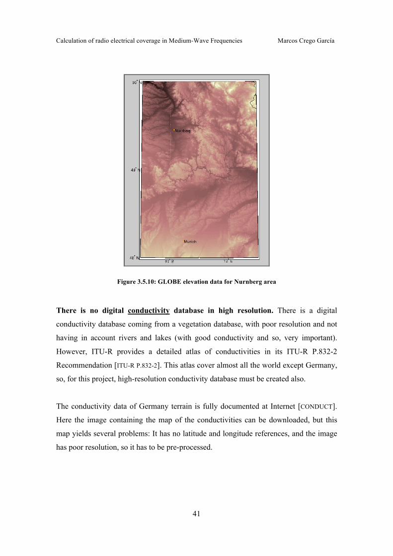
GLOBE returns the elevation of the points over the sea, and the sea marked with a NaN.
This must be changed inside the application to assign sea a zero elevation. An example
of the maps returned by GLOBE for the area of Nuremberg is shown in next figure.
Example of the command:
ScaleFactor = 1;
Latlim = [ 48 50 ];
Lonlim = [ 10.5 12.5 ] ;
[ mapg, mapglegend ] = globedem('c:\globe', ScaleFactor, Latlim, Lonlim );
worldmap(Latlim, Lonlim);
contourfm(mapg, mapglegend);
colormap(pink);
Calculation of radio electrical coverage in Medium-Wave Frequencies Marcos Crego García
41
Figure 3.5.10: GLOBE elevation data for Nurnberg area
There is no digital conductivity database in high resolution. There is a digital
conductivity database coming from a vegetation database, with poor resolution and not
having in account rivers and lakes (with good conductivity and so, very important).
However, ITU-R provides a detailed atlas of conductivities in its ITU-R P.832-2
Recommendation [ITU-R P.832-2]. This atlas cover almost all the world except Germany,
so, for this project, high-resolution conductivity database must be created also.
The conductivity data of Germany terrain is fully documented at Internet [CONDUCT].
Here the image containing the map of the conductivities can be downloaded, but this
map yields several problems: It has no latitude and longitude references, and the image
has poor resolution, so it has to be pre-processed.
Calculation of radio electrical coverage in Medium-Wave Frequencies Marcos Crego García
42
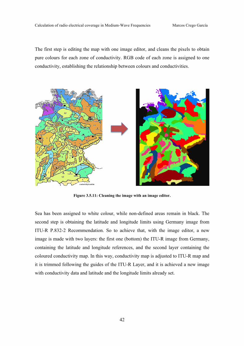
The first step is editing the map with one image editor, and cleans the pixels to obtain
pure colours for each zone of conductivity. RGB code of each zone is assigned to one
conductivity, establishing the relationship between colours and conductivities.
Figure 3.5.11: Cleaning the image with an image editor.
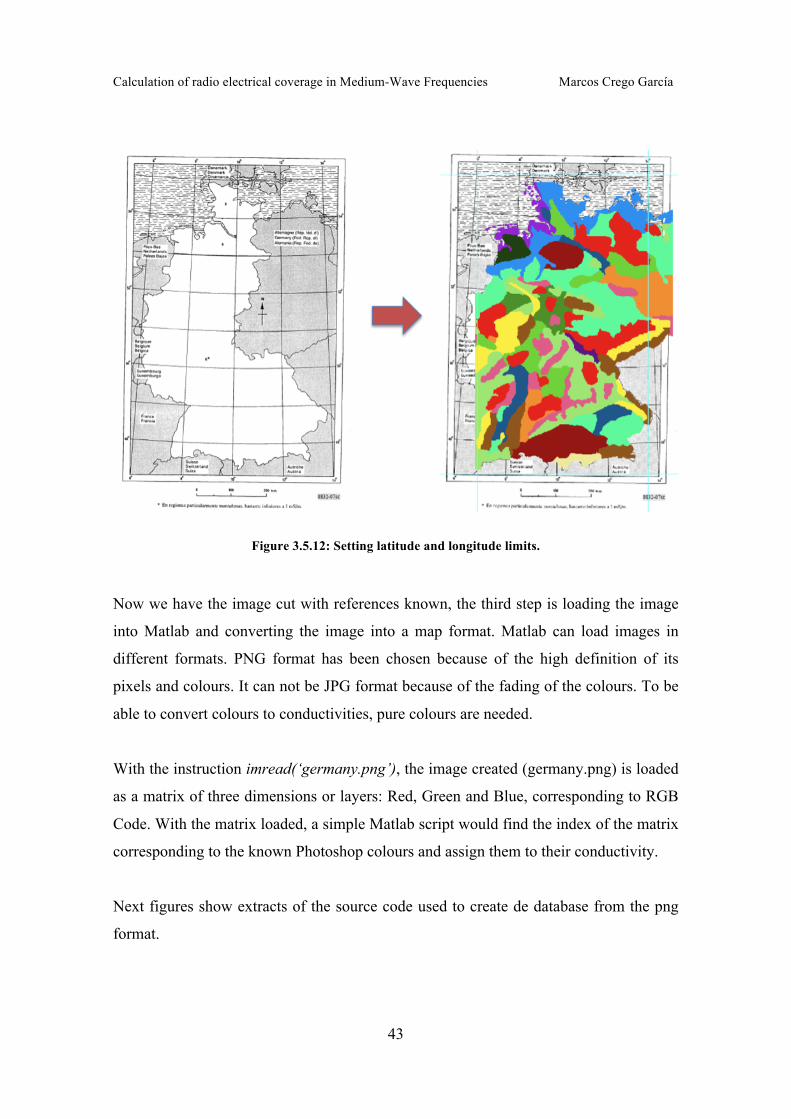
Sea has been assigned to white colour, while non-defined areas remain in black. The
second step is obtaining the latitude and longitude limits using Germany image from
ITU-R P.832-2 Recommendation. So to achieve that, with the image editor, a new
image is made with two layers: the first one (bottom) the ITU-R image from Germany,
containing the latitude and longitude references, and the second layer containing the
coloured conductivity map. In this way, conductivity map is adjusted to ITU-R map and
it is trimmed following the guides of the ITU-R Layer, and it is achieved a new image
with conductivity data and latitude and the longitude limits already set.
Calculation of radio electrical coverage in Medium-Wave Frequencies Marcos Crego García
43
Figure 3.5.12: Setting latitude and longitude limits.
Now we have the image cut with references known, the third step is loading the image
into Matlab and converting the image into a map format. Matlab can load images in
different formats. PNG format has been chosen because of the high definition of its
pixels and colours. It can not be JPG format because of the fading of the colours. To be
able to convert colours to conductivities, pure colours are needed.
With the instruction imread(‘germany.png’), the image created (germany.png) is loaded
as a matrix of three dimensions or layers: Red, Green and Blue, corresponding to RGB
Code. With the matrix loaded, a simple Matlab script would find the index of the matrix
corresponding to the known Photoshop colours and assign them to their conductivity.
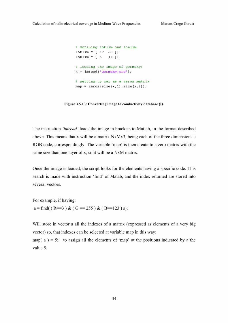
Next figures show extracts of the source code used to create de database from the png
format.
Calculation of radio electrical coverage in Medium-Wave Frequencies Marcos Crego García
44
Figure 3.5.13: Converting image to conductivity database (I).
The instruction ‘imread’ loads the image in brackets to Matlab, in the format described
above. This means that x will be a matrix NxMx3, being each of the three dimensions a
RGB code, correspondingly. The variable ‘map’ is then create to a zero matrix with the
same size than one layer of x, so it will be a NxM matrix.
Once the image is loaded, the script looks for the elements having a specific code. This
search is made with instruction ‘find’ of Matab, and the index returned are stored into
several vectors.
For example, if having:
a = find( ( R==3 ) & ( G == 255 ) & ( B==123 ) s);
Will store in vector a all the indexes of a matrix (expressed as elements of a very big
vector) so, that indexes can be selected at variable map in this way:
map( a ) = 5; to assign all the elements of ‘map’ at the positions indicated by a the
value 5.
Calculation of radio electrical coverage in Medium-Wave Frequencies Marcos Crego García
45
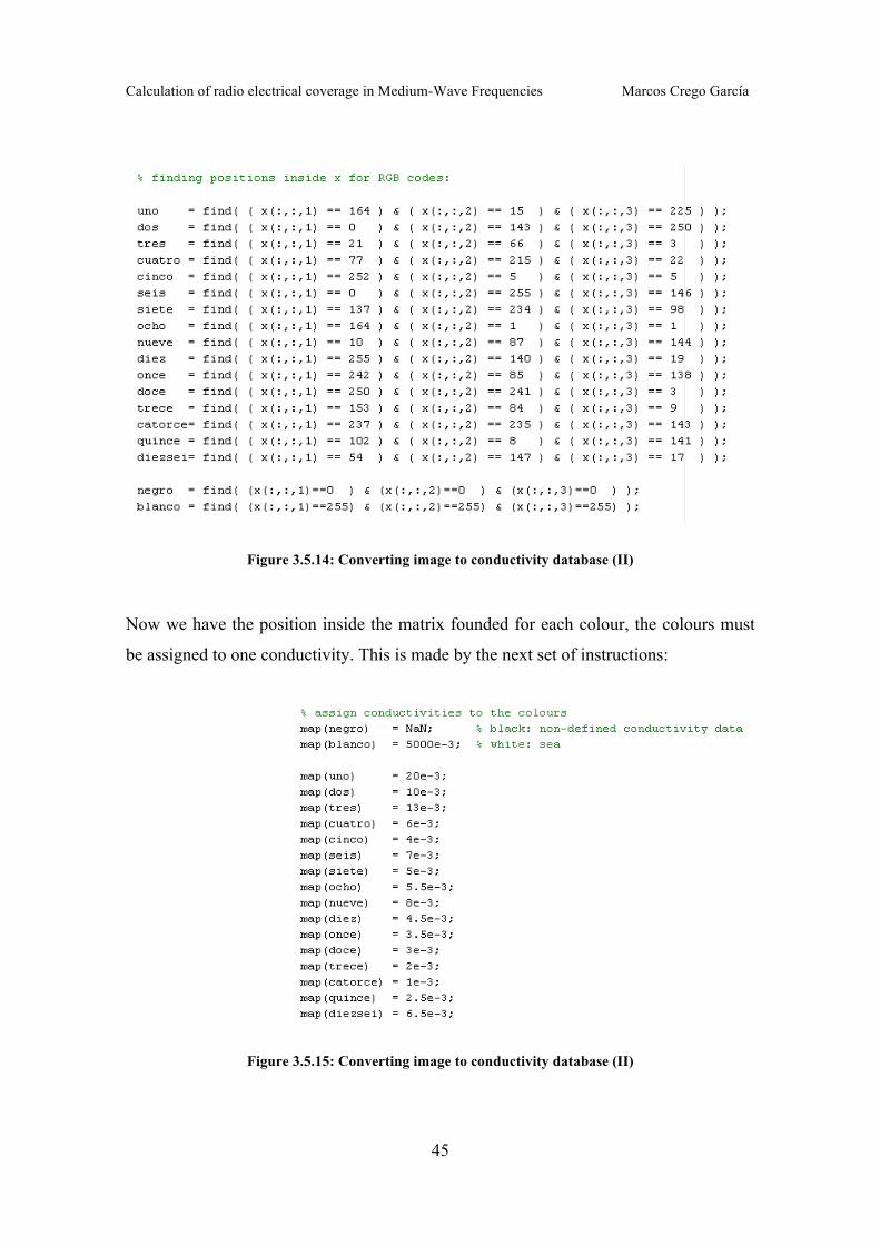
Figure 3.5.14: Converting image to conductivity database (II)
Now we have the position inside the matrix founded for each colour, the colours must
be assigned to one conductivity. This is made by the next set of instructions:
Figure 3.5.15: Converting image to conductivity database (II)
Calculation of radio electrical coverage in Medium-Wave Frequencies Marcos Crego García
46
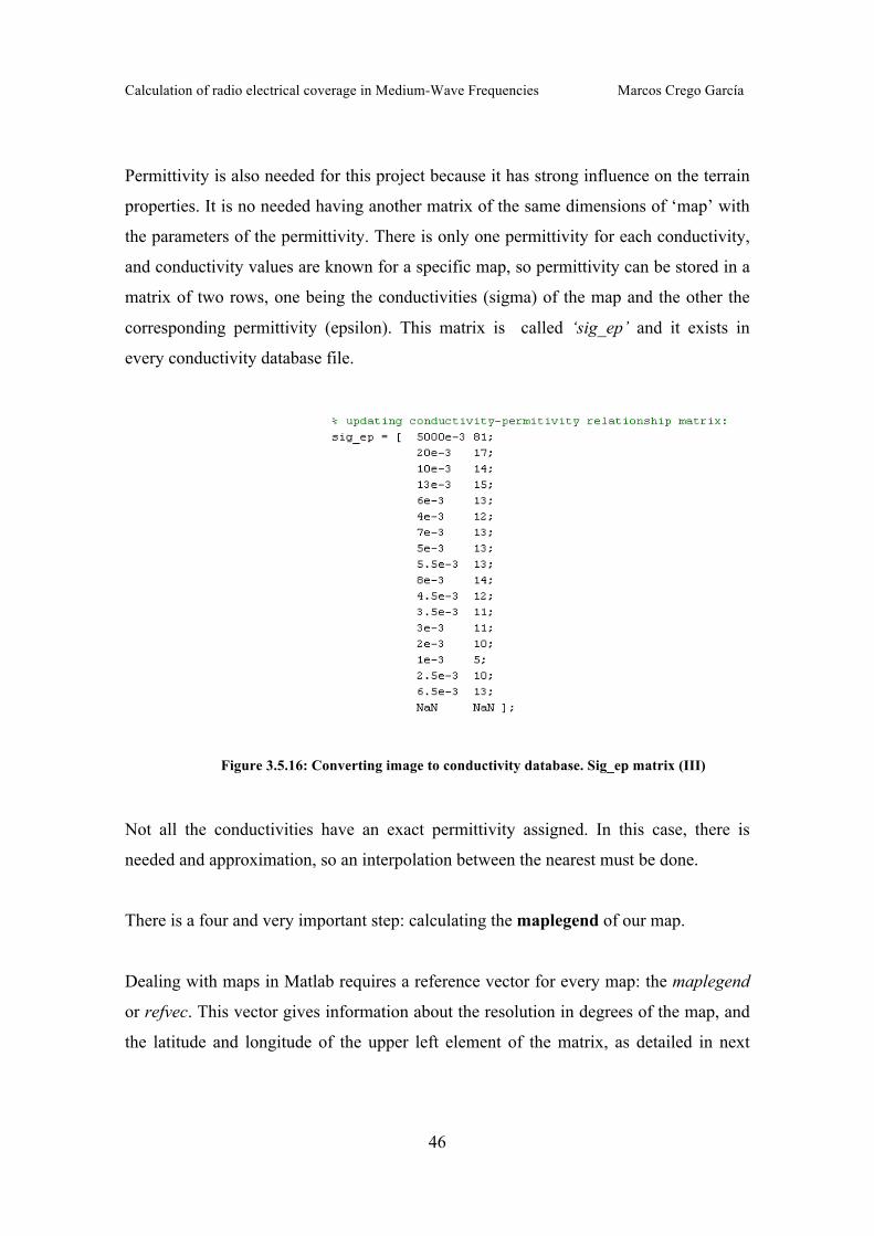
Permittivity is also needed for this project because it has strong influence on the terrain
properties. It is no needed having another matrix of the same dimensions of ‘map’ with
the parameters of the permittivity. There is only one permittivity for each conductivity,
and conductivity values are known for a specific map, so permittivity can be stored in a
matrix of two rows, one being the conductivities (sigma) of the map and the other the
corresponding permittivity (epsilon). This matrix is called ‘sig_ep’ and it exists in
every conductivity database file.
Figure 3.5.16: Converting image to conductivity database. Sig_ep matrix (III)
Not all the conductivities have an exact permittivity assigned. In this case, there is
needed and approximation, so an interpolation between the nearest must be done.
There is a four and very important step: calculating the maplegend of our map.
Dealing with maps in Matlab requires a reference vector for every map: the maplegend
or refvec. This vector gives information about the resolution in degrees of the map, and
the latitude and longitude of the upper left element of the matrix, as detailed in next
Calculation of radio electrical coverage in Medium-Wave Frequencies Marcos Crego García
47
chapters. The procedure to achieve a maplegend from a map coming from an image is
quite difficult and inaccurate. To avoid inaccuracies, the maplegend will be taken the
equivalent map of GLOBE, and, to do so, a GLOBE map should be created for the same
limits of latitude and longitude. The maplegend of GLOBE will be created in calling to
GLOBEDEM instruction. After that, conductivity map is resized to the GLOBE map. In
this way, both maplegends should be the same, and the obtaining of the maplegend of
the conductivity map is done.
As conductivity database has been created from GLOBE, and both have same
resolution, this means that the resolution should be also 1Km with Scale Factor of 1,
accurate enough to groundwave propagation.
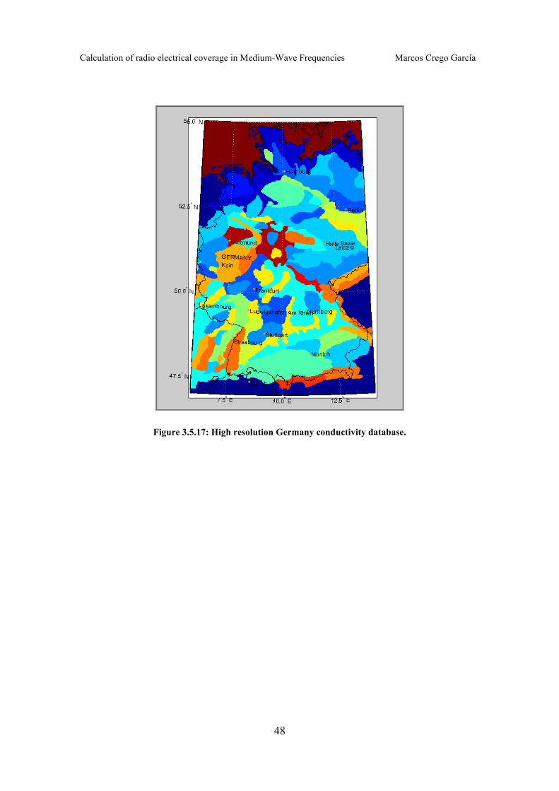
The same procedure can be followed to complete the database with other countries
conductivities defined in the ITU-R Recommendation. In this project, due to time
restrictions, only two countries have been digitalized: Germany and South Korea.
Resulting conductivity maps are shown in next figures:
Calculation of radio electrical coverage in Medium-Wave Frequencies Marcos Crego García
48
Figure 3.5.17: High resolution Germany conductivity database.
Calculation of radio electrical coverage in Medium-Wave Frequencies Marcos Crego García
49
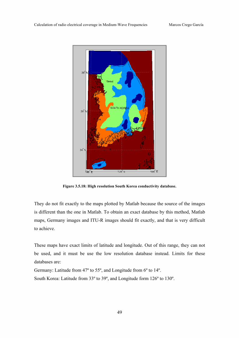
Figure 3.5.18: High resolution South Korea conductivity database.
They do not fit exactly to the maps plotted by Matlab because the source of the images
is different than the one in Matlab. To obtain an exact database by this method, Matlab
maps, Germany images and ITU-R images should fit exactly, and that is very difficult
to achieve.
These maps have exact limits of latitude and longitude. Out of this range, they can not
be used, and it must be use the low resolution database instead. Limits for these
databases are:
Germany: Latitude from 47º to 55º, and Longitude from 6º to 14º.
South Korea: Latitude from 33º to 39º, and Longitude form 126º to 130º.
Calculation of radio electrical coverage in Medium-Wave Frequencies Marcos Crego García
50
3.5.4 Code errors returned
The application exits when certain errors appear. These errors are not produced by an
application malfunction, and they are the result of checking the input configuration of
the system. The input data are verified at the User Interface, but also at the beginning of
some functions. This has been made in this way to make the functions independent of
the guided user interface, and, in this way, be able to improve and add functionalities to
it in the future.
So, errors returned are next:
Code Error ‘0’: Non-error code. The returning of a zero means that the
simulation has finished correctly.
Code Error ‘1’: Error in Frequencies. This error will appear when calling
Millington function with a frequency out of the range of the ITU-R, that is, with
a frequency lower than 0.1 MHz or higher than 30 MHz.
Code Error ‘2’: Error in Elevation. This error will appear when, checking paths
to call Millington function, it is detected some possible elevation that does not
match with ITU-R maximum available.
Code Error ‘3’: Error in the conductivities of the path between transmitter and
receiver. Due to the nature of the conductivity high-resolution database, it is
possible to have in the path a non-defined value of conductivity. In this case,
two options were possible: the first one should be ignore that intermediate points
and keep on calculating the field strength with the other points with conductivity
defined, and the second option should be do not calculate the field strength at
all. In the first case, Millington’s Method and GRWAVE should give a value,
but, since there are intermediate points where there is no information of
Calculation of radio electrical coverage in Medium-Wave Frequencies Marcos Crego García
51
conductivity, the result is not reliable and it yields to a very inaccurate result. To
avoid inaccuracies and reliabilities, the second option has been chosen, so in
these cases, field strength will not be calculated.
Code Error ‘4’: Error in Map. Application deals with two different types of
databases: high-resolution and low-resolution database. When choosing low-
resolution one, the user can choose any area of the world desired to calculate, for
example, the coverage, with no problem, because any part of the world can be
trimmed from a worldwide map. However, high resolution databases have exact
limits of latitude and longitude and, if the user choose a region, a receiver or a
transmitter falling out of this range, the application will not be able to calculate
the field strength with the database desired by user, and so on, it will exit.
3.5.5 Mapping Toolbox
Matlab Mapping Toolbox [MATLAB] is a huge set of functions to allow the management
and representation of maps. A map in Matlab is a NxM matrix with a reference vector,
called maplegend or refvec.
3.5.5.1 Common variables
This maplegend is very important and provides next information, explained using as an
example the maplegend of the Germany’s conductivity database:
maplegend = [ 120 55 6 ];
The first element of maplegend gives the number of elements (cells) per grade. In this
case, horizontal (longitude) resolution should be 120 columns per degree, while latitude
resolution should be 120 rows per degree.
Calculation of radio electrical coverage in Medium-Wave Frequencies Marcos Crego García
52
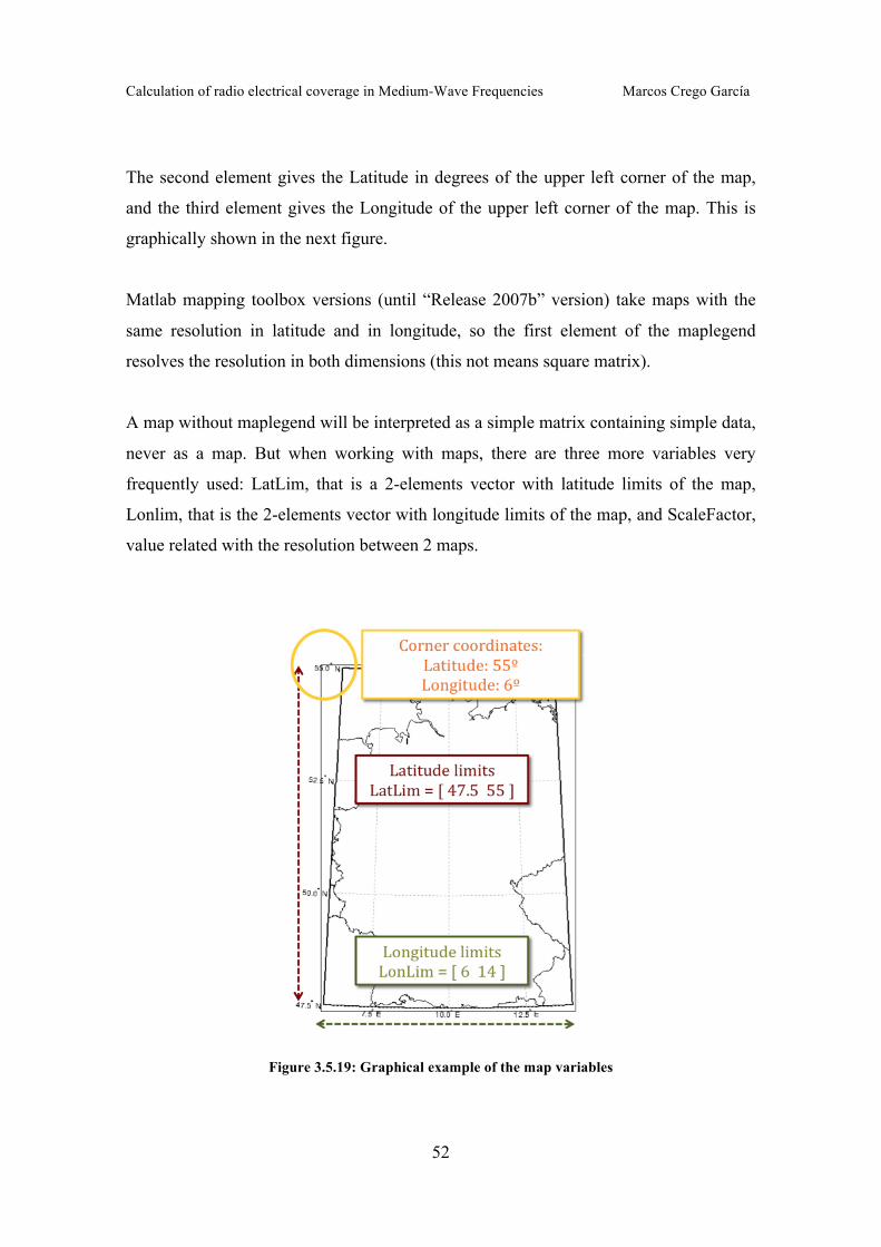
The second element gives the Latitude in degrees of the upper left corner of the map,
and the third element gives the Longitude of the upper left corner of the map. This is
graphically shown in the next figure.
Matlab mapping toolbox versions (until “Release 2007b” version) take maps with the
same resolution in latitude and in longitude, so the first element of the maplegend
resolves the resolution in both dimensions (this not means square matrix).
A map without maplegend will be interpreted as a simple matrix containing simple data,
never as a map. But when working with maps, there are three more variables very
frequently used: LatLim, that is a 2-elements vector with latitude limits of the map,
Lonlim, that is the 2-elements vector with longitude limits of the map, and ScaleFactor,
value related with the resolution between 2 maps.
Figure 3.5.19: Graphical example of the map variables
Calculation of radio electrical coverage in Medium-Wave Frequencies Marcos Crego García
53
3.5.5.2 Resolution of a Map
Another important question is how to calculate the resolution in degrees or kilometres
of one map. If the map has been obtained from GLOBE to maximum resolution, then,
by the characteristics of GLOBE, it is known that the resolution is 1 km and 120 cells
per degree.
To calculate the resolution of any map, the maplegend is the only element needed to
calculate the resolution in degrees or in Km of a map. So on, the resolution in degrees
can be calculated as:
Resolution (º) = 1/maplegend(1) (3.5.5.2.1)
And the resolution in Km can be calculated using Mapping Toolbox as:
Resolution (Km) = deg2km( Resolution(º) ) (3.5.5.2.2)
Functions referring to maps used to have a common header structure with the variables
seen before. In this project, most used dealing with maps were:
Globedem: Load GLOBE maps from a directory.
Resizem: Resize a map with a scale factor or to a size desired.
Mapprofile: Given two points inside a map, create the interpolation line joining
them, with distances, latitudes and longitudes of each them.
Maptrims: Trims an area from a bigger map.
Setltln: Given a position in a matrix by its row and column, this function returns
its latitude and longitude.
Setpostn: Given a latitude and longitude, returns the position in the matrix as
row and column.

Calculation of radio electrical coverage in Medium-Wave Frequencies Marcos Crego García
54
3.5.5.3 Most used functions
Some examples of the most important functions for this application are:
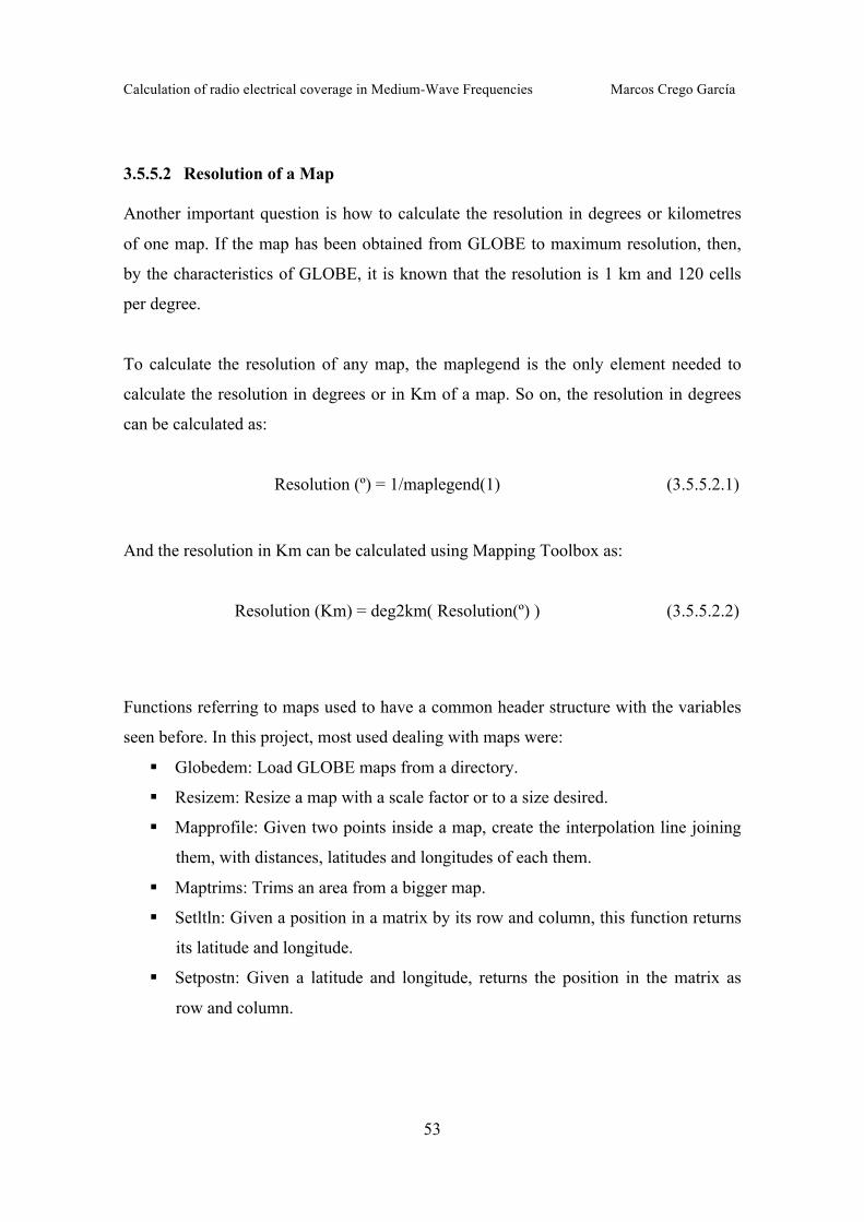
a. Mapprofile: [ z, d, lat, lon ] = mapprofile(map,maplegend, Lat, Lon, method)
This useful function creates the interpolated line between a receiver and a
transmitter to calculate the paths for Millington. Both Lat and Lon are 2-elements
vector containing the information of both latitude and longitude of the two point to
join with a interpolated line. In this project, these two points used to be the
transmitter and the receiver, so these two vectors used to have the sintaxis:
Lat = [ latTX latRX];
Lon = [ lonTX lonRX];
Method is the interpolation method to be used, that can be nearest, bilinear or
bicubic. In case of conductivities, values are fixed, so ‘nearest’ is the interpolation
needed. In case of elevation profiles, it should be more accurate interpolate the
value of height at one point with another method. Bilinear method has been chosen
in this case.
The values returned are:
z: A vector of interpolated values between transmitter and receiver. The origin of
the data contained in this vector (conductivities, elevations, etc.) depends on the
map over this function is applied. If the map is elevation map, z will be an elevation
vector.
d: Vector of distances of every point of z to the first point located in vectors Lat and
Lon, in this case, the transmitter.
lat and lon: Similar to d, but containing the latitude and longitude over the map of
each element of z.
Calculation of radio electrical coverage in Medium-Wave Frequencies Marcos Crego García
55
Figure 3.5.20: Example of mapprofile
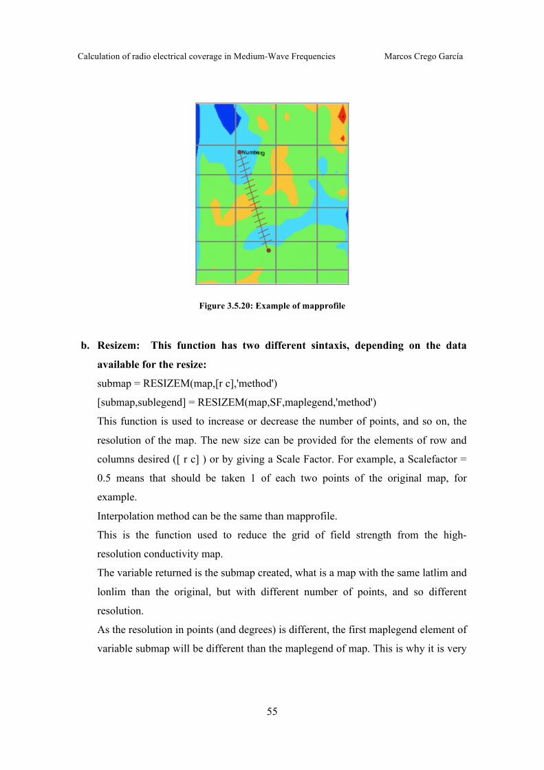
b. Resizem: This function has two different sintaxis, depending on the data
available for the resize:
submap = RESIZEM(map,[r c],'method')
[submap,sublegend] = RESIZEM(map,SF,maplegend,'method')
This function is used to increase or decrease the number of points, and so on, the
resolution of the map. The new size can be provided for the elements of row and
columns desired ([ r c] ) or by giving a Scale Factor. For example, a Scalefactor =
0.5 means that should be taken 1 of each two points of the original map, for
example.
Interpolation method can be the same than mapprofile.
This is the function used to reduce the grid of field strength from the high-
resolution conductivity map.
The variable returned is the submap created, what is a map with the same latlim and
lonlim than the original, but with different number of points, and so different
resolution.
As the resolution in points (and degrees) is different, the first maplegend element of
variable submap will be different than the maplegend of map. This is why it is very
Calculation of radio electrical coverage in Medium-Wave Frequencies Marcos Crego García
56
recommendable calling resizem in the second format to return the new sublegend
(or submap-legend).
Figure 3.5.21: Example of resizem
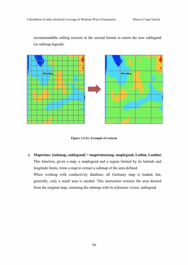
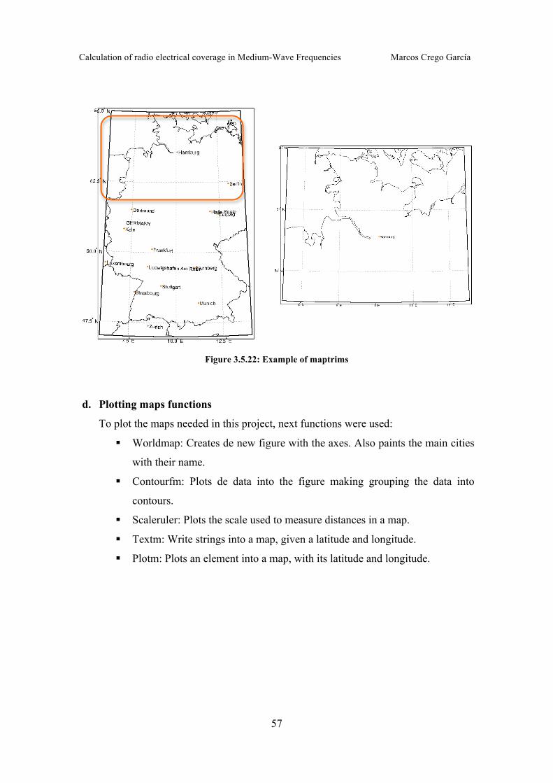
c. Maptrims: [submap, sublegend] = maptrims(map, maplegend, Latlim, Lonlim)
This function, given a map, a maplegend and a region limited by its latitude and
longitude limits, trims a map to extract a submap of the area defined.
When working with conductivity database, all Germany map is loaded, but,
generally, only a small area is needed. This instruction extracts the area desired
from the original map, returning the submap with its reference vector, sublegend.
Calculation of radio electrical coverage in Medium-Wave Frequencies Marcos Crego García
57
Figure 3.5.22: Example of maptrims
d. Plotting maps functions
To plot the maps needed in this project, next functions were used:
Worldmap: Creates de new figure with the axes. Also paints the main cities
with their name.
Contourfm: Plots de data into the figure making grouping the data into
contours.
Scaleruler: Plots the scale used to measure distances in a map.
Textm: Write strings into a map, given a latitude and longitude.
Plotm: Plots an element into a map, with its latitude and longitude.
Calculation of radio electrical coverage in Medium-Wave Frequencies Marcos Crego García
58
e. Unit conversion functions and others:
Mapping Toolbox also has several functions to convert from one format to another,
as:
Deg2km: Converts degrees to km.
Str2deg: Converts a string 00d00m00sN (for example) into latitude in
degrees.
Distance: Measures distance in degrees from two elements given by their
latitude and longitude.
Time2str: Converts timing format to a string.
Etime: Calculates the difference between two time vectors in seconds.
3.5.5.4 Application function LOADMAP
The application has to load several maps. Most of the requests to maps are done in the
function loadmap, so here will be explained an extraction of its code to show how to
deal with maps.
In the first instance, database must be loaded. The database selected by user is stored in
the variable Country, which can take the values of Germany, Korea or other. In the two
first cases, high-resolution databases will be loaded. In any other case, low-resolution
will be the one selected.
So, loadmap, first check, with a case sentence, the value of the variable ‘Country’ to
load one database or the other, as shown in the figure below.
Calculation of radio electrical coverage in Medium-Wave Frequencies Marcos Crego García
59
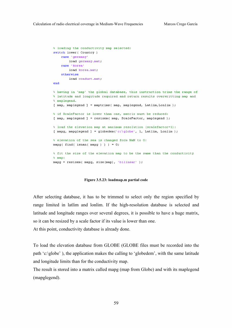
Figure 3.5.23: loadmap.m partial code
After selecting database, it has to be trimmed to select only the region specified by
range limited in latlim and lonlim. If the high-resolution database is selected and
latitude and longitude ranges over several degrees, it is possible to have a huge matrix,
so it can be resized by a scale factor if its value is lower than one.
At this point, conductivity database is already done.
To load the elevation database from GLOBE (GLOBE files must be recorded into the
path ‘c:\globe’ ), the application makes the calling to ‘globedem’, with the same latitude
and longitude limits than for the conductivity map.
The result is stored into a matrix called mapg (map from Globe) and with its maplegend
(mapglegend).
Calculation of radio electrical coverage in Medium-Wave Frequencies Marcos Crego García
60
GLOBE database marks the sea level as a NaN to differentiate from the rest of the
elevations. We need to work with entire numbers, so it is needed to change the NaN by,
for example, a zero. This is made with the instruction find to locate de index having a
NaN.
To be accurate, it is needed that elevation map and conductivity map have the same
resolution, rows and columns. So this is why the last instruction is included: to resize
GLOBE map to the same size than the conductivity map.
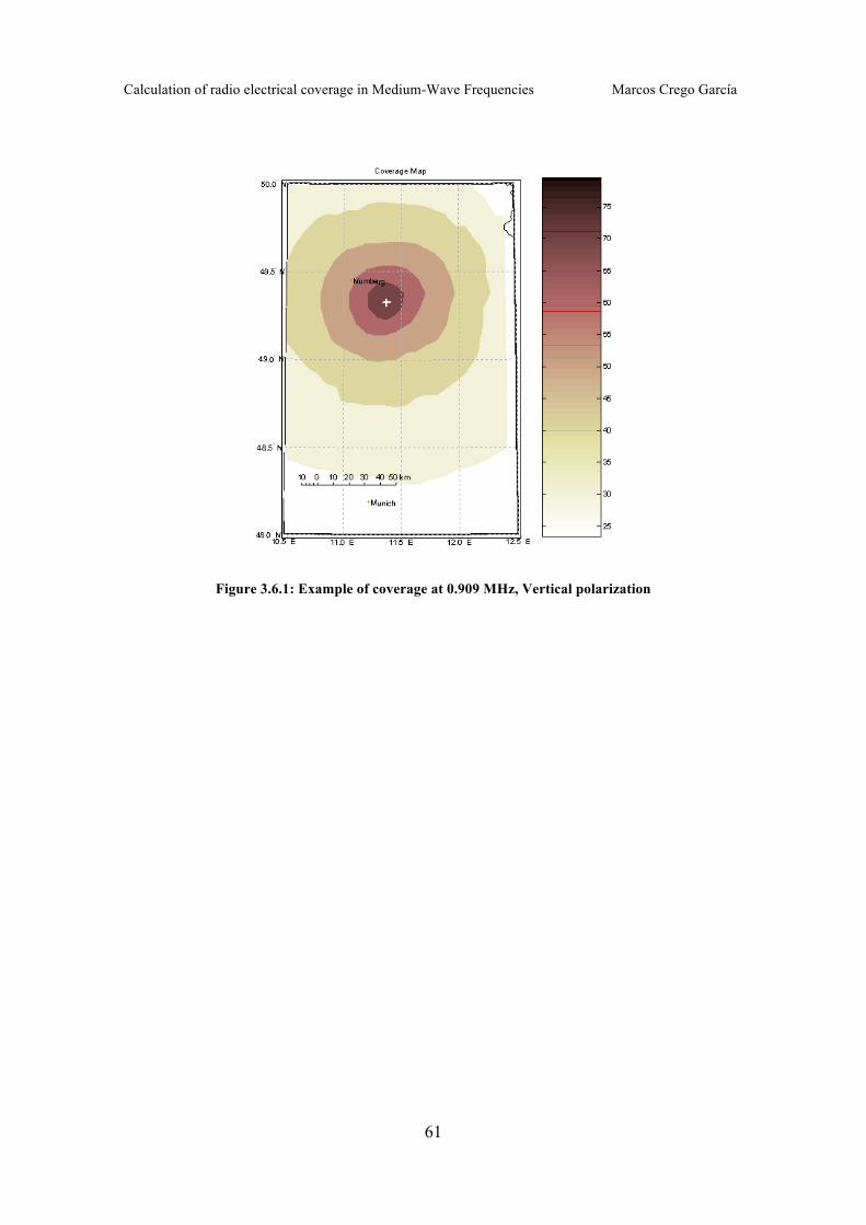
3.6 Practical examples
The Groundwave propagation is very important in the lowest part of the frequency band
and in vertical polarization. To demonstrate those facts, lets compare the coverage
results in both cases with a practical example.
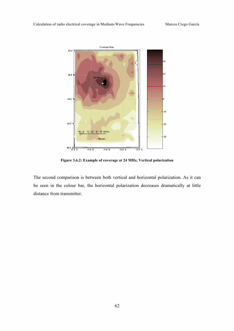
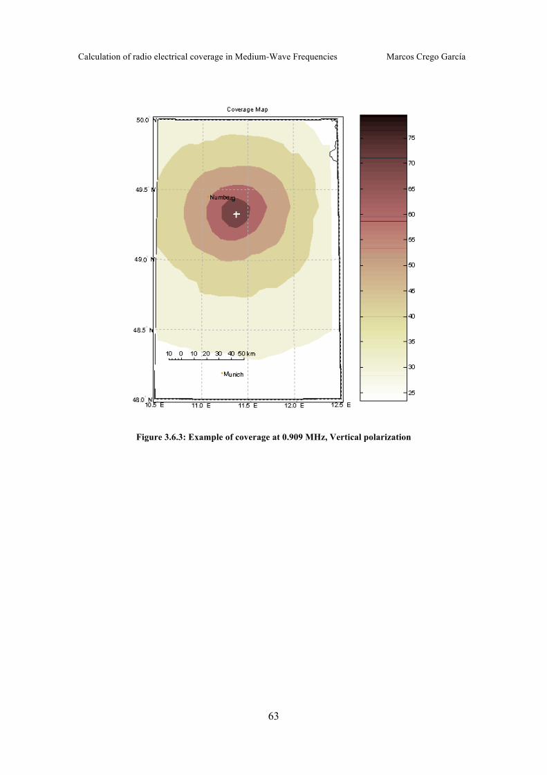
At the first instance, the coverage for low and high frequencies is compared. The figures
below show that at low frequencies, the effect of the conductivity and/or the elevation
of the terrain and antennas are negligible. But, as the frequency is increased, both
effects turn important and coverage is reduced dramatically.
As the colours of the map are relative, there is attached the colour bar to indicate the
field strength assigned to each colour.
Calculation of radio electrical coverage in Medium-Wave Frequencies Marcos Crego García
61
Figure 3.6.1: Example of coverage at 0.909 MHz, Vertical polarization
Calculation of radio electrical coverage in Medium-Wave Frequencies Marcos Crego García
62
Figure 3.6.2: Example of coverage at 24 MHz, Vertical polarization
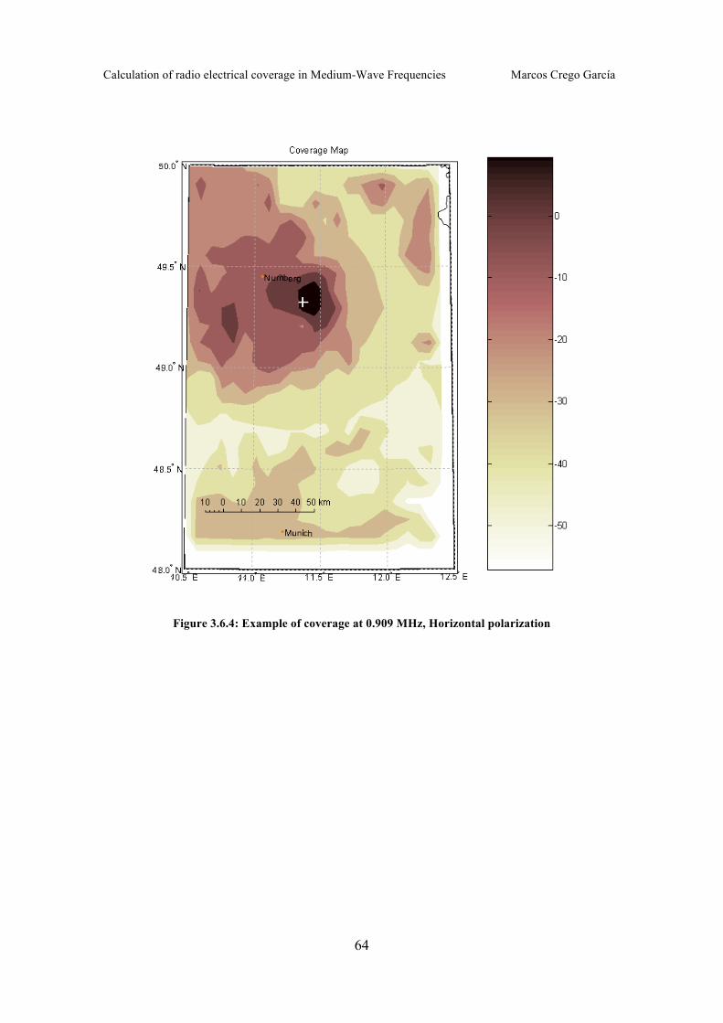
The second comparison is between both vertical and horizontal polarization. As it can
be seen in the colour bar, the horizontal polarization decreases dramatically at little
distance from transmitter.
Calculation of radio electrical coverage in Medium-Wave Frequencies Marcos Crego García
63
Figure 3.6.3: Example of coverage at 0.909 MHz, Vertical polarization
Calculation of radio electrical coverage in Medium-Wave Frequencies Marcos Crego García
64
Figure 3.6.4: Example of coverage at 0.909 MHz, Horizontal polarization
Calculation of radio electrical coverage in Medium-Wave Frequencies Marcos Crego García
65
4 Conclusions
The software developed fits with all the objectives:
Matlab interface for GRWAVE has been done.
Fitting to the ITU-R Recommendations.
o With homogeneous paths
o With non-homogeneous paths and Millington method
o With frequency and elevation ITU-R limits.
Calculate areas of coverage fields due to a single transmitter operating in a site.
Calculate field strength at single points (receivers) due to one or several
transmitters.
Checking in case of several transmitters if there should be ISI at one point or
not.
Printing data at the screen when needed.
A graphical interface make the application easy-to-use.
Saving data at binary .mat files to be able to load them after the simulation is
done in Matlab to have a data post-process.
Radioelectrical conclusions obtained from the data observed from several simulations
are:
Vertical polarization is stronger than horizontal polarization in every path and
distance between transmitter and receiver.
At low frequencies elevation and conductivity terrain is negligible and coverage
diagrams are very rounded.
At high frequencies conductivity and elevation affect strongly to the
Groundwave propagation, and distance of coverage (and so, field strength) is
reduced dramatically in comparison to low frequencies.
Antenna elevation has its influence over the field calculated, so the transmitter
site must be the highest site inside the area of coverage.
Calculation of radio electrical coverage in Medium-Wave Frequencies Marcos Crego García
66
5 Future guidelines
This project could be expanded in several ways:
Adding more countries to the high-resolution conductivity database. This point
was not made at this Project due to time restrictions.
Matlab is optimized to work with matrix. Dealing with files at the main function,
GRWAVE decreases dramatically the application speed. This could be solved
partially modifying GRWAVE source code in Fortran, and making a MEX file
to be able to work with a binary DLL at Matlab, instead of working with files.
The application has been developed in Matlab, and, right now, Matlab 7 R14 is
needed to be executed. Another improvement should be assembling a .EXE file
to make the application independent from Matlab.
Add tools for DRM Calculations or for any other specific system working in this
frequency band.
All this improvements have not been made at this project by time restrictions.
Calculation of radio electrical coverage in Medium-Wave Frequencies Marcos Crego García
67
6 Bibliography and references
[CONDUCT]
BRUMMER, Walter. Über die Ausbreitung von Lang- und Mittelwellen. Germany
conductivity image map in HF Frequencies to be load as a database.
http://members.aon.at/wabweb/radio/grundl3.htm
(Consultation: November 2008)
[COMMERCIALFM]
MOLLO, J.C. Campos electromagnéticos. Determinación de la zona de protección a las
personas por transmisiones de FM comerciales. INTI- Electrónica e Informática.
http://www.inti.gov.ar/sabercomo/sc23/inti9.php
(Consultation: December 2008)
[DRM]
MATÍAS, José María. La Radio Digital Terrestre en Europa Eureka 147 y DRM”.
www.sincompromisos.com/Documentos/Radiocomunicacion/Radio-Digital-
Terrestre.pdf
(Consultation: December 2008)
Calculation of radio electrical coverage in Medium-Wave Frequencies Marcos Crego García
68
[GLOBE]
THE GLOBAL LAND ONE-KM BASE ELEVATION PROJECT (GLOBE). A 30-arc-second
(1-km) gridded, quality-controlled global Digital Elevation Model (DEM). NOAA.
http://www.ngdc.noaa.gov/mgg/topo/globe.html
(Consultation: October 2008)
[GRWAVE]
GRWAVE USER MANUAL. Software concerning Tropospheric Propagation: Ground-
wave propagation (GRWAVE). International Telecommunication Union,
Radiocommunication Sector (ITU-R), Study Group 3 (SG 3) - Radiowave propagation.
http://www.itu.int/ITU-R/index.asp?category=documents&link=rsg3&lang=en
(Consultation: October 2008)
[ITU-R P.368-9]
ITU-R P.368-9 RECOMMENDATION. “Ground-wave propagation curves for frequencies
between 10 kHz and 30 MHz”. Approved on February 2007 (in force).
[ITU-R P.832-2]
ITU-R P.832-2 RECOMMENDATION. “Atlas mundial de la conductividad del suelo”.
Approved on July 1997 (in force).
Calculation of radio electrical coverage in Medium-Wave Frequencies Marcos Crego García
69
[MATLAB]
MATHWORKS. Mapping Toolbox User’s Guide: Analyze and visualize geographic
information.
http://www.mathworks.com/access/helpdesk/help/toolbox/map/
(Consultation: October 2008)
Calculation of radio electrical coverage in Medium-Wave Frequencies Marcos Crego García
70
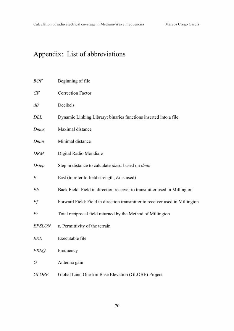
Appendix: List of abbreviations
BOF Beginning of file
CF Correction Factor
dB Decibels
DLL Dynamic Linking Library: binaries functions inserted into a file
Dmax Maximal distance
Dmin Minimal distance
DRM Digital Radio Mondiale
Dstep Step in distance to calculate dmax based on dmin
E East (to refer to field strength, Et is used)
Eb Back Field: Field in direction receiver to transmitter used in Millington
Ef Forward Field: Field in direction transmitter to receiver used in Millington
Et Total reciprocal field returned by the Method of Millington
EPSLON ε, Permittivity of the terrain
EXE Executable file
FREQ Frequency
G Antenna gain
GLOBE Global Land One-km Base Elevation (GLOBE) Project
Calculation of radio electrical coverage in Medium-Wave Frequencies Marcos Crego García
71
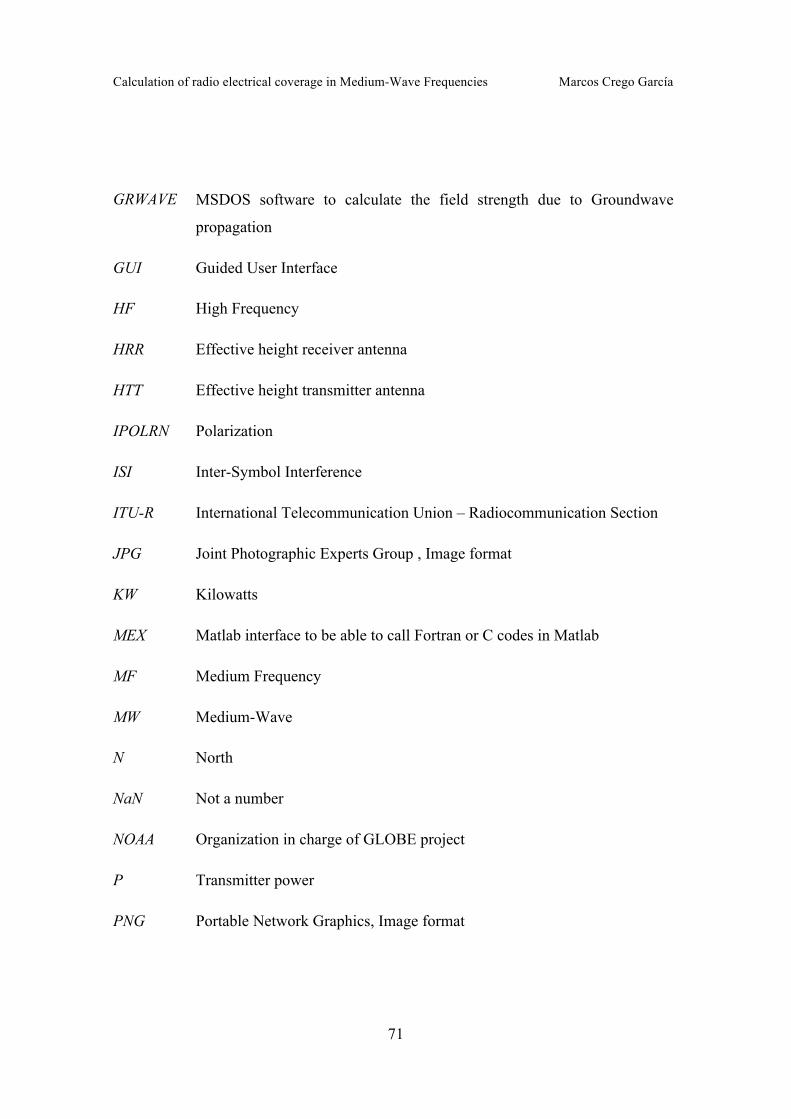
GRWAVE MSDOS software to calculate the field strength due to Groundwave
propagation
GUI Guided User Interface
HF High Frequency
HRR Effective height receiver antenna
HTT Effective height transmitter antenna
IPOLRN Polarization
ISI Inter-Symbol Interference
ITU-R International Telecommunication Union – Radiocommunication Section
JPG Joint Photographic Experts Group , Image format
KW Kilowatts
MEX Matlab interface to be able to call Fortran or C codes in Matlab
MF Medium Frequency
MW Medium-Wave
N North
NaN Not a number
NOAA Organization in charge of GLOBE project
P Transmitter power
PNG Portable Network Graphics, Image format
Calculation of radio electrical coverage in Medium-Wave Frequencies Marcos Crego García
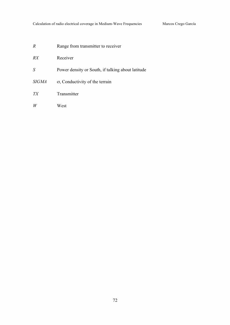
72
R Range from transmitter to receiver
RX Receiver
S Power density or South, if talking about latitude
SIGMA σ, Conductivity of the terrain
TX Transmitter
W West