CALCULATING TRANSPORT CONGESTION ANDSCARCITY COSTS

FINAL REPORT OF THE EXPERT ADVISORS TO THEHIGH LEVEL GROUP ON INFRASTRUCTURE CHARGING

(WORKING GROUP 2)

MAY 7 1999

This report was prepared by Professor Chris Nash and Mr TomSansom, (ITS) and finalised in agreement with the other experts inthe group including:

Dr JohnDodgsonNERA, UK

Professor RainerFriedrichIER, Germany

Dr LarsHanssonResearch LeaderIIIEE , Lund UniversitySweden

Professor ChrisNashITS, Leeds UniversityLeeds, UK

Dr MarkusPennekampDeutsche Bahn AGGermany

Mr StephenPerkinsECMT, France

Professor StefProostCenter for EconomicStudiesKatolische UniversiteitLeuven, Belgium

Professor RémyPrud’hommeUniversité Paris XIIFrance

Professor EmileQuinetEcole Nationale Pontset ChausséesFrance

Dr AndreaRicciISIS, Italy

Professor Dr WernerRothengatterInst. for EconomicPolicy Research(IWW), University ofKarlsruheKarlsruhe, Germany

Dr RanaRoyAdviserInternational Union ofRailwaysUK

Professor MichelSavyENPCFrance

Meetings were chaired by Professor Phil Goodwin, member of the HighLevel Group.

3

TABLE OF CONTENTS

SUMMARY AND RECOMMENDATIONS............................................................................................................ 4

INTRODUCTION....................................................................................................................................................... 8

1. ROAD CONGESTION ................................................................................................................................... 10

RECOMMENDATIONS................................................................................................................................ 15

2. CONGESTION AND SCARCITY COSTS OF RAIL....................................................................................... 15

RECOMMENDATIONS..................................................................................................................................... 17

3. MONETARY VALUATION................................................................................................................................ 17

RECOMMENDATIONS...................................................................................................................................... 20

4. CONCLUSIONS.............................................................................................................................................. 21

REFERENCES.......................................................................................................................................................... 21

ANNEX A: EXAMPLES OF SPEED FLOW RELATIONS AND CONGESTION COSTS.......................... 24

ANNEX B: TYPICAL VALUES OF TIME (PETS D7) .................................................................................... 29

4

SUMMARY AND RECOMMENDATIONS

Efficient pricing requires that prices reflect social marginal cost. To implement this, it isnecessary that estimates be made of all the elements of social marginal cost. The current reportaims to advise on the best approach to estimate external congestion and scarcity costs for roadand rail infrastructure. This requires a method of forecasting the increase in journey time andunreliability for other traffic caused by an increase in traffic on the mode in question, and thenplacing appropriate money values on them. These values vary with vehicle type, road type andtime of day, and thus fully reflecting them in prices requires price mechanisms which canthemselves vary in these dimensions. Although it is outside our remit to consider the issue ofimplementation in detail, we consider that a combination of electronic road pricing in congestedcities and on congested trunk roads, fuel tax and annual licence duty (and possibly electronickilometre-based changes for certain vehicle categories) is capable of achieving a reasonableapproximation to marginal social cost.

In the case of rail, as with other types of transport infrastructure where specific slots are allocatedto particular users, the major issue is not so much congestion as the scarcity value of slots; whenthe infrastructure approaches capacity, other users are unable to obtain the slot they want.Whereas for road, keeping track of the use of the infrastructure by all individual users is a majorproblem, for rail the information is readily available to the infrastructure manager. It is thereforeassumed that there is no great practical difficulty in implementing complex pricing structures forrail infrastructure - including two part tariffs or individually negotiated contracts - if this isdesired.

It is not the task of this paper to review the arguments for and against marginal social costpricing. However, we acknowledge that a number of issues other than economic efficiency, suchas distributional effects, implementation costs and acceptability must be considered before suchan approach is implemented. The degree of accuracy to which it is worth reflecting marginalsocial cost in price for roads must always be the subject of a cost-benefit analysis, given therelatively high implementation costs of electronic road pricing. Recent studies have shown netbenefits from road pricing in London of £225m per annum after allowing for implementationcosts (MVA, 1995), and of 2.5 billion francs per year before implementation costs in Paris(Prud'homme, 1999). Whilst these figures suggest that investments in these measures show veryhigh benefit-cost ratios relative to other transport investments in large cities, they are an order ofmagnitude smaller than the often quoted but irrelevant figure of the total cost of congestion as2% of GDP.

The environmental and safety implications of road congestion are not considered here as they arecovered in the reports of other working groups.

The recommendations are grouped into three areas:

1. Forecasting road congestion and unreliability.

The requirement here is not simply to be able to estimate the impact on other road usersof an additional vehicle at existing traffic levels. Rather it is necessary also to be able toforecast how road users would adapt to being charged for these costs, in order to find an

5

equilibrium combination of charges and traffic levels. Bearing this in mind, we make thefollowing recommendations:

1.1 Wherever possible, external road congestion costs should be estimated from a modelwhich simulates the interaction of demand and supply on the road network. The modelcan then be used to approximate the marginal external costs of congestion by rerunning itwith small changes in traffic volumes, and examining the effects on journey time forexisting traffic. This model would ideally incorporate a detailed network description, withboth speed/flow relationships and junction delays, and allow for user behaviour in termsof rerouteing, retiming, changing destination or mode or changing frequency of travel, inorder to obtain a new set of flows and journey times following imposition of a charge.Data is therefore required on the base origin/destination matrix, base generalised costsand responses to changes in these values. The calculation of generalised cost requiresknowledge of operating costs, values of time and vehicle occupancy rates. Only when thecharge is equal to the marginal external cost in this new position has the optimal level ofcharge and traffic been found.

1.2 Where this is not possible, we recommend that calculations are undertaken for typicalinter urban or rural roads at alternative traffic levels and mixes of vehicle types using linkspeed/flow relationships. Separate calculations will be needed according to the type ofroad (number of lanes; motorway or conventional road). Again, data on base traffic flowsand generalised costs are needed, and traffic volumes should again be adjusted for theintroduction of charges, if necessary by means of a simple price elasticity of demand, inorder to obtain an equilibrium value.

1.3 For urban areas, the degree of interaction between roads means that such anapproximation will be particularly crude. If a full network model is not available, the useof area speed/flow relationships relating to the entire network for central, inner and outerurban areas is likely to be preferable to link based speed/flow relationships.

1.4 Forecasting the impact of increased traffic on unreliability is more difficult, but given theimportance of the issue it should be attempted wherever possible. A variety of approachesexists, including the use of micro-simulation models which model individual vehicles andcan thus estimate the spread of journey times, and purely empirical approaches, whichrequire data on unreliability and on traffic flows for a set of roads over time.

1.5 All the above relationships should relate to local conditions in the area concerned, andrelate to conditions such as driving styles and typical speeds in that location. It would becounter-productive therefore to attempt to specify Europe-wide relationships, althoughresults may with care be transferred from comparable situations elsewhere in Europe iflocal information is not available.

2. Forecasting rail delays and scarcity values

Fundamentally the approach we take to pricing on rail is consistent with ourrecommendations on road. That is we seek to reflect in the price all the social costsimposed by the operator on the rest of society by the use of a particular slot. However, inpractice there are significant differences. Given the fact that specific slots are allocated toparticular operators on rail infrastructure, the main effect of excess demand is notcongestion as such, but the inability of particular operators to obtain the slots they want.The element of social cost to which this gives rise is the 'scarcity value' of the slot - i.e. its

6

value in the next best use. This cost is strictly only an externality however where it isborne by another operator; when the next best use is by the same operator the cost shouldbe already internalised in that - provided they are efficient - they will already haveassessed the alternative uses of the slot. There is no general way of calculating this'scarcity value' from information about the volume of traffic and the characteristics of theroute. This means that a rather different approach is needed to the estimation of themarginal social cost of rail infrastructure from that taken in the case of roads.

2.1 Estimation of the scarcity value of specific slots on rail infrastructure requires a way ofrevealing the value placed on the slots by alternative possible users, both in terms ofcommercial rail operators and in terms of government bodies wishing to provide socialservices. It may be possible in some cases to reveal these values by auctioning the slots,but given the complexities involved in terms of the alternative ways in which theinfrastructure may be used, this is difficult. Some pre-packaging of slots is probablynecessary, in order to offer attractive combinations to alternative bidders. In general, aprocess of negotiation appears the most practicable way forward. This might work interms of train operators first registering their wishes, the infrastructure manager usingthese to produce packages of paths and charges and further negotiation then taking placeto determine whether operators would be prepared to pay more to improve their package,or to surrender some of their paths in return for a reduced charge. Such negotiationswould also naturally encompass investment in expanded or enhanced capacity and thesharing of the development costs.

2.2 Unscheduled delays imposed by one train operator on another may be measured ex post ifadequate monitoring is undertaken to measure both the extent and the cause of delays.However, this will only measure the delays directly caused and not those where thepresence of the additional train has worsened the consequences of other delays byabsorbing part of the recovery margin. It is therefore more accurate to measure anticipateddelays by simulation modelling and charge these as part of the tariff. Of course theseadditional delays will vary by route, type of train and time of day.

3. Monetary valuation

Changes in speed may lead to changes in operating costs in terms of fuel, tyres andbrakes. This may be estimated from appropriate formulae, and converted to resource costby deducting taxes. But the main effects of congestion and unreliability are in terms of thetime of people, poorer utilisation of vehicles and delays to the goods they carry. In allcases, values for these must be converted to per-vehicle values (e.g. for passengers, byweighting by the occupancy of vehicles).

3.1 For staff working in the transport industry, the usual approach of estimating the marginalcost of their time as their wage rate plus an allowance for the overhead costs of employinglabour is generally appropriate. Similarly, the costs of poorer vehicle utilisation may beestimated by calculating the impact on fleet size of the delay, and the additional interestand depreciation costs of a larger fleet.

3.2 For other staff who travel in the course of their work, a more sophisticated approach,which takes account of factors such as their ability to work on route, the fact that part oftheir journey time may be at the expense of leisure time and the fact that the length of

7

their journey time may affect their productivity later in the day, is needed. Appropriateformulae exist, and a number of studies have made estimates of the elements involved.

3.3 Values of commuting and leisure time should be based on empirical evidence, andsegmented by variables such as journey purpose, length, mode and income of travellers,whenever evidence of significant variation by this variable exists. A large number ofstudies, using revealed and stated preference methods, exists, and both methods appearcapable of producing reliable results when used with care.

3.4 The evidence that travelling in congested conditions produces higher values of time thanin uncongested conditions requires particularly careful examination because of itsimportance in the current context.

3.5 Empirical estimates also exist, and should be used, for valuing time spent waiting forpublic transport, late arrivals and the difference between desired departure time and thetime at which the service actually departs. All may be affected by congestion or scarcityof slots.

3.6 As a first approximation, values of time for passengers may reasonably be assumed toincrease over time in proportion with income. The value of marginal external cost ofcongestion will also need to be updated for changes in traffic volumes, infrastructurecapacity, technology and operating cost.

3.7 Valuations of time for freight consignments for which transit time is increased, or mademore unreliable, are an important component of social costs, and should be based onempirical estimation (using revealed and/or stated preference methods) rather than thealternative approach which is in use, which is to make estimates of the interest cost ofstock in transit.

8

INTRODUCTION

The background to this report is the conclusion of the Commission in its White Paper oninfrastructure pricing, and following the deliberations of the High Level Group on infrastructurepricing, that social marginal cost pricing of infrastructure is the most efficient policy to follow.However, in order to implement this conclusion, practical methods of estimating social marginalcosts are needed. The scope of this report is to consider alternative ways of estimating the costsof congestion and scarcity that are relevant for the pricing of existing transport infrastructure.

Detailed consideration of the resulting price structure, and of the implications of this for equity,or of considerations such as administrative costs of pricing systems and of the implications ofsecond best theory, are outside the scope of this report. However, it should be noted that for roadcharging, because the value of marginal social cost varies with vehicle type, road type and timeof day, full implementation of marginal social cost pricing requires a pricing system that can alsovary in these dimensions. We consider that a combination of electronic road pricing in congestedcities and on congested trunk roads, fuel tax and annual licence duty (and possibly electronickilometre-based changes for certain vehicle categories) is capable of achieving a reasonableapproximation to marginal social cost.

In the case of rail, as with other types of transport infrastructure where specific slots are allocatedto particular users, the major issue is not so much congestion as the scarcity value of slots; whenthe infrastructure approaches capacity, other users are unable to obtain the slot they want.Whereas for road, keeping track of the use of the infrastructure by all individual users is a majorproblem, for rail the information is readily available to the infrastructure manager. It is thereforeassumed that there is no great practical difficulty in implementing complex pricing structures forrail infrastructure - including two part tariffs or individually negotiated contracts - if this isdesired.

It is not the task of this paper to review the arguments for and against marginal social costpricing. However, we acknowledge that a number of issues other than economic efficiency, suchas distributional effects, implementation costs and acceptability must be considered before suchan approach is implemented. The degree of accuracy to which it is worth reflecting marginalsocial cost in price for roads must always be the subject of a cost-benefit analysis, given therelatively high implementation costs of electronic road pricing. Recent studies have shown netbenefits from road pricing in London of £225m per annum after allowing for implementationcosts (MVA, 1995), and of 2.5 billion francs per year before implementation costs in Paris(Prud'homme, 1999). Whilst these figures suggest that investments in these measures show veryhigh benefit-cost ratios relative to other transport investments in large cities, they are an order ofmagnitude smaller than the often quoted but irrelevant figure of the total cost of congestion as2% of GDP.

The environmental and safety implications of road congestion are not considered here as they arecovered in the reports of other working groups..

In contrast to the case of environmental externalities, congestion and scarcity costs are internal tothe transport sector as a whole. They are of concern in the current context not because they areunpriced, but because existing ways of pricing for the use of transport infrastructure areinadequate. The result is that additional users of transport infrastructure may well imposeexternalities on other transport users, as well as experiencing congestion themselves.

9

It is very important to distinguish between this external element of the cost of congestion orscarcity and total or average congestion cost. It is sometimes argued that the total cost ofcongestion is borne by the sum of users themselves. The point, however, is that, in a situation ofcongestion, each additional user inflicts costs on other users as well as suffering costs himself orherself. It is this external element – that inflicted by one user on other users – that is relevant forpricing purposes.

A further reason why estimates of total congestion costs are not helpful for pricing purposes isthat congestion costs vary enormously in time and space. It is thus necessary to prepare estimatesof the marginal external cost of congestion for various circumstances. For roads, we might thinkin terms of a three way categorisation e.g.

- location: inner city, outer city, other urban area, inter urban, rural

- type of road: motorway, dual carriageway, single carriageway

- time of day: peak, inter peak, off peak

How many categories to adopt depends on a trade off between the accuracy with which costs arereflected in prices and the cost and complexity of the pricing instruments.

For railway lines, and other infrastructure on which specific slots are prebooked, no such simplecategorisation is likely to be helpful, as discussed in section 2 below.

A key distinction must be made between infrastructure where access is open to anyone withoutprebooked slots, as is the case with roads, and infrastructure where pre-booking of specific slotsis required, such as railways, airports and ports. For roads, increased demand materialises asmore traffic coming on to the road. Beyond a certain level, the result is reduced speeds andqueuing at junctions and other bottlenecks; in other words congestion. In congested conditions,there is a clear externality involved, as additional road users delay others.

For systems where access takes the form of allocation of specific slots, the situation is verydifferent. It may still be the case that additional users impose costs on existing users by causingdelays, and indeed delays do become more common the closer the system is to capacity. But thekey point on a scheduled system is that as it approaches capacity some users are unable to get theslots or run to the schedules they want. As a result, slots acquire scarcity value. Strictly, this isonly an externality where the competition for slots is between different train operatingcompanies; otherwise it is already internalised. However, with separation of infrastructure fromoperations now a part of European Rail Policy, this situation is becoming more common, andpricing of rail infrastructure therefore needs to take it into account. Of course, congestion mayalso take place on trains themselves, leading to a case for taking this into account in prices tofinal users, but that is outside the scope of this note.

For both road and rail systems one obvious reaction to shortages of capacity is to invest in newcapacity. One approach to marginal cost pricing would be to try to estimate the costs of capacityexpansion caused by additional traffic. However, this is inclined to vary enormously with theprecise circumstances and the extent of the capacity expansion required. Charging this amountwill also lead to misallocation of the existing infrastructure capacity during the (often long) timeperiod before the capacity is adjusted.

10

The approach adopted by the Commission, correctly in our view, is to examine the costs ofadding additional traffic to the existing infrastructure. This is consistent with the short runmarginal cost approach taken by Working Group 1, on infrastructure costs, which does notinclude the capital costs of infrastructure expansion. It should be stressed however that anoptimal outcome requires that such capacity expansion takes place whenever the benefits ofdoing so exceed the costs. The result is that charges will adjust according to the level of capacity;as investment takes place on a congested road other things being equal, optimal charges will fall,whereas traffic growth on currently uncongested roads may cause the optimal charge to rise.

This note considers first road congestion, then rail congestion and scarcity values and finally thecrucial issue of value of time. Ports and airports are not considered further, although many of thesame issues arise, and indeed there is a much greater literature on slot allocation at airports thanexists for rail systems.

1. ROAD CONGESTION

External congestion costs occur when the presence of one vehicle increases the journey time ofanother. This phenomenon may happen for two distinct reasons as traffic builds up. Firstly,increased traffic density obliges drivers to drive more slowly simply because the gap betweenvehicles is reduced. Secondly, queuing may occur at junctions or other bottlenecks. The standardway of estimating levels of congestion for inter-urban roads is via the use of speed-flow curves.Estimated speed/flow curves differ with the characteristics of the road (number of lanes, lanewidth, urban or rural etc). Frequently – as in the COBA manual (UK DOT, 1996) used for cost-benefit analysis of road schemes in Britain - they are estimated as a series of linear segmentsaccording to the traffic level on the road as well. The COBA manual suggests speed-flow curveswhich consist of two linear segments, with a steeper slope of the segment at higher flow levelsindicating that at higher densities additional vehicles have a greater impact on reducing speeds.Some difficulties with this relationship are that:

� the relationship breaks down near capacity (e.g. for COBA it is undefined below 40kph);

� this is the most important segment for charging purposes – it is where charges risesteeply and the role of charging is most important and effective1.

Thus, a more appropriate speed-flow relationship will be non-linear, or have a large number oflinear segments to enable the approximation of non-linear relationships.

Most countries will have estimated speed-flow relationships to suit their own situation in termsof road characteristics, topography and driving styles, and we do not consider that it would besensible to try to adopt a single set of speed flow curves throughout Europe (see Annex A).

Particularly in urban areas, however, heavily congested roads are almost always the result ofbottlenecks. These bottlenecks are frequently due to junctions but also sections with steep

1 For more complex non-linear functions, external congestion pricing will become relevant at around 90% ofcapacity; for simpler non-linear functions at around 75% of capacity. Thus, the choice of speed-flow function whichis appropriate to the observed road characteristics is a fundamental issue, particularly in the region where anequilibrium congestion charge is likely to lie. As an example, HGV speeds begin to be affected only in the highestpeaks.

11

gradients, reduced carriageway width, reduced number of lanes or roadworks or accidents. (Thecosts of congestion caused by roadworks or accidents should of course be attributed to thevehicles that create that condition.)

Bottlenecks require an alternative form of model based on queuing (Small, 1992). Basicallywhenever demand exceeds the capacity of the bottleneck, queues build up, and these will onlydissipate when demand falls below capacity. The result is that in a queuing model, vehicles thatarrive when the queue first starts to form impose delays on all subsequent vehicles for theduration of the queue; the external cost of congestion in this situation declines steadily throughthe duration of the queue. The implied pattern of charges is very different from those implied bythe standard speed/flow relationship.

In practice, in a road network, delays occur for a mixture of reasons, and traffic between differentorigin/destination pairs interacts at junctions, where the capacity in one direction depends also onthe flows on the other arms of the junction. In addition, traffic may reassign itself to differentroutes, so that the delay occurs because of a longer journey distance rather than a reduced speed.Ideally, the additional congestion created by extra traffic is best measured by running a detailedtraffic simulation model, which assigns traffic to specific roads. An example of such a model isSATURN, which has been used to estimate the costs of congestion in Cambridge (Newbery,1998).

Another approach is to approximate the speed-flow relationship for a discrete area of the roadnetwork. The aggregate relationship derived is known as an area speed/flow curve. Thisestimates a relationship between the time per kilometre and the overall volume of traffic in anarea of the road network, allowing for the re-routing possibilities in an urban network, and for thecrucial issue of delays at junctions. Such a relationship may be estimated by repeated running ofa traffic simulation model (May et al, 1998); it will of course need modification if thecharacteristics of the network change. It is the approach taken to the urban studies in theTRENEN project.

For the development of a practical charging system for an urban area it may be appropriate toestimate a number of area speed-flow relationships, for example, working out from the centralcore, inner city area and suburban area.

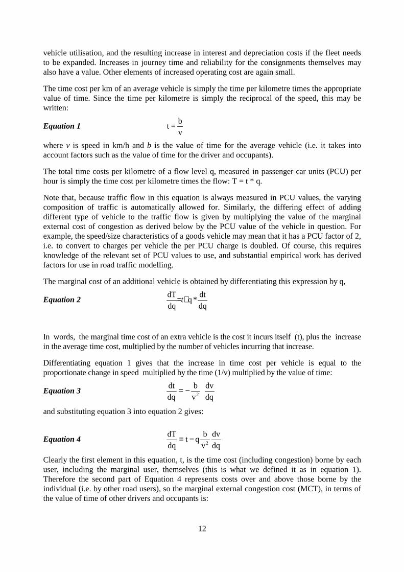
The two main components of delay costs for road users (leaving aside accident andenvironmental costs, which may also vary with the level of congestion2), are time costs, andvehicle operating costs represented in terms of fuel, tyres, etc. The derivation of the externalelement of time costs from a speed-flow relationship is given below, following Newbery (1990).External operating costs may be derived in a similar fashion. Formulae are available showinghow vehicle operating costs for various types of vehicles vary with speed (see for example theCOBA manual in the UK). It should be noted that if elements of vehicle operating cost, such asfuel, are subject to tax in excess of the standard level of Value Added Tax, this should bededucted from any additional costs, as it does not constitute a true resource cost; rather it is atransfer between vehicle users and the government concerned. Since they are typically verysmall compared with time costs, changes in vehicle operating costs are not considered in detailhere. For public transport and freight vehicles, the time costs should be expanded to consider

2 These are not the focus of this paper, although they are highly relevant for pricing purposes and should beconsidered in conjunction with the environmental and accident papers.

12

vehicle utilisation, and the resulting increase in interest and depreciation costs if the fleet needsto be expanded. Increases in journey time and reliability for the consignments themselves mayalso have a value. Other elements of increased operating cost are again small.

The time cost per km of an average vehicle is simply the time per kilometre times the appropriatevalue of time. Since the time per kilometre is simply the reciprocal of the speed, this may bewritten:

Equation 1v

b=t

wherev is speed in km/h andb is the value of time for the average vehicle (i.e. it takes intoaccount factors such as the value of time for the driver and occupants).

The total time costs per kilometre of a flow level q, measured in passenger car units (PCU) perhour is simply the time cost per kilometre times the flow: T = t * q.

Note that, because traffic flow in this equation is always measured in PCU values, the varyingcomposition of traffic is automatically allowed for. Similarly, the differing effect of addingdifferent type of vehicle to the traffic flow is given by multiplying the value of the marginalexternal cost of congestion as derived below by the PCU value of the vehicle in question. Forexample, the speed/size characteristics of a goods vehicle may mean that it has a PCU factor of 2,i.e. to convert to charges per vehicle the per PCU charge is doubled. Of course, this requiresknowledge of the relevant set of PCU values to use, and substantial empirical work has derivedfactors for use in road traffic modelling.

The marginal cost of an additional vehicle is obtained by differentiating this expression by q,

Equation 2dq

dt*q

dq

dT +=t

In words, the marginal time cost of an extra vehicle is the cost it incurs itself (t), plus the increasein the average time cost, multiplied by the number of vehicles incurring that increase.

Differentiating equation 1 gives that the increase in time cost per vehicle is equal to theproportionate change in speed multiplied by the time (1/v) multiplied by the value of time:

Equation 3dt

dq

b

v= − 2

dv

dq

and substituting equation 3 into equation 2 gives:

Equation 4dq

dv

v

bqt

dq

dT2

−=

Clearly the first element in this equation, t, is the time cost (including congestion) borne by eachuser, including the marginal user, themselves (this is what we defined it as in equation 1).Therefore the second part of Equation 4 represents costs over and above those borne by theindividual (i.e. by other road users), so the marginal external congestion cost (MCT), in terms ofthe value of time of other drivers and occupants is:

13

Equation 5dq

dv

v

bqMCT

2−=

It is clear that the marginal external cost of congestion will vary with:-

dv

dq

- the slope of the speed/flow relationship, which varies with the type ofroad and volume of traffic

q - the volume of traffic (in PCUs)

v - the resulting speed, which varies with the type of road and volume oftraffic

b - the value of time, which varies with the mix of journey purpose andincome of the users

It is therefore necessary to think in terms of varying charges whenever these characteristics of theroad or its traffic vary. DIW et al (1998) survey speed/flow relationships and congestion coststhroughout Europe, and produce estimates of marginal congestion costs for some countriesincluding the UK (Annex A).

Clearly, weather conditions have a direct impact on the speed-flow characteristics of roads. Thepractical implications of this impact raise the possibility of varying charges to take account ofweather conditions; indeed, this currently occurs in San Diego, California, where dynamic tollsbased on traffic levels may be doubled during adverse weather conditions.

Apart from congestion due to the volume of traffic, other causes of congestion can include roadmaintenance, vehicle breakdowns and accidents. The delays due to such factors may becalculated by means of a simple traffic model which takes account of road capacity and(essentially random) events such as vehicle breakdowns and accidents. In the UK, the QUADROmodel is used to calculate time delays due to road works and incidents in road works leading todelays. This model is also used to calculate charges to road maintenance companies, “lane rentalcharges”, to build in incentives for timely completion of maintenance. A similar model could beused in order to calculate appropriate ex-ante vehicle charges.

It is important to note that the optimal congestion charge will be at the point where the marginalsocial cost equals the marginal social benefit of travel. Since congestion is currently unpriced,this will occur at a traffic flow lower than the current flow. Thus a model showing the reaction ofusers to alternative levels of congestion and to prices for the use of the road is needed to computethe optimal congestion charge. The need to calculate congestion charges at this point ofequilibrium implies the need for an iterative process in determination of the optimal charge.

As well as the expected delay, congestion can lead to variability in travel time, or in other wordsunreliability. Valuation of unreliability is discussed below, but the bigger difficulty is forecastingits increase as congestion builds up. Ideally this requires a micro simulation model, whichsimulates the journey times of individual vehicles and which can be run for a large number of

14

days, so that distributions of travel time for different levels of traffic may be estimated, orextensive observations to estimate such a relationship from real data.

15

RECOMMENDATIONS

1.1 Wherever possible, external road congestion costs should be estimated from a modelwhich simulates the interaction of demand and supply on the road network. The modelcan then be used to approximate the marginal external costs of congestion by rerunning itwith small changes in traffic volumes, and examining the effects on journey time forexisting traffic. This model would ideally incorporate a detailed network description, withboth speed/flow relationships and junction delays, and allow for user behaviour in termsof rerouteing, retiming, changing destination or mode or changing frequency of travel, inorder to obtain a new set of flows and journey times following imposition of a charge.Data is therefore required on the base O/D matrix, base generalised costs and responses tochanges in these values. The calculation of generalised cost requires knowledge ofoperating costs, values of time and vehicle occupancy rates. Only when the charge isequal to the marginal external cost in this new position has the optimal level of chargeand traffic been found

1.2 Where this is not possible, we recommend that calculations are undertaken for typicalinter urban or rural roads at alternative traffic levels and mixes of types of vehicle usinglink speed/flow relationships. Separate calculations will be needed according to the typeof road (number of lanes; motorway or conventional road). Again, data on base trafficflows and generalised costs are needed, and traffic volumes should again be adjusted forthe introduction of charges, if necessary by means of a simple price elasticity of demand,in order to obtain an equilibrium value.

1.3 For urban areas, the degree of interaction between roads means that such anapproximation will be particularly crude. If a full network model is not available, the useof area speed/flow relationships relating to the entire network for central, inner and outerurban areas is likely to be preferable to link based speed/flow relationships.

1.4 Forecasting the impact of increased traffic on unreliability is more difficult, but given theimportance of the issue it should be attempted wherever possible. A variety of approachesexists, including the use of micro-simulation models which model individual vehicles andcan thus estimate the spread of journey times, and purely empirical approaches, whichrequire data on unreliability and on traffic flows for a set of roads over time.

1.5 All the above relationships should relate to local conditions in the area concerned, andrelate to conditions such as driving styles and typical speeds in that location. It would becounter-productive therefore to attempt to specify Europe-wide relationships, althoughresults may with care be transferred from comparable situations elsewhere in Europe iflocal information is not available.

2. CONGESTION AND SCARCITY COSTS OF RAIL

In principle, the approach we take to estimating the social marginal cost of rail traffic isconsistent with that for road - namely, we try to estimate the additional costs imposed on societyby the use of the infrastructure by an additional train. However the methodology for rail is quitedifferent from that for road transport. The reason is that for rail the volume of traffic is directlycontrolled by allocation of slots, so capacity should never be exceeded. Nevertheless, as trafficapproaches capacity, so delays become more frequent. Where one operator delays trains ofanother through unscheduled departure from the timetable, compensation may be paid directly

16

for increased costs and passengers’ time, provided that adequate records are kept of amounts andcauses of delay. This is a feature of the ‘performance regime’ embodied in track accessagreements in Great Britain. However, this is only likely to measure the delays directly causedby the train in question. Simulation modelling, using a model such as the MERIT model used byRailtrack, which simulates a large number of days operations using probability distributions ofthe various causes of delay, will estimate the full effect of running additional trains, including theworsening of delays from other causes by the reduction of the recovery margin in the system.

But the main consequence of full utilisation of capacity is that users simply cannot get thecapacity they want when they want it; they have to run their trains at times and possibly speedsdifferent to their preferred alternative, or to give up the journey.

The carrying capacity of a railway link is the maximum number of physical transport units whichcan use the link, and can be expressed as a function of the number of tracks in a section, averagetrain speeds, geometry, signalling and safety systems, section lengths, length of trains, etc.(Rothengatter et al, 1996). However, over and above all these factors, the mix of train speeds andthe precise order in which trains are run is crucial. For instance, on a predominantly high speedline an additional slow freight train may remove the paths of several high speed passenger trains;on a heavy freight route the reverse may be true. Capacity is also maximised by grouping trainsof like speeds, so that a 'flight' of fast passenger trains is followed by a 'flight' of slow freightsand vice versa. However, this conflicts with providing a good service of well spaced trains atregular intervals for the public. More complicated still is the interaction of trains on differentroutes or between different origins and destinations; as with roads, junctions and otherbottlenecks (e.g. speed restrictions) are key factors determining capacity.

The result of all these considerations is that it is impossible to come to a ready definition of thecapacity of a rail route corresponding to that for roads. More seriously, the impact of anadditional train of a particular type on the paths available to other trains will differ enormouslyaccording to the precise mix of traffic on the line. At the same time, the value of a slot to othercommercial operators or to government bodies providing social services will also differenormously in time and space. It does not therefore seem possible to come to a generalmethodology to estimate scarcity values for rail slots in a variety of typical circumstances, in theway in which we have for road.

There are other ways of seeking to derive scarcity values. One is by competitive bidding for theslots. However, in rail systems capacity can be used in such a wide variety of ways to producedifferent mixes of trains of different types, origins and destinations that any bidding exercise islikely to be very complex. Moreover the value of a particular slot depends very much on whatother slots are obtained, in order to put together a commercially attractive service. We see somescope for bidding processes for alternative packages of slots in a pre-planned timetable, but ingeneral we do not consider bidding processes as a practical way of revealing scarcity values.

We see it as inevitable that the use of rail infrastructure will be planned by the infrastructuremanager rather than being determined by a purely market process. The most efficient mechanismfor revealing scarcity values is probably to allow the infrastructure manager to negotiate with thepotential users about their willingness to pay for alternative slots in determining that plan. Thisallows for negotiation over desired packages of access rights and iteration to improve upon theinitial solution. It might work in terms of train operators first registering their wishes, theinfrastructure manager using these to produce packages of paths and charges and furthernegotiation then taking place to determine whether operators would be prepared to pay more to

17

improve their package, or to surrender some of their paths in return for a reduced charge. Suchnegotiations would also naturally encompass investment in expanded or enhanced capacity andthe sharing of the development costs.

It does raise fears that the infrastructure manager or the larger train operating companies mayexert undue monopoly power over the process (particularly when the two are part of the sameorganisation), and calls for an independent regulator to intervene where that happens. However,in a situation in which there is no ideal solution, it does appear to be the best way forward.

RECOMMENDATIONS

2.1 Estimation of the scarcity value of specific slots on rail infrastructure requires a way ofrevealing the value placed on the slots by alternative possible users, both in terms ofcommercial rail operators and in terms of government bodies wishing to provide socialservices. It may be possible in some cases to reveal these values by auctioning the slots,but given the complexities involved in terms of the alternative ways in which theinfrastructure may be used, this is difficult. Some pre-packaging of slots is probablynecessary, in order to offer attractive combinations to alternative bidders. In general, aprocess of negotiation appears the most practicable way forward. This might work interms of train operators first registering their wishes, the infrastructure manager usingthese to produce packages of paths and charges and further negotiation then taking placeto determine whether operators would be prepared to pay more to improve their package,or to surrender some of their paths in return for a reduced charge. Such negotiationswould also naturally encompass investment in expanded or enhanced capacity and thesharing of the development costs.

2.2 Unscheduled delays imposed by one train operator on another may be measured ex post ifadequate monitoring is undertaken to measure both the extent and the cause of delays.However, this will only measure the delays directly caused and not those where thepresence of the additional train has worsened the consequences of other delays byabsorbing part of the recovery margin. It is therefore more accurate to measure anticipateddelays by simulation modelling and charge these as part of the tariff. Of course theseadditional delays will vary by route, type of train and time of day.

3. MONETARY VALUATION

In general it is found that the external costs of congestion are dominated by time losses (ratherthan effects on operating costs) and thus are extremely sensitive to the value of time. In order toestimate the marginal cost of congestion, it is necessary to choose monetary valuations to be usedin the evaluation of increased journey time and congestion in both the passenger and freightmarkets. Valuations are required for private car, bus, van, HGV, train, and aircraft.

In addition, disaggregations by journey purpose for passenger travel would be desirable, so thatthe differing mix of journey purposes by time and location can be allowed for. A distinctionaccording to the duration of trip may also be made since it could well have a bearing on timeconstraints and disutility of the journey.

18

The value of time represents the maximum amount an individual is prepared to pay for a timesaving or the minimum acceptable amount to compensate for an increase in journey time. Themarginal value of time is made up of two components:

� the marginal utility of time; and,

� the marginal utility of money.

Hence variations in the value of time can arise from variations in the marginal utility of time orin the marginal utility of money. Variations in the former will depend on the conditions in whichtravel time is spent and on the opportunity cost of travel time. Variations in the latter depend onpersonal characteristics and particularly on income. Congestion may impact on the conditions oftravel and thus may affect the value of time.

For car, van and HGV users, the impacts of increased congestion can be expected to be:

� increases in the average journey time, with the additional time being spent in congestedtraffic which can be expected to be more highly valued than time spent in free flowtraffic because of the greater stress, frustration and unpleasantness involved; and,

� increases in the variability of travel time, with a wider distribution around average traveltime. This is measured by the standard deviation of travel times or a proportion ofvehicles arriving late.

For public transport users, the situation is a little different because of the fixed schedulesinvolved. Congestion may again lead to increases in both the mean and the variability of invehicle time, but it will also lead to more waiting time, as vehicles became bunched and fail toarrive at stops on schedule.

For values of time it is desirable to use values selected for the specific context concerned as faras possible, since values of time will vary with income and other characteristics of the travellersconcerned. For many purposes this means that values estimated for the country concerned willbe the best choice. On international routes, it will be necessary to use a weighted average of thevalues for the countries from which the travellers come.

There are established values of working time for passenger travel, based on the cost of employingworkers, (which reflects the wage rate and an overhead). These are appropriate for workerswhose job is actually driving. However, this approach may not be appropriate where passengersmay work en route, as is the case of many business travellers when travelling by rail, or wheremuch of the journey takes place outside normal working hours. Hensher (1977) outlines anapproach which may be used to estimate values empirically in such circumstances, but fewcountries have applied this, perhaps because many of the elements are difficult to value inpractice. However, a number of studies are available which have taken this approach, usingsurveys to quantify elements such as the gain in subsequent productivity as a result of fasterjourneys leading to the traveller arriving at a meeting feeling more refreshed. The equation to beestimated is the following:

Equation 6 VB = (1 – r – p.q)MP + (1 – r)vw + rv l + MPF

where:

VB = value of business time savings

19

r is share of saved time used for leisurep is share of saved time used productivelyq is relative productivity of time saved that was used for workMP is marginal productivity of labourvw is employee value of saved time otherwise spent in workvl is employee value of saved time otherwise spent in leisureMPF is the value of increased productivity from reduced fatigue

For passenger travel in non-working time, the general approach is to use behavioural valuesestimated from either revealed preference or stated preference data. In general, revealedpreference models have the benefit of being based on actual data, but stated preference modelsallow much more precise estimation with a given sample size. There is some evidence that a welldesigned stated preference survey is relatively free from bias, but this issue remainscontroversial. A fair amount of evidence suggest that the value of time for leisure purposes isrelated to income, and a figure of the order of 25% of the wage rate is often used.

There is evidence that inter-urban travel is valued higher than urban travel, on which most valuesof time are based. Wardman (1998) provides this evidence on the basis of regression analysis ofthe inter-urban and urban values of time of over 100 revealed preference and stated preferencestudies. The principal reason for this distinction appears to be the higher relative income levels ofinter-urban travellers. Time spent in congested road conditions is also valued more highly,because of the discomfort of driving in stop-start conditions and the uncertainty associated withthe journey.

For rail, the appropriate values for in-vehicle time should be used for scheduled travel time, for‘late’ time for delays and for wait time for any additional waiting time involved. Where scarcityof capacity requires a change in departure time, the value per minute of switch in departure timeis also needed. All of these values may in principal be estimated by either revealed or statedpreference methods, although in practice their estimation by stated preference methods is muchmore straightforward, as appropriate trade-offs may be postulated without having to find them inpractice.

For freight transport, values of time need to take account not just of the additional operating costsand drivers’ wages caused by congestion, but also of the value to the consignor of receiving thegoods more quickly and - perhaps even more important - more reliably. A traditional approach isto look at the value of the goods, and then consider the interest charges on the additional time thestock is in transit. Except for very long journeys (e.g. inter continental sea transits) this gives verylow valuations. Empirical evidence suggests that consignors typically value journey time morehighly, presumably because slow transits make it more difficult to cope with short termfluctuations in demand, and thus increase the amount of buffer stock held in the system. Butmuch more important still is reliability. Given the spread of ‘just in time’ distribution andproduction systems, failures in reliability may be very expensive, in again leading to additionalbuffer stock or to failures to supply goods at the promised time. Obviously all these values willvary with the commodity but also with other factors. For instance the values of time andreliability for transits to depots holding buffer stock are typically below those applying to thejourney to the final customer.

Again values of time for freight may be estimated by either revealed or stated preferenceanalysis. There is a growing trend towards the use of stated preference analysis, because

20

appropriate revealed preference data is hard to obtain (both due to issues of confidentiality andbecause of a lack of real alternatives for a lot of freight - road is dominant on all criteria).

Current evidence is not conclusive but suggests that values of time may rise over time inproportion to income. Of course, this is not the only factor that needs updating over time;changes in traffic levels, infrastructure capacity and operating costs all also need to be taken intoaccount.

RECOMMENDATIONS

3.1 For staff working in the transport industry, the usual approach of estimating the marginalcost of their time as their wage rate plus an allowance for the overhead costs ofemploying labour is generally appropriate. Similarly, the costs of poorer vehicleutilisation may be estimated by calculating the impact on fleet size of the delay, and theadditional interest and depreciation costs of a larger fleet.

3.2 For other staff who travel in the course of their work, a more sophisticated approach,which takes account of factors such as their ability to work on route, the fact that part oftheir journey time may be at the expense of leisure time and the fact that the length oftheir journey time may affect their productivity later in the day, is needed. Appropriateformulae exist, and a number of studies have made estimates of the elements involved.

3.3 Values of commuting and leisure time should be based on empirical evidence, andsegmented by variables such as journey purpose, length, mode and income of travellers,whenever evidence of significant variation by this variable exists. A large number ofstudies, using revealed and stated preference methods, exists, and both methods appearcapable of producing reliable results when used with care.

3.4 The evidence that travelling in congested conditions produces higher values of time thanin uncongested conditions requires particularly careful examination because of itsimportance in the current context.

3.5 Empirical estimates also exist, and should be used, for valuing time spent waiting forpublic transport, late arrivals and the difference between desired departure time and thetime at which the service actually departs. All may be affected by congestion or scarcityof slots.

3.6 As a first approximation, values of time for passengers may reasonably be assumed toincrease over time in proportion with income. The value of marginal external cost ofcongestion will also need to be updated for changes in traffic volumes, infrastructurecapacity, technology and operating cost.

3.7 Valuations of time for freight consignments for which transit time is increased, or mademore unreliable, are an important component of social costs, and should be based onempirical estimation (using revealed and/or stated preference methods) rather than thealternative approach which is in use, which is to make estimates of the interest cost ofstock in transit.

21

4. CONCLUSIONS

Externalities occur between vehicles when the presence of one vehicle increases the journey timeof another. The marginal external congestion cost of additional traffic comprises the additionaltime costs and vehicle operating costs imposed on others by an additional unit of travel. Forroads the calculation of additional travel time can be done using speed flow relationships, for thecountry or corridor in question. However, the way in which traffic interacts in a network of roadsmeans that really a network simulation model is needed, particularly in urban areas; the results ofthis may be approximated by an area/speed flow relationship. It is also necessary to rememberthat the optimal charge represents the marginal external congestion cost at the optimum; it is thusnecessary to model the reactions of traffic to changes in road user charges and levels ofcongestion to find the appropriate charge.

For rail, there are important differences. Use of the system is controlled through the allocation ofslots and the main consequence of full capacity is the inability to run the train when desired. Thecosts of congestion and scarcity are only external when imposed by one train operator on another;costs imposed on other trains of the same operator are already internalised. The complexities ofrail systems are such that no simple formula can be found to estimate scarcity values of slots for avariety of typical circumstances. We recommend that negotiation between infrastructuremanagers and train operating companies is the best way to reveal scarcity values of rail slots.

For values of time we recommend the use of values related to local conditions as far as possible.There are established values of working time for passenger travel, based on the cost of employingworkers, (which reflects the wage rate and an overhead.), but for business travel the alternative ofempirical estimation is to be preferred. For passenger travel in non-working time, values basedon analysis of revealed or stated preference data and disaggregated in a number of dimensionssuch as purpose, trip length and degree of congestion, are needed. There is evidence that inter-urban travel is valued more highly than urban travel, on which most of the values of time arebased. Time spent in road congestion is also valued more highly. For rail and air public transportthe appropriate values for delay/late and wait time are also required.

For freight transport the value of time should cover not just drivers’ wages and operating costsavings, but also the value to the consignor of receiving the goods more quickly and/or reliably.Freight values of time vary by commodity and other relevant factors, although a simple mean willoften suffice.

A comprehensive survey of the evidence on values of time for passenger and freight traffic,including all the separate values discussed above, is given in PETS deliverable D7 (See AnnexB).

REFERENCESDepartment of Transport:The COBA Manual. HMSO, 1996

DIW et al (1998):

22

Infrastructure, Capital, Maintenance and Road Damage Costs for Different Heavy GoodsVehicles in the EU.

EURET:Cost-Benefit and Multi-Criteria Analysis for New Road Construction Phase II. Draft Report onReview Measurement Methods for Existing Criteria. Prepared for Commission of the EuropeanCommunities, 1993.

EURET:Cost-Benefit and Multi-Criteria Analysis for New Road Construction: Final Report. Report to theCommission of the European Communities, Directorate General for Transport, 1994. DocEURET/385/94.

EVA Consortium:Evaluation Process for Road Transport Informatics: EVA-Manual. Prepared for the Commissionof the European Communities, 1991.

Fowkes, AS, Nash, C.A. and Tweddle G.:Valuing the Attributes of Freight Transport Quality: Results from the Stated Preference Surveys.Working Paper 276, Institute for Transport Studies, University of Leeds, 1989.

Hensher DA (1977):Value of Business Travel Time. Pergamon Press, Oxford.

May AD, Shepherd SP, Bates JJ (1998, forthcoming)Supply Curves for Urban Road Networks

The MVA Consultancy (1995) the London Congestion Charging Research Programme:Principal Findings, Government Office for London, HMSO.

Newbery, D (1990):Pricing and Congestion: Economic Principles Relevant to Pricing Roads",Oxford Review ofEconomic Policy, vol 6, 22-38, 1990

Newbery, D. (1998)

PETS D7 (1998)Internalisation of Externalities, University of Leeds, 1998.

Prud’homme, R (1999) Potential Welfare Gains of Road Congestion Pricing (unpublished note).

Rothengatter W et al (1996)Bottlenecks in the European Transport Infrastructure.Technical Report. Study on behalf of theEuropean Centre for Infrastructure Studies (ECIS). April, 1996

Small KA (1992)Urban Transportation Economy, Harwood Academic Publishers, Chur.

23

TransPrice:Evaluation Framework Proposal. Annex A.5, Deliverable 2 - Common Analytical Framework.Prepared for European Commission, 1996.

Tweddle G, Fowkes AS and Nash CAImpact of the Channel Tunnel: A Survey of Anglo-European Unitised Freight. Working Paper443, Institute for Transport Studies, University of Leeds, 1995.

Wardman MRoute Choice and the Value of Motorists' Travel Time: Empirical Findings. Working Paper 224,Institute for Transport Studies, University of Leeds, 1986.

Wardman MA Review of Evidence on the Value of Travel Time in Great Britain. Working Paper 495.Institute for Transport Studies, University of Leeds, 1997.

24

ANNEX A: EXAMPLES OF SPEED FLOW RELATIONS ANDCONGESTION COSTS

A.1 Speed-Flow Relationships

This annex gives examples of speed-flow relationships for inter-urban motorways. These relateto Austria, Germany, the UK and the USA.

A1.1 Austrian Example (from DIW et al, 1998)

The following formula was referenced in DIW et al. 1998:V = vk + (vG - vk)*(1-a)α

with: a traffic volume / capacity

vk speed, if a --> 1:

dual carriage way 55 km/h

normal road 50 km/h if > 3.00 m lane width

45 km/h if < 3.00 m lane width

vG speed, if a --> 0

A1.2 Example of Speed-Flow Relationships from the German EWS Manual3

The function that relates to car speeds in free-flow conditions can be expressed as:

VP = c0 + c1*exp(c2*(QP + 2*QG)))

where:

VP: Speed passenger car

QP: Flow passenger car

QG: Flow heavy goods vehicle

c0: Constant, depending on road type, gradient and curvature

c1,c2: Constant, depending on road type (c1<0, c2>0)

3 EWS (1997) Forschungsgesellschaft für Straßen- und Verkehrswesen,1997:Empfehlungen für Wirtschaftlichkeitsuntersuchungen an Strassen (EWS).Aktualisierung der RAS-W '86, Köln,1997. This text provided by Michael Schoch, IWW, Karlsruhe University).

25

The slope of this function, a fundamental part of the marginal external congestion cost function isthen given by:

dVP/dQP = c1 * c2 * exp(c2 * (QP+2*QG))

A1.3 UK COBA Curves

This was the type of relationship adopted in the DIW et al (1998) study. It is referenced in PETSD7 (1998), from which the following text comes. The following examples relate to light vehiclesonly.

� Speed of a light vehicle on a two-lane motorway.

The speed-flow relationship provided by COBA is of the form v =a - ßq. When the flow level isless than 1200 veh/hour/lane the following expression provides speed:

v =107 - 0.006 Q

The discontinuity point is given at Q=1200 veh/hour/lane. When flow levels are higher than 1200vehs/hour/lane then

v =139 - 0.033 Q

Note that flow Q in this relationship is measured in vehs/hour/lane, and speed v in km/hour`.

Table A1.1: Parameters of the Speed-Flow Relationships for Light vehiclesType of Road QB

(veh/hour/lane)

Constant

a before QB

Constant

a after QB

ß beforeQB

ßafterQB

Rural single carriageways 80% of capacity1 77 - 0.0152 0.0502

All-purpose dual carriageways 1080 Two lane: 103

Three lane: 110

Two lane: 132

Three lane: 139

0.006 0.033

Motorways 1200 Two lane: 107

Three lane: 114

Four lane: 114

Two lane: 139

Three lane: 147

Four lane: 147

0.006 0.033

1 The capacity of rural single carriageways depends on road width and the percentage of heavy vehicles.

2 Assuming a 15% of heavy vehicles.

A1.4 USA Freeway Estimates (Highway Capacity Manual, 1994)

For basic freeway sections, the manual gives speed-flow curves which are characterised by:• flows from zero to around 75% of capacity - a very flat, almost linear;• flows from around 75% of capacity – non-linear, with slope increasing;

26

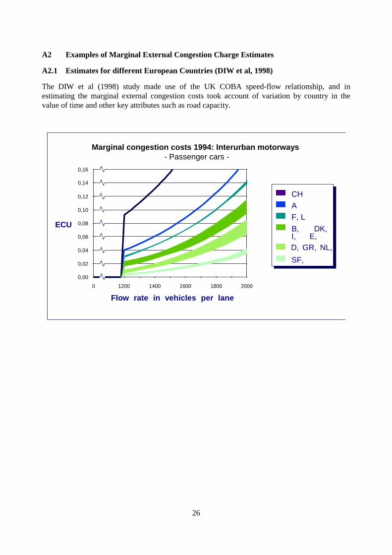
A2 Examples of Marginal External Congestion Charge Estimates

A2.1 Estimates for different European Countries (DIW et al, 1998)

The DIW et al (1998) study made use of the UK COBA speed-flow relationship, and inestimating the marginal external congestion costs took account of variation by country in thevalue of time and other key attributes such as road capacity.

0,00

0,02

0,04

0,06

0,08

0,10

0,12

0,14

0,16

0 1200 1400 1600 1800 2000

Marginal congestion costs 1994: Interurban motorways- Passenger cars -

ECU

CH

F, L

B, DK,I, E,

SF,

A

D, GR, NL,

Flow rate in vehicles per lane

27

Marginal congestion costs 1994: Interurban motorways- Goods vehicles -

0,00

0,05

0,10

0,15

0,20

0,25

0,30

0 1200 1400 1600 1800 2000

ECU

CH

F, L

B, DK,I, E,

SF,

A

D, GR, NL,

Flow rate in vehicles per lane

:

28

A2.2 USA Estimates, for 2000 (HCAS, 19974)

The following table summarises values estimated for 2000 (cents per mile). It provides a clearindication of the range of variation in charges with:

• type of vehicle;• type of road; and,• high, medium and low levels of estimates (according to traffic volume).

Rural Highways Urban Highways All Highways

High Middle

Low High Middle Low High Middle Low

Automobiles 3.76 1.28 0.34 18.27 6.21 1.64 13.17 4.48 1.19

Pickups andVans

3.80 1.29 0.34 17.78 6.04 1.60 11.75 4.00 1.06

Buses 6.96 2.37 0.63 37.59 12.78 3.38 24.79 8.43 2.23

Single UnitTrucks

7.43 2.53 0.67 42.65 14.50 3.84 26.81 9.11 2.41

CombinationTrucks

10.87 3.70 0.98 49.34 16.78 4.44 25.81 8.78 2.32

All Vehicles 4.40 1.50 0.40 19.72 6.71 1.78 13.81 4.70 1.24

4 Federal Highway Cost Allocation Study (1997)

29

ANNEX B: TYPICAL VALUES OF TIME (PETS D7)

PETS D7 quotes the following values of working time. However, these are based on the wagerate, and should not be used for business travel for the reasons discussed above.

Country Value† Country Value† Country Value†Belgium 23.06 Ireland 18.69 Spain 11.15Denmark 20.81 Italy 22.60 UK 17.63France 26.44 Luxembourg 21.40 Finland 20.36Germany 26.44 Netherlands 21.45 Sweden 22.92Greece 6.90 Portugal 5.54 Average 21.02Norway 18.4 ECU (152.50 Kr): Source Handbook 140, Public Roads Administration

Norway† Figures were updated taking into consideration changes in GDP in the 15 countries of the European Union and the rates of inflation publishedby the OECD

For non working time, most empirical evidence suggests values of the order of 25% of the wagerate. There is evidence that inter-urban travel is valued more highly than urban travel, on whichmost of the values of time are based., with typical evidence suggesting that the value of timeshould be increased by 60%.

Time spent in road congestion is also valued more highly, with evidence suggesting that‘congested time’ for passengers only is valued at 150% of normal time. For rail and air publictransport estimates of the appropriate values for wait time, departure time shifts and late time arealso recommended.

For freight transport the value of time should cover not just drivers’ wages and operating costsavings, but also the value to the consignor of receiving the goods more quickly and/or reliably.Typical studies suggest that a value of around 37 ECU's per hour should be used for LGV's. Thevalue of time for HGV's appears to be 10% more, ECU per hour, whilst the value of time for railshould be only 25% that for LGV. If the proportion of the driver costs of these recommendedvalues can be established, then different values across countries can be used according tovariations in drivers' wage rates. Freight values of time by commodity are also given.

Reliability is generally highly valued by freight operators. Evidence was found that a value ofreliability (defined as a percentage of on time arrivals.) of5% of the freight rate for a 1%improvement in reliability index used in Tweddle et al. (1995) was appropriate. The indiceswhich most closely relate to the situations prevailing before and after the increased congestionwould be used.

d:\ts\capri\hlg\can0507.doc