Georgia Journal of ScienceVolume 74 No. 2 Scholarly Contributions from theMembership and Others Article 13

2016

Calculating the Sun's Photospheric Temperature, anUndergraduate Physics LaboratoryAustin B. KerlinUniversity of West Georgia, akerlin2@gmail.com

L Ajith DeSilvaUniversity of West Georgia, ldesilva@westga.edu

Shea RoseUniversity of West Georgia, srose@westga.edu

Javier E. HasbunUniversity of West Georgia, jhasbun@westga.edu

Follow this and additional works at: http://digitalcommons.gaacademy.org/gjs

This Research Articles is brought to you for free and open access by Digital Commons @ the Georgia Academy of Science. It has been accepted forinclusion in Georgia Journal of Science by an authorized editor of Digital Commons @ the Georgia Academy of Science.

Recommended CitationKerlin, Austin B.; DeSilva, L Ajith; Rose, Shea; and Hasbun, Javier E. (2016) "Calculating the Sun's Photospheric Temperature, anUndergraduate Physics Laboratory," Georgia Journal of Science, Vol. 74, No. 2, Article 13.Available at: http://digitalcommons.gaacademy.org/gjs/vol74/iss2/13

CALCULATING THE SUN’S PHOTOSPHERIC TEMPERATURE, AN UNDERGRADUATE PHYSICS LABORATORY

Austin B. Kerlin†, L. Ajith DeSilva†, Shea Rose‡, and Javier E. Hasbun†*

Departments of †Physics and ‡Geosciences University of West Georgia Carrollton, Georgia, 30118

*Corresponding author E-mail: jhasbun@westga.edu

ABSTRACT We provide physics students and teachers with a simple technique for measuring the solar spectrum and a method for analyzing that spectrum through popular computer software. We discuss modern physics concepts related to blackbody radiation while modeling the sun's spectrum to determine the temperature of the sun's photosphere. We provide a reliable method to determine the sun's photospheric temperature with a typical error of less than 10%, primarily dependent on atmospheric conditions. The focus of this work is on data analysis, not acquisition. Keywords: Blackbody radiation, solar spectrum, Planck's radiation distribution, undergraduate physics experiment, modern physics laboratory

INTRODUCTION

The sun's temperature has been calculated in a variety of ways, such as by the heating and cooling rates of different objects in sunlight (Lee et al. 1997; Perry 1979), or by using Wien's displacement law (Marr and Wilkin 2012; Biermann et al. 2002; Bell 1968), and surely through many other methods. Many of the experiments in the literature focus on narrow band intensities (Bell 1968; Goldberg 1955; Ratcliff et al. 1992; Zanetti 1984). Several authors, with whom we agree, also contend that the use of Wien's displacement law for such an experiment is misleading and support the use of Planck's radiation distribution (Marr and Wilkin 2012; Biermann et al. 2002; Zanetti 1984). However, there seems to be a lack of literature related to determining the sun's temperature using wide-range spectral data, which is easily obtained by newer spectrometers. This project provides step-by-step instructions about the experiment, simulation, and modeling processes.

This laboratory develops students' abilities in applying basic physics concepts to real-life applications, and gives them significant experience in computational physics. It encourages them to use MATLAB software (MathWorks 2016) to develop their own scripts toward that purpose. This project also gives students hands-on experience in working with spectrometers and analyzing real data, while promoting and developing a rigorous and consistent application of the scientific method. The setting in which we envision carrying out this exercise is the upper level undergraduate physics laboratory.

Here the students apply concepts such as blackbody radiation distributions and the Stefan-Boltzmann law (Maslov 2008). In particular students experience how such measurements apply to real world situations. The principles required to create and understand this experiment coincide with both introductory physics as well as upper

1

Kerlin et al.: THE SUN'S PHOTOSPHERIC TEMPERATURE

Published by Digital Commons @ the Georgia Academy of Science, 2016

level courses, including modern physics, where blackbody radiation is first discussed in the typical university undergraduate physics curriculum. Making use of a correctly calibrated spectrometer and capture software in conjunction with a programming tool, blackbody spectral data can be obtained and its associated temperature can be determined to an accuracy primarily dependent on atmospheric conditions. This particular application uses an Ocean Optics QE65 Pro spectrometer, an Ocean Optics HL-2000-Cal calibrated halogen lamp, a 200 μm optical fiber, a cc-3 cosine corrector, SpectraSuite software, and a programming environment (we use MATLAB).

The nature of the sun is complex, and it is important to realize we make several assumptions here. We assume the sun is a perfect sphere of radius R, with a uniform temperature. Furthermore, absorption and scattering by the atmosphere play a major role in distorting the spectrum, the effects of which are essentially ignored here. Regardless of these large assumptions on our part, we can still calculate the effective temperature of the sun's photosphere with fair accuracy.

THEORY It is known that all objects with a temperature above absolute zero radiate

electromagnetic waves, and this phenomenon is known as blackbody radiation. The amount of radiated energy in a given wavelength range depends on the temperature. This property is described by Planck's blackbody radiation distribution, Sλ (Planck 2013):

𝑺𝝀 =𝟐𝝅𝒉𝒄𝟐

𝝀𝟓(𝒆𝒙𝒑[𝒉𝒄

𝝀𝒌𝑻]−𝟏)

, ( 1 )

where h (~6.626 x 10-34 m2·kg·s-1) is Planck's constant, T (K) is the blackbody temperature, k (~1.381 x 10-23 m2·kg·s-2·K-1) is the Boltzmann constant, λ(m) is the wavelength, and c (~2.998 x 108 m·s-1) is the speed of light. From Planck's distribution, it can be seen that hotter objects' radiation peaks at shorter wavelengths than cooler objects. For example, about 39% of the sun's radiation is in the visible spectrum, with a peak (Soffer and Lynch 1999) near 500 nm, while the earth's radiation primarily peaks in the infrared. The power per unit area radiated can be determined by integrating the Planck distribution over all wavelengths, yielding the Stefan-Boltzmann law

𝑺𝝀 = (𝟏

𝑨)𝒅𝑷

𝒅𝝀, ( 2 )

where A (m2) is the effective surface area. Solving Eq. (2) for P, the approximate power radiated by the sun is given by

𝑷 = 𝟒𝝅𝑹𝟐𝝈𝑻𝟒, ( 3 )

where 4πR2 is the surface area of the sun's photosphere, which we have assumed to be spherical, and σ (~5.67 x 10-8 W·m-2·K-4) is the Stefan-Boltzmann constant. The irradiance, I (W·m-2), at a distance r from the sun, is approximately given by the ratio P/Ar

2

Georgia Journal of Science, Vol. 74 [2016], Art. 13

http://digitalcommons.gaacademy.org/gjs/vol74/iss2/13

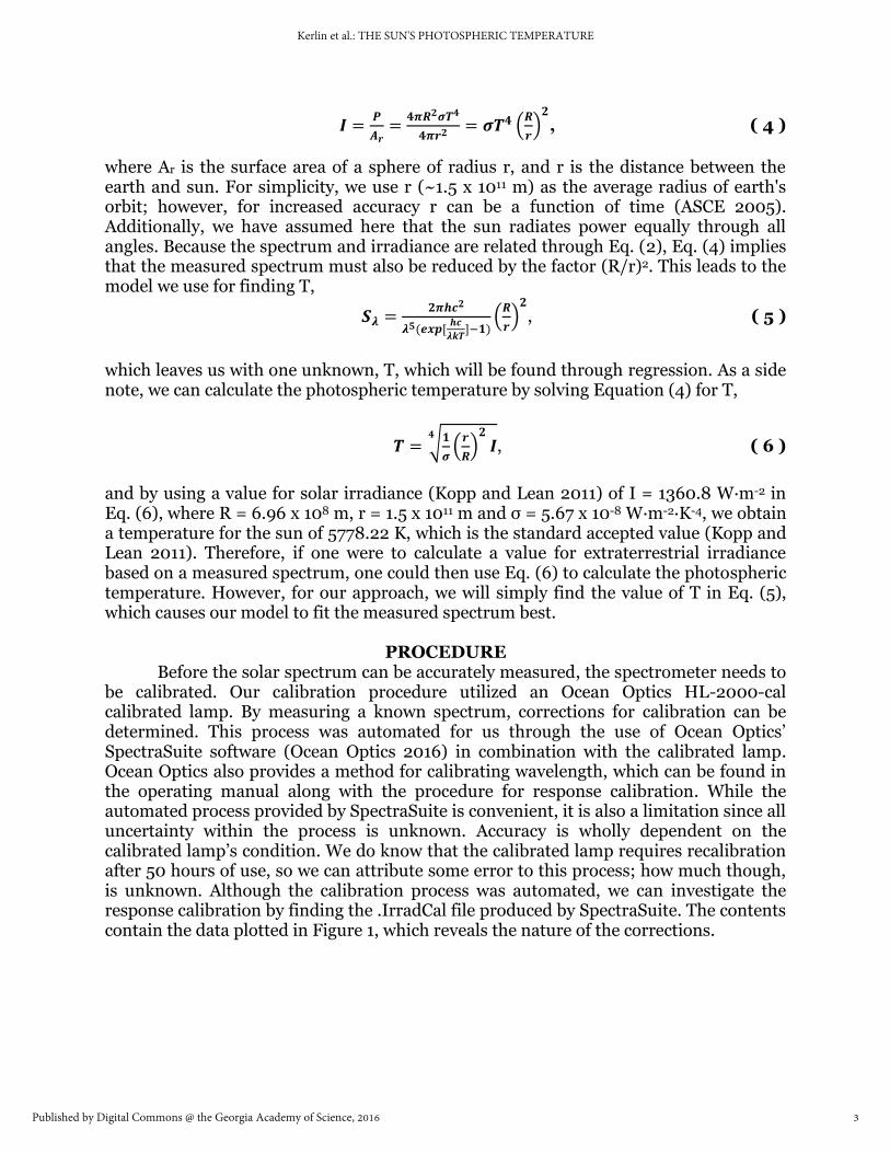
𝑰 =𝑷

𝑨𝒓=

𝟒𝝅𝑹𝟐𝝈𝑻𝟒

𝟒𝝅𝒓𝟐= 𝝈𝑻𝟒 (

𝑹

𝒓)𝟐

, ( 4 )

where Ar is the surface area of a sphere of radius r, and r is the distance between the earth and sun. For simplicity, we use r (~1.5 x 1011 m) as the average radius of earth's orbit; however, for increased accuracy r can be a function of time (ASCE 2005). Additionally, we have assumed here that the sun radiates power equally through all angles. Because the spectrum and irradiance are related through Eq. (2), Eq. (4) implies that the measured spectrum must also be reduced by the factor (R/r)2. This leads to the model we use for finding T,

𝑺𝝀 =𝟐𝝅𝒉𝒄𝟐

𝝀𝟓(𝒆𝒙𝒑[𝒉𝒄

𝝀𝒌𝑻]−𝟏)

(𝑹

𝒓)𝟐

, ( 5 )

which leaves us with one unknown, T, which will be found through regression. As a side note, we can calculate the photospheric temperature by solving Equation (4) for T,

𝑻 = √𝟏

𝝈(𝒓

𝑹)𝟐

𝑰𝟒

, ( 6 )

and by using a value for solar irradiance (Kopp and Lean 2011) of I = 1360.8 W·m-2 in Eq. (6), where R = 6.96 x 108 m, r = 1.5 x 1011 m and σ = 5.67 x 10-8 W·m-2·K-4, we obtain a temperature for the sun of 5778.22 K, which is the standard accepted value (Kopp and Lean 2011). Therefore, if one were to calculate a value for extraterrestrial irradiance based on a measured spectrum, one could then use Eq. (6) to calculate the photospheric temperature. However, for our approach, we will simply find the value of T in Eq. (5), which causes our model to fit the measured spectrum best.

PROCEDURE Before the solar spectrum can be accurately measured, the spectrometer needs to be calibrated. Our calibration procedure utilized an Ocean Optics HL-2000-cal calibrated lamp. By measuring a known spectrum, corrections for calibration can be determined. This process was automated for us through the use of Ocean Optics’ SpectraSuite software (Ocean Optics 2016) in combination with the calibrated lamp. Ocean Optics also provides a method for calibrating wavelength, which can be found in the operating manual along with the procedure for response calibration. While the automated process provided by SpectraSuite is convenient, it is also a limitation since all uncertainty within the process is unknown. Accuracy is wholly dependent on the calibrated lamp’s condition. We do know that the calibrated lamp requires recalibration after 50 hours of use, so we can attribute some error to this process; how much though, is unknown. Although the calibration process was automated, we can investigate the response calibration by finding the .IrradCal file produced by SpectraSuite. The contents contain the data plotted in Figure 1, which reveals the nature of the corrections.

3

Kerlin et al.: THE SUN'S PHOTOSPHERIC TEMPERATURE

Published by Digital Commons @ the Georgia Academy of Science, 2016

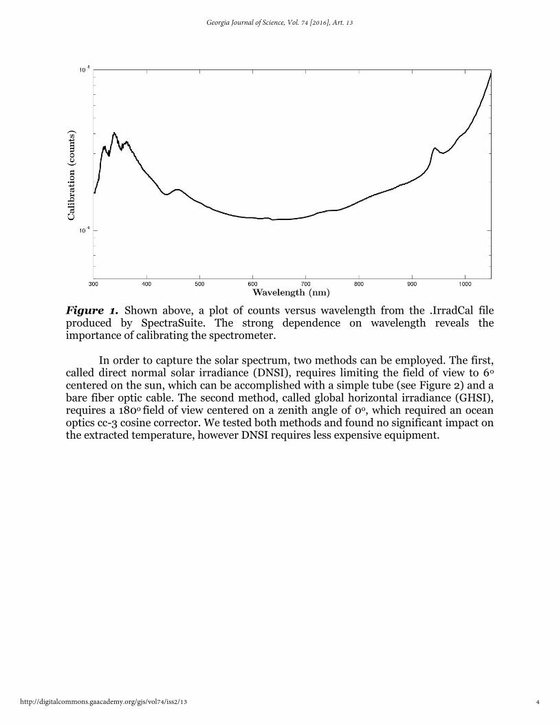
Figure 1. Shown above, a plot of counts versus wavelength from the .IrradCal file produced by SpectraSuite. The strong dependence on wavelength reveals the importance of calibrating the spectrometer.

In order to capture the solar spectrum, two methods can be employed. The first, called direct normal solar irradiance (DNSI), requires limiting the field of view to 6o

centered on the sun, which can be accomplished with a simple tube (see Figure 2) and a bare fiber optic cable. The second method, called global horizontal irradiance (GHSI), requires a 180o field of view centered on a zenith angle of 0o, which required an ocean optics cc-3 cosine corrector. We tested both methods and found no significant impact on the extracted temperature, however DNSI requires less expensive equipment.

4

Georgia Journal of Science, Vol. 74 [2016], Art. 13

http://digitalcommons.gaacademy.org/gjs/vol74/iss2/13

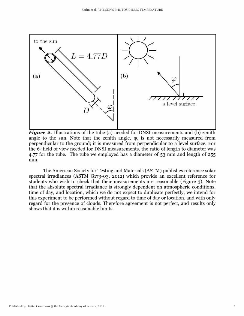
Figure 2. Illustrations of the tube (a) needed for DNSI measurements and (b) zenith angle to the sun. Note that the zenith angle, φ, is not necessarily measured from perpendicular to the ground; it is measured from perpendicular to a level surface. For the 6o field of view needed for DNSI measurements, the ratio of length to diameter was 4.77 for the tube. The tube we employed has a diameter of 53 mm and length of 255 mm.

The American Society for Testing and Materials (ASTM) publishes reference solar spectral irradiances (ASTM G173-03, 2012) which provide an excellent reference for students who wish to check that their measurements are reasonable (Figure 3). Note that the absolute spectral irradiance is strongly dependent on atmospheric conditions, time of day, and location, which we do not expect to duplicate perfectly; we intend for this experiment to be performed without regard to time of day or location, and with only regard for the presence of clouds. Therefore agreement is not perfect, and results only shows that it is within reasonable limits.

5

Kerlin et al.: THE SUN'S PHOTOSPHERIC TEMPERATURE

Published by Digital Commons @ the Georgia Academy of Science, 2016

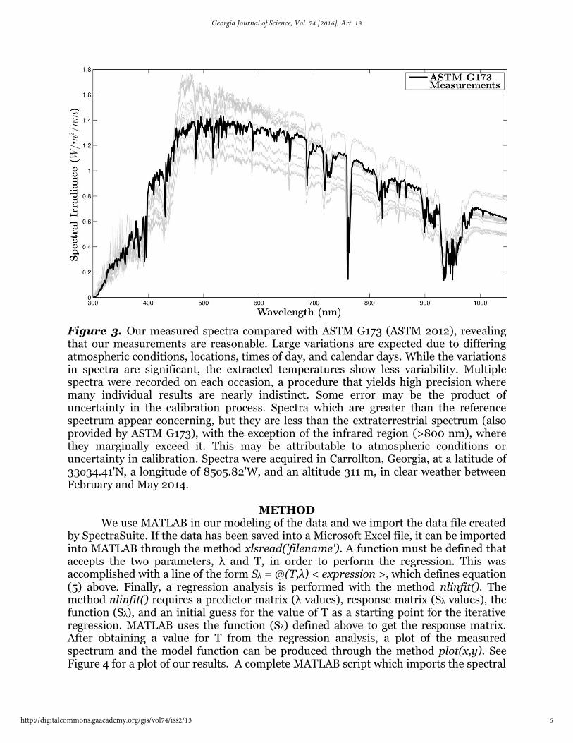
Figure 3. Our measured spectra compared with ASTM G173 (ASTM 2012), revealing that our measurements are reasonable. Large variations are expected due to differing atmospheric conditions, locations, times of day, and calendar days. While the variations in spectra are significant, the extracted temperatures show less variability. Multiple spectra were recorded on each occasion, a procedure that yields high precision where many individual results are nearly indistinct. Some error may be the product of uncertainty in the calibration process. Spectra which are greater than the reference spectrum appear concerning, but they are less than the extraterrestrial spectrum (also provided by ASTM G173), with the exception of the infrared region (>800 nm), where they marginally exceed it. This may be attributable to atmospheric conditions or uncertainty in calibration. Spectra were acquired in Carrollton, Georgia, at a latitude of 33o34.41'N, a longitude of 85o5.82'W, and an altitude 311 m, in clear weather between February and May 2014.

METHOD We use MATLAB in our modeling of the data and we import the data file created

by SpectraSuite. If the data has been saved into a Microsoft Excel file, it can be imported into MATLAB through the method xlsread('filename'). A function must be defined that accepts the two parameters, λ and T, in order to perform the regression. This was accomplished with a line of the form Sλ = @(T,λ) < expression >, which defines equation (5) above. Finally, a regression analysis is performed with the method nlinfit(). The method nlinfit() requires a predictor matrix (λ values), response matrix (Sλ values), the function (Sλ), and an initial guess for the value of T as a starting point for the iterative regression. MATLAB uses the function (Sλ) defined above to get the response matrix. After obtaining a value for T from the regression analysis, a plot of the measured spectrum and the model function can be produced through the method plot(x,y). See Figure 4 for a plot of our results. A complete MATLAB script which imports the spectral

6

Georgia Journal of Science, Vol. 74 [2016], Art. 13

http://digitalcommons.gaacademy.org/gjs/vol74/iss2/13

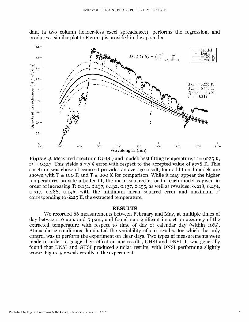
data (a two column header-less excel spreadsheet), performs the regression, and produces a similar plot to Figure 4 is provided in the appendix.

Figure 4. Measured spectrum (GHSI) and model: best fitting temperature, T = 6225 K, r2 = 0.317. This yields a 7.7% error with respect to the accepted value of 5778 K. This spectrum was chosen because it provides an average result; four additional models are shown with T ± 100 K and T ± 200 K for comparison. While it may appear the higher temperatures provide a better fit, the mean squared error for each model is given in order of increasing T: 0.151, 0.137, 0.132, 0.137, 0.155, as well as r2 values: 0.218, 0.291, 0.317, 0.288, 0.196, with the minimum mean squared error and maximum r2 corresponding to 6225 K, the extracted temperature.

RESULTS We recorded 66 measurements between February and May, at multiple times of

day between 10 a.m. and 5 p.m., and found no significant impact on accuracy of the extracted temperature with respect to time of day or calendar day (within 10%). Atmospheric conditions dominated the variability of our results, for which the only control was to perform the experiment on clear days. Two types of measurements were made in order to gauge their effect on our results, GHSI and DNSI. It was generally found that DNSI and GHSI produced similar results, with DNSI performing slightly worse. Figure 5 reveals results of the experiment.

7

Kerlin et al.: THE SUN'S PHOTOSPHERIC TEMPERATURE

Published by Digital Commons @ the Georgia Academy of Science, 2016

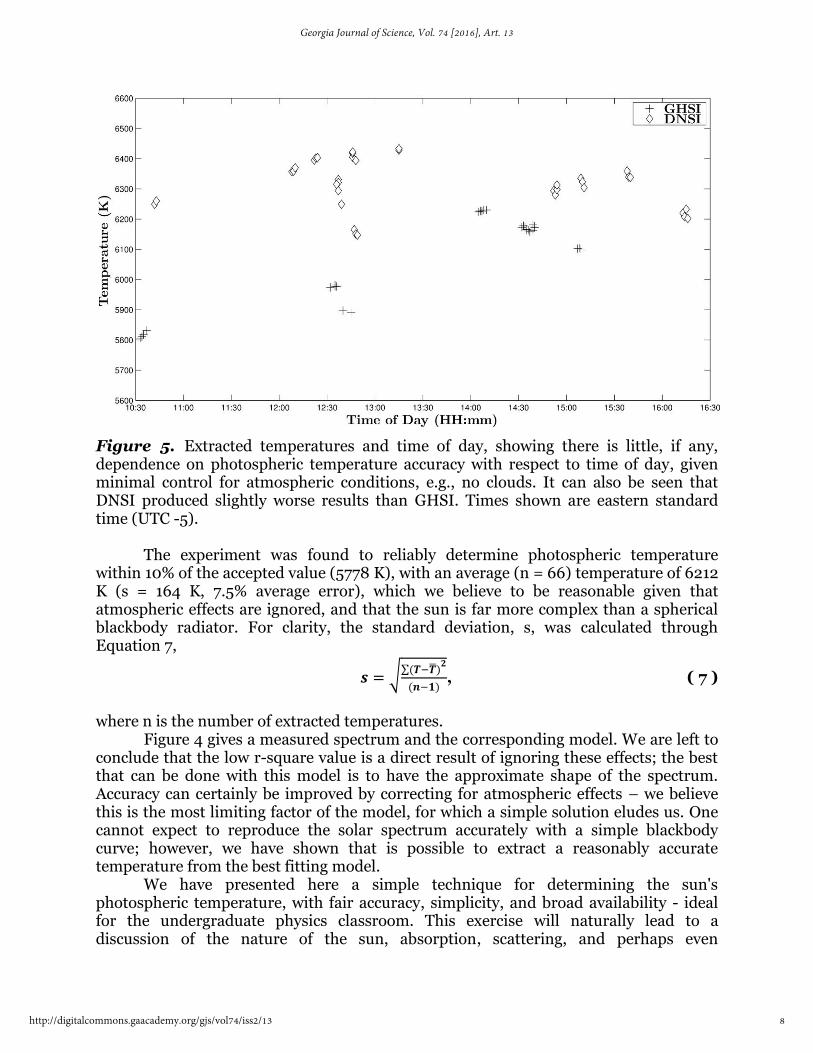
Figure 5. Extracted temperatures and time of day, showing there is little, if any, dependence on photospheric temperature accuracy with respect to time of day, given minimal control for atmospheric conditions, e.g., no clouds. It can also be seen that DNSI produced slightly worse results than GHSI. Times shown are eastern standard time (UTC -5).

The experiment was found to reliably determine photospheric temperature within 10% of the accepted value (5778 K), with an average (n = 66) temperature of 6212 K (s = 164 K, 7.5% average error), which we believe to be reasonable given that atmospheric effects are ignored, and that the sun is far more complex than a spherical blackbody radiator. For clarity, the standard deviation, s, was calculated through Equation 7,

𝒔 = √∑(𝑻−�̅�)𝟐

(𝒏−𝟏), ( 7 )

where n is the number of extracted temperatures. Figure 4 gives a measured spectrum and the corresponding model. We are left to

conclude that the low r-square value is a direct result of ignoring these effects; the best that can be done with this model is to have the approximate shape of the spectrum. Accuracy can certainly be improved by correcting for atmospheric effects – we believe this is the most limiting factor of the model, for which a simple solution eludes us. One cannot expect to reproduce the solar spectrum accurately with a simple blackbody curve; however, we have shown that is possible to extract a reasonably accurate temperature from the best fitting model.

We have presented here a simple technique for determining the sun's photospheric temperature, with fair accuracy, simplicity, and broad availability - ideal for the undergraduate physics classroom. This exercise will naturally lead to a discussion of the nature of the sun, absorption, scattering, and perhaps even

8

Georgia Journal of Science, Vol. 74 [2016], Art. 13

http://digitalcommons.gaacademy.org/gjs/vol74/iss2/13

composition determinations. We believe that by doing this exercise, students will have a solid understanding of how to use a spectrometer, how to work with data, and most importantly, they will develop skills in computational physics and gain experience with a programming environment.

ACKNOWLEDGEMENTS

We gratefully acknowledge partial funding through the UWise and SRAP programs at the University of West Georgia.

REFERENCES

ASTM G173-03(2012), Standard Tables for Reference Solar Spectral Irradiances: Direct Normal and Hemispherical on 37° Tilted Surface, ASTM International, West Conshohocken, PA, 2012, www.astm.org. doi:10.1520/G0173-03R12

Bell, J.A. 1968. TPT NOTES: The temperature of the sun: a demonstration experiment. The Physics Teacher, 6, 466-467. doi:10.1119/1.2351339

Biermann, M.L., D.M. Katz, R. Aho, J.D. Barriga, and J. Petron. 2002. Wien’s Law and the temperature of the sun. The Physics Teacher, 40, 398-400. doi:10.1119/1.1517878

Goldberg, L. 1955. Infrared solar spectrum. Am. J. Phys., 23, 203-222.doi:10.1119/ 1.1933953

Lee, W., H.L. Gilley, and J.B. Caris. 1997. Finding the surface temperature of the sun using a parked car. Am. J. Phys., 65(11), 1105-1109. doi:10.1119/1.18729

Kopp, G. and J.L. Lean. 2011. A new, lower value of total solar irradiance: Evidence and climate significance. Geophysical Research Letters, 38, L01706. doi:10.1029/ 2010GL045777

Marr, J.M. and F.P. Wilkin. 2012. A better presentation of Planck’s radiation law. Am. J. Phys., 80(5), 399-405. doi:10.1119/1.3696974

Maslov, V.P. (2008). Quasithermodynamics and a correction to the Stefan-Boltzmann law. Mathematical Notes, 83(1), 72-79.

Matlab 30-Day Free Trial. 2016. MathWorks. https://www.mathworks.com/campaigns/ products/ppc/google/matlab-trial-request.html?s_eid=ppc_5852767762&q= %2Bmatlab%20download

Perry, S.K. 1979. Measuring the sun’s temperature. The Physics Teacher, 17, 531-533. doi:10.1119/1.2340350

Soffer, B.H. and D.K. Lynch. 1999. Some paradoxes, errors, and resolutions concerning the spectral optimization of human vision. Am. J. Phys., 67(11), 946-953. doi:10.1119/1.13742

SpectraSuite Software download. 2016. Ocean Optics. http://oceanoptics.com/support/ software-downloads/

Planck, M. 2013. The theory of heat radiation. Courier Corporation. Ratcliff, S.J., D.K. Noss, J.S. Dunham, E.B. Anthony, J.H. Cooley, and A. Alvarez. 1992.

High resolution solar spectroscopy in the undergraduate physics laboratory. Am. J. Phys., 60(7), 645-649. doi:10.1119/1.17119

9

Kerlin et al.: THE SUN'S PHOTOSPHERIC TEMPERATURE

Published by Digital Commons @ the Georgia Academy of Science, 2016

The ASCE standardized reference evapotranspiration equation. 2005. Task Committee on Standardization of Reference Evapotranspiration. Environmental and Water Resources Institute of the American Society of Civil Engineers. http://www.kimberly.uidaho.edu/water/asceewri/ascestzdetmain2005.pdf

Zanetti, V. 1984. Sun and lamps. Am. J. Phys., 52(12), 1127-1130.

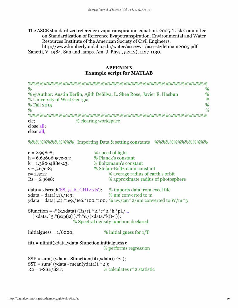
APPENDIX Example script for MATLAB

%%%%%%%%%%%%%%%%%%%%%%%%%%%%%%%%%%%%%%%%%%%%%%%% % % @Author: Austin Kerlin, Ajith DeSilva, L. Shea Rose, Javier E. Hasbun % % University of West Georgia % % Fall 2015 % % % %%%%%%%%%%%%%%%%%%%%%%%%%%%%%%%%%%%%%%%%%%%%%%% clc; % clearing workspace close all; clear all; %%%%%%%%%%%% Importing Data & setting constants %%%%%%%%%%%%%% c = 2.998e8; % speed of light h = 6.62606957e-34; % Planck's constant k = 1.3806488e-23; % Boltzmann's constant s = 5.67e-8; % Stefan-Boltzmann constant r= 1.5e11; % average radius of earth's orbit Rs = 6.96e8; % approximate radius of photosphere data = xlsread('SS_5_6_GHI2.xls'); % imports data from excel file xdata = data(:,1)./1e9; % nm converted to m ydata = data(:,2).*1e9./1e6.*100.*100; % uw/cm^2/nm converted to W/m^3 Sfunction = @(x,xdata) (Rs/r).^2.*c^2.*h.*pi./... ( xdata.^5.*(exp(x(1).*h*c./(xdata.*k))-1)); % Spectral density function declared initialguess = 1/6000; % initial guess for 1/T fit1 = nlinfit(xdata,ydata,Sfunction,initialguess); % performs regression SSE = sum( (ydata - Sfunction(fit1,xdata)).^2 ); SST = sum( (ydata - mean(ydata)).^2 ); R2 = 1-SSE/SST; % calculates r^2 statistic

10

Georgia Journal of Science, Vol. 74 [2016], Art. 13

http://digitalcommons.gaacademy.org/gjs/vol74/iss2/13

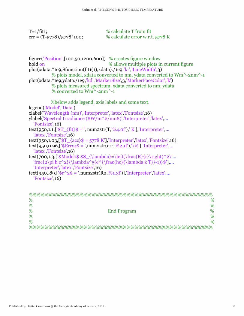
T=1/fit1; % calculate T from fit err = (T-5778)/5778*100; % calculate error w.r.t. 5778 K figure('Position',[100,50,1200,600]) % creates figure window hold on % allows multiple plots in current figure plot(xdata.*1e9,Sfunction(fit1(1),xdata)./1e9,'k-','LineWidth',3) % plots model, xdata converted to nm, ydata converted to Wm^-2nm^-1 plot(xdata.*1e9,ydata./1e9,'kd','MarkerSize',3,'MarkerFaceColor','k') % plots measured spectrum, xdata converted to nm, ydata % converted to Wm^-2nm^-1 %below adds legend, axis labels and some text. legend('Model','Data') xlabel('Wavelength (nm)','Interpreter','latex','Fontsize',16) ylabel('Spectral Irradiance ($W/m^2/nm$)','Interpreter','latex',... 'Fontsize',16) text(950,1.1,['$T_{fit}$ = ', num2str(T,'%4.0f'),' K'],'Interpreter',... 'latex','Fontsize',16) text(950,1.03,['$T_{acc}$ = 5778 K'],'Interpreter','latex','Fontsize',16) text(950,0.96,['$Error$ = ',num2str(err,'%2.1f'),'\%'],'Interpreter',... 'latex','Fontsize',16) text(700,1.3,['$Model:$ $S_{\lambda}=\left(\frac{R}{r}\right)^2\'... 'frac{2\pi h c^2}{\lambda^5(e^{\frac{hc}{\lambda k T}}-1)}$'],... 'Interpreter','latex','Fontsize',16) text(950,.89,['$r^2$ = ',num2str(R2,'%1.3f')],'Interpreter','latex',... 'Fontsize',16) %%%%%%%%%%%%%%%%%%%%%%%%%%%%%%%%%%%%%%%%%%%%%%% % % % % % End Program % % % % % %%%%%%%%%%%%%%%%%%%%%%%%%%%%%%%%%%%%%%%%%%%%%%%

11

Kerlin et al.: THE SUN'S PHOTOSPHERIC TEMPERATURE

Published by Digital Commons @ the Georgia Academy of Science, 2016