Journal of Health Economics 28 (2009) 169–175

Contents lists available at ScienceDirect

Journal of Health Economics

journa l homepage: www.e lsev ier .com/ locate /econbase

Note

Calculating concentration index with repetitive valuesof indicators of economic welfare�

Zhuo Chen ∗, Kakoli RoyCenters for Disease Control and Prevention, Office of Workforce and Career Development,1600 Clifton Rd NE, MS-E94, Atlanta, GA 30333, United States

a r t i c l e i n f o

Article history:Received 25 July 2007Received in revised form 29 July 2008Accepted 22 September 2008Available online 30 September 2008

JEL classification:D31D63I12

Keywords:Categorical variableConcentration indexHealth inequalitiesRepetitive values

a b s t r a c t

Repetitive values of the ranking indicators of economic welfare are often introduced due toincidental ties or censoring in the welfare variable, or the categorical nature of welfare vari-ables used in numerous national surveys. In calculating concentration index (CI), assigningdifferent fractional ranks to observations that have same values of the welfare measureleads to unstable and inconsistent CI estimates when the welfare variable is categoricalor censored. In this paper, we establish an interval within which the CI estimates lie, andpropose a solution, which is an extension of (Kakwani, N.C., Wagstaff, A., van Doorslaer,E., 1997. Socioeconomic inequalities in health: measurement, computation, and statisticalinference. Journal of Econometrics 77, 87–103), for consistent and replicable estimates of CIwhen there are a substantial number of ties of the welfare indicator.

Published by Elsevier B.V.

1. Introduction

The concentration index (CI) is an important tool widely used by health economists to quantify income-related (orsocioeconomic-related) health inequality (Wagstaff et al., 1989, 1991; Wagstaff and van Doorslaer, 1994; Van Doorslaer etal., 1997; Humphries and van Doorslaer, 2000; Jones and Nicolas, 2004; Gerdtham et al., 1999; Gundgaard, 2005, 2006;Gundgaard and Lauridsen, 2006a,b). First introduced in Wagstaff et al. (1989), CI has become a standard measure for quan-tifying the degree of income-related inequality in a health outcome and can be used to assess the extent to which healthsubsidies are better targeted toward the disadvantaged. Pioneered and advanced by European researchers, the CI method-ology has been applied to the U.S. (Zhang and Wang, 2004, 2007; Xu, 2006), China (Chen et al., 2007) and other regions(Rannan-Eliya and Somanathan, 2006; Zere and McIntyre, 2003). CI has been used to decompose income-related healthinequality (Wagstaff et al., 2003) and applied to categorical health outcomes (Van Doorslaer and Jones, 2003) as well aslongitudinal data sets (Jones and Nicolas, 2004). The list is far from exhaustive with such applications providing importantinformation for both policymakers (Keppel et al., 2005) and the research community (Van Doorslaer et al., 1997, 2006; VanDoorslaer and Masseria, 2004).

� The findings and conclusions in this article are those of the authors and do not necessarily represent the views of the Centers for Disease Control andPrevention.

∗ Corresponding author. Tel.: +1 404 498 6317; fax: +1 404 498 6505.E-mail address: chenzhuo@gmail.com (Z. Chen).

0167-6296/$ – see front matter. Published by Elsevier B.V.doi:10.1016/j.jhealeco.2008.09.004

170 Z. Chen, K. Roy / Journal of Health Economics 28 (2009) 169–175

A critical problem arises when researchers are calculating CIs from data with repetitive values of the ranking indicatorof economic welfare, i.e., two or more observations have the same value of the welfare variable. This results in practicaldifficulties and estimation issues in calculating the welfare-related fractional rank (the cumulative percentage of the sampleranked by the welfare variable). If left unattended, it leads to unstable point and variance estimates of CI. van Ourti (2004)and World Bank (2004) noted the existence of such repetitive values and proposed a convenient solution, which will bediscussed later in this paper. The issue, however, continues to be unheeded in many empirical applications.

This paper is the first to examine in-depth the problem associated with ties in a welfare variable when calculating CI.We propose an extension of an existing approach (specifically, Kakwani et al., 1997) to handle such ties and compare it withother existing approaches. We provide some background of the CI and examine three scenarios that might lead to repetitivevalues of the welfare variable. The impact of not attending to the issue differs across the scenarios, which include incidentalties, categorical nature, and censoring of the welfare variable. We also explain why these scenarios are common and meritour attention.

The remainder of this paper is organized as follows. Section 2 provides a background of CI and more details of the threescenarios. Section 3 summarizes some theoretical results and provides empirical illustrations using both a hypothetical dataset and the 2004 National Health Interview Survey (NHIS) data set. Section 4 proposes an extension of the KWD methodologyto address the issue of repetitive values of welfare variable. A comparison of the standard error estimates by the extendedKWD approach and the approach used in van Ourti (2004) and World Bank (2004) with that of the bootstrapping procedureis included in Section 4. The last section offers concluding remarks.

2. Repetitive values of the welfare variable

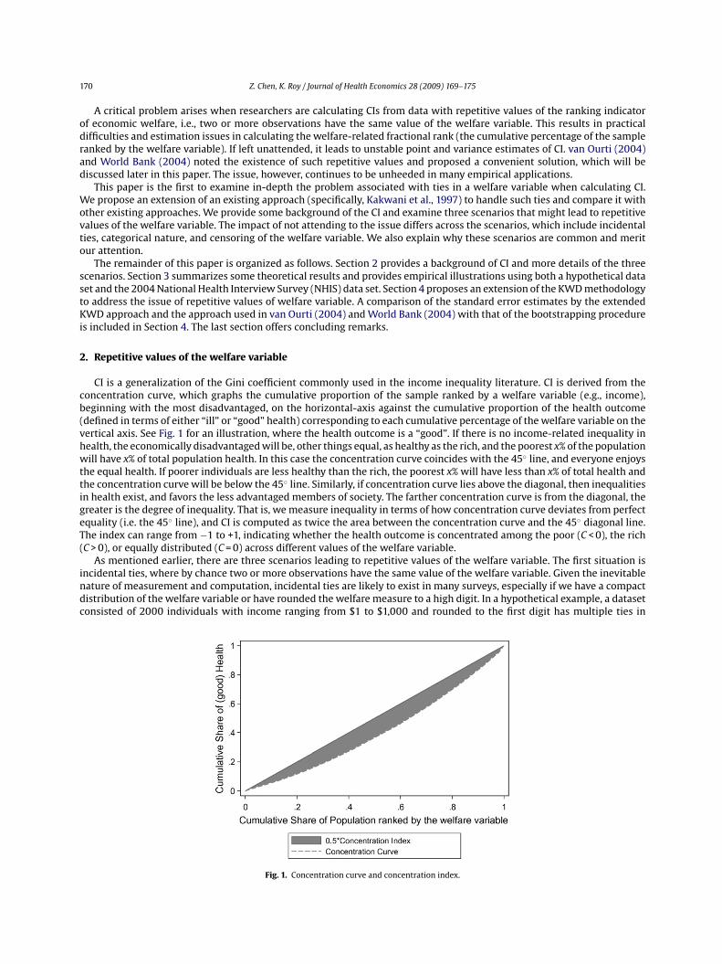
CI is a generalization of the Gini coefficient commonly used in the income inequality literature. CI is derived from theconcentration curve, which graphs the cumulative proportion of the sample ranked by a welfare variable (e.g., income),beginning with the most disadvantaged, on the horizontal-axis against the cumulative proportion of the health outcome(defined in terms of either “ill” or “good” health) corresponding to each cumulative percentage of the welfare variable on thevertical axis. See Fig. 1 for an illustration, where the health outcome is a “good”. If there is no income-related inequality inhealth, the economically disadvantaged will be, other things equal, as healthy as the rich, and the poorest x% of the populationwill have x% of total population health. In this case the concentration curve coincides with the 45◦ line, and everyone enjoysthe equal health. If poorer individuals are less healthy than the rich, the poorest x% will have less than x% of total health andthe concentration curve will be below the 45◦ line. Similarly, if concentration curve lies above the diagonal, then inequalitiesin health exist, and favors the less advantaged members of society. The farther concentration curve is from the diagonal, thegreater is the degree of inequality. That is, we measure inequality in terms of how concentration curve deviates from perfectequality (i.e. the 45◦ line), and CI is computed as twice the area between the concentration curve and the 45◦ diagonal line.The index can range from −1 to +1, indicating whether the health outcome is concentrated among the poor (C < 0), the rich(C > 0), or equally distributed (C = 0) across different values of the welfare variable.

As mentioned earlier, there are three scenarios leading to repetitive values of the welfare variable. The first situation isincidental ties, where by chance two or more observations have the same value of the welfare variable. Given the inevitablenature of measurement and computation, incidental ties are likely to exist in many surveys, especially if we have a compactdistribution of the welfare variable or have rounded the welfare measure to a high digit. In a hypothetical example, a datasetconsisted of 2000 individuals with income ranging from $1 to $1,000 and rounded to the first digit has multiple ties in

Fig. 1. Concentration curve and concentration index.

Z. Chen, K. Roy / Journal of Health Economics 28 (2009) 169–175 171

income. van Ourti (2004) and World Bank (2004) are among the first to have observed this and proposed a correction offractional rank to obtain consistent estimates of CI.1

Second, survey questionnaires are often not designed to obtain a continuous measure of a welfare variable (e.g., income oreducation). The majority of surveys in Europe provide a continuous measure of income (e.g., actual income) (Van Doorslaerand Masseria, 2004), with a limited number of exceptions (Gundgaard, 2005, 2006; Gundgaard and Lauridsen, 2006a,b).However, income is predominantly reported as a categorical measure in most health-related surveys in the U.S. (Centers forDisease Control and Prevention, 2006a,b; National Center for Health Statistics, 2005).

Lastly, repetitive values of welfare variable may be introduced by censoring. A common type of censoring is top-coding,2

which is used to protect individuals (we use individual as an observational unit throughout the paper, but our analyses applyto households as well) with very high income from being identified (U.S. Census Bureau, 2006). Zhang and Wang (2007)used poverty-income ratio (PIR) (the ratio of household income to the Federal poverty guidelines) as the ranking welfarevariable, which is top-coded where all households having the actual PIR greater than 5 were assigned a value of 5 in thepublic use dataset. The other type of censoring is zeroes in income, which is relatively rare in high-income countries but canbe prevalent in developing countries.

Not correcting the fractional rank as described in these situations with repetitive values of the welfare variable affectsthe CI estimation. The case of incidental ties may not be problematic unless the sample includes individuals whose healthoutcomes deviate substantially from those with same values of the welfare variable. Not attending to the repetitive valuesin the case of incidental ties results in estimates of CI which are close to the true value but with certain deviations, oftentrivial but change with every unique sorting. The case of categorical welfare variable is the most problematic but can behandled as grouped data with estimated standard errors of group means as in Kakwani et al. (1997) (henceforth KWD).Empirical applications that do not correct the fractional rank produce different CI estimates when individuals within awelfare group are sorted differently, as will be demonstrated in the following sections both theoretically and with empiricalapplications. A number of studies noted these discrepancies and proposed random sorting within a welfare category as asolution (Gundgaard, 2005, 2006; Gundgaard and Lauridsen, 2006a,b). This produces an estimate that is close to the truevalue, depending on the realization of the random sorting. Ideally, researchers intend to minimize the randomness associatedwith the CI estimates. The interval enclosed by the upper boundary and lower boundary of CI estimates associated withdifferent sorting mechanisms can be substantial in some cases, as will be demonstrated in our simulation analysis. Thethird and final situation can be treated as a special case of the second situation, with a large number of miniscule groupshaving only one observation and a large group consisting of those tied in the welfare measure. Again, the impact of such tiesdepends on the within-group variation of the health outcome and the number of individuals with the same values of welfaremeasure.

3. Empirical issues related to repetitive values of welfare variable

Repetitive values of the welfare variable are not unusual, as previously discussed. The empirical problem largely stemsfrom incorrect calculation of fractional rank. Given a microdataset, individuals who have same values of the welfare variableshould be assigned with a common fractional rank. Not attending to the ties is a de facto random sorting. For example, thealgorithm in the widely used Stata module GLCURVE is written for microdata with non-repetitive welfare measures butnot for data sets with grouped welfare variable (Jenkins and van Kerm, 2007).3 With random sorting, even if a number ofindividuals have a same value of the welfare variable, they are assigned different values of welfare-related fractional rank.Employing this approach for a data set with multiple repetitive values of the welfare variable leads to a fictitious ranking ofindividuals within a group consisted of individuals with same value of welfare variable (for simplicity, we refer it as a welfaregroup hereafter). Given the numerous possibilities of such ranking, different estimates of CI can be obtained for a given dataset. We establish the upper and lower boundary of the estimate in the following theorem. Note that the health outcome isassumed to be a good (positive outcome) throughout the analysis.

Theorem 1. If individuals in a survey sample have repetitive values of the ranking welfare variable and the CI is estimatedwithout correcting the fractional rank of ties, the following occurs: (a) different permutations of observations within a welfaregroup produce different CI estimates; (b) sorting observations within each welfare group with a weakly increasing order in thehealth outcome produces the upper boundary of CI; and (c) sorting the observations within each welfare group with a weaklydecreasing order in the health outcome produces the lower boundary of CI.

1 In its SPSS code, World Bank (2004) has assigned equal fractional rank to ties.2 An example of the top-coding is that, in the Census surveys, if the individual interviewed has earnings higher than $999,999, those earnings are recorded

simply as $999,999.3 GLCURVE was updated in February 2007. Prior to the update, GLCURVE does not address the ties and thus the sorting order of individuals within a

welfare group may depend on the order before the command is executed. The current algorithm of GLCURVE, as stated in its help file, produces fractionalranks corresponding to the maximum CI case. The resulting CI estimate will attain the upper bound. Although the algorithm produces a stable estimatenow, it could deviate from the true estimates in the case when the welfare variable is censored or categorical. The help file of GLCURVE indicates that theprogram is not intended for datasets with categorical welfare variables, which are essentially grouped data.

172 Z. Chen, K. Roy / Journal of Health Economics 28 (2009) 169–175

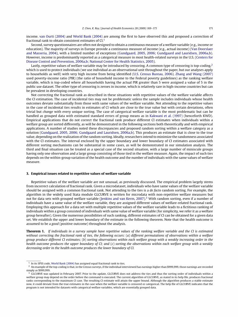
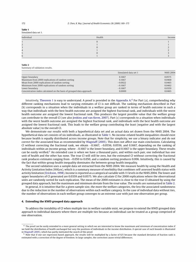
Table 1Simulated data set 1.

Individual Health Income

1 0 12 1 13 0 24 1 25 0 36 1 3

Table 2Summary of validation results.

Simulated data set 1 NHIS 2004

Upper boundary 0.1667 0.0575Maximum from 2000 replications of random sorting 0.1667 0.0468Mean from 2000 replications of random sorting −0.0022 0.0465Minimum from 2000 replications of random sorting −0.1667 0.0462Lower boundary −0.1667 0.0359Concentration index calculated on the basis of grouped data approach 0.0000 0.0465

Intuitively, Theorem 1 is easy to understand. A proof is provided in the Appendix A.4 For Part (a), comprehending whydifferent ranking mechanisms lead to varying estimates of CI is not difficult. The ranking mechanism described in Part(b) corresponds to a situation when the individuals in a welfare group are ranked in terms of health outcome in such away that individuals with the best health outcome are assigned the highest fractional rank, and individuals with the worsthealth outcome are assigned the lowest fractional rank. This produces the largest possible value that the welfare groupcan contribute to the overall CI (see also Jenkins and van Kerm, 2007). Part (c) corresponds to a situation when individualswith the worst health outcome are assigned the highest fractional rank, and individuals with the best health outcome areassigned the lowest fractional rank. This leads to the welfare group contributing the least (negative and with the largestabsolute value) to the overall CI.

We demonstrate our results with both a hypothetical data set and an actual data set drawn from the NHIS 2004. Thehypothetical data set consists of six individuals, as illustrated in Table 1. No income-related health inequalities should existbecause health is equally distributed across income groups. Note that for simplicity, we use a binary indicator and do notcorrect for the associated bias as recommended by Wagstaff (2005). This does not affect our main conclusions. CalculatingCI without correcting the fractional rank, we obtain −0.1667, −0.0556, 0.0556, and 0.1667, depending on the ranking ofindividuals within an income group, where −0.1667 is the lower boundary, and 0.1667 is the upper boundary. These resultscan be easily verified.5 An extended case is when we have a thousand pairs, and within each pair, one individual has oneunit of health and the other has none. The true CI will still be zero, but the estimated CI without correcting the fractionalrank produces estimates ranging from −0.050 to 0.050, and a random sorting produces 0.006. Intuitively, this is caused bythe fact that within-group health inequality dominates the between-group health inequality.

The second validation uses a sample data set extracted from the NHIS 2004. We measure health by using the Health andActivity Limitation Index (HALex), which is a summary measure of morbidity that combines self-assessed health status withactivity limitation (Erickson, 1998). Income is reported as a categorical variable with 11 levels in the NHIS 2004. The lower andupper boundaries of CI generated are 0.0359 and 0.0575. We also calculate CI for 2000 replications where the observationalunits are randomly sorted for each replication. The mean of the 2000 estimates is close to the true CI obtained by using thegrouped data approach, but the maximum and minimum deviate from the true value. The results are summarized in Table 2.

In general, it is intuitive that for a given sample size, the more the welfare categories, the less the associated randomnessdue to the reduction in the number of observations within each welfare category. In the case of individual data without ties,the number of observations in each welfare group converges to an extreme case with just one observation per group.

4. Extending the KWD grouped data approach

To address the instability of CI when multiple ties in welfare variable exist, we propose to extend the KWD grouped dataapproach to individual datasets where there are multiple ties because an individual can be treated as a group comprised ofone observation.

4 The proof can be easily extended to a more general setting in which we are interested to know the maximum and minimum of concentration index ifwe hold the distribution of health unchanged but vary the positions of individuals in the income distribution. A special case of such bounds is illustratedin Wagstaff (2005), which has partly motivated the search of this proof.

5 Note that if one use regression-based approach, the results will be multiplied by a factor of 6/5 because the standard deviation of fraction rank isestimated with a correction of the degree of freedom. In large samples, the correction causes trivial differences.

Z. Chen, K. Roy / Journal of Health Economics 28 (2009) 169–175 173

KWD provided the estimators of CI and its variance.

C = 2n�

n∑i=1

yiRi − 1 (1)

var(C) = 1n

[T∑

t=1

fta2t − (1 + C)2

]+ 1

n�2

T∑t=1

ft�2t (2Rt − 1 − C)2 (2)

where C denotes the value of CI, y is the health outcome of interest, n is the number of observations, � is the overall meanof y, �t is the mean of y among group t, and ft is the population relative frequency of the tth group. We assume there areT socioeconomic groups and the fractional rank Rt =

∑t−1r=1fr + ft/2. In addition, we have �2

t as the variance of y among the

group t, at = �t/�((2Rt − 1 − C) + 2 − qt−1 − qt), and qt = (1/�)∑t

r=1�rfr .We can apply the KWD grouped approach to the three situations previously discussed. The case of categorical welfare

variable is essentially grouped data but to estimate the variance of CI we need to replace �2t with (1/nt)

∑nti (yt

i− �t)

2, whereyt

iindicates ith observation of tth group, nt is the number of observations in tth group, and �t is the mean of y in tth group.

For the cases of incidental ties and censored welfare variable, �2t associated with the observations with unique values of

welfare variable can be set as zero and for the rest we can replace �2t with (1/nt)

∑nti (yt

i− �t)

2.6

It is of interest to compare the extended KWD approach with the method used in van Ourti (2004) and World Bank (2004)(henceforth we refer it as van Ourti approach for convenience). The van Ourti approach uses corrected fractional rank andthen applies the convenient regression to obtain CI and its robust (sandwich) variance estimates. It is straightforward fromKakwani et al. (1997) that the estimates of CI produced by the extended KWD and the van Ourti approach are identical.However, the variance estimates differ in general. The extended KWD approach incorporates the serial correlation of thefractional rank directly but the van Ourti approach exploits the individual information and variation more explicitly. Wedevise two simulation exercises to compare the standard error estimates calculated using the two approaches. To comparethe two variance estimates, we need a baseline variance estimate. Because there are no well-established analytical varianceestimators in such cases, we use bootstrapped standard errors as an approximate baseline estimate, as suggested in theliterature (e.g., Xu, 2006).

The first exercise involves the use of the NHIS 2004. To reduce the burden of computation associated with bootstrapping,we randomly select 2000 observations from the original data. We use the original categories as the categorical incomemeasure. We simulate a pseudo continuous income measure by adding a random component to the mid-point value of thecategories to generate incidental ties. Finally we subtract from the pseudo continuous income its 10th percentile and setall the negative values (10% of the sample) as zero. For each situation, we calculate the estimates of the standard error byusing the extended KWD approach and the van Ourti approach. We also compute the bootstrapped standard error with 200replications. The actual differences between the two analytical estimates and the bootstrapped standard error, the absolutevalues of the differences, and the absolute percentage differences (calculated as the ratio of the absolute difference to thebootstrapped standard error) are computed. To reduce randomness associated with bootstrapping, we repeat this process1000 times. The results are summarized in Table 3. The means of the differences and absolute differences show that thestandard error estimates by the extended KWD approach is closer to the bootstrapped standard errors than those by the vanOurti approach. Note that the standard deviations of the difference are the same for both approaches because it reflects thevariation of the bootstrapped errors as the point and variance estimates of CI of the analytical methods are fixed in this case.The results also show that the estimates of standard error produced by the KWD approach are more conservative in general.

The second simulation exercise is to randomly simulate a dataset of 2000 observations and two variables, i.e., health andincome. We impose a correlation between health and income with the correlation coefficient randomly generated in eachrun of the simulation. This avoids the case of zero CI if health and income are not correlated. We then use deciles of the incomevariable to construct a categorical income and use the procedure described in the first exercise to generate a censored incomemeasure. We then follow with the rest of the first exercise with 2000 repetitions. The results of this simulation exercise aresummarized in Table 4. In contrary to the first exercise, where the result is associated with a particular dataset, this exerciseaverages the (absolute) differences or absolute percentage differences over different types (i.e., with different correlationbetween income and health) of dataset. It is interesting to observe that the two approaches have similar estimates, whichmight be attributed to the fact we did not introduce unequal variance across welfare groups.7 Hence, the extended KWDapproach is as efficient as the van Ourti approach in terms of variance estimation. In addition, since all mean absolutepercentage differences are less than 6%, it is safe to conclude that both approaches produce standard error estimates closeto those generated by bootstrapping.

6 We have used 1nt −1

∑nt

i(yt

i− �t )2 to correct for the loss of degree of freedom as an alternative estimator but our simulation exercises suggest the

unadjusted version is preferred. Our conjecture is that CI is related to a population rather a sample hence the population variance estimator is preferred.The estimator adjusted for the loss of degree of freedom actually inflates the variance estimates in the simulations.

7 The NHIS data is likely to have unequal variance across income groups thus the extended KWD approach may be able to capture the variance structurebetter than the van Ourti approach does.

174 Z. Chen, K. Roy / Journal of Health Economics 28 (2009) 169–175

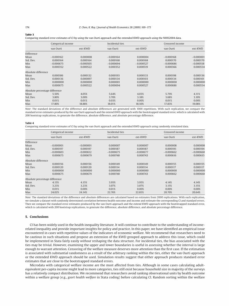
Table 3Comparing standard error estimates of CI by using the van Ourti approach and the extended KWD approach using the NHIS2004 data.

Categorical income Incidental ties Censored income

van Ourti ext-KWD van Ourti ext-KWD van Ourti ext-KWD

DifferenceMean −0.000162 0.000008 −0.000164 0.000004 −0.000168 −0.000001Std. Dev. 0.000164 0.000164 0.000168 0.000168 0.000170 0.000170Min −0.000675 −0.000505 −0.000694 −0.000527 −0.000686 −0.000518Max 0.000352 0.000522 0.000352 0.000519 0.000366 0.000534

Absolute differenceMean 0.000186 0.000132 0.000193 0.000133 0.000198 0.000136Std. Dev. 0.000136 0.000097 0.000134 0.000103 0.000134 0.000101Min 0.000000 0.000000 0.000001 0.000000 0.000000 0.000000Max 0.000675 0.000522 0.000694 0.000527 0.000686 0.000534

Absolute percentage differenceMean 5.50% 4.05% 5.64% 4.03% 5.79% 4.11%Std. Dev. 3.80% 3.00% 3.70% 3.18% 3.68% 3.10%Min 0.01% 0.01% 0.03% 0.00% 0.01% 0.00%Max 17.80% 18.88% 18.01% 18.50% 17.83% 19.08%

Note: The standard deviations of the difference and absolute differences are generated with 1000 repetitions. With each replication, we compare thestandard error estimates produced by the van Ourti approach and the extend KWD approach with the bootstrapped standard error, which is calculated with200 bootstrap replications, to generate the difference, absolute difference, and absolute percentage difference.

Table 4Comparing standard error estimates of CI by using the van Ourti approach and the extended KWD approach using randomly simulated data.

Categorical income Incidental ties Censored income

van Ourti ext-KWD van Ourti ext-KWD van Ourti ext-KWD

DifferenceMean −0.000001 −0.000001 0.000007 0.000007 0.000008 0.000008Std. Dev. 0.000197 0.000197 0.000187 0.000187 0.000195 0.000194Min −0.000603 −0.000612 −0.000675 −0.000677 −0.000662 −0.000660Max 0.000675 0.000679 0.000740 0.000743 0.000616 0.000615

Absolute differenceMean 0.000156 0.000156 0.000149 0.000149 0.000155 0.000155Std. Dev. 0.000120 0.000120 0.000114 0.000114 0.000117 0.000117Min 0.000000 0.000000 0.000000 0.000000 0.000000 0.000000Max 0.000675 0.000679 0.000740 0.000743 0.000662 0.000660

Absolute percentage differenceMean 4.15% 4.15% 3.95% 3.95% 4.14% 4.14%Std. Dev. 3.23% 3.23% 3.07% 3.07% 3.15% 3.15%Min 0.01% 0.00% 0.01% 0.00% 0.00% 0.00%Max 24.02% 24.14% 22.76% 22.85% 20.70% 20.64%

Note: The standard deviations of the difference and absolute differences are calculated based on estimates from 2000 replications. With each replication,we simulate a dataset with randomly determined correlation between health outcome and income and estimate the corresponding CI and standard errors.Then we compare the standard error estimates produced by the van Ourti approach and the extend KWD approach with the bootstrapped standard error,which is calculated with 200 bootstrap replications, to generate the difference, absolute difference, and absolute percentage difference.

5. Conclusions

CI has been widely used in the health inequality literature. It will continue to contribute to the understanding of income-related inequality and provide important insights for policy and practice. In this paper, we have identified an empirical issueencountered in cases with repetitive values of the indicators of economic welfare. We recommend that researchers need tobe cautious in such situations and propose an extension of the KWD grouped approach to address this issue, which couldbe implemented in Stata fairly easily without reshaping the data structure. For incidental ties, the bias associated with theties may be trivial. However, examining the upper and lower boundaries is useful in assessing whether the interval is largeenough to warrant attention. Censoring of the welfare measure deserves more attention than the first case. If the estimationis associated with substantial randomness as a result of the arbitrary ranking within the ties, either the van Ourti approachor the extended KWD approach should be used. Simulation results suggest that either approach produces standard errorestimates that are close to the bootstrapped standard errors.

Microdata with categorical welfare income are the most affected from ties. Although in some cases calculating adult-equivalent per-capita income might lead to more categories, ties still exist because household size in majority of the surveyshas a relatively compact distribution. We recommend that researchers avoid ranking observational units by health outcomewithin a welfare group (e.g., gsort health welfare in Stata coding) before calculating CI. Random sorting within the welfare

Z. Chen, K. Roy / Journal of Health Economics 28 (2009) 169–175 175

group has been reported as a convenient solution, but the extended KWD approach is recommended if one intends to obtainconsistent and replicable estimates. Correcting the fractional rank and then applying the convenient regression method onmicrodata directly can provide a correct estimate of CI, but the estimates of standard error may not fully account for theserial correlation introduced by the ranking variable. Rather, calculating CI by using the extended KWD approach is feasible,necessary, and also efficient in terms of computation time. We recommend this as the preferred method when multiplerepetitive values of the ranking welfare variable exist.

Appendix A. Supplementary data

Supplementary data associated with this article can be found, in the online version, at doi:10.1016/j.jhealeco.2008.09.004.

References

Centers for Disease Control and Prevention (CDC), 2006a. National Center for Health Statistics (NCHS). National Health and Nutrition Examination SurveyQuestionnaire. US Department of Health and Human Services, CDC, Hyattsville, MD.

Centers for Disease Control and Prevention (CDC). 2006b. Behavioral Risk Factor Surveillance System Survey Questionnaire. US Department of Health andHuman Services, CDC, Atlanta, GA (1984–2005).

Chen, Z., Eastwood, D.B., Yen, S.T., 2007. A decade’s story of childhood malnutrition inequality in China: where do you live does matter. China EconomicReview 18, 139–154.

Erickson, P., 1998. Evaluation of a population-based measure of quality of life: the health and activity limitation index (HALex). Quality of Life Research 7(2), 101–114.

Gerdtham, U.G., Johannesson, M., Lundberg, L., Isacson, D., 1999. A note on validating Wagstaff and van Doorslaer’s health measure in the analysis ofinequalities in health. Journal of Health Economics 18 (1), 117–124.

Gundgaard, J., 2005. Income related inequality in prescription drugs in Denmark. Pharmacoepidemiology and Drug Safety 14, 307–317.Gundgaard, J., 2006. Income-related inequality in utilization of health services in Denmark: evidence from Funen County. Scandinavian Journal of Public

Health 34 (5), 462–471.Gundgaard, J., Lauridsen, J., 2006a. Decomposition of sources of income-related health inequality applied on SF-36 summary scores: a Danish health survey.

Health and Quality of Life Outcomes 4, Art. No. 53.Gundgaard, J., Lauridsen, J., 2006b. A decomposition of income-related health inequality applied to EQ-5D. European Journal of Health Economics 7 (4),

231–237.Humphries, K., van Doorslaer, E., 2000. Income-related inequalities in health in Canada. Social Science & Medicine 50, 663–671.Jenkins, S.P., van Kerm, P., 2007. GLCURVE: Stata module to derive generalised Lorenz curve ordinates. Statistical Software Components S366302, Boston

College Department of Economics, 2004 (revised February 29, 2007).Jones, A.M., Nicolas, A.L., 2004. Measurement and explanation of socioeconomic inequality in health with longitudinal data. Health Economics 13, 1015–1030.Kakwani, N.C., Wagstaff, A., van Doorslaer, E., 1997. Socioeconomic inequalities in health: measurement, computation, and statistical inference. Journal of

Econometrics 77, 87–103.Keppel, K., Pamuk, E., Lynch, J., et al., 2005. Methodological issues in measuring health disparities. National Center for Health Statistics. Vital Health Statistics

2 (141), 1–16.National Center for Health Statistics, 2005. Data File Documentation, National Health Interview Survey, 2004. US Department of Health and Human Services,

CDC, Hyattsville, MD.Rannan-Eliya, R., Somanathan, A., 2006. Equity in health and health care systems in Asia. In: Jones, A.M. (Ed.), The Elgar Companion to Health Economic.

Edward Elgar, Cheltenham, UK, pp. 205–220.U.S. Census Bureau, 2006. Current Population Survey, Annual Social and Economic (ASEC) Supplement. http://www.census.gov/apsd/techdoc/cps/

cpsmar06.pdf. Accessed October 2006.Van Doorslaer, E., Jones, A., 2003. The determinants of inequalities in self reported health: a validation of a new approach to measurement. Journal of Health

Economics 22, 61–87.Van Doorslaer, E., Masseria, C., 2004. Income-Related Inequality in the Use of Medical Care in 21 OECD Countries. OECD Health Working Papers, No. 14,

OECD Publishing. doi:10.1787/687501760705.Van Doorslaer, E., Wagstaff, A., Bleichrodt, H., et al., 1997. Income-related inequalities in health: some international comparisons. Journal of Health Economics

16, 93–112.Van Doorslaer, E., Masseria, C., Koolman, X., 2006. Inequalities in access to medical care by income in developed countries. Canadian Medical Association

Journal 174 (2), 177–183.van Ourti, T., 2004. Measuring horizontal inequity in Belgian health care using a Gaussian random effects two part count data model. Health Economics 13

(7), 705–724.Wagstaff, A., 2005. The bounds of the concentration index when the variable of interest is binary, with an application to immunization inequality. Health

Economics 14 (4), 429–432.Wagstaff, A., van Doorslaer, E., 1994. Measuring inequalities in health in the presence of multiple-category morbidity indicators. Health Economics 3,

281–291.Wagstaff, A., van Doorslaer, E., Paci, P., 1989. Equity in the finance and delivery of health care: some tentative cross-country comparisons. Oxford Review of

Economic Policy 5, 89–112.Wagstaff, A., Paci, P., van Doorslaer, E., 1991. On the measurement of inequalities in health. Social Science & Medicine 33, 545–557.Wagstaff, A., van Doorslaer, E., Watanabe, N., 2003. On decomposing the causes of health sector inequalities with an application to malnutrition inequalities

in Vietnam. Journal of Econometrics 112, 207–223.World Bank, 2004. Quantitative Techniques for Health Equity Analysis: Technical Notes #7. http://www1.worldbank.org/prem/poverty/health/wbact/

health eq tn07.pdf. Accessed October 2006.Xu, K.T., 2006. State-level variations in income-related inequality in health and health achievement in the US. Social Science & Medicine 63, 457–464.Zere, E., McIntyre, D., 2003. Inequities in under-five child malnutrition in South Africa. International Journal for Equity in Health 2 (7), doi:10.1186/1475-

9276-2-7.Zhang, Q., Wang, Y., 2004. Socioeconomic inequality of obesity in the United States: do gender, age, and ethnicity matter? Social Science & Medicine 58 (6),

1171–1180.Zhang, Q., Wang, Y., 2007. Using concentration index to study changes in socio-economic inequality of overweight among US adolescents between 1971

and 2002. International Journal of Epidemiology 36 (4), 916–925.