1

Calamity, Aid and Indirect reciprocity: the Long Run Impact of Tsunami on Altruism*

Leonardo Becchetti, University of Rome Tor Vergata†

Stefano Castriota, University of Rome Tor Vergata

Pierluigi Conzo, CSEF

Abstract

Natural disasters have been shown to produce effects on social capital, risk and time preferences of victims. We run experiments on altruistic, time and risk preferences on a sample of Sri Lankan microfinance borrowers affected/unaffected by the tsunami shock in 2004 at a 7-year distance from the event (a distance longer than in most empirical studies). We find that people who suffered at least a damage from the event behave less altruistically as senders (and expect less as receivers) than those who do not report any damage. Interestingly, among damaged, those who suffered also house damages or injuries send (expect) more than those reporting only losses to the economic activity. Since the former are shown to receive significantly more help than the latter we interpret this last finding as a form of indirect reciprocity.

Keywords: tsunami, disaster recovery, social preferences, time preferences, risk preferences, altruism, aid.

JEL codes: C90, D03, O12.

__________________________________ * We thank CSEF and EIEF fellows for all useful comments and suggestions. We also thank C. Angelico, C. Pagano, E. Agostino and N. Kurera for the precious support on field data collection. Etimos Foundation, Etimos Lanka and AMF is fully acknowledged for financial and logistic aid. † Address correspondence to Leonardo Becchetti, Department of Economics, University of Rome “Tor Vergata”, Via Columbia 2, 00133 Roma. Email: becchetti@economia.uniroma2.it.

2

1. Introduction

Natural disasters are dramatic shocks which produce severe consequences on at least two

main economic dimensions. At macro level they cause widespread destruction of material

wealth and capital stock - with consequent job losses - creating the premises for a following

phase of reconstruction. At micro level they affect expectations, preferences and choices of

economic agents with consequences on their consumption/saving and human capital

investment decisions.

A first and still ongoing branch of the literature has mainly focused on empirical research at

macro level (Skydmore 2001; Toya and Skidmore, 2002 and 2007; Kahn, 2005; Cuaresma et al.

2008; Noy, 2009) while, more recently, a new branch of empirical papers has started to

analyze with experimental data the impact of calamities on individual preferences with

conflicting results which represent an unsolved puzzle in the literature.1

To quote just an example, on the one side, Cassar et al. (2011) find that Thai tsunami victims

become slightly more impatient. The interpretation is that one of the factors affecting

subjective discount rates is uncertainty about the future and the calamity leads to a

restatement of how much the future is uncertain2. On the other side, Callen’s (2010) empirical

findings go in opposite direction with respect to those of Cassar et al. (2011) documenting a

significant reduction of impatience in the Sri Lankan victims of the same Tsunami calamity.

Natural and manmade disasters have been tested and found to affect not only discount rates,

but also other domains of human behavior like social capital, trust and trustworthiness, and

risk aversion. Whitt and Wilson (2007) find increased group cooperation among individuals

who were evacuated from New Orleans to Houston shelters in the aftermath of Hurricane

1 Along this line an increasingly consolidated body of empirical papers (e.g., Loewenstein and Angner, 2003; Malmendier and Nagel, 2010) has de facto challenged the classical stance in the economic literature of time invariant individual preferences (Stigler and Becker, 1977). 2 See Vastfjall et al. (2008) for a psychological research on this issue using a sample of Swedish undergraduate students.

3

Katrina, while Solnit (2009) provides evidence that disasters are more often catalysts for

social capital increase than for social order collapse. Castillo and Carter (2011) estimate the

impact of the 1998 hurricane Mitch on altruism, trust and reciprocity on a sample of

Honduran victims. The authors find a non-linear effect of the severity of the shock on the

mean and variance of behaviors: intermediate shocks help coordination around a higher

equilibrium in an anonymous interaction game, while extreme shocks undercut such

cooperation. Fleming et al. (2011) show that people hit by the Chilean 2010 earthquake reveal

significantly lower trustworthiness. Eckel et al. (2009) document that survivors of Hurricane

Katrina in New Orleans tended to act more risk lovingly in the short term. Cassar et al. (2011)

find that Tsunami victims are more trusting, moderately more trustworthy and, contrary to

what found by Eckel et al. (2009), more risk-averse. Cameron and Shah (2011), similarly to

Cassar et al. (2011), register a significant increase in risk aversion among individuals who

experienced a natural disaster in Indonesia. The authors have also the opportunity to provide

evidence on this rationale by finding that calamity survivors report significantly and

unrealistically higher probabilities of natural disasters for the months following the event.

When looking at manmade calamities, Voors et al. (2012) find that people exposed to violence

in Burundi have higher discount rates. In a similar vein, Becchetti et al. (2011) run a

randomized field experiment in Kenya and find that violence suffered during the 2007

political outbreaks negatively affects trustworthiness.

We intend to contribute originally to this literature in four main respects.

First, we believe that, given its heterogeneous and conflicting results, one of the most relevant

contributions would be the attempt of interpreting such variability by considering a more

complex pattern of relationships than the simple calamity experience/non experience. We are

aware that part of the heterogeneity in the existing results on catastrophes and social

preferences may be well due to cultural differences and/or differences in experimental

4

designs and methodologies. However, we argue that a factor which may help to explain a

great deal of variation is the type of damages suffered. In order to capture such factor we

measure in different ways experiences of aid and recovery in our survey and distinguish six

different types of economic and psychological damages, namely: i) family members dead or

injured or, alternatively, damages to ii) house; iii) office buildings; iv) working tools; v) raw

materials; vi) economic activity in general.

Second, Callen (2010) and Cassar et al. (2011) collected data and run experiments on the

effect of Tsunami respectively in mid 2007 and mid 2009, while our database refers to

December 2011, seven years after the catastrophe. This longer time horizon allows us to

disentangle longer versus short run calamity and recovery effects on social, risk and time

preferences.

Third, differently from both Callen (2010) and Cassar et al. (2011), we do not measure the

impact of the shock at the village but at the individual level. This may help to reduce

heterogeneity between the “treatment” (participants to the experiment hit by the Tsunami)

and the control group (inhabitants of the same village who are not hit by the calamity).

Fourth, we look at differences not just between victims and non victims but within the group

of damaged based on the different types of damages suffered discriminating among damages

to individuals, to their homes and economic losses.

The combination of these four original features also contributes to solve the identification

problem arising from the impossibility of randomizing ex ante the calamity experience. What

we need to verify from this point of view is the plausibility of the alternative interpretation to

a causality link going from the tsunami shock to social preferences, that is, the hypothesis that

more altruistic individuals selected areas (in which they have family, house and economic

activities) which were more likely to be inundated by the tsunami.

5

We document that such interpretation is hardly plausible given that: i) people did not change

residence before and after the tsunami; ii) very limited differences on observables (and,

arguably, on unobservables) exist between damaged and non damaged living in the same

villages; iii) differences on observables (and, arguably, on unobservables) are not significant

in the within-victims analysis when we compare damaged who suffered different types of

shocks (ie. the difference in distance from the coast for the two groups with different types of

damages falls to 40 meters).

A further element which reduces heterogeneity is that both damaged and non damaged

belong to a restricted and selected group of individuals borrowing from the same

microfinance organisation. This implies that they share some common unobservable factors

(ie. sense of entrepreneurship, trustworthiness which are typically out of reach for the

experimenter and are the main suspect of self-selection) which helped them to pass the

screening of the same organisation which has salient incentives to select only potentially

successful borrowers. Furthermore, since this MFI, as many others traditionally do, organises

frequent borrower meetings, we also reasonably assume that damaged and non damaged

share similar cultural elements represented by the organization ethos.

To sum up, our identification strategy hinges on three elements. Balancing properties on

observables are met by comparing damaged and non damaged living at small distance from

each other in the same village and, even more, damaged suffering different types of damages.

The conditional independence assumption (unobservables and outcomes are independent

conditionally upon observables) is likely to be met in this framework given that both

treatment and control group participants are borrowers from the same MFI, a factor which is

likely to control for what is considered the most important observable in the literature

(enterprising attitude).

6

The main findings of the paper support the hypothesis that the shock affects participants’

altruistic preferences even in the long run. First, those who suffered at least one damage give

and expect less than those who did not. Second, we find a significant difference among

damaged since those suffering only losses to the economic activities give and expect

significantly less than those who suffer also injuries or house damages. Since the latter are

shown to receive significantly more help than the former, we interpret the superior

generosity of house damaged as a form of indirect reciprocity.

The paper is divided into seven sections (introduction and conclusions included). In the

second section we present our research design. In the third section we present descriptive

findings and in the fourth our research hypothesis. In the fifth and sixth sections we illustrate

and comment our empirical findings. The seventh section concludes.

2. Research Design

In what follows we briefly sketch the historical scenario in which our research is carried out

(section 2.1) and then enter into details of our experiment design (section .2.2)

2.1 The Background

Sri Lanka was severely hit by the 2004 tsunami. Over 1,000 kilometers of coast (two thirds of

the country’s coastline) were affected by the wave. The calamity caused dramatic human

(over 35,000 dead and 443,000 displaced people) and economic losses (24,000 boats, 11,000

businesses and 88,500 houses damaged or destroyed). Several international organizations

and NGOs stepped in to provide help and support.

The specific characteristics of this event was that of affecting almost randomly individuals

living at short distance from each other based on their location at the moment of the tsunami

with respect to the waterline (see Figure 1). This unfortunate event therefore created a

7

particularly favourable scenario to investigate the effects of calamities and aid on individual

preferences in a quasi-experimental environment with reduced identification problems.

From November 2011 our research team carried out the field part of the study in Sri Lanka

with the support of a local staff (driver and translators). From a list of borrowers of a local

microfinance institution (Agro Micro Finance, hereon AMF) we randomly selected 380

borrowers. Out of those, with the help of the AMF staff, we identified a group of individuals hit

by the 2004 tsunami and a group who were not.3 Participants to our experiment originate

from three villages located on the southern coast of Sri Lanka, namely Galle, Matara and

Hambantota. Differently from the studies summarized in the introduction (in which all

damaged people were selected from one village whereas all non-damaged from another not

exposed to the shock), we sampled both damaged and non-damaged participants at village

level 4. As documented by Figure 2, the three chosen villages were only partially affected by

the calamity and this gave us the opportunity to exploit such within-village heterogeneity.

We decided to carry out our analysis on a sample of borrowers from the same microfinance

institution for two reasons. First, the initial screening by AMF (and/or potential self-selection

into it) is likely to reduce heterogeneity among the two groups whose social preferences are

to be compared, i.e. damaged vs. non damaged borrowers. Second, AMF loan officers informed

us about the damaged/non-damaged status of their borrowers before implementing the

experiment. Thanks to this prior information, we were able to stratify ex-ante our sample per

village and damaged/non-damaged status. Hence we randomized people to the two groups in

3 The damaged/non damaged status of the borrowers is checked and confirmed in the ex post-experimental survey. Damaged are slightly oversampled with respect to the control sample (201 against 179) in order to have sufficient groups for within damaged experiments. 4 The distribution of damaged borrowers within villages is as follows: 66.2 percent in Galle, 52.5 percent in Matara and 44.5 percent in Hambantota.

8

each village and avoided potential framing effects arising from asking players for their

damaged/non-damaged status before the beginning of the game. 5

2.2 The Experiment

The study is composed of three parts, i.e in the order: i) an experimental session, ii) a socio-

demographic survey, iii) a final lottery.

As far as the experimental session is concerned, we implement two games, i.e. a "Dictator

Game" (DG) and a "Risky Investment Game" (RG). We randomly alternate the two games to

avoid order effects. The DG is a standard and simple game largely adopted in the literature to

elicit altruistic preferences in an incentive compatible way (see, for instance, Eckel and

Grossman, 1996 and Engel, 2011). The game involves two players, a Sender (S) and a Receiver

(R). Their true identity is not revealed so that no player can identify whom (s)he is playing

with. S is endowed with 900 LKR (the equivalent of 5.74 €) and has to decide how much of it

to send to R; R takes no actions in this game and receives the amount of money S has sent.

According to the classic utility theory, S's maximum utility is reached by sending 0 LKR and

keeping the whole endowment (900 LKR). Any S's deviation from 0 can be interpreted as a

measure of altruism. 6

The RG provides us with a behavioral measure of risk aversion through a simple game which

does not require a great deal of participants' familiarity with numbers and probabilities nor it

leaves much room for interpretation to translators/experimenters. The game, adopted (in a

slightly different framework) also by Charness and Genicot (2009) and Gneezy and Potters

5 As mentioned in the introduction, a borrower is classified as "damaged" if she/he suffered at least one type of physical or material harm from the 2004 tsunami (i.e. injuries to family members, damage to the economic activity and/or to the house). 6 A recent meta-paper of Engel (2011) actually shows that departures from the self-interested benchmark are huge. Using data from 328 different dictator game experiments for a total of 20,813 observations the author finds that the share of individuals following Nash rationality is around 36 percent. The share of dictators giving zero falls to 28 percent if the money property rights are of the recipient and the dictator may take from him, 25 percent if players handle real money in the game, and 19 percent if the recipient is deserving (ie. is identified as poor). It falls further for adult or elder dictators.

9

(1997), consists of an investment decision. Each participant is endowed with 300 LKR and

has to decide whether keeping the money (option 1) or investing any portion x of it in a risky

asset that has a 50% chance of success (option 2). The investment pays 3x if successful but

zero if unsuccessful; the decision maker keeps all uninvested units .7 The amount invested (x)

provides us with a measure of risk aversion (the higher the investment, the less risk averse

being the individual).

After participants make their choice, the game ends and they are asked to answer to questions

concerning socio-demographic information, their social preferences8 and the kind and

intensity of damage they received in the 2004 on six dimensions, i.e. family members, house,

economic activity, buildings/assets, working tools, raw materials.

The final stage is a lottery which provides us with a behavioral measure of all participants’

time preferences. In order to elicit time preferences in a standard incentivized way we

implemented a (simplified) procedure similar to Andersen et al. (2008) and Cassar et al.

(2011). We tell participants they are involved in a lottery we are running among all the 380

people we are interviewing. If (s)he will be extracted, s(he) can win at least 10,000 LKR. The

participant has to choose among two payment methods for the lottery, i.e. receive a prize of

10,000 LKR after 2 months from the interview date (A) or receive a prize of 10,000 LKR + x

after 8 months (B). Each participant repeats this decision for eight potential lotteries; in each

of those, we increment x in option B, rewarding the "patient" option more than the previous.

The increments in x are accounted for by a variation of the interest rate from 2% to 100%. 9

7 A part from being easy to understand, using a 50% probability of success also avoids the problem of subjective over-weighting of low-probability events (Charness and Genicot, 2009). In order to further simplify the comprehension of the chances of success/failure, we assigned the two events to the toss of a coin. 8 We used some standard GSS questions regarding trust, negative reciprocity, sociability, etc. The questionnaire is omitted for reasons of space but available from the authors upon request. 9 See the relevant experimental sheet in the Appendix for the lottery and payoff table.

10

We use the "switch point" - namely, the potential lottery number at which the participant

switches from option A to option B - as a measure of impatience.10

Interviews and games are conducted mainly house-by-house by three teams composed of a

field-researcher and a translator. Translators were intensively trained on the questionnaire,

the game and standard experimental rules before the beginning of the project. 11

2.2. The protocol

Participants are told about the sequence of the interview process, i.e. an experimental session

composed of two games, a survey and a final lottery. They are informed they are paid just for

one randomly extracted game. The game has been extracted before they play12 so that their

decisions in the game do not affect game-selection for payment. As far as the DG is concerned,

the participant is told that, if that game is the one extracted for payment, (s)he can earn real

money (up to 900 LKR) according to her/his own or the matched counterpart's choices in the

game. Then the game is explained and the participant is informed on her/his role, i.e. S or R13.

We show only to R-players a close envelope containing the answer sheet of their matched S-

player. Then the game starts and the participant reports her/his choices. If the participant is

chosen to be R, no choice is required and we elicit her/his First Order Beliefs (FOBs), i.e. how

much (s)he thinks S has sent to him/her (we pay 50 LKR for a correct guess). The protocol is

similar for the RG (except from the matched-player answer sheet since no roles are involved

10 In particular, the later (sooner) the switch from option A to B - i.e. the higher (lower) the switch number - the more (less) participants are considered "impatient". 11 Notice that in a preliminary version of the experiment we originally designed a more complex experimental scheme to elicit risk and time preferences by using an approach more closely related to Anderson et al. (2008) and Holt and Laury (2002). Once in the field, we however opted for the simpler one described above, thus sacrificing completeness/complexity in order to ensure an adequate level of comprehension for both translators and participants and, consequently, more reliable data. Consider that with our original framework each interview process would have lasted for more than two hours and a half for each participant with the risk of producing non reliable answers because of the high degree of stress induced to translators and participants. 12 The randomly extracted game was contained in a sealed envelope. The envelope was shown to the participant before the experimental session started. 13 We kept the wording neutral in all games in order to avoid framing effects (For instance, we never presented the game as a "dictator game", but we rather called it "DG". Roles were phrased as "player 1" and "player 2" respectively for S and R).

11

in this game). Participants are told they can earn up to 900 LKR - if such game is selected for

payment - according to their choice and the outcome of a fair coin that will be tossed at the

end of the interview process14. Then the game is explained, the participant makes his/her

decision and the game ends. When the experimental session ends, the socio-demographic

survey is delivered and, finally, the lottery described above is explained.

Payments are carried out as follows. When the interview process finishes, we open the

envelope containing the game extracted for payment. If the game selected for payment is the

RG, we toss the coin and pay the subject according to her/his choice if (s)he opted for option

2; we pay 300 LKR otherwise. If the game selected for payment is the DG, if a participant

played as S, (s)he is given the amount of money (s)he has chosen to keep; if (s)he played as R,

we show the answer sheet of the matched S-player and pay accordingly15. As far as the

payment for the lottery is concerned, we inform the participant that when all the other

interviews are finished, we extract one out of all the names of the people interviewed; that

person will be the only winner of this lottery. Then, we extract from another urn a number

from 1 to 8 and we pay the winner only according to his/her choice in the potential lottery

number equal to the one extracted.16

Despite the potential interviewer-bias due to the presence of a translator, we believe in

truthful reporting since the amount at stake is very large considering participants' standards

of living --- even if we ignore the payment from the lottery, the maximum payoff from one of

the games (900 LKR) represents in our sample about 51% of the median per capita monthly

food expenditure. Moreover, even if the presence of translators might have influenced

participants' reported decisions, the unobservable interview bias is not likely to explain

14 We decide to pay at the end of the interview process (i.e. when decisions or questions are no longer required) in order to avoid potential confounding effects of pay-off revelation on later stages of the interview. 15 We interviewed each day first S-players and then R-players in order to make this payment procedure feasible. 16 For example, if the number selected is 5, we pay the winner the amount corresponding to his/her choice in lottery 5. If the winner in lottery 5 chose to receive "10,000 after two months", we transfer that amount via “Western Union” after two months from his/her interview date.

12

completely the different altruistic behavior between damaged vs. non damaged participants

since both are exposed to the same source of bias.

3. Descriptive findings

Summary statistics of our sample document that participants’ age is 47 on average while the

gender split (around 93 percent women) reproduces that of some of the main microfinance

organizations in Asia (Table 1.1).17 The average number of household members is 4.5. Most of

the women are married (84 percent). The average number of education years among

participants is 10.5 (two and a half years of secondary school). Almost 63 percent of them

reveal to be relatively impatient18 and on average 60 percent of the amount at disposal is

invested in the risky option.

The experience of the calamity and its intensity is the most important variable of our research.

Slightly more than half of participants to the experiment (53 percent) suffered from at least

one type of damage from the tsunami (Table 1.1).

We divide damage types into three categories: i) injuries to family members; ii) losses to

economic activities (i.e. damages to raw materials, to the economic activity or to working

tools); iii) damages to one’s own house. We document in this respect that the majority of

people hit by the tsunami experienced losses to the economic activity (84 percent). A much

smaller share of them (24 percent) experienced injuries and a similar share damages to the

house (26 percent). When we look at overlaps among different types of damages we find that

6.5 percent experienced injuries only, 17.4 percent experienced both injuries and losses to

economic activity, 25.4 percent both losses to economic activities and house damages and

around 47 percent of the sample only losses to economic activities.

17 Roodman (2012) documents that after 1985, the year in which the policy of lending to women becomes official, Grameen converged to a 97 percent of loans to women. This figure is close to the 93 percent share of the other main microfinance institution (BRAC) operating in South Asia. 18 They switch from option A to option B in a potential lottery number greater or equal then the median one (i.e. seven).

13

In order to have a clue on whether the identification problem is serious we inspect balancing

properties between damaged and non damaged and find that some differences are significant

even if we look at individuals who all share the experience of being borrowers of the same

microfinance organisation (Table 1.3).

More specifically, the damaged are on average 5 year older and married in a higher

proportion. As expected, they are significantly less distant from the coast in terms of house

location (3.5 against 10.7 Km). The higher share of damaged working in fishery and the lower

share of them working in agriculture is also consistent with such difference in geographical

distance.

This important point confirms that the Tsunami shock is far from perfect in randomly select

damaged and non damaged in terms of observables. However, if we discriminate within

damaged using different types of shocks, we find that heterogeneity in terms of observables is

practically eliminated. More specifically, the partition we consider relevant (also in order to

have a sufficient number of observations in the two samples) is that discriminating between

those who suffered only economic losses and those who suffered house damages or injuries to

relatives (with or without concurring losses to economic activity). This for two reasons. First,

house and family are different from business activities and a damage to them has a different

psychological impact. Second, aid received by donors after the tsunami is substantially

different according to the type of damage. This last point is documented in Table 1.4: 44.2

percent of interviewed with house damages received monetary help against only 23.2 percent

among those reporting only losses to the economic activity (the difference is significant at 95

percent). The shares of the same two groups receiving aid under the form of credit is 13.5

against 8.5 percent, while 48 against 28.4 percent in terms of food aid, 40 against 18 percent

in terms of medicines, 30.8 percent against 6.3 percent in terms of raw materials. A similar

pattern is observed also for what concerns tools and consumption aids.

14

To summarize this information we create for each respondent a synthetic aid index (the

helpindex variable) which is equal to the sum of the types of aid received (receivehelp) divided

by the maximum potential number of aid typologies an individual might receive (eight, in our

case). Consistently with the above pattern of each different aid typology, those who report

damages to the house show a higher score of the helpindex variable than those who report

only losses to the economic activity. The former declare to have received 36.1 percent of the

total potential aid, whereas the latter only 17.2 percent and the difference is statistically

significant in our non-parametric test (z-stat = 3.661, p-value = 0.0003). Such a difference

remains significant also when comparing those who report only losses to the economic

activity against those who declare house damages or injuries to relatives (29 vs. 17.2 percent,

with z = 2.801 and p-value =0.0051).

Balancing properties for these two categories are shown in Table 1.5. Age and marital status

do not significantly discriminate anymore and, more in general, there are no socio-

demographic variables which are significantly different at 5 percent between the two groups.

Differences in geographical distance from the coast are now minimal (just 40 meters !) and no

more significant in the parametric test. What is more likely is that some random factors (i.e.

presence or not of natural or artificial barriers which reduce the wave impact on the house or

workplace, difference of some meters in the position of the damaged at the moment of the

Tsunami), have crucially influenced the probability of having just losses to the economic

activity or also house damages or injuries and that, beyond such random factors, no other

significant differences in observables and unobservables exist between the two different

groups of microfinance borrowers hit by the tsunami.

It is important to be noticed that in the preliminary tests just described, damaged and non-

damaged participants do not show significant differences in terms of risk and time

preferences. We also run further econometric analysis on the relations between tsunami

15

damages and risk/time preferences, but no significant patterns have been found 19. This

evidence does not necessarily contradict the hypothesis that the calamity may have affected

risk and time preferences soon after the event 20. It however documents that in a longer run

perspective such an effect is not present. This leads us to focus on altruistic preferences,

which seem to be significantly and persistently affected from the tsunami damages even at a

seven year distance from the event. Hence, in the next sessions we concentrate our analysis

on the comparison among damaged and non-damaged responses in the dictator game and use

risk and time attitudes as controls.

4. Hypothesis testing

The hypothesis we want to test is whether the tsunami shock in dictator games affects:

i) sender’s giving,

ii) receiver’s expectation on sender’s giving;

iii) a "solidarity norm" which, if existing, we assume as being equal to the amount

given for the sender and the expectation about the amount to be received for the

receiver.

The third point refers to the ample literature on social norms as explicit or implicit rules

which individuals from the same community follow in order not to incur in informal sanctions

from the same community members or in psychological sanctions arising from deviations

from the social norms when these are interiorized and become also moral norms.21 We call

the latter "solidarity norm" since the motivation for the sender’s giving may just be pure

19 Econometric results on the effects of tsunami damages on time and risk preferences are omitted for reasons of space and for the lack of significant patterns. They are, however, available upon request. 20 Thus, this does not necessarily contradict neither Callen et al. (2010) finding on tsunami-damaged people's discount rates at 2.5 years from the event, nor those by Cassar et al. (2011) at a 5-year distance from it. 21 According to Bicchieri (2006), two conditions must be satisfied for a social norm to exist in a given population. First, a sufficient number of individuals must know that the norm exists and applies to a situation. Second, a sufficient number of individuals must have a conditional preference to comply with the norm, given the right expectations are satisfied. This second condition—the presence of a sufficient number of conditional followers—is the one that justifies distinguishing social and moral norms.

16

altruism or conformity to a solidarity norm. In the same way the rationale for the receiver’s

expectation is the average forecast on what an anonymous individual of the same village

would do in these situations. The rational expectation in this case is therefore the social norm

of the village about solidarity and giving.

What also seems to justify the existence of such rule is the extremely low standard deviation

in dictator giving (2 percent) if compared to the average (34 percent) and the closeness of

such average to a 1/3 rule of thumb and to the world modal giving interval documented by

the most important meta paper on dictator games (Engel, 2011). The average amount

expected by the receiver does not coincide but is also close (41.5 percent). Receivers

therefore reveal excess optimism in their expectations on the amount received by senders.

Given the longer time distance from the shock in our experiment with respect to similar

results in the literature our three hypotheses may be considered as tests on the long run

effects of the tsunami calamity on social preferences.

More formally we test what follows

i) Sender giving H0A: GSr Dam = GSr NonDam vs. H1A: GSr Dam < GSr NonDam

ii) Recipient

expected receiving

H0B: E[R]RcDam = E[R] Rc NonDam vs. H1B: E[R] Rc Dam < E[R] Rr NonDam

iii) Solidarity norm H0C: Sn Dam = Sn NonDam vs. H1C: Sn Dam < Sn NonDam

where GSr Dam and GSr NonDam are, respectively, the amounts given by damaged and non damaged,

E[R]Rc Dam and E[R] Rc NonDam the amounts that recipients from the two groups expect to receive

and Sn the solidarity norm which is the amount sent for senders and the expectation about

the amount received for recipients.

Furthermore, if we believe that damaged individuals are affected differently according to

whether they had only losses to the economic activity or also house damages and personal

17

injuries (due to the psychological effect or to the more significant experience of aid lived) we

also test

iv) Sender giving H0A: G Sr HighDam = GSr LowDam vs. H1A: GHighDam > GS LowDam

v) Recipient expected receiving H0B: E[R]Rc HighDam = E[R] Rc LowDam vs. H1B: E[R]Rc HighDam > E[R] Rc LowDam

vi) Solidarity norm H0C: Sn HighDam = SnS LowDam vs. H1C: Sn HighDam > SnS LowDam

where HighDam are victims who suffered also house damages or injuries (ie. in addition or

not to losses to the economic activity), while LowDam are damaged people suffering only

losses to the economic activity.

Note that the rejection of the null in direction of the alternative may be conceived here as a

test of indirect reciprocity (Stanca, 2010, Nowak and Sigmund, 2005) if the result is

interpreted in the light of the difference in the help received by the two groups.

We first perform parametric and non parametric tests on the hypothesis that the tsunami

shock has long run effects on social preferences looking at the difference between damaged

and non damaged. When we consider test i) on dictator‘s giving we find that the null is

rejected at 95 percent significance level (Table 2.1). On average damaged give 31 percent of

what they receive, while non damaged 6 percent more. Note that the share of experiment

participants which are fully self-interested is very low and equal to 2.62 percent (only five

players with two tsunami damaged among them).22

When we perform the test in the subsample of damaged (excluding non damaged and

comparing the two different damage groups) we find that the null of hypothesis iv) is not

rejected. Consider however that the number of observations is very small and that we find

22 The share of fully self-interested participants is far lower than that reported by Engel (2011) in his meta paper (36 percent). Note however that the Engel’s share falls considerably in the subgroups of deserving, adult and non student recipients. We may as well think that a further fall may be caused by the impact of the tsunami event even on non victims.

18

that those who suffered a damage to their house give on average 37 percent, much more than

those who suffered only economic losses (29 percent). Those suffering injuries are in the

middle (32 percent).23

When testing hypothesis ii) between damaged and non damaged we find that the null is

rejected with both rank sum non parametric and parametric tests at 95 percent (p-value

0.017 in non parametric and 0.046 in parametric tests). Non damaged expect on average 44

percent while damaged 39 percent. Again, we find among damaged a difference between

those suffering only losses to the economic activity (expecting 33 percent) and those suffering

injuries (43 percent) and house damages (42 percent). This creates in this case a significant

difference within damaged between those suffering only losses to the economic activity and

those having also injuries or house damages (p-value 0.025 in non parametric and 0.012 in

parametric tests) leading to reject hyp. v) in favour of the alternative. Given what considered

in the previous section and in the introduction, it is very hard to attribute such differences to

some form of selection into treatment in this case, both on logical grounds and after observing

balancing properties on observables in Table 1.5.

Note that the fact that results on giving and expected giving go in the same direction supports

the hypothesis that the shock affects the way participants behave as senders and they expect

to be treated as receivers, presumably because they expect to be treated as they would do in

the senders’ position.

As it is reasonable to expect, results from Tables 2.1 and 2.2 when aggregated generate

significant differences in terms of solidarity norms leading to strong rejection of hypothesis

iii). In the comparison between damaged and non damaged the average share (given or

expected to be received) is 41 percent for non damaged while 35 percent for damaged (p-

23 Note that these average giving shares are consistent with the world modal value of the distribution of giving in the meta paper of Engel (2011) which is in the 30-40 percent interval.

19

value .002 in the non parametric test and .004 in the parametric test). This also indicates a

strongly significant impact of the tsunami shock on the solidarity norm in the long run.

What is more impressive here is that the null is strongly rejected also within damaged (hyp.

vi). Those suffering not only economic losses give or expect to receive on average 39 percent

against 31 percent of the complementary sample (p-value 0.004 in the rank sum non

parametric test and 0.002 in the parametric test). As we already commented above

identification problems are much more limited in this comparison since the two categories do

not differ in terms of observables (see the balancing properties at Table 1.5) and even the

difference in the average distance from the coast for the two groups is minimal.

Note that participants to the experiment know that their identity (and therefore their

damaged/non damaged status) is not revealed to the counterpart. Furthermore, the design

eliminates any reference to the damage experience (the survey including questions on the

tsunami experience is administered after the experiment). Hence damaged receivers cannot

expect more because they assume that senders will give more to them knowing their

damaged status.

On the other hand, senders may think they have the right to give less since they have been

damaged even though they cannot share this motivation with the receivers who, in turn,

cannot internalize it in their utility function. However, it has to be also noted that, if this

reasoning applies, no differences in giving should be observed between those who report only

damages to the economic activity vs. those who report also injuries or house damages. Our

data do not support this last point: more specifically, the inferior giving of those suffering only

losses to the economic activity relative to those who report also injuries or house damages

appears counterintuitive since the latter may expect and think that they have the right to give

less (receive more).

20

The rationale for our findings may be of two different types. First, there may be different

psychological effects when the damage concerns one’s own dwellings and body (or physical

integrity of close relatives) with respect to a damage to one’s own business. Second, the aid

received may be different in the two cases. As a matter of fact we have documented that house

damaged tend to receive significantly more aid than those suffering only losses to economic

activities (see Table 1.3). In this sense our findings appear to support the hypothesis of

generalised indirect reciprocity (Stanca, 2010, Nowak and Sigmund, 2005) according to which

a kind (or unkind) action received directly or indirectly - in our case by development aid

agencies or other donors24 - is reciprocated towards a third agent - in our case, the receiver in

a dictator game. Note that our result is particularly strong since the indirect reciprocating act

occurs in a one-shot anonymous interaction and it cannot therefore be explained by

reputational concerns as it occurs in some empirical tests of indirect reciprocity with iterated

interactions (e.g. Wedekind and Milinski, 2000, Engelmann and Fischbacher, 2003, Seinen and

Schram, 2004, Bolton, Katok and Ockenfels, 2004, Greiner and Levati, 2005).25 Furthermore

the first action triggering indirect reciprocity is not produced experimentally but is a 7-year

distance event, even though is an event certainly more important and memorable to affected

players than those produced in artificial experiments.

5. Econometric analysis

Econometric estimates may enrich our parametric and non parametric tests by verifying the

impact of additional covariates on giving and giving norms.

24 Agro Micro Finance reported direct and indirect losses on 620 clients in the districts of Galle, Matara, and Hambantota and estimated that they amounted to almost 24.4% of the MFI loan portfolio at the tsunami date. Support to AMF refinancing needs came from USAID, UNDP, and an Italian MFI (Etimos). On the short run effects of this intervention see Becchetti and Castriota (2010 and 2011) . 25 Relatively less evidence is available on strong indirect reciprocity (e.g. Dufwenberg et. al, 2000, Guth et al., 2001), and the results are generally not conclusive.

21

The general specification we test is

Yi = α0 +α1Damagedi + ∑kγkXki + εit

where Y is the dependent variable, that is, the share of the endowment sent for senders (in

senders’ estimates) or the amount that receivers expect to receive (in receivers’ estimates),

Damaged is the treatment dummy variable and the X socio-demographic controls include age,

gender, years of education, two village dummies, marital status dummies, the body mass

index, a variable measuring borrower’s seniority (the number of loan cycles) plus three

dummies for the respondent’s working activity (trading, fishery and manufacturing). For a

robustness check we estimate the model with and without controls and we replace the

damage dummy with two different types of damages (losses to the economic activity and

injury) and keep the third as omitted benchmark (house damage).

We finally introduce as additional controls two experimental measures of impatience and risk

attitudes. As already explained above, we did not find any significant effect of the

damaged/non damaged status or the kind of damages on risk/time preferences. For this

reason we use these experimental measures just as further controls in the estimates

concerning altruistic preferences.

First of all, when considering giving as dependent variable (the giving variable), estimates

findings document that none of the controls is significant at 5% (Table 3.1), except for the

investment into the risky option (risk_loving ratio).

The damage dummy is negative and significant since senders hit by the tsunami give about 6

percent less than those who are not hit (a magnitude equal to the effect measured in

parametric/non parametric tests in section 4). When we decompose the general effect into

damage types (specifically losses to the economic activity and injuries with house damages as

22

omitted benchmark), we find that those suffering the former give 5.6 percent less relative to

those who report house damages while there is no significant impact of the latter on giving.

The adoption of Tobit estimates which take into account the left and right limit of our

dependent variable does not change results discussed above.

In order to reduce further identification concerns we re-estimate the model with weighted

least squares by weighting each observation inversely with the probability of being

damaged26. Results are in this way enhanced since the damage dummy is more significant and

the effect moves from 6 to 9/10 percent. Again, the effect is all concentrated on the loss to

economic activity experience while house damage and personal injuries do not affect the

giving choice (Table 3.2).

As far as the determinants of expected giving are concerned, we repeat the econometric

analysis for receivers' expectation on sender's giving (Tables 4.1 and 4.2). Here we find

exactly the same pattern of results observed for senders. The only difference from the

previous regression is that time (and not risk) preferences are now significant predictors of

expected giving. In particular, impatient participants tend to expect around 7% less than

patient ones.

Regarding the impact of tsunami, having received at least a damage reduces receiver's

expected giving by 5 percent in the baseline estimate and by around 7 percent when we

include other covariates. This effect is mainly driven by the losses to the economic activity

since those who report such losses expect 6-7 percent less from the sender than those with

house damages. Also in this case, there is no significant impact of injuries.

26 Specifically, for each individual, the weights are computed as:

( )̂

( )̂, where pscore is

a non-parametric estimate of the propensity score (probability of damaged). The pscore is estimated using as regressors the following variables: age, years_schooling, galle, hambantota, years_schooling, trading, fishery, manufacturing, BMI, distant, loancycle (see variable legend). For details on this strategy see, among others, Blattman and Annan (2010) and Hirano, Imbens and Ridder (2003).

23

Finally, we extend the econometric analysis also to hypothesis iii) as in the previous section.

Specifically, we check the impact of the tsunami shock and of the various types of damage on

the solidarity norm in the overall sample of experiment participants (Tables 5.1 and 5.2). The

specification adopted allows us to control for the heterogeneity in the sender/receiver status

with a receiver dummy and includes first the damage dummy (Tables 5.1a and 5.1b) and then

the two types of damage separately (Tables 5.2a and 5.2b). Consistently with the previous

analysis, for both cases we re-estimate the specifications by weighing each observation with

the inverse of the propensity score of receiving at least a damage from the tsunami (Table

5.1b and 5.2b). The significance of the receiver dummy in all the specifications suggests that,

net of the impact of all other controls and of the damage/non damage type, receivers expect 7-

8 percent more than what the senders actually give (Table 5.1a and 5.1b ). As far as the impact

of the specific damages is concerned, we find that losses to the economic activity generate a

deviation from the solidarity norm of around 6-7 percent relative to damages to the house

(Table 5.2 a and b, columns 1, 3, 5 and 7). Consistently with all the previous results, there is no

evidence supporting a possible impact of injuries on the solidarity norm. Moreover,

confirming the results from parametric and non parametric tests in section 4, we find that

borrowers who receive only losses to the economic activity tend to deviate from the solidarity

norm by 6-8 percent relative to those who reported injuries or were house damaged (Table

5.2 -a and b-, columns 2, 4, 6 and 8 – variable OnlyEcLoss). Among other controls, we find a

significant impact of time preferences, with impatient participants negatively reacting to the

solidarity norm, whereas no significant effects of risk attitudes are found.

6. IV estimates

We enrich our identification strategy through the instrumental variable re-estimation of the

specifications that are more suspected of endogeneity (those on the damaged/non damaged

effect) given the documented presence of some differences in observables (see Table 1.3).

24

Specifically, we repeat the estimates of Table 5.1 instrumenting the damaged dummy. The

first natural candidate in our set of instruments is the individual's distance from the coast at

the moment of the tsunami (even though the presence/absence of natural barriers makes the

protecting capacity of such distance heterogeneous). The instrument is logically and

statistically (see Table 1.3) relevant since those living closer to the coast were more likely to

be damaged from the tsunami. It is also very likely to be logically valid since it is hard to

assume that a difference of a few kilometers in terms of distance from the coast may affect

altruistic preferences.27

A second instrument we use is individual's body mass index (BMI) defined as the individual's

body mass divided by the square of his/her height. Also in this case the instrument appears

logically valid since it is hard to think of a direct and statistically significant link between a

proxy for human body fat and social preferences. In addition, interpreting BMI as a measure

of health status or fitness, we have also a relevant instrument since more fit individuals (i.e.,

for instance, not over nor underweighted or in good health conditions) are reasonably more

likely to escape harsh damages and recover faster than less fit ones.

We re-estimate the OLS specifications of Table 5.2 instrumenting the damaged dummy first

with a dummy equal to one if the individual lived above the median sample distance from the

coast at the time of tsunami (distant), then with the individual's BMI and finally with both

instruments. Results are reported in Table 5.3. In all the specifications (with/without

demographic controls) with the distant instrument the effect of receiving at least one damage

from the tsunami on the solidarity norm is significant and strong in magnitude (i.e. tsunami

damaged send/expect roughly 10 percent less than non damaged). Even if consistent in

magnitude and direction, the damaged dummy is not significant when instrumented only with

27 Note that the few observables in which the two groups of victims/non victims do not affect altruism in previous econometric estimates (see Tables 3.1 and 3.2).

25

BMI. In particular, while the high values of the first-stage F-statistics as well as results of the

Stock-Yogo test (2002 and 2005) when the instrument distant is adopted confirm us the

relevance of latter (given an acceptable bias of the instrumented coefficient), the

specifications in which the instrument is just BMI are, conversely, subject to a weak

instrument problem (Table 5.3, columns 3 and 4). This would not allow us to make robust

inference on results obtained using only BMI as instrument. In contrast, when both

instruments are used, the damaged effect remains significant and relatively close in

magnitude to the one found in previous estimates (Table 5.3, columns 5 and 6); the first stage

F-statistics are significantly high, confirming the logical relevance of our instruments;

furthermore, the model is not overidentified since the Sargan test (1958) on overidentifying

restrictions does not reject the null in the specification in which more than one instrument is

used.

Last, to determine whether selected instruments are uncorrelated with the error term in the

original equation (i.e. instrument validity assumption), the Wooldridge's (1995)

heteroskedasticity-robust score test is performed.28 We are confident about the inference from

results obtained from our IV estimations (especially when distant is used as instrument alone or

with BMI) since in all of them the null of instrument exogeneity is never rejected (table 5.3).

7. Conclusions

The tsunami shock is an unfortunate event which creates a unique framework for

investigating the effects of a calamity on individual preferences. The characteristics of the

event are such that people living or being at a few meters from each other at the event time

28 This test consists in verifying whether the residual (from a “modified specification” in which instruments replace the endogenous regressor) has significant effects when introduced into the standard non-instrumented equation. Instrumented variables are exogenous if the null of the insignificance of the added variable (residual from the “modified specification”) in the standard non-instrumented equation is not rejected.

26

are randomly affected or unaffected. The opportunity has been already exploited by several

studies in the past. The originality of our paper is in testing similar hypotheses at a longer

time distance, using within village variability between damaged and non damaged and

exploiting the variability across damage types. In particular, we test the effect of the shock

within two groups of victims, i.e. those who report only losses to the economic activity vs.

those who report also damages to the house and/or injuries to relatives (i.e. with or without

concurring losses to economic activity). The advantage of this last comparison is that

differences in observables (including the distance from the coast) between the two groups

disappear. We further reduce identification problems by selecting for the treatment and

control group (damaged and non damaged) borrowers from the same microfinance

organization which are therefore very likely to share some important common unobservables

(i.e. entrepreneurial skills, trustworthiness usually out of reach for the researchers and main

suspect of self-selection) - which the microfinance organization takes into account in its

screening activity. We complete our identification strategy with an IV estimate documenting

that our main findings remain significant when instrumented with various exogenous

instruments which we document as being valid and relevant.

Empirical evidence highlights two main results: i) those who report at least one damage from

the tsunami give and expect less than those who do not; ii) among damaged, those suffering

not only losses to economic activities (but also damages to house or injuries to relatives) give

and expect significantly more than other damaged. Note that the two groups of people

receiving different kinds of damage do not differ in terms of observable characteristics, nor on

other controls such as income which as well do not affect per se giving or expected giving. As a

consequence we cannot attribute the result to different long run economic effects of the three

types of damages. Since - as documented in the paper – those who report only losses to

economic activity experience on average less aid than those who also report house damages

27

or injuries, we interpret the superior pro-sociality (expected pro-sociality) of the latter in

terms of indirect reciprocity. If the interpretation is correct, we identify an original hidden

effect of recovery after calamities documenting that the benevolence experienced from

donors may heal the loss of pro social attitudes generated by the calamity shock.

28

References

[1] Andersen, S., G.W. Harrison, M.I. Lau, E. Rutstro (2008). "Eliciting risk and time

preferences", Econometrica, 76, pp. 583–618

[2] Becchetti L., Pierluigi Conzo, Alessandro Romeo (2011). "Violence and social capital:

Evidence of a microeconomic vicious circle," Working Papers 197, ECINEQ, Society for

the Study of Economic Inequality.

[3] Becchetti, Leonardo & Castriota, Stefano (2010). "The Effects of a Calamity on Income

and Wellbeing of Poor Microfinance Borrowers: The Case of the 2004 Tsunami Shock,"

The Journal of Development Studies, Taylor and Francis Journals, vol. 46(2), pages 211-

233.

[4] Becchetti, Leonardo & Castriota, Stefano (2011). "Does Microfinance Work as a Recovery

Tool After Disasters? Evidence from the 2004 Tsunami," World Development, Elsevier,

vol. 39(6), pages 898-912, June.

[5] Bicchieri, C. (2006). "The Grammar of Society". New York: Cambridge University Press.

[6] Blattman C. and Annan A. J. (2010). "The Consequences of Child Soldiering". Review of

Economics and Statistics 42(4).

[7] Bolton, G.E., Katok, E., and Ockenfels, A. (2005). "Cooperation among Strangers with

Limited Information about Reputation", Journal of Public Economics, 89, 2005, 1457-

1468.

[8] Callen, M. (2010). “Catastrophes and Time Preference: Evidence from the Indian Ocean.

Earthquake.” working paper.

[9] Cameron, L. and M. Shah (2011), “Risk-Taking Behavior in the Wake of Natural

Disasters”, working paper, University of California-Irvine.

[10] Cassar, A., Healy, A., von Kessler, C. (2011). "Trust, risk, and time preferences after

natural disasters: Experimental evidence from Thailand". Working paper, University of

San Francisco.

[11] Castillo, M & Michael Carter (2011). "Behavioral Responses to Natural Disasters,"

Working Papers 1026, George Mason University, Interdisciplinary Center for Economic

Science.

[12] Cuaresma, J.C., J. Hlouskova, and M. Obersteiner (2008). “Natural disasters as Creative

Destruction? Evidence from Developing Countries.” Economic Inquiry 46(2): 214-226.

[13] Dufwenberg, M., U. Gneezy, W. GÄuth, and E. van Damme (2001) "Direct versus Indirect

Reciprocity: An Experiment", Homo Oeconomicus, 2001, vol. 18, pages 19-30.

[14] Eckel, Catherine C, El-Gamal, Mahmoud A. and Wilson, Rick K., (2009). "Risk loving after

the storm: A Bayesian-Network study of Hurricane Katrina evacuees", Journal of

Economic Behavior & Organization, 69, issue 2, p. 110-124,

[15] Eckel, Catherine C. & Grossman, Philip J. (1996). "Altruism in Anonymous Dictator

Games," Games and Economic Behavior, Elsevier, vol. 16(2), pages 181-191, October.

29

[16] Engel, Christoph (2011), "Dictator games: a meta study". Experimental Economics.

583(28).

[17] Engelmann, D. and Fischbacher, U. (2002) "Indirect Reciprocity and Strategic Reputation

Building in an Experimental Helping Game". Working Paper n. 132, Institute for

Empirical Research in Economics, University of Zurich.

[18] Engelmann, Dirk & Fischbacher, Urs (2009). "Indirect reciprocity and strategic

reputation building in an experimental helping game," Games and Economic Behavior,

Elsevier, vol. 67(2), pages 399-407, November.

[19] Fleming, David A. & Chong, Alberto E. & Bejarano, Hernan D. (2011). "Do Natural

Disasters Affect Trust/Trustworthiness? Evidence from the 2010 Chilean Earthquake,"

2011 Annual Meeting, July 24-26, 2011, Pittsburgh, Pennsylvania 104522, Agricultural

and Applied Economics Association.

[20] Greiner, B., and Levati, M.V., (2005). "Indirect reciprocity in cyclical networks: An

experimental study," Journal of Economic Psychology, Elsevier, vol. 26(5), pages 711-

731, October.

[21] Greiner, Ben & Vittoria Levati, M. (2005). "Indirect reciprocity in cyclical networks: An

experimental study," Journal of Economic Psychology, Elsevier, vol. 26(5), pages 711-

731, October.

[22] Guth, W., Konigstein, M., Marchand, N., K. Nehring, (2001). "Trust and Reciprocity in the

Investment Game with Indirect Reward", Homo Oeconomicus, vol. 18, pages 241-262.

[23] Hirano K, Imbens G.W. and Ridder G. (2003). "Efficient Estimation of Average Treatment

Effects Using the Estimated Propensity Score," Econometrica, Econometric Society, vol.

71(4), pages 1161-1189, 07.

[24] Ilan Noy (2009) "The macroeconomic consequences of disasters", Journal of

Development Economics, Volume 88, Issue 2, March, Pages 221-231, ISSN 0304-3878,

10.1016/j.jdeveco.2008.02.005.

[25] Kahn, Matthew E. (2005). "The Death Toll from Natural Disasters: The Role of Income,

Geography, and Institutions," The Review of Economics and Statistics, MIT Press, vol.

87(2), pages 271-284, 02.

[26] Loewenstein, George and Erik Angner (2003). “Predicting and indulging changing

preferences.” In Time and Decision: Economic and Psychological Perspectives on

Intertemporal Choice. Russell Sage Foundation Publications, 351–391.

[27] Malmendier, Ulrike and Stefan Nagel (2011). "Depression Babies: Do Macroeconomic

Experiences Affect Risk Taking?" The Quarterly Journal of Economics 126(1): 373-416

[28] Nowak, M.A., and Sigmund, K. (2005). "Evolution of indirect reciprocity", Nature, Vol 437,

n. 27, p. 1291-1298.

[29] Roodman, D. (2012) "Due Diligence: An Impertinent Inquiry into Microfinance". CGDEV

working paper

30

[30] Seinen, I. and Schram, A. (2006). "Social Status and Group Norms: Indirect Reciprocity in

a Repeated Helping Experiment, European Economic Review, vol. 50, no. 3, pp. 581-602.

[31] Skidmore, D., (2001). “Civil Society, Social Capital and Economic Development”, Global

Society, Vol. 15., No. 1, 53-72.

[32] Skidmore, M. and H. Toya (2002). "Do natural disasters promote long‐run growth?",

Economic Inquiry 40, 664‐687.

[33] Solnit, R. (2009). "A Paradise Built in Hell: The Extraordinary Communities that Arise in

Disaster". Penguin Books, London.

[34] Stanca, Luca, 2010. "How to be kind? Outcomes versus intentions as determinants of

fairness," Economics Letters, Elsevier, vol. 106(1), pages 19-21, January.

[35] Stock, J.H., Wright, J.H. and Yogo, M. (2002). “A Survey of Weak Instruments and Weak

Identification in Generalized Method of Moments”, Journal of Business & Economic

Statistics, 20, 4.

[36] Stock, J.H. and Yogo, M. (2005). "Testing for weak instruments in IV regressions", in

Andrews, D.W.K. and Stock, J.H. (eds.), Identification and Inference for Econometric

Models: Essays in Honor of Thomas Rothenberg, Cambridge University Press, New York,

pp. 80-108.

[37] Toya, H. and Skidmore, M. (2007), "Economic Development and the Impacts of Natural

Disasters", Economics Letters, 94, 20-25.

[38] Vastfjall, D., Peters, E., & Slovic, P. (2008). Affect, risk perception and future optimism

after the tsunami disaster. Judgment and Decision Making, 3, 64–72.

[39] Voors, Maarten, Eleonora Nillesen, Philip Verwimp, Erwin Bulte, Robert Lensink and

Daan van Soest (2010). "Does Conflict affect Preferences? Results from Field

Experiments in Burundi." MICROCON Research Working Paper 21.

[40] Wedekind, C. & Milinski, M. (2000). "Cooperation through image scoring in humans".

Science 288, 850^852.

[41] Wedekind, C. and Milinski, M. (2000) "Cooperation through image scoring in humans",

Science 288, 850-852.

[42] Whitt, S., Wilson, RK (2007), "Public goods in the field: Katrina evacuees in Houston",

Southern Economic Journal, Vol. 74 No.2, pp.377-87

[43] Wooldridge, J. M. (1995). "Selection correction for panel data models under conditional

mean independence assumption", Journal of Econometrics, 68, 115–132.

31

Figure 1. The Tsunami waterline: satellite view

32

Figure 2. Sri Lankan areas affected by the tsunami and the location of the selected villages

Legend: in the red circle the three villages of Galle, Matara and Hambantota in which we run our experiment.

33

Table 1. Variable legend

Giving amount sent by the sender / max amount (s)he can send (900 LKR)

Expected_Receiving sender's amount expected by the receiver / max amount the receiver can send (900 LKR)

Solidarity Norm = "Giving" if the player is a Sender or "Expected_Receiving" if the player is a Receiver.

receiver = 1 if the player is a Receiver; = 0 if the player is a Sender.

age respondent’s age

male =1 if the respondent is male

married =1 if the respondent is married

widowed =1 if the respondent is widowed

separated =1 if the respondent is separated

single =1 if the respondent is single

n_house_members n. of house components

years_schooling respondent’s years of schooling

food_exp_std monthly respondent's household food expenditure (in LKR, scaled by 1000).

agriculture = 1 if the respondent works in the agricultural sector

manufacturing = 1 if the respondent works in the manufacturing sector

fishery = 1 if the respondent works in the fishery sector

trading = 1 if the respondent works in the trading sector

riskloving amount invested in the risky option of the risky investment game.

riskloving_ratio amount invested in the risky option of the risky investment game / maximum amount investible (300 LKR).

switch

potential lottery number at which the participant switches from option A (receive 10.000 LKR after 2 months) to option B (receive 10.000 + x LKR after 8 months). It is a real number between 1 and 9; it is =1 if the participant chooses B from the first potential lottery and never switches to A (maximum degree of patience); it is =9 if the participant chooses A from the first potential lottery and never switches to B (maximum degree of impatience). See relevant game sheets in the Appendix for the options in each single lottery.

impatient = 1 if switch ≥ 7, i.e the respondent is equal-or-above the median level of impatience--- (s)he has switched to option B (highest payoff with latest payment) from or after the seventh potential lottery. See relevant game sheets in the Appendix for the options in each single lottery.

galle = 1 If the respondent lives in Galle district.

matara = 1 If the respondent lives in Matara district.

hambantota = 1 If the respondent lives in Hambantota district.

most_can_be_trusted "Generally speaking, would you say that most people can be trusted or that you need to be very careful in dealing with people?". 2 = Most people can be trusted; 1 = Have to be careful

cant_rely respondent's 1-5 Likert scale agreement on the statement: "Nowadays, you can’t rely on anybody"

people_take_advantage respondent's 1-5 Likert scale agreement on the statement: "If you are not careful, other people will take advantage of you"

trustindex = (most_can_be_trusted+cant_rely+ people_take_advantage)/3

BMI respondent's body mass index = weight/height^2

distance_housecoast respondent's distance from the coast at the time of 2004 Tsunami (in Km)

distant =1 if respondent lived above the median distance from the coast (3 Km) at the time of 2004 Tsunami

distantAMF =1 if respondent lived above the median distance from the AMF closest office when (s)he received the first loan

loancycle total n. of loan repaid (borrower's seniority)

injury =1 if the respondent reports injuries to family members

economicloss =1 if the respondent reports damages to the economic activity/buildings/assets/working tools

eclossonly =1 if the respondent reports ONLY damages to the economic activity/buildings/assets/working tools

housedamage =1 if the respondent reports damages to the house

InjuryOrHouseDamaged =1 if the respondent reports damages to the house OR injuries to relatives

injuryonly =1 if the respondent reports ONLY injuries to family members

housedamageonly =1 if the respondent reports ONLY damages to the house

injuryhousedamage =1 if the respondent reports damages to the house AND injuries to relatives

injuryeconomic =1 if the respondent reports damages to the economic activity/buildings/assets/working tools AND injuries to relatives

eclosshousedamage =1 if the respondent reports damages to the economic activity/buildings/assets/working tools AND to the house

alldamages =1 if the respondent reports all types of damage

damage =1 if the respondent reports at least one type of damages (among injury, economicloss and housedamage)

money_aid =1 if the respondent received financial aid (non microfinance) after the Tsunami

credit_aid =1 if the respondent received financial support (microfinance) after the Tsunami

food_aid =1 if the respondent received assistance in terms of food after the Tsunami

medicines_aid =1 if the respondent received assistance in terms of medicines after the Tsunami

rawmaterials_aid =1 if the respondent received assistance in terms of raw materials for repairing/rebuilding your house after the Tsunami

tools_aid =1 if the respondent received assistance in terms of working tools after the Tsunami

consumption_aid =1 if the respondent received consumption aid after the Tsunami

other_aid =1 if the respondent received other kind of aids after the Tsunami

receivehelp = sum of *_aid dummies

helpindex = receivehelp/8

34

Table 1.1 Summary statistics

Variable Obs Mean Std. Dev. Min Max

Age 380 46.855 12.216 12 71 Male 380 0.071 0.257 0 1 Married 380 0.839 0.368 0 1 Separated 380 0.018 0.135 0 1 Widowed 380 0.097 0.297 0 1 Single 380 0.045 0.207 0 1 N_house_members 380 4.537 1.409 1 10 Years_schooling 374 10.535 2.466 0 16 Food_exp_std 379 8.742 6.942 0.4 120 Agriculture 380 0.218 0.414 0 1 Manufacturing 380 0.321 0.467 0 1 Fishery 380 0.037 0.189 0 1 Trading 380 0.374 0.484 0 1 Galle 380 0.195 0.397 0 1 Matara 380 0.516 0.500 0 1 Hambantota 380 0.289 0.454 0 1 Switch 380 5.900 2.998 1 9 Impatient 380 0.629 0.484 0 1 Riskloving 380 177.790 86.212 0 300 Trustindex 378 1.207 0.340 0.6666667 2.666667 Most_can_be_trusted 378 1.966 0.182 1 2 Cant_rely 380 1.505 0.842 1 5 People_take_advantage 378 1.087 0.365 1 4 BMI 377 23.576 5.432 12.09451 74.00188 Distance_housecoast 370 6.900 10.743 0 100 Distant 380 0.497 0.501 0 1 Loancycle 380 2.066 3.231 0 28 Giving 190 0.340 0.188 0 1 Expected_Receiving 190 0.415 0.201 0 1 Solidarity Norm 380 0.378 0.198 0 1 Receiver 380 0.500 0.501 0 1 Damaged 380 0.529 0.500 0 1

Table 1.2 The damage experience in the sample (tsunami damaged only)

Variable Obs Mean Std. Dev. Min Max

Injury 201 0.239 0.427 0 1 Economicloss 201 0.841 0.367 0 1 Housedamage 201 0.259 0.439 0 1 Injuryonly 201 0.065 0.247 0 1 Eclossonly 201 0.473 0.500 0 1 Housedamageonly 201 0.005 0.071 0 1 Injuryhousedamage 201 0.060 0.238 0 1 Injuryeconomic 201 0.174 0.380 0 1 Eclosshousedamage 201 0.254 0.436 0 1 Alldamages 201 0.060 0.238 0 1

35

Table 1.3 Balancing properties (damaged versus non damaged)

Variable Group Obs Mean Std dev Non-par test (z, p) T-test, P(T<t) T-test, (|T|>|t|) T-test, P(T>t)

age Rest of sample 179 44.53 12.671 -3.410 1.000 0.000 0.000

Damaged 201 48.93 11.433 0.001 . . .

male Rest of sample 179 0.05 0.219 -1.485 0.931 0.138 0.069

Damaged 201 0.09 0.286 0.137 . . .

married Rest of sample 179 0.90 0.302 3.001 0.001 0.003 0.999

Damaged 201 0.79 0.411 0.003 . . .

separated Rest of sample 179 0.01 0.075 -1.754 0.960 0.080 0.040

Damaged 201 0.03 0.171 0.080 . . .

widowed Rest of sample 179 0.07 0.251 -1.880 0.970 0.060 0.030

Damaged 201 0.12 0.331 0.060 . . .

single Rest of sample 179 0.03 0.165 -1.493 0.932 0.136 0.068

Damaged 201 0.06 0.238 0.135 . . .

n_house_members Rest of sample 179 4.37 1.381 -2.598 0.986 0.028 0.014

Damaged 201 4.69 1.420 0.009 . . .

years_school ing Rest of sample 178 10.81 2.352 1.981 0.020 0.040 0.980

Damaged 196 10.29 2.546 0.048 . . .

foodexp_std Rest of sample 178 8.27 3.724 -0.646 0.892 0.217 0.108

Damaged 201 9.16 8.856 0.518 . . .

agricolture Rest of sample 179 0.31 0.463 3.950 0.000 0.000 1.000

Damaged 201 0.14 0.347 0.000 . . .

manufacturing Rest of sample 179 0.32 0.467 -0.103 0.541 0.918 0.459

Damaged 201 0.32 0.469 0.918 . . .

fishery Rest of sample 179 0.01 0.105 -2.503 0.994 0.012 0.006

Damaged 201 0.06 0.238 0.012 . . .

trading Rest of sample 179 0.32 0.467 -2.098 0.982 0.036 0.018

Damaged 201 0.42 0.495 0.036 . . .

galle Rest of sample 179 0.14 0.348 -2.555 0.995 0.010 0.005

Damaged 201 0.24 0.430 0.011 . . .

matara Rest of sample 179 0.52 0.501 0.138 0.445 0.890 0.555

Damaged 201 0.51 0.501 0.890 . . .

hambantota Rest of sample 179 0.34 0.475 2.078 0.019 0.037 0.981

Damaged 201 0.24 0.430 0.038 . . .

switch Rest of sample 179 5.70 3.064 -1.292 0.885 0.229 0.115 Damaged 201 6.07 2.934 0.197 . . .

impatient Rest of sample 179 0.60 0.492 -1.186 0.882 0.236 0.118

Damaged 201 0.66 0.476 0.236 . . .

riskloving Rest of sample 179 176.31 87.241 -0.146 0.623 0.753 0.377

Damaged 201 179.10 85.482 0.884 . . .

trustindex Rest of sample 179 1.21 0.333 0.538 0.392 0.784 0.608

Damaged 199 1.20 0.348 0.591 . . .

most_can_be_trusted Rest of sample 179 1.97 0.180 0.088 0.465 0.930 0.535

Damaged 199 1.96 0.185 0.930 . . .

cant_rely Rest of sample 179 1.54 0.869 0.802 0.212 0.424 0.788

Damaged 201 1.47 0.819 0.423 . . .

people_take_advantage Rest of sample 179 1.06 0.303 -1.202 0.904 0.192 0.096

Damaged 199 1.11 0.412 0.229 . . .

BMI Rest of sample 177 22.97 4.555 -1.671 0.979 0.043 0.021

Damaged 200 24.11 6.065 0.095 . . .

distance_housecoast Rest of sample 173 10.73 12.563 9.988 0.000 0.000 1.000

Damaged 197 3.54 7.383 0.000 . . .

distant Rest of sample 179 0.74 0.438 9.026 0.000 0.000 1.000

Damaged 201 0.28 0.449 0.000 . . .

36

Table 1.4 Aid experience and type of tsunami shock suffered

money_aid credit_aid food_aid medicines_aid rawmaterials_aid tools_aid consumpion_aid other_aid helpindex receivehelp

damaged

Obs 201 200 200 200 201 201 201 198 201 201

Mean 0.249 0.080 0.305 0.245 0.124 0.204 0.154 0.015 0.211 1.687

Std. Err. 0.031 0.019 0.033 0.030 0.023 0.028 0.026 0.009 0.019 0.155

[95% CI] .1884799 .3090325

.0420764

.1179236 .2406404 .3693596

.1848788

.3051212 .0783631 .1703931 .1477945 .2601657 .1038697 .204588

-.0020119 .0323149

.1726659

.2489759 1.381327 1.991807

non damaged

Obs 179 178 179 179 179 179 179 177 179 179

Mean 0.061 0.034 0.078 0.061 0.028 0.061 0.056 0.006 0.071 0.570

Std. Err. 0.018 0.014 0.020 0.018 0.012 0.018 0.017 0.006 0.012 0.093

[95% CI] .0259304 .0969746

.0069371

.0604786 .0384974 .1179272

.0259304

.0969746 .00356 .0523059 .0259304 .0969746 .0218963 .0898356

-.0055002 .0167996

.0482759

.0941822 .3862072 .7534576

Injury

Obs 48 48 48 47 48 48 48 47 48 48

Mean 0.229 0.083 0.292 0.340 0.146 0.250 0.167 0.000 0.240 1.917

Std. Err. 0.061 0.040 0.066 0.070 0.051 0.063 0.054 0.000 0.043 0.343

[95% CI] .1058338 .3524996

.0022301

.1644366 .1582883 .425045

.1997932

.4810579 .042266 .2494007 .1229357 .3770643 .0573071 .2760262 0 0

.1532893

.3258774 1.226314 2.607019

Economic Losses

Obs 169 168 169 169 169 169 169 166 169 169

Mean 0.284 0.095 0.343 0.260 0.130 0.213 0.172 0.018 0.231 1.846

Std. Err. 0.035 0.023 0.037 0.034 0.026 0.032 0.029 0.010 0.022 0.174

[95% CI] .215339

.3527083 .0503924 .1400838

.2708813

.4155092 .1935163 .3271937 .0789248 .1814302

.1506552

.2753803 .1141715 .2290238 -.0024039 .0385485

.1877707

.2737678 1.502166 2.190142

House damage

Obs 52 52 52 52 52 52 52 50 52 52

Mean 0.442 0.135 0.481 0.404 0.308 0.365 0.269 0.040 0.361 2.885

Std. Err. 0.070 0.048 0.070 0.069 0.065 0.067 0.062 0.028 0.046 0.365

[95% CI] .3026875 .5819279

.0386664

.2305644 .3403143 .6212242

.2659108

.5417816 .1779456 .4374391 .2300157 .5007536 .1445381 .3939235

-.0162564 .0962564

.2689816

.4521723 2.151853 3.617378

Injury OrHouseDamage

Obs 88 88 88 87 88 88 88 86 88 88

Mean 0.318 0.091 0.386 0.368 0.205 0.318 0.205 0.023 0.290 2.318

Std. Err. 0.050 0.031 0.052 0.052 0.043 0.050 0.043 0.016 0.033 0.261

[95% CI] .2189289 .4174347

.0296489

.1521693 .2826049 .4901224

.2644472 .471185 .1185899 .290501

.2189289

.4174347 .1185899 .290501 -.009247 .0557587

.2249546

.3545909 1.799637 2.836727

Ec. Loss only

Obs 95 94 95 95 95 95 95 94 95 95

Mean 0.232 0.085 0.284 0.179 0.063 0.116 0.137 0.011 0.172 1.379

Std. Err. 0.044 0.029 0.047 0.040 0.025 0.033 0.035 0.011 0.025 0.200

[95% CI] .1451896 .3179683

.027647 .1425657

.191842

.376579 .1004492 .2574455 .0133431 .1129727

.050262

.181317 .0664594 .2072248 -.0104873 .0317638

.1227889 .221948

.982311 1.775584

37

Table 1.5 Balancing properties (individuals with only losses to economic activity versus individuals with house damage and/or injuries)

Variable Group Obs Mean Std dev Non-par test (z, p) P(T<t) P(|T|>|t|) P(T>t)

age InjuryOrHouseDamaged 88 49.67 11.603 1.618 0.055 0.109 0.945

Only Ec. Loss 95 46.93 11.459 0.106 . . .

male InjuryOrHouseDamaged 88 0.08 0.272 -0.363 0.641 0.718 0.359

Only Ec. Loss 95 0.09 0.294 0.717 . . .

married InjuryOrHouseDamaged 88 0.78 0.414 -0.627 0.734 0.532 0.266

Only Ec. Loss 95 0.82 0.385 0.531 . . .

separated InjuryOrHouseDamaged 88 0.02 0.150 -0.366 0.642 0.715 0.358

Only Ec. Loss 95 0.03 0.176 0.714 . . .

widowed InjuryOrHouseDamaged 88 0.15 0.357 1.869 0.031 0.061 0.969

Only Ec. Loss 95 0.06 0.245 0.062 . . .

single InjuryOrHouseDamaged 88 0.05 0.209 -1.055 0.854 0.293 0.146

Only Ec. Loss 95 0.08 0.279 0.291 . . .

n_house_members InjuryOrHouseDamaged 88 4.66 1.492 -0.422 0.794 0.413 0.206

Only Ec. Loss 95 4.83 1.350 0.673 . . .

years_schooling InjuryOrHouseDamaged 84 10.05 2.574 -1.144 0.907 0.185 0.093

Only Ec. Loss 94 10.54 2.390 0.252 . . .

foodexp_std InjuryOrHouseDamaged 88 8.40 3.856 -0.494 0.719 0.562 0.281

Only Ec. Loss 95 8.75 4.126 0.621 . . .

agricolture InjuryOrHouseDamaged 88 0.14 0.345 0.201 0.421 0.842 0.579

Only Ec. Loss 95 0.13 0.334 0.841 . . .

manufacturing InjuryOrHouseDamaged 88 0.31 0.464 -0.433 0.667 0.666 0.333

Only Ec. Loss 95 0.34 0.475 0.665 . . .

fishery InjuryOrHouseDamaged 88 0.10 0.305 1.925 0.027 0.054 0.973

Only Ec. Loss 95 0.03 0.176 0.054 . . .

trading InjuryOrHouseDamaged 88 0.43 0.498 0.291 0.386 0.772 0.614

Only Ec. Loss 95 0.41 0.495 0.771 . . .

galle InjuryOrHouseDamaged 88 0.20 0.406 -1.554 0.940 0.121 0.060

Only Ec. Loss 95 0.31 0.463 0.120 . . .

matara InjuryOrHouseDamaged 88 0.55 0.501 1.536 0.062 0.125 0.938

Only Ec. Loss 95 0.43 0.498 0.125 . . .

hambantota InjuryOrHouseDamaged 88 0.25 0.435 -0.203 0.580 0.840 0.420

Only Ec. Loss 95 0.26 0.443 0.839 . . .

switch InjuryOrHouseDamaged 88 5.77 3.012 -1.130 0.881 0.237 0.119 Only Ec. Loss 95 6.28 2.823 0.259 . . .

impatient InjuryOrHouseDamaged 88 0.60 0.492 -1.307 0.904 0.192 0.096

Only Ec. Loss 95 0.69 0.463 0.191 . . .

riskloving InjuryOrHouseDamaged 88 188.86 87.749 1.606 0.069 0.138 0.931

Only Ec. Loss 95 169.89 84.356 0.108 . . .

trustindex InjuryOrHouseDamaged 87 1.18 0.355 -1.836 0.887 0.225 0.113

Only Ec. Loss 94 1.25 0.356 0.066 . . .

most_can_be_trusted InjuryOrHouseDamaged 87 2.00 0.000 2.575 0.005 0.010 0.995

Only Ec. Loss 95 1.93 0.263 0.010 . . .

cant_rely InjuryOrHouseDamaged 88 1.42 0.827 -1.649 0.883 0.234 0.117

Only Ec. Loss 95 1.57 0.846 0.099 . . .

people_take_advantage InjuryOrHouseDamaged 87 1.14 0.510 -0.274 0.312 0.623 0.688

Only Ec. Loss 94 1.11 0.343 0.784 . . .

BMI InjuryOrHouseDamaged 88 24.13 4.819 0.704 0.461 0.921 0.539

Only Ec. Loss 94 24.04 7.174 0.481 . . .

distance_housecoast InjuryOrHouseDamaged 86 3.39 9.215 -2.406 0.483 0.967 0.517

Only Ec. Loss 95 3.35 5.359 0.016 . . .

distant InjuryOrHouseDamaged 88 0.25 0.435 -0.363 0.641 0.718 0.359

Only Ec. Loss 95 0.27 0.448 0.717 . . .

38

Table 2.1 Testing Giving By Damage Giving by: Obs Mean Std dev Non-par test (z, p) P(T<t) P(|T|>|t|) P(T>t)

Rest of sample 89 0.37 0.205 2.051 0.015 0.030 0.985 Damaged 101 0.31 0.168 0.040 . . .

Rest of sample 169 0.34 0.191 0.518 0.267 0.534 0.733 Injury 21 0.32 0.160 0.604 . . .

Rest of sample 103 0.37 0.200 2.069 0.019 0.038 0.981 Economicloss 87 0.31 0.169 0.039 . . .

Rest of sample 165 0.34 0.194 -1.056 0.798 0.404 0.202 Housedamage 25 0.37 0.139 0.291 . . .

Rest of sample 96 0.37 0.202 0.410 0.274 0.547 0.726 Only injured 6 0.32 0.170 0.682 . . .

Rest of sample 96 0.37 0.202 2.329 0.011 0.023 0.989 Only economicloss 54 0.29 0.181 0.020 . . .

Rest of sample 96 0.37 0.202 -0.977 . . . Only housedamage 1 0.50 . 0.329 . . .

Injury 21 0.32 0.160 0.837 0.295 0.589 0.705 Only Ec. Losses 54 0.29 0.181 0.403 . . .

InjuryOrHouseDamage 40 0.34 0.148 1.667 0.088 0.176 0.912 Only Ec. Losses 54 0.29 0.181 0.096 . . .

Table 2.2 Testing Expected Receiving By Damage Expected Receiving by: Obs Mean Std dev Non-par test (z, p) P(T<t) P(|T|>|t|) P(T>t)

Rest of sample 90 0.44 0.189 2.396 0.046 0.092 0.954 Damaged 100 0.39 0.209 0.017 . . .

Rest of sample 163 0.41 0.194 0.067 0.704 0.591 0.296 Injury 27 0.43 0.242 0.947 . . .

Rest of sample 108 0.44 0.191 2.473 0.026 0.053 0.974 Economicloss 82 0.38 0.209 0.013 . . .

Rest of sample 163 0.42 0.204 0.198 0.509 0.983 0.491 Housedamage 27 0.42 0.185 0.843 . . .

Rest of sample 101 0.44 0.183 0.151 0.623 0.754 0.377 Only injured 7 0.46 0.307 0.880 . . .

Rest of sample 101 0.44 0.183 3.221 0.002 0.003 0.998 Only economicloss 41 0.33 0.203 0.001 . . .

Injury 27 0.43 0.242 1.647 0.033 0.067 0.967 Only Ec. Losses 41 0.33 0.203 0.100 . . .

InjuryOrHouseDamage 48 0.44 0.220 2.235 0.012 0.024 0.988 Only Ec. Losses 41 0.33 0.203 0.025 . . .

Table 2.3 Testing the Solidarity Norm by Damage Solidarity Norm by: Obs Mean Std dev Non-par test (z, p) P(T<t) P(|T|>|t|) P(T>t)

Rest of sample 179 0.41 0.200 3.164 0.004 0.007 0.996 Damaged 201 0.35 0.193 0.002 . . .

Rest of sample 332 0.38 0.195 0.271 0.574 0.852 0.426 Injury 48 0.38 0.216 0.786 . . .

Rest of sample 211 0.40 0.198 3.298 0.002 0.004 0.998 Economicloss 169 0.34 0.193 0.001 . . .

Rest of sample 328 0.38 0.203 -0.588 0.734 0.532 0.266 housedamage 52 0.39 0.165 0.557 . . .

Rest of sample 197 0.40 0.195 0.436 0.437 0.875 0.563 Only injured 13 0.39 0.255 0.663 . . .

Rest of sample 197 0.40 0.195 4.106 0.000 0.000 1.000 Only economicloss 95 0.31 0.191 0.000 . . .

Rest of sample 379 0.38 0.198 -0.869 . . . Only housedamage 1 0.50 . 0.385 . . .

Injury 48 0.38 0.216 1.870 0.020 0.041 0.980 Only Ec. Losses 95 0.31 0.191 0.062 . . .

InjuryOrHouseDamage 88 0.39 0.196 2.863 0.002 0.004 0.998 Only Ec. Losses 95 0.31 0.191 0.004 . . .

39

Table 3.1 Determinants Of Giving

Dep. Var: Giving (1) (2) (3) (4) (5) (7) (9) (11)

OLS OLS OLS OLS TOBIT TOBIT TOBIT TOBIT

damaged -0.0593** -0.0582**

-0.0590** -0.0566**

(0.0274) (0.0291)

(0.0282) (0.0284)

injury

-0.0111 -0.0180

-0.00903 -0.0160

(0.0381) (0.0419)

(0.0381) (0.0402)

economicloss

-0.0556** -0.0505*

-0.0560** -0.0494*

(0.0272) (0.0299)

(0.0278) (0.0293)

age

-0.00194

-0.00193

-0.00199*

-0.00198*

(0.00122)

(0.00123)

(0.00119)

(0.00119)

single

-0.0566

-0.0551

-0.0531

-0.0513

(0.0684)

(0.0695)

(0.0655)

(0.0665)

widowed

0.0268

0.0225

0.0286

0.0246

(0.0350)

(0.0354)

(0.0337)

(0.0341)

separated

0.110

0.108

0.109

0.108

(0.0784)

(0.0805)

(0.0745)

(0.0763)

male

0.0301

0.0211

0.0271

0.0182

(0.0603)

(0.0602)

(0.0596)

(0.0593)

food_exp_std

-0.000497

-0.000866

-0.000427

-0.000783

(0.000965)

(0.00102)

(0.000937)

(0.000992)

galle

-0.00525

-0.00551

-0.00453

-0.00469

(0.0359)

(0.0359)

(0.0354)

(0.0353)

hambantota

-0.0472

-0.0470

-0.0458

-0.0458

(0.0356)

(0.0363)

(0.0346)

(0.0352)

years_schooling

-0.00171

-0.00142

-0.00174

-0.00148

(0.00652)

(0.00670)

(0.00630)

(0.00644)

n_house_members

-0.00731

-0.00713

-0.00796

-0.00779

(0.0102)

(0.0103)

(0.01000)

(0.0101)

trading

-0.0282

-0.0267

-0.0280

-0.0265

(0.0281)

(0.0284)

(0.0275)

(0.0277)

fishery

0.0418

0.0476

0.0422

0.0477

(0.0486)

(0.0499)

(0.0464)

(0.0475)

manufacturing

0.00113

0.00302

-0.00114

0.000658

(0.0305)

(0.0305)

(0.0301)

(0.0301)

impatient

-0.0452

-0.0460

-0.0478

-0.0486*

(0.0298)

(0.0299)

(0.0291)

(0.0291)

trustindex

-0.0209

-0.0139

-0.0244

-0.0176

(0.0509)

(0.0515)

(0.0508)

(0.0514)

loancycle

-0.00224

-0.00256

-0.00236

-0.00269

(0.00247)

(0.00255)

(0.00243)

(0.00250)

riskloving_ratio

0.108**

0.107**

0.111**

0.110**

(0.0486)

(0.0504)

(0.0478)

(0.0494)

Observations 190 185 190 185 190 185 190 185

R-squared 0.025 0.127 0.023 0.123

Robust standard errors in parentheses; *** p<0.01, ** p<0.05, * p<0.1. Variable legend, seeTable 1.

40

Table 3.2 Determinants Of Giving (Inv Pscore Weighed)

Dep. Var: Giving (1) (2) (3) (4) (5) (7) (9) (11)

WLS WLS WLS WLS I.W.TOBIT I.W.TOBIT I.W.TOBIT I.W.TOBIT

damaged -0.0913*** -0.0802**

-0.0913*** -0.0784**

(0.0338) (0.0346)

(0.0349) (0.0340)

injury

-0.0579 -0.0662

-0.0563 -0.0661

(0.0501) (0.0509)

(0.0500) (0.0490)

economicloss

-0.0848** -0.0667**

-0.0855** -0.0647*

(0.0327) (0.0336)

(0.0336) (0.0331)

age

-0.00130

-0.00129

-0.00133

-0.00131

(0.00128)

(0.00129)

(0.00125)

(0.00125)

single

-0.145*

-0.148*

-0.143*

-0.147**

(0.0758)

(0.0762)

(0.0731)

(0.0734)

widowed

0.0420

0.0304

0.0439

0.0323

(0.0395)

(0.0389)

(0.0381)

(0.0376)

separated

0.177**

0.166**

0.177**

0.166**

(0.0749)

(0.0760)

(0.0719)

(0.0725)

male

0.0631

0.0529

0.0608

0.0508

(0.0721)

(0.0725)

(0.0699)

(0.0701)

food_exp_std

-0.000549

-0.000948

-0.000419

-0.000811

(0.00138)

(0.00139)

(0.00137)

(0.00138)

galle

-0.0156

-0.0183

-0.0142

-0.0170

(0.0439)

(0.0441)

(0.0426)

(0.0425)

hambantota

-0.0318

-0.0274

-0.0285

-0.0240

(0.0481)

(0.0500)

(0.0486)

(0.0505)

years_schooling

-0.000360

-0.000155

-0.000126

9.57e-05

(0.00912)

(0.00929)

(0.00889)

(0.00903)

n_house_members

-0.00400

-0.00378

-0.00450

-0.00429

(0.0138)

(0.0139)

(0.0139)

(0.0139)

trading

-0.00960

-0.00879

-0.00959

-0.00887

(0.0317)

(0.0321)

(0.0316)

(0.0318)

fishery

0.0464

0.0601

0.0466

0.0599

(0.0586)

(0.0636)

(0.0559)

(0.0606)

manufacturing

0.0130

0.0174

0.0129

0.0174

(0.0314)

(0.0311)

(0.0313)

(0.0308)

impatient

-0.0757**

-0.0760**

-0.0805**

-0.0808**

(0.0354)

(0.0353)

(0.0353)

(0.0351)

trustindex

0.0321

0.0386

0.0307

0.0368

(0.0792)

(0.0795)

(0.0831)

(0.0834)

loancycle

-0.00189

-0.00216

-0.00220

-0.00244

(0.00351)

(0.00354)

(0.00355)

(0.00357)

riskloving_ratio

0.136***

0.139***

0.143***

0.145***

(0.0520)

(0.0524)

(0.0524)

(0.0526)

Observations 184 183 184 183 184 183 184 183

R-squared 0.047 0.184 0.050 0.186

Robust standard errors in parentheses; *** p<0.01, ** p<0.05, * p<0.1. the weights are computed as:

( )̂

( )̂,

where pscore is a non-parametric estimate of the propensity score (probability of damaged). The pscore is estimated using as regressors the following variables: age, years_schooling, galle, hambantota, years_schooling, trading, fishery, manufacturing, BMI, distant loancycle (see variable legend in Table 1).

41

Table 4.1 Determinants Of Expected Receiving

Dep Var (1) (2) (3) (4) (5) (7) (9) (11)

Expected Receiving OLS OLS OLS OLS TOBIT TOBIT TOBIT TOBIT

damaged -0.0491* -0.0754**

-0.0488 -0.0759**

(0.0289) (0.0304)

(0.0302) (0.0301)

injury

0.0460 0.0242

0.0534 0.0317

(0.0511) (0.0546)

(0.0540) (0.0554)

economicloss

-0.0651** -0.0715**

-0.0678** -0.0751**

(0.0314) (0.0320)

(0.0329) (0.0319)

age

-0.000981

-0.00127

-0.00122

-0.00151

(0.00137)

(0.00139)

(0.00138)

(0.00140)

single

-0.00278

0.000327

2.56e-05

0.00519

(0.0579)

(0.0608)

(0.0561)

(0.0590)

widowed

0.0594

0.0496

0.0619

0.0523

(0.0433)

(0.0439)

(0.0423)

(0.0428)

separated

0.149***

0.125**

0.154***

0.128**

(0.0565)

(0.0625)

(0.0580)

(0.0626)

male

-0.0637

-0.0612

-0.0630

-0.0604

(0.0676)

(0.0707)

(0.0644)

(0.0675)

food_exp_std

-0.000846

-0.000403

-0.000912

-0.000446

(0.00441)

(0.00450)

(0.00435)

(0.00442)

galle

-0.0752**

-0.0677**

-0.0773**

-0.0690**

(0.0336)

(0.0336)

(0.0335)

(0.0332)

hambantota

-0.0408

-0.0350

-0.0457

-0.0400

(0.0403)

(0.0410)

(0.0409)

(0.0415)

years_schooling

-0.0105*

-0.0108**

-0.0111**

-0.0116**

(0.00539)

(0.00541)

(0.00534)

(0.00534)

n_house_members

0.0102

0.0119

0.0104

0.0122

(0.0119)

(0.0124)

(0.0118)

(0.0122)

trading

0.0595*

0.0600*

0.0630**

0.0638**

(0.0316)

(0.0316)

(0.0313)

(0.0311)

fishery

0.0132

0.0175

0.0137

0.0173

(0.0671)

(0.0710)

(0.0651)

(0.0689)

manufacturing

-0.0477*

-0.0422

-0.0496*

-0.0441

(0.0275)

(0.0273)

(0.0276)

(0.0273)

impatient

-0.0689**

-0.0677**

-0.0723**

-0.0712**

(0.0302)

(0.0299)

(0.0300)

(0.0295)

trustindex

-0.0353

-0.0320

-0.0324

-0.0284

(0.0435)

(0.0412)

(0.0443)

(0.0421)

loancycle

0.0126

0.0112

0.0135

0.0121

(0.00810)

(0.00815)

(0.00847)

(0.00854)

riskloving_ratio

-0.0353

-0.0360

-0.0413

-0.0423

(0.0602)

(0.0590)

(0.0620)

(0.0607)

Observations 190 187 190 187 190 187 190 187

R-squared 0.015 0.185 0.026 0.181

Robust standard errors in parentheses; *** p<0.01, ** p<0.05, * p<0.1. Variable legend, seeTable 1.

42

Table 4.2 Determinants Of Expected Giving (Inv Pscore Weighed)

Dep Var (1) (2) (3) (4) (5) (7) (9) (11)

Expected Receiving WLS WLS WLS WLS I.W.TOBIT I.W.TOBIT I.W.TOBIT I.W.TOBIT

damaged -0.0313 -0.0507

-0.0296 -0.0490

(0.0314) (0.0326)

(0.0322) (0.0319)

injury

-0.0579 -0.0662

0.0276 0.00737

(0.0501) (0.0509)

(0.0697) (0.0555)

economicloss

-0.0848** -0.0667**

-0.0529 -0.0576*

(0.0327) (0.0336)

(0.0330) (0.0315)

age

-0.000416

-0.00129

-0.000519

-0.000595

(0.00124)

(0.00129)

(0.00122)

(0.00120)

single

-0.0427

-0.148*

-0.0420

-0.0357

(0.0478)

(0.0762)

(0.0458)

(0.0469)

widowed

0.0263

0.0304

0.0275

0.0202

(0.0433)

(0.0389)

(0.0414)

(0.0410)

separated

0.129**

0.166**

0.131**

0.118*

(0.0549)

(0.0760)

(0.0528)

(0.0623)

male

-0.0925

0.0529

-0.0920

-0.0952

(0.0793)

(0.0725)

(0.0757)

(0.0791)

food_exp_std

-0.00220

-0.000948

-0.00245

-0.00180

(0.00485)

(0.00139)

(0.00472)

(0.00472)

galle

-0.0567

-0.0183

-0.0573

-0.0528

(0.0368)

(0.0441)

(0.0363)

(0.0361)

hambantota

0.00268

-0.0274

0.00243

0.00472

(0.0391)

(0.0500)

(0.0381)

(0.0384)

years_schooling

-0.00990

-0.000155

-0.0103*

-0.0105*

(0.00606)

(0.00929)

(0.00595)

(0.00592)

n_house_members

0.00607

-0.00378

0.00684

0.00754

(0.0149)

(0.0139)

(0.0144)

(0.0146)

trading

0.0771**

-0.00879

0.0796***

0.0809***

(0.0308)

(0.0321)

(0.0302)

(0.0302)

fishery

0.00179

0.0601

0.000771

0.0135

(0.0649)

(0.0636)

(0.0627)

(0.0643)

manufacturing

-0.0418

0.0174

-0.0425

-0.0380

(0.0277)

(0.0311)

(0.0274)

(0.0265)

impatient

-0.0999***

-0.0760**

-0.103***

-0.102***

(0.0326)

(0.0353)

(0.0319)

(0.0319)

trustindex

-0.00241

0.0386

-0.000136

0.00225

(0.0399)

(0.0795)

(0.0399)

(0.0398)

loancycle

0.0117

-0.00216

0.0120

0.0111

(0.00731)

(0.00354)

(0.00736)

(0.00734)

riskloving_ratio

-0.0381

0.139***

-0.0448

-0.0451

(0.0554)

(0.0524)

(0.0557)

(0.0545)

Observations 187 186 184 183 187 186 187 186

R-squared 0.007 0.190 0.050 0.186

Robust standard errors in parentheses; *** p<0.01, ** p<0.05, * p<0.1. the weights are computed as:

( )̂

( )̂,

where pscore is a non-parametric estimate of the propensity score (probability of damaged). The pscore is estimated using as regressors the following variables: age, years_schooling, galle, hambantota, years_schooling, trading, fishery, manufacturing, BMI, distant loancycle (see variable legend in Table 1).

43

Table 5.1a Whole Sample - Determinants of the Solidarity Norm

Dep Var: (1) (2) (3) (5)

Solidarity Norm OLS OLS TOBIT TOBIT

receiver 0.0750*** 0.0780*** 0.0761*** 0.0794***

(0.0198) (0.0204) (0.0205) (0.0207)

damage -0.0542*** -0.0619*** -0.0539*** -0.0618***

(0.0199) (0.0213) (0.0206) (0.0215)

age

-0.00195**

-0.00208**

(0.000918)

(0.000934)

single

-0.0241

-0.0202

(0.0490)

(0.0482)

widowed

0.0586**

0.0613**

(0.0293)

(0.0290)

separated

0.126***

0.128***

(0.0426)

(0.0419)

male

0.00277

0.00172

(0.0435)

(0.0436)

food_exp_std

-0.000479

-0.000444

(0.000944)

(0.000948)

galle

-0.0465*

-0.0476*

(0.0243)

(0.0246)

hambantota

-0.0524**

-0.0537**

(0.0252)

(0.0257)

years_schooling

-0.00675*

-0.00697*

(0.00406)

(0.00407)

n_house_members

0.000894

0.000904

(0.00806)

(0.00809)

trading

0.0189

0.0207

(0.0208)

(0.0210)

fishery

0.0340

0.0343

(0.0371)

(0.0364)

manufacturing

-0.0219

-0.0246

(0.0206)

(0.0211)

impatient

-0.0626***

-0.0653***

(0.0214)

(0.0217)

trustindex

-0.0300

-0.0304

(0.0328)

(0.0338)

loancycle

0.00456

0.00492

(0.00396)

(0.00415)

riskloving_ratio

0.0407

0.0394

(0.0388)

(0.0401)

Observations 380 372 380 372

R-squared 0.055 0.132

Robust standard errors in parentheses; *** p<0.01, ** p<0.05, * p<0.1. Variable legend, seeTable

1.

44

Table 5.1b Whole Sample - Determinants of the Solidarity Norm

Dep Var: (1) (2) (3) (4)

Solidarity Norm WLS WLS I. W. TOBIT I. W. TOBIT

receiver 0.0582** 0.0646*** 0.0588** 0.0655***

(0.0243) (0.0234) (0.0251) (0.0238)

damaged -0.0611*** -0.0648*** -0.0602** -0.0637***

(0.0232) (0.0238) (0.0239) (0.0238)

age

-0.00124

-0.00130

(0.000872)

(0.000874)

single

-0.0821*

-0.0798*

(0.0465)

(0.0456)

widowed

0.0473

0.0497

(0.0325)

(0.0321)

separated

0.127***

0.128***

(0.0366)

(0.0364)

male

0.000206

-0.000412

(0.0544)

(0.0535)

food_exp_std

-0.000229

-0.000179

(0.00129)

(0.00130)

galle

-0.0385

-0.0383

(0.0267)

(0.0268)

hambantota

-0.0261

-0.0247

(0.0297)

(0.0302)

years_schooling

-0.00619

-0.00625

(0.00510)

(0.00508)

n_house_members

-0.00111

-0.000826

(0.0103)

(0.0104)

trading

0.0347

0.0362*

(0.0217)

(0.0218)

fishery

0.0334

0.0334

(0.0375)

(0.0368)

manufacturing

-0.0120

-0.0127

(0.0206)

(0.0208)

impatient

-0.0957***

-0.0998***

(0.0243)

(0.0247)

trustindex

0.0159

0.0170

(0.0373)

(0.0390)

loancycle

0.00381

0.00380

(0.00410)

(0.00420)

riskloving_ratio

0.0529

0.0524

(0.0397)

(0.0404)

Observations 371 369 371 369

R-squared 0.045 0.149

Robust standard errors in parentheses; *** p<0.01, ** p<0.05, * p<0.1. the weights are computed as:

( )̂

( )̂,

where pscore is a non-parametric estimate of the propensity score (probability of damaged). The pscore is estimated using as regressors the following variables: age, years_schooling, galle, hambantota, years_schooling, trading, fishery, manufacturing, BMI, distant loancycle (see variable legend in Table 1).

45

Table 5.2a Whole Sample - Determinants of the Solidarity Norm

Dep Var: (1) (2) (3) (4) (5) (7) (9) (11)

Solidarity Norm OLS OLS OLS OLS TOBIT TOBIT TOBIT TOBIT

receiver 0.0731*** 0.0695*** 0.0762*** 0.0728*** 0.0740*** 0.0703*** 0.0774*** 0.0740***

(0.0198) (0.0197) (0.0205) (0.0205) (0.0205) (0.0205) (0.0208) (0.0209)

injury 0.0200

0.0149

0.0246

0.0201

(0.0328)

(0.0365)

(0.0340)

(0.0372)

economicloss -0.0598***

-0.0612***

-0.0612***

-0.0632***

(0.0206)

(0.0226)

(0.0214)

(0.0230)

eclossonly

-0.0845***

-0.0711***

-0.0878***

-0.0744***

(0.0227)

(0.0233)

(0.0239)

(0.0241)

age

-0.00208** -0.00216**

-0.00221** -0.00230**

(0.000918) (0.000901)

(0.000932) (0.000917)

single

-0.0176 -0.0256

-0.0124 -0.0210

(0.0500) (0.0510)

(0.0494) (0.0504)

widowed

0.0537* 0.0464

0.0567* 0.0490*

(0.0292) (0.0295)

(0.0289) (0.0291)

separated

0.116** 0.118***

0.119*** 0.121***

(0.0462) (0.0404)

(0.0456) (0.0397)

male

-0.00387 -0.00387

-0.00505 -0.00481

(0.0437) (0.0432)

(0.0438) (0.0432)

food_exp_std

-0.000671 -0.000718

-0.000630 -0.000688

(0.000988) (0.000963)

(0.000995) (0.000969)

galle

-0.0425* -0.0410*

-0.0430* -0.0415*

(0.0238) (0.0239)

(0.0240) (0.0242)

hambantota

-0.0528** -0.0480*

-0.0544** -0.0493*

(0.0257) (0.0251)

(0.0262) (0.0256)

years_schooling

-0.00684* -0.00536

-0.00713* -0.00559

(0.00411) (0.00410)

(0.00410) (0.00410)

n_house_members

0.00165 0.00163

0.00174 0.00177

(0.00823) (0.00793)

(0.00825) (0.00798)

trading

0.0201 0.0158

0.0222 0.0180

(0.0211) (0.0208)

(0.0212) (0.0210)

fishery

0.0375 0.0127

0.0374 0.0131

(0.0390) (0.0391)

(0.0383) (0.0384)

manufacturing

-0.0201 -0.0210

-0.0229 -0.0238

(0.0206) (0.0203)

(0.0211) (0.0208)

impatient

-0.0624*** -0.0605***

-0.0651*** -0.0631***

(0.0212) (0.0212)

(0.0215) (0.0215)

trustindex

-0.0247 -0.0257

-0.0247 -0.0258

(0.0324) (0.0323)

(0.0335) (0.0333)

loancycle

0.00385 0.00348

0.00417 0.00383

(0.00404) (0.00411)

(0.00423) (0.00430)

riskloving_ratio

0.0374 0.0354

0.0357 0.0337

(0.0389) (0.0385)

(0.0402) (0.0398)

Observations 380 380 372 372 380 380 372 372

R-squared 0.058 0.070 0.130 0.133

Robust standard errors in parentheses; *** p<0.01, ** p<0.05, * p<0.1. Variable legend, seeTable 1.

46

Table 5.2b Whole Sample - Determinants of the Solidarity Norm

Dep Var: (1) (2) (3) (4) (5) (6) (7) (8)

Solidarity Norm WLS WLS WLS WLS I.W.TOBIT I.W.TOBIT I.W.TOBIT I.W.TOBIT

receiver 0.0580** 0.0560** 0.0638*** 0.0618*** 0.0586** 0.0567** 0.0646*** 0.0627***

(0.0241) (0.0246) (0.0232) (0.0237) (0.0249) (0.0254) (0.0236) (0.0242)

economicloss -0.0683***

-0.0627***

-0.0690***

-0.0634***

(0.0231)

(0.0230)

(0.0237)

(0.0232)

injury -0.0143

-0.0284

-0.0105

-0.0246

(0.0434)

(0.0426)

(0.0444)

(0.0429)

eclossonly

-0.0725***

-0.0608***

-0.0739***

-0.0621***

(0.0244)

(0.0231)

(0.0251)

(0.0233)

age

-0.00129 -0.00146*

-0.00135 -0.00152*

(0.000871) (0.000859)

(0.000873) (0.000861)

single

-0.0807* -0.0825*

-0.0776* -0.0799*

(0.0473) (0.0466)

(0.0466) (0.0458)

widowed

0.0393 0.0389

0.0421 0.0416

(0.0317) (0.0316)

(0.0313) (0.0312)

separated

0.116*** 0.112***

0.117*** 0.114***

(0.0402) (0.0418)

(0.0402) (0.0415)

male

-0.00660 -0.0125

-0.00731 -0.0128

(0.0552) (0.0556)

(0.0542) (0.0545)

food_exp_std

-0.000327 -0.000322

-0.000263 -0.000269

(0.00133) (0.00134)

(0.00133) (0.00134)

galle

-0.0381 -0.0368

-0.0373 -0.0361

(0.0260) (0.0263)

(0.0261) (0.0264)

hambantota

-0.0260 -0.0257

-0.0249 -0.0244

(0.0302) (0.0301)

(0.0307) (0.0306)

years_schooling

-0.00612 -0.00534

-0.00624 -0.00544

(0.00516) (0.00526)

(0.00513) (0.00524)

n_house_members

-0.000524 -0.00130

-0.000225 -0.000984

(0.0104) (0.0103)

(0.0105) (0.0105)

trading

0.0360 0.0321

0.0377* 0.0338

(0.0219) (0.0218)

(0.0220) (0.0219)

fishery

0.0481 0.00262

0.0479 0.00321

(0.0394) (0.0387)

(0.0385) (0.0380)

manufacturing

-0.00930 -0.00896

-0.0100 -0.00987

(0.0203) (0.0206)

(0.0205) (0.0209)

impatient

-0.0942*** -0.0942***

-0.0983*** -0.0983***

(0.0241) (0.0244)

(0.0245) (0.0248)

trustindex

0.0196 0.0202

0.0211 0.0216

(0.0377) (0.0375)

(0.0395) (0.0393)

loancycle

0.00316 0.00220

0.00311 0.00219

(0.00415) (0.00417)

(0.00426) (0.00427)

riskloving_ratio

0.0526 0.0529

0.0521 0.0524

(0.0398) (0.0401)

(0.0405) (0.0408)

Observations 371 371 369 369 371 371 369 369

R-squared 0.049 0.042 0.149 0.140

Robust standard errors in parentheses; *** p<0.01, ** p<0.05, * p<0.1. the weights are computed as:

( )̂

( )̂,

where pscore is a non-parametric estimate of the propensity score (probability of damaged). The pscore is estimated using as regressors the following variables: age, years_schooling, galle, hambantota, years_schooling, trading, fishery, manufacturing, BMI, distant loancycle (see variable legend in Table 1)

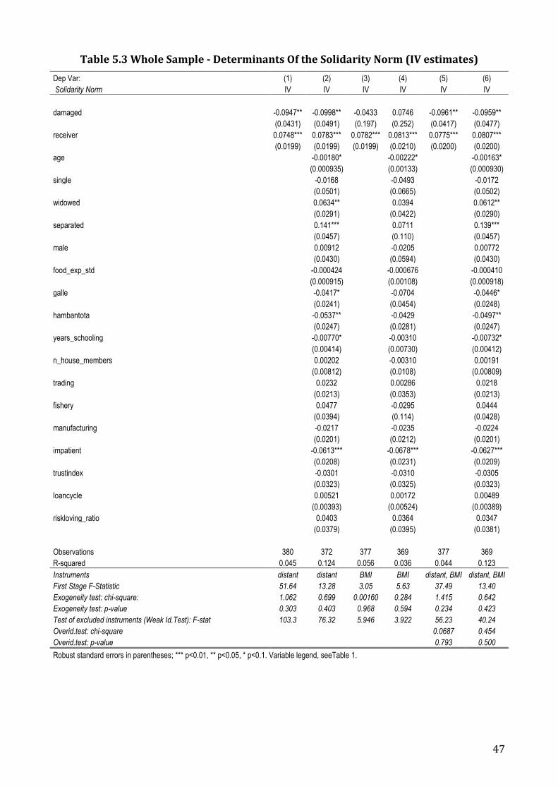
47

Table 5.3 Whole Sample - Determinants Of the Solidarity Norm (IV estimates)

Dep Var: (1) (2) (3) (4) (5) (6)

Solidarity Norm IV IV IV IV IV IV

damaged -0.0947** -0.0998** -0.0433 0.0746 -0.0961** -0.0959**

(0.0431) (0.0491) (0.197) (0.252) (0.0417) (0.0477)

receiver 0.0748*** 0.0783*** 0.0782*** 0.0813*** 0.0775*** 0.0807***

(0.0199) (0.0199) (0.0199) (0.0210) (0.0200) (0.0200)

age

-0.00180*

-0.00222*

-0.00163*

(0.000935)

(0.00133)

(0.000930)

single

-0.0168

-0.0493

-0.0172

(0.0501)

(0.0665)

(0.0502)

widowed

0.0634**

0.0394

0.0612**

(0.0291)

(0.0422)

(0.0290)

separated

0.141***

0.0711

0.139***

(0.0457)

(0.110)

(0.0457)

male

0.00912

-0.0205

0.00772

(0.0430)

(0.0594)

(0.0430)

food_exp_std

-0.000424

-0.000676

-0.000410

(0.000915)

(0.00108)

(0.000918)

galle

-0.0417*

-0.0704

-0.0446*

(0.0241)

(0.0454)

(0.0248)

hambantota

-0.0537**

-0.0429

-0.0497**

(0.0247)

(0.0281)

(0.0247)

years_schooling

-0.00770*

-0.00310

-0.00732*

(0.00414)

(0.00730)

(0.00412)

n_house_members

0.00202

-0.00310

0.00191

(0.00812)

(0.0108)

(0.00809)

trading

0.0232

0.00286

0.0218

(0.0213)

(0.0353)

(0.0213)

fishery

0.0477

-0.0295

0.0444

(0.0394)

(0.114)

(0.0428)

manufacturing

-0.0217

-0.0235

-0.0224

(0.0201)

(0.0212)

(0.0201)

impatient

-0.0613***

-0.0678***

-0.0627***

(0.0208)

(0.0231)

(0.0209)

trustindex

-0.0301

-0.0310

-0.0305

(0.0323)

(0.0325)

(0.0323)

loancycle

0.00521

0.00172

0.00489

(0.00393)

(0.00524)

(0.00389)

riskloving_ratio

0.0403

0.0364

0.0347

(0.0379)

(0.0395)

(0.0381)

Observations 380 372 377 369 377 369

R-squared 0.045 0.124 0.056 0.036 0.044 0.123

Instruments distant distant BMI BMI distant, BMI distant, BMI

First Stage F-Statistic 51.64 13.28 3.05 5.63 37.49 13.40

Exogeneity test: chi-square: 1.062 0.699 0.00160 0.284 1.415 0.642

Exogeneity test: p-value 0.303 0.403 0.968 0.594 0.234 0.423

Test of excluded instruments (Weak Id.Test): F-stat 103.3 76.32 5.946 3.922 56.23 40.24

Overid.test: chi-square 0.0687 0.454

Overid.test: p-value 0.793 0.500

Robust standard errors in parentheses; *** p<0.01, ** p<0.05, * p<0.1. Variable legend, seeTable 1.