Embed Size (px)
Citation preview
CAE-based application for
identification and verification of
hyperelastic parameters
Yevgen Gorash∗, Tugrul Comlekci and Robert Hamilton
Department of Mechanical & Aerospace Engineering, University of Strathclyde, James Weir Building, 75
Montrose Street, Glasgow G1 1XJ, UK
Abstract
The main objective of this study is to develop a CAE-based application with a convenient GUI for identification and verification of material
parameters for hyperelastic models available in the current release of the FE-code ANSYS Mechanical APDL. This Windows-application
implements a 2-step procedure: 1) fitting of experimental stress-strain curves provided by user; 2) verification of obtained material parameters
by the solution of a modified benchmark problem. The application, which was developed using Visual Basic .NET language, implements a
two-way interaction with ANSYS as a single loop using the APDL-script as an input and text, graphical and video files as an output. With this
application, 9 isotropic incompressible hyperelastic material models are compared by fitting them to the conventional Treloar’s experimental
dataset (1944) for a vulcanised rubber. The ranking of hyperelastic models is constructed according to the models efficiency, which is
estimated using a fitting quality criterion. The models ranking is done based upon the complexity of their mathematical formulation and
ability of accurately reproducing the test data. Recent hyperelastic models (Extended Tube and Response Function) are found more efficient
compared to conventional ones. The verification is done by the comparison of an analytical solution to a FEA result for the benchmark
problem of rubber cylinder under compression proposed by Lindley (1967). In the application, the classical formulation of the benchmark
is improved mathematically to become valid for larger deformations. The wide applicability of the proposed 2-steps approach is confirmed
using stress-strains curves for 7 different formulations of natural rubber and 7 different grades of synthetic rubbers.
Keywords
Benchmark, elastomer, Finite Element Analysis, hyperelasticity, ranking, software
Introduction
This study addresses nine isotropic incompressible hypere-
lastic models for rubber-like materials, which are available in
the current release of FE-code ANSYS 1 . ANSYS Mechan-
ical APDL v. 15.0 has been chosen for the implementation of
the WARC research project C22, since it has been a leading
CAE product for FE-analysis for over 40 years. Moreover, it
is capable of all the essential FE-simulation features required
for the analysis of elastomeric components and comprises
recently developed hyperelastic models. Totally, ANSYS
includes the following models1:
• Nearly-incompressible isotropic models: Neo-
Hookean3,4, Mooney-Rivlin5,6, Polynomial Form7,
Ogden Potential8, Arruda-Boyce9, Gent10, Yeoh11,
and Extended Tube12.
• Compressible isotropic models: Blatz-Ko13 and Ogden
Compressible Foam14 options are applicable to com-
pressible foam or foam-type materials.
• Nearly-incompressible isotropic response function
hyperelastic model. The “response function” model in
ANSYS is equivalent to the Marlow model15 imple-
mented in ABAQUS and Sussman-Bathe model16
implemented in ADINA. This model is an exception
∗ Corresponding author. Tel.: +44 790 9780901; E-mail: [email protected]; URL: www.strath.ac.uk/mae/
2 CAE-based application for identification and verification of hyperelastic parameters
from classification, because it obtains the constitutive
response functions directly from experimental data.
• Invariant-based anisotropic strain-energy potential.
It should be noted that anisotropic and compressible
isotropic models are out of the scope of this study.
Over the last decade, a significant number of reviews
and comparative studies on hyperelastic constitutive models
has been published. Availability of these studies is caused
by a great choice of hyperelastic material models and rec-
ommendations17–19 for their selection and application in
FEA. To describe the elastic behaviour of rubber-like mate-
rials, numerous specific forms of strain energy functions
have been proposed in the literature so far. They are per-
manently evolving and improving in mathematical formu-
lations, because of a great demand for a reliable constitu-
tive model to be used in FE-simulations for a variety of
applications. Generally, these studies address the ability of
hyperelastic models to capture the complex behaviours of
rubber-like materials including the material model stability
aspect and quality of experimental data fitting. Seibert and
Schöche20 compared six different models using their own
experimental data obtained with uniaxial and biaxial ten-
sion tests on the 17 wt % carbon black-filled HNBR rubber.
Boyce and Arruda21 compared five models using the classi-
cal data set by Treloar22 for uniaxial and biaxial tension and
pure shear tests on 8%S vulcanised rubber. Xia et al.23 com-
pared three compressible hyperelastic models using their
own experimental data obtained with uniaxial tension tests
on five variants of rubber compounds. Chagnon et al.24
compared three recent models using Treloar’s22 set of exper-
imental data. Attard & Hunt25 considered experimental data
of different authors for five different deformation modes to
demonstrate the efficiency of their proposed model. Mar-
ckmann & Verron26 published a thorough comparison of
twenty hyperelastic models using two classical sets of exper-
imental data – Treloar’s22 and biaxial extension of the sheet
specimens made of isoprene rubber vulcanizate by Kawa-
bata et al.27. Moreover, a ranking of these twenty models
with respect to their ability to fit test data is established
by Marckmann & Verron26, highlighting new efficient con-
stitutive equations that could advantageously replace well-
known models. The corresponding material parameters for
both sets of experimental data22,27 are identified using own
fitting procedure and reported in Ref.26 Ruíz & González28
present a review of the application of hyperelastic mod-
els to the analysis of fabrics using FEA. For this purpose
seven models available in ANSYS were compared using
own experimental data obtained with uniaxial and biaxial
tension and simple shear tests on a fabric. In result, a com-
parison and ranking of models were implemented through
the 3D benchmark problem of a rigid body in contact with
a hyperelastic fabric. Vahapoglu & Karadeniz29 provided
a comprehensive bibliography (1930 – 2003) containing a
list of references on the strain energy functions for rubber-
like materials on isothermal condition. The classification of
models29 includes eighty seven material models, and it is
based on either specific strain energy function formulations
or the discussions on such suggested forms using the phe-
nomenological approach. Another bibliographic review on
constitutive models used in FEA packages for analysis of
rubber components was proposed by Ali et al.30 Dimitrov31
discussed three classes of hyperelastic models (phenomeno-
logical, response-type and micromechanical), which are
available in ANSYS 13. The ranking31 of models is also pro-
posed according to their capability of accurately reproducing
the multiaxial loading states observed in reality. Li et al.32
compared classical Mooney-Rivlin5,6 and Ogden8 models
using their own experimental data obtained with uniaxial,
biaxial and planar tension tests on natural rubber specimens
filled with 46 phr carbon black. One of the most recent and
comprehensive comparative studies of hyperelastic models
is presented by Steinmann and his co-workers33,34. They
provided both accurate stress tensors and tangent opera-
tors for a group of totally twenty five phenomenological
and micromechanical models at large deformations (14 con-
ventional models in Ref.33 and 11 more recent models in
Ref.34). For comparison of all selected models in repro-
ducing the well-known Treloar’s experimental data22, the
analytical expressions for the three homogeneous deforma-
tion modes (uniaxial tension, biaxial tension and pure shear)
have been derived and the performances of the models are
analysed in Refs33,34. Finally, Beda35 developed a mathe-
matical approach for the best way to structure incompress-
ible hyperelastic models, and applied it to the estimation
of convectional phenomenologicalmodels using Treloar’s22
dataset.
Gorash, Comlekci and Hamilton 3
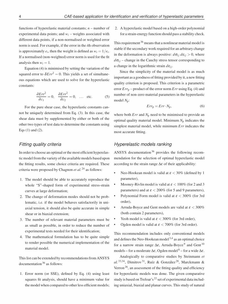
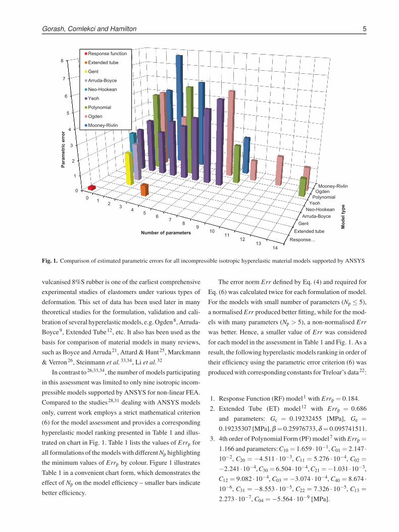
Table 1. Comparison of estimated parametric errors for all incompressible isotropic hyperelastic material models supported by ANSYS
0 1 2 3 4 5 6 7 8 9 10 11 12 13 14
1 Mooney-Rivlin 5.192 7.677 5.968 2.544
2 Ogden 5.189 3.643 4.381 5.792 1.366 1.964 1.548
3 Polynomial 5.192 5.968 2.544 1.166
4 Yeoh 2.848 3.595 2.922 3.779 3.583 4.232 4.922 5.624
5 Extended tube 0.686
6 Arruda-Boyce 2.499
7 Gent 2.161
8 Neo-Hookean 2.848
9 Response function 0.184
number of parametersmaterial modelno.
Assessment of hyperelastic models effi-
ciency
Curve fitting tools
The ANSYS curve fitting tool36 is an application embedded
into ANSYS for estimating material constants by inputting
user’s experimental data. Quality of the fitting is assessed
by comparing visually the curves obtained with hyperelas-
tic material models to experimental data. User’s stress-strain
curves can be converted to any of the supported hyperelastic
models mentioned above. The curve fitting can be performed
either interactively (GUI) or via batch commands by doing
the 7-steps procedure36. In this study, ANSYS curve fitting
tool is operated in batch mode by the external application
using APDL commands.
Alternative curve fitting tools for hyperelastic and other
non-linear material models are available as stand-alone
applications and add-ins for other CAD/CAE products:
1. MCalibration37 – a software, which enables semi-
automatic extraction of pertinent material parameters
from test data for a number of advanced non-linear
material models.
2. Hyperfit38 – a curve fitting utility for automatic param-
eter identification for a large number of hyperelastic
constitutive models.
3. Curve fitting tools incorporated into FE-codes of alter-
native CAE-systems (e.g. ABAQUS, COMSOL and
MSC Marc) and FE-addins of CAD-systems (e.g. Creo
Simulate and SolidWorks Simulation).
These tools are different in their functionality, mathematical
methods for fitting, number and types of supported material
models. All applications support conventional hyperelastic
material models like Mooney-Rivlin5,6, Ogden8, Arruda-
Boyce9, Gent10, Yeoh11, etc. Some of these tools support
more recent advanced material models, which require more
computational efforts, like Extended Tube model12.
Least squares fit analysis
The curve fitting process is based upon a regression anal-
ysis using the computational method called least squares
method39. By performing a least squares fit analysis the
material constants can be determined from experimental
stress-strain data and constitutive equations for the principal
true stress σ11 under uniaxial and biaxial tension and pure
shear correspondingly:
σ11 = 2(
λ 21 −λ−1
1
)
[
∂W
∂ I1
+λ−11
∂W
∂ I2
]
, (1)
σ11 = 2(
λ 21 −λ−4
1
)
[
∂W
∂ I1
+λ 21
∂W
∂ I2
]
, (2)
σ11 = 2(
λ 21 −λ−2
1
)
[
∂W
∂ I1
+∂W
∂ I2
]
, (3)
where λ1 – 1st principal stretch ratio, W – strain energy den-
sity function defined by material model, I1 and I2 - 1st and
2nd principal strain invariants correspondingly. Equations
(1)-(3) are fitted simultaneously to the available experimen-
tal curves. Briefly, the least squares fit minimises the sum of
squared error (SSE) between experimental and Cauchy pre-
dicted stress values. The sum of the squared error or error
norm is defined by:
Err =n
∑i=1
wi
[
σexpi −σ
engi (c j)
]2, (4)
where Err – SSE or least squares residual error; σexpi – exper-
imental stress values; σengi – engineering stress values as
4 CAE-based application for identification and verification of hyperelastic parameters
functions of hyperelastic material constants; n – number of
experimental data points; and wi – weights associated with
different data points, if a non-normalised or weighted error
norm is used. For example, if the error in the ith observation
is approximately ei, then the weight is defined as wi = 1/ei.
If a normalised (non-weighted) error norm is used for the fit
analysis then wi = 1.
Equation (4) is minimised by setting the variation of the
squared error to δErr2 = 0. This yields a set of simultane-
ous equations which are used to solve for the hyperelastic
constants:
∂Err2
∂c1
= 0,∂Err2
∂c2
= 0, . . . etc. (5)
For the pure shear case, the hyperelastic constants can-
not be uniquely determined from Eq. (3). In this case, the
shear data must by supplemented by either or both of the
other two types of test data to determine the constants using
Eqs (1) and (2).
Fitting quality criteria
In order to choose an optimal or the most efficient hyperelas-
tic model from the variety of the available models based upon
the fitting results, some choice criteria are required. These
criteria were proposed by Chagnon et al.24 as follows:
1. The model should be able to accurately reproduce the
whole “S”-shaped form of experimental stress-strain
curves at large deformation;
2. The change of deformation modes should not be prob-
lematic, i.e. if the model behaves satisfactorily in uni-
axial tension, it should also be quite accurate in simple
shear or in biaxial extension;
3. The number of relevant material parameters must be
as small as possible, in order to reduce the number of
experimental tests needed for their identification;
4. The mathematical formulation has to be quite simple
to render possible the numerical implementation of the
material model.
This list can be extended by recommendations from ANSYS
documentation36 as follows:
1. Error norm (or SSE), defined by Eq. (4) using least
squares fit analysis, should have a minimum value for
the model when compared to other less efficient models;
2. A hyperelastic model based on a high-order polynomial
for a strain-energy function should pass a stability check.
This requirement36 means that a nonlinear material model is
stable if the secondary work required for an arbitrary change
in the deformation is always positive: dσi j dεi j > 0, where
dσi j – change in the Cauchy stress tensor corresponding to
a change in the logarithmic strain dεi j.
Since the simplicity of the material model is as much
important as a goodness of fitting provided by it, a new fitting
quality criterion is proposed. This criterion is a parametric
error Errp – product of the error norm Err using Eq. (4) and
number of non-zero material parameters in the hyperelastic
model Np:
Errp = Err ·Np, (6)
where both Err and Np need to be minimised to provide an
optimal quality material model. Minimum Np indicates the
simplest material model, while minimum Err indicates the
most accurate fitting.
Hyperelastic models ranking
ANSYS documentation36 provides the following recom-
mendation for the selection of optimal hyperelastic model
according to the strain range ∆ε of their applicability:
• Neo-Hookean model is valid at ε < 30% (defined by 1
parameter),
• Mooney-Rivlin model is valid at ε < 100% (for 2 and 3
parameters) and at ε < 200% (for 5 and 9 parameters),
• Polynomial Form model is valid at ε < 300% (for 3rd
order),
• Arruda-Boyce and Gent models are valid at ε < 300%
(both contain 2 parameters),
• Yeoh model is valid at ε < 300% (for 3rd order),
• Ogden model is valid at ε < 700% (for 3rd order).
This recommendation includes only conventional models
and defines the Neo-Hookean model3,4 as an optimal choice
for a narrow strain range ∆ε , Arruda-Boyce9 and Gent10
models – for a moderate ∆ε , Ogden model8 – for a wide ∆ε .
Analogically to comparative studies by Steinmann et
al.33,34, Dimitrov31, Ruíz & González28, Marckmann &
Verron26, an assessment of the fitting quality and efficiency
for hyperelastic models was done. The given comparative
study is based on Treloar’s22 set of experimental data includ-
ing uniaxial, biaxial and planar curves. This study of natural
Gorash, Comlekci and Hamilton 5
Response…
Extended tube
Gent
Arruda-Boyce
Neo-Hookean
Yeoh
Polynomial
OgdenMooney-Rivlin
0
1
2
3
4
5
6
7
8
01
23
45
67
89
1011
1213
14
Mo
del
typ
e
Para
metr
ic e
rro
r
Number of parameters
Response function
Extended tube
Gent
Arruda-Boyce
Neo-Hookean
Yeoh
Polynomial
Ogden
Mooney-Rivlin
Fig. 1. Comparison of estimated parametric errors for all incompressible isotropic hyperelastic material models supported by ANSYS
vulcanised 8%S rubber is one of the earliest comprehensive
experimental studies of elastomers under various types of
deformation. This set of data has been used later in many
theoretical studies for the formulation, validation and cali-
bration of several hyperelastic models, e.g. Ogden8, Arruda-
Boyce9, Extended Tube12, etc. It also has been used as the
basis for comparison of material models in many reviews,
such as Boyce and Arruda21, Attard & Hunt25, Marckmann
& Verron26, Steinmann et al.33,34, Li et al.32
In contrast to26,33,34, the number of models participating
in this assessment was limited to only nine isotropic incom-
pressible models supported by ANSYS for non-linear FEA.
Compared to the studies28,31 dealing with ANSYS models
only, current work employs a strict mathematical criterion
(6) for the model assessment and provides a corresponding
hyperelastic model ranking presented in Table 1 and illus-
trated on chart in Fig. 1. Table 1 lists the values of Errp for
all formulations of the models with different Np highlighting
the minimum values of Errp by colour. Figure 1 illustrates
Table 1 in a convenient chart form, which demonstrates the
effect of Np on the model efficiency – smaller bars indicate
better efficiency.
The error norm Err defined by Eq. (4) and required for
Eq. (6) was calculated twice for each formulation of model.
For the models with small number of parameters (Np ≤ 5),
a normalised Err produced better fitting, while for the mod-
els with many parameters (Np > 5), a non-normalised Err
was better. Hence, a smaller value of Err was considered
for each model in the assessment in Table 1 and Fig. 1. As a
result, the following hyperelastic models ranking in order of
their efficiency using the parametric error criterion (6) was
produced with corresponding constants for Treloar’s data22:
1. Response Function (RF) model1 with Errp = 0.184.
2. Extended Tube (ET) model12 with Errp = 0.686
and parameters: Gc = 0.19232455 [MPa], Ge =
0.19235307 [MPa], β = 0.25976733, δ = 0.095741511.
3. 4th order of Polynomial Form (PF) model7 with Errp =
1.166 and parameters: C10 = 1.659 ·10−1, C01 = 2.147 ·
10−2, C20 = −4.511 · 10−3, C11 = 5.276 · 10−4, C02 =
−2.241 ·10−4, C30 = 6.504 ·10−4, C21 =−1.031 ·10−3,
C12 = 9.082 ·10−4, C03 = −3.074 ·10−4, C40 = 8.674 ·
10−6, C31 = −8.553 · 10−5, C22 = 7.326 · 10−5, C13 =
2.273 ·10−7, C04 =−5.564 ·10−9 [MPa].
6 CAE-based application for identification and verification of hyperelastic parameters
0
1
2
3
4
5
6
7
0 1 2 3 4 5 6 7
En
gin
ee
rin
g s
tre
ss (
MP
a)
Engineering strain
uniaxial test
uniaxial FEA
planar test
planar FEA
biaxial test
biaxial FEA
y = 1.1074x5 - 3.5586x4 + 4.4549x3 - 2.9455x2 + 1.4681x0
0.2
0.4
0.6
0.8
1
0 0.25 0.5 0.75 1 1.25 1.5 1.75 2En
gin
ee
rin
g s
tre
ss (
MP
a)
Engineering strain
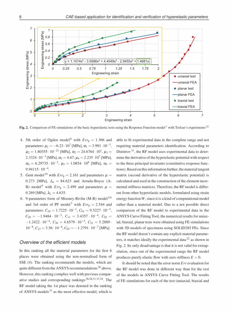
Fig. 2. Comparison of FE-simulations of the basic hyperelastic tests using the Response Function model1 with Treloar’s experiments22
4. 5th order of Ogden model8 with Errp = 1.366 and
parameters: µ1 =−6.23 ·107 [MPa], α1 = 3.991 ·10−3,
µ2 = 1.80355 · 10−21 [MPa], α2 = 24.6764 · 101, µ3 =
2.3324 ·10−3 [MPa], α3 = 4.67, µ4 = 2.235 ·107 [MPa],
α4 = 6.29735 · 10−3, µ5 = 1.0854 · 108 [MPa], α5 =
9.94115 ·10−4.
5. Gent model10 with Errp = 2.161 and parameters µ =
0.273 [MPa], Jm = 84.623 and Arruda-Boyce (A-
B) model9 with Errp = 2.499 and parameters µ =
0.269 [MPa], λL = 4.635.
6. 9-parameters form of Mooney-Rivlin (M-R) model5,6
and 3rd order of PF model7 with Errp = 2.544 and
parameters: C10 = 1.7225 · 10−1, C01 = 9.5227 · 10−3,
C20 = −1.9484 · 10−3, C11 = 3.4357 · 10−4, C02 =
−1.2422 · 10−4, C30 = 4.6579 · 10−5, C21 = 5.2889 ·
10−8, C12 = 3.56 ·10−6, C03 =−1.2791 ·10−7 [MPa].
Overview of the efficient models
In this ranking all the material parameters for the first 6
places were obtained using the non-normalised form of
SSE (4). The ranking recommends the models, which are
quite different from the ANSYS recommendations36 above.
However, this ranking complies well with previous compar-
ative studies and corresponding rankings26,28,31,33,34. The
RF model taking the 1st place was denoted in the ranking
of ANSYS models31 as the most effective model, which is
able to fit experimental data in the complete range and not
requiring material parameters identification. According to
Dimitrov31, the RF model uses experimental data to deter-
mine the derivative of the hyperelastic potential with respect
to the three principal invariants (constitutive response func-
tions). Based on this information further, the material tangent
matrix (second derivative of the hyperelastic potential) is
calculated and used in the construction of the element incre-
mental stiffness matrices. Therefore, the RF model is differ-
ent from other hyperelastic models, formulated using strain
energy function W , since it is a kind of computational model
rather than a material model. Due to a not possible direct
comparison of the RF model to experimental data in the
ANSYS Curve Fitting Tool, the numerical results for uniax-
ial, biaxial, planar tests were obtained using FE-simulations
with 3D models of specimens using SOLID285 FEs. Since
the RF model doesn’t contain any explicit material parame-
ters, it matches ideally the experimental data22 as shown in
Fig. 2. Its only disadvantage is that it is not valid for extrap-
olation, since out of the experimental range the RF model
produces purely elastic flow with zero stiffness E = 0.
It should be noted that the error norm Err evaluation for
the RF model was done in different way than for the rest
of the models in ANSYS Curve Fitting Tool. The results
of FE-simulations for each of the test (uniaxial, biaxial and
Gorash, Comlekci and Hamilton 7
0
1
2
3
4
5
6
7
0 1 2 3 4 5 6 7
En
gin
ee
rin
g s
tre
ss (
MP
a)
Engineering strain
uniaxial test
uniaxial FEA
planar test
planar FEA
biaxial test
biaxial FEA
y = 1.1074x5 - 3.5586x4 + 4.4549x3 - 2.9455x2 + 1.4681x0
0.2
0.4
0.6
0.8
1
0 0.25 0.5 0.75 1 1.25 1.5 1.75 2
En
gin
ee
rin
g s
tre
ss (
MP
a)
Engineering strain
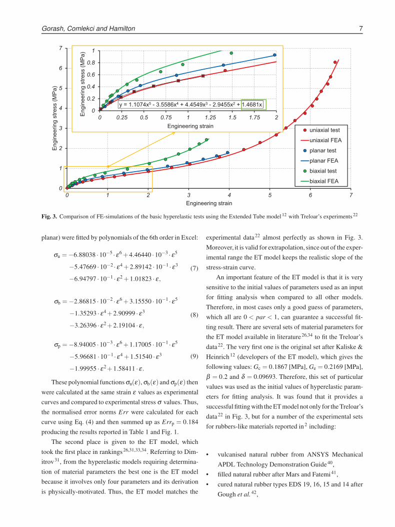
Fig. 3. Comparison of FE-simulations of the basic hyperelastic tests using the Extended Tube model12 with Treloar’s experiments22
planar) were fitted by polynomials of the 6th order in Excel:
σu =−6.88038 ·10−5· ε6 + 4.46440 ·10−3
· ε5
−5.47669 ·10−2 · ε4 + 2.89142 ·10−1 · ε3
−6.94797 ·10−1 · ε2 + 1.01823 · ε,
(7)
σb =−2.86815 ·10−2· ε6 + 3.15550 ·10−1
· ε5
−1.35293 · ε4+ 2.90999 · ε3
−3.26396 · ε2+ 2.19104 · ε,
(8)
σp =−8.94005 ·10−3· ε6 + 1.17005 ·10−1
· ε5
−5.96681 ·10−1 · ε4 + 1.51540 · ε3
−1.99955 · ε2+ 1.58411 · ε.
(9)
These polynomial functions σu(ε), σb(ε) and σp(ε) then
were calculated at the same strain ε values as experimental
curves and compared to experimental stress σ values. Thus,
the normalised error norms Err were calculated for each
curve using Eq. (4) and then summed up as Errp = 0.184
producing the results reported in Table 1 and Fig. 1.
The second place is given to the ET model, which
took the first place in rankings26,31,33,34. Referring to Dim-
itrov31, from the hyperelastic models requiring determina-
tion of material parameters the best one is the ET model
because it involves only four parameters and its derivation
is physically-motivated. Thus, the ET model matches the
experimental data22 almost perfectly as shown in Fig. 3.
Moreover, it is valid for extrapolation, since out of the exper-
imental range the ET model keeps the realistic slope of the
stress-strain curve.
An important feature of the ET model is that it is very
sensitive to the initial values of parameters used as an input
for fitting analysis when compared to all other models.
Therefore, in most cases only a good guess of parameters,
which all are 0 < par < 1, can guarantee a successful fit-
ting result. There are several sets of material parameters for
the ET model available in literature26,34 to fit the Treloar’s
data22. The very first one is the original set after Kaliske &
Heinrich12 (developers of the ET model), which gives the
following values: Gc = 0.1867 [MPa], Ge = 0.2169 [MPa],
β = 0.2 and δ = 0.09693. Therefore, this set of particular
values was used as the initial values of hyperelastic param-
eters for fitting analysis. It was found that it provides a
successful fitting with the ET model not only for the Treloar’s
data22 in Fig. 3, but for a number of the experimental sets
for rubbers-like materials reported in2 including:
• vulcanised natural rubber from ANSYS Mechanical
APDL Technology Demonstration Guide40,
• filled natural rubber after Mars and Fatemi41,
• cured natural rubber types EDS 19, 16, 15 and 14 after
Gough et al.42,
8 CAE-based application for identification and verification of hyperelastic parameters
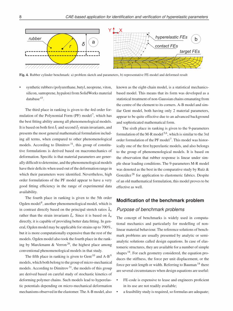
r δrubber hyperelastic FEs
contact FEs
target FEs
ab
Y X
Fig. 4. Rubber cylinder benchmark: a) problem sketch and parameters, b) representative FE-model and deformed result
• synthetic rubbers (polyurethane, butyl, neoprene, viton,
silicon, santoprene, hypalon) from SolidWorks material
database43.
The third place in ranking is given to the 4rd order for-
mulation of the Polynomial Form (PF) model7, which has
the best fitting ability among all phenomenological models.
It is based on both first I1 and second I2 strain invariants, and
presents the most general mathematical formulation includ-
ing all terms, when compared to other phenomenological
models. According to Dimitrov31, this group of constitu-
tive formulations is derived based on macromechanics of
deformation. Specific is that material parameters are gener-
ally difficult to determine, and the phenomenological models
have their deficits when used out of the deformation range in
which their parameters were identified. Nevertheless, high
order formulations of the PF model appear to have a very
good fitting efficiency in the range of experimental data
availability.
The fourth place in ranking is given to the 5th order
Ogden model8, another phenomenological model, which is
in contrast directly based on the principal stretch ratios λn
rather than the strain invariants In. Since it is based on λn
directly, it is capable of providing better data fitting. In gen-
eral, Ogden model may be applicable for strains up to 700%,
but it is more computationally expensive than the rest of the
models. Ogden model also took the fourth place in the rank-
ing by Marckmann & Verron26, the highest place among
conventional phenomenological models in that study.
The fifth place in ranking is given to Gent10 and A-B9
models, which both belong to the group of micro-mechanical
models. According to Dimitrov31, the models of this group
are derived based on careful study of stochastic kinetics of
deforming polymer chains. Such models lead to hyperelas-
tic potentials depending on micro-mechanical deformation
mechanisms observed in the elastomer. The A-B model, also
known as the eight-chain model, is a statistical mechanics-
based model. This means that its form was developed as a
statistical treatment of non-Gaussian chains emanating from
the centre of the element to its corners. A-B model and sim-
ilar Gent model, both having only 2 material parameters,
appear to be quite effective due to an advanced background
and sophisticated mathematical form.
The sixth place in ranking is given to the 9-parameters
formulation of the M-R model5,6, which is similar to the 3rd
order formulation of the PF model7. This model was histor-
ically one of the first hyperelastic models, and also belongs
to the group of phenomenological models. It is based on
the observation that rubber response is linear under sim-
ple shear loading conditions. The 9-parameters M-R model
was denoted as the best in the comparative study by Ruíz &
González28 for application to elastomeric fabrics. Despite
of an old mathematical formulation, this model proves to be
effective as well.
Modification of the benchmark problem
Purpose of benchmark problems
The concept of benchmarks is widely used in computa-
tional mechanics and particularly for modelling of non-
linear material behaviour. The reference solutions of bench-
mark problems are usually presented by analytic or semi-
analytic solutions called design equations. In case of elas-
tomeric structures, they are available for a number of simple
shapes18. For each geometry considered, the equation pro-
duces the stiffness, the force per unit displacement, or the
force per unit length or width. Referring to Bauman18 there
are several circumstances when design equations are useful:
• FE-code is expensive to lease and engineers proficient
in its use are not readily available;
• a feasibility study is required, so formulas are adequate;
Gorash, Comlekci and Hamilton 9
• only simple shapes described by the formulas are used;
• the part is not structurally critical;
• stress-strain data required to determine the coefficients
for the constitutive law for FEA are not available.
In this study, the benchmark problem is used for the basic
verification of the hyperelastic material input by comparing
the FEA solution to a corresponding reference solution.
The subdivision into two broad categories of formu-
las is proposed by Bauman18. The first set consists of
the traditional ones that depend on small rubber deforma-
tions (typically < 30%), approximately linear rubber stress-
strain behaviour, and incompressible material. These equa-
tions have been studied and systematised by Lindley44 and
Gent45. The second category, developed by Yeoh, Pinter and
Banks46 applies to larger strains, allows for slight compress-
ibility and approximates FEA solutions for some simple
shapes. However, this study presents a modification of the
reference solution for a conventional benchmark from the
first category, which extends its applicability to large strains
of about 150%.
Compression of rubber cylinder
Referring to Lindley44, when a curved surface of a rubber
component is compressed against a rigid plane, the stiffness
generally increases as the area of contact increases during
the deformation. Thus, the load-deformation characteristics
tend to be markedly non-linear. For the rollers (solid, hollow
and rubber-covered) the relationships apply for plane strain
conditions, i.e. for length ≫ rubber thickness.
This conventional benchmark problem for elastomers
is comprehensively studied by Sussman and Bathe47 using
a displacement-pressure (u/p) FE-formulation for the geo-
metrically and materially nonlinear analysis of compressible
and almost incompressible solids. One of the study objec-
tives47 was a determination of the force-deflection curve
for the cylinder and also the location and magnitude of the
maximum stresses when the applied displacement equals
one-half of the initial diameter of the cylinder. The geome-
try is defined in Fig. 4a and shows r as the outside radius of
the roller and δ as the compressive displacement.
For small displacements, the Hertz contact assump-
tions are valid, and the following force per unit length ( f )
vs. deflection (δ ) relationship48 results in:
δ =4 f
π
1−ν2
E0
(
1
3+ ln
[
4r
b
])
,
with b = 1.6
√
2r f1−ν2
E0
,
(10)
where E0 and ν are the small strain Young’s modulus and
Poisson’s ratio correspondingly.
For larger displacements during compression of solid
rubber rollers, an approximate solution based on experi-
ments is given by Lindley44 for the force per unit length
as follows
f
6r G= 1.25
(
δ
2r
)1.5
+ 50
(
δ
2r
)6
, (11)
which doesn’t account for the effect of friction. Using
incompressibility assumption ν ≈ 0.5 in formula for shear
modulus
G =τ
γ=
E
2(1+ν), (12)
the Eq. (11) is simplified to the following form:
f = E0 r
[
2.5
(
δ
2r
)1.5
+ 100
(
δ
2r
)6]
, (13)
where the Young’s modulus E0 is assumed to be constant.
In order to assess the accuracy of the available analytic
solutions presented by Eqs (10) and (13), a sample bench-
mark case has been analysed numerically in the FE-code
ANSYS. This case is based upon the sample benchmark for-
mulation used by Sussman & Bathe47 for FE-code ADINA
shown in Fig. 4a, which comprised:
• cylinder radius of r = 200 mm;
• plane strain consideration with infinite cylinder length;
• frictionless contact using node-to-surface contact type;
• maximum displacement of the plate as δ = 200 mm.
The objective is to determine the force-deflection
response using FEA and compare it to the reference solu-
tions (10) and (13). Due to geometric and loading symmetry,
the FE-analysis is performed using one quarter of the cyclin-
der cross section with 14 FEs per radius as shown in Fig. 4b.
All nodes on the left edge (X = 0) are constrained in UX .
All nodes on the top edge (Y = 0) are coupled in UY . An
imposed displacement of δ/2 acts upon the coupled nodes.
The quasistatic problem is solved using the 2D lower order
10 CAE-based application for identification and verification of hyperelastic parameters
0
1000
2000
3000
4000
5000
6000
7000
0 20 40 60 80 100 120 140 160 180 200 220 240 260 280
Fo
rce
pe
r u
nit
le
ng
th (
N/m
m)
Displacement (mm)
0
2
4
6
8
10
12
14
0 0.5 1 1.5 2 2.5 3 3.5 4 4.5 5
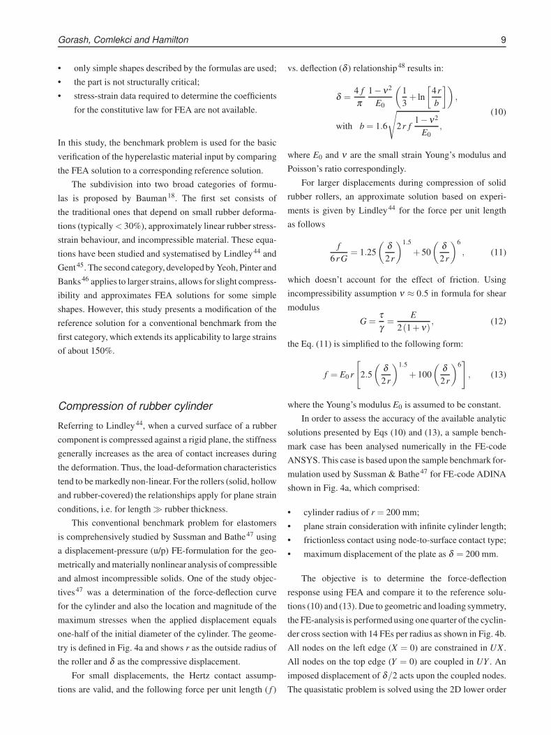
Fig. 5. Comparison of analytical solutions, Lindley’s Eq. (13), Hertz’s Eq. (10) and their average Eq. (15), to FEA results obtained in
ANSYS using Mooney-Rivlin5,6 and Ogden8 material models
solid elements (PLANE182), rigid target (type TARGE169)
and contact (CONTA175) elements. The solution is obtained
in a number of substeps using large deformations assumption
and default contact algorithm.
Modification of the reference solution
There are a few improvements in the formulation of the cur-
rent benchmark when compared to the previous one47 as
explained below. Firstly, The maximum imposed displace-
ment is increased from original δ = 200 to 273 mm, which
corresponds to εt = 150% of equivalent true strain in struc-
ture or εe = 350% of equivalent engineering strain on the
stress-strain curve.
Secondly, the Treloar’s experimental data set22 is used
in this study instead of hyperelastic model fits47 based upon
the 3-terms form of Mooney-Rivlin model5,6 and the 3rd
order of Ogden model8. The corresponding solution of the
benchmark problem, previously obtained in ADINA47, was
derived in ANSYS as illustrated in Fig. 5. It should be noted
that for displacements up to δ = 200 mm, FE-results with
both material models are quite close to Lindley’s Eq. (13) as
obtained by Sussman & Bathe47. However, for the larger dis-
placements up to δ = 273 mm, the FE-result with the Ogden
model deviates from Lindley’s solution, while FE-result with
M-R model keeps close to it. Moreover, the material fit
using 6-terms Ogden model is more accurate than the fit
with 3-terms M-R model. This fact reveals that the Lindley’s
solution (13) is non-conservative for large displacements and
significant compression of the cylinder, since the FE-result
with Ogden model is more realistic. The stress-strain curve
of the M-R fit provides a much softer material response than
the more advanced Ogden fit.
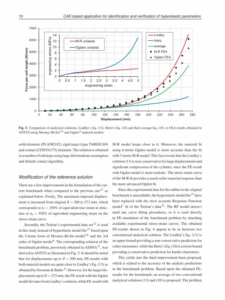
Since the experimental data for the rubber in the original
benchmark is unavailable, the hyperelastic model fits47 have
been replaced with the most accurate Response Function
model1 fit of the Treloar’s data22. The RF model doesn’t
need any curve fitting procedures, so it is used directly
in FE-simulation of the benchmark problem by attaching
available experimental stress-strain curves. The obtained
FE-results shown in Fig. 6 appear to be in between two
conventional analytical solution. The Lindley’s Eq. (13) is
an upper bound providing a non-conservative prediction for
softer elastomers, while the Hertz’s Eq. (10) is a lower bound
providing a conservative prediction for harder elastomers.
This yields into the third improvement been proposed,
which is related to the accuracy of the analytic predictions
in the benchmark problem. Based upon the obtained FE-
results for the benchmark, an average of two conventional
analytical solutions (13) and (10) is proposed. The problem
Gorash, Comlekci and Hamilton 11
0
500
1000
1500
2000
2500
3000
3500
0 20 40 60 80 100 120 140 160 180 200 220 240 260 280
Fo
rce
pe
r u
nit
le
ng
th (
N/m
m)
Displacement (mm)
0
1
2
3
4
5
6
7
0 1 2 3 4 5 6 7
Fig. 6. Comparison of analytical solutions, Lindley’s Eq. (13), Hertz’s Eq. (10) and their average Eq. (15), to FEA results obtained in
ANSYS using the Response Function material model1
of this combination is that the Lindley’s solution is given
as force dependent on displacement f (δ ), while the Hertz’s
solution is given as displacement dependent on force δ ( f ).
Since they are not dependent on one variable, one of them
needs to be reversed mathematically to become compatible
for their combination. The direct mathematical reversion is
problematic for both of the formulas (13) and (10), since
the dependent variables are presented twice in both of them
within the power-law functions with different power expo-
nents. Thus, a non-direct recursive approach is applied here
to reverse the function δ ( f ) in (10) as
fn+1 =δ
π
4
E0
1−ν2
1
3+ ln
4r
1.6
√
2r fn1−ν2
E0
, (14)
where n ≥ 10 and the initial iteration f0 is defined by (13).
This recursive approach is similar to the one used by Gorash
& Chen49,50 to reverse the formula for bending moment
dependent on total strain, which is applied to a beam with
a square cross-section to deform it plastically using the
Ramberg-Osgood material model.
Then a simple averaging is applied to Eqs (13) and (14)
f ave(δ ) =f Hn+1(δ )+ f L(δ )
2, (15)
where f Hn+1(δ ) is the Hertz’s Eq. (14) in the reversed form
and f L(δ ) is the Lindley’s Eq. (13).
The average solution (15) of the benchmark problem
using Treloar’s data22 illustrated in Fig. 6 matches perfectly
the FE-results obtained with the RF model1, which is the
most accurate compared to other hyperelastic models. Thus,
an introduction of the average solution using Eqs (14) and
(15) extends the applicability of the benchmark problem
to large displacements. The conventional Lindley’s solution
(13), limited to about 50% of true strain, becomes valid for
about 150% of true strain in combination with the reversed
Hertz’s solution (14).
It should be noted that the analytical benchmark input
requires only one material parameter – E0, elasticity modu-
lus or initial slope of the hyperelastic stress-strain curve. It
is defined by application of the trendline in Excel to the ini-
tial range of the uniaxial stress-strain curve. The regression
type of the trendline is usually a polynomial of the 5th or 6th
order, which intercepts the coordinates origin [0,0]. There-
fore, the coefficient of the 1st order component represents
E0, since it is the only non-zero number of the polynomial
12 CAE-based application for identification and verification of hyperelastic parameters
derivative defined in the location [0,0]. An example of the
E0 estimation is illustrated in Figs 2 and 3, where the 5th
order polynomial is applied to the strain range of [0,1.17] of
uniaxial curve, and correspondent E0 = 1.468 MPa.
Benchmark applied to other elastomers
Apart from Treloar’s data22, the benchmark was applied to
other natural and synthetic rubbers investigated in report2.
Each set of stress-strain curves2 has a polynomial trendline
attached with a correspondent equation, last component of
which represents E0. Numerical solutions of the benchmark
were derived with the Response Function model used to fit
stress-strain curves, while analytical solutions (13), (10) and
(15) were obtained using a correspondent value of E0. All
the range of FE-solutions is located between Lindley’s (13)
and Hertz’s (10) solutions. Harder rubbers with a steeper
initial slope are closer to the Hertz’s (10) solution, while
softer rubbers with less steep initial slope are closer to the
Lindley’s (13) solution. The full classification of material
response according to the numerical benchmark response is
following:
Pure soft: Neoprene and butyl rubbers43;
Soft-average: Vulcanised natural rubber40 and hypalon rub-
ber43;
Pure average: Filled natural rubber41, rubber EDS 1942 and
polyurethane43;
Hard-average: Rubber EDS 1442, silicon rubber and viton
fluoroelastomer43;
Pure hard: Santoprene43;
Mixed (initially hard): Rubbers EDS 16 and 1542.
It should be noticed that the proposed benchmark enables
verification of material model fits for a wide number of
elastomers, which are quite different in the shape of experi-
mental stress-strain curves. Since the numerical solution for
the majority of the tested elastomers tends to the average
analytical solution (15), the proposed modification of the
benchmark proves to be quite significant.
Functionality of the developed CAE-based
application
Fitting of test stress-strain curves by hyperelastic models
and verification of obtained material parameters by the
solution of an improved benchmark problem, which are
described in previous sections, are implemented in a stan-
dalone Windows-application. This application was devel-
oped using Visual Basic .NET language in Microsoft Visual
Studio 2010 environment. Different inter-process commu-
nication mechanisms are used in interactions with several
external applications. The most important component of its
functionality is an implementation of a two-way interaction
with ANSYS as a single loop using the APDL-script as an
input and text, graphical and video files as an output. Each
time when the analysis is run in the application, the following
3-steps procedure is executed:
• generation of the input APDL-script in a text file
according to the above defined options;
• starting of ANSYS executable file in batch mode, which
reads and executes the input APDL-script;
• text, graphical and video files generated by ANSYS are
uploaded into the application for review.
The Windows API functionality is used by the applica-
tion to start ANSYS executable file as a process and to wait
until it is completed. The hyperelastic identification module
of the application has the following structure as shown in
Fig. 7:
1. ComboBox with choice of available experimental data
for a number of elastomers considered in this work2.
2. ComboBox with choice of isotropic hyperelastic mate-
rial models supported by ANSYS1 as indicated in
Introduction.
3. TextBox with a small strain (initial) elasticity modulus
E0 identified using a uniaxial stress-strain curve in Excel
as explained in the Benchmark Modification. It is a part
of the data set provided by a user along with stress-strain
curve in separate text files.
4. Options for a hyperelastic model formulation com-
prising a choice of polynomial order or number of
constants.
5. CheckBox for a choice of normalised or non-normalised
error norm used in fitting analysis as explained in the
Least Squares Fit Analysis.
6. TextBox defines a maximum number of iterations in
fitting analysis governing the accuracy and duration of
analysis.
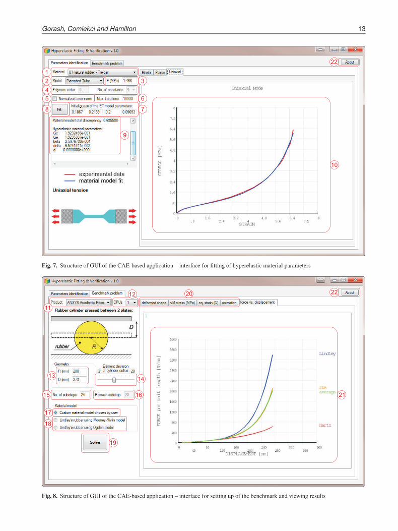
Gorash, Comlekci and Hamilton 13
1
2 3
4
5 6
78
9
10
22
Fig. 7. Structure of GUI of the CAE-based application – interface for fitting of hyperelastic material parameters
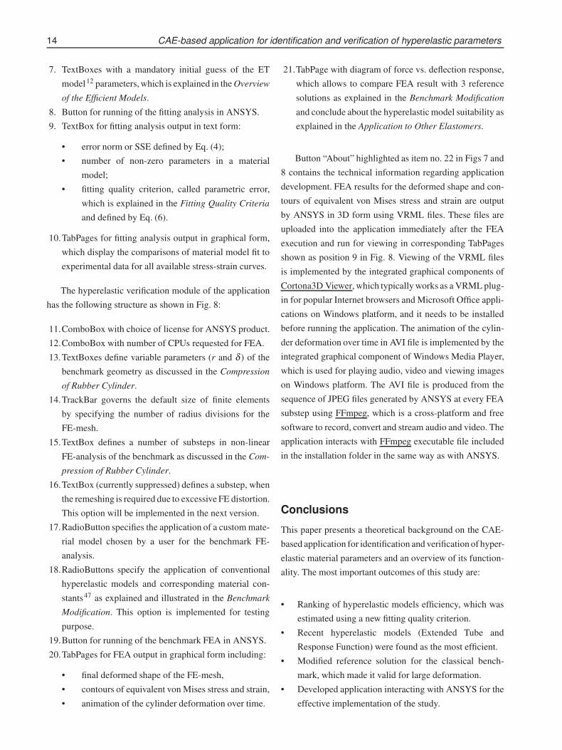
1314
15 16
17
18
19
20
21
11
12 22
Fig. 8. Structure of GUI of the CAE-based application – interface for setting up of the benchmark and viewing results
14 CAE-based application for identification and verification of hyperelastic parameters
7. TextBoxes with a mandatory initial guess of the ET
model12 parameters, which is explained in the Overview
of the Efficient Models.
8. Button for running of the fitting analysis in ANSYS.
9. TextBox for fitting analysis output in text form:
• error norm or SSE defined by Eq. (4);
• number of non-zero parameters in a material
model;
• fitting quality criterion, called parametric error,
which is explained in the Fitting Quality Criteria
and defined by Eq. (6).
10.TabPages for fitting analysis output in graphical form,
which display the comparisons of material model fit to
experimental data for all available stress-strain curves.
The hyperelastic verification module of the application
has the following structure as shown in Fig. 8:
11.ComboBox with choice of license for ANSYS product.
12.ComboBox with number of CPUs requested for FEA.
13.TextBoxes define variable parameters (r and δ ) of the
benchmark geometry as discussed in the Compression
of Rubber Cylinder.
14.TrackBar governs the default size of finite elements
by specifying the number of radius divisions for the
FE-mesh.
15.TextBox defines a number of substeps in non-linear
FE-analysis of the benchmark as discussed in the Com-
pression of Rubber Cylinder.
16.TextBox (currently suppressed) defines a substep, when
the remeshing is required due to excessive FE distortion.
This option will be implemented in the next version.
17.RadioButton specifies the application of a custom mate-
rial model chosen by a user for the benchmark FE-
analysis.
18.RadioButtons specify the application of conventional
hyperelastic models and corresponding material con-
stants47 as explained and illustrated in the Benchmark
Modification. This option is implemented for testing
purpose.
19.Button for running of the benchmark FEA in ANSYS.
20.TabPages for FEA output in graphical form including:
• final deformed shape of the FE-mesh,
• contours of equivalent von Mises stress and strain,
• animation of the cylinder deformation over time.
21.TabPage with diagram of force vs. deflection response,
which allows to compare FEA result with 3 reference
solutions as explained in the Benchmark Modification
and conclude about the hyperelastic model suitability as
explained in the Application to Other Elastomers.
Button “About” highlighted as item no. 22 in Figs 7 and
8 contains the technical information regarding application
development. FEA results for the deformed shape and con-
tours of equivalent von Mises stress and strain are output
by ANSYS in 3D form using VRML files. These files are
uploaded into the application immediately after the FEA
execution and run for viewing in corresponding TabPages
shown as position 9 in Fig. 8. Viewing of the VRML files
is implemented by the integrated graphical components of
Cortona3D Viewer, which typically works as a VRML plug-
in for popular Internet browsers and Microsoft Office appli-
cations on Windows platform, and it needs to be installed
before running the application. The animation of the cylin-
der deformation over time in AVI file is implemented by the
integrated graphical component of Windows Media Player,
which is used for playing audio, video and viewing images
on Windows platform. The AVI file is produced from the
sequence of JPEG files generated by ANSYS at every FEA
substep using FFmpeg, which is a cross-platform and free
software to record, convert and stream audio and video. The
application interacts with FFmpeg executable file included
in the installation folder in the same way as with ANSYS.
Conclusions
This paper presents a theoretical background on the CAE-
based application for identification and verification of hyper-
elastic material parameters and an overview of its function-
ality. The most important outcomes of this study are:
• Ranking of hyperelastic models efficiency, which was
estimated using a new fitting quality criterion.
• Recent hyperelastic models (Extended Tube and
Response Function) were found as the most efficient.
• Modified reference solution for the classical bench-
mark, which made it valid for large deformation.
• Developed application interacting with ANSYS for the
effective implementation of the study.
Gorash, Comlekci and Hamilton 15
Section “Introduction” presents an overview of the
isotropic hyperelastic models supported by ANSYS and lit-
erature review on comparative studies, rankings and hyper-
elastic model assessments over the last years. Section
“Assessment of hyperelastic models efficiency” includes
curve fitting tools overview, basics of least squares fit analy-
sis, formulation of the new fitting quality criteria, ranking of
isotropic incompressible hyperelastic models supported by
ANSYS, and analysis of the most efficient models. Section
“Modification of the benchmark problem” includes expla-
nation of benchmark problems purpose, formulation and
FEA of a classical benchmark for rubber cylinder com-
pression, proposed modification of the reference solution
for this benchmark, and application of this benchmark to
available experimental data for other elastomers. The last
section presents the overview of the programming, structure
and functionality of the developed CAE-based application.
The wide applicability of the developed approach and CAE-
based application has been confirmed using experimental
stress-strains curves for 7 natural and 7 synthetic rubbers.
However, one important aspect of elastomeric compo-
nents modelling has not been investigated in this work. It
is the effect of friction on the force response of the O-ring,
which has quite a significant contribution. In general, the
friction between elastomers and solid materials is a complex
phenomenon, where the coefficient of friction µ is depen-
dent on the normal pressure in contact surface, e.g. in the
power-law form as discussed by Wriggers51. The significant
contribution of the friction on contact pressure compared
to other factors in a seal mechanism has been experimen-
tally studied by Ma et al.52, who indicated an increase of
µ (e.g. from 0.3 to 0.7) with increase of external loading.
Moreover, Lindley53 also studied experimentally the effect
of friction on the load-compression behaviour of an O-ring
for different values of µ (0.02, 0.1, 0.7) and indicated a lift
of load-deformation curve with increase of µ . Equation (11)
has also been extended by inclusion of µ providing an oppor-
tunity to study the effect of friction analytically. However,
the numerical simulations with consideration of friction (µ
> 0.1) get obstructed by highly distorted elements for large
displacement of the plate δ > 100 mm. In order to inves-
tigate the compression of O-ring with friction by FEA for
the larger displacements up to δ = 273 mm, an application
of adaptive remeshing technique in ANSYS is required. The
initial study54 of this relatively new numerical technique has
recently been carried out by simulation of the extrusion of
rubber O-rings through the gaps in flanges. The work on con-
sideration of frictional contact with application of adaptive
remeshing for the simulations of elastomeric components
undergoing large deformation is currently in progress.
Supplementary files
This paper is supplemented with the above-discussed
Windows-application “Hyperelastic fitting & verification”
in the form of ZIP-archive containing the following files:
• main executable file of the application titled
“hyper_fit_n_verify.exe”;
• 4 dynamic-link libraries (DLL) used for interaction with
Cortona3D Viewer and Windows Media Player;
• folder with experimental stress-strain curves for the
hyperelastic materials investigated in this work;
• text file “readme.txt” with short instruction related to
prerequisites and proper running of this application.
Acknowledgements
The authors greatly appreciate the R&D Elastomer Devel-
opment department of Weir Minerals for the financial and
material support in the frames of WARC project C22 and
the University of Strathclyde for hosting during the course
of this work.
References
[1] ANSYSr Academic Research. Help System // Mechanical
APDL // Material Reference // 3. Material Models // 3.6.
Hyperelasticity. Canonsburg (PA), USA; 2013.
[2] Gorash Y, Comlekci T, Hamilton R. Material modelling and
numerical simulation of elastomeric components in pumps
and valves. University of Strathclyde, Glasgow, UK: Weir
Advanced Research Centre (WARC); 2014. Project C2.
[3] Macosko CW. Rheology: principles, measurement and appli-
cations. New York, USA: Wiley-VCH; 1994.
[4] Ogden RW. Nonlinear elastic deformations. New York, USA:
Dover Publications; 1997.
[5] Mooney M. A theory of large elastic deformation. J Appl Phys.
1940;11(9):582–592. DOI: 10.1063/1.1712836.
[6] Rivlin RS. Large elastic deformations of isotropic
materials. IV. Further developments of the general the-
ory. Phil Trans R Soc Lond A. 1948;241(835):379–397.
DOI: 10.1098/rsta.1948.0024.
16 CAE-based application for identification and verification of hyperelastic parameters
[7] Rivlin RS, Saunders DW. Large elastic deformations of
isotropic materials. VII. Experiments on the deformation of
rubber. Phil Trans R Soc Lond A. 1951;243(865):251–288.
DOI: 10.1098/rsta.1951.0004.
[8] Ogden RW. Large deformation isotropic elasticity: On the
correlation of theory and experiment for compressible rubber-
like solids. Proc R Soc Lond A. 1972;328(1575):567–583.
DOI: 10.1098/rspa.1972.0096.
[9] Arruda EM, Boyce MC. A three-dimensional constitu-
tive model for the large stretch behavior of rubber elas-
tic materials. J Mech & Phys Solids. 1993;41(2):389–412.
DOI: 10.1016/0022-5096(93)90013-6.
[10] Gent AN. A new constitutive relation for rubber. Rubber Chem
& Technol. 1996;69(1):59–61. DOI: 10.5254/1.3538357.
[11] Yeoh OH. Some forms of the strain energy function for
rubber. Rubber Chem & Technol. 1993;66(5):754–771.
DOI: 10.5254/1.3538343.
[12] Kaliske M, Heinrich G. An extended tube-model for rub-
ber elasticity: Statistical-mechanical theory and finite element
implementation. Rubber Chem & Technol. 1999;72(4):602–
632. DOI: 10.5254/1.3538822.
[13] Blatz PJ, Ko WL. Application of finite elastic theory to
the deformation of rubbery materials. Trans Soc Rheol.
1962;6(1):223–252. DOI: 10.1122/1.548937.
[14] Ogden RW. Recent advances in the phenomenological theory
of rubber elasticity. Rubber Chem & Technol. 1986;59(3):361–
383. DOI: 10.5254/1.3538206.
[15] Marlow RS. A general first-invariant hyperelastic constitutive
model. In: Busfield J, Muhr A, editors. Proc. 3rd Euro. Conf.
on Constitutive Models for Rubber III. London, UK: Taylor &
Francis; 2003. p. 157–160.
[16] Sussman T, Bathe K -J. A model of incompressible isotropic
hyperelastic material behavior using spline interpolations of
tension-compression test data. Commun Numer Meth Engng.
2009;25(1):53–63. DOI: 10.1002/cnm.1105.
[17] Gough J, Gregory IH, Muhr AH. The Uncertainty of Imple-
mented Curve-Fitting Procedures in Finite Element Software.
In: Boast D, Coveney VA, editors. Finite Element Analysis
of Elastomers. London: Professional Engineering Publishing;
1999. p. 141–151.
[18] Bauman JT. Fatigue, Stress, and Strain of Rubber Components.
Munich: Carl Hanser Verlag; 2008.
[19] Finney RH. Finite Element Analysis. In: Gent AN, editor. Engi-
neering with Rubber: How to Design Rubber Components. 3rd
ed. Munich: Carl Hanser Verlag; 2012. p. 295–343.
[20] Seibert DJ, Schöche N. Direct comparison of some
recent rubber elasticity models. Rubber Chem & Technol.
2000;73(2):366–384. DOI: 10.5254/1.3547597.
[21] Boyce MC, Arruda EM. Constitutive models of rubber elastic-
ity: A review. Rubber Chem & Technol. 2000;73(3):504–523.
DOI: 10.5254/1.3547602.
[22] Treloar LRG. Stress-strain data for vulcanised rubber under var-
ious types of deformation. Trans Faraday Soc. 1944;40:59–70.
DOI: 10.1039/TF9444000059.
[23] Xia Y, Li W, Xia Y. Study on the compressible hyperelastic con-
stitutive model of tire rubber compounds under moderate finite
deformation. Rubber Chem & Technol. 2004;77(2):230–241.
DOI: 10.5254/1.3547820.
[24] Chagnon G, Marckmann G, Verron E. A comparison of the Hart-
Smith model with Arruda-Boyce and Gent formulations for rub-
ber elasticity. Rubber Chem & Technol. 2004;77(4):724–735.
DOI: 10.5254/1.3547847.
[25] Attard MM, Hunt GW. Hyperelastic constitutive modeling
under finite strain. Int J Solids & Struct. 2004;41(18-19):5327–
5350. DOI: 10.1016/j.ijsolstr.2004.03.016.
[26] Marckmann G, Verron E. Comparison of hyperelastic mod-
els for rubber-like materials. Rubber Chem & Technol.
2006;79(5):835–858. DOI: 10.5254/1.3547969.
[27] Kawabata S, Matsuda M, Tei K, Kawai H. Experimen-
tal survey of the strain energy density function of isoprene
rubber vulcanizate. Macromolecules. 1981;14(1):154–162.
DOI: 10.1021/ma50002a032.
[28] Ruíz MJG, González LYS. Comparison of hyperelastic material
models in the analysis of fabrics. Int J Clothing Sci & Technol.
2006;18(5):314–325. DOI: 10.1108/09556220610685249.
[29] Vahapoglu V, Karadeniz S. Constitutive equations for isotropic
rubber-like materials using phenomenological approach: A
bibliography (1930–2003). Rubber Chem & Technol.
2006;79(3):489–499. DOI: 10.5254/1.3547947.
[30] Ali A, Hosseini M, Sahari BB. A review of constitutive
models for rubber-like materials. Amer J Eng & Appl Sci.
2010;3(1):232–239. DOI: 10.3844/ajeassp.2010.232.239.
[31] Dimitrov S. Review of the basic hyperelas-
tic constitutive models in ANSYS 13.0. CAD-
FEM Infoplaner. 2011;01/2011:52–53. URL:
www.cadfem.de/unternehmen/cadfem-journal/.
[32] Li M, Hu X, Luo W, Huang Y, Bu J. Compari-
son of two hyperelastic models for carbon black filled
rubber. Appl Mech & Mater. 2013;275–277:28–32.
DOI: 10.4028/www.scientific.net/AMM.275-277.28.
Gorash, Comlekci and Hamilton 17
[33] Steinmann P, Hossain M, Possart G. Hyperelastic models for
rubber-like materials: consistent tangent operators and suitabil-
ity for Treloar’s data. Arch Appl Mech. 2012;82(9):1183–1217.
DOI: 10.1007/s00419-012-0610-z.
[34] Hossain M, Steinmann P. More hyperelastic models for
rubber-like materials: consistent tangent operators and com-
parative study. J Mech Behav Mater. 1998;22(1-2):27–50.
DOI: 10.1515/jmbm-2012-0007.
[35] Beda T. An approach for hyperelastic model-building
and parameters estimation: A review of constitutive
models. European Polymer Journal. 2014;50:97–108.
DOI: 10.1016/j.eurpolymj.2013.10.006.
[36] ANSYSr Academic Research. Help System // Mechanical
APDL // Material Reference // 5. Material Curve Fitting // 5.1.
Hyperelastic Material Curve Fitting. Canonsburg (PA), USA;
2013.
[37] Bergstrom J. MCalibration – Fast and pow-
erful material model calibration tool; 2015.
http://polymerfem.com/content.php?9-MCalibration. Forum:
PolymerFEM – Constitutive Models.
[38] Skacel P. Hyperfit – A fitting utility for parameter identification
of hyperelastic constitutive models; 2015. http://hyperfit.wz.cz.
Website: Fitting of Hyperelastic Models.
[39] Wolberg J. Data Analysis Using the Method of Least Squares:
Extracting the Most Information from Experiments. Berlin:
Springer-Verlag; 2006.
[40] ANSYS, Inc . Calibrating and Validating a Hyperelastic Con-
stitutive Model. In: ANSYS Mechanical APDL Technology
Demonstration Guide. Release 15.0 ed. Canonsburg, USA: SAS
IP, Inc.; 2013. p. 143–153.
[41] Mars WV, Fatemi A. Observations of the Constitutive Response
and Characterization of Filled Natural Rubber Under Mono-
tonic and Cyclic Multiaxial Stress States. J Eng Mat & Tech.
2004;126(1):19–28. DOI: 10.1115/1.1631432.
[42] Gough J, Gregory IH, Muhr AH. Determination of Constitu-
tive Equations for Vulcanized Rubber. In: Boast D, Coveney
VA, editors. Finite Element Analysis of Elastomers. London:
Professional Engineering Publishing; 1999. p. 5–26.
[43] Dassault Systèmes SolidWorks Corp . SolidWorks 2012 Mate-
rial Library; 2011. SolidWorksrEducation Edition, Academic
Year 2012-2013. Interactive database of material properties for
SolidWorks Simulation.
[44] Lindley PB, Fuller KNG, Muhr AH. Engineering Design with
Natural Rubber. Tun Abdul Razak Laboratory, Brickendonbury,
Hertford, UK: The Malaysian Rubber Producers’ Research
Association; 1992. 5th edition.
[45] Gent AN. Elasticity. In: Gent AN, editor. Engineering with
Rubber: How to Design Rubber Components. 3rd ed. Munich:
Carl Hanser Verlag; 2012. p. 37–88.
[46] Yeoh OH, Pinter GA, Banks HT. Compression of Bonded Rub-
ber Blocks. Rubber Chem & Technol. 2002;75(3):549–562.
DOI: 10.5254/1.3547682.
[47] Sussman T, Bathe K -J. A finite element formu-
lation for nonlinear incompressible elastic and inelastic
analysis. Int J Comp & Struct. 1987;26(1-2):357–409.
DOI: 10.1016/0045-7949(87)90265-3.
[48] Young WC, Budynas RG. Roark’s Formulas for Stress and
Strain. 7th ed. New York, USA: McGraw-Hill Professional;
2001.
[49] Gorash Y, Chen H. A parametric study on creep-
fatigue strength of welded joints using the linear
matching method. Int J of Fatigue. 2013;55:112–125.
DOI: 10.1016/j.ijfatigue.2013.06.011.
[50] Gorash Y, Chen H. On creep-fatigue endurance
of TIG-dressed weldments using the linear match-
ing method. Eng Failure Analysis. 2013;34:308–323.
DOI: 10.1016/j.engfailanal.2013.08.009.
[51] Wriggers P. Constitutive Equations for Contact
Interfaces. In: Computational Contact Mechanics.
Berlin/Heidelberg, Germany: Springer-Verlag; 2006. p.
69–108. DOI: 10.1007/978-3-540-32609-0.
[52] Ma W, Qu B, Guan F. Effect of the friction coefficient for
contact pressure of packer rubber. Proc IMechE Part C: J
Mechanical Engineering Science. 2014;228(16):2881–2887.
DOI: 10.1177/0954406214525596.
[53] Lindley PB. Compression Characteristics of Laterally-
unrestrained Rubber O-rings. J Inst Rubber Ind.
1967;1(Jul/Aug):209–213.
[54] Connolly S. Simulation of the extrusion of rubber O-rings
through the gaps in flanges [4th Year Project Thesis]. University
of Strathclyde. Dep. of Mechanical & Aerospace Engineering;
2015.