Principal Curvature Ridges and Geometrically Salient

Regions of Parametric B-Spline Surfaces

Suraj Musuvathya,∗, Elaine Cohenb, James Damonc, Joon-Kyung Seongd

aSchool of Computing, University of UtahbSchool of Computing, University of Utah

cDepartment of Mathematics, University of North Carolina at Chapel HilldKorea Advanced Institute of Science and Technology

Abstract

Ridges are characteristic curves of a surface that mark salient intrinsic fea-tures of its shape and are therefore valuable for shape matching, surfacequality control, visualization and various other applications. Ridges are lociof points on a surface where one of the principal curvatures attain a criticalvalue in its respective principal direction. We present a new algorithm foraccurately extracting ridges on B-Spline surfaces and define a new type ofsalient region corresponding to major ridges that characterize geometricallysignificant regions on surfaces. Ridges exhibit complex behavior near umbil-ics on a surface, and may also pass through certain turning points causingadded complexity for ridge computation. We present a new numerical tracingalgorithm for extracting ridges that also accurately captures ridge behaviorat umbilics and ridge turning points. The algorithm traverses ridge segmentsby detecting ridge points while advancing and sliding in principal directionson a surface in a novel manner, thereby computing connected curves of ridgepoints. The output of the algorithm is a set of curve segments, some or all ofwhich, may be selected for other applications such as those mentioned above.The results of our technique are validated by comparison with results fromprevious research and with a brute-force domain sampling technique.

Keywords: ridge, parametric B-Spline surface, geometrically salient region

∗Corresponding AuthorEmail addresses: srm@cs.utah.edu (Suraj Musuvathy), cohen@cs.utah.edu

(Elaine Cohen), jndamon@math.unc.edu (James Damon), seong@kaist.ac.kr(Joon-Kyung Seong)

Preprint submitted to Computer-Aided Design September 1, 2010

Femur Ridges Crests

Figure 1: Ridges and crests of a femur B-Spline surface model.

1. Introduction

Ridge curves mark important intrinsic features of the shape of a sur-face. The formal mathematical study of the role of ridges in geometry beganwith the research of Porteous [1] and was first emphasized for shape analysisby Koenderink [2]. Since then, ridges have proven valuable in a variety ofapplications spanning diverse domains. They are view independent curvesand more stable with surface deformation compared to other feature curvessuch as curvature lines, which makes them very useful for shape match-ing [3, 4, 5, 6]. They are useful in visualization applications since they cap-ture perceptually salient features of an object [7, 8, 9]. Other applicationsinclude freeform surface quality control [10] and geophysical analysis [11, 12].Figure 1 shows ridges and special types of ridges called crests of a B-Splinesurface model of the upper part of a femur bone that have been computedusing the technique presented in this paper.

A variety of approaches have been previously presented for computingridges of discrete surface representations including polygonal meshes and im-ages and implicit surface representations that are typically used to approxi-mate discrete data. Estimating principal curvatures and their derivatives aremajor challenges for discrete surface representations. Tracing is relativelysimpler and is typically performed by detecting crossings of ridges on theboundaries of mesh polygons or image voxels.

In contrast, principal curvatures and their derivatives can be computedexactly at specific points given a parametric surface representation with suf-

2

ficient smoothness, but tracing ridges is more difficult. In addition, ridgesexhibit complex behavior around umbilics where multiple segments may co-alesce, or form loops. Umbilics represent important features on surfaces andhave been used in shape matching [13]. Therefore, it is essential to computeridges around umbilics accurately. There are relatively few methods thataddress ridge computation at umbilics on parametric surfaces.

The main contribution of this paper is a new algorithm for computingridges on tensor product B-Spline surfaces that also accurately captures ridgebehavior at umbilics and other special points such as turning points. Thealgorithm traces ridges using localized curvilinear coordinate systems formedby principal curvature lines. Key results on computing principal curvaturelines at umbilics, presented in [14], are utilized in the approach presented inthis paper. The output of the algorithm is a set of ridge curve segments, thatare available for use in other applications such as those mentioned previously.While the technique presented in this paper has been designed for tensorproduct piecewise rational parametric surfaces, it is quite general and extendsto surface representations with multiple or trimmed patches with sufficientsmoothness.

This paper also introduces a new type of geometrically salient region cor-responding to major ridges. These salient regions also provide a means ofmeasuring the importance of a ridge and its surrounding region in terms ofhigher order shape features. Earlier methods for quantifying the importanceof ridges account for geometric properties only at ridge points [15, 16, 17].The method introduced in this paper also considers salient neighborhood ofridges. Salient regions provide additional information for studying geometricvariation of similar shapes and are especially useful when the ridges them-selves do not provide sufficient information. For example, the location of theridges may be very similar across a set of similar surfaces but the geome-try of regions surrounding the ridges may vary. An example is presented inSection 8 to illustrate this situation.

1.1. Definition and Classification of Ridges

There are a number of different definitions of ridge curves on surfaceswith different meaning and intent. We follow the notation given in [18,19] and present that definition here. Consider a tensor product parametricsurface S(u, v) ∈ R3. Every point on S(u, v), excluding umbilics, has twodifferent principal curvatures (κ1 > κ2) and two corresponding principal

3

Table 1: Classification of Ridges

Ridge Type Definition

κ1-ridge ∇t1κ1def= 〈∇κ1, t1〉 = 0

κ2-ridge ∇t2κ2def= 〈∇κ2, t2〉 = 0

Elliptic ridge ∇t1κ1 = 0, tT1Hκ1t1 < 0

∇t2κ2 = 0, tT2Hκ2t2 > 0

Hκi=

[κiuu κiuv

κiuv κivv

], i = 1, 2

Crest ∇t1κ1 = 0, tT1Hκ1t1 < 0, |κ1| > |κ2|

(κ2-crest → ravine or valley) ∇t2κ2 = 0, tT2Hκ2t2 > 0, |κ1| < |κ2|

4

directions (t1, t2)1. Ridges are loci of points on a surface where one of the

principal curvatures attains a critical value (i.e., local maximum, minimum orinflection) in its respective principal direction. This turns out to be equivalentto φi(u, v) = 〈∇κi, ti〉 = 0, i = 1 or 2 (See [18, 20]). In this paper, wewill henceforth refer to φi(u, v) as the ridge condition for the correspondingprincipal curvature.

Table 1 presents a classification of the various types of ridges. A ridge iscalled elliptic if κ1 (κ2) at a ridge point attains a local maximum (minimum)in the t1 (t2) direction, and termed hyperbolic otherwise. A crest is an ellipticridge of the principal curvature with larger magnitude (See Table 1). Thecrest curve corresponding to the minimum principal curvature is typicallycalled a valley or a ravine. It should be noted that some authors prefer todefine ridges as the crest corresponding to the maximum principal curvature,while others refer to crests as κ1-ridges, where |κ1| ≥ |κ2|. In this paper, theterm ridges encompasses crests, elliptic, and hyperbolic ridges.

1.2. Generic Properties of Ridges

Various aspects of the behavior of ridges on surfaces are summarized inthis section (See [2, 18, 19, 21, 22] for discussions and proofs). In this paper,only the generic case is considered.

1. Two different ridges of the same principal curvature do not cross eachother, except at umbilics. This property reduces the complexity ofridge tracing significantly.

2. κ1-ridges may cross κ2-ridges at so called purple points.

3. Ridges of a particular principal curvature do not have start or endpoints within a model (excluding the boundary of an open surface),except at umbilics.

4. Although principal directions are not defined at umbilics, ridges dooccur at umbilics and exhibit complex behavior around umbilics.

5. Elliptic ridges, and therefore crests, do not occur at umbilics.

6. An umbilic may be classified as either a 1-ridge umbilic or a 3-ridgeumbilic depending on the number of ridges arriving at the umbilic.

7. Ridges of a principal curvature intersect its corresponding principaldirection transversally on the surface (R3) except at a few isolated

1t1 and t2 are 2D vectors denoting elements of the tangent plane at S(u, v).

5

locations. This property enables tracing ridges on local coordinatesystems formed by principal directions on a surface.

8. Locations on the surface where a ridge is tangential to the correspond-ing principal direction are called turning points (also known as A4

points in geometry and singularity theory). Turning points are de-tected using this property in the approach presented in this paper.

9. At a turning point, a ridge attains a local inflection in the correspond-ing principal direction and changes from being elliptic to hyperbolicor vice versa. This condition is given by tTi Hκi

ti = 0, i = 1 or 2. Inthis paper, this equation is not used since Property 8 allows identifi-cation of turning points without computing second order derivatives ofcurvatures.

10. A ridge of one principal curvature may be tangential to the other prin-cipal curvature direction on the surface (R3) i.e., a κ1-ridge may betangential to the minimum curvature direction and vice versa. A goodexample is the equator of an ellipsoid.

This paper is organized as follows. Related research results on ridgecomputation are presented in Section 2. Section 3 presents background ondifferential geometry of surfaces. An overview of the ridge tracing algorithmis presented in Section 4 and the details are presented in Sections 5 and 6.Results and discussion on ridge computation are presented in Section 7. Newresults on identifying salient regions associated to major ridges are presentedin Section 8, after which concluding remarks are made.

2. Previous Work on Extracting Ridges

Previous results on computing ridges of parametric surfaces can be clas-sified into two categories: 1) direct computation of zero sets of the ridgecondition equations, and 2) evaluation of the ridge condition on a tessella-tion of the parametric domain or other locations on a surface. The researchpresented in Cazals et al. [18, 21, 22] falls into the first category. In [18], asystem of equations that encodes all the ridges and umbilics of a parametricsurface represented by a single polynomial is presented. This system is essen-tially the product of the ridge conditions for both the principal curvatures.An algorithm is presented to solve the resulting polynomial equations usingalgebraic techniques [21, 22], and to compute topologically correct ridges.Their research presents the first technique to compute the topology of ridges

6

exactly at umbilics. Examples have been provided for single patch Beziersurfaces. The results computed using the technique presented in this paperare validated with an example from their research.

Other prior results for computing ridges on parametric surfaces fall intothe second category. A method based on sampling the ridge condition on thecurvature lines of a parametric surface and reporting a collection of points(without connectivity information) that satisfy the ridge condition (withinsome error criteria) is presented in Hosaka [10]. The notion of crest bands hasbeen introduced in Jefferies [23]. Crest bands are soft ridges that satisfy theridge condition within a given threshold at uniform samples in the parametricdomain. This technique is also used for comparison and validation of theresults presented in this paper. A similar approach for sampling the ridgecondition on a regular rectangular grid in the parametric space of a surfacerepresented by thin-plate splines and connecting neighboring ridge points onthe grid has been presented in Gueziec [3]. Approximation of ridges on theedges of a triangulation of the parametric domain has been presented in Kentet al. [4] and Morris [24]. In the research presented by Morris [24], umbilicsare first detected and ridge points are identified on circles surrounding theumbilics.

This paper presents a new approach based on numerically tracing zeros ofthe ridge condition within a user defined error bound, which may be arbitrar-ily small. Within the bounds of the numerical error, our technique accuratelycaptures generic ridge behavior at all locations on a surface including umbil-ics. Our technique has been designed for rational B-Splines, which are usedto represent complex surfaces in a rich variety of applications, and is reason-ably fast for complex surfaces. For rational parametric surfaces (NURBS),the ridge equations have a very high degree, and hence, directly solving forthe zero sets of the ridge condition is computationally expensive in termsof memory and processing time. In addition, to the best of our knowledge,there is no technique in the existing literature that can accurately computethe topology of ridges of NURBS surfaces at all locations from a disjointset of ridge points. The authors of [21, 22] note that at the time of writ-ing (2007), their technique for processing single polynomial surfaces was tooslow to compute results in reasonable time for a bi-quintic Bezier patch. Adomain tessellation or sampling-based method, albeit computationally fast,has other disadvantages. It is hard to obtain accurate ridges (exact zeros ofthe ridge condition) and connectivity information, especially at umbilics.

We briefly review some of the techniques used for computing ridges for

7

polygonal meshes, implicit surface representations and discrete images. Thisis by no means an exhaustive review, but enlists representative works ineach area. For polygonal meshes, curvatures and their derivatives are ap-proximated by a discrete differential geometry method [17, 25], by fittinga local or global smooth surface [15, 16, 26], or a combination of the twoapproaches [27]. The tracing methods typically follow vertices classified asridge points or along the zero crossings of the ridge condition on the poly-gon edges. Geometric filtering approaches have been presented in Belyaev etal. [28] and Lai et al. [29]. For implicit surface representations, techniques forcomputing ridges via the intersection of the implicit surface and other im-plicit equations describing the ridges have been presented [30, 31, 32]. Therehas also been work on detecting ridges on images using nonlinear filteringtechniques [28, 33]. Most of these techniques present results for only crestcurves and thus, do not address ridges at umbilics.

3. Background

In this section, we review fundamental results on differential geometrythat are utilized in this paper. For details, the reader is referred to [14, 34, 35].

3.1. Principal Curvatures and Principal Directions

Consider a regular tensor product parametric B-Spline surface S(u, v) :[u1, u2] × [v1, v2] → R3, S ∈ C2. The surface normal, n(u, v) = Su×Sv

||Su×Sv||

(assumed oriented inward for a closed surface, and ||Su × Sv|| 6= 0 since S

is regular) where, subscripts indicate the partial derivatives with respect tothe corresponding parameter variable. The matrix of the first fundamentalform of the surface is given by,

I =

[E F

F G

]=

[〈Su, Su〉 〈Su, Sv〉〈Su, Sv〉 〈Sv, Sv〉

](3.1)

The matrix of the second fundamental form is given by,

II =

[L M

M N

]=

[〈Suu, n〉 〈Suv, n〉〈Suv, n〉 〈Svv, n〉

](3.2)

Let A, B, C be defined as follows.

A = EG− F 2

B = 2FM −GL−EN

C = LN −M2

(3.3)

8

Then, the principal curvatures at a point on the surface are given by,

κ1 =−B +

√B2 − 4AC

2A; κ2 =

−B −√B2 − 4AC

2A

κ1 ≥ κ2

(3.4)

κ1 is termed the maximum principal curvature and κ2 is termed the min-imum principal curvature. The corresponding principal curvature directionsare given by,

t1 =

[t11t21

]=

[−(M − κ1F )L− κ1E

]or

[−(N − κ1G)M − κ1F

]

t2 =

[t12t22

]=

[−(M − κ2F )L− κ2E

]or

[−(N − κ2G)M − κ2F

] (3.5)

The coefficients in the above equation are chosen so that the principaldirection vectors are non-degenerate and as well-conditioned as possible. Ifonly one of the vectors is well-conditioned, the following property enablescomputation of the other vector.

3.2. Orthogonal Property of Principal Directions

The vectors t1 and t2 lie in the tangent plane at S(u, v) spanned by Su

and Sv. The model or Euclidean space vectors, denoted by T1 and T2 aregiven by,

T1 = t11Su + t21Sv

T2 = t12Su + t22Sv

(3.6)

If κ1 6= κ2, then 〈T1, T2〉 = 0, so the two principal directions are or-thogonal at all non-umbilic points on the surface. (see lemma 12.47 of [34] or[35]). This property enables tracing ridges on a surface using local coordinatesystems formed by T1 and T2 at non-umbilic points.

3.3. Three Types of Umbilics

Umbilics are points on the surface where the normal curvatures in alldirections are equal. Therefore, κ1 = κ2 and the principal directions are notdefined. However, lines of curvature exhibit three different patterns around

9

Lemon Star Monstar

Figure 2: Patterns of principal curvature lines around umbilics. κ1 curvature lines areindicated in pale blue and κ2 curvature lines are in magenta.

generic umbilics denoted as the lemon, star, and (le)monstar patterns. Fig-ure 2 shows the three different patterns formed by the principal curvaturelines around umbilics2. At a lemon umbilic, there is a single principal direc-tion that changes from being a maximum curvature principal direction to aminimum curvature principal direction. At a star umbilic, there are threesuch principal directions. A monstar umbilic is similar to a star umbilic, ex-cept that all maximum (minimum) curvature directions are contained withina right angle.

3.4. Principal Directions Around Umbilics

Maekawa and Patrikalakis [14, 36] presented a technique to distinguishbetween generic and non-generic umbilics and classify generic umbilics aslemon, star and monstar, and to compute exact principal direction patternsaround umbilics. The principal directions were used in their work to tracecurvature lines on a surface around umbilics. We employ this method tocharacterize behavior of ridges near umbilics. The idea is to represent thesurface locally as a Monge patch in a reference frame centered at the um-bilic and aligned with the tangent space of the surface at the umbilic. Then,the position vectors of the local maxima and minima of the Monge patcharound the umbilic in the tangent space represent the maximum and mini-mum principal direction vectors. Details of this method can be found in [14].Their approach also detects non-generic umbilics. We have not found anyliterature characterizing the behavior of principal curvature lines and ridges

2In geometry literature, blue and red colors have been used to indicate principal cur-vature lines as well as κ1 and κ2 ridges. In this paper, pale blue and magenta are used todepict curvature lines in order to distinguish between curvature lines and ridges.

10

R0

R1

p2

p1

p0

S(u,v)

Advance

Project

Slide

Project

Ridge

(a) Advance and slide steps for a singleprogress operation

R0

R1

R2

R3

S(u,v)

Ridge

Advance

Slide

(b) Several progress operations in atrace (projection steps not shown)

Figure 3: Tracing overview - advance and slide steps. Advance steps are shown in brown,projection operations are shown in black, slide steps are shown in green. Also shown areprincipal directions and ridges (dark blue).

around non-generic umbilics and hence chose not to address them in thispaper.

At generic umbilics, there can either be a single maximum and minimum(lemon) or three maxima and minima (star and monstar). Maxima andminima occur on opposite sides of each other i.e., the angle between theirposition vectors is π. This phenomenon is shown in Figure 2, where therelevant maximum and minimum principal directions are opposite to eachother.

4. Overview of Tracing Algorithm

The input surface, S(u, v), is assumed to be regular (i.e., Su × Sv 6= 0),having only isolated umbilics, and ridges that exhibit only generic propertiesas specified in Section 1.2. The surface is also required to be C3 smooth, inorder to have continuous first order derivatives of principal curvatures. κ1-ridges and κ2-ridges are traced separately. In our discussion, we present thealgorithm for tracing ridges corresponding to the maximum principal curva-ture (κ1). The tracing procedure for κ2-ridges is similar, and the differencesare indicated at the end of the section after an overview of the algorithm hasbeen presented.

Traces are started at various seed points including critical points of cur-vature and umbilics. Curvature critical points trivially satisfy the ridge con-dition since the curvature gradient is identically zero at these locations. Um-

11

bilics are also included as seed points since ridges may pass through thesepoints.

Our strategy is based on the property that κ1-ridges intersect the κ1

curvature lines transversally except at a few isolated turning points. Theidea is to trace a κ1 curvature line to a zero of the ridge condition, where theκ1 curvature line intersects a ridge. In order to progress to the next tracepoint, the algorithm steps along the κ2 curvature line (T2 direction) and thentraces the κ1 curvature line from the new location. Since the curvature linesare orthogonal, the algorithm is guaranteed to progress further along a ridge.

Each trace consists of several progress operations. Each progress opera-tion consists of two steps viz., an advance step, and a slide step, as illustratedin Figure 3.

1. Advance step - compute a new point in the tangent plane of the cur-rent ridge point in the Euclidean minimum principal direction (T2) andproject it onto the surface.

2. Slide step - slide along the Euclidean maximum principal direction (T1)and project onto the surface. Iterate until a zero of the ridge conditionis reached (T1 recomputed at each point).

Figure 3(a) shows an advance step and a slide that consists of a single step.In general, a slide may consist of several small sub-steps and the principalcurvatures and directions are recomputed at every sub-step (Figure 3(b)).

The step sizes are varied adaptively (See Section 6). A trace ends whenit reaches either another seed point or a parametric domain boundary. Anew trace is also computed from the same seed point but by advancing inthe opposite (−T2) direction. Special care is needed when the trace is closeto a turning point and when the trace is started at an umbilic. The followingsections present details on computing seed points and the different tracingsteps.

The algorithm for tracing κ2-ridges differs in that the advance step is donealong the maximum principal direction (T1) and the slide step is performedalong the minimum principal direction (T2).

Away from umbilics, classical tracing methods via solutions of ordinarydifferential equations (ODEs) representing the ridges may be employed. How-ever, such methods require higher order surface smoothness and are compu-tationally more demanding since derivatives of the ridge condition are re-quired. In our experiments, much smaller step sizes were required by the

12

ODE based method for achieving the same accuracy as the algorithm pre-sented in this paper. In addition, singular points of the ridge condition arerequired for robust tracing via ODEs and the task of locating such points iscomputationally demanding due to the complexity of the ridge condition andits derivatives. Due to all the above reasons, the algorithm presented in thispaper is computationally more suitable than ODE based methods for ridgetracing.

5. Computing Seed Points

This section presents systems of equations required to compute curva-ture critical points and umbilics based on [37, 14]. A robust and efficientsubdivision-based constraint solving technique [38, 39] is used to computethe roots of relevant piecewise rational equations. The subdivision-basedtechnique will compute all roots upto a user-specified tolerance [38].

5.1. Curvature Critical Points

Critical points of curvature occur at the locations on a surface wherethe curvature gradient is identically zero. Using the notation introduced inSection 3.1, and writing both principal curvatures in one equation,

κ(u, v) =−B ±

√B2 − 4AC

2A(5.1)

It is necessary to solve for simultaneous roots of

κu(u, v) = 0,κv(u, v) = 0.

(5.2)

B(u, v) is not rational since it involves the coefficients of the second funda-mental form, which in turn have a square root in the denominator. Notingthat ||Su × Sv|| =

√A,

L =L√A, M =

M√A, N =

N√A

B =B√A, C =

C

A

κ(u, v) =−B ±

√B2 − 4AC

2A3

2

(5.3)

13

where L, M , N , B, C are piecewise polynomial or piecewise rational depend-ing on whether S(u, v) is piecewise polynomial or rational, respectively.

The first order derivatives of κ(u, v) are given by,

κu = P (u) ± R(u)

√Q

= 0

κv = P (v) ± R(v)

√Q

= 0

(5.4)

where,

P (u) = 12[(−A

−3

2 Bu +32A

−5

2 AuB)]

P (v) = 12[(−A

−3

2 Bv +32A

−5

2 AvB)]

R(u) = 12[(A

−3

2 BuB − 2A−1

2 Cu + 4A−3

2 AuC − 32A

−5

2 AuB2)]

R(v) = 12[(A

−3

2 BvB − 2A−1

2 Cv + 4A−3

2 AvC − 32A

−5

2 AvB2)]

Q = B2 − 4AC

(5.5)

Note that,

κ1u = P (u) +R(u)

√Q, κ1v = P (v) +

R(v)

√Q

κ2u = P (u) − R(u)

√Q, κ2v = P (v) − R(v)

√Q

(5.6)

Moving the terms with the square root in Equation 5.4 to the right handside, squaring both sides and simplifying we get,

QP (u)2 − R(u)2 = 0

QP (v)2 − R(v)2 = 0(5.7)

The above equations encode the critical points of both κ1 and κ2. Aftersolving for the roots of the above system of equations, they are classified ascritical points of κ1 or κ2 by evaluating Equation 5.6.

14

5.2. Umbilics

At umbilics, κ1 = κ2. Therefore, from Equation 5.3 it is apparent that,

Q(u, v) = B2 − 4AC = 0 (5.8)

In addition, Q(u, v) attains a minimum at the umbilic (since Q(u, v) ≥ 0).Therefore, the roots of the following system of equations are computed.

∂Q(u, v)

∂u= 2BBu − 4AuC − 4ACu = 0

∂Q(u, v)

∂v= 2BBv − 4AvC − 4ACv = 0

(5.9)

Equation 5.8 is then evaluated to ensure Q(u, v) = 0 (since there may belocal extrema of Q(u, v) that do not occur at umbilics).

6. Tracing

As mentioned in Section 4, each trace consists of a series of advanceand slide steps. For both these steps, consistent orientation of the principaldirections and prudent step sizes must be chosen in order to successfully tracea ridge. We discuss each operation with respect to tracing a κ1-ridge. Thestrategy for tracing at umbilics and the technique used for projecting pointsonto the surface at every step are also presented.

6.1. Advance Step

6.1.1. Orientation

At every advance step, it is necessary to ensure that the new T2 vector isalong the same direction as the previous T2 vector and not opposite (by en-suring that the angle between the vectors in acute). The heuristic, called theacute angle rule [15], has been used for tracing ridges on polygonal meshes.

6.1.2. Step size

A judicious choice of step size is critical when two ridges are close. Atevery advance step, an initial step size δ0 is first selected3. Let ri ∈ R2

3In our experiments, initial step sizes of 0.1% of the length of the diagonal of thebounding box of the surface worked well.

15

(b) (c)

(w) (w) (w)

(a)

w wri ri ri rjrj rjw

Figure 4: Robust initial advance step size selection. ri is a ridge point and rj is the advancepoint.The graph of φ(w) between ri and rj (w ∈ [0, 1]) is shown as a thick curve. Brokencurve segments indicate φ(w), w < 0, w > 1. δ0 should be chosen such that φ(w) doesnot have any local extrema between ri and rj . a) indicates a correct step size selection.b) and c) indicate incorrect step size selections. In case b), the trace will get stuck in alocal minimum of φ(w) and will not reach a ridge. In case c), the trace will converge toan adjacent ridge segment.

S(u,v)

Ridge

T

Advance step

Turning point

1

Figure 5: Advance step size (turning point aware). Advance steps are shown in brown,maximum curvature principal directions are shown in pale blue, ridge is shown in darkblue.

16

be the parameter values for the current ridge point and rj ∈ R2 be theparameter values for the point arrived at by advancing along the T2 directionand projecting onto the surface. Let φ(u, v) represent the ridge condition forthe current principal curvature. γ(w) = (u(w), v(w)) = ri + w(rj − ri), w ∈[0, 1] is the line segment joining ri and rj. φ(γ(w)) is the corresponding curvesegment of the ridge condition between ri and rj . In order to guaranteerobustness, the trace must not slide to either a local extremum of φ(u, v) oran adjacent ridge segment (See Figure 4). This condition can be enforced byensuring that φ(γ(w)) does not have any local extrema. The test would theninvolve checking whether or not the graph of φ(γ(w)) has a zero slope atany point. However, computation of the slope requires higher order surfacesmoothness. In addition, φ(γ(w)) is not a rational function. Therefore acomputationally efficient approach similar to a Monte Carlo method requiringonly samples of φ(γ(w)) is used. The interval w = [0, 1] is sampled randomlyand φ(γ(w)) is evaluated at the samples. The robustness test then checks ifthe samples of φ(γ(w)) are monotonic with respect to w. δ0 must be reduceduntil this condition is satisfied.

The advance step size is additionally varied adaptively during the tracedepending on nearness to a turning point. The step size can be additionallyscaled using curvature magnitude and curvature gradient magnitude at ev-ery step. Initially, at a seed point, there is no information about the ridgedirection. From the next advance step onward the ridge direction is trackedusing the previous trace points. The angle between the ridge direction andthe T1 direction computed at the current location is related to the proximityof a turning point. An angle close to zero implies that a turning point is veryclose. The step size is reduced accordingly during the trace until it falls be-low a threshold (turning point stepsize threshold4). Once it falls belowthe threshold, the orientation of the T2 vector is reversed since the ridge willnow progress in the opposite direction. From the next advance step onward,the trace will use the new orientation of the T2 vector. The ridge progressdirection is used to avoid backtracking along the previously computed traceafter a flip. The adaptive step size variation in the vicinity of a turningpoint is illustrated in Figure 5. Also, using a larger step size immediatelyafter detecting a potential turning point and searching for a ridge by slidingfrom an advance step in both T2 and −T2 directions helps detect a geodesic

4We have used a threshold value of 10−6 in our experiments.

17

(b)(a) (c) (d)

Figure 6: Sliding to a ridge. Advance step is shown in brown, slide steps are shown ingreen. a) First slide step is moving toward ridge but has not yet reached ridge, b) Secondslide step has crossed ridge, c) Slide is recomputed with reduced step size, new slide pointhas not yet reached ridge, d) Slide has reached ridge after a few steps of b) and c).

inflection point of the ridge.

6.2. Slide Step

After an advance step is done, the slide begins with an initial step sizeand a local search is performed for a ridge in both T1 and −T1 directions.The technique presented in Section 6.1.2 can be used to ensure robust initialstep size selection. Figure 6 shows a sample sliding scenario. The valuesof the ridge condition at the current location and a step from the currentlocation in the T1 direction are compared. If the ridge conditions at thetwo points have the same sign and have increasing magnitude, a slide is notperformed in that direction. If they have the same sign and are decreasingin magnitude, the new location is accepted and the slide is repeated fromthe new location. If the signs are different (implying that the slide crossed aridge), the slide step size is reduced5 and a new location is recomputed fromthe current point along the T1 direction at the current point. This process isrepeated iteratively until the ridge condition falls below a specified threshold(ridge accuracy threshold)6. A local acute angle heuristic is used to selectconsistent T1 vector orientations.

6.3. Tracing from Umbilics

The algorithm sweeps around umbilics using the principal curvature di-rections to detect ridges. If a ridge is found, a seed point is created anda trace is started in the direction away from the umbilic (See Figure 7 forillustration).

5In our experiments, we found that halving the step size works well.6ridge accuracy threshold value of 10−3 was used in our experiments.

18

Lemon Star Monstar

Figure 7: Tracing around umbilics. Scout points are shown in green.

Recall from Section 3.4 that there are either one or three pairs of minimumand maximum curvature directions oriented opposite each other. In any ofthese cases, a scout point is created at a small distance from the umbilicalong each of the minimum curvature directions and traces are started fromeach of them as presented in the previous section. If the scout does not detecta ridge, it will stop automatically. If the scout does detect a trace, it willcontinue as if it were tracing from any other regular point. In addition, scoutpoints are also created along the maximum principal directions in order tocompletely sweep around the umbilic.

It should be noted that it is possible to trace the same ridge multipletimes (from start to end and reverse). At umbilics, a ridge can be tracedmultiple times from different seed points. Duplicate ridges are detected byinspecting the start and end points of the respective traces. In the lattercase, the start points are the same umbilic point. In addition, the curvaturelines may have a large geodesic curvature very close to an umbilic. The localacute angle rule may not guarantee consistent orientations in such cases, asnoted by [15]. Therefore, to avoid such situations, the scout points mustnot be created too close to an umbilic. Tracing κ2 ridges from umbilics isidentical, since scout points are created in all principal directions.

6.4. Projecting Points onto Surface

At every step, when a motion is performed in either principal directionin the tangent plane of the surface, it is necessary to project the point ontothe surface. In order to find the point on the surface S(u, v) (and the cor-responding parameter values) closest to a given point X ∈ R3, a globalapproach involves solving the following system of equations.

〈Su(u, v), (S(u, v)−X)〉 = 0

〈Sv(u, v), (S(u, v)−X)〉 = 0(6.1)

19

The solution set of this system of equations gives all points on the surfacewhere the vector from the point X to a point on the surface is in the directionof the surface normal at that point. The actual closest point is determinedby computing the distances from X to all the solutions and selecting thenearest one.

The global approach is too slow since the tracing algorithm may involve avery large number of projection operations. In this paper, a two dimensionalNewton’s method is used to find the closest point on the surface. This tech-nique is very fast and has been used for interactive applications that requirecomputing closest points at a very large rate (several hundred times a sec-ond) [40]. Since the step sizes used in the algorithm are typically very small,this works well. An alternative method presented in [41] can be used for pointprojection. In the event that the Newton’s method fails to give accurate re-sults, the algorithm reverts to the global method. In our experiments, thissituation did not occur very often. The two dimensional Newton’s methodinvolves solving the following linear system of equations for variables u andv.

∂(〈Su,Z〉)

∂u

∂(〈Su,Z〉)∂v

∂(〈Sv ,Z〉)∂u

∂(〈Sv ,Z〉)∂v

[u− u0

v − v0

]= −

[〈Su, Z〉〈Sv, Z〉

]

Z = S −X

(6.2)

The Jacobian matrix can be expanded as,[〈Suu, Z〉+ 〈Su, Su〉 〈Suv, Z〉+ 〈Su, Sv〉〈Suv, Z〉+ 〈Su, Sv〉 〈Svv, Z〉+ 〈Sv, Sv〉

]

(6.3)

Symbolic representations of the partial derivatives of the surface are precom-puted so that they can be evaluated quickly for the projection operations.The parameter values of the current advance or slide point are used as theinitial point (u0, v0). This system is solved iteratively until the error is smallenough. The error is computed as the residual from the evaluation of Equa-tion 6.1.

7. Results on Ridge Computation and Discussion

The tracing algorithm has been implemented in the IRIT [42] program-ming environment. Experiments have been performed on an Intel 2.4GHz

20

Figure 8: Ridges on a Bezier patch. κ1-ridges are in blue and κ2-ridges are in red.

Figure 9: Ridges of Bezier patch depicted in parametric space. Black cross-hairs indicateumbilics.

21

processor with 8GB memory. We first present results for a simple bi-quarticBezier patch (See Figures 8 and 9). This surface was selected to allow di-rect comparison with the results presented in [22] (See Figures 8.4 and 8.5therein), which are topologically correct at all locations including umbilics.The results are best compared in parametric space. Figure 9 and Figure 8.4of [22] are indeed very similar.

We also present ridges traced on complex models from different appli-cation domains including a human femur bone model and a terrain eleva-tion map [43]. The surfaces are represented by tensor product bi-quarticB-Splines. The results are compared with a brute force sampling of the ridgecondition in the parametric domain in Figures 10 and 11. Soft ridges, similarto the style presented in [23], are computed to present a better visualiza-tion. However, there is no topology associated with the sampled ridges. Theimages showing the sampled κ1-ridges are colored with regions varying fromblue fading into yellow. Images of the sampled κ2-ridges are colored withregions varying from red fading into cyan. Darker blue colors in the former,and brighter red in the latter images correspond to regions closer to κ1 andκ2 ridges respectively.

The sampling approach can falsely indicate the presence (false positives)or absence (false negatives) of ridges. In Figure 12, the rectangular outlineregion shows an example where the presence of a κ1-ridge is falsely indicatedon the terrain elevation model. The κ1 ridge samples indicate the presence ofa ridge. However, a close inspection of the κ2 ridge samples and the tracedridges indicate that there is a κ2-ridge in that region, which is verified bythe topology of the traced ridges in the surrounding region. False positives(+ve) occur when the magnitude of the ridge condition is small enough topass a threshold used for coloring the samples, but not zero. Figure 12also shows an example where the sampling approach fails to detect a κ2-ridge (elliptic outline region) of the terrain elevation model, but is accuratelycaptured using the tracing approach. False negatives(-ve) occur when widthof the ridges is narrower (which can be arbitrarily narrow) than the samplingfineness. Figure 12.(b) shows that the tracing approach presented in thispaper avoids the problems associated with sampling-based techniques andaccurately captures ridge behavior.

While our algorithm is not designed for non-generic situations, end pointsof non-generic ridges that stop within the surface boundary are detected inour algorithm when the trace cannot detect any ridge during the slide step.Non-generic ridges of the same type may cross each other. The technique

22

presented here does not capture the topology at the junctions of ridges of thesame type. This is an area for future work. Some non-generic ridge segmentsmay be missed if the algorithm does not find seed points in those segments.Determining seed points that are neither curvature critical points nor umbil-ics to account for non-generic ridges is also an area for future work. However,since the curvature critical points and umbilics represent important featurepoints on a surface, the algorithm presented in this paper is guaranteed tocapture salient ridges on a surface.

The constraint solver for computing seed points may give extraneous rootsif too large a tolerance is allowed. These false roots will result in traces thatend within a few steps, which is a non-generic situation. Such ridge tracesare detected and removed.

Computational aspects for the different models on a single CPU are com-pared in Table 27. The computation times vary depending on the complexityof the models, not only in terms of representation size, but also in terms ofthe features on the surfaces, on the accuracy of the ridge tracing and theaverage trace length. We used a ridge accuracy threshold of 10−3 for alldata sets. The femur and the terrain models are quite complex, and our tech-nique gives results in a few minutes. In comparison, an ODE based tracingmethod took several hours to compute ridges with the same accuracy. Sincetraces computed from different seed points are independent of each other, itis possible to perform them in parallel, which would further reduce compu-tation time. The sampling method took 10 and 9 seconds for a 200 x 200grid for the femur and terrain models respectively. However, as mentionedearlier, the sampled result does not provide accurate locations and topologyof ridge points.

The technique presented in this paper requires C3 surface smoothness. Itis desirable to have similar techniques for surfaces with lower order smooth-ness. We are currently developing techniques to address this problem (See [44]).This research assumes surface regularity and the presence of only isolatedgeneric umbilics. Addressing such situations is an area for future work.

8. Geometrically Significant Regions Associated with Ridges

Elliptic ridges (See Section 1.1) are identified in our work as major ridgesand hyperbolic ridges are identified as secondary ridges. This section defines

7Time taken to create surface patches is not included.

23

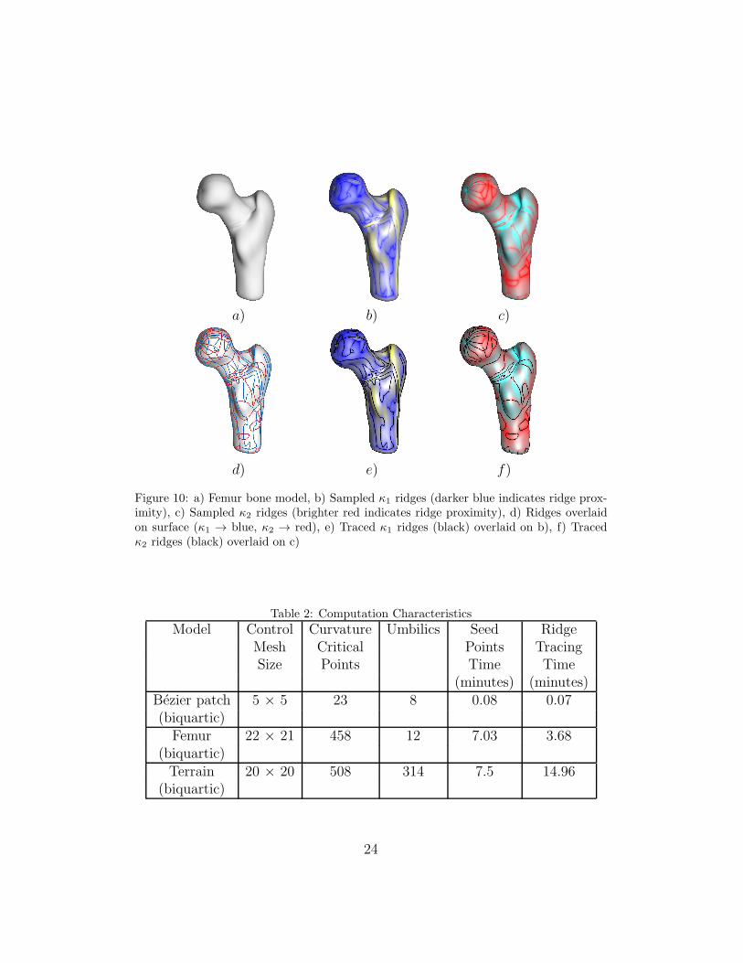
a) b) c)

d) e) f)

Figure 10: a) Femur bone model, b) Sampled κ1 ridges (darker blue indicates ridge prox-imity), c) Sampled κ2 ridges (brighter red indicates ridge proximity), d) Ridges overlaidon surface (κ1 → blue, κ2 → red), e) Traced κ1 ridges (black) overlaid on b), f) Tracedκ2 ridges (black) overlaid on c)

Table 2: Computation Characteristics

Model Control Curvature Umbilics Seed RidgeMesh Critical Points TracingSize Points Time Time

(minutes) (minutes)Bezier patch 5 × 5 23 8 0.08 0.07(biquartic)Femur 22 × 21 458 12 7.03 3.68

(biquartic)Terrain 20 × 20 508 314 7.5 14.96

(biquartic)

24

a) b) c)

d) e) f)

Figure 11: a) Terrain elevation model, b) Sampled κ1 ridges (darker blue indicates ridgeproximity), c) Sampled κ2 ridges (brighter red indicates ridge proximity), d) Ridges over-laid on surface (κ1 → blue, κ2 → red), e) Traced κ1 ridges (black) overlaid on b), f) Tracedκ2 ridges (black) overlaid on c)

(a) k1 ridge samples (b) Traced k1 and k2 ridges (c) k2 ridge samples

−ve

+ve +vek1 false k1 false

k2 false

Figure 12: An example of a false positive in κ1-ridge samples (rectangle outline) and afalse negative (ellipse outline) in κ2-ridge samples of the terrain elevation model. (a), (b)and (c) represent enlarged views of κ1-ridge samples, traced ridges and κ2-ridge samplesof the same region of the terrain elevation model.

25

a type of salient region associated with major ridges that indicate geomet-rically significant regions on surfaces. First, we distinguish different typesof major and secondary ridges. Second, we define the new type of salientregion associated with elliptic ridges. Third, we present generic propertiesof boundaries of these salient regions. Fourth, we present a heuristic expla-nation of the nature of the regions and their relation to the elliptic ridges.Finally, we present an example of how these salient regions can be used foranalyzing geometric variation.

8.1. Major and Secondary Ridges

Major Ridges. Let κ1 > κ2 denote the principal curvatures at a nonum-bilic point, and let p1, respectively p2 denote the principal curves associatedwith these curvatures. Then the major ridges associated with major geomet-ric features of the surface are curves consisting of points at which one of thefollowing conditions is satisfied:

1. Convex Ridge: κ1 > κ2 > 0 such that κ1 has a local maximum alongp1 at the point.

2. Saddle (type I) Ridge: κ1 > 0 > κ2 such that κ1 has a local maximumalong p1 at the point.

3. Saddle (type II) Ridge: κ1 > 0 > κ2 such that κ2 has a local minimumalong p2 at the point.

4. Concave Ridge: 0 > κ1 > κ2 such that κ2 has a local minimum alongp2 at the point.

All of these are types of elliptic ridges, with the convex and concave ellipticridges occurring in regions of positive Gauss curvature and both types ofsaddle elliptic ridges occurring in regions of negative Gauss curvature. Also,note that the saddle elliptic ridges in the second and third cases can crosstransversally. For example, in Figure 13, the convex and saddle elliptic ridgesof type I are shown in cyan and the concave and saddle elliptic ridges of typeII are shown in magenta.

Secondary Ridges. Secondary ridges may not correspond to perceptu-ally obvious geometric features but provide useful insight into variation ofcurvature on surfaces. They are defined by one of the following conditions.

1. κ1 > κ2 > 0 with κ1 having a local minimum along p12. κ1 > 0 > κ2 with κ1 having a local minimum along p1.

3. κ1 > 0 > κ2 with κ2 having a local maximum along p2.

26

a) b)

Figure 13: Major and secondary ridges of an object; a) side view, b) top view. Majorridges of κ1 are shown in cyan and those of κ2 are shown in magenta. Secondary ridgesof κ1 are shown in blue and those of κ2 are shown in red.

4. 0 > κ1 > κ2 with κ2 having a local maximum along p2.

Again in Figure 13, the secondary ridges of κ1 are shown in blue and thoseof κ2 are shown in red.

8.2. Salience Boundaries and Salient Regions

Thus far, we have divided the ridges into two distinct classes of majorand secondary ridges; and for the major ridges, these are further dividedinto four distinct types which correspond to specific geometric features. Wenext further extend this analysis to associate salient regions surrounding themajor ridges.

To define these regions, consider the partial flow along the principal curvesfrom the major ridge points. At a major ridge point, where κ1 has a localmaximum that is not a turning point, the corresponding principal curve istransverse to the ridge. By following the principal curve away from theridge point, eventually a point is reached where κ1 has a local minimum thatis a point on a secondary κ1-ridge. Along the curve between these pointsthere is a point where the function κ1 changes from concave downward toconcave upward. Since there are no intrinsic coordinates on a surface, thistransition point depends upon the choice of coordinates being used. The

27

parameterization of the principal curve can be normalized using the unitspeed parameterization. Then, in these unit speed coordinates along theprincipal curve, κ1 has an inflection point on the curve between the localmaximum and minimum where tT1Hκ1

t1 = 0. There is another inflectionpoint reached by flowing along the principal curve from the major ridgepoint in the negative direction. We term these inflection points the salienceboundary points of the corresponding major ridge point and we term the flowalong the principal direction from the major ridges to the salience boundarypoints the salience flow. Salience boundary points of major ridges of κ2 areidentified in a similar manner by flowing along principal curves of κ2.

The salience boundary for a major ridge then is the collection of salienceboundary points identified from the flow along the corresponding principalcurves from the major ridges. The regions surrounding such a ridge curve andbounded by the salience boundaries defines salient regions associated to themajor ridges. Following are the types of salience boundaries correspondingto the type of major ridges:

Types of Salience Boundaries:

1. Convex Salience Boundary : κ1 > κ2 > 0 and κ1 has a first inflectionpoint moving along p1 from a convex elliptic ridge point in a directionof decreasing κ1.

2. Saddle Salience Boundary (Type I) : κ1 > 0 > κ2 and κ1 has a firstinflection point moving along p1 from a saddle elliptic ridge point oftype I in a direction of decreasing κ1.

3. Saddle Salience Boundary (Type II) : κ1 > 0 > κ2 and κ2 has a firstinflection point moving along p2 from a saddle elliptic ridge point oftype II in a direction of increasing κ2.

4. Concave Salience Boundary : 0 > κ1 > κ2 and κ2 has a first inflectionpoint moving along p2 from a concave elliptic ridge point in a directionof increasing κ2.

In order to compute salience boundaries and salient regions, principalcurves are traced from each major ridge point on either side of the ridgeusing the method presented in [36]. The first inflection point on both sides,identified as the location where the sign of tTi Hκi

ti changes, are marked assalience boundary points.

Salient regions and salience boundaries associated with major ridges ofa surface are shown in Figure 14. For the convex and type I saddle ellipticridges, salient regions are shown in green and for concave and type II saddle

28

inflection pointDegenerate

Figure 14: Salience boundaries and salient regions associated with major ridges. For κ1,major ridges are shown in cyan, principal curve segments in salient regions are shownin green and inflection points are shown in dark blue. For κ2, major ridges are shownin magenta, principal curve segments in salient regions are shown in yellow and inflectionpoints are shown in dark red. Also shown is a closeup of a region that indicates a degenerateinflection point.

a) b)

Figure 15: a) Salience boundary points and other inflection points on principal curvestraced from a few major ridge points. b) Results superimposed on surface indicatingsampling of κ2 ridge function. For κ1, major ridges are shown in cyan, principal curvesegments in salient regions are shown in green and inflection points are shown in dark blue.For κ2, major ridges are shown in magenta, principal curve segments in salient regions areshown in yellow and inflection points are shown in dark red.

29

elliptic ridges, the salient regions are shown in yellow. It is possible formultiple inflection points to exist between a major ridge and a secondaryridge along a principal curve. In this case, the first inflection points reachedby flowing from the major ridge points are treated as the salience boundarypoints. In Figure 15 there are other inflection points that occur on the κ2

principal curves between the magenta and red ridges and the number ofsuch points is consistent with the number of sign changes of tT2Hκ2

t2 betweenmajor and secondary ridges. Note that there are no additional ridges betweenthe additional inflection points. This is validated in Figure 15 b) where thesampled ridge condition for κ2 is shown. In this image, the intensity of thered color is higher in the regions closer to a κ2 ridge.

8.3. Properties of Salience Boundaries

With the exception of turning points on a ridge, the principal curve picorresponding to a principal curvature κi for that ridge is transverse to thecorresponding ridge. In a small neighborhood of a non-turning point x0,generically, the principal curvature does not have critical points at inflectionpoints, so the implicit function theorem implies that the inflection pointsform a regular differentiable curve. Generically this curve is transverse to thecorresponding principal curves and is disjoint from the corresponding majorridge curve except at isolated points. These properties can fail in two distinctways at isolated points. One is when the inflection point is degenerate,and then the curve of inflection points meets the corresponding major ridge(which ends there). The other is when the curve of inflection points is tangentto the principal curve at a point disjoint from the corresponding major ridge.We describe both of these situations.

8.3.1. Salience Boundaries at Degenerate Inflection Points

For exceptional non-turning points on a ridge, the inflection point occursat a critical point for κi along the principal curve. We explain the behaviorat such points for the case of a convex ridge curve. The behavior of κ1 willbe modeled by the behavior of the family g(x, u) = −x3 + ux. Here x is theunit speed coordinate along the principal curves, and u parameterizes thefamily of principal curves with the degenerate inflection point occurring atthe origin. The graph of g is shown in Figure 16.

The inflection points of g, as a function of x, lie along the u axis as shownin Figure 17. For fixed u < 0, there are no critical points, and a singleinflection point where x = 0. However, the direction of the salience flow is

30

u

x

Figure 16: Graph of g illustrating degenerate inflection points

u

x

local maxlocal min

inflection ptsline of

+

-+

-

Figure 17: Decomposition of Salient Region resulting from a Degenerate Inflection Point

determined by the sign of g′′ as shown in Figure 17. On each side the flow isaway from the origin. At u = 0 the inflection point becomes degenerate andfor u > 0 two critical points are created, one a local maximum for g (= κ1)which is a convex ridge point and the other a local minimum for g (= κ1),which is a secondary ridge. These occur on each side of 0; and the sign of g′′

indicates the flow inside the parabola is toward the origin.Hence, for this model, the positive u axis is one part of the salience

boundary corresponding to the ridge formed from the local maxima with theother given by the positive x-axis representing the principal curve tangent tothe curve of local maxima at the degenerate point. Then, the salient regionis the shaded region. An example of a degenerate inflection point is shown

31

in Figure 14.

8.3.2. Salience Boundaries Tangent to Principal Curves

The second possibility is that the curve of inflection points is tangent toa principal curve at an isolated point. If we again denote κ1 by g then thiswill happen at points where g′′ = 0 (i.e., an inflection point) and g′′′ = 0(corresponding to the principal curve being tangent to the curve of inflectionpoints at that point). Figure 19 b) presents an example of this situation.

8.4. Properties of Salient Regions

Consider a convex elliptic ridge. Suppose the principal curvature κ1 islarge. A large curvature corresponds to a small radius of curvature. If theridge is part of a larger region, then this high curvature can only be main-tained for a short time along the corresponding principal curve. Hence, thedecrease must be rapid initially which then begins to decrease more gradu-ally. This is where an inflection point occurs. Hence, the salient region isconcentrated in a small region about the major ridge curve, as illustrated inFigure 14 at the cyan ridge in the center of the image where the surface issharply curving. If instead the curvature is much smaller, then the decreasecan be more gradual so the inflection point occurs much farther along theprincipal curve. Then, the salient region is much larger but changes moregradually. The cyan ridges on either side of the image center of Figure 14illustrate this behavior. Also, in Figure 15 a) the salience boundaries of κ2

are further away from the magenta ridge since the curvature change is moregradual. An analogy here is with placing an ink pad at a point on a ridge.The sharper the change in the curvature κ1, the smaller the region that wouldbe marked by the ink. By contrast, if the curvature κ1 changes more grad-ually, a much larger region will be marked by the ink. The salient region issimilar to such a marked region.

8.5. Analyzing Geometric Variation using Salient Regions

Salient regions are an effective visualization tool for analyzing higher ordergeometric properties of surfaces and can also be used to measure geometricvariation of similar objects. Salient regions are especially useful in distin-guishing geometric properties of a population of similar objects when ridgeson the surfaces occur at similar locations. Figure 18 shows front and backviews of an object that is slightly asymmetric. The major and secondaryridges are slightly different on the front and back sides of the model but do

32

a) b)

c) d)

e) f)

g) h)

Figure 18: Visualizing geometric differences using salient regions. a) front view and, b)back view of a slightly asymmetric object, c) and d) major ridges only, e) and f) all ridges,g) and h) salient regions.

33

to principal curveSalience boundary tangent

a) b)

Figure 19: Visualizing geometric differences using salient regions. a) the major ridgecorresponding to the bump in the surface lies in the center on both asymmetric regions,other major ridges are slightly different across plane of symmetry, b) salient regions clearlyindicate geometric differences in the asymmetric regions pointed by the arrows. Also shownis a close up view of a region that contains a point where the salience boundary is tangentto the principal curve.

not clearly distinguish the differences. In particular, the major ridge run-ning along the bump of the model is almost identical on both sides. In thiscase the salient regions clearly indicate the geometric differences and enablequantitative evaluation of the differences. The differences are clearly visiblefrom the top view of the object as shown in Figure 19.

9. Conclusions

Ridges are important feature curves and have a wide variety of appli-cations. Umbilics and therefore, ridges around umbilics, also represent im-portant aspects of the shape of a surface. Ridges exhibit complex behavioraround umbilics. This paper presents a new algorithm for numerically tracingridges on B-Spline surfaces that has been designed using generic properties ofridges. In addition, a new type of geometrically salient region correspondingto major ridges is defined.

The tracing algorithm involves traversing curvature lines in a novel man-ner and accurately captures the behavior of ridges at all points on a surfaceincluding umbilics. The technique takes into account turning points withoutdirectly computing them, thereby allowing ridge computation on C3 models,instead of requiring C4 smoothness. Our technique has been designed for

34

rational tensor product B-Spline surface representations. Since ridge compu-tation is local to a tensor product patch, it is directly extensible for modelswith multiple patches. Some special cases, such as ridges parallel to a domainboundary, may need to be addressed. Trimmed freeform surfaces also maybe addressed by minor modifications to the algorithm. The algorithm de-sign enables optimization using parallel processing techniques, which wouldfurther improve computation time. The approach can be further extendedto surfaces with isolated irregular points. We plan to pursue these modifi-cations in future work. The technique presented in this paper avoids errorsin ridge computation associated with sampling-based approaches, while atthe same time, it can generate results for complex models that were previ-ously computationally intractable. The result is a set of trace segments thatare available for other applications, such as surface segmentation, matching,quality control and visualization.

We identify elliptic ridges as major ridges with geometric significance.These ridges supplemented with salient regions are very useful for studyinggeometric variation across a population of similar objects. Earlier methodsfor computing significance of ridges only account for geometric properties ofsurfaces only at the ridge points. The type of salient region presented in thispaper provides a new method of quantifying geometric importance of ridgesthat also takes into account salient neighborhoods of ridges. We are currentlyinvestigating several measures based on salient regions to precisely quantifygeometric properties of surfaces at and in the neighborhood of ridges.

10. Acknowledgements

This work was supported in part by NSF (CCF0541402), NSF DMS-0706941, the Basic Science Research Program through the National ResearchFoundation of Korea (NRF) funded by the Ministry of Education, Scienceand Technology (2010-0028631), and the Korea Science and EngineeringFoundation (KOSEF) grant funded by the Korea government (MEST) (2010-0015879). All opinions, findings, conclusions or recommendations expressedin this document are those of the authors and do not necessarily reflect theviews of the sponsoring agencies.

[1] I. Porteous, The normal singularities of a submanifold, Journal of Dif-ferential Geometry 5 (1971) 543–564.

[2] J. Koenderink, Solid shape, MIT Press Cambridge, MA, USA, 1990.

35

[3] A. Gueziec, Large deformable splines, crest lines and matching, in: Com-puter Vision, 1993. Proceedings., Fourth International Conference on,1993, pp. 650–657.

[4] J. Kent, K. Mardia, J. West, Ridge curves and shape analysis, in: TheBritish Machine Vision Conference 1996, 1996, pp. 43–52.

[5] X. Pennec, N. Ayache, J.-P. Thirion, Landmark-based registration usingfeatures identified through differential geometry, in: I. Bankman (Ed.),Handbook of Medical Image Processing and Analysis - New edition,Academic Press, 2008, Ch. 34, pp. 565–578.

[6] G. Subsol, Crest lines for curve-based warping, Brain Warping (1999)241–262.

[7] F. Cole, A. Golovinskiy, A. Limpaecher, H. S. Barros, A. Finkelstein,T. Funkhouser, S. Rusinkiewicz, Where do people draw lines?, ACMTransactions on Graphics (Proc. SIGGRAPH) 27 (3).

[8] V. Interrante, H. Fuchs, S. Pizer, Enhancing transparent skin surfaceswith ridge and valley lines, in: Proceedings of the 6th conference onVisualization’95, IEEE Computer Society Washington, DC, USA, 1995.

[9] K. Ma, V. Interrante, Extracting feature lines from 3D unstructuredgrids, in: Visualization’97., Proceedings, 1997, pp. 285–292.

[10] M. Hosaka, Modeling of curves and surfaces in CAD/CAM with 90figures Symbolic computation, Springer, 1992.

[11] J. Little, P. Shi, Structural lines, TINs, and DEMs, Algorithmica 30 (2)(2001) 243–263.

[12] T. Tasdizen, R. Whitaker, Feature preserving variational smoothingof terrain data, in: Proceedings of the Second IEEE Workshop onVariational, Geometric and Level Set Methods in Computer Vision(VLSM’03)(Institute of Electrical and Electronics Engineers, 2003), pp.121–128.

[13] K. Ko, T. Maekawa, N. Patrikalakis, H. Masuda, F. Wolter, Shape in-trinsic fingerprints for free-form object matching, in: Proceedings of theeighth ACM symposium on Solid modeling and applications, ACM NewYork, NY, USA, 2003, pp. 196–207.

36

[14] N. Patrikalakis, T. Maekawa, Shape interrogation for computer aideddesign and manufacturing, Springer, 2002.

[15] F. Cazals, M. Pouget, Topology driven algorithms for ridge extractionon meshesINRIA Technical Report.

[16] Y. Ohtake, A. Belyaev, H. Seidel, Ridge-valley lines on meshes via im-plicit surface fitting, ACM Transactions on Graphics 23 (3) (2004) 609–612.

[17] S. Yoshizawa, A. Belyaev, H. Yokota, H. Seidel, Fast and faithful ge-ometric algorithm for detecting crest lines on meshes, in: ComputerGraphics and Applications, 2007. PG’07. 15th Pacific Conference on,2007, pp. 231–237.

[18] F. Cazals, J. Faugere, M. Pouget, F. Rouillier, The implicit structureof ridges of a smooth parametric surface, Computer Aided GeometricDesign 23 (7) (2006) 582–598.

[19] I. Porteous, Geometric differentiation: for the intelligence of curves andsurfaces, Cambridge University Press, 2001.

[20] P. Hallinan, G. Gordon, A. Yuille, P. Giblin, D. Mumford, Two-andthree-dimensional patterns of the face, AK Peters, Ltd. Natick, MA,USA, 1999.

[21] F. Cazals, J. Faugere, M. Pouget, F. Rouillier, Topologically certifiedapproximation of umbilics and ridges on polynomial parametric sur-faceINRIA Technical Report.

[22] F. Cazals, J. Faugere, M. Pouget, F. Rouillier, Ridges and umbilicsof polynomial parametric surfaces, Geometric Modeling and AlgebraicGeometry (2007) 141–159Juttler, B. and Piene, R. (eds.).

[23] M. Jefferies, Extracting Crest Lines from B-spline Surfaces, ArizonaState University, 2002.

[24] R. Morris, Symmetry of Curves and the Geometry of Surfaces, Ph.D.thesis, PhD thesis, University of Liverpool (1990).

37

[25] K. Hildebrandt, K. Polthier, M. Wardetzky, Smooth feature lines onsurface meshes, in: Symposium on geometry processing, 2005, pp. 85–90.

[26] S. Kim, C. Kim, Finding ridges and valleys in a discrete surface usinga modified MLS approximation, Computer-Aided Design 37 (14) (2005)1533–1542.

[27] G. Stylianou, G. Farin, Crest lines extraction from 3D triangulatedmeshes, Hierarchical and geometrical methods in scientific visualization(2003) 269–281.

[28] A. Belyaev, Y. Ohtake, K. Abe, Detection of ridges and ravines on rangeimages and triangular meshes, in: Proceedings of SPIE, Vol. 4117, 2000,p. 146.

[29] Y. Lai, Q. Zhou, S. Hu, J. Wallner, H. Pottmann, Robust feature classi-fication and editing, IEEE Transactions on Visualization and ComputerGraphics 13 (1) (2007) 34–45.

[30] A. Belyaev, A. Pasko, T. Kunii, Ridges and ravines on implicit surfaces,in: Computer Graphics International, 1998. Proceedings, 1998, pp. 530–535.

[31] I. Bogaevski, V. Lang, A. Belyaev, T. Kunii, Color ridges on implicitpolynomial surfaces, GraphiCon 2003, Moscow, Russia.

[32] J. Thirion, A. Gourdon, The 3D marching lines algorithm and its appli-cation to crest lines extraction.

[33] O. Monga, S. Benayoun, Using partial derivatives of 3D images to ex-tract typical surface features, Computer Vision and Image Understand-ing 61 (2) (1995) 171–189.

[34] E. Cohen, R. Riesenfeld, G. Elber, Geometric modeling with splines: anintroduction, AK Peters, Ltd., 2001.

[35] B. O’Neill, Elementary differential geometry, 2nd Edition, Academicpress, 2006.

38

[36] T. Maekawa, F. Wolter, N. Patrikalakis, Umbilics and lines of curvaturefor shape interrogation, Computer Aided Geometric Design 13 (2) (1996)133–161.

[37] T. Maekawa, N. Patrikalakis, Interrogation of differential geometry prop-erties for design and manufacture, The Visual Computer 10 (4) (1994)216–237.

[38] G. Elber, M. Kim, Geometric constraint solver using multivariate ratio-nal spline functions, in: Proceedings of the sixth ACM symposium onSolid modeling and applications, ACM New York, NY, USA, 2001, pp.1–10.

[39] G. Elber, T. Grandine, Efficient solution to systems of multivariate poly-nomials using expression trees, in: IEEE International Conference onShape Modeling and Applications, 2008. SMI 2008, 2008, pp. 163–169.

[40] D. Johnson, E. Cohen, An improved method for haptic tracing of sculp-tured surfaces, in: Symp. on Haptic Interfaces, ASME InternationalMechanical Engineering Congress and Exposition, Anaheim, CA, 1998.

[41] X. Liu, L. Yang, J. Yong, H. Gu, J. Sun, A torus patch approximationapproach for point projection on surfaces, Computer Aided GeometricDesign 26 (5) (2009) 593–598.

[42] G. Elber. The IRIT modeling environment, version 10.0 [online] (2008).

[43] D. Hastings, P. Dunbar, G. Elphingstone, M. Bootz, H. Murakami,H. Maruyama, H. Masaharu, P. Holland, J. Payne, N. Bryant, et al.,The global land one-kilometer base elevation (GLOBE) digital elevationmodel. Version 1.0. National Oceanic and Atmospheric Administration,National Geophysical Data Center, Boulder, Colorado, National Geo-physical Data Center, Digital data base on the World Wide Web (URL:http://www.ngdc.noaa.gov/mgg/topo/globe.html) and CD-ROMs.

[44] S. Musuvathy, E. Cohen, Extracting Principal Curvature Ridges fromB-Spline Surfaces with Deficient Smoothness, Advances in Visual Com-puting (2009) 101–110.

39