MODULE – 2

Numerical Control (NC)

Numerical control (NC) refers to the automation of machine tools that are operated by

abstractly programmed commands encoded on a storage medium, as opposed to manually

controlled via handwheels or levers or mechanically automated via cams alone. The first

NC machines were built in the 1940s and 50s, based on existing tools that were modified

with motors that moved the controls to follow points fed into the system on paper tape.

These early servomechanisms were rapidly augmented with analog and digital

computers, creating the modern computer numerical controlled (CNC) machine tools

that have revolutionized the design process.

In modern CNC systems, end-to-end component design is highly automated using

CAD/CAM programs. The programs produce a computer file that is interpreted to extract

the commands needed to operate a particular machine, and then loaded into the CNC

machines for production. Since any particular component might require the use of a

number of different tools - drills, saws, etc. - modern machines often combine multiple

tools into a single "cell". In other cases, a number of different machines are used with an

external controller and human or robotic operators that move the component from

machine to machine. In either case the complex series of steps needed to produce any part

is highly automated and produces a part that closely matches the original CAD design.

Computer Numerical Control (CNC)

Many of the commands for the experimental parts were programmed "by hand" to

produce the punch tapes that were used as input. While the system was being

experimented with, John Runyon made a number of subroutines on the famous

Whirlwindd to produce these tapes under computer control. Users could input a list of

points and speeds, and the program would generate the punch tape. In one instance, this

process reduced the time required to produce the instruction list and mill the part from 8

hours to 15 minutes. This led to a proposal to the Air Force to produce a generalized

"programming" language for numerical control, which was accepted in June 1956.

Starting in September Ross and Pople outlined a language for machine control that was

based on points and lines, developing this over several years into the APT programming

language.[10] In 1957 the Aircraft Industries Association (AIA) and Air Material

Command at the Wright-Patterson Air Force Base joined with MIT to standardize this

work and produce a fully computer-conrolled NC system. On 25 February 1959 the

combined team held a press conference showing the results, including a 3D machined

aluminum ash tray that was handed out in the press kit.[14]

Meanwhile, Patrick Hanratty was making similar developments at GE as part of their

partnership with G&L on the Numericord. His language, PRONTO, beat APT into

commercial use when it was "released" in 1958.[15] Hanratty then went on to develop

MICR magnetic ink characters that were used in cheque processing, before moving to

General Motors to work on the groundbreaking DAC-1 CAD system.

APT was soon extended to include "real" curves in 2D-APT-II. With its release, MIT

reduced its focus on CNC as it moved into CAD experiments. APT development was

picked up with the AIA in San Diego, and in 1962, to Illinois Institute of Technology

Research. Work on making APT an international standard started in 1963 under USASI

X3.4.7, but many manufacturers of CNC machines had their own one-off additions (like

PRONTO), so standardization was not completed until 1968, when there were 25

optional add-ins to the basic system.[14]

Just as APT was being released in the early 1960s, a second generation of lower-cost

transistorized computers was hitting the market that were able to process much larger

volumes of information in production settings. This so lowered the cost of implementing

a NC system that by the mid 1960s, APT runs accounted for a third of all computer time

at large aviation firms.

CAD and CNC

While the Servomechanisms Lab was in the process of developing their first mill, in 1953

MIT's Mechanical Engineering Department dropped the requirement that undergraduates

take courses in drawing. The instructors formerly teaching these programs were merged

into the Design Division, where an informal discussion of computerized design started.

Meanwhile the Electronic Systems Laboratory, the newly rechristened Servomechanisms

Laboratory, had been discussing whether or not design would ever start with paper

diagrams in the future.[16]

In January 1959, an informal meeting was held involving individuals from both the

Electronic Systems Laboratory and the Mechanical Engineering Department's Design

Division. Formal meetings followed in April and May, which resulted in the "Computer-

Aided Design Project". In December 1959, the Air Force issued a one year contract to

ESL for $223,000 to fund the Project, including $20,800 earmarked for 104 hours of

computer time at $200 per hour.[17] This proved to be far too little for the ambitious

program they had in mind, although their engineering calculation system, AED, was

released in March 1965.

In 1959 General Motors started an experimental project to digitize, store and print the

many design sketches being generated in the various GM design departments. When the

basic concept demonstrated that it could work, they started the DAC-1 project with IBM

to develop a production version. One part of the DAC project was the direct conversion

of paper diagrams into 3D models, which were then converted into APT commands and

cut on milling machines. In November 1963 a trunk lid design moved from 2D paper

sketch to 3D clay prototype for the first time.[18] With the exception of the initial sketch,

the design-to-production loop had been closed.

Meanwhile MIT's offsite Lincoln Labs was building computers to test new transistorized

designs. The ultimate goal was essentially a transistorized Whirlwind known as TX-2, but

in order to test various circuit designs a smaller version known as TX-0 was built first.

When construction of TX-2 started, time in TX-0 freed up and this led to a number of

experiments involving interactive input and use of the machine's CRT display for

graphics. Further development of these concepts led to Ivan Sutherland's groundbreaking

Sketchpad program on the TX-2.

Sutherland moved to the University of Utah after his Sketchpad work, but it inspired

other MIT graduates to attempt the first true CAD system, Electronic Drafting Machine

(EDM). It was EDM, sold to Control Data and known as "Digigraphics", that Lockheed

used to build production parts for the C-5 Galaxy, the first example of an end-to-end

CAD/CNC production system.

By 1970 there were a wide variety of CAD firms including Intergraph, Applicon,

Computervision, Auto-trol Technology, UGS Corp. and others, as well as large vendors

like CDC and IBM.

Proliferation of CNC

The price of computer cycles fell drastically during the 1960s with the widespread

introduction of useful minicomputers. Eventually it became less expensive to handle the

motor control and feedback with a computer program than it was with dedicated servo

systems. Small computers were dedicated to a single mill, placing the entire process in a

small box. PDP-8's and Data General Nova computers were common in these roles. The

introduction of the microprocessor in the 1970s further reduced the cost of

implementation, and today almost all CNC machines use some form of microprocessor to

handle all operations.

The introduction of lower-cost CNC machines radically changed the manufacturing

industry. Curves are as easy to cut as straight lines, complex 3-D structures are relatively

easy to produce, and the number of machining steps that required human action have

been dramatically reduced. With the increased automation of manufacturing processes

with CNC machining, considerable improvements in consistency and quality have been

achieved with no strain on the operator. CNC automation reduced the frequency of errors

and provided CNC operators with time to perform additional tasks. CNC automation also

allows for more flexibility in the way parts are held in the manufacturing process and the

time required to change the machine to produce different components.

During the early 1970s the Western economies were mired in slow economic growth and

rising employment costs, and NC machines started to become more attractive. The major

U.S. vendors were slow to respond to the demand for machines suitable for lower-cost

NC systems, and into this void stepped the Germans. In 1979, sales of German machines

surpassed the U.S. designs for the first time. This cycle quickly repeated itself, and by

1980 Japan had taken a leadership position, U.S. sales dropping all the time. Once sitting

in the #1 position in terms of sales on a top-ten chart consisting entirely of U.S.

companies in 1971, by 1987 Cincinnati Milacron was in 8th place on a chart heavily

dominated by Japanese firms.[19]

Many researchers have commented that the U.S. focus on high-end applications left them

in an uncompetitive situation when the economic downturn in the early 1970s led to

greatly increased demand for low-cost NC systems. Unlike the U.S. companies, who had

focused on the highly profitable aerospace market, German and Japanese manufacturers

targeted lower-profit segments from the start and were able to enter the low-cost markets

much more easily.[19][20]

Although modern data storage techniques have moved on from punch tape in almost

every other role, tapes are still relatively common in CNC systems. This is because it was

often easier to add a punch tape reader to a microprocessor controller than it was to re-

write large libraries of tapes into a new format. One change that was implemented fairly

widely was the switch from paper to mylar tapes, which are much more mechanically

robust. Floppy disks, USB flash drives and local area networking have replaced the tapes

to some degree, especially in larger environments that are highly integrated.

The proliferation of CNC led to the need for new CNC standards that were not

encumbered by licensing or particular design concepts, like APT. A number of different

"standards" proliferated for a time, often based around vector graphics markup languages

supported by plotters. One such standard has since become very common, the "G-code"

that was originally used on Gerber Scientific plotters and then adapted for CNC use. The

file format became so widely used that it has been embodied in an EIA standard. In turn,

G-code was supplanted by STEP-NC, a system that was deliberately designed for CNC,

rather than grown from an existing plotter standard.

A more recent advancement in CNC interpreters is support of logical commands, known

as parametric programming. Parametric programs include both device commands as well

as a control language similar to BASIC. The programmer can make if/then/else

statements, loops, subprogram calls, perform various arithmetic, and manipulate variables

to create a large degree of freedom within one program. An entire product line of

different sizes can be programmed using logic and simple math to create and scale an

entire range of parts, or create a stock part that can be scaled to any size a customer

demands.

As digital electronics has spread, CNC has fallen in price to the point where hobbyists

can purchase any number of small CNC systems for home use. It is even possible to build

your own.

Direct Numerical Control (DNC)

Direct Numerical Control, also known as Distributed Numerical Control, (both DNC)

is a common manufacturing term for networking CNC machine tools. On some CNC

machine controllers, the available memory is too small to contain the machining program

(for example machining complex surfaces), so in this case the program is stored in a

separate computer and sent Direct to the machine, one block at a time. If the computer is

connected to a number of machines it can Distribute programs to different machines as

required. Usually, the manufacturer of the control provides suitable DNC software.

However, if this provision is not possible, some software companies provide DNC

applications that fulfill the purpose. DNC networking or DNC communication is always

required when CAM programs are to run on some CNC Machine control.

Programmable logic Controllers

A programmable logic controller (PLC) or programmable controller is a digital

computer used for automation of electromechanical processes, such as control of

machinery on factory assembly lines, amusement rides, or lighting fixtures. PLCs are

used in many industries and machines, such as packaging and semiconductor machines.

Unlike general-purpose computers, the PLC is designed for multiple inputs and output

arrangements, extended temperature ranges, immunity to electrical noise, and resistance

to vibration and impact. Programs to control machine operation are typically stored in

battery-backed or non-volatile memory. A PLC is an example of a real time system since

output results must be produced in response to input conditions within a bounded time,

otherwise unintended operation will result.

The main difference from other computers is that PLCs are armored for severe conditions

(such as dust, moisture, heat, cold) and have the facility for extensive input/output (I/O)

arrangements. These connect the PLC to sensors and actuators. PLCs read limit switches,

analog process variables (such as temperature and pressure), and the positions of complex

positioning systems. Some use machine vision. On the actuator side, PLCs operate

electric motors, pneumatic or hydraulic cylinders, magnetic relays, solenoids, or analog

outputs. The input/output arrangements may be built into a simple PLC, or the PLC may

have external I/O modules attached to a computer network that plugs into the PLC.

System scale

A small PLC will have a fixed number of connections built in for inputs and outputs.

Typically, expansions are available if the base model has insufficient I/O.

Modular PLCs have a chassis (also called a rack) into which are placed modules with

different functions. The processor and selection of I/O modules is customised for the

particular application. Several racks can be administered by a single processor, and may

have thousands of inputs and outputs. A special high speed serial I/O link is used so that

racks can be distributed away from the processor, reducing the wiring costs for large

plants.

User interface

PLCs may need to interact with people for the purpose of configuration, alarm reporting

or everyday control.

A Human-Machine Interface (HMI) is employed for this purpose. HMIs are also referred

to as MMIs (Man Machine Interface) and GUI (Graphical User Interface).

A simple system may use buttons and lights to interact with the user. Text displays are

available as well as graphical touch screens. More complex systems use a programming

and monitoring software installed on a computer, with the PLC connected via a

communication interface.

Communications

PLCs have built in communications ports usually 9-Pin RS232, and optionally for RS485

and Ethernet. Modbus or DF1 is usually included as one of the communications

protocols. Others' options include various fieldbuses such as DeviceNet or Profibus.

Other communications protocols that may be used are listed in the List of automation

protocols.

Most modern PLCs can communicate over a network to some other system, such as a

computer running a SCADA (Supervisory Control And Data Acquisition) system or web

browser.

PLCs used in larger I/O systems may have peer-to-peer (P2P) communication between

processors. This allows separate parts of a complex process to have individual control

while allowing the subsystems to co-ordinate over the communication link. These

communication links are also often used for HMI devices such as keypads or PC-type

workstations. Some of today's PLCs can communicate over a wide range of media

including RS-485, Coaxial, and even Ethernet for I/O control at network speeds up to 100

Mbit/s.

PLC compared with other control systems

PLCs are well-adapted to a range of automation tasks. These are typically industrial

processes in manufacturing where the cost of developing and maintaining the automation

system is high relative to the total cost of the automation, and where changes to the

system would be expected during its operational life. PLCs contain input and output

devices compatible with industrial pilot devices and controls; little electrical design is

required, and the design problem centers on expressing the desired sequence of

operations in ladder logic (or function chart) notation. PLC applications are typically

highly customized systems so the cost of a packaged PLC is low compared to the cost of

a specific custom-built controller design. On the other hand, in the case of mass-produced

goods, customized control systems are economic due to the lower cost of the

components, which can be optimally chosen instead of a "generic" solution, and where

the non-recurring engineering charges are spread over thousands or millions of units.

For high volume or very simple fixed automation tasks, different techniques are used. For

example, a consumer dishwasher would be controlled by an electromechanical cam timer

costing only a few dollars in production quantities.

A microcontroller-based design would be appropriate where hundreds or thousands of

units will be produced and so the development cost (design of power supplies and

input/output hardware) can be spread over many sales, and where the end-user would not

need to alter the control. Automotive applications are an example; millions of units are

built each year, and very few end-users alter the programming of these controllers.

However, some specialty vehicles such as transit busses economically use PLCs instead

of custom-designed controls, because the volumes are low and the development cost

would be uneconomic.

Very complex process control, such as used in the chemical industry, may require

algorithms and performance beyond the capability of even high-performance PLCs. Very

high-speed or precision controls may also require customized solutions; for example,

aircraft flight controls.

Programmable controllers are widely used in motion control, positioning control and

torque control. Some manufacturers produce motion control units to be integrated with

PLC so that G-code (involving a CNC machine) can be used to instruct machine

movements.

PLCs may include logic for single-variable feedback analog control loop, a "proportional,

integral, derivative" or "PID controller." A PID loop could be used to control the

temperature of a manufacturing process, for example. Historically PLCs were usually

configured with only a few analog control loops; where processes required hundreds or

thousands of loops, a distributed control system (DCS) would instead be used. As PLCs

have become more powerful, the boundary between DCS and PLC applications has

become less distinct.

PLCs have similar functionality as Remote Terminal Units. An RTU, however, usually

does not support control algorithms or control loops. As hardware rapidly becomes more

powerful and cheaper, RTUs, PLCs and DCSs are increasingly beginning to overlap in

responsibilities, and many vendors sell RTUs with PLC-like features and vice versa. The

industry has standardized on the IEC 61131-3 functional block language for creating

programs to run on RTUs and PLCs, although nearly all vendors also offer proprietary

alternatives and associated development environments.

Digital and analog signals

Digital or discrete signals behave as binary switches, yielding simply an On or Off signal

(1 or 0, True or False, respectively). Push buttons, limit switches, and photoelectric

sensors are examples of devices providing a discrete signal. Discrete signals are sent

using either voltage or current, where a specific range is designated as On and another as

Off. For example, a PLC might use 24 V DC I/O, with values above 22 V DC

representing On, values below 2VDC representing Off, and intermediate values

undefined. Initially, PLCs had only discrete I/O.

Analog signals are like volume controls, with a range of values between zero and full-

scale. These are typically interpreted as integer values (counts) by the PLC, with various

ranges of accuracy depending on the device and the number of bits available to store the

data. As PLCs typically use 16-bit signed binary processors, the integer values are limited

between -32,768 and +32,767. Pressure, temperature, flow, and weight are often

represented by analog signals. Analog signals can use voltage or current with a

magnitude proportional to the value of the process signal. For example, an analog 4-20

mA or 0 - 10 V input would be converted into an integer value of 0 - 32767.

Current inputs are less sensitive to electrical noise (i.e. from welders or electric motor

starts) than voltage inputs.

Example

As an example, say a facility needs to store water in a tank. The water is drawn from the

tank by another system, as needed, and our example system must manage the water level

in the tank.

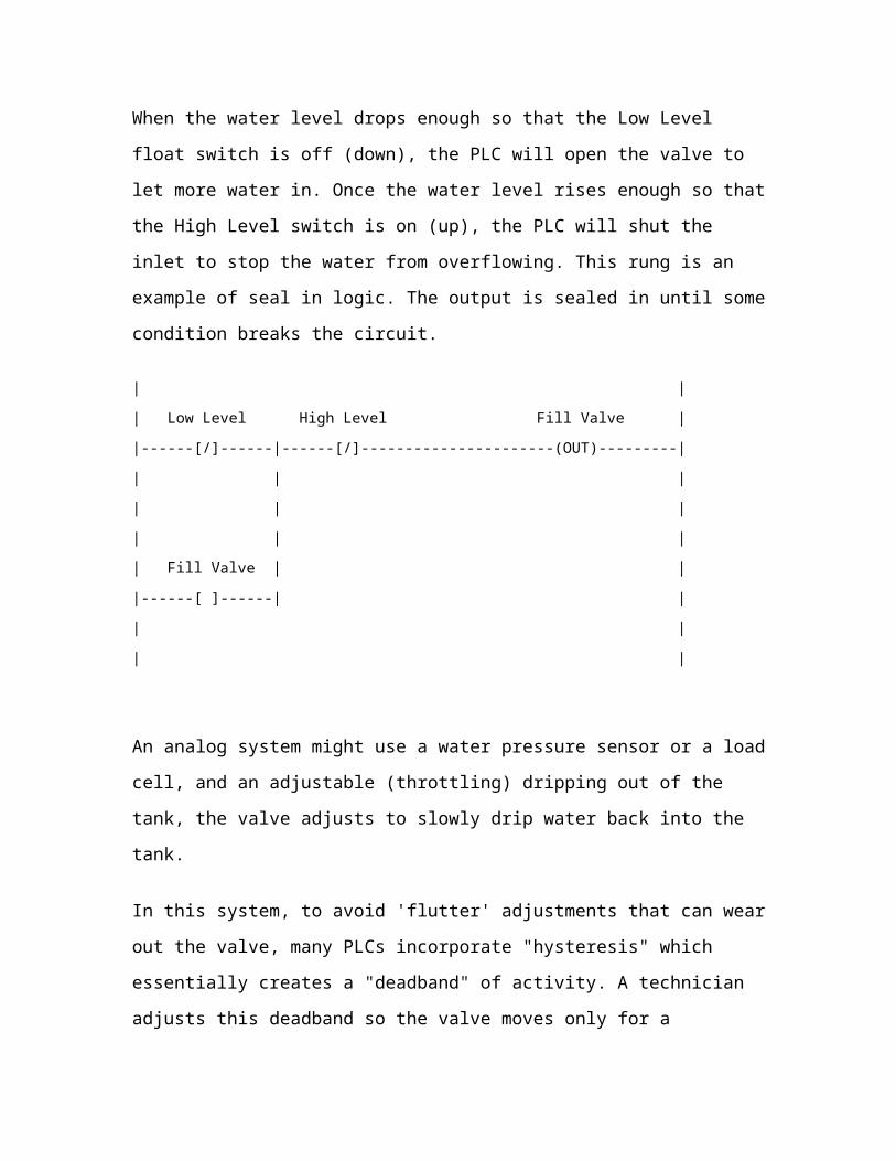
Using only digital signals, the PLC has two digital inputs from float switches (Low Level

and High Level). When the water level is above the switch it closes a contact and passes a

signal to an input. The PLC uses a digital output to open and close the inlet valve into the

tank.

When the water level drops enough so that the Low Level float switch is off (down), the

PLC will open the valve to let more water in. Once the water level rises enough so that

the High Level switch is on (up), the PLC will shut the inlet to stop the water from

overflowing. This rung is an example of seal in logic. The output is sealed in until some

condition breaks the circuit.

| |

| Low Level High Level Fill Valve |

|------[/]------|------[/]----------------------(OUT)---------|

| | |

| | |

| | |

| Fill Valve | |

|------[ ]------| |

| |

| |

An analog system might use a water pressure sensor or a load cell, and an adjustable

(throttling) dripping out of the tank, the valve adjusts to slowly drip water back into the

tank.

In this system, to avoid 'flutter' adjustments that can wear out the valve, many PLCs

incorporate "hysteresis" which essentially creates a "deadband" of activity. A technician

adjusts this deadband so the valve moves only for a significant change in rate. This will

in turn minimize the motion of the valve, and reduce its wear.

A real system might combine both approaches, using float switches and simple valves to

prevent spills, and a rate sensor and rate valve to optimize refill rates and prevent water

hammer. Backup and maintenance methods can make a real system very complicated.

Programming

PLC programs are typically written in a special application on a personal computer, then

downloaded by a direct-connection cable or over a network to the PLC. The program is

stored in the PLC either in battery-backed-up RAM or some other non-volatile flash

memory. Often, a single PLC can be programmed to replace thousands of relays.

Under the IEC 61131-3 standard, PLCs can be programmed using standards-based

programming languages. A graphical programming notation called Sequential Function

Charts is available on certain programmable controllers.

Recently, the International standard IEC 61131-3 has become popular. IEC 61131-3

currently defines five programming languages for programmable control systems: FBD

(Function block diagram), LD (Ladder diagram), ST (Structured text, similar to the

Pascal programming language), IL (Instruction list, similar to assembly language) and

SFC (Sequential function chart). These techniques emphasize logical organization of

operations.

While the fundamental concepts of PLC programming are common to all manufacturers,

differences in I/O addressing, memory organization and instruction sets mean that PLC

programs are never perfectly interchangeable between different makers. Even within the

same product line of a single manufacturer, different models may not be directly

compatible.

History

Origin

The PLC was invented in response to the needs of the American automotive

manufacturing industry. Programmable controllers were initially adopted by the

automotive industry where software revision replaced the re-wiring of hard-wired control

panels when production models changed.

Before the PLC, control, sequencing, and safety interlock logic for manufacturing

automobiles was accomplished using hundreds or thousands of relays, cam timers, and

drum sequencers and dedicated closed-loop controllers. The process for updating such

facilities for the yearly model change-over was very time consuming and expensive, as

the relay systems needed to be rewired by skilled electricians.

In 1968 GM Hydramatic (the automatic transmission division of General Motors) issued

a request for proposal for an electronic replacement for hard-wired relay systems.

The winning proposal came from Bedford Associates of Bedford, Massachusetts. The

first PLC, designated the 084 because it was Bedford Associates' eighty-fourth project,

was the result. Bedford Associates started a new company dedicated to developing,

manufacturing, selling, and servicing this new product: Modicon, which stood for

MOdular DIgital CONtroller. One of the people who worked on that project was Dick

Morley, who is considered to be the "father" of the PLC. The Modicon brand was sold in

1977 to Gould Electronics, and later acquired by German Company AEG and then by

French Schneider Electric, the current owner.

One of the very first 084 models built is now on display at Modicon's headquarters in

North Andover, Massachusetts. It was presented to Modicon by GM, when the unit was

retired after nearly twenty years of uninterrupted service. Modicon used the 84 moniker

at the end of its product range until the 984 made its appearance.

The automotive industry is still one of the largest users of PLCs.

Development

Early PLCs were designed to replace relay logic systems. These PLCs were programmed

in "ladder logic", which strongly resembles a schematic diagram of relay logic. Modern

PLCs can be programmed in a variety of ways, from ladder logic to more traditional

programming languages such as BASIC and C. Another method is State Logic, a Very

High Level Programming Language designed to program PLCs based on State Transition

Diagrams.

Many of the earliest PLCs expressed all decision making logic in simple ladder logic

which appeared similar to electrical schematic diagrams. This program notation was

chosen to reduce training demands for the existing technicians. Other early PLCs used a

form of instruction list programming, based on a stack-based logic solver.

Programming

Early PLCs, up to the mid-1980s, were programmed using proprietary programming

panels or special-purpose programming terminals, which often had dedicated function

keys representing the various logical elements of PLC programs. Programs were stored

on cassette tape cartridges. Facilities for printing and documentation were very minimal

due to lack of memory capacity. The very oldest PLCs used non-volatile magnetic core

memory.

Functionality

The functionality of the PLC has evolved over the years to include sequential relay

control, motion control, process control, distributed control systems and networking. The

data handling, storage, processing power and communication capabilities of some

modern PLCs are approximately equivalent to desktop computers. PLC-like

programming combined with remote I/O hardware, allow a general-purpose desktop

computer to overlap some PLCs in certain applications.

MODULE – 3

Programming NC Machines

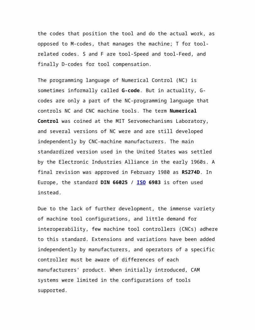
G-Code, or preparatory code or function, are functions in the Numerical control

programming language. The G-codes are the codes that position the tool and do the actual

work, as opposed to M-codes, that manages the machine; T for tool-related codes. S and

F are tool-Speed and tool-Feed, and finally D-codes for tool compensation.

The programming language of Numerical Control (NC) is sometimes informally called

G-code. But in actuality, G-codes are only a part of the NC-programming language that

controls NC and CNC machine tools. The term Numerical Control was coined at the

MIT Servomechanisms Laboratory, and several versions of NC were and are still

developed independently by CNC-machine manufacturers. The main standardized

version used in the United States was settled by the Electronic Industries Alliance in the

early 1960s. A final revision was approved in February 1980 as RS274D. In Europe, the

standard DIN 66025 / ISO 6983 is often used instead.

Due to the lack of further development, the immense variety of machine tool

configurations, and little demand for interoperability, few machine tool controllers

(CNCs) adhere to this standard. Extensions and variations have been added independently

by manufacturers, and operators of a specific controller must be aware of differences of

each manufacturers' product. When initially introduced, CAM systems were limited in

the configurations of tools supported.

Today, the main manufacturers of CNC control systems are GE Fanuc Automation (joint

venture of General Electric and Fanuc), Siemens, Mitsubishi, and Heidenhain, but there

still exist many smaller and/or older controller systems.

Some CNC machine manufacturers attempted to overcome compatibility difficulties by

standardizing on a machine tool controller built by Fanuc. Unfortunately, Fanuc does not

remain consistent with RS-274 or its own previous versions, and has been slow at adding

new features, as well as exploiting increases in computing power. For example, they

changed G70/G71 to G20/G21; they used parentheses for comments which caused

difficulty when they introduced mathematical calculations so they use square parentheses

for macro calculations; they now have nano technology recently in 32-bit mode but in the

Fanuc 15MB control they introduced HPCC (high-precision contour control) which uses

a 64-bit RISC (reduced instruction set computer) processor and this now has a 500 block

buffer for look-ahead for correct shape contouring and surfacing of small block programs

and 5-axis continuous machining.

This is also used for NURBS to be able to work closely with industrial designers and the

systems that are used to design flowing surfaces. The NURBS has its origins from the

ship building industry and is described by using a knot and a weight as for bending

steamed wooden planks and beams.

Common Codes

G-codes are also called preparatory codes, and are any word in a CNC program that

begins with the letter 'G'. Generally it is a code telling the machine tool what type of

action to perform, such as:

rapid move

controlled feed move in a straight line or arc

series of controlled feed moves that would result in a hole being bored, a

workpiece cut (routed) to a specific dimension, or a decorative profile shape

added to the edge of a workpiece.

change a pallet

set tool information such as offset.

There are other codes; the type codes can be thought of like registers in a computer

X absolute position

Y absolute position

Z absolute position

A position (rotary around X)

B position (rotary around Y)

C position (rotary around Z)

U Relative axis parallel to X

V Relative axis parallel to Y

W Relative axis parallel to Z

M code (another "action" register or Machine code(*)) (otherwise referred to as a

"Miscellaneous" function")

F feed rate

S spindle speed

N line number

R Arc radius or optional word passed to a subprogram/canned cycle

P Dwell time or optional word passed to a subprogram/canned cycle

T Tool selection

I Arc data X axis

J Arc data Y axis.

K Arc data Z axis, or optional word passed to a subprogram/canned cycle

D Cutter diameter/radius offset

H Tool length offset

(*) M codes control the overall machine, causing it to stop, start, turn on coolant, etc.,

whereas other codes pertain to the path traversed by cutting tools. Different machine tools

may use the same code to perform different functions; even machines that use the same

CNC control.

Partial list of M-Codes

M0=Program Stop (non-optional)

M1=Optional Stop, machine will only stop if operator selects this option

M2=End of Program

M3=Spindle on (CW rotation)

M4=Spindle on (CCW rotation)

M5=Spindle off

M6=Tool Change

M7=Coolant on (flood)

M8=Coolant on (mist)

M9=Coolant off

M10=Pallet clamp

M11=Pallet un-clamp

M30=End of program/rewind tape (may still be required for older CNC machines)

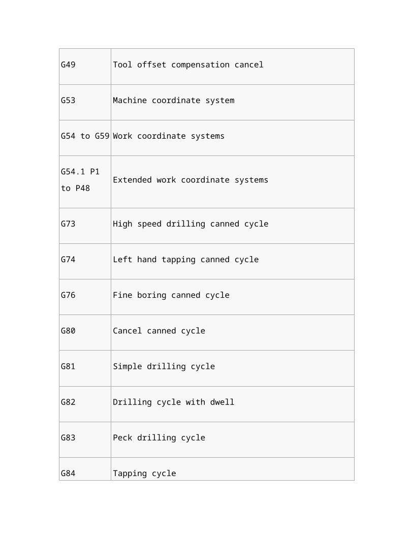
Common FANUC G Codes for Mill

Code Description

G00 Rapid positioning

G01 Linear interpolation

G02 CW circular interpolation

G03 CCW circular interpolation

G04 Dwell

G05.1 Q1. Ai Nano contour control

G05 P10000 HPCC

G10/G11 Programmable Data input/Data write cancel

G17 X-Y plane selection

G18 X-Z plane selection

G19 Y-Z plane selection

G20 Programming in inches

G21 Programming in mm

G28 Return to home position

G30 2nd reference point return

G31 Skip function (used for probes and tool length measurement systems)

G33 Constant pitch threading

G34 Variable pitch threading

G40 Tool radius compensation off

G41 Tool radius compensation left

G42 Tool radius compensation right

G43 Tool offset compensation negative

G44 Tool offset compensation positive

G45 Axis offset single increase

G46 Axis offset single decrease

G47 Axis offset double increase

G48 Axis offset double decrease

G49 Tool offset compensation cancel

G53 Machine coordinate system

G54 to G59 Work coordinate systems

G54.1 P1 to

P48Extended work coordinate systems

G73 High speed drilling canned cycle

G74 Left hand tapping canned cycle

G76 Fine boring canned cycle

G80 Cancel canned cycle

G81 Simple drilling cycle

G82 Drilling cycle with dwell

G83 Peck drilling cycle

G84 Tapping cycle

G84.2 Direct right hand tapping canned cycle

G90 Absolute programming (type B and C systems)

G91 Incremental programming (type B and C systems)

G92 Programming of absolute zero point

G94/G95 Inch per minute/Inch per revolution feed (type A system)

G98/G99 Return to Initial Z plane/R plane in canned cycle

G96/G97Constant cutting speed (Constant surface speed)/Constant rotation speed

(constant RPM)

A standardized version of G-code known as BCL is used, but only on very few machines.

G-code files may be generated by CAM software. Those applications typically use

translators called post-processors to output code optimized for a particular machine type

or family. Post-processors are often user-editable to enable further customization, if

necessary. G-code is also output by specialized CAD systems used to design printed

circuit boards. Such software must be customized for each type of machine tool that it

will be used to program. Some G-code is written by hand for volume production jobs. In

this environment, the inherent inefficiency of CAM-generated G-code is unacceptable.

Some CNC machines use "conversational" programming, which is a wizard-like

programming mode that either hides G-code or completely bypasses the use of G-code.

Some popular examples are Southwestern Industries' ProtoTRAK, Mazak's Mazatrol,

Hurco's Ultimax and Mori Seiki's CAPS conversational software.

Example Program

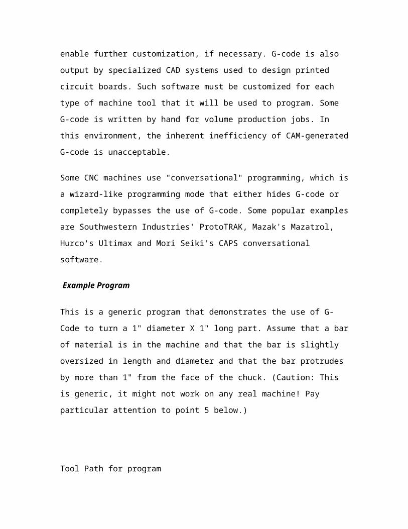
This is a generic program that demonstrates the use of G-Code to turn a 1" diameter X 1"

long part. Assume that a bar of material is in the machine and that the bar is slightly

oversized in length and diameter and that the bar protrudes by more than 1" from the face

of the chuck. (Caution: This is generic, it might not work on any real machine! Pay

particular attention to point 5 below.)

Tool Path for program

Sample

Line Code Description

N01 M216 Turn on load monitor

N02 G00 X20 Z20Rapid move away from the part, to ensure the starting position of

the tool

N03 G50 S2000 Set Maximum spindle speed

N04 M01 Optional stop

N05 T0303 M6Select tool #3 from the carousel, use tool offset values located in

line 3 of the program table, index the turret to select new tool

N06G96 S854 M42

M03 M08

Variable speed cutting, 854 ft/min, High spindle gear, Start spindle

CW rotation, Turn the mist coolant on

N07 G00 X1.1 Z1.1Rapid feed to a point 0.1" from the end of the bar and 0.05" from

the side

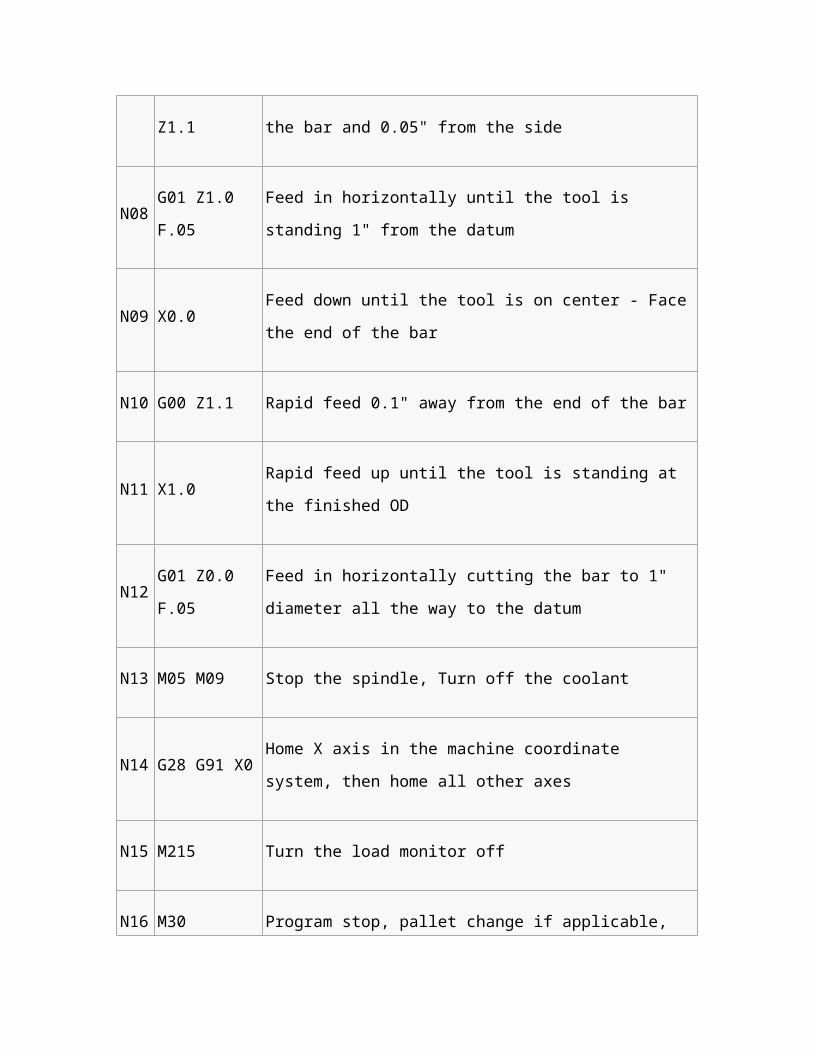
N08 G01 Z1.0 F.05 Feed in horizontally until the tool is standing 1" from the datum

N09 X0.0 Feed down until the tool is on center - Face the end of the bar

N10 G00 Z1.1 Rapid feed 0.1" away from the end of the bar

N11 X1.0 Rapid feed up until the tool is standing at the finished OD

N12 G01 Z0.0 F.05Feed in horizontally cutting the bar to 1" diameter all the way to

the datum

N13 M05 M09 Stop the spindle, Turn off the coolant

N14 G28 G91 X0Home X axis in the machine coordinate system, then home all

other axes

N15 M215 Turn the load monitor off

N16 M30Program stop, pallet change if applicable, rewind to beginning of

the program

Several points to note:

1. There is room for some programming style, even in this short program. The

grouping of codes in line N06 could have been put on multiple lines. Doing so

may have made it easier to follow program execution.

2. Many codes are "Modal" meaning that they stay in effect until they are cancelled

or replaced by a contradictory code. For example, once variable speed cutting had

been selected (G96), it stayed in effect until the end of the program. In operation,

the spindle speed would increase as the tool neared the center of the work in order

to maintain a constant cutting speed. Similarly, once rapid feed was selected

(G00) all tool movements would be rapid until a feed rate code (G01, G02, G03)

was selected.

3. It is common practice to use a load monitor with CNC machinery. The load

monitor will stop the machine if the spindle or feed loads exceed a preset value

that is set during the set-up operation. The job of the load monitor is to prevent

machine damage in the event of tool breakage or a programming mistake. On

small or hobby machines, it can warn of a tool that is becoming dull and needs to

be replaced or sharpened.

4. It is common practice to bring the tool in rapidly to a "safe" point that is close to

the part - in this case 0.1" away - and then start feeding the tool. How close that

"safe" distance is, depends on the skill of the programmer and maximum material

condition for the raw stock.

5. If the program is wrong, there is a high probability that the machine will crash, or

ram the tool into the part under high power. This can be costly, especially in

newer machining centers. It is possible to intersperse the program with optional

stops (M01 code) which allow the program to be run piecemeal for testing

purposes. The optional stops remain in the program but they are skipped during

the normal running of the machine. Thankfully, most CAD/CAM software ships

with CNC simulators that will display the movement of the tool as the program

executes. Many modern CNC machines also allow programmers to execute the

program in a simulation mode and observe the operating parameters of the

machine at a particular execution point. This enables programmers to discover

semantic errors (as opposed to syntax errors) before losing material or tools to an

incorrect program. Depending on the size of the part, wax blocks may be used for

testing purposes as well.

6. For pedagogical purposes, line numbers have been included in the program above.

They are usually not necessary for operation of a machine, so they are seldom

used in industry. However, if branching or looping statements are used in the

code, then line numbers may well be included as the target of those statements

(e.g. GOTO N99).

Basic ISO CNC Code

|

M03, M04, M05 Spindle CW, Spindle CCW, Spindle Stop

|

M08, M09 Coolant/lubricant On, Coolant/lubricant Off

M02 Program Stop(Is most commonly used)

M30 Program end, rewind

M98 Subprogram call

M99 Return to call program

M00, M01 Program stop, optional stop

|

G96, G97 Constant surface speed, Constant Spindle speed

G50 Maximum spindle speed

G95, G94 Feed mm per revolution, feed mm/min

G00, G01 rapid movement, Linear Interpolation (cutting in a straight line)

|

F Feed

S Spindle Speed

|

direction Coordinates X Y Z A B C U V W

MODULE – 4

Group Technology

Group Technology or GT is a manufacturing philosophy in which the parts having

similarities (Geometry, manufacturing process and/or function) are grouped together to

achieve higher level of integration between the design and manufacturing functions of a

firm.[1]. The aim is to reduce work-in-progress and improve delivery performance by

reducing lead times. GT is based on a general principle that many problems are similar

and by grouping similar problems, a single solution can be found to a set of problems,

thus saving time and effort. The group of similar parts is known as part family and the

group of machineries used to process an individual part family is known as machine cell.

It is not necessary for each part of a part family to be processed by every machine of

corresponding machine cell. This type of manufacturing in which a part family is

produced by a machine cell is known as cellular manufacturing. The manufacturing

efficiencies are generally increased by employing GT because the required operations

may be confined to only a small cell and thus avoiding the need for transportation of in-

process parts.

Cellular manufacturing

Cellular Manufacturing is a model for workplace design, and is an integral part of lean

manufacturing systems. The goal of lean manufacturing is the aggressive minimisation of

waste, called muda, to achieve maximum efficiency of resources. Cellular manufacturing,

sometimes called cellular or cell production, arranges factory floor labor into semi-

autonomous and multi-skilled teams, or work cells, who manufacture complete products

or complex components. Properly trained and implemented cells are more flexible and

responsive than the traditional mass-production line, and can manage processes, defects,

scheduling, equipment maintenance, and other manufacturing issues more efficiently.

History

Cellular manufacturing is a fairly new application of group technology, although the

Portsmouth Block Mills offers what by definition constitutes an early example of cellular

manufacturing. By 1808, using machinery designed by Marc Isambard Brunel and

constructed by Henry Maudslay, the Block Mills were producing 130,000 blocks

(pulleys) for the Royal Navy per year in single unit lots, with 10 men operating 42

machines arranged in three production flow lines. This installation apparently reduced

manpower requirements by 90% (from 110 to 10), reduced cost substantially and greatly

improved block consistency and quality. Group Technology is a management strategy

with long term goals of staying in business, growing, and making profits. Companies are

under relentless pressure to reduce costs while meeting the high quality expectations of

the customer to maintain a competitive advantage. Successfully implementing Cellular

manufacturing allows companies to achieve cost savings and quality improvements,

especially when combined with the other aspects of lean manufacturing. Cell

manufacturing systems are currently used to manufacture anything from hydraulic and

engine pumps used in aircraft to plastic packaging components made using injection

molding.

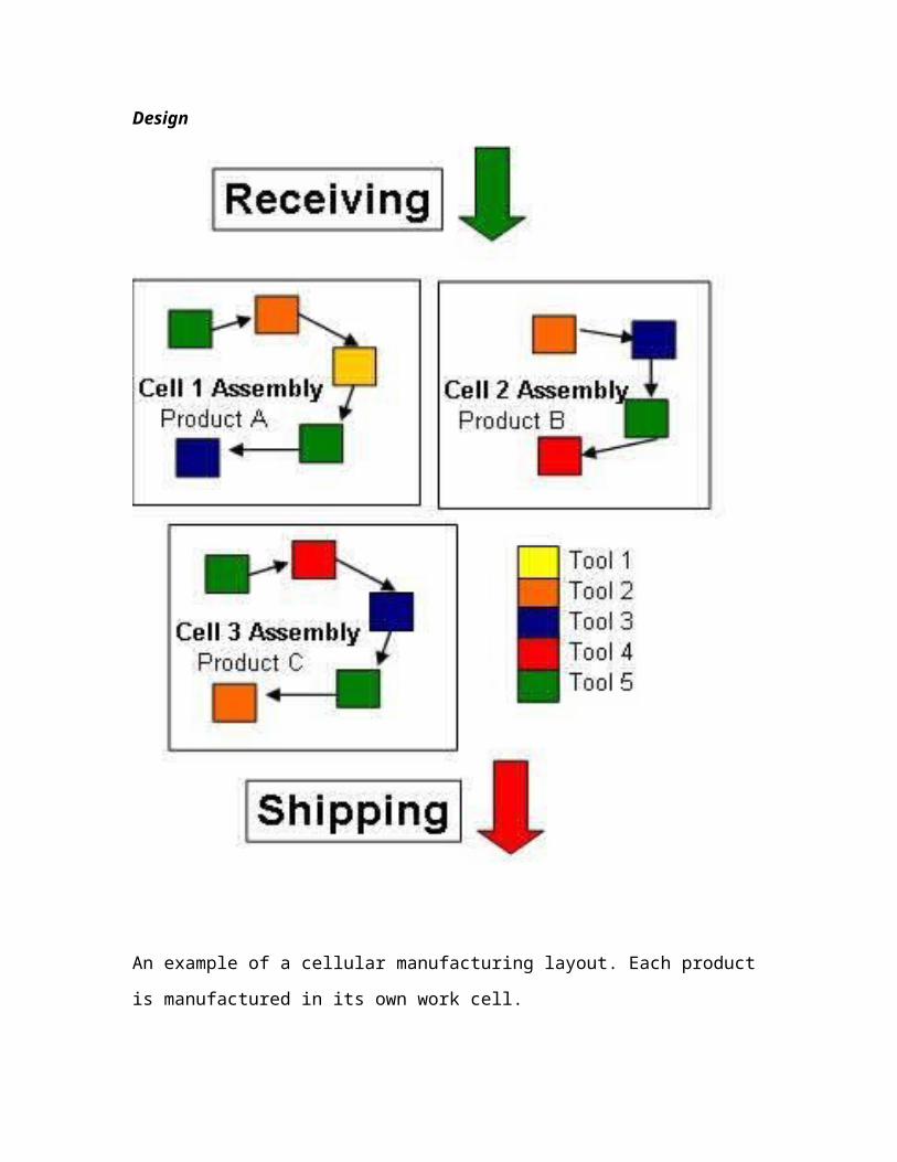
Design

An example of a cellular manufacturing layout. Each product is manufactured in its own

work cell.

The goal of cellular manufacturing is having the flexibility to produce a high variety of

low demand products, while maintaining the high productivity of large scale production.

Cell designers achieve this through modularity in both process design and product design.

Process Design

The division of the entire production process into discrete segments, and the assignment

of each segment to a work cell, introduces the modularity of processes. If any segment of

the process needs to be changed, only the particular cell would be affected, not the entire

production line. For example, if a particular component was prone to defects, and this

could be solved by upgrading the equipment, a new work cell could be designed and

prepared while the obsolete cell continued production. Once the new cell is tested and

ready for production, the incoming parts to and outgoing parts from the old cell will

simply be rerouted to the new cell without having to disrupt the entire production line. In

this way, work cells enable the flexibility to upgrade processes and make variations to

products to better suit customer demands while largely reducing or eliminating the costs

of stoppages. While the machinery may be functionally dissimilar, the family of parts

produced contains similar processing requirements or has geometric similarities. Thus, all

parts basically follow the same routing with some minor variations (e.g., skipping an

operation). The cells may have no conveyorized movement of parts between machines, or

they may have a flow line connected by a conveyor that can provide automatic transfer.

Product Design

Product modularity must match the modularity of processes. Even though the entire

production system becomes more flexible, each individual cell is still optimised for a

relatively narrow range of tasks, in order to take advantage of the mass-production

efficiencies of specialisation and scale. To the extent that a large variety of products can

be designed to be assembled from a small number of modular parts, both high product

variety and high productivity can be achieved. For example, a varied range of

automobiles may be designed to use the same chassis, a small number of engine

configurations, and a moderate variety of car bodies, each available in a range of colors.

In this way, a large variety of automobiles, with different performances and appearances

and functions, can be produced by combining the outputs from a more limited number of

work cells.

In combination, each modular part is designed for a particular work cell, or dedicated

clusters of machines or manufacturing processes. Cells are usually bigger than typical

conventional workstations, but smaller than a complete conventional department. After

conversion, a cellular manufacturing layout usually requires less floor space as a result of

the optimized production processes. Each cell is responsible for its own internal control

of quality, scheduling, ordering, and record keeping. The idea is to place the

responsibility of these tasks on those who are most familiar with the situation and most

able to quickly fix any problems. The middle management no longer has to monitor the

outputs and interrelationships of every single worker, and instead only has to monitor a

smaller number of work cells and the flow of materials between them, often achieved

using a system of kanbans.

Implementation

The biggest challenge when implementing cellular manufacturing in a company is

dividing the entire manufacturing system into cells. The issues may be conceptually

divided in the "hard" issues of equipment, such as material flow and layout, and the "soft"

issues of management, such as upskilling and corporate culture.

The hard issues are a matter of design and investment. The entire factory floor is

rearranged, and equipment is modified or replaced to enable cell manufacturing. The

costs of work stoppages during implementation can be considerable, and lean

manufacturing literature recommend that implementation should be phased to minimize

the impacts of such disruptions as much as possible. The rearrangement of equipment

(which is sometimes bolted to the floor or built into the factory building) or the

replacement of equipment that is not flexible or reliable enough for cell manufacturing

also pose considerable costs, although it may be justified as the upgrading obsolete

equipment. In both cases, the costs have to be justified by the cost savings that can be

realistically expected from the more flexible cell manufacturing system being introduced,

and miscalculations can be disastrous. A common oversight is the need for multiple jigs,

fixtures and or tooling for each cell. Properly designed, these requirements can be

accommodated in specific-task cells serving other cells; such as a common punch press

or test station. Too often, however, the issue is discovered late and each cell is found to

require its own set of tooling.

The soft issues are more difficult to calculate and control. The implementation of cell

manufacturing often involves employee training and the redefinition and reassignment of

jobs. Each of the workers in each cell should ideally be able to complete the entire range

of tasks required from that cell, and often this means being more multi-skilled than they

were previously. For this reason, transition from a progressive assembly line type of

manufacturing to cellular is often best managed in stages with both types co-existing for a

period of time. In addition, cells are expected to be self-managing (to some extent), and

therefore workers will have to learn the tools and strategies for effective teamwork and

management, tasks that workers in conventional factory environments are entirely unused

to. At the other end of the spectrum, the management will also find their jobs redefined,

as they must take a more "hands-off" approach to allow work cells to effectively self-

manage. Instead, they must learn to perform a more oversight and support role,

maintaining a system where work cells self-optimize through supplier-input-process-

output-customer (SIPOC) relationships. These soft issues, while difficult to pin down,

pose a considerable challenge for cell manufacturing implementation; a factory with a

cell manufacturing layout but without cell manufacturing workers and managers is

unlikely to achieve the cell manufacturing benefits.

Product start-ups can be more difficult to manage if assembly training was traditionally

accomplished station-by-station on a fixed assembly line. As each operator in a cell is

responsible for a larger number of assembled parts and operations, the time needed to

master the sequence and techniques is considerably longer. If multiple parallel cells are

used, each cell must be launched separately (meaning slower production ramp) or with

equal training resources (meaning more in total). The consideration of the cell's internal

group dynamics, personalities and other traits is often more of a concern in cellular

manufacturing due to the closer proximity and co-dependency of the team members;

however properly implemented this is a major benefit of cellular manufacturing.

Benefits and Costs

There are many benefits of cellular manufacturing for a company if applied correctly.

Most immediately, processes become more balanced and productivity increases because

the manufacturing floor has been reorganized and tidied up.

Part movement, set-up time, and wait time between operations are reduced, resulting in a

reduction of work in progress inventory freeing idle capital that can be better utilized

elsewhere. Cellular manufacturing, in combination with the other lean manufacturing and

just-in-time processes, also helps eliminate overproduction by only producing items when

they are needed. The results are cost savings and the better control of operations.

There are some costs of implementing cellular manufacturing, however, in addition to the

set-up costs of equipment and stoppages noted above. Sometimes different work cells can

require the same machines and tools, possibly resulting in duplication causing a higher

investment of equipment and lowered machine utilization. However, this is a matter of

optimization and can be addressed through process design.

Computer aided Process Planning

Computer-Aided Process Planning (CAPP) is the use of computer technology to aid in

the process planning of a part or product, in manufacturing. CAPP is the link between

CAD and CAM in that it provides for the planning of the process to be used in producing

a designed part.

Process planning is concerned with determining the sequence of individual

manufacturing operations needed to produce a given part or product. The resulting

operation sequence is documented on a form typically referred to as a route sheet

containing a listing of the production operations and associated machine tools for a

workpart or assembly. Process planning in manufacturing also refers to the planning of

use of blanks, spare parts, packaging material, user instructions (manuals) etc.

The term "Computer-Aided Production Planning" is used in different context on different

parts of the production process; to some extent CAPP overlaps with the term "PIC"

(Production and Inventory control.

Process planning translates design information into the process steps and instructions to

efficiently and effectively manufacture products. As the design process is supported by

many computer-aided tools, computer-aided process planning (CAPP) has evolved to

simplify and improve process planning and achieve more effective use of manufacturing

resources.[2]

Process planning encompasses the activities and functions to prepare a detailed set of

plans and instructions to produce a part. The planning begins with engineering drawings,

specifications, parts or material lists and a forecast of demand. The results of the planning

are:

Routings which specify operations, operation sequences, work centers, standards,

tooling and fixtures. This routing becomes a major input to the manufacturing

resource planning system to define operations for production activity control

purposes and define required resources for capacity requirements planning

purposes.

Process plans which typically provide more detailed, step-by-step work

instructions including dimensions related to individual operations, machining

parameters, set-up instructions, and quality assurance checkpoints.

Fabrication and assembly drawings to support manufacture (as opposed to

engineering drawings to define the part).

Keneth Crow [3] statest that "Manual process planning is based on a manufacturing

engineer's experience and knowledge of production facilities, equipment, their

capabilities, processes, and tooling. Process planning is very time-consuming and the

results vary based on the person doing the planning".

According to Engelke [4], the need for CAPP is directly proportional to the number of

different types of parts being manufactured and the complexity of the manufacturing

process.

Computer-aided process planning initially evolved as a means to electronically store a

process plan once it was created, retrieve it, modify it for a new part and print the plan.

Other capabilities were table-driven cost and standard estimating systems, for sales

representatives to create customer quotations and estimate delivery time.

Future development of CAPP

Generative or dynamic CAPP is the main focus of development, the ability to automaticly

generate production plans for new products, or dynamicly update production plans on the

basis of resource availabilty. Generative CAPP will probably use iterative methods,

where simple production plans are applied to automatic CAD/CAM development to

refine the initial production plan.

Traditional CAPP methods that optimise plans in a linear manner have not been able

provide the need for flexible planning, so new dynamic systems will explore all possible

combinations of production processes, and then generate plans according to available

machining resources. For example, K.S. Lee et. al states that "By considering the multi-

selection tasks simultaneously, a specially designed genetic algorithm searches through

the entire solution space to identify the optimal plan"

MODULE – 5

Industrial Robotics

Robotics is the science and technology of robots, and their design, manufacture, and

application.[1] Robotics has connections to electronics, mechanics, and software.

Origins

Stories of artificial helpers and companions and attempts to create them have a long

history, but fully autonomous machines only appeared in the 20th century. The first

digitally operated and programmable robot, the Unimate, was installed in 1961 to lift hot

pieces of metal from a die casting machine and stack them. Today, commercial and

industrial robots are in widespread use performing jobs more cheaply or with greater

accuracy and reliability than humans. They are also employed for jobs which are too

dirty, dangerous, or dull to be suitable for humans. Robots are widely used in

manufacturing, assembly and packing, transport, earth and space exploration, surgery,

weaponry, laboratory research, safety, and mass production of consumer and industrial

goods.

Date Significance Robot Name Inventor

First century A.D. and earlier

Descriptions of more than 100 machines and automata, including a fire engine, a wind organ, a coin-operated machine, and a steam-powered engine, in Pneumatica and Automata by Heron of Alexandria

Ctesibius, Philo of Byzantium, Heron of Alexandria, and others

1206 First programmable humanoid robotsBoat with four robotic musicians

Al-Jazari

c. 1495 Designs for a humanoid robot Mechanical Leonardo da Vinci

knight

1738 Mechanical duck that was able to eat, flap its wings, and excrete

Digesting Duck

Jacques de Vaucanson

1800s Japanese mechanical toys that served tea, fired arrows, and painted Karakuri toys Tanaka Hisashige

1921 First fictional automatons called "robots" appear in the play R.U.R.

Rossum's Universal Robots

Karel Čapek

1930s Humanoid robot exhibited at the 1939 and 1940 World's Fairs Elektro

Westinghouse Electric Corporation

1948 Simple robots exhibiting biological behaviors[4]

Elsie and Elmer

William Grey Walter

1956

First commercial robot, from the Unimation company founded by George Devol and Joseph Engelberger, based on Devol's patents[5]

Unimate George Devol

1961 First installed industrial robot Unimate George Devol

1963 First palletizing robot[6] Palletizer Fuji Yusoki Kogyo

1973 First industrial robot with six electromechanically driven axes[7] Famulus KUKA Robot

Group

1975 Programmable universal manipulation arm, a Unimation product PUMA Victor Scheinman

Components of robots

Structure

The structure of a robot is usually mostly mechanical and can be called a kinematic chain

(its functionality being similar to the skeleton of the human body). The chain is formed of

links (its bones), actuators (its muscles), and joints which can allow one or more degrees

of freedom. Most contemporary robots use open serial chains in which each link connects

the one before to the one after it. These robots are called serial robots and often resemble

the human arm. Some robots, such as the Stewart platform, use a closed parallel

kinematical chain. Other structures, such as those that mimic the mechanical structure of

humans, various animals, and insects, are comparatively rare. However, the development

and use of such structures in robots is an active area of research (e.g. biomechanics).

Robots used as manipulators have an end effector mounted on the last link. This end

effector can be anything from a welding device to a mechanical hand used to manipulate

the environment.

Power source

At present; mostly (lead-acid) batteries are used, but potential powersources could be:

compressed air canisters

flywheel energy storage

organic garbages (trough anaerobic digestion)

feces (human, animal); may be interesting in a military context as feces of small

combat groups may be reused for the energy requirements of the robot assistant

(see DEKA's project Slingshot stirling engine on how the system would operate)

still untested energy sources (eg Joe Cell, ...)

radioactive source (such as with the proposed Ford car of the '50); too proposed in

movies as Red Planet (film)

Actuation

A robot leg powered by Air Muscles

Actuators are the "muscles" of a robot, the parts which convert stored energy into

movement. By far the most popular actuators are electric motors, but there are many

others, powered by electricity, chemicals, and compressed air.

Motors: The vast majority of robots use electric motors, including brushed and

brushless DC motors.

Stepper motors: As the name suggests, stepper motors do not spin freely like DC

motors; they rotate in discrete steps, under the command of a controller. This

makes them easier to control, as the controller knows exactly how far they should

have rotated, without having to use a sensor. The controller can't tell if the motor

was stalled, and the shaft didn't turn. They are used on many robots and CNC

machines, as their main advantage over DC motors, is that you can specify how

much to turn, for more precise control, rather than a "spin and see where it went"

approach.

Piezo motors: A recent alternative to DC motors are piezo motors or ultrasonic

motors. These work on a fundamentally different principle, whereby tiny

piezoceramic elements, vibrating many thousands of times per second, cause

linear or rotary motion. There are different mechanisms of operation; one type

uses the vibration of the piezo elements to walk the motor in a circle or a straight

line.[10] Another type uses the piezo elements to cause a nut to vibrate and drive a

screw. The advantages of these motors are nanometer resolution, speed, and

available force for their size.[11] These motors are already available commercially,

and being used on some robots.[12][13]

Air muscles: The air muscle is a simple yet powerful device for providing a

pulling force. When inflated with compressed air, it contracts by up to 40% of its

original length. The key to its behavior is the braiding visible around the outside,

which forces the muscle to be either long and thin, or short and fat. Since it

behaves in a very similar way to a biological muscle, it can be used to construct

robots with a similar muscle/skeleton system to an animal.[14] For example, the

Shadow robot hand uses 40 air muscles to power its 24 joints.

Electroactive polymers: Electroactive polymers are a class of plastics which

change shape in response to electrical stimulation.[15] They can be designed so that

they bend, stretch, or contract, but so far there are no EAPs suitable for

commercial robots, as they tend to have low efficiency or are not robust.[16]

Indeed, all of the entrants in a recent competition to build EAP powered arm

wrestling robots, were beaten by a 17 year old girl.[17] However, they are expected

to improve in the future, where they may be useful for microrobotic applications.[18]

Elastic nanotubes: These are a promising, early-stage experimental technology.

The absence of defects in nanotubes enables these filaments to deform elastically

by several percent, with energy storage levels of perhaps 10J per cu cm for metal

nanotubes. Human biceps could be replaced with an 8mm diameter wire of this

material. Such compact "muscle" might allow future robots to outrun and outjump

humans.[19]

Sensing

Touch

Current robotic and prosthetic hands receive far less tactile information than the human

hand. Recent research has developed a tactile sensor array that mimics the mechanical

properties and touch receptors of human fingertips.[20] The sensor array is constructed as a

rigid core surrounded by conductive fluid contained by an elastomeric skin. Electrodes

are mounted on the surface of the rigid core and are connected to an impedance-

measuring device within the core. When the artificial skin touches an object the fluid path

around the electrodes is deformed, producing impedance changes that map the forces

received from the object. The researchers expect that an important function of such

artificial fingertips will be adjusting robotic grip on held objects.

Vision

Manipulation

Robots which must work in the real world require some way to manipulate objects; pick

up, modify, destroy, or otherwise have an effect. Thus the 'hands' of a robot are often

referred to as end effectors,[21] while the arm is referred to as a manipulator.[22] Most robot

arms have replaceable effectors, each allowing them to perform some small range of

tasks. Some have a fixed manipulator which cannot be replaced, while a few have one

very general purpose manipulator, for example a humanoid hand.

Mechanical Grippers: One of the most common effectors is the gripper. In its

simplest manifestation it consists of just two fingers which can open and close to

pick up and let go of a range of small objects. See end effectors.

Vacuum Grippers: Pick and place robots for electronic components and for large

objects like car windscreens, will often use very simple vacuum grippers. These

are very simple astrictive [23] devices, but can hold very large loads provided the

prehension surface is smooth enough to ensure suction.

General purpose effectors: Some advanced robots are beginning to use fully humanoid hands, like the Shadow Hand, MANUS[24], and the Schunk hand.[25]

Locomotion

Rolling robots

Segway in the Robot museum in Nagoya.

For simplicity, most mobile robots have four wheels. However, some researchers have

tried to create more complex wheeled robots, with only one or two wheels.

Two-wheeled balancing: While the Segway is not commonly thought of as a

robot, it can be thought of as a component of a robot. Several real robots do use a

similar dynamic balancing algorithm, and NASA's Robonaut has been mounted

on a Segway.[28]

Ballbot: Carnegie Mellon University researchers have developed a new type of

mobile robot that balances on a ball instead of legs or wheels. "Ballbot" is a self-

contained, battery-operated, omnidirectional robot that balances dynamically on a

single urethane-coated metal sphere. It weighs 95 pounds and is the approximate

height and width of a person. Because of its long, thin shape and ability to

maneuver in tight spaces, it has the potential to function better than current robots

can in environments with people.[29]

Track Robot: Another type of rolling robot is one that has tracks, like NASA's

Urban Robot, Urbie.[30]

Control

A robot-manipulated marionette, with complex control systems

The mechanical structure of a robot must be controlled to perform tasks. The control of a

robot involves three distinct phases - perception, processing, and action (robotic

paradigms). Sensors give information about the environment or the robot itself (e.g. the

position of its joints or its end effector). This information is then processed to calculate

the appropriate signals to the actuators (motors) which move the mechanical.

The processing phase can range in complexity. At a reactive level, it may translate raw

sensor information directly into actuator commands. Sensor fusion may first be used to

estimate parameters of interest (e.g. the position of the robot's gripper) from noisy sensor

data. An immediate task (such as moving the gripper in a certain direction) is inferred

from these estimates. Techniques from control theory convert the task into commands

that drive the actuators.

At longer time scales or with more sophisticated tasks, the robot may need to build and

reason with a "cognitive" model. Cognitive models try to represent the robot, the world,

and how they interact. Pattern recognition and computer vision can be used to track

objects. Mapping techniques can be used to build maps of the world. Finally, motion

planning and other artificial intelligence techniques may be used to figure out how to act.

For example, a planner may figure out how to achieve a task without hitting obstacles,

falling over, etc.

Control systems may also have varying levels of autonomy. Direct interaction is used for

haptic or tele-operated devices, and the human has nearly complete control over the

robot's motion. Operator-assist modes have the operator commanding medium-to-high-

level tasks, with the robot automatically figuring out how to achieve them. An

autonomous robot may go for extended periods of time without human interaction.

Higher levels of autonomy do not necessarily require more complex cognitive

capabilities. For example, robots in assembly plants are completely autonomous, but

operate in a fixed pattern.

Dynamics and kinematics

The study of motion can be divided into kinematics and dynamics. Direct kinematics

refers to the calculation of end effector position, orientation, velocity, and acceleration

when the corresponding joint values are known. Inverse kinematics refers to the opposite

case in which required joint values are calculated for given end effector values, as done in

path planning. Some special aspects of kinematics include handling of redundancy

(different possibilities of performing the same movement), collision avoidance, and

singularity avoidance. Once all relevant positions, velocities, and accelerations have been

calculated using kinematics, methods from the field of dynamics are used to study the

effect of forces upon these movements. Direct dynamics refers to the calculation of

accelerations in the robot once the applied forces are known. Direct dynamics is used in

computer simulations of the robot. Inverse dynamics refers to the calculation of the

actuator forces necessary to create a prescribed end effector acceleration. This

information can be used to improve the control algorithms of a robot.

In each area mentioned above, researchers strive to develop new concepts and strategies,

improve existing ones, and improve the interaction between these areas. To do this,

criteria for "optimal" performance and ways to optimize design, structure, and control of

robots must be developed and implemented.

Robot Research

Much of the research in robotics focuses not on specific industrial tasks, but on

investigations into new types of robots, alternative ways to think about or design robots,

and new ways to manufacture them.

A first particular new innovation in robotdesign is the opensourcing of robot-projects. To

describe the level of advancement of a robot, the term Generation Robots can be used.

This term is coined by Professor Hans Moravec, Principal Research Scientist at the

Carnegie Mellon University Robotics Institute in describing the near future evolution of

robot technology.[67] First, second and third generation robots are First generation

robots, Moravec predicted in 1997, should have an intellectual capacity comparable to

perhaps a lizard and should become available by 2010. Because the first generation robot

would be incapable of learning, however, professor Moravec predicts that the second

generation robot would be an improvement over the first and become available by 2020,

with an intelligence maybe comparable to that of a mouse. The third generation robot

should have an intelligence comparable to that of a monkey. Though fourth generation

robots, robots with human intelligence, professor Moravec predicts, would become

possible, he does not predict this happening before around 2040 or 2050.

The second is Evolutionary Robots. This is a methodology that uses evolutionary

computation to help design robots, especially the body form, or motion and behavior

controllers. In a similar way to natural evolution, a large population of robots is allowed

to compete in some way, or their ability to perform a task is measured using a fitness

function. Those that perform worst are removed from the population, and replaced by a

new set, which have new behaviors based on those of the winners. Over time the

population improves, and eventually a satisfactory robot may appear. This happens

without any direct programming of the robots by the researchers. Researchers use this

method both to create better robots,[68] and to explore the nature of evolution.[69] Because

the process often requires many generations of robots to be simulated, this technique may

be run entirely or mostly in simulation, then tested on real robots once the evolved

algorithms are good enough.