Embed Size (px)
Citation preview
COMNET III________________________
Planning for Network Managers______________________
Release 1.3
CACICall or Fax for an Immediate Response
Worldwide Wash., DC Area UKCACI Products CACI Products CACI Products3333 N Torrey Pines Ct 1600 Wilson Blvd Watchmoor ParkThird Floor Thirteenth Floor Riverside WayLa Jolla, California Arlington, Virginia Camberley, Surrey92037 USA 22209 USA GU15 3YL UKTel (619) 457-9681 Tel (703) 875-2900 Tel +44 (0) 1276 671 671Fax (619) 457-1184 Fax (703) 875-2904 Fax +44 (0) 1276 670 677

ssume ein is ch
Copyright © 1995 CACIRelease 1.2 June 1996
All rights reserved. No part of this publication may be reproduced by any means without written permission from CACI.
For product information contact:
CACI Products Company CACI Products Division3333 North Torrey Pines Ct Watchmoor Park, Riverside WayLa Jolla, California 92037 Camberley, Surrey, GU15 3YL, UKTelephone: (619) 457-9681 Telephone: +44 (0) 1276 671 671Fax: (619) 457-1184 Fax: +44 (0) 1276 670 677
The information in this publication is believed to be accurate in all respects. However, CACI cannot athe responsibility for any consequences resulting from the use therof. The information contained hersubject to change. Revisions to this publication or new editions of it may be issued to incorporate suchange.
COMNET III is a trademark of CACI Product Company.
1. Introduction .............................................................................................1
1.1 COMNET III and Network Planning ..............................................................1
1.2 Background ......................................................................................................1
1.3 Description ......................................................................................................1
1.4 Applicability ....................................................................................................2
1.5 Availability ......................................................................................................2
1.6 Overall Approach ............................................................................................2
1.7 Types Of Network ...........................................................................................3
1.8 Choosing the Correct Level of Detail ..............................................................4
1.8.1 A Backbone Network ..............................................................................41.8.2 A Local Area Network ............................................................................51.8.3 Summary: Level of Detail ......................................................................5
1.9 Uses of COMNET III ......................................................................................5
2. Quick Start ...............................................................................................7
2.1 Getting Started .................................................................................................7
2.2 How Models are Stored ...................................................................................7
2.3 Running a Pre-Built Model .............................................................................7
2.3.1 Starting COMNET III .............................................................................72.3.2 Loading and Running the Model .............................................................8
2.4 Building a Simple Model ...............................................................................14
2.4.1 Simple Model Layout ............................................................................14
3. Overview of Modeling Constructs .......................................................21
3.1 Overview .......................................................................................................21
3.1.1 Terminology ..........................................................................................21
3.2 Network Topology .........................................................................................21
3.2.1 Nodes .....................................................................................................213.2.2 Links ......................................................................................................223.2.3 Subnets ..................................................................................................223.2.4 Transit Nets ...........................................................................................233.2.5 WAN Clouds .........................................................................................233.2.6 Arcs and Ports .......................................................................................23
3.3 Network Traffic and Workload .....................................................................23
iii
TABLE OF CONTENTS
3.3.1 Scheduling .............................................................................................243.3.2 Applications ..........................................................................................243.3.3 Traffic Sources ......................................................................................253.3.4 Call Sources ...........................................................................................253.3.5 External Sources ....................................................................................25
3.4 Network Operation ........................................................................................26
3.4.1 Routing Algorithm ................................................................................263.4.2 Transport Protocols ...............................................................................27
3.5 Simulation Control ........................................................................................28
3.6 Statistics Reporting ........................................................................................28
3.7 User Distributions ..........................................................................................29
3.8 Libraries .........................................................................................................29
3.9 Model Files ....................................................................................................29
4. Modeling Constructs .............................................................................31
4.1 Access Point ..................................................................................................32
4.2 Buffer Processing ..........................................................................................35
4.3 Circuit-switched Model .................................................................................38
4.4 Clouds ............................................................................................................40
4.5 Cloud Access Links .......................................................................................47
4.6 Cloud VCs .....................................................................................................50
4.7 Command: Answer Message .........................................................................53
4.8 Command: Process Data ................................................................................56
4.9 Command: Read File .....................................................................................59
4.10 Command: Setup Session ..............................................................................63
4.11 Command: Transport Message ......................................................................68
4.12 Command: Wait For ......................................................................................72
4.13 Command: Write File ....................................................................................76
4.14 COMNET Baseliner ......................................................................................80
4.15 Destination: Least Busy List .........................................................................81
4.16 Destination: Multicast List ............................................................................82
4.17 Destination: Random List ..............................................................................84
4.18 Destination: Random Neighbor .....................................................................86
4.19 Destination: Round Robin List ......................................................................87
iv
4.20 Destination: Weighted List ............................................................................88
4.21 Distributions: System ....................................................................................90
4.22 Distributions: Table .......................................................................................92
4.23 Distributions: User .........................................................................................94
4.24 External Model Files .....................................................................................95
4.25 External Traffic Files .....................................................................................96
4.26 Flow Control ..................................................................................................97
4.27 Flow Control: Fixed Window ......................................................................100
4.28 Flow Control: Sliding Window ...................................................................101
4.29 Flow Control: Jumping Window .................................................................102
4.30 Flow Control: Leaky Bucket .......................................................................103
4.31 Flow Control: SNA Pacing ..........................................................................104
4.32 Flow Control: TCP/IP Window ...................................................................105
4.33 IEEE 802 .....................................................................................................106
4.34 Link ..............................................................................................................107
4.35 Link: Binary Exponential Backoff Parameters ............................................109
4.36 Link: Framing Characteristics .....................................................................111
4.37 Link: ISDN and SONET Parameter Sets .....................................................113
4.38 Link: Loading ..............................................................................................114
4.39 Link: Aloha ..................................................................................................121
4.40 Link: CSMA ................................................................................................126
4.41 Link: CSMA/CA Wireless LAN IEEE 802.11 ...........................................131
4.42 Link: CSMA/CD .........................................................................................135
4.43 Link: Demand-Assigned Multiple Access (DAMA) ...................................139
4.44 Link: FDDI and Priority FDDI ....................................................................140
4.45 Link: Point-To-Point ...................................................................................143
4.46 Link: Polling ................................................................................................148
4.47 Link: Port .....................................................................................................152
4.48 Link: Priority Token Ring and Token Ring Enhancements ........................156
4.49 Link: Token Passing ....................................................................................157
4.50 Message Source: Interarrival Time .............................................................160
4.51 Message Source: Packetizing Delay ............................................................163
v
TABLE OF CONTENTS
4.52 Message Source: Priority .............................................................................165
4.53 Message Source: Size Calculation ...............................................................167
4.54 Message Source: Size Units ........................................................................169
4.55 Message Source: Message Text ...................................................................170
4.56 Node ............................................................................................................172
4.57 Node: Switch ...............................................................................................174
4.58 Node: Processing Node ...............................................................................179
4.59 Node: Computer Group ...............................................................................194
4.60 Node: Router ...............................................................................................197
4.61 Node: Router - Updated Router Library ......................................................206
4.62 Packet Switched Networks ..........................................................................207
4.63 Parameter Sets .............................................................................................209
4.64 Penalty Tables .............................................................................................211
4.65 Protocol Rate Controls ................................................................................216
4.66 Protocol Rate Controls: Available Rate ......................................................217
4.67 Protocol Rate Controls: Constant Rate ........................................................218
4.68 Protocol Rate Controls: Throttled Rate .......................................................219
4.69 Protocol Rate Controls: Variable Rate ........................................................220
4.70 Received Message Scheduling ....................................................................221
4.71 Remotes .......................................................................................................224
4.72 Reports .........................................................................................................225
4.73 Routing Class: Call ......................................................................................227
4.74 Routing Class: Packet ..................................................................................230
4.75 Routing Protocol: Call .................................................................................233
4.76 Routing Protocol: Packet .............................................................................244
4.76.1 Max Idle Bandwidth ............................................................................2524.76.2 Min Delay ............................................................................................2524.76.3 Min Queue ...........................................................................................2534.76.4 Min Sessions .......................................................................................2534.76.5 Random List ........................................................................................2544.76.6 Round Robin .......................................................................................254
4.77 Simulation: Animation ................................................................................256
4.78 Simulation: Animation - Dynamic Color Change .......................................259
4.79 Simulation: Parameters ................................................................................260
vi
4.80 Simulation: Tracing .....................................................................................262
4.81 Sockets .........................................................................................................264
4.82 Statistics: Export File ..................................................................................266
4.83 Statistics: Link .............................................................................................267
4.84 Statistics: Message .......................................................................................268
4.85 Statistics: Monitors ......................................................................................270
4.86 Statistics: Plot Parameters ...........................................................................273
4.87 Subnetwork ..................................................................................................274
4.88 Traffic Policing: ATM .................................................................................277
4.89 Traffic Policing: Frame Relay .....................................................................278
4.90 Traffic Source: Application .........................................................................279
4.91 Traffic Source: Call .....................................................................................283
4.92 Traffic Source: Message ..............................................................................286
4.93 Traffic Source: Packet Flow/Packet Rate Matrix ........................................288
4.94 Traffic Source: Response ............................................................................289
4.95 Traffic Source: Session ................................................................................291
4.96 Transit Networks .........................................................................................293
4.97 Transport Protocol .......................................................................................296
4.98 Trigger Events .............................................................................................300
5. Creating COMNET III Models ..........................................................303
5.1 Introduction .................................................................................................303
5.2 Using the COMNET III Tool Palette ..........................................................303
5.2.1 Object Creation Tools .........................................................................3045.2.2 Connection Tools ................................................................................3055.2.3 Selection Tool .....................................................................................3055.2.4 Selecting a Group of Objects ..............................................................3065.2.5 Text Tool .............................................................................................3065.2.6 Background Icon Tool .........................................................................3065.2.7 Subnetwork Node Tool .......................................................................306
5.3 Moving or Repositioning Objects ...............................................................307
5.4 Moving Around the Layout .........................................................................307
5.5 COMNET III Menus ...................................................................................307
5.5.1 File Menu ............................................................................................308
vii
TABLE OF CONTENTS
5.5.2 Edit Menu ............................................................................................3105.5.3 View Menu ..........................................................................................3115.5.4 Layout Menu .......................................................................................3145.5.5 Create Menu ........................................................................................3185.5.6 Define Menu ........................................................................................3205.5.7 Simulate Menu ....................................................................................3225.5.8 Report Menu ........................................................................................3245.5.9 Library Menu .......................................................................................3255.5.10 Help Menu ...........................................................................................326
5.6 Program Operation Aids ..............................................................................327
5.6.1 Tool Tips and Status Bar Messages ....................................................3275.6.2 Multiple Report Windows ...................................................................3275.6.3 3D View ..............................................................................................3275.6.4 Dockable Palettes and Toolbar ............................................................3275.6.5 Arc Editing ..........................................................................................3275.6.6 Color Palette ........................................................................................3275.6.7 Shapes ..................................................................................................3275.6.8 Bitmap Import .....................................................................................3275.6.9 Export Encapsulated PostScript ..........................................................3275.6.10 Export Raster Bitmap ..........................................................................3285.6.11 Background Text .................................................................................3285.6.12 Model Editing Features .......................................................................3285.6.13 Report Request Manager .....................................................................328
6. Advanced Software Modeling Features ............................................329
6.1 Introduction .................................................................................................329
6.2 User Variables .............................................................................................329
6.2.1 Variable Scope: ...................................................................................3296.2.2 Defining Variables: .............................................................................3296.2.3 Initial Values: ......................................................................................3306.2.4 Assigning Values: ...............................................................................3306.2.5 Querying Values: .................................................................................3306.2.6 Variable Errors: ...................................................................................3306.2.7 Exclusive Access and Semaphore Behavior: ......................................3306.2.8 Troubleshooting: .................................................................................330
6.3 New Commands ..........................................................................................331
6.3.1 Assign Variable Command: ................................................................3316.3.2 Wait For Command: ............................................................................3316.3.3 Macro Command: ................................................................................332
6.4 Expressions ..................................................................................................333
viii
7. Automatic Parameter Iterator ...........................................................337
7.1 Introduction .................................................................................................337
7.2 Terminology ................................................................................................337
7.3 Specifying an Experiment ...........................................................................337
7.4 Running an Experiment ...............................................................................338
7.5 Analyzing the Results of an Experiment .....................................................338
8. Reports .................................................................................................341
8.1 Node Utilization ..........................................................................................344
8.2 Application Delays ......................................................................................345
8.3 Received Message Count ............................................................................346
8.4 File Warnings ..............................................................................................347
8.5 Node Buffer Policy ......................................................................................348
8.6 Link Delays & Utilization ...........................................................................349
8.7 Random Access Link Performance .............................................................351
8.8 Link Frame Size Report ...............................................................................353
8.9 Link Utilization by Application ...................................................................354
8.10 Link Utilization by Protocol ........................................................................355
8.11 Message Delays For Message & Response Sources ...................................356
8.12 Message Delays For Session Sources ..........................................................357
8.13 Message Delays For Transport & Answer Commands ...............................358
8.14 Message Delays For Setup Commands .......................................................359
8.15 Packet Statistics For Message & Response Sources ...................................360
8.16 Message Delivery Report ............................................................................361
8.17 Transport Retransmission Report ................................................................362
8.18 Transport Window and Packet Interval Report ...........................................363
8.19 Transport Timeout Report ...........................................................................364
8.20 Transport Ack Delay ...................................................................................365
8.21 Transport Assembly Interval .......................................................................366
8.22 Transport Burst Size ....................................................................................367
8.23 Transport Packet Flag Report ......................................................................368
ix
TABLE OF CONTENTS
8.24 Transport Packet Size ..................................................................................369
8.25 Packet Delays For Session Sources .............................................................370
8.26 Packet Delays For Transport & Answer Commands ..................................371
8.27 Packet Delays For Setup Commands ..........................................................372
8.28 Blocked Call Statistics .................................................................................373
8.29 Disconnected Call Statistics ........................................................................374
8.30 Preempted Call Statistics .............................................................................375
8.31 Call Statistics by Node ................................................................................376
8.32 Call Statistics by Link .................................................................................377
8.33 Node Utilization Statistics For Calls ...........................................................378
8.34 Link Utilization Statistics for Calls .............................................................379
8.35 Setup Delays For Session Sources ..............................................................380
8.36 Setup Delays For Setup Commands ............................................................381
8.37 Sessions Setup by Node ...............................................................................382
8.38 Sessions Setup by Link ................................................................................383
8.39 Session Lengths by Setup Command ..........................................................384
8.40 Session Lengths by Session Source .............................................................385
8.41 Session Blocking By Session Command .....................................................386
8.42 Session Blocking By Session Source ..........................................................387
8.43 Buffer Input By Node ..................................................................................388
8.44 Buffer Input By Port ....................................................................................389
8.45 Buffer Output By Node ...............................................................................391
8.46 Buffer Output By Port .................................................................................392
8.47 Cloud Throughput .......................................................................................394
8.48 Cloud VC Frame Delay and Burst Size .......................................................395
8.49 Cloud Access Link ......................................................................................396
8.50 Cloud Access Buffer Policy Report ............................................................397
8.51 Cloud Early/Partial Packet Discard Report .................................................398
8.52 Global Traffic Command Reports ...............................................................399
8.53 Response And Answer Destinations ...........................................................400
8.54 Snapshot Reports and Alarms .....................................................................401
9. Percentiles and Plots ...........................................................................403
x
9.1 Overview of Plots and Percentiles ...............................................................403
9.2 Statistics Request Buttons ...........................................................................403
9.2.1 Access Link Statistics ..........................................................................4059.2.2 Virtual Circuit Statistics ......................................................................406
9.3 Exporting Statistics Files .............................................................................406
10. SIMGRAPHICS II Graphics Editor ...............................................407
10.1 The SIMGRAPHICS II Graphics Editor .....................................................407
10.2 Starting SIMDRAW ....................................................................................407
10.3 Editor Windows ...........................................................................................408
10.4 Setting Modes, Styles, Colors and Line Widths ..........................................409
10.5 Constructing Graphic Images ......................................................................409
10.6 Selecting ......................................................................................................410
10.7 Moving, Painting, Resizing, and Changing Priority ....................................411
10.8 Editing Points ..............................................................................................412
10.9 Cutting and Copying Objects ......................................................................412
10.10 Using the Grid .............................................................................................413
10.11 Canvas Dimensions and Coordinates ..........................................................413
10.12 The Library — Saving and Loading Objects ..............................................413
10.13 Managing the Library ..................................................................................413
10.14 Grouping Images .........................................................................................413
10.15 Recentering Images .....................................................................................414
10.16 Importing Text into SIMDRAW .................................................................414
10.17 Exiting SIMDRAW .....................................................................................414
11. COMNET Baseliner ..........................................................................415
11.1 INTRODUCTION .......................................................................................415
11.1.1 Overview .............................................................................................41511.1.2 The System Architecture .....................................................................41511.1.3 Network Topology Information ..........................................................41611.1.4 Network Load Characterization ..........................................................416
12. Statistical Distribution Functions ....................................................417
xi
TABLE OF CONTENTS
12.1 The Beta Distribution ..................................................................................417
12.2 The Erlang Distribution ...............................................................................418
12.3 The Exponential Distribution ......................................................................419
12.4 The Gamma Distribution .............................................................................420
12.5 The Geometric Distribution .........................................................................421
12.6 The Hyperexponential Distribution .............................................................422
12.7 The Integer Distribution ..............................................................................423
12.8 The Lognormal Distribution ........................................................................424
12.9 The Normal Distribution .............................................................................425
12.10 The Pareto Distribution ...............................................................................426
12.11 The Poisson Distribution .............................................................................427
12.12 The Triangular Distribution .........................................................................428
12.13 The Uniform Distribution ............................................................................429
12.14 The Weibull Distribution .............................................................................430
12.15 User Distributions ........................................................................................431
12.16 Table Distributions ......................................................................................431
13. Menus .................................................................................................433
13.1 File Menu .....................................................................................................433
13.2 Edit Menu ....................................................................................................434
13.3 View Menu ..................................................................................................435
13.4 Layout Menu ...............................................................................................436
13.5 Create Menu ................................................................................................437
13.6 Define Menu ................................................................................................438
13.7 Simulate Menu .............................................................................................439
13.8 Report Menu ................................................................................................440
13.9 Library Menu ...............................................................................................441
13.10 Help Menu ...................................................................................................442
xii
anginguccess
lET IIIsted to
ios.uration
all typese systemis for the
. New decideent and
ns. risk?
t
panies,kle lead-the chal-
alterna-actuallyow the
ours to
rt p you can
on of a
l exe-
1
1. Introduction
1.1 COMNET III and Network PlanningCOMNET III, a graphical, off-the-shelf package, lets you analyze and predict the performance of networks rfrom simple LANs to complex enterprise-wide systems—quickly and easily. This new product builds on the sof COMNET II.5 and CACI's thirty-two years of experience in simulation technology.
COMNET III supports a building-block approach where the blocks are “objects” you are familiar with in the reaworld. You start with a library of objects that closely model the objects in your real networks, with one COMNobject representing one or more real world objects. The COMNET III object’s parameters are easily adjumatch the real-world object.
COMNET III's object-oriented framework gives you the flexibility to try an unlimited number of “what if” scenarYour recommendations will be supported by an easy-to-understand animated picture of the network configyou have selected—no programming required.
1.2 BackgroundThere is increasing dependence on computing and communication networks in the day-to-day operation of of organizations. As these networks become larger and more complex the design and management of thbecomes an ever more challenging task. “Back-of-the-envelope” calculations are no longer a reasonable basdesign validation of a multimillion dollar network. Elaborate spreadsheets won’t do the job because of the stochasticnature of network traffic and the complexity of the total system. New technologies are always being introducedapplications of communication and computing networks are constantly being explored. How do organizationwhich combinations of technology and applications are right for them? As needs grow the needed investmoperating costs increase. As the organization places more dependence on its network to support its critical businessoperations, the risk of failure caused by poor network performance or availability may have serious repercussioHow can these alternatives be assessed at an early stage and the design of the network adapted to minimize
System designers and network planners are increasingly looking for support tools to help them decide on the besdesign. They use the results from these tools to make their cases to clients and management.
CACI provides analysis tools for just this purpose. We have been supplying solutions to major blue chip comgovernment organizations, universities and research institutes around the world for the last 30 years. We tacing edge problems and strive to provide techniques and tools that help you, our customer, to stand up to lenges you face.
Our specialty is performance prediction through simulation. A model may be used to assess different designtives, or different operational policies. The analyst can explore the behavior of a proposed system without building it. It would be expensive, impractical, or even impossible to build 3 alternatives, pick the best, and throther two away. Alternatively, planned modifications to an existing system can be pre-tested through simulationwithout disturbing the actual network. A bank cannot take down its mainframe computer center during peak htest its recovery time performance.
We welcome feedback on the simulation tools we provide. Since they are often used to solve state-of-the-arob-lems we need to know where they succeed and where they do not. Only by having a constant dialogue withwe keep our models current in the face of rapid technological change.
1.3 DescriptionCOMNET III is a performance analysis tool for computer and communication networks. Based on a descriptinetwork, its control algorithms and workload, COMNET III simulates the operation of the network and providesmeasures of network performance. No programming is required. Network descriptions are created graphicallythrough a highly intuitive interface that speeds model formulation and experimentation.
COMNET III is integrated into a single windowed package which performs all functions of model design, modecution and presentation of results. A model is built and executed in several straightforward steps:
1. Introduction
ption to Spec-
rs
OM-tailedlications
lterna-
fects of
topolo-
sity
l Com-ntationterface
results.
ication
utes aed traf-ne
2
• Nodes, links and traffic sources are selected from a palette and dragged into position on the screen. An oautomatically import the topology from Network Management Systems such as OpenView, NetView, andtrum is available.
• These elements are connected (using the connection tool) to define their interrelationships.
• The user double clicks on either nodes, links or traffic sources. A dialog box with all adjustable parameteappears and the user specifies the parameters for this particular item.
• Network operation and protocol parameters are set on additional dialog boxes accessed through the menubar.
• The model is verified and executed, after which the results are presented in various reports.
1.4 ApplicabilityCOMNET III can be used to model both Wide Area Networks (WANs) and Local Area Networks (LANs). CNET III models may contain both types of facilities in one integrated model. COMNET III can also provide demodeling of network node logic. A node's computers, their I/O subsystems, their databases and the appwhich run on the computers can all be modeled.
By using discrete event simulation methodology, COMNET III provides realistic and accurate results. The ative to discrete event simulation is to use traditional mathematically based analytical methods which cannot cope withthe effects of random variance. The simplifying assumptions required by analytical methods ignore the efqueuing, event interdependence and random variance when analyzing complex communication networks.
The network modeling approach used in COMNET III is designed to accommodate a wide variety of network gies and routing algorithms. These include:
• LAN, WAN & Internetworking systems
• Circuit, message and packet switching networks
• Connection-oriented and connectionless traffic
• Static, adaptive and user-defined algorithms
A significant new feature of COMNET III is the ability to abstract portions of a network model and treat them amodular components. This capability follows from the object-oriented design of COMNET III. This new facilalso allows the user to build a library of network components which can be “plugged in” and swapped at will.
1.5 AvailabilityCOMNET III is available on most computer systems. These include many UNIX workstations and Personaputers running Microsoft Windows, Microsoft NT, and OS/2. Each of these systems runs the same implemeof COMNET III. The only difference from one system to another is the appearance of the graphical user inbecause COMNET III uses each system's style for windows, dialog boxes and other controls.
COMNET III models built on one machine type can be moved to another machine type and run with identical COMNET III is written in MODSIM II, a high-level, object-oriented simulation programming language.
1.6 Overall ApproachCOMNET III is designed to accurately estimate the performance characteristics of computing and communnetworks.
Estimating means that the network under study is described to COMNET III via data. COMNET III then execdynamic simulation of the network which builds a computer representation of the network and routes simulatfic over it. Reports are produced on the measured performance of the different model elements and overall tworkcharacteristics, and are presented as the estimations of network performance.
This data, which is entered via a graphical user interface, describes:
1.7 Types Of Network
o be
ependentnd
r
ight beage oftransfer
a sta-nds with
imum
on
, data, adapt-d proces-c. types
The
bevices youint serv-have apose ofrk
,
uchercial
rom thed. For
3
1. The topology of the network: nodes, computer centers, connectivity, etc.
2. The workload placed on the network. This includes the applications that run on end systems and the traffic tdelivered across the network. The frequency and size of different tasks may be described statistically.
3. The protocols or rules for scheduling applications and routing traffic.
The reports produced are an estimate of the expected performance of the real network. Their accuracy is don the data that has been entered to describe the network. One of the major questions is how accurate is the data aconsequently how accurate are the estimates of performance.
Another factor which determines accuracy is the run-length or amount of simulation time the model is run. Thelength of the run determines how many random events are used to represent the statistically generated traffic. Foinstance, you may specify that file transfers are to be modeled, and that the file sizes are randomly picked between10KB and 50KB. If you only run the model long enough to represent 5 file transfers then the file sizes m37KB, 21KB, 17KB, 11KB, 31KB which gives an average file transfer of 23.4KB versus an expected aver30KB. However, if you run the model longer and obtain results over 1,000 file transfers, then the average file size will converge on the expected average.
With run length in mind, the accuracy of the results of a simulation are normally quantified with a variation andtistical confidence estimate. For instance, file transfers are completed with an average of delay of 10.5 secoan observed standard deviation of 2.3 seconds and with a 95% confidence of statistical correctness.
COMNET III can run multiple, independent replications of the simulation and generate mean, maximum, minand standard deviations, as well as plots and histograms of system performance. We recommend Simulation Mode-ling & Analysis (Averill M. Law, W. David Kelton. 2nd ed. New York: McGraw-Hill, 1991.) for a full discussion the statistical treatment of simulation experiments.
Once you have built a model which produces accurate estimates of the performance of your network, you can thenuse the model for a variety of “what if” experiments. These are discussed further below.
1.7 Types Of NetworkA network is taken to mean an arbitrary interconnection of computing and communication devices for voicevideo, or other types of network traffic. These may include terminals, workstations, servers, network interfaceers, connection media (i.e. Ethernet cable, twisted pair), repeaters, bridges, gateways, routers, pads, front ensors, hubs, packet switches, PTT exchange equipment, pbx's, handsets, leased lines, satellite links, etYourorganization will have your own particular network design which may include some or all of the equipmentlisted above and possibly others that are not listed.
The goal of COMNET III is to provide the capability to include any network equipment type in the simulation.user interface provides flexible interconnection of different devices so that you can describe your network to the sys-tem. COMNET III does not provide a list of every possible device ever built and used in a network as this would an impossible task. Rather, it uses generic building blocks which can be parameterized to represent the dewant to model. For instance, you may be a publisher and want to model a LAN system which has several prers connected to it. Printing large image files is the main bottleneck in the system. COMNET III does not print server object, but it does have a Computer & Communications Node which can be used for the purreceiving and processing print jobs. Consequently, when you use COMNET III you have to look at your real netwoand make mappings of the devices and functions you have in your network to the COMNET III constructs, or addnew components to the COMNET III model.
A computing network is a system like a Local Area Network (LAN) or a computer center. There is a population ofusers connected to it and they demand applications to be run either on their local workstations, remotely on a serveror on a mainframe.
A telecommunication network is generally a bearer system like a backbone network or a public service network sas an X.25 system. It may be private to the organization, or it may carry third party traffic as in a PTT or commtelecommunications system. As with a computing network, there are users connected to the network but, fpoint of view of the network operator, there is little knowledge of the end systems that are being service
1. Introduction
pli- do with a des-
unica-in theions net-
can be
er thearefully
ent.
roduce a over thetion, you. If thiscity or
fices are point-to- are basi-p.ter and is
neck inel them,
e-enve-g of the
s per sec-
gestion,world is
e type
connec-s. You
4
instance, an X.25 service provider does not know whether you are using a PC or a workstation or what software apcation you are using to send messages over the network— nor does the provider know what the recipient willany received information. What the service provider sees is simply a demand for traffic flow from an origin totination. The provider wants to fulfill this requirement as quickly and reliably as possible. Wide Area and Metropol-itan Area networks fall into this category.
There is a rapid growth in internetworking. This is where computing networks are interconnected over commtion networks (WAN or MAN) to provide access from one computing network to another. A major concern design of internetwork systems is the adequacy of data transmission rates offered by the telecommunicatwork. Computer to computer traffic normally expects to see a high speed LAN.
Voice networks can also be modeled with COMNET III. Trunk capacity, routing and peak loading issues investigated.
1.8 Choosing the Correct Level of DetailWhichever type of network you are modeling, you have to pick the right level of detail in the model to answquestions that are important to you. This is sometimes referred to as the granularity of the model. Think cabout this aspect of modeling as it will greatly influence the degree of success that you have with simulation.
Not enough detail and you may miss some important aspect of the system's behavior. Too much detail and you willend up with a model which is larger than needed and which takes longer to run than necessary each experim
1.8.1 A Backbone NetworkConsider the backbone network for a bank. The bank's application development department is about to intnew application in all of the bank's branches. You know the size and frequency of transactions to be postednetwork, and you have estimates of the number of users and their geographical locations. Given this informawould like to know whether current response times will be degraded when the new application comes on lineis the case, you must identify the cause of the bottleneck. In this case it could be inadequate leased line capainadequate capacity in the network routers. It is important to know in advance whether potential bottlenecks can beavoided by acquiring additional leased line capacity or by upgrading routers.
A model of this situation can be constructed using the COMNET III nodes to represent the pads the branch ofconnected to, the backbone switches/routers, and the mainframe computer center. These are connected withpoint links to represent the leased lines in the system. The technical characteristics of the pads and routerscally their throughput rate (switching times), while the point to point links are defined in terms of their speed. On toof this network you define a traffic load which originates at the pads to represent the user demands on the systemThis traffic is defined as messages which carry the transaction data between the pads and the computer censpecified by how often messages occur and how big they are.
Building a model like this allows you to determine if leased line capacity or router speeds will cause a bottleyour system. The model contains sufficient details about their performance characteristics to reasonably modand also sufficient information about the traffic load.
As an alternative to the model building approach you could have done a simple spreadsheet or “back-of-thlope” model by adding the average transaction rates from all of the branches and comparing this with the ratinequipment in the computer center. For example, 50 transactions per second from users with 100 transactionond capability on the computer center. The problem with this approach, however, is that it does not allow for thebursty nature of traffic. In real systems you would not have a transaction every 20 ms exactly. If there is cona spreadsheet does not tell you where it will be or allow you to investigate solutions. In other words, the real not known for its ability to present you with events that occur at evenly spaced intervals at the known average rate.The variability of real world situations can only be handled with a true discrete event simulation model of thprovided by COMNET III.
Of course, you could also build a COMNET III model with more detail than this. You could assert that modelingdown to the branch level and aggregating traffic there is not sufficient, and that you want to model every user tion to the system. This will increase the size of your model with little or no increase in accuracy of the result
1.9 Uses of COMNET III
asedem, youou haveega
detailedhich isinder ofdel (and
t) inter- isle thisrnet, itIn this affects on
eristicshat server. If., CPUe serverad that it
e run-
year. peri-rstand-
used the
f per- failed the real
5
will have much more information, but the additional information will not contribute to your knowledge about leline or router adequacies. You would be faced with the task of collecting and entering more data into the systwould have longer run times and you would have larger report files to examine because of all the devices ymodeled. Your model would be larger than it needs to be to provide the answers to the particular questions rrdingline capacity and router speed.
If you added the requirement to examine the effect of the proposed change on individual users, then a moremodel is justified, but it is not necessary to explicitly model every single user in the system. The approach woften used in this situation is to model one or several users connections explicitly while aggregating the remathe users’ connections. This gives performance estimates for the single user without overloading the moyourself) with detail.
1.8.2 A Local Area NetworkAt the other end of the scale from backbone Wide Area Networks, consider modeling the performance of a local areanetwork (LAN). LANs are characterized by a high speed transmission medium (e.g., 10 MB/sec for Etherneconnecting workstations, servers, printers, gateways etc. If you are running a database application over a LAN, itoften insufficient to model just to an arrival stream of inquiries with a corresponding stream of replies. Whiwill probably give a reasonable prediction of LAN utilization and transmission queueing delays over the Ethewill not tell you what aspects of workstation or server operation are contributing to delay time for inquiries. case you will have to model the end systems, such as the database server, in more detail in order to see theirthe system.
Modeling more detail on end systems in COMNET III is achieved by modeling more of the hardware charactof the end systems, together with the software load that is being placed on them. It is generally the case tpoorserver performance is caused by many users demanding concurrent processing or data retrieval on the desired, COMNET III can model server performance in considerable detail. The speed of the processor (i.ecycle time) and disk access times can be specified together with the sequence of software actions that thundertakes in response to any particular demand. For each of the software actions in a sequence, the loplaces on the system (in terms of CPU cycles) can be specified.
1.8.3 Summary: Level of DetailYou have to choose the appropriate level of detail for the system you are trying to model and the performance ques-tions you are asking. COMNET III is capable of modeling on many levels, from modeling a specific subroutinning on a specific computer in a worldwide network, to aggregating the throughput capacity of the same network as anumber of transactions per second.
1.9 Uses of COMNET IIITypical COMNET III applications include:
• Peak Loading StudiesGenerally a network is subject to heavy levels of traffic at particular times of the day, week, month orIf the network design can cope with this level of traffic then it can cope with the workload during otherods. The typical use of COMNET III is therefore to model these peak loading periods to gain an undeing of the stress points in the network.
• Network sizing at the design stageWhen designing a new network some provision for growth has to be allowed for. COMNET III can beto assess that the design meets current traffic levels, and it can be used to see what room there is indesign for system growth.
• Resilience & contingency planningIt is often important to know that a network design has sufficient resilience to offer a reasonable level oformance in various failure scenarios. The nodes and link components in a COMNET III model can beand recovered at various times in the simulation to test various contingencies that are not testable in system.
1. Introduction
dict re a
III as
er and na-tential
6
• Introduction of new users/applicationsNew users and/or applications will typically add more load onto the network. It is useful to try and pretheir impact before their introduction so that potential bottlenecks can be identified and resolved befomajor problem appears
• Evaluating performance improvement optionsMany networks have year on year traffic growth. This results in deteriorating network performance until the network is upgraded in some way. The various options for upgrading can be investigated in COMNETpart of a cost vs. benefit study.
• Evaluating grade of service contractsIt is increasingly common practice for service level contracts to be negotiated between the network usthe network provider, even when they are part of the same organization. COMNET III can be used to alyze the performance service levels that can be attained during contract negotiation, and to predict poproblem areas as usage patterns of network components change over time.
t out.
ing
model.
esults
eces the
-
nsac-h a net-
enter inn Ring-een the
s down.
ce everyich gen-r of 0.5e have asee thee.
ndowing will be
7
2. Quick Start
2.1 Getting StartedThe best way to become familiar with the capabilities of COMNET III is to sit down at a computer and try iThis chapter will show you how to run a prebuilt model which comes with the COMNET III installation. Once youhave run the model, you can perform experiments with the model by modifying some parts of the model and seethe effect the changes have.
Next, we’ll show how to build a very simple model. This will show how easy the basics are and how to save a
This chapter does not discuss installation of COMNET III on your particular machine since installation differs frommachine to machine. There is an installation program for each machine type. Details are discussed in a separateinstallation guide which comes with the software.
Once COMNET III is installed on any system, however, its operation is identical and it will provide identical rwhen a model is run on any machine type.
2.2 How Models are StoredA COMNET III model is stored in a file which has the extension .c3 . At the same time, a subdirectory of the samname (without the .c3) is created for holding the output reports, trace files, etc. The installation program plasample models in the same directory as COMNET III.
After a model is run, reports are written to a file called Stat1.rpt. The report files are written in the model's subdirectory.
2.3 Running a Pre-Built ModelThe model is called the Acme Bank model. It is a simple model of a bank ATM (Automatic Teller Machine tration processing network. It isn't meant to be completely realistic, but it has each of the major elements of sucwork.
Acme Bank is a small bank with branches in Boston and Washington and an ATM transaction processing cNew York. There are 60 ATMs in Boston and 60 in Washington. The ATMs in each area are on a 4MB TokeLocal Area Network (LAN). Each LAN is connected to a CISCO packet switching router which is connected, inturn, by a backbone link to the router at the New York processing center. There is a backup connection betwrouters in Boston and Washington through which packets can be rerouted if one of the backbone links goeThe routers are connected over 9.6 kbps point-to-point links.
The model is setup to represent a busy peak of ATM usage where each ATM is generating a transaction on30 seconds. Rather than model 60 different devices in each area, we have modelled a ‘composite’ device wherates 120 transactions per minute (2 per ATM) by using an average interarrival time on the traffic generatoseconds. We have also added another single node in each area (giving a total of 61 ATMs each) where wtransaction generator with an interarrival time of 30 seconds. When we come to look at the reports we will response time for these single transactions as they contend with the traffic generated from the composite nod
2.3.1 Starting COMNET IIIOn versions for Microsoft Windows double click on the COMNET III program icon.
On versions for various UNIX environments, it is first necessary to start the particular window environment for themachine type. On some machines this is the default operating mode, on others you will have to start the wisystem from the standard UNIX prompt. Open a command window and change to the directory in which youworking. Type the command comnet.
2. Quick Start
ttethe top of
d
used to
l will
ani-
8
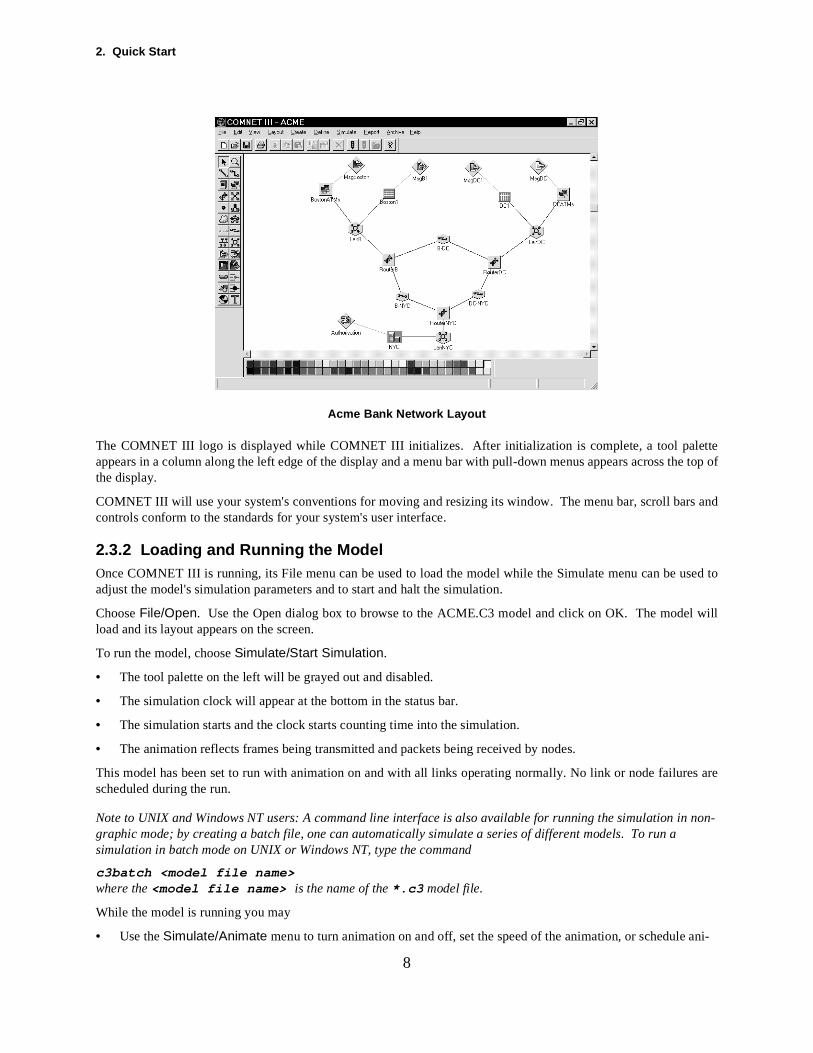
Acme Bank Network Layout
The COMNET III logo is displayed while COMNET III initializes. After initialization is complete, a tool paleappears in a column along the left edge of the display and a menu bar with pull-down menus appears across the display.
COMNET III will use your system's conventions for moving and resizing its window. The menu bar, scroll bars ancontrols conform to the standards for your system's user interface.
2.3.2 Loading and Running the ModelOnce COMNET III is running, its File menu can be used to load the model while the Simulate menu can be adjust the model's simulation parameters and to start and halt the simulation.
Choose File/Open. Use the Open dialog box to browse to the ACME.C3 model and click on OK. The modeload and its layout appears on the screen.
To run the model, choose Simulate/Start Simulation.
• The tool palette on the left will be grayed out and disabled.
• The simulation clock will appear at the bottom in the status bar.
• The simulation starts and the clock starts counting time into the simulation.
• The animation reflects frames being transmitted and packets being received by nodes.
This model has been set to run with animation on and with all links operating normally. No link or node failures arescheduled during the run.
Note to UNIX and Windows NT users: A command line interface is also available for running the simulation in non-graphic mode; by creating a batch file, one can automatically simulate a series of different models. To run a simulation in batch mode on UNIX or Windows NT, type the command
c3batch <model file name>where the <model file name> is the name of the *.c3 model file.
While the model is running you may
• Use the Simulate/Animate menu to turn animation on and off, set the speed of the animation, or schedule
2.3 Running a Pre-Built Model
pear You can
You
is graph
rings upta-
process-
or
etwork to
9
mation to turn on or off at a future time.
• Use the Simulate/Trace menu to turn tracing on or off, or to specify whether execution trace statements apon the screen or go to a file. The trace statements appear in the status box at the bottom of the screen. also specify that you'd like to single step through the execution.
• Double click on any link or node icon and bring the device up or down, to simulate a link or node failure. can also schedule a failure or recovery event at some time in the future.
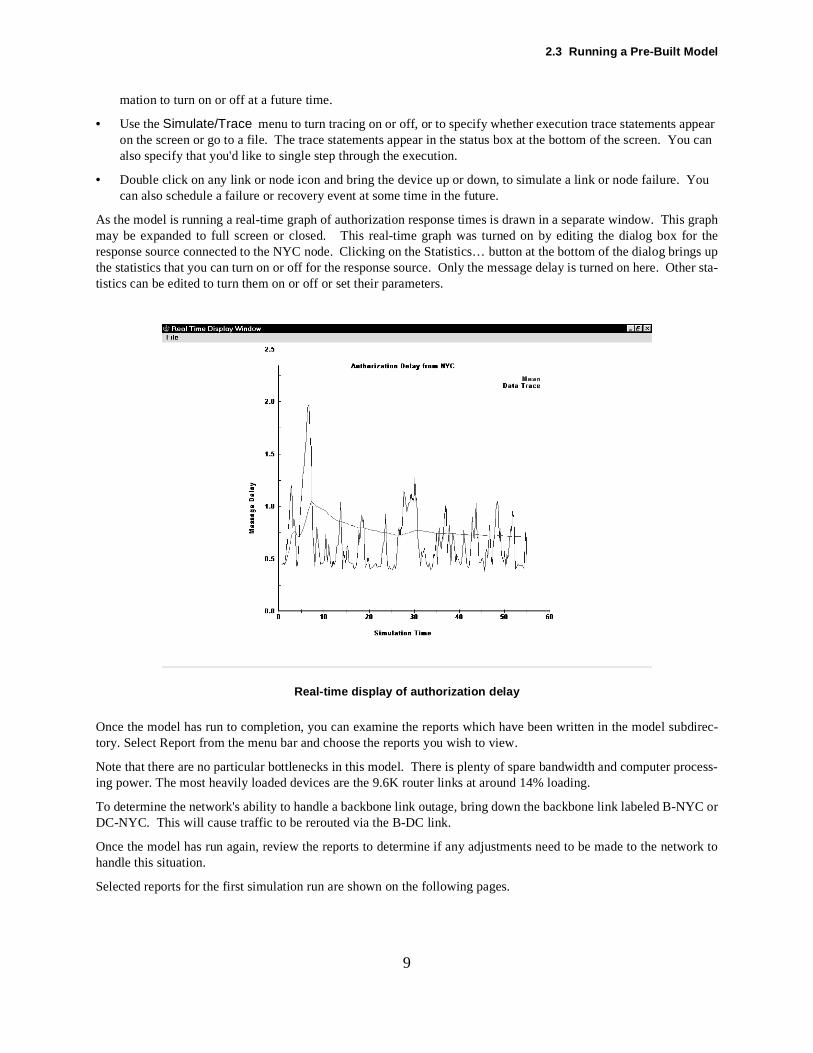
As the model is running a real-time graph of authorization response times is drawn in a separate window. Thmay be expanded to full screen or closed. This real-time graph was turned on by editing the dialog box for theresponse source connected to the NYC node. Clicking on the Statistics… button at the bottom of the dialog bthe statistics that you can turn on or off for the response source. Only the message delay is turned on here. Other stistics can be edited to turn them on or off or set their parameters.
Real-time display of authorization delay
Once the model has run to completion, you can examine the reports which have been written in the model subdirec-tory. Select Report from the menu bar and choose the reports you wish to view.
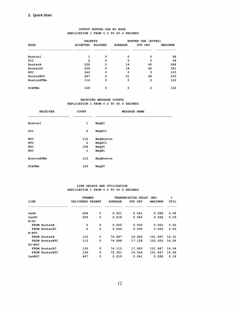
Note that there are no particular bottlenecks in this model. There is plenty of spare bandwidth and computer ing power. The most heavily loaded devices are the 9.6K router links at around 14% loading.
To determine the network's ability to handle a backbone link outage, bring down the backbone link labeled B-NYCDC-NYC. This will cause traffic to be rerouted via the B-DC link.
Once the model has run again, review the reports to determine if any adjustments need to be made to the nhandle this situation.
Selected reports for the first simulation run are shown on the following pages.
2. Quick Start
10
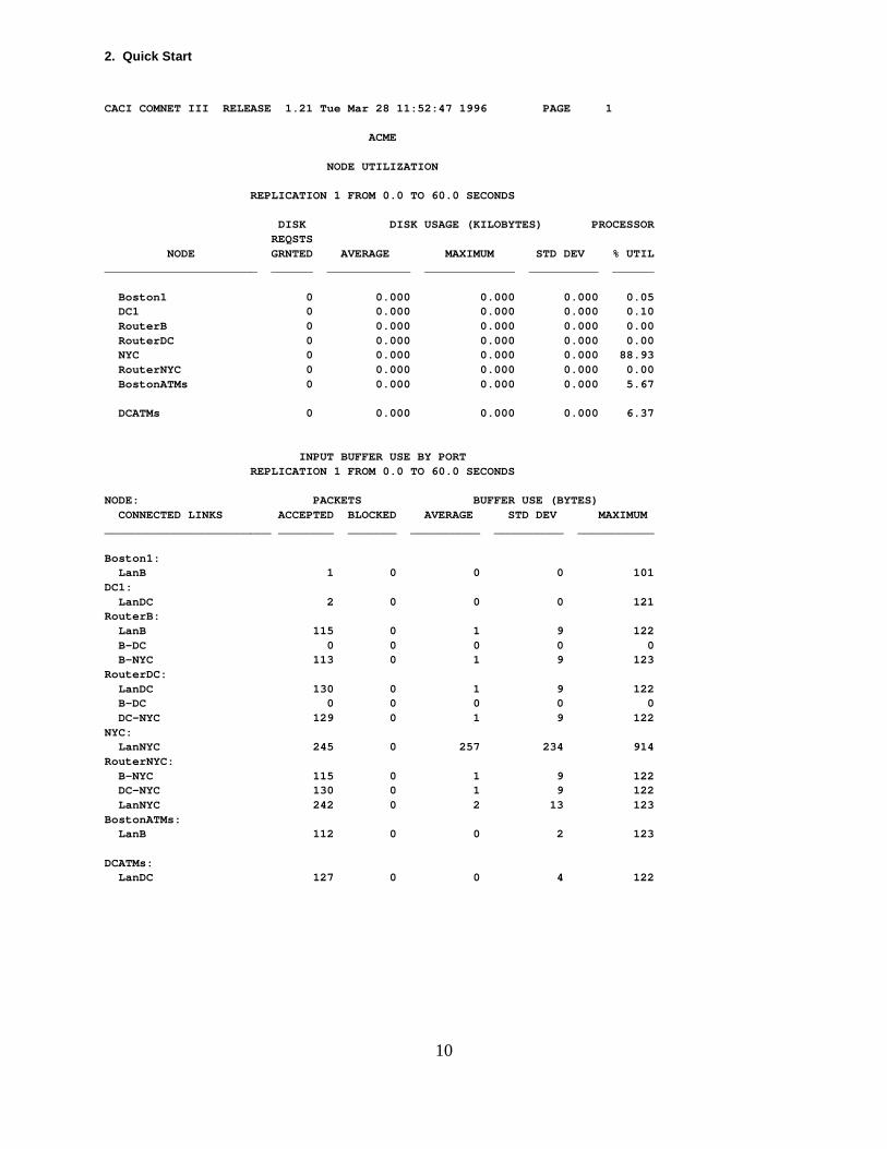
CACI COMNET III RELEASE 1.21 Tue Mar 28 11:52:47 1996 PAGE 1
ACME
NODE UTILIZATION
REPLICATION 1 FROM 0.0 TO 60.0 SECONDS
DISK DISK USAGE (KILOBYTES) PROCESSOR REQSTS NODE GRNTED AVERAGE MAXIMUM STD DEV % UTIL______________________ ______ ____________ _____________ __________ ______
Boston1 0 0.000 0.000 0.000 0.05 DC1 0 0.000 0.000 0.000 0.10 RouterB 0 0.000 0.000 0.000 0.00 RouterDC 0 0.000 0.000 0.000 0.00 NYC 0 0.000 0.000 0.000 88.93 RouterNYC 0 0.000 0.000 0.000 0.00 BostonATMs 0 0.000 0.000 0.000 5.67
DCATMs 0 0.000 0.000 0.000 6.37
INPUT BUFFER USE BY PORT REPLICATION 1 FROM 0.0 TO 60.0 SECONDS
NODE: PACKETS BUFFER USE (BYTES) CONNECTED LINKS ACCEPTED BLOCKED AVERAGE STD DEV MAXIMUM________________________ ________ _______ __________ __________ ___________
Boston1: LanB 1 0 0 0 101DC1: LanDC 2 0 0 0 121RouterB: LanB 115 0 1 9 122 B-DC 0 0 0 0 0 B-NYC 113 0 1 9 123RouterDC: LanDC 130 0 1 9 122 B-DC 0 0 0 0 0 DC-NYC 129 0 1 9 122NYC: LanNYC 245 0 257 234 914RouterNYC: B-NYC 115 0 1 9 122 DC-NYC 130 0 1 9 122 LanNYC 242 0 2 13 123BostonATMs: LanB 112 0 0 2 123
DCATMs: LanDC 127 0 0 4 122
2.3 Running a Pre-Built Model
11
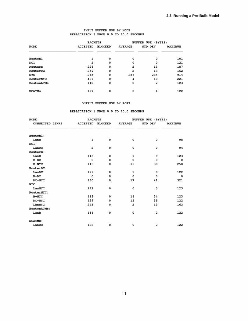
INPUT BUFFER USE BY NODE REPLICATION 1 FROM 0.0 TO 60.0 SECONDS
PACKETS BUFFER USE (BYTES)NODE ACCEPTED BLOCKED AVERAGE STD DEV MAXIMUM________________________ ________ _______ __________ __________ ___________
Boston1 1 0 0 0 101DC1 2 0 0 0 121RouterB 228 0 2 13 187RouterDC 259 0 2 13 162NYC 245 0 257 234 914RouterNYC 487 0 4 18 221BostonATMs 112 0 0 2 123
DCATMs 127 0 0 4 122
OUTPUT BUFFER USE BY PORT
REPLICATION 1 FROM 0.0 TO 60.0 SECONDS
NODE: PACKETS BUFFER USE (BYTES) CONNECTED LINKS ACCEPTED BLOCKED AVERAGE STD DEV MAXIMUM________________________ ________ _______ __________ __________ ___________
Boston1: LanB 1 0 0 0 98DC1: LanDC 2 0 0 0 94RouterB: LanB 113 0 1 9 123 B-DC 0 0 0 0 0 B-NYC 115 0 15 38 258RouterDC: LanDC 129 0 1 9 122 B-DC 0 0 0 0 0 DC-NYC 130 0 17 41 321NYC: LanNYC 242 0 0 3 123RouterNYC: B-NYC 113 0 14 34 123 DC-NYC 129 0 15 35 122 LanNYC 245 0 2 13 163BostonATMs: LanB 114 0 0 2 122
DCATMs: LanDC 128 0 0 2 122
2. Quick Start
12
OUTPUT BUFFER USE BY NODE REPLICATION 1 FROM 0.0 TO 60.0 SECONDS
PACKETS BUFFER USE (BYTES)NODE ACCEPTED BLOCKED AVERAGE STD DEV MAXIMUM________________________ ________ _______ __________ __________ ___________
Boston1 1 0 0 0 98DC1 2 0 0 0 94RouterB 228 0 16 40 268RouterDC 259 0 18 42 321NYC 242 0 0 3 123RouterNYC 487 0 31 46 235BostonATMs 114 0 0 2 122
DCATMs 128 0 0 2 122
RECEIVED MESSAGE COUNTS REPLICATION 1 FROM 0.0 TO 60.0 SECONDS
RECEIVER COUNT MESSAGE NAME______________________ __________ _________________________________________
Boston1 1 MsgB1
DC1 2 MsgDC1
NYC 112 MsgBoston NYC 2 MsgDC1 NYC 128 MsgDC NYC 1 MsgB1
BostonATMs 112 MsgBoston
DCATMs 126 MsgDC
LINK DELAYS AND UTILIZATION REPLICATION 1 FROM 0.0 TO 60.0 SECONDS
FRAMES TRANSMISSION DELAY (MS) %LINK DELIVERED RESENT AVERAGE STD DEV MAXIMUM UTIL_____________________ _________ ______ _________ _________ _________ _____
LanB 228 0 0.221 0.041 0.288 0.08LanDC 259 0 0.218 0.040 0.286 0.09B-DC FROM RouterB 0 0 0.000 0.000 0.000 0.00 FROM RouterDC 0 0 0.000 0.000 0.000 0.00B-NYC FROM RouterB 115 0 74.667 16.825 101.667 14.31 FROM RouterNYC 113 0 74.668 17.128 102.500 14.06DC-NYC FROM RouterDC 130 0 74.115 17.083 101.667 16.06 FROM RouterNYC 129 0 72.351 16.554 101.667 15.56LanNYC 487 0 0.219 0.041 0.288 0.18
2.3 Running a Pre-Built Model
13
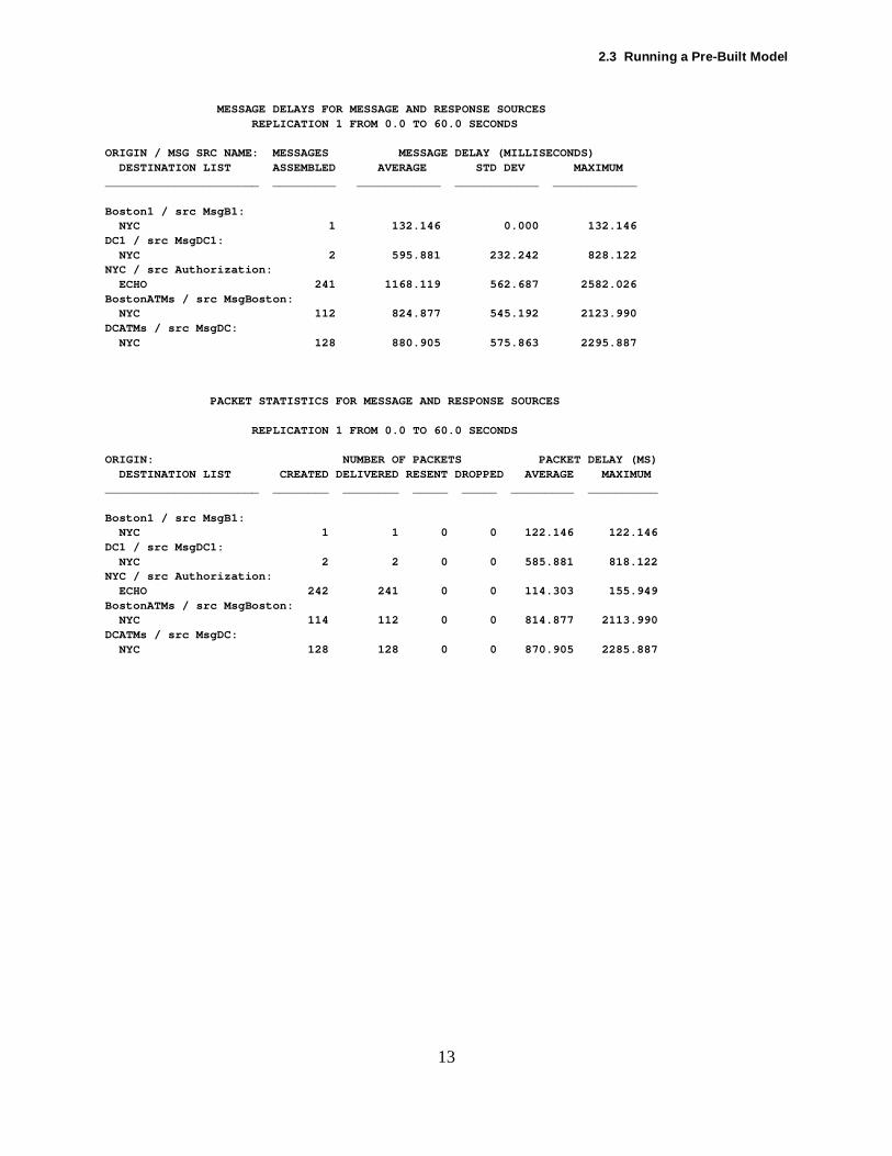
MESSAGE DELAYS FOR MESSAGE AND RESPONSE SOURCES REPLICATION 1 FROM 0.0 TO 60.0 SECONDS
ORIGIN / MSG SRC NAME: MESSAGES MESSAGE DELAY (MILLISECONDS) DESTINATION LIST ASSEMBLED AVERAGE STD DEV MAXIMUM______________________ _________ ____________ ____________ ____________
Boston1 / src MsgB1: NYC 1 132.146 0.000 132.146DC1 / src MsgDC1: NYC 2 595.881 232.242 828.122NYC / src Authorization: ECHO 241 1168.119 562.687 2582.026BostonATMs / src MsgBoston: NYC 112 824.877 545.192 2123.990DCATMs / src MsgDC: NYC 128 880.905 575.863 2295.887
PACKET STATISTICS FOR MESSAGE AND RESPONSE SOURCES
REPLICATION 1 FROM 0.0 TO 60.0 SECONDS
ORIGIN: NUMBER OF PACKETS PACKET DELAY (MS) DESTINATION LIST CREATED DELIVERED RESENT DROPPED AVERAGE MAXIMUM______________________ ________ ________ _____ _____ _________ __________
Boston1 / src MsgB1: NYC 1 1 0 0 122.146 122.146DC1 / src MsgDC1: NYC 2 2 0 0 585.881 818.122NYC / src Authorization: ECHO 242 241 0 0 114.303 155.949BostonATMs / src MsgBoston: NYC 114 112 0 0 814.877 2113.990DCATMs / src MsgDC: NYC 128 128 0 0 870.905 2285.887
2. Quick Start
olayout:
iagram of
creen.d drag it
sition a
ools juste it with-lick on
log boxe.
14
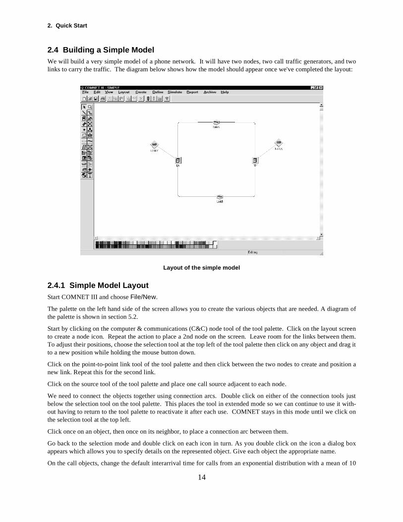
2.4 Building a Simple ModelWe will build a very simple model of a phone network. It will have two nodes, two call traffic generators, and twlinks to carry the traffic. The diagram below shows how the model should appear once we've completed the
Layout of the simple model
2.4.1 Simple Model LayoutStart COMNET III and choose File/New.
The palette on the left hand side of the screen allows you to create the various objects that are needed. A dthe palette is shown in section 5.2.
Start by clicking on the computer & communications (C&C) node tool of the tool palette. Click on the layout sto create a node icon. Repeat the action to place a 2nd node on the screen. Leave room for the links between themTo adjust their positions, choose the selection tool at the top left of the tool palette then click on any object anto a new position while holding the mouse button down.
Click on the point-to-point link tool of the tool palette and then click between the two nodes to create and ponew link. Repeat this for the second link.
Click on the source tool of the tool palette and place one call source adjacent to each node.
We need to connect the objects together using connection arcs. Double click on either of the connection tbelow the selection tool on the tool palette. This places the tool in extended mode so we can continue to usout having to return to the tool palette to reactivate it after each use. COMNET stays in this mode until we cthe selection tool at the top left.
Click once on an object, then once on its neighbor, to place a connection arc between them.
Go back to the selection mode and double click on each icon in turn. As you double click on the icon a diaappears which allows you to specify details on the represented object. Give each object the appropriate nam
On the call objects, change the default interarrival time for calls from an exponential distribution with a mean of 10
2.4 Building a Simple Model
e button
s in this
out-hoosetod load
dialog
(initiallyutes’
ong the
and
o Endx
t can ben com-eturn to
15
seconds to an exponential distribution with a mean of 30 seconds. This can be accomplished by clicking on thwith 2 dots next to the interarrival time and then typing 30 into the mean value box.
Set the call routing algorithm for the backbone network to user defined table routing (there are no subnetworkmodel). This can be accomplished by picking the Define/Backbone Routing menu option and then clicking on thedown arrow of the call routing protocol list box to see the choice of routing algorithms. Pick user defined table ring. We will shortly set two alternate routes between the two nodes. We need to tell COMNET III how to cbetween them. Click on the parameters button next to the call routing protocol and set the primary route selection random list. This will cause traffic to be randomly routed over the different routes, thus resulting in a balancesharing mode of operation. Click on OK on each dialog box to get back to the layout screen.
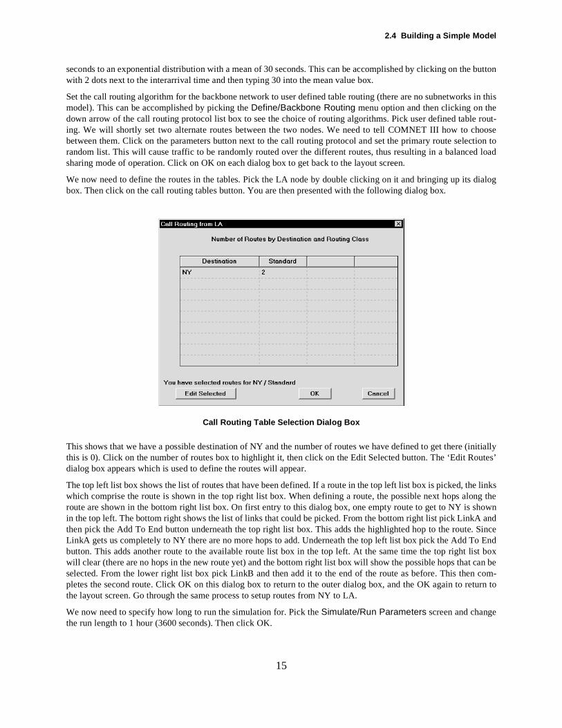
We now need to define the routes in the tables. Pick the LA node by double clicking on it and bringing up itsbox. Then click on the call routing tables button. You are then presented with the following dialog box.
Call Routing Table Selection Dialog Box
This shows that we have a possible destination of NY and the number of routes we have defined to get therethis is 0). Click on the number of routes box to highlight it, then click on the Edit Selected button. The ‘Edit Rodialog box appears which is used to define the routes will appear.
The top left list box shows the list of routes that have been defined. If a route in the top left list box is picked, the linkswhich comprise the route is shown in the top right list box. When defining a route, the possible next hops alroute are shown in the bottom right list box. On first entry to this dialog box, one empty route to get to NY is shownin the top left. The bottom right shows the list of links that could be picked. From the bottom right list pick LinkAthen pick the Add To End button underneath the top right list box. This adds the highlighted hop to the route. SinceLinkA gets us completely to NY there are no more hops to add. Underneath the top left list box pick the Add Tbutton. This adds another route to the available route list box in the top left. At the same time the top right list bowill clear (there are no hops in the new route yet) and the bottom right list box will show the possible hops thaselected. From the lower right list box pick LinkB and then add it to the end of the route as before. This thepletes the second route. Click OK on this dialog box to return to the outer dialog box, and the OK again to rthe layout screen. Go through the same process to setup routes from NY to LA.
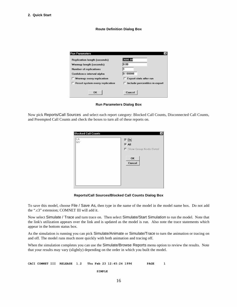
We now need to specify how long to run the simulation for. Pick the Simulate/Run Parameters screen and changethe run length to 1 hour (3600 seconds). Then click OK.
2. Quick Start
unts,
add
ts which
e
16
Route Definition Dialog Box
Run Parameters Dialog Box
Now pick Reports/Call Sources and select each report category: Blocked Call Counts, Disconnected Call Coand Preempted Call Counts and check the boxes to turn all of these reports on.
Reports/Call Sources/Blocked Call Counts Dialog Box
To save this model, choose File / Save As, then type in the name of the model in the model name box. Do notthe “.c3” extension; COMNET III will add it.
Now select Simulate / Trace and turn trace on. Then select Simulate/Start Simulation to run the model. Note thatthe link's utilization appears over the link and is updated as the model is run. Also note the trace statemenappear in the bottom status box.
As the simulation is running you can pick Simulate/Animate or Simulate/Trace to turn the animation or tracing onand off. The model runs much more quickly with both animation and tracing off.
When the simulation completes you can use the Simulate/Browse Reports menu option to review the results. Notthat your results may vary (slightly) depending on the order in which you built the model.
CACI COMNET III RELEASE 1.2 Thu Feb 23 12:45:24 1996 PAGE 1
SIMPLE

2.4 Building a Simple Model
17
CALL STATISTICS BY NODE
REPLICATION 1 FROM 0.0 TO 3600.0 SECONDS
CALLS CALLS CALLS CALLS CALLS CALLS BLOCK BLOCK BLOCK DISCON- PRE- NODE NAME ATTEMPTD AVAIL TRAFF PROB CARRIED NECTED EMPTED_________________________ ________ ______ ______ ____ ________ ______ ______
LA 124 0 0 0.00 124 0 0NY 124 0 0 0.00 124 0 0
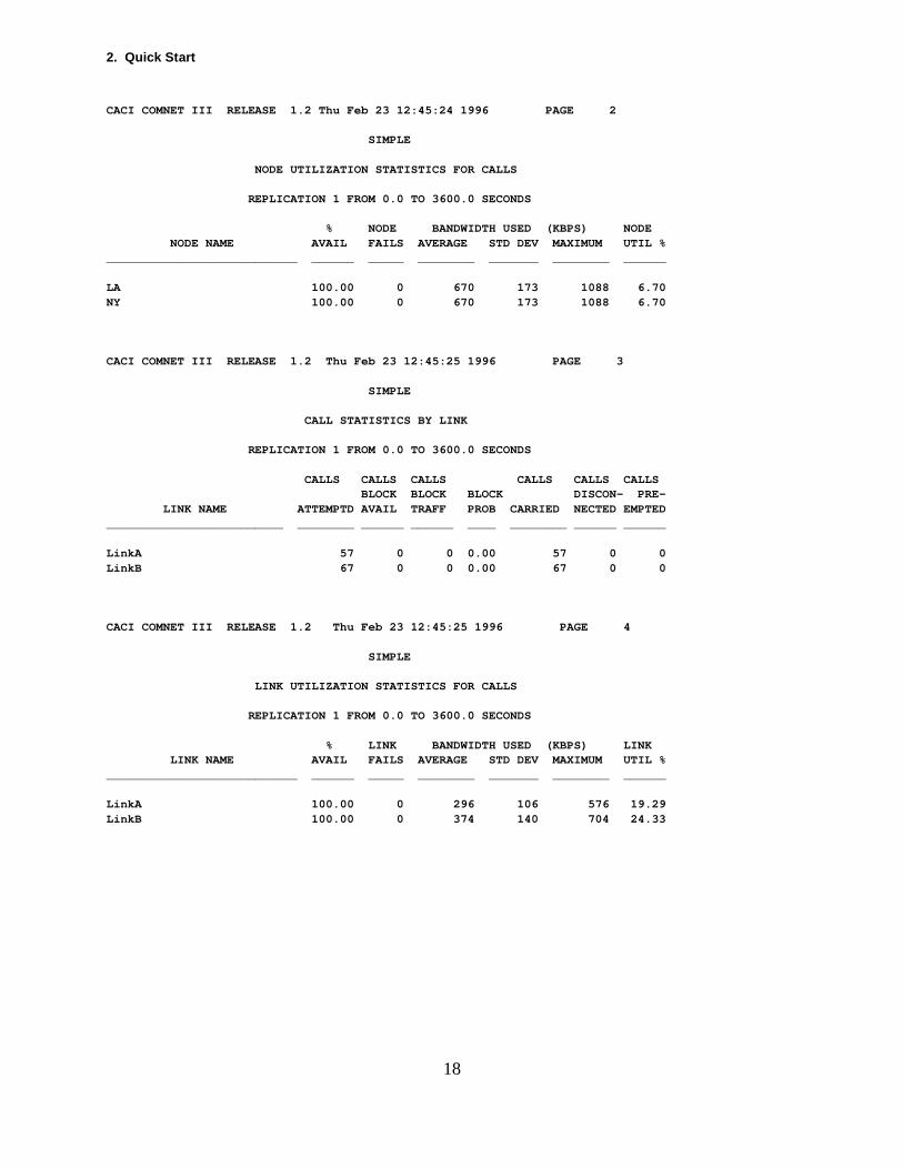
2. Quick Start
18
CACI COMNET III RELEASE 1.2 Thu Feb 23 12:45:24 1996 PAGE 2
SIMPLE
NODE UTILIZATION STATISTICS FOR CALLS
REPLICATION 1 FROM 0.0 TO 3600.0 SECONDS
% NODE BANDWIDTH USED (KBPS) NODE NODE NAME AVAIL FAILS AVERAGE STD DEV MAXIMUM UTIL %___________________________ ______ _____ ________ _______ ________ ______
LA 100.00 0 670 173 1088 6.70NY 100.00 0 670 173 1088 6.70
CACI COMNET III RELEASE 1.2 Thu Feb 23 12:45:25 1996 PAGE 3
SIMPLE
CALL STATISTICS BY LINK
REPLICATION 1 FROM 0.0 TO 3600.0 SECONDS
CALLS CALLS CALLS CALLS CALLS CALLS BLOCK BLOCK BLOCK DISCON- PRE- LINK NAME ATTEMPTD AVAIL TRAFF PROB CARRIED NECTED EMPTED_________________________ ________ ______ ______ ____ ________ ______ ______
LinkA 57 0 0 0.00 57 0 0LinkB 67 0 0 0.00 67 0 0
CACI COMNET III RELEASE 1.2 Thu Feb 23 12:45:25 1996 PAGE 4
SIMPLE
LINK UTILIZATION STATISTICS FOR CALLS
REPLICATION 1 FROM 0.0 TO 3600.0 SECONDS
% LINK BANDWIDTH USED (KBPS) LINK LINK NAME AVAIL FAILS AVERAGE STD DEV MAXIMUM UTIL %___________________________ ______ _____ ________ _______ ________ ______
LinkA 100.00 0 296 106 576 19.29LinkB 100.00 0 374 140 704 24.33
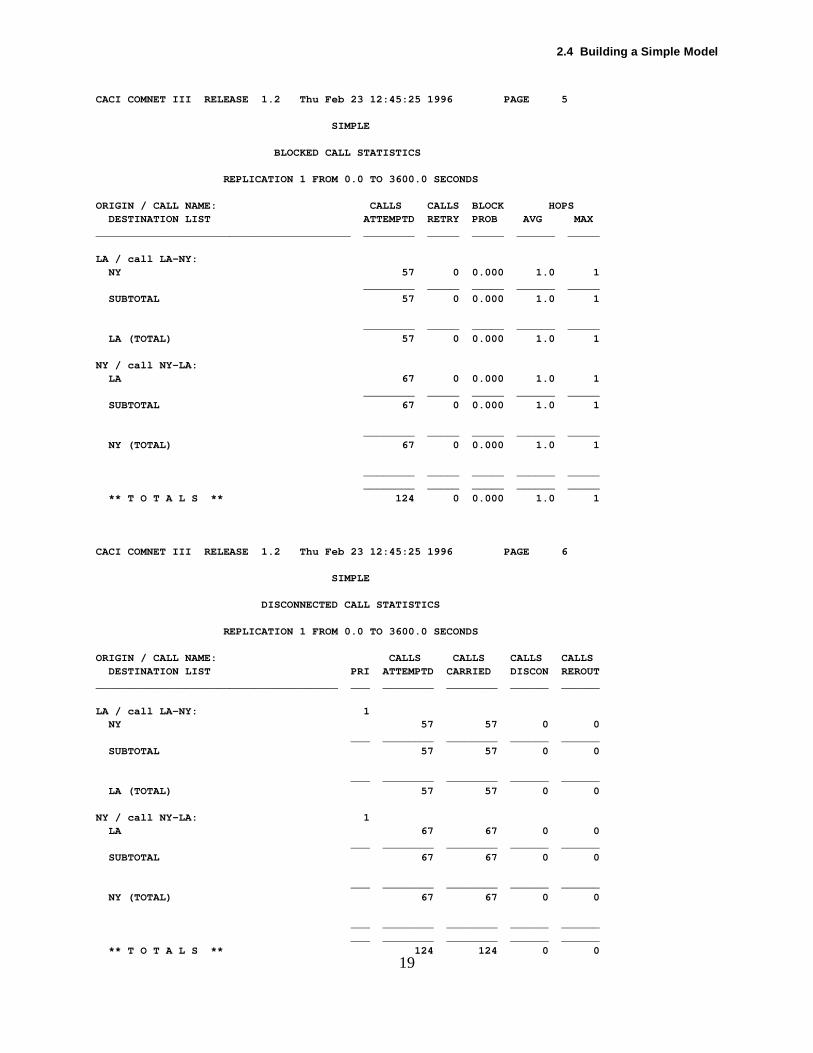
2.4 Building a Simple Model
19
CACI COMNET III RELEASE 1.2 Thu Feb 23 12:45:25 1996 PAGE 5
SIMPLE
BLOCKED CALL STATISTICS
REPLICATION 1 FROM 0.0 TO 3600.0 SECONDS
ORIGIN / CALL NAME: CALLS CALLS BLOCK HOPS DESTINATION LIST ATTEMPTD RETRY PROB AVG MAX________________________________________ ________ _____ _____ ______ _____
LA / call LA-NY: NY 57 0 0.000 1.0 1 ________ _____ _____ ______ _____ SUBTOTAL 57 0 0.000 1.0 1
________ _____ _____ ______ _____ LA (TOTAL) 57 0 0.000 1.0 1
NY / call NY-LA: LA 67 0 0.000 1.0 1 ________ _____ _____ ______ _____ SUBTOTAL 67 0 0.000 1.0 1
________ _____ _____ ______ _____ NY (TOTAL) 67 0 0.000 1.0 1
________ _____ _____ ______ _____ ________ _____ _____ ______ _____ ** T O T A L S ** 124 0 0.000 1.0 1
CACI COMNET III RELEASE 1.2 Thu Feb 23 12:45:25 1996 PAGE 6
SIMPLE
DISCONNECTED CALL STATISTICS
REPLICATION 1 FROM 0.0 TO 3600.0 SECONDS
ORIGIN / CALL NAME: CALLS CALLS CALLS CALLS DESTINATION LIST PRI ATTEMPTD CARRIED DISCON REROUT______________________________________ ___ ________ ________ ______ ______
LA / call LA-NY: 1 NY 57 57 0 0 ___ ________ ________ ______ ______ SUBTOTAL 57 57 0 0
___ ________ ________ ______ ______ LA (TOTAL) 57 57 0 0
NY / call NY-LA: 1 LA 67 67 0 0 ___ ________ ________ ______ ______ SUBTOTAL 67 67 0 0
___ ________ ________ ______ ______ NY (TOTAL) 67 67 0 0
___ ________ ________ ______ ______ ___ ________ ________ ______ ______ ** T O T A L S ** 124 124 0 0
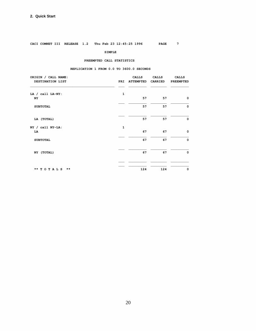
2. Quick Start
20
CACI COMNET III RELEASE 1.2 Thu Feb 23 12:45:25 1996 PAGE 7
SIMPLE
PREEMPTED CALL STATISTICS
REPLICATION 1 FROM 0.0 TO 3600.0 SECONDS
ORIGIN / CALL NAME: CALLS CALLS CALLS DESTINATION LIST PRI ATTEMPTED CARRIED PREEMPTED__________________________________________ ___ _________ ________ _________
LA / call LA-NY: 1 NY 57 57 0 ___ _________ ________ _________ SUBTOTAL 57 57 0
___ _________ ________ _________ LA (TOTAL) 57 57 0
NY / call NY-LA: 1 LA 67 67 0 ___ _________ ________ _________ SUBTOTAL 67 67 0
___ _________ ________ _________ NY (TOTAL) 67 67 0
___ _________ ________ _________ ___ _________ ________ _________ ** T O T A L S ** 124 124 0
model.
, and
tworkrior toer Dis-eteriza-d re- The other
nica-
defined
rametersr arcs to
Node,
can
thr
21
3. Overview of Modeling Constructs
3.1 OverviewThis overview section describes the relationships of the various COMNET III components to a simulation This section is divided into eight parts of a communication network simulation: Network Topology, Network TrafficAnd Workload, Network Operation, Simulation Control, Statistics Reporting, User Distributions, LibrariesModel Files.
These subsections correspond to the different steps of building a COMNET III model. Typically, a Network Topol-ogy is built first, followed by adding the sources for Traffic and Workload, and setting the parameters for NeOperation. The Simulation Control parameters set up the experiment and the running of the simulation. Pstarting a simulation, various statistics reports may be turned on for viewing during or after the simulation. Ustributions are available to bring in tabular distributions or named distributions representing a specific paramtion of a built-in analytic distribution. As the model is built, COMNET III maintains several libraries for use anuse within the model, and there is an archive library available to allow the user to re-use objects across models. model file contains all the information required for running the model and thus the model file is portable tomachines running COMNET III.
3.1.1 TerminologyFor the parameters in the COMNET III components, the following terminology is used:
Byte = 8 Bits; a byte is the smallest data unit that Comnet uses to measure message sizes.
Kilobyte (kB) = 1024 Bytes; this is the common binary definition of kilo as opposed to the metric kilo.
Kilobit (kb) = 1000 bits, and
Kilobits per second (kbps) = 1000 bits per second; These are the common metric definitions used for commutions channels
Megabyte (MB) = 1024 Kilobytes = 1,048,576 Bytes
Megabits per second = 1,000,000 bits per second.
3.2 Network TopologyThe network topology describes the layout and resources that model the physical network. The topology isby three basic components: nodes to represent hardware (computers or switches), links that carry traffic betweennodes, and arcs to associate nodes to links. The arcs show which nodes use links, and in particular, they model thenode’s port connection to the link.
In addition to the basic nodes and links, there are three objects that have internal topologies: the Subnet and TransitNet for modeling of independent routing domains and hierarchical topology and the WAN Cloud for modeling wide-area network services. In either case, the icons have a detail similar to nodes or links for setting overall paand an internal topology for more detailed modeling. Access points (or pads) are used to mark interfaces foconnect between the external and internal topologies.
3.2.1 NodesCOMNET III has four basic node types: Computer and Communications Node (C&C Node), Computer GroupRouter Node, and Switch Node.
C&C Nodes and Computer Groups model computers. These nodes can generate or receive traffic, and theymodel more complex applications concerning processor utilization and internal storage.
C&C Nodes may also model bridges, gateways, and communications switches because it can route trafficough
3. Overview of Modeling Constructs
sinks
rnd out-
pt sourcesations,he Appli-
uting
like the
tweenre
hop net-
l-
ltipleernet),
e inde-milar to a
ccess pointr betweentive of the
aendentd by a
opologyr to that canl
22
itself. In contrast, Computer Groups are restricted to modeling end systems because they can only be sources orfor traffic.
The Router Node models hardware used for routing traffic, including routers, hubs, and switches. The Router Nodeis similar to the C&C Node in that it can source or sink traffic and run applications that utilize the internal processoand internal storage. However, it adds a model for an internal bus structure for moving traffic between input aput ports.
The above three nodes can be sources of traffic and resources for workload. This means that they can acceof traffic and applications which are described in the Network Traffic and Workload section. To model applicthese nodes include a command repertoire as well as a parameter set. Application modeling is described in tcations Section.
In addition to the C&C Node and Router Node for routing traffic, there is an Switch node which is just for rotraffic. The Switch node models a switching fabric that is relevant for many switches that take very short times tomove a packet from an input buffer to an output buffer. This node can handle any packet size. However, unabove nodes, this node can not be a source or sink of traffic and thus no sources can attach to this node.
The C&C, Router, and Switch nodes are also capable of modeling nodes in a circuit switched call network.
3.2.2 LinksThere are two classes of link models available in COMNET III: point-to-point links to represent a channel beonly two nodes, and multiaccess links for local-area networks and other situations where more than two nodes shathe same communications media.
Point-to-point links model communication channels between two nodes. Typically, these connections are dedicatedlines such as a serial line or a dedicated line connection, particularly between routers in a wide-area or multiworks. They are also the only type of link that can carry circuit-switched call traffic.
The WAN Cloud model provides access links to the WAN service by using a variation of a point-to-point link avaiable inside that cloud (see WAN Clouds, sect. 3.2.4).
The multiaccess links available in COMNET III model various protocols for sharing a single medium with munodes. Multiaccess protocols include Carrier-Sense Multiple-Access with Carrier Detection (CSMA/CD or ethCSMA, Aloha, Token Passing (token ring, FDDI, token bus), Polling, FDDI, Priority Token Ring, CSMA/CA,Demand Assigned Multiple Access (DAMA) and ISDN and SONET parameter sets.
3.2.3 SubnetsThe subnet object in COMNET III is used for modeling a topology hierarchically so that separate subnets havpendent and separate routing algorithms that are also independent from the backbone. The subnet icon is sinode in that it can only connect to links. Internal to the Subnet, the topology is similar to the top level (backbonelevel) and it is possible to nest subnets within subnets.
Connections between the internal topology of the subnet and the backbone topology is through the Access Points.There may be as many access points on a subnet as required. Internal to the subnet, a node attaches to an aand that node becomes a gateway node that can route packets both at the backbone and subnet levels (othem). Outside the subnet, the access point may be edited to access that gateway node but from the perspecbackbone.
The subnet is used primarily for modeling interconnected subnets of independent routing algorithms. It may lso beused for building a complex network hierarchically to hide detail from an upper view. Furthermore, the indeprouting algorithm of the subnet often conflicts with the requirement to have a complex network that is governesingle routing algorithm. In cases where large networks need to be modeled in a single routing domain, the tshould all be in the backbone. The view menu item “Work Area Size” is available to make the canvas area largecontain a larger model. Using the zoom-out menu item to see the entire model, and placing items in clustersbe zoomed into with the zoom-tool from the palette bar can organize the model similar to subnets but keep the modein the backbone routing domain.
3.3 Network Traffic and Workload
net. A the out-
ally, the
lex net-a single
odel, anddel sim-
ssary or
anets ofed line to
Link is a
t whichoint of a
nted by Cloud:
the nodesline-card
. Net-al activ-
that
for trafficst, the
pack- to links;f a link or when
23
3.2.4 Transit NetsTransit Nets can be thought of as an intermediate network modelling the flow of packets through the transittransit net can behave both as a link and a subnet. It is really an abstraction of a link that sends packets fromput buffer of one node connected to the net to the input buffer of another node connected to the net. Interntransit net behaves like a subnet and introduces an additional protocol layer at the transit net boundaries. Further-more, the independent routing algorithm of the transit net often conflicts with the requirement to have a compwork that is governed by a single routing algorithm. In cases where large networks need to be modeled in routing domain, the topology should all be in the backbone. The view menu item “Work Area Size” is available tomake the canvas area larger to contain a larger model. Using the zoom-out menu item to see the entire mplacing items in clusters that can be zoomed into with the zoom-tool from the palette bar can organize the moilar to subnets but keep the model in the backbone routing domain.
3.2.5 WAN CloudsThe WAN Cloud is available for modeling WAN services abstractly in terms of Access Links and Virtual Circuits.An abstract model is useful when the additional detail of a more explicit model of the service is either unneceunavailable.
Topologically, the WAN Cloud is similar to a link in that its icon can only connect to nodes. The WAN Cloud hasinternal topology consisting of just Access Links and Virtual Circuits. Virtual Circuits are abstract models of sswitches and links and connect to Access Links only: the arc connection to an Access Link appears as a dashdistinguish this abstract path from the physical connections used in the backbone topologies. The Access special case of a Point-To-Point Link that works with the WAN Cloud.
Outside of the WAN Cloud, the connection between a node and the WAN Cloud is through the Access Poinrepresents an Access Link in the internal topology of the cloud. Only one node can connect to an Access PWAN Cloud and only one Access Link can connect to an Access Point from inside the WAN Cloud.
Virtual Circuits may be placed between any two source and destination Access Links. For any source/destinationaccess link pair, there can be at most one Virtual Circuit. The Virtual Circuit models are directional as represearrows on the dashed arcs connecting them to the Access Links. Virtual Circuits are optional inside the WANif a Virtual Circuit is missing between the source and destination of a frame, that frame may still be routed throughthe WAN Cloud.
3.2.6 Arcs and PortsIn the backbone and Subnet topologies, the arcs connecting the links to nodes represent the connections atthat interface to the link media. These arcs are editable to set parameters for the port (delay, buffers, and ID) and for the link (penalty tables for routing).
3.3 Network Traffic and WorkloadThe sources for network traffic and workload add the stimulus to the network topology to drive the simulationwork traffic refers to the messages that are sent between nodes in the topology, and workload refers to internities of the node’s processors or busses.
There are several kinds of traffic sources available in COMNET III. Application sources execute commands introduce either traffic into the network or workload inside the node. Message, Response, Session & Call sourcessimpler sources that generate traffic between nodes. Because nodes may have processing requirements moving between them, traffic sources and commands will also implicitly add workload to the nodes. In contraworkload commands can only delay traffic by utilizing the processor when the traffic needs to use it.
During a simulation, COMNET III can show animation of the traffic as moving tokens representing frames andets entering and leaving the links. The animation is along the arcs which represent the ports or connectionsthus the animation occurs in zero elapsed time to show merely the entry or exit of the token. The delay ooccurs when there is no animation—when the packet is waiting in a buffer or being processed inside the node
3. Overview of Modeling Constructs
have differ-l enter a
ere aree at leaste or in a
received atssage. The not repre-sage textsgering
efter that
appli-e a
fault, e param-
s com-
e
The mes-e
ssion is
he routing
ssage that
d used by
he
24
the frame is transmitting or propagating inside the link.
3.3.1 SchedulingThere are three methods in which sources may be scheduled: by Iteration time or by received message text, or a Trig-ger. There may be as many sources attached to a node as necessary, and sources connected to a node mayent or identical scheduling methods. If multiple sources are triggered simultaneously, then the commands wilqueue at the node to be served by the processor one at a time.
Time scheduling allows sources to be scheduled according to an interval from the previous arrival, and thoptions to have a source start or stop at specific times in the simulation. In a simulation model, there has to bone time triggered source to get the simulation to start. The Interarrival times of the sources in the backbonsubnet can be scaled by a Traffic Time Scale parameter in the Backbone or Subnet detail.
Scheduling by received message text provides a method to schedule sources to be dependent on messagesthe node. The message text is a label attached to a message at the source or command that sends that mepurpose of the message text is to trigger a desired source at the destination—the message text usually doessent the content of the message. The source that is triggered by received message may require multiple mesand/or multiple instances of a message text before it is triggered. A wild card symbol is available to allow trigby classes of messages.
At the destination node, there may be several sources connected that will be waiting for the same received messagtext; in this case, one source will be active and get the next instance of the message until it is triggered. Asource is triggered, future instances of that message text will be used to trigger the other sources in round-robin order.Usually, however, there will be just one source, if any, waiting for a particular message text.
3.3.2 ApplicationsApplications provide a flexible means to model both workload and traffic generation at a particular node. Thecation is built in three parts: the node parameters for specifying the processing and storage-device speeds, thcom-mand repertoire for specifying the various actions that can occur at the node, and the application source to schedule sequence of commands.
Workload at a node is controlled by the physical parameters for processing and storage-device times. By dethese times are zero, thus representing infinitely fast processors and storage. To get workload into a node, theters have to be set to non-zero. Parameters are available for processing time per cycle used by the Procesmand, storage parameters for the Read and Write commands, and packet processing times for traffic going through, originating, or terminating at this node.
The traffic commands include the Transport Message Command, Setup Session Command which also transmits thmessages sent within that session, Answer Message Command, and Filter Message Command.
The Transport Message Command sends a single message to a single destination or a set of destinations. sages from a Transport Command are always sent as datagrams where each packet of the message is routed indpend-ently.
The Setup Command initializes by sending a setup packet and receiving a confirmation packet. After the seestablished, a number of messages may be sent during session and these messages are specified inside the SetupCommand. Messages sent within a session may be routed as datagrams or as virtual circuits depending on talgorithm of the backbone or subnet containing the node for executing the command.
The Answer Message Command is a special command that sends its message back to the sender of the metriggered the application source, thus the Answer Command can only be used in sources that are triggered by receivedmessage. The Answer command message is routed either as datagram or virtual circuit, copying the methothe triggering message.
The Filter Message Command causes the node to suspend all operations until it receives an appropriate message textstring defined by the Filter Message Command parameters. Once the message text has been received by the node, tFilter Message Command terminates, and the next command in the Application Source executes.
3.3 Network Traffic and Workload
amount
ting filesload to for file
plicationionhenpertoire
he com-d to, or inences in
ation consists
ed
d
g
erms ofir-ulation.
ntrces.
usinging atination,fromlls. Thea-s
le for file.d traffic
25
Workload is introduced to the node implicitly by the traffic through the node’s packet processing parameters. Inaddition, there are three workload-specific commands.
The Process Command is for modeling internal calculation that makes the node’s processor busy for a certainof time.
The Read and Write Commands also make the processor busy, but this is in the context of reading and wri(for example, the time required for the operation depends on the size of the file). In addition to adding workthe node’s processor, the Read and Write Commands will modify the storage space which may be monitoredspace used.
The Application Source contains a sequence of commands that are executed in sequence when the ApSource is triggered either by time or by received message text. Typically, the command sequence of the ApplicatSource is filled in after the Command Repertoire of the node has been modified to include a desired command. Wan Application Source is connected to a node via an arc, the list of commands available in the Command Reof the node will be available in the choices for selection when adding a new command to the sequence. Tmand sequence can contain commands that are either in the Command Repertoire of the node it is attachethe list of Global commands available from the Define menu. Commands may be reused in command sequseveral sources or multiple times in the same command sequence.
3.3.3 Traffic SourcesThe traffic sources are simplifications of the applications since the single traffic source contains all the informfor specifying the source. In fact, a traffic source is a special application source whose command sequenceof a single traffic command.
The Message Source is the combination of an Application Source with a Transport Message Command and is usfor modeling specific user or protocol-control messages.
The Response Source is the combination of an Application Source with an Answer Message Command and is usefor modeling replies or acknowledgments to messages.
The Session Source is the combination of an Application Source with a Setup Command and is used for modelinsessions of multiple messages, bursts of messages, or messages that are routed in virtual circuits.
3.3.4 Call SourcesThe Call Source is the source to use for modeling circuit-switched calls. The Call Sources specify calls in tinter-arrival times, durations, and (through the routing class) the bandwidth requirement. In COMNET III both ccuit-switched traffic and packet-switched traffic can be modeled and both may be modeled in the same simHowever, the circuit switch model only uses the C&C Node, Router Node, ATM Switch Node and the Poi-To-Point link. The resources for circuit-switched traffic are separate and independent from the data traffic resou
3.3.5 External SourcesIn addition to source objects, traffic can also be introduced into COMNET III through external traffic files by the External Traffic menu item in the Define menu. The external traffic file is a formatted text file containrecord for each traffic event: each record contains information about the time of the event, the source and desand other information. The traffic file may come directly from various network analyzers or it may be created some other tool. COMNET III can interpret the events in the file as being either messages, sessions, or caadditional information that COMNET III requires is specified with the Edit External Sources button of the same dilog box and finally the sources are mapped to messages in the file through the Map Message ID To Message Sourcebutton.
The AutoBaseliner utility is used to read in external traffic files and format them into an intermediate fiCOMNET III use. This utility will allow multiple traffic sources to be merged into a single intermediate eventFurthermore, the timing of the events in the external file may be scaled to speed up or slow down the recordefor the simulation.
3. Overview of Modeling Constructs
d trans-
y theare han-ntedwing
tablesorithms.tween a"fromcify the
that thesing the
e distinc-te or set Class setmessage.
even ifroute
ires the
tput
s. It is a
differ-rithm is
enalty
lected
fewest
differ-
26
3.4 Network OperationThe network operation specifies how messages are routed through the network with a Routing Algorithm anmitted through the network with a Transport Protocol.
3.4.1 Routing AlgorithmEach Subnet, Transit Net, and the Backbone have separate and independent algorithms that are specified brespective detail dialogs. In addition, there are separate choices for packet routing and for call routing which dled independently by COMNET III. The detail for the routing algorithm also includes a “Connection-OrieRouting for Sessions” checkbox for using virtual circuits for data traffic, or a “Preemption” checkbox for allocall preemption for call traffic.
Several routing algorithms are available in COMNET III. There are static algorithms that compute the routingjust at the start of the simulation and whenever a link or node fails (or recovers). There are also dynamic algthat periodically update the routing tables based on dynamic measures that are monitored during specified intervalsIn addition, some routing protocols require Penalty Tables to be applied to each port arc (a connection benode and link) to assign penalties for each direction of traffic into the link. COMNET III uses a convention of a node to a link" to establish traffic direction for the penalty tables. For each routing class, Penalty Tables spedifferent penalties that class incurs when moving through a particular arc specified in the Penalty Table. Notedefault Penalty Tables assigned to the links have a penalty of 1 for each hop, thus making any algorithm uPenalty Tables to revert to minimum hop routing unless additional tables are used.
The routing tables are created or updated based on that route or set of routes that have the least penalty. Thtion between the routing algorithms concern how the penalties are computed. The routing tables contain a rouof routes for each triplet of source-node, destination-node, and Routing Class. Each message has a Routingby the message’s source or command. The Routing Class specifies some routing properties for this class of
By default, the routing algorithms will select a single route for each source-destination-Routing Class triplet, multiple routes are available with identical penalties to the minimum penalty (in which case, COMNET III will all the traffic on the first route found). Load balancing across multiple shortest paths is available through the “Devia-tion % for multiple shortest paths” value-box in the detail for the selected routing algorithm: if this value is zero thenall traffic for a triplet will be routed on the first path found with the minimum penalty.
For packet switched (data) traffic there are six routing algorithms available:
• RIP Minimum Hop algorithm assigns a penalty of 1 for each hop and thus selects the route that requfewest number of hops. This is a static algorithm that does not use Penalty Tables at links.
• Shortest Measured Delay assigns penalties to links based on the measured delay that is the sum of the oubuffer delay, the transmission delay, and packet delay for each link on the path.
• Link-State Shortest Path First uses the Penalty Tables assigned to the various links of paths for penaltiestatic routing algorithm but does require setting up the Penalty Tables for each link.
• Minimum Penalty uses the Penalty Tables which for each Routing Class may have different penalties forent levels of congestion (measured as delay or utilization). Due to the congestion thresholds, this algodynamic and has a routing update interval.
• IGRP uses a penalty that is a sum of different penalties for available bandwidth, utilization, and delay pfrom the Penalty Table. This algorithm is dynamic.
• User Defined Routing Tables allow the user to specify arbitrary routes through the network with user-semethods for choosing among the possible alternatives.
For circuit-switched (call) traffic there are three routing algorithms available:
• Minimum Hop algorithm assigns a penalty of 1 for each hop and thus selects the route that requires thenumber of hops. This is a static algorithm that does not use Penalty Tables at links.
• Minimum Penalty uses the Penalty Tables which for each Routing Class may have different penalties for
3.4 Network Operation
outing
lected
network
ET IIItansport
n rout-meters ofier fieldprotocols
colshe
e carriedder and
dow,P/IP’sutinge of theersions
ting the meas-
earlierts when
cifica-lgorithm
th the ic can be
ed at
s: a ag ly dis-
ckets olling
27
ent levels of link utilization. Due to the congestion thresholds, this algorithm is dynamic and has a rupdate interval.
• User Defined Routing Tables allow the user to specify arbitrary routes through the network with user-semethods for choosing among the possible alternatives.
3.4.2 Transport ProtocolsThe Transport Protocol controls how the network delivers a message from the source to a destination. At the sourcenode, a message will have a particular transport protocol. This Transport Protocol will set the packet size for the mes-sage, overhead in the packet, the type of flow control to use, and when to retransmit blocked packets. Thethen routes each packet from node to node until it arrives at its intended destination.
COMNET III’s Transport Protocol models transport layer protocols in terms of a routed-protocol identifier, the end-to-end packet size, a flow control method, and a retransmission interval for errors or lost packets. COMNmaintains a list of transport protocols. Each Transport Protocol entry represents a different combination of transporlayer parameters. To model a particular suite of protocols such as TCP/IP, IPX, DECNet, SNA, etc., the TrProtocol list may be built up to include a set of transport protocol entries to represent different situations.
The routed-protocol identifier is a name that classifies a class or suite of protocols that will incur like delays iers. For instance, IP packets will have similar processing requirements at routers even though the other parathe transport protocol may vary for many conditions. The routing node, then, uses the routed-protocol identifto determine the speed of processing the packet. Many transport protocol entries representing a suite of may have the same identifier. This field is especially important for modeling multiprotocol routers that will requiredifferent amounts of processing depending on the protocol being routed. In the physical world, different protowill impose different amounts of processing at the routing nodes and this may be modeled in COMNET III with trouted protocol identifier used to select different delays at the routing nodes.
The end-to-end packet created by the Transport Protocol determines the maximum size of the data that can bin a single packet. The transmitted packet will additionally include overhead bytes that represent the heatrailer bytes – in other words, all the bytes of a packet that are not part of the desired message.
The packets will be sent according to a flow control method. COMNET III provides fixed window, sliding winSNA-pacing window, no flow control, enhanced models of these algorithms, plus an algorithm spcific to TCcongestion window. X.25 networks and LAN protocols typically use fixed window protocols while many roprotocols such as TCP/IP use sliding window protocols. The window protocols have parameters for the sizwindow and the size and priority of the acknowledgments required to implement the window. The enhanced vof the windowed protocol introduce choices of error control methods (including selective repeat or re-transmitfull window), options for delaying the acknowledgement, and for adjusting the re-transmission time based onured round-trip time and multiple re-transmissions. The simpler versions are available for compatibility with releases of COMNET III, but they may also be useful to save simulation processing and memory requirementhe enhanced features are not needed in the model.
The windowed flow control algorithms use a window size specified in terms of a number of packets. This spetion is still relevant for some protocols such as TCP/IP that use windows sizes in bytes because the specific arestricts the packet window size to an integer numer of full sized packets.
COMNET III provides sockets to model the negotiation of maximum packet and window sizes supported at bosource and destination nodes. These sockets are icons to which sources may be attached and to which traffdestined. The sockets have parameters such as maximum packet and window size that are used to modify the proto-col's packet and window size. The socket also provides parameters for determining how packets are packetizthe sources attached to this socket, or assembled for traffic destined to this socket.
For modeling frame-level services (such as frame-relay and ATM), the protocols have two additional algorithmtraffic policing algorithm and a traffic shaping or rate control algorithm. The traffic policing algorithm is used to flcertain packets as discard eligible (which are preferentially discarded at a congested node) and for immediatecarding packets that exceed the traffic contract. The traffic shaping algorithms control the presentation of painto the network so that the specified burst requirements are met. These algorithms can model specific contr
3. Overview of Modeling Constructs
t i
there iskets of a
n.
ulation.he user
replica-l--
ermine box tolation simula-
for
Duringeaving acent utili-
choice to mes-d exe-
ffic willt that is
eful forem is
st mem-
variouscting justnitoring.how thee as the
28
algorithms (such at ATM's Available Bit Rate algorithm) or it can model sources (such as phone or video) thanher-ently introduce packets into the network at a regular rate.
A packet may be blocked at a node due to lack of buffer space or in a WAN Cloud due to a dropped frame. If apacket is dropped, then the transport protocol can retransmit the packet to correct the error. In COMNET III, an option to retransmit the lost packet and a parameter to set the delay before resending the packet. All pacmessage have to be received at the destination before the message is counted as delivered or assembled.
3.5 Simulation ControlAfter a model is ready for simulation, the commands under the Simulate menu may be used to control the simulatio
The Verify command tests the model for correctness and completeness in terms of its being ready for simThis command is executed automatically before the simulation is started. However, while building a model, tmay use this command alone to test the current model for correctness without starting a simulation.
The Run Parameters Dialog is where the simulation experiment is defined. The Run Parameters include thetion time for the duration of the simulation for statistics collection, the warmup period when statistics are not colected, the number of replications for the number of reports, and two checkboxes for resetting the system to emptyand-idle at the end of each replication and for running a warmup for each replication.
The Start Simulation menu item will start the simulation. This command first checks the current model to detif it has been modified since the last save — if the model has been modified, COMNET III presents a dialoggive the user the option to re-save the model. Prior to starting the simulation, COMNET III will verify the simuto catch any errors in the model before the simulation starts. After the model has been saved and verified, thetion will begin.
Before or during the simulation, the Animate… and Trace… menu items are available for setting the parametersanimation or for tracing.
Animation parameters include switches for the animation and the clock as well as a field for the token speed.the simulation with animation on, tokens representing the frames are shown entering the link and packets llink. Also, numbers may appear above nodes representing numbers of sessions established on the item, perzation, etc.
Trace parameters include switches to trace to the screen or to a file. When tracing to the screen, there is adelay the trace message for a period of time or to single step with a button to step to the next event. The tracesages are for high-level events down to the packet level: these events include application triggering, commancution, and packet actions, but generally not at the frame level. When tracing to the screen, packet trahighlight the node where the event is occurring in green, and call events are highlighted to show the circuieither established or blocked.
In addition to the above simulation control menu items, there is also the Memory Usage menu item that is usmonitoring the number of objects allocated by COMNET III and how much memory is used. When this itselected, COMNET III writes a file named “memstat.txt” to the working directory. This file is useful for identifyingwhether the model is running out of RAM and for checking to see what aspects of the model are using the moory.
3.6 Statistics ReportingCOMNET III reports statistics in a formatted report and also from statistics buttons on various objects.
The formatted reports present statistics for a particular topic for the items selected. The Report menu lists thereports that can be turned on, and the desired report can be turned on for specific items in the model. Selethe desired items and statistics helps to keep the report file small and reduces processing for statistics moThe last menu item in the Reports menu is Browse Reports which invokes an editor to open the model file to sresults of a simulation. The actual report file is stored as an ASCII file in the subdirectory with the same nammodel and in files “report.n” where n is the number of the replication.
In addition to reports, there are statistics that are collected for specific objects through a “Statistics…” button. Statis-
3.7 User Distributions
imum, Wheneal-timer is
ic statis-
list of
stle from
ilities to Table,
ets ford
they aren of thedel.
o that itsmaticallychive archive
ll haveodifica-
1.3 toMNETn if thehe libraryel. Thea model
ialog toe menu
lus the
29
tics buttons are available on Links, Traffic Sources, and Virtual Circuits. Depending on the type of object, there are avariety of statistics monitors available. For each monitor, there is the option to collect basic statistics (minmaximum, mean, and standard deviation) or collect observations for plotting after the simulation is complete.observations are saved for post-run plotting and analysis, histograms and percentiles are also available. Rplot monitors are also available for plotting a variable while the simulation is running. When a statistics monitoselected in the statistics button dialog, that monitor may be edited to turn it on or off, or viewed to see the bastics or plots.
3.7 User DistributionsCOMNET III makes available several analytic distributions for parameters that are random variables. Thisavailable distributions may be extended to include new distributions through Distribution Tables or by having NamedDistributions reference a specific set of parameters for a particular analytic distribution.
A Named Distribution is a distribution with a label and a specific set of parameters for a particular analytic diribu-tion. Named Distributions are very useful for managing complex models because all distributions are availabthe Named Distributions menu and a Named Distribution may be used in many places.
A Distribution Table is also referenced by name, but it consists of a table of values and corresponding probabrepresent either discrete or continuous distributions. To generate random values that use a DistributionCOMNET III samples from the user-specified table.
3.8 LibrariesCOMNET III maintains several model-specific libraries of objects. These include libraries of parameter snodes and links, routing classes and transport protocols for messages, penalty tables for routing algorithms, annamed distributions and table distributions. As new items are created, they are entered in libraries so thatavailable for re-use within the model. These libraries are saved as part of the model so that future modificatiomodel has the libraries available and so that the model file has all the information required for running the mo
In addition to the model libraries described above, there is an archive library stored separate from the model selements can be re-used across models and in new models created in the future. This library is read in autowhen COMNET III is loaded, and thus it becomes part of the COMNET III environment for all models. The Armenu has a menu item for Objects which opens a dialog box for editing the various objects that are in thislibrary. The libraries may be edited to add new objects library or edit existing objects elements in the library.
Editing an external library makes the modified elements available in all new models but the old models will stithe old library elements available because each model file includes a copy of the library used to create it. Mtion of the archive library only affects future models.
3.8.1 Enhanced Library Access
The user interface for copying objects from the library to a model has been improved in COMNET III Versionprovide more user control over the library objects included in an individual model. In previous releases, COIII automatically copied to a model all of the parameter sets in the library when the model was loaded, eveparameter sets were not needed. The new user interface presents the user with 2 lists: a list of objects in tand a list of objects in the model. the user can select which items from the library are to be copied to the modnew dual list interface also results in a more intuitive mechanism for adding objects (such as commands) to based on template objects in the library.
3.9 Model FilesBefore a model can be simulated the first time, the model must be saved to a file. There will be a save dprompt for the name of the model. After being saved, the model name shows up in the context box below thbar in the COMNET III window. When a model is saved, the model file names is the name of the model pextension “.c3”, and also there will be a subdirectory with the same name as the model and this subdirectory is wherethe simulation output files will be written.

3. Overview of Modeling Constructs
T IIIorted as
a intoof thegh the
clude
faultseck thed
savehe next
dcalledME
30
COMNET III stores the model in a special file formatted for COMNET’s internal use. By default, COMNEstores the models in binary files to improve read and write performance. As a result, the model has to be expan ASCII file before it can be moved to a different computer type.
3.9.1 External Model File (.C3E File)
In addition to the internal file format, there is an external file format for bringing models and model datCOMNET III. The external file is in a readable, easy to use format that can specify any or all aspects COMNET III model. This format is available for importing model data from other programs or databases throuImport and Merge menu items in the File Menu.
When selecting the Export...C3E option from the File menu, you will have the additional option whether to inattributes that still have their default values, ad objects named "DEFAULT".
Omitting defaults is handy in reducing the size and clutter of the .C3E file. More importantly, omitting dereduces the chance that names over which you have no control will collide during export. In fact, if you unch"include defaults" checkbox, then the "change block names" checkbox will automatically be unchecked, anyourobject names will go into the exported file unchanged.
One caveat: Optiong to omit defaults will result in a .C3E file that is "defaults-sensitive". In other words, if yousuch an external model file now, and in the next release of COMNET III we change some dfault value, then ttime the external model file is loaded, the model may behave differently.
Selecting the "Preserve original names via TRUE-NAME=" option will cause a TRUE_NAME attribute to be emitteDuring import, the TRUE_NAME attribute informs the reader that, while the message source may be "Email(ID23)" to avoid name collisions in the external model file, its true name is simply "Emai". TRUE_NAeffectively reverses the effects of name changing.

at may
31
4. Modeling ConstructsThis section lists all of the components of COMNET III in alphabetical order, together with the parameters thbe specified. A description of the execution of each component is included.
In addition, description of external model files, external traffic files, and the statistics export file are included.
4. Modeling Constructs
ctual node
the.
more
link,
a net-
omthen
subnet-ccess
e. Thed or
ectednet,
ide or
de ory bede of
, edits user-tina-
ubnet
des-
theo
32
4.1 Access PointPurpose: An access point is used for graphical layout purposes only and is not an a
element of the model. For subnets, an access point connects a subnetworkto one or more backbone links. It is treated as an extension of the subnetworknode it is connected to. There is no distinction between the access point and node, except that the access point is visible on both sides of the subnetwork
For a transit net, an access point connects a transit network link to one or backbone nodes. It is treated as an extension of the transit network link it isconnected to. There is noe distinction between the access point and the expect that the access point is visible on both sides or the transit network.
For WAN Clouds, access points represent the points-of-presence for the datwork.
Creating: An access point can be created inside a subnetwork (or transit net or WANCloud) or dropped onto a subnet icon (or transit net or WAN Cloud icon) frthe backbone level. Click on the Access Point tool on the tool palette and click on the background where the access point is required. An access point auto-matically snaps to the edge of the window. A subnetwork or transit network mayhave as many access points as required. Each access point must have a work node to connect to on a one-to-one relationship. In a transit net each apoint must be able to connect to a transit network link.
Connectivity: Inside the subnetwork, an access point must be connected to a single nodnode may only connect to one access point. Similarly, inside the WAN Cloutransit net, the access point must be connected to an access link.
Outside of the subnetwork or transit network the access point must be connto one or more links in the backbone. Outside of the WAN Cloud or transit the access point must connect to one (an only one) node.
Access points cannot be directly connected to other access points either insoutside the subnetwork or WAN Cloud.
Editing: If the access point is picked and edited, the dialog box for the subnetwork noWAN Cloud access link it is connected to is displayed. An access point madragged to a new location from either inside the subnetwork, or on the outsithe subnetwork. An access point may not be Cut—however, it may be selectedand Cleared.
To edit the backbone routing table used by a gateway node in a subnetworkthe node via its access point in the backbone, assuming the backbone usedefined table-routing. To edit a routing table used by a gateway node for destions within a subnet, edit the node from inside the subnet, assuming the suses user-defined table routing.
Execution: During model execution, traffic may originate in the subnetwork and have a tination outside the subnetwork. In this case the subnetwork algorithm will routethe traffic to the “best” subnetwork access point (“best” in the sense of selected routing algorithm of the subnetwork) and then hand the traffic over tthe backbone routing algorithm for forwarding onwards.
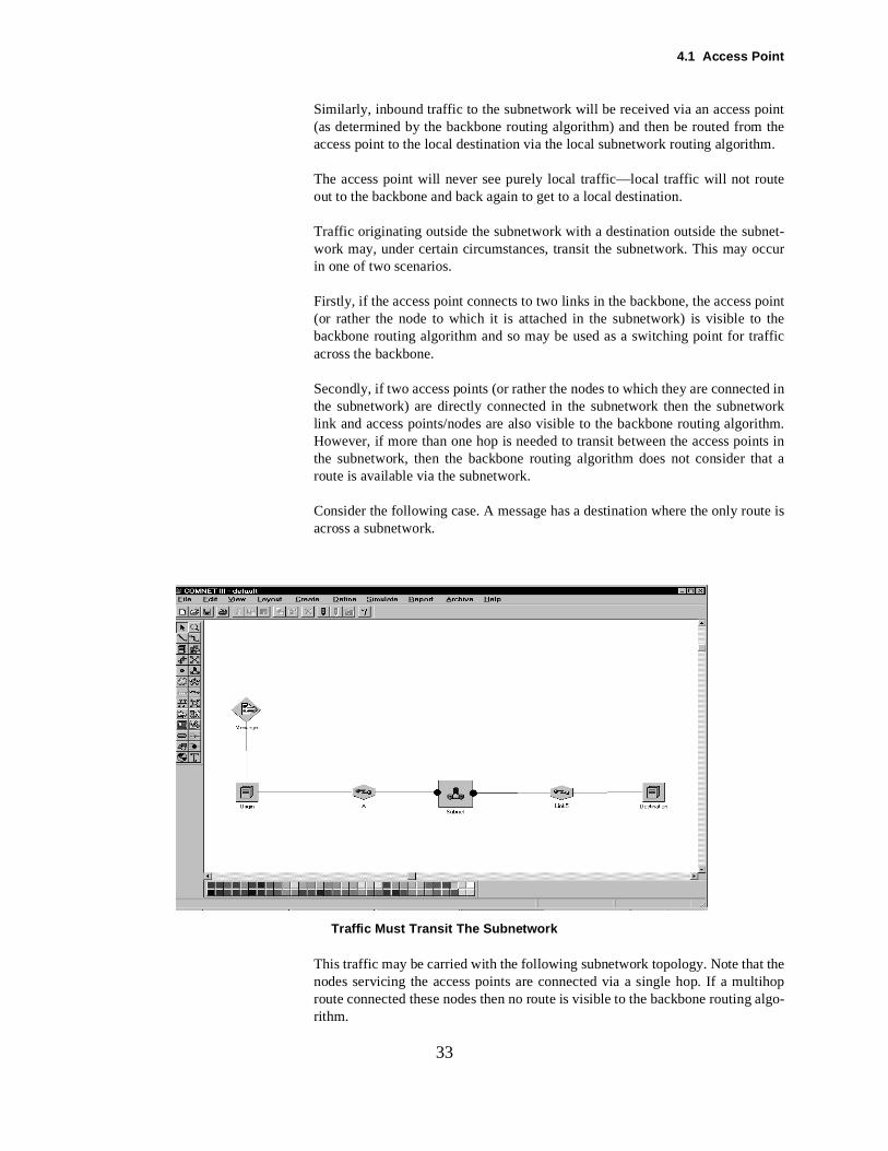
4.1 Access Point
inthe
te
ccur
point
affic
ted inwork
hat a
ute is
theltihop algo-
33
Similarly, inbound traffic to the subnetwork will be received via an access po(as determined by the backbone routing algorithm) and then be routed from taccess point to the local destination via the local subnetwork routing algorithm.
The access point will never see purely local traffic—local traffic will not rouout to the backbone and back again to get to a local destination.
Traffic originating outside the subnetwork with a destination outside the subnet-work may, under certain circumstances, transit the subnetwork. This may oin one of two scenarios.
Firstly, if the access point connects to two links in the backbone, the access(or rather the node to which it is attached in the subnetwork) is visible to thebackbone routing algorithm and so may be used as a switching point for tracross the backbone.
Secondly, if two access points (or rather the nodes to which they are connecthe subnetwork) are directly connected in the subnetwork then the subnetlink and access points/nodes are also visible to the backbone routing algorithm.However, if more than one hop is needed to transit between the access points inthe subnetwork, then the backbone routing algorithm does not consider troute is available via the subnetwork.
Consider the following case. A message has a destination where the only roacross a subnetwork.
Traffic Must Transit The Subnetwork
This traffic may be carried with the following subnetwork topology. Note that nodes servicing the access points are connected via a single hop. If a muroute connected these nodes then no route is visible to the backbone routingrithm.
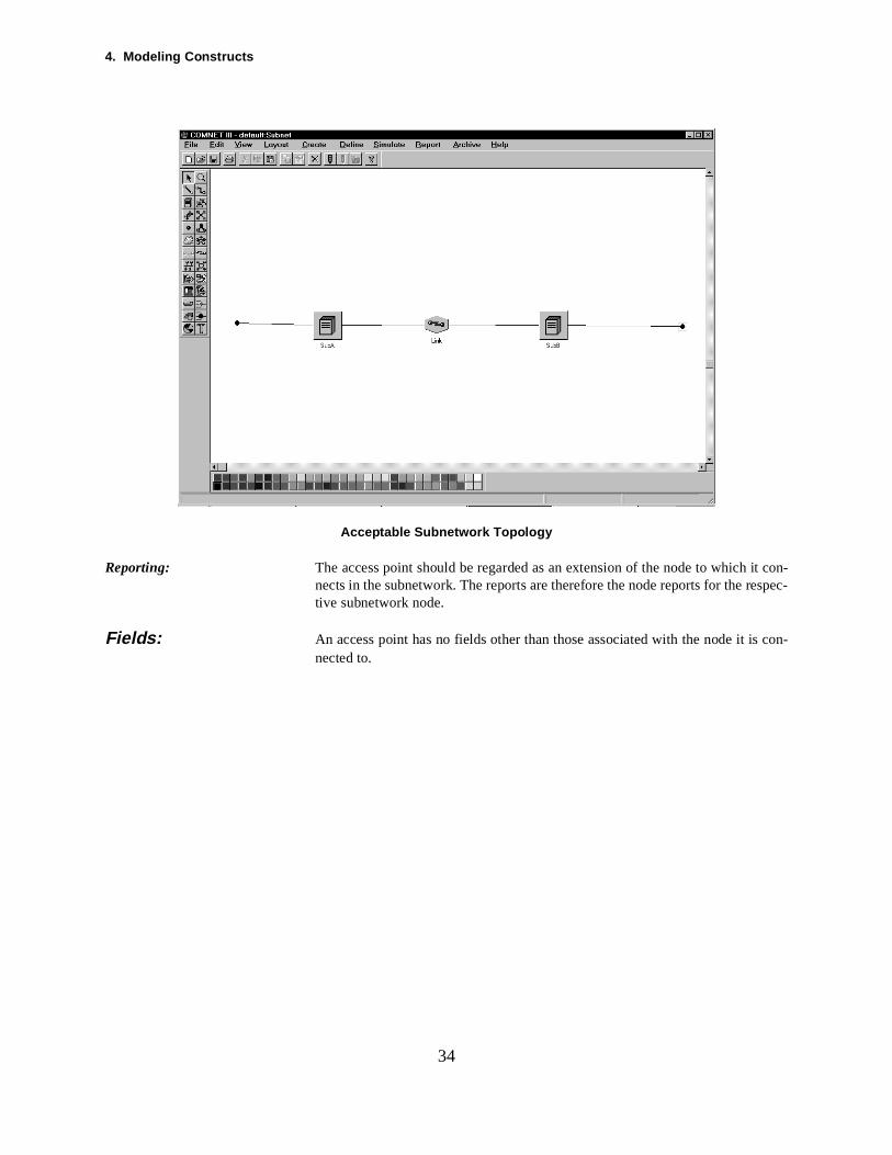
4. Modeling Constructs
it con-ec-
34
Acceptable Subnetwork Topology
Reporting: The access point should be regarded as an extension of the node to which nects in the subnetwork. The reports are therefore the node reports for the resptive subnetwork node.
Fields: An access point has no fields other than those associated with the node it iscon-nected to.
4.2 Buffer Processing
ach
ale thegram-
arts:ckets leave
axi-r alltes ore arcaram-
t theingtput)eters.
sizenodes asbuffert thenodeer case,buffere port
en ife isutt howherecked
forf andpoli-
35
4.2 Buffer ProcessingIn COMNET III, the nodes have separate buffers for input and output on elink. The buffer operation has two components -- a policy for which packets itwill admit and how they will be sorted, and a processing time to model locprocessing that occurs before the packet in the buffer is available to leavbuffer. These buffer operations involve parameters that are on the arc connectinthe node to the link for connection (or port) parameters and on the node's paeter set for common parameters.
The operation of either the input or the output buffer consists of three pdetermining whether a packet will be accepted at the buffer, ordering the paadmitted to the buffer, and processing that must occur before the packet canthe buffer.
Buffer Size There are two size constraints for either the input or the output buffer: the mmum size available for the specific port and the maximum size available foports on the node. In each case, the size may be measured in terms of bypackets. The port parameters are available by editing the properties of thconnecting the node to the link. The node parameters are available in the peter set for the node.
The buffer determines that there is room for a packet by first checking thaspecific input or output buffer has buffer space available to fit the incompacket, and then it checks that the total space used for all similar (input or oubuffers on the node do not exceed the buffer constraint in the node's paramThe packet may be accepted in a buffer if it fits in both the port-specific bufferand in the total buffer space available on the node.
This approach of having both port specific buffer size and node total buffer is meant to be general to model different types of buffers. For example, a may have a central buffer space that is dynamically allocated to all bufferthey need them, and in this case all of the port buffer sizes and the node's size can be set to be the total size available and COMNET III will check thatotal size buffered on the node will not exceed the available size on the while allowing all the node's buffer space to be used by a single port. In anothexample, a node may have dedicated buffer space for each port, and in thisthe port buffer sizes can be set to be this dedicated size and the nodes parameter should be set to be a large value greater than the sum of all thbuffer sizes.
Frequently, it is desirable to model the buffers with the default large value evit is unlikely that the real node has that much buffer space. If the buffer sizunknown, COMNET III's reports on buffer utilization can give information abowhether an unreasonable amount of buffer space would be required or aboumuch buffer space would be needed for the scenario. Another example is wthe buffer size is known but the node is also known to be sized so that no blopackets will occur and thus the user may save the step of filling out the bufferparameters because the simulation results will be the same.
Buffer Policies The above description of checking buffer size constraints is the initial testadmitting the packet into a buffer, and in particular, it describes the operation othe default buffer policy. There are two other policies available at the portsthey refine this decision: a threshold policy and a preemption policy. These
4. Modeling Constructs
, if a the
thisil the
e areodes
t so
ffer.cardrks
velyalue
st ifuffi-
ing
le foring
This on
s oftion
itsffic
rely
le-ove
ET for
ted), by
36
cies determine which packets may be accepted at the buffer. Generallypacket is not accepted in a buffer, it will be blocked and retransmitted fromsource (depending on the protocol). An exception occurs for the output buffer ofa switch node (which models head-of-line blocking at the input buffer): in particular case, the packet that is not accepted waits at the input buffer untoutput buffer accepts it.
In addition to determining which packets are accepted at the buffers, theroptions for flagging the accepted packets for congestion to inform the end nthat they should reduce their rate because the buffer is getting filled.
Threshhold Policy Checking conformance with the threshold policy occurs after the default testhat if a packet fits in the buffer it can be rejected if the buffer size is above athreshold and the packet lacks sufficient priority to use the congested buThis mechanism is commonly used for rejecting packets that are marked "diseligible" when the buffers are above their threshold in frame-switching netwosuch as ATM or frame-relay. The mechanism is also available for selectiadmitting packets depending on whether their priority is above a minimum vallowed when the occupied buffer space exceeds the threshold.
Preemption Policy Checking conformance with the preemption policy occurs after the default tethe packet does not initially fit in the buffer. In this case, if the packet has scient priority, it can cause lower priority packets to be ejected from the buffer(and thus blocked) until there is enough space in the buffer for the incompacket. The lower priority packets will be ejected only if there can be enoughspace made available for the incoming packet. The packets that are eligibejection from the buffer can either be packets of lower priority than the incompacket or just lower in priority than the minimum priority for preemption.
This policy is also available for packets that are not marked discard-eligible topreempt packets that are already in the buffer but marked discard eligible. may be a useful approximation for modeling more complex buffer policiesswitches.
Explicit Congestion Notification (all policies)All buffer policies have options for flagging packets to inform the end nodecongestion at this buffer. There are two forms of explicit congestion notificathat may be used separately or together: forward and backward.
The forward explicit congestion notification (FECN) is set at a buffer when level exceeds a notification threshold. This informs the destination of the trathat there is congestion in the network. This is simple to implement but muston logic at the destination to then inform the source to reduce its traffic.
The backward explicit congestion notification (BECN) is set when the compmentary buffer (for example, the output buffer if this buffer is the input) is abits threshold. This will inform the source of the traffic that there is congestionand thus it should reduce the traffic it is providing to the network. In COMNIII, the congestion notifications are counted in a report and they are usedsome of the rate control options for the protocols.
Buffer Sorting The port buffers in COMNET III have options for how the packets are soronce they are admitted. The packets may be sorted first-in-first-out (FIFOpriority, or by discard-eligibility where DE packets are sorted last.
4.2 Buffer Processing
delle to beto ber until
nd the nodee delayscific
This port
ssingn theg an
all
at all-con-n the
timen
37
Processing at Buffers COMNET III provides an optional processing delay at the buffers to modelays for processing that may occur at a port before the packet is availableave the buffer. This processing delay is sequential -- only one packet mayundergoing the delay at a time and so the other packet queue up waiting processed. If a processing delay is in effect, a packet can not leave a buffethat packet is processed.
The processing delay parameters are available in two places: the port arc anode. The port arc specifies the default processing delay at the port. Theparameters has a set of special case processing delays. These special caswill override the default delay on the port arc if the special case is for the spetype of link that the arc connects and the special case is for the specific protocolID on the protocol that created the packet.
In addition, the node's parameter set has a default port processing time. parameter is only used to set the default processing parameters when newarcs are added to the node. During the simulation, the default port procedelay is obtained from the port arc and the default port delay parameter onode is ignored. If the node's default port delay parameter changes durinediting session, COMNET III will provide a dialog to allow the user to resetthe delays on the port arcs already defined.
The design goal is to have node parameters specify the processing delaysports so that the node can be configured and archived in the library. For prefigured nodes, there should be no need to edit the port processing times oport arcs unless specific information is available that indicates that the should be different. COMNET III will pre-set the port processing times onewly added port arcs based on the node's parameter set.
4. Modeling Constructs
rry
s of-to-
te isf notion)
tina-ks.idth
ar-
ustmalluit-ch
g
38
4.3 Circuit-switched Model
Purpose: COMNET III may be used to model circuit-switched networks which cavoice, fax, video, or circuit-switched data types of traffic.
Circuit-switched traffic between an origin and destination is defined in terman interarrival time, a holding time, and a bandwidth requirement for the endend connection.
As calls originate, a routing decision is made to reach the destination. If a rouavailable, bandwidth along the route is taken for the duration of the call. Iroute is available (either because of link/node failure or because of congesthe call is blocked and a reattempt optionally made some time later.
Creating: A circuit-switched model is constructed by using C&C nodes as origins, destions and switches. The connectivity is implemented using point to point linCall sources are used to generate circuit-switched call traffic. The bandwrequirement for a call is defined using its routing class.
Connectivity: Circuit-switched traffic may only originate on C&C nodes and may only be cried over point to point links.
Router and ATM nodes will also switch circuit-switched traffic.
Editing: See the appropriate object section (e.g., C & C, router, ATM switch, point-to-point link, call sources).
Execution: When a circuit-switched call is made a call request or call routing decision mbe made in order to establish the route. In a real system this will take a samount of time, after which an end to end circuit is available for the circswitched traffic. The duration of the traffic (e.g. a voice call) is typically mulonger than the setup delays.
In COMNET III the setup delays are ignored. When a call originates a routin
AB Trunk
Call Request Signal
Call Accept Signal
Data
A B C D
BC Trunk CD Trunk
Propagation delay
Time spent huntingfor an outgoingtrunk
Time
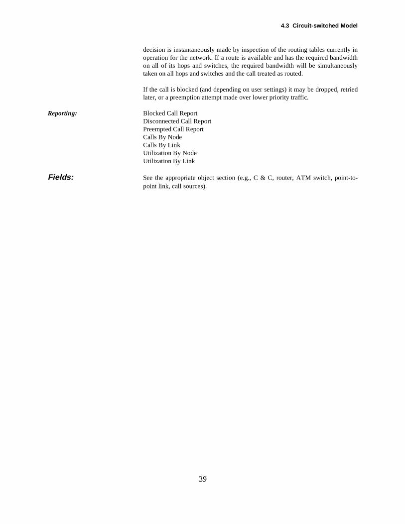
4.3 Circuit-switched Model
tly inidth
usly
tried
39
decision is instantaneously made by inspection of the routing tables currenoperation for the network. If a route is available and has the required bandwon all of its hops and switches, the required bandwidth will be simultaneotaken on all hops and switches and the call treated as routed.
If the call is blocked (and depending on user settings) it may be dropped, relater, or a preemption attempt made over lower priority traffic.
Reporting: Blocked Call ReportDisconnected Call ReportPreempted Call ReportCalls By NodeCalls By LinkUtilization By NodeUtilization By Link
Fields: See the appropriate object section (e.g., C & C, router, ATM switch, point-to-point link, call sources).
4. Modeling Constructs
pro-icalrch
er, inandt the. link
the
as theitch
oes,
link
simpleility
-l cir-
rn-udethe cir-
its, dur-h asver a
eral forasic alter-
40
4.4 CloudsPurpose: The cloud provides an abstract model for public or private data networks. It
vides a higher level of abstraction than is available if modeling the physnodes and links of the network. The cloud model was designed specifically foframe relay networks, but it may also be used for modeling other networks suas X.25, TCP/IP, and cell-relay networks.
The cloud model is an alternative for modeling WANs instead of explicitly mod-eling the topology with routers and links. The cloud behaves like a link object inthat it connects nodes and transfers frames. The cloud is different, howevthat its internal building blocks can be defined graphically with access links virtual circuits. In routing terms, the cloud appears as a single hop such thanodes connected to the cloud are separated from each other by one hop Thecloud model consists of the cloud icon and internal detail for access links andvir-tual circuits. Each node connects to the cloud through a separate accesswhich has its own parameters for data-rate in each direction. Double-clicking onthe cloud icon or using the “enter” menu item in the edit menu will open upcloud’s internal detail.
The cloud icon represents the common characteristics of the network, such framing parameters, frame dropping (or discarding) probabilities and swdelay characteristics. The virtual circuit object uses the frame dropping probabil-ities and switch delay to determine whether a frame gets delivered, and if it dhow long it takes to get through the network.
Within a real network, frames may be lost or dropped due to unrecoverableerrors, failures, lack of buffers at a router, or intentionally dropped by the serviceif the burst rate is exceeded. The cloud models these mechanisms as a probability of dropping the frame perhaps depending on the discard-eligib(DE flag) of the frame.
For enhanced modeling, the cloud has three levels of congestion (normal, moderate, and extreme) which can change during a simulation to change the virtuacuit delay experienced by a frame and the probabilities for losing frames. Thecongestion changes can be scheduled randomly or periodically.
During the simulation, COMNET III will keep track of several statistics conceing the WAN performance. The statistics written to the output reports inclthe following: the link utilization and buffer usage for each access link, throughput and frame-loss for both the normal or DE frames in each virtualcuit, and the frame delay and burst size for each virtual circuit.
Additionally, through the statistics button of the access links and virtual circuobservations of many of the statistics measures may be collected for plottinging the simulation or afterwards. The observations include statistics sucaverage utilization, that are sampled periodically based on an average omeasurement interval.
The cloud object has many parameters to provide flexibility in modeling sevaspects of WAN clouds. In order to simplify the appearance of the cloudcommon models or for new users, the initial editing mode of the cloud is a bmode with the enhanced parameters deactivated. The analyst may select annative editing mode that activates the enhanced parameters.
4.4 Clouds
he thef to
hind for
pointss con-
resentilableccessccess
cular
eachloud. the
lationliv-
41
COMNET III Network with Frame Relay Cloud
Creating: Clouds are created by choosing the cloud icon from the palette or Create/Clouds from the menu bar. The cloud may be placed in the model at either tbackbone or subnetwork level. Double-clicking on the cloud or selectingcloud and then using Edit/Enter on the menubar will open up the internal view othe cloud. The user may substitute any icon for the cloud by using SIMDRAWadd this icon to the usercld.sg2 library file. The cloud icon is displayed bemost other network icons and thus background maps may be useful iconsclouds.
Connectivity: Connections are made through access points. Outside the cloud the accessare connected to other parts of the model. Inside the cloud the access pointnect to the cloud access links.
In order to connect nodes to the cloud, access points must be added to repthe access links or points-of-presence. The access point for the cloud is avaon the palette bar as the black dot next to the subnet symbol. Since the apoint represents a point of presence, only one node may connect to an apoint. Also, a single node may only connect to one access point of a particloud; however, there is no limit on the number of clouds that a node may con-nect.
In order to prepare the cloud for simulation, access links must be defined foraccess point to the cloud. The access links exist in the internal view of the cIn the internal view, the access link icon (the point-to-point icon) is active onpalette bar as well as in the Create menu under Cloud Access Links. Onceeach access point is connected to an access link, the cloud is ready for simuby using default behaviors which would model a packet-switched, reliable-deery network.
4. Modeling Constructs
andeown
Nity theachelower set
sticster-iodicsizesow-
t
stateely
r-box.abili-
rame-
emeat if theran- alsorom not
42
Editing: To get to the internal structure of the cloud, double-click on it or choose Edit/Enter from the menu bar. To edit the details of the cloud, select the cloudthen choose Edit/Properties. From the Cloud Detail dialog box, you can edit thparameters of the cloud and select Frame Relay or ATM, or design your parameter set.
The first combo box provides a list of cloud types. Currently, only the WAcloud configuration is available. This configuration provides a lot of flexibilfor modeling many types of services. New configurations may be added infuture, or added through the COMNET III development environment. For econfiguration there is a list of parameter sets available in the combo box bthe cloud-type combo box. The parameter combo box selects the parametto be used for this particular cloud, and the list may be edited though the “..” but-ton on the right side of the combo box.
Following the parameter combo box, is the parameter for specifying a staticollection interval for internal measurements. This parameter is marked “Inval for Mean Stats (sec)” and is measured in seconds. It is used for permeasurements of average utilization, frame delays, and sampled burst within the cloud. This parameter is also available during the simulation, alling the analyst to adjust the sampling interval as the simulation is in progress.{ This interval will “leak” expired values out of the virtual circuit leaky-buckealgorithms, and thus a periodic interval may improve the simulation perform-ance by reducing memory requirements for expired samples.}
The lower half of the dialog box specifies the congestion variations that will beused less frequently in models. These fields define when congestion changes will occur during the simulation and allow the user to interactivchange congestion during the simulation. There are three congestion states (Nomal, Moderate, and Extreme) that are available from the bottom combo These congestion states correspond to different frame delays and drop probties set by the cloud parameters. Above the current congestion field is a pater for specifying the next time that the congestion state will change.
The congestion state changes from Normal to either Moderate or Extraccording to the entry in the probability of extreme congestion field. Note thonly Moderate or Extreme congestion is desired in addition to Normal, thenprobability of Extreme congestion will be either 0 or 1, respectively (and no dom number will be drawn for either of these values). The stream number isprovided for cases where it is important to keep the probability calculation finterfering with other random number streams. If the current congestion isNormal, then the next state change will always be to Normal.
4.4 Clouds
ingd
43
Cloud Internal Detail Showing Access Links and Virtual Circuits
Cloud Detail Dialog Box
The parameters for the cloud type of “WAN Cloud” are available from editthe parameter list through the “..” button beside the parameter list of the ClouOperation dialog described above. From the intermediate list box dialog, anexisting parameter set may be edited or a new parameter set may be added.
Fields
4. Modeling Constructs
ame
workrtual
ns
intsd. If
at nover-both relayimumacket
beher
s or
Theindi- ise the
tionnedeitor.
enr isCs
ctive, the
lay/
gths
elayat thehisel is
44
Parameter Set Name The first line of this dialog is the name of this set of parameters: this is the nthat will appear in the combo box in the initial dialog box for the cloud.
Session Limit The session limit refers to the total number of sessions that may be set up throughthe cloud at one time when connection-oriented routing is selected in the netrouting parameters. This session limit is independent of the number of vicircuits set up within the cloud; however, with connection-oriented routingturned on, the network-level routing algorithm will not route new sessiothrough the cloud if the cloud's session limit is exceeded.
Frame min, max, overhead The frame parameters of “min”, “max”, and “overhead” specify the constrafor all frames (or encapsulation packets) created and routed through the clouthe frame minimum is greater than zero, then padding will be modeled so thframe is less than the specified size. If the frame minimum, maximum, and ohead are all zero, then the frames will take on the size of the packet. If parameters are equal, then the frames become cells (in other words, framebecomes cell relay because all frames are the same fixed size). The minand maximum sizes include the frame overhead such that the amount of pdata that fits in the frame is the frame size minus the overhead.
Frame Priority The frame priority parameter is available for specifying how the frames willtreated when arriving at buffers within the cloud. The frame priority may eitbe none (where all frames are equal), equal to the packet priority, or related thestatus of the DE condition of the frame.
Frame Assembly Frame Assembly allows a singel frame to carry as many waiting packetpacket fragments as will fit in the frame.
Use CIR in VCs The virtual circuits measure burst size with the leaky bucket algorithm. leak-interval of the bucket may either be described directly as an interval or rectly through a committed information rate (CIR). If the “Use CIR in VCs”turned on, then the leak parameter is specified in the VC as a CIR, otherwisinterval is specified directly.
Transmit Non-VCs VCs are optional in the cloud: the cloud will deliver frames to the destinaeven where a VC is not defined. The “Transmit Non-VCs” switch may be turoff to have the cloud drop frames whose destinations have no defined VCs. Thdefault behavior with this switch on is to have default VCs which do not monthe burst size but still delay the frame as if it had gone through an explicit VC
Routing Interval The “Routing Interval” field provides a possibly random interval betweupdates of the number of switches a virtual circuit contains. This behavioonly active when the “Enhanced Model” switch is turned on; otherwise, all Vdelay frames with the same delay parameter. When the routing interval is athe VC will select a random integer for the number of switches traversed byVC and then use that number to multiply the delay specified by the “DeSwitch (ms)” field described below. The purpose of this parameter is to modelvariations in delay that occur in a real WAN as a result of varying route lenbetween different access links.
Delay Switch The delay that the frame will experience for each frame in a VC. This dparameter is meant to model both the queuing delay and the switch latency switches within the cloud. Typically each VC will use the value drawn from tdistribution to determine the delay for its current frame. If the enhanced mod
4.4 Clouds
VCamenges-ant
nd-
tion
uit
or asibil-
45
in effect, each VC will scale the delay by the number of switches that thespecifies. The congestion level determines which distribution is used for frdelay, but these values may all be equal if the delay does not depend on cotion, and they may be constants if the variation (or jitter) in delay is insignificto the model.
Frame Drop Probability The probabilities that the frames will be dropped by the virtual circuits depeing on both the congestion state of the cloud and the DE state of the frame. Typ-ically, the frames will be more likely to be dropped at higher levels of congesor when the frames are marked DE.
In normal conditions, the normal frame will not be dropped by the virtual circunless it arrives at a switch that is extremely congested and is refusing to acceptany frames or one of the network’s links experiences transmission errors. Fcase where an extremely congested switch or a transmission error is a posity, the probability of dropping a normal frame may be non-zero.
4. Modeling Constructs
46
Frame Relay Cloud Parameters
VC Behavior Dialog
4.5 Cloud Access Links
: thishedel
mes Thisll vir-
her
s for
ese
oose
fromct to
r spe-
47
4.5 Cloud Access LinksPurpose: Cloud access links model the connections between the user and the cloud
connection may be either the link from DTE or PAD in X.25 or the link from tframe relay access device in frame relay services. Typically, this link will mothe local line between the user and the network’s point of presence (POP).
The access link also models the buffer at the POP switch for the exiting frathat may arrive simultaneously from many sources connected to the cloud. buffer allows the cloud to model cases where the combined data rate from atual circuits momentarily exceeds the data rate for the access link. This buffersorts the waiting frames by priority (see Frame Priority under 4.3 Clouds. Higpriority frames may preempt waiting frames with lower priority.
Important parameters of the access link include the data rate and number of cir-cuits of the link and how much buffer space the network POP switch providetraffic arriving at the node.
The access link collects statistics on link utilization and exit buffer size. Thstatistics are available for post-analysis and real-time plotting.
Creating: A cloud access link can be created while within a cloud. You can either chthe point-to-point link tool from the palette or choose Create/Cloud AccessLinks from the menu bar.
Connectivity: The pads that are available from the tool palette are the connection pointsoutside the cloud to the access link. Within the cloud each pad must conneone access link and each access link must connect to one pad.
Editing: Cloud access link parameters are edited by double-clicking on the link or choos-ing Edit/Detail while the access link is selected (highlighted in red).
Cloud Access Link Parameters
Fields
Number of Circuits The number of circuits in the access link, this is usually left at one.
Entry, Exit Bandwidth These are usually set to the same value, but can be set to different values fo
4. Modeling Constructs
., no
lly
link.liverait for
e is
ept
r the
48
cial cases. A value of zero has the special meaning of infinite bandwidth (i.etransmission delay).
Propagation Propagation time of the signal across the access link itself. This value is usuainsignificant and may be left as zero.
Exit (Egress) buffer This a buffer that is available at the input side of the exit part of the accessA particular access link may be connected to several virtual circuits that deframes at the same time, in which case the frames may have to queue to wthe earlier frames to get transmitted. This buffer is sorted by priority of theframes (the method for determining frame priority is set in the cloud parameters).
Buffer limit The buffer limit may be specified in terms of packets or bytes. If this valuexceeded then the buffer will block incoming frames.
Use unlimited buffer If this box is checked there is no buffer limit and the buffer will always accincoming frames.
Buffer units The buffer size can be specified in either packets or bytes.
Buffer definition The buffer may be separate for each VC (Per VC) or just a single buffer fowhole access link (Per Access Link).
Buffer policy Described earlier under Buffers.
Early Packet Discard/Partial Packet Discard:
Buffer threshold (buffer units) Specifies at what level of buffer congestion the logic for Early Packet Discardand Partial Packet Discard will become active.
Discard type Early packet discard and partial packet discard are options for rejecting frames
4.5 Cloud Access Links
larlygher havethatg. In
d andtherives,earstch on
49
once a previous frame from the same packet is lost. This option is particurelevant to modeling cell-based services such as ATM that will segment a hilayer protocol packet into many small cells. Because these services do notprovisions for error corrections by retransmitting the cells, a lost cell implies the service will not be able to reassemble the packet that that cell is carryinthis case, the buffer that drops the cell can recognize that any further cells fromthe same packet need not be forwarded. This is called partial packet discarit can avoid wasting bandwidth on unusable transmissions. This logic is furextended to early packet discard for when the first cell of a new packet arrthe buffer can immediately begin to reject all the cells of that packet if it appthat all of the cells in the packet will not be able to fit in the buffer. The swidetermines that all the cells in a packet will not fit by using a fixed thresholdthe buffer based perhaps on the maximum size packet possible for the packet.
4. Modeling Constructs
t of adelshat isy
tiont to
e-cloud
intsketrtual
e vir-
le a thet will
ligi-l be
the
t oneen a, asrrowsuiturst
lid-ursty beetersterval
ualingrk theom-
50
4.6 Cloud VCsPurpose: A cloud VC represents the virtual circuit or path through the network that con-
nects a source to a destination. In the actual network, the path may consisnumber of intermediate routers and link hops, and the virtual circuit icon mothis path in terms of a delay consisting of a propagation delay, plus a delay tthe product of the specified number of switches the path contains and the delaper switch.
Multiple transits through the cloud are allowed in order to get to a destinathat does not have a direct VC. COMNET III will attempt to find a way to gethe next hop destination by following the explicit VCs through multiple transitsuntil the destination is reached. This is particularly helpful for modeling framrelay services where remote offices communicate to each other through the with a central site acting as a router.
The primary purpose of the virtual circuit object is to specify the burst constrafor traffic on this virtual circuit. Burst sizes are measured with a leaky bucalgorithm: the leaky-bucket burst is the amount of data accepted by the vicircuit for the previous interval of time. For example with a one second interval,the burst size will be the amount of data that entered the virtual circuit over theprevious second. The burst is recalculated for each frame that arrives at thtual circuit.
The virtual circuit uses the burst size calculation to determine how to handframe entering the network from an access link. If the frame would result inburst being over the committed plus excess burst size, then the virtual circuiimmediately drop the frame. If the frame would result in the burst size beingover the committed burst size, then the frame will be marked DE (discard eble); otherwise, the frame is marked normal. The DE or normal frame wilsuccessfully transmitted to the exit access link unless it is dropped due to FrameDrop Probability (see Clouds).
Creating: A cloud VC can only be created while within the cloud, either by selecting Cloud VC icon from the palette or choosing Create/Cloud VCs from the menubar.
Connectivity: The virtual circuits connect between two access links—there can be at mosvirtual circuit between a particular source and destination access link. Whconnection is made, the arcs will be broken to indicate a virtual connectionopposed to the physical connections used between nodes and links. The aon the arcs indicate the direction of information flow. Generally, a virtual circhas to be defined for both directions of a pair of access links to specify bparameters and collect statistics independently for the different directions.
The virtual circuit will measure information rate bursts using a leaky bucket, sing window, or jumping window and mark frames according to the current bsize. This behavior is specifically designed for frame-relay service but it mauseful for modeling or measuring bursts in other services. The burst paraminclude a committed burst size and an excess burst size measured over an inthat is either specified or implied by a committed information rate. The virtcircuit will (1) immediately drop frames if the burst size resulting from acceptthe frame exceeds the sum of the committed and excess burst sizes, (2) maframe as discard eligible (DE) if the resulting burst size is greater than the c

4.6 Cloud VCs
f theeas-
or
IR)s. Ifsizel is
slid-
o the
for seturst
51
mitted burst size, or (3) just leave the frame unmarked (non-DE or “normal”) ifthe burst size is less than the committed burst size. For dropped frames, thecloud does not model error correction and thus the associated packets odropped frames will be blocked by cloud. For more details on burst rate murements, see the specific sections on flow control.
Editing: Cloud VC parameters are edited by double-clicking on the virtual circuitchoosing Edit/Detail while inside the cloud.
Cloud Virtual Circuit Dialog Box
Fields
Committed Information Rate or Burst IntervalThe burst interval may be specified either as a committed information rate (Cor an interval depending on the setting of the switch in the cloud parameterCIR is specified, the burst interval is computed as the committed burst divided by the CIR unless either value is zero, in which case the intervaassumed to be one second. The CIR is in units of kilobits per second.
Committed burst size The committed burst size, measured in kilobits (1000 bits), is the threshold on theburst size, beyond which the new frames will be marked DE.
Burst Type Sets the type of burst measurement used: leaky bucket, jumping window, oring window.
Excess burst size The excess burst size, in kilobits, is the threshold on the amount in addition tcommitted burst size above which all frames will be dropped immediately.
Mark DE Frames This option allows you to bypass the traffic policing when it is known that a cer-tain type of traffic will never (or always) be set discard eligible. The optionsbypassing the algorithm for setting discard eligibility of packets are to alwaysthe DE flag or to never set the flag. The "use algorithm" option uses the bmeasurement algorithm with the thresholds to determine discard eligibility.
4. Modeling Constructs
ffic
ts of
l cir-s fielde vir- theittedly at
tualsizeed
at the
52
Never Drop Due To Excess BurstThis is a checkbox for preventing the algorithm from rejecting any excess trathat occurs after the burst exceeds the committed plus excess burst size.
Propagation delay The propagation delay across the virtual circuit, between entry and exit poinpresence.
Number of switches There is an additional parameter for the number of switches that this virtuacuit uses. If the enhanced model is not selected in the cloud parameters, thiwill be deactivated and the number will be assumed to be one. Otherwise thtual circuit will have a preset or random number of switches which multipliesframe delay from the cloud parameter to get the frame delay for each transmframe. In the enhanced model, the number of switches may change randomeach routing update interval in the cloud parameters.
Show burst size This check box is for the graphical display of the current burst size of this vircircuit. Each virtual circuit has independent control on whether the burst will be displayed above it during simulation. The burst size will be displaywhen the box is checked (even when animation is off). This check box is activeduring the simulation so that the display can be interactively changed during thesimulation. The displayed burst size represents the sampled burst size measurement interval specified in the initial cloud dialog box.
4.7 Command: Answer Mes sage
nd acute.
ssage the
: data-
to thementsatis-
om--
swer
el. Aappli-
. Inle for
ticular the glo-
user
tions fromm-
local
the
odels
53
4.7 Command: Answer MessagePurpose: An Answer Message command is used within an Application Source to se
reply back to the origin of the message which caused the application to exeIn other words, the application must have been started by received mescheduling for an answer message command to return a reply back toreceived message’s origin.
Answer messages are routed according to the message that triggers themgram if the triggering message is a datagram, connection-oriented if the trigger-ing message is connection-oriented (session source).
If the application has several message requirements then the reply is sent origin of the first message in the requirement list. If the first message requireis a wildcard, the reply is sent to whichever node sent the message which fied the message requirement.
Creating: Answer message commands can be created in one of three ways.
Firstly, they may be created locally on computer & communication nodes, cputer group nodes, and router nodes. The respective node dialog box has a Commands button which, when pressed, brings up a dialog box for editing andcreating commands. If this method of creation is used then the respective ancommand only has local scope to the node on which it is defined.
Secondly, answer commands may also be created using the Define/Commandsmenu option. In this case, the scope of the command is global to the modcommand defined globally can be executed by any node in response to an cation which runs on the node and calls the global command.
Thirdly, answer commands can be added to the library via the Archive/Objectmenu option and then picking the Commands line from the offered list boxthis case the new answer command is saved in a library and is then availabuse across models. To use an answer command defined this way in a parmodel, it must be copied out of the library file to the model by using eitherfirst or second method outlined above. It will then be either local to a node orbal, depending on the method used.
In addition, an Answer Message command is created automatically when thecreates a Response Source.
Connectivity: An answer message command must be defined on a computer & communicanode, on a computer group node, on a router node, or as a global commandthe Define/Commands menu. Once defined, it may be referenced in the comand list of any application which runs on the node.
If a global command and a local command have the same name, then thecommand will take precedence.
Editing: Edit the details of the answer command from the node dialog boxes, or fromDefine/Commands menu option, or from the Archive/Objects menu option.
When the answer command is edited in the library (via Archive/Objects) thechanges made are not automatically copied into the local model, or other m
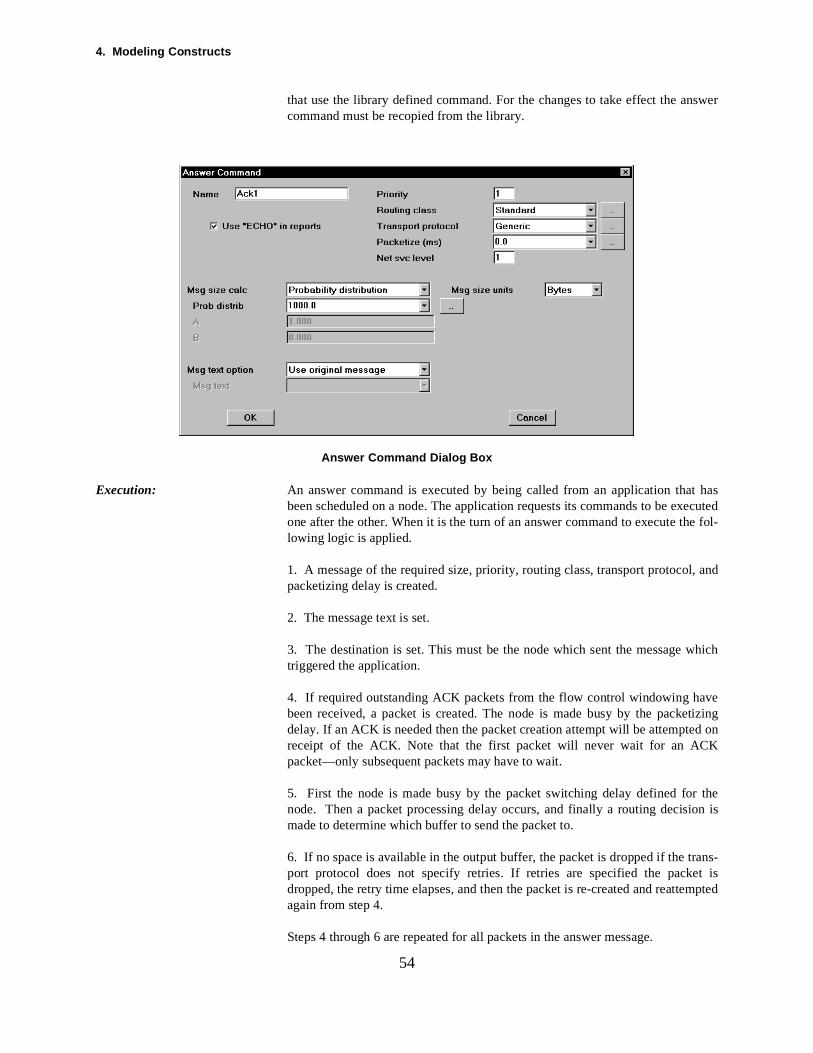
4. Modeling Constructs
nswer
hasecutede fol-
d
which
tizingd onK
eon is
t ised
54
that use the library defined command. For the changes to take effect the acommand must be recopied from the library.
Answer Command Dialog Box
Execution: An answer command is executed by being called from an application thatbeen scheduled on a node. The application requests its commands to be exone after the other. When it is the turn of an answer command to execute thlowing logic is applied.
1. A message of the required size, priority, routing class, transport protocol, anpacketizing delay is created.
2. The message text is set.
3. The destination is set. This must be the node which sent the message triggered the application.
4. If required outstanding ACK packets from the flow control windowing havebeen received, a packet is created. The node is made busy by the packedelay. If an ACK is needed then the packet creation attempt will be attemptereceipt of the ACK. Note that the first packet will never wait for an ACpacket—only subsequent packets may have to wait.
5. First the node is made busy by the packet switching delay defined for thnode. Then a packet processing delay occurs, and finally a routing decisimade to determine which buffer to send the packet to.
6. If no space is available in the output buffer, the packet is dropped if the trans-port protocol does not specify retries. If retries are specified the packedropped, the retry time elapses, and then the packet is re-created and reattemptagain from step 4.
Steps 4 through 6 are repeated for all packets in the answer message.
4.7 Command: Answer Mes sage
ocesscludesmmandsnm-
erateand as nototfternode
ated
they ref-mati-
55
At the node there may be more than one application scheduled and in the prof generating the required packets for the respective messages. This also inmessage sources, session sources and response sources as well as cocalled directly from applications. In fact the respective sources map onto aapplication which has a command list containing either a single transport comand, setup command, or answer command respectively.
In this case, a list of applications that are concurrently scheduled to genpackets at the node is kept. The application at the top of the list is selected packet for its message created as outlined above. Application scheduling iquite round robin: an application waiting for flow control authorization will nblock another application, even if it’s at the top of the application queue. Aexecution the application is then placed at the bottom of the list. When the becomes free, a packet for the next application is created.
Reporting: See the following reports:Message Delays For Transport And Answer CommandsPacket Statistics For Transport And Answer CommandsReceived Message Counts
Also individual node and link reports indicate loading by the packets generfrom the Answer command.
Fields:
Name An alphanumeric field to identify the command. The name must be unique onnode, or unique in the global command list. If the name is changed, then anerences to the name in an application command list will be changed autocally. The name is case sensitive.
Priority Integer value (see Message: Priority)
Packet Routing Class Pick from list (see Routing Class: Packet)
Transport Protocol Pick from list (see Transport Protocol)
Packetizing Delay Real value including distributions(see Message: Packetizing Delay)
Message Size Units Bytes or Packets(see Message: Size Units)
Message Size Calculation DistributionMessage LinearFile Linear(see Message: Size Calculation)
Message Text Use Original MessageCopy Message NameSet Message Text(see Message: Text)
4. Modeling Constructs
cess-
d inad is
andhas a
com-
these to
list thend thisl byocal
tions
any
local
s, or
odelscess-
56
4.8 Command: Process DataPurpose: A Process Data command is used within an application to model some pro
ing task on a node. This would be used to represent some major subroutine orsoftware task that has to run on the node. The loading is effectively definetime duration terms as the node has a cycle time and the processing lodescribed as the number of cycles to execute.
Creating: Processing commands can be created in one of three ways.
Firstly, they may be created locally on computer & communication nodes, computer group nodes, and router nodes. The respective node dialog box Commands button which, when pressed, brings up a dialog box for editing andcreating commands. If this method is used then the respective processingmand has local scope to the node on which it is defined.
Secondly, Process Data commands may also be created using the Define/Com-mands menu option. In this case, the scope of the command is global tomodel. A command defined globally can be executed by any node in responan application which runs on the node and calls the global command.
Thirdly, Process Data commands can be added to the library via the Archive/Object menu option and then picking the Commands line from the offeredbox. In this case the new processing command is saved in a library and isavailable for use across models. To use a Process Data command defineway in a particular model, it must be copied out of the library file to the modeusing either the first or second method outlined above. It will then be either lto a node or global, depending on the method used.
Connectivity: A Process Data command must be defined on a computer & communicanode, on a computer group node, or as a global command from the Define/Com-mands menu. Once defined, it may be referenced in the command list of application which runs on the node.
If a global command and a local command have the same name, then thecommand will take precedence.
Editing: Edit the details of the Process Data command from the node dialog boxefrom the Define/Commands menu option, or from the Archive/Objects menuoption.
When the processing command is edited in the library (via Archive/Objects) thechanges made are not automatically copied into the local model, or other mthat use the library defined command. For the changes to take effect the proing command must be recopied from the library.
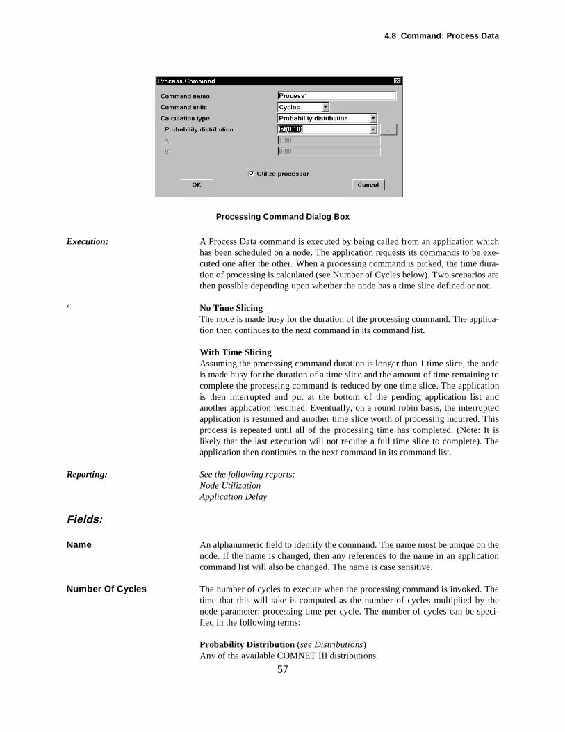
4.8 Command: Pr ocess Data
hiche exe-dura-s arenot.
plica-
nodeg toationand
This It ishe
thecation
. The
speci-
57
Processing Command Dialog Box
Execution: A Process Data command is executed by being called from an application whas been scheduled on a node. The application requests its commands to bcuted one after the other. When a processing command is picked, the time tion of processing is calculated (see Number of Cycles below). Two scenariothen possible depending upon whether the node has a time slice defined or
‘ No Time SlicingThe node is made busy for the duration of the processing command. The aption then continues to the next command in its command list.
With Time SlicingAssuming the processing command duration is longer than 1 time slice, the is made busy for the duration of a time slice and the amount of time remainincomplete the processing command is reduced by one time slice. The applicis then interrupted and put at the bottom of the pending application list another application resumed. Eventually, on a round robin basis, the interruptedapplication is resumed and another time slice worth of processing incurred.process is repeated until all of the processing time has completed. (Note:likely that the last execution will not require a full time slice to complete). Tapplication then continues to the next command in its command list.
Reporting: See the following reports:Node UtilizationApplication Delay
Fields:
Name An alphanumeric field to identify the command. The name must be unique onnode. If the name is changed, then any references to the name in an applicommand list will also be changed. The name is case sensitive.
Number Of Cycles The number of cycles to execute when the processing command is invokedtime that this will take is computed as the number of cycles multiplied by thenode parameter: processing time per cycle. The number of cycles can be fied in the following terms:
Probability Distribution (see Distributions)Any of the available COMNET III distributions.

4. Modeling Constructs
itselfs) can
n of
a file,. Thisified.
58
Based On Message SizeIf the application which wants to execute the processing command was scheduled by received message, the size of the scheduling message (in bytebe used to calculate the number of cycles. This is done on a linear calculationwhere a multiplier and an offset can be specified. The size calculation is thethe form:
Multiplier * Message Size + Offset
Based On File SizeIf the application which wants to execute the processing command has read the size of the first file read can be used to calculate the size of the messageis done on a linear calculation where a multiplier and an offset can be specThe size calculation is then of the form:
Multiplier * Number of Bytes Read + Offset
4.9 Command: Read File
n theom-
n theNETin the
andhas a
mand
andsel. Aappli-om-E.
ject. Inle foricularthere or
ode,
and
local
from
odelsRead
59
4.9 Command: Read FilePurpose: A Read File command is used within an application to model the time delay asso-
ciated with reading from a local disk. The disk access times are specified onode, and the amount of information to read is specified in the read file cmand. The time delay to execute the read can then be computed.
In addition to modeling workload on a node, the read may be used to obtainumber of bytes stored by an early (possibly asynchronous) write, and COMIII monitors reads to count errors where more bytes read than are available file.
Creating: Read File commands can be created in one of three ways.
Firstly, they may be created locally on computer & communication nodes, computer group nodes and router nodes. The respective node dialog box Commands button which, when pressed, brings up a dialog box for editing andcreating commands. If this method is used then the respective read file comhas local scope to the node on which it is defined.
Secondly, read file commands may also be created using the Define/Commmenu option. In this case, the scope of the command is global to the modcommand defined globally can be executed by any node in response to an cation which runs on the node and calls the global command. A read file cmand define in this way may only access the file called GENERAL STORAG
Thirdly, read file commands can be added to the library via the Archive/Obmenu option and then picking the Commands line from the offered list boxthis case the new read file command is saved in a library and is then availabuse across models. To use a read file command defined this way in a partmodel then it must be copied out of the library file to the model by using eithe first or second method outlined above. It will then be either local to a nodglobal, depending on the method used.
Connectivity: A Read File command must be defined on a computer & communications non a computer group node, on a router node, or as a global command from theDefine/Commands menu. Once defined, it may be referenced in the commlist of any application which runs on the node.
If a global command and a local command have the same name, then thecommand will take precedence.
Editing: Edit the details of the Read File command from the node dialog boxes, or the Define/Commands menu option, or from the Archive/Objects menuoption.
When the Read File command is edited in the library (via Archive/Objects) thechanges made are not automatically copied into the local model, or other mthat use the library defined command. For the changes to take effect the File command must be recopied from the library.
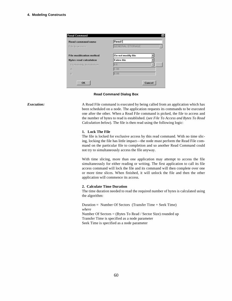
4. Modeling Constructs
hasecuteds andad
slic-om-ould
fileileoneher
g
60
Read Command Dialog Box
Execution: A Read File command is executed by being called from an application whichbeen scheduled on a node. The application requests its commands to be exone after the other. When a Read File command is picked, the file to accesthe number of bytes to read is established. (see File To Access and Bytes To ReCalculation below). The file is then read using the following logic:
1. Lock The FileThe file is locked for exclusive access by this read command. With no time ing, locking the file has little impact—the node must perform the Read File cmand on the particular file to completion and so another Read Command cnot try to simultaneously access the file anyway.
With time slicing, more than one application may attempt to access thesimultaneously for either reading or writing. The first application to call its faccess command will lock the file and its command will then complete over or more time slices. When finished, it will unlock the file and then the otapplication will commence its access.
2. Calculate Time DurationThe time duration needed to read the required number of bytes is calculated usinthe algorithm:
Duration = Number Of Sectors (Transfer Time + Seek Time)whereNumber Of Sectors = (Bytes To Read / Sector Size) rounded upTransfer Time is specified as a node parameterSeek Time is specified as a node parameter
4.9 Command: Read File
and.
uired time
t the lists thed so
sliceswant first
read the The
thecation
t the
timessi-
The
estedcon-
the
61
3. Busy The ProcessorThe node’s processor is made busy for the duration of the Read File commWithout time slicing, this is a straightforward time delay.
With time slicing, the node is made busy for as many time slices as are reqto complete the calculated time duration. The last time slice may be a partialslice.
When one time slice completes the application is interrupted and placed abottom of the pending application list on the node. The top application on therestarted. The restarted application resumes its current command and hanode for one time slice. Eventually the interrupted application is resumed anuses another time slice to count towards the read duration. Between time the file being read remains locked. Therefore other applications which may to access the file cannot do so and will not consume time slices until theapplication has read the file and unlocked it so that the file is then available.
Update File InformationThe respective file information is updated to reflect its new size after the command. The file is then unlocked. If time slicing operation is being usedfile is now available for other read or write accesses by other applications.Read File command is now complete.
Reporting: See the following reports:Node UtilizationApplication DelayFile Warnings
Fields:
Name An alphanumeric field to identify the command. The name must be unique onnode. If the name is changed, then any references to the name in an applicommand list will also be changed. The name is case sensitive.
File To Access The name of the file to read from. If the file does not exist on the local disk atime of executing the command a run time warning will be put on the File Warn-ing report and the command will continue as if the file exists—or at least the delay will be incurred but the file will not be created. This is taken as the pemistic response to this error.
File Modification Method As data is to be read from the file, you may specify the effect on the file. allowed choices are:
Do Not ModifyThe file size is left untouched.
Decrement FileThe file is decremented by the number of bytes read. If more bytes are requthan available a warning is put on the File Warning report but the command tinues as if all the requested bytes were read.
Delete FileAfter reading the requested bytes the file is erased from the local disk on
4. Modeling Constructs
arecom-oices
hed-an be
then
uslyubse-ffset
62
node.
Bytes To Read Calculation The number of bytes to read from the file must be specified. If more bytesrequested than available a warning is put on the File Warning report and the mand continues as if all the requested bytes were read. The calculation chinclude:
Entire FileRead however many bytes are currently in the file.
Probability Distribution ( see Distributions)Any of the available COMNET III distributions.
Based On Message SizeIf the application which wants to execute the read file command was itself sculed by received message, the size of the scheduling message (in bytes) cused to calculate the number of bytes to read. This is done with a linear calcula-tion where a multiplier and an offset can be specified. The size calculation isof the form:
Multiplier * Message Size + Offset
Based On File SizeIf the application which wants to execute the read file command has previoread a file, the size of the first read can be used to calculate the size of the squent read. This is done with a linear calculation where a multiplier and an ocan be specified. The size calculation is then of the form:
Multiplier * First Number of Bytes Read + Offset
4.10 Command: Setup Session
ssion
s.
ted and the
ied).lts in
ession
In thissum-the
uter-reat-ssion
these to
lists thend this
l byocal
tions fromm-
local
s, or
other
63
4.10 Command: Setup SessionPurpose: A Setup Session command is used within an application to establish a se
between the node and some other node in the network. This is useful for model-ling switched or permanent virtual circuits which arise from within application
When a setup session command is executed a session setup packet is crearouted to the destination. A session confirmation packet is then returned toorigin via the same route (assuming connection-oriented routing is specifMessages are then created on an interarrival pattern, each of which resupackets being transmitted to the destination over the session route. When all ofthe packets for all of the messages in the session have been received the sis complete.
Responses may be triggered at the destination by the session messages.case the response packets will follow the session route back to the origin (asing connection-oriented routing). The session will not be complete until all message responses have completed.
Creating: Setup Session commands can be created in one of three ways.
Firstly, they may be created locally on computer & communication nodes, ronodes, and computer group nodes. The respective node dialog box has a Commands button which, when pressed, brings up a dialog box for editing and cing commands. If this method is used then the respective Setup Secommand has local scope to the node on which it is defined.
Secondly, Setup Session commands may also be created using the Define/Com-mands menu option. In this case, the scope of the command is global tomodel. A command defined globally can be executed by any node in responan application which runs on the node and calls the global command.
Thirdly, Setup Session commands can be added to the library via the Archive/Object menu option and then picking the Commands line from the offeredbox. In this case the new Setup Session command is saved in a library and iavailable for use across models. To use a Setup Session command defineway in a particular model, it must be copied out of the library file to the modeusing either the first or second method outlined above. It will then be either lto a node or global, depending on the method used.
Connectivity: A Setup Session command must be defined on a computer & communicanode, on a computer group node, on a router node, or as a global commandthe Define/Commands menu. Once defined, it may be referenced in the comand list of any application which runs on the node.
If a global command and a local command have the same name, then thecommand will take precedence.
Editing: Edit the details of the Setup Session command from the node dialog boxefrom the Define/Commands menu option, or from the Archive/Objects menuoption.
When the Setup Session command is edited in the library (via Archive/Objects)the changes made are not automatically copied into the local model, or
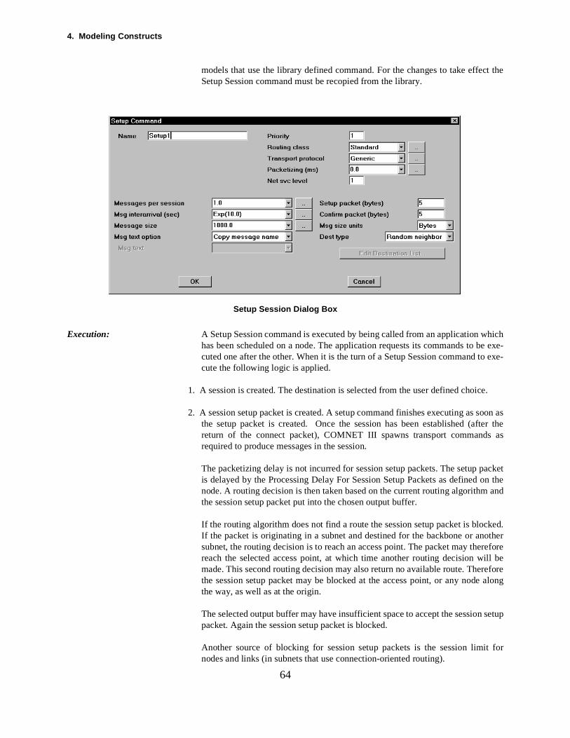
4. Modeling Constructs
ct the
hiche exe- exe-
e.
oon aster the as
acketon the and
ked.otherfore
ill beefore a
setup
t for
64
models that use the library defined command. For the changes to take effeSetup Session command must be recopied from the library.
Setup Session Dialog Box
Execution: A Setup Session command is executed by being called from an application whas been scheduled on a node. The application requests its commands to bcuted one after the other. When it is the turn of a Setup Session command tocute the following logic is applied.
1. A session is created. The destination is selected from the user defined choic
2. A session setup packet is created. A setup command finishes executing as sthe setup packet is created. Once the session has been established (afreturn of the connect packet), COMNET III spawns transport commandsrequired to produce messages in the session.
The packetizing delay is not incurred for session setup packets. The setup pis delayed by the Processing Delay For Session Setup Packets as defined node. A routing decision is then taken based on the current routing algorithmthe session setup packet put into the chosen output buffer.
If the routing algorithm does not find a route the session setup packet is blocIf the packet is originating in a subnet and destined for the backbone or ansubnet, the routing decision is to reach an access point. The packet may therereach the selected access point, at which time another routing decision wmade. This second routing decision may also return no available route. Therthe session setup packet may be blocked at the access point, or any nodelongthe way, as well as at the origin.
The selected output buffer may have insufficient space to accept the sessionpacket. Again the session setup packet is blocked.
Another source of blocking for session setup packets is the session liminodes and links (in subnets that use connection-oriented routing).
4.10 Command: Setup Session
ssioner the
i- next
e theitch-diateout-
ceivedupeated setupts.
of they is
ession
eenlay. Ifceiptly
o. If thent. The
sportd, then from
rrivalis next
ocesso-
65
When a block occurs and if the routing class for the session species a seretry interval, the session setup packet will be recreated and reattempted aftspecified retry time. The attempt will continue to be made until a route or bufferspace is found or the simulation terminates. If no session retry interval is specfied (i.e. set to None) the session is dropped and the application moves to itscommand.
The session setup packet is then routed to the destination. At each nodProcessing Delay For Session Setup Packets is incurred, plus any buffer swing or queueing delays. If the session setup packet is blocked at any intermepoint then again retries will be attempted from the origin depending on the ring class settings.
3. Eventually the session setup packet reaches the destination node. It is rethrough the input buffer and then incurs the Processing Delay For Session Setpackets on the destination node. At this point a session confirm packet is crand routed back to the originating node, reversing the route traversed by thepacket but undergoing no further processing delay for Session Setup Packe
4. On receipt of the session confirm packet at the originating node, a messagerequired size, priority, routing class, transport protocol, and packetizing delacreated.
5. The message text is set.
6. The destination is set. This is the same as the destination picked for the ssetup packet.
7. If required outstanding ACK packets from the flow control windowing have breceived, a packet is created. The node is made busy by the packetizing dean ACK is needed then the packet creation attempt will be attempted on reof the ACK. Note that the first packet will never wait for an ACK packet—onsubsequent packets may have to wait.
8. A routing decision is made to determine which buffer to send the packet tconnection oriented routing for sessions is selected on the routing protocolthe message packet will follow the same route as the session setup packenode is made busy by the packet switching delay defined for the node.
9. If no space is available in the output buffer, the packet is dropped if the tranprotocol does not specify retries. If retries are specified the packet is dropperetry time elapses, and then the packet is recreated and reattempted agaistep 4.
Steps 7 through 9 are repeated for all packets in the message.
If there is more than one message specified then, after the requisite interatime, another message is created and steps 5 through 9 are repeated for thmessage.
Scheduling: At the node there may be more than one application scheduled and in the prof generating the required packets for the respective messages. This alsincludes message sources, session sources and response sources as well as commands called directly from applications. In fact the respective sources map onto
4. Modeling Constructs
portvely.
erateand as nototfternode
thecation.
inatingtes of
acketuting
at then. Thes have
66
an application which has a command list containing either a single transcommand, session setup command, or answer message command respecti
In this case, a list of applications that are concurrently scheduled to genpackets at the node is kept. The application at the top of the list is selected packet for its message created as outlined above. Application scheduling iquite round robin: an application waiting for flow control authorization will nblock another application, even if it’s at the top of the application queue. Aexecution the application is then placed at the bottom of the list. When the becomes free, a packet for the next application is created.
Reporting: Messages: Setup CommandsPackets: Delays For Setup CommandsSessions: Setup Delay By Setup CommandSessions: Length by Session CommandSessions: Blocking by Session Command
Node: Utilization (Loaded by session packets)Node: Application Delays (Session command is part of delay)Link: Delays and Utilization (Loaded by session packets)Link: Random Access Link Performance (Loaded by session packets)
Sessions: By Node (For connection-oriented routing only)Sessions: By Link (For connection-oriented routing only)
Fields:
Name An alphanumeric field to identify the command. The name must be unique onnode. If the name is changed, then any references to the name in an applicommand list will also be changed automatically. The name is case sensitive
Priority Integer value (see Packet: Priority)
Packet Routing Class Pick from list (see Routing Class: Packet)
Transport Protocol Pick from list (see Transport Protocol)
Setup Packet Size When a session command executes, a setup packet is created at the orignode and routed to the destination. The setup packet size is the size in bythis packet.
Confirm Packet Size When the setup packet of the session arrives at the destination, a confirm pis returned to the origin by the same route (assuming connection oriented rofor packets). The confirm packet size is the size in bytes of this packet.
Messages Per Session Once the session has been established by the confirm packet arriving backorigin, messages are then generated at the origin and sent to the destinationumber of messages to send may be specified—after all of these messagearrived at the destination the session is complete.
The messages per session is entered as a statistical distribution.(see Distributions)
4.10 Command: Setup Session
t theplete
tely
age isllow
cket isn the
67
To model a permanent virtual circuit established as part of an application, senumber of messages per session to a value which will take longer to comthan the simulation run length will allow. The session will then be up for theduration of the simulation. A setup command finishes executing immediaafter the setup packet is created.
Message Interarrival Time The interarrival time between the messages of the session. The first messsent immediately after the confirm packet is received; all other messages fowith specified interarrival time.(see Message: Interarrival Time)
Message Size Units Bytes or Packets(see Message: Size Units)
Message Size Calculation Distribution(see Message: Size Calculation)
Message Linear is not supported on sessions.
File Linear is not supported on sessions.
Message Text Copy Message NameSet Message Text(see Message: Text)
Use Original Message is not supported on sessions.
Packetizing Time The time it takes to make a packet for the messages on this session.(see Packet: Packetizing Delay)
Destination Type The destination of the messages on the session. The session setup parouted to the destination, the connect packet is returned to the origin, and thesession messages are sent to the destination a packet at a time.
The destination type may be picked from:Random List (see Destination: Random List)Random Neighbor (see Destination: Random Neighbor)Weighted List (see Destination: Weighted List)Multicast List (see Destination: Multicast List)
4. Modeling Constructs
ween
ever,r the
andbuttonnds.pe to
ndsel. Aappli-
. Inilableartic-
there or
ode,
and
local
from
odelsrans-
68
4.11 Command: Transport MessagePurpose: A Transport Command is used within an application to send a message bet
the node and some other node in the network. The inherent routing is on a data-gram basis where each packet is individually routed to the destination. Howthe routing protocols in force may route each packet in the message ovesame path.
Creating: Transport commands can be created in one of three ways.
Firstly, they may be routed locally on computer & communication nodes computer group nodes. The respective node dialog box has a Commands which, when pressed, brings up a dialog box for editing and creating commaIf this method is used then the respective Transport command has local scothe node on which it is defined.
Secondly, Transport commands may also be created using the Define/Commamenu option. In this case, the scope of the command is global to the modcommand defined globally can be executed by any node in response to an cation which runs on the node and calls the global command.
Thirdly, Transport commands can be added to the library via the Archive/Objectmenu option and then picking the Commands line from the offered list boxthis case the new Transport command is saved in a library and is then avafor use across models. To use a Transport command defined this way in a pular model, it must be copied out of the library file to the model by using eithe first or second method outlined above. It will then be either local to a nodglobal, depending on the method used.
Connectivity: A Transport command must be defined on a computer & communications non a computer group node, on a router node, or as a global command from theDefine/Commands menu. Once defined, it may be referenced in the commlist of any application which runs on the node.
If a global command and a local command have the same name, then thecommand will take precedence.
Editing: Edit the details of the Transport command from the node dialog boxes, or the Define/Commands menu option, or from the Archive/Objects menuoption.
When the Transport command is edited in the library (via Archive/Objects) thechanges made are not automatically copied into the local model, or other mthat use the library defined command. For the changes to take effect the Tport command must be recopied from the library.
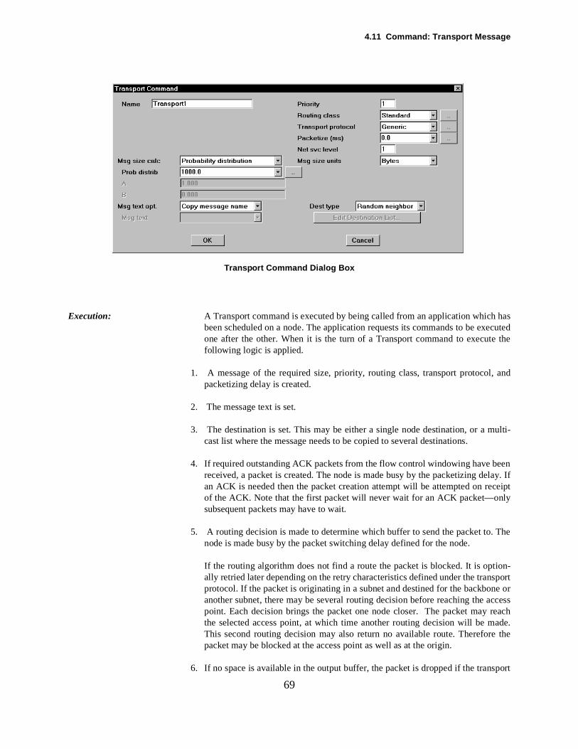
4.11 Command: Transport Mes sage
ecutede the
and
ulti-
enlay. Ifceiptly
The
sporte orccess
reachade. the
port
69
Transport Command Dialog Box
Execution: A Transport command is executed by being called from an application which hasbeen scheduled on a node. The application requests its commands to be exone after the other. When it is the turn of a Transport command to executfollowing logic is applied.
1. A message of the required size, priority, routing class, transport protocol,packetizing delay is created.
2. The message text is set.
3. The destination is set. This may be either a single node destination, or a mcast list where the message needs to be copied to several destinations.
4. If required outstanding ACK packets from the flow control windowing have bereceived, a packet is created. The node is made busy by the packetizing dean ACK is needed then the packet creation attempt will be attempted on reof the ACK. Note that the first packet will never wait for an ACK packet—onsubsequent packets may have to wait.
5. A routing decision is made to determine which buffer to send the packet to.node is made busy by the packet switching delay defined for the node.
If the routing algorithm does not find a route the packet is blocked. It is option-ally retried later depending on the retry characteristics defined under the tranprotocol. If the packet is originating in a subnet and destined for the backbonanother subnet, there may be several routing decision before reaching the apoint. Each decision brings the packet one node closer. The packet may the selected access point, at which time another routing decision will be mThis second routing decision may also return no available route. Thereforepacket may be blocked at the access point as well as at the origin.
6. If no space is available in the output buffer, the packet is dropped if the trans
4. Modeling Constructs
ifiedand
accesscket
madeutesmonp. At hop
nd ifen an theived
ocess
rcesnglemand
erateand as nototfternode
om-
70
protocol does not specify retries (see Transport Protocol). If retries are specthe packet is dropped, the retry time elapses, and then the packet is recreated reattempted again.
7. The packet then is transmitted across each link and through each node or point until it reaches its destination. If a block occurs at any point then the pais dropped and optionally retried from the origin depending upon the transportprotocol settings.
8. If the destination of the message is a multicast list then a routing decision is at the origin for all of the destinations in the list. This may result in several robeing picked, some of which share initial hops. Where an initial hop is comto several routes then the packet will only be transmitted once across the hothe node where the routes diverge a packet will be cloned for each outgoingas determined by the routing decision.
9. When the packet reaches its destination, and if flow control is in operation, athe receipt of the packet demands that an ACK be sent back to the origin, thACK will be created at the destination and routed back to the origin usingsame routing class, transport protocol and routing algorithms as the recepacket.
Steps 4 through 9 are repeated for all packets in the message.
At the node there may be more than one application scheduled and in the prof generating the required packets for the respective messages.
This also includes message sources, session sources and response sources as wellas commands called directly from applications. In fact the respective soumap onto an application which has a command list containing either a sitransport command, session setup command, or answer message comrespectively.
In this case, a list of applications that are concurrently scheduled to genpackets at the node is kept. The application at the top of the list is selected packet for its message created as outlined above. Application scheduling iquite round robin: an application waiting for flow control authorization will nblock another application, even if it’s at the top of the application queue. Aexecution the application is then placed at the bottom of the list. When the becomes free, a packet for the next application is created.
Reporting: Messages: Delays For Transport & Answer CommandsPackets: Delays For Transport & Answer Commands
The following reports indicate loading caused by packets from Transport Cmands:Node UtilizationNode Application DelaysNode Received MessagesLink Delays and UtilizationLink Random Access Link PerformanceBuffer Input By NodeBuffer Input By PortBuffer Output By Node
4.11 Command: Transport Mes sage
theme ine.
cket isn the
71
Buffer Output By Port
Fields:
Name An alphanumeric field to identify the command. The name must be unique innode’s command list. If the name is changed, then any references to the naan application command list will also be changed. The name is case sensitiv
Priority Integer value (see Packet: Priority)
Packet Routing Class Pick from list (see Routing Class: Packet)
Transport Protocol Pick from list (see Transport Protocol)
Message Size Units Bytes or Packets(see Message: Size Units)
Message Size Calculation DistributionMessage Linear.File Linear.(see Message: Size Calculation)
Message Text Copy Message NameSet Message TextUse Original Message(see Message: Text)
Packetizing Time The time it takes to make a packet for the messages on this transport command.(see Packet: Packetizing Delay)
Destination Type The destination of the messages on the session. The session setup parouted to the destination, the connect packet is returned to the origin, and thesession messages are sent to the destination a packet at a time.
The destination type may be picked from:Random List (see Destination: Random List)Random Neighbor (see Destination: Random Neighbor)Weighted List (see Destination: Weighted List)Multicast List (see Destination: Multicast List)
4. Modeling Constructs
om-n iser
the
ntilsfied.mes-pplica-
s are "Getived
aitnd in
thatated onweenneourcerns torksta- note
and
om- wereit Fors to
nce)com- othere of
l cli-g fore thatrenttion
72
4.12 Command: Wait ForPurpose: The Wait For command evaluates a condition, and if the condition is met, it c
pletes and gets out of the way for the next command to run. If the conditionot met, Wait For blocks until the condition is met, or until the time-out timexpires, whichever comes first. By “block,” we mean the application runningcommand sequence is suspended.
The condition can be of three types: Received Message, Alarm , or Expression.
Wait For Received Message: Causes an application to suspend execution uthe received message text requirement for the Wait For command is satiThe only attribute of a Wait For command besides its name is its received sage text requirement. When a message arrives at a node, any suspended ations get to use the incoming message text before any new applicationscheduled. There are three additional options that may be set by checkingrequired msg text from command’s input parameter", "Retain previous recemesssage (if any)", and "Only accept msg responding to this app" options.
The "Get required msg text from command’s input parameter" allows the WFor command to utilize an ouput parameter generated by a previous commathe command sequence, as a response mechanism to complete the Wait For com-mand.
The "Retain previous received message (if any)" option is useful for calculatingthe round-trip time for a Wait For message. To better illustrate this, assumea node sends a message request to a server requesting a database file locanother host system. In this scenario, the server is the connecting link betthe workstation and the host (a typical client/server application). The applicatiosource on the file server responds to the message request and generates a messagrequest to the host system, requesting the database file. The application sthen waits for the database file to be returned. When the database file retuthe server, the application source answers the request using the original wotion message request, and sends the file to the workstation. It is important tothat when the application source sends the file to the workstaion, the messagetext option needs to be set to "use original message" in order to calculatetrack the total round-trip time for the original workstation request.
The "Only accept msg responding to this app" option restricts the Wait For cmand to respond to messages only from specific application instances thattriggered by earlier messages from the same application that has this Wacommand. The purpose of this switch is to bind two application instanceinteract in a seqential way.
In modeling detailed interactions between two nodes (client-server, for instathere may be a pair of detailed applications, each with a long sequence of mands separated by Wait For commands that wait for a message from theapplication. This is fairly simple to model as long as there is just one instancboth applications. The new option is required when one side (for example, theserver side) has multiple instances of the application conversing with severaents. In this case, there may be several instances of the application waitinthe same message text but from different application instances -- a messagarrives at this node may end up triggering a Wait For command in a diffeapplication instance than intended. The new option allows the applica
4.12 Command: Wait For
com-s thelivered
ionsnt andplica-onse., sus-in until
ible to
ndand is
y the
inginsicto a
UE,uted.mesnly time.bles
s notait-ted,
r-tion,d spe-tion “upon
73
instance to respond to only messages from a specific application instance.
The option has a couple drawbacks that can cause the application to neverplete. In one case, the Wait For command can activate too late and misrequired message. In another case, the required message may not get debecause the message experiences errors and the transport protocol does notretransmit blocked packets. Please see the Stop Waiting section below for asolution to this problem.
The Wait For command is especially useful for modeling client-server operatwith dependent sequences of messages going back and forth between clieserver. Without this command, it would be necessary to have a separate aption source for each type of incoming message that requires a different respBy using the “Wait For” command, a single application can send a messagepend until it gets a response, send another message and then suspend agait gets the appropriate response, etc. The Wait For command makes it possbuild process-oriented models of applications, in contrast to event-oriented mod-els.
Wait For Alarm: If the specified alarm is already sounding when this commaexecutes, no blocking occurs, the command completes and the next commexecuted. If the alarm is not already sounding, the command blocks until thealarm does sound.
The alarm combo box shows all the alarms that are currently set. Use the two-dotbutton to set additional alarms if necessary, and pick an alarm. Then specifnode or link on which the alarm must sound.
Wait For Expression: The expression can be almost any expression, involvconstants, user variables, and most of the intrinsic functions. Some intrfunctions, like SimTime, are prohibited. The expression must evaluate boolean value.
When the command is executed, the expression is evaluated, and if it is TRno blocking occurs, the command completes and the next command is execIf the expression is FALSE, the command blocks until the expression becoTRUE. Of the limited number of things permitted in a Wait For expression, ouser variables are liable to change after the expression is evaluated the firstThus, the expression is only re-evaluated if and when referenced variachange.
Clearly, a Wait For expression that does not involve one or more variables iof much use, UNLESS the “stop waiting” option is checked. If the “stop wing” option is checked, then either the expression is FALSE when first evaluaor the command will block for the duration of the time-out time.
Stop Waiting: The blocking process you’re modeling will probably not wait foever. To model a process that times out, check the “stop waiting after” opand give the time limit you’re willing to wait. After that time limit, the commanand the application will be terminated. To catch this event and do somethingcial in response to it, click the Triggered Sources button on the applicasource, select the source that will perform the special response, and use thewait timeout” triggering rule.
4. Modeling Constructs
dist inded/d and
andhas a
com-
these to
. Inilablerticu- the glo-
ode,
any
local
odelscess-
they ref-mati-
74
Troubleshooting: With the increased flexibility of the Wait For commancomes increased complexity and potential for mistakes in the model. To assfinding wayward applications that are in perpetual Waits, turn on the SuspenPending Apps snapshot. This snapshot will show you a count of suspendepending applications on any node on which it’s enabled.
Creating: Wait For commands can be created in one of three ways.
Firstly, they may be created locally on computer & communication nodes, computer group nodes, and router nodes. The respective node dialog box Commands button which, when pressed, brings up a dialog box for editing andcreating commands. If this method is used then the respective processingmand has local scope to the node on which it is defined.
Secondly, Wait For commands may also be created using the Define/Com-mands menu option. In this case, the scope of the command is global tomodel. A command defined globally can be executed by any node in responan application which runs on the node and calls the global command.
Thirdly, Wait For commands can be added to the library via the Archive/Objectmenu option and then picking the Commands line from the offered list boxthis case the new processing command is saved in a library and is then avafor use across models. To use a Wait For command defined this way in a palar model, it must be copied out of the library file to the model by using eitherfirst or second method outlined above. It will then be either local to a node orbal, depending on the method used.
Connectivity: A Wait For command must be defined on a computer & communications non a computer group node, or as a global command from the Define/Com-mands menu. Once defined, it may be referenced in the command list of application which runs on the node.
If a global command and a local command have the same name, then thecommand will take precedence.
Editing: Edit the details of the Wait For command from the node dialog boxes, or from theDefine/Commands menu option, or from the Archive/Objects menu option.
When the Wait For command is edited in the library (via Archive/Objects) thechanges made are not automatically copied into the local model, or other mthat use the library defined command. For the changes to take effect the proing command must be recopied from the library.
Reporting: See the following reports:Node UtilizationApplication Delay
Fields:
Wait For Command Name An alphanumeric field to identify the command. The name must be unique onnode, or unique in the global command list. If the name is changed, then anerences to the name in an application command list will be changed autocally. The name is case sensitive.
4.12 Command: Wait For
ables,are
UE,uted.mesnly time.bles
s notait-ted,
, nod. If
es
y the
inue
ner-hanism
ve
spe-same two
deltimea-onset theout”
75
Wait For Expression: The expression can be almost any expression, involving constants, user variand most of the intrinsic functions. Some intrinsic functions, like SimTime, prohibited. The expression must evaluate to a boolean value.
When the command is executed, the expression is evaluated, and if it is TRno blocking occurs, the command completes and the next command is execIf the expression is FALSE, the command blocks until the expression becoTRUE. Of the limited number of things permitted in a Wait For expression, ouser variables are liable to change after the expression is evaluated the firstThus, the expression is only re-evaluated if and when referenced variachange.
Clearly, a Wait For expression that does not involve one or more variables iof much use, UNLESS the “stop waiting” option is checked. If the “stop wing” option is checked, then either the expression is FALSE when first evaluaor the command will block for the duration of the time-out time.
Wait For Alarm If the specified alarm is already sounding when this command executesblocking occurs, the command completes and the next command is executethe alarm is not already sounding, the command blocks until the alarm dosound.
The alarm combo box shows all the alarms that are currently set. Use the two-dotbutton to set additional alarms if necessary, and pick an alarm. Then specifnode or link on which the alarm must sound.
Required Message Text The message text that the Wait For Command is waiting for in order to contthe suspended application source.
Get required msg text from command’s input parameterThis option allows the Wait For command to utilize an ouput parameter geated by a previous command in the command sequence, as a response mecto complete the Wait For command.
Retain Previous Received Message If AnyUsed for calculating the round-trip time for a filtered message. Please see abosection under Command:Wait For, for a full description.
Only Accept Message Responding To This AppThis option restricts the filter command to respond to messages only from cific application instances that were triggered by earlier messages from the application that has this filter command. The purpose of this switch is to bindapplication instances to interact in a seqential way.
Stop Waiting (and terminate app) after The blocking process you’re modeling will probably not wait forever. To moa process that times out, check the “stop waiting after” option, and give the limit you’re willing to wait. After that time limit, the command and the appliction will be terminated. To catch this event and do something special in respto it, click the Triggered Sources button on the application source, selecsource that will perform the special response, and use the “upon wait timetriggering rule.
4. Modeling Constructs
layn theFile
aalso
uter-reat-and
these torite
AL
ject. Inlableartic-ingto a
ode,m theand
local
romn.
theodelsWrite
76
4.13 Command: Write FilePurpose: A Write File command is used within an application to model the time de
associated with writing to a local disk. The disk access times are specified onode, and the amount of information to be written is specified in the Write command. The time delay to execute the Write can then be computed.
In addition to introducing workload, the Write command may be used to store number of bytes for later access by the Read command. COMNET III will flag errors when write exceeds the size of available storage.
Creating: Write File commands can be created in one of three ways.
Firstly, they may be created locally on computer & communication nodes, ronodes, and computer group nodes. The respective node dialog box has a Commands button which, when pressed, brings up a dialog box for editing and cing commands. If this method is used then the respective Write File commhas local scope to the node on which it is defined.
Secondly, Write File commands may also be created using the Define/Com-mands menu option. In this case, the scope of the command is global tomodel. A command defined globally can be executed by any node in responan application which runs on the node and calls the global command. A WFile command define in this way may only access the file called GENERSTORAGE.
Thirdly, Write File commands can be added to the library via the Archive/Obmenu option and then picking the Commands line from the offered list boxthis case the new Write File command is saved in a library and is then avaifor use across models. To use a Write File command defined this way in a pular model then it must be copied out of the library file to the model by useither the first or second method outlined above. It will then be either local node or global, depending on the method used.
Connectivity: A Write File command must be defined on a computer & communications non a router node, on a computer group node, or as a global command froDefine/Commands menu. Once defined, it may be referenced in the commlist of any application which runs on the node.
If a global command and a local command have the same name, then thecommand will take precedence.
Editing: Edit the details of the Write File command from the node dialog boxes, or fthe Define/Commands menu option, or from the Archive/Objects menu optio
When the Write File command is edited in the library (via Archive/Objects) changes made are not automatically copied into the local model, or other mthat use the library defined command. For the changes to take effect the File command must be recopied from the library.
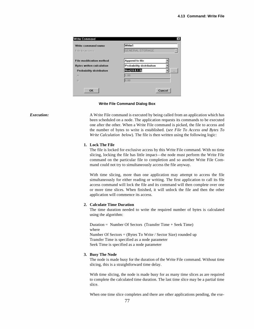
4.13 Command: Write File
hasecuted ando
imeile
om-
fileileoneher
lated
time
uired time
exe-
77
Write File Command Dialog Box
Execution: A Write File command is executed by being called from an application whichbeen scheduled on a node. The application requests its commands to be exone after the other. When a Write File command is picked, the file to accessthe number of bytes to write is established. (see File To Access and Bytes TWrite Calculation below). The file is then written using the following logic:
1. Lock The FileThe file is locked for exclusive access by this Write File command. With no tslicing, locking the file has little impact—the node must perform the Write Fcommand on the particular file to completion and so another Write File Cmand could not try to simultaneously access the file anyway.
With time slicing, more than one application may attempt to access thesimultaneously for either reading or writing. The first application to call its faccess command will lock the file and its command will then complete over or more time slices. When finished, it will unlock the file and then the otapplication will commence its access.
2. Calculate Time DurationThe time duration needed to write the required number of bytes is calcuusing the algorithm:
Duration = Number Of Sectors (Transfer Time + Seek Time)whereNumber Of Sectors = (Bytes To Write / Sector Size) rounded upTransfer Time is specified as a node parameterSeek Time is specified as a node parameter
3. Busy The NodeThe node is made busy for the duration of the Write File command. Without slicing, this is a straightforward time delay.
With time slicing, the node is made busy for as many time slices as are reqto complete the calculated time duration. The last time slice may be a partialslice.
When one time slice completes and there are other applications pending, the
4. Modeling Constructs
lica-rtedslice. slicettene file
rit-
ritesedFile
thecation
the
ed
rivesfer not
rivesfer not
rit-rning. The
78
cuting application is interrupted and placed at the bottom of the pending apption list on the node. The top application on the list restarted. The restaapplication resumes its current command and has the node for one time Eventually the interrupted application is resumed and so uses another timeto count towards the write duration. Between time slices the file being wriremains locked. Therefore other applications which may want to access thcannot do so and will not consume time slices until the first application has wten the file and unlocked it so that the file is then available.
Update File InformationThe respective file information is updated to reflect its new size after the WFile command. The file is then unlocked. If time slicing operation is being uthe file is now available for other access by other applications. The Write command is now complete.
Reporting: See the following reports:Node UtilizationApplication DelayFile Warnings
Fields:
Name An alphanumeric field to identify the command. The name must be unique onnode. If the name is changed, then any references to the name in an applicommand list will also be changed. The name is case sensitive.
File To Access The name of the file to write to. If the file does not exist on the local disk attime of executing the command it will be created.
File Modification Method As data is written to the file, you may specify the effect on the file. The allowchoices are:
AppendThe file size is increased by the amount of data written. If the modeled disk doverflows then a warning is written to the File Warnings report and the trantakes the length of time needed to write all the data. The local disk isincreased in size.
ReplaceThe file is replaced by the number of bytes written. If the modeled disk doverflows then a warning is written to the File Warnings report and the trantakes the length of time needed to write all the data. The local disk isincreased in size.
UpdateThe file size is not changed but the time delay for writing is incurred. This mod-els updating data in the middle of a file.
Bytes To Write Calculation The number of bytes to write to the file must be specified. If more bytes are wten than there is space available on the disk a warning is put on the File Wareport and the command continues as if all the requested bytes were writtencalculation choices include:

4.13 Command: Write File
selfytes or on a cal-
uslyubse-
79
Probability Distribution (see Distributions)Any of the allowed COMNET III distributions.
Based On Message SizeIf the application which wants to execute the write file command was itscheduled by received message, the size of the scheduling message (in bpackets) can be used to calculate the number of bytes to write. This is donelinear calculation where a multiplier and an offset can be specified. The sizeculation is then of the form:
Multiplier * Message Size + Offset
Based On File SizeIf the application which wants to execute the write file command has previoread a file, the size of the first read can be used to calculate the size of the squent write. This is done with a linear calculation where a multiplier and an off-set can be specified. The size calculation is then of the form:
Multiplier * First Number of Bytes Read + Offset
4. Modeling Constructs
is
er,
se-
80
4.14 COMNET Baseliner
Purpose: COMNET III provides an interface to a utility called COMNET Baseliner thatused to import network topology files and traffic information gathered from net-work management discovery tools, and captured network traffic data from net-work analyzers and RMON and RMON II probes. Using COMNET BaselinCOMNET III can import topology data from the following tools:
Network General’s - Expert Sniffer
Hewlett Packard’s - OpenView
IBM’s - Netview 6000
Cabletron Systems - SPECTRUM
Castlerock Computing - SNMPc
Digital Equipment Corporation’s - Polycenter
Network traffic data can be imported from the following tools:
Network General’s - Expert Sniffer, and Sniffer
Axon Networks’ - LANServant
Frontier Systems’ - NETscout
Hewlet Packard’s - Netmetrix
Wandel and Golterman’s - Domino analyzer
For more information about AutoBaseliner, see Chapter 11. COMNET Baliner and also the COMNET Baseliner User’s Guide.
4.15 Destination: Least Busy List
osen.roces-
thedd
t thetion
gen-d. Forf an
net-efixedTM caser the
ed
oudesti-Busyeter-
estina-hose
em-
liza-
NETes, its
81
4.15 Destination: Least Busy List
Purpose: From the list of destinations, the one whose processor is least busy is chThe statistic used to determine busyness is the same statistic used by the Psor Utilization snapshot report.
Creating: Destination lists are created by clicking on the destination list button for source which requires a destination. A list box then appears with options to aor remove nodes from the displayed destination list. For a Least Busy Lisprobability button is grayed out as the probability of sending to each destinain the list is governed by which destination is the least busy.
Connectivity: A Least Busy List is allowed as a destination choice for all types of messageerators, other than a Response Source and an Answer Message Commanthese latter two types of generators the destination is implicitly the sender oinbound message.
A destination is any other node in the model, including nodes in the local subwork, remote subnetworks or the backbone. Subnetwork node names are prwith the subnetwork name. Destination nodes cannot include routers or Aswitches. Messages may be sent to SELF (i.e., the originating node). In thisthe node will be busy by the packetizing delay and packet switching times fopackets in the message, but the packet will not be placed in an output port bufferas it is already at its destination.
If a traffic generator should only send to a single destination, this may be enteras a Least Busy List with a single entry.
Editing: Edit the details of the destination list from the Destination List dialog box. Yhave the options to add a new destination to the list, or remove an existing nation from the list. The Set Probability button does not appear on a Least Destination list because the probability of sending to each destination is dmined by which destination is the least busy.
Execution: When a message, session or call is scheduled at some originating node, a dtion has to be selected. If a Least Busy List is in use then the destination wprocessor is being used the least is chosen from the list of destinations.
When the least busy destination turns out to be a group node, or if the only mber of the list is a group node, the specific destination in the group will be chosenby the same Least Busy algorithm.
If two or more destinations are equally busy (for example, both have 0% utition), the tie is broken by round robin selection. If all the nodes remain un-busy,the result will be identical to a round robin list.
Reporting: Node Received Message Counts.
Fields:
Destination Node Name The names of the destination nodes as defined on their dialog boxes. COMIII makes references to the actual nodes, so that if the node’s name changname in the list will be changed automatically.
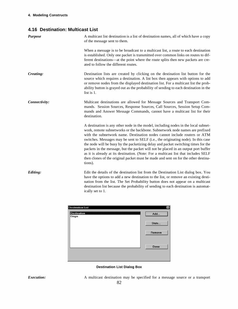
4. Modeling Constructs
opy
nationo dif-e cre-
thedd
the
om-p Com- their
net-efixedTM caser the
stina-
oudesti-icastmat-
sport
82
4.16 Destination: Multicast ListPurpose A multicast list destination is a list of destination names, all of which have a c
of the message sent to them.
When a message is to be broadcast to a multicast list, a route to each destiis established. Only one packet is transmitted over common links on routes tferent destinations—at the point where the route splits then new packets arated to follow the different routes.
Creating: Destination lists are created by clicking on the destination list button for source which requires a destination. A list box then appears with options to aor remove nodes from the displayed destination list. For a multicast list the prob-ability button is grayed out as the probability of sending to each destination inlist is 1.
Connectivity: Multicast destinations are allowed for Message Sources and Transport Cmands. Session Sources, Response Sources, Call Sources, Session Setumands and Answer Message Commands, cannot have a multicast list fordestination.
A destination is any other node in the model, including nodes in the local subwork, remote subnetworks or the backbone. Subnetwork node names are prwith the subnetwork name. Destination nodes cannot include routers or Aswitches. Messages may be sent to SELF (i.e., the originating node). In thisthe node will be busy by the packetizing delay and packet switching times fopackets in the message, but the packet will not be placed in an output port bufferas it is already at its destination. (Note: For a multicast list that includes SELFthen clones of the original packet must be made and sent on for the other detions).
Editing: Edit the details of the destination list from the Destination List dialog box. Yhave the options to add a new destination to the list, or remove an existing nation from the list. The Set Probability button does not appear on a multdestination list because the probability of sending to each destination is autoically set to 1.
Destination List Dialog Box
Execution: A multicast destination may be specified for a message source or a tran
4.16 Destination: Multicast List
the logice
esti-e tipleutputd thee out-node out-amel be
e ofcketsCK
estina-n rea-veralwed
d as-mayne ofbut its hadle at
tionicast
e des-e des-ingletion,s-
NETes, its
83
command. The originating node executes the application which will generatepackets for the message that is to be sent. For a description of the executionsee the appropriate section on transport commands, message sources, and nodscheduling. The following differences should be noted:
At the originating node, and at intermediate nodes on route to one or more dnations, an output port has to be selected through which the packet may bfor-warded to its destination(s). The routing algorithm determines whether muldestinations may be reached by using either one port or by using several oports. If more than one output port must be used then the packet is cloneappropriate number of times and the cloned packets placed in the respectivput port buffers. This cloning of the message packet occurs after any processing delays immediately before placing the ongoing packet(s) into theput port buffer. Note that if multiple destinations can all be reached via the soutput port then only one packet will leave the node and that packet wilplaced in that output port.
No flow control is used when multicast destinations are specified, irrespectivthe transport protocol settings. The sending application keeps generating paas allowed by the node on which it is executing—no check is made that Apackets have been received. Indeed, no ACK packets are generated at the dtion node when packets addressed via a multicast list are received. The maison for this is that one packet transmitted at the origin may be cloned setimes on route to multiple destinations and so it is indeterminate how windoflow control could work with several destinations.
If a packet which has a multicast destination is blocked, then it is counteblocked and immediately dropped. No retries are scheduled irrespective of transport protocol settings. The main reason for this is that an original packet have been cloned several times in order to reach multiple destinations. If othe clones blocks then the original packet would have to be retransmitted, would have to then know which destinations not to send to (as other packetalready been sent to non-blocked destinations). While this may seem simpface value, the problems of multiple blocking, subnetwork routing, link & nodefailures during retransmission attempts etc., make this a difficult implementaissue. Consequently, the simplification is that blocked packets sent to multdestinations are dropped.
It is not recommended to use a multicast list for sending messages to a singltination. The previous three points mean that a message sent out to a singltination on a multicast list is treated differently from a message sent to a sdestination on either a random list or a weighted list. For the multicast situaeven though there is only one destination, the flow control and retry characteritics are inoperative. Use a random list to send to a single destination.
Reporting: Node Received Message Counts.
Fields:
Destination Node Name The names of the destination nodes as defined on their dialog boxes. COMIII makes references to the actual nodes, so that if the node’s name changname in the list will be changed automatically.
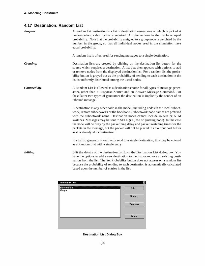
4. Modeling Constructs
d at
ave
thedd
ener-rf an
net-efixedTM caser the
ed
oudesti-
listlated
84
4.17 Destination: Random ListPurpose A random list destination is a list of destination names, one of which is picke
random when a destination is required. All destinations in the list have equalprobability. Note that the probability assigned to a group node is weighted by thenumber in the group, so that all individual nodes used in the simulation hequal probability.
A random list is often used for sending messages to a single destination.
Creating: Destination lists are created by clicking on the destination list button for source which requires a destination. A list box then appears with options to aor remove nodes from the displayed destination list. For a random list the proba-bility button is grayed out as the probability of sending to each destination in thelist is uniformly distributed among the listed nodes.
Connectivity: A Random List is allowed as a destination choice for all types of message gators, other than a Response Source and an Answer Message Command. Fothese latter two types of generators the destination is implicitly the sender oinbound message.
A destination is any other node in the model, including nodes in the local subwork, remote subnetworks or the backbone. Subnetwork node names are prwith the subnetwork name. Destination nodes cannot include routers or Aswitches. Messages may be sent to SELF (i.e., the originating node). In thisthe node will be busy by the packetizing delay and packet switching times fopackets in the message, but the packet will not be placed in an output port bufferas it is already at its destination.
If a traffic generator should only send to a single destination, this may be enteras a Random List with a single entry.
Editing: Edit the details of the destination list from the Destination List dialog box. Yhave the options to add a new destination to the list, or remove an existing nation from the list. The Set Probability button does not appear on a randombecause the probability of sending to each destination is automatically calcubased upon the number of entries in the list.
Destination List Dialog Box

4.17 Destination: Random List
estina-ade
NETes, its
85
Execution: When a message, session or call is scheduled at some originating node, a dtion has to be selected. If a Random List is in use then a statistical pick is mfrom the destinations in the list. All destinations have equal weight.
Reporting: Node Received Message Count.
Fields:
Destination Node Name The names of the destination nodes as defined on their dialog boxes. COMIII makes references to the actual nodes, so that if the node’s name changname in the list will be changed automatically.
4. Modeling Constructs
nat-
stina-hav-
i-modi-.
avect
ot
least
estina-ck is have
86
4.18 Destination: Random NeighborPurpose: A random neighbor destination list is automatically constructed for the origi
ing node by COMNET III. In this case the nodes that are reachable within onehop from the origin in the same subnet are considered neighbors. When a detion is required one of the neighbors will be picked at random, all neighbors ing equal probability.
Note: The list of nodes that are one hop away may change as the model is modfied and thus the random neighbor may send to unexpected nodes in future fications of the model. For more control over destinations, use a random list
Creating: A random neighbor list does not have to be explicitly entered. Once you hselected Random Neighbor in the “Type” box, then COMNET III will construinternally the nodes in the destination list.
Connectivity: Random neighbors are nodes found over 1 hop in the local network (i.e., back-bone or subnetwork). It will not include routers or ATM switches. It will ninclude SELF.
It is a verification error if a Random Neighbor destination is selected, and at one one-hop destination does not exist.
Editing: N/A
Execution: When a message, session or call is scheduled at some originating node, a dtion has to be selected. If Random Neighbor is in use then a statistical pimade from those destinations reachable in one hop. All such destinationsequal weight.
Reporting: Node received message counts.
Fields: N/A
4.19 Destination: Round Robin List
willthem
thedd
tion
oudesti-und
mand.er of
net-efixedTM caser the
ed
estina-hat iscer of
NETes, its
87
4.19 Destination: Round Robin List
Purpose: TheRound Robin list forms an ordered sequence of destinations. The first time adestination is chosen from the list, the first member will be picked, the secondtime it will be the second member, and so on. After the last member, the firstbe picked again. Ordering of the list is based on the order in which you add to the list, unless you change it using the Set Order button.
Creating: Destination lists are created by clicking on the destination list button for source which requires a destination. A list box then appears with options to aor remove nodes from the displayed destination list. For a Round Robin List theprobability button is grayed out as the probability of sending to each destinain the list is governed by which destination is the next in the list order.
Editing: Edit the details of the destination list from the Destination List dialog box. Yhave the options to add a new destination to the list, or remove an existing nation from the list. The Set Probability button does not appear on a RoRobin List because the probability of sending to each destination is based uponthe order of the destination entries in the list.
Connectivity: A Round Robin List is allowed as a destination choice for all types of messagegenerators, other than a Response Source and an Answer Message ComFor these latter two types of generators the destination is implicitly the sendan inbound message.
A destination is any other node in the model, including nodes in the local subwork, remote subnetworks or the backbone. Subnetwork node names are prwith the subnetwork name. Destination nodes cannot include routers or Aswitches. Messages may be sent to SELF (i.e., the originating node). In thisthe node will be busy by the packetizing delay and packet switching times fopackets in the message, but the packet will not be placed in an output port bufferas it is already at its destination.
If a traffic generator should only send to a single destination, this may be enteras a Round Robin List with a single entry.
Execution: When a message, session or call is scheduled at some originating node, a dtion has to be selected. If a Round Robin List is in use then the destination tthe first member will be chosen. The next message, session, or call that is shed-uled will be sent to the second member in the destination list. Each membthe destinaton list will be chosen in turn.
If the selected destination is a group node, or if the only list member is a groupnode, the specific destination in the group will be chosen by the same RoundRobin algorithm.
Reporting: Node Received Message Count.
Fields:
Destination Node Name The names of the destination nodes as defined on their dialog boxes. COMIII makes references to the actual nodes, so that if the node’s name changname in the list will be changed automatically.
4. Modeling Constructs
ked an
tion.
thedds a
d as
era-se an
net-efixedTM casemest port the
ed
has
bili-rifyhe
88
4.20 Destination: Weighted ListPurpose A weighted list destination is a list of destination names, one of which is pic
at random when a destination is required. All destinations in the list haveassigned probability, so that you can specify which is the most likely destinaThe total of all the probabilities must add up to 1.
Creating: Destination lists are created by clicking on the destination list button for source which requires a destination. A list box then appears with options to aor remove nodes from the displayed destination list. A random list includeprobability button which is used to set the probability of the node being pickethe destination.
Connectivity: A Weighted List is allowed as a destination choice for all types of traffic gentors, other than a Response Source and an Answer Message Command. For thelatter two types of generators the destination is implicitly the sender ofinbound message.
A destination is any other node in the model, including nodes in the local subwork, remote subnetworks or the backbone. Subnetwork node names are prwith the subnetwork name. Destination nodes cannot include routers or Aswitches. Messages may be sent to SELF (i.e., the originating node). In thisthe node will be may busy by the packetizing delay and packet switching tifor the packets in the message, but the packet will not be placed in an outpubuffer as it is already at its destination. For each destination entered inWeighted List the probability of picking that destination must be entered.
If a traffic generator should only send to a single destination, this may be enteras a Weighted List with a single entry whose probability of selection is 1.
Editing: Edit the details of the list from the appropriate dialog box. Once a destinationbeen added to the list, the probability of picking it must be set. The default prob-ability is 1, which means that when a new entry is added the sum of all probaties will be greater than 1 (except on the first entry). This will result in a veerror unless the new entry probability is set to an appropriate value such that tsum total of all probabilities in the list is 1.
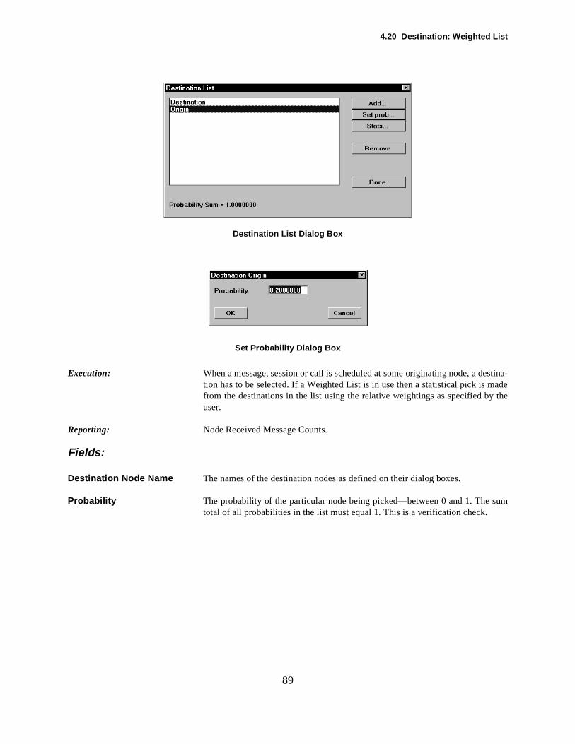
4.20 Destination: Weighted List
estina-ade
the
sum
89
Destination List Dialog Box
Set Probability Dialog Box
Execution: When a message, session or call is scheduled at some originating node, a dtion has to be selected. If a Weighted List is in use then a statistical pick is mfrom the destinations in the list using the relative weightings as specified byuser.
Reporting: Node Received Message Counts.
Fields:
Destination Node Name The names of the destination nodes as defined on their dialog boxes.
Probability The probability of the particular node being picked—between 0 and 1. The total of all probabilities in the list must equal 1. This is a verification check.
4. Modeling Constructs
sple is
“ran-
e newted.
xt soou
npriate
a seed
ts, upg its
en 0ich
can
iated
alog
log
90
4.21 Distributions: SystemPurpose COMNET III provides built-in probability distributions, each of which provide
a stream of random samples on successive executions. The value of the samdistributed according to the type and parameters of the distribution.
The basic random number generation algorithm is based on a multiplicativecon-gruence technique which uses a starting seed to mathematically generate adom” number between 0 and 1 and the next seed. On the next invocation thseed is used so a different “random” number and new seed are then genera
The starting seeds are initialized identically between one run and the neCOMNET III will produce identical results if a model is repeated (unless ychange some model parameter).
The “random” number sequence is therefore pseudorandom. In other words, evethough it is repeatable and mathematically derived it does pass the approstatistical tests to qualify as a random number sequence.
On a 32 bit machine, the random number sequence does not repeat (i.e.,
value is not repeated) inside 232-1 pulls.
To provide multiple, independent random number generators so that differentsequences of random numbers can be used for different modelling constructo 99 streams may be used in COMNET III. Each stream is defined as havinown starting seed and so each stream produces its own unique sequence of ran-dom numbers.
Not all interarrival times, message sizes etc., are uniformly distributed betweand 1. Consequently a number of distribution functions are provided whmanipulate the basic random number pulls into a weighted distribution whichthen be used to represent model data.
Creating: To use a distribution, select “Probability Distribution” when a choice is madeavailable (such as interarrival times, message sizes, retry times, etc.). A dropdown list then appears which has some sample distributions with their assocparameters set to some default value. Pick the closest one.
You can then edit the numbers in the text box where the distribution appearsdirectly, or you can click on the adjacent button with two dots and obtain a dibox with full names and parameter prompts for the selected distribution.
From this latter dialog box you may also elect to graph the distribution with theparameters you have set.
Connectivity: N/A
Editing: Edit the details of the distribution directly from its text box, or pull up the diabox with the double-dot button.
Execution: N/A
Reporting: N/A

4.21 Distributions: System
91
Fields:
The various distributions with their fields are as follows:
Beta Shape1, Shape2, Min, Max, Stream
Erlang Mean, Shape, Stream
Exponential Mean, Stream
Gamma Mean, Shape, Stream
Geometric Min, Mean, Stream
Hyperexponential Mean1, Mean2, Prob Mean1, Stream
Integer Min, Max, Stream
Lognormal Mean, Standard Deviation, Stream
Normal Mean, Standard Deviation, Stream
Poisson Mean, Stream
Triangular Min, Max, Mode, Stream
Uniform Min, Max, Stream
Weibull Shape, Scale, Stream
Graphical representations of the distributions are shown in the appendix.
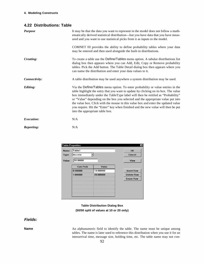
4. Modeling Constructs
ath-
you
d.
elue
ity”
alue put
or an con-
92
4.22 Distributions: TablePurpose It may be that the data you want to represent in the model does not follow a m
ematically derived statistical distribution—but you have data that you have meas-ured and you want to use statistical picks from it as inputs to the model.
COMNET III provides the ability to define probability tables where your datamay be entered and then used alongside the built-in distributions.
Creating: To create a table use the Define/Tables menu option. A tabular distributions listdialog box then appears where you can Add, Edit, Copy or Remove probabilitytables. Pick the Add button. The Table Detail dialog box then appears wherecan name the distribution and enter your data values to it.
Connectivity: A table distribution may be used anywhere a system distribution may be use
Editing: Via the Define/Tables menu option. To enter probability or value entries in thtable highlight the entry that you want to update by clicking on its box. The vabox immediately under the TableType label will then be retitled as “Probabilor “Value” depending on the box you selected and the appropriate value put intothe value box. Click with the mouse in this value box and enter the updated vyou require. Hit the “Enter” key when finished and the new value will then beinto the appropriate table box.
Execution: N/A
Reporting: N/A
Table Distribution Dialog Box
(50/50 split of values at 10 or 20 only)
Fields:
Name An alphanumeric field to identify the table. The name must be unique amongtables. The name is later used to reference this distribution when you use it finterarrival time, message size, holding time, etc. The table name may not
4.22 Distributions: Table
their
is theillcurve
ula-
e one
93
tain spaces.
Table Type There are two ways of interpreting the data values that you enter:
DiscreteThe values that you enter are taken as observation points, together withcumulative probabilities. When COMNET III picks from the table any one of theentered values may be picked with the probability determining its likelihood.
ContinuousThe values that you enter are taken as observations on the curve which envelope of the distribution. When COMNET III picks from the table it winterpolate between the adjacent points and pick any value that is on the using the interpolated probability.
Probability The probability of the value occurring. The probabilities are entered cumtively—i.e., the last probability must equal 1. As a consequence, each probabil-ity must be equal or greater than the previous one in the list.
Value The associated value to the probability. Each value must be greater than thpreceding it in the list.
4. Modeling Constructs
f there-is a
onetribu-from
es anmes- thece to
r is
y orf thens
sed.
iqueution
94
4.23 Distributions: UserPurpose It may be that the data you want to represent in the model follows one o
COMNET III distributions with particular parameter values. Rather than entering this in several places you can make a User Distribution, which named version of one of the standard distributions with its parameters set.
This named distribution then appears in the drop down list of probability distri-butions and may be picked equally with any of the other choices.
One benefit of this approach is that the User Distribution is only defined in place. Therefore, if you change the parameters then all places where the distion is used will see the change. Also, all user distributions are accessible single user-distributions list.
For instance, you can make a user distribution called Generator which usExponential(10,2) standard distribution. You may then use Generator on 10 sage generators to control the interarrival time. Then, if you want to doubletraffic on these generators, you only need to edit Generator and change it onExponential(5,2) and this will then be applied to all the places where Generatoused.
Creating: To create a user distribution use the Define/User Distribution menu option. Auser distributions list dialog box then appears where you can Add, Edit, CopRemove user distributions. Pick the Add button. You then enter the name ouser distribution and pick from one of the standard COMNET III distributioand enter its parameters.
Connectivity: A Named Distribution may be used anywhere a system distribution may be u
Editing: Via the Define/User Distribution menu option.
Execution: N/A
Reporting: N/A
Fields:
Name An alphanumeric field to identify the user distribution. The name must be unbetween user distributions. The name is later used to reference this distribwhen you use it for an interarrival time, message size, holding time, etc.
Probability Distribution One of the standard COMNET III distributions with its parameters set.(See Distributions: System)
4.24 External Model Files
ce.thejectsed inent,
orktron
dalor a
worknd
-
95
4.24 External Model FilesPurpose: COMNET III 1.1 supports an easy-to-read ASCII model file format that allows
creation of model files without using the COMNET III graphical user interfaThese files are loaded into COMNET III using a new Import command on File menu. In addition, there is a Merge command that merges the obdescribed in an external model file with a model that has already been loadCOMNET III. The external file format is described in a separate documCOMNET III External Model File Format, which is available upon request.
The external model file is used by CACI to provide the interface to NetwManagement Systems. After extracting the network topology from CableSpectrum, HP OpenView, or IBM NetView 6000, the extracted file is convertedby a COMNET III utility into an external model file, which is then importedirectly into COMNET III. The conversion of the topology file to the externmodel file is performed automatically when the Import command is used ftopology file from one of the above named Network Management Systems.
The external model file is also used to provide an interface between the NetAnalysis Center, Inc.’s WinMIND network design and pricing software aCOMNET III. After using COMNET III to design and model your network, youcan import data from COMNET III into WinMIND using COMNET III’s external model file format, to produce a least cost network design.
4. Modeling Constructs
e, anns an ori-
ze forolding
ternaltes toby the to a
field
mes-sportes-
edare
ierbe.ames
96
4.25 External Traffic FilesPurpose: A model can have external message, session, and call sources that are triggered
by an external event file. Each model can have an external message filexternal session file, and an external call file. An external event file contaisequence of records in chronological order. Each record has a time stamp, agin, a destination, an ID, and a “size.” The “size” represents the message sithe message file, the number of messages for the session file, and the call htime for the call file.
The model has a list of external message source prototypes (and a list of exsession and call sources). COMNET III uses these prototypes as templaautomatically add message sources where they are needed as indicated originating nodes in the external message file. An event record is mappedparticular type of external message source at an originating node by the IDon the record.
The mapping of different types of messages to different types of external sage sources lets the user specify additional properties (such as priority, tranlayer, or routed protocol) for external traffic that may vary by the type of msage. The traffic in the external file can be automatically scaled.
COMNET III provides an interface to a utility called AutoBaseliner that is usto specify the format of the user’s external file. Built-in format specifications provided for trace files from Network General Sniffer and Expert Sniffer,Hewlett Packard’s NetMetrix, Wandel & Goltermans Domino Analyzer, FrontTechnology’s NetScout RMON Probe, and CastleRock SNMP RMON proAutoBaseliner is also used to match names in each external file with node nused in the COMNET III model. After specifying the file format and matchingnames, AutoBaseliner produces an event file “linked” to model names; the“linked” file is what actually drives the simulation.
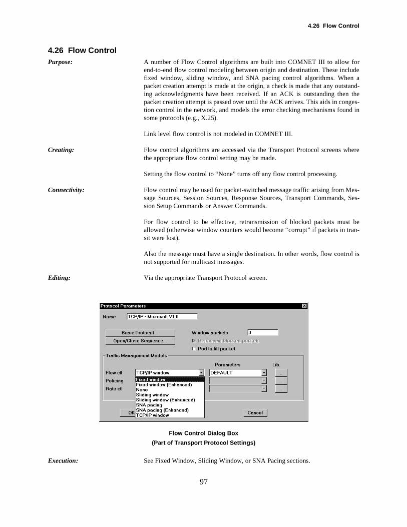
4.26 Flow Control
rlude astand- theges-d in
here
es-s, Ses-
bean-
rol is
97
4.26 Flow ControlPurpose: A number of Flow Control algorithms are built into COMNET III to allow fo
end-to-end flow control modeling between origin and destination. These incfixed window, sliding window, and SNA pacing control algorithms. Whenpacket creation attempt is made at the origin, a check is made that any outing acknowledgments have been received. If an ACK is outstanding thenpacket creation attempt is passed over until the ACK arrives. This aids in contion control in the network, and models the error checking mechanisms founsome protocols (e.g., X.25).
Link level flow control is not modeled in COMNET III.
Creating: Flow control algorithms are accessed via the Transport Protocol screens wthe appropriate flow control setting may be made.
Setting the flow control to “None” turns off any flow control processing.
Connectivity: Flow control may be used for packet-switched message traffic arising from Msage Sources, Session Sources, Response Sources, Transport Commandsion Setup Commands or Answer Commands.
For flow control to be effective, retransmission of blocked packets mustallowed (otherwise window counters would become “corrupt” if packets in trsit were lost).
Also the message must have a single destination. In other words, flow contnot supported for multicast messages.
Editing: Via the appropriate Transport Protocol screen.
Flow Control Dialog Box
(Part of Transport Protocol Settings)
Execution: See Fixed Window, Sliding Window, or SNA Pacing sections.
4. Modeling Constructs
con-ent ave
beenener-
cket
quiva-herjustsured
back
and pri-
ket, thel.
win-ilar
willandatliesow
one
ent
dg-ssagesec-
98
Reporting: N/A
Fields: (Common to all flow control methods)
Window Size Acknowledgments are generated at the destination depending upon the flowtrol algorithm and the window size setting. Once the originating node has swindow size worth of packets, it will wait for the acknowledgment to arribefore it may generate the next packet in the message.
If the originating node attempts to generate a packet and the ACK has not received, it will pass over the generation attempt and return to attempt the gation after other pending tasks have been finished (see Node Scheduling).
If there are no other tasks to complete then the node will wait for the ACK pato be received and then generate the next packet in the message.
Some protocols use window sizes specified in bytes. In those cases, use elent (or approximate) number of full-sized packets that fit in the window. Otprotocols (such as IP) advertise windows in bytes but the internal logic adthe size in full packets for efficiency reasons—thus these windows are measaccurately as a number of packets.
End-To-End ACK Bytes The size of the ACK packet generated at the destination. This will be routed to the origin based upon the effective network routing protocols, and the routingclass and transport protocol settings of the inbound packet.
Retransmit time (ms) The time before retransmission of a blocked packet is attempted.
ACK Priority The priority of the ACK packets. This is used for ordering packets in input output buffers at nodes en route back to the origin. ACKs are usually higherority than user data packets.
Retransmit Blocked Packets This flag must be on for flow control to be effective. If a data or ACK pacblocks en route because of link/node failure, or because of buffer congestionpacket transmission will be reattempted from the origin after the retry interva
Fields for Enhanced Flow Control:
Error Contol Options There are three error control options available for the enhanced flow-control dows. The selective repeat will retransmit just the packet that is blocked (simto how the simple windows handle blocked packets). The go-back-n optionretransmit the entire window of unacknowledged packets, which for fixed SNA-pacing windows is the entire window, but for sliding windows it is just thportion of the window that is still outstanding. The fast-recovery option appjust to sliding windows (such as TCP/IP) that would retransmit the entire windunless it detects multiple duplicate acknowledgements that indicates onlypacket needs to be retransmitted.
Holding ACKs for More Data Some sliding window protocols have a provision to delay the acknowledgemin order to improve the chance to piggy-back data on the acknowledgement.COMNET III does not model the piggy-back of reverse data on the acknowlement but it does model this delay because it has an impact on overall medelay. The Hold-1 option allows for the delay to be interrupted if there is a
4.26 Flow Control
allnt isthat
leasty andular that
n andsmis-
tive,s-
99
ond acknowledgement waiting, while the Hold-all option accumulates acknowledgements until the delay has expired. When an acknowledgemedelayed, the transmitted acknowledgement will acknowledge all packets have been received during that delay.
Retransmit Timeout Calculated from Estimated Round-Trip TimeBecause the sliding-window algorithms acknowledge each packet (or at most packets), they have an opportunity to measure round-trip packet delause that delay to adjust the retransmission time-out timer. TCP/IP in particdoes this. There are two options for estimating the round-trip time and usingestimate for the retransmission time-out. The first option estimates the round-triptime and uses a multiple of that time for the retransmission time. The secondoption estimates both the average round trip time and its standard deviatiothen uses the average plus a multiple of the standard deviation for the retransion time.
Retransmit Timeout Backoff This option applies if a packet is blocked when it is retransmitted. When acthis option will double the previous retransmission time to determine the retranmission time for successive retransmissions of the same packet.
4. Modeling Constructs
er oftion isdow
100
4.27 Flow Control: Fixed WindowPurpose: To model fixed window flow control.
Creating: Via the Transport Protocol screens.
Connectivity: For packet oriented message traffic.
Editing: Via the Transport Protocol screens.
Execution: The origin creates and transmits a packet. This is repeated until the numbpackets sent equals the window size. The last packet to reach the destinaacknowledged. When the ACK is received back at the origin another winsize worth of packets may be created and transmitted.
Reporting: N/A
Fields: See Flow Control and Transport Protocol

4.28 Flow Control: Sliding Window
tos thember
101
4.28 Flow Control: Sliding WindowPurpose: To provide an appropriate model of Sliding Window Flow Control that runs fast.
Creating: Via the Transport Protocol screens.
Connectivity: For packet oriented message traffic.
Editing: Via the Transport Protocol screens.
Execution: The Sliding Window Flow Control allows up to the window size (n) of packetsbe transmitted without an acknowledgement. Each acknowledgement allowwindow to advance by one, so that the window slides by ack sequence nuinstead of jumping the full window size as Fixed Window Flow Control does.
Reporting: N/A
Fields: See Flow Control and Transport Protocol

4. Modeling Constructs
withst to ofsess the
er ofion is may
102
4.29 Flow Control: Jumping WindowPurpose: The jumping window measures the burst based on accumulating a burst size
each packet, but then clearing that accumulation at fixed intervals. In contrathe sliding window which always accounts for all traffic in a previous periodtime, the jumping window clears its burst periodically and thus periodically lomemory of the recently accepted packets. As a result, the jumping window imost lenient of the three burst measurement algorithms.
Creating: Via the Transport Protocol screens.
Connectivity: For packet oriented message traffic.
Editing: Via the Transport Protocol screens.
Execution: The origin creates and transmits a packet. This is repeated until the numbpackets sent equals the window size. Every packet to reach the destinatacknowledged. When an ACK is received back at the origin another packetbe created and transmitted.
Reporting: N/A
Fields: See Flow Control and Transport Protocol
4.30 Flow Control: Leaky Bucket
forple-ess
llytainsd theping
er ofion is may
103
4.30 Flow Control: Leaky BucketPurpose: The leaky bucket algorithm (or the Generalized Cell Rate Algorithm, GCRA,
ATM) is a common algorithm for measuring bursts because it is simple to imment and it is not as lenient as the jumping window in terms of allowing exctraffic. It is similar to the jumping window algorithm except that it periodicasubtracts off an amount equal to the rate times the burst-interval. This mainsome memory of the previous burst interval, especially if that burst exceedevalue of the burst rate times the burst interval. It is more strict than the jumwindow in terms of accepting traffic but not as strict as the sliding window.
Creating: Via the Transport Protocol screens.
Connectivity: For packet oriented message traffic.
Editing: Via the Transport Protocol screens.
Execution: The origin creates and transmits a packet. This is repeated until the numbpackets sent equals the window size. Every packet to reach the destinatacknowledged. When an ACK is received back at the origin another packetbe created and transmitted.
Reporting: N/A
Fields: See Flow Control and Transport Protocol
4. Modeling Constructs
ze. crea-
cing may
104
4.31 Flow Control: SNA PacingPurpose: To model SNA Pacing flow control.
Creating: Via the Transport Protocol screens.
Connectivity: For packet oriented message traffic.
Editing: Via the Transport Protocol screens.
Execution: With SNA Pacing flow control, a pacing counter is initialized to the window siThe pacing counter is decremented every time a packet is created. Packettion stops when the counter reaches zero. Only the first packet in a window isacknowledged. When the ACK packet is received back at the origin the pacounter is incremented by the window size and another window of packetsbe created and transmitted.
Reporting: N/A
Fields: See Flow Control and Transport Protocol
4.32 Flow Control: TCP/IP Window
cificeal-w
asesiallynec-
henwin-
owly isindi-.
105
4.32 Flow Control: TCP/IP WindowPurpose: The TCP/IP window is based upon the sliding window plus adds the spe
congestion window algorithm to avoid congesting a network. It provides a ristic flow control option for TCP/IP that explicitly models the adaptive windosize of the TCP/IP protocol.
Creating: Via the Transport Protocol screens.
Connectivity: For packet oriented message traffic.
Editing: Via the Transport Protocol screens.
Execution: A TCP/IP connection starts with a window size of one packet and then increthe window by one for each acknowledgement to result in an exponentincreasing window. If congestion has been previously detected on this contion, the window will increase until it reaches one half of the window size wthe congestion was detected, otherwise it will increase to the full available dow for that connection. For the congestion case, the window advances approxi-mately one packet per window of packets so that the window grows more slto avoid any congestion that may still be in the network. If congestiondetected, the window will return to one unless duplicate acknowledgements cate that only one packet has been lost – a condition known as fast recovery
Reporting: N/A
Fields: See Flow Control and Transport Protocol
4. Modeling Constructs
106
4.33 IEEE 802The IEEE 802 standards are listed here for your reference.
• 802.1 Higher Layer Interface
• 802.2 Logical Link Control (additional overhead on frame)
• 802.3 CSMA/CD Networks (CSMA/CD link)
• 802.4 Token Bus Networks (Token-passing)
• 802.5 Token Ring Networks (Token-passing)
• 802.6 Metropolitan Area Networks
• 802.7 Broadband Technical Advisory Group
• 802.8 Fiber Optic Technical Advisory Group
• 802.9 Integrated Voice And Data LAN Interface
• 802.10 Standard For Interoperable LAN Security
• 802.11 CSMA/CA Wireless LAN
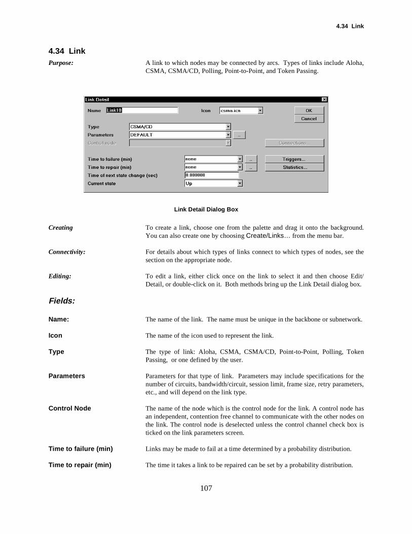
4.34 Link
ha,
und.
e the
dit/x.
ork.
n
ers,
hases onox is
107
4.34 LinkPurpose: A link to which nodes may be connected by arcs. Types of links include Alo
CSMA, CSMA/CD, Polling, Point-to-Point, and Token Passing.
Link Detail Dialog Box
Creating To create a link, choose one from the palette and drag it onto the backgroYou can also create one by choosing Create/Links… from the menu bar.
Connectivity: For details about which types of links connect to which types of nodes, sesection on the appropriate node.
Editing: To edit a link, either click once on the link to select it and then choose EDetail, or double-click on it. Both methods bring up the Link Detail dialog bo
Fields:
Name: The name of the link. The name must be unique in the backbone or subnetw
Icon The name of the icon used to represent the link.
Type The type of link: Aloha, CSMA, CSMA/CD, Point-to-Point, Polling, TokePassing, or one defined by the user.
Parameters Parameters for that type of link. Parameters may include specifications for thenumber of circuits, bandwidth/circuit, session limit, frame size, retry parametetc., and will depend on the link type.
Control Node The name of the node which is the control node for the link. A control nodean independent, contention free channel to communicate with the other nodthe link. The control node is deselected unless the control channel check bticked on the link parameters screen.
Time to failure (min) Links may be made to fail at a time determined by a probability distribution.
Time to repair (min) The time it takes a link to be repaired can be set by a probability distribution.
4. Modeling Constructs
hek theication
nk
cific. Forthe
108
Time of next state change A time at which the state of the link will be toggled: if the link is currently up tlink will be brought down; if the link is currently down it will be brought bacon-line. The time is given is in terms of the simulation time. For example, ifTime of the next state change is 30 seconds, then 30 seconds into each replthe state will be changed.
Current state Whether the link is currently operating (up) or failed (down). This can be tog-gled during the simulation by double-clicking on the link to bring up the lidetail dialog box and editing this field.
Connections… This button allows you to specify the ordering of nodes connected to a spelink. The order determines the node sequence for token-passing and pollingpoint-to-point links with different transmission speeds in each direction, order determines which speed applies to each transmitting node.
4.35 Link: Binary Exponential Backoff Parameters
g aA/
may infi- as on
e
meaxi-s is
con- and
is
109
4.35 Link: Binary Exponential Backoff ParametersPurpose The binary exponential backoff algorithm is defined by the IEEE for computin
retry time for nodes connected to collision detecting links - CSMA and CSMCD Links. Upon collision each node has to calculate a retry time so that it attempt transmission again. Each node should pick a different time to avoidnite collisions. The time is an integral number of time slots calculatedexplained in the Execution section below. This distribution is available onlycollision links: Aloha, CSMA, CSMA/CD.
Creating: The binary exponential backoff algorithm is built into COMNET III. It may bpicked as one of the options when a retry time is required.
Connectivity: N/A
Editing: Via the appropriate dialog box (e.g., ALOHA link, CSMA link etc.)
IEEE Binary Exponent ial Backoff Dialog Box
(as part of CSMA/CD parameters)
Execution: The binary exponential backoff algorithm doubles the retry interval for a fraevery time the frame collides. Once the frame has collided 10 times, the mmum possible retry time stops increasing. Assuming the number of collisionbelow some maximum value (the retry limit), the retry time is computed as a stant offset time plus the slot time multiplied by a random integer between 0
2(min[10,Collision Count]). If a frame has exceeded the retry limit, the retry timegiven by the limit delay.
Reporting: N/A
Fields:

4. Modeling Constructs
n the
ngest
ulten
the
mit-ack
slot
110
Slot Time The slot time is chosen to be large enough to guarantee that two nodes starting totransmit at different slot time boundaries will not collide again.
This results in an interval at least equal to the round trip propagation time olink plus the jam time.
IEEE 802.3 sets the slot time at 0.0512 milliseconds to accommodate the lopath allowed by 802.3 (2.5km and 4 repeaters).
The retry time computed by the Binary Exponential Backoff algorithm will resin an integral number of slot times, or the limit delay if the retry limit has bereached.
Offset A constant added to the IEEE 802.3 retry time.
Retry Limit After a frame collides this number of times, the node stops trying and waitslimit delay.
Limit Delay When the number of collisions for a frame reaches the retry limit, the transting node waits the limit delay before trying again. The collision count is set bto 0.
Stream The random number stream to pick the random integers used to multiply thetime in the retry time calculation.
4.36 Link: Framing Characteristics
n intomesket is
of thetion thecter-y be
portkenaink.
trans-e timeans- link
111
4.36 Link: Framing CharacteristicsPurpose When packet transmission is modeled across a link, packets are broken dow
transmission frames which are then transmitted across the link. When all frafrom the packet have been received at the other end of the link then the pacreassembled and placed in the input buffer of the receiving node.
The framing characteristics are the place where the layer 2 characteristics link are specified. While COMNET III does not include a detailed representaof all of the layer 2 protocol on the link (e.g., time outs, CRC checks, etc.)framing characteristics contain sufficient details of the layer 2 protocol charaistics such that the transmission time for packets and overall link loading mapredicted.
Creating: Framing characteristics are defined on the link parameters screens.
Connectivity: All types of links may have framing characteristics set.
Editing: Via the link parameters screens.
Link Parameters Dialog Box For A Point-to-Point Link
Execution: The packets are queued in priority and FIFO order in the output buffer of theconnecting the node to the link. Depending on the MAC protocol (i.e., topassing, CSMA, Point-to-Point, etc.), the node will at some point in time gaccess to the link such that the first packet may be transmitted across the lin
Based on the framing characteristics, the packet is broken into a number of mission frames. Each frame has a size. The link has a transmission rate. Thdelay for transmission is then calculated by dividing the frame size by the trmission speed. The link is made busy for this transmission time and then the
4. Modeling Constructs
ed in
amecessbled
d the
it
a
um
flow
wit oneing
ess-ula-, link IIIes.
ans-then
ans- link.p
ameg the
112
is made idle. The frame is then delayed by the propagation delay. After this timethe frame is considered to have arrived at the next node, but it is not yet placthe input port buffer.
This calculation is repeated for all the frames (Note: there may be interfrgaps and recontention for the link for each frame if the link has a multiple acprotocol such as CSMA). When the last frame arrives, the packet is reassemand placed into the receive buffer on the input port at the receiving node, anpacket releases its buffer space at the sending node.
Frame Delay is the time for each frame to go from one node to the next:includes transmission, propagation, and LAN contention delays.
Link utilization is the fraction of the time that the link is busy transmittingframe.
Reporting: Frame transmission is shown on the following reports:Link Delays and UtilizationRandom Access Link Performance
Fields:
Frame Min Packets smaller than the minimum frame size will be padded up to the minimframe size from the point of view of calculating their transmission time.
If a large packet is broken down into several full size frames plus an overframe, the overflow frame will be padded to the minimum size.
Frame Max Large packets are broken down into several full size frames plus an overfloframe. A frame max of 0 bytes is taken to mean that there is no upper limframe size. In this case packets will be transmitted in their entirety without bbroken into frames.
Frame Overhead The number of bytes used by the link level protocol for error checking, addring, etc. The detailed link protocol is not modeled other than by the time calctions described in this framing section. Particularly, issues such as timeoutslevel acknowledgments and error recovery are not part of the COMNETmodel. The frame overhead is inclusive in the frame min and frame max valu
Frame Error Probability The probability that a maximum size frame arrives in error and requires retrmission. If a statistical pull decides that the frame requires retransmission the link will be made busy for the frame transmission time again.
This parameter is aimed at modelling lines with infrequent errors where retrmission may impose increased workload or increased frame delay on theThe error detection and recovery mechanisms is selective repeat which is apro-priate for low error rate links.
Automatically Retransmit Frame ErrorsLink frame errors can optionally not be corrected at the datalink layer. If a frerror occurs, the packet carried by the frame is treated as blocked, causinprotocol to either retransmit the packet or to simply drop the packet and fail toreassemble the message at the destination.

4.37 Link: ISDN and SONET Parameter Sets
113
4.37 Link: ISDN and SONET Parameter SetsPurpose: The parameter set library for point-to-point links has been expanded to include a
range of ISDN and SONET parameter values:
ISDN:
ISDN BRI(2B)ISDN BRI(2B w/bonding)ISDN BRI(2B+D w/bonding)ISDN PRI(24B)ISDN PRI(H11)ISDN PRI(H12)
SONET:
STS-1/OC-1STS-3/OC-3/STM-1STS-9/OC-9/STM-3STS-12/OC-12/STM-4STS-18/OC-18/STM-6STS-24/OC-24/STM-8STS-36/OC-36/STM-12STS-48/OC-48/STM-16
4. Modeling Constructs
withack-
e of
thete the gen-rovides
sed, and More
the
ri-ula-on
t areion.and
-ndndent
anded.aitted
114
4.38 Link: Loading
Overview: Simulation models of large networks often divide the traffic into two types: fore-ground traffic representing detailed models of applications and their protocols,and background traffic representing the existing utilization that competes the foreground traffic. Such models require a mechanism for modeling bground or baseline loading of the network. Often, this load is known only from ameasurement of utilization on the link without any information as to the naturthat traffic.
The most accurate model of background traffic is with detailed modeling ofapplications that are generating the traffic and the protocols used to generapackets. This kind of model uses traffic sources (or application sources) toerate the messages and model the associated protocols. This approach pthe flexibility to model the following to a high level of accuracy:
•The message interarrival and the bursts of packets created by protocols.
•The node utilization as well as the link utilization as these are not inde-pendent.
•The mix of packet sizes and priorities that will compete for access to the link.
•The destination of the traffic to accurately model the traffic taking differentroutes due to congestion or changes in link or node states.
Modeling background traffic with message sources is often impractical becauthe size of the network requires too many message sources to be configurethe message sources themselves require entry of many detailed attributes. importantly, it is very common that most of the above details are not knownabout the background traffic, or that the only aspect known about the traffic isutilization that is present on the individual links in the network.
Release 1.3 of COMNET III introduces an alternative method for modeling theload on a link by simply identifying the utilization for that link. There are a vaety of load models available to allow a choice of compromises between simtion speed and fidelity. Lower fidelity models allow for the practical simulatiof larger networks since the computational demands are reduced.
•The highest fidelity load model consists of a generator of random frames thaintroduced to the buffers of the link according to the desired level of utilizatThe random frame model avoids the modeling of node activity for the traffic, as a result it can simulate background utilization of the link more quickly thanmodels using message sources for background traffic. This increase in simulation performance comes at a loss of flexibility for modeling the backgrouframes and treats each link load independently and each link load as indepeof the load on the node.
•A lower fidelity model waits until an end-to-end packet arrives at the buffer then computes the utilization of the link from the last time the link was usThis back-fill may result in excess background frames that would not have had chance to transmit across the link, and these frames would then be transmbefore the foreground packet is allowed to transmit.
4.38 Link: Loading
mel least
k, or callen
nges
i-fail-
ithIIImu-
r the, thisd by
sent-
allse thes uti-
theink.
in
115
•A very low fidelity model uses an analytical algorithm to determine the tirequired to access the link based on queuing theory equations. This moderunsvery fast because there are no additional frames to model, but it can be theaccurate, especially if the foreground traffic significantly contributes to the linkutilization compared with the background utilization.
The link loading model may use a constant utilization parameter for each linit use the call bandwidth as the utilization parameter. In this context, thesource is an abstract model of packet traffic bandwidth requirements betwepairs of nodes. Using calls to indicate bandwidth provides the opportunity tomodel end-to-end background traffic, and to model background load that chaduring the course of the simulation. The ability to model end-to-end backgroundtraffic is useful for modeling the interdependence of traffic (links will have simlar loads at the same time) and for modeling the rerouting of traffic due to ures or repairs of links or nodes.
There is an additional load model for modeling call bandwidth competing wthe packet bandwidth on point-to-point links. In earlier releases of COMNETthe point-to-point links could be used in packet networks to model data comnications or in circuit-switched networks to model voice or dedicated channelcommunications, but if they were used in models with both, the resources focalls and packets were treated as distinct and independent. In particularmeant that the bandwidth available for transmitting packets was unaffectethe amount of call bandwidth allocated on the link.
In release 1.3, there is a call-based loading model that allows the calls (repreing, for example, voice calls) to take bandwidth away from the available band-width for packets. This allows the link to be more heavily utilized as more cuse the link, and thus increase the delays for transmitting the frames. Unlikother load models, the call-based load model does not model random framelizing the link, instead it models the call utilization on the link directly and thenadjusts the transmission time of individual frames based on the available band-width.
Loaded Link Model : In Release 1.3, the loaded link model is available for point-to-point links andcall-loading is available on a demand-assigned multiple-access (DAMA) lThe loading is specified on the initial dialog for the link as shown in figure 1.Automatically loaded links will be supported for the multiple access link typesa future release.
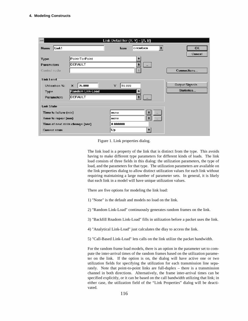
4. Modeling Constructs
idslinke ofle onutkely
k.
com-ame-wopa-ion be; inti-
116
Figure 1. Link properties dialog.
The link load is a property of the link that is distinct from the type. This avohaving to make different type parameters for different kinds of loads. The load consists of three fields in this dialog: the utilization parameters, the typload, and the parameters for that type. The utilization parameters are availabthe link properties dialog to allow distinct utilization values for each link withorequiring maintaining a large number of parameter sets. In general, it is lithat each link in a model will have unique utilization values.
There are five options for modeling the link load:
1) "None" is the default and models no load on the link.
2) "Random Link-Load" continuously generates random frames on the link.
3) "Backfill Rnadom Link-Load" fills in utilization before a packet uses the lin
4) "Analytical Link-Load" just calculates the dlay to access the link.
5) "Call-Based Link-Load" lets calls on the link utilize the packet bandwidth.
For the random frame load models, there is an option in the parameter set topute the inter-arrival times of the random frames based on the utilization parter on the link. If the option is on, the dialog will have active one or tutilization fields for specifying the utilization for each transmission line serately. Note that point-to-point links are full-duplex – there is a transmisschannel in both directions. Alternatively, the frame inter-arrival times canspecified explicitly, or it can be based on the call bandwidth utilizing that linkeither case, the utilization field of the “Link Properties” dialog will be deacvated.
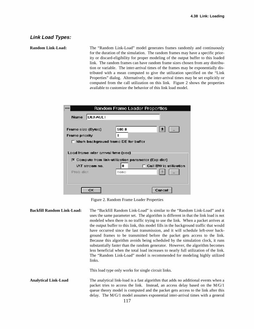
4.38 Link: Loading
uslyrior-edtribu-dis-inkr
ties
itis nots at
ack- link.runsomesink.d
en aM/G/1r thiseral
117
Link Load Types:
Random Link-Load: The “Random Link-Load” model generates frames randomly and continuofor the duration of the simulation. The random frames may have a specific pity or discard-eligibility for proper modeling of the output buffer to this loadlink. The random frames can have random frame sizes chosen from any distion or variable. The inter-arrival times of the frames may be exponentially tributed with a mean computed to give the utilization specified on the “LProperties” dialog. Alternatively, the inter-arrival times may be set explicitly ocomputed from the call utilization on this link. Figure 2 shows the properavailable to customize the behavior of this link load model.
Figure 2. Random Frame Loader Properties
Backfill Random Link-Load: The “Backfill Random Link-Load” is similar to the “Random Link-Load” and uses the same parameter set. The algorithm is different in that the link load modeled when there is no traffic trying to use the link. When a packet arrivethe output buffer to this link, this model fills in the background traffic that wouldhave occurred since the last transmission, and it will schedule left-over bground frames to be transmitted before the packet gets access to theBecause this algorithm avoids being scheduled by the simulation clock, it substantially faster than the random generator. However, the algorithm becless beneficial when the total load increases to nearly full utilization of the lThe “Random Link-Load” model is recommended for modeling highly utilizelinks.
This load type only works for single circuit links.
Analytical Link-Load The analytical link-load is a fast algorithm that adds no additional events whpacket tries to access the link. Instead, an access delay based on the queue theory model is computed and the packet gets access to the link aftedelay. The M/G/1 model assumes exponential inter-arrival times with a gen
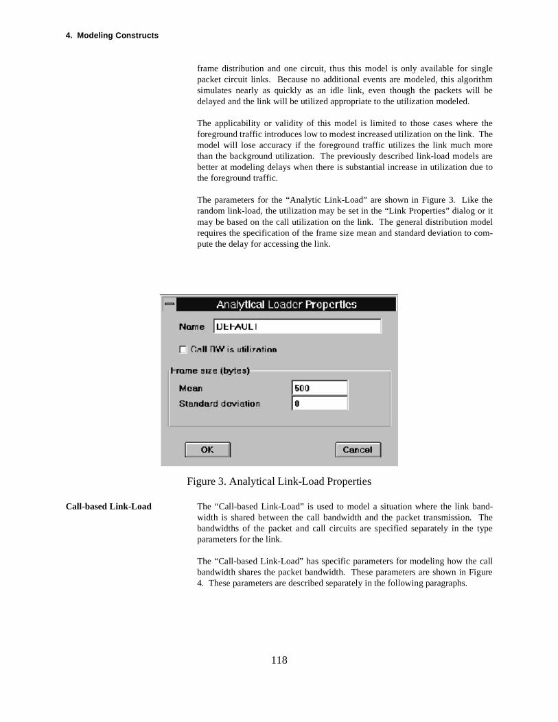
4. Modeling Constructs
gleithml be
theThe
areue to
r itodelcom-
nd- Thetype
calligure
118
frame distribution and one circuit, thus this model is only available for sinpacket circuit links. Because no additional events are modeled, this algorsimulates nearly as quickly as an idle link, even though the packets wildelayed and the link will be utilized appropriate to the utilization modeled.
The applicability or validity of this model is limited to those cases where foreground traffic introduces low to modest increased utilization on the link. model will lose accuracy if the foreground traffic utilizes the link much morethan the background utilization. The previously described link-load modelsbetter at modeling delays when there is substantial increase in utilization dthe foreground traffic.
The parameters for the “Analytic Link-Load” are shown in Figure 3. Like therandom link-load, the utilization may be set in the “Link Properties” dialog omay be based on the call utilization on the link. The general distribution mrequires the specification of the frame size mean and standard deviation to pute the delay for accessing the link.
Figure 3. Analytical Link-Load Properties
Call-based Link-Load The “Call-based Link-Load” is used to model a situation where the link bawidth is shared between the call bandwidth and the packet transmission. bandwidths of the packet and call circuits are specified separately in the parameters for the link.
The “Call-based Link-Load” has specific parameters for modeling how the bandwidth shares the packet bandwidth. These parameters are shown in F4. These parameters are described separately in the following paragraphs.
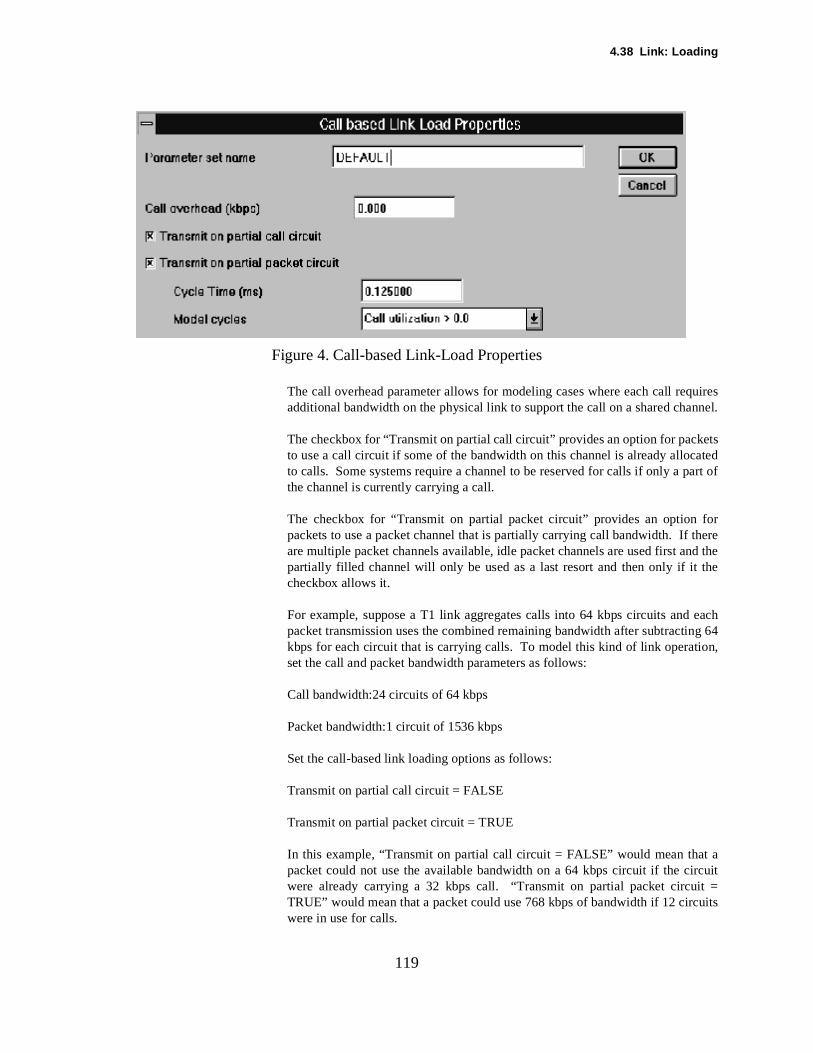
4.38 Link: Loading
uiresnnel.
tsatedart of
forhered the
the
eachng 64on,
t arcuitit =uits
119
Figure 4. Call-based Link-Load Properties
The call overhead parameter allows for modeling cases where each call reqadditional bandwidth on the physical link to support the call on a shared cha
The checkbox for “Transmit on partial call circuit” provides an option for packeto use a call circuit if some of the bandwidth on this channel is already allocto calls. Some systems require a channel to be reserved for calls if only a pthe channel is currently carrying a call.
The checkbox for “Transmit on partial packet circuit” provides an option packets to use a packet channel that is partially carrying call bandwidth. If tare multiple packet channels available, idle packet channels are used first anpartially filled channel will only be used as a last resort and then only if it checkbox allows it.
For example, suppose a T1 link aggregates calls into 64 kbps circuits andpacket transmission uses the combined remaining bandwidth after subtractikbps for each circuit that is carrying calls. To model this kind of link operatiset the call and packet bandwidth parameters as follows:
Call bandwidth:24 circuits of 64 kbps
Packet bandwidth:1 circuit of 1536 kbps
Set the call-based link loading options as follows:
Transmit on partial call circuit = FALSE
Transmit on partial packet circuit = TRUE
In this example, “Transmit on partial call circuit = FALSE” would mean thapacket could not use the available bandwidth on a 64 kbps circuit if the ciwere already carrying a 32 kbps call. “Transmit on partial packet circuTRUE” would mean that a packet could use 768 kbps of bandwidth if 12 circwere in use for calls.
4. Modeling Constructs
s an two
ithm
way)
utess asitted
aries
s)”re-r sec-
heys”.0”lgo-
ion the
120
Transmitting a packet on a channel that is partially occupied by calls requirealgorithm for the delay that the packet experiences on the link. There arealgorithms available.
1) One algorithm computes a transmission time for the packet based on the chan-nel bandwidth available at the start of the packet transmission. This algorsimulates efficiently but it can result in errors when the packet can take advan-tage of bandwidth opened up (or be penalized if more bandwidth is taken aby calls during the transmission of the packet.
2) A second algorithm slices the packet transmission into “cycles” and compthe number of bits transmitted through the channel during each cycle, thucalls are added or removed, the number of bits of the packet that are transmduring the cycle can change. This models the available bandwidth that vwhile the packet is in transmission.
The second algorithm uses the cycle time specified in the “Cycle Time (mfield. An appropriate value for many kinds of links is 0.125 milliseconds repsenting the time between voice samples when sampled at 8000 samples peond.
The “Model cycles” list box allows the selection of which algorithm is used. T“Scale entire frame once” option selects the first algorithm, and the “Alwaoption selects the second option. There is a third option “Call utilization > 0that uses the first algorithm if the call utilization is zero or uses the second arithm if the utilization is greater than zero. This third option gains simulatefficiency by assuming that packets will transmit so quickly when they havefull bandwidth that the cycles do not need to be modeled.
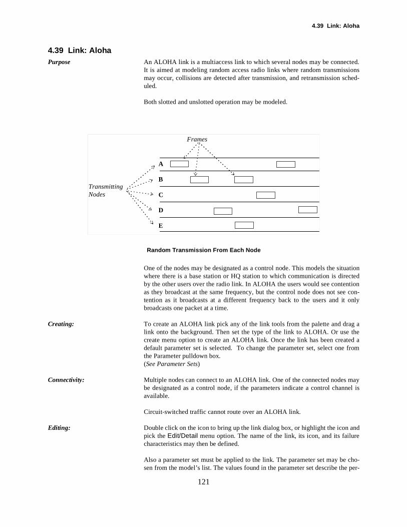
4.39 Link: Aloha
ted.sionsched-
uationctedtione con- only
g aheted ae from
maynel is
ndre
cho- per-
121
4.39 Link: AlohaPurpose An ALOHA link is a multiaccess link to which several nodes may be connec
It is aimed at modeling random access radio links where random transmismay occur, collisions are detected after transmission, and retransmission suled.
Both slotted and unslotted operation may be modeled.
Random Transmission From Each Node
One of the nodes may be designated as a control node. This models the sitwhere there is a base station or HQ station to which communication is direby the other users over the radio link. In ALOHA the users would see contenas they broadcast at the same frequency, but the control node does not setention as it broadcasts at a different frequency back to the users and itbroadcasts one packet at a time.
Creating: To create an ALOHA link pick any of the link tools from the palette and dralink onto the background. Then set the type of the link to ALOHA. Or use tcreate menu option to create an ALOHA link. Once the link has been creadefault parameter set is selected. To change the parameter set, select onthe Parameter pulldown box.(See Parameter Sets)
Connectivity: Multiple nodes can connect to an ALOHA link. One of the connected nodes be designated as a control node, if the parameters indicate a control chanavailable.
Circuit-switched traffic cannot route over an ALOHA link.
Editing: Double click on the icon to bring up the link dialog box, or highlight the icon apick the Edit/Detail menu option. The name of the link, its icon, and its failucharacteristics may then be defined.
Also a parameter set must be applied to the link. The parameter set may besen from the model’s list. The values found in the parameter set describe the
A
B
C
D
E
TransmittingNodes
Frames
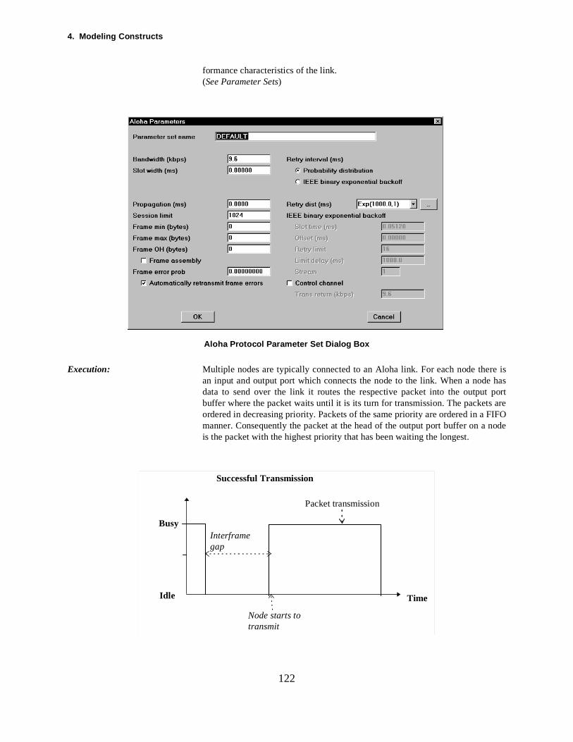
4. Modeling Constructs
re is has
port areFIFO node
122
formance characteristics of the link.(See Parameter Sets)
Aloha Protocol Parameter Set Dialog Box
Execution: Multiple nodes are typically connected to an Aloha link. For each node thean input and output port which connects the node to the link. When a nodedata to send over the link it routes the respective packet into the outputbuffer where the packet waits until it is its turn for transmission. The packetsordered in decreasing priority. Packets of the same priority are ordered in a manner. Consequently the packet at the head of the output port buffer on ais the packet with the highest priority that has been waiting the longest.
Busy
Idle
Successful Transmission
Time
Interframegap
Packet transmission
Node starts totransmit
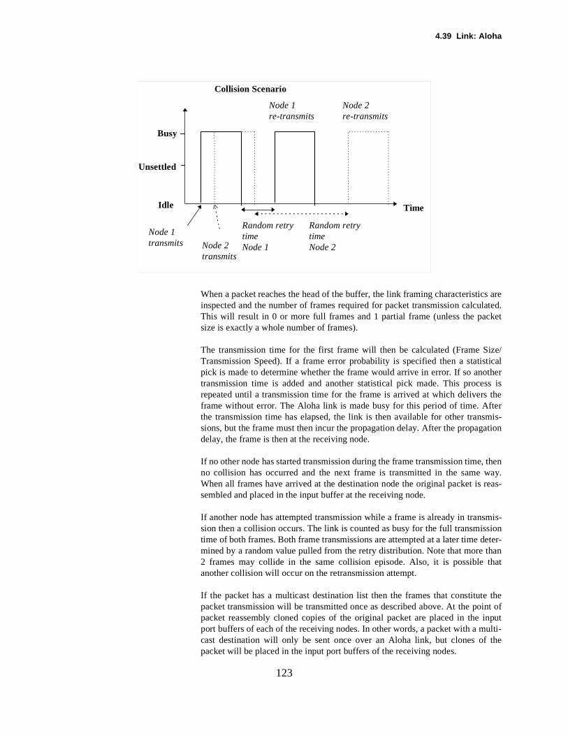
4.39 Link: Aloha
s arelated.ket
e/tical
ss is thetermis-
ation
, thenway.reas-
smis-sioneter-hanthat
e theint ofinputulti-the
123
When a packet reaches the head of the buffer, the link framing characteristicinspected and the number of frames required for packet transmission calcuThis will result in 0 or more full frames and 1 partial frame (unless the pacsize is exactly a whole number of frames).
The transmission time for the first frame will then be calculated (Frame SizTransmission Speed). If a frame error probability is specified then a statispick is made to determine whether the frame would arrive in error. If so anothertransmission time is added and another statistical pick made. This procerepeated until a transmission time for the frame is arrived at which deliversframe without error. The Aloha link is made busy for this period of time. Afthe transmission time has elapsed, the link is then available for other transsions, but the frame must then incur the propagation delay. After the propagdelay, the frame is then at the receiving node.
If no other node has started transmission during the frame transmission timeno collision has occurred and the next frame is transmitted in the same When all frames have arrived at the destination node the original packet is sembled and placed in the input buffer at the receiving node.
If another node has attempted transmission while a frame is already in transion then a collision occurs. The link is counted as busy for the full transmistime of both frames. Both frame transmissions are attempted at a later time dmined by a random value pulled from the retry distribution. Note that more t2 frames may collide in the same collision episode. Also, it is possible another collision will occur on the retransmission attempt.
If the packet has a multicast destination list then the frames that constitutpacket transmission will be transmitted once as described above. At the popacket reassembly cloned copies of the original packet are placed in the port buffers of each of the receiving nodes. In other words, a packet with a mcast destination will only be sent once over an Aloha link, but clones of packet will be placed in the input port buffers of the receiving nodes.
Busy
Unsettled
Idle
Collision Scenario
Node 1transmits Node 2
transmits
Time
Random retrytimeNode 2
Node 1re-transmits
Node 2re-transmits
Random retrytimeNode 1
4. Modeling Constructs
e areiffer-izeso the
ck-
otherannel
ansrans-ssion
two
t foraga-t
s thedy atthen
124
If slotted operation is being used then the frame transmissions at each nodalways attempted on a slot boundary. If two frames begin transmission at dent slot boundaries, then they will not collide, given properly chosen frame sand slot times. This has the effect of lessening the total amount of time lost tcollision episodes and improves the throughput performance of the link.
Reporting: Link Delays & Utilization ReportRandom Access Link Performance Report
Fields:
Name An alphanumeric field to identify the link. The name must be unique in the babone or subnetwork.
Icon The name of the icon used to represent the link.
Control Node The name of the node which is the control node for the ALOHA link. A controlnode has an independent, contention free channel to communicate with thenodes on the link. The control node is deselected unless the control chcheck box is ticked on the link parameters screen.
Time To Failure (see Link)
Time To Repair (see Link)
Time Of Next State Change (see Link)
Current State (see Link)
Statistics Contention and control channel utilization.(see Statistics: Link)
Parameter Set Fields:
Bandwidth The speed of the link in kilobits per second.
Slot Width If no slot time is entered, COMNET III models unslotted operation. This methat any node may attempt to transmit at any time. If a collision occurs, the tmission continues until the end, the collision is detected, and a retransmiwill then be attempted after the retry time.
If a slot time is entered, a node will only transmit on a slot time boundary. If frames begin transmission at different slot boundaries, then they will not collide,given properly chosen frame sizes and slot times.
Propagation Delay The time to propagate a signal across a link. This is generally not significanterrestrial radio links. For satellite links to geostationary satellites the proption delay is of the order of 270-300 milliseconds. Propagation delay does noaffect link utilization statistics.
Session Limit The maximum number of sessions that can be concurrently routed acroslink. If a session setup packet attempts to route across a link which is alreaits session limit, the routing attempt fails. The alternate routes (if any) are
4.39 Link: Aloha
ssion
ons ran-ed as
s—
con-
125
tested. If there is still no route the session setup packet is blocked. The SeLimit only applies if connection-oriented routing is used.
Framing Characteristics The framing characteristics for the link. Packets are broken down into transmis-sion frames which are then modeled as being transmitted across the link.(see Link:Framing )
Retry Interval On the ALOHA protocol, if two or more nodes have overlapping transmissithen a collision occurs. In this event, the transmitting nodes will each pick adom retry time and attempt transmission again. The retry time can be entereither:
Probability DistributionUse any of the standard COMNET III distributions.(see Distributions: System)
Binary Exponential BackoffThis algorithm is defined by the IEEE for use in collision detecting protocolparticularly CSMA/CD. It may also be picked for the ALOHA retry interval.(see Link: Binary Exponential Backoff)
Control Channel Check box to indicate whether there is a control channel on this link.
Transmission Return Rate If there is a control channel, what is its speed for transmission between thetrol node and the other nodes on the link.
4. Modeling Constructs
ev-wherenset-
eferre-
ns- not notndomission
ver
time
. If
dom
untilnd
n have
g a
thet
y be
ndre
126
4.40 Link: CSMAPurpose A CSMA (Carrier Sense Multiple Access) link is a multiaccess link to which s
eral nodes may be connected. It is aimed at modelling random access links random transmissions may occur, but only if the link is detected as idle (or utled). Like, in Aloha, collisions are detected, and retransmissions will be sched-uled.
CSMA differs from Aloha in that a node may detect that a link is busy and dits transmission until the link is idle. With Aloha, the transmission occurs irspective of whether the link is idle or not.
CSMA differs from CSMA/CD in that collisions are detected at the end of tramission rather than at the instant when the collision occurs. CSMA doesreally do collision detection; it relies on timeouts to indicate that a frame wasdelivered (for whatever reason) and schedules retransmission after a radelay. This means that there is wasted bandwidth on CSMA as the transmduration is effectively lost.
With 1-persistent CSMA, each station transmits with a probability of 1 wheneit finds the link idle. The stations continuously sense the carrier when it is busyand start to send as soon as it is idle. On collision, it backs off for a randomperiod.
With p-persistent CSMA, a station transmits only with a certain probabilitythe channel is found to be idle, a random number is generated. If this is greaterthen p, then the station defers the transmission until the next slot. If the rannumber is less than or equal to p, the station starts transmission.
With non-persistent CSMA, a station does not keep on sensing the channelit is idle. If it finds the link busy, it waits a random interval without sensing athen senses again after this interval has elapsed.
COMNET III only models 1-persistent CSMA.
One of the nodes may be designated as a control node. This node may thea contention free channel to communicate with the other nodes on the link.
Creating: To create a CSMA link pick the appropriate link tool from the palette and dralink onto the background. Or use the create menu option to create a CSMA link.Double clicking on the icon brings up a dialog box where you can indicate intype box to use CSMA operation. Once the link has been created a parameter semust be applied to it via a selection in the Parameter pulldown box.(See Parameter Sets)
Connectivity: Multiple nodes can connect to a CSMA link. One of the connected nodes madesignated as a control node.
Circuit-switched traffic cannot route over a CSMA link.
Editing: Double click on the icon to bring up the link dialog box, or highlight the icon apick the Edit/Detail menu option. The name of the link, its icon, and its failucharacteristics may then be defined.
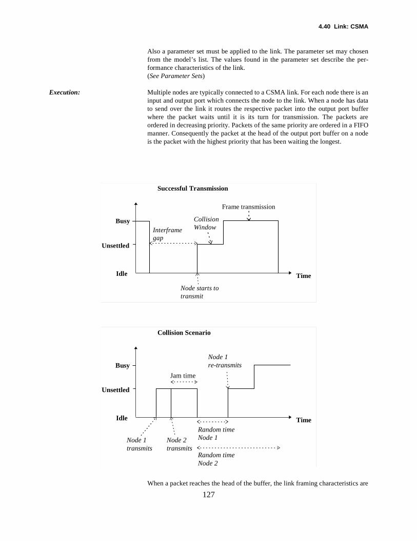
4.40 Link: CSMA
hosenr-
s an data
areFIFO node
s are
127
Also a parameter set must be applied to the link. The parameter set may cfrom the model’s list. The values found in the parameter set describe the peformance characteristics of the link.(See Parameter Sets)
Execution: Multiple nodes are typically connected to a CSMA link. For each node there iinput and output port which connects the node to the link. When a node hasto send over the link it routes the respective packet into the output port bufferwhere the packet waits until it is its turn for transmission. The packets ordered in decreasing priority. Packets of the same priority are ordered in a manner. Consequently the packet at the head of the output port buffer on ais the packet with the highest priority that has been waiting the longest.
When a packet reaches the head of the buffer, the link framing characteristic
Busy
Unsettled
Idle
Successful Transmission
Time
Interframegap
CollisionWindow
Frame transmission
Node starts totransmit
Busy
Unsettled
Idle
Collision Scenario
Node 1transmits
Node 2transmits
Time
Jam time
Random timeNode 1
Random timeNode 2
Node 1re-transmits
4. Modeling Constructs
lated.ket
inkthen
Thesiontosionntil aoutfter
the
reas-
link are
ptedledn theion
retryan 2 that
e theint ofinputulti-the
ck-
trol
128
inspected and the number of frames required for packet transmission calcuThis will result in 0 or more full frames and 1 partial frame (unless the pacsize is exactly a whole number of frames).
If the link is busy, the transmission attempt will be deferred until the lbecomes idle, plus a time delay equal to the interframe gap. If the link is idle a transmission attempt can be made immediately.
The link is then placed in an unsettled state for the collision window period. transmission time for the frame will be calculated (Frame Size/TransmisSpeed). If a frame error probability is specified then a statistical pick is made determine whether the frame would arrive in error. If so another transmistime is added and another statistical pick made. This process is repeated utransmission time for the frame is arrived at which delivers the frame witherror. The link is then made busy for the calculated transmission time, awhich it is made idle. The link is then available for other transmissions, butframe must then incur the propagation delay. After the propagation delay theframe is then at the receiving node.
When all frames have arrived at the receiving node the original packet is sembled and placed in the input buffer at the receiving node.
The most likely collision scenario occurs when two or more nodes sense theis busy and wait until it becomes idle to start transmitting. Since two or moretrying to transmit at the same time, collisions result.
Another, less likely, collision scenario occurs if another node has attemtransmission during the collision window while the CSMA link is in an unsettstate. Both nodes keep transmitting for the calculated transmission time. Thelink may be jammed for the optional jam time to alert all stations that a collisepisode has occurred. A random pull is then made for each frame from thedistribution and both frame transmissions attempted later. Note that more thframes may collide in the same collision episode. Also there is no guaranteeanother collision will not reoccur on the retransmission attempt.
If the packet has a multicast destination list then the frames that constitutpacket transmission will be transmitted once as described above. At the popacket reassembly cloned copies of the original packet are placed in the port buffers of each of the receiving nodes. In other words, a packet with a mcast destination will only be sent once over a CSMA link, but clones of packet will be placed in the input port buffers of the receiving nodes.
Reporting: Link Delays & Utilization ReportRandom Access Link Performance Report
Fields:
Name An alphanumeric field to identify the link. The name must be unique in the babone or subnetwork.
Icon The name of the icon used to represent the link.
Control Node The name of the node which is the control node for the CSMA link. A con
4.40 Link: CSMA
otherannel
ins
mis-jamas
ns-
s itsing aeachait-
emptsmpt ses-
ions jam
129
node has an independent, contention free channel to communicate with thenodes on the link. The control node is deselected unless the control chcheck box is ticked on the link parameters screen.
Time To Failure (see Link)
Time To Repair (see Link)
Time Of Next State Change (see Link)
Current State (see Link)
Statistics Contention and control channel utilization.(see Statistics: Link)
Parameter Set Fields :
Bandwidth The speed of the link in kilobits per second.
Collision Window The period of time that the link is vulnerable to collision after a node begtransmitting.
Jam Interval With CSMA, after a node recognizes a collision at the end of a frame transsion, it may send a jamming signal to alert other nodes of collision for the interval. After a collision, the link is not idle again until the jam time hexpired.
With CSMA the jam time is used to model the interval from the end of the tramission until the sending node learns that retransmission is required.
Interframe Gap The duration of an interframe gap which is the length of time a node delaytransmission attempt after a link becomes idle. The node may be transmittnumber of frames sequentially—the interframe gap is applied between frame followed by recontention for the link. Alternatively, the node may be wing for a transmission by another node to finish—again it will wait the interframegap after transmission completes before contending for the link.
Propagation Delay The time to propagate a signal across a link.
Session Limit If connection-oriented routing is used, this is the maximum number of sessionsthat can be concurrently routed across the link. If a session setup packet attto route across a link which is already at its session limit, the routing attefails. The alternate routes (if any) are then tested. If there is still no route thesion setup packet is blocked.
Framing Characteristics The framing characteristics for the link. Packets are broken down into transmis-sion frames which are then modeled as being transmitted across the link.(see Link:Framing )
Retry Interval On the CSMA protocol, if two or more nodes have overlapping transmissthen a collision occurs. In this event the transmitting nodes will each wait thetime followed by a random retry time and attempt transmission again. The retrytime can be entered as either:

4. Modeling Constructs
to-
130
Probability DistributionUse any of the standard COMNET III distributions.(see Distributions)
Binary Exponential BackoffThis algorithm is defined by the IEEE for use in 802.3 collision detecting procols.(see Link: Binary Exponential Backoff)
Control Channel Check box to indicate whether there is a control channel on this link.
Transmission Return Rate If there is a control channel, specifies its speed in kilobits per second.
4.41 Link: CSMA/CA Wireless LAN IEEE 802.11
Dis-cifi-
othereed.
eendium is
Aftersful
ts thevalA/CA
ions
dom allCK
hysi-ps or
f 1
.tem.
inU)r thel, thees. pre-for a
,
em.tion.
131
4.41 Link: CSMA/CA Wireless LAN IEEE 802.11Purpose: The CSMA/CA model is a shared medium access mechanism based on the
tributed Convergence Function (DCF) of the IEEE 802.11 Wireless LAN specation. The basic procedure for accessing the shared medium is as follows.
Each station wishing to transmit first senses the medium to determine if anstation is transmitting. If the medium is not busy, the transmission may procThe IEEE802.11 distributed algorithm mandates that a gap of a minimum speci-fied duration (called the Distributed Inter-Frame Space, or DIFS) exists betwcontiguous frame transmissions. A transmitting station ensures that the meis idle for this DIFS duration before attempting to transmit. If the mediumsensed busy, the station defers until the end of the current transmission. deferral, or prior to attempting to transmit again immediately after a succestransmission, the station selects a random backoff interval and decremenbackoff interval counter while the medium is free. When the backoff intercounter reaches zero, the station proceeds to transmit the data. The CSMprotocol is designed to reduce rather than eliminate the collision probabilitybetween multiple stations accessing a medium at the point where colliswould most likely occur. Just after the medium becomes free following a busyperiod is when the highest probability of a collision occurs. Therefore a ranbackoff arrangement is immediately applied in this situation. In addition,directed (non-multicast) traffic uses immediate positive acknowledgments (Aframes). Retransmission is scheduled by the sender if no ACK is received.
Bandwidth: This parameter defines the bit rate supported by the 802.11 wireless LAN pcal medium. The supported data rates in the IEEE standard are either 1 Mb2 Mbps (but COMNET III does not limit you to these values).
Propagation: This parameter specifies the air propagation time it takes a transmitted signal togo from the transmitting station to the receiving station. A nominal value omicrosecond has been allocated for this parameter in the IEEE 802.11.
Slot time: The parameter Slot time is used to define the Short and Distributed InterframeSpaces and to update the backoff interval in the shared medium access algorithmA nominal value of 6 microseconds is specified for the infrared physical sysUsers shall specify this value according to their manufacturer’s product specifi-cation.
Short IFS: The Short Interframe Space is the shortest of the interframe spaces definedIEEE 802.11. It is used to provide an efficient MAC Service Data Unit (MSDdelivery mechanism. Once the medium is seized, the station will keep it foduration of the frame exchange it has to perform. In the implemented modeShort IFS is used between fragments of one MSDU and their ACK framUsing the smallest gap between transmissions within the frame exchangevents other stations, which are required to wait for the medium to be free longer gap (the Distributed IFS, see below) from attempting to use the mediumthus giving priority to completion of the frame exchange in progress.
A nominal value of 7 microseconds is specified for infrared physical systUser shall specify this parameter based on manufacturer’s product specifica
The Short IFS (SIFS) is also used to compute the Distributed IFS (DIFS) basedon the following equation:
4. Modeling Constructs
tialm to
for
2-bittationfault
f thehe
ation by) ingerified (ordent
smis-
sys-truma sin-nce
s (by
can theme orrtu-
s
e, in
beent.
sion
ion is theCKhe sta- thesion
132
Distributed IFS = Short IFS + 2 * Slot Time
The DIFS is used by the CSMA/CA model to contend for the channel for iniframe transmissions. A station is allowed to transmit if it detects the mediube free for the DIFS duration and its backoff time has expired.
Frame max: This parameter specifies the maximum MSDU length that will be acceptedtransmission. The default value is 2304 octets.
Frame OH: The frame overhead parameter includes the 802.11 MAC header, an IEEE 3CRC, and 8 octets of shared key for authentication. In the case of fragmen(see below), this is also the overhead of transmitting a fragment. The devalue of the frame overhead is 42 octets.
Frgmt thrshld: The fragmentation threshold specifies the current maximum size, in octets, oMac Protocol Data Unit (MPDU) that will be delivered to the physical layer. Tdefault value is 2304, which is equal to the maximum frame size. Fragmentcreates MPDUs smaller than the MSDU (frame) size to increase reliabilityincreasing the probability of successful transmission of the MSDU (framecases where channel characteristics limit transmission reliability for lonframes. When a frame is received with MSDU size greater than the spec“Fragmentation Threshold,” the frame must be fragmented. The MPDUsfragments) resulting from the fragmentation of an MSDU are sent as indepentransmissions, each of which is separately acknowledged. This permits transion retries to occur per fragment, rather than per MSDU (frame).
Unless interrupted due to medium occupancy limitations for a given physicaltem, such as a dwell time boundary in a Frequency Hopping Spread Spec(FHSS) system, the fragments of a single MSDU are sent as a burst, using gle invocation of the CSMA/CA medium access procedure. In other words, othe station has contended for the channel, it will continue to send fragmentusing the Short Interframe Space instead of the Distributed Interframe Space)until either all fragments of a MSDU have been sent, an acknowledgment is notreceived for directed data due to collision or transmission error, or the stationnot send any additional fragments due to a dwell time boundary. Shouldsending of the fragments be interrupted due to one of these reasons, the frathe fragment will enter a retransmission backoff period; when the next opponity for transmission occurs the station resumes sending the rest of the fragmentof the frame.
Frgmt error prob: This parameter specifies the error rate of transmitting one fragment (or framcase of no fragmentation) over the physical medium.
ACK timeout: This parameter specifies the length of time by which an ACK frame shouldreceived in response to transmission of a frame which requires acknowledgmIt is timed from the instant that the transmitting station finishes the transmisof the frame or fragment.
The reception of an unicast frame (or fragment in the case where fragmentatneeded) requires the receiving station to respond with an ACK frame, ifreceived frame (fragment) is correct. Lack of reception of an expected Aframe indicates to the source station that an error has occurred and causes ttion to retransmit the frame (or fragment). An erroneous ACK frame causesretransmission of the transmitted frame (or fragment) as well. The transmis

4.41 Link: CSMA/CA Wireless LAN IEEE 802.11
.
the
afterthe per
Thedwellin.
ingsmit-s to
-
tion
f the
nched,ticsme-it in
isck-hen
thencre-
133
of the ACK frame commences after the Short IFS without regard to the busy/freestate of the medium.
The ACK Timeout may not be less than (2 * Propagation + Short IFS + AckTransmission Time). Otherwise an error message will occur in the dialog box
ACK error prob: This parameter specifies the error rate of transmitting an ACK frame overphysical medium. An ACK frame is 14 octets long.
Frame TxLifeTime: The frame transmission life time parameter is defined as the elapsed time,initial transmission of an MSDU, after which further attempts to transmit MSDU will be terminated. Therefore, this parameter is per frame and notfragment. The default value is 512 milliseconds.
FH dwell time: The FH dwell time parameter is specified for an FHSS physical system. attribute is defined as the time the physical medium dependent system can on an FH channel and meet the requirements of the current regulatory doma
In the implemented CSMA/CA model, the FH dwell time is used for determinif the station can retain the control of the channel during the process of tranting fragments of an MSDU. Once the dwell boundary is up, the frame haenter the backoff period and contend again for the channel.
IEEE 802.11 Backoff: This part of the dialog box provides a group of parameters for the backoff algorithm. A station that desires to initiate transfer of data and finds the medium busyfollows the backoff procedure. To begin the backoff procedure, the staselects a backoff time based on the following equations.
Backoff Time = INT(CW * Random()) * Slot Time
where:
CW = An integer between the values of CW min and CW maxRandom() = Pseudo-random number between 0 and 1Slot Time = the value specified above
The Contention Window (CW) parameter takes an initial value of the CW min forevery MPDU queued for transmission. The CW will take the next value in theseries at every retry to send a particular MPDU until it reaches the value oCW max. The set of CW values are 7 (CW min), 15, 31, 63, 127, 255 (CW max).
The parameter “Retry limit” indicates the maximum number of retransmissioattempts of a fragment. It is set as the default value 7. Once this limit is reaa failure condition is indicated to the next higher layer. Note that the statisreport on “Number of tries to resolve” may have a bigger value than this parater. This is because the statistics field is on frame basis while the retry limthe implemented CSMA/CA is on fragment basis.
All backoff periods occur following a DIFS period during which the mediumfree. A station in backoff monitors the medium for carrier activity during baoff periods. If no carrier activity is seen for the duration of a particular slot, tthe random backoff process decrements the backoff timer by Slot time specifiedabove. If there is carrier activity sensed at any time during a backoff period, the backoff procedure is suspended; that is, the backoff timer will not be de
4. Modeling Constructs
n of aom-
y toair-
preta-oretry
the OFrors.
134
ment for that slot. The medium must be sensed as idle again for the duratioDIFS before the backoff procedure is allowed to resume. Transmission cmences whenever the backoff timer reaches zero.
A station that had just transmitted an MSDU and has another MSDU readtransmit will perform the backoff procedure in order to produce a level of fness of access to the medium amongst stations.
Some of the performance measures on the output reports have special intertions for CSMA/CA links. On the Channel Utilization report, the column fFRAMES RST/ERR shows a count of the number of frames that reach the RLimit or the XmitLifeTime. On the same report, utilization does not include time required for transmissions in error. On the Collision Stats report, NBRTRIES TO RESOLVE includes retransmissions due to both collisions and er

4.42 Link: CSMA/CD
aodel-s areIEEEernet
the
n have
ndayounce
SMA/00BaseT
2
135
4.42 Link: CSMA/CDPurpose A CSMA/CD (Carrier Sense Multiple Access With Collision Detection) link is
multiaccess link to which several nodes may be connected. It is aimed at mling random access links where random transmissions may occur, collisiondetected, and retransmission scheduled. The protocol is modeled on the 802.3 standards and, as such, is suitable for modelling a wide variety of Ethbased protocols.
A number of CSMA/CD implementations are contained in the system library,details of which are outlined in the table below.
One of the nodes may be designated as a control node. This node may thea contention free channel to communicate with the other nodes on the link.
Creating: To create a CSMA/CD link pick the appropriate link tool from the palette adrag a link onto the background. Or use the create menu option to create CSMA/CD link. On the dialog box accessed via double clicking on the icon, can indicate in the type box whether to use CSMA or CSMA/CD operation. O
Table 1: CSMA/CD Implementation Details
CSMA/CD10Base5
CSMA/CD10Base2
CSMA/CD1Base5
CSMA/CD1Base5 Star
CSMA/CD10BaseT
TOPEthernet 10Base5
CCD1
Media Coax 50 Ohm
Coax 50 Ohm
Unshielded Twisted Pair
Unshielded Twisted Pair
Unshielded Twisted Pair
Coax50 Ohm
Diameter mm 10 5 0.4-0.6 0.4-0.6 0.4-0.6 10
Max segment length m 500 185 500 500 100 500
Max length m 2500 925 2500 2500 500 2500
Transmission speed km/sec
231000 195000 177000 177000 177000 231000
Max propagation delay ms.
0108225 0.0047358 .01412420 . 00282485 .0108225
Nodes per segment 100 30 - - 100
Data Rate Mbps 10 10 1 1 10 10 10
Collision Window ms .01 .0018 .14 .1 .002 .01 .01 .002
Jam Time ms .0032 .0032 .032 .032 .0032 .0032 .0032 .0032
Interframe Gap ms .0096 .0096 .096 .096 .0096 .0096 .0096 .0096
Propagation Delay
Session Limit 1024 1024 1024 1024 1024 1024 1024 1024
Frame Min 72 72 72 72 72 72 72 72
Frame Max 1526 1526 1526 1526 1526 1526 1526 1526
Frame Overhead 30 30 30 29 30 29 26 30
Slot Time ms .0512 .0512 .0512 .0512 .0512 .0512 .0512 .0051
Offset ms 0 0 0 0 0 0 0 0
Retry Limit 16 16 16 16 16 16 16 16
Limit Delay ms 1000 1000 1000 1000 1000 1000 1000 1000
4. Modeling Constructs
tion in
des
ndre
cho- per-
eree has port areFIFO node
lated.ket
inkthen
iod.is-
. If aineded
issionk is idle.ncurceiv-
reas-
the fordomans-
136
the link has been created a parameter set must be applied to it via a selecthe Parameter pulldown box.(See Parameter Sets)
Connectivity: Multiple nodes can connect to a CSMA/CD link. One of the connected nomay be designated as a control node.
Circuit-switched traffic cannot route over a CSMA/CD link.
Editing: Double click on the icon to bring up the link dialog box, or highlight the icon apick the Edit/Detail menu option. The name of the link, its icon, and its failucharacteristics may then be defined.
Also a parameter set must be applied to the link. The parameter set may besen from the model’s list. The values found in the parameter set describe theformance characteristics of the link.(See Parameter Sets)
Execution: Multiple nodes are typically connected to a CSMA/CD link. For each node this an input and output port which connects the node to the link. When a noddata to send over the link it routes the respective packet into the outputbuffer where the packet waits until it is its turn for transmission. The packetsordered in decreasing priority. Packets of the same priority are ordered in a manner. Consequently the packet at the head of the output port buffer on ais the packet with the highest priority that has been waiting the longest.
When a packet reaches the head of the buffer the link framing characteristics areinspected and the number of frames required for packet transmission calcuThis will result in 0 or more full frames and 1 partial frame (unless the pacsize is exactly a whole number of frames).
If the link is busy, the transmission attempt will be deferred until the lbecomes idle, plus a time delay equal to the interframe gap. If the link is idle a transmission attempt can be made immediately.
The link is then placed in an unsettled state for the collision window perAssuming the no collisions have occurred in the collision window the transmsion time for the frame will be calculated (Frame Size/Transmission Speed)frame error probability is specified then a statistical pick is made to determwhether the frame would arrive in error. If so another transmission time is adand another statistical pick made. This process is repeated until a transmtime for the frame is arrived at which delivers the frame without error. The linthen made busy for the calculated transmission time, after which it is madeThe link is then available for other transmissions, but the frame must then ithe propagation delay. After the propagation delay the frame is then at the reing node.
When all frames have arrived at the receiving node the original packet is sembled and placed in the input buffer at the receiving node.
If another node has attempted transmission during the collision window whileCSMA/CD link is in an unsettled state, a collision occurs. The link is jammedthe jam time to alert all stations that a collision episode has occurred. A ranpull is then made for each frame from the retry distribution and both frame tr
4.42 Link: CSMA/CD
n thel not
e theint ofinputulti-
the
ck-
on-h theannel
ins thisway
y bed a
l to
137
missions are attempted later. Note that more than 2 frames may collide isame collision episode. Also there is no guarantee that another collision wilreoccur on the retransmission attempt.
If the packet has a multicast destination list then the frames that constitutpacket transmission will be transmitted once as described above. At the popacket reassembly cloned copies of the original packet are placed in the port buffers of each of the receiving nodes. In other words, a packet with a mcast destination will only be sent once over a CSMA/CD link, but clones ofpacket will be placed in the input port buffers of the receiving nodes.
Reporting: Link Delays & Utilization ReportRandom Access Link Performance Report
Fields:
Name An alphanumeric field to identify the link. The name must be unique in the babone or subnetwork.
Icon The name of the icon used to represent the link.
Control Node The name of the node which is the control node for the CSMA/CD link. A ctrol node has an independent, contention free channel to communicate witother nodes on the link. The control node is deselected unless the control chcheck box is ticked on the link parameters screen.
Time To Failure (see Link)
Time To Repair (see Link)
Time Of Next State Change (see Link)
Current State (see Link)
Statistics Contention and control channel utilization.(see Statistics: Link)
Parameter Set Fields:
Bandwidth The speed of the link in kilobits per second.
Collision Window The period of time that the link is vulnerable to collision after a node begtransmitting. On a 2500 meter cable at 4.33 microseconds per kilometer,would be approximately .01 milliseconds. The worst case would be the two transmission time between nodes at the opposite end of the cable—the averagecase for 2 arbitrary nodes would be half the worst case. This window maadjusted for different conditions: a smaller window for short connections anlonger interval for long connections.
Jam Interval With CSMA/CD, after a node recognizes a collision it sends a jamming signaalert other nodes of the collision for the jam interval. After a collision the link isnot idle again until the jam time has expired.
4. Modeling Constructs
ans-
s itsing aeachait-
ap
ng
ses-ackettingoute
is-n a
imetime
to-
138
In contrast, CSMA models the jam time as the interval from the end of the trmission until the sending node learns that retransmission is required.
Interframe Gap The duration of an interframe gap which is the length of time a node delaytransmission attempt after a link becomes idle. The node may be transmittnumber of frames sequentially—the interframe gap is applied between frame followed by recontention for the link. Alternatively, the node may be wing for a transmission by another node to finish—again it will wait the interframegap after transmission completes before contending for the link.
The default value for a 10MB IEEE 802.3 LAN is .0096 milliseconds. This gprovides recovery time for other Ethernet stations and provides opportunity forother stations to acquire the link by colliding with (interrupting) a station’s losequence of frames.
Propagation Delay The time to propagate a signal across a link.
Session Limit If connection-oriented routing is used, then this is the maximum number of sions that can be concurrently routed across the link. If a session setup pattempts to route across a link which is already at its session limit, the rouattempt fails. The alternate routes (if any) are then tested. If there is still no rthe session setup packet is blocked.
Framing Characteristics The framing characteristics for the link. Packets are broken down into transmis-sion frames which are then modeled as being transmitted across the link.(see Framing Characteristics)
Retry Interval On the CSMA/CD protocol, if two or more nodes have overlapping transmsions (i.e., two or more transmission attempts within the collision window) thecollision occurs. In this event the transmitting nodes will each wait the jam tfollowed by a random retry time and attempt transmission again. The retry can be entered as either:
Probability DistributionUse any of the standard COMNET III distributions.(see Distributions)
Binary Exponential BackoffThis algorithm is defined by the IEEE for use in 802.3 collision detecting procols.(see Link: Binary Exponential Backoff)
Control Channel Check box to indicate whether there is a control channel on this link.
Transmission Return Rate If there is a control channel, specifies its speed in kilobits per second.

4.43 Link: Demand-Assigned Mul tiple Access (DAMA)
toint-to-themeo theamit
th the
139
4.43 Link: Demand-Assigned Multiple Access (DAMA)Purpose: The Demand-Assigned Multiple Access (DAMA) link allows multiple nodes
share a pool of circuits. The link has the same set of parameters as a popoint link and can carry both packets and circuit-switched calls. As with point-to-point link, the DAMA link allows calls and packets to share the sabandwidth using the call-based link loading option. Each node connected tDAMA link can access only 1 circuit of the DAMA link’s pool of circuits at time. A circuit is allocated to a node for the amount of time required to transa packet. When several nodes are waiting to transmit packets, the node wiearliest arriving packet uses the first circuit to become available.
4. Modeling Constructs
tydoack ofrelin-e left
has athe
vily
time the con-
psedTRT,
aiting time
e, sotherrent are
d to
thatse thed to
bethes in-s to
140
4.44 Link: FDDI and Priority FDDIPurpose: COMNET III includes two models of FDDI--a Basic FDDI model and a Priori
FDDI model. As with the token-passing link, the COMNET III FDDI models not actually schedule each token-passing event; instead, the model keeps trthe last node to have relinquished the token and the time when the node quished the token. Given the last token location and the time that the framthat location, COMNET III computes the appropriate amount of time (tokenpassing delay) required for the token to advance the next time some nodeframe to transmit. COMNET III monitors the actual token rotation time and token-ring report includes a count of the number of times that the actual tokenrotation time exceeds twice the target token rotation time to help identify healoaded conditions that may trigger FDDI re-initialization.
The Basic FDDI model has a Token-Passing Delay that determines the required to pass the token from one node on the FDDI’s connection list tonext node on the connection list. The time that a node can hold the token istrolled through the Target Token Rotation Time (TTRT). When a node receivesthe token, before transmitting a frame it determines the time that has elasince the node last received the token. If the elapsed time exceeds the Tthen the node passes the token to the next node without transmitting the wframe. The node can continue to transmit frames as long as the elapsedsince last receiving the token does not exceed the TTRT.
The Priority FDDI model allows the TTRT to vary by frame priority which is thhighest priority of the packets it carries. The TTRTs can also vary by portthat some nodes on the Priority FDDI link can hold the token longer than onodes. The priority FDDI parameter set maintains a list of tables for diffetoken rotation time targets (T_Pr) that vary by priority and the different tablesavailable for assignment to different ports (node interfaces). By default, there isone table called “DEFAULT” and it will be assigned to each new port addethe link.
The Priority FDDI parameter set dialog box has a button “T_Pr tablesÖ” manages the sets of tables that may be assigned to the individual ports. U“T_Pr tablesÖ” button to edit the list of port properties available to be assigneeach port connecting to the priority FDDI link. Each port properties dialog boxconsists of a table of threshold values for different levels of priority that mayedited as shown in the following dialog. The table shows the lower limit of frame priority that will use the threshold values in the T_Pr column. PrioritieCOMNET III are such that the larger the number the higher the priority. Generally the threshold token-rotation times should increase for increasing prioritieallow those priorities to use the link longer than the lower priorities.
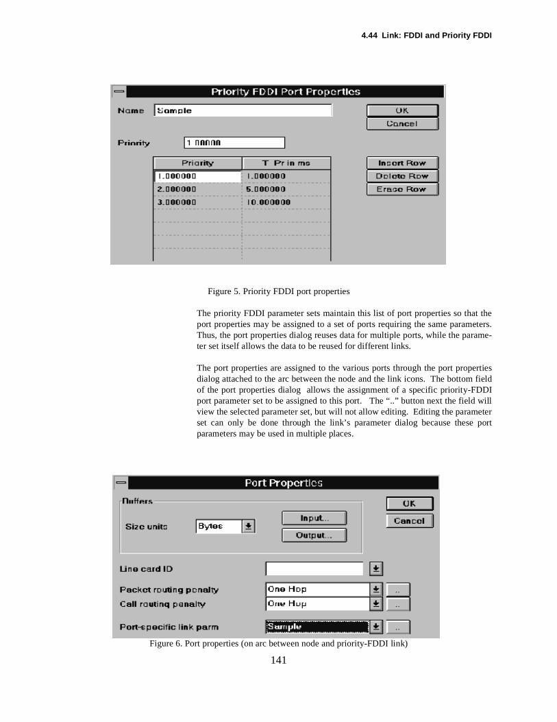
4.44 Link: FDDI and Priority FDDI
theeters.
field
willeter port
141
Figure 5. Priority FDDI port properties
The priority FDDI parameter sets maintain this list of port properties so thatport properties may be assigned to a set of ports requiring the same paramThus, the port properties dialog reuses data for multiple ports, while the parame-ter set itself allows the data to be reused for different links.
The port properties are assigned to the various ports through the port propertiesdialog attached to the arc between the node and the link icons. The bottomof the port properties dialog allows the assignment of a specific priority-FDDIport parameter set to be assigned to this port. The “..” button next the fieldview the selected parameter set, but will not allow editing. Editing the paramset can only be done through the link’s parameter dialog because theseparameters may be used in multiple places.
Figure 6. Port properties (on arc between node and priority-FDDI link)

4. Modeling Constructs
EEon toior-era-
142
The priority FDDI is closely related to the priority scheme used in the IE802.4 standard except that in 802.4 the highest priority frame has permissitransmit for a holding limit instead of a token-rotation threshold time. The Prity FDDI parameter set has an option to use this 802.4 option of priority option and provides a field for specifying the holding limit value.
4.45 Link: Point-To-Point
sedtlan-
alnnels.ad of
y bes-
tteacon linkin the
ode
ndre
cop-uesnk.
143
4.45 Link: Point-To-PointPurpose A point-to-point link connects two nodes together. It is aimed at modelling lea
lines, serial lines, trunk circuits, and general WAN data paths (such as transatic links or satellite links) established between two points.
For data communications the point-to-point link is a full duplex bidirectioncommunications path that is characterized by its speed and number of chaFrames are multiplexed onto the link in the order that they appear at the hethe link port transmission buffer.
For voice or circuit-switched traffic, separate bandwidth and/or channels madefined. Only point to point links may carry circuit-switched traffic on their deignated circuit-switched capacity.
Creating: To create a Point-To-Point link, pick the appropriate link tool from the paleand drag a link onto the background. Or use the create menu option to create Point-To-Point link. On the dialog box accessed via double clicking on the iyou can indicate in the type box to use Point-To-Point operation. Once thehas been created a parameter set must be applied to it via a selection Parameter pulldown box.(See Parameter Sets)
Connectivity: Only two nodes may connect to a Point-To-Point link. A Computer Group ncannot be connected to a Point-To-Point link.
Editing: Double click on the icon to bring up the link dialog box, or highlight the icon apick the Edit/Detail menu option. The name of the link, its icon, and its failucharacteristics may then be defined.
Also a parameter set must be applied to the link. The parameter set may beied from the system library, or created locally within the model. The valfound in the parameter set describe the performance characteristics of the liSee Parameter Sets.
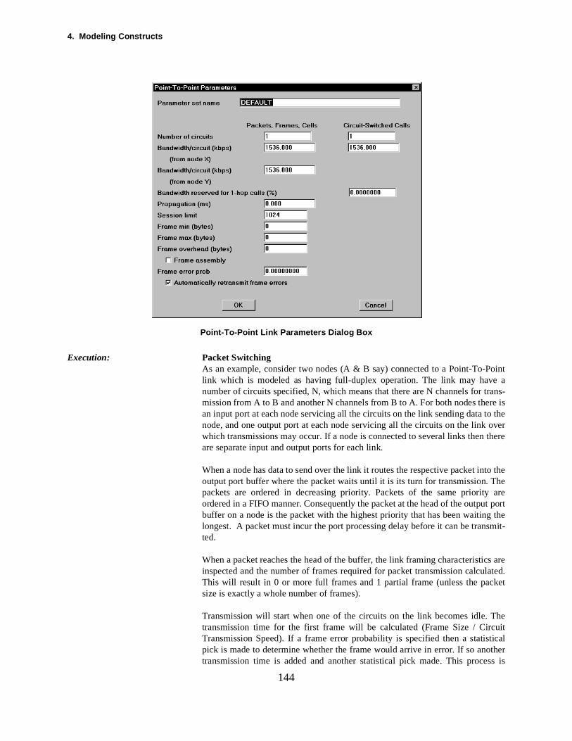
4. Modeling Constructs
oint a
rans-re iso the overthere
to theThe aret port the
smit-
s arelated.ket
Theuittical
ss is
144
Point-To-Point Link Parameters Dialog Box
Execution: Packet SwitchingAs an example, consider two nodes (A & B say) connected to a Point-To-Plink which is modeled as having full-duplex operation. The link may havenumber of circuits specified, N, which means that there are N channels for tmission from A to B and another N channels from B to A. For both nodes thean input port at each node servicing all the circuits on the link sending data tnode, and one output port at each node servicing all the circuits on the linkwhich transmissions may occur. If a node is connected to several links then are separate input and output ports for each link.
When a node has data to send over the link it routes the respective packet inoutput port buffer where the packet waits until it is its turn for transmission. packets are ordered in decreasing priority. Packets of the same priorityordered in a FIFO manner. Consequently the packet at the head of the outpubuffer on a node is the packet with the highest priority that has been waitinglongest. A packet must incur the port processing delay before it can be tranted.
When a packet reaches the head of the buffer, the link framing characteristicinspected and the number of frames required for packet transmission calcuThis will result in 0 or more full frames and 1 partial frame (unless the pacsize is exactly a whole number of frames).
Transmission will start when one of the circuits on the link becomes idle. transmission time for the first frame will be calculated (Frame Size / CircTransmission Speed). If a frame error probability is specified then a statispick is made to determine whether the frame would arrive in error. If so anothertransmission time is added and another statistical pick made. This proce
4.45 Link: Point-To-Point
thesionmer theiving
reas-
Theandsionhenhen
by 1. on
l asde-at-
n to theother
edich
the call
rityth
ports.
ck-
145
repeated until a transmission time for the frame is arrived at which deliversframe without error. The link is then made busy for the calculated transmistime, after which it is made idle. The link is then available for the next fratransmission, but the frame that has just been transmitted must then incupropagation delay. After the propagation delay the frame is then at the recenode.
When all frames have arrived at the receiving node the original packet is sembled and placed in the input buffer at the receiving node.
No particular distinction is made between one circuit or another on the link. link object has two integer attributes—the total number of circuits on the link the number of circuits in use. The link has capacity to start a frame transmiswhen the number of circuits in use is less than the total number of circuits. Wthe transmission starts the number of circuits in use is incremented by 1. Wthe transmission completes the number of circuits in use is decremented The individual circuits per se are not modeled. If a link fails, all the circuitsthe link fail.
Circuit SwitchingA Point-To-Point link may have a circuit-switched bandwidth defined as wela packet-switch bandwidth. The circuit-switched bandwidth is completely inpendent of the packet-switched bandwidth. Only circuit-switched traffic origining from Call Sources utilizes the circuit-switched bandwidth.
When a circuit-switched call originates, a routing decision is made from origidestination. This will result in zero, one, or more links being selected to carrycall. The routing decision is instantaneous in the model and checks (among things such as hop limits, availability, etc.) that there is sufficient bandwidth onthe link to satisfy the call requirement. The required bandwidth is then claimfrom the link and held for the duration of the circuit-switched call, after whthe call terminates and the bandwidth is given back to the link.
A call routed over a link may terminate early for two reasons. These are:
1.. The link (or another node or link on the route) may fail which will mean that call is disconnected and the bandwidth on all nodes and links over which thewas routed instantaneously relinquished.
2.. If preemption is enabled then a higher priority call may preempt a lower priocall on the link. This will cause the low priority call to relinquish its bandwidacross its entire route.
Reporting: Link Delays & Utilization ReportCall Statistics by LinkLink Utilization Statistics for Calls
Link delays are also inclusive on the Message, Session and Packet delay reBuffering on the links is reported in the Buffer reports.
Fields:
Name An alphanumeric field to identify the link. The name must be unique in the ba
4. Modeling Constructs
ointnels
ffic beuit-
f the calluire-
th
to theuted
ant
s thedy atthen
146
bone or subnetwork.
Icon The name of the icon used to represent the link.
Control Node Not supported for point-to-point links.
Link State Indicates whether the link is in a failed state or not.(see Link)
Statistics Various statistics may be collected and graphically displayed for Point-To-Plink utilization. These include Busy Channels From Node 1 and Busy ChanFrom Node 2 utilization.(see Statistics: Link)
Parameter Set Fields:
Point-To-Point Link— Circuit Switching Characteristics
Number Of Circuits The number of identical trunk circuits available to carry circuit-switched traffic.
Bandwidth The bandwidth per circuit. The total capacity for carrying circuit-switched trais the number of circuits multiplied by the bandwidth. A trunk could thereforedescribed as 30 circuits each at 64K, or 1 circuit at 1920K. When a circswitched call is routed over the link, the call has a bandwidth requirement. Icurrent free capacity on the link is greater than the call requirement then themay be carried. The free capacity is therefore reduced by the bandwidth reqment for the call holding time.
Bandwidth Reserved For 1-Hop CallsIt is common for directly-routed traffic in a voice network to have bandwidreserved for it on the trunk. The amount of reserved bandwidth for one-hop callsmay be specified. The one-hop calls can originate at either node connected point-to-point link. The reserved bandwidth is never available to alternate-rocalls.
Point-To-Point Link — Packet Switching Characteristics
Number Of Circuits The number of identical circuits available to carry packet-switched traffic.
Bandwidth From Node 1 The speed of each circuit in kilobits per second from node 1 to node 2.
Bandwidth From Node 2 The speed of the link in kilobits per second from node 2 to node 1.
Propagation Delay The physical transmission time across a link. This is generally only significfor satellite (270-300ms) or long distance cable connections (150-200ms).
Session Limit The maximum number of sessions that can be concurrently routed acroslink. If a session setup packet attempts to route across a link which is alreaits session limit, the routing attempt fails. The alternate routes (if any) are tested. If there is still no route the session setup packet is blocked.

4.45 Link: Point-To-Point
147
Framing Characteristics The framing characteristics for the link. Packets are broken down into transmis-sion frames which are then modeled as being transmitted across the link.(see Link: Framing )
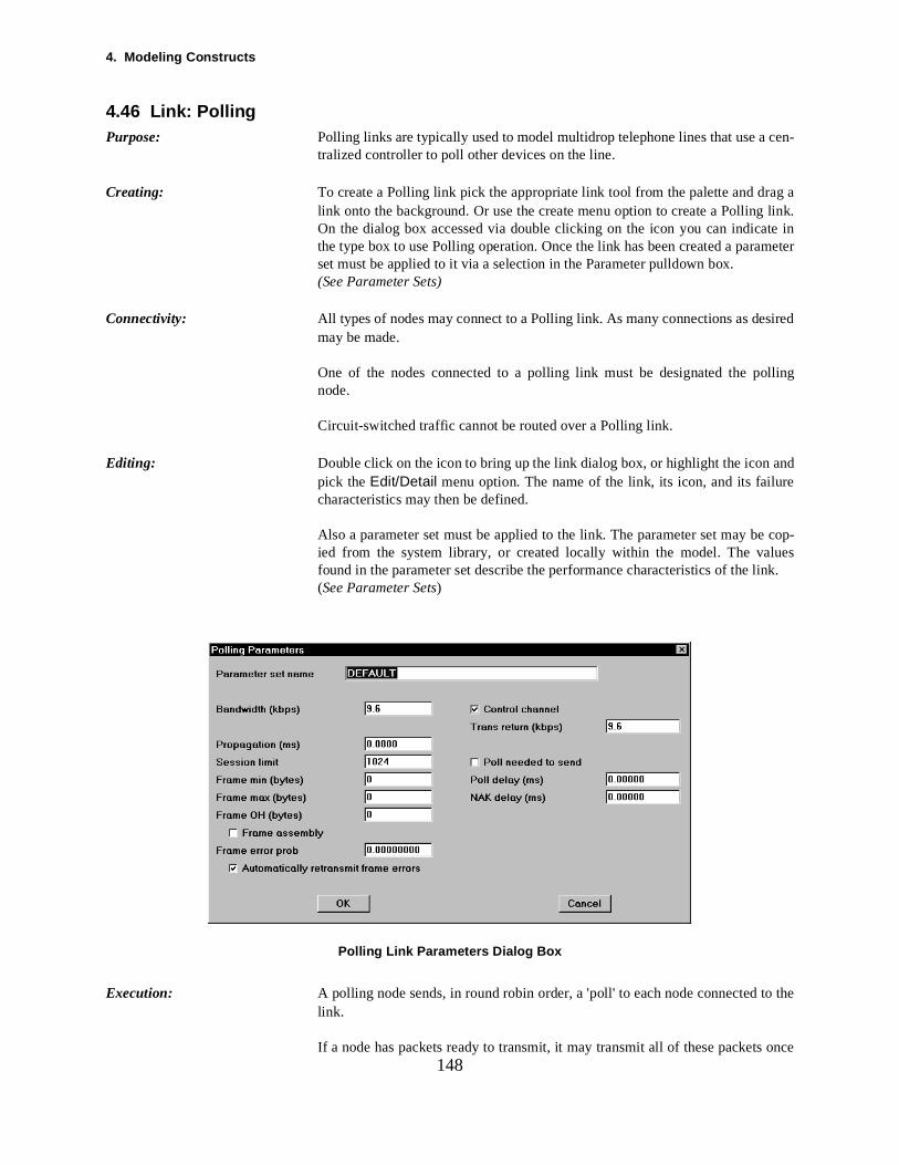
4. Modeling Constructs
cen-
a
inmeter
sired
lling
ndre
cop-uesnk.
the
once
1484.46 Link: PollingPurpose: Polling links are typically used to model multidrop telephone lines that use a
tralized controller to poll other devices on the line.
Creating: To create a Polling link pick the appropriate link tool from the palette and draglink onto the background. Or use the create menu option to create a Polling link.On the dialog box accessed via double clicking on the icon you can indicatethe type box to use Polling operation. Once the link has been created a paraset must be applied to it via a selection in the Parameter pulldown box.(See Parameter Sets)
Connectivity: All types of nodes may connect to a Polling link. As many connections as demay be made.
One of the nodes connected to a polling link must be designated the ponode.
Circuit-switched traffic cannot be routed over a Polling link.
Editing: Double click on the icon to bring up the link dialog box, or highlight the icon apick the Edit/Detail menu option. The name of the link, its icon, and its failucharacteristics may then be defined.
Also a parameter set must be applied to the link. The parameter set may beied from the system library, or created locally within the model. The valfound in the parameter set describe the performance characteristics of the li(See Parameter Sets)
Polling Link Parameters Dialog Box
Execution: A polling node sends, in round robin order, a 'poll' to each node connected to link.
If a node has packets ready to transmit, it may transmit all of these packets
4.46 Link: Polling
e poll
cket,uiredd 1 Theuitticaltherss is thesionmer theiet is
ment
ther thennel
s istrans-tedpectsion, the
t itst only
theirletes
nodelly
d.
ports.
149
the poll has been received. Once the packets have been transmitted then this available to the controller to poll the next node.
Packets will be transmitted in turn from the head of the buffer. For each pathe link framing characteristics are inspected and the number of frames reqfor packet transmission calculated. This will result in 0 or more full frames anpartial frame (unless the packet size is exactly a whole number of frames).transmission time for the first frame will be calculated (Frame Size/CircTransmission Speed). If a frame error probability is specified then a statispick is made to determine whether the frame would arrive in error. If so, anotransmission time is added and another statistical pick made. This procerepeated until a transmission time for the frame is arrived at which deliversframe without error. The link is then made busy for the calculated transmistime, after which it is made idle. The link is then available for the next fratransmission, but the frame that has just been transmitted must then incupropagation delay. After the propagation delay, the frame is then at the recevingnode. When all frames have arrived at the receiving node, the original packreassembled and placed in the input buffer at the receiving node.
If a node has no packets to transmit, it returns a negative acknowledg(NAK) to the polling node, and the polling node then polls the next node on thelink.
A polled node can only transmit on receipt of the poll. The polling node andpolled nodes may transmit over the same channel (half duplex operation), opolling node may transmit to the polled nodes over a separate control cha(full duplex operation).
The poll itself is not explicitly modeled as data transmitted over the link. Thibecause the model would then consume much CPU time representing poll fers, even when the link is otherwise idle. In COMNET III, the poll is represenusing a time calculation. When a node has packets ready to transmit it inswhere the poll is currently located and the time it would have left that locatand makes a time calculation for how long it will take to reach itself based onpoll and NAK times. After this length of time the node is then able to transmidata. Consequently, the overhead of poll representation and managemencome into play when there is data waiting to be transmitted over the link.
While a node is transmitting, two or more other nodes may place data in port output buffers ready for transmission. When the transmitting node compits transmission the poll is passed in connection order to the nearest node, even ifthe packets at the other node have been waiting longer. If some intermediatereadies a packet during this poll passing delay the poll will still go to the initiaselected node—it will not be interrupted en route to that node. The connectionorder is the order in which connections were made when the link was define
Reporting: Link Delays & Utilization Report
Link delays are also inclusive on the Message, Session, and Packet delay reBuffering on the link is reported in the Buffer reports.
4. Modeling Constructs
ck-
odeniza-
muni-ified
n.
or thentroltroller
catest, or
not free datam-
-se the
ther
ode.
150
Fields:
Name An alphanumeric field to identify the link. The name must be unique in the babone or subnetwork.
Icon The name of the icon used to represent the link.
Control Node The name of the node which is the control node for the Polling link. A Pollinglink must have a control node which will act as the poll controller. It is this nwhich sends the poll to the other nodes on the link and controls the synchrotion of transmission.
The control node may have an independent, contention free channel to comcate with the other nodes on the link. If such a channel is required, it is specas part of the Parameter Set for the Polling link.
Link State Indicates whether the link is in a failed state or not.(see Link)
Statistics Various statistics may be collected and graphically displayed for Polling Linkutilization. These include Contention Channel and Control Channel utilizatio(see Statistics: Link)
Parameter Set Fields:
Bandwidth The transmission speed of the Polling link in kilobits per second.
Control Channel Check box to indicate whether there is a separate, contention free channel fcontrol node to transmit to the other stations connected to the link. If no cochannel is indicated then the transmissions between nodes and the poll conare half duplex.
Transmission Return Rate If a control channel is in use, the transmission speed on the control channel.
Poll Needed To Send If the control node needs to send to one of the other nodes, this flag indiwhether the control node requires the poll before transmission can starwhether the control node may transmit irrespective of where the poll is.
If a control channel is specified then it may be that the control node doesrequire the poll in order to transmit to other nodes since it has a contentionchannel to them, and the control node is the only node which can transmitover this channel. Turning the “Poll Needed To Send” flag on in this circustance results in half duplex operation even though there is a full duplex connection between any node and the control node. This is the case for lines that uBSC (Binary Synchronous Communication) protocol.
Poll Delay The time it takes for a poll to be sent from the control node to any of the onodes connected to the link.
NAK Delay The time it takes a node to send a negative acknowledgment to the control n
4.46 Link: Polling
t can routeThesetup
151
Propagation Delay The time to transmit a signal across a link.
Session Limit In connection-oriented routing, this is the maximum number of sessions thabe concurrently routed across the link. If a session setup packet attempts toacross a link which is already at its session limit, the routing attempt fails. alternate routes (if any) are then tested. If there is still no route the session packet is blocked.
Framing Characteristics The framing characteristics for the link. Packets are broken down into transmis-sion frames which are then modeled as being transmitted across the link.(see Link: Framing)
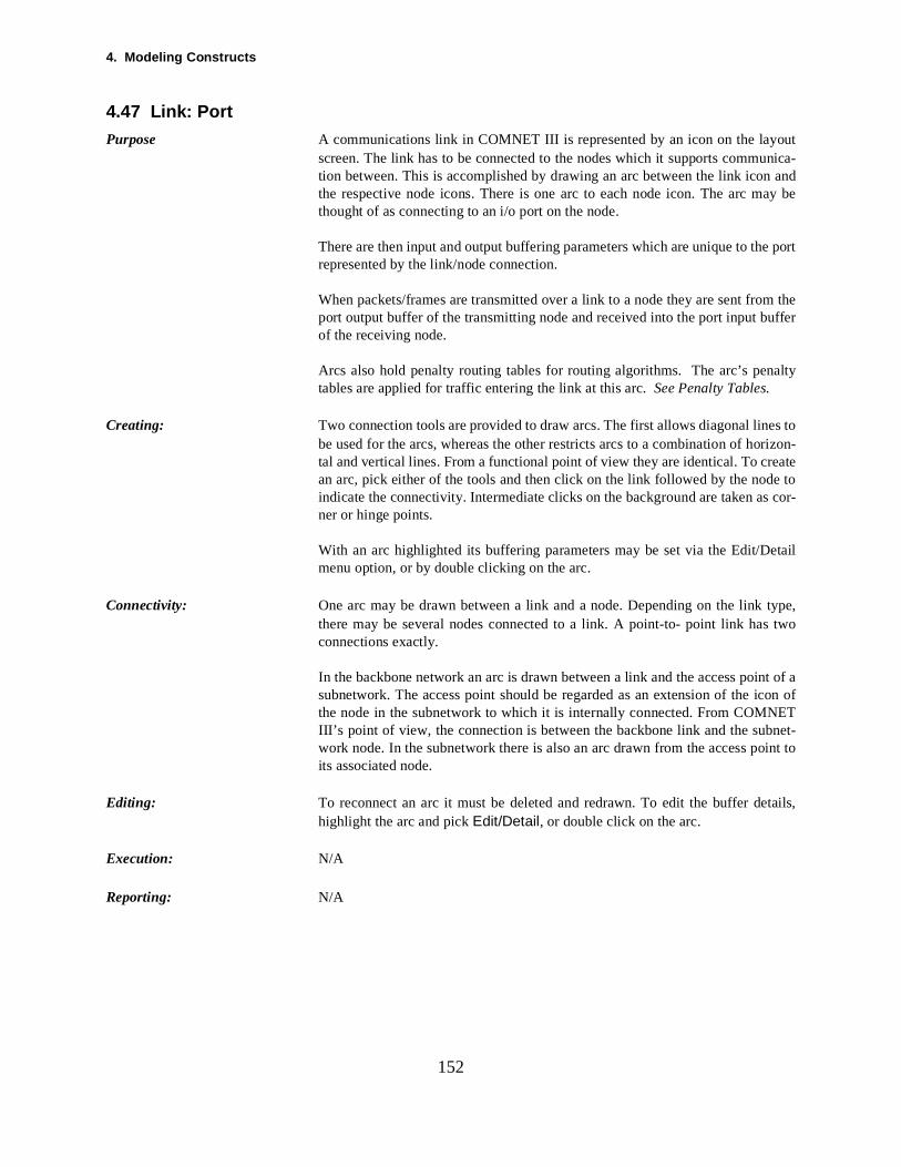
4. Modeling Constructs
out
anday be
port
m theffer
alty
s toriate
e to
etail
type, two
tails,
152
4.47 Link: Port
Purpose A communications link in COMNET III is represented by an icon on the layscreen. The link has to be connected to the nodes which it supports communica-tion between. This is accomplished by drawing an arc between the link iconthe respective node icons. There is one arc to each node icon. The arc mthought of as connecting to an i/o port on the node.
There are then input and output buffering parameters which are unique to therepresented by the link/node connection.
When packets/frames are transmitted over a link to a node they are sent froport output buffer of the transmitting node and received into the port input buof the receiving node.
Arcs also hold penalty routing tables for routing algorithms. The arc’s pentables are applied for traffic entering the link at this arc. See Penalty Tables.
Creating: Two connection tools are provided to draw arcs. The first allows diagonal linebe used for the arcs, whereas the other restricts arcs to a combination of hozon-tal and vertical lines. From a functional point of view they are identical. To crean arc, pick either of the tools and then click on the link followed by the nodindicate the connectivity. Intermediate clicks on the background are taken as cor-ner or hinge points.
With an arc highlighted its buffering parameters may be set via the Edit/Dmenu option, or by double clicking on the arc.
Connectivity: One arc may be drawn between a link and a node. Depending on the link there may be several nodes connected to a link. A point-to- point link hasconnections exactly.
In the backbone network an arc is drawn between a link and the access point of asubnetwork. The access point should be regarded as an extension of the icon ofthe node in the subnetwork to which it is internally connected. From COMNETIII’s point of view, the connection is between the backbone link and the subnet-work node. In the subnetwork there is also an arc drawn from the access point toits associated node.
Editing: To reconnect an arc it must be deleted and redrawn. To edit the buffer dehighlight the arc and pick Edit/Detail, or double click on the arc.
Execution: N/A
Reporting: N/A
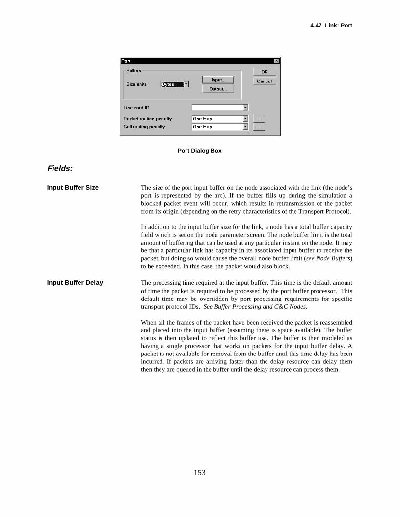
4.47 Link: Port
de’sn acket
city total may the
ount Thiscific
mbled
d as
them
153
Port Dialog Box
Fields:
Input Buffer Size The size of the port input buffer on the node associated with the link (the noport is represented by the arc). If the buffer fills up during the simulatioblocked packet event will occur, which results in retransmission of the pafrom its origin (depending on the retry characteristics of the Transport Protocol).
In addition to the input buffer size for the link, a node has a total buffer capafield which is set on the node parameter screen. The node buffer limit is theamount of buffering that can be used at any particular instant on the node. Itbe that a particular link has capacity in its associated input buffer to receivepacket, but doing so would cause the overall node buffer limit (see Node Buffers)to be exceeded. In this case, the packet would also block.
Input Buffer Delay The processing time required at the input buffer. This time is the default amof time the packet is required to be processed by the port buffer processor.default time may be overridden by port processing requirements for spetransport protocol IDs. See Buffer Processing and C&C Nodes.
When all the frames of the packet have been received the packet is reasseand placed into the input buffer (assuming there is space available). The bufferstatus is then updated to reflect this buffer use. The buffer is then modelehaving a single processor that works on packets for the input buffer delay. Apacket is not available for removal from the buffer until this time delay has beenincurred. If packets are arriving faster than the delay resource can delay then they are queued in the buffer until the delay resource can process them.
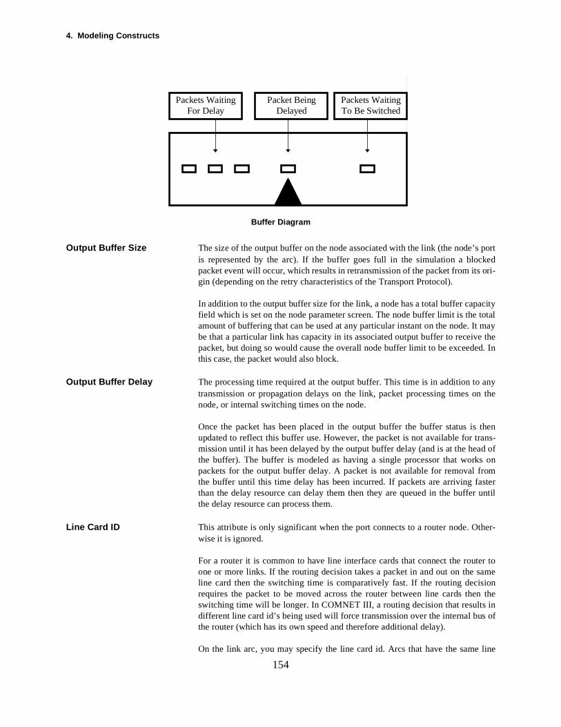
4. Modeling Constructs
port
ori-
city total may
d. In
anyn the
ans-ad ofs onromster
r until
ther-
er toameionn the
ins of
line
154
Buffer Diagram
Output Buffer Size The size of the output buffer on the node associated with the link (the node’sis represented by the arc). If the buffer goes full in the simulation a blockedpacket event will occur, which results in retransmission of the packet from itsgin (depending on the retry characteristics of the Transport Protocol).
In addition to the output buffer size for the link, a node has a total buffer capafield which is set on the node parameter screen. The node buffer limit is theamount of buffering that can be used at any particular instant on the node. Itbe that a particular link has capacity in its associated output buffer to receive thepacket, but doing so would cause the overall node buffer limit to be exceedethis case, the packet would also block.
Output Buffer Delay The processing time required at the output buffer. This time is in addition totransmission or propagation delays on the link, packet processing times onode, or internal switching times on the node.
Once the packet has been placed in the output buffer the buffer status is thenupdated to reflect this buffer use. However, the packet is not available for trmission until it has been delayed by the output buffer delay (and is at the hethe buffer). The buffer is modeled as having a single processor that workpackets for the output buffer delay. A packet is not available for removal fthe buffer until this time delay has been incurred. If packets are arriving fathan the delay resource can delay them then they are queued in the buffethe delay resource can process them.
Line Card ID This attribute is only significant when the port connects to a router node. Owise it is ignored.
For a router it is common to have line interface cards that connect the routone or more links. If the routing decision takes a packet in and out on the sline card then the switching time is comparatively fast. If the routing decisrequires the packet to be moved across the router between line cards theswitching time will be longer. In COMNET III, a routing decision that resultsdifferent line card id’s being used will force transmission over the internal buthe router (which has its own speed and therefore additional delay).
On the link arc, you may specify the line card id. Arcs that have the same
Packets WaitingFor Delay
Packets WaitingTo Be Switched
Packet BeingDelayed
4.47 Link: Port
cardting
hich cost table
illinedtheron
useld be
155
non-blank card id will be treated as connecting to one card and so traffic routingbetween them will not see bus delays. Arcs that have different or blank line id’s will be treated as connecting to different line cards and so traffic roubetween them will have to also incur a bus delay.
Call Routing Penalty Table When penalty based routing is specified for the backbone or subnetwork in wthe link is defined, the link must have an associated penalty table so that itscan be looked up. The table name to use is specified on the arc detail—theitself is constructed on the Define/Penalty Table menu option.
The table is defined from the point of view of the node from which routing wbe attempted. A point-to-point link could therefore have a penalty table deffor routing in one direction, and a separate penalty table for routing in the odirection. This allows the user to prohibit traffic flow in a particular direction a link.(see Penalty Table: Call Routing)
Packet Routing Penalty Table The same as for the call routing penalty table, except this defines the table to for packet routing. For a multiaccess link such as CSMA/CD, each node couuse a different penalty table for the link.(see Penalty Table: Packet Routing)
4. Modeling Constructs
flex-en
theeful
theokennitors, pri-
.5rnet
156
4.48 Link: Priority Token Ring and Token Ring EnhancementsPurpose: Release 1.3 improves the token passing model for better performance, more
ibility, and better monitoring. In addition new link types derived from the tokring model provide better models for priority token-rings (including 100VG-AnyLAN), and FDDI.
The token-passing model has a new option for a holding limit based onnumber of frames instead of a holding time, and this may be particularly uswhen the node may hold a token for exactly one frame.
New statistics monitors and a token-ring report are available to measureactual token rotation times, and the number of active nodes waiting for the tand how long these nodes remain actively accessing the link. These moand reports are available for all the token-passing link types (token passingority token ring, FDDI, priority FDDI).
The priority token-ring model provides parameter sets for IEEE 802.4 and 802token rings, and 2 new parameter sets for 100VG-AnyLAN: 1 set for etheports and 1 set for token ring ports.
4.49 Link: Token Passing
andoken-
beenr pull-
s as
ndre
cop-uesnk.
hold-
157
4.49 Link: Token Passing
Purpose: Token-Passing links are used to model 802.4, 802.5 and FDDI operation.
Creating: To create a Token-Passing link pick the appropriate link tool from the palettedrag a link onto the background. Or use the create menu option to create a TPassing link. On the dialog box accessed via double clicking on the icon you canindicate in the type box to use Token-Passing operation. Once the link hascreated a parameter set must be applied to it via a selection in the Parametedown box.(See Parameter Sets)
Connectivity: All types of node may connect to a Token-Passing link. As many connectiondesired may be made.
Circuit-switched traffic cannot be routed over a Token-Passing link.
Editing: Double click on the icon to bring up the link dialog box, or highlight the icon apick the Edit/Detail menu option. The name of the link, its icon, and its failucharacteristics may then be defined.
Also a parameter set must be applied to the link. The parameter set may beied from the system library, or created locally within the model. The valfound in the parameter set describe the performance characteristics of the li(See Parameter Sets)
Token Passing Link Parameters Dialog Box
Execution: A Token-Passing link sends, in round robin order, a 'token' to each node con-nected to the link.
When the token is received the node may transmit packets up to the token
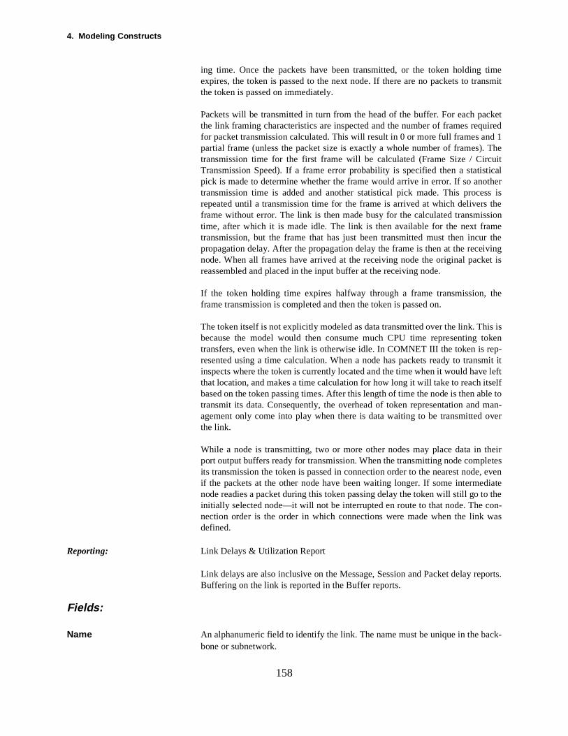
4. Modeling Constructs
timensmit
uiredd 1 Theuittical
ss is thesionmer theivinget is
the
is istoken
mit ite leftselfble to man-over
theirletes, evendiateo theon-was
ports.
ck-
158
ing time. Once the packets have been transmitted, or the token holding expires, the token is passed to the next node. If there are no packets to trathe token is passed on immediately.
Packets will be transmitted in turn from the head of the buffer. For each packetthe link framing characteristics are inspected and the number of frames reqfor packet transmission calculated. This will result in 0 or more full frames anpartial frame (unless the packet size is exactly a whole number of frames).transmission time for the first frame will be calculated (Frame Size / CircTransmission Speed). If a frame error probability is specified then a statispick is made to determine whether the frame would arrive in error. If so anothertransmission time is added and another statistical pick made. This procerepeated until a transmission time for the frame is arrived at which deliversframe without error. The link is then made busy for the calculated transmistime, after which it is made idle. The link is then available for the next fratransmission, but the frame that has just been transmitted must then incupropagation delay. After the propagation delay the frame is then at the recenode. When all frames have arrived at the receiving node the original packreassembled and placed in the input buffer at the receiving node.
If the token holding time expires halfway through a frame transmission, frame transmission is completed and then the token is passed on.
The token itself is not explicitly modeled as data transmitted over the link. Thbecause the model would then consume much CPU time representing transfers, even when the link is otherwise idle. In COMNET III the token is rep-resented using a time calculation. When a node has packets ready to transinspects where the token is currently located and the time when it would havthat location, and makes a time calculation for how long it will take to reach itbased on the token passing times. After this length of time the node is then atransmit its data. Consequently, the overhead of token representation andagement only come into play when there is data waiting to be transmitted the link.
While a node is transmitting, two or more other nodes may place data in port output buffers ready for transmission. When the transmitting node compits transmission the token is passed in connection order to the nearest nodeif the packets at the other node have been waiting longer. If some intermenode readies a packet during this token passing delay the token will still go tinitially selected node—it will not be interrupted en route to that node. The cnection order is the order in which connections were made when the link defined.
Reporting: Link Delays & Utilization Report
Link delays are also inclusive on the Message, Session and Packet delay reBuffering on the link is reported in the Buffer reports.
Fields:
Name An alphanumeric field to identify the link. The name must be unique in the babone or subnetwork.
4.49 Link: Token Passing
sing
en
thatpts to
ion
159
Icon The name of the icon used to represent the link.
Link State Indicates whether the link is in a failed state or not.(see Linksee Node)
Statistics Various statistics may be collected and graphically displayed for Token PasLink utilization.(see Statistics: Link)
Parameter Set Fields:
Bandwidth The transmission speed of the Token-Passing link in kilobits per second.
Token Passing Delay The time it takes for a token to be sent from one node to the next node.
Token Holding Limit The time limit for a node to hold the token. A limit of 0 implies keeping the tokuntil all the packets have been transmitted.
Propagation Delay The time to transmit a signal across a link.
Session Limit For connection-oriented routing, this is the maximum number of sessionscan be concurrently routed across the link. If a session setup packet attemroute across a link which is already at its session limit, the routing attempt fails.The alternate routes (if any) are then tested. If there is still no route the sesssetup packet is blocked.
Framing Characteristics The framing characteristics for the link. Packets are broken down into transmis-sion frames which are then modeled as being transmitted across the link.(see Link: Framing)
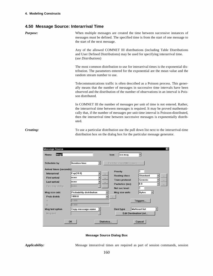
4. Modeling Constructs
ces ofage to
s
dis-
e beenois-
ther,
ted,istrib-
ime
ssion
160
4.50 Message Source: Interarrival Time
Purpose: When multiple messages are created the time between successive instanmessages must be defined. The specified time is from the start of one messthe start of the next message.
Any of the allowed COMNET III distributions (including Table Distributionand User Defined Distributions) may be used for specifying interarrival time.(see Distributions)
The most common distribution to use for interarrival times is the exponentialtribution. The parameters entered for the exponential are the mean value and therandom stream number to use.
Telecommunications traffic is often described as a Poisson process. This gner-ally means that the number of messages in successive time intervals haveobserved and the distribution of the number of observations in an interval is Pson distributed.
In COMNET III the number of messages per unit of time is not entered. Rathe interarrival time between messages is required. It may be proved mathemati-cally that, if the number of messages per unit time interval is Poisson-distributhen the interarrival time between successive messages is exponentially duted.
Creating: To use a particular distribution use the pull down list next to the interarrival-tdistribution box on the dialog box for the particular message generator.
Message Source Dialog Box
Applicability: Message interarrival times are required as part of session commands, se
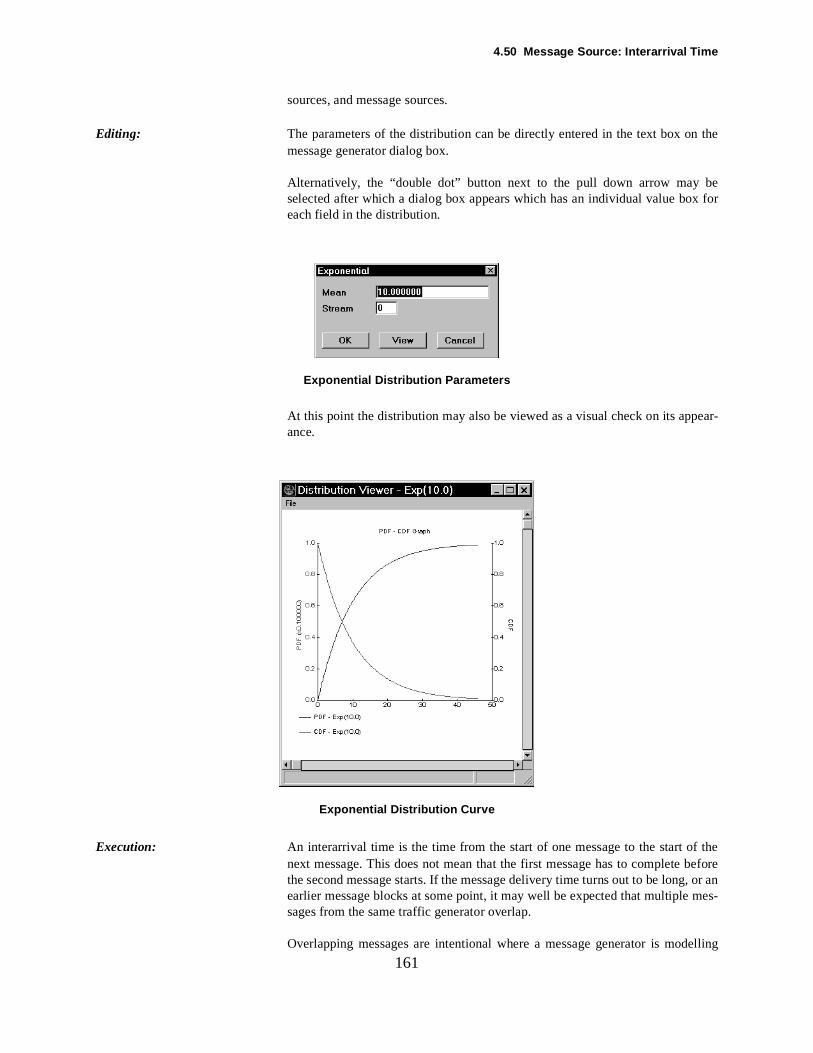
4.50 Message Sour ce: Interarrival Time
the
bex for
ear-
f the before, or anmes-
elling
161
sources, and message sources.
Editing: The parameters of the distribution can be directly entered in the text box onmessage generator dialog box.
Alternatively, the “double dot” button next to the pull down arrow may selected after which a dialog box appears which has an individual value boeach field in the distribution.
Exponent ial Distribution Parameters
At this point the distribution may also be viewed as a visual check on its appance.
Exponent ial Distribution Curve
Execution: An interarrival time is the time from the start of one message to the start onext message. This does not mean that the first message has to completethe second message starts. If the message delivery time turns out to be longearlier message blocks at some point, it may well be expected that multiple sages from the same traffic generator overlap.
Overlapping messages are intentional where a message generator is mod
4. Modeling Constructs
h theaggre-each
en
eter-
es-
hasicated
sage
e.
mple,as 10ated at
162
the creation of messages from a number of users. Maybe the node at whicgeneration occurs represents a pad, concentrator or terminal server and the gate rate of message generation from it is required rather than modelling individual user.
If no specific start time is entered for the message generator, a time T will bepicked from the interarrival-time distribution, and the first arrival will be chosfrom the uniform distribution between time 0 and T. When the first message iscreated then another statistical pick is made from the given distribution to dmine when the next message should be created. This process continues until theend of the simulation or the message generator stop time (if one is entered).
Reporting: N/A
Fields:
Start Time The time in seconds from the start of simulation (time = 0) when the first msage should be scheduled. This may be a constant, or a statistical pick.
If nothing is entered (Start Time = None), a time T is drawn from the interarrival-time distribution and the first arrival time is then drawn uniformly from [0, T].
If a constant of 0 is entered, the first message will go at time 0.
If the interarrival time is None and the Stop Time is None and the Start Timesome constant value (5 say), then only 1 message will be created at the indtime.
Interarrival Time The time from the start of one message to the start of the next.
Stop Time The time in seconds from the start of simulation (time = 0) when the last messhould be scheduled. This may be a constant, or a statistical pick.
If nothing is entered (Stop Time = None), the end of simulation is the stop tim
If a Stop Time is entered a message will be scheduled at this time. For exaif the first message was scheduled at 0.5 seconds, the Interarrival Time wseconds and the Stop Time 11 seconds, the next message would be cre10.5 seconds and the last one at 11 seconds.
4.51 Message Source: Packetizing Delay
made
at a repre-ta
he hosttizingcur theely a trans-tizing by
y
ssing
to theetup,
e to
mand,
ectiven to
t-acketlso a
cur theur the
163
4.51 Message Source: Packetizing Delay
Purpose: Nodes are modeled as having a node processor which, at packet creation, isbusy for the packetizing delay. In other words, the packetizing delay is theamount of processing time it takes to make a packet at the originating node.
The packetizing delay could be used to model transaction processing timehost. Messages which represent transactions may be sent to a node whichsents a host. Upon receipt of the message the host may be required to echo daback to the sender (e.g., a credit card authorization network) via a responsesource. If the response message is a single packet, a simple way to model tprocessing delay on the host would be to specify a packetizing delay. If thecould process 100 transactions per second (say) this would imply a packedelay of 10 milliseconds. As response messages are made, each has to in10 millisecond processing delay on the host processor, which is then effectivsingle server, single queue resource. If the host were then upgraded to 200actions per second then the only parameter to change would be the packedelay (to 5 milliseconds). Obviously a more detailed model could be madeusing read, write, processing and transport commands from within an applicationrunning on the host—but a simple response source with a packetizing delay masuffice as a first pass model.
The packetizing delay might also be used to model transport layer proceoverhead.
Creating The packetizing delay is specified on the traffic generators that are attached originating node, or as part of traffic generating commands (session sanswer message, transport command). This allows the packet creation timvary by application and type of traffics.
Connectivity: Defined on each message generator.
Editing: Edited via the message generator dialog box.
Execution: Packets are created as a result of a transport command, session setup comor response command being picked for execution on a node. Message, session,and response sources result in internally generated applications with a respcommand to perform this function. When the node schedules the applicatioexecute its command, the transport protocol is queried to establish that any oustanding ACKs have been received. If these requirements are satisfied the pis created and the node processor made busy by the packetizing delay. Acheck is made that buffer space is available and that a route can be found.
The sequence of events that occurs is as follows:
1. Create message2. Incur packetizing delay3. Create packet4. Incur the packet processing delay5. Route the packet.
Session setup packets, session connect packets and ACK packets do not inpacketizing delay. The packets which represent the message data do inc

4. Modeling Constructs
y.
164
packetizing delay.
Reporting: Packetizing delay counts towards Node Utilization.It is also part of the respective Message Delay and End-To-End Packet Dela
Fields:
Packetizing Delay Use any of the standard COMNET III distributions.(see Distributions)
4.52 Message Source: Pri ority
acketwith the
rsed on
rentet tosmit-order
rt
d forcess-ort
port
eledey are
y aret pri-t and forrityssingckets by
eadmitsode.ceiv-
IFOto the
165
4.52 Message Source: Priority
Purpose: The priority field is used to assign a priority to packets as they are created. Ppriority is used to order packets in input and output port buffers on nodes, highest priority packets being placed at the head of queue of packets inbuffer. Packets of equal priority are treated on a FIFO basis.
The Priority field is not used to imply priority between multiple traffic generatoor applications on the same node. Multiply scheduled generators are executa round-robin basis.(See Node Scheduling)
Also the Priority field is not used to arbitrate between packets waiting at diffenodes to access a link. It is up to the link protocol to choose which packtransmit from those packets at the head of the output port buffers of the tranting nodes. For instance, in token passing the next packet in connection would be serviced—irrespective of the priority of packets on other buffers. SeeLink: Token Passing
Creating: Priority is defined on the dialog box which describes the message or transpocommand which is going to create the packet.
Connectivity: N/A
Editing: Via the dialog box.
Execution: When a packet is created it is assigned a priority based on the priority enterethe message generator dialog box. After creation, the packet incurs node proing delays followed by a routing decision which determines which output pbuffer to route through. The packet is then placed in the selected outputbuffer.
The buffer may have a buffer processing time. In this case the buffer is modas having a single delay resource which is used to delay the packets as thundergoing processing in the buffer. The packet is inserted into the buffer behindthis delay resource. If there are multiple packets behind the resource theordered in decreasing priority order, then by FIFO. Consequently the highesority packet that has waited the longest is allocated the delay resource firsincurs the buffer processing delay first. Other low priority packets must waitthe higher priority packets to be delayed in the buffer before the low priopackets may incur their delay. Once packets have incurred the buffer procedelay they are then waiting for transmission across the connected link. Pawaiting for transmission are again ordered in decreasing priority followedFIFO order.
At some point in time the link protocol will determine that the packet at the hof the port output buffer queue is to be transmitted. The link protocol transthe packet frame-by-frame until all of the frames have arrived at the next nThe packet is then reassembled and placed in the input port buffer on the reing node. Again the input port buffer is ordered in decreasing priority plus Forder, and has an associated delay resource to model processing delays inbuffer.

4. Modeling Constructs
the isTheon the with
gen-
166
A packet with some origin and destination is routed from node to node byrouting algorithm in force for the network. At each intermediate node itreceived into the input port buffer and switched into an output port buffer. manner in which the packet is switched and the associated delay depends type of node and its parameter settings. Each buffer exhibits the same logicrespect to packet priority.
Reporting: N/A
Fields:
Priority An integer value between 1 and 99 that is used to set the priority of packetserated by the message source. Larger values have higher priority.
4.53 Message Source: Size Calculation
eachctronicneedssT III
bion is
d,
f sizes there pack-
-
ands.ntered.
distri-es orack-ing aula-
ave its
r theting
167
4.53 Message Source: Size Calculation
Purpose: The message size field is used to assign a total size in bytes or packets tomessage as it is generated. If a message source is being used to model elemail, file transfers, database inquiries, etc., then the size of the data transfer to be described to the model. Message sizes are not necessarily constant—forinstance, not all file transfers are of the same size. Consequently COMNEprovides for the message size to be entered as a statistical distribution.
Also, it may be that a message size needs to be related to the size of an inoundmessage, or the size of data which has been read from disk. Such provismade within COMNET III.
If the message is sized in bytes, the transport protocol settings will be inspecteto determine how many full packets represent the message (with possibly onesmaller overflow packet).
If the message size is given as N packets, COMNET III creates messages oN times the packet size, so all COMNET III messages internally use bytes asize unit, once the message has been created. When these messages aetized, there will be no overflow packets.
Creating: Message size is defined on the dialog box which describes the message or transport command.
Connectivity: Messages are generated by Message Sources, Response Sources, SessionSources, Transport Commands, Setup Commands and Answer CommWherever a message may be generated, a message size definition may be e
Editing: Via the appropriate message generator dialog box.
Any of the standard COMNET III distributions may be used.(see Distributions)
Execution: When a message is created a statistical pick is made from the message sizebution to determine the total size of the message. This may be in either bytfull size packets. If the message size is in bytes a calculation of how many pets are required is made, based upon the transport protocol settings. Assumstatistical distribution is being used (rather than a constant), then as the simtion proceeds and different messages are generated, each message will hown, individual size as returned by the statistical pick.
The originating node then creates the required number of packets one afteother taking note of node scheduling requirements, flow control settings, roudecisions, etc., until all of the packets have been generated.
Reporting: N/A
Fields:
Message Size Three choices are available for setting the message size. These include:
Probability Distribution (see Distributions)

4. Modeling Constructs
s itselfe usedre a
the
ill be
of thesing a cal-
s the
168
Any of the allowed COMNET III distributions.
Based On Message SizeIf the application or message source which wants to create the message wascheduled by received message, the size of the scheduling message can bto calculate the size of the reply. This is done using a linear calculation whemultiplier and an offset can be specified. The size calculation is then ofform:
Multiplier * Message Size + Offset
If the multiplier is 1 and the offset is 0 then a message of the same size wreturned.
Based On File SizeIf the application which wants to create the message has read a file, the sizefirst read can be used to calculate the size of the message. This is done ulinear calculation where a multiplier and an offset can be specified. The sizeculation is then of the form:
Multiplier * Number of Bytes Read + Offset
If the multiplier is 1 and the offset is 0 then a message of the same size anumber of bytes read from file will be created.
4.54 Message Source: Size Units
en thee thesage
r
ands.ay be
169
4.54 Message Source: Size Units
Purpose: Messages may be sized in bytes or packets. If they are sized in packets, thmessage size calculation specifies the number of full size packets, wherpacket size is derived from the transport protocol settings. Note that the MesLinear distributions always use the received message size in bytes.
Creating: Message Size Unit is defined on the dialog box which describes the message otransport command dialog box.
Connectivity: Messages are generated by Message Sources, Response Sources, SessionSources, Transport Commands, Setup Commands and Answer CommWherever a message may be generated a message size unit definition mentered.
Editing: Via the appropriate message generator dialog box.
Reporting: N/A
Fields:
Size Unit Only the values “Bytes” or “Packets” may be selected.
4. Modeling Constructs
mes-ceivedources.quirednt for
t hasessagehed-uery”of the
f differ-e same
size,
mes-sageage isseful
trans-
ands.
age text mes-ciated
eduleurce orming
racterples
170
4.55 Message Source: Message Text
Purpose: When a message is sent, there is an arbitrary text label associated with thesage. This message text is particularly used to trigger sources based on remessage scheduling for application, message, response and session sReceived Message Scheduling means that when a message with the remessage text arrives at the destination node then the scheduling requiremethat application at the destination node has been met and may be started.
For instance, a model of a client server architecture may be built. Each cliena message source which sends a query message to the server with the mtext “Database Query.” On the server there may be an application which is sculed by received message and is looking for the message text “Database Qto be received. When a message with this text is received a new instance server’s application may be started.
Because the message text is separate from the message name, a number oent message sources may send the same message text and thus trigger thsource at a destination, despite differences of the message itself (in terms of source, protocol, etc.).
Message text can be useful for measuring message delays: essentially, thesage delays reported in the output reports measure the “lifetime” of the mestext. If a message uses the original message text, the delay for that messmeasured from the creation time of the incoming message text. This is a umechanism for getting round-trip delays.
Creating: Message Text is defined on the dialog box which describes the message or port command.
Connectivity: Messages are generated by Message Sources, Response Sources, SessionSources, Transport Commands, Setup Commands and Answer CommWherever a message may be generated, a message text may be entered.
Editing: Via the appropriate message generator dialog box.
Execution: When a message is created, its message text is set based upon the messsettings. This is either a copy of the message name, the text of the originalsage, or specific text entered by the user. This text, or label, is then assowith the message as it moves to its destination.
When the message arrives at the destination its text may be used to schsome activity at the destination, such as a message source or a response soan application. Scheduling can be made to depend on more than one incomessage: through a received message list identifying
—Required number of a message text (all must be received) to trigger. —list of different message texts (all must be received)
Each message text in the received message list may use the wildcard cha“*” to accept classes of message texts. For example, the following are examusing the wildcard character “*”:
4.55 Message Source: Message Text
ing. anyatchardceived
ssage
n themainsedul-ling
and so
st be
, etc.,
171
**RequestRequest**Request*
The first case, where the wildcard character is by itself, will match everythThe second case, where the wildcard character appears first, will matchreceived message that ends with “Request.” Similarly, the third case will many received message that begins with “Request.” Finally, with the wildccharacter appearing at both the beginning and end of the message, any remessage that contains “Request” anywhere in the text will be matched.
If the message text is not required by any source at the destination the meand its associated text are discarded.
If the text is specified as a requirement by some source at the destination themessage text is placed in a received message list at the destination and rethere until such time as it (or rather its message text) is used to satisfy a sching requirement. A particular message instance will only satisfy one schedurequirement at the destination, after which the message is considered used discarded.(See Received Message Scheduling)
Reporting: N/A
Fields:
Message Text From the sender of the message point of view, the text of the message muset. The options for setting the text are:
Use Original MessageUse the text of the message which scheduled the application, responsewhich is creating the new message.
Copy Message Name (Default)Use the name of the message as the message text.
Set Message TextExplicitly set the message text with a label typed by the user.
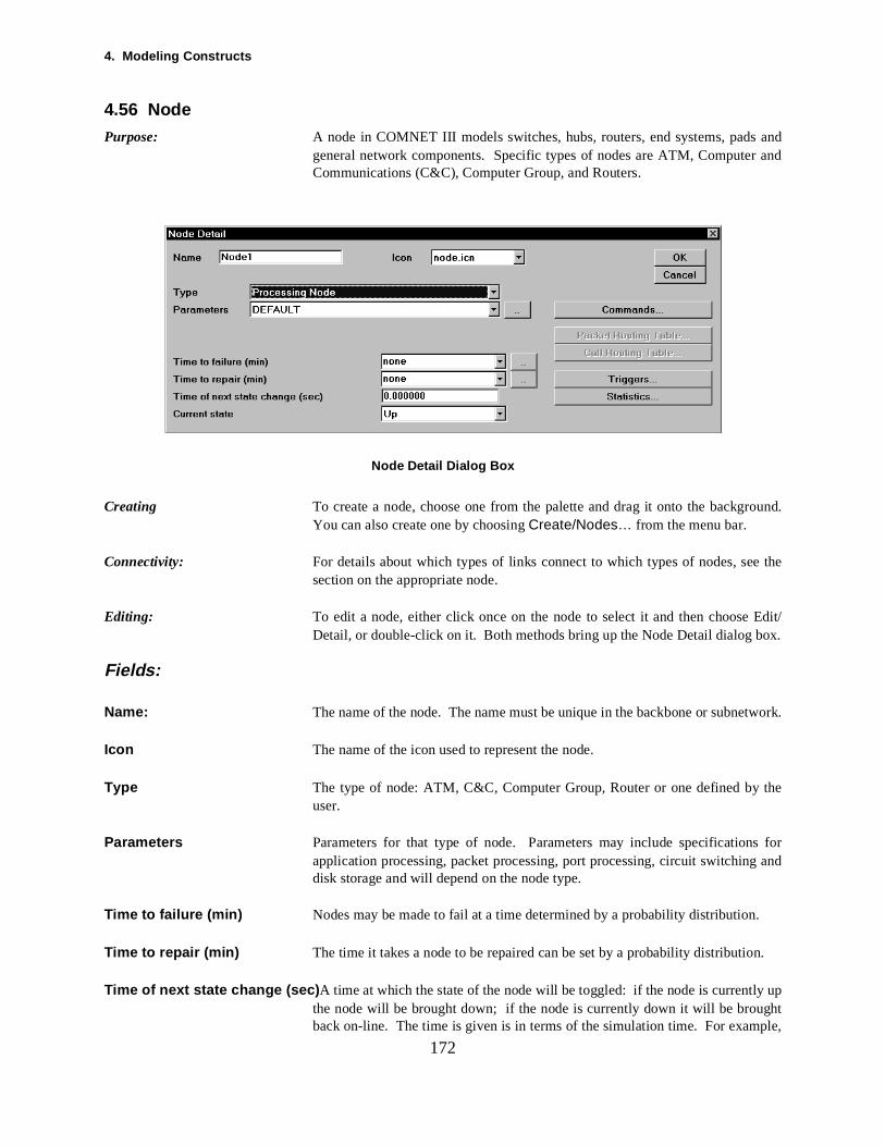
4. Modeling Constructs
and and
e the
Edit/ox.
t
the
s for and
.
n.
upghtple,
172
4.56 Node
Purpose: A node in COMNET III models switches, hubs, routers, end systems, padsgeneral network components. Specific types of nodes are ATM, ComputerCommunications (C&C), Computer Group, and Routers.
Node Detail Dialog Box
Creating To create a node, choose one from the palette and drag it onto the background.You can also create one by choosing Create/Nodes… from the menu bar.
Connectivity: For details about which types of links connect to which types of nodes, sesection on the appropriate node.
Editing: To edit a node, either click once on the node to select it and then chooseDetail, or double-click on it. Both methods bring up the Node Detail dialog b
Fields:
Name: The name of the node. The name must be unique in the backbone or subnework.
Icon The name of the icon used to represent the node.
Type The type of node: ATM, C&C, Computer Group, Router or one defined by user.
Parameters Parameters for that type of node. Parameters may include specificationapplication processing, packet processing, port processing, circuit switchingdisk storage and will depend on the node type.
Time to failure (min) Nodes may be made to fail at a time determined by a probability distribution
Time to repair (min) The time it takes a node to be repaired can be set by a probability distributio
Time of next state change (sec) A time at which the state of the node will be toggled: if the node is currentlythe node will be brought down; if the node is currently down it will be brouback on-line. The time is given is in terms of the simulation time. For exam

4.56 Node
h rep-
tog-ode
ed or, seeages,
173
if the Time of the next state change is 30 seconds, then 30 seconds into eaclication the state will be changed.
Current state Whether the node is currently operating (up) or failed (down). This can be gled during the simulation by double-clicking on the node to bring up the ndetail dialog box and editing this field.
Commands Brings up the Command Repertoire dialog box. Here commands can be addremoved from the node’s repertoire. For more information about commandsthe section on the specific type of command: Answer Message, Filter MessProcess Data, Read File, Setup Session, Transport Message, or Write File
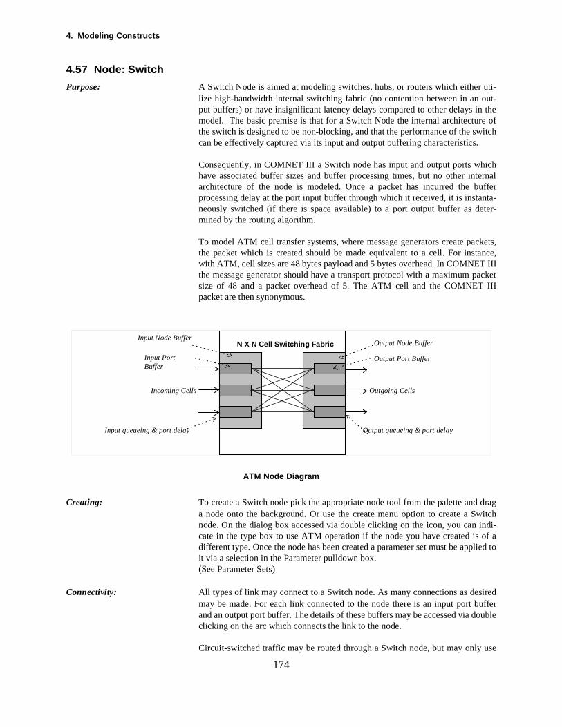
4. Modeling Constructs
uti-ut-there ofwitch
ichternal
eter-
ckets,ance,T IIIacket III
dragh
of alied to
iredufferouble
e
174
4.57 Node: Switch
Purpose: A Switch Node is aimed at modeling switches, hubs, or routers which eitherlize high-bandwidth internal switching fabric (no contention between in an oput buffers) or have insignificant latency delays compared to other delays in model. The basic premise is that for a Switch Node the internal architectuthe switch is designed to be non-blocking, and that the performance of the scan be effectively captured via its input and output buffering characteristics.
Consequently, in COMNET III a Switch node has input and output ports whhave associated buffer sizes and buffer processing times, but no other inarchitecture of the node is modeled. Once a packet has incurred the bufferprocessing delay at the port input buffer through which it received, it is instanta-neously switched (if there is space available) to a port output buffer as dmined by the routing algorithm.
To model ATM cell transfer systems, where message generators create pathe packet which is created should be made equivalent to a cell. For instwith ATM, cell sizes are 48 bytes payload and 5 bytes overhead. In COMNEthe message generator should have a transport protocol with a maximum psize of 48 and a packet overhead of 5. The ATM cell and the COMNETpacket are then synonymous.
ATM Node Diagram
Creating: To create a Switch node pick the appropriate node tool from the palette anda node onto the background. Or use the create menu option to create a Switcnode. On the dialog box accessed via double clicking on the icon, you can indi-cate in the type box to use ATM operation if the node you have created isdifferent type. Once the node has been created a parameter set must be appit via a selection in the Parameter pulldown box.(See Parameter Sets)
Connectivity: All types of link may connect to a Switch node. As many connections as desmay be made. For each link connected to the node there is an input port band an output port buffer. The details of these buffers may be accessed via dclicking on the arc which connects the link to the node.
Circuit-switched traffic may be routed through a Switch node, but may only us
Incoming Cells Outgoing Cells
Input Node Buffer
Input PortBuffer
N X N Cell Switching Fabric Output Node Buffer
Output Port Buffer
Input queueing & port delay Output queueing & port delay
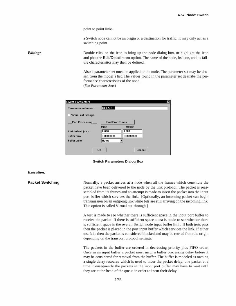
4.57 Node: Switch
as a
onil-
e cho- per-
thereas- inputginnk.
er to thereasstherrigin
der.re itningt at a
until
175
point to point links.
a Switch node cannot be an origin or a destination for traffic. It may only act switching point.
Editing: Double click on the icon to bring up the node dialog box, or highlight the icand pick the Edit/Detail menu option. The name of the node, its icon, and its faure characteristics may then be defined.
Also a parameter set must be applied to the node. The parameter set may bsen from the model’s list. The values found in the parameter set describe theformance characteristics of the node.(See Parameter Sets)
Switch Parameters Dialog Box
Execution:
Packet Switching Normally, a packet arrives at a node when all the frames which constitutepacket have been delivered to the node by the link protocol. The packet is sembled from its frames and an attempt is made to insert the packet into theport buffer which services the link. [Optionally, an incoming packet can betransmission on an outgoing link while bits are still arriving on the incoming liThis option is called Virtual cut-through.]
A test is made to see whether there is sufficient space in the input port buffreceive the packet. If there is sufficient space a test is made to see whetheris sufficient space in the overall Switch node input buffer limit. If both tests pthen the packet is placed in the port input buffer which services the link. If eitest fails then the packet is considered blocked and may be retried from the odepending on the transport protocol settings.
The packets in the buffer are ordered in decreasing priority plus FIFO orOnce in an input buffer a packet must incur a buffer processing delay befomay be considered for removal from the buffer. The buffer is modeled as owa single delay resource which is used to incur the packet delay, one packetime. Consequently the packets in the input port buffer may have to wait they are at the head of the queue in order to incur their delay.
4. Modeling Constructs
port.ile ity thecket
r. Ifacketer’sefores (orans-
oth
headodesmit-itheriorityack-t to
d Of
t portport sim-any
ess-singifiedr to
typi- path routery theibleed
the
stantitch
176
A packet occupies buffer space while it waits its turn to be processed at theOnce it has finished processing, it continues to occupy input buffer space whwaits its turn to be processed by the node processor. After it is processed bnode, a routing decision is made that determines which output port the pashould use (assuming the packet is not yet at its destination).
The packet is then moved form the input buffer to the selected output buffethe input and output ports have the same non-blank line card IDs, then the pis transferred from the input to the output buffer without traversing the routbus. If the line card IDs are different, the packet must traverse the bus bentering the selected output buffer. If there is contention for the router’s bubuses), the packet will continue to reside in the input buffer until it can be trmitted on the bus. (See Routing Protocol: Packet)
The attempt to move the packet may fail because the selected port output bufferhas insufficient space available. Again, two tests are made against the availableport output buffer space and the overall Switch node output buffer space. Btests must pass for the packet to be moved to the selected output buffer.
If either of the buffer tests fail then the packet is blocked, and remains at the of the input port buffer. This is in contrast to C&C node and Router nprocessing, where blocked packets would be dropped and optionally retranted. The packet will remain at the head of the port input buffer queue until espace becomes available in the selected output port buffer, or a higher prpacket arrives and so moves in front of the blocked packet. However, other pets waiting behind the blocked packet will have to wait for the blocked packebe switched before they can be considered for switching. This typifies HeaLine blocking as seen in many ATM switch implementations.
If there are several packets simultaneously at the head of different port inpubuffers they will all be switched instantaneously to their selected output buffers (assuming no blocking). Instantaneously means at the same point inulation time. In other words, the Switch node can switch in parallel as mpackets as required between input and output buffers. The sequence in whichinput buffers are served is in connection order.
Once a packet is placed in the port output buffer it must incur the buffer procing delay for the port. Similar to the input port, the packets queue in decreapriority and FIFO order for the single delay resource, are delayed by the spectime, and then wait in the output buffer in decreasing priority and FIFO ordebe transmitted by the downstream link.
Circuit-Switching When a circuit-switched call originates, a sequence of routing decisions is cally required, depending on the number of routes composing the end-to-endand the number of hops in each route. The nodes and links along a possibleare inspected to determine whether the complete route has capacity to carcall. From the point of view of a Switch node, the node has a maximum possbandwidth which it can concurrently switch for all circuit-switched calls routthrough it. As a call is routed through the Switch node, the amount of remainingbandwidth available for circuit-switched traffic is reduced. When a call clearsused bandwidth is given back.
Consequently, a Switch node is available to carry a particular call if, at the inthe routing decision is being made, the amount of free bandwidth on the Sw
4.57 Node: Switch
l (as
ity iseous
is acolail-here
trol- also
node
the
s.
is-enond beacketeivedk iseven
177
node is greater than (or equal to) the bandwidth requirement for the caldefined on the routing class dialog box).
Only when the routing decision has checked that a route has sufficient capacthe bandwidth claimed. However, it should be noted that this is an instantandecision.
If the Switch node is a congestion point for the circuit-switched traffic (i.e., it point on the route where there is insufficient bandwidth), the routing protowill first of all test other routes to see if one is available. If no other route is avable, the routing protocol may revisit the blocking node and test whether tare any calls routed through the node which may be preempted to release suffi-cient bandwidth to route the required call. The preemption mechanism is conled by call priority as set on the call source dialog box and preemptions mustbe activated on the call routing protocol dialog box.(See Routing Protocol: Call)
Reporting: The buffer reports indicate buffer congestion on the Switch node. See: InputBuffer Report By Port
Input Buffer Report By NodeOutput Buffer Report By PortOutput Buffer Report By Node
The Message Delay and Packet Delay reports reflect delays at the ATM where the Switch node is part of the selected route.
Fields:
Name An alphanumeric field to identify the node. The name must be unique inbackbone or subnetwork.
Icon The name of the icon used to represent the node.
Node State Indicates whether the node is in a failed state or not.(see Node)
Packet Routing Table (see Routing Table: Packets)
Call Routing Table (see Routing Table: Calls)
Parameter Set Fields:
Parameter Set Name The name you wish to use for a specific implementation of switch parameter
Virtual cut-through The virtual cut-through operation allows an incoming packet to begin transmsion on an outgoing link while bits are still arriving on tthe incoming link. Whcut-through is enabled for a node, the node must be connected to at least twlinks, and all connected links must be point-to-point, have the same speed, aconfigured so the size of a packet and a frame are the same. When a pbegins transmission to a cut-through node, the header of the packet is recand inspected to determine the next link the packet will take, and if that linavailable, the packet immediately begins transmission on the outgoing link,
4. Modeling Constructs
B to tors
entiretrol
d toere is
d.
k to
and
ed to first
to seeacket
k
thenmesitch
178
before the rest of the packet has arrived. Thus, for a packet to go from A toC, where B is a cut-through node, the expected delays from A to B and from BC will overlap in time, reducing the total delay: This pipelining effect occubecause transmission of a packet on an outgoing link can begin before the packet has been received on an incoming link. There is no link-level flow conor error checking over links connected to cut-through nodes.
Input Buffer Max The maximum allowable of input buffer usage across all input ports connectethe Switch node. When a packet is received, a test is first made to see if thspace in the port buffer, and then a test is made to see whether the total bufferusage limit (as defined here) would be exceeded if the packet were accepte
The input port buffer size is defined on the arc which connects a particular linthe Switch node.
If there is insufficient space to receive a packet then the packet is blockedoptionally retried depending on the transport protocol settings.
Output Buffer Max The maximum allowable output buffer usage across all output ports connectthe Switch node. When a packet is switched to an output port, then a test ismade to see if there is space in the port buffer, and then a test is made whether the total buffer usage (as defined here) would be exceeded if the pwere accepted.
The output port buffer size is defined on the arc which connects a particular linto the Switch node.
If there is insufficient space to receive a packet into the output port buffer, the packet is blocked and remains in the input port buffer until space becoavailable. This treatment of holding blocked packets is unique to the Swnode.
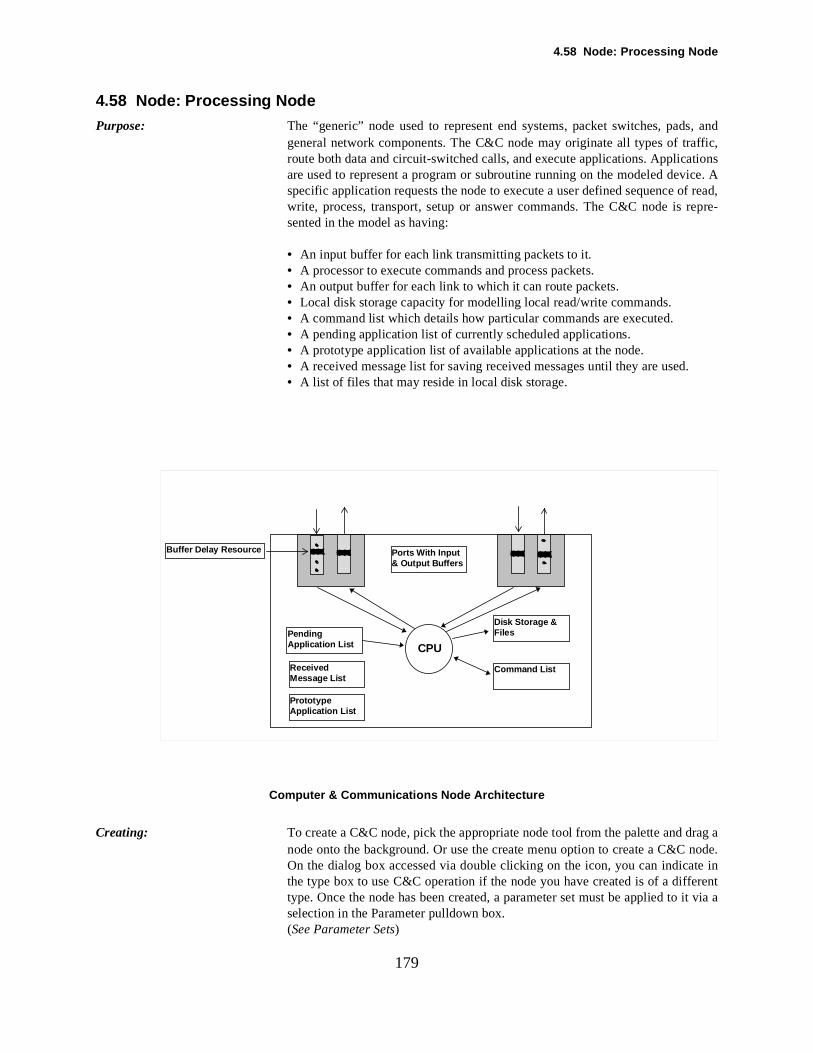
4.58 Node: Processing Node
s, and
tions
f read,epre-
.
rag a
rentit via a
179
4.58 Node: Processing Node
Purpose: The “generic” node used to represent end systems, packet switches, padgeneral network components. The C&C node may originate all types of traffic,route both data and circuit-switched calls, and execute applications. Applicaare used to represent a program or subroutine running on the modeled device. Aspecific application requests the node to execute a user defined sequence owrite, process, transport, setup or answer commands. The C&C node is rsented in the model as having:
• An input buffer for each link transmitting packets to it.• A processor to execute commands and process packets.• An output buffer for each link to which it can route packets.• Local disk storage capacity for modelling local read/write commands.• A command list which details how particular commands are executed.• A pending application list of currently scheduled applications.• A prototype application list of available applications at the node.• A received message list for saving received messages until they are used• A list of files that may reside in local disk storage.
Computer & Communications Node Architecture
Creating: To create a C&C node, pick the appropriate node tool from the palette and dnode onto the background. Or use the create menu option to create a C&C node.On the dialog box accessed via double clicking on the icon, you can indicate inthe type box to use C&C operation if the node you have created is of a diffetype. Once the node has been created, a parameter set must be applied to selection in the Parameter pulldown box.(See Parameter Sets)
CPUPendingApplication List
ReceivedMessage List
PrototypeApplication List
Disk Storage &Files
Command List
Ports With Input& Output Buffers
Buffer Delay Resource
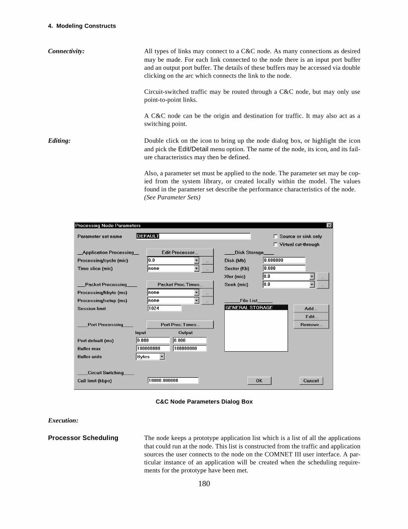
4. Modeling Constructs
iredufferouble
s a
onil-
e cop-uesode.
ionstion par-ire-
180
Connectivity: All types of links may connect to a C&C node. As many connections as desmay be made. For each link connected to the node there is an input port band an output port buffer. The details of these buffers may be accessed via dclicking on the arc which connects the link to the node.
Circuit-switched traffic may be routed through a C&C node, but may only usepoint-to-point links.
A C&C node can be the origin and destination for traffic. It may also act aswitching point.
Editing: Double click on the icon to bring up the node dialog box, or highlight the icand pick the Edit/Detail menu option. The name of the node, its icon, and its faure characteristics may then be defined.
Also, a parameter set must be applied to the node. The parameter set may bied from the system library, or created locally within the model. The valfound in the parameter set describe the performance characteristics of the n(See Parameter Sets)
C&C Node Parameters Dialog Box
Execution:
Processor Scheduling The node keeps a prototype application list which is a list of all the applicatthat could run at the node. This list is constructed from the traffic and applicasources the user connects to the node on the COMNET III user interface. Aticular instance of an application will be created when the scheduling requments for the prototype have been met.
4.58 Node: Processing Node
byction.
ationoces-
type the
ne oray beeveral thoses are, andnly be
s also
type, list. thisplica-entlyhen
a fileave
acketscider will
ichation
s inach
re is
ionisted in
181
The scheduling requirement may be by iteration time, by delay time, orreceived message, depending on the type of application and the user seleChecking and testing that scheduling criteria have been met for an applicprototype does not involve any load or overhead on the modeled node prsor—but it does take time on the computer on which you are running the simula-tion
Time-based scheduling requirements are simply met by the application protopicking the time the next application instance is required and then creatinginstance at the required time.
Received Message Scheduling means that an application may require omore messages to be received before a new instance of the application mcreated. In this case a list of received messages must be kept so that, if smessages are required by an application, the messages are kept until allrequired by the application have been received. Once all the messagereceived they are then “used” by the creation of the new application instanceso are no longer in the received message list. A particular message can oused to start one application instance.(see Received Message Scheduling)
In addition to application sources, message, response and session sourceresult in an application prototype. For instance, a message source is an applica-tion source specialized to execute a single transport command.
When a new instance of an application is created from the application protothe new application instance is added to the end of the pending applicationWhen the node becomes idle it will pick the application instance at the top oflist and so becomes loaded by the commands requiring execution by the aption. Since new instances are added at the end of the list, the node will inherpick the application that has waited longest. An exception to this may occur wsome applications have commands that are waiting for an ack or waiting for to be unlocked, they will be bypassed in favor of applications that do not hsuch requirements.
As well as executing applications, the node processor must also process pfrom input buffers. When the node processor becomes idle it must dewhether to execute an application next or process a packet. The processocompare the packets at the head of each input buffer and the application at thehead of the application pending list. It will select the packet or application whhas waited longest and perform the requisite task (packet switching or applicexecution) next.
Note that this algorithm does not compare priority between waiting packetdifferent queues—only waiting time. However, the packet at the head of einput port buffer queue will be the highest priority packet in that queue. Theno priority attribute for applications.
The packet processing task will take processor time from the node processor(assuming non-zero entries on the node parameter settings).
No Time Slice Execution If “no time slicing operation” is specified, the processor picks an applicatinstance to execute as described above, and then executes the commands lthe application command list in sequential order.
4. Modeling Constructs
. Thet andin theonse-om-
sor to exe-o per-
mandsndWhencurs istes a(5) are
xecu-mpt
eed
twoone,of thecket for
ing on
ns, itt hasll be
buttingtion
nd ise offer iscom- theted.ccess
182
The application tells the processor by name which command to execute nextprocessor compares this name to the commands in its local command lisexecutes the command it finds which has the same name. If no command local list has the same name, the node looks in the global command list. Cquently local names override global names. It is a verification check that a cmand named in an application exists either locally or globally.
When the command completes execution, the application asks the procesexecute the next command. And so on until all of the commands have beencuted. Then the processor makes a scheduling decision about which task tform next as described above.
Message creation commands, such as transport commands, answer comand setup commands, are exceptions to this rule. A message creation commais a requirement to generate packets and route them across the network. the processor executes such a command, the sequence of events that octhat it (1) creates the message, (2) incurs the packetizing delay, (3) creapacket, (4) processes the packet, (5) routes the packets. Steps (3) through repeated, as necessary, to packetize the entire message.
After a message has been created, a transport command will not resume etion until it has flow control clearance, so there will be no packet creation atteuntil after the transport command finishes its packetizing delay. The applicationis only removed from the pending list if it’s ready to execute, so there is no nto return it to the queue if it does not have flow control clearance.
This scheme of application scheduling has several features:
• If two message sources schedule overlapping transmissions, there will be application instances in the pending list. The processor will take the first generate a packet, and then replace the application instance at the back pending list. It will then take the other application instance and generate a pafor it—and so on. Packets will generally be generated alternately over timethe two message sources, although they may not alternate exactly, dependthe transport layer flow control.
• If a node performs both packet processing and message generation functiowill create or process a packet based on which generator or waiting packebeen delayed the longest. Packets moved from input to output buffers wiinterleaved with newly created packets.
With Time Slicing If time slicing operation is specified, the basic algorithm is as outlined abovewith the additional logic that, at the end of a time slice, the currently execucommand of the current application instance is interrupted and the applicainstance is put back at the end of the pending list.
When the application instance is rescheduled later, the interrupted commaresumed where it left off and the balance of work is performed. In the casread and write commands, the remaining number of bytes in the data transcompleted. For a process command, the remaining number of cycles is pleted. It is important to note that if a read or write command is interrupted,file it was accessing will remain locked until the entire command is compleThis ensures file integrity in the event that some other application needs to athe same file.
4.58 Node: Processing Node
d
s, as
have from
er to thereasstherrigin
der.re itningt at a
until
now
portg list.is a thethener toto the
cre-e lastits
theable.
to be
cre-t kedl.
ess-sing
183
Message generation commands (such as transport commands) are not interrupteby time slices. Packet creation is done one packet at a time on a round robin basis(subject to flow control constraints) for the scheduled message generatordescribed in the previous section.
Buffer Processing A packet arrives at a node when all the frames which constitute the packetbeen delivered to the node by the link protocol. The packet is reassembledits frames and an attempt is made to insert the packet into the input port bufferwhich services the link.
A test is made to see whether there is sufficient space in the input port buffreceive the packet. If there is sufficient space a test is made to see whetheris sufficient space in the overall C&C node input buffer limit. If both tests pthen the packet is placed in the port input buffer which services the link. If eitest fails then the packet is considered blocked and may be retried from the odepending on the transport protocol settings.
The packets in the buffer are ordered in decreasing priority plus FIFO orOnce in an input buffer a packet must incur a buffer processing delay befomay be considered for removal from the buffer. The buffer is modeled as owa single delay resource which is used to incur the packet delay, one packetime. Consequently the packets in the input port buffer may have to wait they are at the head of the queue in order to incur their delay.
Packets that have incurred their delay are still in the input port buffer but areavailable for switching. Again these packets are ordered by decreasing priorityplus FIFO. The C&C node compares the packets at the head of each of itsinput buffer queues and the application at the head of the application pendinIt will schedule the item that has been waiting the longest. Assuming this packet at the head of a port input buffer queue, the processor will removepacket from the queue and then incur the packet processing delay. It will make an instantaneous routing decision to determine which output port buffplace the packet in, and then attempt to instantaneously insert the packet inselected port output buffer.(See Routing Protocol: Packet)
If the packet is now at its destination any required acknowledgments will beated, delivery statistics updated, and the packet destroyed. If the packet is thpacket of a message, the message is now counted as having been delivered and text can be used to satisfy received message scheduling requirements.
If the packet is being routed onwards, the attempt to insert the packet inselected port output buffer may fail because there is insufficient space availAgain, two tests are made against the available port output buffer space and theoverall C&C node output buffer space. Both tests must pass for the packet inserted into the selected output buffer.
If either of the buffer tests fail, then the packet is blocked, and optionally reated and retransmitted from the originating node (depending on the transporpro-tocol settings). This is in contrast to ATM node processing where blocpackets would remain in the input port buffer if the output port buffer was ful
Once a packet is placed in the port output buffer it must incur the buffer procing delay for the port. Similar to the input port, the packets queue in decrea
4. Modeling Constructs
ifiedr to
&Cay beut-of
ere or of
d
typi- path routery theibleeding
the
tant&C
l (as
ity iseous
s acolail-here
trol- also
184
priority and FIFO order for the single delay resource, are delayed by the spectime, and then wait in the output buffer in decreasing priority and FIFO ordebe transmitted by the downstream link.
Command Execution See the appropriate command section.
Circuit- Switching A C&C node may originate, switch, and receive circuit-switched calls. If a Cnode originates a call, then the destination may be the same node. This mused if the node models a local switch which carries local traffic as well as oarea-traffic, but the local network topology is not desired to be modeled.
The circuit-switched traffic is independent of the packet-switched traffic. This no impact on the port buffers or on node utilization for creating, routingreceiving circuit-switched traffic. While the one node can service all typestraffic the resources on the node are separately specified for circuit switching anpacket switching.
When a circuit-switched call originates, a sequence of routing decisions is cally required, depending on the number of routes composing the end-to-endand the number of hops in each route. The nodes and links along a possibleare inspected to determine whether the complete route has capacity to carcall. From the point of view of an C&C node, the node has a maximum possbandwidth which it can concurrently switch for all circuit-switched calls routthrough it. As a call is routed through the C&C node, the amount of remainbandwidth available for circuit-switched traffic is reduced. When a call clearsused bandwidth is given back.
Consequently, a C&C node is available to carry a particular call if, at the insthe routing decision is being made, the amount of free bandwidth on the Cnode is greater than (or equal to) the bandwidth requirement for the caldefined on the routing class dialog box).
Only when the routing decision has checked that a route has sufficient capacthe bandwidth claimed. However, it should be noted that this is an instantandecision.
If the C&C node is a congestion point for the circuit-switched traffic (i.e., it ipoint on the route where there is insufficient bandwidth), the routing protowill first of all test other routes to see if one is available. If no other route is avable, the routing protocol may revisit the blocking node and test whether tare any calls routed through the node which may be preempted to release suffi-cient bandwidth to route the required call. The preemption mechanism is conled by call priority as set on the call source dialog box and preemptions mustbe activated on the call routing protocol dialog box.(See Routing Protocol: Call)
Reporting: Node Utilization.File Warning Report.Buffer Reports.All delay reports are affected by C&C node performance.
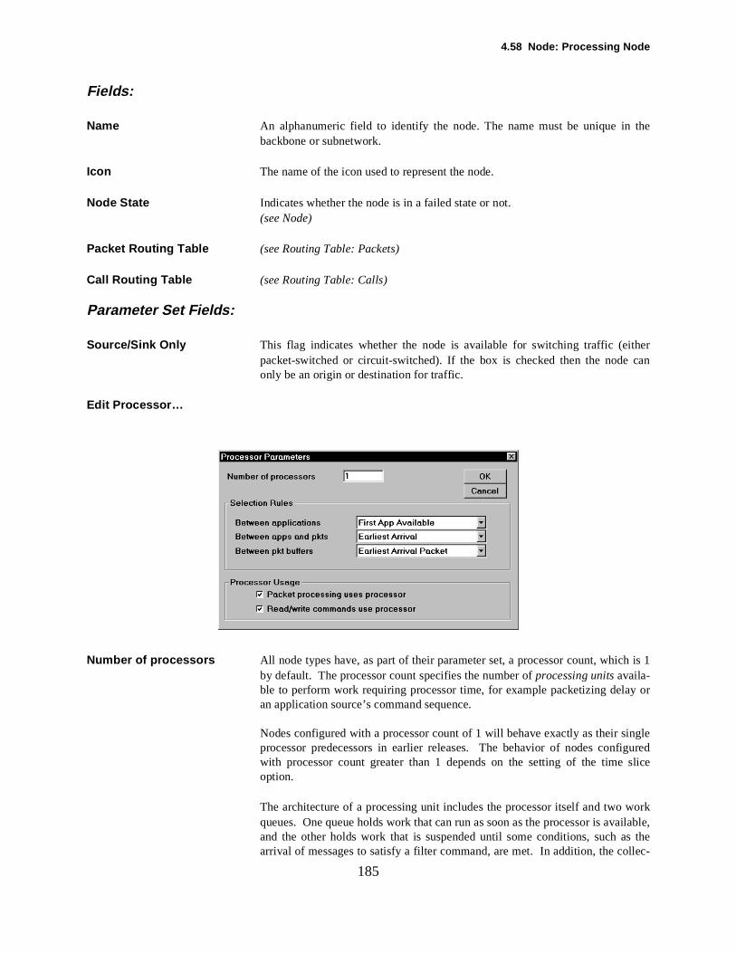
4.58 Node: Processing Node
the
her can
h is 1
y or
ngleiguredslice
ailable,thellec-
185
Fields:
Name An alphanumeric field to identify the node. The name must be unique inbackbone or subnetwork.
Icon The name of the icon used to represent the node.
Node State Indicates whether the node is in a failed state or not.(see Node)
Packet Routing Table (see Routing Table: Packets)
Call Routing Table (see Routing Table: Calls)
Parameter Set Fields:
Source/Sink Only This flag indicates whether the node is available for switching traffic (eitpacket-switched or circuit-switched). If the box is checked then the nodeonly be an origin or destination for traffic.
Edit Processor…
Number of processors All node types have, as part of their parameter set, a processor count, whicby default. The processor count specifies the number of processing units availa-ble to perform work requiring processor time, for example packetizing delaan application source’s command sequence.
Nodes configured with a processor count of 1 will behave exactly as their siprocessor predecessors in earlier releases. The behavior of nodes confwith processor count greater than 1 depends on the setting of the time option.
The architecture of a processing unit includes the processor itself and two workqueues. One queue holds work that can run as soon as the processor is avand the other holds work that is suspended until some conditions, such as arrival of messages to satisfy a filter command, are met. In addition, the co
4. Modeling Constructs
s serve
eenr the
hasessingessor robin
untilocess
work
ill be
ackethesel fre-g thees.
ssor
ppli-
o theit is
sing
been
g atns
Thisd canling
186
tion of processing units share a single pair of queues. These shared queuethe same purpose as their cousins on the processing units, but the shared queueshold work that has not yet been assigned to a processing unit.
A key aspect of COMNET’s multiprocessor model is that, once work has bassigned to a processing unit, it remains on that processing unit (in eitheprocessor itself, or one of the two local work queues) until it’s finished.
When time slicing is enabled, at the beginning of each time slice, work thatnot yet been assigned to a processing unit is selected, assigned to a procunit, and given processor time. Whenever there is no unassigned work, proctime is shared among the processes of a processing unit in a same roundfashion
When time slicing is not enabled, work is assigned to available processorsall processors have active work, at which point the processors continue to prtheir work until finished. When a processor becomes available, because all itswork is either finished or suspended, it selects work from one of the shared queues using the same algorithm as that used to select work from local queues.
An application’s command sequence makes up a single item of work, and wassigned to one processing unit.
Selection Rules The node's processor has options for how it selects the next application or pto process after it finishes processing the current application or packet. Toptions are important when modeling heavily congested processors that wilquently have many choices for selecting the next task. The rules for selectinnext task can have significant effects on the delay of applications or messag
The application and packet selection options are available in the proceparameters that are part of the node's parameter set.
Between applications There are the following selection options for when the processor selects an acation from among multiple ready applications in the application queue:
First App Available This option selects the application ready for processing and that is closest tfront of the application queue. After the application is done processing placed at the back of the queue so that this approximates a round robin process-ing of applications that are ready. Applications that are not ready for proceswill tend migrate to the front of the queue and thus it will get preference as soonas the application becomes available.
App Ready The Longest This option searches the full application queue for the application that has ready for processing the longest.
Between Apps and Packets The processor may have different criteria for picking between packets waitininput buffers and applications waiting in the application queue. The optioinclude the following choices:
Pkts Have Priority For this option, the processor will process any packet that is ready at an inputbuffer before processing any applications waiting at the application queue. type of processing places more importance on routing than on processing anbe useful for modeling networking devices. This may also be useful for mode
4.58 Node: Processing Node
e
will
ter-hereproc-
rliestlica-
r that
me its tossing
appli- they
thet the
oreeady
ntrol
rrives
rede.
acket
pre- the
ed at
187cases where the arrival of a packet triggers an interrupt that make the procssorprocess the incoming packet immediately after finishing the current task.
Apps Have Priority For this option, the processor will process any waiting application before it process any packet waiting at an input buffer. This can be useful for modelingsimpler devices that do not frequently check for waiting packets nor use inrupts for packets. It can also be useful for modeling complex scenarios wnew packets will give the processor new tasks and it is desired to have the essor finish with the current task before introducing a new one.
Earliest Arrival This option selects the application or packet that arrived at the node at the eatime. The packet arrives at the node when it enters the input buffer. The apption arrives at the node when it is generated or triggered. This is the behaviowas modeled in earlier releases.
Note that an application or packet may not be ready for processing at the tiarrives at a node: the application may wait for one of a number of conditionoccur before being ready to process, and the packet may require port procebefore it is ready to be processed by the node. In either case, the packet orcation will not be processed until they are ready, but when they are ready,will be picked based on which one arrived at the node the earliest.
Ready The Longest This option is similar to the earliest arrival option except that the time thatapplication is ready to run is compared with the time that the packet arrived ainput buffer. The applications ready-to-run time may be substantially mrecent than its arrival time in the queue. Examples of when an application's rto run time may be set are when:
1) a transport command has to retransmit a blocked packet
2) a transport command receives an acknowledgement to advance its flow cowindow
3) a transport command is allowed to transmit by its rate control algorithm
4) a filter command is satisfied
5) a file is unlocked for a waiting read or write command
Note that the packet's time that is compared is still the time that the packet aat the buffer instead of when it is ready after being processed and arriving at thefront of the buffer. Generally this should be an insignificant difference compawith the difference between the applications' ready-to-run time and arrival tim
Between pkt buffers There are the following selection options for when the processor selects a pto process from among multiple input buffers:
Earliest Arrival This option searches all the buffers for the packet that arrived the earliest.
Packet Priority This option only considers the packets at the front of the buffer and thus will serve the sorting within the buffer. If multiple buffers have packets waiting,highest priority packet will be selected, and if there are multiple head-of-linepackets with the same priority, the processor will select the packet that arriv
4. Modeling Constructs
y of thetiallycurthe onrs that any
t thessor
lays
roc-essore is torager to
NETe the thats it.
ion ofcess-oces-
l dif-s. If
entimeReadteris-t per-
icro-o be as if
nven-
188
its buffer the earliest.
Processor Usage COMNET III makes the utilization of the node's processor an option for manthe modeled delays. If the delay is modeled with processor utilization, thenitems will have to wait for an available processor and then process sequenuntil finished. Delays without utilization can allow many such delays to ocsimultaneously and, just as importantly, without affecting the utilization of node. A delay without processor utilization is useful for modeling delaysresources that are not part of the model (such as human delays or processoare outside of the model) or they may be used for waiting delays unrelated tosequential processor.
Packet processing uses processorThe packet processing parameters (for modeling network-layer processing anode) may optionally utilize the processor. This option is also in the proceparameters that are part of the node's parameters. It is useful for modelingdevices with complex multiprocessor or switching fabrics that allow most deto occur simultaneously.
Read/write commands use processorThe storage delay for read and write commands may optionally utilize the pessor. The option to utilize the processor for storage delays is in the procparameters that are part of the node's parameter set. The primary intent hermodel the separate disk controller for doing the main processing of the stodevice without utilizing the main processor. This allows the main processoprocess other activities while the disk controller delay is in progress.
Note that if multiple commands access the same file simultaneously, COMIII will model the accesses sequentially even when the delay does not utilizcentral processor because when one command begins, it locks the file soother commands have to wait until the file is unlocked before they can acces
Processing Time/Cycle Processing command execution times are scaled in cycles. The actual durata processing command is the number of cycles multiplied by the node’s proing time per cycle. When the processing command is executed, the node prsor will be made busy for this time period.
If, for example, a C&C node is modeling a server, then it may have severaferent process commands that are called from several different applicationone of the goals of a simulation is to investigate the effect of server processorspeed on network performance, the processing time per cycle field allows thspeed to be ramped up or down by changing only the one parameter (rather thachanging all the process commands individually). Note that the processing per cycle field only affects the speed of execution of process commands. and write command durations are controlled by the disk performance charactics, and the packet switching delays are controlled by the buffer and packeformance characteristics.
If a server runs at 50MHz, the processing time need not be entered as .02 mseconds. It may be more convenient to choose a processing time per cycle tconvenient unit for the processing delays modeled at this node, and perhapnor-malized to a unit value for the default processor being modeled. For exampleserver commands take on the order of milliseconds to complete, then a co
4.58 Node: Processing Node
werively.
era-
d canp the
pack-
tion
oces-outed
100essingoto-ply
tched
thisould
ingn its
puterocol.
oto-es in
time isg forf noT is
189
ient processing time per cycle would be 1 millisecond. Faster or slomachines may be modeled by adjusting that time smaller or larger, respectFor example, a 10% faster machine would have 0.9 milliseconds per cycle.
Time Slice If no time slice value is entered then COMNET III assumes no time slice option for the node.
If a value is entered then, as commands are executed, a particular commanuse the node processor for one time slice duration and then must give uprocessor to other pending applications.
For commands which create packets, a packet is not created until after the etizing elapses, as specified on the respective message source dialog box incurredby the node processor. The packetizing delay is not subject to time slicing.
Likewise, packet processing delays are not subject to time slicing.
Operation of the node with and without time slicing is discussed in the Execusection above.
Processing Time/Packet After a packet is created or after a packet leaves an input buffer, the node prsor is made busy for the Processing Time/Packet value depending on the rprotocol ID of the transport layer that created the packet.
For instance, if a C&C node is modeling a packet switch rated at switchingpackets per second, this performance could be captured by entering a ProcTime/Packet of 10 milliseconds as the default or for this particular routed prcol ID. Upgrading the switch to a 500 packet per second rating would then imreducing the Processing Time/Packet to 2 milliseconds.
The Processing Time/Packet is a delay applied to each packet as it is swithrough the node. It is in addition to any input or output buffer queueing delays orbuffer processing delays.
After incurring a packetizing delay, packets would be created at a node andwould then be followed by the packet processing delay, then the packets wbe inserted in an output port buffer.
Packets destined for the node would first incur any input port buffer switchand queueing delays, followed by this packet processing delay based orouted protocol ID. They are then counted as having arrived.
The packet processing time at a Computer and Communication Node, ComGroup Node, and Router Node can vary according to a packet’s routed protThe packet’s routed protocol is determined by the transport protocol referencedby the packet. A transport protocol has a new field identifying its routed prcol. In setting the routed protocol field, the user may select one of the namthe combo box list or type in a new name.
When a packet is about to be processed at a node, the packet processing determined by going to the node’s list of packet processing times and lookina routed protocol in the list that matches the packet’s routed protocol. Imatch is found, the processing time for the routed protocol named DEFAUL
4. Modeling Constructs
singackete size kilo-ted asme per
click-s dia-
cket
as to be thatur the estab-
e
beTime/
theere is
d.
k to
and
theade
hether
190
used. The DEFAULT entry is always present in the list. The total procestime for a packet is given by the protocol-dependent processing time per p(as just described) plus a separate factor that varies linearly according to thof the packet. The size-dependent factor is given by the processing time perbyte field times the packet size in kilobytes. Session setup packets are treaa special case and have a packet processing time given by the processing tisetup packet field.
The list of packet processing times for each routed protocol is accessed by ing on the Edit Times button in the Packet Processing part of the Parameterlog box for C&C Nodes, Computer Groups, and Routers.
(see also Processing Time/kbyte following)
Processing Time/kbyte Some devices exhibit the behavior where it takes longer to switch a large pathan a small packet. The C&C node makes allowance for this by providing aProcessing Time/kbyte field.
The switching time for a packet is then calculated using the formula:
Switching Time = Ax + B
whereA = Processing Time/kbytex = Size of packet in kilobytesB = Processing Time/Packet (see immediately previous section)
Processing Time/Setup PacketWhen a session is established across a network, the session setup packet hrouted at each node. Assuming connection-oriented routing, data packetssubsequently follow the same route as the session setup packet do not incsame routing overhead at the node, because as the route has already beenlished by the setup packet. Thus the processing for the setup packet may bsub-stantially longer than the packets that follow in that session.
Consequently, COMNET III provides the Processing Time/Setup Packet toentered for the setup packet delay at the node. The Packet Processing Packet delay will be used for the following data packets.
Input Buffer Size The maximum allowable buffer usage across all input ports connected toC&C node. When a packet is received, then a test is first made to see if thspace in the port buffer, and then a test is made to see whether the total bufferusage limit (as defined here) would be exceeded if the packet were accepte
The input port buffer size is defined on the arc which connects a particular linthe C&C node.
If there is insufficient space to receive a packet then the packet is blockedoptionally retried depending on the transport protocol settings.
Output Buffer Size The maximum allowable buffer usage across all output ports connected toC&C node. When a packet is switched to an output port, then a test is first mto see if there is space in the port buffer, and then a test is made to see w
4.58 Node: Processing Node
cket
k
then the
h the
C&Cit are
d the
firstrame- proto- time timeetime
anged
thel andly to
de isodealong
on-
des for
mod-
191
the total buffer usage limit (as defined here) would be exceeded if the pawere accepted.
The output port buffer size is defined on the arc which connects a particular linto the C&C node.
If there is insufficient space to receive a packet into the output port buffer, the packet is blocked and optionally retried from the origin depending ontransport protocol settings.
Session Limit The maximum number of sessions that can be concurrently routed througC&C node at any particular instant.
When a session routing decision is being made for a session setup packet,nodes that are already carrying a number of sessions equal to the session limnot available for routing the session setup packet.(see Routing Protocol: Packet)
Port Processing Times Port processing times can vary as a function of a packet’s routed protocol antype of link connected to the port. To determine the port processing time for apacket that has just arrived at an input or output port buffer, the model checks the special case port processing times included with the node’s paters. It searches the list of special cases to find a case with the same routedcol and type of link. If a match is found, the model uses the port processinggiven for the special case. If no match is found, it uses the port processingset for the port. The processing time for the port is set on the arc connecting thnode to the link. When a node is initially connected to a link, the processing that is set for the port is the default port processing time on the node parametersdialog box. The port processing time set on a port can subsequently be chby editing detail on the arc connecting the node and link.
To edit the list of special case port processing times, click on Edit Times inPort Processing part of the node parameters dialog box. Note that protocolink-dependent port processing times and default port processing times appany type of COMNET III node. As explained above, the default port processingtime on the node parameters dialog box is used only at edit time when a noconnected to a link. Including the default port processing time with the nparameters allows port-dependent processing times to be saved in a library with the other parameters describing a node.
Call Limit The maximum amount of bandwidth for circuit-switched traffic that can be ccurrently routed through the C&C node at any particular instant.
When a circuit-switched routing decision is being made for a call, C&C nothat have insufficient remaining bandwidth to carry the call are not availablerouting the call.(see Routing Protocol: Call)
Disk Size If read and write commands are required on the C&C node, the size of the eled disk connected to the node must be specified.
The value is entered In Megabytes (1024 Kbytes = 1024 * 1024 bytes =1,048,576 bytes)
4. Modeling Constructs
filesningugh,
d or
e)
tion
doesends
an beand
isk,
truc-s aary the
es
only
192
If a write command adds data to a file which results in the total space for all exceeding the specified disk size, a warning will be added to the File Warreport and the command will continue as if the full transfer completed, althothe disk will not be increased in size. This is taken as a pessimistic response tooverflowing the disk.(see also Command: Write File & Command: Read File)
Disk Sector Size The size of a disk sector in Kilobytes (1024 bytes).
A read or write command will result in a number of disk sectors to be reawritten, depending on the amount of data and the sector size.
Disk Transfer Time The length of time it takes to read or write a disk sector.
Disk Transfer Overhead The overhead time to seek to a particular disk sector.
The duration of any particular transfer is calculated on the basis of:
Transfer Time = Number of Sectors * (Transfer Time+Overhead Tim
(see also Command: Write File & Command: Read File)
File List A list of files that are to be created on the modeled disk before the simulastarts. Only files with a positive size are considered to have been created.
Files may also be created by executing a write command. If the named file not exist, then the write command will create it, provided the command appa positive number of bytes to the file.
However, it is common to need a number of files on the disk and so these cadded to the file list, rather than having to create and execute a write commfor each file. When the model initializes, the listed files are created on the dprovided they have a positive size.
It may be that at the time the simulation is being performed the detailed file sture of the modeled system is not known. In this case COMNET III providefile called GENERAL STORAGE which can be used to read and write arbitrnumbers of bytes, thereby modelling the transfer delays but without knowingdetailed file structure.
File Name The name of the file. The name must be unique on the C&C node.
File Size The initial size of the file. It is a verification check that the size of all initial fildoes not exceed the size of the disk.
File Read Only Flag Indicates whether the file is read-only or not. Attempting to update a read-file will cause an error to be reported when verifying a model.
Command List Answer Message Command(see Command: Answer Message)Processing Command (see Command: Processing)Read File Command (see Command: Read File)Setup Session Command (see Command: Setup Session)

4.58 Node: Processing Node
193
Transport Command (See Command: Transport)Write File Command (see Command: Write File)
4. Modeling Constructs
, andto be
It has by the
theepre-
eceiveets.
createn the
ated a box.
o
mayt-to-
y beputer
om-
on-ircuit
ode
onil-
e cop-uesode.
194
4.59 Node: Computer Group
Purpose: It is a common requirement to want to model a population of similar users con-nected to a network. Rather than making a node to represent each of themthen editing the details of each node, a Computer Group Node only has defined once to represent a number of end systems.
In many respects, the Computer Group Node is the same as a C&C node. largely the same parameters and performance characteristics, as evidenceduser interface. However, the Computer Group node has a Quantity attributewhich indicates how many identical instances of the node to generate withComputer Group node parameters. Hereafter, one of the individual nodes rsented by the computer group is referred to as an Instance Node.
Each Instance Node may execute applications, generate packets, and rpackets, as if it were a C&C Node. However, it may not switch or route pack
Creating: To create a Computer Group node, pick the appropriate node tool from the pal-ette and drag a node onto the background. Or use the create menu option toa Computer Group node. On the dialog box accessed via double clicking oicon, you can indicate in the type box to use Computer Group operation if thenode you have created is of a different type. Once the node has been creparameter set must be applied to it via a selection in the Parameter pulldown(See Parameter Sets)
Connectivity: A Computer Group can connect to just one of the multiaccess links. Point tpoint links may not be connected to such a node. Note that a Computer Groupnode represents a population of Instance Nodes, but a point to point link only connect to one node at either end. This explains the restriction on poinpoint link connectivity.
Each Instance Node in the Computer Group has an input port buffer and an out-put port buffer for the link it is connected to. The details of these buffers maaccessed via double clicking on the arc which connects the link to the ComGroup node.
Circuit-switched traffic cannot be created, routed through, or received by a Cputer Group node (or any of the Instance Nodes). Circuit-switched traffic canonly be carried over point-to-point links. Since a point-to-point link cannot cnect to a Computer Group node, the Computer Group node can have no cswitching capability.
Multiple Message, Session, Response and Application sources may be connectedto a Computer Group node. A source connected to a Computer Group Nimplies that there is a separate source for each Instance Node in that group.
Editing: Double click on the icon to bring up the node dialog box, or highlight the icand pick the Edit/Detail menu option. The name of the node, its icon, and its faure characteristics may then be defined.
Also a parameter set must be applied to the node. The parameter set may bied from the system library, or created locally within the model. The valfound in the parameter set describe the performance characteristics of the n(See Parameter Sets)
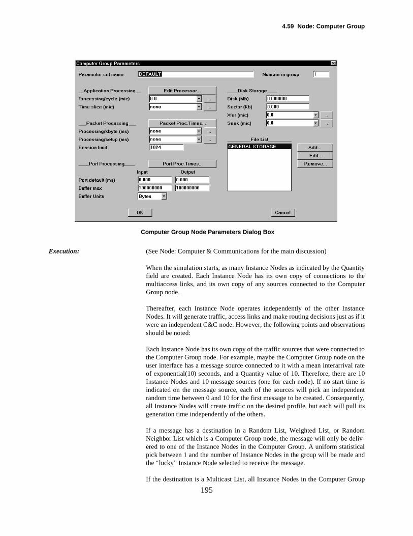
4.59 Node: Computer Group
antityo theputer
ces if ittions
ted ton the
al ratere 10isndentently,
dom-tical and
195
Computer Group Node Parameters Dialog Box
Execution: (See Node: Computer & Communications for the main discussion)
When the simulation starts, as many Instance Nodes as indicated by the Qufield are created. Each Instance Node has its own copy of connections tmultiaccess links, and its own copy of any sources connected to the ComGroup node.
Thereafter, each Instance Node operates independently of the other InstanNodes. It will generate traffic, access links and make routing decisions just awere an independent C&C node. However, the following points and observashould be noted:
Each Instance Node has its own copy of the traffic sources that were connecthe Computer Group node. For example, maybe the Computer Group node ouser interface has a message source connected to it with a mean interarrivof exponential(10) seconds, and a Quantity value of 10. Therefore, there aInstance Nodes and 10 message sources (one for each node). If no start time indicated on the message source, each of the sources will pick an indeperandom time between 0 and 10 for the first message to be created. Consequall Instance Nodes will create traffic on the desired profile, but each will pull itsgeneration time independently of the others.
If a message has a destination in a Random List, Weighted List, or RanNeighbor List which is a Computer Group node, the message will only be delivered to one of the Instance Nodes in the Computer Group. A uniform statispick between 1 and the number of Instance Nodes in the group will be madethe “lucky” Instance Node selected to receive the message.
If the destination is a Multicast List, all Instance Nodes in the Computer Group

4. Modeling Constructs
s alltance
ing
ode.ed toompu-
nly.
196
will receive the message.
Reporting: As for a C&C node.On the Report Selection screen you may indicate whether Computer GroupDetail should be reported. If this is off, then only sum total statistics acrosInstance Nodes in a Computer Group are reported. If this is on, each InsNode in the Computer Group is reported.
Fields: A Computer Group Node has the same fields as a C&C Node, with the followexceptions:
Quantity The number of identical C&C nodes represented by the Computer Group NIndividual copies of the node are made up to this quantity. These are referras Instance Nodes. Each Instance Node has connections to any links the Cter Group Node is connected to. Connected traffic generators are copied for eachInstance Node.
Call Bandwidth Not SupportedCircuit-switched traffic cannot originate, be switched through, or be destined fora Computer Group Node.
Source/Sink Only Not necessary because computer group instances are always source/sink o
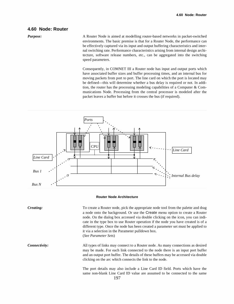
4.60 Node: Router
hede can-rchi-tching
ichus formayddi-om-r the
dragr
s of alied to
siredufferouble
thesame
197
4.60 Node: Router
Purpose: A Router Node is aimed at modelling router-based networks in packet-switcenvironments. The basic premise is that for a Router Node, the performancbe effectively captured via its input and output buffering characteristics and internal switching rate. Performance characteristics arising from internal design atecture, software release numbers, etc., can be aggregated into the swispeed parameters.
Consequently, in COMNET III a Router node has input and output ports whhave associated buffer sizes and buffer processing times, and an internal bmoving packets from port to port. The line card on which the port is located be defined—this will determine whether a bus delay is required or not. In ation, the router has the processing modeling capabilities of a Computer & Cmunications Node. Processing from the central processor is modeled aftepacket leaves a buffer but before it crosses the bus (if required).
Router Node Architecture
Creating: To create a Router node, pick the appropriate node tool from the palette anda node onto the background. Or use the Create menu option to create a Routenode. On the dialog box accessed via double clicking on the icon, you can indi-cate in the type box to use Router operation if the node you have created idifferent type. Once the node has been created a parameter set must be appit via a selection in the Parameter pulldown box.(See Parameter Sets)
Connectivity: All types of links may connect to a Router node. As many connections as demay be made. For each link connected to the node there is an input port band an output port buffer. The details of these buffers may be accessed via dclicking on the arc which connects the link to the node.
The port details may also include a Line Card ID field. Ports which havesame non-blank Line Card ID value are assumed to be connected to the
Internal Bus delayBus 1
Bus N
Line Card
Line Card
Ports
CPU
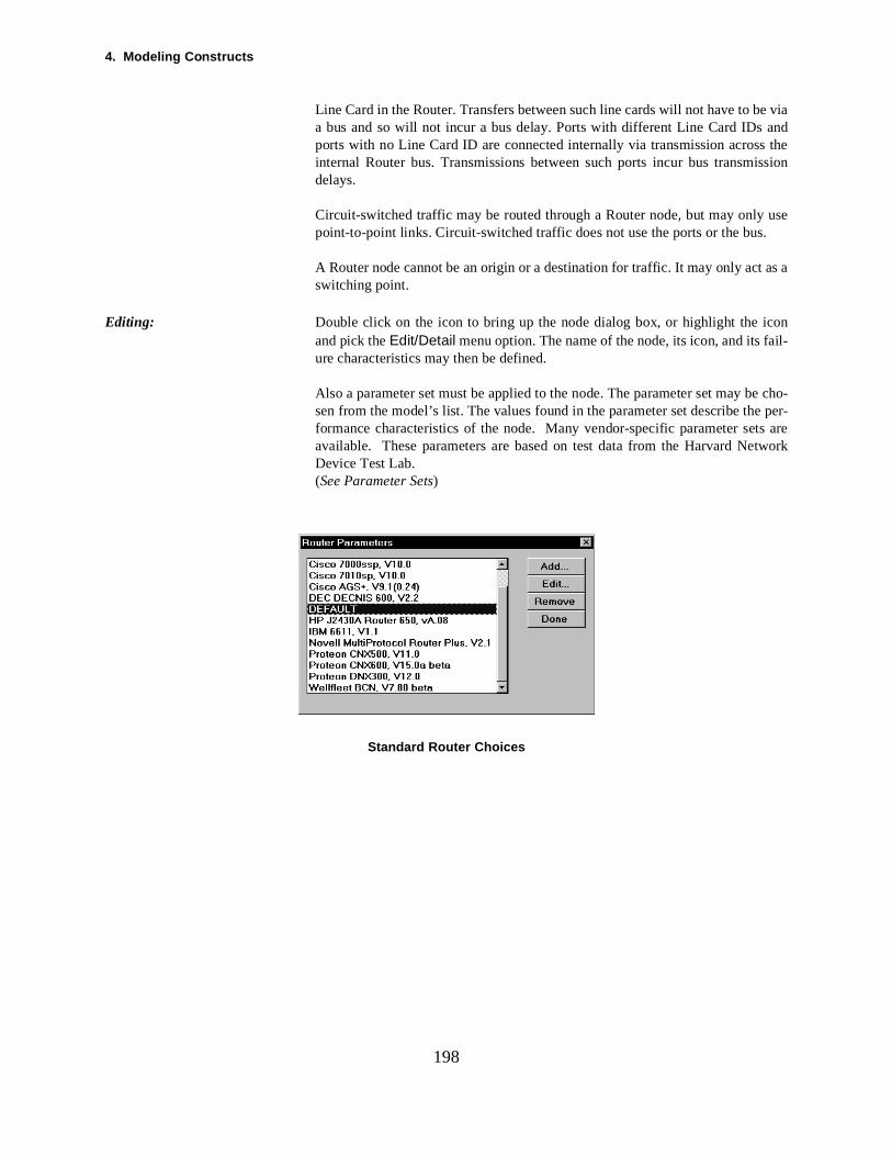
4. Modeling Constructs
e viaand the
ission
e
as a
onil-
e cho- per-s aretwork
198
Line Card in the Router. Transfers between such line cards will not have to ba bus and so will not incur a bus delay. Ports with different Line Card IDs ports with no Line Card ID are connected internally via transmission acrossinternal Router bus. Transmissions between such ports incur bus transmdelays.
Circuit-switched traffic may be routed through a Router node, but may only uspoint-to-point links. Circuit-switched traffic does not use the ports or the bus.
A Router node cannot be an origin or a destination for traffic. It may only act switching point.
Editing: Double click on the icon to bring up the node dialog box, or highlight the icand pick the Edit/Detail menu option. The name of the node, its icon, and its faure characteristics may then be defined.
Also a parameter set must be applied to the node. The parameter set may bsen from the model’s list. The values found in the parameter set describe theformance characteristics of the node. Many vendor-specific parameter setavailable. These parameters are based on test data from the Harvard NeDevice Test Lab.(See Parameter Sets)
Standard Router Choices
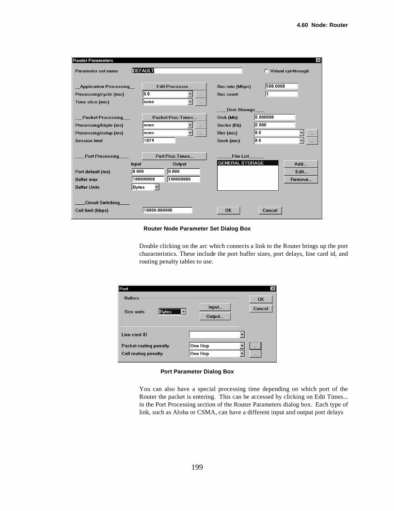
4.60 Node: Router
port
f thees...pe ofys
199
Router Node Parameter Set Dialog Box
Double clicking on the arc which connects a link to the Router brings up the characteristics. These include the port buffer sizes, port delays, line card id, androuting penalty tables to use.
Port Parameter Dialog Box
You can also have a special processing time depending on which port oRouter the packet is entering. This can be accessed by clicking on Edit Timin the Port Processing section of the Router Parameters dialog box. Each tylink, such as Aloha or CSMA, can have a different input and output port dela
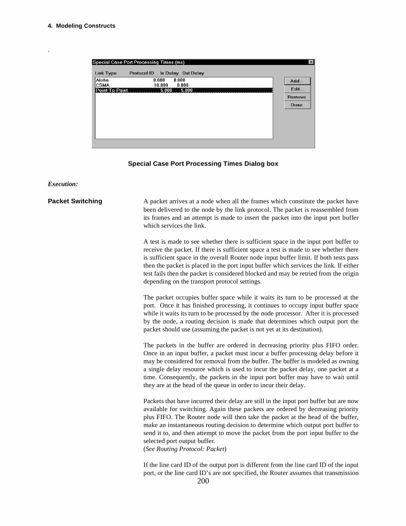
4. Modeling Constructs
have from
er to thereasstherrigin
t thepacessedt the
der.re itningt at a
until
now
er to the
utssion
200
.
Special Case Port Processing Times Dialog box
Execution:
Packet Switching A packet arrives at a node when all the frames which constitute the packetbeen delivered to the node by the link protocol. The packet is reassembledits frames and an attempt is made to insert the packet into the input port bufferwhich services the link.
A test is made to see whether there is sufficient space in the input port buffreceive the packet. If there is sufficient space a test is made to see whetheris sufficient space in the overall Router node input buffer limit. If both tests pthen the packet is placed in the port input buffer which services the link. If eitest fails then the packet is considered blocked and may be retried from the odepending on the transport protocol settings.
The packet occupies buffer space while it waits its turn to be processed aport. Once it has finished processing, it continues to occupy input buffer swhile it waits its turn to be processed by the node processor. After it is proceby the node, a routing decision is made that determines which output porpacket should use (assuming the packet is not yet at its destination).
The packets in the buffer are ordered in decreasing priority plus FIFO orOnce in an input buffer, a packet must incur a buffer processing delay befomay be considered for removal from the buffer. The buffer is modeled as owa single delay resource which is used to incur the packet delay, one packetime. Consequently, the packets in the input port buffer may have to wait they are at the head of the queue in order to incur their delay.
Packets that have incurred their delay are still in the input port buffer but areavailable for switching. Again these packets are ordered by decreasing priorityplus FIFO. The Router node will then take the packet at the head of the buffer,make an instantaneous routing decision to determine which output port buffsend it to, and then attempt to move the packet from the port input buffer toselected port output buffer.(See Routing Protocol: Packet)
If the line card ID of the output port is different from the line card ID of the inpport, or the line card ID’s are not specified, the Router assumes that transmi
4.60 Node: Router
e, nontil afrom input out-
y failts are nodee
rdedrt kets
st
ess-singifiedr to
typi- path routery thesibleedining the
stantouterl (as
ity iseous
is acolail-here
trol-
201across an internal bus is required. At the point the routing decision is madbus may be available so the packet has to remain in the input port buffer ubus is available. A transmission time across the bus will then be computed the packet size and bus transmission speed, the packet removed from theport, the delay time incurred, and an attempt made to insert the packet in theput port buffer.
If no bus transmission is required, then the packet will be removed from the inputport buffer and an attempt made to insert it in the output port buffer.
In either case, the attempt to insert the packet into the output port buffer mabecause the selected buffer has insufficient space available. Again, two tesmade against the available port output buffer space and the overall Routeroutput buffer space. Both tests must pass for the packet to be inserted into thselected output buffer.
If either of the buffer tests fail then the packet is blocked and is either discaor retransmitted on an end-to-end basis, depending on the selected transpopro-tocol option. This is in contrast to ATM node processing, where blocked pacwould remain in the input port buffer.
When a bus becomes idle, it pulls the packet that has been waiting the longe
Once a packet is placed in the port output buffer, it must incur the buffer procing delay for the port. Similar to the input port, the packets queue in decreapriority and FIFO order for the single delay resource, are delayed by the spectime, and then wait in the output buffer in decreasing priority and FIFO ordebe transmitted by the downstream link.
Circuit-Switching When a circuit-switched call originates, a sequence of routing decisions is cally required, depending on the number of routes composing the end-to-endand the number of hops in each route. The nodes and links along a possibleare inspected to determine whether the complete route has capacity to carcall. From the point of view of an Router node, the node has a maximum posbandwidth which it can concurrently switch for all circuit-switched calls routthrough it. As a call is routed through the Router node, the amount of remabandwidth available for circuit-switched traffic is reduced. When a call clearsused bandwidth is given back.
Consequently, a Router node is available to carry a particular call if, at the inthe routing decision is being made, the amount of free bandwidth on the Rnode is greater than (or equal to) the bandwidth requirement for the caldefined on the routing class dialog box).
Only when the routing decision has checked that a route has sufficient capacthe bandwidth claimed. However, it should be noted that this is an instantandecision.
If the Router node is a congestion point for the circuit-switched traffic (i.e., it point on the route where there is insufficient bandwidth), the routing protowill first of all test other routes to see if one is available. If no other route is avable, the routing protocol may revisit the blocking node and test whether tare any calls routed through the node which may be preempted to release suffi-cient bandwidth to route the required call. The preemption mechanism is con
4. Modeling Constructs
also
ode.
the
ion of.made
ad attions
era-
d canp the
pack-
tion
oces-
202
led by call priority as set on the call source dialog box and preemptions mustbe activated on the call routing protocol dialog box.(See Routing Protocol: Call)
Reporting The buffer reports indicate buffer congestion on the Router node. See:Input Buffer Report By PortInput Buffer Report By NodeOutput Buffer Report By PortOutput Buffer Report By Node
The Message Delay and Packet Delay reports reflect delays at the Router n
Fields:
Name An alphanumeric field to identify the node. The name must be unique inbackbone or subnetwork.
Icon The name of the icon used to represent the node.
Node State Indicates whether the node is in a failed state or not.(see Node)
Packet Routing Table (see Routing Table: Packets)
Call Routing Table (see Routing Table: Calls)
Parameter Set Fields:
Processing Time/Cycle Processing command execution times are scaled in cycles. The actual duratthe command is the number of cycles multiplied by the processing time per cycleWhen the processing command is executed, the node processor will be busy for this time period.
Processing commands are useful for modeling internal processing overhethe router’s CPU, such as for routing table calculations or management func
Time Slice If no time slice value is entered then COMNET III assumes no time slice option for the node.
If a value is entered then, as commands are executed, a particular commanuse the node processor for one time slice duration and then must give uprocessor to other pending applications.
For commands which create packets, a packet is not created until after the etizing elapses, as specified on the respective message source dialog box incurredby the node processor. The packetizing delay is not subject to time slicing.
Operation of the node with and without time slicing is discussed in the Execusection above.
Processing Time/Packet After a packet is created or after a packet leaves an input buffer, the node prsor is made busy for the Processing Time/Packet value.
4.60 Node: Router
100essing
ds.
tched
this
ingted as
ket’s pro-yinge of
time isg forf noT issingackete size kilo-ted asme per
click-s dia-
cket
203
For instance, if a C&C node is modeling a packet switch rated at switchingpackets per second, this performance could be captured by entering a ProcTime/Packet of 10 milliseconds. Upgrading the switch to a 500 packet per secondrating would then imply reducing the Processing Time/Packet to 2 millisecon
The Processing Time/Packet is a delay applied to each packet as it is swithrough the node. It is in addition to any input or output buffer queueing delays orbuffer processing delays.
After incurring a packetizing delay, packets would be created at a node andwould then be followed by a processing delay, then the packets would be insertedin an output port buffer.
Packets destined for the node would first incur any input port buffer switchand queueing delays, followed by this processing delay. They are then counhaving arrived.
The packet processing time at a Router Node can vary according to a pacrouted protocol. The packet’s routed protocol is determined by the transporttocol referenced by the packet. A transport protocol has a new field identifits routed protocol. In setting the routed protocol field, the user may select onthe names in the combo box list or type in a new name.
When a packet is about to be processed at a node, the packet processing determined by going to the node’s list of packet processing times and lookina routed protocol in the list that matches the packet’s routed protocol. Imatch is found, the processing time for the routed protocol named DEFAULused. The DEFAULT entry is always present in the list. The total procestime for a packet is given by the protocol-dependent processing time per p(as just described) plus a separate factor that varies linearly according to thof the packet. The size-dependent factor is given by the processing time perbyte field times the packet size in kilobytes. Session setup packets are treaa special case and have a packet processing time given by the processing tisetup packet field.
The list of packet processing times for each routed protocol is accessed by ing on the Edit Times button in the Packet Processing part of the Parameterlog box for C&C Nodes, Computer Groups, and Routers.
(see also Processing Time/kbyte following)
Processing Time/kbyte Some devices exhibit the behavior where it takes longer to switch a large pathan a small packet. The router node makes allowance for this by providing aProcessing Time/kbyte field.
The switching time for a packet is then calculated using the formula:
Switching Time = Ax + B
whereA = Processing Time/kbytex = Size of packet in kilobytesB = Processing Time/Packet (see immediately previous section)
4. Modeling Constructs
as to be thatur the estab-
bet delay
d the
firstrame- proto- time timeetime
anged
thel andly to
de isodealong
vedittednd bus
times out-t same
e thathere
d tof there
d.
k to
204
Processing Time/Setup PacketWhen a session is established across a network, the session setup packet hrouted at each node. Assuming connection-oriented routing, data packetssubsequently follow the same route as the session setup packet do not incsame routing overhead at the node, because as the route has already beenlished by the setup packet.
Consequently, COMNET III provides the Processing Time/Setup Packet toentered for the setup packet delay at the node. The Processing Time/Packewill be used for the following data packets.
Port Processing Times Port processing times can vary as a function of a packet’s routed protocol antype of link connected to the port. To determine the port processing time for apacket that has just arrived at an input or output port buffer, the model checks the special case port processing times included with the node’s paters. It searches the list of special cases to find a case with the same routedcol and type of link. If a match is found, the model uses the port processinggiven for the special case. If no match is found, it uses the port processingset for the port. The processing time for the port is set on the arc connecting thnode to the link. When a node is initially connected to a link, the processing that is set for the port is the default port processing time on the node parametersdialog box. The port processing time set on a port can subsequently be chby editing detail on the arc connecting the node and link.
To edit the list of special case port processing times, click on Edit Times inPort Processing part of the node parameters dialog box. Note that protocolink-dependent port processing times and default port processing times appany type of COMNET III node. As explained above, the default port processingtime on the node parameters dialog box is used only at edit time when a noconnected to a link. Including the default port processing time with the nparameters allows port-dependent processing times to be saved in a library with the other parameters describing a node.
Bus Rate The bus transmission speed inside the node. Packets that have to be mobetween ports that have different (or no) line card ID have to be transmacross a bus and so incur a transmission delay based on the packet size arate. A bus can transmit one packet at a time.
In some router implementations, a packet may need to cross a bus multiple (for example, once from input to central processor and then again to get toput). In these cases, the bus rate should represent the effective rate as if thapacket only crossed once.
Bus Count Routers or switches able to switch a number of packets simultaneously, havnumber as bus count. Also, nonblocking switch fabrics may be modeled wbus count equals or exceeds the number of connected links (or line cards).
Input Buffer Limit The maximum allowable input buffer usage across all input ports connectethe Router node. When a packet is received then a test is first made to see iis space in the port buffer, and then a test is made to see whether the total bufferusage limit (as defined here) would be exceeded if the packet were accepte
The input port buffer size is defined on the arc which connects a particular lin
4.60 Node: Router
and
ed tos firstto seef the
k
then
205
the Router node.
If there is insufficient space to receive a packet then the packet is blockedoptionally retried depending on the transport protocol settings.
Output Buffer Limit The maximum allowable output buffer usage across all output ports connectthe Router node. When a packet is switched to an output port then a test imade to see if there is space in the port buffer, and then a test is made whether the total buffer usage limit (as defined here) would be exceeded ipacket were accepted.
The output port buffer size is defined on the arc which connects a particular linto the Router node.
If there is insufficient space to receive a packet into the output port buffer, the packet is blocked and is optionally retransmitted from the origin dependingon the Transport protocol settings.

4. Modeling Constructs
itional
206
4.61 Node: Router - Updated Router LibraryThe router library has been updated to include Bradner test results published as of July 1996, as well as addrouters from Bay Networks and Cisco. Parameter sets are now available for the following routers:
3Com NetBuilder II3Com ONcore ACC ACS 4200, V5.0.3Bay Networks BCNBay Networks BLNBay Networks ASN (1 unit)Bay Networks ASN (2 units)Bay Networks ASN (3 units)Bay Networks ASN (4 units)Cabletron ATX LAN SwitchCisco AGS+Cisco 2500Cisco 4000Cisco 4500Cisco 7000/7010 spCisco 7000/7010 sspCisco 7500Cray Communications ES-1520DEC DECNIS 600, V2.2Digital RouteAbout Central EWFORE Systems PowerHub 7000FORE Systems PowerHub 3150HP AdvanceStack Router 650IBM 2210 Nways Router 24EIBM Nways 6611Novell MultiProtocol Router Plus, V2.1Proteon CNX500, V11.0Proteon CNX600, V15.0a betaProteon DNX300, V12.0RAD Network Devices VgateRetix rx7500
4.62 Packet Switched Networks
ks./IP,s are cellell.
the
tion(E-
the
om-ay
iled
size.natingit that, CRC
haveuted to
acketgment
llyin the
207
4.62 Packet Switched Networks
Purpose: One of the main aims of COMNET III is to model packet-switched networExamples include X.25 networks, router-based networks running under TCPetc. Message-switched networks may also be modeled where messagerouted on a store-and-forward basis to the destination. Likewise, frame orswitched networks may be modeled where the packet models the frame or c
Creating: There are three main steps in building a packet-switched model.
σDefine the network architecture in terms of nodes, links, routers etc. Specifyperformance characteristics of each device.
σDefine the traffic load to be carried between the different origin/destinacombinations in the network. This may be broken down by type of traffic mail, file transfer, database query, etc.), and by transport protocol.
σDefine the routing protocol which will make the routing decisions to move traffic from origin to destination.
Connectivity: Packet-switched traffic originates, is switched by, and is destined for either Cputer & Communications Nodes or Computer Group Nodes. All nodes mswitch packets.
All types of links may carry packets.
Editing: Via the appropriate object dialog box.
Execution: This description is a high level overview of packet switching. For the detaexecution logic at a node or link, see the appropriate section in this manual.
Traffic load is defined in terms of message interarrival time and message This causes messages to be created at the appropriate time at the originode. The message generator has a transport protocol associated with defines the maximum packet size and packet overhead (i.e., size of headercheck, etc.).
Therefore packets are created one after the other until sufficient packets been made to match the overall size of the message. Each packet is then roits destination by the network and associated routing protocol.
With session-type traffic and connection-oriented routing, a session setup pestablishes the route to the destination—all subsequent data and acknowledpackets follow the established route.
If connection-oriented routing is turned off then all packets are individuarouted for all types of message sources. This means that some packets same message may take a different route from others in order to reach the desti-nation.
4. Modeling Constructs
208
Packet Transmission Diagram
Reporting: Message Delay Report.Packet Delay Report.Node, Link & Buffer Reports reflect packet loading.Session reports.
Fields: See the appropriate object section.
BC LinkAB Link
A B C D
CD Link
Propagation delayTime
PacketsTransmission delay
Queueing & processing delay
Pkt1
Pkt2
Pkt3
Pkt1
Pkt2
Pkt3
Pkt1
Pkt2
Pkt3
4.63 Parameter Sets
hichbject
unt.
bjectjects.ecificcts.
ich ists are Theyded tod thisn the
ia theence
fol-
r setse orssage
thes of
209
4.63 Parameter Sets
Purpose: Each node and link type in COMNET III has parameters associated with it wdefine the performance characteristics of the object. For instance, a Router ohas parameters for input buffer size, output buffer size, bus rate, and bus co
Rather than each node or link having its own local parameter values, the opoints to a stand-alone set of values that may be shared among many obThis means that where objects share common parameter values, any spvalue has to only be updated once to make the change known to all the obje
Parameter sets for each node and link type are kept in a system library whaccessible by all models when they are created. The library parameter secopied when a new model is made and become local to the created model.can then be used by the objects in the model. If a new parameters set is adthe system library after a model has been created, provision is made to adnew parameter set to a particular model via the Add button which appears oparameter set list box.
As local values of the parameters in a model’s parameter set are changed (vEdit button on the parameter set list box) then the nodes or links, which refermodel’s modified parameter set see the changed values.
In addition to its lists of node and link parameter sets, a model also has thelowing lists:
• Call Routing Classes• Packet Routing Classes• Transport Protocols• Packet Routing Penalties• Call Routing Penalties• User Distributions• Table Distributions
Each of these model lists is analogous to a model’s list of different parametefor a particular node or link type. Many elements in a model can referenc“share” the same parameter set in a model’s list. For example, many mesources could reference the same transport protocol in the model’s list of trans-port protocols.
Each model list has a counterpart list of objects in the system library. As withnode and link parameter sets, each model list is initially populated with copiethe object from the counterpart list in the system library.
4. Modeling Constructs
del.
y thelater
eter
d fromtersodes orde or
ox forton iserentodel
ary.
it is
me-ter set
system
of the-
meter
type
210
Creating: Parameter sets may be created either in the system library or in the local mo
If a parameter set is created in the system library (Via the Archive/Objects menuoption), then it must be copied into the model in order to be accessed bmodel. This is done automatically when a new model is made, or manually by using the Add button on the parameter set list box.
A parameter set may also be created locally in the model. A model’s paramsets can be accessed using Define/Node Parameters or Define/Link Parame-ters on the menubar. In addition, a model’s parameter sets can be accessea node or link dialog box by clicking on the detail button next to the Parameentry. Remember that these parameters sets can be shared among many nlinks in the model, even if the parameter set is created from a particular nolink’s dialog box.
The objects in the other kinds of model lists can also be accessed using Defineon the menubar. In addition, a model list can be accessed from the dialog bthe object that needs to reference a member of the model list. The Add butused to copy a library parameter set to a new local parameter set with a diffname. The new parameter set may then be edited. Nodes or links in the mmay then reference this parameter set.
There is no provision to move a locally created object into the system librThe parameter values must be retyped via the Archive/Objects menu option.
Connectivity: A parameter set defined in the system library is available to all models.
A parameter set defined locally is only accessible in the model where defined.
Editing: To edit a local definition pull up the parameter set list box, highlight the parater set to change, and then select Edit. Any object which uses the paramewill see the changes.
To edit a system library definition use the Archive/Objects menu option toselect and edit the required parameter set. The changes are saved in the library but are not automatically transmitted to existing models.
To gain access to changed system library parameter sets, the local copy parameter set must be deleted (via the Define menu option) and the updated system parameter set recopied from the system library via the Add button on theparameter set list box.
Any references to the local parameter set must be deleted before the paraset can be removed and recopied from the system library.
Execution: N/A
Reporting: N/A
Fields : See discussion of parameters under each type of node or link or under eachof model list element.
4.64 Penalty Tables
andting
ffic.
dis-t), orues byk to
ing
be route the
e samek; the
g the.
ain-
d theylty intionsesle.
tionfines
odel
for forreach
e. A
ns a
211
4.64 Penalty Tables
Purpose: If Minimum Penalty routing is selected then the route chosen between origindestination is the one which has the least total penalty. Minimum Penalty roumay be specified independently for packet-switched and circuit-switched tra
“Penalty” is a weighting factor applied to a link. It may be used to represent tance (higher penalty = longer distance), cost (higher penalty = higher cosother metrics as desired by the user. Penalties are entered as integer valrouting class in tables. A particular table is then applied to a particular lindefine the link penalties for the different routing classes using the link.
A negative penalty for a routing class forbids that routing class traffic form usthat direction of that link.
Penalties may also vary depending on utilization of link bandwidth. It maythat increasing utilization causes increased congestion and so it is desired totraffic away from congested links by increasing the penalty incurred for usinglink.
Creating: The penalty values are entered as tables. There may be several tables in thmodel. Once a table has been created it may then be applied to a specific linlink picks up the penalties as defined in the table.
One table may be applied to several links. Consequently the task of updatinpenalty applied to several links may result in only one table requiring update
Separate tables for packet-switched traffic and circuit-switched traffic are mtained.
Connectivity: The penalty tables are applied to arcs connecting the nodes to the links, anrepresent the penalties for traffic entering the link from that node. The penaone direction over the link may be different from the penalty in another direcby applying different tables at either end of the link. Different routing clasmay apply different penalties to the same link via multiple columns in the tab
Packet-switched traffic may route over all types of link. Each port connecbetween a node and a link may have a penalty table attached to it which dethe penalty for using that port for output to the link.
Penalty tables are global in scope—they may be seen by all links in the mincluding those in subnetworks and in the backbone.
Note that a routing algorithm is chosen for the backbone and individuallyeach subnetwork. If Minimum Penalty based routing is selected it will applythe specific backbone or subnet. The routing decision being made is then to the destination in the backbone or subnet, or to reach an access point that getscloser to the destination, with the least incurred penalty.
Editing: The Penalty Tables are accessed from the Define/Routing Penalties menuoption. A list of tables is presented. Select the one to edit, or add a new ondefault penalty table is always initialized in a model with the name “One Hop,”which is also set by default to each new arc in the model. This table assig

4. Modeling Constructs
el
1 to
link.
of 1.
212
penalty of 1 for all routing classes and if it is the only table used in the modthen the routing algorithm reverts to minimum hop.
As an example, take the network shown below. The primary route from NodeNode4 is over link 1-3, then link 3-4. In order to achieve this by the use of pen-alty tables, two tables are required.
The “Alternate Route” table is defined to apply a cost of 3 or more to each This cost is increased with increasing link utilization.
A new table called “Best Route” is created which has a default penalty entry This is applied to link 1-3 and link 3-4.
4.64 Penalty Tables
213
Example Network
Alternate Route Routing Table
4. Modeling Constructs
theed.
be
rowe is user.
orn the
. There.
l- class pen- the
214
Best Route Routing Table
To apply the table to a link, double click on the arc which connects the link torouting node. The arc dialog box then enables the penalty table to be specifi
Execution: See Routing Protocol: CallSee Routing Protocol: Packet
Reporting: N/A
Fields:
Name The name of the table.
Threshold One row may be entered per threshold level to make the table adapt to differentutilization levels on the link. Note that the first Threshold value will always 0; despite the fact that it is editable, you should not need to change it.
The first row is from 0% up to the next threshold level (30% say). The next to the next level (to 50% say). The last row is from whatever the last valuthrough to 100%. The specific threshold values required are entered by theAs many rows as desired may be added.
For packet-routing penalties, the threshold values can be utilization percentagedelay (in seconds), depending on the congestion threshold type chosen openalty routing dialog box. See Routing Class: Packet.
If only one row is present it covers the range 0% to 100%.
Penalty Per Routing Class Across each row are a number of columns, one column per routing classactual penalty value for the routing class at the threshold level is entered he
The first column is titled “Default.” This value is applied to all routing class coumns across the row, unless an actual value is entered in a specific routingcolumn. This means that if all routing classes across the row need the samealty value, it need only be entered once. Or only those values that differ fromdefault need be entered.

4.64 Penalty Tables
odel
boxes. and user.
215
There is generally a column for the “Standard” routing class. When a new mis made, COMNET III introduces a single routing class called “Standard” whichappears as the available choice on the message and call generator dialog The “Standard” routing class is just like any other user defined routing classso appears as a penalty table column, unless it is deleted or renamed by the
4. Modeling Constructs
eratelgo-
kephone,ssed
ples ofelayM.
affice orsend and allhaviorameircuit
216
4.65 Protocol Rate Controls
Purpose: The rate control options for protocols model those traffic sources that gentraffic at a rate slower than the line speed available or for modeling those arithms that regulate the admission of traffic on a network to respond to some traf-fic burst constraint to network congestion. Examples of traffic that may mapackets available at slow rates include constant rate sources such as televideo, or sensor outputs, and traffic that may be more variable are compreversions of the constant rate sources as well as more bursty sensing. Examthe intentional regulation of traffic are the rate throttling at access to frame rservices in the presence of congestion or the available-rate algorithm for AT
All of the rate controls involve burst measurements that measure all the trfrom a particular source (or traffic command in a particular application sourcconnection through a transit net) to a particular destination. A source may multiple messages to the same destination so that these messages overlapthese message instances will be governed by the same rate control. This beallows using the rate controls for modeling services such as ATM and frrelay which may aggregate many instances on the same permanent virtual c(PVC) or usage parameter control (UPC) function.
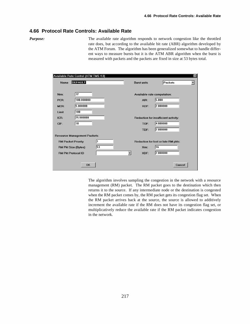
4.66 Protocol Rate Controls: Available Rate
d byiffer-st is
urcethen
estedhen
ivelyt, ortion
217
4.66 Protocol Rate Controls: Available Rate
Purpose: The available rate algorithm responds to network congestion like the throttledrate does, but according to the available bit rate (ABR) algorithm developethe ATM Forum. The algorithm has been generalized somewhat to handle dent ways to measure bursts but it is the ATM ABR algorithm when the burmeasured with packets and the packets are fixed in size at 53 bytes total.
The algorithm involves sampling the congestion in the network with a resomanagement (RM) packet. The RM packet goes to the destination which returns it to the source. If any intermediate node or the destination is congwhen the RM packet comes by, the RM packet gets its congestion flag set. Wthe RM packet arrives back at the source, the source is allowed to additincrement the available rate if the RM does not have its congestion flag semultiplicatively reduce the available rate if the RM packet indicates congesin the network.
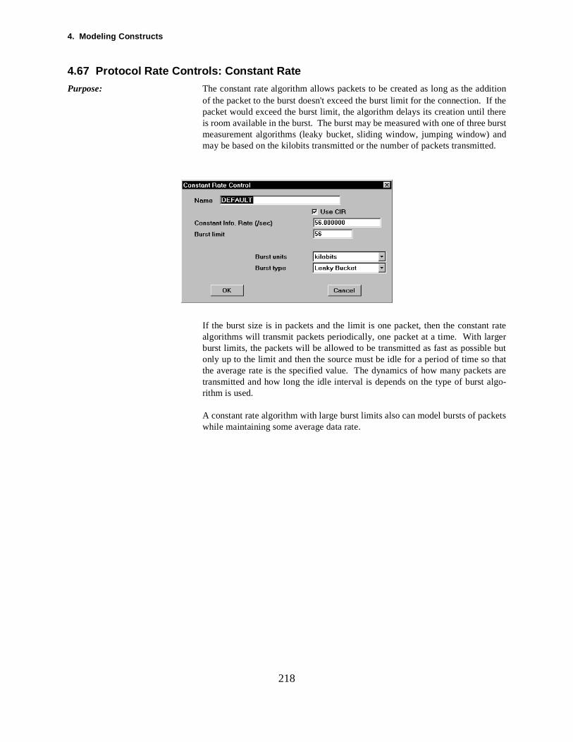
4. Modeling Constructs
dition
ere burstndd.
t rategere but thatts arelgo-
kets
218
4.67 Protocol Rate Controls: Constant Rate
Purpose: The constant rate algorithm allows packets to be created as long as the adof the packet to the burst doesn't exceed the burst limit for the connection. If thepacket would exceed the burst limit, the algorithm delays its creation until this room available in the burst. The burst may be measured with one of threemeasurement algorithms (leaky bucket, sliding window, jumping window) amay be based on the kilobits transmitted or the number of packets transmitte
If the burst size is in packets and the limit is one packet, then the constanalgorithms will transmit packets periodically, one packet at a time. With larburst limits, the packets will be allowed to be transmitted as fast as possiblonly up to the limit and then the source must be idle for a period of time sothe average rate is the specified value. The dynamics of how many packetransmitted and how long the idle interval is depends on the type of burst arithm is used.
A constant rate algorithm with large burst limits also can model bursts of pacwhile maintaining some average data rate.
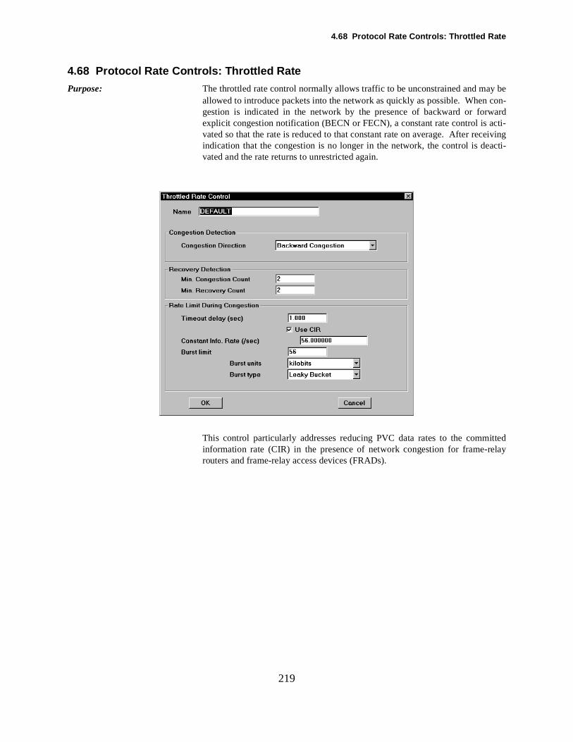
4.68 Protocol Rate Controls: Throttled Rate
y be
cti-eivingacti-
itted
219
4.68 Protocol Rate Controls: Throttled Rate
Purpose: The throttled rate control normally allows traffic to be unconstrained and maallowed to introduce packets into the network as quickly as possible. When con-gestion is indicated in the network by the presence of backward or forwardexplicit congestion notification (BECN or FECN), a constant rate control is avated so that the rate is reduced to that constant rate on average. After recindication that the congestion is no longer in the network, the control is devated and the rate returns to unrestricted again.
This control particularly addresses reducing PVC data rates to the comminformation rate (CIR) in the presence of network congestion for frame-relayrouters and frame-relay access devices (FRADs).
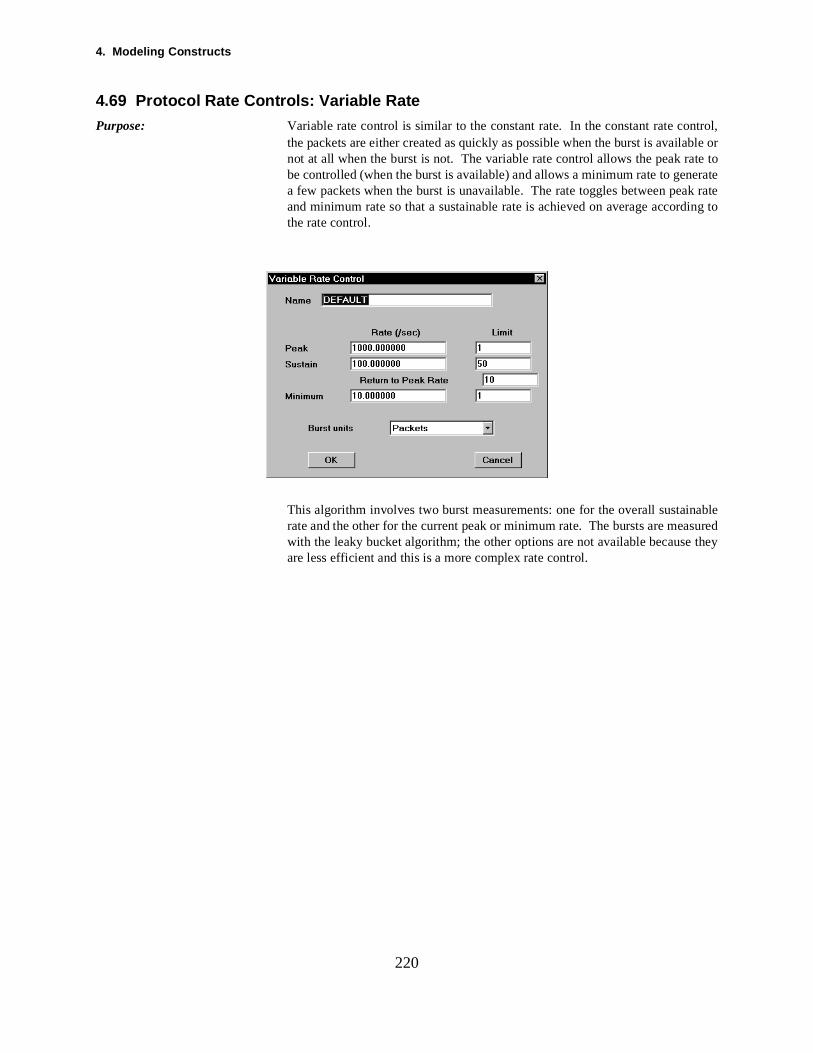
4. Modeling Constructs
trol,ble orte toeratek rateing to
ablesured they
220
4.69 Protocol Rate Controls: Variable Rate
Purpose: Variable rate control is similar to the constant rate. In the constant rate conthe packets are either created as quickly as possible when the burst is availanot at all when the burst is not. The variable rate control allows the peak rabe controlled (when the burst is available) and allows a minimum rate to gena few packets when the burst is unavailable. The rate toggles between peaand minimum rate so that a sustainable rate is achieved on average accordthe rate control.
This algorithm involves two burst measurements: one for the overall sustainrate and the other for the current peak or minimum rate. The bursts are meawith the leaky bucket algorithm; the other options are not available becauseare less efficient and this is a more complex rate control.
4.70 Received Message Scheduling
This isessagehis isions,ge withdulingt and
mayith the
whichetance
f differ-
trans-
ands.
age text mes- with
eduleurce or
ssage
n themainssage
uire-nd so
urces. Thepli-
n thermine
221
4.70 Received Message SchedulingPurpose: When a message is sent, there is a text label associated with the message.
a mechanism used to trigger desired sources at the destination once the mhas arrived; it is usually not a description of the message or its contents. Tparticularly used when received message scheduling is defined for applicatresponses etc. Received Message Scheduling means that when a messathe required message text arrives at the destination node then the scherequirement for some new generator at the destination node has been memay be started.
For instance, a model of a client server architecture may be built. Each clienthave a message generator which sends a query message to the server wmessage text “Database Query.” On the server there may be an application is scheduled by received message and is looking for the message text “DatabasQuery” to be received. When a message with this text is received, a new insof the server application may be started.
Because the message text is separate from the message name, a number oent message sources may send the same message text.
Creating: Message Text is defined on the dialog box which describes the message or port command.
Connectivity: Messages are generated by Message Sources, Response Sources, SessionSources, Transport Commands, Setup Commands and Answer CommWherever a message may be generated, a message text may be entered.
Editing: Via the appropriate message generator dialog box.
Execution: When a message is created, its message text is set based upon the messsettings. This is either a copy of the message name, the text of the originalsage, or specific text entered by the user. This text label is then associatedthe message as it moves to its destination.
When the message arrives at the destination its text may be used to schsome activity at the destination, such as a message source or a response soan application.
If the message text is not required by any source at the destination the meand its associated text are discarded.
If the text is specified as a requirement by some source at the destination themessage text is placed in a received message list at the destination and rethere until such time as it is used to satisfy a scheduling requirement. A mestext from a particular message instance will only satisfy one scheduling reqment at the destination, after which the message text is considered used adiscarded.
It may be that at the destination for the message there are several traffic soor applications which require the message text before they can be scheduledreceiving node keeps an application prototype list, which is a list of all the apcations (including traffic sources and response sources) which may run onode. When a message is received this list is scanned in order to dete
4. Modeling Constructs
a newhaplica-
type
sageives,
sageso mes- in the mes-roto-
f theto the
hewd of top1 isonlytartt thetype
is
n timeed upon of the-trip
essageuire-or is
imul-
st be
222
whether the received message satisfies any message requirement. If so, instance of the application is scheduled and the message is considered as vingbeen used. If an application has multiple message text requirements, the aption instance is not created until all of its requirements are satisfied. The proto-type which “consumed” the message is then moved to the end of the protolist so that it will be considered last next time.
This means that if two entries in the prototype list have the same mesrequirement they will be satisfied alternately as the particular message arrassuming each has only one message text requirement.
It may be that one or more entries in the prototype list require several mestexts before a new instance may be created. When one message arrives nsage requirement is completely satisfied. In this case, the message is savedreceived message list. When the next message arrives there are now twosages which could possibly satisfy a message requirement. The application ptype list is scanned in order—as applications within the prototype list are foundthat can have all of their message requirement satisfied a new instance oapplication is started, the messages used, and the prototype entry moved end of the prototype list.
If Application1 requires MsgA and Application2 requires MsgA and MsgB tfollowing may happen. A MsgA arrives which satisfies Application1. A neApplication1 is created, the MsgA used, and Application1 moved to the enthe prototype list. Another MsgA arrives. Application2 is tested as it is at theof the prototype list but it cannot be started as there is no MsgB. Applicationtested and its requirement satisfied—another Application1 is started. The way an Application2 can start is for a MsgB to arrive first. The MsgB cannot sApplication2 on its own so MsgB is saved in the received message list anode. When a MsgA arrives there is now a MsgB already there. The protolist is scanned and, as Application2 is now at the top, the MsgA and Msg2requirement for Application2 can be met. Therefore a new Application2started, the MsgA and MsgB “consumed,” and the Application2 prototype put tothe end of the prototype list.
The message delays included in the output reports are based on the creatioof the message text for a message. For a message that has its text set basthe original message, the message delay is measured from the creation timeincoming message text. This provides a mechanism for measuring rounddelay when an incoming message triggers a response and the response messageuses the original (i.e., incoming) message’s text.
Reporting: N/A
Fields:
Delay Application message, response, and session sources that use received mscheduling can now include a delay measured from when all message reqments satisfied until the application attempts to begin execution. No processrequired during this delay, thus multiple source instances may be delaying staneously after being triggered by received message.
Message Text From the sender-of-the-message point of view, the text of the message mu
4.70 Received Message Scheduling
, etc.,
223
set. The options for setting the text are:
Use Original MessageUse the text of the message which scheduled the application, responsewhich is creating the new message.
Copy Message NameUse the name of the message as the message text.
Set Message TextExplicitly set the message text with a label typed by the user.
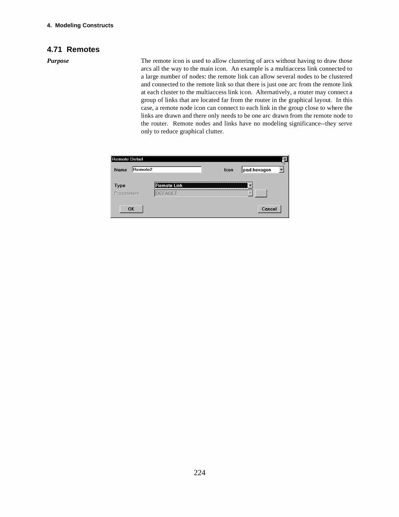
4. Modeling Constructs
osed totered
e linkect a
re theode toerve
224
4.71 RemotesPurpose The remote icon is used to allow clustering of arcs without having to draw th
arcs all the way to the main icon. An example is a multiaccess link connectea large number of nodes: the remote link can allow several nodes to be clusand connected to the remote link so that there is just one arc from the remotat each cluster to the multiaccess link icon. Alternatively, a router may conngroup of links that are located far from the router in the graphical layout. In thiscase, a remote node icon can connect to each link in the group close to whelinks are drawn and there only needs to be one arc drawn from the remote nthe router. Remote nodes and links have no modeling significance--they sonly to reduce graphical clutter.
4.72 Reports
ithfont.
meancludeports
r thef
portenu
portodel.
uns.arlier
irec-
iew.stem
font
theys-
cu-
225
4.72 Reports
Purpose: To report on the performance of the modeled network in a tabular fashion. Thereports produced are written out to file in an 80 column ASCII format wASCII page breaks for 81/2" x 11" paper and a fixed 10 characters per inch
The tabular reports give a statistical assessment of performance. Generally,values, maxima, minima and standard deviations are reported. These indelay times, response times, device loading and utilization, etc. These reprovide information useful for judging performance of the model.
Creating: A set of reports is produced automatically at the end of each replication. Fofirst replication they are saved in the file Stat1.rpt , Each subsequent run othe model will replace the contents of the Stat1.rpt with the newly collectedreults. If you wish to save the conents of a simulation run to a different reyou will need to set a new file name for the report by selecting the Report Moption and choosing the Set File Name option. Click on the Add button andtyupe in a new report name Stat2.rpt . Then click on the Done buton andwhen the simulation is rerun the results will be saved to the newly named refile. These files are located in a directory which has the same name as the m
Also, restarting a simulation automatically deletes reports from previous rBeware of this and if necessary rename or move desired output files from eruns so they will not be deleted.
Saving a model to a different name will automatically create a new output dtory and thus protect old reports.
Connectivity: N/A
Editing: To review the results and to print them out use the Simulate/Browse Reportsmenu option. The dialog prompts you to enter the replication you want to revThe respective reports are then shown in a separate window using your sytext editor.
You may also open the report text files in a word processing package. For bestresults, open the file as ASCII text (no formatting) and use a fixed-space (such as Courier) small enough to fit the full record on each line.
A different text editor can be used by changing the comnet.ini file found inCOMNET III executable directory (not to be confused with the Windows stem.ini file on the PC implementation).
Execution: As the simulation executes statistics are collected in memory. When the replica-tion ends the collected statistics are used to write out the reports.
If a model is re-run then the reports from previous runs are overwritten.
Reporting: N/A
Fields:
Reports On the Report menu option you may select which reports to collect for a parti

4. Modeling Constructs
dataort.
hat itre ton the
lss for
226
lar model being worked with. This selection is saved as part of the model file. See the reports section of the manual for a fuller description of each rep
Show Group Node Detail A Group Node is the same as a Computer & Communications node except thas a quantity field. This specifies how many identical copies of the node abe included in the simulation when it runs—but the copies do not appear ouser interface.
From a reporting point of view, with “Show Group Node Detail” off, only totafor all nodes in the group are reported. If it is set to on, then a line appeareach node in the group on each report, followed by a total for all nodes in thegroup.
On When checked, this turns the selected report(s) on for the simulation run.
Select All Selects all reports in the list.
4.73 Routing Class: Call
of asame-
olslass.net-ben be
r call
Keepts for
urceclassd
theryrary
odel
igh-r
oubletton.
227
4.73 Routing Class: Call
Purpose: Routing Class is a label which is applied to a call source. It may be thought a description of the type of call which applies various characteristics and parter values to the call.
Different Routing Class labels may be applied to different call sources. As manyRouting Classes as desired may be defined in the model.
When either the Minimum Penalty or the User-Defined Table routing protocare used, different penalties or different routes may be defined by Routing CThis allows different “types” of traffic to be routed separately over the same work. For instance, routing classes for “Voice Traffic” and “Fax Traffic” may specified. Selection of penalty table or user-defined table for routing can themade based on whether the traffic is for voice or for fax.
Call routing classes are also important for setting bandwidth requirements fosources.
Note that each routing class has associated with it a complete routing table. the number of classes to a minimum in order to reduce memory requirementhe model and to reduce processing time for updating tables.
Creating: To create a Routing Class edit the appropriate type of traffic source (call soin this case) and click on the double dot button at the side of the routing box. Also the Define/Routing Classes menu option may be used to createand/or edit routing class definitions.
A Routing Class definition may also be added to the system library via Archive/Objects menu option. If a routing class is defined in the system librait will become available when a new model is made, or when the system libdefinition is specifically copied into the local model.
COMNET III always creates a routing class called “Standard” when a new mis made.
Connectivity: A call source references a routing class label in the model’s list of call routingclasses.
Editing: Double click on a call source icon to bring up the call source dialog box, or hlight the icon and pick the Edit/Detail menu option. The Routing Class to use fothe call source can then be applied using the routing class pulldown box.
The Routing Class parameters themselves are edited by clicking on the ddots next to the routing class pulldown box, and then by selecting the Edit bu
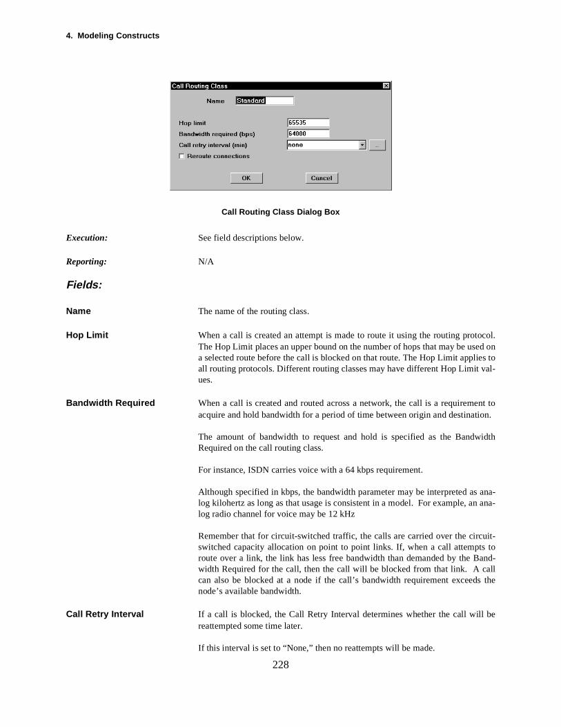
4. Modeling Constructs
ocol.ed ones toal-
ent toon.
idth
ana- ana-
uit- toand-alls the
be
228
Call Routing Class Dialog Box
Execution: See field descriptions below.
Reporting: N/A
Fields:
Name The name of the routing class.
Hop Limit When a call is created an attempt is made to route it using the routing protThe Hop Limit places an upper bound on the number of hops that may be usa selected route before the call is blocked on that route. The Hop Limit appliall routing protocols. Different routing classes may have different Hop Limit vues.
Bandwidth Required When a call is created and routed across a network, the call is a requiremacquire and hold bandwidth for a period of time between origin and destinati
The amount of bandwidth to request and hold is specified as the BandwRequired on the call routing class.
For instance, ISDN carries voice with a 64 kbps requirement.
Although specified in kbps, the bandwidth parameter may be interpreted aslog kilohertz as long as that usage is consistent in a model. For example, anlog radio channel for voice may be 12 kHz
Remember that for circuit-switched traffic, the calls are carried over the circswitched capacity allocation on point to point links. If, when a call attemptsroute over a link, the link has less free bandwidth than demanded by the Bwidth Required for the call, then the call will be blocked from that link. A ccan also be blocked at a node if the call’s bandwidth requirement exceednode’s available bandwidth.
Call Retry Interval If a call is blocked, the Call Retry Interval determines whether the call willreattempted some time later.
If this interval is set to “None,” then no reattempts will be made.

4.73 Routing Class: Call
n anhasether
links.to re-ilurete theutet no
229
Note that a call may block on a primary route, but still be able to be carried oalternate route. This will not invoke the Call Retry Interval. Only when a call blocked on all routes, and cannot preempt on any route, would it inspect wha Call Retry Interval were specified or not.
Reroute Connections Calls are carried between origin and destination over intervening nodes and If a node or link on the route fails then a decision has to be made whether establish the connection or not. If “Reroute Connections” is on, then, at a faevent, the routing tables are recalculated and a new attempt made to roucall. This will result in a different route being picked to carry the call. If ReroConnections is off, the routing tables are still recalculated (for later calls), buattempt is made to reconnect current calls.
4. Modeling Constructs
oughtistics
s. As
Pen-tffer-nce, ofer the
Keepts for
sle dot
theryrary
odel
-
high-r
oubletton.
230
4.74 Routing Class: Packet
Purpose: Routing Class is a label which is applied to a message source. It may be thof as a description of the type of message which applies various characterand parameter values to the message.
Different Routing Class labels may be applied to different message sourcemany Routing Classes as desired by be defined in the model.
The Routing Class is also important for messages when either the Minimumalty or the User-Defined Table routing protocols are used. In this case differenpenalties or different routes may be defined by Routing Class. This allows dient “types” of traffic to be routed separately over the same network. For instarouting classes for “File Transfer” and “E-Mail” may be specified. Selectionpenalty table or user-defined table routing can then be made based on whethtraffic is File Transfer or E-Mail.
Note that each routing class has associated with it a complete routing table. the number of classes to a minimum in order to reduce memory requirementhe model and to reduce processing time for updating tables.
Creating: To create a Routing Class edit the appropriate type of traffic source (mesage,response, session source, or equivalent command) and click on the doubbutton at the side of the routing class box. Also the Define/Routing Classesmenu option may be used to create and/or edit routing class definitions.
A Routing Class definition may also be added to the system library via Archive/Objects menu option. If a routing class is defined in the system librait will become available when a new model is made, or when the system libdefinition is specifically copied into the local model.
COMNET III always creates a routing class called “Standard” when a new mis made.
Connectivity: A message, response, and session source and a transport, setup, and answer command each have a reference to a routing class in the model’s list of packet-rout-ing classes.
Editing: Double click on a message source icon to bring up the source dialog box, or light the icon and pick the Edit/Detail menu option. The Routing Class to use fothe source can then be applied using the routing class pulldown box.
The Routing Class parameters themselves are edited by clicking on the ddots next to the routing class pulldown box, and then by selecting the Edit bu
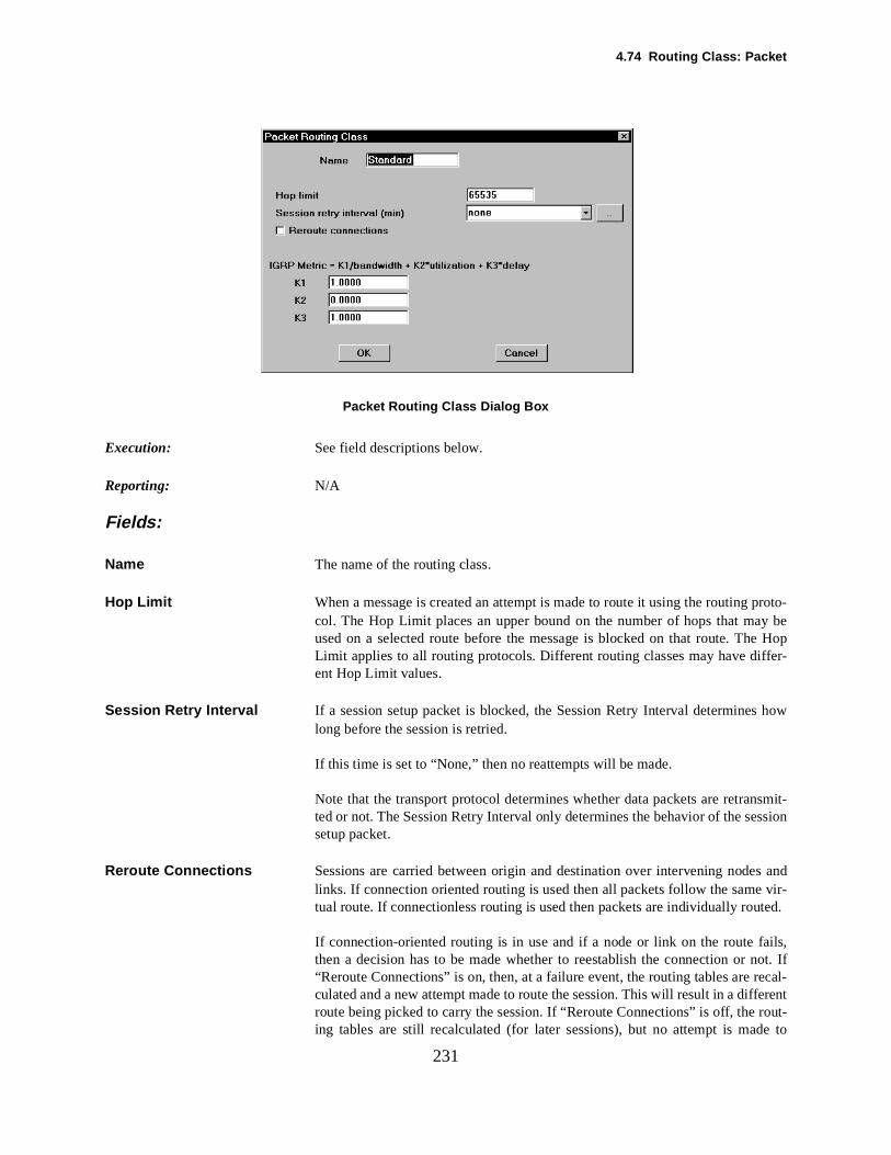
4.74 Routing Class: Packet
proto-
e Hoper-
how
smit-ssion
s and vir-ted.
ils,not. Ifecal-erentout-o
231
Packet Routing Class Dialog Box
Execution: See field descriptions below.
Reporting: N/A
Fields:
Name The name of the routing class.
Hop Limit When a message is created an attempt is made to route it using the routing col. The Hop Limit places an upper bound on the number of hops that may beused on a selected route before the message is blocked on that route. ThLimit applies to all routing protocols. Different routing classes may have diffent Hop Limit values.
Session Retry Interval If a session setup packet is blocked, the Session Retry Interval determineslong before the session is retried.
If this time is set to “None,” then no reattempts will be made.
Note that the transport protocol determines whether data packets are retranted or not. The Session Retry Interval only determines the behavior of the sesetup packet.
Reroute Connections Sessions are carried between origin and destination over intervening nodelinks. If connection oriented routing is used then all packets follow the sametual route. If connectionless routing is used then packets are individually rou
If connection-oriented routing is in use and if a node or link on the route fathen a decision has to be made whether to reestablish the connection or “Reroute Connections” is on, then, at a failure event, the routing tables are rculated and a new attempt made to route the session. This will result in a diffroute being picked to carry the session. If “Reroute Connections” is off, the ring tables are still recalculated (for later sessions), but no attempt is made t

4. Modeling Constructs
thesport
utingtingues
232
reconnect current sessions.
If connectionless routing is being used, then upon node or link failure, onlypackets at the node or link need to be retransmitted according to the tranprotocol settings.
IGRP Routing Bandwidth Factor & IGRP Routing Delay FactorIf messages which use the routing class are being routed via an IGRP roalgorithm, a bandwidth, utilization, and delay factor are required for the roualgorithm to calculate the metric for using a particular link. The default valare the standard IGRP default valuesSee “Routing Protocol: Packet” for more detail.
4.75 Routing Protocol: Call
e of
plesery
ons. sult.
optina-rout-
re thenis isusedab-vent,
ient
ls
atedbles
eachubnetack-
233
4.75 Routing Protocol: Call
Purpose: To make a routing decision for a call that has not reached its destination.
As call traffic arises in COMNET III, a route must be picked via a sequencnodes and links in order for the call to reach the destination.
In a real network this function may be accomplished in many ways. Examinclude by a centralized controller, by distributed tables maintained in evswitch, or by separate packet-switched routing transactions across the network.COMNET III does not mimic exactly the logic and sequencing of such decisiRather, the goal is to model the effect of the real routing mechanism and topro-vide in the simulation a routing protocol which arrives at the same routing re
For instance, the end result of routing decisions in many networks is to establishthe least hop route across the network. In COMNET III there is a Minimum Hrouting protocol. This arrives at a least hop route between an origin and destion, and so exhibits the same result as a real network using minimum hop ing.
When a link or node fails, in COMNET III the minimum hop tables which akept internally are instantaneously (in simulation time) recalculated and areavailable at the same instant for all calls which require a routing decision. Thnot the same as a real network, but the COMNET III approach is valid when for overall network capacity planning. If the goal of your simulation is to estlish the detailed sequencing of routing table updates in the case of a failure ethe standard COMNET III simulation environment does not capture sufficdetail.
Creating: The routing protocols are built into COMNET III. For call traffic, the protocowhich are provided are:
• Minimum Hop• Minimum Penalty• User Defined Routing Tables
If minimum penalty routing is used, then penalty tables will need to be creand applied to link arcs. If User-Defined Table routing is used then routing tamust be manually created.
Connectivity: A routing protocol is applied to the backbone network, and independently to subnet. If a call originates in one subnet and has a destination in another sthen 3 routing protocols would be queried—1 for each subnet and 1 for the bbone.
The origin and destination may be in the same subnetwork or backbone, or in dif-ferent subnetworks. The possibilities are:
Origin Destination Number of RoutingNetwork Network Algorithms AppliedBackbone Backbone 1Backbone Subnet 2Subnet Same Subnet 1Subnet Backbone 2
4. Modeling Constructs
ss
tocol
y be
the
the
o the link/ link/f theoute
rily
le is The
ode).d. Byand-ched,oc-
hese
tingrouteall
234
Subnet Different Subnet 3
If a route crosses a boundary between a subnet and the backbone then an accepoint must be involved. In the backbone, the backbone routing protocol willroute the call to/from an access point. In the subnet the subnet routing prowill route to/from the closest access point.
Editing: The routing protocol selected for the backbone or particular subnet machanged at any time. The backbone routing protocol is specified on the Define/Backbone Routing menu option.
The subnet routing protocol is specified by highlighting the subnet icon andselecting the Edit/Detail menu option. (Double clicking on a subnet icon causesthe subnet to be entered.)
Execution:
Minimum Hop Routing The Minimum Hop Routing protocol finds the least number of hops betweenorigin and destination.
When the simulation starts each node calculates all the possible routes tother nodes in the model. A table is stored at each node which lists the nextnext node pair to use for each route to reach a particular destination. Thenext node pair entries in the table are ordered by increasing hop count oroute to which they belong. The link at the top of the table belongs to the rwith the least hop count and the route at the bottom belongs to the route with thelargest hop count. Links for routes with the same hop count are arbitraordered.
When a call requires routing, the link/next node pair at the top of the tabinspected. This is the link that follows the least hop route to the destination.link must pass the following tests:
• be inside the hop limit for the routing class• have sufficient bandwidth available• the node at the other end of the link must have sufficient bandwidth• not connect to a previously visited node
If the link passes these tests then the call may use the link (and the next nThe routing decision then passes to the next node and an outgoing link founrepeating this process the route is built up link by link and the required bwidth acquired until the destination is reached. When the destination is reathe bandwidth will be held for the duration of the call. Note that this routing press is instantaneous in simulation time.
If the first link/next node pair in the table at a routing node does not pass ttests the next pair is checked, and so on until an outgoing link is found.
If no route is found, and if the preemption flag is set to yes, then the routing pro-tocol will start back at the first node and reattempt to route the call by tesnode by node whether sufficient capacity can be preempted. If a complete can be found with preemption, then existing call(s) will be preempted and the crouted.

4.75 Routing Protocol: Call
l beteris-
n therbi-theientiche thel it in
mes hasent isrtest
ngth if
nd sotheruc-then thatdeci-
ted./nextde ornces
t thesti-
athis this theereck”tter
rout-e, a
hop
time. set
the
235
If no route can be found either normally or by preemption, then the call wilblocked and optionally retried later depending on the routing class charactics.
If there is more than one route from a node with the same hop count, theordering of the link/next node pairs for these routes in the routing table is atrary. One of them will be at the top and so will be preferentially picked by routing protocol. When this pair fails a routing test (such as having insufficbandwidth for a particular call), the next pair in the table for another route whhas the same hop count would come into play. This pair is then moved abovother pair in the table and so becomes the preferred link/next node pair untiturn becomes full.
Rather than waiting for links to go full before other links on routes of the sahop count are considered, a “Deviation Percent” parameter is provided. If thithe value 0 then the operation is as described above. If the deviation percpositive then links for routes that are within the deviation percent of the shoroute will be considered equivalent and routed over on a round robin basis. Forinstance, a route of 4 hops and a route of 5 hops are considered the same lethe deviation percent is 25% or more.
The destination of the route may be an access point at a subnet/backbone bound-ary. The routing protocol establishes that a route exists as far as this point athe bandwidth on each node and link comprising the route is claimed. Anorouting decision may be required to carry the call further. If this decision sceeds then the call is carried. If this decision fails to find an onwards route the bandwidth claimed from the earlier decision must be given back. Notethis bandwidth would have been instantaneously relinquished as the routing sions are instantaneous in simulation time.
At the point of link or node failure the minimum hop tables are recalculaRoutes which contain failed components are no longer valid and so the linknode pair references are removed from the node routing tables. When the nolink recovers, routes are again recalculated and link/next node pair refereplaced back in the node routing tables.
If a routing decision is being made at some intermediate node, it may be thafirst choice link/next node pair which follows the minimum hop path to the denation has insufficient capacity to carry the call. In this case the next pair will betested, and so on, until a pair is found or the call counted as blocked. Assumingpair is found, this pair will reflect the minimum hop route that is available at instant between the currently routing node and the destination. However,route may not be the minimum hop route between the origin of the call anddestination—some better route may exist if a different routing decision wtaken earlier than the current routing node. COMNET III does not “crank bafrom the current node to earlier nodes under minimum hop routing to find beroutes. However, it does provide a routing update interval which forces the ing tables to be recalculated periodically. This means that at the update timcomplete end-to-end analysis is performed to establish the best minimumroutes. Consequently, you may observe nonoptimal routes being picked betweena time when a node or link becomes saturated and the next routing updateTo minimize the effects of this behavior the routing update interval should beto a small value. However, frequent routing table updates will slow downsimulation.
4. Modeling Constructs
ed to
normase
s is an
o the/next/nextte to theroute are
le isa-
ode).d. Byand-ched,oc-
hese
tingrouteall
l beteris-
n therbi-theextlay.
e pre-
236Minimum Penalty Routing The Minimum Penalty Routing protocol finds the route with the least total pen-alty between the origin and destination. Penalties are integer factors applilinks by the use of penalty tables. If the penalty for each link is 1 then MinimumHop and Minimum Penalty routing are identical.
The penalty values can be made variable depending on link utilization. The would be that, as link utilization increases, the penalty on a link would increand so cause the link not to be selected as part of a least penalty route. Thiadaptive routing strategy.
When the simulation starts each node calculates all the possible routes tother nodes in the model. A table is stored at each node which lists the linknode pair to use for each route to reach a particular destination. The linknode entries in the table are ordered by increasing total penalty of the rouwhich they belong. The link/next node pair at the top of the table belongs toroute with the least total penalty and the route at the bottom belongs to the with the largest total penalty. Links for routes with the same total penaltyarbitrarily ordered.
When a call requires routing, the link/next node pair at the top of the tabinspected. This is the hop that follows the least total penalty route to the destintion. The hop must pass the following tests:
• be inside the hop limit for the routing class• have sufficient bandwidth available• the node at the other end of the link must have sufficient bandwidth• not connect to a previously visited node.
If the link passes these tests then the call may use the link (and the next nThe routing decision then passes to the next node and an outgoing link founrepeating this process the route is built up link by link and the required bwidth acquired until the destination is reached. When the destination is reathe bandwidth will be held for the duration of the call. Note that this routing press is instantaneous in simulation time.
If the first link/next node pair in the table at a routing node does not pass ttests the next pair is checked, and so on until an outgoing link is found.
If no route is found, and if the preemption flag is set to yes, then the routing pro-tocol will start back at the first node and reattempt to route the call by tesnode by node whether sufficient capacity can be preempted. If a complete can be found with preemption, then existing call(s) will be preempted and the crouted.
If no route can be found either normally or by preemption, then the call wilblocked and optionally retried later depending on the routing class charactics.
If there is more than one route from a node with the same total penalty, theordering of the link/next node pairs for these routes in the routing table is atrary. One of them will be at the top and so will be preferentially picked by routing protocol. When this link fails a routing test (such as being full), the npair for another route which has the same total penalty would come into pThis pair is then moved above the other pair in the table and so becomes th
4.75 Routing Protocol: Call
me thisercentort-
nsid-
nd sotheruc-then thatdeci-
utesoder link
d back
i-
t thesti-
acity
uteist if
ode.der
out-ally.rmedks inen ae. To
t to aani-
on0% overe uti- then
237
ferred link/next node pair until it in turn becomes full.
Rather than waiting for links to go full before other links on routes of the satotal penalty are considered, a “Deviation Percent” parameter is provided. Ifhas the value 0 then the operation is as described above. If the deviation pis positive then links for routes that are within the deviation percent of the shest route will be considered equivalent and routed over on a round robin basis.For instance, a route of total penalty 4 and a route of total penalty 5 are coered the same length if the deviation percent is 25% or more.
The destination of the route may be an access point at a subnet/backbone bound-ary. The routing protocol establishes that a route exists as far as this point athe bandwidth on each node and link comprising the route is claimed. Anorouting decision may be required to carry the call further. If this decision sceeds then the call is carried. If this decision fails to find an onwards route the bandwidth claimed from the earlier decision must be given back. Notethis bandwidth would have been instantaneously relinquished as the routing sions are instantaneous in simulation time.
At the point of link or node failure the penalty tables are recalculated. Rowhich contain failed components are no longer valid and so the link/next npair references are removed from the node routing tables. When the node orecovers, routes are again recalculated and link/next node references placein the node routing tables.
The purpose of the routing update interval for minimum hop routing is to optmize the routing tables as links or nodes become saturated
If a routing decision is being made at some intermediate node, it may be thafirst choice link/next node pair which follows the least penalty path to the denation has insufficient capacity to carry the call. In this case the next pair will betested, and so on, until a pair is found or the call counted as blocked. Assumingpair is found, this will be the lowest penalty pair of those pairs that have capato carry the call. However, this may not reflect the minimum penalty robetween the origin of the call and the destination—some better route may exa different routing decision were taken earlier than the current routing nCOMNET III does not “crank back” from the current node to earlier nodes unminimum penalty routing to find better routes. However, it does provide a ring update interval which forces the routing tables to be recalculated periodicThis means that at the update time, a complete end-to-end analysis is perfoto establish the best minimum penalty routes with congested nodes and linsitu. Consequently, you may observe nonoptimal routes being picked betwetime when a node or link becomes saturated and the next routing update timminimize the effects of this behavior the routing update interval should be sesmall value. However, frequent routing update intervals will slow down the mation.
The minimum penalty protocol allows the penalty on a link to vary dependingthe link utilization. For example, the penalty may have the value 1 for 0-3loading and 5 for over 30% loading. As the model runs and calls are routeda link, the routing tables are recalculated every user defined time period. Thlization level on each link at the instant the routing tables are recalculated isused to compute the minimum penalty routes.
4. Modeling Constructs
thaty beerme-o
rion is
at some
g andrt
boxaloging ay be
utes
238
User-Defined Routing Tables The User-Defined Routing protocol selects a route from 1 or more routeshave been manually entered by the user. Multiple alternate routes maentered. Partial routes may also be entered which route the call to some intdiate node. At the intermediate node one or more routes, must be available tfor-ward the call towards the destination.
When a user enters a number of possible alternate routes a selection criterequired to determine which alternate to use. These criteria include:
• Dynamic Alternate• First Available• Max Idle Bandwidth• Random List• Round Robin
A route in User-Defined routing is implemented by keeping a routing tableeach node. Each table may contain a choice of single links to use to reachnext node, or it may list several links and so route the call all the way to the desti-nation. These may be regarded as implementations of Node-By-Node routinSource Node routing respectively. In addition, partial routes that only get paway to the destination are allowed.
The routing tables are entered for each node by bringing up the node dialogand then selecting the Call Routing Table button. A Destination Selection dibox then presents a table of destinations and routing classes. After highlightparticular destination/routing class intersection, routes to that destination maentered by selecting the “Edit Selected” button.
Destination Selection Dialog Box
A Route Definition dialog box is then presented. This allows a number of routesto the particular destination/routing class combination to be entered. The romay completely reach the destination, or partially reach the destination.
4.75 Routing Protocol: Call
beand adary
aode
boxps”
e the
natese:
and
d. Ann all, is are such). At
239
Route Definition Dialog Box
With User-Defined Table routing, both primary and secondary routes maydefined. When a routing decision is made, the primary routes are inspected route found. If no route can be found from the primary routes, then the seconroutes are evaluated. If still no route can be found then the call is counted asblocked (unless preemption is on and a preemptive route found).
The “Avoid Backtracking” check box has no impact on model execution. Whenroute is being defined, and with the box checked, links which return to a nalready in the route will not appear in the “Possible Next Hops” list. With the unchecked, all outgoing links from a node appear in the “Possible Next Holist.
Backtracking may be useful for certain routers or equipment that must handlcall even if the call must go to that device and backtrack to return to its path.
If there are several routes defined at a routing node, then when a call origiand requires routing some tie breaking mechanism is required. These includ
Dynamic AlternateThe intent is that the primary route selection would be “First Available” say, the secondary route selection is “Dynamic Alternate.” When a routing decision ismade the primary routes are inspected and the first available route returneavailable route is one that is inside the hop limit and has sufficient capacity othe nodes and links along its path. If no route is available in the primaries thenwith “Dynamic Alternate,” one of the secondary routes with available capacitypicked at random. Thereafter, when a call originates the primary routesretested and, if full, the same secondary route is used. This continues untiltime as the secondary route cannot carry the call (i.e., insufficient capacity
4. Modeling Constructs
ient
nd if
lter-
. Each link thehese
t theth one thataredh. In best,
city
tion.
o notutes
tion.edi-hop any
each
inksute. Ifll be
240
this time, another random pick from those secondary routes with sufficcapacity is made and a new secondary route established.
If a call cannot be routed over either the primary or secondary routes, apreemption is off or no preemptive route can be found, then the call would betreated as blocked and optionally retried later.
This is the alternate route selection rule used in British Telecom’s dynamic anate routing algorithm.
First AvailableThe routes are evaluated in the same order as defined on the user interfaceroute is tested in turn to establish whether it is within the hop limit, that eachhas sufficient bandwidth, that each node has sufficient bandwidth to routecall, and that no previous routing node is revisited. The first route to meet tcriteria is selected, the bandwidth claimed, and the call routed.
Max Idle BandwidthA route comprises one or more hops. On each route one of the hops will, ainstant that the routing decision is made, have the least amount of bandwidthat route. If there are several routes then there will be one hop on each routhas the least available bandwidth. These “least bandwidth” hops are compand the route selected which owns the hop which has the most bandwidtother words, find the worst hop on each route and take the route that has theworst hop.
The route found must be within the hop limit and have sufficient spare capato carry the call, and not revisit any previous routing nodes.
Random ListThe routing table lists one or more routes which lead to or reach the destinaA sublist is made of these routes which includes those that stay in the hop limitand have sufficient capacity on each node and link to carry the call, and drevisit any previous routing nodes. A random pick is then made from the roin the sublist.
Round RobinThe routing table lists one or more routes which lead to or reach the destinaThe routes are evaluated in the order of definition starting with the route immately after the one which was last used. The first route which is within the limit and has sufficient capacity on each node and link and does not revisitprevious routing nodes is selected.
Once the call has been routed to the destination, the claimed bandwidth onnode and link is held for the duration of the call. At the end of the call the band-width on each node and link is simultaneously released.
If no route is found, and if the preemption flag is set to yes, then the routing pro-tocol will start back at the first route and test whether sufficient nodes and lon the route can be preempted so that there is capacity across the entire roso then existing call(s) will be preempted and the call routed. Each route witested in turn until either a route is found or there are no more routes to test.
4.75 Routing Protocol: Call
l beteris-
g the
thisardsack.ting
red.
he
ting
outecomen aodelt in
riodi-
ation
point hops25%.d for
hsitive
241
If no route can be found either normally or by preemption, then the call wilblocked and optionally retried later depending on the routing class charactics.
The destination of the route may be an intermediate node partially completinroute to the destination, or an access point at a subnet/backbone boundary. At thispoint another routing decision may be required to carry the call further. If decision succeeds, then the call is carried. If this decision fails to find an onwroute, then the bandwidth claimed from the earlier decision must be given bNote that this bandwidth would be instantaneously relinquished as the roudecisions are instantaneous in simulation time.
Reporting: N/A
Fields:
Link Utilization Update IntervalNot used for call routing. All link utilization figures used in the call routing pro-tocols are instantaneous measurements made at the time the figure is requi
The “Link Utilization Update Interval” is used in the routing protocols under tpacket-switched model.See Routing Protocol: Packets
Minimum Hop Routing
Routing Update Interval Every routing update interval period, the minimum hop calculations are per-formed to find the minimum hop routes through the network. The tables kept ateach node which record which next link/next node pair to use from the rounode are updated.
This updating is included because the availability of nodes and links to rcalls is not static. As congestion increases then some nodes or links may befully loaded and are not therefore available for carrying more traffic. Wherouting node sees the link/next node pair is full, it picks the next best link/nfrom its local table. While this is the best local decision to make, it may resuan end-to-end route which is not the minimum hop between the end points. Toovercome this problem, the complete end-to-end routes are recalculated pecally and so take into account such congestion effects.
Note that a node/link failure or recovery event causes an immediate recalculof routing tables.
Deviation Percentage Indicates those routes which are to be treated as equivalent from a distanceof view, as a percentage difference from the shortest route. For example, 4and 5 hops are considered the same if the deviation percent is at least Routes that are the same distance within the deviation percent will be selecterouting on a round-robin basis.
A deviation percent of 0 suppresses the round robin routing even on routes whichave the same hop count. To round robin on such routes use a small podeviation percent (such as 1%).
4. Modeling Constructs
ior-
outecomen arom an. Toriodi-
ation
byse use
naltyalty.me ifin the
hsitive
ior-
reachuld beoutes use.
242
Preemption Flag to indicate whether higher priority calls are allowed to preempt lower prity calls.
Minimum Penalty Routing
Routing Update Interval Every routing update interval period the minimum penalty calculations are per-formed to find the least penalty routes through the network. The tables kept ateach node which record which next link to use from the node are updated.
This updating is included because the availability of nodes and links to rcalls is not static. As congestion increases then some nodes or links may befully loaded and are not therefore available for carrying more traffic. Wherouting node sees the next link/node is full it picks the next best link/node fits local table. While this is the best local decision to make, it may result inend-to-end route which is not the minimum penalty between the end pointsovercome this problem, the complete end to end routes are recalculated pecally and so take into account such congestion effects.
Note that a node/link failure or recovery event causes an immediate recalculof routing tables.
In addition, the penalty values defined for a link may vary be defined to varylink utilization. At the point of routing table recalculation the penalty value to ufor a link is established by looking up in the penalty table the penalty value togiven the current utilization level.
Deviation Percentage Indicates those routes which are to be treated as equivalent from a total pepoint of view as a percentage difference from the route with the lowest penFor example, total penalty 4 and total penalty 5 routes are considered the sathe deviation percent is at least 25%. Routes that are the same distance withdeviation percent will be selected for routing on a round robin basis.
A deviation percent of 0 suppresses the round robin routing even on routes whichave the same total penalty. To round robin on such routes use a small podeviation percent (such as 1%).
Preemption Flag to indicate whether higher priority calls are allowed to preempt lower prity calls.
User Defined Routing Tables
Primary Route Selection A number of routes at a node may be specified to reach a destination, or to a node closer to the destination. Primary routes are those routes which shotested first to establish whether a route is available. Where several primary rare specified some tie breaking criterion is needed to decide which route toThe selection criteria are
•Dynamic Alternate •First Available •Max Idle Bandwidth •Random List •Round Robin
4.75 Routing Protocol: Call
ined,
on is
.
ior-
243
See the above section on Execution for a fuller explanation of each criterion.
Secondary Route Selection If the primary routes do not yield a route, and if secondary routes are defthen the secondary routes will be tested to see if a route can be established.Where several secondary routes are specified some tie breaking criterineeded to decide which route to use. The selection criteria are
•Dynamic Alternate•First Available•Max Idle Bandwidth•Random List•Round Robin
See the above section on Execution for a fuller explanation of each criterion
Preemption Flag to indicate whether higher priority calls are allowed to preempt lower prity calls.
4. Modeling Constructs
t has
traf-s fol-
sion
e of
ples
uchnismme
um des-
re thenis isusedab-vent,
ient
telywn
eachout-ains
he
244
4.76 Routing Protocol: Packet
Purpose: To make a routing decision for a packet that has not reached its destination.
Inherently COMNET III routes packets on a datagram basis; each packeindividual routing decisions applied to it.
If “Connection-Oriented Routing For Sessions” is specified then for session fic only, the session setup packets are specifically routed. The data packetlow the route established for the session setup packets. This would be the mostcommon setting for modelling virtual circuit based operation. Other nonsespackets are still routed in a datagram sense.
As packet traffic arises in COMNET III, a route must be picked via a sequencnodes and links in order for the packet to reach the destination.
In a real network this function may be accomplished in many ways. Examinclude by a centralized controller, or by distributed tables maintained in everyswitch. COMNET III does not mimic exactly the logic and sequencing of sdecisions. Rather, the goal is to model the effect of the real routing mechaand to provide in the simulation a routing protocol which arrives at the sarouting result.
For instance, the end result of routing decisions in many networks is to establishthe least hop route across the network. In COMNET III there is a RIP MinimHop routing protocol. This arrives at a least hop route between an origin andtination, and so exhibits the same result as a real network using RIP.
When a link or node fails, in COMNET III the minimum hop tables which akept internally are instantaneously (in simulation time) recalculated and areavailable at the same instant for all calls which require a routing decision. Thnot the same as a real network, but the COMNET III approach is valid when for overall network capacity planning. If the goal of your simulation is to estlish the detailed sequencing of routing table updates in the case of a failure ethe standard COMNET III simulation environment does not capture sufficdetail.
The management and routing of packet-switched traffic is modeled compleindependently of the circuit-switched traffic. Packet-switched traffic has its oswitching resource on each node, and its own transmission bandwidth onlink. These are not shared with the circuit-switched traffic. Also the packet ring protocol is entered separately from the call routing protocol and maintindependent routing tables.
Creating: The routing protocols are built into COMNET III. For packet-switched traffic tprotocols which are provided are:
•IGRP•Link-State Shortest-Path First•RIP Minimum Hop•Minimum Penalty•Shortest Delay•User-Defined Routing Tables
4.76 Routing Protocol: Packet
les
cre-
each
r the
ss
tocol
y be
then
to the
ofcessouldt-if-
eingowingNote
ute” over fac-
245
For IGRP, Link State Shortest Path, & Minimum Penalty, routing penalty tabmay need to be created and applied to link arcs.
If User-Defined Table routing is used, then routing tables must be manuallyated.
Connectivity: A routing protocol is applied to the backbone network, and independently to subnet. If a packet originates in one subnet and has a destination in another sub-net then 3 routing protocols would be queried—1 for each subnet and 1 fobackbone.
The origin and destination may be in the same subnetwork or backbone, or in dif-ferent subnetworks. The possibilities are:
Origin Destination Number of RoutingNetwork Network Algorithms AppliedBackbone Backbone 1Backbone Subnet 2Subnet Same Subnet 1Subnet Backbone 2Subnet Different Subnet 3
If a route crosses a boundary between a subnet and the backbone then an accepoint must be involved. In the backbone, the backbone routing protocol willroute the packet to/from an access point. In the subnet the subnet routing prowill route to/from the closest access point.
Editing: The routing protocol selected for the backbone or particular subnet machanged at any time. The backbone routing protocol is specified on the Define/Backbone Routing menu option.
The subnet routing protocol is specified by highlighting the subnet icon andselecting the Edit/Detail menu option. (Note: Double clicking on a subnet icocauses the subnet to be entered.)
Execution: When the simulation starts, each node calculates all the possible routes other destination nodes in its local subnet (or locally in the backbone).
For the purposes of this discussion, a hop is considered to be the combinationlink plus node at the other end. For instance, when routing over a multiaclink such as token ring, there may be two different nodes on the ring which cbe routed through. These would be represented as two different hops in the rouing table even though they both refer to the same link. Or there may be two dferent links connecting to the same next node.
The order of hops in the routing table at a node is determined by the metric bused to evaluate alternate routes. These metrics are discussed in the follsections. Some general comments which apply to all metrics are required. that User-Defined Tables are somewhat different from the other metrics.
A weighting factor is calculated for each of these routes so that the best “rocan be ascertained. For each route starting at a node, there is a first hopwhich the packets would be sent. Each such hop is tagged with the weighting
4. Modeling Constructs
ctors.
theyrrentiled
to theuffi- totald in
roto- until
the portM
ilables theigin
utpe offoreach
samebele a
thisercenthort-
a% or
246
tor that was calculated for the end-to-end route.
Note that there may be several first hops that have the same weighting faThe ordering of such hops in the list is arbitrary.
When a packet requires routing, the hops are evaluated in the order thatappear in the table. The first hop would reflect the best route under the curouting metric assuming that the route is currently available (i.e., has no facomponents). For a hop to be accepted the following tests must be passed:
• the hop limit for the routing class must not be exceeded.
• both the node and link on the hop must be up.
• the hop must not return to a previously visited node.
• if a session setup packet is being routed, the link and next node must beunder its session limit.
If these tests are passed then an attempt will be made to route the packet onhop. This can only succeed if the port output buffer on the routing node has scient capacity to accept the packet, and the routing node has sufficient spareoutput buffer capacity. Assuming there is buffer capacity, the packet is placethe selected port output buffer and then is transmitted onwards by the link pcol to the next node. A similar decision is made at the next node, and so on,the packet arrives at the destination.
If the routing node does not have sufficient buffer space on the port output bufferfor the selected hop, the packet is blocked and optionally retried later fromorigin depending on the transport protocol settings. (A packet blocked on aoutput buffer on an ATM node will remain in a port input buffer at the ATnode.)
If the first hop does not pass the tests outlined above, then the next best avahop is selected, and so on until a hop selection is made. If no hop satisfietests, then the packet is blocked and optionally retried later from the ordepending on the transport protocol settings. Note that the buffer tests are madeafter the hop has been selected.
As the packet is switched through nodes, placed in port input and port outpbuffers, and transmitted over links, the packet consumes the respective tyresource. The process of moving the packet from origin to destination thereextends over simulation time, but the individual routing decisions made at eintermediate node are instantaneous.
Where there are several hops listed in the routing table for routes of the total weighting factor, generally only the route at the top of the list will picked. It is an arbitrary choice which of the routes will be at the top. To enabload balancing mechanism, a “Deviation Percent” parameter is provided. Ifhas the value 0 then the operation is as described above. If the deviation pis positive then hops for routes that are within the deviation percent of the sest route are considered equivalent and routed over on a round robin basis. Forinstance, if the routing metric is RIP Minimum Hop then a route of 4 hops and route of 5 hops are considered the same length if the deviation percent is 25
4.76 Routing Protocol: Packet
it willoutes
back-cesslinkbnet.ET
t thetes to
opsrkedvers,artic-
thenl ould
,
h
by
cally
illi-thery.
s not pen-etric.elayre a
t thesti-
247
morewhen load balancing is in effect. Once the top hop has been selected be moved after the hops with the same weighting factor. This means that rwith the same weighting factors will be selected on a round-robin basis.
The destination of a routing decision may be an access point at a subnet/bone boundary. There is no guarantee that once a packet has reached an acpoint that there will be an ongoing route to reach the ultimate destination—or node failures may have made the destination unreachable in the suAssuming the access point is reachable for the first routing decision, COMNIII will route the packet to the access point. The packet would then block aaccess point as the subnet routing protocol would not have any available rouuse to reach the destination.
At the time of link or node failure the routing tables are recalculated. The hlisted in the routing table for routes which contain failed components are maas such and so will not pass the availability test. When the node or link recoroutes are again recalculated and listed first hops marked as available. If a pular destination is unreachable (for instance, the only link to it has failed) there are no routes from any node to the unreachable node. In this case, alhopslisted in routing tables would be marked as unavailable and so packets wblock at the origin and not part way to the destination.
IGRP Metric The IGRP metric calculates compound route weighting factors based bandwidthutilization and delay metrics.
When a routing table update is made the compound penalty calculated for eaclink is given by the formula:
K1*bandwidth factor + K2 * bandwidth factor/(256-load) + K3 * Delay Factor
K1, K2 & K3 are specified on the routing class dialog box and they can varyrouting class. For standard IGRP they have the values 1,0 & 1 respectively.
Bandwidth Factor = 1010 / (Bandwidth)The Bandwidth for links is expressed in bits per second, computed automatiby COMNET III based on link parameters.
Load = Utilization Percentage * 255
Delay Factor = topological delay in units of 10 microsecondsFor LANs this defaults to 100 (corresponding to 1000 microseconds or 1 msecond). For other links it defaults to 2000 (or 20 ms). In COMNET III, delay factor is set from the penalty tables and thus the values may be arbitra
The IGRP default delay values are used if the penalty assigned to a port habeen changed from its default value of 1. If a port has been assigned somealty value other than 1, that value is used as the delay penalty in the IGRP mIt is only necessary to edit the packet routing penalties if the default IGRP dvalues are not satisfactory. This might be the case for a satellite link, whedelay of 2 seconds would correspond to a delay penalty of 200,000.
The load calculation is based on the most recent link utilization estimate atime of the routing table update. The interval for updating link utilization e
4. Modeling Constructs
K2 isnec-t tossary
idth
n on are
eld.on
d onnalty are
ther
n oneri-
on
n oned as
sed pen-re
cketlay
248
mates is specified on the dialog boxes for backbone and subnet detail. If zero, you may want to set the update interval to a large value to eliminate unessary updates. Similarly, if K2 is left at its default value of 0, you may wanset the routing table update interval to a large value to eliminate unnecerouting table updates.
Under IGRP delay weighting factors are additive across a route, but bandwfactors are only calculated for the least bandwidth link on the route.
The routing table calculation is performed at the start of simulation, and theeach node or link failure or recovery event. In addition periodic updatesrequired as the penalties applied to each link may vary over time due to changingutilization levels.
The time period between updates is given in the “Routing Update Interval” fiIf link penalties are changing due to changing link utilization, the link utilizatiis averaged over the time specified by the “Link Utilization Update Interval.”
The Deviation Percent is based on total composite metric of a route.
Link-State Shortest-Path Metric (OSPF)The Link State Shortest Path metric calculates route weighting factors baseinteger penalty values applied to links by the use of penalty tables. If the pefor each link is 1 then Minimum Hop and Link State Shortest Path routingidentical.
Only the penalty values in the first line of the penalty table are used. In owords, the penalty values are fixed by the user at the start of the simulation.
The routing table calculation is performed at the start of simulation, and theeach node or link failure or recovery event. As the link penalties are fixed, podic updates are not required.
The Deviation Percent is based on the total penalty metric of a route.
RIP Minimum Hop Metric The Minimum Hop Routing metric calculates route weighting factors basedthe hop count between the origin and destination.
The routing table calculation is performed at the start of simulation, and theeach node or link failure or recovery event. Periodic updates are not requirthe hop count between nodes is static, unless there are failures.
The Link Utilization Update Interval is not used by this metric.
The Deviation Percent is based on the hop count of a route.
Minimum Penalty Metric The Minimum Penalty Routing metric calculates route weighting factors baon integer penalty values applied to links by the use of penalty tables. If thealty for each link is 1, then Minimum Hop and Minimum Penalty routing aidentical.
The penalty values can be made variable depending on link utilization or padelay across the link. The norm would be that, as link utilization or link de
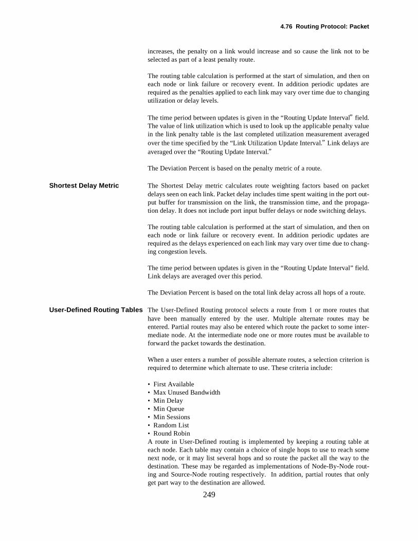
4.76 Routing Protocol: Packet
to be
n on are
lueaged
ckett out-aga-ys.
n on are
eld.
ute.
thaty be inter-ble to
rion is
at someo the
only
249
increases, the penalty on a link would increase and so cause the link not selected as part of a least penalty route.
The routing table calculation is performed at the start of simulation, and theeach node or link failure or recovery event. In addition periodic updatesrequired as the penalties applied to each link may vary over time due to changingutilization or delay levels.
The time period between updates is given in the “Routing Update Interval” field.The value of link utilization which is used to look up the applicable penalty vain the link penalty table is the last completed utilization measurement averover the time specified by the “Link Utilization Update Interval.” Link delays areaveraged over the “Routing Update Interval.”
The Deviation Percent is based on the penalty metric of a route.
Shortest Delay Metric The Shortest Delay metric calculates route weighting factors based on padelays seen on each link. Packet delay includes time spent waiting in the porput buffer for transmission on the link, the transmission time, and the proption delay. It does not include port input buffer delays or node switching dela
The routing table calculation is performed at the start of simulation, and theeach node or link failure or recovery event. In addition periodic updatesrequired as the delays experienced on each link may vary over time due to chang-ing congestion levels.
The time period between updates is given in the “Routing Update Interval” fiLink delays are averaged over this period.
The Deviation Percent is based on the total link delay across all hops of a ro
User-Defined Routing Tables The User-Defined Routing protocol selects a route from 1 or more routeshave been manually entered by the user. Multiple alternate routes maentered. Partial routes may also be entered which route the packet to somemediate node. At the intermediate node one or more routes must be availaforward the packet towards the destination.
When a user enters a number of possible alternate routes, a selection criterequired to determine which alternate to use. These criteria include:
• First Available• Max Unused Bandwidth• Min Delay• Min Queue• Min Sessions• Random List• Round RobinA route in User-Defined routing is implemented by keeping a routing tableeach node. Each table may contain a choice of single hops to use to reachnext node, or it may list several hops and so route the packet all the way tdestination. These may be regarded as implementations of Node-By-Node rout-ing and Source-Node routing respectively. In addition, partial routes that get part way to the destination are allowed.
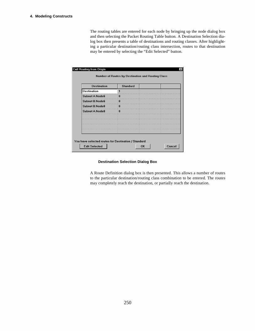
4. Modeling Constructs
box dia-light-tion
utes
250
The routing tables are entered for each node by bringing up the node dialogand then selecting the Packet Routing Table button. A Destination Selectionlog box then presents a table of destinations and routing classes. After highing a particular destination/routing class intersection, routes to that destinamay be entered by selecting the “Edit Selected” button.
Destination Selection Dialog Box
A Route Definition dialog box is then presented. This allows a number of routesto the particular destination/routing class combination to be entered. The romay completely reach the destination, or partially reach the destination.
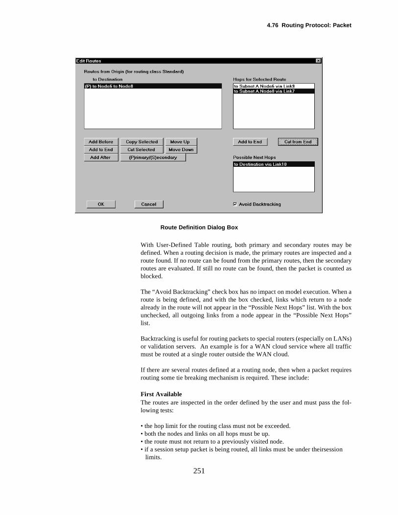
4.76 Routing Protocol: Packet
beand adaryed as
aode
boxps”
ffic
quires
e fol-
on
251
Route Definition Dialog Box
With User-Defined Table routing, both primary and secondary routes maydefined. When a routing decision is made, the primary routes are inspected route found. If no route can be found from the primary routes, then the seconroutes are evaluated. If still no route can be found, then the packet is countblocked.
The “Avoid Backtracking” check box has no impact on model execution. Whenroute is being defined, and with the box checked, links which return to a nalready in the route will not appear in the “Possible Next Hops” list. With the unchecked, all outgoing links from a node appear in the “Possible Next Holist.
Backtracking is useful for routing packets to special routers (especially on LANs)or validation servers. An example is for a WAN cloud service where all tramust be routed at a single router outside the WAN cloud.
If there are several routes defined at a routing node, then when a packet rerouting some tie breaking mechanism is required. These include:
First AvailableThe routes are inspected in the order defined by the user and must pass thlowing tests:
• the hop limit for the routing class must not be exceeded.• both the nodes and links on all hops must be up.• the route must not return to a previously visited node.• if a session setup packet is being routed, all links must be under theirsessi
limits.
4. Modeling Constructs
thatb
rriesdi- in theme-
usert, are lim-h the
band-ink lessnt of
e one“leasthich on
lastlue.
at 5,uting
then
arevaila- (if a least
delay,r arey.
com-ce, if
252
Note that buffer space and availability is not part of the tests. The first routepasses the tests will be selected and the packet directed to the selected uffer,even if this results in immediate blocking because of buffer overflow.
If a multihop route is picked for a packet at a routing node, then the packet cawith it the list of hops it must use in order to follow the route. At each intermeate node the packet only has to look at the established route and be placedappropriate port output buffer (if possible)—the routing protocol at each interdiate node does not have to be queried.
4.76.1 Max Idle Bandwidth
With maximum idle bandwidth selection, the alternate routes defined by the are inspected and a sublist made of routes which are inside the hop limiavailable, do not visit previous nodes, and have all links inside their sessionits (if a session setup packet is being routed). From this sublist the route witmost idle bandwidth is selected.
A route comprises one or more hops. The link on each hop has an averagewidth use, averaged over the “Link Utilization Update Interval” period. The ltherefore has an amount of unused bandwidth (equal to the total bandwidththe used bandwidth). On each route one of the links will have the least amouunused bandwidth on that route. If there are several routes, then there will blink on each route that has the least available unused bandwidth. These bandwidth” links are compared and the route selected which owns the link whas the most unused or idle bandwidth. In other words, find the “worst” linkeach route and take the route that has the best, “worst” link.
Note that the bandwidth figure that is used is the one which resulted from thecompleted measurement based on the “Link Utilization Update Period” vaFor instance, if the “Link Utilization Update Period” is set to 5 seconds then theutilization percentages for each link will be computed every 5 seconds—i.e., 10, 15, 25, etc., seconds into the simulation. If a max unused bandwidth rodecision is made at 22.396 seconds into the simulation, the utilization figuresavailable at that time are those that were last made at 20 seconds.
If two or more routes are tied in terms of their maximum unused bandwidth they will be selected for routing on a round-robin basis.
4.76.2 Min Delay
With minimum delay selection the alternate routes defined by the userinspected and a sublist made of routes which are inside the hop limit, are able, do not visit previous nodes, and have all links inside their session limitssession setup packet is being routed). From this sublist the route with thedelay is selected.
A route comprises one or more hops. The link on each hop has an average averaged over the “Delay Update Period.” The current value of average delay foall links on the route are totalled to give the total delay for the route. If thereseveral routes, then there will be one route which has the smallest total dela
Note that the delay figure that is used is the one which resulted from the last pleted measurement based on the “Delay Update Period” value. For instan
4.76 Routing Protocol: Packet
intonds
e last
theones
r arevaila- (if amini-
utputcessould
. Thehas thed
of the
p inafterlt in
r arevaila- (if a is the
n ther theult in-reated, setupult in
253
the “Delay Update Period” is set to 5 seconds then the average delays for eachlink will be computed every 5 seconds—i.e., at 5, 10, 15, 25, etc., secondsthe simulation. If a minimum delay routing decision is made at 22.396 secointo the simulation, the delay figures available at that time are those that wermade at 20 seconds.
If two or more routes are tied in terms of their delay the hop in the table forfirst one will be selected and then that hop will be placed after the remaining of the same delay in the table. This will result in round robin selection among tiedtable entries.
4.76.3 Min Queue
With minimum queue selection, the alternate routes defined by the useinspected and a sublist made of routes which are inside the hop limit, are able, do not visit previous nodes, and have all links inside their session limitssession setup packet is being routed). From this sublist the route with the mum queue is selected.
A route comprises one or more hops. The link on each hop has a port obuffer which queues the packets waiting to complete transmission. A multiaclink has several port output buffers queueing packets, but only one of them wbe used on a particular route. Across the route, one of the port output bufferqueues will be longest. For each route there is therefore a longest queuelongest queues between routes are compared and the route selected which shortest value; in other words, compare the “worst” queues between routes anselect the route with the best “worst” queue.
The queue lengths used are instantaneous measurements made at the timerouting decision.
If two or more routes are tied in terms of their minimum queue length, the hothe table for the first one will be selected and then that route will be placed the remaining ones of the same queue length in the table. This will resuround-robin selection among tied table entries.
4.76.4 Min Sessions
With minimum session selection the alternate routes defined by the useinspected and a sublist made of routes which are inside the hop limit, are able, do not visit previous nodes, and have all links inside their session limitssession setup packet is being routed). From this sublist, the selected routeone with the minimum number of sessions currently established.
If two or more routes are tied in terms of the number of sessions, the route itable for the first one will be selected and then that route will be placed afteremaining ones of the same number of sessions in the table. This will resround-robin selection among tied table entries. For instance, if “minimum sessions” selection were used but only messages (rather than sessions) were cor if connectionless routing for sessions is set, then no sessions are everacross a route and so all routes would have 0 sessions. This would resround-robin operation as described.
4. Modeling Constructs
sion
d
sion
g the
this an
ried
heged
l is 5ationint ish an sec-
over
nsid-
er-
254
4.76.5 Random List
With random list selection, the alternate routes defined by the user are inspectedand a sublist made of routes which are inside the hop limit, are available, do notvisit previous nodes, and have all links inside their session limits (if a sessetup packet is being routed). A random pick is made from this sublist.
4.76.6 Round Robin
With round robin selection, the alternate routes defined by the user are inspecteand a sublist made of routes which are inside the hop limit, are available, do notvisit previous nodes, and have all links inside their session limits (if a sessetup packet is being routed). The route at the top of this list is used, after whichit is placed at the bottom of the list. This results in round robin operation.
The destination of the route may be an intermediate node partially completinroute to the destination, or an access point at a subnet/backbone boundary. At thispoint another routing decision may be required to carry the packet further. Ifdecision succeeds then the packet is carried. If this decision fails to findonwards route then the packet will block at this point and optionally be retfrom the origin.
Reporting: N/A
Fields:
Link Utilization Update IntervalThe “Link Utilization Update Interval” is used in the routing protocols under tpacket-switched model. Where a link utilization figure is required, it is averaover this time period.
Each link has a utilization measurement. For example, if the update intervaseconds, then the utilization figures are updated every 5 seconds. If a utilizfigure is needed between update points, the figure from the last update potaken. For instance, if a utilization figure was needed at 24.5 seconds witupdate period of 5 seconds, the utilization calculated over the range 15 to 20onds would be used.
Routing Update Interval The time period between periodic routing table updates.
Delay Update Interval On user defined table routing with minimum delay selection, the time period which the delay statistics are collected.
Deviation Percentage The percentage relative to the shortest route within which other routes are coered equivalent.
Congestion Threshold Type On minimum penalty routing, the penalty factors can vary by link utilization pcentage or by link delay (seconds).
Connection-Oriented Routing For Sessions

4.76 Routing Protocol: Packet
by
ram
255
If checked, then session setup packets are routed in a connection-oriented man-ner. A virtual circuit is established across the network which is then followedthe data packets and any response or ACK packets.
If connection-oriented routing is off then all packets are routed on a datagbasis.
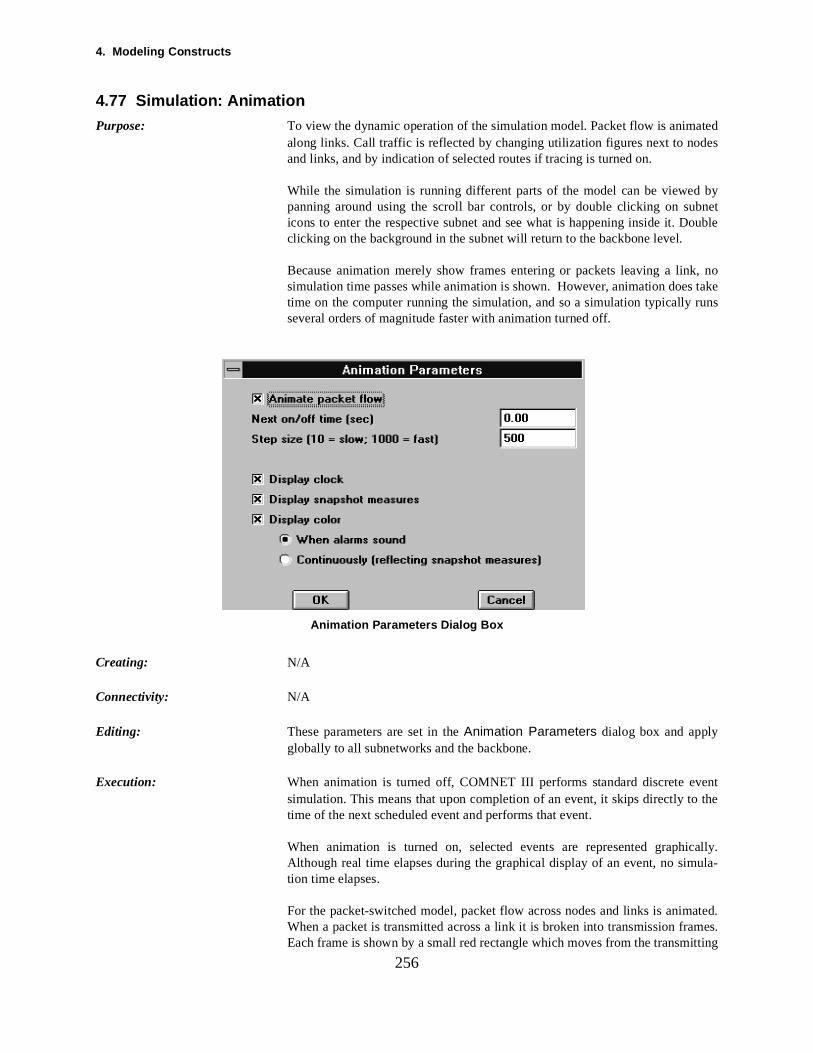
4. Modeling Constructs
tedes
bybnetouble
, no take
ent the
cally.ula-
ated.mes.itting
256
4.77 Simulation: Animation
Purpose: To view the dynamic operation of the simulation model. Packet flow is animaalong links. Call traffic is reflected by changing utilization figures next to nodand links, and by indication of selected routes if tracing is turned on.
While the simulation is running different parts of the model can be viewedpanning around using the scroll bar controls, or by double clicking on suicons to enter the respective subnet and see what is happening inside it. Dclicking on the background in the subnet will return to the backbone level.
Because animation merely show frames entering or packets leaving a linksimulation time passes while animation is shown. However, animation doestime on the computer running the simulation, and so a simulation typically runsseveral orders of magnitude faster with animation turned off.
Animation Parameters Dialog Box
Creating: N/A
Connectivity: N/A
Editing: These parameters are set in the Animation Parameters dialog box and applyglobally to all subnetworks and the backbone.
Execution: When animation is turned off, COMNET III performs standard discrete evsimulation. This means that upon completion of an event, it skips directly totime of the next scheduled event and performs that event.
When animation is turned on, selected events are represented graphiAlthough real time elapses during the graphical display of an event, no simtion time elapses.
For the packet-switched model, packet flow across nodes and links is animWhen a packet is transmitted across a link it is broken into transmission fraEach frame is shown by a small red rectangle which moves from the transm
4.77 Simulation: Animation
ittedm
the
smis-
at ane rec-
e is a
ther the
band-
ess- in
ll be
ther
be
ima-
be set
cu-
or-
they
257node icon across the arc to the link icon. When all frames have been transmthen, after the propagation delay for the last one, the packet can be rebuilt frothe frames and placed in the port input buffer of the receiving node. This isreflected by a small blue rectangle moving from the link icon across the arc toreceiving node icon.
The movement of these rectangles reflects the event of starting frame transion, or of receiving the packet into a port buffer. These events are instantaneousin simulation time. The time duration of the movement of the rectangle shouldnot be interpreted as reflecting a transmission delay—they really indicate thinstantaneous state transition has taken place. The time between a red framtangle starting to move and the time a blue packet rectangle starts to movbetter indication of link transmission time.
For circuit-switched call traffic, the default animation mode is to indicate instantaneous link and node utilization as a number next to the respective link onode icon. As a call is routed, it takes bandwidth from nodes and links alongselected route and so their utilization is increased. When a call clears the width is given back and so the utilization is decreased.
The trace option shows additional animation for circuit-switched calls. Succful routing decisions will then be shown by highlighting the chosen routegreen. Blocked routing decisions are shown in red.
Reporting: N/A
Fields:
On/Off A check box to indicate whether animation is on or off. This check box can bechanged while the simulation is running.
If the model is saved with animation on then when the model executes it wianimated. Similarly it will not be animated if saved with animation off.
At the end of simulation the check box is changed back to its initial setting rathan remaining in its last changed value.
Time Of Next Change The simulation time at which the current setting of the on/off check box willtoggled; i.e., the time at which, if it is off, it will turn on and vice versa.
This can be used skip “boring” parts of the animation and then turn on the antion just prior to some interesting event (such as a failure event).
Step Size The speed of animation is controlled by the Step size parameter which can in the range 10 (which is slow) and 1,000 (which is fast).
Turning animation completely off with the On/Off check box is the fastest exetion mode.
Display Clock Checking this box will turn on the simulation clock in the lower right hand cner of COMNET III canvas.
Display Snapshot Measures By checking this box, reporting snapshot measurements will be displayed if
4. Modeling Constructs
arm
ld
elves,
258
have been enabled under the Reports Snapshots.
Display Color Checking this box will allow objects to change color based upon existing alcondition thresholds.
When Alarm Sounds: A static change in object color when an alarm wouoccur.
Continuously (reflecting snapshot measures): This will allow for a continuouscolor change to be used to indicate the levels of snapshot measures themsbased upon alarm conditions.
4.78 Simulation: Animation - Dynamic Color Change
olorange
pecifys. By% toeas-
olore toercent
shots classcolor
nks,
fol-
hen-
259
4.78 Simulation: Animation - Dynamic Color ChangeIn release 1.2, if you checked the “show alarms” checkbox, dynamic cchanges would be used to indicate alarm conditions. Specifically, a color chindicated an alarm had sounded. It was a discrete indication, on or off.
In release 1.3, dynamic color changes can be more continuous. You can sthat color be used to indicate the levels of snapshot measures themselvedefault, a color range from blue to red is used to indicate a measure from 0100%. By default, continuous color changes are shown only for snapshot mures that reflect a percent value, such as channel utilization.
Additionally, if you set an alarm threshold on a snapshot, the continuous cchanges will then reflect the range from 0 to the threshold, again from blured. This effect applies to any snapshot that has an alarm set, whether pvalued or otherwise.
Note that, just like measures, continuous color changes reflect only the snapselected for display in the Select Snapshots dialog. Only one snapshot perof objects can be selected for display. In other words, to show continuous for channel utilization, you must
1) Go to Select Snapshots and turn on Channel Utilization for one or more li
2) Select Channel Utilization as the display snapshot for links,
3) Go to Animation and be sure “Display color” is checked,
4) Select the “Continuously” radio button.
The controls of the Animation dialog can now be used to obtain any of thelowing combinations of snapshot display:
• Display measures (the little numbers over the icons) and change colors wever an alarm sounds
• Display measures and reflect the measures in color changes
• Don’t display measures, but change colors whenever an alarm sounds
• Don’t display measures, but indicate the measures by color changes.
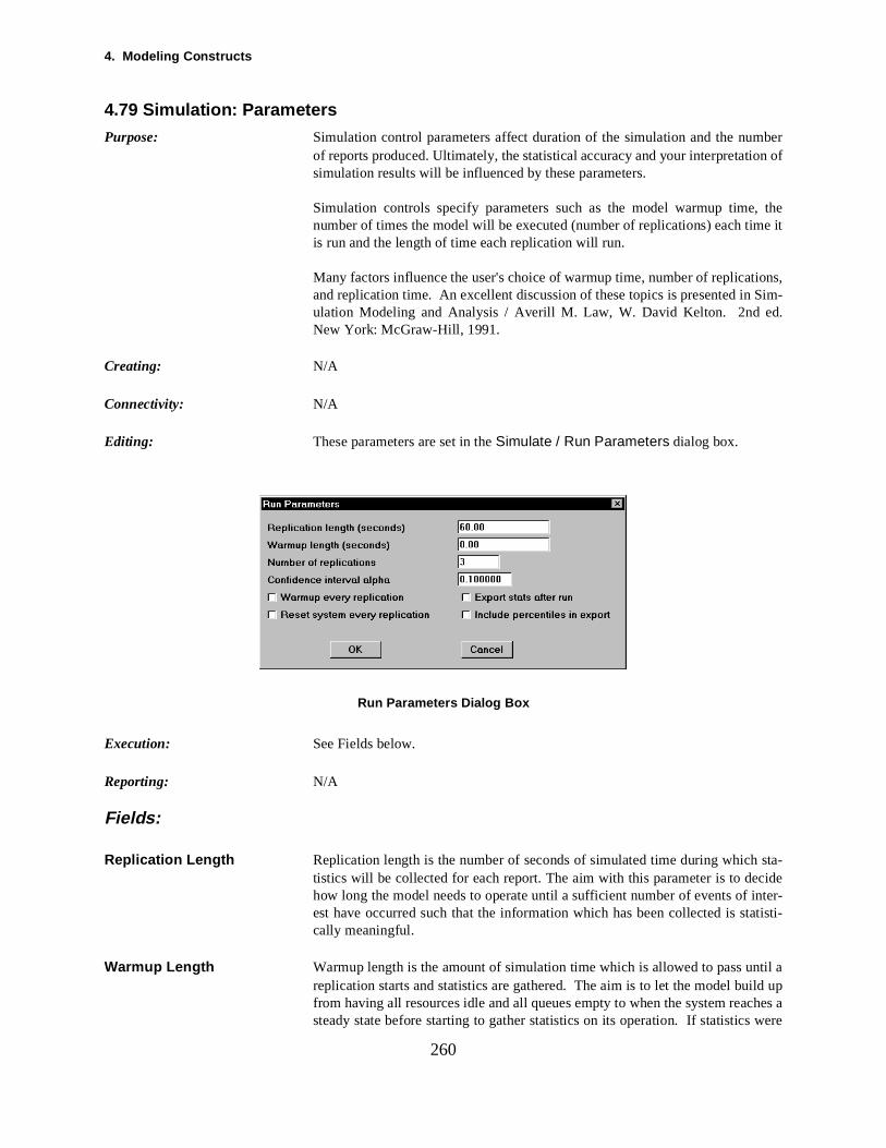
4. Modeling Constructs
ber
, thee it
ons,Sim-d.
ta-cideter-
atisti-
til aild uphes a
were
260
4.79 Simulation: Parameters
Purpose: Simulation control parameters affect duration of the simulation and the numof reports produced. Ultimately, the statistical accuracy and your interpretation ofsimulation results will be influenced by these parameters.
Simulation controls specify parameters such as the model warmup timenumber of times the model will be executed (number of replications) each timis run and the length of time each replication will run.
Many factors influence the user's choice of warmup time, number of replicatiand replication time. An excellent discussion of these topics is presented in ulation Modeling and Analysis / Averill M. Law, W. David Kelton. 2nd eNew York: McGraw-Hill, 1991.
Creating: N/A
Connectivity: N/A
Editing: These parameters are set in the Simulate / Run Parameters dialog box.
Run Parameters Dialog Box
Execution: See Fields below.
Reporting: N/A
Fields:
Replication Length Replication length is the number of seconds of simulated time during which stistics will be collected for each report. The aim with this parameter is to dehow long the model needs to operate until a sufficient number of events of inest have occurred such that the information which has been collected is stcally meaningful.
Warmup Length Warmup length is the amount of simulation time which is allowed to pass unreplication starts and statistics are gathered. The aim is to let the model bufrom having all resources idle and all queues empty to when the system reacsteady state before starting to gather statistics on its operation. If statistics
4.79 Simulation: Parameters
and
omn theen to
ork thes withe
col-
hieve
ettingation
ient
er of caseplica-
. If
lica-orms ares.
fileorted
e
261
gathered right from the start, they could be distorted by low utilization rateslow congestion levels while the system came up to steady state.
Number Of Replications The number of times the simulation will be repeated with different randnumber values selected so that a full statistical spread of different events imodel can be tested. At the end of each replication, a set of reports is writtfile.
If the “Reset System After Every Replication” flag is set to yes then the netwis emptied of traffic and all devices reset to their initial conditions; however,random number seeds are not reset. Therefore the next replication executedifferent starting seeds to the previous one and so is a statistically separate xper-iment.
A common simulation technique is to run a simulation a long period of time lecting statistical measures periodically as the simulation runs. COMNET III pro-vides a set of reports at the end of each replication. Therefore, in order to acthe equivalent of a long run, set the number of replications to the number ofreports you want and do not reset the system for each replication. Not resthe system means that the traffic that is established at the end of one replicwill act as the starting condition for the next replication.
Many COMNET III models are designed to simulate operations under transor dynamic conditions such as link outages or sudden peaks in traffic. In thesecases the user is well served by repeating the transient condition a numbtimes and accumulating statistics over a number of these replications. In thisthe system should be reset between replications so that traffic from one retion is cleared before starting the next replication. Then the network starts froman empty condition on each replication.
Warmup Every Replication Indicates whether a warmup period should be included for every replicationset to “No,” then only the first replication has a warmup period.
Reset System Every ReplicationIndicates whether the model should be completely reinitialized from one reption to the next, or whether the ending conditions of one replication should fthe starting conditions of the next. In either case, the random number seednot reset so that the next replication has different random number sequence
Export Stats After Run This option automatically produces an export file of all monitor statistics uponcompleting the simulation. The labeling of rows and columns in the exporthave been improved to be much more readable. The export file can be impdirectly into spreadsheet packages like Microsoft Excel for further analysis.
Include percentiles in export This option when turned on, exports percentiles for every Statistics... button entrywhere the user selects the Save Observations checkbox. Percentiles are availableverywhere observations are saved.
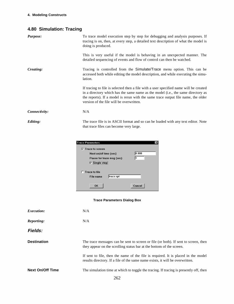
4. Modeling Constructs
el is
The
imu-
atedory aslder
ote
, then
del
hen
262
4.80 Simulation: Tracing
Purpose: To trace model execution step by step for debugging and analysis purposes. Iftracing is on, then, at every step, a detailed text description of what the moddoing is produced.
This is very useful if the model is behaving in an unexpected manner. detailed sequencing of events and flow of control can then be watched.
Creating: Tracing is controlled from the Simulate/Trace menu option. This can beaccessed both while editing the model description, and while executing the slation.
If tracing to file is selected then a file with a user specified name will be crein a directory which has the same name as the model (i.e., the same directthe reports). If a model is rerun with the same trace output file name, the oversion of the file will be overwritten.
Connectivity: N/A
Editing: The trace file is in ASCII format and so can be loaded with any text editor. Nthat trace files can become very large.
Trace Parameters Dialog Box
Execution: N/A
Reporting: N/A
Fields:
Destination The trace messages can be sent to screen or file (or both). If sent to screenthey appear on the scrolling status bar at the bottom of the screen.
If sent to file, then the name of the file is required. It is placed in the moresults directory. If a file of the same name exists, it will be overwritten.
Next On/Off Time The simulation time at which to toggle the tracing. If tracing is presently off, t
4.80 Simulation: Tracing
ecifies overall
es-ialog
trace
263
turn it on at the specified time, and vice versa.
Pause For Message When the model is running and if trace messages are sent to screen, then the mes-sages may pass so fast that there is no chance to read them. This field sphow many seconds each trace message should remain on the screen. Oneimpact is the model is then throttled to run at this speed.
Single Step If the “Single Step” box is checked then the model moves from one trace msage to the next and then waits for user input (a mouse click on a Continue dbox) before continuing.
When the Continue dialog box is waiting for input, the Simulate/Trace menuoption is still accessible so that single stepping can be turned off and other controls accessed.
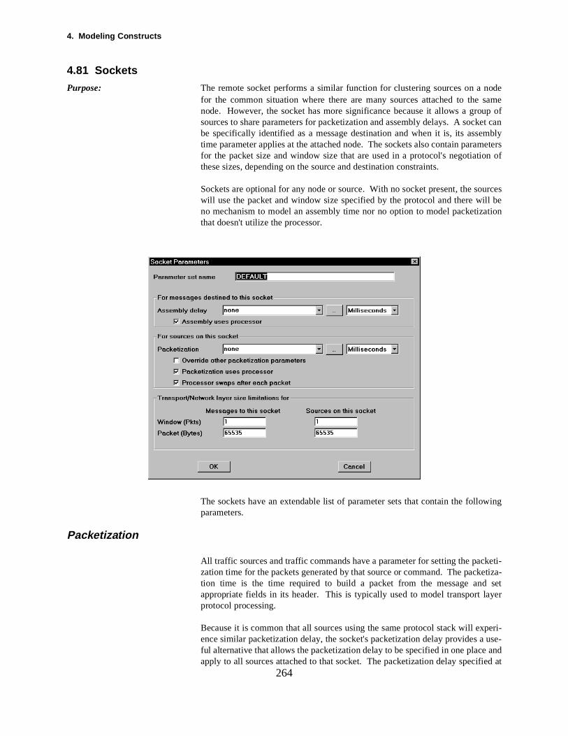
4. Modeling Constructs
nodesameup ofet canmblymeterson of
urcesll beation
wing
keti-etiza- setayer
peri- use- andied at
264
4.81 Sockets
Purpose: The remote socket performs a similar function for clustering sources on a for the common situation where there are many sources attached to the node. However, the socket has more significance because it allows a grosources to share parameters for packetization and assembly delays. A sockbe specifically identified as a message destination and when it is, its assetime parameter applies at the attached node. The sockets also contain parafor the packet size and window size that are used in a protocol's negotiatithese sizes, depending on the source and destination constraints.
Sockets are optional for any node or source. With no socket present, the sowill use the packet and window size specified by the protocol and there wino mechanism to model an assembly time nor no option to model packetizthat doesn't utilize the processor.
The sockets have an extendable list of parameter sets that contain the folloparameters.
Packetization
All traffic sources and traffic commands have a parameter for setting the paczation time for the packets generated by that source or command. The packtion time is the time required to build a packet from the message andappropriate fields in its header. This is typically used to model transport lprotocol processing.
Because it is common that all sources using the same protocol stack will exence similar packetization delay, the socket's packetization delay provides aful alternative that allows the packetization delay to be specified in one placeapply to all sources attached to that socket. The packetization delay specif
4.81 Sockets
'sds.
and,sent.cket
pack-dingation
ck-ssedrelin-ificant
des-t is onrocessas ansor
les.
ts.
usedstina-
xistndaintsrcesnts forific
t sizeurce at the
nal atow
265
the socket includes options for modeling the delay without utilizing the nodeprocessor or specifying that delay in terms of processor cycles or millisecon
Because there is also a packetization time specified on the source or commCOMNET will use the sum of both packetization times when sockets are preIt is recommended, however, to specify the packetization delay at the sowhen the socket is used.
The socket provides an additional option for how the processor handles the etization with a large window when there are other applications that are penat the same time. One option is for the processor to swap the current applicand begin working on a different application as soon as one packet is created,while the other option is for the processor to continue working on the same mes-sage until the flow-control window or the rate control prevents any further paets from being created. Typically the other applications waiting to be procewill be other instances of messages so that how quickly the processor quishes the processing of a particular message instance can have a signimpact on that message's overall delay.
Assembly
Packet assembly time complements the packetization time but applies to thetination node. If a message source has a destination of a specific socket thaa node, then that socket's assembly time is used to calculate the delay to pthat packet to rebuild the message at the destination. The assembly time hoption to model this delay without utilizing the destination node's procesalthough it is most useful when such utilization does occur. Also, the socket pro-vides an option to interpret the assembly time in terms of milliseconds or cyc
There is no alternative way to specify an assembly time without using socke
Socket-Based Protocol Constraints
As discussed in the protocol section, the actual packet size and window sizefor a protocol can be modified based on the constraints at the source and detion. Recall that the protocol definition itself is globally available and may eon many sources throughout a model. The socket can refine the packet size awindow size in two ways. First, there are parameters to specify the constrfor packet and window sizes for traffic leaving the node through any souattached to this socket. Secondly, there are parameters for these constraitraffic arriving to this node from other sources with destinations of this specsocket.
When sockets are involved at the source and destination ends, the packechosen will be the minimum packet size from the protocol's field and the sopacket size on the socket at the source end and the destination packet sizesocket at the destination end. (Note, however, that the sockets are optioeither end.) The window size for this connection will be the minimum windcalculated in bytes from each of these three places.
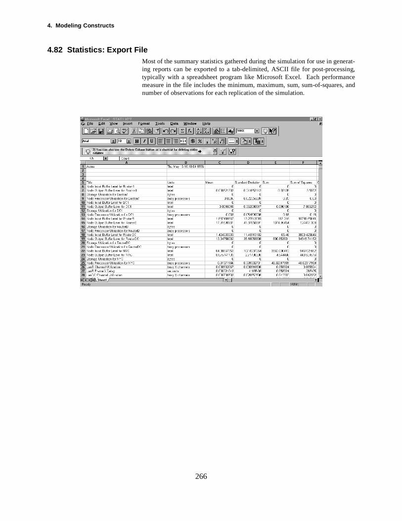
4. Modeling Constructs
erat-
nce, and
266
4.82 Statistics: Export FileMost of the summary statistics gathered during the simulation for use in gening reports can be exported to a tab-delimited, ASCII file for post-processing,typically with a spreadsheet program like Microsoft Excel. Each performameasure in the file includes the minimum, maximum, sum, sum-of-squaresnumber of observations for each replication of the simulation.
4.83 Statistics: Link
ults
ns-oth
mayy be
ofd bytis-ted
ics”w”
hed
sta-va-
data
raph
267
4.83 Statistics: Link
Purpose: To collect utilization and loading statistics on a link and present the resgraphically.
A point-to-point link is implemented on a full duplex basis and so there is tramission capacity in both directions. Consequently there is utilization in bdirections and so two graphs may be plotted.
For contention based links (such as Aloha or CSMA/CD) a control channel be specified. The contention channel and the control channel utilization maseparately plotted.
Creating: In order to obtain graphs for link loading and utilization, collection and savingstatistics must both be turned on before the simulation is run. This is achieveselecting the “Statistics” button on the link dialog box, picking the desired static from the list box, and editing the statistic detail to ensure that it is collecand saved.
The simulation is then run.
After the simulation is run the graphs can be viewed by picking the “Statistbutton on the link dialog box, selecting the statistic, and then picking the “Viebutton.
Connectivity: Link statistics in terms of graphical output are available for the packet-switcbandwidth on all types of link.
Editing: Click on the Statistics button on the link dialog box.
Execution: When the simulation runs, if collection of link status has been turned on, linktistics are saved to the file “statfile” in the model directory. If “save obsertions” has been requested, the raw data are saved in the file stattrc.out .After the simulation has completed and when graphs are requested, it is thein this file which is read and graphed.
Running the simulation again will overwrite any previous statfile and stat-trc.out in the model directory.
Reporting: N/A
Fields:
Collect Statistics A check box to indicate that statistics should be collected on link utilization.
Save Observations A check box to indicate that the raw data should be saved to file so that they canbe plotted after the simulation finishes.
View View the graphs on the collected statistics. Plot parameters to control the gscaling, etc., may be entered.(see Statistics: Plot Parameters)
4. Modeling Constructs
results
isticscting sta-
col-
l exe-
hen
ssage
dialog
rnedy. If
ed, it
del
ard
268
4.84 Statistics: Message
Purpose: To collect message delay and message in transit statistics and present the graphically.
Creating: In order to obtain graphs for message statistics, collection and saving of statmust both be turned on before the simulation is run. This is achieved by selethe “Statistics” button on the message source dialog box, picking the desiredtistic from the list box, and editing the statistic detail to ensure that it is both lected and saved.
Real time graphs are produced as the simulation is run. Note that production ofreal time graphs takes computation resources and so slows down the modecution.
After the simulation is run the (non real time) graphs can be viewed by pickingthe “Statistics” button on the link dialog box, selecting the statistic, and tpicking the “View” button.
Connectivity: Message statistic plots are available for messages which arise from mesources, response sources, and session setup sources.
Plots are not available for message commands defined directly on a node.
Editing: Click on the Statistics button on the message, response, or session sourceboxes.
Execution: When the simulation runs, if collection of message information has been tuon, message statistics are saved to the file “statfile” in the model director“save observations” has been requested, the raw data are saved in the file stat-trc.out . After the simulation has completed and when graphs are requestis the data in this file which is read and graphed.
Running the simulation again will overwrite any previous statfile in the modirectory.
Reporting: N/A
Fields:
Collect Statistics A check box to indicate that statistics (mean, minimum, maximum, standdeviation) should be collected.Applies to:Message DelayMessages In Transit
Save Observations A check box to indicate that the raw data should be saved to file so that they canbe plotted later in the COMNET III session.Applies to:Message Delay Messages In Transit
Plot Parameters (see Statistics: Plot Parameters)Applies to:Message Delay

4.84 Statistics: Mes sage
ph is
ph is
ph is
ph is
269
Messages In Transit
On/Off For real time graphs, indicates whether the graph should be drawn or not.Applies to: Real Time Message Delay
Real Time Messages in Transit
Initial Y Axis Minimum For real time graphs, the minimum y axis value to be plotted when the grafirst drawn. As the simulation runs, the graphs are auto-scaling.Applies to:Real Time Message Delay Real Time Messages in Transit
Initial Y Axis Maximum For real time graphs, the maximum y axis value to be plotted when the grafirst drawn. As the simulation runs, the graphs are auto-scaling.Applies to:Real Time Message Delay Real Time Messages in Transit
Initial X Axis Minimum For real time graphs, the minimum x axis value to be plotted when the grafirst drawn. As the simulation runs, the graphs are auto-scaling.Applies to:Real Time Message Delay Real Time Messages in Transit
Initial X Axis Maximum For real time graphs, the maximum x axis value to be plotted when the grafirst drawn. As the simulation runs, the graphs are auto-scaling.Applies to:Real Time Message Delay Real Time Messages in Transit
4. Modeling Constructs
ari-gs.
to be Theer an
ng.sser-
ge.
perch asatlys antilestili-or
abe-ter-n the
ble of
ereof allcol- Thesoft
singleproc-le to
270
4.85 Statistics: MonitorsCOMNET III offers many statistics request monitor and allows many more vables to be monitored through the statistics request buttons on various dialo
Option to Store Averaged Observations
The statistics request monitors enable the collection of raw observation dataplotted or to be analyzed for percentiles or exported to other statistics tools.option allows the sampled observations to be averaged observations ovinterval.
If the interval is zero, then the monitors will collect raw observations for plottiFor many values such as utilization or buffer levels, there can be a tremendounumber of observations—making the simulation run slow to store all those obvations to the hard drive and then create observation files too large to mana
If the interval is larger than zero, then the monitors will collect one sampleinterval and that sample will be averaged (either time-weighted for values suutilization, or tallied for values such as delay) over the interval. This can grereduce the number of samples that have to be stored in a file. It also addadvantage by providing more meaningful plots, histograms, or percenbecause of the smoothing it provides. It is especially useful for monitoring uzation and buffer levels but it can also be helpful for plotting averaged delay flarge numbers of messages.
Monitor Statistics and Confidence Intervals
The table for viewing monitor statistics has been improved to provide better lling and precision. When multiple replications are available, confidence invals are also provided. The desired confidence interval alpha is specified oRun Parameters dialog, immediately after the number of replications. If monitorobservations have been saved, percentiles can also be included in the tamonitor statistics.
Export to Excel
An improved export capability is also available for all statistical monitors. This a new Run Parameters option that automatically produces an export file monitor statistics upon completing the simulation. The labeling of rows and umns in the export file have been improved to be much more readable. export file can be imported directly into spreadsheet packages like MicroExcel for further analysis.
Node Monitors
Release 1.2 provides a statistics request button on nodes to provide the following statistics on the node:
Processor Utilization This monitor measures the number of busy processors at any time. For a processor node, the result is the utilization of the processor. Frequently the essor will be busy with short duration tasks and thus it is generally desirab
4.85 Statistics: Monitors
rages that
ives
-llect
call
ly to
of ae forlobal
lay is
Due togener-mes-
ges
thin aan be
wket
271
collect this utilization averaged over a convenient interval.
Storage This monitor measures how much file space is used in this node's disk stospace. This monitor is useful for models that have read and write commandchange the size of files.
Call Bandwidth Level (Utilization) This monitor measures the call bandwidth allocated through this node. It isuseful when modeling bandwidth-switched calls with call sources, and it gthe total bandwidth of all the calls using this node.
Buffer Monitors
Buffer Level The input and output buffers have a monitor for monitoring the buffer level. Thismonitor may be available for off-line analysis or real-time plotting. Since packets arrive and leave buffers very frequently, it is generally desirable to coaveraged buffer levels for plotting.
New Link Monitors Two new monitors have been added to monitor the link:
Call Bandwidth Level (Utilization )This monitor measures the call bandwidth allocated through this link. Callbandwidth is allocated on the link when a bandwidth switched call (from a source) uses this link.
Frame Size This monitor measures the size of frames using this link. Since there are likebe a large number of frames using a link during a simulation, this monitor shouldbe averaged over an interval for best results.
New Message Destination MonitorsThere is a set of detailed protocol monitors available for each destination message command or a traffic source. These monitors are only availablmessages with explicit destination lists, and they are not yet available for gcommands.
Message Delivery and Message Transmission DelaysThe message delay is now measured from two perspectives: the delivery dethe time required for the receiver to reconstruct the message while the messagedelay is the time required before the source closes the message command. acknowledgements, retransmissions, or a close-sequence, the sender will ally close the message transmission later than the receiver will receive the sage.
Window Size The window size monitor is only for the TCP/IP congestion window that chanover time based on congestion on the network.
Inter-Packet Interval This monitor measures the time between when new packets are created wimessage. It is only useful for messages that generate multiple packets. It cuseful as a measure of the effectiveness of the protocol's flow control window orrate control mechanism.
IPackets in Retransmission EventThis monitor is primarily useful for the sliding window and TCP/IP windooption for "fast recovery" to avoid retransmitting a whole window when a pac
4. Modeling Constructs
ame
wl-nges-
This
col
t the or. one
272
is blocked.
Retransmissions for Blocked PacketsThis monitor measures the number of retransmissions required for the spacket before the packet is received by the destination without errors.
Retransmission Timeout This monitor is useful for the sliding window and TCP/IP window option to cal-culate the retransmission time based on the round-trip time of the packets. How-ever, it is only updated when a retransmission actually occurs.
Round-Trip Time (Ack Delay) This monitor measures the ack delay which is set up to measure the round-triptime of a packet. It is most useful for sliding windows that generate acknoedgements for each packet. It also provides a simple measure of network cotion.
Packet Size This monitor measures the size of the packets generated by the protocol. monitor is probably most useful for messages that consist of one packet.
Burst Size This monitor measures the main burst size from the traffic policy of the protowhen the traffic policy is used.
Inter-Assembly Interval This monitor measures the interval between successive packets arriving adestination. This is particularly useful for time-critical traffic such as voicevideo transmissions where a near constant inter-assembly interval is desiredWhen modeling ATM networks, this measures the cell-delay variation that ismeasure of quality of service.
4.86 Statistics: Plot Parameters
after
n the may
data
f the
serva-o plotthereeas-
mes-ute
e t isote
e -
273
4.86 Statistics: Plot Parameters
Purpose: To display statistics collected on various measures (such as link utilization) the simulation has run.
Creating: The graphs of collected statistics are accessed via the statistics buttons olinks, traffic generators etc. Once the raw data have been saved then youview the graphs by clicking on the view button.
Connectivity: N/A
Editing: The data that is graphed is collected during the simulation run. to change thethe simulation needs to be rerun.
Various interactive parameters are available to control the appearance ographs. These are listed below.
Execution: N/A
Reporting: N/A
Fields:
Observed Data Plot the data points that have been observed.
Smoothed Data Plot smoothed data where each data point represents an average of the obtions over an interval. In the case of delay measures, the number of points tdetermines the averaging interval (more points means a smaller interval). If is no delay observation on an interval, zero is plotted. In the case of level mures, the user specifies the averaging interval.
Number of Points The number of points to plot.
Start Time The simulation time at which to start graphing.
Stop Time The simulation time at which to stop graphing.
Averaging Interval Applies only to level measures (e.g., number of busy channels, number of sages in-transit, buffer level). Specifies the time interval over which to compthe time-weighted average level that is to be plotted. The point plotted at timthe average level over the interval , where is the averaging interval. N
that the minimum value for is the interval covered by the plot (Stop TimStart Time) divided by the number of points.
Histogram Plot a histogram on the data that has been collected.
Number Of Bins The number of bins to plot.
Minimum The lower data limit for the first bin.
Maximum The upper data limit for the last bin.
t δ– δδ
4. Modeling Constructs
oneari-epre-
s in ar siteteack-net-is
t-
w
n be level of a
ack-
to a
o one
cted.for thetwork
is
than
274
4.87 Subnetwork
Purpose: The subnetwork serves two purposes.
Firstly, it aids in managing the display of a large network. Rather than havingflat picture that has either very small icons or requires extensive scrolling, vous sites or domains in the network can be placed in a subnetwork which is rsented by just one icon at the backbone level.
Secondly, different subnetworks can be used to represent different domainnetwork which operate under different routing protocols. For instance, a usemay be running a VAX network running DECNET which would run a link stashortest path algorithm. This may have one or more gateways into an X.25 bbone which operates under minimum hop. By making the DECNET a subwork in COMNET III, it may then have a routing protocol defined for it which different from the backbone (and other subnetworks).
Creating: To create a subnetwork use the subnetwork tool on the palette and drag a subnework onto the backbone layout.
Double clicking on the icon will then enter the subnetwork. Alternatively thesubnetwork icon can be highlighted and the Edit/Enter menu option selected.
Upon entering a new subnetwork there are no network components in the nesubnetwork. At least one access point must be created inside the subnetwork (byusing the access point tool on the tool palette) before any connections camade to the subnetwork. An access point can also be added at the networkby dragging the access point from the palette and dropping it on the edgesubnetwork icon.
To leave the subnetwork and return to the backbone, double click on the bground of the subnetwork. Or select the Edit/Leave menu option.
Subnetworks cannot be created inside other subnetworks.
Connectivity: Within the backbone network, links are used to connect a backbone nodesubnetwork access point.
Within the subnetwork, an access point is connected to a node on a one trelationship.
In fact, the access point and the node to which it is connected are synonymous.Editing the access point is the same as editing the node to which it is conneTherefore only one node can connect to an access point. The main reason existence of access points is that their icons can be seen both in the subneand in the backbone.
Editing: To edit the parameters for a subnetwork, highlight the subnetwork icon and thenselect the Edit/Detail menu option. The dialog box for subnetwork parametersthen presented.
Note that double clicking on a subnetwork icon enters the subnetwork ratherpresenting its dialog box.
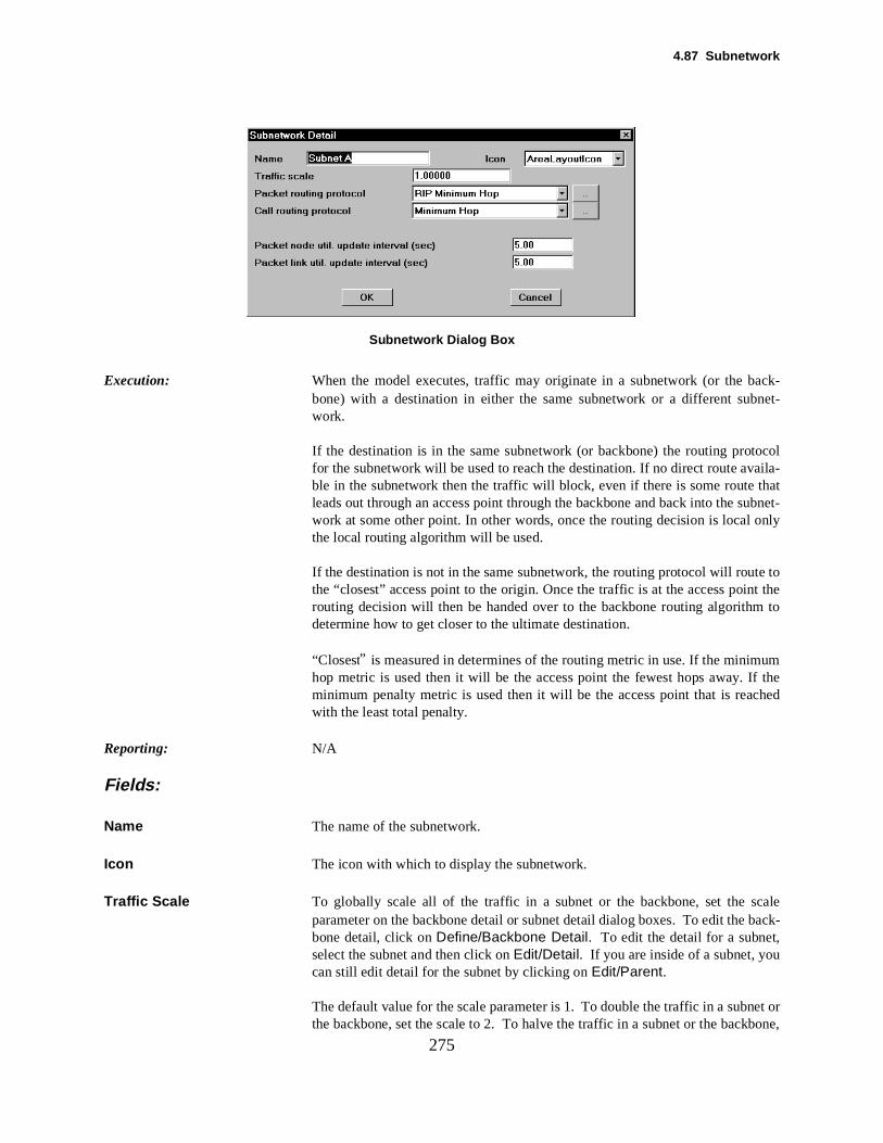
4.87 Subnetwork
-
ocol
thatubnet-only
t the to
umf theched
caleback-,
et orbone,
275
Subnetwork Dialog Box
Execution: When the model executes, traffic may originate in a subnetwork (or the back-bone) with a destination in either the same subnetwork or a different subnetwork.
If the destination is in the same subnetwork (or backbone) the routing protfor the subnetwork will be used to reach the destination. If no direct route availa-ble in the subnetwork then the traffic will block, even if there is some route leads out through an access point through the backbone and back into the swork at some other point. In other words, once the routing decision is local the local routing algorithm will be used.
If the destination is not in the same subnetwork, the routing protocol will route tothe “closest” access point to the origin. Once the traffic is at the access poinrouting decision will then be handed over to the backbone routing algorithmdetermine how to get closer to the ultimate destination.
“Closest” is measured in determines of the routing metric in use. If the minimhop metric is used then it will be the access point the fewest hops away. Iminimum penalty metric is used then it will be the access point that is reawith the least total penalty.
Reporting: N/A
Fields:
Name The name of the subnetwork.
Icon The icon with which to display the subnetwork.
Traffic Scale To globally scale all of the traffic in a subnet or the backbone, set the sparameter on the backbone detail or subnet detail dialog boxes. To edit the bone detail, click on Define/Backbone Detail. To edit the detail for a subnetselect the subnet and then click on Edit/Detail. If you are inside of a subnet, youcan still edit detail for the subnet by clicking on Edit/Parent.
The default value for the scale parameter is 1. To double the traffic in a subnthe backbone, set the scale to 2. To halve the traffic in a subnet or the back
4. Modeling Constructs
tribu-e is
by
oserct on
ure-
f link
276
set the scale to 0.5. The scale parameter applies to the interarrival time distions for all traffic sources in a subnet (or in the backbone). When a valudrawn from an interarrival time distribution, the value is scaled by dividingthe scale parameter for the subnet where the traffic is originating. Thus, a largescale factor increases the arrival rate by making the interarrival times cltogether and conversely for a small scale factor. The scale factor has no effemessage sizes or holding times.
Call Routing Protocol (see Routing Protocol: Call)
Packet Routing Protocol (see Routing Protocol: Packet)
Link Utilization Update IntervalUsed by those Packet Routing Protocols which require a link utilization measment. This is the period over which the average is taken.
When required, Call Routing Protocols use instantaneous measurements outilization and so this parameter is not used in the call model.
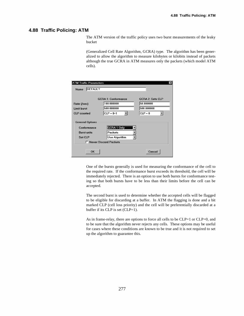
4.88 Traffic Policing: ATM
aky
ner-ketsTM
ell toill be test-n be
d bitt a
andusefulto set
277
4.88 Traffic Policing: ATMThe ATM version of the traffic policy uses two burst measurements of the lebucket
(Generalized Cell Rate Algorithm, GCRA) type. The algorithm has been gealized to allow the algorithm to measure kilobytes or kilobits instead of pacalthough the true GCRA in ATM measures only the packets (which model Acells).
One of the bursts generally is used for measuring the conformance of the cthe required rate. If the conformance burst exceeds its threshold, the cell wimmediately rejected. There is an option to use both bursts for conformanceing so that both bursts have to be less than their limits before the cell caaccepted.
The second burst is used to determine whether the accepted cells will be flaggeto be eligible for discarding at a buffer. In ATM the flagging is done and amarked CLP (cell loss priority) and the cell will be preferentially discarded abuffer if its CLP is set (CLP=1).
As in frame-relay, there are options to force all cells to be CLP=1 or CLP=0,to be sure that the algorithm never rejects any cells. These options may be for cases where these conditions are known to be true and it is not required up the algorithm to guarantee this.
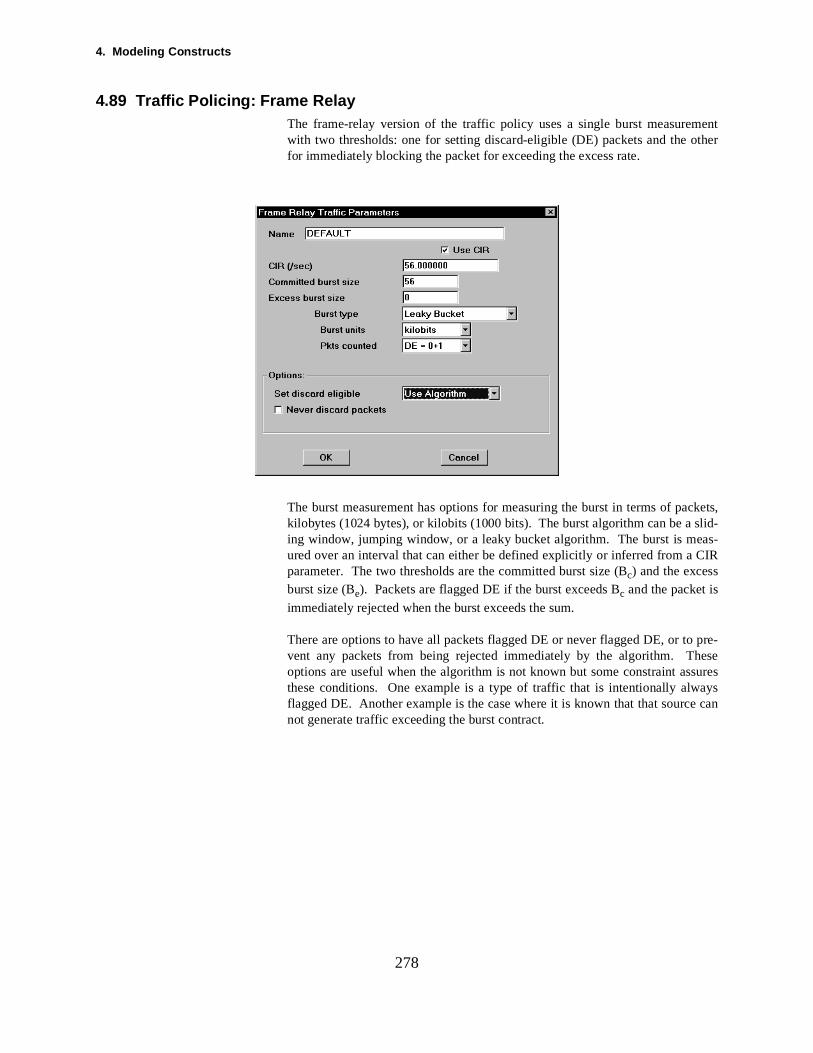
4. Modeling Constructs
entther
ckets,slid-as-CIR
pre-ese
suresays
278
4.89 Traffic Policing: Frame RelayThe frame-relay version of the traffic policy uses a single burst measuremwith two thresholds: one for setting discard-eligible (DE) packets and the ofor immediately blocking the packet for exceeding the excess rate.
The burst measurement has options for measuring the burst in terms of pakilobytes (1024 bytes), or kilobits (1000 bits). The burst algorithm can be a ing window, jumping window, or a leaky bucket algorithm. The burst is meured over an interval that can either be defined explicitly or inferred from a parameter. The two thresholds are the committed burst size (Bc) and the excessburst size (Be). Packets are flagged DE if the burst exceeds Bc and the packet is
immediately rejected when the burst exceeds the sum.
There are options to have all packets flagged DE or never flagged DE, or tovent any packets from being rejected immediately by the algorithm. Thoptions are useful when the algorithm is not known but some constraint asthese conditions. One example is a type of traffic that is intentionally alwflagged DE. Another example is the case where it is known that that source cannot generate traffic exceeding the burst contract.
4.90 Traffic Source: Application
sys-me, aa print
uted.
or thein the
exe-ram-
tailedialog
up tots.
new
d, then.
s,.o the
ctingthere
s that in thendsds on
d to the
theen
279
4.90 Traffic Source: Application
Purpose: An application source models the loading of some software task on an endtem. Examples might be a transaction processing task on a host mainfradatabase access on a database server, or printing a spooled print job on server.
The application comprises a sequence of commands which must be execThese may be any combination of read, write, process, transport, answer, or setupcommands as required by the application.
It is each command which requests some resource to be allocated in order fcommand to execute. The description of each command execution is found respective command section.
It is the task of the application to schedule when the commands are to becuted, and to control command sequencing. Consequently the application paeters are all related to scheduling and sequencing, and not to the decommand description. The command description is described via the node dboxes, or via the global command dialog boxes.
Multiple concurrent applications can be scheduled on the same node. It is the node to determine how it will respond to simultaneous application reques
Creating: To create an application pick the application tool from the palette and drag aapplication onto the background. Or use the create menu option to create a newapplication. Once an application is drawn on the background it must be con-nected to a node using one of the arc tools. Once created and connecteapplication icon can be double clicked to bring up the details of the applicatio
Connectivity: An application can only run on Computer & Communication (C&C) nodeComputer Group nodes, and Router nodes. Connecting an application tATM node is not allowed.
Connecting an application to a Computer Group node is the same as connean application to each of the nodes in the computer group. In other words, if are 10 nodes in the computer group then connecting an application to the groupicon is the same as connecting 10 applications to the group members.
Once an application is connected to a node, it can then “see” the commandhave been defined on that node. Such commands can then be referencedcommand sequence of the application. In addition, globally defined commacan also be referenced. Consequently, it is easier to first define the commana node and then the command sequence on an application source connectenode.
Editing: Either double click on the application icon, or highlight the icon and selectEdit/Detail menu option. The dialog box for editing the application detail is thpresented.
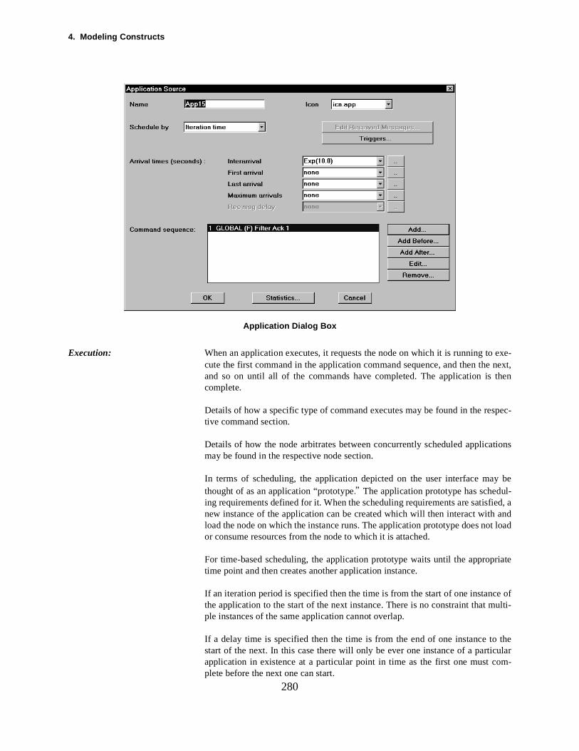
4. Modeling Constructs
next,then
tions
y bel-ed, a andt load
riate
e ofulti-
thecularom-
280
Application Dialog Box
Execution: When an application executes, it requests the node on which it is running to exe-cute the first command in the application command sequence, and then theand so on until all of the commands have completed. The application is complete.
Details of how a specific type of command executes may be found in the respec-tive command section.
Details of how the node arbitrates between concurrently scheduled applicamay be found in the respective node section.
In terms of scheduling, the application depicted on the user interface mathought of as an application “prototype.” The application prototype has scheduing requirements defined for it. When the scheduling requirements are satisfinew instance of the application can be created which will then interact withload the node on which the instance runs. The application prototype does noor consume resources from the node to which it is attached.
For time-based scheduling, the application prototype waits until the approptime point and then creates another application instance.
If an iteration period is specified then the time is from the start of one instancthe application to the start of the next instance. There is no constraint that mple instances of the same application cannot overlap.
If a delay time is specified then the time is from the end of one instance tostart of the next. In this case there will only be ever one instance of a partiapplication in existence at a particular point in time as the first one must cplete before the next one can start.
4.90 Traffic Source: Application
ed theequire-n of
cutionnext.
.
mple-f the
art ofplica-dul-
y toime
rrive atlica-n thege
ld be a
281
For message-based scheduling, when the application prototype has receivrequisite messages, a new application instance can be created. Message rments can include multiple messages and wildcards. For a fuller descriptiomessage based scheduling see Received Message Scheduling.
Once an application instance has been created, it is then considered for exeby the node on which it is running. Determining which instance to execute and whether to single task or multitask is a decision which is left to the nodeSee Node: Computer & Communications (C&C Node)Node: Computer Group
Reporting: Node: Application DelaysOther reports are affected by the traffic generated from within an application
Fields:
Name An alphanumeric field to identify the application.
Icon The name of the icon used to represent the application.
Schedule By Application instances can be scheduled by either “Delay Time,” by “IterationTime” or by “Received Message.”
Delay time scheduling uses the given times as the interval between the cotion of one instance of the application and the start of the next instance oapplication.
Iteration time scheduling uses the given times as the interval between the stone instance of the application and the start of the next instance of the aption. Overlapping instances of the same application can exist with this scheing.
If only one instance of an application is required in a replication, one waachieve this is to use iteration time scheduling and to set the “Interarrival TDistribution” to “None,” the “Last Arrival” to “None,” and the “First Arrival” tothe time when the single instance is required.
Received message scheduling requires that one or more messages must athe node where the application prototype exists for new instances of the apption to be created. In fact the scanning for received messages is based oincoming “Message Text.” Multiple messages may be waited for, and messatext may be scanned by wildcard.See Received Message Scheduling
Interarrival Time Distribution For time-based scheduling, the “Interarrival Time Distribution” is used to make astatistical pick for the time between application instance creation.
Any of the statistical distributions found in COMNET III may be used.See Distributions sections.
First Arrival For time-based scheduling, the time when the first application instance shoustarted. If this is left at “None,” the first application instance will be created at
4. Modeling Constructs
rar-
ll bed
this
thatft at
st be
satis-
on ons that other.
any
d are
ation
define
282
time picked uniformly at random between 0 and a random pick from the “Interival time Distribution.”
Last Arrival For time-based scheduling the time when the last application instance wistarted. If this is left at “None,” application instances will continue to be createup to the replication length. Otherwise, the last application will be started attime.
Max Arrivals For time-based scheduling, the maximum number of application instancescan be created from the application prototype in the replication. If this is le“None,” there is no limit on the number of instances.
Received Message List If received message scheduling is used, the message texts which mureceived in order to create a new application instance must be listed.See Received Message Scheduling.
Received Message Delay For received message scheduling, the time after the received message list isfied when the command sequence starts.
Command Sequence When an application instance has been created, it will then demand executithe node to which it is attached. Demands for execution are, in fact, requesta sequence of commands are executed by the node processor one after theIt is up to the node processor to determine when it is available to forwardparticular command.
On the application prototype, the sequence of commands that are requirelisted in order in the “Command Sequence” list box. Against each command thenumber of times it is to be executed is specified.
When the last command in the sequence has completed then the applicinstance is counted as completed.
The commands can be any sequence of commands that have either beenlocally on the host node, or globally in the global command list.
4.91 Traffic Source: Call
the for
ated.
newall node
e.
theen
r for
allyton met
nse-
2834.91 Traffic Source: Call
Purpose: A Call Source is used to model the generation of circuit-switched traffic.
Separate Call Sources could be used to model different types of traffic fromsame origin—for instance one for voice traffic, one for data traffic and onefax traffic.
The Call Source specifies the volume of a particular call type to be generThe routing of each call instance is handled by the “Call routing Protocol.”
Creating: To create a Call Source, pick the Call source tool from the palette and drag acall icon onto the background. Or use the create menu option to create a new cicon. Once a call icon is drawn on the background it must be connected to ausing one of the arc tools. Once created and connected, the call icon can bedou-ble clicked to bring up the details of the call.
Connectivity: A Call Source can only be connected to a Computer & Communications nod
Editing: Either double click on the Call Source icon, or highlight the icon and selectEdit/Detail menu option. The dialog box for editing the Call Source detail is thpresented.
Note that the required bandwidth for this call is in the routing class parametethe call source.
Call Source Dialog Box
Execution: The Call Source may be thought of as a prototype call which will periodiccreate new call instances for the model to route. It is the task of the prototype check when the scheduling requirements for a new call instance have beeand so create the new instance.
The only scheduling method provided is by “Iteration Time.” This is the timefrom the start of one call instance to the time of the next call instance. Co
4. Modeling Constructs
route
om
this
d.
, the
rigin
notall
284
quently, over the period of a replication, new call instances will be created.
Once a call instance has been created it is up to the call routing protocol to the call to its destination.
Reporting: • Calls: Blocked• Calls: Disconnected• Calls: Preempted• Calls: By Node• Calls: By Link• Calls: Utilization by Node• Calls: Utilization by Link
Fields:
Name An alphanumeric field to identify the Call Source.
Icon The name of the icon used to represent the Call Source.
Interarrival Time Distribution Used to make a statistical pick for the time between call instance creation.
Any of the statistical distributions found in COMNET III may be used.See Distributions sections.
It would be typical for the interarrival time to be based on an Exponential distri-bution, which results in call generation according to a Poisson process.
First Arrival The time when the first call instance should be started. If this is left at “None,”the first call instance will be created at a time picked uniformly at randbetween 0 and the mean of the “Interarrival Time Distribution.”
If only one instance of a call is required in a replication, one way to achieveis to set the “Interarrival Time Distribution” to “None,” the “Last Arrival” to“None,” and the “First Arrival” to the time when the single instance is require
Last Arrival The time when the last call instance will be started. If this is left at “None,” callinstances will continue to be created up to the replication length. Otherwiselast call will be scheduled at this time.
Duration The time a call instance is to last.
Any of the statistical distributions found in COMNET III may be used.See Distributions sections.
A call instance is a demand to hold an amount of bandwidth between an oand destination for a given duration.
It is common to quantify voice traffic in terms of Erlangs. The Erlang load is directly entered into COMNET III. Rather the call interarrival time and the cduration are entered, which are related to the Erlang load by the formula:
Erlang Load = Mean Holding Time / Mean Interarrival Time
4.91 Traffic Source: Call
nits.e of
uit-bles so
may
and-call.
ulti-
285
The holding time and interarrival time must be specified in the same time uNote that the Erlang load and the Erlang distribution are not the same typobject and should not be confused.
Voice call duration is usually based on a Normal distribution.
Priority The priority field is used to set the priority of each call instance. In the circswitched model priority is used when preemption is specified. This enahigher priority calls that cannot find a route to preempt lower priority calls andbe routed. Depending on the routing class settings, the lower priority call then be reattempted.
The preempting call does not have to share the same origin or destination as thepreempted call. The only requirement is that the preempting call requires bwidth on some node or link common to its desired route and the preempted
Higher priority values reflect higher priority (i.e., priority 1 is lowest priority).
Call Routing Class Pick from list (see Routing Class: Call)
Destination Type The destination of the call. A call destination must be another C&C node. Mcast destinations for calls are not allowed.
The destination type may be picked from:Random List (see Destination: Random List)Random Neighbor (see Destination: Random Neighbor)Multicast List (see Destination: Multicast List)Weighted List (see Destination: Weighted List)
4. Modeling Constructs
s fromlways
rface.whichource
stageand on
ndtoound itd mes-
de, toroup,de.
p. Aever,
t
286
4.92 Traffic Source: Message
Purpose: A Message Source is a message generator which is used to send messageorigin to one or more destinations. Packet routing for Message Sources is aon a datagram basis.
Message sources are useful for modeling many forms of data transport, includinggeneral transaction oriented traffic, e-mail, and file transfers.
A Message Source may be created and represented directly on the user inteBeneath the surface, the Message Source is translated into an application executes a single transport command. In other words, creating a Message Sis the same as:
• Defining a transport command on a node• Creating an application and attaching it to the node• Calling the transport command from the application.
Directly creating and editing a Message Source is easier than this three process, because it is not necessary to define a separate transport commthe node.
Creating: To create a Message Source, pick the Message source tool from the palette adrag a new message icon onto the background. Or use the create menu option create a new message icon. Once a message icon is drawn on the backgrmust be connected to a node using one of the arc tools. Once created ancon-nected, the message icon can be double clicked to bring up the details of thesage.
Connectivity: A Message Source can be connected to a Computer & Communications noa Computer Group node, or to a router node. If connected to a Computer Gthen internally to the model there is a Message Source for each instance no
If the destination of a Message Source is a Computer Group node then any partic-ular message will only be sent to one instance node in the Computer Grouuniform random pick is used to determine which instance node to use. Howif a Computer Group node is included in a multicast destination list then the mes-sage will be sent to all instance nodes in the Computer Group.
Editing: Either double click on the Message Source icon, or highlight the icon and selecthe Edit/Detail menu option. The dialog box for editing the Message Sourcedetail is then presented.
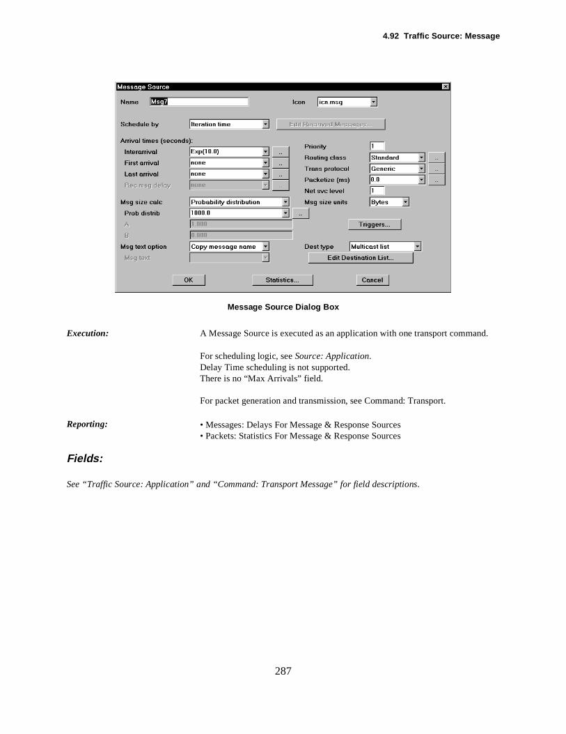
4.92 Traffic Source: Mes sage
d.
287
Message Source Dialog Box
Execution: A Message Source is executed as an application with one transport comman
For scheduling logic, see Source: Application.Delay Time scheduling is not supported.There is no “Max Arrivals” field.
For packet generation and transmission, see Command: Transport.
Reporting: • Messages: Delays For Message & Response Sources• Packets: Statistics For Message & Response Sources
Fields:
See “Traffic Source: Application” and “Command: Transport Message” for field descriptions.
4. Modeling Constructs
outfulabouthas atina-col.
nter--endck-a-. In
T III
dels
sti-, but
288
4.93 Traffic Source: Packet Flow/Packet Rate MatrixPurpose: COMNET III now includes a new mechanism, the Packet Rate Matrix for
directly generating packet traffic without scheduling applications and withproducing messages with transport commands. Such a mechanism is usewhen data are available on packet rates and sizes, but not much is known the internals of the application producing a stream of packets. The model list of such background packet flows. Each packet flow has an origin, a destion, a packet interarrival time and size distribution, application, and protoThe application and protocol types are used solely for reporting purposes--theydo not affect packet scheduling in any way.
AutoBaseliner can now obtain end-to-end packet statistics through new ifaces to Expert Sniffer and Frontier and Axon RMON data. Each end-topacket stream identified by AutoBaseliner is modeled in COMNET III by a baground packet flow. For a typical imported packet stream, the available informtion includes the origin, destination, packet rate, and average packet sizesome cases, there is a breakdown by application and protocol. COMNEautomatically builds a background packet flow for each imported packet stream.You can edit the list of packet flows to make any adjustments to the flow mobuilt by COMNET III.
Creating: The Packet Rate Matrix is accessed by pulling down the Define menu optionfrom the main menu, and selecting Packet Rate Matrix. From the Packet RateMatrix dialog window you can add packet flow information from source to denation. The packet flow information entered would not appear on the modelwhen the model is run, the packet flow information would be generated.
4.94 Traffic Source: Response
ages in
r trig-ction-llow
replies,ed by
.whichsponse
on the
drag aaust bed, the mes-
node,inter-
of the
electrce
289
4.94 Traffic Source: Response
Purpose: A Response Source is a message generator which is used to send messreply to received messages.
Packet routing for Response Sources is based upon the routing protocol fogering messages. If the triggering message is part of a session and conneoriented routing for sessions is specified, then the response packets will fothe session route. Otherwise they will be routed on a datagram basis.
Response sources are useful for modeling transaction responses, database e-mail replies, etc. They are separate from ACK packets which are generatthe transport protocol’s end-to-end flow control algorithm.
A Response Source may be created and represented directly on the user interfaceBeneath the surface, the Response Source is translated into an application executes a single answer message command. In other words, creating a ReSource is the same as:
• Defining an answer message command on a node• Creating an application and attaching it to the node• Calling the answer message command from the application.
Directly creating and editing a Response Source is easier than this three stageprocess, because it is not necessary to define a separate answer commandnode.
Creating: To create a Response Source pick the Response tool from the palette and new response icon onto the background. Or use the create menu option to create new response icon. Once a response icon is drawn on the background it mconnected to a node using one of the arc tools. Once created and connecteresponse icon can be double clicked to bring up the details of the responsesage.
Connectivity: A Response Source can be connected to a Computer & Communications and to a Computer Group node. If connected to a Computer Group, then nally to the model there is a Response Source for each instance node.
The destination node for a response source message is the origin node incoming message that triggered the response.
Editing: Either double click on the Response Source icon, or highlight the icon and sthe Edit/Detail menu option. The dialog box for editing the Response Soudetail is then presented.
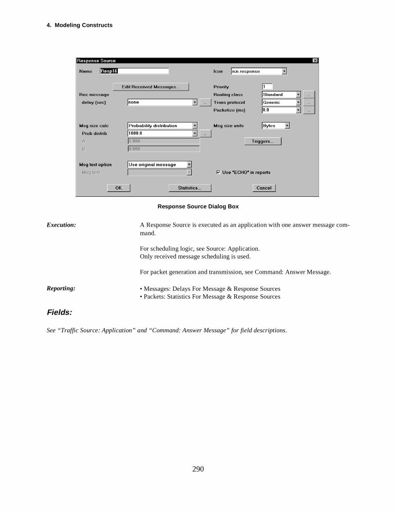
4. Modeling Constructs
e com-
290
Response Source Dialog Box
Execution: A Response Source is executed as an application with one answer messagmand.
For scheduling logic, see Source: Application.Only received message scheduling is used.
For packet generation and transmission, see Command: Answer Message.
Reporting: • Messages: Delays For Message & Response Sources• Packets: Statistics For Message & Response Sources
Fields:
See “Traffic Source: Application” and “Command: Answer Message” for field descriptions.
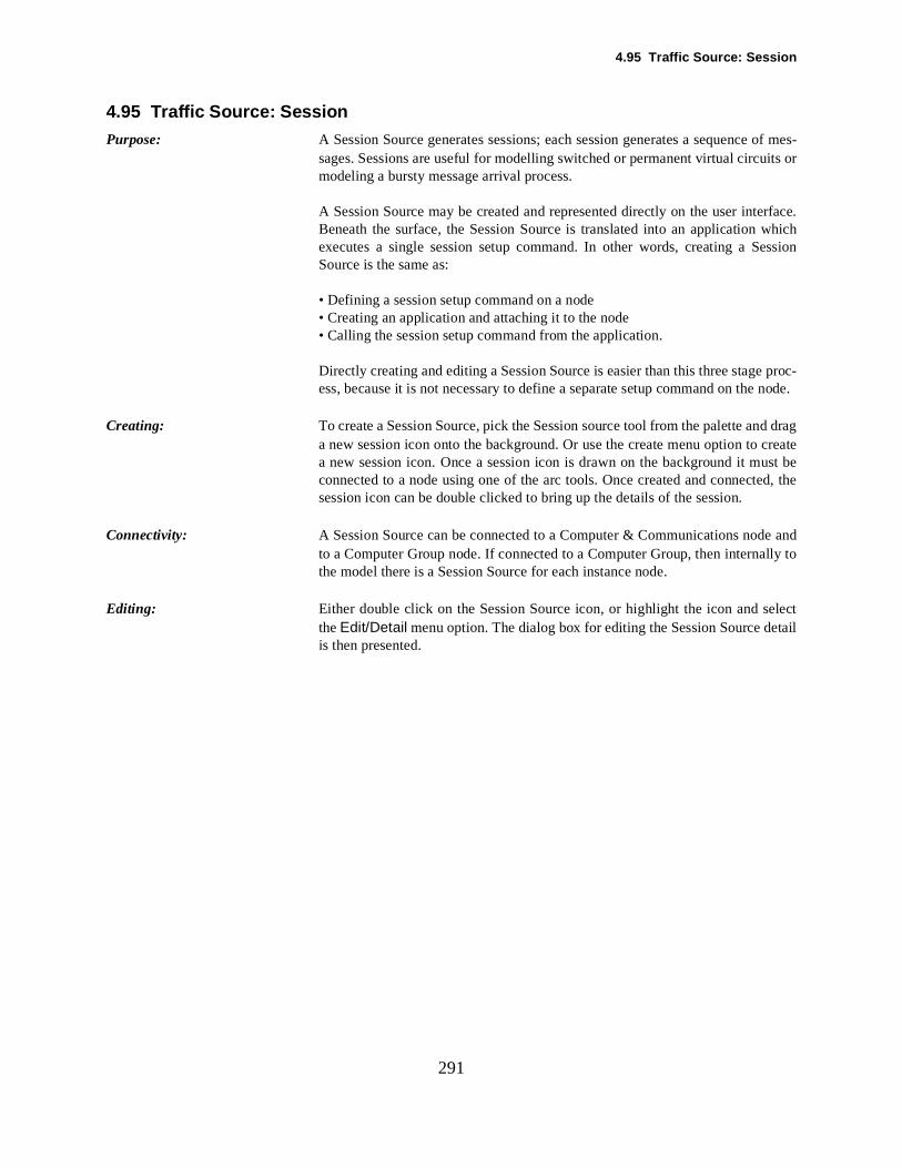
4.95 Traffic Source: Session
of mes-its or
ce.whichession
proc- node.
d dragcreate
d, the
e andlly to
electtail
291
4.95 Traffic Source: Session
Purpose: A Session Source generates sessions; each session generates a sequencesages. Sessions are useful for modelling switched or permanent virtual circumodeling a bursty message arrival process.
A Session Source may be created and represented directly on the user interfaBeneath the surface, the Session Source is translated into an application executes a single session setup command. In other words, creating a SSource is the same as:
• Defining a session setup command on a node• Creating an application and attaching it to the node• Calling the session setup command from the application.
Directly creating and editing a Session Source is easier than this three stageess, because it is not necessary to define a separate setup command on the
Creating: To create a Session Source, pick the Session source tool from the palette ana new session icon onto the background. Or use the create menu option to a new session icon. Once a session icon is drawn on the background it must beconnected to a node using one of the arc tools. Once created and connectesession icon can be double clicked to bring up the details of the session.
Connectivity: A Session Source can be connected to a Computer & Communications nodto a Computer Group node. If connected to a Computer Group, then internathe model there is a Session Source for each instance node.
Editing: Either double click on the Session Source icon, or highlight the icon and sthe Edit/Detail menu option. The dialog box for editing the Session Source deis then presented.
4. Modeling Constructs
mand.
292
Session Source Dialog Box
Execution: A Session Source is executed as an application with one setup session com
For scheduling logic, see Source: Application.Delay Time scheduling is not supported.The “Max Arrivals” field is not available.
For packet generation and transmission, see Command: Setup Session.
Reporting: • Sessions: Setup Delay By Session Source• Sessions: By Node• Sessions: By Link• Sessions: Length by Session Source• Sessions: Blocking by Session Source
Fields:
See “Traffic Source: Application” and “Command: Setup Session” for field descriptions.
4.96 Transit Networks
fhe
ary
kets
ectiveends
inputtransit
col.mentedoutedherentin-
to exit
h theunit.
nderit netce toutedramesideTM the
orewly atheon-
earon orran-
293
4.96 Transit Networks
Purpose: A transit network is an intermediate network that interconnects a collection onodes. It provides an additional level of segmentation and reassembly at tboundaries of the transit net. It is called a transit network because its primpurpose is to model packets that enter on one side of the net, flow through thenet, and finally exit on the other side of the net. In other words, it models pactransiting a network.
Link Behavior A transit net behaves as both a link and a subnet. From the external perspof the nodes connected to a transit net, the transit net looks like a link that spackets from the output buffer of one node connected to the net to the buffer of another node connected to the net. The nodes connected to the net have no knowledge of how the packets are routed internally through the net toreach the desired node on the other side of the net.
Subnet Behavior Internally the transit net behaves like a subnet. It contains a topology of intercon-nected nodes, links, and traffic sources. It also has its own routing protoWhen a node has a packet to send across a transit net, the packet is seginto new packets at the boundary of the net. The spawned packets are rthrough the transit net to the target node on the other side of the transit net, wthe original packet is reassembled. After reassembly, the original packet coues on its journey to its ultimate destination.
Protocol Layering The transit net introduces an additional protocol layer at the transit net bounda-ries. Packets are segmented and reassembled and flow from entry node node in conformance with the protocol parameters for the type of connectionbetween entry node and exit node. The segmented units that flow througtransit net can model packets, frames, cells, or any other protocol data Since transit nets can be nested within transit nets, it is possible to model anynumber of protocol layers.
TCP/IP over Frame Relay or ATMFor example, in a model where messages flow from source to destination uthe control of TCP/IP, the TCP/IP packets could traverse a frame relay transon the way to their destination. When a TCP/IP packet arrives at the interfathe frame relay net, it would be segmented into frames, which would be rothrough the net and reassembled into TCP/IP packets upon exiting the frelay net. It is also possible that an ATM transit net could be embedded inthe frame relay transit net. When a frame arrives at the boundary of the Atransit net, it would be segmented into cells, which would be routed throughATM net and reassembled into frames upon exiting the ATM transit net.
Link-Level Flow Control One can also use the protocol layering capability of the transit net to do mdetailed link-layer protocol modeling. For example, to model link-level flocontrol on a point-to-point link, one could define a transit net that contains onsingle point-to-point link. The transit net would use a protocol with one of windowed flow-control options for each connection across the “net” (which csists here of only a single link).
Compression or Encryption When a packet needs to be routed across a transit net, the packet is first convertedto a data unit whose size is a linear function of the original packet. This lintransformation of the original packet size can be used to model compressiencryption of the packet prior to segmenting it for transmission through the t
4. Modeling Constructs
f thef the
ed toasses. andrvice
viceined
list ofn
lass,other no
ectionserv-f con-ULT
ittedin aneen
ffer- For
nd
listransit classh con- s for
to theoingport.entedgular
294
sit net. When the transformed data unit is reassembled at the exit node otransit net, then a packet of the original size is delivered to the input buffer oreceiving node.
Service Classes and Connection TypesWhen a packet arrives at an interface to a transit net, the packet is mappa service class. Each port connected to a transit net has a list of service clA packet has a required network service class level (a number between 1100). Each service class has a minimum service level and a maximum selevel. A packet is mapped to that service level for which its required serlevel is in the interval [min svc level, max svc level]. The service classes defat a transit net interface must serve non-overlapping service level intervals.
Each service class has a list of connection types. Each connection type hasspecific destination nodes on the boundary of the subnet. A separate connectioinstance is created during the simulation for each of the nodes in the connectiontype’s destination list. Each connection type also has a priority, routing cprotocol parameters, compression factor, segmentation time, and a few parameters. A service class includes a DEFAULT Connection Type withexplicitly listed destinations.
After a packet has been mapped to a service class, it is assigned to the conninstance for the exiting node on the other side of the transit net. For a given ice class, a destination node can appear only once among the class’s list onection types. If a connection to the desired node does not exist, the DEFAConnection Type for the service class is used.
By using multiple service classes, different classes of packets can be transmto the same destination using different protocol parameters. For example, ATM transit net, both ABR and CBR traffic may need to be transmitted betwthe same pair of switches.
By using different connection types for a given service class, deliveries to dient destination nodes can be controlled by different protocol parameters. example, in a frame relay network, the CIR to one node may be 128 kbps aanother node might be 256 kbps.
When a node is initially connected to a transit net, the resulting port’s initialof service classes is copied from the list of service classes included in the tnet’s parameter set. In the transit net’s parameter set, none of the serviceconnection types have assigned destinations. The destination nodes for eacnection type are assigned only at the port interfaces to the transit net. Thecon-nection types defined in the transit net’s parameters serve only as templateinitializing the connection types at individual ports.
Interface Ports Arcs connect nodes to access points on transit network boundaries. The accesspoint graphically represents the connection to a link inside the transit network.The arc connecting to a transit net access point represents the node’s porttransit net. The port’s input and output buffers store incoming and outgpackets as usual. The arc also has attributes for an additional “interface” The interface port has an input and output buffer that is used by the segmpackets. The interface port buffers can have different attributes from the report buffers.
4.96 Transit Networks
ses.
d toae con-
ck to
l theer
thatssion
entedultip-
copyons.acket.des-f the.
295
Traffic Constraints Only packet traffic can flow through a transit net. At the present time, call trafficcannot be routed through a transit net. A transit net can include mesage,response, and session sources. It can not include call and application sourc
The destinations for messages originating inside a transit network are limitenodes in the same transit network. In addition, messages originating outside of transit net can not terminate inside a transit net. As a consequence of thesstraints, when a transit net is cloned, any nodes in a traffic source’s destinationlist are changed to the cloned nodes in the cloned net instead of pointing bathe nodes in the original net.
The primary purpose of the traffic sources inside a transit net is to modenet’s own routing or administrative traffic. The model assumes that the othtraffic carried by the net is flowing through or transiting the net.
Session Routing Transit nets do not internally enforce connection-oriented routing of sessionstransit the net. Thus, packets flowing as part of a connection-oriented sewill always enter and leave a transit net at the same pair of nodes, but inside thetransit net the segmented packets are routed independently. To force segmpackets to follow the same routes inside of transit nets, avoid adaptive or math routing options.
Multicasting When a multicast packet arrives at the boundary of a transit net, a separateof the packet is cloned for delivery to each of its ultimate multicast destinatiThus, each packet routed across a transit net is a single destination pWithin a transit net, multicasting operates as always in COMNET, where the tination list is partitioned among selected outgoing ports and one copy opacket is cloned for each selected port, rather than each ultimate destination
4. Modeling Constructs
with
rces.
XCP
-double
themtem
n a
-
high-o
Edit
296
4.97 Transport Protocol
Purpose: Transport Protocol is a label which is applied to a message source. It carriesit a description of the end-to-end network parameters which need to be applied tothe data flow between the origin and destination.
Different Transport Protocol labels may be applied to different message souAs many Transport Protocols as desired by may be defined in the model.
COMNET III includes parameters for TCP/IP, UDP/IP, NCP/IPX and NCP/IPBurst Mode in the Transport Protocol Library. However, other models of Tand UDP may be added as well as models of all other kinds of transports.
Creating: To create a Transport Protocol, edit the appropriate type of traffic source (message, response, session source, or equivalent command) and click on the dot button at the side of the transport protocol box. Also the Define/TransportProtocols menu option may be used to created and/or edit transport protocol def-initions.
A Transport Protocol definition may also be added to the system library viaArchive/Objects menu option. If a Transport Protocol is defined in the systelibrary it will become available when a new model is made, or when the syslibrary definition is specifically copied into the local model.
COMNET III always creates a Transport Protocol class called “Generic” whenew model is made.
Connectivity: A message, response, and session source and a transport, answer, and setup com-mand each references a transport protocol in the model’s list of transport protocols.
Call traffic does not have a transport protocol.
Editing: Double click on a message source icon to bring up the source dialog box, or light the icon and pick the Edit/Detail menu option. The Transport Protocol tuse for the source can then be applied in the Transport Protocol value box.
The Transport Protocol parameters themselves are edited by clicking on the dou-ble dots next to the Transport Protocol value box, and then by selecting thebutton.
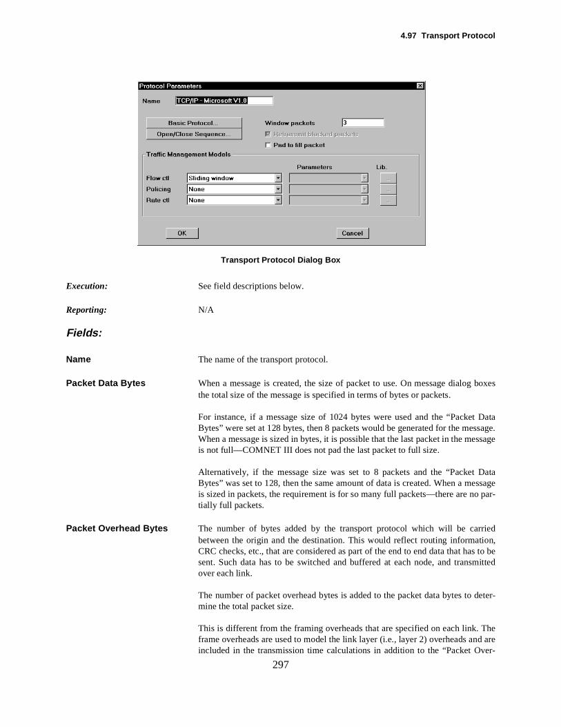
4.97 Transport Protocol
boxes
ssage.ssage
Datassage par-
riedion,s to bemitted
deter-
Thed are
ver-
297
Transport Protocol Dialog Box
Execution: See field descriptions below.
Reporting: N/A
Fields:
Name The name of the transport protocol.
Packet Data Bytes When a message is created, the size of packet to use. On message dialogthe total size of the message is specified in terms of bytes or packets.
For instance, if a message size of 1024 bytes were used and the “Packet DataBytes” were set at 128 bytes, then 8 packets would be generated for the meWhen a message is sized in bytes, it is possible that the last packet in the meis not full—COMNET III does not pad the last packet to full size.
Alternatively, if the message size was set to 8 packets and the “Packet Bytes” was set to 128, then the same amount of data is created. When a meis sized in packets, the requirement is for so many full packets—there are notially full packets.
Packet Overhead Bytes The number of bytes added by the transport protocol which will be carbetween the origin and the destination. This would reflect routing informatCRC checks, etc., that are considered as part of the end to end data that hasent. Such data has to be switched and buffered at each node, and transover each link.
The number of packet overhead bytes is added to the packet data bytes tomine the total packet size.
This is different from the framing overheads that are specified on each link.frame overheads are used to model the link layer (i.e., layer 2) overheads anincluded in the transmission time calculations in addition to the “Packet O
4. Modeling Constructs
the
lgo-
on-
t tobackCK
er
the
totalroute car-
totalcketwill
arerded.
f theETackety after
er the
ustedorigi-
plic-tillt
298
head Bytes.” However, the frame overheads are not buffered or switched byintermediate nodes.
Window Size The end-to-end window size to be used in association with the flow control arithm.
An application with a transport or answer command that is waiting for flow ctrol authorization is not eligible to execute until an ACK is received.
For instance, if fixed window flow control is in use and the window size is se1, then every packet arriving at the destination will cause an ACK to be sent to the origin. The origin cannot create and send the next packet until the Afrom the preceding packet has been received back at the origin.
Note that the flow control is end-to-end. COMNET III does not model link lay(layer 2) flow control.
End-to-End ACK Bytes The size of the ACK packets generated by end-to-end flow control.
Retransmit Time If a packet is blocked en route to its destination, it will be retransmitted after“Retransmit Time” from the origin.
A packet may be blocked because some port input buffer or port output bufferhas insufficient space to receive it, some node has insufficient total input or output buffer space to receive it, or a routing decision at some point on the cannot route the packet further. It may also be blocked if one or more framesrying part of it was discarded by the WAN cloud.
Note that a packet blocked because the selected port output buffer, or theoutput buffer space, on an ATM node has insufficient space will cause the pato remain in the port input buffer on the ATM node. In this case the packet not be retransmitted from the origin.
If the option to retransmit blocked packets is inactive, then blocked packetsdropped. The blocked packet will be counted as dropped and then discaAny message generating such a packet will not count as being delivered
The retransmission timer in Release 1.2 is improved to account for the age opacket before it is blocked. For the sake of simulation efficiency, COMNdoes not model individual timers on each packet to determine whether a pneeds to be retransmitted. Instead, it schedules a packet retransmission onlthe packet is actually blocked somewhere in the network. In earlier releases, thespecified retransmission time was applied after the packet was blocked (undassumption that the packet delay through the network was insignificant comparedwith the retransmission time). In release 1.2, the retransmission time is adjso that the packet is retransmitted the specified delay after the packet was nally transmitted. The option is available for backward compatibility.
Note that because COMNET III doesn't model the retransmission timers exitly, COMNET will not model the retransmission of a packet that is late but sin transit through the network. COMNET III provides an acknowledgemendelay report to flag when this condition is happening in the model.
4.97 Transport Protocol
igint is nonpack-
y be thate
inputhed.
bemayas antrolts soce.
ntialn on
aintsssagege so
d win-
ack-roto-ilableowss
299
Setting the “Retransmit Time” to 0 and having a routing decision at the orreturn no route will effectively put the model into an infinite loop as a packeblocked and then immediately reattempted. Simulation time may advance ifzero packet switching times have been entered on the originating node, or a etizing delay has been specified.
ACK Priority ACK packets are routed back to the origin as if they were data packets. It mathat ACK packets should have higher priority at intermediate nodes in orderwindowing delays can be minimized. If so then the “ACK priority” can bincreased.
The result of increasing priority is to place the packet at the head of the port buffer and port output buffer queues on the nodes where the packet is switc
Error Control Ack Used for modeling an extra acknowledgement that acknowledges the delivery ofthe packet or window at the destination but does not allow the window toadvanced. This can be considered an error control acknowledgement that appear as a separate acknowledgement when flow control is used, or acknowledgement when no flow control is used. COMNET III's error conmechanisms do not require the explicit modeling of these acknowledgementhat this option is primarily to model the traffic introduced by their presenThese extra acknowledgements impact local area networks because their timingis slightly delayed from the delivery of the packet and thus enhances the potefor collisions on random access links (such as CSMA/CD) and uses a tokethe token-ring networks.
Negotiated Packet and Window SizesAllows the protocol's packet size and window size may be reduced by constron the socket to which the source is attached and the socket to which the meis destined. This refinement is determined at the start of each new messathat different messages from the same source may have different packet andow sizes when they have different destinations.
Padded Packets A way to model protocols that are constrained to always transmit full sized pets (such as ATM). This padding option is only available for the enhanced pcols or for when no packet retransmission is required. When data are avafor transmission but these data do not fill a full-sized packet, this option allCOMNET to model a full-sized packet even though the delivered data is lesthan the full packet.
Retransmit Blocked Packets Indicates whether blocked packets should be retransmitted or dropped.
Flow Control Method NoneFixed WindowSliding WindowSNA Pacing Control(see appropriate Flow Control entry)
4. Modeling Constructs
d alsonodesurceduled.
nodehe
e only other exe-
ce, say ses-nd
am- theg1’s
r of whene say
for ahich
es-set,
suc-ecifynt ant thewhich
havee the speci- aremly,
300
4.98 Trigger Events
Purpose: Triggers can be used to model time dependencies among traffic sources, antime dependencies between traffic sources and significant state changes of and links. An individual trigger specifies that, when the associated traffic soor node or link enters a specified state, a specified successor source is scheFor example, using triggers you can easily model the situation in which a multi-cast routing table message is sent from a central location a short time after aor link fails, or the situation in which call traffic is initiated in response to tarrival of a packet-switched message, or vice-versa.
Successor sources can be scheduled by trigger only, meaning they executwhen a trigger causes them to execute, or they may be scheduled by anymeans. In the latter case, executions caused by triggers will be in addition tocutions caused by other means. For example, if you have a message sourMsg1, scheduled by iteration time, say every 1 minute, and you also have asion source, Ses1, that triggers Msg1, then Msg1 will execute every minute aalso every time Ses1’s trigger fires.
It is important to keep clear the distinction between a triggering source/node/link, and a “triggered” source, referred to as the successor. The trigger itself willbe found in a list accessed by clicking the Triggers button on a source/node/link.The source/node/link whose trigger list you are examining, say Msg1 for exple, is the triggering source/node/link. Another way to refer to the triggers inlist is by ownership. We say the triggers in the list are Msg1’s triggers. Mstriggers will fire when Msg1 enters a specified state.
When you edit a trigger in the list, you will see that the trigger has a numbeattributes, one of which is the successor. That successor will be scheduledthe conditions of the trigger are met. When the successor is scheduled, wthe trigger fires.
The conditions of the trigger, referred to as the triggering rule, are chosen from aset that varies depending on the triggering source/node/link. For example, message source, say Msg1, the list of rules includes “upon source startup,” wmeans the trigger will fire when Msg1 starts executing. Msg1’s list also includes“upon message creation,” which means the trigger will fire when Msg1’s msage is first created. On the other hand, a link will have a very different including “upon alarm first sounding” and “upon link failure.”
Other attributes of the trigger include the triggering delay, which is the delay thatwill elapse between the firing of the trigger and the actual execution of the cessor. In addition, depending on the triggering rule, you might have to spthe command or alarm to which the rule applies. For example, you may waapplication source to have a trigger that fires “upon message creation,” buapplication creates several different messages, so you have to specify to message the rule applies. This additional information is referred to as therulequalifier.
When the trigger list contains more than one trigger, all of the triggers must the same triggering rule and qualifier, so the only differences among them arsuccessors and the delays. Such a list is interpreted in one of two ways, asfied by the Weighted List check box: Either all of the successors in the listtriggered when the rule is satisfied, or one of the triggers is chosen rando
4.98 Trigger Events
ht)
-
l-
301
based on a sample from the uniform distribution and a probability (weigassigned to each trigger.
Here is a summary of the possible trigger rules:
Trigger rule Explanation
upon source startup When source begins execution
upon source completion When source completes execution
upon msg creation When specified message is first created
upon msg delivery When specified message is successfuly delivered to all destinations
upon session initiation When session setup begins
upon session establish When session setup completes and session is established
upon session completion When session is terminated
upon alarm first sound-ing
When specified alarm first sounds
upon alarm clear When specified alarm stops sounding
upon link failure When link fails
upon link recovery When link recovers after failure
upon node failure When node fails
upon node recovery When node recovers after failure
upon filter time-out When specified filter command’s tim-er expires

4. Modeling Constructs
302
g
ions net-rs
, but it is be intui-
fterar with
and to
urces
d. Theining tools
ive tool in
303
5. Creating COMNET III Models
5.1 Introduction
COMNET III's graphical user interface is used to create and modify a network description. The network descriptionis saved in a file (modelname.c3) for future COMNET III sessions so it can be modified or run with new operatinparameters.
This chapter describes COMNET's graphical user interface and shows how to use it to create a communicatwork model. It focuses on how to build a model rather than the details of the model itself. Previous chaptepro-vided detailed background on the underlying network model components and their attributes.
This chapter uses some screen shots of COMNET III menus and dialog boxes to illustrate important featuresnot an exhaustive tour of the user interface. Since graphical user interfaces are, by their nature, designed totive, it isn't necessary to explain the operation of each dialog box.
To start COMNET III, double-click on the COMNET III icon or type the command comnet3, depending on the com-puter and window system you are using. The COMNET III logo is displayed while COMNET III initializes. Ainitialization is complete, a tool palette appears in a column along the left edge of the display and a menu bpull-down menus appears across the top of the display.
COMNET III's main window is shown in Fig 4.1. It is used to build and edit models, run animated models show model results.
5.2 Using the COMNET III Tool Palette
The tool palette on the left side of the COMNET III display includes tools for creating Nodes, Links, Traffic Soand tools for editing.
Most of the tools in the palette can be activated in two ways. If you click once on a tool it becomes activatetool which has been selected changes appearance so that it looks as if it has been pushed in while the remacontinue to appear raised. This is standard mode. Having activated the tool, you can carry out one action. As soonas you complete the action, the chosen tool becomes inactive and the selection tool takes its place as the actthe palette. You can then use the selection tool or return to the palette to activate another tool.
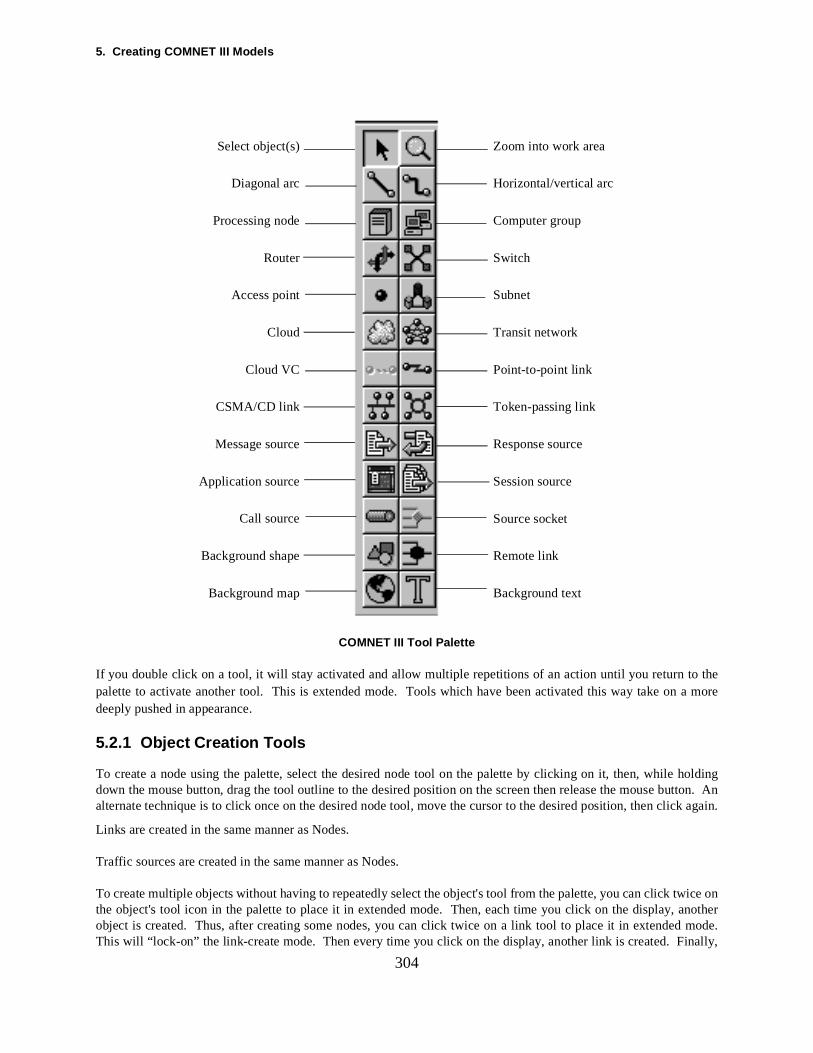
5. Creating COMNET III Models
o the a more
holdingutton. Ank again.
wice onanothere.nally,
304
COMNET III Tool Palette
If you double click on a tool, it will stay activated and allow multiple repetitions of an action until you return tpalette to activate another tool. This is extended mode. Tools which have been activated this way take ondeeply pushed in appearance.
5.2.1 Object Creation Tool s
To create a node using the palette, select the desired node tool on the palette by clicking on it, then, whiledown the mouse button, drag the tool outline to the desired position on the screen then release the mouse balternate technique is to click once on the desired node tool, move the cursor to the desired position, then clic
Links are created in the same manner as Nodes.
Traffic sources are created in the same manner as Nodes.
To create multiple objects without having to repeatedly select the object's tool from the palette, you can click tthe object's tool icon in the palette to place it in extended mode. Then, each time you click on the display, object is created. Thus, after creating some nodes, you can click twice on a link tool to place it in extended modThis will “lock-on” the link-create mode. Then every time you click on the display, another link is created. Fi
Zoom into work area
Horizontal/vertical arc
Computer group
Switch
Subnet
Transit network
Point-to-point link
Token-passing link
Response source
Session source
Source socket
Remote link
Background text
Select object(s)
Diagonal arc
Processing node
Router
Access point
Cloud
Cloud VC
CSMA/CD link
Message source
Application source
Call source
Background shape
Background map
5.2 Using the COMNET III Tool Palette
mode.
he pal-
o
A
lt node, default
ID code
by a
n then
etweennce of line desired,
nectionnect the
links and network
it, then
editor.
ionl is acti-
305
to connect the nodes to links, click twice on one of the palette's connection tools to “lock-on” the connectOnce you are in connect-mode, you do not need to click repeatedly on the connect tool.
To return to the standard mode of operation, click on the selection tool, which is the arrow at the top left of tette.
Nodes, links and traffic sources are created with default attributes, including default ID codes and default icons. Tchange the attributes of an object, select the object by clicking on it. Then click on Edit (on the menu bar) and thenDetail (on the pull-down menu). Edit/Detail displays a dialog box showing the current attributes of the object.simpler technique is to simply double click on the object's icon to bring up the Edit/Detail dialog box.
A helpful technique for keeping track of which nodes and links have had their attributes set to the values you desireand which ones have only default attributes is to look at the ID code displayed next to the icon. Unique defaulink and source ID codes are automatically assigned by COMNET III when objects are created. Examples ofIDs are Link10 , Node14 and Msg25. All types of Nodes are labeled Node. All types of Links are labeled Link .Traffic sources are labeled by type of source: App, Msg, Call , Sess . Subnetworks are labeled Net. Network Padsare not labeled. When you edit the detailed attributes for an object, it is a good practice to specify your own so you can recognize at a glance which objects have been edited and which ones have not.
5.2.2 Connection Tools
To connect a traffic source to a node or a node to a link, select one of the connection tools by clicking on it. Thenclick once on each network object to be connected. The order does not matter. The connection is representedline between the elements.
Alternatively, you can click on the first object, move to the second object while holding down the mouse buttorelease the button when you have arrived at the second object.
There are two connection tools The standard “jointed arc” tool represents the connection with a direct line bthe network elements using the shortest path. If the user desires, the path can be represented by a sequesegments drawn at the users discretion. Click once on the first object, click once on each intermediate pointthen click on the second object. Multisegment connections have no effect on the function of the connection.
The other tool represents the connection with lines which travel only at right angles. As with the standard contool, a sequence of intermediate points can be specified, but the tool will ensure that all lines drawn to conpoints are at right angles.
There is no functional difference between the tools, the distinction is purely aesthetic.
If a connection does not make sense, nothing will happen. Connections are only valid between nodes and between traffic sources and nodes. In a backbone layout, connections are also valid between links andaccess points. In a subnetwork layout, connections are valid between nodes and network access points.
If you are not happy with the resulting appearance of the connection, simply delete the connection (selectchoose Edit/Cut) then redraw it with greater artistry.
Note that only two nodes can be connected to a point-to-point link. This restriction is enforced by the layoutFor multinode links, you should choose CSMA/CD, CSMA, Token Passing, Polling or ALOHA links instead. It isalso possible to change the link access protocol on an existing link by selecting the link and using Edit/Detail.
5.2.3 Selection Tool
Objects must be selected before performing actions such as edits. To select an object, first ensure that the selecttool has been activated. This is the arrow at the top left position of the tool palette. Once the selection too
5. Creating COMNET III Models
nce an
cts
ns red toe, objects
desiredhe mouse
xes
n
es
le.cs editore
on thethe
levelion and
n. It sim-ub-net-ayout.
306
vated, you can select an object by clicking on it once. It will turn red to indicate that it has been selected. Oobject has been selected, use Edit on the menu bar and one of the functions on the Edit pull-down menu (Cut ,Copy , Select All , Detail... , Move , Enter , Leave , Paste , Clear , Duplicate , Clone... , and Scale ) to manipulatethe object. Double clicking on an object is a short cut for performing an Edit/Detail after selecting the object.
5.2.4 Selecting a Group of Objects
The extended select mode lets you select a group of objects on the display and then perform operations on all objein the group. To select multiple objects, click twice on the selection tool displayed at the top left of the palette. Thisplaces the selection tool into extended select mode.
Then each time you click on an object, it is added to the group of selected objects. Each selected object turindicate that it has been added to the group of selected objects. When the selection tool is in extended modon which you click will be toggled in and out of select mode each time you click.
Once in extended select mode, you can also select a group of objects by drawing a selection rectangle around them.This is accomplished by clicking at one corner of the desired area then dragging to the opposite corner of thearea while holding the mouse button down. When the desired area is surrounded by the rectangle, release tbutton. All objects included in the rectangle will be selected.
To select all items in a model, choose Edit/Select All .
When you perform Edit/Detail on a group of objects, COMNET III automatically cycles through the dialog bofor each selected object as you click on Ok or Cancel .
5.2.5 Text Tool
The text tool is used to add text labels anywhere on your model layout. Select the text tool icon on the palette theclick on the position where the text is to be placed. A dialog box appears. Type the text into the dialog box thenselect OK or Cancel .
Once the text appears, it can easily be moved to adjust its position and its size can be changed using Edit/Scale .
5.2.6 Background Icon Tool
Often it is useful to place the model layout against a background which adds information to the layout and improvits appearance. A typical use might be to place a model of a Wide Area Network against a map.
The background icon tool allows the user to insert into the layout any icon from the “user.sg2” graphics library fiThe default “user.sg2” file already contains several pre-defined maps. This manual's appendix on the graphiexplains how to create or import additional icons into that library file. The imported graphics can be simple lindrawings or photographs stored as bit maps.
To insert a background icon from the “user.sg2” file, choose the background icon tool on the palette then clicklayout. A dialog box appears. The dialog box contains the names of each icon in the “user.sg2” file. Select desired icon then click Ok or Cancel . Once the icon appears, it can be moved and scaled if desired.
5.2.7 Subnetwork Node Tool
COMNET III allows subnetworks to be represented as icons within a larger network. This allows for higherabstractions of a network to remain uncluttered, but makes the underlying detail easily available for inspectediting.
This alternative representation of the layout does not cause any shortcuts to be taken in the model's operatioply allows an uncluttered and hierarchical model layout. When the simulation is run, all components of the swork such as nodes, links and traffic generators fully participate in the simulation as if they were in the main l
5.3 Moving or Repositioning Objects
would
k's name.
ermain.-ed within
appear atain level.ne
twork.
bying the
chor the
arel lay-
screen.i- seeing
face, the
s whichh yield
307
The subnetwork node tool is selected from the palette and inserted into a model layout just as any other nodebe. When this subnetwork icon is selected, the screen switches to a representation of the subnetwork's layout screenand the model name which normally appears at the top left of the screen is supplemented with the subnetworThus the title would change to ModelName: SubnetName .
A subnet may now contain other subnets, and there is no limit to the nesting depth. However, nested subnets difffrom non-nested subnets in one very important respect: a nested subnet does not have its own routing doInstead, routing takes place as if there were no nested subnets. In other words, the highest subnet of the nest establishes a routing domain that includes all the nodes contained therein, whether or not those nodes are containnested subnets.
Nested subnets are really only for graphical convenience; they reduce clutter in the model layout, but have no effecton simulation.
Connections between subnetworks and the main network are accomplished through access points which both levels of the model. The access point tool on the palette is grayed out and deactivated when at the mAccess points can only be inserted in the subnetwork. They will then show as connection points to the subtworkicon when viewed from the main level.
To switch from the main network layout to a sub-network, double click on a sub-network icon.
To switch back to the main network layout from a sub-network, double click on the background of the sub-ne
5.3 Moving or Repositioning Objects
You can move individual objects (node, link, traffic, text or background icons) to another position on the displayclicking once on the object, holding the mouse button down while dragging to the new location then releasmouse button at the desired location. Connections to the object adjust automatically after the moves.
To move a group of objects, select several objects using extended select mode. Select Edit then Move from themenu. A rectangle containing the objects appears. Drag the rectangle to a new location then click to anobjects in their new position.
5.4 Moving Around the Layout
If you have a large model or are zoomed in, its layout may not fit in the viewing window. You can either pan oundthe model, viewing portions of the model through the viewing window, or you zoom out to see the entire modout at once.
Panning is accomplished by using the vertical and horizontal scroll bars along the right side and bottom of theThese operate identically to those in other applications on your machine. Note that the size of the scroll button indcates how much of the model you are seeing at any given time. If the button fills the entire scroll bar, you areall of the model (on that axis). If the button fills half of the scroll bar, you are seeing half of the model.
5.5 COMNET III Menus
Just as the tool palette gives the user access to the more frequently used parts of COMNET III graphical interCOMNET main menu bar and its pull down menus give the user access to the finer details of COMNET.
Each item on the main menu bar has a pull down menu with a number of choices. Items in pull down menuare followed by an ellipsis will pop up a dialog box when selected. Some dialog boxes contain choices whicpull down lists or yet more dialog boxes.
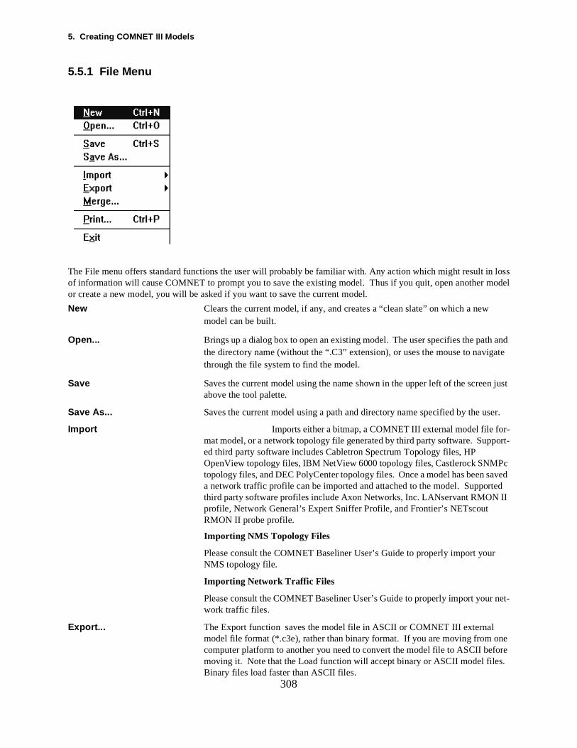
5. Creating COMNET III Models
n lossmodel
and ate
n just
ser.
c aved ted II
net-
ne ore .
308
5.5.1 File Menu
The File menu offers standard functions the user will probably be familiar with. Any action which might result iof information will cause COMNET to prompt you to save the existing model. Thus if you quit, open another or create a new model, you will be asked if you want to save the current model.
New Clears the current model, if any, and creates a “clean slate” on which a newmodel can be built.
Open... Brings up a dialog box to open an existing model. The user specifies the paththe directory name (without the “.C3” extension), or uses the mouse to navigthrough the file system to find the model.
Save Saves the current model using the name shown in the upper left of the screeabove the tool palette.
Save As... Saves the current model using a path and directory name specified by the u
Import Imports either a bitmap, a COMNET III external model file for-mat model, or a network topology file generated by third party software. Support-ed third party software includes Cabletron Spectrum Topology files, HP OpenView topology files, IBM NetView 6000 topology files, Castlerock SNMPtopology files, and DEC PolyCenter topology files. Once a model has been sa network traffic profile can be imported and attached to the model. Supporthird party software profiles include Axon Networks, Inc. LANservant RMON profile, Network General’s Expert Sniffer Profile, and Frontier’s NETscout RMON II probe profile.
Importing NMS Topology Files
Please consult the COMNET Baseliner User’s Guide to properly import yourNMS topology file.
Importing Network Traffic Files
Please consult the COMNET Baseliner User’s Guide to properly import your work traffic files.
Export... The Export function saves the model file in ASCII or COMNET III external model file format (*.c3e), rather than binary format. If you are moving from ocomputer platform to another you need to convert the model file to ASCII befmoving it. Note that the Load function will accept binary or ASCII model filesBinary files load faster than ASCII files.

5.5 COMNET III Menus
ost
Post-
l in at
309
You can also export the simulation statistics to a file that can be loaded into mspreadsheets, such as Microsoft Excel. See Simulation Statistics in Chapter 4 formore information.
You can also export an image of the model layout to either an encapsulatedScript file (*.eps) or to a bitmap.
Merge… Merges the current model file with specifications from a COMNET III externafile format model (*.c3e). If your are familiar with the external file format, thismay be the fastest way to test a number of models with only small variationseach one. For more information see the COMNET III external model file formdocument.
Print... Prints a copy of the current layout screen to an attached printer
Exit Exits COMNET III. Prompts the user to save the model if necessary.
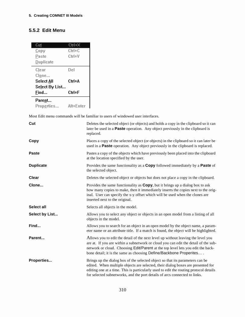
5. Creating COMNET III Models
it can
er be .
oard
oard.
orig-
all
ram-ted.
sub-
for
ails
310
5.5.2 Edit Menu
Most Edit menu commands will be familiar to users of windowed user interfaces.
Cut Deletes the selected object (or objects) and holds a copy in the clipboard so later be used in a Paste operation. Any object previously in the clipboard is replaced.
Copy Places a copy of the selected object (or objects) in the clipboard so it can latused in a Paste operation. Any object previously in the clipboard is replaced
Paste Pastes a copy of the objects which have previously been placed into the clipbat the location specified by the user.
Duplicate Provides the same functionality as a Copy followed immediately by a Paste of the selected object.
Clear Deletes the selected object or objects but does not place a copy in the clipb
Clone... Provides the same functionality as Copy , but it brings up a dialog box to ask how many copies to make, then it immediately inserts the copies next to theinal. User can specify the x-y offset which will be used when the clones are inserted next to the original.
Select all Selects all objects in the model.
Select by List... Allows you to select any object or objects in an open model from a listing of objects in the model.
Find... Allows you to search for an object in an open model by the object name, a paeter name or an attribute title. If a match is found, the object will be highligh
Parent... Allows you to edit the detail of the next level up without leaving the level youare at. If you are within a subnetwork or cloud you can edit the detail of the network or cloud. Choosing Edit/Parent at the top level lets you edit the back-bone detail; it is the same as choosing Define/Backbone Properites… .
Properties... Brings up the dialog box of the selected object so that its parameters can beedited. When multiple objects are selected, their dialog boxes are presentedediting one at a time. This is particularly used to edit the routing protocol detfor selected subnetworks, and the port details of arcs connected to links.
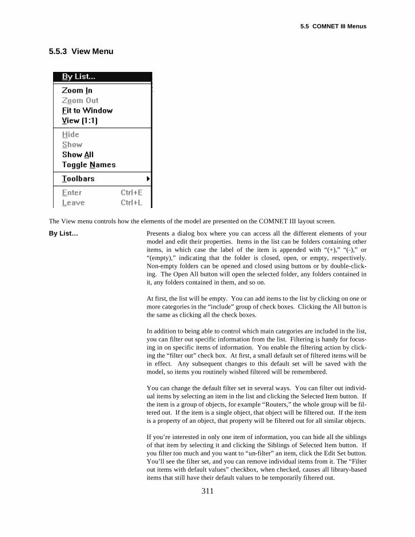
5.5 COMNET III Menus
orly.lick-
d in
orn is
list,
k-e the
. If fil-emts.
. Ifn.terased
311
5.5.3 View Menu
The View menu controls how the elements of the model are presented on the COMNET III layout screen.
By List… Presents a dialog box where you can access all the different elements ofyourmodel and edit their properties. Items in the list can be folders containing otheritems, in which case the label of the item is appended with “(+),” “(-),” “(empty),” indicating that the folder is closed, open, or empty, respectiveNon-empty folders can be opened and closed using buttons or by double-cing. The Open All button will open the selected folder, any folders containeit, any folders contained in them, and so on.
At first, the list will be empty. You can add items to the list by clicking on onemore categories in the “include” group of check boxes. Clicking the All buttothe same as clicking all the check boxes.
In addition to being able to control which main categories are included in theyou can filter out specific information from the list. Filtering is handy for focus-ing in on specific items of information. You enable the filtering action by clicing the “filter out” check box. At first, a small default set of filtered items will bin effect. Any subsequent changes to this default set will be saved withmodel, so items you routinely wished filtered will be remembered.
You can change the default filter set in several ways. You can filter out individ-ual items by selecting an item in the list and clicking the Selected Item buttonthe item is a group of objects, for example “Routers,” the whole group will betered out. If the item is a single object, that object will be filtered out. If the itis a property of an object, that property will be filtered out for all similar objec
If you’re interested in only one item of information, you can hide all the siblingsof that item by selecting it and clicking the Siblings of Selected Item buttonyou filter too much and you want to “un-filter” an item, click the Edit Set buttoYou’ll see the filter set, and you can remove individual items from it. The “Filout items with default values” checkbox, when checked, causes all library-bitems that still have their default values to be temporarily filtered out.
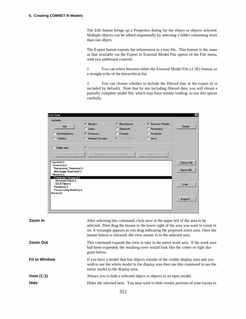
5. Creating COMNET III Models
d.ore
ame,
t, or
it is
tion
m in ce the
area -
ou e the
t to
312
The Edit button brings up a Properties dialog for the object or objects selecteMultiple objects can be edited sequentially by selecting a folder containing mthan one object.
The Export button exports the information to a text file. This feature is the sas that available via the Export to External Model File option of the File menuwith two additional controls:
1. You can select between either the External Model File (.C3E) formaa straight echo of the hierarchical list.
2. You can choose whether to include the filtered data in the export (included by default). Note that by not including filtered data, you will obtain apartially complete model file, which may have trouble loading, so use this opcarefully.
Zoom In After selecting this command, click once at the upper left of the area to be selected. Then drag the mouse to the lower right of the area you want to zooon. A rectangle appears as you drag indicating the proposed zoom area. Onmouse button is released, the view zooms in to the selected area.
Zoom Out This command expands the view to take in the entire work area. If the work had been expanded, the resulting view would look like the center or right diagram below.
Fit to Window If you have a model that has objects outside of the visible display area and ywish to see the whole model in the display area then use this command to seentire model in the display area.
View (1:1) Allows you to hide a selected object or objects in an open model.
Hide Hides the selected item. You may wish to hide certain portions of your layou

5.5 COMNET III Menus
.
l lay-
r on
d k
313
decrease the screen complexity. They will remain in your model functionally
Show Displays an item that has been hidden.
Show All Unhides all elements of the model that have been hidden.
Toggle Names Turns names on and off. This can be useful because in a complicated modeout the names may overlap and cause confusion.
Toolbars This menu item lets you turn the color palette, menu toolbar, and 3-D toolbaor off. The toolbars may also be moved to anywhere on your screen.
Enter If the selected object is a subnetwork, this will leave the top level of the layout and enter the subnetwork. When a group of objects are selected, the first selectesubnetwork is entered. This item is grayed and disabled when in a subnetworlayout.
Leave When in a subnetwork layout, returns to the main model layout. This item is grayed and disabled at the main layout level.
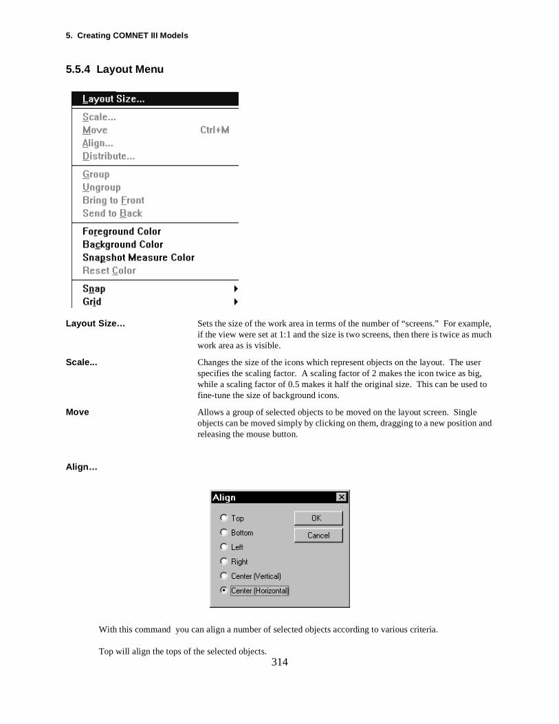
5. Creating COMNET III Models
ple, much
er , to
and
314
5.5.4 Layout Menu
Layout Size … Sets the size of the work area in terms of the number of “screens.” For examif the view were set at 1:1 and the size is two screens, then there is twice as work area as is visible.
Scale... Changes the size of the icons which represent objects on the layout. The usspecifies the scaling factor. A scaling factor of 2 makes the icon twice as bigwhile a scaling factor of 0.5 makes it half the original size. This can be usedfine-tune the size of background icons.
Move Allows a group of selected objects to be moved on the layout screen. Singleobjects can be moved simply by clicking on them, dragging to a new positionreleasing the mouse button.
Align…
With this command you can align a number of selected objects according to various criteria.
Top will align the tops of the selected objects.
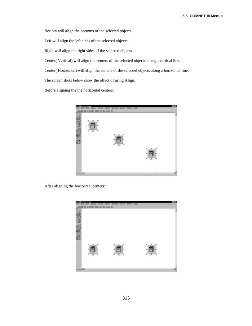
5.5 COMNET III Menus
315
Bottom will align the bottoms of the selected objects.
Left will align the left sides of the selected objects
Right will align the right sides of the selected objects
Center( Vertical) will align the centers of the selected objects along a vertical line.
Center( Horizontal) will align the centers of the selected objects along a horizontal line.
The screen shots below show the effect of using Align.
Before aligning the the horizontal centers:
After aligning the horizontal centers:
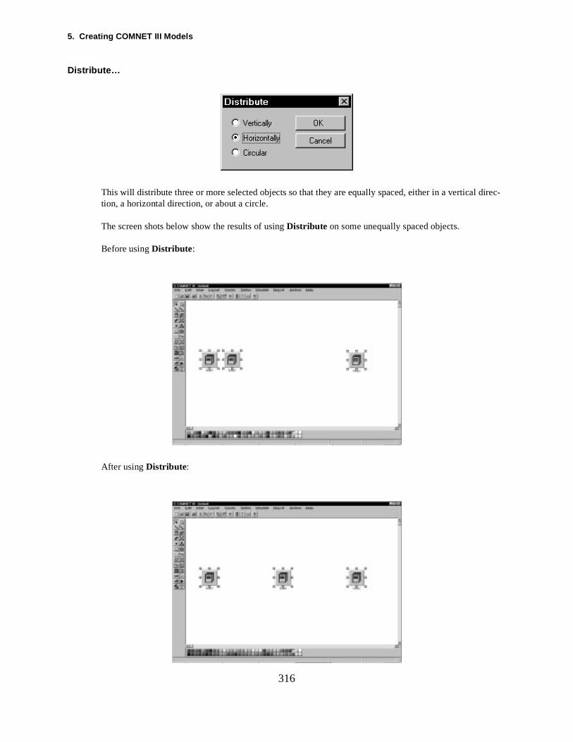
5. Creating COMNET III Models
direc-
316
Distribute…
This will distribute three or more selected objects so that they are equally spaced, either in a vertical tion, a horizontal direction, or about a circle.
The screen shots below show the results of using Distribute on some unequally spaced objects.
Before using Distribute :
After using Distribute :

5.5 COMNET III Menus
he nd
tion he ste it
up.
n be
dit-
text
r bar
nter-
grid ium,
317
Group Combines multiple objects into a group. Once objects are grouped, all normal editing operations that can be done on an individual object can be done on tgroup. This can be useful when your model is divided into logical sections, ayou may be happy with the way each section appears, but not with their relato one another. You can group a section, and then move it with respect to tother sections. You could also cut the group from the layout, or copy and pato create an identical group.
If you wish to edit individual components of a group, you will have to use Ungroup.
Ungroup Breaks up a group into the original component that went into making the gro
Bring to Front Brings an object that is behind another on the layout to the front so that it caedited.
Send to Back Sends an object that is at the front of the model layout to the back, to allow eing of objects that were behind it, or hide behind the other objects.
Foreground Color Changes the foreground color to the selected color. This will be the color of labels on objects.
Background Color Changes the background color of the layout to the selected color. If the colois not visible, the new color of the background may be a surprise!
Reset Color Resets the color of the selected object to the default color.
Snap If Snap to Grid is turned on, you can only place objects on the layout at grid isections.
Grid Places a grid on the model layout as a convenience in aligning objects. Thehas no significance to your model. The grid spacing can be set fo fine, medor coarse.
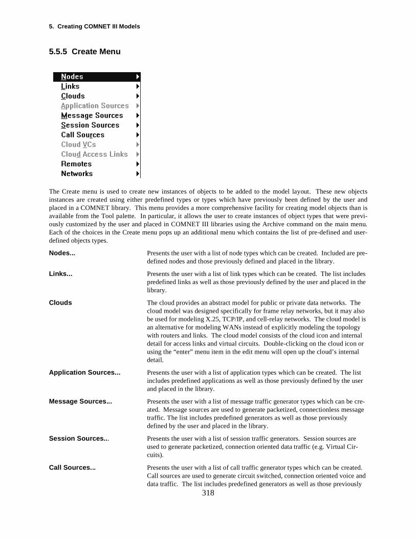
5. Creating COMNET III Models
w objectsuser and is
e previ- menu.nd user-
e pre-
des n the
lso al
l
list ser
cre-essage
re r-
ted. and sly
318
5.5.5 Create Menu
The Create menu is used to create new instances of objects to be added to the model layout. These neinstances are created using either predefined types or types which have previously been defined by the placed in a COMNET library. This menu provides a more comprehensive facility for creating model objects thanavailable from the Tool palette. In particular, it allows the user to create instances of object types that werously customized by the user and placed in COMNET III libraries using the Archive command on the mainEach of the choices in the Create menu pops up an additional menu which contains the list of pre-defined adefined objects types.
Nodes... Presents the user with a list of node types which can be created. Included ardefined nodes and those previously defined and placed in the library.
Links... Presents the user with a list of link types which can be created. The list inclupredefined links as well as those previously defined by the user and placed ilibrary.
Clouds The cloud provides an abstract model for public or private data networks. The cloud model was designed specifically for frame relay networks, but it may abe used for modeling X.25, TCP/IP, and cell-relay networks. The cloud model isan alternative for modeling WANs instead of explicitly modeling the topologywith routers and links. The cloud model consists of the cloud icon and interndetail for access links and virtual circuits. Double-clicking on the cloud icon or using the “enter” menu item in the edit menu will open up the cloud’s internadetail.
Application Sources... Presents the user with a list of application types which can be created. The includes predefined applications as well as those previously defined by the uand placed in the library.
Message Sources... Presents the user with a list of message traffic generator types which can beated. Message sources are used to generate packetized, connectionless mtraffic. The list includes predefined generators as well as those previously defined by the user and placed in the library.
Session Sources.. . Presents the user with a list of session traffic generators. Session sources aused to generate packetized, connection oriented data traffic (e.g. Virtual Cicuits).
Call Sources... Presents the user with a list of call traffic generator types which can be creaCall sources are used to generate circuit switched, connection oriented voicedata traffic. The list includes predefined generators as well as those previou
5.5 COMNET III Menus
-of a els at is be at nec- The on
his e
e
the iv-
ould
that .
319
defined by the user and placed in the library.
Cloud VCs A cloud VC represents the virtual circuit or path through the network that connects a source to a destination. In the actual network, the path may consist number of intermediate routers and link hops, and the virtual circuit icon modthis path in terms of a delay consisting of a propagation delay plus a delay ththe product of the specified number of switches the path contains and the delayper switch. The virtual circuits connect between two access links--there can most one virtual circuit between a particular source and destination access link.When a connection is made, the arcs will be a broken to indicate a virtual contion, as opposed to the physical connections used between nodes and links.arrows on the arcs indicate the direction of information flow. This menu optiis only available inside WAN Clouds
Cloud Access Links Cloud access links model the connections between the user and the cloud: tconnection may be either the link to DTE or PAD in X.25 or the link to the framrelay access device in frame relay services. Typically, this link will model thlocal line between the user and the network’s point of presence. Important parameters of the access link include the data rate and number of circuits oflink and how much buffer space is available at the network end for traffic arring at the node. This menu option is only available inside WAN Clouds
Remotes Remotes are used to allow clustering of arcs or sources where the display wbe cluttered if all of them were visible. The remote socket also allows a group of sources to share parameters for packetization and assembly delays. It can be used as a message destination.
Networks Used to create transit networks. Transit networks are intermediate networksinterconnect a collection of nodes. They model packets transiting a network
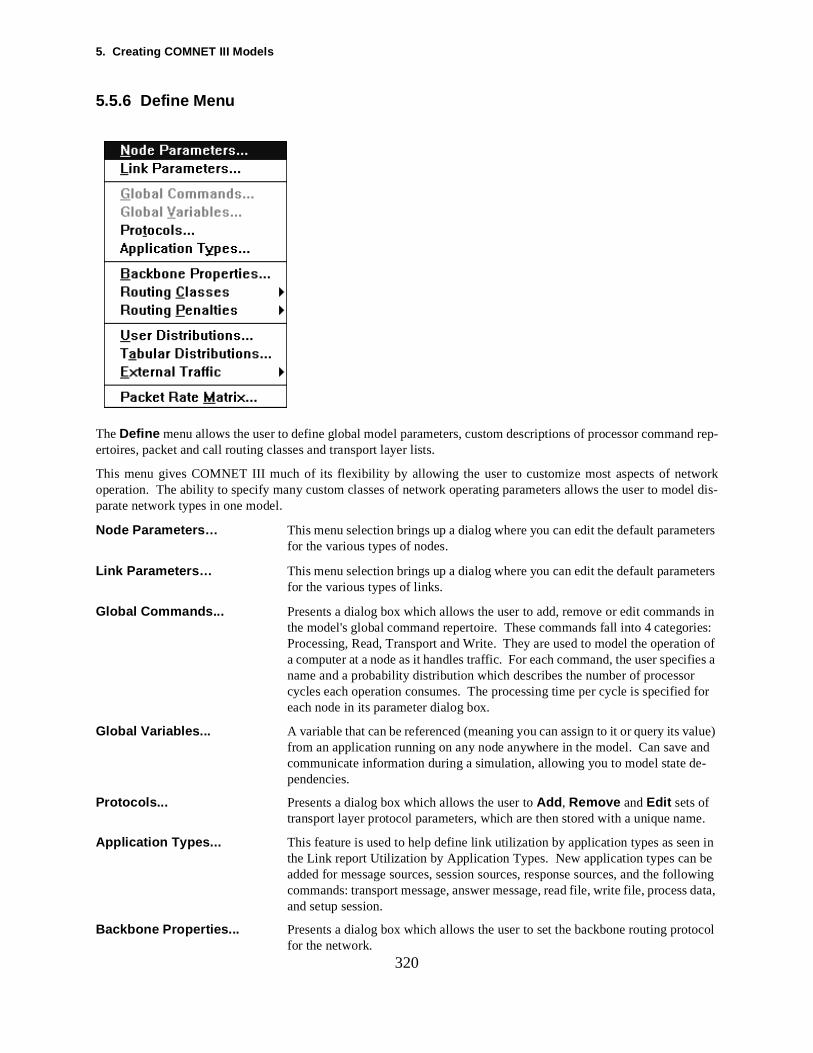
5. Creating COMNET III Models
and rep-
workdel dis-
eters
eters
ds in ries: f ifies a r for
alue) and -
e.
n in e
llowing data,
tocol
320
5.5.6 Define Menu
The Define menu allows the user to define global model parameters, custom descriptions of processor commertoires, packet and call routing classes and transport layer lists.
This menu gives COMNET III much of its flexibility by allowing the user to customize most aspects of netoperation. The ability to specify many custom classes of network operating parameters allows the user to moparate network types in one model.
Node Parameters… This menu selection brings up a dialog where you can edit the default paramfor the various types of nodes.
Link Parameters… This menu selection brings up a dialog where you can edit the default paramfor the various types of links.
Global Commands... Presents a dialog box which allows the user to add, remove or edit commanthe model's global command repertoire. These commands fall into 4 categoProcessing, Read, Transport and Write. They are used to model the operation oa computer at a node as it handles traffic. For each command, the user specname and a probability distribution which describes the number of processocycles each operation consumes. The processing time per cycle is specifiedeach node in its parameter dialog box.
Global Variables... A variable that can be referenced (meaning you can assign to it or query its vfrom an application running on any node anywhere in the model. Can save communicate information during a simulation, allowing you to model state dependencies.
Protocols... Presents a dialog box which allows the user to Add , Remove and Edit sets of transport layer protocol parameters, which are then stored with a unique nam
Application Types... This feature is used to help define link utilization by application types as seethe Link report Utilization by Application Types. New application types can badded for message sources, session sources, response sources, and the focommands: transport message, answer message, read file, write file, processand setup session.
Backbone Properties... Presents a dialog box which allows the user to set the backbone routing profor the network.
5.5 COMNET III Menus
e
give ility
give ical ly in a
rk
nd
rnals
321
Routing Classes... Presents a dialog box which allows the user to Add , Remove and Edit packet or call routing classes which are then stored with a unique name.
Routing Penalties... Presents a dialog box which allows the user to Add , Remove and Edit packet or call routing penalties which are then stored as penalty tables with a uniquname.
User Distributions... Presents a dialog box which allows the user to define user distributions and them unique names. A user distribution is simply one of the standard probabdistribution functions for which default parameters have been specified.
Tabular Distributions... Presents a dialog box which allows the user to define table distributions and them unique names. A tablular distribution allows you to use actual or empirdata to describe the distribution of a random variable. Such data are typicalthe form of histograms or frequency plots. The parameters required to buildtablular distribution are described in Appendix B.
External Traffic Allows you to set up an external traffic file to be used by COMNET III. The external traffic file can be generated by a third party program such as NetwoGeneral Sniffer or HP NetMetrix.
Packet Rate Matrix Allows you to directly generate packet traffic without scheduling applications awithout producing messages with transport commands. This is useful when data is available on packet rates and sizes, but not much is known about the inteof the application producing the stream of packets.
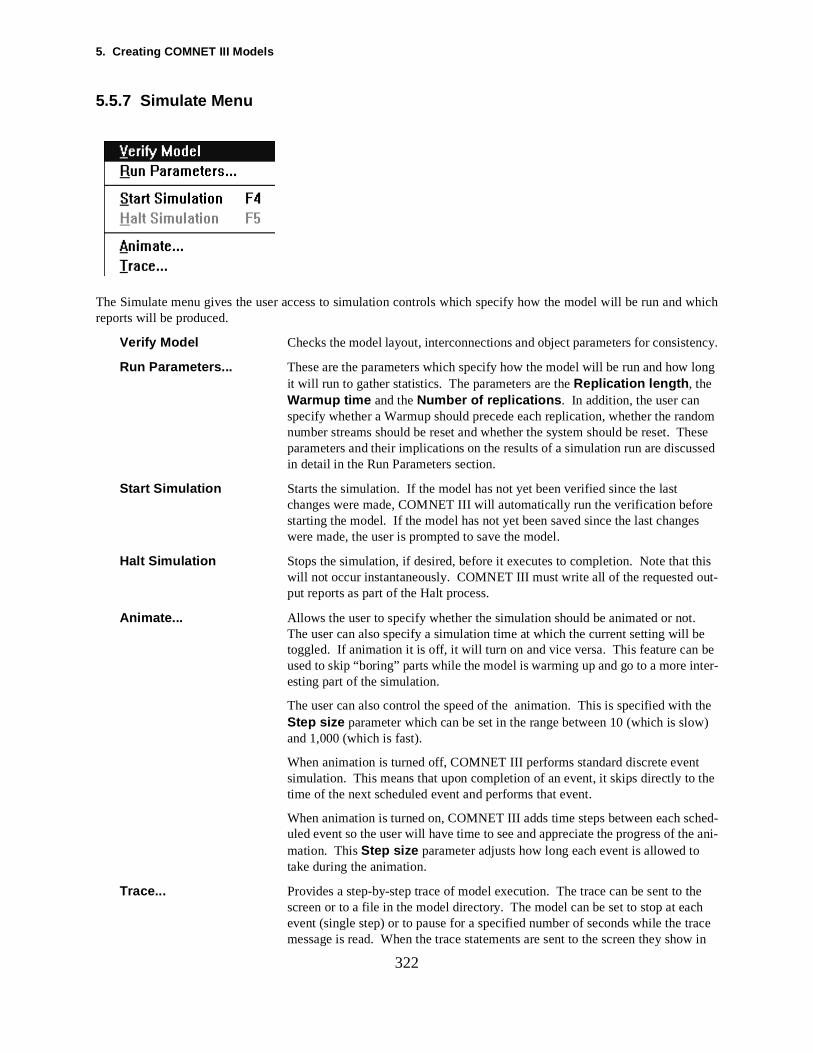
5. Creating COMNET III Models
ency.
long
ssed
re
this ut-
. e be ter-
the w)
the
hed-e ani-
ch race ow in
322
5.5.7 Simulate Menu
The Simulate menu gives the user access to simulation controls which specify how the model will be run and whichreports will be produced.
Verify Model Checks the model layout, interconnections and object parameters for consist
Run Parameters... These are the parameters which specify how the model will be run and how it will run to gather statistics. The parameters are the Replication length , the Warmup time and the Number of replications . In addition, the user can specify whether a Warmup should precede each replication, whether the random number streams should be reset and whether the system should be reset. These parameters and their implications on the results of a simulation run are discuin detail in the Run Parameters section.
Start Simulation Starts the simulation. If the model has not yet been verified since the last changes were made, COMNET III will automatically run the verification befostarting the model. If the model has not yet been saved since the last changes were made, the user is prompted to save the model.
Halt Simulation Stops the simulation, if desired, before it executes to completion. Note that will not occur instantaneously. COMNET III must write all of the requested oput reports as part of the Halt process.
Animate... Allows the user to specify whether the simulation should be animated or notThe user can also specify a simulation time at which the current setting will btoggled. If animation it is off, it will turn on and vice versa. This feature can used to skip “boring” parts while the model is warming up and go to a more inesting part of the simulation.
The user can also control the speed of the animation. This is specified withStep size parameter which can be set in the range between 10 (which is sloand 1,000 (which is fast).
When animation is turned off, COMNET III performs standard discrete eventsimulation. This means that upon completion of an event, it skips directly totime of the next scheduled event and performs that event.
When animation is turned on, COMNET III adds time steps between each sculed event so the user will have time to see and appreciate the progress of thmation. This Step size parameter adjusts how long each event is allowed totake during the animation.
Trace... Provides a step-by-step trace of model execution. The trace can be sent to the screen or to a file in the model directory. The model can be set to stop at eaevent (single step) or to pause for a specified number of seconds while the tmessage is read. When the trace statements are sent to the screen they sh

5.5 COMNET III Menus
323
the status box at the bottom of the screen.
5. Creating COMNET III Models
ult the
cifica-
a-
d an
-
l cir-ust ou and nd
324
5.5.8 Report Menu
Set File Name... Allows you to specify a report name for information to be written to. The defaname is Stat1.rpt. Before any simulation is run you can change the name of output report so that you can compare the results of one simulation run to another.
This menu lets you turn the various output reports for your model on or off. Individual menu items allow spetion of reports for each of the following items:
Nodes
Links
WAN Clouds
Application Sources
Message and Response Sources
Call Sources
Session Sources
Transport Commands
Setup Commands
Global Transport and Answer Commands
Global Setup Commands
Background Packet Flows
To view the reports, choose the following menu item:
Browse Reports... This item presents a dialog box which allows the user to specify which repliction of reports to display to the user. When the user clicks on VIEW the system editor of the operating system is invoked to display the requested reports
Select Snapshots ... This feature allows you to display utilization percentages for nodes, links, ancloud virtual circuits on the model during a simulation run. Threshold limits cbe set along with color identification for alarm conditions that will turn a particu-lar node, link or virtual circuit the color of the alarm condition. Utilization percentages are updated every 5 seconds during a simulation.
Take Snapshot ... This feature allows you to take a snapshot of a particular node, link, or virtuacuit at any time during the simulation. In order for this feature to work, you mfirst turn on the snapshot report for the particular node, link or virtual circuit yare interested in. Then during the simulation, you need to highlight the objectfrom the Report Menu select Take Snapshot. The simulation will be halted athe information displayed to the screen.
For more information about the reports, see Chapter 8. Reports.

5.5 COMNET III Menus
ries ts, new M-
ou hen
325
5.5.9 Library Menu
Edit Contents... Allows you to define custom classes of COMNET III objects and manage libraof these objects. New object types can be created by copying existing objecelaborating the attributes of the object to define a new type then saving this object type to a library. The objects shown in this list are available to all CONET III models; they are not limited to the current model.
Software Objects Allows you to load or unload the advanced features pack of COMNET III. Ywill only be able to load the advanced features pack if you have purchased it wyou purchased COMNET III.

5. Creating COMNET III Models
Me
OM-
M. ust
326
5.5.10 Help Menu
The Help menu provides access to the COMNET III help system. In the present version this capability is availableonly on the Windows version.
Index... Provides access to Widnows online help.
Dump Memory Usage... Shows the current amount of memory that COMNET III is using.
About COMNET III... Displays the current release number and build number for COMNET IIIReadFile...
ReadMe File... Displays a readme file with the latest release information and notes about CNET III.
Reference Manual... Launches the online Refence manual which is found on the installation CD ROIn order to access the online Reference manual, the COMNET III CD ROM mbe in the CD ROM drive.
5.6 Program Operation Aids
rief delaylbar iconool
wsingons.
eparate-
s
an
are nowf 2 sepa-
t the fore-
mize the
m It is no
IX ver-
327
5.6 Program Operation Aids
5.6.1 Tool Tips and Status Bar MessagesWhen you position the mouse cursor over an icon on the palette or toolbar, a short message pops up after a bto indicate the icon function. Messages are also provided in the status bar after you click on a palette or tooor when you scroll through menubar items. The UNIX versions provide status bar messages, but not the pop-up ttips.
The palettes and toolbars can be located anywhere on your screen. The color palette, menu toolbar, and 3D toolbarcan be toggled on and off.
5.6.2 Multiple Report WindowsThe Report/Browse Reports menu item now allows you to open multiple asynchronous windows for broreports. It is no longer necessary to close the report file editor before continuing with other COMNET operati
5.6.3 3D ViewA 3D view showing all levels of the network hierarchy can be displayed in a separate window. There is a stoolbar of controls for moving the camera location so you can view the network from any perspective. Trace highlighting and alarms are displayed in the 3D window if the window is open during the simulation. At the present time,the 3D view is available only on the Windows NT version. Support for 3D graphics is expected soon for Window95, at which time the 3D view capability will also be available on the Windows 95 version of COMNET III.
5.6.4 Dockable Palettes and ToolbarThe palettes and toolbars can be located anywhere on your screen. The color palette, menu toolbar, and 3D toobar cbe toggled on and off.
5.6.5 Arc EditingThe joints on an arc can be added, moved, or deleted without cutting and redrawing the entire arc. Arc joints rounded to distinguish between a corner belonging to a single arc and a corner created by the intersection orate arcs. Users can now set arc color using the color palette.
5.6.6 Color PaletteThe color palette can be used to paint icons, arcs, text, or various miscellaneous shapes. It is also used to seground and background colors.
5.6.7 ShapesA variety of shapes can be added to the display and edited, combined, and colored to form your own icons. Theseicons can be used as background art for your network layout or can be grouped with model objects to custoappearance of objects.
5.6.8 Bitmap ImportUsing File/Import/Bitmap, you can now directly import your own bitmap icons for nodes, links, background aps,and other objects. Your icon is automatically added to the list of icon choices for the designated object class.longer necessary to use SIMDRAW to import bitmap icons.
5.6.9 Export Encapsulated PostScriptThe File/Export/Encapsulated PostScript menu item produces an image of the entire network layout. On UNsions of COMNET, this item is the same as File/Print. On Windows versions, File/Print produces a native Windowsprint of the layout visible on the screen.
5. Creating COMNET III Models
el ele-iew by
aultta that
e
r to thatsubnet-
. in the
cting a
rti
gs es anyg that
dden vai
not
ems inhical listports or
328
5.6.10 Export Raster BitmapFile/Export/Raster Bitmap dumps the screen image to a bitmap file.
5.6.11 Background TextUsers can now set the color, size, and font of background text.
5.6.12 Model Editing Features
View by List:
The View by List option of the Edit menu allows you to create a list of all model elements or a subset of modments. By navigating the list, you can find an edit a particular element, or attributes of the element. The VList is handy for navigating a model that is either very large or has numerous subnetworks or both.
By selecting the Filter Items with Default Value all attributes whose values have not changed from their defsetting are filtered out of the list. This is convenient if you are interested in viewing only the user defined dayou have enetered.
By selecting the Filter "DEFAULT" Objects , all objecs with names like DEFAULT and STATNDARD, i.e. thosprovided in the default parameter sets will be filtered out.
Select by List:
The Select by List option of the Edit menu allows you to select model elements using an interface very similaof View by List. The Select by List is handy for navigating a model that is either very large or has numerous works or both.
The Select by List allows multiple selection, but all of the selections must be at the same hierarchial level, i.esame subnetworks.
Find:
The Edit menu now has a Find operation, which is also easily invoked using CTRL+F. Find is handy for loaparticular model element in a model that is either very large or has numerous subnetworks or both.
Using Matching Rules you can search for an element by name, you can search for an element having a pacularparameter set, or you can search for an element having a particular attribute.
Using Options you can elect to match case, to match all strings containing the search string, ro to match strincon-taining a pattern. The pattern must be of the form [part1]*[part2]. Both parts are optional. [Part1]* matchstring beginning with part1, *[part2] matches any string ending in part2, and [part1]*[part2] matches any strinbegins with part1 and ends in part2.
If you check the "Search hidden items too" and if the Find operation matches a model element that’s been hithe Hide option of View menu, the found item will be unhidden.
In all cases the result of the Find selects the found element, and if the element is located in a subnetwork that isthe currently open subnetwork, the editor will move to the appropriate subnetwork.
5.6.13 Report Request ManagerThe report request manager provides an interface to selectively turn on or off certain reports for individual itthe model or for the entire model. The report request manager presents the possible reports in a hierarcarranged by type of report. The reports may be selectively added to specific model elements by editing the rethe reports may be turned on or off for everything with a single button in the dialog.
s. After
h capa-
signedad the
dencies.
e can be in.. User
ning on
nds ofdr, and thatand has
ame, thet.
efined appli-
329
6. Advanced Software Modeling Features
6.1 Introduction
COMNET III release 1.3 has added a number of advanced features for modeling distributed software systeminstallation, the Advanced Software Modeliing Features will be disabled. The reason for this is to simplify model for-mulation for novice users and to steer users away from the more complex aspects of COMNET III unless sucbilities are essential for the performance measures of interest.
To Access the COMNET III Advanced Software Modeling Capabilites:
1) Select the Library menu option from the Main Menu Bar
2) Select the Software Objects option
3) Select the Load option
The Advanced Software Modeling features are now available for all models. If you had existing models dewith an earlier release of COMNET III, and those models used application sources you would need to loAdvanced Software Modeling features before the previous models would load.
The Advanced Software Modeling capabilites will be described in detail in the following sections.
6.2 User Variables
User variables can save and communicate information during a simulation, allowing you to model state depen
Variable Scope:
Scope” is a term borrowed from the world of programming languages, and it means when and where a variablreferenced. A variable is known in a scope in much the same way as an internet address is known in a domavariables have one of three scopes: global, node, and application.
A global variable can be referenced (meaning you can assign to it or query its value) from an application runany node anywhere in the model.
A node variable can be referenced only on the node on which it was defined.
An application variable is a very special kind of variable. Each application has one implicitly, and only commathat application can reference it. If you are conversant in programming terminology, an alternative way to understanapplication variables is to imagine that a command in a command sequence can generate an output parameteoutput parameter can flow downward to subsequent commands’ input parameters. The Assign Variable comman implicit output parameter, and every command has an implicit input parameter.
If you have a global variable and a node variable with the same name, and an application references that nnode variable will be referenced. When matching names to variables, node variables are always checked firs
Defining Variables:
A global variable is defined by selecting the User Variables option from the Define menu. A node variable is dby clicking the Variables button on the node properties dialog. Application variables are implicitly present on
6. Advanced Soft ware Modeling Features
e storedold in-xt, much
be set
ou can in an ex-
is sim-t report
plicationight being
to induce
variablechangesehavior
COM-
ication
for mis-
330
cations, and need not be defined.
When defining a variable, you give it a name, and you specify its type. The type dictates what data that can bin the variable, and will be one of the following: integer, real, boolean, and string. Integer and real variables hteger and real numbers, respectively. Boolean variables hold the value True or False. String variables hold telike the message text of a transport command.
Initial Values:
At the beginning of simulation, all variables are initialized with default values. Integer and real variables will to zero, boolean variables will be set to false, and string variables will be made empty.
Assigning Values:
During the simulation, a value is given to a variable using the Assign Variable command.
Querying Values:
During the simulation, you can query the value of a variable in a number of different contexts. For example, yuse the value of a variable as part of a message size calculation. To do so, simply use the variable’s namepression (see the section on Expressions).
Variable Errors:
During the simulation, any invalid operation on a variable will be reported as a variable error. A variable error ilar to a disk access error, and is reported similarly. Unless you have turned it off, the Variable Error snapshowill be active, and its alarm will be set to sound whenever errors are greater than zero.
Exclusive Access and Semaphore Behavior:
Because applications in your model can execute simultaneously, it’s very conceivable that more than one apmight reference the same global or node variable simultaneously. Depending on the logic of the model, you mconcerned about one application assigning to the variable while another is querying it, or two applications assignto the variable at the same time.
To prevent simultaneous access of a variable, set the Exclusive Access checkbox, and give an access time. The exactvalue of the access time is probably incidental to the simulation, the important thing is that only one application willbe allowed to access the variable (to either assign or query) during that access time. The access time servesordering on events that would otherwise occur simultaneously.
Using the exclusive access option, it’s possible to create logic whereby several applications are waiting for a to achieve a certain value, but when it does, only one of the waiting applications executes, and it immediately the variable’s value, thus ensuring that the other applications will continue to wait. This simultaneous waiting bis common in semaphore modeling.
Just like in the real world, it’s possible for applications to vie for overlapping sets of variables and deadlock. InNET III, such deadlocks are temporary, because each side will try only a finite number of times, as specified in the“max no. of tries” field of the variable. After that number of tries, a variable error will be generated, and the applwill continue on as if it did obtain access.
Troubleshooting:
Using variables to control model behavior can lead to complex interactions, and offers tremendous potential
6.3 New Commands
anye
node var-ill
enu.
s the
mand,
ther var-
or com- met, itntil then
mpletesrm does
larms if
331
takes in the model. To help find unintended variable behavior, turn on the Variable Value snapshot. You must specifyone variable to track, then the snapshot will show you the value of the variable as it changes. The value shown onnode on which the snapshot is enable will correspond to the value of the lowest scoped variable matching the namyou specified. For example, suppose you have a global variable named FOO, and on Node1 you also have aiable named FOO, and you enable the Variable Value snapshot for Node1 and Node2. The snapshot on Node1 wreflect the value of the node FOO, while the snapshot on Node2 will reflect the value of the global FOO.
Also handy for troubleshooting is the old Trace To File option, available via the Trace option of the Simulate mEvery variable assignment causes an informative trace message to be generated.
6.3 New Commands
Assign Variable Command:
Use the Assign Variable command to give a value to a variable. The variable combo box on the command propertiedialog will allow you to specify the target of the assignment. Select a global or node variable by name, or specifyapplication variable by selecting “output parameter.”
The “two-dot” button next to the variable combo box allows you to add variables. If you’re editing a node comyou’ll be permitted to add node variables, and if you’re editing a global command, you’ll be permitted to add globalvariables.
Specify the value for the assignment in the text box. The value can be any expression, involving constants, oiables, random number distributions, and intrinsic functions.
Wait For Command:
The Wait For command is a generalization of the old Filter Messages command. In fact, by default, the Wait Fmand functions exactly the way Filter Messages did. Wait For evaluates a condition, and if the condition iscompletes and gets out of the way for the next command to run. If the condition is not met, Wait For blocks ucondition is met, or until the time-out timer expires, whichever comes first. By “block,” we mean the applicatiorun-ning the command sequence is suspended.
The condition can be of three types: Received Message, Alarm, or Expression.
Wait For Received Message:
Behaves exactly as the old Filter Messages command.
Wait For Alarm:
If the specified alarm is already sounding when this command executes, no blocking occurs, the command coand the next command is executed. If the alarm is not already sounding, the command blocks until the alasound.
The alarm combo box shows all the alarms that are currently set. Use the two-dot button to set additional anecessary, and pick an alarm. Then specify the node or link on which the alarm must sound.
6. Advanced Soft ware Modeling Features
nctions.
nd com-sion be-able toferenced
op wait-t eval-
the
iggered
in theg
h it’s en-
om-
from the is execut-
quence.ultiple
332
Wait For Expression:
The expression can be almost any expression, involving constants, user variables, and most of the intrinsic fuSome intrinsic functions, like SimTime, are prohibited. The expression must evaluate to a boolean value.
When the command is executed, the expression is evaluated, and if it is TRUE, no blocking occurs, the commapletes and the next command is executed. If the expression is FALSE, the command blocks until the exprescomes TRUE. Of the limited number of things permitted in a Wait For expression, only user variables are lichange after the expression is evaluated the first time. Thus, the expression is only re-evaluated if and when revariables change.
Clearly, a Wait For expression that does not involve one or more variables is not of much use, UNLESS the “sting” option is checked. If the “stop waiting” option is checked, then either the expression is FALSE when firsuated, or the command will block for the duration of the time-out time.
Stop Waiting:
The blocking process you’re modeling will probably not wait forever. To model a process that times out, check“stop waiting afterÖ” option, and give the time limit you’re willing to wait. After that time limit, the command andthe application will be terminated. To catch this event and do something special in response to it, click the TrSources button on the application source, select the source that will perform the special response, and use the “uponwait timeout” triggering rule.
Troubleshooting:
With the increased flexibility of the Wait For command comes increased complexity and potential for mistakesmodel. To assist in finding wayward applications that are in perpetual Waits, turn on the Suspended/PendinAppssnapshot. This snapshot will show you a count of suspended and pending applications on any node on whicabled.
Macro Command:
Programmers can think of the Macro command as a subroutine. The Macro command is a handy way to organize cmands that are frequently used together.
Command Sequence
A Macro command contains a command sequence, similar to that of an application source. Other commandscommand repertoire, or global commands, can appear in this command sequence. When a macro commanded, each of the commands in its command sequence is executed.
Looping
A Macro command can be used to implement a simple looping behavior in an application source’s command seIf a Macro command has a “number of executions” value greater than 1, the Macro command will execute mtimes, and it will be as if the commands in it were being looped.
Hint: To set the loop count on the fly, you can use “input parameter” for the number of executions of the Macro com-mand, and add an Assign command higher up that computes the value.
6.4 Expressions
d this if to be-complishe “exclu-it’s nowd and aneen.could get
variableds, put
ariable is Use theexecuteorary,
hich to themrrors,
he lat-
d using +ils number
l times,rence is
f a User
Dist
333Atomic Execution
Not a high-tech form of capital punishment, but nevertheless a feature for advanced users. You might neeyou’re modeling a semaphore-like behavior, for example you have multiple applications waiting for a variablecome zero, and you want only one of them to resume execution when the variable does become zero. To acthis, you need to ensure that only one application accesses the variable at a time. No problem, you enable thsive access” option on the variable. But you also need one application to 1) query the variable and find that zero, and 2) change the variable to something non-zero. Actions 1 and 2 translate into a Wait For commanAssign Variable command, and somehow you need to do both of them without another application getting in betwFor example, after the first command is done seeing that the variable has become zero, another application a chance to query the variable before you have a chance to change it.
For this example, what you need is a way to say “do commands 1 and 2, and don’t let anyone else touch theuntil they’re both done.” To keep everyone else away from the variable for the duration of the two commanboth commands in a Macro command, and check the “atomic wrt variables” checkbox on the Macro command.
There can be more than one variable referenced in the commands of an atomic Macro’s sequence. As each vaccessed, it becomes locked for use only by this application, and remains locked until the Macro completes. atomic feature with care, it’s very easy for two Macro commands that need overlapping sets of variables to simultaneously and deadlock (just like in the real world!). Note that, in COMNET III, deadlocks are only tempbecause after the number of tries specified on the variable, one party will give up.
6.4 Expressions
Expressions are used to give a value to a variable in an Assign Variable command, to specify a condition for wwait in a Wait For command, and to specify a random number distribution in a User Distribution. You typefree-form into a text box. The verification that takes place for the dialog will verify that you have no syntax ebut it will not tell you that you misspelled a variable name, or that you’re trying to add 1 to a string variable. Tter sorts of errors will be detected when you Verify Model.
Expressions are either numeric, string, or boolean.
Numeric Expressions
Formally speaking, a numeric expression is an algebraic expression made up of one or more terms combineand - operators, and each term is made up one or more factors combined using * and / operators. A factor bodownto either a pair of parentheses containing a numeric expression, or one of the following: a constant, a randomdistribution, a variable, or an intrinsic function returning a numeric type.
Constants:
Integer constants look like this: 1, 2, 3. Real constants require a decimal point, like this: 1.0, 2., 3.5.
Random Number Distributions:
These are the things you’re used to seeing in combo boxes on property dialogs, for specifying inter-arrivamessage sizes, etc. You enter them in an expression exactly as you would in a combo box. The only diffethat you have to remember the format, there is no combo box to help you (except for the expression field oDistribution, where you CAN get some help from a combo box).
Note that User Distributions can be used here as well.
At the moment the expression is evaluated, a random number is drawn from the sample. Random Number ribu-
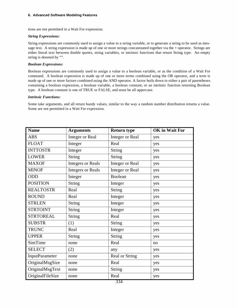
6. Advanced Soft ware Modeling Features
d as mes-trings areempty
Wait Fora term isnthesesBoolean
334
tions are not permitted in a Wait For expression.
String Expressions:
String expressions are commonly used to assign a value to a string variable, or to generate a string to be usesage text. A string expression is made up of one or more strings concatenated together via the + operator. Seither literal text between double quotes, string variables, or intrinsic functions that return String type. An string is denoted by “”.
Boolean Expressions:
Boolean expressions are commonly used to assign a value to a boolean variable, or as the condition of a command. A boolean expression is made up of one or more terms combined using the OR operator, and made up of one or more factors combined using the AND operator. A factor boils down to either a pair of parecontaining a boolean expression, a boolean variable, a boolean constant, or an intrinsic function returning type. A boolean constant is one of TRUE or FALSE, and must be all uppercase.
Intrinsic Functions:
Some take arguments, and all return handy values, similar to the way a random number distribution returns a value.Some are not permitted in a Wait For expression.
Name Arguments Return type OK in Wait ForABS Integer or Real Integer or Real yes
FLOAT Integer Real yes
INTTOSTR Integer String yes
LOWER String String yes
MAXOF Integers or Reals Integer or Real yes
MINOF Integers or Reals Integer or Real yes
ODD Integer Boolean yes
POSITION String Integer yes
REALTOSTR Real String yes
ROUND Real Integer yes
STRLEN String Integer yes
STRTOINT String Integer yes
STRTOREAL String Real yes
SUBSTR (1) String yes
TRUNC Real Integer yes
UPPER String String yes
SimTime none Real no
SELECT (2) any yes
InputParameter none Real or String yes
OriginalMsgSize none Real yes
OriginalMsgText none String yes
OriginalFileSize none Real yes
6.4 Expressions
If bool is
n which
itraryn clip an
tions, in
“Sam-n”
and maybe a User may bee com-
335
(1) SUBSTR (pos1, pos2, string), pos1 and pos2 are integer expressions, returns portion of string between pos1 andpos2 inclusive.
(2) Select (bool, exp1, exp2), bool is a boolean expression, exp1 and exp2 are expressions of any type. TRUE, returns value of exp1, otherwise returns value of exp2.
Examples:
“Message to “ + StrVar1
ABS(Exp(10.0) - 2.0)
MsgCountVar * MsgSizeVar
(MsgCountVar > 10) AND (SesCountVar > 10)
Generalized User Distributions
User Distributions have been generalized in 1.3. In 1.2, they were customized random number distributions, ithe user had set the parameters of the distribution. There was no way to shift or clip the distribution, your shapemanipulations were limited to those made by changing the parameters.
In 1.3, you can still create User Distributions that have only parameter changes, or you can also give an arbexpression, and of course this expression can feature a random number distribution. So, for example, you caexponential distribution so that it returns only values less then 12:
MAXOF(Exp(10.0), 12)
Note that the expression may also involve user variables, and it need not involve any random number distribuwhich case a sample from the distribution returns a state dependent number rather than a random number.
Hint: If you’re planning to create a shaped distribution based on a random number distribution, first select theple only option” and pick the random number distribution using the combo box. Then switch to the “Expressiooption. When you switch, the text of the sample combo will be copied to the expression text box, giving you a headstart.
Variable Execution Count for Commands
While specifying the command sequence of an application source, the number of executions for each commnow be a Sample. The sample may be one of the standard random number distributions. The sample may Distribution, in which case it might be a state-dependent number instead of a random number. The sample“input parameter,” which means a number generated by an Assign Variable command occurring earlier in thmand sequence.

6. Advanced Soft ware Modeling Features
336
f the
and ini-tor...” aken to
n use
337
7. Automatic Parameter Iterator
7.1 Introduction
Before the release of COMNET III version 1.3, model experimentation was conducted in the following way:
1) Manually change something in the model.
2) Manually change the name of the report file and associated statistics files using the Set File Name option oReports menu.
3) Run the simulation.
4) Go to step 1, and repeat for all the intended changes.
5) Manually compare the statistics collected for the various runs.
In COMNET III release 1.3, the above steps can now be automated.
7.2 Terminology
Experiment:
Steps 1-5 (listed above) are repeated for every change, and the resulting sets of output files.
Scenario:
Steps 1-5 (listed above) run once, correspond to only one change in the model.
Factor:
The thing in the model being changed.
Level:
One of the values given to the factor in step 1.
7.3 Specifying an Experiment
Select the Run Parameters option of the Simulation menu. There is a combo box labeled “experiment on...” tially it indicates “none,” or no experiment specified. The other option available in the combo box is “Select facThis combo box functions something like a pop-up menu, because when you select “Select factor...” you are tanother dialog, where you select a factor.
Select Factor:
The factor selection dialog is very similar in operation to the View By List dialog, and as a matter of fact you caView By List as an alternative method of specifying an experiment.
7. Automatic Parameter Iterator
e ence
and to lues, will be rmed
e e mes-urces in
x on ne”
he tore
ame
and Expt1 you et plots,
s, ns in r rio,
338
Find the attribute on which you want to experiment. You will notice right away that relatively few attributes aravailable for experimentation. We’ve tried to provide experimentation on the attributes that most directly influtraffic level and delay.
Levels:
After you’ve selected the attribute, click the Factor button. You will be asked to give the experiment a name, specify levels. The current value of the attribute is offered as the default level. Change it and/or add more vaseparated by semicolons. When you click OK, the validity of each level will be tested, and any obvious errors reported. Note that it’s possible to give unsuitable values via this interface, because the normal checks perfoduring normal dialog interaction are not performed.
Apply to All:
An option available for some factors is the “Apply to all” option. If you check it, then the levels you give will bapplied to all model entities of the same class. For example, if the factor you specify is Bytes or Cycles of somsage source, you have the option of applying the levels only to that message source, or to all the message sothe model.
Changing the Experiment:
When you’re satisfied that you’ve picked the right factor and given the right levels, click Done. The combo bothe Run Parameters dialog will then indicate the currently selected factor. To clear the experiment, select “noagain. To change it, select “Select new factor and/or levelsÖ”
The experiment you specified will be saved with the model.
7.4 Running an Experiment
To run the experiment, simply select Start Simulation or click the green light button, as you normally would. Titerator automatically assigns your first level, runs the simulation, and so on. After the run, the iterator will resthe value of the factor to the value it had before the experiment.
7.5 Analyzing the Results of an Experiment
Statistics and reports files will be named automatically; for example, Expt1-1.rpt (substitute your experiment nfor Expt1). You can browse reports as is normal, but you’ll have more report files than normal to look at.
Familiar Territory:
To examine statistics, go to the properties dialog of the model element whose statistics you want to examine,click the Statistics button, as usual. You will be asked the question, “Statistics from which experiment?” and (or your experiment name or names) will be in the list. After selecting the experiment and clicking Continue, will go to the Statistics Requests dialog, where you can select a statistic and click View to see the data and gas usual.
If you use multiple replications in your model, you probably need some orientation, as there are now N x M statisticwhere N is the number of scenarios (= number of levels) in the experiment, and M is the number of replicatioeach scenario. The stats table will display a row for each replication, showing min, mean, and standard deviation fothe statistic during that replication. You will see M rows of data, but all the data applies only to the first scenaExpt1-1. To switch to the data for the second scenario, select Expt1-2 from the “Stat file names” combo box.

7.5 Analyzing the Results of an Experiment
row of
s expe-xper-
of one replica-ly
y sce-
339
To plot the statistic for one replication from one scenario, make sure the right scenario is showing, select the the desired replication, and click the Plot button.
All Checkbox:
For the most part, the interactions above are familiar territory, they’re not much different from what most userrienced in release 1.2. The All checkbox is not new in 1.3, but its utility in combination with a multi-scenario eiment is great.
When you check the All checkbox, the per-replication data goes away, and the data that replaces it consists row for each scenario, showing the summary min, max, and std. dev. for that scenario, averaged over all the tions in that scenario. In the All table, you see a side-by-side comparison of each scenario, so you can quickappraise the effect of the different levels on this statistic.
Now when you click the Plot button, you are given a bar graph showing how the mean of the statistic varies bnario.

7. Automatic Parameter Iterator
340
341
8. Reports
The following reports are produced by COMNET III:
Node Reports• Processor + Disk Utilization
• Input Buffer Use by Port
• Input Buffer Totals
• Output Buffer Use by Port
• Output Buffer Totals
• Received Message Counts
• Disk Access Error Counts
• Session Level
• Call Counts
• Call Level
Link Reports
• Channel Utilization
• Utilization by Application
• Utilization by Protocol
• Collision Statistics
• Session Level
• Call Counts
• Call Level
WAN Cloud Reports• Frame Delay by Virtual Circuit
• Frame Counts by Virtual Circuit
• Access Link Statistics
Application Source Reports• Application Run Length
Message + Response Source Reports• Message Delay
• Packet Delay
Call Source Reports• Blocked Call Counts
• Disconnected Call Counts
8. Reports
box
edrts, you
342
• Preempted Call Counts
Session Source Reports• Message Delay
• Packet Delay
• Setup Delay
• Session Length
• Setup Counts
Transport + Answer Commands Reports• Message Delay
• Packet Delay
Setup Command Reports• Message Delay
• Packet Delay
• Setup Delay
• Session Length
• Setup Commands
These reports are produced at the end of each replication of the model. They can be selectively turned on by choosingthe menu item Report and then selecting the appropriate report from the pulldown and flyout menus. A dialogwill appear where reports can be turned on or off for each individual model element (node, link, etc.). Here is anexample of one of these dialog boxes.
Statistical monitoring during the simulation is active only for the statistics that need to be included in formattreports (or viewed through statistics buttons). By requesting fewer reports and including fewer objects in repocan speed up the simulation.
Reporters dialog box
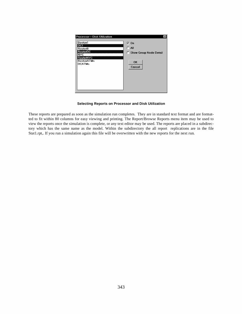
re format-sed to
the file
343
Selecting Reports on Processor and Disk Utilization
These reports are prepared as soon as the simulation run completes. They are in standard text format and ated to fit within 80 columns for easy viewing and printing. The Report/Browse Reports menu item may be uview the reports once the simulation is complete, or any text editor may be used. The reports are placed in a subdirec-tory which has the same name as the model. Within the subdirectory the all report replications are in Stat1.rpt,. If you run a simulation again this file will be overwritten with the new reports for the next run.
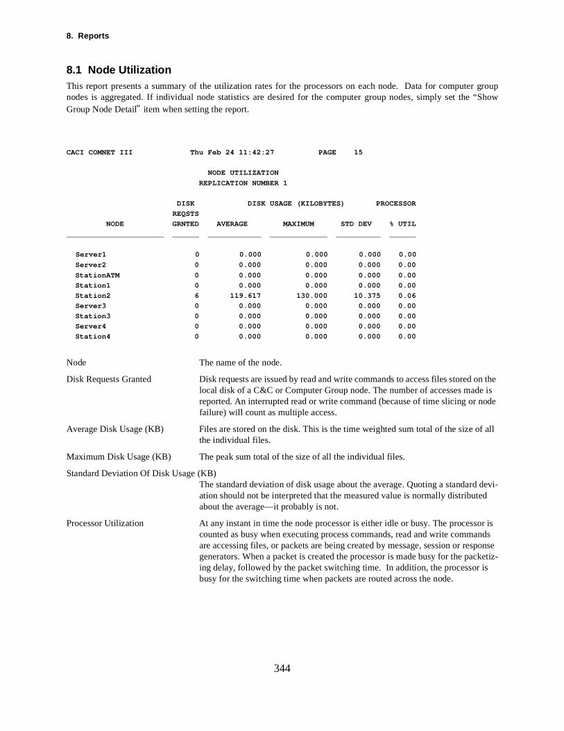
8. Reports
er g
d on the e is ode
of all
devi-d
sor is
sponse cketiz-s
344
8.1 Node UtilizationThis report presents a summary of the utilization rates for the processors on each node. Data for computroupnodes is aggregated. If individual node statistics are desired for the computer group nodes, simply set the “ShowGroup Node Detail” item when setting the report.
CACI COMNET III Thu Feb 24 11:42:27 PAGE 15
NODE UTILIZATION
REPLICATION NUMBER 1
DISK DISK USAGE (KILOBYTES) PROCESSOR
REQSTS
NODE GRNTED AVERAGE MAXIMUM STD DEV % UTIL
______________________ ______ ____________ _____________ __________ ______
Server1 0 0.000 0.000 0.000 0.00
Server2 0 0.000 0.000 0.000 0.00
StationATM 0 0.000 0.000 0.000 0.00
Station1 0 0.000 0.000 0.000 0.00
Station2 6 119.617 130.000 10.375 0.06
Server3 0 0.000 0.000 0.000 0.00
Station3 0 0.000 0.000 0.000 0.00
Server4 0 0.000 0.000 0.000 0.00
Station4 0 0.000 0.000 0.000 0.00
Node The name of the node.
Disk Requests Granted Disk requests are issued by read and write commands to access files storelocal disk of a C&C or Computer Group node. The number of accesses madreported. An interrupted read or write command (because of time slicing or nfailure) will count as multiple access.
Average Disk Usage (KB) Files are stored on the disk. This is the time weighted sum total of the sizethe individual files.
Maximum Disk Usage (KB) The peak sum total of the size of all the individual files.
Standard Deviation Of Disk Usage (KB)The standard deviation of disk usage about the average. Quoting a standardation should not be interpreted that the measured value is normally distributeabout the average—it probably is not.
Processor Utilization At any instant in time the node processor is either idle or busy. The procescounted as busy when executing process commands, read and write commands are accessing files, or packets are being created by message, session or regenerators. When a packet is created the processor is made busy for the paing delay, followed by the packet switching time. In addition, the processor ibusy for the switching time when packets are routed across the node.
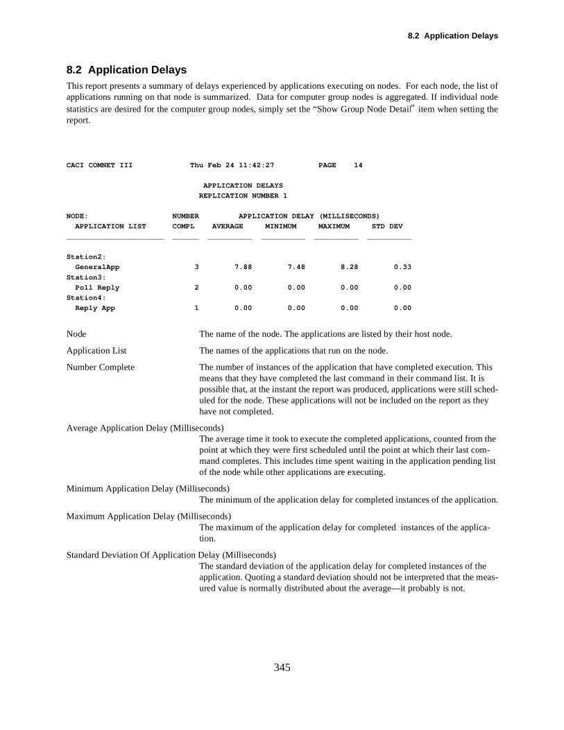
8.2 Application Delays
the list ofe
his is -ey
the - list
tion.
a-
e eas-
345
8.2 Application DelaysThis report presents a summary of delays experienced by applications executing on nodes. For each node, applications running on that node is summarized. Data for computer group nodes is aggregated. If individual nodstatistics are desired for the computer group nodes, simply set the “Show Group Node Detail” item when setting thereport.
CACI COMNET III Thu Feb 24 11:42:27 PAGE 14
APPLICATION DELAYS
REPLICATION NUMBER 1
NODE: NUMBER APPLICATION DELAY (MILLISECONDS)
APPLICATION LIST COMPL AVERAGE MINIMUM MAXIMUM STD DEV
______________________ ______ __________ __________ __________ __________
Station2:
GeneralApp 3 7.88 7.48 8.28 0.33
Station3:
Poll Reply 2 0.00 0.00 0.00 0.00
Station4:
Reply App 1 0.00 0.00 0.00 0.00
Node The name of the node. The applications are listed by their host node.
Application List The names of the applications that run on the node.
Number Complete The number of instances of the application that have completed execution. Tmeans that they have completed the last command in their command list. It possible that, at the instant the report was produced, applications were still scheduled for the node. These applications will not be included on the report as thhave not completed.
Average Application Delay (Milliseconds)The average time it took to execute the completed applications, counted frompoint at which they were first scheduled until the point at which their last command completes. This includes time spent waiting in the application pendingof the node while other applications are executing.
Minimum Application Delay (Milliseconds)The minimum of the application delay for completed instances of the applica
Maximum Application Delay (Milliseconds)The maximum of the application delay for completed instances of the appliction.
Standard Deviation Of Application Delay (Milliseconds)The standard deviation of the application delay for completed instances of thapplication. Quoting a standard deviation should not be interpreted that the mured value is normally distributed about the average—it probably is not.

8. Reports
for compu-
me of
346
8.3 Received Message CountThis report presents a count of received messages for each destination node listed by message name. Data ter group nodes is aggregated. If individual node statistics are desired for the computer group nodes, simply set the“Show Group Node Detail” item when setting the report.
CACI COMNET III Thu Feb 24 11:42:27 PAGE 9
RECEIVED MESSAGE COUNTS
REPLICATION NUMBER 1
RECEIVER COUNT MESSAGE NAME
______________________ __________ _________________________________________
StationATM 9 MsgATM
StationATM 6 SessATM
Station1 9 MsgATM
Station1 6 SessATM
Station2 1 Aloha Session
Station2 2 Poller Message
Server3 1 Poller Message
Station3 2 Poller Message
Server4 2 Aloha Session
Station4 1 Aloha Session
Node The name of the receiving node.
Count The number of messages received during the simulation.
Message Name The name of the received message. This is not the message text but the nathe message, session, answer, or transport command that sent the message.
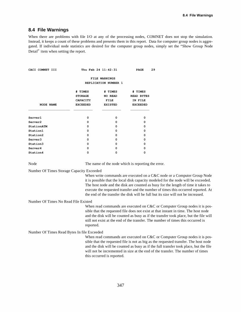
8.4 File Warnings
ulation. is aggre-
ode ed. s to d. At
de
will
node file s
347
8.4 File WarningsWhen there are problems with file I/O at any of the processing nodes, COMNET does not stop the simInstead, it keeps a count of these problems and presents them in this report. Data for computer group nodesgated. If individual node statistics are desired for the computer group nodes, simply set the “Show Group NodeDetail” item when setting the report.
CACI COMNET III Thu Feb 24 11:42:31 PAGE 29
FILE WARNINGS
REPLICATION NUMBER 1
# TIMES # TIMES # TIMES
STORAGE NO READ READ BYTES
CAPACITY FILE IN FILE
NODE NAME EXCEEDED EXISTED EXCEEDED
______________________ __________ __________ __________
Server1 0 0 0
Server2 0 0 0
StationATM 0 0 0
Station1 0 0 0
Station2 0 0 0
Server3 0 0 0
Station3 0 0 0
Server4 0 0 0
Station4 0 0 0
Node The name of the node which is reporting the error.
Number Of Times Storage Capacity ExceededWhen write commands are executed on a C&C node or a Computer Group Nit is possible that the local disk capacity modeled for the node will be exceedThe host node and the disk are counted as busy for the length of time it takeexecute the requested transfer and the number of times this occurred reportethe end of the transfer the disk will be full but its size will not be increased.
Number Of Times No Read File ExistedWhen read commands are executed on C&C or Computer Group nodes it ispos-sible that the requested file does not exist at that instant in time. The host noand the disk will be counted as busy as if the transfer took place, but the filestill not exist at the end of the transfer. The number of times this occurred is reported.
Number Of Times Read Bytes In file ExceededWhen read commands are executed on C&C or Computer Group nodes it ispos-sible that the requested file is not as big as the requested transfer. The hostand the disk will be counted as busy as if the full transfer took place, but thewill not be incremented in size at the end of the transfer. The number of timethis occurred is reported.
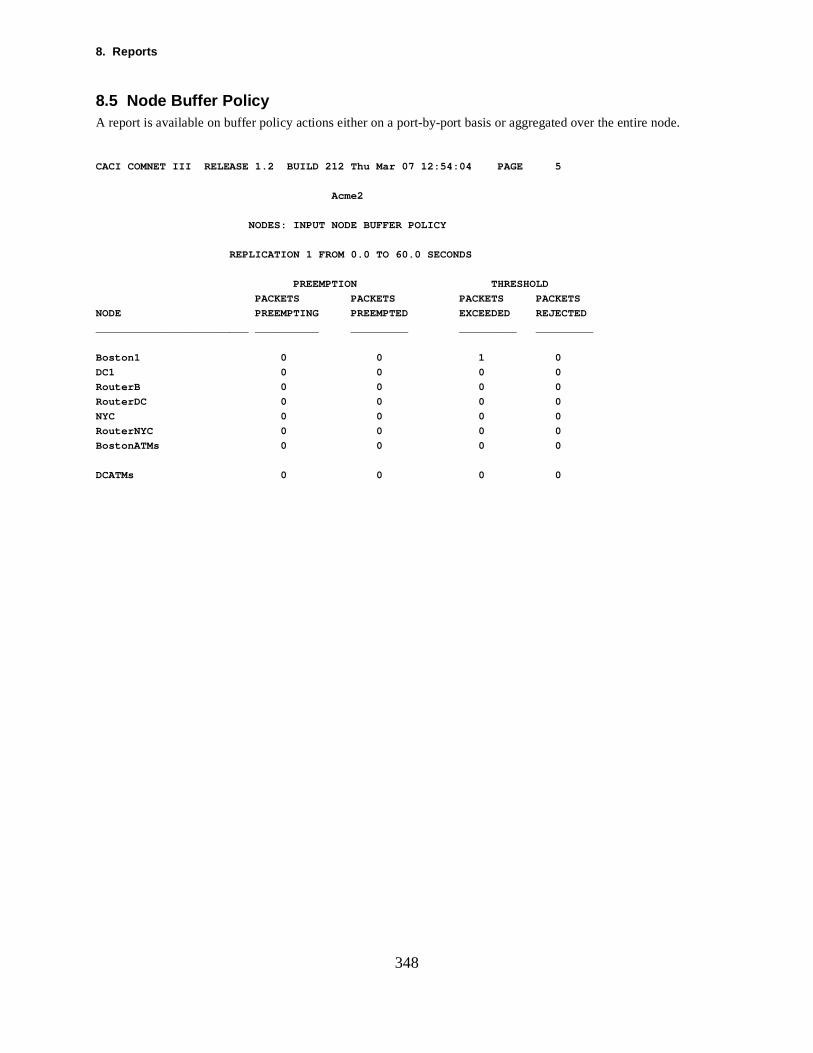
8. Reports
.
348
8.5 Node Buffer PolicyA report is available on buffer policy actions either on a port-by-port basis or aggregated over the entire node
CACI COMNET III RELEASE 1.2 BUILD 212 Thu Mar 07 12:54:04 PAGE 5
Acme2
NODES: INPUT NODE BUFFER POLICY
REPLICATION 1 FROM 0.0 TO 60.0 SECONDS
PREEMPTION THRESHOLD
PACKETS PACKETS PACKETS PACKETS
NODE PREEMPTING PREEMPTED EXCEEDED REJECTED
________________________ __________ _________ _________ _________
Boston1 0 0 1 0
DC1 0 0 0 0
RouterB 0 0 0 0
RouterDC 0 0 0 0
NYC 0 0 0 0
RouterNYC 0 0 0 0
BostonATMs 0 0 0 0
DCATMs 0 0 0 0
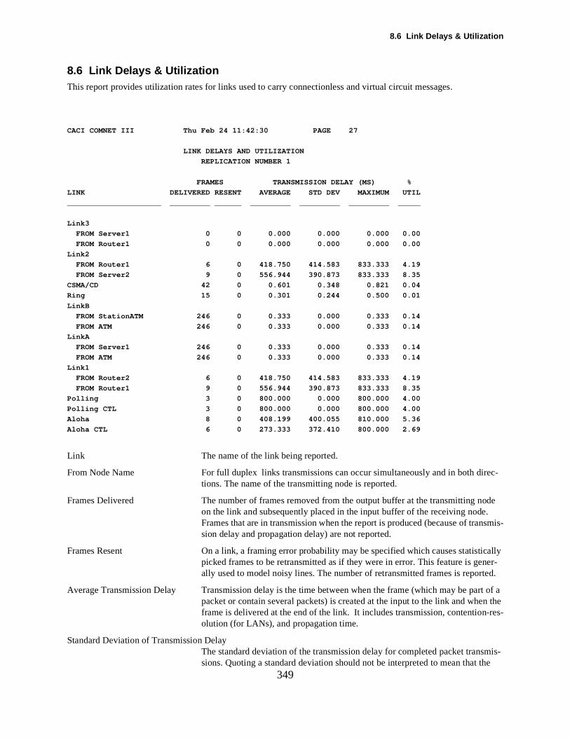
8.6 Link Delays & Utilization
c-
.
ally er-
ed.
of a n the -res-
mis-he
349
8.6 Link Delays & UtilizationThis report provides utilization rates for links used to carry connectionless and virtual circuit messages.
CACI COMNET III Thu Feb 24 11:42:30 PAGE 27
LINK DELAYS AND UTILIZATION
REPLICATION NUMBER 1
FRAMES TRANSMISSION DELAY (MS) %
LINK DELIVERED RESENT AVERAGE STD DEV MAXIMUM UTIL
_____________________ _________ ______ _________ _________ _________ _____
Link3
FROM Server1 0 0 0.000 0.000 0.000 0.00
FROM Router1 0 0 0.000 0.000 0.000 0.00
Link2
FROM Router1 6 0 418.750 414.583 833.333 4.19
FROM Server2 9 0 556.944 390.873 833.333 8.35
CSMA/CD 42 0 0.601 0.348 0.821 0.04
Ring 15 0 0.301 0.244 0.500 0.01
LinkB
FROM StationATM 246 0 0.333 0.000 0.333 0.14
FROM ATM 246 0 0.333 0.000 0.333 0.14
LinkA
FROM Server1 246 0 0.333 0.000 0.333 0.14
FROM ATM 246 0 0.333 0.000 0.333 0.14
Link1
FROM Router2 6 0 418.750 414.583 833.333 4.19
FROM Router1 9 0 556.944 390.873 833.333 8.35
Polling 3 0 800.000 0.000 800.000 4.00
Polling CTL 3 0 800.000 0.000 800.000 4.00
Aloha 8 0 408.199 400.055 810.000 5.36
Aloha CTL 6 0 273.333 372.410 800.000 2.69
Link The name of the link being reported.
From Node Name For full duplex links transmissions can occur simultaneously and in both diretions. The name of the transmitting node is reported.
Frames Delivered The number of frames removed from the output buffer at the transmitting node on the link and subsequently placed in the input buffer of the receiving nodeFrames that are in transmission when the report is produced (because of transmis-sion delay and propagation delay) are not reported.
Frames Resent On a link, a framing error probability may be specified which causes statisticpicked frames to be retransmitted as if they were in error. This feature is genally used to model noisy lines. The number of retransmitted frames is report
Average Transmission Delay Transmission delay is the time between when the frame (which may be partpacket or contain several packets) is created at the input to the link and wheframe is delivered at the end of the link. It includes transmission, contentionolution (for LANs), and propagation time.
Standard Deviation of Transmission DelayThe standard deviation of the transmission delay for completed packet transsions. Quoting a standard deviation should not be interpreted to mean that t

8. Reports
t.
nk ink ula-
350
measured value is normally distributed about the average—it probably is no
Maximum Transmission DelayThe maximum delay observed for any packet across the link.
Link Utilization The transmission time for a frame is calculated from its size divided by the lispeed. The link is in use for this time plus the propagation delay across the lfor each frame. Utilization is then reported as the total usage time in the simtion run divided by the simulation run length.
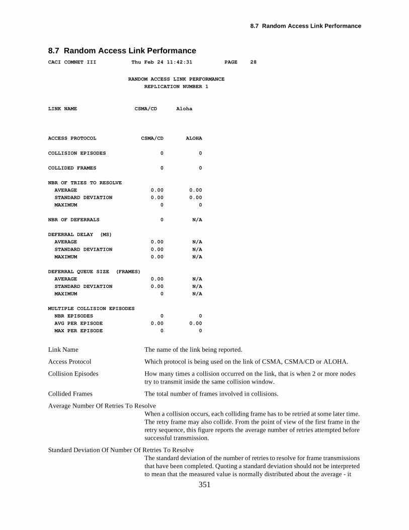
8.7 Random Access Link Performance
ime. he efore
ions reted it
351
8.7 Random Access Link PerformanceCACI COMNET III Thu Feb 24 11:42:31 PAGE 28
RANDOM ACCESS LINK PERFORMANCE
REPLICATION NUMBER 1
LINK NAME CSMA/CD Aloha
ACCESS PROTOCOL CSMA/CD ALOHA
COLLISION EPISODES 0 0
COLLIDED FRAMES 0 0
NBR OF TRIES TO RESOLVE
AVERAGE 0.00 0.00
STANDARD DEVIATION 0.00 0.00
MAXIMUM 0 0
NBR OF DEFERRALS 0 N/A
DEFERRAL DELAY (MS)
AVERAGE 0.00 N/A
STANDARD DEVIATION 0.00 N/A
MAXIMUM 0.00 N/A
DEFERRAL QUEUE SIZE (FRAMES)
AVERAGE 0.00 N/A
STANDARD DEVIATION 0.00 N/A
MAXIMUM 0 N/A
MULTIPLE COLLISION EPISODES
NBR EPISODES 0 0
AVG PER EPISODE 0.00 0.00
MAX PER EPISODE 0 0
Link Name The name of the link being reported.
Access Protocol Which protocol is being used on the link of CSMA, CSMA/CD or ALOHA.
Collision Episodes How many times a collision occurred on the link, that is when 2 or more nodes try to transmit inside the same collision window.
Collided Frames The total number of frames involved in collisions.
Average Number Of Retries To ResolveWhen a collision occurs, each colliding frame has to be retried at some later tThe retry frame may also collide. From the point of view of the first frame in tretry sequence, this figure reports the average number of retries attempted bsuccessful transmission.
Standard Deviation Of Number Of Retries To ResolveThe standard deviation of the number of retries to resolve for frame transmissthat have been completed. Quoting a standard deviation should not be interpto mean that the measured value is normally distributed about the average -

8. Reports
be
ns-
e ean ly is
tion
ore es,
wo s
352
probably is not.
Maximum Number Of Retries To ResolveDuring the simulation, the maximum observed number of retries that had to attempted before an initially collided frame was transmitted.
Number Of Deferrals If a node attempts to transmit a frame and sees the link busy, it defers its tramission until the link becomes idle (plus the contention interval). This figure reports how many transmission attempts had to be deferred.
Average Deferral Delay The average delay due to transmission deferrals.
Standard Deviation Of Deferral DelayThe standard deviation of the deferral delay for frame transmissions that havbeen completed. Quoting a standard deviation should not be interpreted to mthat the measured value is normally distributed about the average - it probabnot.
Maximum Deferral Delay The worst case deferral delay observed in the simulation.
Average Deferral Queue Size(Frames)The average number of frames queued in buffer because of deferral.
Standard Deviation Of Deferral Queue Size(Frames)The standard deviation of the deferral queue size. Quoting a standard deviashould not be interpreted to mean that the measured value is normally distributed about the average— it probably is not.
Maximum Deferral Queue Size(Frames)The maximum deferral queue size observed during the simulation.
Number Of Multiple Collision EpisodesWhen a collision occurs in the collision window, it may be between two or mframes arising from different nodes. The simple case is between just two frambut in a heavily congested system it is possible that frames from more than tnodes are involved in the collision. This figure reports the number of episodewhere more than two frames are involved.
Average Collisions Per Multiple Collision EpisodeThe average number of frames colliding in a multiple collision episode. This does not include collisions of the retry frames.
Maximum Collisions Per Multiple Collision EpisodeThe maximum number of frames colliding in one contention interval for multiple collision episodes.
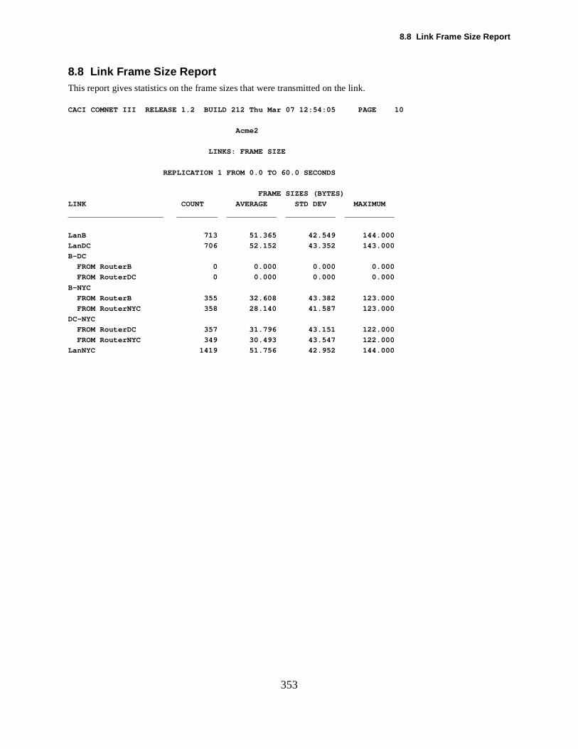
8.8 Link Frame Size Report
353
8.8 Link Frame Size ReportThis report gives statistics on the frame sizes that were transmitted on the link.
CACI COMNET III RELEASE 1.2 BUILD 212 Thu Mar 07 12:54:05 PAGE 10
Acme2
LINKS: FRAME SIZE
REPLICATION 1 FROM 0.0 TO 60.0 SECONDS
FRAME SIZES (BYTES)
LINK COUNT AVERAGE STD DEV MAXIMUM
_____________________ _________ ___________ ___________ ___________
LanB 713 51.365 42.549 144.000
LanDC 706 52.152 43.352 143.000
B-DC
FROM RouterB 0 0.000 0.000 0.000
FROM RouterDC 0 0.000 0.000 0.000
B-NYC
FROM RouterB 355 32.608 43.382 123.000
FROM RouterNYC 358 28.140 41.587 123.000
DC-NYC
FROM RouterDC 357 31.796 43.151 122.000
FROM RouterNYC 349 30.493 43.547 122.000
LanNYC 1419 51.756 42.952 144.000

8. Reports
ory oflivery inuced by
354
8.9 Link Utilization by ApplicationThe Link Utilization by Application report provides a breakdown of link usage by application. For each categpackets flowing on a link, the report gives a count of the number of packets dlivered, the average rate of dekilobits per second (kbps), the percentage of bytes in the category, and the link utilization percentage prodpackets in the category.
A packet’s application type is determined by the command (or source) that produced the packet.

8.10 Link Utilization by Protocol
pack- in kilo-
355
8.10 Link Utilization by ProtocolThe Link Utilization by Protocol report provides a breakdown of link usage by protocol. For each category ofets flowing on a link, the report gives a count of the number of packets dlivered, the average rate of deliverybits per second (kbps), the percentage of bytes in the category, and the link utilization percentage produced bypackets in the category.
A packet’s protocol is determined by the command (or source) that produced the packet.
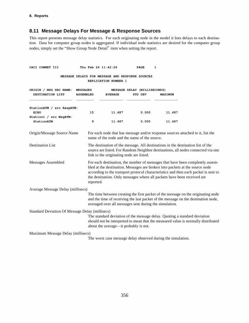
8. Reports
destina-
t the
e
ssem-e
node ode,
356
8.11 Message Delays For Message & Response SourcesThis report presents message delay statistics. For each originating node in the model it lists delays to eachtion. Data for computer group nodes is aggregated. If individual node statistics are desired for the computer groupnodes, simply set the “Show Group Node Detail” item when setting the report.
CACI COMNET III Thu Feb 24 11:42:26 PAGE 1
MESSAGE DELAYS FOR MESSAGE AND RESPONSE SOURCES
REPLICATION NUMBER 1
ORIGIN / MSG SRC NAME: MESSAGES MESSAGE DELAY (MILLISECONDS)
DESTINATION LIST ASSEMBLED AVERAGE STD DEV MAXIMUM
______________________ _________ ____________ ____________ ____________
StationATM / src RespATM:
ECHO 15 11.487 0.000 11.487
Station1 / src MsgATM:
StationATM 9 11.487 0.000 11.487
Origin/Message Source Name For each node that has message and/or response sources attached to it, lisname of the node and the name of the source.
Destination List The destination of the message. All destinations in the destination list of the source are listed. For Random Neighbor destinations, all nodes connected via onlink to the originating node are listed.
Messages Assembled For each destination, the number of messages that have been completely abled at the destination. Messages are broken into packets at the source nodaccording to the transport protocol characteristics and then each packet is sent tothe destination. Only messages where all packets have been received are reported.
Average Message Delay (millisecs)The time between creating the first packet of the message on the originating and the time of receiving the last packet of the message on the destination naveraged over all messages sent during the simulation.
Standard Deviation Of Message Delay (millisecs)The standard deviation of the message delay. Quoting a standard deviation should not be interpreted to mean that the measured value is normally distributed about the average—it probably is not.
Maximum Message Delay (millisecs)The worst case message delay observed during the simulation.
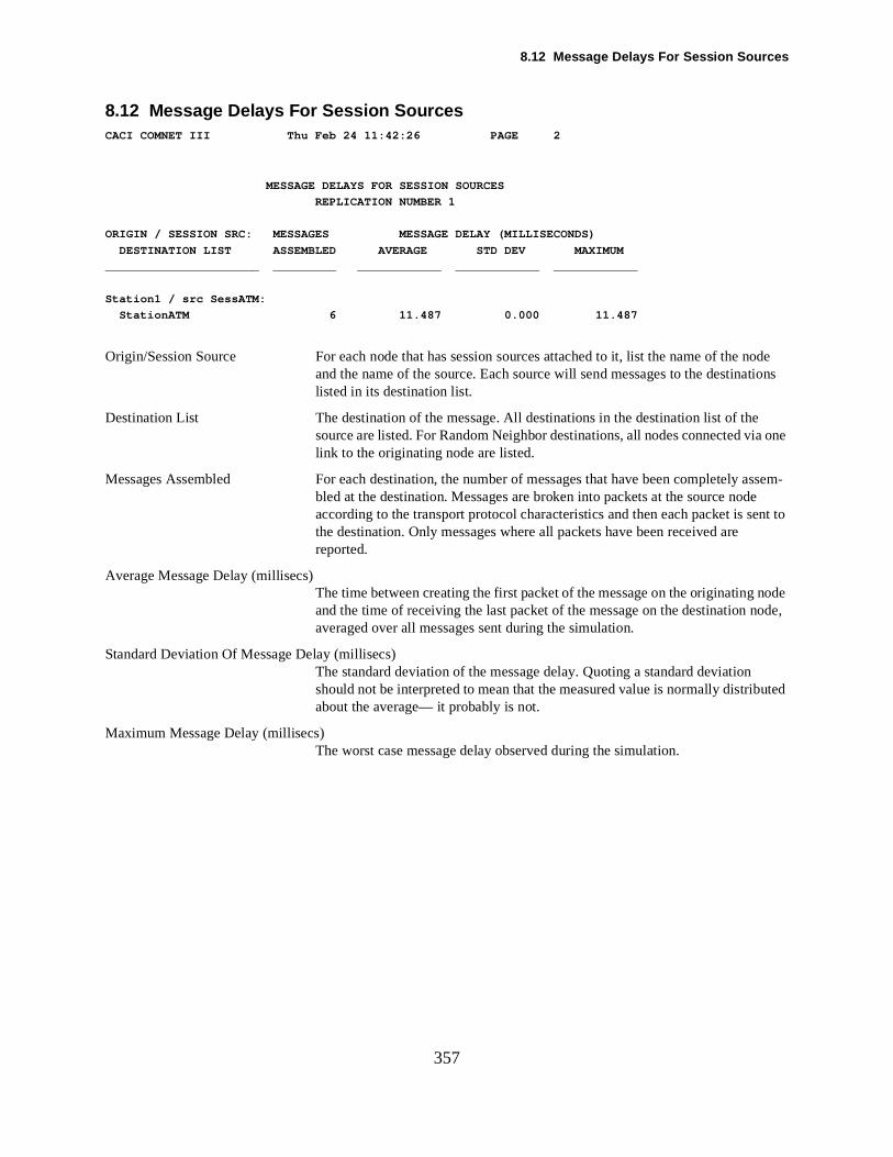
8.12 Message Delays For Session Sources
ode tions
e
ssem-e
node ode,
357
8.12 Message Delays For Session SourcesCACI COMNET III Thu Feb 24 11:42:26 PAGE 2
MESSAGE DELAYS FOR SESSION SOURCES
REPLICATION NUMBER 1
ORIGIN / SESSION SRC: MESSAGES MESSAGE DELAY (MILLISECONDS)
DESTINATION LIST ASSEMBLED AVERAGE STD DEV MAXIMUM
______________________ _________ ____________ ____________ ____________
Station1 / src SessATM:
StationATM 6 11.487 0.000 11.487
Origin/Session Source For each node that has session sources attached to it, list the name of the nand the name of the source. Each source will send messages to the destinalisted in its destination list.
Destination List The destination of the message. All destinations in the destination list of the source are listed. For Random Neighbor destinations, all nodes connected via onlink to the originating node are listed.
Messages Assembled For each destination, the number of messages that have been completely abled at the destination. Messages are broken into packets at the source nodaccording to the transport protocol characteristics and then each packet is sent tothe destination. Only messages where all packets have been received are reported.
Average Message Delay (millisecs)The time between creating the first packet of the message on the originating and the time of receiving the last packet of the message on the destination naveraged over all messages sent during the simulation.
Standard Deviation Of Message Delay (millisecs)The standard deviation of the message delay. Quoting a standard deviation should not be interpreted to mean that the measured value is normally distributed about the average— it probably is not.
Maximum Message Delay (millisecs)The worst case message delay observed during the simulation.
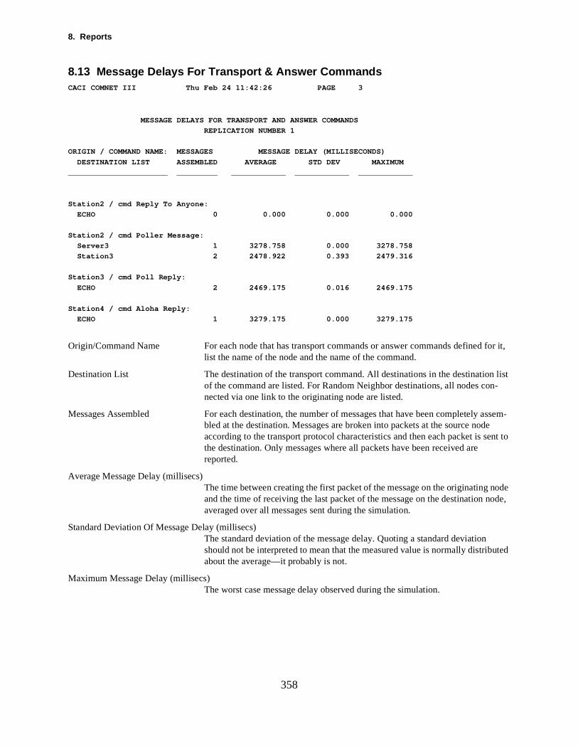
8. Reports
list
ssem-e
node ode,
358
8.13 Message Delays For Transport & Answer CommandsCACI COMNET III Thu Feb 24 11:42:26 PAGE 3
MESSAGE DELAYS FOR TRANSPORT AND ANSWER COMMANDS
REPLICATION NUMBER 1
ORIGIN / COMMAND NAME: MESSAGES MESSAGE DELAY (MILLISECONDS)
DESTINATION LIST ASSEMBLED AVERAGE STD DEV MAXIMUM
______________________ _________ ____________ ____________ ____________
Station2 / cmd Reply To Anyone:
ECHO 0 0.000 0.000 0.000
Station2 / cmd Poller Message:
Server3 1 3278.758 0.000 3278.758
Station3 2 2478.922 0.393 2479.316
Station3 / cmd Poll Reply:
ECHO 2 2469.175 0.016 2469.175
Station4 / cmd Aloha Reply:
ECHO 1 3279.175 0.000 3279.175
Origin/Command Name For each node that has transport commands or answer commands defined for it, list the name of the node and the name of the command.
Destination List The destination of the transport command. All destinations in the destinationof the command are listed. For Random Neighbor destinations, all nodes con-nected via one link to the originating node are listed.
Messages Assembled For each destination, the number of messages that have been completely abled at the destination. Messages are broken into packets at the source nodaccording to the transport protocol characteristics and then each packet is sent tothe destination. Only messages where all packets have been received are reported.
Average Message Delay (millisecs)The time between creating the first packet of the message on the originating and the time of receiving the last packet of the message on the destination naveraged over all messages sent during the simulation.
Standard Deviation Of Message Delay (millisecs)The standard deviation of the message delay. Quoting a standard deviation should not be interpreted to mean that the measured value is normally distributed about the average—it probably is not.
Maximum Message Delay (millisecs)The worst case message delay observed during the simulation.
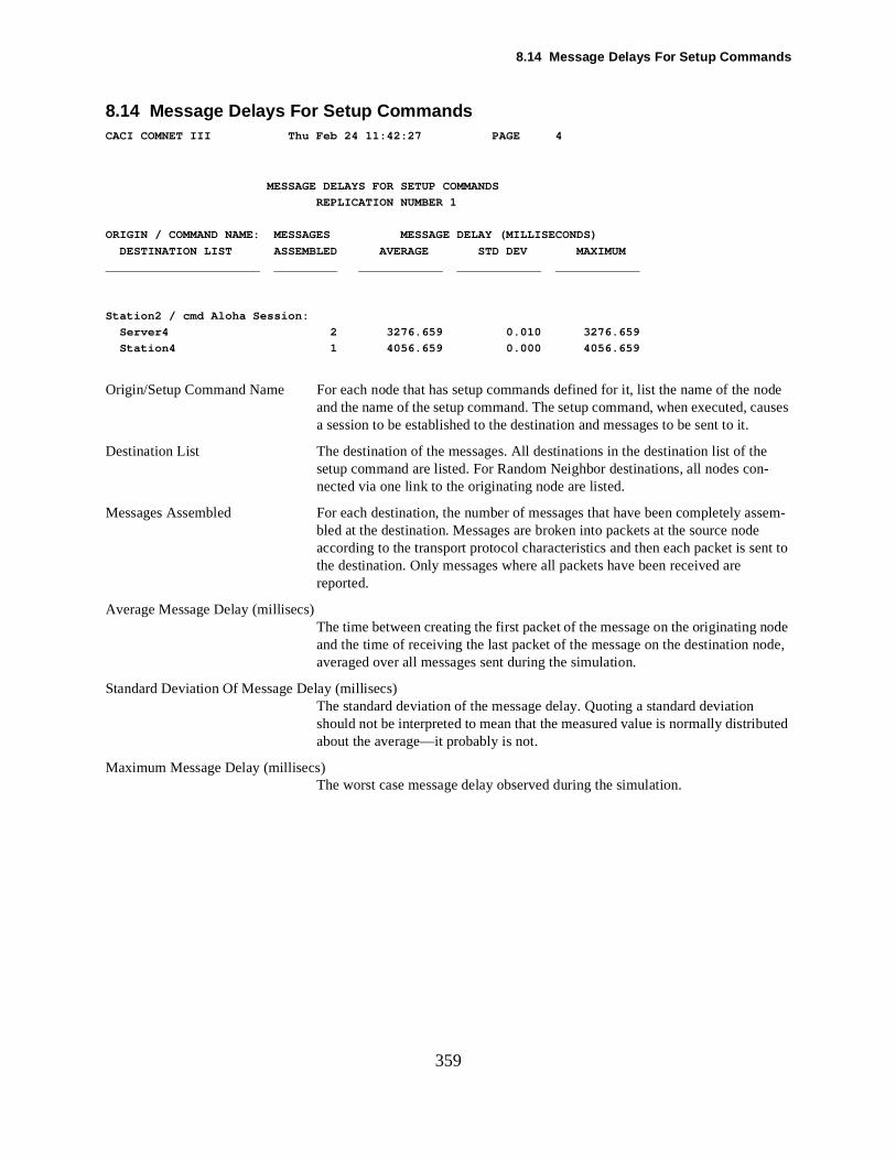
8.14 Message Delays For Setup Commands
ode auses
n-
ssem-e
node ode,
359
8.14 Message Delays For Setup CommandsCACI COMNET III Thu Feb 24 11:42:27 PAGE 4
MESSAGE DELAYS FOR SETUP COMMANDS
REPLICATION NUMBER 1
ORIGIN / COMMAND NAME: MESSAGES MESSAGE DELAY (MILLISECONDS)
DESTINATION LIST ASSEMBLED AVERAGE STD DEV MAXIMUM
______________________ _________ ____________ ____________ ____________
Station2 / cmd Aloha Session:
Server4 2 3276.659 0.010 3276.659
Station4 1 4056.659 0.000 4056.659
Origin/Setup Command Name For each node that has setup commands defined for it, list the name of the nand the name of the setup command. The setup command, when executed, ca session to be established to the destination and messages to be sent to it.
Destination List The destination of the messages. All destinations in the destination list of thesetup command are listed. For Random Neighbor destinations, all nodes conected via one link to the originating node are listed.
Messages Assembled For each destination, the number of messages that have been completely abled at the destination. Messages are broken into packets at the source nodaccording to the transport protocol characteristics and then each packet is sent tothe destination. Only messages where all packets have been received are reported.
Average Message Delay (millisecs)The time between creating the first packet of the message on the originating and the time of receiving the last packet of the message on the destination naveraged over all messages sent during the simulation.
Standard Deviation Of Message Delay (millisecs)The standard deviation of the message delay. Quoting a standard deviation should not be interpreted to mean that the measured value is normally distributed about the average—it probably is not.
Maximum Message Delay (millisecs)The worst case message delay observed during the simulation.
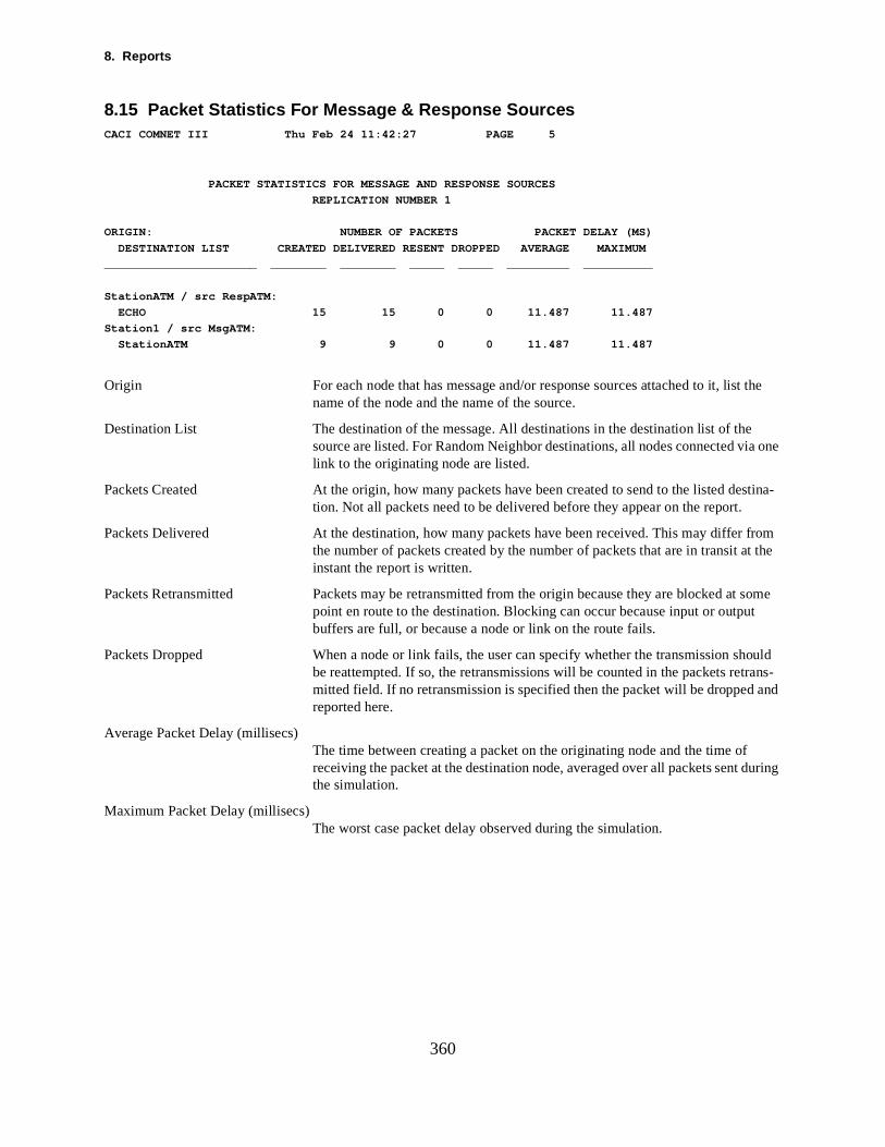
8. Reports
t the
e
tina-
om t the
ome t
uld ans-and
uring
360
8.15 Packet Statistics For Message & Response SourcesCACI COMNET III Thu Feb 24 11:42:27 PAGE 5
PACKET STATISTICS FOR MESSAGE AND RESPONSE SOURCES
REPLICATION NUMBER 1
ORIGIN: NUMBER OF PACKETS PACKET DELAY (MS)
DESTINATION LIST CREATED DELIVERED RESENT DROPPED AVERAGE MAXIMUM
______________________ ________ ________ _____ _____ _________ __________
StationATM / src RespATM:
ECHO 15 15 0 0 11.487 11.487
Station1 / src MsgATM:
StationATM 9 9 0 0 11.487 11.487
Origin For each node that has message and/or response sources attached to it, lisname of the node and the name of the source.
Destination List The destination of the message. All destinations in the destination list of the source are listed. For Random Neighbor destinations, all nodes connected via onlink to the originating node are listed.
Packets Created At the origin, how many packets have been created to send to the listed destion. Not all packets need to be delivered before they appear on the report.
Packets Delivered At the destination, how many packets have been received. This may differ frthe number of packets created by the number of packets that are in transit ainstant the report is written.
Packets Retransmitted Packets may be retransmitted from the origin because they are blocked at spoint en route to the destination. Blocking can occur because input or outpubuffers are full, or because a node or link on the route fails.
Packets Dropped When a node or link fails, the user can specify whether the transmission shobe reattempted. If so, the retransmissions will be counted in the packets retrmitted field. If no retransmission is specified then the packet will be dropped reported here.
Average Packet Delay (millisecs)The time between creating a packet on the originating node and the time of receiving the packet at the destination node, averaged over all packets sent dthe simulation.
Maximum Packet Delay (millisecs)The worst case packet delay observed during the simulation.
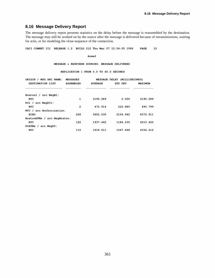
8.16 Message Delivery Report
estination.s, waiting
361
8.16 Message Delivery ReportThe message delivery report presents statistics on the delay before the message is reassembled by the dThe message may still be worked on by the source after the message is delivered because of retransmissionfor acks, or for modeling the close-sequence of the connection.
CACI COMNET III RELEASE 1.2 BUILD 212 Thu Mar 07 12:54:05 1996 PAGE 12
Acme2
MESSAGE + RESPONSE SOURCES: MESSAGE DELIVERED
REPLICATION 1 FROM 0.0 TO 60.0 SECONDS
ORIGIN / MSG SRC NAME: MESSAGES MESSAGE DELAY (MILLISECONDS)
DESTINATION LIST ASSEMBLED AVERAGE STD DEV MAXIMUM
______________________ _________ ____________ ____________ ____________
Boston1 / src MsgB1:
NYC 1 3190.089 0.000 3190.089
DC1 / src MsgDC1:
NYC 2 472.914 222.885 695.799
NYC / src Authorization:
ECHO 228 3602.530 2104.942 8372.911
BostonATMs / src MsgBoston:
NYC 122 1937.642 1184.235 4510.420
DCATMs / src MsgDC:
NYC 115 1618.511 1047.468 4332.212

8. Reports
s such as a blocked
362
8.17 Transport Retransmission ReportThis report presents retransmission statistics when blocked packets are retransmitted. It reports on quantitiethe number of times a packet has to be retransmitted, and the number of packets that are retransmitted whenpacket occurs.
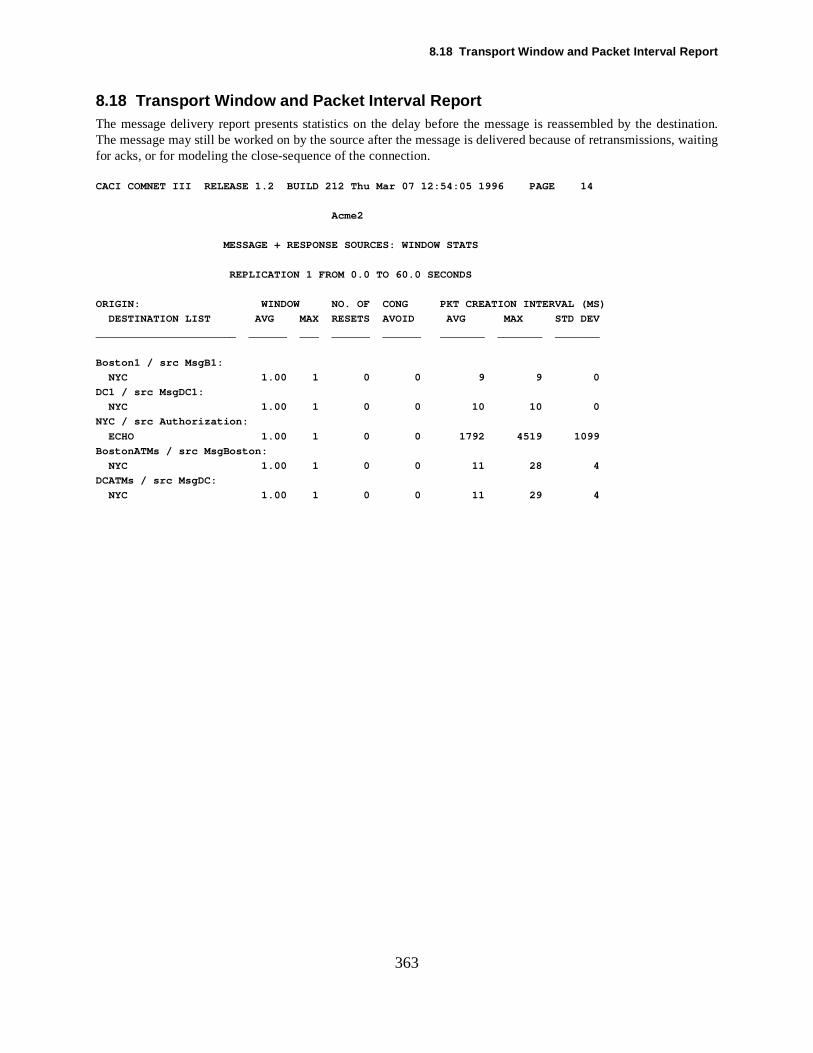
8.18 Transport Window and Packet Interval Report
estination.s, waiting
363
8.18 Transport Window and Packet Interval ReportThe message delivery report presents statistics on the delay before the message is reassembled by the dThe message may still be worked on by the source after the message is delivered because of retransmissionfor acks, or for modeling the close-sequence of the connection.
CACI COMNET III RELEASE 1.2 BUILD 212 Thu Mar 07 12:54:05 1996 PAGE 14
Acme2
MESSAGE + RESPONSE SOURCES: WINDOW STATS
REPLICATION 1 FROM 0.0 TO 60.0 SECONDS
ORIGIN: WINDOW NO. OF CONG PKT CREATION INTERVAL (MS)
DESTINATION LIST AVG MAX RESETS AVOID AVG MAX STD DEV
______________________ ______ ___ ______ ______ _______ _______ _______
Boston1 / src MsgB1:
NYC 1.00 1 0 0 9 9 0
DC1 / src MsgDC1:
NYC 1.00 1 0 0 10 10 0
NYC / src Authorization:
ECHO 1.00 1 0 0 1792 4519 1099
BostonATMs / src MsgBoston:
NYC 1.00 1 0 0 11 28 4
DCATMs / src MsgDC:
NYC 1.00 1 0 0 11 29 4
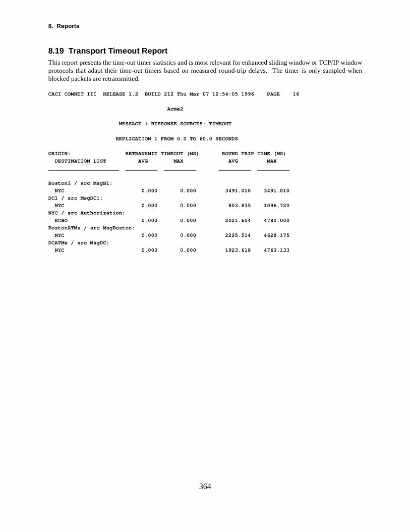
8. Reports
windown
364
8.19 Transport Timeout ReportThis report presents the time-out timer statistics and is most relevant for enhanced sliding window or TCP/IP protocols that adapt their time-out timers based on measured round-trip delays. The timer is only sampled wheblocked packets are retransmitted.
CACI COMNET III RELEASE 1.2 BUILD 212 Thu Mar 07 12:54:05 1996 PAGE 16
Acme2
MESSAGE + RESPONSE SOURCES: TIMEOUT
REPLICATION 1 FROM 0.0 TO 60.0 SECONDS
ORIGIN: RETRANSMIT TIMEOUT (MS) ROUND TRIP TIME (MS)
DESTINATION LIST AVG MAX AVG MAX
______________________ __________ __________ __________ __________
Boston1 / src MsgB1:
NYC 0.000 0.000 3491.010 3491.010
DC1 / src MsgDC1:
NYC 0.000 0.000 803.835 1096.720
NYC / src Authorization:
ECHO 0.000 0.000 2021.604 4780.000
BostonATMs / src MsgBoston:
NYC 0.000 0.000 2225.514 4628.175
DCATMs / src MsgDC:
NYC 0.000 0.000 1923.618 4763.133
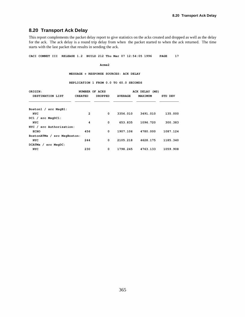
8.20 Transport Ack Delay
the delayhe time
365
8.20 Transport Ack DelayThis report complements the packet delay report to give statistics on the acks created and dropped as well asfor the ack. The ack delay is a round trip delay from when the packet started to when the ack returned. Tstarts with the last packet that results in sending the ack.
CACI COMNET III RELEASE 1.2 BUILD 212 Thu Mar 07 12:54:05 1996 PAGE 17
Acme2
MESSAGE + RESPONSE SOURCES: ACK DELAY
REPLICATION 1 FROM 0.0 TO 60.0 SECONDS
ORIGIN: NUMBER OF ACKS ACK DELAY (MS)
DESTINATION LIST CREATED DROPPED AVERAGE MAXIMUM STD DEV
______________________ ________ ________ __________ __________ __________
Boston1 / src MsgB1:
NYC 2 0 3356.010 3491.010 135.000
DC1 / src MsgDC1:
NYC 4 0 653.835 1096.720 300.383
NYC / src Authorization:
ECHO 456 0 1907.106 4780.000 1087.124
BostonATMs / src MsgBoston:
NYC 244 0 2105.218 4628.175 1185.340
DCATMs / src MsgDC:
NYC 230 0 1798.245 4763.133 1059.908

8. Reports
assembly
service
366
8.21 Transport Assembly IntervalThis report provides statistics on the delay between when packets are assembled at the destination. The interval can result from delay variation through the network (due to varying buffer delays) or it can result from con-gestion on the destination node. In cell-based networks, this measure is the cell-delay variation, a quality ofmeasure for these services.
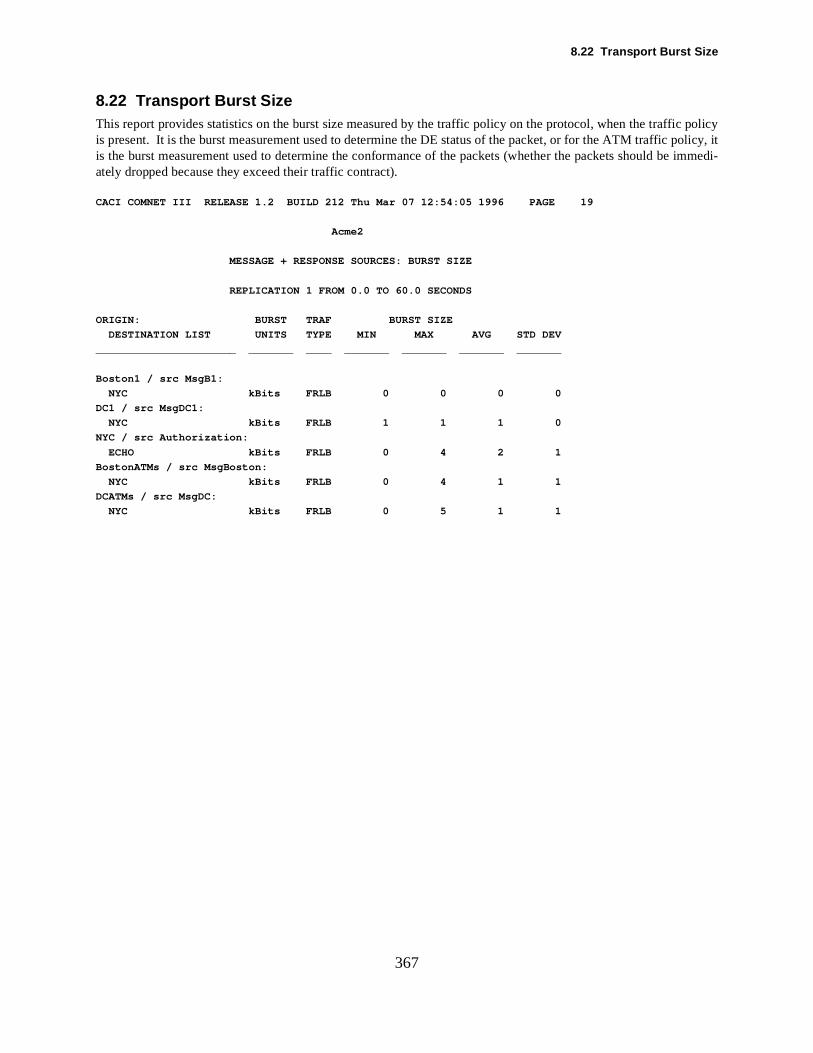
8.22 Transport Burst Size
policyolicy, it
e immedi-
367
8.22 Transport Burst SizeThis report provides statistics on the burst size measured by the traffic policy on the protocol, when the trafficis present. It is the burst measurement used to determine the DE status of the packet, or for the ATM traffic pis the burst measurement used to determine the conformance of the packets (whether the packets should bately dropped because they exceed their traffic contract).
CACI COMNET III RELEASE 1.2 BUILD 212 Thu Mar 07 12:54:05 1996 PAGE 19
Acme2
MESSAGE + RESPONSE SOURCES: BURST SIZE
REPLICATION 1 FROM 0.0 TO 60.0 SECONDS
ORIGIN: BURST TRAF BURST SIZE
DESTINATION LIST UNITS TYPE MIN MAX AVG STD DEV
______________________ _______ ____ _______ _______ _______ _______
Boston1 / src MsgB1:
NYC kBits FRLB 0 0 0 0
DC1 / src MsgDC1:
NYC kBits FRLB 1 1 1 0
NYC / src Authorization:
ECHO kBits FRLB 0 4 2 1
BostonATMs / src MsgBoston:
NYC kBits FRLB 0 4 1 1
DCATMs / src MsgDC:
NYC kBits FRLB 0 5 1 1

8. Reports
proto-ECN.
368
8.23 Transport Packet Flag ReportThis report provides information about the flags set on the packet: the DE (descard eligibility) flag from thecol’s traffic policing algorithm, and the congestion flags set by the buffers when they are set up for FECN or BThe report also shows the number of pacets blocked, separated by their DE status.
8.24 Transport Packet Size
t eithercol win-
nitources.
369
8.24 Transport Packet SizeThis report provides two functions.
The first function is to report on the maximum packet and window size resulting from the socket constraints aend. This is important because the sockets' packet or window size constraint can reduce the maximum protodow or packet size.
The second function is to report on the packet sizes that were actually created. This part is most useful for mooringthe sizes for message that are smaller than the packet sizes or for monitoring the sizes from external traffic s
CACI COMNET III RELEASE 1.2 BUILD 212 Thu Mar 07 12:56:14 1996 PAGE 39
Acme2
MESSAGE + RESPONSE SOURCES: PKT SIZE
REPLICATION 2 FROM 60.0 TO 120.0 SECONDS
ORIGIN: MAX MAX PACKET SIZE
DESTINATION LIST PKT WINDOW MIN AVG MAX
______________________ _______ _______ _______ _______ _______
Boston1 / src MsgB1:
NYC 128 1 63 75 86
DC1 / src MsgDC1:
NYC 128 1 53 71 86
NYC / src Authorization:
ECHO 128 1 50 83 120
BostonATMs / src MsgBoston:
NYC 128 1 51 85 120
DCATMs / src MsgDC:
NYC 128 1 51 86 119
8. Reports
ode rans-on-
urce nk to
tina-
m t the
ome t
uld ns-and
uring
370
8.25 Packet Delays For Session SourcesCACI COMNET III Thu Feb 24 11:42:27 PAGE 6
PACKET DELAYS FOR SESSION SOURCES
REPLICATION NUMBER 1
ORIGIN / SESSION SRC: NUMBER OF PACKETS PACKET DELAY (MS)
DESTINATION LIST CREATED DELIVERED RESENT DROPPED AVERAGE MAXIMUM
______________________ ________ ________ _____ _____ _________ __________
Station1 / src SessATM:
StationATM 6 6 0 0 11.487 11.487
Origin/Session Source Name For each node that has session sources attached to it, list the name of the nand the name of the source. A session source will create a setup packet to tmit to the destination to establish a route, followed by messages, once the cnect packet has been received back from the destination.
Destination List The destination of the session. All destinations in the destination list of the soare listed. For Random Neighbor destinations, all nodes connected via one lithe originating node are listed.
Packets Created At the origin, how many packets have been created to send to the listed destion. Not all packets need to be delivered before they appear on the report.
Packets Delivered At the destination, how many packets have been received. This may differ frothe number of packets created by the number of packets that are in transit ainstant the report is written.
Packets Retransmitted Packets may be retransmitted from the origin because they are blocked at spoint en route to the destination. Blocking can occur because input or outpubuffers are full, or because a node or link on the route fails.
Packets Dropped When a node or link fails, the user can specify whether the transmission shobe reattempted. If so the retransmissions will be counted in the packets retramitted field. If no retransmission is specified, then the packet will be dropped reported here.
Average Packet Delay (millisecs)The time between creating a packet on the originating node and the time of receiving the packet at the destination node, averaged over all packets sent dthe simulation.
Maximum Packet Delay (millisecs)The worst case packet delay observed during the simulation.
8.26 Packet Delays For Tr ansport & Answer Commands
d via
tina-
m t the
ome t
uld ns-
and
uring
371
8.26 Packet Delays For Transport & Answer CommandsCACI COMNET III Thu Feb 24 11:42:27 PAGE 7
PACKET DELAYS FOR TRANSPORT AND ANSWER COMMANDS
REPLICATION NUMBER 1
ORIGIN / COMMAND NAME: NUMBER OF PACKETS PACKET DELAY (MS)
DESTINATION LIST CREATED DELIVERED RESENT DROPPED AVERAGE MAXIMUM
______________________ ________ ________ _____ _____ _________ __________
Station2 / cmd Reply To Anyone:
ECHO 0 0 0 0 0.000 0.000
Station2 / cmd Poller Message:
Server3 1 1 0 0 3277.758 3277.758
Station3 2 2 0 0 2477.922 2478.316
Station3 / cmd Poll Reply:
ECHO 2 2 0 0 2469.175 2469.175
Station4 / cmd Aloha Reply:
ECHO 1 1 0 0 3279.175 3279.175
Origin/Command Name For each node that has transport and/or answer commands, list the name of the node and the name of the command.
Destination List The destination of the command. All destinations in the destination list of thecommand are listed. For Random Neighbor destinations, all nodes connecteone link to the originating node are listed.
Packets Created At the origin, how many packets have been created to send to the listed destion. Not all packets need to be delivered before they appear on the report.
Packets Delivered At the destination how many packets have been received. This may differ frothe number of packets created by the number of packets that are in transit ainstant the report is written.
Packets Retransmitted Packets may be retransmitted from the origin because they are blocked at spoint en route to the destination. Blocking can occur because input or outpubuffers are full, or because a node or link on the route fails.
Packets Dropped When a node or link fails, the user can specify whether the transmission shobe reattempted. If so the retransmissions will be counted in the packets retramitted field. If no retransmission is specified then the packet will be dropped reported here.
Average Packet Delay (millisecs)The time between creating a packet on the originating node and the time of receiving the packet at the destination node, averaged over all packets sent dthe simulation.
Maximum Packet Delay (millisecs)The worst case packet delay observed during the simulation.
8. Reports
node t to he
urce nk to
tina-
om t the
ome t
uld ans-and
uring
372
8.27 Packet Delays For Setup CommandsCACI COMNET III Thu Feb 24 11:42:27 PAGE 8
PACKET DELAYS FOR SETUP COMMANDS
REPLICATION NUMBER 1
ORIGIN / COMMAND NAME: NUMBER OF PACKETS PACKET DELAY (MS)
DESTINATION LIST CREATED DELIVERED RESENT DROPPED AVERAGE MAXIMUM
______________________ ________ ________ _____ _____ _________ __________
Station2 / cmd Aloha Session:
Server4 2 2 0 0 3276.659 3276.659
Station4 1 1 0 0 4056.659 4056.659
Origin/Setup Command Name For each node that has setup commands attached to it, list the name of the and the name of the command. A setup command will create a setup packetransmit to the destination to establish a route, followed by messages once tconnect packet has been received back from the destination.
Destination List The destination of the session. All destinations in the destination list of the soare listed. For Random Neighbor destinations, all nodes connected via one lithe originating node are listed.
Packets Created At the origin, how many packets have been created to send to the listed destion. Not all packets need to be delivered before they appear on the report.
Packets Delivered At the destination how many packets have been received. This may differ frthe number of packets created, by the number of packets that are in transit ainstant the report is written.
Packets Retransmitted Packets may be retransmitted from the origin because they are blocked at spoint en route to the destination. Blocking can occur because input or outpubuffers are full, or because a node or link on the route fails.
Packets Dropped When a node or link fails, the user can specify whether the transmission shobe re-attempted. If so the retransmissions will be counted in the packets retrmitted field. If no retransmission is specified then the packet will be dropped reported here.
Average Packet Delay (millisecs)The time between creating a packet on the originating node and the time of receiving the packet at the destination node, averaged over all packets sent dthe simulation.
Maximum Packet Delay (millisecs)The worst case packet delay observed during the simulation.
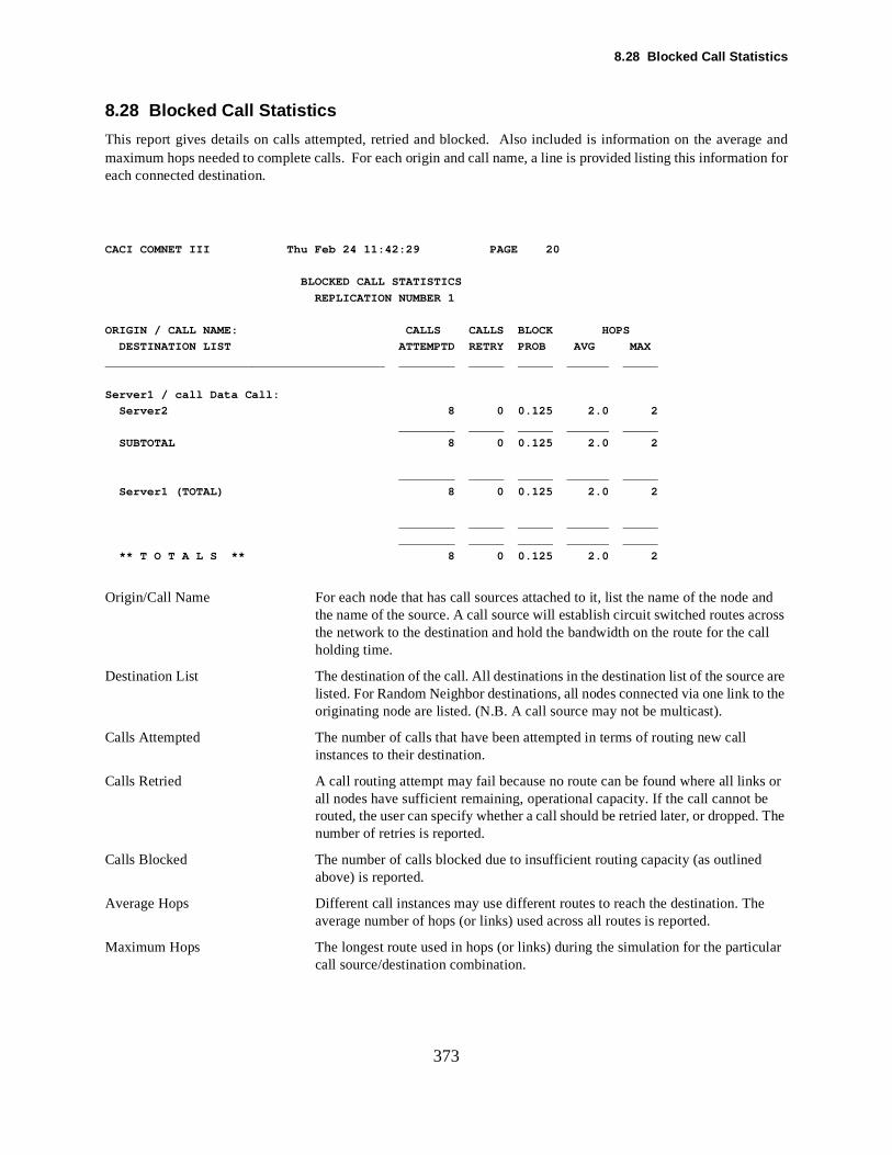
8.28 Blocked Call Statistics
ge and
and ross ll
are he
or e . The
e
lar
373
8.28 Blocked Call Statistics
This report gives details on calls attempted, retried and blocked. Also included is information on the averamaximum hops needed to complete calls. For each origin and call name, a line is provided listing this information foreach connected destination.
CACI COMNET III Thu Feb 24 11:42:29 PAGE 20
BLOCKED CALL STATISTICS
REPLICATION NUMBER 1
ORIGIN / CALL NAME: CALLS CALLS BLOCK HOPS
DESTINATION LIST ATTEMPTD RETRY PROB AVG MAX
________________________________________ ________ _____ _____ ______ _____
Server1 / call Data Call:
Server2 8 0 0.125 2.0 2
________ _____ _____ ______ _____
SUBTOTAL 8 0 0.125 2.0 2
________ _____ _____ ______ _____
Server1 (TOTAL) 8 0 0.125 2.0 2
________ _____ _____ ______ _____
________ _____ _____ ______ _____
** T O T A L S ** 8 0 0.125 2.0 2
Origin/Call Name For each node that has call sources attached to it, list the name of the node the name of the source. A call source will establish circuit switched routes acthe network to the destination and hold the bandwidth on the route for the caholding time.
Destination List The destination of the call. All destinations in the destination list of the sourcelisted. For Random Neighbor destinations, all nodes connected via one link to toriginating node are listed. (N.B. A call source may not be multicast).
Calls Attempted The number of calls that have been attempted in terms of routing new call instances to their destination.
Calls Retried A call routing attempt may fail because no route can be found where all linksall nodes have sufficient remaining, operational capacity. If the call cannot brouted, the user can specify whether a call should be retried later, or droppednumber of retries is reported.
Calls Blocked The number of calls blocked due to insufficient routing capacity (as outlined above) is reported.
Average Hops Different call instances may use different routes to reach the destination. Thaverage number of hops (or links) used across all routes is reported.
Maximum Hops The longest route used in hops (or links) during the simulation for the particucall source/destination combination.
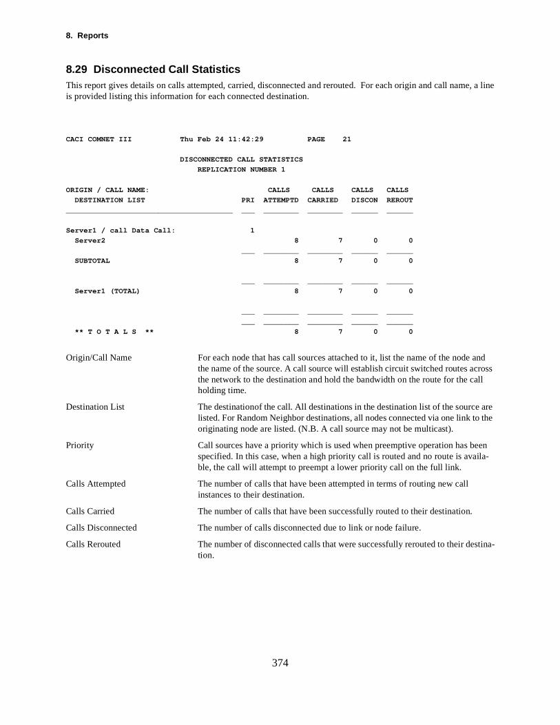
8. Reports
e, a line
and ross
he
een ila-
stina-
374
8.29 Disconnected Call StatisticsThis report gives details on calls attempted, carried, disconnected and rerouted. For each origin and call namis provided listing this information for each connected destination.
CACI COMNET III Thu Feb 24 11:42:29 PAGE 21
DISCONNECTED CALL STATISTICS
REPLICATION NUMBER 1
ORIGIN / CALL NAME: CALLS CALLS CALLS CALLS
DESTINATION LIST PRI ATTEMPTD CARRIED DISCON REROUT
______________________________________ ___ ________ ________ ______ ______
Server1 / call Data Call: 1
Server2 8 7 0 0
___ ________ ________ ______ ______
SUBTOTAL 8 7 0 0
___ ________ ________ ______ ______
Server1 (TOTAL) 8 7 0 0
___ ________ ________ ______ ______
___ ________ ________ ______ ______
** T O T A L S ** 8 7 0 0
Origin/Call Name For each node that has call sources attached to it, list the name of the node the name of the source. A call source will establish circuit switched routes acthe network to the destination and hold the bandwidth on the route for the call holding time.
Destination List The destinationof the call. All destinations in the destination list of the source are listed. For Random Neighbor destinations, all nodes connected via one link to toriginating node are listed. (N.B. A call source may not be multicast).
Priority Call sources have a priority which is used when preemptive operation has bspecified. In this case, when a high priority call is routed and no route is avable, the call will attempt to preempt a lower priority call on the full link.
Calls Attempted The number of calls that have been attempted in terms of routing new call instances to their destination.
Calls Carried The number of calls that have been successfully routed to their destination.
Calls Disconnected The number of calls disconnected due to link or node failure.
Calls Rerouted The number of disconnected calls that were successfully rerouted to their detion.
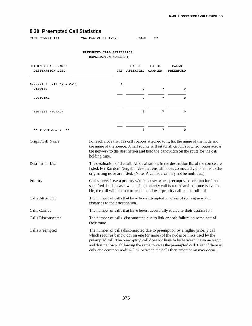
8.30 Preempted Call Statistics
and ross ll
are he
een ila-
f
origin re is
r.
375
8.30 Preempted Call StatisticsCACI COMNET III Thu Feb 24 11:42:29 PAGE 22
PREEMPTED CALL STATISTICS
REPLICATION NUMBER 1
ORIGIN / CALL NAME: CALLS CALLS CALLS
DESTINATION LIST PRI ATTEMPTED CARRIED PREEMPTED
__________________________________________ ___ _________ ________ _________
Server1 / call Data Call: 1
Server2 8 7 0
___ _________ ________ _________
SUBTOTAL 8 7 0
___ _________ ________ _________
Server1 (TOTAL) 8 7 0
___ _________ ________ _________
___ _________ ________ _________
** T O T A L S ** 8 7 0
Origin/Call Name For each node that has call sources attached to it, list the name of the node the name of the source. A call source will establish circuit switched routes acthe network to the destination and hold the bandwidth on the route for the caholding time.
Destination List The destination of the call. All destinations in the destination list of the sourcelisted. For Random Neighbor destinations, all nodes connected via one link to toriginating node are listed. (Note: A call source may not be multicast).
Priority Call sources have a priority which is used when preemptive operation has bspecified. In this case, when a high priority call is routed and no route is avable, the call will attempt to preempt a lower priority call on the full link.
Calls Attempted The number of calls that have been attempted in terms of routing new call instances to their destination.
Calls Carried The number of calls that have been successfully routed to their destination.
Calls Disconnected The number of calls disconnected due to link or node failure on some part otheir route.
Calls Preempted The number of calls disconnected due to preemption by a higher priority callwhich requires bandwidth on one (or more) of the nodes or links used by thepreempted call. The preempting call does not have to be between the same and destination or following the same route as the preempted call. Even if theonly one common node or link between the calls then preemption may occu
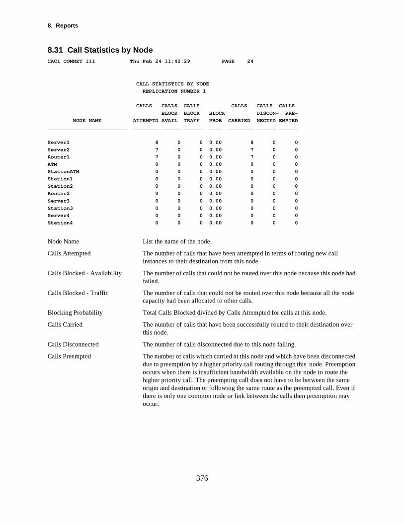
8. Reports
e had
node
ver
cted
e n if
ay
376
8.31 Call Statistics by NodeCACI COMNET III Thu Feb 24 11:42:29 PAGE 24
CALL STATISTICS BY NODE
REPLICATION NUMBER 1
CALLS CALLS CALLS CALLS CALLS CALLS
BLOCK BLOCK BLOCK DISCON- PRE-
NODE NAME ATTEMPTD AVAIL TRAFF PROB CARRIED NECTED EMPTED
_________________________ ________ ______ ______ ____ ________ ______ ______
Server1 8 0 0 0.00 8 0 0
Server2 7 0 0 0.00 7 0 0
Router1 7 0 0 0.00 7 0 0
ATM 0 0 0 0.00 0 0 0
StationATM 0 0 0 0.00 0 0 0
Station1 0 0 0 0.00 0 0 0
Station2 0 0 0 0.00 0 0 0
Router2 0 0 0 0.00 0 0 0
Server3 0 0 0 0.00 0 0 0
Station3 0 0 0 0.00 0 0 0
Server4 0 0 0 0.00 0 0 0
Station4 0 0 0 0.00 0 0 0
Node Name List the name of the node.
Calls Attempted The number of calls that have been attempted in terms of routing new call instances to their destination from this node.
Calls Blocked - Availability The number of calls that could not be routed over this node because this nodfailed.
Calls Blocked - Traffic The number of calls that could not be routed over this node because all the capacity had been allocated to other calls.
Blocking Probability Total Calls Blocked divided by Calls Attempted for calls at this node.
Calls Carried The number of calls that have been successfully routed to their destination othis node.
Calls Disconnected The number of calls disconnected due to this node failing.
Calls Preempted The number of calls which carried at this node and which have been disconnedue to preemption by a higher priority call routing through this node. Preemption occurs when there is insufficient bandwidth available on the node to route the higher priority call. The preempting call does not have to be between the samorigin and destination or following the same route as the preempted call. Evethere is only one common node or link between the calls then preemption moccur.
8.32 Call Statistics by Link
ad
nd-
on
ver
to
cted nk. ation om-
377
8.32 Call Statistics by LinkCACI COMNET III Thu Feb 24 11:42:29 PAGE 23
CALL STATISTICS BY LINK
REPLICATION NUMBER 1
CALLS CALLS CALLS CALLS CALLS CALLS
BLOCK BLOCK BLOCK DISCON- PRE-
LINK NAME ATTEMPTD AVAIL TRAFF PROB CARRIED NECTED EMPTED
_________________________ ________ ______ ______ ____ ________ ______ ______
Link3 7 0 0 0.00 7 0 0
Link2 7 0 0 0.00 7 0 0
LinkB 0 0 0 0.00 0 0 0
LinkA 0 0 0 0.00 0 0 0
Link1 0 0 0 0.00 0 0 0
Link Name List the name of the link.
Calls Attempted The number of calls that have been attempted in terms of routing call instances to their destination over this link. The origin and destination are not necessarily connected to this link—it may be an intermediate part of the route.
Calls Blocked - Availability The number of calls that could not be routed over this link because this link hfailed.
Calls Blocked - Traffic The number of calls that could not be routed over this link because all its bawidth had been allocated to other calls.
Blocking Probability Total Calls Blocked divided by Calls Attempted, for calls blocked and carriedthis link.
Calls Carried The number of calls that have been successfully routed to their destination othis link.
Calls Disconnected The number of calls carried on this link and subsequently disconnected due failure of this link.
Calls Preempted The number of calls which carried on this link and which have been disconnedue to preemption by a higher priority call which requires bandwidth on this liThe preempting call does not have to be between the same origin and destinor following the same route as the preempted call. Even if there is only one cmon node or link between the calls then preemption may occur.
8. Reports
use
vail-
e is
tage.
378
8.33 Node Utilization Statistics For CallsCACI COMNET III Thu Feb 24 11:42:30 PAGE 26
NODE UTILIZATION STATISTICS FOR CALLS
REPLICATION NUMBER 1
% NODE BANDWIDTH USED (KBPS) NODE
NODE NAME AVAIL FAILS AVERAGE STD DEV MAXIMUM UTIL %
___________________________ ______ _____ ________ _______ ________ ______
Server1 100.00 0 5 3 10 0.05
Server2 100.00 0 5 3 8 0.05
Router1 100.00 0 5 3 8 0.05
ATM 100.00 0 0 0 0 0.00
StationATM 100.00 0 0 0 0 0.00
Station1 100.00 0 0 0 0 0.00
Station2 100.00 0 0 0 0 0.00
Router2 100.00 0 0 0 0 0.00
Server3 100.00 0 0 0 0 0.00
Station3 100.00 0 0 0 0 0.00
Server4 100.00 0 0 0 0 0.00
Station4 100.00 0 0 0 0 0.00
Node Name List the name of the node. Each node has a bandwidth capacity which it mayto carry call traffic.
% Availability A node is not available when it is in the failed state. The percentage of time aable is reported. This is the Up Time divided by the Run Length.
Node Failures The number of failures that occurred in the simulation.
Average Bandwidth Used (Kbps)When calls are routed through the node, each call has a bandwidth requirement. The average total bandwidth requirement for all calls routed through the nodreported.
Standard Deviation Of Bandwidth Used (Kbps)The standard deviation of the bandwidth used. Quoting a standard deviationshould not be interpreted to mean that the measured value is normally distributed about the average—it probably is not.
Maximum Bandwidth Used (Kbps)The maximum peak bandwidth used on the node during the simulation.
Node Utilization Average Bandwidth Used/Total Available Bandwidth expressed as a percen
8.34 Link Utilization Statistics for Calls
raffic.
o
ail-
The ted.
tage.
379
8.34 Link Utilization Statistics for Calls
This report provides utilization rates and other statistics for each link's circuit switched call t
CACI COMNET III Thu Feb 24 11:42:29 PAGE 25
LINK UTILIZATION STATISTICS FOR CALLS
REPLICATION NUMBER 1
CIRCUIT CIRCUIT CIRCUIT
% GROUP BANDWIDTH USED (KBPS) GROUP
LINK NAME AVAIL FAILS AVERAGE STD DEV MAXIMUM UTIL %
___________________________ ______ _____ ________ _______ ________ ______
Link3 100.00 0 5 3 8 56.93
Link2 100.00 0 5 3 8 56.93
LinkB 100.00 0 0 0 0 0.00
LinkA 100.00 0 0 0 0 0.00
Link1 100.00 0 0 0 0 0.00
Link Name The name of the link. Each link has a bandwidth capacity which it may use tcarry call traffic. This is not shared with packet switched traffic.
Availability % A link is not available when it is in the failed state. The percentage of time avable is reported. This is the Up Time divided by the Run Length.
Link Failures The number of link failures that occurred in the simulation.
Average Bandwidth Used (Kbps)When calls are routed over the link, each call has a bandwidth requirement. average total bandwidth requirement for all calls routed over the link is repor
Standard Deviation Of Bandwidth Used (Kbps)The standard deviation of the bandwidth used. Quoting a standard deviationshould not be interpreted to mean that the measured value is normally distributed about the average—it probably is not.
Maximum Bandwidth Used (Kbps)The maximum peak bandwidth used on the link during the simulation.
Link Utilization Average Bandwidth Used/Total Available Bandwidth expressed as a percen
8. Reports
and mit to
urce nk to
nd a is fig-
back
uld bout
380
8.35 Setup Delays For Session SourcesCACI COMNET III Thu Feb 24 11:42:27 PAGE 11
SETUP DELAYS FOR SESSION SOURCES
REPLICATION NUMBER 1
ORIGIN / SESSION SRC: SESSIONS SETUP DELAY (MILLISECONDS)
DESTINATION LIST SETUP AVERAGE STD DEV MAXIMUM
______________________ _________ ____________ ____________ ____________
Station1 / src SessATM:
StationATM 6 1.436 0.000 1.436
Origin/Session Source Name For each node that has session sources attached to it, the name of the nodethe name of the source. A session source will create a setup packet to transthe destination to establish a route, followed by messages once the connectpacket has been received back from the destination.
Destination List The destination of the session. All destinations in the destination list of the soare listed. For Random Neighbor destinations, all nodes connected via one lithe originating node are listed.
Sessions Setup When a session is started a session setup packet is sent to the destination asession connect packet is returned. The session is then counted as setup Thure reports how many such setups occurred in the simulation.
Average Setup Delay (millisecs) The time difference between creating the session setup packet and receivingthe session connect packet.
Standard Deviation Of Setup Delay (millisecs)The standard deviation of the setup delay. Quoting a standard deviation shonot be interpreted to mean that the measured value is normally distributed athe average—it probably is not.
Maximum Setup Delay (millisecs)The worst case session setup delay observed during the simulation.
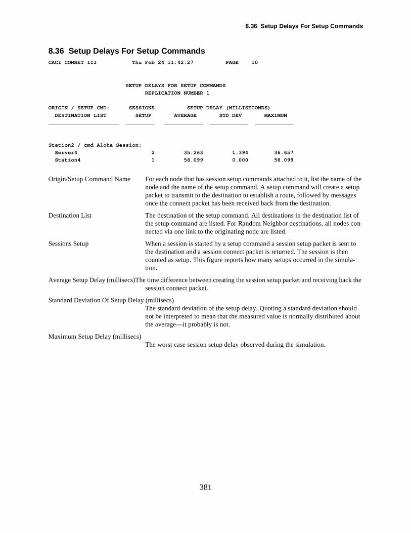
8.36 Setup Delays For Setup Commands
of the etup es
of con-
nt to n la-
back the
uld bout
381
8.36 Setup Delays For Setup CommandsCACI COMNET III Thu Feb 24 11:42:27 PAGE 10
SETUP DELAYS FOR SETUP COMMANDS
REPLICATION NUMBER 1
ORIGIN / SETUP CMD: SESSIONS SETUP DELAY (MILLISECONDS)
DESTINATION LIST SETUP AVERAGE STD DEV MAXIMUM
______________________ _________ ____________ ____________ ____________
Station2 / cmd Aloha Session:
Server4 2 35.263 1.394 36.657
Station4 1 58.099 0.000 58.099
Origin/Setup Command Name For each node that has session setup commands attached to it, list the namenode and the name of the setup command. A setup command will create a spacket to transmit to the destination to establish a route, followed by messagonce the connect packet has been received back from the destination.
Destination List The destination of the setup command. All destinations in the destination listthe setup command are listed. For Random Neighbor destinations, all nodesnected via one link to the originating node are listed.
Sessions Setup When a session is started by a setup command a session setup packet is sethe destination and a session connect packet is returned. The session is thecounted as setup. This figure reports how many setups occurred in the simution.
Average Setup Delay (millisecs)The time difference between creating the session setup packet and receiving session connect packet.
Standard Deviation Of Setup Delay (millisecs)The standard deviation of the setup delay. Quoting a standard deviation shonot be interpreted to mean that the measured value is normally distributed athe average—it probably is not.
Maximum Setup Delay (millisecs)The worst case session setup delay observed during the simulation.
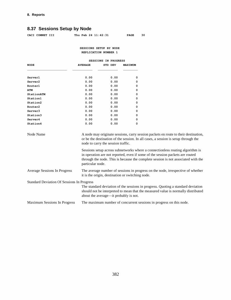
8. Reports
ation,
m h the
ation
382
8.37 Sessions Setup by NodeCACI COMNET III Thu Feb 24 11:42:31 PAGE 30
SESSIONS SETUP BY NODE
REPLICATION NUMBER 1
SESSIONS IN PROGRESS
NODE AVERAGE STD DEV MAXIMUM
______________________ ___________ ___________ ________
Server1 0.00 0.00 0
Server2 0.00 0.00 0
Router1 0.00 0.00 0
ATM 0.00 0.00 0
StationATM 0.00 0.00 0
Station1 0.00 0.00 0
Station2 0.00 0.00 0
Router2 0.00 0.00 0
Server3 0.00 0.00 0
Station3 0.00 0.00 0
Server4 0.00 0.00 0
Station4 0.00 0.00 0
Node Name A node may originate sessions, carry session packets en route to their destinor be the destination of the session. In all cases, a session is setup through the node to carry the session traffic.
Sessions setup across subnetworks where a connectionless routing algorith is in operation are not reported, even if some of the session packets are routedthrough the node. This is because the complete session is not associated witparticular node.
Average Sessions In Progress The average number of sessions in progress on the node, irrespective of whether it is the origin, destination or switching node.
Standard Deviation Of Sessions In ProgressThe standard deviation of the sessions in progress. Quoting a standard devishould not be interpreted to mean that the measured value is normally distributed about the average—it probably is not.
Maximum Sessions In Progress The maximum number of concurrent sessions in progress on this node.
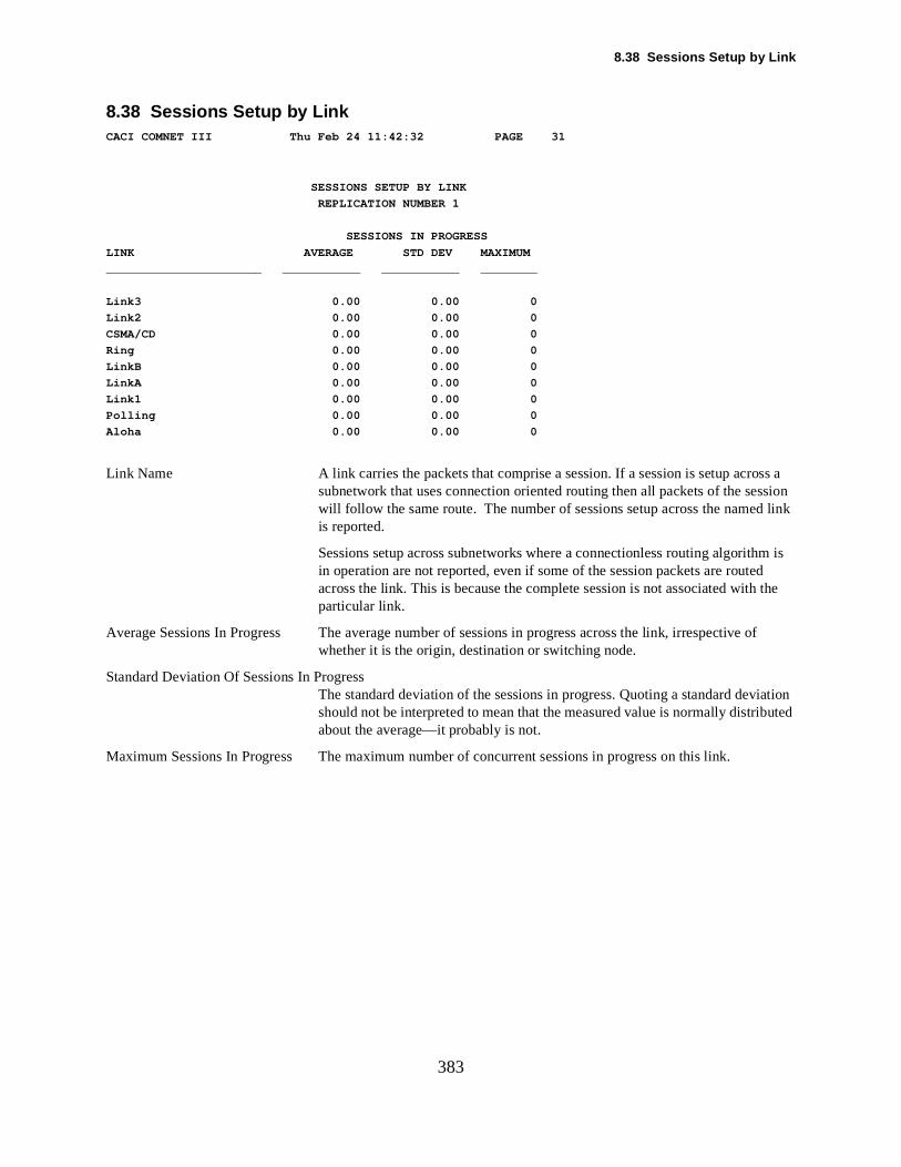
8.38 Sessions Setup by Link
ss a link
m the
ation
383
8.38 Sessions Setup by LinkCACI COMNET III Thu Feb 24 11:42:32 PAGE 31
SESSIONS SETUP BY LINK
REPLICATION NUMBER 1
SESSIONS IN PROGRESS
LINK AVERAGE STD DEV MAXIMUM
______________________ ___________ ___________ ________
Link3 0.00 0.00 0
Link2 0.00 0.00 0
CSMA/CD 0.00 0.00 0
Ring 0.00 0.00 0
LinkB 0.00 0.00 0
LinkA 0.00 0.00 0
Link1 0.00 0.00 0
Polling 0.00 0.00 0
Aloha 0.00 0.00 0
Link Name A link carries the packets that comprise a session. If a session is setup acrosubnetwork that uses connection oriented routing then all packets of the sessionwill follow the same route. The number of sessions setup across the namedis reported.
Sessions setup across subnetworks where a connectionless routing algorith is in operation are not reported, even if some of the session packets are routedacross the link. This is because the complete session is not associated with particular link.
Average Sessions In Progress The average number of sessions in progress across the link, irrespective of whether it is the origin, destination or switching node.
Standard Deviation Of Sessions In ProgressThe standard deviation of the sessions in progress. Quoting a standard devishould not be interpreted to mean that the measured value is normally distributed about the average—it probably is not.
Maximum Sessions In Progress The maximum number of concurrent sessions in progress on this link.
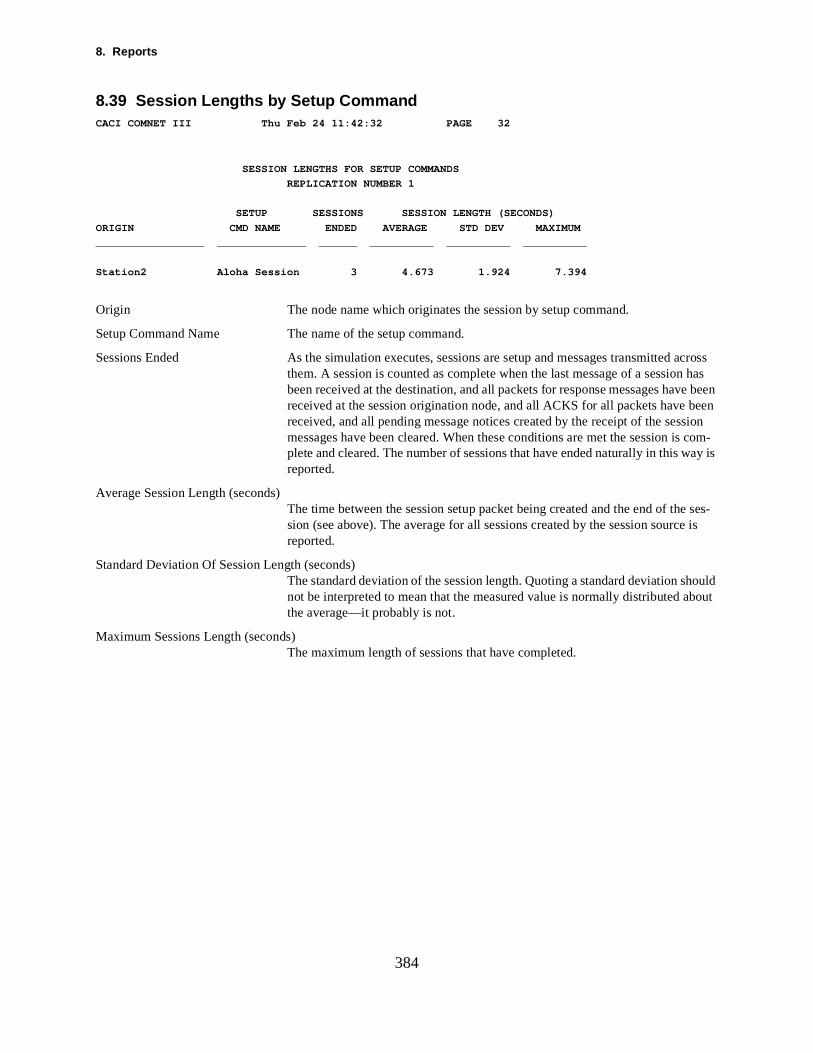
8. Reports
cross has
een sion com-ay is
ses-e is
hould bout
384
8.39 Session Lengths by Setup CommandCACI COMNET III Thu Feb 24 11:42:32 PAGE 32
SESSION LENGTHS FOR SETUP COMMANDS
REPLICATION NUMBER 1
SETUP SESSIONS SESSION LENGTH (SECONDS)
ORIGIN CMD NAME ENDED AVERAGE STD DEV MAXIMUM
_________________ ______________ ______ __________ __________ __________
Station2 Aloha Session 3 4.673 1.924 7.394
Origin The node name which originates the session by setup command.
Setup Command Name The name of the setup command.
Sessions Ended As the simulation executes, sessions are setup and messages transmitted athem. A session is counted as complete when the last message of a sessionbeen received at the destination, and all packets for response messages have been received at the session origination node, and all ACKS for all packets have breceived, and all pending message notices created by the receipt of the sesmessages have been cleared. When these conditions are met the session isplete and cleared. The number of sessions that have ended naturally in this wreported.
Average Session Length (seconds)The time between the session setup packet being created and the end of thesion (see above). The average for all sessions created by the session sourcreported.
Standard Deviation Of Session Length (seconds)The standard deviation of the session length. Quoting a standard deviation snot be interpreted to mean that the measured value is normally distributed athe average—it probably is not.
Maximum Sessions Length (seconds)The maximum length of sessions that have completed.
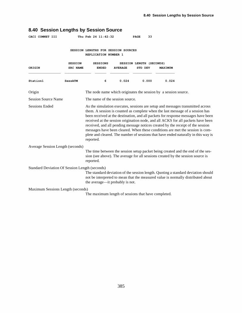
8.40 Session Lengths by Session Source
cross has
een sion com-ay is
ses-e is
hould bout
385
8.40 Session Lengths by Session SourceCACI COMNET III Thu Feb 24 11:42:32 PAGE 33
SESSION LENGTHS FOR SESSION SOURCES
REPLICATION NUMBER 1
SESSION SESSIONS SESSION LENGTH (SECONDS)
ORIGIN SRC NAME ENDED AVERAGE STD DEV MAXIMUM
_________________ ______________ ______ __________ __________ __________
Station1 SessATM 6 0.024 0.000 0.024
Origin The node name which originates the session by a session source.
Session Source Name The name of the session source.
Sessions Ended As the simulation executes, sessions are setup and messages transmitted athem. A session is counted as complete when the last message of a sessionbeen received at the destination, and all packets for response messages have been received at the session origination node, and all ACKS for all packets have breceived, and all pending message notices created by the receipt of the sesmessages have been cleared. When these conditions are met the session isplete and cleared. The number of sessions that have ended naturally in this wreported.
Average Session Length (seconds)The time between the session setup packet being created and the end of thesion (see above). The average for all sessions created by the session sourcreported.
Standard Deviation Of Session Length (seconds)The standard deviation of the session length. Quoting a standard deviation snot be interpreted to mean that the measured value is normally distributed athe average—it probably is not.
Maximum Sessions Length (seconds)The maximum length of sessions that have completed.
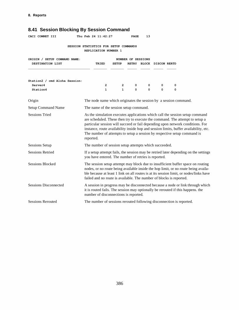
8. Reports
nd p a r
tc.
ttings
ting ila-ave
hich
386
8.41 Session Blocking By Session CommandCACI COMNET III Thu Feb 24 11:42:27 PAGE 13
SESSION STATISTICS FOR SETUP COMMANDS
REPLICATION NUMBER 1
ORIGIN / SETUP COMMAND NAME: NUMBER OF SESSIONS
DESTINATION LIST TRIED SETUP RETRY BLOCK DISCON RERTD
_________________________________ _______ _______ _____ _____ _____ _____
Station2 / cmd Aloha Session:
Server4 2 2 0 0 0 0
Station4 1 1 0 0 0 0
Origin The node name which originates the session by a session command.
Setup Command Name The name of the session setup command.
Sessions Tried As the simulation executes applications which call the session setup commaare scheduled. These then try to execute the command. The attempt to setuparticular session will succeed or fail depending upon network conditions. Foinstance, route availability inside hop and session limits, buffer availability, eThe number of attempts to setup a session by respective setup command isreported.
Sessions Setup The number of session setup attempts which succeeded.
Sessions Retried If a setup attempt fails, the session may be retried later depending on the seyou have entered. The number of retries is reported.
Sessions Blocked The session setup attempt may block due to insufficient buffer space on rounodes, or no route being available inside the hop limit, or no route being avable because at least 1 link on all routes is at its session limit, or nodes/links hfailed and no route is available. The number of blocks is reported.
Sessions Disconnected A session in progress may be disconnected because a node or link through wit is routed fails. The session may optionally be rerouted if this happens. the number of disconnections is reported.
Sessions Rerouted The number of sessions rerouted following disconnection is reported.
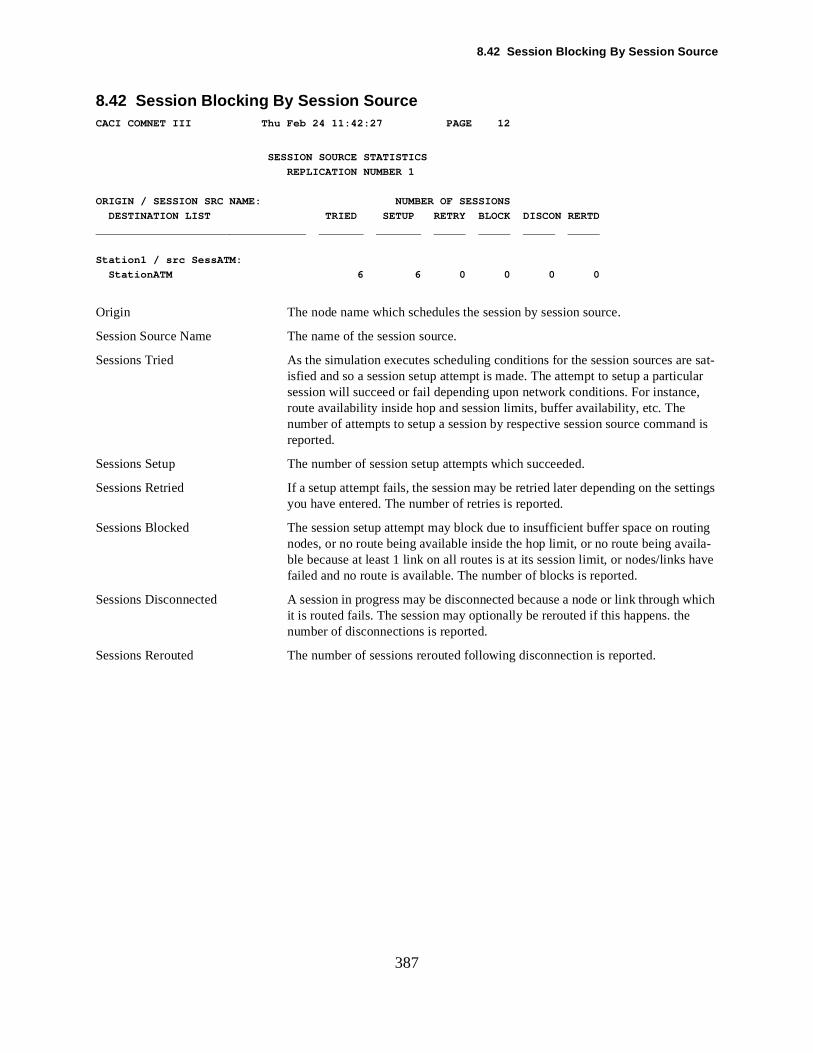
8.42 Session Blocking By Session Source
e sat-ular ,
nd is
ttings
ting ila-ave
hich
387
8.42 Session Blocking By Session SourceCACI COMNET III Thu Feb 24 11:42:27 PAGE 12
SESSION SOURCE STATISTICS
REPLICATION NUMBER 1
ORIGIN / SESSION SRC NAME: NUMBER OF SESSIONS
DESTINATION LIST TRIED SETUP RETRY BLOCK DISCON RERTD
_________________________________ _______ _______ _____ _____ _____ _____
Station1 / src SessATM:
StationATM 6 6 0 0 0 0
Origin The node name which schedules the session by session source.
Session Source Name The name of the session source.
Sessions Tried As the simulation executes scheduling conditions for the session sources arisfied and so a session setup attempt is made. The attempt to setup a particsession will succeed or fail depending upon network conditions. For instanceroute availability inside hop and session limits, buffer availability, etc. The number of attempts to setup a session by respective session source commareported.
Sessions Setup The number of session setup attempts which succeeded.
Sessions Retried If a setup attempt fails, the session may be retried later depending on the seyou have entered. The number of retries is reported.
Sessions Blocked The session setup attempt may block due to insufficient buffer space on rounodes, or no route being available inside the hop limit, or no route being avable because at least 1 link on all routes is at its session limit, or nodes/links hfailed and no route is available. The number of blocks is reported.
Sessions Disconnected A session in progress may be disconnected because a node or link through wit is routed fails. The session may optionally be rerouted if this happens. the number of disconnections is reported.
Sessions Rerouted The number of sessions rerouted following disconnection is reported.
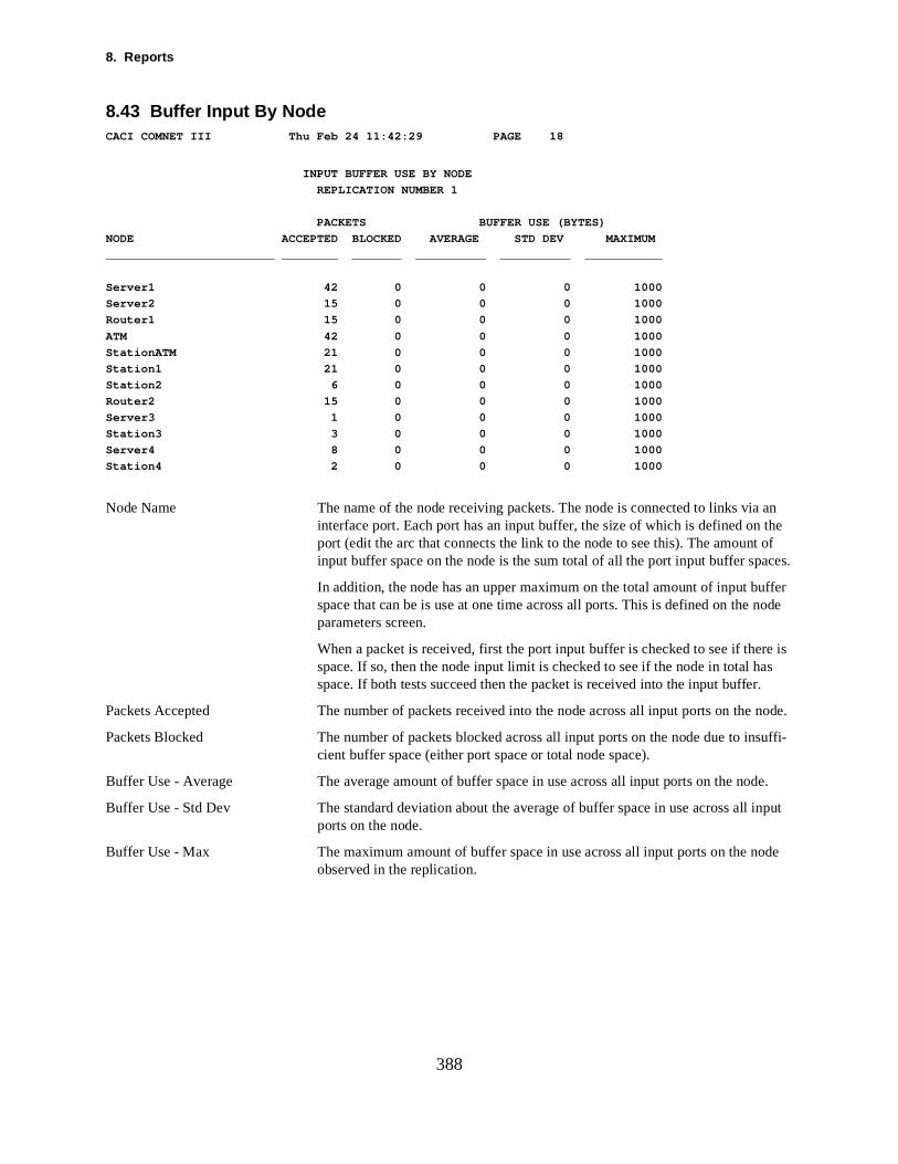
8. Reports
an the of ces.
ffer ode
e is s
.
ode.
uffi-
e.
put
de
388
8.43 Buffer Input By NodeCACI COMNET III Thu Feb 24 11:42:29 PAGE 18
INPUT BUFFER USE BY NODE
REPLICATION NUMBER 1
PACKETS BUFFER USE (BYTES)
NODE ACCEPTED BLOCKED AVERAGE STD DEV MAXIMUM
________________________ ________ _______ __________ __________ ___________
Server1 42 0 0 0 1000
Server2 15 0 0 0 1000
Router1 15 0 0 0 1000
ATM 42 0 0 0 1000
StationATM 21 0 0 0 1000
Station1 21 0 0 0 1000
Station2 6 0 0 0 1000
Router2 15 0 0 0 1000
Server3 1 0 0 0 1000
Station3 3 0 0 0 1000
Server4 8 0 0 0 1000
Station4 2 0 0 0 1000
Node Name The name of the node receiving packets. The node is connected to links viainterface port. Each port has an input buffer, the size of which is defined on port (edit the arc that connects the link to the node to see this). The amount input buffer space on the node is the sum total of all the port input buffer spa
In addition, the node has an upper maximum on the total amount of input buspace that can be is use at one time across all ports. This is defined on the nparameters screen.
When a packet is received, first the port input buffer is checked to see if therspace. If so, then the node input limit is checked to see if the node in total haspace. If both tests succeed then the packet is received into the input buffer
Packets Accepted The number of packets received into the node across all input ports on the n
Packets Blocked The number of packets blocked across all input ports on the node due to inscient buffer space (either port space or total node space).
Buffer Use - Average The average amount of buffer space in use across all input ports on the nod
Buffer Use - Std Dev The standard deviation about the average of buffer space in use across all inports on the node.
Buffer Use - Max The maximum amount of buffer space in use across all input ports on the noobserved in the replication.
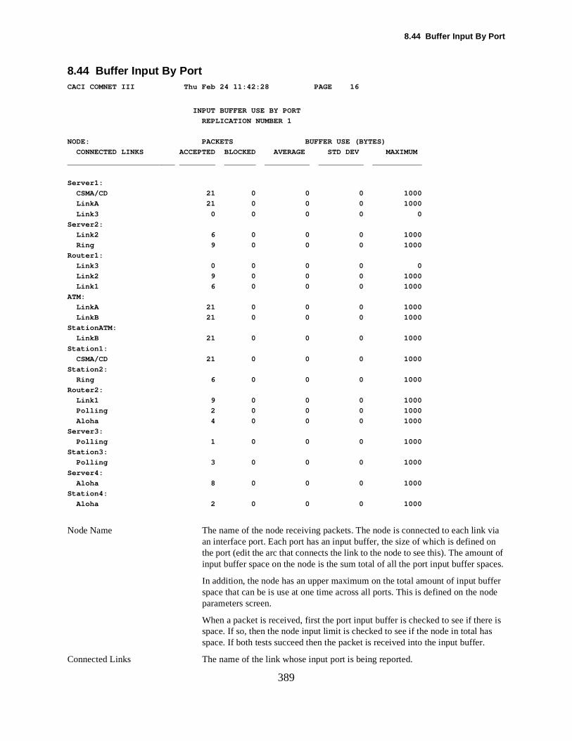
8.44 Buffer Input By Port
via on
ces.
ffer ode
e is s
.
389
8.44 Buffer Input By PortCACI COMNET III Thu Feb 24 11:42:28 PAGE 16
INPUT BUFFER USE BY PORT
REPLICATION NUMBER 1
NODE: PACKETS BUFFER USE (BYTES)
CONNECTED LINKS ACCEPTED BLOCKED AVERAGE STD DEV MAXIMUM
________________________ ________ _______ __________ __________ ___________
Server1:
CSMA/CD 21 0 0 0 1000
LinkA 21 0 0 0 1000
Link3 0 0 0 0 0
Server2:
Link2 6 0 0 0 1000
Ring 9 0 0 0 1000
Router1:
Link3 0 0 0 0 0
Link2 9 0 0 0 1000
Link1 6 0 0 0 1000
ATM:
LinkA 21 0 0 0 1000
LinkB 21 0 0 0 1000
StationATM:
LinkB 21 0 0 0 1000
Station1:
CSMA/CD 21 0 0 0 1000
Station2:
Ring 6 0 0 0 1000
Router2:
Link1 9 0 0 0 1000
Polling 2 0 0 0 1000
Aloha 4 0 0 0 1000
Server3:
Polling 1 0 0 0 1000
Station3:
Polling 3 0 0 0 1000
Server4:
Aloha 8 0 0 0 1000
Station4:
Aloha 2 0 0 0 1000
Node Name The name of the node receiving packets. The node is connected to each linkan interface port. Each port has an input buffer, the size of which is defined the port (edit the arc that connects the link to the node to see this). The amount of input buffer space on the node is the sum total of all the port input buffer spa
In addition, the node has an upper maximum on the total amount of input buspace that can be is use at one time across all ports. This is defined on the nparameters screen.
When a packet is received, first the port input buffer is checked to see if therspace. If so, then the node input limit is checked to see if the node in total haspace. If both tests succeed then the packet is received into the input buffer
Connected Links The name of the link whose input port is being reported.

8. Reports
input
390
Packets Accepted The number of packets received into the port input buffer.
Packets Blocked The number of packets blocked at this port input buffer.
Buffer Use - Average The average amount of buffer space in use at this port input buffer.
Buffer Use - Std Dev The standard deviation about the average of buffer space in use at this port buffer.
Buffer Use - Max The maximum amount of buffer space in use at this port input buffer.
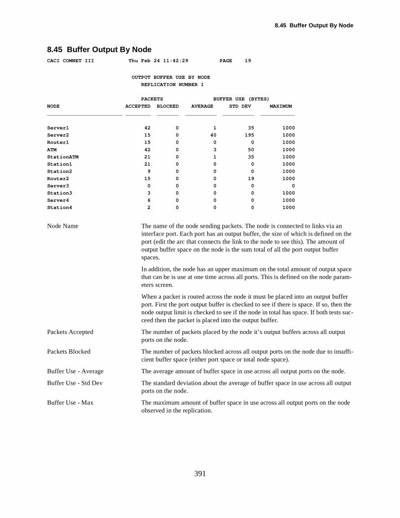
8.45 Buffer Output By Node
n of
pace aram-
ffer the suc-
ut
de.
utput
ode
391
8.45 Buffer Output By NodeCACI COMNET III Thu Feb 24 11:42:29 PAGE 19
OUTPUT BUFFER USE BY NODE
REPLICATION NUMBER 1
PACKETS BUFFER USE (BYTES)
NODE ACCEPTED BLOCKED AVERAGE STD DEV MAXIMUM
________________________ ________ _______ __________ __________ ___________
Server1 42 0 1 35 1000
Server2 15 0 40 195 1000
Router1 15 0 0 0 1000
ATM 42 0 3 50 1000
StationATM 21 0 1 35 1000
Station1 21 0 0 0 1000
Station2 9 0 0 0 1000
Router2 15 0 0 19 1000
Server3 0 0 0 0 0
Station3 3 0 0 0 1000
Server4 6 0 0 0 1000
Station4 2 0 0 0 1000
Node Name The name of the node sending packets. The node is connected to links via ainterface port. Each port has an output buffer, the size of which is defined on theport (edit the arc that connects the link to the node to see this). The amount output buffer space on the node is the sum total of all the port output buffer spaces.
In addition, the node has an upper maximum on the total amount of output sthat can be is use at one time across all ports. This is defined on the node peters screen.
When a packet is routed across the node it must be placed into an output buport. First the port output buffer is checked to see if there is space. If so, thennode output limit is checked to see if the node in total has space. If both testsceed then the packet is placed into the output buffer.
Packets Accepted The number of packets placed by the node it’s output buffers across all outpports on the node.
Packets Blocked The number of packets blocked across all output ports on the node due to insuffi-cient buffer space (either port space or total node space).
Buffer Use - Average The average amount of buffer space in use across all output ports on the no
Buffer Use - Std Dev The standard deviation about the average of buffer space in use across all oports on the node.
Buffer Use - Max The maximum amount of buffer space in use across all output ports on the nobserved in the replication.
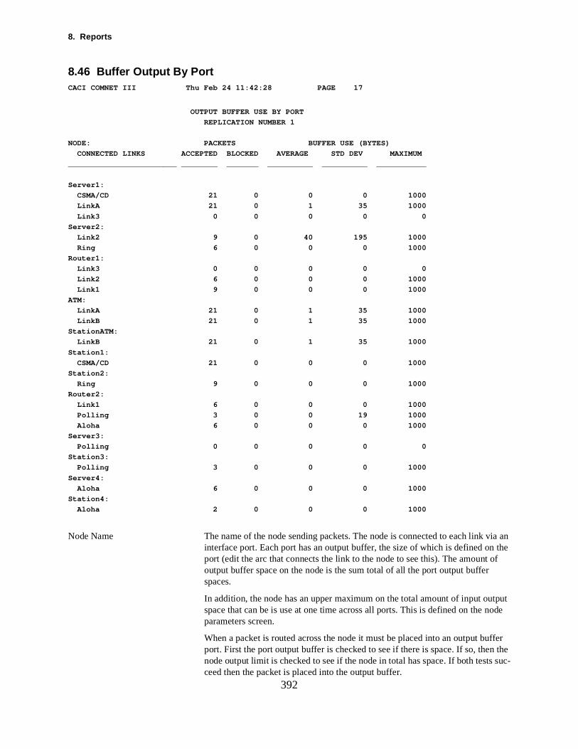
8. Reports
via an of
tput ode
ffer the suc-
392
8.46 Buffer Output By PortCACI COMNET III Thu Feb 24 11:42:28 PAGE 17
OUTPUT BUFFER USE BY PORT
REPLICATION NUMBER 1
NODE: PACKETS BUFFER USE (BYTES)
CONNECTED LINKS ACCEPTED BLOCKED AVERAGE STD DEV MAXIMUM
________________________ ________ _______ __________ __________ ___________
Server1:
CSMA/CD 21 0 0 0 1000
LinkA 21 0 1 35 1000
Link3 0 0 0 0 0
Server2:
Link2 9 0 40 195 1000
Ring 6 0 0 0 1000
Router1:
Link3 0 0 0 0 0
Link2 6 0 0 0 1000
Link1 9 0 0 0 1000
ATM:
LinkA 21 0 1 35 1000
LinkB 21 0 1 35 1000
StationATM:
LinkB 21 0 1 35 1000
Station1:
CSMA/CD 21 0 0 0 1000
Station2:
Ring 9 0 0 0 1000
Router2:
Link1 6 0 0 0 1000
Polling 3 0 0 19 1000
Aloha 6 0 0 0 1000
Server3:
Polling 0 0 0 0 0
Station3:
Polling 3 0 0 0 1000
Server4:
Aloha 6 0 0 0 1000
Station4:
Aloha 2 0 0 0 1000
Node Name The name of the node sending packets. The node is connected to each link interface port. Each port has an output buffer, the size of which is defined on theport (edit the arc that connects the link to the node to see this). The amount output buffer space on the node is the sum total of all the port output buffer spaces.
In addition, the node has an upper maximum on the total amount of input ouspace that can be is use at one time across all ports. This is defined on the nparameters screen.
When a packet is routed across the node it must be placed into an output buport. First the port output buffer is checked to see if there is space. If so, thennode output limit is checked to see if the node in total has space. If both testsceed then the packet is placed into the output buffer.

8.46 Buffer Output By Port
utput
393
Connected Links The name of the link whose output port is being reported.
Packets Accepted The number of packets routed into the port output buffer.
Packets Blocked The number of packets blocked at the port output buffer.
Buffer Use - Average The average amount of buffer space in use at the port output buffer.
Buffer Use - Std Dev The standard deviation about the average of buffer space in use at the port obuffer.
Buffer Use - Max The maximum amount of buffer space in use at the port output buffer.
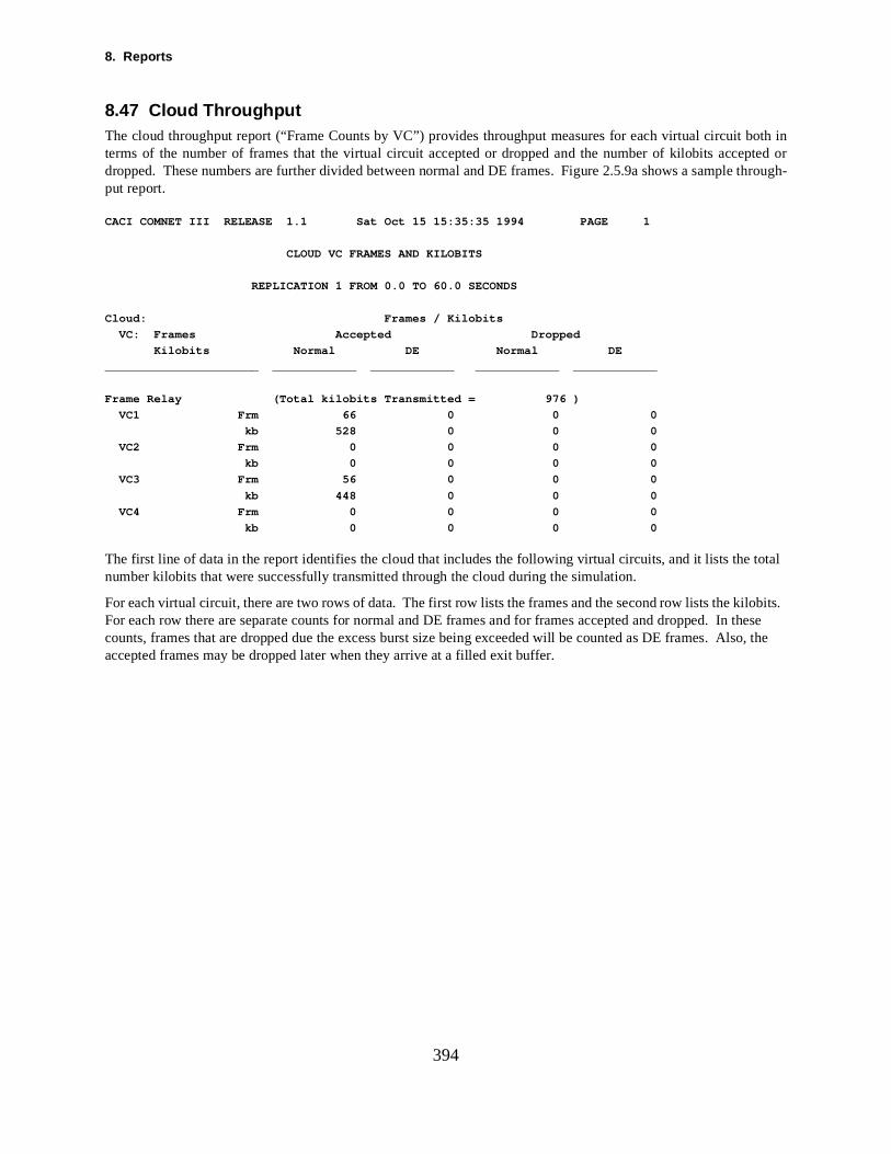
8. Reports
pted or thro
total
he
394
8.47 Cloud ThroughputThe cloud throughput report (“Frame Counts by VC”) provides throughput measures for each virtual circuit both interms of the number of frames that the virtual circuit accepted or dropped and the number of kilobits accedropped. These numbers are further divided between normal and DE frames. Figure 2.5.9a shows a sampleugh-put report.
CACI COMNET III RELEASE 1.1 Sat Oct 15 15:35:35 1994 PAGE 1
CLOUD VC FRAMES AND KILOBITS
REPLICATION 1 FROM 0.0 TO 60.0 SECONDS
Cloud: Frames / Kilobits
VC: Frames Accepted Dropped
Kilobits Normal DE Normal DE
______________________ ____________ ____________ ____________ ____________
Frame Relay (Total kilobits Transmitted = 976 )
VC1 Frm 66 0 0 0
kb 528 0 0 0
VC2 Frm 0 0 0 0
kb 0 0 0 0
VC3 Frm 56 0 0 0
kb 448 0 0 0
VC4 Frm 0 0 0 0
kb 0 0 0 0
The first line of data in the report identifies the cloud that includes the following virtual circuits, and it lists the number kilobits that were successfully transmitted through the cloud during the simulation.
For each virtual circuit, there are two rows of data. The first row lists the frames and the second row lists the kilobits. For each row there are separate counts for normal and DE frames and for frames accepted and dropped. In these counts, frames that are dropped due the excess burst size being exceeded will be counted as DE frames. Also, taccepted frames may be dropped later when they arrive at a filled exit buffer.
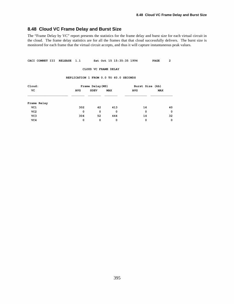
8.48 Cloud VC Frame Delay and Burst Size
int size is
395
8.48 Cloud VC Frame Delay and Burst SizeThe “Frame Delay by VC” report presents the statistics for the frame delay and burst size for each virtual circuit the cloud. The frame delay statistics are for all the frames that that cloud successfully delivers. The bursmonitored for each frame that the virtual circuit accepts, and thus it will capture instantaneous peak values.
CACI COMNET III RELEASE 1.1 Sat Oct 15 15:35:35 1994 PAGE 2
CLOUD VC FRAME DELAY
REPLICATION 1 FROM 0.0 TO 60.0 SECONDS
Cloud: Frame Delay(MS) Burst Size (kb)
VC AVG SDEV MAX AVG MAX
______________________ _______ _______ _______ ____________ ____________
Frame Relay
VC1 302 42 413 16 40
VC2 0 0 0 0 0
VC3 304 52 444 14 32
VC4 0 0 0 0 0
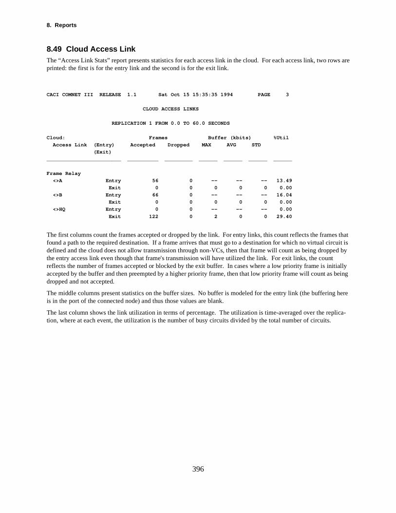
8. Reports
rows are
t rcuit is y
t
being
g here
plica-
396
8.49 Cloud Access LinkThe “Access Link Stats” report presents statistics for each access link in the cloud. For each access link, two printed: the first is for the entry link and the second is for the exit link.
CACI COMNET III RELEASE 1.1 Sat Oct 15 15:35:35 1994 PAGE 3
CLOUD ACCESS LINKS
REPLICATION 1 FROM 0.0 TO 60.0 SECONDS
Cloud: Frames Buffer (kbits) %Util
Access Link (Entry) Accepted Dropped MAX AVG STD
(Exit)
________________________ __________ _________ ______ ______ ______ ______
Frame Relay
<>A Entry 56 0 -- -- -- 13.49
Exit 0 0 0 0 0 0.00
<>B Entry 66 0 -- -- -- 16.04
Exit 0 0 0 0 0 0.00
<>HQ Entry 0 0 -- -- -- 0.00
Exit 122 0 2 0 0 29.40
The first columns count the frames accepted or dropped by the link. For entry links, this count reflects the frames thafound a path to the required destination. If a frame arrives that must go to a destination for which no virtual cidefined and the cloud does not allow transmission through non-VCs, then that frame will count as being dropped bthe entry access link even though that frame's transmission will have utilized the link. For exit links, the counreflects the number of frames accepted or blocked by the exit buffer. In cases where a low priority frame is initially accepted by the buffer and then preempted by a higher priority frame, then that low priority frame will count asdropped and not accepted.
The middle columns present statistics on the buffer sizes. No buffer is modeled for the entry link (the bufferinis in the port of the connected node) and thus those values are blank.
The last column shows the link utilization in terms of percentage. The utilization is time-averaged over the retion, where at each event, the utilization is the number of busy circuits divided by the total number of circuits.

8.50 Cloud Access Buffer Policy Report
access
397
8.50 Cloud Access Buffer Policy ReportThis report is similar to the buffer policy report on node buffers but it applies to the buffer policy on the cloud exit (or egress) buffer.

8. Reports
he cloud
398
8.51 Cloud Early/Partial Packet Discard ReportThis report presents statistics on the early and partial packet discard algorithms when they are used on taccess link.

8.52 Global Traffic Command Reports
lobal
d to the the statis-by aggre-d uses the
f the glo-te reportsd copy ofired sincerable and
399
8.52 Global Traffic Command ReportsAll of the reports that are available for local transport, answer, and set-up commands are also available for the gcommands.
The reports work a little differently, however. The local commands may be used in several sources attachesame node but the statistics are collected at one place (on the command) and thus this command aggregatestics across multiple application sources that use this source. This subtlety can affect message delay results gating unrelated delays in the same report when the command is used on multiple sources and the comman"use original message" text option or the command is an answer command.
The global command however, is cloned so that each source that uses a global command has its own copy obal command. Thus different sources on the same node using the same global command will have separafor these commands. However, if the source reuses the same global command, it will reuse the same clonethe command and thus aggregate the statistics of these instances. This behavior is likely to be what is desthe reused command is probably doing something similar in each instance so that the statistics are comparelated.

8. Reports
on. If theray have
When
O option
400
8.53 Response And Answer DestinationsThe response sources and answer commands have a checkbox to make using the catch-all "ECHO" an opticheckbox is off, then the statistics are reported separately for each destination responded to by the response oanswer. This is useful because the destinations may have different levels of congestion or the destinations mdifferent paths so that the delays are not appropriately aggregated in the same statistic.
However, this detail comes at the cost of longer initialization times and more memory than the simple ECHO.statistics are not required or when it is appropriate to aggregate the statistics over all possible destinations (when allsuch destinations are on the same LAN segment, for instance), it is advantageous to continue using the ECHto save memory and improve the speed of the simulation.

8.54 Snapshot Reports and Alarms
napshot
is run-
lization,d andtion, or for later
he poten-
e value ofcts. Note
e Snap-d on for
are updatede former value is ae. The
d for dis-
larme
alarms
e, youation to-
few the Diskhen the
401
8.54 Snapshot Reports and AlarmsSnapshot reports convey statistical information about the state of a simulated model, very much like post-run reports.They are also turned on and off using a hierarchical list interface similar to that of post-run report selection. Sreports differ from post-run reports in these key ways:
1.Snapshot reports may be turned on or off, not only before the simulation starts, but also while the simulationning.
2.The information provided by a snapshot report consists only of the value of a measurement, such as link utiat an instant in time or over a brief interval of time. At the next instant or interval, new information is computepresented, and the previous information is lost. You obtain this perishable information by watching the simulaby selecting the menu/toolbar option Take Snapshots. If you need the information to be collected and saveduse, you should instead use a post-run report.
3.Alarms can be set on snapshot performance measures. Alarm conditions ARE recorded, and alarms have ttial to trigger model traffic. Alarms can also be configured to pause the simulation.
As mentioned above, snapshot reports may be observed in one of two ways:
1.For each class of layout objects, such as nodes, you may select one snapshot report to be displayed. Ththe snapshot will be displayed as a small number or set of numbers above the icons associated with the objethat the default condition is that no snapshot reports are displayed for any objects.
2.At any point in the simulation, you may select a layout object and then select the menu/toolbar option Takshots. A dialog will appear listing the current values of all the snapshot performance measures currently turnethat object.
Some snapshot reports, such as session counts, are updated whenever the value changes. Most, however, at one of two times: at the end of a user-specified interval, or when the user selects Take Snapshots. In thcase, the reported value is an average of the measurement over the interval. In the latter case, the reportedweighted combination of the current average (over only a partial interval) and the previously reported valumeasurement interval is specified separately for nodes and links on the backbone or subnet property dialog.
Some snapshot reports, such as link utilization, involve two numbers, and when these snapshots are selecteplay, you might have difficulty determining which number has which meaning. The Take Snapshots option presentsa more verbose report that is handy for associating the numbers with their meanings.
Each snapshot report may be set to sound an alarm when the value exceeds a specified threshold. When the asounds, the icon of the offending object will change to a specified color, and a record of the alarm condition will bkept and later added to the post-run report file. When an alarm sounds on an object inside a subnet, transit network,or cloud, the subnet/transit net/cloud icon will be colored in the 2-D view, and will retain that color until the alarmclears, even if subsequent alarms of different colors sound.
Note that nodes and links can be configured to trigger model traffic upon the sounding or clearing of an alarm. Thisa very powerful, and very dangerous, feature. It is important to remember that, in combination with triggers,have the ability to change model behavior, in which case they are more than mere instrumentation.
If you have an alarm set in your model, but you don’t want to watch the simulation waiting for a color changcan configure the alarm to force the simulation into single step mode when it sounds. To permit the simulcontinue running without further interruption, typically you must first reconfigure the alarm so it no longer forces single step mode, then use the Trace menu option to turn off single step.
As with post-run reports, your simulation will run slower when you have more snapshot reports turned on. Asnapshot reports are on by default, but these snapshots will have no effect on speed of simulation. One isError snapshot report. It counts number of disk errors, such as attempting to read from a non-existent file. W

8. Reports
402
number exceeds 1, an alarm sounds. For most models, a disk error indicates a mistake in the model.
9.1 Overview of Plots and Percentiles
on, use ats and t the obtain
ny lays from
e interval f utiliza-tiliza-
vided equal
e calcu-
l statis-e
eplica-e-
ks o collect
403
9. Percentiles and Plots
9.1 Overview of Plots and PercentilesPercentiles and plots can be obtained via any dialog box with a Statistics button. Before running the simulatithe Statistics button to select the desired statistics; edit the desired statistic in the list to turn on the Collect StSave Observations options. After running the simulation, use the Statistics button again to view and then ploselected statistic. After bringing up the plot window by clicking on the plot button, use Plot on the menubar to histograms, percentiles, or plots of smoothed data.
When plots of saved data are viewed after the simulation using the statistics buttons, it is possible to obtain adesired percentile for the saved data. For example, one could determine the 95th percentile for message dea particular message source, provided “save data” was requested for that source prior to the simulation.
Post-processed plots of saved data allow the user to choose the number of points to be plotted, as well as thover which each plotted value is to be computed. For example, one could choose to plot 100 observations otion over an 80 second interval, with each observation of utilization computed as the time-weighted average ution over the previous 2 second interval. If you request a plot of smoothed data for a delay type of statistic, you specify the time period [T1, T2] to be plotted and the number of points, N, to be plotted. The time period is diinto (T2 - T1) / N intervals and a single point is plotted for each interval. The point plotted for each interval is to the average of all of the delays observed during the interval. If no delays are observed, 0 is plotted.
If you request a plot of smoothed data for a level type of statistic (e.g., channel utilization), you specify the timperiod [T1, T2] to be plotted, the number of points, N, to be plotted, and the averaging interval, I, to be used inlating the utilization at each plotted point. The point plotted at time T is the time-weighted average of the levetic during the time interval [T-I, T]. If I > T, the time-weighted average is computed over the interval [0, T]. Thaveraging interval must be greater than or equal to (T2 - T1) / N. If the time period to be plotted is an entire rtion and the averaging interval is set to the length of the replication, then each plotted point represents the timweighted average of the level statistic from the beginning of the replication to the time of the plotted point.
9.2 Statistics Request ButtonsThere are specific statistical monitors available for many of COMNET III’s modeling elements. For example, linsession sources, virtual circuits, access links, etc., all have statistics buttons on their dialog boxes . In order tstatistics during a simulation, the desired statistics switches must be edited before starting the simulation.
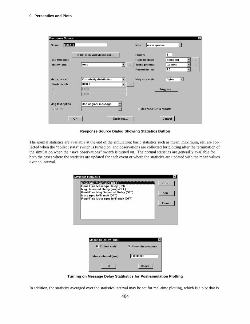
9. Percentiles and Plots
are col-tion of for an values
404
Response Source Dialog Showing Stat istics Button
The normal statistics are available at the end of the simulation: basic statistics such as mean, maximum, etc.lected when the “collect stats” switch is turned on, and observations are collected for plotting after the terminathe simulation when the “save observations” switch is turned on. The normal statistics are generally availableboth the cases where the statistics are updated for each event or where the statistics are updated with the meover an interval.
Turning on Message Delay Statitistics for Post-simulation Plotting
In addition, the statistics averaged over the statistics interval may be set for real-time plotting, which is a plot that is
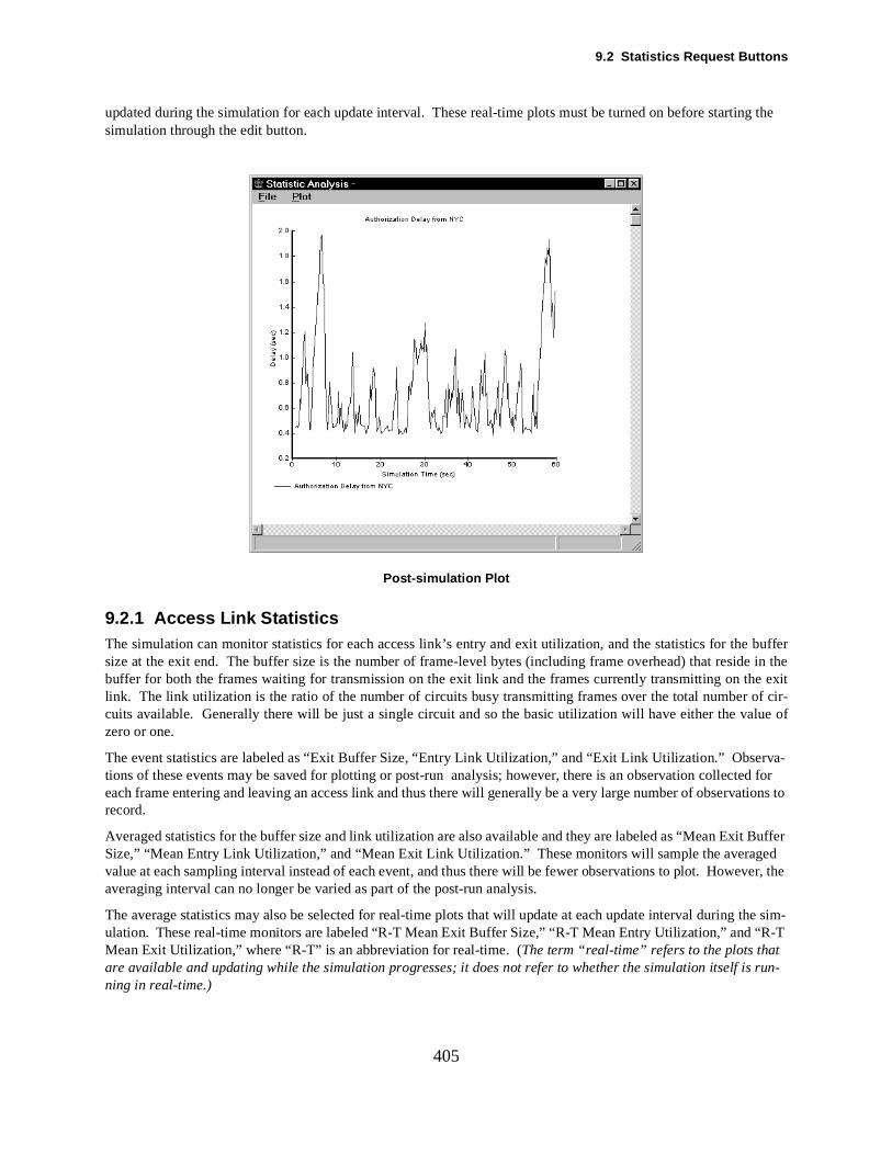
9.2 Statistics Request Buttons
ng the
thee exit
lue of
va-ed for ations to
fer d e
the sim-R-T
-
405
updated during the simulation for each update interval. These real-time plots must be turned on before startisimulation through the edit button.
Post-simulation Plot
9.2.1 Access Link StatisticsThe simulation can monitor statistics for each access link’s entry and exit utilization, and the statistics for thebuffersize at the exit end. The buffer size is the number of frame-level bytes (including frame overhead) that reside inbuffer for both the frames waiting for transmission on the exit link and the frames currently transmitting on thlink. The link utilization is the ratio of the number of circuits busy transmitting frames over the total number of cir-cuits available. Generally there will be just a single circuit and so the basic utilization will have either the vazero or one.
The event statistics are labeled as “Exit Buffer Size, “Entry Link Utilization,” and “Exit Link Utilization.” Obsertions of these events may be saved for plotting or post-run analysis; however, there is an observation collecteach frame entering and leaving an access link and thus there will generally be a very large number of observrecord.
Averaged statistics for the buffer size and link utilization are also available and they are labeled as “Mean Exit BufSize,” “Mean Entry Link Utilization,” and “Mean Exit Link Utilization.” These monitors will sample the averagevalue at each sampling interval instead of each event, and thus there will be fewer observations to plot. However, thaveraging interval can no longer be varied as part of the post-run analysis.
The average statistics may also be selected for real-time plots that will update at each update interval during ulation. These real-time monitors are labeled “R-T Mean Exit Buffer Size,” “R-T Mean Entry Utilization,” and “Mean Exit Utilization,” where “R-T” is an abbreviation for real-time. (The term “real-time” refers to the plots that are available and updating while the simulation progresses; it does not refer to whether the simulation itself is running in real-time.)
9. Percentiles and Plots
the entryssfullyrDelay”y”
cuit andckets and
monitoronitors update
st size.
ill be
tatis-
,
s for nd
the lev-
statis-
406
9.2.2 Virtual Circuit StatisticsFor virtual circuits, the simulation can measure the frame delay and the leaky-bucket burst size.
The frame delay is the time the frame takes to traverse the cloud from the moment it is created at the input to link to the time it is delivered at the output of the exit link. This frame delay counts only the frames that succego through the cloud, and thus it does not count frames that are dropped within the cloud. The frame delay monitolabeled “Frame Delay” collects statistics for the delay for each frame that is delivered. The “Mean Frame monitors the averaged frame delay over the mean-statistics interval, and the “Real-Time Mean Frame Delapro-vides a real-time plot of the averaged delay for this virtual circuit.
The burst size is the current size of the leaky-bucket burst at the time a frame is accepted by the virtual cirthus the frame size is added to the burst. The burst size contains only the data bytes for the encapsulated pathus it does not include the frame overhead or any padding necessary to meet minimum frame size. Thelabeled “Burst Size” will collect the burst statistics for each frame accepted at the virtual circuit. The mlabeled “Sampled Burst Size” collects burst size statistics based on a sample at the time of the mean-statisticinterval controlled by the cloud. “Real-Time Sampled Burst Size” provides a real-time plot of the sampled bur
Also, if the virtual circuit's “Show Burst Size” switch is on, then the sampled burst size for that virtual circuit wdisplayed over the virtual circuit icon during the simulation.
9.3 Exporting Statistics FilesAll of the simulation statistics collected during the file can be exported by clicking on File/Export/Simulation Stics, which writes the simulation statistics to the file statfile.xpt in the model directory. Each line in the file has thefollowing tab-delimited fields:
Owner Type—the type of object owning the statistic (e.g., PORT)
Owner Name—a name for fully identifying the object (e.g., for a PORT, the owner name is given by link:node:xwhere x is I or O for input or output buffer).
Statistic Type—name of the type of statistic (e.g., possible values for a PORT are portbufferlevelI or portbufferlev-elO).
Replication—the replication number; when there is more than one replication, replication -1 combines statisticall reps as though the simulation consisted of 1 long rep; replication 0 treats each replication as one observation aprovides the statistics based on these summary observations.
Minimum—the smallest observed value or level.
Maximum—the largest observed value or level.
Sum—for delay types of performance measures, the sum of the delays; for level statistics (e.g., buffer usage),els are time-weighted; to compute the mean for a level statistic, divide the Sum by the length of a replication.
Sum of Squares—for delay types of performance measures, the sum of the observed values squared; for level tics, the levels are time-weighted.
Count—the number of observations.

, andm
gram graphic such
raries
images
le. This
s wellnti-
-d.
407
10. SIMGRAPHICS II Graphics Editor
10.1 The SIMGRAPHICS II Graphics EditorSIMDRAW, the SIMGRAPHICS II graphics editor, constructs images for animation, presentation graphicsinteractive graphical input. We will discuss here only those of its capabilities which are used to create or odifyCOMNET III icons and backgrounds.
The concept used by COMNET III and its SIMGRAPHICS II graphical interface is that graphic images, promenus and program dialog boxes are described using the SIMDRAW editor. These descriptions are stored inlibrary files which use the extension .sg2. The graphics images in these files can be tied to objects in a program,as COMNET III.
COMNET III allows the user to provide new graphic images which can be stored in COMNET III's graphics liband used as icons and backgrounds in layouts.
Backgrounds can be added to layouts to give them more meaning or simply to improve their appearance. The iconscan be associated with objects such as nodes, links and traffic sources.
Graphic images are built by drawing lines, circles, polygons, arcs, sectors. They can also include bitmapswhich are imported into SIMDRAW and added to graphic images. All of these graphics primitives can be groupedtogether to form complex images containing parts that can be manipulated independently.
A collection of these images (as well as graphs, menus and dialog boxes) may be stored in a single library fifile can be used with any language which supports SIMGRAPHICS II.
The graphics libraries delivered with COMNET III already contain icons for all standard program constructs aas a selection of background images. The background image collection includes maps of various countries and conents against which network layouts can be constructed.
SIMDRAW is written entirely in MODSIM II using SIMGRAPHICS II.
10.2 Starting SIMDRAWThe SIMDRAW graphics editor is started by executing the program simdraw. On systems with graphical user interfaces, such as Windows, select the simdraw program icon to run it. After initialization three windows are displayeThe Palette windowPalette: Window is shown here, the Canvas and Tag windows are initially empty.
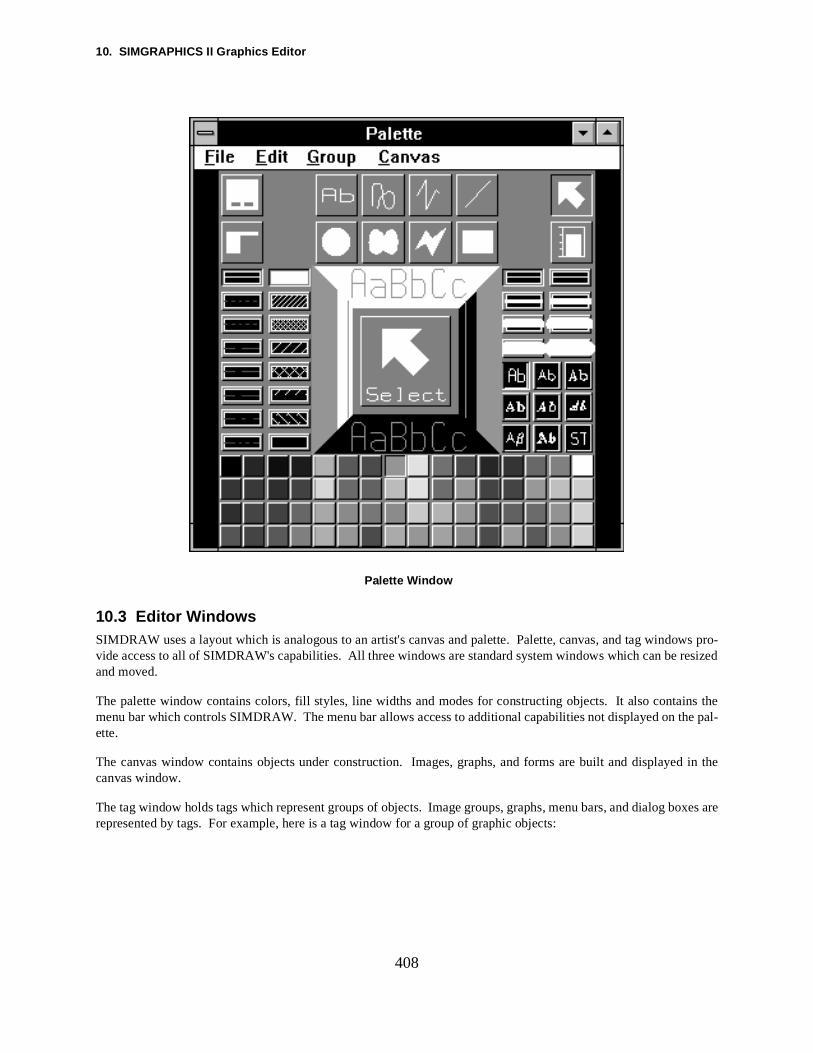
10. SIMGRAPHICS II Graphics Editor
ows pro-resized
ins thethe pal-
d in the
s are
408
Palette Window
10.3 Editor WindowsSIMDRAW uses a layout which is analogous to an artist's canvas and palette. Palette, canvas, and tag windvide access to all of SIMDRAW's capabilities. All three windows are standard system windows which can be and moved.
The palette window contains colors, fill styles, line widths and modes for constructing objects. It also contamenu bar which controls SIMDRAW. The menu bar allows access to additional capabilities not displayed on ette.
The canvas window contains objects under construction. Images, graphs, and forms are built and displayecanvas window.
The tag window holds tags which represent groups of objects. Image groups, graphs, menu bars, and dialog boxerepresented by tags. For example, here is a tag window for a group of graphic objects:
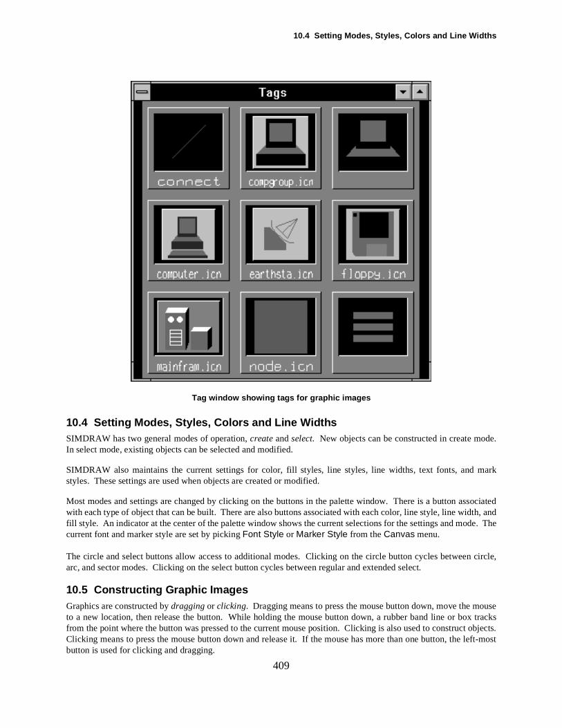
10.4 Setting Modes, Styles, Colors and Line Widths
de.
sociateddth, andde. The
n circle,
ouse
objects. left-most
409
Tag window showing tags for graphic images
10.4 Setting Modes, Styles, Colors and Line WidthsSIMDRAW has two general modes of operation, create and select. New objects can be constructed in create moIn select mode, existing objects can be selected and modified.
SIMDRAW also maintains the current settings for color, fill styles, line styles, line widths, text fonts, and markstyles. These settings are used when objects are created or modified.
Most modes and settings are changed by clicking on the buttons in the palette window. There is a button aswith each type of object that can be built. There are also buttons associated with each color, line style, line wifill style. An indicator at the center of the palette window shows the current selections for the settings and mocurrent font and marker style are set by picking Font Style or Marker Style from the Canvas menu.
The circle and select buttons allow access to additional modes. Clicking on the circle button cycles betweearc, and sector modes. Clicking on the select button cycles between regular and extended select.
10.5 Constructing Graphic ImagesGraphics are constructed by dragging or clicking. Dragging means to press the mouse button down, move the mto a new location, then release the button. While holding the mouse button down, a rubber band line or box tracksfrom the point where the button was pressed to the current mouse position. Clicking is also used to constructClicking means to press the mouse button down and release it. If the mouse has more than one button, thebutton is used for clicking and dragging.
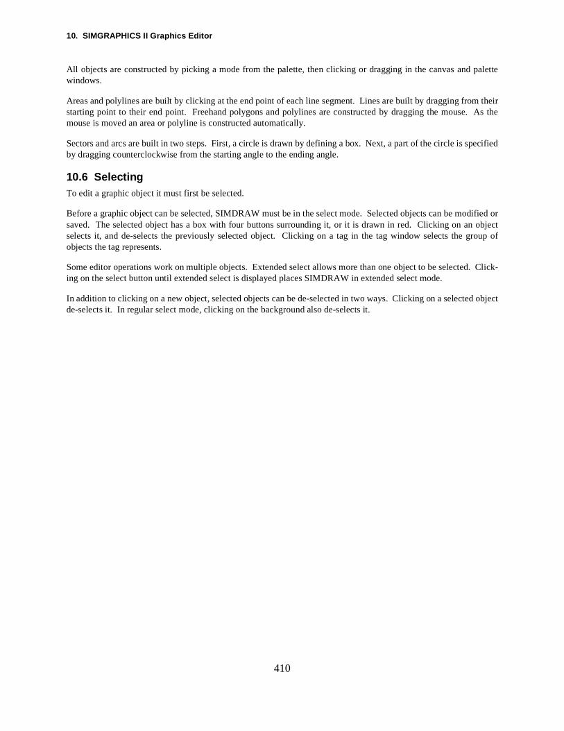
10. SIMGRAPHICS II Graphics Editor
palette
m their As the
pecified
dified orctgroup of
Click-
d object
410
All objects are constructed by picking a mode from the palette, then clicking or dragging in the canvas andwindows.
Areas and polylines are built by clicking at the end point of each line segment. Lines are built by dragging frostarting point to their end point. Freehand polygons and polylines are constructed by dragging the mouse.mouse is moved an area or polyline is constructed automatically.
Sectors and arcs are built in two steps. First, a circle is drawn by defining a box. Next, a part of the circle is sby dragging counterclockwise from the starting angle to the ending angle.
10.6 SelectingTo edit a graphic object it must first be selected.
Before a graphic object can be selected, SIMDRAW must be in the select mode. Selected objects can be mosaved. The selected object has a box with four buttons surrounding it, or it is drawn in red. Clicking on an objeselects it, and de-selects the previously selected object. Clicking on a tag in the tag window selects the objects the tag represents.
Some editor operations work on multiple objects. Extended select allows more than one object to be selected. ing on the select button until extended select is displayed places SIMDRAW in extended select mode.
In addition to clicking on a new object, selected objects can be de-selected in two ways. Clicking on a selectede-selects it. In regular select mode, clicking on the background also de-selects it.
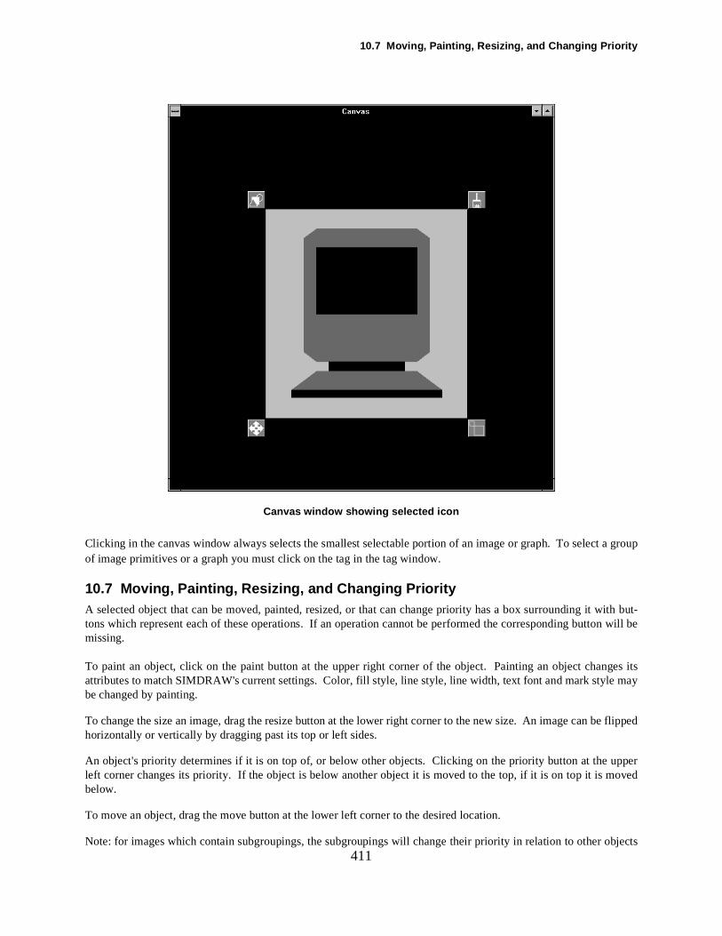
10.7 Moving, Painting, Resizing, and Changing Priority
a g
nges its may
e flipped
upperoved
411
Canvas window showing selected icon
Clicking in the canvas window always selects the smallest selectable portion of an image or graph. To selectroupof image primitives or a graph you must click on the tag in the tag window.
10.7 Moving, Painting, Resizing, and Changing PriorityA selected object that can be moved, painted, resized, or that can change priority has a box surrounding it with but-tons which represent each of these operations. If an operation cannot be performed the corresponding button will bemissing.
To paint an object, click on the paint button at the upper right corner of the object. Painting an object chaattributes to match SIMDRAW's current settings. Color, fill style, line style, line width, text font and mark stylebe changed by painting.
To change the size an image, drag the resize button at the lower right corner to the new size. An image can bhorizontally or vertically by dragging past its top or left sides.
An object's priority determines if it is on top of, or below other objects. Clicking on the priority button at the left corner changes its priority. If the object is below another object it is moved to the top, if it is on top it is mbelow.
To move an object, drag the move button at the lower left corner to the desired location.
Note: for images which contain subgroupings, the subgroupings will change their priority in relation to other objects
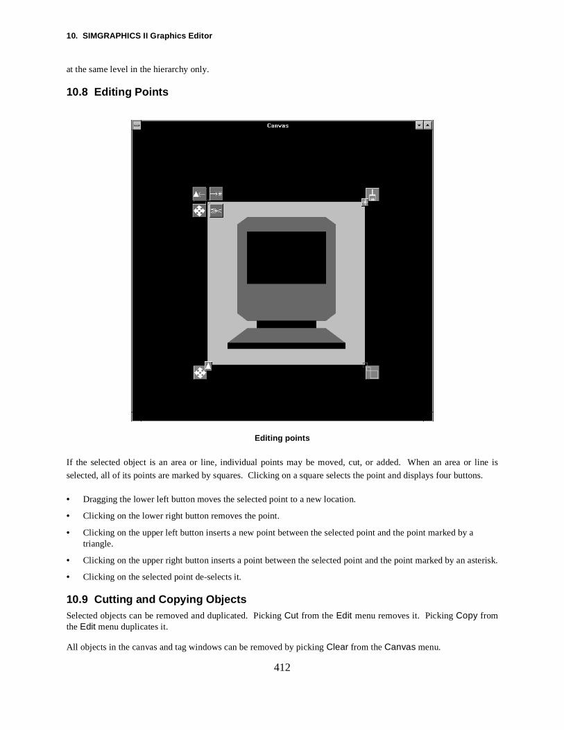
10. SIMGRAPHICS II Graphics Editor
r line is
tons.
a
sterisk.
412
at the same level in the hierarchy only.
10.8 Editing Points
Editing points
If the selected object is an area or line, individual points may be moved, cut, or added. When an area o
selected, all of its points are marked by squares. Clicking on a square selects the point and displays four but
• Dragging the lower left button moves the selected point to a new location.
• Clicking on the lower right button removes the point.
• Clicking on the upper left button inserts a new point between the selected point and the point marked by triangle.
• Clicking on the upper right button inserts a point between the selected point and the point marked by an a
• Clicking on the selected point de-selects it.
10.9 Cutting and Copying ObjectsSelected objects can be removed and duplicated. Picking Cut from the Edit menu removes it. Picking Copy fromthe Edit menu duplicates it.
All objects in the canvas and tag windows can be removed by picking Clear from the Canvas menu.
10.10 Using the Grid
up into
picking
hould betm for
r as
ached to
entultiple
he
ved. It
med by
nt until
g to,
413
10.10 Using the GridA grid can be used to perform precise positioning and sizing of images and graphs by breaking the canvasdivisions. The grid is controlled by picking Change Grid from the Canvas menu.
If Snap is set, positioning and resizing is restrained to the intersections of the grid.
If Grid is set, lines are drawn on the canvas. The color of the grid lines can be set to the current color byChange Grid Color from the Canvas menu.
10.11 Canvas Dimensions and CoordinatesThe dimensions of the canvas determine an object's coordinate system when it is saved. The dimensions sset to match the world coordinate system used within the program. This ensures that the positions of objects sewithin SIMDRAW will remain the same when it is displayed within a program. The default coordinate systeSIMDRAW and COMNET III is (0...32767, 0...32767). It may be changed by picking Dimension from the Canvasmenu.
The current location of the pointer relative to the canvas dimensions is displayed by picking Show Coordinatesfrom the Canvas menu. Picking Hide Coordinates removes it. The coordinates are displayed in the same colothe grid at the lower left corner of the canvas window.
Allow Icons to Scale is an option available under Canvas/Dimension. If this option is set, an icon will automati-cally be scaled using the dimensions set in the editor, and the world coordinate system of the object it is attwithin the program. If it is not set, the icon will stay the same size no matter what world it is attached to.
10.12 The Library — Saving and Loading ObjectsAll objects are saved to and loaded from library files which have the extension “.sg2”. SIMDRAW always has a cur-rent library that objects are added to and removed from.
Selected objects can be saved by picking Save from the File menu. When an object is saved it is added to the currlibrary and the entire library is written to a file. While in the save mode tags may selected. This allows mobjects to be saved before returning.
Objects may be loaded from a library file by picking Load from the File menu. Before an object can be loaded, tlibrary containing the object must be loaded. Multiple objects may be loaded before returning.
Note: Individual image primitives cannot be saved. They must be grouped first.
10.13 Managing the LibrarySince the library file can contain a collection of objects, individual objects may need to be renamed or remomay also be necessary to remove all of the objects in the library. These tasks can be performed by picking ManageLibrary from the File menu.
Individual objects are selected by clicking on their name in the list box provided. The selected object is renaentering a new name, and clicking on Update. It is removed by clicking on Remove. Clicking on Remove Allremoves all objects in the library.
Removing and renaming modifies the current working library only. The change to the library is not permaneSave To Library is clicked on. You may undo any changes you have made by clicking on Cancel. If all of theobjects are removed from the library and it is saved then the library file is deleted.
10.14 Grouping ImagesImages can be grouped into complex hierarchies. SIMDRAW provides functions for creating, destroying, addinand removing from groups.
10. SIMGRAPHICS II Graphics Editor
fied.
gts can
d on thelso used
s-
414
Creating a group does not restrict the editing of the individual primitives. They can still be selected and modiSelected image groups and primitives are grouped by picking Create from the Group menu. A tag is created whichrepresents the new grouping. The selected group can be destroyed by picking Destroy from the Group menu.
After a group is created, additional primitives or groups may be added to it. Selected objects are added to a roup bypicking Add To from the Group menu, then selecting the tag representing the group to add to. Selected objecbe removed from their groups by picking Remove From from the Group menu.
Note: When creating a group, the selected objects cannot be members of any existing group.
10.15 Recentering ImagesEach image or subimage has a center point which defines where the image will be drawn when it is placescreen. When an image is drawn at a (x,y) location its center point is aligned at (x,y). The center point is afor rotation and scaling. The default center for an image is the middle of the smallest box which will enclose theimage. The default center is set when an image or group is created or scaled.
Selected images are recentered by picking Re-center from the Edit menu. The current center of the image is diplayed as a set of cross hairs. Clicking at a new location sets the center point.
10.16 Importing Text into SIMDRAWText files can be loaded into the graphics editor and added to an image. To do this, pick Load from the File menu.Type in the name of the text file as the name of the library, then press both the Load Library then Load Object but-tons. A tag will appear in the tag window containing the text of the file.
10.17 Exiting SIMDRAWPicking Exit from the File menu exits SIMDRAW. Any objects which have not been saved will be lost.
ner is-arac-lanning.dvanced be most
varietyss in
415
11. COMNET Baseliner
11.1 INTRODUCTION
11.1.1 OverviewCOMNET Baseliner provides an interface between COMNET III and other networking tools. COMNET Baselia tool developed to assimilate data from your existing networking tools and automatically generate base-line COMNET III model information Baseline model information reflects your existing network architecture and load chteristics. The automation process saves time which can be utilized on the important issues of design and pThe automation process can run in either default mode, requiring the least intervention by the user, or in an auser mode, where the user can tailor the process to meet their specific needs. Typically, this process woulduseful during “what-if” scenarios of the model under study.
11.1.2 The System Architecture
COMNET Baseliner helps you build a baseline model of your network by transforming data collected from a of network management and monitoring tools, into COMNET III model information. The model building proceCOMNET III, see figure 1.2, can be split into two phases:
a) building a network architecture model and,
b) building a network load profile for the resulting model network.
NetworkManagementSystems
COMNET Baseliner
COMNET Baseliner
COMNET III
Network TrafficAnalyzers/
Monitoring Tools
Import Network Traffic
Import Network Topology

11. COMNET Baseliner
cap-S)s anmationilable,ointnd link
tools lev-such asividual
poi
asoblems
aves
T Base-
416
11.1.3 Network Topology InformationThe first step of building a COMNET III simulation model is to construct a topology of the network under study.COMNET Baseliner helps you build an accurate representation of your network architecture, by using the datatured by your existing network management tools. Currently supported Network Management Systems (NMinclude HP OpenView, Cabletron SPECTRUM, IBM NetView/6000 and Digital PolyCenter. It also provideinterface to basic SNMP tools such as Castlerock’s SNMPc. COMNET Baseliner extracts node and link inforfrom the data, in the topology file, to automatically generate a COMNET III model file. Based on the data avaCOMNET Baseliner can identify different types of links, i.e. Ethernet, Token Ring, FDDI Ring or Point-to-P(WAN) link. The import process may be tailored to suit your need in the advanced user mode. The node aparameters, once in the COMNET environment, can be modified as needed.
11.1.4 Network Load CharacterizationTo represent your network further, COMNET Baseliner also allows you to add “real” traffic to your network archi-tecture model. This is achieved by transforming traffic captured by network analyzers or network monitoringinto load characteristics for COMNET III. COMNET III provides interface to external traffic collected at variousels of detail. At the highest level, traffic data may be collected at the application-layer level containing data packet counts and bytes counts. Or it may be collected at the frame-level detail, containing information on indpackets.
With conversation pair traffic, representing the highest level of detail, the import process uses the interrupted ssonprocess for characterizing the traffic flow. In the scenario, where the import process does not have enough data avail-able, it will use the default poisson process for characterizing the traffic. On the other end of the spectrum, suchevent trace traffic, the events recorded in the data file govern the traffic flow during simulation. The type of prunder study would determine what kind of data to import. External traffic can include traffic from multiple sourcebeing sent over multiple segments.
External traffic may be mixed with internal traffic within the model. Within the simulation, external traffic behsimilar to internal traffic. This is particularly useful for trying out multiple “what-if” scenarios.
For a more detailed explanation of COMNET Baseliner and its features, please consult the seperate COMNEliner Users Manual.
s which
o shap-to bemi-
417
12. Statistical Distribution Functions
12.1 The Beta Distribution
The Beta distribution function takes two positive real parameters, shape1 and shape2 which provide information onthe shape of the probability distribution. It returns a positive, real number. The stream parameter specifierandom number stream will be used to provide the sample.
Beta(shape1, shape2, min, max, stream)
This is one of the most versatile distribution functions. It can take on a variety of shapes depending on the twing parameters. Normally its return, x, falls in the interval 0 < x < 1, but COMNET III allows the distribution mapped over the interval specified by min and max. Note that the distribution plots above use the statistical ternology shape1 and shape2 for the two shaping parameters.
X
Beta(shape1, shape2, min,max)
0
0.5
1
1.5
2
2.5
3
0 0.2 0.4 0.6 0.8 1 1.2 1.4 1.6 1.8 2
shape1 =1.5, shape2 = 5
shape1 = 1.5, shape2 = 3
shape1 = 5, shape2 = 1.5
shape1 = 3, shape2 = 1.5
shape1 = 5, shape2 = 5
12. Statistical Distribution Functions
pro-ce in sam-eld of
418
12.2 The Erlang Distribution
The Erlang distribution function takes two parameters, mean is a positive real number and shape is a positive integer.It returns a positive, real number. The stream parameter specifies which random number stream will be used to vide the sample. The larger the shape parameter, the sharper the peak in the distribution, and the less varianples. This distribution is named after A. K. Erlang, a Danish mathematician, who pioneered in the fitelecommunications analysis.
Erlang (mean, shape, stream)
Erlang(1, K, x)
X
0
0.2
0.4
0.6
0.8
1
1.2
1.4
0 0.5 1 1.5 2 2.5 3
shape = 1
shape = 2
shape = 4
shape = 10
(Mean = 1 for all curves)
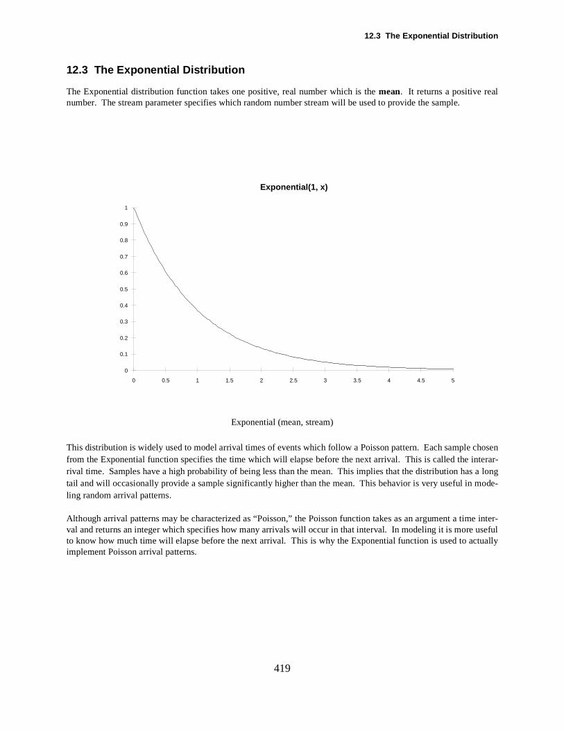
12.3 The Exponent ial Distribution
chosennterar-s a mode-
me inter-usefully
419
12.3 The Exponential Distribution
The Exponential distribution function takes one positive, real number which is the mean. It returns a positive realnumber. The stream parameter specifies which random number stream will be used to provide the sample.
Exponential (mean, stream)
This distribution is widely used to model arrival times of events which follow a Poisson pattern. Each sample from the Exponential function specifies the time which will elapse before the next arrival. This is called the irival time. Samples have a high probability of being less than the mean. This implies that the distribution halongtail and will occasionally provide a sample significantly higher than the mean. This behavior is very useful in ling random arrival patterns.
Although arrival patterns may be characterized as “Poisson,” the Poisson function takes as an argument a tival and returns an integer which specifies how many arrivals will occur in that interval. In modeling it is more to know how much time will elapse before the next arrival. This is why the Exponential function is used to actualimplement Poisson arrival patterns.
Exponential(1, x)
0
0.1
0.2
0.3
0.4
0.5
0.6
0.7
0.8
0.9
1
0 0.5 1 1.5 2 2.5 3 3.5 4 4.5 5
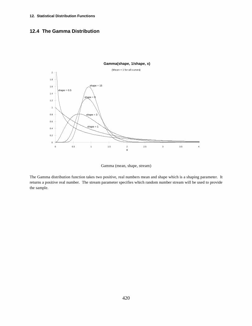
12. Statistical Distribution Functions
r. It provide
420
12.4 The Gamma Distribution
Gamma (mean, shape, stream)
The Gamma distribution function takes two positive, real numbers mean and shape which is a shaping parametereturns a positive real number. The stream parameter specifies which random number stream will be used tothe sample.
Gamma(shape, 1/shape, x)
X
0
0.2
0.4
0.6
0.8
1
1.2
1.4
1.6
1.8
2
0 0.5 1 1.5 2 2.5 3 3.5 4
shape = 1
shape = 0.5
shape = 3
shape = 9
shape = 15
(Mean = 1 for all curves)
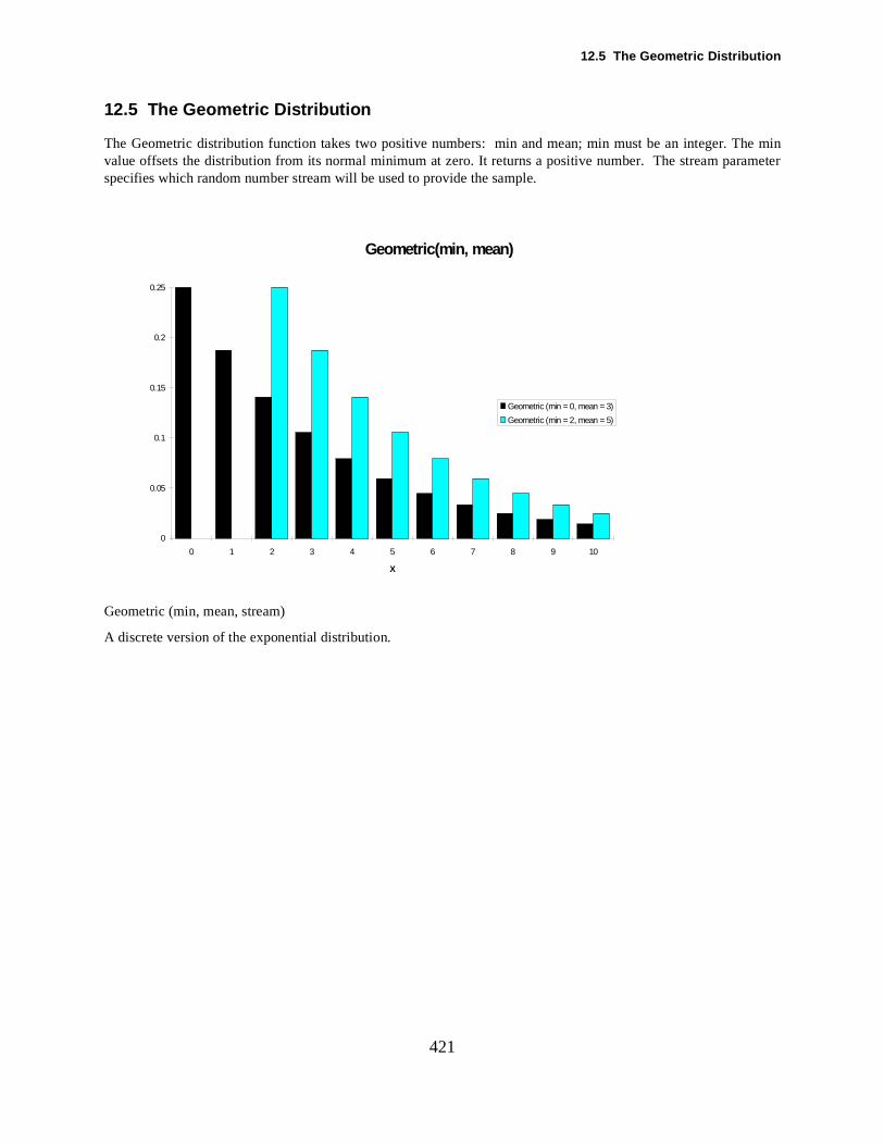
12.5 The Geometric Distribution
he minameter
421
12.5 The Geometric Distribution
The Geometric distribution function takes two positive numbers: min and mean; min must be an integer. Tvalue offsets the distribution from its normal minimum at zero. It returns a positive number. The stream parspecifies which random number stream will be used to provide the sample.
Geometric (min, mean, stream)
A discrete version of the exponential distribution.
Geometric(min, mean)
0
0.05
0.1
0.15
0.2
0.25
0 1 2 3 4 5 6 7 8 9 10
X
Geometric (min = 0, mean = 3)
Geometric (min = 2, mean = 5)
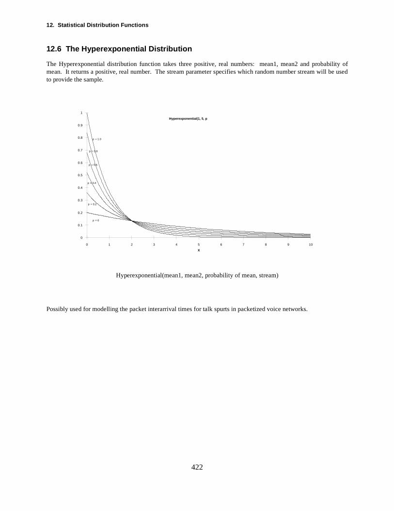
12. Statistical Distribution Functions
bility of be used
422
12.6 The Hyperexponential Distribution
The Hyperexponential distribution function takes three positive, real numbers: mean1, mean2 and probamean. It returns a positive, real number. The stream parameter specifies which random number stream willto provide the sample.
Hyperexponential(mean1, mean2, probability of mean, stream)
Possibly used for modelling the packet interarrival times for talk spurts in packetized voice networks.
X
0
0.1
0.2
0.3
0.4
0.5
0.6
0.7
0.8
0.9
1
0 1 2 3 4 5 6 7 8 9 10
p = 0
p = 0.2
p = 1.0
p = 0.8
p = 0.6
p = 0.4
Hyperexponential(1, 5, p )
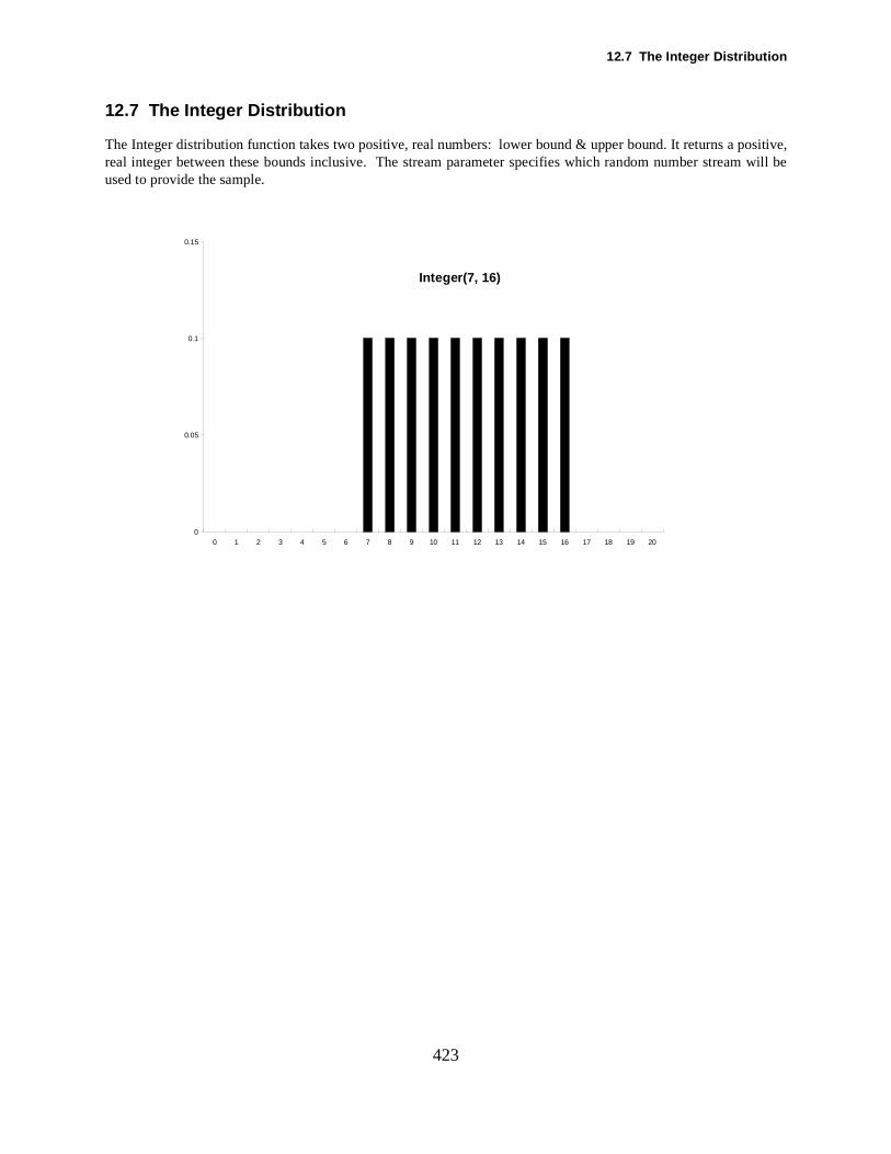
12.7 The Integer Distribution
ositive,m will be
423
12.7 The Integer Distribution
The Integer distribution function takes two positive, real numbers: lower bound & upper bound. It returns a preal integer between these bounds inclusive. The stream parameter specifies which random number streaused to provide the sample.
0
0.05
0.1
0.15
0 1 2 3 4 5 6 7 8 9 10 11 12 13 14 15 16 17 18 19 20
Integer(7, 16)
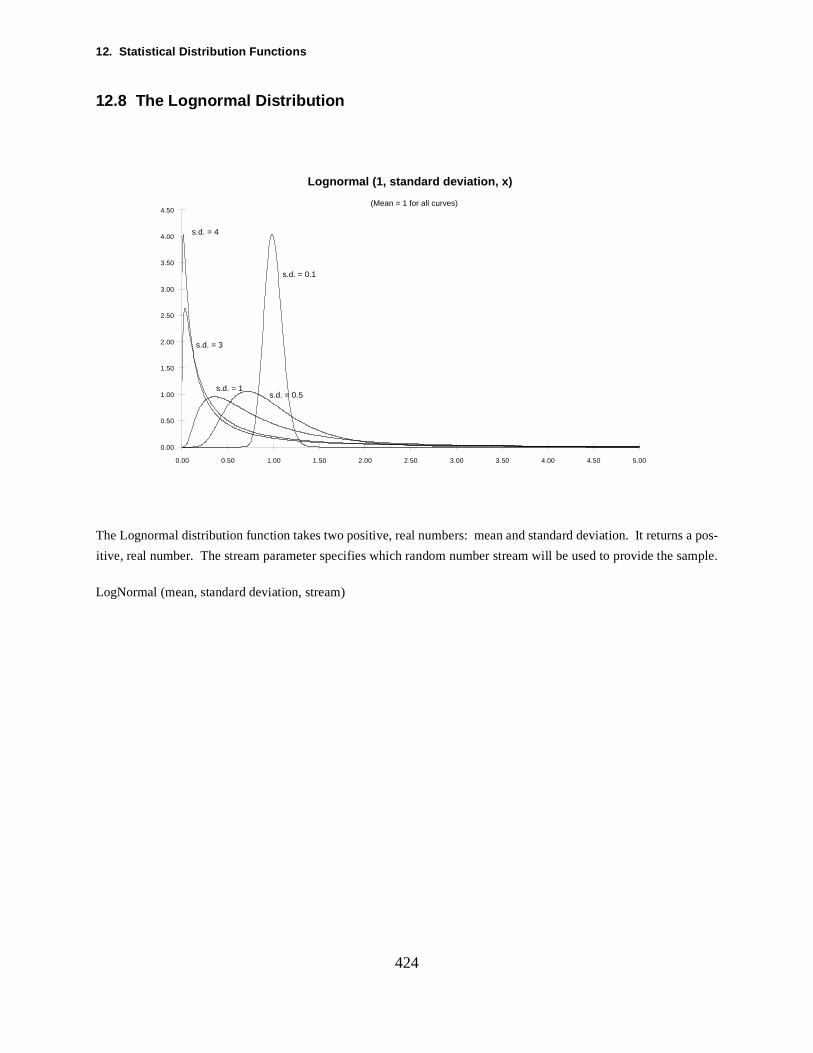
12. Statistical Distribution Functions
os-
sample.
424
12.8 The Lognormal Distribution
The Lognormal distribution function takes two positive, real numbers: mean and standard deviation. It returns a p
itive, real number. The stream parameter specifies which random number stream will be used to provide the
LogNormal (mean, standard deviation, stream)
Lognormal (1, standard deviation, x)
0.00
0.50
1.00
1.50
2.00
2.50
3.00
3.50
4.00
4.50
0.00 0.50 1.00 1.50 2.00 2.50 3.00 3.50 4.00 4.50 5.00
s.d. = 0.1
s.d. = 0.5s.d. = 1
s.d. = 3
s.d. = 4
(Mean = 1 for all curves)
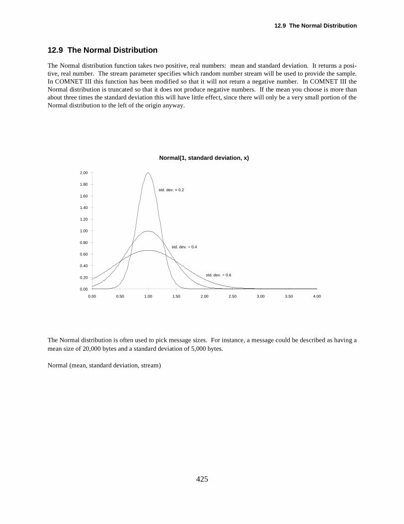
12.9 The Normal Distribution
a posi-e.I theore than of the
g a
425
12.9 The Normal Distribution
The Normal distribution function takes two positive, real numbers: mean and standard deviation. It returnstive, real number. The stream parameter specifies which random number stream will be used to provide the samplIn COMNET III this function has been modified so that it will not return a negative number. In COMNET IINormal distribution is truncated so that it does not produce negative numbers. If the mean you choose is mabout three times the standard deviation this will have little effect, since there will only be a very small portionNormal distribution to the left of the origin anyway.
The Normal distribution is often used to pick message sizes. For instance, a message could be described as havinmean size of 20,000 bytes and a standard deviation of 5,000 bytes.
Normal (mean, standard deviation, stream)
Normal(1, standard deviation, x)
0.00
0.20
0.40
0.60
0.80
1.00
1.20
1.40
1.60
1.80
2.00
0.00 0.50 1.00 1.50 2.00 2.50 3.00 3.50 4.00
std. dev. = 0.2
std. dev. = 0.4
std. dev. = 0.6
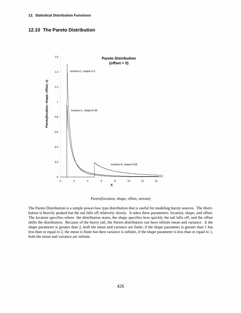
12. Statistical Distribution Functions
tri- offset.
. It thethan 1 butqual to 1,
426
12.10 The Pareto Distribution
Pareto(location, shape, offset, stream)
The Pareto Distribution is a simple power-law type distribution that is useful for modeling bursty sources. The disbution is heavily peaked but the tail falls off relatively slowly. It takes three parameters: location, shape, andThe location specifies where the distribution starts, the shape specifies how quickly the tail falls off, and the offsetshifts the distribution. Because of the heavy tail, the Pareto distribution can have infinite mean and varianceshape parameter is greater than 2, both the mean and variance are finite; if the shape parameter is greater less than or equal to 2, the mean is finite but then variance is infinite, if the shape parameter is less than or eboth the mean and variance are infinite.
Pareto Distribution(offset = 0)
0
0.2
0.4
0.6
0.8
1
1.2
1.4
1.6
0 2 4 6 8 10 12 14
X
Par
eto(
loca
tion,
sha
pe, o
ffset
, x)
location=1, shape=1.5
location=1, shape=0.95
location=5, shape=0.95
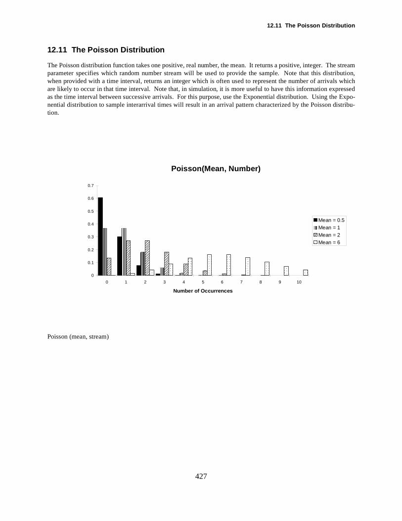
12.11 The Poisson Distribution
e streamibution,s whichessede stribu-
427
12.11 The Poisson Distribution
The Poisson distribution function takes one positive, real number, the mean. It returns a positive, integer. Thparameter specifies which random number stream will be used to provide the sample. Note that this distrwhen provided with a time interval, returns an integer which is often used to represent the number of arrivalare likely to occur in that time interval. Note that, in simulation, it is more useful to have this information expras the time interval between successive arrivals. For this purpose, use the Exponential distribution. Using thExpo-nential distribution to sample interarrival times will result in an arrival pattern characterized by the Poisson dition.
Poisson (mean, stream)
AAAAAAAAAAAAAAAAAAAAAAAAAAAAAAAAAAAAAAAAAAAAAAAAAAAAAAAAAAAA
AAAAAAAAAAAAAAAAAAAAAAAAAAAAAAAAAAAAAAAAAAAAAAAAAAAAAAAAAAAA
AAAAAAAAAAAAAAAAAAAAAAAAAAAAAAAAA
AAAAAAAAAAAAAAA
AAAAAA
AAAAAA
AAAAAA
AAAAAAAAAAAAAAAAAAAAAAAA
AAAAAAAAAAAAAAAAAAAAAAAAAAAAAAAAAAAAAAAAAAAAA
AAAAAAAAAAAAAAAAAAAAAAAAAAAAAAAAAAAAAAAAAAAAA
AAAAAAAAAAAAAAAAAAAAAAAAAAAAAAAAA
AAAAAAAAAAAAAAAAAA
AAAAAAAAA
AAAAAA
AAAAAA
AAAAAA
AAAAAA
AAAAAA
AAAAAAAAAAAA
AAAAAAAAAAAAAAAAAA
AAAAAAAAAAAAAAAAAAAAAAAA
AAAAAAAAAAAAAAAAAAAAAAAAAAAAAA
AAAAAAAAAAAAAAAAAAAAAAAAAAAAAA
AAAAAAAAAAAAAAAAAAAAAAAAAAA
AAAAAAAAAAAAAAAAAAAAA
AAAAAAAAAAAAAAA
AAAAAAAAAAAA
Poisson(Mean, Number)
0
0.1
0.2
0.3
0.4
0.5
0.6
0.7
0 1 2 3 4 5 6 7 8 9 10
Number of Occurrences
Mean = 0.5
AAAAAAMean = 1
AAAAAAMean = 2
AAAAAAMean = 6
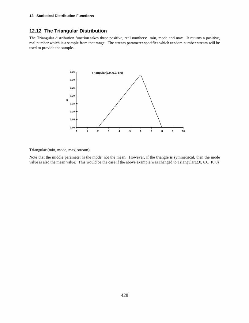
12. Statistical Distribution Functions
ositive,m will be
e.0, 10.0)
428
12.12 The Triangular DistributionThe Triangular distribution function takes three positive, real numbers: min, mode and max. It returns a preal number which is a sample from that range. The stream parameter specifies which random number streaused to provide the sample.
Triangular (min, mode, max, stream)
Note that the middle parameter is the mode, not the mean. However, if the triangle is symmetrical, then the modvalue is also the mean value. This would be the case if the above example was changed to Triangular(2.0, 6
0.00
0.05
0.10
0.15
0.20
0.25
0.30
0.35
0 1 2 3 4 5 6 7 8 9 10
p
Triangular(2.0, 6.0, 8.0)
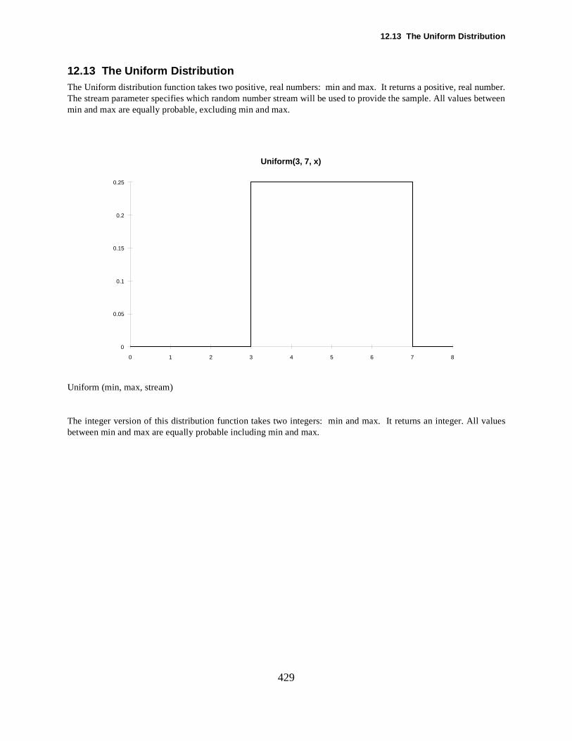
12.13 The Uniform Distribution
umber.between
values
429
12.13 The Uniform DistributionThe Uniform distribution function takes two positive, real numbers: min and max. It returns a positive, real nThe stream parameter specifies which random number stream will be used to provide the sample. All values min and max are equally probable, excluding min and max.
Uniform (min, max, stream)
The integer version of this distribution function takes two integers: min and max. It returns an integer. All between min and max are equally probable including min and max.
Uniform(3, 7, x)
0
0.05
0.1
0.15
0.2
0.25
0 1 2 3 4 5 6 7 8
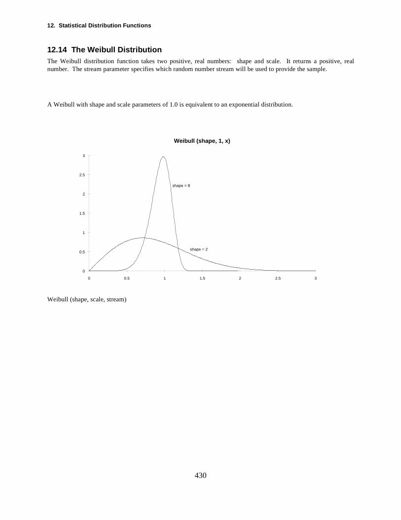
12. Statistical Distribution Functions
al
430
12.14 The Weibull DistributionThe Weibull distribution function takes two positive, real numbers: shape and scale. It returns a positive, renumber. The stream parameter specifies which random number stream will be used to provide the sample.
A Weibull with shape and scale parameters of 1.0 is equivalent to an exponential distribution.
Weibull (shape, scale, stream)
Weibull (shape, 1, x)
0
0.5
1
1.5
2
2.5
3
0 0.5 1 1.5 2 2.5 3
shape = 2
shape = 8
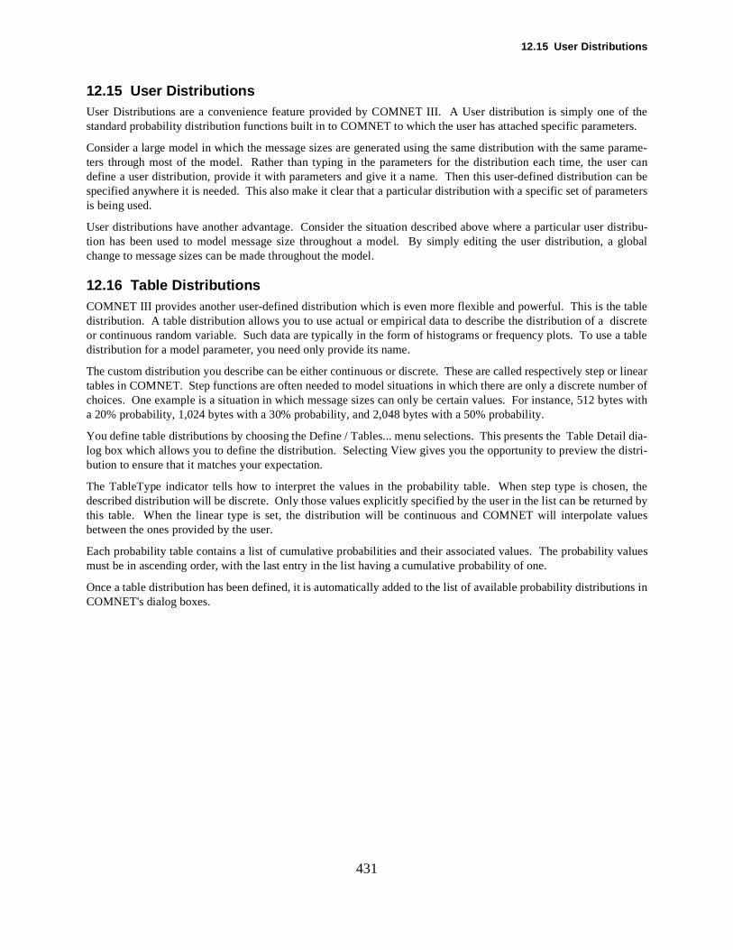
12.15 User Distributions
eters.
parame-ser can can beameters
distribu-l
tablerete a table
or linearmber ofytes with
tail dia-tri-
en, thened by
values
ions in
431
12.15 User DistributionsUser Distributions are a convenience feature provided by COMNET III. A User distribution is simply one of thstandard probability distribution functions built in to COMNET to which the user has attached specific parame
Consider a large model in which the message sizes are generated using the same distribution with the sameters through most of the model. Rather than typing in the parameters for the distribution each time, the udefine a user distribution, provide it with parameters and give it a name. Then this user-defined distributionspecified anywhere it is needed. This also make it clear that a particular distribution with a specific set of paris being used.
User distributions have another advantage. Consider the situation described above where a particular usertion has been used to model message size throughout a model. By simply editing the user distribution, a globachange to message sizes can be made throughout the model.
12.16 Table DistributionsCOMNET III provides another user-defined distribution which is even more flexible and powerful. This is thedistribution. A table distribution allows you to use actual or empirical data to describe the distribution of a discor continuous random variable. Such data are typically in the form of histograms or frequency plots. To usedistribution for a model parameter, you need only provide its name.
The custom distribution you describe can be either continuous or discrete. These are called respectively steptables in COMNET. Step functions are often needed to model situations in which there are only a discrete nuchoices. One example is a situation in which message sizes can only be certain values. For instance, 512 ba 20% probability, 1,024 bytes with a 30% probability, and 2,048 bytes with a 50% probability.
You define table distributions by choosing the Define / Tables... menu selections. This presents the Table Delog box which allows you to define the distribution. Selecting View gives you the opportunity to preview the disbution to ensure that it matches your expectation.
The TableType indicator tells how to interpret the values in the probability table. When step type is chosdescribed distribution will be discrete. Only those values explicitly specified by the user in the list can be returthis table. When the linear type is set, the distribution will be continuous and COMNET will interpolate valuesbetween the ones provided by the user.
Each probability table contains a list of cumulative probabilities and their associated values. The probabilitymust be in ascending order, with the last entry in the list having a cumulative probability of one.
Once a table distribution has been defined, it is automatically added to the list of available probability distributCOMNET's dialog boxes.

12. Statistical Distribution Functions
432
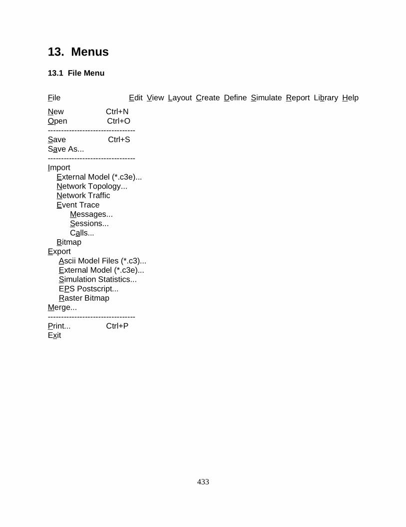
433
13. Menus
13.1 File Menu
File Edit View Layout Create Define Simulate Report Library Help
New Ctrl+N Open Ctrl+O ---------------------------------Save Ctrl+S Save As...---------------------------------Import External Model (*.c3e)... Network Topology... Network Traffic Event Trace Messages... Sessions... Calls... Bitmap Export Ascii Model Files (*.c3)... External Model (*.c3e)... Simulation Statistics... EPS Postscript... Raster BitmapMerge...--------------------------------- Print... Ctrl+P Exit

13. Menus
434
13.2 Edit Menu
File Edit View Layout Create Define Simulate Report Library Help
Cut Ctrl+X Copy Ctrl+C Paste Ctrl+V Duplicate ---------------------------- Clear Del Clone Select All Ctrl+A Select By List... Find... ----------------------------- Parent... Properties...

13.3 View Menu
435
13.3 View Menu
File Edit View Layout Create Define Simulate Report Library Help
By List... ---------------------------- Zoom In Zoom Out Fit to Window View (1:1) ---------------------------- Hide Show Show All Toggle Names ----------------------------- Toolbars Menubar Colorbar 3D Bar ----------------------------- Enter Ctrl+E Leave Ctrl+L
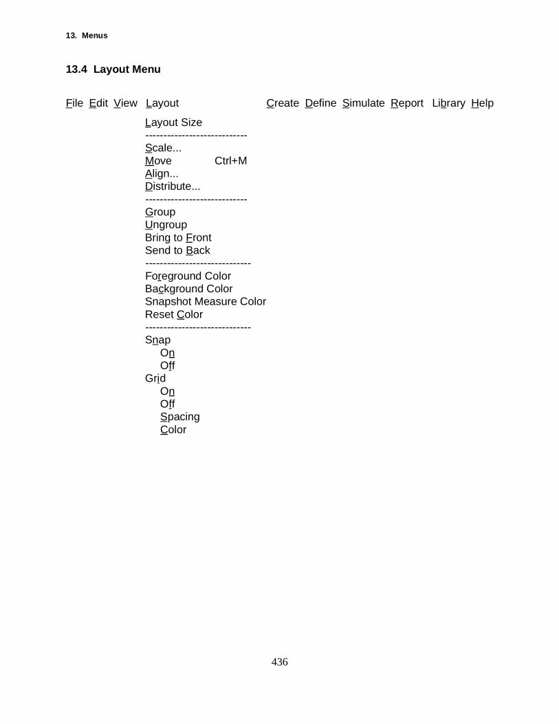
13. Menus
436
13.4 Layout Menu
File Edit View Layout Create Define Simulate Report Library Help
Layout Size ---------------------------- Scale... Move Ctrl+M Align... Distribute... ---------------------------- Group Ungroup Bring to Front Send to Back ----------------------------- Foreground Color Background Color Snapshot Measure Color Reset Color ----------------------------- Snap On Off Grid On Off Spacing Color

13.5 Create Menu
437
13.5 Create Menu
File Edit View Layout Create Define Simulate Report Library Help
Nodes Processing Node Router Computer Group Switch Links Point-To-Point DAMA Aloha CSMA CSMA/CD Polling Token Passing CSMA/CA FDDI Basic Priority Token Ring Priority FDDI Clouds WAN Clouds Frame Relay ATM Application Sources Application Source Message Sources Message Source Response Source Session Sources Session Source Call Sources Call Source Cloud VCs Cloud VC Cloud Access Link Cloud Access Remotes Remote Link Remote Node Socket Networks Network
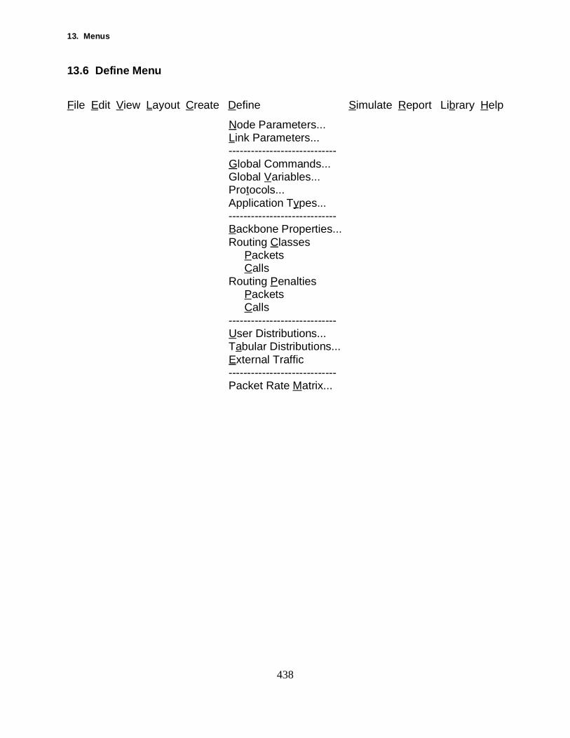
13. Menus
438
13.6 Define Menu
File Edit View Layout Create Define Simulate Report Library Help
Node Parameters... Link Parameters... ----------------------------- Global Commands... Global Variables... Protocols... Application Types... ----------------------------- Backbone Properties... Routing Classes Packets Calls Routing Penalties Packets Calls ----------------------------- User Distributions... Tabular Distributions... External Traffic ----------------------------- Packet Rate Matrix...

13.7 Simulate Menu
439
13.7 Simulate Menu
File Edit View Layout Create Define Simulate Report Library Help
Verify Model Run Parameters ----------------------------- Start Simulation F4 Halt Simulation F5 ----------------------------- Animate... Trace...

13. Menus
440
13.8 Report Menu
File Edit View Layout Create Define Simulate Report Library Help
Set File Name... Select File Name... Browse Reports... ----------------------------- Select Snapshots... Take Snapshot...

13.9 Library Menu
441
13.9 Library Menu
File Edit View Layout Create Define Simulate Report Library Help
Edit Contents... Software Objects Load Unload

13. Menus
442
13.10 Help Menu
File Edit View Layout Create Define Simulate Report Library Help
Index Dump Memory Usage... About COMNET III...
Index
443
AAccess Link..............................23, 47, 50
Statistics.......................................405Access Link Statistics........................341access links........................................318Access Point.......21, 22, 23, 32, 305, 307
Connectivity...................................32Creating..........................................32Editing............................................32Execution.......................................32Fields..............................................34Purpose...........................................32Reporting.......................................34
Accuracy........................................2, 3, 4Acme Bank Model.................................7Add To...............................................414Aloha....................................................22Analytical Methods................................2Animation................................8, 23, 407
Control.........................................322Speed............................................322Step Size......................................322
Answer Message Command....24, 25, 53Connectivity...................................53Creating..........................................53Editing............................................53Execution.......................................54Fields..............................................55
Message Size Calculation........55Message Size Units..................55Message Text...........................55Name........................................55Packet Routing Class...............55Packetizing Delay....................55Priority .....................................55Transport Protocol...................55
Purpose...........................................53Reporting.......................................55
ApplicationDelay............................................345Instance........................................345Pending List.................................345Scheduling.......................................3Suspended......................................72
Application Command.......................345Application Run Length.....................341
Application Source........................24, 25Application Source Reports...............341Applications.........................................24
End User..........................2, 3, 4, 5, 6Arc .........................21, 23, 407, 409, 410Archive Library....................................21Archive Menu....................................325Areas..................................................410Automatic Parameter Iterator.............337Averaged Statistics............................405
BBackbone.......................................22, 26
Model Layout...............................305User System.........................3, 4, 5, 7
Backbone Links...................................32Bandwidth
Circuit Switched373, 374, 375, 376, 377, 378, 379
Banking Network...................................4batch mode.............................................8binary files...........................................30Bitmap........................................306, 407Block
Call...............................373, 376, 377Packet...................360, 370, 371, 372
Blocked Call Counts..........................341Bottleneck..................................3, 4, 6, 9bridges..................................................21Browse Reports..................................343Buffer Processing.................................35
Backward Explicit Congestion Notifica-tion (BECN).......................36
Buffer Policy..................................35Buffer Size.....................................35Buffer Sorting................................36Explicit Congestion Notification...36Forward Explicit Congestion Notification
(FECN)...............................36Preemption Policy..........................36Processing at Buffers.....................37Threshold Policy............................36
Building Blocks.....................................3burst size..............................................50bursty sources....................................426Bursty Traffic.....................................4, 5
Index
t
444
BusyLink ..............................................352Node.....................................344, 347
Byte......................................................21
CCall Counts........................................341Call Holding Time.............373, 374, 375Call Level...........................................341Call Source...................25, 373, 374, 375
Call Holding Time distribution373, 374, 375
Destination...373, 374, 375, 376, 377Call Source Reports...........................341Canvas....................................22, 23, 409
Dimension....................................413Canvas Window.........408, 410, 411, 412Carrier-Sense Multiple-Access............22Cell-Relay Network...........................318Cell-Relay Networks............................40Channel Utilization............................341Circle..........................................407, 409Circuit Switched Network.....................2Circuit Switched Traffic318, 373, 374, 375,
376, 377, 378, 379Circuit-Switched Model.......................38
Connectivity...................................38Creating..........................................38Editing............................................38Execution.......................................38Fields..............................................39Purpose...........................................38Reporting.......................................39
ClearMenu Option................................412Pending Messages................384, 385
client-server operations........................73Cloud..........................21, 22, 23, 40, 318
Behavior.........................................40Congestion Levels..........................40Congestion States...........................42Connectivity...................................41Creating..........................................41Editing............................................42Fields..............................................43
Delay Switch............................44
Frame Assembly......................44Frame Drop Probability...........45Frame Max...............................44Frame Min................................44Frame Overhead.......................44Frame Priority..........................44Parameter Set Name.................44Routing Interval.......................44Session Limit...........................44Transmit Non-Virtual Circuits (VCs)
44Use of Comitted Information Rate
(CIR) in Virtual Circuits(VC) .............................44
Handling Frame Dropping.............40Purpose...........................................40
Cloud Access Link ...............................47Connectivity...................................47Creating..........................................47Editing............................................47Fields..............................................47
Buffer Definition......................48Buffer Limit .............................48Buffer Policy............................48Buffer Units.............................48Early Packet Discard/Partial Packe
Discard.........................48Buffer Threshold (Buffer Units)
48Discard Type......................48
Entry Bandwidth......................47Exit (Egress) Buffer.................48Exit Bandwidth........................47Number of Circuits..................47Propagation..............................48Use Unlimited buffer...............48
Purpose...........................................47Cloud Access Links...........................319Cloud VCs..........................................319Cloud Virtual Circuit...........................50
Connectivity...................................50Creating..........................................50Editing............................................51Fields..............................................51
Burst Type................................51Committed Burst Size..............51
445
Committed Information Rate (CIR)or Burst Interval...........51
Excess Burst Size.....................51Mark Discard Eligible (DE) Frames
51Never Drop Due to Excess Burst52Number of Switches.................52Propagation Delay....................52Show Burst Size.......................52
Purpose...........................................50Collision.............................................351Collision Statistics.............................341Color..........................................409, 411
Palette...........................................408Command
Processing............................320, 344Read.....................................344, 347Response..............................358, 371Session.................359, 372, 381, 384Transport..............................358, 371Write ....................................344, 347
command line interface..........................8command repertoire.............................24committed burst size............................50committed information rate.................50COMNET Baseliner....................80, 415
Network Load Characterization...416Network Topology Information...416Overview......................................415System Architecture.....................415
COMNET III3D View.......................................327Arc Editing...................................327Background Text..........................328Bitmap Import..............................327Color Palette................................327Dockable Palettes and Toolbar....327Export Encapsulated PostScript...327Export Raster Bitmap...................328Model Editing Features................328Object Creation Tools..................304Report Request Manager.............328Shapes..........................................327starting.............................................7Starting the Program....................303Terminology...................................21
Tool Tips and Status Bar Messages327Using the Tool Palette..................303
Computer & Communication Node.3, 14Computer and Communications Node.21Computer Group Node.........................21Computers............................................21Connection Oriented Routing2, 318, 349,
383Connection Tool..............................2, 14Connectionless Routing.2, 318, 349, 383Connection-Oriented Routing..............26Contention Interval............................352Continuous Probability Distributions431Copy
From Clipboard............................310Simdraw.......................................412To Clipboard................................310
CostDollar ...........................................1, 6
Count..................................................406Create
Application...................................318Call...............................................318File & Subdirectory.................7, 308Group In Simdraw.......................414Icon......................................306, 407Link ........................................14, 318Menu............................................318Message.......................................318Network Description................1, 308Node.......................................14, 318Packet...........344, 360, 370, 371, 372Pending Message Notice......384, 385Session.........................318, 380, 381Session Connect Packet372, 380, 381Session Setup Packet372, 380, 381, 384,
385Tag in Simdraw............................414
Create Menu.......................................318CSMA..........................................22, 351
Contention Interval......................352CSMA/CA Link...................................22CSMA/CD...........................................22Cut
COMNET III................................305Simdraw.......................................412
Index
-
446
CycleSimdraw.......................................409
Cycle Time.....................................5, 320
Ddata traffic............................................26DE........................................................50DECNet................................................27Define Menu......................................320Delay
Queuing............................................5Demand Assigned Multiple Access Link22Demo Model..........................................7Desintaion
Random Neighbor..........................86Destination.............................4, 346, 356
Call Source...373, 374, 375, 376, 377Least Busy List..............................81
Connectivity.............................81Creating....................................81Editing......................................81Execution.................................81Fields........................................81
Destination Node Name.....81Purpose.....................................81Reporting.................................81
Message357, 358, 359, 360, 370, 371, 372
Multicast List.................................82Random List...................................84Random Neighbor..........................86Round Robin List...........................87
Connectivity.............................87Creating....................................87Editing......................................87Execution.................................87Fields........................................87
Destination Node Name.....87Purpose.....................................87Reporting.................................87
Session.380, 381, 382, 383, 384, 385Weighted List.................................88
Destination List356, 357, 358, 359, 360, 370, 371, 372, 373, 374, 375, 380, 381
DimensionCanvas..........................................413
Icon..............................................413Disconnected CallCounts...................341Discrete Event Simulation.........2, 4, 322Discrete Probability Distributions.....431Disk Access Error Counts..................341Disk Access Time..................................5Disk Capacity.............................344, 347Distribution
Beta..............................................417Erlang...........................................418Exponential..................................419Gamma.........................................420Geometric.....................................421Hyperexponential.........................422Integer..........................................423Lognormal....................................424Normal.........................................425Poisson.........................................427System............................................90
Connectivity.............................90Creating....................................90Editing......................................90Execution.................................90Fields........................................91
Beta....................................91Erlang.................................91Exponential........................91Gamma...............................91Geometric...........................91Hyperexponential...............91Integer................................91Lognormal..........................91Normal...............................91Poisson...............................91Triangular...........................91Uniform..............................91Weibull...............................91
Purpose.....................................90Random Number Generation Al
gorithm...................90Random Number Starting Seed
90Reporting.................................90
Table..............................................92Connectivity.............................92Creating....................................92
447
Editing......................................92Execution.................................92Fields........................................92
Name..................................92Probability..........................93Table Type.........................93Value..................................93
Purpose.....................................92Reporting.................................92
Triangular.....................................428Uniform........................................429UniformInteger............................429User Defined..................................94
Connectivity.............................94Creating....................................94Editing......................................94Execution.................................94Fields........................................94
Name..................................94Probability Distribution.....94
Purpose.....................................94Reporting.................................94
Weibull.........................................430Distribution Table................................29distribution, power-law......................426distributions.........................................29Duplicate
Simdraw.......................................412dynamic algorithms..............................26
EEdit
Commands...................................320Graphics.......................................306Menu Option................................310Packet Routing Class...................321Packet Routing Penalties.............321Simdraw Editor............................407Table Distributions......................321Transport Layer Protocol.............320User Distributions........................321
Edit Features......................................328Edit Menu..................................305, 306End System........................................3, 5Enter...................................................313Entry Link Utilization........................405
Erlang Distribution............................418Ethernet........................................3, 5, 22excess burst size...................................50Exit Buffer Size.................................405Exit Link Utilization..........................405Exponential Distribution............419, 427Export.................................................308Exporting Statistics............................406Extended Mode............14, 304, 306, 409external file format...............................30External Model File.............................30
ExportDefaults....................................30TRUE_NAME.........................30
External Sources..................................25External Traffic..................................321External Traffic File.............................25External Traffic Sources......................25
FFDDI ....................................................22FDDI Link............................................22File
COMNET III Data File..............7, 16COMNET III Report File................7File Size...........................................3File Transfer.....................................3
file format............................................30File Menu.......................................8, 308Fill Style.............................408, 409, 411Filter Message Command....................24
FieldsFilter Command Name.............74
Flow Control........................................97Connectivity...................................97Creating..........................................97Editing............................................97Execution.......................................97Fields..............................................98
ACK Priority............................98End-To-End ACK Bytes..........98Retransmit Blocked Packets....98Retransmit Time......................98Window Size............................98
Fields for Enhanced Flow Control.98Error Control Options..............98
Index
448
Holding ACKs for More Data.98Retransmit Timeout Backoff...99Retransmit Timeout Calculated from
Estimated Round-Trip Time99
Fixed Window..............................100Connectivity...........................100Creating..................................100Editing....................................100Execution...............................100Fields......................................100Purpose...................................100Reporting...............................100
Jumping Window.........................102Connectivity...........................102Creating..................................102Editing....................................102Execution...............................102Fields......................................102Purpose...................................102Reporting...............................102
Leaky Bucket...............................103Connectivity...........................103Creating..................................103Editing....................................103Execution...............................103Fields......................................103Purpose...................................103Reporting...............................103
Purpose...........................................97Reporting.......................................98Sliding Window...........................101
Connectivity...........................101Creating..................................101Editing....................................101Execution...............................101Fields......................................101Purpose...................................101Reporting...............................101
SNA Pacing..................................104Connectivity...........................104Creating..................................104Editing....................................104Execution...............................104Fields......................................104Purpose...................................104
Reporting...............................104TCP/IP Window...........................105
Connectivity...........................105Creating..................................105Editing....................................105Execution...............................105Fields......................................105Purpose...................................105Reporting...............................105
Font Style...........................................409Frame
Collision.......................................351Error probability..........................349Report...........................................349Transmission Time......................350
Frame Counts.....................................341Frame Delay.......................................341Frame Relay.........................................47
Networks........................................40frames...................................................23from....................................................414Full Duplex........................................349
GGamma Distribution..........................420Gateway.................................................5gateway node.......................................22gateways...............................................21Geometric Distribution......................421Grade Of Service...............................4, 6Granularity.............................................4Graphic
Editing Points...............................412Editor ...........................................407Icon..............................................407Image...................................407, 409Importing.....................................306Library File..........................306, 407Primitive.......................................407Priority .........................................411
Graphical User Interface1, 303, 307, 407Graphical user interface.........................2Graphing
Real Time.........................................9Grid....................................................413Grouping Images................................413
449
HHelp Menu.........................................326HP NetMetrix.....................................321Hub.......................................................22Hyperexponential Distribution..........422
IIcon
Background Tool.........................306Creating........................................407Dimension....................................413Link ..................................................9Moving.................................307, 314Node.................................................9Program............................................7Scaling.........................................314Subnetwork..................................306Text Tool......................................306
ID Code..............................................305Idle
Link ..............................................352Node.............................................344
IEEE 802............................................106Standards......................................106
Broadband Technical AdvisoryGroup.........................106
CSMA/CD Networks.............106Fiber Optic Technical Advisory
Group.........................106Higher Layer Interface...........106Integrated Voice and Data LAN Inter-
face.............................106Logical Link Control.............106Metropolitan Area Networks.106Standard for Interoperable LAN Se-
curity ..........................106Token Bus Networks.............106Token Ring Networks............106Wireless LAN........................106
IGRP....................................................26Importing Network Traffic Files........308Importing NMS Topology Files........308Input Buffer Totals.............................341Input Buffer Use................................341Installation of COMNET III..................7Integer Distribution............................423
Interarrival time.................................419internal file format...............................30Internetworking......................................4IPX.......................................................27ISDN................................................2, 22Iteration Time......................................24
KKelton, W. David...................................3Kilobyte ...............................................21
LLAN ...........................................2, 3, 5, 7Law, Averill ...........................................3Layer 4...............................................320Leased Line........................................4, 5Least Busy List....................................81Level Of Detail..................................4, 5libraries................................................29Library
Graphic Images............306, 407, 413Network Components..............2, 318
Line Style...................................409, 411Line Width.................................409, 411Lines...................................................410Link ........................................21, 22, 107
Aloha............................................121Connectivity...........................121Creating..................................121Editing....................................121Execution...............................122Fields......................................124
Control Node....................124Current State....................124Icon..................................124Name................................124Statistics...........................124Time Of Next State Change124Time to Failure.................124Time To Repair................124
Parameter Set Fields..............124Bandwidth........................124Control Channel...............125Framing Characteristics...125Propagation Delay............124Retry Interval...................125
Binary Exponential Backoff
Index
450
125Probability Distribution125
Session Limit...................124Slot Width........................124Transmission Return Rate125
Purpose...................................121Reporting...............................124
Binary Exponential Backoff........109Connectivity...........................109Creating..................................109Editing....................................109Execution...............................109Fields......................................109
Limit Delay......................110Offset...............................110Retry Limit.......................110Slot Time..........................110Stream..............................110
Purpose...................................109Reporting...............................109
Connections.................................305Connectivity.................................107Creating........................................107Creation..................................14, 304CSMA..........................................126
Connectivity...........................126Creating..................................126Editing....................................126Execution...............................127Fields......................................128
Control Node....................128Current State....................129Icon..................................128Name................................128Statistics...........................129Time Of Next State Change129Time To Failure...............129Time To Repair................129
Parameter Set Fields..............129Bandwidth........................129Collision Window............129Control Channel...............130Framing Characteristics...129Interframe Gap.................129Jam Interval......................129Propagation Delay............129
Retry Interval...................129Binary Exponential Backoff
130Probability Distribution130
Session Limit...................129Transmission Return Rate130
Purpose...................................126Reporting...............................128
CSMA/CD...................................135Connectivity...........................136Creating..................................135Editing....................................136Execution...............................136Fields......................................137
Control Node....................137Current State....................137Icon..................................137Name................................137Statistics...........................137Time Of Next State Change137Time To Failure...............137Time To Repair................137
Parameter Set Fields..............137Bandwidth........................137Binary Exponential Backoff138Collision Window............137Control Channel...............138Framing Characteristics...138Interframe Gap.................138Jam Interval......................137Probability Distribution...138Propagation Delay............138Retry Interval...................138Session Limit...................138Transmission Return Rate138
Purpose...................................135Reporting...............................137
Editing..........................................107Failure..........................................5, 9Fields............................................107
Connections...........................108Control Node..........................107Current State..........................108Icon........................................107Name......................................107Parameters..............................107
451
Time Of Next State Change...108Time To Failure.....................107Time To Repair......................107Type.......................................107
Framing........................................111Connectivity...........................111Creating..................................111Editing....................................111Execution...............................111Fields......................................112
Automatically Retransmit FrameErrors...................112
Frame Error Probability...112Frame Max.......................112Frame Min........................112
Frame Assembly....................111Frame Overhead.....................112Purpose...................................111Reporting...............................112
ISDN and SONET Parameter Sets113Point To Point Protocol....................4Point-To-Point.............................143
Connectivity...........................143Creating..................................143Editing....................................143Execution...............................144
Circuit Switching.............145Packet Switching..............144
Fields......................................145Control Node....................146Icon..................................146Link State.........................146Name................................145Statistics...........................146
Parameter Set FieldsCircuit Switching.............146
Bandwidth..................146Bandwidth Reserved for 1-
Hop Calls.......146Number Of Circuits...146
Packet Switching..............146Bandwidth From Node 1146Bandwidth From Node 2146Framing Characteristics147Number Of Circuits...146Propagation Delay......146
Session Limit.............146Purpose...................................143Reporting...............................145
Polling..........................................148Connectivity...........................148Editing....................................148Execution...............................148Fields......................................150
Control Node....................150Icon..................................150Link State.........................150Name................................150Statistics...........................150
Parameter Set Fields..............150Bandwidth........................150Control Channel...............150Framing Characteristics...151NAK (Negative Acknowledment)
Delay....................150Poll Delay........................150Poll Needed To Send.......150Propagation Delay............151Session Limit...................151Transmission Return Rate150
Purpose...................................148Reporting...............................149
Port...............................................152Connectivity...........................152Creating..................................152Editing....................................152Execution...............................152Fields......................................153
Call Routing Penalty Table155Input Buffer Delay...........153Input Buffer Size..............153Line Card ID....................154Output Buffer Delay........154Output Buffer Size...........154Packet Routing Penalty Table155
Purpose...................................152Reporting...............................152
Purpose.........................................107Token Passing..............................157
Connectivity...........................157Creating..................................157Editing....................................157
Index
452
Execution...............................157Fields......................................158
Icon..................................159Link State.........................159Name................................158Statistics...........................159
Parameter Set Fields..............159Bandwidth........................159Framing Characteristics...159Propagation Delay............159Session Limit...................159Token Holding Limit.......159Token Passing Delay.......159
Purpose...........................156, 157Reporting...............................158
Utilization ......................................16Link Reports......................................341Link-State Shortest Path First..............26Load...................................1, 3, 4, 5, 413Loading A Model...................................8Loading COMNET III...........................8Loading Graphic Libraries.................413Lognormal Distribution.....................424
MMain Menu.........................................307Mainframe......................................1, 3, 4Mark Style..........................................409Maximum...........................................406Mean Entry Link Utilization..............405Mean Exit Buffer Size.......................405Mean Exit Link Utilization................405Megabyte.............................................21Menu..................................................433
Archive.........................................325Create...................................318, 437Define...................................320, 438Edit.......................305, 306, 310, 434File ...................................8, 308, 433Help......................................326, 442Layout..........................................436Library .........................................441Main.............................................307Report...........................................440Simulate...........................8, 322, 439View.....................................311, 435
Menu Option......................................307Create
Application Source................318Call Sources...........................318Cloud Access Links...............319Cloud Virtual Circuits............319Clouds....................................318Links ......................................318Message Sources....................318Networks................................319Nodes.....................................318Remotes.................................319Session Sources......................318
DefineApplication Types..................320Backbone Routing..................320External Traffic......................321Global Commands.................320Global Variables....................320Link Parameters.....................320Node Parameters....................320Packet Rate Matrix.................321Packet Routing Penalties.......321Routing Class.........................321Tables.....................................321Transport Protocols................320User Dists...............................321
Define Backbone Routing..............15Edit
Clear.......................................310Clone......................................310Copy.......................................310Cut..........................................310Duplicate................................310Find........................................310Parent.....................................310Paste.......................................310Properties...............................310Select All................................310Select by List.........................310
Edit Detail............................305, 306Edit Move....................................307File
Exit.........................................309Export.....................................308Import.....................................308
453
Merge.....................................309New........................................308Open.......................................308Print........................................309Save........................................308Save As..................................308
File Export...................................308File Import...................................308File Save As...................................16Help
About COMNET III...............326Dump Memory Message........326Index......................................326ReadMe File...........................326Reference Manual..................326
LayoutAlign ......................................314Background Color..................317Bring to Front.........................317Distribute...............................316Foreground Color...................317Grid........................................317Group.....................................317Layout Size............................314Move......................................314Reset Color............................317Scale.......................................314Send to Back..........................317Snap.......................................317Ungroup.................................317
LibraryEdit Contents..........................325Software Objects....................325
ReportApplication Sources...............324Background Packet Flows.....324Browse Reports......................324Call Sources...........................324Global Setup Commands.......324Global Transport and Answer Com-
mands.........................324Links ......................................324Message and Response Sources324Nodes.....................................324Select Snapshots....................324Session Sources......................324
Set File Name.........................324Setup Commands...................324Take Snapshot........................324Transport Commands.............324WAN Clouds..........................324
Reports/Call Sources......................16Simulate
Animate..................................322Halt.........................................322Run Parameters......................322Start........................................322Trace......................................322Verify .....................................322
Simulate Run Parameters...............15Simulate/Browse Reports..............16Simulate/Start.................................16Simulate/Trace...............................16Table Detail..................................431View
By List....................................311Enter.......................................313Fit to Window........................312Hide........................................312Leave......................................313Show......................................313Show All ................................313Toggle Names........................313Toolbars.................................313View (1 to 1)..........................312Zoom In..................................312Zoom Out...............................312
Merge.................................................309Message
Destination357, 358, 359, 360, 370, 371, 372
Source..........................................318Message Delay...........................341, 342Message ID..........................................25Message Response Source Reports....341Message Source...................................25
Interarrival Time..........................160Applicability ..........................160Creating..................................160Editing....................................161Execution...............................161Fields......................................162
Index
454
Interarrival Time..............162Start Time........................162Stop Time.........................162
Purpose...................................160Reporting...............................162
Message Text...............................170Connectivity...........................170Creating..................................170Editing....................................170Execution...............................170Fields......................................171
Message Text...................171Copy Message Name.171Set Message Text.......171Use Original Message171
Purpose...................................170Reporting...............................171
Packetizing Delay........................163Connectivity...........................163Creating..................................163Editing....................................163Execution...............................163Fields......................................164
Packetizing Delay............164Purpose...................................163Reporting...............................164
Priority .........................................165Connectivity...........................165Creating..................................165Editing....................................165Execution...............................165Fields......................................166
Priority .............................166Purpose...................................165Reporting...............................166
Size Calculation...........................167Connectivity...........................167Creating..................................167Editing....................................167Execution...............................167Fields......................................167
Message Size....................167Based On File Size.....168Based On Message Size168Probability Distribution167
Purpose...................................167
Reporting...............................167Size Units.....................................169
Connectivity...........................169Creating..................................169Editing....................................169Fields......................................169
Size Unit..........................169Purpose...................................169Reporting...............................169
Message Switched Network...................2Message Traffic.....................................4Metropolitan Area Network...................4Microsoft Windows...........................2, 7Minimum ...........................................406Minimum Hop Routing........................26Minimum Penalty................................26Model
Creation........................................303Background Icon Tool...........306Connection Tool....................305
Jointed Arc Tool..............305Right Angle Tool.............305
Import Bitmaps......................327Link ........................................304Moving Around the Layout
Panning............................307Moving Objects......................307Multiple Objects....................304Node.......................................304Object Creation Tools............304Selecting a Group of Objects.306Selection Tool........................305Subnetwork Tool....................306Text Tool................................306Traffic Source........................304Using the Tool Palette............303
Filename.......................................303Modify a Network Description....303
Model Building..........................1, 14, 21Model Bulding.....................................21Model Editing Features......................328
Find..............................................328Matching Rules......................328Options...................................328
Select by List...............................328View by List.................................328
455
Filter "DEFAULT" Objects...328Filter Items with Default Value328
Model File......................................29, 95External..........................................95
Purpose.....................................95Modeling Constructs............................31Modeling Terminology........................21Moving Icons.....................................307Multicast List.......................................82
Connectivity...................................82Creating..........................................82Editing............................................82Execution.......................................82
Dropped Packets......................83Flow Control............................83Routing Alogorithm.................83
Fields..............................................83Destination Node Name...........83
Purpose...........................................82Reporting.......................................83
NNamed Distributions............................29Network
Access Point.........................305, 307ACME Bank Model.........................7Analyzers.......................................25Backbone.............................3, 4, 305Banking............................................4Bearer...............................................3Capacity.......................................4, 5Description...................................303Design......................................1, 4, 5General.............................................1Grade Of Service.............................6Internetworking................................4LAN .........................................2, 3, 5Load.............................................3, 6MAN ................................................4Operation.....................................320Peak Loading...................................5Performance.............................2, 3, 6Protocols..........................................3Resilience.........................................5Subnetwork..................................306Topology......................................2, 3
User..................................................6Voice................................................4WAN ............................................2, 3
Network General Sniffer....................321Network Topology...............................21Network Traffic and Workload............23Node.............................................21, 172
Computer Group..........................194Connectivity...........................194Creating..................................194Editing....................................194Execution...............................195Fields......................................196
Call Bandwidth................196Quantity...........................196Source/Sink Only.............196
Purpose...................................194Reporting...............................196
Connectivity.................................172Creating........................................172Creation........................................304Cycle Time...............................5, 320Disk Access Time............................5Disk Capacity.......................344, 347Editing..........................................172Failure..........................................5, 9Fields............................................172
Icon........................................172Name......................................172Parameters..............................172
Commands.......................173Current State....................173Time of Next State Change172Time To Failure...............172Time To Repair................172
Type.......................................172Input Buffer..................................349Output Buffer...............................349Parameters......................................24Processing Node..........................179
Connectivity...........................180Creating..................................179Editing....................................180Execution...............................180
Buffer Processing.............183Circuit Switching.............184
Index
456
Command Execution........184No Time Slice..................181Processor Scheduling.......180With Time Slicing............182
Fields......................................185Call Routing Table...........185Icon..................................185Name................................185Node State........................185Packet Routing Table.......185
Parameter Set Fields..............185App Ready The Longest..186Apps Have Priority..........187Between Applications......186Between Apps And Packets186Between Pkt Buffers........187Call Limit .........................191Command List..................192Disk Sector Size...............192Disk Size..........................191Disk Transfer Overhead...192Disk Transfer Time..........192Earliest Arrival.................187Edit Processor..................185File List............................192File Name.........................192File Read Only Flag.........192File Size...........................192First App Available..........186Input Buffer Size..............190Number Of Processors.....185Output Buffer Size...........190Packet Priority..................187Packet Processing Uses Proces-
sor.........................188Pkts Have Priority............186Port Processing Times.....191Processing Time/Cycle....188Processing Time/KByte...190Processing Time/Packet...189Processing Time/Setup Packet
190Processor Usage...............188Read/Write Commands Use Proc-
essor.....................188Ready The Longest..........187
Selection Rules................186Session Limit...................191Source/Sink Only.............185Time Slice........................189
Purpose...................................179Reporting...............................184
Purpose.........................................172Router...........................................197
Connectivity...........................197Creating..................................197Editing....................................198Execution...............................200
Circuit Switching.............201Packet Switching..............200
Fields......................................202Call Routing Table...........202Icon..................................202Name................................202Node State........................202Packet Routing Table.......202
Parameter Set Fields..............202Bus Count........................204Bus Rate...........................204Input Buffer Limit............204Output Buffer Limit.........205Port Processing Times.....204Processing Time/Cycle....202Processing Time/KByte...203Processing Time/Packet...202Processing Time/Setup Packet
204Time Slice........................202
Purpose...................................197Reporting...............................202Updated Router Library.........206
Switch..........................................174Connectivity...........................174Creating..................................174Editing....................................175Execution...............................175
Circuit Switching.............176Packet Switching..............175
Fields......................................177Call Routing Table...........177Icon..................................177Name................................177
457
Node State........................177Packet Routing Table.......177
Parameter Set Fields..............177Input Buffer Max.............178Output Buffer Max...........178Parameter Set Name.........177Virtual Cut-Through........177
Purpose...................................174Reporting...............................177
Types of.........................................21Node Reports.....................................341Nodes...................................................21Normal Distribution...........................425
OObject Creation..................................304Object Libary Access...........................29Object Library......................................29Objects...................................................1Origin.....................................................4Output Buffer Totals..........................341Output Buffer Use..............................341Overview of Modeling Constructs.......21Owner Name......................................406Owner Type.......................................406
PPacket
Animation........................................8Routing.........................................321Switch..............................................3
Packet Delay..............................341, 342Packet Rate Matrix.............................288Packet Switched Network......................2Packet Switched Networks................207
Connectivity.................................207Creating........................................207Editing..........................................207Execution.....................................207Fields............................................208Purpose.........................................207Reporting.....................................208
packets.................................................23Pad...............................................3, 4, 21Painting..............................................411Palette.................................................407
Tool..............................2, 8, 303, 305
Window........................408, 409, 410Parameter Iterator..............................337Parameter Sets....................................209
Connectivity.................................210Creating........................................210Editing..........................................210Execution.....................................210Purpose.........................................209Reporting.....................................210
parameter sets......................................29Parent.................................................310PC...........................................................4Peak Loading.....................................4, 5Penalty Tables..............................26, 211
Connectivity.................................211Creating........................................211Editing..........................................211Execution.....................................214Fields............................................214
Name......................................214Penalty Per Routing Class......214Threshold...............................214
Purpose.........................................211Reporting.....................................214
penalty tables.......................................23Percentiles..........................................403Percentiles and Plots..........................403
Access Link Statistics..................405Exporting Statistics......................406
statfile.xpt..............................406Count................................406Maximum.........................406Minimum .........................406Owner Name....................406Owner Type.....................406Replication.......................406Statistics Type..................406Sum..................................406Sum of Squares................406
Overview......................................403Post-processed Plots....................403Real-time Plots.....................404, 405Smoothed Data.............................403Statistics Request Buttons............403Virtual Circuit Statistics...............406
Burst Size...............................406
Index
458
Frame Delay...........................406Performance...............................1, 2, 3, 5Plots...................................................403Point To Point Link................................4Point-To-Point Link.............................22Poisson Distribution...........................427Polling..................................................22Polygon......................................407, 410Polyline..............................................410Port.......................................................23port parameters....................................23Portability...............................................2power-law type distribution...............426Preempted Call Counts......................342Preemption...................26, 375, 376, 377Print Server............................................3print server.............................................3Priority
Call.......................................374, 375Graphic.........................................411
Priority Token Ring Link.....................22private data networks.........................318Probability
Blocking...............................376, 377Distribution..........................320, 417
Process & Disk Utilization Reports...342Process Data.........................................56Process Data Command.......................56
Connectivity...................................56Creating..........................................56
Global Command.....................56Library Command....................56Local Command.......................56
Editing............................................56Execution.......................................57
No Time Slicing.......................57With Time Slicing....................57
Fields..............................................57Name........................................57Number Of Cycles...................57
Based On File Size.............58Probability Distribution.....57
Number Of CyclesBased On Message Size...........58
Purpose...........................................56Reporting.......................................57
ProcessingCommand.....................................320
processing time....................................24Processor
Speed................................................5Processor Command..........................320
Number Of Cycles.......................320Processor Disk Utilization.................341Propagation Delay................50, 349, 350Protocol..............................................296
Call...............................................233Connectivity...........................233Creating..................................233Editing....................................234Minimum Hop Routing..........234Minimum Penalty Routing.....236Purpose...................................233User Defined Routing Tables238
Connectivity.................................296Creating........................................296Editing..........................................296Execution.....................................297Fields............................................297
Ack Priority............................299End-to-End ACK Bytes.........298Error Control ACK................299Flow Control Method.............299Name......................................297Negotiated Packet Window Sizes299Packet Data Bytes..................297Packet Overhead Bytes..........297Padded Packets......................299Retransmit Blocked Packets..299Retransmit Time....................298Window Size..........................298
Max Idle Bandwidth....................252Minimum Delay...........................252Minimum Hop Routing................241
Deviation Percentage.............241Preemption.............................242Routing Update Interval.........241
Minimum Penalty Routing...........242Deviation Percentage.............242Preemption.............................242Routing Update Interval.........242
Minimum Queue..........................253
459
Minimum Session........................253Packet...........................................244
IGRP Metric...........................247Link State Shortest-Path Metric248Minimum Penalty Metric.......248OSPF......................................248Rip Minimum Hop Metric.....248Shortest Delay Metric............249User-Defined Routing Tables249
Purpose.........................................296Random List.................................254Reporting.....................................297Round Robin List.........................254User Defined Routing Tables......242
Preemption.............................243Primary Route Selection........242Secondary Route Selection....243
Protocol Rate Control........................216Available Rate
Purpose...................................217Constant Rate...............................218
Purpose...................................218Purpose.........................................216
Network Congestion..............216Throttled Rate
Purpose...................................219Variable Rate...............................220
Purpose...................................220Protocol Rate Controls
Throttled Rate..............................219Protocols............................................3, 4public data networks..........................318
QQuick Start.............................................7
RRandom List.........................................84
Connectivity...................................84Creating..........................................84Destination Node Name.................85Editing............................................84Execution.......................................85Fields..............................................85Purpose...........................................84Reporting.......................................85
Random Neighbor................................86
Connectivity...................................86Creating..........................................86Editing............................................86Execution.......................................86Fields..............................................86Purpose...........................................86Reporting.......................................86
Random Number Stream...........322, 417Random Variables..............................417Random Variance..................................2Read.....................................................24Read Command..........................344, 347Read File Command............................59
Connectivity...................................59Creating..........................................59
Global Command.....................59Library Command....................59Local Command.......................59
Editing............................................59Execution.......................................60
Busy The Processor.................61Calculate Time Duration..........60Lock The File...........................60Update File Information...........61
Fields..............................................61Bytes To Read Calculation......62
Based On File Size.............62Based On Message Size.....62Entire File..........................62Probability Distribution.....62
File Modification Method........61Decrement File...................61Delete File..........................61Do Not Modify...................61
File To Access.........................61Name........................................61
Purpose...........................................59Reporting.......................................61
Received Message Count...........341, 346Received Message Scheduling...........221
Connectivity.................................221Creating........................................221Editing..........................................221Execution.....................................221Fields............................................222
Delay......................................222
Index
se
r
r
se
460
Message Text.........................222Copy Message Name.......223Set Message Text.............223Use Original Message......223
Purpose.........................................221Reporting.....................................222
received message schedulingdelay.............................................222
Received Message Text.......................24Recenter.............................................414Remote...............................................224Remove From....................................414Replication.........................................406
Independent......................................3Length......................3, 350, 378, 379
replication reports..............................343replication time....................................28Reports.......2, 3, 7, 9, 225, 322, 341, 342
Alarms..........................................401Application Delays......................345Application Source Reports.........341Blocked Call Statistics.................373Browse Reports............................343Buffer Input by Node...................388Buffer Input by Port.....................389Buffer Output by Node................391Buffer Output by Port..................392Call Source Reports.....................341Call Statistics by Link..................377Call Statistics by Node.................376Cloud Access Buffer Policy Report397Cloud Access Link .......................396Cloud Early/Partial Packet Discard Re-
port...................................398Cloud Throughput........................394Cloud Virtual Circuit Frame Delay and
Burst Size.........................395Connectivity.................................225Creating........................................225Disconnected Call Statistics.........374Editing..........................................225Execution.....................................225Fields....................................225, 226
Reports...................................225Select All................................226Show Group Node Detail.......226
File Warnings...............................347Global Traffic Command.............399Link Delays & Utilization............349Link Frame Size Report...............353Link Reports................................341Link Utilization by Application...354Link Utilization by Protocol........355Link Utilization Statistics for Calls379Message & Response Source Reports341Message Delays for Message & Respon
Sources.............................356Message Delays for Session Sources357Message Delays for Setup Commands
359Message Delays for Transport & Answe
Commands.......................358Message Delivery........................361Multiple Report Windows...........327Node Buffer Policy......................348Node Reports...............................341Node Utilization...........................344Node Utilization Statistics for Calls378Packet Delays for Session Sources370Packet Delays for Setup Commands372Packet Delays for Transport & Answe
Commands.......................371Packet Statistics for Message & Respon
Sources.............................360Preempted Call Statistics.............375Purpose.........................................225Random Access Link Performance351Received Message Count.............346Report Request Manager.............328Reporting.....................................225Response and Answer Destinations400Selecting.......................................342Session Blocking by Session Command
386Session Blocking by Session Source387Session Lengths by Session Source385Session Lengths by Setup Command384Session Setup by Link..................383Session Setup by Node................382Session Source Reports................342Setup Command Reports.............342Setup Delays for Session Sources380
461
Setup Delays for Setup Commands381Snapshot and Alarms...................401Transport & Answer Commands Reports
342Transport Ack Delay....................365Transport Assembly Interval.......366Transport Burst Size....................367Transport Packet Flag Report......368Transport Packet Size..................369Transport Retransmission............362Transport Timeout.......................364Transport Window and Packet Interval
363WAN Cloud Reports....................341When Produced............................342
Resilience...............................................5Response
Time.................................................4Response Command..................358, 371Response Source..................................25RIP Minimum Hop..............................26Round Robin List.................................87Router...............................3, 4, 5, 22, 197
Connectivity.................................197Creating........................................197Editing..........................................198Execution.....................................200Fields............................................202Purpose.........................................197Reporting.....................................202Updated Library...........................206
Router Node.........................................21Routing Algorithm.....2, 22, 26, 382, 383Routing Class...............................26, 320
Call...............................................227Connectivity...........................227Creating..................................227Editing....................................227Execution...............................228Fields......................................228
Bandwidth Required........228Call Retry Interval...........228Hop Limit.........................228Name................................228Reroute Connections........229
Purpose...................................227
Reporting...............................228Packet...........................................230
Connectivity...........................230Creating..................................230Editing....................................230Execution...............................231Fields......................................231
Hop Limit.........................231IGRP Routing Bandwidth Factor
232IGRP Routing Delay Factor232Name................................231Reroute Connections........231Session Retry Interval......231
Purpose...................................230Reporting...............................231
Routing ProtocolCall...............................................233
Connectivity...........................233Creating..................................233Editing....................................234Execution...............................234
Minimum Hop Routing....234Minimum Penalty Routing236User Defined Routing Tables238
Dynamic Alternate.....239First Available............240Max Idle Bandwidth..240Random List...............240Round Robin..............240
Fields......................................241Link Utilization Update Interval
241Minimum Hop Routing..........241
Deviation Percentage.......241Preemption.......................242Routing Update Interval...241
Minimum Penalty Routing.....242Deviation Percentage.......242Preemption...............242, 243Primary Route Selection..242Routing Update Interval...242Secondary Route Selection243
Purpose...................................233Reporting...............................241User Defined Routing Table..242
Index
462
Packet...........................................244Connectivity...........................245Creating..................................244Editing....................................245Execution...............................245
IGRP Metric.....................247Bandwidth Factor.......247Delay Factor...............247K1,K2,K3...................247Load...........................247
Link-State Shortest-Path Metric(OSPF).................248
Minimum Penalty Metric.248RIP Minimum Hop Metric248Shortest Delay Metric......249User Defined Routing Tables249
First Available............251Fields......................................254
Congestion Threshold Type254Connection-Oriented Routing For
Sessions................254Delay Update Interval......254Deviation Percentage.......254Link Utilization Update Interval
254Routing Update Interval...254
Maximum Idle Bandwidth.....252Minimum Delay.....................252Minimum Queue....................253Minimum Sessions.................253Purpose...................................244Random List...........................254Reports...................................254Round Robin..........................254
Routing Table......................................15Routing Tables
User Defined..................................15routing tables........................................26Run Length....................3, 350, 378, 379Run Parameters....................................28
SSample Model........................................7Satellite..................................................3Save................................7, 308, 322, 413Save To Library.................................413
Scheduling...........................................24Scroll Bars......................................8, 307Sector.................................407, 409, 410Select
Group Of Objects.........................306Object...........................................305
Selection Rules..................................186Selection Tool..............................14, 305Server.................................................3, 5Service Provider.................................4, 6Session
Command.............359, 372, 381, 384Destination380, 381, 382, 383, 384, 385Source..........................................318
Session Length...................................342Session Level.....................................341Session Source Reports......................342Setup Command...................................25Setup Command Reports...................342Setup Commands...............................342Setup Counts......................................342Setup Delay........................................342Setup Session Command...............24, 63
Connectivity...................................63Creating..........................................63
Global Command.....................63Library Command....................63Local Command.......................63
Editing............................................63Execution.......................................64Fields..............................................66
Confirm Packet Size................66Destination Type......................67
Multicast List.....................67Random List.......................67Random Neighbor..............67Weighted List.....................67
Message Interarrival Time.......67Message Size Calculation........67Message Size Units..................67Message Text...........................67Messages Per Session..............66Name........................................66Packet Routing Class...............66Packetizing Time.....................67Priority .....................................66
463
Setup Packet Size.....................66Transport Protocol...................66
Purpose...........................................63Reporting.......................................66Scheduling.....................................65
Shortest Measured Delay.....................26SIMDRAW ........................................407
modes, setting..............................409SIMGRAPHICS II.............................407
Graphics Editor............................407Managing the Library ............413SIMDRAW ............................407
Canvas Dimensions and Coordi-nates.....................413
Constructing Graphic Images409Cutting and Copying Objects412Editing Points...................412Editor Windows...............408Exiting..............................414Grouping Images..............413Importing Text.................414Moving, Painting, Resizing, and
Changing Priority.411Recentering Images..........414Saving and Loading Objects413Selecting Objects.............410Setting Modes,Styles, Colors and
Line Widths..........409The Library......................413Using the Grid..................413
Starting SIMDRAW..............407Simulate Menu.........................8, 28, 322Simulation
Animation....................................256Connectivity...........................256Creating..................................256Dynamic Color Change.........259Editing....................................256Execution...............................256Fields......................................257
On/Off..............................257Step Size..........................257Time Of Next Change......257
Purpose...................................256Reporting...............................257
Parameters....................................260
Connectivity...........................260Creating..................................260Editing....................................260Execution...............................260Fields......................................260
Export Stats After Run.....261Include percentiles in export261Number Of Replications..261Replication Length...........260Reset System Every Replication
261Warmup Every Replication261Warmup Length...............260
Purpose...................................260Reporting...............................260
Tracing.........................................262Connectivity...........................262Creating..................................262Editing....................................262Execution...............................262Fields......................................262
Destination.......................262Next On/Off Time............262Pause For Messages.........263Single Step.......................263
Purpose...................................262Reporting...............................262
Simulation Control...............................28Single Step...............................9, 322Step Size......................................322
Simulation Modeling & Analysis..........3sliding interval.....................................50sliding window.....................................27SNA .....................................................27Snap...................................................413Socket.................................................264
Assembly.....................................265Packetization................................264Purpose.........................................264Socket-Based Protocol Constraints265
Sockets.................................................27Software Modeling Features
Advanced.....................................329SONET.................................................22Spreadsheet........................................1, 4Start Simulation...................................28
Index
e
-
t
-
-
464
Starting COMNET III............................7Stat1.rpt..............................................343statfile.xpt..........................................406Statistic Type.....................................406Statistical Distribution Functions.......417
Beta Distribution..........................417Erlang Distribution......................418Exponential Distribution..............419Gamma Distribution....................420Geometric Distribution................421Hyperexponential Distribution....422Integer Distribution......................423Lognormal Distribution...............424Normal Distribution.....................425Pareto Distribution.......................426Poisson Distribution.....................427Table Distribution........................431Triangular Distribution................428Uniform Distribution...................429User Distribution..........................431Weibull Distribution....................430
Statistical monitoring.........................342Statistical Monitors............................403Statistical Reporting.............................28Statistics
Exporting.....................................266Link ..............................................267
Collect Statistics....................267Connectivity...........................267Creating..................................267Editing....................................267Execution...............................267Fields......................................267Purpose...................................267Reporting...............................267Save Observations..................267View.......................................267
Message.......................................268Connectivity...........................268Creating..................................268Editing....................................268Execution...............................268Fields......................................268
Collect Statistics..............268Initial X Axis Maximum..269Initial X Axis Minimum ..269
Initial Y Axis Maximum..269Initial Y Axis Minimum ..269On/Off..............................269Plot Parameters................268Save Observations............268
Purpose...................................268Reporting...............................268
Monitors.......................................270Buffer Monitors.....................271
Buffer Level.....................271Burst Size.........................272Call Bandwidth Level (Utiliza-
tion)......................271Frame Size.......................271Inter Packet Interval.........271Inter-Assembly Interval...272Message Delivery and Messag
Transmission Delays271New Link Monitors..........271New Message Destination Moni
tors.......................271Packet Size.......................272Packets in Retransmission Even
271Retransmission Timeout..272Retransmissions for Blocked
Packets.................272Round-Trip Time (Ack Delay)
272Window Size....................271
Export to Excel......................270Monitor Statistics and Confidence In
tervals.........................270Node Monitors.......................270
Call Bandwidth Level (Utiliza-tion)......................271
Processor Utilization........270Storage.............................271
Option to Store Averaged Observations............................270
Plot Parameters............................273Connectivity...........................273Creating..................................273Editing....................................273Execution...............................273Fields......................................273
465
Averaging Interval...........273Histogram.........................273Maximum.........................273Minimum .........................273Number of Bins................273Number Of Points............273Observed Data..................273Smoothed Data.................273Start Time........................273Stop Time.........................273
Purpose...................................273Reporting...............................273
statistics................................................28Statistics Button...........................28, 403Step Size............................................322Stream
Random Number..................322, 417Subnet............................................22, 26Subnets.................................................21Subnetwork..................................22, 274
Connectivity.................................274Creating........................................274Editing..........................................274Execution.....................................275Fields............................................275
Call Routing Protocol............276Icon........................................275Link Utilization Update Interval276Name......................................275Packet Routing Protocol........276Traffic Scale...........................275
Leaving........................................313Naming Convention.....................307Purpose.........................................274Reporting.....................................275
subnetwork node..................................32Sum....................................................406Sum of Squares..................................406suspended applications........................72Switch................................4, 21, 22, 174
Connectivity.................................174Creating........................................174Editing..........................................175Execution.....................................175Fields............................................177Purpose.........................................174
Reporting.....................................177switches................................................21Switching Delay.....................................4
TTable Distribution......................321, 431
FieldsTable Type
Continuous.........................93Discrete..............................93
Tag Window..............................408, 412TCP/IP...................................27, 40, 318Text Font............................................409throughput rate.......................................4token bus..............................................22Token Passing......................................22token ring.............................................22Tool
Access Point.................................307Background..................................306Call Source.....................................14Connection.........................2, 14, 305Link ........................................14, 304Node.......................................14, 304Palette...................................2, 8, 303Selection.................................14, 305Subnetwork..................................306
Topology..............................................21Trace..........................................7, 9, 322Traffic Files
External..........................................96AutoBaseliner..........................96
Traffic PolicingATM.............................................277Frame Relay.................................278
Traffic Policing Algorithm..................27Traffic Shaping Algorithm...................27Traffic Source................................23, 25
Application.......................23, 24, 279Connectivity...........................279Creating..................................279Editing....................................279Execution...............................280Fields......................................281
Command Sequence........282First Arrival......................281
Index
466
Icon..................................281Interarrival Time Distribution281Last Arrival......................282Max Arrivals....................282Name................................281Received Message Delay.282Received Message List....282Schedule By.....................281
Purpose...................................279Reporting...............................281
Call.........................................23, 283Connectivity...........................283Creating..................................283Editing....................................283Execution...............................283Fields......................................284
Call Routing Class...........285Destination Type..............285Duration...........................284First Arrival......................284Icon..................................284Interarrival Time Distribution284Last Arrival......................284Name................................284Priority .............................285
Purpose...................................283Reporting...............................284
Message.................................23, 286Connectivity...........................286Creating..................................286Editing....................................286Execution...............................287Fields......................................287Purpose...................................286Reporting...............................287
Packet Flow..................................288Creating..................................288Purpose...................................288
Response................................23, 289Connectivity...........................289Creating..................................289Editing....................................289Execution...............................290Fields......................................290Purpose...................................289Reporting...............................290
Session...................................23, 291Connectivity...........................291Creating..................................291Editing....................................291Execution...............................292Fields......................................292Purpose...................................291Reporting...............................292
TRAFLINK ..........................................25Purpose...........................................80
Transit Network.........21, 23, 26, 32, 293Compression or Encryption.........293Interface Ports..............................294Link Behavior..............................293Link Level Flow Control.............293Multicasting.................................295Protocol Layering........................293Purpose.........................................293Service Classes and Connection Types
294Session Routing...........................295Subnet Behavior...........................293TCP/IP over Frame Relay or ATM293Traffic Constraints.......................295
Transit Networks................................293Transport & Answer Commands Reports342Transport Command..................358, 371Transport Message Command.24, 25, 68
Connectivity...................................68Creating..........................................68
Global Command.....................68Library Command....................68Local Command.......................68
Editing............................................68Execution.......................................69Fields..............................................71
Destination Type......................71Multicast List.....................71Random List.......................71Random Neighbor..............71Weighted List.....................71
Message Size Calculation........71Message Size Units..................71Message Text...........................71Name........................................71Packet Routing Class...............71
-
o
If
f-
467
Packetizing Time.....................71Transport Protocol...................71
Priority ...........................................71Purpose...........................................68Reporting.......................................70
Transport Protocol.....296, 356, 358, 359Connectivity.................................296Creating........................................296Editing..........................................296Execution.....................................297Fields............................................297
ACK Priority..........................299End-to-End ACK Bytes.........298Error Control ACK................299Flow Control Method.............299Name......................................297Negotiated Packet and Window Siz-
es................................299Packet Data Bytes..................297Packet Overhead Bytes..........297Padded Packets......................299Retransmit Blocked Packets..299Retransmit Time....................298Window Size..........................298
Purpose.........................................296Reporting.....................................297
Transport Protocols..............................27Triangular Distribution......................428Trigger.................................................24Trigger Events....................................300
Purpose.........................................300Trigger Rules...............................301
UUniform Distribution.........................429UniformInteger Distribution..............429UNIX .................................................2, 7User Defined Routing Tables........26, 27User distribution........................321, 431User Distributions................................29Utilization by Application.................341Utilization by Protocol.......................341
VVC........................................................50View Menu..................................23, 311view menu............................................22
Virtual CircuitStatistics.......................................406
Burst Size...............................406Frame Delay...........................406
virtual circuit........................................50Virtual Circuits....................................23virtual circuits........................25, 40, 318Voice..................................................318Voice Network.......................................4
WWait For Command.............................72
Connectivity...................................74Creating..........................................74
Global Command.....................74Library Command....................74Local Command.......................74
Editing............................................74Fields..............................................74
Command Name......................74Get required msg text from com
mand’s input parameter75Only Accept Message Responding T
This App......................75Required Message Text...........75Retain Previous Received Message
Any...............................75Stop Waiting (and terminate app) a
ter.................................75Wait For Alarm........................75Wait for Expression.................75
Purpose...........................................72Reporting.......................................74Stop Waiting..................................73Troubleshooting.............................74Wait For Alarm..............................73Wait For Expression......................73Wait For Received Message..........72
WAN ........................................2, 4, 5, 22WAN Cloud...................................21, 22WAN Cloud Reports..........................341WAN Clouds........................................23WANs ..................................................40warmup................................................28Weibull Distribution..........................430Weighted List.......................................88
Index
468
Connectivity...................................88Creating..........................................88Editing............................................88Execution.......................................89Fields..............................................89
Destination Node Name...........89Probability................................89
Purpose...........................................88Reporting.......................................89
Wide Area Network.............................21window
fixed ...............................................27sliding.............................................27
Workstation........................................4, 5Write ....................................................24Write Command.........................344, 347Write File Command...........................76
Connectivity...................................76Creating..........................................76
Global Command.....................76Library Command....................76Local Command.......................76
Editing............................................76Execution.......................................77
Busy The Node........................77Calculate Time Duration..........77Lock The File...........................77Update File Information...........78
Fields..............................................78Bytes To Write Calculation.....78
Based On File Size.............79Based On Message Size.....79Probability Distribution.....79
File Modification Method........78Append...............................78Replace...............................78Update................................78
File To Access.........................78Name........................................78
Purpose...........................................76Reporting.......................................78
XX.25..............................3, 27, 40, 47, 318