Embed Size (px)
Citation preview

CAA PAPER 2008/02
Offshore Helideck Environmental Research
Part 1 – Validation of the Helicopter Turbulence Criterion for
Operations to Offshore Platforms
Part 2 – Review of 0.9 m/s Vertical Wind Component
Criterion for Helicopters Operating to Offshore Platforms
www.caa.co.uk
Safety Regulation Group

CAA PAPER 2008/02
Offshore Helideck Environmental Research
Part 1 – Validation of the Helicopter Turbulence Criterion for
Operations to Offshore Platforms
Safety Regulation Group
May 2009

CAA Paper 2008/02 Offshore Helideck Environmental Research
© Civil Aviation Authority 2009
All rights reserved. Copies of this publication may be reproduced for personal use, or for use within acompany or organisation, but may not otherwise be reproduced for publication.
To use or reference CAA publications for any other purpose, for example within training material forstudents, please contact the CAA at the address below for formal agreement.
ISBN 978 0 11792 051 4
Published May 2009
Enquiries regarding the content of this publication should be addressed to:Research and Strategic Analysis Department, Safety Regulation Group, Civil Aviation Authority, AviationHouse, Gatwick Airport South, West Sussex, RH6 0YR.
The latest version of this document is available in electronic format at www.caa.co.uk, where you mayalso register for e-mail notification of amendments.
Published by TSO (The Stationery Office) on behalf of the UK Civil Aviation Authority.
Printed copy available from: TSO, PO Box 29, Norwich NR3 1GN www.tso.co.uk/bookshopTelephone orders/General enquiries: 0870 600 5522 E-mail: [email protected] orders: 0870 600 5533 Textphone: 0870 240 3701

CAA Paper 2008/02 Offshore Helideck Environmental Research
Part Section Page Date Part Section Page Date
List of Effective Pages
iii May 2009
iv May 2009
Contents 1 May 2009
Contents 2 May 2009
Foreword 1 May 2009
Part 1 Executive Summary 1 May 2009
Part 1 1 May 2009
Part 1 2 May 2009
Part 1 3 May 2009
Part 1 4 May 2009
Part 1 5 May 2009
Part 1 6 May 2009
Part 1 7 May 2009
Part 1 8 May 2009
Part 1 9 May 2009
Part 1 10 May 2009
Part 1 11 May 2009
Part 1 12 May 2009
Part 1 13 May 2009
Part 1 14 May 2009
Part 1 15 May 2009
Part 1 16 May 2009
Part 1 17 May 2009
Part 1 18 May 2009
Part 1 19 May 2009
Part 1 20 May 2009
Part 1 21 May 2009
Part 1 22 May 2009
Part 1 23 May 2009
Part 1 24 May 2009
Part 1 25 May 2009
Part 1 26 May 2009
Part 1 27 May 2009
Part 1 28 May 2009
Part 1 29 May 2009
Part 1 30 May 2009
Part 1 31 May 2009
Part 1 32 May 2009
Part 1 33 May 2009
Part 1 34 May 2009
Part 1 35 May 2009
Part 1 36 May 2009
Part 1 37 May 2009
Part 1 38 May 2009
Part 1 39 May 2009
Part 1 40 May 2009
Part 1 41 May 2009
Part 1 42 May 2009
Part 1 43 May 2009
Part 1 44 May 2009
Part 1 45 May 2009
Part 1 46 May 2009
Part 1 47 May 2009
Part 1 48 May 2009
Part 1 49 May 2009
Part 1 50 May 2009
Part 1 51 May 2009
Part 1 52 May 2009
Part 1 53 May 2009
Part 1 54 May 2009
Part 1 55 May 2009
Part 1 56 May 2009
Part 1 57 May 2009
Part 1 58 May 2009
Part 1 59 May 2009
Part 1 60 May 2009
Part 1 61 May 2009
Part 1 62 May 2009
Part 1 63 May 2009
Part 1 64 May 2009
Part 1 65 May 2009
Part 1 66 May 2009
Part 1 67 May 2009
Part 1 68 May 2009
Part 1 Appendix A 1 May 2009
Part 1 Appendix B 1 May 2009
Part 1 Appendix C 1 May 2009
Part 1 Appendix C 2 May 2009
Part 1 Appendix C 3 May 2009
Part 1 Appendix C 4 May 2009
Part 1 Appendix C 5 May 2009
Part 1 Appendix C 6 May 2009
Part 1 Appendix C 7 May 2009
Part 1 Appendix D 1 May 2009
Part 1 Appendix D 2 May 2009
Part 1 Appendix D 3 May 2009
Part 1 Appendix D 4 May 2009
Part 1 Appendix D 5 May 2009
Part 1 Appendix D 6 May 2009
Part 1 Appendix D 7 May 2009
Part 1 Appendix D 8 May 2009
Part 1 Appendix D 9 May 2009
Page iiiMay 2009
CAA Paper 2008/02 Offshore Helideck Environmental Research
Part Section Page Date Part Section Page Date
Part 1 Appendix D 10 May 2009
Part 1 Appendix D 11 May 2009
Part 1 Appendix D 12 May 2009
Part 1 Appendix D 13 May 2009
Part 1 Appendix D 14 May 2009
Part 1 Appendix D 15 May 2009
Part 1 Appendix D 16 May 2009
Part 1 Appendix D 17 May 2009
Part 1 Appendix D 18 May 2009
Part 1 Appendix D 19 May 2009
Part 1 Appendix D 20 May 2009
Part 1 Appendix D 21 May 2009
Part 1 Appendix D 22 May 2009
Part 1 Appendix D 23 May 2009
Part 1 Appendix D 24 May 2009
Part 1 Appendix D 25 May 2009
Part 1 Appendix D 26 May 2009
Part 1 Appendix D 27 May 2009
Part 1 Appendix D 28 May 2009
Part 1 Appendix D 29 May 2009
Part 1 Appendix D 30 May 2009
Part 2 Executive Summary 1 May 2009
Part 2 1 May 2009
Part 2 2 May 2009
Part 2 3 May 2009
Part 2 4 May 2009
Part 2 5 May 2009
Part 2 6 May 2009
Part 2 7 May 2009
Part 2 8 May 2009
Part 2 9 May 2009
Part 2 10 May 2009
Part 2 11 May 2009
Part 2 12 May 2009
Part 2 13 May 2009
Part 2 14 May 2009
Part 2 15 May 2009
Part 2 16 May 2009
Part 2 17 May 2009
Part 2 18 May 2009
Part 2 19 May 2009
Part 2 20 May 2009
Part 2 21 May 2009
Part 2 22 May 2009
Part 2 23 May 2009
Part 2 24 May 2009
Part 2 25 May 2009
Part 2 26 May 2009
Part 2 27 May 2009
Part 2 28 May 2009
Part 2 29 May 2009
Part 2 30 May 2009
Part 2 31 May 2009
Part 2 32 May 2009
Part 2 33 May 2009
Part 2 34 May 2009
Part 2 35 May 2009
Part 2 36 May 2009
Part 2 37 May 2009
Part 2 38 May 2009
Part 2 39 May 2009
Part 2 40 May 2009
Part 2 41 May 2009
Part 2 42 May 2009
Part 2 43 May 2009
Part 2 44 May 2009
Part 2 45 May 2009
Part 2 46 May 2009
Part 2 47 May 2009
Part 2 48 May 2009
Part 2 49 May 2009
Part 2 50 May 2009
Part 2 51 May 2009
Part 2 52 May 2009
Part 2 53 May 2009
Part 2 54 May 2009
Part 2 55 May 2009
Part 2 56 May 2009
Part 2 57 May 2009
Part 2 58 May 2009
Part 2 59 May 2009
Part 2 60 May 2009
Part 2 Appendix A 1 May 2009
Part 2 Appendix A 2 May 2009
Page ivMay 2009
CAA Paper 2008/02 Offshore Helideck Environmental Research
Contents
Foreword
Part 1 – Validation of the Helicopter Turbulence Criterion for
Operations to Offshore Platforms
Executive Summary
Introduction 1
Background 1
Objectives 4
The Pilot Workload Predictor 5
Application of Pilot Workload Predictor to Low Sample Rate Data 7
Update of the Workload Predictor 13
Further Development of the Workload Predictor for use with HOMP Data 15
The Significance of Automatic Flight Control Systems 21
Analysis of Sample HOMP Data 24
Implementation of the Workload Algorithm in HOMP 26
The HOMP Data Archive 28
HOMP Results 32
Discussion 63
Conclusions 65
Recommendations 66
Abbreviations 67
References 68
Appendix A Specification of the HOMP Workload Algorithm
Appendix B Practical Issues Associated with Implementing The Pilot
Workload Algorithm in a HOMP Software Environment
Appendix C Comparison of HOMP Results with HLL Entries
Appendix D Example Time Series – HOMP Trace Plots
High Workload Landings Example HOMP Traces 1
Low Workload Landing Example HOMP Traces 25
Contents Page 1May 2009

CAA Paper 2008/02 Offshore Helideck Environmental Research
Part 2 – Review of 0.9 m/s Vertical Wind Component Criterion for
Helicopters Operating to Offshore Platforms
Executive Summary
Introduction 1
Objectives 2
Phase 1 – HOMP Torque Analysis 2
Phase 2 – Evaluate 0.9 m/s Criterion Violations in BMT Archive 20
Phase 3 – Correlate Wind Tunnel Data with HOMP Archive 37
Phase 4 – Helideck Air-Gap Wind Tunnel Tests 45
Conclusions 58
Recommendations 59
References 60
Appendix A Wind Tunnel Results for Brae-A at 5m Above the Helideck
Contents Page 2May 2009

CAA Paper 2008/02 Offshore Helideck Environmental Research
Foreword Page 1
Foreword
The research reported in this paper was funded by the Safety Regulation Group of the UK CivilAviation Authority and the Offshore Safety Division of the Health and Safety Executive, andwas performed by BMT Fluid Mechanics Limited with support from QinetiQ Bedford and GEAviation. The work follows on from the research to develop a helicopter turbulence criterionfor operations to offshore platforms reported in CAA Paper 2004/03, itself commissioned inresponse to a recommendation (10.2 (i)) that resulted from earlier research into offshorehelideck environmental issues reported in CAA Paper 99004.
Part 1 of this paper covers the validation of the turbulence criterion as recommended in CAAPaper 2004/03 (Recommendation 3). The main outcome of the exercise was that theturbulence criterion is considered to have been validated, albeit at a lower value than thatoriginally determined (1.75 m/s Std. Dev. of the vertical component, versus the initial value of2.4 m/s). Accordingly, the criterion was added to CAP 437 in the 6th Edition published inDecember 2008. A secondary outcome was the development of a turbulence mappingcapability for implementation in helicopter operations monitoring programmes (HOMP). Thiswas fully briefed to the helicopter operators at the 16th April 2008 meeting of the HelicopterManagement Liaison Committee (HMLC), and CAA is actively encouraging its implementationand use. This facility will enable helicopter operators to validate and refine existing operatingrestrictions, and to monitor for changes on a continuous basis. An incident early in 2008 at aNorth Sea platform illustrated the potential hazards of unannounced modifications to platformtopsides which continuous monitoring via HOMP would likely have detected at lower windspeeds where helicopters would not have been exposed to excessive turbulence. This wouldenable the early implementation of mitigating actions, helping to avoid serious incidents oraccidents.
Regarding Part 2 of this paper, the review of the 0.9 m/s vertical flow criterion in CAP 437found no evidence of any link between vertical flow and helicopter performance or handlinghazards. As recommended in Part 2 of this paper, the industry has been consulted with a viewto removing the criterion from the CAP 437 guidance material. Specifically, this work waspresented to the industry Helideck Certification Agency (HCA) NNS Helideck SteeringCommittee meeting held on 05 December 2007, where it was agreed that the 0.9 m/s criterionbe removed once the turbulence criterion was in place. This change was implemented whenCAP 437 was updated to the 6th Edition, published in December 2008.
Safety Regulation GroupMay 2009
May 2009

INTENTIONALLY LEFT BLANK
CAA Paper 2008/02 Offshore Helideck Environmental Research
Part 1 Executive Summary Page 1
Part 1 – Validation of the Helicopter Turbulence Criterion for
Operations to Offshore Platforms
Executive Summary
This report describes a two-phase project conducted in response to recommendationscontained in the final report on the development of a turbulence criterion for safe helicopteroperations to offshore helidecks [1]. The overall objective of the work was to use data fromthe Helicopter Operations Monitoring Programme (HOMP) to seek operational validation of theturbulence criterion developed in [1].
The development of the turbulence criterion was based on a pilot workload predictor thatestimates a handling qualities rating (HQR) using pilot control actions as input. The predictorhad been developed using relatively high sample rate data, and was based on a flying task ofmaintaining a fixed position hover. Phase 1 of the work designed the filtering and windowingrequired to adapt the predictor to cope with complete approaches, and verified that theresulting algorithm would work satisfactorily at the lower sampling rate of the HOMP data.Data from the earlier flight simulator trials and example data from HOMP were used in thedesign and specification of the revised pilot workload algorithm.
In Phase 2, the adapted algorithm was implemented and tested in the HOMP data analysissystem. A 16 month archive of HOMP data containing some 13,000 helideck landings wasthen analysed, and the statistics of maximum pilot workload experienced during eachapproach and landing were analysed and interpreted. The plots of maximum workload for eachplatform were compared with operational experience as evidenced by turbulence warnings inthe Helideck Limitations List [2]. For five platforms it was also possible to compare the pilotworkload plots with measurements of vertical turbulence made in wind tunnel tests.
It was found that in most cases the wind speed and direction causing high pilot workloadcompared well with the warnings of turbulent conditions found in the HLL. In the case of twoplatforms where no turbulent sectors have hitherto been defined, it is recommended thatconsideration be given to adding turbulent sectors to the HLL entries based on the workloadpatterns seen in the HOMP data. The HOMP workload data also agreed well with the windtunnel aerodynamic data for the five platforms for which the comparison was possible, and thisrepresents the most direct validation of the turbulence criterion.
The provisional turbulence criterion specified in the guidance was set at 2.4 m/s based on thepilot workload boundary between safe and unsafe flight of HQR=6.5. The criterion made noallowance for flight in reduced visual cueing conditions, or for the less able or less experiencedpilot. When the HOMP database was analysed it was found that only one of the 13,000helideck landings had violated the HQR=6.5 criterion. It is recommended, therefore, that theturbulence criterion of standard deviation of the vertical component of airflow be reduced to1.75 m/s (equivalent to a pilot workload of HQR=5.5), and that the guidance material [3] shouldbe amended accordingly.
It is also recommended that routine analysis of HOMP data should include the monitoring ofpilot workload, and that this should be used to continuously inform and enhance the quality ofthe HLL entries for each platform. It is recommended that a pilot workload event thresholdlower than HQR=5.5 should be set in order to capture a range of higher workload events. Thisprocess should also alert helicopter operators to any unexpected changes in the helideckenvironment caused, for example, by modifications to platform topsides or combinedoperations. Operators should also look for turbulence reports from pilots that occur at lowworkload values, because these might indicate that the turbulence criterion has been set toohigh.
May 2009

INTENTIONALLY LEFT BLANK
CAA Paper 2008/02 Offshore Helideck Environmental Research
Part 1 – Validation of the Helicopter Turbulence Criterion for
Operations to Offshore Platforms
1 Introduction
The scope of work described in this report was conducted in response torecommendations contained in the final report on the development of a turbulencecriterion for safe helicopter operations to offshore helidecks [1]1. The previous workof [1] is briefly summarised in Section 2.
The relevant parts of the recommendations of [1] were as follows (numbering as peroriginal):
A two-phase programme of work was defined in order to address theserecommendations. The work was performed by BMT Fluid Mechanics (BMT)supported by subcontractors QinetiQ, and Smiths Aerospace2.]
2 Background
A turbulence criterion for safe helicopter operations to offshore helidecks has beendeveloped and reported in [1]. The work arose as a result of a wide-ranging researchproject into the environment around helidecks [4], and a key recommendation fromthat research was that a criterion for turbulence should be developed to complementexisting criteria for vertical flow and temperature rise.
1. References are listed in Section 17.
2. Reanalyse the predictors used to estimate HQR from pilot control activityusing all the data available from the BRAE02 trial in order to derive coeffi-cients of improved reliability for future general use.
3. Seek validation of the entire modelling process and the limiting turbulencecriterion against operational experience by means of:
b. Implement the optimised HQR predictors (see recommendation 2above) in the Helicopter Operations Monitoring Programme (HOMP)analysis, apply the analysis to the HOMP data archive and compare theresulting turbulence mapped around offshore installations with turbulentsectors.
c. Use the analysis performed in (b) above to identify specific severe turbu-lence events in the HOMP data archive, establish the turbulence levelslikely to have been experienced from the associated wind conditionsand wind tunnel data for the platforms concerned, and correlate thiswith the workload values obtained from the HOMP analysis.
5. In the longer term, use data collected from the full-scale implementation ofHOMP and optimised HQR predictors (see recommendation 2 above) to rou-tinely map HQR around offshore installations, and make this informationavailable to BHAB Helidecks1 to help improve and maintain the quality of theIVLL2 [2].
1. Now Helideck Certification Agency (HCA)2. Now the Helideck Limitations List (HLL)
2. Now GE Aviation.
Part 1 Page 1May 2009

CAA Paper 2008/02 Offshore Helideck Environmental Research
Piloted flight simulation trials using three qualified and experienced test pilots wereused to establish a relationship between turbulence (measured in terms of thestandard deviation of the vertical velocity) and pilot workload (or handling qualitiesrating, HQR). Pilot workload was defined in terms of the well-known Cooper-Harperrating scale [5] shown in Figure 1.
The implicit assumption in this work was that the Cooper-Harper handling qualitiesrating scale could be used as an inverse measure of safety. That is, the higher the pilotworkload or HQR, then the lower the margin of safety.
Due to the lack of any existing suitable data, it was necessary to conduct a series ofwind tunnel tests on an offshore platform in order to generate the wind flow datarequired for the simulations. The tests were performed in flow conditions with arealistic representation of the atmospheric boundary layer found at sea. The BMTFluid Mechanics Boundary Layer Wind Tunnel was used for these tests. This facilityhas a long working section and incorporates special features to model the variation inmean wind speed with height and the level of naturally occurring turbulence.
A 1:100 scale model of the North Sea Brae A was rotated on a turntable in the windtunnel to generate a range of wind directions. These directions were chosen so thatthe flow was sampled when the helideck was upwind and unobstructed, and alsowhen it was downwind of identifiable obstructions to the wind flow such as thedrilling derricks, or gas turbine exhaust stacks.
The results from hot wire probe measurements made during the tests provided a 3-axis turbulent environment with realistic spatial variation in mean velocity andturbulence. These wind tunnel data were processed to provide time histories of bothvelocity and velocity gradients at the rotor hub. The distribution of vertical flows overthe rotor disc was allowed to vary linearly in both longitudinal and lateral directions,thereby enabling the interaction of the helicopter with the airflow to be moreaccurately modelled.
Figure 1 Cooper-Harper workload rating scale
Part 1 Page 2May 2009
CAA Paper 2008/02 Offshore Helideck Environmental Research
Using this data, complete approaches could be flown in the simulator in arepresentative turbulence field. The pilots all commented that the result was the mostrealistic simulation of flight in turbulence in close proximity to an offshore platformthat they had experienced. It did not exhibit the usual ‘plank-like’ characteristicsevident in simulations where the entire rotor disc is subjected to the same wind flow.
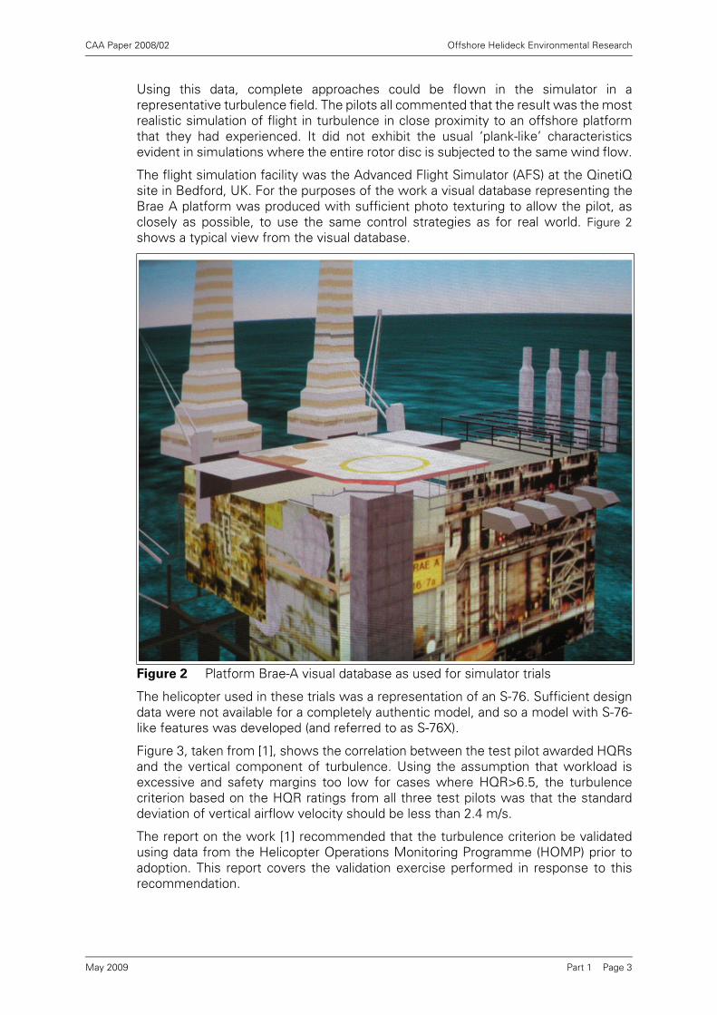
The flight simulation facility was the Advanced Flight Simulator (AFS) at the QinetiQsite in Bedford, UK. For the purposes of the work a visual database representing theBrae A platform was produced with sufficient photo texturing to allow the pilot, asclosely as possible, to use the same control strategies as for real world. Figure 2shows a typical view from the visual database.
The helicopter used in these trials was a representation of an S-76. Sufficient designdata were not available for a completely authentic model, and so a model with S-76-like features was developed (and referred to as S-76X).
Figure 3, taken from [1], shows the correlation between the test pilot awarded HQRsand the vertical component of turbulence. Using the assumption that workload isexcessive and safety margins too low for cases where HQR>6.5, the turbulencecriterion based on the HQR ratings from all three test pilots was that the standarddeviation of vertical airflow velocity should be less than 2.4 m/s.
The report on the work [1] recommended that the turbulence criterion be validatedusing data from the Helicopter Operations Monitoring Programme (HOMP) prior toadoption. This report covers the validation exercise performed in response to thisrecommendation.
Figure 2 Platform Brae-A visual database as used for simulator trials
Part 1 Page 3May 2009

CAA Paper 2008/02 Offshore Helideck Environmental Research
3 Objectives
The two-phase programme of work had the following objectives:
3.1 Phase 1 Objectives
a) To check that the workload predictor will function at the lower sampling ratesavailable with HOMP data. (See Section 5)
b) To develop a modified pilot workload algorithm for application to helicopter controlrecords for complete approaches. (See Sections 7.1 to 7.3)
c) To derive more reliable workload predictor coefficients by utilising all the availablepiloted flight simulation data. (See Sections 6.1 to 6.2)
d) To validate the modified workload algorithm against the original version usingexisting computer and flight simulation data. (See Section 7.4)
e) To specify the modified algorithm to enable it to be programmed into the HOMPsystem in Phase 2. (See Section 7.2 and Appendix A)
3.2 Phase 2 Objectives
a) Implement the modified workload algorithm in the HOMP data analysis system.(See Section 10)
b) Use analysis of the HOMP data archive to validate the workload algorithm. (SeeSections 12 and 13)
Figure 3 Pilot HQR plotted against standard deviation of vertical flow [1]
Part 1 Page 4May 2009
CAA Paper 2008/02 Offshore Helideck Environmental Research
c) Deliver the modified HOMP software to the helicopter operators. (SeeRecommendations in Section 15)
4 The Pilot Workload Predictor
The basic pilot workload predictor was developed in earlier work, and is fullydocumented in [1].
4.1 Pilot Workload
For the purposes of discussing workload, the pilot has two main tasks at any onetime. The first is the guidance of the helicopter to the desired location in space andtime. The second is to compensate for external influences and the inherent instabilityof the aircraft. The first of these two tasks is not generally considered to be a majordriver of pilot workload, but the second increases workload when the helicopterexperiences increasing amounts of turbulence.
The pilot workload predictor was developed around the flying task of maintaining afixed position hover in turbulence and was thus based on control activity, and henceworkload, comprising stabilisation type inputs with little or no guidance activity. Incontrast, flying an approach to a helideck involves a number of changes to flight pathand flight conditions and hence includes both guidance and stabilisation activity.
The fundamental hypothesis upon which workload prediction is based is that thepilot’s control activity is a reliable indicator of his perceived workload. It is known thatother factors impinge on the pilot’s assessment of workload. For instance, adegradation of the visual environment in which the pilot is operating affects hiscontrol strategy. Some of these factors are believed to be represented in increasedcontrol activity. This has not been quantified or identified at this time and, therefore,an underlying assumption in this work is that the visual environment is good and doesnot affect pilot workload. However, the value set for the turbulence criterion hastaken some account of this assumption (see Section 13).
Sections 4.2 to 4.4 below summarise and review the analysis of the test pilots’control movements recorded during the QinetiQ simulator-based trials, and reportedin [1].
4.2 Data Summary
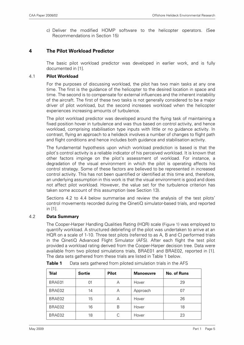
The Cooper-Harper Handling Qualities Rating (HQR) scale (Figure 1) was employed toquantify workload. A structured debriefing of the pilot was undertaken to arrive at anHQR on a scale of 1-10. Three test pilots (referred to as A, B and C) performed trialsin the QinetiQ Advanced Flight Simulator (AFS). After each flight the test pilotprovided a workload rating derived from the Cooper-Harper decision tree. Data wereavailable from two piloted simulations trials, BRAE01 and BRAE02, reported in [1].The data sets gathered from these trials are listed in Table 1 below.
Table 1 Data sets gathered from piloted simulation trials in the AFS
Trial Sortie Pilot Manoeuvre No. of Runs
BRAE01 01 A Hover 29
BRAE02 14 A Approach 07
BRAE02 15 A Hover 26
BRAE02 16 B Hover 18
BRAE02 18 C Hover 23
Part 1 Page 5May 2009

CAA Paper 2008/02 Offshore Helideck Environmental Research
4.3 HQR Prediction Method
This section describes the method of calculating HQR predictors from the pilot ratingsand measured control time history data (see [6] for further information).
A predictor is a coefficient vector c that relates a chosen set of metrics to the HQRawarded by the pilot. In this case, the metrics used were the standard deviation ofthe control input and the standard deviation of the control input rate. These metricswere calculated for the lateral cyclic control, longitudinal cyclic control, and thecollective lever. The relationship between the metrics and the HQR awarded by thepilot is:
r = c1 + c2 σ(ξ) + c3 σ*(ξ) + c4 σ(η) + c5 σ*(η) + c6 σ(θ0) + c7 σ*(θ0)
where,
r = HQR awarded by pilot
c1 – c7 = predictor coefficients
ξ= lateral cyclic position
η= longitudinal cyclic position
θ0 = collective lever position
σ(x) = function : standard deviation of x
σ*(x) = function : standard deviation of first derivative of x with time
Using data from multiple runs leads to the matrix equation of the form:
Xc=r+e,
where X is the m by n matrix of the n metrics from the m runs, r is the vector of pilotHQRs, and e is an error vector. The matrix X is factored using singular valuedecomposition into:
X=USVH
where U and V are unitary matrices, S is an m by n diagonal matrix containing thesingular values of X, and the superscript H denotes the conjugate transpose operator.Singular value decomposition produces singular values that are ordered in reducingmagnitude. Small singular values indicate a rank deficiency (occurs when the rows orcolumns of a matrix are not independent, in this case related to the correlationbetween control time histories) in the original data, and thus there is a need to avoidover-fitting to a particular data set. Small singular values also indicate an ill-conditionedsystem. An ill-conditioned system is overly sensitive to small perturbations in theinput.
The error is minimised in a least squares sense by:
c=VS-1UHr
where S-1 is n by m and is the inverse of S, since S is diagonal this is quite simply theinverse of the diagonal elements themselves.
A full set of coefficients can be calculated corresponding to retaining 1 to 7 singularvalues. For each increase in the order of the solution, the number of retained singularvalues is increased by one. However, the composition of each singular value in termsof raw variables will change with each successive change to the solution order, andhence the coefficients cannot be expected to be similar for different orders ofsolution. The trade off is between using smaller singular values to better fit thecurrent data set and compromising any future use of the coefficients as predictors.Having determined a predictor vector c, a vector of control activity metrics m isconverted into the predicted HQR, ŕ, by the product:
ŕ = ctm
Part 1 Page 6May 2009

CAA Paper 2008/02 Offshore Helideck Environmental Research
4.4 Predictor Coefficients derived during Validation Trials
The full set of predictor coefficients (as originally processed at Glasgow CaledonianUniversity (GCU) [1]) is presented in Table 2. These predictor coefficients werecalculated from the pilot ratings and measured control activity from the BRAE01 trialdata. The order five set of predictor coefficients are highlighted in Table 2, as this setwas used for the workload predictor in the validation exercise reported in [1]. For eachincrease in the order the number of retained singular values is increased by one. Sincethere are six metrics and one constant term in the workload predictor there are a totalof seven singular values. There are no hard and fast criteria for determining how manyorders should be selected - the choice, instead, is one requiring judgement. On thebasis of quality of fit, the final choice was between orders 4 and 5. Order 5 waschosen as it gave a better fit to the higher workload cases.
5 Application of Pilot Workload Predictor to Low Sample Rate Data
The first objective of Phase 1 was to check that the workload predictor continued tofunction adequately when applied to data of a lower sampling rate than that used inits development. This was in anticipation of the application of the predictor to HOMPdata, which is recorded at sample frequencies of 2 to 4 Hz as opposed to the 20Hzsample rate used in the simulator work.
As an initial step, the original predictor was applied to simulator data with a reducedsample rate to assess the effect on the predicted HQRs. The data used were thosefrom trial BRAE02, providing control movements and pilot HQRs using three differentpilots (A, B, C) conducting the hover task. Workload estimates for all pilot data werecalculated using three sampling rates – 20Hz, 4Hz and 2Hz.
This part of the work addressed objective a) stated in Section 3.1.
5.1 Results
Figure 4 to Figure 6 show a comparison of predicted workloads with pilot HQRs forthe three sampling rates for each pilot in turn. The 20Hz data reproduce the resultsgiven in Table O-1 of ref [1]. For all three pilots, as the sample rate reduces, so doesthe estimate of workload, especially where the workload is high. This is particularlynoticeable in the results for pilot B in Figure 5.
Table 2 Original predictor set for trial BRAE01 (obtained from GCU analysis)
Order 1 2 3 4 5 6 7
c1 4.1832 1.8924 1.8978 2.0971 2.1238 1.3434 0.7878
c2 0.2434 1.0325 1.4531 1.5840 0.6240 9.7234 46.5698
c3 1.1954 6.0130 7.4460 7.5999 7.2237 5.9211 -2.3776
c4 0.1961 0.7600 0.3611 0.3568 -0.7879 65.4232 60.3412
c5 0.9879 4.4560 2.5453 2.2804 0.8214 -12.4400 -9.6098
c6 0.3168 -0.3030 0.1992 -1.4695 -4.7042 -5.2539 -5.1046
c7 0.3875 1.1395 1.0590 0.3926 8.8116 16.2860 19.9755
Part 1 Page 7May 2009

CAA Paper 2008/02 Offshore Helideck Environmental Research
Figure 4 HQR predictions for pilot A data at 20Hz, 4Hz and 2Hz
Figure 5 HQR predictions for pilot B data at 20Hz, 4Hz and 2Hz
Part 1 Page 8May 2009

CAA Paper 2008/02 Offshore Helideck Environmental Research
Figure 7 to Figure 9 show how the workload predictor parameters vary between theresults from 20Hz and 2Hz for pilot A, B and C respectively. Ignoring the constantoffset (2.1238) there are six parameters in the workload predictor, three based onstandard deviation of control positions, and three based on the standard deviation ofthe control rates. In each figure the left hand graph relates to control position and theright hand graph to control rate. The vertical axis gives the parameter values from the2Hz data and the horizontal axis gives the same parameter from the 20Hz data.
Each point on each graph is generated from analysis of a single time history and is theappropriate standard deviation multiplied by the magnitude of the associatedcoefficient in the workload predictor. The dashed line represents a one-to-onecorrelation between 2Hz and 20Hz results. It is clear that the calculation of standarddeviation of control position is unaffected by the reduced sampling rate whereas thestandard deviation of control rate is underestimated in all cases. This is most apparentfor lateral and longitudinal cyclic with the collective only marginally affected. Overall,the reduced sampling rate does have a significant effect on the calculation of standarddeviation of control rate data.
The reduced sampling of the data has clearly caused some of the features of thecontrol activity to be lost. The nature of this effect is that the gradients of controlposition i.e. the rates as used in the workload predictor, are more likely to be lowerwith a lower sampling rate.
Figure 6 HQR predictions for pilot C data at 20Hz, 4Hz and 2Hz
Part 1 Page 9May 2009

CAA Paper 2008/02 Offshore Helideck Environmental Research
Figure 7 Comparisons of factored standard deviations from 20Hz and 2Hz - pilot A
Figure 8 Comparisons of factored standard deviations from 20Hz and 2Hz - pilot B
Part 1 Page 10May 2009

CAA Paper 2008/02 Offshore Helideck Environmental Research
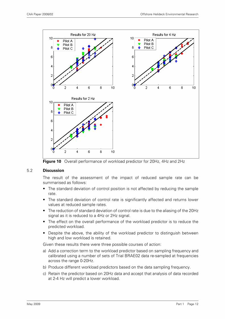
Figure 10 shows the overall quality of the HQR predictions for all pilots using data at20Hz, 4Hz and 2Hz. The first graph, generated with 20Hz data, is equivalent to Figure4.4 of [1]. The second and third graphs show results for 4Hz and 2Hz datarespectively.
Despite the fact that the reduced sampling has an effect on the analysis of controlrate data, it does not affect the ability of the workload predictor to distinguish casesof high and low workload. In fact, the results from 4Hz data have a better match thanthose from 20Hz data due to the over prediction of workload when applied to 20Hz3data being opposed by the tendency of calculations using data sampled at 4 Hz tohave a lower workload estimate. In this particular case the two opposing effects havecancelled each other.
Figure 9 Comparisons of factored standard deviations from 20Hz and 2Hz - pilot C
3. This tendency to over-prediction of the 20Hz data is removed when the workload predictor coefficients are recalculatedusing all the data from the BRAE01 and BRAE02 trials.
Part 1 Page 11May 2009
CAA Paper 2008/02 Offshore Helideck Environmental Research
5.2 Discussion
The result of the assessment of the impact of reduced sample rate can besummarised as follows:• The standard deviation of control position is not affected by reducing the sample
rate.• The standard deviation of control rate is significantly affected and returns lower
values at reduced sample rates.• The reduction of standard deviation of control rate is due to the aliasing of the 20Hz
signal as it is reduced to a 4Hz or 2Hz signal.• The effect on the overall performance of the workload predictor is to reduce the
predicted workload.
• Despite the above, the ability of the workload predictor to distinguish betweenhigh and low workload is retained.
Given these results there were three possible courses of action:
a) Add a correction term to the workload predictor based on sampling frequency andcalibrated using a number of sets of Trial BRAE02 data re-sampled at frequenciesacross the range 0-20Hz.
b) Produce different workload predictors based on the data sampling frequency.
c) Retain the predictor based on 20Hz data and accept that analysis of data recordedat 2-4 Hz will predict a lower workload.
Figure 10 Overall performance of workload predictor for 20Hz, 4Hz and 2Hz
Part 1 Page 12May 2009

CAA Paper 2008/02 Offshore Helideck Environmental Research
The fact that the effect of sampling frequency is dependent on the exact form of thecontrol time history may make quantifying its effect problematic, particularly for caseswhere either pilot or aircraft have changed. Hence action a) was not considereddesirable.
The tuning of the predictor for data at specific sample frequencies, as in b), makes thepredictor more complicated and introduces the potential for it to be incorrectlyapplied. Furthermore, it would apply a level of fine tuning that is inappropriate at thisstage given that there are other more fundamental properties of the predictor (suchas the effects of using it for different aircraft and control systems) which would needto be tested when the HOMP data analysis has been completed.
In view of the above, retaining the previously derived 20Hz predictor for the currentstudy was considered to be the most appropriate way forward.
6 Update of the Workload Predictor
One of the recommendations of [1] had been that all the flight simulator data shouldbe used to recalculate coefficients to produce an improved workload predictor. Thisaspect of the work was intended to address objective (c) stated in Section 3.1.
The predictors developed in [1] had been calculated by Glasgow CaledonianUniversity (GCU), and so before recalibrating the predictor coefficients using all thedata from the BRAE01 and BRAE02 trials, it was necessary to check that the originalcoefficients could be reproduced using QinetiQ’s data and software.
6.1 Reproduction of Workload Predictor Coefficients
The predictors based on BRAE01 and re-calculated during this current work are givenin Table 3.
There are slight differences between predictors shown here in Table 3 and thosegiven earlier in Table 2. This is due to clipping of the recorded control time history datawhen they were processed at GCU.
The effect on estimations of the HQR is shown in Figure 11, and seem to be quitesmall. The standard deviation of the error in the HQR prediction is only 0.0343 HQRpoints and highlights the insignificance of the effect that the small change in predictorcoefficients has on workload prediction.
Table 3 Full predictor set for trial BRAE01 re-calculated for current work
Order 1 2 3 4 5 6 7
c1 4.1759 1.9158 1.9324 2.1532 2.1792 1.4474 1.2382
c2 0.2455 1.0171 1.5839 1.7209 0.7209 10.5846 24.4932
c3 1.2096 5.9844 7.8818 8.0511 7.7061 5.6636 2.5605
c4 0.1959 0.7400 0.2311 0.2360 -0.9217 56.1689 53.6936
c5 0.9865 4.3103 1.6934 1.3941 0.0292 -10.8481 -9.6717
c6 0.3162 -0.2861 0.3985 -1.4381 -4.5469 -5.0921 -5.1356
c7 0.3869 1.1048 1.0039 0.2671 8.3063 15.6116 17.0355
Part 1 Page 13May 2009

CAA Paper 2008/02 Offshore Helideck Environmental Research
6.2 Recalibration of Workload Predictor Coefficients
The workload predictor coefficients determined above were calibrated using BRAE01data and validated using BRAE02 data. For the current work, in order to make thepredictor more robust it had been recommended in [1] that the workload predictorshould be recalibrated using all available data, including data from BRAE01 and thehover data from BRAE02.
Table 4 presents the resulting new predictor coefficients.
Figure 11 Workload predictions of BRAE01 using original predictor coefficients versus re-calculated predictor coefficients
Part 1 Page 14May 2009

CAA Paper 2008/02 Offshore Helideck Environmental Research
Order four is highlighted as the best compromise between using the highest orderpossible and avoiding over fitting of the data. Over fitting is indicated here by the rapidchange in coefficient values between orders 4 and 5, whereas between orders 1 and4 they follow more of a trend.
An important feature of this predictor compared to the previous ones shown in Tables2 and 3, is that the coefficients are now all positive. This means that all of the controlterms now contribute positively to the workload, which seems intuitively correct.
A further point to note is that the standard deviation of control rate coefficients arelarger than those for the standard deviation of control position terms. This isconsistent with general operational experience where the magnitude of control rates,and therefore the corresponding standard deviations, are greater than the magnitudeof control positions. Given these two factors, it is expected that the control rate termswill contribute more to the workload prediction than the control position terms.
7 Further Development of the Workload Predictor for use with HOMP Data
7.1 Frequency Analysis
Frequency analysis was used to compare the frequency content of the hover data andapproach data from the simulator trials. The difference between the sets of data isthat the approach task contains guidance and stabilisation inputs and the hover taskhas stabilisation inputs only. The objective was therefore to remove, or at leastreduce, the guidance inputs from the approach data using filters (objective 3.1(b)stated in Section 3.1).
From [7] the premise is made that guidance control movements are conducted at arelatively low rate compared to stabilisation control movements. A power spectraldensity (PSD) plot of control input should therefore exhibit peaks at the twofrequencies corresponding to these two types of control input. The requirement,therefore, was to identify the frequency that partitioned the two peaks in the PSDplots of control time histories. Using a filter, the guidance control inputs wereremoved from the control time histories to leave only the stabilisation control inputs.This focused the workload predictor on the stabilisation control inputs that are theprimary cause of workload for the pilot.
Table 4 Coefficients recalculated using both BRAE01 and BRAE02 hover data
Order 1 2 3 4 5 6 7
c1 4.3361 2.4586 2.5070 2.4069 2.1231 2.0331 2.2641
c2 0.3239 1.0041 1.2249 1.0356 18.5402 3.5865 -1.0695
c3 1.4853 5.0522 4.8974 3.9514 0.8447 4.1494 5.0940
c4 0.2202 0.5196 0.4390 0.7333 12.4763 32.6162 45.7145
c5 1.0306 2.7132 1.5106 2.8197 1.8485 -2.5162 -5.1532
c6 0.2091 0.5492 1.1153 1.3430 3.1070 14.8465 -12.4518
c7 0.5901 1.8644 3.7069 4.4501 1.4366 -2.0655 5.8053
Part 1 Page 15May 2009

CAA Paper 2008/02 Offshore Helideck Environmental Research
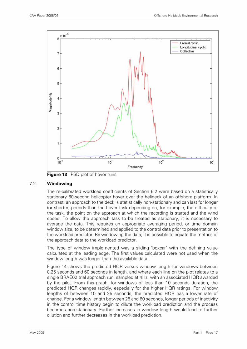
Figure 12 shows a PSD plot of trial BRAE02 approach data. In this figure, a peak isclearly visible in the lateral cyclic at around 0.5 Hz. At frequencies below 0.1 Hz apossible second peak is also apparent as the curve begins to rise towards lowerfrequencies. In contrast to the full approach spectra of Figure 12, Figure 13 shows thePSD of hover only data.
From these two plots, it is evident that there is a difference in the power of the signalsbelow 0.1 Hz. Following on from the hypothesis that guidance control inputs arespectrally separated from stabilisation control inputs, the power in the signal below0.1 Hz is identified as relating to guidance control inputs and the power in the signalabove 0.1 Hz is identified as relating to stabilisation. From this, a cut-off frequency of0.1 Hz was chosen to eliminate the guidance control inputs of the pilot from thecontrol time histories.
Figure 12 PSD plot of approach runs
Part 1 Page 16May 2009
CAA Paper 2008/02 Offshore Helideck Environmental Research
7.2 Windowing
The re-calibrated workload coefficients of Section 6.2 were based on a statisticallystationary 60-second helicopter hover over the helideck of an offshore platform. Incontrast, an approach to the deck is statistically non-stationary and can last for longer(or shorter) periods than the hover task depending on, for example, the difficulty ofthe task, the point on the approach at which the recording is started and the windspeed. To allow the approach task to be treated as stationary, it is necessary toaverage the data. This requires an appropriate averaging period, or time domainwindow size, to be determined and applied to the control data prior to presentation tothe workload predictor. By windowing the data, it is possible to equate the metrics ofthe approach data to the workload predictor.
The type of window implemented was a sliding ‘boxcar’ with the defining valuecalculated at the leading edge. The first values calculated were not used when thewindow length was longer than the available data.
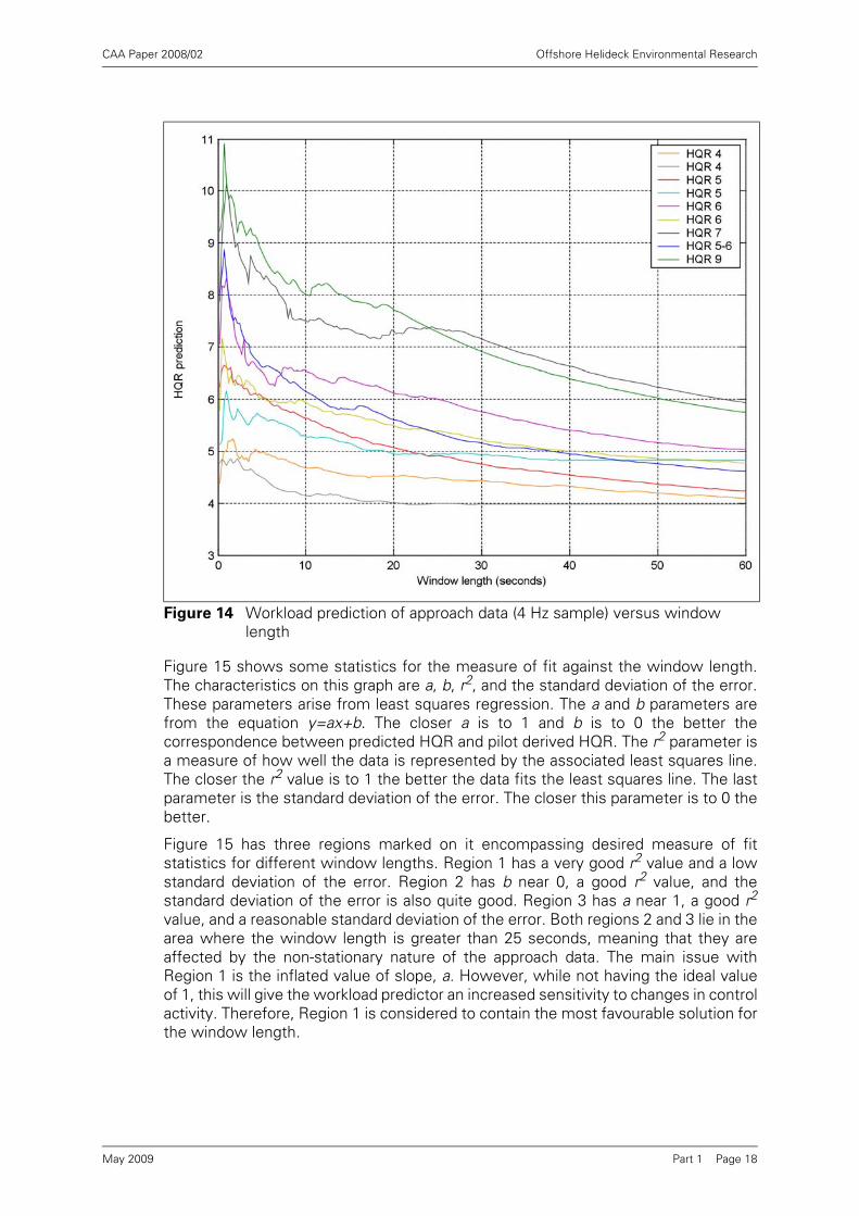
Figure 14 shows the predicted HQR versus window length for windows between0.25 seconds and 60 seconds in length, and where each line on the plot relates to asingle BRAE02 trial approach run, sampled at 4Hz, with an associated HQR awardedby the pilot. From this graph, for windows of less than 10 seconds duration, thepredicted HQR changes rapidly, especially for the higher HQR ratings. For windowlengths of between 10 and 25 seconds, the predicted HQR has a lower rate ofchange. For a window length between 25 and 60 seconds, longer periods of inactivityin the control time history begin to dilute the workload prediction and the processbecomes non-stationary. Further increases in window length would lead to furtherdilution and further decreases in the workload prediction.
Figure 13 PSD plot of hover runs
Part 1 Page 17May 2009
CAA Paper 2008/02 Offshore Helideck Environmental Research
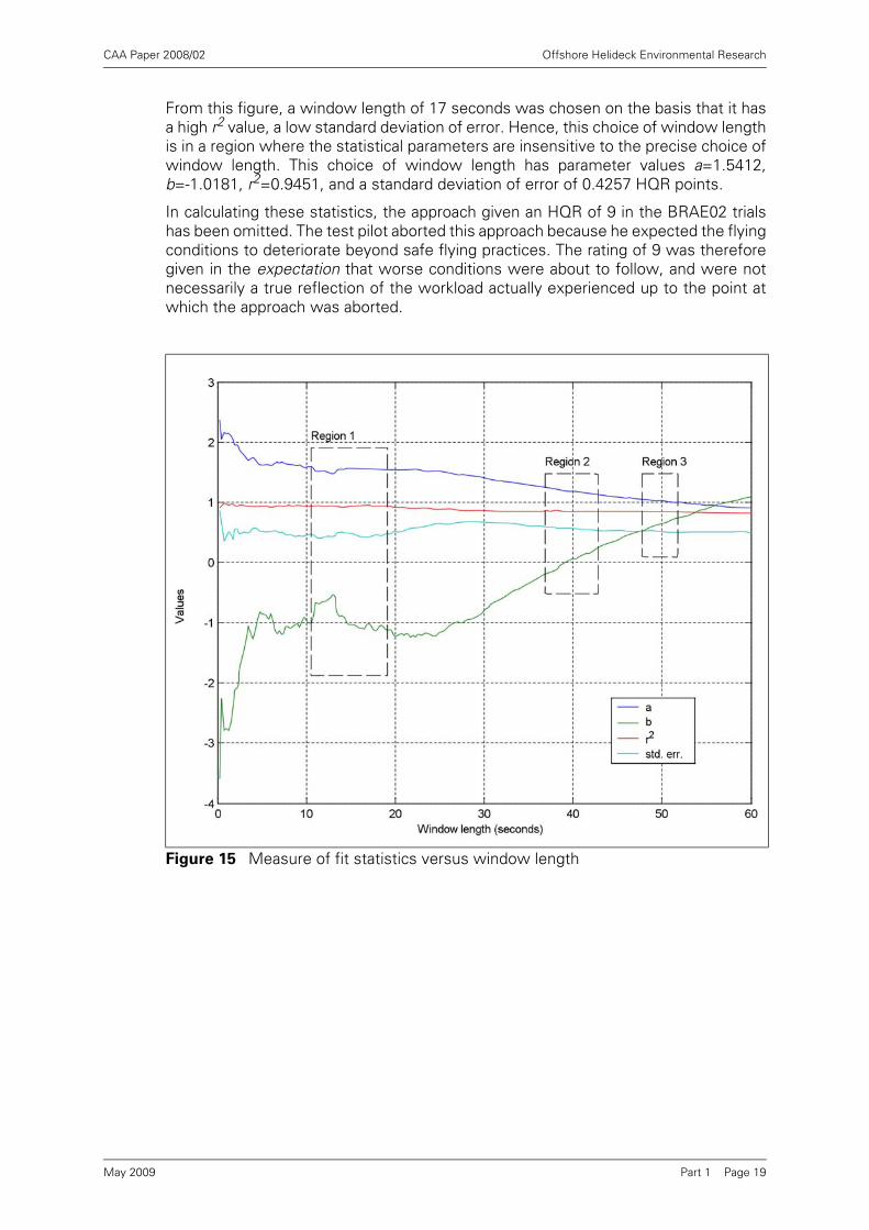
Figure 15 shows some statistics for the measure of fit against the window length.The characteristics on this graph are a, b, r2, and the standard deviation of the error.These parameters arise from least squares regression. The a and b parameters arefrom the equation y=ax+b. The closer a is to 1 and b is to 0 the better thecorrespondence between predicted HQR and pilot derived HQR. The r2 parameter isa measure of how well the data is represented by the associated least squares line.The closer the r2 value is to 1 the better the data fits the least squares line. The lastparameter is the standard deviation of the error. The closer this parameter is to 0 thebetter.
Figure 15 has three regions marked on it encompassing desired measure of fitstatistics for different window lengths. Region 1 has a very good r2 value and a lowstandard deviation of the error. Region 2 has b near 0, a good r2 value, and thestandard deviation of the error is also quite good. Region 3 has a near 1, a good r2
value, and a reasonable standard deviation of the error. Both regions 2 and 3 lie in thearea where the window length is greater than 25 seconds, meaning that they areaffected by the non-stationary nature of the approach data. The main issue withRegion 1 is the inflated value of slope, a. However, while not having the ideal valueof 1, this will give the workload predictor an increased sensitivity to changes in controlactivity. Therefore, Region 1 is considered to contain the most favourable solution forthe window length.
Figure 14 Workload prediction of approach data (4 Hz sample) versus window length
Part 1 Page 18May 2009
CAA Paper 2008/02 Offshore Helideck Environmental Research
From this figure, a window length of 17 seconds was chosen on the basis that it hasa high r2 value, a low standard deviation of error. Hence, this choice of window lengthis in a region where the statistical parameters are insensitive to the precise choice ofwindow length. This choice of window length has parameter values a=1.5412,b=-1.0181, r2=0.9451, and a standard deviation of error of 0.4257 HQR points.
In calculating these statistics, the approach given an HQR of 9 in the BRAE02 trialshas been omitted. The test pilot aborted this approach because he expected the flyingconditions to deteriorate beyond safe flying practices. The rating of 9 was thereforegiven in the expectation that worse conditions were about to follow, and were notnecessarily a true reflection of the workload actually experienced up to the point atwhich the approach was aborted.
Figure 15 Measure of fit statistics versus window length
Part 1 Page 19May 2009
CAA Paper 2008/02 Offshore Helideck Environmental Research
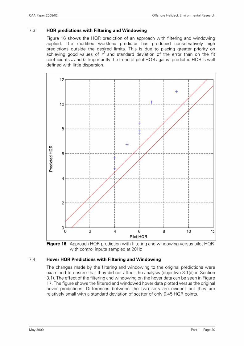
7.3 HQR predictions with Filtering and Windowing
Figure 16 shows the HQR prediction of an approach with filtering and windowingapplied. The modified workload predictor has produced conservatively highpredictions outside the desired limits. This is due to placing greater priority onachieving good values of r2 and standard deviation of the error than on the fitcoefficients a and b. Importantly the trend of pilot HQR against predicted HQR is welldefined with little dispersion.
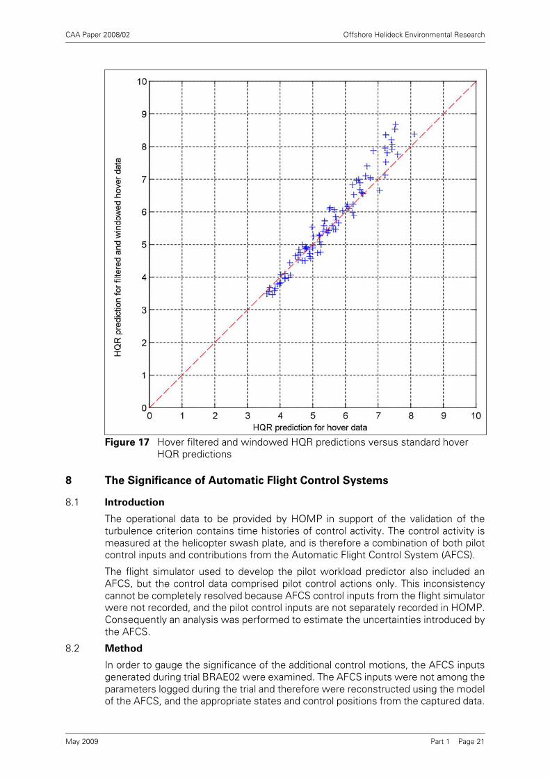
7.4 Hover HQR Predictions with Filtering and Windowing
The changes made by the filtering and windowing to the original predictions wereexamined to ensure that they did not affect the analysis (objective 3.1(d) in Section3.1). The effect of the filtering and windowing on the hover data can be seen in Figure17. The figure shows the filtered and windowed hover data plotted versus the originalhover predictions. Differences between the two sets are evident but they arerelatively small with a standard deviation of scatter of only 0.45 HQR points.
Figure 16 Approach HQR prediction with filtering and windowing versus pilot HQR with control inputs sampled at 20Hz
Part 1 Page 20May 2009
CAA Paper 2008/02 Offshore Helideck Environmental Research
8 The Significance of Automatic Flight Control Systems
8.1 Introduction
The operational data to be provided by HOMP in support of the validation of theturbulence criterion contains time histories of control activity. The control activity ismeasured at the helicopter swash plate, and is therefore a combination of both pilotcontrol inputs and contributions from the Automatic Flight Control System (AFCS).
The flight simulator used to develop the pilot workload predictor also included anAFCS, but the control data comprised pilot control actions only. This inconsistencycannot be completely resolved because AFCS control inputs from the flight simulatorwere not recorded, and the pilot control inputs are not separately recorded in HOMP.Consequently an analysis was performed to estimate the uncertainties introduced bythe AFCS.
8.2 Method
In order to gauge the significance of the additional control motions, the AFCS inputsgenerated during trial BRAE02 were examined. The AFCS inputs were not among theparameters logged during the trial and therefore were reconstructed using the modelof the AFCS, and the appropriate states and control positions from the captured data.
Figure 17 Hover filtered and windowed HQR predictions versus standard hover HQR predictions
Part 1 Page 21May 2009
CAA Paper 2008/02 Offshore Helideck Environmental Research
The host model, FLIGHTLAB, was not the most appropriate for simulating thissubsystem, and so the control system was re-implemented in MATLAB/Simulink.The pedal control movements are not used in the workload predictor and thereforewere not reconstructed. The AFCS contributions to collective could not bereconstructed because they depend in part on the normal acceleration, and thisacceleration was not logged during the trial. Consequently the HQR predictions givenin the following are based on modified signals for longitudinal and lateral cyclic, andthe ‘raw’ collective lever position.
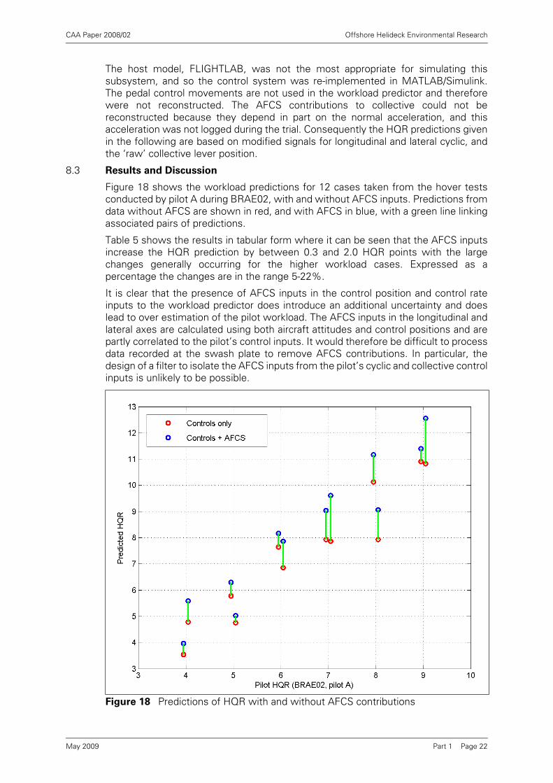
8.3 Results and Discussion
Figure 18 shows the workload predictions for 12 cases taken from the hover testsconducted by pilot A during BRAE02, with and without AFCS inputs. Predictions fromdata without AFCS are shown in red, and with AFCS in blue, with a green line linkingassociated pairs of predictions.
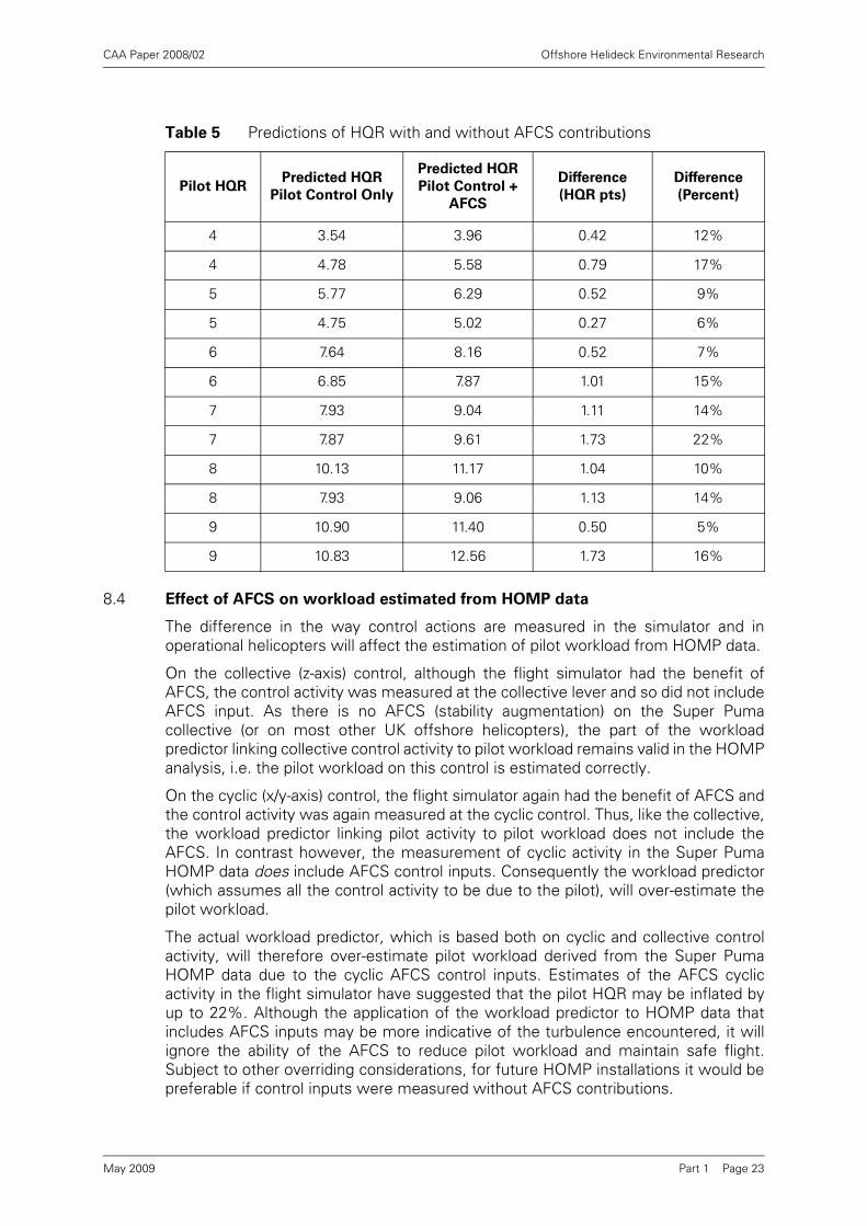
Table 5 shows the results in tabular form where it can be seen that the AFCS inputsincrease the HQR prediction by between 0.3 and 2.0 HQR points with the largechanges generally occurring for the higher workload cases. Expressed as apercentage the changes are in the range 5-22%.
It is clear that the presence of AFCS inputs in the control position and control rateinputs to the workload predictor does introduce an additional uncertainty and doeslead to over estimation of the pilot workload. The AFCS inputs in the longitudinal andlateral axes are calculated using both aircraft attitudes and control positions and arepartly correlated to the pilot’s control inputs. It would therefore be difficult to processdata recorded at the swash plate to remove AFCS contributions. In particular, thedesign of a filter to isolate the AFCS inputs from the pilot’s cyclic and collective controlinputs is unlikely to be possible.
Figure 18 Predictions of HQR with and without AFCS contributions
Part 1 Page 22May 2009
CAA Paper 2008/02 Offshore Helideck Environmental Research
8.4 Effect of AFCS on workload estimated from HOMP data
The difference in the way control actions are measured in the simulator and inoperational helicopters will affect the estimation of pilot workload from HOMP data.
On the collective (z-axis) control, although the flight simulator had the benefit ofAFCS, the control activity was measured at the collective lever and so did not includeAFCS input. As there is no AFCS (stability augmentation) on the Super Pumacollective (or on most other UK offshore helicopters), the part of the workloadpredictor linking collective control activity to pilot workload remains valid in the HOMPanalysis, i.e. the pilot workload on this control is estimated correctly.
On the cyclic (x/y-axis) control, the flight simulator again had the benefit of AFCS andthe control activity was again measured at the cyclic control. Thus, like the collective,the workload predictor linking pilot activity to pilot workload does not include theAFCS. In contrast however, the measurement of cyclic activity in the Super PumaHOMP data does include AFCS control inputs. Consequently the workload predictor(which assumes all the control activity to be due to the pilot), will over-estimate thepilot workload.
The actual workload predictor, which is based both on cyclic and collective controlactivity, will therefore over-estimate pilot workload derived from the Super PumaHOMP data due to the cyclic AFCS control inputs. Estimates of the AFCS cyclicactivity in the flight simulator have suggested that the pilot HQR may be inflated byup to 22%. Although the application of the workload predictor to HOMP data thatincludes AFCS inputs may be more indicative of the turbulence encountered, it willignore the ability of the AFCS to reduce pilot workload and maintain safe flight.Subject to other overriding considerations, for future HOMP installations it would bepreferable if control inputs were measured without AFCS contributions.
Table 5 Predictions of HQR with and without AFCS contributions
Pilot HQRPredicted HQR
Pilot Control Only
Predicted HQR
Pilot Control +
AFCS
Difference
(HQR pts)
Difference
(Percent)
4 3.54 3.96 0.42 12%
4 4.78 5.58 0.79 17%
5 5.77 6.29 0.52 9%
5 4.75 5.02 0.27 6%
6 7.64 8.16 0.52 7%
6 6.85 7.87 1.01 15%
7 7.93 9.04 1.11 14%
7 7.87 9.61 1.73 22%
8 10.13 11.17 1.04 10%
8 7.93 9.06 1.13 14%
9 10.90 11.40 0.50 5%
9 10.83 12.56 1.73 16%
Part 1 Page 23May 2009
CAA Paper 2008/02 Offshore Helideck Environmental Research
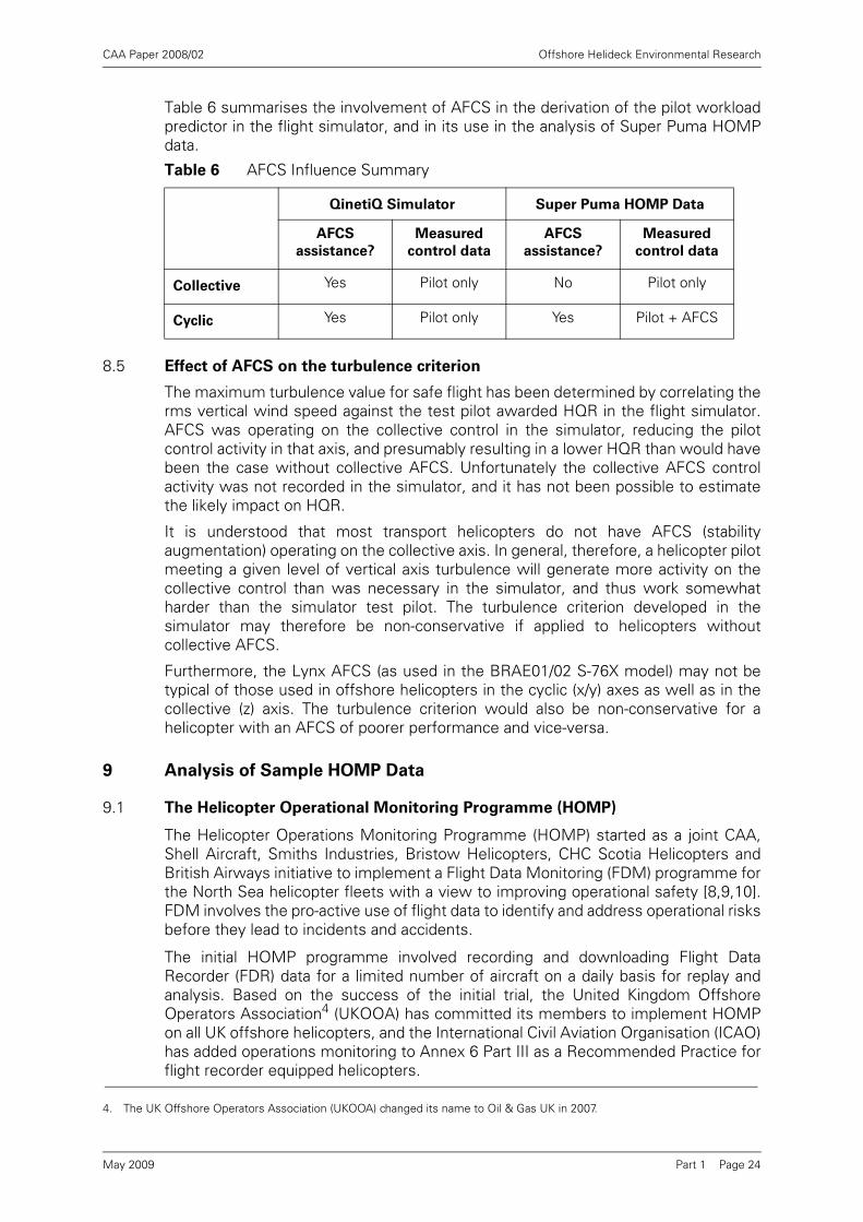
Table 6 summarises the involvement of AFCS in the derivation of the pilot workloadpredictor in the flight simulator, and in its use in the analysis of Super Puma HOMPdata.
8.5 Effect of AFCS on the turbulence criterion
The maximum turbulence value for safe flight has been determined by correlating therms vertical wind speed against the test pilot awarded HQR in the flight simulator.AFCS was operating on the collective control in the simulator, reducing the pilotcontrol activity in that axis, and presumably resulting in a lower HQR than would havebeen the case without collective AFCS. Unfortunately the collective AFCS controlactivity was not recorded in the simulator, and it has not been possible to estimatethe likely impact on HQR.
It is understood that most transport helicopters do not have AFCS (stabilityaugmentation) operating on the collective axis. In general, therefore, a helicopter pilotmeeting a given level of vertical axis turbulence will generate more activity on thecollective control than was necessary in the simulator, and thus work somewhatharder than the simulator test pilot. The turbulence criterion developed in thesimulator may therefore be non-conservative if applied to helicopters withoutcollective AFCS.
Furthermore, the Lynx AFCS (as used in the BRAE01/02 S-76X model) may not betypical of those used in offshore helicopters in the cyclic (x/y) axes as well as in thecollective (z) axis. The turbulence criterion would also be non-conservative for ahelicopter with an AFCS of poorer performance and vice-versa.
9 Analysis of Sample HOMP Data
9.1 The Helicopter Operational Monitoring Programme (HOMP)
The Helicopter Operations Monitoring Programme (HOMP) started as a joint CAA,Shell Aircraft, Smiths Industries, Bristow Helicopters, CHC Scotia Helicopters andBritish Airways initiative to implement a Flight Data Monitoring (FDM) programme forthe North Sea helicopter fleets with a view to improving operational safety [8,9,10].FDM involves the pro-active use of flight data to identify and address operational risksbefore they lead to incidents and accidents.
The initial HOMP programme involved recording and downloading Flight DataRecorder (FDR) data for a limited number of aircraft on a daily basis for replay andanalysis. Based on the success of the initial trial, the United Kingdom OffshoreOperators Association4 (UKOOA) has committed its members to implement HOMPon all UK offshore helicopters, and the International Civil Aviation Organisation (ICAO)has added operations monitoring to Annex 6 Part III as a Recommended Practice forflight recorder equipped helicopters.
Table 6 AFCS Influence Summary
QinetiQ Simulator Super Puma HOMP Data
AFCS
assistance?
Measured
control data
AFCS
assistance?
Measured
control data
Collective Yes Pilot only No Pilot only
Cyclic Yes Pilot only Yes Pilot + AFCS
4. The UK Offshore Operators Association (UKOOA) changed its name to Oil & Gas UK in 2007.
Part 1 Page 24May 2009

CAA Paper 2008/02 Offshore Helideck Environmental Research
9.2 HQRs from Filtered and Windowed BRAE02 Approach Data
Since the HOMP data are recorded at 4 Hz, the effect of using the complete (filteredand windowed) workload algorithm was investigated using data from the BRAE02approach cases down-sampled to 4 Hz. It has already been shown in Section 5 that areduction of the data sampling rate reduces the workload prediction for the hovercases. Figure 19 shows HQR predictions from the BRAE02 approach data that havebeen down-sampled to 4 Hz.
The figure shows that applying the workload algorithm to 4 Hz sample rate data givesa very good correlation between predicted HQR and pilot HQR. The increase inpredicted HQR through the filtering and windowing of the approach data is balancedby the decrease in predicted HQR caused by the reduction in the sampling rate. Thisis encouraging, although with only nine approach cases available it is not possible tocreate definitive statistics. By comparison with Figure 16, reducing the sampling ratefrom 20 Hz to 4 Hz has dropped the predicted HQR overall, and suggests an increasedtail-off for the highest HQR values. The overall drop is consistent with theexpectations reported in Section 5.
Figure 19 Approach HQR predictions with filtering and windowing versus pilot HQR, with control inputs sampled at 4 Hz
Part 1 Page 25May 2009

CAA Paper 2008/02 Offshore Helideck Environmental Research
9.3 Results using Sample data from HOMP
The workload algorithm was applied to the data from 20 example records suppliedfrom the HOMP project. For these data, there was no pilot HQR, however a so-called“Digicoll” value was supplied as a measure of turbulence. Figure 20 is a plot ofpredicted HQR versus “Digicoll” value. From this figure it can be seen that the HQRprediction ranges from 3.1 to 6.7 HQR points and is generally increasing with“Digicoll” value. This trend is not necessarily an indication of a robust workloadalgorithm as the “Digicoll” has not been the subject of a rigorous validation exercise.
10 Implementation of the Workload Algorithm in HOMP
Having developed the workload algorithm to operate on flight data from operationalhelicopters, and verified that it worked well on helideck approaches flown in thesimulator (see Section 7), it was necessary to implement the workload algorithm inthe HOMP analysis, and test it to demonstrate that it generated the same result asthe original implementation when supplied with the same input data.
Three HOMP helideck landings were selected for checking, and the workload timeseries independently calculated by QinetiQ using the original Matlab code, and bySmiths within the HOMP system. Intermediate results in the workload calculation(e.g. windowed standard deviation of each control axis) were also output andcompared.
This task proved to be a little more difficult than had been anticipated, with the initialimplementation in the HOMP system showing a number of discrepancies in theresults produced by the development analysis (which had been coded in Matlab), andthe workload results produced by the HOMP system. The most important issue
Figure 20 Predicted HQR for 20 example HOMP cases
Part 1 Page 26May 2009
CAA Paper 2008/02 Offshore Helideck Environmental Research
proved to be the numerical precision in the 8th order Butterworth filter. The HOMPanalysis environment was performing arithmetic at a lower numerical precision and,as a result, the filter characteristics proved to be significantly different from thoseimplemented in the Matlab coding of the algorithm. When this was discovered thesolution was to implement the 8th order filter as 4 x 2nd order filters, which achievedan almost identical result without requiring excessive arithmetical precision.
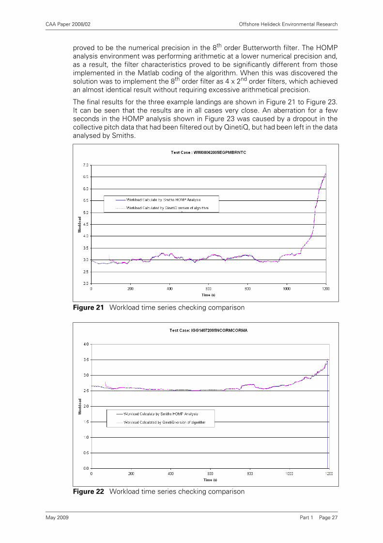
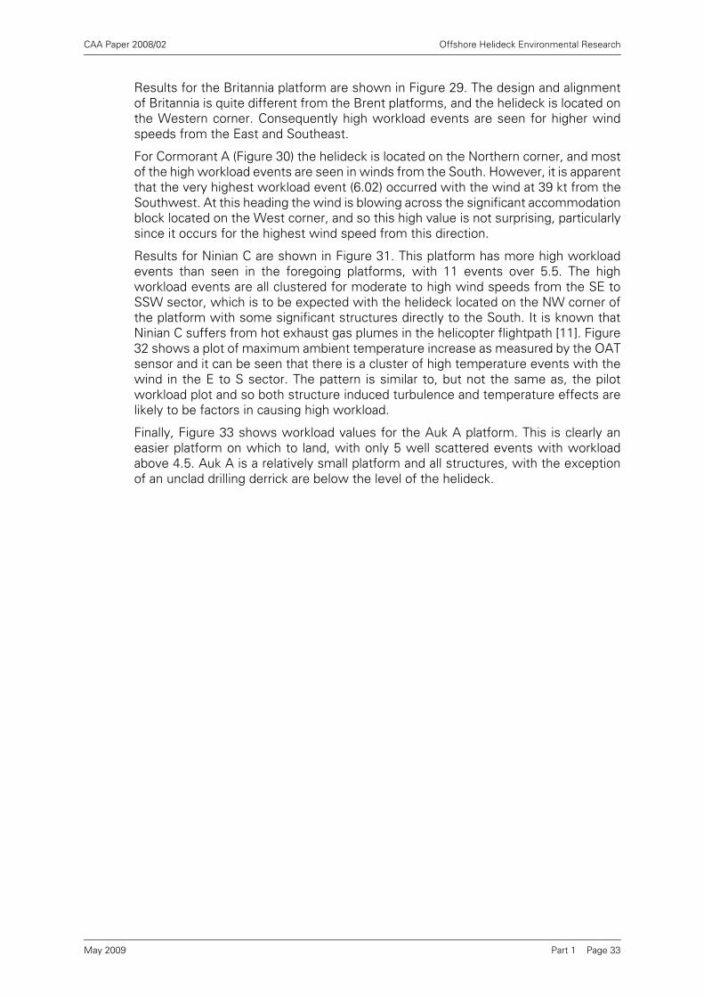
The final results for the three example landings are shown in Figure 21 to Figure 23.It can be seen that the results are in all cases very close. An aberration for a fewseconds in the HOMP analysis shown in Figure 23 was caused by a dropout in thecollective pitch data that had been filtered out by QinetiQ, but had been left in the dataanalysed by Smiths.
Figure 21 Workload time series checking comparison
Figure 22 Workload time series checking comparison
Part 1 Page 27May 2009

CAA Paper 2008/02 Offshore Helideck Environmental Research
Appendix B contains guidance on programming the pilot workload algorithm into aHOMP analysis system.
11 The HOMP Data Archive
The HOMP data used in the workload analysis was not live data from currenthelicopter operations, but an archive of some 32,000 flight sectors operated byBristow Helicopters in the North Sea between the dates of 1st July 2003 and 31st
October 2004. Altogether 122 different offshore helidecks had been visited by theseflights. Once helideck landings had been selected, and a proportion of landings withbad data had been eliminated, there remained about 13,000 valid landings over the 16month period that could be used in the analysis.
Of the 122 platforms visited a number had relatively few landings, which preventedany pattern being reliably presented and interpreted for that platform, but certainmanipulations and presentations could be performed for the population of landings asa whole (e.g. the overall distribution of pilot workload values are presented in Figure34 and discussed in Section 12.2).
It was decided to focus on helidecks that had received more than 20 landings, andhelidecks for which platform layout sketches had been provided, this permittinginterpretation of the results in terms of wind directions and the relative locations ofinstallation structures likely to cause turbulence over the helideck. This resulted in a‘top 70’ list of platforms. These platforms are listed in the table in Appendix C, whichshows the number of landings in the database for each of these platforms. This tablealso summarises HLL entries and the main features of the workload plots (seeSection 12.2).
The availability of platform sketches also enabled wind directional sectors to bedefined that would be either ‘open’ (i.e. no significant platform structures upstreamto cause turbulence), or ‘turbulent’ (i.e. for the wind directions where the turbulentwake of platform structures upwind would be expected to have a significant effect).This in turn enabled the ensemble data for the ‘open’ and ‘obstructed’ wind directionsto be presented separately.
Figure 23 Workload time series checking comparison
Part 1 Page 28May 2009

CAA Paper 2008/02 Offshore Helideck Environmental Research
The HOMP parameters used in this particular pilot workload analysis are listed inTable 7:
The wind speed and direction estimated from the helicopter FDR at the‘measurement point’ (COR_MX_WSPDLDG and COR_MX_WANGLDG) is derived fromGPS track and heading information. The accuracy of this is dependent on the aircraftflying straight and level, and at a reasonable airspeed. If the airspeed is low, or theaircraft is turning, the GPS derived wind speed and direction will be unreliable, and soreasonably accurate data is ensured by:
1. Averaging GPS wind speed / wind angle data over a 10 s period;
2. Identifying the data as valid only if the aircraft roll angle is < 5.5 degrees;
3. Identifying the data as valid only if indicated airspeed is > 55 kt at the start andend of the 10 s averaging period;
4. Acquiring landing wind measurements when the aircraft is 1500 m from thelanding point (when conditions 2, 3 and 4 are more likely to be satisfied).
The wind speed data were then corrected (MX_CORWSPDLDG) for the altitudedifference between that at the helicopter ‘measurement point’ and the helideckheight using a standard atmospheric boundary layer power law profile:
where:
u1 = wind speed at height 1 [m/s]u2 = wind speed at height 2 [m/s]z1 =height 1 [m]z2 =height 2 [m]
With this rather complex derivation of the corrected wind speed and direction it isvery difficult to know the accuracy of the resulting wind estimates, and thisuncertainty needs to be taken into account in the interpretation of the results of theanalyses presented in this report.
Table 7
Variable name Description
FlightType Flight type (from imported ops data, 1,2,6 = revenue, 4 = training, 5 = air test)
MX_WORK_LDG Maximum Pilot Workload Rating from 500m to landing
MXWORKTIMLDG Number of Frames from Landing point to recorded MX_WORK_LDG (2 frames = 1 sec)
MX_WORK_XDIST Lateral distance between MX_WORK_LDG and Landing Point (m)
MX_WORK_YDIST Longitudinal distance between MX_WORK_LDG and Landing Point (m)
COR_MX_WSPDLDG Wind speed in the Landing Phase at Measurement Point (1500m from Landing) (m/s)
COR_MX_WANGLDG Wind angle in the Landing Phase at Measurement Point (1500m from Landing) (m/s)
MX_CORWSPDLDG COR_MX_WSPDLDG corrected to helideck height (m/s)
( ) 4.12121 / zzuu =
Part 1 Page 29May 2009

CAA Paper 2008/02 Offshore Helideck Environmental Research
In order to obtain some guidance as to the likely repeatability of the wind data ananalysis was performed, searching the database for all helideck landings made by thesame aircraft, on the same day, within 30 minutes of each other. It was argued thatsuch landings must be on platforms reasonably close to each other, and with notmuch time for the wind conditions to change.
In the 13,000 landings there were 424 that met this criterion, and the standarddeviation of the difference in speed and direction for the two observations wascalculated, and found to be 7 kt for the wind speed and 10 degrees for the winddirection. Given that wind speed and direction are usually changing with time, and arelikely to be slightly different for the different platform locations, this level of variabilityis considered reasonable. If the variation in readings was solely caused bymeasurement error, and if these errors were normally distributed, then one wouldexpect 95% of samples to lie within 2 standard deviations (i.e. within ±14 kt and ±20degrees) of the true wind velocity.
In addition to the HOMP parameters listed above, separate but related researchprojects were analysing ambient temperature and rotor torque, and as some exampleresults from these are presented here, the additional HOMP parameters are listed inTable 8:
Part 1 Page 30May 2009

CAA Paper 2008/02 Offshore Helideck Environmental Research
Table 8
Variable name Description
MX_LDGWGHT Landing weight (lb)
MXTORQ Maximum Total Torque from 500m to landing (%)
MXTORQTIMLDG Number of Frames from Landing point to recorded MXTORQ (2 frames = 1 sec)
MX_TORQ_XDIST Lateral distance between MXTORQ and Landing Point (m)
MX_TORQ_YDIST Longitudinal distance between MXTORQ and Landing Point (m)
MXINCRTORQ Maximum Increase in Torque from 500m to Landing Point (%)
MXINCTRQTIMLDG Number of Frames from Landing point to recorded MXINCRTORQ (2 frames = 1 sec)
MX_INCRTQ_XDIST Lateral distance between maximum MXINCTORQ and Landing Point (m)
MX_INCRTQ_YDIST Longitudinal distance between maximum MXINCTORQ and Landing Point (m)
MX_INCRTQ_TORQ Total Torque at finish point of MXINCTORQ (%)
OATMPLDG Averaged OAT at point 500m from landing
ALTMPLDG Radio Altitude at point 500m from landing
COROATMPLDG Averaged OAT at point 500m from landing corrected to helideck height
MX_AVTEMPDIFFL1 Maximum Averaged Temperature Difference from COROATMPLDG from 500m to landing
MXTPL1TIMLDG Number of Frames from Landing point to recorded MX_AVTEMPDIFFL1 (2 frames = 1 sec)
MX_TEMPL1_XDIST Lateral distance between MX_AVTEMPDIFFL1 and Landing Point (m).
MX_TEMPL1_YDIST Longitudinal distance between MX_AVTEMPDIFFL1 and Landing Point (m).
AVOATLDG Averaged OAT measured at Landing point
MX_AVTEMPDIFFL2 Maximum Averaged Temperature Difference from AVOATLDG from 500m to landing
MXTPL2TIMLDG Number of Frames from Landing point to recorded MX_AVTEMPDIFFL2 (2 frames = 1 sec)
MX_TEMPL2_XDIST Lateral distance between MX_AVTEMPDIFFL2 and Landing Point (m).
MX_TEMPL2_YDIST Longitudinal distance between MX_AVTEMPDIFFL2 and Landing Point (m).
Part 1 Page 31May 2009

CAA Paper 2008/02 Offshore Helideck Environmental Research
12 HOMP Results
12.1 Example Platform Results
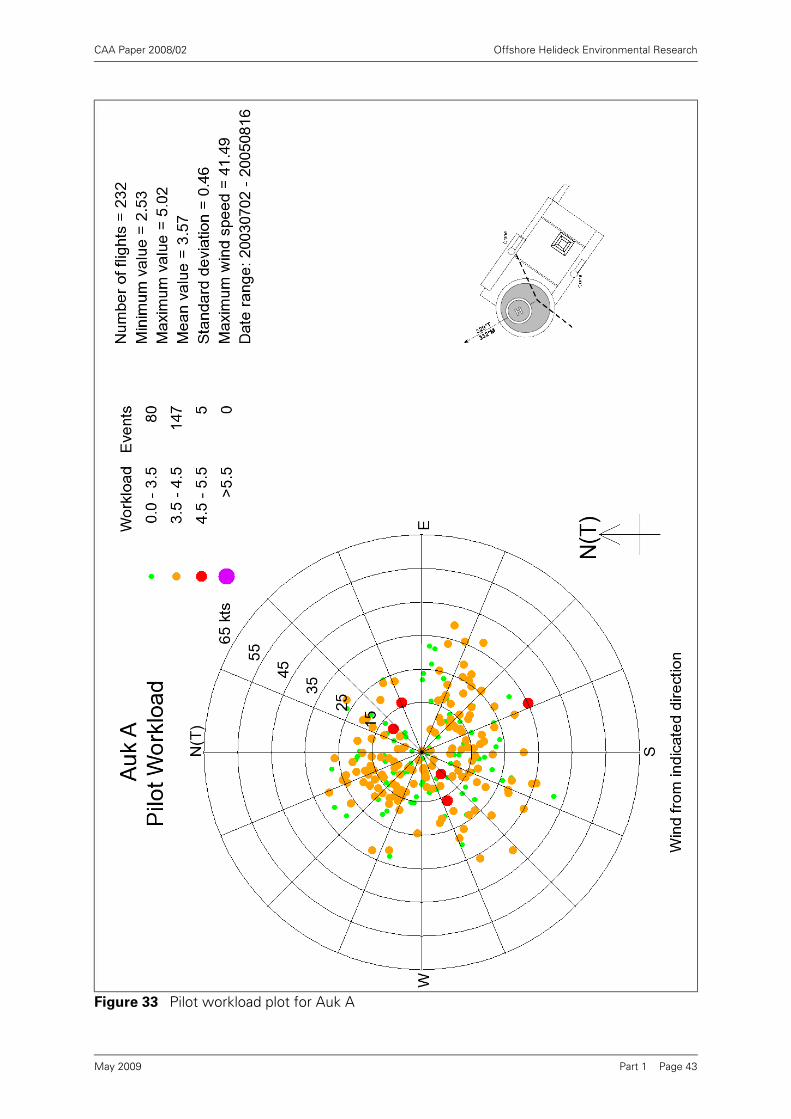
The plots in this section show the maximum pilot workload values with points colourcoded according to the workload value, and with the position of the point on the plotrepresenting the estimated wind speed and direction at the time of the landing.
Each plot includes a sketch of the platform layout correctly orientated with respect totrue North, so that the relationship between wind directions and platformobstructions that might cause turbulence can be assessed. The sketches of theplatforms were obtained from the ‘Aerad Plates’ published by European AeronauticalGroup (now part of Navtech Inc). In some cases an appropriate plan view sketch ofthe platform was not readily available. In a few cases it was noticed that the sketchescontained errors. Examples of these were; Alba Northern (unobstructed sectormarkings wrongly aligned on the sketch), Brae A (4o to 5o error in helideckorientation), K14-FA-1 (major alignment error), and K15-FA-1 (major alignment error).
Workload plots are presented here for 8 platforms, Brae A, Brent A, Brent B, Brent C,Britannia, Cormorant A, Ninian Central, and Auk A. The first 7 were selected becausethey all contained examples of high workload landings (> 5.5), whilst Auk A bycontrast tended to exhibit lower workload landings.
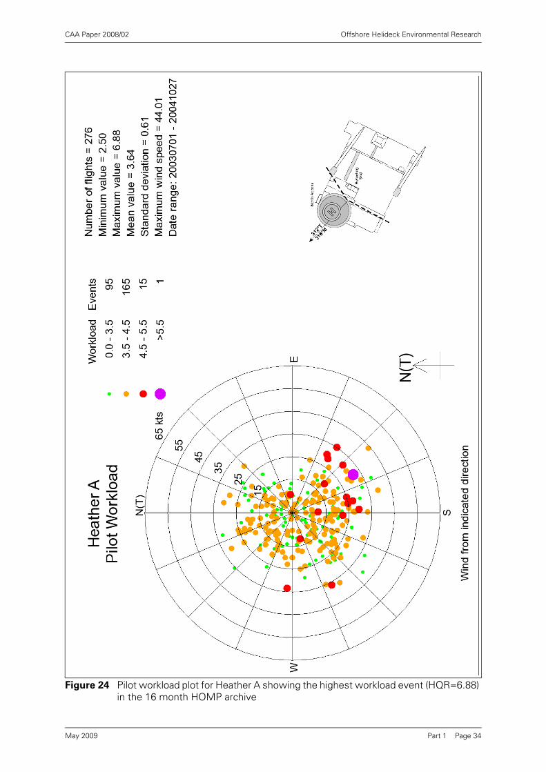
In general the Heather A platform does not appear to suffer from regular severeturbulence. The single high workload landing was the only landing with a value greaterthan 6.5. However, as noted in Appendix C, and as can be seen from the plot of theworkload values for Heather A in Figure 24, there is a cluster of higher workloadevents for wind directions in the range 115 to 180 degrees.
The HLL entry for Heather A (Appendix C) mentions turbulence, and requeststurbulence reports, but does not define a range of wind directions in which turbulencemight be expected. This is a good illustration of the benefit of the HOMP dataanalysed in this research project. The HLL, being largely reliant on subjective reportssubmitted by pilots, is an imperfect description of the helideck environment. TheHOMP data provides objective evidence on which to base a turbulent sector, andoffers the opportunity for a more specific warning in the HLL entry for this platform.
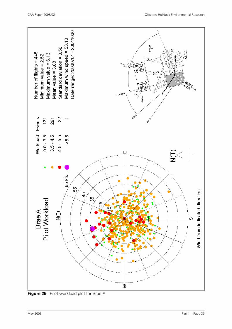
Figure 25 shows the data for Brae A, and it can be seen that the highest (purple)workload landing occurred when the wind was from just west of north at about 35 kt.There is a cluster of high workload landings from around this wind sector and for arange of wind speeds from 15 kt to 40 kt. This would be expected to be a winddirection that would cause significant turbulence over the helideck, as the helideck isdownwind of the large clad derrick for this wind sector. There is also a small clusterof higher workload (red) points for winds from the South at about 10-20 kt. It ispossible that these are due to the a relatively challenging landing manoeuvre involvingpoor visual cues when the helicopter is landing facing South into the Southerly wind.
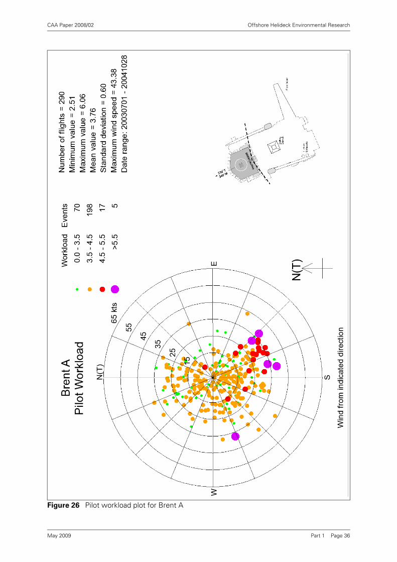
Figure 26 shows similar information for the Brent A platform. For this installation thehelideck is located on the Northwest end of the platform, and so highest workloadevents are seen in winds from the Southeast. There is one high workload event (>5.5)with wind at about 36 kt from WSW.
Data for Brent B is shown in Figure 27. Although the detailed design of the platformis quite different from Brent A, the helideck is again located on the Northwest end,and so the general pattern of the pilot workload is very similar.
The design and alignment of Brent C is somewhat similar to Brent B, and so a verysimilar picture is seen again in Figure 28.
Part 1 Page 32May 2009
CAA Paper 2008/02 Offshore Helideck Environmental Research
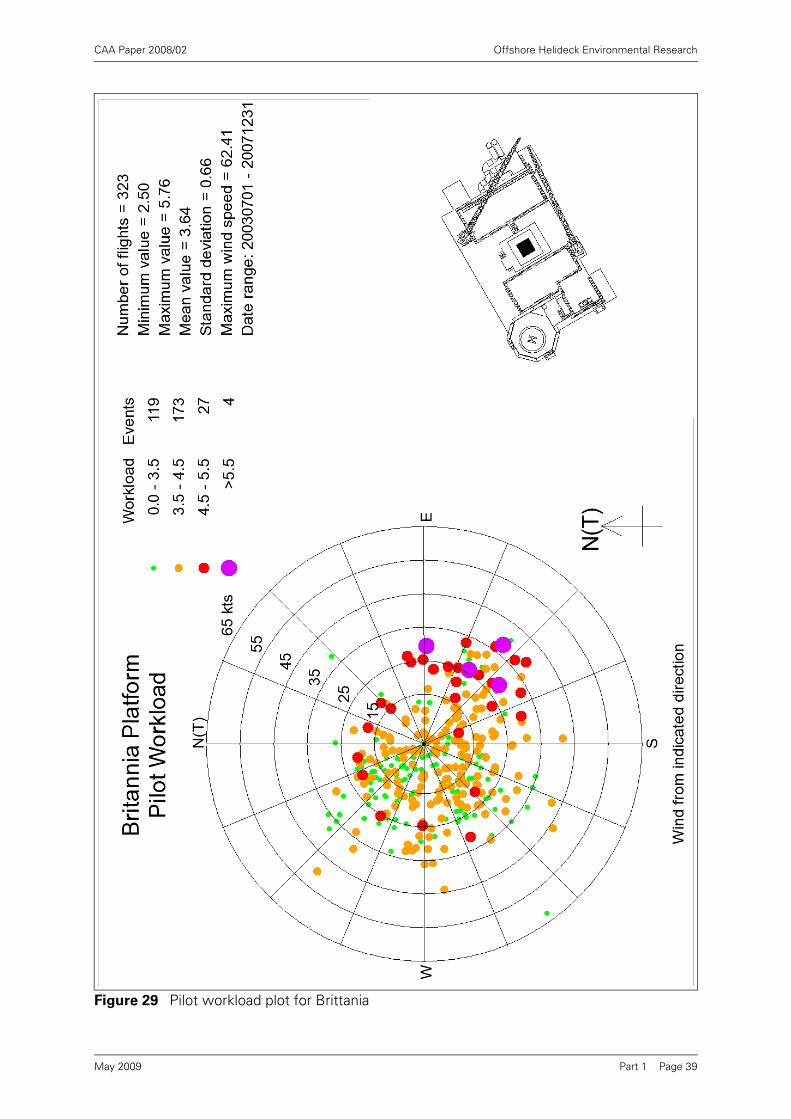
Results for the Britannia platform are shown in Figure 29. The design and alignmentof Britannia is quite different from the Brent platforms, and the helideck is located onthe Western corner. Consequently high workload events are seen for higher windspeeds from the East and Southeast.
For Cormorant A (Figure 30) the helideck is located on the Northern corner, and mostof the high workload events are seen in winds from the South. However, it is apparentthat the very highest workload event (6.02) occurred with the wind at 39 kt from theSouthwest. At this heading the wind is blowing across the significant accommodationblock located on the West corner, and so this high value is not surprising, particularlysince it occurs for the highest wind speed from this direction.
Results for Ninian C are shown in Figure 31. This platform has more high workloadevents than seen in the foregoing platforms, with 11 events over 5.5. The highworkload events are all clustered for moderate to high wind speeds from the SE toSSW sector, which is to be expected with the helideck located on the NW corner ofthe platform with some significant structures directly to the South. It is known thatNinian C suffers from hot exhaust gas plumes in the helicopter flightpath [11]. Figure32 shows a plot of maximum ambient temperature increase as measured by the OATsensor and it can be seen that there is a cluster of high temperature events with thewind in the E to S sector. The pattern is similar to, but not the same as, the pilotworkload plot and so both structure induced turbulence and temperature effects arelikely to be factors in causing high workload.
Finally, Figure 33 shows workload values for the Auk A platform. This is clearly aneasier platform on which to land, with only 5 well scattered events with workloadabove 4.5. Auk A is a relatively small platform and all structures, with the exceptionof an unclad drilling derrick are below the level of the helideck.
Part 1 Page 33May 2009
CAA Paper 2008/02 Offshore Helideck Environmental Research
Figure 24 Pilot workload plot for Heather A showing the highest workload event (HQR=6.88) in the 16 month HOMP archive
Part 1 Page 34May 2009
CAA Paper 2008/02 Offshore Helideck Environmental Research
Figure 25 Pilot workload plot for Brae A
Part 1 Page 35May 2009
CAA Paper 2008/02 Offshore Helideck Environmental Research
Figure 26 Pilot workload plot for Brent A
Part 1 Page 36May 2009

CAA Paper 2008/02 Offshore Helideck Environmental Research
Figure 27 Pilot workload plot for Brent B
Part 1 Page 37May 2009

CAA Paper 2008/02 Offshore Helideck Environmental Research
Figure 28 Pilot workload plot for Brent C
Part 1 Page 38May 2009
CAA Paper 2008/02 Offshore Helideck Environmental Research
Figure 29 Pilot workload plot for Brittania
Part 1 Page 39May 2009

CAA Paper 2008/02 Offshore Helideck Environmental Research
Figure 30 Pilot workload plot for Cormorant A
Part 1 Page 40May 2009

CAA Paper 2008/02 Offshore Helideck Environmental Research
Figure 31 Pilot workload plot for Ninian C
Part 1 Page 41May 2009

CAA Paper 2008/02 Offshore Helideck Environmental Research
Figure 32 Air temperature difference plot for Ninian C
Part 1 Page 42May 2009
CAA Paper 2008/02 Offshore Helideck Environmental Research
Figure 33 Pilot workload plot for Auk A
Part 1 Page 43May 2009
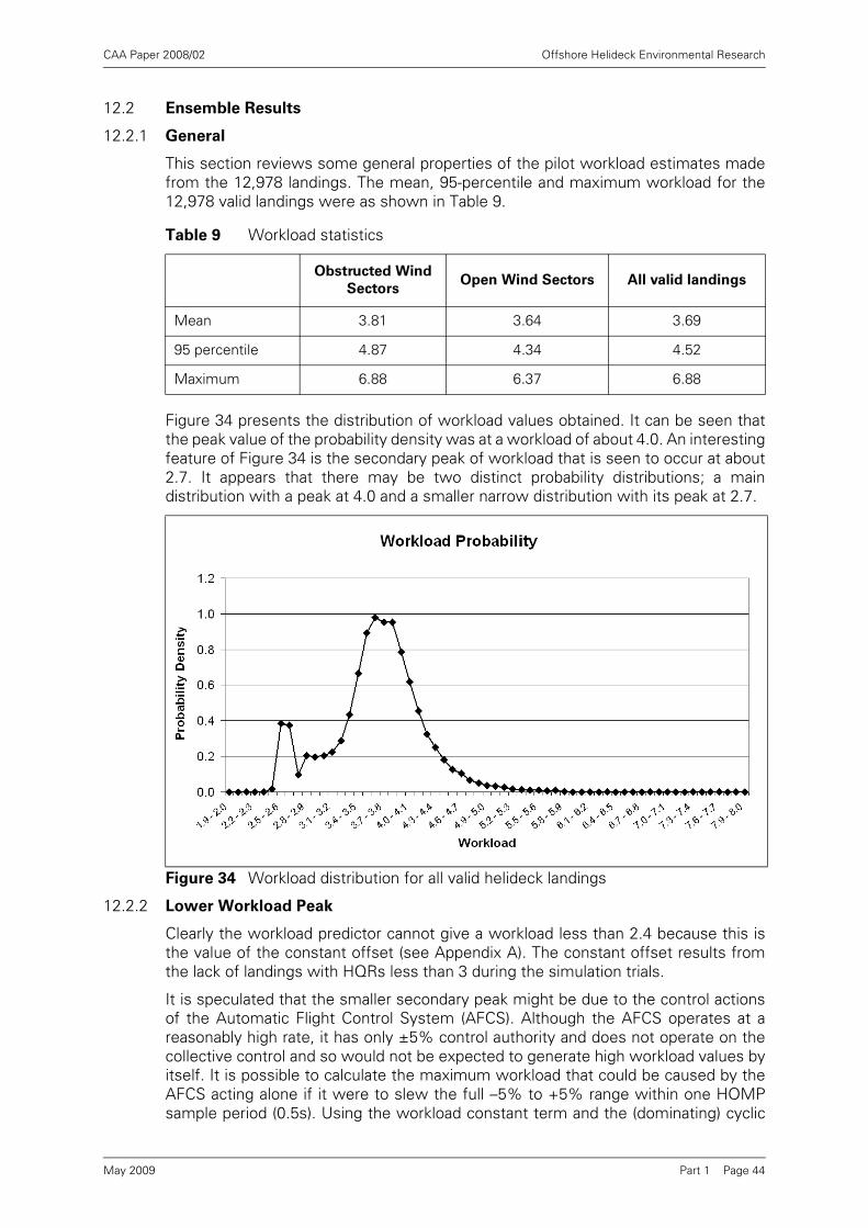
CAA Paper 2008/02 Offshore Helideck Environmental Research
12.2 Ensemble Results
12.2.1 General
This section reviews some general properties of the pilot workload estimates madefrom the 12,978 landings. The mean, 95-percentile and maximum workload for the12,978 valid landings were as shown in Table 9.
Figure 34 presents the distribution of workload values obtained. It can be seen thatthe peak value of the probability density was at a workload of about 4.0. An interestingfeature of Figure 34 is the secondary peak of workload that is seen to occur at about2.7. It appears that there may be two distinct probability distributions; a maindistribution with a peak at 4.0 and a smaller narrow distribution with its peak at 2.7.
12.2.2 Lower Workload Peak
Clearly the workload predictor cannot give a workload less than 2.4 because this isthe value of the constant offset (see Appendix A). The constant offset results fromthe lack of landings with HQRs less than 3 during the simulation trials.
It is speculated that the smaller secondary peak might be due to the control actionsof the Automatic Flight Control System (AFCS). Although the AFCS operates at areasonably high rate, it has only ±5% control authority and does not operate on thecollective control and so would not be expected to generate high workload values byitself. It is possible to calculate the maximum workload that could be caused by theAFCS acting alone if it were to slew the full –5% to +5% range within one HOMPsample period (0.5s). Using the workload constant term and the (dominating) cyclic
Table 9 Workload statistics
Obstructed Wind
SectorsOpen Wind Sectors All valid landings
Mean 3.81 3.64 3.69
95 percentile 4.87 4.34 4.52
Maximum 6.88 6.37 6.88
Figure 34 Workload distribution for all valid helideck landings
Part 1 Page 44May 2009
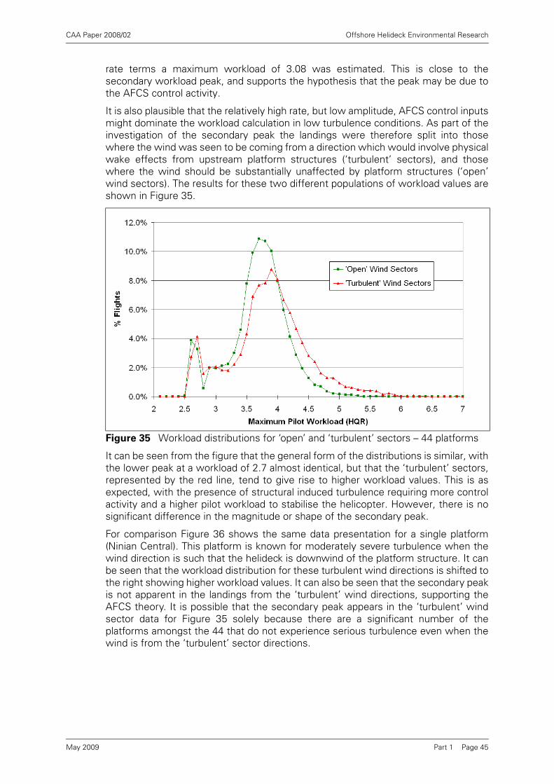
CAA Paper 2008/02 Offshore Helideck Environmental Research
rate terms a maximum workload of 3.08 was estimated. This is close to thesecondary workload peak, and supports the hypothesis that the peak may be due tothe AFCS control activity.
It is also plausible that the relatively high rate, but low amplitude, AFCS control inputsmight dominate the workload calculation in low turbulence conditions. As part of theinvestigation of the secondary peak the landings were therefore split into thosewhere the wind was seen to be coming from a direction which would involve physicalwake effects from upstream platform structures (‘turbulent’ sectors), and thosewhere the wind should be substantially unaffected by platform structures (‘open’wind sectors). The results for these two different populations of workload values areshown in Figure 35.
It can be seen from the figure that the general form of the distributions is similar, withthe lower peak at a workload of 2.7 almost identical, but that the ‘turbulent’ sectors,represented by the red line, tend to give rise to higher workload values. This is asexpected, with the presence of structural induced turbulence requiring more controlactivity and a higher pilot workload to stabilise the helicopter. However, there is nosignificant difference in the magnitude or shape of the secondary peak.
For comparison Figure 36 shows the same data presentation for a single platform(Ninian Central). This platform is known for moderately severe turbulence when thewind direction is such that the helideck is downwind of the platform structure. It canbe seen that the workload distribution for these turbulent wind directions is shifted tothe right showing higher workload values. It can also be seen that the secondary peakis not apparent in the landings from the ‘turbulent’ wind directions, supporting theAFCS theory. It is possible that the secondary peak appears in the ‘turbulent’ windsector data for Figure 35 solely because there are a significant number of theplatforms amongst the 44 that do not experience serious turbulence even when thewind is from the ‘turbulent’ sector directions.
Figure 35 Workload distributions for ‘open’ and ‘turbulent’ sectors – 44 platforms
Part 1 Page 45May 2009
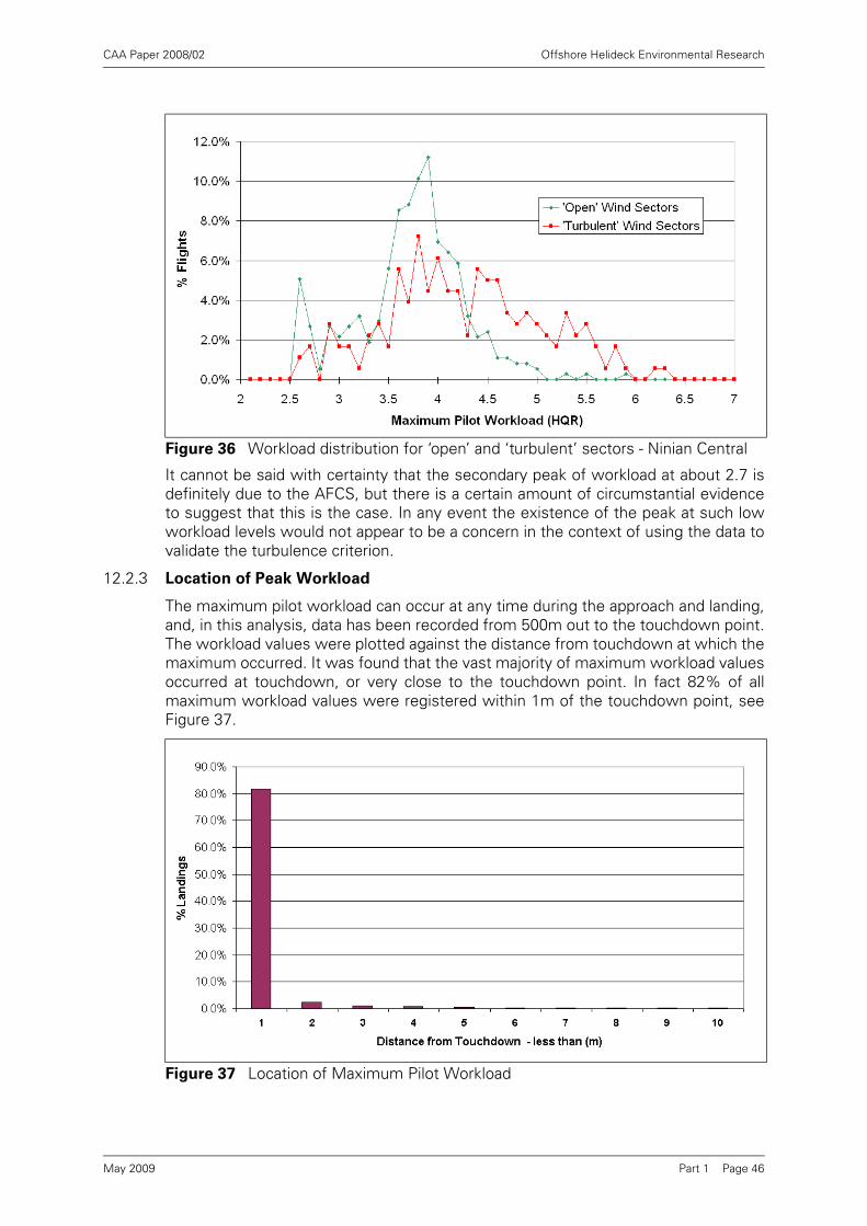
CAA Paper 2008/02 Offshore Helideck Environmental Research
It cannot be said with certainty that the secondary peak of workload at about 2.7 isdefinitely due to the AFCS, but there is a certain amount of circumstantial evidenceto suggest that this is the case. In any event the existence of the peak at such lowworkload levels would not appear to be a concern in the context of using the data tovalidate the turbulence criterion.
12.2.3 Location of Peak Workload
The maximum pilot workload can occur at any time during the approach and landing,and, in this analysis, data has been recorded from 500m out to the touchdown point.The workload values were plotted against the distance from touchdown at which themaximum occurred. It was found that the vast majority of maximum workload valuesoccurred at touchdown, or very close to the touchdown point. In fact 82% of allmaximum workload values were registered within 1m of the touchdown point, seeFigure 37.
Figure 36 Workload distribution for ‘open’ and ‘turbulent’ sectors - Ninian Central
Figure 37 Location of Maximum Pilot Workload
Part 1 Page 46May 2009
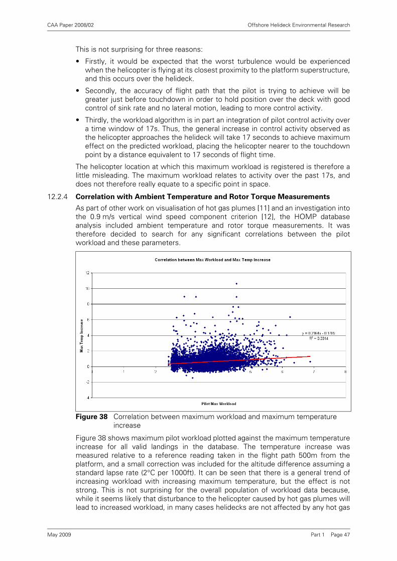
CAA Paper 2008/02 Offshore Helideck Environmental Research
This is not surprising for three reasons:
• Firstly, it would be expected that the worst turbulence would be experiencedwhen the helicopter is flying at its closest proximity to the platform superstructure,and this occurs over the helideck.
• Secondly, the accuracy of flight path that the pilot is trying to achieve will begreater just before touchdown in order to hold position over the deck with goodcontrol of sink rate and no lateral motion, leading to more control activity.
• Thirdly, the workload algorithm is in part an integration of pilot control activity overa time window of 17s. Thus, the general increase in control activity observed asthe helicopter approaches the helideck will take 17 seconds to achieve maximumeffect on the predicted workload, placing the helicopter nearer to the touchdownpoint by a distance equivalent to 17 seconds of flight time.
The helicopter location at which this maximum workload is registered is therefore alittle misleading. The maximum workload relates to activity over the past 17s, anddoes not therefore really equate to a specific point in space.
12.2.4 Correlation with Ambient Temperature and Rotor Torque Measurements
As part of other work on visualisation of hot gas plumes [11] and an investigation intothe 0.9 m/s vertical wind speed component criterion [12], the HOMP databaseanalysis included ambient temperature and rotor torque measurements. It wastherefore decided to search for any significant correlations between the pilotworkload and these parameters.
Figure 38 shows maximum pilot workload plotted against the maximum temperatureincrease for all valid landings in the database. The temperature increase wasmeasured relative to a reference reading taken in the flight path 500m from theplatform, and a small correction was included for the altitude difference assuming astandard lapse rate (2°C per 1000ft). It can be seen that there is a general trend ofincreasing workload with increasing maximum temperature, but the effect is notstrong. This is not surprising for the overall population of workload data because,while it seems likely that disturbance to the helicopter caused by hot gas plumes willlead to increased workload, in many cases helidecks are not affected by any hot gas
Figure 38 Correlation between maximum workload and maximum temperature increase
Part 1 Page 47May 2009

CAA Paper 2008/02 Offshore Helideck Environmental Research
hazards. In contrast, examination of the pattern of workload and temperature forindividual platforms subject to hot gas effects is expected to show a strongercorrelation (see for example Figure 31 and Figure 32 on pages 41 and 42 respectively,and described in Section 12.1). A similar weak correlation is seen between workloadand maximum rotor torque in Figure 39. The correlation is much stronger betweenworkload and maximum torque increase (over 2s) shown in Figure 40. Thisconnection is not surprising given that the workload predictor is particularly sensitiveto collective pitch control rate, and that a high rate of change of collective pitch willinevitably induce a rapid change in torque. (Note that the data presented in Figure 39and Figure 40 has been limited to a helicopter landing weight range 17,000lb –18,500lb in order to remove any major effects of weight on torque.)
Figure 39 Correlation between maximum workload and maximum torque
Figure 40 Correlation between maximum workload and maximum torque increase
Part 1 Page 48May 2009
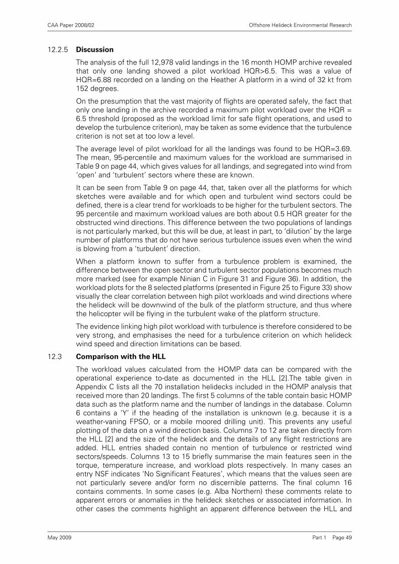
CAA Paper 2008/02 Offshore Helideck Environmental Research
12.2.5 Discussion
The analysis of the full 12,978 valid landings in the 16 month HOMP archive revealedthat only one landing showed a pilot workload HQR>6.5. This was a value ofHQR=6.88 recorded on a landing on the Heather A platform in a wind of 32 kt from152 degrees.
On the presumption that the vast majority of flights are operated safely, the fact thatonly one landing in the archive recorded a maximum pilot workload over the HQR =6.5 threshold (proposed as the workload limit for safe flight operations, and used todevelop the turbulence criterion), may be taken as some evidence that the turbulencecriterion is not set at too low a level.
The average level of pilot workload for all the landings was found to be HQR=3.69.The mean, 95-percentile and maximum values for the workload are summarised inTable 9 on page 44, which gives values for all landings, and segregated into wind from‘open’ and ‘turbulent’ sectors where these are known.
It can be seen from Table 9 on page 44, that, taken over all the platforms for whichsketches were available and for which open and turbulent wind sectors could bedefined, there is a clear trend for workloads to be higher for the turbulent sectors. The95 percentile and maximum workload values are both about 0.5 HQR greater for theobstructed wind directions. This difference between the two populations of landingsis not particularly marked, but this will be due, at least in part, to ‘dilution’ by the largenumber of platforms that do not have serious turbulence issues even when the windis blowing from a ‘turbulent’ direction.
When a platform known to suffer from a turbulence problem is examined, thedifference between the open sector and turbulent sector populations becomes muchmore marked (see for example Ninian C in Figure 31 and Figure 36). In addition, theworkload plots for the 8 selected platforms (presented in Figure 25 to Figure 33) showvisually the clear correlation between high pilot workloads and wind directions wherethe helideck will be downwind of the bulk of the platform structure, and thus wherethe helicopter will be flying in the turbulent wake of the platform structure.
The evidence linking high pilot workload with turbulence is therefore considered to bevery strong, and emphasises the need for a turbulence criterion on which helideckwind speed and direction limitations can be based.
12.3 Comparison with the HLL
The workload values calculated from the HOMP data can be compared with theoperational experience to-date as documented in the HLL [2].The table given inAppendix C lists all the 70 installation helidecks included in the HOMP analysis thatreceived more than 20 landings. The first 5 columns of the table contain basic HOMPdata such as the platform name and the number of landings in the database. Column6 contains a ‘Y’ if the heading of the installation is unknown (e.g. because it is aweather-vaning FPSO, or a mobile moored drilling unit). This prevents any usefulplotting of the data on a wind direction basis. Columns 7 to 12 are taken directly fromthe HLL [2] and the size of the helideck and the details of any flight restrictions areadded. HLL entries shaded contain no mention of turbulence or restricted windsectors/speeds. Columns 13 to 15 briefly summarise the main features seen in thetorque, temperature increase, and workload plots respectively. In many cases anentry NSF indicates ‘No Significant Features’, which means that the values seen arenot particularly severe and/or form no discernible patterns. The final column 16contains comments. In some cases (e.g. Alba Northern) these comments relate toapparent errors or anomalies in the helideck sketches or associated information. Inother cases the comments highlight an apparent difference between the HLL and
Part 1 Page 49May 2009

CAA Paper 2008/02 Offshore Helideck Environmental Research
what has been seen in the HOMP results, perhaps suggesting that the turbulentsector identified in the HLL might be extended (e.g. Britannia).
Overall, there is good consistency between the HOMP results and the turbulentsectors identified in the HLL. In the cases of Alba Northern, Britannia, Brent A, BrentB, Brent D, Magnus, Ninian C, and NW Hutton, there is the suggestion in the HOMPdata that the HLL turbulent sectors might be extended or redefined slightly5. In thecases of Gannet and Heather A it is suggested that the HLL should include a definedturbulent sector. There appear to be errors in the helideck sketches for Alba Northern,Brae A, K14-FA-1, K15-FA-1 and North Cormorant.
Despite the good consistency of the data with the advice in the HLL, it is difficult tointerpret this data, or the other comparisons with operational experience presentedin this report, to verify that the turbulence criterion has not been set at too high a level.It was seen that only one landing out of 12,978 registered a workload higher than 6.5,which indicates that operationally such pilot workload/turbulence levels are only metvery rarely. However, it is possible that the workload threshold for safe flight shouldin fact be set at a lower level, to offer a greater margin of safety, particularly for theless experienced pilot flying at night, in poor visibility or in otherwise challengingconditions. It is therefore considered important that pilots should continue to bestrongly encouraged to submit turbulence reports, and that these reports should becorrelated against HOMP pilot workload in order to look for any evidence ofturbulence difficulties at lower pilot workload values. Any such evidence could beused to justify a reduction in acceptable level of pilot workload / HQR and theassociated turbulence criterion. The discussion in Section 13 develops these pointsfurther.
12.4 Comparison with Wind Tunnel Data
BMT Fluid Mechanics holds an archive of wind tunnel test data for offshoreinstallations that have been tested in its wind tunnels. However, only five of the BMTarchive North Sea platforms were visited by Bristow helicopters during the periodcovered by the HOMP archive. These were; Clair, Britannia, Cormorant A, East Braeand Scott.6
HOMP data from Clair is not easy to interpret because there were only 72 landingsrecorded in the archive. However, these data are presented here in Figure 41 and itcan be seen that the highest workload events occurred for wind directions in therange 120 to 190 degrees and speeds 20 to 35 kt.
The wind tunnel measured turbulence data for Clair is shown in Figure 42. The figureshows a blue area, the outer boundary of which indicates the wind speeds anddirections at which the 2.4 m/s vertical component standard deviation turbulencecriterion is violated7. Also shown is a green area, the outer boundary of the green areaindicates wind speeds and directions at which a vertical turbulence standard deviationof over 1.75 m/s is experienced. The value of 1.75 m/s was selected here because itapproximated to a HQR=5.5 in the flight simulator trials of [1] (see Figure 3 in Section2) and is therefore more directly comparable with the higher workload valuesexperienced in the HOMP data. For Clair it can be seen that the severest turbulenceoccurred for winds from headings 40-100 degrees. At these headings the turbulencelimit is violated for winds of about 40 kt and above. The HOMP archive does not
5. Any such redefinition based on the HOMP data will need to take account of the likely accuracy of the HOMP wind speedand direction estimates (see Section 11).
6. There was also data for the MacCulloch FPSO, but this could not be interpreted owing to a lack of information on thevessel heading at the time of the landing in the HOMP database.
7. The notation of the figures uses the shorter abbreviation rms (root mean square). Standard deviation and rms are oneand the same for a turbulence record that has already been corrected to zero mean.
Part 1 Page 50May 2009

CAA Paper 2008/02 Offshore Helideck Environmental Research
include any winds of this magnitude from this direction for the Clair platform, nor doesit include any pilot workload values of HQR>5.5, but it is noted that the highestworkload events occur with winds from 135 to 190 degrees. 8
In the case of Britannia there are 323 landings in the HOMP archive and so the datais easier to interpret. The HOMP data is presented in Figure 43 and the wind tunnelturbulence data in Figure 44.
It can be seen that the highest workload events (of which 4 are HQR>5.5) occur forwind directions in the range 90 to 140 degrees and speeds 25 to 40 kt. The windtunnel data shows that turbulence in excess of 1.75 m/s and thus HQR>5.5 would beexpected to occur for directions 80 to 150 degrees and wind speeds above 30 to40 kt. The wind tunnel data and the HOMP data are therefore consistent for thisplatform.
For Cormorant A the HOMP data is presented in Figure 45 and the wind tunnel datain Figure 46.
It can be seen that the majority of higher pilot workload events occur for wind speedsin the heading range 135-180 degrees and speeds 25-40 kt. This is again broadlyconsistent with the wind tunnel data, which shows that turbulence in excess of1.75 m/s would be experienced for wind speeds of around 35 kt at a heading of 225degrees. This coincides with the single very high workload value that occurred with awind speed of 40 kt at 225 degrees.
HOMP data for East Brae is presented in Figure 47, and the wind tunnel turbulencedata is shown in Figure 48. It is evident from the wind tunnel data that the worstturbulence is expected to occur with wind headings in the range 340 to 80 degreeswith the turbulence criterion being violated for wind speeds above about 30 to 40 kt.However there have been no landings recorded in the HOMP database for windspeeds above 25 kt for these headings. This is consistent with the HLL entry for thisplatform which warns of turbulence for headings in the range 335 to 035 degrees andspeeds above 30 kt. The evidence from the HOMP data is that these wind conditionsare indeed being avoided.
Data for the Scott platform is shown in Figure 49 and Figure 50. The wind tunnel datain Figure 50 shows that there is reasonably high turbulence for a number of winddirections, but the worst wind headings are 345-080 degrees where the turbulencecriterion is violated at a wind speed of about 40 kt. The HOMP data shows no landingsat wind speeds above 30 kt for these headings. There is no turbulence entry for Scottin the HLL.
The figures are evidence of validation of the turbulence criterion as defined in [1].
8. Only one landing exhibited a high workload at a 190 degree wind heading, and it is possible that this is an example of anindividual poor estimate of direction from the HOMP analysis.
Part 1 Page 51May 2009

CAA Paper 2008/02 Offshore Helideck Environmental Research
Figure 41 Clair Platform pilot workload
Figure 42 Clair Platform vertical turbulance – green boundary urms>1.75 m/s, blue boundary urms >2.4 m/s
Part 1 Page 52May 2009
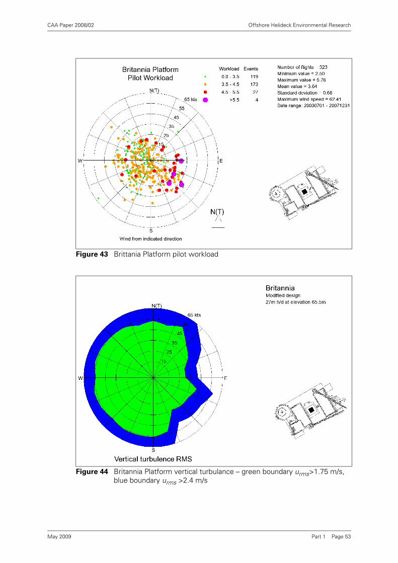
CAA Paper 2008/02 Offshore Helideck Environmental Research
Figure 43 Brittania Platform pilot workload
Figure 44 Britannia Platform vertical turbulance – green boundary urms>1.75 m/s, blue boundary urms >2.4 m/s
Part 1 Page 53May 2009
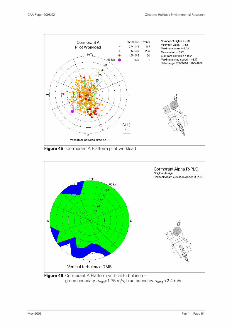
CAA Paper 2008/02 Offshore Helideck Environmental Research
Figure 45 Cormorant A Platform pilot workload
Figure 46 Cormorant A Platform vertical turbulance – green boundary urms>1.75 m/s, blue boundary urms >2.4 m/s
Part 1 Page 54May 2009

CAA Paper 2008/02 Offshore Helideck Environmental Research
Figure 47 East Brae Platform pilot workload
Figure 48 East Brae Platform vertical turbulance – green boundary urms>1.75 m/s, blue boundary urms >2.4 m/s
Part 1 Page 55May 2009
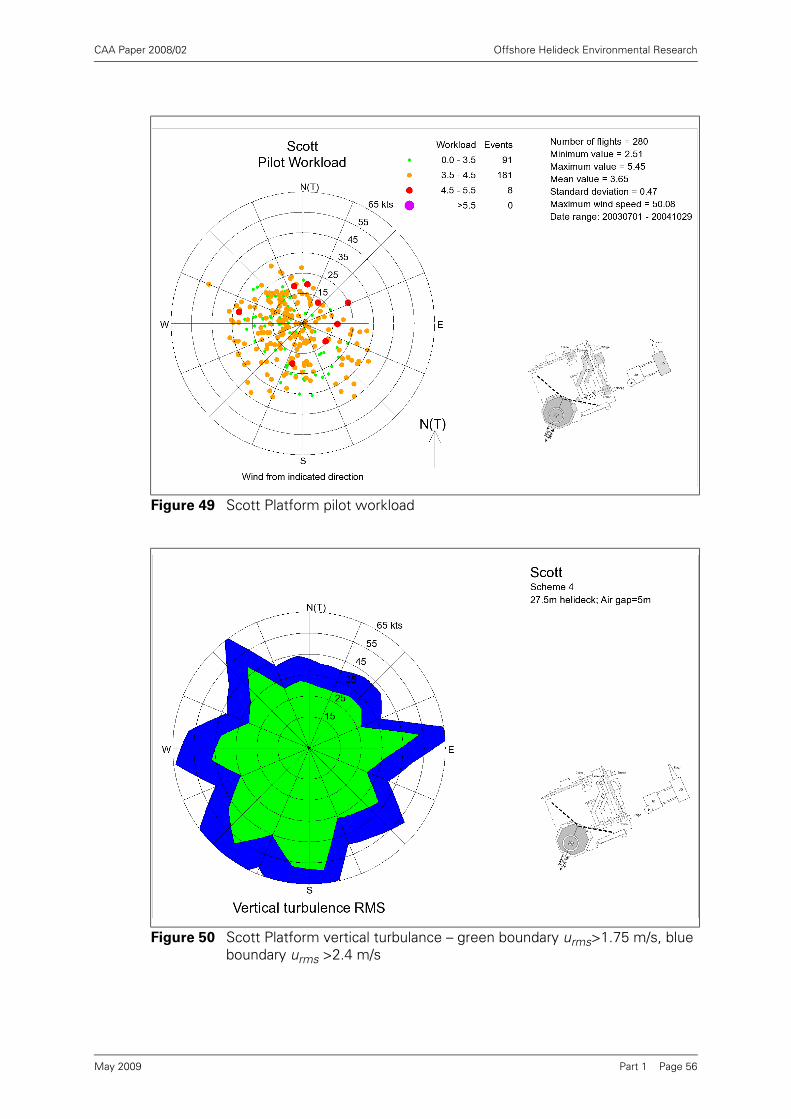
CAA Paper 2008/02 Offshore Helideck Environmental Research
Figure 49 Scott Platform pilot workload
Figure 50 Scott Platform vertical turbulance – green boundary urms>1.75 m/s, blue boundary urms >2.4 m/s
Part 1 Page 56May 2009
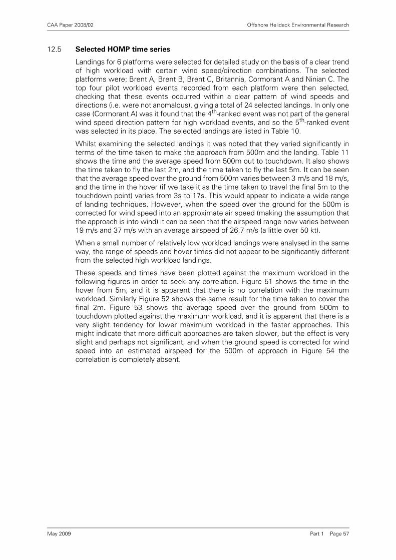
CAA Paper 2008/02 Offshore Helideck Environmental Research
12.5 Selected HOMP time series
Landings for 6 platforms were selected for detailed study on the basis of a clear trendof high workload with certain wind speed/direction combinations. The selectedplatforms were; Brent A, Brent B, Brent C, Britannia, Cormorant A and Ninian C. Thetop four pilot workload events recorded from each platform were then selected,checking that these events occurred within a clear pattern of wind speeds anddirections (i.e. were not anomalous), giving a total of 24 selected landings. In only onecase (Cormorant A) was it found that the 4th-ranked event was not part of the generalwind speed direction pattern for high workload events, and so the 5th-ranked eventwas selected in its place. The selected landings are listed in Table 10.
Whilst examining the selected landings it was noted that they varied significantly interms of the time taken to make the approach from 500m and the landing. Table 11shows the time and the average speed from 500m out to touchdown. It also showsthe time taken to fly the last 2m, and the time taken to fly the last 5m. It can be seenthat the average speed over the ground from 500m varies between 3 m/s and 18 m/s,and the time in the hover (if we take it as the time taken to travel the final 5m to thetouchdown point) varies from 3s to 17s. This would appear to indicate a wide rangeof landing techniques. However, when the speed over the ground for the 500m iscorrected for wind speed into an approximate air speed (making the assumption thatthe approach is into wind) it can be seen that the airspeed range now varies between19 m/s and 37 m/s with an average airspeed of 26.7 m/s (a little over 50 kt).
When a small number of relatively low workload landings were analysed in the sameway, the range of speeds and hover times did not appear to be significantly differentfrom the selected high workload landings.
These speeds and times have been plotted against the maximum workload in thefollowing figures in order to seek any correlation. Figure 51 shows the time in thehover from 5m, and it is apparent that there is no correlation with the maximumworkload. Similarly Figure 52 shows the same result for the time taken to cover thefinal 2m. Figure 53 shows the average speed over the ground from 500m totouchdown plotted against the maximum workload, and it is apparent that there is avery slight tendency for lower maximum workload in the faster approaches. Thismight indicate that more difficult approaches are taken slower, but the effect is veryslight and perhaps not significant, and when the ground speed is corrected for windspeed into an estimated airspeed for the 500m of approach in Figure 54 thecorrelation is completely absent.
Part 1 Page 57May 2009

CAA Paper 2008/02 Offshore Helideck Environmental Research
Table 10 High workload landings selected for detailed examination
Part 1 Page 58May 2009
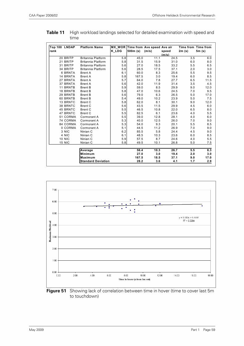
CAA Paper 2008/02 Offshore Helideck Environmental Research
Table 11 High workload landings selected for detailed examination with speed and time
Figure 51 Showing lack of correlation between time in hover (time to cover last 5m to touchdown)
Top 100 rank
LNDAP Platform Name MX_WORK_LDG
Time from 500m (s)
Ave speed (m/s)
Ave air speed (m/s)
Time from 2m (s)
Time from 5m (s)
20 BRITP Britannia Platform 5.8 45.0 11.1 24.5 3.5 6.021 BRITP Britannia Platform 5.8 31.5 15.9 31.0 6.0 8.031 BRITP Britannia Platform 5.6 27.0 18.5 33.2 5.5 6.534 BRITP Britannia Platform 5.6 28.5 17.5 37.1 2.0 3.0
6 BRNTA Brent A 6.1 60.0 8.3 25.6 5.5 9.514 BRNTA Brent A 5.8 167.5 3.0 19.4 6.0 8.527 BRNTA Brent A 5.7 64.0 7.8 27.7 6.5 11.537 BRNTA Brent A 5.6 42.0 11.9 31.4 3.5 4.511 BRNTB Brent B 5.9 59.0 8.5 29.9 9.0 12.018 BRNTB Brent B 5.8 47.0 10.6 24.5 7.0 9.529 BRNTB Brent B 5.6 79.0 6.3 26.5 5.0 17.060 BRNTB Brent B 5.4 49.0 10.2 23.9 5.0 7.513 BRNTC Brent C 5.8 62.0 8.1 30.1 9.0 12.038 BRNTC Brent C 5.6 43.5 11.5 29.9 4.5 6.045 BRNTC Brent C 5.5 46.5 10.8 22.0 6.5 8.047 BRNTC Brent C 5.5 82.5 6.1 23.6 4.0 5.551 CORMA Cormorant A 5.5 39.0 12.8 28.1 4.0 6.074 CORMA Cormorant A 5.3 40.0 12.5 26.0 7.0 9.084 CORMA Cormorant A 5.3 54.0 9.3 20.1 5.5 8.5
0 CORMA Cormorant A 5.1 44.5 11.2 26.9 7.0 9.03 NIC Ninian C 6.2 85.5 5.8 24.4 4.5 9.04 NIC Ninian C 6.1 48.5 10.3 23.6 6.0 8.5
10 NIC Ninian C 5.9 57.5 8.7 24.6 4.0 5.515 NIC Ninian C 5.8 49.5 10.1 26.8 5.0 7.5
Average 56.4 10.3 26.7 5.5 8.3Minimum 27.0 3.0 19.4 2.0 3.0Maximum 167.5 18.5 37.1 9.0 17.0Standard Deviation 28.2 3.6 4.1 1.7 2.9
Part 1 Page 59May 2009

CAA Paper 2008/02 Offshore Helideck Environmental Research
Figure 52 Showing lack of correlation between time in hover (time to cover last 2m to touchdown)
Figure 53 Showing lack of correlation between speed of approach and workload
Part 1 Page 60May 2009

CAA Paper 2008/02 Offshore Helideck Environmental Research
Appendix D shows the HOMP time series traces for the selected 24 high workloadlandings. In addition, 6 relatively low workload landings (all but one had a workloadless than 3.0) are shown starting on Appendix D page 25. The traces show the lastminute of the approach to touchdown.
The traces provide a graphic demonstration of how the workload algorithm works,and particularly the effect of the 17s ‘window’ over which the standard deviation ofthe control activity is evaluated. Figure 55 shows a detail from one of the landingtraces presented in Appendix D.
Figure 54 Showing lack of correlation between estimated airspeed of approach and workload
Figure 55 Detail of HOMP trace
Part 1 Page 61May 2009
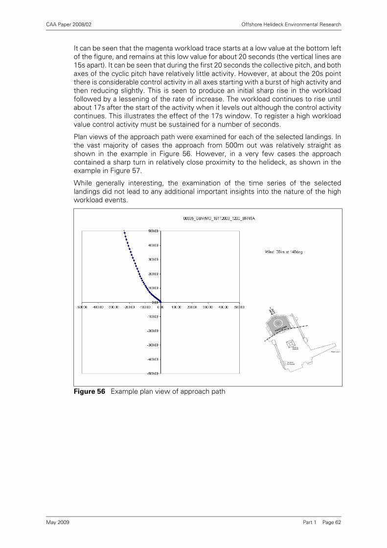
CAA Paper 2008/02 Offshore Helideck Environmental Research
It can be seen that the magenta workload trace starts at a low value at the bottom leftof the figure, and remains at this low value for about 20 seconds (the vertical lines are15s apart). It can be seen that during the first 20 seconds the collective pitch, and bothaxes of the cyclic pitch have relatively little activity. However, at about the 20s pointthere is considerable control activity in all axes starting with a burst of high activity andthen reducing slightly. This is seen to produce an initial sharp rise in the workloadfollowed by a lessening of the rate of increase. The workload continues to rise untilabout 17s after the start of the activity when it levels out although the control activitycontinues. This illustrates the effect of the 17s window. To register a high workloadvalue control activity must be sustained for a number of seconds.
Plan views of the approach path were examined for each of the selected landings. Inthe vast majority of cases the approach from 500m out was relatively straight asshown in the example in Figure 56. However, in a very few cases the approachcontained a sharp turn in relatively close proximity to the helideck, as shown in theexample in Figure 57.
While generally interesting, the examination of the time series of the selectedlandings did not lead to any additional important insights into the nature of the highworkload events.
Figure 56 Example plan view of approach path
Part 1 Page 62May 2009

CAA Paper 2008/02 Offshore Helideck Environmental Research
.
13 Discussion
The provisional turbulence criterion specified in the guidance [3] was set at 2.4 m/sbased on the pilot workload boundary between safe and unsafe flight of HQR=6.5(Section 2 and [1]). At the time it was noted that this criterion had been based on theassessment of three experienced test pilots flying a simulator in ideal visual cueingconditions. The criterion made no allowance for flight in reduced visual cueingconditions due to darkness, precipitation (rain, snow, hail) or poor visibility (mist, fog,low cloud), or for the less able or less experienced pilot. A clear link between pilotworkload and visual cueing conditions has been established in other research [13]. Itwas evident from the outset, therefore, that there might be strong arguments for areduction of the provisional turbulence criterion to a lower level to provide someallowance for these factors.
In the analysis of pilot workload from the HOMP data presented in this report (Section12), it has been seen that only one helideck landing in 12,978 generated a pilotworkload that exceeded the HQR=6.5 value. Such a frequency, however, seemsinconsistent with the findings of an earlier pilot questionnaire survey [14], in which thepilots identified the principal safety hazard and source of highest workload duringoffshore operations as turbulence around platforms. It also conflicts with anecdotalevidence collected from a small sample of offshore pilots during a presentation inAberdeen in November 2006 which suggests that, on average, pilots consider around1 in 50 helideck landings to be significantly affected by turbulence.
If turbulence reports had been submitted by pilots during the 16-month periodcovered by the HOMP data archive, then these could have been correlated with theHOMP pilot workload values to help establish a lower limit. Unfortunately, however,the turbulence reporting system appears to have fallen into disuse, and there wereno turbulence reports submitted during the period in question.
Figure 57 Example plan view of approach path
Part 1 Page 63May 2009
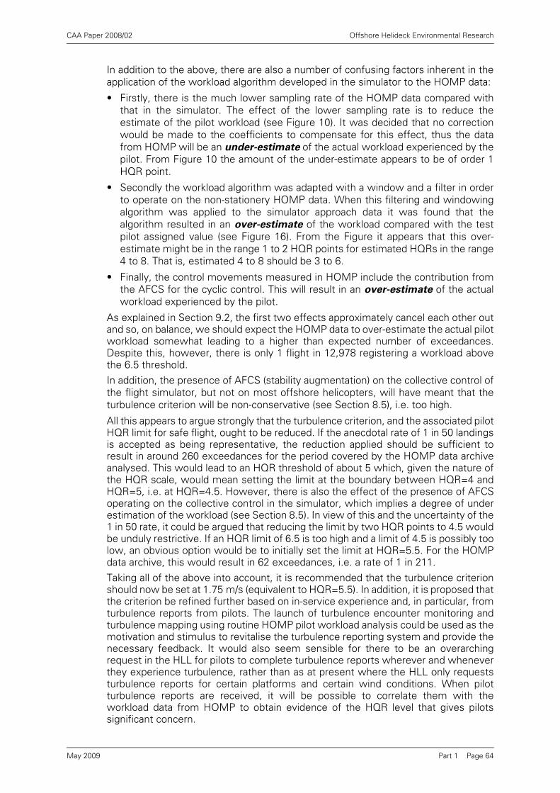
CAA Paper 2008/02 Offshore Helideck Environmental Research
In addition to the above, there are also a number of confusing factors inherent in theapplication of the workload algorithm developed in the simulator to the HOMP data:
• Firstly, there is the much lower sampling rate of the HOMP data compared withthat in the simulator. The effect of the lower sampling rate is to reduce theestimate of the pilot workload (see Figure 10). It was decided that no correctionwould be made to the coefficients to compensate for this effect, thus the datafrom HOMP will be an under-estimate of the actual workload experienced by thepilot. From Figure 10 the amount of the under-estimate appears to be of order 1HQR point.
• Secondly the workload algorithm was adapted with a window and a filter in orderto operate on the non-stationery HOMP data. When this filtering and windowingalgorithm was applied to the simulator approach data it was found that thealgorithm resulted in an over-estimate of the workload compared with the testpilot assigned value (see Figure 16). From the Figure it appears that this over-estimate might be in the range 1 to 2 HQR points for estimated HQRs in the range4 to 8. That is, estimated 4 to 8 should be 3 to 6.
• Finally, the control movements measured in HOMP include the contribution fromthe AFCS for the cyclic control. This will result in an over-estimate of the actualworkload experienced by the pilot.
As explained in Section 9.2, the first two effects approximately cancel each other outand so, on balance, we should expect the HOMP data to over-estimate the actual pilotworkload somewhat leading to a higher than expected number of exceedances.Despite this, however, there is only 1 flight in 12,978 registering a workload abovethe 6.5 threshold.In addition, the presence of AFCS (stability augmentation) on the collective control ofthe flight simulator, but not on most offshore helicopters, will have meant that theturbulence criterion will be non-conservative (see Section 8.5), i.e. too high.
All this appears to argue strongly that the turbulence criterion, and the associated pilotHQR limit for safe flight, ought to be reduced. If the anecdotal rate of 1 in 50 landingsis accepted as being representative, the reduction applied should be sufficient toresult in around 260 exceedances for the period covered by the HOMP data archiveanalysed. This would lead to an HQR threshold of about 5 which, given the nature ofthe HQR scale, would mean setting the limit at the boundary between HQR=4 andHQR=5, i.e. at HQR=4.5. However, there is also the effect of the presence of AFCSoperating on the collective control in the simulator, which implies a degree of underestimation of the workload (see Section 8.5). In view of this and the uncertainty of the1 in 50 rate, it could be argued that reducing the limit by two HQR points to 4.5 wouldbe unduly restrictive. If an HQR limit of 6.5 is too high and a limit of 4.5 is possibly toolow, an obvious option would be to initially set the limit at HQR=5.5. For the HOMPdata archive, this would result in 62 exceedances, i.e. a rate of 1 in 211.Taking all of the above into account, it is recommended that the turbulence criterionshould now be set at 1.75 m/s (equivalent to HQR=5.5). In addition, it is proposed thatthe criterion be refined further based on in-service experience and, in particular, fromturbulence reports from pilots. The launch of turbulence encounter monitoring andturbulence mapping using routine HOMP pilot workload analysis could be used as themotivation and stimulus to revitalise the turbulence reporting system and provide thenecessary feedback. It would also seem sensible for there to be an overarchingrequest in the HLL for pilots to complete turbulence reports wherever and wheneverthey experience turbulence, rather than as at present where the HLL only requeststurbulence reports for certain platforms and certain wind conditions. When pilotturbulence reports are received, it will be possible to correlate them with theworkload data from HOMP to obtain evidence of the HQR level that gives pilotssignificant concern.
Part 1 Page 64May 2009

CAA Paper 2008/02 Offshore Helideck Environmental Research
14 Conclusions
14.1 Implementation of the Workload Predictor in HOMP
The pilot workload predictor developed in [1] has been successfully adapted for usewith operational flight data generated by the Helicopter Operations MonitoringProgramme (HOMP). The workload algorithm has been successfully implemented inthe HOMP data analysis system by Smiths Aerospace, and its performance checkedagainst the original QinetiQ version using three example flight records (Section 10).With regard to the detailed performance of the modified workload algorithm in thenew application, it is concluded that:
14.1.1 The HQR predictor coefficients based on 20 Hz data are suitable for use on approachdata sampled at 4 Hz when filtering and windowing is applied. The increase inpredicted HQR through filtering and windowing is balanced by the decrease inpredicted HQR caused by the reduction in the sampling rate. (Section 9.2)
14.1.2 HQR predictions from HOMP data follow the trend indicated by the “Digicoll” value.This trend is not necessarily an indication of a robust workload algorithm as the“Digicoll” has not been the subject of a rigorous validation exercise. (Section 9.3)
14.1.3 On the Bristow Helicopters Super Puma aircraft, HOMP cyclic and collective controlactivity is measured at the swash plate and, in the case of the cyclic, this includescontributions from both the pilot and the AFCS. The workload algorithm has,however, been developed using pilot control activity only. This inconsistency is likelyto increase workload estimates made from similarly derived HOMP data. (Section 8)
14.1.4 The turbulence criterion will be slightly non-conservative for helicopters without AFCSon the collective control due to its presence in the simulator used to establish thelimiting turbulence criterion. (Section 8.5)
14.2 Validation of the Workload Predictor using HOMP Data
The analysis of data from 12,978 landings contained in a 16 month archive of flightsperformed by the Bristow North Sea helicopter fleet resulted in the following keyconclusions:
14.2.1 The maximum pilot workload determined in the analysis was 6.88. The mean valuewas 3.69, the 95-percentile value was 4.52, and the peak of the probability distributionwas at 3.9. (Section 12.2)
14.2.2 There are two peaks in the workload probability distributions indicating the probablepresence of two separate processes. There was some evidence that the lower peakat around HQR=2.7 could be due to the action of the AFCS in stabilising the aircraft,but it was not possible to draw a firm conclusion. In any event, it is not considered amaterial issue in the context of the validation of the turbulence criterion which isconcerned with pilot workloads at higher levels. (Section 12.2)
14.2.3 Only one landing in the archive recorded a maximum pilot workload over theHQR=6.5 threshold (proposed in [1] as the workload limit for safe flight operationsand used to develop the turbulence criterion). On the presumption that the vastmajority of flights are operated safely, this may be taken as some evidence that thepreliminary turbulence criterion was not set at too low a level. (Section 12.2)
14.2.4 It proved more difficult to use the data to verify that the turbulence criterion was notset at too high a level, and recommendations have been made concerning thecontinued monitoring of the HOMP pilot workload values and their correlation withpilot turbulence reports. (Section 12.2 and 13)
Part 1 Page 65May 2009

CAA Paper 2008/02 Offshore Helideck Environmental Research
14.2.5 There was a clear difference in the pilot workload distributions for wind directionsfrom ‘turbulent’ sectors and ‘open’ sectors. The difference was even more markedfor individual platforms known to particularly suffer from turbulence. This, coupledwith the plots of workload versus wind speed and direction presented for selectedplatforms, shows that a strong link between turbulence and pilot workload isconfirmed by the HOMP operational data. (Sections 12.1 and 12.2)
14.2.6 Comparison of the pilot workload plots for individual platforms with their entries listedin the HLL shows a good degree of consistency. In most cases higher workloadevents seen in the HOMP data coincide with the ‘turbulent’ sectors as defined in theHLL. In some cases there is the suggestion that the HLL turbulent sector might beextended in terms of wind heading range. (Section 12.2)
14.2.7 Comparisons between the HOMP pilot workload values and the vertical turbulencecomponent measured in wind tunnel tests were possible for five platforms in theBMT wind tunnel data archive. This comparison indicated that there was reasonablyclose agreement between occurrences of HQR>5.5 and vertical turbulence standarddeviation of >1.75 m/s, thus indicating agreement with the turbulence workloadrelationship developed in [1] and presented here in Figure 3. (Sections 2, and 12.4)
14.2.8 The provisional turbulence criterion specified in the guidance [3] was set at 2.4 m/sbased on the pilot workload boundary between safe and unsafe flight of HQR=6.5(Section 2 and [1]). The criterion made no allowance for flight in reduced visual cueingconditions due to darkness, precipitation (rain, snow, hail) or poor visibility (mist, fog,low cloud), or for the less able or less experienced pilot. It has been concluded that,in order to take account of this and other factors, the turbulence criterion should bereduced to 1.75 m/s, equivalent to HQR=5.5. (Section 13)
14.3 ‘Incidental’ Conclusions
14.3.1 In the cases of Gannet and Heather A it is suggested that consideration be given toincluding a defined turbulent sector in the HLL. (Section 12.2)
14.3.2 In a few cases it was found that the sketches of helideck and platform layout whichhad been obtained from the ‘Aerad plates’ contained errors. HCA and EuropeanAeronautical Group, the publishers of the plates, have been informed of these errors.(Section 12.1)
15 Recommendations
It is recommended that:
15.1 The turbulence criterion of standard deviation of the vertical component of airflowshould be reduced to 1.75 m/s (equivalent to a pilot workload of HQR=5.5), and thatthe guidance material [3] should be amended accordingly.
15.2 The criterion should be refined further using in-service experience and, in particular,based on turbulence reports from pilots.
15.3 Flow studies of offshore installation designs should present wind speed/ directionboundaries for the exceedance of the criterion.
15.4 The pilot workload algorithm developed in this project and programmed into theHOMP data analysis system should be made available to all helicopter operators.
15.5 The operators should be encouraged to use the analysis to routinely monitorturbulence around offshore installations, and to correlate these with turbulencereports submitted by pilots. It is recommended that a pilot workload event thresholdlower than HQR=5.5 should be set in order to capture a range of higher workloadevents.
Part 1 Page 66May 2009
CAA Paper 2008/02 Offshore Helideck Environmental Research
15.6 The launch of turbulence encounter monitoring and turbulence mapping using routineHOMP pilot workload analysis should be used as the motivation and stimulus torevitalise the pilot turbulence reporting system and provide the necessary feedback.
15.7 The HLL should encourage pilots to complete turbulence reports wherever andwhenever they experience turbulence, rather than as at present only for certainplatforms and certain wind conditions.
15.8 In particular operators should look for turbulence reports from pilots that occur at lowHOMP HQR values, because these might indicate that the turbulence criterion hasbeen set too high.
15.9 The outcome of routine monitoring should be passed to the Helideck CertificationAgency (HCA) so that the HLL can be regularly updated to reflect the best informationon turbulence.
16 Abbreviations
AFCS Automatic Flight Control System
AFS Advanced Flight Simulator, QinetiQ, Bedford
BHA British Helicopter Association (was BHAB)
BHAB British Helicopter Advisory Board (now BHA)
BMT BMT Fluid Mechanics Limited
CAA Civil Aviation Authority
Digicoll Bristow HOMP Turbulence Parameter
FDR Flight Data Recorder
GCU Glasgow Caledonian University
HCA Helicopter Certification Agency (previously BHAB Helidecks)
HLL Helideck Limitation List (was IVLL)
HOMP Helicopter Operations Monitoring Programme
HQR Handling Qualities Rating (Cooper-Harper Scale)
IVLL Installation/Vessel Limitation List (now HLL)
rms root mean square
S-76 Sikorsky type S-76 helicopter
S-76X The approximate numerical model of the S-76 used in the simulations.
SyCoS GCU developed helicopter pilot model (Synthesis through ConstrainedSimulation)
UKOOA United Kingdom Offshore Operators Association (Oil & Gas UK from 2007)
Part 1 Page 67May 2009
CAA Paper 2008/02 Offshore Helideck Environmental Research
17 References
[1] Helicopter Turbulence Criteria for Operations to Offshore Platforms, CAA Paper2004/03, 2004.
[2] Installation/Vessel Limitation Lists, Issued by the British Helicopter Advisory Board,Helideck Sub Committee, Issue No. 10 August 1999. (More recent lists have nowbeen published by the Helideck Certification Agency, and are referred to as HelideckLimitations List or HLL. The latest version is available from http://www.helidecks.org.)
[3] Offshore Helicopter Landing Areas – Guidance on Standards, CAA CAP437, Aug2005.9
[4] Research on Offshore Helideck Environmental Issues, CAA Paper 99004, August2000.
[5] Cooper G E, Harper R P, The use of pilot rating in the evaluation handling qualities.Report NASA-TN-D-5153, April 1969.
[6] MacDonald C. ‘The Development of an Objective Methodology for the Prediction ofHelicopter Pilot Workload’, PhD Thesis, Department of Mathematics, GlasgowCaledonian University, 2001.
[7] G. Padfield, J. Jones, M. Charlton, S. Howell and R. Bradley, ‘Where does theWorkload go when Pilots Attack Maneouvres? An Analysis of Results from HandlingQualities Theory and Experiment’, 20th European Rotorcraft Forum, Amsterdam,October 1994.
[8] Final Report on the Helicopter Operations Monitoring Programme (HOMP) trial, CAAPaper 2002/02, 2002.
[9] Helicopter Operations Monitoring Programme (HOMP) – A helicopter Flight DataMonitoring (FDM) program, Proceedings of the 59th Annual Forum of the AmericanHelicopter Society, Phoenix, May 2003
[10] Final Report on the Follow-on Activities to the HOMP Trial, CAA Paper 2004/12,October 2004
[11] Offshore Helideck Environmental Issues – Visualisation of Offshore Gas TurbineExhaust Plumes, CAA Paper 2007/02, 2007
[12] Review of 0.9 m/s Vertical Wind Component Criterion for Helicopters, CAA Paper2008/02, Part 2.
[13] Helicopter Flight in Degraded Visual Conditions – CAA Paper 2007/03
[14] A Questionnaire Survey of Workload and Safety Hazards Associated with North Seaand Irish Sea Helicopter Operations 0150 – CAA Paper 97009
9. Now at 6th edition, Jan 2009.
Part 1 Page 68May 2009

CAA Paper 2008/02 Offshore Helideck Environmental Research
Part 1 Appendix A Page 1
Appendix A Specification of the HOMP Workload Algorithm
The following specifies the algorithm for workload estimation from control activity developedby QinetiQ for BMT Fluid Mechanics Ltd under contract 43431/sc/01 for the purposes ofderiving a prediction of workload rating using records of control activity from operational data.
The following steps should be followed:
1 Extract control time history records from HOMP data. Do not include regions whereweight-on-wheels flag is true.
2 Normalise the control time histories by the quantity relating to full travel for each axisand adjust to the following convention:
• Collective: 0, fully down and +1, fully up
• Lateral Cyclic: -1, fully left and +1, fully right
• Longitudinal Cyclic: -1, fully forward and +1 fully aft
3 Filter longitudinal cyclic, lateral cyclic and collective using a high pass eighth-orderButterworth filter with a cut-off frequency of 0.1 Hz1.
4 Calculate the control rate time histories from the filtered control positions.
5 Apply the following to a Boxcar window of duration 17 seconds that begins with thefirst 17 seconds and moves through the time history advancing one sample intervalat a time.
i) Calculate standard deviations of control positions and rates
ii) Combine the standard deviations using the following weighted sum to give aworkload rating for each window:
Workload Rating = c1 + c2 σ(ξ) + c3 σ*(ξ) + c4 σ(η) + c5 σ*(η) + c6 σ(θ0) + c7 σ*(θ0)
Where,
c1 – c7 = predictor coefficients
ξ = lateral cyclic position
η = longitudinal cyclic position
θ0 = collective lever position
σ(x) = function : standard deviation of x
σ*(x) = function : standard deviation of first derivative of x with time
The values of coefficients are as follows:
6 Identify the maximum value of workload rating for all windows to give the overallworkload rating for the data sample.
1. The 8th order Butterworth filter proved difficult to implement in HOMP due to arithmetic precision problems, and so 4 x
2nd order filters were used instead - see Appendix B.
c1 2.4069
c2 1.0356
c3 3.9514
c4 0.7333
c5 2.8197
c6 1.3430
c7 4.4501
May 2009

INTENTIONALLY LEFT BLANK

CAA Paper 2008/02 Offshore Helideck Environmental Research
Part 1 Appendix B Page 1
Appendix B Practical Issues Associated with Implementing
The Pilot Workload Algorithm in a HOMP
Software Environment
The specified pilot workload algorithm contained two elements that required some researchand development activity to enable a satisfactory implementation of the algorithm within theexisting HOMP software environment.
The first was a requirement to perform standard deviation calculations on moving windows oflongitudinal cyclic, lateral cyclic and collective control position and rate data, with the windowshaving a duration of 17 seconds and advancing one sample interval at a time. This calculationcould not be performed using the existing set of mathematical functions for flight dataanalysis, therefore it was necessary to implement a new standard deviation function within theHOMP software.
A more significant issue was the requirement to filter longitudinal cyclic, lateral cyclic andcollective data using a high pass eighth-order Butterworth filter with a cut-off frequency of0.1 Hz. It was found that a filter implementation within the HOMP software gave slightlydifferent outputs to a previous development implementation within Matlab. An investigationindicated that this was due to differences in the rounding precision of internal calculationswithin the HOMP system and Matlab filter implementations.
Infinite Impulse Response (IIR) filters involve recursion (i.e. feedback terms) and this givesthem their high performance. It also makes high order filters very sensitive to errors, and evenunstable under some conditions. The error caused by truncating the coefficients and internalcalculations is approximately proportional to the exponential of the filter order. It is thereforerecommended that IIR filters are never implemented as having a higher order than 2. Highorder filters should be factorised into several concatenated stages of 2nd order filters.(Generally, 1st order stages would give rise to complex coefficients, therefore 2nd orderstages are chosen with 2 roots that are complex conjugates, and this ensures realcoefficients.) Figure 58 below shows how an 8th order IIR filter can be implemented as 4stages of 2nd order filter (each stage having different coefficients) together with a final gainmultiplier.
Testing showed that this Second Order Section (SOS) implementation was extremely resilientto rounding errors. Compared with the original 8th order filter, the same performance could beobtained with far fewer decimal places in the precision of the coefficients, and the filter hadbetter numerical stability.
Figure 58 Structure of a second order section
May 2009

INTENTIONALLY LEFT BLANK
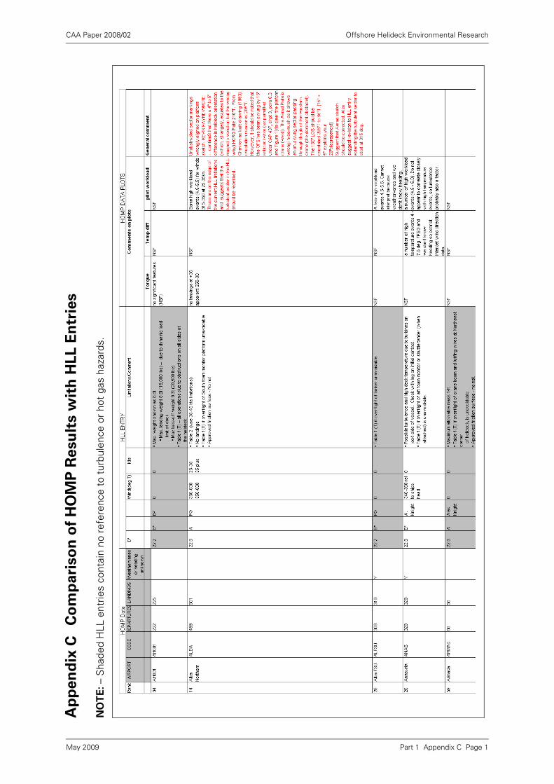
CAA Paper 2008/02 Offshore Helideck Environmental Research
Ap
pe
nd
ix C
Co
mp
ari
so
n o
f H
OM
P R
esu
lts w
ith
HL
L E
ntr
ies
NO
TE
: – S
hade
d H
LL e
ntrie
s co
ntai
n no
ref
eren
ce t
o tu
rbul
ence
or
hot
gas
haza
rds.
Part 1 Appendix C Page 1May 2009
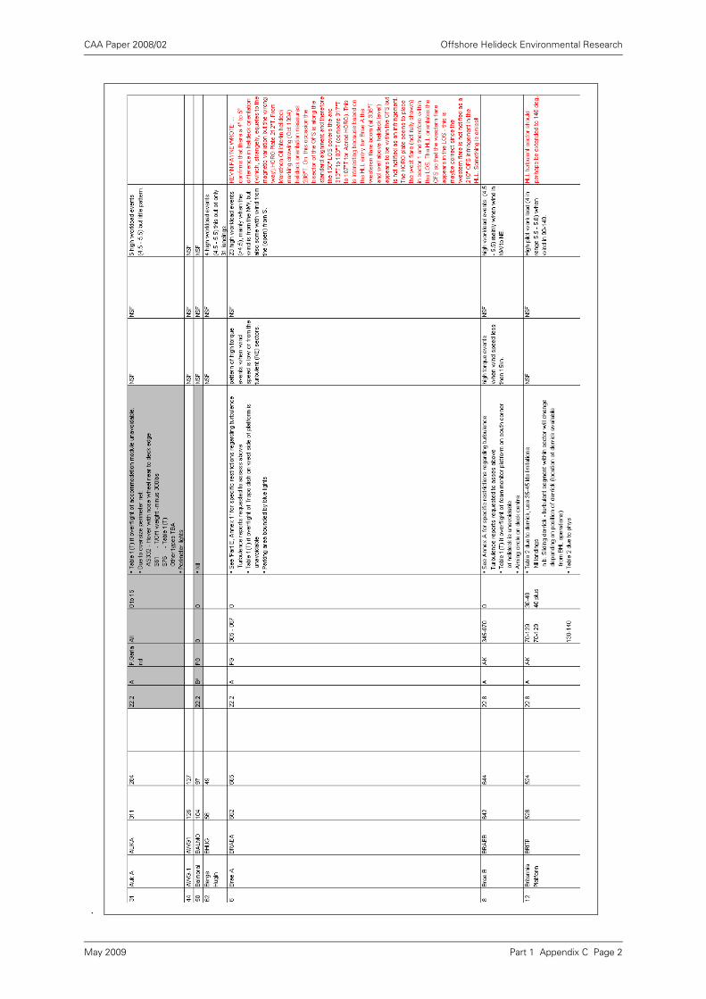
CAA Paper 2008/02 Offshore Helideck Environmental Research
.
Part 1 Appendix C Page 2May 2009
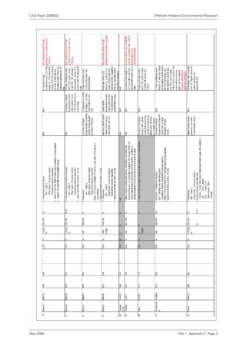
CAA Paper 2008/02 Offshore Helideck Environmental Research
.
Part 1 Appendix C Page 3May 2009
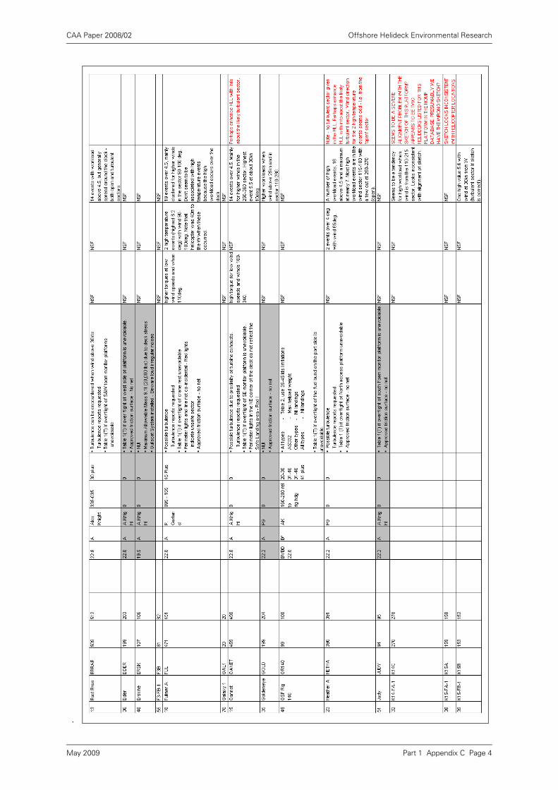
CAA Paper 2008/02 Offshore Helideck Environmental Research
.
Part 1 Appendix C Page 4May 2009
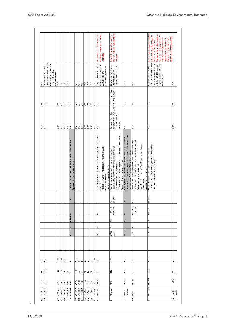
CAA Paper 2008/02 Offshore Helideck Environmental Research
.
Part 1 Appendix C Page 5May 2009

CAA Paper 2008/02 Offshore Helideck Environmental Research
.
Part 1 Appendix C Page 6May 2009

CAA Paper 2008/02 Offshore Helideck Environmental Research
.
Part 1 Appendix C Page 7May 2009

INTENTIONALLY LEFT BLANK

CAA Paper 2008/02 Offshore Helideck Environmental Research
Appendix D Example Time Series – HOMP Trace Plots
1 High Workload Landings Example Homp Traces
Part 1 Appendix D Page 1May 2009
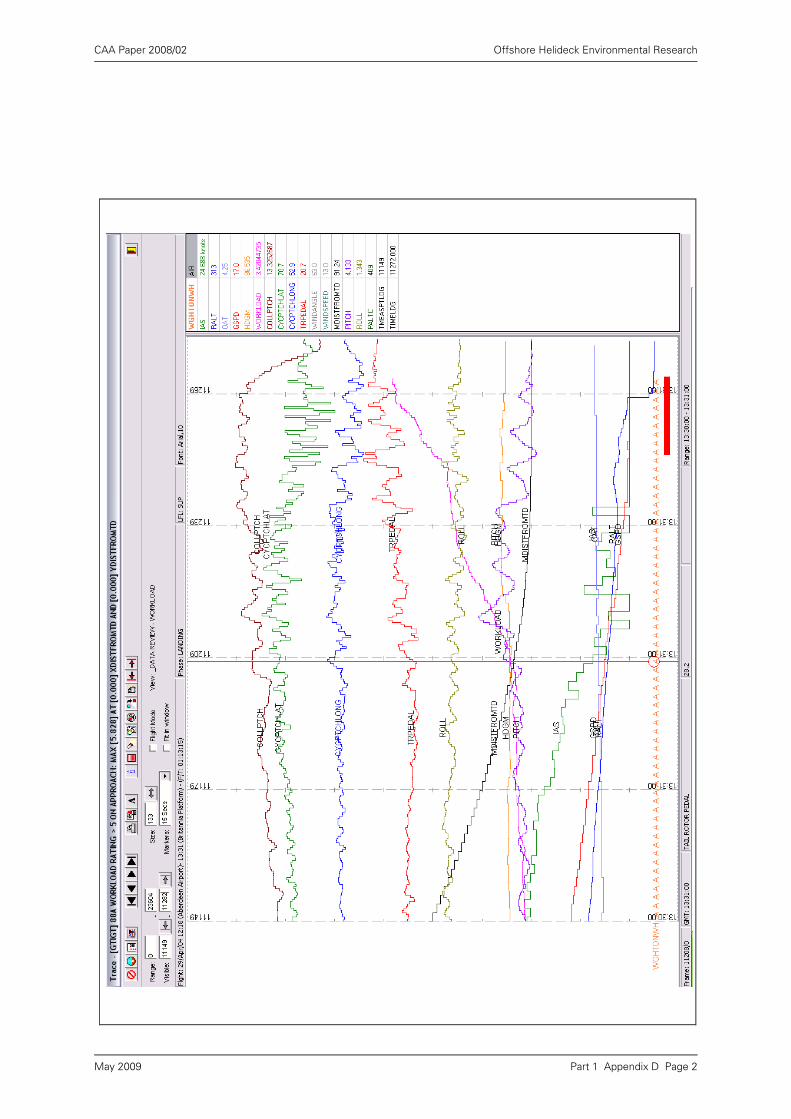
CAA Paper 2008/02 Offshore Helideck Environmental Research
Part 1 Appendix D Page 2May 2009
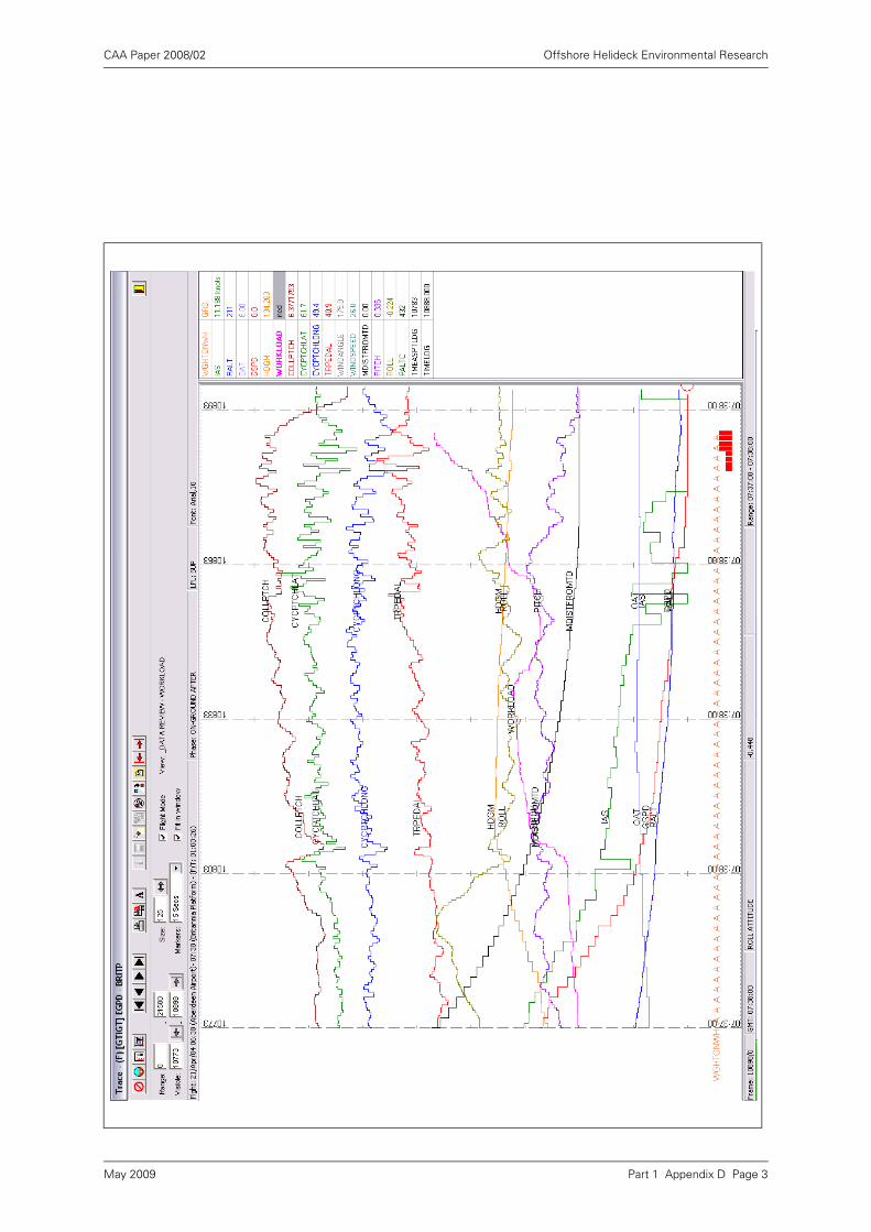
CAA Paper 2008/02 Offshore Helideck Environmental Research
Part 1 Appendix D Page 3May 2009

CAA Paper 2008/02 Offshore Helideck Environmental Research
Part 1 Appendix D Page 4May 2009
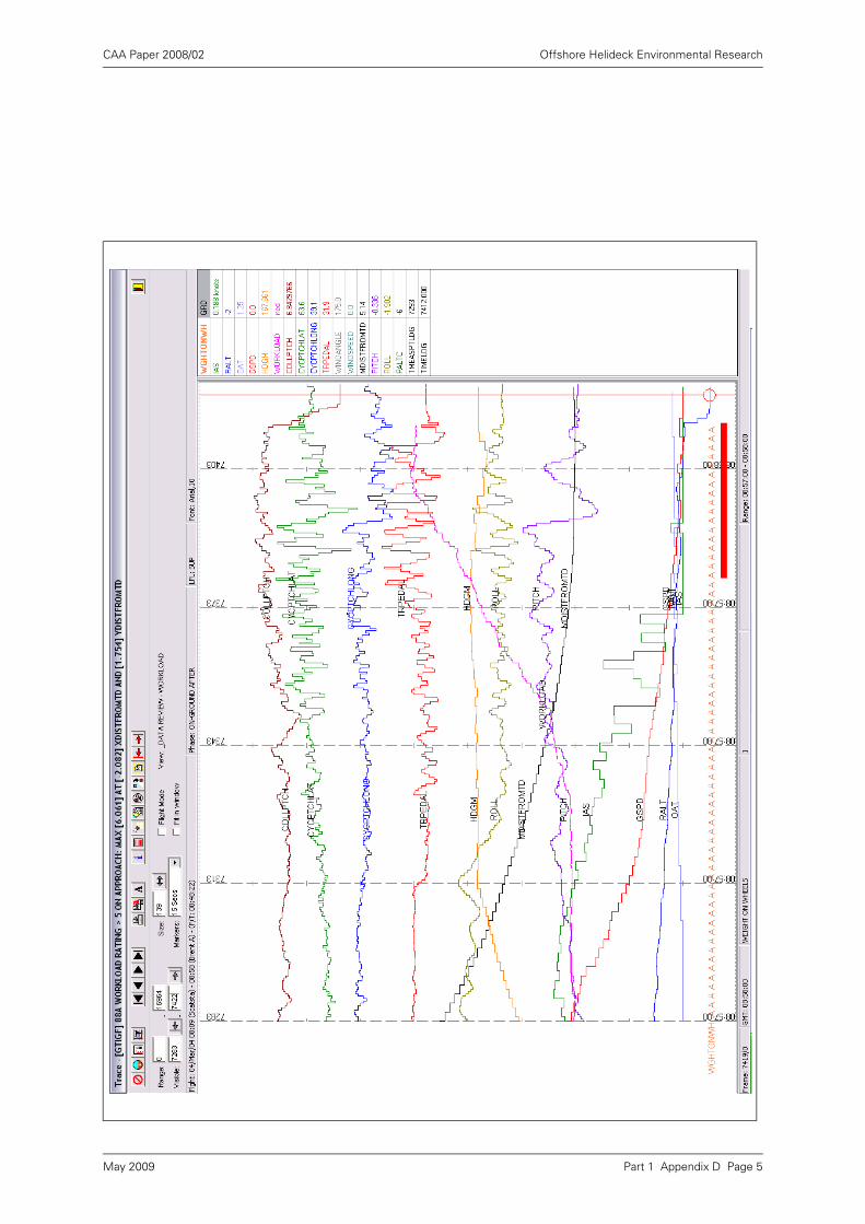
CAA Paper 2008/02 Offshore Helideck Environmental Research
Part 1 Appendix D Page 5May 2009
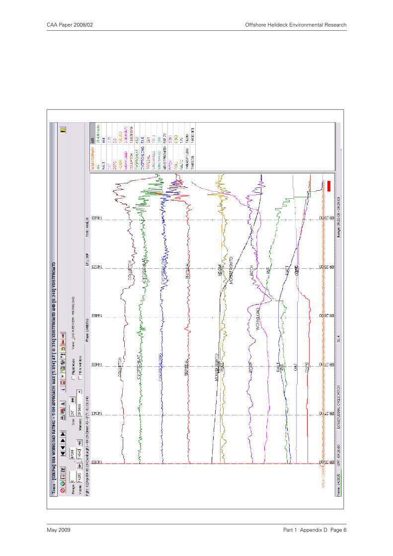
CAA Paper 2008/02 Offshore Helideck Environmental Research
Part 1 Appendix D Page 6May 2009

CAA Paper 2008/02 Offshore Helideck Environmental Research
Part 1 Appendix D Page 7May 2009

CAA Paper 2008/02 Offshore Helideck Environmental Research
Part 1 Appendix D Page 8May 2009
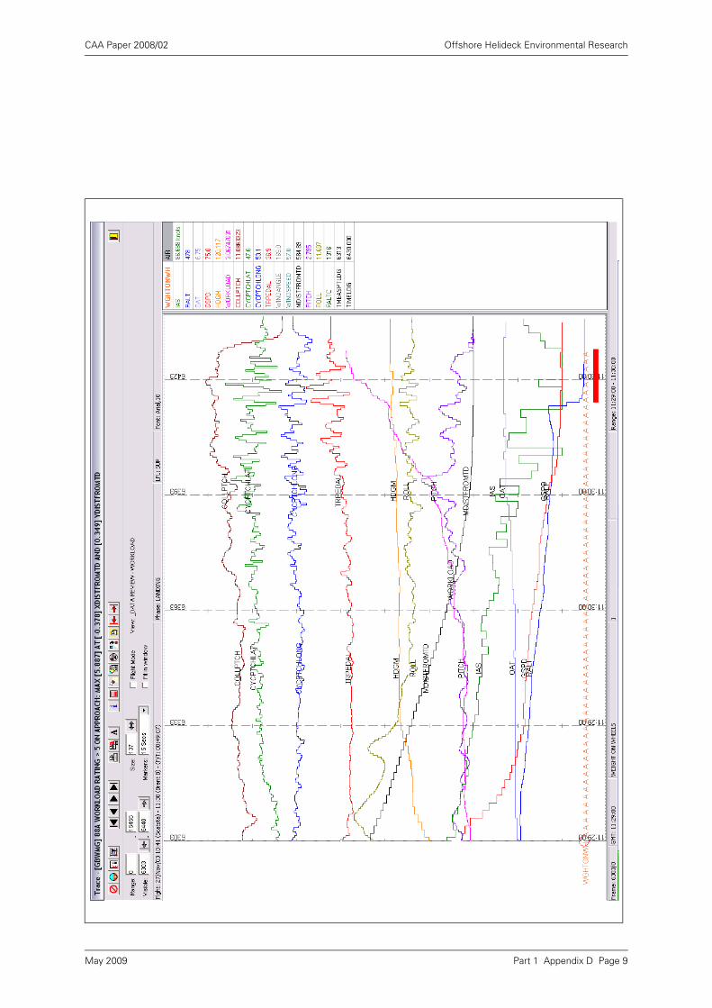
CAA Paper 2008/02 Offshore Helideck Environmental Research
Part 1 Appendix D Page 9May 2009
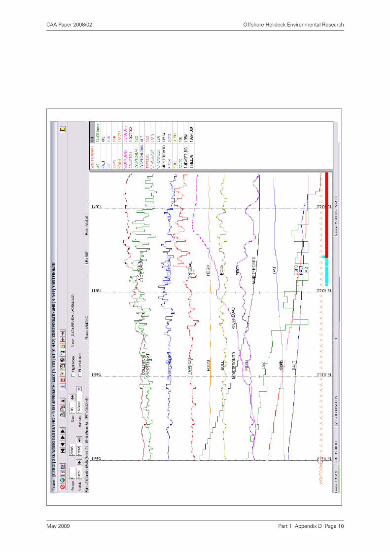
CAA Paper 2008/02 Offshore Helideck Environmental Research
Part 1 Appendix D Page 10May 2009

CAA Paper 2008/02 Offshore Helideck Environmental Research
Part 1 Appendix D Page 11May 2009
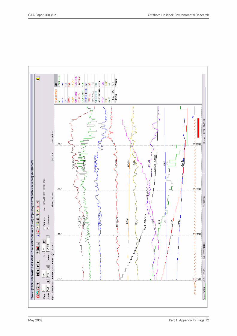
CAA Paper 2008/02 Offshore Helideck Environmental Research
Part 1 Appendix D Page 12May 2009
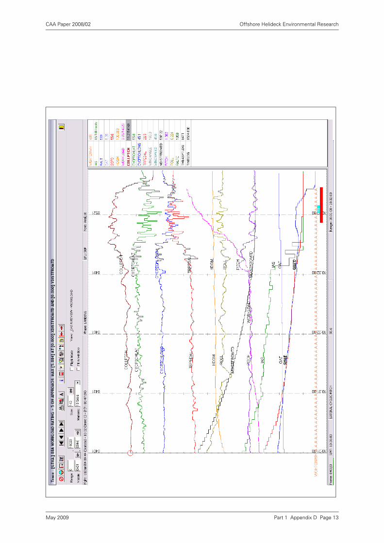
CAA Paper 2008/02 Offshore Helideck Environmental Research
Part 1 Appendix D Page 13May 2009
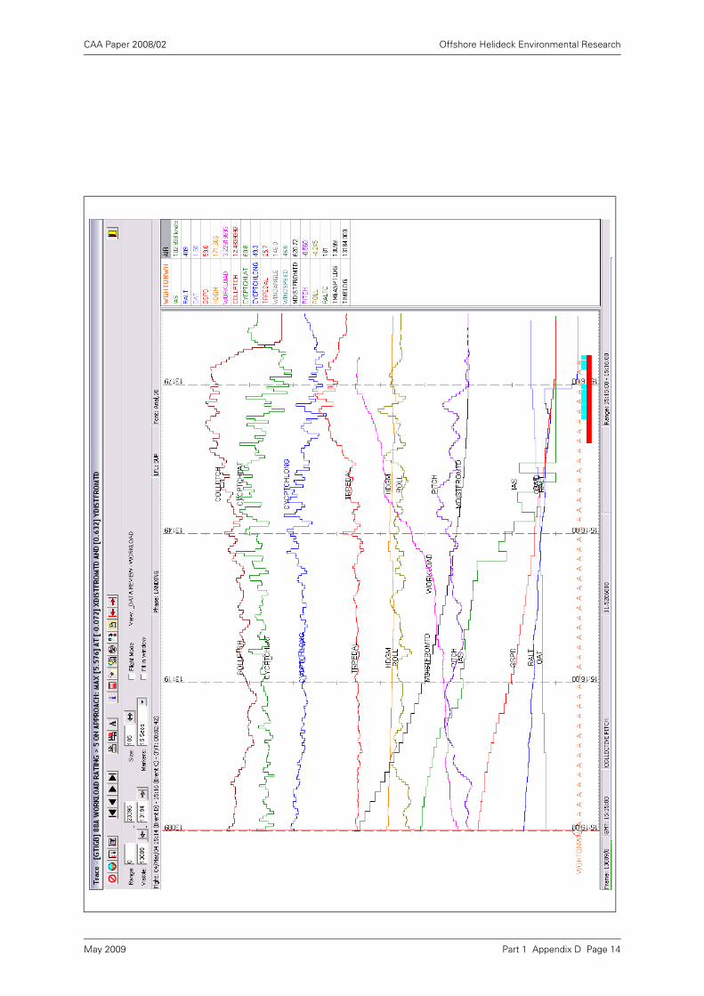
CAA Paper 2008/02 Offshore Helideck Environmental Research
Part 1 Appendix D Page 14May 2009
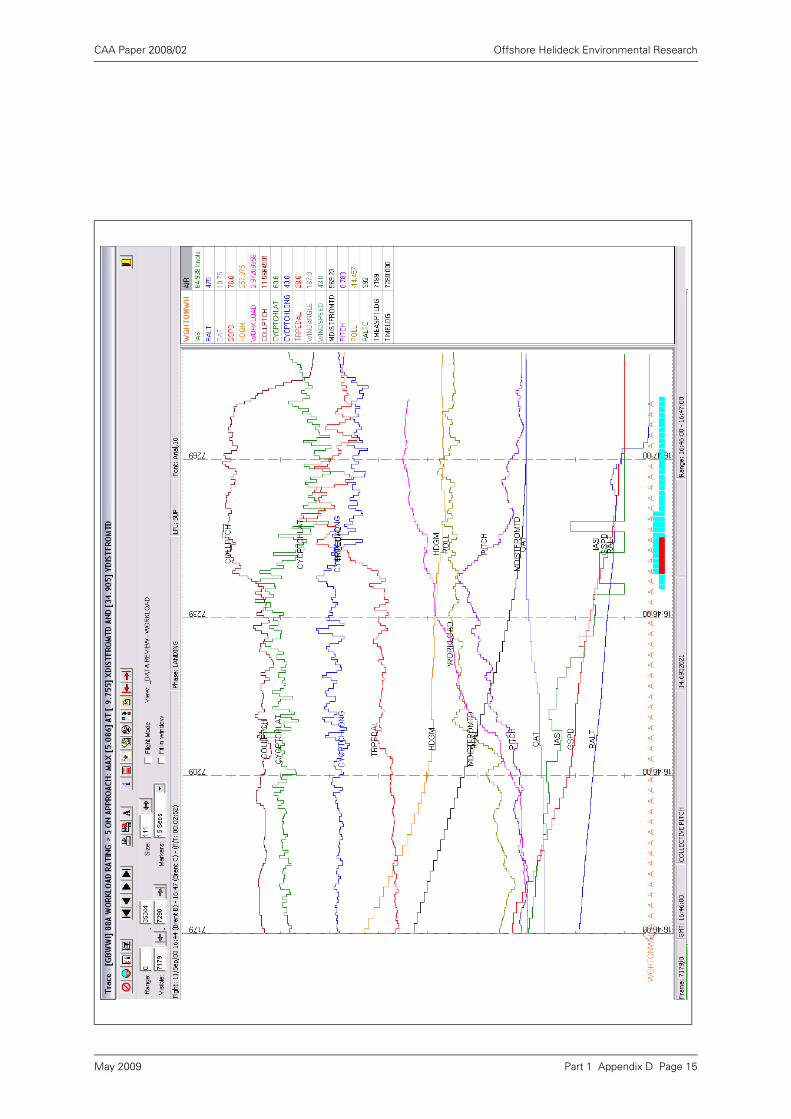
CAA Paper 2008/02 Offshore Helideck Environmental Research
Part 1 Appendix D Page 15May 2009
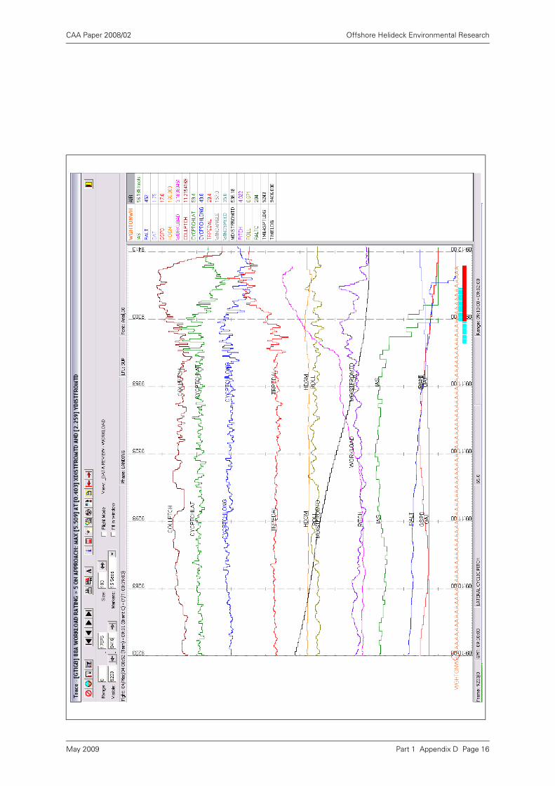
CAA Paper 2008/02 Offshore Helideck Environmental Research
Part 1 Appendix D Page 16May 2009
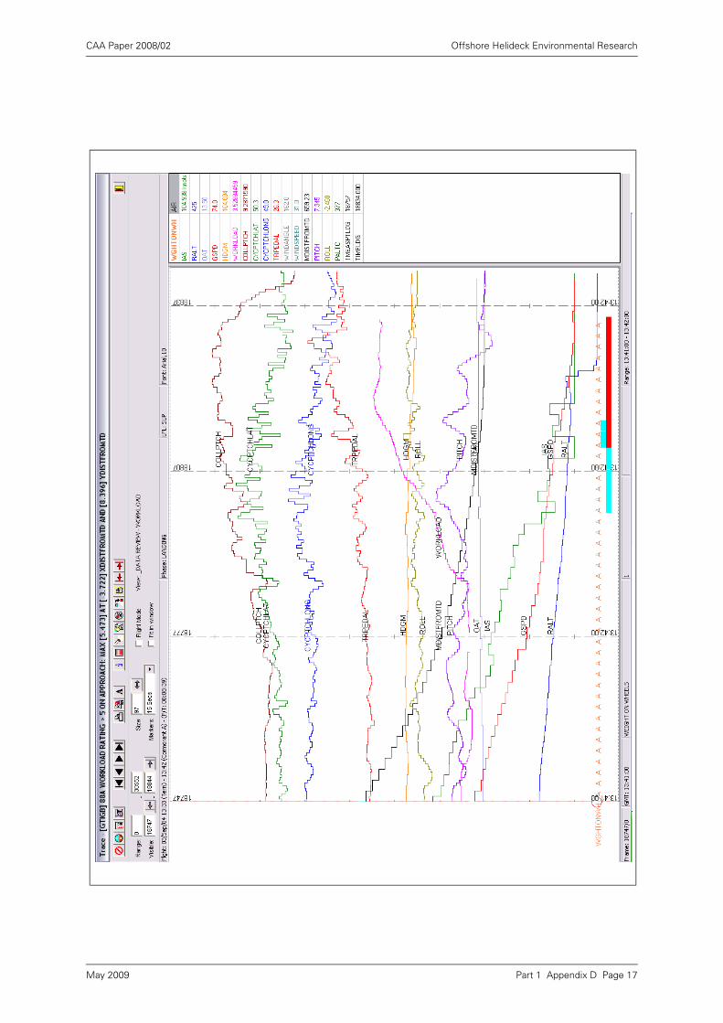
CAA Paper 2008/02 Offshore Helideck Environmental Research
Part 1 Appendix D Page 17May 2009

CAA Paper 2008/02 Offshore Helideck Environmental Research
Part 1 Appendix D Page 18May 2009
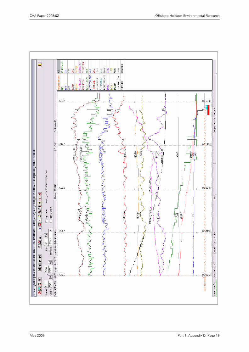
CAA Paper 2008/02 Offshore Helideck Environmental Research
Part 1 Appendix D Page 19May 2009
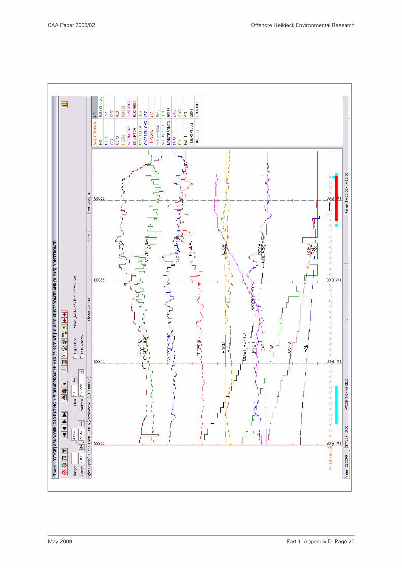
CAA Paper 2008/02 Offshore Helideck Environmental Research
Part 1 Appendix D Page 20May 2009
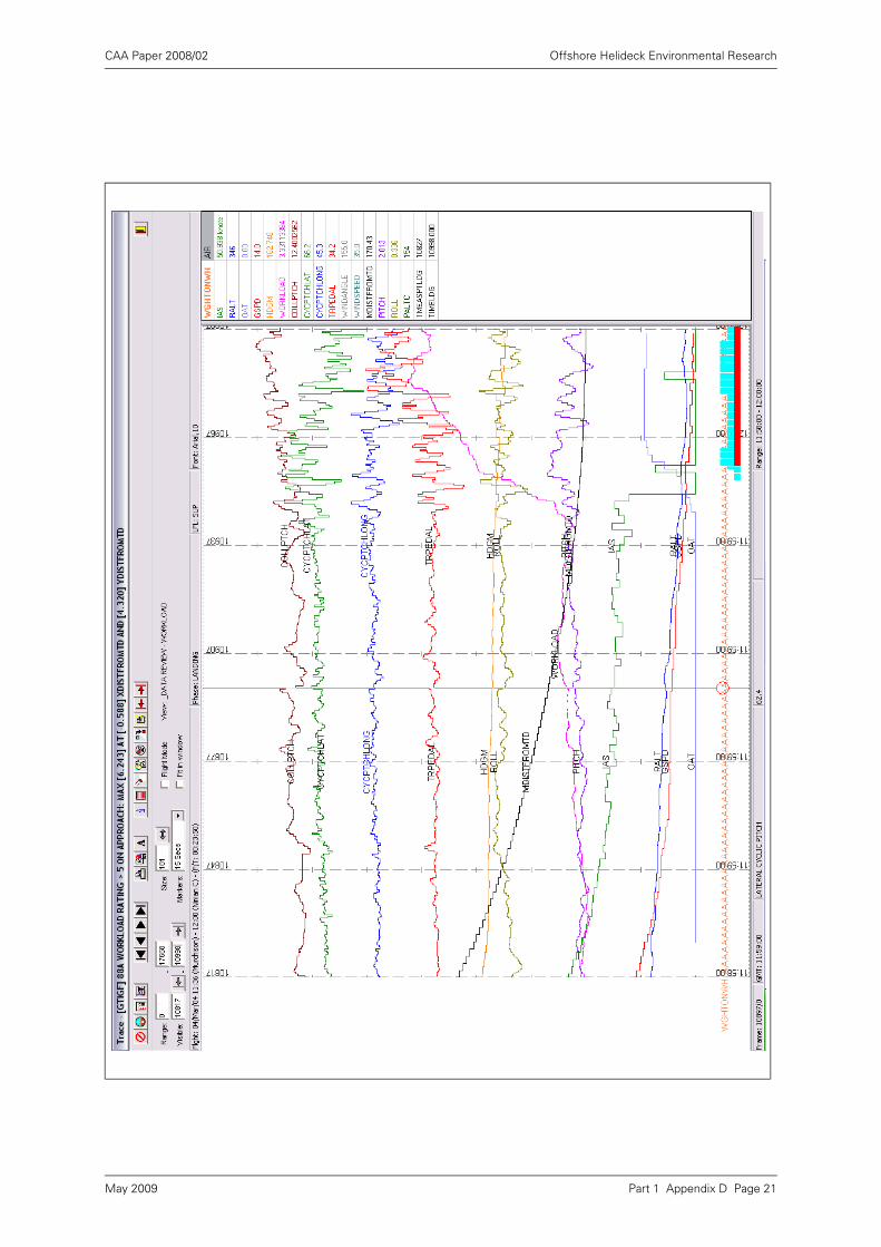
CAA Paper 2008/02 Offshore Helideck Environmental Research
Part 1 Appendix D Page 21May 2009
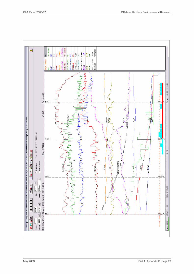
CAA Paper 2008/02 Offshore Helideck Environmental Research
Part 1 Appendix D Page 22May 2009

CAA Paper 2008/02 Offshore Helideck Environmental Research
Part 1 Appendix D Page 23May 2009

CAA Paper 2008/02 Offshore Helideck Environmental Research
Part 1 Appendix D Page 24May 2009
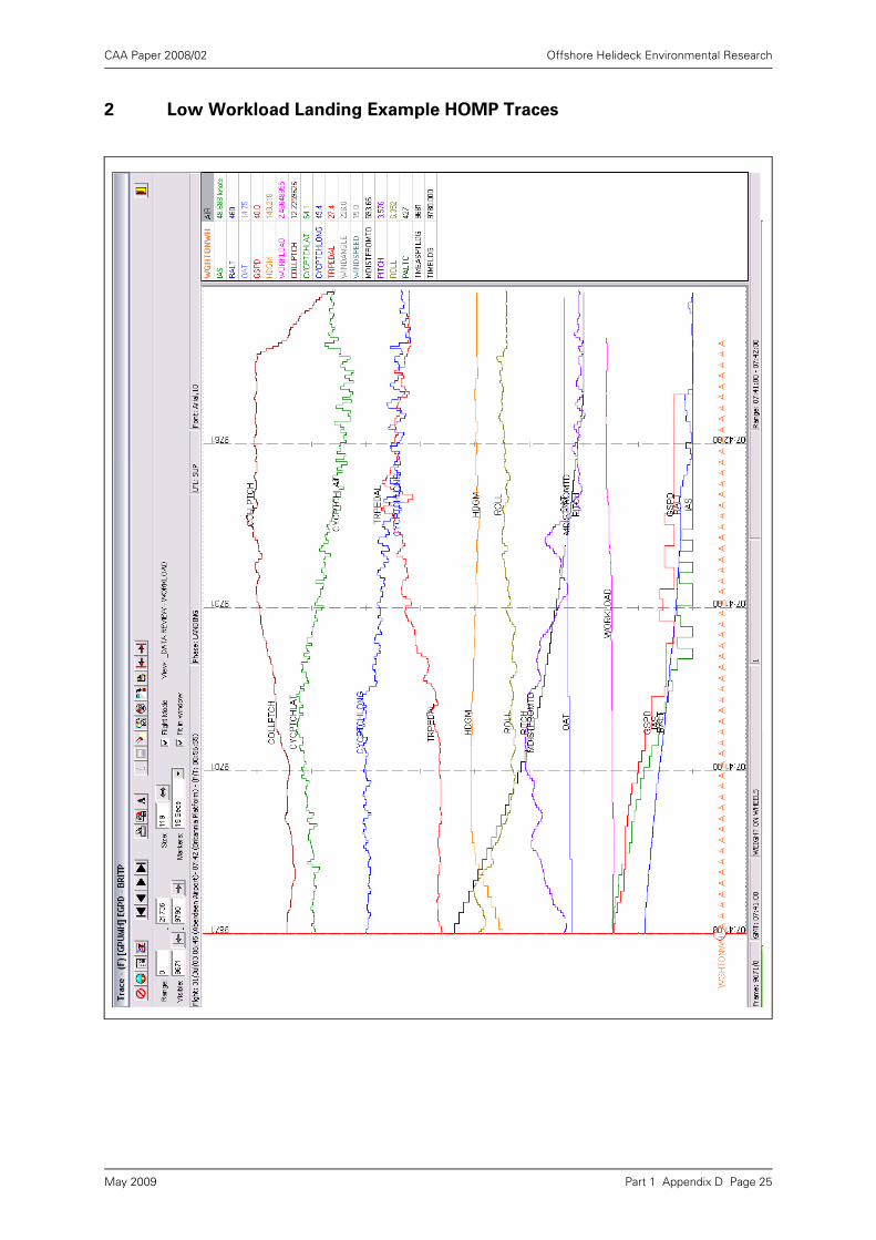
CAA Paper 2008/02 Offshore Helideck Environmental Research
2 Low Workload Landing Example HOMP Traces
Part 1 Appendix D Page 25May 2009

CAA Paper 2008/02 Offshore Helideck Environmental Research
Part 1 Appendix D Page 26May 2009

CAA Paper 2008/02 Offshore Helideck Environmental Research
Part 1 Appendix D Page 27May 2009

CAA Paper 2008/02 Offshore Helideck Environmental Research
Part 1 Appendix D Page 28May 2009
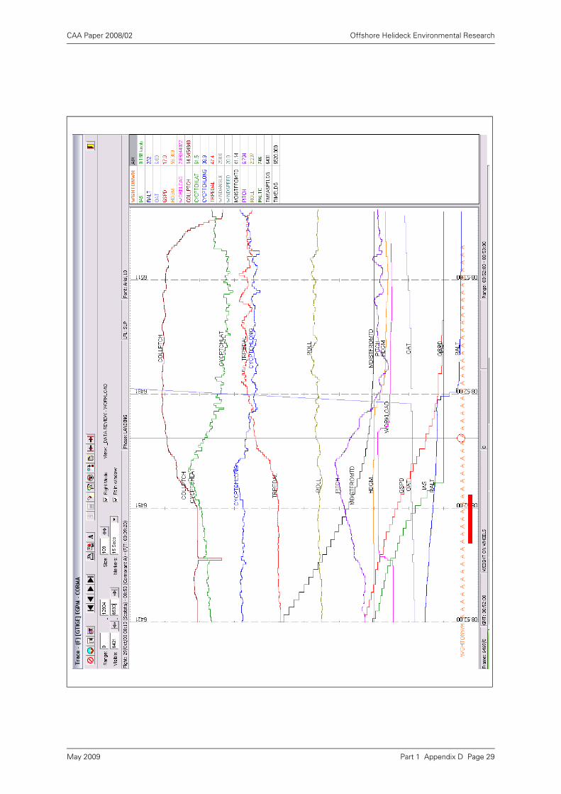
CAA Paper 2008/02 Offshore Helideck Environmental Research
Part 1 Appendix D Page 29May 2009

CAA Paper 2008/02 Offshore Helideck Environmental Research
Part 1 Appendix D Page 30May 2009

CAA PAPER 2008/02
Offshore Helideck Environmental Research
Part 2 – Review of 0.9 m/s Vertical Wind Component
Criterion for Helicopters Operating to Offshore Platforms
Safety Regulation Group
May 2009

INTENTIONALLY LEFT BLANK

CAA Paper 2008/02 Offshore Helideck Environmental Research
Part 2 Executive Summary Page 1
Part 2 – Review of 0.9 m/s Vertical Wind Component
Criterion for Helicopters Operating to Offshore Platforms
Executive Summary
Following the establishment of a new turbulence criterion for helicopters operating to offshoreinstallations, the need for retention of the longstanding CAP 437 criterion relating to a verticalwind component of 0.9 m/s has been reviewed. This report presents the results of a four-phase study to evaluate the effectiveness of the criterion.
The overall objective for the project was to determine whether the existing 0.9 m/s verticalflow criterion was protecting offshore helicopters against an identifiable hazard other thanturbulence and, if so, establish whether the form of the present criterion was the mostappropriate, or whether a new criterion was required to form a rational link with helicopterperformance or handling. Alternatively, it might be established that a vertical flow criterion wasnot necessary.
Overall it is concluded that violation of the 0.9 m/s vertical mean flow criterion cannot be linkedto any helicopter performance (i.e. torque-related), or handling (i.e. pilot workload-related)hazard. The highest vertical components of flow almost always occur when the wind is froman ‘open’ or unobstructed direction. These are conditions when the horizontal component offlow is likely to be high ensuring that the helicopter has a high margin of lift, and whenturbulence levels are likely to be low, resulting in relatively low torque and pilot workloadvalues.
As it has not proven possible to link the criterion to a helicopter performance or handlinghazard, consideration should be given to removing the 0.9 m/s criterion from the guidancematerial. The first step should be consultation with the helicopter operators in order to seektheir views on the validity or otherwise of the criterion from an operational perspective, and tocheck whether there may be safety benefits implicit in the criterion that have not been evidentduring the study.
Concerns that removal of the 0.9 m/s criterion might reduce the pressure on the platformdesign process to include a generous air gap between the helideck and the accommodationblock, have been allayed to some extent. Wind tunnel tests on an example of a large North Seaplatform demonstrated that the application of the new turbulence criterion was also likely toresult in the inclusion of a significant air gap.
May 2009

INTENTIONALLY LEFT BLANK
CAA Paper 2008/02 Offshore Helideck Environmental Research
Part 2 – Review of 0.9 m/s Vertical Wind Component
Criterion for Helicopters Operating to Offshore Platforms
1 Introduction
Following the establishment of a new turbulence criterion for helicopter operations tooffshore installations, the need for the longstanding CAP 437 criterion relating to avertical wind component of 0.9 m/s has been reviewed. This report presents theresults of a four-phase study to evaluate the effectiveness of the criterion.
Currently CAP 437 [1] uses the following wording:
2.3.2 As a general rule, the vertical mean wind speed above the helideck should notexceed ± 0.9 m/s (1.75 kt) for a windspeed of up to 25 m/s (48.6 kt). Thisequates to a wind vector slope of 2°.
The Research on Offshore Helideck Environmental Issues report [2] linked the0.9 m/s with a hover-thrust margin of 3%. The report says:
Simple theory suggests that, in the absence of ground effect, a thrust margin of atleast 3% would be required to overcome the effects of this magnitude of gust andmaintain a hover over the deck in zero wind. However, it should be noted that it isunlikely that with current helideck designs a helicopter could ever experience a0.9 m/s downdraught in the absence of the beneficial effect on thrust margin of asignificant horizontal wind component.
No detailed evaluation had been performed prior to this study, but experience of windtunnel testing many platforms at BMT Fluid Mechanics (BMT) had suggested that the0.9 m/s (mean) vertical wind component is usually only exceeded in wind directionsthat are clear of upstream obstructions (‘open’ sectors). One of the objectives of thecurrent study was to verify this perception. In such cases the 0.9 m/s criterion isexceeded because of the general curvature of the flow around the bulk of theplatform, and the vertical component is therefore accompanied by a horizontalcomponent of similar magnitude to the 25 m/s free wind speed. Clearly this horizontalcomponent gives the helicopter a major lift performance benefit, and the 3% still airhover thrust margin does not appear to be particularly relevant.
Furthermore, the consideration in [2] which resulted in the 3% hover thrust marginconclusion was based on an analysis of pilot/helicopter response to a sudden ‘verticalgust’. It was therefore very much an analysis of a transient situation in a temporalsense. It seems probable that any hazard that is being protected against is alsoprimarily a transient hazard but caused by flying from one flow field into another, andso it is possible that a better criterion might explicitly recognise the spatial change ofthis vertical component.
Questions raised by the above are therefore:
1 Does violation of the existing 0.9 m/s vertical component in the presence of ahigh horizontal wind speed pose any real hazard to the helicopter? If it does,then what is the precise nature of the hazard, and does the existing criterionadequately protect against it?
2 If the application of the existing 0.9 m/s vertical component criterion is notcurrently protecting against an identifiable hazard, then what is the nature of thereal hazard (if any), and how should a new criterion be framed? Should thecriterion be framed more in terms of a transient phenomenon (e.g. the spatial
Part 2 Page 1May 2009

CAA Paper 2008/02 Offshore Helideck Environmental Research
variation in mean vertical velocity).1 Alternatively, if there is no real hazard thenconsideration should be given to removing any flight restrictions on platforms inthese ‘high horizontal flow’ cases.
With the above questions in mind, BMT produced two proposals [3, 4]. Thesesuggested that a useful initial step would be to analyse the Bristow HelicoptersHelicopter Operations Monitoring Programme (HOMP) data archive (which wasalready being analysed in support of the turbulence criterion validation [5]) to look forany evidence of high torque events that might indicate a performance-related hazardfor the helicopter.
Following on from this, the BMT archive of wind tunnel data was analysed to evaluatethe occurrence of violations of the 0.9 m/s criterion and confirm, or otherwise, theperception that this criterion was mostly exceeded in the ‘open’ wind directions, clearof upstream obstructions.
The wind tunnel data were correlated with torque and pilot workload data gathered inthe initial phase to seek any correlations between the HOMP measured parametersand the vertical wind components in these open wind directions.
Finally, a programme of wind tunnel testing was performed on a model of the Brae-Aplatform in order to investigate the likely effect of removing the 0.9 m/s criterion onthe selection of a helideck height / clearance (air gap) from the accommodation block.
2 Objectives
The overall objectives for the project were defined as follows:
2.1 To determine whether the existing 0.9 m/s vertical flow criterion is protectingoffshore helicopters against an identifiable hazard. If so, refine the magnitude of thecriterion so that there is a rational link with helicopter performance and/or handling.
2.2 If the existing 0.9 m/s criterion cannot be linked to an identifiable hazard, thenestablish the nature of any associated vertical flow hazard and develop a new flowcriterion that satisfactorily protects against the hazard. Alternatively, determinewhether the existing 0.9 m/s vertical flow criterion can be removed.
3 Phase 1 – HOMP Torque Analysis
3.1 Introduction
The helideck turbulence criterion project Phase 2 (Helicopter Operational MonitoringProgramme (HOMP) validation [5]), offered the possibility to examine the HOMP dataarchive [6, 7] for evidence of performance-related hazards during the approach whichmight be linked to a vertical wind component. It was proposed that the maximumtorque, and the maximum increase in torque (over a 2 second period), should bestudied. These would then be plotted against wind speed and direction (much as it isintended to plot pilot workload and ambient temperature), and overlaid on sketchesof the platform plans2.
1. BMT currently uses some empirically derived pilot workload criteria for warship flight decks that are based on spatialgradients of longitudinal mean, longitudinal rms, lateral mean and vertical mean wind speed. They were derived bycorrelating Ship Helicopter Operating Limitation (SHOL) data against wind tunnel measurements down the flight path.Unfortunately the same method is not directly applicable to an offshore helideck because there isn’t a well-definedapproach flight path.
2. Appropriate sketches of most platforms were obtained from the ‘Aerad Plates’ published by European AeronauticalGroup (now part of Navtech Inc).
Part 2 Page 2May 2009

CAA Paper 2008/02 Offshore Helideck Environmental Research
In BMT’s experience, the 0.9 m/s criterion is routinely not met at high wind speedsin ‘open’ sectors. The plots generated would therefore be examined for evidence thathigh torque values, or sudden large increases in torque, occurred in high wind speedsand ‘open’ wind directions.3 The rationale was that any such occurrences might lendsupport to the notion that the current 0.9 m/s criterion was performing a usefulfunction, the assumption being that the data would likely contain instances ofhelicopters being exposed to vertical flows in excess of 0.9 m/s. On the other hand,an absence of such occurrences might be interpreted to suggest that the currentcriterion is inappropriate or redundant
However, vertical flows in excess of 0.9 m/s are unlikely to present a hazard tohelicopters in the presence of high horizontal flows, but rapid changes in the airflowcould [2]. The hazard of temporal variation of the airflow (turbulence) is nowaccounted for by the recently developed turbulence criterion [5, 8]. However,disturbances to the airflow in ‘open’ sectors resulting in high torque values, or suddenlarge increases in torque, could be the result of spatial variation, i.e. shear, whicharguably is not adequately covered. The presence of any such occurrences mighttherefore indicate a need for a new criterion to address spatial variation that wouldreplace the present 0.9 m/s criterion.
It was accepted that the HOMP maximum torque values might be difficult to use inthis context for a number of reasons, including the effects of helicopter weight andground effect. However, if there was a genuine lift performance hazard associatedwith vertical wind component in the presence of high horizontal flow speeds, thensome evidence of high torque values in high wind speeds and ‘open’ wind directionsought to be apparent in the HOMP data. The inclusion of the maximum increase intorque in the analysis was expected to make interpretation of the torque somewhateasier.
The task therefore included the following main activities:
3.1.1 Gather and present HOMP maximum torque and maximum positive increase intorque data.
3.1.2 Gather sketches of platform helidecks in order to identify the ‘open’ wind directions.
3.1.3 Evaluate the data to identify any evidence of high torque / torque increaseperformance challenges in the ‘open’ wind sectors.
3. Helidecks for floating systems / FPSOs were omitted from this analysis because vessel heading information was notreadily available.
Part 2 Page 3May 2009

CAA Paper 2008/02 Offshore Helideck Environmental Research
3.2 Measured Parameters
The HOMP parameters used in this analysis were as follows:
3.3 Derived Parameters
3.3.1 Maximum torque corrected for helicopter landing weight
It was recognised that the maximum torque values recorded during a landing wouldbe very much dependent on the landing weight of the helicopter. This is borne out byFigure 1, which shows all valid maximum torque values plotted against helicopterlanding weight. It can be seen that there is a clear and unsurprising trend of increasingmaximum torque with landing weight.
Table 1 HOMP Parameters used in the torque analysis
Variable name Description
MX_LDGWGHT Landing weight (lb)
MX_WSPEEDLDG Average wind speed at measurement point (1500 m from Landing) (m/s)
MX_WANGLELDG Average wind direction at measurement point (1500 m from Landing) (degrees magnetic)
FlightType Flight type (from imported ops data, 1,2,6 = revenue, 4 = training, 5 = air test)
MXTORQ Maximum Total Torque from 500 m to landing (%)
MXTORQTIMLDG Number of Frames from Landing point to recorded MXTORQ (2 frames = 1 sec)
MX_TORQ_XDIST Lateral distance between MXTORQ and Landing Point (m)
MX_TORQ_YDIST Longitudinal distance between MXTORQ and Landing Point (m)
MXINCRTORQ Maximum Increase in Torque from 500 m to Landing Point (%)
MXINCTRQTIMLDG Number of Frames from Landing point to recorded MXINCRTORQ (2 frames = 1 sec)
MX_INCRTQ_XDIST Lateral distance between maximum MXINCTORQ and Landing Point (m)
MX_INCRTQ_YDIST Longitudinal distance between maximum MXINCTORQ and Landing Point (m)
MX_INCRTQ_TORQ Total Torque at finish point of MXINCTORQ (%)
COR_MX_WSPDLDG Wind speed in the Landing Phase at Measurement Point (1500 m from Landing) (m/s)
COR_MX_WANGLDG Wind angle in the Landing Phase at Measurement Point (1500 m from Landing) (m/s)
MX_CORWSPDLDG COR_MX_WSPDLDG corrected to helideck height (m/s)
Part 2 Page 4May 2009

CAA Paper 2008/02 Offshore Helideck Environmental Research
It was proposed [9] that the maximum torque might be corrected for the effect ofweight, and it was hoped that the maximum torque values corrected in this waywould prove to be a better indicator of the presence of a performance or lift hazard.A correction of the following form was proposed:
Tq2 = Tq1(W2/W1)3/2
where:
Tq2 = max torque value to be plotted
Tq1 = max torque value from the HOMP data (MXTORQ)
W2 = max landing weight (18,960 lb)
W1 = actual landing weight from the HOMP data (MX_LDGWGHT).
However, when maximum torque data corrected in this way were examined it wasclear that there were now many high ‘corrected torque’ events, and that they wereassociated with lower landing weights. Figure 2 shows this trend of higher correctedmaximum torques at lower landing weights.
It was suspected that the reason for this preponderance of high corrected torquevalues at lower weights was due to pilot behaviour. A pilot flying at close to maximumweight and/or in light winds will be very aware of a real torque limit, and will be usingthe collective lever judiciously to avoid an over-torque. In contrast, a pilot flying a lighthelicopter or flying in a strong wind will know that he has plenty of torque in hand, andmay therefore use the collective lever more freely to maintain his desired flight path.Such free use of the collective lever will tend to appear as high corrected torquevalues at low landing weights.
In order to reduce this effect in the results it was decided to plot the correctedmaximum torque over a restricted range of landing weights. It was found that about60% of landings were at a landing weight in the range 17,000lb – 18,500lb, and socorrected maximum torque plots were plotted for this range of landing weights only.
Figure 1 Maximum torque versus landing weight
Part 2 Page 5May 2009

CAA Paper 2008/02 Offshore Helideck Environmental Research
3.3.2 Maximum torque increase expressed as a percentage of instantaneous torque
margin
There was a similar issue in relation to the interpretation of the maximum torqueincrease experienced in 2 seconds. At low weights and/or in high wind speeds lesscollective and less torque is required to effect a given flight path correction, and a pilotwho knows that he has plenty of torque margin in hand will be less averse to applyinga large torque increase in order to maintain his desired flight path, and will thusregister a high torque increase value in the HOMP database. A pilot flying close to thetorque limit will be very much more careful with the collective lever.
In order to take some account of this in the interpretation of the results it was decidedto derive a parameter for the torque increase as a percentage of remaining torquemargin. The expression for this in terms of the HOMP measurements is as follows:
Tincrm = 100 Tincr / (100 - (TTi – Tincr))
Where:
Tincrm = max torque increase as percentage of the instantaneous torque margin
Tincr = max torque increase from HOMP data (MXINCRTORQ)
TTi = Torque value at the end of the 2 second max increase in torque(MX_INCRTQ_TORQ)
Thus a pilot applying a 25% increase in torque over 2 seconds from an initial torqueof 50% will register a 50% of torque margin value. Similarly a pilot applying a 5%increase in torque from a 90% value will also register a 50% torque margin value.
3.4 Results
A complete set of results for all the torque parameters, and all the platform landingsin the HOMP archive (with 20+ landings) can be found in [10]. Some selectedexamples of these plots are presented in the following in order to illustrate the mainfeatures of the torque data.
Figure 2 Maximum torque corrected for weight versus landing weight
Part 2 Page 6May 2009

CAA Paper 2008/02 Offshore Helideck Environmental Research
3.4.1 Torque Plot Examples
A complete set of the five different torque plotting options is presented for oneplatform (Brae-A) in order to emphasise the importance of the derived parametersoutlined in Sections 3.3.1 and 3.3.2.
Figure 3 and Figure 4 show the ‘raw’ maximum torque increase data for the 445landings in the database for the Brae-A platform. The upper plot Figure 3 shows thetorque increase values with points colour coded according to the maximum torquevalue, and with the position of the point showing the wind speed and direction at thetime of the landing. The lower plot Figure 4 shows the same data, but in this case theposition of the coloured point on the plot shows the position of the helicopter relativeto the helideck touchdown point at the time the maximum torque occurred, and thevector arrows associated with each point indicate the speed and direction of the wind.Each plot includes a small sketch of the platform layout correctly orientated withrespect to true North, so that the relationship between wind directions and platformobstructions that might cause turbulence can be assessed.
It should be noted that, although the theoretical accuracy of the helicopter positionrelative to the actual touchdown point is reasonably high (≈1 m), the plots showingthe position of the helicopter at the time of the maximum torque are subject to anumber of sources of error. In particular the plots assume that all landings touchdownat the centre of the helideck, and the helicopter locations are worked back from thisorigin. In reality, although the pilot is permitted to land anywhere within the safelanding area (typically 22 m ‘diameter’), the pilot will normally touchdown byreference to the aiming circle (typically having an 11 m inner diameter). Furthermore,the fact that the GPS antenna is located partway down the helicopter tail boomintroduces a further helicopter heading-related error into the plots. In view of theseinaccuracies it is considered that the positions shown on the plots are probably onlyreliable to about ±5 m.
It can be seen from Figure 3 that the highest value in the 445 landings is an increaseof 34.7%, and the four highest values in the range 30%-40% all occur either in stillconditions, or in winds of about 15-20 kt from the N-E sector. Wind from thesedirections will contain turbulence caused by the upstream bulk of the platform.
Figure 4 shows that these higher torque increase events occurred when thehelicopter was either directly over the helideck or about 20 m to the SW of thetouchdown point.
In Figure 5 and Figure 6 the same torque data has been expressed as a percentageof the torque margin (as per the formula given above in Section 3.3.2). The patternlooks a little different because of the different numeric ranges and colour coding, butit can be seen that, once again, the 3 landings that utilised 80% or more of the torquemargin all occurred in still or NE wind conditions, and with the helicopter either overthe landing spot or to the SW of it.
None of the plots in Figures 3 to 6 would appear to provide any evidence of hightorque events occurring in high winds from the ‘open’ sector.
The maximum torque data is presented in Figure 7 and Figure 8. Figure 7 shows apattern not dissimilar to the torque increase data of Figure 3. The high values aregenerally experienced in lower wind speeds and in winds from the turbulent N-Esector.
When the landing weight correction is applied to the maximum torque for the fullrange of landing weights in Figure 9 and Figure 10 there is a much larger number ofhigh torque events, and the winds in which they occur are spread more evenly aroundthe compass. However, none of the >100% events occur in wind speeds over 20 kt.
Part 2 Page 7May 2009

CAA Paper 2008/02 Offshore Helideck Environmental Research
When the correction is applied and presented for only a limited range of landingweights (17,000lb – 18,500lb) in Figure 11 and Figure 12, the number of landings isreduced by about half to 220, but the overall pattern of the high torque values doesnot appear to change significantly.
None of the plots in Figures 7 to 12 show any evidence that high torque events occurin winds from the ‘open’ sectors.
.
Figure 3 Brae-A ‘raw’ maximum torque increase data – wind rose plot
Figure 4 Brae-A ‘raw’ maximum torque increase data – helicopter location plot
Part 2 Page 8May 2009
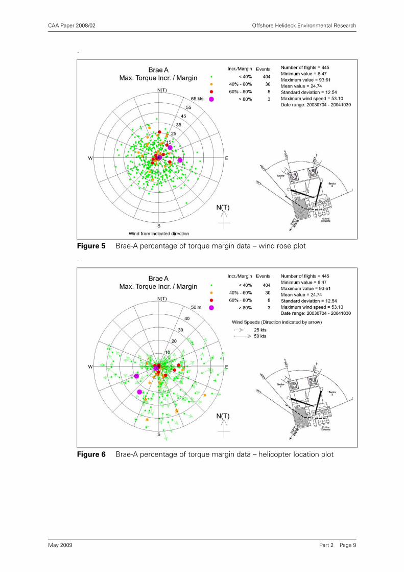
CAA Paper 2008/02 Offshore Helideck Environmental Research
.
.
Figure 5 Brae-A percentage of torque margin data – wind rose plot
Figure 6 Brae-A percentage of torque margin data – helicopter location plot
Part 2 Page 9May 2009
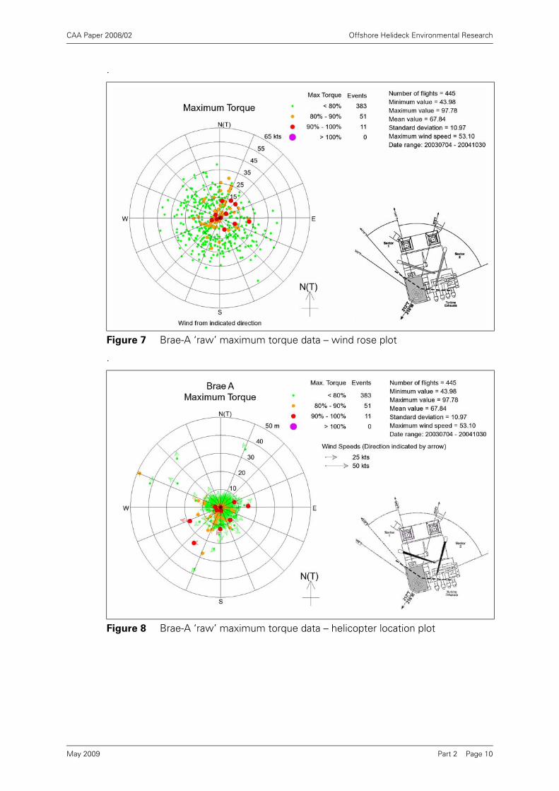
CAA Paper 2008/02 Offshore Helideck Environmental Research
.
.
Figure 7 Brae-A ‘raw’ maximum torque data – wind rose plot
Figure 8 Brae-A ‘raw’ maximum torque data – helicopter location plot
Part 2 Page 10May 2009

CAA Paper 2008/02 Offshore Helideck Environmental Research
.
.
Figure 9 Brae-A ‘weight corrected’ maximum torque data – wind rose plot
Figure 10 Brae-A ‘weight corrected’ maximum torque data – helicopter location plot
Part 2 Page 11May 2009

CAA Paper 2008/02 Offshore Helideck Environmental Research
.
.
Figure 11 Brae-A ‘weight corrected’ maximum torque data for limited weight range – wind rose plot
Figure 12 Brae-A ‘weight corrected’ maximum torque data for limited weight range – helicopter location plot
Part 2 Page 12May 2009

CAA Paper 2008/02 Offshore Helideck Environmental Research
3.4.2 Torque values from typical Platforms
The figures presented in this section provide examples of the torque increase/margin,and the weight-corrected maximum torque for a limited weight range, for twoplatforms considered to be generally typical of the range of values found in the entireHOMP archive [10].
Alba Northern is regarded as a relatively benign platform, and torque increase/marginvalues for the 238 landings in the archive are presented in Figure 13 and Figure 14. Itcan be seen that the highest values all occur at low wind speeds. The corrected andlimited weight range maximum torque data is shown in Figure 15 and Figure 16, andpresents a similar picture.
Figure 17 and Figure 18 show torque increase/margin data for the much morechallenging Ninian Central platform. This platform has more landings in the archive(550) and there are a larger percentage of high values. However, it is clear that thevast majority of the high values are for low wind speeds, or for wind directions fromthe ‘turbulent’ E-S wind sector.
The pattern exhibited by the corrected maximum torque data in Figure 19 and Figure20 is very similar. The highest values are associated with either low wind speeds orwind directions from the E-S sector.
Once again there is no evidence of any higher torque events in winds from the opensector.
Part 2 Page 13May 2009

CAA Paper 2008/02 Offshore Helideck Environmental Research
.
.
Figure 13 Alba Northern percentage of torque margin data – wind rose plot
Figure 14 Alba Northern percentage of torque margin data – helicopter location plot
Part 2 Page 14May 2009

CAA Paper 2008/02 Offshore Helideck Environmental Research
.
.
Figure 15 Alba Northern ‘weight corrected’ maximum torque data for limited weight range – wind rose plot
Figure 16 Alba Northern ‘weight corrected’ maximum torque data for limited weight range – helicopter location plot
Part 2 Page 15May 2009

CAA Paper 2008/02 Offshore Helideck Environmental Research
.
.
Figure 17 Ninian C percentage of torque margin data – wind rose plot
Figure 18 Ninian C percentage of torque margin data – helicopter location plot
Part 2 Page 16May 2009

CAA Paper 2008/02 Offshore Helideck Environmental Research
.
.
Figure 19 Ninian C ‘weight corrected’ maximum torque data for limited weight range – wind rose plot
Figure 20 Ninian C ‘weight corrected’ maximum torque data for limited weight range – helicopter location plot
Part 2 Page 17May 2009

CAA Paper 2008/02 Offshore Helideck Environmental Research
3.4.3 Ensemble Data
Examination of the plots for all the platforms [10] generally shows the same patternof high values as demonstrated in the previous section. However, for the 44 platformsfor which sketches were available, it is possible to segregate all the torque data intowind directions from inside the obstructed or ‘turbulent’ sectors, and the remaining‘open’ sectors. In the following figures data for maximum torque and maximumtorque increase are presented against wind speed.Figure 21 shows the maximum torque corrected for weight, but plotted for only alimited landing weight range (17,000 lb – 18,500 lb) in order to minimise any bias in thecorrection caused by pilot behaviour. The figure shows data for the obstructed winddirectional sectors, whilst similar data is presented for the open sectors in Figure 22.It can be seen that there is the expected trend of reducing maximum torque withwind speed, but this trend is stronger in the open sector data of Figure 22. This meansthat there is also a tendency for the corrected torque in wind from the obstructedsector to be higher than that from the open sector at higher wind speeds. . .
Figure 21 Maximum Torque, corrected for weight (17,000lb - 18,500lb) – Obstructed Sector
Figure 22 Maximum Torque, corrected for weight (17,000lb - 18,500lb) – Open Sector
Part 2 Page 18May 2009

CAA Paper 2008/02 Offshore Helideck Environmental Research
Similarly, Figures 23 and 24 show torque increase data expressed as a percentage ofthe instantaneous torque margin presented in the same way for all the valid datalandings to the 44 platforms. It can be seen that there is a noticeable reduction in thetorque increase/margin with wind speed when the wind is from open sectors, but thistrend is absent for winds from the obstructed or turbulent sectors. Torqueincrease/margin is higher in high winds from the obstructed sectors. Put another way,high values of torque increase/margin at higher wind speeds are invariably associatedwith turbulent conditions.
Figure 23 Torque increase as percentage of margin – Obstructed Sector
Figure 24 Torque increase as percentage of margin – Open Sector
Part 2 Page 19May 2009
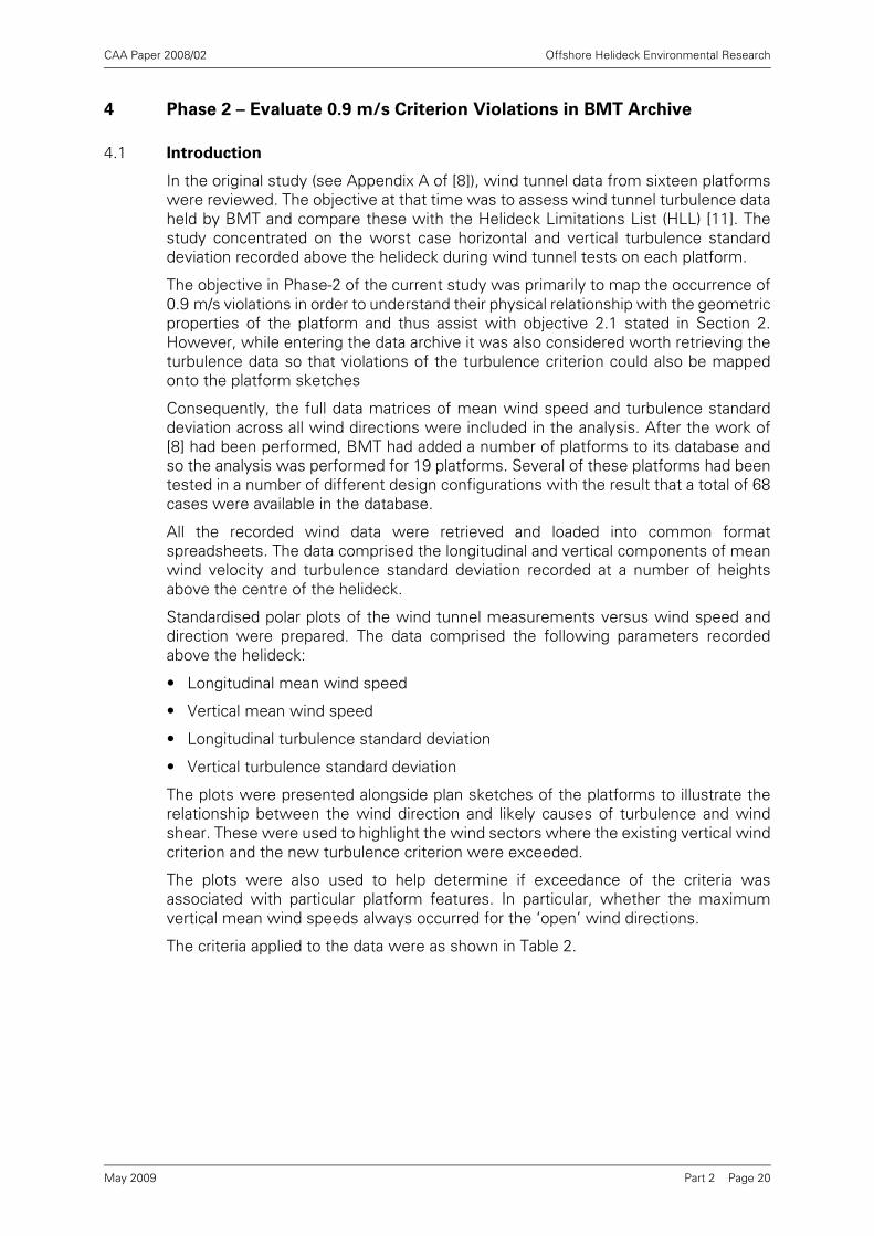
CAA Paper 2008/02 Offshore Helideck Environmental Research
4 Phase 2 – Evaluate 0.9 m/s Criterion Violations in BMT Archive
4.1 Introduction
In the original study (see Appendix A of [8]), wind tunnel data from sixteen platformswere reviewed. The objective at that time was to assess wind tunnel turbulence dataheld by BMT and compare these with the Helideck Limitations List (HLL) [11]. Thestudy concentrated on the worst case horizontal and vertical turbulence standarddeviation recorded above the helideck during wind tunnel tests on each platform.
The objective in Phase-2 of the current study was primarily to map the occurrence of0.9 m/s violations in order to understand their physical relationship with the geometricproperties of the platform and thus assist with objective 2.1 stated in Section 2.However, while entering the data archive it was also considered worth retrieving theturbulence data so that violations of the turbulence criterion could also be mappedonto the platform sketches
Consequently, the full data matrices of mean wind speed and turbulence standarddeviation across all wind directions were included in the analysis. After the work of[8] had been performed, BMT had added a number of platforms to its database andso the analysis was performed for 19 platforms. Several of these platforms had beentested in a number of different design configurations with the result that a total of 68cases were available in the database.
All the recorded wind data were retrieved and loaded into common formatspreadsheets. The data comprised the longitudinal and vertical components of meanwind velocity and turbulence standard deviation recorded at a number of heightsabove the centre of the helideck.
Standardised polar plots of the wind tunnel measurements versus wind speed anddirection were prepared. The data comprised the following parameters recordedabove the helideck:
• Longitudinal mean wind speed
• Vertical mean wind speed
• Longitudinal turbulence standard deviation
• Vertical turbulence standard deviation
The plots were presented alongside plan sketches of the platforms to illustrate therelationship between the wind direction and likely causes of turbulence and windshear. These were used to highlight the wind sectors where the existing vertical windcriterion and the new turbulence criterion were exceeded.
The plots were also used to help determine if exceedance of the criteria wasassociated with particular platform features. In particular, whether the maximumvertical mean wind speeds always occurred for the ‘open’ wind directions.
The criteria applied to the data were as shown in Table 2.
Part 2 Page 20May 2009

CAA Paper 2008/02 Offshore Helideck Environmental Research
Each chart presents four plots as follows:
1. Vertical turbulence rms: the undisturbed mean wind speed at helideck height atwhich the vertical turbulence criterion of standard deviation = 1.75 m/s is violated.The green-shaded area indicates where the turbulence criterion is not violated.
2. Longitudinal turbulence rms: the undisturbed mean wind speed at helideck heightat which a nominal longitudinal turbulence criterion of standard deviation = 5.0 m/sis violated. The green-shaded area indicates where the criterion is not violated.
3. Vertical mean wind speed: the undisturbed mean wind speed at helideck height atwhich the vertical mean wind speed criterion of = ±0.9 m/s is violated. The green-shaded area indicates where the criterion is not violated. The violation zone, shownin red, extends to a wind speed of 25 m/s to reflect the fact that the criterion valueis defined for wind speeds up to this value.
4. Longitudinal mean wind speed: the undisturbed mean wind speed at helideckheight at which the nominal longitudinal mean wind speed criterion of 25 ± 5 m/sis violated. The violation zone is shown in red.
A summary of the key information for each of the 68 cases is provided in Table 3.
Note that the platforms have been de-identified, as the BMT wind tunnel data isowned by the companies who commissioned the original studies, and it wasimpractical to seek permission to publish.
In view of the similarity of the results from most of the alternate configurationsavailable for a particular platform it was decided to present a single case for eachplatform graphically in Figure 25 to Figure 43. The ‘as-built’ configuration was selectedwhen it was known. If it was not known, then the first configuration tested as listedin Table 3 was used. The maximum vertical mean flow component results for eachplatform are summarised in Table 4 in Section 4.2.
Table 2 Wind Flow Criteria
Flow property Criterion Source
Longitudinal mean wind speed(at 25 m/s wind speed)
±5.0 m/s A BMT-derived criterion, developed from experience of interpreting results of wind tunnel tests.
Vertical mean wind speed(at 25 m/s wind speed)
±0.9 m/s [1]
Longitudinal turbulence standard deviation
5.0 m/s A BMT-derived criterion, developed from experience of interpreting results of wind tunnel tests.
Vertical turbulence standard deviation
1.75 m/s [5]
Part 2 Page 21May 2009
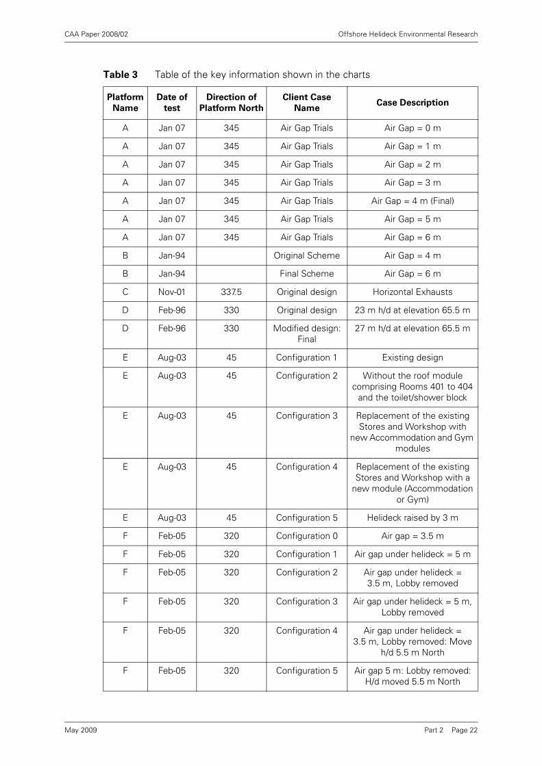
CAA Paper 2008/02 Offshore Helideck Environmental Research
Table 3 Table of the key information shown in the charts
Platform
Name
Date of
test
Direction of
Platform North
Client Case
NameCase Description
A Jan 07 345 Air Gap Trials Air Gap = 0 m
A Jan 07 345 Air Gap Trials Air Gap = 1 m
A Jan 07 345 Air Gap Trials Air Gap = 2 m
A Jan 07 345 Air Gap Trials Air Gap = 3 m
A Jan 07 345 Air Gap Trials Air Gap = 4 m (Final)
A Jan 07 345 Air Gap Trials Air Gap = 5 m
A Jan 07 345 Air Gap Trials Air Gap = 6 m
B Jan-94 Original Scheme Air Gap = 4 m
B Jan-94 Final Scheme Air Gap = 6 m
C Nov-01 337.5 Original design Horizontal Exhausts
D Feb-96 330 Original design 23 m h/d at elevation 65.5 m
D Feb-96 330 Modified design: Final
27 m h/d at elevation 65.5 m
E Aug-03 45 Configuration 1 Existing design
E Aug-03 45 Configuration 2 Without the roof module comprising Rooms 401 to 404
and the toilet/shower block
E Aug-03 45 Configuration 3 Replacement of the existing Stores and Workshop with
new Accommodation and Gym modules
E Aug-03 45 Configuration 4 Replacement of the existing Stores and Workshop with a
new module (Accommodation or Gym)
E Aug-03 45 Configuration 5 Helideck raised by 3 m
F Feb-05 320 Configuration 0 Air gap = 3.5 m
F Feb-05 320 Configuration 1 Air gap under helideck = 5 m
F Feb-05 320 Configuration 2 Air gap under helideck = 3.5 m, Lobby removed
F Feb-05 320 Configuration 3 Air gap under helideck = 5 m, Lobby removed
F Feb-05 320 Configuration 4 Air gap under helideck = 3.5 m, Lobby removed: Move
h/d 5.5 m North
F Feb-05 320 Configuration 5 Air gap 5 m: Lobby removed: H/d moved 5.5 m North
Part 2 Page 22May 2009

CAA Paper 2008/02 Offshore Helideck Environmental Research
F Feb-05 320 Configuration 6 Air gap 5 m: Lobby removed: H/d moved 5.5 m north and
extended 2.1 m west
F Feb-05 320 Configuration 7 Air gap 5 m: Lobby removed: H/d moved 5.5 m north and
aiming circle moved 2.1 m east
F Feb-05 320 Configuration 8 Air gap 5 m: Lobby removed: H/d at original NS position and aiming circle moved 2.1 m east
F Feb-05 320 Configuration 9 Repeat of 8. Air gap 5 m: Lobby removed: H/d at original NS position and aiming circle
moved 2.1 m east
F Mar-05 321 Configuration 10 Air gap 5 m: Lobby removed: H/d moved 5.5 m north, 2.1 m west and aiming circle moved
2.1 m east
G Nov-94 340 Original design Helideck at 4 m elevation above R-PLQ
H Jul-92 354 Detailed Engineering Phase
Air gap = 8.2 m, less 2.8 m, less 2.4 m; without Tender
Support Vessel
I Jul-90 333 Idealised helideck 30 m helideck with edge vanes; air gap = 3 m
I Jul-90 333 Optimised helideck: Final
30 m helideck without edge vanes; air gap = 3 m
J Apr-98 10 2/4H at Option 2A location
Hotel platform located north of 2/4J, Gallant installed
J Apr-98 10 2/4H at Option 2A location
Hotel platform located north of 2/4J, Gallant removed
J Apr-98 10 2/4H at Option 2B location
Hotel platform located south of 2/4J, Gallant installed
J Apr-98 10 2/4H at Option 2B location
Hotel platform located south of 2/4J, Gallant removed
J Apr-98 10 2/4H at Option 2C location
Hotel platform located south east of 2/4J, Gallant installed
J Apr-98 10 2/4H at Option 2C location
Hotel platform located south east of 2/4J, Gallant removed
K Nov-97 303 Original design Helideck as designed
K Nov-97 303 Recommended design
Helideck extended by 3 m all round. Parking bay widened by
4.5 m
Table 3 Table of the key information shown in the charts (Continued)
Platform
Name
Date of
test
Direction of
Platform North
Client Case
NameCase Description
Part 2 Page 23May 2009
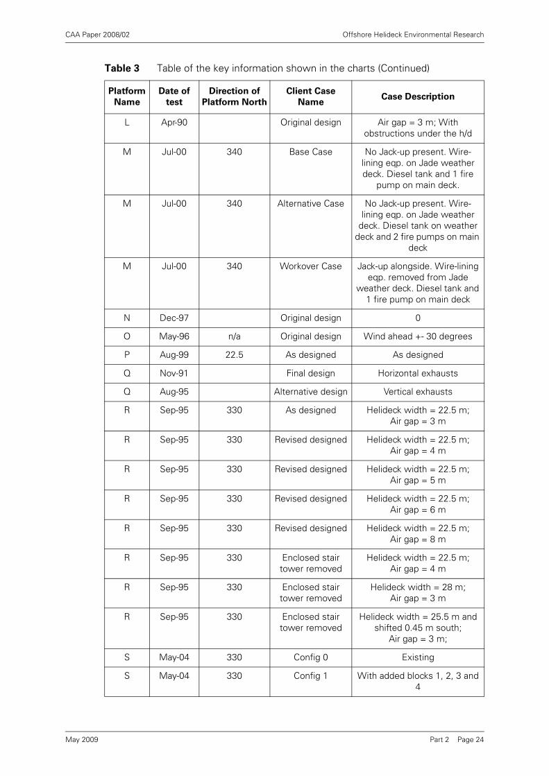
CAA Paper 2008/02 Offshore Helideck Environmental Research
L Apr-90 Original design Air gap = 3 m; With obstructions under the h/d
M Jul-00 340 Base Case No Jack-up present. Wire-lining eqp. on Jade weather deck. Diesel tank and 1 fire
pump on main deck.
M Jul-00 340 Alternative Case No Jack-up present. Wire-lining eqp. on Jade weather
deck. Diesel tank on weather deck and 2 fire pumps on main
deck
M Jul-00 340 Workover Case Jack-up alongside. Wire-lining eqp. removed from Jade
weather deck. Diesel tank and 1 fire pump on main deck
N Dec-97 Original design 0
O May-96 n/a Original design Wind ahead +- 30 degrees
P Aug-99 22.5 As designed As designed
Q Nov-91 Final design Horizontal exhausts
Q Aug-95 Alternative design Vertical exhausts
R Sep-95 330 As designed Helideck width = 22.5 m; Air gap = 3 m
R Sep-95 330 Revised designed Helideck width = 22.5 m; Air gap = 4 m
R Sep-95 330 Revised designed Helideck width = 22.5 m; Air gap = 5 m
R Sep-95 330 Revised designed Helideck width = 22.5 m; Air gap = 6 m
R Sep-95 330 Revised designed Helideck width = 22.5 m; Air gap = 8 m
R Sep-95 330 Enclosed stair tower removed
Helideck width = 22.5 m; Air gap = 4 m
R Sep-95 330 Enclosed stair tower removed
Helideck width = 28 m; Air gap = 3 m
R Sep-95 330 Enclosed stair tower removed
Helideck width = 25.5 m and shifted 0.45 m south;
Air gap = 3 m;
S May-04 330 Config 0 Existing
S May-04 330 Config 1 With added blocks 1, 2, 3 and 4
Table 3 Table of the key information shown in the charts (Continued)
Platform
Name
Date of
test
Direction of
Platform North
Client Case
NameCase Description
Part 2 Page 24May 2009

CAA Paper 2008/02 Offshore Helideck Environmental Research
S May-04 330 Config 2 With added blocks 2, 3 and 4
S May-04 330 Config 3 With added blocks 1, 2 and 3
S May-04 330 Config 4 With added blocks 2 and 3 i.e. blocks 1 and 4 removed
T Aug-96 n/a As designed Without parking area extension to helideck
T Aug-96 n/a Optional design With parking area extension to helideck
U Mar-91 338 Scheme 1 22.5 m helideck; Air gap = 3 m
U Mar-91 338 Scheme 2 22.5 m helideck; Air gap = 5 m
U Mar-91 338 Scheme 3 22.5 m helideck; Air gap = 8 m
U Mar-91 338 Final Design 27.5 m helideck; Air gap = 5 m
Figure 25 Platform A wind tunnel data
Table 3 Table of the key information shown in the charts (Continued)
Platform
Name
Date of
test
Direction of
Platform North
Client Case
NameCase Description
Platform A
Part 2 Page 25May 2009
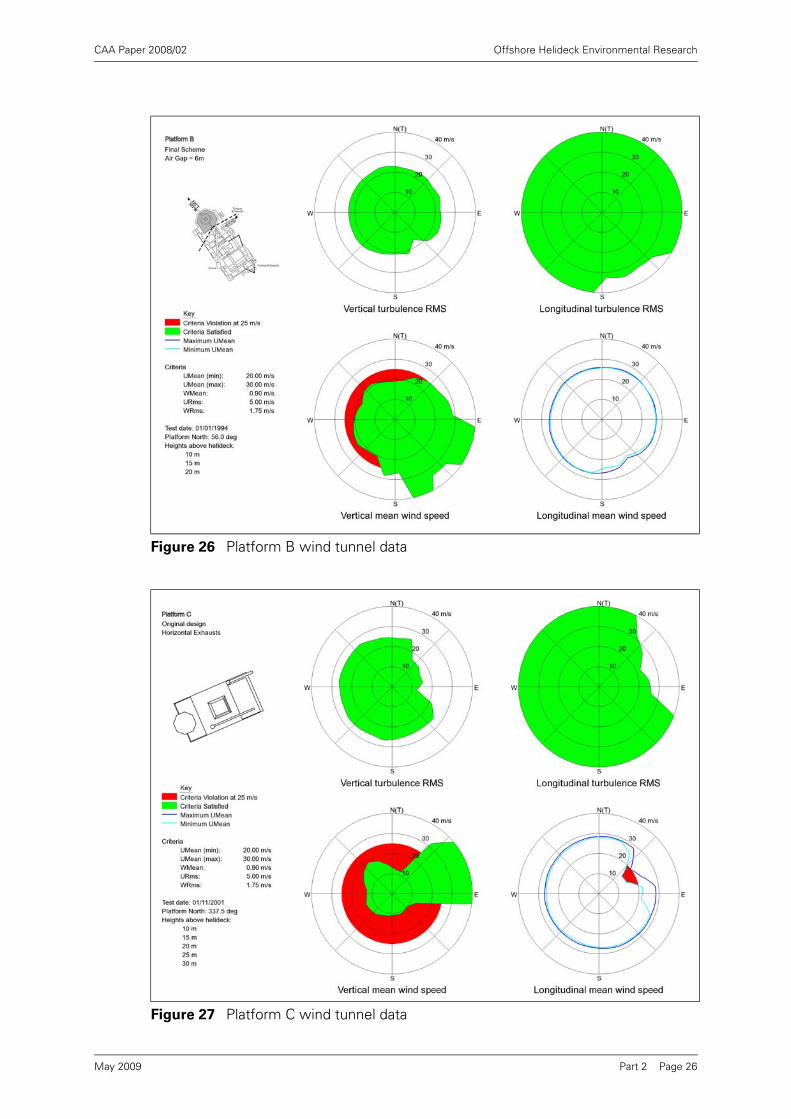
CAA Paper 2008/02 Offshore Helideck Environmental Research
Figure 26 Platform B wind tunnel data
Figure 27 Platform C wind tunnel data
Part 2 Page 26May 2009

CAA Paper 2008/02 Offshore Helideck Environmental Research
Figure 28 Platform D wind tunnel data
Figure 29 Platform E wind tunnel data
Part 2 Page 27May 2009
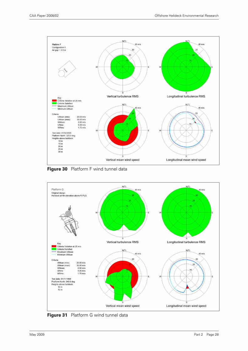
CAA Paper 2008/02 Offshore Helideck Environmental Research
Figure 30 Platform F wind tunnel data
Figure 31 Platform G wind tunnel data
Platform G
Part 2 Page 28May 2009
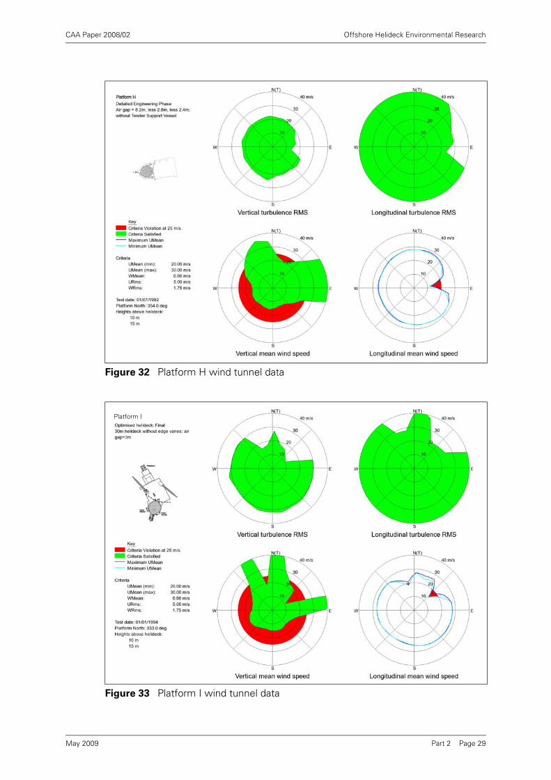
CAA Paper 2008/02 Offshore Helideck Environmental Research
Figure 32 Platform H wind tunnel data
Figure 33 Platform I wind tunnel data
Platform I
Part 2 Page 29May 2009

CAA Paper 2008/02 Offshore Helideck Environmental Research
Figure 34 Platform J wind tunnel data
Figure 35 Platform K wind tunnel data
Part 2 Page 30May 2009

CAA Paper 2008/02 Offshore Helideck Environmental Research
Figure 36 Platform L wind tunnel data
Figure 37 Platform M wind tunnel data
Part 2 Page 31May 2009

CAA Paper 2008/02 Offshore Helideck Environmental Research
Figure 38 Platform N wind tunnel data
Figure 39 Platform P wind tunnel data
Part 2 Page 32May 2009

CAA Paper 2008/02 Offshore Helideck Environmental Research
Figure 40 Platform Q wind tunnel data
Figure 41 Platform R wind tunnel data
Part 2 Page 33May 2009

CAA Paper 2008/02 Offshore Helideck Environmental Research
Figure 42 Platform S wind tunnel data
Figure 43 Platform U wind tunnel data
Platform U
Part 2 Page 34May 2009
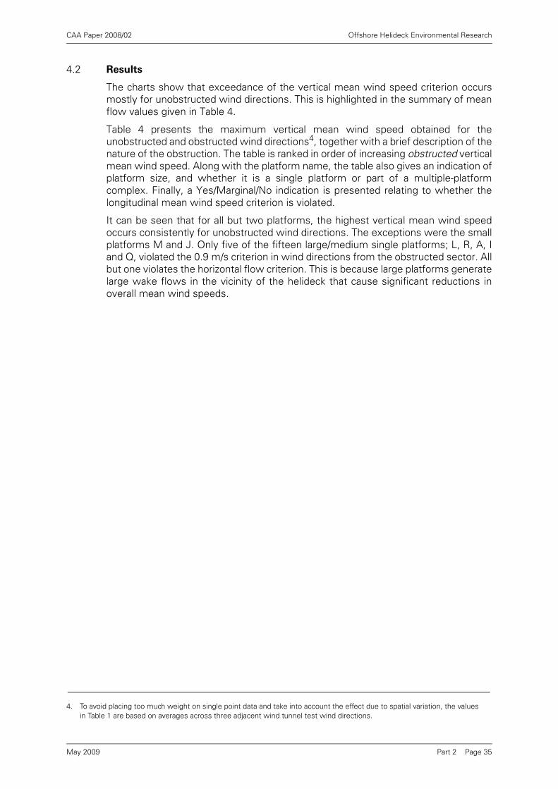
CAA Paper 2008/02 Offshore Helideck Environmental Research
4.2 Results
The charts show that exceedance of the vertical mean wind speed criterion occursmostly for unobstructed wind directions. This is highlighted in the summary of meanflow values given in Table 4.
Table 4 presents the maximum vertical mean wind speed obtained for theunobstructed and obstructed wind directions4, together with a brief description of thenature of the obstruction. The table is ranked in order of increasing obstructed verticalmean wind speed. Along with the platform name, the table also gives an indication ofplatform size, and whether it is a single platform or part of a multiple-platformcomplex. Finally, a Yes/Marginal/No indication is presented relating to whether thelongitudinal mean wind speed criterion is violated.
It can be seen that for all but two platforms, the highest vertical mean wind speedoccurs consistently for unobstructed wind directions. The exceptions were the smallplatforms M and J. Only five of the fifteen large/medium single platforms; L, R, A, Iand Q, violated the 0.9 m/s criterion in wind directions from the obstructed sector. Allbut one violates the horizontal flow criterion. This is because large platforms generatelarge wake flows in the vicinity of the helideck that cause significant reductions inoverall mean wind speeds.
4. To avoid placing too much weight on single point data and take into account the effect due to spatial variation, the valuesin Table 1 are based on averages across three adjacent wind tunnel test wind directions.
Part 2 Page 35May 2009

CAA Paper 2008/02 Offshore Helideck Environmental Research
It is not clear why the two small platforms M and J are inconsistent with the basictrend. However, in general, smaller platforms will generate less severe wake flowsor allow some wake recovery to take place, resulting in generally higher wind speedsat the helideck. This is reflected in the longitudinal mean wind speed criterion, whichis complied with for the small platforms. Consequently the high vertical mean flow
Table 4 Summary of the vertical mean wind speed
PlatformPlatform
size1
1. Large = >80 m (nominal); Medium = 50 to 80 m (nominal); Small = <50 m (nominal)
Single or
Multiple
platform
layout
Wmean
(max) for
unobstructed
wind
directions
Wmean
(max) for
obstructed
wind
directions
Nature of
Obstruction
Violation of
longitudinal
mean wind
speed
criterion
U Large Single 1.81 0.18 Exhaust stacks Yes
H Medium Single 1.45 0.28 Derrick Yes
C Large Single 2.16 0.45 Derrick Yes
G Large Single 2.43 0.54 Derrick and flare tower
Yes
B Large Single 1.17 0.57 Derrick No
K Large Single 2.22 0.63 Exhaust stacks Yes
F Medium Single2
2. Platform F is actually bridge linked to an adjacent platform. Unlike other multiple installations, however, it is of comparable size to its neighbours and is therefore relatively insensitive to them. For this report therefore, it is classed as single.
1.75 0.75 Exhaust stacks Yes
N Large Single 1.13 0.81 Flare tower Marginal
D Large Single 1.79 0.82 Derrick Yes
P Large Single 1.62 0.88 Exhaust stacks No
S Small Multiple 1.5 0.88 Adjacent platform No
L Large Single 2.4 0.97 Derrick Yes
R Large Single 2.29 1.06 Derrick Yes
E Small Multiple 1.98 1.27 Blockage underneath the
helideck
No
A Large Single 2.46 1.35 Derricks Yes
I (Final)
Large Single 1.55 1.37 Exhaust stacks Yes
Q (Vertical
exhausts)
Medium Single 2.13 1.58 Flare tower Yes
M(Base Case)
Small Single 1.36 1.68 Crane plus blockage underneath the
helideck
No
J (2A) Small Multiple 0.75 1.75 Adjacent platform Marginal
Part 2 Page 36May 2009
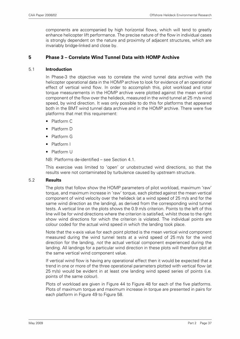
CAA Paper 2008/02 Offshore Helideck Environmental Research
components are accompanied by high horizontal flows, which will tend to greatlyenhance helicopter lift performance. The precise nature of the flow in individual casesis strongly dependent on the nature and proximity of adjacent structures, which areinvariably bridge-linked and close by.
5 Phase 3 – Correlate Wind Tunnel Data with HOMP Archive
5.1 Introduction
In Phase-3 the objective was to correlate the wind tunnel data archive with thehelicopter operational data in the HOMP archive to look for evidence of an operationaleffect of vertical wind flow. In order to accomplish this, pilot workload and rotortorque measurements in the HOMP archive were plotted against the mean verticalcomponent of the flow over the helideck, measured in the wind tunnel at 25 m/s windspeed, by wind direction. It was only possible to do this for platforms that appearedboth in the BMT wind tunnel data archive and in the HOMP archive. There were fiveplatforms that met this requirement:
• Platform C
• Platform D
• Platform G
• Platform I
• Platform U
NB: Platforms de-identified – see Section 4.1.
This exercise was limited to ‘open’ or unobstructed wind directions, so that theresults were not contaminated by turbulence caused by upstream structure.
5.2 Results
The plots that follow show the HOMP parameters of pilot workload, maximum ‘raw’torque, and maximum increase in ‘raw’ torque, each plotted against the mean verticalcomponent of wind velocity over the helideck (at a wind speed of 25 m/s and for thesame wind direction as the landing), as derived from the corresponding wind tunneltests. A vertical line on the plots shows the 0.9 m/s criterion. Points to the left of thisline will be for wind directions where the criterion is satisfied, whilst those to the rightshow wind directions for which the criterion is violated. The individual points arecolour coded for the actual wind speed in which the landing took place.
Note that the x-axis value for each point plotted is the mean vertical wind componentmeasured during the wind tunnel tests at a wind speed of 25 m/s for the winddirection for the landing, not the actual vertical component experienced during thelanding. All landings for a particular wind direction in these plots will therefore plot atthe same vertical wind component value.
If vertical wind flow is having any operational effect then it would be expected that atrend in one or more of the three operational parameters plotted with vertical flow (at25 m/s) would be evident in at least one landing wind speed series of points (i.e.points of the same colour).
Plots of workload are given in Figure 44 to Figure 48 for each of the five platforms.Plots of maximum torque and maximum increase in torque are presented in pairs foreach platform in Figure 49 to Figure 58.
Part 2 Page 37May 2009
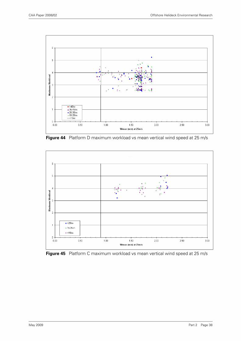
CAA Paper 2008/02 Offshore Helideck Environmental Research
Figure 44 Platform D maximum workload vs mean vertical wind speed at 25 m/s
Figure 45 Platform C maximum workload vs mean vertical wind speed at 25 m/s
Part 2 Page 38May 2009

CAA Paper 2008/02 Offshore Helideck Environmental Research
Figure 46 Platform G maximum workload vs mean vertical wind speed at 25 m/s
Figure 47 Platform I maximum workload vs mean vertical wind speed at 25 m/s
Figure 48 Platform U maximum workload vs mean vertical wind speed at 25 m/s
Part 2 Page 39May 2009
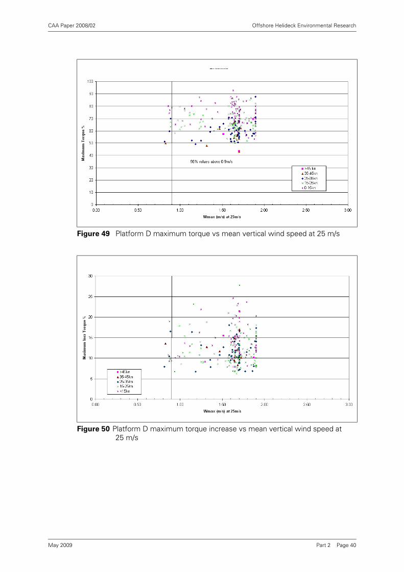
CAA Paper 2008/02 Offshore Helideck Environmental Research
Figure 49 Platform D maximum torque vs mean vertical wind speed at 25 m/s
Figure 50 Platform D maximum torque increase vs mean vertical wind speed at 25 m/s
Part 2 Page 40May 2009
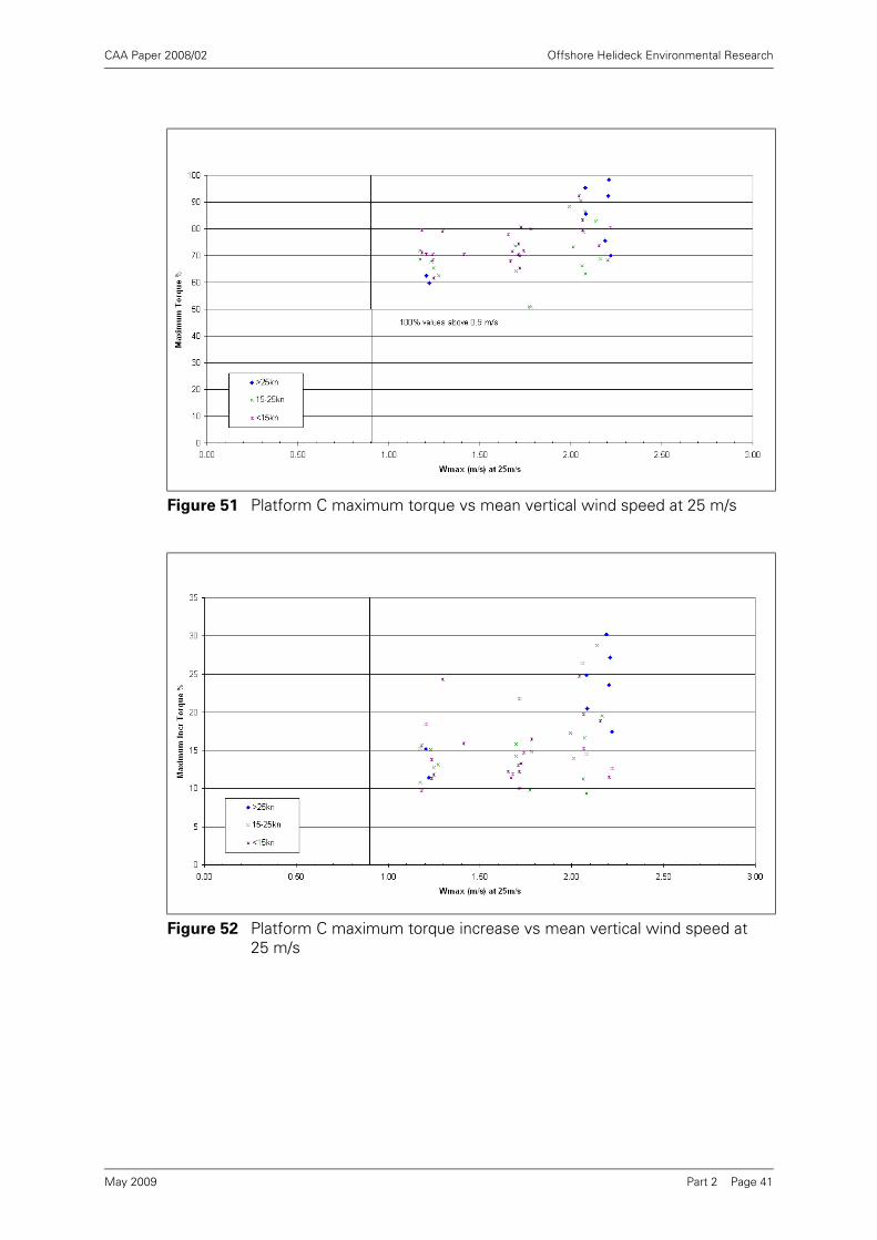
CAA Paper 2008/02 Offshore Helideck Environmental Research
Figure 51 Platform C maximum torque vs mean vertical wind speed at 25 m/s
Figure 52 Platform C maximum torque increase vs mean vertical wind speed at 25 m/s
Part 2 Page 41May 2009

CAA Paper 2008/02 Offshore Helideck Environmental Research
Figure 53 Platform G maximum torque vs mean vertical wind speed at 25 m/s
Figure 54 Platform G maximum torque increase vs mean vertical wind speed at 25 m/s
Part 2 Page 42May 2009
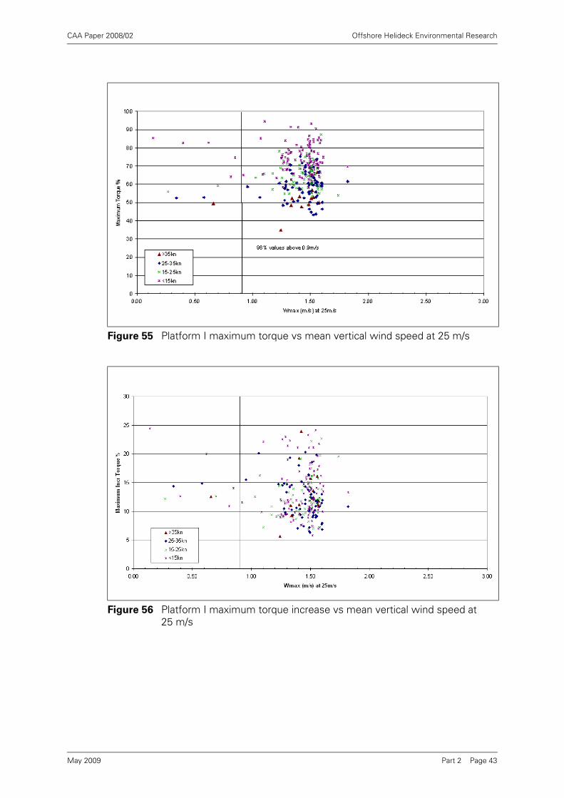
CAA Paper 2008/02 Offshore Helideck Environmental Research
Figure 55 Platform I maximum torque vs mean vertical wind speed at 25 m/s
Figure 56 Platform I maximum torque increase vs mean vertical wind speed at 25 m/s
Part 2 Page 43May 2009
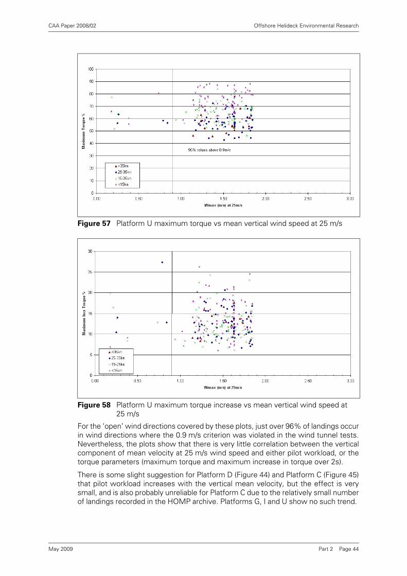
CAA Paper 2008/02 Offshore Helideck Environmental Research
For the ‘open’ wind directions covered by these plots, just over 96% of landings occurin wind directions where the 0.9 m/s criterion was violated in the wind tunnel tests.Nevertheless, the plots show that there is very little correlation between the verticalcomponent of mean velocity at 25 m/s wind speed and either pilot workload, or thetorque parameters (maximum torque and maximum increase in torque over 2s).
There is some slight suggestion for Platform D (Figure 44) and Platform C (Figure 45)that pilot workload increases with the vertical mean velocity, but the effect is verysmall, and is also probably unreliable for Platform C due to the relatively small numberof landings recorded in the HOMP archive. Platforms G, I and U show no such trend.
Figure 57 Platform U maximum torque vs mean vertical wind speed at 25 m/s
Figure 58 Platform U maximum torque increase vs mean vertical wind speed at 25 m/s
Part 2 Page 44May 2009

CAA Paper 2008/02 Offshore Helideck Environmental Research
The lack of any correlation with pilot workload suggests that the existence of highmean vertical velocities in open wind sectors does not cause the pilot any difficultieswith control. If spatial variations in the vertical component were causing a controlproblem, then one would expect such variations to occur during landings in winddirections causing the greatest vertical component over the helideck and that, in turn,this would result in high pilot control activity registering a higher workload. However,this is certainly not evident in the data.
As with workload, there is a slight trend for the highest torque values to occur in winddirections with higher vertical mean velocities on Platform D (Figure 49 and Figure 50)and Platform C (Figure 51 and Figure 52). Again this trend is not seen on the otherthree platforms. It can be seen that most of the plots exhibit the expected trend ofhigher torque values in lower wind speeds.
The lack of any correlation with rotor maximum torque or maximum torque increasesuggests that the existence of high mean vertical velocities does not cause anyhelicopter performance problems. Entering a region of high downdraft would beexpected to result in a need for increased collective and thus increased torque, butthis is not evident in the data. It is presumed that in high wind speeds the effect isnot seen because the presence of high horizontal wind components result in a highmargin of lift, and small adjustments in collective are sufficient to compensate for anydowndraft. In low wind speeds the actual vertical component of velocity and theeffect on the helicopter sink or climb rate is small.
Overall it is concluded that there is no evidence of any correlation between the extentof the violation of the 0.9 m/s criterion and either pilot workload or torque.
6 Phase 4 – Helideck Air-Gap Wind Tunnel Tests
6.1 Introduction
The 0.9 m/s criterion has been the main driver for the raising of helidecks, and themaintenance of a good clearance between the helideck and the accommodationblock. While it is usually not possible to comply fully with the criterion, wind tunneltests usually demonstrate a compliance benefit if the helideck height is raised and theclearance increased, and it has therefore often been a key factor in the eventualselection of helideck height in the platform design process.
With the possibility that the 0.9 m/s criterion might be removed from the guidance,there was concern that the pressure on designers to maintain a good helideck air gapmight be lost. It was not known whether the application of the new turbulencecriterion [5, 8] might take over the role of driving designers towards a similar air gap.Wind tunnel test data in the BMT archive generally did not cover an adequate rangeof helideck heights to permit conclusions to be drawn on this point.
Consequently, a programme of wind tunnel tests was performed to examine theimpact of helideck height on ‘open’ sector wind flow properties over a wider range ofheights. A single representative model of a large North Sea platform (Brae-A) wasused, and the results interpreted in terms of the helideck height that would have beenselected for design if individual flow criteria were the key determinant.
The objectives of the wind tunnel test programme were therefore as follows:
1 To carry out a series of wind tunnel tests on a typical large offshore platform tomeasure the wind flow over the helideck for a wide range of helideck heights.
2 To compare the results with CAA vertical turbulence and mean speed criteriaand with two additional guidelines used by BMT in the assessment of helidecks(see Table 2).
Part 2 Page 45May 2009

CAA Paper 2008/02 Offshore Helideck Environmental Research
3 To determine how the application of the turbulence criterion might influence theselection of helideck heights in platform design in the absence of a 0.9 m/svertical mean speed criterion.
6.2 Scope of Work
The scope of work was as follows:
• Refurbish an existing 1:100 scale model of the Brae-A platform (Figure 59) andmodify it to enable the helideck height above the accommodation to be varied.
• Measure the longitudinal and vertical mean wind speed and turbulence intensity at5 m, 10 m, 15 m and 20 m above the helicopter landing spot for the full range ofwind direction in 15° steps.
• Carry out the tests for 7 helideck heights (air gap clearances between the helideckand the accommodation block of 0 m – 6 m in 1 m steps).
6.3 Presentation of Results
Longitudinal and vertical mean wind speed and turbulence standard deviations weremeasured at 5 m, 10 m, 15 m, and 20 m above the landing spot of the Brae-Ahelideck for wind directions 0° to 360° in steps of 15° (where wind direction is relativeto platform north defined in Figure 60). The tests were carried out for 7 helideck airgaps from 0 m to 6 m (the air gap on the as-built platform was 3 m).
When a helicopter is in flight over a helideck there is a tendency for the rotor to drawdown air from heights well above the rotor height. When on the deck the rotor isapproximately 5 m above the helideck. Consequently data measured at the 5 mheight are not particularly relevant to an assessment of impact on helicopterperformance and so these results are presented in Appendix A for completenessonly. Data measured at 10 m, 15 m and 20 m above the deck have much more effecton helicopter performance and handling during the landing or takeoff manoeuvre, andmore weight has therefore been given to these results.
The measured data were scaled to a free-stream mean wind speed at helideck heightof 25 m/s. The scaled results are plotted in Figure 61 to Figure 72.
Figure 59 1:100 scale Brae-A wind tunnel model in the BMT Atmospheric Boundary Layer Wind Tunnel
Part 2 Page 46May 2009

CAA Paper 2008/02 Offshore Helideck Environmental Research
The highest vertical mean wind speeds, which form the current basis for helideckdesign assessment and mitigation, invariably occur for unobstructed or ‘open’ winddirections, and so the results presented here are for these unobstructed winddirections in the sector 150° to 330°. 5
Figure 60 Definition of platform north
5. The results from the wind directions from 330° - 150° are omitted because they do not include large vertical mean flowcomponents, and are also very much influenced by distortions and turbulence specific to Brae-A.
Wind from platform north = 0 degs
270 degs
90 degs
180 degs
Part 2 Page 47May 2009
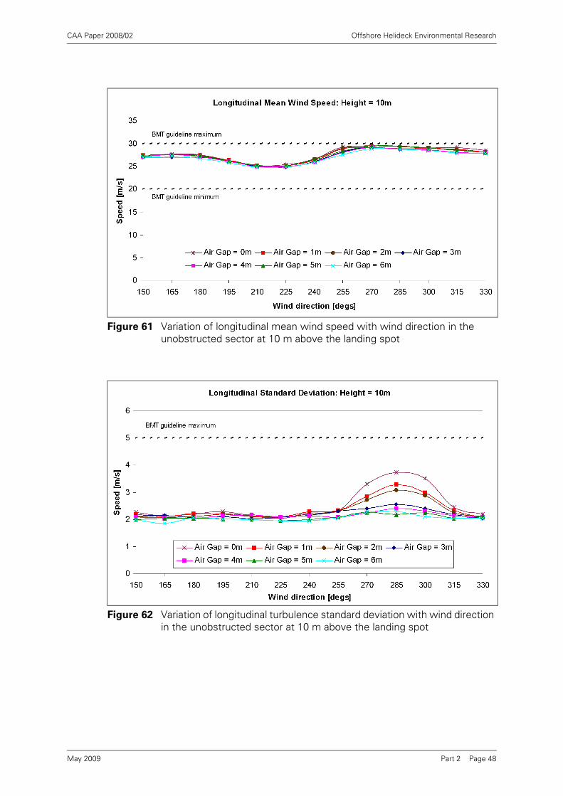
CAA Paper 2008/02 Offshore Helideck Environmental Research
Figure 61 Variation of longitudinal mean wind speed with wind direction in the unobstructed sector at 10 m above the landing spot
Figure 62 Variation of longitudinal turbulence standard deviation with wind direction in the unobstructed sector at 10 m above the landing spot
Part 2 Page 48May 2009
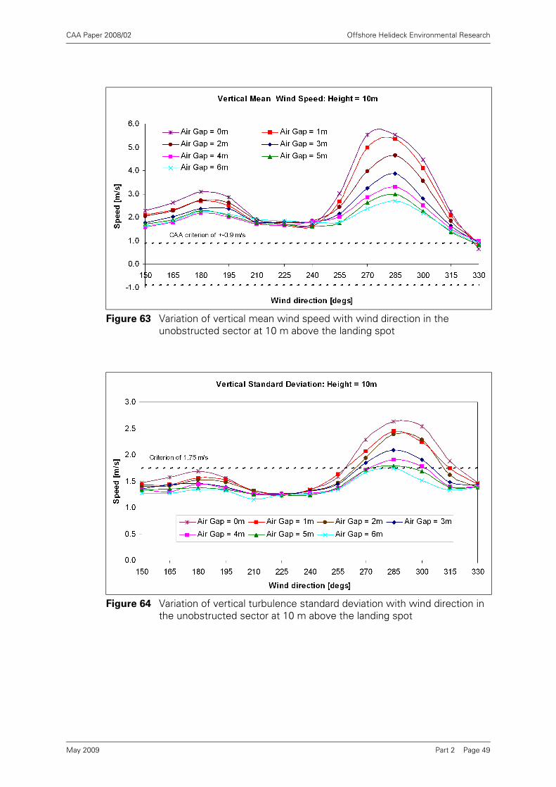
CAA Paper 2008/02 Offshore Helideck Environmental Research
Figure 63 Variation of vertical mean wind speed with wind direction in the unobstructed sector at 10 m above the landing spot
Figure 64 Variation of vertical turbulence standard deviation with wind direction in the unobstructed sector at 10 m above the landing spot
Part 2 Page 49May 2009

CAA Paper 2008/02 Offshore Helideck Environmental Research
Figure 65 Variation of longitudinal mean wind speed with wind direction in the unobstructed sector at 15 m above the landing spot
Figure 66 Variation of longitudinal turbulence standard deviation with wind direction in the unobstructed sector at 15 m above the landing spot
Part 2 Page 50May 2009
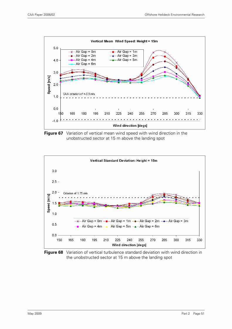
CAA Paper 2008/02 Offshore Helideck Environmental Research
Figure 67 Variation of vertical mean wind speed with wind direction in the unobstructed sector at 15 m above the landing spot
Figure 68 Variation of vertical turbulence standard deviation with wind direction in the unobstructed sector at 15 m above the landing spot
Part 2 Page 51May 2009

CAA Paper 2008/02 Offshore Helideck Environmental Research
Figure 69 Variation of longitudinal mean wind speed with wind direction in the unobstructed sector at 20 m above the landing spot
Figure 70 Variation of longitudinal turbulence standard deviation with wind direction in the unobstructed sector at 20 m above the landing spot
Part 2 Page 52May 2009

CAA Paper 2008/02 Offshore Helideck Environmental Research
Figure 71 Variation of vertical mean wind speed with wind direction in the unobstructed sector at 20 m above the landing spot
Figure 72 Variation of vertical turbulence standard deviation with wind direction in the unobstructed sector at 20 m above the landing spot
Part 2 Page 53May 2009

CAA Paper 2008/02 Offshore Helideck Environmental Research
6.4 Discussion of results
All of the results demonstrate that increasing the helideck air gap improves the flowparameters for all wind directions in the ‘open’ sector. The wind direction for whichthe air gap is seen to influence the flow the most is centred on 285°.
Figure 63 shows that the peak vertical mean wind speed at 10 m above the landingspot for the ‘open’ direction of 285° decreases by over 50% as the air gap isincreased. The impact is also highlighted in Figure 73 which shows that, for thisparticular direction, most of the decrease in vertical mean wind speed is obtained withan air gap of 3 m to 4 m and that further increase of the air gap produces only marginal
Figure 73 Variation of vertical mean wind speed with air gap for heights above the landing spot of 10 m, 15 m and 20 m for a wind direction of 285°
Figure 74 Variation of vertical turbulence standard deviation with air gap for heights above the landing spot of 10 m, 15 m and 20 m for a wind direction of 285o
Part 2 Page 54May 2009
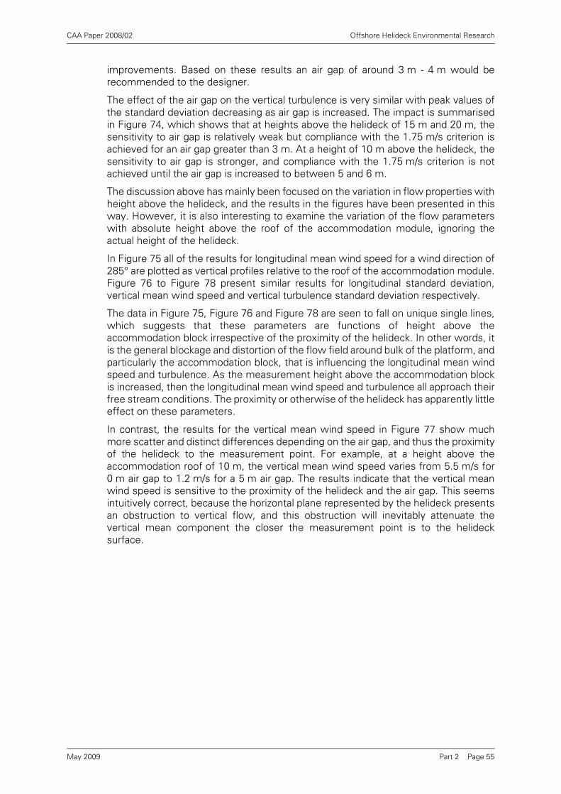
CAA Paper 2008/02 Offshore Helideck Environmental Research
improvements. Based on these results an air gap of around 3 m - 4 m would berecommended to the designer.
The effect of the air gap on the vertical turbulence is very similar with peak values ofthe standard deviation decreasing as air gap is increased. The impact is summarisedin Figure 74, which shows that at heights above the helideck of 15 m and 20 m, thesensitivity to air gap is relatively weak but compliance with the 1.75 m/s criterion isachieved for an air gap greater than 3 m. At a height of 10 m above the helideck, thesensitivity to air gap is stronger, and compliance with the 1.75 m/s criterion is notachieved until the air gap is increased to between 5 and 6 m.
The discussion above has mainly been focused on the variation in flow properties withheight above the helideck, and the results in the figures have been presented in thisway. However, it is also interesting to examine the variation of the flow parameterswith absolute height above the roof of the accommodation module, ignoring theactual height of the helideck.
In Figure 75 all of the results for longitudinal mean wind speed for a wind direction of285° are plotted as vertical profiles relative to the roof of the accommodation module.Figure 76 to Figure 78 present similar results for longitudinal standard deviation,vertical mean wind speed and vertical turbulence standard deviation respectively.
The data in Figure 75, Figure 76 and Figure 78 are seen to fall on unique single lines,which suggests that these parameters are functions of height above theaccommodation block irrespective of the proximity of the helideck. In other words, itis the general blockage and distortion of the flow field around bulk of the platform, andparticularly the accommodation block, that is influencing the longitudinal mean windspeed and turbulence. As the measurement height above the accommodation blockis increased, then the longitudinal mean wind speed and turbulence all approach theirfree stream conditions. The proximity or otherwise of the helideck has apparently littleeffect on these parameters.
In contrast, the results for the vertical mean wind speed in Figure 77 show muchmore scatter and distinct differences depending on the air gap, and thus the proximityof the helideck to the measurement point. For example, at a height above theaccommodation roof of 10 m, the vertical mean wind speed varies from 5.5 m/s for0 m air gap to 1.2 m/s for a 5 m air gap. The results indicate that the vertical meanwind speed is sensitive to the proximity of the helideck and the air gap. This seemsintuitively correct, because the horizontal plane represented by the helideck presentsan obstruction to vertical flow, and this obstruction will inevitably attenuate thevertical mean component the closer the measurement point is to the helidecksurface.
Part 2 Page 55May 2009

CAA Paper 2008/02 Offshore Helideck Environmental Research
Figure 75 Variation of longitudinal mean wind speed with height above the roof deck for air gaps of 0 m to 6 m and a wind direction of 285°
Figure 76 Variation of longitudinal turbulence standard deviation with height above the roof deck for air gaps of 0 m to 6 m and a wind direction of 285°
Part 2 Page 56May 2009
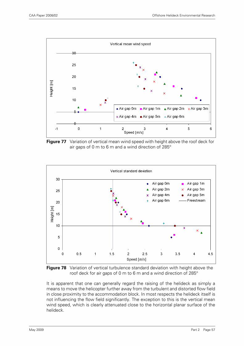
CAA Paper 2008/02 Offshore Helideck Environmental Research
It is apparent that one can generally regard the raising of the helideck as simply ameans to move the helicopter further away from the turbulent and distorted flow fieldin close proximity to the accommodation block. In most respects the helideck itself isnot influencing the flow field significantly. The exception to this is the vertical meanwind speed, which is clearly attenuated close to the horizontal planar surface of thehelideck.
Figure 77 Variation of vertical mean wind speed with height above the roof deck for air gaps of 0 m to 6 m and a wind direction of 285°
Figure 78 Variation of vertical turbulence standard deviation with height above the roof deck for air gaps of 0 m to 6 m and a wind direction of 285°
Part 2 Page 57May 2009

CAA Paper 2008/02 Offshore Helideck Environmental Research
The work described in this section has concerned only one example North Seaproduction platform, but the key conclusion is that the application of the turbulencecriterion to the flow field above the helideck for ‘open’ wind directions is likely tocause designers to introduce a reasonable air gap under the helideck.
7 Conclusions
The four phases of the study of the 0.9 m/s vertical flow criterion have generated thefollowing conclusions:
7.1 In Phase-1 the HOMP data archive was examined for evidence of high torque eventsassociated with high wind speeds and ‘open’ wind sectors, which might be indicativeof a helicopter performance hazard associated with the vertical component of windspeed. From the results of this phase it is concluded that:
7.1.1 No evidence of high torque events or large torque increase events (over 2 seconds)associated with higher wind speeds and ‘open’ wind directional sectors was found.(Section 3.4)
7.1.2 Plots of all valid torque data for all 44 platforms for which sketches were availableshow that torque values are generally higher for lower wind speeds and for windsfrom sectors that would be expected to feature turbulence caused by the upwindstructure of the platform. (Section 3.4)
7.2 In Phase-2 the BMT wind tunnel data archive was analysed to map the occurrence ofviolations of the 0.9 m/s criterion against wind directions, and thus establish whetherthe violations could be associated with particular platform features and, in particular,confirm whether violations mainly occur in unobstructed or ‘open’ wind directions.From the results of Phase-2 it is concluded that:
7.2.1 For large single platforms overall velocity reductions in the wake of obstructions meanthat violations of the 0.9 m/s criterion are most likely to occur in winds from the opensectors. In fact, for the 15 medium and large platforms analysed from the BMTdatabase, only five violated the 0.9 m/s criterion in winds from obstructed or‘turbulent’ directions. (Section 4.2), and for all 15 the vertical mean wind speed wasgreatest for winds from the open sectors.
7.2.2 For smaller platforms and multiple platform configurations, where there are lesssevere wake effects, violations of the 0.9 m/s criterion can occur in winds from allsectors, but are likely to be accompanied by high horizontal wind components withconsequent helicopter performance benefits. (Section 4.2)
7.3 In Phase-3 HOMP data on pilot workload and torque were compared with wind tunneldata on 0.9 m/s criterion violations for ‘open’ wind directions. This was possible for 5platforms that appeared in both the BMT wind tunnel database and the 16-monthHOMP data archive. From this it has been concluded that:
7.3.1 There is no evidence of high torque or torque increase values being associated withhigh vertical flow components. (Section 5.2)
7.3.2 Similarly, there is no evidence of high pilot workload being associated with highvertical flow components. (Section 5.2)
7.4 Overall it is concluded that violation of the 0.9 m/s vertical mean flow criterion cannotbe linked to any helicopter performance (i.e. torque-related), or handling (i.e. pilotworkload-related) hazard.
Part 2 Page 58May 2009
CAA Paper 2008/02 Offshore Helideck Environmental Research
7.5 The highest vertical components of flow almost always occur when the wind is froman ‘open’ direction for medium and large platforms, or from the obstructed directionon small platforms generating little wake. These are conditions when the horizontalcomponent of flow is likely to be high ensuring that the helicopter has a high marginof lift, and when turbulence levels and associated pilot workload values are likely tobe low.
7.6 In Phase 4 of the project a programme of wind tunnel tests was performed toexamine the impact of helideck height on ‘open’ sector wind flow properties over awider range of heights. A model of a single representative large North Sea platform(Brae-A) was used, and the results interpreted in terms of the helideck height thatwould have been selected for design if individual given flow criteria were the keydeterminate. It was concluded that:
7.6.1 Increasing the air gap from 0 m to 6 m systematically reduces the vertical mean windspeed and the turbulence standard deviation. (Section 6.4)
7.6.2 Based on the vertical mean wind speeds at a height of 15 m above the helideck forunobstructed wind directions, an air gap of 3 m to 4 m would be recommended forBrae-A.6 The results showed that further increase in helideck height provided littleadditional improvement. (Section 6.4)
7.6.3 A turbulence criterion of 1.75 m/s would result in an air gap of 5 to 6 m beingrecommended. (Section 6.4)
8 Recommendations
As the criterion cannot be linked to a helicopter performance or handling hazard, it isrecommended that consideration be given to removing the 0.9 m/s criterion from theguidance material [1].
It is recommended that the first step should be consultation with the helicopteroperators in order to seek their views on the validity or otherwise of the criterion froman operational perspective, and to check whether there may be safety benefitsimplicit in the criterion that have not been evident during the study.
6. The as-built design has a 3 m air gap.
Part 2 Page 59May 2009
CAA Paper 2008/02 Offshore Helideck Environmental Research
9 References
[1] Offshore Helicopter Landing Areas - Guidance on Standards, CAP 437, Fifth editionpublished by the CAA, London, August 2005.7
[2] Research on Offshore Helideck Environmental Issues, CAA Paper 99004, August2000.
[3] Review of 0.9 m/s Vertical Wind Component Criterion for Helicopters, BMT FluidMechanics Proposal No. Q/84266q2, 26th January 2005.
[4] Vertical Wind Component Criterion for Helicopters - Review of Wind Tunnel Data,BMT Fluid Mechanics Proposal No. Q/84375q2, 18th May 2006.
[5] Validation of the Helicopter Turbulence Criterion for Operations to Offshore Platforms,CAA Paper 2008/02 Part 1.
[6] Final Report on the Helicopter Operations Monitoring Programme (HOMP) trial, CAAPaper 2002/02, 2002.
[7] Final Report on the Follow-on Activities to the HOMP Trial, CAA Paper 2004/12,October 2004
[8] Helicopter Turbulence Criteria for Operations to Offshore Platforms, CAA Paper2004/03.
[9] D Howson email dated 17th March 2005.
[10] BMT Fluid Mechanics Document homp_full_plots_named_v2.doc, 21st November2005.
[11] Helideck Limitations List (HLL), The Helideck Certification Agency,http://www.helidecks.org/.
7. Now at 6th edition.
Part 2 Page 60May 2009

CAA Paper 2008/02 Offshore Helideck Environmental Research
Appendix A Wind Tunnel Results for Brae-A at 5 m Above
the Helideck
Figure 79 Variation of longitudinal mean wind speed with wind direction in the unobstructed sector at 5 m above the landing spot for a free wind speed of 25 m/s
Figure 80 Variation of longitudinal turbulence standard deviation with wind direction in the unobstructed sector at 5 m above the landing spot for a free wind speed of 25 m/s
Part 2 Appendix A Page 1May 2009

CAA Paper 2008/02 Offshore Helideck Environmental Research
Figure 81 Variation of vertical mean wind speed with wind direction in the unobstructed sector at 5 m above the landing spot for a free wind speed of 25 m/s
Figure 82 Variation of vertical turbulence standard deviation with wind direction in the unobstructed sector at 5 m above the landing spot for a free wind speed of 25 m/s
Part 2 Appendix A Page 2May 2009