CA684: Deep Learning 04/Apr/2014

Tsuyoshi Okita

Dublin City University,tokita@computing.dcu.ie

1 Overview

Fig. 1. Hierarchical feature representations of picture of faces [Lee]. For given trainingset of face images, deep learning aims at obtaining hierarchical feature representationsin an automatic way.

This class aims at grasping the overview of deep learning as one hottestarea of research (Figure 1 shows the idea of deep learning). However, as wehaven’t properly introduced neither feed-forward neural networks nor undirectedgraphical models, this class only covers the very introductory materials. The goalof this class is to understand three questions below.

1. What is deep learning?2. Grasp the basic algorithm of Recurrent Neural Network (RNN) or Restricted

Boltzmann Machine (RBM)?3. Can you explain some toy application? (e.g. a summation of two binary

numbers)

We restrict ourselves to introduce very basic characteristics of deep learningby two algorithms, RNN and RBM. Nevertheless, the understanding of thesetwo algorithms will facilitate the further reading of the deep learning literaturesalthough it will need at least one more lecture to complete the rapid overviewof this field. Note that deep learning is a state-of-the-art in Machine Learningand is evolving (Hinton, 2007; Bengio, 2009; Murphy, 2012). A topic might beconsiderably updated in a few years time.

Fig. 2. Schematic illustration of sparse coding of Olshausen et al. using artificial data.Olshausen et al. observed that sparse coding of natural images produces wavelet-likeoriented filters that resemble the receptive fields of simple cells in the visual cortex.Given a potentially large set of input patterns (left figure = observed data of 25,000characters), sparse coding algorithms attempt to automatically find a small numberof representative basis vectors (right figure of 1000 patterns). In test phase, these ba-sis vectors reproduce the original input patterns. The human primary visual cortexis estimated to be overcomplete (Overcomplete codings smoothly interpolate betweeninput vectors and are robust under input noise) by a factor of 500, so that, for exam-ple, a 14 x 14 patch of input (a 196-dimensional space) is coded by roughly 100,000neurons.[Salakhutdinov, Tutorial]

Deep learning is to learn automatically the hierarchical feature representa-tions, which we follow the definition of Yann LeCun (See ICML2013 TutorialVideo on techtalks.tv), Yoshua Bengio (Bengio, 2009), Geoffrey Hinton (Hinton,2007), or others. Hence, the focus of this class is on “feature extraction” and“automatic Machine Learning algorithm” in order to realize this. One impor-tant question which was asked by Hinton (Hinton and Teh, 2001) in 2001 still in

the formation period of deep learning, “Is a linear causal model of Olshausen etal. (Olshausen and Field, 1996) plausible enough to explain the human vision?”

“Early research on the response properties of individual neurons in visual cor-tex typically assumed that neurons were rather specific feature detectors thatonly fired when they found a close match to the feature of interest. For the earlystages of the visual cortex, this assumption has largely been replaced by theidea that the receptive fields of neurons represent basis functions and the neuralactivities represent coefficients on these basis functions. The sensory input isthen represented as a weighted linear combination of the basis functions whichis equivalent to assuming that the sensory input is generated by a causal linearmodel with one layer of latent variables and that low-level perception consistsof inferring the most likely values of the latent variables given the sensory data.With the added assumption that the latent variables have heavy-tailed distri-butions, it is possible to learn biologically realistic receptive fields by fitting alinear, causal generative model to patches of natural images (Olshausen andField, 1996)”. (Text itself is from (Hinton and Teh, 2001). See Figure 2).

We study two algorithms, Recurrent Neural Network (RNN) and RestrictedBoltzmann Machine (RBM): RNN is in the form of directed graphical modelwhile RBM is undirected graphical model. These two can be thought of as anintroduction to such algorithms, rather than these are the goals themselves.

2 Deep Learning

This section is based on mostly the excerpts from the following article.

– Yoshua Bengio. 2009. Learning deep architectures for ai. Foundations andTrends in Machine Learning, 2(1):1–127.

Deep Learning Deep learning will be useful when we are trying to solve somecomplicated AI task such as computer vision, speech, and NLP. In these tasks,we may need to assume that the computational machinery necessary to expresscomplex behaviors requires highly varying mathematical functions. Furthermore,depth of architecture, which refers to the number of levels of composition ofnon-linear operations in the function learned, may be large. In this case, ourinterest will be related to the complicated functions which represents high-levelabstractions. In order to learn some kind of complicated functions that can repre-sent high-level abstractions, one may need deep learning and deep architectures.Note that once a good representation has been found at each level, it can beused to initialize and successfully train a deep neural network by supervisedgradient-based optimization. Deep learning aims at learning feature hi-erarchies with features from higher levels of the hierarchy formed bythe composition of lower level features (”hierarchical feature repre-sentations”). Automatically learning features at multiple levels of abstractionallows a system to learn complex functions mapping the input to the output di-rectly from data, without depending completely on human-crafted features. This

is unsupervised learning. Deep architectures are composed of multiple levelsof non-linear operations, such as in neural nets with many hidden layers or incomplicated propositional formulae re-using many sub-formulae. Searching theparameter space of deep architectures is a difficult task. Recent deep learningalgorithms such as Deep Belief Networks can tackle this problem with notablesuccess, beating the state-of-the-art.

Automatic Discovery Ideally we would like learning algorithms that enable thisdiscovery with as little human effort as possible. In general and for most factors ofvariation underlying natural images, we do not have an analytical understandingof these factors of variation. We do not have enough formalized prior knowledgeabout the world to explain the observed variety of images. The number of visualand semantic categories that we would like an ”intelligent” machine to capture israther large. The focus of deep architecture learning is to automatically discoversuch abstractions, from the lower level features to the highest level concepts.

Analogy of Humans The mammal brain is organized in a deep architecture with agiven input percept1 represented at multiple levels of abstraction, each levelcorresponding to a different area of cortex. The brain appears to process infor-mation through multiple stages of transformation of abstraction. Thisis particularly clear in the primate visual system: detection of edges, primitiveshapes, and moving up to gradually more complex visual shapes. Each level ofabstraction found in the brain consists of the ”activation” (neural excitation)of a small subset of a large number of features, which is called a distributedrepresentation (Hinton et al., 1986).

Fig. 3. Deep learning and neural networks are biologically motivated.

Technological Breakthrough in Neural Network Inspired by the architecturaldepth of the brain, neural network researchers had wanted for decades to train

1 the mental result of perceiving

deep multi-layer neural networks, but no successful attempts were reported be-fore 2006. A breakthrough happened in 2006; Hinton and collaboratorsintroduced Deep Belief Networks, with a learning algorithm that greedilytrains one layer at a time, exploiting an unsupervised learning algorithm for eachlayer, a Restricted Boltzmann Machine.

Statistical Strength Even though statistical efficiency is not necessarily poorwhen the number of tunable parameters is large, good generalization can beobtained only when adding some form of prior. In contrast to learning methodsbased on local generalization, the total number of patterns that can be dis-tinguished using a distributed representation scales possibly exponentially withthe dimension of representation. Deep learning algorithms are based on learningintermediate representations which can be shared across tasks. Many of theselearned features are shared among m tasks provides sharing of statistical strengthin proportion to m.

Benefits versus Shallow Learning Some functions may not be able to be effi-ciently represented (in terms of number of tunable elements) by architecturesthat are too shallow. In such a case, deep architectures may be able to com-pactly represent highly-varying functions 2 which would otherwise require avery large size to be represented with an inappropriate architecture. The depthof architecture can be very important from the point of view of statisticalefficiency. Many shallow architectures associated with non-parametric learningalgorithms has weakness in its locality in input space of the estimator. This issince functions that can be compactly represented with a depth k architecturecould require a very large number of elements in order to be represented by ashallower architecture. Reorganizing the way in which computational units arecomposed can have a drastic effect on the efficiency of representation size. The-oretical results suggest that it is not the absolute number of levels that matters,but the number of levels relative to how many are required to represent efficientlythe target function. We would expect that compact representations of the targetfunction would yield better generalization.

3 Recurrent Neural Network

This section is based on mostly the excerpts from the following article.

– Alex Graves. 2012. Supervised sequence labeling with recurrent neural net-works (textbook, studies in computational intelligence). Springer.

– Tomas Mikolov. 2012. Statistical language models based on neural networks.PhD thesis at Brno University of Technology.

2

Definition 1 (highly-varying function). We say that a function is highly-varying

when a piecewise approximation of that function would require a large number of pieces.

– Deep learning page of Jurgen Schmidhuber. http://www.idsia.ch/ juergen/deeplearning.htmland http://www.idsia.ch/ juergen/DeepLearning17April2014.pdf

– Feed-forward Neural Network. (Andrew Ng’s coursera lecture, Bishop’s books(Bishop, 1995; Bishop, 2006)).

From earlier days, it is known that the computational power of (fully con-nected) RNN (with rational valued weights) is theoretically equivalent to theuniversal Turing machine (finite state automata) (Siegelmann and Sontag, 1991).However, due to the practical difficulty of training the networks of many layerscorrectly it took 15-20 years until neural networks regain popularity. First, one ofthe biggest problems has been the vanishing gradient problem (Hochreiter,1991). Among numerous attempts to overcome this vanishing gradient prob-lem, one important architecture is Long Short-Term Memory (LSTM) (Hochre-iter and Schmidhuber, 1997). It is tempting to focus on this but in order tounderstand this we need to understand feed-forward neural networks and RNN.Due to the timing constraints, we only study feed-forward neural networks andRNN. The details of LSTM can be found, for example, in the paper of AlexGraves. Second, RNN fits for handling sequential data which appears in NLP,or time-series data in financial mathematics. In NLP, language modeling is oneimportant research area. It is noted that the abbreviation of Recursive NeuralNetwork is also RNN (Socher et al., 2012) which is different.

3.1 Feed-forward Neural Network

Suppose we solve a multiclass classification problem by a feed-forward neuralnetwork classifier. Let {(X1, Y1), . . . , (Xm, Ym)} ∈ Rd×{1, . . . ,K} be a trainingset and g(x) : Rd → {1, . . . ,K}. We use a cross-entropy loss function ℓ(y, y)(=

−∑K

k=1 yk log yk) where y(= g(x)).

input layer

output layer

Feedforward Neural Network

hidden layer

hidden layer

Fig. 4. Left figure shows a feed-forward neural network which has two (or more) hiddenlayers.

Figure 4 shows a feed-forward neural network. Let w(k)ij be the weight from

unit i in the (k − 1)-th layer to unit j in the k-th layer, a denote the weightedsum of the previous units, and b denote the activation of a, and σ(x)(= 1

1+e−x )

denote a logistic activation function. We denote by superfix (n) a n-th layer,

which we will use for wij , a, b: hence w(n)ij , a(n), and b(n) means n-th layer of

weights, a, and b. (For simplicity, we omit bias terms.)

Gradient Descent Optimization A gradient descent method shows a gen-eral method to update weights systematically by gradient information. Thereare several variants which improve some aspect of this method. One method iscalled a stochastic gradient descent method. In order to find a sufficiently goodminimum, it will be required to run a gradient-based algorithm multiple times,each time using a different starting point which is randomly chosen, and com-paring the performance on an independent validation set. The overall algorithmfor feed-forward neural network is shown in Algorithm 1.

Algorithm 1 Gradient Descent Algorithm.

1: while stopping criteria not met do2: for each example in the training set do3: Run forward path and backward path to calculate the gradient.4: ∆wi ← ∆wi + ηℓ(w[τ ]) (gradient descent)5: Update weights with gradient descent algorithm6: wi ← wi +∆wi

Let ℓ denote a loss function, ∇ℓ denote a gradient of loss function, η denotelearning rate, and w[τ ] is the weights at an iteration [τ ]. Gradient descent isw[τ+1] = w[τ ] − η∇ℓ(w[τ ]), while stochastic gradient descent w[τ+1] = w[τ ] −

η∇ℓn(w[τ ]) where ℓ(w) =

∑Nn=1 ℓn(w).

3

Forward Path and Backward Path Line 3 and 4 of Algorithm 1 needs tocalculate the gradient information, which is done by the forward and backwardpath.

Forward path is straight forward in which we need to calculate the following.{

b(1)j ← xj input layer

{

a(2)j =

∑mi=1 w

(1)ij b

(1)i

b(2)j = σ(a

(2)j )

1-st hidden layer

. . .{

a(n−1)j =

∑mi=1 w

(n−2)ij b

(n−2)i

b(n−1)j = σ(a

(n−1)j )

(n− 2)-th hidden layer

3 Other than these, there are several methods: conjugate gradients, BFGS, and L-BFGS.

a(n)j =

∑Ki=1 w

(n−1)ij b

(n−1)i

b(n)j = σ(a

(n)j )

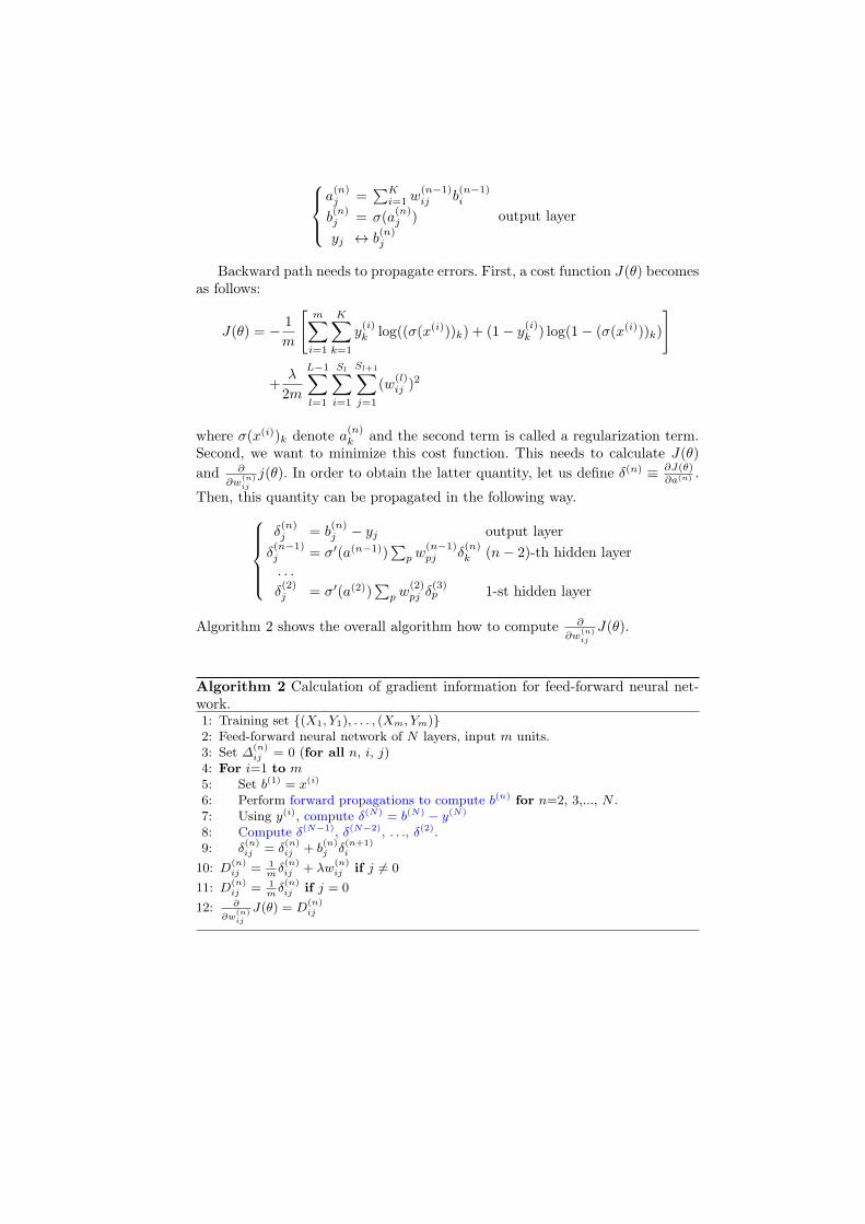
yj ↔ b(n)j

output layer

Backward path needs to propagate errors. First, a cost function J(θ) becomesas follows:

J(θ) = −1

m

[

m∑

i=1

K∑

k=1

y(i)k log((σ(x(i)))k) + (1− y

(i)k ) log(1− (σ(x(i)))k)

]

+λ

2m

L−1∑

l=1

Sl∑

i=1

Sl+1∑

j=1

(w(l)ij )

2

where σ(x(i))k denote a(n)k and the second term is called a regularization term.

Second, we want to minimize this cost function. This needs to calculate J(θ)

and ∂

∂w(n)ij

j(θ). In order to obtain the latter quantity, let us define δ(n) ≡ ∂J(θ)∂a(n) .

Then, this quantity can be propagated in the following way.

δ(n)j = b

(n)j − yj output layer

δ(n−1)j = σ′(a(n−1))

∑

p w(n−1)pj δ

(n)k (n− 2)-th hidden layer

. . .

δ(2)j = σ′(a(2))

∑

p w(2)pj δ

(3)p 1-st hidden layer

Algorithm 2 shows the overall algorithm how to compute ∂

∂w(n)ij

J(θ).

Algorithm 2 Calculation of gradient information for feed-forward neural net-work.1: Training set {(X1, Y1), . . . , (Xm, Ym)}2: Feed-forward neural network of N layers, input m units.3: Set ∆

(n)ij = 0 (for all n, i, j)

4: For i=1 to m5: Set b(1) = x(i)

6: Perform forward propagations to compute b(n) for n=2, 3,..., N .7: Using y(i), compute δ(N) = b(N) − y(N)

8: Compute δ(N−1), δ(N−2), . . ., δ(2).9: δ

(n)ij = δ

(n)ij + b

(n)j δ

(n+1)i

10: D(n)ij = 1

mδ(n)ij + λw

(n)ij if j 6= 0

11: D(n)ij = 1

mδ(n)ij if j = 0

12: ∂

∂w(n)ij

J(θ) = D(n)ij

3.2 Recurrent Neural Network

The left two figures in Figure 5 shows recurrent neural networks (RNNs): theleft most figure shows the folded form and the second left figure shows the un-folded form. The unfolded form is often called backpropagation through time(BPTT) (Robinson and Fallside, 1987). RNNs allow cycles between hidden lay-ers, which is the difference from the feed-forward neural networks. However, thissimple difference is considered to be a key characteristic of RNNs that (fullyconnected) RNNs (with rational valued weights) is equivalent to the universalTuring machine (finite state automata) (Siegelmann and Sontag, 1991) despiteof its difficulty of training and its set up.

There are various models of RNNs. Figure 5 show some of these: from left,RNN, Backpropagation through time (BPTT) (Robinson and Fallside, 1987),bidirectional RNNs (Schuster and Paliwal, 1997),4 and Long Short-Term Mem-ory (LSTM) (Hochreiter and Schmidhuber, 1997).5

hidd

en la

yer

at t−

2

hidd

en la

yer

at t−

1

hidd

en la

yer

at t

input layer

output layer

tt−1t−2

t−2 t−1 t

input layer input layer

output layer output layer

hidd

en la

yer

at t−

2

hidd

en la

yer

at t−

1

hidd

en la

yer

at t

input layertt−1t−2

input layer input layer

output layert−2 t−1 t

output layer output layer

input layer

output layer

hidden layer

recurrent loop

Recurrent Neural Network Recurrent Neural Network (Unfolded) BidirectionalRNNs Recurrent Neural Network (LSTM)

input layertt−1t−2

input layer input layer

output layert−2 t−1 t

output layer output layer

Fig. 5. From left to right, RNN, RNN with BPTT (unfolded), bidirectional RNN, RNNwith LSTM.

As the representative model of RNNs we focus on RNN with backpropagationthrough time (BPTT) (See the second figure from the left in Figure 5). Consider

the network with I input units, H hidden units, and K output units. Let x(t)i

denote the value of input i at time t, a(t)j be the network input to unit j at time

t, b(t)j be the activation of unit j at time t. Similarly with feed-foward network,

4 Bidirectional RNNs intend to access not only the past context but also the futurecontext, which has advantage in sequence labeling task.

5 Other than these, there are Elman networks, Jordan networks, time delay neuralnetworks, and echo state networks.

let us define δ(t)j ≡

∂J(θ)

∂a(t)j

.

Forward Path

{

a(t) =∑I

i=1 wihx(t)i +

∑Hh′=1 wh′hb

(t−1)h′

b(t) = σ(a(t))

Backward Path

{

δ(t) = σ′(a(t))(∑K

k=1 δ(t)k whk +

∑Hh′=1 δ

(t+1)h′ whh′)

δ(t)j = ∂J(θ)

∂a(t)j

(1)

The key difference is that the recurrent path is executed along with time elapse,which are appeared in the equations of forward and backward paths. For theforward path, the contribution of first term of input remains. For the backwardpath, the contribution of first term of output remains. It would be easy to under-stand intuitively if you do Example 1 which calculates forward path. (Althoughthe backward path is more elaborate, it is similar if once understanding thebackpropagation of feed-forward neural network).

Example 1. For given weights shown in Figure below (Ignore biases), run theforward path to obtain y. Consider a logistic sigmoid activation function σ(x) =

11+e−x in output layer (Ignore activation function in hidden layer). Consider therecurrent loop is calculated according to time (BPTT) from t = 0 to t = 2. Notethat the table below is the answer.

0.1 0.10.4 0.4

0.3 0.20.4 0.1

0.1 0.10.4 0.4

0.2 00 0.2

0.3 0.20.4 0.1

0.06 0.060.3 0.3W1

W3

hidden

output Y

input x

Feedforward neural network Recurrent neural network

output Y

input x

output Y output Y

t=0 t=2t=1

W2(t=1)W2(t=0)

W1

W3

Feed-forward NN

x1 x2 h1 h2 y1 y2 h(y1) h(y2)

0 0 0 0 0 0 1.0 1.00 1 0.1 0.4 0.11 0.08 1.12 1.081 0 0.1 0.4 0.11 0.08 1.12 1.081 1 0.2 0.8 0.22 0.16 1.24 1.17

Recurrent NN (t=0)

x1 x2 h1 h2 y1 y2 h(y1) h(y2)

0 0 0 0 0 0 1.0 1.00 1 0.1 0.4 0.11 0.08 1.12 1.081 0 0.1 0.4 0.11 0.08 1.12 1.081 1 0.2 0.8 0.22 0.16 1.24 1.17

Recurrent NN (t=1)

x1 x2 h1 h2 y1 y2 h(y1) h(y2)

0 0 0 0 0 0 1.0 1.00 1 0.48 0.13 0.17 0.21 1.19 1.231 0 0.48 0.13 0.17 0.21 1.19 1.231 1 0.24 0.96 0.26 0.19 1.30 1.21

Recurrent NN (t=2)

x1 x2 h1 h2 y1 y2 h(y1) h(y2)

0 0 0 0 0 0 1.0 1.00 1 0.48 0.13 0.03 0.18 1.03 1.191 0 0.48 0.13 0.03 0.18 1.03 1.191 1 0.24 0.96 0.07 0.36 1.07 1.43

4 Restricted Boltzmann Machine

This section is based on mostly the excerpts from the following article.

– Geoffrey E. Hinton. 2007. Learning multiple layers of representation. Trendsin Cognitive Sciences, 11.

– Geoffrey E. Hinton. 2010. A practical guide to training restricted Boltzmannmachines. UTML TR2010-003.

– Yoshua Bengio. 2009. Learning deep architectures for ai. Foundations andTrends in Machine Learning, 2(1):1–127.

– Deep learning tutorial on the net provides detailed explanation about RBMincluding software implementation using Theano. http://deeplearning.net/tutorial/rbm.html.

Restricted Boltzmann Machine is an energy-based machine (Markov randomfield). This is undirected graphical model in which the topological ordering isnot defined (as in directed graphical model). Instead, potential functions witheach maximal clique is defined. An energy-based model is popular in Physics /statistical mechanics: the characteristic of “memory” is often mentioned in isingmodel or Hopfield network. This class of algorithms include Hopfield network,Boltzmann machine, Restricted Boltzmann machine, and Ising model. It is notedthat some basic materials of undirected graphical model may be useful such asHammersley-Clifford theorem and potential functions (Refer Appendix).

4.1 Predictive Samples

Definition 2 (Energy models; Hopfield Net, Boltzmann Machine, RBM).The energy of these three models are defined as follows.

– Hopfield Net

E(s) = −∑

j

sibi −∑

i<j

sisjwij

v2

v1

v3

2 1

−1

Boltzmann MachineHpfield Net Restricted Boltzmann Machine

v1 v2

h2h1

−1

21

1

v1 v2

h2h1

−1

2 1

Fig. 6. From left to right three figures show Hopfield network, Boltzmann machineand RBM. The number attached near the arc shows weights which are used for a smallexcercise in Example 2.

Hopfield Net

s1 s2 s3 -E e−E p(v)

0 0 00 0 10 1 00 1 11 0 01 0 11 1 01 1 1

Boltzmann Machine

v1 v2 h1 h2 -E e−E p(v, h) p(v)

0 0 0 00 0 0 10 0 1 00 0 1 1

0 1 0 00 1 0 10 1 1 00 1 1 1

1 0 0 01 0 0 11 0 1 01 0 1 1

1 1 0 01 1 0 11 1 1 01 1 1 1

RBM

-E e−E p(v, h) p(v)

Table 1. Question is to fill in the yellow column in the above three tables. There arethree tables where each table corresponds to the networks written in Figure 6: the leftmost corresponds to Hopfield net, the middle is Boltzmann Machine, and the rightmost is Restricted Boltzmann Machine.

– Boltzmann Machine

E(v, h) = −∑

i∈visible

vibi −∑

k∈hidden

hkbk −∑

vivjwij −∑

vihjwik −∑

hkhlwkl

– Restricted Boltzmann Machine

E(v, h) = −∑

i∈visible

vibi −∑

k∈hidden

hkbk −∑

vihjwik

Example 2 (Energy-based Model). By this example we are going to infer the pos-terior samples (to generate samples) by hand when the model is specified. Weconsider three kinds of energy-based models: Hopfield net, Boltzmann machine,and Restricted Boltzmann Machine. For simplicity, we are given the model pa-rameters of weights (we ignore bias) as in Figure 6.

1. For simplicity we suppose that all the bias bi = 0. For all configurations,calculate energy E. (Hint. In Hopfield net, suppose that v1, v2, v3 = [1, 1, 1].The energy can be calculated by E(s) = −

∑

i<j sisjwij = 1 × 1 × 2 + 1 ×1× (−1) + 1× 1× 1 = 0.)

2. Then for Hopfield net, calculate e−E , p(v). (Hint. In Hopfield net, calculateit using a calculator. If you use python, use numpy.exp(1).) In order to

calculate p(v), use p(v) = e−E∑

e−E .

3. For Boltzmann Machine and RBM, calculate e−E , p(v, h), then p(v). For thecalculation of p(v), you need to marginalize out h1 and h2 from the tables.

The answer of the above example is in Table 2.

Hopfield Net

s1 s2 s3 -E e−E p(v)

0 0 0 0 1 0.0450 0 1 0 1 0.0450 1 0 0 1 0.0450 1 1 -1 0.37 0.0171 0 0 0 1 0.0451 0 1 1 2.72 0.1241 1 0 2 7.39 0.3371 1 1 2 7.39 0.337

- - - - 21.87 -

Boltzmann Machine

v1 v2 h1 h2 -E e−E p(v, h) p(v)

0 0 0 0 0 1 0.025 0.0840 0 0 1 0 1 0.0250 0 1 0 0 1 0.0250 0 1 1 -1 0.37 0.009

0 1 0 0 0 1 0.025 0.1440 1 0 1 1 2.72 0.0690 1 1 0 0 1 0.0250 1 1 1 0 1 0.025

1 0 0 0 0 1 0.025 0.3061 0 0 1 0 1 0.0251 0 1 0 2 7.39 0.1871 0 1 1 1 2.72 0.069

1 1 0 0 0 1 0.025 0.4681 1 0 1 1 2.72 0.0691 1 1 0 2 7.39 0.1871 1 1 1 2 7.39 0.187

- - - - - 39.60 - -

RBM

-E e−E p(v, h) p(v)

0 1 0.0140 0.0560 1 0.01400 1 0.01400 1 0.0140

0 1 0.0140 0.0712-1 0.37 0.00521 2.72 0.0380 1 0.0140

0 1 0.0140 0.4362 7.39 0.1031 2.72 0.0383 20.1 0.281

0 1 0.0140 0.4361 2.72 0.0382 7.39 0.1033 20.1 0.281

- 71.5Table 2. This table shows an answer for Example 2.

4.2 Negative Log-Likelihood

In Example 2 we inferred the predictive samples when the model is specified. Weunderstand that the global energy is the sum of many contributions and thateach contribution depends on one connection weight and the binary states oftwo neurons.

For an energy-based model without hidden variables (e.g. Hopfield networks),we consider to evaluate the negative log-likelihood (Refer Figure 3 for variousloss functions) and learn the parameters.

p(x) =e−E(x)

Zwhere Z =

∑

x

e−E(x) (2)

Using the (stochastic) gradient descent which seeks the direction of the gradientof the negative log-likelihood of the training data, we learn the optimal modelparameters by minimizing the negative log-likelihood.

ℓ(θ,D) = −L(θ,D) where L(θ,D) =1

N

∑

x(i)∈D

log p(x(i)) (3)

For an energy-based model with hidden variables (e.g. Boltzmann Machineand RBM) we use the free energy where free energy is defined as the negativelog of the probability with the state of the binary hidden variable integrated out(Hinton and Teh, 2001; Bengio, 2009):

F(x) = − log∑

h

e−E(x,h) (4)

By this, we can write the following.

P (x) =e−F(x)

Zwhere Z =

∑

x

e−F(x) (5)

The gradient of the negative log-likelihood, in this case, is as follows:

−∂ log p(x)

∂θ=

∂F(x)

∂θ−

∑

x

p(x)∂F(x)

∂θ(6)

=∂F(x)

∂θ−

1

|N |

∑

x∈N

∂F(x)

∂θ. (7)

where the second line means that we are doing sampling. The first term ∂F(x)∂θ

in-creases the probability of training data by reducing the corresponding free energy

(positive phase), while the second term 1|N |

∑

x∈N∂F(x)∂θ

decreases the probabil-

ity of samples generated by the model (negative phase). Figure 7 illustrates thepositive phase as “push down” and the negative phase as “pull up”.

F(v) = −∑

i∈visible

vibi −∑

i

log∑

hi

ehi(ci+Wiv) (8)

4.3 RBM

In the previous two subsections we briefly overview the energy-based machine.

1. RBM does not have hidden-hidden and visible-visible interactions. (Comparethe network architecture of RBM with Boltzmann Machine in Figure 6).

2. The gradient of negative log-likelihood in RBM has two terms. (See Equation(7). Compare the model without hidden variables and the model with hiddenvariables)

The network architecture of RBM is depicted in Figure 8. There is no con-nection between nodes in the same layers: all the links are between hidden andvisible variables. Hence, the hidden variables in RBM are conditionally inde-pendent given the visible variables. We say this using “explaining away” (Seethe explanation of “explaining away” in Figure 9). With this restriction, the

Fig. 7. The first term needs “push down” the energy while the second term needs “pullup” the energy in the left side of figure. [LeCun]

RBM possesses the useful properties. First, the conditional distribution over thehidden units factorizes given the visibles as in (9):

P (h|v) =∏

i

P (hi|v)

P (hi = 1|v) = σ(∑

j

Wjivj + di) (9)

Second, the conditional distribution over the visible units given the hidden unitsfactorizes as well as in (10):

P (v|h) =∏

j

P (vj |h)

P (vj = 1|h) = σ(∑

j

Wjihi + bj) (10)

These conditional factorization properties imply that most inferences of our in-terests are readily tractable. Given the conditional independence in Eq. (9) theRBM feature representation, which is the set of posterior marginals P (hi|v), be-comes instantly available. Hence the positive phase of Eq. 7 is readily tractable.

For the negative phase of Eq. 7, the partition function, however, still involvessumming an exponential number of terms. However, due to the conditional in-

hidden

visible

h1 h3h2

v2v1

Fig. 8. Network architecture of RBM.

dependence property of RBM we can sample (v(l), h(l)) using a block Gibbssampling as in (11):

v(l) ∼ P (v|h(l−1))

h(l) ∼ P (h|v(l)) (11)

The most naive approach is to start a Gibbs sampling chain until the chainconverges to the equilibrium distribution and then draw a sufficient number ofsamples to approximate the expected gradient with respect to the model (joint)distribution. Then, restart the process for the next step of approximate gradientascent on the log-likelihood. However, this is prohibitively expensive.

The contrastive divergence (CD) method, instead, initializes the Markovchain with a training data used in the positive phase. The training data inthe positive phase is likely to be already close to the (final) true distribution.Hence, even with a very short (one step) Gibbs chain, this method is believed toapproximate the negative phase expectation. Although the samples drawn fromvery short Gibbs chain may be a poor representation of the model distribution,they are at least moving in the direction of the model distribution relative tothe data distribution represented by the positive phase training data. Eventu-ally, they may combine to produce a good estimate of the gradient. Note thatCD with only 1 step of Gibbs sampling is practically used.

5 Materials for Further Study

This lecture note only covers very rapid way until 38 page of the following article.

– Yoshua Bengio. 2009. Learning deep architectures for AI. Foundations andTrends in Machine Learning, 2(1):1–127.

In order to obtain hierarchical feature representation, RBM needs to be stackedin layers via Deep Belief Network or Deep Boltzmann Machine. We skip all thedescription about auto-encoder and its variants.

The deep learning portal is on http://deeplearning.net, which provides soft-ware, tutorials, papers, and so forth. There are many excellent videos availableon internet in which the researchers who contributed the progress in this areaexplain this area by their words.

earthquake truck hits house

house jumps

A

C

head−to−headhead−to−tailtail−to−tail

BD

E F

G

H

I

Fig. 9. Explain what is “explaining away”? Node D is tail-to-tail w.r.t the path fromE to F (left). Node H is head-to-tail w.r.t. the path from G to I (middle). Node Cis head-to-head w.r.t. the path from A to B (right). A tail-to-tail node or a head-to-tail node leaves a path unblocked unless it is observed in which case it blocks thepath. In contrast, a head-to-head node blocks a path if it is unobserved, but once thenode is observed the path becomes unblocked (This phenomenon is called “explainingaway”). In other words, as a result of (C) (=observing the house jumps), event (A)(=earthquake) and (B) (=truck hits house) becomes dependent on each other..

– Yann LeCun (ICML 2013 tutorial) techtalks.tv– Geoffrey Hinton (Google tech talk, coursera)– Andrew Ng (UCLA IPAM summer school, coursera) / Christopher Manning

(NAACL tutorial) techtalks.tv– Yoshua Bengio youtube.com

Many video lectures are available in the following sites.

– youtube.com– videolectures.net– techtalks.tv– UCLA IPAM summer school.– googletechtalk– coursera– NIPS tutorials

There are many software for deep learning. Among these, Theano and deeplearning tutorials are good start point to do excercise.

– RNN related software• rnnlib http://sourceforge.net/projects/rnnl/.• rnnlm toolkit http://rnnlm.org, word2vec https://code.google.com/p/word2vec/.• PyBrain http://pybrain.org.

– RBM related software

Fig. 10. Landscape of deep learning algorithms [LeCun]

• Theano http://deeplearning.net/software/theano.• Deep Learning Tutorials http://deeplearning.net/tutorial.• PyLearn2 https://github.com/lisa-lab/pylearn2.• EBlearn http://koray.kavukcuoglu.org/.• Torch http://torch.ch.

– Other software (auto-encoder, etc)• Look at http://deeplearning.net/software links.

References

Yoshua Bengio. 2009. Learning deep architectures for ai. Foundations andTrends in Machine Learning, 2(1):1–127.

Christopher M. Bishop. 1995. Neural networks for patttern recognition. OxfordUniversity Press.

Christopher M. Bishop. 2006. Pattern recognition and machine learning.Springer.

Geoffrey Hinton and Yee-Whye Teh. 2001. Discovering multiple constraintsthat are frequently approximately satisfied. In Proceedings of Uncertainty inArtificial Intelligence (UAI 2001), pages 227–234.

Geoffry E. Hinton, J. L. McClelland, and D.E. Rumelhart. 1986. Distributedrepresentations. Parallel Distributed Processing: Explorations in the Mi-crostructure of Cognition(Edited by D.E. Rumelhart and J.L. McClelland)MIT Press, 1.

Geoffrey E. Hinton. 2007. Learning multiple layers of representation. Trends inCognitive Sciences, 11.

Sepp Hochreiter and Jurgen Schmidhuber. 1997. Long short-term memory.Neural Computation, 9(8).

Sepp Hochreiter. 1991. Untersuchungen zu dynamischen neuronalen netzen.Diploma thesis (Institut fur Informatik Technische Universitat Munchen).

Kevin P. Murphy. 2012. Machine learning: A probabilistic perspective. MITPress.

B.A. Olshausen and D.J. Field. 1996. Emergence of simple-cell receptive fieldproperties by learning a sparse code for natural images. Nature, 381:607–609.

A.J. Robinson and F. Fallside. 1987. The utility driven dynamic errorpropagation network. Technical report (Cambridge University), CUED/F-INFENG/TR1.

Schuster and Paliwal. 1997. Bidirectional recurrent neural networks. IEEETransactions on Signal Processing, 45:2673–81.

Hava T. Siegelmann and Eduardo D. Sontag. 1991. On the computational powerof neural nets. Journal of Computer and System Sciences, 50:132–150.

Richard Socher, Brody Huval, Christopher D. Manning, and Andrew Y. Ng.2012. Semantic compositionality through recursive matrix-vector spaces.Conference on Empirical Methods in Natural Language Processing.

Background Knowledge of Neural Networks

1-of-K coding scheme This coding scheme encodes the original encodinginto the binary vector with all elements equal to zero except one element. Forexample in multiclass classification problem of 5 class (={a, b, c, d, e}, the classa is encoded as a = [1, 0, 0, 0, 0], the class b as [0, 1, 0, 0, 0], and so forth.

Activation Function

– linear activation function σ(x) = x

– binary threshold function σ(x) = 1 if x > θ (0 otherwise).

– logistic sigmoid function σ(x) = 11+e−x

– tanh function σ(x) = e2x−1e2x+1

– rectified linear function (linear threshold function) σ(x) = x if x > 0 (0otherwise).

– softmax output function σ(xi) =exi

∑Kk′=1

exk′

Nonlinearity It is essential to use nonlinear activation functions, such as tanhand logistic sigmoid, if the network as a whole need to capture nonlinearity.

Differentiability It is required to use differentiable activation function such astanh and logistic sigmoid when you train the network with gradient descentmethods.

undirected graphical model directed graphical model

1

2 3

4

1

2 3

4 5 5

Fig. 11. The figure on the left shows undirected graphical model: this model has threemaximal cliques {1, 2, 3},{2, 3, 4},{3, 5}. The figure on the right shows directed graph-ical model where the number is in topological order where node 1 is the root.

Background Knowledge of Undirected Graphical Model

A clique is a subset of its vertices such that every two vertices in the subsetare connected by an edge. For example in Figure 1, the following is an exampleof clique: {1, 2}, {1, 3}, {2, 3}, {2, 4}, {3, 4}, {3, 5}, {1, 2, 3}, and {2, 3, 4}. (If 1and 4 were connected, {1, 2, 3, 4} would be also a clique; but it is not in thiscase). A maximal clique is a clique which cannot be made any larger withoutlosing the clique property. In this case, maximal cliques are {1, 2, 3},{2, 3, 4}, and{3, 5}. The following Hammersley-Clifford theorem connects potential functionsφc(yc|θc) for clique c with each maximal clique in the graph.

Definition 3 (Hammersley-Clifford). A positive distribution p(y) > 0 sat-isfies the conditional independence properties of an undirected graph G iff p canbe represented as a product of factors, one per maximal clique, i.e.,

p(y|θ) =1

Z(θ)

∏

c∈C

φc(yc|θc) (12)

where C is the set of all the (maximal) cliques of G, and Z(θ) is the partitionfunction given by

Z(θ) =∑

x

∏

c∈C

φc(yc|θc) (13)

Note that the partition function is what ensures the overall distribution sums to1.

By this Hammersley-Clifford theorem, if p satisfies the conditional indepen-dence properties, the model which is drawn in the left in Figure 11 can be written

as follows

p(y|θ) =1

Z(θ)φ123(y1, y2, y3)φ234(y2, y3, y4)φ35(y3, y5) (14)

where partition function Z =∑

y φ123(y1, y2, y3)φ234(y2, y3, y4)φ35(y3, y5).By the connection with statistical physics, there is a model known as the

Gibbs distribution:

p(y|θ) =1

Z(θ)exp(−

∑

c

E(yc|θc)) (15)

where E(yc) > 0 is the energy associated with the variables in clique c. This canbe converted into undirected graphical model.

φc(yc|θc) = exp(−E(yc|θc)) (16)

This undirected graphical model is called an energy-based model (energy-basedprobabilistic model): the high probability states correspond to the low energyconfigurations.

loss formula margin

NLL / MMI E(W,Y i, Xi) + 1βlog

∫y∈Y

e−E(W,y,Xi) >0

energy loss E(W,Y i, Xi) noneperceptron E(W,Y i, Xi)−minY ∈(Y ) E(W,Y,Xi) none

hinge max(0,m+ E(W,Y i, Xi)− E(W,Y i, Xi)) m

log log(1 + eE(W,Y i,Xi)−E(W,Y i,Xi)) >0LVQ2 min(M,max(0, E(W,Y i, Xi)− E(W,Y i, Xi)) 0

MCE (1 + eE(W,Y i,Xi)−E(W,Y i,Xi))−1 >0square-square E(W,Y i, Xi)2 - (max(0, E(W,Y i, Xi)− E(W,Y i, Xi)))2 m

square-exp E(W,Y i, Xi)2 + βe−E(W,Y i,Xi) >0

MEE 1− e−βE(W,Y i,Xi)/∫y∈Y

e−E(W,y,Xi) >0

Table 3. Table shows the overview of various loss functions. “NLL” means negativelog-likelihood. [LeCun]