Embed Size (px)
Citation preview

C6 GPMG and 40 mm AGL weapon
integrated on RWS mounted on TAPV
platformProbability of hit methodology
Dominic Couture
Pierre Gosselin
Prepared By:
Numerica Technologies InC.
3420 rue Lacoste
Québec, QC G2E 4P8 Canada
Project Manager: Pierre Gosselin, (418) 455-1354
Scientific Authority: Rogerio Pimentel, (418) 844-4000 Ext. 4170
Defence R&D Canada – ValcartierContract Report
DRDC Valcartier CR 2010-237
September 2010
The scientific or technical validity of this Contract Report is entirely the responsibility of the contractor and the
contents do not necessarily have the approval or endorsement of Defence R&D Canada.


C6 GPMG and 40 mm AGL weapon integrated on RWS mounted on TAPV platform Probability of hit methodology
Dominic Couture Pierre Gosselin Numerica Technologies Inc. Prepared By: Numerica Technologies Inc. 3420 Lacoste Québec, G2E 4P8, QC Canada Contract Project Manager: Pierre Gosselin, (418) 455-1354 CSA: Dr. Rogerio Pimentel, Defence Scientist, (418) 844-4000 Ext. 4170 The scientific or technical validity of this Contract Report is entirely the responsibility of the Contractor and the contents do not necessarily have the approval or endorsement of Defence R&D Canada.
Defence R&D Canada – Valcartier Contract Report DRDC Valcartier CR 2010-237 September 2010

Principal Author
Original signed by Dominic Couture
Dominic Couture
Numerica Technologies Inc.
Approved by
Original signed by Rogerio Pimentel
Rogerio Pimentel
Contract Scientific Authority, Defence R & D Canada-Valcartier
Approved for release by
Original signed by Marc Lauzon
Marc Lauzon
Section Head, Precision Weapons Section, Defence R & D Canada-Valcartier
© Her Majesty the Queen in Right of Canada, as represented by the Minister of National Defence, 2010
© Sa Majesté la Reine (en droit du Canada), telle que représentée par le ministre de la Défense nationale,
2010

DRDC Valcartier CR 2010-237 i
Abstract ……..
A probability of hit (PHit) methodology has been developed to characterize the overall
performance of the C6 General Purpose Machine Gun (GPMG) and 40 mm Automatic Grenade
Launcher (AGL) Integrated on a Remote Weapon Station (RWS) Mounted on a Tactical
Armoured Patrol Vehicle (TAPV) Platform. The methodology takes into account four (4)
different scenarios (static/moving vehicle to engage a static/moving target) to develop an error
budget of the weapon system.
The error budget analysis breaks down the total dispersion, i.e., the standard deviation (SD) of the
impact point position, into four (4) main error sources: weather, gun, projectile and the Fire
Control System (FCS) Dispersion. The weather dispersion can be developed to see the individual
contributions of the standard deviation of the wind speed, atmospheric temperature and
atmospheric pressure. The Gun dispersion can be developed to see the individual contributions to
the standard deviation of the gun support and the gun barrel. The projectile dispersion can be
developed to see the individual contributions to the standard deviation of the ammunition
dispersion, muzzle velocity, drag-mass ratio and tracer effect. The FCS dispersion can be
developed to see the individual contributions to the standard deviation of the gun laying, target
tracking, vehicle movement and mutual interaction effects.
The PRODAS (PROjectile and Design and Analysis System) budget error and simulation
package were used to model the weapon system performance for different firings conditions. The
experimental data from the static/moving vehicle against static/moving target scenarios necessary
to validate the PRODAS modeling is being obtained in the CFB (Canadian Forces Base).
Résumé ….....
Une méthodologie de probabilité d’impact (PHit) a été développée pour caractériser la
performance globale de la mitrailleuse polyvalente (GPMG) C6 et du lanceur automatique de
grenade (AGL) 40 mm intégrés sur un système d’armement télécommandé (RWS) monté sur un
véhicule de patrouille blindé tactique (TAPV). La méthodologie prend en considération quatre
(4) scénarios différents (véhicule statique/en mouvement qui engage une cible statique/en
mouvement) pour le développement du budget d’erreur du système d’arme.
L’analyse du budget d’erreur décompose la dispersion totale, soit la déviation standard (SD) de la
position du point d’impact, en quatre (4) principales sources d’erreur : Météo, l’arme, projectile et
le système de conduite de tir (FCS). La dispersion météo peut être développée pour analyser les
différentes contributions individuelles de la déviation standard de la vitesse du vent, de la
température atmosphérique et de la pression atmosphérique. La dispersion de l’arme peut être
développée pour analyser les différentes contributions individuelles de la déviation standard du
support et de l’âme de l’arme. La dispersion du projectile peut être développée pour analyser les
différentes contributions individuelles de la déviation standard de la dispersion de la munition, de
la vitesse initiale du projectile, du rapport traînée-masse et l’effet du traceur. La dispersion du
FCS peut être développée pour analyser les différentes contributions individuelles de la déviation

ii DRDC Valcartier CR 2010-237
standard du support de l’arme, du système de pointage de l’arme, le mouvement du véhicule et les
effets d’interactions mutuelles.
L’ensemble numérique de simulation et de calcul du budget d’erreur PRODAS (PROjectile and
Design and Analysis System) ont été utilisés pour la modélisation de la performance du système
d’armement pour différentes conditions de tirs. Les données expérimentales provenant des
scénarios véhicule statique/en mouvement qui engage une cible statique/en mouvement
nécessaires pour valider la modélisation PRODAS seront obtenus à la BFC (Base des Forces
canadiennes).

DRDC Valcartier CR 2010-237 iii
Executive summary
C6 GPMG and 40 mm AGL weapon integrated on RWS mounted on TAPV platform: Probability of hit methodology
; DRDC Valcartier CR 2010-237; Defence R&D Canada – Valcartier; September 2010.
The Tactical Armoured Patrol Vehicle (TAPV) is a general-utility combat vehicle that will fulfill
a wide variety of roles on the battlefield, including but not limited to reconnaissance and
surveillance, security, command and control, cargo and armoured personnel carrier. It will have a
high degree of tactical mobility and provide a very high degree of protection to its crew. The
TAPV is a high-priority procurement project of the Canadian Forces (CF) aiming to replace the
capabilities of the Coyote, RG-31 and increase the Light Utility Vehicle Wheeled (LUVW) fleet.
The TAPV will integrate a Remote Weapon Station (RWS), which shall be capable of mounting
two (2) weapons simultaneously (dual RWS). At time of Request for Proposal (RFP) closing, the
dual RWS shall be capable of mounting a 40 mm Automatic Grenade Launcher (AGL) as a
primary weapon and a C6 (7.62 mm) General Purpose Machine Gun (GPMG) as a secondary
weapon. The TAPV dual RWS shall be operable by the crew commander and gunner from their
respective crew stations inside the vehicle.
A probability of hit (PHit) methodology has been developed to characterize the overall
performance of the C6 GPMG and 40 mm AGL Integrated on a RWS mounted on a TAPV
Platform. The methodology takes into account four (4) different scenarios (static/moving vehicle
to engage a static/moving target) to develop an error budget model of the weapon system. The
error budget analysis breaks down the total dispersion (standard deviation of the impact point
position) into four (4) main error sources: weather, gun, projectile and the Fire Control System
(FCS) dispersion. The weather dispersion can be developed to see the individual contributions of
the standard deviation of the wind speed, atmospheric temperature and atmospheric pressure. The
Gun dispersion can be developed to see the individual contributions of the standard deviation of
the gun support play and the gun barrel. The projectile dispersion can be developed to see the
individual contributions of the standard deviation of the ammunition dispersion, muzzle velocity,
drag mass ratio and tracer effect. The fire control system dispersion can be developed to see the
individual contributions of the standard deviation of the gun laying, target’s tracking, vehicle
movement and mutual interaction effects.
The PRODAS (PROjectile and Design and Analysis System) budget error and simulation
package were used to model the weapon system performance for different firing conditions. The
experimental data from the static/moving vehicle against static/moving target scenarios necessary
to validate the PRODAS modeling is being obtained in the CFB (Canadian Forces Base). The
main difficulties are to characterise the target tracking, vehicle movement and mutual interaction
effect. These effects need to take into account the vehicle, gunner and RWS interaction effect on
the weapon accuracy. Also, the RWS does not have a wind speed and direction sensor to take
into account the weather effect on the accuracy. In addition, the driver and gunner experience can
have a significant influence on the overall weapon system. All these effects need to be
approximated to be able to characterize the realistic weapon performance.
iv DRDC Valcartier CR 2010-237
Sommaire .....
C6 GPMG and 40 mm AGL weapon integrated on RWS mounted on TAPV platform: Probability of hit methodology
; DRDC Valcartier CR 2010-237; R & D pour la défense Canada – Valcartier; Septembre 2010.
Le véhicule de patrouille blindé tactique (TAPV) est un véhicule de combat d’utilité générale qui
répondra à une grande variété de rôles sur le champ de bataille, incluant mais sans se limiter à la
reconnaissance et la surveillance, la sécurité, le commandement et contrôle, fret et transport de
troupes blindé. Il aura un degré élevé de mobilité tactique et fournira un très haut degré de
protection à son équipage. Le TAPV est un projet d’acquisition de haute priorité pour les Forces
canadiennes, qui a pour but de remplacer les capacités du Coyote, RG-31 et augmenter les flottes
de Véhicule utilitaire léger à roues (LUVW). Le TAPV intégrera un système d’armement
télécommandé (RWS) qui sera capable de recevoir le montage de deux (2) armes simultanément
(double RWS). Au moment de la clôture de la demande de proposition (RFP), le double RWS
devra être capable de monter un lanceur automatique de grenades (AGL) 40 mm comme arme
primaire et un C6 (7.62 mm), mitrailleuse polyvalente (GPMG) comme arme secondaire. Le
TAPV avec double RWS devra pouvoir être opéré par le commandant d'équipage et le canonnier
à partir de leurs stations respectives de l'équipage à l'intérieur du véhicule.
Une méthodologie de probabilité d’impact (PHit) a été développée pour caractériser la
performance globale de la C6 et du lanceur automatique de grenade 40 mm (AGL) intégrés sur un
RWS monté sur un TAPV. La méthodologie prend en considération quatre (4) scénarios
différents (véhicule statique/en mouvement qui engage une cible statique/en mouvement) pour le
calcul du facteur erreur. Le calcul du budget d’erreur décompose la dispersion totale (déviation
standard de la position du point d’impact) en quatre (4) principales sources d’erreur : météo,
canon, projectile et le système de conduite de tir. La dispersion météo peut être développée pour
analyser les différentes contributions individuelles de la déviation standard de la vitesse du vent,
température atmosphérique et pression atmosphérique. La dispersion du canon peut être
développée pour analyser les différentes contributions individuelles de la déviation standard du
support à canon et le l’âme du canon. La dispersion du projectile peut être développée pour
analyser les différentes contributions individuelles de la déviation standard de la dispersion de la
munition, vitesse initiale, rapport traînée masse et effet du traceur. La dispersion du système de
conduite de tir peut être développée pour analyser les différentes contributions individuelles de la
déviation standard du pointage du canon, poursuite de cibles, mouvement du véhicule et effet
d’interaction mutuel.
Le budget d’erreur et programme de simulation PRODAS (PROjectile and Design and Analysis
System) ont été utilisés pour modéliser la performance du système d'arme dans des conditions
différentes de tirs. Les données expérimentales provenant des scénarios véhicule statique/en
mouvement qui engage une cible statique/en mouvement nécessaires pour valider la modélisation
PRODAS seront obtenus à la BFC (Base des Forces canadiennes). Les principales difficultés
sont de caractériser le suivi de la cible, le mouvement du véhicule et l’effet de l’interaction
mutuelle. Ces effets doivent prendre en considération l’effet d’interaction du véhicule, canonnier
et du RWS sur la précision de l’arme. Aussi, le RWS n’a pas d’anémomètre ni de capteur de

DRDC Valcartier CR 2010-237 v
direction pour prendre en considération l’effet de la météo sur la précision. De plus, l’expérience
du conducteur et du canonnier peut avoir une influence significative sur la performance globale
de l’arme. Tous ces effets ont besoin d’être approximés pour être en mesure de caractériser une
performance réaliste de l’arme.

vi DRDC Valcartier CR 2010-237
This page intentionally left blank.

DRDC Valcartier CR 2010-237 vii
Table of contents
Abstract …….. ................................................................................................................................. i
Résumé …..... ................................................................................................................................... i
Executive summary ........................................................................................................................ iii
Sommaire ..... .................................................................................................................................. iv
Table of contents ........................................................................................................................... vii
List of figures ................................................................................................................................. ix
List of tables .................................................................................................................................... x
1 Introduction ............................................................................................................................... 1
2 Objectives & Requirements ...................................................................................................... 2
3 Methodology ............................................................................................................................. 2
3.1 Error source ................................................................................................................... 2
3.1.1 Global dispersion ............................................................................................ 5
3.1.2 Weather dispersion .......................................................................................... 6
3.1.3 Gun dispersion ................................................................................................ 8
3.1.3.1 Overall gun dispersion .................................................................. 8
3.1.3.2 Gun dispersion .............................................................................. 9
3.1.3.3 Gun support play dispersion ......................................................... 9
3.1.4 Projectile dispersion ...................................................................................... 10
3.1.4.1 Ammunition dispersion .............................................................. 11
3.1.4.2 Muzzle velocity dispersion ......................................................... 12
3.1.4.3 Drag/Mass dispersion ................................................................. 14
3.1.4.4 Tracer dispersion ........................................................................ 16
3.1.5 Fire Control System dispersion ..................................................................... 18
3.1.5.1 Gun laying dispersion ................................................................. 19
3.1.5.2 Target’s tracking dispersion ....................................................... 21
3.1.5.3 Vehicle movement dispersion..................................................... 23
3.1.5.4 Mutual interaction dispersion ..................................................... 24
3.2 Error budget ................................................................................................................. 25
3.2.1 Static-Static scenario (step 1) ........................................................................ 26
3.2.2 Static- Moving scenario (step 2) ................................................................... 27
3.2.3 Moving-Static scenario (step 3) .................................................................... 28
3.2.4 Moving- Moving scenario (step 4) ................................................................ 29
3.3 PRODAS simulation package ..................................................................................... 30
3.3.1 Inputs to PRODAS module ........................................................................... 32
3.3.1.1 Geometry and mass module........................................................ 32
3.3.1.2 The aero predictions module ...................................................... 34
3.3.1.3 Exit muzzle module .................................................................... 35

viii DRDC Valcartier CR 2010-237
3.3.1.4 Thrust/Tracer/Base burn module ................................................ 36
3.3.1.5 Ground-to-Ground module ......................................................... 36
4 Probability of hit formulation ................................................................................................. 40
4.1 Target standard ............................................................................................................ 42
4.1.1 Personal target ............................................................................................... 42
4.1.2 Vehicle target ................................................................................................ 42
4.2 Formulation ................................................................................................................. 43
5 Comments and Conclusions .................................................................................................... 44
References ..... ............................................................................................................................... 45
List of symbols/abbreviations/acronyms/initialisms ..................................................................... 46
Distribution list .............................................................................................................................. 50

DRDC Valcartier CR 2010-237 ix
List of figures
Figure 1: Dispersion analysis block diagram. ................................................................................. 4
Figure 2: Representation of the standard deviation of the relative target velocity. ....................... 22
Figure 3: Representation of a possible static-static scenario. ........................................................ 26
Figure 4: Representation of a possible static vehicle and moving target engagement. ................. 27
Figure 5: Representation of a possible moving vehicle and static target engagement. ................. 28
Figure 6: Representation of a possible moving vehicle and moving target engagement............... 29
Figure 7: PRODAS analysis options. ............................................................................................ 32
Figure 8: Projectile geometry example - 7.62 mm C19. ................................................................ 33
Figure 9: System effectiveness simulation block diagram. ........................................................... 36

x DRDC Valcartier CR 2010-237
List of tables
Table 1: Global dispersion parameter. ............................................................................................. 5
Table 2: Weather dispersion parameters. ........................................................................................ 6
Table 3: Gun dispersion parameters. ............................................................................................... 8
Table 4: Projectile dispersion parameter. ...................................................................................... 10
Table 5: Ammunition dispersion parameters. ................................................................................ 11
Table 6: Muzzle velocity dispersion parameters. .......................................................................... 12
Table 7: Drag/Mass dispersion parameters. .................................................................................. 14
Table 8: Tracer dispersion parameters. .......................................................................................... 16
Table 9: Fire Control System dispersion parameter. ..................................................................... 18
Table 10: Gun laying dispersion parameters. ................................................................................ 19
Table 11: Target’s tracking dispersion parameters. ....................................................................... 21
Table 12: Vehicle movement dispersion parameter. ..................................................................... 23
Table 13: Mutual interaction dispersion parameter. ...................................................................... 24
Table 14: Error budget. .................................................................................................................. 25
Table 15: Ammunition mass model properties. ............................................................................. 33
Table 16: Example of the aerodynamic coefficients and stability derivatives. ............................. 34
Table 17: Typical inputs file for system effectiveness simulation (fictive values). ...................... 37
Table 18: PRODAS error budget. ................................................................................................. 41

DRDC Valcartier CR 2010-237 1
1 Introduction
The Tactical Armoured Patrol Vehicle (TAPV) is a general-utility combat vehicle that will fulfill
a wide variety of roles on the battlefield, including but not limited to reconnaissance and
surveillance, security, command and control, cargo and armoured personnel carrier. It will have a
high degree of tactical mobility and provide a very high degree of protection to its crew. The
TAPV will replace the capabilities of the Coyote, RG-31 and increase the Light Utility Vehicle
Wheeled (LUVW) fleet.
The TAPV will integrate a Remote Weapon Station (RWS), which shall be capable of mounting
two (2) weapons simultaneously (dual RWS). At time of Request for Proposal (RFP) closing, the
dual RWS shall be capable of mounting a 40mm automatic grenade launcher (AGL) as a primary
weapon and a C6 (7.62 mm) general purpose machine gun as a secondary weapon. The TAPV
dual RWS shall be operable by the crew commander and gunner from their respective crew
stations inside the vehicle.
The C6 provided will be one of the in-service Canadian Forces (CF) weapons. It is unknown at
this time which 40 mm AGL will be the weapon that is awarded through the Close Area
Suppression Weapon System (CASW) project. However, for the purpose of this task given that it
will be an in-service weapon, the CASW technical data can be used as a benchmark or reference.

2 DRDC Valcartier CR 2010-237
2 Objectives & Requirements
The objective of this report is to provide a methodology to obtain the ammunition PHit of the C6
GPMG and 40 mm AGL weapons, integrated on a RWS mounted on a TAPV platform to be used
within the Statement of Operational Requirements (SOR) and in turn translated into Vehicle
Performance Specifications (VPS) for the TAPV project [1]. This methodology requires
development for:
Identifying error sources
Modeling a budget error for different scenarios
Static TAPV versus static target
Static TAPV versus moving target
Moving TAPV versus static target
Moving TAPV versus moving target
Input process into PRODAS numerical tools
From this study, future fire tests could be reviewed to improve the overall requirements and
procedures.
3 Methodology
In support to CASW project, error budget modeling in PRODAS has already been used with
success in previous studies at DRDC Valcartier for accessing performance of 40 mm AGL for
static weapon against static target scenario [2],[3],[4]. In the present study, to identify the main
error sources for evaluation of the overall performance of the C6 GPMG and 40 mm AGL
Integrated on a RWS mounted on a TAPV Platform, the methodology has been slightly modified
to take into account the particularity of the weapon system and the different operational scenarios.
This study was developed in three (3) sections: Error source, Error Budget and PRODAS
Simulation Package [5]. The first section describes all error sources and their inter-relation
required to characterize the weapon system. The second section identifies the methodology to
resolve the budget error for each scenario (static/moving vehicle to hit a static/moving target).
The last section presents the PRODAS Simulation Package used to simulate PHit of the weapon
system.
3.1 Error source
A multitude of error sources have been identified to support the PHit modeling of the weapon
system for various scenarios. The block diagram presented in Figure 1 show a dispersion analysis
used in this study.

DRDC Valcartier CR 2010-237 3
In general, the dispersion errors presented in this report will require two (2) independent
components, since they can be different in the azimuth and elevation planes. Nonetheless, some
comments will be added if the azimuth and elevation planes require a different analysis. Each
error is defined in a one-sigma standard deviation and the unit used is mils. The mils unit is
defined by a deviation of 1 meter at a distance of 1000 m and is approximately equal to 1 mrad.
Equation (1) shows the relation between mils and mrad:
mrad 1 rad 0.001rad 1000
1tan mils 1
1000m
1m 1
(1)
Also, some parameters require a statistic analysis of the experimental data. Equations (2) and (3)
show the average and the standard deviation equations respectively:
N
xx
N
ii
1
(2)
1
1
2
N
xxN
ii
(3)

4 DRDC Valcartier CR 2010-237
Global Dispersion TotalS
WDS
FCSS
GDS
PDS
Fire Control System
GLDS TTDS
SD
AM
SD
RD
SD
RND
SDLOS
SD
SOLB
SD
Gunș SD
Gunș
SDVTarget
TargetR SD
TargetR
TargetH SD
TargetH
SD
Gun SD
Gun
Projectile Dispersion
D/MSTDS
MVVSADS
MV
RRSD
MV
LLSD
MV
SD
%Tr SDMD%
SDM
M
X0C
SD
X0C
DA
DAJ
DPJ
Weather Dispersion Gun DispersionSD
WV SD
AP SD
AT
Experimental Data
Processed Data
Error Source
Main Error Source
SD
DGS SD
DG
VMD
S MIDS
Figure 1: Dispersion analysis block diagram.

DRDC Valcartier CR 2010-237 5
3.1.1 Global dispersion
The global dispersion is the standard deviation of the projectile impact about the mean point of
impact (MPI). This parameter needs to be evaluated for each round fired. Table 1 shows the
global dispersion parameter.
Table 1: Global dispersion parameter.
Symbol Unit Description
TotalS mils Global dispersion
(SD of the impact points)
SD
TotalX meter SD of the impact points
Experimentally, the global dispersion ( TotalS ) represents the standard deviation of the impact
points measured (SD
TotalX ) on the target azimuth and elevation planes. The standard deviation is
calculated with equation (3) on all impact points. The global dispersion can be evaluated in mils
by equation (4), where TargetR is the average target’s range in meter.
Target
SD
Total1
Total
Xtan1000S
R (4)
Theoretically, the global dispersion can be obtained by equation (5), where the global dispersion
equals the root of the square summation of the four (4) different dispersion subsections, which are
the Weather, Gun, Projectile and Fire Control System:
2
FCS
2
WD
2
GD
2
PDTotal SSSSS (5)
Equations (4) and (5) are similar for the azimuth and elevation planes, but their values can be
different.
6 DRDC Valcartier CR 2010-237
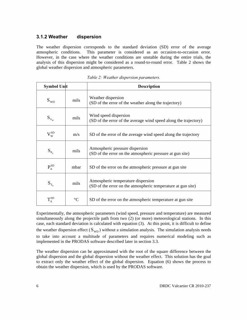
3.1.2 Weather dispersion
The weather dispersion corresponds to the standard deviation (SD) error of the average
atmospheric conditions. This parameter is considered as an occasion-to-occasion error.
However, in the case where the weather conditions are unstable during the entire trials, the
analysis of this dispersion might be considered as a round-to-round error. Table 2 shows the
global weather dispersion and atmospheric parameters.
Table 2: Weather dispersion parameters.
Symbol Unit Description
WDS mils Weather dispersion
(SD of the error of the weather along the trajectory)
WVS mils Wind speed dispersion
(SD of the error of the average wind speed along the trajectory)
SD
WV m/s SD of the error of the average wind speed along the trajectory
APS mils Atmospheric pressure dispersion
(SD of the error on the atmospheric pressure at gun site)
SD
AP mbar SD of the error on the atmospheric pressure at gun site
ATS mils Atmospheric temperature dispersion
(SD of the error on the atmospheric temperature at gun site)
SD
AT °C SD of the error on the atmospheric temperature at gun site
Experimentally, the atmospheric parameters (wind speed, pressure and temperature) are measured
simultaneously along the projectile path from two (2) (or more) meteorological stations. In this
case, each standard deviation is calculated with equation (3). At this point, it is difficult to define
the weather dispersion effect ( WDS ) without a simulation analysis. The simulation analysis needs
to take into account a multitude of parameters and requires numerical modeling such as
implemented in the PRODAS software described later in section 3.3.
The weather dispersion can be approximated with the root of the square difference between the
global dispersion and the global dispersion without the weather effect. This solution has the goal
to extract only the weather effect of the global dispersion. Equation (6) shows the process to
obtain the weather dispersion, which is used by the PRODAS software.

DRDC Valcartier CR 2010-237 7
2
effect weather ewithout th dispersion global
0
SD
A0
SD
A0
SD
W PRODAS
2
effect weather with the dispersion global
SD
A
SD
A
SD
W PRODASWD T,P,VT,P,VS
ff (6)
Equation (6) is the same for the azimuth and elevation planes, but their values can be different. In
addition, the same procedure can be reused three (3) times to separate only the wind speed (WVS ),
pressure (AP
S ) or temperature (ATS ) dispersion effect. The weather dispersion can be obtained at
this time by equation (7).
2
T
2
P
2
VWD AAWSSSS (7)

8 DRDC Valcartier CR 2010-237
3.1.3 Gun dispersion
The overall gun dispersion is a round-to-round error and it is the component of the dispersion
attributed to the gun support play and gun barrel. The gun support play dispersion corresponds to
the looseness of the fixed gun on its support and the RWS assembly itself. The gun dispersion is
the dispersion exclusively due to the barrel. Table 3 shows the general gun dispersion
parameters.
Table 3: Gun dispersion parameters.
Symbol Unit Description
GDS mils Gun Dispersion
(SD of the overall Gun Dispersion)
SDXGD meter SD of the overall gun barrel head position
GSPS mils Gun Support Play Dispersion
(SD of the Gun Support Play Dispersion)
GBS mils Gun Barrel Dispersion
(SD of the Gun Barrel Dispersion)
3.1.3.1 Overall gun dispersion
Experimentally, the overall gun dispersion ( GDS ) represents the standard deviation of the overall
gun barrel head position (SDXGD ) during the fire trials on the target azimuth and elevation planes.
The standard deviation is obtained with equation (3) on the overall gun barrel head position. The
gun barrel head position is evaluated usually with two (2) perpendiculars high-speed videos (side
and top views). The overall gun dispersion can be evaluated in mils with equation (8),
where M/RWSD is the distance between the RWS elevation axis and the barrel muzzle exit.
M/RWS
Trials FireWith
SD
1
GD
Xtan1000S
DGD
(8)
Also, equation (9) shows that the overall gun dispersion can also be obtained by the root of the
square summation of the dispersion of the gun support and gun.

DRDC Valcartier CR 2010-237 9
2GB
2
GSPGD SSS (9)
3.1.3.2 Gun dispersion
Experimentally, the gun barrel dispersion ( GBS ) represents the standard deviation of the gun
barrel head position during the fire trials on the target azimuth and elevation planes. However,
the weapon needs to be rigidly fixed to the ground to take into account only the gun barrel
dispersion effect without any support and RWS mechanical play. This procedure requires that the
same gun has to be used.
3.1.3.3 Gun support play dispersion
Theoretically, gun support play dispersion can be approximated with the root of the square
difference between the overall gun dispersion and the gun barrel dispersion. This solution has the
goal to extract only the gun support and the RWS mechanical play effects of the overall gun
dispersion. Equation (10) shows the process to obtain the gun support play dispersion:
2GB
2
GDGSP SSS (10)
Experimentally, the maximum gun support play dispersion can be directly approximated by an
evaluation of the gun support play limits without the fire trials. In this case, the methodology
consists to evaluate of the maximum overall gun barrel head position (with the initial position as
reference), when the gunner moves manually the muzzle exit in the limits of the gun support and
the RWS mechanical play. However, this procedure doesn’t take into account the RWS and
TAPV effects during the firing. The gun support dispersion can be evaluated in mils by equation
(11), where M/RWSD is the distance between the RWS rotation axis and the barrel muzzle exit.
M/RWS
Trials FireWithout
Maxium
1
GSP
Xtan1000S
DGD
(11)
Equations (8), (9), (10) and (11) are the same for the azimuth and elevation planes, but their
values can be different.

10 DRDC Valcartier CR 2010-237
3.1.4 Projectile dispersion
The projectile dispersion can be a round-to-round error and an occasion-to-occasion error. It is
the component of the dispersion attributed to the muzzle gun properties and ammunition flight-
out. Table 4 shows the general projectile dispersion parameters.
Table 4: Projectile dispersion parameter.
Symbol Unit Description
PDS mils Projectile Dispersion
(SD of the Projectile Dispersion)
Experimentally, the projectile dispersion represents the standard deviation of the projectile during
the flight-out. However, the projectile dispersion can’t be obtained directly from the
experimental data. Thus, the projectile dispersion is a summarized value and is obtained
analytically to characterize the muzzle gun properties and ammunition flight-out. Equation (12)
shows that the projectile dispersion is obtained by the root of the square summation the four (4)
different dispersion subsections as: ammunition, muzzle velocity, drag/mass effect and tracer
effect.
2
TD
2
D/M
2
V
2
ADPD SSSSSMV
(12)
Equation (12) is the same for the azimuth and elevation planes, but their values can be different.

DRDC Valcartier CR 2010-237 11
3.1.4.1 Ammunition dispersion
The ammunition dispersion is a round-to-round error and is the component of the dispersion
attributed to the ammunition shell from a fixed mount. Table 5 shows the general ammunition
dispersion parameters.
Table 5: Ammunition dispersion parameters.
Symbol Unit Description
ADS , DA mils Ammunition Dispersion
(SD of the Overall Ammunition Dispersion.)
DPJ mils SD of the Projectile jump
DAJ mils SD of the Aerodynamic jump
Experimentally, the ammunition dispersion represents the standard deviation of the projectile
jump and the aerodynamic jump using the “Mann Barrel” on a fix mount. The aerodynamic jump
can be calculated with the linear theory of ballistic using the first maximum yaw measured from
an aeroballistics’ range trial. The projectile jump can be also calculated with an effect of a center
of gravity (offset from a projectile x-axis). Both jumps are determined by the analytical equations
shown in section 3.3.1.3. The ammunition dispersion is defined by the magnitude of the previous
combined effects shown by equation (13).
2
D
2
DDAD AJPJAS (13)
Equation (13) is the same for the azimuth and elevation planes and their values are also the same
for both planes.

12 DRDC Valcartier CR 2010-237
3.1.4.2 Muzzle velocity dispersion
The muzzle velocity dispersion corresponds to the standard deviation of the error of the muzzle
velocity effect. This analysis takes into account the round-to-round error and the occasion-to-
occasion error into two (2) different parameters. Table 6 shows the general muzzle velocity
dispersion and parameters.
Table 6: Muzzle velocity dispersion parameters.
Symbol Unit Description
MVVS mils Muzzle Velocity Dispersion
(SD of overall muzzle velocity effect)
MV m/s Reference muzzle velocity at 21 °C
RRSD
MV m/s
SD of muzzle velocity within a lot of ammunition at 21 °C
(round-to-round error)
LLSD
MV m/s
SD of muzzle velocity between lots of ammunition at 21 °C
(occasion-to-occasion error)
Experimentally, the reference muzzle velocity is an average value measured and deduced from
Doppler radar tests. From these values, the standard deviations of the muzzle velocity are defined
with equation (3) for the projectile within a lot and between lots of ammunition. At this point, it
is difficult to define only the muzzle velocity dispersion effect (MVVS ) without a simulation
analysis. The simulation analysis needs to take into account a multitude of parameters and
requires a software simulation such as PRODAS as described in section 3.3. The muzzle velocity
dispersion can be approximated with the root of the square difference between the global
dispersion and the global dispersion without the weather error effect. This solution has the goal
to extract only the muzzle velocity effect of the global dispersion. Equation (14) shows the
process to obtain the muzzle velocity dispersion, which is used by the PRODAS software
simulation.
2
effect velocity muzzle ewithout th dispersion global
0
LLSD
M0
RRSD
M PRODAS
2
effect velocity muzzle with the dispersion global
LLSD
M
RRSD
M PRODASWD V,VV,VS
ff (14)

DRDC Valcartier CR 2010-237 13
Equation (14) is the same for the azimuth and elevation planes, but their values can be different.
In addition, the same procedure can be reused two (2) times to separate the muzzle velocity
dispersion effect of the projectile within a lot and between lots of ammunition.

14 DRDC Valcartier CR 2010-237
3.1.4.3 Drag/Mass dispersion
The Drag/Mass dispersion is a round-to-round error and corresponds to the standard deviation of
the error of the projectile drag and mass percentage ratio. Table 7 shows the general drag/mass
dispersion and parameters.
Table 7: Drag/Mass dispersion parameters.
Symbol Unit Description
D/MS mils Drag/Mass Dispersion
(SD of Drag/Mass percentage ratio)
SDMD%
% SD of Drag Mass percentage ratio
M kg Average of the mass of projectile
SDM kg SD of the mass of projectile
SD
%M % Percentage of the SD of the mass of projectile
0XC Average of the drag coefficient of projectile
(Average of the axial force coefficient)
SD
0C X SD of the drag coefficient of projectile
(SD of the axial force coefficient)
SD
0%C X % Percentage of the SD of the drag coefficient of projectile
The drag error is the variation of the drag coefficient (axial force coefficient) over the trajectory.
It is essentially a result of the shape reproduction/tolerance and the non-uniform rotating band
ware. Experimentally, the drag coefficient of the projectile ( 0XC ) is obtained from the velocity
Doppler radar trace measured over the trajectory. Equation (15) shows the relation to obtain the
axial force coefficient form the velocity Doppler radar trace, where M is the projectile mass,
A is the atmospheric air density, refA is the projectile reference area and V is the projectile
velocity:

DRDC Valcartier CR 2010-237 15
2
refA
0VA21
MV
dt
dCX (15)
From equation (15), the average and standard deviations of the drag coefficient ( 0XC ,SD
0C X ) is
defined with equations (2) and (3) at each Mach number on the overall projectiles fired. The
average and the standard deviations of the projectile mass ( M ,SDM ) are calculated with
equations (2) and (3) on the overall projectiles fired. At this point, it is difficult to define only the
Drag/Mass dispersion effect ( D/MS ) without a simulation analysis. The simulation analysis needs
to take into account a multitude of parameters and requires a software simulation such as
PRODAS as described in section 3.3. The Drag/Mass dispersion can be approximated with the
root of the square difference between the global dispersion and the global dispersion without the
Drag/Mass error effect. This solution has the goal to extract only the Drag/Mass effect of the
global dispersion. Equations (16) and (17) show the process to obtain the Drag/Mass dispersion,
which is used by the PRODAS software simulation and SDMD%
is a specific PRODAS
parameter to define the percentage of the standard deviation of Drag/Mass ratio.
SDSD0 0
2
CM
M M
SD X XCD M (16)
2
effect Drag/Mass ewithout th dispersion global
0% PRODAS
2
effect Drag/Mass with the dispersion global
% PRODASD/MS
SDSD MDfMDf (17)
Equation (17) is the same for the azimuth and elevation planes, but their values can be different.

16 DRDC Valcartier CR 2010-237
3.1.4.4 Tracer dispersion
The tracer dispersion is a round-to-round error and corresponds to the standard deviation of the
error of the projectile tracer. Table 8 shows the general tracer dispersion and parameter.
Table 8: Tracer dispersion parameters.
Symbol Unit Description
TDS mils Tracer Dispersion
(SD of the tracer)
Tr Average of the thrust coefficient of projectile
(Average of the axial force coefficient)
SDTr SD of the tracer
SD
%Tr % Percentage of SD of the tracer
The tracer error is the variation of the drag coefficient (or axial force coefficient or retard) over
the trajectory when the tracer is active. It is essentially a result of the tracer powder mass
tolerance and the gun barrel temperature interaction during the combustion. Experimentally, the
tracer coefficient of the projectile ( Tr ) is approximated from the difference of the velocity
Doppler radar trace measured between the active and without tracer effect over the trajectory.
Equation (18) shows the relation to obtain the tracer coefficient of the projectile ( Tr ) from the
active tracer effect (AT
0XC ) and without the tracer effect (WT
0XC ):
TracerWithout
WT
0
Tracer Active
AT
0 Tr XX CC (18)
Equation (19) shows the relation to obtain the tracer coefficient of the active tracer effect (AT
0XC )
that can be obtained by the axial force coefficient from the velocity Doppler radar trace, when the
tracer is active. M is the projectile mass, tPM is the tracer powder mass as function of time,
A is the atmospheric air density, refA is the projectile reference area and V is the projectile
velocity:
2
refA
PAT
0VA21
MMV
tdtd
CX
(19)

DRDC Valcartier CR 2010-237 17
Equation (20) shows the relation to obtain the tracer coefficient without tracer effect (WT
0XC ) that
can be obtained by the axial force coefficient from the velocity Doppler radar trace, when the
tracer doesn’t have the tracer powder. M is the projectile mass, A is the atmospheric air density,
refA is the projectile reference area and V is the projectile velocity:
2
refA
WT
0VA21
MV
dt
dCX (20)
From equation (18), the average and standard deviations of the drag coefficient ( Tr ,SDTr ) are
defined with equations (2) and (3) at each Mach number on the overall projectiles fired. At this
point, it is difficult to define only the tracer dispersion effect ( TDS ) without a simulation analysis.
The simulation analysis needs to take into account a multitude of parameters and requires a
software simulation such as PRODAS described in section 3.3. The tracer dispersion can be
approximated with the root of the square difference between the global dispersion and the global
dispersion without the tracer error effect. This solution has the goal to extract only the tracer
effect of the global dispersion. Equations (21) and (22) show the process to obtain the tracer
dispersion, which is used by the PRODAS software simulation. SD
%Tr is a specific PRODAS
parameter to define the percentage of the standard deviation of the tracer.
Tr
TrTr
SD
SD
% (21)
2
effect tracer ewithout th dispersion global
0
SD
% PRODAS
2
effect tracer with the dispersion global
SD
% PRODASTD TrTrS
ff (22)
Equation (22) is the same for the azimuth and elevation planes, but their values can be different.

18 DRDC Valcartier CR 2010-237
3.1.5 Fire Control System dispersion
The FCS dispersion is an occasion-to-occasion error. It is the component of the dispersion
attributed to the alignment, aiming, target’s tracking and vehicle movement errors. For a RWS
mounted on TAPV platform, the fire control system is considered as a black box, where the
performances are evaluated on the overall system. The performance of the system can be
evaluated without the gunner interaction, since for a perfect system it has always the human
factor. For this reason, the fire control system (black box) takes into account the driver and the
gunner interaction. For this analysis, the fire control system dispersion is broken into four (4)
different effects to observe a specific overall effect and will be shown in the following sections.
However, each effect can be broken also in other source effects, but the analysis can become a
difficult and long process. Table 9 shows the general fire control system dispersion parameter.
Table 9: Fire Control System dispersion parameter.
Symbol Unit Description
FCSS mils Fire Control System Dispersion
Experimentally, the FCS dispersion represents the standard deviation of the projectile dispersion
attributed to the gun laying, tracking target and vehicle movement errors. However, the fire
control system dispersion can’t be obtained directly from the experimental data and an analysis is
required to extract the fire control system dispersion. Equation (23) shows that the fire control
system dispersion is obtained by the root of the square summation of the four (4) different
dispersion subsections as: gun laying, target’s tracking, vehicle movement and mutual interaction.
2
MID
2
VMD
2
TTD
2
GLDFCS SSSSS (23)
Equation (23) is the same for the azimuth and elevation planes, but their values can be different.

DRDC Valcartier CR 2010-237 19
3.1.5.1 Gun laying dispersion
The gun laying dispersion is an occasion-to-occasion error and corresponds to the standard
deviation of the error of the gun mainly due to the fire control system, display and the gunner aim
interpretation. Table 10 shows the general gun laying dispersion and parameters.
Table 10: Gun laying dispersion parameters.
Symbol Unit Description
GLDS mils Standard Deviation of the Gun Laying Dispersion
SD
GLX meter Standard Deviation of the gun laying position
SD
AM mrad Misalignment error of FCS with gun (Boresight Error)
SD
RD mrad Display resolution error
SD
RND mrad Night/day resolution error
SDLOS mrad Line of sight stability error
SD
SOLB Ballistic FCS solution error
Experimentally, the gun laying dispersion represents the standard deviation of the gun alignment
attributed to a gunner’s fire control system interaction and the gun alignment in the case where
the target and gunner is static. At this point, it is difficult to define each component effect of the
overall gun laying dispersion effect ( GLDS ) without a complex process analysis. For this reason,
the gun laying dispersion can be approximated with the standard deviation of the final gun barrel
head position, when the gunner requires aiming at a fixed point on the target before the firing.
The standard deviation is obtained with equation (3) on the final gun barrel head position (SD
GLX ).
The gun barrel head position is usually evaluated with two (2) perpendiculars videos (side and top
views). The gun laying dispersion can be evaluated in mils by equation (24), where M/RWSD is the
distance between the RWS rotation axis and the barrel muzzle exit.

20 DRDC Valcartier CR 2010-237
M/RWS
Trials FireWithout
SD
GLD1
GLD
Xtan1000S
D (24)
Equation (24) is the same for the azimuth and elevation planes, but their values can be different.
This approach takes into account the boresight error, display resolution error, night/day resolution
error, line of sight stability error and the misalignment error of FCS with gun. However, the
ballistic FCS solution error (difference between the fire control system and the experimental
ballistic solution) assumes that it has no dispersion effect and has only a bias from the predicted
mean point of impact. In this case, the bias will be taken into account during the boresight
procedure and doesn’t have any effect on the gun laying dispersion.
Theoretically, the gun laying dispersion can be approximated by the static-static budget error
resolution shown in section 3.2.1. The procedure consists to extract the gun laying effect ( GLDS )
from the global dispersion ( TotalS ) by subtracting all known effects ( WDS , GDS and PDS ).

DRDC Valcartier CR 2010-237 21
3.1.5.2 Target’s tracking dispersion
The target’s tracking dispersion (or aiming error) is an occasion-to-occasion error and is the
component of the dispersion attributed to the gun, mainly from a mechanical aspect and gunner
interaction. In the remote weapon station, the gunner can choose two (2) different options: auto
or manual tracking. However, depending on each option, the aiming concept can be difficult to
characterize and is dependant on the gunner’s experience. Table 11 shows the general target
tracking dispersion and parameters.
Table 11: Target’s tracking dispersion parameters.
Symbol Unit Description
TTDS mils Standard Deviation Target’s Tracking Dispersion
Error
Gunș deg Cant angle error of gun mounts in the azimuth plane
Gun rad/s The angular velocity of the cant angle of gun mounts in the
azimuth plane
SD
Gun rad/s Standard Deviation of the angular velocity of the cant angle of
gun mounts in the azimuth plane
SDVTarget meter/s Standard Deviation in the average relative target velocity
TargetR meter The average target range
SD
TargetR meter Standard Deviation of the error of the target range.
TargetH meter The average target base altitude
SD
TargetH meter Standard Deviation of the error knowing the target base altitude.
Experimentally, the target’s tracking dispersion represents the standard deviation of the gun
alignment attributed to a gunner’s fire control system interaction to aim a moving target.
However, it is difficult experimentally to define only the target’s tracking dispersion effect.
Figure 2 shows the main target’s tracking difficulty to evaluate the standard deviation in the
average relative target velocity.

22 DRDC Valcartier CR 2010-237
SDVTarget
TargetR
SD
Gun
Figure 2: Representation of the standard deviation of the relative target velocity.
This process requires evaluating the standard deviation of the angular velocity cant of the gun
mounts in an azimuth plane to track a moving target on a static vehicle. The standard deviation of
the angular velocity is obtained by the error between the experimental and the theoretical angular
velocity cant of gun mounts in the azimuth plane to track a moving target on a static vehicle.
From this value, Equation (25) shows the process to obtain the approximation of the standard
deviation of the average relative target velocity.
Gun
SD
Target
SD
GunTargetTarget ȥȥ RRV SD (25)
The simulation analysis needs to take into account a multitude of parameters and requires a
software simulation such as PRODAS as described in section 3.3. The target’s tracking
dispersion can be approximated with the root of the square difference between the global
dispersion and the global dispersion without the target’s tracking error effect. This solution has
the goal to extract the only target’s tracking effect of the global dispersion. Equation (26) shows
the process to obtain the target’s tracking dispersion, which is used by the PRODAS software
simulation.
effect trackings target'he without tdispersion global
Erro
Gun0
Target0
Target0
Target PRODAS
2
effect trackings target' with thedispersion global
Error
GunTargetTargetTarget PRODASTTD ,,,,,,S
SDSDSDSDSDSD VHRfVHRf
(26)
Equation (26) is the same for the azimuth and elevation planes, but their values can be different.
In addition, the same procedure can be reused four (4) times to separate the target range, altitude,
average relative target velocity and cant angle dispersion effect.

DRDC Valcartier CR 2010-237 23
Theoretically, the target’s tracking dispersion can be approximated by the static-moving budget
error resolution shown in section 3.2.2. The procedure consists to extract the target’s tracking
effect ( TTDS ) from the global dispersion ( TotalS ) by subtracting all known effects
( WDS , GDS , PDS and GLDS ).
3.1.5.3 Vehicle movement dispersion
The vehicle movement dispersion is an occasion-to-occasion error and is the component of the
dispersion attributed to the vehicle from a road/land aspect and driver interaction. For a remote
weapon station, the gun can be stabilized on 1 or 2 axis. However, depending of the environment,
the vehicle movement concept can be difficult to characterize and usually will have a large
dependency with the road/land aspect. Table 11 shows the general vehicle movement dispersion
parameter.
Table 12: Vehicle movement dispersion parameter.
Symbol Unit Description
VMDS mils Vehicle Movement Dispersion
Experimentally, the vehicle movement dispersion represents the standard deviation of the gun
alignment attributed to the vehicle suspension, road/land type and the driver’s abilities. However,
it is difficult to define the vehicle movement dispersion effect without a complex analysis.
Nonetheless, the vehicle movement dispersion can be approximated theoretically by the moving-
static budget error resolution shown in section 3.2.3. The procedure consist to extract the vehicle
movement effect ( VMDS ) from the global dispersion ( TotalS ) by subtracting all known effects
( WDS , GDS , PDS , GLDS and TTDS ).

24 DRDC Valcartier CR 2010-237
3.1.5.4 Mutual interaction dispersion
The mutual interaction dispersion is a round-to-round error and is the component of the
dispersion attributed to the driver and gunner interaction. For a remote weapon station, the
gunner can increase the vehicle movement dispersion in the case where gunner has difficulty to
take into account the relative velocity between the vehicle and the target. However, depending of
the environment, the mutual interaction error can be difficult to characterize and usually will have
a large dependency with the gunner’s aiming. Table 13 shows the general mutual interaction
dispersion parameter.
Table 13: Mutual interaction dispersion parameter.
Symbol Unit Description
MIDS mils Mutual Interaction Dispersion
Experimentally, the mutual interaction dispersion represents the standard deviation of the gun
alignment attributed to the gunner’s abilities to take into account the relative velocity between the
vehicle and the target. In the best case, the target’s tracking and the vehicle movement effect will
characterize the overall engagement dynamic and thus, the mutual interaction effect will tend to
zero (always positive). However, it is difficult to define the mutual interaction movement
dispersion effect without a complex analysis. Nonetheless, the mutual interaction dispersion can
be approximated theoretically by the moving-moving budget error resolution shown in section
3.2.4. The procedure consist to extract the mutual interaction effect ( MIDS ) from the global
dispersion ( TotalS ) by subtracting all known effects ( WDS , GDS , PDS , GLDS , TTDS and VMDS ).

DRDC Valcartier CR 2010-237 25
3.2 Error budget
The budget error has the goal to index the overall effect with the same unit. The budget error
gives also the possibility to observe the direct impact of each effect on the global dispersion and
at the same time to complete or to deduce the unknown values. For the following budget error,
each effect error can be different in the azimuth and elevation planes. In this case, all errors
presented will require two (2) different balances for the azimuth and elevation planes. However,
both cases use exactly the same methodology and for this reason, this section will be showing
only the general balance. Table 14 shows each error source taken into account in the budget
error.
Table 14: Error budget.
Dispersion Effect
Azimuth Plane
Elevation Plane
TotalS
GDS
GSPS
GBS
WDS
WVS
APS
ATS
PDS
ADS
MVVS
D/MS
TDS
FCSS
GLDS
TTDS
VMDS
MIDS
To fill the budget error, multitudes of data are required, which can come from various sources
such as experimental data, analytical study and also maybe a guest value. In this study, the data
came from four (4) different scenarios where a static/moving vehicle was engaging a

26 DRDC Valcartier CR 2010-237
static/moving target with a RWS mounted on TAPV platform. With these scenarios and a step-
to-step procedure, the overall budget error can be completely filled. With the complete budget
error, the weapon system will be characterized and the numerical simulation will be available to
extrapolate its performance for various operating conditions.
3.2.1 Static-Static scenario (step 1)
The static-static scenario is the case where a static vehicle engages a static target (Figure 3). This
scenario is the simplest system and gives the possibility to fill the gun laying dispersion ( GLDS )
shown in the budget error. However, section 3.1.5.1 presents another methodology to obtain the
gun laying dispersion. In this case, this static-static scenario can be used to update or validate one
parameter if the analyst feels less confident in his assumption. Nonetheless, this static-static
scenario will be used only to obtain the gun laying dispersion.
Figure 3: Representation of a possible static-static scenario.
This following analysis assumes that some data (error source) of the static-static scenario are
available from the experimental trials (for example) to fill part of the budget error such as: TotalS ,
GDS , WDS and PDS . For this simplest engagement scenario, the fire control system dispersion
can be simplified to the gun laying dispersion, because the target’s tracking, vehicle movement
and mutual interaction dispersion becomes null without the vehicle and/or target movement,
equation (27):
GLD
0
2
MID
0
2
VMD
0
2
TTD
2
GLDFCS SSSSSS (27)
In this case, the gun laying dispersion is obtained by the resolution of equation (28).
2
WD
2
GD
2
PD
2
TotalFCSGLD SSSSSS (28)

DRDC Valcartier CR 2010-237 27
3.2.2 Static- Moving scenario (step 2)
The static-moving scenario is the case where the vehicle is static and engages a moving target
(Figure 4). This scenario is the second step procedure and gives the possibility to fill the target’s
tracking dispersion ( TTDS ) shown in the budget error. The target’s tracking dispersion can also
be obtained experimentally, but the methodology to evaluate the standard deviation in the average
relative target velocity becomes a difficult process (Shown in section 3.1.5.2). However, the
budget error analysis gives the simplest methodology to approximate the target’s tracking effect.
Figure 4: Representation of a possible static vehicle and moving target engagement.
This following analysis assumes that some data (error source) of the static-moving scenario are
available from the experimental trials (for example) to fill part of the budget error such as: TotalS ,
GDS , WDS and PDS . Also, the analysis takes into account the value obtained for the gun laying
dispersion ( GLDS ) from the static-static scenario (Step 1). For the second scenario, the target’s
tracking dispersion can be easily extracted from the fire control system dispersion, because the
vehicle movement and the mutual interaction dispersion becomes null without the vehicle
movement, equations (29) and (30):
0
2
TMD
0
2
VMD
2
TTD
2
GLDFCS SSSSS (29)
2
GLD
2
FCSTTD SSS (30)
In this case, the target’s tracking dispersion is obtained by the resolution of equation (31).
2
GLD
2
WD
2
GD
2
PD
2
TotalTTD SSSSSS (31)
28 DRDC Valcartier CR 2010-237
3.2.3 Moving-Static scenario (step 3)
The moving-static scenario is the case where the moving vehicle engages a static target (Figure
5). This scenario is the third step procedure and gives the possibility to fill the vehicle movement
dispersion ( VMDS ) shown in the budget error. The vehicle movement dispersion can also be
obtained experimentally, but the methodology will require a specific resource, such as the vehicle
dynamic respond test rig. The experimental methodology will be an offline firing analysis.
However, the budget error analysis gives the simplest methodology to approximate the vehicle
movement effect.
Figure 5: Representation of a possible moving vehicle and static target engagement.
This following analysis assumes that some data (error source) of the moving-static scenario are
available from the experimental trials (for example) to fill part of the budget error such as: TotalS ,
GDS , WDS and PDS . Also, the analysis takes into account the value obtained for the gun laying
( GLDS ) and target’s tracking ( TTDS ) dispersion from previous scenarios (Step 1 and 2). For the
third scenario, the vehicle movement dispersion can be easily extracted from the fire control
system dispersion, because the mutual interaction dispersion becomes null without the target
movement, equations (32) and (33):
0
2
TMD
2
VMD
2
TTD
2
GLDFCS SSSSS (32)
2
TTD
2
GLD
2
FCSVMD SSSS (33)
In this case, the vehicle movement dispersion is obtained by the resolution of equation (34).
2
TTD
2
GLD
2
WD
2
GD
2
PD
2
TotalVMD SSSSSSS (34)

DRDC Valcartier CR 2010-237 29
3.2.4 Moving- Moving scenario (step 4)
The moving-moving scenario is the case where the moving vehicle engages a moving target
(Figure 6). This scenario is the last step procedure and gives the possibility to fill the mutual
interaction dispersion ( MIDS ) shown in the budget error. The vehicle mutual interaction can also
be obtained experimentally, but the methodology will be a difficult process. However, the budget
error analysis gives the simplest methodology to approximate the mutual interaction effect.
Figure 6: Representation of a possible moving vehicle and moving target engagement.
This following analysis assumes that some data (error source) of the moving-moving scenario are
available from the experimental trials (for example) to fill a part of the budget error such
as: TotalS , GDS , WDS and PDS . Also, the analysis takes into account the value obtained for the
gun laying ( GLDS ), target’s tracking ( TTDS ) and vehicle movement ( VMDS ) dispersion from the
previous scenarios (Steps 1, 2 and 3). For the last scenario, the mutual interaction dispersion can
be easily extracted from the fire control system dispersion, equations (35) and (36):
2
MID
2
VMD
2
TTD
2
GLDFCS SSSSS (35)
2
VMD
2
TTD
2
GLD
2
FCSMID SSSSS (36)
In this case, the vehicle movement dispersion is obtained by the resolution of equation (37).
2
VMD
2
TTD
2
GLD
2
WD
2
GD
2
PD
2
TotalMID SSSSSSSS (37)

30 DRDC Valcartier CR 2010-237
3.3 PRODAS simulation package
To provide an ammunition PHit simulation of the C6 GPMG and 40 mm AGL weapons
integrated on a RWS mounted on a typical TAPV, the PRODAS© (PROjectile Design/Analysis
System) [5] software package, version 3.5.3 with the Ground-to-Ground System Effectiveness
Simulation module version 4.1.0, will be used to accomplish this work. This section provides a
brief summary of the PRODAS Simulation Package. The software was developed to satisfy a
need for a rapid performance evaluation of ammunition characteristics.
Projectile design and performance evaluation, in general, requires a detailed analysis and testing
involving interior, exterior, and terminal ballistics. The design process can be formulated in
many ways depending on the information available concerning the target, weapon system and
application. The ammunition performance characteristics resulting from the design process plays
an important role in defining other components of the weapon system.
The basic projectile design analysis considerations that must be addressed are briefly stated as
followed but are not limited to:
Ammunition Type: 7.62 mm C19 tracer
7.62 mm C21 ball
40 mm Target Practice (TP)
40 mm High Explosive (HE)
40 mm High Explosive Dual Purpose (HEDP)
40 mm Air Bursting Ammunition (ABM)
Physical Constraints - Geometric and Physical Properties
Exterior Ballistics: Spin-Fin-Rare Stabilized
Aerodynamics
Stability
Time of Flight
Velocity
Accuracy – Dispersion
Tracer
Interior Ballistics: Impulse
Chamber Pressure
Velocity – Acceleration
Propellant
Primer
Rotating Band

DRDC Valcartier CR 2010-237 31
Structural Integrity: Setback
Torque
Deflections
Balloting
Terminal Ballistics: Target Penetration
HE / Fragmentation Effectiveness
Ewing
Lethality
System Analysis: Engagement Scenarios
Atmospheric Errors
Fire Control Error
Aiming Errors
Single Shot vs. Bursts
Projectile Accuracy/Dispersion
These design/analysis considerations are not all inclusive. They illustrate the diversity of the
analyses required, and the need for trade-off analyses and iterative procedures, to arrive at the
optimum projectile or rocket design. It is obvious, due to the coupled nature of the analyses
required, that a unified analytical approach would have a significant effect on the design and
performance evaluation cycle time.
The development of an effective design/analysis tool for use by the design engineer in the
development and evaluation of projectiles has been a multi-year project, which began at General
Electric in 1972 and has continued at Arrow Tech Associates, Inc. since 1991. The developed
tool is called PRODAS, which is an acronym for the Projectile Design/Analysis System.
The primary objective of the PRODAS development has been to provide an effective analytical
tool that allows for rapid and complete design of projectiles and rockets. In general, the system
makes use of the display and interaction capabilities of interactive graphics to provide the
engineer with a user-friendly working environment. The basic approach has been to develop
PRODAS in an open-ended fashion, such that, as its capabilities are extended, it always exists as
a functional design analysis tool. The projectile modeling phase and interactive graphics medium
provide the design capability. The analysis capability is provided by the methodology and
techniques contained in the individual analysis segments.
PRODAS has been developed using proven methodologies and techniques such that predicted
performance estimates are based in part on prior experimental testing. The approach has been to
link these diversified analyses together by means of a common database such that the required
results of one analysis feeds directly to the subsequent analysis. For example, the stability
analysis results in the estimation of the aerodynamic force and moment coefficients. These are
passed directly to the trajectory analysis for input towards evaluating the motion patterns that may
result during the actual firings. The common database provides inherent continuity. Utilizing the
interactive graphics medium provides effective presentation of the results for rapid interpretation
by the engineer and subsequent iteration with modified input conditions. The database is
maintained such that, as experimental data becomes available, the analysis may be easily redone
using the actual parameters instead of estimated parameters.

32 DRDC Valcartier CR 2010-237
Program input/output at the users option, can be either Metric or English. The PRODAS analysis
options are outlined in the following diagram.
Figure 7: PRODAS analysis options.
3.3.1 Inputs to PRODAS module
In the following sections, each individual module that will be used and required in the system
analysis study will be briefly explained and inputs required will be stated.
3.3.1.1 Geometry and mass module
Computation of the weight, axial and transverse inertia and center of gravity location for each
components, sub-assemblies and total assembly, as well as for several pre-defined assemblies, is
done in this module.
The aforementioned parameters are actually computed on an element-by-element basis. The
element results are summed to compute values for the higher-level entities. An element with a
radius (concave or convex) is automatically broken down into fifty (50) frustums; computations
are done for each frustum and the results appropriately summed. The centers of gravity computed
for components, sub-assemblies, and the total assembly are referenced from the reference location
of the component or sub-assembly, whereas the centers of gravity for the pre-defined sub-
assemblies are referenced from the nose of the sub-assembly. Pre-defined sub-assemblies
include:
Total Projectile (all components in the model)
Launch Vehicle (excludes propellant and cartridge case, if modeled)
Flight Vehicle (further excludes discarded components, such as sabot)
Flight Vehicle after burnout (further excludes tracer material)
Projectile Carrier (includes only discarding components, such as sabot)

DRDC Valcartier CR 2010-237 33
Figure 8 shows an example of the geometry model needed and Table 15 gives a summary of the
projectile’s properties required to run correctly the PRODAS model.
Figure 8: Projectile geometry example - 7.62 mm C19.
Table 15: Ammunition mass model properties.
Symbol Description
d Reference diameter (mm)
l Reference length (mm)
m Reference mass (g)
XI Axial moment of inertia (g.cm2)
YI Transverse moment of inertia about center of gravity (g.cm2)
CGX
Center of gravity from nose (mm)

34 DRDC Valcartier CR 2010-237
3.3.1.2 The aero predictions module
The Aero Prediction module predicts the aerodynamic coefficient and stability derivatives that are
necessary to conduct stability analysis, trajectory computations, generate firing tables and
perform other analyses. The aerodynamic coefficients that are necessary are also defined in
NATO STANAG 4355 [6] and NATO STANAG 4144 [7]. Table 16 shows an example of the
aerodynamic coefficients and stability derivatives required to run correctly the PRODAS model.
Table 16: Example of the aerodynamic coefficients and stability derivatives.
Mach oCx 2Cx CN Cm qCm pCl Cnp
0.01 0.25 2.29 1.85 2.18 -5.20 -0.02 -1.63
0.40 0.25 2.29 1.85 2.15 -5.20 -0.02 -1.63
0.60 0.25 2.29 1.85 2.13 -5.20 -0.02 -1.63
0.70 0.25 2.54 1.85 2.13 -5.20 -0.02 -1.75
0.75 0.25 2.64 1.85 2.13 -5.40 -0.02 -1.70
0.80 0.25 2.73 1.90 2.20 -5.60 -0.02 -1.53
0.85 0.25 2.85 1.93 2.22 -6.00 -0.02 -1.20
0.88 0.22 2.96 1.97 2.27 -6.50 -0.02 -1.00
0.90 0.20 3.07 2.01 2.34 -7.20 -0.02 -0.98
0.93 0.22 3.23 2.07 2.45 -8.10 -0.02 -0.84
0.95 0.25 3.41 2.13 2.54 -9.20 -0.02 -0.59
0.98 0.27 3.61 2.17 2.55 -10.10 -0.02 -0.31
1.00 0.33 3.85 2.19 2.49 -11.10 -0.02 -0.18
1.03 0.36 4.09 2.19 2.42 -12.30 -0.02 0.04
1.05 0.40 4.35 2.20 2.37 -13.40 -0.02 0.13
1.10 0.39 4.81 2.26 2.34 -15.30 -0.02 0.25
1.20 0.37 5.21 2.37 2.35 -17.20 -0.02 0.29
1.35 0.36 4.63 2.49 2.30 -17.60 -0.02 0.35
1.50 0.34 4.09 2.60 2.05 -17.20 -0.02 0.44
1.75 0.32 3.55 2.73 1.82 -16.60 -0.02 0.42
2.00 0.31 2.97 2.82 1.70 -15.90 -0.01 0.42
2.25 0.30 2.68 2.88 1.58 -15.50 -0.01 0.41
2.50 0.29 2.41 2.89 1.51 -15.20 -0.01 0.41
3.00 0.28 1.94 2.87 1.43 -14.20 -0.01 0.40
3.50 0.27 1.72 2.76 1.42 -12.80 -0.01 0.40
4.00 0.26 1.55 2.69 1.50 -12.10 -0.01 0.40
4.50 0.25 1.36 2.64 1.54 -11.40 -0.01 0.40
5.00 0.24 1.18 2.60 1.57 -10.80 -0.01 0.40
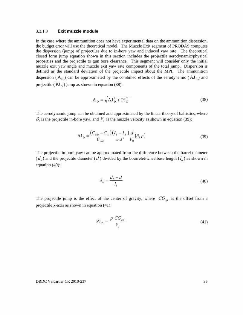
DRDC Valcartier CR 2010-237 35
3.3.1.3 Exit muzzle module
In the case where the ammunition does not have experimental data on the ammunition dispersion,
the budget error will use the theoretical model. The Muzzle Exit segment of PRODAS computes
the dispersion (jump) of projectiles due to in-bore yaw and induced yaw rate. The theoretical
closed form jump equation shown in this section includes the projectile aerodynamic/physical
properties and the projectile to gun bore clearance. This segment will consider only the initial
muzzle exit yaw angle and muzzle exit yaw rate components of the total jump. Dispersion is
defined as the standard deviation of the projectile impact about the MPI. The ammunition
dispersion ( DA ) can be approximated by the combined effects of the aerodynamic ( DAJ ) and
projectile ( DPJ ) jump as shown in equation (38):
2
D
2
DD PJAJA (38)
The aerodynamic jump can be obtained and approximated by the linear theory of ballistics, where
b is the projectile in-bore yaw, and 0V is the muzzle velocity as shown in equation (39):
pVd
mdII
CCC
bXY
m
XN
0
2DAJ
(39)
The projectile in-bore yaw can be approximated from the difference between the barrel diameter
( bd ) and the projectile diameter ( d ) divided by the bourrelet/wheelbase length ( bl ) as shown in
equation (40):
b
bb l
dd (40)
The projectile jump is the effect of the center of gravity, where offCG is the offset from a
projectile x-axis as shown in equation (41):
0
DPJVCGp off (41)

36 DRDC Valcartier CR 2010-237
3.3.1.4 Thrust/Tracer/Base burn module
In the case where the ammunition has a tracer capability, the Thrust/Tracer/Base Burn segment of
PRODAS computes the thrust, tracer and/or base effect during the trajectory analysis. The model
requires the thrust or drag variation data versus time.
3.3.1.5 Ground-to-Ground module
The Ground-to-Ground System Effectiveness Simulation is a state-of-the-art computer tool
designed to facilitate tradeoffs between candidate ammunition and gun system, burst length,
targets, sensor errors and system accuracy. This program is focused on the effectiveness in
hitting and killing the intended target.
The simulation brings together the models for the gun, ammunition, fire control system and target
into a simultaneous simulation. First the probability of hit is calculated and then the kill
assessment is established based on the user input target vulnerability.
Figure 9: System effectiveness simulation block diagram.
The fragment hit probability and lethality shall be conducted with other computer simulation tools
such as GVAM. Separate classified reports will be published to investigate the terminal aspects,
i.e., the lethality studies, based on the outputs of the Ground-to-Ground System Effectiveness
Simulations.
The Ground-to-Ground system effectiveness analysis consists of a Monte Carlo methodology
with various system errors as inputs to provide standard deviations in range, cross range and
height at specified ranges.
The inputs to this module basically consist of an error budget that will characterize the gun-
ammunition combination. It assumes that corrections for biases have been done, as for example:
constant wind (head/tail), non-standard atmospheric conditions, change of muzzle velocities due
to propellant temperature, etc... It assumes that the aim point of the intended target will be at the

DRDC Valcartier CR 2010-237 37
center of the target and that system errors will be added on. Due to this, the trajectory flyout
routine consists of a 2DOF.
Various attack scenarios can be modeled:
Direct attack impact fuze against vertical target. This mode is used for validating the
probability of hit against side profile vehicle targets.
Top attack (Material) impact fuze against a horizontal target with direct (low QE) and
indirect (high QE) fire options. This mode is used for va1idating the “heating zone”
requirement.
Top attack (troops) impact or airburst fuze against a number of troops in a given area
with direct (low QE) and indirect (high QE) fire options. This mode will be used for the
validation of airburst requirements.
A typical input error file for this module is provided in Table 17. As seen in the table, the errors
are classified as occasion-to-occasion and round-to-round. All the errors either contribute in the
azimuth plane (drift) or in the elevation plane (range). When firing in burst mode, only the errors
in the round-to-round columns are acted upon.
Table 17: Typical inputs file for system effectiveness simulation (fictive values).
Each individual error from Table 17 is described below. However, the required inputs of the
Ground-to-Ground System Effectiveness Simulation are slightly different of the methodology
developed in sections 3.1 and 3.2. Thus, each individual description would be described in the
implementation of the methodology parameter.
1. FC Range (m or %): This is the error in determining the range to the target from the
firing position, in terms of meter or percentage of the range. It is mainly composed (if
38 DRDC Valcartier CR 2010-237
direct firing) of the Laser Range Finder accuracy. The model allows that the range error
be entered as either a fixed distance value (previous error) or a percentage (linear value).
It should be noted that the accuracy of the LRF could be affected by the target type and
shape. Therefore, various simulations should be conducted for anti-personnel and anti-
vehicle scenarios. In sections 3.1 and 3.2, this error is the standard deviation of the error
of the target range (SD
TargetR ).
2. Tar Vel (m/s): This is the error due to the target velocity (if applicable). This input is
one of the inputs that will be used to simulate the target’s tracking error of section
3.1.5.2. In sections 3.1 and 3.2, this error is the standard deviation in the average relative
target velocity (SDVTarget ) and the evaluation of this parameter has been evaluated by
equation (25) and by the analysis of the experimental data.
3. Boresight (mils): The Boresight error is an alignment error, which is composed of all the
errors that are attributed to the fire control system/display. It can be different in azimuth
and in elevation. In sections 3.1 and 3.2, this error is the standard deviation of the gun
laying ( GLDS ) and the evaluation of this parameter is done by equation (24).
4. Gun Aim (mils): The aiming error is composed of all errors from the mechanical aiming
of the gun that is not related to the fire control system. It can be different in azimuth and
in elevation. In sections 3.1 and 3.2, this error is the root of the square summation the
two (2) different dispersion subsections such as: vehicle movement and mutual
interaction. Equation (42) shows this relation and the evaluation of this parameter has
been done by the analysis of the experimental data.
Aiming Error 2
MID
2
VMD SS (42)
5. Cant (deg): This is the cant angle error of the gun in the azimuth plane. It is mainly
composed (if measured) of the cant sensor value. This input is one of the inputs that will
be used to simulate the target’s tracking error of section 3.1.5.2. In sections 3.1 and 3.2,
this error is the cant angle of gun mounts in the azimuth plane (Error
Gunș ).
6. Gun Disp (mils): The Gun Dispersion error is the error of the overall gun dispersion
(Gun Support and Gun Barrel Dispersion). This error is a round-to-round error. It can be
different in azimuth and in elevation. In sections 3.1 and 3.2, this error is the standard
deviation of the overall gun dispersion ( GDS ) and the evaluation of this parameter has
been done by the experimental data analysis.
7. Ammo Di sp (mils): The Ammunition dispersion error, as measured through Projectile
Jump testing in an aeroballistics range trial. This error is a round-to-round error. In
sections 3.1 and 3.2, this error is also the standard deviation of Ammunition Dispersion
( ADS ) and the evaluation of this parameter can’t be used for the theoretical analysis
(section 3.3.1.3) or the experimental aeroballistics range data.
DRDC Valcartier CR 2010-237 39
8. Muz Vel (m/s): This is the Muzzle Velocity error, between lots (Occasion-to-occasion)
and within a Lot (Round-to-round). In sections 3.1 and 3.2, this error is also the Muzzle
Velocity error where LLSD
MV is for occasion-to-occasion and
RRSD
MV is for round-to-
round. The evaluation of this parameter has been done usually with the experimental
Doppler radar data.
9. Drag/Mass (%): This is the ammunition mass and drag error. The ammunition mass
error is the round-to-round mass tolerance over an ammunition lot. The Drag error is the
variation of the drag coefficient (or the retard) over the trajectory (from the shape
reproduction/tolerance, rotating band ware, etc). This error affects the velocity of the
projectile as the projectile flies downrange. It is provided as a percentage over the mean
and the standard deviation of measured values. In sections 3.1 and 3.2, this error is also
the standard deviation of Drag/Mass percentage ratio (SDMD%
). The evaluation of this
parameter is done by equation (16) and by the experimental Doppler radar and mass data.
10. Thrust (%): This is the ammunition tracer error (if applicable). The ammunition tracer
error is the round-to-round delta drag variation over an ammunition lot. In sections 3.1
and 3.2, this error is also the standard deviation of the tracer (SD
%Tr ). The evaluation of
this parameter is obtained by equation (21) and by the experimental aeroballistics range
data.
11. Winds (m/s): This is the error in the average wind speed. In sections 3.1 and 3.2, this
error is also the standard deviation of the error of the average wind speed along the
trajectory (SD
WV ). Experimentally, the error due to the average wind speed is calculated
simultaneously along the projectile path from two (2) (or more) meteorological stations.
12. Temp (oC): This is the temperature error at gun site. It is mainly composed (if measured)
of the temperature sensor accuracy. In sections 3.1 and 3.2, this error is also the standard
deviation of the error on the atmospheric temperature at gun site (SD
AT ). Experimentally,
the temperature error is calculated simultaneously along the projectile path from two (2)
(or more) meteorological stations.
13. Pressure ( mbar): This is the atmospheric pressure error at gun site. It is mainly
composed (if measured) of the pressure sensor accuracy. In sections 3.1 and 3.2, this
error is also the standard deviation of the error on the atmospheric pressure at gun site
(SD
AP ). Experimentally, the pressure error is calculated simultaneously along the
projectile path from two (2) (or more) meteorological stations.
14. Time fu ze ( %): This is time fuze error for the airburst ammunition, in terms of
percentage of time flight.

40 DRDC Valcartier CR 2010-237
4 Probability of hit formulation
The RFP for the TAPV acquisition project requires providing recommendations for the following,
considering that the weapons are integrated on an RWS mounted on typical TAPV:
Threshold and rated PHit data for the CF in service C6 GPMG weapons;
Threshold and rated PHit data for the CASW 40 mm AGL High Explosive Dual Purpose
– Self Destruct (HEDP-SD) ammunition on vehicle and infantry targets;
Threshold and rated PHit data for the CASW 40 mm AGL Practice Rounds (Target
Practice and Target Practice with Tracer);
Threshold and rated PHit data for the CASW 40 mm AGL Airburst Ammunition (ABM)
round on infantry targets;
Studies shall be conducted to evaluate the various parameters for a multitude of firing scenarios
from various data sources such as: theoretical analysis, references and/or experimental data.
Monte Carlo simulations shall be conducted at various ranges and on various targets based on the
above errors to obtain expected hits on personal and vehicle targets in a direct hit scenario. These
errors are then added from standard initial conditions obtained from the firing table.
The PRODAS Ground-to-Ground simulation tool can provide the average and the standard
deviations in range, cross range and height at specified ranges with a PRODAS error budget
(Table 18). The expected probabilities of hits are then calculated based on a target size and firing
scenarios.
The PRODAS simulation tool can also compute the above for a burst of N shots. For our
particular cases, a group of N shots in a burst will be considered as one shot since the dispersions
for a group of 3, 5 and more hot burst will be known and treated as independent shots.
For a direct attack scenario against a vertical target, the average standard deviations in the vertical
and horizontal directions are calculated for specified ranges.

DRDC Valcartier CR 2010-237 41
Table 18: PRODAS error budget.
Symbol Unit Description SD
%Tr % Standard Deviation of the tracer
SDMD%
% Standard Deviation of Drag Mass percentage ratio
RRSD
MV m/s
Standard Deviation of muzzle velocity within a lot of ammunition at
21 °C
LLSD
MV m/s
Standard Deviation of muzzle velocity between lots of ammunition at
21 °C
DA mils Standard Deviation of the Ammunition Dispersion.
SD
DGS mils Standard Deviation of the Gun Support Dispersion
SD
DG mils Standard Deviation of the Gun Barrel Dispersion
SD
WV m/s Standard Deviation of the error of the average wind speed along the
trajectory
SD
AP mbar Standard Deviation of the error on the atmospheric pressure at gun site
SD
AT °C Standard Deviation of the error on the atmospheric temperature at gun
site
GLDS mils Standard Deviation of the Gun Laying Dispersion
SD
TargetR m Standard Deviation of the error of the target range.
Error
Gunș deg Cant angle of gun mounts in the azimuth plane
SDVTarget meter/s Standard Deviation in the average relative target velocity.
VMDS mils Standard Deviation of the Vehicle Movement Dispersion
MIDS mils Standard Deviation of Mutual Interaction Dispersion

42 DRDC Valcartier CR 2010-237
4.1 Target standard
To provide a threshold and rated PHit, the knowledge of the target dimensions is important. The
probability of hit can depend largely on the target height and width. In this case, the present
section shows the distinction between the personal and vehicle target.
4.1.1 Personal target
The dismounted personal target dimensions that are necessary to conduct to the threshold and
rated Probability of Hit for a specific weapon are defined in NATO STANAG 4512 [8].
However, Project Management Office (PMO) Tactical Armoured Patrol Vehicle (TAPV)
recommends using a simplified rectangular target form. The dismounted personal target
dimensions will be 1.5 m (height) by 0.6 m (width).
4.1.2 Vehicle target
The vehicle target dimensions that are necessary to conduct to the threshold and rated PHit for a
specific weapon are defined in NATO STANAG 4512 [9]. However, Project Management Office
(PMO) Tactical Armoured Patrol Vehicle (TAPV) recommends using a simplified rectangular
target form. The vehicle target dimensions will be 2.3 m (height) by 2.3 m (width).

DRDC Valcartier CR 2010-237 43
4.2 Formulation
For a specified target size, the PRODAS Ground-to-Ground simulation module calculates the
expected hits for a direct and top attack scenario. The expected probability of at least one hit over
N shots is given by equation (43):
N
*
HitM
E11P
(43)
N - Number of rounds in a burst
E - Expected number of hits for M rounds (From the PRODAS Monte Carlo simulations)
M - Number of rounds fired for Monte-Carlo Method (predefined in PRODAS)
If N = 1; M
EP *
Hit , i.e. the expected probability of hit for one shot. This is the value obtained
from PRODAS Monte Carlo simulations.
Equation (43) can be reformulated as followed to obtain the required M
E for a given
*
HitP and N
number of shots in a burst, equation (44):
1/N*
HitN
P1ln
1S
Hit P111PM
E
*Hit
e (44)
or to obtain the number of shots required to achieve a probability of at least one hit, equation (45):
1S
Hit
*
Hit
P1ln
P1lnN
(45)

44 DRDC Valcartier CR 2010-237
5 Comments and Conclusions
A PHit methodology has been developed to characterize the overall performance of the C6
GPMG and 40 mm AGL integrated on RWS mounted on TAPV Platform. The methodology
takes into account four (4) different scenarios (static/moving vehicle to engage the static/moving
target) into an error budget.
The error budget analysis breaks down the total dispersion (standard deviation of the impact point
position) into four (4) main error sources: weather, gun, projectile and FCS dispersion. The
weather dispersion can be developed to see the individual contributions of the standard deviation
of the wind speed, atmospheric temperature and atmospheric pressure. The Gun dispersion can
be developed to see the individual contributions of the standard deviation of the gun support play
and the gun barrel. The projectile dispersion can be developed to see the individual contributions
of the standard deviation of the ammunition dispersion, muzzle velocity, drag mass ratio and
tracer effect. The fire control system dispersion can be developed to see the individual
contributions of the standard deviation of the gun laying, target’s tracking, vehicle movement and
mutual interaction effect.
To fill the error budget, each error source and the relation between them were described in the
experimental and theoretical point view (if applicable). Also, by resolving the error budget, it’s
now possible to easily extract the fire control system, gun laying, target’s tracking, vehicle
movement and mutual interaction dispersion.
The error budget can be represented on a pie plot in square mils (mils2), because each error source
has the same unit (mils). The error budget can be also represented on a stacked area plot in
square mils (mils2) for different target range and/or different parametric studies.
To create the error budget, the PRODAS budget error was built to describe the required inputs for
the system simulation (PRODAS). The methodology to fill the PRODAS budget error was also
presented. With the PRODAS budget error and simulation package, the numerical simulation can
be easily used to obtain the weapon system performance for different firings conditions.
Experimental data is required to refine the numerical simulation on the TAPV RWS system. The
main difficulties are to characterise the target’s tracking, vehicle movement and mutual
interaction effect. These effects need to take into account the vehicle, gunner and RWS
interaction effect on the weapon accuracy. Also, the RWS doesn’t have a wind speed and
direction sensor to take into account the weather effect on the accuracy. In addition, the driver
and gunner experience can have a large influence on the overall system weapon. All these effects
need to be approximated to be able to characterize the realistic weapon performance.

DRDC Valcartier CR 2010-237 45
References .....
[1] Pimentel, R., Lestage, R., PHit Methodology for PMO TAPV Requirements, SL 2010-411,
DRDC Valcartier, June 2010.
[2] Dupuis A. (2005). System modeling tool and accuracy trials for a 40 mm AGL. DRDC
Valcartier TM 2005-275, Defence R&D Canada - Valcartier
[3] Corriveau, D. (2006). Evaluation of the performance of an Automatic Grenade Launcher
(AGL) system – Part 1: System simulation and sensitivity analyses. DRDC Valcartier TM
2006-551, Defence R&D Canada - Valcartier
[4] Corriveau, D. (2006). Evaluation of the performance of an Automatic Grenade Launcher
(AGL) system – Part 2: Comparisons with test data. DRDC Valcartier TM 2006-552,
Defence R&D Canada - Valcartier
[5] PRODAS (Projectile Design/Analysis System, Version 3.5.3), Technical and User Manual,
Arrow Tech Associates, Burlington, Vermont, USA.
[6] NATO STANAG 4355 – “The Modified Point Mass and five Degrees of Freedom Trajectory
Models”, Draft Edition 5.0A, 25 September 2003.
[7] NATO STANAG 4144 – “Procedure to Determine the Fire Control Inputs to use in indirect
Fire control System”, Edition 2, 2002.
[8] NATO STANAG 4512 – “Dismounted Personal Target”, Edition 1, 1995.
[9] NATO STANAG 4498 – “Unarmoured Vehicle, Helicopters and flied fortification targets”,
Edition 1, 2004.

46 DRDC Valcartier CR 2010-237
List of symbols/abbreviations/acronyms/initialisms
refA
projectile reference area, m2
DAJ Standard deviation of the Aerodynamic jump, mils
SD
SOLB
Ballistic FCS solution error
AT
0XC
Tracer coefficient of the projectile with the active tracer effect
WT
0XC
Tracer coefficient of the projectile without the tracer effect
0XC, oCx
Drag coefficient of the projectile (Axial force coefficient)
0XC
Average of the drag coefficient of the projectile
SD
0C X SD of the drag coefficient of the projectile
SD
0%C X
Percentage of the SD of the drag coefficient of the projectile
2Cx Square-yaw axial force coefficient
offCG
Center of gravity offset from a projectile x-axis, m
pCl
Roll damping moment coefficient
Cm
Pitching moment coefficient
qCm
Pitch damping moment coefficient
CN
Normal force coefficient
Cnp
Magnus moment coefficient
d Projectile reference diameter, m
M/RWSD
Distance between the RWS rotation axis and the barrel muzzle exit, m
SD
RD Display resolution error, mrad
SDMD%
SD of Drag Mass percentage ratio, %
E Expected number of hits for M rounds
TargetH
Average target base altitude, m
SD
TargetH
Standard Deviation of the error in knowing the target base altitude, m
XI Axial moment of inertia, g cm2
YI Transverse moment of inertia about center of gravity, g cm2
l Reference length, m
bl bourrelet/wheelbase length, m
SDLOS
Line of sight stability error, mrad
m , M Projectile mass, kg
M Average of the mass of projectile, kg SDM SD of the mass of projectile, kg

DRDC Valcartier CR 2010-237 47
SD
%M
Percentage of the SD of the mass of projectile, %
SD
AM Misalignment error of FCS with gun, mrad
tPM tracer powder mass as function of time, kg
Mach Mach Number
N Number of round SD
RND Night/day resolution error, mrad
p is the spin rate, rad/s
SD
AP Std. deviation of the error on the atmospheric pressure at gun site, mbar
DPJ Standard deviation of the Projectile jump, mils
*
HitP
Probability of at least one hit over N shots
1S
HitP
Probability of hit for one shot
TargetR
Average target range, m
SD
TargetR
Standard Deviation of the error of the target range, m
ADS , DA Ammunition Dispersion, mils
D/MS
Drag/Mass Dispersion, mils
FCSS
Fire Control System Dispersion, mils
GBS
Gun Barrel Dispersion, mils
GDS
Gun Dispersion, mils
GLDS
Standard Deviation of the Gun Laying Dispersion, mils
GSPS
Gun Support Play Dispersion, mils
MIDS Mutual Interaction Dispersion, mils
APS
Atmospheric pressure dispersion, mils
PDS Projectile Dispersion, mils
ATS
Atmospheric temperature dispersion, mils
TDS Tracer Dispersion, mils
TTDS
Standard Deviation Target’s Tracking Dispersion, mils
TotalS
Global dispersion, mils
MVVS
Muzzle Velocity Dispersion, mils
WVS
Wing speed dispersion, mils
VMDS
Vehicle Movement Dispersion, mils
WDS
Weather dispersion, mils
SD, Standard deviation SD
AT Std. deviation of the error on the atmospheric temperature at gun site, °C

48 DRDC Valcartier CR 2010-237
Tr Thrust/tracer coefficient of the projectile
Tr Average of the thrust/tracer coefficient of projectile SDTr
SD of the tracer
SD
%Tr
Percentage of SD of the tracer, %
V Projectile velocity
MV Muzzle velocity at 21 °C, m/s
RRSD
MV
SD of muzzle velocity within a lot of ammunition at 21 °C, m/s
LLSD
MV
SD of muzzle velocity between lots of ammunition at 21 °C, m/s
SDVTarget Standard Deviation in the average relative target velocity, m/s
SD
WV
Standard deviation of the error of the average wind speed along the
trajectory, m/s
CGX
Center of gravity from nose, m
SDXGD Standard deviation of the overall gun barrel head position, m
SD
GLX
Standard Deviation of the gun laying position, m
SD
TotalX
Standard deviation of the impacts points, m
b Projectile in-bore yaw
Error
Gunș Cant angle error of gun mounts in the azimuth plane, deg
A Atmospheric air density, kg/m3
Gun
The angular velocity of the cant angle of gun mounts in azimuth plane, rad/s
SD
Gun
Std Deviation of the angular velocity of the cant angle of gun mounts in
azimuth plane, rad/s
AGL Automatic Grenade Launcher
ATC Aberdeen Test Center
CASW Close Area Suppression Weapon System
CF Canadian Force
CFB Canadian Force Base
FCS Fire Control System
GPMG General Purpose Machine Gun
LRF Laser Range Finder
LUVW Light Utility Vehicle Wheeled fleet
MPI Mean Point of Impact
NATO North Atlantic Treaty Organization
PHit Probability of hit
PMO Project Management Office
PRODAS PROjectile and Design and Analysis System
QE Quadrant Elevation
RFP Request For Proposal
RWS Remote Weapon Station
SD Standard Deviation
SOR Statement of Operational Requirements

DRDC Valcartier CR 2010-237 49
TAPV Tactical Armoured Patrol Vehicle
VPS Vehicle Performance Specifications

DOCUMENT CONTROL DATA (Security classification of title, body of abstract and indexing annotation must be entered when the overall document is classified)
1. OR IGINATOR (The name and address of the organization preparing the document.
Organizations for whom the document was prepared, e.g. Centre sponsoring a
contractor's report, or tasking agency, are entered in section 8.)
Numerica Technologies Inc. 3420 Lacoste Québec, QC G2E 4P8
2. SECURITY CLASSIFICATION (Overall security classification of the document
including special warning terms if applicable.)
UNCLASSIFIED
3. TITLE (The complete document title as indicated on the title page. Its classification should be indicated by the appropriate abbreviation (S, C or U)
in parentheses after the title.)
C6 GPMG and 40 m m AGL weapon int egrated on RWS mounted on TAPV platform: Probability of hit methodology
4. AUTHORS (last name, followed by initials – ranks, titles, etc. not to be used)
Dominic Couture, Pierre Gosselin
5. DATE OF PUBLICATION (Month and year of publication of document.)
September 2010
6a. NO. OF PAGES
(Total containing information,
including Annexes, Appendices,
etc.)
64
6b. NO. OF REFS
(Total cited in document.)
9
7. DESCRIPTIVE NOTES (The category of the document, e.g. technical report, technical note or memorandum. If appropriate, enter the type of report,
e.g. interim, progress, summary, annual or final. Give the inclusive dates when a specific reporting period is covered.)
Contract Report
8. SPONSORING ACTIVITY (The name of the department project office or laboratory sponsoring the research and development – include address.)
Defence R&D Canada – Valcartier 2459 Pie-XI Blvd North Quebec (Quebec) G3J 1X5 Canada
9a. PROJECT OR GRANT NO. (If appropriate, the applicable research
and development project or grant number under which the document
was written. Please specify whether project or grant.)
9b. CONTRACT NO. (If appropriate, the applicable number under
which the document was written.)
W7701-073141/0010/QCV
10a. ORIGINATOR'S DOCUMENT NUMBER (The official document
number by which the document is identified by the originating
activity. This number must be unique to this document.)
12qw14
10b. OTHER DOCUMENT NO(s). (Any other numbers which may be
assigned this document either by the originator or by the sponsor.)
DRDC Valcartier CR 2010-237
11. DOCUMENT AVAILABILITY (Any limitations on further dissemination of the document, other than those imposed by security classification.)
Unlimited
12. DOCUMENT ANNOUNCEMENT (Any limitation to the bibliographic announcement of this document. This will normally correspond to the
Document Availability (11). However, where further distribution (beyond the audience specified in (11) is possible, a wider announcement
audience may be selected.))
Unlimited
13. ABSTRACT (A brief and factual summary of the document. It may also appear elsewhere in the body of the document itself. It is highly desirable
that the abstract of classified documents be unclassified. Each paragraph of the abstract shall begin with an indication of the security classification
of the information in the paragraph (unless the document itself is unclassified) represented as (S), (C), (R), or (U). It is not necessary to include
here abstracts in both official languages unless the text is bilingual.)
A probability of hit (PHit) methodology has been developed to characterize the overall performance of
the C6 General Purpose Machine Gun (GPMG) and 40 mm Automatic Grenade Launcher (AGL)
Integrated on a Remote Weapon Station (RWS) Mounted on a Tactical Armoured Patrol Vehicle (TAPV)
Platform. The methodology takes into account four (4) different scenarios (static/moving vehicle to
engage a static/moving target) to develop an error budget of the weapon system.
The error budget analysis breaks down the total dispersion, i.e., the standard deviation (SD) of the impact
point position, into four (4) main error sources: weather, gun, projectile and the Fire Control System
(FCS) Dispersion. The weather dispersion can be developed to see the individual contributions of the
standard deviation of the wind speed, atmospheric temperature and atmospheric pressure. The Gun
dispersion can be developed to see the individual contributions to the standard deviation of the gun
support and the gun barrel. The projectile dispersion can be developed to see the individual contributions
to the standard deviation of the ammunition dispersion, muzzle velocity, drag-mass ratio and tracer effect.
The FCS dispersion can be developed to see the individual contributions to the standard deviation of the
gun laying, target tracking, vehicle movement and mutual interaction effects.
The PRODAS (PROjectile and Design and Analysis System) budget error and simulation package were
used to model the weapon system performance for different firings conditions. The experimental data
from the static/moving vehicle against static/moving target scenarios necessary to validate the PRODAS
modeling is being obtained in the CFB (Canadian Forces Base).
Une méthodologie de probabilité d’impact (PHit) a été développée pour caractériser la performance
globale de la mitrailleuse polyvalente (GPMG) C6 et du lanceur automatique de grenade (AGL) 40 mm
intégrés sur un système d’armement télécommandé (RWS) monté sur un véhicule de patrouille blindé
tactique (TAPV). La méthodologie prend en considération quatre (4) scénarios différents (véhicule
statique/en mouvement qui engage une cible statique/en mouvement) pour le développement du budget
d’erreur du système d’arme.
L’analyse du budget d’erreur décompose la dispersion totale, soit la déviation standard (SD) de la
position du point d’impact, en quatre (4) principales sources d’erreur : Météo, l’arme, projectile et le
système de conduite de tir (FCS). La dispersion météo peut être développée pour analyser les différentes
contributions individuelles de la déviation standard de la vitesse du vent, de la température atmosphérique
et de la pression atmosphérique. La dispersion de l’arme peut être développée pour analyser les
différentes contributions individuelles de la déviation standard du support et de l’âme de l’arme. La
dispersion du projectile peut être développée pour analyser les différentes contributions individuelles de
la déviation standard de la dispersion de la munition, de la vitesse initiale du projectile, du rapport traînée-
masse et l’effet du traceur. La dispersion du FCS peut être développée pour analyser les différentes
contributions individuelles de la déviation standard du support de l’arme, du système de pointage de
l’arme, le mouvement du véhicule et les effets d’interactions mutuelles.
L’ensemble numérique de simulation et de calcul du budget d’erreur PRODAS (PROjectile and Design
and Analysis System) ont été utilisés pour la modélisation de la performance du système d’armement
pour différentes conditions de tirs. Les données expérimentales provenant des scénarios véhicule
statique/en mouvement qui engage une cible statique/en mouvement nécessaires pour valider la
modélisation PRODAS seront obtenus à la BFC (Base des Forces canadiennes).
14. KEYWORDS, DESCRIPTORS or IDENTIFIERS (Technically meaningful terms or short phrases that characterize a document and could be
helpful in cataloguing the document. They should be selected so that no security classification is required. Identifiers, such as equipment model
designation, trade name, military project code name, geographic location may also be included. If possible keywords should be selected from a
published thesaurus, e.g. Thesaurus of Engineering and Scientific Terms (TEST) and that thesaurus identified. If it is not possible to select
indexing terms which are Unclassified, the classification of each should be indicated as with the title.)
TAPV; Error budget; PRODAS;Ground-to-Ground;Ballistics;C6 GPMG;40 mm AGL


Canada’s Leader in Defence
and National Security
Science and Technology
Chef de file au Canada en matière
de science et de technologie pour
la défense et la sécurité nationale
www.drdc-rddc.gc.ca
Defence R&D Canada R & D pour la défense Canada