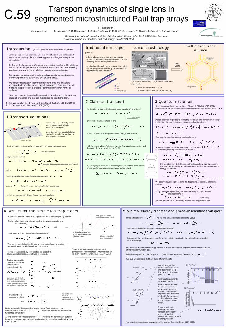
Transport dynamics of single ions in segmented microstructured Paul trap arrays

R. Reichle1,2

with support by: D. Leibfried2, R.B. Blakestad2, J. Britton2, J.D. Jost2, E. Knill2, C. Langer2, R. Ozeri2, S. Seidelin2, D.J. Wineland2

1 Quantum Information Processing, Universität Ulm, Albert-Einstein-Allee 11, D-89069 Ulm, Germany2 National Institute for Standards and Technology, Boulder/CO, USA

Introduction (content available from arXiv quant-ph/0606237)

RF

−DC+DC

+ion

C.59

Small groups of ions as qubit carriers in miniaturized, two-dimensional electrode arrays might be a scalable approach for large-scale quantum computation1,2.

By this method processing of quantum information is achieved by shuttling ions to and from separate memory and qubit manipulation zones enabling quantum computation via principles of quantum communication.

Transport of ion groups in this scheme plays a major role and requires precise experimental control and fast shuttling times.

We discuss theoretically the transport performance and limitations associated with shuttling ions in typical miniaturized Paul trap arrays by modeling the process by a dragged, parametrically driven harmonic oscillator.

Here, we present a theoretical framework to describe and optimize these transport processes and discuss implications on trap technology.

1 D.J. Wineland et al., J. Res. Natl. Inst. Stand. Technol. 103, 259 (1998) 2 D. Kielpinski et al., Nature 417, 709 (2002)

4 Results for the simple ion trap model 5 Minimal energy transfer and phase-insensitive transport

principle:

in the 4rod geometry below, ions are trapped radially by RF fields applied to the blue rods, and axially by two DC endcap electrodes.

trapping ion strings along the center axis requiresthat the (degenerate) radial trap frequencies are larger than the axial frequency.

1 Transport equations

traditional ion traps current technology

3 Quantum solution

2 1 1 2t

1

0.5

0.5

1

q0t erf2ttp

tp2 4 6 8 10 12 14

x2Π

109108107106105104103102101

xΩ0Ω0y2

2 1 1 2t

1

0.5

0.5

1q0tsinΠt2t0

2 4 6 8 10 12 14x2Π

108107106105104103102101

xΩ0Ω02

2 Classical transport

Surface-electrode trap at NIST:

S. Seidelin et al. PRL 96, 253003 (2006)

next years

manipulatonzone

multiplexed traps& vision

assume equispaced configurationfor the control electrodes totransport in x direction.

apply time varying potentials to theelectrodes in order to translate thetrapping well of the ion.

An Ermakov ansatz to the homogeneous equation (f=0) of Eq.(1)

gives two equations instead of one

with the use of a Green’s function we can find a particular solution andthus write the general solution of Eq. (1)

We observe squeezing by relating the dispersions to classical amplitudechanges

that governs the classical energy transfer to the oscillatory motion by the external time-dependentforce according to

In the adiabatic limit we can find an approximate solution to Eq.(2)

2,5: endcap electrodes; 1,3,4: control electrodes;rf electrode;

+initial conditions

define

design potential so that

resulting equation in moving frame with coordinate

Newton’s equation (to describe a transport in lab frame along q=x axis)

expand only to 2nd order, neglect higher terms, and use

result is a parametrically driven, forced harmonic oscillator

transport function (moves minimum of the well)

Utilizing a generalized invariant theory (Kim et al. PRA 53, 3767 (1996))we can define the annihiliation and creation operators by the class. terms

We can use their properties to define the coordinate and momentum operator,and Hamiltonian in a Heisenberg picture as a function of time

If we use the standard operators at initial time –t0

by averaging over the initial classical phase we find the classical meanenergy and energy dispersion (ω assumed constant)

we can determine the mean values in a coherent state to find the equivalency to the classical trajectory

If ω is constant, lhs of equation (2) has the general solution

In the constant frequency regime we can employ Eq.(3) to see that are proportional to

and that they exhibit an oscillatory behaviour with opposite phase., respectively,

How to find optimum waveforms of potentials for safely transporting an ion?

Recipe: solve linear near-singular system for waveform vector a at any position q0:

S contains overlaps of control potentials φi with φj

a well controlled transport is where

and

Typical superpositionof nearby electrodesto form a localparabolic potential

dashed curve is desiredparabolic potential, verticallines define the optimizationrange; participating electrodesare numbered from left to right.

The common minimization of these two terms stabilizes the solution because it feeds back information to the system.

We employ a Tikhonov regularization to find a[q0]K describes overlap of φi with desired potential (dashed curve)

In a classical description the energy transfer is phase-sensitive and depends on the temporal shapeof the transport function q0(t).

What is the optimum choice for q0(t) ? (let’s assume a constant frequency and )

We give two examples that have quite different results.

Then we can define the adiabatic suppression amplitude

Normalize q0 so thatstart location is at -1 and final destination at +1. The transport duration isgiven by .

For typical experimentalparameters we find:

there is a slow decay ofthe adiabatic amplitudefor a sine as transportfunction. Transport of asingle ion over a distanceof about 1.2 mm requires~100 oscillation periodsto stay near the groundstate *.

For an error functiontransport, the sametransport can be donein about 6 oscillationPeriods with similar amountof energy transfer.

* consistent with experimental observations of Rowe et al. Quant. Inf. Comp. 4, 257 (2002)

figure on the right shows residual frequency and force modulation fordifferent aspect ratios of (see fig in 1) during a transport fortypical trap parameters.

endcaps

storage zones

control electrode

phase functionamplitude function

this provides the interlink between the classical and quantal solution.For constant frequency we can also obtain the first two moments of theenergy distribution

φi is the potential of control electrode i

Time-dependent waveforms to move theparabolic well from electrode 19 to electrode 23,i.e. over 4 electrode widths (ai=2 means 2V applied).

Results for an examplary configuration for a set of 40equispaced electrodes as illustrated in section 1.

Adding up more electrodes for smaller improves the performance but alsoincreases resources. Our example configuration suggests that a value ofto be optimal.

blue dotted curve shows the comparison to thetransporting force.

with

Equi-valence