Embed Size (px)
Citation preview
C O M M U N I C A T I O N S
DE LA FACULTE DES SCIENCES FACULTY OF SCIENCES
DE L’UNIVERSITE D’ANKARA UNIVERSITY OF ANKARA
Series A1: Mathematics and Statistics
VOLUME: 62 Number: 1 YEAR: 2013
Faculty of Sciences, Ankara University
06100 Beşevler, Ankara – Turkey
ISSN 1303-5991
C O M M U N I C A T I O N S DE LA FACULTE DES SCIENCES FACULTY OF SCIENCES
DE L’UNIVERSITE D’ANKARA UNIVERSITY OF ANKARA
Series A1: Mathematics and Statistics
Owner
MUAMMER CANEL
Editor-in-Chief (Publishing Manager)
CAFER COŞKUN
Editor
ELGİZ BAYRAM
Managing Editor
SAİT HALICIOĞLU
ADVISORY BOARD
Ş.ALPAY METU I.GYORI Veszprem Univ.
A.ALTIN Ankara Univ. H.H.HACISALİHOĞLU Ankara Univ.
A.AŞKAR Koç Univ. V.KALANTAROV Koç Univ.
A.AYTUNA Sabancı Univ. A.M.KRALLThe Pensylvania State Univ.
D.BAINOV Sofia Univ. A.O.MORRIS Wales Univ.
L.M.BROWN Hacettepe Univ. T.NOIRI Yatsushiro Coll.Tech.
O.ÇELEBİ Yeditepe Univ C.ORHAN Ankara Univ.
F. ÖZTÜRK Ankara Univ. Y.TUNÇER Ankara Univ.
This Journal is published two issues in a year by the Faculty of Sciences, University of Ankara. Articles and any other material published in this journal represent the opinions of the author(s) and should
not be construed to reflect the opinions of the Editor(s) and the Publisher(s).
Correspondence Address:
COMMUNICATIONS
DERGİ BAŞEDİTÖRLÜĞÜ
Ankara Üniversitesi Fen Fakültesi, 06100 Tandoğan , ANKARA – TURKEY
Tel: (90) 312-212 67 20 Fax: (90) 312-223 23 95
e-mail: [email protected]
Print:
Ankara Üniversitesi Basımevi
İncitaş Sokak No:10 06510 Beşevler
ANKARA – TURKEY
Tel: (90) 312-213 65 65
Basım Tarihi:
C O M M U N I C A T I O N S
DE LA FACULTE DES SCIENCES FACULTY OF SCIENCES
DE L’UNIVERSITE D’ANKARA UNIVERSITY OF ANKARA
Series A1: Mathematics and Statistics
VOLUME: 62 Number: 1 YEAR: 2013
Abstracted in
Mathematical Reviews, Zentralblatt MATH &Tübitak - Ulakbim
Faculty of Sciences, Ankara University
06100 Beşevler, Ankara – Turkey
ISSN 1303-5991

A N K A R A U N I V E R S I T Y P R E S S A N K A R A, 2 013
C O M M U N I C A T I O N S
DE LA FACULTE DES SCIENCES FACULTY OF SCIENCES
DE L’UNIVERSITE D’ANKARA UNIVERSITY OF ANKARA
Volume :62 Number : 1 Year : 2013
Series : A1
A.Ö. ÜNAL; On the Kolmogorov-Petrovskii-Piskunov equation ………………….1
E. KOÇ; Some results in semiprime rings with derivation …………………….….11
H. KOCAYİĞİT, M. ÖNDER and K. ARSLAN; Some characterizations of timelike
and spacelike curves with harmonic 1-type Darboux instantaneous rotation
vector in the Minkowski 3-spaceE₁ ³...…………………………………..21
M. YEŞİLKAYAGİL and F. BAŞAR; Composite dual summability methods of the
new sort ………………………………………………………………….33
F. BAŞAR; Survey On the domain of the matrix lambda in the normed and
paranormed sequence spaces …………………………...……………….45
S. AKBIYIK and İ. SİAP; MacWilliams identities over some special posets …….61
S. AYTAR; A neighbourhood system of Fuzzy numbers and its topology ……….73
M. KİRİŞÇİ; On the spaces of Euler almost null and Euler almost convergent
sequences …...….……………………………………………………….85
A. RAHİMA; Local and extremal solutions of some fractional integrodifferential
equation with impulses ……...………………………………...………101
A. ŞAHİNER; Cone convergence for multiple sequences …...……...…………115
A. GUEZANE-LAKOUD, N. HAMİDANE and R. KHALDİ; Existence and
uniqueness of solution for a second order boundary value problem ….121
A. MERAD and A. BOUZIANI; A computational method for integro-differential
hyperbolic equation with integral conditions ………..…………..……131

Commun.Fac.Sci.Univ .Ank.Series A1Volum e 62, Number 1, Pages 1—10 (2013)ISSN 1303—5991
ON THE KOLMOGOROV-PETROVSKII-PISKUNOV EQUATION
ARZU ÖGÜN ÜNAL
Abstract. We prove existence and uniqueness of the solutions of Kolmogorov-Petrovskii-Piskunov (KPP) equation. We study asymptotic stability and in-stability of the equilibrium solution u(x, t) ≡ 0 of KPP equation with subjectto the traveling wave solutions. We show that KPP equation has not got anyperiodic traveling wave solution. Also, we obtain some exact traveling wavesolutions of KPP equation by the first integral method.
1. Introduction
In this paper, we are interested in the equation of Kolmogorov-Petrovskii-Piskunov
ut − uxx + µu+ νu2 + δu3 = 0, x ∈ R, t ∈ [0,∞) (1)
with the initial condition
u(0, x) = u0(x), x ∈ R. (2)
KPP equation first appeared in the genetics model for the spread of an advan-tageous gene through a population [12]. Later, it has been applied to a number ofphysics, biological and chemical models. KPP equation contains various well knownnonlinear equations in mathematical physics; In the case of µ = −1, ν = 0, δ = 1,it reduces to the Newell-Whitehead equation, for µ = a, ν = −(a + 1), δ = 1, itis called FitzHugh-Nagumo equation and for µ = −1, ν = 1, δ = 0, it is a specialcase of Fisher equation ut − uxx = u− u2.The reason for our interest in the KPP equation is that there exist solutions to the
KPP equation whose qualitative behavior resembles the traveling wave solutions.In recent years, various techniques such as Bäcklund transformation method [10, 15,17], tanh method [11], Adomian method [2], G
′
G -expansion method [8], numericalmethods [5] and as well a direct algebraic method [13] have been used to obtainsome exact traveling wave solutions of Eq. (1). Yet as we know, the first integralmethod has not been applied to Eq. (1) for the same purpose. This method first
Received by the editors Nov. 22, 2012, Accepted: Feb. 22, 2013.2000 Mathematics Subject Classification. Primary 35B35, 35B40, 35B10, 35C07 .Key words and phrases. Existence and uniqueness of solutions, asymptotic stability, instability,
periodicity, traveling wave solutions, first integral method.
c©2013 Ankara University
1
2 ARZU ÖGÜN ÜNAL
introduced by Feng to solve the Burgers Korteweg-de Vries equation [9] and afterthat it was applied to various types of nonlinear equations [1, 3, 7, 14, 18, 20].Our aim is firstly to study the asymptotic stability and instability of zero so-
lution of KPP equation with subject to all traveling wave solutions by means ofqualitative theory of ordinary dfferential equations, secondly to explore the periodictraveling wave solution of KPP equation and thirdly to find some exact travelingwave solutions of KPP equation by using the first integral method. But, for allthese, it is necessary to guarantee the existence and uniqueness of solutions of IVP(1)-(2). So, this paper is designed as follow:In Section 2, the existence and uniqueness solutions of (1)-(2) is proved. In Section3, asymptotic stability and instability of zero solution u(x, t) ≡ 0 of KPP equationare studied. The stability regions of zero solution are sketched. Also, a negativeresult is given for the periodicity. In Section 4, some exact traveling wave solutionsof KPP equation are obtained by the first integral method. In the final section, weshowed that if our conditions are satisfied, then a traveling wave solution that weobtained can approach to zero.
2. Existence and Uniqueness of Solutions
Let us consider the initial value problem (IVP)
∂u
∂t= f(u) +D
∂2u
∂x2, x ∈ Ω, t ∈ (0,∞), (3)
u(x, 0) = u0(x), x ∈ Ω. (4)
where Ω ⊂ R and D is a diffusion coeffi cient. Equation (3) is known as a reaction-diffusion equation which includes the KPP equation. We first give the followingwell known result about existence and uniqueness for the solution of (3)-(4). [4, 6,16]
Theorem 1. Consider the IVP (3)-(4) problem. Suppose that u0(x) is continuousfor x ∈ Ω or x ∈ R. In addition, suppose there exists constants a and b such thata ≤ u0(x) ≤ b for x ∈ Ω, f(a) ≥ 0, f(b) ≤ 0, and f is uniformly Lipschitzcontinuous, that is, there exists a constant c such that,
|f(y)− f(z)| ≤ c |y − z| (5)
for all values y, z ∈ [a, b]. Then the Cauchy problem (3)-(4) has a unique boundedsolution u(x, t) for x ∈ Ω or x ∈ R and t ∈ (0,∞). In addition, the solutionu(x, t) ∈ [a, b].
Now, it is easy to prove that there exists a unique bounded solution of the IVP(1)-(2).
Theorem 2. Suppose that u0(x) is continuous and 0 ≤ u0(x) ≤ β for x ∈ R suchthat β satisfies µ + νβ + δβ2 = 0, β ∈ R. Then there is a unique solution of IVP(1)-(2) defined on x ∈ R, t ∈ [0,∞). Moreover, u(x, t) ∈ [0, β].
ON THE KPP 3
Proof. Eq. (1) is a special case of Eq. (3). The function f(u) = −µu− νu2 − δu3
is Lipschitz continuous on the interval [0, β] and the Lipschitz constant is c =∣∣µ+ 2βν + 3β2δ∣∣ . So, due to Theorem 1, the Cauchy problem (1)-(2) has a unique
bounded solution u(x, t) defined on x ∈ R and t ∈ [0,∞). Also u(x, t) ∈ [0, β].
3. Stability and Periodicity
Definition 1. Let u(x, t) be the solution of IVP (3)-(4). Then u(x, t) is said to bea stable solution if given an ε > 0, there exists a δ > 0 such that whenever u0(x)satisfies
||u0(x)− u0(x)|| < δ,
the solution u(x, t) with u(x, 0) = u0(x) of equation (1) satisfies
||u(x, t)− u(x, t)|| < ε
for all t ≥ 0. If the solution u(x, t) is not stable, then it is said to be unstable.The solution u(x, t) is said to be locally asymptotically stable if it is stable and, inaddition,
||u(x, t)− u(x, t)|| → 0, as t→∞.
To study the asymptotic stability and instability of the equilibrium solutionu(x, t) ≡ 0 of KPP equation with subject to traveling wave solutions of KPP equa-tion, we first of all have to find these kinds of solutions. To do this, we apply thewave transform
u(x, t) = U(ξ), ξ = x− ωt (6)
to Equation (1), where ω represent the wave speed. Then we obtain second ordernonlinear ordinary differential equation
U ′′ + ωU ′ − µU − νU2 − δU3 = 0. (7)
If ω > 0 (ω < 0), then U(x− ωt) represents a wave traveling to the right (left). Ifwe introduce the new dependent variables X(ξ) and Y (ξ) as
X(ξ) = U(ξ), Y (ξ) = U ′(ξ), (8)
then Eq. (7) reduce to the first-order system of ordinary differential equations inX and Y as follow
X ′ = Y,Y ′ = −ωY + µX + νX2 + δX3.
(9)
So, the stability of (7) is equivalent to the stability of the system (9).
Remark 1. We note that system (9) has at most three critical (equilibrium) points.If ν2 < 4δµ, then (0,0) is only critical point. If ν2 = 4δµ, then there are two criticalpoints: (0,0) and (− ν
2δ , 0). If ν2 > 4δµ, then there are three equilibrium points:
(0,0), (−ν−√ν2−4δµ
2δ , 0) and (−ν+√ν2−4δµ
2δ , 0). Hence the possible equilibrium solu-
tions of Eq. (1) are u = 0, u = − ν2δ , u =
−ν±√ν2−4δµ
2δ .
4 ARZU ÖGÜN ÜNAL
Now we can prove the following results.
Theorem 3. The equilibrium point (0, 0) of system (9) is locally asymptoticallystable iff ω > 0 and µ < 0.Proof. Since
lim(X,Y )→(0,0)
0√X2 + Y 2
= lim(X,Y )→(0,0)
νX2 + δX3
√X2 + Y 2
= 0,
(0,0) is a simple critical point of system (9). On the other hand, (0,0) is also theunique equilibrium point of the linear system
X ′ = YY ′ = µX − ωY. (10)
The characteristic equation of linear system (10) is
λ2 + ωλ− µ = 0. (11)
Since ω > 0 and µ < 0, both characteristic roots of (11) have negative real parts.So, it is clear that the equilibrium point (0,0) of system (10) is asymptotically stableas ξ → +∞. Due to the qualitative theory of ordinary differential equation, thereis an asymptotical equivalance between linear system (10) and perturbed system(9). Therefore the zero solution of (9) is also asymptotically stable as ξ → +∞.
Theorem 4. Under the conditions of Theorem 3, the zero solution of KPP equationu(x, t) ≡ 0 is asymptotically stable.Proof Repeating the proof of Theorem 3 and considering (6) and (8), the proof iscompleted.
Theorem 5. The equilibrium point (0, 0) of system (10) is unstable iff either ω < 0or µ > 0.Proof From (11), at least one eigenvalue of (11) is positive or has positive real partiff either ω < 0 or µ > 0. Thus the proof is completed.
Remark 2. Due to the above study, certain stability and instability regions for thezero solution of KPP equation and as well as the types of it can be given in theωµ− plane. For this, in Fig. 1 the ωµ− plane is divided into six subregions asfollows:
In Fig. 1, shaded regions show that the zero solution u(x, t) ≡ 0 of KPP equationis asymptotical stable. In other regions, u(x, t) ≡ 0 is unstable. On the other hand,the types of the equilibrium point u(x, t) ≡ 0 can be identified as in ordinarydifferential equations: It is called a saddle point in regions I and II, a node pointin regions III and VI, a spiral point in regions IV and V.
Now, we can state a negative criter for the periodicity of Eq. (1).
ON THE KPP 5
Theorem 6. KPP equation has no periodic traveling wave solution.Proof. We have already showed that all traveling wave solutions of KPP equationcome from system (9). Now, let us demonstrate the second hands of system (9) as
F (X,Y ) = Y, G(X,Y ) = −ωY + µX + νX2 + δX3
respectively. Then,∂F
∂X+∂G
∂Y= −ω.
Since ω 6= 0, ∂F∂X + ∂G
∂Y is always positive or negative for all X, Y. Therefore,due to well known Bendixon theorem [19], system (9) has no closed trajectory inXY−phase plane. This means that Eq. (7) does not have any periodic solutions.So, KPP equation has no periodic traveling wave solutions.
Remark 3. Due to Theorem 6, there is no periodic solution of KPP equation. But,in paper [8], the traveling wave solutions that obtained in [15]
u(ξ) = ∓√−2δ∆
2δtan
1
2
√−∆ξ − ν
2δand
u(ξ) = ±√−2δ∆
2δcot
1
2
√−∆ξ − ν
2δhave been refered as periodic solutions of KPP equation. As a matter of the factthat, they can not be solutions of KPP equation for everywhere. Because, they arenot defined at the points ξ = π√
−∆+ 2kπ√
−∆, and ξ = 2kπ√
−∆, k ∈ Z, respectively.
4. Traveling Wave Solutions of KPP Equation
In Section 3, we showed that all traveling wave solutions of KPP equation areequivalent to the solutions of system (9). Because the component X(ξ) of anysolution (X(ξ), Y (ξ)) of (9) is equal to U(ξ) which indicates the traveling wavesolutions of KPP equation.According to the qualitative theory of differential equations if we can find two
first independent integrals of system (9), then the general solutions of (9) can beexpressed explicitly and so can all kinds of traveling wave solutions of KPP equation.However, it is generally diffi cult to find even one of the first integrals. Because thereis not any systematic way to tell us how to find these integrals. So, our aim is toobtain at least one first integral of system (9). To do this, we will apply the DivisionTheorem which is based on the Hilbert-Nullsellensatz Theorem [10]. Now, we recallthe Division Theorem for two variables in the complex domain C.
Division Theorem. Suppose that P(w,z) and Q(w,z) are polynomials in C[w, z]and P(w,z) is irreducible in C[w, z]; if Q(w,z) vanishes at all zero points of P(w,z),then there exist a polynomial H(w,z) in C[w, z] such that,
Q(w, z) = P (w, z)H(w, z).
6 ARZU ÖGÜN ÜNAL
According to the first integral method, we assume that (X(ξ), Y (ξ)) is a non-trivial solution of (9) and
Q(X,Y ) =
m∑i=0
ai(X)Y i (12)
is an irreducible polynomial in the complex domain C such that
Q(X(ξ), Y (ξ)) =
m∑i=0
ai(X(ξ))Y (ξ)i = 0 (13)
where ai(X) (i = 0, 1, ...,m) are polynomials of X and am(X) 6= 0. Equation (12)is called the first integral of (9). According to the Division Theorem, there exists apolynomial g(X) + h(X)Y in the complex domain C such that
dQ
dξ=∂Q
∂X
dX
dξ+∂Q
∂Y
dY
dξ= (g(X) + h(X)Y )
m∑i=0
ai(X)Y i. (14)
We consider two different cases for (12) m = 1 and m = 2.Case 1. m = 1
Equating the coeffi cients of Y i on both sides of equation (14), we have
a′1(X) = h(X)a1(X), (15a)
a′0(X) = (ω + g(X))a1(X) + h(X)a0(X), (15b)
a1(X)[µX + νX2 + δX3] = g(X)a0(X). (15c)
Since ai(X) are polynomials, from (15a) we deduce that a1(X) is constant andh(X) = 0. For simplification we take a1(X) = 1. Hence (15) can be rewritten as
a′0(X) = ω + g(X), (16a)µX + νX2 + δX3 = g(X)a0(X) (16b)
Balancing the degrees of a0(X) and g(x), we conclude that deg g(X) = 1 only.Assume that
g(X) = AX +B (17)
where A, B ∈ C. Then, from (16a)
a0(X) =A
2X2 + (B + ω)X + C (18)
where C is an arbitrary integration constant. Substituting (17) and (18) into (16b)and setting all coeffi cients of Xi (i = 0, 1, 2, 3) to be zero, we obtain
A1 =√
2δ, B1 =2ν
3√
2δ− 2ω
3, C = 0, µ1 =
2ν2
9δ− 2νω
9√
2δ− 2ω2
9(19a)
A1 = −√
2δ, B1 = − 2ν
3√
2δ− 2ω
3, C = 0, µ2 =
2ν2
9δ+
2νω
9√
2δ− 2ω2
9. (19b)
ON THE KPP 7
Using the conditions (19a-b) in equation (13), we have
Y +
√2δ
2X2 + (
2ν
3√
2δ+ω
3)X = 0 (20a)
and
Y −√
2δ
2X2 + (− 2ν
3√
2δ+ω
3)X = 0. (20b)
Solving Eqs. (20a) and (20b) with subject to Y and substituting them into Eq.(9), we obtain the following exact solutions of KPP equation, respectively,
u1(x, t) = (ν
3δ+
ω
3√
2δ)[coth(
ν
3√
2δ+ω
6)(x− ωt+ ξ0)− 1] (21)
u2(x, t) = (ν
3δ− ω
3√
2δ)[coth(− ν
3√
2δ+ω
6)(x− ωt+ ξ0)− 1] (22)
where ξ0 is an arbitrary constant.Case 2. m = 2.
By equating the coeffi cients of Y i on both sides of (14) we have
a′2(X) = h(X)a2(X), (23a)a′1(X) = (2ω + g(X))a2(X) + h(X)a1(X), (23b)a′0(X) = −2a2(µX + νX2 + δX3) + (ω + g(X))a1(X) + h(X)a0(X), (23c)a1(X)[µX + νX2 + δX3] = g(X)a0(X). (23d)
Since ai(X) are polynomials, from (23a), we deduce that a2(X) is constant andh(X) = 0. Again, let us take a2(X) = 1. Thus the system can be rewritten asfollow
a′1(X) = 2ω + g(X), (24a)a′0(X) = −2(µX + νX2 + δX3) + (ω + g(X)a1(X), (24b)a1(X)[µX + νX2 + δX3] = g(X)a0(X). (24c)
Balancing the terms of a0(X), a1(X) and g(X), we conclude that either deg g(X) =0 or deg g(X) = 1.Let us consider the case of deg g(X) = 0, that is,
g(x) = A (25)
where A 6= 0. Then, from (24a-b), we get
a1(X) = (2ω +A)X +B, (26)
a0(X) = −δ2X4− 2ν
3X3 + [ω2 +
ωA
2−µ+ωA+
A2
2]X2 + (Bω+AB)X +C (27)
where B and C are integration constants. Let us substitute a0(X), a1(X) andg(X) into (24c) and equate the all coeffi cients of Xi (i = 0, 1, 2, 3, 4) to the zero.Therefore, it follows
A = −6ω
5, B = 0, µ = −6ω2
25, δ = 0, C = 0. (28)
8 ARZU ÖGÜN ÜNAL
Combining (28), (12) and (9), we find two differential equations as
X ′ +2ω
5X +
√2ν
3X3/2 = 0, (29a)
X ′ +2ω
5X −
√2ν
3X3/2 = 0. (29b)
These equations have the following solutions, respectively,
X(ξ) =4ω2
25ν
(−√
2ν3 + e
2ω5 (ξ+ξ0))2
, (30a)
X(ξ) =4ω2
25ν
(√
2ν3 + e
2ω5 (ξ+ξ0))2
. (30b)
Byeη
1 + eη=
1
2[tanh
η
2+ 1] and
eη
1− eη = −1
2[coth
η
2+ 1],
the above solutions (30a) and (30b) that are the solitary wave solutions of KPPequation with δ = 0 can be rewritten as, respectively,
u3(x, t) =3ω2
50ν(coth
ω
10(x− ωt+ ξ0)− 1)2 (31a)
u4(x, t) =3ω2
50ν(tanh
ω
10(x− ωt+ ξ0)− 1)2 (31b)
where ξ0 is an arbitrary constant.We note that in the case of δ = 0, µ = −1, ν = 1, the KPP equation reduces toFisher equation. Hence from (31a-b), some exact solutions of Fisher equation areobtained as follows
u(x, t) =1
4[coth(
x
2√
6± 5
12t+ ξ0)± 1]2
u(x, t) =1
4[tanh(
x
2√
6± 5
12t+ ξ0)± 1]2.
Now we assume that deg g(X) = 1; that is, g(X) = AX+B. Then, from (24a-b)we find
a1 =A
2X2 + (B + 2ω)X + C, (32a)
a0 = (A2
8− δ
2)X4 + (
5Aω
6− 2ν
3+AB
2)X3 (32b)
+(3Bω
2+ ω2 − µ+
AC
2+B2
2)X2 + (Cω +BC)X +D
ON THE KPP 9
where C, D are arbitrary integration constants. Substituting a0(X), a1(X) andg(X) into (24c) and setting all the coeffi cients of powers X to be zero, we obtainthe following nonlinear algebraic system
Aδ2 = A3
8 −Aδ2
Aν2 + (B + 2ω) = A( 5Aω
6 −2ν3 + AB
2 ) +B(A2
8 −δ2 )
Aµ2 + (B + 2ω)ν + Cδ = A( 3Bω
2 + ω2 − µ+ AC2 + B2
2 ) +B( 5Aω6 −
2ν3AB2 )
(B + 2ω)µ+ Cν = AC(ω +B) +B( 3Bω2 + ω2 − µ+ AC
2 + B2
2 )Cµ+AD +BC(ω +B) = 0BD = 0
which has the solution
A = ±2√
2δ, B =νA
3δ− 4ω
3, C = 0, D = 0, µ =
2ν2
9δ− 2ω2
9− 2νω
9A. (33)
Putting (33) into (13), we obtain the same equations as (20a) and (20b). So wehave the same exact solutions as (21) and (22).
5. Conclusion
In this work, we showed that the zero solution u(x, t) = 0 of KPP equation isasymptotically stable if ω > 0 and µ < 0 and it is unstable if either ω < 0 orµ > 0. After that we proved that KPP equation has no periodic solution. Finally,we obtained some new exact traveling wave solutions of KPP equation that aredifferent from those in [5-8]. For a verification of Theorem 4, let us choose theparameters ω, ν, δ and µ as ω = 1, ν = 1, δ = 2, µ = − 2
9 . Then from (21), wehave the solution u1(x, t) = − 1
3 + 13 coth(x−t3 ) which is plotted in Fig. 2. This
solution goes to the zero as x − t → ∞. This case is agree with the asymptoticstability of the zero solution. Indeed, the values ω = 1, µ = − 2
9 come from theasymptotic stability region VI.
References
[1] Abbasbandy S., Shirzadi A., The first integral method for modified Benjamin-Bona-Mahonyequation, Commun. Nonlinear Sci. Numer. Simul., 15 (2010),1759—1764.
[2] Adomian G., The generalized Kolmogorov-Petrovskii-Piskunov equation, Foundation of Pyh-sics Letters, 8 (1995), 99-101.
[3] Ali A. H. A., Raslan K. R., The first integral method for solving a system of nonlinear partialdifferential equations, Int. J. Nonlinear Sci., 5 (2008),111—119.
[4] Allen L. J. S., An Introduction to Mathematical Biology, 2007, Pearson.[5] Branco J.R., Ferreira J.A., Oliveira P. Numerical methods for the generalized Fisher—
Kolmogorov—Petrovskii—Piskunov equation, Applied Numerical Mathematics, 57 (2007), 89-102.
[6] Britton N. F. Reaction-Diffusion Equations and Their Applications to Biology, 1986, Acad-emic Press, New York.
[7] Deng X., Exact peaked wave solution of CH-γ equation by the first-integral method, Appl.Math. Comput., 206 (2008), 806—809.
10 ARZU ÖGÜN ÜNAL
[8] Feng J., Li W., Wan Q., Using G′
G-expansion method to seek the traveling wave solution
of Kolmogorov—Petrovskii—Piskunov equation, Applied Mathematics and Computation, 217(2011), 5860-5865.
[9] Feng Z.S., The first-integral method to the Burgers—KdV equation, J. Phys. A, 35 (2002),343—350.
[10] Hong W. P., Jung Y.D., Auto-bäclund transformation and analytic solutions for generalvariable coeffi cient KdV equation, Phys. Lett. A, 257 (1999), 149—152.
[11] Khater A.H., Malfliet W., Callebaut D.K, Kamel E.S., The tanh method, a simple trans-formation and exact analytical solutions for nonlinear reaction diffusion equations, ChaosSolitons Fractals, 14(3) (2002), 513 - 522.
[12] Kolmogorov A. N., Petrovskii I. G., Piskunov N. S., Etude de la diffusion avec croissancede la quantité de matière et son application à un problème biologique, Moscow Univ. Math.Bull., 1 (1937), 1—25.
[13] Liu C., The relation between the kink-type solution and the kink-bell-type solution of non-linear evolution equations, Physics Letters A, 312 (2003), 41-48.
[14] Lu B., Zhang H.Q., XIE F.D., Travelling wave solutions of nonlinear partial equations byusing the first integral method, Appl. Math. Comput., 216 (2010),1329-1336.
[15] Ma W. X., Fuchssteiner B., Explicit and exact solutions to a Kolmogorov-Petrovskii-Piskunovequation, Int. J. Non-Linear Mech., 31 (1996), 329-338.
[16] Murray J. D., Mathematical Biology I: An Introduction, 2002, Springer, Berlin.[17] Ögün A., Kart C., Exact solutions of Fisher and generalized Fisher equations with variable
coeffi cients, Acta Math. Appl. Sin. Engl Ser., 23 (2007), 563-568.[18] Raslan K. R., The first integral method for solving some important nonlinear partial differ-
ential equations, Nonlinear Dynam., 53 (2008), 281—286.[19] Sımmons G. F., Differential Equations, 1989, McGraw-Hill, New York, pp. 341.[20] Taghizadeh N., Mirzazadeh M., Farahrooz F., Exact solutions of the nonlinear Schrödinger
equation by the first integral method, J. Math. Anal. Appl., 374 (2011), 549—553.
Current address : Arzu Ögün Ünal; Ankara University, Faculty of Sciences, Dept. of Mathe-matics, Ankara, TURKEYE-mail address : [email protected]: http://communications.science.ankara.edu.tr/index.php?series=A1
Commun.Fac.Sci.Univ .Ank.Series A1Volum e 62, Number 1, Pages 11—20 (2013)ISSN 1303—5991
SOME RESULTS IN SEMIPRIME RINGS WITH DERIVATION
EMINE KOÇ
Abstract. Let R be a semiprime ring and S be a nonempty subset of R. Amapping F from R to R is called centralizing on S if [F (x), x] ∈ Z for allx ∈ S. The mapping F is called strong commutativity preserving (SCP) onS if [F (x), F (y)] = [x, y] for all x, y ∈ S. In the present paper, we investigatesome relationships between centralizing derivations and SCP-derivations ofsemiprime rings. Also, we study centralizing properties derivation which actshomomorphism or anti-homomorphism in semiprime rin
1. Introduction
Throughout R will represent an assosiative ring with center Z. A ring R is saidto be prime if xRy = 0 implies that either x = 0 or y = 0 and semiprime if xRx = 0implies that x = 0, where x, y ∈ R. A prime ring is obviously semiprime. For anyx, y ∈ R, the symbol [x, y] stands for the commutator xy − yx and the symbol xoystands for the commutator xy + yx. An additive mapping d : R → R is called aderivation if d(xy) = d(x)y + xd(y) holds for all x, y ∈ R.Let S be a nonempty subset of R. A mapping F from R to R is called centralizing
on S if [F (x), x] ∈ Z, for all x ∈ S and is called commuting on S if [F (x), x] = 0,for all x ∈ S. Also, F is called strong commutativity preserving (simply, SCP)on S if [x, y] = [F (x), F (y)], for all x, y ∈ S. The study of centralizing mappingswas initiated by E. C. Posner [2] which states that there existence of a nonzerocentralizing derivation on a prime ring forces the ring to be commutative (Posner’ssecond theorem). There has been an ongoing interest concerning the relationshipbetween the commutativity of a ring and the existence of certain specific types ofderivations of R (see [5] for a partial bibliography). Derivations as well as SCPmappings have been extensively studied by researchers in the context of operatoralgebras, prime rings and semiprime rings too. For more information on SCP, werefere [3] , [8], [7] and references therein.On the other hand, in [9] M.N. Daif and H.E. Bell showed that if a semiprime
ring R has a derivation d satisfiying the following condition, then I is a central
Received by the editors October 31, 2012; Accepted: May 16, 2013.2000 Mathematics Subject Classification. 16W25, 16W10, 16U80.Key words and phrases. Semiprime rings, derivations, centralizing mappings, scp maps.
c©2013 Ankara University
11
12 EMINE KOÇ
ideal;
there exists a nonzero ideal I of R such that
either d([x, y]) = [x, y] for all x, y ∈ I or d([x, y]) = −[x, y] for all x, y ∈ I.This result was extended for semiprime rings in [11].In [4], H. E. Bell and L. C. Kappe have proved that d is a derivation of R which is
either an homomorphism or anti-homomorphism in semiprime ring R or a nonzeroright ideal of R then d = 0. Some recent results were shown on specific types ofderivations of R. In [1], A. Ali, M. Yasen and M. Anwar showed that if R is asemiprime ring, f is an endomorphism which is a strong commutativity preservingmap on a non-zero ideal U of R, then f is commuting on U . In [10], M. S. Sammanproved that an epimorphism of a semiprime ring is strong commutativity preservingif and only if it is centralizing. The purpose of this paper is to investigate somerelationships between derivations mentioned above in semiprime rings. Throughoutthe present paper, we shall make use of the following basic identities without anyspecific mention:i) [x, yz] = y[x, z] + [x, y]zii) [xy, z] = [x, z]y + x[y, z]iii) xyoz = (xoz)y + x[y, z] = x(yoz)− [x, z]yiv) xoyz = y(xoz) + [x, y]z = (xoy)z + y[z, x].
2. Results
Lemma 2.1. [6, Lemma 1.1.8] Let R be a semiprime ring and suppose that a ∈ Rcentralizes all commutators xy − yx, x, y ∈ R. Then a ∈ Z.
Theorem 2.2. Let R be a semiprime ring and d be a derivation of R. If d satisfiesone of the following conditions, then d is centralizing.i) d([x, y]) = [x, y], for all x, y ∈ R.ii) d([x, y]) = −[x, y], for all x, y ∈ R.iii) For each x, y ∈ R, either d([x, y]) = [x, y] or d([x, y]) = −[x, y].
Proof. i) Assume that
d ([x, y]) = [x, y], for all x, y ∈ R.Replacing y by yx, we get
d ([x, y]x) = [x, y]x,
and sod ([x, y])x+ [x, y]d (x) = [x, y]x.
Using the hypothesis, we obtain
[x, y]d (x) = 0, for all x, y ∈ R. (2.1)
Substituting d (x) y for y in (2.1) and using (2.1), we have
[x, d (x)]yd (x) = 0, for all x, y ∈ R. (2.2)
SOME RESULTS IN SEMIPRIME RINGS WITH DERIVATION 13
Replacing y by yx in (2.2), we find that
[x, d (x)]yxd (x) = 0, for all x, y ∈ R. (2.3)
Multiplying (2.2) on the right by x, we have
[x, d (x)]yd (x)x = 0, for all x, y ∈ R. (2.4)
Subtracting (2.4) from (2.3), we arrive at
[x, d (x)]y[x, d (x)] = 0, for all x, y ∈ R.
By the semiprimeness of R, we conclude that [x, d (x)] = 0, for all x ∈ R, and so[x, d (x)] ∈ Z.ii) If d is a derivation satisfying the property d([x, y]) = −[x, y], for all x, y ∈ R,
then (−d) satisfies the condition (−d) ([x, y]) = −[x, y], for all x, y ∈ R. Hence d iscentralizing by (i).iii) For each x ∈ R, we put Rx = y ∈ R | d([x, y]) = [x, y] and R∗x = y ∈ R |
d([x, y]) = −[x, y]. Then (R,+) = Rx ∪ R∗x, but a group cannot be the union ofproper subgroups, hence R = Rx or R = R∗x. By the same method in (i) or (ii), wecomplete the proof.
We can give the following useful corollaries by the preceding theorem.
Corollary 1. Let R be a prime ring and d be a derivation of R. If d satisfies oneof the following conditions, then R is a commutative integral domain.i) d([x, y]) = [x, y], for all x, y ∈ R.ii) d([x, y]) = −[x, y], for all x, y ∈ R.iii) For each x, y ∈ R, either d([x, y]) = [x, y] or d([x, y]) = −[x, y].
Corollary 2. Let R be a semiprime ring and d be a derivation of R. If d satisfiesone of the following conditions, then d is centralizing.i) d(xy) = xy, for all x, y ∈ R.ii)d(xy) = −xy, for all x, y ∈ R.iii) For each x, y ∈ R, either d(xy) = xy or d(xy) = −xy.
Proof. i) By the hypothesis, we get d(xy) = xy, for all x, y ∈ R. Then, we obtainthat
d (xy − yx) = d (xy)− d (yx) = xy − yx.Therefore, d([x, y]) = [x, y], for all x, y ∈ R. By Theorem 2.2 (i), we conclude thatd is centralizing.ii) Using the same arguments in the proof of (i), we find the required result.iii) It can be proved by using the similar arguments in Theorem 2.2 (iii).
Theorem 2.3. Let R be a semiprime ring with charR 6= 2 and d be a derivationof R. If d is strong commutativity preserving, then d is centralizing.
14 EMINE KOÇ
Proof. For all x, y ∈ R, we get [d (x) , d (y)] = [x, y] . Replacing y by yz, z ∈ R, weobtain
[d (x) , d (y) z + yd (z)] = [x, yz] .
By the hypothesis, we have
d (y) [d (x) , z] + [d (x) , y] d (z) = 0.
Taking d (x) instead of z in the above equation, we find that
[d (x) , y] d2 (x) = 0, for all x, y ∈ R.Again replacing y by d (y) , we get
[d (x) , d (y)] d2 (x) = 0, for all x, y ∈ R.Using the hypothesis, we see that
[x, y] d2 (x) = 0, for all x, y ∈ R. (2.5)
Substituting yr for y in (2.5) and using (2.5), we have
[x, y] rd2 (x) = 0 for all x, y, r ∈ R. (2.6)
Multiplying (2.6) on the right by [x, y] and the left by d2 (x) , we get
d2 (x) [x, y]Rd2 (x) [x, y] = 0, for all x, y ∈ R.By the semiprimeness of R, we obtain
d2 (x) [x, y] = 0, for all x, y ∈ R.Replacing y by ry in the last equation, we see that
d2 (x) r [x, y] = 0, for all x, y, r ∈ R. (2.7)
Writing x+ z by x in (2.5) and using (2.5), we have
[x, y] d2 (z) + [z, y] d2 (x) = 0
and so[x, y] d2 (z) = − [z, y] d2 (x) , for all x, y, z ∈ R. (2.8)
Moreover, equation (2.8) implies that, we arrive at
[x, y] d2 (z) r [x, y] d2 (z) = − [x, y] d2 (z) r [z, y] d2 (x)Using (2.7), we find that
[x, y] d2 (z) r [x, y] d2 (z) = 0, for all x, y, z, r ∈ R.By the semiprimeness of R, we get
[x, y] d2 (z) = 0, for all x, y, z ∈ R. (2.9)
Taking yr instead of y in (2.9) and using (2.9), we have
[x, y] rd2 (z) = 0, for all x, y, z, r ∈ R. (2.10)
SOME RESULTS IN SEMIPRIME RINGS WITH DERIVATION 15
Multiplying (2.10) on the right by [x, y] and the left by d2 (z) , we obtain that
d2 (z) [x, y] rd2 (z) [x, y] = 0, for all x, y, z, r ∈ R.Since R is semiprime ring, we have
d2 (z) [x, y] = 0, for all x, y, z ∈ R. (2.11)
Using the equations (2.9) and (2.11), we get
d2 (z) [x, y] = [x, y] d2 (z) , for all x, y, z ∈ R.By Lemma 2.1, we have d2 (z) ∈ Z, for all z ∈ R. Hence we conclude thatd2 ([x, y]) ∈ Z, for all x, y ∈ R. That is[
d2 (x) , y]+ 2 [d (x) , d (y)] +
[x, d2 (y)
]∈ Z, for all x, y ∈ R.
Using d2 (z) ∈ Z for all z ∈ R and charR 6= 2 in this equation, we obtain that[d (x) , d (y)] ∈ Z, for all x, y ∈ R.
By the hypothesis, we find that
[x, y] ∈ Z, for all x, y ∈ R.Commuting this term with d (z)− z ∈ R, we arrive at
[d (z)− z, [x, y]] = 0, for all x, y, z ∈ R.Again using Lemma 2.1, we have d (z)− z ∈ Z for all z ∈ R. This implies that
[d (z)− z, z] = 0, for all z ∈ R,and so [d (z) , z] = 0. Thus d is commuting, and so d is centralizing. This completesproof. Corollary 3. Let R be a prime ring and d be a derivation of R. If d is SCP onR, then R is a commutative integral domain.
Theorem 2.4. Let R be a semiprime ring and d be a derivation of R. If d acts asa homomorphism on R, then d is centralizing.
Proof. Assume that d acts as an anti-homomorphism on R. Now we have
d (xy) = d (x) y + xd (y) = d (x) d (y) , for all x, y ∈ R.Replacing y by yz, z ∈ R in above equation, we get
d (x) yz + xd (y) z + xyd (z) = d (x) d (y) z + d (x) yd (z) .
Using the hypothesis and d is a derivation of R in the last relation gives
xyd (z) = d (x) yd (z)
and so(d (x)− x) yd (z) = 0, for all x, y, z ∈ R. (2.12)
Writing y by d (y) in (2.12), we get
(d (x)− x) d (y) d (z) = 0, for all x, y, z ∈ R.
16 EMINE KOÇ
By the hypothesis, we obtain
(d (x)− x) d (yz) = (d (x)− x) d (y) z + (d (x)− x) yd (z) = 0.Using (2.12), we have
(d (x)− x) d (y) z = 0and so
d (x) d (y) z = xd (y) z
d (xy) z = d (x) yz + xd (y) z = xd (y) z.
That is d (x) yz = 0 for all x, y, z ∈ R. Explain to this part of the, we can shown that[x, d (x)]y[x, d (x)] = 0, for all x, y ∈ R. Since R is semiprime, we get [x, d (x)] = 0,for all x ∈ R. Hence d is commuting, and so d is centralizing.
Corollary 4. Let R be a prime ring and d be a derivation of R. If d acts as ahomomorphism on R, then R is a commutative integral domain.
Theorem 2.5. Let R be a semiprime ring and d be a derivation of R. If d acts asan anti-homomorphism on R, then d is centralizing.
Proof. By the hypothesis, we have
d (xy) = d (x) y + xd (y) = d (y) d (x)
Replacing y by xy in the last relation and using d is a derivation of R, we arrive at
d (x)xy + xd (x) y + xxd (y) = d (x) yd (x) + xd (y) d (x) .
By the hypothesis, we get
d (x)xy + xd (x) y + xxd (y) = d (x) yd (x) + xd (xy)
and so
d (x)xy + xd (x) y + xxd (y) = d (x) yd (x) + xd (x) y + xxd (y) .
That isd (x)xy = d (x) yd (x) , for all x, y ∈ R. (2.13)
Writing yx by y in (2.13), we have
d (x)xyx = d (x) yxd (x) .
Using (2.13), we arrive at
d (x) yd (x)x = d (x) yxd (x)
and so d (x) y [d (x) , x] = 0, for all x, y ∈ R. Using the same arguments in the proofTheorem 2.2 (i), we find that [d (x) , x] = 0. Hence d is commuting, and so d iscentralizing.
Corollary 5. Let R be a prime ring and d be a derivation of R. If d acts as ananti-homomorphism on R, then R is a commutative integral domain.
SOME RESULTS IN SEMIPRIME RINGS WITH DERIVATION 17
Theorem 2.6. Let R be a semiprime ring. If R admits a derivation d such thatd (x) d (y)− xy ∈ Z for all x, y ∈ R, then d is centralizing.
Proof. Replacing x by xz in the hypothesis, we get
d (x) zd (y) + x (d (z) d (y)− zy) ∈ Z, for all x, y, z ∈ R. (2.14)
Commuting (2.14) with x, we have
[d (x) zd (y) , x] = 0, for all x, y, z ∈ Rand so
[d (x) z, x] d (y) + d (x) z [d (y) , x] = 0, for all x, y, z ∈ R.Writing z by zd (t) , t ∈ R in this equation and using this equation yields that
[d (x) zd (t) , x] d (y) + d (x) zd (t) [d (y) , x] = 0, for all t, x, y, z ∈ R.That is,
d (x) zd (t) [d (y) , x] = 0, for all t, x, y, z ∈ R.Taking x instead of y in the above equation, we find that
d (x) zd (t) [d (x) , x] = 0, for all t, x, z ∈ R. (2.15)
Multiplying (2.15) on the left by x, we have
xd (x) zd (t) [d (x) , x] = 0, for all t, x, z ∈ R. (2.16)
Again replacing z by xz in (2.15), we obtain that
d (x)xzd (t) [d (x) , x] = 0, for all t, x, z ∈ R. (2.17)
Subtracting (2.16) from (2.17), we see that
[d (x) , x] zd (t) [d (x) , x] = 0 for all t, x, z ∈ R.Again multiplying this equation on the left by d (t) , we have
d (t) [d (x) , x] zd (t) [d (x) , x] = 0, for all t, x, z ∈ R.Since R is semiprime ring, we get
d (t) [d (x) , x] = 0, for all t, x ∈ R.Substituting xt for t in the last equation and using the last equation, we obtain
d (x) t [d (x) , x] = 0 for all t, x ∈ R.Using the same arguments in the proof Theorem 2.2 (i), we conclude that
[d (x) , x] t [d (x) , x] = 0, for all t, x ∈ R.Again using the semiprimenessly of R, we get [d (x) , x] = 0, for all x ∈ R. Thisyields that d is commuting, and so d is centralizing. Corollary 6. Let R be a prime ring. If R admits a derivation d such that d (x) d (y)−xy ∈ Z for all x, y ∈ R, then R is a commutative integral domain.
Application of similar arguments in Theorem 2.6 yields the following.
18 EMINE KOÇ
Theorem 2.7. Let R be a semiprime ring. If R admits a derivation d such thatd (x) d (y) + xy ∈ Z for all x, y ∈ R, then d is centralizing.
Corollary 7. Let R be a prime ring. If R admits a derivation d such that d (x) d (y)+xy ∈ Z for all x, y ∈ R, then R is a commutative integral domain.
Theorem 2.8. Let R be a semiprime ring and d be a derivation of R. If d satisfiesone of the following conditions, then d is centralizing.i) d(xoy) = xoy, for all x, y ∈ R.ii) d(xoy) = −xoy, for all x, y ∈ R.iii) For each x, y ∈ R, either d(xoy) = xoy or d(xoy) = −xoy.
Proof. i) Assume that
d(xoy) = xoy, for all x, y ∈ R.
Writing y by xy in this equation yields that
d (x) (xoy) + xd(xoy) = x (xoy) , for all x, y ∈ R.
Using the hypothesis, we get
d (x) (xoy) = 0, for all x, y ∈ R.
Replacing y by yz in the above equation and using this equation, we find that
d (x) (xoy)z + d (x) y [z, x] = 0, for all x, y, z ∈ R.
That is
d (x) y [z, x] = 0, for all x, y, z ∈ R.Again replacing z by d (x) in the last equation, we obtain that
d (x) y [d (x) , x] = 0, for all x, y ∈ R.
Using the same techniques in the proof of Theorem 2.2 (i), we can prove that d iscentralizing.iii) It can be proved similarly.iii) It can be proved by using the similar arguments in Theorem 2.2 (iii).
Corollary 8. Let R be a prime ring and d be a derivation of R. If d satisfies oneof the following conditions, then R is a commutative integral domain.i) d(xoy) = xoy, for all x, y ∈ R.ii) d(xoy) = −xoy, for all x, y ∈ R.iii) For each x, y ∈ R, either d(xoy) = xoy or d(xoy) = −xoy.
Theorem 2.9. Let R be a semiprime ring with charR 6= 2. If R admits a derivationd such that d (x) od (y) = xoy, for all x, y ∈ R, then d is centralizing.
SOME RESULTS IN SEMIPRIME RINGS WITH DERIVATION 19
Proof. By the hyphothesis, we get
d (x) od (y) = xoy, for all x, y ∈ R.Replacing x by xz, z ∈ R in the hypothesis, we obtain(d (x) od (y)) z + d (x) [z, d (y)] + x (d (z) od (y))− [x, d (y)] d (z) = (xoy) z + x [z, y] .Using the hypothesis, we have
d (x) [z, d (y)] + x (zoy)− [x, d (y)] d (z) = x [z, y] .This implies that
d (x) [z, d (y)] + xzy + xyz − [x, d (y)] d (z) = xzy − xyzand so
d (x) [z, d (y)]− [x, d (y)] d (z) + 2xyz = 0. (2.18)
Substituting zx for z in (2.18) and using (2.18), we have
d (x) z [x, d (y)] = [x, d (y)] zd (x) , for all x, y, z ∈ R.Writing z by z [x, d (y)] in this equation and using this equation, we find that
[x, d (y)] zd (x) [x, d (y)] = [x, d (y)] z [x, d (y)] d (x) for all x, y, z ∈ Rand so
[x, d (y)] z [d (x) , [x, d (y)]] = 0, for all x, y, z ∈ R. (2.19)
Multiplying (2.19) on the left by d (x) , we have
d (x) [x, d (y)] z [d (x) , [x, d (y)]] = 0, for all x, y, z ∈ R. (2.20)
Taking d (x) z instead of z in (2.19), we find that
[x, d (y)] d (x) z [d (x) , [x, d (y)]] = 0, for all x, y, z ∈ R. (2.21)
Subtracting (2.21) from (2.20), we see that
[d (x) , [x, d (y)]] z [d (x) , [x, d (y)]] = 0, for all x, y, z ∈ R.By the semiprimeness of R, we arrive at
[d (x) , [x, d (y)]] = 0, for all x, y ∈ R.Moreover, replacing z by x in (2.18) and using the last equation, we see that
d (x) [x, d (y)]− [x, d (y)] d (x) + 2xyx = 0That is 2xyx = 0, for all x, y ∈ R. Since charR 6= 2, we obtain xyx = 0, forall x, y ∈ R. By the semiprimeness of R, we conclude that x = 0. Hence, d iscommuting, and so d is centralizing. We complate the proof.
Corollary 9. Let R be a prime ring with charR 6= 2. If R admits a derivationd such that d (x) od (y) = xoy, for all x, y ∈ R, then R is a commutative integraldomain.
20 EMINE KOÇ
References
[1] A. Ali, M. Yasen and M. Anwar, Strong commutativity preserving mappings on semiprimerings, Bull. Korean Math. Soc., 2006, 43(4), 711-713.
[2] E. C. Posner, Derivations in prime rings, Proc. Amer. Soc., 1957, 8, 1093-1100.[3] H. E. Bell, M. N. Daif, On commutativity and strong commutativity preserving maps, Canad.
Math. Bull., 1994, 37(4), 443-447.[4] H. E. Bell, L. C. Kappe, Rings in which derivations satisfy certain algebraic conditions, Acta
Math. Hungarica, 1989, 53, 339-346, .[5] H. E. Bell, W. S. Martindale, Centralizing mappings of semiprime rings, Canad. Math. Bull.,
1987, 30 (1), 92-101.[6] I.N. Herstein, Rings with involution, The University of Chicago Press, Illinois, 1976.[7] J. Ma, X. W. Xu, Strong commutativity-preserving generalized derivations on on semiprime
rings, Acta Math. Sinica, English Series, 2008, 24(11), 1835-1842.[8] M. Bresar, Commuting traces of biadditive mappings, commutativity preserving mappings
and Lie mappings,. Trans. Amer. Math. Soc., 1993, 335(2), 525-546.[9] M. N. Daif, H. E. Bell, Remarks on derivations on semiprime rings, Internat J. Math. Math.
Sci., 1992, 15(1), 205-206.[10] M.S. Samman, On strong commutativity-preserving maps, Internat J. Math. Math. Sci., 2005,
6, 917-923.[11] N. Argaç, On prime and semiprime rings with derivations, Algebra Colloq., 2006, 13(3),
371-380.
Current address : Cumhuriyet University, Faculty of Science, Department of Mathematics,Sivas - TURKEY
E-mail address : [email protected]: http://communications.science.ankara.edu.tr/index.php?series=A1
Commun.Fac.Sci.Univ .Ank.Series A1Volum e 62, Number 1, Pages 21—32 (2013)ISSN 1303—5991
SOME CHARACTERIZATIONS OF TIMELIKE AND SPACELIKECURVES WITH HARMONIC 1-TYPE DARBOUX
INSTANTANEOUS ROTATION VECTOR IN THE MINKOWSKI3-SPACEE31
HÜSEYIN KOCAYIGIT, MEHMET ÖNDER AND KADRI ARSLAN
Abstract. In this study, by using Laplacian and normal Laplacian operators,some characterizations on the Darboux instantaneous rotation vector field oftimelike and spacelike curves are given in Minkowski 3-space E31 .
1. Introduction
In the local differential geometry, the characterizations of special curves are veryimportant and fascinating problem. Especially, finding a relation to characterize thecurves has an important role in the curve theory. The well-known of these specialcurves is constant slope curve or general helix which is defined by the property thatthe tangent vector of the curve makes a constant angle with a fixed direction. Anecessary and suffi cient condition that a curve to be a general helix in Euclidean3-space is that the ratio of curvature to torsion be constant [17]. Helix is oneof the most fascinating curves in science and nature. This curve can be seen inmany subjects of science such as nanosprings, carbon nanotubes, α-helices, DNAdouble and collagen triple helix, lipid bilayers, bacterial flagella in Escherichia coliand Salmonella, aerial hyphae in actinomycetes, bacterial shape in spirochetes,horns, tendrils, vines, screws, springs, helical staircases and sea shells (helico-spiralstructures) (see [5,13,20]). Furthermore, in the fields of computer aided design andcomputer graphics, helices can be used for the tool path description, the simulationof kinematics motion or the design of highways, etc. [21]. So, many mathematiciansfocused their studies on these special curves in different spaces such as Euclideanspace and Minkowski space [1,7,8,9,16,17].Furthermore, in [14] Magden has given a similar characterization for the he-
lices in the Euclidean 4-space E4 and in [12], Kocayigit and Önder have obtainedthe corresponding characterizations of timelike helices in the Minkowski 4-space
Received by the editors Jan 02, 2012; Accepted: June 18, 2013.2000 Mathematics Subject Classification. 14H50, 53B30, 53C50.Key words and phrases. Darboux instantaneous rotation vector, circular helix, general helix.
c©2013 Ankara University
21
22 HÜSEYIN KOCAYIGIT, MEHMET ÖNDER AND KADRI ARSLAN
E41 . Furthermore, Kocayigit has obtained the general differential equations whichcharacterize the Frenet curves in Euclidean 3-space E3 and Minkowski 3-space E31[11].Moreover, Chen and Ishikawa classified biharmonic curves, the curves for which
∆H = 0 holds in semi-Euclidean space Env , where ∆ is Laplacian operator and His mean curvature vector filed of a Frenet curve [4]. Later, Kocayigit has studiedbiharmonic curves and 1-type curves i.e., the curves for which ∆H = λH holds,where λ is constant, in Euclidean 3-space E3 and Minkowski 3-space E31 . He hasshowed the relations between 1-type curves and circular helix and the relationsbetween biharmonic curves and geodesics. He also studied the harmonic 1-typecurves and weak biharmonic curves, i.e., the curves for which ∆⊥H = λH and∆⊥H = 0 hold along the curve, respectively, where ∆⊥ is the normal Laplacianoperator [11]. Barros and Gray studied the curves in the Euclidean space withharmonic mean curvature vector [3]. Further, Kılıç and Arslan considered thecurves in Euclidean space with 1-type mean curvature vector [10]. Then, Arslan,Aydın, Öztürk and Ugail have studied biminimal curves in Euclidean spaces [2].In this paper, we obtain some characterizations on the Darboux vector ~W of a
timelike or spacelike curve in Minkowski 3-space E31 and find the equations char-acterizing the general helices. Furthermore, we give some characterizations of thecurves for which ∆ ~W = λ ~W , ∆ ~W = 0, ∆⊥ ~W⊥ = λ ~W⊥ and ∆⊥ ~W⊥ = 0 hold,where λ is constant. According to these conditions, we give the characterizationsof helices.
2. Preliminaries.
The Minkowski 3-space E31 is the real vector space R3 provided with the standardflat metric given by
g = −dx21 + dx22 + dx23,
where (x1, x2, x3) is a rectangular coordinate system of E31 . An arbitrary vector~v = (v1, v2, v3) in E31 can have one of three Lorentzian causal characters; it canbe spacelike if g(~v,~v) > 0 or ~v = 0, timelike if g(~v,~v) < 0 and null (lightlike)if g(~v,~v) = 0 and ~v 6= 0. Similarly, an arbitrary curve γ(s) : I ⊂ R → E31 isspacelike, timelike or null (lightlike), if all of its velocity vectors γ′(s) are spacelike,timelike or null (lightlike), respectively [15]. We say that a timelike vector is futurepointing or past pointing if the first compound of the vector is positive or negative,respectively. Let ~a = (a1, a2, a3) and ~b = (b1, b2, b3) be two vectors in E31 . Thenthe vector product of ~a and ~b is given by
~a×~b = (a2b3 − a3b2, a1b3 − a3b1, a2b1 − a1b2) .The Lorentzian sphere and hyperbolic sphere of radius r and center 0 in E31 are
given by
SOME CHARACTERIZATIONS OF TIMELIKE AND SPACELIKE CURVES 23
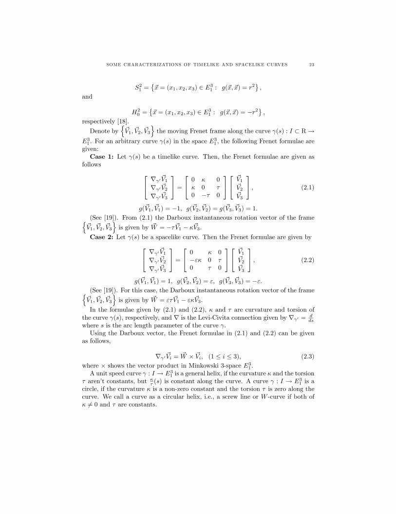
S21 =~x = (x1, x2, x3) ∈ E31 : g(~x, ~x) = r2
,
and
H20 =
~x = (x1, x2, x3) ∈ E31 : g(~x, ~x) = −r2
,
respectively [18].
Denote by~V1, ~V2, ~V3
the moving Frenet frame along the curve γ(s) : I ⊂ R→
E31 . For an arbitrary curve γ(s) in the space E31 , the following Frenet formulae aregiven:Case 1: Let γ(s) be a timelike curve. Then, the Frenet formulae are given as
follows ∇γ′ ~V1∇γ′ ~V2∇γ′ ~V3
=
0 κ 0κ 0 τ0 −τ 0
~V1~V2~V3
, (2.1)
g(~V1, ~V1) = −1, g(~V2, ~V2) = g(~V3, ~V3) = 1.
(See [19]). From (2.1) the Darboux instantaneous rotation vector of the frame~V1, ~V2, ~V3
is given by ~W = −τ ~V1 − κ~V3.
Case 2: Let γ(s) be a spacelike curve. Then the Frenet formulae are given by ∇γ′ ~V1∇γ′ ~V2∇γ′ ~V3
=
0 κ 0−εκ 0 τ0 τ 0
~V1~V2~V3
, (2.2)
g(~V1, ~V1) = 1, g(~V2, ~V2) = ε, g(~V3, ~V3) = −ε.(See [19]). For this case, the Darboux instantaneous rotation vector of the frame~V1, ~V2, ~V3
is given by ~W = ετ ~V1 − εκ~V3.
In the formulae given by (2.1) and (2.2), κ and τ are curvature and torsion ofthe curve γ(s), respectively, and ∇ is the Levi-Civita connection given by ∇γ′ = d
dswhere s is the arc length parameter of the curve γ.Using the Darboux vector, the Frenet formulae in (2.1) and (2.2) can be given
as follows,
∇γ′ ~Vi = ~W × ~Vi, (1 ≤ i ≤ 3), (2.3)where × shows the vector product in Minkowski 3-space E31 .A unit speed curve γ : I → E31 is a general helix, if the curvature κ and the torsion
τ aren’t constants, but κτ (s) is constant along the curve. A curve γ : I → E31 is a
circle, if the curvature κ is a non-zero constant and the torsion τ is zero along thecurve. We call a curve as a circular helix, i.e., a screw line or W -curve if both ofκ 6= 0 and τ are constants.
24 HÜSEYIN KOCAYIGIT, MEHMET ÖNDER AND KADRI ARSLAN
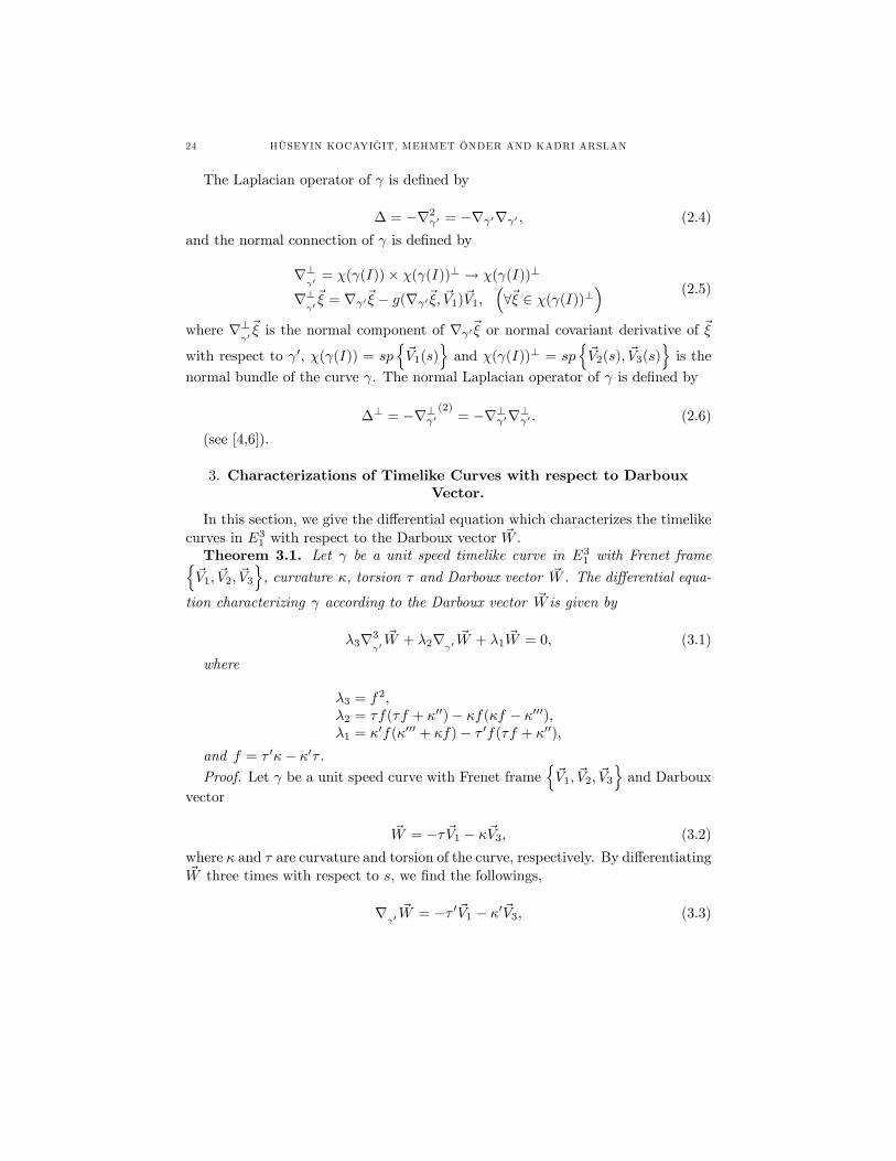
The Laplacian operator of γ is defined by
∆ = −∇2γ′ = −∇γ′∇γ′ , (2.4)
and the normal connection of γ is defined by
∇⊥γ′
= χ(γ(I))× χ(γ(I))⊥ → χ(γ(I))⊥
∇⊥γ′~ξ = ∇γ′~ξ − g(∇γ′~ξ, ~V1)~V1,
(∀~ξ ∈ χ(γ(I))⊥
) (2.5)
where ∇⊥γ′~ξ is the normal component of ∇γ′~ξ or normal covariant derivative of ~ξ
with respect to γ′, χ(γ(I)) = sp~V1(s)
and χ(γ(I))⊥ = sp
~V2(s), ~V3(s)
is the
normal bundle of the curve γ. The normal Laplacian operator of γ is defined by
∆⊥ = −∇⊥γ′(2)
= −∇⊥γ′∇⊥γ′ . (2.6)
(see [4,6]).
3. Characterizations of Timelike Curves with respect to DarbouxVector.
In this section, we give the differential equation which characterizes the timelikecurves in E31 with respect to the Darboux vector ~W .Theorem 3.1. Let γ be a unit speed timelike curve in E31 with Frenet frame~V1, ~V2, ~V3
, curvature κ, torsion τ and Darboux vector ~W . The differential equa-
tion characterizing γ according to the Darboux vector ~W is given by
λ3∇3γ′~W + λ2∇γ′
~W + λ1 ~W = 0, (3.1)
where
λ3 = f2,λ2 = τf(τf + κ′′)− κf(κf − κ′′′),λ1 = κ′f(κ′′′ + κf)− τ ′f(τf + κ′′),
and f = τ ′κ− κ′τ .Proof. Let γ be a unit speed curve with Frenet frame
~V1, ~V2, ~V3
and Darboux
vector
~W = −τ ~V1 − κ~V3, (3.2)
where κ and τ are curvature and torsion of the curve, respectively. By differentiating~W three times with respect to s, we find the followings,
∇γ′~W = −τ ′~V1 − κ′~V3, (3.3)
SOME CHARACTERIZATIONS OF TIMELIKE AND SPACELIKE CURVES 25
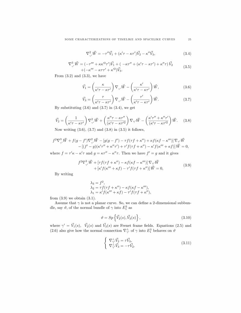
∇2γ′~W = −τ ′′~V1 + (κ′τ − κτ ′)~V2 − κ′′~V3, (3.4)
∇3γ′~W = (−τ ′′′ + κκ′2τ ′)~V1 + ( −κτ ′′ + (κ′τ − κτ ′) + κ′′τ) ~V2
+(−κ′′′ − κττ ′ + κ′2)~V3.(3.5)
From (3.2) and (3.3), we have
~V1 =
(κ
κ′τ − κτ ′
)∇
γ′~W −
(κ′
κ′τ − κτ ′
)~W, (3.6)
~V3 =
(τ
κ′τ − κτ ′
)∇
γ′~W −
(τ ′
κ′τ − κτ ′
)~W. (3.7)
By substituting (3.6) and (3.7) in (3.4), we get
~V2 =
(1
κ′τ − κτ ′
)∇2
γ′~W +
(κ′′τ − κτ ′′(κ′τ − κτ ′2
)∇γ′ ~W −
(κ′τ ′′ + κ′′τ ′
(κ′τ − κτ ′2
)~W. (3.8)
Now writing (3.6), (3.7) and (3.8) in (3.5) it follows,
f2∇3γ′~W + f(g − f ′)∇2
γ′~W − [g(g − f ′)− τf(τf + κ′′) + κf(κf − κ′′′)]∇γ′ ~W
− [(f ′ − g)(κ′τ ′′ + κ′′τ ′) + τ ′f(τf + κ′′)− κ′f(κ′′′ + κf)] ~W = 0,
where f = τ ′κ− κ′τ and g = κτ ′′ − κ′′τ . Then we have f ′ = g and it gives
f2∇3γ′~W + [τf(τf + κ′′)− κf(κf − κ′′′)]∇γ′ ~W
+ [κ′f(κ′′′ + κf)− τ ′f(τf + κ′′)] ~W = 0,(3.9)
By writing
λ3 = f2,λ2 = τf(τf + κ′′)− κf(κf − κ′′′),λ1 = κ′f(κ′′′ + κf)− τ ′f(τf + κ′′),
from (3.9) we obtain (3.1).Assume that γ is not a planar curve. So, we can define a 2-dimensional subbun-
dle, say ϑ, of the normal bundle of γ into E31 as
ϑ = Sp~V2(s), ~V3(s)
, (3.10)
where γ′ = ~V1(s), ~V2(s) and ~V3(s) are Frenet frame fields. Equations (2.5) and(2.6) also give how the normal connection ∇⊥γ′ of γ into E31 behaves on ϑ
∇⊥γ′ ~V2 = τ ~V3,
∇⊥γ′ ~V3 = −τ ~V2.(3.11)
26 HÜSEYIN KOCAYIGIT, MEHMET ÖNDER AND KADRI ARSLAN
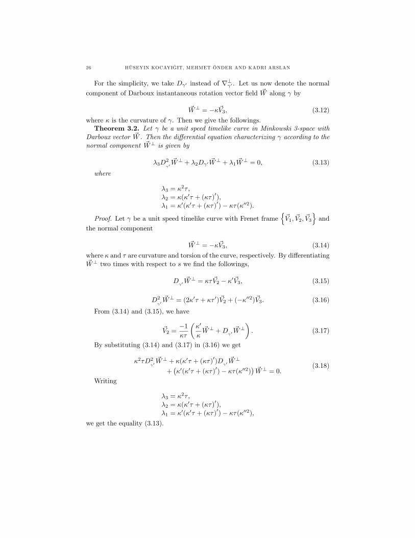
For the simplicity, we take Dγ′ instead of ∇⊥γ′ . Let us now denote the normalcomponent of Darboux instantaneous rotation vector field ~W along γ by
~W⊥ = −κ~V3, (3.12)
where κ is the curvature of γ. Then we give the followings.Theorem 3.2. Let γ be a unit speed timelike curve in Minkowski 3-space with
Darboux vector ~W . Then the differential equation characterizing γ according to thenormal component ~W⊥ is given by
λ3D2γ′~W⊥ + λ2Dγ′
~W⊥ + λ1 ~W⊥ = 0, (3.13)
where
λ3 = κ2τ ,
λ2 = κ(κ′τ + (κτ)′),
λ1 = κ′(κ′τ + (κτ)′)− κτ(κ′′2).
Proof. Let γ be a unit speed timelike curve with Frenet frame~V1, ~V2, ~V3
and
the normal component
~W⊥ = −κ~V3, (3.14)
where κ and τ are curvature and torsion of the curve, respectively. By differentiating~W⊥ two times with respect to s we find the followings,
Dγ′~W⊥ = κτ ~V2 − κ′~V3, (3.15)
D2γ′~W⊥ = (2κ′τ + κτ ′)~V2 + (−κ′′2)~V3. (3.16)
From (3.14) and (3.15), we have
~V2 =−1
κτ
(κ′
κ~W⊥ +D
γ′~W⊥). (3.17)
By substituting (3.14) and (3.17) in (3.16) we get
κ2τD2γ′~W⊥ + κ(κ′τ + (κτ)
′)D
γ′~W⊥
+(κ′(κ′τ + (κτ)
′)− κτ(κ′′2)
)~W⊥ = 0.
(3.18)
Writing
λ3 = κ2τ ,
λ2 = κ(κ′τ + (κτ)′),
λ1 = κ′(κ′τ + (κτ)′)− κτ(κ′′2),
we get the equality (3.13).
SOME CHARACTERIZATIONS OF TIMELIKE AND SPACELIKE CURVES 27
Corollary 1. Let γ be a unit speed timelike curve in E31 . If the curve γ is acircular helix, then the differential equation characterizing the curve according tothe normal Darboux vector ~W⊥is given by
D2γ′~W⊥ + τ2 ~W⊥ = 0, (3.19)
and the normal component of Darboux vector of γ is
~W⊥ = c1 cosh(τs) + c2 sinh(τs),
where c1, c2 are non-zero constants.
4. Timelike Curves with Harmonic 1-type Darboux Vector.
In this section we will give the characterizations of timelike curves with Harmonic1-type Darboux vector in Minkowski 3-space E31 .Definition 1. A regular timelike curve γ in E31 is said to have harmonic Darboux
vector if
∆ ~W = 0, (4.1)
holds. Further, a regular timelike curve γ in E31 is said to have harmonic 1-typeDarboux vector if
∆ ~W = λ ~W, λ ∈ R, (4.2)
holds.First we prove the following theorem.Theorem 4.1. Let γ be a unit speed timelike curve in E31 with Darboux vector
~W . Then,γ has harmonic 1-type Darboux vector if and only if the curvature κ andthe torsion τ of the curve γ satisfy the followings, τ ′′ = −λτ,
κτ ′ − κ′τ = 0,κ′′ = −λκ,
(4.3)
where λis constant.Proof. Let γ be a unit speed timelike curve in E31 with Darboux vector ~W and
let ∆ be the Laplacian associated with ∇. One can use (2.4) and (3.2) to compute
∆ ~W = τ ′′~V1 + (κτ ′ − κ′τ)~V2 + κ′′~V3. (4.4)
We assume that the timelike curve γ is of harmonic 1-type Darboux vector.Substituting (4.4) in (4.2), we have (4.3).Conversely, if the equations (4.3) satisfy for the constant λ, then it is easy to
show that γ has harmonic 1-type Darboux vector.Further, solving the system of differential equations in (4.3) we obtain the fol-
lowing corollary.
28 HÜSEYIN KOCAYIGIT, MEHMET ÖNDER AND KADRI ARSLAN
Corollary 2. Let γ be a unit speed timelike curve in E31 with Darboux vector~W . Then, γ has harmonic 1-type Darboux vector if and only if γ is a general helixwith curvature and torsion
κ = cτ ,
τ = c1 cos(√
λs)
+ c2 sin(√
λs),
respectively, where c, c1, c2 are constants.Corollary 3. Let γ be a unit speed timelike curve in E31 with Darboux vector
~W . Then, γ has harmonic Darboux vector if and only if γ is a general helix withcurvature and torsion
κ(s) = cs, τ(s) = c1s,
where c, c1 are constants.Theorem 4.2. Let γ be a unit speed timelike curve in E31 with Darboux vector
~W . Then,
∆ ~W + λ∇γ′~W + µ ~W = 0, (4.5)
holds along the curve γ for the constants λ and µ if and only if γ is a generaltimelike helix, with curvature and the torsion
κ = cτ ,
τ = c1 exp
(−λ+
√λ2 + 4µ
2s
)+ c2 exp
(λ−
√λ2 + 4µ
2s
),
where c, c1, c2 are constants.Proof. Assume that (4.5) holds along the curve γ. Then from the equalities
(3.2), (3.3) and (4.4) we have τ ′′ − λτ ′ − µτ = 0,κτ ′ − κ′τ = 0,κ′′ − λκ′ − µκ = 0.
(4.6)
The second equation of the system (4.6) gives that κτ is constant, i.e., γ is a
general helix. From the first and third equations, we get
τ = c1 exp
(−λ+
√λ2 + 4µ
2s
)+ c2 exp
(λ−
√λ2 + 4µ
2s
), (4.7)
and
κ = cτ (4.8)
SOME CHARACTERIZATIONS OF TIMELIKE AND SPACELIKE CURVES 29
respectively, where c, c1, c2 are constants.Conversely, if γ is a general timelike helix with curvature κ and torsion τ given
by (4.8) and (4.7), respectively, it is easily seen that (4.5) holds.
5. Timelike Curves with Harmonic 1-type Darboux NormalComponent.
In this section, we will give the characterizations of timelike curves with Har-monic 1-type Darboux normal component vector in Minkowski 3-space E31 .Definition 2. A regular timelike curve γ in E31 is said to have harmonic Darboux
normal component vector ~W⊥ if
∆D ~W⊥ = 0, (5.1)
holds. Further, a regular timelike curve γ in E31 is said to have harmonic 1-typeDarboux vector if
∆D ~W⊥ = λ ~W⊥, λ ∈ R, (5.2)
holds, where ∆D = −Dγ′Dγ′ .Theorem 5.1. Let γ be a unit speed timelike curve in E31 . Then, ~W⊥ is
harmonic 1-type vector if and only if
κ′′2)κ = 0, 2κ′τ + τ ′κ = 0. (5.3)
Proof. Let γ be a unit speed timelike curve in E3 and let ∆D = −Dγ′Dγ′ bethe Laplacian associated with D. From (3.16), we get
∆D ~W⊥ = (2κ′τ + κτ ′)~V2 + (κτ2 − κ′′)~V3. (5.4)
We assume that the normal component ~W⊥ of the Darboux vector field is ofharmonic 1-type. Then substituting (5.4) in (5.2), we get (5.3).Conversely, if the equations (5.3) satisfy then it is easily seen that the normal
component ~W⊥ of the Darboux vector field is of harmonic 1-type.Corollary 4. Let γ be a unit speed timelike curve in E31 with Darboux vector
~W . If γ is a circular timelike helix with torsion τ2 = λ, then the normal component~W⊥ of the Darboux vector field is of harmonic 1-type.
6. Characterizations of the Spacelike Curves with respect to DarbouxVector.
In this section, we give the characterizations of spacelike curves according to theDarboux vector. The proofs of this section can be obtained by the similar waysgiven in previous sections.
30 HÜSEYIN KOCAYIGIT, MEHMET ÖNDER AND KADRI ARSLAN
Theorem 6.1. Let γ be a unit speed spacelike curve in E31 with Frenet frame~V1, ~V2, ~V3
, curvature κ, torsion τ and Darboux vector ~W . The differential equa-
tion characterizing γ according to the Darboux vector ~W is given by
λ4∇3γ′~W + λ3∇2
γ′~W + λ2∇γ′ ~W + λ1 ~W = 0,
where
λ4 = f2,λ3 = −2fg,λ2 = 2g2 − τf(τf − κ′′)− εκf(εκ′′′ − κf),λ1 = 2g(κ′′τ ′ − κ′τ ′′) + τ ′f(τf − κ′′)− εκ′f(εκ′′′ − κf),
and f = κτ ′ − κ′τ , g = κτ ′′ − κ′′τ .Theorem 6.2. Let γ be a unit speed spacelike curve in E31 . Then the differential
equation characterizing γ according to the normal component ~W⊥is given by
λ3D2γ′~W⊥ + λ2Dγ′
~W⊥ + λ1 ~W⊥ = 0,
where λ3 = κ2τ ,
λ2 = −κ(κ′τ + (κτ)′),
λ1 = −εκ′(κ′τ + (κτ)′)− κτ(κ′′2).
Corollary 5. Let γ be a unit speed spacelike curve in E31 . If the curve γ isa circular helix, then the differential equation characterizing the curve according tothe normal component ~W⊥is given by
D2γ′~W⊥ − τ2 ~W⊥ = 0.
From the last differential equation, the normal component of Darboux vector ofγ is
~W⊥ = c1 exp(τs) + c2 exp(−τs),where c1, c2 are non-zero constants.
7. Spacelike Curves with Harmonic 1-type Darboux Vector andHarmonic 1-type Darboux Normal Component.
Theorem 7.1. Let γ be a unit speed spacelike curve in E31 with Darboux vector~W . Then, γ has harmonic 1-type Darboux vector if and only if the curvature κ andthe torsion τ of the curve γ satisfy the followings,
τ ′′ + λτ = 0, κτ ′ − κ′τ = 0, κ′′ + λκ = 0,
where λ is constant.
SOME CHARACTERIZATIONS OF TIMELIKE AND SPACELIKE CURVES 31
Corollary 6. Let γ be a unit speed spacelike curve in E31 with Darboux vector~W . Then, γ has harmonic 1-type Darboux vector if and only if γ is a general helix,with curvature and torsion
κ = cτ ,
τ = c1 cos(√
λs)
+ c2 sin(√
λs),
respectively, where c, c1, c2 are constants.Corollary 7. Let γ be a unit speed spacelike curve in E31 with Darboux vector
~W . Then, γ has harmonic Darboux vector if and only if γ is a general helix withcurvature and torsion
κ(s) = cs, τ(s) = c1s
respectively, where c, c1 are constants.Theorem 7.2. Let γ be a unit speed spacelike curve in E31 with Darboux vector
~W . Then,
∆ ~W + λ∇γ′ ~W + µ ~W = 0,
holds along the curve γ for the constants λ and µ if and only if γ is a generalspacelike helix, with curvature and the torsion
κ = cτ ,
τ = c1 exp
(−λ+
√λ2 + 4µ
2s
)+ c2 exp
(−λ−
√λ2 + 4µ
2s
),
respectively, where c, c1, c2 are constants.Theorem 7.3. Let γ be a unit speed spacelike curve in E31 . Then, ~W⊥ is
harmonic 1-type if and only if
κ′′2)κ = 0, 2κ′τ + τ ′κ = 0.
Corollary 8. Let γ be a unit speed spacelike curve in E31 with Darboux vector ~W .If γ is a circular spacelike helix with torsion λ = −τ2, then the normal component~W⊥ of the Darboux vector field is of harmonic 1-type.
8. Conclusions.
In the space, while the position vector drawing the space curve, the Frenet frameof the curve makes a rotation around an axis which is called Darboux instantaneousrotation vector. In this study, we give some characterizations on the Darboux in-stantaneous rotation vector field of the curves in Minkowski 3-space E31 by usingLaplacian and normal Laplacian operators. We define harmonic type and harmonic
32 HÜSEYIN KOCAYIGIT, MEHMET ÖNDER AND KADRI ARSLAN
1-type Darboux vector and show that the curves having harmonic type and har-monic 1-type Darboux vectors are general helices in Minkowski 3-space.
References
[1] A. Altın, Harmonic curvatures of non-null curves and the helix in Rnv , Hacettepe Bul. of Nat.Sci. and Eng., Vol. 30 (2001) 55-61.
[2] K. Arslan, Y. Aydın, G. Öztürk, H. Ugail, Biminimal Curves in Euclidean Spaces, Interna-tional Electronic Journal of Geometry, 2 (2009) 46-52.
[3] M. Barros, O.J. Gray, On Submanifolds with Harmonic Mean Curvature, Proc. Amer. Math.Soc., 123 (1995) 2545-2549.
[4] B.Y. Chen, S. Ishikawa, Biharmonic surface in pseudo-Euclidean spaces, Mem. Fac. Sci.Kyushu Univ., A 45 (1991) 323-347.
[5] N. Chouaieb, A. Goriely, J.H. Maddocks, Helices, PNAS 103 (25) (2006) 9398-9403.[6] A. Ferrandez, P. Lucas, M.A. Merono, Biharmonic Hopf cylinders, Rocky Mountain J., 28
(1998) 957-975.[7] H.H. Hacısalihoglu, R. Öztürk, On the characterization of inclined curves in En- I., Tensor,
N., S., 64 (2003) 157-162.[8] H.H. Hacısalihoglu, R. Öztürk, On the characterization of inclined curves in En- II., Tensor,
N., S., 64 (2003) 163-169.[9] S. Izumiya, N. Takeuchi, New special curves and developable surfaces, Turk J. Math. Vol. 28
(2004) 153-163.[10] B. Kılıç, K. Arslan, Harmonic 1-type submanifolds of Euclidean spaces, Int. J. Math. Stat.,
3 (2008) A08, 47-53.[11] H. Kocayigit, Biharmonic Curves in Lorentz 3-Manifolds and Contact Geometry, Ph. D.
Thesis, Ankara University, (2004).[12] H. Kocayigit, M. Önder, Timelike curves of constant slope in Minkowski space E41 , BU/JST,
Vol. 1 (2) (2007) 311-318.[13] A. Lucas Amand, P. Lambin, Diffraction by DNA, carbon nanotubes and other helical nanos-
tructures, Rep. Prog. Phys. 68 (2005) 1181-1249.[14] A. Magden, On the curves of constant slope, YYÜ Fen Bilimleri Dergisi, Vol. 4 (1993) 103-109.[15] B. O’neill, Semi-Riemannian Geometry, Academic Press 1983.[16] M. Petrovic-Torgasev, E. Sucurovic, W-curves in Minkowski spac-time, Novi Sad J. Math.,
Vol. 32 No. 2 (2002) 55-65.[17] D.J. Struik, Lectures on Classical Differential Geometry, 2nd ed. Addison Wesley, Dover,
(1988).[18] H.H. Ugurlu, A. Çalıskan, Darboux Ani Dönme Vektörleri ile Spacelike ve Timelike Yüzeyler
Geometrisi, Celal Bayar Üniversitesi Yayınları, Yayın No: 0006. (2012).[19] J. Walrave, Curves and surfaces in Minkowski space, Doctoral thesis, K. U. Leuven, Fac. Of
Science, Leuven, (1995).[20] J.D. Watson, F.H.C. Crick, Genetic implications of the structure of deoxyribonucleic acid,
Nature, 171 (1953) 964-967.[21] X. Yang, High accuracy approximation of helices by quintic curve, Comput. Aided Geometric
Design, 20 (2003) 303-317.
Current address : Hüseyin Kocayigit and Mehmet Önder; Department of Mathematics Facultyof Science and Arts Celal Bayar University, 45047, Manisa, TURKEYKadri Arslan; Department of Mathematics Science and Arts Faculty Uludag University, 16059Bursa, TURKEYE-mail address : [email protected], [email protected], [email protected]: http://communications.science.ankara.edu.tr/index.php?series=A1
Commun.Fac.Sci.Univ .Ank.Series A1Volum e 62, Number 1, Pages 33—43 (2013)ISSN 1303—5991
COMPOSITE DUAL SUMMABILITY METHODS OF THE NEWSORT*
MEDINE YESILKAYAGIL AND FEYZI BASAR
Abstract. Following Altay and Basar [1], we define the duality relation ofthe new sort between a pair of infinite matrices. Our focus is to study thecomposite dual summability methods of the new sort and to give some inclusiontheorems.
1. Introduction
We denote the space of all sequences with complex entries by ω. Any vectorsubspaces of ω is called a sequence space. We shall write `∞, c and c0 for the spacesof all bounded, convergent and null sequences, respectively. A sequence space Xis called an FK−space if it is a complete linear metric space with continuouscoordinates pn : X → C for all n ∈ N with pn(x) = xn for all x = (xk) ∈ X andevery n ∈ N, where C denotes the complex field and N = 0, 1, 2, . . .. A normedFK−spaces is called a BK−space, that is, a BK − space is a Banach space withcontinuous coordinates. The sequence spaces `∞, c and c0 are BK−spaces withthe usual sup-norm defined by ‖x‖∞ = supk∈N |xk|.Let λ and µ be two sequence spaces, and A = (ank) be an infinite matrix of
complex numbers ank, where k, n ∈ N. Then, we say that A defines a matrixmapping from λ into µ, and we denote it by writing A : λ→ µ if for every sequencex = (xk) ∈ λ, the sequence Ax = (Ax)n, the A-transform of x, is in µ; where
(Ax)n =
∞∑k=0
ankxk for each n ∈ N.
Received by the editors Nov. 01, 2012; Accepted: April 30, 2013.2010 Mathematics Subject Classification. 40C05.Key words and phrases. Dual summability methods, sequence spaces, matrix transformations,
composition of summability methods, inclusion theorems.
The main results of this paper were presented in part at the conference Algerian-TurkishInternational Days on Mathematics 2012 (ATIM’2012) to be held October 9—11, 2012 in Annaba,Algeria at the Badji Mokhtar Annaba University.
c©2013 Ankara University
33

34 MEDINE YESILKAYAGIL AND FEYZI BASAR
By (λ : µ), we denote the class of all matrices A such that A : λ → µ. Thus,A ∈ (λ : µ) if and only if the series on the right side of (1.1) converges for eachn ∈ N and each x ∈ λ, and we have Ax = (Ax)nn∈N ∈ µ for all x ∈ λ. A sequencex is said to be A-summable to α if Ax converges to α which is called the A-limit ofx. Also by (λ : µ; p), we denote the subset of (λ : µ) for which the limits or sumsare preserved whenever there is a limit or sum on the spaces λ and µ. The matrixdomain λA of an infinite matrix A in a sequence space λ is defined by
λA = x = (xk) ∈ ω | Ax ∈ λ
which is a sequence space.Let t = (tk) be a sequence of non-negative numbers which are not all zero and
write Tn =n∑k=0
tk for all n ∈ N. Then the matrix Rt = (rtnk) of the Riesz mean
(R, tn) with respect to the sequence t = (tk) is given by
rtnk =
tkTn
, 0 ≤ k ≤ n,0 , k > n
for all k, n ∈ N. It is well-known that the Riesz mean (R, tn) is regular if and only ifTn →∞ as n→∞ (see [11, Theorem 1.4.4]). Let us define the sequence y = (yk),which will be used throughout, as the Rt- transform of a sequence x = (xk), i.e.,
yk =1
Tk
k∑j=0
tjxj for all k ∈ N. (1.1)
2. The Dual Summability Methods of the New Sort
Lorentz introduced the concept of the dual summability methods for the limi-tation methods dependent on a Stieltjes integral and passed to the discontinuousmatrix methods by means of a suitable step function,in [6]. After, several authors,such as Lorentz and Zeller [8], Kuttner [5], Öztürk [10], Orhan and Öztürk [9],Basar and Çolak [4], and the others, worked on the dual summability methods.Basar [3] recently introduced the dual summability methods of the new type whichis based on the relation between the C1-transform of a sequence and itself; whereC1 denotes the Cesàro mean of order 1. Following Kuttner [5] and Lorentz andZeller [8] who defined the dual summability methods by using the relation betweenan infinite series and its sequence of partial sums, we desire to base the similarrelation on (1.1) and call it as the duality of the new sort.Let us suppose that the infinite matrix A = (ank) and B = (bnk) map the
sequences x = (xk) and y = (yk) which are connected with the relation (1.1) to thesequences (un) and (vn), respectively, i.e.,
un = (Ax)n =
∞∑k=0
ankxk for all n ∈ N, (2.1)
COMPOSITE DUAL SUMMABILITY METHODS 35
vn = (By)n =
∞∑k=0
bnkyk for all n ∈ N. (2.2)
It is clear here that the method B is applied to the Rt-transform of the sequencex = (xk), while the method A is directly applied to the entries of the sequencex = (xk). So, the methods A and B are essentially different.Let us assume that the usual matrix product BRt exists which is a much weaker
assumption than the conditions on the matrix B belonging to any class of matrices,in general. We shall say in this situation that the matrices A and B in (2.1) and(2.2) are the dual matrices of the new sort if un reduces to vn (or vn reduces toun) under the application of the formal summation by parts. This leads us to thefact that BRt exists and is equal to A and Ax = (BRt)x = B(Rtx) = By formallyholds, if one side exists. This statement is equivalent to the relation between theentries of the matrices A = (ank) and B = (bnk):
ank :=
∞∑j=k
tkTjbnj or bnk :=
(anktk− an,k+1
tk+1
)Tk = ∆
(anktk
)Tk. (2.3)
for all k, n ∈ N. Now, we may give a short analysis on the dual summabilitymethods of the new sort. One can see that vn reduces to un, as follows: Since theequality
m∑k=0
bnkyk =
m∑k=0
bnk
k∑j=0
tjTkxj =
m∑j=0
m∑k=j
tjTkbnkxj
holds for all m,n ∈ N one can obtain by letting m→∞ that
vn =
∞∑k=0
bnkyk =
∞∑j=0
∞∑k=j
tjTkbnkxj =
∞∑j=0
anjxj = un for all n ∈ N.
But the order of summation may not be reversed. So, the matrices A and B arenot necessarily equivalent.Let us suppose that the entries of the matrices A = (ank) and B = (bnk) are
connected with the relation (2.3) and C = (cnk) be a strongly regular lower trianglematrix. Suppose also that the C−transforms of u = (un) and u = (vn) be t = (tn)and z = (zn), respectively, i.e.,
tn = (Cu)n =
n∑k=0
cnkuk for all n ∈ N, (2.4)
zn = (Cv)n =
n∑k=0
cnkvk for all n ∈ N. (2.5)
36 MEDINE YESILKAYAGIL AND FEYZI BASAR
Define the matrices D = (dnk) and E = (enk) by
dnk :=
n∑j=0
cnjajk and enk :=
n∑j=0
cnjbjk for all n ∈ N.
For short, here and after, we call the methods A and B as "original methods" andcall the methods D and E as "composite methods". Now, we can give the firsttheorem:
Theorem 2.1. The original methods are dual of the new sort if and only if thecomposite methods are dual of the new sort.
Proof. Suppose that the relation (2.3) exists between the elements of the originalmatrices A = (ank) and B = (bnk). This means that A = BRt or equivalently B =A(Rt)−1. Therefore, by applying the strongly regular triangle matrix C = (cnk) to(un) and (vn) in (2.1) and (2.2), we obtain that
Cu = C(Ax) = (CA)x = Dx
Cv = C(By) = (CB)y = Ey
Then, we have Cu = Cv whenever u = v which gives that Ey = Dx. Therefore,we derive that
Ey = E(Rtx) = (ERt)x = Dx.
This shows that the composite methods D and E are dual of the new sort.Conversely, suppose that the duality relation of the new sort exists between the
elements of D = (dnk) and E = (enk), i.e., D = ERt or equivalently E = D(Rt)−1.Then, by applying the inverse matrix C−1 to the sequences t = (tn) and z = (zn)in (2.4) and (2.5), we observe that
C−1z = C−1(Dx) = (C−1D)x = Ax,
C−1v = C−1(Ey) = (C−1E)y = By.
Hence, By = Ax. Therefore, we get B(Rtx) = (BRt)x = Ax which means that theoriginal matrices A and B are dual of the new sort.
Theorem 2.2. Every A−summable sequence is D−summable. However, the con-verse of this fact does not hold, in general.
Proof. Suppose that x = (xk) is A−summable to a ∈ C, i.e.,limn→∞
(Ax)n = limn→∞
un = a.
Since C = (cnk) is a strongly regular triangle matrix, we have
limn→∞
un = limn→∞
(Cu)n = a.
That is to say that
limn→∞
(Cu)n = limn→∞
C(Ax)n = limn→∞
(CA)xn = limn→∞
(Dx)n = a.
COMPOSITE DUAL SUMMABILITY METHODS 37
This shows that the sequence x = (xk) is summable D to the same point. Hence,the inclusion cA ⊂ cD holds.Let us choose the matrix C = (cnk) defined by
cnk =
2(k+1)
(n+1)(n+2) , 0 ≤ k ≤ n,0 , k > n
for all k, n ∈ N. A short calculation gives the inverse matrix C−1 = (c−1nk ) as
c−1nk =
1+(−1)n−k(n+1)
2 , n− 1 ≤ k ≤ n,0 , 0 ≤ k < n− 1 or k > n
for all k, n ∈ N. Let us also choose the matrix D = (dnk)
dnk =
12n , 0 ≤ k < n− 1,−12n , k = n− 1,1 , k = n,0 , k > n
for all k, n ∈ N. Then, the matrix A = (ank) satisfying the equality D = CA isobtained by a straightforward calculation as
ank =
2−n2n+1 , 0 ≤ k < n− 2,3n+22n+1 , k = n− 2,
−n2n+n+22n+1 , k = n− 1,n+22 , k = n,0 , k > n
for all k, n ∈ N. Therefore, ‖A‖ = supn∈N
∞∑k=0
|ank| =∞. Hence, A does not even apply
to the points belonging to the space `∞. This shows that the inclusion cA ⊂ cD isstrict.
Theorem 2.3. Every B−summable sequence is E−summable. However, the con-verse of this fact does not hold, in general.
Proof. Suppose that y = (yk) is B−summable to b ∈ C, i.e.,limn→∞
(By)n = limn→∞
vn = b.
Since C = (cnk) is a strongly regular triangle matrix, then we have
limn→∞
vn = limn→∞
(Cv)n = b
and this yields that
limn→∞
(Cv)n = limn→∞
C(By)n = limn→∞
(CB)yn = limn→∞
(Ey)n = b.
Hence, the sequence y = (yk) is E−summable to the value b which means that theinclusion cB ⊂ cE holds.
38 MEDINE YESILKAYAGIL AND FEYZI BASAR
We choose the matrix C = (cnk) as in Theorem 2.2. Let us also choose thematrix E = (enk) defined by
enk =
(−12 )n−k , n− 1 ≤ k ≤ n,
0 , k > n
for all k, n ∈ N. Then, the matrix B = (bnk) satisfying the matrix equality E = CBis found by a routine calculation as
bnk =
n4 , k = n− 2,
−( 3n+24 ) , k = n− 1,n+22 , k = n,0 , k > n
for all k, n ∈ N. Therefore, ‖B‖ = supn∈N
∞∑k=0
|bnk| = ∞. Hence, B does not apply to
the sequences in the space `∞. This shows that the composite method E is strongerthan the original method B and this step completes the proof.
Definition 2.4. A continuous linear functional φ on `∞ is called a Banach limit(see Banach [2]) if the following statements hold:
(i) φ(x) ≥ 0, where x = (xk) with xk ≥ 0 for every k ∈ N,(ii) φ(xk+1) = φ(xk),(iii) φ(e) = 1, where e = (1, 1, 1, . . .).
A sequence x ∈ `∞ is said to be almost convergent to the generalized limit L ifall of its Banach limits equal to L (see Lorentz, [7]). We denote the set of all almostconvergent sequences by f , i.e.,
f :=x = (xk) ∈ ω | ∃α ∈ C 3 lim
m→∞tmn(x) = α uniformly in n
,
where
tmn(x) =
m∑k=0
xk+nm+ 1
with t−1,n = 0 and α = f − lim xk.
We use the following notation in Theorem 2.5 and Theorem 2.6:
tmn(Ax) =1
m+ 1
m∑j=0
An+j(x) =
∞∑k=0
a(n, k,m)xk,
where
a(n, k,m) =1
m+ 1
m∑j=0
an+j,k for all k,m, n ∈ N.
Theorem 2.5. The inclusion fD ⊃ fA strictly holds.
COMPOSITE DUAL SUMMABILITY METHODS 39
Proof. Suppose that the sequence x = (xk) is almost A−summable to l ∈ C. Thatis, f − lim(Ax)n = l. Since C = (cnk) is a strongly regular triangle matrix, we have
f − lim(Ax)n = f − limC(Ax)n = f − lim(CA)xn = f − lim(Dx)n = l.
Then, the sequence x = (xk) is almost D−summable. This means that the compos-ite method D is stronger than the original method A. Hence, the inclusion fD ⊃ fAholds.Let us choose the matrix C = (cnk) as C1, the Cesàro matrix of order one. Then,
a short calculation gives us the inverse matrix C−1 = (c−1nk ) as
c−1nk =
(−1)n−k(k + 1) , n− 1 ≤ k ≤ n,
0 , 0 ≤ k ≤ n− 2 or k > n
for all k, n ∈ N. Let us also choose the matrix D = (dnk) defined by
dnk =
1+(−1)n(n+1) , 0 ≤ k ≤ n,
0 , k > n
for all k, n ∈ N. Then, the matrix A = (ank) satisfying the matrix equality D = CAis obtained as
ank =
2 , n is even and 0 ≤ k ≤ n,−2 , n is odd and 0 ≤ k ≤ n− 1,
0 , otherwise
for all k, n ∈ N. Now, take x = (xk) =
k(k+1)!
. Then,
1
m+ 1
m∑i=0
(Dx)n+i =1
m+ 1
m∑i=0
n+i∑k=0
dn+i,kxk
if n+ i is odd, dn+i,k will be zero. Therefore,
1
m+ 1
m∑i=0
Dn+i(x) = 0.
if n+ i is even, we’ll have
1
m+ 1
m∑i=0
Dn+i(x) =1
m+ 1
m∑i=0
1 + (−1)n+i
n+ i+ 1
n+i∑k=0
k
(k + 1)!
=1
m+ 1
m∑i=0
2
n+ i+ 1
[1− 1
(n+ i+ 1)!
]
=2
m+ 1
m∑i=0
1
n+ i+ 1− 2
m+ 1
m∑i=0
1
(n+ i+ 1)(n+ i+ 1)!
(2.6)
40 MEDINE YESILKAYAGIL AND FEYZI BASAR
which tends to zero, as m→∞. Because we know that
limm→∞
1n+1 + 1
n+2 + · · ·+ 1n+m+1
m+ 1= lim
m→∞
1
n+m+ 1= 0.
We can observe the second sum on the right hand side of (2.6) is zero, i.e., x ∈ fD.Now, we derive for the matrix A = (ank) that
1
m+ 1
m∑i=0
(Ax)n+i =1
m+ 1
m∑i=0
n+i∑k=0
an+i,kxk for all m,n ∈ N.
If n+ i is even, then we have
1
m+ 1
m∑i=0
(Ax)n+i =1
m+ 1
m∑i=0
2
n+i∑k=0
k
(k + 1)!
=2
m+ 1
m∑i=0
[1− 1
(n+ i+ 1)!
]
= 2− 2
m+ 1
m∑i=0
1
(n+ i+ 1)!
which tends to 2, as m→∞. If n+ i is odd, then we have
1
m+ 1
m∑i=0
(Ax)n+i =1
m+ 1
m∑i=0
(−2)
n+i∑k=0
k
(k + 1)!
=−2
m+ 1
m∑i=0
[1− 1
(n+ i+ 1)!
]
= −2 +2
m+ 1
m∑i=0
1
(n+ i+ 1)!
which tends to -2, as m→∞. Therefore, we have
limm→∞
1
m+ 1
m∑i=0
(Ax)n+i =
2 , n+i is even,−2 , n+i is odd,
i.e., x /∈ fA, so the inclusion fD ⊃ fA strictly holds and this completes the proof.
Theorem 2.6. The inclusion fE ⊃ fB strictly holds.
Proof. Let y = (yk) be almost B−summable to r ∈ C. That is, f − lim(By)n = r.Since C = (cnk) is a strongly regular triangle matrix, we have
f − lim(By)n = f − limC(By)n = f − lim(CB)yn = f − lim(Ey)n = r.
Therefore, y = (yk) is almost E−summable to r. Hence, the inclusion fE ⊃ fBholds.
COMPOSITE DUAL SUMMABILITY METHODS 41
Let us choose the matrix C = (cnk) as in Theorem 2.5 and define the matrixB = (bnk) by
bnk =
n+ 1 , k = n,
−(2n+ 1) , k = n− 1,n , k = n− 2,0 , otherwise
for all k, n ∈ N. Then, the matrix E = (enk) such that E = CB is obtained as
enk =
(−1)n−k , n− 1 ≤ k ≤ n,
0 , otherwise
for all k, n ∈ N. Now, take the sequence y = (yk) = (−1)k. Then, we have
1
m+ 1
m∑i=0
(Ey)n+i =1
m+ 1
m∑i=0
n+i∑k=0
en+i,kyk
=1
m+ 1
m∑i=0
(en+i,n+i−1yn+i−1 + en+i,n+iyn+i)
=1
m+ 1
m∑i=0
[−(−1)n+i−1 + (−1)n+i]
=2(−1)n
m+ 1
m∑i=0
(−1)i
42 MEDINE YESILKAYAGIL AND FEYZI BASAR
which gives by letting m→∞ that the sequence y is almost E−summable to zero,that is, y ∈ fE . On the other hand, we have
1
m+ 1
m∑i=0
(By)n+i (2.7)
=1
m+ 1
m∑i=0
n+i∑k=0
bn+i,kyk
=1
m+ 1
m∑i=0
(bn+i,n+i−2yn+i−2 + bn+i,n+i−1yn+i−1 + bn+i,n+iyn+i)
=1
m+ 1
m∑i=0
[bn+i,n+i−2(−1)n+i−2 + bn+i,n+i−1(−1)n+i−1 + bn+i,n+i(−1)n+i]
=1
m+ 1
m∑i=0
(−1)n+i[(n+ i) + (2n+ 2i+ 1) + (n+ i+ 1)]
=(−1)n
m+ 1
m∑i=0
(−1)i(4n+ 4i+ 2)
=4n(−1)n
m+ 1
m∑i=0
(−1)i +4(−1)n
m+ 1
m∑i=0
(−1)ii+2(−1)n
m+ 1
m∑i=0
(−1)i
It is not hard to see that the first and third sums on the right hand side of (2.7)tend to zero, as m → ∞ and since the second sum on the right hand side of (2.7)is; if m is even,
4(−1)n
m+ 1
m∑i=0
(−1)ii =4(−1)n
m+ 1[−(1 + 3 + · · ·+ (m− 1)) + (2 + 4 + · · ·+m)] =
m
2
and if m is odd,
4(−1)n
m+ 1
m∑i=0
(−1)ii =4(−1)n
m+ 1[−(1+ 3+ · · ·+m)+ (2+4 + · · ·+(m−1))] = −m+ 1
2
which leads us by letting m→∞ that
limm→∞
4(−1)n
m+ 1
m∑i=0
(−1)ii =
2(−1)n , m is even−2(−1)n , m is odd
This shows that y /∈ fB . Therefore, the inclusion fD ⊃ fA strictly holds and thiscompletes the proof.
Theorem 2.7. The duality relation of the new sort is not preserved under the usualinverse operation.
COMPOSITE DUAL SUMMABILITY METHODS 43
Proof. Suppose that the relation (2.3) exists between the original matrices A =(ank) and B = (bnk). Choose the matrix B as the identity matrix I. Then,the dual matrix of the new sort corresponding to the matrix B = I is A = Rt.Nevertheless, the inverses B−1 = I and A−1 = (Rt)−1 are not dual of the new sort.This shows that there are dual matrices of the new sort while their usual inversesare not dual of the new sort. This completes the proof.
Acknowledgement
The authors would like to express their pleasure to the anonymous referee forhis/her many helpful suggestions and interesting comments on the main results ofthe earlier version of the manuscript.
References
[1] B. Altay, F. Basar, Some paranormed Riesz sequence spaces of non-absolute type, SoutheastAsian Bull. Math. 30(5)(2006), 591—608
[2] S. Banach, Théorie des Operations Linéaries, Warsaw, 1932.[3] F. Basar, Matrix transformations between certain sequence spaces of Xp and `p, Soochow J.
Math. 26(2)(2000), 191—204.[4] F. Basar, R. Çolak, Almost-conservative matrix transformations, Doga Mat. 13(3)(1989),
91—100.[5] B. Kuttner, On dual summability methods, Proc. Camb. Phil. Soc. 71(1972), 67—73.[6] G.G. Lorentz, Über Limitierungsverfahren die von einem Stieltjes-Integral abhängen, Acta
Math. 79(1947), 255—272.[7] G. G. Lorentz, A contribution to the theory of divergent sequences, Acta Math. 80(1948),
167—190.[8] G.G. Lorentz, K. Zeller, Summation of sequences and summation of series, Proc. Amer.
Math. Soc. 15(1964), 743—746.[9] C. Orhan, E. Öztürk, On f-regular dual summability methods, Bull. Inst. Math. Acad. Sinica
14(1)(1986), 99—104.[10] E. Öztürk, On dual summability methods, Comm. Fac. Sci. Univ. Ank. Ser. A1 Math. Statist.
25(1)(1976), 1—19.[11] G.M. Petersen, Regular Matrix Transformations, McGraw-Hill Publishing Company Lim-
ited, London, 1966.
Current address : Medine Yesilkayagil; Department of Mathematics, Usak University, 1 EylülCampus, 64200—Usak, TURKEY, Feyzi Basar; Department of Mathematics, Fatih University, The Hadımköy Campus, Büyükçek-mece, 34500—Istanbul, TURKEY,
E-mail address : [email protected], [email protected]: http://communications.science.ankara.edu.tr/index.php?series=A1

Commun.Fac.Sci.Univ .Ank.Series A1Volum e 62, Number 1, Pages 45—59 (2013)ISSN 1303—5991
SURVEY ON THE DOMAIN OF THE MATRIX LAMBDA INTHE NORMED AND PARANORMED SEQUENCE SPACES*
FEYZI BASAR
Abstract. In the present paper, we summarize the literature on the normedand paranormed sequence spaces derived by the domain of the matrix lambda.Moreover, we establish some inclusion relations concerning with those spacesand determine their alpha-, beta- and gamma-duals. Finally, we record someopen problems and further suggestions related with Λ summability.
1. Introduction
By ω, we denote the space of all real valued sequences. Any vector subspaceof ω is called a sequence space. We shall write `∞, c and c0 for the spaces ofall bounded, convergent and null sequences, respectively. Also by bs, cs, `1 and`p; we denote the spaces of all bounded, convergent, absolutely convergent andp−absolutely convergent series, respectively; where 1 < p < ∞. A sequence spaceX is called an FK−space if it is a complete linear metric space with continuouscoordinates pn : X −→ C with pn(x) = xn for all x = (xk) ∈ X and every n ∈ N,where C denotes the complex field and N = 0, 1, 2, . . .. A normed FK−spacesis called a BK−space, that is, a BK−space is a Banach space with continuouscoordinates. The sequence spaces `∞, c and c0 are BK−spaces with the usualsup-norm defined by ‖x‖∞ = supk∈N |xk|.If a normed sequence space X contains a sequence (bn) with the property that
for every x ∈ X there is a unique sequence of scalars (αn) such that
limn→∞
‖x− (α0b0 + α1b1 + · · ·+ αnbn)‖ = 0
Received by the editors Nov. 11, 2012; Accepted: May 20, 2013.2010 Mathematics Subject Classification. Primary 46A45; Secondary 40C05.Key words and phrases. Normed and paranormed sequence spaces, matrix domain, triangle
matrices, lambda matrix, almost convergence, alpha-, beta- and gamma-duals, matrix transfor-mations.The main results of this paper were presented in part at the conference Algerian-Turkish Interna-tional Days on Mathematics 2012 (ATIM’2012) to be held October 9—11, 2012 in Annaba, Algeriaat the Badji Mokhtar Annaba University.
c©2013 Ankara University
45
46 FEYZI BASAR
then (bn) is called a Schauder basis (or briefly basis) for X. The series∑∞k=0 αkbk
which has the sum x is then called the expansion of x with respect to (bn), and iswritten as x =
∑∞k=0 αkbk.
Let X, Y be any two sequence spaces and A = (ank) be an infinite matrix ofcomplex numbers ank, where k, n ∈ N. Then, we say that A defines a matrixmapping from X into Y , and we denote it by writing A : X −→ Y , if for everysequence x = (xk) ∈ X the sequence Ax = (Ax)n, the A−transform of x, is inY ; where
(Ax)n :=
∞∑k=0
ankxk for each n ∈ N. (1.1)
By (X : Y ), we denote the class of all matrices A such that A : X → Y . Thus,A ∈ (X : Y ) if and only if the series on the right side of (1.1) converges for eachn ∈ N and every x ∈ X, and we have Ax = (Ax)nn∈N ∈ Y for all x ∈ X. Asequence x is said to be A−summable to l if Ax converges to l which is called asthe A−limit of x.The shift operator P is defined on ω by P (xn) = xn+1 for all n ∈ N. A Banach
limit L is defined on `∞, as a non-negative linear functional, such that L(Px) =L(x) and L(e) = 1, where e = (1, 1, 1, . . .). A sequence x = (xk) ∈ `∞ is said to bealmost convergent to the generalized limit l if all Banach limits of x are l, and isdenoted by f − limxk = l. Lorentz [25] proved that
f − lim xk = l if and only if limm→∞
m∑k=0
xn+k
m+ 1= l uniformly in n.
It is well-known that a convergent sequence is almost convergent such that itsordinary and generalized limits are equal. By f0 and f , we denote the space of allalmost null and all almost convergent sequences, that is,
f0 :=
x = (xk) ∈ ω : lim
m→∞
m∑k=0
xn+k
m+ 1= 0 uniformly in n
,
f :=
x = (xk) ∈ ω : ∃l ∈ C 3 lim
m→∞
m∑k=0
xn+k
m+ 1= l uniformly in n
.
Assume here and after that (pk) is a bounded sequence of strictly positive realnumbers with sup pk = H and M = max1, H. Then the linear spaces `∞(p),
SURVEY ON THE DOMAIN OF THE MATRIX LAMBDA 47
c(p), c0(p) and `(p) were defined by Maddox [27] (see also Simons [45]) as follows:
`∞(p) :=
x = (xk) ∈ ω : sup
k∈N|xk|pk <∞
,
c(p) :=
x = (xk) ∈ ω : ∃l ∈ C 3 lim
k→∞|xk − l|pk = 0
,
c0(p) :=
x = (xk) ∈ ω : lim
k→∞|xk|pk = 0
,
`(p) :=
x = (xk) ∈ ω :
∞∑k=0
|xk|pk <∞, (0 < pk <∞).
We shall assume throughout that p−1k + (p′k)−1 = 1 provided 0 < inf pk ≤ H < ∞
and denote the collection of all finite subsets of N by F .Define the functions g1 and g2 on the spaces `∞(p), c(p) or c0(p) and `(p) by
g1(x) := supk∈N|xk|pk/M and g2(x) :=
( ∞∑k=0
|xk|pk)1/M
.
Then, c0(p) and c(p) are complete paranormed spaces paranormed by g1 if p ∈ `∞;(cf. [28, Theorem 6]). It is known from [26] that the inclusion c0(p) ⊂ c0(q) holdsif and only if lim inf qk/pk > 0. `∞(p) is also complete paranormed space by g1 ifand only if inf pk > 0. Also, `(p) is complete paranormed space paranormed by g2
and e(k)k∈N is a basis for the space `(p), where e(k) denotes the sequences whoseonly non-zero entry is a 1 in kth place for each k ∈ N.An infinite matrix T = (tnk) is called a triangle if tnn 6= 0 and tnk = 0 for all
k > n. The domain XA of an infinite matrix A in a sequence space X is defined by
XA :=x = (xk) ∈ ω : Ax ∈ X
(1.2)
which is also a sequence space. If A is triangle, then one can easily observe thatthe sequence spaces XA and X are linearly isomorphic, i.e., XA
∼= X.The idea constructing a new sequence space by means of the domain of a triangle
matrix was employed by Wang [48], Ng and Lee [43], Malkowsky [29], Altay andBasar [1, 2, 3, 4, 5, 6, 7, 8], Malkowsky and Savas [33], Basarır [17, 18], Basarır andKayıkçı[19], Basarır and Öztürk [20], Kara and Basarır [21], Kara et al. [22], Aydınand Basar [9, 10, 11, 12, 13], Basar et al. [16], Sengönül and Basar [47], Altay [1],Polat and Basar [44] and, Malkowsky et al. [30]. Additionally, c0(u, p) and c(u, p)are the spaces consisting of the sequences x = (xk) such that ux = (ukxk) is inthe spaces c0(p) and c(p) for u ∈ U , the set of sequences with non-zero entries,respectively, and studied by Basarır [17]. Finally, the new technique for deducingcertain topological properties, for example AB−, KB−, AD−properties, solidityand monotonicity etc., and determining the β− and γ−duals of the domain of atriangle matrix in a sequence space is given by Altay and Basar [7].
48 FEYZI BASAR
Although in most cases the new sequence space XA generated by the trianglematrix A from a sequence spaceX is the expansion or the contraction of the originalspace X, it may be observed in some cases that those spaces overlap. Define thesummation operator S and the backward difference operator ∆ respectively definedby (Sx)n =
∑nk=0 xk and (∆x)n = xn − xn−1, (x−1 ≡ 0), for all n ∈ N, where
x = (xk) ∈ ω. Then, one can easily see that the inclusion XS ⊂ X strictly holdsfor X ∈ `∞, c, c0. Further, one can deduce that the inclusion X ⊂ X∆ alsostrictly holds for X ∈ `∞, c, c0, `p, where 0 < p < ∞. However, if we defineX = c0 ⊕ spanz with z = (−1)k, i.e., x ∈ X if and only if x = s + αz forsome s ∈ c0 and some α ∈ C, and consider the matrix A with the rows An definedby An = (−1)ne(n) for all n ∈ N, we have Ae = z ∈ X but Az = e /∈ X whichlead us to the consequences that z ∈ X \XA and e ∈ XA \X. That is to say thatthe sequence spaces XA and X are overlap but neither contains the other. Thisapproach was employed by number of researchers.Let λ = (λk)
∞k=0 be a strictly increasing sequence of positive reals tending to
infinity, that is
0 < λ0 < λ1 < λ2 < · · · and limk→∞
λk =∞
and (µn)∞n=0 be defined by µn =
∑nk=0 λk for all n ∈ N. Following Mursaleen
and Noman [36], we define the matrix Λ = (λnk) of weighted mean relative to thesequence λ by
λnk :=
λk−λk−1λn
, 0 ≤ k ≤ n0 , k > n
(1.3)
for all k, n ∈ N. Introducing the concept of Λ-strong convergence several resultson Λ-strong convergence of numerical sequences and Fourier series were given byMóricz [34].In this study, following Basar [14], we summarize some knowledge in the existing
literature on the normed and paranormed sequence spaces derived by the domainof the triangle matrix Λ, defined by (1.3), above. Additionally, we note some newdevelopments concerning with the applications of Λ summability.The rest of this paper is organized, as follows:In section 2, we emphasize on the sequence spaces obtained by the domain
of the matrix Λ in some normed spaces. We begin with the spaces of lambda-bounded, lambda-convergent, lambda-null and lambda-absolutely p−summable se-quences which are the domain of the matrix Λ in the classical spaces `∞, c, c0and `p. Additionally, we present some results on the difference and generalizeddifference spaces of lambda-convergent and lambda-null sequences. Section 2 ter-minates by the lines about the spaces fλ0 and f
λ of almost lambda-null and almostlambda-convergent sequences. Section 3 is devoted to the paranormed sequencespaces derived by the matrix Λ from some Maddox’s spaces. In the final section of
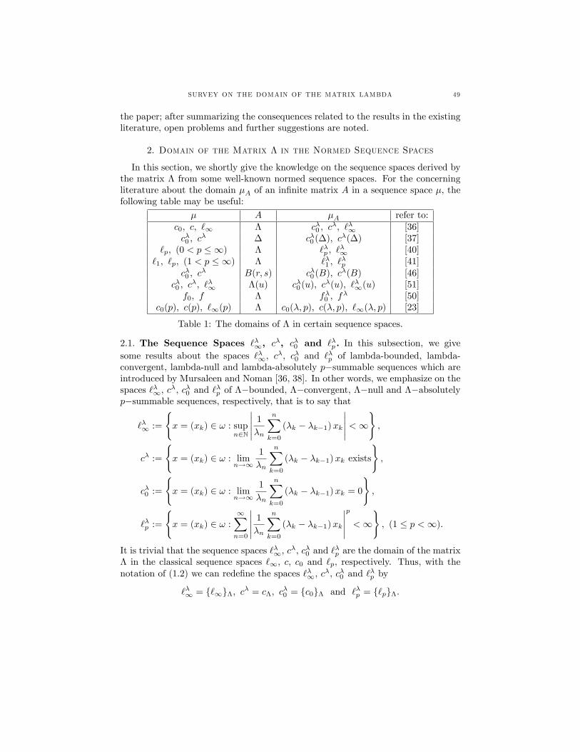
SURVEY ON THE DOMAIN OF THE MATRIX LAMBDA 49
the paper; after summarizing the consequences related to the results in the existingliterature, open problems and further suggestions are noted.
2. Domain of the Matrix Λ in the Normed Sequence Spaces
In this section, we shortly give the knowledge on the sequence spaces derived bythe matrix Λ from some well-known normed sequence spaces. For the concerningliterature about the domain µA of an infinite matrix A in a sequence space µ, thefollowing table may be useful:
µ A µA refer to:c0, c, `∞ Λ cλ0 , c
λ, `λ∞ [36]cλ0 , c
λ ∆ cλ0 (∆), cλ(∆) [37]`p, (0 < p ≤ ∞) Λ `λp , `
λ∞ [40]
`1, `p, (1 < p ≤ ∞) Λ `λ1 , `λp [41]
cλ0 , cλ B(r, s) cλ0 (B), cλ(B) [46]
cλ0 , cλ, `λ∞ Λ(u) cλ0 (u), cλ(u), `λ∞(u) [51]
f0, f Λ fλ0 , fλ [50]
c0(p), c(p), `∞(p) Λ c0(λ, p), c(λ, p), `∞(λ, p) [23]
Table 1: The domains of Λ in certain sequence spaces.
2.1. The Sequence Spaces `λ∞, cλ, cλ0 and `λp . In this subsection, we give
some results about the spaces `λ∞, cλ, cλ0 and `λp of lambda-bounded, lambda-
convergent, lambda-null and lambda-absolutely p−summable sequences which areintroduced by Mursaleen and Noman [36, 38]. In other words, we emphasize on thespaces `λ∞, c
λ, cλ0 and `λp of Λ−bounded, Λ−convergent, Λ−null and Λ−absolutely
p−summable sequences, respectively, that is to say that
`λ∞ :=
x = (xk) ∈ ω : sup
n∈N
∣∣∣∣∣ 1
λn
n∑k=0
(λk − λk−1)xk
∣∣∣∣∣ <∞,
cλ :=
x = (xk) ∈ ω : lim
n→∞
1
λn
n∑k=0
(λk − λk−1)xk exists
,
cλ0 :=
x = (xk) ∈ ω : lim
n→∞
1
λn
n∑k=0
(λk − λk−1)xk = 0
,
`λp :=
x = (xk) ∈ ω :
∞∑n=0
∣∣∣∣∣ 1
λn
n∑k=0
(λk − λk−1)xk
∣∣∣∣∣p
<∞, (1 ≤ p <∞).
It is trivial that the sequence spaces `λ∞, cλ, cλ0 and `
λp are the domain of the matrix
Λ in the classical sequence spaces `∞, c, c0 and `p, respectively. Thus, with thenotation of (1.2) we can redefine the spaces `λ∞, c
λ, cλ0 and `λp by
`λ∞ = `∞Λ, cλ = cΛ, cλ0 = c0Λ and `λp = `pΛ.
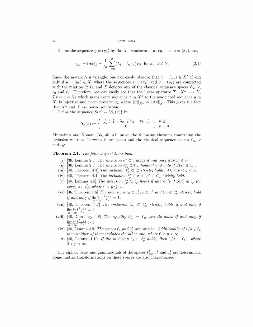
50 FEYZI BASAR
Define the sequence y = (yk) by the Λ−transform of a sequence x = (xk), i.e.,
yk := (Λx)k =1
λk
k∑j=0
(λj − λj−1)xj for all k ∈ N. (2.1)
Since the matrix Λ is triangle, one can easily observe that x = (xk) ∈ Xλ if andonly if y = (yk) ∈ X, where the sequences x = (xk) and y = (yk) are connectedwith the relation (2.1), and X denotes any of the classical sequence spaces `∞, c,c0 and `p. Therefore, one can easily see that the linear operator T : Xλ −→ X,Tx = y = Λx which maps every sequence x in Xλ to the associated sequence y inX, is bijective and norm preserving, where ‖x‖Xλ = ‖Λx‖X . This gives the factthat Xλ and X are norm isomorphic.Define the sequence S(x) = Sn(x) by
Sn(x) :=
1λn
∑nk=1 λk−1(xk − xk−1) , n ≥ 1,
0 , n = 0.
Mursaleen and Noman [36, 40, 41] prove the following theorem concerning theinclusion relations between these spaces and the classical sequence spaces `∞, cand c0:
Theorem 2.1. The following relations hold:
(i) [36, Lemma 2.3] The inclusion cλ ⊂ c holds if and only if S(x) ∈ c0.(ii) [36, Lemma 2.5] The inclusion `λ∞ ⊂ `∞ holds if and only if S(x) ∈ `∞.(iii) [40, Theorem 4.3] The inclusion `λp ⊂ `λq strictly holds, if 0 < p < q <∞.(iv) [40, Theorem 4.4] The inclusions `λp ⊂ cλ0 ⊂ cλ ⊂ `λ∞ strictly hold.(v) [40, Lemma 4.5] The inclusion `λp ⊂ `p holds if and only if S(x) ∈ `p for
every x ∈ `λp , where 0 < p ≤ ∞.(vi) [36, Theorem 4.6] The inclusions c0 ⊂ cλ0 , c ⊂ cλ and `∞ ⊂ `λ∞ strictly hold
if and only if lim infn→∞
λn+1λn
= 1.
(vii) [40, Theorem 4.7] The inclusion `∞ ⊂ `λ∞ strictly holds if and only iflim infn→∞
λn+1λn
= 1.
(viii) [40, Corollary 4.8] The equality `λ∞ = `∞ strictly holds if and only iflim infn→∞
λn+1λn
> 1.
(ix) [40, Lemma 4.9] The spaces `p and `λp are overlap. Additionally, if 1/λ 6∈ `pthen neither of them includes the other one, where 0 < p <∞.
(x) [40, Lemma 4.10] If the inclusion `p ⊂ `λp holds, then 1/λ ∈ `p , where0 < p <∞.
The alpha-, beta- and gamma-duals of the spaces `λ∞, cλ and cλ0 are determined.
Some matrix transformations on these spaces are also characterized.
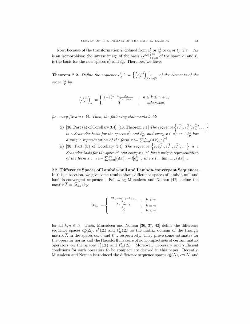
SURVEY ON THE DOMAIN OF THE MATRIX LAMBDA 51
Now, because of the transformation T defined from cλ0 or `λp to c0 or `p; Tx = Λx
is an isomorphism; the inverse image of the basise(k)∞k=0
of the space c0 and `pis the basis for the new spaces cλ0 and `
λp . Therefore, we have:
Theorem 2.2. Define the sequence e(n)λ :=
(e
(n)λ
)k
k∈N
of the elements of the
space `λp by
(e
(n)λ
)k
:=
(−1)k−n λn
λk−λk−1 , n ≤ k ≤ n+ 1,
0 , otherwise,
for every fixed n ∈ N. Then, the following statements hold:
(i) [36, Part (a) of Corollary 3.4], [40, Theorem 5.1] The sequencee
(0)λ , e
(1)λ , e
(2)λ , . . .
is a Schauder basis for the spaces cλ0 and `
λp , and every x ∈ cλ0 or ∈ `λp has
a unique representation of the form x :=∑∞n=0(Λx)ne
(n)λ .
(ii) [36, Part (b) of Corollary 3.4] The sequencee, e
(0)λ , e
(1)λ , e
(2)λ , . . .
is a
Schauder basis for the space cλ and every x ∈ cλ has a unique representationof the form x := le+
∑∞n=0[(Λx)n − l]e(n)
λ , where l = limn→∞(Λx)n.
2.2. Difference Spaces of Lambda-null and Lambda-convergent Sequences.In this subsection, we give some results about difference spaces of lambda-null andlambda-convergent sequences. Following Mursaleen and Noman [42], define thematrix Λ = (λnk) by
λnk :=
2λk−λk−1−λk+1
λn, k < n
λn−λn−1λn
, k = n
0 , k > n
for all k, n ∈ N. Then, Mursaleen and Noman [36, 37, 42] define the differencesequence spaces cλ0 (∆), cλ(∆) and `λ∞(∆) as the matrix domain of the trianglematrix Λ in the spaces c0, c and `∞, respectively. They prove some estimates forthe operator norms and the Hausdorffmeasure of noncompactness of certain matrixoperators on the spaces cλ0 (∆) and `λ∞(∆). Moreover, necessary and suffi cientconditions for such operators to be compact are derived in this paper. Recently,Mursaleen and Noman introduced the difference sequence spaces cλ0 (∆), cλ(∆) and
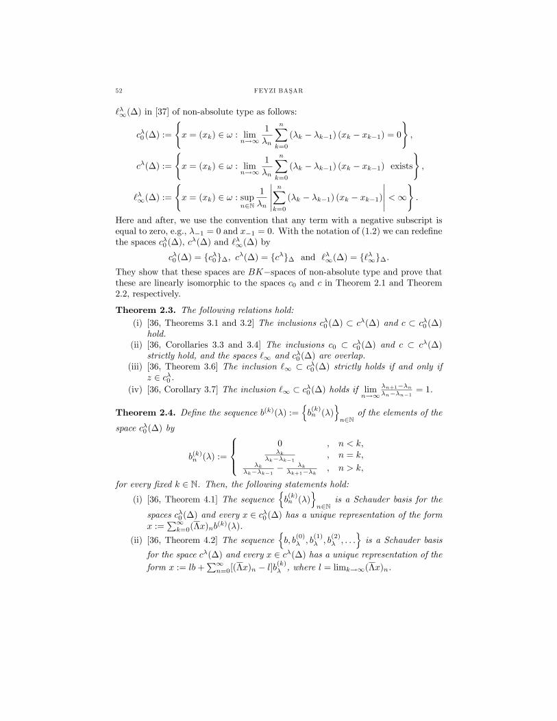
52 FEYZI BASAR
`λ∞(∆) in [37] of non-absolute type as follows:
cλ0 (∆) :=
x = (xk) ∈ ω : lim
n→∞
1
λn
n∑k=0
(λk − λk−1) (xk − xk−1) = 0
,
cλ(∆) :=
x = (xk) ∈ ω : lim
n→∞
1
λn
n∑k=0
(λk − λk−1) (xk − xk−1) exists
,
`λ∞(∆) :=
x = (xk) ∈ ω : sup
n∈N
1
λn
∣∣∣∣∣n∑k=0
(λk − λk−1) (xk − xk−1)
∣∣∣∣∣ <∞.
Here and after, we use the convention that any term with a negative subscript isequal to zero, e.g., λ−1 = 0 and x−1 = 0. With the notation of (1.2) we can redefinethe spaces cλ0 (∆), cλ(∆) and `λ∞(∆) by
cλ0 (∆) = cλ0∆, cλ(∆) = cλ∆ and `λ∞(∆) = `λ∞∆.They show that these spaces are BK−spaces of non-absolute type and prove thatthese are linearly isomorphic to the spaces c0 and c in Theorem 2.1 and Theorem2.2, respectively.
Theorem 2.3. The following relations hold:(i) [36, Theorems 3.1 and 3.2] The inclusions cλ0 (∆) ⊂ cλ(∆) and c ⊂ cλ0 (∆)
hold.(ii) [36, Corollaries 3.3 and 3.4] The inclusions c0 ⊂ cλ0 (∆) and c ⊂ cλ(∆)
strictly hold, and the spaces `∞ and cλ0 (∆) are overlap.(iii) [36, Theorem 3.6] The inclusion `∞ ⊂ cλ0 (∆) strictly holds if and only if
z ∈ cλ0 .(iv) [36, Corollary 3.7] The inclusion `∞ ⊂ cλ0 (∆) holds if lim
n→∞λn+1−λnλn−λn−1 = 1.
Theorem 2.4. Define the sequence b(k)(λ) :=b(k)n (λ)
n∈N
of the elements of the
space cλ0 (∆) by
b(k)n (λ) :=
0 , n < k,λk
λk−λk−1 , n = k,λk
λk−λk−1 −λk
λk+1−λk , n > k,
for every fixed k ∈ N. Then, the following statements hold:(i) [36, Theorem 4.1] The sequence
b(k)n (λ)
n∈N
is a Schauder basis for the
spaces cλ0 (∆) and every x ∈ cλ0 (∆) has a unique representation of the formx :=
∑∞k=0(Λx)nb
(k)(λ).
(ii) [36, Theorem 4.2] The sequenceb, b
(0)λ , b
(1)λ , b
(2)λ , . . .
is a Schauder basis
for the space cλ(∆) and every x ∈ cλ(∆) has a unique representation of theform x := lb+
∑∞n=0[(Λx)n − l]b(k)
λ , where l = limk→∞(Λx)n.
SURVEY ON THE DOMAIN OF THE MATRIX LAMBDA 53
The authors also determine the alpha-, beta- and gamma-duals of those spacesand finally, characterize the classes (cλ0 (∆) : `p), (cλ0 (∆) : `∞), (cλ(∆) : c), (cλ(∆) :c0), (cλ0 (∆) : c), (cλ0 (∆) : c0), (c0 : cλ0 (∆)), (c : cλ0 (∆)), (`p : cλ0 (∆)), (c0 : cλ(∆)),(c : cλ(∆)) and (`p : cλ(∆) of matrix mappings, where 1 ≤ p <∞.
2.3. Domain of the Generalized Difference Matrix B(r, s) In the Spacesof Λ−null and Λ−convergent Sequences. In this subsection, following Sönmezand Basar [46], we introduce the domain of the generalized difference matrix B(r, s)in the spaces cλ0 and c
λ.Let r and s be non—zero real numbers, and define the generalized difference
matrix B(r, s) = bnk(r, s) by
bnk(r, s) :=
r , k = n,s , k = n− 1,0 , otherwise,
(2.2)
for all k, n ∈ N. The B(r, s)−transform of a sequence x = (xk) is
B(r, s)(x)k = rxk + sxk−1 for all k ∈ N.We note that the matrix B(r, s) is reduced to the backward difference matrix ∆ inthe case r = 1 and s = −1. So, the results related to the domain of the matrixB(r, s) are more general and more comprehensive than the consequences of thedomain of the matrix ∆, and include them.Now, following Sönmez and Basar [46] which is the continuation of Basar and
Altay [15], and Aydın and Basar [11], we proceed essentially different than Kızmaz[24] and the other authors following him, and employ a technique of obtaining anew sequence space by means of the matrix domain of a triangle matrix.Quite recently, Sönmez and Basar [46] have introduced the difference sequence
spaces cλ0 (B) and cλ(B), which are the generalization of the spaces cλ0 (∆) and cλ(∆)introduced by Mursaleen and Noman [37], as follows:
cλ0 (B) :=
x = (xk) ∈ ω : lim
n→∞
1
λn
n∑k=0
(λk − λk−1) (rxk + sxk−1) = 0
,
cλ(B) :=
x = (xk) ∈ ω : lim
n→∞
1
λn
n∑k=0
(λk − λk−1) (rxk + sxk−1) exists
.
With the notation of (1.2), we can redefine the spaces cλ0 (B) and cλ(B) as
cλ0 (B) = cλ0B and cλ(B) = cλB , (2.3)
where B denotes the generalized difference matrix B(r, s) = bnk(r, s) defined by(2.2).It is immediate by (2.3) that the sets cλ0 (B) and cλ(B) are linear spaces with
coordinatewise addition and scalar multiplication, that is cλ0 (B) and cλ(B) are thespaces of generalized difference sequences. Sönmez and Basar [46] have proved that
54 FEYZI BASAR
these spaces are the BK−spaces of non-absolute type and norm isomorphic to thespaces c0 and c, respectively.
Theorem 2.5. The following relations hold:
(i) [46, Theorem 3.1] The inclusion cλ0 (B) ⊂ cλ(B) strictly holds.(ii) [46, Theorem 3.2] If s+ r = 0, then the inclusion c ⊂ cλ0 (B) strictly holds.(iii) [46, Corollary 3.3] The inclusions c0 ⊂ cλ0 (B) and c ⊂ cλ(B) strictly hold.(iv) [46, Corollary 3.4] Although the spaces `∞ and cλ0 (B) overlap, the space `∞
does not include the space cλ0 (B).(v) [46, Theorem 3.6] The inclusion `∞ ⊂ cλ0 (B) strictly holds if and only if
z ∈ cλ0 , where the sequence z = (zk) is defined by
zk :=
∣∣∣∣r(λk − λk−1) + s(λk+1 − λk)
λk − λk−1
∣∣∣∣ for all k ∈ N.
Prior to giving the theorem constructing the Schauder bases of the spaces cλ0 (B)
and cλ(B), define the triangle matrix Λ = (λnk) by
λnk :=
r(λk−λk−1)+s(λk+1−λk)
λn, k < n,
r (λn−λn−1)λn
, k = n,
0 , k > n
for all n, k ∈ N.
Theorem 2.6. Let αk(λ) = Λk(x) for all k ∈ N and l = limk→∞ Λk(x). Define
the sequence b(k)(λ) =b(k)n (λ)
∞k=0
for every fixed k ∈ N by
b(k)n (λ) :=
(−sr
)n−k [ λkr(λk−λk−1) + λk
s(λk+1−λk)
], k < n,
1r
λk(λk−λk−1) , k = n,
0 , k > n.
Then, the following statements hold:
(i) [46, Part (a) of Theorem 4.1] The sequenceb(k)(λ)
∞k=0
is a basis for thespace cλ0 (B) and any x ∈ cλ0 (B) has a unique representation of the formx :=
∑k
αk(λ)b(k)(λ).
(ii) [46, Part (b) of Theorem 4.1] The sequenceb, b(0)(λ), b(1)(λ), . . .
is a ba-
sis for the space cλ(B) and any x ∈ cλ(B) has a unique representation of the
form x := lb+∑k
[αk(λ)− l] b(k)(λ), where b = (bk) =∑k
j=0 (−s/r)j /r∞k=0
.
Furthermore, they have determined the α−, β− and γ− duals of those spacesand finally, characterized some matrix classes from the spaces cλ0 (B) and cλ(B) tothe spaces `p, c0 and c.
SURVEY ON THE DOMAIN OF THE MATRIX LAMBDA 55
2.4. Spaces of Almost Lambda-Null and Almost Lambda-Convergent Se-quences. Following Yesilkayagil and Basar [50], in this subsection we introduce thespaces fλ0 and f
λ of almost lambda-null and almost lambda-convergent sequences.Quite recently, Yesilkayagil and Basar [50] have studied the sequence spaces
fλ0 and fλ as the sets of all almost lambda-null and almost lambda-convergentsequences, respectively. That is,
fλ0 :=
x = (xk) ∈ ω : lim
m→∞
1
m+ 1
m∑k=0
(Λx)n+k = 0 uniformly in n
,
fλ :=
x = (xk) ∈ ω : ∃l ∈ C 3 lim
m→∞
1
m+ 1
m∑k=0
(Λx)n+k = l uniformly in n
.
With the notation of (1.2), we can restate the spaces fλ0 and fλ by the matrixdomain of triangle Λ in the spaces f0 and f , respectively, as follows:
fλ0 = (f0)Λ and fλ = fΛ.
Now, we may give the following theorems on some inclusion relations and the alpha-,beta- and gamma-duals of the spaces fλ0 and f
λ:
Theorem 2.7. The following relations hold:(i) [50, Theorem 3.5] The inclusions f0 ⊂ fλ0 and f ⊂ fλ strictly hold. Fur-
thermore, the equalities f0 = fλ0 and f = fλ hold if and only if Sx ∈ f0 forevery x in the spaces fλ and fλ0 , respectively.
(ii) [50, Theorem 3.6] The inclusion fλ0 ⊂ fλ strictly holds.(iii) [50, Theorem 3.7] The inclusions cλ ⊂ fλ ⊂ `λ∞ strictly hold.
Theorem 2.8. The following relations hold:(i) [50, Theorem 4.2] The α−dual of the space fλ is the set aλ1 defined by
aλ1 =
a = (ak) ∈ ω :
∞∑k=0
λkλk − λk−1
|ak| <∞.
(ii) [50, Theorem 4.4] The γ-dual of the space fλ is the set d1 ∩ d2, where
d1 :=
a = (ak) ∈ ω : sup
n∈N
n−1∑k=0
∣∣∣∣∆( akλk − λk−1
)λk
∣∣∣∣ <∞,
d2 :=
a = (ak) ∈ ω :
(anλn
λn − λn−1
)∈ `∞
.
(iii) [50, Theorem 4.6] Let d3 = cs and define the sets d4 and d5 by
d4 :=
a = (ak) ∈ ω :
∆
(ak
λk − λk−1
)λk
∈ c,
d5 :=
a = (ak) ∈ ω :
∣∣∣∣∆ [∆( akλk − λk−1
)λk
]∣∣∣∣ ∈ cs .
56 FEYZI BASAR
Then, fλβ =5∩i=1di.
Finally, Yesilkayagil and Basar [50] they have proven two basic results on thespace f of almost convergent sequences and characterize the classes (fλ : µ) and(µ : fλ) of infinite matrices, and also gave the characterizations of some otherclasses as an application of those main results, where µ is any given sequence space.
3. Domain of the Matrix Λ In the Paranormed Sequence Spaces
In this section, we shortly give the knowledge on the paranormed sequence spacesderived by the matrix Λ from some Maddox’s spaces.Quite recently, Karakaya et al. [23] have introduced the paranormed sequence
spaces c0(λ, p), c(λ, p) and `∞(λ, p), as follows:
c0(λ, p) :=
x = (xk) ∈ ω : lim
n→∞
1
λn
∣∣∣∣∣n∑k=0
(λk − λk−1)xk
∣∣∣∣∣pn
= 0
,
c(λ, p) :=
x = (xk) ∈ ω : ∃l ∈ C 3 lim
n→∞
1
λn
∣∣∣∣∣n∑k=0
(λk − λk−1) (xk − l)∣∣∣∣∣pn
= 0
,
`∞(λ, p) :=
x = (xk) ∈ ω : sup
n∈N
1
λn
∣∣∣∣∣n∑k=0
(λk − λk−1)xk
∣∣∣∣∣pn
<∞.
With the notation of (1.2), we can redefine the spaces c0(λ, p), c(λ, p) and `∞(λ, p)by the domain of the matrix Λ in the spaces c0(p), c(p) and `∞(p), respectively, as
c0(λ, p) = c0(p)Λ, c(λ, p) = c(p)Λ and `∞(λ, p) = `∞(p)Λ.
Theorem 3.1. The following relations hold:(i) [23, Theorem 3] The inclusions c0(λ, p) ⊂ c(λ, p) ⊂ `∞(λ, p) strictly hold.(ii) [23, Theorem 4] If 1 ≤ pn ≤ pn+1 for all n ∈ N, then the inclusions
c0(p) ⊂ c0(λ, p), c(p) ⊂ c(λ, p) and `∞(p) ⊂ `∞(λ, p) hold.(iii) [23, Parts (i) and (ii) of Theorem 5] Let µ denotes any of the spaces c0, c
and `∞. Then, the inclusion µλ ⊂ µ(λ, p) holds if pn > 1 for all n ∈ N andthe inclusion µ(λ, p) ⊂ µλ holds if pn < 1 for all n ∈ N.
Karakaya et al. [23] have investigated some topological properties and addition-ally, computed the alpha-, beta- and gamma-duals of the spaces `∞(λ, p), c(λ, p)and c0(λ, p). Finally, they have characterized the classes (c0(λ, p) : µ), (c(λ, p) : µ)and (`∞(p) : µ) of matrix transformations, where µ ∈ c0(q), c(q), `∞(q) andq = (qk) is the bounded sequence of strictly positive reals.
4. Conclusion
Malkowsky and Rakocevic [31] characterized some matrix classes and studiedrelated compact operators involving cλ0 , c
λ and `λ∞. Malkowsky and Savas [33]
SURVEY ON THE DOMAIN OF THE MATRIX LAMBDA 57
determined the beta-dual of `λp and characterized some matrix classes involving `λp ,
where 1 ≤ p < ∞. Mursaleen and Noman [38] apply the Hausdorff measure ofnoncompactness to characterize some matrix classes of compact operators on thesequence space `λp , where 1 ≤ p <∞.Mursaleen and Alotaibi [35] introduced statistical λ-convergence and strong λq-
convergence and established some relations between λ-statistical convergence, sta-tistical λ-convergence and strong λq-convergence, by using the generalized de laVallée-Poussin mean, where 0 < q < ∞. Also, they proved an analogue of theclassical Korovkin theorem by using the concept of statistical λ-convergence.Mursaleen and Noman [39] established some identities or estimates for the op-
erator norms and the Hausdorff measures of noncompactness of certain matrixoperators on the spaces cλ0 and `
λ∞ which have recently been introduced [36]. Fur-
ther, by using the Hausdorffmeasure of noncompactness, the authors characterizedsome classes of compact operators on the spaces cλ0 and `
λ∞.
Quite recently, Yesilkayagil and Basar [49] have determined the fine spectrumwith respect to Goldberg’s classification of the operator defined by the matrix Λacting on the sequence spaces c0 and c. As a new development, they have giventhe approximate point spectrum, defect spectrum and compression spectrum of thematrix operator Λ on the sequence spaces c0 and c. As a natural continuation of thisstudy, one can work on the fine spectrum with respect to Goldberg’s classificationof the operator defined by the matrix Λ over the sequence spaces cs, `p and bvp,where bvp denotes the space of all sequences whose ∆−transforms are in the space`p and is recently studied in the case 1 ≤ p ≤ ∞ by Basar and Altay [15], and in thecase 0 < p < 1 by Altay and Basar [8]. Of course, determination the fine spectrumof some triangle matrices over the sequence space X will be very interesting, whereX is any of the spaces cλ, cλ0 , `
λp , c
λ0 (∆), cλ(∆), cλ0 (B) and cλ(B).
We should record that to investigate the domain of the matrix Λ in the Maddox’ssequence space `(p) and to examine its algebraic and topological properties will bemeaningful. Finally, we note that the investigation of the Hausdorff measures ofnoncompactness of the matrix operators defined by some triangle matrices on thespaces cλ and `λp is still an open problem.
Acknowledgement
The author has benefited a lot from the constructive report of the anonymousreferee. So, he is thankful for his/her valuable comments and corrections on thefirst draft of this paper which improved the presentation and readability.
References
[1] B. Altay, On the space of p-summable diff erence sequences of order m, (1 ≤ p < ∞), Stud.Sci. Math. Hungar. 43(4)(2006), 387—402.
[2] B. Altay, F. Basar, On the paranormed Riesz sequence spaces of non-absolute type, SoutheastAsian Bull. Math. 26(5)(2002), 701—715.
58 FEYZI BASAR
[3] B. Altay, F. Basar, Some Euler sequence spaces of non-absolute type, Ukrainian Math. J.57(1)(2005), 1—17.
[4] B. Altay, F. Basar, Some paranormed Riesz sequence spaces of non-absolute type, SoutheastAsian Bull. Math. 30(5)(2006), 591—608.
[5] B. Altay, F. Basar, Some paranormed sequence spaces of non-absolute type derived byweighted mean, J. Math. Anal. Appl. 319(2)(2006), 494—508.
[6] B. Altay, F. Basar, Generalization of the sequence space `(p) derived by weighted mean, ibid.330(1)(2007), 174—185.
[7] B. Altay, F. Basar, Certain topological properties and duals of the matrix domain of a trianglematrix in a sequence space, ibid. 336(1)(2007), 632—645.
[8] B. Altay, F. Basar, The matrix domain and the fine spectrum of the diff erence operator ∆
on the sequence space `p, (0 < p < 1), Commun. Math. Anal. 2(2)(2007), 1—11.[9] C. Aydın, F. Basar, On the new sequence spaces which include the spaces c0 and c, Hokkaido
Math. J. 33(2)(2004), 383—398.[10] C. Aydın, F. Basar, Some new paranormed sequence spaces, Inform. Sci. 160(1-4)(2004),
27—40.[11] C. Aydın, F. Basar, Some new diff erence sequence spaces, Appl. Math. Comput.
157(3)(2004), 677—693.[12] C. Aydın, F. Basar, Some new sequence spaces which include the spaces `p and `∞, Demon-
stratio Math. 38(3)(2005), 641—656.[13] C. Aydın, F. Basar, Some generalizations of the sequence space arp, Iran. J. Sci. Technol.
Trans. A, Sci. 30(2006), No. A2, 175—190.[14] F. Basar, Summability Theory and Its Applications, Bentham Science Publishers, e-books,
Monographs, Istanbul-2012.[15] F. Basar, B. Altay, On the space of sequences of p-bounded variation and related matrix
mappings, Ukrainian Math. J. 55(1)(2003), 136—147.[16] F. Basar, B. Altay, M. Mursaleen, Some generalizations of the space bvp of p-bounded vari-
ation sequences, Nonlinear Anal. 68(2)(2008), 273—287.[17] M. Basarır, On some new sequence spaces and related matrix transformations, Indian J. Pure
Appl. Math. 26(10)(1995), 1003—1010.[18] M. Basarır, On the generalized Riesz B-diff erence sequence spaces, Filomat 24(4)(2010),
35—52.[19] M. Basarır, M. Kayıkçı, On the generalized Bm-Riesz sequence space and β-property, J.
Inequal. Appl. 2009 (2009), Article ID 385029, 18 pp.[20] M. Basarır, M. Öztürk, On the Riesz diff erence sequence space, Rend. Circ. Mat. Palermo
(2)57(2008), no. 3, 377—389.[21] E.E. Kara, M. Basarır, On compact operators and some Euler B(m)-diff erence sequence
spaces, J. Math. Anal. Appl. 379 (2011) 499—511.[22] E.E. Kara, M. Öztürk, M. Basarır, Some topological and geometric properties of generalized
Euler sequence spaces, Math. Slovaca 60(3)(2010), 385—398.[23] V. Karakaya, A.K. Noman, H. Polat, On paranormed λ-sequence spaces of non-absolute type,
Math. Comput. Model. 54(2011), 1473—1480.[24] H. Kızmaz, On certain sequence spaces, Canad. Math. Bull. 24(2)(1981), 169—176.[25] G.G. Lorentz, A contribution to the theory of divergent sequences, Acta Math. 80 (1948),
167—190.[26] I.J. Maddox, Spaces of strongly summable sequences, Quart. J. Math. Oxford (2), 18(1967),
345—355.[27] I.J. Maddox, Paranormed sequence spaces generated by infinite matrices, Proc. Camb. Phil.
Soc. 64(1968), 335—340.[28] I.J. Maddox, Some properties of paranormed sequence spaces, London J. Math. Soc.
(2)1(1969), 316—322.
SURVEY ON THE DOMAIN OF THE MATRIX LAMBDA 59
[29] E. Malkowsky, Recent results in the theory of matrix transformations in sequence spaces,Mat. Vesnik 49(1997), 187—196.
[30] E. Malkowsky, Mursaleen, S. Suantai, The dual spaces of sets of diff erence sequences of orderm and matrix transformations, Acta Math. Sin. Eng. Ser. 23(3)(2007), 521—532.
[31] E. Malkowsky, V. Rakocevic, Measure of noncompactness of linear operators between spacesof sequences that are (N, q) summable or bounded, Czechoslovak Math. J. 51(126) (2001),no. 3, 505—522.
[32] E. Malkowsky, V. Rakocevic, S. Zivkovic, Matrix transformations between the sequence spaceswp0(Λ), vp0(Λ), cp0(Λ) (1 < p < ∞) and certain BK spaces, Appl. Math. Comput. 147 (2)(2004), 377—396.
[33] E. Malkowsky, E. Savas, Matrix transformations between sequence spaces of generalizedweighted means, Appl. Math. Comput. 147(2)(2004), 333—345.
[34] F. Móricz, On Λ− strong convergence of numerical sequences and Fourier series, Acta Math.Hung. 54(3-4)(1989), 319—327.
[35] M. Mursaleen, A. Alotaibi, Statistical summability and approximation by de la Vallée-Poussinmean, Appl. Math. Lett. 24(3)(2011), 320—324.
[36] M. Mursaleen, A.K. Noman, On the spaces of λ-convergent and bounded sequences, Thai J.Math. 8(2)(2010), 311—329.
[37] M. Mursaleen, A.K. Noman, On some new diff erence sequence spaces of non-absolute type,Math. Comput. Modelling 52(3-4)(2010), 603—617.
[38] M. Mursaleen, A.K. Noman, Applications of the Hausdorff measure of noncompactness insome sequence spaces of weighted means, Comput. Math. Appl. 60(5)(2010), 1245—1258.
[39] M. Mursaleen, A.K. Noman, The Hausdorff measure of noncompactness of matrix operatorson some BK spaces, Oper. Matrices 5(3)(2011), 473—486.
[40] M. Mursaleen, A.K. Noman, On some new sequence spaces of non-absolute type related tothe spaces `p and `∞ I, Filomat 25(2011), 33—51.
[41] M. Mursaleen, A.K. Noman, On some new sequence spaces of non-absolute type related tothe spaces `p and `∞ II, Math. Commun. 16(2011), 383—398.
[42] M. Mursaleen, A.K. Noman, Compactness of matrix operators on some new diff erence se-quence spaces, Linear Algebra Appl. 436(1)(2012), 41—52.
[43] P.-N. Ng, P.-Y. Lee, Cesàro sequence spaces of non-absolute type, Comment. Math. PraceMat. 20(2)(1978), 429—433.
[44] H. Polat, F. Basar, Some Euler spaces of diff erence sequences of order m, Acta Math. Sci.Ser. B Engl. Ed. 27B(2)(2007),
[45] S. Simons, The sequence spaces `(pv) and m(pv), Proc. London Math. Soc. (3), 15(1965),422—436.
[46] A. Sönmez, F. Basar, Generalized diff erence spaces of non-absolute type of convergent andnull sequences, Abstr. Appl. Anal. 2012, Art. ID 435076, 20 pp.
[47] M. Sengönül, F. Basar, Some new Cesàro sequence spaces of non-absolute type which includethe spaces c0 and c, Soochow J. Math. 31(1)(2005), 107—119.
[48] C.-S. Wang, On Nörlund sequence spaces, Tamkang J. Math. 9(1978), 269—274.[49] M. Yesilkayagil, F. Basar, On the fine spectrum of the operator defined by a lambda matrix
over the sequence space c0 and c, AIP Conference Proceedings 1470(2012), 199—202.[50] M. Yesilkayagil, F. Basar, Spaces of almost lambda null and almost lambda convergent se-
quences, under communication.[51] S. Zeren, Ç.A. Bektas, On some new sequence spaces of non-absolute type, submitted to:
Allahabad Math. Soc.
Current address : Feyzi Basar;Fatih University, Faculty of Arts and Sciences, Department ofMathematics, The Hadımköy Campus, Büyükçekmece, 34500—Istanbul, TurkeyE-mail address : [email protected], [email protected]: http://communications.science.ankara.edu.tr/index.php?series=A1

Commun.Fac.Sci.Univ .Ank.Series A1Volum e 62, Number 1, Pages 61—71 (2013)ISSN 1303—5991
MACWILLIAMS IDENTITIES OVER SOME SPECIAL POSETS*
SEDA AKBIYIK AND IRFAN SIAP
Abstract. In this paper we introduce a level weight enumerator for linearbinary codes whose index set is a forest. This weight enumerator gives most ofthe weight enumerators as a special case by specializing its variables. We provea MacWilliams identity for this weight enumerator over this special familyof posets which also generalizes the previous results in literature. Further,both the code and its dual are considered over this family of posets usingthe definition of this weight enumerator which was not possible before. Weconclude by an illustrative example and some remarks.
1. Introduction
Coding theory has found a well recognised place in the digital era that we arein. It has found applications in transmitting and restoring the digital messages.Encoding and decoding these messages in an effi cient way depends on the structureof the codes. To accomplish this goal codes are defined as linear structures i.e.vector subspaces and endowed with a particular metric that serves as measuring thedistances between the vectors in order to detect and correct errors. Linear codes firstand mainly are considered with the Hamming metric [4]. Later, codes over differentmetrics due to their applications and purposes are considered. The problem ofdetermining the minimum distance d of codes, i.e. error correcting capacity of codes,was generalized by Neiderreiter [7, 8]. A metric which is called poset (partiallyordered set) metric on codes is first considered by Brualdi et. al. [6]. This metricis a very important generalization of the metrics and especially it generalizes thewell known and most important metrics such as the Hamming and Rosenbloom-Tsfasmann (RT) [5] metrics. Due to this generalization studying codes over thismetric has attracted the researchers. However, since it is a generalization theproblems are diffi cult to solve with respect to this metric. One of the main problems
Received by the editors Nov. 30, 2012; Accepted: June 14, 2013.2000 Mathematics Subject Classification. Primary 05C38, 15A15; Secondary 05A15, 15A18.Key words and phrases. Linear P -codes, P -complete weight enumerator, MacWilliams iden-
tity, hierarchical poset, discrete chain poset, tree, forest.The main results of this paper were presented in part at the conference Algerian-Turkish Interna-tional Days on Mathematics 2012 (ATIM’2012) to be held October 9—11, 2012 in Annaba, Algeriaat the Badji Mokhtar Annaba University.
c©2013 Ankara University
61
62 SEDA AKBIYIK AND IRFAN SIAP
is to establish a MacWilliams identity with respect to this metric. This identityenables us to explicitly determine the weight enumerator of its dual algebraicallyby applying a specific change of variables to the weight enumerator of the originalcode. The importance becomes more evident when the dimension of the code is toolarge and hence the dimension of its dual can be very small if the length of the codehas a reasonable size which is the case in general. The problem of establishing aMacWilliams identity with respect to a poset metric has been a challenging problemat first. The first attempts of establishing such identities have failed when theresearchers considered the same metric for both the code and its dual which hasbeen the case with all previous metrics. In order to overcome this diffi culty onposet metrics, the dual of the code is considered over the dual poset and hencea different but a similar metric for the dual space is introduced [2]. Even withthis modification it has also shown that not all posets are suitable for obtaininga MacWilliams identity. Some more work on posets and MacWilliams identity isdone in [6, 8, 10]. It is proven that the family of hierarchical posets which is a verysmall family of posets is the only one suitable for this purpose [2]. The authors haveintroduced a new and more detailed weight enumerator called P-complete weightenumerator to overcome this problem very recently [1]. Therein it is shown thatif such a weight enumerator is defined then MacWilliams identity can be obtainedand further the dual code is considered over the same metric. The work in [1] isdone over a special family of posets, so called discrete chain poset, and this family isdifferent from hierarchical posets. Here, the authors introduce a new level completeweight enumerator which is defined over posets that are represented by forests andthe previous results are obtained as a corollary.The main advantage of defining level complete weight enumerator for codes over
posets is that not only we obtain the MacWilliams identity over a considerablylarge family of posets but further we use the same metric for both the code and itsdual which is a new contribution to the literature.In order to prove the MacWilliams Identity for codes over forests, in the following
section we present the basics for binary codes and graph theory that is needed todefine the posets presented by the forests. In the next section, we present thedefinition of level complete weight enumerator over posets represented by forestsand present some well known auxiliary lemmas that play an important role in theproof of the main theorem. Next we present a moderate example that illustratesthe main theorem. We finalize the paper by some concluding remarks.
2. Preliminaries
Let Z2 = 0, 1 denote the set of integers modulo 2, which is well known to bea finite field with 2 elements, and V = Zn2 . The set V is a Z2-vector space. AZ2 -vector subspace of V is called a linear code of length n. The inner product oftwo vectors v = (v1, . . . , vn) and u = (u1, . . . , un) defined over V is a Z2 -valuedfunction which is 〈v, u〉 =
∑ni=1 viui. To each linear code C of length n a linear code
MACWILLIAMS IDENTITIES OVER SOME SPECIAL POSETS 63
C⊥ = v ∈ V |〈v, u〉 = 0, for all u ∈ C can be associated. The linear code C⊥ iscalled the dual of C. The Hamming distance between two vectors v = (v1, . . . , vn)and u = (u1, . . . , un) is defined by dH(v, u) = |i|vi 6= ui. It is well known thatdH is a metric on V. Another important notation for codes is the Hamming weightof a vector v ∈ V which is wH(v) = |i|vi 6= 0|. The minimum Hamming distanceof a linear code C is dmin(C) = dH(C) = mindH(u, v)|∀u, v ∈ C, u 6= v . Also theHamming weight of a code C is wH(C) = minwH(u)|∀u ∈ C, u 6= 0. When thecode is linear which is the case in this article, dH(C) = wH(C). A linear binarycode of length n, dimension k and minimum Hamming distance d is simply denotedby [n, k, d]. These three parameters play a crucial role for defining a linear code.Especially the Hamming distance d of a code reveals the quality of the code asshown in the following theorem.
Theorem 2.1. [4] If C is a linear code of Hamming distance d = 2t+1 or d = 2t+2,then C can correct up to t errors.
The interested readers for a more detailed treatment of this subject are welcometo refer to [4, 9, 3].Let (P,≤) be a partially ordered set of cardinality n. A subset I of P is called an
ideal if x ∈ I and y ≤ x imply that y ∈ I . For a subset A of the poset P , 〈A〉 willdenote the smallest ideal of P containing A. We assume that P = 1, 2, 3 . . . , nand the coordinate positions of vectors in Z2n are in one-to-one correspondencewith the elements of P . Let x = (x1, x2 . . . , xn) be a vector in Z2n . The P−weight of x is defined as the cardinality wP (x) = |〈supp(x)〉| of the smallest ideal ofP containing the support of x, where supp(x) = i ∈ P : xi 6= 0. The P− (poset)distance of the elements x, y ∈ Z2n is defined as dP (x, y) = wP (x− y).If P is an antichain in which no two elements are comparable, then the P−
weight and the P− distances reduce to the Hamming weight and the Hammingdistance, respectively. If P consists of a single chain, then P− weight and P−distance are Rosenbloom Tsfasmann (RT) weight and RT distance. It is knownthat the P− distance dP (., .) is a metric on Z2n. The metric dP (., .) on Z2n iscalled a poset-metric. If Z2n is endowed with a poset-metric, then a subset C ofZ2n is called a poset-code. If the poset-metric corresponds to a poset P , then C iscalled a P− code.Next, we present some basic definitions from graph theory that will be needed
in the next section.
Definition 2.2. A graph G = (T,E) is defined by a finite nonempty set T whichis called the set of vertices and a finite set E which is called the set of edges whichis a subset of V × V. In general a graph is represented by a diagram consisting ofpoints (vertices) joined by lines (edges).
If (a, b) ∈ E, then we say that an edge between the vertices a and b exits. Ifwe employ a direction from a to b, then the graph is called a directed otherwiseundirected. In the case of the directed graphs, geometrically when drawing them,
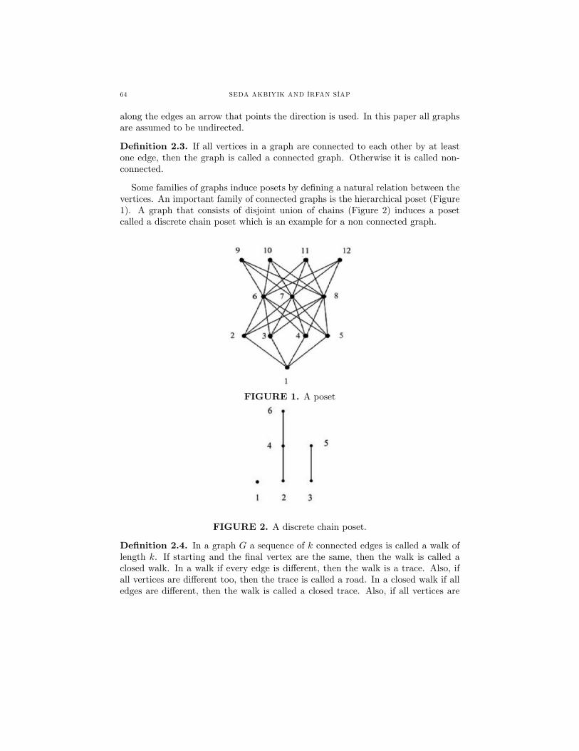
64 SEDA AKBIYIK AND IRFAN SIAP
along the edges an arrow that points the direction is used. In this paper all graphsare assumed to be undirected.
Definition 2.3. If all vertices in a graph are connected to each other by at leastone edge, then the graph is called a connected graph. Otherwise it is called non-connected.
Some families of graphs induce posets by defining a natural relation between thevertices. An important family of connected graphs is the hierarchical poset (Figure1). A graph that consists of disjoint union of chains (Figure 2) induces a posetcalled a discrete chain poset which is an example for a non connected graph.
FIGURE 1. A poset
FIGURE 2. A discrete chain poset.
Definition 2.4. In a graph G a sequence of k connected edges is called a walk oflength k. If starting and the final vertex are the same, then the walk is called aclosed walk. In a walk if every edge is different, then the walk is a trace. Also, ifall vertices are different too, then the trace is called a road. In a closed walk if alledges are different, then the walk is called a closed trace. Also, if all vertices are
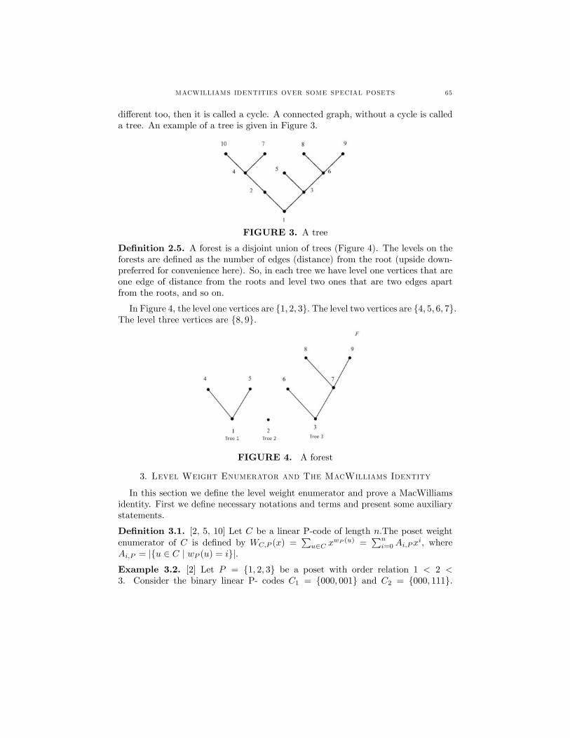
MACWILLIAMS IDENTITIES OVER SOME SPECIAL POSETS 65
different too, then it is called a cycle. A connected graph, without a cycle is calleda tree. An example of a tree is given in Figure 3.
FIGURE 3. A tree
Definition 2.5. A forest is a disjoint union of trees (Figure 4). The levels on theforests are defined as the number of edges (distance) from the root (upside down-preferred for convenience here). So, in each tree we have level one vertices that areone edge of distance from the roots and level two ones that are two edges apartfrom the roots, and so on.
In Figure 4, the level one vertices are 1, 2, 3. The level two vertices are 4, 5, 6, 7.The level three vertices are 8, 9.
FIGURE 4. A forest
3. Level Weight Enumerator and The MacWilliams Identity
In this section we define the level weight enumerator and prove a MacWilliamsidentity. First we define necessary notations and terms and present some auxiliarystatements.
Definition 3.1. [2, 5, 10] Let C be a linear P-code of length n.The poset weightenumerator of C is defined by WC,P (x) =
∑u∈C x
wP (u) =∑n
i=0Ai,Pxi, where
Ai,P = |u ∈ C | wP (u) = i|.Example 3.2. [2] Let P = 1, 2, 3 be a poset with order relation 1 < 2 <3. Consider the binary linear P- codes C1 = 000, 001 and C2 = 000, 111.
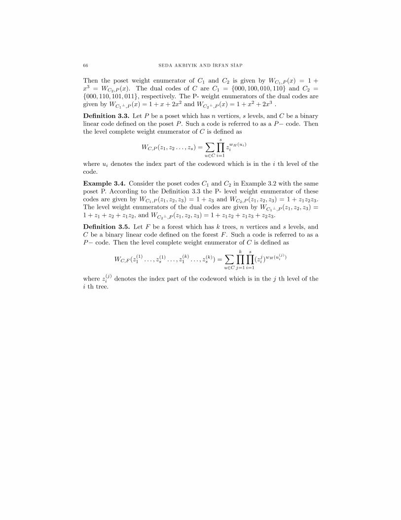
66 SEDA AKBIYIK AND IRFAN SIAP
Then the poset weight enumerator of C1 and C2 is given by WC1,P (x) = 1 +x3 = WC2,P (x). The dual codes of C are C1 = 000, 100, 010, 110 and C2 =000, 110, 101, 011, respectively. The P- weight enumerators of the dual codes aregiven by WC1⊥,P (x) = 1 + x+ 2x
2 and WC2⊥,P (x) = 1 + x2 + 2x3 .
Definition 3.3. Let P be a poset which has n vertices, s levels, and C be a binarylinear code defined on the poset P . Such a code is referred to as a P− code. Thenthe level complete weight enumerator of C is defined as
WC,P (z1, z2 . . . , zs) =∑u∈C
s∏i=1
zwH(ui)i
where ui denotes the index part of the codeword which is in the i th level of thecode.
Example 3.4. Consider the poset codes C1 and C2 in Example 3.2 with the sameposet P. According to the Definition 3.3 the P- level weight enumerator of thesecodes are given by WC1,P (z1, z2, z3) = 1 + z3 and WC2,P (z1, z2, z3) = 1 + z1z2z3.The level weight enumerators of the dual codes are given by WC1⊥,P (z1, z2, z3) =1 + z1 + z2 + z1z2, and WC2⊥,P (z1, z2, z3) = 1 + z1z2 + z1z3 + z2z3.
Definition 3.5. Let F be a forest which has k trees, n vertices and s levels, andC be a binary linear code defined on the forest F . Such a code is referred to as aP− code. Then the level complete weight enumerator of C is defined as
WC,F (z(1)1 . . . , z(1)s . . . , z
(k)1 . . . , z(k)s ) =
∑u∈C
k∏j=1
s∏i=1
(zji )wH(u
(j)i )
where z(j)i denotes the index part of the codeword which is in the j th level of thei th tree.
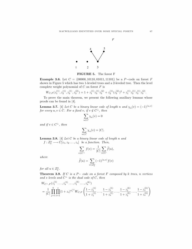
MACWILLIAMS IDENTITIES OVER SOME SPECIAL POSETS 67
FIGURE 5. The forest F
Example 3.6. Let C = 00000, 10110, 01011, 11101 be a P−code on forest Fshown in Figure 5 which has two 1-leveled trees and a 2-leveled tree. Then the levelcomplete weight polynomial of C on forest F is
WC,F (z(1)1 , z
(1)2 , z
(1)3 , z
(2)3 ) = 1 + z
(1)1 z
(1)3 z
(2)3 + z
(1)2 (z
(2)3 )2 + z
(1)1 z
(1)2 z
(1)3 z
(2)3 .
To prove the main theorem, we present the following auxiliary lemmas whoseproofs can be found in [4].
Lemma 3.7. [4] Let C be a binary linear code of length n and χu(v) = (−1)〈u,v〉for every u, v ∈ C. For a fixed v, if v /∈ C⊥, then∑
u∈Cχu(v) = 0
and if v ∈ C⊥, then ∑u∈C
χu(v) = |C|.
Lemma 3.8. [4] Let C be a binary linear code of length n andf : Zn2 −→ C[z1, z2 . . . , zs] be a function. Then,∑
v∈C⊥
f(v) =1
|C|∑u∈C
f(u),
wheref(u) =
∑v∈Zn2
(−1)〈u,v〉f(v)
for all u ∈ Zn2 .Theorem 3.9. If C is a P− code on a forest F composed by k trees, n verticesand s levels and C⊥ is the dual code of C, then
WC⊥,F (z(1)1 . . . , z(1)s . . . , z
(k)1 . . . , z(k)s )
=1
|C|
k∏j=1
s∏i=1
(1 + zi)n(j)i WC,F
(1− z(1)11 + z
(1)1
. . . ,1− z(1)s1 + z
(1)s
. . . ,1− z(k)1
1 + z(k)1
. . . ,1− z(k)s
1 + z(k)s
)
68 SEDA AKBIYIK AND IRFAN SIAP
where the length of each part of u ∈ C in i th tree and level j is denoted by n(j)i .
Proof. In order to apply Lemma 3.8 we first define a function f that represents theterms in the level weight enumerator such that
f(v) =(z(1)1 )wH(v
(1)1 )(z
(1)2 )wH(v
(1)2 ) · · · (z(1)s )wH(v
(1)s ) · · · (z(k)1 )wH(v
(k)1 )(z
(k)2 )wH(v
(k)2 )
· · · (z(k)s )wH(v(k)s )
=
k∏j=1
s∏i=1
(z(j)i )wH(v
(j)i ).
Then by Lemma 3.8,
f(u) =∑v∈Zn2
(−1)〈u,v〉f(v)
=∑v∈Zn2
(−1)〈u,v〉k∏j=1
s∏i=1
(z(j)i )wH(v
(j)i )
=∑
v(1)1 ∈Zn
(1)1
2
...∑
v(k)s ∈Zn
(k)s
2
(−1)∑k
i=1
∑nij=1 u
(j)i v
(j)i
k∏j=1
s∏i=1
(z(j)i )wH(v
(j)i )
=∑
v(1)1 ∈Zn
(1)1
2
...∑
v(k)s ∈Zn
(k)s
2
k∏j=1
s∏i=1
(−1)∑k
i=1
∑nij=1 u
(j)i v
(j)i (z
(j)i )wH(v
(j)i )
=
k∏j=1
s∏i=1
(∑
v(j)i ∈Z
n(j)i
2
(−1)∑k
i=1
∑nij=1 u
(j)i v
(j)i (z
(j)i )wH(v
(j)i ))
=
k∏j=1
s∏i=1
(1 + z(j)i )n
(j)i .
(1− z(j)i1 + z
(j)i
)wH(u(j)i )
Again by using Lemma 3.8, we find that
∑u∈C⊥
f(u) =1
|C|∑u∈C
f(u) =1
|C|
k∏j=1
s∏i=1
(1 + z(j)i )n
(j)i
(1− z(j)i1 + z
(j)i
)wH(u(j)i )
.
So we obtain
WC⊥,F (z(1)1 . . . , z(1)s . . . , z
(k)1 . . . , z(k)s )
=1
|C|
k∏j=1
s∏i=1
(1 + z(j)i )n
(j)i WC,F
(1− z(1)11 + z
(1)1
. . . ,1− z(1)s1 + z
(1)s
. . . ,1− z(k)1
1 + z(k)1
. . . ,1− z(k)s
1 + z(k)s
).
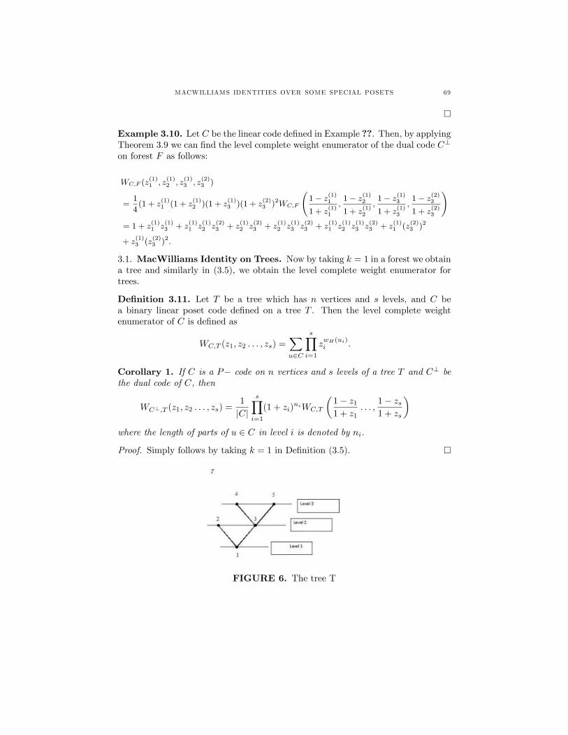
MACWILLIAMS IDENTITIES OVER SOME SPECIAL POSETS 69
Example 3.10. Let C be the linear code defined in Example ??. Then, by applyingTheorem 3.9 we can find the level complete weight enumerator of the dual code C⊥
on forest F as follows:
WC,F (z(1)1 , z
(1)2 , z
(1)3 , z
(2)3 )
=1
4(1 + z
(1)1 (1 + z
(1)2 )(1 + z
(1)3 )(1 + z
(2)3 )2WC,F
(1− z(1)1
1 + z(1)1
,1− z(1)2
1 + z(1)2
,1− z(1)3
1 + z(1)3
,1− z(2)3
1 + z(2)3
)= 1 + z
(1)1 z
(1)3 + z
(1)1 z
(1)2 z
(2)3 + z
(1)2 z
(2)3 + z
(1)2 z
(1)3 z
(2)3 + z
(1)1 z
(1)2 z
(1)3 z
(2)3 + z
(1)1 (z
(2)3 )2
+ z(1)3 (z
(2)3 )2.
3.1. MacWilliams Identity on Trees. Now by taking k = 1 in a forest we obtaina tree and similarly in (3.5), we obtain the level complete weight enumerator fortrees.
Definition 3.11. Let T be a tree which has n vertices and s levels, and C bea binary linear poset code defined on a tree T . Then the level complete weightenumerator of C is defined as
WC,T (z1, z2 . . . , zs) =∑u∈C
s∏i=1
zwH(ui)i .
Corollary 1. If C is a P− code on n vertices and s levels of a tree T and C⊥ bethe dual code of C, then
WC⊥,T (z1, z2 . . . , zs) =1
|C|
s∏i=1
(1 + zi)niWC,T
(1− z11 + z1
. . . ,1− zs1 + zs
)where the length of parts of u ∈ C in level i is denoted by ni.
Proof. Simply follows by taking k = 1 in Definition (3.5).
FIGURE 6. The tree T
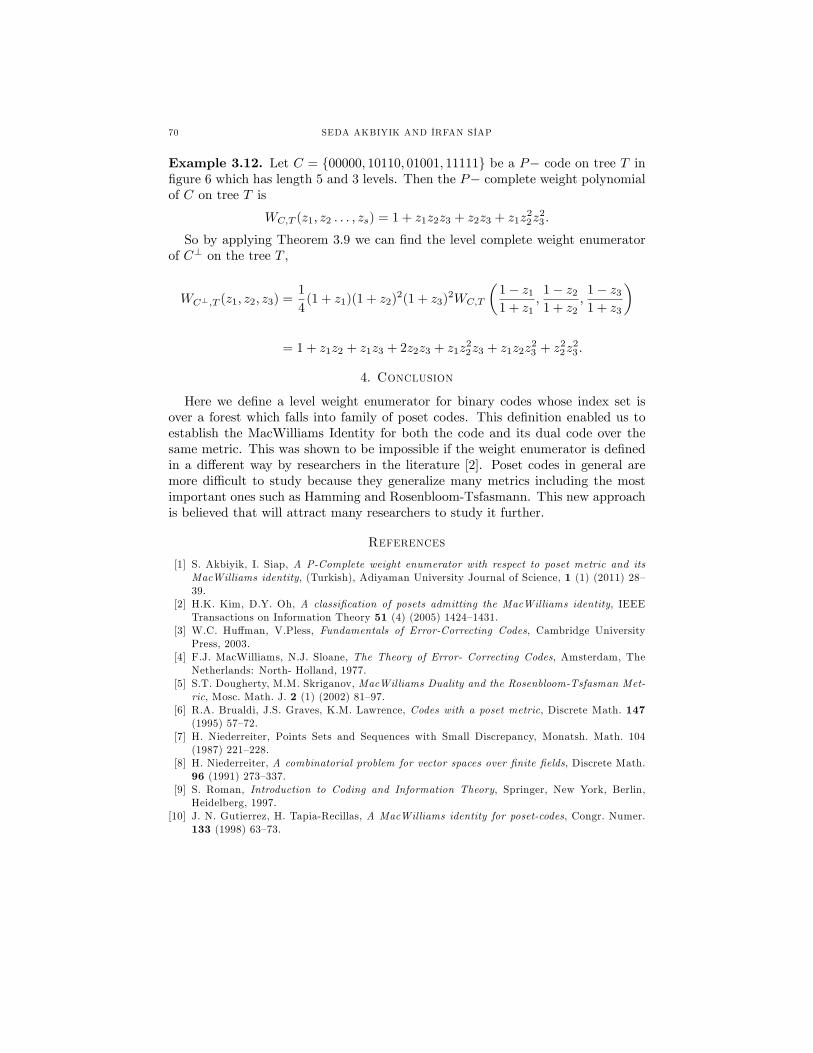
70 SEDA AKBIYIK AND IRFAN SIAP
Example 3.12. Let C = 00000, 10110, 01001, 11111 be a P− code on tree T infigure 6 which has length 5 and 3 levels. Then the P− complete weight polynomialof C on tree T is
WC,T (z1, z2 . . . , zs) = 1 + z1z2z3 + z2z3 + z1z22z23 .
So by applying Theorem 3.9 we can find the level complete weight enumeratorof C⊥ on the tree T ,
WC⊥,T (z1, z2, z3) =1
4(1 + z1)(1 + z2)
2(1 + z3)2WC,T
(1− z11 + z1
,1− z21 + z2
,1− z31 + z3
)
= 1 + z1z2 + z1z3 + 2z2z3 + z1z22z3 + z1z2z
23 + z
22z23 .
4. Conclusion
Here we define a level weight enumerator for binary codes whose index set isover a forest which falls into family of poset codes. This definition enabled us toestablish the MacWilliams Identity for both the code and its dual code over thesame metric. This was shown to be impossible if the weight enumerator is definedin a different way by researchers in the literature [2]. Poset codes in general aremore diffi cult to study because they generalize many metrics including the mostimportant ones such as Hamming and Rosenbloom-Tsfasmann. This new approachis believed that will attract many researchers to study it further.
References
[1] S. Akbiyik, I. Siap, A P-Complete weight enumerator with respect to poset metric and itsMacWilliams identity, (Turkish), Adiyaman University Journal of Science, 1 (1) (2011) 28—39.
[2] H.K. Kim, D.Y. Oh, A classification of posets admitting the MacWilliams identity, IEEETransactions on Information Theory 51 (4) (2005) 1424—1431.
[3] W.C. Huffman, V.Pless, Fundamentals of Error-Correcting Codes, Cambridge UniversityPress, 2003.
[4] F.J. MacWilliams, N.J. Sloane, The Theory of Error- Correcting Codes, Amsterdam, TheNetherlands: North- Holland, 1977.
[5] S.T. Dougherty, M.M. Skriganov, MacWilliams Duality and the Rosenbloom-Tsfasman Met-ric, Mosc. Math. J. 2 (1) (2002) 81—97.
[6] R.A. Brualdi, J.S. Graves, K.M. Lawrence, Codes with a poset metric, Discrete Math. 147(1995) 57—72.
[7] H. Niederreiter, Points Sets and Sequences with Small Discrepancy, Monatsh. Math. 104(1987) 221—228.
[8] H. Niederreiter, A combinatorial problem for vector spaces over finite fields, Discrete Math.96 (1991) 273—337.
[9] S. Roman, Introduction to Coding and Information Theory, Springer, New York, Berlin,Heidelberg, 1997.
[10] J. N. Gutierrez, H. Tapia-Recillas, A MacWilliams identity for poset-codes, Congr. Numer.133 (1998) 63—73.
MACWILLIAMS IDENTITIES OVER SOME SPECIAL POSETS 71
Current address : Seda Akbıyık and Irfan Siap;Yıldız Technical University, Department ofMathematics, Istanbul, TURKEY
E-mail address : [email protected], [email protected]: http://communications.science.ankara.edu.tr/index.php?series=A1

Commun.Fac.Sci.Univ .Ank.Series A1Volum e 62, Number 1, Pages 73—83 (2013)ISSN 1303—5991
A NEIGHBOURHOOD SYSTEM OF FUZZY NUMBERS AND ITSTOPOLOGY*
SALIH AYTAR
Abstract. The neighbourhood system obtained by the neighbourhoods (whoseradii are positive fuzzy numbers) in a fuzzy number-valued metric space is abasis of a topology for the set of all fuzzy numbers. In this paper, the conver-gence with respect to this topology is introduced and its basic properties arestudied.
1. Introduction
In most of the situations in real world problems, the data obtained for decisionmaking are only approximately known. To meet such problems, Zadeh [24] intro-duced the concept of fuzzy set in 1965. Later, Chang and Zadeh [3] defined theconcept of a fuzzy number as a fuzzy subset of the real line. A fuzzy number is aquantity whose value is imprecise, rather than exact as in the case of crisp, single-valued numbers. Any fuzzy number can be thought of as a function whose domainis a specified set (usually the set of real numbers).In fact, there is a wide range of possibilities to define a fuzzy number. However,
many of these definitions are not particularly amenable to practical manipulations.In many cases, exact computations or comparisons of fuzzy numbers, and repre-sentation of ill-defined magnitudes are diffi cult by using those definitions of fuzzynumbers. With this in mind, in this paper, we adopt a widely accepted and practicaldefinition of a fuzzy number encountered in the literature of fuzzy set theory.Fuzzy numbers allow us to make the mathematical models of linguistic quantities
and fuzzy environments. In many respects, fuzzy numbers depict the physicalworld more realistically than the real numbers do. Fuzzy numbers are used instatistics, computer programming, engineering (especially in communications), and
Received by the editors Nov. 24, 2012; Accepted: June 14, 2013.2000 Mathematics Subject Classification. Primary 03E72; Secondary 40A05;26E50.Key words and phrases. Fuzzy number; Fuzzy metric; Types of convergence of a fuzzy number
sequence.The main results of this paper were presented in part at the conference Algerian-Turkish Interna-tional Days on Mathematics 2012 (ATIM’2012) to be held October 9—11, 2012 in Annaba, Algeriaat the Badji Mokhtar Annaba University.
c©2013 Ankara University
73
74 SALIH AYTAR
experimental science. They are also important for the study of fuzzy integrals,fuzzy control problems and fuzzy optimization problems which are widely used infuzzy information theory and fuzzy signal systems (see [5, 8, 23]). Therefore, acareful and scientific mathematical analysis of fuzzy numbers is very important forthe theoretical background of applied studies. In this context, the distance betweentwo fuzzy numbers and the convergence of a sequence of fuzzy numbers with respectto this distance plays a key role in the analysis of fuzzy numbers.In 1991 Fuller [9] calculated the membership function of the product-sum of
triangular fuzzy numbers. Later Hong and Hwang [13] determined the exact mem-bership function of the t-norm-based sum of fuzzy numbers. In 1997 Hwang andHong [14] have studied the membership function of the t-norm-based sum of fuzzynumbers on Banach spaces, which generalizes earlier results Fuller [9] and Hong andHwang [13]. These papers are important ones related to the theory of convergence.Recently, many authors have discussed the convergence of a sequence of fuzzy
numbers and obtained many important results (see [1, 2, 7, 12, 22]). The firststeps towards constructing such convergence theories go back to Matloka’s [16]and Kaleva’s [15] works. To this end, they used the supremum metric that givesa real (crisp) value for the distance between two fuzzy numbers. On the otherhand, via positive fuzzy numbers, it is also possible to define a fuzzy (non-crisp)distance between two fuzzy numbers (as is exemplified by Guangquan [10]), becauseit is more natural that the distance between two fuzzy numbers is a fuzzy numberrather than this distance is a real number. Nevertheless, although a fuzzy distanceis used in Guangquan’s studies [10, 11], the convergence of a sequence of fuzzynumbers discussed in these studies somehow depends on the supremum metric, sincecharacteristic functions of positive numbers are used as radii of open neighborhoodsof fuzzy numbers. In this case, the convergence with respect to the supremummetricand the convergence with respect to the fuzzy distance turn out to be equivalent.We think that it will be a good step to examine the convergence of a sequence of
fuzzy numbers from different perspectives to explore the boundaries of these con-vergence theories related to fuzzy numbers. In this context, we introduce a newtype of convergence by using more positive fuzzy numbers, instead of just the posi-tive characteristic functions used in Guangquan’s [10, 11] definition of convergence.We note that this convergence should not be perceived as a generalization of ordi-nary convergence. Throughout the text, we also compare these different types ofconvergences of a sequence of fuzzy numbers.
2. Preliminaries
First we recall some of the basic concepts and notations in the theory of fuzzynumbers, and we refer to [4, 6, 11, 15, 16, 17, 18, 19, 20, 21] for more details.A fuzzy number is a function X from R to [0, 1], satisfying:
(i) X is normal, i.e., there exists an x0 ∈ R such that X(x0) = 1;
A NEIGHBOURHOOD SYSTEM OF FUZZY NUMBERS 75
(ii) X is fuzzy convex, i.e., for any x, y ∈ R and λ ∈ [0, 1], X(λx+ (1− λ)y) ≥minX(x), X(y);
(iii) X is upper semi-continuous;(iv) the closure of x ∈ R : X(x) > 0, denoted by X0, is compact.
These properties imply that, for each α ∈ (0, 1], the α− level set Xα := x ∈R : X(x) ≥ α =
[Xα, X
α]is a non-empty compact convex subset of R, as is
the support X0. We denote the set of all fuzzy numbers by F(R). Note that thefunction a1 defined by
a1 (x) :=
1 , if x = a,0 , otherwise,
where a ∈ R, is a fuzzy number. By the decomposition theorem of fuzzy sets, wehave
X = supα∈[0,1]
αχ[Xα,Xα]
for every X ∈ F(R), where each χ[Xα,Xα] denotes the characteristic function of the
subinterval[Xα, X
α].
Now we recall the partial order relation on the set of fuzzy numbers. For X,Y ∈F(R), we write X Y, if for every α ∈ [0, 1], the inequalities
Xα ≤ Y α and Xα ≤ Y α
hold. We write X ≺ Y, if X Y and there exists an α0 ∈ [0, 1] such that
Xα0 < Y α0 or Xα0< Y
α0.
If X Y and Y X, then X = Y. Two fuzzy numbers X and Y are said to beincomparable and denoted by X Y, if neither X Y nor Y X holds. WhenX Y or X Y , then we can write X ⊀ Y.Now let us briefly review the operations of summation and subtraction on the
set of fuzzy numbers. For X,Y, Z ∈ F (R) , the fuzzy number Z is called the sum
of X and Y, and we write Z = X + Y, if Zα =[Zα, Z
α]:= Xα + Y α for every
α ∈ [0, 1]. Similarly, we write Z = X − Y, if Zα =[Zα, Z
α]:= Xα − Y α for every
α ∈ [0, 1].We define the set of positive fuzzy numbers by
F+(R) :=X ∈ F (R) : X 01 and X
1> 0.
A subset E of F(R) is said to be bounded from above if there exists a fuzzy numberµ, called an upper bound of E, such that X µ for every X ∈ E. µ is calledthe least upper bound (sup) of E if µ is an upper bound and µ µ′ for all upperbounds µ′. A lower bound and the greatest lower bound (inf) are defined similarly.E is said to be bounded if it is both bounded from above and below. A sequence
76 SALIH AYTAR
of fuzzy numbers (briefly, SFN henceforth) X = Xn is said to be bounded if theset Xn : n ∈ N of fuzzy numbers is bounded.If Xn Xn+1 for all n ∈ N, then X = Xn is said to be a monotone increasing
SFN. A monotone decreasing SFN can be defined similarly.
Definition 2.1. The map dM : F (R)×F(R)→ R+ ∪ 0 defined as
dM (X,Y ) := supα∈[0,1]
max|Xα − Y α| ,
∣∣∣Xα − Y α∣∣∣
is called the supremum metric on F (R).An SFN X = Xn is said to beM−convergent to the fuzzy number X0, written
as M − limXn = X0, if for every ε > 0 there exists a positive integer n0 = n0 (ε)
such that
dM (Xn, X0) < ε for every n > n0.
A fuzzy number λ is called an M−limit point of the SFN X = Xn providedthat there is a subsequence of X that M−converges to λ. We will denote the setof all M−limit points of X = Xn by LMX .
3. τF−convergence of a sequence of fuzzy numbers
Guangquan [10] introduced the concept of fuzzy distance between two fuzzynumbers as in Definition 3.1, and thus presented a concrete fuzzy metric in (3.1),which is very similar to an ordinary metric.
Definition 3.1. [10] A map d : F(R)× F(R) → F(R) is called a fuzzy metric onF(R) provided that the conditions
(i) d(X,Y ) 01,(ii) d (X,Y ) = 01 if and only if X = Y ,(iii) d(X,Y ) = d(Y,X),(iv) d(X,Y ) d(X,Z) + d(Z, Y )are satisfied for all X,Y, Z ∈ F(R).If d is a fuzzy metric on the set of fuzzy numbers, then we call the triple
(R,F(R), d) a fuzzy metric space. Guangquan [10] presented an example of afuzzy metric space via the function dG defined by
dG (X,Y ) := supα∈[0,1]
αχ[|X1−Y 1|, sup
µ∈[α,1]max|Xµ−Y µ|,|Xµ−Y µ|
]. (3.1)
Here the map dG satisfies the conditions (i)-(iv) in Definition 3.1.Now we present a practical example for the fuzzy metric dG. Define two fuzzy
numbers X and Y by
X(x) :=
x , x ∈ [0, 1]2− x , x ∈ [1, 2]0 , otherwise
and Y (x) :=
x−32 , x ∈ [3, 5]
5−x2 + 1 , x ∈ [5, 7]0 , otherwise
.
A NEIGHBOURHOOD SYSTEM OF FUZZY NUMBERS 77
Then the fuzzy distance between the fuzzy numbers X and Y is
dG (X,Y ) (x) =
5− x , x ∈ [4, 5]0 , otherwise
.
Remark 3.2. Let
BF :=K (X,P ) : X ∈ F (R) , P ∈ F+(R)
⊂ P (F(R)) ,
where P(F(R)) is the power set of F(R) and
K (X,P ) :=Z ∈ F ( R) : dG (X,Z) ≺ P, P ∈ F+ (R)
.
Then the set BF forms a basis of a natural topology on F(R) , denoted by τF .Thus, the pair (F(R), τF ) is a topological space.
Now we investigate the properties of the convergence of a sequence in this topo-logical space. Since this convergence is in the topology τF , we will denote it byτF−convergence.
Definition 3.3 (τF−Convergence). Let X = Xn ⊂ F (R) and X0 ∈ F (R).Then Xn is τF−convergent to X0 and we denote this by
τF − limXn = X0 or XnτF→ X0 (n→∞) ,
provided that for any P ∈ F+(R) there exists an n0 = n0 (P ) ∈ N such that
dG (Xn, X0) ≺ P as n > n0.
Example 3.4. Define the sequence Xn by
Xn (x) :=
1− nx
2n−1 , x ∈[0, 2− 1
n
]0 , otherwise
and the fuzzy number X0 by
X0 (x) :=
1− x
2 , x ∈ [0, 2]0 , otherwise
.
It is easy to see that dG (Xn, X0) = supα∈[0,1]
αχ[0, 1n ]. Then we have dG (Xn, X0)
α= 0
and dG (Xn, X0)α= 1
n for every α ∈ [0, 1] and each n ∈ N. Take P ∈ F+(R). Then
we have Pα ≥ 0 and Pα > 0 for every α ∈ [0, 1]. Hence we get dG (Xn, X0)α=
0 ≤ Pα and there exists an n0 = n0 (P ) ∈ N such that dG (Xn, X0)α= 1
n < Pαfor
every n > n0. Consequently, we get dG (Xn, X0) ≺ P for each n > n0, which provesthat τF − limXn = X0.
Now our first step is to compare τF−convergence with M− convergence.
Theorem 3.5. Let X = Xn ⊂ F (R) and X0 ∈ F (R). If τF − limXn = X0
then M − limXn = X0.
78 SALIH AYTAR
Proof. Assume that τF − limXn = X0. By Definition 3.3, for every ε1 ∈ F+(R)there exists an n0 = n0 (ε1) ∈ N such that dG (Xn, X0) ≺ ε1 for all n > n0. Thenwe have
χ[∣∣∣Xn1−X10
∣∣∣, supµ∈[α,1]
max|Xnµ−X0µ|,|Xnµ−X0
µ|] ≺ ε1
for every α ∈ [0, 1] and n > n0. Thus we get
supµ∈[α,1]
max∣∣Xn
µ −X0µ∣∣ , ∣∣∣Xn
µ −X0µ∣∣∣ < ε1
α.
Since supα∈[0,1]
max∣∣Xn
α −X0α∣∣ , ∣∣∣Xn
α −X0α∣∣∣ = dM (Xn, X0), we have dM (Xn, X0)
< ε for all n > n0 and for every ε > 0. Consequently, we haveM−limXn = X0.
The converse of the theorem above does not hold in general as can be seen inthe following example.
Example 3.6. Define the SFN Xn for every x ∈ R by
Xn (x) :=
0 , x ∈ (−∞, 3− 1
n ] ∪ [5−1n ,∞)
x−(3− 1
n
), x ∈
(3− 1
n , 4−1n
)(5− 1
n
)− x , otherwise
,
and let
X0 (x) :=
0 , x ∈ (−∞, 3] ∪ [5,∞)x− 3 , x ∈ (3, 4)5− x , otherwise
.
Then M − limXn = X0. Now we show that τF − limXn 6= X0. Let P ∈ F+(R) bedefined as
P (x) :=
0 , x ∈ (−∞, 0] ∪ [2,∞)x , x ∈ (0, 1]
2− x , otherwise.
We have
dG (Xn, X0) = supα∈[0,1]
αχ[∣∣∣Xn1−X10
∣∣∣, supµ∈[α,1]
max|Xnµ−X0µ|,|Xnµ−X0
µ|]
= supα∈[0,1]
αχ[|(4− 1n )−4|, 1n ]
= supα∈[0,1]
αχ[ 1n ,1n ]=
(1
n
)1
.
In this case P (1n
)1, i.e.,
(1n
)1⊀ P for every n ∈ N. Consequently, τF−limXn 6=
X0.
A NEIGHBOURHOOD SYSTEM OF FUZZY NUMBERS 79
Remark 3.7. We should note that if we define
BG := K (X, ε1) : X ∈ F(R), ε > 0 ⊂ P (F(R)) ,where K (X, ε1) := Z ∈ F (R) : dG (X,Z) ≺ ε1, ε > 0 . It is easy to show thatthe set BG form basis for a topology τG on F (R) . Note that the topology τF isfiner than τG so that the convergences with respect to these topologies are notequivalent. In Definition 3.3, if we introduce a new type of convergence by usingmore positive fuzzy numbers, instead of just the positive characteristic functionsused in Guangquan’s [10, 11] definition of convergence. We note that this conver-gence should not be perceived as a generalization of ordinary convergence. If wereplace the set of positive fuzzy numbers with the set of characteristic functionsof positive real numbers, we obtain the G−convergence (namely, τG−convergence)defined by Guangquan [10].
Definition 3.8 (G−Convergence). [10] Let X = Xn ⊂ F(R) and X0 ∈ F(R).Xn is said to be G− convergent to X0, which is denoted by
G− limXn = X0 or XnG→ X0 (n→∞) ,
provided that for any ε > 0, there exists an n0 = n0 (ε) ∈ N such thatdG (Xn, X0) ≺ ε1 as n > n0.
In this case, G−convergence is equivalent to M−convergence as can be seen bythe following lemma. The first version of this lemma was obtained by Wen-yi Zeng[25].
Lemma 3.9. Let X = Xn ⊂ F (R) and X0 ∈ F(R) . Then G − limXn = X0
if, and only if, M − limXn = X0.
Proof. Necessity. Let G − limXn = X0. By Definition 3.8, for every ε > 0 thereexists an n0 = n0 (ε) ∈ N such that dG (Xn, X0) ≺ ε1 for all n > n0. We have
χ[|Xn1−X0
1|, supµ∈[α,1]
max|Xnµ−X0µ|,|Xnµ−X0
µ|] ≺ χ[ε,ε] = ε1
for every α ∈ [0, 1] and n > n0. Therefore we have
supµ∈[α,1]
max∣∣Xn
µ −X0µ∣∣ , ∣∣∣Xn
µ −X0µ∣∣∣ < ε
for every α ∈ [0, 1], i.e.,
supµ∈[0,1]
max∣∣Xn
µ −X0µ∣∣ , ∣∣∣Xn
µ −X0µ∣∣∣ = dM (Xn, X0) < ε
for every n > n0. Consequently, M − limXn = X0.Suffi ciency. Let M − limXn = X0. Then for each ε > 0 there exists an n0 =n0 (ε) ∈ N such that dM (Xn, X0) < ε for every n > n0. We have
supµ∈[α,1]
max∣∣Xn
µ −X0µ∣∣ , ∣∣∣Xn
µ −X0µ∣∣∣ < ε
80 SALIH AYTAR
for every α ∈ [0, 1] and n > n0. Therefore
χ[|Xn1−X0
1|, supµ∈[α,1]
max|Xnµ−X0µ|,|Xnµ−X0
µ|] ≺ χ[ε,ε] = ε1
for every α ∈ [0, 1] and n > n0. Hence dG (Xn, X0) ≺ ε1 for every n > n0. So,G− limXn = X0.
Now we present suffi cient conditions for an M−convergent SFN to be τF−con-vergent.
Theorem 3.10. Let X = Xn ⊂ F (R) and X0 ∈ F (R) . IfM−limXn = X0 andthere exists an n ∈ N such that Xn
1 = X10 for every n > n, then τF − limXn = X0.
Proof. Assume that M − limXn = X0. Then for every ε > 0 there exists ann0 = n0 (ε) ∈ N such that dM (Xn, X0) < ε for all n > n0. Define N = N (ε) :=max n0, n. Now we show that dG (Xn, X0) ≺ P for all P ∈ F+(R) and n > N.To the contrary, suppose that there exists a P ∈ F+(R) such that dG (Xn, X0) ⊀P for infinitely many n ∈ N. In this case, we have either dG (Xn, X0) Por dG (Xn, X0) P. First assume that there exists a P ∈ F+ (R) such thatdG (Xn, X0) P for infinitely many n. Then we have dG (Xn, X0)
α ≥ Pα and
dG (Xn, X0)α ≥ P
αfor every α ∈ [0, 1] . Since P ∈ F+ (R) , we have Pα >
0 for all α ∈ [0, 1] . Define ε := P0.Hence, by definitions of dG and dM ,we have
dG (Xn, X0)0 ≥ ε, i.e., dM (Xn, X0) ≥ ε for infinitely many n. This contradicts to
M − limXn = X0. Now we assume that dG (Xn, X0) P for infinitely many n.Then the following two cases are possible: There exists an α0 ∈ [0, 1] such that
(i) dG (Xn, X0)α0 > Pα0 , or
(ii) dG (Xn, X0)α0> P
α0 .
Since we have Xn1 = X1
0 , we can write dG (Xn, X0)α0 = 0 , by the definition of
dG, except finitely many n. Hence the case (i) is not valid because P ∈ F+ (R). Inthe case (ii), we have
supµ∈[α0,1]
max∣∣Xn
µ −X0µ∣∣ , ∣∣∣Xn
µ −X0µ∣∣∣ > P
α0
for infinitely many n ∈ N. Define ε := Pα0. By definition of dM , we have dM (Xn, X0)
> ε for infinitely many n ∈ N. However, this contradicts the fact thatM− limXn =X0.
Throughout the rest of paper, we will present fuzzy analogues of some results inclassical mathematical analysis, in the context of τF− convergence.
Theorem 3.11. If τF − limXn = X0 and τF − limXn = Y0, then X0 = Y0.
Proof. Assume that τF − limXn = X0 and τF − limXn = Y0. Then for eachP ∈ F+(R) there exists an n1 = n1 (P ) ∈ N such that dG (Xn, X0) ≺ P for all
A NEIGHBOURHOOD SYSTEM OF FUZZY NUMBERS 81
n > n1. Similarly, there exists an n2 = n2 (P ) ∈ N such that dG (Xn, Y0) ≺ P forall n > n2. Define N := maxn1, n2. Then we have
dG (X0, Y0) dG (Xn, X0) + dG (Xn, Y0) ≺ P + P = 2Pfor every P ∈ F+(R) and n > N . Hence we have X0 = Y0.
Now we introduce the concept of τF−limit point of an SFN, and compare it withthe concept of M−limit point.
Definition 3.12 (τF−limit point). A fuzzy number λ is a τF−limit point of theSFN X = Xn provided that there is a subsequence of X that τF− converges toλ. We denote the set of all τF− limit points of X = Xn by LFX .
Corollary 1. LFX ⊂ LMX for every X = Xn ⊂ F(R).
Proof. If λ ∈ LFX then there is a subsequence Xnk such that τF − limk→∞
Xnk = λ.
By Theorem 3.5, we have M − limk→∞
Xnk = λ, so λ ∈ LMX .
Remark 3.13. In Example 3.6, LFX = ∅, but LMX = X0, i.e., the inclusion relationgiven in Corollary 1 is strict.
4. Conclusion
In order to introduce a more general convergence in Guangquan’s fuzzy metricspace, we have defined a new neigbourhood of a fuzzy number using positive fuzzynumbers, and thus we have obtained τF−convergence of a sequence of fuzzy num-bers with respect to the topology generated by such neigbourhoods. This new typeof convergence is a natural extension of Guangquan’s definition of convergence ina fuzzy metric space. Even though ours is a simple idea, it puts forward a newconcept of convergence which is equivalent neither to the convergence with respectto the supremum metric nor to the convergence in the sense of Guangquan.Furthermore, we point out that the definitions and results presented here signifi-
cantly differ from those in classical analysis. For instance, in Example 3.6, we haveshown that a monotone increasing and bounded sequence of fuzzy numbers is notnecessarily τF−convergent. In detail, although Xn is an SFN where α−cuts of itsterms are close to the α−cuts of X0, the sequence Xn may not be τF−convergentto X0, unless X1
n = X10 except for a finite number of terms. Thus, the theory of
τF−convergence requires extra conditions.Finally, it should be noted that one may obtain some results that are just parallel
to those in classical analysis by modifying the metric dG in a more general context.
acknowledgement
The author grateful to the editor and the referees for their corrections and sug-gestions, which have greatly improved the readability of the paper.
82 SALIH AYTAR
References
[1] Y. Altın, M. Et and R. Çolak, Lacunary statistical and lacunary strongly convergence ofgeneralized diff erence sequences of fuzzy numbers, Comput. Math. Appl. 52(2006), 1011—1020.
[2] S. Aytar and S. Pehlivan, Statistical convergence of sequences of fuzzy numbers and sequencesof α− cuts, International Journal of General Systems 37(2008), 231—237.
[3] S.S.L. Chang and L.A. Zadeh, On fuzzy mapping and control, IEEE Trans. Systems ManCybernet 2(1972), 30—34.
[4] P. Diamond and P. Kloeden, Metric Spaces of Fuzzy Sets: Theory and Applications, WorldScientific, Singapore, 1994.
[5] S. Dhompongsa, A. Kaewkhao and S. Saejung, On topological properties of the Choquet weakconvergence of capacity functionals of random sets, Information Sciences 177(2007), 1852—1859.
[6] D. Dubois and H. Prade, Operations on fuzzy numbers, Int. J. Systems Science 9(1978),613—626.
[7] J-x. Fang and H. Huang, On the level convergence of a sequence of fuzzy numbers, FuzzySets and Systems 147(2004), 417—435.
[8] H.R. Flores, A.F. Franulic, R.C. Bassanezi and M.R. Medar, On the level-continuity of fuzzyintegrals, Fuzzy Sets and Systems 80(1996), 339—344.
[9] R. Fuller, On Hamacher sum of triangular fuzzy numbers, Fuzzy Sets and Systems 42(1991),205—212.
[10] Z. Guangquan, Fuzzy distance and fuzzy limit of fuzzy numbers, Busefal 33(1987), 19—30.[11] Z. Guangquan, Fuzzy continuous function and its properties, Fuzzy Sets and Systems
43(1991), pp.159-171.[12] J. Hancl, L. Mišík and J. T. Tóth, Cluster points of sequences of fuzzy real numbers, Soft
Computing 14(4) (2010), 399—404.[13] D.H. Hong and S.Y. Hwang, On the convergence of T-sum of L-R fuzzy numbers, Fuzzy Sets
and Systems 63(1994), 175—180.[14] S.Y. Hwang and D.H. Hong, The convergence of T-sum of fuzzy numbers on Banach spaces,
Appl. Math. Lett. 10(1997), 129—134.[15] O. Kaleva, On the convergence of fuzzy sets, Fuzzy Sets and Systems 17(1985), 53—65.[16] M. Matloka, Sequences of fuzzy numbers, Busefal 28(1986), 28—37.[17] M. Mizumoto and K. Tanaka, The four operations of arithmetic on fuzzy numbers, Systems-
Computers-Controls 7(1976), 73—81.[18] M. Mizumoto and K. Tanaka, Some properties of fuzzy numbers, Advances in fuzzy set theory
and applications, pp. 153—164, North-Holland, Amsterdam-New York, 1979.[19] S. Nanda, On sequence of fuzzy numbers, Fuzzy Sets and Systems 33(1989), 123—126.[20] H.T. Nguyen, A note on the extension principle for fuzzy sets, J. Math. Anal. Appl. 64(1978),
369—380.[21] M.L. Puri and D.A. Ralescu, Fuzzy random variables, J. Math. Anal. Appl. 114(1986), 409—
422.[22] Ö. Talo and F. Basar, Determination of the duals of classical sets of sequences of fuzzy
numbers and related matrix transformations, Comput. Math. Appl. 59(2009), 717—733.[23] R. Teper, On the continuity of the concave integral , Fuzzy Sets and Systems 160(2009),
1318—1326.[24] L.A. Zadeh, Fuzzy set, Information and Control 8(1965), 338—353.[25] W.Y. Zeng, Implication relations between definitions of convergence for sequences of fuzzy
numbers, Beijing Shifan Daxue Xuebao 33(1997), 301—304.

A NEIGHBOURHOOD SYSTEM OF FUZZY NUMBERS 83
Current address : Süleyman Demirel University, Department of Mathematics, Isparta, TURKEYE-mail address : [email protected]: http://communications.science.ankara.edu.tr/index.php?series=A1

Commun.Fac.Sci.Univ .Ank.Series A1Volum e 62, Number 2, Pages 85—100 (2013)ISSN 1303—5991
ON THE SPACES OF EULER ALMOST NULL AND EULERALMOST CONVERGENT SEQUENCES*
MURAT KIRISÇI
Abstract. Let Er denotes the Euler means of order r. The Euler sequencespaces er0, e
rc and e
rp, e
r∞ consisting of all sequences whose Er-transforms are
in the spaces c0, c and `p, `∞ are introduced by Altay and Basar [2], Altay etal. [3], and Mursaleen et al. [22]. Recently, Polat and Basar have studied theEuler spaces of difference sequences of order m, in [24].
The concept almost convergence of a bounded sequence introduced byLorentz [19]. Quite recently, Basar and Kirisci have worked the domain ofthe generalized difference matrix B(r, s) in the sequence spaces f0 and f ofalmost null and almost convergent sequences, in [8]. In this paper, followingBasar and Kirisci [8], we essentially deal with the domains (f0)Er and fEr ofthe Euler means of order r in the spaces f0 and f . Therefore, we add two newspaces to the Euler sequence spaces.
1. Introduction
By a sequence space, we understand a linear subspace of the space ω = CN ofall complex sequences which contains φ, the set of all finitely non-zero sequences,where C denotes the complex field and N = 0, 1, 2, . . .. We write `∞, c and c0for the classical spaces of all bounded, convergent and null sequences, respectively.Also by bs, cs, `1 and `p, we denote the space of all bounded, convergent, absolutelyand p-absolutely convergent series, respectively.Let λ and µ be two sequence spaces, and A = (ank) be an infinite matrix of
complex numbers ank, where k, n ∈ N. Then, we say that A defines a matrix
Received by the editors Sept. 11, 2012; Accepted: June 24, 2013.1991 Mathematics Subject Classification. :Primary 46A45; Secondary 40C05.Key words and phrases. Almost convergence, matrix domain, sequence space, beta- and
gamma-duals and matrix transformations.
The main results of this paper were presented in part at the conference Algerian-TurkishInternational Days on Mathematics 2012 (ATIM’2012) to be held October 9—11, 2012 in Annaba,Algeria at the Badji Mokhtar Annaba University.
This work was supported by Scientific Projects Coordination Unit of Istanbul University.Project number: 26111.
c©2013 Ankara University
85
86 MURAT KIRISÇI
mapping from λ into µ, and we denote it by writing A : λ→ µ if for every sequencex = (xk) ∈ λ. The sequence Ax = (Ax)n, the A-transform of x, is in µ; where
(Ax)n =∑k
ankxk for each n ∈ N. (1.1)
For simplicity in notation, here and in what follows, the summation without limitsruns from 0 to ∞. By (λ : µ), we denote the class of all matrices A such thatA : λ → µ. Thus, A ∈ (λ : µ) if and only if the series on the right side of (1.1)converges for each n ∈ N and each x ∈ λ and we have Ax = (Ax)nn∈N ∈ µ forall x ∈ λ. A sequence x is said to be A-summable to l if Ax converges to l which iscalled the A-limit of x. If there is some notion of limit or sum in λ and µ, then wewrite (λ, µ; p) to denote the subclass of (λ : µ), which preserves the limit or sum.Further, A ∈ (λ : c) is said to be strongly-multiplicative s, if limAx = s(f− lim xk)for each x = (xk) ∈ λ, where λ ∈ f, f(E). By (λ : µ)s, we denote the class ofall such matrices. It is now trivial in the case s = 1 that the class (λ, µ)s coincideswith the class (λ, µ; p) and thus it is immediate that (λ, µ; p) ⊂ (λ, µ)s ⊂ (λ, µ).The matrix domain λA of an infinite matrix A in a sequence space λ is defined
by
λA = x = (xk) ∈ ω : Ax ∈ λ (1.2)
which is a sequence space. If A = (ank) is triangle, i.e., ann 6= 0 and ank = 0 for allk > n, then one can easily observe that the sequence spaces λA and λ are linearlyisomorphic, i.e., λA ∼= λ.The main purpose of present paper is to introduce the spaces f0(E) and f(E)
of Euler almost null and Euler almost convergent sequences, and to determine theβ- and γ- duals of these spaces. Furthermore, some classes of matrix mappings onthe space of Euler almost convergent sequences are characterized.We shall write throughout for brevity that
ank =
∞∑j=k
(j
k
)(r − 1)j−kr−janj ,
a(n, k) =
n∑j=0
ajk,
a(n, k,m) =1
m+ 1
m∑j=0
an+j,k,
∆ank = ank − an,k+1,∆a(n, k,m) = a(n, k,m)− a(n, k + 1,m)
for all k,m, n ∈ N.
ON THE SPACES OF ALMOST CONVERGENT SEQUENCES 87
2. Euler Sequence Spaces
Firstly, we give the definitions of some sequence spaces in the existing literature.The Euler sequence spaces er0 and e
rc were defined by Altay and Basar [2] and
the spaces erp and er∞ were defined by Altay et al. [3], as follows:
er0 =
x = (xk) ∈ ω : lim
n→∞
n∑k=0
(n
k
)(1− r)n−krkxk = 0
,
erc =
x = (xk) ∈ ω : lim
n→∞
n∑k=0
(n
k
)(1− r)n−krkxk exists
,
erp =
x = (xk) ∈ ω :
∑n
∣∣∣∣∣n∑k=0
(n
k
)(1− r)n−krkxk
∣∣∣∣∣p
<∞, (1 ≤ p <∞),
er∞ =
x = (xk) ∈ ω : sup
n∈N
∣∣∣∣∣n∑k=0
(n
k
)(1− r)n−krkxk
∣∣∣∣∣ <∞,
where Er = (ernk) denotes the Euler means of order r defined by
ernk =
(nk
)(1− r)n−krk , (0 ≤ k ≤ n),
0 , (k > n)
for all k, n ∈ N. It is known that the method Er is regular for 0 < r < 1 and Er isinvertible such that (Er)−1 = E1/r with r 6= 0. We assume unless stated otherwisethat 0 < r < 1.Altay and Basar [2] gave the inclusion relations between the sequence spaces er0
and erc with the classical sequence spaces, determined the Schauder basis for thesespaces. They also calculated the alpha-, beta-, gamma- and continuous duals of theEuler sequence spaces, and characterized some matrix mappings on er0 and e
rc .
Altay et al. [3] calculated the dual spaces of the sequence spaces erp and er∞,
and constructed the Schauder basis of the sequence space erp. In [22], Mursaleen etal. characterized the classes (erp : `∞), (er1 : `p) and (erp : f) of infinite matrices for1 < p ≤ ∞ and gave the characterizations of some other matrix mappings from thespace erp to the Euler, Riesz, difference, etc., sequence spaces, also Mursaleen et al.[22] emphasized on some geometric properties such as Banach—Saks property, weakBanach—Saks property, fixed point property, Banach-Saks type p of the space erp.Kara et al. [15] introduced the Euler sequence spaces er(p) of nonabsolute type
and proved that the spaces er(p) and `(p) are linearly isomorphic. Also the alpha-beta- and gamma-duals of the Euler sequence spaces er(p) of nonabsolute typeare computed in [15]. Kara et al. [15] defined a modular on the generalized Eulersequence spaces er(p) and considered it equipped with the Luxemburg norm. There-fore, they gave some relationships between the modular and Luxemburg norm onthe space er(p) has property (H) but is not rotund (R).
88 MURAT KIRISÇI
Let m be a positive integer. We define the operators ∆(m),∑(m)
: ω → ω by(∆(1)x
)k
= xk − xk−1,
(1)∑x
k
=
k∑j=0
xj for all k ∈ N,
∆(m)x = ∆(1) (∆(m−1))x,
(m)∑x =
(1)∑(m−1)∑ x for all m ≥ 2.
The following equalities hold for m ≥ 1 and k = 0, 1, 2, . . .(∆(m)x
)k
=
m∑j=0
(−1)j(m
j
)xk−j ,(m)∑
x
k
=m∑j=0
(m+ k − j − 1
k − j
)xj ,
∆(m) (m)∑
=
(m)∑∆(m) = I,
where I is the identity on ω. We write ∆ and Σ for the matrices with ∆nk =(∆(1)(e(k)
)nand
∑nk =
(∑(e(k))
)nfor all n, k ∈ N. So the operators ∆(1) and∑(1) are given by the matrices ∆ and∑. Similarly, the operators ∆(m) and
∑(m)
are given by the composition of ∆ and∑with themselves m times.
Altay and Polat [4] defined the Euler sequence spaces with difference operator∆ as follows:
er0(∆) =
x = (xk) ∈ ω : lim
n→∞
n∑k=0
(n
k
)(1− r)n−krk∆xk = 0
,
erc(∆) =
x = (xk) ∈ ω : lim
n→∞
n∑k=0
(n
k
)(1− r)n−krk∆xk exists
,
er∞(∆) =
x = (xk) ∈ ω : sup
n∈N
∣∣∣∣∣n∑k=0
(n
k
)(1− r)n−krk∆xk
∣∣∣∣∣ <∞,
where ∆xk = xk − xk−1. Following Altay and Polat [4], Polat and Basar [24]gave the new sequence spaces er0(∆
(m)), erc(∆(m)) and er∞(∆(m)) consisting of all
sequences x = (xk) such that their ∆(m)−transforms are in Euler the spaces er0, ercand er∞, respectively, that is,
er0
(∆(m)
)=x = (xk) ∈ ω : ∆(m)x ∈ er0
,
erc
(∆(m)
)=x = (xk) ∈ ω : ∆(m)x ∈ erc
,
ON THE SPACES OF ALMOST CONVERGENT SEQUENCES 89
er∞
(∆(m)
)=x = (xk) ∈ ω : ∆(m)x ∈ er∞
.
The sequence spaces er0(∆(m)), erc(∆
(m)) and er∞(∆(m)) are reduced in the casem = 1 to the spaces er0(∆), erc(∆) and er∞(∆) of Altay and Polat[4].
Basarır and Kayıkçı[10] defined the matrix B(m) = (b(m)nk ) by
b(m)nk =
(mn−k)rm−n+ksn−k , (max0, n−m ≤ k ≤ n),
0 , (0 ≤ k < max0, n−m or k > n)
for all k, n ∈ N which is reduced to themth order difference matrix ∆(m) in case r =1, s = −1, where ∆(m) = ∆(∆(m−1)) and m ∈ N. Kara and Basarır [16] introducedthe Bm−Euler difference sequence spaces er0(B(m)), erc(B(m)) and er∞(B(m)) as theset of all sequences whose Bm−transforms are in the Euler spaces er0, erc and er∞,respectively, that is,
er0
(B(m)
)= x = (xk) ∈ ω : Bmx ∈ er0 ,
erc
(B(m)
)= x = (xk) ∈ ω : Bmx ∈ erc ,
er∞
(B(m)
)= x = (xk) ∈ ω : Bmx ∈ er∞ .
Karakaya and Polat [17] defined the new paranormed Euler sequence spaces withdifference operator ∆ as follows:
er0(∆, p) =
x = (xk) ∈ ω : lim
n→∞
∣∣∣∣∣n∑k=0
(n
k
)(1− r)n−krk∆xk
∣∣∣∣∣pn
= 0
,
erc(∆, p) =
x = (xk) ∈ ω : ∃l ∈ C 3 lim
n→∞
∣∣∣∣∣n∑k=0
(n
k
)(1− r)n−krk(∆xk − l)
∣∣∣∣∣pn
= 0
,
er∞(∆, p) =
x = (xk) ∈ ω : sup
n∈N
∣∣∣∣∣n∑k=0
(n
k
)(1− r)n−krk∆xk
∣∣∣∣∣pn
<∞.
The new sequence spaces er0(∆, p), erc(∆, p) and er∞(∆, p) are reduced to some
sequence spaces corresponding to special cases of (pk). For instance, in the casepk = 1 for all k ∈ N, the sequence spaces er0(∆, p), erc(∆, p) and er∞(∆, p) are reducedto the sequence spaces er0(∆), erc(∆) and er∞(∆) defined by Altay and Polat [4].Demiriz and Çakan [11] introduced the sequence spaces er0(u, p) and e
rc(u, p) of
nonabsolute type, as the sets of all sequences such that their Er,u−transforms arein the spaces c0(p) and c(p), respectively, that is,
er0(u, p) =
x = (xk) ∈ ω : lim
n→∞
∣∣∣∣∣n∑k=0
(n
k
)(1− r)n−krkukxk
∣∣∣∣∣pn
= 0
,
erc(u, p) =
x = (xk) ∈ ω : ∃l ∈ C 3 lim
n→∞
∣∣∣∣∣n∑k=0
(n
k
)(1− r)n−krk(ukxk − l)
∣∣∣∣∣pn
= 0
,
90 MURAT KIRISÇI
where u = (uk) is the sequence of non-zero reals. In the case (uk) = (pk) = e =(1, 1, 1, . . .), the sequence spaces er0(u, p) and e
rc(u, p) are, respectively, reduced to
the sequence spaces er0 and erc introduced by Altay and Basar [2].
Djolovic and Malkowsky [12] added a new supplementary aspect to researchof Polat and Basar [24] by characterizing classes of compact operators on thosespaces. In [12], the spaces are treated as the matrix domains of a triangle in theclassical sequence spaces c0, c and `∞. The main tool for their characterizations isthe Hausdorff measure of noncompactness.
3. Spaces of Euler Almost Null and Euler Almost ConvergentSequences
In this section, we study some properties of the spaces of the almost null andalmost convergent Euler sequences.The shift operator P is defined on ω by (Px)n = xn+1 for all n ∈ N. A Banach
limit L is defined on `∞ as a non-negative linear functional, such that L(Px) = L(x)and L(e) = 1. A sequence x = (xk) ∈ `∞ is said to be almost convergent to thegeneralized limit l if all Banach limits of x is l [19], and is denoted by f−lim xk = l.Let P i be the composition of P with itself i times and write for a sequence x = (xk)
tmn(x) :=1
m+ 1
m∑i=0
(P ix)n for all m,n ∈ N. (3.1)
Lorentz [19] proved that f− lim xk = l if and only if limm→∞ tmn(x) = l uniformlyin n. It is well-known that a convergent sequence is almost convergent such thatits ordinary and generalized limits are equal. By f and fs, we denote the space ofall almost convergent sequences and series, respectively, i.e.,
f =
x = (xk) ∈ ω : ∃l ∈ C 3 limm→∞
m∑j=0
xn+jm+ 1
= l uniformly in n
,
fs =
x = (xk) ∈ ω : ∃l ∈ C 3 limm→∞
m∑k=0
n+k∑j=0
xjm+ 1
= l uniformly in n
.
It is proved in [8] that f is a Banach space with the norm
‖x‖f := supm,n∈N
|tmn(x)|,
where tmn(x) is defined as in (3.1).Basar and Kirisci [8] have defined the sequence spaces f0 and f derived by the
domain of generalized difference matrix B(r, s) in the sequence spaces f0 and f ,that is
f0 = x = (xk) ∈ ω : B(r, s)x ∈ f0 ,f = x = (xk) ∈ ω : B(r, s)x ∈ f ,
ON THE SPACES OF ALMOST CONVERGENT SEQUENCES 91
where the generalized difference matrix B(r, s) = bnk(r, s) is defined by
bnk(r, s) =
r , (k = n),s , (k = n− 1),0 , (0 ≤ k < n− 1 or k > n)
for all k, n ∈ N.We introduce the sequence spaces f0(E) and f(E) as the sets of all sequences
whose Er-transforms are in the spaces f0 and f , that is
f0(E) =
x = (xk) ∈ ω : lim
m→∞
m∑j=0
n+j∑k=0
(n+jk
)(1− r)n+j−krkxkm+ 1
= 0 uniformly in n
,
f(E) =
x = (xk) ∈ ω : ∃l ∈ C 3 lim
m→∞
m∑j=0
n+j∑k=0
(n+jk
)(1− r)n+j−krkxkm+ 1
= l unif. in n
.
With the notation of (1.2), we can redefine the spaces f0(E) and f(E) as follows:
f(E) = (f)Er and f0(E) = (f0)Er
It is trivial that f0(E) ⊂ f(E).Define the sequence y = yk(r) by the Er−transform of a sequence x = (xk),
i.e.,
yk(r) =
k∑j=0
(k
j
)(1− r)k−jrjxj for all k ∈ N.
It is trivial that ‖ · ‖f(E) is a norm on the spaces f0(E) and f(E), where ‖x‖f(E) =supm,n∈N |tmn(y)|.Now we give some inclusion relations between the sequence spaces f0(E), f(E),
c and `∞.
Theorem 3.1. The inclusion f(E) ⊂ `∞ is strict.
Proof. It is clear that f(E) ⊂ `∞. Now, we should show that this inclusion is strict.Define the sequence x = E1/ry with the sequence y in the set `∞ \f given by Millerand Orhan [21] as y = 0, . . . , 0, 1, . . . , 1, 0, . . . , 0, 1, . . . , 1, . . ., where the blocks of0’s are increasing by factors of 100 and blocks of 1’s are increasing by factors of 10.Then, the sequence x is not in f(E) but in the space `∞, as desired.
Theorem 3.2. The inclusion c ⊂ f(E) strictly holds.
Proof. It is clear that c ⊂ f(E). Now we show that this inclusion is strict.Now we consider the sequence x = (xk) defined by xk(r) = (−r)−k for all k ∈ N.
The sequence is not convergent but is in the space f(E).
Theorem 3.3. The spaces f0(E) and f(E) are linearly isomorphic to the spacesf0 and f , respectively, i.e., f0(E) ∼= f0 and f(E) ∼= f .
92 MURAT KIRISÇI
Proof. To prove this theorem, we should show the existence of a linear bijectionbetween the spaces f(E) and f . Consider the transformation T from f(E) to fby y = Tx = Erx. The linearity of T is clear. Further, it is obvious that x = θwhenever Tx = θ and hence T is injective.Let us take any y ∈ f and define the sequence x = xk(r) by
xk(r) =
k∑j=0
(k
j
)(r − 1)k−jr−kyj for all k ∈ N.
Then, one can see that
(Erx)n =
n∑k=0
(n
k
)(1− r)n−krk
k∑j=0
(k
j
)(r − 1)k−jr−kyj
= yn for all n ∈ N
which shows that Erx ∈ f , i.e., x ∈ f(E). Consequently, we see from here that Tis surjective. Hence T is a linear bijection which therefore says us that the spacesf(E) and f are linearly isomorphic, as was desired.Since one can show in the similar way that f0(E) ∼= f0, we omit the detail.
Basar and Kirisci [8] proved that sequence space f is a BK−space with the norm‖ · ‖∞ and non-separable closed subspace of (`∞, ‖ · ‖∞). So, the sequence space fhas no Schauder basis. Jarrah and Malkowsky [1] showed that the matrix domainλA of a normed sequence space λ has a basis if and only if λ has a basis wheneverA = (ank) is triangle. Then;The sequence spaces f0(E) and f(E) have no Schauder basis.
4. Duals of the Spaces of Euler Almost Null and Euler AlmostConvergent Sequences
The set S(λ, µ) defined by
S(λ, µ) = z = (zk) ∈ ω : xz = (xkzk) ∈ µ for all x = (xk) ∈ λ (4.1)
is called the multiplier space of the sequence spaces λ and µ. One can eaisly observefor a sequence space υ with λ ⊃ υ ⊃ µ that the inclusions
S(λ, µ) ⊂ S(υ, µ) and S(λ, µ) ⊂ S(λ, υ)
hold. With the notation of (4.1), the alpha-, beta- and gamma-duals of a sequencespace λ, which are respectively denoted by λα, λβ and λγ are defined by
λα = S(λ, `1), λβ = S(λ, cs) and λγ = S(λ, bs).
The alpha-, beta- and gamma-duals of a sequence space are also referred as Köthe-Toeplitz dual, generalized Köthe-Toeplitz dual and Garling dual of a sequence space,respectively.We give the beta- and gamma-duals of the sequence spaces f0(E) and f(E). For
this, we need the following lemma:
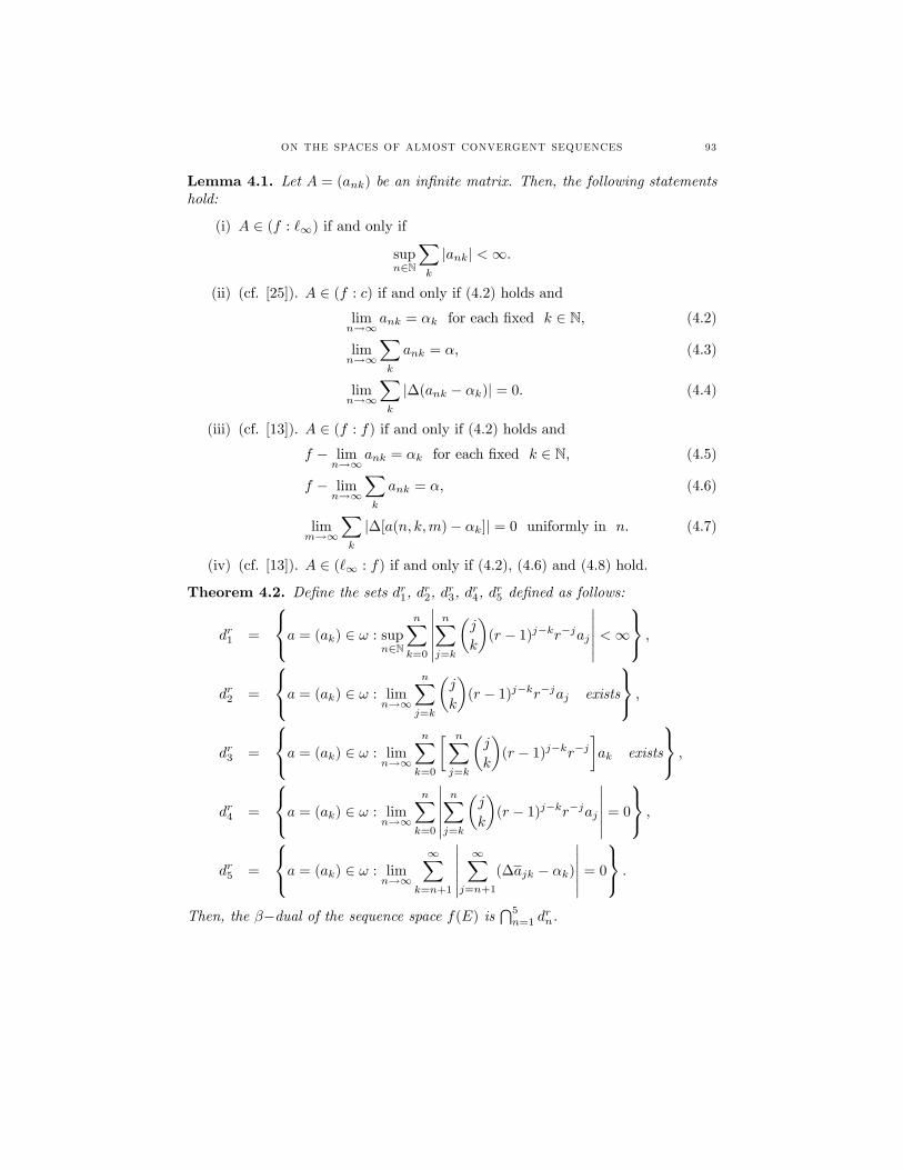
ON THE SPACES OF ALMOST CONVERGENT SEQUENCES 93
Lemma 4.1. Let A = (ank) be an infinite matrix. Then, the following statementshold:
(i) A ∈ (f : `∞) if and only if
supn∈N
∑k
|ank| <∞.
(ii) (cf. [25]). A ∈ (f : c) if and only if (4.2) holds and
limn→∞
ank = αk for each fixed k ∈ N, (4.2)
limn→∞
∑k
ank = α, (4.3)
limn→∞
∑k
|∆(ank − αk)| = 0. (4.4)
(iii) (cf. [13]). A ∈ (f : f) if and only if (4.2) holds and
f − limn→∞
ank = αk for each fixed k ∈ N, (4.5)
f − limn→∞
∑k
ank = α, (4.6)
limm→∞
∑k
|∆[a(n, k,m)− αk]| = 0 uniformly in n. (4.7)
(iv) (cf. [13]). A ∈ (`∞ : f) if and only if (4.2), (4.6) and (4.8) hold.
Theorem 4.2. Define the sets dr1, dr2, d
r3, d
r4, d
r5 defined as follows:
dr1 =
a = (ak) ∈ ω : supn∈N
n∑k=0
∣∣∣∣∣∣n∑j=k
(j
k
)(r − 1)j−kr−jaj
∣∣∣∣∣∣ <∞ ,
dr2 =
a = (ak) ∈ ω : limn→∞
n∑j=k
(j
k
)(r − 1)j−kr−jaj exists
,
dr3 =
a = (ak) ∈ ω : limn→∞
n∑k=0
[ n∑j=k
(j
k
)(r − 1)j−kr−j
]ak exists
,
dr4 =
a = (ak) ∈ ω : limn→∞
n∑k=0
∣∣∣∣∣∣n∑j=k
(j
k
)(r − 1)j−kr−jaj
∣∣∣∣∣∣ = 0
,
dr5 =
a = (ak) ∈ ω : limn→∞
∞∑k=n+1
∣∣∣∣∣∣∞∑
j=n+1
(∆ajk − αk)
∣∣∣∣∣∣ = 0
.
Then, the β−dual of the sequence space f(E) is⋂5n=1 d
rn.
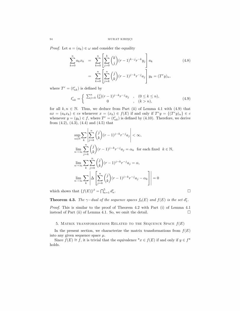
94 MURAT KIRISÇI
Proof. Let a = (ak) ∈ ω and consider the equality
n∑k=0
akxk =
n∑k=0
k∑j=0
(k
j
)(r − 1)k−jr−kyj
ak (4.8)
=
n∑k=0
n∑j=k
(j
k
)(r − 1)j−kr−jaj
yk = (T ry)n,
where T r = (trnk) is defined by
trnk =
∑nj=k
(jk
)(r − 1)j−kr−jaj , (0 ≤ k ≤ n),
0 , (k > n),(4.9)
for all k, n ∈ N. Thus, we deduce from Part (ii) of Lemma 4.1 with (4.9) thatax = (akxk) ∈ cs whenever x = (xk) ∈ f(E) if and only if T ry = (T ry)n ∈ cwhenever y = (yk) ∈ f , where T r = (trnk) is defined by (4.10). Therefore, we derivefrom (4.2), (4.3), (4.4) and (4.5) that
supn∈N
∑k
∣∣∣∣∣∣n∑j=k
(j
k
)(r − 1)j−kr−jaj
∣∣∣∣∣∣ <∞,limn→∞
n∑j=k
(j
k
)(r − 1)j−kr−jaj = αk for each fixed k ∈ N,
limn→∞
∑k
n∑j=k
(j
k
)(r − 1)j−kr−jaj = α,
limn→∞
∑k
∣∣∣∣∣∣∆ n∑j=k
(j
k
)(r − 1)j−kr−jaj − αk
∣∣∣∣∣∣ = 0
which shows that f(E)β =⋂5n=1 d
rn.
Theorem 4.3. The γ−dual of the sequence spaces f0(E) and f(E) is the set dr1.
Proof. This is similar to the proof of Theorem 4.2 with Part (i) of Lemma 4.1instead of Part (ii) of Lemma 4.1. So, we omit the detail.
5. Matrix transformations Related to the Sequence Space f(E)
In the present section, we characterize the matrix transformations from f(E)into any given sequence space µ.Since f(E) ∼= f , it is trivial that the equivalence "x ∈ f(E) if and only if y ∈ f"
holds.
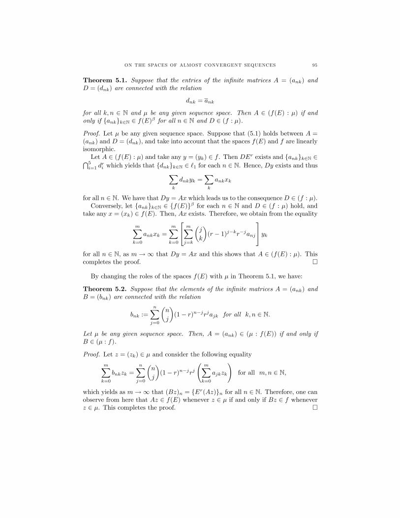
ON THE SPACES OF ALMOST CONVERGENT SEQUENCES 95
Theorem 5.1. Suppose that the entries of the infinite matrices A = (ank) andD = (dnk) are connected with the relation
dnk = ank
for all k, n ∈ N and µ be any given sequence space. Then A ∈ (f(E) : µ) if andonly if ankk∈N ∈ f(E)β for all n ∈ N and D ∈ (f : µ).
Proof. Let µ be any given sequence space. Suppose that (5.1) holds between A =(ank) and D = (dnk), and take into account that the spaces f(E) and f are linearlyisomorphic.Let A ∈ (f(E) : µ) and take any y = (yk) ∈ f . Then DEr exists and ankk∈N ∈⋂5i=1 d
ri which yields that dnkk∈N ∈ `1 for each n ∈ N. Hence, Dy exists and thus∑
k
dnkyk =∑k
ankxk
for all n ∈ N. We have thatDy = Ax which leads us to the consequenceD ∈ (f : µ).Conversely, let ankk∈N ∈ f(E)β for each n ∈ N and D ∈ (f : µ) hold, and
take any x = (xk) ∈ f(E). Then, Ax exists. Therefore, we obtain from the equality
m∑k=0
ankxk =
m∑k=0
m∑j=k
(j
k
)(r − 1)j−kr−janj
ykfor all n ∈ N, as m → ∞ that Dy = Ax and this shows that A ∈ (f(E) : µ). Thiscompletes the proof.
By changing the roles of the spaces f(E) with µ in Theorem 5.1, we have:
Theorem 5.2. Suppose that the elements of the infinite matrices A = (ank) andB = (bnk) are connected with the relation
bnk :=
n∑j=0
(n
j
)(1− r)n−jrjajk for all k, n ∈ N.
Let µ be any given sequence space. Then, A = (ank) ∈ (µ : f(E)) if and only ifB ∈ (µ : f).
Proof. Let z = (zk) ∈ µ and consider the following equalitym∑k=0
bnkzk =
n∑j=0
(n
j
)(1− r)n−jrj
(m∑k=0
ajkzk
)for all m,n ∈ N,
which yields as m→∞ that (Bz)n = Er(Az)n for all n ∈ N. Therefore, one canobserve from here that Az ∈ f(E) whenever z ∈ µ if and only if Bz ∈ f wheneverz ∈ µ. This completes the proof.
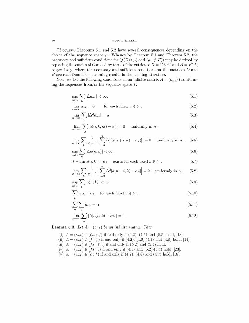
96 MURAT KIRISÇI
Of course, Theorems 5.1 and 5.2 have several consequences depending on thechoice of the sequence space µ. Whence by Theorem 5.1 and Theorem 5.2, thenecessary and suffi cient conditions for (f(E) : µ) and (µ : f(E)) may be derived byreplacing the entries of C and A by those of the entries ofD = CE1/r and B = ErA,respectively; where the necessary and suffi cient conditions on the matrices D andB are read from the concerning results in the existing literature.Now, we list the following conditions on an infinite matrix A = (ank) transform-
ing the sequences from/in the sequence space f :
supn∈N
∑k
|∆ank| <∞, (5.1)
limk→∞
ank = 0 for each fixed n ∈ N , (5.2)
limn→∞
∑k
|∆2ank| = α, (5.3)
limm→∞
∑k
|a(n, k,m)− αk| = 0 uniformly in n , (5.4)
limq→∞
∑k
1
q + 1
∣∣∣ q∑i=0
∆[(a(n+ i, k)− αk)]∣∣∣ = 0 uniformly in n , (5.5)
supn∈N
∑k
|∆a(n, k)| <∞, (5.6)
f − lim a(n, k) = αk exists for each fixed k ∈ N , (5.7)
limq→∞
∑k
1
q + 1
∣∣∣ q∑i=0
∆2[a(n+ i, k)− αk]∣∣∣ = 0 uniformly in n , (5.8)
supn∈N
∑k
|a(n, k)| <∞, (5.9)∑k
ank = αk for each fixed k ∈ N , (5.10)∑n
∑k
ank = α, (5.11)
limn→∞
∑k
|∆[a(n, k)− αk]| = 0. (5.12)
Lemma 5.3. Let A = (ank) be an infinite matrix. Then,
(i) A = (ank) ∈ (`∞ : f) if and only if (4.2), (4.6) and (5.5) hold, [13].(ii) A = (ank) ∈ (f : f) if and only if (4.2), (4.6),(4.7) and (4.8) hold, [13].(iii) A = (ank) ∈ (fs : `∞) if and only if (5.2) and (5.3) hold.(iv) A = (ank) ∈ (fs : c) if and only if (4.3) and (5.2)-(5.4) hold, [23].(v) A = (ank) ∈ (c : f) if and only if (4.2), (4.6) and (4.7) hold, [18].
ON THE SPACES OF ALMOST CONVERGENT SEQUENCES 97
(vi) A = (ank) ∈ (bs : f) if and only if (4.6), (5.2), (5.3) and (5.9) hold, [9].(vii) A = (ank) ∈ (fs : f) if and only if (4.6), (4.8), (5.3) and (5.6) hold, [5].(viii) A = (ank) ∈ (cs : f) if and only if (4.6) and (5.2) hold, [7].(ix) A = (ank) ∈ (bs : fs) if and only if (5.3) and (5.6)-(5.8) hold, [9].(x) A = (ank) ∈ (fs : fs) if and only if (5.6)-(5.9) hold, [5].(xi) A = (ank) ∈ (cs : fs) if and only if (5.7) and (5.8) hold, [7].(xii) A = (ank) ∈ (f : cs) if and only if (5.10)-(5.13) hold, [5].Now, we can give the following results:
Corollary 1. Let A = (ank) be an infinite matrix. The following statements hold:
(i) A ∈ (f(E) : `∞) if and only if ankk∈N ∈ f(E)β for all n ∈ N and (4.2)holds with ank instead of ank.
(ii) A ∈ (f(E) : c) if and only if ankk∈N ∈ f(E)β for all n ∈ N and(4.2)-(4.5) hold with ank instead of ank.
(iii) A ∈ (f(E) : c0) if and only if ankk∈N ∈ f(E)β for all n ∈ N and (4.2)holds, (4.3) and (4.5) hold with αk = 0, and (4.4) holds and α = 0 as ankinstead of ank.
(iv) A ∈ (f(E) : f) if and only if ankk∈N ∈ f(E)β for all n ∈ N and (4.2),(4.6)-(4.8) hold with ank instead of ank.
(v) A ∈ (f(E) : bs) if and only if ankk∈N ∈ f(E)β for all n ∈ N and (5.10)holds.
(vi) A ∈ (f(E) : cs) if and only if ankk∈N ∈ f(E)β for all n ∈ N and(5.10)-(5.13) hold with ank instead of ank.
Corollary 2. Let A = (ank) be an infinite matrix and bnk be defined by (5.2).Then, following statements hold:
(i) A = (ank) ∈ (`∞ : f(E)) if and only if (4.2), (4.6) and (5.5) hold with bnkinstead of ank.
(ii) A = (ank) ∈ (f : f(E)) if and only if (4.2), (4.6), (4.7) and (4.8) hold withbnk instead of ank.
(iii) A = (ank) ∈ (c : f(E)) if and only if (4.2), (4.6) and (4.7) hold with bnkinstead of ank.
(iv) A = (ank) ∈ (bs : f(E)) if and only if (5.2), (5.3), (4.6) and (5.6) hold withbnk instead of ank.
(v) A = (ank) ∈ (fs : f(E)) if and only if (5.3), (4.6), (4.8) and (5.6) hold withbnk instead of ank.
(vi) A = (ank) ∈ (cs : f(E)) if and only if (5.2) and (4.6) hold with bnk insteadof ank.
(vii) A = (ank) ∈ (bs : fs(E)) if and only if (5.3), (5.6)-(5.8) hold with bnkinstead of ank, where fs(E) denotes the domain of the matrix Er in thesequence space fs.
(viii) A = (ank) ∈ (fs : fs(E)) if and only if (5.6)-(5.9) hold with bnk instead ofank.
98 MURAT KIRISÇI
(ix) A = (ank) ∈ (cs : fs(E)) if and only if (5.7) and (5.8) hold with bnk insteadof ank.
Now, we can give some consequences, below:
Corollary 3. A ∈ (f(E) : c)s if and only if (4.2) holds, (4.3) and (4.5) hold withαk = 0 for each k ∈ N and (4.4) also holds with α = s with ank instead of ank.
Corollary 4. A ∈ (f(E) : f)s if and only if (4.2), (4.6) and (4.8) hold with αk = 0and (4.7) also holds with α = s with ank instead of ank.
Now, we may mention about Steinhaus type theorems which were formulatedby Maddox [20], as follows: Consider the class (λ : µ)1 of 1-multiplicative matricesand υ be a sequence space such that υ ⊃ λ. Then a result of the form (λ : µ)1
⋂(υ :
µ) = ∅, where ∅ denotes the empty set, is called a theorem of the Steinhaus type.Now, we can give the next Steinhaus type theorem concerning with the strongly-multiplicative and coercive matrix classes:
Theorem 5.4. The classes (f(E) : c)s and (`∞ : c) are disjoint.
Proof. Suppose that the converse of this is true, that is (f(E) : c)s⋂
(`∞ : c) 6= ∅.Then there exists at least one infinite matrix A satisfying the conditions of Corollary5.6 and Schur’s theorem. Then, we can easily see that limn→∞ ank = 0 whichcontradicts the condition limn→∞
∑k ank = s of Corollary 5.4. This completes the
proof. Theorem 5.5. The classes (f(E) : f)s and (`∞ : f) are disjoint.
Proof. This is similar to the proof of Theorem 5.8. So, we omit the detail.
6. Conclusion
The construction of new sequence spaces with the Euler mean were studied byAltay and Basar [2], Altay et al. [3] and Mursaleen et al. [22]. After Altay andPolat [4], Polat and Basar [24] studied the Euler difference sequence spaces of or-der m. Also, Karakaya and Polat [17] extended the Euler sequence spaces er0(∆),erc(∆) and er∞(∆) defined by Altay and Polat [4] to the paranormed case. Karaet al. [15] studied some topological and geometrical properties of the generalizedEuler spaces. Further Basarır and Kayıkçı[10] defined Euler B(m)-difference se-quence spaces. Demiriz and Çakan [11] introduced the sequence spaces er0(u, p) anderc(u, p) of nonabsolute type, as the sets of all sequences such that E
r,u-transformsof them are in the spaces c0(p) and c(p). Djolovic and Malkowsky [12] added a newsupplementary aspect to research of Polat and Basar [24] by characterizing classesof compact operators on those spaces.The concept of almost convergence has been employed many mathematicians
since 1948. Basar and Kirisci [8] established new almost convergent sequence spaceswith the generalized difference matrix B(r, s) and Sönmez [26] studied the conceptof almost convergence with the triple band matrix B(r, s, t). Basar and Kirisci [8]
ON THE SPACES OF ALMOST CONVERGENT SEQUENCES 99
proved that the space f is a BK−space with the sup-norm, and is a non-seperableclosed subspace of (`∞, ‖ · ‖∞). Since the space f is non-seperable, this space andthe spaces isomorphic to the space f have no Schauder basis.In this paper, we combine the almost convergence with the Euler means. Since
the domain of generalized difference matrix B(r, s) in the space f is studied byBasar and Kirisci [8], the present paper is its natural continuation.Finally, we should note from now on that the investigation of the domain of some
particular limitation matrices, namely the composition of Euler means with themth order difference matrix or generalized weighted mean, the matrix Λ, etc., in thespace f will lead us to new results. Also it can study various matrix transformations,such as sequence-to-sequence, sequence-to-series, series-to-sequences and series-to-series, between the new almost Euler sequence spaces and other spaces.
References
[1] A.M. Al-Jarrah, E. Malkowsky, BK spaces, bases and linear operators, Rend. Circ. Mat.Palermo (2)52, Vol. I (1998), 177—191.
[2] B. Altay, F. Basar, On some Euler sequence spaces of non-absolute type, Ukrainian Math. J.57(1)(2005), 1—17.
[3] B. Altay, F. Basar, M. Mursaleen, On the Euler sequence spaces which include the spaces `pand `∞ I, Inform. Sci. 176(10)(2006), 1450—1462.
[4] B. Altay, H. Polat, On some new Euler diff erence sequence spaces, Southeast Asian Bull.Math. 30 (2006), no. 2, 209—220.
[5] F. Basar, f -conservative matrix sequences, Tamkang J. Math. 22(2)(1991), 205—212[6] F. Basar, Summability Theory and Its Applications, Bentham Science Publ., e-books, Mono-
graphs, Istanbul, 2012.[7] F. Basar, R. Çolak, Almost-conservative matrix transformations, Turkish J. Math.
13(3)(1989), 91—100.[8] F. Basar, M. Kirisçi, Almost convergence and generalized diff erence matrix, Comput. Math.
Appl. 61(3)(2011), 602—611.[9] F. Basar, I. Solak, Almost-coercive matrix transformations, Rend. Mat. Appl.
(7)11(2)(1991), 249—256.[10] M. Basarır, M. Kayıkçı, On the generalized Bm-Riesz sequence space and β-property, J.
Inequal. Appl. (2009), Article ID 385029, 18 pp.[11] S. Demiriz, C. Çakan, On some new paranormed Euler sequence spaces and Euler core, Acta
Math. Sin. (Engl. Ser.) 26 (2010), no. 7, 1207—1222.[12] I. Djolovic, E. Malkowsky, Characterizations of compact operators on some Euler spaces of
diff erence sequences of order m., Acta Math. Sci. Ser. B Engl. Ed. 31 (2011), no. 4, 1465—1474.
[13] J.P. Duran, Infinite matrices and almost convergence, Math. Z. 128(1972), 75—83.[14] P.K. Kampthan, M. Gupta, Sequence Spaces and Series, Marcel Dekker Inc., New York,
Basel, 1981.[15] E.E. Kara, M. Öztürk, M. Basarır, Some topological and geometric properties of generalized
Euler sequence space, Math. Slovaca 60 (2010), no. 3, 385—398.[16] E.E. Kara, M. Basarır, On compact operators and some Euler B(m)-diff erence sequence
spaces, J. Math. Anal. Appl. 379 (2011), no. 2, 499—511.[17] V. Karakaya, H. Polat, Some new paranormed sequence spaces defined by Euler and diff erence
operators, Acta Sci. Math. (Szeged) 76(2010), 87—100.[18] J.P. King, Almost summable sequences, Proc. Amer. Math. Soc. 17(1966), 1219—1225.
100 MURAT KIRISÇI
[19] G.G. Lorentz, A contribution to the theory of divergent sequences, Acta Math. 80(1948),167—190.
[20] I.J. Maddox, On theorems of Steinhaus theorems, J. London Math. Soc. 42 (1967), 239—244.[21] H.I. Miller, C. Orhan, On almost convergent and statistically convergent subsequences, Acta
Math. Hungar. 93(2001), 135—151.[22] M. Mursaleen, F. Basar, B. Altay, On the Euler sequence spaces which include the spaces `p
and `∞ II, Nonlinear Anal. 65(3)(2006), 707—717.[23] E. Öztürk, On strongly regular dual summability methods, Commun. Fac. Sci. Univ. Ank.
Ser. A1 Math. Stat. 32(1983), 1—5.[24] H. Polat, F. Basar, Some Euler spaces of diff erence sequences of order m, Acta Math. Sci.,
Ser. B, Engl. Ed. 27B(2)(2007), 254—266.[25] J.A. Sıddıqi, Infinite matrices summing every almost periodic sequences, Pac. J. Math.
39(1)(1971) 235—251.[26] A. Sönmez, Almost convergence and triple band matrix, Math. and Comp. Modelling 57
(9—10) (2013), 2393—2402.
Current address : Murat Kirisci; Department of Mathematical Education, Hasan Ali YücelEducation Faculty, Istanbul University, Vefa, 34470, Fatih, Istanbul, TURKEY
E-mail address : [email protected]: http://communications.science.ankara.edu.tr/index.php?series=A1
Commun.Fac.Sci.Univ .Ank.Series A1Volum e 62, Number 1, Pages 101—113 (2013)ISSN 1303—5991
LOCAL AND EXTREMAL SOLUTIONS OF SOME FRACTIONALINTEGRODIFFERENTIAL EQUATION WITH IMPULSES*
ATMANIA RAHIMA
Abstract. The subject of this work is to prove existence, uniqueness, and con-tinuous dependence upon the data of solution to integrodifferential hyperbolicequation with integral conditions. The proofs are based on a priori estimatesand Laplace transform method. Finally, the solution by using a numericaltechnique for inverting the Laplace transforms is obtained.
Introduction
The concept of fractional analysis like differentiation and integration can beconsidered as a generalization of ordinary ones with integer order. However, it re-mains a lot to be done before assuming that this generalization is really established.Fractional differential equations have been extensively applied in many fields, forexample, in probability, viscoelasticity and electrical circuits. Different theoreticalstudies about the subject were done by many famous mathematicians over the yearslike Liouville, Riemann, Fourier, Abel, Leibniz. For more details, we refer to thebooks [6, 9, 10].On the other side, the interest in studying impulsive differential equations is
related to their utility for modeling phenomena subject to considerable short-termchanges during their evolution. The fact that the duration of the perturbations isnegligible in comparison with the duration of the phenomena requires us to considerthem in the form of impulses. The theory of impulsive differential equations hasbeen well developed during these twenty last years; to know more see [2, 7]
Received by the editors Nov. 02, 2012; Accepted: Jıne 24, 2013;2010 Mathematics Subject Classification. Primary 34A08, Secondary, 34A12, 34A37.Key words and phrases. Local existence, extremal solution, integrodifferential equation, Ca-
puto fractional derivative, impulsive conditions, fixed point theory, impulsive fractional inequality.
The main results of this paper were presented in part at the conference Algerian-TurkishInternational Days on Mathematics 2012 (ATIM’2012) to be held October 9—11, 2012 in Annaba,Algeria at the Badji Mokhtar Annaba University.
c©2013 Ankara University
101
102 ATMANIA RAHIMA
It is therefore interesting that the impulsive effects may be a part of studies offractional differential problems. This topic has awoken the curiosity of many re-searchers in recent years. Recently, some authors [1, 3, 5, 11] discussed existenceresults of solutions of impulsive fractional differential equations under different con-ditions, boundary ones, non local ones etc. The results are obtained by using fixedpoint principles. We point out that in the papers [1, 3, 5, 11] the authors usedan incorrect formula of solutions; for this reason in [4] the authors introduced theright formula for solutions of some given impulsive Cauchy problem with Caputofractional derivative.In this paper, we study the existence of local and extremal solutions for some
integrodifferential fractional equation involving Caputo’s derivative subject to im-pulses in fixed moments by using fixed-point theory and fractional analysis undersuitable assumptions. This, taking into account the discontinuous nature of impul-sive differential problems compared with non impulsive differential ones preciselyfor the fractional order. A non impulsive fractional problem was treated in [8].The paper is divided into three sections. In Section 2 we recall some basic
notions which will be used in the remainder of the paper. In Section 3 we establishexistence results, first, of local solution based on Schauder fixed point theorem thenof extremal solutions by using impulsive fractional inequalities.
1. Preliminaries
1.1. Fractional calculus. We will introduce notations and definitions that areused in this paper and can be found in [6]. Let a (−∞ < a <∞) a constant on thereal axis R, the Riemann-Liouville fractional integral operator of order α > 0 isdefined by
Iαa+f (t) =1
Γ (α)
∫ t
a
(t− s)α−1 f (s) ds, t > a.
Among the great amount of definitions dealing with fractional derivatives of orderα ≥ 0 we recall the Riemann-Liouville one which is defined by
Dαa+f (t) = DnIn−αa+ f (t) =
1
Γ (n− α)
dn
dtn
∫ t
a
(t− s)n−α−1 f (s) ds, (1.1)
provided that the right-hand-side exists; where n = [α] + 1, Γ (α) is the classicalGamma function. Remark that Dα
a+K 6= 0, for any constant K.The following Caputo’s definition is also widely used due to its practical formu-
lation in real world problems:
cDαa+f (t) = In−αa+ Dnf (t) =
1
Γ (n− α)
∫ t
a
(t− s)n−α−1 f (n) (s) ds. (1.2)
It’s clear that cDαa+K = 0, for any constant K. Thus, the following properties hold
cDna+f (t) = f (n) (t) , cD0
a+f (t) = I0a+f (t) = f (t) , cDαa+I
αa+f (t) = f(t).
SOLUTIONS OF SOME FRACTIONAL INTEGRODIFFERENTIAL EQUATION 103
The function f(t) = c0 + c1 (t− a) + · · · . + cn−1 (t− a)n−1 is a solution of the
equation cDαa+f (t) = 0 with c0, c1, . . . , cn−1 arbitrary real constants, then for
f ∈ Cn [a, b] we have
Iαa+cDα
a+f (t) = f(t) + c1 (t− a) + · · · .+ cn−1 (t− a)n−1
; (1.3)
for n− 1 < α < n.
In particular, when 0 < α < 1, we have
cDαa+f (t) =
1
Γ (1− α)
∫ t
a
f ′ (s)
(t− s)α ds,
Iαa+cDα
a+f (t) = f(t) + c0, c0 ∈ R.
1.2. Impulsive effects. The most real case of the instants of impulsive effectsis as follows: A finite or infinite number of fixed moments noted tk given by anincreasing sequence without accumulation points, i.e., t1 < t2 < · · · < tk < · · · andlimk→∞
tk = +∞.Let us denote the right and left limits of x (t) at t = tk respectively by
x(t+k)
= limh→0+
x (tk + h) ; x(t−k)
= limh→0−
x (tk + h) .
Definition 1.1. The impulsive effects said impulsive condition is measured by thedifference between the limits of the state function x(t) on the right and left of themoment of impulses tk and is noted
∆x (tk) = x(t+k)− x
(t−k), k = 1, 2, 3, . . . .
Remark 1.2. Submitting a system to such conditions deprives the state function ofits continuity but improves significantly other properties especially the numericalresults.
To study an impulsive initial value problem on the interval [t0, t0 + T ], wherethe number of impulses is m; we proceed as follows: [t0, t0 + T ] is subdividedinto m + 1 intervals and we act as if we had a classical Cauchy problem oneach interval (tk, tk+1], k = 0, . . . ,m, where tm+1 = t0 + T . To ensure the ex-istence of a solution we must assume the continuity of x (t) on (tk, tk+1], k =0, . . . ,m and its right limit exists at tk for k = 0, . . . ,m. Hence, the solutionsshould belong to the space of piece continuous functions denoted by PC and de-fined by PC ([t0, t0 + T ] ,R) = x : [t0, t0 + T ] → R : x (t) is continuous for t 6=tk, left continuous at t = tk and x
(t+k)exists for k = 1, . . . ,m which is a Banach
space once endowed with the norm
‖x‖PC = max
sup
t∈(tk,tk+1]|x (t)| , k = 0, 1, . . . ,m
.
104 ATMANIA RAHIMA
2. Main results
2.1. Impulsive fractional integrodifferential initial value problem. We areconcerned by the following scalar integrodifferential equation of fractional order0 < α < 1,
cDαt+0x (t) +G (t, x (t)) =
∫ t
t0
K (t, s, x (s)) ds; t 6= tk; k = 1, . . . ,m; (2.1)
with the initial condition
x (t0) = x0; t0 ≥ 0, (2.2)
and the impulsive conditions
∆x (tk) = Jk(x(t−k))
; k = 1, . . . ,m. (2.3)
We set the following assumptions:
(A1) The instants of impulsive effects tk, k = 1, . . . ,m are such that t0 < t1< · · · < tk < tk+1 < · · · < tm < t0 + T .
(A2) G(t, x) ∈ C([t0, t0+T ] ×R,R); K(t, s, x) ∈ C([t0, t0+T ]×[t0, t0+T ]×R,R)and Jk ∈ C(R,R), k = 1, . . . ,m.
(A3) The integrals∫ tt0
(t−s)α−1∫ st0K(s, σ, x(σ))dσds and
t∫t0
(t−s)α−1G(s , x(s))ds
are pointwise defined on (t0, t0 + T ].
Definition 2.1. A function x ∈ PC ([t0, t0 + T ] , R) with its α-derivatives exist-ing on [t0, t0 + T ] \ tkk=1,...,m for 0 < α < 1, is said to be a solution of theproblem (2.1)-(2.3) if x satisfies the fractional integrodifferential equation (2.1) on[t0, t0 + T ] \ tkk=1,...,m , the impulsive conditions (2.2) for t = tk; k = 1, . . . ,m;
and the initial condition (2.3) for t = t0.
2.2. Impulsive fractional integral equation. We begin with the following lemmawhich allows us to discuss the properties of the impulsive fractional integral equation(2.4) rather than the impulsive fractional integrodifferential problem (2.1)-(2.3).
Lemma 2.2. A function x ∈ PC ([t0, t0 + T ] ,R) is a solution of the problem (2.1)-(2.3) if and only if x satisfies the integral equation of the form
x (t) = x0 +∑
t0<tk<t
Jk (x (tk)) +1
Γ (α)(2.4)
×∫ t
t0
(t− s)α−1∫ s
t0
K (s, σ, x (σ)) dσ −G (s, x (s))
ds.
Proof. Let x (t) be a solution of the problem (2.1)-(2.3). Using appropriate prop-erties of fractional calculus for 0 < α ≤ 1, after applying Iα
t+0to (2.1) on [t0, t1], we
SOLUTIONS OF SOME FRACTIONAL INTEGRODIFFERENTIAL EQUATION 105
obtain
Iαct+0Dαt+0x (t) = x(t) + c0 (2.5)
= Iαt+0
[∫ t
t0
K (t, s, x (s)) ds−G (t, x (t))
].
From (2.2)we get c0 = − x0, then
x(t) = x0 +1
Γ (α)
∫ t
t0
(t− s)α−1∫ s
t0
K (s, σ, x (σ)) dσ −G (s, x (s))
ds.
Doing the same thing on (t1, t2] we obtain from (2.5)
c0 = −x(t+1)
+1
Γ (α)
∫ t1
t0
(t1 − s)α−1∫ s
t0
K (s, σ, x (σ)) dσ −G (s, x (s))
ds,
where
x(t+1)
= x(t−1)
+ J1(x(t−1))
= x0 +1
Γ (α)
∫ t1
t0
(t1 − s)α−1∫ s
t0
K (s, σ, x (σ)) dσ −G (s, x (s))
ds
+J1 (x(t1)) ,
with x(t−k)
= x (tk) , k = 1, . . . ,m. So, on (t1, t2] we get
x(t) = x0 + J1 (x(t1)) +1
Γ (α)
×∫ t
t0
(t− s)α−1∫ s
t0
K (s, σ, x (σ)) dσ −G (s, x (s))
ds.
Then, we obtain by induction for t ∈ (tm, t0 + T ] the form of integral equationsatisfied by x (t)
x (t) = x0 +
m∑k=1
Jk (x(tk)) +1
Γ (α)
∫ t
t0
(t− s)α−1∫ s
t0
K (s, σ, x (σ)) dσ −G (t, x (t))
ds.
This shows the first implication. For the other implication, we apply cDαt+0to (2.4)
to get (2.1). Conditions (2.2) and (2.3) are obtained easily from (2.4) respectivelyfor t = t0 and t = tk, k = 1, . . . ,m.
2.3. Local existence. From the fixed-point theory, we recall the following theoremwhich will be used in the sequel.Schauder’s fixed-point theorem :If E is a closed, bounded, convex subset of a Banach space and the mapping
A : E → E is completely continuous, then A has a fixed point in E.
Theorem 2.3. We assume that(A4) for t0 < s ≤ t ≤ t0 + T and x ∈ R we have
106 ATMANIA RAHIMA
(i) |K (t, s, x)| ≤ h (t, s)ϕ (|x|) ; where h (t, s) ∈ C ([t0, t0 + T ]× [t0, t0 + T ] ,R+)and ϕ ∈ C (R+,R+) is nondecreasing;
(ii) |G (t, x)| ≤ a (t) g (|x|) , where a ∈ C ([t0, t0 + T ] ,R+) and g ∈ C (R+,R+)is nondecreasing.
(iii) |Jk (x)| ≤ ϕk (|x|) , where ϕk ∈ C (R+,R+) is nondecreasing, k = 1, . . . ,m.
Then there exists at least one solution x (t) of the problem (2.1)-(2.3) in PC([t0, t0+β],R) for some positive number β.
Proof. We introduce the following notation
Ω = x ∈ PC ([t0, t0 + β] ,R) such that ‖x− x0‖PC ≤ b ,
for some β such that 0 < β ≤ T and
0 <∑
t0<tk<β
ak +βα
αΓ (α)
(M1
β
α+ 1+M2
)≤ b. (2.6)
From the continuity of the functions given in (A4) on their domains we can findpositive constants M1, M2 and ak, k = 1, . . . ,m such that for x ∈ Ω we have
|K (t, s, x (s))| ≤ supt0<s≤t≤t0+β
h (t, s)ϕ (‖x‖PC) := M1,
|G (t, x (t))| ≤ supt∈[t0,t0+β]
a (t) g (‖x‖PC) := M2,
| Jk (x(tk))| ≤ ϕk (‖x‖PC) := ak, k = 1, . . . ,m.
For applying Schauder’s theorem we need to check that Ω is a non empty closed,bounded and convex subset of the Banach PC ([t0, t0 + β] ,R) which is an easy task.Let us define the operator A on Ω by
Ax (t) = x0 +∑
t0<tk<t
Jk (x(tk)) +1
Γ (α)
t∫t0
(t− s)α−1 (2.7)
×∫ s
t0
K (s, σ, x (σ)) dσ −G (s, x (s))
ds.
It is clear that for each x ∈ Ω we have from (2.7)
|Ax (t)− x0| ≤∑
t0<tk<t
|Jk (x(tk))|+ 1
Γ (α)
∫ t
t0
(t− s)α−1 [M1 (s− t0) +M2] ds
≤∑
t0<tk<β
ak +1
Γ (α)
[M1
∫ t
t0
(t− s)α−1 (s− t0) ds+(t− t0)α
αM2
]
≤∑
t0<tk<β
ak +1
αΓ (α)
[M1
(t− t0)α+1
α+ 1+ βαM2
],
SOLUTIONS OF SOME FRACTIONAL INTEGRODIFFERENTIAL EQUATION 107
then,
‖Ax− x0‖PC ≤ b. (2.8)
Hence A maps Ω into itself. To show that A is completely continuous we will showit is continuous and AΩ is relatively compact in PC ([t0, t0 + β] ,R). Let (yn)n≥0be a sequence such that yn → y in Ω when n→∞. Then, for each t ∈ [t0, t0 + β]
|Ayn (t)−Ay (t)| ≤∑
t0<tk<t
|Jk (yn (tk))− Jk (y (tk))|
+1
Γ (α)
∣∣∣∣∫ t
t0
(t− s)α−1∫ s
t0
|K (s, σ, yn (σ))−K (s, σ, y (σ))| dσds
+1
Γ (α)
∫ t
t0
(t− s)α−1 |G (s, yn (s)) dσ −G (s, y (s))| ds.
Since the functions K, G, Jk with k = 1, . . . ,m are continuous and by the dom-inated convergence theorem we have ‖Ayn −Ay‖PC → 0, when n → ∞. Thus,A is continuous. In view of Arzela-Ascoli theorem it suffi ces to show that AΩ isuniformly bounded and equicontinuous in PC ([t0, t0 + β] ,R) indeed to show thatAΩ is relatively compact. From (2.8) we get the following
‖Ax‖PC ≤ |x0|+ b.
Thus, the functions of AΩ are uniformly bounded in PC ([t0, t0 + β] ,R). To provethat the functions of AΩ are equicontinuous, we consider τ1, τ2 ∈ [t0, t0 + β] suchthat τ1 < τ2, it follows that
|Ax (τ2)−Ax (τ1)| ≤∑
τ1≤tk<τ2
|Jk (x(tk))|
+1
Γ (α)
∣∣∣∣∫ τ2
t0
(τ2 − s)α−1∫ s
t0
K (s, σ, x (σ)) dσ −G (s, x (s))
ds
−∫ τ1
t0
(τ1 − s)α−1∫ s
t0
K (s, σ, x (σ)) dσ −G (s, x (s))
ds
∣∣∣∣ ,so
|Ax (τ2)−Ax (τ1)| ≤∑
τ1≤tk<τ2
ak +M2
Γ (α)
×[∫ τ1
t0
[(τ2 − s)α−1 − (τ1 − s)α−1
]ds+
∫ τ2
τ1
(τ2 − s)α−1 ds]
+M1
Γ (α)
[∫ τ1
t0
[(τ2 − s)α−1 − (τ1 − s)α−1
](s− t0) ds+
∫ τ2
τ1
(τ2 − s)α−1 (s− t0) ds].
108 ATMANIA RAHIMA
Therefore
‖Ax (τ2)−Ax (τ1)‖PC ≤∑
τ1≤tk<τ2
ak +M2
αΓ (α)[(τ2 − t0)α − (τ1 − t0)α]
+M1
α (α+ 1) Γ (α)
[(τ2 − t0)α+1 − (τ1 − t0)α+1
]+
M1
αΓ (α)(τ1 − t0) [(τ2 − t0)α − (τ1 − t0)α] ;
from which we get ‖Ax (τ2)−Ax (τ1)‖PC → 0, when τ2 → τ1, that is, Ax (t) isan equicontinuous family on [t0, t0 + β] . Hence AΩ is compact and so A is com-pletely continuous. Finally, we conclude by virtue of Schauder’s theorem that Ahas at least one fixed-point in Ω which is a solution of the problem ( 2.1)-(2.3). Theproof is complete.
2.4. Extremal solutions. We shall prove the existence of extremal solution of theproblem (2.1)-(2.3) through the following steps by using comparison principles andthe notion of convergence.First we give results regarding the impulsive fractional inequalities in the follow-
ing lemmas.
Lemma 2.4. Further (A1)-(A4), assume that for t0 < s ≤ t ≤ t0 + T ; x ∈ R,(A5) K (t, s, x) is nondecreasing with respect to x and G (t, x) is nonincreasing
with respect to x.Let x, y ∈ PC ([t0, t0 + T ] ,R) satisfying respectively the following inequalities
x (t) < x (t0) +∑
t0<tk<t
Jk (x (tk)) (2.9)
+1
Γ (α)
∫ t
t0
(t− s)α−1∫ s
t0
K (s, σ, x (σ)) dσ −G (s, x (s))
ds
and
y (t) ≥ y (t0) +∑
t0<tk<t
Jk (y (tk)) (2.10)
+1
Γ (α)
∫ t
t0
(t− s)α−1∫ s
t0
K (s, σ, y (σ)) dσ −G (s, y (s))
ds.
If x (t0) < y (t0) , ∆ (x (tk)) < ∆ (y (tk)) , k = 1, . . . ,m, then
x (t) < y (t) for every t ∈ [t0, t0 + T ] . (2.11)
Proof. Suppose that the inequality (2.11) does not hold. Then, there exists someτ1 ∈ (t0, t0 + T ] such that
x (τ1) = y (τ1) . (2.12)
SOLUTIONS OF SOME FRACTIONAL INTEGRODIFFERENTIAL EQUATION 109
Using the fact that x (t0) < y (t0) , Jk (x (tk)) < Jk (y (tk)) , k = 1, . . . ,m, andthe inequalities (2.9), ( 2.10) we get
y (τ1) ≥ y (t0) +∑
t0<tk<τ1
Jk (y (tk)) +1
Γ (α)
×∫ τ1
t0
(τ1 − s)α−1∫ s
t0
K (s, σ, y (σ)) dσ −G (s, y (s))
ds
> x (t0) +∑
t0<tk<τ1
Jk (x (tk)) +1
Γ (α)
×∫ τ1
t0
(τ1 − s)α−1∫ s
t0
K (s, σ, x (σ)) dσ −G (s, x (s))
ds
> x (τ1) .
This contradicts (2.14), which completes the proof.
Remark 2.5. One of the two inequalities (2.9) or (2.10) strictly holds.
Remark 2.6. The condition on the jumps of the state functions∆ (x (tk)) < ∆ (y (tk)),k = 1, . . . ,m, can be replaced by the nondecrease of Jk (x) , k = 1, . . . ,m for x ∈ R.
Lemma 2.7. Let (A1)-(A4) hold and x, y ∈ PC ([t0, t0 + T ] ,R) be solutions of(2.1)-(2.3) satisfying the following
cDαt+0x (t) <c Dα
t+0y (t) , t 6= tk, k = 1, . . . ,m, t ∈ (t0, t0 + T ]. (2.13)
If x (t0) < y (t0) ; ∆ (x (tk)) < ∆ (y (tk)) , k = 1, . . . ,m; then inequality (2.11)holds.
Proof. Suppose that the inequality (2.11) is not true. Then, there exists someτ1 ∈ (t0, t0 + T ] such that
x (τ1) = y (τ1) . (2.14)
Using the fact that x (t0) < y (t0) , Jk (x (tk)) < Jk (y (tk)) , k = 1, . . . ,m, andthe inequalities (2.9), (2.10) we get
y (τ1) ≥ y (t0) +∑
t0<tk<τ1
Jk (y (tk)) +1
Γ (α)
×∫ τ1
t0
(τ1 − s)α−1∫ s
t0
K (s, σ, y (σ)) dσ −G (s, y (s))
ds
> x (t0) +∑
t0<tk<τ1
Jk (x (tk)) +1
Γ (α)
×∫ τ1
t0
(τ1 − s)α−1∫ s
t0
K (s, σ, x (σ)) dσ −G (s, x (s))
ds
> x (τ1) .
110 ATMANIA RAHIMA
This contradicts (2.14) which completes the proof.
Now, we can give the main result of this subsection dealing with existence ofminimal and maximal solutions called extremal solutions.
Theorem 2.8. Assume that (A1)-(A5) are satisfied.Then the problem (2.1)-(2.3) has extremal solutions on [t0, t0 + β] for 0 < β ≤ T.
Proof. First, prove the existence of a maximal solution. Consider the impulsivefractional initial value problem
cDαt+0x (t) +G (t, x (t)) =
∫ tt0K (t, s, x (s)) ds+ ε;
t 6= tk; k = 1, . . . ,m; 0 < ε ≤ b
2 (m+ 1),
x (t0) = x0 + ε; t0 ≥ 0 ;∆x (tk) = Jk
(x(t−k))
+ ε; tk ∈ [t0, t0 + T ] , k = 1, . . . ,m.
(2.15)
Define the closed bounded set in Ω
Ωε = x ∈ PC ([t0, t0 + β] ,R) such that ‖x− (x0 + ε)‖PC ≤ b/2 ,
for some 0 < β ≤ T chosen such that
0 <∑
t0<tk<β
ak +mb
2 (m+ 1)+
βα
αΓ (α)
[M1
β
α+ 1+M2 +
b
2 (m+ 1)
]≤ b
2.
It is clear that all assumptions of Theorem 2.3 are satisfied, then problem (2.15)has a solution x (t, ε) ∈ PC ([t0, t0 + β] ,R) . From Lemma 2.2 the solution of (2.15)satisfies the integral equation of the form
x (t, ε) = x (t0, ε) +∑
t0<tk<t
Jk (x (tk, ε)) +1
Γ (α)
∫ t
t0
(t− s)α−1 (2.16)
×∫ s
t0
K (s, σ, x (σ, ε)) dσ + ε−G (s, x (s, ε))
ds,
with x (t0, ε) = x0 + ε and Jk (x (tk, ε)) = Jk (x (tk)) + ε, k = 1, . . . ,m.Let x (t, ε) be a family of functions in PC ([t0, t0 + β] , R) for ε > 0 satisfying
(2.16) . So, under the assumptions (A1)− (A3) we have
|x (t, ε)| ≤ |x0|+ ε+1
Γ (α)
∫ t
t0
(t− s)α−1 [M1 (s− t0) + ε+M2] ds+∑
t0<tk<β
(ak + ε)
≤ |x0|+ (m+ 1) ε+∑
t0<tk<β
ak +1
αΓ (α)
[M1
βα+1
α+ 1+ βαM2 + βαε
]
≤ |x0|+∑
t0<tk<β
ak +b
2+
βα
Γ (α+ 1)
[M1
β
α+ 1+M2 +
b
2 (m+ 1)
]≤ |x0|+ b.
SOLUTIONS OF SOME FRACTIONAL INTEGRODIFFERENTIAL EQUATION 111
Then, x (t, ε) is a uniformly bounded family in PC ([t0, t0 + β] ,R). It is alsoequicontinuous on [t0, t0 + β]. Indeed, for τ1, τ2 ∈ [t0, t0 + β] such that τ1 < τ2 wehave
|x (τ2, ε)− x (τ1, ε)| ≤∑
τ1≤tk<τ2
∣∣Jk (x(t−k ))
+ ε∣∣
+1
Γ (α)
∣∣∣∣∫ τ2
t0
(τ2 − s)α−1∫ s
t0
K (s, σ, x (σ, ε)) dσ + ε−G (s, x (s, ε))
ds
−∫ τ1
t0
(τ1 − s)α−1∫ s
t0
K (s, σ, x (σ, ε)) dσ + ε−G (s, x (s, ε))
ds
∣∣∣∣ .Then, by the same arguments used in the proof of Theorem 2.3, we obtain
‖x (τ2, ε)− x (τ1, ε)‖PC → 0 when τ1 → τ2.
On the other hand, we point out that for each ε1, ε2 such that 0 < ε1 < ε2 ≤ ε wehave
x (t0, ε1) = x0 + ε1 < x0 + ε2 = x (t0, ε2) ,
and
∆ (x (tk, ε1)) = ∆x (tk) + ε1 < ∆x (tk) + ε2 = ∆x (tk, ε2) , k = 1, . . . ,m.
Let F (t, x (t, ε)) =t∫t0
K (t, s, x (s, ε)) ds − G (t, x (t, ε)) , Fε (t, x) = F (t, x) + ε and
Jk(x(t−k))
+ ε1 = Jk(x(t−k , ε1
))= Jk (x (tk, ε1)) ; we get
x (t, ε1) < x (t0, ε1) +∑
t0<tk<t
Jk (x (tk, ε1)) +1
Γ (α)
×∫ t
t0
(t− s)α−1∫ s
t0
K (s, σ, x (σ, ε1)) dσ + ε2 −G (s, x (s, ε1))
ds
< x (t0, ε1) +∑
t0<tk<t
Jk (x (tk, ε1)) +1
Γ (α)
∫ t
t0
(t− s)α−1 Fε2 (s, x (s, ε1)) ds
and
x (t, ε2) ≥ x (t0, ε2) +1
Γ (α)
∫ t
t0
(t− s)α−1 Fε2 (s, x (s, ε2)) ds+∑
t0<tk<t
Jk (x (tk, ε2)) .
We infer from Lemma 2.4 that x (t, ε1) < x (t, ε2), for t ∈ [t0, t0 + β] .
112 ATMANIA RAHIMA
We conclude by Arzela-Ascoli lemma there is a decreasing sequence εnn≥1such that lim
n→∞εn = 0 and x (t, εn) satisfies the form
x (t, εn) = x0 + εn +∑
t0<tk<t
(Jk (x (tk)) + εn) +1
Γ (α)
∫ t
t0
(t− s)α−1
×∫ s
t0
K (s, σ, x (σ, εn)) dσ + εn −G (s, x (s, εn))
ds.
Since K and G are uniformly continuous, we get the following integral equation by
letting n→∞
x (t) = x0 +∑
t0<tk<t
Jk (x (tk)) +1
Γ (α)
∫ t
t0
(t− s)α−1
×∫ s
t0
K (s, σ, x (σ)) dσ −G (s, x (s))
ds.
Then limn→∞
x (t, εn) = x (t) uniformly on [t0, t0 + β] with x (t0) = x0. Therefore,
x (t) is a solution of (2.1)-(2.3) on [t0, t0 + β]. Now, we have to prove that x (t)is the maximal solution of (2.1)-(2.3)on [t0, t0 + β]. Let y (t) be any solution of(2.1)-(2.3) on [t0, t0 + β] . It is clear that
y (t0) = x0 < x0 + ε = x (t0, ε) ;
and ∆ y (tk) = ∆x (tk) < ∆x (tk) + ε = ∆x (tk, ε) , k = 1, . . . ,m.
The fact that y (t) satisfies (2.1) implies that
cDαt0y (t) <c Dα
t0x (t, ε) , t 6= tk, k = 1, . . . ,m, t ∈ [t0, t0 + β] ; 0 < ε ≤ b
2 (m+ 1).
Then we have by Lemma 2.7 , y (t) < x (t, ε) , t ∈ [t0, t0 + β] . Since the maximalsolution is unique, then lim
ε→0x (t, ε) = x (t) uniformly on [t0, t0 + β] .
Likewise, we can prove by the same arguments the existence of a unique minimalsolution; this completes the proof.
References
[1] K. Balachandran, S. Kiruthika, J.J. Trujillo, Existence results for fractional impulsive in-tegrodiff erential equations in Banach spaces, Commun. Nonlinear Sci. Numer. Simulat. 16(2011) 1970—1977.
[2] M. Benchohra, J. Henderson, S. Ntouyas, Impulsive Diff erential Equations and Inclusions,Hindawi Publishing Corporation, New York, 2006.
[3] M. Benchohra, B. A. Slimani, Existence and uniqueness of solutions to impulsive fractionaldiff erential equations, Electronic Journal of Differential Equations, 2009 (2009), No. 10, pp.1—11.
[4] M. Feckan, Y. Zhou, J. Wang, On the Concept and Existence of Solution for ImpulsiveFractional Diff erential Equations, Commun. Nonlinear Sci. Numer. Simulat. (2011), doi:10.1016/j.cnsns.2011.11.017.
SOLUTIONS OF SOME FRACTIONAL INTEGRODIFFERENTIAL EQUATION 113
[5] G. Wanga, B. Ahmad, L. Zhanga, Some existence results for impulsive nonlinear fractionaldiff erential equations with mixed boundary conditions, Comput. Math. Appl. 62 (2011) 1389—1397.
[6] A.A. Kilbas, H M. Srivastava, J.J. Trujillo, Theory and Applications of Fractional Diff eren-tial Equations, North-Holland Mathematics Studies, 204 Elsevier Science B.V., Amsterdam,2006.
[7] V. Lakshmikantam, D. Bainov, P.S. Simeonov, Theory of Impulsive Diff erential Equations,World Scientific, Singapore, 1989.
[8] V. Lakshmikantam, A.S. Vatsala, Basic theory of fractional diff erential equations, NonlinearAnal. 69 (2008) 2677-2682.
[9] K.S. Miller, B. Ross, An Introduction to the Fractional Calculus and Fractional Diff erentialEquations, John Wiley and Sons, 1993.
[10] K.B. Oldham, J. Spanier, Fractional Calculus: Theory and Applications, Diff erentiation andIntegration to Arbitrary Order, Academic Press, New York, 1974.
[11] X. Wang, Impulsive boundary value problem for nonlinear diff erential equations of fractionalorder, Comput. Math. Appl. 62 (2011) 2383—2391.Current address : LMA, Department of Mathematics, University of Badji-Mokhtar, Annaba,
P.O. box, Annaba 23000, ALGERIAE-mail address : [email protected]: http://communications.science.ankara.edu.tr/index.php?series=A1

Commun.Fac.Sci.Univ .Ank.Series A1Volum e 62, Number 2, Pages 115—119 (2013)ISSN 1303—5991
CONE CONVERGENCE FOR MULTIPLE SEQUENCES*
AHMET SAHINER
Abstract. The aim of this paper is to introduce a new type convergencewhich is useful when a d-multiple sequence is not convergent in some usualsenses.
1. Introduction
Main purpose of this paper is to introduce a new type convergence which espe-cially can be thought to be useful when a multidimensional sequence is not conver-gent. Though the new idea could be, explained in and applied to many subjects offunctional analysis including multiple sequences related to convergence types suchas statistical convergence, ideal convergence and to matrix transformations betweensequence spaces and so on. For the sake of clarity we introduce this notion in someplain part of the notion of statistical convergence.Let Nd be the set of d-tuples k := (k1, k2, . . . , kd) with nonnegative integers for
coordinates kj , where d is a fixed positive integer. Note that Nd is partially orderedby agreeing k ≤ n if and only if kj ≤ nj for each integer j (see [8]). A functionx : Nd → R (C) is called a real (complex) d-multiple sequence. If d = 2 then afunction x : N2 → R (C) is called a real (complex) double sequence. The definitionof the convergence of double sequences was given by Pringsheim in [3]. Rememberthat a double sequence (xnk) is said to be convergent to L in Pringsheim’s sense if forevery ε > 0, there exists N (ε) ∈ N such that |xnk − L| < ε whenever n, k ≥ N (ε)[2, 4, 5, 6].The idea of statistical convergence was first presented by Fast in [1] . The notion
of statistically convergent double sequences has been studied by many authors (seefor instance, [5, 6, 7, 8]). Regarding these works, to be adopted to the definition of
Received by the editors Nov. 20, 2012; Accepted: June. 25, 2013.2010 Mathematics Subject Classification. Primary 40A05, 40B05; Secondary 26A03.Key words and phrases. Double sequence, multiple sequence, statistical convergence, multiple
natural density, cone convergence.The main results of this paper were presented in part at the conference Algerian-Turkish Interna-tional Days on Mathematics 2012 (ATIM’2012) to be held October 9—11, 2012 in Annaba, Algeriaat the Badji Mokhtar Annaba University.
c©2013 Ankara University
115
116 AHMET SAHINER
the density of a subset E of N2, the density ρ (E) of any subset of E ⊆ Nd can begiven by
ρ (E) = limminKi→∞
1
K1 · · ·Kd
∑k1≤K1
· · ·∑
kd≤Kd
χE (k1, . . . , kd) , (i = 1, 2, . . . , d)
provided the limit exists.Now to recall the definition of a cone let Rd≥ denote the set of d-tuples x : =
(x1, x2, . . . , xd) with nonnegative reals for coordinates xj . Suppose that x1: =(x11, x12, . . . , x1d), x2: = (x21, x22, . . . , x2d) , ..., xd: = (xd1, xd2, . . . , xdd) ∈ Rd≥are given such that xi and xj are not co-linear for i 6= j. Then the set
σ = Rd≥x1 + · · ·+ Rd≥xd =α1x1+ · · ·+αdxd : αi ∈ R1≥ for i = 1, . . . , d
is called the cone generated by x1,x2, ...,xd. A cone is said to be pointed if itincludes the null vector 0.For a given cone σ = Rd≥x1 + · · · + Rd≥xd and u : = (u1, u2, . . . , ud) ∈ Rd≥, the
shift of σ with respect to u is defined to be the set u+ σ.
2. Main results
Definition 2.1. Let x =(xk : k ∈Nd
)be a d -multiple sequence of (real or com-
plex) numbers and σ = Rd≥s1 + · · · + Rd≥sd be a fixed cone. Then the d-multiplesequence
(xk : k ∈Nd
)is called σ- Cauchy sequence if for each ε > 0, there exists
a natural number N = N(ε) such that |xn − xk| < ε whenever n ≥ k ≥ N andn,k ∈ σ.
Definition 2.2. A d-multiple sequence x =(xk : k ∈Nd
)is said to be σ-bounded
if there exists M > 0 such that |xk| < M for all k ∈ σ.
Definition 2.3. Let x =(xk : k ∈Nd
)be a d -multiple sequence of (real or com-
plex) numbers and σ = Rd≥s1 + · · · + Rd≥sd be a fixed cone. Then the d-multiplesequence
(xk : k ∈Nd
)is called σ- convergent to a number L if for each ε > 0 there
exists N ∈ Nd such that |xk − L| < ε whenever k (∈ σ)≥ N .
If(xk : k ∈Nd
)is σ-convergent to a real number L we denote this by σ −
lim(xk : k ∈Nd
)= L or
(xk : k ∈Nd
) σ→ L.Note that every double sequence, which is convergent in Pringsheim’s sense, is
convergent with respect to the fixed cone σ = R2≥ (1, 0)+R2≥ (0, 1). More generally,every d-multiple sequence, which is convergent in Pringsheim’s sense, is convergentwith respect to the fixed cone σ = Rd≥ (1, 0, . . . , 0) + Rd≥ (0, 1, , 0, . . . , 0) + · · · +Rd≥ (0, 0, , 0, . . . , 1).
Example 2.4. Let σ = R2≥ (1, 0) + R2≥ (1, 1) and
xk:=(k1,k2) =
k1 , k1 ≤ k2,0 , otherwise.
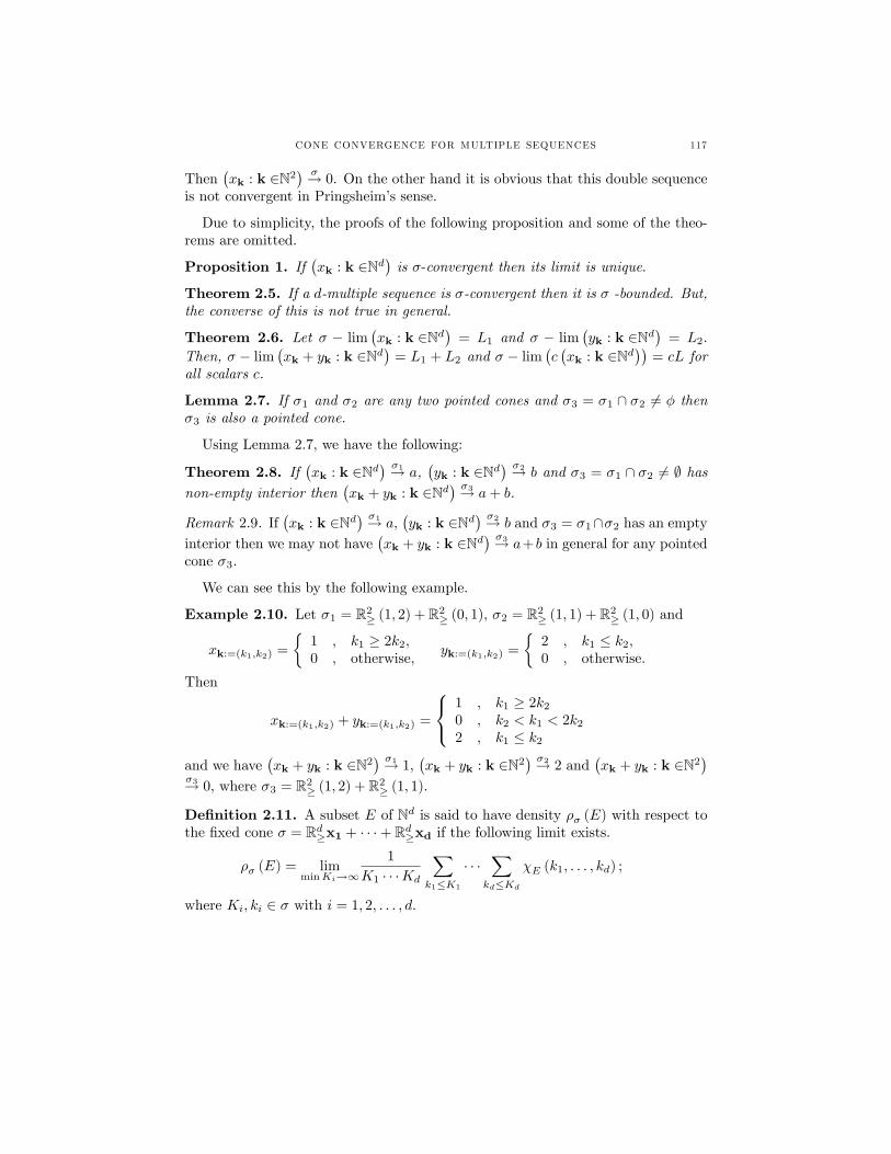
CONE CONVERGENCE FOR MULTIPLE SEQUENCES 117
Then(xk : k ∈N2
) σ→ 0. On the other hand it is obvious that this double sequenceis not convergent in Pringsheim’s sense.
Due to simplicity, the proofs of the following proposition and some of the theo-rems are omitted.
Proposition 1. If(xk : k ∈Nd
)is σ-convergent then its limit is unique.
Theorem 2.5. If a d-multiple sequence is σ-convergent then it is σ -bounded. But,the converse of this is not true in general.
Theorem 2.6. Let σ − lim(xk : k ∈Nd
)= L1 and σ − lim
(yk : k ∈Nd
)= L2.
Then, σ − lim(xk + yk : k ∈Nd
)= L1 + L2 and σ − lim
(c(xk : k ∈Nd
))= cL for
all scalars c.
Lemma 2.7. If σ1 and σ2 are any two pointed cones and σ3 = σ1 ∩ σ2 6= φ thenσ3 is also a pointed cone.
Using Lemma 2.7, we have the following:
Theorem 2.8. If(xk : k ∈Nd
) σ1→ a,(yk : k ∈Nd
) σ2→ b and σ3 = σ1 ∩ σ2 6= ∅ hasnon-empty interior then
(xk + yk : k ∈Nd
) σ3→ a+ b.
Remark 2.9. If(xk : k ∈Nd
) σ1→ a,(yk : k ∈Nd
) σ2→ b and σ3 = σ1∩σ2 has an emptyinterior then we may not have
(xk + yk : k ∈Nd
) σ3→ a+b in general for any pointedcone σ3.
We can see this by the following example.
Example 2.10. Let σ1 = R2≥ (1, 2) + R2≥ (0, 1), σ2 = R2≥ (1, 1) + R2≥ (1, 0) and
xk:=(k1,k2) =
1 , k1 ≥ 2k2,0 , otherwise,
yk:=(k1,k2) =
2 , k1 ≤ k2,0 , otherwise.
Then
xk:=(k1,k2) + yk:=(k1,k2) =
1 , k1 ≥ 2k20 , k2 < k1 < 2k22 , k1 ≤ k2
and we have(xk + yk : k ∈N2
) σ1→ 1,(xk + yk : k ∈N2
) σ2→ 2 and(xk + yk : k ∈N2
)σ3→ 0, where σ3 = R2≥ (1, 2) + R2≥ (1, 1).
Definition 2.11. A subset E of Nd is said to have density ρσ (E) with respect tothe fixed cone σ = Rd≥x1 + · · ·+ Rd≥xd if the following limit exists.
ρσ (E) = limminKi→∞
1
K1 · · ·Kd
∑k1≤K1
· · ·∑
kd≤Kd
χE (k1, . . . , kd) ;
where Ki, ki ∈ σ with i = 1, 2, . . . , d.
118 AHMET SAHINER
Definition 2.12. A d-multiple sequence x =(xk : k ∈Nd
)is said to be σ-statistically
convergent to L if for every ε > 0, ρσ ((k1, . . . , kd) : |xk1...kd − L| ≥ ε) = 0.Definition 2.13. Let x =
(xk : k ∈Nd
)and y =
(yk : k ∈Nd
)be two d -multiple
sequences and σ = Rd≥x1 + · · · + Rd≥xd be a fixed cone. Then we say that(xk : k ∈Nd
)=(yk : k ∈Nd
)for almost all k ∈σ if
δd(k ∈Nd ∩ σ :
(xk : k ∈Nd
)6=(yk : k ∈Nd
))= 0.
Definition 2.14. Let x =(xk : k ∈Nd
)be a d -multiple sequence. A subset D of
Rd said to contain(xk : k ∈Nd
)for almost all k if
δd(k ∈Nd ∩ σ :
(xk : k ∈Nd
)/∈ D
)= 0.
Theorem 2.15. A d-multiple sequence(xk : k ∈Nd
)is σ-statistically convergent if
and only if it is σ-statistically Cauchy.
Proof. Since the necessity is obvious, we only prove the suffi ciency. Let(xk : k ∈Nd
)be a σ- statistically Cauchy sequence. Choose ε = 1, then there exist k11, k
12, . . . , k
1d
such that the closed circle U1 of diameter 2 units with center at k11, k12, . . . , k
1d
contains xk for almost all k ∈σ. Now for ε = 1/2 there exist k21, k22, . . ., k
2d such
that the closed circle U2 of diameter 1 unit with center at xk21k22···k2d contains xkfor almost all k ∈σ. Take U2 = U1 ∩ U2 then U2 which is closed subset of Rdwith diameter less than or equal to 1 unit such that U2 contains xk for almost allk ∈σ. Take ε = 2−2, then there exist k31, k32, . . . , k3d such that the closed circle U3of diameter 1/2 unit with center at xk31k32···k3d contains x k for almost all k ∈σ. Ifwe choose U3 = U2 ∩ U3 then U3 is closed subset of Rd with diameter less than orequal to 1/2 unit such that U3 contains xk for almost all k ∈σ. Following this way,we have a sequence (Un) of closed subsets of Rd such that
(i) Un+1 ⊆ Un for all n ∈ N.(ii) diamUn ≤ 22−n for all n ∈ N.
Then∞⋂n=1
Un contains one point. Let us call this point as L. Then L ∈ Un for
all n ∈ N. If we choose m such that 2−m < ε then Un contains x k for almost allk ∈σ. This means
(xk : k ∈Nd
)is statistically convergent to L.
Now we are ready to give the following cone d-multiple analogues of the resultin [7].
Theorem 2.16. Let x =(xk : k ∈Nd
)is a d -multiple sequence and σ = Rd≥x1 +
· · ·+ Rd≥xd be a fixed cone. Then the following statements are equivalent:
(i)(xk : k ∈Nd
)is σ-statistically convergent to `.
(ii)(xk : k ∈Nd
)is σ-statistically Cauchy.
(iii) There exists a subsequence(yk : k ∈Nd
)of(xk : k ∈Nd
)such that σ −
lim(yk : k ∈Nd
)= `.
CONE CONVERGENCE FOR MULTIPLE SEQUENCES 119
Conclusion
As is mentioned at the beginning of the article this new type convergence canbe applied to many subjects of functional analysis including multiple sequencesrelated to convergence types such as statistical convergence, ideal convergence andso on and to matrix transformations between sequence spaces including multiplesequences. So, application area of this new type convergence is enormous for furtherworks.
References
[1] H. Fast, Sur la convergence statistique, Colloq. Math. 2(1951), 241—244.[2] H.J. Hamilton, Transformations of multiple sequences, Duke Math. J. 2(1936), 29—60.[3] A Pringsheim, Zur theorie der zweifach unendlichen Zahlenfolgen, Math. Ann. 53(3)(1900),
289—321.[4] G.M. Robinson, Divergent double sequences and series, Trans. Amer. Math. Soc. 28(1926),
50—73.[5] B.C. Tripathy, Statistically convergent double sequences, Tamkang J. Math. 34(3)(2003), 231—
237.[6] B.C. Tripathy, On I-convergent double sequences, Soochow J. Math. 31(4)(2005), 549—560.[7] Mursaleen, O.H.H. Edely, Statistical convergence of double sequences, J. Math. Anal. Appl.
288(2003), 223—231.[8] F. Moricz, Statistical convergence of multiple sequences, Arch. Math. 81(1)(2003), 82—89.
Current address : Department of Mathematics, Süleyman Demirel University, 32260, Isparta,TURKEY
E-mail address : [email protected]: http://communications.science.ankara.edu.tr/index.php?series=A1

Commun.Fac.Sci.Univ .Ank.Series A1Volum e 62, Number 1, Pages 121—129 (2013)ISSN 1303—5991
EXISTENCE AND UNIQUENESS OF SOLUTION FOR ASECOND ORDER BOUNDARY VALUE PROBLEM*
A. GUEZANE-LAKOUD, N. HAMIDANE AND R. KHALDI
Abstract. This paper deals with a second order boundary value problem withonly integrals conditions. Our aim is to give new conditions on the nonlinearterm, then, using Banach contraction principle and Leray Schauder nonlinearalternative, we establish the existence of nontrivial solution of the consideredproblem. As an application, some examples to illustrate our results are given.
1. Introduction
We study the existence of solutions for the following second-order boundary valueproblem (BVP)(P1):
u′′ (t) + f(t, u(t)) = 0, 0 < t < 1 (1.1)
u (0) =
∫ 1
0
u (t) dt, u (1) =
∫ 1
0
tu (t) dt, (1.2)
where f : [0, 1] × R → R is a given function. We mainly use the Banach contrac-tion principle and Leray Schauder nonlinear alternative to prove the existence anduniqueness results. For this, we formulated the boundary value problem (P1) asfixed point problem. We also study the compactness of solutions set.The second order equations (1.1) are used to model various phenomena in physics,
chemistry and epidemiology. In general nonlinearities that refer to source terms rep-resent specific physical laws, in chemistry, for example, if f (t, u) = ug(u)e
u−1ε , then
it represents Arheninus law for chemistry reactions, where the positive parameterε represents the activation energy for the reaction and the continuous function grepresents the concentration of the chemical product, see [1].
Received by the editors Nov. 11, 2012; Accepted: June 27, 2013.2010 Mathematics Subject Classification. 34B10, 34B15, 34B18, 34G20.Key words and phrases. Fixed point theorem, two-point boundary value problem, Ba-
nach contraction principle, Leray Schauder nonlinear alternative, second-order equation.
The main results of this paper were presented in part at the conference Algerian-TurkishInternational Days on Mathematics 2012 (ATIM’2012) to be held October 9—11, 2012 in Annaba,Algeria at the Badji Mokhtar Annaba University.
c©2013 Ankara University
121
122 A. GUEZANE-LAKOUD, N. HAMIDANE AND R. KHALDI
Non local conditions come up when values of the function on the boundaryare connected to values inside the domain. The integral conditions arise in quasi-stationary thermoelasticity theory, in modeling the technology of integral circuits,....Some times it is better to impose integral conditions because they lead to more pre-cise measures than those proposed by a local conditions.Very recently there have been several papers on second and third order boundary
value problems, we can cite the paper Graef and Yang [6], Guo et al [10], Hopkinsand Kosmatov [11], and Shunhong et al [15] . Excellent surveys of theoreticalresults can be found in Agarwal [1] and Ma [14]. More results can be found in[2, 3, 4, 5, 7, 8, 9, 10, 12, 13] . Most of the results dealing with these problems usedthe nonlinear alternative of Leray-Schauder, or more generally the theory of fixedpoint on the cone.This paper is organized as follows. In section 2 we list some preliminaries ma-
terials to be used later. Then in Section 3, we give our main results which consistin uniqueness and existence theorems. We end our work with some illustratingexamples.
2. Preliminaries
Let E = C ([0, 1] ,R) be the Banach space of all continuous functions from [0, 1]into R with the norm ||y|| = max
t∈[0,1]|y (t)|. We denote by L1 ([0, 1] ,R) the Banach
space of Lebesgue integrable functions from [0, 1] into R with the norm ||y||L1 =∫ 10|y (t)| dt.
Definition 2.1. A function f : [0, 1]× R→ R is called L1−Carathéodory if(i) The map t 7→ f(t, u) is measurable for all u ∈ R.(ii) The map u 7→ f(t, u) is continuous for almost each t ∈ [0, 1].(iii) For each r > 0, there exists an ψr ∈ L1 [0, 1] such that for almost all
t ∈ [0, 1] and |u| ≤ r we have |f(t, u)| ≤ ψr (t).
Lemma 2.2. [4] Let F be a Banach space and Ω a bounded open subset of F ,0 ∈ Ω. Let T : Ω → F be a completely continuous operator. Then, either thereexists x ∈ ∂Ω, λ > 1 such that T (x) = λx, or there exists a fixed point x∗ ∈ Ω ofT.
Lemma 2.3. Let y ∈ L1 ([0, 1] ,R). Then the solution of the following boundaryvalue problem
u′′ (t) + y(t) = 0, 0 < t < 1 (2.1)
u (0) =
∫ 1
0
u (t) dt, u (1) =
∫ 1
0
tu (t) dt,
is
u(t) =1
3
∫ 1
0
G(t, s)y(s)ds,
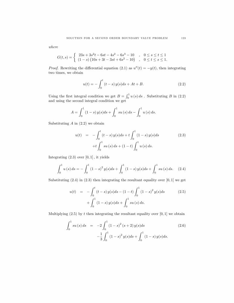
SOLUTION FOR A SECOND ORDER BOUNDARY VALUE PROBLEM 123
where
G(t, s) =
23s+ 3s2t− 6st− 4s2 − 6s3 − 10 , 0 ≤ s ≤ t ≤ 1(1− s)
(10s+ 3t− 3st+ 6s2 − 10
), 0 ≤ t ≤ s ≤ 1.
Proof. Rewriting the differential equation (2.1) as u′′(t) = −y(t), then integratingtwo times, we obtain
u(t) = −∫ t
0
(t− s) y(s)ds+At+B. (2.2)
Using the first integral condition we get B =∫ 10u (s) ds . Substituting B in (2.2)
and using the second integral condition we get
A =
∫ 1
0
(1− s) y(s)ds+
∫ 1
0
su (s) ds−∫ 1
0
u (s) ds.
Substituting A in (2.2) we obtain
u(t) = −∫ t
0
(t− s) y(s)ds+ t
∫ 1
0
(1− s) y(s)ds (2.3)
+t
∫ 1
0
su (s) ds+ (1− t)∫ 1
0
u (s) ds.
Integrating (2.3) over [0, 1] , it yields∫ 1
0
u (s) ds = −∫ 1
0
(1− s)2 y(s)ds+
∫ 1
0
(1− s) y(s)ds+
∫ 1
0
su (s) ds. (2.4)
Substituting (2.4) in (2.3) then integrating the resultant equality over [0, 1] we get
u(t) = −∫ t
0
(t− s) y(s)ds− (1− t)∫ 1
0
(1− s)2 y(s)ds (2.5)
+
∫ 1
0
(1− s) y(s)ds+
∫ 1
0
su (s) ds.
Multiplying (2.5) by t then integrating the resultant equality over [0, 1] we obtain∫ 1
0
su (s) ds = −2
∫ 1
0
(1− s)2 (s+ 2) y(s)ds (2.6)
−1
3
∫ 1
0
(1− s)2 y(s)ds+
∫ 1
0
(1− s) y(s)ds.
124 A. GUEZANE-LAKOUD, N. HAMIDANE AND R. KHALDI
Substituting (2.6) in (2.5) it yields
u(t) = −∫ t
0
(t− s) y(s)ds+1
3
∫ 1
0
(1− s)2 (3t− 6s− 16) y(s)ds (2.7)
+2
∫ 1
0
(1− s) y(s)ds
=1
3
∫ t
0
(23s+ 3s2t− 6st− 4s2 − 6s3 − 10
)y(s)ds
+1
3
∫ 1
t
(1− s)(10s+ 3t− 3st+ 6s2 − 10
)y(s)ds
=1
3
∫ 1
0
G(t, s)y(s)ds.
3. Existence and Uniqueness Results
Theorem 3.1. Assume that the following hypotheses hold.(A1) f is an L1-Carathéodory function.(A2) There exists a nonnegative function g ∈ L1 ([0, 1] ,R+) such that
|f(t, x)− f(t, y)| ≤ g(t) |x− y| ,∀x, y ∈ R, t ∈ [0, 1] , (3.1)∫ 1
0
g(s)ds <3
10, (3.2)
then the BVP (P1) has a unique solution u in E.
Proof. We transform the boundary value problem (1.1)-(1.2) to a fixed point prob-lem. Define the integral operator T : E → E by
Tu(t) =1
3
∫ 1
0
G(t, s)f (s, u (s)) ds,∀t ∈ [0, 1] .
From Lemma 2.3, the BVP (1.1)-(1.2) has a solution if and only if the operator Thas a fixed point in E. Using elementary computations we prove that |G(t, s)| ≤ 10.Let u, v ∈ E, applying (3.1) we get
|Tu(t)− Tv(t)| ≤ 1
3
∫ 1
0
|G(t, s)| |f (s, u (s))− f (s, v (s))| ds
≤ 10
3
∫ 1
0
g(s) |u (s)− v (s)| ds.
Due to (3.2), we obtain ‖Tu− Tv‖ < ‖u− v‖. Consequently T is a contraction,hence it has a unique fixed point which is the unique solution of the BVP (1.1)-(1.2).
Now we give some existence results for the BVP (1.1)-(1.2).
SOLUTION FOR A SECOND ORDER BOUNDARY VALUE PROBLEM 125
Theorem 3.2. Assume that the following hypotheses hold
(B1) f is an L1-Carathéodory function, the map t → f(t, 0) is continuous andf(t, 0) 6= 0, for any t ∈ [0, 1].
(B2) There exist nonnegative functions h, k ∈ L1 ([0, 1] ,R+) and 0 < α < 1,such that
|f (t, x)| ≤ k (t) |x|α + h (t) , (t, x) ∈ [0, 1]× R. (3.3)
Then the BVP (1.1)-(1.2) has at least one nontrivial solution u∗ ∈ E andthe set of its solutions is compact.
Proof. To prove this Theorem, we apply Leray Schauder nonlinear alternative. Firstwe prove that T is completely continuous.(i) T is continuous. Let (un) be a sequence that converges to u in E. Using the
fact that |G(t, s)| ≤ 10, we obtain
|Tun(t)− Tu(t)| ≤ 10
3
∫ 1
0
|f (s, un (s))− f (s, u (s))| ds.
Moreover
‖Tun − Tu‖ ≤10
3‖f (., un (.))− f (, u (.))‖ .
(ii) T maps bounded sets into relatively compact sets in E. Let Br = u ∈ E;‖u‖ ≤ r be a bounded subset.(a) For any u ∈ Br and t ∈ [0, 1]
|Tu(t)| ≤ 10
3
∫ 1
0
(k(s) |u(s)|α + h(s)) ds
≤ 10
3rα∫ 1
0
k(s)ds+10
3
∫ 1
0
h(s)ds,
then T (Br) is uniformly bounded.(b) T (Br) is equicontinuous. Indeed for all t1, t2 ∈ [0, 1] , u ∈ Br, we have from
(3.3) that
|Tu(t1)− Tu(t2)|
≤ 10
3
∫ 1
0
|G(t1, s)−G(t2, s)| (k(s) |u(s)|α + h(s)) ds
≤ 10rα
3
∫ 1
0
|G(t1, s)−G(t2, s)| k(s)ds+10
3
∫ 1
0
|G(t1, s)−G(t2, s)|h(s)ds,
when t1 → t2, then |Tu(t1)− Tu(t2)| tends to 0. Consequently T (Br) is equicon-tinuous. Then T is completely continuous operator.Now we apply Leray Schauder nonlinear alternative.
126 A. GUEZANE-LAKOUD, N. HAMIDANE AND R. KHALDI
Let m =(103
∫ 10k(s)ds+ 10
3
∫ 10h(s)ds
) 11−α
, M = max(1,m), 0 < λ < 1, Ω =
u ∈ E : ‖u‖ < M + 1, u ∈ ∂Ω, such that u = λTu. Using (3.3) we get
|u(t)| = λ |Tu(t)| ≤ 10
3
∫ 1
0
(k(s) |u(s)|α + h(s)) ds
≤ 10
3‖u‖α
∫ 1
0
k(s)ds+10
3
∫ 1
0
h(s)ds
so,
‖u‖ ≤ 10
3‖u‖α
∫ 1
0
k(s)ds+10
3
∫ 1
0
h(s)ds.
If ‖u‖ ≥ 1, then
‖u‖ ≤(
10
3
∫ 1
0
k(s)ds+10
3
∫ 1
0
h(s)ds
) 11−α
= m. (3.4)
Consequently ‖u‖ ≤ max(1,m) = M, then (3.4) contradicts the fact that u ∈ ∂Ω.By Lemma 2.2 we conclude that the operator T has a fixed point u∗ ∈ Ω and thenthe BVP (1.1)− (1.2) has a nontrivial solution u∗ ∈ E.Let Σ be the set of solutions, we shall prove that Σ is compact, for this, we apply
Arzela-Ascoli Theorem. Let unn≥1 be a sequence in Σ, using the same reasoningas above, we prove that the sequence unn≥1 is bounded and equicontinuous,consequently there exists a uniformly convergent subsequence un′n′≥1 of unn≥1,such un′ → u.Now we prove that Σ is closed. From the condition (B2) we have
|f (t, un′)| ≤ k (t) |un′ |α + h (t) ≤ k (t)mα + h (t) , (t, x) ∈ [0, 1]× R.
By Lebesgue Dominated Convergence Theorem and the assumption f is an L1-Carathéodory function one can guaranty thatu(t) = limun(t) = −
∫ 10G(t, s)f (s, u (s)) ds,∀t ∈ [0, 1] , hence u ∈ Σ and conse-
quently Σ is compact.
Theorem 3.3. Assume that the following hypotheses hold:(C1) f is an L1-Carathéodory function, the map t 7→ f(t, 0) is continuous and
f(t, 0) 6= 0, for any t ∈ [0, 1].(C2) There exist nonnegative functions h, k ∈ L1 ([0, 1] ,R+) such that
|f (t, x)| ≤ k (t) |x|+ h (t) , (t, x) ∈ [0, 1]× R,∫ 1
0
k(s)ds <3
10.
Then the BVP (1.1)-(1.2) has at least one nontrivial solution u∗ ∈ E andthe set of its solutions is compact.
SOLUTION FOR A SECOND ORDER BOUNDARY VALUE PROBLEM 127
Proof. From the proof of Theorem 3.2, we know that T is completely continuous.
Let M1 =10∫ 10h(s)ds
3− 10∫ 10k(s)ds
, Ω = u ∈ E : ‖u‖ < M1 + 1 , u ∈ ∂Ω, 0 < λ < 1, such
that u(t) = λTu(t). From hypotheses (C1) and (C2), we have
‖u‖ ≤ 10
3‖u‖
∫ 1
0
k(s)ds+10
3
∫ 1
0
h(s)ds,
consequently ‖u‖ ≤ M1, this contradicts the fact that u ∈ ∂Ω. By Lemma 2.2 weconclude that the operator T has a fixed point u∗ ∈ Ω and then the BVP (1.1)-(1.2)has a nontrivial solution u∗ ∈ E.The proof of the compacity of the set of solutions is similar to the case α ∈
[0, 1[.
Theorem 3.4. Assume that the following hypotheses hold:
(E1) f is an L1-Carathéodory function, the map t → f(t, 0) is continuous andf(t, 0) 6= 0, for any t ∈ [0, 1].
(E2) There exist nonnegative functions h, k ∈ L1 ([0, 1] ,R+) and α > 1 such that
|f (t, x)| ≤ k (t) |x|α + h (t) , (t, x) ∈ [0, 1]× R,
M =10
3
∫ 1
0
k(s)ds <1
2, N =
10
3
∫ 1
0
h(s)ds <1
2.
Then the BVP (1.1)-(1.2) has at least one nontrivial solution u∗ ∈ E andthe set of its solutions is compact.
Proof. Let m =
(N
M
)1/n, where n is the entire part of α. Setting
Ω = u ∈ E : ‖u‖ < m ,
u ∈ ∂Ω, λ > 1 such that Tu(t) = λu(t) and using the same arguments as previous,we get
λ ‖u‖ ≤ 10
3‖u‖α
∫ 1
0
k(s)ds+10
3
∫ 1
0
h(s)ds = ‖u‖αM +N
that implies λm ≤ mαM + N, then λ ≤ M ((n+1)−α)/nN (α−1)/n + M1/nN1−1/n.From hypotheses we know that n ≤ α < n + 1, M < 1/2 and N < 1/2 soM ((n+1)−α)/n < (1/2)
((n+1)−α)/n, N (α−1)/n < (1/2)(α−1)/n, M1/n < (1/2)
1/n andN1−1/n < (1/2)
1−1/n, consequently λ < 1, this contradicts the fact that λ > 1.
By Lemma 2.2 we conclude that the operator T has a fixed point u∗ ∈ Ω then theBVP (P1) has a nontrivial solution u∗ ∈ E.The proof of the compacity of the set of solutions is similar to the case α ∈
[0, 1[.
128 A. GUEZANE-LAKOUD, N. HAMIDANE AND R. KHALDI
Example 3.5. Consider the following boundary value problemu′′ + u sin3 t
4+2 cos tet = 0 , 0 < t < 1,
u (0) =∫ 10u (t) dt , u (1) =
∫ 10tu (t) dt.
(3.5)
One can check that |f(t, x)− f(t, y)| ≤ g(t) |x− y| ,∀x, y ∈ R, t ∈ [0, 1], whereg (t) = sin3 t
4+2 cos 1 and∫ 10
sin3 t4+2 cos 1dt = 0.03522 < 3
10 . From Theorem 3.1, the BVP(3.5) has a unique solution u in E.
Example 3.6. Consider the following boundary value problemu′′ + 1
3u14
(t3 + cos t
)+ arcsin t = 0 , 0 < t < 1,
u (0) =∫ 10u (t) dt , u (1) =
∫ 10tu (t) dt.
(3.6)
We have f (t, u) = 13
(u14
) (t3 + cos t
)+ arcsin t, f (t, 0) 6= 0, 0 < α = 1
4 < 1 and
|f (t, u)| ≤ 1
3
(t3 + cos t
)|u|
14 + arcsin t = k(t) |u|
14 + h(t).
Using Theorem 3.2, we conclude that the BVP (3.6) has at least one nontrivialsolution u∗ in E.
Example 3.7. Consider the following boundary value problemu′′ + 3u4
10(1+u2) sin t+ e−2t cos(1 + t) = 0 , 0 < t < 1
u (0) =∫ 10u (t) dt , u (1) =
∫ 10tu (t) dt.
(3.7)
We have f (t, u) = 3u4
10(1+u3) sin t + e−2t cos(1 + t), so |f (t, u)| ≤ k(t) |u|2 + h(t),
α = 2, k(t) = 3 sin t10 , h(t) = e−2t cos(1 + t). M =
∫ 10
sin sds = 0.45970 < 12 and
N = 103
∫ 10e−2s cos(1 + s)ds = 0.316 55 < 1
2 . Hence, from Theorem 3.4, we deducethat the BVP (3.7) has at least one nontrivial solution u∗ in E.
References
[1] R.A. Agarwal and D. O’Regan, Infinite interval problems modelling phenomena which arisein the theory of plasma and electrical theory , Studies. Appl. Math. 111 (2003) 339—358.
[2] D.R. Anderson, Green’s function for a third-order generalized right focal problem, J. Math.Anal. Appl. 288 (2003), 1—14.
[3] M. Benchohra, J.J. Nieto and A. Ouahab, Second-order boundary value problem with integralboundary conditions, Bound. Value Probl. 2011, ID 260309, 9 pages.
[4] K. Deimling, Non-linear Functional Analysis, Springer, Berlin, 1985.[5] H. Fan and R. Ma, Loss of positivity in a nonlinear second order ordinary diff erential equa-
tions, Nonlinear Anal. 71 (2009), 437—444.[6] J.R. Graef, Bo Yang, Existence and nonexistence of positive solutions of a nonlinear third
order boundary value problem, Electronic Journal of Qualitative Theory of Differential Equa-tions Proc. 8th Coll. QTDE, 2008, No. 9, 1—13.
[7] A. Guezane-Lakoud, N. Hamidane and R. Khaldi, Existence and positivity of solutions fora second order boundary value problem with integral condition, Int. J. Differ. Equ. 2012, ID471975, 14 pages.
SOLUTION FOR A SECOND ORDER BOUNDARY VALUE PROBLEM 129
[8] A. Guezane-Lakoud, N. Hamidane and R. Khaldi, On a third-order three-point boundaryvalue problem. Int. J. Math. Math. Sci. 2012, ID 513189, 7 pages.
[9] C.P. Gupta, Solvability of a three-point nonlinear boundary value problem for a second orderdiff erential equation, J. Math. Anal. Appl. 168 (1992), 540—551.
[10] L.J. Guo, J.P. Sun and Y.H. Zhao, Existence of positive solutions for nonlinear third-orderthree-point boundary value problem, Nonlinear Anal. 68 (10) (2008), 3151—3158.
[11] B. Hopkins and N. Kosmatov, Third-order boundary value problems with sign changing so-lutions, Nonlinear Analysis, 67, 1 (2007) 126—137.
[12] R.A. Khan and N.A. Asif, Positive solutions for a class of singular two point boundary valueproblems, J. Nonlinear. Sci. Appl. 2 (2009), no 2, 126—135
[13] S. Li, Positive solutions of nonlinear singular third-order two-point boundary value problem,J. Math. Anal. Appl. 323 (2006), 413—425.
[14] R. Ma, A survey on nonlocal boundary value problems. Appl. Math. E-Notes 7 (2007), 257—279.
[15] L. Shuhong and Y-P. Sun, Nontrivial solution of a nonlinear second order three point bound-ary value problem, Appl. Math. J. 22 (1) (2007), 37-47.Current address : A. Guezane-Lakoud and N. Hamidane;Laboratory of Advanced Materials,
Faculty of Sciences, Badji Mokhtar-Annaba University, P.O. Box 12, 23000, Annaba, ALGERIA.R. Khaldi; Laboratory LASEA, Faculty of Sciences, Badji Mokhtar-Annaba University, P.O. Box12, 23000, Annaba, ALGERIA.
E-mail address : [email protected]; [email protected], [email protected]: http://communications.science.ankara.edu.tr/index.php?series=A1

Commun.Fac.Sci.Univ .Ank.Series A1Volum e 62, Number 1, Pages 131—142 (2013)ISSN 1303—5991
A COMPUTATIONAL METHOD FOR INTEGRO-DIFFERENTIALHYPERBOLIC EQUATION WITH INTEGRAL CONDITIONS*
AHCENE MERAD AND ABDELFATAH BOUZIANI
Abstract. The subject of this work is to prove existence, uniqueness, and con-tinuous dependence upon the data of solution to integrodifferential hyperbolicequation with integral conditions. The proofs are based on a priori estimatesand Laplace transform method. Finally, the solution by using a numericaltechnique for inverting the Laplace transforms is obtained.
1. Introduction
In this paper we are concerned with the following hyperbolic Integro-differentialequation,
∂2v
∂t2(x, t)− ∂2v
∂x2(x, t) = g(x, t) +
∫ t
0
a(t− s)v (x, s) ds, (1.1)
0 < x < 1, 0 < t ≤ T,
Subject to the initial conditions
v (x, 0) = Φ(x), 0 < x < 1,
∂v (x, 0)
∂t= Ψ(x), 0 < x < 1, (1.2)
Received by the editors Nov. 18, 2012; Accepted: June 28, 2013.2010 Mathematics Subject Classification. Primary 40A05, 40A25; Secondary 45G05.Key words and phrases. Integro-differential parabolic equations; Laplace Transform Method;
integral conditions
The main results of this paper were presented in part at the conference Algerian-TurkishInternational Days on Mathematics 2012 (ATIM’2012) to be held October 9—11, 2012 in Annaba,Algeria at the Badji Mokhtar Annaba University.
c©2013 Ankara University
131
132 AHCENE MERAD AND ABDELFATAH BOUZIANI
and the integral conditions
1∫0
v(x, t)dx = r (t) , 0 < t ≤ T,
1∫0
xv(x, t)dx = q (t) , 0 < t ≤ T, (1.3)
where v is an unknown function, r, q, and Φ(x) are given functions supposed to besuffi ciently regular, a is suitably defined function satisfying certain conditions to bespecified later and T is a positive constant.Certain problems of modern physics and technology can be effectively described
in terms of nonlocal problems for partial differential equations.The linear case of
our problem, that ist∫0
a (t− s) v (x, s) ds, appears, for instance, in the modelling
of the quasistatic flexure of a thermoelastic rod, see [4, 6] and has been studied,firstly, by the first author with a more general second-order parabolic equation ora 2m−parabolic equation in [4, 6, 8] by means of the energy-integrals methodsand, secondly, by the Rothe method [22]. For other models, we refer the reader,for instance,to [3], [6], [7], [9], [10]-[13], [14]-[21], [23]-[28], and references therein.Problem (1.1)-( 1.3) is studied by the Rothe method [15]. Ang [2] has considered aone-dimensional heat equation with nonlocal (integral) conditions. The author hastaken the laplace transform of the problem and then used numerical technique forthe inverse laplace transform to obtain the numerical solution.This paper is organized as follows. In Sect.2, we begin introducing certain func-
tion spaces which are used in the next sections, and we reduce the posed problem toone with homogeneous integral conditions. In Sect.3, we first establish the existenceof solution by the Laplace transform. In Sect.4, we establish a priory estimates,wich give the uniquenss and continuous dependence upon the data.
2. Statement of the problem and notation
Since integral conditions are inhomogenous, it is convenient to convert problem(1.1) − (1.3) to an equivalent problem with homogenous integral conditions. Forthis, we introduce a new function u(x, t) representing the deviation of the functionv(x, t) from the function
u(x, t) = v(x, t)− w(x, t), 0 < x < 1, 0 < t ≤ T, (2.1)
where
w(x, t) = 6 (2q (t)− r (t))x− 2 (3q (t)− 2r (t)) . (2.2)
A COMPUTATIONAL METHOD FOR INTEGRO-DIFFERENTIAL HYPERBOLIC EQUATION133
Problem (1.1)− (1.3) with inhomogenous integral conditions (1.3) can be equiv-alently reduced to the problem of finding a function u satisfying
∂2u
∂t2(x, t)− ∂2u
∂x2(x, t) =
f(x, t) +
t∫0
a (t− s)u (x, s) ds, 0 < x < 1, 0 < t ≤ T, (2.3)
u (x, 0) = ϕ(x), 0 < x < 1,
∂u (x, 0)
∂t= ψ(x), 0 < x < 1, (2.4)
1∫0
u(x, t)dx = 0, 0 < t ≤ T,
1∫0
xv(x, t)dx = 0, 0 < t ≤ T, (2.5)
where
f(x, t) = g(x, t)−
∂2w∂t2
(x, t)− ∂2w
∂x2(x, t)−
t∫0
a (t− s)w (x, s) ds
, (2.6)
and
ϕ(x) = Φ(x)− w (x, 0) ,
ψ(x) = Ψ(x)− ∂w (x, 0)
∂t. (2.7)
Hence, instead of solving for v, we simply look for u.The solution of problem (1.1)− (1.3) will be obtained by the relation (2.1) and
(2.2). We introduce the appropriate function spaces that will be used in the rest ofthe note. Let H be a Hilbert space with a norm ‖.‖H .Let L2(0, 1) be the standard function space.
Definition 2.1. (i) Denote by L2 (0, T,H) the set of all measurable abstract func-tions u(·, t) from (0, T ) into H equiped with the norm
‖u‖L2(0,T,H) =
T∫0
‖u(·, t)‖2H dt
1/2
<∞
(ii) Let C (0, T,H) be the set of all continuous functions u(·, t) : (0, T ) −→ H with
‖u‖C(0,T,H) = max0≤t≤T
‖u(·, t)‖H <∞
134 AHCENE MERAD AND ABDELFATAH BOUZIANI
We denote by C0(0, 1) the vector space of continuous functions with compactsupport in (0, 1). Since such function are Lebesgue integrable with respect to x, wecan define on C0(0, 1) the bilinear form given by
((u,w)) =
1∫0
Jmx u.Jmx wdx, m ≥ 1 (2.8)
where
Jmx u =
x∫0
(x− ζ)m−1
(m− 1)!u(ζ, t)dζ; for m ≥ 1 (2.9)
The bilinear form (2.8) is considered as a scalar product on C0(0, 1) is not com-plete.
Definition 2.2. Denote by Bm2 (0, 1), the comletion of C0 (0, 1) for the scalar prod-uct (2.8), which is denoted (., .)Bm
2 (0,1), introduced by [5]. By the norm of function
u from Bm2 (0, 1), m ≥ 1, we inderstand the nonnegative number:
‖u‖Bm2 (0,1)
=
1∫0
(Jmx u)2dx
1/2
= ‖Jmx u‖ ; for m ≥ 1 (2.10)
Lemma 2.3. For all m ∈ N∗, the following inequality holds:
‖u‖2Bm2 (0,1)
≤ 1
2‖u‖2Bm−1
2 (0,1) . (2.11)
Proof. See[5].
Corollary 1. For all mN∗, we have the elementary inequality
‖u‖2Bm2 (0,1)
≤(
1
2
)m‖u‖2L2(0,1) . (2.12)
Definition 2.4. We denote by L2(0, T ;Bm2 (0, 1)) the space of functions which aresquare integrable in the Bochner sense, with the scalar product
(u,w)L2(0,T ;Bm2 (0,1))
=
∫ T
0
(u (., t) , w(·, t))Bm2 (0,1)
dt. (2.13)
Since the space Bm2 (0, 1) is a Hilbert space, it can be shown that L2(0, T ;Bm2 (0, 1))is a Hilbert space as well. The set of all continuous abstract functions in [0, T ]equipped with the norm
sup0≤t≤T
‖u(·, t)‖Bm2 (0,1)
is denoted C(0, T ;Bm2 (0, 1)).
A COMPUTATIONAL METHOD FOR INTEGRO-DIFFERENTIAL HYPERBOLIC EQUATION135
Corollary 2. For every u ∈ L2(0, 1), from which we deduce the continuity of theimbedding L2(0, 1) −→ Bm2 (0, 1), for m ≥ 1.
Lemma 2.5. (Gronwall Lemma) Let f1 (t) , f2 (t) ≥ 0 be two integrable functionson [0, T ] , f2 (t) is nondecreasing. If
f1 (τ) ≤ f2 (τ) + c
∫ τ
0
f1 (t) dt, ∀τ ∈ [0, T ] , (2.14)
where c ∈ R+, thenf1 (t) ≤ f2 (t) exp (ct) , ∀t ∈ [0, T ] . (2.15)
Proof. The proof is the same as that of Lemma 1.3.19 in [19].
3. Existence of the Solution
In this section we shall apply the Laplace transform technique to find solutionsof partial differential equations, we have the Laplace transform
V (x, s) = L v(x, t); t −→ s =
∫ ∞0
v(x, t) exp (−st) dt, (3.1)
where s is positive reel parameter. Taking the Laplace transforms on both sides of(1.1) , we have(
s2 −A(s))V (x, s)− d2
dx2V (x, s) = G (x, s) + sΦ(x) + Ψ (x) , (3.2)
where G(x, s) = L g(x, t); t −→ s. Similarly, we have∫ 1
0
V (x, s) dx = R(s),∫ 1
0
xV (x, s) dx = Q(s), (3.3)
where
R(s) = L r(t); t −→ s ,Q(s) = L q(t); t −→ s .
Now, we have the following three cases:
Case 1. s2 −A(s) > 0.Case 2. s2 −A(s) < 0.Case 3. s2 −A(s) = 0.
We only consider Cases 2 and 3, as Case 1 can be dealt with similarly as in [2].For
(s2 −A(s)
)= 0, we have
d2
dx2V (x, s) = −G (x, s)− sΦ (x)−Ψ(x), (3.4)
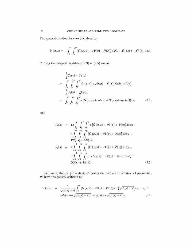
136 AHCENE MERAD AND ABDELFATAH BOUZIANI
The general solution for case 3 is given by
V (x, s) = −∫ x
0
∫ y
0
[G (x, s) + sΦ(x) + Ψ(x)] dzdy + C1 (s)x+ C2(s), (3.5)
Putting the integral conditions (3.3) in (3.5) we get
1
2C1(s) + C2(s)
=
∫ 1
0
∫ x
0
∫ y
0
[G (x, s) + sΦ(x) + Ψ(x)] dzdy +R(s),
1
3C1(s) +
1
2C2(s)
=
∫ 1
0
∫ x
0
∫ y
0
x [G (x, s) + sΦ(x) + Ψ(x)] dzdy +Q(s), (3.6)
and
C1(s) = 12
∫ 1
0
∫ x
0
∫ y
0
x [G (x, s) + sΦ(x) + Ψ(x)] dzdy −
6
∫ 1
0
∫ x
0
∫ y
0
[G (x, s) + sΦ(x) + Ψ(x)] dzdy +
12Q(s)− 6R(s),
C2(s) = 4
∫ 1
0
∫ x
0
∫ y
0
[G (x, s) + sΦ(x) + Ψ(x)] dzdy −
6
∫ 1
0
∫ x
0
∫ y
0
x [G (x, s) + sΦ(x) + Ψ(x)] dzdy −
6Q(s) + 4R(s). (3.7)
For case 2, that is,(s2 −A(s)
)< 0,using the method of variation of parameter,
we have the general solution as
V (x, s) =1√
A(s)− s2
∫ x
0
(G (x, s) + sΦ(x) + Ψ (x)) sin(√
A(s)− s2)
(x− τ) dτ
+d1(s) cos√
(A(s)− s2)x+ d2(s) sin√
(A(s)− s2)x (3.8)
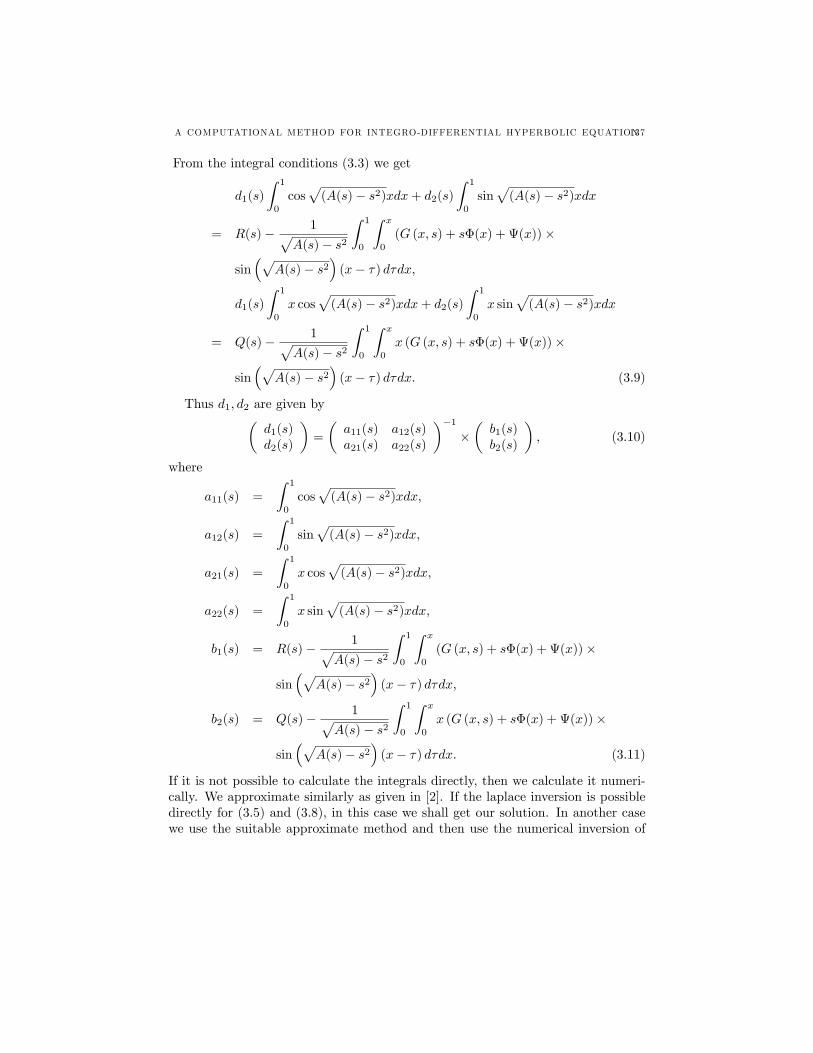
A COMPUTATIONAL METHOD FOR INTEGRO-DIFFERENTIAL HYPERBOLIC EQUATION137
From the integral conditions (3.3) we get
d1(s)
∫ 1
0
cos√
(A(s)− s2)xdx+ d2(s)
∫ 1
0
sin√
(A(s)− s2)xdx
= R(s)− 1√A(s)− s2
∫ 1
0
∫ x
0
(G (x, s) + sΦ(x) + Ψ(x))×
sin(√
A(s)− s2)
(x− τ) dτdx,
d1(s)
∫ 1
0
x cos√
(A(s)− s2)xdx+ d2(s)
∫ 1
0
x sin√
(A(s)− s2)xdx
= Q(s)− 1√A(s)− s2
∫ 1
0
∫ x
0
x (G (x, s) + sΦ(x) + Ψ(x))×
sin(√
A(s)− s2)
(x− τ) dτdx. (3.9)
Thus d1, d2 are given by(d1(s)d2(s)
)=
(a11(s) a12(s)a21(s) a22(s)
)−1×(b1(s)b2(s)
), (3.10)
where
a11(s) =
∫ 1
0
cos√
(A(s)− s2)xdx,
a12(s) =
∫ 1
0
sin√
(A(s)− s2)xdx,
a21(s) =
∫ 1
0
x cos√
(A(s)− s2)xdx,
a22(s) =
∫ 1
0
x sin√
(A(s)− s2)xdx,
b1(s) = R(s)− 1√A(s)− s2
∫ 1
0
∫ x
0
(G (x, s) + sΦ(x) + Ψ(x))×
sin(√
A(s)− s2)
(x− τ) dτdx,
b2(s) = Q(s)− 1√A(s)− s2
∫ 1
0
∫ x
0
x (G (x, s) + sΦ(x) + Ψ(x))×
sin(√
A(s)− s2)
(x− τ) dτdx. (3.11)
If it is not possible to calculate the integrals directly, then we calculate it numeri-cally. We approximate similarly as given in [2]. If the laplace inversion is possibledirectly for (3.5) and (3.8), in this case we shall get our solution. In another casewe use the suitable approximate method and then use the numerical inversion of
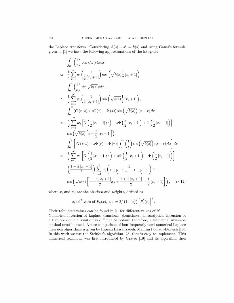
138 AHCENE MERAD AND ABDELFATAH BOUZIANI
the Laplace transform. Considering A(s) − s2 = k(s) and using Gauss’s formulagiven in [1] we have the following approximations of the integrals:∫ 1
0
(1
x
)cos√k(s)xdx
' 1
2
N∑i=1
wi
(1
12 [xi + 1]
)cos
(√k(s)
1
2[xi + 1]
),
∫ 1
0
(1
x
)sin√k(s)xdx
' 1
2
N∑i=1
wi
(1
12 [xi + 1]
)sin
(√k(s)
1
2[xi + 1]
),∫ x
0
(G (x, s) + sΦ(x) + Ψ (x)) sin(√
k(s))
(x− τ) dτ
' x
2
N∑i=1
wi
[G(x
2[xi + 1] ; s
)+ sΦ
(x2
[xi + 1])
+ Ψ(x
2[xi + 1]
)]sin(√
k(s)[x− x
2[xi + 1]
]),∫ 1
0
[[G (τ , s) + sΦ (τ) + Ψ (τ)]
∫ 1
τ
(1
x
)sin(√
k(s))
(x− τ) dx
]dτ
' 1
2
N∑i=1
wi
[G
(1
2[xi + 1] ; s
)+ sΦ
(1
2[xi + 1]
)+ Ψ
(1
2[xi + 1]
)](
1− 12 [xi + 1]
2
) N∑i=1
wj
(1
1− 12 [xi+1]
2 xj +1− 1
2 [xi+1]
2
)×
sin
(√k(s)
[1− 1
2 [xi + 1]
2xj +
1 + 12 [xi + 1]
2− 1
2(xi + 1)
]), (3.12)
where xi and wi are the abscissa and weights, defined as
xi : ith zero of Pn(x), ωi = 2/(1− x2i
) [P′
n(x)]2.
Their tabulated values can be found in [1] for different values of N .Numerical inversion of Laplace transform. Sometimes, an analytical inversion ofa Laplace domain solution is diffi cult to obtain; therefore, a numerical inversionmethod must be used. A nice comparison of four frequently used numerical Laplaceinversion algorithms is given by Hassan Hassanzadeh, Mehran Pooladi-Darvish [18].In this work we use the Stehfest’s algorithm [28] that is easy to implement. Thisnumerical technique was first introduced by Graver [16] and its algorithm then
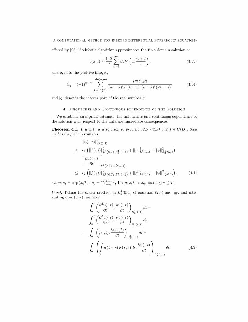
A COMPUTATIONAL METHOD FOR INTEGRO-DIFFERENTIAL HYPERBOLIC EQUATION139
offered by [28]. Stehfest’s algorithm approximates the time domain solution as
v(x, t) ≈ ln 2
t
2m∑n=1
βnV
(x;n ln 2
t
), (3.13)
where, m is the positive integer,
βn = (−1)n+m
min(n,m)∑k=[n+12 ]
km (2k)!
(m− k)!k! (k − 1)! (n− k)! (2k − n)!, (3.14)
and [q] denotes the integer part of the real number q.
4. Uniqueness and Continuous dependence of the Solution
We establish an a priori estimate, the uniqueness and continuous dependence ofthe solution with respect to the data are immediate consequences.
Theorem 4.1. If u(x, t) is a solution of problem (2.3)-(2.5) and f ∈ C(D), thenwe have a priori estimates:
‖u(·, τ)‖2L2(0,1)≤ c1
(‖f(·, t)‖2L2(0,T ; B1
2(0,1))+ ‖ϕ‖2L2(0,1) + ‖ψ‖2B1
2(0,1)
)∥∥∥∥∂u(·, τ)
∂t
∥∥∥∥2L2(0,T ; B1
2(0,1))
≤ c2
(‖f(·, t)‖2L2(0,T ; B1
2(0,1))+ ‖ϕ‖2L2(0,1) + ‖ψ‖2B1
2(0,1)
), (4.1)
where c1 = exp (a0T ) , c2 = exp(a0T )1−a0 , 1 < a(x, t) < a0, and 0 ≤ τ ≤ T .
Proof. Taking the scalar product in B12(0, 1) of equation (2.3) and ∂u∂t , and inte-
grating over (0, τ), we have∫ τ
0
(∂2u(·, t)∂t2
,∂u(·, t)∂t
)B12(0,1)
dt−∫ τ
0
(∂2u(·, t)∂x2
,∂u(·, t)∂t
)B12(0,1)
dt
=
∫ τ
0
(f(·, t), ∂u (., t)
∂t
)B12(0,1)
dt+
∫ τ
0
t∫0
a (t− s)u (x, s) ds,∂u(·, t)∂t
B12(0,1)
dt. (4.2)
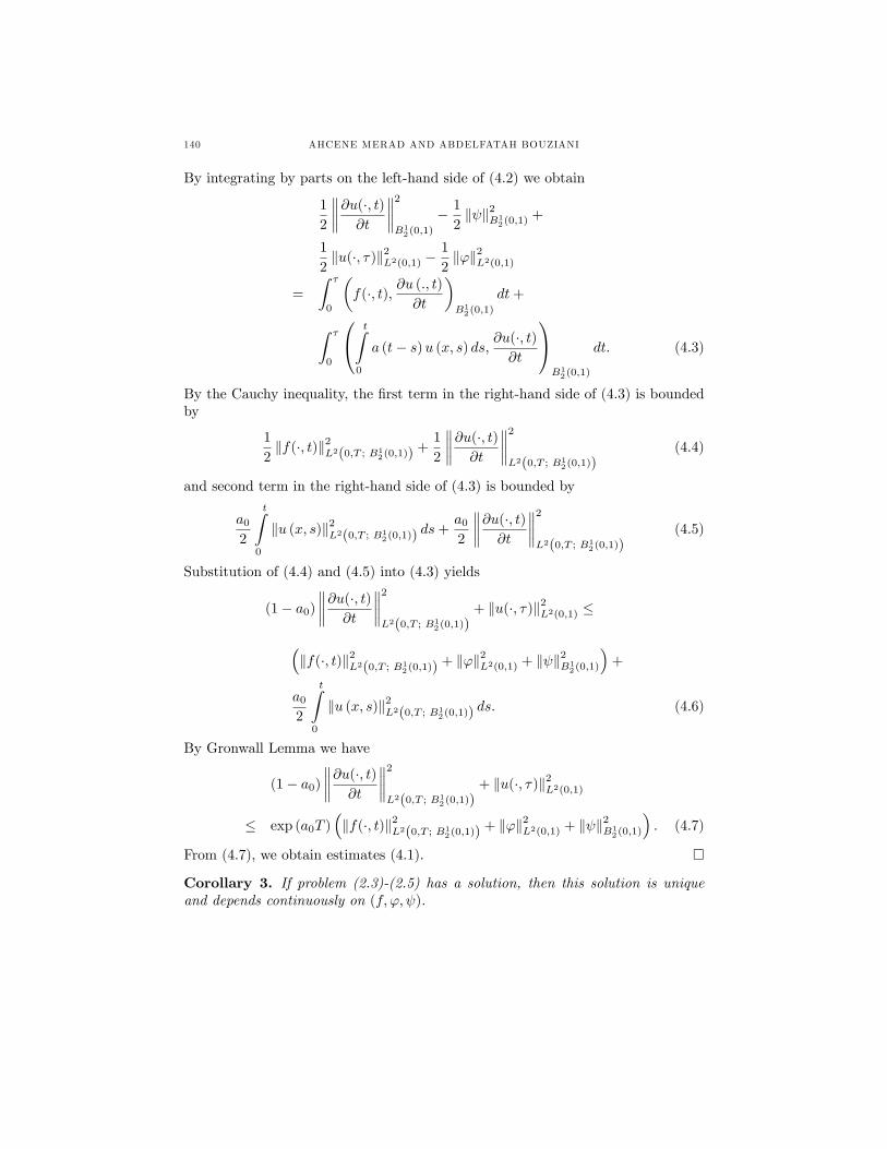
140 AHCENE MERAD AND ABDELFATAH BOUZIANI
By integrating by parts on the left-hand side of (4.2) we obtain
1
2
∥∥∥∥∂u(·, t)∂t
∥∥∥∥2B12(0,1)
− 1
2‖ψ‖2B1
2(0,1)+
1
2‖u(·, τ)‖2L2(0,1) −
1
2‖ϕ‖2L2(0,1)
=
∫ τ
0
(f(·, t), ∂u (., t)
∂t
)B12(0,1)
dt+
∫ τ
0
t∫0
a (t− s)u (x, s) ds,∂u(·, t)∂t
B12(0,1)
dt. (4.3)
By the Cauchy inequality, the first term in the right-hand side of (4.3) is boundedby
1
2‖f(·, t)‖2L2(0,T ; B1
2(0,1))+
1
2
∥∥∥∥∂u(·, t)∂t
∥∥∥∥2L2(0,T ; B1
2(0,1))(4.4)
and second term in the right-hand side of (4.3) is bounded by
a02
t∫0
‖u (x, s)‖2L2(0,T ; B12(0,1))
ds+a02
∥∥∥∥∂u(·, t)∂t
∥∥∥∥2L2(0,T ; B1
2(0,1))(4.5)
Substitution of (4.4) and (4.5) into (4.3) yields
(1− a0)∥∥∥∥∂u(·, t)
∂t
∥∥∥∥2L2(0,T ; B1
2(0,1))+ ‖u(·, τ)‖2L2(0,1) ≤
(‖f(·, t)‖2L2(0,T ; B1
2(0,1))+ ‖ϕ‖2L2(0,1) + ‖ψ‖2B1
2(0,1)
)+
a02
t∫0
‖u (x, s)‖2L2(0,T ; B12(0,1))
ds. (4.6)
By Gronwall Lemma we have
(1− a0)∥∥∥∥∂u(·, t)
∂t
∥∥∥∥2L2(0,T ; B1
2(0,1))+ ‖u(·, τ)‖2L2(0,1)
≤ exp (a0T )(‖f(·, t)‖2L2(0,T ; B1
2(0,1))+ ‖ϕ‖2L2(0,1) + ‖ψ‖2B1
2(0,1)
). (4.7)
From (4.7), we obtain estimates (4.1).
Corollary 3. If problem (2.3)-(2.5) has a solution, then this solution is uniqueand depends continuously on (f, ϕ, ψ).
A COMPUTATIONAL METHOD FOR INTEGRO-DIFFERENTIAL HYPERBOLIC EQUATION141
References
[1] M. Abramowitz, I. A. Stegun, Hand book of Mathematical Functions, Dover, New York, 1972.[2] W.T. Ang, A Method of Solution for the One-Dimentional Heat Equation Subject to Nonlocal
Conditions, Southeast Asian Bull. Math. 26 (2002), 185—191.[3] S.A. Beïlin, Existence of solutions for one-dimentional wave nonlocal conditions, Electron.
J. Differ. Equ. 2001 (2001), no. 76, 1—8.[4] A. Bouziani, Problèmes mixtes avec conditions intégrales pour quelques équations aux dérivées
partielles, Ph.D. thesis, Constantine University, (1996).[5] A. Bouziani, Mixed problem with boundary integral conditions for a certain parabolic equa-
tion, J. Appl. Math. Stochastic Anal. 9(1996), no. 3, 323—330.[6] A. Bouziani, Solution forte d’un problème mixte avec une condition non locale pour une classe
d’équations hyperboliques [Strong solution of a mixed problem with a nonlocal condition fora class of hyperbolic equations], Bull. Cl. Sci., VI. Sér., Acad. R. Belg. 8(1997), 53—70.
[7] A. Bouziani, Strong solution to an hyperbolic evolution problem with nonlocal boundary con-ditions, Maghreb Math. Rev. 9 (2000), no. 1-2, 71—84.
[8] A. Bouziani, On the quasi static flexur of thermoelastic rod, Commun. Appl. Anal. TheoryAppl. 6(2002), no.4, 549—568.
[9] A. Bouziani, Initial-boundary value problem with nonlocal condition for a viscosity equation,Int. J. Math. & Math. Sci. 30 (2002), no. 6, 327—338.
[10] A. Bouziani, On the solvabiliy of parabolic and hyperbolic problems with a boundary integralcondition, Internat. J. Math. Math. Sci. 31 (2002), 435—447.
[11] A. Bouziani, On a class of nonclassical hyperbolic equations with nonlocal conditions, J.Appl. Math. Stochastic Anal. 15 (2002), no. 2, 136—153.
[12] A. Bouziani, Mixed problem with only integral boundary conditions for an hyperbolic equation,Internat. J. Math. & Math. Sci. 26 (2004), 1279—1291.
[13] A. Bouziani, N. Benouar, Problème mixte avec conditions intégrales pour une classed’équations hyperboliques, Bull. Belg. Math. Soc. 3 (1996), 137—145.
[14] A. Bouziani, N. Benouar, Sur un problème mixte avec uniquement des conditions aux limitesintégrales pour une classe d’équations paraboliques, Maghreb Math. Rev. 9 (2000), no. 1-2,55—70.
[15] A. Bouziani, R. Mechri, The Rothe Method to a Parabolic Integro-diff erential Equation witha Nonclassical Boundary Conditions, Int. J. Stochastic Anal. Article ID 519684/ 16 page,doi: 10.1155/519684/ (2010).
[16] D.P. Graver, Observing stochastic processes and aproximate transform inversion, Oper. Res.14 (1966), 444—459.
[17] D.G. Gordeziani, G.A. Avalishvili, Solution of nonlocal problems for one-dimensional oscil-lations of a medium, Mat. Model. 12 (2000), no. 1, 94—103.
[18] H. Hassanzadeh, M. Pooladi-Darvish, Comparision of diff erent numerical Laplace inversionmethods for engineering applications, Appl. Math. Comp. 189 (2007), 1966—1981.
[19] J. Kacur, Method of Rothe in Evolution Equations, Teubner-Texte zur Mathematik 80, BSBB. G. Teubner Verlagsgesellschaft, Leipzig, 1985.
[20] S. Mesloub, A. Bouziani, On a class of singular hyperbolic equation with a weighted integralcondition, Int. J. Math. & Math. Sci. 22 (1999), no. 3, 511—519.
[21] S. Mesloub, A. Bouziani, Mixed problem with integral conditions for a certain class of hyper-bolic equations, J. Appl. Math. 1 (2001), no. 3, 107—116.
[22] N. Merazga, A. Bouziani, Rothe time-discretization method for a nonlocal problem arising inthermoelasticity, J. Appl. Math. Stochastic Anal. 2005 (2005), no. 1, 13—28.
[23] A. Merad, Adomian decomposition method for solution of parabolic equation to nonlocalconditions, Int. J. Contemp. Math. Sci. 6 (2011), no. 29-32, 1491—1496.
142 AHCENE MERAD AND ABDELFATAH BOUZIANI
[24] A. Merad, A.L. Marhoune, Strong solution for a high order boundary value problem withintegral condition, Turk. J. Math. 37 (2013), no.3, 1—9.
[25] L.S. Pul’kina, A non-local problem with integral conditions for hyperbolic equations, Electron.J. Differ. Equ. 1999 (1999), no. 45, 1—6.
[26] L.S. Pul’kina, On the solvability in L2 of a nonlocal problem with integral conditions for ahyperbolic equation, Differ. Equ. 36 (2000), no. 2, 316—318.
[27] L.S. Pul’kina, A mixed problem with integral condition for the hyperbolic equation, Mat.Zametki 74 (2003), no. 3, 435—445.
[28] H. Stehfest, Numerical inversion of the Laplace transform, Comm. ACM 13 (1970), 47—49.[29] A.D. Shruti, Numerical solution for nonlocal Sobolev-type diff erential equations, Electron. J.
Differ. Equ. Conf. 19 (2010), 75—83.Current address : A. Merad and A. Bouziani; Department of Mathematics, Larbi Ben M’hidi
University, 04000, ALGERIAE-mail address : [email protected], [email protected]: http://communications.science.ankara.edu.tr/index.php?series=A1
INSTRUCTIONS TO CONTRIBUTORS
Mathematics and Statistics of COMMUNICATIONS accepts original research
articles written in English in the fields of Mathematics and Statistics. Review
articles written by eminent scientists can also be invited by the Editor.
Three copies of the manuscripts must be submitted in AMS Article Tex format.
Formulas should be numbered consecutively in parentheses ( ) and each rnanuscript
should be accompanied by classification numbers from the American Mathematical
Society's classification scheme.
lt is a fundamental condition that articles submitted to Communications have not
been previously published and will not be simultaneously submitted or published
elsewhere. After the manuscript has been accepted for publication, i.e., after referree-
recommended revisions are complete, the author will not be permitted to rnake any
new additions to the manuscript.
Before publication the gal1ey proof is always sent to the author for correction. Thus
it is solely the author's responsibility for any typographical mistakes which occur in
their article as it appears in the Journal.
1. Title Page: The title should not be long but should be informative. Each title page must contain
(i) The title of the paper in English, (ii) The complete name(s) of the author(s),
(iii) The name and the address of the University.
2. Abstract : The abstract should not exceed 200 words and it should condense the essential
features of the articles with the focus on the major advances in the field.
3. References : References must be listed in alphabetical order at the end of the article and then
numbered in brackets [1]. Within the manuscript, refer to the references by their
given number, again in brackets [1]. They should be styled and punctuated according
to the following examples:
[1] Kel1ey, J.L., General Topology, 1970, New York: Van Nostrand.
[2] Maddox,l.J., Some incusion theorems, Proc. Glasgow Math. Assn. 6 (1964),
161-168.
Abstracts, unpublished data and personal communications should not be given in the
references but they may be mentioned in the text.
4. Footnotes: Footnotes, except a possible acknowledgement of assistance or financial support on
the first page, should be avoided by being incorparated into the text.
5. Tables and Figures: All tables and figures must be numbered consecutively throughout the paper ( Table
1, Figure 2) and also have a caption or legend.
6. Acknowledgements: Acknowledgements should be given as short as possible at the end of the text.
7. Reprints: 25 free reprints will be provided for each paper. Irrespective of their acceptance,
manuscripts will not be returned to the authors.
8. Computer Disk: After the acceptance of manuscripts for publication, we will ask you to submit a
revised electronic copy of the manuscript which is written in AMS tex format. For
electronic submission please visit our WEB page at
http://editor.ankara.edu.tr/index.php/CommunicationsA1 9.Charges: Each paper is due to be charged for the amount of which is determined by the
administiration each year.
10. Address: Text should be sent to the following address:
Asst. Prof. Dr. Cafer COŞKUN - Editor-in-Chief, Communications
Ankara University, Faculty of Sciences
06100, Tandoğan, ANKARA - TURKEY

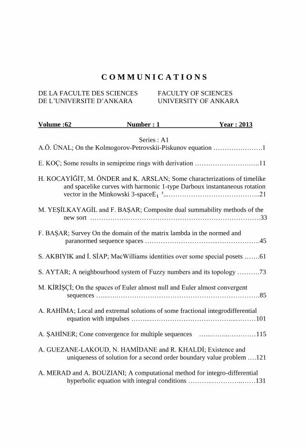
C O M M U N I C A T I O N S
DE LA FACULTE DES SCIENCES FACULTY OF SCIENCES
DE L’UNIVERSITE D’ANKARA UNIVERSITY OF ANKARA
Volume :62 Number : 1 Year : 2013
Series : A1
A.Ö. ÜNAL; On the Kolmogorov-Petrovskii-Piskunov equation ………………….1
E. KOÇ; Some results in semiprime rings with derivation …………………….….11
H. KOCAYİĞİT, M. ÖNDER and K. ARSLAN; Some characterizations of timelike
and spacelike curves with harmonic 1-type Darboux instantaneous rotation
vector in the Minkowski 3-spaceE₁ ³...…………………………………..21
M. YEŞİLKAYAGİL and F. BAŞAR; Composite dual summability methods of the
new sort ………………………………………………………………….33
F. BAŞAR; Survey On the domain of the matrix lambda in the normed and
paranormed sequence spaces …………………………...……………….45
S. AKBIYIK and İ. SİAP; MacWilliams identities over some special posets …….61
S. AYTAR; A neighbourhood system of Fuzzy numbers and its topology ……….73
M. KİRİŞÇİ; On the spaces of Euler almost null and Euler almost convergent
sequences …...….……………………………………………………….85
A. RAHİMA; Local and extremal solutions of some fractional integrodifferential
equation with impulses ……...………………………………...………101
A. ŞAHİNER; Cone convergence for multiple sequences …...……...…………115
A. GUEZANE-LAKOUD, N. HAMİDANE and R. KHALDİ; Existence and
uniqueness of solution for a second order boundary value problem ….121
A. MERAD and A. BOUZIANI; A computational method for integro-differential
hyperbolic equation with integral conditions ………..…………..……131