C. J. Noell, M. F. O’Neill, J. D. Carroll, C. D. Dixon · 2015-11-05 · A bio‐economic model for South Australia’s prawn trawl fisheries C. J. Noell, M. F. O’Neill, J. D

Abio‐economicmodelforSouthAustralia’sprawntrawlfisheries

C.J.Noell,M.F.O’Neill,J.D.Carroll,C.D.Dixon

ProjectNo.2011/750FinalReport

June2015

Thisprojectwasconductedby:

SouthAustralianResearchandDevelopmentInstitute(AquaticSciences)POBox120,HenleyBeachSA5022

Agri‐ScienceQueensland,DepartmentofAgriculture,FisheriesandForestry

POBox5083SCMC,NambourQld4560

Thisreportmaybecitedas:Noell, C.J.,O’Neill,M.F., Carroll, J.D. andDixon,C.D. (2015).Abio‐economicmodel for SouthAustralia’sprawn trawl fisheries. Final Report. Prepared by the South Australian Research and DevelopmentInstitute(AquaticSciences),Adelaide.CRCProjectNo.2011/750.115pp.

ISBN:978‐1‐921563‐77‐5

Copyright,2015:TheSeafoodCRCCompanyLtd, theFisheriesResearchandDevelopmentCorporation,the South Australian Research and Development Institute (Aquatic Sciences), and the Department ofAgriculture,FisheriesandForestry(Qld).This work is copyright. Except as permitted under the Copyright Act 1968 (Cth), no part of thispublication may be reproduced by any process, electronic or otherwise, without the specific writtenpermission of the copyright owners. Neither may information be stored electronically in any formwhatsoeverwithoutsuchpermission.TheAustralianSeafoodCRCisestablishedandsupportedundertheAustralianGovernment’sCooperativeResearchCentresProgramme.Other investors in theCRCare theFisheriesResearchandDevelopmentCorporation,SeafoodCRCcompanymembers,andsupportingparticipants.

ImportantNoticeAlthoughtheAustralianSeafoodCRChastakenallreasonablecareinpreparingthisreport,neithertheSeafoodCRCnoritsofficersacceptanyliabilityfromtheinterpretationoruseoftheinformationsetoutinthisdocument.Informationcontainedinthisdocumentissubjecttochangewithoutnotice.

iii

Table of contents

Non‐technicalsummary..............................................................................................................................................1

1 Introduction...........................................................................................................................................................4

2 Need..........................................................................................................................................................................5

3 Objectives................................................................................................................................................................6

4 Methods...................................................................................................................................................................64.1 Inputdata..............................................................................................................................................................................64.1.1 Overview..........................................................................................................................................................................64.1.2 Commercialharvestdata........................................................................................................................................104.1.3 Standardisedcommercialcatchrates...............................................................................................................114.1.4 Standardisedsurveycatchrates..........................................................................................................................124.1.5 Sizecompositiondata...............................................................................................................................................124.1.6 Size‐transitionmatrices..........................................................................................................................................124.1.7 Economicdata.............................................................................................................................................................12

4.2 Bio‐economicmodel.......................................................................................................................................................154.2.1 Modellingflow.............................................................................................................................................................154.2.2 Populationdynamicmodel....................................................................................................................................174.2.3 Economic(modeland)parameters....................................................................................................................23

4.3 Simulationandmanagementprocedures.............................................................................................................234.4 Summaryofbio‐economicmodel.............................................................................................................................27

5 Results....................................................................................................................................................................275.1 Modelcalibrationanddescription...........................................................................................................................275.1.1 GulfStVincentPrawnFishery..............................................................................................................................275.1.2 SpencerGulfPrawnFishery..................................................................................................................................34

5.2 Referencepoints..............................................................................................................................................................425.2.1 GulfStVincentPrawnFishery..............................................................................................................................425.2.2 SpencerGulfPrawnFishery..................................................................................................................................43

5.3 Simulationofmanagementprocedures.................................................................................................................455.3.1 GulfStVincentPrawnFishery..............................................................................................................................455.3.2 SpencerGulfPrawnFishery..................................................................................................................................50

6 Discussion.............................................................................................................................................................556.1 Modelsanddata...............................................................................................................................................................556.2 Referencepoints..............................................................................................................................................................556.2.1 GulfStVincentPrawnFishery..............................................................................................................................566.2.2 SpencerGulfPrawnFishery..................................................................................................................................56

6.3 Managementprocedures..............................................................................................................................................576.3.1 GulfStVincentPrawnFishery..............................................................................................................................576.3.2 SpencerGulfPrawnFishery..................................................................................................................................576.3.3 Overviewofsimulations.........................................................................................................................................58

6.4 Datalimitationsandfutureresearch......................................................................................................................59

7 Benefitsandadoption.......................................................................................................................................60

8 Furtherdevelopment........................................................................................................................................60

9 Plannedoutcomes..............................................................................................................................................61

10 Conclusion............................................................................................................................................................61

11 References............................................................................................................................................................63

AppendixA Intellectualproperty.....................................................................................................................67

AppendixB Staff......................................................................................................................................................67

AppendixC Sizetransitionmatrixformulation...........................................................................................68

iv

C.1 Introduction.......................................................................................................................................................................68C.2 Model.....................................................................................................................................................................................68C.3 Dataandprocessing.......................................................................................................................................................68C.4 Fittingagetolength........................................................................................................................................................69C.5 Derivationofthegrowthfunction............................................................................................................................70C.6 Derivationofsizetransitionprobabilities(non‐seasonal)...........................................................................70C.7 Derivationofsizetransitionprobabilities(seasonal).....................................................................................72C.8 Size‐transitionmatrix....................................................................................................................................................73

AppendixD RunningMatlab*.mfiles..............................................................................................................75D.1 Loaddatastructures......................................................................................................................................................75D.2 Setupparametersandnegativelog‐likelihoods.................................................................................................75D.3 Runstockmodel(‘sa_wkp_3_popdyn_model’)...................................................................................................75D.4 Fitstockmodeltodata(‘sa_wkp_optimise’)........................................................................................................75D.5 Referencepoints(‘sa_wkp_6_eq_refpts’)..............................................................................................................75D.6 Managementprocedures(‘sa_wkp_8_mse’)........................................................................................................75D.7 Analysemanagementprocedures(‘sa_wkp_10_mse_analysis’).................................................................76

AppendixE Inputdatasummaries...................................................................................................................77E.1 Standardisedcommercialcatchrates.....................................................................................................................77E.2 Standardisedsurveycatchrates...............................................................................................................................81E.3 Sizecompositiondata....................................................................................................................................................85E.4 Size‐transitionmatrices................................................................................................................................................88E.5 Economicdata...................................................................................................................................................................91

AppendixF Supplementaryplots–GulfStVincentPrawnFishery.......................................................92F.1 Modelinputdata..............................................................................................................................................................92F.2 Modeloutputresults......................................................................................................................................................97F.3 Fisherycatchratediagnostics....................................................................................................................................98F.4 Surveycatchratediagnostics..................................................................................................................................100F.5 Size‐gradefrequencydiagnostics..........................................................................................................................102

AppendixG Supplementaryplots–SpencerGulfPrawnFishery........................................................104G.1 Modelinputdata...........................................................................................................................................................104G.2 Modeloutputresults...................................................................................................................................................110G.3 Fisherycatchratediagnostics.................................................................................................................................111G.4 Surveycatchratediagnostics..................................................................................................................................113

AppendixH Supplementaryplots–bothfisheries....................................................................................115H.1 Modelinputdata...........................................................................................................................................................115

v

List of figures

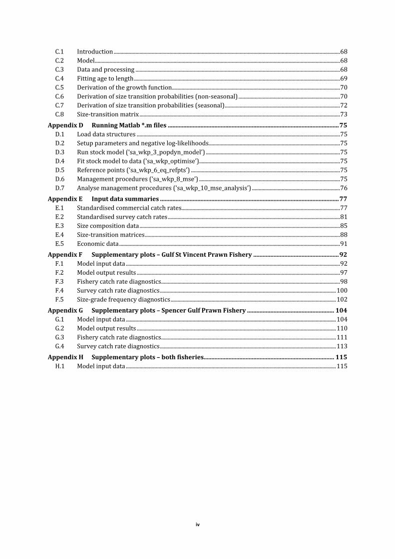
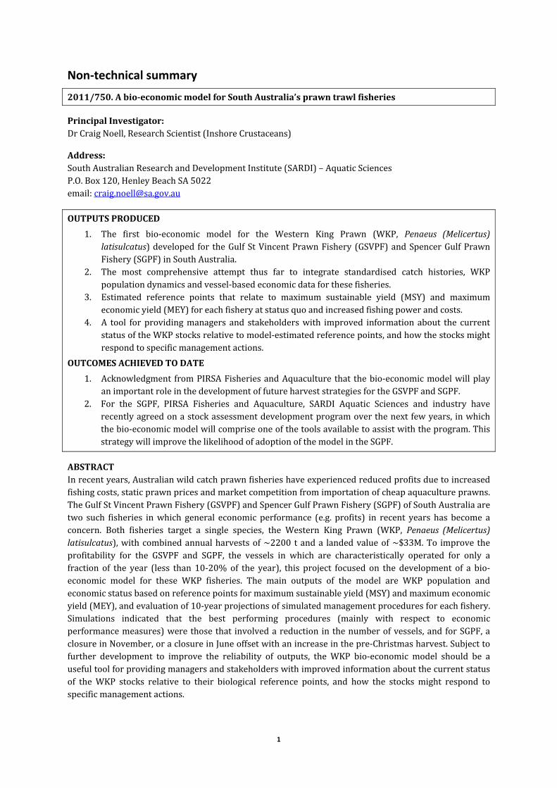
Figure4.1.MapofSouthAustralia’sGSVPF(shadedred)andSGPF(shadedblue)showingthefishingblocks(smallpolygons),regions(largeshadedpolygons),surveyshot locations(dots)and10‐mdepthcontourthatseparatesthefishablearea(≥10m)andprohibitedareatotrawling(<10m).Regionabbreviations:COW,Cowell;CPT,CornyPoint;GUT, the ‘Gutter’;HOL, the ‘Hole’; INV, InvestigatorStrait;MBK,Middlebank;NTH,North;RG1,Region1;RG2,Region2;RG3,Region3;RG4,Region4;RG5,Region5;RG6,Region6;SGU,SouthGutter;THI,Thistle;WAL,Wallaroo;WAR,Wardang;WGU,WestGutter............................................................................................................................................7

Figure4.2.AnnualharvestandeffortofWKPbytheGSVPFfrom1968—2013.............................................................................10Figure4.3.AnnualharvestandeffortofWKPbytheSGPFfrom1968—2013................................................................................10Figure4.4.2013/14monthlyWKPlandingprices($kg‐1)bycarapacelengthbasedonestimatedproportionsofrawandcookedprawnsindemand.......................................................................................................................................................................13

Figure4.5.Flowofoperationsandsource files for theWKPbio‐economicmodel.Abbreviations:NLL,negative log‐likelihood;ML,maximumlikelihood;MCMC,MarkovChainMonteCarlo;MP,managementprocedure......................16

Figure5.1.Observed(standardised)andpredictedfisherycatchratesfortheGSVPFfrom1991—2013.........................27Figure5.2.Observed(standardised)andpredictedsurveycatchratesfortheSGPFfrom2005—2013............................28Figure 5.3. Comparison of standardised fishery and survey catch rate (CPUE) trends in the GSVPF by: a) datasequence;b) regression;andc) fishingmonth.Note: catchrateswerenormalised toensure trendswereon thesamescale................................................................................................................................................................................................................28

Figure 5.4. Observed (bars) and predicted (red line) survey length‐frequency distributions (proportions) formaleWKP in the GSVPF from 2005—2012. Labels refer to fishing year and month; neff indicates the effectivemultinomialsamplesizeforeachsurvey...................................................................................................................................................29

Figure5.5.Observed(bars)andpredicted(redline)surveylength‐frequencydistributions(proportions)forfemaleWKP in the GSVPF from 2005—2012. Labels refer to fishing year and month; neff indicates the effectivemultinomialsamplesizeforeachsurvey...................................................................................................................................................30

Figure5.6.a)MonthlyWKPexploitablebiomassratio(By/B0)andb)harvestfractionintheGSVPFfrom1969—2012.Thedottedreferencelinesinplotsa)andb)indicatetheestimatedlevelofthevirginstock(i.e.t=0at1969)andtheassumednaturalmortality,respectively............................................................................................................................................31

Figure5.7.Predicted relationships forWKP in theGSVPF:a) stock‐recruitment relationship (basedon19yearsofmodelled stochastic recruitment, 1994—2012); b) recruitment pattern (proportion); c) fishery and surveycatchability; and d) vulnerability at carapace length (from surveys).Note: fishery and survey catchabilitywereheldconstantthroughoutthefishingyear................................................................................................................................................32

Figure5.8.Observed(standardised)andpredictedfisherycatchratesfortheSGPFfrom1991—2013............................34Figure5.9.Observed(standardised)andpredictedsurveycatchratesfortheSGPFfrom2005—2013............................34Figure 5.10. Comparison of standardised fishery and survey catch rate (CPUE) trends in the SGPF by: a) datasequence;b) regression;andc) fishingmonth.Note: catchrateswerenormalised toensure trendswereon thesamescale................................................................................................................................................................................................................35

Figure5.11.Observed(bars)andpredicted(redline)surveylength‐frequencydistributions(proportions)formaleWKPintheSGPFfrom2005—2013.Labelsrefertofishingyearandmonth;neffindicatestheeffectivemultinomialsamplesizeforeachsurvey.............................................................................................................................................................................36

Figure5.12.Observed(bars)andpredicted(redline)surveylength‐frequencydistributions(proportions)forfemaleWKPintheSGPFfrom2005—2013.Labelsrefertofishingyearandmonth;neffindicatestheeffectivemultinomialsamplesizeforeachsurvey.............................................................................................................................................................................37

Figure5.13.Observed(bars)andpredicted(red line)size‐grade frequencydistributions(proportions) in theSGPFfrom2003—2013.Size‐gradecategories:1=>20lb‐1;2=16‐20lb‐1;3=10‐15lb‐1;4=<10lb‐1.Labelsrefertofishingyearandmonth,andneffindicatestheeffectivemultinomialsamplesizeforeachmonth...................................38

Figure5.14.a)MonthlyWKPexploitablebiomassratio(By/B0)andb)harvestfractionintheSGPFfrom1969—2013.Thedottedreferencelinesinplotsa)andb)indicatetheestimatedlevelofthevirginstock(i.e.t=0at1969)andtheassumednaturalmortality,respectively............................................................................................................................................39

Figure5.15.Predicted relationships forWKP in theSGPF:a) stock‐recruitment relationship (basedon22yearsofmodelled stochastic recruitment, 1991—2013); b) recruitment pattern (proportion); c) fishery and surveycatchability;andd)vulnerabilityatcarapacelength............................................................................................................................40

vi

Figure5.16.Meanmonthlya) fisheryandb)surveycatchratetargets for theGSVPFatMSYandMEYv.Catchrateswerestandardisedto2011/12fishingpower.........................................................................................................................................43

Figure5.17.Meanmonthlya)fisheryandb)surveycatchratetargetsfortheSGPFatMSYandMEYv.Catchrateswerestandardisedto2012/13fishingpower.....................................................................................................................................................45

Figure 5.18. Performance measures over ten future years (2014—2023) for ten different WKP managementprocedures(MPs)fortheGSVPF(Table4.13).Plotsa)andb)representedindustryfunctioning,plotsd),e),j)andk)representedthemainperformanceindicatorsusedinthecurrentmanagementplan(DixonandSloan,2007),plotsg)andh)measuredpopulationchange,andplotsc), f), i)and l) (lastcolumnofplots) indicatedeconomicconditions.Thedottedreferencelineindicatesthemedian(=1orestimatedvalue)forMP1(statusquo).Theplotsdisplaythesimulateddistributions(1000samples)aroundtheirmedians(solid line inmiddleofeachbox).Thebottomandtopedgesofeachboxarethe25thand75thpercentiles,andthewhiskersindicate~95%coverageofthesimulationestimates...................................................................................................................................................................................48

Figure 5.19. Annual time series of selected performance measures for the GSVPF from 1969—2023 (includingsimulations of three management procedures from 2014—2023, where the median is plotted). Performancemeasures: a) harvest; b) effort; c) eggproduction relative to virgin estimate; d) exploitable biomass relative tovirgin;ande)relativeprofitfv.Managementprocedures:MP1,statusquo;MP3,5vessels (‘best’);MP9,7vesselsand180tquota(‘worst’).Note:effortdatawasnotavailablepriorto1991andprofitfvwasonlyestimatedfortenfutureyears.............................................................................................................................................................................................................49

Figure 5.20. Performance measures over ten future years (2014—2023) for 14 different WKP managementprocedures(MPs)fortheSGPF(Table4.14).Plotsa)andb)representedindustryfunctioning,plotsd),e),j)andk)representedthemainperformanceindicatorsusedinthecurrentmanagementplan(PIRSA,2014),plotsg)andh)measuredpopulationchange,andplotsc), f), i)andl)(lastcolumnofplots) indicatedeconomicconditions.Thedotted reference line indicates themedian (=1orestimatedvalue) forMP1 (statusquo).Theplotsdisplay thesimulateddistributions(1000samples)aroundtheirmedians(solidlineinmiddleofeachbox).Thebottomandtopedgesofeachboxarethe25thand75thpercentiles,andthewhiskersindicate~95%coverageofthesimulationestimates..................................................................................................................................................................................................................53

Figure 5.21. Annual time series of selected performance measures for the SGPF from 1969—2023 (includingsimulations of three management procedures from 2014—2023, where the median is plotted). Performancemeasures: a) harvest; b) effort; c) eggproduction relative to virgin estimate; d) exploitable biomass relative tovirgin; and e) relative profitfv.Management procedures:MP1, status quo;MP4, 20 vessels;MP7, pre‐Christmascatchcapreducedby40%.Note:effortdatawasnotavailablepriorto1991andprofitfvwasonlyestimatedfortenfutureyears.............................................................................................................................................................................................................54

Figure E.1. Comparison of model‐predicted and unstandardised (nominal reported data) mean commercial catchrates by year‐month in the GSVPF. The cube root transformation was chosen for the final model, where thestandardisedcatchbyavesselinablockpernightwaspredictedbyregion,hoursfished,vessel,lunarphaseandcloudcover..............................................................................................................................................................................................................77

FigureE.2.DiagnosticplotsofthePoissonGLMfittedtoGSVPFcommercialcatches.................................................................77FigureE.3.DiagnosticplotsoftheGaussianGLMfittedtountransformedGSVPFcommercialcatches...............................78FigureE.4.DiagnosticplotsoftheGaussianGLMfittedtocube‐roottransformedGSVPFcommercialcatches...............78Figure E.5. Comparison of model‐predicted and unstandardised (nominal reported data) mean commercial catchrates by year‐month in the SGPF. The cube root transformation was chosen for the final model, where thestandardisedcatchbyavesselinablockpernightwaspredictedbyregion,hoursfished,vesselandlunarphase.......................................................................................................................................................................................................................................79

FigureE.6.DiagnosticplotsofthePoissonGLMfittedtoSGPFcommercialcatches....................................................................79FigureE.7.DiagnosticplotsoftheGaussianGLMfittedtountransformedSGPFcommercialcatches.................................79FigureE.8.DiagnosticplotsoftheGaussianGLMfittedtocube‐roottransformedSGPFcommercialcatches..................80FigureE.9.Comparisonofmodel‐predictedandunstandardised(nominalreporteddata)meansurveycatchratesbyyear‐monthintheGSVPF.Thecuberoottransformationwaschosenforthefinalmodel,wherethestandardisedcatchinatrawlshotof~30mindurationwaspredictedbyregionandvessel........................................................................81

FigureE.10.DiagnosticplotsofthePoissonGLMfittedtoGSVPFsurveycatches.........................................................................81FigureE.11.DiagnosticplotsoftheGaussianGLMfittedtountransformedGSVPFsurveycatches......................................82FigureE.12.DiagnosticplotsoftheGaussianGLMfittedtocube‐roottransformedGSVPFsurveycatches......................82

vii

FigureE.13.Comparisonofmodel‐predictedandunstandardised(nominalreporteddata)meansurveycatchratesbyyear‐month in the SGPF.The cube root transformationwas chosen for the finalmodel,where the standardisedcatchinatrawlshotof~30mindurationwaspredictedbyregion,vesselandtidedirection..........................................83

FigureE.14.DiagnosticplotsofthePoissonGLMfittedtoGSVPFsurveycatches.........................................................................83FigureE.15.DiagnosticplotsoftheGaussianGLMfittedtountransformedSGPFsurveycatches.........................................83FigureE.16.DiagnosticplotsoftheGaussianGLMfittedtocube‐roottransformedSGPFsurveycatches.........................84FigureE.17.Lengthfrequenciesofmale(blue)andfemale(red)WKPcollectedfromeachsurveyintheGSVPFfrom2005—2012.Eachplotislabelledwithfishingyearandmonth.....................................................................................................85

FigureE.18.Length frequenciesofmale(blue)andfemale(red)WKPcollected fromeachsurvey intheSGPFfrom2005—2013.Eachplotislabelledwithfishingyearandmonth.....................................................................................................87

FigureE.19.Size‐gradecompositionofmonthlyharvestsbytheGSVPFfrom2007—2012.....................................................88FigureE.20.Sze‐gradecompositionofmonthlyharvestsbytheSGPFfrom2003—2013.........................................................88FigureE.21.SeasonalvonBertalanffygrowthtrajectoriesformaleandfemaleWKPfromtheGSVPFwithabirthdateof1November.......................................................................................................................................................................................................89

FigureE.22.SeasonalvonBertalanffygrowthtrajectoriesformaleandfemaleWKPfromtheSGPFwithabirthdateof1November............................................................................................................................................................................................................89

FigureE.23.SeasonalgrowthrateofmaleandfemaleWKPfromtheGSVPF..................................................................................90FigureE.24.SeasonalgrowthrateofmaleandfemaleWKPfromtheSGPF.....................................................................................90FigureF.1.MonthlyharvestofWKPbytheGSVPFfrom1968—2012................................................................................................92FigureF.2.Standardisedmeana)fisherycatches(1991—2012)andb)surveycatches(2005—2012)intheGSVPF.92FigureF.3.Surveylength‐frequencydistributions(proportions)formale(blue)andfemale(red)WKPintheGSVPFfrom2005—2012.Labelsrefertofishingyearandmonth................................................................................................................93

FigureF.4.Size‐gradefrequencies(proportions)intheGSVPFfrom2007—2012.......................................................................93FigureF.5.Colour‐scalevisualisationofthesize‐transitionmatrixformaleWKPintheGSVPF.Thescalefrombluetoredindicatesincreasingprobabilityofprawnsofcarapacelength‐classlʹinthepreviousmonthgrowingintoanewlengthloveronemonth.....................................................................................................................................................................................94

FigureF.6.Colour‐scalevisualisationofthesize‐transitionmatrixforfemaleWKPintheGSVPF.Thescalefrombluetoredindicatesincreasingprobabilityofprawnsofcarapacelength‐classlʹinthepreviousmonthgrowingintoanewlengthloveronemonth...........................................................................................................................................................................95

FigureF.7.Examplegrowthofacohortofa)maleandb)femaleWKPintheGSVPF.Eachcohortinitiallycomprised10000 prawns of carapace length 1mm in October. Cohort growthwas based on size‐transitionmatrices andnaturalmortality,andtracedfor36months,witheachsuccessivedistributionrepresentingamonth........................96

FigureF.8.WKPstockstatusannualplotsfortheGSVPFfrom1991—2013:a)spawningeggproductionratio(Ey/E0);b) exploitable biomass ratio (By/B0); and c) recruitment ratio (Ry/R0). The dotted reference line indicates theestimatedleveloftheequilibriumvirginstock(i.e.t=0at1969).Deterministicrecruitmentwasmodelledfrom1969—1993andstochastic(variable)recruitmentthereafter........................................................................................................97

FigureF.9.Comparisonofobserved(survey)andpredicted(model)WKPexploitablebiomassbyyear‐monthintheGSVPF........................................................................................................................................................................................................................97

Figure F.10. Fishery catch rate fitted diagnostics for the GSVPF: a) observed (standardised) andmodel‐predictedcatchrateseachmonthfrom1991—2013;b)standardisedfittedvalues;andc)monthlystandardisedresiduals.98

Figure F.11. Normality checks for fishery catch rates in the GSVPF: a) histogram of standardised residuals; b)probabilityplotofstandardisedresiduals;andc)cumulativedensityfunctionofstandardisedresiduals..................99

FigureF.12.SurveycatchratefitteddiagnosticsfortheGSVPF:a)observed(standardised)andmodel‐predictedcatchrateseachmonthfrom2005—2013;b)standardisedfittedvalues;andc)monthlystandardisedresiduals...........100

Figure F.13. Normality checks for survey catch rates in the GSVPF: a) histogram of standardised residuals; b)probabilityplotofstandardisedresiduals;andc)cumulativedensityfunctionofstandardisedresiduals................101

FigureF.14.Observed(bars)andpredicted(redline)size‐gradefrequencydistributions(proportions)intheGSVPFfrom2007—2012.Size‐gradecategories:1=>20lb‐1;2=16‐20lb‐1;3=10‐15lb‐1;4=<10lb‐1.Labelsrefertofishingyearandmonth;neffindicatestheeffectivemultinomialsamplesizeforeachmonth..........................................102

viii

FigureF.15.Observed(bars)andpredicted(redline)size‐gradefrequencydistributions(proportions)intheGSVPFfrom2007—2012afteromittingsize‐gradecategory1(>20lb‐1).Size‐gradecategories:2=16‐20lb‐1;3=10‐15lb‐1;4=<10lb‐1.Labelsrefertofishingyearandmonth...................................................................................................................103

FigureG.1.MonthlyharvestofWKPbytheSGPFfrom1968—2013................................................................................................104FigureG.2.Standardisedmeana)fisherycatches(1991—2013)andb)surveycatches(2005—2013)intheSGPF.104FigureG.3.Survey length‐frequencydistributions(proportions) formale(blue)and female(red)WKP in theSGPFfrom2005—2013.Labelsrefertofishingyearandmonth..............................................................................................................105

FigureG.4.Size‐gradefrequencies(proportions)intheSGPFfrom2003—2013.......................................................................106FigureG.5.Colour‐scalevisualisationofthesize‐transitionmatrixformaleWKPintheSGPF.Thescalefrombluetoredindicatesincreasingprobabilityofprawnsofcarapacelength‐classlʹinthepreviousmonthgrowingintoanewlengthloveronemonth...................................................................................................................................................................................107

FigureG.6.Colour‐scalevisualisationofthesize‐transitionmatrixforfemaleWKPintheSGPF.Thescalefrombluetoredindicatesincreasingprobabilityofprawnsofcarapacelength‐classlʹinthepreviousmonthgrowingintoanewlengthloveronemonth...................................................................................................................................................................................108

FigureG.7.Examplegrowthofacohortofa)maleandb) femaleWKPintheSGPF.Eachcohort initiallycomprised10000 prawns of carapace length 1mm in October. Cohort growthwas based on size‐transitionmatrices andnaturalmortality,andtracedfor36months,witheachsuccessivedistributionrepresentingamonth......................109

FigureG.8.WKPstockstatusannualplotsfortheSGPFfrom1991—2013:a)spawningeggproductionratio(Ey/E0);b) exploitable biomass ratio (By/B0); and c) recruitment ratio (Ry/R0). The dotted reference line indicates theestimatedleveloftheequilibriumvirginstock(i.e.t=0at1969).Deterministicrecruitmentwasmodelledfrom1969—1990andstochastic(variable)recruitmentthereafter......................................................................................................110

FigureG.9.Comparisonofobserved(survey)andpredicted(model)WKPexploitablebiomassbyyear‐monthintheSGPF.........................................................................................................................................................................................................................110

FigureG.10.FisherycatchratefitteddiagnosticsfortheSGPF:a)observed(standardised)andmodel‐predictedcatchrateseachmonthfrom1991—2013;b)standardisedfittedvalues;andc)monthlystandardisedresiduals...........111

Figure G.11. Normality checks for fishery catch rates in the SGPF: a) histogram of standardised residuals; b)probabilityplotofstandardisedresiduals;andc)cumulativedensityfunctionofstandardisedresiduals................112

FigureG.12.SurveycatchratefitteddiagnosticsfortheSGPF:a)observed(standardised)andmodel‐predictedcatchrateseachmonthfrom2005—2013;b)standardisedfittedvalues;andc)monthlystandardisedresiduals...........113

Figure G.13. Normality checks for survey catch rates in the SGPF: a) histogram of standardised residuals; b)probabilityplotofstandardisedresiduals;andc)cumulativedensityfunctionofstandardisedresiduals................114

FigureH.1.BiologicalschedulesforWKPrelativetocarapacelength(bothfisheries):a)weightofmalesandfemales;b)batchfecundity;c)maturity(proportion);andd)recruitment(proportion)....................................................................115

ix

List of tables

Table4.1.Inputdata,datasourcesandworksheetsfortheWKPbio‐economicmodel.................................................................8Table4.2.FinalGLMusedtostandardisecommercialcatchratesintheGSVPFfrom1991—2013......................................11Table4.3.FinalGLMusedtostandardisecommercialcatchratesintheSGPFfrom1991—2013........................................11Table4.4.MonthlyWKPlandingprices($kg‐1)bysizegradeandproducttype...........................................................................13Table 4.5. Input parameter values for the GSVPF economicmodel at different levels of fishing power. Bullets (•)indicatenochangefrom2011/12fishingpower(fpr=1.00)............................................................................................................14

Table 4.6. Input parameter values for the SGPF economic model at different levels of fishing power. Bullets (•)indicatenochangefrom2012/13fishingpower(fpr=1.00)............................................................................................................15

Table4.7.EquationsusedforsimulatingWKPpopulationdynamics(seeTable4.8fornotation)........................................17Table4.8.DefinitionsandvaluesfortheWKPpopulationmodelparameters................................................................................18Table4.9.Negativelog‐likelihood(NLL)functionsforcalibratingpopulationdynamics...........................................................20Table4.10.Negativelog‐likelihood(NLL)functionsforparameterboundsanddistributions................................................21Table4.11.Thetwo‐stageapproachusedtoestimateparametersfortheGSVPFmodel(0=fixed,assumedvalueinparentheses; 1 = estimated). Abbreviations: S1, Stage 1; S2, Stage 2; n/a, not applicable; NLL, negative log‐likelihood.................................................................................................................................................................................................................22

Table4.12.The two‐stageapproachused toestimateparameters for theSGPFmodel (0= fixed, assumedvalue inparentheses; 1 = estimated). Abbreviations: S1, Stage 1; S2, Stage 2; n/a, not applicable; NLL, negative log‐likelihood.................................................................................................................................................................................................................22

Table4.13.ManagementproceduresfortheGSVPFdevelopedbyconsultationandsimulatedovertenfutureyears.Bullets(•)indicatesameasstatusquo.......................................................................................................................................................25

Table 4.14.Managementprocedures for the SGPFdevelopedby consultation and simulatedover ten future years.Bullets(•)indicatesameasstatusquo.......................................................................................................................................................26

Table5.1.Parameterestimatesandstandarderrors forGSVPFmodel calibration (NLL:Stage1, ‐5048.2; Stage2, ‐48.2).η4correspondstothefirstyearforestimatingrecruitmentresiduals(1994).............................................................33

Table 5.2. Correlation matrix of the six leading model parameters estimated for the GSVPF. Correlation strengthincreaseswithcell‐shadingintensity...........................................................................................................................................................33

Table5.3.ParameterestimatesandstandarderrorsforSGPFmodelcalibration(NLL:Stage1,‐4604.1;Stage2,‐25.4).η1correspondstothefirstyearforestimatingrecruitmentresiduals(1991)..........................................................................41

Table 5.4. Correlation matrix of the ten leading model parameters estimated for the SGPF. Correlation strengthincreaseswithcell‐shadingintensity...........................................................................................................................................................41

Table 5.5. Estimatedmanagement quantities (90% confidence intervals) at 2011/12 costs and different levels offishingpower(2011/12fishingpower=1.00)intheGSVPF...........................................................................................................42

Table 5.6. Estimatedmanagement quantities (95% confidence intervals) at 2012/13 costs and different levels offishingpower(2012/13fishingpower=1.00)intheSGPF..............................................................................................................44

TableC.1.Summarystatisticsfortag‐recapturedWKPintheGSVPF.Lreferstocarapacelength(mm)............................69TableC.2.Summarystatisticsfortag‐recapturedWKPintheSGPF.Lreferstocarapacelength(mm)...............................69TableE.1.AnalysisofdeviancetableforthecuberootGLMusedtostandardisecommercialcatchratesintheGSVPF(R2adj=0.86).Abbreviations:SS,sumofsquares;df,degreesoffreedom;F,F‐statistic;P,probability........................78

TableE.2.AnalysisofdeviancetableforthecuberootGLMusedtostandardisecommercialcatchratesintheSGPF(R2adj=0.74).Abbreviations:SS,sumofsquares;df,degreesoffreedom;F,F‐statistic;P,probability........................80

TableE.3.AnalysisofdeviancetableforthecuberootGLMusedtostandardisesurveycatchratesintheGSVPF(R2adj=0.13).Abbreviations:SS,sumofsquares;df,degreesoffreedom;F,F‐statistic;P,probability......................................82

TableE.4.AnalysisofdeviancetableforthecuberootGLMusedtostandardisecommercialcatchratesintheSGPF(R2adj=0.34).Abbreviations:SS,sumofsquares;df,degreesoffreedom;F,F‐statistic;P,probability........................84

Table E.5. Summary statistics for length‐frequency samples from GSVPF pooled by survey month (fish month inparentheses)from2005—2012....................................................................................................................................................................86

x

Table E.6. Summary statistics of length‐frequency samples from SGPF pooled by survey month (fish month inparentheses)from2005—2013....................................................................................................................................................................86

TableE.7.SeasonalvonBertalanffygrowthparametersfittedtoWKPtag‐recapturedatafromtheGSVPF.....................89TableE.8.SeasonalvonBertalanffygrowthparametersfittedtoWKPtag‐recapturedatafromtheSGPF........................89TableE.9.BreakdownofaverageannualvesselcostsWyintheGSVPFfor2011/12...................................................................91TableE.10.BreakdownofaverageannualvesselcostsWyintheSGPFfor2012/13...................................................................91

1

Non‐technical summary

2011/750.Abio‐economicmodelforSouthAustralia’sprawntrawlfisheries

PrincipalInvestigator:DrCraigNoell,ResearchScientist(InshoreCrustaceans)

Address: SouthAustralianResearchandDevelopmentInstitute(SARDI)–AquaticSciencesP.O.Box120,HenleyBeachSA5022email:[email protected]

OUTPUTSPRODUCED

1. The first bio‐economic model for the Western King Prawn (WKP, Penaeus (Melicertus)latisulcatus)developed for theGulfStVincentPrawnFishery(GSVPF)andSpencerGulfPrawnFishery(SGPF)inSouthAustralia.

2. The most comprehensive attempt thus far to integrate standardised catch histories, WKPpopulationdynamicsandvessel‐basedeconomicdataforthesefisheries.

3. Estimated reference points that relate to maximum sustainable yield (MSY) and maximumeconomicyield(MEY)foreachfisheryatstatusquoandincreasedfishingpowerandcosts.

4. A tool for providingmanagers and stakeholderswith improved information about the currentstatusoftheWKPstocksrelativetomodel‐estimatedreferencepoints,andhowthestocksmightrespondtospecificmanagementactions.

OUTCOMESACHIEVEDTODATE

1. Acknowledgment fromPIRSAFisheriesandAquaculture that thebio‐economicmodelwillplayanimportantroleinthedevelopmentoffutureharveststrategiesfortheGSVPFandSGPF.

2. For the SGPF, PIRSA Fisheries and Aquaculture, SARDI Aquatic Sciences and industry haverecentlyagreedonastockassessmentdevelopmentprogramoverthenextfewyears, inwhichthebio‐economicmodelwillcompriseoneofthetoolsavailabletoassistwiththeprogram.ThisstrategywillimprovethelikelihoodofadoptionofthemodelintheSGPF.

ABSTRACTInrecentyears,Australianwildcatchprawnfisherieshaveexperiencedreducedprofitsduetoincreasedfishingcosts,staticprawnpricesandmarketcompetitionfromimportationofcheapaquacultureprawns.TheGulfStVincentPrawnFishery(GSVPF)andSpencerGulfPrawnFishery(SGPF)ofSouthAustraliaaretwo such fisheries inwhich general economic performance (e.g. profits) in recent years has become aconcern. Both fisheries target a single species, the Western King Prawn (WKP, Penaeus (Melicertus)latisulcatus),withcombinedannualharvestsof~2200 tanda landedvalueof~$33M.To improve theprofitability for the GSVPF and SGPF, the vessels in which are characteristically operated for only afraction of the year (less than 10‐20%of the year), this project focused on the development of a bio‐economic model for these WKP fisheries. The main outputs of the model are WKP population andeconomicstatusbasedonreferencepointsformaximumsustainableyield(MSY)andmaximumeconomicyield(MEY),andevaluationof10‐yearprojectionsofsimulatedmanagementproceduresforeachfishery.Simulations indicated that the best performing procedures (mainly with respect to economicperformancemeasures)were thosethat involvedareduction in thenumberofvessels,andforSGPF,aclosureinNovember,oraclosureinJuneoffsetwithanincreaseinthepre‐Christmasharvest.Subjecttofurther development to improve the reliability of outputs, the WKP bio‐economic model should be ausefultoolforprovidingmanagersandstakeholderswithimprovedinformationaboutthecurrentstatusof theWKP stocks relative to their biological reference points, and how the stocks might respond tospecificmanagementactions.

2

ThereporteddeclinesinprofitabilityinwildcatchprawnfisherieshavepromptedfisheriesmanagementtopursuemoreprofitableobjectivessuchasMEYthanMSY,andtheseareachievedwiththedevelopmentandapplicationofabio‐economicmodel.Thebio‐economicmodeldevelopedinthisprojectwasbasedonthemodelrecentlydeveloped for theEasternKingPrawnfisheryofNewSouthWalesandQueensland.Themodelrepresentsthemostcomprehensiveattemptthusfartointegratestandardisedcatchhistories,WKPpopulationdynamicsandvessel‐basedeconomicdatafortheSouthAustralianfisheries.Mostbio‐economicmodelsarebuiltasextensionsofpre‐existingfully‐formedstockassessmentmodelestimators.ThiswasthecaseforTasmanian(PuntandKennedy,1997),WesternAustralian(Hall,2000)andSouthAustralianrock lobster fisheries(McGarveyetal.,2014),andtheNorthernPrawnFishery(Dichmontetal.,2008;Puntetal.,2010). Inthecurrentproject,webuiltapotentiallypowerfulmanagementtool forSouth Australia’s WKP fisheries. In particular, we constructed a fully‐formed length‐based stockassessmentmodelthatincorporatesallavailablebio‐economicdataandincludesaprojectioncomponentabletotestarangeofmanagementstrategies.

Provisional estimates of annual reference points for MSY and MEY were highly dependent on theeconomicparametersandstatusquoeffortlevelsandmonthlyeffortpattern.MSYwasestimatedat~370tfortheGSVPFand~2740tfortheSGPF,andMEYestimateswereat~320tand~2170t,respectively.EffortlevelsrequiredtoachieveMEY(EMEY)werelowerwithindicativeincreasesinfishingpower(andassociated vessel and fuel costs) expectedwith smaller fleet sizes.Meanmonthly catch rate referencepoints corresponding to MEY were ~570 kg block‐1 vessel‐night‐1 for the GSVPF; retrospectivecomparisonwithlogbookdataconfirmedareducedstockinthe2012fishingyearpriortotheclosureofthe fishery (primarily due to economic concerns) in 2013. For the SGPF,MEY referencepoints rangedbetween540and870kgblock‐1vessel‐night‐1,andindicatedthattheexploitablebiomassinthisfisheryhasbeenhigherthanthebiomassatMSYsince1991.

Various candidate management procedures were developed in consultation with industry andgovernment(10fortheGSVPF;14fortheSGPF),andtheseincludedreductionsinthenumberofvesselsto reduce the apparent over‐capitalisation, increases in effort, changes in the pre‐Christmas catch cap(whichcoincideswithpeakspawningofWKP), spatialand/or temporalclosures,and introductionofaharvest(output)quota.Aholisticapproachwasusedtoevaluateeachprocedure,wherewenotonlytookintoaccountthepredictedcatchratesandeconomicperformancemeasures,wealsointerpretedchangesin exploitable biomass and egg production as relative indicators for the stock. Among the simulatedprocedures,we found that importantopportunities for large increases inprofitabilitymaybeachievedthrough fleet‐size reductions, whereas harvest quotas did relatively little to improve economic gains.Specifically for the SGPF, aNovember closure, or a June closure plus an increase in the pre‐Christmascatchcapalsoappearedtoresult ingoodoverallperformance,andwouldberelativelystraightforwardandcost‐effective to implement (financingtheremovalofvesselswasnot included in thesimulations).Whilsttherewasnoevidencetosuggestthatquotawasthebestwayforwardforeitherfisheryfromthemanagement procedures tested, this study does not fully explore the potential benefits of introducingquotamanagement arrangements. Any changes to the specifications of thesemanagement proceduresshouldthereforebeseparatelyevaluated.

ThisstudyisafirstforWKPand,assuch,isapilotforfurtherdevelopment.Althoughthebestavailabledatawereusedinthedevelopmentofthemodel,themainlimitationofthedatawasthetruncatedseriesofstandardisedcatchrates(1991—2013)usedtodefinethestock‐recruitmentrelationship.Therewasanotablelackofcontrastinthesedata(particularlyfortheSGPF),andwhilethismaybesymptomaticofawell‐managed fishery, it alsomeans thatmodel outputs, including reference points forMSY andMEY,tendtobe lesscertain.Furtheranalysesmaybeworthwhile toexplore thepossibilityof includingpre‐1991 catch rates and thereby provide additional contrast for a more accurate representation ofabundanceandfishingmortalitythroughtime.

3

Biennialupdatesofthemodelmaybeappropriateforashort‐livedspeciessuchastheWKP,aswellasprovidingopportunitytoaddressthefollowingidentifiedresearchandmodel‐developmentneeds:

Explore alternative methods for generating size‐transition matrices that will enable thesimultaneousfittingofthemodeltocatchrateandsizecompositiondata(unlikethetwo‐stageapproachrequiredinthisproject);

Undertakingapurpose‐designedsurveytoprovidebetterestimatesofexploitablebiomass; Conductingfurthersensitivityanalysesforsomeassumedparameters(e.g.instantaneousnatural

mortality); Improvingtheaccuracyandrepresentativenessoftheeconomicdata;and Comparingmodeloutputswiththoseusinganothermodel(e.g.delay‐differencemodel).

Although further development of a newly‐developed model is inevitable, the results presented areconsideredreal‐lifeexamplesofhowthemodelcancontributetowardsgreaterprofitabilityfortheGSVPFand SGPF in the future. For the first time, model‐derived reference points for MSY and MEY wereestimatedandmanagement strategiesevaluated.Theproject’soutputs canbe considered in the futurestockassessmentanddevelopmentofharveststrategiesforbothfisheries.Toincreasethelikelihoodofadoption in the SGPF, PIRSA Fisheries and Aquaculture, SARDI Aquatic Sciences and industry haverecentlyagreedonastockassessmentdevelopmentprogramoverthenextfewyears, inwhichthebio‐economicmodelwillcompriseoneofthetoolsavailabletoassistwiththeprogram.

KEYWORDS: Western King Prawn, Penaeus (Melicertus) latisulcatus, fishery economics, managementstrategyevaluation,MSE,maximumsustainableyield,MSY,maximumeconomicyield,MEY,generalisedlinearmodel,GLM.

ACKNOWLEDGMENTS

This project was supported and funded by the Australian Seafood CRC, the Fisheries Research andDevelopmentCorporation(FRDC)and theAustralianCouncil forPrawnFisheries.WeareverygratefulfortheopportunitytheCRChasprovidedtodeveloptheprawnbio‐economicmodel.Theprojectinvolvedcollaboration between SARDI and the Department of Agriculture, Fisheries and Forestry (DAFF,Queensland).WewouldliketothankDrGeorgeLeigh(DAFF,Queensland)forhisworkanddevelopmenton the simulated annealing and MCMC model routines. Valuable input for the development ofmanagementprocedureswasprovidedbyBradMilic (Primary Industries andRegions SouthAustralia,PIRSA),NeilMacDonald(SaintVincent’sGulfPrawnBoatOwners’Association,SVGPBOA),SimonClark,GregPalmerandTonyLukin(SpencerGulfandWestCoastPrawnFishermen’sAssociation,SGWCPFA).Wegratefullyacknowledgethelicenceholderswhoauthorisedtheuseoftheireconomicdata,andStaceyPatersonandJulianMorison(EconSearchPtyLtd)forprovidingsummariesofthesedata.AlanBurnsandJimRaptis(A.Raptis&SonsPtyLtd),TerryRichardson(SouthAustralianPrawnCo‐operative),andIvoKolic (licenceholder)wereveryhelpful inproviding informationonprawnprices.Numerousscientificobservers, industry observers, SARDI staff and volunteers assistedwith the survey observer programunder the coordination and management by Graham Hooper (SARDI). We also thank SARDI staffMelleessaBoyle forproviding the survey andcommercial logbookdata, andVanessaBeekeandLyndaPhoaforadministrativeandfinancialsupport.WeappreciatethecommentsfromDrGrahamMair(CRC),Dr Rick McGarvey, Dr Athol Whitten and Dr Crystal Beckmann (SARDI), Brad Milic (PIRSA), NeilMacDonald (SVGPBOA) and Simon Clark (SGWCPFA). which improved an earlier version of themanuscript.

4

1 Introduction ManyfisheriesinAustraliaarefacingthesignificantchallengeofreversingdeclinesinprofitsasaresultof the economic climate in which they operate. These worrying trends have prompted fisheriesmanagement agencies and affected stakeholders to shift their focus towards objectives of profitability,suchasmaximumeconomicyield(MEY),ratherthanpromotingmaximumsustainableyield(MSY).TheGulfStVincentPrawnFishery(GSVPF)andSpencerGulfPrawnFishery(SGPF)ofSouthAustraliaaretwosuchfisheriesinwhichprofitsandgeneraleconomicperformanceinrecentyearshavebecomeaconcern.Declinesinprofithavebeenattributedtoanincreasedsupplyofaquaculture‐farmedprawnsondomesticandinternationalmarkets,appreciatingAustraliandollar,increasingfuelpricesand,fortheGSVPF,over‐capitalisation,andareexacerbatedduringyearsoflowcatchrates.

The separately‐managed GSVPF and SGPF are the only substantial prawn fisheries in Australia thatexclusivelytargetasinglespecies,i.e.theWesternKingPrawn(WKP,Penaeus(Melicertus)latisulcatus)1.TheSGPFisthelargerofthetwofisheries,andisrestrictedto39activelicencesthatharvest~2000tofWKP annually at a landed value of $30million, whereas the GSVPF is comprised of 10 licences, withlandings of ~200 t valued at $2‐3 million. Both fisheries use demersal otter trawl gear of similarconfiguration, and are permitted to also land two species/groups as by‐product, Southern Calamari(Sepioteuthisaustralis)andscyllaridlobsters(Ibacusspp.).TrawlingoccursinNovember,DecemberandMarch–June around the new moon (between the last and first quarter phases, when catch rates arehighest). Traditionally, the fleet in each fishery operates as one (i.e. fishing the samenights), and thusindividual licencesessentiallyoperateundera competitivequotasystem. In recentyears, annualefforthasaveraged26and51nightspervesselintheGSVPFandSGPF,respectively,whichareonlyfractionsofhistoriclevels.

Referencepointsareakeyrequirement for indicating thestockstatusofany fishery,and thesecanbebasedonmeasures(orperformanceindicators)suchascatchratesormodelestimatesofbiomass.Theirdevelopment is often complex, relying on numerical analyses of data that are accurate and fromsufficientlylongtimeseriestoserveasanindexforpopulationabundance(Hilborn,2002).Model‐basedreferencepointssuchasMSYandthecorrespondingfishingeffortforMSY(EMSY)havebeenreportedformanyprawnfisheriesinAustralia(Dichmontetal.,2001;O'Neilletal.,2005;O'NeillandTurnbull,2006).Empirical reference points are data‐based rather than model‐based, and have been used in prawnfisheries for status reporting (e.g. Rowling et al., 2010; Fisheries Queensland, 2013) and in harveststrategiesanddecisionrulesformanagement(e.g.DepartmentofFisheriesWesternAustralia,2014).TheGSVPFandSGPFareexamplesofthelatter,wherefishery‐independentsurveycatchratesandprawnsizehave historically been used to adaptively determine the area that is subsequently opened to fishing(DixonandSloan,2007;PIRSA,2014).Duringfishing,fleetcatchesaremonitored,anddecisionsaremadetorestrictthenumberofnightsiftheaveragecatchratedropsbelowacceptablelevelsand/oradjusttheareaifprawnsizecriteriaarenotmet.Whilsttheseempiricalreferencepointsappeartohavebeenusefulfor guidingmanagement in thepast to address theobjective of biological sustainability, theyhavenotbeen validated against model‐based reference points, and so it is difficult to know how closely theyactuallyrelatetosustainablestocklevelsorthefisheries’economics.

The economic situations of both fisheries have prompted the need for change. The GSVPF has beensubject to several independent reviews over its history, including three reviews in the last four years(Knuckeyetal., 2011;Morgan and Cartwright, 2013; Dichmont, 2014) on stock assessment, economicperformance,andmanagementframework.Theirtermsofreferencevaried,butallofthesereviewstookplace during a period in which there was protracted poor economic performance of the fishery andthereforegreaterscrutinyofmanagementandresearch.Thesereviewsfoundthatmanagementandstock

1AthirdWKPfisheryexistsinSouthAustralia,theWestCoastPrawnFishery(WCPF).TheWCPFisquitedifferenttotheGSVPFandSGPFinthatitisanoceanicandrelativelysmall‐scaleanddata‐poorfishery.Forthesereasons,thisprojectfocusedonthegulffisheries.

5

assessment of theGSVPFwere sound, but therewere probably toomany vessels for the fishery to beeconomicallyviable.Negativereturnsoninvestmenthavebeenestimatedformostofthepast10years(EconSearch,2013),andinthe2013fishingyear,thefisherywasclosed,primarilyduetocontinuedpooreconomic performance and the need to develop management arrangements that would promote thenecessaryrestructureofthefishery.

TheSGPFhasbeenrecognisedbytheFoodandAgriculturalOrganization(FAO)oftheUnitedNationsasoneofthebestmanagedprawnfisheriesintheworld(Gillett,2008),andin2011becamethefirstprawnfisheryintheSouth‐PacifictobeaccreditedbytheMarineStewardshipCouncil(MSC)foritsecologicallysustainable fishing practices. However, despite these accolades, the SGPF has also experienced adownward turn in economic performance. Consequently, the Spencer Gulf and West Coast PrawnFishermen’sAssociation(SGWCPFA)heldworkshopswithlicenceholdersandsetupasubcommitteetoinvestigatetheneedforeconomicreform.Amongthelicenceholders,therewasgeneralagreementthattheprofitabilityofbusinesseshaddeclinedoverthepast10years,butthereweredifferentviewsonwhatoptions should be pursued to improve their economic situation (S. Clark, ExecutiveOfficer, SGWCPFA,personalcommunication).

The use of vessel‐based economics to calculate MEY as the preferred objective to MSY was firstintroducedintofisheriespolicyinAustraliain2007forAustralia’sCommonwealthfisheries(AustralianGovernment,2007).Thishasbeenappliedtothemulti‐speciesandmulti‐stockNorthernPrawnFishery(NPF) across tropical waters of northern Australia (Puntetal., 2010) and, recently, the Eastern KingPrawn (EKP,M.plebejus) of the East Coast Otter Trawl Fishery (ECOTF) in subtropicalwaters ofNewSouth Wales and Queensland (O'Neilletal., 2014). In South Australia, bio‐economic decision‐supportmodel outputs includingMEY have been developed for evaluatingmanagement strategies in southernrocklobsterfisheriesofSouthAustraliaandneighbouringjurisdictions(McGarveyetal.,2014).

Inthisstudy,thefirstbio‐economicmodelwasdevelopedfortheWKPfisheriesinSouthAustralia.ThemodelisbasedontheworkofO'Neilletal.(2014)fortheEKP,andisthemostcomprehensiveattemptthusfartointegrateWKPpopulationdynamicsandvessel‐basedeconomicdataintheGSVPFandSGPF.Exampleoutputsofthemodelarepresented,andincludeestimatesofMSYandMEYreferencepointsandbio‐economicevaluationofarangeofsimulated‘government‐stakeholder’managementprocedures.BothsetsofoutputswillhelpdeterminethestatusoftheGSVPFandSGPFexplicitlyintermsofMSYandMEYandapathtoamoreprofitablefuture. Inanoverallcontext,thisstudycontributestothemanagement,useanddevelopmentof theWKPresource inamanner that is consistentwithecologically sustainabledevelopment,whichhasbecomepartoffisherieslegislationinSouthAustralia(FisheriesManagementAct2007).

2 Need Inrecentyears,Australianwildcatchprawnfisherieshavehadtocompetewithincreasedimportationofcheapaquacultureprawns.Thisalongwithothereconomicconditionsofincreasingcostsoffishingandstaticprawnpriceshavereducedprofitabilityfordomesticprawnfisheries(e.g.Puntetal.,2010;O'Neilletal., 2014). Given the reported declines in profitability, there is now an important need to examineapproachestoimprovecatchratesandfishingprofit.

South Australia has single‐species prawn fisheries in Spencer Gulf and Gulf St Vincent that target theWKP. Both fisheries havemanagement plans that include a detailed harvest strategy to guide fishingactivitiesandperformanceindicatorsforfisheryassessment.Whilethereareperformanceindicatorstoassessoveralleconomics,fishingeffortisnotsettoachieveoptimaleconomicperformance.

TheGSVPFhasrecentlyundergoneanindependentreviewprocess,inwhichbio‐economicmodellingwasidentifiedas thehighest researchpriority for the fishery.Consequently, theSaintVincent’sGulfPrawnBoatOwners’Association(SVGPBOA)endorsedtheproposalforthisproject.Similarily,theSpencerGulf

6

andWestCoastPrawnFishermen'sAssociation(SGWCPFA)endorsedthedevelopmentofabio‐economicmodelasahighpriorityfortheSGPF.

3 Objectives 1. Collateandanalyseavailabledata for theGulf StVincentandSpencerGulfprawn fisheries for

integrationintoabio‐economicmodel.2. Modify the existing Eastern King Prawn bio‐economic model to fit the Gulf St Vincent and

SpencerGulfprawnfisheriesdata.3. DetermineeconomicallyoptimalfishingstrategiesfortheGulfStVincentandSpencerGulfprawn

fisheries.4. Developanapproachtoincorporateoptimalfishingstrategiesintotheharveststrategyforeach

fishery.5. Provide extension of the developedmodel and its outputs to stakeholders of other Australian

prawntrawlfisheries.

4 Methods

4.1 Input data

4.1.1 Overview

TheinputdatafortheWKPbio‐economicmodeliscomprehensive.ForboththeGSVPFandSGPF(Figure4.1),thesedatacomprise:1)nominalcatchandeffortsincetheinceptionofthefisheriesalmost50yearsago; 2) standardisation ofmore than 20 years of these catches; 3) exploitable biomass estimates, sizecomposition, lengthat recruitment, andotherbiological relationshipsderived fromalmost adecadeoffishery‐independent surveys; 4) estimates of growth from several years of tag‐recapture studies; 5)prawn landing prices and other economic parameters; and 6) a range ofmanagement procedures forsimulation(Table4.1).

Foreachfishery,alldatawerecollated,enteredandstoredinworksheetsinasingleMicrosoftExcelfile.This facilitatedconvenientreadingofthedata intothebio‐economicmodelandthetransparent formatallowedforeasymodificationofinputs.

7

Figure4.1.MapofSouthAustralia’sGSVPF(shadedred)andSGPF(shadedblue)showingthefishingblocks(smallpolygons),regions(largeshadedpolygons),surveyshotlocations(dots)and10‐mdepthcontourthatseparatesthefishablearea(≥10m)andprohibitedareatotrawling(<10m).Regionabbreviations:COW,Cowell;CPT,CornyPoint;GUT,the‘Gutter’;HOL,the‘Hole’;INV,InvestigatorStrait;MBK,Middlebank;NTH,North;RG1,Region1;RG2,Region2;RG3,Region3;RG4,Region4;RG5,Region5;RG6,Region6;SGU,SouthGutter;THI,Thistle;WAL,Wallaroo;WAR,Wardang;WGU,WestGutter.

8

Table4.1.Inputdata,datasourcesandworksheetsfortheWKPbio‐economicmodel.

Worksheet Data Source Notes References

‘cpue’ Nominalcatchandeffort

Fishery‐dependent(FD)datafrom:1)SouthAustralianFishingIndustryCouncil(SAFIC)records(fishingyears1968—1990);and2)commerciallogbooks(fishingyears1991—2013).

Datawereaggregatedbymontht=1…540(correspondingtoOct1968—Sep2013),andalsolabelledwithactualyear/monthandfishingyear/month.Othermonthlydataweresimilarlyorganisedandidentifiablebytimestept.

Standardisedcatchrates(fisheryandsurvey)

1)FDcommerciallogbooks(fishingyears1991‐2013);2)fishery‐independent(FI)surveys(GSVPF:Dec,Mar,Apr,Mayinfishingyears2005—2012;SGPF:Nov,Feb,Aprinfishingyears2005—2013);and3)environmentalfactors(BOM,2014;USNO,2014).

Generalisedlinearmodelswereusedtostandardisecatchratecorrespondingtokgblock‐vessel‐night‐1(fishery)andkgtrawl‐shot‐1(survey).

Surveyexploitablebiomassestimates

FIsurveys(samesurveysusedforstandardisingcatch)

ExploitablebiomasswasestimatedbyextrapolatingsurveycatchratestothefishableareaofthegulfandcorrectingforthefractionofWKPassumedtoberetainedinthetrawlnet.

‘lf’ Lengthfrequency(carapacelength1…75mm)

FIsurveys(samesurveysusedforstandardisingcatch)

Thelength‐frequencydistributionforeachsurveywasmadeupofsamplesfrom112locationsinGulfStVincent(GSV)andupto209locationsinSpencerGulf(SG)(Figure4.1),with~100prawnscollectedateachlocation.

‘lfrec’ Recruitmentatlength

FIsurvey(SGPF,Feb2007,males) AGaussianmixturemodelinMatlab®wasfittedtosurveylength‐frequencydatatopartitionthefirstnormaldensitycomponent,fromwhichposteriorprobabilities(ofrecruitment)wereassignedtoeach1‐mmlengthclass.

‘stm_male’ Size‐transitionmatrix(males)

Tag‐recapturestudies(GSV:Dec1988—Nov1996;SG:Oct1984—Jun1991)

Tag‐recapturedatawereanalysedusingaseasonalvonBertalanffygrowthmodeltogeneratemaleandfemalesize‐transitionmatricesforeachgulf(0).

Xiao(1999);Xiao(2000);XiaoandMcShane(2000b);CarrickandOstendorf(2005);Carrick(2003);Chenetal.(2003)

‘stm_female’ Size‐transitionmatrix(females)

Sameasfor‘stm_male’

9

Worksheet Data Source Notes References

‘bio’ Biologicalscheduleparametervaluesanderrors

Various IncludesestimatesfornaturalmortalityM(month‐1),maturityatlength(females),fecundity,spawningpattern,weightatlength(malesandfemales),catchperuniteffort(CPUE)unitconversionscalars,parameterboundsanddistributions,andfirstyearforestimatingrecruitment.

HallandWatson(2000);XiaoandMcShane(2000a);Carrick(2003);Noelletal.(2014andreferencestherein);O'Neilletal.(2014)

‘grades’ Frequencyofharvestbysize‐gradecategory

FDcommerciallogbooks(GSV:fishingyears2007—2012;SG:fishingyears2003—2013)

Size‐gradecategories:1)small(>20prawnslb‐1);2)medium(16‐20lb‐1);3)large(10‐15lb‐1);and4)extra‐large(<10lb‐1).

‘grade_cat’ Size‐gradecategoryatlength

FIsurveys(length‐weightrelationships)andmarketgrade/categoryinformation.

Size‐gradecategoryatlengthdeterminedby:1)weightatlength;2)thenumberofprawnsperpound;then3)re‐categorisationbylength(therewasnodifferenceincategoryatlengthbetweenmalesandfemales).

Carrick(2003)

‘econ’ Economicparametervalues

MostrecenteconomicsurveysconductedbyEconSearch(2007/08forGSVPF;2012/13forSGPF).

2007/08dataforGSVPFwereadjustedto2011/12basedonannualchangesineffort,pricefrominputsuppliersandconsumerpriceindex(CPI).

EconSearch(2009);EconSearch(2014).

‘mp’ Managementprocedures

Discussionswithindustryandmanagement. DevelopedinconsultationwithPIRSAFisheriesandAquacultureandindustryrepresentatives.

‘tac_xmas’ Pre‐Christmascatchcapschedule

NovemberFIsurveys(meancatchrateofadultprawns)

Pre‐Christmas(November—December)harvestdecisionrulesfortheSGPF.

PIRSA(2014)

‘value’ Monthlylandingpricebylength/grade

Industryco‐operative. Basedon2013/14prices.

(continued)

10

4.1.2 Commercial harvest data

HistoricalharvestsofWKPbytheGSVPFandSGPFdatebacktofishingyear1969(Figure4.2;Figure4.3).Afishingyearwasdefinedasthe12‐monthperiodfromOctober(fishingmonth1)toSeptember(fishingmonth 12) and labeled according to the following calendar year of this period (e.g. October 2012—September2013=fishingyear‘2013’).

Figure4.2.AnnualharvestandeffortofWKPbytheGSVPFfrom1968—2013.

Figure4.3.AnnualharvestandeffortofWKPbytheSGPFfrom1968—2013.

Monthlyharvestsandeffortforfishingyears1969—2013werereconstructedfrom:i)SouthAustralianFishing IndustryCouncil (SAFIC)annual records from1968—1972 (calendaryears); ii)SAFICmonthlyrecordsfromJanuary1973—September1990;andiii)whole‐fleetcompulsorydailycommerciallogbooksfrom October 1990—September 2013. The GSVPF totals include the harvests from Investigator Straitbetween1976and1987when this regionwas fishedunder jurisdictionof theAustralianGovernment.TheGSVPFwasclosedinfishingyears1992,1993and20132.

Annual harvests and effort from 1968—1972 were disaggregated to month by assuming the sameaverageproportionsas1973—1977.SAFICrecords for fishingyears1989and1990wereprovidedbyfishingperiod,sowhereaperioddidnotfallwithinacalendarmonth,monthlyharvestsandeffortwereestimatedbasedontheproportionofnightsfishedinthatmonth.Dailycatchandeffortestimateswererecordedbyeachlicenceholder(orskipper)foreachcommercialfishingblockfished(Figure4.1).Theseestimates were subsequently validated and adjusted according to monthly unloading logbooks, thenaggregatedbymonth.

2During the current project, a decisionwasmade to extend the 2013 closure of the GSVPF for another year (i.e.2014).

11

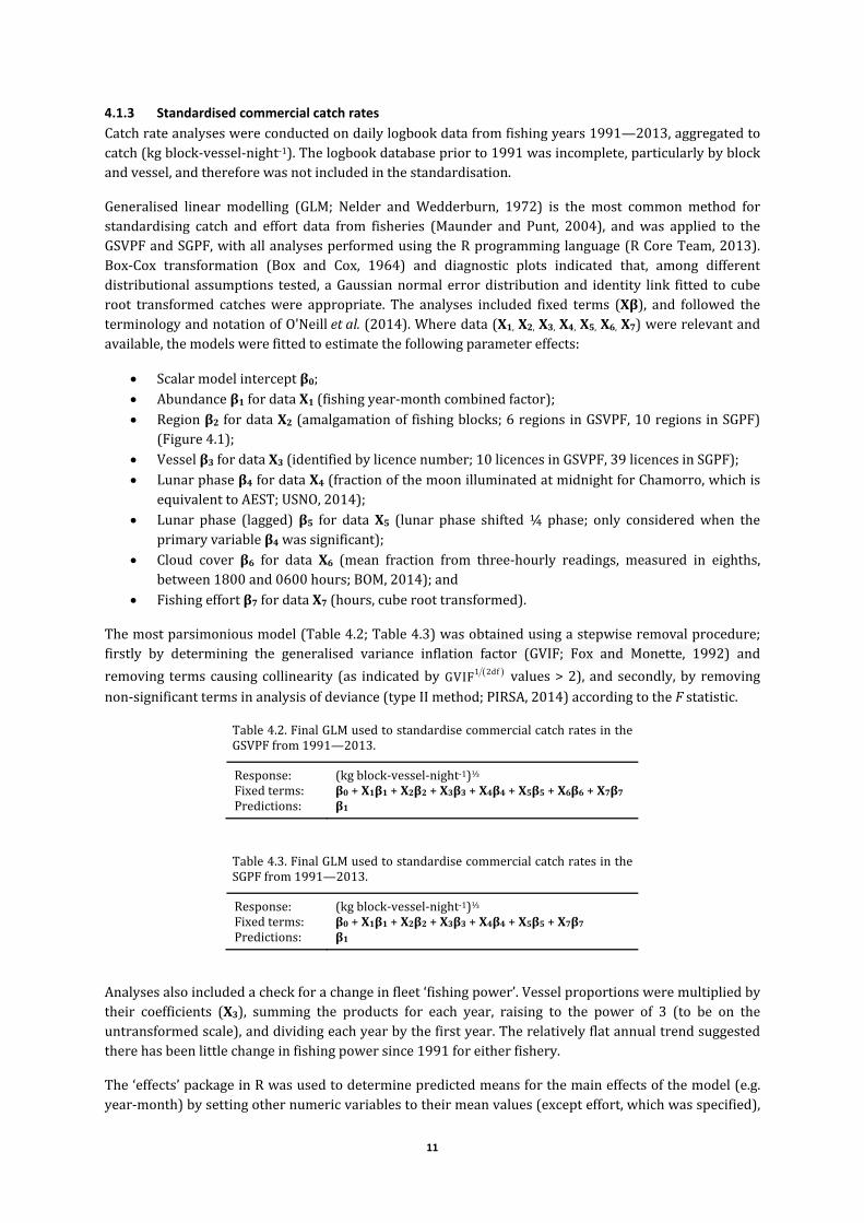
4.1.3 Standardised commercial catch rates

Catchrateanalyseswereconductedondailylogbookdatafromfishingyears1991—2013,aggregatedtocatch(kgblock‐vessel‐night‐1).Thelogbookdatabasepriorto1991wasincomplete,particularlybyblockandvessel,andthereforewasnotincludedinthestandardisation.

Generalised linear modelling (GLM; Nelder and Wedderburn, 1972) is the most common method forstandardising catch and effort data from fisheries (Maunder and Punt, 2004), andwas applied to theGSVPFandSGPF,withallanalysesperformedusingtheRprogramminglanguage(RCoreTeam,2013).Box‐Cox transformation (Box and Cox, 1964) and diagnostic plots indicated that, among differentdistributional assumptions tested, aGaussiannormal errordistributionand identity link fitted to cuberoot transformed catcheswere appropriate. The analyses included fixed terms (Xβ), and followed theterminologyandnotationofO'Neilletal.(2014).Wheredata(X1,X2,X3,X4,X5,X6,X7)wererelevantandavailable,themodelswerefittedtoestimatethefollowingparametereffects:

Scalarmodelinterceptβ0; Abundanceβ1fordataX1(fishingyear‐monthcombinedfactor); Regionβ2 fordataX2 (amalgamationof fishingblocks;6regionsinGSVPF,10regionsinSGPF)

(Figure4.1); Vesselβ3fordataX3(identifiedbylicencenumber;10licencesinGSVPF,39licencesinSGPF); Lunarphaseβ4fordataX4(fractionofthemoonilluminatedatmidnightforChamorro,whichis

equivalenttoAEST;USNO,2014); Lunar phase (lagged)β5 for dataX5 (lunar phase shifted¼ phase; only consideredwhen the

primaryvariableβ4wassignificant); Cloud cover β6 for data X6 (mean fraction from three‐hourly readings, measured in eighths,

between1800and0600hours;BOM,2014);and Fishingeffortβ7fordataX7(hours,cuberoottransformed).

Themostparsimoniousmodel(Table4.2;Table4.3)wasobtainedusingastepwiseremovalprocedure;firstly by determining the generalised variance inflation factor (GVIF; Fox and Monette, 1992) and

removing termscausingcollinearity (as indicatedby 1 2dfGVIF values>2), and secondly,by removingnon‐significanttermsinanalysisofdeviance(typeIImethod;PIRSA,2014)accordingtotheFstatistic.

Table4.2.FinalGLMusedtostandardisecommercialcatchratesintheGSVPFfrom1991—2013.

Response: (kgblock‐vessel‐night‐1)⅓Fixedterms: β0+X1β1 +X2β2 + X3β3 + X4β4 + X5β5 + X6β6 + X7β7Predictions: β1

Table4.3.FinalGLMusedtostandardisecommercialcatchratesintheSGPFfrom1991—2013.

Response: (kgblock‐vessel‐night‐1)⅓Fixedterms: β0+X1β1 + X2β2 + X3β3 + X4β4 + X5β5 + X7β7Predictions: β1

Analysesalsoincludedacheckforachangeinfleet‘fishingpower’.Vesselproportionsweremultipliedbytheir coefficients (X3), summing the products for each year, raising to the power of 3 (to be on theuntransformedscale),anddividingeachyearbythefirstyear.Therelativelyflatannualtrendsuggestedtherehasbeenlittlechangeinfishingpowersince1991foreitherfishery.

The‘effects’packageinRwasusedtodeterminepredictedmeansforthemaineffectsofthemodel(e.g.year‐month)bysettingothernumericvariablestotheirmeanvalues(excepteffort,whichwasspecified),

12

and by setting factors to their proportional distribution in the data by averaging over contrasts (Fox,2003;FoxandHong,2009).Efforthadamultimodaldistribution(fourmodes),sothecubic‐rootofthemeanofthelargesttwomodes(asdeterminedbytheRpackage‘mixdist’,MacdonaldandDu,2012)wasusedtorepresenttypicaleffortperblockpervessel‐nightinthefleet.Asthepredictedmeanswereonthetransformed scale, the cubic‐root bias correction μ3 + 3μσ2 was necessary to back‐transform to theiroriginalscale(Kendalletal.,1983),whereμisthepredictedmeanonthetransformedscale,andσ2isthemodelvariance.

4.1.4 Standardised survey catch rates

IndependentsurveysofabundancewereconductedinGSVinDecember,March,AprilandMayoffishingyears2005—2012(except2012,whenonlyAprilandMaysurveyswereconducted)andSGinNovember,February and April of fishing years 2005—2013 (e.g. Dixon et al., 2012; Noell et al., 2014). Usingcommercialvesselsandtrawlnets, thesurveysmonitoredcatchratesandprawnsizeatfixedlocations(upto112samplesforGSVand209samplesforSG)withinmostregionsnearthebeginning,middleandendofthefishingseason.Inadditiontoprovidinganindexofrelativeabundance,thesesurveysarealsousedtodeterminetheareatobesubsequentlyfishedbasedondecisionrulesinvolvingcatchrateandsizecriteria.

As for commercial catch rates, individual survey catches (adjusted to twonetswherenecessary)wereanalysedusingaGaussianGLMwithcubic‐roottransformationandidentitylink,excepteffort(cubic‐roottransformed)was insertedasanoffset (0).Surveycatch(kg trawl‐shot‐1)waspredicted for the fishingyear‐survey (month) combined factor with the explanatory factors of region, vessel and, for SG, tidedirection (relative tovessel, i.e. against tide,with tideor slack tide).Wherenecessary,predictedmeancatchwasalsoexpressedinkgh‐1andlbmin‐1forindustryreportingneeds.

4.1.5 Size composition data

Two datasets on size structure were available: 1) carapace‐length (CL) frequencies from surveysconductedsince2005;and2)whole‐fleetlogbooksize‐gradefrequenciesobtainedfrom2007—2012fortheGSVPF,and2003—2013fortheSGPF.Together, these twodatasetswereusedtoquantifymonthlychangesinWKPsize.

Carapace‐lengthfrequencieswererecordedroutinelybyobserversateachsurveylocation.Eachprawnwassexedandmeasuredto1‐mmlengthclasses.Gradingcategoriesclassifiedprawnsizebythenumberofprawnsperpound(heads‐onandsexescombined).Size‐gradefrequenciescomprisedfourcategories:1)>20lb‐1(small)≈1‐34mmCL;2)16‐20lb‐1(medium)≈35‐38mm;3)10‐15lb‐1(large)≈39‐45mm;and4)<10lb‐1(extra‐large)≈46‐75mm.‘Softandbroken,’anadditionalcategory,wereinfrequentandnot analysed.No independentdatawereavailable toassess theaccuracyof theat‐sea commercial sizegrading, but the same data were acceptable to processors to determine price paid to fishers. Largerprawnsfetchedahigherpriceforthesameweight.

4.1.6 Size‐transition matrices

Prawntag‐recapturedataobtainedfromDecember1988toNovember1996forGSV(XiaoandMcShane,2000b)andOctober1984toJune1991fromSG(CarrickandOstendorf,2005)werefittedtoaseasonalvon Bertalanffy growth model, and sex‐specific size‐transition matrices for each gulf were generatedfollowing the methods described in Appendix C. Assuming a normal probability density function, thetransitionmatricesallocatedaproportionofWKPincarapacelength‐classlʹattimet–1togrowintoanewlengthloveronetime‐stept,wheretrepresentsonemonth.

4.1.7 Economic data

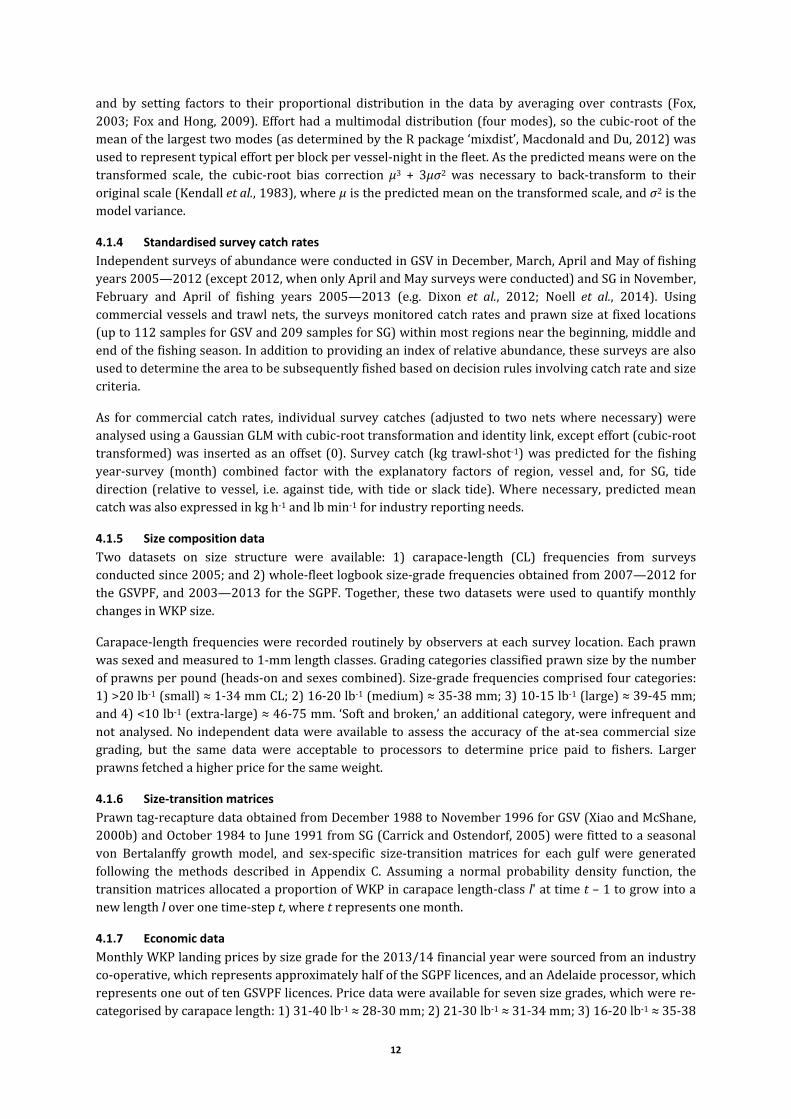
MonthlyWKPlandingpricesbysizegradeforthe2013/14financialyearweresourcedfromanindustryco‐operative,whichrepresentsapproximatelyhalfoftheSGPFlicences,andanAdelaideprocessor,whichrepresentsoneoutoftenGSVPFlicences.Pricedatawereavailableforsevensizegrades,whichwerere‐categorisedbycarapacelength:1)31‐40lb‐1≈28‐30mm;2)21‐30lb‐1≈31‐34mm;3)16‐20lb‐1≈35‐38

13

mm;4)10‐15lb‐1≈39‐45mm;5)8‐10lb‐1≈46‐49mm;6)6‐8lb‐1≈50‐54mm;and7)<6lb‐1≈55‐75mm.Monthlylandingpricesusedforthemodelwerebasedonindustryinformationthatthedemandisgreater forrawprawnsbetween JanuaryandOctoberandcookedprawns inNovemberandDecember,andahigherpriceispaidforcookedprawns(Table4.4;Figure4.4).

Table4.4.MonthlyWKPlandingprices($kg‐1)bysizegradeandproducttype.

Sizegrade

(lb‐1)

Carapacelength(mm)

Cartonsize

Price(AU$kg‐1)

Raw CookedEstimatedmix(raw:cooked)

Nov/DecOthermonths

Nov/DecOthermonths

Nov/Dec(5:95)

Other(80:20)

31‐40 28‐30 10kg 11.00 7.50 12.00 8.50 11.95 7.7021‐30 31‐34 10kg 12.50 9.50 13.50 10.50 13.45 9.7016‐20 35‐38 10kg 17.00 12.50 18.00 13.50 17.95 12.7011‐15 39‐45 10kg 19.00 14.50 20.00 15.50 19.95 14.708‐10 46‐49 5kg 22.00 18.25 23.50 19.75 23.43 18.556‐8 50‐54 5kg 24.25 20.25 25.75 21.75 25.68 20.55<6 55‐75 5kg 26.00 24.00 27.50 25.50 26.30 24.30

Figure4.4.2013/14monthlyWKPlandingprices($kg‐1)bycarapacelengthbasedonestimatedproportionsofrawandcookedprawnsindemand.

Theaveragecombinedby‐productvalueforscyllaridlobstersandSouthernCalamariwascalculatedfromlogbookharvestsandpricedatafromprocessorsandlicenceholders(Table4.5;Table4.6).

Economic parameters were based on survey responses from 4 (40%) GSVPF licence holders and 22(56%)SGPFlicenceholders.Parametervalues(means)wereestimatedforthe2011/12financialyearforthe GSVPF and 2012/13 for the SGPF (EconSearch, 2014) (Table 4.5; Table 4.6). The most recenteconomic survey for theGSVPFwas conducted in2007/08 (EconSearch, 2009).Valueswere thereforeadjustedto2011/12basedonannualchangesinfishingeffort,pricefrominputsuppliers(e.g.fuel)andtheconsumerpriceindex(CPI)forAdelaide(EconSearch,2010;2011;unpublisheddata).Vesselandfuelcostswere also estimated for notional higher levels of fishing power expectedwith a reduction in thenumberofvessels,whileallothereconomicparameterswereheldconstant(Table4.5;Table4.6).

Acoefficientofvariation(CV)of10%wasestimatedforvariablecostsandannualfixedcosts.Weappliedthesameinterestrate(5.0%),opportunitycostofcapital(assumedtoequalinterestrate)andeconomicdepreciationrate(3.7%)astheCommonwealth’sNorthernPrawnFishery(Puntetal.,2010)(Table4.5;Table4.6).

14

Table4.5.InputparametervaluesfortheGSVPFeconomicmodelatdifferentlevelsoffishingpower.Bullets(•)indicatenochangefrom2011/12fishingpower(fpr=1.00).

ParametersFishingpower(fpr;proportion)

1.00 1.05 1.10

Fleetvesseltype

Vesselsize(vs;mean) 19.1 20.8 21.6Numberofvessels(Vy) 10 7 5

Variablecosts

Labour(cL;proportion) 0.40 • •Packaging(cM;$kg‐1) 0.30 • •Repairs(cK;$vessel‐night‐1) 550 • •Fuel(cF;$vessel‐night‐1) 1549 1626 1704Incidentals(cO;$vessel‐night‐1) 46 • •Coefficientofvariation(cvc) 0.1 • •

Annualfixedcosts

Vessel(Wy;$vessel‐year‐1) 89432 93904 98375Investment(Ky;$vessel‐year‐1) 1171493 • •WKP(ρ;proportion) 1 • •Other(fO;$vessel‐year‐1) 0 • •Coefficientofvariation(cvf) 0.1 • •

Revenue

By‐product( ;byB $vessel‐night‐1) 89 • •Coefficientofvariation(cvby) 0.21 • •

Annualeconomicrates

Interest(i;proportion) 0.05 • •Opportunity(o=i;proportion) 0.05 • •Depreciation(d;proportion) 0.037 • •

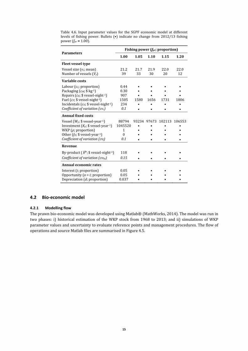
15

Table 4.6. Input parameter values for the SGPF economicmodel at differentlevels of fishing power. Bullets (•) indicate no change from 2012/13 fishingpower(fpr=1.00).

ParametersFishingpower(fpr;proportion)

1.00 1.05 1.10 1.15 1.20

Fleetvesseltype

Vesselsize(vs;mean) 21.2 21.7 21.9 22.0 22.0Numberofvessels(Vy) 39 33 30 20 12

Variablecosts

Labour(cL;proportion) 0.44 • • • •Packaging(cM;$kg‐1) 0.30 • • • •Repairs(cK;$vessel‐night‐1) 907 • • • •Fuel(cF;$vessel‐night‐1) 1505 1580 1656 1731 1806Incidentals(cO;$vessel‐night‐1) 234 • • • •Coefficientofvariation(cvc) 0.1 • • • •

Annualfixedcosts

Vessel(Wy;$vessel‐year‐1) 88794 93234 97673 102113 106553Investment(Ky;$vessel‐year‐1) 1045520 • • • •WKP(ρ;proportion) 1 • • • •Other(fO;$vessel‐year‐1) 0 • • • •Coefficientofvariation(cvf) 0.1 • • • •

Revenue

By‐product( ;byB $vessel‐night‐1) 118 • • • •Coefficientofvariation(cvby) 0.15 • • • •

Annualeconomicrates

Interest(i;proportion) 0.05 • • • •Opportunity(o=i;proportion) 0.05 • • • •Depreciation(d;proportion) 0.037 • • • •

4.2 Bio‐economic model

4.2.1 Modelling flow

Theprawnbio‐economicmodelwasdevelopedusingMatlab®(MathWorks,2014).Themodelwasrunintwo phases: i) historical estimation of theWKP stock from 1968 to 2013; and ii) simulations ofWKPparametervaluesanduncertaintytoevaluatereferencepointsandmanagementprocedures.TheflowofoperationsandsourceMatlabfilesaresummarisedinFigure4.5.

16

Figure 4.5. Flow of operations and source files for the WKP bio‐economic model. Abbreviations: NLL,negative log‐likelihood; ML, maximum likelihood; MCMC, Markov Chain Monte Carlo; MP, managementprocedure.

17

4.2.2 Population dynamic model

The population dynamicmodel forWKP in the GSVPF and SGPFwas based on that developed for theEasternKingPrawn(EKP,M.plebejus)fisheryinQueenslandandNewSouthWales(O'Neilletal.,2014).Themodeloperatedatamonthlytimestepandtrackednumbers(N)andbiomass(B)ofprawnsbytheirsex (s) and length (l) (Table 4.7; Table 4.8), and included the processes of mortality, growth andrecruitmentineverymonth(t).

Table4.7.EquationsusedforsimulatingWKPpopulationdynamics(seeTable4.8fornotation).

Monthlypopulationdynamics Equation

Numberofprawns:

, , , , 1, 1 , 1, ,exp 1 0.5l t s l l t s l t l t s l tl

N M v u N R (1)

Recruitmentnumber—Beverton‐Holtformulation:

1,

1

expyl t y t l

y

ER

E,whereyindicatesthefishingyear.

(2)

Spawningindex—annualnumberofeggs:

, ,y l t s l lt lE N m f ,wheres=female.

(3)

Recruitmentpattern—normalisedmonthlyproportions(modes1and2):

121

1 11

122

2 21

exp cos 2 /12 exp cos 2 ' /12

exp cos 2 /12 exp cos 2 ' /12

tt

tt

t t

t t

1 2(1 )t t t ,wheretindicatesfishingmonth1…12.

exp 1 exp ,whereτisthemixingproportionofseasonal

recruitmentdistributions1and2basedonalogittransformation.Themixingparameterτwastestedtoexploreabimodalrecruitmentpatternbutwasnotusedinfinalanalyses.

(4)

Mid‐monthexploitablebiomasses—forms1and2:

1 f, , ,

2 f, , ,

exp 2

exp 2 1 2t l t s l s ll s

t l t s l s l tl s

B N w v M

B N w v M u

,wherefindicatesfishery(form1)or

survey(form2)vulnerability.

(5)

Harvestrate:

1t t tu C B ,whereCisthemonthlyharvest(kg).

(6)

Prawnvulnerabilitytofishinggear:

f 50f f1 1 explv l l ,wherefindicatesdifferentselectivitybetween

fisheryandsurvey.

(7)

Catchrates:

Fishery(f;kgblock‐vessel‐night‐1):

f f 2t tc q t B ,wheref=fishery.

Survey(s;kgtrawl‐shot‐1): f f 1t tc q B ,wheref=survey.

(8)

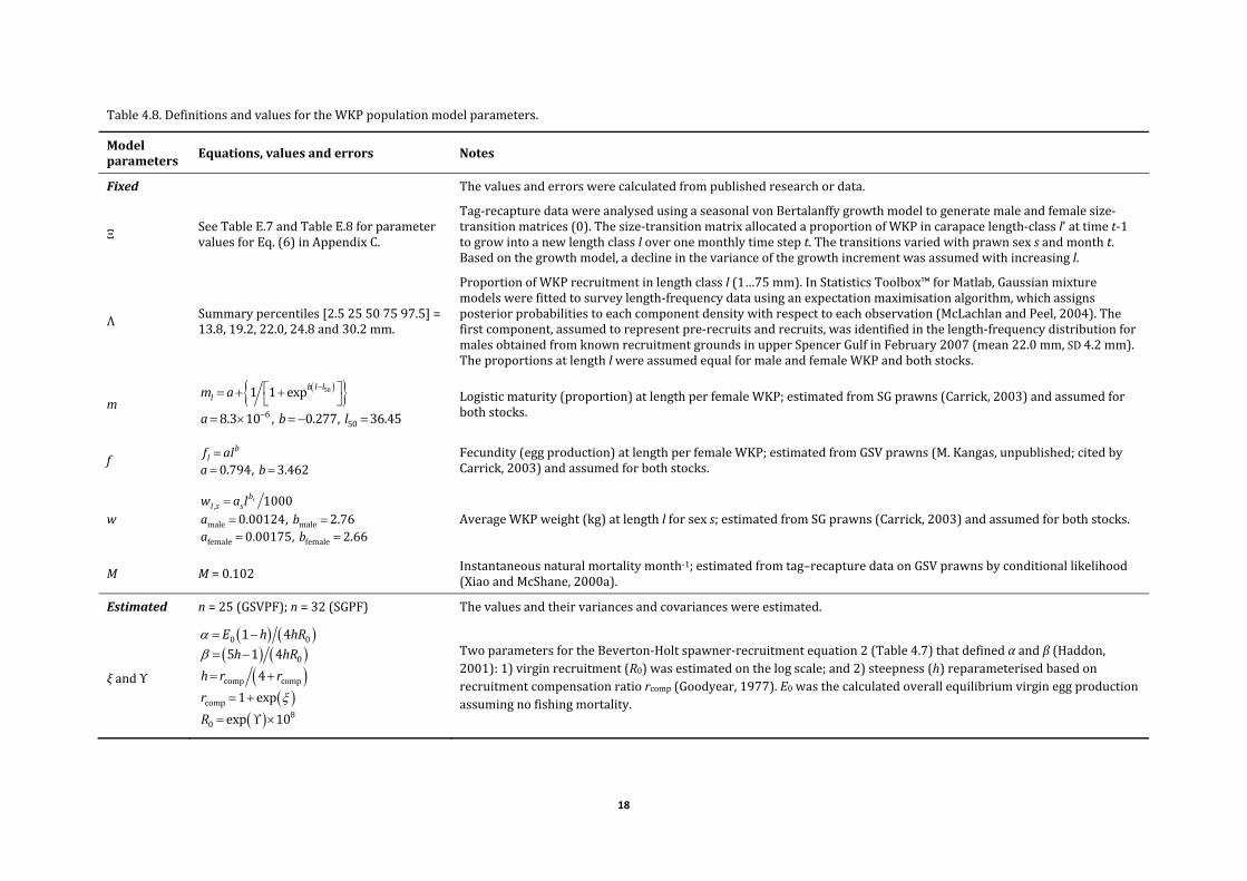
18

Table4.8.DefinitionsandvaluesfortheWKPpopulationmodelparameters.

Modelparameters

Equations,valuesanderrors Notes

Fixed Thevaluesanderrorswerecalculatedfrompublishedresearchordata.

ΞSeeTableE.7andTableE.8forparametervaluesforEq.(6)inAppendixC.

Tag‐recapturedatawereanalysedusingaseasonalvonBertalanffygrowthmodeltogeneratemaleandfemalesize‐transitionmatrices(0).Thesize‐transitionmatrixallocatedaproportionofWKPincarapacelength‐classl'attimet‐1togrowintoanewlengthclassloveronemonthlytimestept.Thetransitionsvariedwithprawnsexsandmontht.Basedonthegrowthmodel,adeclineinthevarianceofthegrowthincrementwasassumedwithincreasingl.

Λ Summarypercentiles[2.525507597.5]=13.8,19.2,22.0,24.8and30.2mm.

ProportionofWKPrecruitmentinlengthclassl(1…75mm).InStatisticsToolbox™forMatlab,Gaussianmixturemodelswerefittedtosurveylength‐frequencydatausinganexpectationmaximisationalgorithm,whichassignsposteriorprobabilitiestoeachcomponentdensitywithrespecttoeachobservation(McLachlanandPeel,2004).Thefirstcomponent,assumedtorepresentpre‐recruitsandrecruits,wasidentifiedinthelength‐frequencydistributionformalesobtainedfromknownrecruitmentgroundsinupperSpencerGulfinFebruary2007(mean22.0mm,SD4.2mm).TheproportionsatlengthlwereassumedequalformaleandfemaleWKPandbothstocks.

m 50

650

1 1 exp

8.3 10 , 0.277, 36.45

b l llm a

a b l

Logisticmaturity(proportion)atlengthperfemaleWKP;estimatedfromSGprawns(Carrick,2003)andassumedforbothstocks.

f 0.794, 3.462

blf ala b

Fecundity(eggproduction)atlengthperfemaleWKP;estimatedfromGSVprawns(M.Kangas,unpublished;citedbyCarrick,2003)andassumedforbothstocks.

w

,

male male

female female

10000.00124, 2.760.00175, 2.66

sbl s sw a l

a ba b

AverageWKPweight(kg)atlengthlforsexs;estimatedfromSGprawns(Carrick,2003)andassumedforbothstocks.

M M=0.102Instantaneousnaturalmortalitymonth‐1;estimatedfromtag–recapturedataonGSVprawnsbyconditionallikelihood(XiaoandMcShane,2000a).

Estimated n=25(GSVPF);n=32(SGPF) Thevaluesandtheirvariancesandcovarianceswereestimated.

ξandϒ

0 0

0

comp comp

comp8

0

1 4

5 1 4

4

1 exp

exp 10

E h hR

h hR

h r r

r

R

TwoparametersfortheBeverton‐Holtspawner‐recruitmentequation2(Table4.7)thatdefinedαandβ(Haddon,2001):1)virginrecruitment(R0)wasestimatedonthelogscale;and2)steepness(h)reparameterisedbasedonrecruitmentcompensationratiorcomp(Goodyear,1977).E0wasthecalculatedoverallequilibriumvirgineggproductionassumingnofishingmortality.

19

Modelparameters

Equations,valuesanderrors Notes

μ1andκ μ1andκTwoparameterstodescribethemonthly(time‐months1…12)recruitmentpattern(primarymodeμ1,andconcentrationκ),equation4(Table4.7),accordingtoavonMisesdirectionaldistribution(MardiaandJupp,2009).Proportionoverlapofthemixturedistributionτwasfixed≊1,thereforesecondarymode(μ2)wasnotapplicable.

l50andδ 50f fandl

Two(GSVPF)orfour(SGPF)parametersfortheestimatedlogisticvulnerabilityofprawnsforfishing(f=fishery)orsurvey(s=survey),equation7(Table4.7).δgovernedtheinitialsteepnessofthecurveandl50wasthelengthat50%selection.FortheGSVPF,fisheryvulnerabilityparametervalueswereestimatedtobethesameasthosefromsurveys.

qf(t) f fexp log cos sin ,q t q t t

wheret=2πseqmonth/12.

Fisherycatchabilitywasbasedonasinusoidalfunctiontomodelmonthlypatternsusingthevariable‘seqmonth’.AsthemaximumwatertemperaturewasinFebruary,seqmonth=1inMarchand12inFebruary.Twocatchabilityparameters,amplitude(ϛ)andpeak(ϑ),wereestimatedfortheSGPF,whereasthesewereheldconstant(=0)fortheGSVPF.Thegeometricmeancatchabilities(f=fisheryorf=survey)werecalculatedasclosed‐formmeanestimatesofstandardisedcatchrates(fisheryandsurvey)dividedbythemid‐monthbiomass(form2forfisherycatchability;form1forsurveycatchability)(Table4.7)(Haddon,2001).

ζ

η=ζee=zeros(nparRresid,nparRresid+1);fori=1:nparRresidhh=sqrt(0.5*i./(i+1));e(i,1:i)=‐hh./i;e(i,i+1)=hh;end;e=e./hh;

Recruitmentparameterstoensurelogdeviationssumtozerowithstandarddeviationσ,equation16(Table4.10).ζwerethe19(GSVPF)or22(SGPF)estimatedparametersknownasbarycentricorsimplexcoordinates,distributedNID(0,σ)withnumbernparRresid=numberofrecruitmentyears–1(Möbius,1827;Sklyarenko,2011).ewasthecoordinatebasismatrixtoscalethedistanceofresiduals(verticesofthesimplex)fromzero(O'Neilletal.,2014).

(continued)

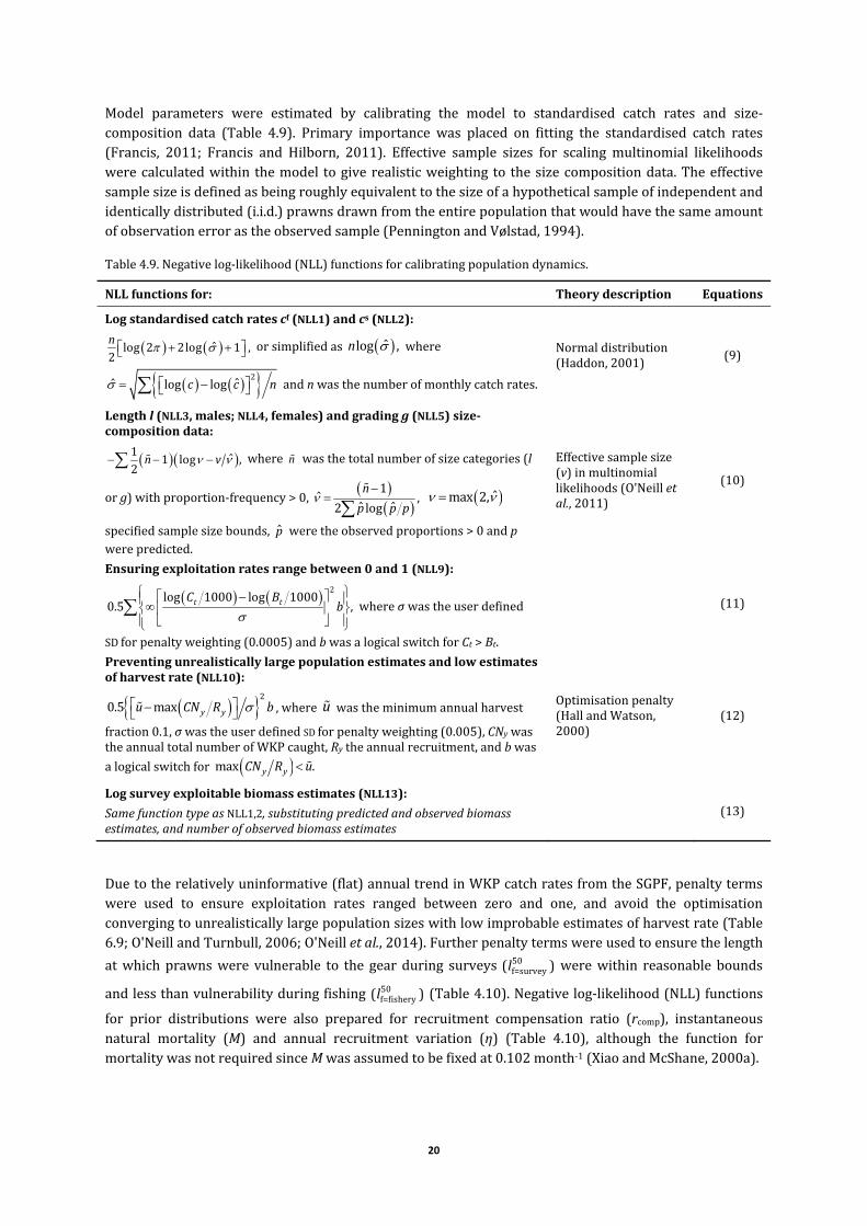
20

Model parameters were estimated by calibrating the model to standardised catch rates and size‐composition data (Table 4.9). Primary importance was placed on fitting the standardised catch rates(Francis, 2011; Francis and Hilborn, 2011). Effective sample sizes for scaling multinomial likelihoodswerecalculatedwithin themodel togiverealisticweighting to thesizecompositiondata.Theeffectivesamplesizeisdefinedasbeingroughlyequivalenttothesizeofahypotheticalsampleofindependentandidenticallydistributed(i.i.d.)prawnsdrawnfromtheentirepopulationthatwouldhavethesameamountofobservationerrorastheobservedsample(PenningtonandVølstad,1994).

Table4.9.Negativelog‐likelihood(NLL)functionsforcalibratingpopulationdynamics.

NLLfunctionsfor: Theorydescription Equations

Logstandardisedcatchratescf(NLL1)andcs(NLL2):

ˆlog 2 2log 1 ,2n orsimplifiedas ̂log ,n where

2

ˆˆ log logc c n andnwasthenumberofmonthlycatchrates.

Normaldistribution(Haddon,2001)

(9)

Lengthl(NLL3,males;NLL4,females)andgradingg(NLL5)size‐compositiondata:

1 ˆ1 log ,2n v where n wasthetotalnumberofsizecategories(l

org)withproportion‐frequency>0,

1ˆ ,

ˆ ˆ2 log

n

p p p ˆmax 2,

specifiedsamplesizebounds, p̂ weretheobservedproportions>0andpwerepredicted.

Effectivesamplesize(v)inmultinomiallikelihoods(O'Neilletal.,2011)

(10)

Ensuringexploitationratesrangebetween0and1(NLL9):

2

log 1000 log 10000.5 ,t tC B

b whereσwastheuserdefined

SDforpenaltyweighting(0.0005)andbwasalogicalswitchforCt>Bt.

(11)

Preventingunrealisticallylargepopulationestimatesandlowestimatesofharvestrate(NLL10):

2

0.5 max y yu CN R b ,where u wastheminimumannualharvest

fraction0.1,σwastheuserdefinedSDforpenaltyweighting(0.005),CNywastheannualtotalnumberofWKPcaught,Rytheannualrecruitment,andbwas

alogicalswitchfor max .y yCN R u

Optimisationpenalty(HallandWatson,2000)

(12)

Logsurveyexploitablebiomassestimates(NLL13):

SamefunctiontypeasNLL1,2,substitutingpredictedandobservedbiomassestimates,andnumberofobservedbiomassestimates

(13)

Duetotherelativelyuninformative(flat)annualtrendinWKPcatchratesfromtheSGPF,penaltytermswere used to ensure exploitation rates ranged between zero and one, and avoid the optimisationconvergingtounrealisticallylargepopulationsizeswithlowimprobableestimatesofharvestrate(Table6.9;O'NeillandTurnbull,2006;O'Neilletal.,2014).Furtherpenaltytermswereusedtoensurethelength

atwhich prawnswere vulnerable to the gear during surveys 50f=survey( )l werewithin reasonable bounds

andlessthanvulnerabilityduringfishing 50f=fishery( )l (Table4.10).Negativelog‐likelihood(NLL)functions

for prior distributions were also prepared for recruitment compensation ratio (rcomp), instantaneousnatural mortality (M) and annual recruitment variation (η) (Table 4.10), although the function formortalitywasnotrequiredsinceMwasassumedtobefixedat0.102month‐1(XiaoandMcShane,2000a).

21

Table4.10.Negativelog‐likelihood(NLL)functionsforparameterboundsanddistributions.

The log‐likelihood function for survey exploitable biomass required observed estimates. These weredeterminedby:1)calculatingthefishablearea(≥10mdepth;Figure4.1)foreachregionusingArcGIS®software;2)extrapolatingmeansurveycatchrate(pertrawledarea)tothefishableareaforeachregion;3)summingacrossthewholegulf;then4)dividingbyaretentionfactorof0.5(i.e.thefractionofWKPinthesweptareaassumedtoberetainedinthecodend;JollandPenn,1990).

The estimation process consisted of amaximum likelihood step usingMatlab’s ‘fminsearch’ optimiserroutine,followedbyasimulatedannealingvariant(Kirkpatricketal.,1983)ofMarkovChainMonteCarlosampling(MCMC)tosearchfurthermaximumlikelihoodsolutionsandestimatetheparametercovariancematrix. Simulated annealing is an efficient method for locating a good approximation of the globalminimumamongmanylocalminima.Weusedthistechniquetosimultaneouslydeterminesolutionsforthe estimated parameters over the log‐likelihood space. Simulated annealing was started from a NLLscalingfactorof100,thenreducedto10and1,withaminimumof5000iterations(jumps)conductedateach level.The covariancematrix isbuiltup from thedifferences in the log‐likelihoodspacewitheachjump.

Duringthefittingprocessdifferentmodelsolutionswereestimatedfromthesizecompositiondataversusthestandardisedcatchrates.Toaddressthisproblem,themaximumlikelihoodestimationprocesswasconductedintwostages:firstly,toestimateselectivityandrecruitmentpatternparameters;andsecondly,tofixtheseparametersinasecondoptimisationtunedprimarilytocatchratedata(Francis,2011;FrancisandHilborn,2011)(Table4.11;Table4.12).Thistwostageapproachwasundesirableandfurtherworkisrequired to achieve simultaneousmodel fits to both the size composition and standardised catch ratedata.Giventhatsimultaneousmodelfitscouldnotbeachieved,wedidnotproceedwiththeMCMCstep(Figure 4.5), which was programmed to document further parameter solutions around the maximumlikelihood results fromsimulatedannealing; theMCMCmodel fittingadds further computation time totheoverallprocess.

NLLfunctionsfor: Equations

Recruitmentcompensationratiorcomp(NLL6):

2

0.5 log 4 1 log 19 , whereσ=0.005definedthe

negativelog‐likelihood.

(14)

InstantaneousnaturalmortalityMmonth‐1(NLL7):

2

0.5 0.102 ,M whereσ=0.031definedthepriordistribution.(15)

Annuallogrecruitmentdeviatesηy(NLL8):

2ˆlog 2 2log ,

2n where min maxˆmin max , , ,

min 0.1 and max 0.4 specifiedbounds, 2ˆ ,y n andnwasthe

numberofrecruitmentyearsy.

(16)

Penalty/priorfor 5 0sl (NLL11):

2

50s0.5 30 ,l b whereσwastheuserdefinedSDforpenaltyweighting

(0.005)andbwasalogicalswitchfor 50s 20l or 50

s 40.l NLL11wasnot

influential.

(17)

Penalty/priorfor 50 50f sl l (NLL12):

2

50 50s f0.5 ,l l b whereσwastheuserdefinedSDforpenaltyweighting

(0.005)andbwasalogicalswitchfor 50 50f s< .l l NLL12wasnotinfluential.

(18)

22

Table 4.11. The two‐stage approach used toestimateparametersfortheGSVPFmodel(0=fixed,assumed value in parentheses; 1 = estimated).Abbreviations: S1, Stage 1; S2, Stage 2; n/a, notapplicable;NLL,negativelog‐likelihood.

Parameter Stage1 Stage2

ξ 1 1Υ 1 1μ1 1 0(=S1)μ2 0(n/a*) 0(n/a*)κ 1 0(=S1)π 0(≈1) 0(≈1)50sl 1 0(=S1)

δs 1 0(=S1)50fl 0(n/a) 0(= 50

s ,l S1)

δf 0(n/a) 0(= s , S1)M 0(=0.102) 0(=0.102)ς 0(=0) 0(=0)ϑ 0(=0) 0(=0)ηy 1 1

NLLswitch

On NLL1‐6,8,9,11,13 NLL1,2,5,6,8,9,13Off NLL7,10,12 NLL3,4,7,10‐12

*μ2 is n/a when π ≈ 1 (i.e. complete overlap, no secondrecruitmentdistribution/modeestimated).

Table 4.12. The two‐stage approach used toestimate parameters for the SGPF model (0 =fixed, assumed value in parentheses; 1 =estimated).Abbreviations:S1,Stage1;S2,Stage2; n/a, not applicable; NLL, negative log‐likelihood.

Parameter Stage1 Stage2

ξ 1 1Υ 1 1μ1 1 0(=S1)μ2 0(n/a*) 0(n/a*)κ 1 0(=S1)π 0(≈1) 0(≈1)50sl 1 0(=S1)

δs 1 0(=S1)50fl 1 0(=S1)

δf 1 0(=S1)M 0(=0.102) 0(=0.102)ς 1 1ϑ 1 1ηy 1 1

NLLswitch

On NLL1‐6,8,9,11‐13 NLL1,2,6,8,9,13Off NLL7,10 NLL3‐5,7,10‐12

*μ2isn/awhenπ≈1(i.e.completeoverlap,nosecondrecruitmentdistribution/modeestimated).

23

4.2.3 Economic (model and) parameters

Theeconomicmodel calculatednetpresentvalue (NPV)basedon totaldiscountedprofit theory (Ross,1995). TheNPVobjective functionusedgeometric discounting that summedprofits over futuremodelprojections:

1

NPV ,yy

y

a

wherea=(1+i)‐1,iwastheannualinterest(discount)rateandπywastheprofitduringyeary.Toavoidmodel projections overmany years, theNPVwas truncated to a terminal yearT and equilibriumwasassumedthereafter:

1

1 1

1

NPV .T

y Ty T

y

a a i

ThisNPV function differs from Equation (13) of Puntetal. (2010), in thatwe consistently discountedannualprofitsbacktothestartofthefirstprojection.

Annualprofitwascalculatedastheharvestvalueminusthevariableandfixedcosts:

V F, , 1 ,by

y t l t l t L y y yt l

v C B c E V

wherevt,lwastheaveragepricereceivedbyfishers forWKPbytime‐monthtand lengthclass l(Figure

4.4),Ct,lwas theWKPharvestweight,Vt was the total variable costs,

byB was the averageby‐product

value($)takeneachboatday,cLwastheshareofthecatchpaidtocrewmembers(alabourcost),Eywas

thetotalannualboatdaysfished,Fy theaverageannual fixedcosts,andVywasthenumberofvessels

(Table4.5;Table4.6).

VariablecostsVt werecalculatedbytime‐montht.Thisincludedtheproportionallabourcost(cL),cost

ofpackagingandmarketing(cM)perunitweightofcatch,costofrepairsandmaintenanceperboat‐day(cK),fuelcostperboat‐day(cF),andotherincidentalcostsperboat‐day(cO)(Table4.5;Table4.6):

V, , .t L t l M t l K F O t

l

c v c C c c c E

AverageannualfixedcostsFy werecalculatedusingannualvesselcosts(Wy),andopportunity(o)and

depreciation(d)ratesonaveragetotalinvestmentvaluepervessel(Ky)(Table4.5;Table4.6):

F ( ) .y y yW o d K

Annualvesselcosts(Wy)werenotrelatedtofishingeffort.Theywerethesumofcostsneededtosupportavesselbeforefishing.

4.3 Simulation and management procedures Model simulations were used to estimate management reference points and evaluate proposedmanagement procedures (MPs). Ten‐year projections, from 2014 to 2023, were simulated using fullmodelerrormethodologysimilartoRichardsetal.(1998).Asbasereferencetotheseprojections,1000random variations of the estimated parameters (GSVPF:n = 25; SGPF:n = 32)were created from thesimulatedannealingcovariancematrix.Foreconomics,1000randomvariationsonparameters listedinTable4.5andTable4.6weregeneratedbasedonanestimatedCVof10%forvariableandfixedcostsand

24

calculated CV of 15% for by‐product revenue. These variations of parameter estimates were used tosimulatefutureuncertainties,includingstochasticrecruitment.

Equilibrium reference points for MSY and MEYv for each fishing power level were calculated byoptimisingthepopulationandeconomicmodelsthroughmeanmonthlyfishingmortalityproportionaltofishingeffort.Allparameteruncertaintiesasoutlinedabovewereincludedexceptstochasticrecruitmentvariation. The population dynamicswere propagated to equilibriumusing themonthly fishing patterncalculatedfromdataforthelastfivefishingyears(2009—2013).

TenMPsfortheGSVPFand14MPsfortheSGPFweredevelopedbyconsultationwithfisherymanagersandstakeholdersthroughface‐to‐facemeetingsandteleconferences(Table4.13;Table4.14).ThefirstMPforeachfisherywasstatusquo.FortheGSVPF,statusquois10vesselsoperatingforatotalof260vessel‐nights(eight‐yearmean:2005—2012)inNovember,DecemberandMarch—June(6months),andwithapre‐Christmascatchcapforthefleetof40t.FortheSGPF,statusquois39vesselsoperatingforatotalof2000vessel‐nights(nine‐yearmean:2005—2013)inNovember,DecemberandMarch—June(6months),and with a variable pre‐Christmas catch cap (dependent on the November stock assessment survey).Relative to status quo (MP1), the remaining MPs for each fishery were characterised by one or acombinationof:i)reductionsinthenumberofvessels;ii)increasesintotaleffort;iii)changesinthepre‐Christmascatchcap; iv)temporalclosures;v)spatialclosures;andvi) introductionofanannualquota.Where aMP included a reduction in the number of vessels, a notional increase in fishing power (andassociatedcosts)fortheremainingvesselswasincludedinthesimulation,asitwasassumedthatsmallerorleastpowerfulvesselswouldexitthefisheryfirst.

Sincetheoperatingmodeldoesnotaccountforspatialstructuringofthepopulation,theeffectofclosedareas inMP8 for theGSVPFandMP10,MP11andMP12 for theSGPFwasmimickedbyestimating theproportionsofthestock insideandoutsidethoseareasduringtherelevantmonths.Usinggeographicalinformation systems (GIS) techniques, these estimateswere based on the product of average nominalcatchratebytrawledareascaleduptothefishablearea.

EachMPwassimulatedtoevaluatemanagementperformanceovertenyearsagainsttwelveperformancemeasures grouped into four categories: i) industry functioning: average annual harvest and effort; ii)currentperformance indicators(DixonandSloan,2007;PIRSA,2014):averagecatchrates(fisheryandsurvey) and average prawn size (length and size grade); iii) 2023 population status: spawning eggproduction and exploitable biomass; and iv) economics: relative profit andNPV against variable costsonlyandbothvariableandfixedcosts.TheNPVcalculatedoverallfutureyearswasusedtorecordalong‐termbenefit for fishingWKP after 10 years,whereas the other performancemeasureswere averagedover10yearstoprovideashorter‐termperspective.

Simulated total fishing effort was split across months based on the logbook‐derived average annualpatternof2009‐2013.Thecontributionofamonth towards theannualpatternwasnormalisedwithameanof1.NegligibleeffortwasrecordedinOctoberandFebruary,sothesemonthswereomittedfromcalculationoftheannualeffortpattern(alongwiththeothernon‐fishingmonthsof JanuaryandJulytoSeptember).Ifamonthwasclosedtofishing,thatmonth’sfishingeffortwasreallocatedtoothermonthsinproportiontothenormalisedpattern.

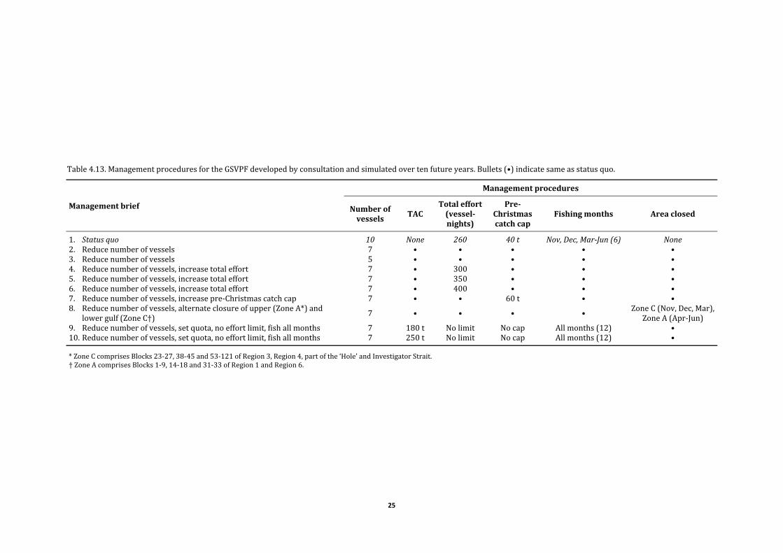
25

Table4.13.ManagementproceduresfortheGSVPFdevelopedbyconsultationandsimulatedovertenfutureyears.Bullets(•)indicatesameasstatusquo.

Managementbrief

Managementprocedures

Numberofvessels

TACTotaleffort(vessel‐nights)

Pre‐Christmascatchcap

Fishingmonths Areaclosed

1. Statusquo 10 None 260 40t Nov,Dec,Mar‐Jun(6) None2. Reducenumberofvessels 7 • • • • •3. Reducenumberofvessels 5 • • • • •4. Reducenumberofvessels,increasetotaleffort 7 • 300 • • •5. Reducenumberofvessels,increasetotaleffort 7 • 350 • • •6. Reducenumberofvessels,increasetotaleffort 7 • 400 • • •7. Reducenumberofvessels,increasepre‐Christmascatchcap 7 • • 60 t • •8. Reducenumberofvessels,alternateclosureofupper(ZoneA*)and

lowergulf(ZoneC†)7 • • • •

ZoneC (Nov,Dec,Mar),ZoneA(Apr‐Jun)

9. Reducenumberofvessels,setquota,noeffortlimit, fishall months 7 180t Nolimit Nocap Allmonths (12) •10. Reducenumberofvessels,setquota,noeffortlimit, fishall months 7 250t Nolimit Nocap Allmonths (12) •

*ZoneCcomprisesBlocks23‐27,38‐45and53‐121ofRegion3,Region4,partofthe‘Hole’andInvestigatorStrait.†ZoneAcomprisesBlocks1‐9,14‐18and31‐33ofRegion1andRegion6.

26

Table4.14.ManagementproceduresfortheSGPFdevelopedbyconsultationandsimulatedovertenfutureyears.Bullets(•)indicatesameasstatusquo.

Managementbrief

Managementprocedures

Numberofvessels

TACTotaleffort(vessel‐nights)

Pre‐Christmascatchcap

Fishingmonths Areaclosed

1. Statusquo 39 None 2000 Variable Nov,Dec,Mar‐Jun(6) None2. Reducenumberofvessels 33 • • • • •3. Reducenumberofvessels 30 • • • • •4. Reducenumberofvessels,nopre‐Christmascatchcap, fishall months 20 • • Nocap Allmonths (12) •5. Reducenumberofvessels,nopre‐Christmascatchcap, fishall months 12 • • Nocap Allmonths (12) •6. ClosefisheryinNovember • • • • Dec,Mar‐Jun(5) •7. Reducepre‐Christmascatchcap • • • ‐40% • •8. ClosefisheryinMarch • • • • Nov,Dec,Apr‐Jun(5) •9. ClosefisheryinJune, increasepre‐Christmascatchcap • • • +190t Nov,Dec,Mar‐May(5) •10. Closenortherngulf* inMarch • • • • • Northerngulf (Mar)11. ClosefisheryinMarchandnortherngulfinApril • • • • Nov,Dec,Apr‐Jun(5) Northerngulf(Apr)12. Close‘NorthEnd’†ofGutterregioninNovemberandDecember • • • • • ‘NorthEnd’(Nov,Dec)13. Setquota, no effortlimit,fishallmonths • 1950t Nolimit • Allmonths (12) •14. Setquota, no effortlimit,fishallmonths • 2200t Nolimit • Allmonths (12) •

*NortherngulfcomprisesBlocks1‐44and109‐125ofNorth,Middlebank,partofWallarooandpartofCowellregions.†‘NorthEnd’comprisesBlocks51and52ofthe‘Gutter’(part)region.

27

4.4 Summary of bio‐economic model In summarising its completeness and sophistication, the WKP bio‐economic model incorporates thefollowingfeatures:

1. Afulllength‐basedfisherypopulationdynamicsmodelsitsatthecentreofitall;2. Fisheryandsurveycatchrateswerestandardised;3. Size‐transitionmatriceswereestimated(usingamethoddescribedinAppendixC);4. Effectivesamplesizeswereaccountedforintheweightingofsizecomposition(lengthandgrade

frequency)data;5. Model parameters were either assumed (fixed) or estimated using a maximum likelihood

method;6. Aparametercovariancematrixwasobtainedbysimulatedannealing;7. Inclusionofvessel‐basedfisheryeconomics;8. A projection model was constructed to simulate MPs over ten future years of stochastic

recruitment;9. ThespecificMPswereobtainedfromconsultationwithindustryandmanagers;10. Variationandparameteruncertainty(fromthecovariancematrix)areexplicitinthesimulations;

and11. Performance of each MP was evaluated holistically using a suite of biological, industry and

economicmeasures.

5 Results

5.1 Model calibration and description Thelength‐basedmodelwascalibratedtocapturethepopulationdynamicsoftheWKPpopulationsintheGSVandSGasaccuratelyaspossiblewiththeavailabledataandbiologicalinformation.

5.1.1 Gulf St Vincent Prawn Fishery

Themodeltrackedthestandardisedfisheryandsurveycatchrateannualtrends,althoughnotsomeoftheseasonalpeaksandtroughs,particularlyforfisherycatchratesinthelastseveralyears(Figure5.1;Figure5.2). As expected, increased catch rateswere predictedwhen the fisherywas closed (1991, 1992 and2013).Standarddeviationsofthestandardisedresidualswere1.00and1.02forfisheryandsurveycatchrates,respectively.FrancisandHilborn(2011)reportthatagoodmodelfitisconditionalonastandarddeviationofnormalised(orstandardised)residuals(SDNR)notmuchgreaterthan1,alongwithacheckoftheplotofobservedandpredictedabundancedata(catchrates).

Figure5.1.Observed (standardised)andpredicted fisherycatchrates for theGSVPFfrom1991—2013.

28

Figure5.2.Observed (standardised)andpredicted survey catch rates for theSGPFfrom2005—2013.

SincetheadoptionofaconsistentsurveydesignintheGSVPFin2005,fishingcatchrateshavecorrelatedreasonably well with survey catch rates, except in December (Figure 5.3). Of all the survey months(December,March,AprilandMay),Decemberisconsideredtheleastrepresentativeofstocksizeasthepeak spawningactivityofWKParound this time is likely toaffect their catchability, thus impactingoncatchratesfromthefixedsurveylocations(FigureF.12).Incontrast,fisherycatchratesinDecemberareoften elevated (Figure F.10) as a result of harvest decision criteria allowing the fleet to target smallerprawns,thusaffordingagreaterlevelofprotectionforlargespawnerswhilealsotakingadvantageofthehighChristmaspricespaidforsmallprawns(DixonandSloan,2007).

Figure 5.3. Comparison of standardised fishery and survey catch rate (CPUE)trends in the GSVPF by: a) data sequence; b) regression; and c) fishingmonth.Note:catchrateswerenormalisedtoensuretrendswereonthesamescale.

29

The large effective sample sizes for male and female length‐frequency distributions (>100 for mostsurveymonths)obtainedfromsurveysandhighagreementbetweenobservedandpredictedlength‐classassignments(Figure5.4;Figure5.5)impliedgoodrepresentationofthepopulationsizestructure(O'Neilletal.,2011).Weighting the length‐frequencydata(via itsmultinomial log‐likelihood)with theeffectivesample size rather than the actual sample size helped to account for any bias caused by schoolingbehaviourofWKP,wherebyprawnsofthesameorsimilarage/lengthmayschooltogetherandthereforeappearasclustersinsamples.

Figure 5.4. Observed (bars) and predicted (red line) survey length‐frequency distributions(proportions) for male WKP in the GSVPF from 2005—2012. Labels refer to fishing year andmonth;neffindicatestheeffectivemultinomialsamplesizeforeachsurvey.

30

Figure 5.5. Observed (bars) and predicted (red line) survey length‐frequency distributions(proportions) for femaleWKP in theGSVPF from2005—2012. Labels refer to fishing year andmonth;neffindicatestheeffectivemultinomialsamplesizeforeachsurvey.

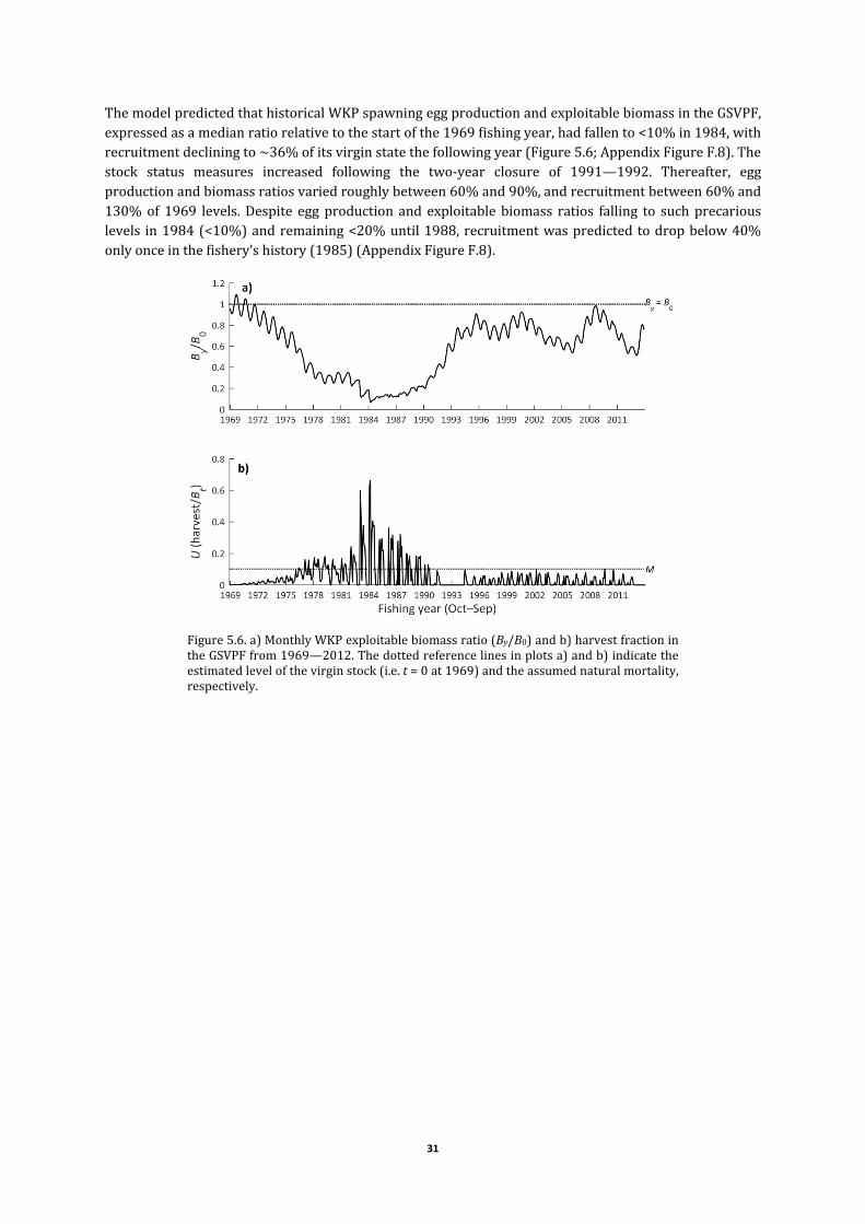
31

ThemodelpredictedthathistoricalWKPspawningeggproductionandexploitablebiomassintheGSVPF,expressedasamedianratiorelativetothestartofthe1969fishingyear,hadfallento<10%in1984,withrecruitmentdecliningto~36%ofitsvirginstatethefollowingyear(Figure5.6;AppendixFigureF.8).Thestock status measures increased following the two‐year closure of 1991—1992. Thereafter, eggproductionandbiomassratiosvariedroughlybetween60%and90%,andrecruitmentbetween60%and130%of 1969 levels.Despite eggproduction and exploitable biomass ratios falling to suchprecariouslevels in1984(<10%)andremaining<20%until1988,recruitmentwaspredictedtodropbelow40%onlyonceinthefishery’shistory(1985)(AppendixFigureF.8).

Figure5.6.a)MonthlyWKPexploitablebiomassratio(By/B0)andb)harvestfractionintheGSVPFfrom1969—2012.Thedottedreferencelinesinplotsa)andb)indicatetheestimatedlevelofthevirginstock(i.e.t=0at1969)andtheassumednaturalmortality,respectively.

32

Virgin recruitment (R0)was estimatedat5.74×107 for theGSVPF (Figure5.7;Table5.1).The relatedsteepnessparameter(h)ofthestockrecruitmentrelationshipwascalibratedat0.60,indicatingthat60%ofpre‐fisheryrecruitment(R0)couldbeexpectedat20%ofvirginspawningstock.Therecruitmentmode(μ1)wasestimatedinApril.Themeancarapacelengthatwhich50%oftheWKPpopulationisvulnerable

to the gear during fishing ( 50f ;l derived from the survey parameter 50

sl )was 33.3mm. There were no

concerningcorrelationsamongthekeyestimatedparameters(Table5.2).Catchabilitywaskeptconstantthroughout the year since earlier model fits yielded unrealistic results when seasonal catchabilityparameters were estimated. Instantaneous natural mortality (M) was also fixed at 0.102 month‐1,estimatedbyXiaoandMcShane(2000a).

Figure 5.7. Predicted relationships forWKP in the GSVPF: a) stock‐recruitmentrelationship (based on 19 years of modelled stochastic recruitment, 1994—2012); b) recruitment pattern (proportion); c) fishery and survey catchability;andd)vulnerabilityatcarapace length(fromsurveys).Note: fisheryandsurveycatchabilitywereheldconstantthroughoutthefishingyear.

33

Table 5.1. Parameter estimates and standard errorsfor GSVPFmodel calibration (NLL: Stage 1, ‐5048.2;Stage 2, ‐48.2). η4 corresponds to the first year forestimatingrecruitmentresiduals(1994).

Parameter EstimateStandarderror

Estimatetransformed

ξ 1.629 0.076 0.604Υ ‐0.554 0.035 0.574μ1 6.770 0.143κ 0.848 0.09050sl 33.252 0.188

δs 0.331 0.02250fl ‐ ‐

δf ‐ ‐ς ‐ ‐ϑ ‐ ‐η1 ‐ ‐η2 ‐ ‐η3 ‐ ‐η4 ‐0.014 0.141η5 ‐0.240 0.128η6 ‐0.017 0.126η7 0.085 0.147η8 0.240 0.113η9 0.118 0.130η10 ‐0.038 0.147η11 ‐0.251 0.130η12 ‐0.215 0.122η13 ‐0.262 0.122η14 ‐0.241 0.097η15 0.094 0.080η16 0.313 0.089η17 0.093 0.092η18 ‐0.040 0.098η19 ‐0.247 0.123η20 ‐0.516 0.104η21 ‐0.304 0.123η22 0.196 0.157

Table 5.2. Correlation matrix of the sixleading model parameters estimated forthe GSVPF. Correlation strength increaseswithcell‐shadingintensity.

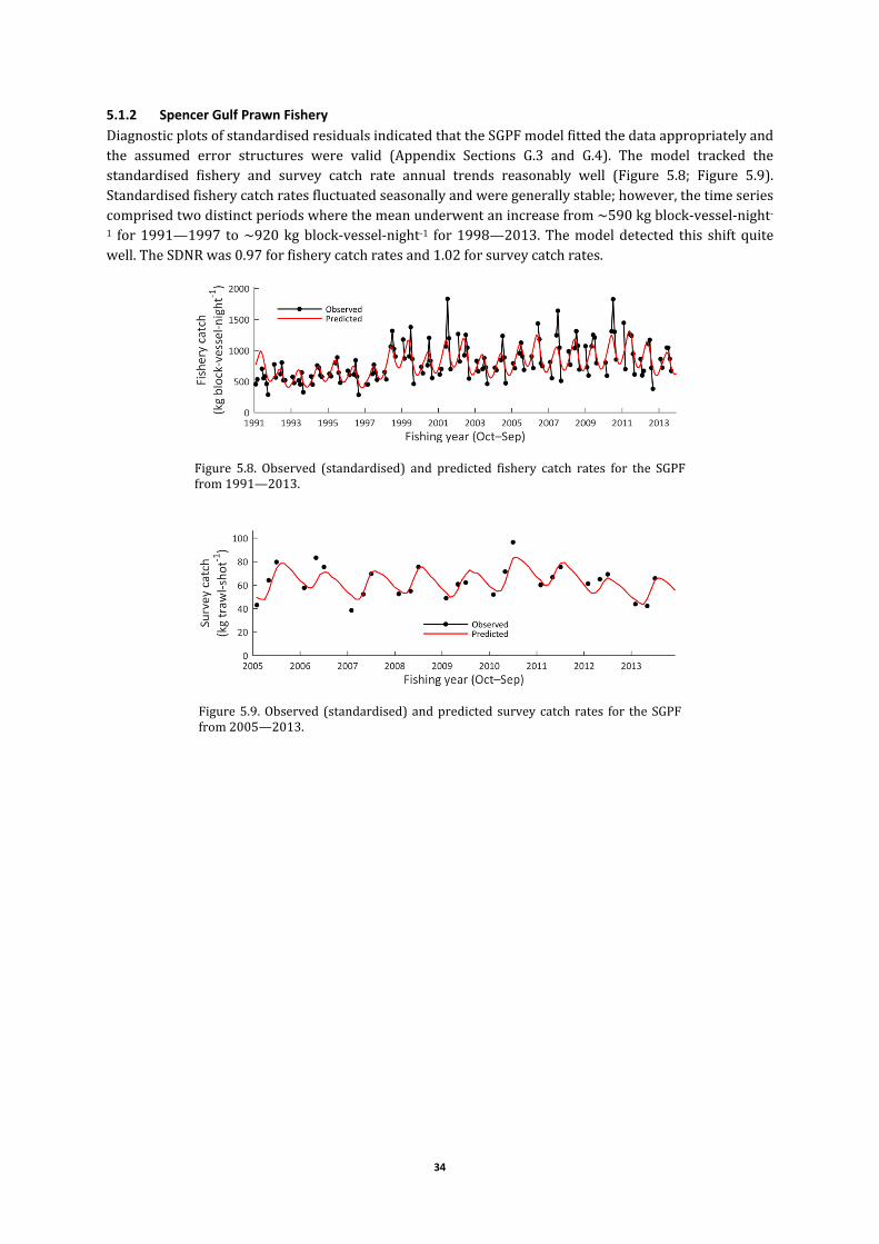
34

5.1.2 Spencer Gulf Prawn Fishery

DiagnosticplotsofstandardisedresidualsindicatedthattheSGPFmodelfittedthedataappropriatelyandthe assumed error structures were valid (Appendix Sections G.3 and G.4). The model tracked thestandardised fishery and survey catch rate annual trends reasonably well (Figure 5.8; Figure 5.9).Standardisedfisherycatchratesfluctuatedseasonallyandweregenerallystable;however,thetimeseriescomprisedtwodistinctperiodswherethemeanunderwentanincreasefrom~590kgblock‐vessel‐night‐1 for1991—1997 to~920kgblock‐vessel‐night‐1 for1998—2013.Themodeldetected this shift quitewell.TheSDNRwas0.97forfisherycatchratesand1.02forsurveycatchrates.

Figure 5.8. Observed (standardised) and predicted fishery catch rates for the SGPFfrom1991—2013.

Figure5.9.Observed (standardised)andpredicted survey catch rates for theSGPFfrom2005—2013.

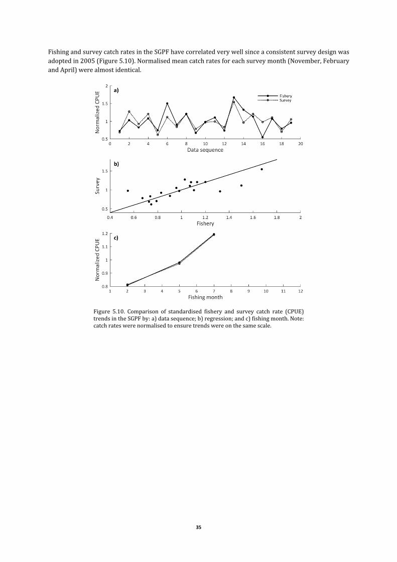
35

FishingandsurveycatchratesintheSGPFhavecorrelatedverywellsinceaconsistentsurveydesignwasadoptedin2005(Figure5.10).Normalisedmeancatchratesforeachsurveymonth(November,FebruaryandApril)werealmostidentical.

Figure 5.10. Comparison of standardised fishery and survey catch rate (CPUE)trendsintheSGPFby:a)datasequence;b)regression;andc)fishingmonth.Note:catchrateswerenormalisedtoensuretrendswereonthesamescale.

36

The large effective sample sizes for male and female length‐frequency distributions (>100 for mostsurveymonths)obtainedfromsurveysandhighagreementbetweenobservedandpredictedlength‐classassignments(Figure5.11;Figure5.12)impliedverygoodrepresentationofthepopulationsizestructure(O'Neill etal., 2011). Large effective sample sizes were also estimated for approximately half of thecommercialsize‐gradedistributions(Figure5.13).Thesmallerestimatedsamplesizesforsomesampleswere typical of fisheries data (Pennington andVølstad, 1994), and indicated that prawnswithin thosesampleswerecorrelated,notnecessarilythatthemodeldidn’tfitthedata.

Figure 5.11. Observed (bars) and predicted (red line) survey length‐frequency distributions (proportions) for male WKP in the SGPF from2005—2013. Labels refer to fishing year and month; neff indicates theeffectivemultinomialsamplesizeforeachsurvey.

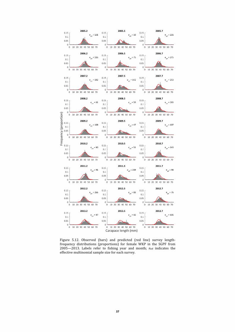
37

Figure 5.12. Observed (bars) and predicted (red line) survey length‐frequency distributions (proportions) for female WKP in the SGPF from2005—2013. Labels refer to fishing year and month; neff indicates theeffectivemultinomialsamplesizeforeachsurvey.

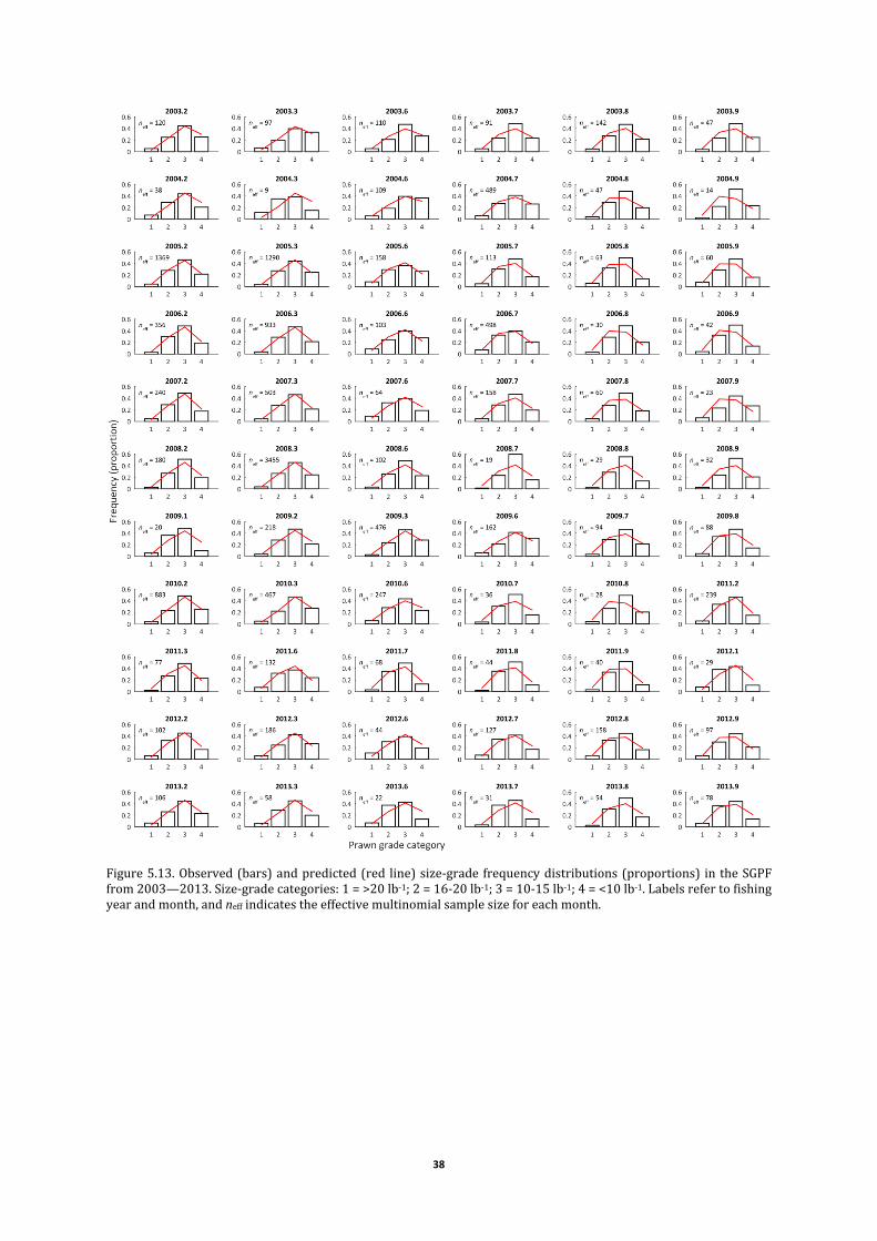
38

Figure5.13.Observed(bars)andpredicted(red line)size‐grade frequencydistributions(proportions) in theSGPFfrom2003—2013.Size‐gradecategories:1=>20lb‐1;2=16‐20lb‐1;3=10‐15lb‐1;4=<10lb‐1.Labelsrefertofishingyearandmonth,andneffindicatestheeffectivemultinomialsamplesizeforeachmonth.

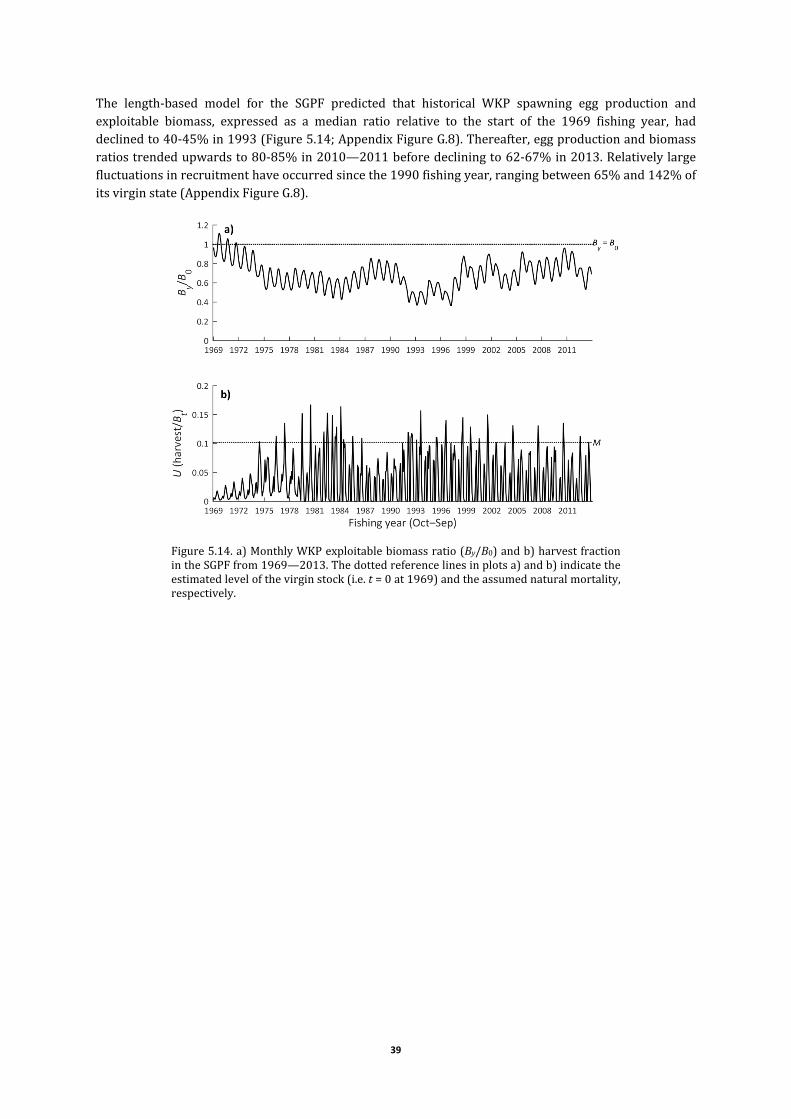
39

The length‐based model for the SGPF predicted that historical WKP spawning egg production andexploitable biomass, expressed as a median ratio relative to the start of the 1969 fishing year, haddeclinedto40‐45%in1993(Figure5.14;AppendixFigureG.8).Thereafter,eggproductionandbiomassratiostrendedupwardsto80‐85%in2010—2011beforedecliningto62‐67%in2013.Relativelylargefluctuationsinrecruitmenthaveoccurredsincethe1990fishingyear,rangingbetween65%and142%ofitsvirginstate(AppendixFigureG.8).

Figure5.14.a)MonthlyWKPexploitablebiomassratio(By/B0)andb)harvestfractionintheSGPFfrom1969—2013.Thedottedreferencelinesinplotsa)andb)indicatetheestimatedlevelofthevirginstock(i.e.t=0at1969)andtheassumednaturalmortality,respectively.

40

Virginrecruitment(R0)wasestimatedat2.99×108fortheSGPF(Figure5.15;Table5.3),andthestocksteepnessparameter(h)wascalibratedat0.83,indicatingthat83%ofpre‐fisheryrecruitment(R0)couldbe expected at 20% of virgin spawning stock. The recruitmentmode (μ1) was estimated in February,whichagreeswiththetimingoftheFebruarysurveydesignedformonitoringannualrecruitmentlevelsinthis fishery. Themean carapace length atwhich50%of theWKPpopulation is vulnerable to the gear

during fishing ( 50fl ) and surveys ( 50

sl )were 34.3mm and 31.1mm, respectively. Catchability (q) was

estimated to peak in February, with a low in August and amplitude of 33%. Instantaneous naturalmortality(M)wasfixedusingtheGSVpopulationestimateof0.102month‐1(XiaoandMcShane,2000a).No concerning correlations were evident among the key estimated parameters (Table 5.4), whichindicatesthatthemodelwasnotover‐parameterisedandissymptomaticofawell‐formulatedmodel.

Figure 5.15. Predicted relationships forWKP in the SGPF: a) stock‐recruitmentrelationship (based on 22 years of modelled stochastic recruitment, 1991—2013); b) recruitment pattern (proportion); c) fishery and survey catchability;andd)vulnerabilityatcarapacelength.

41

Table 5.3. Parameter estimates and standard errorsfor SGPF model calibration (NLL: Stage 1, ‐4604.1;Stage 2, ‐25.4). η1 corresponds to the first year forestimatingrecruitmentresiduals(1991).

Parameter EstimateStandarderror

Estimatetransformed

ξ 2.944 0.060 0.833Υ 1.094 0.012 2.986μ1 5.063 0.114κ 1.318 0.13450sl 31.121 0.148 δs 0.395 0.04550fl 34.280 0.133 δf 1.252 0.106ς 0.334 0.123ϑ ‐0.054 0.097η1 0.104 0.148η2 0.052 0.145η3 0.297 0.133η4 0.007 0.125η5 ‐0.161 0.101η6 0.373 0.112η7 0.539 0.133η8 ‐0.131 0.127η9 0.282 0.141η10 0.417 0.107η11 ‐0.200 0.122η12 ‐0.067 0.118η13 0.197 0.102η14 0.353 0.089η15 ‐0.169 0.089η16 0.281 0.106η17 0.060 0.089η18 0.147 0.097η19 0.372 0.096η20 ‐0.053 0.086η21 ‐0.192 0.106η22 0.086 0.101

Table 5.4. Correlation matrix of the ten leading model parametersestimated for the SGPF. Correlation strength increases with cell‐shadingintensity.

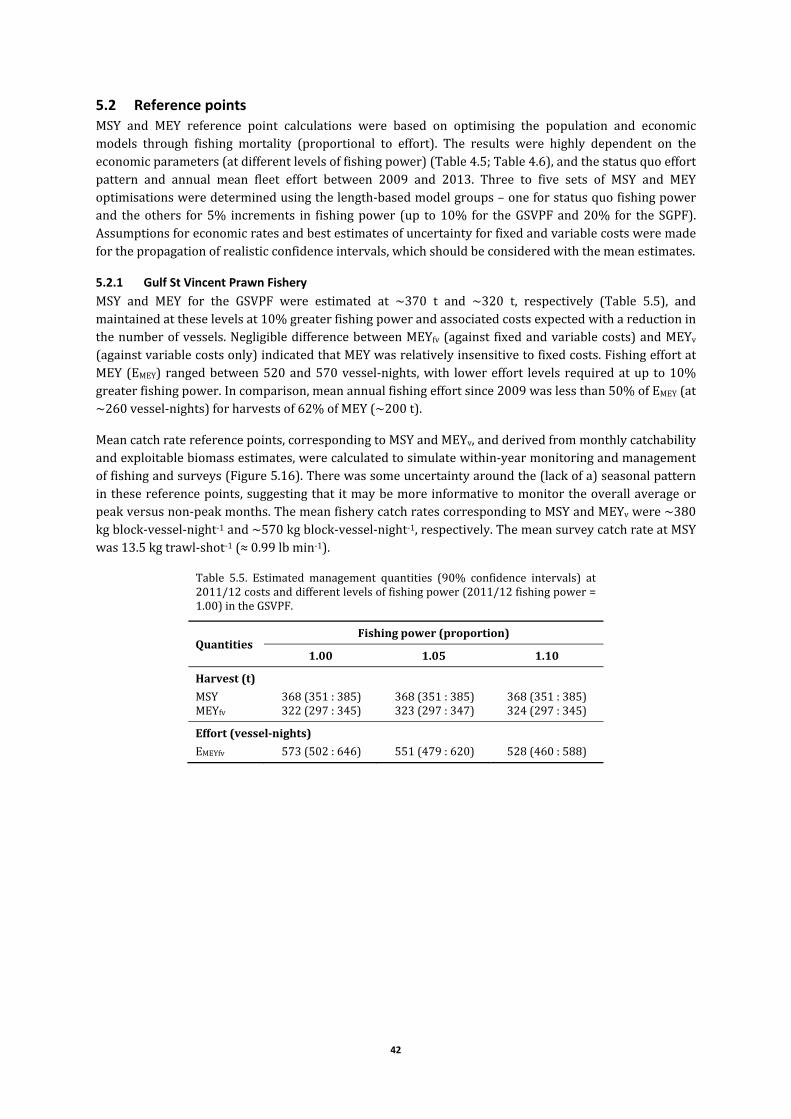
42

5.2 Reference points MSY and MEY reference point calculations were based on optimising the population and economicmodels through fishing mortality (proportional to effort). The results were highly dependent on theeconomicparameters(atdifferentlevelsoffishingpower)(Table4.5;Table4.6),andthestatusquoeffortpattern and annual mean fleet effort between 2009 and 2013. Three to five sets of MSY and MEYoptimisationsweredeterminedusingthelength‐basedmodelgroups–oneforstatusquofishingpowerand theothers for5% increments in fishingpower (up to10% for theGSVPFand20% for the SGPF).Assumptionsforeconomicratesandbestestimatesofuncertaintyforfixedandvariablecostsweremadeforthepropagationofrealisticconfidenceintervals,whichshouldbeconsideredwiththemeanestimates.


MSY and MEY for the GSVPF were estimated at ~370 t and ~320 t, respectively (Table 5.5), andmaintainedattheselevelsat10%greaterfishingpowerandassociatedcostsexpectedwithareductioninthenumberofvessels.NegligibledifferencebetweenMEYfv(againstfixedandvariablecosts)andMEYv(againstvariablecostsonly)indicatedthatMEYwasrelativelyinsensitivetofixedcosts.FishingeffortatMEY(EMEY) rangedbetween520and570vessel‐nights,with lowereffort levels requiredatup to10%greaterfishingpower.Incomparison,meanannualfishingeffortsince2009waslessthan50%ofEMEY(at~260vessel‐nights)forharvestsof62%ofMEY(~200t).

Meancatchratereferencepoints,correspondingtoMSYandMEYv,andderivedfrommonthlycatchabilityandexploitablebiomassestimates,werecalculatedtosimulatewithin‐yearmonitoringandmanagementoffishingandsurveys(Figure5.16).Therewassomeuncertaintyaroundthe(lackofa)seasonalpatterninthesereferencepoints,suggestingthat itmaybemoreinformativetomonitortheoverallaverageorpeakversusnon‐peakmonths.ThemeanfisherycatchratescorrespondingtoMSYandMEYvwere~380kgblock‐vessel‐night‐1and~570kgblock‐vessel‐night‐1,respectively.ThemeansurveycatchrateatMSYwas13.5kgtrawl‐shot‐1(≈0.99lbmin‐1).

Table 5.5. Estimated management quantities (90% confidence intervals) at2011/12costsanddifferentlevelsoffishingpower(2011/12fishingpower=1.00)intheGSVPF.

QuantitiesFishingpower(proportion)

1.00 1.05 1.10

Harvest(t)

MSY 368(351:385) 368(351:385) 368(351:385)MEYfv 322(297:345) 323(297:347) 324(297:345)

Effort(vessel‐nights)

EMEYfv 573(502:646) 551(479:620) 528(460:588)

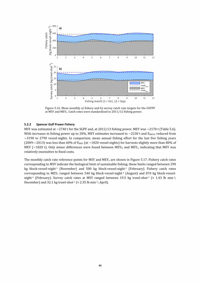
43

Figure5.16.Meanmonthlya)fisheryandb)surveycatchratetargetsfortheGSVPFatMSYandMEYv.Catchrateswerestandardisedto2011/12fishingpower.


MSYwasestimatedat~2740tfortheSGPFand,at2012/13fishingpower,MEYwas~2170t(Table5.6).Withincreasesinfishingpowerupto20%,MEYestimatesincreasedto~2230tandEMEYfvreducedfrom~3190 to 2790 vessel‐nights. In comparison,mean annual fishing effort for the last five fishing years(2009—2013)waslessthan60%ofEMEY(at~1820vessel‐nights)forharvestsslightlymorethan80%ofMEY(~1820 t).Onlyminordifferenceswere foundbetweenMEYfvandMEYv, indicating thatMEYwasrelativelyinsensitivetofixedcosts.

ThemonthlycatchratereferencepointsforMSYandMEYvareshowninFigure5.17.FisherycatchratescorrespondingtoMSYindicatethebiologicallimitofsustainablefishing;theselimitsrangedbetween290kg block‐vessel‐night‐1 (November) and 500 kg block‐vessel‐night‐1 (February). Fishery catch ratescorresponding toMEYv ranged between 540 kg block‐vessel‐night‐1 (August) and 870 kg block‐vessel‐night‐1 (February). Survey catch rates at MSY ranged between 19.5 kg trawl‐shot‐1 (≈ 1.43 lb min‐1;December)and32.1kgtrawl‐shot‐1(≈2.35lbmin‐1;April).

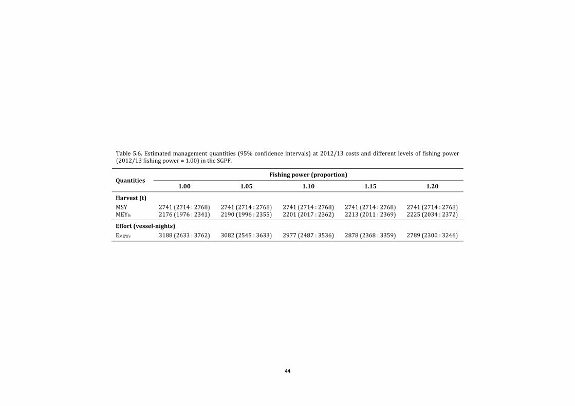
44

Table5.6.Estimatedmanagementquantities (95%confidence intervals) at2012/13costsanddifferent levelsof fishingpower(2012/13fishingpower=1.00)intheSGPF.

QuantitiesFishingpower(proportion)

1.00 1.05 1.10 1.15 1.20

Harvest(t)

MSY 2741(2714:2768) 2741(2714:2768) 2741(2714:2768) 2741(2714:2768) 2741(2714:2768)MEYfv 2176(1976:2341) 2190(1996:2355) 2201(2017:2362) 2213(2011:2369) 2225(2034:2372)

Effort(vessel‐nights)

EMEYfv 3188(2633:3762) 3082(2545:3633) 2977(2487:3536) 2878(2368:3359) 2789(2300:3246)

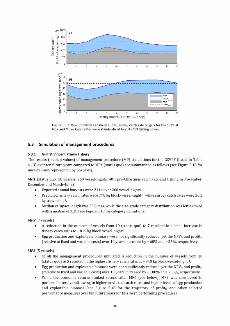
45

Figure5.17.Meanmonthlya)fisheryandb)surveycatchratetargetsfortheSGPFatMSYandMEYv.Catchrateswerestandardisedto2012/13fishingpower.

5.3 Simulation of management procedures


Theresults(medianvalues)ofmanagementprocedure(MP)simulations for theGSVPF(listed inTable4.13)overtenfutureyearscomparedtoMP1(statusquo)aresummarisedasfollows(seeFigure5.18foruncertaintiesrepresentedbyboxplots).

MP1(statusquo:10vessels,260vessel‐nights,40 tpre‐Christmascatchcap,and fishing inNovember,DecemberandMarch–June)

Expectedannualharvestswere211tover260vessel‐nights. Predictedfisherycatchrateswere778kgblock‐vessel‐night‐1,whilesurveycatchrateswere26.2

kgtrawl‐shot‐1. Mediancarapacelengthwas39.8mm,whilethesize‐gradecategorydistributionwasleft‐skewed

withamedianof3.28(seeFigure5.13forcategorydefinitions).

MP2(7vessels) Areduction in thenumberof vessels from10 (statusquo) to7 resulted ina small increase in

fisherycatchratesto~815kgblock‐vessel‐night‐1. Eggproductionandexploitablebiomasswerenotsignificantlyreduced,yettheNPVfvandprofitfv

(relativetofixedandvariablecosts)over10yearsincreasedby~60%and~35%,respectively.

MP3(5vessels) Of all the management procedures simulated, a reduction in the number of vessels from 10

(statusquo)to5resultedinthehighestfisherycatchratesat~840kgblock‐vessel‐night‐1. Eggproductionandexploitablebiomasswerenotsignificantlyreduced,yettheNPVfvandprofitfv

(relativetofixedandvariablecosts)over10yearsincreasedby~100%and~55%,respectively. While the economic returns ranked second after MP6 (see below), MP3 was considered to

performbetteroverall,owingtohigherpredictedcatchrates,andhigherlevelsofeggproductionand exploitable biomass (see Figure 5.18 for the trajectory of profitfv and other selectedperformancemeasuresovertenfutureyearsforthis‘best’performingprocedure).

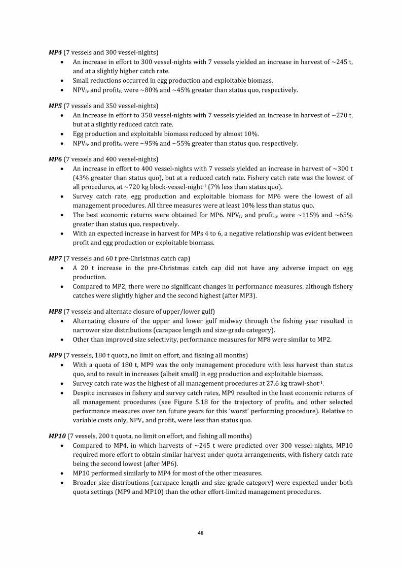
46

MP4(7vesselsand300vessel‐nights) Anincreaseineffortto300vessel‐nightswith7vesselsyieldedanincreaseinharvestof~245t,

andataslightlyhighercatchrate. Smallreductionsoccurredineggproductionandexploitablebiomass. NPVfvandprofitfvwere~80%and~45%greaterthanstatusquo,respectively.

MP5(7vesselsand350vessel‐nights) Anincreaseineffortto350vessel‐nightswith7vesselsyieldedanincreaseinharvestof~270t,

butataslightlyreducedcatchrate. Eggproductionandexploitablebiomassreducedbyalmost10%. NPVfvandprofitfvwere~95%and~55%greaterthanstatusquo,respectively.

MP6(7vesselsand400vessel‐nights) Anincreaseineffortto400vessel‐nightswith7vesselsyieldedanincreaseinharvestof~300t

(43%greaterthanstatusquo),butatareducedcatchrate.Fisherycatchratewasthelowestofallprocedures,at~720kgblock‐vessel‐night‐1(7%lessthanstatusquo).

Survey catch rate, egg production and exploitable biomass for MP6 were the lowest of allmanagementprocedures.Allthreemeasureswereatleast10%lessthanstatusquo.

Thebest economic returnswereobtained forMP6.NPVfv andprofitfvwere~115%and~65%greaterthanstatusquo,respectively.

WithanexpectedincreaseinharvestforMPs4to6,anegativerelationshipwasevidentbetweenprofitandeggproductionorexploitablebiomass.

MP7(7vesselsand60tpre‐Christmascatchcap) A 20 t increase in the pre‐Christmas catch cap did not have any adverse impact on egg

production. ComparedtoMP2,therewerenosignificantchangesinperformancemeasures,althoughfishery

catcheswereslightlyhigherandthesecondhighest(afterMP3).

MP8(7vesselsandalternateclosureofupper/lowergulf) Alternating closure of the upper and lower gulf midway through the fishing year resulted in

narrowersizedistributions(carapacelengthandsize‐gradecategory). Otherthanimprovedsizeselectivity,performancemeasuresforMP8weresimilartoMP2.

MP9(7vessels,180tquota,nolimitoneffort,andfishingallmonths) Withaquotaof180 t,MP9was theonlymanagementprocedurewith lessharvest thanstatus

quo,andtoresultinincreases(albeitsmall)ineggproductionandexploitablebiomass. Surveycatchratewasthehighestofallmanagementproceduresat27.6kgtrawl‐shot‐1. Despiteincreasesinfisheryandsurveycatchrates,MP9resultedintheleasteconomicreturnsof

all management procedures (see Figure 5.18 for the trajectory of profitfv and other selectedperformancemeasuresovertenfutureyearsforthis‘worst’performingprocedure).Relativetovariablecostsonly,NPVvandprofitvwerelessthanstatusquo.

MP10(7vessels,200tquota,nolimitoneffort,andfishingallmonths) Compared toMP4, inwhich harvests of ~245 t were predicted over 300 vessel‐nights, MP10

requiredmoreefforttoobtainsimilarharvestunderquotaarrangements,withfisherycatchratebeingthesecondlowest(afterMP6).

MP10performedsimilarlytoMP4formostoftheothermeasures. Broadersizedistributions(carapacelengthandsize‐gradecategory)wereexpectedunderboth

quotasettings(MP9andMP10)thantheothereffort‐limitedmanagementprocedures.

47

Generalcommentsonperformancemeasures: Achangeinharvestfromstatusquoresultedinachangeinexploitablebiomassintheopposite

direction,butnotnecessarilybythesamemagnitude. Thepercentagechangeforexploitablebiomass,surveycatchrateandeggproductionfromstatus

quowereapproximatelyequal,exceptforMP8,wheresurveycatchratewasreducedby8%withnochangeinbiomassoreggproduction;

Therewasnosignificantchange inmediancarapace lengthandsize‐gradecategoryamongthemanagementprocedures;alldifferenceswerewithin±2%ofstatusquo.

Allmanagementproceduresdemonstratedimprovementsineconomicperformance,exceptMP9,whereNPVvandprofitvwere8‐9%lessthanstatusquo.

48

Figure5.18.Performancemeasuresovertenfutureyears(2014—2023)fortendifferentWKPmanagementprocedures(MPs)fortheGSVPF(Table4.13). Plots a) and b) represented industry functioning, plots d), e), j) and k) represented themain performance indicators used in the currentmanagementplan(DixonandSloan,2007),plotsg)andh)measuredpopulationchange,andplotsc), f), i)and l)(lastcolumnofplots) indicatedeconomicconditions.Thedottedreferencelineindicatesthemedian(=1orestimatedvalue)forMP1(statusquo).Theplotsdisplaythesimulateddistributions(1000samples)aroundtheirmedians(solidlineinmiddleofeachbox).Thebottomandtopedgesofeachboxarethe25thand75thpercentiles,andthewhiskersindicate~95%coverageofthesimulationestimates.

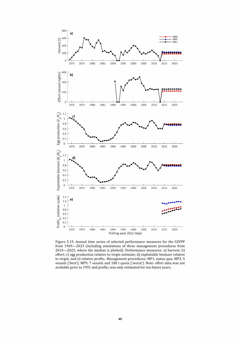
49

Figure5.19.Annual time series of selectedperformancemeasures for theGSVPFfrom 1969—2023 (including simulations of threemanagement procedures from2014—2023,wherethemedian isplotted).Performancemeasures:a)harvest;b)effort;c)eggproductionrelativetovirginestimate;d)exploitablebiomassrelativetovirgin;ande)relativeprofitfv.Managementprocedures:MP1,statusquo;MP3,5vessels(‘best’);MP9,7vesselsand180tquota(‘worst’).Note:effortdatawasnotavailablepriorto1991andprofitfvwasonlyestimatedfortenfutureyears.

50


The results (median values) ofmanagement procedure simulations for the SGPF (listed in Table 4.14)relativetoMP1(statusquo)aresummarisedasfollows(seeFigure5.20foruncertaintiesrepresentedbyboxplots):

MP1(statusquo:39vessels, 2000vessel‐nights, pre‐Christmas catch capdecision rules, and fishing inNovember,DecemberandMarch–June)

Expectedannualharvestswere~1650tover2000vessel‐nights. Predictedfisherycatchrateswere882kgblock‐vessel‐night‐1,whilesurveycatchrateswere58.9

kgtrawl‐shot‐1. Mediancarapacelengthwas40.4mmandmediansize‐gradecategorywas3.30(seeFigure5.13

forcategorydefinitions).

MP2(33vessels) Withthesamelevelofeffortasstatusquo,areductioninthenumberofvesselsto33resultedin

slight(~2‐3%)increasesinharvest(~1680t)andfisherycatchrate. Theslight increase inharvestresulted in~10%increase inNPVfvandprofitfv (relative to fixed

costs),whileeggproductionandexploitablebiomasswerenotsignificantlyreduced.

MP3(30vessels) A reduction in the number of vessels to 30 resulted in small (~5‐6%) increases in harvest

(~1730t)andfisherycatchrate. Anincreaseinharvestresultedin~15%increasesinNPVfvandprofitfv(relativetofixedcosts),

whileeggproductionandexploitablebiomasswerenotsignificantlyreduced.

MP4(20vessels,nopre‐Christmascatchcap,andfishingallmonths) Ofallthemanagementproceduressimulated,predictedharvestwasgreatestforMP4at~1940t

when the sizeof the fleetwashalved (to20vessels), andpre‐Christmas catch capand fishingmonthrestrictionswereremoved.

ThebesteconomicreturnswereobtainedforMP4;NPVfvandprofitfvwere60%and40%higherthan status quo, respectively (see Figure 5.20 for the trajectory of profitfv and other selectedperformancemeasuresovertenfutureyearsforthis‘best’performingprocedure).

Egg production and exploitable biomass were the lowest of the management procedures at~10%lessthanstatusquo.

MP5(12vessels,nopre‐Christmascatchcap,andfishingallmonths) Althoughareductioninthenumberofvesselsto12intheSGPFisunlikely,MP5wasincludedto

broadentherangeoffleetsizesandtherebyenableperformancetobeestimatedformanagementprocedureswithfleetsizesintermediatetothosesimulated.

ThehighestfisherycatchratewaspredictedforMP5at1050kgblock‐vessel‐night‐1,andprofitsweresecondhighest(afterMP4).

Althoughcatchratesandprofitswererelativelyhigh,12vesselswereunabletoreachstatusquoeffortandharvest levels,withonly~1200vessel‐nightsfished(60%)foraharvestof lessthan1400t(84%).

MP6(fisheryclosedNovember) Closure of the fishery in November did not increase egg production; it actually reduced egg

productionby5%. Reducedeggproductionislikelytobeattributedtotheredistributionofefforttohighercatch‐

ratemonths,resultinginincreasedharvestsandreducedexploitablebiomass. Alleconomicperformancemeasuresincreasedby10‐20%.

51

MP7(pre‐Christmascatchcapreducedby40%) Reducingthepre‐Christmascatchcapby40%didnotsignificantlyincreaseeggproduction. Annualharvestswerereducedby~100t,andeconomicreturnswereequalworst(withMP8and

MP11)ofallmanagementprocedures,withNPVandprofitsreducedby~10%(seeFigure5.20forthetrajectoryofprofitfvandotherselectedperformancemeasuresovertenfutureyearsforthis‘worst’performingprocedure).

Therewerenosignificantchangesintheremainingperformancemeasures;allotherdifferenceswerewithin±2%.

MP8(fisheryclosedMarch) ClosureofthefisheryinMarchdidnotsignificantlyincreaseexploitablebiomass,nordidithave

anyeffectonprawnsize. Redistributionofefforttoothermonthsresultedinreducedharvestsby~100tandequalworst

economicperformance(withMP7andMP11),withNPVandprofitsreducedby~10%. AllperformancemeasuresweresimilartothoseforMP7.

MP9(fisheryclosedJuneandpre‐Christmascatchcapincreasedby190t) OffsettingclosureofthefisheryinJunebyaddingthesametonnage(190t)tothepre‐Christmas

catchcapdidnotsignificantlyimpacteggproduction. DuetothehigherpricespaidatChristmas,NPVandprofitsincreasedby~10%.

MP10(northerngulfclosedMarch) ClosureofnortherngulfinMarchdidnothaveanyeffectonexploitablebiomassorprawnsize. Therewerenosignificantchangesinanyperformancemeasuresfromstatusquo;alldifferences

werewithin±2%.

MP11(fisheryclosedMarchandnortherngulfclosedApril) Closure of the fishery in March and the northern gulf in April did not significantly increase

exploitablebiomass,nordidithaveanyeffectonprawnsize. Redistributionof effort toothermonths resulted in reducedharvestsby~100 t and theequal

worsteconomicperformance(withMP7andMP8),withNPVandprofitsreducedby~10%.

MP12(‘NorthEnd’closedNovemberandDecember) Closureofthe‘NorthEnd’oftheGutterregiondidnotresultinincreasedeggproduction. Therewerenosignificantchangesinanyperformancemeasuresfromstatusquo;alldifferences

werewithin±2%.

MP13(1950tquota,nolimitoneffort,andfishingallmonths) Despiteaquotasettingof1950t,thepredictedharvestonlyreached1750t. Anincreaseinharvest(relativetostatusquo)resultedinincreasedNPVandprofits,butreduced

catchrates,eggproductionandexploitablebiomasswerealsopredicted. Fisheryandsurveycatchratesundera1950tquotawererelativelylowat797kgblock‐vessel‐

night‐1and56.7kgtrawl‐shot‐1,respectively.

MP14(2200tquota,nolimitoneffort,andfishingallmonths) Despiteaquotasettingof2200t,thepredictedharvestonlyreached1950t. Anincreaseinharvest(relativetostatusquo)resultedinincreasedNPVandprofits,butreduced

catchrates,eggproductionandexploitablebiomasswerealsopredicted. Fishery and survey catch rates under a 2200 t quota were the lowest of all management

proceduresat757kgblock‐vessel‐night‐1and54.2kgtrawl‐shot‐1,respectively.

52

Generalcommentsonperformancemeasures: Achangeinharvestfromstatusquoresultedinachangeinexploitablebiomassintheopposite

direction,butnotnecessarilybythesamemagnitude. The percentage change for exploitable biomass, survey catch rates and egg production from

statusquowereapproximatelyequal; Therewasnosignificantchange inmediancarapace lengthandsize‐gradecategoryamongthe

managementprocedures;alldifferenceswerewithin±2%ofstatusquo.

53

Figure5.20.Performancemeasuresovertenfutureyears(2014—2023)for14differentWKPmanagementprocedures(MPs)fortheSGPF(Table4.14). Plots a) and b) represented industry functioning, plots d), e), j) and k) represented themain performance indicators used in the currentmanagementplan(PIRSA,2014),plotsg)andh)measuredpopulationchange,andplotsc), f), i)and l) (lastcolumnofplots) indicatedeconomicconditions. The dotted reference line indicates the median (= 1 or estimated value) for MP1 (status quo). The plots display the simulateddistributions(1000samples)aroundtheirmedians(solidlineinmiddleofeachbox).Thebottomandtopedgesofeachboxarethe25thand75thpercentiles,andthewhiskersindicate~95%coverageofthesimulationestimates.

54

Figure5.21.Annual time series of selectedperformancemeasures for the SGPFfrom1969—2023(includingsimulationsof threemanagementprocedures from2014—2023,wherethemedianisplotted).Performancemeasures:a)harvest;b)effort; c) egg production relative to virgin estimate; d) exploitable biomassrelative to virgin; and e) relative profitfv. Management procedures:MP1, statusquo;MP4,20vessels;MP7,pre‐Christmascatchcapreducedby40%.Note:effortdatawasnotavailablepriorto1991andprofitfvwasonlyestimatedfortenfutureyears.

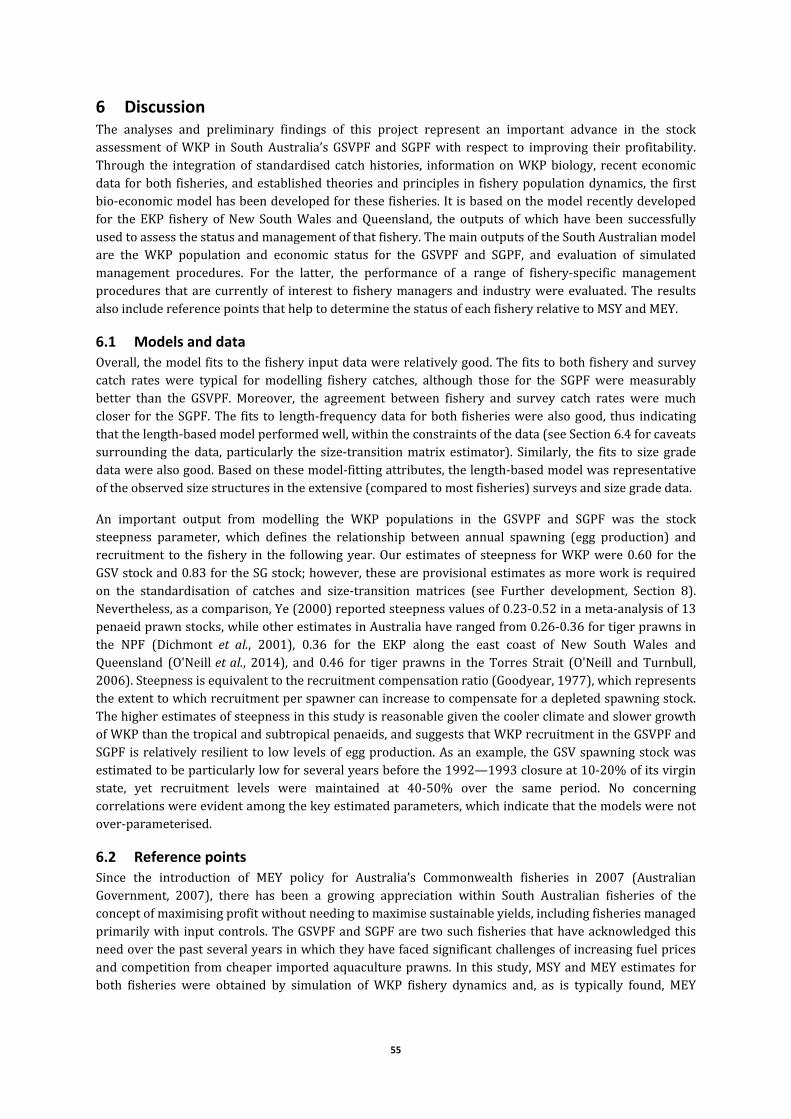
55

6 Discussion The analyses and preliminary findings of this project represent an important advance in the stockassessment ofWKP in SouthAustralia’sGSVPF and SGPFwith respect to improving their profitability.Through the integrationof standardised catchhistories, informationonWKPbiology, recent economicdata forbothfisheries,andestablishedtheoriesandprinciples in fisherypopulationdynamics,the firstbio‐economicmodelhasbeendevelopedforthesefisheries.Itisbasedonthemodelrecentlydevelopedfor the EKP fishery ofNew SouthWales andQueensland, the outputs ofwhichhave been successfullyusedtoassessthestatusandmanagementofthatfishery.ThemainoutputsoftheSouthAustralianmodelare the WKP population and economic status for the GSVPF and SGPF, and evaluation of simulatedmanagement procedures. For the latter, the performance of a range of fishery‐specific managementprocedures thatarecurrentlyof interest to fisherymanagersand industrywereevaluated.TheresultsalsoincludereferencepointsthathelptodeterminethestatusofeachfisheryrelativetoMSYandMEY.

6.1 Models and data Overall,themodelfitstothefisheryinputdatawererelativelygood.Thefitstobothfisheryandsurveycatch rates were typical for modelling fishery catches, although those for the SGPF were measurablybetter than the GSVPF. Moreover, the agreement between fishery and survey catch rates were muchcloser for theSGPF.The fits to length‐frequencydata forboth fisherieswerealsogood, thus indicatingthatthelength‐basedmodelperformedwell,withintheconstraintsofthedata(seeSection6.4forcaveatssurrounding thedata,particularly the size‐transitionmatrix estimator). Similarly, the fits to size gradedatawerealsogood.Basedonthesemodel‐fittingattributes,thelength‐basedmodelwasrepresentativeoftheobservedsizestructuresintheextensive(comparedtomostfisheries)surveysandsizegradedata.

An important output from modelling the WKP populations in the GSVPF and SGPF was the stocksteepness parameter, which defines the relationship between annual spawning (egg production) andrecruitment to the fishery in the followingyear.Ourestimatesof steepness forWKPwere0.60 for theGSVstockand0.83fortheSGstock;however,theseareprovisionalestimatesasmoreworkisrequiredon the standardisation of catches and size‐transition matrices (see Further development, Section 8).Nevertheless,asacomparison,Ye(2000)reportedsteepnessvaluesof0.23‐0.52inameta‐analysisof13penaeidprawnstocks,whileotherestimatesinAustraliahaverangedfrom0.26‐0.36fortigerprawnsinthe NPF (Dichmont et al., 2001), 0.36 for the EKP along the east coast of New South Wales andQueensland (O'Neilletal., 2014), and 0.46 for tiger prawns in the Torres Strait (O'Neill and Turnbull,2006).Steepnessisequivalenttotherecruitmentcompensationratio(Goodyear,1977),whichrepresentstheextenttowhichrecruitmentperspawnercanincreasetocompensateforadepletedspawningstock.ThehigherestimatesofsteepnessinthisstudyisreasonablegiventhecoolerclimateandslowergrowthofWKPthanthetropicalandsubtropicalpenaeids,andsuggeststhatWKPrecruitmentintheGSVPFandSGPFisrelativelyresilientto lowlevelsofeggproduction.Asanexample,theGSVspawningstockwasestimatedtobeparticularlylowforseveralyearsbeforethe1992—1993closureat10‐20%ofitsvirginstate, yet recruitment levels were maintained at 40‐50% over the same period. No concerningcorrelationswereevidentamongthekeyestimatedparameters,whichindicatethatthemodelswerenotover‐parameterised.

6.2 Reference points Since the introduction of MEY policy for Australia’s Commonwealth fisheries in 2007 (AustralianGovernment, 2007), there has been a growing appreciation within South Australian fisheries of theconceptofmaximisingprofitwithoutneedingtomaximisesustainableyields,includingfisheriesmanagedprimarilywith inputcontrols.TheGSVPFandSGPFaretwosuchfisheriesthathaveacknowledgedthisneedoverthepastseveralyearsinwhichtheyhavefacedsignificantchallengesofincreasingfuelpricesandcompetitionfromcheaper importedaquacultureprawns. Inthisstudy,MSYandMEYestimatesforboth fisheries were obtained by simulation of WKP fishery dynamics and, as is typically found, MEY

56

estimatesweresubstantiallylessthanMSY.Graftonetal.(2007)identifiedthatthisratio(ofMEYtoMSY)woulddecreasefurtherathigherfishingcostsand/orlowerproductprices.

Theveryflatnatureofthestock‐recruitmentrelationshipssuggeststhatthereislittleinformationaboutthedependenceof recruitmentoneggproduction.Since theestimationofMSYandMEY followcloselyfrom the stock‐recruitment relationship, it would be reasonable to question the reliability of theseinferredestimates.Therefore,whilstthemodelisabletoproduceestimatesofMSYandMEY,whicharepresentedinthisreport,theseestimatesshouldbetreatedasprovisionalanddemonstrationofsomeofthekeyoutputsfromthemodel.


FortheGSVPF,MSYwasestimatedat~370t.Duetothehighestimateofstocksteepness,highlevelsofeffortatMSY(EMSY)wereestimated,butthesewerenotconsideredrelevant tocurrentmanagementofthe fishery.Uncertainty surroundingEMSY isnotunusual in fisheries assessments, andemphasises thatthis limitshouldnotbeapproachedas it leads todiminishingprofitsand increasingriskofoverfishing(GarciaandStaples,2000).MEYestimatesof~320tfortheGSVPFwereinfluencedbythereportedhighvariablecostsoffishing.Intheabsenceofdetailedinformationonfishingpower,weseta10%increaseinfishing power, vessel and fuel costswith the removal of up to 5 vessels (50%) from the fleet. At thishigher fishingpower, lesseffortwasrequired toachieveMEY(EMEY:~570vessel‐nightsdownto~520vessel‐nights),butMEYestimatesthemselvesdidnotchange.

CatchratereferencepointscorrespondingtoMSYandMEYfortheGSVPFwere~380and~570kgblock‐vessel‐night‐1,respectively.Catchratesabovethesepointsindicatethattheexploitablebiomass(Bcurr)isgreaterthanthebiomassatMSY(BMSY).Asacomparison,theat‐seadecisionrulesofthecurrentharveststrategy(DixonandSloan,2007)requireclosureofareasorcessationoffishingifaveragenightlycatchesover two consecutive nights fall below 350 kg in November/December or 450 kg fromMarch—June.Althoughthecurrentrulesarelessconservative,aretrospectivecomparisonofthemeanmonthlycatchrateswith these referencepoints confirmeda reduced stock in2012.Theseobservations suggest that,underthecurrentleveloffishingpower(relatedtofleetsize)andfishingpattern,thereferencepointsforMSYandMEYmaybemoreappropriatecatchcriteria.


MSYfortheSGPFwasestimatedat~2740t.Increasesinfishingpower,vesselandfuelcostsbyupto20%required 14% less effort to achieveMEY than status quo (EMEYfv:~3190 vessel‐nights down to~2790vessel‐nights);MEYestimatesincreasedmarginally(by~2%).

MonthlycatchratereferencepointscorrespondingtoMSYfortheSGPFrangedbetween290and500kgblock‐vessel‐night‐1,andtheMEYreferencepointsrangedbetween540and870kgblock‐vessel‐night‐1.Theminimumfleetcatchrateofthecurrentharveststrategyisgenerallymoreconservativeat350‐600kg,dependingonmonthandregionofthegulf(PIRSA,2014).Nevertheless,retrospectivecomparisonofmonth‐specificreferencepointstomeanfisherycatchratesindicatedthatBcurr>BMSYsince1991.

Up to now, the stock status of the GSVPF or SGPF has been determined using a weight‐of‐evidenceapproach,and,recentlyfortheSGPF(Noelletal.,2014),estimatedproxiesforBMSYandBMEY.Despitetheinability to previously estimateMSY andMEY (without a bio‐economicmodel), it appears the currentempiricalreferencepointshavebeeneffectiveinmanagement.Thisismostlikelytohavebeentheresultofacombinationof:1)aneffectiveharveststrategy, inwhichsurveysareconductedpriorto fishingtoidentifyareasof target‐sizedprawnsandacceptableabundance;2) real‐timemonitoringofprawnsizeandcatchratesbythefleet;and3)conservativelimitsoninput(e.g.numberoffishingnights)andoutputcontrols(e.g.pre‐ChristmasfleetcatchcapfortheSGPF).

57

6.3 Management procedures Theaveragenumberofnightsfishedinrecentyearswas26pervesselintheGSVPFand51pervesselintheSGPF.Theserelativelylowlevelsofeffortsuggestedtestingastrategyofreducedvesselnumbers.Wetestedseveralstrategies.Thesetofmanagementproceduresimulationsforeachfisheryencompassedabroad spectrum of strategies developed in consultation with fisheries managers and industryrepresentatives. Specifically, they simulated the effects of reducing the numbers of vessels, increasingtotaleffort,modifyingharvestlevelsduringthepeakspawningperiod(November/December),temporalandspatialclosures,andimplementingharvestquotas.Theseproceduresrepresentedtheculminationofideasanddiscussionsthathadtakenplacewiththesestakeholdergroupsoverthepastfewyears.

Assuming the parameter estimates and uncertaintieswere realistic, all management procedures werepredicted to be biologically sustainable. However, despite our best estimates of variability of stockparameters for modelling WKP population dynamics, this may not always safeguard againstunpredictablestockbehaviour.Therefore,aholisticapproachwasusedinevaluatingeachmanagementprocedure, where we not only took into account the predicted change in catch rates and economicperformance measures from status quo, but also interpreted changes in exploitable biomass and eggproductionasrelativeindicatorstothestock.


Two recently conducted independent reviews for the GSVPF (Knuckey et al., 2011; Morgan andCartwright,2013)indicatedthattheoperationof10vesselsinthefisheryisunlikelytobeeconomicallyviableintheforeseeablefuture.Followingonfromtherecommendationsofthesereviews,theGSVPFiscurrentlybeingmanagedunder individual transferableeffort (tradablenights)arrangements toenableamalgamationofnights, the aimofwhich is to removevessels andexcess capacitybefore theplannednextstepofintroducingindividualtransferrablequotas(ITQs).Thismanagementdirectiontakenbythefishery influenced the specifications of the management procedures developed. All simulatedmanagementproceduresincludedareductioninthenumberofvessels(otherthanstatusquo),andtwooftheseincludedquota.

Of themanagement procedures simulated for the GSVPF, MP3, with a reduction in the fleet size to 5vessels, performed best in terms of increasedNPVfv(by~100%), profitfv (by~55%) and fishery catchratesfromstatusquo.Thesearelargeandimportantpotentialincreasesinprofitabilityhighlightedbythemodeloutputs,andareinaccordwiththelogicthatafishery(suchastheGSVPF)thatusesitsvesselslessthan 10% of the year is over‐capitalised and therefore economically underperforming. The vessel‐reductionstrategycurrentlybeingpursued in this fisherymakeperfectsense in termsof reducingthisseeminglyover‐capitalisationtoproduceamoreefficientoperationandrealisesomeoftheseprojectedgains.AlthoughMP6,withafleetsizeof7vesselsandtotaleffortof400vessel‐nights,resultedingreaterNPVfvandprofitfvthanMP3,significantreductionsinexploitablebiomassandeggproductionwerealsopredicted(unlikeMP3,wheretherewerenochangesinthesemeasures).Theimplementationofharvestquotas in MP9 and MP10 did not appear to offer any clear advantages to the other managementproceduresthatweretested.EconomicperformancemeasureswereattheirlowestforMP9,withaquotaof180t,andNPVvandprofitvwere lessthanstatusquodespiteasmaller fleetsize.MP10faredbetterwithaquotaof250t,althoughwhencomparedwithMP4,wheresimilarharvestswerepredictedwiththesamenumberofvessels(7),effortwasrelativelyhighandvariableandprawnsizewassmallerfornoadditionaleconomicreturn.


ItwasrelativelydifficulttoidentifythebestperformingmanagementprocedurefortheSGPF.Ofallthemanagementproceduressimulated,allfoureconomicperformancemeasureswerehighest(e.g.NPVfvandprofitfvwere60%and40%greaterthanstatusquo)forMP4,wherethenumberofvesselswasreducedto20andthepre‐Christmascatchcapwasremoved;however,exploitablebiomassandeggproductionweremarginallylower.Thismanagementprocedurewouldalsorequiresignificantresourcesandplanningto

58

finance the removal of vessels; these costs were not factored into the economic component of thesimulations. Consideration should also be given to the social implications for reducing the number ofvessels(Sloanetal.,2014;Triantafillosetal.,2014).

Amongtheothermanagementprocedures,MP2(33vessels),MP3(30vessels),MP6(Novemberclosure)or MP9 (June closure plus an increase in the pre‐Christmas catch cap) appeared to offer reasonablecompromisesbetweenincreasesinprofitfvandNPVfv intheorderof10‐20%,increasesornochangeinfisherycatchrates,andreductions inexploitablebiomassandeggproductionof lessthan5%.Of thesefour alternatives, MP6 or MP9 would be more straightforward, immediate and cost‐effective toimplementthantheremovalofvesselsunderMP2orMP3(andforasimilaroutcome).AsfortheGSVPF,the implementation of ITQs in the SGPF did not appear to offer any additional benefit to some of theeffort‐limitedprocedures.ComparedtoMP6andMP9,aquotaof1950tforMP13waspredictedtofareworsewith respect to every performancemeasure, andwhile a quota of 2200 t forMP14 resulted insimilareconomicperformance,itwasatthecostofsubstantiallyhigherlevelsofeffort(i.e.20%)atlowerfisherycatchrates,andreductionsinexploitablebiomassandeggproduction.

6.3.3 Overview of simulations

Ingeneral,wefoundthateconomicperformanceimprovedwithfewervessels(untilthereweretoofewvesselstofishatstatusquoeffortlevelsforthefleet,e.g.MP5fortheSGPF)and,fortheGSVPF,aseffortapproached EMEY. Unlike the GSVPF, variations in total fleet effort were not contemplated in thedevelopmentofmanagementproceduresfortheSGPF.However,preliminaryestimatesofMEYandEMEYinthisstudysuggestthatgreaterprofitsfortheSGPFmaybepossibleathigherlevelsofeffort,butwouldneedtobeevaluatedbysimulation.

Of themanagement procedures tested, therewas no evidence to suggest that quotawas thebestwayforwardforeitherfishery.However,astheprimarypurposeoftheprojectwastodevelopthemodelandnot to test anexhaustivenumberofmanagementprocedures, these resultsdonotnecessarily ruleoutquota for futuremanagement. Rather, they demonstrate a limited comparison of specificmanagementprocedures,andanychangestothesespecificationsshouldbeseparatelyevaluated.Forexample,the180tand250tquotasexaminedfortheGSVPFareconsiderablylessthantheestimatedmeanMEY,sowhiletheeconomicperformancemeasuresforthesemanagementproceduresfaredrelativelypoorly,theymaynotbeindicativeofafully‐utilisedresource.WhilethetransitiontoITQs(currentlybeingconsideredfortheGSVPF)mayhelptoensure thatprofitsarenotdissipatedthrough ‘raceto fish‘behaviorandover‐capitalisation,estimatesofharvest targetssuchasMEYcanbehighlyvariable.Updatingthemodelandobtaining revised estimates are also timedemanding,which presents the challenge of estimatingMEYwithinatimeframethatisrelevanttoWKPpopulationdynamics.

Should inputcontrolscontinuetobethepreferred instrument forfuturemanagementofeither fishery,theuseofcatchratereferencepointsthatrelateexploitablebiomasstoMSYorMEYmaybeappropriate.Given the potential variation inWKP population size between and within seasons, the monitoring offishery catches against MSY and MEY reference points can provide fishery managers and industryfeedback on the stock status and help to ensure that economic returns are optimised and the level ofharvestisappropriatetotheexploitablebiomass.Thisapproachemphasisestheimportanceofaccuratecatchmonitoring,soitisencouragingthattheSGWCPFAiscurrentlyinvestigatingthedevelopmentofanelectronic logbook for the SGPF. By monitoring catch rates against reference points, the fishery canaccount for the highs and lows of recruitment, and greater focus can be directed on managementstrategies rather than the uncertainty associated with MSY or MEY estimates. O'Neill et al. (2014)simulatedcatchratereferencepointsfortheEKPfisheryandfoundfavourableperformanceofcatchrateindicators,butonlywhenameaningfulupperlimitwasplacedontotalfleeteffort.

59

6.4 Data limitations and future research TheanalysespresentedinthisstudyarethemostcomprehensiveattemptthusfartoevaluatetheWKPpopulation and economic status of the GSVPF and SGPF through the development of the first bio‐economicmodelforthesefisheries.Althoughthebestavailabledatawereused,theuncertaintiesofsomemodelinputsarenotedhere.

Theestimatedspawner‐recruitmentparameterswerefundamentalfordeterminingstockstatus,andtheassessments assumed that standardised catch rates were proportional to abundance. Unfortunately,vessel‐specificdatawerenotavailablepriorto1991,whichprecludedstandardisationofthosecatches.Consequently,thereappearedtobelittlecontrast,withconsistenttimeseriesofharvestsandeffortsince1991,particularlyfortheSGPF.A lackofcontrast infisheriesdatacanbeproblematic inthat,althoughfisheries management is rarely treated as an experiment, it is difficult to fully understand withoutobservationhowrecruitmentwould respondoverabroad rangeof spawningstock sizes (WaltersandMartell,2004).

Despite a lack of contrast, model estimates of biomass appeared sensible throughout the fisheries’histories, respondingtothedifferent levelsofharvests inanexpectedmanner.Nevertheless, itbecameapparentduringanalysesthattheinclusionofbetterestimatesofexploitablebiomassinthemodelwouldhelp considerably to improve the reliability of the stockassessmentand referencepoints. In the latestindependent review of the GSVPF, Dichmont (2014) also identified the need for better estimates ofbiomassindices,andthatconsiderationshouldbegiventoconductingbiomasssurvey(s)withastratifiedrandom design or post‐stratification of existing survey data. Given that the fraction of prawns in thesweptareathatareactuallyretainedinthetrawlcodendcanhaveasignificantinfluenceonthebiomassestimate,theretentionfractionof~0.5forWKPfromJollandPenn(1990)mayalsorequireinvestigation.

Althoughmostmodelparametersarebasedontheresultsofauxiliarystudiesorbyfittingthemodeltotheavailabledata,thereareassumptionstowhichkeymodeloutputsaresensitive.Oneoftheassumedparameters for the model was instantaneous natural mortality (M). We used the estimate of 0.102month‐1 (1.22 year‐1) and priors derived fromWKP tag‐recapture data in the GSV (Xiao andMcShane,2000a).This isquite lowcomparedtootherpenaeidprawns,whichtendtohavemortalityrates intheorderof2.4±0.3year‐1(García,1988).Futureassessmentsmaybenefitfromsensitivityanalysisofthisparametertoexaminetheeffectofvaryingmortalityaroundthesevalues.

Profit outcomesof themodel are conditional on the economicdata.Due to confidentiality reasons,wewereunabletointerrogateeconomicdatatoverifytheaccuracyofthesuppliedmeansbyEconSearchordetermine the variances.We thereforehad to estimate a coefficient of variation for fixed and variablecosts so that reasonable estimates of uncertainty are passed through to the model outputs. In apresentation of the model and preliminary results to industry representatives, some licence holdersquestionedtheaccuracyofsomeoftheeconomicdata.Forexample,thecostoflabourasaproportionofthe catch value was thought to be too high at ~0.40. To address such concerns over therepresentativenessof theeconomicdata, it is essential that futureeconomic surveys includequestionstailored to the requirements for the bio‐economic model, and licence holders provide accurateinformation and authorisation for the use of the data.We also note simulations by Puntetal. (2010)includedprojectedannualfuelcostsperlitre,whereasinourstudythecostoffuelwasconstant.

Aspartoftheongoingdevelopmentofthebio‐economicmodel,itmaybeusefultoperiodicallycompareoutputswiththoseofadelay‐differencemodel,whichoffersadvantagesintermsofsimplifiedpopulationmathematicsandeasier testingofkeydatauncertainties(Schnute,1985;QuinnandDeriso,1999).TheDeriso‐Schnutedelay‐differencemodelhasbeenusedinthepasttoassesstheTorresStraittigerprawnfishery (O'Neill and Turnbull, 2006) and the NPF (Dichmont et al., 2001) and, more recently, as acomparisontothemorecomplexlength‐spatialmodelforassessmentoftheEKPfishery(Courtneyetal.,2014).Weanticipatethatitwouldberelativelystraightforwardtodevelopadelay‐differencemodelfor

60

comparisonwith thebio‐economicmodel. Alternatively, itmaybe suitable to runbio‐economicmodelsimulationsintheabsenceofastock‐recruitmentrelationship(givenitsflatnature).Ifthesesimulationswere to produce similar outcomes, thiswould increase the confidence in recommendations for futuremanagementoftheWKPresourcebasedonmodelling.

7 Benefits and adoption Themainbeneficiariesof thestudyare the licenceholders in theGSVPFandSGPF, the fishprocessorsinvolvedinthemarketingofWKP,andfisheriesmanagersatPIRSAFisheriesandAquaculture.

TheWKPbio‐economicmodeldeveloped in thisprojectwasused to calculate, forboth fisheries, catchrate reference points for MSY and MEY for the first time. Subject to further development of the bio‐economicmodel(seeSection8),thesereferencepointshavedirectapplicabilitytotheGSVPFandSGPFifmanagement continues toadopt the respectiveharvest strategy frameworksbasedon catch rates.Theprojectalsoevaluated10managementproceduresfortheGSVPFand14managementproceduresfortheSGPF that were developed in consultation with the fisheries manager from PIRSA and industryrepresentativesoftheSVGPBOAandSGWCPFA.Thesemanagementproceduresreflectdiscussionswiththese stakeholder groups over the past few years, and included reductions in the number of vessels,increasesineffort,changesinthepre‐Christmascatchcap,spatialand/ortemporalclosures,andquota.Arange of performance measures relating to industry functioning, current performance indicators,projected future population status and economics were used to evaluate each procedure. Analyses ofmanagement procedure simulations indicated that, in addition to a June closure and increase in pre‐ChristmascatchcapfortheSGPF,areductioninthenumberofvesselsgenerallyresultedingoodoverallperformance in both fisheries (although financing the removal of vessels was not included in thesimulations).

Preliminary results were presented to GSVPF licence holders and the management committee of theSGWCPFAon9September2014.AdoptionofthemainfindingspertainingtoMSY,MEYormanagementprocedures are contingent on further development of the model, ongoing dialogue between PIRSAFisheriesandAquaculture, SARDIand industry, andunderstanding,acceptanceandcommitmentbyallstakeholders.ThemodelhasbeenacknowledgedinthenewmanagementplanfortheSGPFasapotentialmotive for initiating a review of the recently‐updated harvest strategy (PIRSA, 2014). To increase thelikelihoodofadoptionintheSGPF,PIRSA,SARDIandindustryhaverecentlyagreedonastockassessmentdevelopmentprogramoverthenextfewyears,inwhichthebio‐economicmodelwillcompriseoneofthetools available to assistwith the program. For the GSVPF, a newmanagement plan is currently underdevelopment;itisexpectedthatasimilarpath(totheSGPF)willbefacilitatedtomovethefisheryclosertoadoptingthemodel.

WhilstthedevelopedmodelwillgreatlyimprovetheassessmentoftheGSVPFandSGPFwithrespecttoevaluatingbiologicalandeconomicperformance,itdoesnottellthefisheriesmanagersandindustryhowthefisheriesshouldbemanaged.Rather,subjecttofurtherdevelopment,thebio‐economicmodelshouldbeviewedasatoolthat isdesignedtoprovide informationaboutthecurrentstatusoftheWKPstocksrelative to theirbiologicalreferencepoints,andhowthestocksmightrespondtospecificmanagementactions.

8 Further development ThisstudyisafirstforWKPand,assuch,isapilotforfurtherdevelopment.Therefore,advicetoindustryandmanagersshouldbeappropriatetoandacknowledgeanylimitationsofthemodel.Asthemodellingofpopulationdynamicsandeconomics is complex, carewill alsobe taken toensure that this advice isdisseminatedinalanguagethatcanbeunderstood.

61

Future work should include sensitivity analyses of key parameters. For example, the estimated stocksteepnessparameterwasrelativelyhighcomparedtootherpenaeidstocksand,whileslowergrowthinacooler climatemay be a plausible explanation, it is important to understand the effect of varying thisparameteronmodeloutputs.Also,weassumedinstantaneousnaturalmortalityforWKPinSGtobethesame as the estimatederived from tag‐recapture studies inGSV. Sensitivity analysis of this parameterwouldindicatewhetheritisappropriatetousethesameestimateforbothstocks.

Standardisedcatchratesareclearlyoneofthe important inputsforthemodel.Therewassomelackofcontrastinthe1991—2013data,andunderthesecircumstances,modeloutputstendtobelesscertain.Furtheranalysesmaybeworthwhiletoexplorethepossibilityofincludingpre‐1991catchrates,astheymayprovidethecontrastrequiredforamoreaccuraterepresentationofabundanceandfishingmortality.The inclusion of other variables for better quantification of fishing power would also improve thestandardisation of catch rates. In themeantime, ifmodel estimates are to be used formanagement, itwouldbeprudentfordecision‐makerstoerrontheconservativesidewithrespecttoconfidenceintervalsprovidedwiththeseestimates.

Asnotedinthemethods,thecurrentbehaviourandvarianceinthesize‐transitionmatrices(FigureF.7;AppendixFigureG.7)maylimitsimultaneousmodelfitstothesizecompositionandstandardisedcatchratedata.Furtherexploratoryworkisrequiredtocompareasimplergammaapproach(Haddon,2001),buildthecurrentgrowthmodelintothestockmodel,andassesstheuseofatwo‐stagemodeltoestimategrowthbymodelling theprobabilityofmoulting, togetherwithadistribution for themoult increment.Thelattercouldbegamma‐distributedandwouldnotdependonthelengthoftheprawn.Theprobabilityofmoultingwoulddependonlength(withlargerprawnsmoultinglessoften)andbechosentomakethemean growth increment (including the zeroes)match the postulated growth curve. Application of thelatterideawilldependonthedistributionalformofthetag‐recapturedata.

MEYissensitivetochangesinfishingcostsandfishprices;howeveritisnotfeasibletoupdatethemodelandadjustMEYwithrespecttoshort‐termfluctuationsinfactorsaffectingMEY(AustralianGovernment,2007).Whilst3‐5yearsisappropriateformostfishstocks,a2‐yeartimeframemaybemoreappropriateforshort‐livedspeciessuchasWKP.TheharveststrategiesfortheGSVPFandSGPFwouldthereforeneedtobeflexibleinthisregard.Intheinterim,someofthedatalimitations(e.g.concernswiththeeconomicdata) and future research (e.g. compare outputs with those of a delay‐difference model) outlined inSection6.4couldbeaddressed.

9 Planned outcomes The project outputs have contributed directly to the planned outcomes. A major advance in thequantitative stockassessment capabilities for theGSVPFandSGPF isnowavailablewith theWKPbio‐economicmodel.Forthefirsttime,model‐derivedreferencepointsforMSYandMEYwereestimatedandmanagementprocedureswereevaluated.Althoughfurtherdevelopmentofanewly‐developedmodel isinevitable, the resultspresentedcanbeconsideredreal‐life examplesofhow themodel cancontributetowardsgreaterprofitabilityforthesefisheries.

10 Conclusion Objective1.CollateandanalyseavailabledatafortheGulfStVincentandSpencerGulfprawnfisheriesforintegrationintothebio‐economicmodel.

This objective has beenmet. The development of theWKP bio‐economicmodelwould not have beenpossiblewithout consolidatingmuchof the informationanddataon theGSVPandSGPF thathasbeengenerated overmany years of research conducted to supportmanagement of these fisheries. Furtheranalyses were done for each fishery to standardise commercial and survey catch rates, estimate

62

exploitablebiomass, identifyprobabilityof recruitmentby lengthandgeneratemonthly size‐transitionmatricesformaleandfemaleprawns.AllmodelinputswereformattedinExcel.

Objective 2.Modify the existing Eastern King Prawn bio‐economicmodel to fit the Gulf St Vincent andSpencerGulfprawnfisheriesdata.

This objective has beenmet. Themodel forWKPwas adapted from the EKPmodel and developed inMatlabwiththeinputdatafromObjective1.Duringthefittingprocess,weencountereddifferentmodelsolutions fromthesizecompositiondataversus thestandardisedcatchrates.Toaddress thisproblem,themaximumlikelihoodestimationprocesswasconducted intwostages: firstly, toestimateselectivityand recruitment pattern parameters; and secondly, to fix these parameters in a second optimisationtunedprimarily to catch ratedata.This twostageapproachwasundesirableand furtherworkbeyondthisprojectisrequiredtoachievesimultaneousmodelfitstoboththesizecompositionandstandardisedcatchratedata.

Objective 3. Determine economically optimal fishing strategies for the Gulf St Vincent and Spencer Gulfprawnfisheries.

This objective has beenmet. A key output of themodel is the evaluation ofmanagement strategies. Arange of management procedures were developed in consultation with industry and the fisheriesmanager,andtheseincludedreductionsinthenumberofvessels,increasesineffort,changesinthepre‐Christmascatchcap,spatialand/ortemporalclosures,andquota.Simulationsindicatedthat,inadditionto a June closure and increase in pre‐Christmas catch cap for the SGPF, a reduction in the number ofvessels generally resulted in good overall performance in both fisheries, whereas quota did little toimproveprofitability.

Objective4.Developanapproachtoincorporateoptimalfishingstrategiesintotheharveststrategyforeachfishery.

Thisobjectivehasbeenpartiallymet.PreliminaryresultswerepresentedtoGSVPFlicenceholdersandthemanagementcommitteeoftheSGWCPFAon9September2014.Furtherpresentationsarelikelytoberequired,butthiswillbedeterminedinresponsetoneedsof industryandmanagement,asadoptionofthemainfindingspertainingtoMSY,MEYoroptimalmanagementproceduresarecontingentonfurtherdiscussion, acceptance and commitment between all stakeholder groups. We are confident that theproject’sfindingwillinfluencefutureharveststrategydevelopmentfortheGSVPFandSGPF.ThemodelhasbeenacknowledgedinthenewmanagementplanfortheSGPFasapotentialmotivefor initiatingareviewoftherecently‐updatedharveststrategy(PIRSA,2014)and,fortheGSVPF,therehasbeenregulardialoguewithPIRSAinrelationtocompletionofthisprojectandtheimpendingdevelopmentofthenextharveststrategy.

Objective5.Provideextensionof thedevelopedmodeland itsoutputs to stakeholdersofotherAustralianprawntrawlfisheries.

This objective is ongoing. Following completion of the project, the model will undergo furtherdevelopment, regular updates with new data, and simulation of different management procedures asrequired.Whilstextensionofthemodeland itsoutputswillcontinuetobeprovidedtostakeholdersoftheGSVPFandSGPF,extensiontostakeholdersofotherAustralianprawntrawlfisherieswillbeprovidedbydistributionofthefinalreporttotheAustralianCouncilforPrawnFisheries,industryassociationsandprawnresearchersinotherStates.Uponfurtherdevelopmentofthemodel,weplantoalsocommunicatefindings to these groups by publication in a peer‐reviewed journal and presentation at a relevantconference.

63

11 References Australian Government (2007). Commonwealth Fisheries Harvest Strategy: Policy and Guidelines.

Canberra,Australia:DepartmentofAgriculture,FisheriesandForestry.

BOM (2014). Climate data online. Bureau of Meteorology. URLhttp://www.bom.gov.au/climate/data/index.shtml(lastaccessed27September2013).

Box, G. E. P.& Cox,D. R. (1964). An analysis of transformations. JournaloftheRoyalStatisticalSociety.SeriesB(Methodological),211‐252.

Carrick,N.A.(2003).SpencerGulfPrawn(Melicertuslatisulcatus)Fishery.FisheryassessmentreporttoPIRSA Fisheries. RD03/0079‐2. Adelaide, South Australia: South Australian Research andDevelopmentInstitute(AquaticSciences).

Carrick,N.A.&Ostendorf,B. (2005).Modellingprawnmovementand spatialdynamics in theSpencerGulfandWestCoastPrawnFisheries.Canberra,Australia.

Chen, Y., Hunter, M., Vadas, R. & Beal, B. (2003). Developing a growth‐transitionmatrix for the stockassessment of the green sea urchin (Strongylocentrotusdroebachiensis) off Maine. FisheryBulletin101,737‐744.

Courtney,A. J.,O'Neill,M.F.,Braccini,M.,Leigh,G.M.,Kienzle,M.,Pascoe,S.,Prosser,A. J.,Wang,Y.‐G.,Lloyd‐Jones,L.,Campbell,A.B.,Ives,M.,Montgomery,S.S.&Gorring,J.(2014).Biologyandeconomicsmanagement strategy evaluations of the eastern king prawn fishery. Department of Agriculture,Fisheries and Forestry, Queensland: Fisheries Research and Development Corporation, Project No.2008/019.

Department of FisheriesWestern Australia (2014). SharkBayPrawnManagedFisheryHarvestStrategy2014‐2019.FisheriesManagementPaperNo.267.Perth,WesternAustralia:DepartmentofFisheries,GovernmentofWesternAustralia.

Dichmont, C.M. (2014).Areviewofthestockassessmentmethods,processesandoutputsfortheGulfofStVincent Prawn Fishery. A report for Primary Industries and Regions South Australia. Brisbane,Australia:CSIRO.

Dichmont, C.M., Deng, A., Punt, A. E., Ellis,N., Venables,W.N., Kompas, T., Ye, Y., Zhou, S.&Bishop, J.(2008). Beyond biological performance measures in management strategy evaluation: Bringing ineconomicsandtheeffectsoftrawlingonthebenthos.FisheriesResearch94,238‐250.

Dichmont,C.M.,Die,D.,Punt,A.E.,Venables,W.,Bishop, J.,Deng,A.&Dell,Q.(2001).RiskanalysisandsustainabilityindicatorsforprawnstocksintheNorthernPrawnFishery:CSIROMarineResearch.

Dixon, C. & Sloan, S. (2007).ManagementPlan for theSouthAustralianGulfStVincentPrawnFishery.SouthAustralianFisheriesManagementSeries,No.53.Adelaide,SouthAustralia:PrimaryIndustriesandResourcesSouthAustralia.

Dixon, C. D., Hooper, G. E. & Burch, P. (2012). Gulf St Vincent Prawn Penaeus(Melicertus) latisulcatusFishery2010/11.FisheryassessmentreporttoPIRSAFisheriesandAquaculture.SARDIPublicationNo.F2007/000782–5, SARDIResearchReportSeriesNo.631.Adelaide,Australia:SouthAustralianResearchandDevelopmentInstitute(AquaticSciences).

EconSearch (2009). Economic indicators for the Gulf St Vincent Prawn Fishery 2007/08. A reportprepared for Primary Industries and Resources South Australia. Marryatville, South Australia:EconSearch.



EconSearch(2013).EconomicindicatorsforthecommercialfisheriesofSouthAustraliasummaryreport2011/12.AreporttoPIRSAFisheriesandAquaculture.Marryatville,SouthAustralia:EconSearch.

EconSearch(2014).EconomicindicatorsfortheSouthAustralianSpencerGulfPrawnFishery2012/13.AreporttoPIRSAFisheriesandAquaculture.Marryatville,SouthAustralia:EconSearch.

Fisheries Queensland (2013). Stock Status of Queensland's Fisheries Resources 2012: Department ofAgriculture,FisheriesandForestry,StateofQueensland.

64

Fox,J.(2003).EffectdisplaysinRforgeneralisedlinearmodels.JournalofStatisticalSoftware8,1‐27.

Fox, J. & Hong, J. (2009). Effect displays in R for multinomial and proportional‐odds logit models:Extensionstotheeffectspackage.JournalofStatisticalSoftware32,1‐24.

Fox, J. & Monette, G. (1992). Generalized collinearity diagnostics. Journal of the American StatisticalAssociation87,178‐183.

Francis,R. I.C.C. (2011).Corrigendum:Dataweighting instatistical fisheriesstockassessmentmodels.CanadianJournalofFisheries&AquaticSciences68,2228‐2228.

Francis,R. I.C.C.&Hilborn,R. (2011).Dataweighting in statistical fisheries stockassessmentmodels.CanadianJournalofFisheries&AquaticSciences68,1124‐1138.

García, S. (1988). Tropical penaeid prawns. Fishpopulationdynamics:the implicationsformanagement,219‐249.

Garcia,S.M.&Staples,D.J.(2000).Sustainabilityreferencesystemsandindicatorsforresponsiblemarinecapture fisheries: a reviewof conceptsandelements fora setof guidelines.MarineandFreshwaterResearch51,385‐426.

Gillett,R.(2008).GlobalstudyofshrimpfisheriesFAOFisheriesTechnicalPaperNo.475,Rome:FAO.

Goodyear,C.P.(1977).Assessingtheimpactofpowerplantmortalityonthecompensatoryreserveoffishpopulations. InProceedingsoftheconferenceonassessingtheeffectsofpower‐plant‐inducedmortalityonfishpopulations.

Grafton,R.Q.,Kompas,T.&Hilborn,R.W.(2007).Economicsofoverexploitationrevisited.science318,1601‐1601.

Haddon,M.(2001).Modellingandquantitativemethodsinfisheries:CRCpress.

Hall,N.(2000).Modellingtoexploremanagementstrategiestooptimisethevalueoftherocklobsterfisheryof Western Australia: Fisheries Western Australia [and] Fisheries Research & DevelopmentCorporation.

Hall,N.G.&Watson,R.A.(2000).Aspatialrepresentationofthetigerprawn(Penaeusesculentus)fisheryin Shark Bay, Western Australia. FishMovementandMigration’.(EdsDAHancock,DCSmithand JDKoehn.)pp,212‐230.

Hilborn,R.(2002).Thedarksideofreferencepoints.Bulletinofmarinescience70,403‐408.

Joll, L.M.&Penn, J.W. (1990).The applicationofhigh‐resolutionnavigation systems toLeslie‐DeLurydepletionexperimentsforthemeasurementof trawlefficiencyunderopen‐seaconditions.FisheriesResearch9,41‐55.

Kendall,M.G.,Stuart,A.&Ord,J.K.(1983).TheAdvancedTheoryofStatistics,vol.3.Griffin,London.

Kirkpatrick,S.,Gelatt,C.D.&Vecchi,M.P.(1983).Optimizationbysimulatedannealing.science220,671‐680.

Knuckey, I., Kompas, T. & Bodsworth, A. (2011). ReviewoftheGulfofStVincentPrawnFishery. OceanGrove,Victoria:CobaltMRMPtyLtdforPIRSAFisheriesandAquaculture‐September2011.(Internalreport.).

Macdonald,P.&Du,J.(2012).Mixdist:finitemixturedistributionmodels.Rpackageversion0.5‐4.

Mardia,K.V.&Jupp,P.E.(2009).Directionalstatistics:JohnWiley&Sons.

MathWorks (2014). MATLAB. The Language of Technical Computing. R2014a. Natick, MA, US: TheMathWorks,Inc.

Maunder,M.N.&Punt,A.E.(2004).Standardizingcatchandeffortdata:areviewofrecentapproaches.FisheriesResearch70,141‐159.

McGarvey, R., Punt, A. E., Gardner, C., Feenstra, J., Hartmann, K., Hoshino, E., Burch, P., Paterson, S.,Matthews,J.M.&Linnane,A.(2014).BioeconomicdecisionsupporttoolsforSouthernRockLobster.

McLachlan,G.&Peel,D.(2004).Finitemixturemodels:JohnWiley&Sons.

Möbius,A.F.(1827).DerbarycentrischeCalcul,einHülfsmittelzuranalytischenBehandlungderGeometrie(etc.)‐Leipzig,Barth1827:Barth.

Morgan,G.&Cartwright, I. (2013).ReviewoftheGulfStVincentPrawnFisheryManagementFramework.Adelaide,SouthAustralia‐July2013.(Internalreport.).

Nelder, J. A.&Wedderburn, R.W.M. (1972). Generalized linearmodels. JournaloftheRoyalStatisticalSociety.SeriesA(General)135,370‐384.

65

Noell,C. J.,Hooper,G.E.&Beckmann,C.L.(2014).SpencerGulfPrawnPenaeus(Melicertus)latisulcatusFishery2012/13.FisheryassessmentreporttoPIRSAFisheriesandAquaculture.SARDIPublicationNo.F2007/000770–7, SARDIResearchReportSeriesNo.788.Adelaide,Australia:SouthAustralianResearchandDevelopmentInstitute(AquaticSciences).

O'Neill,M.F.,Courtney,A.J.,Good,N.M.,Turnbull,C.T.,Yeomans,K.M.,StauntonSmith,J.&Shootingstar,C. (2005). Reference pointmanagement and the role of catch‐per‐unit effort in prawn and scallopfisheries.

O'Neill,M.F.,Leigh,G.M.,Martin,J.M.,Newman,S.J.,Chambers,M.,Dichmont,C.M.&Buckworth,R.C.(2011). Sustainingproductivity of tropical red snappersusingnewmonitoringand referencepoints:Queensland.DepartmentofEmployment,EconomicDevelopmentandInnovation.

O'Neill,M.F.,Leigh,G.M.,Wang,Y.‐G.,Braccini,J.M.&Ives,M.C.(2014).Linkingspatialstockdynamicsand economics: evaluation of indicators and fishery management for the travelling eastern kingprawn(Melicertusplebejus).ICESJournalofMarineScience:JournalduConseil,fst218.

O'Neill, M. F. & Turnbull, C. (2006). Stockassessmentof theTorresStrait tigerprawn fishery (Penaeusesculentus):DepartmentofPrimaryIndustriesandFisheries.

Pennington,M.&Vølstad,J.H.(1994).Assessingtheeffectofintra‐haulcorrelationandvariabledensityonestimatesofpopulationcharacteristicsfrommarinesurveys.Biometrics,725‐732.

PIRSA (2014).ManagementPlanfortheSouthAustralianCommercialSpencerGulfPrawnFishery. SouthAustralian FisheriesManagement Series, No. 67. Adelaide, SouthAustralia: Primary Industries andRegionsSouthAustralia.

Punt,A.E.,Deng,R.A.,Dichmont,C.M.,Kompas,T.,Venables,W.N.,Zhou,S.,Pascoe,S.,Hutton,T.,Kenyon,R., vanderVelde,T.&Kienzle,M. (2010). Integrating size‐structuredassessmentandbioeconomicmanagementadvice inAustralia'snorthernprawnfishery.ICESJournalofMarineScience:JournalduConseil67,1785‐1801.

Punt, A. E. &Kennedy, R. B. (1997). Populationmodelling of Tasmanian rock lobster, Jasus edwardsii,resources.MarineandFreshwaterResearch48,967‐980.

Quinn,T.J.&Deriso,R.B.(1999).Quantitativefishdynamics:OxfordUniversityPress.

R Core Team (2013). R: A language and environment for statistical computing. Vienna, Austria: RFoundationforStatisticalComputing.URLhttp://www.R‐project.org/.

Richards, L. J., Schnute, J. T. & Olsen, N. (1998). A statistical framework for analysis of limit referencepoints. In Fishery Stock AssessmentModels. Proceedings of the International Symposium on FisheryStockAssessmentModelsforthe,pp.8‐11.

Ross,S.M.(1995).IntroductiontoStochasticDynamicProgramming.

Rowling, K., Hegarty, A.‐M. & Ives,M. (2010). Status of fisheries resources in NSW 2008/09. StatusoffisheriesresourcesinNSW2008/09.

Sadovy,Y.,Punt,A.E.,Cheung,W.,Vasconcellos,M.,Suharti,S.&Mapstone,B.D.(2007).StockAssessmentApproach fortheNapoleonFish,CheilinusUndulatus, in Indonesia:ATool forQuota‐setting forData‐poorFisheriesUnderCITESAppendixIINon‐detrimentFindingRequirements:FAO.

Schnute,J.(1985).Ageneraltheoryforanalysisofcatchandeffortdata.CanadianJournalofFisheriesandAquaticSciences42,414‐429.

Sklyarenko, E. G. (2011). Barycentric coordinates. Encyclopedia of Mathematics. URLhttp://www.encyclopediaofmath.org/index.php/Barycentric_coordinates (last accessed 14September2014).

Sloan,S.,Smith,T.,Gardner,C.,Crosthwaite,K.,Triantafillos,L.,Jeffriess,B.&Kimber,N.(2014).NationalGuidelines toDevelopFisheryHarvestStrategies. Adelaide, South Australia: Fisheries Research andDevelopmentCorporation,ProjectNo.2010/061.

Triantafillos, L.,Brooks,K., Schirmer, J., Pascoe, S., Cannard,T.,Dichmont, C., Thebaud,O.& Jebreen,E.(2014).DevelopingandTestingSocialObjectivesforFisheriesManagement.Adelaide,SouthAustralia:FisheriesResearchandDevelopmentCorporation,ProjectNo.2010/040.

USNO (2014). Fraction of the moon illuminated. U.S. Naval Observatory. URLhttp://aa.usno.navy.mil/data/docs/MoonFraction.php(lastaccessed14September2014).

Walters,C.J.&Martell,S.J.D.(2004).Fisheriesecologyandmanagement:PrincetonUniversityPress.

Xiao, Y. (1999).General age‐ and time‐dependent growthmodels for animals.FisheryBulletin97, 690‐701.

66

Xiao,Y.(2000).UseoftheoriginalvonBertalanffygrowthmodeltodescribethegrowthofbarramundi,Latescalcarifer(Bloch).FisheryBulletin98.

Xiao,Y.&McShane,P.(2000a).Estimationofinstantaneousratesoffishingandnaturalmortalitiesfrommark–recapturedataonthewesternkingprawnPenaeuslatisulcatusintheGulfSt.Vincent,Australia,byconditionallikelihood.TransactionsoftheAmericanFisheriesSociety129,1005‐1017.

Xiao,Y.&McShane,P. (2000b).Useofage‐and time‐dependent seasonalgrowthmodels inanalysisoftag/recapturedataonthewesternkingprawnPenaeuslatisulcatusintheGulfSt.Vincent,Australia.FisheriesResearch49,85‐92.

Ye,Y.(2000).Isrecruitmentrelatedtospawningstockinpenaeidshrimpfisheries?ICESJournalofMarineScience:JournalduConseil57,1103‐1109.

67

Appendix A Intellectual property Thisresearchisforthepublicdomain.Thereportandanyresultingscientificpublicationsareintendedfor wide dissemination and promotion. All data and statistics presented comply with confidentialityarrangements.Matlabcodeforthebio‐economicmodelcanbemadeavailableuponrequesttoCN.

Appendix B Staff DrCraigNoell(ResearchScientist,SARDIAquaticSciences) DrMichaelO’Neill(PrincipalResearchScientist,DAFF,Qld) DrJonathanCarroll(ResearchScientist,SARDIAquaticSciences) DrCameronDixon(Director,ImprovingSustainableProductionPtyLtd;previouslyatSARDI)

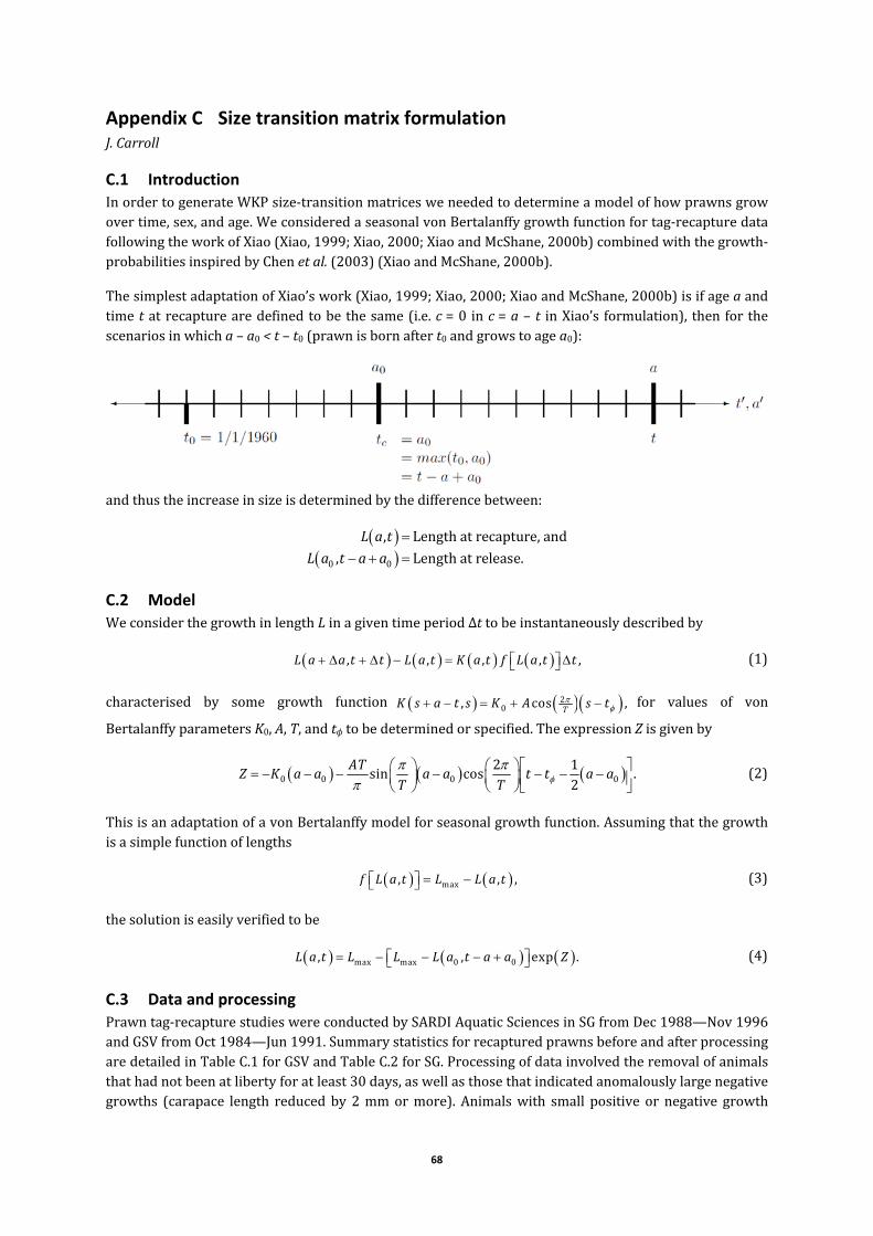
68

Appendix C Size transition matrix formulation J.Carroll

C.1 Introduction InordertogenerateWKPsize‐transitionmatricesweneededtodetermineamodelofhowprawnsgrowovertime,sex,andage.WeconsideredaseasonalvonBertalanffygrowthfunctionfortag‐recapturedatafollowingtheworkofXiao(Xiao,1999;Xiao,2000;XiaoandMcShane,2000b)combinedwiththegrowth‐probabilitiesinspiredbyChenetal.(2003)(XiaoandMcShane,2000b).

ThesimplestadaptationofXiao’swork(Xiao,1999;Xiao,2000;XiaoandMcShane,2000b)isifageaandtimetatrecapturearedefinedtobethesame(i.e.c=0 inc=a–t inXiao’s formulation), thenforthescenariosinwhicha–a0<t–t0(prawnisbornaftert0andgrowstoagea0):

andthustheincreaseinsizeisdeterminedbythedifferencebetween:

0 0

, Lengthatrecapture,and

, Lengthatrelease.

L a t

L a t a a

C.2 Model WeconsiderthegrowthinlengthLinagiventimeperiodΔttobeinstantaneouslydescribedby

, , , , ,L a a t t L a t K a t f L a t t (1)

characterised by some growth function 2

0, cos ,TK s a t s K A s t for values of von

BertalanffyparametersK0,A,T,andtϕtobedeterminedorspecified.TheexpressionZisgivenby

0 0 0 02 1

sin cos .2

ATZ K a a a a t t a a

T T (2)

ThisisanadaptationofavonBertalanffymodelforseasonalgrowthfunction.Assumingthatthegrowthisasimplefunctionoflengths

max, , ,f L a t L L a t (3)

thesolutioniseasilyverifiedtobe

max max 0 0, , exp .L a t L L L a t a a Z (4)

C.3 Data and processing Prawntag‐recapturestudieswereconductedbySARDIAquaticSciencesinSGfromDec1988—Nov1996andGSVfromOct1984—Jun1991.SummarystatisticsforrecapturedprawnsbeforeandafterprocessingaredetailedinTableC.1forGSVandTableC.2forSG.Processingofdatainvolvedtheremovalofanimalsthathadnotbeenatlibertyforatleast30days,aswellasthosethatindicatedanomalouslylargenegativegrowths (carapace length reduced by 2mmormore). Animalswith small positive or negative growth

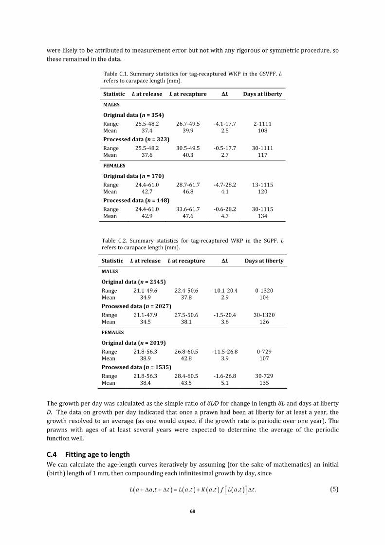
69

werelikelytobeattributedtomeasurementerrorbutnotwithanyrigorousorsymmetricprocedure,sotheseremainedinthedata.

TableC.1.Summarystatistics for tag‐recapturedWKP in theGSVPF.Lreferstocarapacelength(mm).

Table C.2. Summary statistics for tag‐recaptured WKP in the SGPF. Lreferstocarapacelength(mm).

ThegrowthperdaywascalculatedasthesimpleratioofδL∕DforchangeinlengthδLanddaysatlibertyD. Thedataongrowthperday indicatedthatonceaprawnhadbeenat liberty forat leastayear, thegrowthresolved toanaverage (asonewouldexpect if thegrowthrate isperiodicoveroneyear).Theprawns with ages of at least several years were expected to determine the average of the periodicfunctionwell.

C.4 Fitting age to length Wecancalculate theage‐lengthcurves iterativelybyassuming (for thesakeofmathematics)an initial(birth)lengthof1mm,thencompoundingeachinfinitesimalgrowthbyday,since

, , , , .L a a t t L a t K a t f L a t t (5)

Statistic Latrelease Latrecapture ΔL Daysatliberty

MALES

Originaldata(n=354)

Range 25.5‐48.2 26.7‐49.5 ‐4.1‐17.7 2‐1111Mean 37.4 39.9 2.5 108

Processeddata(n=323)

Range 25.5‐48.2 30.5‐49.5 ‐0.5‐17.7 30‐1111Mean 37.6 40.3 2.7 117

FEMALES

Originaldata(n=170)

Range 24.4‐61.0 28.7‐61.7 ‐4.7‐28.2 13‐1115Mean 42.7 46.8 4.1 120


Range 24.4‐61.0 33.6‐61.7 ‐0.6‐28.2 30‐1115Mean 42.9 47.6 4.7 134

Statistic Latrelease Latrecapture ΔL Daysatliberty

MALES

Originaldata(n=2545)

Range 21.1‐49.6 22.4‐50.6 ‐10.1‐20.4 0‐1320Mean 34.9 37.8 2.9 104


Range 21.1‐47.9 27.5‐50.6 ‐1.5‐20.4 30‐1320Mean 34.5 38.1 3.6 126

FEMALES

Originaldata(n=2019)

Range 21.8‐56.3 26.8‐60.5 ‐11.5‐26.8 0‐729Mean 38.9 42.8 3.9 107


Range 21.8‐56.3 28.4‐60.5 ‐1.6‐26.8 30‐729Mean 38.4 43.5 5.1 135

70

Inthisscenario,weuseΔt=1dayandtreattheformulaiteratively.Wefindthatthemodelisnothighlysensitivetotheinitiallengthusedintheiterativeprocedure.

C.5 Derivation of the growth function Giventheinstantaneousgrowthfunction

02

, cos ,K a t K A t tT

(6)

wewishtosolveEq.(5).WecanTaylorexpandthis,assumingthatda∕dt=1andweobtainthepartialdifferentialequation

, ,, , .

L a t L a tK a t f L a t

a t (7)

Wethenwishtosolve

max

, ,, , ,

L a t L a tK a t L L a t

a t (8)

thesolutionforwhichrequiresconstraininganarbitraryvaluewhichwecanfixbyspecifyingtheinitiallengthasL(a0,t–a+a0).Insertingthisvalue,weobtain

max max 0 0, , exp ,L a t L L L a t a a Z (9)

whereZreducesto

0 0 02 sin 2 sin 2

.2

K a a AT t t T AT a a t t TZ (10)

Usingtheidentity

sin sin 2sin cos ,

2 2 (11)

wecantransformZtobethesameasEq.(2).

C.6 Derivation of size transition probabilities (non‐seasonal) This derivation follows the results of Chen etal. (2003). Assuming a simple von Bertalanffy growthfunctionoflengthatagiventime‐stepLtwithvonBertalanffyparameters,suchas:

01 ,K t ttL L e (12)

thegrowthinagiventimestep(e.g.1month)isgivenby:

0 0

0 0

11 1 1

.

K t t K t tt t

K t t K t tK

L L L L e L e

L L e e L L e (13)

Eq.(12)canberearrangedtogive 0K t t

tL L L e andwesubstitutethisintotheabovetogive

71

1 .K

tL L L e (14)

Using the fit values L andK as estimates of the actual parameters, the probability of growth from

lengthL′tolengthbinLisgivenby

max

min,Var .

L

L L LP f x L L dx (15)

Themean L isdefinedassimplyEq.(14)withestimatesinserted.

1 .K

tL L L e (16)

Ifweassumethattheestimatesapproximatethetruevaluessuchthat

, ,L L L K K K (17)

where theerrorsarenormallydistributedas 2 2norm 0, , norm 0, ,L KL K thenwecanwrite

Eq.(14)(utilisingtheTaylorexpansionofeΔx~1+Δx)as

1

1

.

Kt

K K Kt

L L L e

L L e L L Ke L Ke

L

(18)

WewishtofindthevarianceofΔL,whichcomprisesseveralterms.Werequiretheidentity

2

1 1 , ;

Var Var 2 Cov , .n n

i i i i i j i ji i i j i j

a X a X a a X X (19)

InEq.(18),L issimplyanumber,andthushasnovariance.Theremainingtermsweconsiderviatheidentityabove;

2

1 1 11 , , VarKLa e X L X (20)

2

2 2 2, , Var .Kt Ka L L e X K X (21)

WeneglectthehigherorderΔL∞ΔKterm,andapplytheidentitytowhatremains

2 21 1 2 2 1 2Var Var Var 2Cov ,L a X a X X X (22)

2 22 2 21

2Cov , 1 ,

K KL t K

K K

e L L e

L K e L L e (23)

which is the expression found inChen et al. (2003). This is now sufficient information to calculateEq.(15) (i.e. Eq.(43)) and generate the transition probabilities, which can be used to populate a sizetransitionmatrix.

72

ValuesofσL∞,σK, andCov(L∞,K) are calculated aspart of the ‘nls’ fittingprocedure. For simplicity, the

function fis taken tobeanormaldistributionwithmean L andvarianceVar(ΔL∞), thoughnegative

growthsareneglected.

C.7 Derivation of size transition probabilities (seasonal) Wewishtoreproducetheprevioussection’scalculationsforatime‐dependentvonBertalanffyequation.IfwetakeEq.(12)andallowforaseasonalvariation

0,1 ,Z t ttL L e (24)

where the functionZ(t,t0) isnow thatwhichwasobtained in thederivationof thegrowth functionviaMathematica®,butwiththereplacement(a–a0)→(t–t0)

0 0 0 02 2

, sin sin .2 2AT AT

Z t t K t t t t t tT T

(25)

Thecombinationofthesin(x)+sin(y)functionintoasin(x)cos(y)functionislesselegantinthiscase,andweretaintheformer.Inthiscase,thegrowthinonetimestep(e.g.1month)isgivenby

0 0

0

1, ,1

1,

1 1

,

Z t t Z t tt t t

Z t tt

L L L L L e L e

L L L e (26)

usingthereplacementoftherearrangementofEq.(24)

0, .Z t t

tL e L L (27)

TheexponentZ(t+1,t0)requirescarefulconsideration

0 0 0 02 2

1, 1 sin 1 sin .2 2AT AT

Z t t K t t t t t tT T

(28)

Wecanusetheidentity

sin sin cos cos sin , (29)

torearrangethecentraltermintheabove,suchthat

2 2 2 2 2 2sin sin cos cos sin .t t t t t t

T T T T T T (30)

IfwenowTaylorexpandthetime‐independenttrigonometricfunctions,as

2 32 22 2 2

cos ~ 1 , sin ~ ,2! 3!

T T

T T T (31)

thenwefind

2 2 2 2 2

sin sin cos ,t t t t t tT T T T T

(32)

andthustheexponentissimplified;

73

0 0 0

0

2 21, sin sin

2 22 2

cos2

2 2, cos ,

2

AT ATZ t t K t t t t t t

T TAT

K t tT TAT

Z t t K t tT T

(33)

andthus

2

0 0

2cos

21, , ,

ATK t t

TZ t t Z t te e e (34)

andconsequently,Eq.(26)becomes

0

2

0

2

1,

2cos

2,

2cos

21 .

Z t tt

ATK t t

TZ t tt

ATK t t

Tt

L L L L e

L L L e e

L L e

(35)

Usingthefitvalues,themeanchangeinlengthissimply

22

cos2

1 .

ATK t t

TtL L L e (36)

Ifweassumethattheerrorsintheseestimatesarenormallydistributed,as

2norm 0, ,LL (37)

2norm 0, ,KK (38)

2norm 0, ,AA (39)

2norm 0, ,tt (40)

thentheexpandedversionofEq.(35)becomes

.tL L L (41)

C.8 Size‐transition matrix

As defined in Sadovyetal. (2007) the size‐transitionmatrix ,s sL L describes the approximation to the

probabilitydensity function forarandomindividualofsexstogrowfromsize‐classL′ intosize‐classLoveratimestep,as

2

,,, , 2

,

1; exp ,

2s s

s s s s

s ss

Ks Kss s sL L

L L L LL L sL

L L e L e (42)

74

whereL∞,sandKsarethevonBertalanffygrowthparametersforprawnsofsexs, sL istheaverage(mid‐

point)ofsize‐classLs.

Alternatively,asperChenetal.(2003)thetransitionmatrixcanbepopulatedbyprobabilities

max

, , , ,min,Var ,s

s

L

L s L s s sLP f x L L dx (43)

whereinthiscase,

1 .K

tL L L e (44)

75

Appendix D Running Matlab *.m files ThesectionbelowdescribestypicalstepsinWKPstocksimulationmodelling.

With the Matlab code you can estimate MSY/MEY and stock status, quantify uncertainty using theestimatedparametercovariancematrixorMCMCposteriors,projecteffectsofmanagementproceduresonfuturestatusandperformancemeasuresandgraphicallyvisualiseresults.

D.1 Load data structures 1. (Start)Selectfisheryandensure*.xlsxdataarecompleteandformattedasrequired.2. (Load)Type‘sa_wkp_1_data_load’atcommandprompt.

D.2 Setup parameters and negative log‐likelihoods 1. (Setupfixparsandestpars)Selectmodelparameters,type‘sa_wkp_2_param_setup’atcommand

prompt.2. (Setupnllonoff)SelectNLL’sfordataandparameterstoestimate,type‘sa_wkp_4_nll’atprompt.

or

Import(load)savedmodelparameters(estpars,fixpars,mle,nllonoff)from*.matfile.

D.3 Run stock model (‘sa_wkp_3_popdyn_model’) 1. Run m‐file section ‘Run model with current parameter values and plot’ in ‘sa_wkp_optimise’.

Outputssavedintostructures[negll,nll,pred,r].2. Modelstatuswithcurrent‘estpars’canbevisualisedbytyping‘sa_wkp_5_modelplots’atprompt.3. If model components are changed, e.g. qs, ensure ‘sa_wkp_6_popdyn_eqmodel_msymey’ and

‘sa_wkp_9_mse_model’areconsistent.

D.4 Fit stock model to data (‘sa_wkp_optimise’) 1. Runm‐filesection‘Fitandsavemaximumlikelihoodsolution’in‘sa_wkp_optimise’.Optimisation

app,withplots,canalsobeusedhere.a. Firsttrysingleoptimisationruns,thenb. Longcycleruns(overnightorweekend,fminconthenfminsearch).

2. Runsimulatedannealingafterusingoptimisersabove.ThiswillsearchforfurtherMLsolutionsand estimate covariance matrix for MCMC; type ‘mcmc_wrapper_wkp_simulated_annealing’ atprompt.(longruntime;5xnparamsx5000sims).

3. RunMCMCaftersimulatedannealingtoquantifyparameterdistributions.Type ‘sa_wkp_mcmc”atprompt.(longruntimelikeabove).

4. PlotMLestimatedparameterstoevaluatemodelfitbytyping‘sa_wkp_5_modelplots’atprompt.5. Evaluate MCMC parameter simulations using R ‘coda’ package. Use R file

‘R_mcmc_diagnostic_code.R’.SaveMCMCsimulatedparametersinto*.csvfile.

D.5 Reference points (‘sa_wkp_6_eq_refpts’) 1. (Section 1) Reference point estimation on current estpars; simple visual plot included; select

monthlyeffortpatternandobjective.2. (Section2)Referencepointsimulationsforerrors.Referencepointssimulatedfordifferenteffort

patterns,threeobjectives(MSY,MEYfvandMEYv),managementcostsandfishingpowers.3. (Section3)Analyseequilibriumreferencepoints,includingempiricalmeasures.

****************************

D.6 Management procedures (‘sa_wkp_8_mse’) 1. Simulationofmanagementprocedures(MP)canrunseparatetotheprevioussteps.Section1of

‘sa_wkp_8_mse’ loads historical data (‘sa_wkp_1_data_load’) and management data

76

(‘sa_wkp_7_mse_data_load’), and sets data for the simulations. Near line 35, simulationparametersneedtobesetorloadedfromm‐file.

2. Now run the simulation for each MP from Section 2 of ‘sa_wkp_8_mse’ using m‐file‘sa_wkp_9_mse_model’,storingresultsdataintostructuresim.

3. SimulationswillbesavedaccordingtothefisherylabelinMP,withadatetag.

D.7 Analyse management procedures (‘sa_wkp_10_mse_analysis’) 1. This m‐file analyses future simulations for evaluating WKP management procedures (aka

managementstrategyevaluation,MSE).(Section1)Firstpartofm‐fileloadsthesimdatafroma*.matfile.

2. (Section2)Herethesimdataarereshapedforanalysingeachkeyperformancemeasure.3. (Section3)BoxplotsofperformancemeasuresforeachMP.

77

Appendix E Input data summaries

E.1 Standardised commercial catch rates Themodellingofcommercialcatchrates intheGSVPFandSGPFwascarriedoutondaily logbookdatafromfishingyears1991—2013.Olderdatainthefisheriescouldnotberesolvedspatiallyortovesselandwerethereforenotstandardised.ThreeGLMtypeswereexploredforpredictingtheyear‐montheffectoncommercialcatches(inkgblock‐vessel‐night‐1):1)aGaussiannormalerrordistributionandidentitylinkfittedtocubic‐root transformedcatches;2)aPoissondistributionwith log linkanderrorsadjustedforoverdispersion(called‘quasipoisson’inR);and3)aGaussiandistributionwithidentitylink(FigureE.1;E.5). By virtue of residuals most closely resembling a normal distribution, the cube root model waspreferred for standardising catch rates in both fisheries (Figure E.4; E.8). The standardised andunstandardisedmodelfitsshowedsomedifferences,particularlyfortheGSVPF,butnotinoveralltrend(FigureE.1).Effortwasbyfarthemostinfluentialvariableonstandardisedcatches,althoughyear‐month,region, vessel, lunarphaseand, for the SGPFonly, cloud cover,were alsohighly significant (TableE.1;E.2). Overall goodness‐of‐fit was high, with adjusted R2 values of 0.86 and 0.74 for GSVPF and SGPFmodels,respectively.

FigureE.1.Comparisonofmodel‐predictedandunstandardised(nominalreporteddata)meancommercialcatchrates by year‐month in the GSVPF. The cube root transformation was chosen for the final model, where thestandardisedcatchbyavesselinablockpernightwaspredictedbyregion,hoursfished,vessel,lunarphaseandcloudcover.

FigureE.2.DiagnosticplotsofthePoissonGLMfittedtoGSVPFcommercialcatches.

78

FigureE.3.DiagnosticplotsoftheGaussianGLMfittedtountransformedGSVPFcommercialcatches.

Figure E.4. Diagnostic plots of the Gaussian GLM fitted to cube‐root transformed GSVPFcommercialcatches.

Table E.1. Analysis of deviance table for the cube root GLM used tostandardise commercial catch rates in the GSVPF (R2adj = 0.86).Abbreviations:SS,sumofsquares;df,degreesof freedom;F,F‐statistic;P,probability.

Sourceofvariation SS df F P

Year‐month 5375 103 59.7 <2.20E‐16Region 297 9 37.7 <2.20E‐16Effort (hours)⅓ 77954 1 89136.2 <2.20E‐16Vessel 158 9 20.1 <2.20E‐16Lunarphase* 44 1 50.8 1.07E‐12Lunarphase(lagged¼phase) 67 1 77.0 <2.20E‐16Cloud cover† 9 1 10.77 0.00104Residuals 13158 15045

*FractionofthemoonilluminatedatmidnightAEST.†Meanfractionfromthree‐hourlyreadingsbetween1800and0600hours.

79

Figure E.5. Comparison of model‐predicted and unstandardised (nominal reported data) mean commercial catchrates by year‐month in the SGPF. The cube root transformation was chosen for the final model, where thestandardisedcatchbyavesselinablockpernightwaspredictedbyregion,hoursfished,vesselandlunarphase.

FigureE.6.DiagnosticplotsofthePoissonGLMfittedtoSGPFcommercialcatches.

FigureE.7.DiagnosticplotsoftheGaussianGLMfittedtountransformedSGPFcommercialcatches.

80

Figure E.8. Diagnostic plots of the Gaussian GLM fitted to cube‐root transformed SGPFcommercialcatches.

Table E.2. Analysis of deviance table for the cube root GLM used tostandardise commercial catch rates in the SGPF (R2adj = 0.74).Abbreviations:SS, sumof squares;df,degreesof freedom;F,F‐statistic;P,probability.


Year‐month 72870 140 371.9 <2.20E‐16Region 14759 9 1171.6 <2.20E‐16Effort(hours)⅓ 168727 1 120547.7 <2.20E‐16Vessel 2613 38 49.1 <2.20E‐16Lunarphase* 6725 1 4804.8 <2.20E‐16Lunarphase(lagged¼phase) 4582 1 3273.9 <2.20E‐16Residuals 95875 68498

*FractionofthemoonilluminatedatmidnightAEST.

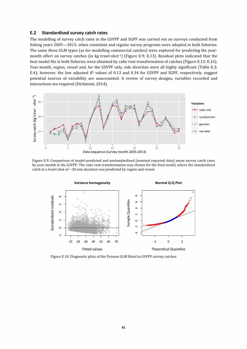
81

E.2 Standardised survey catch rates ThemodellingofsurveycatchratesintheGSVPFandSGPFwascarriedoutonsurveysconductedfromfishingyears2005—2013,whenconsistentandregularsurveyprogramswereadoptedinbothfisheries.ThesamethreeGLMtypes(asformodellingcommercialcatches)wereexploredforpredictingtheyear‐montheffectonsurveycatches (inkg trawl‐shot‐1) (FigureE.9;E.13).Residualplots indicated that thebestmodelfitsinbothfisherieswereobtainedbycuberoottransformationofcatches(FigureE.12;E.16).Year‐month,region,vesseland, fortheGSVPFonly, tidedirectionwereallhighlysignificant(TableE.3;E.4); however, the low adjustedR2 values of 0.13 and 0.34 for GSVPF and SGPF, respectively, suggestpotential sources of variability are unaccounted. A review of survey designs, variables recorded andinteractionsarerequired(Dichmont,2014).

FigureE.9.Comparisonofmodel‐predictedandunstandardised(nominalreporteddata)meansurveycatchratesbyyear‐monthintheGSVPF.Thecuberoottransformationwaschosenforthefinalmodel,wherethestandardisedcatchinatrawlshotof~30mindurationwaspredictedbyregionandvessel.

FigureE.10.DiagnosticplotsofthePoissonGLMfittedtoGSVPFsurveycatches.

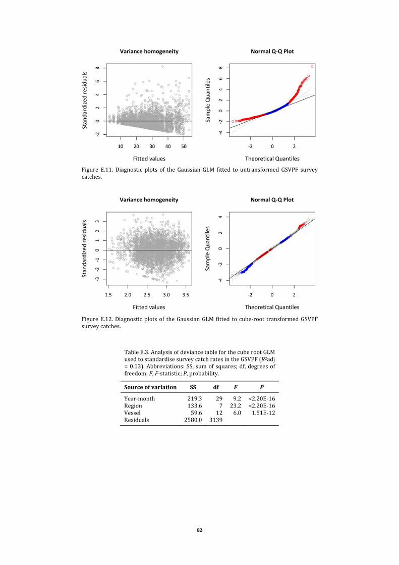
82

Figure E.11.Diagnostic plots of theGaussianGLM fitted to untransformedGSVPF surveycatches.

FigureE.12.Diagnosticplotsof theGaussianGLM fitted to cube‐root transformedGSVPFsurveycatches.

TableE.3.AnalysisofdeviancetableforthecuberootGLMusedtostandardisesurveycatchratesintheGSVPF(R2adj=0.13).Abbreviations:SS, sumofsquares;df,degreesoffreedom;F,F‐statistic;P,probability.


Year‐month 219.3 29 9.2 <2.20E‐16Region 133.6 7 23.2 <2.20E‐16Vessel 59.6 12 6.0 1.51E‐12Residuals 2580.0 3139

83

FigureE.13.Comparisonofmodel‐predictedandunstandardised(nominalreporteddata)meansurveycatchratesbyyear‐monthintheSGPF.Thecuberoottransformationwaschosenforthefinalmodel,wherethestandardisedcatchinatrawlshotof~30mindurationwaspredictedbyregion,vesselandtidedirection.

FigureE.14.DiagnosticplotsofthePoissonGLMfittedtoGSVPFsurveycatches.

Figure E.15. Diagnostic plots of the Gaussian GLM fitted to untransformed SGPF surveycatches.

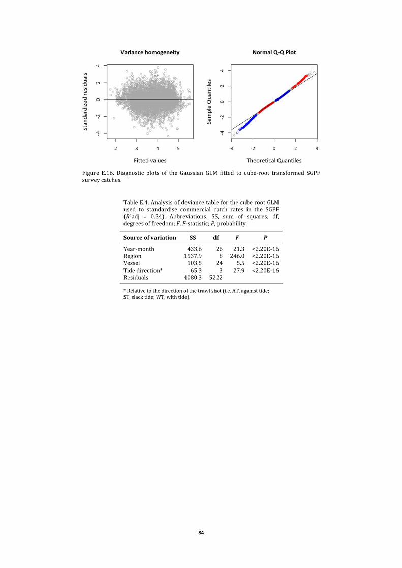
84

Figure E.16. Diagnostic plots of the Gaussian GLM fitted to cube‐root transformed SGPFsurveycatches.

TableE.4.AnalysisofdeviancetableforthecuberootGLMused to standardise commercial catch rates in the SGPF(R2adj = 0.34). Abbreviations: SS, sum of squares; df,degreesoffreedom;F,F‐statistic;P,probability.


Year‐month 433.6 26 21.3 <2.20E‐16Region 1537.9 8 246.0 <2.20E‐16Vessel 103.5 24 5.5 <2.20E‐16Tidedirection* 65.3 3 27.9 <2.20E‐16Residuals 4080.3 5222

*Relativetothedirectionofthetrawlshot(i.e.AT,againsttide;ST,slacktide;WT,withtide).

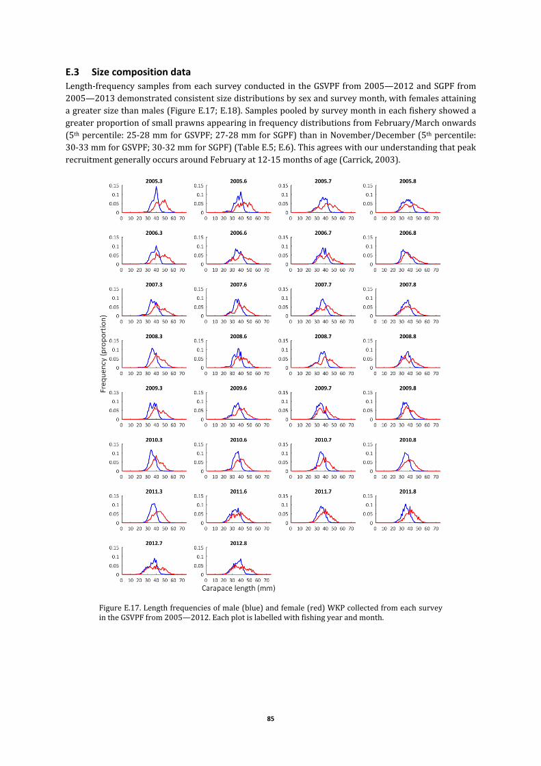
85

E.3 Size composition data Length‐frequencysamples fromeachsurveyconducted in theGSVPF from2005—2012andSGPFfrom2005—2013demonstratedconsistentsizedistributionsbysexandsurveymonth,withfemalesattainingagreatersizethanmales(FigureE.17;E.18).SamplespooledbysurveymonthineachfisheryshowedagreaterproportionofsmallprawnsappearinginfrequencydistributionsfromFebruary/Marchonwards(5thpercentile:25‐28mmforGSVPF;27‐28mmforSGPF)thaninNovember/December(5thpercentile:30‐33mmforGSVPF;30‐32mmforSGPF)(TableE.5;E.6).ThisagreeswithourunderstandingthatpeakrecruitmentgenerallyoccursaroundFebruaryat12‐15monthsofage(Carrick,2003).

FigureE.17.Lengthfrequenciesofmale(blue)andfemale(red)WKPcollectedfromeachsurveyintheGSVPFfrom2005—2012.Eachplotislabelledwithfishingyearandmonth.

86

Table E.5. Summary statistics for length‐frequency samplesfrom GSVPF pooled by survey month (fish month inparentheses)from2005—2012.

TableE.6.Summarystatisticsoflength‐frequencysamplesfromSGPFpooledbysurveymonth(fishmonthinparentheses)from2005—2013.

StatisticCarapacelength(mm)

Nov(2) Feb(5) Apr(7)

Males

Mean 36.0 34.9 34.95th‐95thpercentile 30‐43 27‐44 27‐42

Females

Mean 41.3 40.1 38.45th‐95thpercentile 32‐52 28‐55 27‐51

StatisticCarapacelength(mm)

Dec(3) Mar(6) Apr(7) May(8)

Males

Mean 36.6 35.2 35.2 35.25th‐95thpercentile 30‐43 25‐42 26‐42 27‐43

Females

Mean 43.5 40.7 40.0 39.75th‐95thpercentile 33‐55 28‐53 27‐52 28‐52

87

Figure E.18. Length frequencies of male (blue) and female (red) WKPcollected from each survey in the SGPF from 2005—2013. Each plot islabelledwithfishingyearandmonth.

88

ThemonthlyharvestsbytheGSVPFfrom2007—2012comprised,onaverage,morethanone‐thirdlargeprawns(10‐15 lb‐1;38%),morethanaquarterextra‐large(<10 lb‐1;28%)andmediumprawns(16‐20lb‐1; 26%), and the remainder small prawns (>20 lb‐1; 8%). Regression analysis indicated a significantincrease in theproportionof small andmediumprawnsanddecrease in large and extra‐largeprawnsover this period. In the SGPF, almost half of themonthly harvests from2003—2013weremadeupoflargeprawns(46%),followedbymedium(29%)andextra‐largeprawns(20%,andasmallproportionofsmallprawns(5%).Thesize‐gradecomposition intheSGPFhasbeenrelativelystableoverthisperiod,although therehasbeena slightbut still significant increase in theproportionofmediumprawnsanddecreaseinextra‐largeprawns.

FigureE.19.Size‐gradecompositionofmonthlyharvestsbytheGSVPFfrom2007—2012.

Figure E.20. Sze‐grade composition of monthly harvests by the SGPF from2003—2013.

E.4 Size‐transition matrices The size‐transition matrices generated for the WKP population dynamic model are characterised bystrongseasonalgrowth.MeanparametervaluesoftheseasonalvonBertalanffygrowthmodel(Eq.(6)inAppendixC)fittedtoWKPtag‐recapturedataaresummarisedinTableE.7forGSVandTableE.8forSG,andgrowthtrajectoriesareshowninFigureE.21andFigureE.22,respectively.Thederivation(fromthegrowthmodelparameters)ofgrowthrateKasafunctionoftimepredictedthatmalesinGSVreachtheirmaximumgrowthrateinmid‐March,slowdowntozerogrowthinmid‐August,exhibitnegativegrowth(shrinkage) until mid‐October, then resume positive growth around mid‐October for another cycle(FigureE.23).Thefemalegrowthcycleoccurstwoweeksearlier,withmaximumgrowthratereachedbylateFebruary andminimumgrowth rate approaching zero in early September. In SG, growth rates formalesand females reached theirmaxima inearlyMarch, andwere slowest inearlySeptember (FigureE.24).NogrowthwaspredictedtooccurfromlateJulytomid‐OctoberformalesandfromlateAugusttolate September for females. Both GSV and SG models indicated that female WKP grow almostcontinuouslyinlengththroughouttheyearbutataslowerrateincertainmonthsthanmales.

89

Table E.7. Seasonal von Bertalanffy growthparametersfittedtoWKPtag‐recapturedatafromtheGSVPF.

Model Lmax K0 A tϕ

Males 46.5 0.00237 0.00285 79.5Females 61.3 0.00204 0.00171 61.4

Table E.8. Seasonal von Bertalanffy growthparametersfittedtoWKPtag‐recapturedatafromtheSGPF.

Model Lmax K0 A tϕ

Males 45.9 0.00243 0.00331 69.0Females 57.1 0.00217 0.00229 72.6

FigureE.21.SeasonalvonBertalanffygrowthtrajectoriesformaleandfemaleWKPfromtheGSVPFwithabirthdateof1November.

FigureE.22.SeasonalvonBertalanffygrowthtrajectoriesformaleandfemaleWKPfromtheSGPFwithabirthdateof1November.

90

FigureE.23.SeasonalgrowthrateofmaleandfemaleWKPfromtheGSVPF.

FigureE.24.SeasonalgrowthrateofmaleandfemaleWKPfromtheSGPF.

91

E.5 Economic data

TableE.9. Breakdownof average annual vessel costsWy in theGSVPF for2011/12.

Wyvariables $vessel‐year‐1 Proportion

Licencefee 35443 0.40Insurance 21269 0.24Labour (unpaid,imputed) 13723 0.15Legalandaccounting 7118 0.08Slippingandmooring 4339 0.05Office,administration,etc. 4307 0.05Telephone,fax,etc. 2766 0.03Travelandaccommodation 467 0.01Total 89432

Table E.10. Breakdownof average annual vessel costsWy in the SGPF for2012/13.

Wyvariables $vessel‐year‐1 Proportion

Licencefee 25476 0.29Insurance 19713 0.22Legalandaccounting 10652 0.12Slippingandmooring 5836 0.07Labour(unpaid,imputed) 4751 0.05Membershipandassociationexpenses 3300 0.04Communication 3183 0.04Boatsurvey 2758 0.03Electricity 2594 0.03Rates 2399 0.03Repairsandmaintenance(buildings) 1955 0.02Travelandaccommodation 1272 0.01Repairsandmaintenance(vehicles) 900 0.01Rents 528 0.01Training(other) 527 0.01Exportfees 444 0.01Training(firstaid) 110 0.00Other 2395 0.03Total 88794

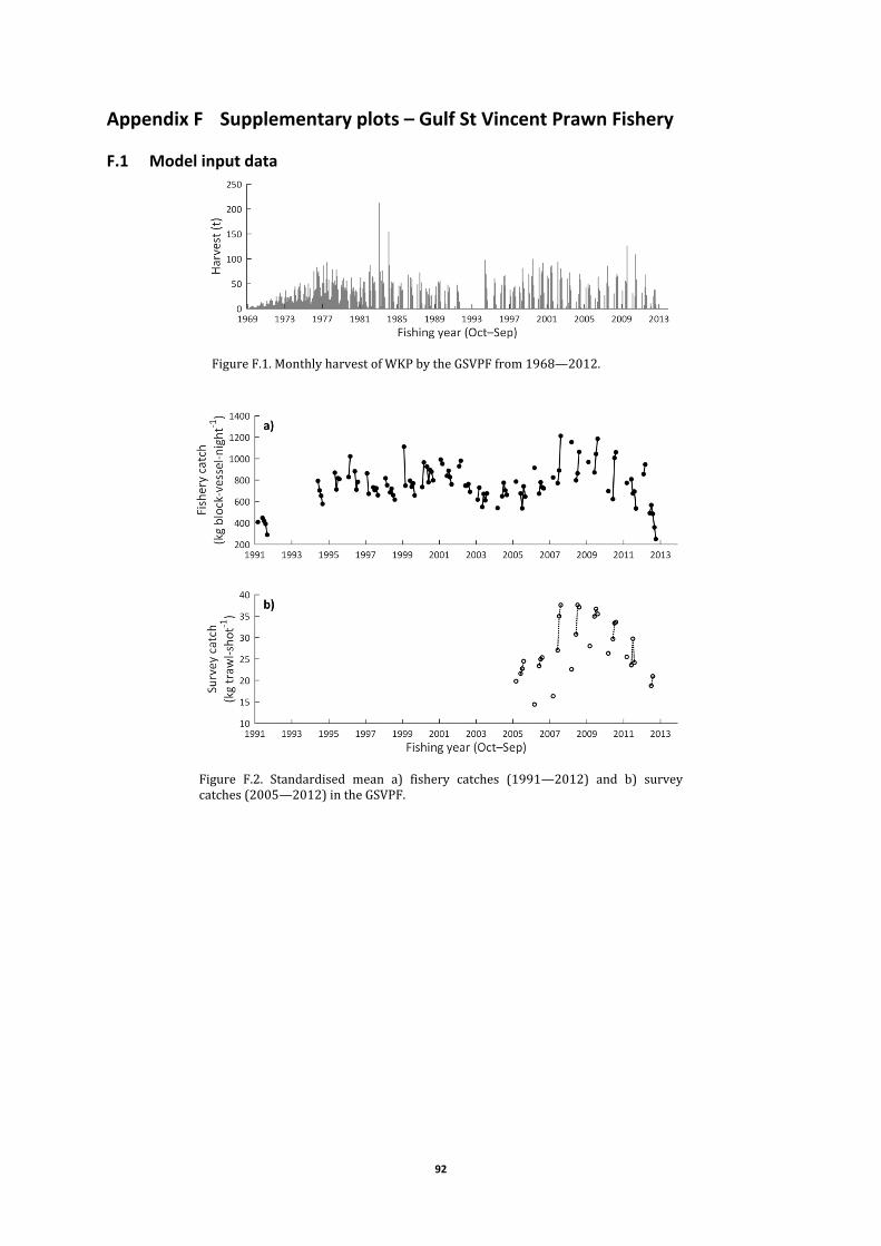
92

Appendix F Supplementary plots – Gulf St Vincent Prawn Fishery

F.1 Model input data

FigureF.1.MonthlyharvestofWKPbytheGSVPFfrom1968—2012.

Figure F.2. Standardised mean a) fishery catches (1991—2012) and b) surveycatches(2005—2012)intheGSVPF.

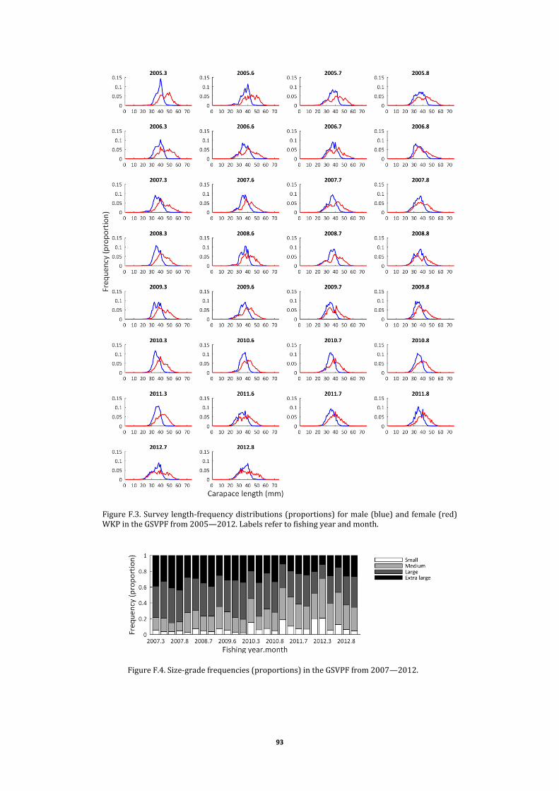
93

FigureF.3.Surveylength‐frequencydistributions(proportions)formale(blue)andfemale(red)WKPintheGSVPFfrom2005—2012.Labelsrefertofishingyearandmonth.

FigureF.4.Size‐gradefrequencies(proportions)intheGSVPFfrom2007—2012.

94

FigureF.5.Colour‐scalevisualisationofthesize‐transitionmatrixformaleWKPintheGSVPF.Thescalefrombluetoredindicatesincreasingprobabilityofprawnsofcarapacelength‐classlʹinthepreviousmonthgrowingintoanewlengthloveronemonth.

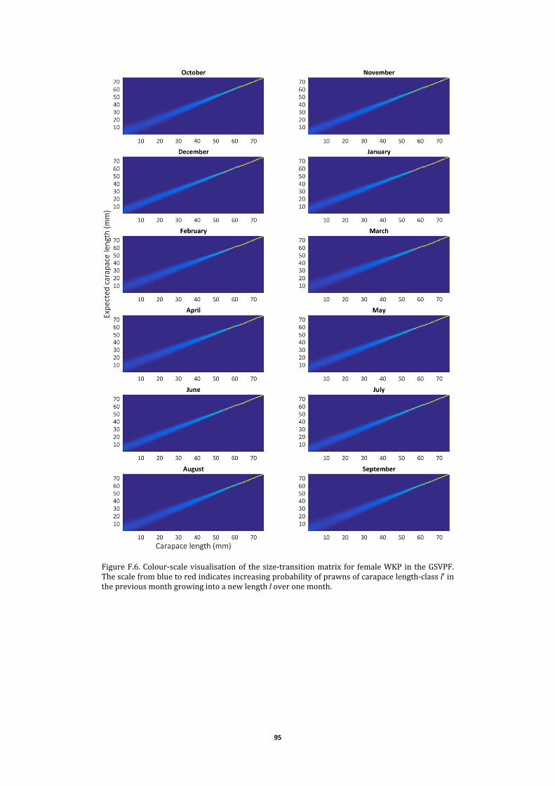
95

FigureF.6.Colour‐scalevisualisationof thesize‐transitionmatrix for femaleWKP in theGSVPF.Thescalefrombluetoredindicatesincreasingprobabilityofprawnsofcarapacelength‐classlʹinthepreviousmonthgrowingintoanewlengthloveronemonth.

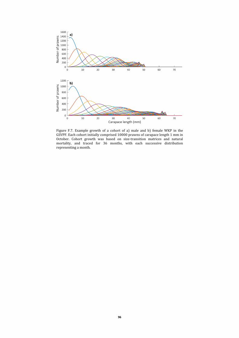
96

Figure F.7. Example growth of a cohort of a) male and b) female WKP in theGSVPF.Eachcohortinitiallycomprised10000prawnsofcarapacelength1mminOctober. Cohort growth was based on size‐transition matrices and naturalmortality, and traced for 36 months, with each successive distributionrepresentingamonth.

97

F.2 Model output results

FigureF.8.WKPstockstatusannualplotsfortheGSVPFfrom1991—2013:a)spawningeggproduction ratio (Ey/E0);b) exploitablebiomass ratio (By/B0); andc) recruitmentratio(Ry/R0).Thedottedreferencelineindicatestheestimatedleveloftheequilibriumvirginstock(i.e.t=0at1969).Deterministicrecruitmentwasmodelled from1969—1993andstochastic(variable)recruitmentthereafter.

FigureF.9.Comparisonofobserved(survey)andpredicted(model)WKPexploitablebiomassbyyear‐monthintheGSVPF.

98

F.3 Fishery catch rate diagnostics

Figure F.10. Fishery catch rate fitted diagnostics for the GSVPF: a) observed(standardised) andmodel‐predicted catch rates eachmonth from1991—2013; b)standardisedfittedvalues;andc)monthlystandardisedresiduals.

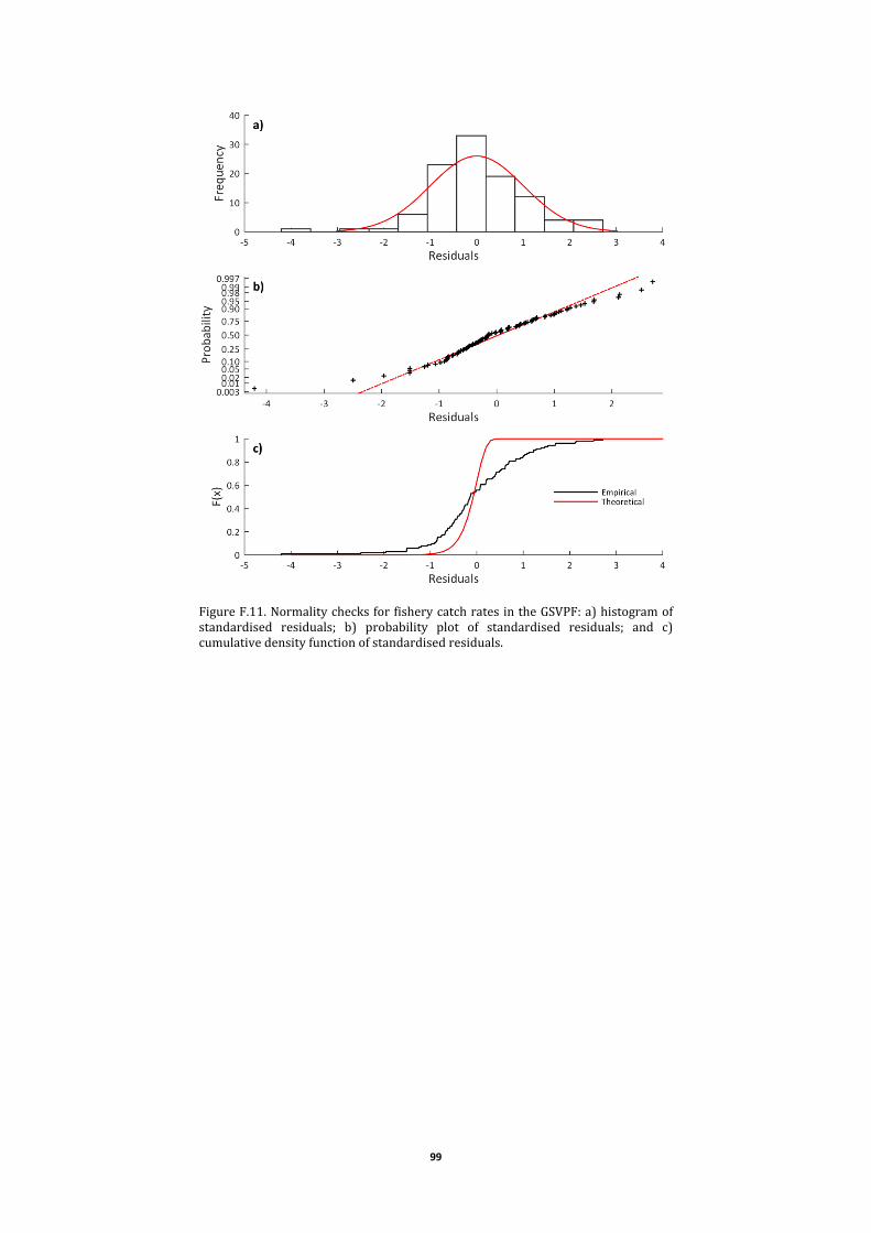
99

FigureF.11.NormalitychecksforfisherycatchratesintheGSVPF:a)histogramofstandardised residuals; b) probability plot of standardised residuals; and c)cumulativedensityfunctionofstandardisedresiduals.

100

F.4 Survey catch rate diagnostics

Figure F.12. Survey catch rate fitted diagnostics for the GSVPF: a) observed(standardised) andmodel‐predicted catch rates eachmonth from2005—2013; b)standardisedfittedvalues;andc)monthlystandardisedresiduals.

101

FigureF.13.NormalitychecksforsurveycatchratesintheGSVPF:a)histogramofstandardised residuals; b) probability plot of standardised residuals; and c)cumulativedensityfunctionofstandardisedresiduals.

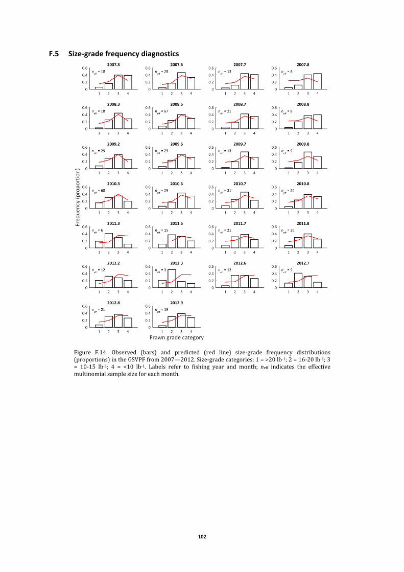
102

F.5 Size‐grade frequency diagnostics

Figure F.14. Observed (bars) and predicted (red line) size‐grade frequency distributions(proportions)intheGSVPFfrom2007—2012.Size‐gradecategories:1=>20lb‐1;2=16‐20lb‐1;3= 10‐15 lb‐1; 4 = <10 lb‐1. Labels refer to fishing year and month; neff indicates the effectivemultinomialsamplesizeforeachmonth.

103

Figure F.15. Observed (bars) and predicted (red line) size‐grade frequency distributions(proportions)intheGSVPFfrom2007—2012afteromittingsize‐gradecategory1(>20lb‐1).Size‐gradecategories:2=16‐20lb‐1;3=10‐15lb‐1;4=<10lb‐1.Labelsrefertofishingyearandmonth.

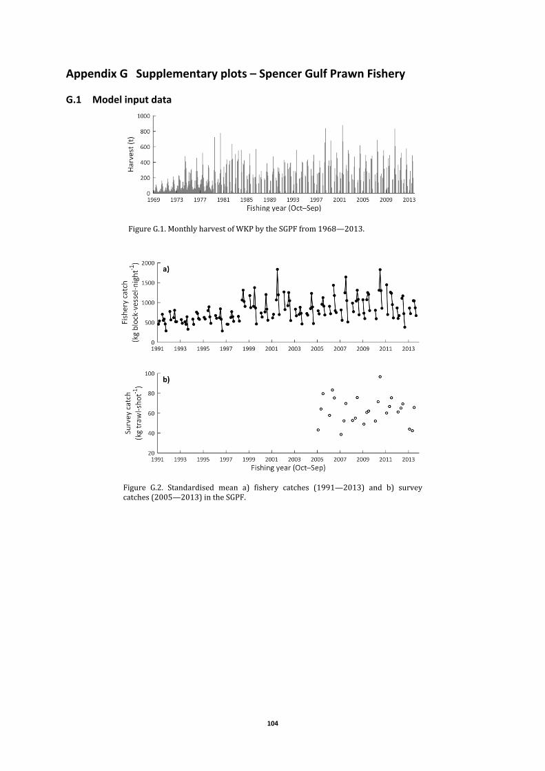
104

Appendix G Supplementary plots – Spencer Gulf Prawn Fishery

G.1 Model input data

FigureG.1.MonthlyharvestofWKPbytheSGPFfrom1968—2013.

Figure G.2. Standardised mean a) fishery catches (1991—2013) and b) surveycatches(2005—2013)intheSGPF.

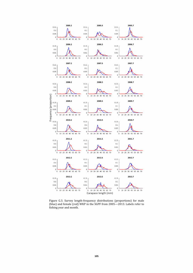
105

Figure G.3. Survey length‐frequency distributions (proportions) for male(blue)andfemale(red)WKPintheSGPFfrom2005—2013.Labelsrefertofishingyearandmonth.

106

FigureG.4.Size‐gradefrequencies(proportions)intheSGPFfrom2003—2013.

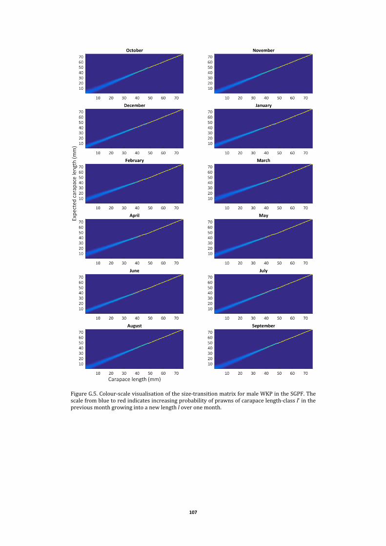
107

FigureG.5.Colour‐scalevisualisationofthesize‐transitionmatrixformaleWKPintheSGPF.Thescalefrombluetoredindicatesincreasingprobabilityofprawnsofcarapacelength‐classlʹinthepreviousmonthgrowingintoanewlengthloveronemonth.

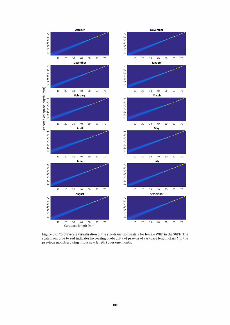
108

FigureG.6.Colour‐scalevisualisationofthesize‐transitionmatrixforfemaleWKPintheSGPF.Thescalefrombluetoredindicatesincreasingprobabilityofprawnsofcarapacelength‐classlʹinthepreviousmonthgrowingintoanewlengthloveronemonth.

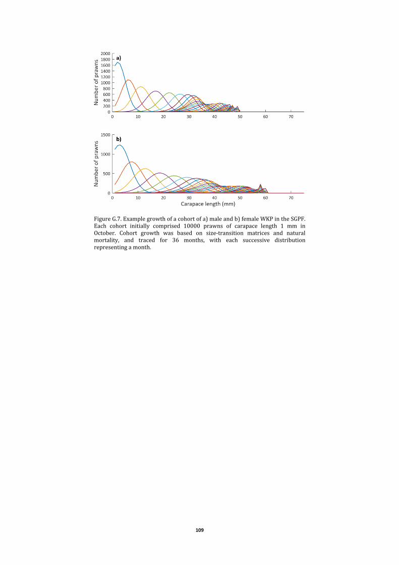
109

FigureG.7.Examplegrowthofacohortofa)maleandb)femaleWKPintheSGPF.Each cohort initially comprised 10000 prawns of carapace length 1 mm inOctober. Cohort growth was based on size‐transition matrices and naturalmortality, and traced for 36 months, with each successive distributionrepresentingamonth.

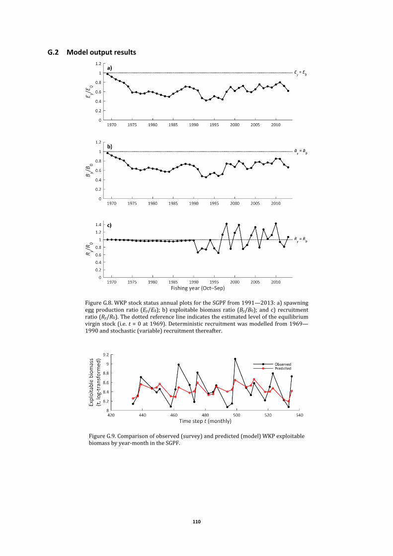
110

G.2 Model output results

FigureG.8.WKPstockstatusannualplotsfortheSGPFfrom1991—2013:a)spawningeggproduction ratio (Ey/E0);b) exploitablebiomass ratio (By/B0); andc) recruitmentratio(Ry/R0).Thedottedreferencelineindicatestheestimatedleveloftheequilibriumvirginstock(i.e.t=0at1969).Deterministicrecruitmentwasmodelled from1969—1990andstochastic(variable)recruitmentthereafter.

FigureG.9.Comparisonofobserved(survey)andpredicted(model)WKPexploitablebiomassbyyear‐monthintheSGPF.

111

G.3 Fishery catch rate diagnostics

Figure G.10. Fishery catch rate fitted diagnostics for the SGPF: a) observed(standardised) andmodel‐predicted catch rates eachmonth from1991—2013; b)standardisedfittedvalues;andc)monthlystandardisedresiduals.

112

FigureG.11.Normalitychecksfor fisherycatchrates in theSGPF:a)histogramofstandardised residuals; b) probability plot of standardised residuals; and c)cumulativedensityfunctionofstandardisedresiduals.

113

G.4 Survey catch rate diagnostics

Figure G.12. Survey catch rate fitted diagnostics for the SGPF: a) observed(standardised) andmodel‐predicted catch rates eachmonth from2005—2013; b)standardisedfittedvalues;andc)monthlystandardisedresiduals.

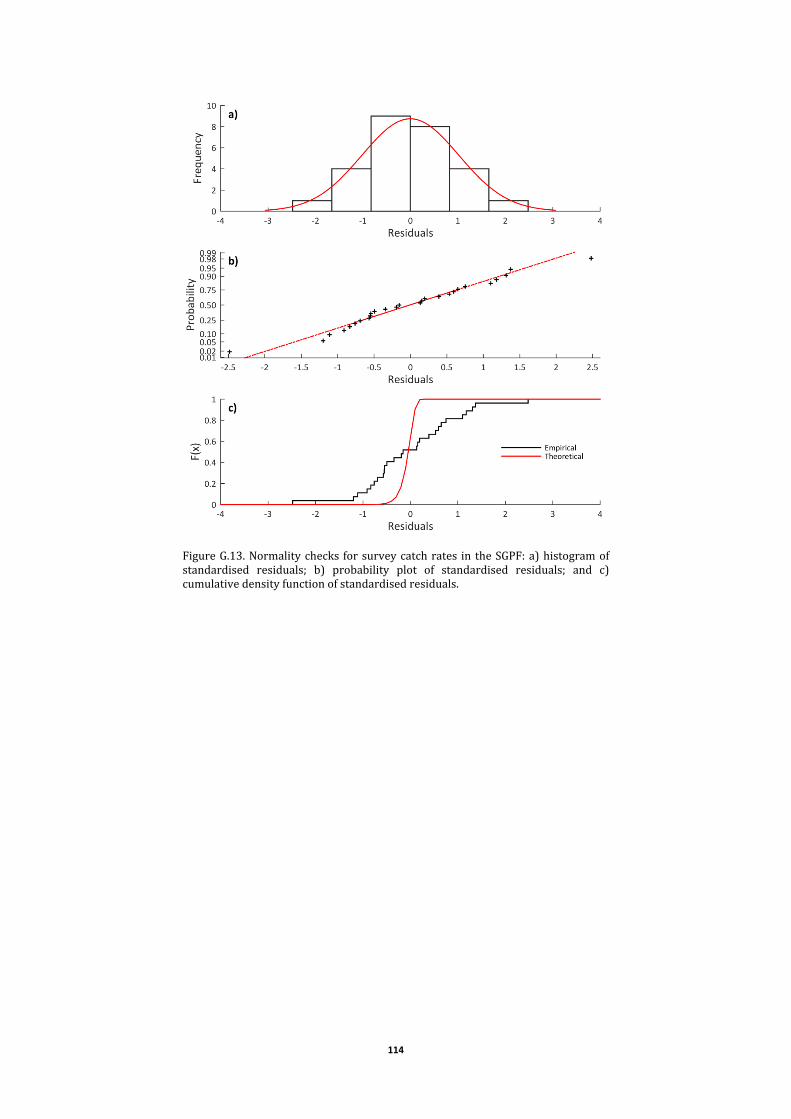
114

FigureG.13.Normalitychecks forsurveycatchrates in theSGPF:a)histogramofstandardised residuals; b) probability plot of standardised residuals; and c)cumulativedensityfunctionofstandardisedresiduals.

115

Appendix H Supplementary plots – both fisheries

H.1 Model input data

Figure H.1. Biological schedules for WKP relative to carapace length (bothfisheries): a) weight of males and females; b) batch fecundity; c) maturity(proportion);andd)recruitment(proportion).

Documents

C. J. Noell, M. F. O’Neill, J. D. Carroll, C. D. Dixon · 2015-11-05 · A bio‐economic model for South Australia’s prawn trawl fisheries C. J. Noell, M. F. O’Neill, J. D